


1. Introduction
On the intertidal mudflats, plants have the ability to capture suspended particles and make the sediment stable, thus promoting their own growth. Nonetheless, the positive feedback also leads to a negative feedback when organic matter banks up in the sediment. The process of anaerobic decomposition by sulphate-reducing bacteria produces toxic sulphides that, if accumulated in large enough quantities, then cause plant death, see Lamers et al. [Reference Lamers, Govers and Janssen15] and Mirlean et al. [Reference Mirlean and Costa20]. Thus, the plant-sulphide feedback framework delineates a mechanism by which sulphide concentrations increase from a process that benefits the plant, but shapes a negative feedback for plant growth.
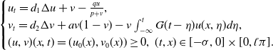
This paper is committed to studying the spatio-temporal dynamics of the following plant-sulphide model under the Neumann boundary condition,
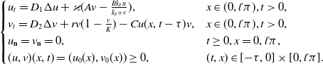 \begin{equation} \begin{cases} u_{t}=D_{1}\Delta u+\varkappa (Av-\frac{Bk_{s}u}{k_{s}+v}), & x\in (0,\mathcal{l}\pi ),t \gt 0,\\ v_{t}=D_{2}\Delta v+rv(1-\frac{v}{K})-Cu(x,t-\tau )v,& x\in (0,\mathcal{l}\pi ),t \gt 0,\\ u_{\textbf{n}}= v_{\textbf{n}}=0, & t\geq 0, x=0,\mathcal{l}\pi, \\ (u,v)(x,t)=(u_{0}(x),v_{0}(x)) \geq 0, & (t,x) \in [{-}\tau, 0]\times [0,\mathcal{l}\pi ]. \end{cases} \end{equation}
where $u$
and
$u$
and $v$
represent, respectively, sulphide concentration and plant biomass at time
$v$
represent, respectively, sulphide concentration and plant biomass at time $t$
.
$t$
. $D_{1}$
and
$D_{1}$
and $D_{2}$
measure sulphide dispersal and plant lateral expansion, respectively.
$D_{2}$
measure sulphide dispersal and plant lateral expansion, respectively. $\Delta$
is the Laplace operator.
$\Delta$
is the Laplace operator. $\varkappa$
is the control parameter.
$\varkappa$
is the control parameter. $A$
denotes the rate at which hydrogen sulphide is produced by plants.
$A$
denotes the rate at which hydrogen sulphide is produced by plants. $B$
describes the maximal escape rate of hydrogen sulphide.
$B$
describes the maximal escape rate of hydrogen sulphide. $k_{s}$
indicates that plants promote the enrichment of sulphides.
$k_{s}$
indicates that plants promote the enrichment of sulphides. $r$
and
$r$
and $K$
measure, respectively, reproductive rate and carrying capacity.
$K$
measure, respectively, reproductive rate and carrying capacity. $C$
describes the plant mortality caused by sulphides.
$C$
describes the plant mortality caused by sulphides.
The biodynamics of ecosystems, including the mechanisms and patterns of spatial dispersal, has become a current focus of mathematical biology. Incorporating diffusion into basic differential equation biological models allows us to more accurately study the lateral expansion of plants and the movement of animals, such as random and density-dependent mobility. A host of scholars have used the reaction-diffusion equation to model and study the biological relationships in various ecosystems. Meanwhile, time lag is another indispensable factor in the modelling process. The addition of diffusion and delay is helpful for us to analyse and understand the real population distribution.
In nature, the species are spatially distributed and interact in diverse spatial location. The biological systems with diffusion have been extensively explored in substantial works. The distinctions among cross-diffusion, self-diffusion and diffusion are expounded by Lou and Ni [Reference Lou and Ni18]. Spatial memory with three types of diffusion just mentioned is studied by Shi et al. [Reference Shi, Wang and Wang22]. Tang and Song [Reference Tang and Song26] studied Turing and Hopf bifurcations of a prey-predator system with self-diffusion and nonlinear mortality. Sun et al. [Reference Sun, Zhang, Song, Li and Jin25] revealed the bistable phenomenon and Turing-Hopf bifurcation in a plant-water system with diffusion. Jiang et al. [Reference Jiang, Wang and Cao12] studied the space-time dynamics of a diffusive Schnakenberg system. Wu and Zhao [Reference Wu and Zhao31] studied the effects of threshold hunting and Allee effect in a diffusive system. Zhou and Xiao [Reference Zhou and Xiao39] researched a competition-diffusion-advection system. Luo and Wang [Reference Luo and Wang19] investigated the pattern dynamics in a reaction-diffusion model with prey-taxis. Lin et al. [Reference Lin, Xu and Li17] studied Hopf-Turing bifurcation in reaction-diffusion neural networks. Chen et al. [Reference Chen, Wu, Liu and Chen3] studied the space-time dynamics near a Hopf-Turing bifurcation point of a diffusive model. Yi et al. [Reference Yi, Wei and Shi35] studied the bifurcations and patterns in a diffusive system, and Wang et al. [Reference Wang, Wei and Shi28] researched the global bifurcation and patterns of a class of diffusive models. Zhang et al. [Reference Zhang, Liu, Meng and Zhang36] studied the space-time kinetics in a planktonic model. There are plentiful works on the space-time dynamics of various systems, such as Wu et al. [Reference Wu, Wang and Zou30], Wu and Hsu [Reference Wu and Hsu32], Yang et al. [Reference Yang, Zou and Hsu33], Yi et al. [Reference Yi34], Fu et al. [Reference Fu, He, Zhang and Wen9].
Another important factor in modelling is time delay, which plays a vital role in physics, biology or engineering problems. In biodynamic systems, time delay is generally due to several processes, such as the pregnancy and maturation period, and the lag of the toxic attack. The implications of adding time delays to modelling have been explored by many researchers. Li et al. [Reference Li, Yuan, Jin and Wang16] explored the joint effects of memory and maturation delays by utilizing crossing curves method in a diffusive system. Chen et al. [Reference Chen, Lou and Wei4] studied Hopf bifurcation of a delayed reaction-diffusion-advection system. Wang and Zou [Reference Wang and Zou29] studied the impact of digestion delay on a prey-predator system. Wang et al. [Reference Wang, Nagy, Gilg and Kuang27] analysed the role of maturation delay in prey-predator cycles. Wu and Song [Reference Wu and Song23] investigated the steady state-Hopf bifurcation derived by distributed effect and delay in a diffusive system. There’s still lots of research on discrete delay, such as An et al. [Reference An, Wang and Wang1], Zhang et al. [Reference Zhang, Xie, Dong, Huang, Ruan and Takeuchi37], Beretta and Breda [Reference Beretta and Breda2], Kumar and Dubey [Reference Kumar and Dubey13], Everett et al. [Reference Everett, Nagy and Kuang8], Kundu and Maitra [Reference Kundu and Maitra14], Dai and Sun [Reference Dai and Sun7], Jiang et al. [Reference Jiang, An and Shi11].
The dynamics of the various ecosystems mentioned above have been studied to a greater or lesser extent. However, the spatial dynamics of plant patterns in salt marsh systems have seldom been studied. Zhao et al. [Reference Zhao, Zhang, Siteur, Li, Liu and Koppel38] proposed the following plant-sulphide model in salt marsh ecosystems,
 \begin{equation} \begin{cases} u_{t}=D_{1}\Delta u+\varkappa \left(Av-\frac{Bk_{s}u}{k_{s}+v}\right), \\[3pt] v_{t}=D_{2}\Delta v+rv\left(1-\frac{v}{K}\right)-Cuv, \end{cases} \end{equation}
They found that the occurrence of transient patterns could recognize the ecological courses behind pattern formation and the factors that decide the ecological restoring force. However, their research focuses on modelling and numerical simulations rather than rigorous mathematical analysis. It’s pointed out that the toxicity of sulphides does not have an immediate effect on plants, thereby creating a toxicity lag. Therefore, we take into account time lag $\tau$
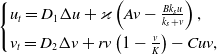
of sulphide toxicity based on their model and study model (1.1). For model (1.1), rescaling
$\tau$
of sulphide toxicity based on their model and study model (1.1). For model (1.1), rescaling
 \begin{align*} &\hat{u}=\frac{C}{\sqrt{ACK\eta }}u, \ \hat{v}=\frac{1}{K}v, \ \hat{t}=\sqrt{ACK\eta }t, \ a=\frac{r}{\sqrt{ACK\eta }}, \ p=\frac{\eta Bk_{s}}{K \sqrt{ACK\eta }}, \ q=\frac{k_{s}}{K},\\ &\ d_{1}=\frac{D_{1}}{\sqrt{ACK\eta }}, \ d_{2}=\frac{D_{2}}{\sqrt{ACK\eta }}, \end{align*}
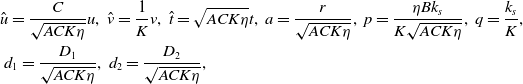
removing the hats, then we get the following model with the same boundary condition as model (1.1).
 \begin{equation} \begin{cases} u_{t}=d_{1}\Delta u+v-\frac{qu}{p+v}, \\ v_{t}=d_{2}\Delta v+av(1-v)-u(x,t-\tau )v. \end{cases} \end{equation}
In addition, the effect of distributed delay on the dynamic behaviour is also important and has captured the attention of numerous scholars. In particular, distributed delay with weak kernel carries profound implications for the study of biodiffusion, e.g. see Cooke and Grossman [Reference Cooke and Grossman6], Gourley and Ruan [Reference Gourley and Ruan10], Shen et al. [Reference Shen, Song and Wang21]. Cooke and Grossman [Reference Cooke and Grossman6] showed that it’s inherently more stable than discrete delay. The model with distributed toxicity delay is as follows:
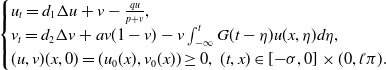
 \begin{equation} \begin{cases} u_{t}=d_{1}\Delta u+v-\frac{qu}{p+v}, \\ v_{t}=d_{2}\Delta v+av(1-v)-v\int _{-\infty }^{t}G(t-\eta )u(x,\eta )d\eta, \\ (u,v)(x,t)=(u_{0}(x),v_{0}(x)) \geq 0, \ (t,x) \in [{-}\sigma, 0]\times [0,\mathcal{l}\pi ]. \end{cases} \end{equation}
where $G(t)=\frac{1}{\sigma }e^{-\frac{t}{\sigma }}$
and other conditions are consistent with system (1.3).
$G(t)=\frac{1}{\sigma }e^{-\frac{t}{\sigma }}$
and other conditions are consistent with system (1.3).
This paper aims to explore the spatio-temporal dynamics of model (1.3) and (1.4) and compare the effects of the discrete delay and distributed delay on model (1.2). One can see our final summary for a detailed comparison.
The structure of remaining paper is as follows. The stability and bifurcation of the local system are explored in Section 2. The stability and the normal form of spatially Hopf bifurcation for the space-time system are computed detailedly in Section 3. The impact of the distributed delay is analysed in Section 4. Numerical illustrations and conclusions are displayed in Section 5 and 6, respectively.
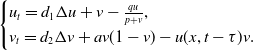
2. Dynamics of the local plant-sulphide model
The local system of (1.3) reads:
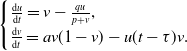 \begin{equation} \begin{cases} \frac{\text{d} u}{\text{d} t}=v-\frac{qu}{p+v}, \\ \frac{\text{d} v}{\text{d} t}=av(1-v)-u(t-\tau )v. \end{cases} \end{equation}
First, we present several results on system (2.1).
Theorem 2.1.
The solution of system (2.1) initiating in $C([{-}\tau, 0],\mathbb{R}_{+}^{2})$
is positive.
$C([{-}\tau, 0],\mathbb{R}_{+}^{2})$
is positive.
Proof. Let $(u(t),v(t))$
be any solution of system (2.1) with
$(u(t),v(t))$
be any solution of system (2.1) with $\tau =0$
. According to
$\tau =0$
. According to $\frac{\text{d} v}{\text{d} t}=av(1-v)-u(t-\tau )v$
, we obtain
$\frac{\text{d} v}{\text{d} t}=av(1-v)-u(t-\tau )v$
, we obtain $v(t)=u(0)e^{\int _{0}^{t}(a(1-v)-u(t-\tau ))dt}\gt 0$
due to
$v(t)=u(0)e^{\int _{0}^{t}(a(1-v)-u(t-\tau ))dt}\gt 0$
due to $v(0)\gt 0$
. Accordingly, we get
$v(0)\gt 0$
. Accordingly, we get
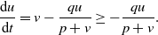 \begin{equation*} \frac {\text {d} u}{\text {d} t}=v-\frac {qu}{p+v}\geq -\frac {qu}{p+v}. \end{equation*}
This combined with $u(0)\gt 0$
shows
$u(0)\gt 0$
shows $u=u(0)e^{-\int _{0}^{t}\frac{q}{p+v}dt}\gt 0$
.
$u=u(0)e^{-\int _{0}^{t}\frac{q}{p+v}dt}\gt 0$
.
By computation, there are two equilibria for system (2.1), namely $E_{0}(0,0)$
and
$E_{0}(0,0)$
and $E_{*}(u_{*},v_{*})$
, where
$E_{*}(u_{*},v_{*})$
, where
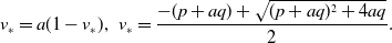 \begin{equation*} v_{*}=a(1-v_{*}), \, \, v_{*}=\frac {-(p+aq)+\sqrt {(p+aq)^{2}+4aq}}{2}. \end{equation*}
Theorem 2.2.
System (2.1) possesses two equilibria $E_{0}(0,0)$
and
$E_{0}(0,0)$
and $E_{*}(u_{*},v_{*})$
. For
$E_{*}(u_{*},v_{*})$
. For $\tau =0$
,
$\tau =0$
, $E_{0}$
is a saddle and
$E_{0}$
is a saddle and $E_{*}$
is a stable node or focus.
$E_{*}$
is a stable node or focus.
Proof. For $\tau =0$
, the Jacobian matrix reads
$\tau =0$
, the Jacobian matrix reads
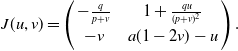 \begin{equation} J(u,v)= \left ( \begin{array}{c@{\quad}c} -\frac{q}{p+v} & 1+\frac{qu}{(p+v)^{2}} \\[3pt] -v & a(1-2v)-u \end{array} \right ). \end{equation}
Hence, we have
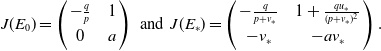 \begin{equation*} J(E_{0})= \left ( \begin {array}{c@{\quad}c} -\frac {q}{p} & 1 \\[3pt] 0 & a \end {array} \right ) \, \, \text {and} \, \, J(E_{*})= \left ( \begin {array}{c@{\quad}c} -\frac {q}{p+v_{*}} & 1+\frac {qu_{*}}{(p+v_{*})^{2}} \\[3pt] -v_{*} & -av_{*} \end {array} \right ). \end{equation*}
Clearly, $E_{0}$
is a saddle.
$E_{0}$
is a saddle. $\text{Tr}(J(E_{*}))=-av_{*}-\frac{q}{p+v_{*}}\lt 0$
and
$\text{Tr}(J(E_{*}))=-av_{*}-\frac{q}{p+v_{*}}\lt 0$
and $\text{det}(J(E_{*}))=\frac{aqv_{*}}{p+v_{*}}+(1+\frac{qu_{*}}{(p+v_{*})^{2}})v_{*}\gt 0$
indicate that
$\text{det}(J(E_{*}))=\frac{aqv_{*}}{p+v_{*}}+(1+\frac{qu_{*}}{(p+v_{*})^{2}})v_{*}\gt 0$
indicate that $E_{*}$
is a stable node or focus.
$E_{*}$
is a stable node or focus.
Theorem 2.3.
For $\tau =0$
, there is no limit cycle of system (2.1).
$\tau =0$
, there is no limit cycle of system (2.1).
Proof. Setting $\Theta _{1}(u,v)=v-\frac{qu}{p+v}, \ \Theta _{2}(u,v)=av(1-v)-uv$
and choosing the Dulac function
$\Theta _{1}(u,v)=v-\frac{qu}{p+v}, \ \Theta _{2}(u,v)=av(1-v)-uv$
and choosing the Dulac function $\mathcal{B}(u,v)=\frac{1}{v}$
, then we gain
$\mathcal{B}(u,v)=\frac{1}{v}$
, then we gain
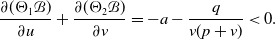 \begin{equation*} \frac {\partial ( {\Theta _{1}\mathcal {B}} )}{\partial {u}}+\frac {\partial {(\Theta _{2} \mathcal {B}})}{\partial {v}}=-a-\frac {q}{v(p+v)}\lt 0. \end{equation*}
Thus, no limit cycle emerges in system (2.1) for $\tau =0$
.
$\tau =0$
.
Theorem 2.4.
For $\tau =0$
, if
$\tau =0$
, if $qu^{2}_{*}\leq 4ap(p+v_{*})^{2}$
, then
$qu^{2}_{*}\leq 4ap(p+v_{*})^{2}$
, then $E_{*}$
is globally asymptotic stable for system (2.1) in the interior of the first quadrant.
$E_{*}$
is globally asymptotic stable for system (2.1) in the interior of the first quadrant.
Proof. Choose the Lyapunov function
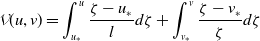 \begin{equation*} \mathcal {V}(u,v)=\int _{u_{*}}^{u}\frac {\zeta -u_{*}}{l}d\zeta +\int _{v_{*}}^{v}\frac {\zeta -v_{*}}{\zeta }d\zeta \end{equation*}
for $u,v \gt 0$
and undetermined
$u,v \gt 0$
and undetermined $l\gt 0$
. Then we obtain
$l\gt 0$
. Then we obtain
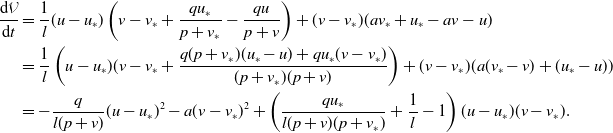 \begin{align*} \frac{\text{d}\mathcal{V}}{\text{d}t}&=\frac{1}{l}(u-u_{*})\left(v-v_{*}+\frac{qu_{*}}{p+v_{*}}-\frac{qu}{p+v}\right)+(v-v_{*})(av_{*}+u_{*}-av-u)\\ &=\frac{1}{l}\left (u-u_{*})(v-v_{*}+\frac{q(p+v_{*})(u_{*}-u) +qu_{*}(v-v_{*})}{(p+v_{*})(p+v)}\right )+(v-v_{*})(a(v_{*}-v)+(u_{*}-u))\\ &=-\frac{q}{l(p+v)}(u-u_{*})^{2}-a(v-v_{*})^{2}+\left (\frac{qu_{*}}{l(p+v)(p+v_{*})}+\frac{1}{l}-1 \right )(u-u_{*})(v-v_{*}). \end{align*}
Taking $l=1$
yields
$l=1$
yields
 \begin{align*} \frac{\text{d}\mathcal{V}}{\text{d}t}&=-\frac{q}{(p+v)}(u-u_{*})^{2}-a(v-v_{*})^{2}+\left (\frac{qu_{*}}{(p+v)(p+v_{*})} \right )(u-u_{*})(v-v_{*}). \end{align*}
Then, we conclude $\frac{qu^{2}_{*}}{(p+v)(p+v_{*})^{2}} \lt 4a$
due to
$\frac{qu^{2}_{*}}{(p+v)(p+v_{*})^{2}} \lt 4a$
due to $qu^{2}_{*}\leq 4ap(p+v_{*})^{2}$
, namely
$qu^{2}_{*}\leq 4ap(p+v_{*})^{2}$
, namely
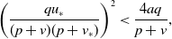 \begin{align*} \left (\frac{qu_{*}}{(p+v)(p+v_{*})} \right )^{2}\lt \frac{4aq}{p+v}, \end{align*}
which implies $\frac{\text{d}\mathcal{V}}{\text{d}t}\lt 0$
. This combined with Lasalle invariance principle gains the global asymptotic stability of
$\frac{\text{d}\mathcal{V}}{\text{d}t}\lt 0$
. This combined with Lasalle invariance principle gains the global asymptotic stability of $E_{*}$
.
$E_{*}$
.
In next section, we’re going to show that (2.1) undergoes Hopf bifurcation with certain conditions. The case is covered by Theorem 3.3, thus see Theorem 3.3 for a detailed proof.
3. Dynamics of the spatial plant-sulphide model with discrete delay
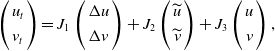
Here we take into account delay-driven instability for system (1.3). Linearizing (1.3) at $E_{*}(u_{*},v_{*})$
generates
$E_{*}(u_{*},v_{*})$
generates
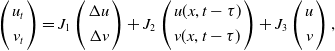 \begin{equation} \left ( \begin{array}{c} u_{t} \\[3pt] v_{t} \end{array} \right ) =J_{1} \left ( \begin{array}{c} \Delta u \\[3pt] \Delta v \end{array} \right ) +J_{2} \left ( \begin{array}{c} u(x,t-\tau ) \\[3pt] v(x,t-\tau ) \end{array} \right ) +J_{3} \left ( \begin{array}{c} u \\[3pt] v \end{array} \right ), \end{equation}
where
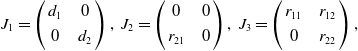 \begin{equation} J_{1}= \left ( \begin{array}{c@{\quad}c} d_{1} & 0 \\[3pt] 0 & d_{2} \end{array} \right ), \ J_{2}= \left ( \begin{array}{c@{\quad}c} 0 & 0 \\[3pt] r_{21} & 0 \end{array} \right ), \ J_{3}= \left ( \begin{array}{c@{\quad}c} r_{11} & r_{12} \\[3pt] 0 & r_{22} \end{array} \right ), \end{equation}
with $r_{11}=-\frac{q}{p+v_{*}}, \ r_{12}=1+\frac{qu_{*}}{(p+v_{*})^{2}}, \ r_{21}=-v_{*}, \ r_{22}= -av_{*}$
.
$r_{11}=-\frac{q}{p+v_{*}}, \ r_{12}=1+\frac{qu_{*}}{(p+v_{*})^{2}}, \ r_{21}=-v_{*}, \ r_{22}= -av_{*}$
.
Denoting the eigenvalues of
 \begin{equation} \Delta \varepsilon (x)+\theta \varepsilon (x)=0, \ x \in (0,\mathcal{l}\pi ), \\ \ \varepsilon _{x}|_{x=0,\mathcal{l}\pi }=0, \end{equation}
by $\theta _{n}$
, then the corresponding eigenfunctions of
$\theta _{n}$
, then the corresponding eigenfunctions of $\theta _{n}=\frac{n^{2}}{\mathcal{l}^{2}}$
are
$\theta _{n}=\frac{n^{2}}{\mathcal{l}^{2}}$
are $\varepsilon _{n}(x)=\cos \frac{n}{\mathcal{l}}x$
.
$\varepsilon _{n}(x)=\cos \frac{n}{\mathcal{l}}x$
.
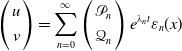
Setting
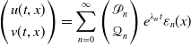 \begin{equation} \left ( \begin{array}{c} u(t,x) \\[3pt] v(t,x) \end{array} \right )= \sum \limits _{n=0}^{\infty } \left ( \begin{array}{c} \mathcal{P}_{n} \\[3pt] \mathcal{Q}_{n} \end{array} \right )e^{\lambda _{n}t}\varepsilon _{n}(x) \end{equation}
and plugging it into (3.1) produces the characteristic equation $\Gamma (\lambda )$
:
$\Gamma (\lambda )$
:
 \begin{align} \lambda ^{2}-(r_{11}+r_{22}-(d_{1}+d_{2})\theta _{n})\lambda +d_{1}d_{2}\theta ^{2}_{n}-(d_{1}r_{22}+d_{2}r_{11})\theta _{n}+r_{11}r_{22}-r_{12}r_{21}e^{-\lambda \tau }=0. \end{align}
Then, we see that $\Gamma (0)=d_{1}d_{2}\theta ^{2}_{n}-(d_{1}r_{22}+d_{2}r_{11})\theta _{n}+r_{11}r_{22}-r_{12}r_{21} \gt 0$
. As a consequence,
$\Gamma (0)=d_{1}d_{2}\theta ^{2}_{n}-(d_{1}r_{22}+d_{2}r_{11})\theta _{n}+r_{11}r_{22}-r_{12}r_{21} \gt 0$
. As a consequence, $E_{*}$
is always stable for (1.3) with
$E_{*}$
is always stable for (1.3) with $\tau =0$
, and (1.3) does not undergo Turing bifurcation for
$\tau =0$
, and (1.3) does not undergo Turing bifurcation for $\tau \geq 0$
. Therefore, the instability could only be caused by Hopf bifurcation.
$\tau \geq 0$
. Therefore, the instability could only be caused by Hopf bifurcation.
For the emergence of Hopf bifurcation, we set $\text{i}w \ (w \gt 0)$
a root of (3.5). Plugging it into (3.5) results in
$\text{i}w \ (w \gt 0)$
a root of (3.5). Plugging it into (3.5) results in
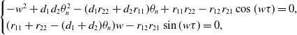 \begin{equation} \begin{cases} -w^{2}+d_{1}d_{2}\theta ^{2}_{n}-(d_{1}r_{22}+d_{2}r_{11})\theta _{n}+r_{11}r_{22}-r_{12}r_{21}\cos (w\tau )=0,\\ (r_{11}+r_{22}-(d_{1}+d_{2})\theta _{n})w-r_{12}r_{21}\sin (w\tau )=0, \end{cases} \end{equation}
which leads to
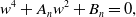 \begin{equation} w^{4}+A_{n}w^{2}+B_{n}=0, \end{equation}
where
 \begin{align} &A_{n}=(d_{1}\theta _{n}-r_{11})^{2}+(d_{2}\theta _{n}-r_{22})^{2}\gt 0, \end{align}
 \begin{align} &B_{n}=C_{n}D_{n}, \end{align}
with
 \begin{align} &C_{n}=d_{1}d_{2}\theta ^{2}_{n}-(d_{1}r_{22}+d_{2}r_{11})\theta _{n}+r_{11}r_{22}+r_{12}r_{21}, \end{align}
 \begin{align} &D_{n}=d_{1}d_{2}\theta ^{2}_{n}-(d_{1}r_{22}+d_{2}r_{11})\theta _{n}+r_{11}r_{22}-r_{12}r_{21}\gt 0. \end{align}
If $r_{11}r_{22}+r_{12}r_{21} \geq 0$
, then
$r_{11}r_{22}+r_{12}r_{21} \geq 0$
, then $B_{n}\gt 0$
, which intimates that Eq. (3.7) has no positive root. We thereby consider the positive root Eq. (3.7) under the condition
$B_{n}\gt 0$
, which intimates that Eq. (3.7) has no positive root. We thereby consider the positive root Eq. (3.7) under the condition $r_{11}r_{22}+r_{12}r_{21} \lt 0$
.
$r_{11}r_{22}+r_{12}r_{21} \lt 0$
.
Defining
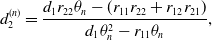 \begin{equation} d^{(n)}_{2}=\frac{d_{1}r_{22}\theta _{n}-(r_{11}r_{22}+r_{12}r_{21})}{d_{1}\theta ^{2}_{n}-r_{11}\theta _{n}}, \end{equation}
then
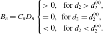 \begin{equation} B_{n}=C_{n}D_{n} \begin{cases} \gt 0, \, \, \ \text{for} \ d_{2} \gt d^{(n)}_{2},\\ =0, \, \, \text{for} \ d_{2} = d^{(n)}_{2},\\ \lt 0, \, \, \ \text{for} \ d_{2} \lt d^{(n)}_{2}. \end{cases} \end{equation}
Hence, Eq. (3.7) has no positive root for $d_{2} \geq d^{(n)}_{2}$
and has a positive root
$d_{2} \geq d^{(n)}_{2}$
and has a positive root $w^{(n)}$
for
$w^{(n)}$
for $d_{2} \lt d^{(n)}_{2}$
, where
$d_{2} \lt d^{(n)}_{2}$
, where
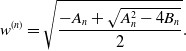 \begin{equation} w^{(n)}=\sqrt{\frac{-A_{n}+\sqrt{A^{2}_{n}-4B_{n}}}{2}}. \end{equation}
By (3.12), we get
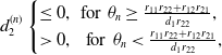 \begin{equation} d^{(n)}_{2} \begin{cases} \leq 0, \, \, \text{for} \, \, \theta _{n} \geq \frac{r_{11}r_{22}+r_{12}r_{21}}{d_{1}r_{22}},\\ \gt 0, \, \, \ \text{for} \, \, \theta _{n} \lt \frac{r_{11}r_{22}+r_{12}r_{21}}{d_{1}r_{22}}, \end{cases} \end{equation}
which intimates that Eq. (3.7) has no positive root for $\theta _{n} \geq \frac{r_{11}r_{22}+r_{12}r_{21}}{d_{1}r_{22}}$
and it’s possible that Eq. (3.7) has a positive root for
$\theta _{n} \geq \frac{r_{11}r_{22}+r_{12}r_{21}}{d_{1}r_{22}}$
and it’s possible that Eq. (3.7) has a positive root for $\theta _{n} \lt \frac{r_{11}r_{22}+r_{12}r_{21}}{d_{1}r_{22}}$
.
$\theta _{n} \lt \frac{r_{11}r_{22}+r_{12}r_{21}}{d_{1}r_{22}}$
.
We first present some results about the root of Eq. (3.7). Let
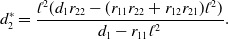 \begin{equation} d^{*}_{2}=\frac{\mathcal{l}^{2}(d_{1}r_{22}-(r_{11}r_{22}+r_{12}r_{21})\mathcal{l}^{2})}{d_{1}-r_{11}\mathcal{l}^{2}}. \end{equation}
Lemma 3.1. For Eq. (3.7), we have:
-
(A) If $r_{11}r_{22}+r_{12}r_{21}\geq 0$
, then there is no positive root for Eq. (3.7);
$r_{11}r_{22}+r_{12}r_{21}\geq 0$
, then there is no positive root for Eq. (3.7); -
(B) If
$r_{11}r_{22}+r_{12}r_{21}\lt 0$
, then


-
(I) if
$\frac{1}{\mathcal{l}^{2}} \geq \frac{r_{11}r_{22}+r_{12}r_{21}}{d_{1}r_{22}}$
, then there is no positive root for Eq. (3.7). -
(II) if
$\frac{1}{\mathcal{l}^{2}} \lt \frac{r_{11}r_{22}+r_{12}r_{21}}{d_{1}r_{22}}$
, then


Proof. For $\frac{1}{\mathcal{l}^{2}} \geq \frac{r_{11}r_{22}+r_{12}r_{21}}{d_{1}r_{22}}$
, we see that
$\frac{1}{\mathcal{l}^{2}} \geq \frac{r_{11}r_{22}+r_{12}r_{21}}{d_{1}r_{22}}$
, we see that $d_{2}\gt 0 \geq d^{(n)}_{2}$
, which means that there is no positive root for Eq. (3.7).
$d_{2}\gt 0 \geq d^{(n)}_{2}$
, which means that there is no positive root for Eq. (3.7).
Next we concern ourself with the case: $\frac{1}{\mathcal{l}^{2}} \lt \frac{r_{11}r_{22}+r_{12}r_{21}}{d_{1}r_{22}}$
. Let
$\frac{1}{\mathcal{l}^{2}} \lt \frac{r_{11}r_{22}+r_{12}r_{21}}{d_{1}r_{22}}$
. Let
 \begin{equation} f(x)=\frac{d_{1}r_{22}x-(r_{11}r_{22}+r_{12}r_{21})}{d_{1}x^{2}-r_{11}x}, \, \, \frac{1}{\mathcal{l}^{2}} \leq x \lt \frac{r_{11}r_{22}+r_{12}r_{21}}{d_{1}r_{22}}, \end{equation}
then
 \begin{equation} f^{\prime }(x)=\frac{-r_{22}d^{2}_{11}x^{2}+2d_{1}(r_{11}r_{22}+r_{12}r_{21})x-r_{11}(r_{11}r_{22}+r_{12}r_{21})}{(d_{1}x-r_{11})^{2}x^{2}}, \end{equation}
this combined with $r_{11}(r_{11}r_{22}+r_{12}r_{21})\gt 0$
shows that
$r_{11}(r_{11}r_{22}+r_{12}r_{21})\gt 0$
shows that $f(x)$
decreases monotonically with respect to
$f(x)$
decreases monotonically with respect to $x$
in
$x$
in $[\frac{1}{\mathcal{l}^{2}},\frac{r_{11}r_{22}+r_{12}r_{21}}{d_{1}r_{22}})$
. Thus,
$[\frac{1}{\mathcal{l}^{2}},\frac{r_{11}r_{22}+r_{12}r_{21}}{d_{1}r_{22}})$
. Thus, $f(x)$
reaches its maximum value at
$f(x)$
reaches its maximum value at $x=\frac{1}{\mathcal{l}^{2}}$
, namely
$x=\frac{1}{\mathcal{l}^{2}}$
, namely
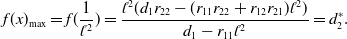 \begin{equation} f(x)_{\max }=f(\frac{1}{\mathcal{l}^{2}})=\frac{\mathcal{l}^{2}(d_{1}r_{22}-(r_{11}r_{22}+r_{12}r_{21})\mathcal{l}^{2})}{d_{1}-r_{11}\mathcal{l}^{2}} = d^{*}_{2}. \end{equation}
As a result of this, Eq. (3.7) has no positive root for $d_{2}\geq d^{*}_{2}$
and has a positive root for
$d_{2}\geq d^{*}_{2}$
and has a positive root for $d_{2} \lt d^{*}_{2}$
.
$d_{2} \lt d^{*}_{2}$
.
According to $\sin (w\tau )=\frac{(r_{11}+r_{22}-(d_{1}+d_{2})\theta _{n})w}{r_{12}r_{21}}\gt 0$
, we obtain
$\sin (w\tau )=\frac{(r_{11}+r_{22}-(d_{1}+d_{2})\theta _{n})w}{r_{12}r_{21}}\gt 0$
, we obtain
 \begin{equation} \tau ^{(n,j)}=\frac{1}{w^{(n)}} \left \{\arccos \left (\frac{-(w^{(n)})^{2}+d_{1}d_{2}\theta ^{2}_{n}-(d_{1}r_{22}+d_{2}r_{11})\theta _{n}+r_{11}r_{22}}{r_{12}r_{21}}\right )+2j\pi \right \}, \end{equation}
and $j\in \mathbb{N}=\{0,1,2,\cdots \}$
.
$j\in \mathbb{N}=\{0,1,2,\cdots \}$
.
Then we point out that $\tau ^{(n,j)}$
increases monotonically with respect to
$\tau ^{(n,j)}$
increases monotonically with respect to $d_{2}$
because of
$d_{2}$
because of
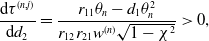 \begin{equation} \frac{\text{d}\tau ^{(n,j)}}{\text{d}d_{2}}=\frac{r_{11}\theta _{n}-d_{1}\theta ^{2}_{n}}{r_{12}r_{21}w^{(n)}\sqrt{1-\chi ^{2}}}\gt 0, \end{equation}
where
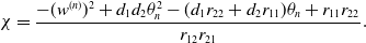 \begin{equation*} \chi =\frac {-(w^{(n)})^{2}+d_{1}d_{2}\theta ^{2}_{n}-(d_{1}r_{22}+d_{2}r_{11})\theta _{n}+r_{11}r_{22}}{r_{12}r_{21}}. \end{equation*}
Next we verify the transversality condition at $\tau =\tau ^{(n,j)}$
.
$\tau =\tau ^{(n,j)}$
.
Lemma 3.2.
If $\lambda (\tau )=\beta (\tau )+\text{i}\gamma (\tau )$
is a pair of roots of Eq. (3.5) near
$\lambda (\tau )=\beta (\tau )+\text{i}\gamma (\tau )$
is a pair of roots of Eq. (3.5) near $\tau =\tau ^{(n,j)}$
satisfying
$\tau =\tau ^{(n,j)}$
satisfying $\beta (\tau ^{(n,j)})=0$
and
$\beta (\tau ^{(n,j)})=0$
and $\gamma (\tau ^{(n,j)})=w^{(n)}$
, then we get
$\gamma (\tau ^{(n,j)})=w^{(n)}$
, then we get $\frac{\text{d}Re(\lambda (\tau ))}{\text{d}\tau }\big |_{\tau =\tau ^{(n,j)}} \gt 0$
.
$\frac{\text{d}Re(\lambda (\tau ))}{\text{d}\tau }\big |_{\tau =\tau ^{(n,j)}} \gt 0$
.
Proof. Taking the derivative of both sides of Eq. (3.5) with respect to $\tau$
yields
$\tau$
yields
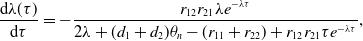 \begin{equation} \frac{\text{d}\lambda (\tau )}{\text{d}\tau }=-\frac{r_{12}r_{21}\lambda e^{-\lambda \tau }}{2\lambda +(d_{1}+d_{2})\theta _{n}-(r_{11}+r_{22})+r_{12}r_{21}\tau e^{-\lambda \tau }}, \end{equation}
that is,
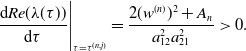 \begin{equation} \frac{\text{d}Re(\lambda (\tau ))}{\text{d}\tau }\Bigg |_{\tau =\tau ^{(n,j)}} =\frac{2(w^{(n)})^{2}+A_{n}}{a^{2}_{12}a^{2}_{21}}\gt 0. \end{equation}
Combining Lemmas 3.1 and 3.2 ultimately leads to the following statement.
Theorem 3.3.
For system (1.3), we suppose that $d^{*}_{2}$
and
$d^{*}_{2}$
and $\tau ^{(n,j)}$
are defined by (3.19) and (3.20), respectively.
$\tau ^{(n,j)}$
are defined by (3.19) and (3.20), respectively.
-
(I) If
$\frac{1}{\mathcal{l}^{2}} \geq \frac{r_{11}r_{22}+r_{12}r_{21}}{d_{1}r_{22}}$
, then
$E_{*}$
is stable for
$\tau \geq 0$
. -
(II) If
$\frac{1}{\mathcal{l}^{2}} \lt \frac{r_{11}r_{22}+r_{12}r_{21}}{d_{1}r_{22}}$
, then


-
(i) if
$d_{2}\geq d^{*}_{2}$
, then
$E_{*}$
is stable for
$\tau \geq 0$
; -
(ii) if
$d_{2}\lt d^{*}_{2}$
, then
$E_{*}$
is stable for
$\tau \lt \tau ^{*}$
and is unstable for
$\tau \gt \tau ^{*}$
, where
(3.24)with
\begin{equation} \tau ^{*}=\min \limits _{n=0,1,2,\cdots, n_{*}}\tau ^{(n,0)} \end{equation}
where
\begin{equation*} n_{*}=\min \{\widehat {n}, \ \widetilde {n}\}, \end{equation*}
$\widetilde{n}=\max \{n\in \mathbb{N}^{+}=\{1,2,\cdots \}\;:\; D_{n}\lt 0\}$
and
(3.25)where
\begin{equation} \widehat{n}= \begin{cases} 1, \, \, \, \, \, \, \, \, \, \, \text{if} \, \, 1 \lt n^{\#} \lt 2, \\ \left [ n^{\#}\right ], \, \, \, \, \ \text{if} \, \, n^{\#} \ \text{is not an integer and} \ n^{\#} \geq 2, \, \, \, \, n^{\#}= \mathcal{l}\sqrt{\frac{r_{11}r_{22}+r_{12}r_{21}}{d_{1}r_{22}}},\\ n^{\#}-1, \, \, \ \text{if} \, \, n^{\#} \ \text{is an integer and} \ n^{\#} \geq 2, \end{cases} \end{equation}
$[\cdot ]$
represents the integer part function;
-
(iii) mode-
$k$
spatially inhomogeneous Hopf bifurcations emerge at
$\tau =\tau ^{(k,j)}$
, where
$k=0,1,2,\cdots, n_{*}$
.


Remark 3.4. From Theorem 3.3, we conclude that if $d_{1}$
or
$d_{1}$
or $d_{2}$
is large enough, then
$d_{2}$
is large enough, then $E_{*}$
is always stable for
$E_{*}$
is always stable for $\tau \geq 0$
. However, the discrete delay
$\tau \geq 0$
. However, the discrete delay $\tau$
could cause Hopf bifurcation for the appropriate dispersal rate
$\tau$
could cause Hopf bifurcation for the appropriate dispersal rate $d_{2}$
. And large enough delay
$d_{2}$
. And large enough delay $\tau$
makes
$\tau$
makes $E_{*}$
unstable.
$E_{*}$
unstable.
Next, we utilize the means in Song et al. [Reference Song, Peng and Zou24] so as to achieve the normal formal computation of spatially Hopf bifurcations at $\tau =\tau ^{(k,j)}$
with
$\tau =\tau ^{(k,j)}$
with $k= 0,1,2,\cdots, n_{*}$
. For generality, we denote these delay thresholds by
$k= 0,1,2,\cdots, n_{*}$
. For generality, we denote these delay thresholds by $\tau ^{*}$
so that (3.5) possesses a pair of purely imaginary roots
$\tau ^{*}$
so that (3.5) possesses a pair of purely imaginary roots $\pm w^{(n)}$
represented by
$\pm w^{(n)}$
represented by $\pm w^{*}$
. Setting
$\pm w^{*}$
. Setting
 \begin{equation*} \gimel \;:\!=\{(u,v) \in (W^{2,2}(0,\mathcal {l}\pi ))^{2}\;:\; (u_{x},v_{x})|_{x=0,\mathcal {l}\pi } =0 \}, \end{equation*} $\widehat{u}(t,\cdot )=u(\tau t,\cdot )-u_{*}, \ \widehat{v}(t,\cdot )=v(\tau t,\cdot )-v_{*}, \ \widehat{Z}(t)=(\widehat{u}(\cdot, t),\widehat{v}(\cdot, t))$
and then removing the hats, (1.3) turns into
$\widehat{u}(t,\cdot )=u(\tau t,\cdot )-u_{*}, \ \widehat{v}(t,\cdot )=v(\tau t,\cdot )-v_{*}, \ \widehat{Z}(t)=(\widehat{u}(\cdot, t),\widehat{v}(\cdot, t))$
and then removing the hats, (1.3) turns into
 \begin{equation} Z_{t}=\tau d \Delta Z(t)+L(\tau )(Z_{t})+f(Z_{t},\tau ), \end{equation}
where
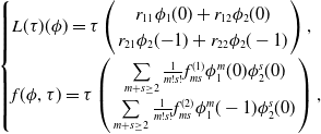 \begin{equation} \begin{cases} L(\tau )(\phi )=\tau \left ( \begin{array}{c} r_{11}\phi _{1}(0)+r_{12}\phi _{2}(0) \\ r_{21}\phi _{2}({-}1)+r_{22}\phi _{2}(-1) \end{array} \right ),\\[10pt] f(\phi, \tau )= \tau \left ( \begin{array}{c} \sum \limits _{m+s\geq 2}\frac{1}{m!s!}f^{(1)}_{ms}\phi ^{m}_{1}(0)\phi ^{s}_{2}(0) \\[3pt] \sum \limits _{m+s\geq 2}\frac{1}{m!s!}f^{(2)}_{ms}\phi ^{m}_{1}(-1)\phi ^{s}_{2}(0) \end{array} \right ),\, \, \end{cases} \end{equation}
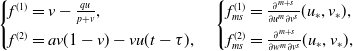 \begin{equation} \begin{cases} f^{(1)}=v-\frac{qu}{p+v},\\[3pt] f^{(2)}=av(1-v)-vu(t-\tau ),\\ \end{cases} \begin{cases} f^{(1)}_{ms}=\frac{\partial ^{m+s}}{\partial u^{m} \partial v^{s}}(u_{*},v_{*}),\\[3pt] f^{(2)}_{ms}=\frac{\partial ^{m+s}}{\partial w^{m} \partial v^{s}}(u_{*},v_{*}), \end{cases} \end{equation}
Setting $\tau =\tau ^{*}+\delta, \delta \in \mathbb{R}$
, Eq. (3.26) thereby turns into
$\tau =\tau ^{*}+\delta, \delta \in \mathbb{R}$
, Eq. (3.26) thereby turns into
 \begin{equation} Z_{t}=\tau ^{*}d\Delta Z(t)+L(\tau ^{*}(Z(t))+F(Z_{t},\delta ), \end{equation}
where $F(\phi, \delta )=\delta d\Delta \phi (0)+L(\delta )(\phi )+f(\phi, \tau ^{*}+\delta )$
for
$F(\phi, \delta )=\delta d\Delta \phi (0)+L(\delta )(\phi )+f(\phi, \tau ^{*}+\delta )$
for $\phi \in \mathcal{C}$
. Hence,
$\phi \in \mathcal{C}$
. Hence, $\Lambda _{0}=\{\text{i}\tau ^{*}w^{*},-\text{i}\tau ^{*}w^{*}\}$
is the set of eigenvalues. The eigenvalues of
$\Lambda _{0}=\{\text{i}\tau ^{*}w^{*},-\text{i}\tau ^{*}w^{*}\}$
is the set of eigenvalues. The eigenvalues of $\tau ^{*}d\Delta$
on
$\tau ^{*}d\Delta$
on $\gimel$
are
$\gimel$
are $\zeta ^{1}_{k}=-n^{2}d_{1}\tau ^{*}$
and
$\zeta ^{1}_{k}=-n^{2}d_{1}\tau ^{*}$
and $\zeta ^{2}_{k}=-n^{2}d_{2}\tau ^{*}$
with
$\zeta ^{2}_{k}=-n^{2}d_{2}\tau ^{*}$
with $n\in \mathbb{N}^{+}$
, and the corresponding normalized eigenfunctions
$n\in \mathbb{N}^{+}$
, and the corresponding normalized eigenfunctions $\alpha ^{(i)}_{n}(x)$
reads
$\alpha ^{(i)}_{n}(x)$
reads
 \begin{equation} \alpha ^{(1)}_{n}(x)= \left ( \begin{array}{c} \beta _{n}(x) \\[3pt] 0 \end{array} \right ), \, \, \alpha ^{(2)}_{n}(x)= \left ( \begin{array}{c} 0 \\[3pt] \beta _{n}(x) \end{array} \right ), \, \, \text{with} \ \beta _{n}(x)=\frac{\cos (nx)}{||\cos (nx)||_{2,2}}, \, \, n\in \mathbb{N}^{+}. \end{equation}
Letting $\mathcal{B}_{n}=\text{span}\{[v(\cdot ), \alpha ^{(i)}_{n}(x)]\alpha ^{(i)}_{n}(x)|v\in \mathcal{C}\}$
and assuming that
$\mathcal{B}_{n}=\text{span}\{[v(\cdot ), \alpha ^{(i)}_{n}(x)]\alpha ^{(i)}_{n}(x)|v\in \mathcal{C}\}$
and assuming that $z_{t}(\rho )\in C([{-}1,0],\mathbb{R}^{2})$
with
$z_{t}(\rho )\in C([{-}1,0],\mathbb{R}^{2})$
with
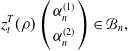 \begin{equation} z^{T}_{t}(\rho ) \left ( \begin{array}{c} \alpha ^{(1)}_{n} \\[3pt] \alpha ^{(2)}_{n} \end{array} \right ) \in \mathcal{B}_{n}, \end{equation}
then we obtain the equivalent ODE on $\mathbb{R}$
reading
$\mathbb{R}$
reading
 \begin{equation} \dot{z}(t)= \left ( \begin{array}{c@{\quad}c} \zeta ^{(1)}_{n} & 0\\[3pt] 0 & \zeta ^{(2)}_{n} \end{array} \right ) z(t)+L(\tau ^{*})z_{t} \end{equation}
whose characteristic equation is (3.5). Define
 \begin{equation*} \lt \psi (s),\phi (\rho )\gt =\psi (0)\phi (0)-\int _{-1}^{0}\int _{0}^{\rho }\psi (\xi -\rho )d\eta (\rho )\phi (\xi )d\xi, \ \text {for} \ \psi \in C^{*}, \, \, \phi \in C. \end{equation*}
Then we get
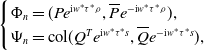 \begin{equation*} \begin {cases} \Phi _{n}=(Pe^{\text {i}w^{*}\tau ^{*}\rho },\overline {P}e^{-\text {i}w^{*}\tau ^{*}\rho }),\\ \Psi _{n}=\text {col}(Q^{T}e^{\text {i}w^{*}\tau ^{*}s},\overline {Q}e^{-\text {i}w^{*}\tau ^{*}s}),\\ \end {cases} \end{equation*}
with $\lt \Phi _{n},\Psi _{n}\gt =I_{2}$
, where
$\lt \Phi _{n},\Psi _{n}\gt =I_{2}$
, where
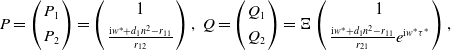 \begin{equation} P= \left ( \begin{array}{c} P_{1} \\[3pt] P_{2} \end{array} \right ) = \left ( \begin{array}{c} 1 \\[3pt] \frac{\text{i}w^{*}+d_{1}n^{2}-r_{11}}{r_{12}} \end{array} \right ), \ Q= \left ( \begin{array}{c} Q_{1} \\[3pt] Q_{2} \end{array} \right ) =\Xi \left ( \begin{array}{c} 1 \\[3pt] \frac{\text{i}w^{*}+d_{1}n^{2}-r_{11}}{r_{21}}e^{\text{i}w^{*}\tau ^{*}} \end{array} \right ), \end{equation}
with
 \begin{equation*} \Xi =\left ( 1+\tau ^{*}(\text {i}w^{*}+d_{1}n^{2}-r_{11})+\frac {(\tau ^{*}r_{22}+e^{\text {i}w^{*}\tau ^{*}} )(\text {i}w^{*}+d_{1}n^{2}-r_{11})^{2}}{r_{12}r_{21}} \right )^{-1}. \end{equation*}
Utilizing the means in Song et al. [Reference Song, Peng and Zou24], we get the following normal form
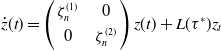
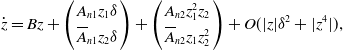 \begin{equation} \dot{z}=Bz+ \left ( \begin{array}{c} A_{n1}z_{1}\delta \\[3pt] \overline{A}_{n1}z_{2} \delta \end{array} \right )+ \left ( \begin{array}{c} A_{n2}z^{2}_{1}z_{2} \\[3pt] \overline{A}_{n2}z_{1}z^{2}_{2} \end{array} \right )+O(|z|\delta ^{2}+|z^{4}|), \end{equation}
where
 \begin{align} &A_{n1}=-n^{2}(d_{1}P_{1}Q_{1}+d_{2}P_{2}Q_{2})+\text{i}w^{*}Q^{T}P, \end{align}
 \begin{align} &A_{n2}=-\frac{\text{i}}{2w^{*}\tau ^{*}}\left ( r_{n20}r_{n11}-2|r_{n11}|^{2}-\frac{1}{3}|r_{n02}|^{2}+\frac{1}{2}(r_{n21}+b_{n21}) \right ), \end{align}
with
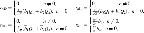 \begin{align*} &r_{n20}= \begin{cases} 0, \, \, \, \, \, \, \, \, \, \, \, \, \, \, \, \, \, \, \, \, \, \, n \neq 0, \\ \frac{\tau ^{*}}{\sqrt{\pi }}(b_{1}Q_{1}+b_{2}Q_{2}), \, \, n=0, \end{cases} r_{n11}= \begin{cases} 0, \, \, \, \, \, \, \, \, \, \, \, \, \, \, \, \, \, \, \, \, \, \, n \neq 0, \\ \frac{\tau ^{*}}{\sqrt{\pi }}(b_{3}Q_{1}+b_{4}Q_{2}), \, \, n=0, \end{cases} \\ &r_{n02}= \begin{cases} 0, \, \, \, \, \, \, \, \, \, \, \, \, \, \, \, \, \, \, \, \, \, \, n \neq 0, \\ \frac{\tau ^{*}}{\sqrt{\pi }}(\overline{b}_{1}Q_{1}+\overline{b}_{2}Q_{2}), \, \, n=0, \end{cases} r_{n21}= \begin{cases} \frac{3\tau ^{*}}{2\pi }b_{4}, \, \, n \neq 0, \\ \frac{\tau ^{*}}{\pi }b_{4}, \, \, n=0, \end{cases} \end{align*}
where
 \begin{align*} b_{1}&=f^{(1)}_{20}P^{2}_{1}+2f^{(1)}_{11}P_{1}P_{2}+f^{(1)}_{02}P^{2}_{2}, \, \, \, \, \, \, \, \, \, \, \, \, \, \, \, \, b_{2}=f^{(2)}_{20}P^{2}_{1}e^{-2\text{i}w^{*}\tau ^{*}}+2f^{(2)}_{11}P_{1}P_{2}e^{-\text{i}w^{*}\tau ^{*}},\\ b_{3}&=f^{(1)}_{20}|P_{1}|^{2}+2f^{(1)}_{11}\text{Re}\{P_{1}\overline{P}_{2}\}+f^{(1)}_{02}|P_{2}|^{2}, \, \, \ \ b_{4}=f^{(2)}_{20}|P_{1}|^{2}+2f^{(2)}_{11}\text{Re}\{ P_{1}\overline{P}_{2} e^{-\text{i}w^{*}\tau ^{*} } \},\\ b_{5}&=Q_{1}\left ( f^{(1)}_{30}P_{1}|P_{1}|^{2}+f^{(1)}_{03}P_{2}|P_{2}|^{2}+f^{(1)}_{21}(P^{2}_{1}|\overline{P}_{2}|+2|P_{1}|^{2}P_{2})+ f^{(1)}_{12}(|\overline{P}_{1}|P^{2}_{2}+2P_{1}|P_{2}|^{2} )\right )\\ &+Q_{2}\left ( f^{(2)}_{30}P_{1}|P_{1}|^{2}e^{-\text{i}w^{*}\tau ^{*}}+f^{(2)}_{21}(P^{2}_{1}|\overline{P}_{2}|e^{-2\text{i}w^{*}\tau ^{*}}+2|P_{1}|^{2}P_{2} )\right ). \end{align*}
And
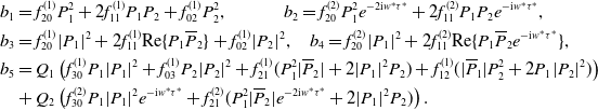
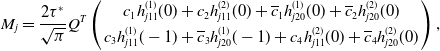
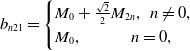 \begin{equation} b_{n21}= \begin{cases} M_{0}+\frac{\sqrt{2}}{2}M_{2n}, \, \, n\neq 0, \\ M_{0}, \, \, \, \, \, \, \, \, \, \, \ \, \, \, \, n=0, \\ \end{cases} \end{equation}
where for $j=0,2n$
,
$j=0,2n$
,
 \begin{equation*} M_{j}=\frac {2\tau ^{*}}{\sqrt {\pi }}Q^{T} \left ( \begin {array}{c} c_{1}h^{(1)}_{j11}(0)+c_{2}h^{(2)}_{j11}(0)+\overline {c}_{1}h^{(1)}_{j20}(0)+\overline {c}_{2}h^{(2)}_{j20}(0) \\[3pt] c_{3}h^{(1)}_{j11}(-1)+\overline {c}_{3}h^{(1)}_{j20}(-1)+c_{4}h^{(2)}_{j11}(0)+\overline {c}_{4}h^{(2)}_{j20}(0) \end {array} \right ), \end{equation*}
with
 \begin{align*} c_{1}=f^{(1)}_{20}P_{1}+f^{(1)}P_{2}, \, \, c_{2}=f^{(1)}_{11}P_{1}+f^{(1)}_{02}P_{2}, \, \, c_{3}=f^{(2)}_{20}P_{1}e^{-\text{i}w^{*}\tau ^{*}}+f^{(2)}_{11}P_{2}, \, \, c_{4}=f^{(2)}_{11}P_{1}e^{-\text{i}w^{*}\tau ^{*}}, \end{align*}
and
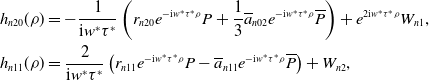 \begin{align*} &h_{n20}(\rho )=-\frac{1}{\text{i}w^{*}\tau ^{*}}\left (r_{n20}e^{-\text{i}w^{*}\tau ^{*}\rho }P +\frac{1}{3}\overline{a}_{n02} e^{-\text{i}w^{*}\tau ^{*}\rho } \overline{P} \right )+e^{2\text{i}w^{*}\tau ^{*}\rho }W_{n1},\\ &h_{n11}(\rho )=\frac{2}{\text{i}w^{*}\tau ^{*}}\left (r_{n11}e^{-\text{i}w^{*}\tau ^{*}\rho }P-\overline{a}_{n11} e^{-\text{i}w^{*}\tau ^{*}\rho } \overline{P} \right )+W_{n2}, \end{align*}
where
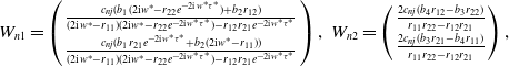 \begin{equation} W_{n1}= \left ( \begin{array}{c} \frac{c_{nj}(b_{1}(2\text{i}w^{*}-r_{22}e^{-2\text{i}w^{*}\tau ^{*}})+b_{2}r_{12})}{(2\text{i}w^{*}-r_{11})(2\text{i}w^{*}-r_{22}e^{-2\text{i}w^{*}\tau ^{*}})-r_{12}r_{21}e^{-2\text{i}w^{*}\tau ^{*}}}\\[3pt] \frac{c_{nj}(b_{1}r_{21}e^{-2\text{i}w^{*}\tau ^{*}}+b_{2}(2\text{i}w^{*}-r_{11}) )}{(2\text{i}w^{*}-r_{11})(2\text{i}w^{*}-r_{22}e^{-2\text{i}w^{*}\tau ^{*}})-r_{12}r_{21}e^{-2\text{i}w^{*}\tau ^{*}}}\\ \end{array} \right ), \ W_{n2}= \left ( \begin{array}{c} \frac{2c_{nj}(b_{4}r_{12}-b_{3}r_{22})}{r_{11}r_{22}-r_{12}r_{21}}\\[3pt] \frac{2c_{nj}(b_{3}r_{21}-b_{4}r_{11})}{r_{11}r_{22}-r_{12}r_{21}} \end{array} \right ), \end{equation}
and
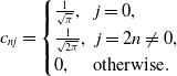 \begin{equation} c_{nj}= \begin{cases} \frac{1}{\sqrt{\pi }}, \, \, \ j=0, \\ \frac{1}{\sqrt{2\pi }}, \, \, j=2n \neq 0, \\ 0, \, \, \, \, \, \, \text{otherwise}. \end{cases} \end{equation}
Using the polar coordinate transformation, (3.34) turns into
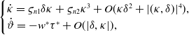 \begin{equation} \begin{cases} \dot{\kappa }=\varsigma _{n1}\delta \kappa +\varsigma _{n2}\kappa ^{3}+O(\kappa \delta ^{2}+|(\kappa, \delta )|^{4}),\\ \dot{\vartheta }=-w^{*}\tau ^{*}+O(|\delta, \kappa |), \end{cases} \end{equation}
where $\varsigma _{n1}=\text{Re}A_{n1}$
and
$\varsigma _{n1}=\text{Re}A_{n1}$
and $\varsigma _{n2}=\text{Re}A_{n2}$
.
$\varsigma _{n2}=\text{Re}A_{n2}$
.
From Chow and Hale [Reference Chow and Hale5], we conclude that Hopf bifurcation remains supercritical for $\varsigma _{n1}\varsigma _{n2}\lt 0$
and remains subcritical for
$\varsigma _{n1}\varsigma _{n2}\lt 0$
and remains subcritical for $\varsigma _{n1}\varsigma _{n2}\gt 0$
; Hopf bifurcation remains stable for
$\varsigma _{n1}\varsigma _{n2}\gt 0$
; Hopf bifurcation remains stable for $\varsigma _{n1}\lt 0$
and remains unstable for
$\varsigma _{n1}\lt 0$
and remains unstable for $\varsigma _{n1}\gt 0$
.
$\varsigma _{n1}\gt 0$
.
4. Dynamics of the spatial plant-sulphide model with distributed delay
System (1.3) with distributed delay $\sigma$
reads:
$\sigma$
reads:
 \begin{equation} \begin{cases} u_{t}=d_{1}\Delta u+v-\frac{qu}{p+v}, \\ v_{t}=d_{2}\Delta v+av(1-v)-v\int _{-\infty }^{t}G(t-\eta )u(x,\eta )d\eta, \\ (u,v)(x,0)=(u_{0}(x),v_{0}(x)) \geq 0, \ (t,x) \in [{-}\sigma, 0]\times (0,\mathcal{l}\pi ). \end{cases} \end{equation}
where $G(t)=\frac{1}{\sigma }e^{-\frac{t}{\sigma }}$
and other conditions are coincident with (1.3).
$G(t)=\frac{1}{\sigma }e^{-\frac{t}{\sigma }}$
and other conditions are coincident with (1.3).
Linearizing system (4.1) at $E_{*}$
generates
$E_{*}$
generates
 \begin{equation} \left ( \begin{array}{c} u_{t} \\[3pt] v_{t} \end{array} \right ) =J_{1} \left ( \begin{array}{c} \Delta u \\[3pt] \Delta v \end{array} \right ) +J_{2} \left ( \begin{array}{c} \widetilde{u} \\[3pt] \widetilde{v} \end{array} \right ) +J_{3} \left ( \begin{array}{c} u \\[3pt] v \end{array} \right ), \end{equation}
where $\widetilde{u}=\int _{-\infty }^{t}G(t-\eta )u(x,\eta )d\eta, \ \widetilde{v}= \int _{-\infty }^{t}G(t-\eta )v(x,\eta )d\eta$
,
$\widetilde{u}=\int _{-\infty }^{t}G(t-\eta )u(x,\eta )d\eta, \ \widetilde{v}= \int _{-\infty }^{t}G(t-\eta )v(x,\eta )d\eta$
, $J_{i} \ (i=1,2,3)$
are consistent with (3.2).
$J_{i} \ (i=1,2,3)$
are consistent with (3.2).
Plugging
 \begin{equation} \left ( \begin{array}{c} u \\[3pt] v \end{array} \right )= \sum \limits _{n=0}^{\infty } \left ( \begin{array}{c} \mathcal{P}_{n} \\[3pt] \mathcal{Q}_{n} \end{array} \right )e^{\lambda _{n}t}\varepsilon _{n}(x) \end{equation}
into (4.1) produces the characteristic equation $\widehat{\Gamma }(\lambda )$
:
$\widehat{\Gamma }(\lambda )$
:
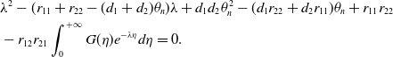 \begin{equation} \begin{aligned} &\lambda ^{2}-(r_{11}+r_{22}-(d_{1}+d_{2})\theta _{n})\lambda +d_{1}d_{2}\theta ^{2}_{n}-(d_{1}r_{22}+d_{2}r_{11})\theta _{n} +r_{11}r_{22}\\ &-r_{12}r_{21}\int _{0}^{+\infty }G(\eta )e^{-\lambda \eta }d\eta =0. \end{aligned} \end{equation}
Due to $\lim \limits _{\sigma \to 0^{+}}G(\eta )e^{-\lambda \eta }d\eta =1$
, thus
$\lim \limits _{\sigma \to 0^{+}}G(\eta )e^{-\lambda \eta }d\eta =1$
, thus $\widehat{\Gamma }(0)=\Gamma (0)\neq 0$
, which suggests that there’s no Turing bifurcation. As a result, Eq. (4.4) becomes
$\widehat{\Gamma }(0)=\Gamma (0)\neq 0$
, which suggests that there’s no Turing bifurcation. As a result, Eq. (4.4) becomes
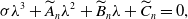 \begin{equation} \sigma \lambda ^{3}+\widetilde{A}_{n} \lambda ^{2}+\widetilde{B}_{n}\lambda +\widetilde{C}_{n}=0, \end{equation}
where
 \begin{align*} &\widetilde{A}_{n}=\sigma (d_{1}+d_{2})\theta _{n}+1-\sigma (r_{11}+r_{22}),\\ &\widetilde{B}_{n}=\sigma (d_{1}d_{2}\theta ^{2}_{n}-(d_{1}r_{22}+d_{2}r_{11})\theta _{n} +r_{11}r_{22})-(r_{11}+r_{22}-(d_{1}+d_{2})\theta _{n}),\\ &\widetilde{C}_{n}=d_{1}d_{2}\theta ^{2}_{n}-(d_{1}r_{22}+d_{2}r_{11})\theta _{n} +r_{11}r_{22}-r_{12}r_{21}. \end{align*}
It’s easy to see $\widetilde{A}_{n}, \ \widetilde{B}_{n}, \ \widetilde{C}_{n}\gt 0$
. In line with the Routh-Hurwitz criterion, we arrive at the following consequence.
$\widetilde{A}_{n}, \ \widetilde{B}_{n}, \ \widetilde{C}_{n}\gt 0$
. In line with the Routh-Hurwitz criterion, we arrive at the following consequence.
Lemma 4.1. For Eq. (4.5), we have:
-
(i) The real parts of whole roots are negative iff
$\widetilde{A}_{n}\widetilde{B}_{n}-\sigma \widetilde{C}_{n}\gt 0$
. -
(ii) A pair of purely imaginary roots
$\pm$
i
$\sqrt{\frac{\widetilde{B}_{n}}{\sigma }}$
exist iff
$\widetilde{A}_{n}\widetilde{B}_{n}-\sigma \widetilde{C}_{n}= 0$
.


Direct calculation displays
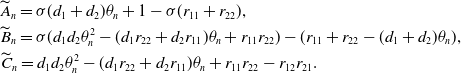
 \begin{align} \widetilde{A}_{n}\widetilde{B}_{n}-\sigma \widetilde{C}_{n}=\widetilde{A}_{n1}\sigma ^{2}+\widetilde{B}_{n1}\sigma +\widetilde{C}_{n1}, \end{align}
where
 \begin{equation*} \begin {aligned} &\widetilde {A}_{n1}=\left ((d_{1}+d_{2})\theta _{n}-(r_{11}+r_{22})\right )\left (d_{1}d_{2}\theta ^{2}_{n}-(d_{1}r_{22}+d_{2}r_{11})\theta _{n} +r_{11}r_{22} \right ),\\ &\widetilde {B}_{n1}=\left ((d_{1}+d_{2})\theta _{n}-(r_{11}+r_{22})\right )^{2}+r_{12}r_{21},\\ &\widetilde {C}_{n1}=(d_{1}+d_{2})\theta _{n}-(r_{11}+r_{22}). \end {aligned} \end{equation*}
It’s easy to see $\widetilde{A}_{n1}, \ \widetilde{C}_{n1}\gt 0$
. Defining
$\widetilde{A}_{n1}, \ \widetilde{C}_{n1}\gt 0$
. Defining
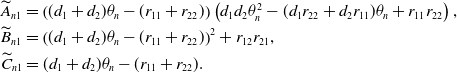
 \begin{equation} \widehat{d}^{(n)}_{2}=\frac{r_{11}+r_{22}+\sqrt{-r_{12}r_{21}}}{\theta _{n}}-d_{1}, \end{equation}
then $\widetilde{B}_{n1}\gt 0$
for
$\widetilde{B}_{n1}\gt 0$
for $d_{2} \gt \widehat{d}^{(n)}_{2}$
. It’s not hard to demonstrate that the maximum value of
$d_{2} \gt \widehat{d}^{(n)}_{2}$
. It’s not hard to demonstrate that the maximum value of $\widehat{d}^{(n)}_{2}$
is
$\widehat{d}^{(n)}_{2}$
is
 \begin{equation} \max \limits _{n\in \mathbb{N}^{+}}\widehat{d}^{(n)}_{2}=(r_{11}+r_{22}+\sqrt{-r_{12}r_{21}})\mathcal{l}^{2}-d_{1} \triangleq d^{\#}_{2}. \end{equation}
Thereby Eq. (4.6) has no positive roots for $d_{2}\geq d^{\#}_{2}$
and it’s possible that Eq. (4.6) possesses positive roots for
$d_{2}\geq d^{\#}_{2}$
and it’s possible that Eq. (4.6) possesses positive roots for $d_{2}\lt d^{\#}_{2}$
.
$d_{2}\lt d^{\#}_{2}$
.
Clearly, the equation $\widetilde{A}_{n1}\sigma ^{2}+\widetilde{B}_{n2}\sigma +\widetilde{C}_{n1}=0$
possesses two positive roots
$\widetilde{A}_{n1}\sigma ^{2}+\widetilde{B}_{n2}\sigma +\widetilde{C}_{n1}=0$
possesses two positive roots $\sigma ^{-}_{n}$
and
$\sigma ^{-}_{n}$
and $\sigma ^{+}_{n}$ $(\sigma ^{-}_{n}\lt \sigma ^{+}_{n})$
iff
$(\sigma ^{-}_{n}\lt \sigma ^{+}_{n})$
iff $\widetilde{B}^{2}_{n1}-4\widetilde{A}_{n1}\widetilde{C}_{n1}\gt 0, \ \widetilde{B}_{n1}\lt 0$
, where
$\widetilde{B}^{2}_{n1}-4\widetilde{A}_{n1}\widetilde{C}_{n1}\gt 0, \ \widetilde{B}_{n1}\lt 0$
, where
 \begin{align*} &\sigma ^{-}_{n}=\frac{-\widetilde{B}_{n1}-\sqrt{\widetilde{B}^{2}_{n1}-4\widetilde{A}_{n1}\widetilde{C}_{n1}}}{2\widetilde{A}_{n1}},\\ &\sigma ^{+}_{n}=\frac{-\widetilde{B}_{n1}+\sqrt{\widetilde{B}^{2}_{n1}-4\widetilde{A}_{n1}\widetilde{C}_{n1}}}{2\widetilde{A}_{n1}}. \end{align*}
Define
 \begin{equation*} S=\{n \in \mathbb {N}^{+}\;:\; \widetilde {B}^{2}_{n1}-4\widetilde {A}_{n1}\widetilde {C}_{n1}\gt 0, \ \widetilde {B}_{n1}\lt 0\}, \end{equation*}
which is obviously a finite set.
The following transversality condition at $\sigma =\sigma ^{\pm }_{n}$
holds.
$\sigma =\sigma ^{\pm }_{n}$
holds.
 \begin{align*} \frac{\text{d}Re(\lambda (\sigma ))}{\text{d}\sigma }\Bigg |_{\sigma =\sigma ^{\pm }_{n}}&=-\frac{\frac{\text{d}\widetilde{A}_{n}}{\text{d}d_{2}}\lambda ^{2}+\frac{\text{d}\widetilde{B}_{n}}{\text{d}d_{2}}\lambda +\frac{\text{d}\widetilde{C}_{n}}{\text{d}d_{2}}}{3\sigma ^{\pm }_{n} \lambda ^{2}+2\widetilde{A}_{n}\lambda +\widetilde{B}_{n}}\\ &=\frac{(\sigma ^{\pm }_{n})^{2}(d_{1}\theta ^{2}_{n}-r_{11}\theta _{n})(r_{11}+r_{22}-(d_{1}+d_{2})\theta _{n})-(\sigma \widetilde{B}_{n}+\widetilde{A}_{n})\theta _{n}}{2(\widetilde{A}^{2}_{n}+\sigma ^{\pm }_{n}\widetilde{B}_{n})}\\ &\lt 0. \end{align*}
This combined with Lemma 4.1 obtains the following consequence.
Theorem 4.2.
For system (4.1), $d^{\#}_{2}$
is defined by (4.8), then we have:
$d^{\#}_{2}$
is defined by (4.8), then we have:
-
(I) If
$d_{2} \geq d^{\#}_{2}$
, then
$E_{*}$
is stable for
$\sigma \geq 0$
. -
(II) If
$d_{2} \lt d^{\#}_{2}$
, then


-
(i)
$E_{*}$
is stable for
$\sigma \lt \sigma _{*}$
or
$\sigma \gt \sigma ^{*}$
and is unstable for
$\sigma _{*} \lt \sigma \lt \sigma ^{*}$
, where
\begin{equation*} \sigma _{*}=\min \limits _{n\in S}\sigma ^{-}_{n}, \ \sigma ^{*}=\max \limits _{n\in S}\sigma ^{+}_{n};\\ \end{equation*}
-
(ii) Hopf bifurcations emerge at
$\sigma =\sigma ^{\pm }_{n}$
for
$n \in S$
.


Remark 4.3. From (4.6) and Theorem 4.2, we conclude that if $d_{1}$
or
$d_{1}$
or $d_{2}$
is large enough, then
$d_{2}$
is large enough, then $E_{*}$
is always stable for
$E_{*}$
is always stable for $\sigma \geq 0$
. However, the distributed delay
$\sigma \geq 0$
. However, the distributed delay $\sigma$
could cause Hopf bifurcation for the appropriate dispersal rate
$\sigma$
could cause Hopf bifurcation for the appropriate dispersal rate $d_{2}$
. In contrast to the discrete delay
$d_{2}$
. In contrast to the discrete delay $\tau$
, a sufficiently large distributed delay
$\tau$
, a sufficiently large distributed delay $\sigma$
still makes
$\sigma$
still makes $E_{*}$
stable. That is, the stability interval for the distributed delay is larger than that for the discrete delay.
$E_{*}$
stable. That is, the stability interval for the distributed delay is larger than that for the discrete delay.
5. Numerical results
For system (1.3), we fix the parameters $(a,p,q,d_{1},\mathcal{l})=(1,0.5,0.2,0.02,1)$
and vary the parameters
$(a,p,q,d_{1},\mathcal{l})=(1,0.5,0.2,0.02,1)$
and vary the parameters $(\tau, d_{2})$
in order to illustrate numerically the results mentioned above.
$(\tau, d_{2})$
in order to illustrate numerically the results mentioned above.
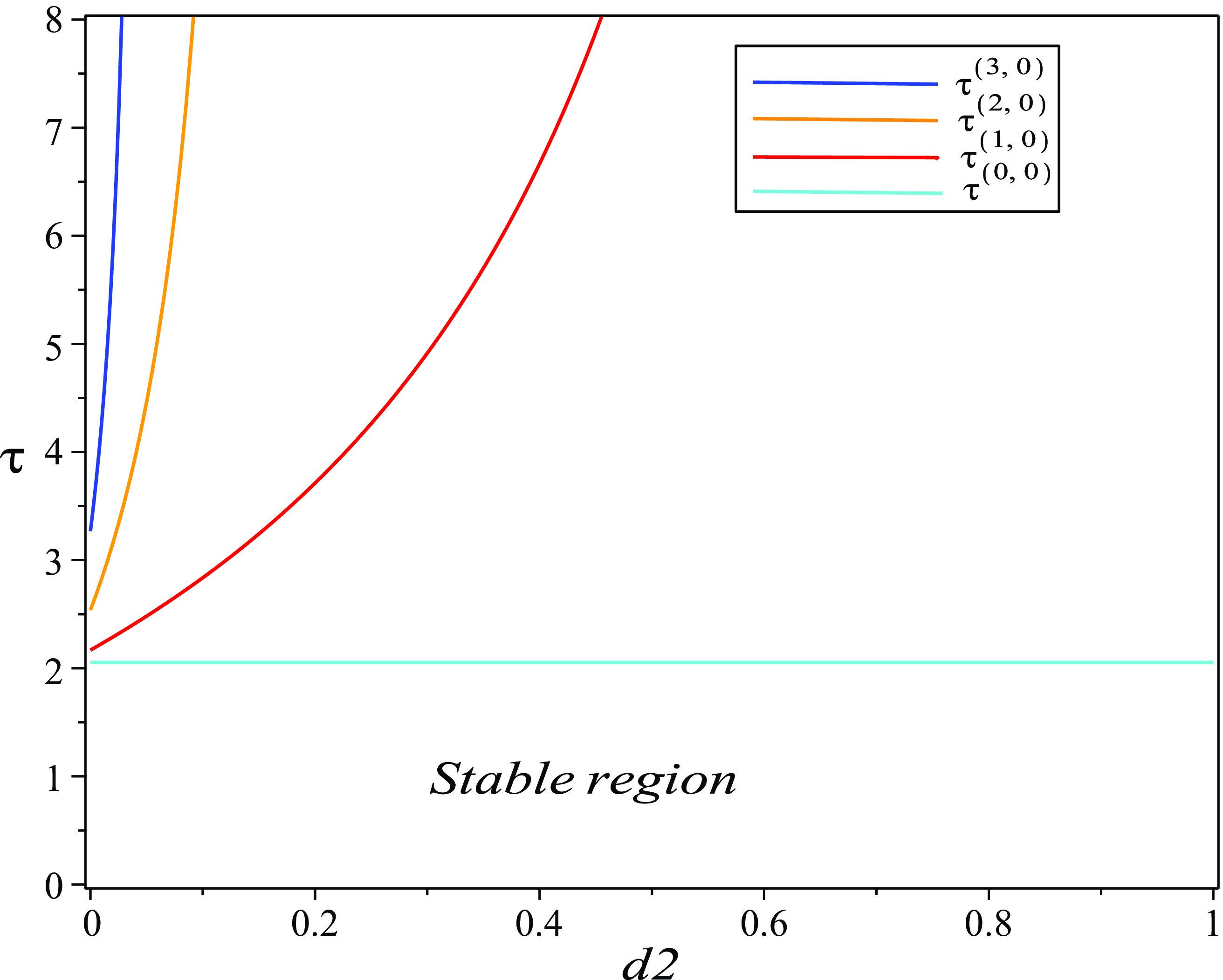
Figure 1 depicts the global stability of $E_{*}$
for the non-delay system (2.1). For fixed
$E_{*}$
for the non-delay system (2.1). For fixed $d_{2}=0.024$
, we get
$d_{2}=0.024$
, we get $d^{*}_{2}=0.7333$
and
$d^{*}_{2}=0.7333$
and $n_{*}=\min \{\widehat{n},\ \widetilde{n}\}=\min \{7,3\}=3$
, which intimates that mode-
$n_{*}=\min \{\widehat{n},\ \widetilde{n}\}=\min \{7,3\}=3$
, which intimates that mode- $k$
spatially inhomogeneous Hopf bifurcations emerge at
$k$
spatially inhomogeneous Hopf bifurcations emerge at $\tau =\tau ^{(k,j)}, \ k=1,2,3$
. System (2.1) undergoes spatially homogeneous Hopf bifurcation near
$\tau =\tau ^{(k,j)}, \ k=1,2,3$
. System (2.1) undergoes spatially homogeneous Hopf bifurcation near $\tau =\tau ^{(0,0)}$
.
$\tau =\tau ^{(0,0)}$
.
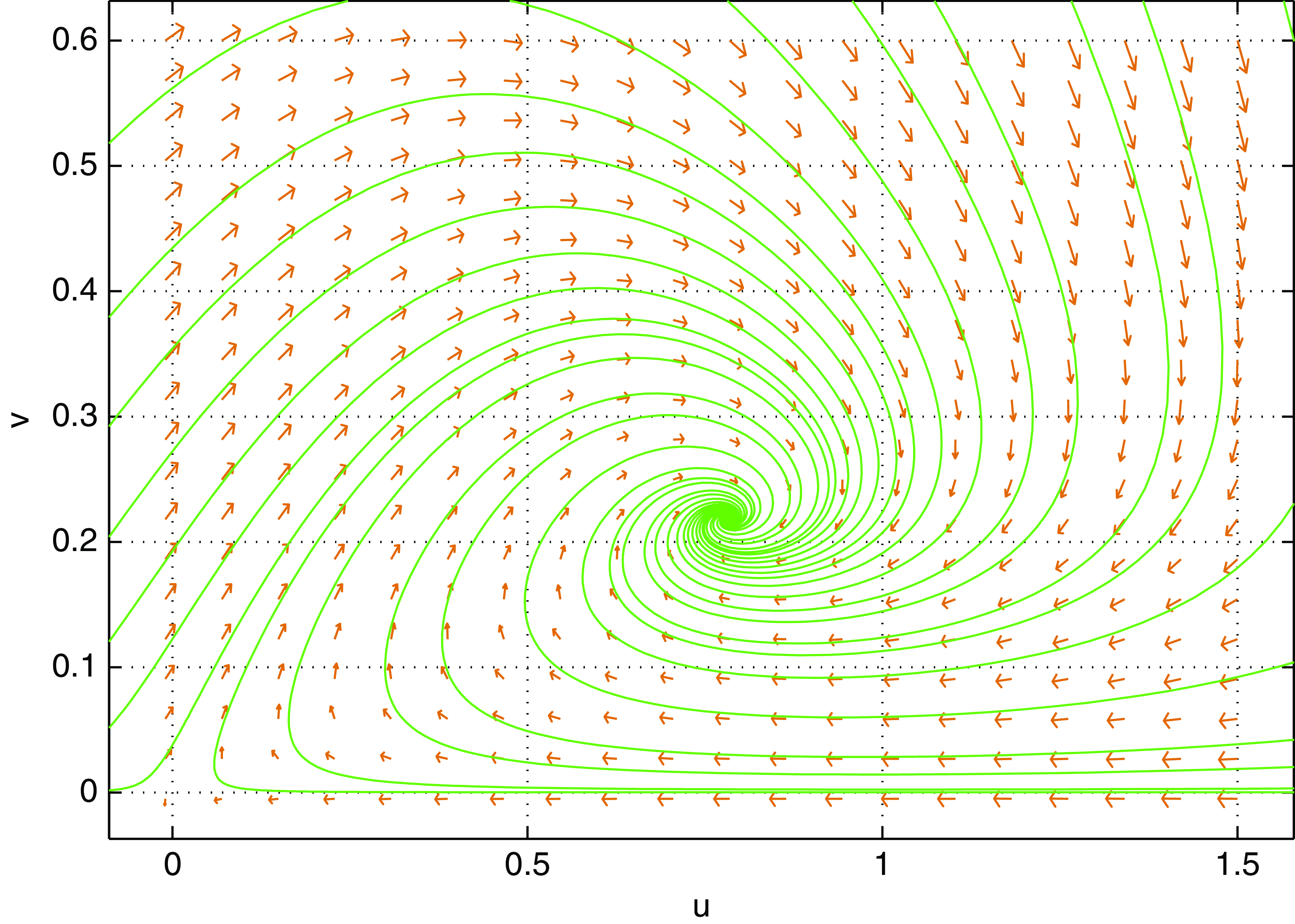
Taking $(a,p,q)=(1,0.5,0.2)$
, then
$(a,p,q)=(1,0.5,0.2)$
, then $E_{*}(0.7821,0.2179)$
of (2.1) with
$E_{*}(0.7821,0.2179)$
of (2.1) with $\tau =0$
is globally asymptotic stable.
$\tau =0$
is globally asymptotic stable.
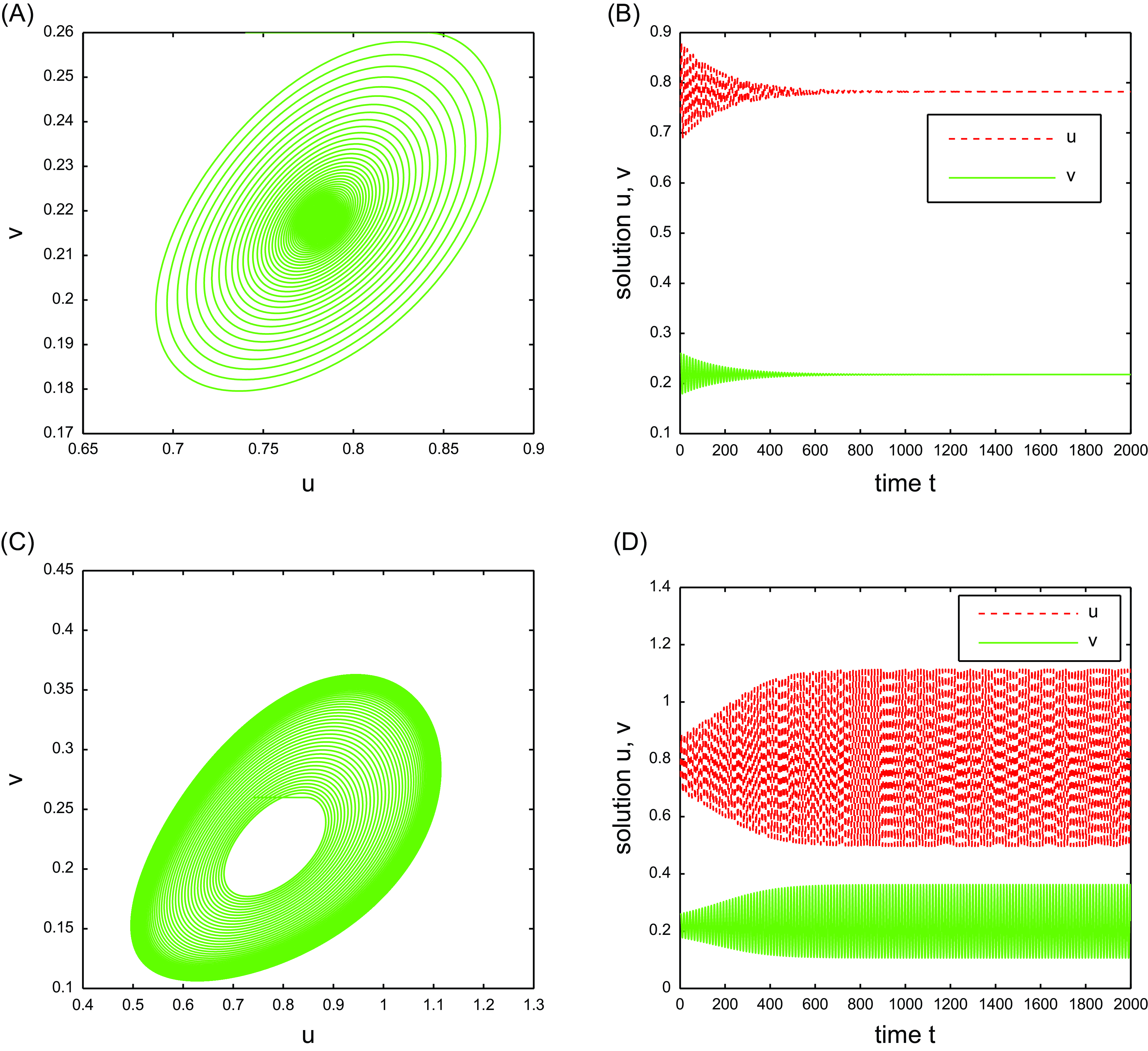
Taking $\tau =1.95 \lt \tau ^{(0,0)}=2.0537$
, then
$\tau =1.95 \lt \tau ^{(0,0)}=2.0537$
, then $(A)$
and
$(A)$
and $(B)$
show that
$(B)$
show that $E_{*}$
is stable. Taking
$E_{*}$
is stable. Taking $\tau =2.1 \gt \tau ^{(0,0)}$
, then
$\tau =2.1 \gt \tau ^{(0,0)}$
, then $(C)$
and
$(C)$
and $(D)$
show that a stable limit cycle arises.
$(D)$
show that a stable limit cycle arises.
Stable region in the $\tau -d_{2}$
plane.
$\tau -d_{2}$
plane.
For system (2.1), Figure 2 depicts the stability and Hopf bifurcation near $E_{*}(0.7821,0.2179)$
. For system (1.3), Figure 3 presents the stability region of the
$E_{*}(0.7821,0.2179)$
. For system (1.3), Figure 3 presents the stability region of the $\tau -d_{2}$
plane. Figure 4 explains the stability when
$\tau -d_{2}$
plane. Figure 4 explains the stability when $d_{2}\gt d^{*}_{2}=0.7333$
and Figure 5 explains the stability when
$d_{2}\gt d^{*}_{2}=0.7333$
and Figure 5 explains the stability when $d_{2}\lt d^{*}_{2}$
. Figures 6 and 7 reveal, respectively, the periodic solutions arising from spatially homogeneous and mode-
$d_{2}\lt d^{*}_{2}$
. Figures 6 and 7 reveal, respectively, the periodic solutions arising from spatially homogeneous and mode- $3$
Hopf bifurcation. Taking
$3$
Hopf bifurcation. Taking $n=0$
and
$n=0$
and $n=3$
for example, we calculate the coefficient to be
$n=3$
for example, we calculate the coefficient to be $\varsigma _{01}=0.6522, \ \varsigma _{02}=-0.2584$
, and
$\varsigma _{01}=0.6522, \ \varsigma _{02}=-0.2584$
, and $\varsigma _{31}=0.0977, \ \varsigma _{32}=-0.5661$
. This suggests that the spatially homogeneous Hopf bifurcation in Figure 6 and mode-3 Hopf bifurcation in Figure 7 are all supercritical and stable.
$\varsigma _{31}=0.0977, \ \varsigma _{32}=-0.5661$
. This suggests that the spatially homogeneous Hopf bifurcation in Figure 6 and mode-3 Hopf bifurcation in Figure 7 are all supercritical and stable.
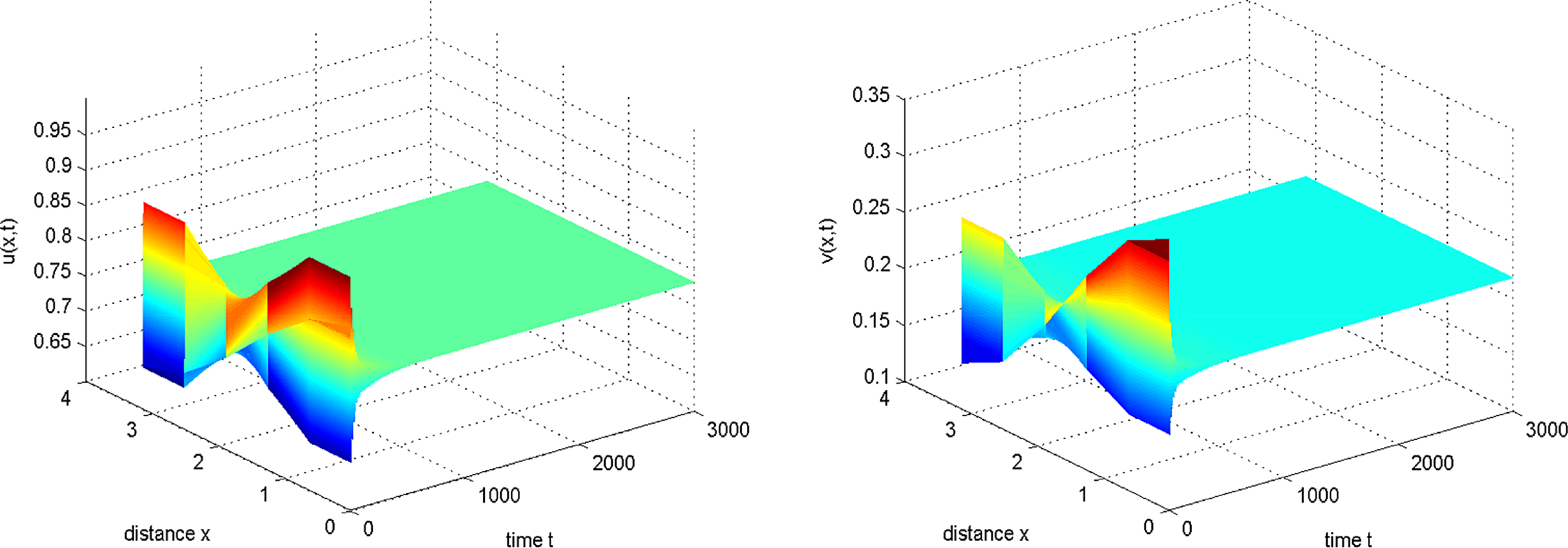
Taking $d_{2}=0.78\gt d^{*}_{2}=0.7333$
,
$d_{2}=0.78\gt d^{*}_{2}=0.7333$
, $\tau =1.95$
, then
$\tau =1.95$
, then $E_{*}$
is always stable. The initial conditions are
$E_{*}$
is always stable. The initial conditions are $u_{0}(x)=0.76+0.1\cos 2x$
and
$u_{0}(x)=0.76+0.1\cos 2x$
and $v_{0}(x)=0.24+0.1\cos 2x$
.
$v_{0}(x)=0.24+0.1\cos 2x$
.
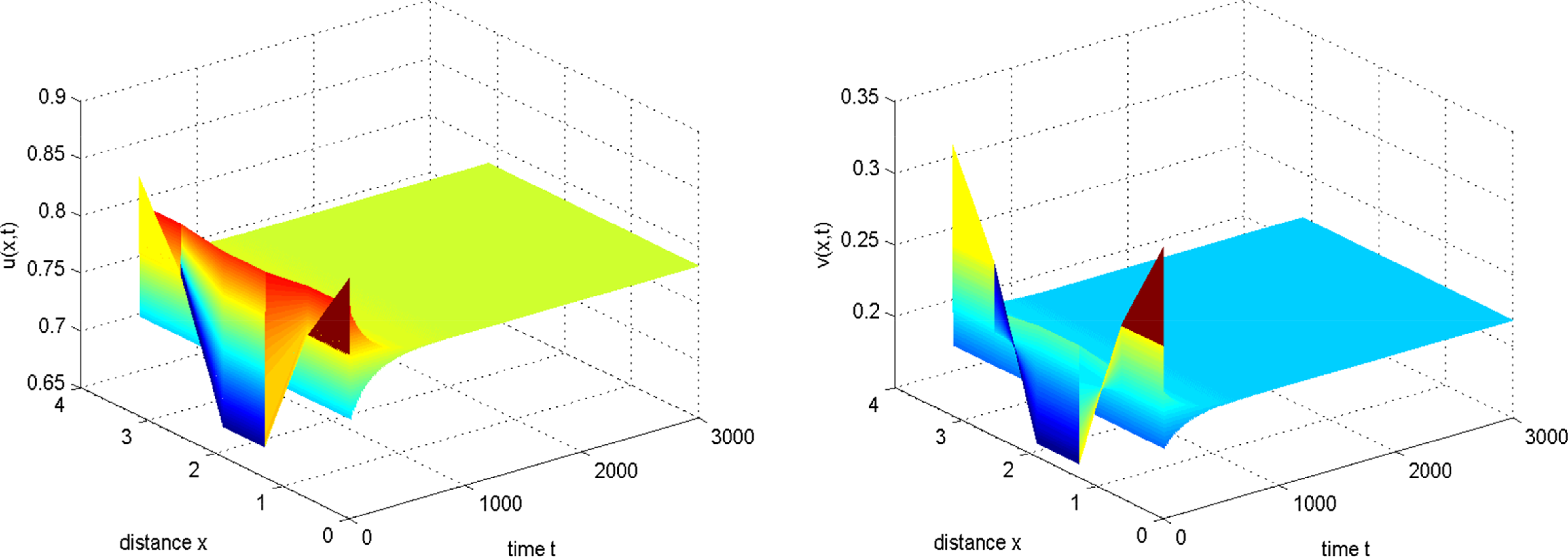
Taking $d_{2}=0.024,\tau =1.95\lt \tau ^{(0,0)}$
, then
$d_{2}=0.024,\tau =1.95\lt \tau ^{(0,0)}$
, then $E_{*}$
is stable. The initial conditions are
$E_{*}$
is stable. The initial conditions are $u_{0}(x)=0.76+0.1\cos x$
and
$u_{0}(x)=0.76+0.1\cos x$
and $v_{0}(x)=0.24+0.1\cos x$
.
$v_{0}(x)=0.24+0.1\cos x$
.
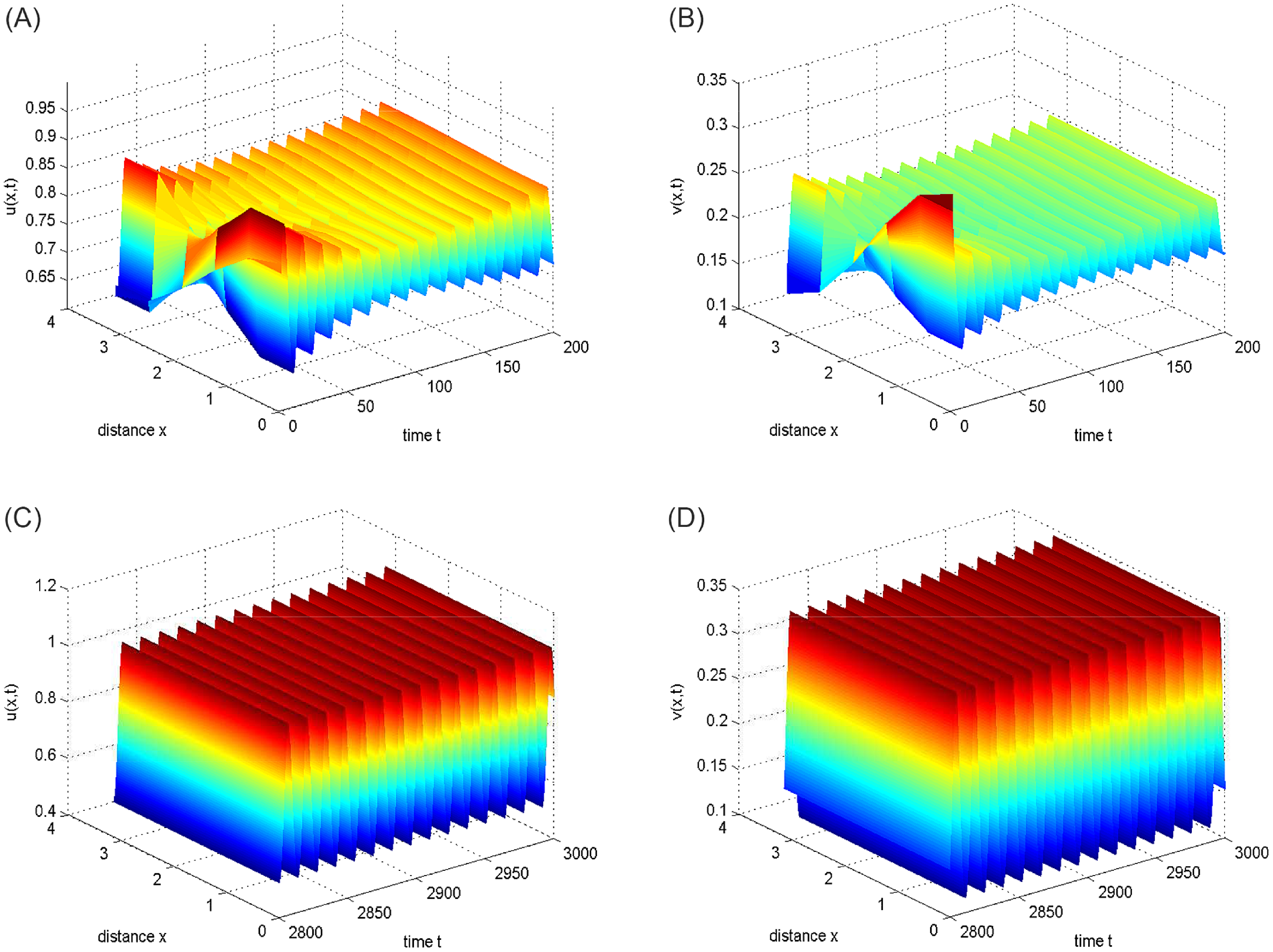
Taking $d_{2}=0.024,\tau =2.1 \gt \tau ^{(0,0)}$
, then stable spatially homogeneous periodic solutions appear. The initial conditions are
$d_{2}=0.024,\tau =2.1 \gt \tau ^{(0,0)}$
, then stable spatially homogeneous periodic solutions appear. The initial conditions are $u_{0}(x)=0.76+0.1\cos x$
and
$u_{0}(x)=0.76+0.1\cos x$
and $v_{0}(x)=0.24+0.1\cos x$
.
$v_{0}(x)=0.24+0.1\cos x$
.
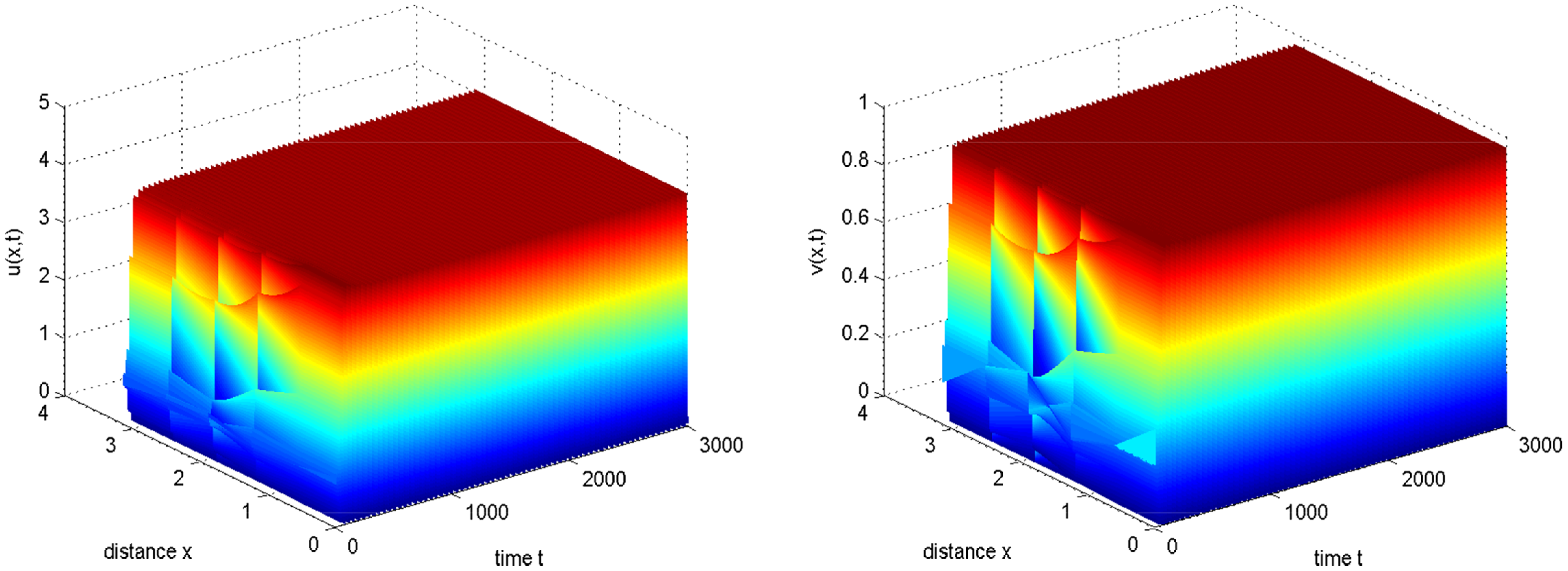
Taking $d_{2}=0.024,\tau =6.98 \gt \tau ^{(3,0)}=6.8066$
, then stable spatially inhomogeneous periodic solutions arise from mode-3 Hopf bifurcation. The initial conditions are
$d_{2}=0.024,\tau =6.98 \gt \tau ^{(3,0)}=6.8066$
, then stable spatially inhomogeneous periodic solutions arise from mode-3 Hopf bifurcation. The initial conditions are $u_{0}(x)=0.76+0.1\cos 3x$
and
$u_{0}(x)=0.76+0.1\cos 3x$
and $v_{0}(x)=0.24+0.1\cos 3x$
.
$v_{0}(x)=0.24+0.1\cos 3x$
.
For system (1.4), we choose $(a,p,q,d_{1},d_{2},\mathcal{l})=(1,1,0.1,0.01,0.1,4)$
, then we obtain
$(a,p,q,d_{1},d_{2},\mathcal{l})=(1,1,0.1,0.01,0.1,4)$
, then we obtain $E_{*}(0.9156,0.0844)$
and
$E_{*}(0.9156,0.0844)$
and $d^{\#}_{2}=1.9904 \gt d_{2}$
. In order to implement numerical simulations of system (4.1), we introduce the equivalent system by setting
$d^{\#}_{2}=1.9904 \gt d_{2}$
. In order to implement numerical simulations of system (4.1), we introduce the equivalent system by setting $w(x,t)=\int _{-\infty }^{t}G(t-\eta )u(x,\eta )d\eta$
.
$w(x,t)=\int _{-\infty }^{t}G(t-\eta )u(x,\eta )d\eta$
.
 \begin{equation} \begin{cases} u_{t}=d_{1}\Delta u+v-\frac{qu}{p+v}, \\ v_{t}=d_{2}\Delta v+av(1-v)-vw,\\ w_{t}=\frac{1}{\sigma }(u-w). \end{cases} \end{equation}
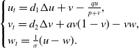
Because of the complexity of formulas $\widetilde{B}_{n1}$
and
$\widetilde{B}_{n1}$
and $\Delta _{n}=\widetilde{B}^{2}_{n1}-4\widetilde{A}_{n1}\widetilde{C}_{n1}$
, we determine set
$\Delta _{n}=\widetilde{B}^{2}_{n1}-4\widetilde{A}_{n1}\widetilde{C}_{n1}$
, we determine set $S=\{1,2\}$
by numerical simulations under the target parameters, see Figure 8. Thus, we have
$S=\{1,2\}$
by numerical simulations under the target parameters, see Figure 8. Thus, we have $\sigma ^{-}_{1}=3.5390 \lt \sigma ^{-}_{2}=5.38 \lt \sigma ^{+}_{2}=17.9333 \lt \sigma ^{+}_{1}=33.5642$
, which means
$\sigma ^{-}_{1}=3.5390 \lt \sigma ^{-}_{2}=5.38 \lt \sigma ^{+}_{2}=17.9333 \lt \sigma ^{+}_{1}=33.5642$
, which means $\sigma _{*}=3.5390, \sigma ^{*}=33.5642$
. By choosing the values of the gradually increasing
$\sigma _{*}=3.5390, \sigma ^{*}=33.5642$
. By choosing the values of the gradually increasing $\sigma$
, we demonstrate the correctness of Theorem 4.2. Figures 9 and 10 depict that
$\sigma$
, we demonstrate the correctness of Theorem 4.2. Figures 9 and 10 depict that $E_{*}$
is stable. Figure 11 describes a series of inhomogeneous periodic solutions at
$E_{*}$
is stable. Figure 11 describes a series of inhomogeneous periodic solutions at $\sigma =\sigma ^{\pm }_{j} \ (j=1,2)$
. And all initial values are
$\sigma =\sigma ^{\pm }_{j} \ (j=1,2)$
. And all initial values are $u_{0}(x)=w_{0}(x)=0.9156+0.1\cos x, v_{0}(x)=0.0844+0.01\cos x$
.
$u_{0}(x)=w_{0}(x)=0.9156+0.1\cos x, v_{0}(x)=0.0844+0.01\cos x$
.
Taking $(a,p,q,d_{1},d_{2},\mathcal{l})=(1,1,0.1,0.01,0.1,4)$
, then
$(a,p,q,d_{1},d_{2},\mathcal{l})=(1,1,0.1,0.01,0.1,4)$
, then $(A)$
and
$(A)$
and $(B)$
denote the graphs of
$(B)$
denote the graphs of $\widetilde{B}_{n1}$
and
$\widetilde{B}_{n1}$
and $\Delta _{n}=\widetilde{B}^{2}_{n1}-4\widetilde{A}_{n1}\widetilde{C}_{n1}$
, respectively. Then we obtain
$\Delta _{n}=\widetilde{B}^{2}_{n1}-4\widetilde{A}_{n1}\widetilde{C}_{n1}$
, respectively. Then we obtain $S=\{1,2\}$
.
$S=\{1,2\}$
.
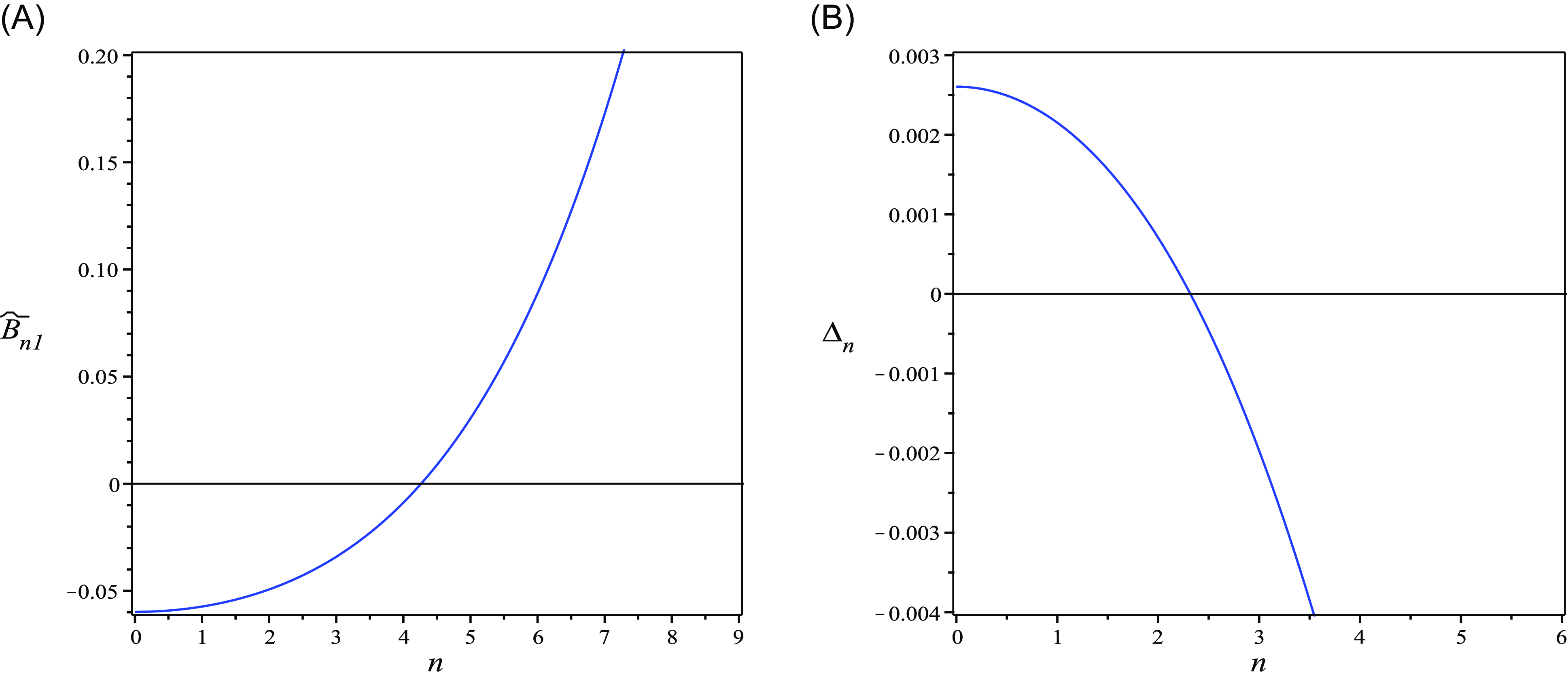
For fixed $(a,p,q,d_{1},d_{2},\mathcal{l})=(1,1,0.1,0.01,0.1,4)$
, we take
$(a,p,q,d_{1},d_{2},\mathcal{l})=(1,1,0.1,0.01,0.1,4)$
, we take $\sigma =3.02 \lt \sigma _{*}=3.5390$
, then
$\sigma =3.02 \lt \sigma _{*}=3.5390$
, then $E_{*}$
is stable.
$E_{*}$
is stable.
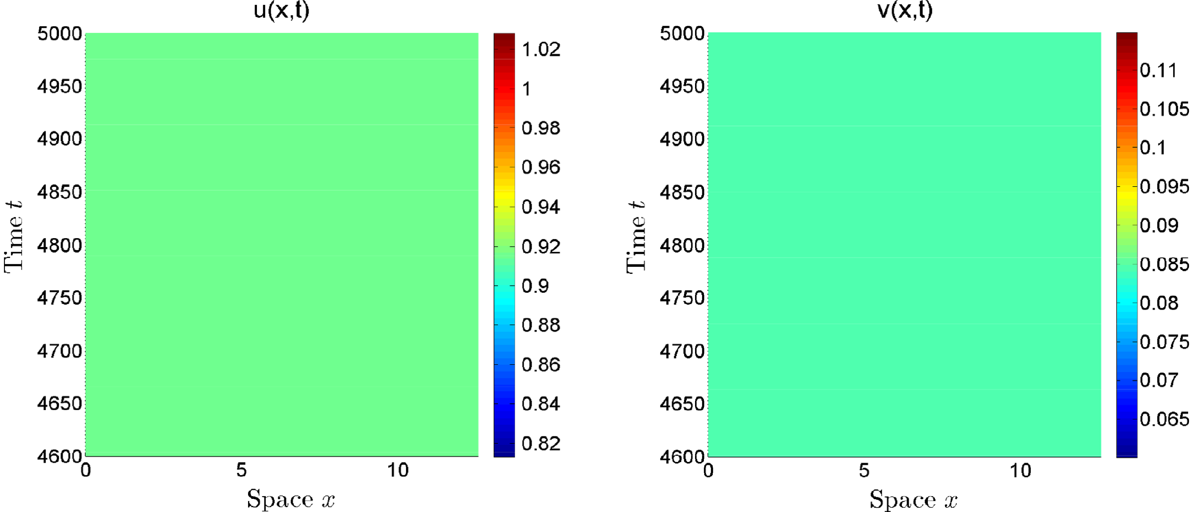
For fixed $(a,p,q,d_{1},d_{2},\mathcal{l})=(1,1,0.1,0.01,0.1,4)$
, we take
$(a,p,q,d_{1},d_{2},\mathcal{l})=(1,1,0.1,0.01,0.1,4)$
, we take $\sigma =45 \gt \sigma ^{*}=33.5642$
, then
$\sigma =45 \gt \sigma ^{*}=33.5642$
, then $E_{*}$
is stable.
$E_{*}$
is stable.
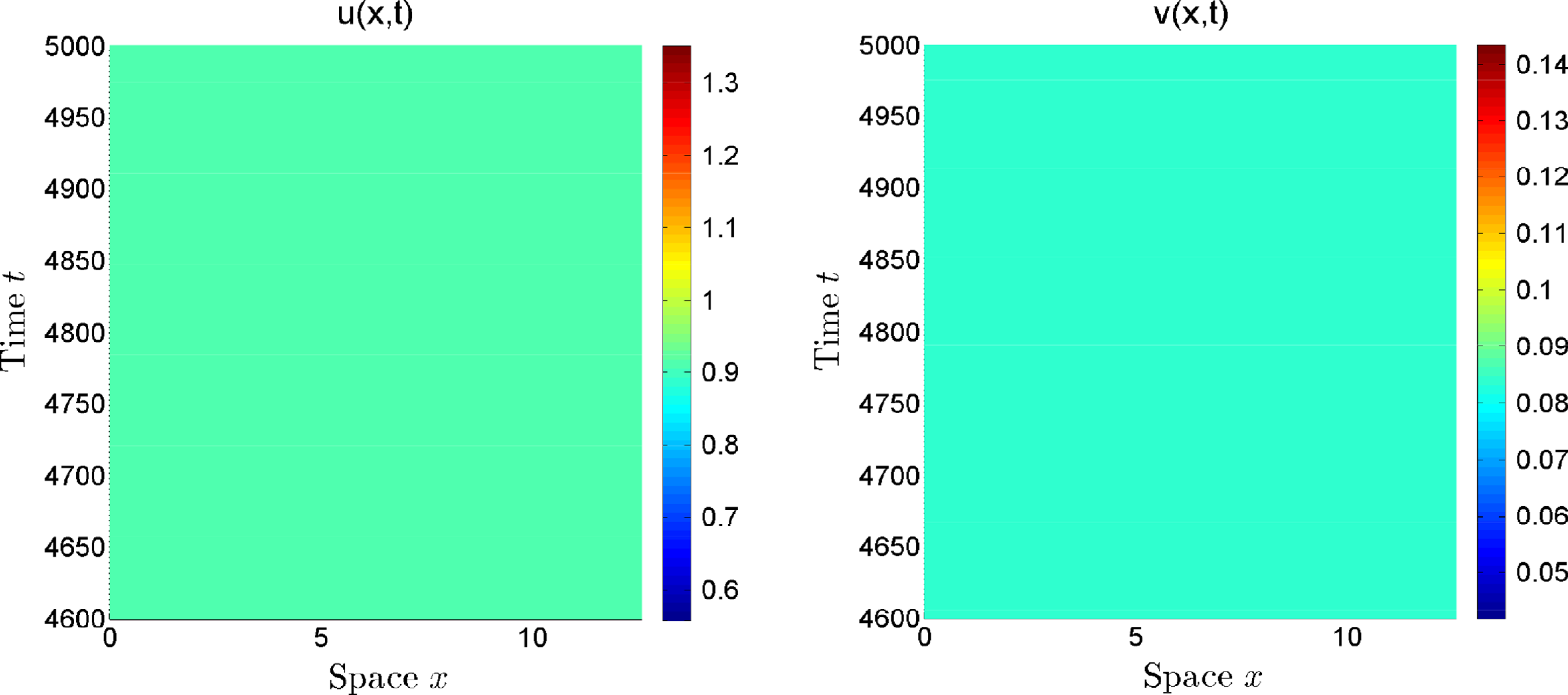
For fixed $(a,p,q,d_{1},d_{2},\mathcal{l})=(1,1,0.1,0.01,0.1,4)$
, we vary the values of
$(a,p,q,d_{1},d_{2},\mathcal{l})=(1,1,0.1,0.01,0.1,4)$
, we vary the values of $\sigma$
to get different periodic solutions.
$\sigma$
to get different periodic solutions. $(a)$
and
$(a)$
and $(e)$
:
$(e)$
: $\sigma =3.56\gt \sigma ^{-}_{1}=3.5390$
.
$\sigma =3.56\gt \sigma ^{-}_{1}=3.5390$
. $(b)$
and
$(b)$
and $(f)$
:
$(f)$
: $\sigma =5.42\gt \sigma ^{-}_{2}=5.38$
.
$\sigma =5.42\gt \sigma ^{-}_{2}=5.38$
. $(c)$
and
$(c)$
and $(g)$
:
$(g)$
: $\sigma =17.6\lt \sigma ^{+}_{2}=17.9333$
.
$\sigma =17.6\lt \sigma ^{+}_{2}=17.9333$
. $(e)$
and
$(e)$
and $(h)$
:
$(h)$
: $\sigma =33.4\lt \sigma ^{+}_{1}=33.5642$
.
$\sigma =33.4\lt \sigma ^{+}_{1}=33.5642$
.
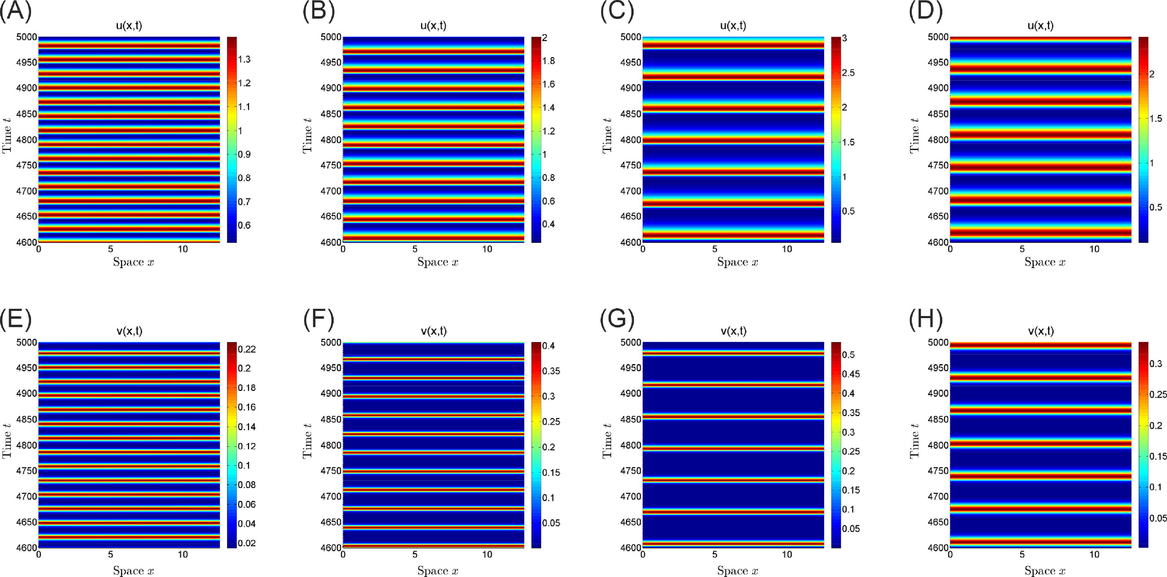
6. Conclusion
The aim of this paper is to research the impacts of time lag and diffusion on the system. We deliberate different time lag on the space-time system. We analyse the stability and bifurcation in detail and discover that both the discrete delay and distributed delay do not induce Turing bifurcation. Simply put, the instability could only be caused by Hopf bifurcation. We judge the direction and stability of periodic solutions by deducing the normal form. We found that appropriate time lag destabilizes the system, and there is a series of delay thresholds inducing Hopf bifurcations. Our findings once again demonstrate the importance of time lag in biodiffusion. Through Remarks 3.4 and 4.3, the findings are summarized below.
Common grounds:
-
(i) Neither of these two delays induces Turing bifurcation.
-
(ii) These two delays
$\tau$
and
$\sigma$
do not change the stability if sulphides disperse quickly or plants expand laterally quickly. Nonetheless, if sulphides disperse slowly, then delays
$\tau$
and
$\sigma$
do not alter the stability as plants expand laterally quickly, and delays
$\tau$
and
$\sigma$
could induce Hopf bifurcation as plants expand slowly.


Differences:
If plants expand laterally slowly, then the stability interval induced by distributed delay $\sigma$
is much larger than that of discrete delay
$\sigma$
is much larger than that of discrete delay $\tau$
. More specifically, in the case of the discrete delay and small enough
$\tau$
. More specifically, in the case of the discrete delay and small enough $d_{2}$
(the rate of plant lateral expansion), large enough delay
$d_{2}$
(the rate of plant lateral expansion), large enough delay $\tau$
makes
$\tau$
makes $E_{*}$
unstable. However, in the case of the distributed delay and small enough
$E_{*}$
unstable. However, in the case of the distributed delay and small enough $d_{2}$
, large enough delay
$d_{2}$
, large enough delay $\sigma$
still makes
$\sigma$
still makes $E_{*}$
stable.
$E_{*}$
stable.
Funding statement
This work was jointly supported by the National Natural Science Foundation of China (No. 12331017 and No. 12071074 ), and the Zhejiang Provincial Natural Science Foundation of China (No. LZ24A010006).
Competing interests
The authors declare that they have no conflict of interest.
Author contributions
We declare that the authors are ranked in alphabetic order of their names and all of them have the same contributions to this paper.


 Open access