


1. Introduction
Flow over the finite wall-mounted cylinder (FWMC) exhibits complex flow structures and vortex–vortex interactions due to geometric modifications at the free end and the cylinder–wall junction (Finnigan Reference Finnigan2000; Krajnovic Reference Krajnovic2011; Nepf Reference Nepf2012). This phenomenon is widely observed in engineering applications, such as high-rise buildings and aquatic vegetation. Understanding the emergence, development and interaction of vortical structures with different rotations is crucial for advancing the fundamental theory of FWMC flow (Wang & Zhou Reference Wang and Zhou2009; Zhu et al. Reference Zhu, Wang, Wang and Wang2017; Yauwenas et al. Reference Yauwenas, Porteous, Moreau and Doolan2019; Cao et al. Reference Cao, Tamura, Zhou, Bao and Han2022). Over the past few decades, significant progress has been made in uncovering the underlying physics of FWMC flow (Adaramola et al. Reference Adaramola, Akinlade, Sumner, Bergstrom and Schenstead2006; Wang & Zhou Reference Wang and Zhou2009; Luhar & Nepf Reference Luhar and Nepf2011; Li & Fuhrman Reference Li and Fuhrman2022; Hu & Li Reference Hu and Li2023; Hu, Huang & Li Reference Hu, Huang and Li2023). A comprehensive review of these findings is essential to establish a foundational understanding before addressing more multifaceted configurations, such as fluid–structure interaction (FSI) of wall-mounted flexible structures with varying flexibility (or stiffness).
1.1. Flow over the finite wall-mounted rigid structure
Based on cross-sectional shape, structures can be classified into three categories (Derakhshandeh & Alam Reference Derakhshandeh and Alam2019). The first structure consists of a continuous and finite curvature shape, such as a circular or elliptical cylinder (e.g. most of the stems), while the second one is sharp edged with an infinitely large curvature, for example, a square or triangular cylinder (e.g. plates or walls). The third one is a hybrid of the two, and a typical case is a semi-circular cylinder (e.g. breakwater structures). Studies of FWMC have primarily focused on the first two categories, as they are more prevalent in natural and engineered environments. We start with these two types of wall-mounted structures, providing a detailed discussion of the flow structures of a rigid FWMC. Differences arising from cross-sectional shape are highlighted when relevant.
Flow structures around a circular FWMC are strongly influenced by the aspect ratio (AR $=l/D$
, where
$=l/D$
, where $l$
is the height of the structure and
$l$
is the height of the structure and $D$
is the diameter or side length), Reynolds number (
$D$
is the diameter or side length), Reynolds number ( $Re = U_\infty D/\nu$
, where
$Re = U_\infty D/\nu$
, where $U_\infty$
is incoming flow velocity and
$U_\infty$
is incoming flow velocity and $\nu$
is the fluid kinematic viscosity), boundary layer thickness (
$\nu$
is the fluid kinematic viscosity), boundary layer thickness ( $\delta /D$
), and turbulent intensity (
$\delta /D$
), and turbulent intensity ( $T_i = u^{\prime }/U_\infty$
, where
$T_i = u^{\prime }/U_\infty$
, where $u^{\prime }$
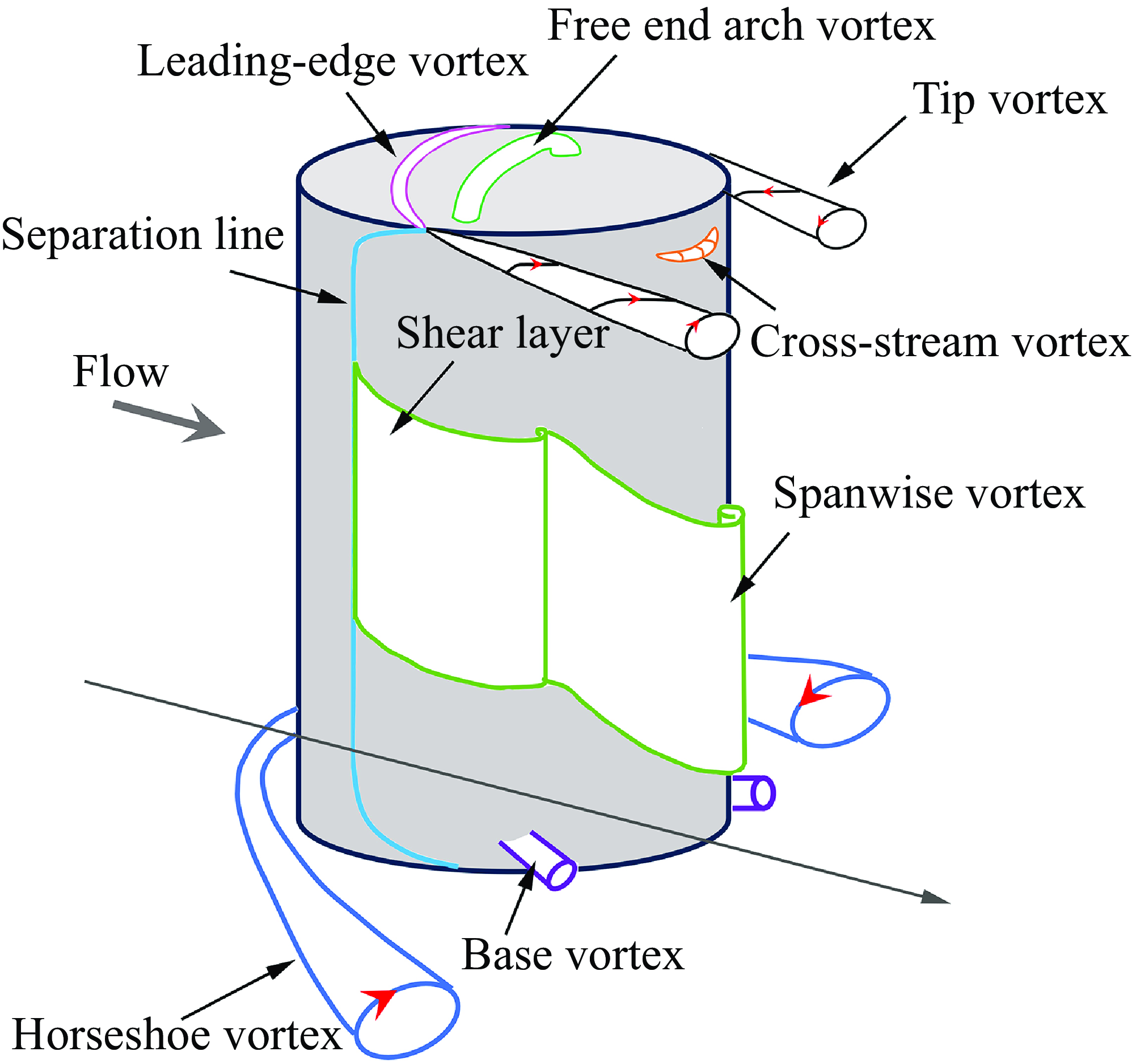
is the root-mean-square (r.m.s.) of the turbulent velocity fluctuation), among other factors (Sakamoto & Arie Reference Sakamoto and Arie1983; Bourgeois, Sattari & Martinuzzi Reference Bourgeois, Sattari and Martinuzzi2011; Porteous, Moreau & Doolan Reference Porteous, Moreau and Doolan2014; Hearst, Gomit & Ganapathisubramani Reference Hearst, Gomit and Ganapathisubramani2016). Based on the time-averaged distribution of vortical structures, the wake of an FWMC can be divided into three types (Zhang et al. Reference Zhang, Cheng, An and Zhao2017), i.e. dipole type (i.e. one pair of the streamwise vortices at the upper part), quadrupole type (i.e. two pairs of the streamwise vortices at the upper and lower parts) and six-vortex type (i.e. transitional structures involved). Particular vortical structures of the FWMC with a height over the critical value are presented in figure 1. The transition from dipole to quadrupole is marked by a critical aspect ratio (Sumner, Heseltine & Dansereau Reference Sumner, Heseltine and Dansereau2004; Wang & Zhou Reference Wang and Zhou2009; Hosseini, Bourgeois & Martinuzzi Reference Hosseini, Bourgeois and Martinuzzi2013; Sumner Reference Sumner2013). When the height exceeds this critical value, a tip vortex pair and a base vortex pair appear at the free end and junction, respectively (Bourgeois et al. Reference Bourgeois, Sattari and Martinuzzi2011; Hajimirzaie, Wojcik & Buchholz Reference Hajimirzaie, Wojcik and Buchholz2012; Porteous et al. Reference Porteous, Moreau and Doolan2014). The appearance of these vortex pairs is highly dependent on the AR. A sufficiently thick boundary layer and AR above the critical value promote the formation of the tip vortex pair at the free end (Sumner et al. Reference Sumner, Heseltine and Dansereau2004; Adaramola et al. Reference Adaramola, Akinlade, Sumner, Bergstrom and Schenstead2006; Sumner & Heseltine Reference Sumner and Heseltine2008; Bourgeois et al. Reference Bourgeois, Sattari and Martinuzzi2011, Reference Bourgeois, Sattari and Martinuzzi2012; Sumner Reference Sumner2013). The origin of the tip vortex differs depending on the cross-sectional shape. In a square FWMC, streamwise vorticity near the free end arises from the reorientation of vertical vorticity in the sidewall shear layers due to lateral vorticity of the free-end shear layer (Bourgeois et al. Reference Bourgeois, Sattari and Martinuzzi2011). Here, the tip vortex is essentially a deformed Kármán vortex. In contrast, for a circular FWMC, the tip vortex originates from the leading or trailing edge of the free end and is not associated with the Kármán vortex (Hunt et al. Reference Hunt, Abell, Peterka and Woo1978; Kawamura et al. Reference Kawamura, Hiwada, Hibino, Mabuchi and Kumada1984; Hwang & Yang Reference Hwang and Yang2004; Pattenden, Turnock & Zhang Reference Pattenden, Turnock and Zhang2005; Hain, Kahler & Michaelis Reference Hain, Kahler and Michaelis2008; Palau-Salvador et al. Reference Palau-Salvador, Stoesser, Frohlich, Kappler and Rodi2010; Krajnovic Reference Krajnovic2011; Saeedi, LePoudre & Wang Reference Saeedi, LePoudre and Wang2014). This highlights the pivotal role of cross-sectional shape in the tip vortex generation.
$u^{\prime }$
is the root-mean-square (r.m.s.) of the turbulent velocity fluctuation), among other factors (Sakamoto & Arie Reference Sakamoto and Arie1983; Bourgeois, Sattari & Martinuzzi Reference Bourgeois, Sattari and Martinuzzi2011; Porteous, Moreau & Doolan Reference Porteous, Moreau and Doolan2014; Hearst, Gomit & Ganapathisubramani Reference Hearst, Gomit and Ganapathisubramani2016). Based on the time-averaged distribution of vortical structures, the wake of an FWMC can be divided into three types (Zhang et al. Reference Zhang, Cheng, An and Zhao2017), i.e. dipole type (i.e. one pair of the streamwise vortices at the upper part), quadrupole type (i.e. two pairs of the streamwise vortices at the upper and lower parts) and six-vortex type (i.e. transitional structures involved). Particular vortical structures of the FWMC with a height over the critical value are presented in figure 1. The transition from dipole to quadrupole is marked by a critical aspect ratio (Sumner, Heseltine & Dansereau Reference Sumner, Heseltine and Dansereau2004; Wang & Zhou Reference Wang and Zhou2009; Hosseini, Bourgeois & Martinuzzi Reference Hosseini, Bourgeois and Martinuzzi2013; Sumner Reference Sumner2013). When the height exceeds this critical value, a tip vortex pair and a base vortex pair appear at the free end and junction, respectively (Bourgeois et al. Reference Bourgeois, Sattari and Martinuzzi2011; Hajimirzaie, Wojcik & Buchholz Reference Hajimirzaie, Wojcik and Buchholz2012; Porteous et al. Reference Porteous, Moreau and Doolan2014). The appearance of these vortex pairs is highly dependent on the AR. A sufficiently thick boundary layer and AR above the critical value promote the formation of the tip vortex pair at the free end (Sumner et al. Reference Sumner, Heseltine and Dansereau2004; Adaramola et al. Reference Adaramola, Akinlade, Sumner, Bergstrom and Schenstead2006; Sumner & Heseltine Reference Sumner and Heseltine2008; Bourgeois et al. Reference Bourgeois, Sattari and Martinuzzi2011, Reference Bourgeois, Sattari and Martinuzzi2012; Sumner Reference Sumner2013). The origin of the tip vortex differs depending on the cross-sectional shape. In a square FWMC, streamwise vorticity near the free end arises from the reorientation of vertical vorticity in the sidewall shear layers due to lateral vorticity of the free-end shear layer (Bourgeois et al. Reference Bourgeois, Sattari and Martinuzzi2011). Here, the tip vortex is essentially a deformed Kármán vortex. In contrast, for a circular FWMC, the tip vortex originates from the leading or trailing edge of the free end and is not associated with the Kármán vortex (Hunt et al. Reference Hunt, Abell, Peterka and Woo1978; Kawamura et al. Reference Kawamura, Hiwada, Hibino, Mabuchi and Kumada1984; Hwang & Yang Reference Hwang and Yang2004; Pattenden, Turnock & Zhang Reference Pattenden, Turnock and Zhang2005; Hain, Kahler & Michaelis Reference Hain, Kahler and Michaelis2008; Palau-Salvador et al. Reference Palau-Salvador, Stoesser, Frohlich, Kappler and Rodi2010; Krajnovic Reference Krajnovic2011; Saeedi, LePoudre & Wang Reference Saeedi, LePoudre and Wang2014). This highlights the pivotal role of cross-sectional shape in the tip vortex generation.
The sketch of the vortical structures for flow over a wall-mounted rigid circular cylinder. The sketch is based on the models proposed by Pattenden et al. (Reference Pattenden, Turnock and Zhang2005), Frederich et al. (2007), Krajnovic (Reference Krajnovic2011), Zhu et al. (Reference Zhu, Wang, Wang and Wang2017) and Essel, Tachie & Balachandar (Reference Essel, Tachie and Balachandar2021). Note that only part of the shear layer and spanwise vortex are shown.
When AR $\gt$
3, the base vortex pair forms at the junction (Sumner et al. Reference Sumner, Heseltine and Dansereau2004; Adaramola et al. Reference Adaramola, Akinlade, Sumner, Bergstrom and Schenstead2006), developing behind the cylinder and inducing an upwash flow (Etzold & Fiedler Reference Etzold and Fiedler1976; Hajimirzaie et al. Reference Hajimirzaie, Wojcik and Buchholz2012). Its formation is strongly influenced by
$\gt$
3, the base vortex pair forms at the junction (Sumner et al. Reference Sumner, Heseltine and Dansereau2004; Adaramola et al. Reference Adaramola, Akinlade, Sumner, Bergstrom and Schenstead2006), developing behind the cylinder and inducing an upwash flow (Etzold & Fiedler Reference Etzold and Fiedler1976; Hajimirzaie et al. Reference Hajimirzaie, Wojcik and Buchholz2012). Its formation is strongly influenced by $\delta /D$
(Wang et al. Reference Wang, Zhou, Chan and Lam2006). Compared with the tip vortex pair, the base vortex pair is weaker and dissipates more quickly downstream.
$\delta /D$
(Wang et al. Reference Wang, Zhou, Chan and Lam2006). Compared with the tip vortex pair, the base vortex pair is weaker and dissipates more quickly downstream.
The trailing vortex (not shown in figure 1), which is typically located far from the free end, is not a continuation of the tip vortex pair. According to Frederich, Wassen & Thiele (Reference Frederich, Wassen and Thiele2008) and Palau-Salvador et al. (Reference Palau-Salvador, Stoesser, Frohlich, Kappler and Rodi2010), it arises from strong downwash effects and associated upwash motion away from the wake centreline, triggered by the finite cylinder width. Initially believed to be visible only in the mean flow field (Fröhlich & Rodi Reference Fröhlich and Rodi2004), tomographic particle image velocimetry results from Zhu et al. (Reference Zhu, Wang, Wang and Wang2017) suggest that this structure can also be observed in the instantaneous flow field where AR is low.
Vortex shedding from FWMC sidewalls is influenced by the AR and boundary layer conditions, primarily due to variations in downwash flow and near-wake base vortices (Fröhlich and Rodi, 2004; Pattenden et al. Reference Pattenden, Turnock and Zhang2005; Wang et al. Reference Wang, Zhou, Chan and Lam2006; Palau-Salvador et al. Reference Palau-Salvador, Stoesser, Frohlich, Kappler and Rodi2010; Tsutsui Reference Tsutsui2012). A thick boundary layer could enhance the base vortex and induce upwash flow. Spanwise vortices can adopt antisymmetric and/or symmetric patterns depending on upwash and downwash flow (Wang et al. Reference Wang, Zhou, Chan and Lam2006; Wang & Zhou Reference Wang and Zhou2009). For FWMC with larger AR, both types of vortex shedding may coexist. Wang, Cao & Zhou (Reference Wang, Cao and Zhou2014) found that vortex shedding near the free end is predominantly symmetric, whereas alternating vortex shedding dominates the wake near the centre and lower regions. The separation line (shown in figure 1), corresponding to points where the shear layers detach from the side surface, indicates that separation occurs earlier around the centre than near the free end or lower part due to the influences of downwash and upwash flow.
The free-end arch vortex appears in the mean wake field when AR $\lt$
3 (Lee Reference Lee1997; Krajnovic Reference Krajnovic2011). This vortex takes on a reversed U-shape (Fröhlich and Rodi, 2004). The legs of the mean arch vortex are inclined in the streamwise direction at a relatively constant angle (Krajnovic Reference Krajnovic2011). For low AR cases, the dominant downwash effect increases the likelihood of symmetric vortex shedding (Wang et al. Reference Wang, Cao and Zhou2014). This symmetric shedding may induce instantaneous arch vortex formation in short cylinders (Zhu et al. Reference Zhu, Wang, Wang and Wang2017).
$\lt$
3 (Lee Reference Lee1997; Krajnovic Reference Krajnovic2011). This vortex takes on a reversed U-shape (Fröhlich and Rodi, 2004). The legs of the mean arch vortex are inclined in the streamwise direction at a relatively constant angle (Krajnovic Reference Krajnovic2011). For low AR cases, the dominant downwash effect increases the likelihood of symmetric vortex shedding (Wang et al. Reference Wang, Cao and Zhou2014). This symmetric shedding may induce instantaneous arch vortex formation in short cylinders (Zhu et al. Reference Zhu, Wang, Wang and Wang2017).
In front of the arch vortex, the leading-edge vortex forms at the forward half of the free end surface (Kawamura et al. Reference Kawamura, Hiwada, Hibino, Mabuchi and Kumada1984; Krajnovic Reference Krajnovic2011). This vortex is attributed to the reverse flow along the centre of the free end surface, which is entrained by the separated flow from the leading edge (Kawamura et al. Reference Kawamura, Hiwada, Hibino, Mabuchi and Kumada1984; Pattenden et al. Reference Pattenden, Turnock and Zhang2005; Palau-Salvador et al. Reference Palau-Salvador, Stoesser, Frohlich, Kappler and Rodi2010; Krajnovic Reference Krajnovic2011). The attachment length of this vortex is strongly affected by both AR and $Re$
(Sumner Reference Sumner2013). Downstream of the surface, the forward free-end flow interacts with the wake behind the FWMC, leading to the emergence of the upper near-wake cross-stream vortex (as shown in figure 1). Additional vortices may also form, such as the horseshoe vortex at the junction. The horseshoe vortex may interact with the vortices behind the FWMC, significantly influencing the overall wake dynamics.
$Re$
(Sumner Reference Sumner2013). Downstream of the surface, the forward free-end flow interacts with the wake behind the FWMC, leading to the emergence of the upper near-wake cross-stream vortex (as shown in figure 1). Additional vortices may also form, such as the horseshoe vortex at the junction. The horseshoe vortex may interact with the vortices behind the FWMC, significantly influencing the overall wake dynamics.
The flow structures around the FWMC are highly complex, with their formation, development and dissipation closely tied to the vortex interactions, including rotational effects, upwash and downwash flows. The FWMC height and boundary layer conditions play crucial roles in this dynamics. In this study, we focus on the hydrodynamic forces and vortex dynamics of a circular FWMC across a wide range of $Re$
. Specific flow behaviours are analysed, and distinctive vortex structures are reported.
$Re$
. Specific flow behaviours are analysed, and distinctive vortex structures are reported.
1.2. Flow over the finite wall-mounted flexible structure
When the structure is flexible, FSI becomes significant. In nature, wall-mounted structures appear in various forms, such as flexible plate, blade, filament, aquatic plant and stem. Research on these structures is essential for understanding their behaviours under different flow conditions. However, most studies have focused on predicting drag, wave attenuation, flow profiles and structural reconfiguration, with relatively few investigations into their vortex dynamics. Furthermore, the parameters considered in these studies are scattered, making it difficult to establish a comprehensive understanding of FSI of wall-mounted flexible structures.
Zeller et al. (Reference Zeller, Weitzman, Abbett, Zarama, Fringer and Koseff2014) proposed a novel formulation of the Keulegan–Carpenter number ( $KC=$
$KC=$ $U_m T/D$
, where
$U_m T/D$
, where $U_m$
is the maximum flow velocity and
$U_m$
is the maximum flow velocity and $T$
is the oscillatory period) for predicting drag coefficients and developed a model for wave attenuation. They estimated the averaged turbulence production over the wave period using the maximum flow velocity and the relative velocity between the current and waves. Mullarney et al. (Reference Mullarney and Henderson2010) demonstrated that stem stiffness significantly affects its motion relative to the wave under wave forcing. A highly flexible stem moves with the surrounding water, whereas a stiff stem exhibits minimal motion, leading the surrounding water by
$T$
is the oscillatory period) for predicting drag coefficients and developed a model for wave attenuation. They estimated the averaged turbulence production over the wave period using the maximum flow velocity and the relative velocity between the current and waves. Mullarney et al. (Reference Mullarney and Henderson2010) demonstrated that stem stiffness significantly affects its motion relative to the wave under wave forcing. A highly flexible stem moves with the surrounding water, whereas a stiff stem exhibits minimal motion, leading the surrounding water by $90^{\circ }$
. They developed an analytical model to describe the wave-forced motion of a single stem and derived an equation to predict frequency-dependent wave dissipation. Luhar & Nepf (Reference Luhar and Nepf2016) observed that blade motion is governed mainly by two dimensionless parameters: (i) the Cauchy number (
$90^{\circ }$
. They developed an analytical model to describe the wave-forced motion of a single stem and derived an equation to predict frequency-dependent wave dissipation. Luhar & Nepf (Reference Luhar and Nepf2016) observed that blade motion is governed mainly by two dimensionless parameters: (i) the Cauchy number ( $Ca$
) and (ii) the ratio of the blade length to wave orbital excursion. Here,
$Ca$
) and (ii) the ratio of the blade length to wave orbital excursion. Here, $Ca$
is defined as
$Ca$
is defined as $C a=0.5 \rho _f D l^3 U_{ref}^2 / E I$
, where
$C a=0.5 \rho _f D l^3 U_{ref}^2 / E I$
, where $\rho _f$
is the fluid density,
$\rho _f$
is the fluid density, $D$
is the side length or stem diameter,
$D$
is the side length or stem diameter, $l$
is the stem height,
$l$
is the stem height, $E$
is Young’s modulus,
$E$
is Young’s modulus, $I$
is the cross-sectional momentum of inertia and
$I$
is the cross-sectional momentum of inertia and $U_{ref}$
is the incoming flow velocity. When
$U_{ref}$
is the incoming flow velocity. When $Ca$
$Ca$ $\gg$
1, drag on the flexible blade is lower. However, when
$\gg$
1, drag on the flexible blade is lower. However, when $Ca\sim$
O(1), drag is higher than that of a rigid blade. Hu et al. (Reference Hu, Mei, Chang and Liu2021) developed a theoretical model to predict the motion of rigid and flexible stems under wave conditions, identifying a phase lag between flow motion and stem response. Zhang & Nepf (Reference Zhang and Nepf2022) developed a scaling equation to predict the reconfiguration of flexible plants with leaves due to the hydrodynamic drag using water channel experiments and numerical simulations.
$Ca\sim$
O(1), drag is higher than that of a rigid blade. Hu et al. (Reference Hu, Mei, Chang and Liu2021) developed a theoretical model to predict the motion of rigid and flexible stems under wave conditions, identifying a phase lag between flow motion and stem response. Zhang & Nepf (Reference Zhang and Nepf2022) developed a scaling equation to predict the reconfiguration of flexible plants with leaves due to the hydrodynamic drag using water channel experiments and numerical simulations.
In terms of flexible filaments, Silva-Leon & Cioncolini (Reference Silva-Leon and Cioncolini2020) experimentally investigated their motions and identified different filament responses, including static reconfiguration, small-amplitude vibration, large-amplitude periodic vibration and large-amplitude aperiodic vibration. These behaviours were found to be influenced by $Re$
and the filament length (
$Re$
and the filament length ( $l$
). Huang, Shin & Sung (Reference Huang, Shin and Sung2007) numerically observed bistability in flexible filaments by varying their length. Revstedt (Reference Revstedt2013) studied the deformation of a flexible cantilever at
$l$
). Huang, Shin & Sung (Reference Huang, Shin and Sung2007) numerically observed bistability in flexible filaments by varying their length. Revstedt (Reference Revstedt2013) studied the deformation of a flexible cantilever at $Re=$
400 and a reduced velocity range of
$Re=$
400 and a reduced velocity range of $\pi /4-2\pi$
. In the desynchronisation regime, the stem motion has negligible effects on vortical structures, whereas in the synchronisation regime, the stem significantly alters the mean flow field, frequencies and vortical structures. Zhang, He & Zhang (Reference Zhang, He and Zhang2020) explored the dynamics of a wall-mounted flexible filament by varying the bending rigidity, mass ratio (
$\pi /4-2\pi$
. In the desynchronisation regime, the stem motion has negligible effects on vortical structures, whereas in the synchronisation regime, the stem significantly alters the mean flow field, frequencies and vortical structures. Zhang, He & Zhang (Reference Zhang, He and Zhang2020) explored the dynamics of a wall-mounted flexible filament by varying the bending rigidity, mass ratio ( $m^{*} = m/m_f$
, where
$m^{*} = m/m_f$
, where $m$
is the structure mass and
$m$
is the structure mass and $m_f$
is the displaced fluid mass) and
$m_f$
is the displaced fluid mass) and $Re$
. They observed three distinct dynamic modes, referred to as lodging, regular vortex-induced vibration (VIV) and static reconfiguration. In regular VIV, the filament frequency locks onto the second natural frequency. However, when the filament is with a nearly upright orientation, the vortex shedding is weak and no lock-in is observed. At higher
$Re$
. They observed three distinct dynamic modes, referred to as lodging, regular vortex-induced vibration (VIV) and static reconfiguration. In regular VIV, the filament frequency locks onto the second natural frequency. However, when the filament is with a nearly upright orientation, the vortex shedding is weak and no lock-in is observed. At higher $Re$
, vortex shedding intensifies, leading to first-mode frequency lock-in, as reported in Py, De Langre & Moulia (Reference Py, De Langre and Moulia2006) and Jin et al. (Reference Jin, Kim, Mao and Chamorro2018). Rota et al. (Reference Rota, Koseki, Agrawal, Olivieri and Rosti2024) observed two flapping states of a wall-mounted flexible filament in turbulent wall flow by direct numerical simulations. One state is with a more flexible filament which oscillates at the frequency of the largest eddies, and the other is with a more rigid filament which is governed by the structural natural frequency.
$Re$
, vortex shedding intensifies, leading to first-mode frequency lock-in, as reported in Py, De Langre & Moulia (Reference Py, De Langre and Moulia2006) and Jin et al. (Reference Jin, Kim, Mao and Chamorro2018). Rota et al. (Reference Rota, Koseki, Agrawal, Olivieri and Rosti2024) observed two flapping states of a wall-mounted flexible filament in turbulent wall flow by direct numerical simulations. One state is with a more flexible filament which oscillates at the frequency of the largest eddies, and the other is with a more rigid filament which is governed by the structural natural frequency.
For a single stem, Jacobsen et al. (Reference Jacobsen, Bakker, Uijttewaal and Uittenbogaard2019) experimentally studied its motion subjected to regular waves, focusing on several critical aspects: (i) predicting the stem motion and static shape, (ii) force reduction due to flexibility, (iii) hydrodynamic forces on the flexible stem, (iv) estimating external hydrodynamic loading and internal shear forces and (v) examining the relationship between phase lags and internal shear forces. They found that when the stem is stiffer, the phase lags remain nearly uniform along its length, whereas in more flexible stem, phase lags vary. The drag force shows better overall coherence with varying $KC$
. Toward the stem base, shear force increases monotonically for certain stems; however, it reaches local maximum near the stem tip. Zhu et al. (Reference Zhu, Zou, Huguenard and Fredriksson2020) developed a consistent-mass cable model to solve the flow and flexible stem interaction. They observed that, even under symmetric waves, the blade can experience asymmetric motion, with asymmetry of the tip motion growing with wave height and blade length but reducing as flexural rigidity increases. Using numerical simulations, O’Connor & Revell (Reference O’Connor and Revell2019) investigated the dynamic behaviours of a two-dimensional (2-D) flexible flap in channel flow. They identified four different response modes: static, flapping, period doubling and chaotic motion. Additionally, they discussed the stabilising and destabilising effects of the bending stiffness and mass ratio. Leclercq & de Langre (Reference Leclercq and De Langre2018) observed four kinematic regimes, referred to as the fully static, large-amplitude, convective and modal regimes, based on the flow oscillation amplitude and frequency relative to the blade dimensions and natural frequency. Jin et al. (Reference Jin, Kim, Fu and Chamorro2019) experimentally examined the unsteady dynamics of individual wall-mounted flexible plates with varying rigidities. They identified three dominant modes of tip oscillation: flutter, twisting and orbital modes. Neshamar et al. (Reference Neshamar, van der A and O’Donoghue2022) experimentally investigated the flow-induced oscillation of a cantilevered cylinder. They found that, depending on the reduced velocity, the dominant response could manifest as in-line vibration, figure-eight vibration or transverse vibration, each with distinct features. They further developed an empirical model to reasonably predict the amplitude of in-line vibration.
$KC$
. Toward the stem base, shear force increases monotonically for certain stems; however, it reaches local maximum near the stem tip. Zhu et al. (Reference Zhu, Zou, Huguenard and Fredriksson2020) developed a consistent-mass cable model to solve the flow and flexible stem interaction. They observed that, even under symmetric waves, the blade can experience asymmetric motion, with asymmetry of the tip motion growing with wave height and blade length but reducing as flexural rigidity increases. Using numerical simulations, O’Connor & Revell (Reference O’Connor and Revell2019) investigated the dynamic behaviours of a two-dimensional (2-D) flexible flap in channel flow. They identified four different response modes: static, flapping, period doubling and chaotic motion. Additionally, they discussed the stabilising and destabilising effects of the bending stiffness and mass ratio. Leclercq & de Langre (Reference Leclercq and De Langre2018) observed four kinematic regimes, referred to as the fully static, large-amplitude, convective and modal regimes, based on the flow oscillation amplitude and frequency relative to the blade dimensions and natural frequency. Jin et al. (Reference Jin, Kim, Fu and Chamorro2019) experimentally examined the unsteady dynamics of individual wall-mounted flexible plates with varying rigidities. They identified three dominant modes of tip oscillation: flutter, twisting and orbital modes. Neshamar et al. (Reference Neshamar, van der A and O’Donoghue2022) experimentally investigated the flow-induced oscillation of a cantilevered cylinder. They found that, depending on the reduced velocity, the dominant response could manifest as in-line vibration, figure-eight vibration or transverse vibration, each with distinct features. They further developed an empirical model to reasonably predict the amplitude of in-line vibration.
Although significant progress has been made in recent years, several key questions remain unsolved, which are critical for both engineering applications and theoretical advancements. (i) Amongst existing studies, the three-dimensional (3-D) vortical structures, particularly their spatial evolution, remain largely unexplored, despite their central role in flow physics. (ii) The complex dynamics of a flexible stem is closely associated with unsteady vortex shedding events (Lunar and Nepf, 2016), and these interactions play a crucial role in regulating the system’s behaviour. (iii) Most theoretical and experimental studies have overlooked motion-induced forces, despite their demonstrated significance in force amplification (Triantafyllou et al. Reference Triantafyllou, Bourguet, Dahl and Modarres-Sadeghi2016). Among the different motion components, transverse motion makes the greatest contribution to force amplification, exceeding the streamwise and vertical motion effects. (iv) The tip motion and dynamic distributions along the vertical direction need to be clarified.
1.3. The objective of the present study
In this study, we introduce, for the first time, a coupled immersed boundary method (IBM)–vector form intrinsic finite element (VFIFE) method to simulate wall-mounted structures. This novel approach enables us to address several unexplored aspects of uniform flow over a circular FWMC. We start with a wall-mounted rigid stem to provide a foundational understanding of the vortex dynamics and to facilitate comparisons with flexible stems. We then shift our focus to the FSI of a wall-mounted flexible stem. The remains of this study are structured as follows. In § 2, we provide the details of the numerical methodology adopted in this study. In § 3, we validate the developed model through a comparison with theoretical and experimental results. In § 4, we present the details of the parameters applied in the simulation of the wall-mounted stem. In § 5, we present the flow over the rigid stem and discuss the evolution of the 3-D vortical structures. Additionally, we analyse the development of upwash and downwash flows and inherent 3-D wake instabilities. In § 6, the FSI response and vortex dynamics of a flexible stem are presented. In § 7, we further discuss several phenomena in the flexible case. In § 8, the main findings of this study are summarised.
2. Methodology
In this section, we present the adopted numerical method for simulating the wall-mounted structure. In § 2.1, the filtered Navier–Stokes (N-S) and continuity equations in the large-eddy simulation are presented. In §§ 2.2 and 2.3, the details of VFIFE and IBM are introduced. In § 2.4, information on the coupling between the fluid and structure is provided.
2.1. Large-eddy simulation (LES)
The governing equations for the incompressible flow are the filtered N-S and continuity equations expressed as follows:
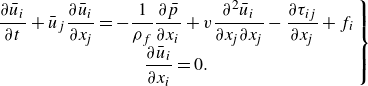 \begin{equation} \left .\begin{array}{cc} & \displaystyle\frac {\partial \bar {u}_i}{\partial t}+\bar {u}_j \frac {\partial \bar {u}_i}{\partial x_{\!j}}=-\frac {1}{\rho _f} \frac {\partial \bar {p}}{\partial x_i}+v \frac {\partial ^2 \bar {u}_i}{\partial x_{\!j} \partial x_{\!j}}-\frac {\partial \tau _{i j}}{\partial x_{\!j}}+f_{i} \\ & \displaystyle\frac {\partial \bar {u}_i}{\partial x_i}=0 .\end{array}\right \} \end{equation}
Here, $u_i$
(
$u_i$
( $i=$
1, 2, 3) is the flow velocity of three directions in the Cartesian coordinate system, an overbar stands for the filtering procedure,
$i=$
1, 2, 3) is the flow velocity of three directions in the Cartesian coordinate system, an overbar stands for the filtering procedure, $p$
is the pressure,
$p$
is the pressure, $t$
is the time,
$t$
is the time, $\rho _f$
is the fluid density,
$\rho _f$
is the fluid density, $\nu$
is the kinematic viscosity of the fluid,
$\nu$
is the kinematic viscosity of the fluid, $f_i$
is the extra force that represents the action of immersed objects on the fluid and
$f_i$
is the extra force that represents the action of immersed objects on the fluid and $\tau _{i j}$
is the subgrid-scale stress, representing the influences of the filtered small-scale turbulent structures on the flow field (Smagorinsky Reference Smagorinsky1963). To ensure the closure of (2.1), the Smagorinsky eddy viscosity model is applied, which is given as
$\tau _{i j}$
is the subgrid-scale stress, representing the influences of the filtered small-scale turbulent structures on the flow field (Smagorinsky Reference Smagorinsky1963). To ensure the closure of (2.1), the Smagorinsky eddy viscosity model is applied, which is given as
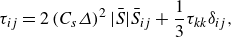 \begin{equation} \tau _{i j}=2\left (C_s \varDelta \right )^2|\bar {S}| \bar {S}_{i j}+\frac {1}{3} \tau _{k k} \delta _{i j}, \end{equation}
where $C_s$
is the Smagorinsky constant. In the present study,
$C_s$
is the Smagorinsky constant. In the present study, $C_s=$
0.1 (Deardorff Reference Deardorff1970). The filter width
$C_s=$
0.1 (Deardorff Reference Deardorff1970). The filter width $\varDelta$
is adopted as
$\varDelta$
is adopted as $\varDelta =\sqrt [3]{\Delta x \Delta y \Delta z}$
with
$\varDelta =\sqrt [3]{\Delta x \Delta y \Delta z}$
with $\Delta x$
,
$\Delta x$
, $\Delta y$
, and
$\Delta y$
, and $\Delta z$
as the grid sizes in the three directions. Here,
$\Delta z$
as the grid sizes in the three directions. Here, $|\bar {S}|= (2 \bar {S}_{i j} \bar {S}_{i j} )^{1 / 2}$
is the magnitude of large-scale strain rate tensor, where
$|\bar {S}|= (2 \bar {S}_{i j} \bar {S}_{i j} )^{1 / 2}$
is the magnitude of large-scale strain rate tensor, where $\bar {S}_{i j}=({1}/{2}) (({\partial \bar {u}_i}/{\partial x_{\!j}})+({\partial \bar {u}_j}/{\partial x_i}) )$
.
$\bar {S}_{i j}=({1}/{2}) (({\partial \bar {u}_i}/{\partial x_{\!j}})+({\partial \bar {u}_j}/{\partial x_i}) )$
.
2.2. Vector form intrinsic finite element
The VFIFE method was first introduced by Ting, Shih & Wang (Reference Ting, Shih and Wang2004a ,Reference Ting, Shih and Wang b , Reference Ting, Duan and Wu2012), Ting & Wang (Reference Ting and Wang2008) and Shih, Wang & Ting (Reference Shih, Wang and Ting2004). It is an analytical and numerical method in structural mechanics based on point value description and vector form theory. The point value description in the VFIFE method relies on a lumped mass matrix, meaning that external force on one spatial point does not influence the motion dynamics of other spatial points. As a result, the method eliminates the need to construct complex rigidity matrix or solve large-scale nonlinear equations. Compared with conventional methods, the VFIFE method effectively avoids certain nonlinear issue that arise when structures undergo large deformations, dislocations, collisions or elastoplastic behaviours, such as iteration non-convergence and matrix singularity. Additionally, by appropriately discretising path elements, the characteristics between two path elements can be adjusted, allowing the method to handle structural discontinuities. Consequently, the VFIFE method has been widely applied to address challenging nonlinear and discontinuous scenarios (Duan et al. Reference Duan, He, Zhang, Ting, Wang, Chen and Wang2014; Xu et al. Reference Xu, Li, Jiang and Liu2015; Xu & Lin Reference Xu and Lin2017; Hou, Fang & Zhang Reference Hou, Fang and Zhang2018; Li, Wei & Bai Reference Li, Wei and Bai2020; Wu et al. Reference Wu, Zeng, Xiao, Yu, Dai and Yu2020).
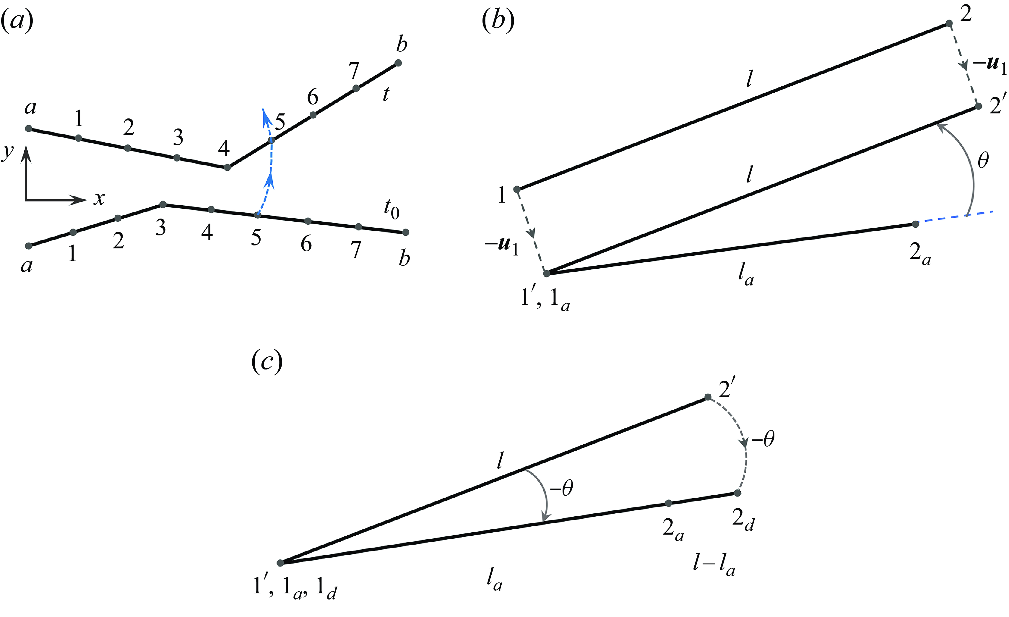
The foundation of the VFIFE lies in its spatial and temporal structural point value description. In the spatial point value description, the structural mass is concentrated at a series of discretised spatial points. The motion and deformation of structure can be determined through the positions of these spatial points, which are interconnected by linear beam elements, see figure 2( $a$
). It is assumed that the cross-sectional profiles of the elements remain identical and perpendicular to the principal axis at any position. Unlike conventional methods, the beam elements in the VFIFE are responsible solely for internal structural force and are independent of the governing equations. For cases involving multiple internal forces between two spatial points, multiple beam elements are used. These elements are positioned between the two spatial points to represent the internal force without needing to define it across the entire structural range (Ting, Duan & Wu Reference Ting, Duan and Wu2012).
$a$
). It is assumed that the cross-sectional profiles of the elements remain identical and perpendicular to the principal axis at any position. Unlike conventional methods, the beam elements in the VFIFE are responsible solely for internal structural force and are independent of the governing equations. For cases involving multiple internal forces between two spatial points, multiple beam elements are used. These elements are positioned between the two spatial points to represent the internal force without needing to define it across the entire structural range (Ting, Duan & Wu Reference Ting, Duan and Wu2012).
In the temporal point value description, the structure’s dynamics is represented by a series of path elements that follow the principle of ‘large dislocation and small deformation’. Within each path element, the shift of a spatial point comes from the two components: rigid body motion and pure deformation. The displacement due to rigid body motion is determined using Newton’s second law and the rotational equation, while the displacement caused by pure deformation is described by Hooke’s law through the introduction of a virtual reverse motion. Ensuring consistency of the structural properties and motion trajectories is crucial for accurately calculating pure deformation within each path unit via reverse motion. In the VFIFE, reverse motion is introduced to distinguish dislocations caused by rigid body movement from those caused by pure structural deformation, see figure 2( $b$
,
$b$
, $c$
). The processing steps are as follows. (i) The calculation of structural internal force is based on the state at the initial instant
$c$
). The processing steps are as follows. (i) The calculation of structural internal force is based on the state at the initial instant $t_a$
. (ii) Due to the consistency of structural properties and motion trajectories within each path element, a virtual structural state at any instant
$t_a$
. (ii) Due to the consistency of structural properties and motion trajectories within each path element, a virtual structural state at any instant $t$
is generated through a virtual reverse motion, which includes reverse translational and rotational motions for the spatial position at that instant. Subsequently, minor dislocations and deformations are identified by comparing the reference and virtual structural states. (iii) These small deformations and dislocations are then resolved using the structural deformation–internal force relationship. Finally, the structural state at
$t$
is generated through a virtual reverse motion, which includes reverse translational and rotational motions for the spatial position at that instant. Subsequently, minor dislocations and deformations are identified by comparing the reference and virtual structural states. (iii) These small deformations and dislocations are then resolved using the structural deformation–internal force relationship. Finally, the structural state at $t_b$
is obtained through a forward rigid body motion.
$t_b$
is obtained through a forward rigid body motion.
( $a$
) The beam elements, (
$a$
) The beam elements, ( $b$
) reverse translation and (
$b$
) reverse translation and ( $c$
) reverse rotation in the VFIFE.
$c$
) reverse rotation in the VFIFE.
The dynamics of a wall-mounted flexible stem is simulated using VFIFE method. Based on the point value description, the stem is discretised into a set of spatial nodes that connect to each other by beam elements. The motion of each node is applied to describe the movement and deformation of the stem and satisfies Newton’s second law
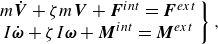 \begin{equation} \left .\begin{array}{rc} & m \dot {\boldsymbol{V}}+\zeta m \boldsymbol{V}+\boldsymbol{F}^{i n t}=\boldsymbol{F}^{e x t} \\ & I \dot {\boldsymbol{\omega }}+\zeta I \boldsymbol{\omega }+\boldsymbol{M}^{i n t}=\boldsymbol{M}^{e x t} \end{array}\right \}, \end{equation}
where $m$
and
$m$
and $I$
are the mass and momentum of inertia matrix of the node, respectively. Here,
$I$
are the mass and momentum of inertia matrix of the node, respectively. Here, $\dot {\boldsymbol{V}}$
,
$\dot {\boldsymbol{V}}$
, $\boldsymbol{V}$
,
$\boldsymbol{V}$
, $\dot {\boldsymbol{\omega }}$
and
$\dot {\boldsymbol{\omega }}$
and $\boldsymbol{\omega }$
are the acceleration, velocity, angular acceleration and angular velocity of the node, respectively,
$\boldsymbol{\omega }$
are the acceleration, velocity, angular acceleration and angular velocity of the node, respectively, $\boldsymbol{F}^{i n t}$
,
$\boldsymbol{F}^{i n t}$
, $\boldsymbol{F}^{e x t}$
,
$\boldsymbol{F}^{e x t}$
, $\boldsymbol{M}^{i n t}$
and
$\boldsymbol{M}^{i n t}$
and $\boldsymbol{M}^{e x t}$
are the internal force, external force, internal momentum and external momentum, respectively, and
$\boldsymbol{M}^{e x t}$
are the internal force, external force, internal momentum and external momentum, respectively, and $\zeta$
is the structural damping coefficient, which is zero in the present study. An explicit iterative scheme based on the central difference is adopted to solve equation (2.3) as follows:
$\zeta$
is the structural damping coefficient, which is zero in the present study. An explicit iterative scheme based on the central difference is adopted to solve equation (2.3) as follows:
 \begin{equation} \left .\begin{array}{cc} \boldsymbol{x}^{n+1}=\Delta t_s^2 \frac {\boldsymbol{F}^{e x t}-\boldsymbol{F}^{i n t}}{m}+2 \boldsymbol{x}^n-\boldsymbol{x}^{n-1} \\ \boldsymbol{\alpha }^{n+1}=\Delta t_s^2 \frac {\boldsymbol{M}^{e x t}-\boldsymbol{M}^{i n t}}{I}+2 \boldsymbol{\alpha }^n-\boldsymbol{\alpha }^{n-1} \\ \boldsymbol{V}^{n+1}=\frac {\boldsymbol{x}^{n+1}-\boldsymbol{x}^n}{\Delta t_s}, \boldsymbol{\omega }^{n+1}=\frac {\boldsymbol{\alpha }^{n+1}-\boldsymbol{\alpha }^n}{\Delta t_s} \end{array}\right \}, \end{equation}
where $\boldsymbol{x}$
,
$\boldsymbol{x}$
, $\boldsymbol{\alpha }$
and
$\boldsymbol{\alpha }$
and $\Delta t_s$
represent the node position, rotation angle of the node and the structural time step, respectively. The temporal trajectory of any node on the stem is described by a set of spatial points, and the process between the spatial points is defined as the path element. Proper division of the path element allows the properties of each node to vary between two elements.
$\Delta t_s$
represent the node position, rotation angle of the node and the structural time step, respectively. The temporal trajectory of any node on the stem is described by a set of spatial points, and the process between the spatial points is defined as the path element. Proper division of the path element allows the properties of each node to vary between two elements.
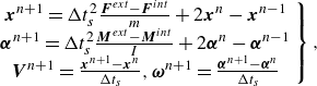
The layout of the immersed boundary method. The discrete volumes ( $V_i$
) of the immersed boundary points (IBPs), marked by the dashed region, form a thin shell of thickness equal to one mesh width around each IBP.
$V_i$
) of the immersed boundary points (IBPs), marked by the dashed region, form a thin shell of thickness equal to one mesh width around each IBP.
2.3. Immersed boundary method
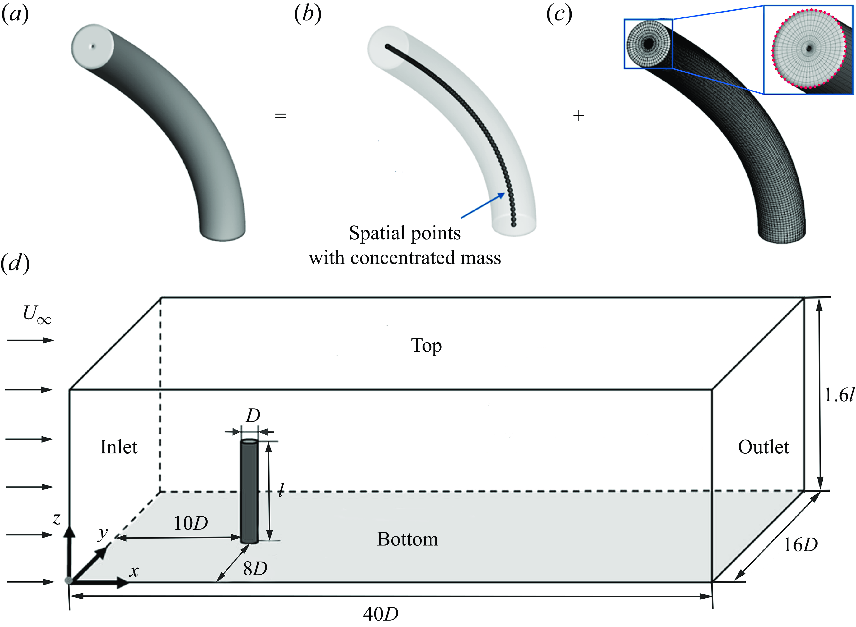
The IBM was first introduced by Peskin (Reference Peskin1972) for simulating blood flow around the flexible leaflet of a human heart. Compared with conventional numerical methods, IBM offers key advantages, particularly in FSI simulations involving topological changes. Another significant advantage is its parameterised and fast implementation, enabling the rapid simulation of numerous cases with different geometric configurations, unlike conventional methods that rely on body-conformal grids. In the IBM framework, the flow motion equations are discretised on a fixed Cartesian grid, while the structure is represented by a series of IBPs on a Lagrangian grid, which is curvilinear and free to move, see figure 3. The Cartesian grid does not conform to the geometry of a moving structure. As a result, the boundary conditions on the fluid–body interface cannot be imposed directly. Instead, an extra body force is incorporated into the fluid momentum equation to account for this interaction. This body force is updated during pressure iterations (Ji, Munjiza & Williams Reference Ji, Munjiza and Williams2012), ensuring that it is solved simultaneously with pressure and that the boundary condition on the immersed boundary is fully satisfied. In the current simulation, the stem is discretised into 160 elements along its height, resulting in 161 circular slices. Each slice is represented as a circle, further discretised into 256 IBPs uniformly distributed along its circumferences, as illustrated in figure 4( $c$
). This ensures that at least one IBP is present in each grid cell, maintaining accurate spatial resolution. Given an aspect ratio of AR
$c$
). This ensures that at least one IBP is present in each grid cell, maintaining accurate spatial resolution. Given an aspect ratio of AR $= 10$
, the resolution is 1/16 . Notably, when the stem deforms, the plane of each layer, composed of 256 IBPs, remains perpendicular to the tangent line at the corresponding node. As the structure’s surface is formed by these IBPs, the internal fluid remains entirely isolated from the external fluid, inherently satisfying the condition of a zero normal pressure gradient on the surface.
$= 10$
, the resolution is 1/16 . Notably, when the stem deforms, the plane of each layer, composed of 256 IBPs, remains perpendicular to the tangent line at the corresponding node. As the structure’s surface is formed by these IBPs, the internal fluid remains entirely isolated from the external fluid, inherently satisfying the condition of a zero normal pressure gradient on the surface.
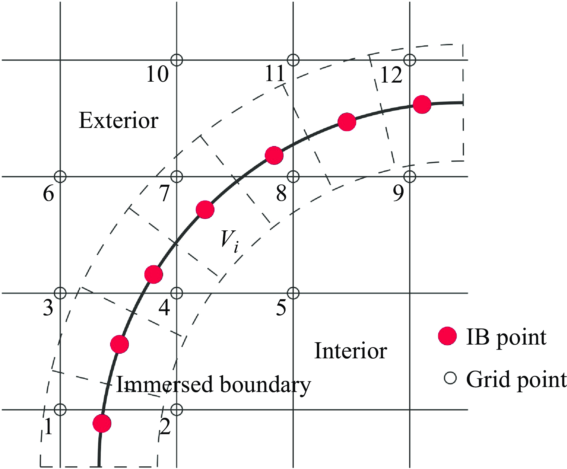
To discretise equation (2.1), the second-order Adams–Bashforth time scheme and the second-order central difference scheme are applied, which lead to the following conservation form:
 \begin{equation} \left .\begin{array}{cc} \boldsymbol{u}^{n+1}=\boldsymbol{u}^n+\delta t\left (\frac {3}{2} \boldsymbol{h}^n-\frac {1}{2} \boldsymbol{h}^{n-1}-\frac {3}{2} \nabla p^n+\frac {1}{2} \nabla p^{n-1}\right )+\boldsymbol{f}^{n+\frac {1}{2}} \delta t \\ \nabla \cdot \boldsymbol{u}^{n+1}=0 ,\end{array}\right \} \end{equation}
where $\boldsymbol{h}=\nabla \cdot (-\boldsymbol{u} \boldsymbol{u}+ (v+v_t ) (\nabla \boldsymbol{u}+\nabla \boldsymbol{u}^T ) )$
is composed of the convective and diffusive terms, in which the superscript
$\boldsymbol{h}=\nabla \cdot (-\boldsymbol{u} \boldsymbol{u}+ (v+v_t ) (\nabla \boldsymbol{u}+\nabla \boldsymbol{u}^T ) )$
is composed of the convective and diffusive terms, in which the superscript $T$
is the transpose of a matrix and
$T$
is the transpose of a matrix and $\nu _t$
is the turbulence eddy viscosity. Superscripts
$\nu _t$
is the turbulence eddy viscosity. Superscripts $n$
+1,
$n$
+1, $n$
+1/2,
$n$
+1/2, $n$
and
$n$
and $n$
–1 indicate the time steps. The extra force
$n$
–1 indicate the time steps. The extra force $\boldsymbol{f}$
is determined by setting the velocity consistent condition
$\boldsymbol{f}$
is determined by setting the velocity consistent condition $U^{n+1}=V^{n+1}$
on the fluid–structure interface, where
$U^{n+1}=V^{n+1}$
on the fluid–structure interface, where $U^{n+1}$
is the interpolated fluid velocity and
$U^{n+1}$
is the interpolated fluid velocity and $V^{n+1}$
is the update structure velocity. Extra force
$V^{n+1}$
is the update structure velocity. Extra force $\boldsymbol{f}$
is formally evaluated at the time step
$\boldsymbol{f}$
is formally evaluated at the time step $n + 1/2$
 \begin{equation} \boldsymbol{f}^{n+\frac {1}{2}} \delta t=D\big(\boldsymbol{F}^{n+\frac {1}{2}}\big)=D\left (\!\boldsymbol{v}^{n+1}-I\left (\!\boldsymbol{u}^n+\delta t\left (\frac {3}{2} \boldsymbol{h}^n-\frac {1}{2} \boldsymbol{h}^{n-1}-\frac {3}{2} \nabla p^n+\frac {1}{2} \nabla p^{n-1}\right )\!\right )\!\right )\! ,\end{equation}
where $\boldsymbol{F}$
is the extra body force on the structure and
$\boldsymbol{F}$
is the extra body force on the structure and $\boldsymbol{v}^{n+1}=\boldsymbol{V}^{n+1}+\boldsymbol{r} \times \boldsymbol{\omega }^{n+1}$
is the desired velocity on the IBPs obtained by solving equation (2.3), in which
$\boldsymbol{v}^{n+1}=\boldsymbol{V}^{n+1}+\boldsymbol{r} \times \boldsymbol{\omega }^{n+1}$
is the desired velocity on the IBPs obtained by solving equation (2.3), in which $\boldsymbol{r}$
is a vector from a node to an IBP. The interpolation and distribution functions,
$\boldsymbol{r}$
is a vector from a node to an IBP. The interpolation and distribution functions, $I$
and
$I$
and $D$
, suggested in Peskin (Reference Peskin1972) are applied, which are responsible for data transfer between the non-conforming Eulerian and Lagrangian grids.
$D$
, suggested in Peskin (Reference Peskin1972) are applied, which are responsible for data transfer between the non-conforming Eulerian and Lagrangian grids.
( $a$
,
$a$
, $b$
,
$b$
, $c$
) The wall-mounted flexible stem model in the present simulation and (
$c$
) The wall-mounted flexible stem model in the present simulation and ( $d$
) the numerical set-up of the computational domain (not to scale). Part of the IBPs on the top surface are marked by the red dots in (
$d$
) the numerical set-up of the computational domain (not to scale). Part of the IBPs on the top surface are marked by the red dots in ( $c$
).
$c$
).
2.4. Coupling between the fluid and structures
As mentioned earlier, in the present method, the wall-mounted flexible stem is materialised by the IBPs on the solid surface, see figure 4(a–c). However, as the stem’s motion is defined by spatial points with concentrated mass, an appropriate approach is needed to effectively transfer the fluid force from the surface IBPs to these spatial points. During each iteration of fluid-structure coupling, the solid surface surrounding these mass points is reconstructed using IBPs, see figure 4( $c$
). The fluid force on these reconstructed solid surface IBPs is then applied to the corresponding mass points as external forces. Consequently, the motion of each node is determined using (2.3). Simultaneously, the flow velocity and pressure are updated, and the velocity on the immersed boundary is corrected, thereby establishing the coupling between the fluid and the structure. It is important to note that the critical time step for solid motion is significantly smaller than that for the fluid. Therefore, within each fluid time step, the solid motion must be iterated multiple times under the assumption that the fluid forces remain unchanged.
$c$
). The fluid force on these reconstructed solid surface IBPs is then applied to the corresponding mass points as external forces. Consequently, the motion of each node is determined using (2.3). Simultaneously, the flow velocity and pressure are updated, and the velocity on the immersed boundary is corrected, thereby establishing the coupling between the fluid and the structure. It is important to note that the critical time step for solid motion is significantly smaller than that for the fluid. Therefore, within each fluid time step, the solid motion must be iterated multiple times under the assumption that the fluid forces remain unchanged.
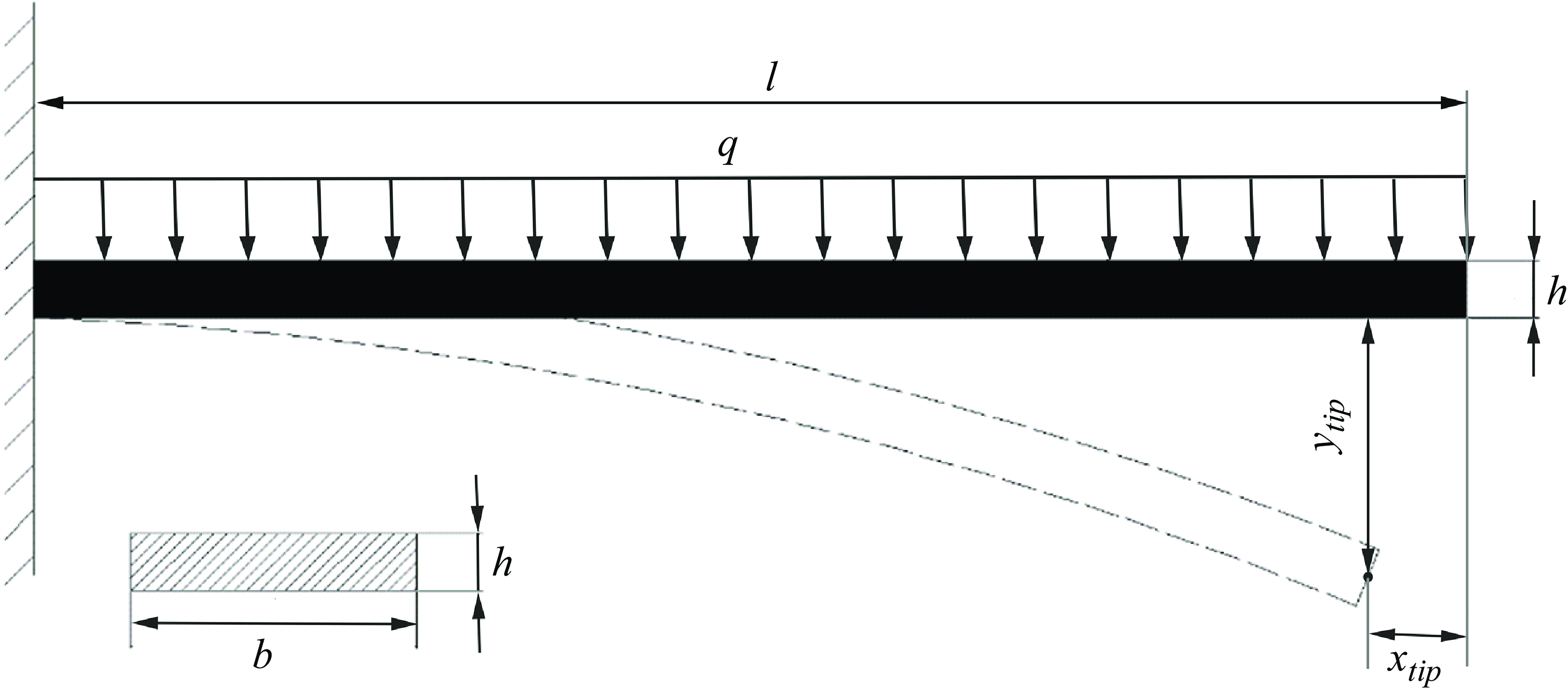
Model for the deformation of a flexible stem under uniform loading.
3. Validation
3.1. The deformation of a cantilever plate under uniform loading
First, we verify the codes for pure deformation of a wall-mounted flexible stem with a rectangular cross-section under uniform loading. As modelled in figure 5, the cantilever plate is wall mounted under uniform loading. The geometric parameters for the plate are the length ( $l$
) of 5 cm, the width (
$l$
) of 5 cm, the width ( $b$
) of 1 cm and the thickness (
$b$
) of 1 cm and the thickness ( $h$
) of 0.2 cm. The plate density is 0.678 g cm–
$h$
) of 0.2 cm. The plate density is 0.678 g cm– $^3$
, the elastic modulus is 5
$^3$
, the elastic modulus is 5 $\times$ $10^5$
Pa and Poisson’s ratio is 0.4. The uniform loading varies in the range of
$10^5$
Pa and Poisson’s ratio is 0.4. The uniform loading varies in the range of $q=$
0.0001–0.0008 N cm–1. The plate is divided into elements, i.e. 10, 25 and 50. The corresponding grid in the vertical direction (along the length) is
$q=$
0.0001–0.0008 N cm–1. The plate is divided into elements, i.e. 10, 25 and 50. The corresponding grid in the vertical direction (along the length) is ${\rm d}x_s$
. For different situations, the time step is controlled to be smaller than the critical time step
${\rm d}x_s$
. For different situations, the time step is controlled to be smaller than the critical time step ${\rm d}t_s^0$
calculated using the equation of
${\rm d}t_s^0$
calculated using the equation of ${\rm d}t_s^0 = {\rm d}x_s/\sqrt{E/\rho_s}$
, where E is Young’s modulus, and
${\rm d}t_s^0 = {\rm d}x_s/\sqrt{E/\rho_s}$
, where E is Young’s modulus, and $\rho_s$
is the plate density. The structural damping is set as
$\rho_s$
is the plate density. The structural damping is set as $\zeta=$
0.
$\zeta=$
0.
Based on the deformation theory of a plate under uniform loading ( $q$
), the final deformation curve follows the equation
$q$
), the final deformation curve follows the equation
 \begin{equation} v(x)=-\frac {q x^2}{24 E I}\left (x^2-4 x l+6 l^2\right ), \end{equation}
where $x$
is the distance of one point to the fixed end (positive in the
$x$
is the distance of one point to the fixed end (positive in the $x$
direction),
$x$
direction), $v(x)$
is the final deformation of the plate and
$v(x)$
is the final deformation of the plate and $I=bh^3/12$
is the cross-sectional inertial moment of the plate.
$I=bh^3/12$
is the cross-sectional inertial moment of the plate.
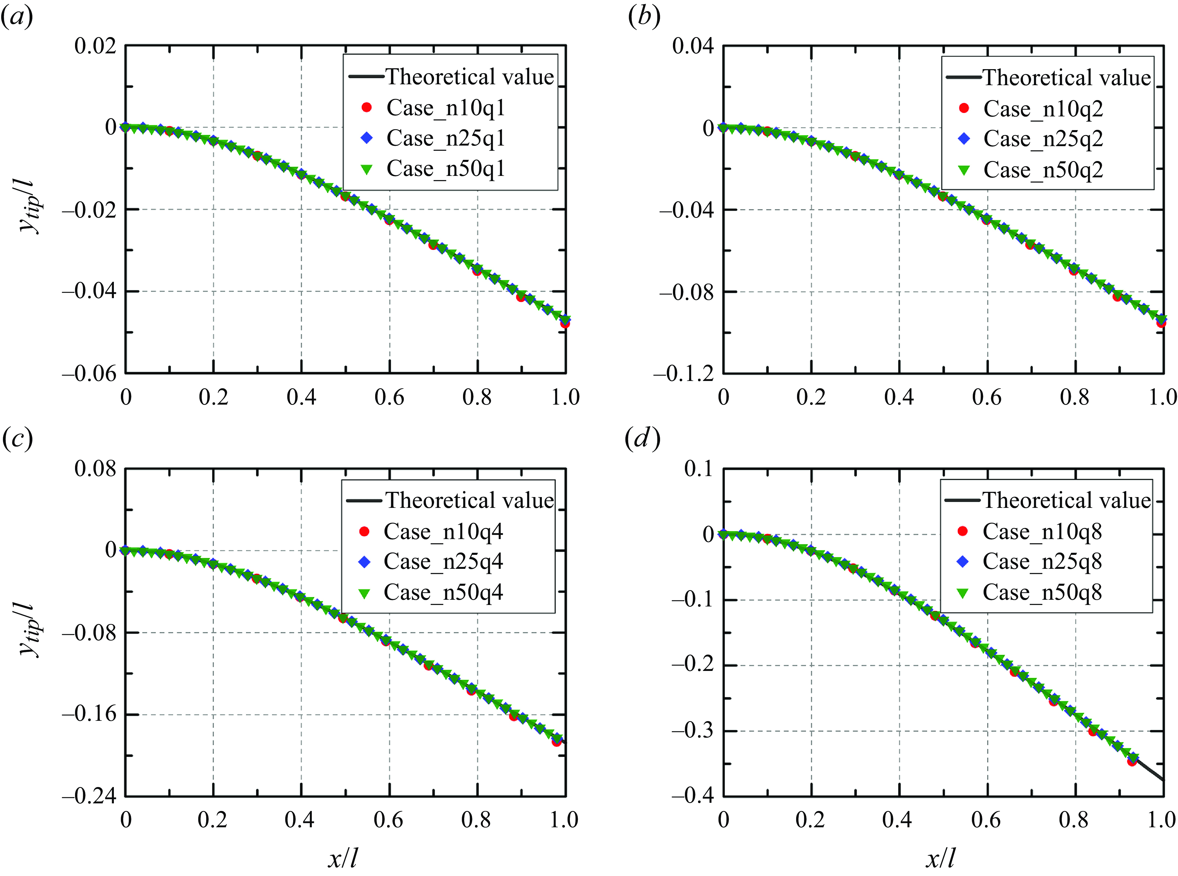
Comparison of the transverse shift of the tip with the theoretical value for a plate under uniform loading. Here, Case_n10q1 represents the case of the plate divided into 10 elements and under the loading of $q = 0.0001$
N cm–1. The naming scheme is applied for other cases. For example, Case_n25q8 denotes the case of the plate divided into 25 elements and under the loading of
$q = 0.0001$
N cm–1. The naming scheme is applied for other cases. For example, Case_n25q8 denotes the case of the plate divided into 25 elements and under the loading of $q = 0.0008$
N cm−1.
$q = 0.0008$
N cm−1.
( $a$
) The relative difference of the deformation at the free plate end versus the dimensions of the uniform loading, and (
$a$
) The relative difference of the deformation at the free plate end versus the dimensions of the uniform loading, and ( $b$
) the relative difference of the vibration frequency of the plate with different elements versus the uniform loading.
$b$
) the relative difference of the vibration frequency of the plate with different elements versus the uniform loading.
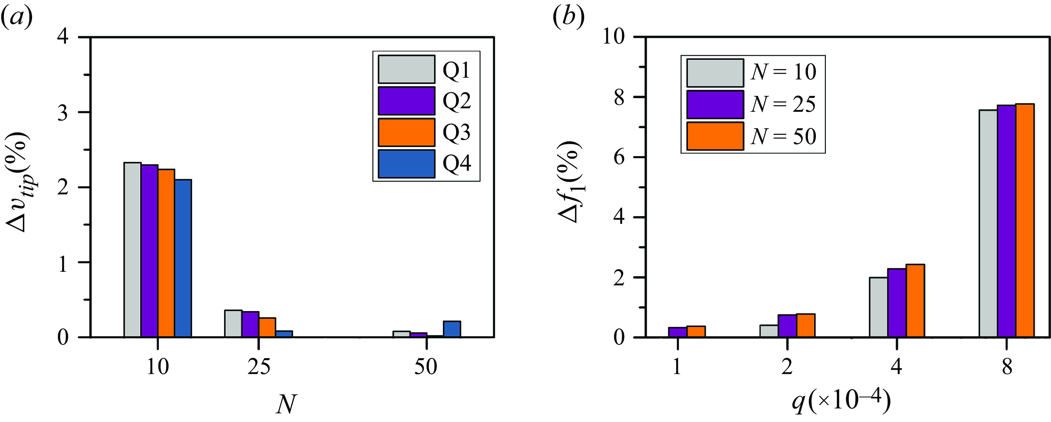
Figure 6 shows the comparison of the simulated results and theoretical results. It is seen that the model for the plate motion can accurately predict the deformation of the plate. Further, the number of elements in the simulation is also essential. The difference (in percentage) between the simulation and the theoretical value becomes higher as it gets closer to the free end of the plate, which is related to the deformation growing smaller. Thus, it requires a higher number of elements. As shown in figure 7, after the element number exceeds 25, the simulated deformation and vibration frequency match very well the theoretical results. The relative difference generally gets smaller when the loading is higher. Here, the relative differences for the deformation and vibration frequency are defined as $\Delta v_{tip}=(v_{tip}-v_{tip}^0 )/v_{tip}^0$
and
$\Delta v_{tip}=(v_{tip}-v_{tip}^0 )/v_{tip}^0$
and $\Delta f_{1}=(f_{1}-f_{1}^0 )/f_{1}^0$
, respectively, where
$\Delta f_{1}=(f_{1}-f_{1}^0 )/f_{1}^0$
, respectively, where $v_{tip}$
is the simulated deformation,
$v_{tip}$
is the simulated deformation, $v_{tip}^0$
is the theoretical solution,
$v_{tip}^0$
is the theoretical solution, $f_{1}$
is the simulated vibration frequency and
$f_{1}$
is the simulated vibration frequency and $f_{1}^0$
is the theoretical value.
$f_{1}^0$
is the theoretical value.
3.2. Flexible plate in uniform channel flow
In this section, we validate the codes through a benchmark case of a wall-mounted flexible plate in uniform channel flow. Interactions between the fluid and plate are considered. Luhar & Nepf (Reference Luhar and Nepf2011) carried out a series of model experiments in the channel flow on a flexible plate, widely used to compare numerical or experimental results. To check the fidelity of our present numerical methodology, we compare our numerical results with those of Luhar & Nepf (Reference Luhar and Nepf2011).
In our present simulation, the setting of the computational domain is very similar to the water flume experiment in Luhar & Nepf (Reference Luhar and Nepf2011), see their figure 3. Based on this, the computational domain is 40 cm $\times$
16 cm
$\times$
16 cm $\times$
16 cm in length, width and height, respectively. The water depth in the channel is 16 cm. In the inlet, the incoming flow is a uniform velocity
$\times$
16 cm in length, width and height, respectively. The water depth in the channel is 16 cm. In the inlet, the incoming flow is a uniform velocity $U_\infty$
, while the velocity condition is applied in the outlet. For the top and lateral walls, free-slip boundaries are adopted. The bottom is a no-slip boundary and the wall function developed by Werner & Wengle (Reference Werner, Wengle, Durst, Friedrich, Launder, Schumann and Whitelaw1993) was used. The geometric parameters for the flexible plate are the length (
$U_\infty$
, while the velocity condition is applied in the outlet. For the top and lateral walls, free-slip boundaries are adopted. The bottom is a no-slip boundary and the wall function developed by Werner & Wengle (Reference Werner, Wengle, Durst, Friedrich, Launder, Schumann and Whitelaw1993) was used. The geometric parameters for the flexible plate are the length ( $l$
) of 5 cm, width (
$l$
) of 5 cm, width ( $b$
) of 1 cm and thickness (
$b$
) of 1 cm and thickness ( $h$
) of 0.2 cm, respectively. The density of the flexible plate is 0.678 g cm–
$h$
) of 0.2 cm, respectively. The density of the flexible plate is 0.678 g cm– $^3$
, the elastic modulus is
$^3$
, the elastic modulus is $5 \times 10^5$
Pa and the Poisson ratio is 0.4.
$5 \times 10^5$
Pa and the Poisson ratio is 0.4.
Before the validation, we first carry out a convergence test. A uniform mesh is applied around the flexible plate, and a large region is adopted to cover the possible motion of the plate. Outside this region, the stretched mesh with the constant ratio (not larger than 1.02) is adopted. Therefore, the total meshes is affordable in the present simulations. Four uniform meshes are selected, i.e. $\Delta h/b=$
0.2, 0.1, 0.0625 and 0.05. Here,
$\Delta h/b=$
0.2, 0.1, 0.0625 and 0.05. Here, $h$
is the minimum mesh. The dimension (
$h$
is the minimum mesh. The dimension ( ${\rm d}x_s$
) of the solid element is the same as the minimum mesh adopted. The fluid time step (
${\rm d}x_s$
) of the solid element is the same as the minimum mesh adopted. The fluid time step ( ${\rm d}t_f$
) for each situation is smaller than the critical time step (
${\rm d}t_f$
) for each situation is smaller than the critical time step ( ${\rm d}t_f^0$
) calculated through the equation below
${\rm d}t_f^0$
) calculated through the equation below
 \begin{equation} \mathrm{d} t_f^0=\frac {\min \left ({\rm d} x_f, {\rm d} x_s\right )}{\sqrt {E / \rho _s}+2 U_{\infty }} ,\end{equation}
where ${\rm d}x_f$
is the fluid mesh,
${\rm d}x_f$
is the fluid mesh, ${\rm d}x_s$
is the dimension of the solid element,
${\rm d}x_s$
is the dimension of the solid element, $E$
is Young’s modulus,
$E$
is Young’s modulus, $\rho _s$
is the solid (or structure) density and
$\rho _s$
is the solid (or structure) density and $U_\infty$
is the incoming flow velocity. The Reynolds number is
$U_\infty$
is the incoming flow velocity. The Reynolds number is $Re_b=$
1600 when the width (
$Re_b=$
1600 when the width ( $b$
) of the plate is used as the characteristic length.
$b$
) of the plate is used as the characteristic length.
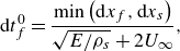
Figure 8( $a$
) compares the simulation results and those (
$a$
) compares the simulation results and those ( $D_x/b=$
2.14,
$D_x/b=$
2.14, $D_z/b=$
0.59 and
$D_z/b=$
0.59 and $C_d=$
1.03) of model experiments in Luhar & Nepf (Reference Luhar and Nepf2011) under different mesh spacings. Here,
$C_d=$
1.03) of model experiments in Luhar & Nepf (Reference Luhar and Nepf2011) under different mesh spacings. Here, $D_x$
is the deflection of the plate at the free end in the streamwise direction,
$D_x$
is the deflection of the plate at the free end in the streamwise direction, $D_z$
is the height reduction of the plate at the free end and
$D_z$
is the height reduction of the plate at the free end and $C_d$
is the drag force because of the flow around the vegetation. It is seen that the relative difference between the present simulation and the experiments of Luhar & Nepf (Reference Luhar and Nepf2011) becomes lower as the mesh is finer. When the mesh is no larger than
$C_d$
is the drag force because of the flow around the vegetation. It is seen that the relative difference between the present simulation and the experiments of Luhar & Nepf (Reference Luhar and Nepf2011) becomes lower as the mesh is finer. When the mesh is no larger than $\Delta h/b=$
0.0625, the relative errors for
$\Delta h/b=$
0.0625, the relative errors for $D_x/b$
and
$D_x/b$
and $C_d$
are lower than 1
$C_d$
are lower than 1 $\, \%$
and smaller than 6
$\, \%$
and smaller than 6 $\, \%$
for
$\, \%$
for $D_z/b$
. Thus, our numerical results agree well with the experiments of Luhar & Nepf (Reference Luhar and Nepf2011), suggesting a high fidelity of the present numerical methodology. Further, the mesh with
$D_z/b$
. Thus, our numerical results agree well with the experiments of Luhar & Nepf (Reference Luhar and Nepf2011), suggesting a high fidelity of the present numerical methodology. Further, the mesh with $h/b$
smaller than 0.0625 is an appropriate choice for our following simulations.
$h/b$
smaller than 0.0625 is an appropriate choice for our following simulations.
The incoming flow velocities, including $U_\infty=$
3.6, 11.0, 16.0 and 27.0 cm s–1, are simulated and compared with the experiments in Luhar & Nepf (Reference Luhar and Nepf2011) for further validation. The mesh with
$U_\infty=$
3.6, 11.0, 16.0 and 27.0 cm s–1, are simulated and compared with the experiments in Luhar & Nepf (Reference Luhar and Nepf2011) for further validation. The mesh with $\Delta h/b=$
0.0625 is adopted. Figure 8(
$\Delta h/b=$
0.0625 is adopted. Figure 8( $b$
) compares the drag force (
$b$
) compares the drag force ( $F_d$
) acting on the plate of the present simulation with both model predictions and experiment results. It is seen that the present simulation results are well matched with those in the experiments. This again indicates that our present methodology has high fidelity in simulating flexible plates in uniform channel flow.
$F_d$
) acting on the plate of the present simulation with both model predictions and experiment results. It is seen that the present simulation results are well matched with those in the experiments. This again indicates that our present methodology has high fidelity in simulating flexible plates in uniform channel flow.
( $a$
) The relative errors in hydrodynamic forces with different
$a$
) The relative errors in hydrodynamic forces with different $b/h$
values and (
$b/h$
values and ( $b$
) comparison of the drag force with prediction values and experimental results in Luhar & Nepf (Reference Luhar and Nepf2011).
$b$
) comparison of the drag force with prediction values and experimental results in Luhar & Nepf (Reference Luhar and Nepf2011).
3.3. Flexible stem under uniform loading
In this section, the deformation, including the tip position in the $x$
and
$x$
and $z$
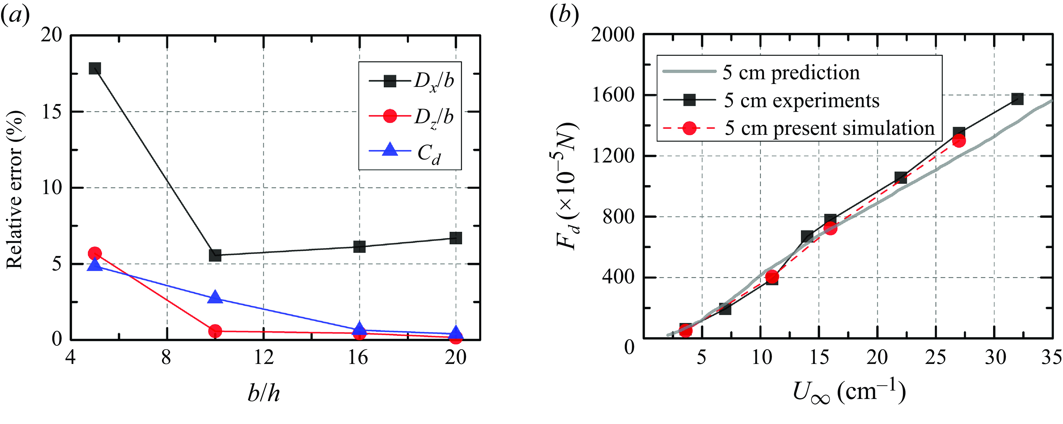
directions and inclination angle of the chord line (i.e. between the tip and root) and horizontal line of a wall-mounted stem under uniform loading, is investigated and verified against the theoretical value, see figure 9(
$z$
directions and inclination angle of the chord line (i.e. between the tip and root) and horizontal line of a wall-mounted stem under uniform loading, is investigated and verified against the theoretical value, see figure 9( $a$
). The aspect ratio is AR
$a$
). The aspect ratio is AR $= 10$
and the uniform loading
$= 10$
and the uniform loading $q$
is given according to the drag coefficient on the rigid stem. Figure 9(b–d) compares our simulation results with the theoretical value. It shows a good agreement for all three deformation quantities, thus suggesting a high fidelity.
$q$
is given according to the drag coefficient on the rigid stem. Figure 9(b–d) compares our simulation results with the theoretical value. It shows a good agreement for all three deformation quantities, thus suggesting a high fidelity.
As shown in figure 9( $b$
,
$b$
, $c$
), the tip position in either direction is dominated by stem stiffness while it is independent of
$c$
), the tip position in either direction is dominated by stem stiffness while it is independent of $Re$
. With increasing
$Re$
. With increasing $K$
,
$K$
, $x_{tip}/l$
decreases while
$x_{tip}/l$
decreases while $h_{tip}/l$
increases gradually, corresponding to the state changing from upright to lodging. However, when lg(
$h_{tip}/l$
increases gradually, corresponding to the state changing from upright to lodging. However, when lg( $K$
)
$K$
) $\gt$
0,
$\gt$
0, $h_{tip}/l$
remains almost constant while
$h_{tip}/l$
remains almost constant while $x_{tip}/l$
decreases approximately linearly when the log–log coordinate is used. When lg(
$x_{tip}/l$
decreases approximately linearly when the log–log coordinate is used. When lg( $K$
)
$K$
) $\lt$
–3,
$\lt$
–3, $h_{tip}/l$
follows the relationship
$h_{tip}/l$
follows the relationship $h_{tip}/l$ $\sim$ $K^{1/3}$
. This relationship was reported in Luhar & Nepf (Reference Luhar and Nepf2011).
$K^{1/3}$
. This relationship was reported in Luhar & Nepf (Reference Luhar and Nepf2011).
As shown in figure 9( $d$
), the inclination angle
$d$
), the inclination angle $\theta$
grows with
$\theta$
grows with $K$
, following the theoretical line. When
$K$
, following the theoretical line. When $K$
is large, the stem maintains upright, thus
$K$
is large, the stem maintains upright, thus $\theta$ $\approx$
90
$\approx$
90 $^\circ$
; while
$^\circ$
; while $K$
is extremely small, the stem maintains nearly parallel to the wall,
$K$
is extremely small, the stem maintains nearly parallel to the wall, $\theta$
approaches 0
$\theta$
approaches 0 $^\circ$
, indicating a lodging state.
$^\circ$
, indicating a lodging state.
( $a$
) Schematic of a wall-mounted flexible stem and deformation quantities, (
$a$
) Schematic of a wall-mounted flexible stem and deformation quantities, ( $b$
,
$b$
, $c$
) the tip position in the
$c$
) the tip position in the $x$
and
$x$
and $z$
directions with
$z$
directions with $K$
, and (
$K$
, and ( $d$
) the inclination angle
$d$
) the inclination angle $\theta$
with
$\theta$
with $K$
. The theoretical value is superimposed for comparison.
$K$
. The theoretical value is superimposed for comparison.
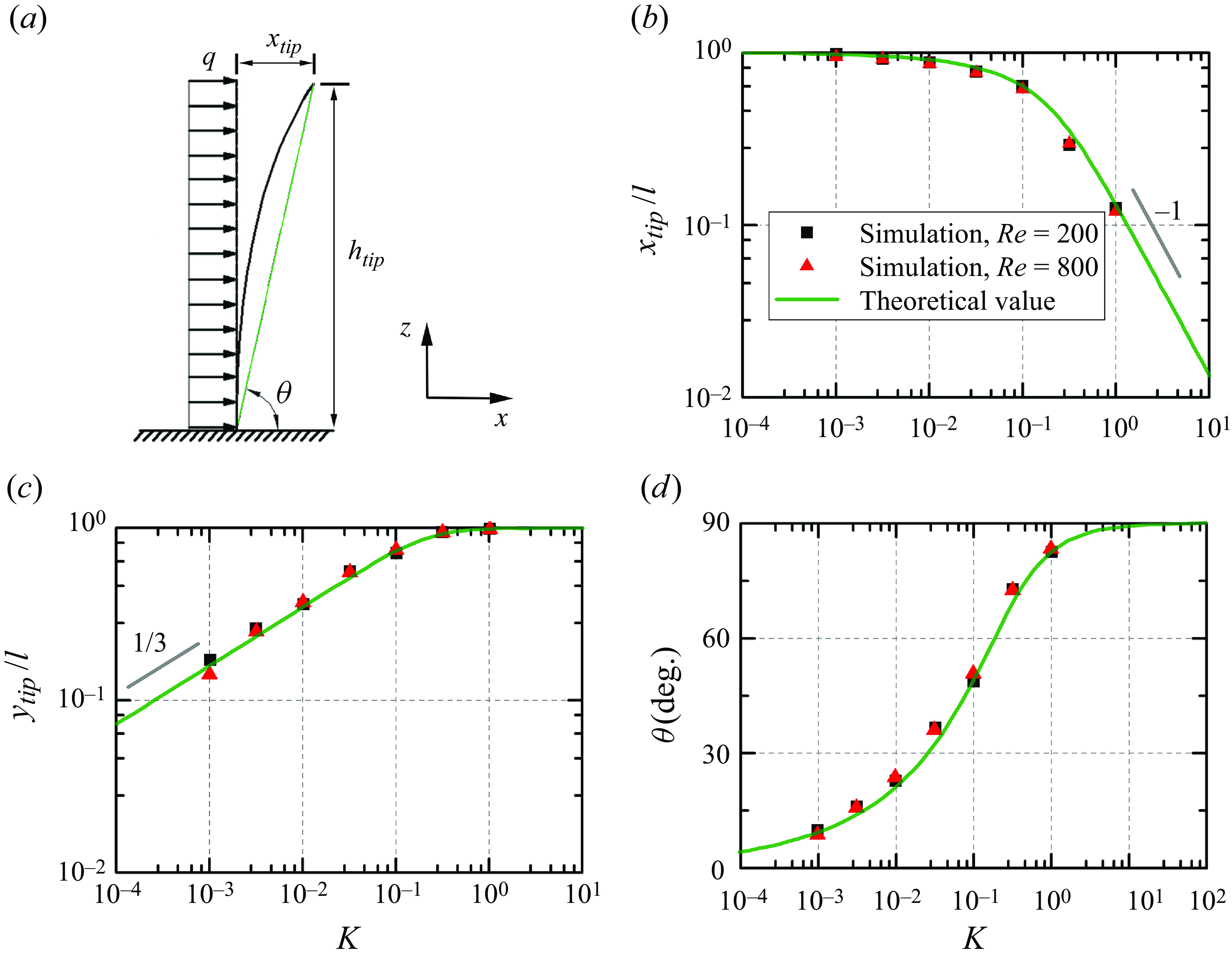
( $a$
,
$a$
, $c$
) Comparison of the time history of the inclination angle (
$c$
) Comparison of the time history of the inclination angle ( $\theta$
) of the present study with Zhang et al. (Reference Zhang, He and Zhang2020), and (
$\theta$
) of the present study with Zhang et al. (Reference Zhang, He and Zhang2020), and ( $b$
,
$b$
, $d$
) time history of the inclination angle (
$d$
) time history of the inclination angle ( $\theta$
) at different grid spacings. (
$\theta$
) at different grid spacings. ( $a$
,
$a$
, $b$
) Are for the case of
$b$
) Are for the case of $Re = 400$
and
$Re = 400$
and $\gamma = 0.008$
, and (
$\gamma = 0.008$
, and ( $c$
,
$c$
, $d$
) are for the case of
$d$
) are for the case of $Re = 400$
and
$Re = 400$
and $\gamma = 0.004$
.
$\gamma = 0.004$
.
3.4. Dynamics of a flexible filament in uniform flow
In this section, we validate the dynamics of a flexible filament by comparing our simulation results with those in Zhang et al. (Reference Zhang, He and Zhang2020). The computation domain and parameter settings are the same as those in Zhang et al. (Reference Zhang, He and Zhang2020). Two cases are selected: one is at $\gamma = 0.008$
and the other is at
$\gamma = 0.008$
and the other is at $\gamma = 0.004$
, with
$\gamma = 0.004$
, with $\beta$
and
$\beta$
and $Re$
being constant at 1.0 and 400, respectively. Here,
$Re$
being constant at 1.0 and 400, respectively. Here, $ Re = {U_{\infty } L}/{v}$
,
$ Re = {U_{\infty } L}/{v}$
, $\beta = {\rho _s \delta_1 }/{\rho _f L}$
and
$\beta = {\rho _s \delta_1 }/{\rho _f L}$
and $ \gamma ={B}/{\rho _f U_{\infty }^2 L^3}$
, where
$ \gamma ={B}/{\rho _f U_{\infty }^2 L^3}$
, where $B$
is the bending rigidity,
$B$
is the bending rigidity, $L$
is the length of the filament,
$L$
is the length of the filament, $\rho _s$
is the filament density and
$\rho _s$
is the filament density and $\delta_1$
is the thickness of the filament.
$\delta_1$
is the thickness of the filament.
The time history of the inclination angle ( $\theta$
) is plotted to check the consistency of the filament dynamics. Figure 10(
$\theta$
) is plotted to check the consistency of the filament dynamics. Figure 10( $a$
,
$a$
, $c$
) shows the comparison of our simulation results with those in Zhang et al. (Reference Zhang, He and Zhang2020). Note that the results in figure 10(
$c$
) shows the comparison of our simulation results with those in Zhang et al. (Reference Zhang, He and Zhang2020). Note that the results in figure 10( $a$
,
$a$
, $c$
) are using the mesh resolution of 1/8. It is seen that our present simulation agrees well with those in Zhang et al. (Reference Zhang, He and Zhang2020) for the two cases. However, differences are also observed. For the first case (i.e.
$c$
) are using the mesh resolution of 1/8. It is seen that our present simulation agrees well with those in Zhang et al. (Reference Zhang, He and Zhang2020) for the two cases. However, differences are also observed. For the first case (i.e. $\gamma = 0.008$
), the dominant frequency of the angular oscillation is slightly smaller than that in Zhang et al. (Reference Zhang, He and Zhang2020). For the second case (i.e.
$\gamma = 0.008$
), the dominant frequency of the angular oscillation is slightly smaller than that in Zhang et al. (Reference Zhang, He and Zhang2020). For the second case (i.e. $\gamma = 0.004$
), the filament is much closer to the wall and the dynamics of the filament is influenced by the mesh resolution near the wall. The slight difference is at the smaller peaks of the angular oscillation. The mesh convergence is also shown in figure 10(
$\gamma = 0.004$
), the filament is much closer to the wall and the dynamics of the filament is influenced by the mesh resolution near the wall. The slight difference is at the smaller peaks of the angular oscillation. The mesh convergence is also shown in figure 10( $b$
,
$b$
, $d$
). For the first case, the angular oscillations for the meshes of 1/16 and 1/32 are well matched. This indicates that the mesh of 1/16 is appropriate for the present simulation. However, for the second case, the angular oscillation is convergent when the mesh is not coarser than 1/32, see figure 10(
$d$
). For the first case, the angular oscillations for the meshes of 1/16 and 1/32 are well matched. This indicates that the mesh of 1/16 is appropriate for the present simulation. However, for the second case, the angular oscillation is convergent when the mesh is not coarser than 1/32, see figure 10( $d$
). This means that the latter case requires a finer mesh. For a more flexible filament, its tip goes much closer to the wall, and accordingly, it requires a finer mesh to deal well with the collision process. We also check the influence of the non-dimensional time step (not shown here). To achieve a convergent result, in our present simulation significantly small time steps are adopted. The difference observed on halving the adopted time step is insignificant.
$d$
). This means that the latter case requires a finer mesh. For a more flexible filament, its tip goes much closer to the wall, and accordingly, it requires a finer mesh to deal well with the collision process. We also check the influence of the non-dimensional time step (not shown here). To achieve a convergent result, in our present simulation significantly small time steps are adopted. The difference observed on halving the adopted time step is insignificant.
3.5. The non-dimensional time step for a wall-mounted stem in uniform flow
In this section, we check the influence of the non-dimensional time step in the simulation of a wall-mounted flexible stem. The aspect ratio is constant at AR $= 10$
and the Reynolds number is
$= 10$
and the Reynolds number is $Re = 400$
. As shown in table 1, by reducing the non-dimensional time step by half, the largest difference for
$Re = 400$
. As shown in table 1, by reducing the non-dimensional time step by half, the largest difference for $A_x$
is only 3.2
$A_x$
is only 3.2 $\, \%$
.
$\, \%$
.
Comparison of the oscillation amplitudes in three directions and dominant frequency in the transverse direction at different non-dimensional time steps for a wall-mounted flexible stem at $Re = 400$
and lg(
$Re = 400$
and lg( $K) = -0.5$
.
$K) = -0.5$
.
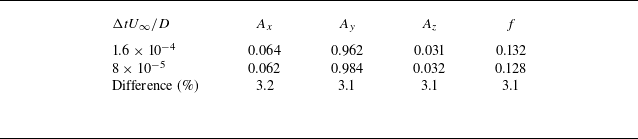
3.6. Other validation
Another validation, such as flow over a rigid circular cylinder in unbounded flow with the $Re$
up to 1000, has been provided in our previous work (Chen et al. Reference Chen, Ji, Alam and Yan2022). The mesh settings in the present study are approximately the same as those adopted in the direct numerical simulation. The convergence analysis of the grid spacing and non-dimensional time step has been conducted in our previous work.
$Re$
up to 1000, has been provided in our previous work (Chen et al. Reference Chen, Ji, Alam and Yan2022). The mesh settings in the present study are approximately the same as those adopted in the direct numerical simulation. The convergence analysis of the grid spacing and non-dimensional time step has been conducted in our previous work.
4. Numerical set-up for a wall-mounted stem in uniform flow
In this section, we present the numerical set-up employed in this study and explain the practical rationale behind its design. It is noted that only dimensionless quantities are employed in our numerical simulations of a wall-mounted stem.
-
(i) Cross-section of the wall-mounted stem: numerous natural applications feature a wall-mounted configuration, such as trees in a forest, seaweed on the seafloor, cilia on membranes and bivalves inhabiting riverbeds. These structures exhibit a variety of shapes, including circular, rectangular, plate-like and thin filamentous forms. In this study, we aim at the 3-D flow characteristics and dynamic response of a wall-mounted stem. The circular cross-sectional shape is chosen as it is more representative and rotational symmetry and thus insensitive to incoming flow directions.
-
(ii) Aspect ratio: the aquatic plants generally have large aspect ratios (ARs), ranging from 10 to 100 (Ghisalberti & Nepf Reference Ghisalberti and Nepf2002; Luhar et al. Reference Luhar, Coutu, Infantes, Fox and Nepf2010; Luhar & Nepf Reference Luhar and Nepf2011). To save computational resources and conduct more simulation cases, a lower end of AR ( $= 10$
) is adopted in this study.
$= 10$
) is adopted in this study. -
(iii) Reynolds number: the flow velocity at the location of the aquatic plants is strongly influenced by factors such as the topography, ocean currents, tides and geographical location. Near the coast, tides play a significant role, with flow velocity typically ranging from 0.1 to 1 m s–1. In contrast, plants in the deep sea are primarily affected by ocean currents, where the flow velocity is generally more stable, typically within the range of 0.01–0.2 m s–1. The characteristic width of these plants is of the order of 1 cm (Luhar et al. Reference Luhar, Coutu, Infantes, Fox and Nepf2010; Luhar & Nepf Reference Luhar and Nepf2011). Accordingly, the Reynolds number
$Re$
(
$= U_\infty D/\nu$
) based on the width (or diameter) is in the range of
$10^{2}$
–
$10^{4}$
. In a coastal system, a condition with
$Re$
$\gtrsim$
200 is common (Munson, Young & Okiishi Reference Munson, Young and Okiishi1990; Leonard & Luther Reference Leonard and Luther1995). However, in a freshwater system not exposed to strong tides, a condition with
$Re$
$\lesssim$
200 is more typical. For
$Re$
$\lesssim$
200, the wake production is negligible and turbulent components are greatly reduced (Ghisalberti Reference Ghisalberti2000). A moderate
$Re$
range is selected, i.e.
$Re=$
200–1000, covering the conditions from river to coast, which is obtained by setting different initial
$U_\infty$
. -
(iv) Stiffness ratio: for flexible stems, the stiffness ratio, representing the ratio of the elastic force and inertia force, is introduced, defined as
$K=1/Ca$
. Here, the Cauchy number
$Ca$
is defined as
$C a=0.5 \rho _f D l^3 U_{r e f}^2 / E I$
, where
$\rho _f$
is the fluid density,
$l$
is the stem length,
$D$
is the stem diameter,
$E$
is Young’s modulus,
$I$
is the cross-section moment of inertia, defined as
$I=\pi D^4/64$
for the circular cross-section, and
$U_{ref}$
is the incoming flow velocity. For a single stem,
$U_{ref}=U_\infty$
. For aquatic plant, the stiffness ratio is in the range of
$K = 2.0\times 10^{-4}-3.0\times 10^2$
(Luhar & Nepf Reference Luhar and Nepf2011), corresponding to lg(
$K) = -3.59-2.48$
. Our simulation indicates that, when lg(
$K$
)
$\gt$
0, the dynamic response is insignificant. In this study, eight different stiffness ratios, i.e. lg(
$K) = -3.5$
, 3.0, ……, 0 with an increment of 0.5, are applied for each
$Re$
. -
(v) Density of the stem: the density
$\rho _s=$
1.0 is applied, which is a typical density of aquatic plants (Gaylord & Denny Reference Gaylord and Denny1997; Bradley & Houser Reference Bradley and Houser2009; Luhar & Nepf Reference Luhar and Nepf2011; Vettori & Nikora Reference Vettori and Nikora2018; O’Connor & Revell Reference O’Connor and Revell2019). -
(vi) Structural damping: in this study, the structural damping coefficient (
$\zeta$
) is set as zero. Thus, the flexible stem experiences the strongest oscillation. -
(vii) Computational domain: as shown in figure 4(
$d$
), the distance is 10
$D$
from the stem centre to the inlet and 30
$D$
to the outlet. The stem to each side of the lateral boundary is 8
$D$
and the height in the
$z$
-direction is 16
$D$
. The value
$\Delta z /l=$
1/16 is applied. At the stem position, the boundary layer thickness (
$\delta /D$
) is low, varying from 1.1 to 0.5 within
$Re=$
200–1000. The computational domain is discretised by a non-uniform Cartesian grid with a resolution of 1536
$\times$
512. The non-dimensional grid spacing in the
$x{-}y$
plane is 1/32. A total of 160 points are applied in the VFIFE method. -
(viii) Boundary conditions: a Dirichlet-type boundary is adopted at the inflow, and a Neumann-type boundary is employed at the outflow. The top and bottom walls are free slip and no slip, respectively, and the free-slip boundary condition is adopted at two lateral boundaries.
-
(ix) Non-dimensional time step and time span: in our present simulation, both the time span and time step depend strongly on
$Re$
and
$K$
. To provide a convergent result, the non-dimensional time step is of the order of
$10^{-4}$
or
$10^{-5}$
, and the corresponding Courant–Friedrichs–Lewy number is of the order of 0.01 or 0.001. It is found that the non-dimensional time span is closely associated with the response type. For periodic or regular response, the time span may reach
$\sim$
1000, while for chaotic response it may reach
$\sim$
3000. It should be pointed out here that, although the time span is already long, some cases are still unstable, such as the case at
$Re = 200$
and lg(
$K = -2.0$
) where slow flapping behaviour occurs.


Dependence of ( $a$
) mean drag (
$a$
) mean drag ( $\bar {C}_d$
), (
$\bar {C}_d$
), ( $b$
) fluctuating (r.m.s.) drag (
$b$
) fluctuating (r.m.s.) drag ( $C_d^{\prime }$
) and (
$C_d^{\prime }$
) and ( $c$
) fluctuating (r.m.s.) lift (
$c$
) fluctuating (r.m.s.) lift ( $C_l^{\prime }$
) coefficients on
$C_l^{\prime }$
) coefficients on $Re\, (= 200-1000)$
. The triangle symbols in (
$Re\, (= 200-1000)$
. The triangle symbols in ( $a$
,
$a$
, $c$
) represent the results of flow over an infinite circular cylinder from Jiang and Cheng (2021). The results in (
$c$
) represent the results of flow over an infinite circular cylinder from Jiang and Cheng (2021). The results in ( $b$
) are provided by H. Jiang (personal communication). Here, R1, R2 and R3 denote different regimes based on the features of lift spectra and the vortex dynamics.
$b$
) are provided by H. Jiang (personal communication). Here, R1, R2 and R3 denote different regimes based on the features of lift spectra and the vortex dynamics.
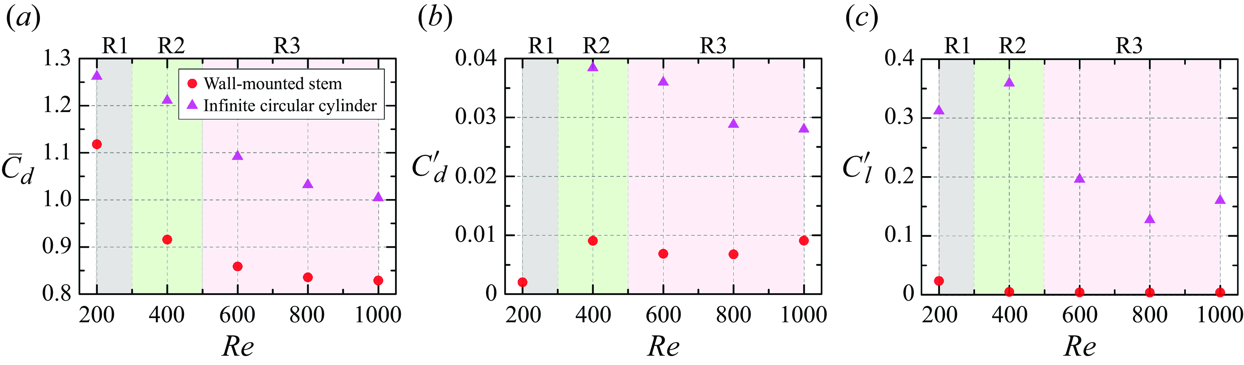
5. Wall-mounted rigid stem in uniform flow
This section reports the characteristics of the hydrodynamic forces, vortex shedding frequency and flow structures of a wall-mounted rigid stem to provide some primary understanding and to facilitate further comparison with the flexible stem.
5.1. Statistics of fluid forces and vortex shedding frequency
Figure 11 shows the vertically averaged fluid forces on the rigid stem at $Re = 200-1000$
. Here, the drag and lift coefficients are defined as
$Re = 200-1000$
. Here, the drag and lift coefficients are defined as $C_d=2F_d/\rho U_\infty ^2 Dl$
and
$C_d=2F_d/\rho U_\infty ^2 Dl$
and $C_l=2F_l/\rho U_\infty ^2 Dl$
, respectively. As shown in figure 11(
$C_l=2F_l/\rho U_\infty ^2 Dl$
, respectively. As shown in figure 11( $a$
), the mean drag coefficient (
$a$
), the mean drag coefficient ( $\bar {C}_d$
) is 1.12 at
$\bar {C}_d$
) is 1.12 at $Re = 200$
and gradually decreases as
$Re = 200$
and gradually decreases as $Re$
increases. The
$Re$
increases. The $\bar {C}_d$
values for a circular cylinder in an unbounded flow (represented by triangular symbols) are slightly higher than those for the wall-mounted case. This discrepancy arises because, in the wall-mounted case: (i) the oscillating shear layers near the junction are suppressed by the wall, and (ii) the free end delays flow separation, resulting in a less negative wake pressure (Luo, Gan & Chew Reference Luo, Gan and Chew1996). As discussed later, the downwash flow from the free end pushes the shear layers away from the stem base, contributing to the reduction in
$\bar {C}_d$
values for a circular cylinder in an unbounded flow (represented by triangular symbols) are slightly higher than those for the wall-mounted case. This discrepancy arises because, in the wall-mounted case: (i) the oscillating shear layers near the junction are suppressed by the wall, and (ii) the free end delays flow separation, resulting in a less negative wake pressure (Luo, Gan & Chew Reference Luo, Gan and Chew1996). As discussed later, the downwash flow from the free end pushes the shear layers away from the stem base, contributing to the reduction in $\bar {C}_d$
.
$\bar {C}_d$
.
Power spectral density (PSD) of the vertically averaged lift coefficient of a wall-mounted rigid stem within $Re = 200-1000$
. Panels show (
$Re = 200-1000$
. Panels show ( $a$
)
$a$
) $Re = 200$
, (
$Re = 200$
, ( $b$
)
$b$
) $Re = 400$
, (
$Re = 400$
, ( $c$
)
$c$
) $Re = 600$
, (
$Re = 600$
, ( $d$
)
$d$
) $Re = 800$
and (
$Re = 800$
and ( $e$
)
$e$
) $Re = 1000$
. The inset in (
$Re = 1000$
. The inset in ( $b$
) shows the spectrum of the lift coefficient of an infinite circular cylinder at
$b$
) shows the spectrum of the lift coefficient of an infinite circular cylinder at $Re = 400$
.
$Re = 400$
.
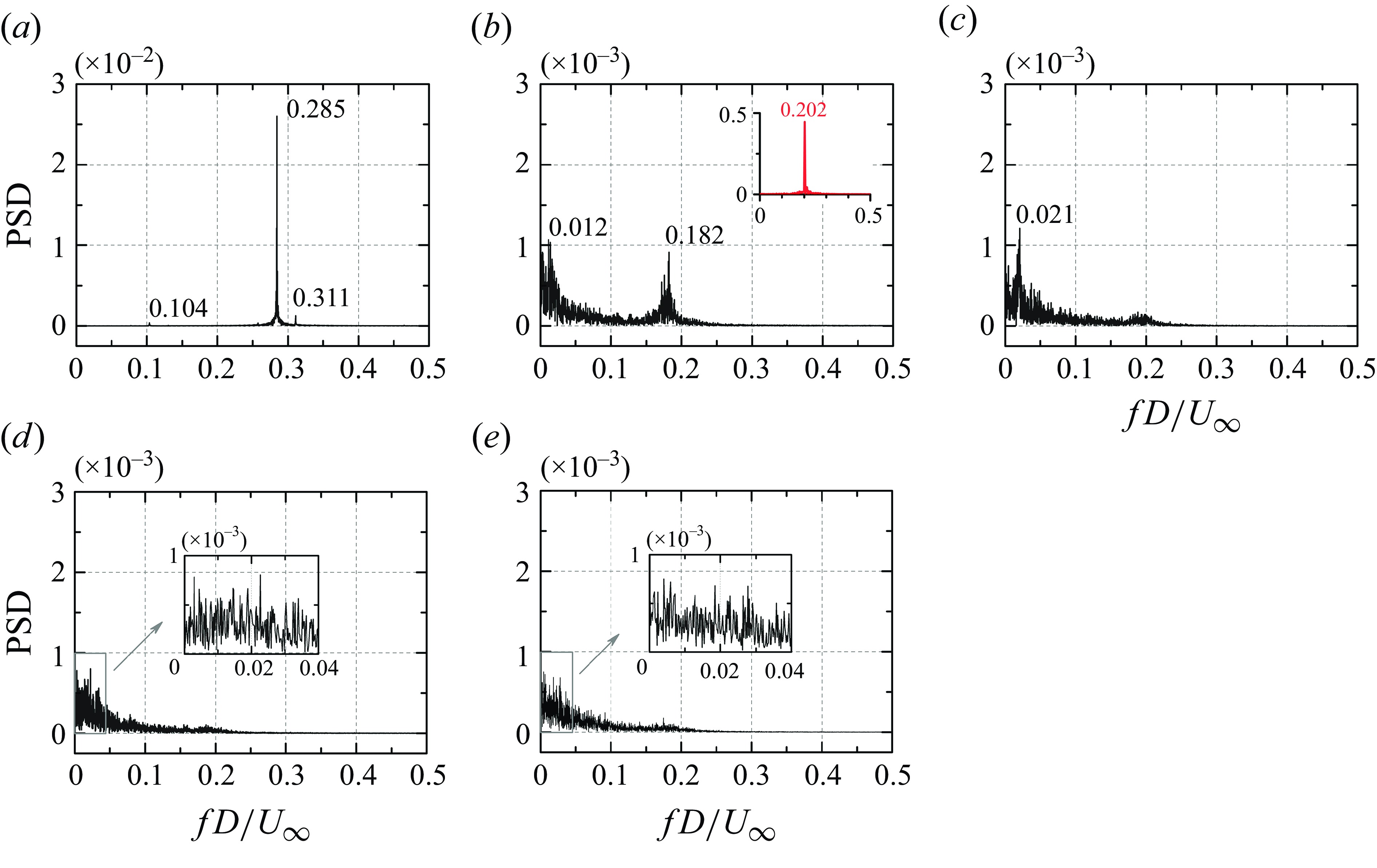
The r.m.s. drag coefficient ( $C_d^{\prime }$
), shown in figure 11(
$C_d^{\prime }$
), shown in figure 11( $b$
), exhibits a different behaviour with
$b$
), exhibits a different behaviour with $Re$
. At
$Re$
. At $Re = 200$
,
$Re = 200$
, $C_d^{\prime }$
is approximately zero (0.001). For higher
$C_d^{\prime }$
is approximately zero (0.001). For higher $Re$
values,
$Re$
values, $C_d^{\prime }$
stabilises around 0.08, which is significantly higher than at
$C_d^{\prime }$
stabilises around 0.08, which is significantly higher than at $Re = 200$
. This suggests a fundamental difference in the vortical structures between
$Re = 200$
. This suggests a fundamental difference in the vortical structures between $Re = 200$
and
$Re = 200$
and $Re$
$Re$ $\gt$
200. The
$\gt$
200. The $C_d^{\prime }$
values for an infinite circular cylinder at the corresponding
$C_d^{\prime }$
values for an infinite circular cylinder at the corresponding $Re$
are also plotted in figure 11(
$Re$
are also plotted in figure 11( $b$
). It is seen that the
$b$
). It is seen that the $C_d^{\prime }$
values in triangular symbols are much higher than those for the wall-mounted case, implying that the vortical structures near the free end and junction supress shear layer fluctuations (Baban, So & Otugen Reference Baban, So and Otugen1989; Wang & Zhou Reference Wang and Zhou2009; Kumar & Tiwari Reference Kumar and Tiwari2019).
$C_d^{\prime }$
values in triangular symbols are much higher than those for the wall-mounted case, implying that the vortical structures near the free end and junction supress shear layer fluctuations (Baban, So & Otugen Reference Baban, So and Otugen1989; Wang & Zhou Reference Wang and Zhou2009; Kumar & Tiwari Reference Kumar and Tiwari2019).
Due to the rotational symmetry of circular cross-section, the time-averaged lift coefficient ( $\bar {C}_l$
) is zero and will not be discussed further. As shown in figure 11(
$\bar {C}_l$
) is zero and will not be discussed further. As shown in figure 11( $c$
), the r.m.s. lift coefficient (
$c$
), the r.m.s. lift coefficient ( $C_l^{\prime }$
) for the wall-mounted stem is relatively large at
$C_l^{\prime }$
) for the wall-mounted stem is relatively large at $Re = 200$
, with a value of 0.023. However, at higher
$Re = 200$
, with a value of 0.023. However, at higher $Re$
,
$Re$
, $C_l^{\prime }$
stabilises at approximately 0.005. The transitions for
$C_l^{\prime }$
stabilises at approximately 0.005. The transitions for $C_d^{\prime }$
and
$C_d^{\prime }$
and $C_l^{\prime }$
from
$C_l^{\prime }$
from $Re = 200$
to
$Re = 200$
to $Re$
$Re$ $\gt$
200 exhibit contrasting behaviours, highlighting the influence of different vortical structures in these two
$\gt$
200 exhibit contrasting behaviours, highlighting the influence of different vortical structures in these two $Re$
clusters. These two
$Re$
clusters. These two $Re$
clusters will be analysed further to explore the roles of different flow structures in the transition. The
$Re$
clusters will be analysed further to explore the roles of different flow structures in the transition. The $C_l^{\prime }$
values for the infinite circular cylinder, represented by triangular symbols in figure 11(
$C_l^{\prime }$
values for the infinite circular cylinder, represented by triangular symbols in figure 11( $c$
), are much higher due to the reduced fluctuations in the shear layers of the wall-mounted stem.
$c$
), are much higher due to the reduced fluctuations in the shear layers of the wall-mounted stem.
The vortex shedding frequency is a key indicator of flow physics and is significantly influenced by the vortex dynamics at both the free end and the junction (Liu, So & Cui Reference Liu, So and Cui2005; Yauwenas et al. Reference Yauwenas, Porteous, Moreau and Doolan2019). Figure 12 shows the spectra of the vertical-averaged lift coefficient at $Re = 200-1000$
, representing the vortex shedding frequency. As
$Re = 200-1000$
, representing the vortex shedding frequency. As $Re$
increases, the spectral characteristics exhibit three distinct patterns. At
$Re$
increases, the spectral characteristics exhibit three distinct patterns. At $Re = 200$
, three frequencies are observed, but two have trivial magnitudes, as shown in figure 12(
$Re = 200$
, three frequencies are observed, but two have trivial magnitudes, as shown in figure 12( $a$
). The dominant frequency is
$a$
). The dominant frequency is $f^\ast (= \textit{fD} / U_\infty) = 0.285$
. However, at
$f^\ast (= \textit{fD} / U_\infty) = 0.285$
. However, at $Re = 400$
, the dominant frequency decreases to
$Re = 400$
, the dominant frequency decreases to $f^\ast = 0.182$
, significantly lower than at
$f^\ast = 0.182$
, significantly lower than at $Re = 200$
. Compared with the unbounded case, the dominant frequency is slightly lower, see the inset in figure 12(
$Re = 200$
. Compared with the unbounded case, the dominant frequency is slightly lower, see the inset in figure 12( $b$
). A secondary frequency,
$b$
). A secondary frequency, $f^\ast = 0.012$
, is approximately one order of magnitude lower than the dominant one. At
$f^\ast = 0.012$
, is approximately one order of magnitude lower than the dominant one. At $Re = 600$
, only one low frequency is detected at
$Re = 600$
, only one low frequency is detected at $f^\ast = 0.021$
, as shown in figure 12(
$f^\ast = 0.021$
, as shown in figure 12( $c$
). For
$c$
). For $Re = 800-1000$
, no dominant frequency is observed, as multiple low-frequency components below 0.03 exhibit comparable but weak magnitudes, see figure 12(
$Re = 800-1000$
, no dominant frequency is observed, as multiple low-frequency components below 0.03 exhibit comparable but weak magnitudes, see figure 12( $d$
,
$d$
, $e$
).
$e$
).
Based on the features of hydrodynamic forces and vortex shedding frequencies, the investigated $Re$
can be categorised into three regimes. The first regime (R1) corresponds to
$Re$
can be categorised into three regimes. The first regime (R1) corresponds to $Re = 200$
, where vortex shedding is periodic, and correspondingly, a regular lift spectrum appears. The second regime (R2) occurs at
$Re = 200$
, where vortex shedding is periodic, and correspondingly, a regular lift spectrum appears. The second regime (R2) occurs at $Re = 400$
, where both low and high frequencies appear due to different vortical structures. The third regime (R3) spans at
$Re = 400$
, where both low and high frequencies appear due to different vortical structures. The third regime (R3) spans at $Re = 600-1000$
, where only low-frequency components are present. A slight distinction exists between
$Re = 600-1000$
, where only low-frequency components are present. A slight distinction exists between $Re = 600$
and
$Re = 600$
and $Re = 800-1000$
in that the lift spectrum becomes chaotic at higher
$Re = 800-1000$
in that the lift spectrum becomes chaotic at higher $Re$
. These variations are linked to the evolution of different 3-D vortical structures.
$Re$
. These variations are linked to the evolution of different 3-D vortical structures.
Three-dimensional vortical structures behind the wall-mounted rigid stem at ( $a$
)
$a$
) $Re=$
200, (
$Re=$
200, ( $b$
)
$b$
) $Re=$
400, (
$Re=$
400, ( $c$
)
$c$
) $Re=$
600, (
$Re=$
600, ( $d$
)
$d$
) $Re = 800$
and (
$Re = 800$
and ( $e$
)
$e$
) $Re = 1000$
. The
$Re = 1000$
. The $Q$
-criterion is adopted to visualise the vortex structures (Hunt et al. 1988), i.e.
$Q$
-criterion is adopted to visualise the vortex structures (Hunt et al. 1988), i.e. $Q = 5$
, 20, 45, 80 and 125 for panels (a–e). The arrow indicates the flow direction (i.e. from left to right).
$Q = 5$
, 20, 45, 80 and 125 for panels (a–e). The arrow indicates the flow direction (i.e. from left to right).
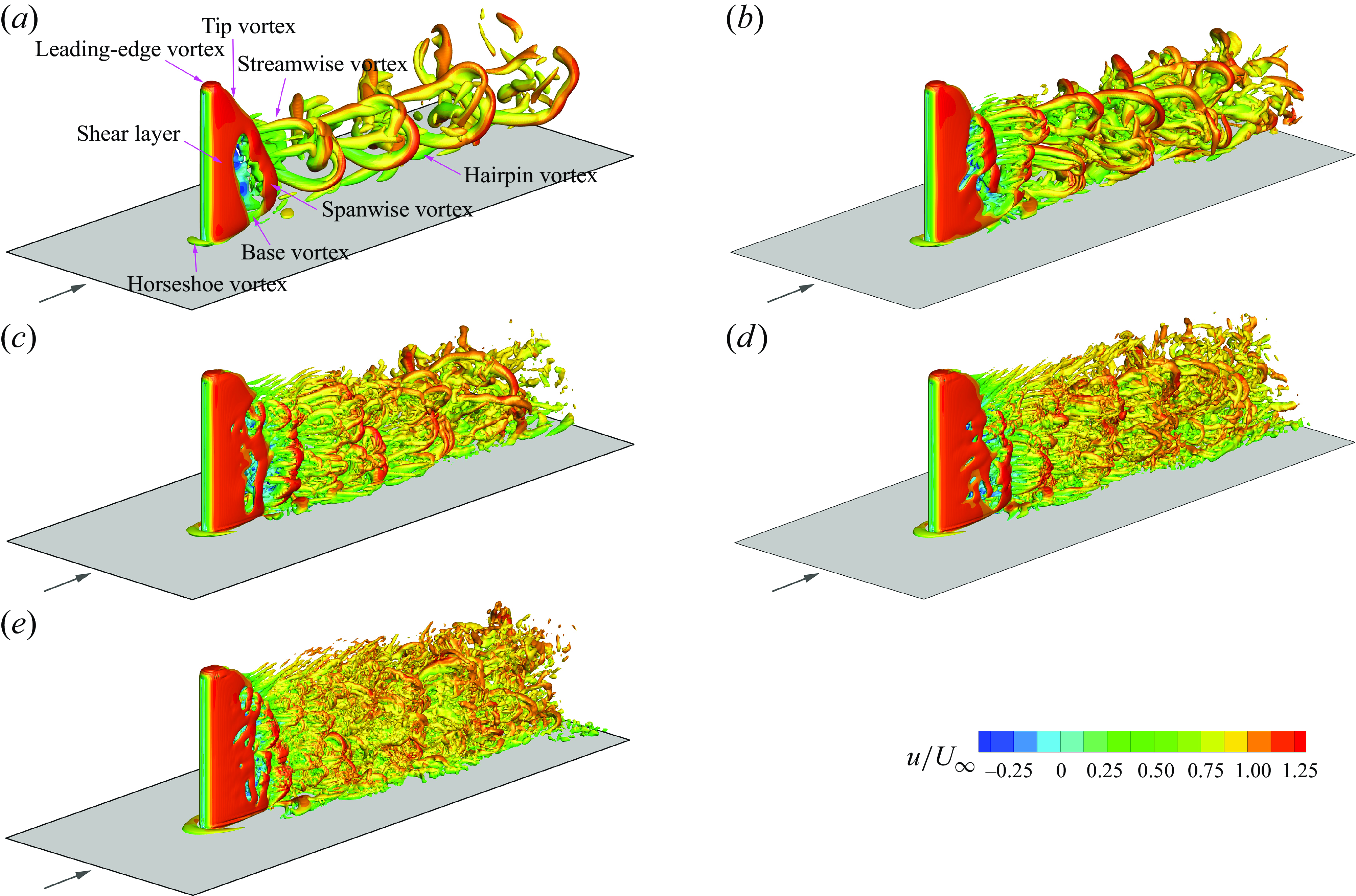
The vorticity field of a wall-mounted stem at the vertical position of $z/D=$
0.1. (a–c) For a rigid stem and (
$z/D=$
0.1. (a–c) For a rigid stem and ( $d$
,
$d$
, $e$
) for a flexible stem. Panels show (
$e$
) for a flexible stem. Panels show ( $a$
)
$a$
) $Re=$
200, (
$Re=$
200, ( $b$
)
$b$
) $Re = 400$
, (
$Re = 400$
, ( $c$
)
$c$
) $Re = 600$
, (
$Re = 600$
, ( $d$
)
$d$
) $Re=$
200 and lg(
$Re=$
200 and lg( $K) = -0.5$
and (
$K) = -0.5$
and ( $e$
)
$e$
) $Re = 600$
and lg(
$Re = 600$
and lg( $K) = -2.0$
. The HV in each plot is marked; (i) and (ii) at different instants. The legs of the HV system, visualised by the
$K) = -2.0$
. The HV in each plot is marked; (i) and (ii) at different instants. The legs of the HV system, visualised by the $x$
-vorticity at
$x$
-vorticity at $x/D = 0$
, are marked in the subplot.
$x/D = 0$
, are marked in the subplot.
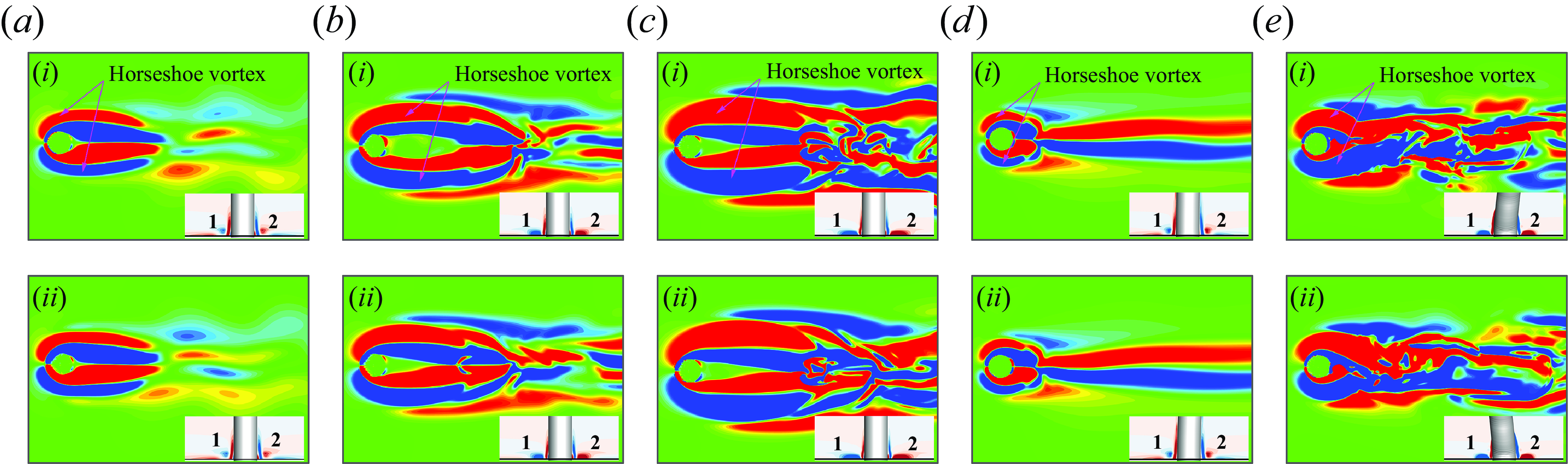
5.2. Details of the 3-D vortical structures
The vortical structures in the studied $Re$
range are shown in figure 13. Since the AR exceeds the critical value (Bourgeois et al. Reference Bourgeois, Sattari and Martinuzzi2011, Reference Bourgeois, Sattari and Martinuzzi2012), the shear layer from the front side is reattached onto the free-end surface due to flow reversal (Pattenden et al. Reference Pattenden, Turnock and Zhang2005; Krajnovic Reference Krajnovic2011; Essel et al. Reference Essel, Tachie and Balachandar2021). The leading-edge vortex emerges at the free end surface, while near the bottom, horseshoe vortices form upstream of the stem, wrapping around its sides and trailing behind it (Hussein & Martinuzzi Reference Hussein and Martinuzzi1996; Simpson Reference Simpson2001; Wang & Zhou Reference Wang and Zhou2009; Chang et al. Reference Chang, Constantinescu and Tsai2017, Reference Chang, Constantinescu and Tsai2020) due to the adverse pressure gradient. These vortices tend to drive the flow downward inside its vortical trails. Figure 14 shows the horseshoe vortex (HV) system circling the stem base at a vertical position of
$Re$
range are shown in figure 13. Since the AR exceeds the critical value (Bourgeois et al. Reference Bourgeois, Sattari and Martinuzzi2011, Reference Bourgeois, Sattari and Martinuzzi2012), the shear layer from the front side is reattached onto the free-end surface due to flow reversal (Pattenden et al. Reference Pattenden, Turnock and Zhang2005; Krajnovic Reference Krajnovic2011; Essel et al. Reference Essel, Tachie and Balachandar2021). The leading-edge vortex emerges at the free end surface, while near the bottom, horseshoe vortices form upstream of the stem, wrapping around its sides and trailing behind it (Hussein & Martinuzzi Reference Hussein and Martinuzzi1996; Simpson Reference Simpson2001; Wang & Zhou Reference Wang and Zhou2009; Chang et al. Reference Chang, Constantinescu and Tsai2017, Reference Chang, Constantinescu and Tsai2020) due to the adverse pressure gradient. These vortices tend to drive the flow downward inside its vortical trails. Figure 14 shows the horseshoe vortex (HV) system circling the stem base at a vertical position of $z/D = 0.1$
. Within the studied
$z/D = 0.1$
. Within the studied $Re$
, the HV system is characterised by a single necklace vortex, as marked in figure 14. In the current simulation, both
$Re$
, the HV system is characterised by a single necklace vortex, as marked in figure 14. In the current simulation, both $Re$
and
$Re$
and $\delta /D$
increase simultaneously as the incoming flow velocity rises. As expected, the HV grows with increasing
$\delta /D$
increase simultaneously as the incoming flow velocity rises. As expected, the HV grows with increasing $Re$
, exhibiting greater strength and a longer extension into the wake. This suggests that the dynamics of the HV system is affected by
$Re$
, exhibiting greater strength and a longer extension into the wake. This suggests that the dynamics of the HV system is affected by $Re$
, the characteristics of the upstream boundary layer and the shape of the cylinder (Baker Reference Baker1979; Seal et al. Reference Seal, Smith, Akin and Rockwell1995). As shown in figure 14(
$Re$
, the characteristics of the upstream boundary layer and the shape of the cylinder (Baker Reference Baker1979; Seal et al. Reference Seal, Smith, Akin and Rockwell1995). As shown in figure 14( $a$
), the HV at
$a$
), the HV at $Re = 200$
remains nearly constant, with weak interactions with the two side shear layers and no noticeable amalgamation. However, at higher
$Re = 200$
remains nearly constant, with weak interactions with the two side shear layers and no noticeable amalgamation. However, at higher $Re\, (=400-600)$
, the HV legs extend further downstream, see figure 14(
$Re\, (=400-600)$
, the HV legs extend further downstream, see figure 14( $b$
,
$b$
, $c$
). At
$c$
). At $Re=$
400, the HV system encircles the two side shear layers, and their interactions intensify. In the wake, vortices shed from the HV system and the two side shear layers mix together, and amalgamation occurs. At
$Re=$
400, the HV system encircles the two side shear layers, and their interactions intensify. In the wake, vortices shed from the HV system and the two side shear layers mix together, and amalgamation occurs. At $Re=$
600, the interactions between the HV system, the shear layers on either side of the stem and the resulting vortices become more pronounced. The conditions at
$Re=$
600, the interactions between the HV system, the shear layers on either side of the stem and the resulting vortices become more pronounced. The conditions at $Re= 800-1000$
are very similar to those at
$Re= 800-1000$
are very similar to those at $Re=$
600 and are therefore not shown. The HV system could be either laminar or turbulent. The laminar type is typically classified into five, transiting from steady to periodic by increasing
$Re=$
600 and are therefore not shown. The HV system could be either laminar or turbulent. The laminar type is typically classified into five, transiting from steady to periodic by increasing $Re$
and/or
$Re$
and/or $\delta /D$
(Greco Reference Greco1990; Seal et al. Reference Seal, Smith and Rockwell1997; Wei, Chen & Du Reference Wei, Chen and Du2001; Kirkil & Constantinescu Reference Kirkil and Constantinescu2012). In the present simulation, the HV system remains laminar, with a steady necklace vortex persisting at
$\delta /D$
(Greco Reference Greco1990; Seal et al. Reference Seal, Smith and Rockwell1997; Wei, Chen & Du Reference Wei, Chen and Du2001; Kirkil & Constantinescu Reference Kirkil and Constantinescu2012). In the present simulation, the HV system remains laminar, with a steady necklace vortex persisting at $Re= 200-1000$
due to the combined effects of lower
$Re= 200-1000$
due to the combined effects of lower $Re$
and a thin
$Re$
and a thin $\delta /D$
(Wei et al. Reference Wei, Chen and Du2001). In Kirkil & Constantinescu (Reference Kirkil and Constantinescu2012), where the boundary layer thickness is
$\delta /D$
(Wei et al. Reference Wei, Chen and Du2001). In Kirkil & Constantinescu (Reference Kirkil and Constantinescu2012), where the boundary layer thickness is $\delta /D \cong 0.6$
, the laminar HV system transitions from steady to periodic oscillating and then to periodic breakaway as
$\delta /D \cong 0.6$
, the laminar HV system transitions from steady to periodic oscillating and then to periodic breakaway as $Re$
increases. In the flexible case, the HV system also remains steady but is significantly influenced by the redistribution of vortical structures. As will be shown later, the flexible stem experiences stronger vortex shedding near the tip due to larger amplitudes and significant deformation. At
$Re$
increases. In the flexible case, the HV system also remains steady but is significantly influenced by the redistribution of vortical structures. As will be shown later, the flexible stem experiences stronger vortex shedding near the tip due to larger amplitudes and significant deformation. At $Re=$
200, the HV system remains stable but its vortex legs extend a shorter distance downstream compared with the rigid stem, see figure 14(
$Re=$
200, the HV system remains stable but its vortex legs extend a shorter distance downstream compared with the rigid stem, see figure 14( $d$
). A similar behaviour is noticed at
$d$
). A similar behaviour is noticed at $Re=$
600, see figure 14(
$Re=$
600, see figure 14( $e$
). It should be noted that as the stem becomes more flexible, the HV system is strongly affected because the two side shear layers (or separated vortices) move closer to the wall, influencing the HV system’s development. More details of the interactions between different vortex structures will be discussed later.
$e$
). It should be noted that as the stem becomes more flexible, the HV system is strongly affected because the two side shear layers (or separated vortices) move closer to the wall, influencing the HV system’s development. More details of the interactions between different vortex structures will be discussed later.
The evolution of 3-D vortical structures at $Re=$
200 is shown in figure 13(
$Re=$
200 is shown in figure 13( $a$
). Due to the high AR, the shear layers are allowed to develop and separate from the stem (Fröhlich and Rodi, 2004; Pattenden et al. Reference Pattenden, Turnock and Zhang2005; Tsutsui Reference Tsutsui2012). The spanwise vortices exhibit a slanted arrangement with an inclination angle of roughly 32.6
$a$
). Due to the high AR, the shear layers are allowed to develop and separate from the stem (Fröhlich and Rodi, 2004; Pattenden et al. Reference Pattenden, Turnock and Zhang2005; Tsutsui Reference Tsutsui2012). The spanwise vortices exhibit a slanted arrangement with an inclination angle of roughly 32.6 $^\circ$
(measured between the vertical axis and the slanted shear layer line) due to the influences of downwash flow from the free end (Lee Reference Lee1997; Fröhlich and Rodi, 2004). In the near wake, the spanwise vortices are significantly bent and stretched. Upwash and downwash flow entrain free-stream flow into the wake, pushing the spanwise vortices away from the centreline. Meanwhile, the streamwise vortices gradually develop. As a result of vortex twisting and interaction, the deformation of the spanwise and streamwise vortices becomes more evident further downstream. However, the interactions between these vortices weaken as they move apart. Compared with
$^\circ$
(measured between the vertical axis and the slanted shear layer line) due to the influences of downwash flow from the free end (Lee Reference Lee1997; Fröhlich and Rodi, 2004). In the near wake, the spanwise vortices are significantly bent and stretched. Upwash and downwash flow entrain free-stream flow into the wake, pushing the spanwise vortices away from the centreline. Meanwhile, the streamwise vortices gradually develop. As a result of vortex twisting and interaction, the deformation of the spanwise and streamwise vortices becomes more evident further downstream. However, the interactions between these vortices weaken as they move apart. Compared with $Re = 200$
, the 3-D vortical structures at
$Re = 200$
, the 3-D vortical structures at $Re = 400$
are more complex, featuring finer-scale vortices. Despite these differences, similarities remain, such as the presence of downwash flow, see figure 13(
$Re = 400$
are more complex, featuring finer-scale vortices. Despite these differences, similarities remain, such as the presence of downwash flow, see figure 13( $b$
). At this
$b$
). At this $Re$
, the spanwise vortices take over a longer length, but their formation region is larger near the wall. Near the free end, spanwise vortices are absent, while streamwise vortices develop more quickly due to increased flow velocity. As a result, vortex interactions intensify, leading to faster dissipation.
$Re$
, the spanwise vortices take over a longer length, but their formation region is larger near the wall. Near the free end, spanwise vortices are absent, while streamwise vortices develop more quickly due to increased flow velocity. As a result, vortex interactions intensify, leading to faster dissipation.
At $Re=$
600–1000, the vortex dynamics is characterised by finer-scale vortices. As shown in figure 13(c–e), spanwise vortices separate from the stem simultaneously and remain approximately parallel. Compared with the lower
$Re=$
600–1000, the vortex dynamics is characterised by finer-scale vortices. As shown in figure 13(c–e), spanwise vortices separate from the stem simultaneously and remain approximately parallel. Compared with the lower $Re$
cases (200–400), the finer-scale spanwise vortices exhibit more irregular behaviour in the near wake, as indicated by significantly low dominant frequencies. Similarly, the streamwise vortices are smaller in scale and mix with the spanwise vortices (Zhang et al. Reference Zhang, Cheng, An and Draper2021), leading to faster dissipation. Although the downwash flow persists, it is considerably weaker, as indicated by the formation of spanwise vortices closer to the free end.
$Re$
cases (200–400), the finer-scale spanwise vortices exhibit more irregular behaviour in the near wake, as indicated by significantly low dominant frequencies. Similarly, the streamwise vortices are smaller in scale and mix with the spanwise vortices (Zhang et al. Reference Zhang, Cheng, An and Draper2021), leading to faster dissipation. Although the downwash flow persists, it is considerably weaker, as indicated by the formation of spanwise vortices closer to the free end.
Figure 15 shows the $z$
-vorticity contours at different vertical positions. It is evident that vortex shedding varies significantly along the length within the studied
$z$
-vorticity contours at different vertical positions. It is evident that vortex shedding varies significantly along the length within the studied $Re$
range. At
$Re$
range. At $Re=$
200, vortex shedding is regular near the junction. As shown in figure 15(
$Re=$
200, vortex shedding is regular near the junction. As shown in figure 15( $a$
-i), the vortex shedding in this region (i.e.
$a$
-i), the vortex shedding in this region (i.e. $z/D=$
0.5) is characterised by the formation of horseshoe and hairpin vortices in the wake. The hairpin vortex comes from disturbances in the stretched vortices affecting the boundary layer over the stationary wall, a behaviour similar to the bypass transition observed over a circular cylinder (He et al. Reference He, Wang, Pan, Feng, Gao and Rinoshika2017). The shear layers on both sides extend further downstream, and the separated vortices gradually dissipate in the far wake. At the middle plane (i.e.
$z/D=$
0.5) is characterised by the formation of horseshoe and hairpin vortices in the wake. The hairpin vortex comes from disturbances in the stretched vortices affecting the boundary layer over the stationary wall, a behaviour similar to the bypass transition observed over a circular cylinder (He et al. Reference He, Wang, Pan, Feng, Gao and Rinoshika2017). The shear layers on both sides extend further downstream, and the separated vortices gradually dissipate in the far wake. At the middle plane (i.e. $z/D = 5.0$
), vortices shed alternately from both sides of the stem. In the near wake, they appear nearly identical, apart from their opposite rotation directions, see figure 15(
$z/D = 5.0$
), vortices shed alternately from both sides of the stem. In the near wake, they appear nearly identical, apart from their opposite rotation directions, see figure 15( $a$
-ii). Further downstream, these vortices become increasingly irregular due to the bending and twisting of spanwise vortices and the emergence of stretched streamwise vortices, leading to a broader wake. Higher up, i.e.
$a$
-ii). Further downstream, these vortices become increasingly irregular due to the bending and twisting of spanwise vortices and the emergence of stretched streamwise vortices, leading to a broader wake. Higher up, i.e. $z/D=$
7.5, the shear layers weaken, and fluctuations of shear layers occur farther downstream, with dissipation occurring more rapidly than at the middle plane, see figure 15(
$z/D=$
7.5, the shear layers weaken, and fluctuations of shear layers occur farther downstream, with dissipation occurring more rapidly than at the middle plane, see figure 15( $a$
-iii). Near the free end, i.e.
$a$
-iii). Near the free end, i.e. $z/D = 9.5$
, the shear layers on both sides remain stable, with no visible vortices in the wake, forming a symmetric wake, see figure 15(
$z/D = 9.5$
, the shear layers on both sides remain stable, with no visible vortices in the wake, forming a symmetric wake, see figure 15( $a$
-iv).
$a$
-iv).
At $Re=$
400, vortex strength increases compared with
$Re=$
400, vortex strength increases compared with $Re=$
200. As shown in figure 15(
$Re=$
200. As shown in figure 15( $b$
-i), the HV near the junction is more intense and extends farther downstream. Compared with
$b$
-i), the HV near the junction is more intense and extends farther downstream. Compared with $Re=$
200, the shear layers on both sides of the stem extend further downstream. The hairpin vortex appears in the near wake but exhibits greater irregularity. Interaction between the hairpin vortex and spanwise vortices occurs where the spanwise vortices separate. At the midspan (i.e.
$Re=$
200, the shear layers on both sides of the stem extend further downstream. The hairpin vortex appears in the near wake but exhibits greater irregularity. Interaction between the hairpin vortex and spanwise vortices occurs where the spanwise vortices separate. At the midspan (i.e. $z/D=$
5.0), the vortex shedding pattern is similar to that at
$z/D=$
5.0), the vortex shedding pattern is similar to that at $Re=$
200, although the vortices are slightly smaller, see figure 15(
$Re=$
200, although the vortices are slightly smaller, see figure 15( $b$
-ii). In the near wake, vortices become finer and more irregular before the wake widens. At
$b$
-ii). In the near wake, vortices become finer and more irregular before the wake widens. At $z/D=$
7.5, weak fluctuations in the shear layers are observed, see figure 15(
$z/D=$
7.5, weak fluctuations in the shear layers are observed, see figure 15( $b$
-iii). Further downstream, the shear layers thin out due to dissipation. Near the free end, i.e.
$b$
-iii). Further downstream, the shear layers thin out due to dissipation. Near the free end, i.e. $z/D = 9.5$
, the shear layers remain stable, with no vortices shed into the wake, see figure 15(
$z/D = 9.5$
, the shear layers remain stable, with no vortices shed into the wake, see figure 15( $b$
-iv). Compared with
$b$
-iv). Compared with $Re = 200$
, the downwash flow at
$Re = 200$
, the downwash flow at $Re = 400$
is stronger but extends over a shorter length.
$Re = 400$
is stronger but extends over a shorter length.
As shown in figure 15(c–e), the vortex shedding patterns at the same vertical position remain similar for $Re = 600-1000$
. As
$Re = 600-1000$
. As $Re$
increases, vortices become stronger but more irregular. As shown in figure 15(
$Re$
increases, vortices become stronger but more irregular. As shown in figure 15( $c$
-i,
$c$
-i, $d$
-i,
$d$
-i, $e$
-i), the HV intensifies, and its legs extend further downstream. Vortex shedding occurs at a relatively shorter downstream position with increasing
$e$
-i), the HV intensifies, and its legs extend further downstream. Vortex shedding occurs at a relatively shorter downstream position with increasing $Re$
. The formed vortices subsequently interact with the HV. Further downstream, the vortices become finer and dissipate more quickly, leading to a wider wake. At midspan, vortex formation shifts further downstream compared with the low
$Re$
. The formed vortices subsequently interact with the HV. Further downstream, the vortices become finer and dissipate more quickly, leading to a wider wake. At midspan, vortex formation shifts further downstream compared with the low $Re$
case, see figure 15(
$Re$
case, see figure 15( $c$
-ii,
$c$
-ii, $d$
-ii,
$d$
-ii, $e$
-ii). At higher vertical position, i.e.
$e$
-ii). At higher vertical position, i.e. $z/D = 7.5$
, the wake narrows significantly. Near the free end, the shear layers are slightly unstable with small vortices formed in the wake for Re = 800–1000, see figure 15(
$z/D = 7.5$
, the wake narrows significantly. Near the free end, the shear layers are slightly unstable with small vortices formed in the wake for Re = 800–1000, see figure 15( $c$
-iv,
$c$
-iv, $d$
-iv,
$d$
-iv, $e$
-iv).
$e$
-iv).
The vorticity contours ( $\omega _z^*=({D}/{2 U_{\infty })}(({\partial v}/{\partial x})- ({\partial u}/{\partial y})$
) of a single stem at several vertical positions. Panels show (
$\omega _z^*=({D}/{2 U_{\infty })}(({\partial v}/{\partial x})- ({\partial u}/{\partial y})$
) of a single stem at several vertical positions. Panels show ( $a$
)
$a$
) $Re = 200$
, (
$Re = 200$
, ( $b$
)
$b$
) $Re = 400$
, (
$Re = 400$
, ( $c$
)
$c$
) $Re = 600$
, (
$Re = 600$
, ( $d$
)
$d$
) $Re = 800$
and (
$Re = 800$
and ( $e$
)
$e$
) $Re = 1000$
.
$Re = 1000$
.
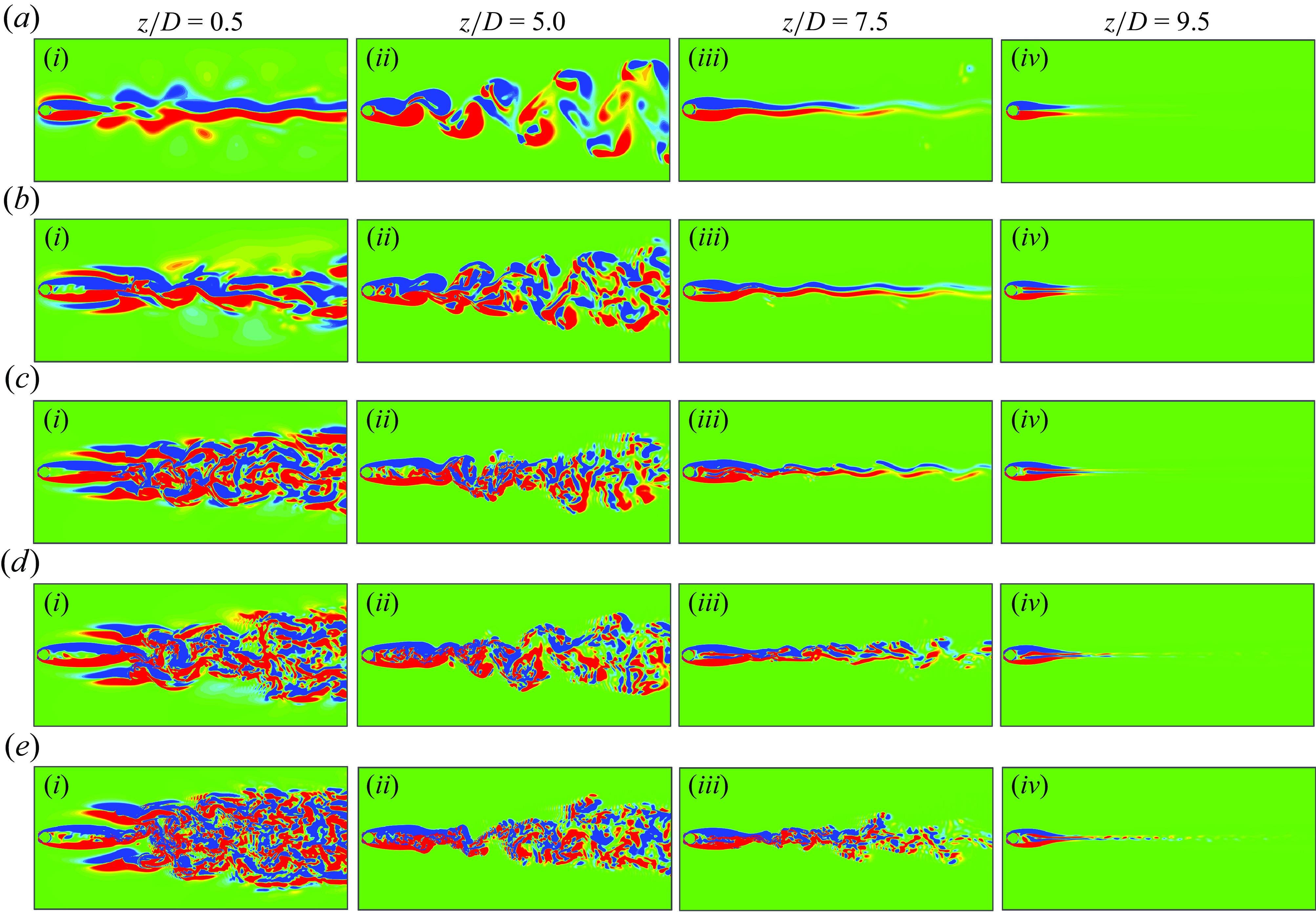
5.3. The downwash and upwash flow
In §§ 5.1 and 5.2 , we discussed the effects of downwash and upwash flow on the vortex dynamics. Figure 16 shows side views of these flows. For each $Re$
, the separated flow from the free end enters the near wake at a nearly constant angle relative to the streamwise direction (Krajnovic Reference Krajnovic2011). As shown in figure 16(
$Re$
, the separated flow from the free end enters the near wake at a nearly constant angle relative to the streamwise direction (Krajnovic Reference Krajnovic2011). As shown in figure 16( $a$
), at
$a$
), at $Re = 200$
, the flow from the free end moves downward directly along the bottom (i.e.
$Re = 200$
, the flow from the free end moves downward directly along the bottom (i.e. $x/D = 1.0$
), indicating that the downwash flow initiates immediately behind the stem but weakens gradually. Beyond
$x/D = 1.0$
), indicating that the downwash flow initiates immediately behind the stem but weakens gradually. Beyond $x/D$
$x/D$ $\geqslant$
4.0, the downwash flow becomes nearly negligible.
$\geqslant$
4.0, the downwash flow becomes nearly negligible.
Instantaneous vertical velocity ( $w^{\ast }$
) at the
$w^{\ast }$
) at the $y$
(
$y$
( $=8D$
) plane for
$=8D$
) plane for $Re= 200{-}600$
. Panels show (
$Re= 200{-}600$
. Panels show ( $a$
)
$a$
) $Re = 200$
, (
$Re = 200$
, ( $b$
)
$b$
) $Re=$
400, (
$Re=$
400, ( $c$
)
$c$
) $Re=$
600 and (
$Re=$
600 and ( $d$
)
$d$
) $Re=$
1000. Flow is from left to right. The rectangle in each plot indicates the stem position.
$Re=$
1000. Flow is from left to right. The rectangle in each plot indicates the stem position.
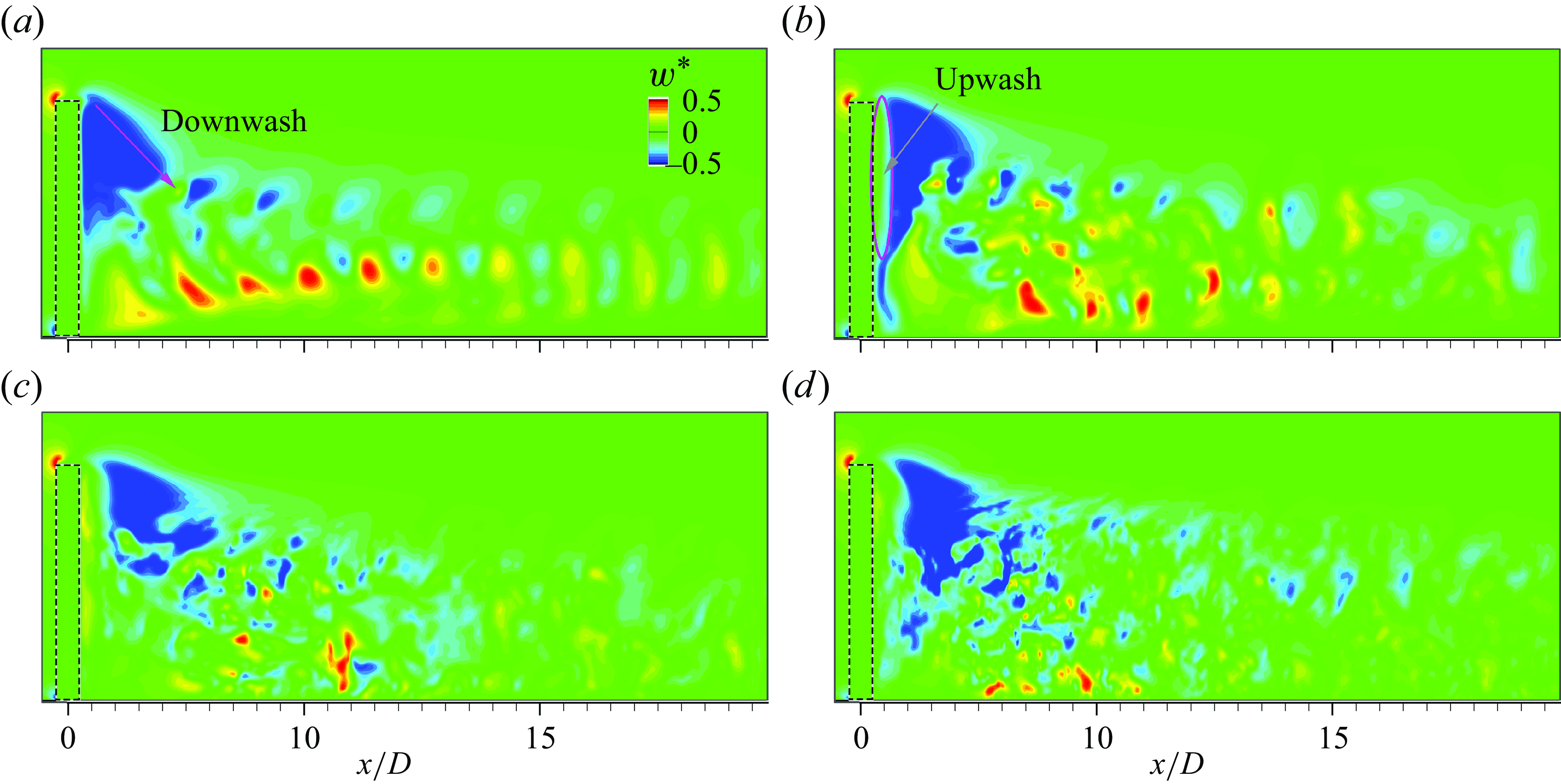
At $Re = 400$
, the downwash flow extends slightly farther downstream. As shown in figure 16(
$Re = 400$
, the downwash flow extends slightly farther downstream. As shown in figure 16( $b$
), downwash begins just past the free end but primarily affects the lower part of the stem at
$b$
), downwash begins just past the free end but primarily affects the lower part of the stem at $x/D = 1.0$
. A slight upward flow is observed at the upper part, indicating the presence of upwash flow. The downwash flow weakens quickly and disappears around
$x/D = 1.0$
. A slight upward flow is observed at the upper part, indicating the presence of upwash flow. The downwash flow weakens quickly and disappears around $x/D = 8.0.$
At $Re = 600$
, the downwash flow behaves similarly, as shown in figure 16(
$Re = 600$
, the downwash flow behaves similarly, as shown in figure 16( $c$
). Behind the stem, an upward flow is observed, pushing the downwash flow further downstream. Between
$c$
). Behind the stem, an upward flow is observed, pushing the downwash flow further downstream. Between $x/D = 4.0$
and 8.0, the downwash flow weakens but spreads toward the wall. In contrast, at
$x/D = 4.0$
and 8.0, the downwash flow weakens but spreads toward the wall. In contrast, at $Re = 800-1000$
, the downwash flow reaches the wall, whereas at
$Re = 800-1000$
, the downwash flow reaches the wall, whereas at $Re = 600$
, it does not, see figure 16(
$Re = 600$
, it does not, see figure 16( $c$
,
$c$
, $d$
).
$d$
).
Upwash flow appears at $Re = 400{-}1000$
, where it coexists with downwash flow. At
$Re = 400{-}1000$
, where it coexists with downwash flow. At $Re = 600$
, the upwash flow originates from the junction and is associated with the development of the near-wake base vortex (Etzold & Fiedler Reference Etzold and Fiedler1976; Essel et al. Reference Essel, Tachie and Balachandar2021). As indicated in figure 1, the base vortex consists of a pair of streamwise counter-rotating vortices near the base of the stem, influenced by
$Re = 600$
, the upwash flow originates from the junction and is associated with the development of the near-wake base vortex (Etzold & Fiedler Reference Etzold and Fiedler1976; Essel et al. Reference Essel, Tachie and Balachandar2021). As indicated in figure 1, the base vortex consists of a pair of streamwise counter-rotating vortices near the base of the stem, influenced by $Re$
and
$Re$
and $\delta /D$
(Sumner et al. Reference Sumner, Heseltine and Dansereau2004; Wang et al. Reference Wang, Zhou, Chan and Lam2006; Wang & Zhou Reference Wang and Zhou2009). As shown in figure 16(
$\delta /D$
(Sumner et al. Reference Sumner, Heseltine and Dansereau2004; Wang et al. Reference Wang, Zhou, Chan and Lam2006; Wang & Zhou Reference Wang and Zhou2009). As shown in figure 16( $c$
,
$c$
, $d$
), the upwash flow intensifies with increasing
$d$
), the upwash flow intensifies with increasing $Re$
. However, at
$Re$
. However, at $Re = 400$
, the upwash flow is only present in the upper region (see figure 16
$Re = 400$
, the upwash flow is only present in the upper region (see figure 16 $b$
), exhibiting a different behaviour from higher
$b$
), exhibiting a different behaviour from higher $Re$
cases.
$Re$
cases.
5.4. Three-dimensional wake instability comparison with the infinite cylinder case
In this section, we compare the 3-D wake instability of a wall-mounted cylinder with that of an infinite cylinder to deepen our understanding of the effects of the impermeable wall and free end. For flow past an infinite circular cylinder, the wake exhibits distinct patterns due to the presence of inherent 3-D wake instabilities (i.e. modes A and B) as $Re$
increases from approximately 190 to 300 (Williamson Reference Williamson1996; Jiang et al. Reference Jiang, Cheng, Draper, An and Tong2016). The transition from mode A to mode B has been well documented. Notably, mode A remains stable only for a short period before transitioning into a more stable pattern, mode A*, which exhibits significant dislocation. At
$Re$
increases from approximately 190 to 300 (Williamson Reference Williamson1996; Jiang et al. Reference Jiang, Cheng, Draper, An and Tong2016). The transition from mode A to mode B has been well documented. Notably, mode A remains stable only for a short period before transitioning into a more stable pattern, mode A*, which exhibits significant dislocation. At $Re$
$Re$ $\leqslant$
220, mode A* dominates, while modes A* and B coexist in the range of 230
$\leqslant$
220, mode A* dominates, while modes A* and B coexist in the range of 230 $\leqslant$ $Re$
$Re$ $\leqslant$
265. When
$\leqslant$
265. When $Re$
$Re$ $\geqslant$
270, mode A* disappears, and mode B becomes the dominant instability. Modes A* and B exhibit distinct characteristics. Mode A*, induced by an elliptic instability of the primary vortex cores, features streamwise vortices that are out of phase between neighbouring braids. Due to spanwise waviness, the primary vortex cores become significantly stretched. In contrast, mode B, caused by the hyperbolic instability of the braid shear layer, exhibits an in-phase pattern. Compared with mode A, the primary vortices in mode B are more stable, with no noticeable spanwise waviness.
$\geqslant$
270, mode A* disappears, and mode B becomes the dominant instability. Modes A* and B exhibit distinct characteristics. Mode A*, induced by an elliptic instability of the primary vortex cores, features streamwise vortices that are out of phase between neighbouring braids. Due to spanwise waviness, the primary vortex cores become significantly stretched. In contrast, mode B, caused by the hyperbolic instability of the braid shear layer, exhibits an in-phase pattern. Compared with mode A, the primary vortices in mode B are more stable, with no noticeable spanwise waviness.
As discussed in § 5.2, the vortex dynamics of a wall-mounted cylinder is significantly altered by the presence of the impermeable wall and free end. A key feature of this configuration is the suppression of vortex formation near both the cylinder base and the free end. Consequently, the separation of the spanwise shear layers typically occurs in a slanted manner, see figure 13( $a$
,
$a$
, $b$
). Compared with the infinite cylinder case, the wake transition of the wall-mounted cylinder is influenced by additional factors, including
$b$
). Compared with the infinite cylinder case, the wake transition of the wall-mounted cylinder is influenced by additional factors, including $Re$
, AR and
$Re$
, AR and $\delta /D$
. Kumar & Tiwari (Reference Kumar and Tiwari2019) found that, at AR
$\delta /D$
. Kumar & Tiwari (Reference Kumar and Tiwari2019) found that, at AR $=5$
, no vortex shedding occurs when
$=5$
, no vortex shedding occurs when $Re$
$Re$ $\leqslant$
100, indicating a symmetric wake structure. When
$\leqslant$
100, indicating a symmetric wake structure. When $Re$
$Re$ $\geqslant$
150, spanwise vortex shedding emerges, with vortices transitioning into hairpin-like structures. The critical
$\geqslant$
150, spanwise vortex shedding emerges, with vortices transitioning into hairpin-like structures. The critical $Re$
for the onset of vortex shedding increases as AR decreases (Saha Reference Saha2013). It is expected that if the wall-mounted cylinder has a much larger AR, modes A* (or A) and B would likely emerge. However, for a short cylinder, the wake structures are primarily governed by downwash and upwash flows (Zhu et al. Reference Zhu, Wang, Wang and Wang2017), resulting in a distinctly different flow behaviour.
$Re$
for the onset of vortex shedding increases as AR decreases (Saha Reference Saha2013). It is expected that if the wall-mounted cylinder has a much larger AR, modes A* (or A) and B would likely emerge. However, for a short cylinder, the wake structures are primarily governed by downwash and upwash flows (Zhu et al. Reference Zhu, Wang, Wang and Wang2017), resulting in a distinctly different flow behaviour.
In the present simulation, we observe two patterns of 3-D wake instabilities. As shown in figure 13( $a$
), the streamwise vortices primarily result from the suppression of shear layer separation. In the near wake, the separated vortices undergo significant stretching before transitioning into the hairpin-like structures. At higher
$a$
), the streamwise vortices primarily result from the suppression of shear layer separation. In the near wake, the separated vortices undergo significant stretching before transitioning into the hairpin-like structures. At higher $Re\, (=400)$
, the formation of streamwise vortices resembles mode A*. As shown in figure 13(
$Re\, (=400)$
, the formation of streamwise vortices resembles mode A*. As shown in figure 13( $b$
), streamwise vortices appear after the spanwise vortices separate from the shear layers, exhibiting large dislocations. The emergence of mode-A*-like instability is closely associated with slanted vortex shedding. However, in the near wake, the formed streamwise vortices undergo significant stretching, preventing the mode-A*-like vortices from persisting farther downstream. Additionally, mode B, which typically appears in an in-phase pattern, is absent in the wall-mounted case. This absence may be attributed to the slanted nature of vortex shedding.
$b$
), streamwise vortices appear after the spanwise vortices separate from the shear layers, exhibiting large dislocations. The emergence of mode-A*-like instability is closely associated with slanted vortex shedding. However, in the near wake, the formed streamwise vortices undergo significant stretching, preventing the mode-A*-like vortices from persisting farther downstream. Additionally, mode B, which typically appears in an in-phase pattern, is absent in the wall-mounted case. This absence may be attributed to the slanted nature of vortex shedding.
It is important to note that the 3-D wake instabilities observed in this study apply specifically to the simulated conditions. Further investigation in needed to explore these phenomena in great detail.
6. Fluid–structure interaction of a wall-mounted flexible stem in uniform flow
In this section, we examine the behaviour of a wall-mounted flexible stem in uniform flow, focusing on shape deformation, stem response, vortex dynamics, hydrodynamic forces and the spectral characteristics of displacement. Key aspects are analysed, including the evolution of 3-D vortical structures, wake topologies and tip movements under varying stiffnesses. The aspect ratio is set at AR = 10, the Reynolds number ranges from $Re=$
200 to 1000 and the stiffness ratio is lg(
$Re=$
200 to 1000 and the stiffness ratio is lg( $K$
) = −3.5–0 with an increment of 0.5. As discussed in § 4, no structural damping is applied. In total, 40 LES are carried out. Notably, in certain cases, the stem response is highly chaotic, and no convergent state is reached even over a longer non-dimensional time span, i.e.
$K$
) = −3.5–0 with an increment of 0.5. As discussed in § 4, no structural damping is applied. In total, 40 LES are carried out. Notably, in certain cases, the stem response is highly chaotic, and no convergent state is reached even over a longer non-dimensional time span, i.e. $tU_\infty /D$ $\sim$
O(
$\sim$
O( $10^3$
).
$10^3$
).
6.1. Characteristics of shape deformation and stem response
The mean position of the stem tip in different directions serves as a crucial indicator of hydrodynamic loading. Figure 17 shows the mean position, vibration amplitude and frequency of the stem tip in different directions. The mean position shifts are defined as $\Delta x^{\ast }=(\bar {x}_t - \bar {x}_{t,0})/D$
,
$\Delta x^{\ast }=(\bar {x}_t - \bar {x}_{t,0})/D$
, $\Delta y^{\ast }=(\bar {y}_t- \bar {y}_{t,0})/D$
and
$\Delta y^{\ast }=(\bar {y}_t- \bar {y}_{t,0})/D$
and $\Delta z^{\ast }=(\bar {l}_t- \bar {l}_{t,0})/D$
, where the subscript
$\Delta z^{\ast }=(\bar {l}_t- \bar {l}_{t,0})/D$
, where the subscript $0$
denotes initial values. Due to the circular cross-section’s rotational symmetry, transverse shifts remain zero in most simulations and are not further discussed. As shown in figure 17(
$0$
denotes initial values. Due to the circular cross-section’s rotational symmetry, transverse shifts remain zero in most simulations and are not further discussed. As shown in figure 17( $a$
), for
$a$
), for $Re=$
200–1000, the streamwise shift (
$Re=$
200–1000, the streamwise shift ( $\Delta x^{\ast }$
) follows a consistent trend. Excluding divergent cases, the best-fit nonlinear equation is
$\Delta x^{\ast }$
) follows a consistent trend. Excluding divergent cases, the best-fit nonlinear equation is $\Delta x^*=9.4 / (1+e^{1.96(\lg (K)+1.88)} )$
with a correlation coefficient (
$\Delta x^*=9.4 / (1+e^{1.96(\lg (K)+1.88)} )$
with a correlation coefficient ( $R^2$
$R^2$ $\gt$
0.99), see figure 17(
$\gt$
0.99), see figure 17( $a$
). This suggests that the streamwise deformation is independent of
$a$
). This suggests that the streamwise deformation is independent of $Re$
. Similarly, the vertical shift (
$Re$
. Similarly, the vertical shift ( $\Delta z^{\ast }$
) follows a similar equation:
$\Delta z^{\ast }$
) follows a similar equation: $\Delta z^*=8.1 / (1+e^{2.42(\lg (K)+2.54)} )$
, see figure 17(
$\Delta z^*=8.1 / (1+e^{2.42(\lg (K)+2.54)} )$
, see figure 17( $b$
). Luhar & Nepf (Reference Luhar and Nepf2011) proposed a scaling law for the effective length of the blade under uniform flow. The effective length could be scaled as
$b$
). Luhar & Nepf (Reference Luhar and Nepf2011) proposed a scaling law for the effective length of the blade under uniform flow. The effective length could be scaled as $l_e/l\sim K^{1/3}$
. Here, the effective length (
$l_e/l\sim K^{1/3}$
. Here, the effective length ( $l_e$
) is defined as the length of a rigid vertical blade that generates the same drag as the flexible blade of total length (
$l_e$
) is defined as the length of a rigid vertical blade that generates the same drag as the flexible blade of total length ( $l$
). In the present study, the deflected length (
$l$
). In the present study, the deflected length ( $l_d$
) is scaled as
$l_d$
) is scaled as $l_d/l\sim K^{1.05}$
. The exponent is higher than that in Luhar & Nepf (Reference Luhar and Nepf2011). We assume the difference is likely caused by three factors: (i) the stem in the present study is circular cross-sectional, (ii) the consistently higher deflected height compared with effective height (Luhar & Nepf Reference Luhar and Nepf2011; Luhar Reference Luhar2012) and (iii) for a circular stem, the transverse vibration leads to stronger spanwise vortices, contributing to higher mean drag (Sarpkaya Reference Sarpkaya2004).
$l_d/l\sim K^{1.05}$
. The exponent is higher than that in Luhar & Nepf (Reference Luhar and Nepf2011). We assume the difference is likely caused by three factors: (i) the stem in the present study is circular cross-sectional, (ii) the consistently higher deflected height compared with effective height (Luhar & Nepf Reference Luhar and Nepf2011; Luhar Reference Luhar2012) and (iii) for a circular stem, the transverse vibration leads to stronger spanwise vortices, contributing to higher mean drag (Sarpkaya Reference Sarpkaya2004).
Statistics of the stem response with different stiffness ratios at $Re=$
200–1000. (
$Re=$
200–1000. ( $a$
,
$a$
, $b$
) The mean position shift, (
$b$
) The mean position shift, ( $c$
) the transverse amplitude and (
$c$
) the transverse amplitude and ( $d$
) dominant frequency of the transverse displacement. The solid lines in (
$d$
) dominant frequency of the transverse displacement. The solid lines in ( $a$
) and (
$a$
) and ( $b$
) denote the fitted equations and the correlation coefficients (
$b$
) denote the fitted equations and the correlation coefficients ( $R^2$
) are both 0.997. The solid lines in (
$R^2$
) are both 0.997. The solid lines in ( $d$
) represent the first natural frequency (
$d$
) represent the first natural frequency ( $f_{n,1}$
) at different
$f_{n,1}$
) at different $Re$
values. The arrow indicates the increase of
$Re$
values. The arrow indicates the increase of $Re$
from 200 to 1000.
$Re$
from 200 to 1000.
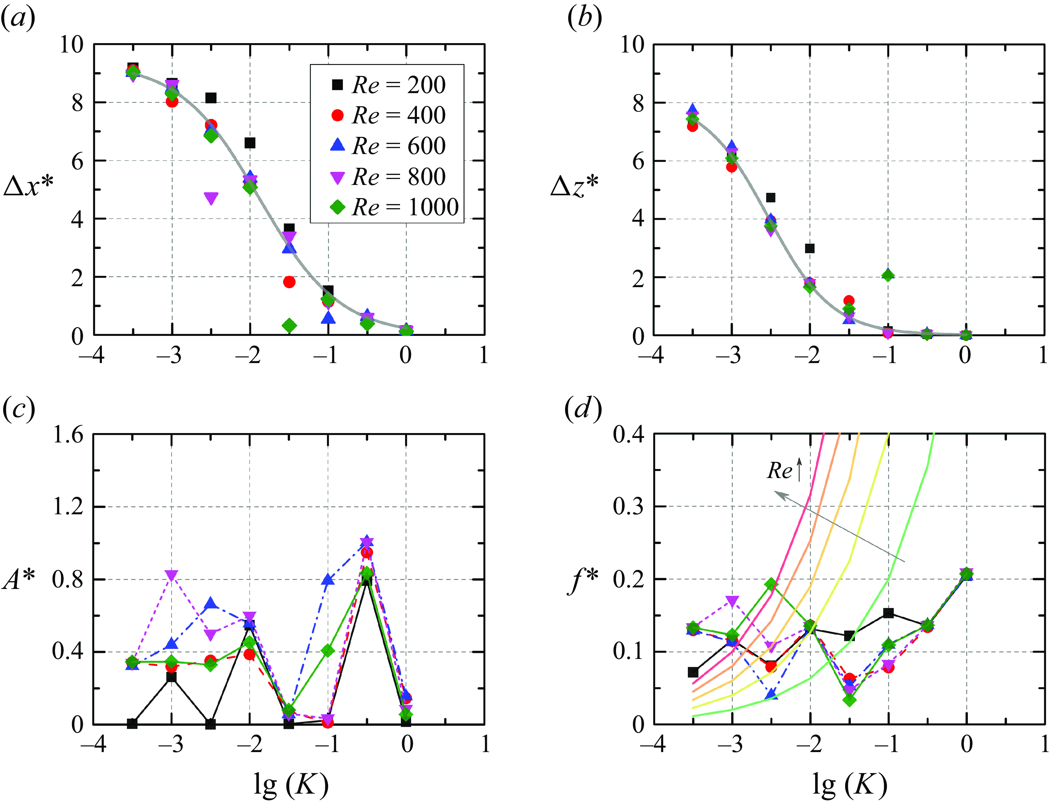
Despite significant deformation in streamwise and vertical directions, vibrations in these directions remain negligible. No further discussion on them is presented. The transverse amplitude is defined as $A^* = \sqrt {2} y_{rms} / D$
, where
$A^* = \sqrt {2} y_{rms} / D$
, where $y_{rms}$
is the r.m.s. transverse displacement. Figure 17(
$y_{rms}$
is the r.m.s. transverse displacement. Figure 17( $c$
) shows that the transverse response does not exhibit a clear dependence on lg(
$c$
) shows that the transverse response does not exhibit a clear dependence on lg( $K$
), suggesting that vortex shedding is not persistently locked to the natural frequency. The
$K$
), suggesting that vortex shedding is not persistently locked to the natural frequency. The $i^{}$
th natural frequency of the flexible stem is given by
$i^{}$
th natural frequency of the flexible stem is given by
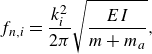 \begin{equation} f_{n,i}=\frac {k_i^2}{2 \pi } \sqrt {\frac {E I}{m+m_a}}, \end{equation}
where $i$
is the mode number,
$i$
is the mode number, $m$
is the structure mass,
$m$
is the structure mass, $m_a$
is the added mass of the fluid defined as
$m_a$
is the added mass of the fluid defined as $m_a = \pi D^2 \rho _f l /4$
and
$m_a = \pi D^2 \rho _f l /4$
and $k_i$
is the dimensionless frequency parameter of the
$k_i$
is the dimensionless frequency parameter of the $i^{}$
th mode. The first and second modal parameters are
$i^{}$
th mode. The first and second modal parameters are $k_1=$
1.875 and
$k_1=$
1.875 and $k_2=$
4.694 (Blevins Reference Blevins2016). For conciseness, only the first natural frequency (i.e.
$k_2=$
4.694 (Blevins Reference Blevins2016). For conciseness, only the first natural frequency (i.e. $f_{n,1}$
) is shown in figure 17(
$f_{n,1}$
) is shown in figure 17( $d$
). At specific lg(
$d$
). At specific lg( $K$
) values, the dominant frequency aligns with
$K$
) values, the dominant frequency aligns with $f_{n,1}$
, with locking to
$f_{n,1}$
, with locking to $f_{n,2}$
observed at
$f_{n,2}$
observed at $Re=$
200 (not shown).
$Re=$
200 (not shown).
The highest amplitude occurs at lg( $K$
) = −0.5. At the lowest lg(
$K$
) = −0.5. At the lowest lg( $K$
), transverse amplitude is tiny as the stem yields more readily to the incoming flow, exhibiting ‘high flexibility-induced rigidity’ (He, Liu & Shen Reference He, Liu and Shen2022). The dominant frequency (i.e.
$K$
), transverse amplitude is tiny as the stem yields more readily to the incoming flow, exhibiting ‘high flexibility-induced rigidity’ (He, Liu & Shen Reference He, Liu and Shen2022). The dominant frequency (i.e. $f^*$
) of transverse displacement is shown in figure 17(
$f^*$
) of transverse displacement is shown in figure 17( $d$
). At
$d$
). At $Re=$
200, the dominant frequency grows roughly with lg(
$Re=$
200, the dominant frequency grows roughly with lg( $K$
). However, for
$K$
). However, for $Re=$
400–1000, dominant frequencies are irregular, mostly clustering around
$Re=$
400–1000, dominant frequencies are irregular, mostly clustering around $f^*=$
0.1. As discussed in § 5, more complex vortical structures at the higher
$f^*=$
0.1. As discussed in § 5, more complex vortical structures at the higher $Re$
influence displacement. Unlike an infinite cylinder experiencing VIV, where
$Re$
influence displacement. Unlike an infinite cylinder experiencing VIV, where $f^*$
$f^*$ $\gt$
0.2 for
$\gt$
0.2 for $Re$
$Re$ $\gt$
200 (Wang, Xiao & Incecik Reference Wang, Xiao and Incecik2017; Gsell, Bourguet & Braza Reference Gsell, Bourguet and Braza2019; Yu et al. Reference Yu, Wang, Bao, Xiao, Li, Incecik and Lin2024), vortex shedding in a wall-mounted flexible cylinder is significantly slower due to junction-induced vortex retardation.
$\gt$
200 (Wang, Xiao & Incecik Reference Wang, Xiao and Incecik2017; Gsell, Bourguet & Braza Reference Gsell, Bourguet and Braza2019; Yu et al. Reference Yu, Wang, Bao, Xiao, Li, Incecik and Lin2024), vortex shedding in a wall-mounted flexible cylinder is significantly slower due to junction-induced vortex retardation.
The regimes of the response are defined based on ( $a$
) the transverse amplitude and (
$a$
) the transverse amplitude and ( $b$
) the spectral features of the displacement. Here, the minor vibration is defined as
$b$
) the spectral features of the displacement. Here, the minor vibration is defined as $A^*$
$A^*$ $\lt$
0.2, medium vibration is defined as 0.2
$\lt$
0.2, medium vibration is defined as 0.2 $\leqslant$ $A^*$
$A^*$ $\leqslant$
0.6 and substantial vibration is defined as
$\leqslant$
0.6 and substantial vibration is defined as $A^* \gt$
0.6. The phase portrait of the transverse displacement is applied to identify the types.
$A^* \gt$
0.6. The phase portrait of the transverse displacement is applied to identify the types.
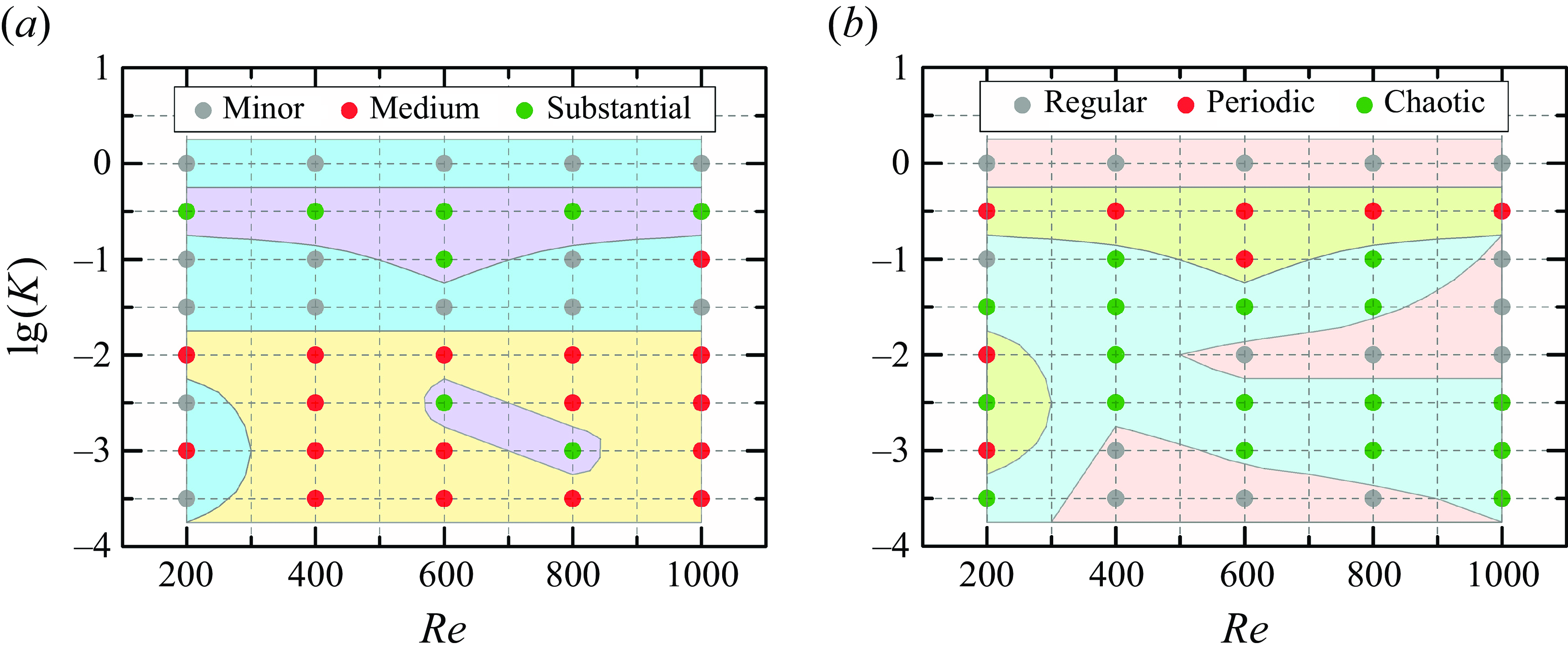
Time histories (left column), power spectral density (middle column) and phase portraits of the transverse displacement (right column) at the stem tip at different $Re$
and lg(
$Re$
and lg( $K$
). Panels show (
$K$
). Panels show ( $a$
)
$a$
) $Re=$
200 and lg(
$Re=$
200 and lg( $K$
) = 0, (
$K$
) = 0, ( $b$
)
$b$
) $Re=$
800 and lg(
$Re=$
800 and lg( $K$
) = –1.5, (
$K$
) = –1.5, ( $c$
)
$c$
) $Re=$
400 and lg(
$Re=$
400 and lg( $K$
) = –3.0, (
$K$
) = –3.0, ( $d$
)
$d$
) $Re=$
600 and lg(
$Re=$
600 and lg( $K$
) = –0.5, (
$K$
) = –0.5, ( $e$
)
$e$
) $Re=$
600 and lg(
$Re=$
600 and lg( $K$
) = –2.5 and (
$K$
) = –2.5 and ( $f$
)
$f$
) $Re=$
600 and lg(
$Re=$
600 and lg( $K$
) = –3.5. Note that the discrete points are used in the phase portraits.
$K$
) = –3.5. Note that the discrete points are used in the phase portraits.
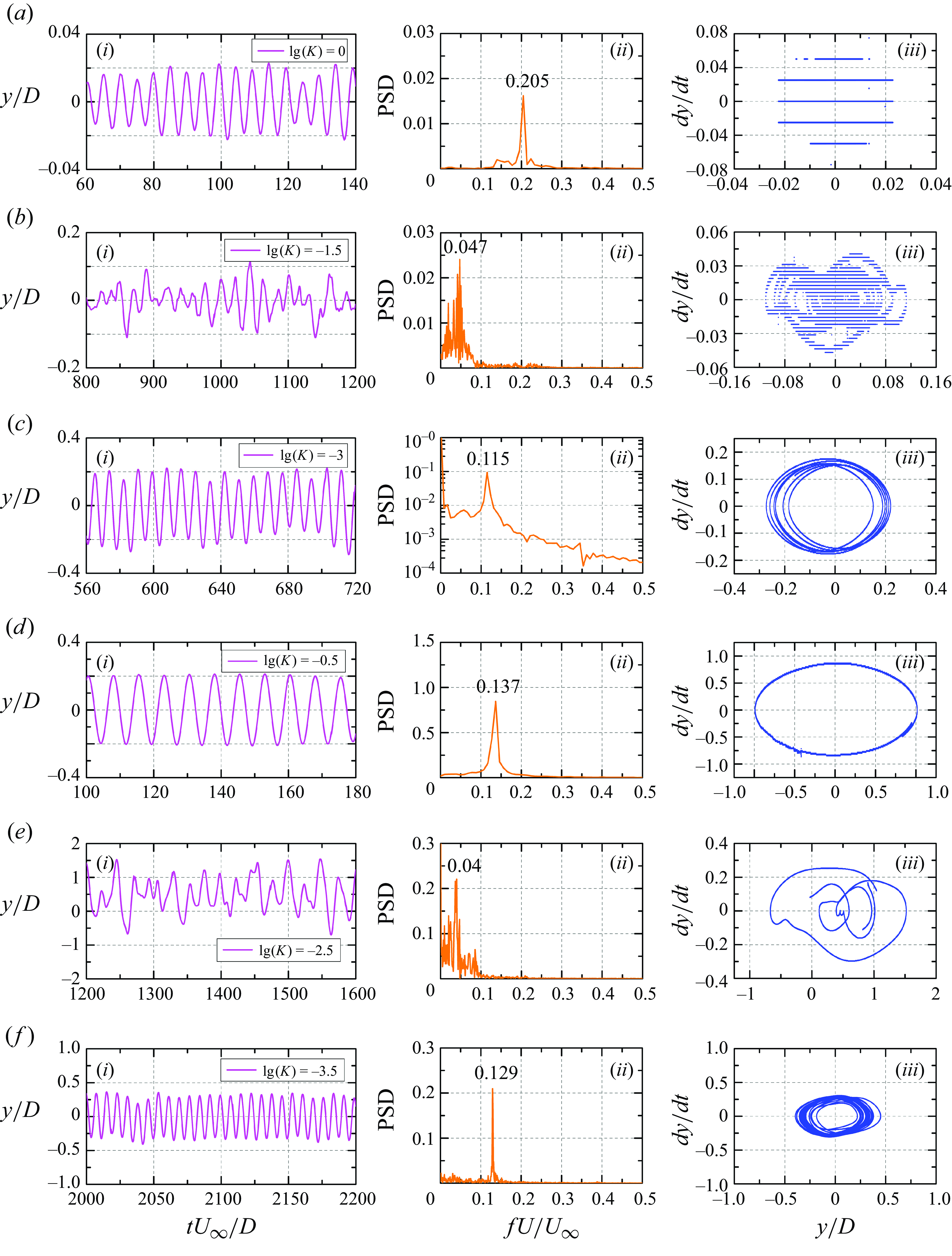
Based on transverse amplitude and displacement characteristics, responses are categorised into three types, see figure 18. Based on the amplitude, the three types are minor vibration (i.e. $A^*$
$A^*$ $\lt$
0.2), medium vibration (i.e. 0.2
$\lt$
0.2), medium vibration (i.e. 0.2 $\leqslant$ $A^*$
$A^*$ $\leqslant$
0.6) and substantial vibration (i.e.
$\leqslant$
0.6) and substantial vibration (i.e. $A^* \gt$
0.6), see figure 18(
$A^* \gt$
0.6), see figure 18( $a$
). Minor vibration primarily occurs in three regions: lg(
$a$
). Minor vibration primarily occurs in three regions: lg( $K$
) = 0, lg(
$K$
) = 0, lg( $K$
) = –1.0–1.5, and lg(
$K$
) = –1.0–1.5, and lg( $K$
) = –2.5–3.5 (for
$K$
) = –2.5–3.5 (for $Re=$
200 only). In the first region, the stem is relatively rigid, with small transverse amplitude, and vortex shedding dominates vibration (
$Re=$
200 only). In the first region, the stem is relatively rigid, with small transverse amplitude, and vortex shedding dominates vibration ( $f^*=$
0.205), see figure 19(
$f^*=$
0.205), see figure 19( $a$
-i). With the same
$a$
-i). With the same $K$
but at a higher
$K$
but at a higher $Re$
, stronger vortex shedding increases the hydrodynamic loads, slightly amplifying the vibration while still remaining in the minor vibration category. In the second region, the vortex shedding frequency deviates from the stem’s first natural frequency. As shown in figure 19(
$Re$
, stronger vortex shedding increases the hydrodynamic loads, slightly amplifying the vibration while still remaining in the minor vibration category. In the second region, the vortex shedding frequency deviates from the stem’s first natural frequency. As shown in figure 19( $b$
-i,
$b$
-i, $b$
-ii), the dominant frequency (
$b$
-ii), the dominant frequency ( $f^*=$
0.047) in this region is much lower and significantly differs from the natural frequency. Unlike the first region, multiple comparable low frequencies are observed, even though the transverse amplitude is higher. The third region occurs at lg(
$f^*=$
0.047) in this region is much lower and significantly differs from the natural frequency. Unlike the first region, multiple comparable low frequencies are observed, even though the transverse amplitude is higher. The third region occurs at lg( $K$
)
$K$
) $\lt$
–2.0 and
$\lt$
–2.0 and $Re=$
200, where the stem approaches a lodging state, and the vortical structures remain regular, as discussed in § 6.3.
$Re=$
200, where the stem approaches a lodging state, and the vortical structures remain regular, as discussed in § 6.3.
Medium vibration mainly appears at lg( $K$
)
$K$
) $\leqslant$
–2.0, see figure 18(
$\leqslant$
–2.0, see figure 18( $a$
). As shown in figure 19(
$a$
). As shown in figure 19( $c$
-i), although the transverse amplitude is slightly above
$c$
-i), although the transverse amplitude is slightly above $A^*=$
0.2, the displacement remains regular. The dominant frequency is
$A^*=$
0.2, the displacement remains regular. The dominant frequency is $f^*=$
0.115, with a magnitude significantly higher than those of other frequency components, see figure 19(
$f^*=$
0.115, with a magnitude significantly higher than those of other frequency components, see figure 19( $c$
-ii). Due to substantial deformation, the vortex shedding frequency in this case is lower.
$c$
-ii). Due to substantial deformation, the vortex shedding frequency in this case is lower.
Substantial vibration occurs in two regions: lg( $K$
) = –0.5–1.0 with
$K$
) = –0.5–1.0 with $Re=$
200–1000 and g(
$Re=$
200–1000 and g( $K$
) = –2.0–3.0 with
$K$
) = –2.0–3.0 with $Re=$
600–800, see figure 18(
$Re=$
600–800, see figure 18( $a$
). In the first region, the transverse amplitude is larger than in the second region, which may indicator better synchronisation between stem vibration and vortex shedding. In the first region, the displacement is periodic, and the stem vibration is dominated by a single frequency (
$a$
). In the first region, the transverse amplitude is larger than in the second region, which may indicator better synchronisation between stem vibration and vortex shedding. In the first region, the displacement is periodic, and the stem vibration is dominated by a single frequency ( $f^*=$
0.137), see figure 19(
$f^*=$
0.137), see figure 19( $d$
-i,
$d$
-i, $d$
-ii). In contrast, in the second region, the displacement is chaotic, and multiple low-frequency components dominate stem vibration, see figure 19(
$d$
-ii). In contrast, in the second region, the displacement is chaotic, and multiple low-frequency components dominate stem vibration, see figure 19( $e$
-i,
$e$
-i, $e$
-ii). The dominant frequency is
$e$
-ii). The dominant frequency is $f^*=$
0.04, which is significantly lower than the stem’s natural frequency.
$f^*=$
0.04, which is significantly lower than the stem’s natural frequency.
The phase portrait provides a geometric representation of a dynamical system’s trajectories in the phase plane and is used to confirm the system dynamics (Jordan & Smith Reference Jordan and Smith2007). In this study, phase portraits of displacement are employed to illustrate the system dynamics (Chang & Modarres-Sadeghi Reference Chang and Modarres-Sadeghi2014). Based on the characteristics of transverse displacement portraits, the response is classified into three categories, i.e. periodic, regular (quasiperiodic) and chaotic. The distribution of these categories is shown in figure 18( $b$
). The spectral content of the displacement serves as a supplementary indicator. Periodic vibration is characterised by a dominant frequency with a significantly higher magnitude than other frequencies, see figure 19(
$b$
). The spectral content of the displacement serves as a supplementary indicator. Periodic vibration is characterised by a dominant frequency with a significantly higher magnitude than other frequencies, see figure 19( $d$
-ii,
$d$
-ii, $d$
-iii). Synchronisation between vortex shedding and stem vibration is observed. Comparing figures 18(
$d$
-iii). Synchronisation between vortex shedding and stem vibration is observed. Comparing figures 18( $a$
) and 18(
$a$
) and 18( $b$
), the first periodic region coincides with the first substantial vibration region, suggesting that higher amplitudes facilitate periodic vortex shedding. The second periodic region appears at lg(
$b$
), the first periodic region coincides with the first substantial vibration region, suggesting that higher amplitudes facilitate periodic vortex shedding. The second periodic region appears at lg( $K$
) = –2.0–3.0 but only for
$K$
) = –2.0–3.0 but only for $Re=$
200. In this region, the transverse amplitude is moderate, and vortex shedding remains periodic. Beyond
$Re=$
200. In this region, the transverse amplitude is moderate, and vortex shedding remains periodic. Beyond $Re=$
200 finer vortices emerge, and low-frequency components appear. A more flexible stem is more susceptible to turbulent fluctuation, making periodic vibration nearly impossible when lg(
$Re=$
200 finer vortices emerge, and low-frequency components appear. A more flexible stem is more susceptible to turbulent fluctuation, making periodic vibration nearly impossible when lg( $K$
)
$K$
) $\lt$
–1.0.
$\lt$
–1.0.
Regular vibration is observed in three regions, see figure 18( $b$
). The first region occurs at lg(
$b$
). The first region occurs at lg( $K$
) = 0 with
$K$
) = 0 with $Re=$
200–1000, where the stem is relatively rigid, and its vibration is regulated by vortex shedding, maintaining a steady rhythm, see figure 19(
$Re=$
200–1000, where the stem is relatively rigid, and its vibration is regulated by vortex shedding, maintaining a steady rhythm, see figure 19( $a$
-ii). The phase portrait in figure 19(
$a$
-ii). The phase portrait in figure 19( $a$
-iii) indicates that stem vibration follows a nearly constant trajectory. The second region, at lg(
$a$
-iii) indicates that stem vibration follows a nearly constant trajectory. The second region, at lg( $K$
) = –1.0–2.0 with
$K$
) = –1.0–2.0 with $Re=$
600–1000, exhibits transverse amplitude ranging from minor to substantial. As shown in figure 19(
$Re=$
600–1000, exhibits transverse amplitude ranging from minor to substantial. As shown in figure 19( $c$
-ii), the dominant frequency is
$c$
-ii), the dominant frequency is $f^*=$
0.115, while other frequency components are insignificant in magnitude. The phase portrait in figure 19(
$f^*=$
0.115, while other frequency components are insignificant in magnitude. The phase portrait in figure 19( $c$
-iii) is highly regular. The third region, at lg(
$c$
-iii) is highly regular. The third region, at lg( $K$
) = –3.0–3.5 with
$K$
) = –3.0–3.5 with $Re=$
400–800, shows an intermediate stem amplitude with a single frequency,
$Re=$
400–800, shows an intermediate stem amplitude with a single frequency, $f^*=$
0.129, see figure 19(
$f^*=$
0.129, see figure 19( $f$
-ii).
$f$
-ii).
The chaotic regime spans lg( $K) = -1.0-3.5$
and
$K) = -1.0-3.5$
and $Re = 200-1000$
, see figure 18(
$Re = 200-1000$
, see figure 18( $b$
). A comparison of figures 18(
$b$
). A comparison of figures 18( $a$
) and 18(
$a$
) and 18( $b$
) reveals that chaotic vibration can occur regardless of whether the transverse amplitude is small, medium or substantial. At moderate lg(
$b$
) reveals that chaotic vibration can occur regardless of whether the transverse amplitude is small, medium or substantial. At moderate lg( $K)\, (= -1.0-1.5)$
, the transverse amplitude is small, but multiple low frequencies appear, see figure 19(
$K)\, (= -1.0-1.5)$
, the transverse amplitude is small, but multiple low frequencies appear, see figure 19( $b$
-i,
$b$
-i, $b$
-ii). The phase portrait in figure 19(
$b$
-ii). The phase portrait in figure 19( $b$
-iii) further confirms this chaotic behaviour. At lower lg(
$b$
-iii) further confirms this chaotic behaviour. At lower lg( $K)\, (= -2.0-3.5)$
, the transverse amplitude may be medium or substantial, but stem vibration is strongly influenced by turbulent structures, leading to chaotic behaviour, see figure 19(
$K)\, (= -2.0-3.5)$
, the transverse amplitude may be medium or substantial, but stem vibration is strongly influenced by turbulent structures, leading to chaotic behaviour, see figure 19( $e$
-i,
$e$
-i, $e$
-ii). The dominant frequency (
$e$
-ii). The dominant frequency ( $f^* = 0.04$
) is significantly low, with several comparable low-frequency component. The phase portrait in figure 19(
$f^* = 0.04$
) is significantly low, with several comparable low-frequency component. The phase portrait in figure 19( $e$
-iii) indicates no fixed trajectory for the stem to follow.
$e$
-iii) indicates no fixed trajectory for the stem to follow.
6.2. Hydrodynamic forces and comparison with the rigid stem
The hydrodynamic forces on the flexible stem are key factors influencing stem oscillation and shape deformation. Figure 20 shows the variation of hydrodynamic forces on the flexible stem as a function of $Re$
and lg(
$Re$
and lg( $K$
). For comparison, results of a rigid stem are superimposed. As shown in figure 20(
$K$
). For comparison, results of a rigid stem are superimposed. As shown in figure 20( $a$
), the mean drag coefficient (
$a$
), the mean drag coefficient ( $\bar {C}_d$
) generally decreases as lg(
$\bar {C}_d$
) generally decreases as lg( $K$
) decreases, indicating that
$K$
) decreases, indicating that $\bar {C}_d$
is primarily affected by stem deformation. As mentioned in § 6.1, when stiffness is significantly low, the deflected height of the stem decreases, resulting in a more streamlined shape and a corresponding reduction in
$\bar {C}_d$
is primarily affected by stem deformation. As mentioned in § 6.1, when stiffness is significantly low, the deflected height of the stem decreases, resulting in a more streamlined shape and a corresponding reduction in $\bar {C}_d$
drops. For the two cases with the highest stiffnesses, i.e. lg(
$\bar {C}_d$
drops. For the two cases with the highest stiffnesses, i.e. lg( $K$
) = 0 and −0.5, the
$K$
) = 0 and −0.5, the $\bar {C}_d$
of the flexible stem is higher than that of the rigid stem. In these cases, shape deformation is minimal, but stem oscillation develops, particularly for lg(
$\bar {C}_d$
of the flexible stem is higher than that of the rigid stem. In these cases, shape deformation is minimal, but stem oscillation develops, particularly for lg( $K$
) = –0.5. This suggests that transverse oscillation has a significant impact on
$K$
) = –0.5. This suggests that transverse oscillation has a significant impact on $\bar {C}_d$
when the stem is relatively rigid.
$\bar {C}_d$
when the stem is relatively rigid.
The r.m.s. drag and lift coefficients vary significantly with lg( $K$
). As shown in figure 20(
$K$
). As shown in figure 20( $b$
), the r.m.s. drag coefficient (
$b$
), the r.m.s. drag coefficient ( $C_d^{\prime }$
) increases gradually with increasing lg(
$C_d^{\prime }$
) increases gradually with increasing lg( $K$
). However, it is slightly lower for the cases with lg(
$K$
). However, it is slightly lower for the cases with lg( $K$
) = 0 and −1 due to weak transverse oscillation. For a flexible stem with identical deformation, stronger transverse oscillation enhances vortex shedding, leading to higher
$K$
) = 0 and −1 due to weak transverse oscillation. For a flexible stem with identical deformation, stronger transverse oscillation enhances vortex shedding, leading to higher $C_d^{\prime }$
. As shown in figure 20(
$C_d^{\prime }$
. As shown in figure 20( $c$
), in most cases, the r.m.s. lift coefficient (
$c$
), in most cases, the r.m.s. lift coefficient ( $C_l^{\prime }$
) on the flexible stem is comparable to that of the rigid stem. However, it is significantly higher for lg(
$C_l^{\prime }$
) on the flexible stem is comparable to that of the rigid stem. However, it is significantly higher for lg( $K$
) = 0, −0.5 and −2.0, where transverse amplitude is larger. This suggests that
$K$
) = 0, −0.5 and −2.0, where transverse amplitude is larger. This suggests that $C_l^{\prime }$
is strongly influenced by transverse oscillation.
$C_l^{\prime }$
is strongly influenced by transverse oscillation.
Hydrodynamic forces on a wall-mounted flexible stem with lg( $K$
) at
$K$
) at $Re=$
200–1000. (
$Re=$
200–1000. ( $a$
) Mean drag (
$a$
) Mean drag ( $\bar {C}_d$
), (
$\bar {C}_d$
), ( $b$
) r.m.s. drag (
$b$
) r.m.s. drag ( $C_d^{\prime }$
) and (
$C_d^{\prime }$
) and ( $c$
) r.m.s. lift (
$c$
) r.m.s. lift ( $C_l^{\prime }$
). In each plot, the horizontal lines (with the same colours as the flexible case) denote the corresponding forces on the rigid stem.
$C_l^{\prime }$
). In each plot, the horizontal lines (with the same colours as the flexible case) denote the corresponding forces on the rigid stem.
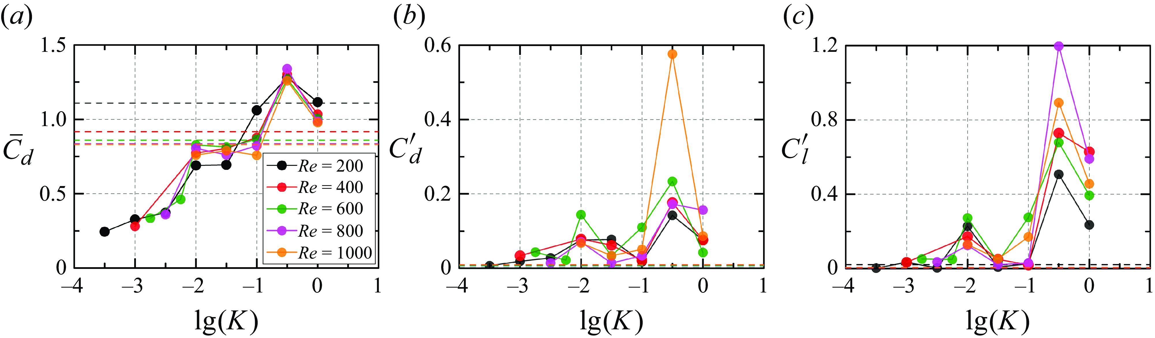
6.3. Characteristics of the 3-D vortical structures at different regimes
The 3-D vortical structures provide valuable insights into the physics of different responses and hydrodynamic loads acting on the flexible stem. Figure 21 shows the detailed 3-D vortical structures at $Re=$
200 with lg(
$Re=$
200 with lg( $K$
) = 0–3.5. The vortex dynamics of the flexible stem, including vortex arrangement and shedding behaviour, differs significantly from the rigid case. At the highest lg(
$K$
) = 0–3.5. The vortex dynamics of the flexible stem, including vortex arrangement and shedding behaviour, differs significantly from the rigid case. At the highest lg( $K$
), the stem experiences minimal deformation and behaves similarly to a rigid stem (Luhar & Nepf Reference Luhar and Nepf2011, Reference Luhar and Nepf2016; Jacobsen et al. Reference Jacobsen, Bakker, Uijttewaal and Uittenbogaard2019). As shown in figure 21(
$K$
), the stem experiences minimal deformation and behaves similarly to a rigid stem (Luhar & Nepf Reference Luhar and Nepf2011, Reference Luhar and Nepf2016; Jacobsen et al. Reference Jacobsen, Bakker, Uijttewaal and Uittenbogaard2019). As shown in figure 21( $a$
), at lg(
$a$
), at lg( $K$
) = 0, the wake resembles that of a rigid stem, although some alterations occur due to stem vibration. The spanwise vortex shedding occurs at an angle of approximately 6
$K$
) = 0, the wake resembles that of a rigid stem, although some alterations occur due to stem vibration. The spanwise vortex shedding occurs at an angle of approximately 6 $^\circ$
relative to the wall surface, which is considerably lower than the
$^\circ$
relative to the wall surface, which is considerably lower than the $\approx$
21
$\approx$
21 $^\circ$
observed in the rigid case. The downwash flow in the flexible case has a weaker effect on vortex formation, and similar to the rigid case, the spanwise vortices mainly appear around the midspan. At lg(
$^\circ$
observed in the rigid case. The downwash flow in the flexible case has a weaker effect on vortex formation, and similar to the rigid case, the spanwise vortices mainly appear around the midspan. At lg( $K$
) = –0.5, the stem oscillates with a large transverse amplitude (
$K$
) = –0.5, the stem oscillates with a large transverse amplitude ( $A^*=$
0.79), leading to significant changes in vortical structures. The shift in vortex shedding is associated with the increased transverse amplitude, which enhances vortex formation near the tip despite minor deformation. Consequently, the downwash flow effect becomes negligible. As shown in figure 21(
$A^*=$
0.79), leading to significant changes in vortical structures. The shift in vortex shedding is associated with the increased transverse amplitude, which enhances vortex formation near the tip despite minor deformation. Consequently, the downwash flow effect becomes negligible. As shown in figure 21( $b$
), vortex shedding initiates at the free end and weakens closer to the wall, ceasing at approximately 2.8
$b$
), vortex shedding initiates at the free end and weakens closer to the wall, ceasing at approximately 2.8 $D$
from the wall.
$D$
from the wall.
As lg( $K$
) decreases further, stem deformation becomes pronounced, altering the 3-D vortex distribution. As shown in figure 21(
$K$
) decreases further, stem deformation becomes pronounced, altering the 3-D vortex distribution. As shown in figure 21( $c$
), deformation leads to a more evenly distributed flow along the stem length. Near the free end, vortex shedding remains approximately parallel, but further downstream, the separated vortices stretch into hairpin-vortex like structures (Robinson Reference Robinson1991). Additionally, vortices from both sides of the stem initially connect during the formation, as marked in figure 21(
$c$
), deformation leads to a more evenly distributed flow along the stem length. Near the free end, vortex shedding remains approximately parallel, but further downstream, the separated vortices stretch into hairpin-vortex like structures (Robinson Reference Robinson1991). Additionally, vortices from both sides of the stem initially connect during the formation, as marked in figure 21( $c$
), although these connections disappear downstream due to increased vortex head velocity. In the far wake, the vortices are fully hairpin-vortex like.
$c$
), although these connections disappear downstream due to increased vortex head velocity. In the far wake, the vortices are fully hairpin-vortex like.
The 3-D vortical structures of a wall-mounted flexible stem at $Re=$
200 and different
$Re=$
200 and different $K$
values. Panels show (
$K$
values. Panels show ( $a$
) lg(
$a$
) lg( $K$
) = 0, (
$K$
) = 0, ( $b$
) lg(
$b$
) lg( $K$
) = –0.5, (
$K$
) = –0.5, ( $c$
) lg(
$c$
) lg( $K$
) = –1.0, (
$K$
) = –1.0, ( $d$
) lg(
$d$
) lg( $K$
) = –1.5, (
$K$
) = –1.5, ( $e$
) lg(
$e$
) lg( $K$
) = –2.0 and (
$K$
) = –2.0 and ( $f$
) lg(
$f$
) lg( $K$
) = –3.0. Flow is from left to right. Here,
$K$
) = –3.0. Flow is from left to right. Here, $Q=$
5. The plot in (
$Q=$
5. The plot in ( $b$
) is the corresponding vertical velocity field at the midplane of the
$b$
) is the corresponding vertical velocity field at the midplane of the $y$
-direction.
$y$
-direction.
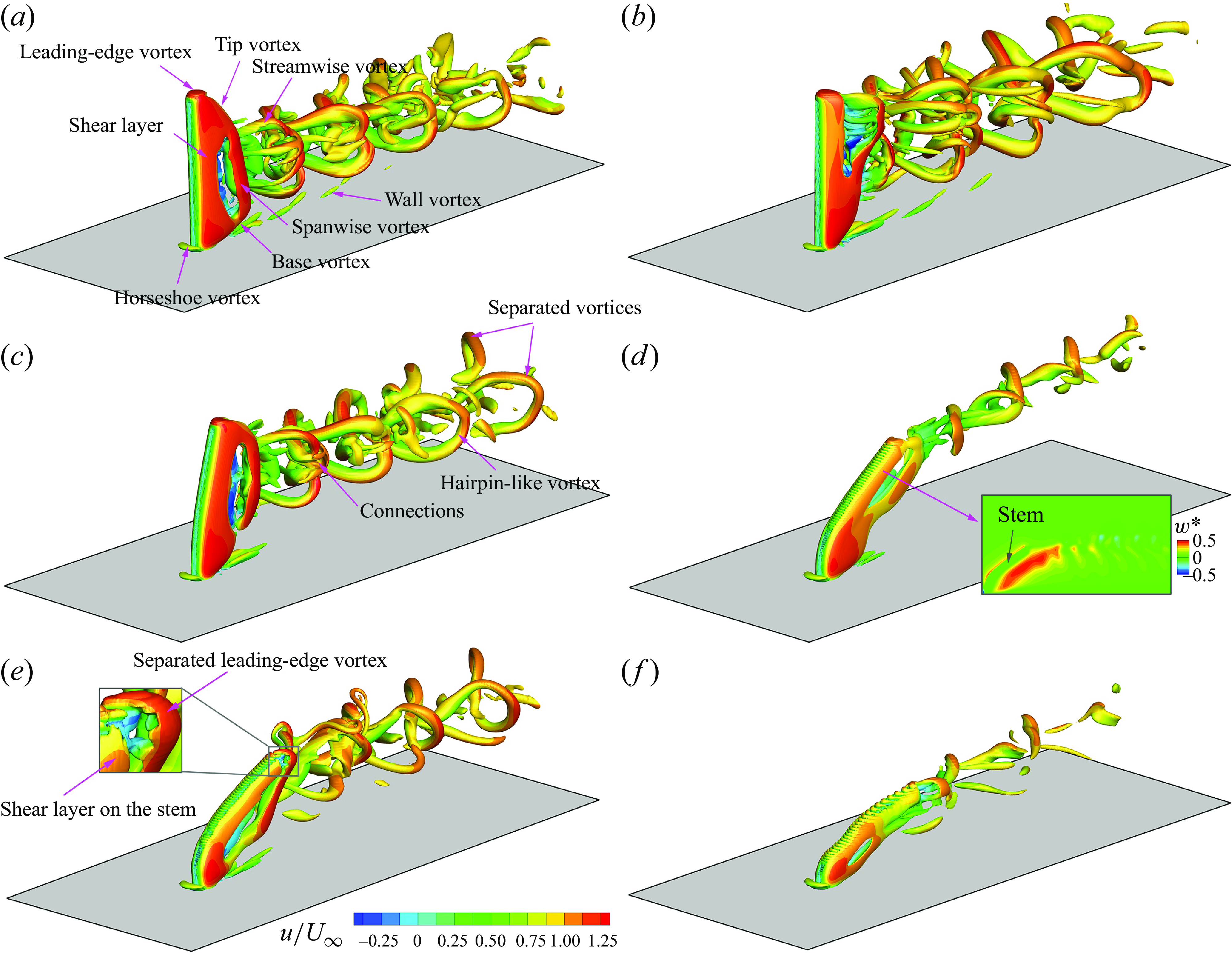
The 3-D vortical structures of a wall-mounted flexible stem at $Re=$
400 and different
$Re=$
400 and different $K$
values. Panels show (
$K$
values. Panels show ( $a$
) lg(
$a$
) lg( $K$
) = 0, (
$K$
) = 0, ( $b$
) lg(
$b$
) lg( $K$
) = –0.5, (
$K$
) = –0.5, ( $c$
) lg(
$c$
) lg( $K$
) = –1.0, (
$K$
) = –1.0, ( $d$
) lg(
$d$
) lg( $K$
) = –1.5, (
$K$
) = –1.5, ( $e$
) lg(
$e$
) lg( $K$
) = –2.0 and (
$K$
) = –2.0 and ( $f$
) lg(
$f$
) lg( $K$
) = –3.0. Flow is from left to right. Here,
$K$
) = –3.0. Flow is from left to right. Here, $Q=$
20. The inset in (
$Q=$
20. The inset in ( $a$
) is the corresponding vertical velocity field at the midplane of the
$a$
) is the corresponding vertical velocity field at the midplane of the $y$
-direction.
$y$
-direction.
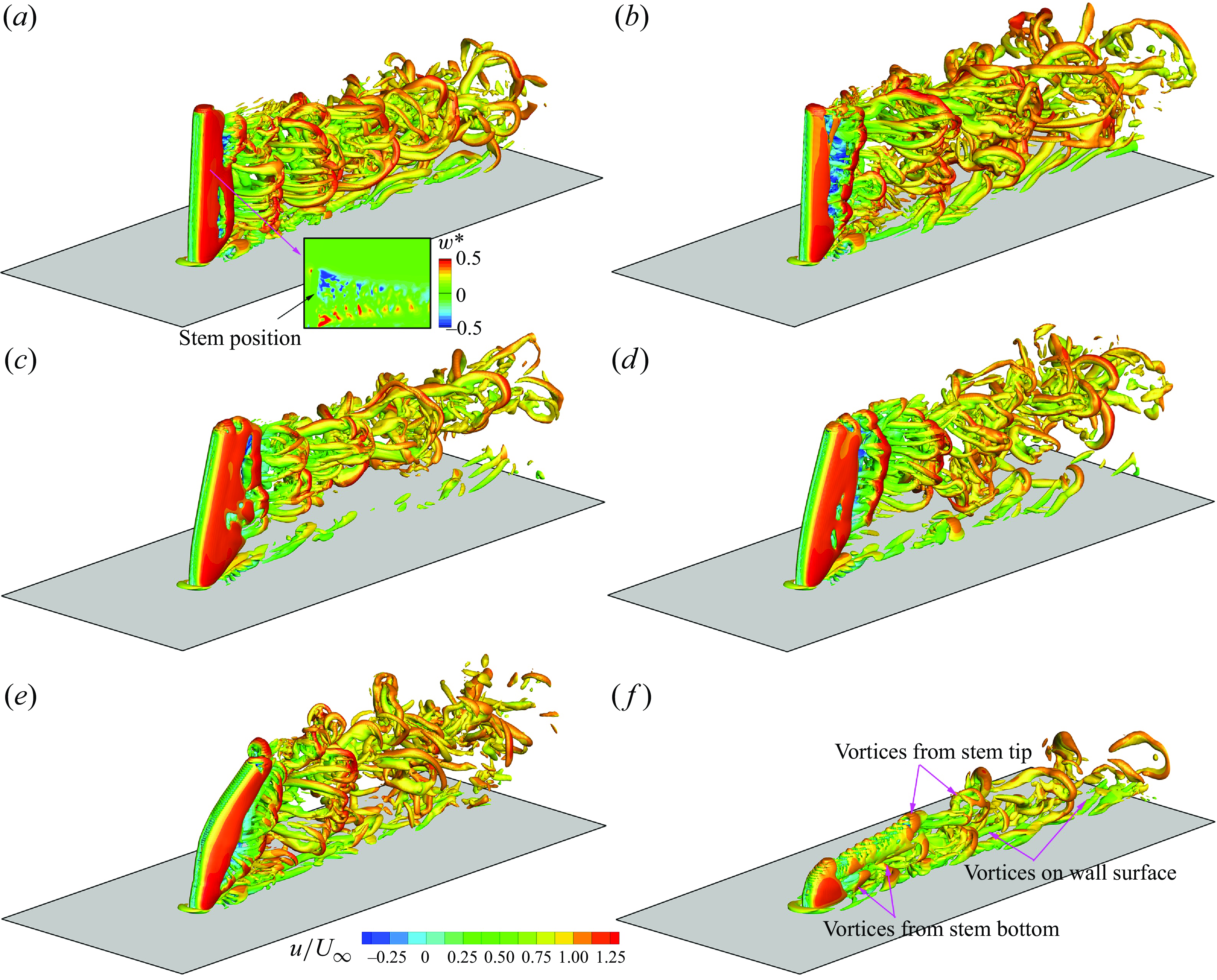
The 3-D vortical structures of a wall-mounted flexible stem at $Re = 600-1000$
and
$Re = 600-1000$
and $K$
values. Panels show (
$K$
values. Panels show ( $a$
)
$a$
) $Re=$
600 and lg(
$Re=$
600 and lg( $K$
) = –0.5, (
$K$
) = –0.5, ( $b$
)
$b$
) $Re=$
600 and lg(
$Re=$
600 and lg( $K$
) = –2.0, (
$K$
) = –2.0, ( $c$
)
$c$
) $Re=$
800 and lg(
$Re=$
800 and lg( $K$
) = –1.5, (
$K$
) = –1.5, ( $d$
)
$d$
) $Re=$
800 and lg(
$Re=$
800 and lg( $K$
) = –2.0, (
$K$
) = –2.0, ( $e$
)
$e$
) $Re=$
1000 and lg(
$Re=$
1000 and lg( $K$
) = –0.5, and (
$K$
) = –0.5, and ( $f$
)
$f$
) $Re=$
1000 and lg(
$Re=$
1000 and lg( $K$
) = –2.0. Flow is from left to right. Here,
$K$
) = –2.0. Flow is from left to right. Here, $Q=$
45, 80 and 125 for the cases at
$Q=$
45, 80 and 125 for the cases at $Re=$
600, 800 and 1000, respectively.
$Re=$
600, 800 and 1000, respectively.
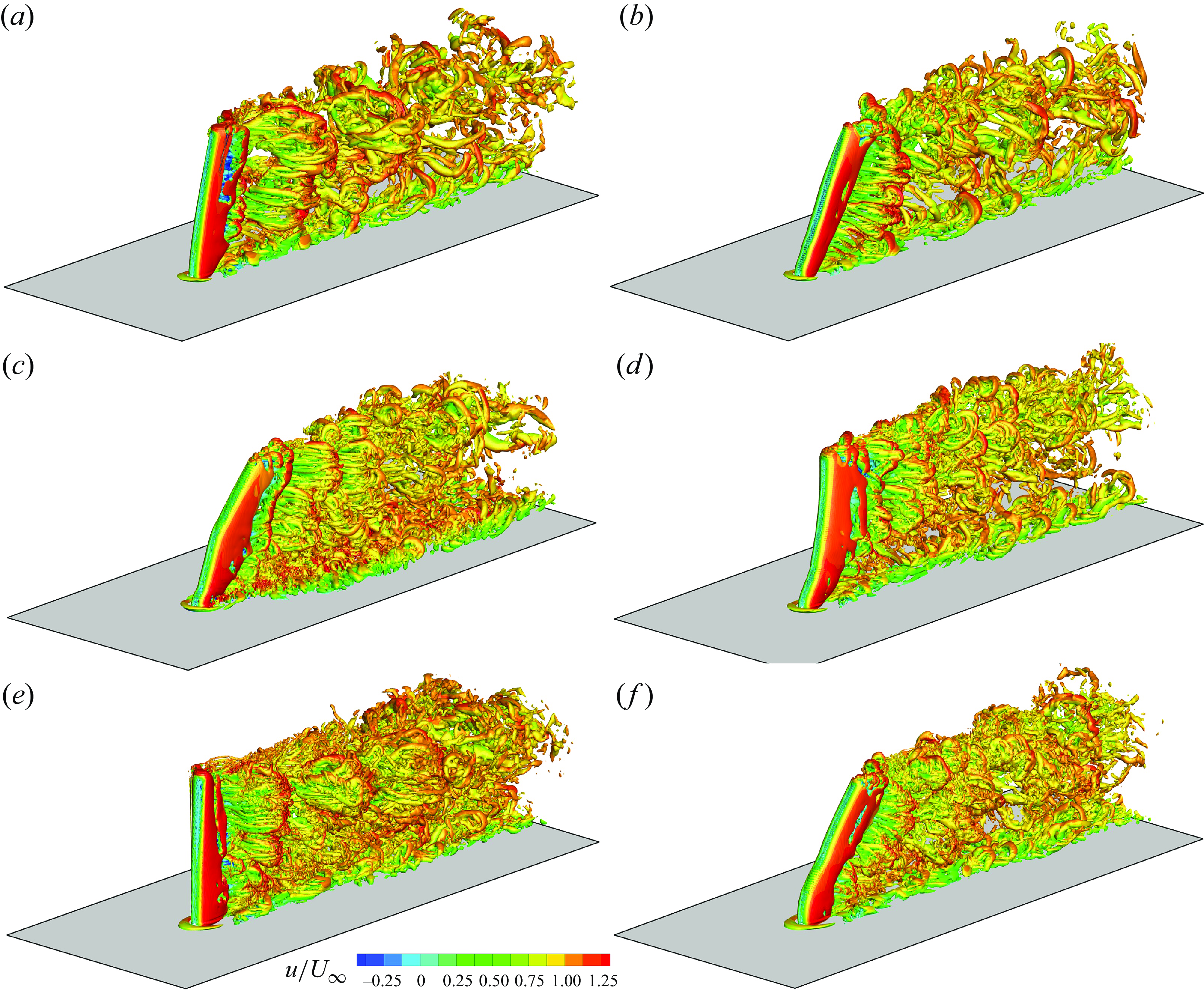
At lg( $K$
)
$K$
) $\leqslant$
–1.5, significant stem deformation results in spanwise vortex shedding along the entire stem length, although this is weaker than in less deformed cases, see figure 21(d–f). As lg(
$\leqslant$
–1.5, significant stem deformation results in spanwise vortex shedding along the entire stem length, although this is weaker than in less deformed cases, see figure 21(d–f). As lg( $K$
) drops, vortices form progressively closer to the free end. At lg(
$K$
) drops, vortices form progressively closer to the free end. At lg( $K$
) = –1.5 and –3.0, transverse amplitudes are smaller, and vortical structures are weaker compared with lg(
$K$
) = –1.5 and –3.0, transverse amplitudes are smaller, and vortical structures are weaker compared with lg( $K$
) = –2.0, where the transverse amplitude is higher (
$K$
) = –2.0, where the transverse amplitude is higher ( $A^*=$
0.55). Comparing figures 21(
$A^*=$
0.55). Comparing figures 21( $d$
) and 21(
$d$
) and 21( $e$
), despite a slightly stronger stem oscillation at lg(
$e$
), despite a slightly stronger stem oscillation at lg( $K$
) = –3.0 than at lg(
$K$
) = –3.0 than at lg( $K$
) = –1.5, the vortical structures at lg(
$K$
) = –1.5, the vortical structures at lg( $K$
) = –3.0 are weaker due to greater deformation. A common feature across these cases is the slow upward movement of vortices, see the inset in figure 21(
$K$
) = –3.0 are weaker due to greater deformation. A common feature across these cases is the slow upward movement of vortices, see the inset in figure 21( $d$
). For significantly deformed stems, separation of the attached shear layer at the free-end surface occurs, forming a leading-edge vortex and/or free-end arch vortex (observed in high
$d$
). For significantly deformed stems, separation of the attached shear layer at the free-end surface occurs, forming a leading-edge vortex and/or free-end arch vortex (observed in high $Re$
flow, e.g.
$Re$
flow, e.g. $Re \gtrsim 4\times 10^3$
, see figure 1). As shown in the inset of figure 21(
$Re \gtrsim 4\times 10^3$
, see figure 1). As shown in the inset of figure 21( $e$
), the reattached shear layer at the free-end surface separates, alternately aligned with the vortex shedding. This behaviour is absent in the rigid case. Large deformation makes the attached shear layer more prone to detachment.
$e$
), the reattached shear layer at the free-end surface separates, alternately aligned with the vortex shedding. This behaviour is absent in the rigid case. Large deformation makes the attached shear layer more prone to detachment.
Figure 22 shows the organisation of 3-D vortical structures at $Re = 400$
. As in the rigid case, vortices behind the flexible stem at
$Re = 400$
. As in the rigid case, vortices behind the flexible stem at $Re=$
400 are stronger than at
$Re=$
400 are stronger than at $Re = 200$
. As lg(
$Re = 200$
. As lg( $K$
) decreases, stem deformation intensifies, altering the vortical structures. At lg(
$K$
) decreases, stem deformation intensifies, altering the vortical structures. At lg( $K$
) = 0, deformation is negligible, and vortex shedding remains similar to the rigid case, see figures 13(
$K$
) = 0, deformation is negligible, and vortex shedding remains similar to the rigid case, see figures 13( $b$
) and 22(
$b$
) and 22( $a$
). The downwash flow near the free end impacts a shorter span in the flexible case. As shown in figure 22(
$a$
). The downwash flow near the free end impacts a shorter span in the flexible case. As shown in figure 22( $a$
), vortex shedding remains approximately parallel but occurs in two phases, potentially influenced by free-end downwash flow and junction upwash flow. At lg(
$a$
), vortex shedding remains approximately parallel but occurs in two phases, potentially influenced by free-end downwash flow and junction upwash flow. At lg( $K$
) = –0.5, vortex shedding changes drastically, as in the case of
$K$
) = –0.5, vortex shedding changes drastically, as in the case of $Re=$
200. Shedding occurs near the free end, with spanwise vortices forming earlier than those closer to the wall, see figure 22(
$Re=$
200. Shedding occurs near the free end, with spanwise vortices forming earlier than those closer to the wall, see figure 22( $b$
). In the near wake, spanwise vortices undergo considerable stretching and slowly move toward the wall. The hairpin vortex on the wall develops and directly interacts with the lower-side vortices from the stem. At lg(
$b$
). In the near wake, spanwise vortices undergo considerable stretching and slowly move toward the wall. The hairpin vortex on the wall develops and directly interacts with the lower-side vortices from the stem. At lg( $K$
) = –0.5, stem oscillation is stronger, and vortex strength is higher than at lg(
$K$
) = –0.5, stem oscillation is stronger, and vortex strength is higher than at lg( $K$
) = 0.
$K$
) = 0.
For lower lg( $K$
), deformation increase significantly. As shown in figure 22(c–f), the vortex dynamics is considerably different as the stem tip nears the wall. Similar to
$K$
), deformation increase significantly. As shown in figure 22(c–f), the vortex dynamics is considerably different as the stem tip nears the wall. Similar to $Re=$
200, vortex shedding shifts toward the free end as deformation increases, with vortex intensity generally weakening. However, transverse oscillation impacts both formation position and vortex strength. At lg(
$Re=$
200, vortex shedding shifts toward the free end as deformation increases, with vortex intensity generally weakening. However, transverse oscillation impacts both formation position and vortex strength. At lg( $K$
) = –2.0, transverse amplitude is larger than at lg(
$K$
) = –2.0, transverse amplitude is larger than at lg( $K$
) = –1.0 and –1.5, leading to stronger vortices, see figure 22(
$K$
) = –1.0 and –1.5, leading to stronger vortices, see figure 22( $c$
,
$c$
, $d$
,
$d$
, $e$
). At lg(
$e$
). At lg( $K$
) = –3.0, the stem is nearly lodged against the wall, producing a distinct vortex dynamics, see figure 22(
$K$
) = –3.0, the stem is nearly lodged against the wall, producing a distinct vortex dynamics, see figure 22( $f$
). Here, spanwise vortices shed only from the stem base and free end. In the near wake, vortices from these positions interact.
$f$
). Here, spanwise vortices shed only from the stem base and free end. In the near wake, vortices from these positions interact.
Figure 23 shows the arrangement of 3-D vortical structures at $Re = 600{-}1000$
. At these higher
$Re = 600{-}1000$
. At these higher $Re$
, vortex shedding occurs along nearly the entire stem length, forming finer vortices. Due to increased instability from lower-part vortices, the wall-developing hairpin vortex strengthens compared with lower
$Re$
, vortex shedding occurs along nearly the entire stem length, forming finer vortices. Due to increased instability from lower-part vortices, the wall-developing hairpin vortex strengthens compared with lower $Re\, (=200{-}400)$
cases. As shown in figure 23(
$Re\, (=200{-}400)$
cases. As shown in figure 23( $a$
,
$a$
, $b$
), at
$b$
), at $Re=$
600, vortex shedding extends from top to bottom but is suppressed at the junction due to the presence of a HV. At
$Re=$
600, vortex shedding extends from top to bottom but is suppressed at the junction due to the presence of a HV. At $Re=$
800, vortex strength increases further, see figure 23(
$Re=$
800, vortex strength increases further, see figure 23( $c$
,
$c$
, $d$
). At lg(
$d$
). At lg( $K$
) = –1.5, upper-part vortex shedding aligns closely with the deformed stem, while lower-part vortex shedding occurs but dissipates quickly, see figure 23(
$K$
) = –1.5, upper-part vortex shedding aligns closely with the deformed stem, while lower-part vortex shedding occurs but dissipates quickly, see figure 23( $c$
). Compared with lg(
$c$
). Compared with lg( $K$
) = –1.5, transverse oscillation at lg(
$K$
) = –1.5, transverse oscillation at lg( $K$
) = –2.0 is stronger, significantly influencing vortex shedding. As shown in figure 23(
$K$
) = –2.0 is stronger, significantly influencing vortex shedding. As shown in figure 23( $d$
), upper-part vortex shedding remains nearly parallel, but lower-part vortex shedding is not synchronised, leading to vortices gradually shifting upward downstream. Consequently, interactions between hairpin and spanwise vortices weaken. The stem exhibits a low-frequency back-and-forth motion, resembling a slow wave, as indicated in figure 23(
$d$
), upper-part vortex shedding remains nearly parallel, but lower-part vortex shedding is not synchronised, leading to vortices gradually shifting upward downstream. Consequently, interactions between hairpin and spanwise vortices weaken. The stem exhibits a low-frequency back-and-forth motion, resembling a slow wave, as indicated in figure 23( $d$
). At
$d$
). At $Re=$
1000, vortex strength intensifies further. At high lg(
$Re=$
1000, vortex strength intensifies further. At high lg( $K$
), vortex shedding near the tip experiences minor influence from downwash flow, see figure 23(
$K$
), vortex shedding near the tip experiences minor influence from downwash flow, see figure 23( $e$
). The upper and lower parts of the stem shed vortices at different frequencies. In the near wake, separated vortices are significantly stretched and finer than those at the lower
$e$
). The upper and lower parts of the stem shed vortices at different frequencies. In the near wake, separated vortices are significantly stretched and finer than those at the lower $Re$
. As lg(
$Re$
. As lg( $K$
) = –2.0, stem deformation is pronounced, with upper-part vortex shedding nearly parallel, see figure 23(
$K$
) = –2.0, stem deformation is pronounced, with upper-part vortex shedding nearly parallel, see figure 23( $f$
). Lower-part vortices interact with the hairpin vortex but dissipate quickly downstream.
$f$
). Lower-part vortices interact with the hairpin vortex but dissipate quickly downstream.
The non-dimensional vertical velocity ( $w^*$
) of a wall-mounted flexible stem at
$w^*$
) of a wall-mounted flexible stem at $Re=$
400 and lg(
$Re=$
400 and lg( $K$
) = –0.5. (
$K$
) = –0.5. ( $a$
,
$a$
, $b$
) instantaneous flow field and (
$b$
) instantaneous flow field and ( $c$
) time-averaged flow field. The stem position in (
$c$
) time-averaged flow field. The stem position in ( $a$
,
$a$
, $b$
) is roughly denoted by the solid lines.
$b$
) is roughly denoted by the solid lines.

7. Discussion
In this section, we discuss particular flow dynamics and the stem response in the flexible case, such as significantly weakened downwash flow and physics of low-frequency oscillation in the streamwise and vertical directions.
7.1. Significantly weakened downwash flow
As discussed in § 6.3, stem oscillation and shape deformation can significantly modify the vortex dynamics. In this section, we concentrate on the significantly weakened downwash flow through the case of $Re=$
400 and lg(
$Re=$
400 and lg( $K$
) = –0.5. In the rigid case, the flow through the free end moves downward, as shown in figures 13(
$K$
) = –0.5. In the rigid case, the flow through the free end moves downward, as shown in figures 13( $b$
) and 16(
$b$
) and 16( $b$
). Due to the downwash flow, spanwise vortex shedding occurs in the lower part of the stem. Near the junction, the downwash flow also appears. However, in the flexible case, the vortex dynamics differs significantly. As shown in figure 22(
$b$
). Due to the downwash flow, spanwise vortex shedding occurs in the lower part of the stem. Near the junction, the downwash flow also appears. However, in the flexible case, the vortex dynamics differs significantly. As shown in figure 22( $b$
), spanwise vortex shedding appears in the upper part of the stem, with a leading phase closer to the stem tip. The vortex strength also increases due to the larger oscillation amplitude near the tip. Figure 24 shows the vertical velocity field around and behind the stem at
$b$
), spanwise vortex shedding appears in the upper part of the stem, with a leading phase closer to the stem tip. The vortex strength also increases due to the larger oscillation amplitude near the tip. Figure 24 shows the vertical velocity field around and behind the stem at $Re=$
400 and lg(
$Re=$
400 and lg( $K$
) = –0.5. The vertical velocity along the stem base remains almost entirely positive, indicating that the flow moves upward starting from the junction. This contrasts with the rigid case, where no upwash flow occurs at the same position, see figures 16(
$K$
) = –0.5. The vertical velocity along the stem base remains almost entirely positive, indicating that the flow moves upward starting from the junction. This contrasts with the rigid case, where no upwash flow occurs at the same position, see figures 16( $b$
) and 24(
$b$
) and 24( $a$
,
$a$
, $b$
). As shown in figures 16(
$b$
). As shown in figures 16( $b$
) and 24(
$b$
) and 24( $c$
), the downwash flow near the free end is much weaker compared with the rigid case, suggesting that downwash flow in the flexible case is greatly reduced.
$c$
), the downwash flow near the free end is much weaker compared with the rigid case, suggesting that downwash flow in the flexible case is greatly reduced.
To further illustrate the development of positive transverse velocity, we analyse the streamlines of the instantaneous flow field corresponding to figure 24( $a$
,
$a$
, $b$
) (not shown here for brevity). We see that the arriving flow near the wall surface goes downstream through both sides of the stem. However, due to the emergence of the near-wake base vortex at the stem base, the flow gradually moves upward along the stem bottom. In the near wake, upwash flow partially appears above the growing hairpin vortices on the wall surface, see figure 24(
$b$
) (not shown here for brevity). We see that the arriving flow near the wall surface goes downstream through both sides of the stem. However, due to the emergence of the near-wake base vortex at the stem base, the flow gradually moves upward along the stem bottom. In the near wake, upwash flow partially appears above the growing hairpin vortices on the wall surface, see figure 24( $a$
,
$a$
, $b$
), significantly promoting the upward motion of lower-part vortices shed from the stem sidewalls. In the far wake, this upward motion slows down. The variations in oscillation amplitude at different vertical positions also play a crucial role. The stem oscillation is expected to be stronger near the free end, causing spanwise vortices to shed earlier, thereby enhancing the upward flow dynamics. On the other hand, as the spanwise vortices form closer to the stem bottom, the recirculation region narrows, reducing the amount of upward-moving flow, as indicated by figure 24(
$b$
), significantly promoting the upward motion of lower-part vortices shed from the stem sidewalls. In the far wake, this upward motion slows down. The variations in oscillation amplitude at different vertical positions also play a crucial role. The stem oscillation is expected to be stronger near the free end, causing spanwise vortices to shed earlier, thereby enhancing the upward flow dynamics. On the other hand, as the spanwise vortices form closer to the stem bottom, the recirculation region narrows, reducing the amount of upward-moving flow, as indicated by figure 24( $c$
). In the time-averaged flow field, spanwise vortices at the free end shed alternately and subsequently move downward. as a result, only a very weak downwash flow is observed near the free end, significantly weaker than in the rigid case.
$c$
). In the time-averaged flow field, spanwise vortices at the free end shed alternately and subsequently move downward. as a result, only a very weak downwash flow is observed near the free end, significantly weaker than in the rigid case.
Time histories of the displacement of stem tip at the streamwise, transverse, and spanwise directions for $Re=$
400 and lg(
$Re=$
400 and lg( $K$
) = −3.5. (
$K$
) = −3.5. ( $a$
) for the displacement in the transverse direction and (
$a$
) for the displacement in the transverse direction and ( $b$
) for the displacements in the streamwise and spanwise directions. (
$b$
) for the displacements in the streamwise and spanwise directions. ( $c$
) The PSD of the displacements in the three directions.
$c$
) The PSD of the displacements in the three directions.
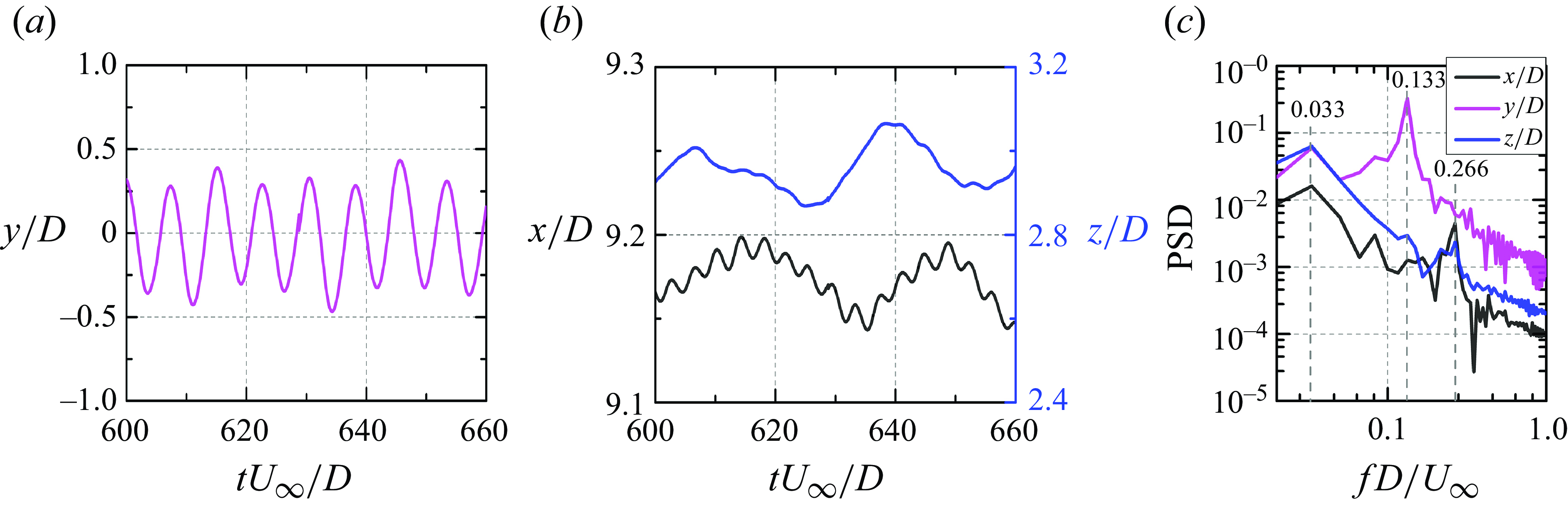
7.2. Low-frequency oscillation in the streamwise and vertical directions
A unique low-frequency oscillation phenomenon is observed in the present study. As shown in figure 25( $a$
,
$a$
, $c$
), transverse oscillation is relatively strong, with a dominant frequency of
$c$
), transverse oscillation is relatively strong, with a dominant frequency of $f^*=$
0.133. However, oscillations in the streamwise and vertical directions are much weaker and dominated by a significantly low frequency of
$f^*=$
0.133. However, oscillations in the streamwise and vertical directions are much weaker and dominated by a significantly low frequency of $f^*=$
0.033, see figure 25(
$f^*=$
0.033, see figure 25( $b$
,
$b$
, $c$
). This suggests that the oscillations in these two directions are governed by flow structures with a very low frequency. In the transverse direction, a secondary frequency of
$c$
). This suggests that the oscillations in these two directions are governed by flow structures with a very low frequency. In the transverse direction, a secondary frequency of $f^*=$
0.266 is observed, which corresponds to the second harmonic of the dominant frequency. This is an intrinsic feature of VIV of a circular cylinder (Sarpkaya Reference Sarpkaya2004). The secondary frequency in the streamwise and vertical directions also matches this second harmonic frequency, see figure 25(
$f^*=$
0.266 is observed, which corresponds to the second harmonic of the dominant frequency. This is an intrinsic feature of VIV of a circular cylinder (Sarpkaya Reference Sarpkaya2004). The secondary frequency in the streamwise and vertical directions also matches this second harmonic frequency, see figure 25( $c$
). Furthermore, the low-frequency displacement in the vertical direction has a greater magnitude than in the streamwise direction, indicating that the associated vortical structures have a higher impact in the vertical direction.
$c$
). Furthermore, the low-frequency displacement in the vertical direction has a greater magnitude than in the streamwise direction, indicating that the associated vortical structures have a higher impact in the vertical direction.
As indicated by figure 17(a–c), when the stiffness is notably lower, i.e. lg( $K$
)
$K$
) $\leqslant -3.0$
, the deflected height (
$\leqslant -3.0$
, the deflected height ( $l_d$
) of the stem is very small, and the stem aligns almost parallel to the wall. Unsurprisingly, vortex development and subsequent interactions at lg(
$l_d$
) of the stem is very small, and the stem aligns almost parallel to the wall. Unsurprisingly, vortex development and subsequent interactions at lg( $K$
) = –3.0 and –3.5 are similar. Because of significant shape deformation, vortex shedding from the stem can be classified into two regimes, similar to the condition shown in figure 22(
$K$
) = –3.0 and –3.5 are similar. Because of significant shape deformation, vortex shedding from the stem can be classified into two regimes, similar to the condition shown in figure 22( $f$
). Near the stem base (i.e. the lower part), spanwise vortex shedding appears, with separated vortices travelling downstream. At the formation position, these vortices have negligible influences on displacement at the stem tip in the streamwise and vertical directions. Meanwhile, the upper part of the stem undergoes significant deformation, becoming nearly parallel to the wall. The incoming flow moves smoothly along the stem length, and the vortex shedding dynamics contrasts with that at the base. Vortex shedding at the stem tip occurs at a high frequency (
$f$
). Near the stem base (i.e. the lower part), spanwise vortex shedding appears, with separated vortices travelling downstream. At the formation position, these vortices have negligible influences on displacement at the stem tip in the streamwise and vertical directions. Meanwhile, the upper part of the stem undergoes significant deformation, becoming nearly parallel to the wall. The incoming flow moves smoothly along the stem length, and the vortex shedding dynamics contrasts with that at the base. Vortex shedding at the stem tip occurs at a high frequency ( $f^* \approx$
0.13, estimated based on the average velocity and streamwise distance between consecutive vortices) and primarily drives transverse oscillation. Interactions between lower-part vortices and shear layers from the upper part are also witnessed. As vortices from the lower part expand, shear layer development around the upper part, particularly near the lower side, is significantly influenced. Near the stem tip, these interactions reach their strongest, affecting the local pressure distribution. This interaction is responsible for the low-frequency components of displacement in the streamwise and vertical directions.
$f^* \approx$
0.13, estimated based on the average velocity and streamwise distance between consecutive vortices) and primarily drives transverse oscillation. Interactions between lower-part vortices and shear layers from the upper part are also witnessed. As vortices from the lower part expand, shear layer development around the upper part, particularly near the lower side, is significantly influenced. Near the stem tip, these interactions reach their strongest, affecting the local pressure distribution. This interaction is responsible for the low-frequency components of displacement in the streamwise and vertical directions.
8. Conclusions
In this study, we simulated the wall-mounted stem in uniform flow using a newly coupled method – the IBM–VFIFE method. The 3-D flow characteristics and stem dynamics were analysed in detail. In the rigid case, we identified three flow regimes based on force spectra and the vortex dynamics. The first regime (R1, at $Re=$
200) features periodic hydrodynamic forces and a single vortex shedding frequency. The second regime (R2, at
$Re=$
200) features periodic hydrodynamic forces and a single vortex shedding frequency. The second regime (R2, at $Re=$
400) is characterised by higher forces and two vortex shedding frequencies, one of which is significantly lower than the other. The third regime (R3, at
$Re=$
400) is characterised by higher forces and two vortex shedding frequencies, one of which is significantly lower than the other. The third regime (R3, at $Re=$
600–1000) is dominated by one low frequency. Distinctive 3-D vortex structures were observed in these regimes. In R1, the vortex structures are regular but slant-arranged in the near wake. In R2, the vortex structures become irregular while take over a longer length. In R3, vortex sheddings at different vertical positions are nearly synchronised. As
$Re=$
600–1000) is dominated by one low frequency. Distinctive 3-D vortex structures were observed in these regimes. In R1, the vortex structures are regular but slant-arranged in the near wake. In R2, the vortex structures become irregular while take over a longer length. In R3, vortex sheddings at different vertical positions are nearly synchronised. As $Re$
increases, the streamwise vortices become finer in scale.
$Re$
increases, the streamwise vortices become finer in scale.
The dynamics of a flexible stem at $Re=$
200–1000 was thoroughly explored. It demonstrated that stem oscillation and shape deformation are closely correlated with stiffness (
$Re=$
200–1000 was thoroughly explored. It demonstrated that stem oscillation and shape deformation are closely correlated with stiffness ( $K$
). Transverse oscillation is much stronger than oscillation in the other two directions, playing a more prominent role in vortex shedding. Within the studied
$K$
). Transverse oscillation is much stronger than oscillation in the other two directions, playing a more prominent role in vortex shedding. Within the studied $Re$
, the highest amplitude is observed at lg(
$Re$
, the highest amplitude is observed at lg( $K$
) = −0.5. Stem deformation is well approximated by a nonlinear equation. The deflected length is scaled as
$K$
) = −0.5. Stem deformation is well approximated by a nonlinear equation. The deflected length is scaled as $l_d/l \sim K^{1.05}$
, with a higher exponent compared with that reported for a blade in Luhar & Nepf (Reference Luhar and Nepf2011), likely due to differences in cross-section, greater deflected height and stronger spanwise vortex shedding. Hydrodynamic forces are influenced by both stem oscillation and shape deformation: oscillation dominates at high
$l_d/l \sim K^{1.05}$
, with a higher exponent compared with that reported for a blade in Luhar & Nepf (Reference Luhar and Nepf2011), likely due to differences in cross-section, greater deflected height and stronger spanwise vortex shedding. Hydrodynamic forces are influenced by both stem oscillation and shape deformation: oscillation dominates at high $K$
, while deformation has a stronger effect at low
$K$
, while deformation has a stronger effect at low $K$
.
$K$
.
We identified three oscillation regimes in terms of the transverse amplitude: minor vibration for $A^* \lt$
0.2, medium vibration for 0.2
$A^* \lt$
0.2, medium vibration for 0.2 $\leqslant A^* \leqslant$
0.6 and substantial vibration for
$\leqslant A^* \leqslant$
0.6 and substantial vibration for $A^* \gt$
0.6. Minor vibration occurs when the stem is either highly rigid or highly flexible, or when there is a frequency mismatch between vortex shedding and stem’s natural frequency. Medium vibration is mostly observed at lg(
$A^* \gt$
0.6. Minor vibration occurs when the stem is either highly rigid or highly flexible, or when there is a frequency mismatch between vortex shedding and stem’s natural frequency. Medium vibration is mostly observed at lg( $K$
)
$K$
) $\leqslant$
–2.0. Substantial vibration occurs in two regions: one at lg(
$\leqslant$
–2.0. Substantial vibration occurs in two regions: one at lg( $K$
) = –0.5–1.0 for
$K$
) = –0.5–1.0 for $Re=$
600–800 and the other at lg(
$Re=$
600–800 and the other at lg( $K$
) = –2.0–3.0 for all studied
$K$
) = –2.0–3.0 for all studied $Re$
. In terms of transverse displacement characteristics, the response can be classified into three regimes: regular, periodic and chaotic regimes. Periodic vibration is observed in two regions: one corresponding to the first substantial vibration region and the other at lg(
$Re$
. In terms of transverse displacement characteristics, the response can be classified into three regimes: regular, periodic and chaotic regimes. Periodic vibration is observed in two regions: one corresponding to the first substantial vibration region and the other at lg( $K$
) = –2.0
$K$
) = –2.0 $\sim$
–3.0 but only
$\sim$
–3.0 but only $Re=$
200. The regular regime is assigned to three parts: the first at lg(
$Re=$
200. The regular regime is assigned to three parts: the first at lg( $K$
) = 0 within the studied
$K$
) = 0 within the studied $Re$
, the second at lg(
$Re$
, the second at lg( $K$
) = –1.0
$K$
) = –1.0 $\sim$
–2.0 and
$\sim$
–2.0 and $Re=$
600–1000, and the third at lg(
$Re=$
600–1000, and the third at lg( $K$
) = –3.0
$K$
) = –3.0 $\sim$
–3.5 and
$\sim$
–3.5 and $Re=$
400–800. Chaotic vibration spans lg(
$Re=$
400–800. Chaotic vibration spans lg( $K$
) = –1.0
$K$
) = –1.0 $\sim$
–3.5 within the simulated
$\sim$
–3.5 within the simulated $Re$
, regardless of the amplitude. We revealed the influences of stem oscillation and shape deformation on hydrodynamic forces acting on the flexible stem. It is found that the flexible stem experiences higher drag under relatively rigid conditions compared with a fully rigid stem.
$Re$
, regardless of the amplitude. We revealed the influences of stem oscillation and shape deformation on hydrodynamic forces acting on the flexible stem. It is found that the flexible stem experiences higher drag under relatively rigid conditions compared with a fully rigid stem.
We found that both the stem oscillation and shape deformation are crucial in determining vortex dynamics around the stem. Oscillation enhances vortex strength and alters vortex distribution, while shape deformation significantly modifies the flow field, such as by generating strong upwash flow from the junction. Compared with the rigid case, downwash flow in the flexible case has a weaker effect on vortex formation. We confirmed distinctive physical behaviours of flexible stems, depending on $Re$
and lg(
$Re$
and lg( $K$
). Downwash flow is notably weakened or absent due to strong deformation, which induces upwash flow. Low-frequency oscillation occurs in the streamwise and vertical directions, suggesting that different flow structures govern oscillations in these two directions.
$K$
). Downwash flow is notably weakened or absent due to strong deformation, which induces upwash flow. Low-frequency oscillation occurs in the streamwise and vertical directions, suggesting that different flow structures govern oscillations in these two directions.
The numerical method provided in this study has clear advantages for simulating wall-mounted structures under different flow conditions. It shows great potential for engineering applications and theoretical advancements, such as understanding how the total drag of a circular or rectangular patch of vegetation/stems is affected by stem flexibility (Koken & Constantinescu Reference Koken and Constantinescu2021, Reference Koken and Constantinescu2023).
Acknowledgements
We thank Professor C. Ji from Tianjin University, Professor D. Xu from Hohai University, Mr Y. Wu and J. Ni from Tianjin University for their contributions to the IBM–VFIFE method. We thank anonymous referees for their constructive suggestions and comments, which help a lot in improving the quality of this paper. This work was supported with computational resources provided by the National Supercomputing Centre, Singapore (https://www.nscc.sg), under project ID: 11002459 and 11003759.
Funding
This project is funded by the Research, Innovation and Enterprise 2025 Coastal Protection and Flood Management Research Programme. The authors are grateful to the National Research Foundation of Singapore, PUB (Singapore’s National Water Agency) for supporting this work done in the Coastal Protection and Flood Resilience Institute (CFI) Singapore under the project grant H1-P3.
Declaration of interests
The authors report no conflict of interest.


 Open access