


Non-technical Summary
Extinct vertebrate species are often represented by a limited number of specimens. With the growing application of artificial intelligence (AI) and machine learning (ML) across scientific disciplines, great potential exists to leverage these technologies to facilitate tasks such as taxonomic identification (e.g., of species) and paleobiological interpretations (e.g., ecological preferences) in paleontology. However, relative to many other scientific fields, a challenge of ML applied to paleontology is that for extinct vertebrates, oftentimes few fossils are available for study. However, shark teeth, which are abundantly preserved as fossils, provide a unique opportunity to explore ML performance across datasets of different sizes. Here we evaluate six species of Neogene shark teeth for taxonomic identification using a customized ML model and curated dataset of 3150 digital photos. The available sample size per class affects the accuracy of ML identifications. We found that smaller sample sizes, for example, 50 per species, yielded a mean accuracy of 93.4%, but accuracy plateaus at ~99% between 200 and 500 images per class, suggesting that high accuracy can be achieved with samples of these sizes. Misidentifications followed consistent patterns, often reflecting morphological similarities between specific classes. Artificially increasing the size of training datasets using data augmentation did not substantially increase overall accuracy, but did improve confidence of the identifications. This case study demonstrates that small vertebrate sample sizes can be used for ML identifications of fossils.
Introduction
The size of a sample—the total number of specimens available to study a population or species—is of fundamental importance in paleontology. While taxonomic identifications can be accomplished with limited specimens, paleontologists have long realized that larger samples are needed for meaningful statistical comparisons of morphological variation and paleobiological interpretations. The recent proliferation of machine learning (ML) applications in paleontology has further emphasized this requirement. Recent fossil image classification typically uses extensive datasets, often consisting of thousands to tens of thousands of specimens per “class” (e.g., Hou et al. Reference Hou, Lin, Hunag, Xu, Fan, Shi and Lv2023; Liu et al. Reference Liu, Jiang, Wu, Shu, Hou, Sun, Sun, Chu, Wu and Song2023; Yaqoob et al. Reference Yaqoob, Ishaq, Ansari, Qaiser, Hussain, Rabbani, Garwood and Seers2025) or groups being compared. Within the context of the identification of fossils in paleontology, each “class” pertains to a particular taxon, for example, the species compared in this study.
Thus, the small number of vertebrate fossils typically available for a given taxon presents a further challenge in developing comprehensive datasets for ML image classification. Unlike the invertebrate world, in which hard parts are oftentimes complete, for example, foraminifera tests and mollusk shells (Yu et al. Reference Yu, Qin, Watanabe, Yao, Li, Qin and Liu2024), the samples available for vertebrate taxa are often limited to teeth and partial skeletal elements. Due to the cartilaginous skeletons of elasmobranchs, which rarely fossilize, their durable teeth constitute a particularly valuable and abundant resource for taxonomic identifications and other paleobiological analyses. Shark teeth are among the most abundant vertebrate fossils in marine Phanerozoic sediments, particularly in Neogene deposits, owing to sharks’ continuous tooth replacement and the exceptional preservation potential of tooth enameloid (fluorapatite) (Visaggi and Godfrey Reference Visaggi and Godfrey2010; Perez Reference Perez2022).
Complementing the inherent advantages of shark teeth, recent advances in bioinformatics have further facilitated the compilation of large datasets (also see MacLeod et al. Reference MacLeod, Benfield and Culverhouse2010). Two major factors have influenced this trend: (1) The widespread digitization of museum collections has moved specimens from the realm of dark data and opened access for research in a way that was impossible beforehand. As a relevant example, Perez (Reference Perez2022) was able to study the evolution and ecology of Cenozoic shark faunas, primarily from Florida, based on 117,000 specimen records contained in the digitized collections at the Florida Museum of Natural History. (2) Likewise, the widespread advent of digital images online facilitates their discovery via web searches or web crawlers (Kumar et al. Reference Kumar, Bhatia and Rattan2017). These developments for big data in the field of paleontology provide a foundation to facilitate automated computer vision identification through ML.
Building on these technological advancements, recent studies (e.g., Wäldchen and Mäder Reference Wäldchen and Mäder2018; Valan et al. Reference Valan, Makonyi, Maki, Vondráček and Ronquist2019; Prabha et al. Reference Prabha, Suchitra and Saravanan2023; Durand et al. Reference Durand, Paillard, Ménard, Suranyi, Grondin and Blarquez2024; Adaimé et al. Reference Adaimé, Urban, Kong, Jaramillo and Punyasena2025) have demonstrated the efficacy of ML-based computer vision in species identifications either in extant or extinct taxa, or both. Their success has largely depended on access to extensive datasets of well-preserved specimens and the widespread use of pretrained models. Within the geosciences and related disciplines, interest in relevant studies has increased exponentially over the past decade. For example, Liu et al. (Reference Liu, Jiang, Wu, Shu, Hou, Sun, Sun, Chu, Wu and Song2023) reported about 10,000 ML citations within this disciplinary field during 2020.
Also of relevance here, Liu et al. (Reference Liu, Jiang, Wu, Shu, Hou, Sun, Sun, Chu, Wu and Song2023) achieved greater than 90% accuracy in classifying fossil specimens, including fossil shark teeth, into taxonomic classes using convolutional neural networks (CNNs) trained on more than 415,000 images. Barucci et al. (Reference Barucci, Ciacci, Liò, Azevedo, Di Cencio, Merella, Bianucci, Bosio, Casati and Collareta2024) reported similar success rates using diverse fossil shark tooth datasets. While these studies highlight the potential of computer vision in taxonomic identification, they incompletely address the challenges posed by the limited sample sizes and suboptimal preservation that are common constraints in vertebrate paleontology. A central question, therefore, is how can small samples of vertebrate fossils benefit from computer vision using ML techniques?
Shark teeth provide an ideal system for investigating these methodological questions due to their abundance in the fossil record. Their prevalence enables controlled manipulation of ML to facilitate evaluation of how sample size influences model performance. Addressing the central question posed earlier about sample size, we present here an ML analysis using 3150 teeth of six taxa of Neogene sharks: Otodus megalodon, Carcharodon carcharias, Carcharodon hastalis, Galeocerdo cuvier, Hemipristis serra, and Carcharhinus spp. (Fig. 1). These taxa are widespread in the fossil record and morphologically distinct.
Representative examples of the six machine learning (ML) classes of Neogene shark teeth used during this study, lingual view: A, Carcharodon carcharias (UF 131981); B, Carcharodon hastalis (UF 231961); C, Carcharhinus sp. (UF 228647); D, Galeocerdo cuvier (UF/TRO 13692); E, Hemipristis serra (UF/TRO 7145); F, Otodus megalodon (USNM PAL 530605). Not to scale (normalized to vertical dimension).

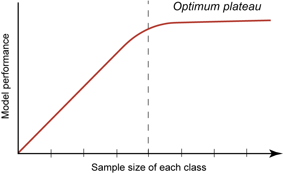
This case study aims to elucidate the methodological processes, outcomes, and challenges of applying computer vision to vertebrate fossil classification. Our research examines several key aspects of this application, including workflow optimization, relationship between sample size and ML model performance, misidentification patterns, and impact of fine-tuning and data augmentation (DA) on overall model performance outcomes (Fig. 2). Related to Figure 2, we might ask what is an “acceptable” level of model performance? While this certainly is of interest, arriving at a definitive and generalizable metric (e.g., accuracy, confidence, or precision) in ML is elusive. It can be highly dependent on so many variables with a specific ML model and goals as to lack meaning. Regarding paleontology, one way of looking at this is to compare previous studies’ performances as a baseline for our current study presented here, even if no two studies are exactly alike. For example, in a similar study focused on fossil shark teeth, some including the same taxa as we report here, Barucci et al. (Reference Barucci, Ciacci, Liò, Azevedo, Di Cencio, Merella, Bianucci, Bosio, Casati and Collareta2024) report an accuracy for their model performance of >90%.
Theoretical machine learning (ML) performance with increasing sample size in each class, producing a logarithmic curve in which metrics, such as accuracy or confidence, plateau at a model optimum. Dashed vertical line indicates the inflection point, after which at higher sample sizes, the model achieves optimal performance.

Through examination of these topics, we aim to contribute to the expanding literature on artificial intelligence (AI)-driven paleontological methods and assess the viability of computer vision for reliable identification in contexts of limited data. We assert that this study offers insights for image classification of vertebrates and other fossil samples constrained by relatively small sample sizes, as well as a methodological approach for consistent evaluation of ML models.
Abbreviations
CNN, convolutional neural network; DA, data augmentation; HF, horizontal flip DA; ipc, images per class; ML, machine learning; N, total sample size of population; n, subsample of total population; RG, random grayscale DA.
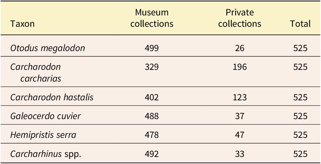
Institutional abbreviations for cataloged museum specimens are presented in Table 1.
Sampling of the fossil shark teeth used to develop the digital image datasets for the analyses presented here. Generic assignment for Otodus megalodon follows Cappetta (Reference Cappetta2012) and Shimada et al. (Reference Shimada, Chandler, Lam, Tanaka and Ward2016). Generic assignment for Carcharodon hastalis follows Ehret et al. (Reference Ehret, MacFadden, Jones, DeVries, Foster and Salas-Gismondi2013; also see Rojas Reference Rojas2012). Also see Supplementary Material 2. Institutional Abbreviations: CMM, Calvert Marine Museum; NCMNS, North Carolina Museum of Natural Sciences; UCMP, University of California Museum of Paleontology; UF, University of Florida, Florida Museum; USNM, National Museum of Natural History. For private collections see “Acknowledgments”

Background and Conceptual Framework
Morphological Variation in Neogene Shark Teeth
As mentioned earlier, fossil shark teeth were selected for this study because they are easily recognizable and among the most abundant vertebrate fossils worldwide (Ginter et al. Reference Ginter, Hampe and Duffin2010; Cappetta Reference Cappetta2012). In addition, they are mostly two-dimensional (flat), which simplifies digital imaging and 2D ML image recognition. Our training datasets also account for the actual variation seen in fossil shark teeth. For our model design and experimentation, we intentionally selected species that are morphologically distinct (e.g., serrations present or absent), but also possess some similar morphological features (e.g., generally triangular-shaped tooth).
Individual variation in vertebrate dentitions can be broadly characterized into three categories: homodont, monognathic heterodont, or dignathic heterodont. Homodonty refers to dentitions with relatively consistent tooth morphology (e.g., Galeocerdo cuvier), monognathic heterodonty refers to dentitions with variable tooth morphology within the upper or lower jaws (e.g., Otodus megalodon; Fig. 3), and dignathic heterodonty refers to dentitions with variable tooth morphology between the upper and lower jaws (e.g., Hemipristis serra; Fig. 4Z–AF). Most extant sharks exhibit both monognathic and dignathic heterodonty to take advantage of different tooth functions and a wider array of prey options (Cullen and Marshall Reference Cullen and Marshall2019).
Individual variation of an associated dentition of Otodus megalodon, illustrating both monognathic and dignathic heterodonty. Scale bar, 5 cm. Modified from Perez et al. (Reference Perez, Leder and Badaut2021).

Morphological and taphonomic variation of the lingual surfaces of selected examples of the six taxonomic groups included in this study. Conventional orientation is with apex down for upper teeth and apex up for lower teeth. All specimens are contained in the UF Vertebrate Paleontology collection (https://www.floridamuseum.ufl.edu/vertpaleo/). A–G, Otodus megalodon: A, UF 245000, B, UF 17932, C, UF 229802, D, UF/TRO 8488, E, UF 311000, F, UF/TRO 5343, G, UF/TRO 5600; H–M, Carcharodon hastalis: H, UF/TRO 7664, I, UF/TRO 7125, J, UF/TRO 14350, K, UF/TRO15970, L, UF/TRO 11513, M, UF/TRO 7128; N–S, Carcharodon carcharias: N, UF 132025, O, UF 123304, P, UF 234841, Q, UF/TRO 2369, R, UF 85092, S, UF 123105; T–Y, Galeocerdo cuvier: T, UF/TRO 11010, U, UF 233649, V, UF/TRO 11590, W, UF/TRO 13684, X, UF/TRO 6010, Y, UF/TRO 2384; Z–AF, Hemipristis serra: Z, UF/TRO 7131, AA, UF/TRO 13597, AB, UF/TRO 7598, AC. UF/TRO 7145, AD, UF 232388, AE, UF/TRO 11092, AF, UF/TRO 7146; AG–AR, Carcharhinus spp.: AG, UF 233474, AH, UF 80284, AI, UF 17920a, AJ, UF 123090, AK, UF 80026, AL, UF 233674, AM, UF 17920b, AN, UF 80621, AO, UF 17920c, AP, UF 17920d, AQ, UF 7920e, AR, UF 17920f. Scale bars, 1 cm.

Intraspecific variation in dental morphology of sharks may also be related to factors such as ontogenetic differences and sexual dimorphism (French et al. Reference French, Stürup, Rizzuto, Van Wyk, Edwards, Dolan, Wintner, Towner and Hughes2017; Tomita et al. Reference Tomita, Miyamoto, Kawaguchi, Toda, Oka, Nozu and Sato2017; Cullen and Marshall Reference Cullen and Marshall2019). These forms of dental morphological variation often contribute to niche partitioning to avoid, or at least reduce, intraspecific competition for dietary resources (Grainger et al. Reference Grainger, Peddemors, Raubenheimer and Machovsky-Capuska2020; Goodman et al. Reference Goodman, Niella, Bliss‐Henaghan, Harcourt, Smoothey and Peddemors2022). Among the taxa selected for this study, the species exhibit relatively minimal or no sexual dimorphism in their tooth morphology and the ontogenetic variability is relatively minor compared with other sources of morphological variation (Tomita et al. Reference Tomita, Miyamoto, Kawaguchi, Toda, Oka, Nozu and Sato2017; Cullen and Marshall Reference Cullen and Marshall2019; Türtscher et al. Reference Türtscher, Jambura, López‐Romero, Kindlimann, Sato, Tomita and Kriwet2022). There is likely also some temporal and spatial variation in dental morphology, because different populations became isolated and/or merged across time and space. These sources of morphological variation may be difficult to reconcile in the fossil record, especially for rarer species that are typically represented by small samples.
Machine Learning Applied to Vertebrate Fossil Classification
In recent years, the application of deep learning–based computer vision techniques has shown the potential to transform paleontological research by simplifying the traditionally labor-intensive process of fossil identification. Paleontologists have long relied on trained experts to classify fossil specimens, a time-consuming process that can create significant bottlenecks for research, especially when dealing with fragmentary fossils and those affected by taphonomic biases. Furthermore, most institutions with paleontological collections lack staff and volunteers with the broad taxonomic expertise necessary to accurately classify every fossil occurrence. This lack of experience can result in misidentifications that potentially impact downstream users, for example, during large-scale online searches and web crawling. While recent studies have demonstrated that deep learning–based computer vision can greatly accelerate this work, their success has largely depended on the availability of large datasets containing relatively well-preserved skeletal elements. As also mentioned earlier, Liu et al. (Reference Liu, Jiang, Wu, Shu, Hou, Sun, Sun, Chu, Wu and Song2023) analyzed a large dataset of >415,000 images to classify fossil specimens into taxonomic classes with >90% precision, while Barucci et al. (Reference Barucci, Ciacci, Liò, Azevedo, Di Cencio, Merella, Bianucci, Bosio, Casati and Collareta2024) achieved similarly high accuracy on a diverse dataset of fossil shark teeth. These studies illustrate the potential of computer vision to facilitate taxonomic identification of fossils. However, they leave open the question of how these approaches perform when sample sizes are small, which is common in vertebrate paleontology.
Related to ML, data augmentation (DA) can be an effective solution in many image-analysis workflows. Especially in studies with small sample sizes, like the one we present here, DA can artificially increase the sample size and variation within classes through different pixel-based transformations, including image cropping, rotation, resizing, vertical and horizontal flipping, color and contrast changes, and masking portions of the original image. The overall purpose of these transformations is to improve the model’s performance and usability by increasing the diversity of the training dataset (Perez and Wang Reference Perez and Wang2017; Shorten and Khoshgoftaar Reference Shorten and Khoshgoftaar2019). DA can also aid in mitigating overfitting, in which the model performs well based on an internal validation dataset that is highly similar to the training dataset, but fails to perform well when exposed to a more diverse external dataset. The risk of overfitting is particularly high for models with small sample sizes, because the model learns to rely on features that are specific to the training dataset. If applied effectively, DA can introduce novel variables into the training dataset, forcing the model to rely on more broadly transferable features to accurately classify different images.
During the process of ML image analysis, certain morphological parts, features, or pixels of an object can have more importance in the identification of a particular class within the model. The analysis of these is called feature visualization (Olah Reference Olah2017). The results of this analysis can be visually displayed, such as with saliency maps (Shokoufandeh et al. Reference Shokoufandeh, Marsic and Dickinson1999). These maps can graphically indicate how certain pixels, or groups of adjacent pixels, have different salience values (Fig. 5). These maps therefore can represent the relative importance of regions for ML image classification. These visualization techniques and transformations can be valuable in providing a comparison of human-derived characters used for identification relative to the feature analysis of an ML model.
Comparison of fossil shark tooth, Galeocerdo cuvier, UF 234137. A, digital photograph at 384 pixels; B, saliency map showing pixel “hotspots” represented by saliency values greater than ~0.90.

Materials and Methods
Selection of Fossil Shark Teeth
Six classes, each representing a different taxon, were selected from isolated Neogene shark teeth from the collections that we studied. These include the species Otodus megalodon, Carcharodon carcharias, Carcharodon hastalis, Galeocerdo cuvier, Hemipristis serra, and multiple species of the genus Carcharhinus (Figs. 1, 4). These taxa were chosen because they are typically abundant in fossil collections and show a range of interesting morphologies for ML comparisons.
For this study, a total of 3150 teeth were digitized (i.e., 525 images per class [ipc], with 400 images in the training dataset, 100 images in the validation dataset, and 25 images in the test dataset). All teeth are morphologically complete, or nearly complete, the latter typically representing more than ~95% of the original tooth (Fig. 4). About 85% (2688) of these teeth were taken from existing cataloged museum collections (Table 1). Two of the species, C. carcharias and C. hastalis, occurred in limited numbers in the collections (Table 1). For some of the species samples in short supply, digital vouchers (Minteer et al. Reference Minteer, Collins, Love and Puschendorf2014; Greene et al. Reference Greene, Teixidor-Toneu and Odonne2023) were taken from private collections (see “Acknowledgments”) to complete the datasets containing the 525 teeth. Taken together, these teeth were primarily collected from localities in Florida (Perez Reference Perez2022), Maryland (Kent Reference Kent and Godfrey2018), North Carolina (Purdy et al. Reference Purdy, Schneider, Applegate, McLellan, Meyer, Slaughter, Ray and Bohaska2001), and Panama (Pimiento et al. Reference Pimiento, González-Barba, Ehret, Hendy, MacFadden and Jaramillo2013; Perez et al. Reference Perez, Pimiento, Hendy, González-Barba, Hubbell and MacFadden2017). Selecting teeth from different localities is of particular importance for the training datasets because of potential taphonomic and intraspecific variation, including, for example, the range of colors resulting from different diagenetic settings.
Specimen Digital Imaging
Computer vision studies frequently mine digital image data from numerous external sources, primarily the web, oftentimes aggregating images with different backgrounds, orientations, lighting, and resolutions. Despite the massive quantity of data that can be analyzed this way, because of potential nonstandardized images within an aggregated dataset, this method can potentially bias the resulting computer vision model. In contrast, all images taken for our analysis were photographed by us using a standardized imaging workflow to minimize such variations. Specimens were oriented with the tooth apex facing downward on a black background with a scale, the latter of which is removed before ML analysis. Each specimen was photographed lingually and labially, although only the lingual side is included in this study. Each specimen in our study set has a museum catalog number or, in private collections, a unique voucher identifier (Table 1; Supplementary Material 2).
For the teeth that we processed, images were taken with a Nikon D5100 camera, Micro-NIKKOR 60mm f/2.8 lens mounted on a Beseler CS-21 copy stand. Specimens were photographed with a black velvet backdrop, providing a consistent, featureless background. Lighting was provided by two diffused sources for soft, shadowless lighting effect. Raw images were in NEF (Nikon Electronic Format). Camera Control Pro 2.0 software was used to adjust settings and directly transfer images to the computer. Nikon NX Studio (v. 1.6) was used to add metadata and export the raw NEF images as full resolution (4928×3264 pixels). Preprocessed images were saved as TIFF (Tag Image File Format) files with 16 bits per color channel to preserve maximum quality.
Image Processing
We developed an image-processing workflow to further standardize the dataset used for our computer vision models in this study. The image backgrounds and scales were removed in Adobe Photoshop (v. 25.7), resulting in null (transparent) pixels surrounding each specimen. A layer mask was added to reveal the selected specimen and mask off all other parts of the image. All images were standardized to 1:1 aspect ratio, normalized to each specimen’s longest dimension. The image was then saved to a Portable Network Graphic (PNG) file to flatten layers and preserve transparency.
Our study analyzed all specimens at the same pixel density. We found that the optimal density for our digital images is 384×384 pixels (Supplementary Material 3). To avoid edge distortion when translating the NEF and TIFF images to this optimal density, the images were resized in Photoshop to two pixels less than the optimal resolution (i.e., 382×382 pixels). A one-pixel transparent border was then applied to each image, resulting in a uniform density of 384×384 pixels that provided a consistent edge buffer to minimize edge distortion. Each postprocessed batch was exported in PNG format in digital storage (Supplementary Material 2).
Machine Learning Model Architecture and Computational Infrastructure
We implemented a CNN-based model for shark tooth image classification (Alzubaidi et al. Reference Alzubaidi, Zhang, Humaidi, Al-Dujaili, Duan, Al-Shamma, Santamaría, Fadhel, Al‑Amidie and Farhan2021). Models were developed in Python 3.11 and TensorFlow 2.15 (Abadi et al. Reference Abadi, Barham, Chen, Chen, Davis, Dean and Devin2016), using EfficientNetV2 backbones (Tan and Le Reference Tan and Le2021) pretrained on ImageNet-21K and fine-tuned on ImageNet-1K. Later variants attached a task-specific classifier head to the backbone and were fine-tuned for fossil shark tooth recognition. We deployed five versions of our model (https://github.com/brberis/djtensor; Supplementary Material 4):
-
v1, frozen EfficientNetV2 backbone with a trainable classifier head (pretrained only);
-
v2, end-to-end fine-tuning of the backbone + the classifier head (includes the pretrained initialization);
-
v3, fine-tuned (includes pretrained) + random-grayscale (RG) DA;
-
v4, fine-tuned (includes pretrained) + horizontal-flip (HF) DA; and
-
v5, fine-tuned (includes pretrained) + RG+HF DA.
A “pretrained” model (v1) learns broad visual features from training on a large, general dataset (e.g., ImageNet; also see Xu et al. Reference Xu, Zhang, Ding, Gu, Liu, Huo and Qui2021). “Fine-tuning” (model v2) then can be deployed to adjust the pretrained model parameters using the training datasets (e.g., fossil shark tooth images) to enhance model performance. This two-stage approach leverages both general feature representations and specialized learning to boost classification performance. In addition, DA (models v3–v5) was explored during training to address dataset-specific variability.
With these five different model variants, we explored factors that optimize performance. Models v1 and v2 were designed to assess classification accuracy with the fine-tuning parameter either disabled (v1) or enabled (v2). In v1, the backbone layers are frozen (i.e., fine-tuning is “off”), whereas in v2 the backbone is unfrozen for end-to-end training (i.e., fine-tuning is “on”). As we document in the “Results,” we focused on the fine-tuned model (v2) because of its superior performance relative to the pretrained model (v1). Models v3–v5 then explored DA techniques, that is, random grayscale and horizontal flip. Because these were exploratory, that is, applied to only a subset of 3 of the 10 incremental steps, as we describe next, and performed similarly to v2, our primary analyses emphasize v2.
Thus, using models v1 and v2, performance (i.e., accuracy and confidence) for each class (taxon) was assessed for progressively larger sample sizes in 10 incremental steps of 50, that is, from 50 to 500 ipc. During the first incremental step of 50 ipc, the 50 images were selected randomly. In successive steps, the images from the previous step were retained in the set being analyzed and 50 more randomly selected images were then added to it. For example, the second incremental step of 100 ipc includes 50 from the previous incremental step combined with 50 newly added, randomly selected images. For each step, we trained for 20 epochs with batch size 16 and ran 10 independent replicates with new random seeds/splits. At each step, data were randomly split 80%/20% into training/validation. Every model was evaluated against the same fixed external test set of 25 randomly preselected images per class held out from training/validation. The test dataset introduces new, previously unseen images to the model, thereby testing the model’s ability to accurately predict or classify images into the predetermined classes. The rationale for using the same test data set of 25 images during the analysis was to limit potential variability that might be introduced using a new randomized test dataset in successive incremental steps.
For the latter models v3–v5, DA used random grayscale (RG; v3), horizontal flipping (HF; v4), and both of these together (RG + HF; v5) to explore improvement of model parameters and performance outcomes. In our implementation, DA was applied on the fly during training: each epoch drew from the same pool of original training images and applied random transformations dynamically, so that individual images could appear multiple times under different treatments (e.g., one instance in full color and another with grayscale applied). We did not create a fixed set of augmented files ahead of time; instead, each batch was assembled from randomly transformed variants of the original images, ensuring maximal diversity without inflating the stored dataset.
During the initial stages of this study, we encountered challenges with computational capacity when analyzing larger datasets of shark teeth. These limitations were especially evident during ML workflows that often required significant processing time (Alzubaidi et al. Reference Alzubaidi, Zhang, Humaidi, Al-Dujaili, Duan, Al-Shamma, Santamaría, Fadhel, Al‑Amidie and Farhan2021) and occasionally failed to complete on standard laptop computers. To address this limitation, we centralized our computational infrastructure using a dedicated server at Adaptive Computing in Naples, Florida, equipped with an NVIDIA A100 GPU. This computer infrastructure significantly improved processing efficiency and ensured consistency across our team. Other specific technical details regarding hardware and software configurations that were critical to our workflow have been documented in our GitHub project repository (https://github.com/brberis/djtensor; Supplementary Material 4). This GitHub repository can be used in conjunction with our images (Supplementary Material 2) to reproduce the results of this research.
To complement this hardware upgrade, we built an application to interface with our TensorFlow model. This was developed using Python and Django for the back end and React for the front end, creating a streamlined and user-friendly interface. Additionally, we integrated Celery tasks to run training processes in the background that improved the overall efficiency of workflows. To facilitate deployment and modularity, we containerized the entire setup using Docker. Each service was isolated into its own container, simplifying updates and maintenance. To further streamline deployment, we leveraged Adaptive Computing’s Adaptive Cluster Manager. This tool allowed us to efficiently manage resources and deployment.
Saliency Maps
Saliency maps are an essential tool for visualizing the features that most influence an ML model classification (Shokoufandeh et al. Reference Shokoufandeh, Marsic and Dickinson1999). In this study, we used the tf-keras-vis library (v. 0.87; Kubota Reference Kubota2022) to generate saliency maps for each fossil shark tooth image classified. By comparing these maps on the input images, we can explore key topographic regions and patterns of feature visualization (Olah Reference Olah2017) that contribute to predictions and fossil specimen classifications. For each image, the saliency map was calculated using the Saliency class with a CategoricalScore function targeting the predicted class index. This method computes gradients relative to the predicted class, revealing the model’s focus areas (“hotspots”). To enhance interpretability, the saliency maps were normalized and further refined using Sobel filters to emphasize edges and morphological details. Finally, the normalized saliency maps were combined with edge maps of the physical object boundaries to create a composite visualization that highlights both feature intensity and morphological boundaries.
Statistical Analyses
These analyses were primarily done to explore the statistical similarities and differences in performance parameters (i.e., accuracy and confidence) of our models produced during the ML workflow (also see Rainio et al. Reference Rainio, Teuho and Klén2024). These included tests for normal distributions (Shapiro-Wilk) for all datasets, nonparametric statistics (Wilcoxon, Kruskal-Wallis) for those that included non-normal distributions, and the Levene’s test for variance, along with graphic comparisons using box plots using R (R Studio Team 2020; R Core Team 2022). The results of these tests are presented in either the following text or the relevant Supplementary Materials.
For description of the sample size performance comparisons (accuracy and confidence), we report the mean values of 10 iterations (Supplementary Material 5, 6). Accuracy is reported as percent (0% to 100%) and confidence on a scale from 0 to 1. Accuracy and confidence were selected as two performance indicators because they are oftentimes used as metrics in ML model outcomes (Rechkemmer and Yin Reference Rechkemmer, Yin, Barbosa, Lampe, Appert, Shamma, Drucker, Williamson and Yatani2022). Accuracy is the proportion of correctly classified samples on a held-out evaluation set. Confidence is the model’s predicted probability for its chosen class. It corresponds to the probability of being correct only if the model is well calibrated and the evaluation data match the training distribution.
Results
Sample Size Accuracy and Confidence
As one of the primary aims of this study, we predicted that model performance would improve with increasing sample size, eventually reaching an optimal plateau (Fig. 2). We tested these predictions incrementally with 10 sample sets ranging from 50 to 500 ipc (Supplementary Material 5). The improvement of mean accuracy and confidence metrics illustrates the impacts of increasing sample sizes in the training and validation datasets on model performance (Fig. 6).
Median box plots showing model accuracy and confidence scores as sample sizes increase from 50 to 500 (x-axis) specimen images per class (ipc). A, Mean accuracy for model v1, without fine-tuning enabled; B, mean confidence scores for model v1, without fine-tuning enabled; C, mean accuracy for model v2, with fine-tuning enabled; D, mean confidence scores for model v2, with fine-tuning enabled. Mean indicated by “X”; median indicated by horizontal black line within colored boxes.

In model v1, with no fine-tuning, the mean ipc accuracy partially aligned with our predicted logarithmic growth pattern; however, it did so noisily (Fig. 6A). While this mean accuracy gradually increased from 93.40% (50 ipc) to 96.60% (100 ipc) to 97.80% (150 ipc), model accuracy then decreased at 200 ipc (95.40%). At sample sizes of 250 ipc and above, model accuracy improved again and eventually began to plateau around 300 ipc. Interestingly, the highest performance was at 400 ipc, with a mean accuracy of 98.73%. All of these iterations thus performed relatively well, with the mean accuracy exceeding 90%. In contrast, confidence did not follow our predicted logarithmic pattern (Fig. 6B).
In model v2, with fine-tuning enabled, the mean accuracy and confidence scores at each sample size are more closely aligned with our predicted logarithmic pattern (Fig. 6C,D). For the first three sample sizes, the mean accuracy gradually increased from 96.67% (50 ipc) to 98.33% (100 ipc) to 99.33% (150 ipc). Thereafter, for the remaining sample sizes ranging from 200 to 500 images per class, the mean accuracy plateaued around 99%. Again, the model performed well at all sample sizes tested, with the mean accuracy exceeding 96% in all cases. Likewise, the confidence score at each sample size step also followed the predicted logarithmic pattern, increasing from 81.76% at 50 ipc to 90.53% at 500 ipc (Fig. 6D). Similarly, confidence scores began to plateau at 150 ipc, with all subsequent scores ranging from ~89% to 91%.
For the samples presented in Figure 6, the variances (vertical width, or dispersion) of the box plots are significantly smaller for both the accuracy (Levene’s F = 2.6665, p-value = 0.0003961) and confidence (Levene’s F = 2.5872, p-value = 0.000592) in the fine-tuned model (v2; Fig. 6C,D) as compared with the pretrained (non-fine-tuned) model (v1; Fig. 6A,B). Coupled with visual inspection of the box plots in Figure 6, these results demonstrate that with regard to accuracy, confidence, and variance, enabling fine-tuning improves the model’s performance, with model v2 consistently outperforming model v1.
Data Augmentation
DA refers to techniques that are widely used to boost performance of ML models (Shokoufandeh et al. Reference Shokoufandeh, Marsic and Dickinson1999). They can also potentially help to mitigate overfitting. Using the accuracy of our fine-tuned model (Fig. 6C) as a guide, we were interested to determine whether simple DA transformations might boost this parameter for the smaller sample sizes (i.e., 50, 100, and 150 ipc) before the optimal plateau in accuracy is reached at larger sample sizes. We employed three simple DA techniques, including RG, HF, and RG + HF together (Supplementary Material 6).
Regarding model performance, the three incremental steps of DA (Fig. 7) did not improve accuracy relative to those with no DA, that is, 50 ipc (Kruskal-Wallis χ2 (3) = 6.33, p-value = 0.09673), 100 ipc (Kruskal-Wallis χ2 (3) = 1.50, p-value = 0.6817), and 150 ipc (Kruskal-Wallis χ2 (3) = 4.91, p-value = 0.1786; Supplementary Material 4). All of these incremental steps had accuracy values between 96.67% and 99.33%. It should be noted, however, that the variances in the 10 iterations per run, as indicated in the interquartile ranges of the box plots, are smaller in those that included DA relative to the models without DA. Regarding confidence, the two smaller sample sizes showed highly significant increases in the runs that included DA relative to the non-DA, that is, for 50 ipc (Kruskal-Wallis χ2 (3) = 27.39, p-value = 4.883e-06), 100 (Kruskal-Wallis χ2 (3) = 22.78, p-value = 4.506e-05), and significantly better performance for 150 (Kruskal-Wallis χ2 (3) = 7.82, p-value = 0.04985). For example, in the 50 ipc (Fig. 7B), mean confidence of the non DA set was 81.76%, whereas it increased for RG (85.10%), HF (83.76%), and for RG + HF (85.24%; Supplementary Material 6). To summarize here, our results indicate that while the DA dataset transformations did not significantly increase accuracy at these smaller sample sizes, they did boost confidence (Fig. 7; Supplementary Material 6).
Median box plots of data augmentation (DA) for 50, 100, and 150 specimen images per class (ipc) using a fine-tuned model showing accuracy percentage (A, C, E) and confidence scores (B, D, F). Abbreviations on x-axis: nDA, no data augmentation; RG, random grayscale DA; HF, horizontal flip DA; RG + HF, random grayscale and horizontal flip together. Mean indicated by “X”; median indicated by horizontal black line within colored box. Data and relevant statistics are in Supplementary Material 6.

Incremental Model Training: Learning Loss and Accuracy
Learning loss is another parameter that can be used to assess ML model performance (Riva Reference Riva2025). The results of fine-tuned model v2 using the test set (n = 25 for each class) of three sample sizes are presented in Figure 8. These were chosen because they represent the end-member smallest (50 ipc) and largest sample sizes (500 ipc) and the interpreted plateau inflection point at 150 ipc. To exemplify these results, the 10th iteration of training was chosen with 384 pixel density, batch sizes of 16, and an 80% training and 20% validation split across 20 epochs. The 10th (last) model iteration was selected to represent this aspect of performance because it typically approximates the stable and representative performance plateaus of earlier iterations (i.e., 1 through 9).
Training and validation parameters (80%/20% split), including learning loss and accuracy, for three sample sizes of the Neogene fossil sharks, that is, (A, D) 50 specimen images per class (ipc), (B, E) 150 ipc, and (C, F) 500 ipc, respectively.

Regarding learning loss, the smallest sample size (50 ipc; Fig. 8A) was the last one to plateau after the third epoch for training and eighth epoch for validation. For all metrics, this was the only sample size to show any significant amount of overfitting, evidenced by the degree of noisiness of the validation loss and its plateauing at around ~8% lower accuracy values. In contrast, for the 150 ipc (Fig. 8B,E) and 500 ipc (Fig. 8C,F), both the training and validation datasets converged in their learning loss and accuracy plateaus after the first few epochs. Using these three examples, it is clear that the smallest sample size, 50 ipc, is the most vulnerable to overfitting.
Misidentifications—General Patterns
At each sample size step, from 50 to 500 ipc, 10 iterations of the model were trained. For each of these iterations, the models were evaluated with an external test dataset of 25 ipc. Thus, across all 10 iterations for each sample size step, there were 250 identifications made by the model for every class. Here we assess the total number of misidentifications and total number of specimens that were misidentified using model v2 (Table 2), that is, fine-tuned without DA. As sample size per class increased, the total number of misidentified specimens decreased, as would be expected based on the performance metrics and patterns reported earlier. The model’s confidence was also significantly lower for these misidentified teeth relative to the model’s overall performance. Whereas the average confidence (Fig. 6) is typically greater than 80% across all samples, the average confidence for the misidentified teeth is lower than 60% (Table 2).
Total number of misidentifications of test specimens per sample size (all 10 iterations) for model v2 (Supplementary Material 7). Note that some specimens may be misidentified multiple times in different iterations

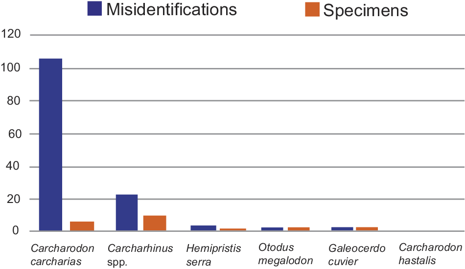
Regarding the taxonomic distribution of the misidentifications from 50 to 500 ipc, each with 10 iterations (i.e., 100 total iterations), Carcharodon carcharias teeth were the most frequently misidentified (106 times), followed by Carcharhinus spp. (22 times). Hemipristis serra was misidentified three times, whereas Otodus megalodon and Galeocerdo cuvier were each misidentified two times. Carcharodon hastalis was never misidentified during any of the 100 iterations of the models (Fig. 9). Looking at the 106 misidentifications of C. carcharias, which represent 78.51% of all misidentifications, only four specimens were misidentified, and most of these instances occurred with the same specimen during different iterations (Fig. 9). CMM-V-10324 (also see next section) was consistently misidentified as O. megalodon (50 times) and C. hastalis (9 times). Three additional specimens of C. carcharias UF 234885C (30 times), BF 27 (13 times), and LC 41 (4 times) accounted for the remaining 47 misidentifications (Supplementary Material 7).
Patterns of tooth image misidentifications and the number of specimens affected for each of the six taxonomic classes studied (Supplementary Material 7). Blue bars record the total number of misidentifications for each class, while orange bars record the total number of specimens misidentified for each class.

Confusion Matrices and Saliency Maps
To help clarify which taxa were being confused during these misidentifications, we generated representative (i.e., 10th iteration) confusion matrices for the training model v2 at 50, 150, and 500 ipc (Fig. 10). Again, these results are based on our external test dataset (n = 25 ipc). During the training incremental step at 50 ipc, four teeth were misidentified. One C. carcharias tooth was misidentified as O. megalodon, and three Carcharhinus spp. teeth were misidentified, two as G. cuvier and one as C. hastalis (Fig. 10A). At 150 ipc, only one tooth of C. carcharias was misidentified as O. megalodon (Fig. 10B). Finally, at 500 ipc, there were no misidentified teeth during this iteration of training (Fig. 10C).
Model v2 showing confusion matrices for 10th iteration of external testing (n = 25 per class). A, Trained with 50 specimen images per class (ipc); B, trained with 150 ipc; C, trained with 500 ipc.

Saliency maps can reveal which pixels in the image are emphasized during feature visualization to classify the teeth (Shokoufandeh et al. Reference Shokoufandeh, Marsic and Dickinson1999). For our study, at sample sizes of 50 and 150 ipc, during the 10th iteration of training, the models misidentified the same specimen of C. carcharias, CMM-V-10324; however, the saliency maps reveal that the models relied on different features to make this misclassification (Fig. 11A–C). At 50 ipc, CMM-V-10324 has a saliency map that emphasizes features extracted along the margins of the tooth (Fig. 11B); whereas, at 150 ipc, the entire crown of the tooth has greater saliency values, with less emphasis on the basal root margin (Fig. 11C). The three other teeth, all misidentified during the 10th iteration of training at 50 ipc, generally have different patterns of saliency values. For UF 17846AF, the highest saliency values are concentrated along the distal cutting edge and apex of the tooth (Fig. 11D,E). For UF 230862, the highest saliency values are widely distributed across the entire crown, especially toward the crown apex. There is less emphasis on the root; although, there are some high saliency values near the center of the root that may correspond with the nutrient groove (Fig. 11F,G). For UF 233726, the highest saliency values are distributed along the edges of the tooth, with two hotspots near the base of the crown (Fig. 11H,I).
Comparisons of digital photos and saliency maps for the five misidentified specimens. A, Carcharodon carcharias (CMM-V-10324), identified as Otodus megalodon at 50 specimen images per class (ipc) (B) and 150 ipc (C); D, E, Carcharhinus sp. (UF 17846AF), identified as Galeocerdo cuvier at 50 ipc; F, G, Carcharhinus sp. (UF 230862), identified as Galeocerdo cuvier at 50 ipc; H, I, Carcharhinus sp. (UF 233726), identified as Carcharodon hastalis at 50 ipc. Tooth images scaled to saliency map, otherwise not to scale relative to other specimens illustrated here.

Discussion
Effects of Different Sample Sizes on Model Performance
A primary aim of our research is to determine the applicability of ML to the small sample sizes typically encountered with fossil vertebrates. Our model (Fig. 2) predicted that at small sample sizes, model performance would progressively increase with larger samples. This is demonstrated in the results presented earlier (Fig. 6), with accuracy and confidence increasing until an optimal plateau is reached. We also discovered that the fine-tuned model v2 outperformed the pretrained model v1 with fine-tuning disabled. In model v2, for sample sizes greater than 100 ipc, mean accuracy plateaued at ~99%, and mean confidence plateaued at ~90.5% (Fig. 7C,D). These results can serve as a model for other studies in paleontology that have relatively small sample size available for analyses.
Patterns of Misidentified Teeth
Within the six species of fossil sharks evaluated in our model v2, by far the largest number of misidentifications were of Carcharodon carcharias (106 times), as Otodus megalodon (50 times), Carcharodon hastalis (43 times), Galeocerdo cuvier (7 times), and Carcharhinus spp. (6 times). Misidentifications between C. carcharias and O. megalodon are perhaps not surprising, because both generally have broadly triangular, serrated crowns. Paleontologists often distinguish the two species based on the presence of a bourlette (i.e., triangular-shaped region between root and crown; e.g., Fig. 4A,E) in O. megalodon; coarser and more uneven serrations in C. carcharias; dispersed nutrient pores in the root of O. megalodon versus a large central nutrient pore in C. carcharias; and the overall maximum size of O. megalodon. The first three features mentioned can all easily be obscured by taphonomic processes (Fig. 4). Similarly, misidentifications between C. carcharias and C. hastalis are understandable given that they are part of a chronospecific lineage, with the only distinguishing feature being the presence of serrations in C. carcharias (Fig. 4H–S). These serrations can easily become worn down by taphonomic processes, making them less obvious in a 2D image (see Fig. 4P). Further, the serrated edges are often more difficult to observe from the lingual view, which is the only perspective included in our datasets. On the other hand, misidentifications between C. carcharias and G. cuvier are more surprising, because their morphologies are quite distinct, particularly due to the prominent distal notch in G. cuvier. All of the misidentifications with G. cuvier were of the same posterior tooth that has mottled coloration on the crown, especially near the distal edge (BF 27; Supplementary Material 7); this may have led to confusion with the distal notch of G. cuvier. Misidentifications between C. carcharias and Carcharhinus spp. are somewhat understandable, particularly for the broadly triangular, serrated upper anterolateral positions of Carcharhinus. Likewise, given the fact that our ML model is independent of size, these differences are not analyzed in the model.
Overall, among all the taxa included in our study, we had the most difficulty finding well-preserved examples of C. carcharias, which is why 196 of the 525 specimens needed for our models came from private collections (see Table 1). One of the main reasons for this is because the roots of C. carcharias teeth are often not well mineralized and become heavily abraded, so many examples were excluded from our study due to poor preservation. Even with the assistance of private collectors, the specimens representing C. carcharias exhibit poorer preservation than the other taxa in our study (e.g., Fig. 4P). This is almost certainly a leading factor in C. carcharias performing the worst among the six taxa included in our models. Despite being the worst performing class in our model v2, C. carcharias was only misidentified 4.24% of the time in our test dataset (i.e., 106 misidentifications out of 2500 total predictions). Further, most of these misidentifications were for the same three specimens accounting for 76% of all misidentifications, with one specimen (CMM-V-10324; Fig. 11A) accounting for 44% of all misidentifications. In fact, these three specimens of C. carcharias were the only teeth to be misidentified at training sample sizes of 150 to 500 ipc.
The second most frequently misidentified class was Carcharhinus spp., with seven specimens accounting for 22 misidentifications as Carcharodon hastalis (11 times), G. cuvier (10 times), and O. megalodon (1 time). Misidentifications with C. hastalis are somewhat surprising, given that they are relatively distinct from Carcharhinus spp. teeth morphologically; however, again taphonomic processes may obscure the serrations of upper Carcharhinus teeth possibly making them appear similar to upper lateral teeth of C. hastalis. In addition, lower teeth of Carcharhinus spp. often lack serrations and could be confused with lower tooth positions of C. hastalis (Fig. 11H,I). Misidentifications with G. cuvier are less surprising, as some of the more asymmetric upper lateral teeth of Carcharhinus spp. could be confused with G. cuvier teeth. In Figure 11D,E, the saliency map shows an emphasis on the distal cutting edge of the Carcharhinus tooth, which is where the diagnostic distal notch of G. cuvier is present, seemingly indicating that the model identified similarity between the two. Likewise, in Figure 11F,G, there is a transition in serration size from coarse to fine that the model may be relating to the distal notch in G. cuvier. The last misidentification with O. megalodon is again somewhat understandable, especially without the context of size, there are a lot of morphological similarities between the upper teeth of Carcharhinus spp. (e.g., Fig. 4AG) and O. megalodon (e.g., Fig. 4B), both possessing a broadly triangular crown, uniform serrations, and a bourlette at the crown–root margin.
The Carcharhinus spp. class likely includes the greatest morphological variability, as it is the only class in our model that is represented by more than one species. Further, Carcharhinus spp. exhibit dignathic heterodonty, with a wide range of morphologies represented within individuals, across individuals, and across species. However, Carcharhinus spp. are often only identified to the genus level in paleobiological studies, particularly because some tooth positions of these species, especially within the lower jaw, are morphologically indistinguishable. It is worth noting that a future study that focuses on upper teeth of Carcharhinus may be effective in identifying these taxa to the species level (Naylor and Marcus Reference Naylor and Marcus1994).
The other four taxa in our study had relatively few misidentifications. Hemipristis serra had three misidentifications as Carcharhinus spp. (2 times) and Carcharodon hastalis (1 time). The same specimen (UF 17895BM) was responsible for all three misidentifications. This specimen is a lower lateral tooth, with a relatively narrow crown and heavily worn down serrations, which could easily be confused for a lower tooth of Carcharhinus and, presumably, confused for a lower posterior tooth for C. hastalis. Otodus megalodon had two misidentifications as Carcharhinus spp. and C. hastalis. Galeocerdo cuvier had two misidentifications also as Carcharhinus spp. and C. hastalis. Finally, somewhat surprisingly, the 25 C. hastalis teeth in our test dataset were never misidentified. That being said, the model was not perfect at identifying C. hastalis, as it often predicted that other taxa were C. hastalis (i.e., false positives). This may be because C. hastalis has the simplest morphology of all the taxa included in our models, with a broadly triangular crown that lacks serrations. Thus, when unique features of other taxa were not recognized by the model, it seemingly defaulted to predicting C. hastalis.
Biases and Limitations
Regarding study set design and availability, the datasets developed for our six classes of fossil shark teeth, totaling 3150 specimens (Table 1), are inherently biased, as are all human-mediated datasets selected for study (Boesch Reference Boesch2024). First and foremost, the taxa selected are not representative of all Neogene sharks, with only six common species being included in our models. The results could change significantly when additional taxa are introduced into the model, increasing the scope and complexity of the task. As an example, the addition of Negaprion brevirostris, another common Neogene taxon in Florida, would likely lead to more misidentifications with Carcharhinus spp.
Within each class containing 525 specimens, we intentionally selected specimens that represent the known morphological variation for each species by accounting for different tooth positions (Fig. 4). However, we did not ensure that each tooth position was evenly represented, so our datasets could over- or underrepresent different regions of the dentition. We likewise selected samples from different collections in North America (i.e., Panama, Florida, North Carolina, and Maryland) and different times during the Neogene (i.e., Miocene to Pleistocene), assuming them to be representative of the geographic and temporal variability of each species in terms of dental morphology. We thus recognize that a wider range of morphologies could be present globally and/or temporally that are not accounted for in our datasets. Although many Neogene fossil sharks are cosmopolitan (PBDB; e.g., Neogene Selachii), there is a significant North American bias (MacFadden and Guralnick Reference MacFadden and Guralnick2016) in our selected specimens of the six taxa available for study in museum collections (Supplementary Material 8).
Another bias, inherent in our project research design, is the mode of fossilization of the individual shark teeth. We selected complete or nearly complete specimens (i.e., approximately >95% of the tooth preserved). Our ML model dataset is therefore biased toward better preserved (non-fragmentary) fossils. Likewise, our model dataset is biased toward the diagenetic colors of the fossils from certain localities (Fig. 4). To a certain extent, using the Random Grayscale DA likely mitigated this bias by lessening the contribution of surface coloration to the ML feature extraction. In summary, our biases are primarily focused on human-centered selection bias.
Model Overfitting
A major challenge in applying ML to vertebrate paleontology, as well as to other disciplines, is the risk of overfitting, where a model memorizes its training data and therefore fails to generalize to unseen specimens. Given that this study aims to provide an effective image classification workflow, developing a strategy to deal with overfitting is essential. Rather than relying on isolated approaches, we employed a multifaceted approach to mitigate overfitting.
Our mitigation strategy was composed of several components (also see Ying Reference Ying2019). First, we leveraged EfficientNetV2, a model pretrained on large and general datasets, which provides an initial baseline for recognizing robust visual features and reduces the risk of memorization in our smaller fossil datasets. Rather than using these pretrained models only as fixed feature extractors, we further enabled model fine-tuning, which allowed it to learn key features needed to successfully identify fossil shark teeth. Furthermore, we implemented DA not just to artificially increase sample size, but as a regularization method to mitigate overfitting. By dynamically transforming training images using RG and HF, we forced the model to learn robust morphological patterns. Finally, we prevented overfitting by limiting the training of each model iteration to 20 epochs.
The success of this strategy is evidenced by representative learning curves in Figure 8. The convergence of the training and validation loss and accuracy plots, especially for sample sizes of 150 ipc and above, demonstrates that the model generalized well from the training data to the unseen validation data. While some overfitting was observed at the smallest sample size of 50 ipc, the minimal gap between the training and validation curves at larger sample sizes indicates that significant overfitting was successfully controlled overall.
For other paleontological studies facing similar challenges of limited sample sizes, we recommend this multifaceted approach as a general framework. In other words, researchers can benefit from prioritizing the use of fine-tuned, pretrained models over building new ones from scratch. We also suggest employing DA as a standard regularization practice to encourage model generalizability. Even when accuracy gains were not significant, DA greatly improved model confidence. Notably, monitoring of validation and training learning curves throughout the process is the most direct indicator of a model generalization. Finally, an evaluation on a separate test set, as was done in our study, remains a key test of generalizability.
Conclusions and Significance
AI, and of relevance here, ML for computer vision tasks, typically analyzes large samples, oftentimes thousands or greater, per class. On the other hand, samples in paleontology typically include far fewer specimens available for analysis (although Liu et al. [Reference Liu, Jiang, Wu, Shu, Hou, Sun, Sun, Chu, Wu and Song2023] is a notable exception). Before this study, little was known about the impact of small fossil samples on the efficacy of ML applied to paleontology, despite the fact that sample size is fundamentally important in this field for taxonomic identification and paleobiological interpretations. Our study used sample sizes from 50 to 500 ipc for the training and validation datasets with relatively high performance (i.e., with optimal plateaus for mean accuracy of ~99% and confidence of 90.5%). These results, and the workflow that we have developed, indicate potential efficacy for ML analyses for the scope and scales of samples typically encountered in vertebrate paleontology. Our fine-tuned TensorFlow–Python model v2 yielded high performance metrics, particularly at sample sizes greater than 100 ipc. Although simple DA techniques using random grayscale and horizontal transformation did not increase performance in the 50 ipc and 100 ipc datasets for mean accuracy, mean confidence did increase. These DA techniques could also be more valuable in larger, more complex models that account for additional taxa and/or anatomical elements.
Future Research and Extensions
The Black Box of AI Models
A challenge of many AI models is that they act as a “black box” (e.g., Rudin and Radin Reference Rudin and Radin2019), in which no real explanation is given for how the models make their final predictions. This lack of confidence in our predictions can result from complex factors within the underlying neural network. This lack of transparency represents a challenge to make improvements to these models when errors occur. The use of saliency maps for computer vision applications aids in mapping which features the model uses to make its predictions; however, these graphics can still be somewhat ambiguous and difficult to interpret. Naturally, we attempt to interpret these saliency maps by relating these highlighted features to the characters an expert paleontologist would use to identify each taxon. Nevertheless, fundamental differences exist between how the model “sees” the image versus how a human sees the image. It is possible that future models could integrate more complex decision trees that reflect the logical reasoning used by paleontologists to aid ML models in focusing on relevant features for identification, similar to the way humans learn to classify taxonomy with dichotomous keys. This could lead to additional human bias, because not all experts agree on taxonomic identifications, but this still may offer a pathway toward more accurate and transparent ML models.
Incomplete Fossils
In addition to the small sample sizes typically encountered in many fossil samples, particularly vertebrates, many individual specimens are broken to varying degrees. (Somewhat whimsically, Battista and Schultz [Reference Battista and Schultz2024] refer to broken or fragmentary fossils as part of the “ugly fossil syndrome.”) Our dataset developed in this study is based on primarily complete or nearly complete fossil specimens. It therefore remains to be determined how well ML models can perform on incomplete fossils. Likewise, it is unclear if our dataset could perform well with more sophisticated DA techniques (i.e., masking; Shorten and Khoshgoftaar Reference Shorten and Khoshgoftaar2019) that simulate breakage. An avenue for future research could focus on the development of a new training dataset that includes partial shark tooth specimens and fragments. Of course, increasing the complexity of the task to include broken fossils would essentially increase the range of morphological variation to be infinite, as there is no limit to the variety of taphonomic processes that could distort these fossils. Thus, the real aim of these future studies would likely focus on how much of a specimen needs to be preserved to be identified and/or what specific features of a specimen need to be present to be identified.
More Robust Applications
While the number of samples per class is considered sufficient for our ML model performance, our case study uses only six different Neogene shark taxa. As future studies continue to apply AI to aid in fossil shark tooth identification (e.g., Barucci et al. Reference Barucci, Ciacci, Liò, Azevedo, Di Cencio, Merella, Bianucci, Bosio, Casati and Collareta2024), there will certainly be a desire to include a larger number of classes to make these models meaningful for real-world applications. The number of classes in these models will be dictated by the task at hand, potentially ranging from regional models focused on specific geologic epochs to global models that aim to account for the entire Phanerozoic. While the models presented in this study do not offer an immediate real-world application, our study does provide a protocol that can be applied to evaluate any future models as they are being developed. Further, this protocol could be used to evaluate other classification systems beyond biological taxonomy, such as various classification schemes that focus on functional morphology or ecomorphotypes (Perez Reference Perez2022).
Other Vertebrate Fossils, 2D and 3D
Neogene shark teeth are a model system because they are plentiful in the fossil record and they possess numerous relevant features for identification that can be viewed in a 2D image. Our study focused on morphological features of the lingual side of the tooth, yet an extension could also include labial or lateral views to incorporate other relevant characteristics for identification. As ML is extended to other vertebrate groups, particularly ones in which the cranial and skeletal elements are more three-dimensionally complex, training datasets based on 2D images may be insufficient. Further, with the smaller sample sizes typically available for other taxonomic groups, DA may be a more critical tool to successfully develop effective computer vision models.
Acknowledgments
This project was supported by the Florida Museum of Natural History (Office of the Director) and U.S. National Science Foundation (DRL 2157625). We thank L. Cone, B. Fite, and C. O’Connor, who allowed us to photograph important specimens in their private collections as part of our fossil study sets. S. Groff of the CMM photographed some specimens, and UF student A. Neilson assisted in the digital image processing and copyediting of this article. S. Moran of the North Carolina Museum of Natural Sciences curated and arranged for the loan of fossil shark specimens in his care that were used in this study. We thank Adaptive Computing (Naples, Florida) for the use of their computer infrastructure. This is University of Florida Contribution to Paleobiology 893.
Competing Interests
The authors declare no competing interests.
Data Availability Statement
All original images of shark teeth are archived within the FLMNH digital resources for this study (also see Supplementary Material). These are also cataloged or vouchered as summarized in Table 1. These images are currently reposited in the Zenodo repository (https://doi.org/10.5281/zenodo.14861122). The ML code and related files are archived at https://github.com/brberis/djtensor (also see Supplementary Material 3). These are designated CC BY-NC 4.0. Supplementary material can be accessed at https://doi.org/10.5061/dryad.zpc866tpq.


 Open access