


1. Introduction
The proper orthogonal decomposition (POD) analysis of a time-dependent velocity field proceeds by first obtaining a time mean flow and then forming the average spatial covariance of the components of the velocity fluctuations about this mean flow. The eigenfunctions of this covariance are the POD modes of the flow (Lumley Reference Lumley1967; Aubry et al. Reference Aubry, Holmes, Lumley and Stone1988; Moin & Moser Reference Moin and Moser1989; Sirovich, Ball & Keefe Reference Sirovich, Ball and Keefe1990; Berkooz, Holmes & Lumley Reference Berkooz, Holmes and Lumley1993; Moehlis et al. Reference Moehlis, Smith, Holmes and Faisst2002; Hellström, Sinha & Smits Reference Hellström, Sinha and Smits2011; Hellström & Smits Reference Hellström and Smits2017). The Eckart–Young–Mirsky theorem (Eckart & Young Reference Eckart and Young1936; Mirsky Reference Mirsky1960) assures that the POD modes constitute an optimal basis for the fluctuation covariance consistent with which the POD modes comprise an orthogonal basis ordered in contribution to the fluctuation variance, which can be used to study and compare simulations to other simulations or to observations. POD modes have also been proposed as a means to identify structures appearing in the flow, and in particular coherent structures. However, caution is needed in the use of POD modes for purposes other than the optimally compact representation of a covariance obtained from a dataset, which is the purpose validated by the Eckart–Young–Mirsky theorem. One reason for using caution when interpreting POD modes is that there is arbitrariness in the structures that produce a given covariance. As Cantwell (Reference Cantwell1981) points out, there is no unique relationship between the covariance obtained from a dataset and the states that produced it. Indeed, the most general class of states that produce the same covariance is that of a unitary transformation of the POD modes (Schroedinger Reference Schroedinger1936; Farrell & Ioannou Reference Farrell and Ioannou2002). It follows that while the POD modes provide a basis for representing optimally the fluctuation variance, there is no reason to expect that the members of this basis will resemble structures appearing in the flow, and ancillary information is required to connect the POD modes to structure. A trivial example of such ancillary information would be a rank one covariance in which a single POD mode identifies the only structure that appears in the flow. This example is perhaps not as trivial as it seems because often a single POD mode does dominate the variance, as revealed by its eigenvalue being substantially larger than the others, in which case one can expect this dominant mode to be seen prominently in the flow. Unfortunately, a second structure cannot in general be identified with the POD mode having the next largest eigenvalue. This is because, except in the special cases such as the Langevin system mentioned in the next paragraph, the structure of the second most prominent contributor to variance appearing in the flow will not in general be orthogonal to the first, so its structure will be influenced by the requirement that it be projected onto the subspace orthogonal to the first, and so on for all other POD modes. Given that the POD modes form a basis, what is needed as ancillary information to obtain structure identification are the amplitude and displacement among the POD modes so that their superposition is accounted for in forming the structure. From this viewpoint, the POD modes are regarded as constituting a compact basis, but the structure of the individual POD mode is not regarded as providing complete structure information, which requires accounting properly for the superposition of the POD modes. For a turbulence that arises from a dynamics that is homogeneous in a given coordinate, random perturbations eventually mix any coherent structures that arise in that homogeneous coordinate so that the POD modes comprise a Fourier basis in that coordinate, and structure information is encoded in the amplitudes and phases of the harmonics. If one makes the random phase assumption, then the fluctuations have minimal coherence, and in that coordinate take the form of a spatially stochastic process; while if one makes the zero phase assumption, then a compact structure is obtained in which the harmonics add coherently at the chosen origin.
A case for which explicit interpretation of the POD modes can be made is that of a normal linear dynamical system of Langevin form forced white in space and time. In this case, the POD modes identify the eigenmodes of the system and the real parts of their eigenvalues (North Reference North1984). This example has led to the inference that the POD modes can be used to infer information about both structure and dynamics in turbulent flows. This inference is misleading except under the highly restricting assumptions mentioned. Not only are the individual POD modes not necessarily structures that appear in the flow, but neither do they provide an optimal basis for the flow dynamics. In particular, as the dynamics in wall-bounded flows is non-normal, the growing structures that give rise to the POD modes are very different from the POD modes themselves, and exploiting POD modes to reduce the dimension of the system maintaining the turbulence requires retaining a separate set of growing structures in addition to the set of retained POD modes when forming the basis supporting the dynamics (Farrell & Ioannou Reference Farrell and Ioannou1993, Reference Farrell and Ioannou2001; Rowley Reference Rowley2005).
POD analysis was originally advanced as a method for identifying coherent structures in wall turbulence and investigating their dynamics (Lumley Reference Lumley1967; Berkooz et al. Reference Berkooz, Holmes and Lumley1993). It was presumed that as the coherent structures represent a substantial fraction of the variance, the POD modes would identify these structures. However, this project of associating the POD modes with coherent structures faced the difficulties mentioned above, and in addition issues specific to the wall turbulence problem. The model problems addressed in studies of wall turbulence are homogeneous in the streamwise and spanwise directions. Consistent with the above discussion, the structures in these turbulent flows explore all spanwise and streamwise locations equally, resulting in a time mean flow and covariance that are asymptotically homogeneous in the spanwise and streamwise directions. The mean flow then depends only on the cross-stream direction, and the covariance depends only on the relative separation of points in the spanwise and streamwise directions. This implies that the POD modes are harmonic in the spanwise and streamwise coordinates, and eigenanalysis of the covariance can only identify the time mean variance of these harmonic POD modes together with their associated cross-stream structure, the cross-stream being the only inhomogeneous direction, but leaves their amplitude, phase, and therefore their structure in the spanwise and streamwise directions undetermined. This absence of information about the amplitude and phase of the POD modes in the spanwise and streamwise directions renders the POD modes incapable of identifying coherent structures, which, ironically, was the original motivation for studying them. This was recognized by Lumley (Reference Lumley1981), who proposed to obtain relative phase information in the homogeneous coordinates from higher-order statistics, and in this way to complete the identification of the coherent structures using POD analysis. In the pursuit of this goal, of particular interest are the results and methods of Moin & Moser (Reference Moin and Moser1989), who used statistical methods for estimating the POD modes in a turbulent channel flow, by which they identified a dominant coherent structure consisting of a compact streamwise elongated low-speed streak flanked by a pair of compact rolls, which they associated with the coherent structure that arises in the bursting process; Jiménez (Reference Jiménez2018) contains a recent review of these methods. The result of these attempts to obtain the phases of the POD modes by statistical means is to elicit structure similar to that predicted by the minimum entropy assumption of aligning the phases among the modes to produce a maximally compact structure. A related problem of identifying travelling coherent structures using POD analysis was addressed using slicing and centring methods (Rowley & Marsden Reference Rowley and Marsden2000; Froehlich & Cvitanović Reference Froehlich and Cvitanović2012; Willis, Cvitanović & Avila Reference Willis, Cvitanović and Avila2013). An analogous procedure is employed in this paper to isolate the low-speed streak and its associated fluctuation field.
We have reviewed the conceptual basis for, as well as the limitations of, POD-based analyses. Our objective in this work is to adapt POD-based analysis to facilitate the study of aspects of the dynamical mechanism supporting the turbulence. We do this by applying modified POD analysis methods to compare structure and dynamics between the restricted nonlinear (RNL) quasi-linear system and the associated direct numerical simulations (DNS). The motivation for doing this comparison is that the RNL system is obtained directly from the Navier–Stokes equations with only the omission of the nonlinear interaction of the streamwise-varying components of the flow. This elimination of the nonlinear perturbation term greatly simplifies the turbulence dynamics while retaining the essential mechanisms supporting turbulence, which facilitates study of these mechanisms. Important for our study is that the RNL system sustains a realistic turbulence despite its highly simplified dynamics. Also, as we will describe further, the RNL system is to a substantial degree characterized analytically (Farrell et al. Reference Farrell, Ioannou, Jiménez, Constantinou, Lozano-Durán and Nikolaidis2016). It follows that if a convincing case can be made for essential similarity in the structure, and by extension the dynamics underlying turbulence in DNS and RNL systems, then the simplicity of the dynamics of RNL turbulence can be exploited to provide insight into the mechanism of wall turbulence.
We proceed by reviewing briefly the formulation of RNL dynamics as a quasi-linear approximation of the Navier–Stokes (N–S) equations, the simplifications that result from this approximation, and the insights that this approximation provides for understanding the mechanism of wall turbulence (Farrell, Gayme & Ioannou Reference Farrell, Gayme and Ioannou2017a). To obtain the RNL approximation, the N–S equations are first decomposed into equations governing the streamwise mean flow and the fluctuations from the streamwise mean. At this point, no approximations have been made to the Navier–Stokes equations. The RNL approximation consists in neglecting the fluctuation–fluctuation interactions in the fluctuation equations. It follows that RNL dynamics comprises the quasi-linear interaction between the time-dependent streamwise mean flow and the fluctuation field. It is important to recognize that the fluctuation equation, which has been isolated from the nonlinear streamwise mean equation by this partition of the dynamics, is linear in the fluctuations. However, while the fluctuation equation is linear in the fluctuations, it is also time-dependent due to the time dependence of the streamwise mean flow, and therefore it can extract energy from the mean flow through the parametric mechanism, which is supported by concatenation of non-normal growth events. This time-dependent parametric interaction with the mean flow provides periods of fluctuation growth and decay. Given that the fluctuation field is bounded, its time mean growth must be exactly zero, or equivalently, the top Lyapunov exponent of fluctuations growing on the time-varying streamwise mean flow must be exactly the real number zero, which requires that the time-varying mean flow be regulated to neutral Lyapunov stability by the Reynolds stresses of the fluctuations. This implies that the fluctuation field of RNL turbulence lies in the subspace of the Lyapunov vectors of the time-varying streamwise mean flow that have zero Lyapunov exponent, and the mean flow is regulated by feedback from the Reynolds stresses of these Lyapunov vectors to neutral Lyapunov stability. This simplification of the turbulence to a subset of analytically characterized fluctuations supported by as few as a single streamwise-varying harmonic occurs spontaneously in the RNL system. The fact that RNL dynamics is supported on the small set of Lyapunov vectors with precisely zero Lyapunov exponent, and that the time mean state is feedback-regulated to exact Lyapunov neutrality, provides comprehensive analytic characterization of both the fluctuations and the regulation of the statistical mean state of RNL turbulence.
It is interesting to note that this quasi-linear adjustment to neutral stability constitutes a solution for the statistical state of the turbulence to second order that vindicates the program of Malkus (Reference Malkus1956) to obtain a quasi-linear equilibration identifying the statistical mean state of turbulence in shear flow – it being required to recognize only that it is not the inflectional or the viscous instability of the time mean turbulent profile that is neutralized, as proposed by Malkus (Reference Malkus1956) and critiqued by Reynolds & Tiederman (Reference Reynolds and Tiederman1967), but rather the parametric instability of the streamwise mean flow, which arises from the temporal variation of the roll-streak (R-S) structure. An important insight, inherent in the RNL formulation, arises from isolation in the mean equation of the primary coherent structure, which is the R-S. This partition of structure in the turbulence into mean and fluctuation, with the R-S forming spontaneously in the mean equation, poses a fundamental constraint on mechanistic theories of wall turbulence. The necessary inference is that the R-S in RNL dynamics is maintained by fluctuation Reynolds stresses arising from a non-normal parametric growth process and not by a fluctuation–fluctuation scattering regeneration as proposed by Trefethen et al. (Reference Trefethen, Trefethen, Reddy and Driscoll1993), Farrell & Ioannou (Reference Farrell and Ioannou1993) and Gebhardt & Grossmann (Reference Gebhardt and Grossmann1994). In these regeneration mechanisms, optimal perturbations that have been recycled from turbulent debris, typically ascribed in the case of wall turbulence to streak breakdown, sustain the turbulence through their growth (Jiménez & Moin Reference Jiménez and Moin1991; Jiménez Reference Jiménez2018). Another example of the regeneration mechanism sustaining turbulence is the baroclinic turbulence of the mid-latitude atmosphere (DelSole Reference DelSole2007; Farrell & Ioannou Reference Farrell and Ioannou2009). It was shown recently by Lozano-Durán et al. (Reference Lozano-Durán, Constantinou, Nikolaidis and Karp2021) that non-normal amplification of fluctuations regenerated through fluctuation–fluctuation interactions in an externally maintained stable time-independent mean flow can sustain a turbulent fluctuation field. Clearly, the nonlinear scattering regeneration mechanism is available to support turbulence. However, RNL turbulence makes a radical departure from this regeneration mechanism by sustaining turbulence without any fluctuation–fluctuation nonlinearity. The mechanism sustaining turbulence in RNL dynamics is consistent conceptually with the self-sustaining process (SSP) mechanism advanced in Hamilton, Kim & Waleffe (Reference Hamilton, Kim and Waleffe1995) and illustrated by the toy-model-based studies of Waleffe (Reference Waleffe1997), in that the streak in RNL dynamics is similarly supported by roll-induced lift-up with the roll in turn being maintained by torques from Reynolds stresses produced by the associated fluctuation field. However, in understanding the SSP, the origin, maintenance and collocation with the streak of the roll-inducing torques is the central dynamical problem. The primary mechanisms advanced to account for the roll-inducing torques are Reynolds stresses arising from modal structures (Waleffe Reference Waleffe1997, Reference Waleffe2001; Hall & Sherwin Reference Hall and Sherwin2010) and Reynolds stresses arising from optimally growing transient structures (Schoppa & Hussain Reference Schoppa and Hussain2002; Farrell & Ioannou Reference Farrell and Ioannou2012). This question of the mechanism underlying the SSP has been addressed in recent work that verified that turbulence maintenance is essentially unaffected when modal instability is suppressed at every time step in DNS of constant mass flux pipe flow or in RNL simulations of Couette turbulence, which provides constructive proof that instability is not related to turbulence, at least in these systems (Farrell & Ioannou Reference Farrell and Ioannou2012; Lozano-Durán et al. Reference Lozano-Durán, Constantinou, Nikolaidis and Karp2021). In this work, we provide evidence that in both DNS and RNL systems, the Reynolds stresses that induce torques maintaining the SSP arise from transiently growing structures. However, in RNL dynamics, the non-normal fluctuations arise from parametric interaction with the mean flow rather than from fluctuation–fluctuation nonlinearity. Regardless of how the SSP is maintained, the SSP mechanism for sustaining the R-S is fundamentally different from the mechanism proposed by e.g. Jiménez (Reference Jiménez2013a,Reference Jiménezb); Jiménez (Reference Jiménez2022), in which streaks arise as scars left in the streamwise velocity from the linear growth of episodically excited optimal perturbations (Encinar & Jiménez Reference Encinar and Jiménez2020).
The goal of this work is to use POD-based diagnostics to demonstrate that DNS and RNL turbulence exhibit compellingly similar dynamical structures, which suggests similarity in the dynamics underlying these structures. This dynamics is maintenance of streak-collocated roll circulations by Reynolds stress torques arising from the transient growth of optimal perturbations. This is the universal mechanism by which optimal perturbations induce streak-collocated roll circulations (Farrell & Ioannou Reference Farrell and Ioannou2012; Farrell, Ioannou & Nikolaidis Reference Farrell, Ioannou and Nikolaidis2017b, Reference Farrell, Ioannou and Nikolaidis2022a). This mechanism will be also the subject of a companion paper focusing on the dynamics of R-S formation using the same DNS and RNL dataset (Nikolaidis, Ioannou & Farrell Reference Nikolaidis, Ioannou and Farrell2023).
In this paper, we first compare the POD modes of the streamwise mean flow predicted under the assumption of spanwise homogeneity in DNS and RNL dynamics. We then obtain a converged estimate, in both DNS and RNL dynamics, of the coherent R-S by collocating the observed streaks in both systems. Having obtained the coherent R-S in DNS and RNL, we compare their structures, which are found to be remarkably similar. Having a converged estimate of the R-S structures in these systems, we next verify that the POD amplitudes obtained under the assumption of spanwise homogeneity are convincingly coincident with the Fourier amplitudes arising from Fourier analysis of these R-S structures. In this way, we verify that the collocation process correctly identifies the phases of the POD modes. Together, these results verify that the spontaneous symmetry breaking in the spanwise direction by the emergence of the R-S instability, as predicted by the stability analysis of the statistical state dynamics (SSD) closed at second order in the framework of the stochastic structural stability theory (S3T), is occurring in both DNS and RNL systems (Farrell & Ioannou Reference Farrell and Ioannou2012; Farrell et al. Reference Farrell, Ioannou and Nikolaidis2017b).
Having obtained the time mean R-S structure in both DNS and RNL systems, we turn next to obtaining POD analyses of the streamwise inhomogeneous fluctuations about the mean R-S in both DNS and RNL systems, and verify that the fluctuation fields educed by this fluctuation component POD analysis are consistent with the prediction of oblique waves as being responsible for maintaining the coherent streamwise roll in the SSP (Farrell et al. Reference Farrell, Ioannou and Nikolaidis2022a). The fluctuation POD modes are then shown to be consistent with predictions for optimally growing structures over typical temporal correlation times in these turbulent flows by comparing them with the average structure of stochastically excited evolving fluctuations over 30 advective time units. This identification of wave-like structures maintaining the R-S in DNS and RNL systems with optimally growing perturbations constitutes a compelling argument that the turbulence in both systems is supported by the SSP that has been identified analytically in RNL dynamics, and that this SSP is maintained by Reynolds stress torques produced by optimally growing perturbations.
2. DNS and their RNL approximation
We study a pressure-driven constant mass flux plane Poiseuille flow in a channel that is doubly periodic in the streamwise ( $x$) and spanwise ( $z$) directions. The incompressible non-dimensional Navier–Stokes equations governing the channel flow are decomposed into equations for the streamwise mean flow, $\boldsymbol {U}=(U,V,W)$, and the fluctuations, ${\boldsymbol {u}}=(u,v,w)$, as follows:
 \begin{gather} \partial_t\boldsymbol{U}+ \boldsymbol{U} \boldsymbol{\cdot} \boldsymbol{\nabla} \boldsymbol{U} - G(t)\, \hat{\boldsymbol{x}} + \boldsymbol{\nabla} P - R^{{-}1}\,\Delta \boldsymbol{U} ={-} \overline{{\boldsymbol{u}} \boldsymbol{\cdot} \boldsymbol{\nabla} {\boldsymbol{u}}}, \end{gather}
 \begin{gather}\partial_t{\boldsymbol{u}}+ \boldsymbol{U} \boldsymbol{\cdot} \boldsymbol{\nabla} {\boldsymbol{u}} + {\boldsymbol{u}} \boldsymbol{\cdot} \boldsymbol{\nabla} \boldsymbol{U} + \boldsymbol{\nabla} p- R^{{-}1}\,\Delta {\boldsymbol{u}} ={-}({\boldsymbol{u}} \boldsymbol{\cdot} \boldsymbol{\nabla} {\boldsymbol{u}} - \overline{{\boldsymbol{u}} \boldsymbol{\cdot} \boldsymbol{\nabla} {\boldsymbol{u}}}), \end{gather}
 \begin{gather}\boldsymbol{\nabla} \boldsymbol{\cdot} \boldsymbol{U} = 0,\quad \boldsymbol{\nabla} \boldsymbol{\cdot} \boldsymbol{u} = 0. \end{gather}
No-slip impermeable boundaries are placed at  $y=0$ and $y= 2$, in the wall-normal variable. The pressure gradient $G(t)\,\hat {\boldsymbol {x}}$ is adjusted in time to maintain constant mass flux, and $\hat {\boldsymbol {x}}$ is the unit vector in the streamwise direction. An overline, e.g. $\overline {{\boldsymbol {u}}\boldsymbol {\cdot } \boldsymbol {\nabla } {\boldsymbol {u}}}$, denotes averaging in $x$. Capital letters indicate streamwise-averaged quantities. Lengths have been made non-dimensional by $h$, the channel's half-width, velocities by $\langle U \rangle _c$, the centre velocity of the time mean flow, and time, by $h/\langle U\rangle _c$. The Reynolds number is $R= \langle U \rangle _c h / \nu$, with $\nu$ the kinematic viscosity.
The corresponding RNL equations are obtained by suppressing nonlinear interactions among streamwise-varying flow components in the fluctuation equations, resulting in the right-hand side of (2.1b) being neglected. The RNL equations are
 \begin{gather} \partial_t\boldsymbol{U}+ \boldsymbol{U} \boldsymbol{\cdot} \boldsymbol{\nabla} \boldsymbol{U} - G(t)\,\hat{\boldsymbol{x}} + \boldsymbol{\nabla} P - R^{{-}1}\,\Delta \boldsymbol{U} ={-} \overline{{\boldsymbol{u}} \boldsymbol{\cdot} \boldsymbol{\nabla} {\boldsymbol{u}}}, \end{gather}
 \begin{gather}\partial_t{\boldsymbol{u}}+ \boldsymbol{U} \boldsymbol{\cdot} \boldsymbol{\nabla} {\boldsymbol{u}}+ {\boldsymbol{u}} \boldsymbol{\cdot} \boldsymbol{\nabla} \boldsymbol{U} + \boldsymbol{\nabla} p- R^{{-}1}\,\Delta {\boldsymbol{u}} = 0, \end{gather}
 \begin{gather}\boldsymbol{\nabla} \boldsymbol{\cdot} \boldsymbol{U} = 0,\quad \boldsymbol{\nabla} \boldsymbol{\cdot} \boldsymbol{u} = 0. \end{gather}
Under this quasi-linear restriction, the fluctuation field interacts nonlinearly only with the mean flow  $\boldsymbol {U}$, and not with itself. This quasi-linear restriction of the dynamics results in the spontaneous collapse of the support of the fluctuation dynamics to a small subset of streamwise Fourier components. It is important to recognize that this restriction in the support of RNL turbulence to a small subset of streamwise Fourier components is not imposed but rather is a property of the dynamics with significant implication. The components that are retained spontaneously by the RNL dynamics identify the streamwise harmonics that are dynamically active in the sense that this subset of streamwise harmonics participates in the parametric instability that sustains the fluctuation component of the turbulent state (Farrell & Ioannou Reference Farrell and Ioannou2012, Reference Farrell and Ioannou2017; Thomas et al. Reference Thomas, Lieu, Jovanović, Farrell, Ioannou and Gayme2014, Reference Thomas, Farrell, Ioannou and Gayme2015; Nikolaidis & Ioannou Reference Nikolaidis and Ioannou2022).
The data were obtained from DNS of (2.1) and from simulation of the associated RNL system governed by (2.2). The Reynolds number  $R = \langle U\rangle _c h/\nu =1650$ is imposed in both the DNS and RNL simulations. A summary of the parameters of the simulations is given in table 1. The time-averaged streamwise mean flow $\langle \boldsymbol {U} \rangle =\langle U \rangle \,\hat {\boldsymbol {x}}$ and its associated shear in the DNS and RNL simulation are shown in figure 1, and the time-averaged root mean square (r.m.s.) profiles of the fluctuations from the mean flow $\langle \boldsymbol {U} \rangle$, ${\boldsymbol {u}}'={\boldsymbol {u}}-\langle U \rangle \, \hat {\boldsymbol {x}}$, are shown in figure 2. The RNL simulation reported here is supported by only three streamwise components, with wavelengths $\lambda _x/h = 4 {\rm \pi}, 2 {\rm \pi}, 4{\rm \pi} /3$, which correspond to the three largest streamwise Fourier components of the channel, $n_x=1,2,3$. These streamwise Fourier components sustained in the RNL system are not imposed, but rather the RNL system spontaneously selects the streamwise Fourier components that are retained in the turbulent state. We have included 16 streamwise wavenumbers in the integration of the RNL system in order to allow freedom for it to select the streamwise wavenumbers that it sustains.
(a) The mean velocity profile of the DNS (red) and RNL simulations (blue) normalized to the average centreline velocity  $\langle U \rangle _c$. (b) The corresponding normalized mean shear in the two simulations.

Wall-normal profiles of the r.m.s. of velocity fluctuations (a–c) and the tangential Reynolds stress (d) for the DNS (red) and RNL simulations (blue).

Simulation parameters. Here,  $[L_x,L_y,L_z]/h$, where $h$ is the channel half-width, is the domain size in the streamwise, wall-normal and spanwise directions. Similarly, $[L^+_x,L^+_y,L^+_z]$ indicates the domain size in wall-units. Also, $N_x,N_z$ are the numbers of Fourier components after dealiasing, and $N_y$ is the number of Chebyshev components; $R_\tau = u_\tau h / \nu$ is the Reynolds number of the simulation based on the friction velocity $u_\tau = \sqrt {\nu \,\textrm {d} \langle U\rangle /\textrm {d} y|_{w}}$, where $\textrm {d} \langle U\rangle /\textrm {d} y|_{w}$ is the shear at the wall.

For the numerical integration, the dynamics was expressed in the form of evolution equations for the wall-normal vorticity and the Laplacian of the wall-normal velocity, with spatial discretization and Fourier dealiasing in the two wall-parallel directions and Chebyshev polynomials in the wall-normal direction (Kim, Moin & Moser Reference Kim, Moin and Moser1987). Time stepping was implemented using the third-order semi-implicit Runge–Kutta method.
3. Analysis method used in obtaining the POD modes
POD analysis requires the two-point same-time spatial covariance of the flow variables. The perspective on turbulence dynamics adopted in this work is that of the S3T statistical state dynamics (SSD) closed at second order (Farrell & Ioannou Reference Farrell and Ioannou2012) and its RNL approximation (Thomas et al. Reference Thomas, Lieu, Jovanović, Farrell, Ioannou and Gayme2014). The insights on turbulence dynamics obtained by using this SSD proceed from its formulation, which is based on using the streamwise mean and associated fluctuations to express the dynamics. The choice of the streamwise mean in the cumulant expansion of this SSD serves to isolate the dynamics of the dominant coherent structure supporting turbulence, which is the R-S, in the mean equation. If the R-S were not supported by the Reynolds stress torque mechanism, then it would appear in the fluctuation equation. In order to further isolate the R-S structure, the  $k_x=0$ POD analysis is confined to deviations of the streamwise mean flow from its spanwise mean. Adopting the notation $\langle {\cdot }\rangle$ for the time average, $[{\cdot }]$ for the spanwise average, and $({\cdot })^{\rm T}$ for transposition, the covariance of deviations of the streamwise mean velocity field from its spanwise mean is
 \begin{equation} C = \big\langle {\mathcal{UU}}^T \big\rangle , \end{equation}
in which
 \begin{equation} {\mathcal{U}}= [U_s , V_s , W_s ]^{\rm T} \end{equation}
is the column vector comprising deviations of the three streamwise mean components from their spanwise mean, ( $[U](y,t),[V](y,t),[W](y,t)$), i.e. $U_s= U-[U]$, $V_s= V - [V]$ and $W_s=W-[W]$. A requirement for $\mathcal {C}$ to be a covariance is that $\langle U_s \rangle =0$, $\langle V_s \rangle =0$ and $\langle W_s \rangle =0$, which demands that $\langle [ U ] \rangle = \langle U \rangle$, $\langle [ V ] \rangle = \langle V \rangle$ and $\langle [ W ] \rangle = \langle W \rangle$. This condition places a requirement of homogeneity on the velocity components in $z$, which was verified.
The dominant structures in the fluctuation field are localized about the streamwise streak. In order to isolate these structures, the fluctuations are obtained by first collocating the dominant streak together with its associated fluctuation field in the flow prior to extracting the fluctuations from the dominant streak. These fluctuations are used to form the covariance on which the POD analysis of fluctuations from the streamwise mean R-S structure is done, as described in § 5. The covariance of the fluctuation flow field is expressed as
 \begin{equation} c = \big\langle \mathcal{U}' \mathcal{U}'^{\rm T}\big\rangle , \end{equation}
with
 \begin{equation} {\mathcal{U}}'= [ u, v, w ]^{\rm T}, \end{equation}
which is the column vector of the three velocity components of the streamwise-varying flow, i.e. the components of the velocity deviations from the average streak structure in the flow.
The POD modes for the mean flow fluctuations and for the fluctuations from the dominant streak are obtained by eigenanalysis of the two-point covariances  $C$ and $c$. The resulting orthonormal set of eigenvectors is then ordered by descending eigenvalues. The eigenvalue of each POD mode is its time-averaged contribution to the variance of the velocity.
To obtain a sufficiently converged covariance to identify the primary POD modes for the streamwise mean flow requires a long time series of the turbulent flow field. Convergence is further facilitated by assuming the statistical symmetries of the flow fields: homogeneity in the  $x$ and $z$ directions, mirror symmetry in $y$ about the $x\unicode{x2013}z$ plane at the channel centre, and mirror symmetry in $z$ about the $y\unicode{x2013}x$ plane at the channel centre. Because of the mirror symmetry in $y$, the POD modes come in symmetric and antisymmetric pairs about the $y\unicode{x2013}x$ plane at the channel centre. Details of the implementation of these symmetries in calculating the POD modes are given in Appendix A. Because the R-S structure appears at the upper and lower boundaries randomly in spanwise position and time, it is appropriate to concentrate our analysis on the R-S at a single boundary. The modes appropriate for composing the R-S at the lower boundary are obtained by adding the symmetric and antisymmetric $y$ components of the POD mode pairs.
Statistics of flow quantities have been verified to approach asymptotically these symmetries, as the averaging time increases. These statistical symmetries are not necessary consequences of the translation and mirror symmetry of the Navier–Stokes equations in a periodic channel because the turbulent flow field may undergo symmetry breaking. For example, stability analysis of the S3T SSD of wall-bounded flows in periodic domains predicts symmetry breaking of spanwise homogeneity before the turbulent state is established, and an imperfect manifestation of this symmetry breaking is seen clearly in the related DNS (Farrell & Ioannou Reference Farrell and Ioannou2012; Farrell et al. Reference Farrell, Ioannou and Nikolaidis2017b). Casting the Navier–Stokes equations in SSD form permits identification of the instability underlying this symmetry breaking, an instability without counterpart in the Navier–Stokes equations written in traditional velocity–pressure component state variables (Farrell & Ioannou Reference Farrell and Ioannou2019).
If an underlying symmetry breaking instability exists in a turbulent system but stochastic fluctuations cause the equilibrated modes of this instability to random walk in a homogeneous coordinate so that in the limit of long time the phase information localizing the mode is lost, rendering the phase random, then one approach to identifying the symmetry breaking mode in a simulation is to obtain an approximation to the covariance over short enough times that the phase randomization is not complete. Another approach is to collocate the symmetry breaking structures in the flow so the effect of the random walk is removed. We employ the latter method in this work, which is equivalent to the centring or slicing method for unveiling coherent structure in data in dynamics with continuous symmetries (Rowley & Marsden Reference Rowley and Marsden2000; Froehlich & Cvitanović Reference Froehlich and Cvitanović2012).
4. POD modes of the DNS and RNL streamwise mean flow
The POD basis for the  $k_x=0$ component of the deviations from the time and spanwise mean velocity in the DNS and the RNL simulation will first be described under the assumption of spanwise statistical homogeneity. Accepting the assumption of statistical homogeneity in $z$ implies that the eigenvectors of $C$, which are the POD modes, are single Fourier harmonics in the spanwise direction (Berkooz et al. Reference Berkooz, Holmes and Lumley1993). Under this assumption, the POD mode $n_z$ with spanwise wavenumber $k_z=2 {\rm \pi}n_z/L_z$ is given by
 \begin{equation} \varPhi_{k_z} = \left( \begin{array}{@{}c@{}} A_{k_z}(y)\\ B_{k_z} (y)\\ \varGamma_{k_z}(y) \end{array} \right) {\rm e}^{{\rm i} k_z z}, \end{equation}
where  $A_{k_z}(y)$ is the streamwise component of the velocity field associated with the POD, $B_{k_z}(y)$ is the wall-normal component, and $\varGamma _{k_z}(y)$ is the spanwise component. All these components are specified as $N_y$-dimensional column vectors, with $N_y$ the number of discretization points in $y$. At each sampling time, the $3 N_y$ column vector of a $k_z \ne 0$ Fourier component ${\mathcal {U}}_{k_z}(t)$ of the flow field $\mathcal {U}$ is obtained and used to form $N_{k_z}$ average covariances:
 \begin{equation} C_{k_z} = \left\langle {\mathcal{U}}_{k_z}(t)\,{\mathcal{U}}_{k_z}^{{\dagger}}(t) \right\rangle ,\end{equation}
where  $N_{k_z}$ is the number of $k_z\ne 0$ Fourier components retained in the simulation, and ${{\dagger}}$ is the Hermitian transpose. Eigenanalysis of these covariances determines $3N_y \times N_{k_z}$ eigenvectors comprising the POD orthonormal basis of the $k_x=0$ flow field taking into account the restriction to deviations from the spanwise mean mentioned above. These POD modes are ordered by decreasing eigenvalue, which corresponds to variance.
As discussed above, because of the statistical homogeneity of the flow in the  $z$ direction, the $k_x=0$ POD modes come in $\sin (k_z z)$ and $\cos (k_z z)$ pairs, and these modes contribute equally to the variance. The first three spanwise harmonics of the POD modes of both the DNS and RNL simulation account for $75\,\%$ of the $k_x=0$ variance, as in figure 3, which shows both the streak velocity and vectors of the corresponding roll velocity field for each POD mode. Note that the POD modes obtained from the DNS and the RNL simulation exhibit a similar structure, consisting of a streamwise velocity collocated with a supporting roll. The variances explained by the first three POD modes are similar, and the structures of the modes are also similar, as shown in figure 4, although the variance accounted for by the individual modes is not identical. The result of importance is the structural similarity of the modes, which is indicative of the underlying dynamics.
(a,c,e) The structure of the first three POD modes of the streamwise mean flow appropriate for the lower boundary obtained from 310 000 advective time units DNS. (b,d,f) The corresponding modes of the streamwise mean flow from 83 000 advective time units RNL simulation. The contours show levels of the streamwise  $U_s$ velocity, and the arrows show the cross-stream spanwise velocity vector $(V_s,W_s)$. The ratio $U_s/V_s$ is in all cases approximately 10. Notice that in DNS, the POD mode with the largest contribution to the variance is the $n_z=2$ mode, while in RNL simulations it is the $n_z=1$ mode. The contour level is $0.2$ in all plots.

(a) Percentage variance of the streamwise mean ( $k_x= 0$) flow explained by the POD modes in the DNS and RNL simulation as a function of mode index. (b) Cumulative variance accounted for by the POD modes in the DNS and RNL simulation as a function of the number of POD modes included in the sum. In DNS, the first POD mode has spanwise wavenumber $n_z=2$, and the second POD mode has $n_z=1$. In RNL simulation, the first POD mode has spanwise wavenumber $n_z=1$, and the second POD mode has $n_z=2$.

Of dynamical significance is the systematic correlation between the wall-normal velocity  $V_s$ of the roll and the corresponding streak velocity in these POD modes: positive $V_s$ is correlated with low-speed streaks (defects in the streamwise average flow), and vice versa, in all the POD modes. That all the POD modes exhibit this correlation is consistent with the interpretation that the rolls and the streaks form a coherent structure in which the lift-up mechanism arising from the roll is acting to maintain the streak. Consistently, previous work has revealed that the Reynolds stress from streak-induced organization of turbulence in S3T and RNL simulation results in a lift-up process supporting an R-S with the same structure as these POD modes (Farrell & Ioannou Reference Farrell and Ioannou2012; Farrell et al. Reference Farrell, Ioannou, Jiménez, Constantinou, Lozano-Durán and Nikolaidis2016). Note that the first three DNS POD modes with $k_x=0$ have R-S structure nearly identical to those in the RNL model, as shown in figure 3. The wall-normal velocities of the roll component of the POD modes in both DNS and RNL are approximately $1/10$ the streak velocity, which, assuming an average non-dimensional mean flow shear of magnitude 2 (cf. figure 1), is consistent with the emergence of the associated streak through the lift-up mechanism over 5 time units.
This similarity of the DNS and RNL streamwise mean POD modes suggests that the same dynamics is operating. In the case of RNL systems, this dynamics is known to be that the streaks organize the fluctuations so that their associated Reynolds stresses produce streamwise torque configured to force rolls collocated with the streak in such a manner as to reinforce the preexisting streak by the lift-up process. This reinforcement mechanism is manifest persuasively in the idealized problem of the instability of a background of spanwise homogeneous turbulence to the formation of streamwise streaks. Statistical state dynamics calculations closed at second order identify this instability – which is the fundamental instability underlying the dynamics of turbulence in shear flow – by showing that the R-S is the streamwise mean component of the most unstable eigenfunction in the SSD. Moreover, this unstable eigenfunction has the same form as the POD modes that we have identified in both DNS and RNL simulation. Furthermore, these eigenfunctions have the property of destabilizing the R-S structure at all scales, indicating that the mechanism of R-S formation is intrinsically scale-independent (Farrell & Ioannou Reference Farrell and Ioannou2012; Farrell et al. Reference Farrell, Ioannou and Nikolaidis2017b).
5. POD modes of the streamwise-varying fluctuations from the dominant streak occurring in flow realizations
A fundamental dynamical property of turbulence in wall-bounded flows is the spontaneous breaking of the spanwise symmetry by the formation of the R-S structure. Although there is no instability associated with this symmetry breaking in the traditional formulation of the Navier–Stokes equations using velocity components for the state, this symmetry is broken by the most unstable mode of the simplest non-trivial SSD, which is a cumulant expansion closed at second order using streamwise mean velocity and fluctuation covariance for the state variables (Farrell & Ioannou Reference Farrell and Ioannou2012; Farrell et al. Reference Farrell, Ioannou and Nikolaidis2017b). While the underlying R-S symmetry breaking instability is analytic in pre-transitional flow analyses made using the S3T SSD, the manifestation of this symmetry breaking instability is made imperfect by time dependence in both the pre-transitional and post-transitional DNS and RNL solutions, so that the R-S structure, while prominent, is randomly displaced spatially rather than persisting at a fixed spanwise location. Nevertheless, the existence of the underlying symmetry break in the spanwise by the R-S S3T instability is clearly manifest in the substantial spatial extent in the streamwise direction and persistence in time of the R-S structure in DNS and RNL simulation, indicative of the underlying analytical bifurcation. Informed by the existence of an analytic bifurcation to a time- and space-independent R-S structure in pre-transitional flow, we wish to isolate structures underlying this fundamental mechanism of R-S maintenance from the secondary property of random variation of the streak location in the spanwise direction. By this simplification, we are able to concentrate on the interaction of the R-S with streamwise fluctuations, which is widely recognized to be associated with the maintenance of turbulence, although the dynamics of this interaction remains controversial (cf. Jiménez & Moin Reference Jiménez and Moin1991; Hamilton et al. Reference Hamilton, Kim and Waleffe1995; Waleffe Reference Waleffe1997; Jiménez & Pinelli Reference Jiménez and Pinelli1999; Schoppa & Hussain Reference Schoppa and Hussain2002; Farrell & Ioannou Reference Farrell and Ioannou2012, Reference Farrell and Ioannou2017; Farrell et al. Reference Farrell, Gayme and Ioannou2017a; Lozano-Durán et al. Reference Lozano-Durán, Constantinou, Nikolaidis and Karp2021). A point of agreement of these studies is that the streak and fluctuations are collocated to form a dynamical structure. Thus an accurate statistical description of the  $k_x\ne 0$ structures will be sought by performing at every instant of time a spanwise translation of the entire flow field data so that the dominant streak together with its associated fluctuations is at the centre of the channel, $z/h={\rm \pi} /2$.
A reliable indicator of the streak location is the spanwise  $z/h$ coordinate of $\min (U_s)$ associated with the dominant low-speed streak structure (figures 5a,b). We proceed to identify this location in the flow realizations by finding the $z$ coordinate of this minimum velocity at a fixed distance from the wall, $y/h=0.21$, where $|\min (U_s)|$ attains its largest values, and translate the total flow field so that the $U_s$ minima occur at the same spanwise locations at the centre of the channel at $z/h={\rm \pi} /2$, while retaining the time order. The effect of this operation on the streamwise average $U_s$ velocity is shown in the top plots of figures 5(c) and 5(d) for NL100 and RNL100, respectively. The modified time series of $U_s$ produces an aligned slow-speed region at $z/h={\rm \pi} /2$ in both cases, while further away from this core region, the uncorrelated high- and low-speed streaks cancel out. The streamwise mean streak $U_s$ on the plane $y/h=0.21$ resulting from this procedure is shown in the bottom plots of figures 5(c) and 5(d). The structure in the $y$–
$y$– $z$ plane of the R-S for NL100 and RNL100 is shown in figures 6(a) and 6(b) using contours for $U_s$ and vectors for $(W_s,V_s)$.
(a) Top plot: a snapshot of the streamwise velocity  $u$ at $t [U]_c/h = 177\,768$ from the NL100 simulation at the wall-normal plane $y/h=0.21$. Bottom plot: the $U_s$ component of the above snapshot. The white dashed line in both plots indicates the spanwise location of the $U_s$ minimum. (b) Same as (a) for a snapshot of the RNL100 simulation at $t [U]_c/h = 76\,827$. (c) Top plot: a temporal sequence of $U_s$ snapshots for which the streak minima have been aligned at the channel half-width $z/h={\rm \pi} /2$. The total flow snapshot is also subjected to the same shift. Bottom plot: the ensemble average $U_s$ converges to a negative central streak region with weak positive regions on its flanks, whereas the remaining flow is almost spanwise homogeneous. (d) Same as (c) for the ensemble average $U_s$ of the RNL100 simulation.

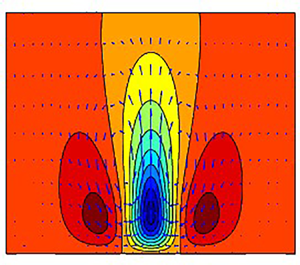
Contours of the time-averaged collocated  $U_s$ and vectors of the roll $(W_s,V_s)$ velocity on the $z$–
$z$– $y$ plane for: (a) the NS100, with $\max (|U_s|) = 0.21$, $\max (V_s)=0.024$; and (b) the RNL100, with $\max (|U_s|) = 0.32$, $\max (V_s)=0.03$. The contour level step is 0.025 in both panels.

5.1. Relating POD modes to R-S structures in the flow
There are alternative explanations for the striking appearance of POD modes for  $k_x=0$ that differ in spanwise wavenumber while exhibiting R-S structure (cf. figure 3). One interpretation of these structures is that they correspond to stable linear S3T modes that are maintained by fluctuations in the homogeneous background of turbulence. Due to the scale insensitivity of the R-S formation process, a spectral hierarchy of self-similar R-S structures is supported as modes by the turbulence as revealed by S3T (Farrell & Ioannou Reference Farrell and Ioannou2012). These R-S modes have different scales and damping rates, and are therefore expected to be excited at different amplitudes. This interpretation of the POD modes is appropriate in the case of an R-S that emerges in pre-transitional flow, as discussed in Farrell et al. (Reference Farrell, Ioannou and Nikolaidis2017b). Also, in beta-plane turbulence, one observes intermittent emergence of jets with structure corresponding to stochastically excited S3T modes, manifestations of which are referred to in observations as latent jets (Constantinou, Farrell & Ioannou Reference Constantinou, Farrell and Ioannou2014; Farrell & Ioannou Reference Farrell and Ioannou2019). In this interpretation of the POD modes with various spanwise wavenumbers, the POD modes are identifying structures that are regarded in the traditional manner as being independent harmonic structures in $z$, as is appropriate for a homogeneous coordinate in the flow.
However, there is an alternative interpretation, which is that the dominant structure in the flow is the finite-amplitude localized low-speed streak of figure 6. In this interpretation, the POD modes reflect the amplitude and structure of the spanwise Fourier components collocated to comprise the Fourier synthesis of this R-S structure rather than corresponding to structures with independent existence. The assumption underlying this interpretation is that a mode has arisen in the flow that results in a spontaneous symmetry breaking; in the example under analysis here, the S3T R-S instability is implicated.
In order to determine which of these alternative explanations for the POD structure at  $k_x=0$ is correct, we obtain the spanwise Fourier decomposition of the three velocity components of the mean streak and roll velocities shown in figure 6. We now compare the spanwise Fourier decomposition of the R-S (cf. figure 6) with the POD modes that have necessarily Fourier structure in $z$. The percentage variance accounted for by the first 10 spanwise harmonics in the Fourier decomposition of the streak, and the percentage variance of the POD modes with the same spanwise wavenumber, are compared in figure 7. These spectra are similar enough to suggest that the POD modes are the Fourier components of the streak, and indeed, if the POD modes are used to compose a structure by using the corresponding POD variances collocated at zero phase, then this produces a close correspondence to the streak in figure 6 (not shown). Consistent with this interpretation is the comparison of structure between the POD modes shown in figure 3 and the Fourier modes of the streak shown in figure 8. This agreement is expected given that in our DNS, $65\,\%$ of the $k_x=0$ fluctuation energy is accounted for by the mean streak structures in figure 6 (the low-speed streak accounts for $40\,\%$, and the high-speed streak for $25\,\%$, not shown; the RNL percentages are similar). The agreement shown in these figures leads us to conclude that the second of these explanations, that the POD spectrum arises primarily from Fourier decomposition of the low-speed R-S, is correct. In summary, we conclude that while POD analysis is consistent with identification of independent R-S structures, the alternative interpretation that the POD modes rather identify the individual components comprising the Fourier synthesis of a nonlinearly equilibrated localized coherent structure with complex R-S form, requiring many Fourier modes in its representation, is clearly preferable.
The percentage variance accounted for by the first Fourier spanwise components of the mean streaks in figure 6. Solid red line for the mean streak of the DNS; solid blue line for the mean streak of the RNL simulation; dashed lines with the corresponding colours for the percentage variances of the corresponding POD modes with spanwise wavenumbers  $n_z=1,\ldots,10$.

Contours of  $U_s$ and vectors of the roll $(W_s,V_s)$ velocity on the $z$–
$z$– $y$ plane of the first three spanwise Fourier components of the mean streaks of figure 6: (a,c,e) DNS, (b,d,f) RNL simulation. The contour level step is 0.2 in all panels.

5.2. Determining the  $k_x \ne 0$ POD modes associated with the collocated low-speed streak flows

Having isolated the streamwise mean R-S structure in DNS and RNL simulation, and identified the  $k_x=0$ POD modes as consistent with Fourier synthesis of this coherent structure, we turn now to exploiting POD analysis to obtain and interpret dynamically the fluctuations about the mean flow containing the streak structures of figure 6. We first Fourier decompose the fluctuation velocity ${\mathcal {U}}'= [ u(\boldsymbol {x},t), v(\boldsymbol {x},t), w(\boldsymbol {x},t) ]^{\rm T}$ in $x$ so that ${\mathcal {U}}'= {\mathcal {U}}'_{k_x}(y,z)\,{\rm e}^{{\rm i} k_x x}$ The POD modes are obtained from eigenanalysis of the two point spatial covariance
 \begin{equation} C_{k_x}(y_i,z_i,y_j,z_j) = \left\langle {\mathcal{U}}'_{k_x}(y_i,z_i)\, {\mathcal{U}}'^{{{{\dagger}}}}_{k_x}(y_j z_j) \right\rangle, \end{equation}
where  $\langle {\cdot } \rangle$ denotes the time mean, and ${{\dagger}}$ indicates the Hermitian transpose. Each POD mode is of the form $[\alpha _{k_x}{(y,z)}, \beta _{k_x}{(y,z)}, \gamma _{k_x}{(y,z)}]^{\rm T}\,{\rm e}^{{\rm i} k_x x}$, with $\alpha _{k_x}(y,z)$, $\beta _{k_x}(y,z)$ and $\gamma _{k_x}(y,z)$ determining the $(y,z)$ spatial structure of the velocity components of the POD mode. Note that the $n_x$ component of the velocity field has streamwise wavenumber $k_x= n_x \alpha$,
The flow fields shown in figure 6 reveal spanwise localized R-S structures symmetric about  $z/h={\rm \pi} /2$. In order to isolate the streamwise-varying POD modes associated with the localized low-speed streaks while avoiding contamination by the far field, we weight the data used to calculate the covariances $C_{k_x}$ with a spatial filter that suppresses the variance in the far field. We have chosen a Tukey filter in the interval $z=[0,{\rm \pi} ]$ with equation
 \begin{equation} f(z)
=\begin{cases} 0.5 \left [ 1+\cos \left ({\rm \pi}/\delta
\left (({\rm \pi}-2 z)/{\rm \pi} + (1 -\delta) \right )\right )\right
], & ({\rm \pi}-2 z)/{\rm \pi}<\delta-1,\\ 1, & |({\rm \pi}-2
z)/{\rm \pi}|\leq 1-\delta,\\ 0.5 \left [1+\cos \left
({\rm \pi}/\delta \left ((({{\rm \pi}-2 z})/{\rm \pi}-(1 -\delta)
\right) \right )\right ], & ({\rm \pi}-2 z)/{\rm \pi}> 1-\delta .
\end{cases}
\end{equation}
\begin{equation} f(z)
=\begin{cases} 0.5 \left [ 1+\cos \left ({\rm \pi}/\delta
\left (({\rm \pi}-2 z)/{\rm \pi} + (1 -\delta) \right )\right )\right
], & ({\rm \pi}-2 z)/{\rm \pi}<\delta-1,\\ 1, & |({\rm \pi}-2
z)/{\rm \pi}|\leq 1-\delta,\\ 0.5 \left [1+\cos \left
({\rm \pi}/\delta \left ((({{\rm \pi}-2 z})/{\rm \pi}-(1 -\delta)
\right) \right )\right ], & ({\rm \pi}-2 z)/{\rm \pi}> 1-\delta .
\end{cases}
\end{equation} The parameter  $\delta$ dictates the width of the filter and is chosen to sample the fluctuation field in the vicinity of the streak. The values $\delta =0.7$ and $0.55$ are selected for NL100 and RNL100, respectively, since the RNL100 streak covers a wider area of the spanwise flow.
5.3. Results for the POD modes with $k_x \ne 0$ associated with the collocated low-speed streak flows

The energy density accounted for by the first 10 POD modes for each of the first three  $n_x$ wavenumbers is shown in figure 9(a) for NL100, and in figure 9(b) for RNL100. Similarly, in figures 10, 11 and 12 are shown the corresponding structures of the first three sinuous POD modes with streamwise wavenumbers $n_x=1,2,3$. Note that the dominant POD modes in both DNS and RNL are characterized by a similar intricate complex three-dimensional structure that reflects the complexity of the underlying dynamics.
Percentage variance accounted for by the POD modes as a function of the order of the mode:(a) in NL100, and (b) in RNL100. POD modes with streamwise Fourier component  $n_x=1$ are in blue; those with streamwise Fourier component $n_x=2$ are in red; and those with streamwise Fourier component $n_x=3$ are in green. The sinuous modes are indicated with $S$, the varicose with $V$. The corresponding streamwise wavenumber is $k_x=2 {\rm \pi}n_x/L_x$.

The first sinuous POD mode with streamwise Fourier component  $n_x=1$ in (a,c,e) NL100 and (b,d,f) RNL100. (a,b) Contours of the $u$ velocity of the POD mode in the $z$–
$z$– $y$ plane at $x=0$, and vectors of $(w,v)$ velocity on this plane. (c,d) Contours of the $w$ velocity in the $x$–
$x$– $y$ plane at the centre of the streak where the $u$ and $v$ velocities vanish. (e,f) Contours of the $v$ velocity in the $x$–
$x$– $z$ plane at the centre of the streak, and vectors of $(u,w)$ velocity on this plane. The mean flow structure is indicated by the solid black line. The black contours in (a,b) show the streak contours in the interval $[-0.35,-0.1]$ at contour intervals of $0.05$. All other quantities have been normalized to 1, and the contour level is $0.2$. The first sinuous DNS POD mode accounts for $9.8\,\%$ of the total variance of the streamwise-varying velocity fluctuations of the flow (which includes all $k_x\ne 0$), while the first sinuous RNL POD mode accounts for $21.6\,\%$ of the total fluctuation variance (cf. figure 9).

As in figure 10 for the first sinuous POD mode with streamwise Fourier component  $n_x=2$. A single streamwise wavelength of the POD mode has been plotted. The first sinuous DNS POD mode (which is the first in variance POD) accounts for $5.7\,\%$ of the total variance of the streamwise-varying velocity fluctuations of the flow, while the first sinuous RNL POD mode (which is also the first in variance POD) accounts for $7.6\,\%$ of the total fluctuation variance.

As in figure 10 for the first sinuous POD mode with streamwise Fourier component  $n_x=3$. A single streamwise wavelength of the POD mode has been plotted. The first sinuous DNS POD mode (which is the first in variance POD) accounts for $5.7\,\%$ of the total variance of the streamwise varying velocity fluctuations of the flow, while the first sinuous RNL POD mode (which is also the first in variance POD) accounts for $1.2\,\%$ of the total fluctuation variance.

In the  $y\unicode{x2013}z$ cross-sections (figures 10a,b, 11a,b, 12a,b), the POD modes exhibit streamwise streaks produced by lift-up, which are seen to be coincident with supporting roll circulations. Similar roll circulation and associated streak structures were educed from analysis of DNS data to arise in association with sweep and ejection events by Lozano-Durán, Flores & Jiménez (Reference Lozano-Durán, Flores and Jiménez2012) (cf. their figure 12d) and Encinar & Jiménez (Reference Encinar and Jiménez2020) (cf. their figure 12). Note that these streaks and associated rolls are located at the flanks of the central streamwise streak and are harmonic in the streamwise direction, and should not be confused with the entirely different R-S structure that arises from lift-up induced by the Reynolds stresses of the fluctuations, and which, in contrast, forces the central streak with $k_x=0$.
In the  $x\unicode{x2013}y$ cross-sections (figures 10c,d, 11c,d, 12c,d), the POD modes exhibit the tilted structure indicative of linear amplification by the Orr mechanism. This characteristic Orr structure has been associated with sweep and ejection events in wall turbulence by Encinar & Jiménez (Reference Encinar and Jiménez2020) (cf. their figure 1), and evolution of these structures was found to accord with the linear evolution of optimal perturbations with Orr form on the cross-stream shear (Jiménez Reference Jiménez2013a; Encinar & Jiménez Reference Encinar and Jiménez2020).
In the  $x\unicode{x2013}z$ cross-sections (figures 10e,f, 11e,f, 12e,f), the POD modes exhibit orientation with the streak indicative of an energy-extracting sinuous oblique wave collocated with the streak. Sinuous structure of streak fluctuations has been associated with inflectional instability (Waleffe Reference Waleffe1997) and with optimally growing perturbations (Schoppa & Hussain Reference Schoppa and Hussain2002).
The dominance of the top sinuous structure variance, shown in figure 9(a), indicates that it is preferentially expressed relative to the other components of the fluctuation field in both DNS and RNL simulations. The second in variance POD mode is usually varicose, and it also exhibits a similar structure in DNS and RNL (not shown). The sinuous and varicose ordering of the POD modes is indicated in figures 9(a) and 9(b).
Qualitative agreement in structure between the top POD modes of the DNS and RNL simulations is apparent. Despite differences such as the greater extent in  $y$ of the streak structure of the RNL POD modes (cf. figures 10a,b, 11a,b, 12a,b), the compelling similarity in structural features, and the phasing between fluctuation fields revealed by the DNS and RNL POD modes argues for the operation of a parallel dynamics in these two systems. The exact statistical steady state, including the amplitude and spatial extent of the similar structures, is determined by the nonlinear feedback regulation between the mean and fluctuation fields (Farrell & Ioannou Reference Farrell and Ioannou2012). In particular, the feedback regulation produces an RNL equilibrium with a 50 % greater spatial extent in the fluctuation streak shown in the aforementioned figures, which is consistent with a similarly greater $V$ velocity in the RNL simulation (cf. figure 6). While similarity of the R-S structure between DNS and RNL simulation is manifest, there is no simple argument for the exact amplitude of the mean velocity components that the associated nonlinear regulator settles on. Intuitively, this can be understood from considering that the feedback regulation is using the Reynolds stresses to adjust the R-S to Lyapunov neutrality, and this can be accomplished by adjusting the amplitude, structure and temporal variation of the R-S in many ways, so that a single easily predicted equilibrium structure is not to be expected.
5.4. Relation of the POD modes of the fluctuations in DNS to the POD modes of the fluctuations in a linear stochastic turbulence model
As remarked earlier, the striking structural similarity in the POD modes of fluctuations on the streamwise mean streak in DNS and RNL simulations suggests a common dynamical origin. Given that the streak is modally stable, the default explanation would be excitation of transiently growing fluctuations to the streamwise streak by the turbulent background velocity field. Transient growth of optimal perturbations on a cross-stream shear has been shown recently to accord reasonably with the short-time evolution of the structures that arise during sweep–ejection events (Encinar & Jiménez Reference Encinar and Jiménez2020). These structures, when evolved, assume the characteristic tilt of the POD modes shown in figures 10(c,d), 11(c,d) and 12(c,d). Within the context of POD analysis, the appropriate extension of the optimal transient growth analysis of Encinar & Jiménez (Reference Encinar and Jiménez2020) would be calculation of the POD modes arising from the ensemble mean fluctuation covariance excited by the background turbulence.
This can be implemented by calculating the covariance using the stochastic turbulence model (STM) governed by the equations
 \begin{equation} \partial_t{\boldsymbol{u}} + U\,\partial_x {\boldsymbol{u}} + ( {\boldsymbol{u}} \boldsymbol{\cdot} \boldsymbol{\nabla} ) U\hat{\boldsymbol{x}} + \boldsymbol{\nabla} p- R^{{-}1}\,\Delta {\boldsymbol{u}} = {\boldsymbol{f}},\quad \boldsymbol{\nabla} \boldsymbol{\cdot} \boldsymbol{u} = 0, \end{equation}
with no-slip boundary conditions at the channel walls, and periodic boundary conditions in  $x$ and $z$, where $U(y,z)\,\hat {\boldsymbol {x}}$ is the equilibrium low-speed streak of the DNS (or the RNL simulations). The equations are the fluctuation equations of the DNS (2.1b) in which the fluctuation–fluctuation nonlinearity has been replaced by a state-independent forcing ${\boldsymbol {f}}$, white in space and time. This simplest parametrization imposes the least a priori assumption on the structures arising from the dynamics, and is adequate for our purpose. The time-dependent streamwise mean flow, $\boldsymbol {U}$, of the DNS has been replaced by the time-independent flow $U(y,z)\,\hat {\boldsymbol {x}}$, obtained by collocating and averaging the low-speed streak. This mean streak is shown in figure 6.
Stability of the mean flows shown in figure 6 assures the asymptotic approach of the covariance of the fluctuations governed by (5.3a,b) to a statistical equilibrium covariance  ${\boldsymbol {C}}_\infty$, satisfying in matrix form the Lyapunov equation
 \begin{equation} {\boldsymbol{A}} {\boldsymbol{C}}_\infty + {\boldsymbol{C}}_\infty {\boldsymbol{A}}^{{\dagger}}={-} {\boldsymbol{I}}, \end{equation}
where  ${\boldsymbol {A}}$ is the operator, in matrix form, governing the linear dynamics associated with (5.3a,b), ${\boldsymbol {A}}^{{\dagger}}$ is the Hermitian transpose of ${\boldsymbol {A}}$, and ${\boldsymbol {I}}$ is the spatial covariance $\langle\,\boldsymbol{f\,f}^{{\dagger}} \rangle$ appropriate for the white in space stochastic excitation $\boldsymbol {f}$, with the implication that equal energy input is imparted to each degree of freedom (cf. Farrell & Ioannou Reference Farrell and Ioannou1993, Reference Farrell and Ioannou1996). As mentioned above, this choice of excitation has the attribute that the forcing does not impart a bias to the structure.
However, in turbulence the mean flow is time-dependent, and the time-invariant formulation of the STM producing the infinite horizon fluctuation covariance  ${\boldsymbol {C}}_\infty$ is not an appropriate model for the covariance arising in a time-dependent mean flow. In DNS and RNL simulations, the coherence time for fluctuation growth is limited by the temporal coherence of the mean flow. Typical temporal coherence of the mean flow is of the order $T_{d} = 1\, h/u_{\tau}$ (Lozano-Durán et al. Reference Lozano-Durán, Constantinou, Nikolaidis and Karp2021), which corresponds in our simulation to $T_d = {O}( 20 h/U)$, and it is therefore appropriate to restrict the fluctuation development to extend over a time interval $T_d$ consistent with this coherence time. In relating the POD mode structure to the STM, this coherence time is appropriate for both DNS and the RNL simulations. However, while in the DNS the excitation term $\boldsymbol {f}$ has traditionally been related to the fluctuation–fluctuation nonlinearity, in the case of the RNL simulations, a similar excitation arises from the effective nonlinear scattering of the fluctuations by their interaction with the time-dependent mean flow.
It can be shown (cf. Farrell & Ioannou Reference Farrell and Ioannou1998) that the covariance of the dynamics governed by (5.3a,b) when restricted in time to  $T_d$ is
 \begin{align} {\boldsymbol{C}}_{T_d} &= {\rm e}^{{\boldsymbol{A}} T_d}\,{\boldsymbol{I}} \,{\rm e}^{{\boldsymbol{A}}^{{\dagger}} T_d}+\int_0^{T_d} {\rm d}s\, {\rm e}^{{\boldsymbol{A}} s}\,{\boldsymbol{I}}\,{\rm e}^{{\boldsymbol{A}}^{{\dagger}} s} \nonumber\\ &= {\rm e}^{{\boldsymbol{A}} T_d}\,{\rm e}^{{\boldsymbol{A}}^{{\dagger}} T_d} + {\boldsymbol{C}}_\infty - {\rm e}^{{\boldsymbol{A}} T_d}\,{\boldsymbol{C}}_\infty \,{\rm e}^{{\boldsymbol{A}}^{{\dagger}} T_d}. \end{align}
An alternative to limiting the temporal extent over which fluctuations develop is the inclusion in (5.3a,b) of an appropriate eddy viscosity (del Álamo & Jiménez Reference del Álamo and Jiménez2006). Either intervention in the linear dynamics of (5.3a,b) has been shown to result in dynamical structures and spectra commensurate with those observed (Butler & Farrell Reference Butler and Farrell1993; Farrell & Ioannou Reference Farrell and Ioannou1998; del Álamo & Jiménez Reference del Álamo and Jiménez2006; Hwang & Cossu Reference Hwang and Cossu2010; Madhusudanan, Illingworth & Marusic Reference Madhusudanan, Illingworth and Marusic2019).
Eigenanalysis of the covariance  ${\boldsymbol {C}}_{T_d}$ determines the POD modes as predicted by the STM. This covariance is obtained by integration of (5.5), in which the initial state covariance ${\boldsymbol {I}}$ is evolved over a time $T_d$ while also being continuously excited with covariance ${\boldsymbol {I}}$. We have obtained best agreement with the observed POD modes in both DNS and RNL simulations when we choose a disruption time $T_d=30$ in the STM. The covariance obtained from (5.5) reflects the influence of the transient growth of an unbiased initial state as well as the accumulated transient growth of an unbiased excitation over the coherence interval $T_d$. We find that in this problem for $T_d=30$, the initial condition does not influence the covariance appreciably.
Because the streamwise mean streak is mirror-symmetric in the spanwise direction, the POD modes of the STM will be either sinuous or varicose. We find that in both DNS and RNL simulations, as well as in the STM, the top POD modes are sinuous. This result is consistent with the optimally growing perturbation to a low-speed streak being of sinuous form. It is worth noting the further consistency in the coincidence of the sinuous optimal with the low-speed streak arising from the fact that the Reynolds stresses of the sinuous fluctuations are configured favourably to amplify the low-speed streak through the lift-up process (Farrell et al. Reference Farrell, Ioannou and Nikolaidis2022a; Nikolaidis et al. Reference Nikolaidis, Ioannou and Farrell2023).
The top POD modes with streamwise wavenumbers  $n_x=1,2,3$ of the STM are shown in figures 13, 14 and 15 next to the corresponding POD modes of the DNS. The STM POD modes obtained from the RNL mean flow are similar to those obtained from the DNS mean flow and are not shown. This similarity in structure is expected because the mean low-speed streaks in DNS and RNL simulations have similar structure, as seen in figures 6 and 7.
Comparison of (a,c,e) the first sinuous POD mode in NL100 with streamwise Fourier component  $n_x=1$ with (b,d,f) the first sinuous and first POD mode of the STM with $T_d=30$ on the DNS mean low-speed streak shown in figure 6(a). The velocity fields are as in figure 10. The POD with the largest variance is the sinuous mode in both DNS and STM.

As in figure 13 for  $n_x=2$ fluctuations. A single streamwise wavelength of the POD mode has been plotted.

As in figure 13 for  $n_x=3$ fluctuations. A single streamwise wavelength of the POD mode has been plotted.

The dominant POD modes of the STM (cf. figures 13, 14 and 15) exhibit complex three-dimensional velocity fields that are striking similar in structure and phasing to those of DNS and RNL simulations (cf. figures 10, 11 and 12), which is indicative of a parallel mechanism underlying their dynamics. This similarity in the dynamical structure of the POD modes among STM, DNS and RNL simulations argues strongly for identifying the dynamical origin of the fluctuation variance in DNS and RNL simulations with the growth of optimal perturbations in the mean flow streak. This identification of the origin of perturbations on the R-S with optimally growing structures explains the similarity in structure of the POD modes in DNS and RNL simulations as consistent with the robust dynamics of optimal perturbation growth in shear flow.
6. Discussion and conclusion
POD analysis was carried out on DNS of turbulent Poiseuille flow at  $R=1650$ and the corresponding quasi-linear RNL simulation. The RNL system was chosen for this comparison because it is dynamically similar to S3T so that the ${\rm S3T}\rightarrow {\rm RNL} \rightarrow {\rm DNS}$ sequence of dynamical systems forms a conceptual bridge connecting the analytically comprehensive characterization of turbulence in S3T to DNS turbulence, which lacks a similarly complete analytic characterization. The motivation for this work is to exploit this conceptual bridge to extend the comprehensive understanding of S3T dynamics to obtain a similar comprehensive understanding of the dynamics of DNS.
The POD modes analysed were chosen to correspond to the first and second cumulants of the S3T SSD, these being the streamwise mean flow and the covariance of fluctuations from it. In general, this SSD is closed by parametrizing the third cumulant using stochastic excitation. In the present case, this stochastic excitation has been set to zero. In RNL simulations, the equivalent to the covariance in S3T is the covariance of the Lyapunov vectors, with zero Lyapunov exponent of the time-varying linear operator linearized about the fluctuating streamwise mean flow. The Lyapunov vectors that are spontaneously emergent in the dynamics of RNL turbulence are analogous to neutral eigenmodes supporting a time-independent mean state. The structure of the first cumulant corresponds to the streamwise mean dynamics subject to forcing arising from the Reynolds stresses of the analytically known structures of the second cumulant. And finally, the statistical state of the turbulence is regulated by feedback from the second cumulant to bring the time-varying streamwise mean flow to neutral stability, in the sense that the characteristic Lyapunov exponent of the linear operator governing the second cumulant is exactly zero. As an illustrative example of the power and utility of being in possession of an analytic theory for the dynamics of wall turbulence, consider the problem of understanding the mechanism determining the statistical mean state of the turbulence. Of all the possible mechanisms that one might hypothesize, this mechanism is identified analytically in S3T-RNL dynamics to be modification of the time-dependent streamwise mean state by Reynolds stress feedback arising from the fluctuations specifically to bring the characteristic Lyapunov exponent of the linear fluctuation equation to the real number zero. Extensive study of DNS data has verified that the characteristic exponent of the DNS streamwise mean state corresponds to this parametric growth stabilization mechanism (Nikolaidis, Farrell & Ioannou Reference Nikolaidis, Farrell and Ioannou2018; Farrell et al. Reference Farrell, Kim, Bae, Nikolaidis and Ioannou2022b). It is worth noting that this mechanism of regulating turbulence to its statistical mean state by feedback regulation operating between the fluctuations and the mean state such as to stabilize the mean state to linear instability is similar to that hypothesis by Malkus (Reference Malkus1956), who posited that the statistical state of turbulence is determined by feedback regulation to neutrality of the mean state's inflectional modes. This hypothesis was not verified for the case of wall-bounded turbulence (Reynolds & Tiederman Reference Reynolds and Tiederman1967), but needed, as we have seen above, only substitution of parametric neutrality of the time- and spanwise-varying streamwise mean flow for the posited inflection mode neutrality of the temporal mean flow to correspond with the mechanism regulating the statistical mean state of wall turbulence.
In our study of the POD modes, we considered first the streamwise mean component of the turbulence. We found close correspondence in structure between the POD modes of the DNS and RNL fields. An initial interpretation of this similarity suggested that the scale-invariant R-S formation mechanism identified analytically in the S3T-RNL SSD is also operating in DNS. Although scale-invariant R-S dynamics provides a possible explanation for the POD modes found in both DNS and RNL simulations, the random phase assumption – which is traditionally taken to characterize the POD modes in directions in which solutions to the equations are statistically homogeneous – is not necessarily valid when a mechanism of symmetry breaking is active. In the present case, an instability process, which has analytic expression in the SSD stability analysis of the stability of streamwise and spanwise homogeneous mean flows, occurs to break the spanwise symmetry, resulting in R-S structures (Farrell & Ioannou Reference Farrell and Ioannou2012; Farrell et al. Reference Farrell, Ioannou and Nikolaidis2017b). If this process is active, then it would imply that the random phase assumption in the spanwise for the POD  $k_x=0$ modes is not valid. In order to examine this possibility, we aligned the most prominent low-speed streak of the flow to obtain a spatially coherent time-averaged low-speed streak, and determined the spanwise Fourier components of this coherent streak. We then verified that the Fourier components of this coherent streak corresponded to the structure and the amplitudes of the POD modes that were obtained making the random phase assumption. Furthermore, we have verified that removing the random phase assumption among the POD modes of harmonic form by aligning them to zero phase difference revealed that the POD modes constituted the Fourier components of the coherent non-harmonic R-S structure educed by aligning the low-speed streak in the turbulence simulation.
After having determined the temporal mean structure of the R-S by collocation, it remained to identify the  $k_x\ne 0$ POD modes associated with this R-S. In order to isolate the POD modes of the $k_x \ne 0$ fluctuations that are associated with the R-S structure, the associated fluctuation velocity fields were also translated to be aligned with the collocated low-speed streak. POD analysis of the aligned velocity fields revealed close correspondence between the $k_x\ne 0$ POD modes in DNS and RNL simulations. The dominant streamwise-varying POD modes in both DNS and RNL simulations were found to be characterized by a prominent component of streak-localized sinuous oblique waves that had been identified previously in analysis of the S3T SSD (Farrell & Ioannou Reference Farrell and Ioannou2012). In those studies, sinuous oblique waves were shown to give rise to Reynolds stresses properly collocated with the streak to force roll circulation that amplify the streak through the lift-up process. Moreover, these sinuous oblique waves are exactly the structures that are predicted to arise from a turbulent background flow field because they are the optimally growing perturbations. In this paper, it was confirmed using an STM that the sinuous POD modes found in both our DNS and RNL simulations similarly correspond closely to the time-average response to unbiased stochastic excitation and are therefore consistently dominated by the optimally growing perturbations. In a companion paper (Nikolaidis et al. Reference Nikolaidis, Ioannou and Farrell2023), we show, using the same DNS and RNL dataset, that the Reynolds stress of the sinuous POD modes in both DNS and RNL simulations sustains the low-streak streak, while the varicose POD modes suppress it, and that the effect of the sinuous and varicose POD modes is reversed in the case of high-speed streaks.
Although we have connected the POD modes in both DNS and RNL simulations to the growth of optimal perturbations through the STM analysis, we have not addressed in this paper the mechanism by which these optimal perturbations are excited. In the case of RNL systems, this is the parametric growth process, while in the case of DNS, it is a combination of the parametric growth process and excitation by the fluctuation–fluctuation nonlinearity. This question is of importance because, to the extent that parametric growth dominates the fluctuation dynamics in DNS turbulence, DNS turbulence inherits the analytic characterization of RNL turbulence. While this paper does not settle this question, ongoing work indicates that the parametric growth mechanism does dominate in DNS (Nikolaidis et al. Reference Nikolaidis, Farrell and Ioannou2018; Farrell et al. Reference Farrell, Kim, Bae, Nikolaidis and Ioannou2022b).
Funding
This work was funded in part by the Second Multiflow Programme of the European Research Council. M.-A.N. gratefully acknowledges the support of the Hellenic Foundation for Research and Innovation (HFRI) and the General Secretariat for Research and Technology (GSRT), under the HFRI PhD Fellowship grant 1718/14518. B.F.F. was partially supported by NSF AGS-1640989. A.L.-D. was supported by the National Science Foundation under grant no. 2140775. We would like to thank J. Jiménez, D. Gayme, D. Chung, G. Rigas and N. Constantinou, and the three anonymous reviewers, for their helpful comments.
Declaration of interests
The authors report no conflict of interest.
Appendix A. Construction of the covariances with symmetry restrictions
Homogeneity in the streamwise and spanwise directions allows the decomposition of velocity field snapshots into sums of plane waves with Fourier coefficients that depend on the wall-normal direction. Application of mirror-symmetries in  $y$ and $z$ incorporates the 2-point statistics from the total flow field into a single covariance for each $\vert k_x \vert, \vert k_z \vert$ wavenumber pair. Convergence towards these statistical symmetries is slow. For example, in figure 16, we demonstrate the slow convergence of the statistics to the asymptotic mirror-symmetric state about the wall-normal plane at the centre of the channel.
The 1-norm of the difference  $C_{k_z} - \hat {S}_y C_{k_z}\hat {S}_y^{{\dagger}}$ between the covariance matrix $C_{k_z}$ (see (4.2)) and the covariance of the reflected flow about the $x$–
$x$– $z$ plane at the centre of the flow ( $\,y=1$) as a function of the averaging time $T_{av}$, for $h k_z=2,4,6,8$ for DNS of NL100, where $\hat {S}_y$ is defined in (A8). This plot verifies that reflection symmetry about the centreline is a statistical symmetry of the flow, and that this symmetry is approached at the rate $1/T_{av}$, consistent with the law of large numbers for quadratic statistics. Time is non-dimensionalized by $h/U$.

For a single  $k_z,k_x$ pair, the three components of the velocity field are given by two independent plane waves:
 \begin{equation} \boldsymbol{\varPhi}_{k_x}\exp({{\rm i}k_x x})= \left( \begin{array}{@{}c@{}} A_{k_x,k_z}(y)\\ B_{k_x,k_z} (y)\\ \varGamma_{k_x,k_z}(y) \end{array} \right) \exp({{\rm i}(k_x x + k_z z)}) + \left( \begin{array}{@{}c@{}} A_{k_x,-k_z}(y)\\ B_{k_x,-k_z} (y)\\ \varGamma_{k_x,-k_z}(y) \end{array} \right) \exp({{\rm i}(k_x x - k_z z)}). \end{equation}
With  $A$, we denote the streamwise component of the velocity field, $B$ the wall-normal component, and $\varGamma$ the spanwise component. A special case is the $k_x=0$ component for which the coefficients of $k_z$ and $-k_z$ will be complex conjugates. The two symmetries that we consider are mirror-symmetry in $y$ with respect to the half-channel $x$–
$x$– $z$ plane at $y=1$, and in $z$ with respect to the half-width $x$–
$x$– $y$ plane at $z={\rm \pi} /2$. Those produce a fourfold increase in the amount of data that will be included in the covariance matrix.
First, we consider the spanwise mirroring operation. This will transform  $z$ to ${\rm \pi} -z$ and change sign in the spanwise velocity component:
 \begin{align} \hat{S}_{z} \boldsymbol{\varPhi}_{k_x}{\rm e}^{{\rm i}k_x x}&= \left( \begin{array}{@{}c@{}} A_{k_x,-k_z}(y)\\ B_{k_x,-k_z} (y)\\ -\varGamma_{k_x,-k_z}(y) \end{array} \right) \exp({{\rm i} (k_x x + k_z (z -{\rm \pi}))})\nonumber\\ &\quad + \left(\begin{array}{@{}c@{}} A_{k_x,k_z}(y)\\ B_{k_x,k_z} (y)\\ -\varGamma_{k_x,k_z}(y) \end{array} \right) \exp({{\rm i} (k_x x - k_z (z - {\rm \pi}))}). \end{align}
The  $-{\rm i} k_z {\rm \pi}$ phase that appears in the plane wave will cancel out when the covariance is formed.
In the wall-normal mirroring, the effect is to transform  $y$ to $2-y$ and change sign in the wall-normal velocity component:
 \begin{align} \hat{S}_{y} \boldsymbol{\varPhi}_{k_x}\exp({{\rm i}k_x x}) &= \left( \begin{array}{@{}c@{}} A_{k_x,k_z}(2-y)\\ -B_{k_x,k_z} (2-y)\\ \varGamma_{k_x,k_z}(2-y) \end{array} \right) \exp({{\rm i} (k_x x + k_z z )})\nonumber\\ &\quad + \left( \begin{array}{@{}c@{}} A_{k_x,-k_z}(2-y)\\ -B_{k_x,-k_z} (2-y)\\ \varGamma_{k_x,-k_z}(2-y) \end{array} \right) \exp({{\rm i} (k_x x - k_z z)}). \end{align}
What the  $2-y$ coordinate implies is that the wall-normal structure will be inverted for each component. Summarizing the above operations, the total covariance will be comprised of the individual covariances obtained for each of the following four components:
 \begin{equation} \left.\begin{gathered} \varPhi_{k_z} = \left(\begin{array}{@{}c@{}} A_{k_z}(y)\\ B_{k_z} (y)\\ \varGamma_{k_z}(y) \end{array}\right) {\rm e}^{{\rm i} k_z z},\quad \hat{S}_{z} \varPhi_{k_z} = \left( \begin{array}{@{}c@{}} A_{{-}k_z}(y)\\ B_{{-}k_z} (y)\\ -\varGamma_{{-}k_z}(y) \end{array} \right) {\rm e}^{{\rm i} k_z z},\\ \hat{S}_{y} \varPhi_{k_z} = \left( \begin{array}{@{}c@{}} A_{k_z}(2-y)\\ B_{k_z} (2-y)\\ \varGamma_{k_z}(2-y) \end{array} \right) {\rm e}^{{\rm i} k_z z},\quad \hat{S}_{z}\hat{S}_{y} \varPhi_{k_z} = \left( \begin{array}{@{}c@{}} A_{{-}k_z}(2-y)\\ -B_{{-}k_z} (2-y)\\ -\varGamma_{{-}k_z}(2-y) \end{array} \right) {\rm e}^{{\rm i} k_z z}, \end{gathered}\right\} \end{equation}
where the  $k_x$ subscript has been omitted.
We form the covariance obtained from the initial wave. To highlight the inner structure of this covariance due to the different velocity components, the following representation is chosen:
 \begin{equation} C_{k_z} = \left( \begin{array}{@{}ccc@{}} C_{k_z}^{uu} & C_{k_z}^{uv} & C_{k_z}^{uw} \\ C_{k_z}^{vu} & C_{k_z}^{vv} & C_{k_z}^{vw} \\ C_{k_z}^{wu} & C_{k_z}^{wv} & C_{k_z}^{ww} \end{array} \right), \end{equation}
with  $C_{k_z}^{u_iu_j}=(C_{k_z}^{u_ju_i})^{{\dagger}}$. In the following, the $k_z$ subscript will be omitted where possible, and instead of $u_iu_j$, the superscript $ij$ will be used. So the covariance can be written as
 \begin{equation} C = \left( \begin{array}{@{}ccc@{}} C^{11} & C^{12} & C^{13} \\ C^{21} & C^{22} & C^{23} \\ C^{31} & C^{32} & C^{33} \end{array} \right). \end{equation}
 Statistical symmetry in reflections of the velocities in  $z$ merge the covariance of the $-k_z$ component with that of $k_z$. The negative $k_z$ covariance will be modified to account for this symmetry:
 \begin{equation} \hat{S}_zC_{{-}k_z}\hat{S}_z^{{\dagger}}{=} \left( \begin{array}{@{}ccc@{}} (C^{11}) & (C^{12}) & -(C^{13}) \\ (C^{21}) & (C^{22}) & -(C^{23}) \\ -(C^{31}) & -(C^{32}) & (C^{33}) \end{array} \right). \end{equation}
Reflections in  $y$ require us to reverse the order of the row and column indexes in each individual covariance, and if this operation is noted as $\hat {S}_y C^{ij}\hat {S}_y^{{\dagger}} = C^{ij}_R$, then we have
 \begin{equation} \hat{S}_yC\hat{S}_y^{{\dagger}}{=} \left( \begin{array}{@{}ccc@{}} C^{11}_R & -C^{12}_R & C^{13}_R \\ -C^{21}_R & C^{22}_R & -C^{23}_R \\ C^{31}_R & -C^{32}_R & C^{33}_R \end{array} \right).\end{equation}
The total covariance will be comprised of the following components:
 \begin{equation} C^{t}_{k_z}=(C_{k_z}+\hat{S}_yC_{k_z} \hat{S}_y^{{\dagger}}{+} \hat{S}_zC_{{-}k_z}\hat{S}_z^{{\dagger}}{+} \hat{S}_y\hat{S}_zC_{{-}k_z} \hat{S}_z^{{\dagger}}\hat{S}_y^{{\dagger}})/4. \end{equation}
To account correctly for the relative energy between  $k_z=0$ and $k_z \ne 0$ components, the eigenvalues of covariances with $k_z \ne 0$ are doubled in the ordering process.


 Open access