





1. Introduction
In this paper, we study the following free boundary problem modelling the growth of radially symmetric tumours with three-layer structure:
 \begin{equation*} \kern35pt\begin{cases} \Delta _r \sigma = f(\sigma )\chi _{\{\sigma \gt \sigma _Q\}}+g(\sigma ) \chi _{\{\sigma _D\lt \sigma \le \sigma _Q\}} \qquad \mbox{for}\;\; 0\lt r\lt R(t),\;\;t\gt 0, \kern90pt (1.1)\nonumber\\[2pt] \sigma _r(0,t)=0,\qquad \quad \sigma (R(t),t)=\bar \sigma \qquad \quad \mbox{for}\;\;t\gt 0, \kern145.3pt (1.2)\nonumber \\[2pt] R'(t)=\dfrac{1}{R^2(t)}\int _0^{R(t)} \big (S(\sigma (r,t))\chi _{\{\sigma \gt \sigma _Q\}} -\nu _1\chi _{\{\sigma _D\lt \sigma \le \sigma _Q\}}-\nu _2\chi _{\{\sigma \le \sigma _D\}}\big )r^2dr \quad \mbox{for}\;t\gt 0,\kern35.3pt (1.3)\nonumber\\[4pt] R(0)=R_0,\kern305pt (1.4)\nonumber\end{cases} \end{equation*}
where $\sigma (r, t)$
and
$\sigma (r, t)$
and $R(t)$
are both unknown functions representing the concentration of nutrients and the tumour radius at time
$R(t)$
are both unknown functions representing the concentration of nutrients and the tumour radius at time $t\gt 0$
,
$t\gt 0$
, $\chi _E$
is the indicator function on a set
$\chi _E$
is the indicator function on a set $E$
, namely
$E$
, namely $\chi _E(x)=1$
for
$\chi _E(x)=1$
for $x\in E$
and
$x\in E$
and $\chi _E(x)=0$
for
$\chi _E(x)=0$
for $x\notin E$
. The constants
$x\notin E$
. The constants $\sigma _Q$
and
$\sigma _Q$
and $\sigma _D$
are two positive nutrient concentration threshold values for distinguishing between the proliferating phase and the quiescent phase and between the quiescent phase and the necrotic phase, respectively. It makes that the region
$\sigma _D$
are two positive nutrient concentration threshold values for distinguishing between the proliferating phase and the quiescent phase and between the quiescent phase and the necrotic phase, respectively. It makes that the region $\{\sigma (r, t)\gt \sigma _Q\}$
is the proliferating layer with only proliferating cells,
$\{\sigma (r, t)\gt \sigma _Q\}$
is the proliferating layer with only proliferating cells, $\{\sigma _D\lt \sigma (r,t)\le \sigma _Q\}$
is the quiescent layer with only quiescent cells and
$\{\sigma _D\lt \sigma (r,t)\le \sigma _Q\}$
is the quiescent layer with only quiescent cells and $\{\sigma (r,t)\le \sigma _D\}$
is the necrotic core with only dead cells. The constants
$\{\sigma (r,t)\le \sigma _D\}$
is the necrotic core with only dead cells. The constants $\bar \sigma$
,
$\bar \sigma$
, $\nu _1$
and
$\nu _1$
and $\nu _2$
are all positive, and
$\nu _2$
are all positive, and $\bar \sigma$
represents the external nutrient supply,
$\bar \sigma$
represents the external nutrient supply, $\nu _1$
and
$\nu _1$
and $\nu _2$
represent the removal rates for quiescent and necrotic cells, respectively. The functions
$\nu _2$
represent the removal rates for quiescent and necrotic cells, respectively. The functions $f$
and
$f$
and $g$
represent the nutrient consumption rate for proliferating cells and quiescent cells, respectively. The function
$g$
represent the nutrient consumption rate for proliferating cells and quiescent cells, respectively. The function $S$
is the growth rate of proliferating cells. They are typically given by linear functions of the form
$S$
is the growth rate of proliferating cells. They are typically given by linear functions of the form
 \begin{equation} f(\sigma )=\lambda _1\sigma ,\qquad g(\sigma )=\lambda _2\sigma ,\qquad S(\sigma )=\mu (\sigma -\tilde \sigma ), \end{equation}
where $\mu ,\tilde \sigma ,\lambda _1,\lambda _2$
are all positive constants. Finally,
$\mu ,\tilde \sigma ,\lambda _1,\lambda _2$
are all positive constants. Finally, $R_0\gt 0$
is the initial tumour radius.
$R_0\gt 0$
is the initial tumour radius.
Problem (1.1)–(1.4) describes a three-layer tumour model suggested by Byrne and Chaplain [Reference Byrne and Chaplain3]. In the limiting case $\sigma _Q=\sigma _D=0$
, it becomes the classical one-layer tumour model with only proliferating cells. Many illuminating results concerning this classical model have been extensively established over the decades, including the asymptotic behaviour of radial solutions and non-radial solutions, the existence of symmetry-breaking bifurcation stationary solutions and the Hopf bifurcations; see [Reference Cui5, Reference Cui7–Reference Cui and Escher9, Reference Escher and Matioc11–Reference Friedman and Hu14, Reference He, Xing and Hu18–Reference Huang, Zhang and Hu20, Reference Zhao and Shi34] and the references cited therein. In the case
$\sigma _Q=\sigma _D=0$
, it becomes the classical one-layer tumour model with only proliferating cells. Many illuminating results concerning this classical model have been extensively established over the decades, including the asymptotic behaviour of radial solutions and non-radial solutions, the existence of symmetry-breaking bifurcation stationary solutions and the Hopf bifurcations; see [Reference Cui5, Reference Cui7–Reference Cui and Escher9, Reference Escher and Matioc11–Reference Friedman and Hu14, Reference He, Xing and Hu18–Reference Huang, Zhang and Hu20, Reference Zhao and Shi34] and the references cited therein. In the case $\sigma _Q=\sigma _D\gt 0$
, it can be regarded as a two-layer necrotic tumour model. For the existence of radial stationary solutions, asymptotic stability of radial stationary solutions under radial or non-radial perturbations and the existence of non-flat bifurcation stationary solutions, we refer the readers to see [Reference Bueno, Ercole and Zumpano2, Reference Cui6, Reference Cui and Friedman10, Reference Lu, Hao, Hu and Li25, Reference Wu27–Reference Wu and Xu31, Reference Xu, Zhang and Zhou33]. In the case
$\sigma _Q=\sigma _D\gt 0$
, it can be regarded as a two-layer necrotic tumour model. For the existence of radial stationary solutions, asymptotic stability of radial stationary solutions under radial or non-radial perturbations and the existence of non-flat bifurcation stationary solutions, we refer the readers to see [Reference Bueno, Ercole and Zumpano2, Reference Cui6, Reference Cui and Friedman10, Reference Lu, Hao, Hu and Li25, Reference Wu27–Reference Wu and Xu31, Reference Xu, Zhang and Zhou33]. In the case $\sigma _Q\gt \sigma _D=0$
, this problem is another two-layer tumour model that contains a quiescent core and an outer shell of proliferating cells. The existence and uniqueness of radial stationary solutions and asymptotic behaviour of radial solutions have also been established (cf. [Reference Liu and Zhuang21, Reference Liu and Zhuang22, Reference Wu, Xu and Zhuang32]).
$\sigma _Q\gt \sigma _D=0$
, this problem is another two-layer tumour model that contains a quiescent core and an outer shell of proliferating cells. The existence and uniqueness of radial stationary solutions and asymptotic behaviour of radial solutions have also been established (cf. [Reference Liu and Zhuang21, Reference Liu and Zhuang22, Reference Wu, Xu and Zhuang32]).
In the three-layer case $\sigma _Q\gt \sigma _D\gt 0$
, there exist three free boundaries and discontinuous terms. Even for the radial model, the interactive relationships among free boundaries become very complicated, and many new difficulties arise. For simplicity, Byrne and Chaplain [Reference Byrne and Chaplain4] first considered the case
$\sigma _Q\gt \sigma _D\gt 0$
, there exist three free boundaries and discontinuous terms. Even for the radial model, the interactive relationships among free boundaries become very complicated, and many new difficulties arise. For simplicity, Byrne and Chaplain [Reference Byrne and Chaplain4] first considered the case $f(\sigma )=g(\sigma )\equiv \lambda _0$
, and Zheng, Li and Zhuang [Reference Zheng, Li and Zhuang35] considered the case
$f(\sigma )=g(\sigma )\equiv \lambda _0$
, and Zheng, Li and Zhuang [Reference Zheng, Li and Zhuang35] considered the case $f(\sigma )=g(\sigma )=\lambda \sigma$
, where the model can be handled as a two-layer one and the difficulty in the discontinuity at
$f(\sigma )=g(\sigma )=\lambda \sigma$
, where the model can be handled as a two-layer one and the difficulty in the discontinuity at $\sigma _Q$
is avoided. Recently, based on technical computations with explicit solution expressions, Liu and Zhuang [Reference Liu and Zhuang23] further considered a special case
$\sigma _Q$
is avoided. Recently, based on technical computations with explicit solution expressions, Liu and Zhuang [Reference Liu and Zhuang23] further considered a special case $f(\sigma )=\delta _1+\lambda \sigma$
and
$f(\sigma )=\delta _1+\lambda \sigma$
and $g(\sigma )\equiv \delta _2$
by solving nutrient concentration and the inner two free boundaries as functions of tumour radius. But for general functions
$g(\sigma )\equiv \delta _2$
by solving nutrient concentration and the inner two free boundaries as functions of tumour radius. But for general functions $f$
and
$f$
and $g$
, such as linear functions (1.5) with
$g$
, such as linear functions (1.5) with $\lambda _1\neq \lambda _2$
, the computation is too complex and the classical method (taking tumour domain as a fixed domain first) seems infeasible. On the other hand, the proliferating cells and the quiescent cells in reality have different mechanisms of nutrient consumption and cell growth. The formation of necrotic cores with multiple-layers configuration in tumour growth is an interesting problem in modelling and analysis (cf. [Reference Bellomo, Li and Maini1, Reference Byrne and Chaplain4, Reference Greenspan15, Reference Lowengrub, Frieboes and Jin24, Reference Perthame, Tang and Vauchelet26]). It is essential to incorporate nonlinear functions for nutrient consumption and cell growth rates in tumour models to advance our understanding of tumour growth.
$\lambda _1\neq \lambda _2$
, the computation is too complex and the classical method (taking tumour domain as a fixed domain first) seems infeasible. On the other hand, the proliferating cells and the quiescent cells in reality have different mechanisms of nutrient consumption and cell growth. The formation of necrotic cores with multiple-layers configuration in tumour growth is an interesting problem in modelling and analysis (cf. [Reference Bellomo, Li and Maini1, Reference Byrne and Chaplain4, Reference Greenspan15, Reference Lowengrub, Frieboes and Jin24, Reference Perthame, Tang and Vauchelet26]). It is essential to incorporate nonlinear functions for nutrient consumption and cell growth rates in tumour models to advance our understanding of tumour growth.
In this paper, we aim to develop a unified method for this radial three-layer tumour model and consider general functions with the following assumptions:
(A1) $f$
,
$f$
, $g\in C^1[0,+\infty )$
,
$g\in C^1[0,+\infty )$
, $f'\gt 0$
,
$f'\gt 0$
, $g'\gt 0$
,
$g'\gt 0$
, $\displaystyle \sup _{[0,+\infty )} f'(x)+ g'(x)\lt +\infty$
.
$\displaystyle \sup _{[0,+\infty )} f'(x)+ g'(x)\lt +\infty$
.
(A2) $S\in C^1[0,+\infty )$
,
$S\in C^1[0,+\infty )$
, $S'\gt 0$
and
$S'\gt 0$
and $S(\tilde \sigma )=0$
for some
$S(\tilde \sigma )=0$
for some $\tilde \sigma \gt 0$
.
$\tilde \sigma \gt 0$
.
(A3) $0\lt \sigma _D\lt \sigma _Q\lt \tilde \sigma$
,
$0\lt \sigma _D\lt \sigma _Q\lt \tilde \sigma$
, $g(\sigma _D)\gt 0$
,
$g(\sigma _D)\gt 0$
, $f(\sigma _Q)\ge g(\sigma _Q)$
and
$f(\sigma _Q)\ge g(\sigma _Q)$
and $S(\sigma _Q)\ge -\nu _1\ge -\nu _2$
.
$S(\sigma _Q)\ge -\nu _1\ge -\nu _2$
.
These assumptions are all biologically meaningful. $(A1)$
and
$(A1)$
and $(A2)$
mean that nutrient consumption rate functions
$(A2)$
mean that nutrient consumption rate functions $f$
and
$f$
and $g$
and the cell growth rate function
$g$
and the cell growth rate function $S$
are all strictly increasing in the nutrient concentration. The constant
$S$
are all strictly increasing in the nutrient concentration. The constant $\tilde \sigma$
can be regarded as the nutrient concentration threshold at which the birth rate and the death rate of proliferating cells are in balance. The first two inequalities in
$\tilde \sigma$
can be regarded as the nutrient concentration threshold at which the birth rate and the death rate of proliferating cells are in balance. The first two inequalities in $(A3)$
are natural (cf. [Reference Byrne and Chaplain4]). The third inequality in
$(A3)$
are natural (cf. [Reference Byrne and Chaplain4]). The third inequality in $(A3)$
means that proliferating cells consume nutrients faster than quiescent cells at their threshold concentration
$(A3)$
means that proliferating cells consume nutrients faster than quiescent cells at their threshold concentration $\sigma _Q$
. Since
$\sigma _Q$
. Since $-\nu _1$
and
$-\nu _1$
and $-\nu _2$
can be regarded as the growth rates of quiescent cells and necrotic cells, respectively, the last inequality in
$-\nu _2$
can be regarded as the growth rates of quiescent cells and necrotic cells, respectively, the last inequality in $(A3)$
means that proliferating cells always grow faster than quiescent cells, and necrotic cells are removed more rapidly than quiescent cells. For more discussion on these assumptions, see [Reference Cui5, Reference Wu and Wang30, Reference Zheng, Li and Zhuang35].
$(A3)$
means that proliferating cells always grow faster than quiescent cells, and necrotic cells are removed more rapidly than quiescent cells. For more discussion on these assumptions, see [Reference Cui5, Reference Wu and Wang30, Reference Zheng, Li and Zhuang35].
Note that for nonlinear functions $f$
and
$f$
and $g$
, the nutrient concentration
$g$
, the nutrient concentration $\sigma$
cannot be solved explicitly in tumour radius
$\sigma$
cannot be solved explicitly in tumour radius $R$
any more. The cell growth rate function and the consumption rate function both have discontinuity across the inner two free boundaries. Compared with two-layer tumour models, the three-layer model features three free boundaries, and we need to investigate several new elliptic free boundary problems and new nonlinear critical problems, see Lemmas 2.3 and 2.4. Besides, the potential relations between these three free boundaries become very complicated, and we need to provide some insights into the growth mechanisms of these layers with different types of tumour cells.
$R$
any more. The cell growth rate function and the consumption rate function both have discontinuity across the inner two free boundaries. Compared with two-layer tumour models, the three-layer model features three free boundaries, and we need to investigate several new elliptic free boundary problems and new nonlinear critical problems, see Lemmas 2.3 and 2.4. Besides, the potential relations between these three free boundaries become very complicated, and we need to provide some insights into the growth mechanisms of these layers with different types of tumour cells.
We shall employ an inside-to-outside method to overcome these difficulties. We first solve a Cauchy problem for $\sigma$
in the region
$\sigma$
in the region $\{r\gt \rho \}$
with any given necrotic radius
$\{r\gt \rho \}$
with any given necrotic radius $\rho \gt 0$
and use the shooting method to get the quiescent radius
$\rho \gt 0$
and use the shooting method to get the quiescent radius $\eta =\eta (\rho )$
. Then, by using the continuity of nutrient flux across the boundary
$\eta =\eta (\rho )$
. Then, by using the continuity of nutrient flux across the boundary $r=\eta$
, we continue to solve another Cauchy problem for
$r=\eta$
, we continue to solve another Cauchy problem for $\sigma$
in the region
$\sigma$
in the region $\{r\gt \eta \}$
and similarly get the tumour radius
$\{r\gt \eta \}$
and similarly get the tumour radius $R=R(\eta )$
. To study the relationships between
$R=R(\eta )$
. To study the relationships between $\rho$
,
$\rho$
, $\eta$
,
$\eta$
, $R$
and solutions of Cauchy problems on different model parameters, we carefully choose boundary value conditions and apply the linearization method to related elliptic problems. Based on the maximum principle and some delicate arguments, we completely figure out various dependence relationships between three free boundaries and the external nutrient supply
$R$
and solutions of Cauchy problems on different model parameters, we carefully choose boundary value conditions and apply the linearization method to related elliptic problems. Based on the maximum principle and some delicate arguments, we completely figure out various dependence relationships between three free boundaries and the external nutrient supply $\bar \sigma$
. We finally find two critical nutrient values
$\bar \sigma$
. We finally find two critical nutrient values $\sigma ^*$
and
$\sigma ^*$
and $\sigma _*$
with
$\sigma _*$
with $\sigma ^{*}\gt \sigma _*\gt \tilde \sigma$
such that free boundary problem (1.1)–(1.4) has a unique three-layer stationary solution if and only if
$\sigma ^{*}\gt \sigma _*\gt \tilde \sigma$
such that free boundary problem (1.1)–(1.4) has a unique three-layer stationary solution if and only if $\bar \sigma \gt \sigma ^{*}$
, has a unique two-layer proliferating-quiescent stationary solution if and only if
$\bar \sigma \gt \sigma ^{*}$
, has a unique two-layer proliferating-quiescent stationary solution if and only if $\sigma _*\lt \bar \sigma \le \sigma ^*$
and has a unique one-layer proliferating stationary solution if and only if
$\sigma _*\lt \bar \sigma \le \sigma ^*$
and has a unique one-layer proliferating stationary solution if and only if $\tilde \sigma \lt \bar \sigma \le \sigma _*$
. Moreover, we establish the global asymptotic stability of all these stationary solutions. It is noteworthy that our method based on analysing boundary value problems layer by layer from the inside to outside is also applicable to similar problems with multiple layers.
$\tilde \sigma \lt \bar \sigma \le \sigma _*$
. Moreover, we establish the global asymptotic stability of all these stationary solutions. It is noteworthy that our method based on analysing boundary value problems layer by layer from the inside to outside is also applicable to similar problems with multiple layers.
The outline of the rest of this paper is as follows. In Section 2, we give the existence and uniqueness of stationary solutions of problem (1.1)–(1.4). In Section 3, we establish the global well-posedness of problem (1.1)–(1.4) and the asymptotic stability of stationary solutions. In the last section, we draw a conclusion and give some biological implications.
2. Stationary solutions
In this section, we study the existence of stationary solutions of problem (1.1). The dormant tumour may have three-layer, two-layer or one-layer structure. We will give a complete classification of all stationary solutions.
The tumour with three layers contains a necrotic core $\{r\lt \rho (t)\}$
, an intermediate quiescent layer
$\{r\lt \rho (t)\}$
, an intermediate quiescent layer $\{\rho (t)\lt r\lt \eta (t)\}$
and an outer proliferating shell
$\{\rho (t)\lt r\lt \eta (t)\}$
and an outer proliferating shell $\{\eta (t)\lt r\lt R(t)\}$
. From (1.1) and the maximum principle, the nutrient concentration
$\{\eta (t)\lt r\lt R(t)\}$
. From (1.1) and the maximum principle, the nutrient concentration $\sigma (r,t)\equiv \sigma _D$
in the necrotic core. We denote the three-layer stationary solution of problem (1.1)–(1.4) by
$\sigma (r,t)\equiv \sigma _D$
in the necrotic core. We denote the three-layer stationary solution of problem (1.1)–(1.4) by $(\sigma _s,\rho _s,\eta _s,R_s)$
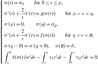
. Clearly, it is the solution of the following problem:
$(\sigma _s,\rho _s,\eta _s,R_s)$
. Clearly, it is the solution of the following problem:
 \begin{equation} \left \{ \begin{array}{l} \sigma (r)=\sigma _D \qquad \mbox{for}\;\; 0\le r\le \rho , \\[4pt]\displaystyle \sigma ''(r)+{\frac 2r}\sigma '(r) = g(\sigma (r)) \qquad \mbox{for}\;\; \rho \lt r\lt \eta , \\[9pt]\sigma '(\rho )=0,\qquad \sigma (\eta )=\sigma _Q, \\[4pt]\displaystyle \sigma ''(r)+{\frac 2r}\sigma '(r) = f(\sigma (r)) \qquad \mbox{for}\;\; \eta \lt r\lt R, \\[9pt]\sigma '(\eta -0)= \sigma '(\eta +0),\quad \sigma (R)=\bar \sigma , \\[4pt]\displaystyle \int _{\eta }^R S(\sigma (r))r^2dr-\int _{\rho }^{\eta }\nu _1 r^2dr-\int _0^{\rho }\nu _2 r^2dr=0. \end{array} \right . \end{equation}
To study the above problem, we first consider a Cauchy problem for any given $\rho \ge 0$
as follows:
$\rho \ge 0$
as follows:
 \begin{equation} \left \{ \begin{array}{l} \displaystyle u''(r)+\frac {2}{r}u'(r) = g(u(r)) \qquad \mbox{for}\;\; r\gt \rho , \\[0.3 cm] u(\rho )=\sigma _D,\qquad u'(\rho )=0. \end{array} \right . \end{equation}
Lemma 2.1.
Under assumption $(A1)$
and
$(A1)$
and $(A3)$
, for any given
$(A3)$
, for any given $\rho \ge 0$
, problem (
2.2
) admits a unique solution
$\rho \ge 0$
, problem (
2.2
) admits a unique solution $u=U_1(r,\rho )\in C^2[\rho ,+\infty )$
with the following properties:
$u=U_1(r,\rho )\in C^2[\rho ,+\infty )$
with the following properties: $(i)$
$(i)$ $\displaystyle {\partial U_1\over \partial r}(r,\rho )\gt 0$
,
$\displaystyle {\partial U_1\over \partial r}(r,\rho )\gt 0$
, $\displaystyle {\partial ^2 U_1\over \partial r^2}(r,\rho )\gt 0$
for
$\displaystyle {\partial ^2 U_1\over \partial r^2}(r,\rho )\gt 0$
for $r\gt \rho$
and
$r\gt \rho$
and $\displaystyle \lim _{r\to +\infty } U_1(r,\rho )=+\infty$
.
$\displaystyle \lim _{r\to +\infty } U_1(r,\rho )=+\infty$
. $(ii)$ $\displaystyle \frac {\partial U_1}{\partial \rho }(r,\rho )\lt 0$
,
$\displaystyle \frac {\partial U_1}{\partial \rho }(r,\rho )\lt 0$
, $\displaystyle \frac {\partial ^2 U_1}{\partial \rho \partial r}(r,\rho )\lt 0$
for
$\displaystyle \frac {\partial ^2 U_1}{\partial \rho \partial r}(r,\rho )\lt 0$
for $r\gt \rho$
,
$r\gt \rho$
, $\rho \gt 0$
.
$\rho \gt 0$
.
Proof. The local existence and uniqueness of solutions to problem (2.2) can be proved by using a Banach fixed point argument, similarly to the proof of Lemma2.2 in [Reference Wu, Xu and Zhuang32]. The global existence is guaranteed by the global Lipschitz continuity of $g$
due to
$g$
due to $(A1)$
. Hence, problem (2.2) has a unique global solution
$(A1)$
. Hence, problem (2.2) has a unique global solution $u = U_1(r, \rho )$
for
$u = U_1(r, \rho )$
for $r\in [\rho ,+\infty )$
. Clearly,
$r\in [\rho ,+\infty )$
. Clearly, $U_1(r, \rho )\ge \sigma _D$
. Then, we have
$U_1(r, \rho )\ge \sigma _D$
. Then, we have $g(U_1(r,\rho ))\ge g(\sigma _D)$
, which together with integrating (2.2) implies
$g(U_1(r,\rho ))\ge g(\sigma _D)$
, which together with integrating (2.2) implies
 \begin{equation} u'(r)=\frac {1}{r^2} \int _{\rho }^r g(U_1(\tau ,\rho ))\tau ^2d\tau \ge g(\sigma _D)\frac {r^3-\rho ^3}{3r^2}\gt 0 \qquad \mbox{for}\;\;r\gt \rho . \end{equation}
Combining $(A1)$
with (2.3), we derive that
$(A1)$
with (2.3), we derive that
 \begin{equation*} \lim \limits _{r\to +\infty }U_1(r,\rho )=\lim \limits _{r\to +\infty }(U_1)_r(r,\rho )=+\infty . \end{equation*}
By $(A1)$
,
$(A1)$
, $(A3)$
, (2.2)
$(A3)$
, (2.2) $_1$
and (2.3), we further get
$_1$
and (2.3), we further get
 \begin{equation} \begin{matrix} \begin{aligned} u''(r) -\displaystyle \frac {u'(r)}{r} &=g(U_1(r,\rho )) -\displaystyle \frac {3}{r^3}\int _{\rho }^r g(U_1(\tau ,\rho ))d\tau \\ &\gt g(U_1(r,\rho ))-\frac {3}{r^3} g(U_1(r,\rho ))\frac {1}{3}(r^3-\rho ^3)\\ &=g(U_1(r,\rho ))\frac {\rho ^3}{r^3}\ge 0. \end{aligned} \end{matrix} \end{equation}
Thus, assertion $(i)$
follows. Finally, we observe that for
$(i)$
follows. Finally, we observe that for $r\gt \rho$
,
$r\gt \rho$
,
 \begin{equation} r^2 (U_1)_r(r,\rho )=\int _\rho ^r g( U_1(\tau ,\rho ))\tau ^2 d\tau . \end{equation}
By $(A1)$
,
$(A1)$
, $(A3)$
, (2.5) and a similar argument with slight modifications of the proof of Lemma2.2
$(A3)$
, (2.5) and a similar argument with slight modifications of the proof of Lemma2.2 $(iii)$
in [Reference Wu, Xu and Zhuang32], we get assertion
$(iii)$
in [Reference Wu, Xu and Zhuang32], we get assertion $(ii)$
.
$(ii)$
.
Note that $\sigma _Q\gt \sigma _D$
, Lemma 2.1 ensures the existence and uniqueness of
$\sigma _Q\gt \sigma _D$
, Lemma 2.1 ensures the existence and uniqueness of $\eta =\eta (\rho )$ $\in (\rho ,+\infty )$
such that
$\in (\rho ,+\infty )$
such that
 \begin{equation} U_1(\eta (\rho ),\rho )=\sigma _Q. \end{equation}
Moreover, $\eta (\rho )$
is continuous and strictly increasing on
$\eta (\rho )$
is continuous and strictly increasing on $[0,+\infty )$
. Let
$[0,+\infty )$
. Let
 \begin{equation} \eta ^*\,:\!=\,\eta (0). \end{equation}
Since $g(\sigma _D)\gt 0$
, we see
$g(\sigma _D)\gt 0$
, we see $\eta ^*\gt 0$
, and
$\eta ^*\gt 0$
, and $\eta ^*$
is the critical radius of the quiescent layer with the necrotic radius
$\eta ^*$
is the critical radius of the quiescent layer with the necrotic radius $\rho =0$
.
$\rho =0$
.
By the strict monotonicity of $\eta =\eta (\rho )$
, we infer that the mapping
$\eta =\eta (\rho )$
, we infer that the mapping $\rho \mapsto \eta (\rho )$
is a 1-1 correspondence from
$\rho \mapsto \eta (\rho )$
is a 1-1 correspondence from $[0,+\infty )$
to
$[0,+\infty )$
to $[\eta ^*,+\infty )$
. For convenience, we rewrite
$[\eta ^*,+\infty )$
. For convenience, we rewrite $\rho =\rho (\eta )$
for
$\rho =\rho (\eta )$
for $\eta \in [\eta ^*,+\infty )$
and denote
$\eta \in [\eta ^*,+\infty )$
and denote
 \begin{equation*} \widetilde U_1(r,\eta )\,:\!=\,U_1(r,\rho (\eta )) \qquad \mbox{for}\;\;\rho (\eta )\le r\le \eta ,\,\eta \geq \eta ^*. \end{equation*}
Then, for any given $\eta \ge \eta ^*$
, the function
$\eta \ge \eta ^*$
, the function $(u(r),\rho )=(\widetilde U_1(r,\eta ),\rho (\eta ))$
uniquely solves (2.1)
$(u(r),\rho )=(\widetilde U_1(r,\eta ),\rho (\eta ))$
uniquely solves (2.1) $_2$
–(2.1)
$_2$
–(2.1) $_3$
.
$_3$
.
Define
 \begin{equation} \Phi (\eta )\,:\!=\,(\widetilde U_1)_r(\eta ,\eta )=\frac {1}{\eta ^2}\int _{\rho (\eta )}^{\eta }g(\widetilde U_1(\tau ,\eta ))\tau ^2d\tau \quad \mbox{for}\;\; \eta \ge \eta ^*. \end{equation}
By $(A1)$
and (2.3), there holds
$(A1)$
and (2.3), there holds
 \begin{equation} 0\lt \Phi (\eta )\lt {1\over 3}g(\sigma _Q)\eta \quad \mbox{for} \;\;\eta \ge \eta ^*. \end{equation}
Moreover, we claim that
 \begin{equation} \Phi '(\eta )\gt 0 \qquad \mbox{for}\;\; \eta \gt \eta ^*. \end{equation}
In fact, by (2.1) $_2$
–(2.1)
$_2$
–(2.1) $_3$
, we see that for any
$_3$
, we see that for any $\eta \gt \eta ^*$
, the function
$\eta \gt \eta ^*$
, the function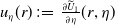 $u_{\eta }(r)\,:\!=\,\frac {\partial \widetilde U_1}{\partial \eta }(r,\eta )$
satisfies the following elliptic problem
$u_{\eta }(r)\,:\!=\,\frac {\partial \widetilde U_1}{\partial \eta }(r,\eta )$
satisfies the following elliptic problem
 \begin{equation} \left \{ \begin{array}{l} \displaystyle (u_{\eta })''+\frac {2}{r}(u_{\eta })' = g'(\widetilde U_1)u_{\eta } \qquad \mbox{for}\;\; \rho \lt r\lt \eta , \\[0.3 cm] u_{\eta }(\rho )=0,\qquad u_{\eta }(\eta )=-(\widetilde U_1)_r(\eta ,\eta )\lt 0, \end{array} \right . \end{equation}
where $\rho =\rho (\eta )$
. Then, by the strong maximum principle,
$\rho =\rho (\eta )$
. Then, by the strong maximum principle,
 \begin{equation} u_\eta (r)=\frac {\partial \widetilde U_1}{\partial \eta }(r,\eta )\lt 0 \qquad \mbox{for} \;\; \rho \lt r\lt \eta . \end{equation}
Moreover, the function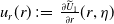 $u_r(r)\,:\!=\,\frac {\partial \widetilde U_1}{\partial r}(r,\eta )$
satisfies
$u_r(r)\,:\!=\,\frac {\partial \widetilde U_1}{\partial r}(r,\eta )$
satisfies
 \begin{equation*} \left \{ \begin{array}{l} \displaystyle (u_r)''+\frac {2}{r}(u_r)' = g'(\widetilde U_1) u_r+\frac {2}{r^2}u_r \qquad \mbox{for}\;\; \rho \lt r\lt \eta , \\[0.3 cm] u_r(\rho )=0,\qquad u_r(\eta )=(\widetilde U_1)_r(\eta ,\eta )\gt 0, \end{array} \right . \end{equation*}
where $\rho =\rho (\eta )$
. Denote
$\rho =\rho (\eta )$
. Denote $w(r)=u_r(r)+u_{\eta }(r)$
. It satisfies
$w(r)=u_r(r)+u_{\eta }(r)$
. It satisfies
 \begin{equation*} \left \{ \begin{array}{l} \displaystyle w''(r)+\frac {2}{r}w'(r)= g'(\widetilde U_1)w(r)+\frac {2}{r^2} u_r \qquad \mbox{for}\;\; \rho \lt r\lt \eta , \\[0.3 cm] w(\rho )=0, \qquad w(\eta )=0. \end{array} \right . \end{equation*}
Note that $g'(\widetilde U_1)\gt 0$
and
$g'(\widetilde U_1)\gt 0$
and $u_r(r)\gt 0$
for
$u_r(r)\gt 0$
for $r\gt \rho$
. Then, by applying the strong maximum principle and Hopf lemma, we obtain
$r\gt \rho$
. Then, by applying the strong maximum principle and Hopf lemma, we obtain
 \begin{equation} w'(\eta ) =(\widetilde U_1)_{rr}(\eta ,\eta )+(\widetilde U_1)_{r\eta }(\eta ,\eta )=\Phi '(\eta )\gt 0. \end{equation}
This proves (2.10).
Next, we proceed to solve problem (2.1) $_4$
–(2.1)
$_4$
–(2.1) $_5$
by considering the following initial value problem:
$_5$
by considering the following initial value problem:
 \begin{equation} \left \{ \begin{array}{l} \displaystyle u''(r)+\frac {2}{r}u'(r) = f(u(r)) \qquad \mbox{for}\;\; r\gt \eta , \\[0.3 cm] u(\eta )=\sigma _Q, \\[0.3 cm] u'(\eta )= \Phi (\eta ). \end{array} \right . \end{equation}
Lemma 2.2.
Under assumptions $(A1)$
and
$(A1)$
and $(A3)$
, for any given
$(A3)$
, for any given $\eta \ge \eta ^*$
, problem (
2.14
) has a unique solution
$\eta \ge \eta ^*$
, problem (
2.14
) has a unique solution $u= U_2(r,\eta )\in C^2\left [\eta , +\infty \right )$
with the following properties:
$u= U_2(r,\eta )\in C^2\left [\eta , +\infty \right )$
with the following properties: $(i)$
$(i)$ $\displaystyle {\partial U_2\over \partial r}(r,\eta )\gt 0$
,
$\displaystyle {\partial U_2\over \partial r}(r,\eta )\gt 0$
, $\displaystyle {\partial ^2 U_2\over \partial r^2}(r,\eta )\gt 0$
for
$\displaystyle {\partial ^2 U_2\over \partial r^2}(r,\eta )\gt 0$
for $r\gt \eta$
and
$r\gt \eta$
and $\displaystyle \lim _{r\to +\infty }U_2(r,\eta )=+\infty$
.
$\displaystyle \lim _{r\to +\infty }U_2(r,\eta )=+\infty$
. $(ii)$ $\displaystyle \frac {\partial U_2}{\partial \eta }(r,\eta )\lt 0$
for
$\displaystyle \frac {\partial U_2}{\partial \eta }(r,\eta )\lt 0$
for $r\gt \eta$
,
$r\gt \eta$
, $\eta \gt \eta ^*$
.
$\eta \gt \eta ^*$
.
Proof. The existence and uniqueness of solutions to problem (2.14) and assertion $(i)$
can be easily verified similarly as Lemma 2.1
$(i)$
can be easily verified similarly as Lemma 2.1 $(i)$
, so we only need to prove assertion
$(i)$
, so we only need to prove assertion $(ii)$
. For any given
$(ii)$
. For any given $\eta \gt \eta ^*$
, define
$\eta \gt \eta ^*$
, define
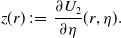 \begin{equation*} z(r)\,:\!=\,\displaystyle \frac {\partial U_2}{\partial \eta }(r,\eta ). \end{equation*}
Then, by (2.8), (2.9) and (2.14), we have
 \begin{equation} \left \{ \begin{array}{l} z''(r)+\displaystyle \frac {2}{r}z'(r)=f'(U_2)z(r)\qquad \mbox{for} \;\; r\gt \eta , \\[0.3cm] z(\eta )=-\Phi (\eta )\lt 0, \\[0.3cm] z'(\eta )=\Phi '(\eta )+\displaystyle \frac {2}{\eta }\Phi (\eta )-f(\sigma _Q), \end{array} \right . \end{equation}
and
 \begin{equation} \Phi '(\eta )=-\frac {2}{\eta }\Phi (\eta )+g(\sigma _Q)+\Psi (\eta ), \end{equation}
where
 \begin{equation*} \Psi (\eta )=-\frac {\rho ^2(\eta )}{\eta ^2}g(\sigma _D)\rho '(\eta )+\frac {1}{\eta ^2}\int _{\rho (\eta )}^{\eta }g'\big (\widetilde U_1(\tau ,\eta )\big )\frac {\partial \widetilde U_1}{\partial \eta }(\tau ,\eta )\tau ^2d\tau . \end{equation*}
From $(A1)$
,
$(A1)$
, $(A3)$
, (2.12) and
$(A3)$
, (2.12) and $\rho '(\eta )\ge 0$
, we have
$\rho '(\eta )\ge 0$
, we have
 \begin{equation} \Psi (\eta )\lt 0 \qquad \mbox{for} \;\; \eta \gt \eta ^*. \end{equation}
Substituting (2.16) into (2.15) $_3$
and using
$_3$
and using $(A3)$
, (2.17), we obtain
$(A3)$
, (2.17), we obtain
 \begin{equation*} z'(\eta )=g(\sigma _Q)-f(\sigma _Q)+\Psi (\eta )\lt 0. \end{equation*}
Thus, by $f'\gt 0$
and (2.15), we easily get
$f'\gt 0$
and (2.15), we easily get
 \begin{equation*} z'(r)\lt 0\quad \mbox{and}\quad z(r) \lt 0 \qquad \mbox{for}\;\; r\gt \eta . \end{equation*}
The proof is complete.
Given $\bar \sigma \gt \sigma _Q$
and
$\bar \sigma \gt \sigma _Q$
and $\eta \ge \eta ^*$
, Lemma 2.2 implies that there exists a unique
$\eta \ge \eta ^*$
, Lemma 2.2 implies that there exists a unique $R=R(\eta ,\bar \sigma )\in (\eta ,+\infty )$
such that
$R=R(\eta ,\bar \sigma )\in (\eta ,+\infty )$
such that
 \begin{equation} U_2(R(\eta ,\bar \sigma ),\eta )=\bar \sigma . \end{equation}
Moreover, we see that $R(\eta ,\bar \sigma )$
is strictly increasing in
$R(\eta ,\bar \sigma )$
is strictly increasing in $\eta$
for any given
$\eta$
for any given $\bar \sigma \gt \sigma _Q$
. Define
$\bar \sigma \gt \sigma _Q$
. Define
 \begin{equation} R^*(\bar \sigma )\,:\!=\, R(\eta ,\bar \sigma )\Big |_{\eta =\eta ^*} \quad \mbox{for}\quad \bar \sigma \gt \sigma _Q. \end{equation}
Clearly, it is the critical radius such that problem (2.1) $_1$
–(2.1)
$_1$
–(2.1) $_5$
has a unique solution satisfying
$_5$
has a unique solution satisfying $\sigma (0)=\sigma _D$
,
$\sigma (0)=\sigma _D$
, $R=R^*(\bar \sigma )$
and
$R=R^*(\bar \sigma )$
and $\eta =\eta ^*$
for
$\eta =\eta ^*$
for $\rho =0$
. Evidently,
$\rho =0$
. Evidently, $R^*(\bar \sigma )\gt \eta ^*\gt 0$
. Similarly, for any fixed
$R^*(\bar \sigma )\gt \eta ^*\gt 0$
. Similarly, for any fixed $\bar \sigma \gt \sigma _Q$
, the mapping
$\bar \sigma \gt \sigma _Q$
, the mapping $\eta \mapsto R(\eta ,\bar \sigma )$
is a 1-1 correspondence from
$\eta \mapsto R(\eta ,\bar \sigma )$
is a 1-1 correspondence from $[\eta ^*,+\infty )$
to
$[\eta ^*,+\infty )$
to $[R^*(\bar \sigma ),+\infty )$
. So we can also regard
$[R^*(\bar \sigma ),+\infty )$
. So we can also regard $\rho$
and
$\rho$
and $\eta$
as functions of
$\eta$
as functions of $R$
and
$R$
and $\bar \sigma$
, i.e.,
$\bar \sigma$
, i.e.,
 \begin{equation*} \rho =\rho (R,\bar \sigma ), \quad \eta =\eta (R,\bar \sigma ) \qquad \mbox{for}\;\; \bar \sigma \gt \sigma _Q,\;R\ge R^*(\bar \sigma ). \end{equation*}
Obviously, we have $\rho (R^*(\bar \sigma ),\bar \sigma )=0$
and
$\rho (R^*(\bar \sigma ),\bar \sigma )=0$
and $\eta (R^*(\bar \sigma ),\bar \sigma )=\eta ^*$
for
$\eta (R^*(\bar \sigma ),\bar \sigma )=\eta ^*$
for $\bar \sigma \gt \sigma _Q$
.
$\bar \sigma \gt \sigma _Q$
.
Rewrite
 \begin{equation*} \widetilde U_2(r, R)=U_2(r, \eta (R,\bar \sigma )) \qquad \mbox{for}\;\; \eta (R)\le r\le R, \; R\ge R^*(\bar \sigma ), \end{equation*}
and denote
 \begin{equation} \Sigma (r,R,\bar \sigma )\,:\!=\,\left \{ \begin{array}{l@{\quad}l} \sigma _D, \qquad &\mbox{for}\;\; 0\le r\le \rho (R,\bar \sigma ), \\[0.3cm] \widetilde {U}_1(r,\eta (R,\bar \sigma )), \qquad &\mbox{for}\;\; \rho (R,\bar \sigma )\lt r\le \eta (R,\bar \sigma ), \\[0.3cm] \widetilde {U}_2(r,R),\qquad & \mbox{for}\;\; \eta (R,\bar \sigma )\lt r\le R. \end{array} \right . \end{equation}
According to Lemmas 2.1 and 2.2, we conclude that for any $\bar \sigma \gt \sigma _Q$
and
$\bar \sigma \gt \sigma _Q$
and $R\ge R^*(\bar \sigma )$
, the triple
$R\ge R^*(\bar \sigma )$
, the triple $(\sigma , \rho , \eta )=(\Sigma (r,R,\bar \sigma ), \rho (R,\bar \sigma ), \eta (R,\bar \sigma ))$
uniquely solves problem (2.1)
$(\sigma , \rho , \eta )=(\Sigma (r,R,\bar \sigma ), \rho (R,\bar \sigma ), \eta (R,\bar \sigma ))$
uniquely solves problem (2.1) $_1$
–(2.1)
$_1$
–(2.1) $_5$
.
$_5$
.
For any $\bar \sigma \gt \sigma _Q$
and
$\bar \sigma \gt \sigma _Q$
and $R\ge R^*(\bar \sigma )$
, define
$R\ge R^*(\bar \sigma )$
, define
 \begin{equation} F(R,\bar \sigma )\,:\!=\,\frac {1}{R^3}\left[\int _{\eta (R,\bar \sigma )}^{R}S(\Sigma (r, R,\bar \sigma ))r^2 dr- \frac {\nu _1}{3}\eta ^3(R,\bar \sigma )-\frac {\nu _2-\nu _1}{3}\rho ^3(R,\bar \sigma )\right]\!. \end{equation}
Then, we have for any $\bar \sigma \gt \sigma _Q$
,
$\bar \sigma \gt \sigma _Q$
,
 \begin{equation} \mbox{problem } (2.1) \mbox{ is equivalent to equation } F(R,\bar \sigma )=0. \end{equation}
Now we study the monotonicity of $F(R,\bar \sigma )$
in
$F(R,\bar \sigma )$
in $R$
for fixed
$R$
for fixed $\bar \sigma \gt \sigma _Q$
. By taking variable transformation
$\bar \sigma \gt \sigma _Q$
. By taking variable transformation $s=r/R$
, we rewrite
$s=r/R$
, we rewrite
 \begin{equation*} \psi (R,\bar \sigma )=\rho (R,\bar \sigma )/R,\qquad \phi (R,\bar \sigma )=\eta (R,\bar \sigma )/R, \qquad \mathcal{V}(s,R,\bar \sigma )=\Sigma (sR,R,\bar \sigma ). \end{equation*}
Consider the following problem
 \begin{equation} \left \{ \begin{array}{l} \displaystyle v''(s)+\frac {2}{s}v'(s) = R^2g(v) \qquad \mbox{for}\;\; \psi \lt s\lt \phi , \\[0.3cm] v(\psi )=\sigma _D, \quad v'(\psi )=0,\quad v(\phi )=\sigma _Q, \\[0.3 cm] \displaystyle v''(s)+\frac {2}{s}v'(s) = R^2f(v) \qquad \mbox{for}\;\; \phi \lt s\lt 1, \\[0.3 cm] v'(\phi +0)=v'(\phi -0)= R\Phi (\phi R), \\[0.3 cm] v(1)=\bar \sigma . \end{array} \right . \end{equation}
We have
Lemma 2.3.
Under assumptions $(A1)$
,
$(A1)$
, $(A3)$
and
$(A3)$
and $\bar \sigma \gt \sigma _Q$
, problem (
2.23
) possesses a unique solution
$\bar \sigma \gt \sigma _Q$
, problem (
2.23
) possesses a unique solution $(v,\psi ,\phi )=(\mathcal{V}(s,R,\bar \sigma ), \psi (R,\bar \sigma ),\phi (R,\bar \sigma ))$
for any
$(v,\psi ,\phi )=(\mathcal{V}(s,R,\bar \sigma ), \psi (R,\bar \sigma ),\phi (R,\bar \sigma ))$
for any $R\ge R^*(\bar \sigma )$
. Furthermore, the solution satisfies:
$R\ge R^*(\bar \sigma )$
. Furthermore, the solution satisfies: $(i)$
$(i)$ $\mathcal{V}(s,R,\bar \sigma )$
is strictly increasing and strictly convex in
$\mathcal{V}(s,R,\bar \sigma )$
is strictly increasing and strictly convex in $s$
.
$s$
. $(ii)$ $\mathcal{V}(s, R,\bar \sigma )$
is strictly decreasing in R.
$\mathcal{V}(s, R,\bar \sigma )$
is strictly decreasing in R. $(iii)$ $\phi (R,\bar \sigma )$
and
$\phi (R,\bar \sigma )$
and $\psi (R,\bar \sigma )$
are both continuous and strictly increasing for
$\psi (R,\bar \sigma )$
are both continuous and strictly increasing for $R\ge R^*(\bar \sigma )$
, and
$R\ge R^*(\bar \sigma )$
, and
 \begin{equation} \psi (R^*(\bar \sigma ),\bar \sigma )=0,\qquad \phi (R^*(\bar \sigma ),\bar \sigma )=\eta ^*/R^*(\bar \sigma ), \end{equation}
 \begin{equation} \lim _{R\to +\infty }\psi (R,\bar \sigma )=\lim \limits _{R\to +\infty }\phi (R,\bar \sigma )=1. \end{equation}
Proof. By taking variable transformation in problem (2.3) ${}_1$
–(2.3)
${}_1$
–(2.3) ${}_5$
, it is easy to verify that
${}_5$
, it is easy to verify that $(v,\psi ,\phi )=(\mathcal{V}(s,R,\bar \sigma ), \psi (R,\bar \sigma ),\phi (R,\bar \sigma ))$
is the unique solution of problem (2.23). The proof of the monotonicity and the convexity of
$(v,\psi ,\phi )=(\mathcal{V}(s,R,\bar \sigma ), \psi (R,\bar \sigma ),\phi (R,\bar \sigma ))$
is the unique solution of problem (2.23). The proof of the monotonicity and the convexity of $\mathcal{V}(s, R,\bar \sigma )$
in
$\mathcal{V}(s, R,\bar \sigma )$
in $s$
is similar to that of Lemma 2.1
$s$
is similar to that of Lemma 2.1 $(i)$
, we omit it here. By the definition (2.7) and (2.19), we easily get (2.24).
$(i)$
, we omit it here. By the definition (2.7) and (2.19), we easily get (2.24).
Next, we show the monotonicity of $\mathcal{V}(s, R,\bar \sigma )$
,
$\mathcal{V}(s, R,\bar \sigma )$
, $\psi (R,\bar \sigma )$
and
$\psi (R,\bar \sigma )$
and $\phi (R,\bar \sigma )$
in
$\phi (R,\bar \sigma )$
in $R$
. Denote
$R$
. Denote
 \begin{equation*} z(s)=\frac {\partial \mathcal{V}}{\partial R}(s,R,\bar \sigma ),\qquad \xi =\frac {\partial \psi (R,\bar \sigma )}{\partial R}, \qquad \zeta =\frac {\partial \phi (R,\bar \sigma )}{\partial R}. \end{equation*}
By the linearization of (2.23), we see $z(s)$
,
$z(s)$
, $\xi$
and
$\xi$
and $\zeta$
satisfy the following problem:
$\zeta$
satisfy the following problem:
 \begin{equation} \left \{ \begin{array}{l} \displaystyle z''(s)+\frac {2}{s}z'(s)=R^2g'(\mathcal{V})z + 2 R g(\mathcal{V}) \qquad \mbox{for}\;\; \psi \lt s\lt \phi , \\[10pt] z(\psi )=0,\quad z'(\psi )=-R^2g(\sigma _D)\xi ,\quad \\[7pt] z'(\phi -0)=\Phi (\phi R)+\phi R\Phi '(\phi R)+\Psi (\phi R)R^2\zeta , \\[7pt] z(\phi )=-R\Phi (\phi R)\zeta , \\[7pt] \displaystyle z''(s)+\frac {2}{s}z'(s)=R^2f'(\mathcal{V})z + 2 R f(\mathcal{V}) \qquad \mbox{for}\;\; \phi \lt s\lt 1, \\[9pt] z'(\phi +0)=\Phi (\phi R)+\phi R\Phi '(\phi R)+\big (g(\sigma _Q)-f(\sigma _Q) +\Psi (\phi R)\big )R^2\zeta , \\[3pt] z(1)=0, \end{array} \right . \end{equation}
where $\phi =\phi (R,\bar \sigma )$
and
$\phi =\phi (R,\bar \sigma )$
and $\psi =\psi (R,\bar \sigma )$
. In fact, by (2.23)
$\psi =\psi (R,\bar \sigma )$
. In fact, by (2.23) $_1$
, (2.23)
$_1$
, (2.23) $_3$
and (2.23)
$_3$
and (2.23) $_4$
, we have
$_4$
, we have
 \begin{equation*} \left \{ \begin{array}{l} v''(\phi -0)=R^2g(\sigma _Q)-\displaystyle \frac {2}{\phi }R\Phi (\phi R), \\[8pt]v''(\phi +0)=R^2f(\sigma _Q)-\displaystyle \frac {2}{\phi }R\Phi (\phi R), \\[8pt]z'(\phi \pm 0)=\Phi (\phi R)+R\Phi '(\phi R)(\zeta R+\phi )-v''(\phi \pm 0)\zeta . \end{array} \right . \end{equation*}
Combining the above relations with (2.16), one can derive (2.26) $_3$
and (2.26)
$_3$
and (2.26) $_6$
, other equations of (2.26) are obvious.
$_6$
, other equations of (2.26) are obvious.
To prove assertions $(ii)$
and
$(ii)$
and $(iii)$
, we use a contradiction argument to show that
$(iii)$
, we use a contradiction argument to show that
 \begin{equation} z(s)=\frac {\partial \mathcal{V}}{\partial R}\lt 0 \quad \mbox{for}\;\; \psi \lt s\lt 1, \quad \xi =\frac {\partial \psi }{\partial R}\gt 0,\quad \zeta =\frac {\partial \phi }{\partial R}\gt 0. \end{equation}
If $\zeta \le 0$
, by
$\zeta \le 0$
, by $(A1)$
,
$(A1)$
, $(A3)$
, (2.9), (2.10), (2.17), (2.26)
$(A3)$
, (2.9), (2.10), (2.17), (2.26) $_4$
and (2.26)
$_4$
and (2.26) $_6$
, we see that
$_6$
, we see that $z(\phi )\ge 0$
and
$z(\phi )\ge 0$
and $z'(\phi +0)\gt 0$
. On the other hand, since
$z'(\phi +0)\gt 0$
. On the other hand, since $f(\mathcal{V})\gt 0$
and
$f(\mathcal{V})\gt 0$
and $f'(\mathcal{V})\gt 0$
, by applying strong maximum principle and Hopf Lemma to (2.26)
$f'(\mathcal{V})\gt 0$
, by applying strong maximum principle and Hopf Lemma to (2.26) $_4$
–(2.26)
$_4$
–(2.26) $_7$
, we get that
$_7$
, we get that $z'(\phi +0)\lt 0$
. This is a contradiction and thus
$z'(\phi +0)\lt 0$
. This is a contradiction and thus $\zeta \gt 0$
; consequently, we have
$\zeta \gt 0$
; consequently, we have $z(\phi )\lt 0$
. Combining (2.26)
$z(\phi )\lt 0$
. Combining (2.26) $_4$
, (2.26)
$_4$
, (2.26) $_5$
, (2.26)
$_5$
, (2.26) $_7$
and strong maximum principle, we have
$_7$
and strong maximum principle, we have $z(s)\lt 0$
for
$z(s)\lt 0$
for $\phi \lt s\lt 1$
. By (2.26)
$\phi \lt s\lt 1$
. By (2.26) $_1$
, (2.26)
$_1$
, (2.26) $_2$
, (2.26)
$_2$
, (2.26) $_4$
,
$_4$
, $g(\mathcal{V})\gt 0$
and
$g(\mathcal{V})\gt 0$
and $g'(\mathcal{V})\gt 0$
, we can apply strong maximum principle again to deduce that
$g'(\mathcal{V})\gt 0$
, we can apply strong maximum principle again to deduce that $z(s)\lt 0$
for
$z(s)\lt 0$
for $\psi \lt s\lt \phi$
. By Hopf lemma, we get that
$\psi \lt s\lt \phi$
. By Hopf lemma, we get that $z'(\psi )\lt 0$
, which implies that
$z'(\psi )\lt 0$
, which implies that $\xi \gt 0$
.
$\xi \gt 0$
.
Finally, from integrating (2.23) $_3$
–(2.23)
$_3$
–(2.23) $_5$
, we have
$_5$
, we have
 \begin{equation*} \frac {\bar {\sigma }-\sigma _Q}{R^2}=\frac {\phi ^2}{R}\left(\frac {1} {\phi }-1\right)\Phi (\phi R) +\int _{\phi }^1\frac {1}{\alpha ^2}\int _{\phi }^{\alpha }s^2f(\mathcal{V}(s,R,\bar \sigma ))dsd\alpha , \end{equation*}
where $\phi =\phi (R,\bar \sigma )$
. If
$\phi =\phi (R,\bar \sigma )$
. If $\lim \limits _{R\to +\infty }\phi (R,\bar \sigma )\in (0,1)$
, a contradiction can be obtained by taking limit
$\lim \limits _{R\to +\infty }\phi (R,\bar \sigma )\in (0,1)$
, a contradiction can be obtained by taking limit $R\to +\infty$
in the above relation with noting that
$R\to +\infty$
in the above relation with noting that $\mathcal{V}\ge \sigma _Q\gt 0$
for
$\mathcal{V}\ge \sigma _Q\gt 0$
for $\phi (R,\bar \sigma )\lt s\lt 1$
and (2.9) hold. Thus,
$\phi (R,\bar \sigma )\lt s\lt 1$
and (2.9) hold. Thus,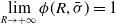 $\displaystyle \lim _{R\to +\infty }\phi (R,\bar \sigma )=1$
.
$\displaystyle \lim _{R\to +\infty }\phi (R,\bar \sigma )=1$
.
By integrating (2.23) $_1$
–(2.23)
$_1$
–(2.23) $_2$
, we also have
$_2$
, we also have
 \begin{equation*} \frac {\sigma _Q-\sigma _D}{R^2}=\int ^{\phi (R,\bar \sigma )}_{\psi (R,\bar \sigma )}\frac {1}{\alpha ^2}\int _{\psi (R,\bar \sigma )}^{\alpha }g(\mathcal{V}(s,R,\bar \sigma ))s^2dsd\alpha . \end{equation*}
Likewise, there holds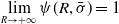 $\displaystyle \lim _{R\to +\infty }\psi (R,\bar \sigma )=1$
.
$\displaystyle \lim _{R\to +\infty }\psi (R,\bar \sigma )=1$
.
With the help of Lemma 2.3, we now study the monotonicity of $F(R,\bar \sigma )$
with respect to
$F(R,\bar \sigma )$
with respect to $R$
. By the variable transformation
$R$
. By the variable transformation $r=sR$
, we rewrite
$r=sR$
, we rewrite
 \begin{equation*} F(R,\bar \sigma ) = \int _{\phi (R,\bar \sigma )}^1 S(\mathcal{V}(s,R,\bar \sigma ))s^2ds-\frac {\nu _1}{3}\phi ^3(R,\bar \sigma )-\frac {\nu _2-\nu _1}{3} \psi ^3(R,\bar \sigma ) \qquad \mbox{for}\;\; R\ge R^*(\bar \sigma ). \end{equation*}
By $(A2)$
,
$(A2)$
, $(A3)$
and (2.27), we see that for any
$(A3)$
and (2.27), we see that for any $\bar \sigma \gt \sigma _Q$
and
$\bar \sigma \gt \sigma _Q$
and $R\gt R^*(\bar \sigma )$
,
$R\gt R^*(\bar \sigma )$
,
 \begin{equation} \frac {\partial F(R,\bar \sigma )}{\partial R}=\int _{\phi (R,\bar \sigma )}^1 S'(\mathcal{V})\frac {\partial \mathcal{V}}{\partial R}s^2ds -(S(\sigma _Q)+\nu _1)\phi ^2\frac {\partial \phi }{\partial R}-(\nu _2-\nu _1)\psi ^2\frac {\partial \psi }{\partial R} \lt 0. \end{equation}
From Lemma 2.3 $(iii)$
, we also have
$(iii)$
, we also have
 \begin{equation} \lim _{R\to +\infty } F(R,\bar \sigma )=-\frac {\nu _2}{3}\lt 0. \end{equation}
Next, we need to determine the sign of $F(R^*(\bar \sigma ),\bar \sigma )$
. Recall
$F(R^*(\bar \sigma ),\bar \sigma )$
. Recall $R^*=R^*(\bar \sigma )$
in (2.19) and denote
$R^*=R^*(\bar \sigma )$
in (2.19) and denote
 \begin{equation*} \phi ^*=\phi ^*(\bar \sigma )\,:\!=\,\eta ^*/R^*(\bar \sigma ), \end{equation*}
where $\eta ^*$
actually does not depend on
$\eta ^*$
actually does not depend on $\bar \sigma$
. We consider the following critical problem, which characterizes the nutrient concentration at the centre of a tumour containing a quiescent core, is exactly
$\bar \sigma$
. We consider the following critical problem, which characterizes the nutrient concentration at the centre of a tumour containing a quiescent core, is exactly $\sigma _D$
:
$\sigma _D$
:
 \begin{equation} \left \{ \begin{array}{l} \displaystyle \sigma ''(r)+\frac {2}{r}\sigma '(r) = g(\sigma ) \qquad \mbox{for}\;\; 0\lt r\lt \eta ^*, \\[10pt]\sigma '(0)=0, \quad \sigma (0)=\sigma _D, \quad \sigma (\eta ^*)=\sigma _Q, \\[5pt]\displaystyle \sigma ''(r)+\frac {2}{r}\sigma '(r) = f(\sigma ) \qquad \mbox{for}\;\; \eta ^*\lt r\lt R^*, \\[10pt]\sigma '(\eta ^*-0)=\sigma '(\eta ^*+0),\quad \sigma (R^*)=\bar \sigma . \end{array} \right . \end{equation}
Denote $ \mathcal{W}(s,\bar \sigma )\,:\!=\,\mathcal{V}(s,R^*(\bar \sigma ),\bar \sigma )$
for
$ \mathcal{W}(s,\bar \sigma )\,:\!=\,\mathcal{V}(s,R^*(\bar \sigma ),\bar \sigma )$
for $0\lt s\lt 1$
. Then,
$0\lt s\lt 1$
. Then, $(\mathcal{W}, \phi ^*,R^*)$
satisfies
$(\mathcal{W}, \phi ^*,R^*)$
satisfies
 \begin{equation} \left \{ \begin{array}{l} \displaystyle W''(s)+\frac {2}{s}W'(s) = (R^*)^2g(W) \qquad \mbox{for}\;\; 0\lt s\lt \phi ^*, \\[9pt]W'(0)=0, \quad W(0)=\sigma _D, \quad W(\phi ^*)=\sigma _Q, \\[5pt]\displaystyle W''(s)+\frac {2}{s}W'(s) = (R^*)^2f(W) \qquad \mbox{for}\;\; \phi ^*\lt s\lt 1, \\[10pt]W'(\phi ^*-0)=W'(\phi ^*+0)=R^*\Phi (\phi ^*R^*), \\[9pt]W(1)=\bar \sigma . \end{array} \right . \end{equation}
Moreover, we have the following result.
Lemma 2.4.
Under assumptions $(A1)$
–
$(A1)$
– $(A3)$
and
$(A3)$
and $\bar \sigma \gt \sigma _Q$
, problem (
2.31
) possesses a unique solution
$\bar \sigma \gt \sigma _Q$
, problem (
2.31
) possesses a unique solution $(\mathcal{W},\phi ^*,R^*)$
satisfying the following properties:
$(\mathcal{W},\phi ^*,R^*)$
satisfying the following properties: $(i)$
$(i)$ $\mathcal{W}(s,\bar \sigma )$
and
$\mathcal{W}(s,\bar \sigma )$
and $R^*(\bar \sigma )$
are both strictly increasing in
$R^*(\bar \sigma )$
are both strictly increasing in $\bar \sigma$
, and
$\bar \sigma$
, and $\phi ^*(\bar \sigma )$
is strictly decreasing in
$\phi ^*(\bar \sigma )$
is strictly decreasing in $\bar \sigma$
, i.e.,
$\bar \sigma$
, i.e.,
 \begin{equation} \frac {\partial \mathcal{W}}{\partial \bar \sigma }(s,\bar \sigma )\gt 0\quad \mbox{for}\;\; s\in (0,1), \qquad \frac {d\phi ^*}{d\bar \sigma }(\bar \sigma )\lt 0,\qquad \frac {dR^*}{d\bar \sigma }(\bar \sigma )\gt 0. \end{equation}
Moreover,
 \begin{equation} \lim \limits _{\bar \sigma \to +\infty }R^*(\bar \sigma )=+\infty , \qquad \lim \limits _{\bar \sigma \to \infty }\phi ^*(\bar \sigma )=0. \end{equation} $(ii)$
The function
$(ii)$
The function
 \begin{equation*} \displaystyle \mathcal G(\bar \sigma )\,:\!=\,F(R^*(\bar \sigma ),\bar \sigma ) =\int _{\phi ^*(\bar \sigma )}^1 S(\mathcal{W}(s,\bar \sigma ))s^2ds- \frac {\nu _1}{3}(\phi ^*(\bar \sigma ))^3 \end{equation*}
is strictly increasing for $\bar \sigma \gt \sigma _Q$
.
$\bar \sigma \gt \sigma _Q$
.
Proof. The uniqueness of the solution is trivial. Note that
 \begin{equation*}\displaystyle \Phi (\eta ^*)=\frac {1}{(\eta ^*)^2}\int _0^{\eta ^*} g(\widetilde {U}_1(\tau ,\eta ^*))\tau ^2d\tau \qquad \mbox{for}\;\; \eta ^*\gt 0. \end{equation*}
From (2.6) and (2.7), we obtain that $\eta ^*=\phi ^*(\bar \sigma )R^*(\bar \sigma )$
is determined only by the parameters
$\eta ^*=\phi ^*(\bar \sigma )R^*(\bar \sigma )$
is determined only by the parameters $\sigma _Q$
and
$\sigma _Q$
and $\sigma _D$
. Consequently,
$\sigma _D$
. Consequently, $\Phi (\eta ^*)$
is independent of
$\Phi (\eta ^*)$
is independent of $\bar \sigma$
, resulting in
$\bar \sigma$
, resulting in
 \begin{equation} \frac {\partial \Phi }{\partial \bar \sigma }(\eta ^*)=0. \end{equation}
From (2.18), we have
 \begin{equation} U_2(R^*(\bar \sigma ),\eta ^*)=\bar \sigma . \end{equation}
By differentiating (2.35) with respect to $\bar \sigma$
and Lemma 2.2
$\bar \sigma$
and Lemma 2.2 $(i)$
, we have
$(i)$
, we have
 \begin{equation} \frac {dR^*}{d\bar \sigma } (\bar \sigma )=\frac {1}{(U_2)_r(R^*(\bar \sigma ),\eta ^*)}\gt 0. \end{equation}
Using Lemma 2.2 $(i)$
, the property that
$(i)$
, the property that $R^* (\bar \sigma )$
is strictly increasing in
$R^* (\bar \sigma )$
is strictly increasing in $\bar \sigma$
and (2.35), we easily obtain
$\bar \sigma$
and (2.35), we easily obtain
 \begin{equation} \displaystyle \lim \limits _{\bar \sigma \to +\infty }R^*(\bar \sigma )=+\infty . \end{equation}
For $\bar \sigma \gt \sigma _Q$
, denote
$\bar \sigma \gt \sigma _Q$
, denote
 \begin{equation*}\displaystyle z(s)\,:\!=\,\frac {\partial \mathcal{W}}{\partial \bar \sigma }(s,\bar \sigma ),\quad \bar \zeta \,:\!=\,\frac {dR^*}{d\bar \sigma } (\bar \sigma ),\quad \bar \xi \,:\!=\,\frac {d\phi ^*}{d\bar \sigma }(\bar \sigma ). \end{equation*}
By differentiating $R^*(\bar \sigma )\phi ^*(\bar \sigma )=\eta ^*$
with respect to
$R^*(\bar \sigma )\phi ^*(\bar \sigma )=\eta ^*$
with respect to $\bar \sigma$
, using (2.36) and the fact that
$\bar \sigma$
, using (2.36) and the fact that $\eta ^*$
is independent of
$\eta ^*$
is independent of $\bar \sigma$
, we have
$\bar \sigma$
, we have
 \begin{equation} \bar \xi =-\frac {\eta ^*}{(R^*(\bar \sigma ))^2}\bar \zeta \lt 0. \end{equation}
Thus, $\phi ^*(\bar \sigma )$
is strictly decreasing in
$\phi ^*(\bar \sigma )$
is strictly decreasing in $\bar \sigma$
and due to (2.37),
$\bar \sigma$
and due to (2.37),
 \begin{equation} \lim \limits _{\bar \sigma \to +\infty }\phi ^*(\bar \sigma )=0. \end{equation}
With (2.31) and (2.34), one can verify that there holds
 \begin{equation} \left \{ \begin{array}{l} \displaystyle z''(s)+\frac {2}{s}z'(s)=(R^*)^2g'(\mathcal{W})z+2 R^* \bar \zeta g(\mathcal{W}) \qquad \mbox{for}\;\; 0\lt s\lt \phi ^*, \\[0.3cm] z'(0)=0,\qquad z(0)=0, \qquad z(\phi ^*)=-R^*\Phi (\phi ^*R^*)\bar \xi , \\[0.1cm] z'(\phi ^*-0)=\bar \zeta \Phi (\phi ^*R^*)+\bar \xi \left(\displaystyle \frac {2}{\phi ^*}R^*\Phi (\phi ^*R^*)-(R^*)^2g(\sigma _Q)\right)\!, \\[0.3cm] \displaystyle z''(s)+\frac {2}{s}z'(s)= (R^*)^2f'(\mathcal{W})z+2 R^*\bar \zeta f(\mathcal{W}) \qquad \mbox{for}\;\; \phi ^*\lt s\lt 1, \\[0.3 cm] z'(\phi ^*+0)=\bar \zeta \Phi (\phi ^*R^*)+\bar \xi \left(\displaystyle \frac {2}{\phi ^*}R^*\Phi (\phi ^*R^*)-(R^*)^2f(\sigma _Q)\right)\!, \\[0.3cm] z(1)=1.\qquad \end{array} \right . \end{equation}
In fact, from (2.31) $_1$
, (2.31)
$_1$
, (2.31) $_3$
and (2.31)
$_3$
and (2.31) $_4$
, we have
$_4$
, we have
 \begin{equation*} \left \{ \begin{array}{l} W''(\phi ^*-0)=(R^*)^2g(\sigma _Q)-\displaystyle \frac {2}{\phi ^*}R^*\Phi (\phi ^*R^*), \\[0.3cm] W''(\phi ^*+0)=(R^*)^2f(\sigma _Q)-\displaystyle \frac {2}{\phi ^*}R^*\Phi (\phi ^*R^*), \\[0.3cm] z'(\phi ^*\pm 0)=\bar \zeta \Phi (\phi ^*R^*)+R^*\partial _{\bar \sigma }(\Phi (\phi ^*R^*))-\bar \xi W''(\phi ^*\pm 0). \end{array} \right . \end{equation*}
Then from (2.31) $_4$
and (2.34), we get (2.40)
$_4$
and (2.34), we get (2.40) $_3$
and (2.40)
$_3$
and (2.40) $_5$
. Similarly, the others of (2.40) can be checked.
$_5$
. Similarly, the others of (2.40) can be checked.
Based on a standard contradiction argument and maximum principle, we show that
 \begin{equation} z(s)=\frac {\partial \mathcal{W}}{\partial \bar \sigma }(s,\bar \sigma )\gt 0\quad \mbox{for} \;\; 0\lt s\lt 1. \end{equation}
We first prove that $z(s)\gt 0$
for
$z(s)\gt 0$
for $s\in (0,\phi ^*)$
. By (2.40)
$s\in (0,\phi ^*)$
. By (2.40) $_1$
–(2.40)
$_1$
–(2.40) $_2$
, we obtain
$_2$
, we obtain
 \begin{equation*} 3z''(0)=2R^*(\bar \sigma )g(\sigma _D)\bar \zeta \gt 0. \end{equation*}
If there exists a $s_0\in (0,\phi ^*)$
such that
$s_0\in (0,\phi ^*)$
such that $z(s_0)\le 0$
, then
$z(s_0)\le 0$
, then $z(s)$
must attain a positive maximum in
$z(s)$
must attain a positive maximum in $(0,s_0)$
, which contradicts (2.40)
$(0,s_0)$
, which contradicts (2.40) $_1$
. Therefore,
$_1$
. Therefore,
 \begin{equation*} z(s)=\frac {\partial \mathcal{W}}{\partial \bar \sigma }(s,\bar \sigma )\gt 0 \quad \mbox{for} \;\; 0\lt s\lt \phi ^*. \end{equation*}
By (2.9) and assumption $(A3)$
, we have
$(A3)$
, we have
 \begin{equation} \displaystyle \frac {2}{\phi ^*}R^*\Phi (\phi ^*R^*)-(R^*)^2f(\sigma _Q)\le \frac {2}{3}(R^*)^2g(\sigma _Q)-(R^*)^2f(\sigma _Q)\lt 0. \end{equation}
With (2.9), $\bar \xi \lt 0$
,
$\bar \xi \lt 0$
, $\bar \zeta \gt 0$
and (2.42), there hold
$\bar \zeta \gt 0$
and (2.42), there hold
 \begin{equation*} z(\phi ^*)\gt 0,\qquad z'(\phi ^*+0)\gt 0,\qquad z(1)=1. \end{equation*}
If there exists some $s_1\in (\phi ^*,1)$
such that
$s_1\in (\phi ^*,1)$
such that $z(s_1)\le 0$
, then
$z(s_1)\le 0$
, then $z(s)$
attains a positive maximum in the interval
$z(s)$
attains a positive maximum in the interval $(\phi ^*,s_1)$
. Combining (2.40)
$(\phi ^*,s_1)$
. Combining (2.40) $_4$
, there is a contradiction, which implies that
$_4$
, there is a contradiction, which implies that $z(s)\gt 0$
for
$z(s)\gt 0$
for $s\in (\phi ^*,1)$
. This completes the proof of the assertion
$s\in (\phi ^*,1)$
. This completes the proof of the assertion $(i)$
.
$(i)$
.
According to (2.38), (2.41), $(A2)$
and
$(A2)$
and $(A3)$
, we have
$(A3)$
, we have
 \begin{equation*} \mathcal{G}'(\bar \sigma )=\int _{\phi ^*}^1 S'(\mathcal{W})z(s)s^2ds-(S(\sigma _Q)+\nu _1)(\phi ^*)^2\bar \xi \gt 0 \qquad \mbox{for}\;\; \bar \sigma \gt \sigma _Q. \end{equation*}
We get assertion $(ii)$
. The proof is complete.
$(ii)$
. The proof is complete.
Lemma 2.5.
Let $\bar \sigma \gt \sigma _Q$
. Under assumptions
$\bar \sigma \gt \sigma _Q$
. Under assumptions $(A1)$
–
$(A1)$
– $(A3)$
, there exists a critical nutrient value
$(A3)$
, there exists a critical nutrient value $\sigma ^{*} \in (\tilde {\sigma }, +\infty )$
such that equation
$\sigma ^{*} \in (\tilde {\sigma }, +\infty )$
such that equation $F(R, \bar {\sigma }) = 0$
has a unique root
$F(R, \bar {\sigma }) = 0$
has a unique root $R_{s}=R_s(\bar \sigma ) \in (R^{*}(\bar {\sigma }), +\infty )$
if and only if
$R_{s}=R_s(\bar \sigma ) \in (R^{*}(\bar {\sigma }), +\infty )$
if and only if $\bar {\sigma } \gt \sigma ^{*}$
.
$\bar {\sigma } \gt \sigma ^{*}$
.
Proof. From Lemma 2.3, we see that for any given $\bar \sigma \gt \sigma _Q$
,
$\bar \sigma \gt \sigma _Q$
,
 \begin{equation*} \sigma _Q\lt \mathcal{W}(s,\bar \sigma )\lt \bar \sigma \quad \mbox{for}\;\;\phi ^*\lt s\lt 1, \end{equation*}
which with $(A2)$
and
$(A2)$
and $(A3)$
implies that
$(A3)$
implies that $\mathcal G(\tilde \sigma )\lt g(\tilde \sigma )=0$
. Moreover, by (2.37), the definition of
$\mathcal G(\tilde \sigma )\lt g(\tilde \sigma )=0$
. Moreover, by (2.37), the definition of $\mathcal{G}$
in Lemma 2.4
$\mathcal{G}$
in Lemma 2.4 $(ii)$
and variable transformation, we find
$(ii)$
and variable transformation, we find
 \begin{equation*} \lim \limits _{\bar \sigma \to +\infty }\big (R^*(\bar \sigma )\big )^3\mathcal{G}(\bar \sigma )=\lim \limits _{R^*\to +\infty }\left(\int _{\eta ^*}^{R^*}S(U_2(r,\eta ^*))r^2dr-\frac {\nu _1}{3}(\eta ^*)^3\right), \end{equation*}
which, combined with $(A2)$
, implies that
$(A2)$
, implies that $\mathcal G(+\infty )\gt 0$
. Thus, there exists a unique
$\mathcal G(+\infty )\gt 0$
. Thus, there exists a unique $\sigma ^*\gt \tilde \sigma$
such that
$\sigma ^*\gt \tilde \sigma$
such that
 \begin{equation} F(R^*(\bar \sigma ),\bar \sigma )=\mathcal G(\bar \sigma ) \left \{ \begin{array}{ll} \gt 0,\qquad \mbox{for}\;\; \bar \sigma \gt \sigma ^*, \\ =0, \qquad \mbox{for}\;\; \bar \sigma =\sigma ^*, \\ \lt 0,\qquad \mbox{for}\;\; \sigma _Q\lt \bar \sigma \lt \sigma ^*. \end{array} \right . \end{equation}
By (2.28), (2.29) and (2.43), we conclude that for $\bar \sigma \gt \sigma _Q$
, the equation
$\bar \sigma \gt \sigma _Q$
, the equation $F(R,\bar \sigma )=0$
has a unique solution
$F(R,\bar \sigma )=0$
has a unique solution $R_s\in ( R^*(\bar \sigma ),+\infty )$
if and only if
$R_s\in ( R^*(\bar \sigma ),+\infty )$
if and only if $\bar \sigma \gt \sigma ^*$
.
$\bar \sigma \gt \sigma ^*$
.
Since problem (2.1) is equivalent to equation $F(R,\bar \sigma )=0$
, Lemma2.5 implies that there exists a unique three-layer stationary solution
$F(R,\bar \sigma )=0$
, Lemma2.5 implies that there exists a unique three-layer stationary solution $(\sigma _s, \rho _s, \eta _s, R_s)$
of problem (1.1)–(1.4) if and only if
$(\sigma _s, \rho _s, \eta _s, R_s)$
of problem (1.1)–(1.4) if and only if $\bar \sigma \gt \sigma ^*$
, where
$\bar \sigma \gt \sigma ^*$
, where $R_s$
is the root of
$R_s$
is the root of $F(R,\bar \sigma )=0$
with
$F(R,\bar \sigma )=0$
with $R_s\gt R^*(\bar \sigma )$
.
$R_s\gt R^*(\bar \sigma )$
.
By the above analysis, for $\bar \sigma \gt \sigma _Q$
, we see in case
$\bar \sigma \gt \sigma _Q$
, we see in case $R\lt R^*(\bar \sigma )$
, the tumour will no longer have three-layer structure. From
$R\lt R^*(\bar \sigma )$
, the tumour will no longer have three-layer structure. From $(A1)$
,
$(A1)$
, $(A3)$
and the maximum principle, the nutrient concentration
$(A3)$
and the maximum principle, the nutrient concentration $\sigma (r)$
attains the minimum at the tumour centre. In this case, the tumour may contain a quiescent core
$\sigma (r)$
attains the minimum at the tumour centre. In this case, the tumour may contain a quiescent core $\{r\lt \eta \}$
and a proliferating shell
$\{r\lt \eta \}$
and a proliferating shell $\{\eta \lt r\lt R\}$
or consist of only proliferating cells.
$\{\eta \lt r\lt R\}$
or consist of only proliferating cells.
Denote the corresponding two-layer stationary solution of problem (1.1)–(1.4) by $(\sigma _s,\eta _s,R_s)$
. Clearly, it satisfies the following problem:
$(\sigma _s,\eta _s,R_s)$
. Clearly, it satisfies the following problem:
 \begin{equation} \left \{ \begin{array}{l} \displaystyle \sigma ''(r)+\frac {2}{r}\sigma '(r) = g(\sigma ) \qquad \mbox{for}\;\; 0\lt r\lt \eta , \\[0.3 cm]\sigma '(0)=0, \quad \sigma (0)\ge \sigma _D, \quad \sigma (\eta )=\sigma _Q, \\[0.1cm]\displaystyle \sigma ''(r)+\frac {2}{r}\sigma '(r) = f(\sigma ) \qquad \mbox{for}\;\; \eta \lt r\lt R, \\[0.3 cm]\sigma '(\eta -0)=\sigma '(\eta +0),\quad \sigma (R)=\bar \sigma , \\[0.1cm]\displaystyle \int _{\eta }^R S(\sigma (r))r^2dr-\int _0^\eta \nu _1r^2dr=0. \end{array} \right . \end{equation}
We also denote the one-layer stationary solution by $(\sigma _s,R_s)$
, which satisfies
$(\sigma _s,R_s)$
, which satisfies
 \begin{equation} \left \{ \begin{array}{l} \displaystyle \sigma ''(r)+\frac {2}{r}\sigma '(r) = f(\sigma ) \qquad \mbox{for}\;\; 0\lt r\lt R, \\[0.3 cm] \sigma '(0)=0, \quad \sigma (0)\ge \sigma _Q, \quad \sigma (R)=\bar \sigma , \\[0.3 cm] \displaystyle \int _0^R S(\sigma (r))r^2dr=0. \end{array} \right . \end{equation}
The above two-layer problem (2.44) and one-layer problem (2.45) without the constraints on $\sigma (0)$
have been well studied in [Reference Cui5, Reference Wu, Xu and Zhuang32], where
$\sigma (0)$
have been well studied in [Reference Cui5, Reference Wu, Xu and Zhuang32], where $f(\sigma _0)=g(\sigma _0)=0$
for some
$f(\sigma _0)=g(\sigma _0)=0$
for some $\sigma _0\ge 0$
. Recalling (2.6)–(2.7), (2.18) and (2.19), for any given
$\sigma _0\ge 0$
. Recalling (2.6)–(2.7), (2.18) and (2.19), for any given $\bar \sigma \gt \sigma _Q$
, we know that
$\bar \sigma \gt \sigma _Q$
, we know that $R^*=R^*(\bar \sigma )$
is a threshold radius for the two-layer tumour structure with
$R^*=R^*(\bar \sigma )$
is a threshold radius for the two-layer tumour structure with $\sigma (0)=\sigma _D$
. Similarly, by analyzing the problem (2.44)
$\sigma (0)=\sigma _D$
. Similarly, by analyzing the problem (2.44) $_1$
–(2.44)
$_1$
–(2.44) $_4$
, we can also prove that there exists another critical tumour radius
$_4$
, we can also prove that there exists another critical tumour radius $R_*=R_*(\bar \sigma )$
corresponding to the one-layer tumour with only proliferating cells and
$R_*=R_*(\bar \sigma )$
corresponding to the one-layer tumour with only proliferating cells and $\sigma (0)=\sigma _Q$
.
$\sigma (0)=\sigma _Q$
.
More precisely, we have the following result.
Lemma 2.6.
Under assumption $(A1)$
,
$(A1)$
, $(A3)$
and
$(A3)$
and $\bar \sigma \gt \sigma _Q$
, there exists a unique critical radius
$\bar \sigma \gt \sigma _Q$
, there exists a unique critical radius $R_*=R_*(\bar \sigma )\in (0,R^*(\bar \sigma ))$
, which is strictly increasing in
$R_*=R_*(\bar \sigma )\in (0,R^*(\bar \sigma ))$
, which is strictly increasing in $\bar \sigma$
such that
$\bar \sigma$
such that $(i)$
For any
$(i)$
For any $R\in (R_*(\bar \sigma ),R^*(\bar \sigma )]$
, there exists a unique solution
$R\in (R_*(\bar \sigma ),R^*(\bar \sigma )]$
, there exists a unique solution $(\Sigma _1(r,R,\bar \sigma ),\eta (R,\bar \sigma ))$
of problem (
2.44
)
$(\Sigma _1(r,R,\bar \sigma ),\eta (R,\bar \sigma ))$
of problem (
2.44
) $_1$
–(
2.44
)
$_1$
–(
2.44
) $_4$
.
$_4$
. $(ii)$
For any
$(ii)$
For any $R\in (0,R_*(\bar \sigma )]$
, there exists a unique solution
$R\in (0,R_*(\bar \sigma )]$
, there exists a unique solution $\Sigma _2(r,R,\bar \sigma )$
of problem (
2.45
)
$\Sigma _2(r,R,\bar \sigma )$
of problem (
2.45
) $_1$
–(
2.45
)
$_1$
–(
2.45
) $_2$
.
$_2$
.
Proof. For any given $\eta \in (0,\eta ^*)$
, we consider
$\eta \in (0,\eta ^*)$
, we consider
 \begin{equation} \left \{ \begin{array}{l} \displaystyle u''(r)+\frac {2}{r}u'(r) = g(u(r)) \qquad \mbox{for}\;\; 0\lt r\lt \eta , \\[0.3 cm] u'(0)=0,\qquad u(\eta )=\sigma _Q. \end{array} \right . \end{equation}
From (2.6)–(2.7) and Lemma 2.1, $U_1(r,0)$
satisfies problem (2.2),
$U_1(r,0)$
satisfies problem (2.2), $U_1(\eta ^*,0)=\sigma _Q$
and
$U_1(\eta ^*,0)=\sigma _Q$
and $\sigma _D\le U_1(r,0)\lt \sigma _Q$
for
$\sigma _D\le U_1(r,0)\lt \sigma _Q$
for $0\le r\lt \eta ^*$
. It follows that
$0\le r\lt \eta ^*$
. It follows that $\sigma _Q$
and
$\sigma _Q$
and $U_1(r,0)$
are a pair of upper and lower solutions to problem (2.46). Hence by the upper and lower solution method, problem (2.46) has a unique solution
$U_1(r,0)$
are a pair of upper and lower solutions to problem (2.46). Hence by the upper and lower solution method, problem (2.46) has a unique solution $u=U_3(r,\eta )$
with
$u=U_3(r,\eta )$
with $\sigma _D\le U_3(r,\eta )\le \sigma _Q$
for
$\sigma _D\le U_3(r,\eta )\le \sigma _Q$
for $r\in [0,\eta ]$
. From
$r\in [0,\eta ]$
. From $(A1)$
, we see
$(A1)$
, we see $u=U_3(r,\eta )$
is strictly increasing in
$u=U_3(r,\eta )$
is strictly increasing in $r$
for any
$r$
for any $\eta \in (0,\eta ^*)$
. Rewrite
$\eta \in (0,\eta ^*)$
. Rewrite $U_3(r,\eta ^*)=U_1(r,0)$
. We conclude that for every
$U_3(r,\eta ^*)=U_1(r,0)$
. We conclude that for every $\eta \in (0,\eta ^*]$
, problem (2.44)
$\eta \in (0,\eta ^*]$
, problem (2.44) $_1$
–(2.44)
$_1$
–(2.44) $_2$
has a unique solution
$_2$
has a unique solution $u=U_3(r,\eta )$
for
$u=U_3(r,\eta )$
for $0\le r\le \eta$
. Define
$0\le r\le \eta$
. Define
 \begin{equation*} \widetilde \Phi (\eta )\,:\!=\,(U_3)_r(\eta ,\eta )=\frac {1}{\eta ^2}\int _0^\eta g(U_3(\tau ,\eta ))\tau ^2d\tau \qquad \mbox{for}\;\; 0\lt \eta \le \eta ^*. \end{equation*}
Note that $U_3(r,\eta )$
is strictly decreasing in
$U_3(r,\eta )$
is strictly decreasing in $\eta$
for
$\eta$
for $0\lt \eta \le \eta ^*$
, similarly as (2.10) we have (cf. Lemma2.1 in [Reference Wu, Xu and Zhuang32])
$0\lt \eta \le \eta ^*$
, similarly as (2.10) we have (cf. Lemma2.1 in [Reference Wu, Xu and Zhuang32])
 \begin{equation} 0\lt \widetilde \Phi (\eta )\lt \frac {1}{3}g(\sigma _Q)\eta \quad \mbox{and} \quad \widetilde \Phi '(\eta )\gt 0\quad \text{for} \;\; 0\lt \eta \le \eta ^*. \end{equation}
By (2.47) and continuity, we set $\widetilde \Phi (0)=0$
. To solve problem (2.44)
$\widetilde \Phi (0)=0$
. To solve problem (2.44) $_3$
–(2.44)
$_3$
–(2.44) $_4$
, we next consider the following initial value problem for given
$_4$
, we next consider the following initial value problem for given $\eta \in [0,\eta ^*]$
:
$\eta \in [0,\eta ^*]$
:
 \begin{equation*} \left \{ \begin{array}{l} u''(r)+\displaystyle \frac {2}{r}u'(r)=f(u(r))\qquad \mbox{for} \;\; r\gt \eta , \\[0.3cm] u(\eta )=\sigma _Q, \qquad u'(\eta )=\widetilde \Phi (\eta ). \end{array} \right . \end{equation*}
From the proof of Lemma 2.2, we easily see this problem admits a unique solution $u(r)=U_4(r,\eta )$
on
$u(r)=U_4(r,\eta )$
on $[\eta ,+\infty )$
strictly increasing in
$[\eta ,+\infty )$
strictly increasing in $r$
and decreasing in
$r$
and decreasing in $\eta$
with
$\eta$
with
 \begin{equation} \lim \limits _{r\to +\infty }U_4(r,\eta )=+\infty \quad \mbox{for}\;\; 0\le \eta \le \eta ^*, \end{equation}
For any given $\bar \sigma \gt \sigma _Q$
and
$\bar \sigma \gt \sigma _Q$
and $0\le \eta \le \eta ^*$
, there thus exists a unique
$0\le \eta \le \eta ^*$
, there thus exists a unique $R(\eta ,\bar \sigma )\gt 0$
such that
$R(\eta ,\bar \sigma )\gt 0$
such that
 \begin{equation} U_4(R(\eta ,\bar \sigma ),\eta )=\bar \sigma . \end{equation}
From the monotonicity of $U_4(r,\eta )$
, we can obtain that
$U_4(r,\eta )$
, we can obtain that $R(\eta ,\bar \sigma )$
is strictly increasing in
$R(\eta ,\bar \sigma )$
is strictly increasing in $\eta$
for
$\eta$
for $0\le \eta \le \eta ^*$
. Define
$0\le \eta \le \eta ^*$
. Define
 \begin{equation} R_*(\bar \sigma )=R(\eta ,\bar \sigma )\Big |_{\eta =0}, \end{equation}
which is the critical radius such that problem (2.45) $_1$
–(2.45)
$_1$
–(2.45) $_2$
has a unique solution
$_2$
has a unique solution $\sigma (r)$
satisfying
$\sigma (r)$
satisfying $\sigma (0)=\sigma _Q$
. Utilizing (2.19) and the monotonicity of
$\sigma (0)=\sigma _Q$
. Utilizing (2.19) and the monotonicity of $R(\eta ,\bar \sigma )$
in
$R(\eta ,\bar \sigma )$
in $\eta$
for
$\eta$
for $0\le \eta \le \eta ^*$
, we have
$0\le \eta \le \eta ^*$
, we have
 \begin{equation} R^*(\bar \sigma )=R(\eta ^*,\bar \sigma )\gt R(\eta ,\bar \sigma )\Big |_{\eta =0}=R_*(\bar \sigma ). \end{equation}
Similarly, by regarding $R$
and
$R$
and $\bar \sigma$
as the variables and letting
$\bar \sigma$
as the variables and letting
 \begin{equation*} \eta =\eta (R,\bar \sigma ),\quad \widetilde U_3(r,R,\bar \sigma )=U_3(r,\eta (R,\bar \sigma )),\quad \widetilde U_4(r,R,\bar \sigma )=U_4(r,\eta (R,\bar \sigma )), \end{equation*}
 \begin{equation*} \Sigma _1(r,R,\bar \sigma )=\left \{ \begin{array}{l} \widetilde U_3(r,R,\bar \sigma ) \quad \mbox{for}\;\; 0\le r\le \eta (R,\bar \sigma ), \\[0.3cm] \widetilde U_4(r,R,\bar \sigma ) \quad \mbox{for}\;\; \eta (R,\bar \sigma )\lt r\le R, \end{array} \right . \end{equation*}
we see $(\Sigma _1(r,R,\bar \sigma ),\eta (R,\bar \sigma ))$
solves problem (2.44)
$(\Sigma _1(r,R,\bar \sigma ),\eta (R,\bar \sigma ))$
solves problem (2.44) $_1$
–(2.44)
$_1$
–(2.44) $_4$
for
$_4$
for $\bar \sigma \gt \sigma _Q$
and
$\bar \sigma \gt \sigma _Q$
and $R\in (R_*(\bar \sigma ),R^*(\bar \sigma )]$
. The proof of
$R\in (R_*(\bar \sigma ),R^*(\bar \sigma )]$
. The proof of $R_*'(\bar \sigma )\gt 0$
is similar to that of (2.19) in [Reference Wu, Xu and Zhuang32]. Hence, we obtain assertion
$R_*'(\bar \sigma )\gt 0$
is similar to that of (2.19) in [Reference Wu, Xu and Zhuang32]. Hence, we obtain assertion $(i)$
.
$(i)$
.
The proof of assertion $(ii)$
is similar and simpler; we omit it here. The proof is complete.
$(ii)$
is similar and simpler; we omit it here. The proof is complete.
Now for any $\bar \sigma \gt \sigma _Q$
, we extend the definition of
$\bar \sigma \gt \sigma _Q$
, we extend the definition of $F(R,\bar \sigma )$
in (2.21) as follows:
$F(R,\bar \sigma )$
in (2.21) as follows:
 \begin{equation} F(R,\bar \sigma )\,:\!=\,\left \{ \begin{array}{lll} \displaystyle \frac {1}{R^3}\left[\int _{\eta (R,\bar \sigma )}^{R} S(\Sigma (r, R,\bar \sigma ))r^2 dr- \frac {\nu _1}{3}\eta ^3(R,\bar \sigma )-\frac {\nu _2-\nu _1}{3}\rho ^3(R,\bar \sigma )\right]\!, \\[0.4cm] \,\,\qquad \qquad \qquad \qquad \qquad \qquad \qquad \qquad \qquad \;\;\; \mbox{for}\;\; R\in (R^*(\bar \sigma ),+\infty ), \\[0.1cm] \displaystyle \frac {1}{R^3}\left[\int _{\eta (R,\bar \sigma )}^RS(\Sigma _1(r,R,\bar \sigma ))r^2dr-\frac {\nu _1}{3}\eta ^3(R,\bar \sigma )\right]\!, \quad\kern-0.8pt \mbox{for}\;\; R\in (R_*(\bar \sigma ),R^*(\bar \sigma )], \\[0.4cm] \displaystyle \frac {1}{R^3}\int _0^RS(\Sigma _2(r,R,\bar \sigma ))r^2dr, \qquad \qquad \qquad \qquad\, \;\mbox{for} \;\; R\in (0,R_*(\bar \sigma )]. \end{array} \right . \end{equation}
Then, we have
Lemma 2.7.
Under assumptions $(A1)$
–
$(A1)$
– $(A3)$
and
$(A3)$
and $\bar \sigma \gt \sigma _Q$
, the following assertions hold:
$\bar \sigma \gt \sigma _Q$
, the following assertions hold: $(i)$
$(i)$ $\displaystyle \frac {\partial F(R,\bar \sigma )}{\partial R}\lt 0$
for
$\displaystyle \frac {\partial F(R,\bar \sigma )}{\partial R}\lt 0$
for $R\in (0,R_*(\bar \sigma ))\cup (R_*(\bar \sigma ), R^*(\bar \sigma ))$
. Moreover,
$R\in (0,R_*(\bar \sigma ))\cup (R_*(\bar \sigma ), R^*(\bar \sigma ))$
. Moreover,
 \begin{equation} \lim _{R \to 0^+}F(R,\bar \sigma )=\frac {1}{3}g(\bar \sigma ) \left \{ \begin{array}{l} \gt 0,\qquad \mbox{for}\;\; \bar \sigma \gt \tilde \sigma , \\ \le 0,\qquad \mbox{for}\;\; \sigma _Q\lt \bar \sigma \le \tilde \sigma . \end{array} \right . \end{equation} $(ii)$
There exists a critical nutrient value
$(ii)$
There exists a critical nutrient value $\sigma _*\in (\tilde \sigma ,\sigma ^*)$
such that
$\sigma _*\in (\tilde \sigma ,\sigma ^*)$
such that
 \begin{equation} \mathcal{F}(\bar \sigma )\,:\!=\,F(R_*(\bar \sigma ),\bar \sigma ) \left \{ \begin{array}{ll} \gt 0,\qquad \mbox{for}\;\; \bar \sigma \gt \sigma _*, \\ =0, \qquad \mbox{for}\;\; \bar \sigma =\sigma _*, \\ \lt 0,\qquad \mbox{for}\;\; \sigma _Q\lt \bar \sigma \lt \sigma _*. \end{array} \right . \end{equation}
Moreover, $\mathcal{F}(\bar \sigma )$
is strictly increasing on
$\mathcal{F}(\bar \sigma )$
is strictly increasing on $(\sigma _Q,+\infty )$
.
$(\sigma _Q,+\infty )$
.
Proof. By a slight modification of the proofs of (2.17), (2.20)–(2.23) in [Reference Wu, Xu and Zhuang32], we get the assertion $(i)$
and
$(i)$
and $(ii)$
with
$(ii)$
with $\sigma _*\gt \tilde \sigma$
. We only need to prove that
$\sigma _*\gt \tilde \sigma$
. We only need to prove that $\sigma _*\lt \sigma ^*$
. Combining (2.28), (2.52) and assertion
$\sigma _*\lt \sigma ^*$
. Combining (2.28), (2.52) and assertion $(i)$
in this Lemma, we can derive that for any
$(i)$
in this Lemma, we can derive that for any $\bar \sigma \gt \sigma _Q$
,
$\bar \sigma \gt \sigma _Q$
, $F(R,\bar \sigma )$
is strictly decreasing in
$F(R,\bar \sigma )$
is strictly decreasing in $R\in (0,+\infty )$
. Then, from (2.43), (2.51), (2.54) and Lemma 2.4
$R\in (0,+\infty )$
. Then, from (2.43), (2.51), (2.54) and Lemma 2.4 $(ii)$
, we have
$(ii)$
, we have
 \begin{equation*} \mathcal{G}(\sigma _*)=F(R^*(\sigma _*),\sigma _*)\lt F(R_*(\sigma _*),\sigma _*)=0=F(R^*(\sigma ^*),\sigma ^*)=\mathcal{G}(\sigma ^*), \end{equation*}
which implies that $\tilde \sigma \lt \sigma _*\lt \sigma ^*$
. The proof is complete.
$\tilde \sigma \lt \sigma _*\lt \sigma ^*$
. The proof is complete.
With the above preparations, now we can state our main result on the existence and uniqueness of stationary solutions.
Theorem 2.8.
Under assumptions $(A1)$
–
$(A1)$
– $(A3)$
, the existence and structure of the stationary solutions to problem (1.1)–(1.4) are classified by the external nutrient supply
$(A3)$
, the existence and structure of the stationary solutions to problem (1.1)–(1.4) are classified by the external nutrient supply $\bar \sigma$
as follows:
$\bar \sigma$
as follows: $(i)$
For
$(i)$
For $\bar \sigma \gt \sigma ^*$
, there exists a unique stationary solution
$\bar \sigma \gt \sigma ^*$
, there exists a unique stationary solution $(\sigma _s(r),\eta _s, \rho _s, R_s)$
with a three-layer structure to problem (
1.1
)–(1.4), where
$(\sigma _s(r),\eta _s, \rho _s, R_s)$
with a three-layer structure to problem (
1.1
)–(1.4), where $\eta _s=\eta (R_s,\bar \sigma )$
,
$\eta _s=\eta (R_s,\bar \sigma )$
, $\rho _s=\rho (R_s,\bar \sigma )$
and
$\rho _s=\rho (R_s,\bar \sigma )$
and $R_s$
correspond to the radius of the interface between proliferating cells and quiescent cells, the radius of the necrotic core and the unique root of
$R_s$
correspond to the radius of the interface between proliferating cells and quiescent cells, the radius of the necrotic core and the unique root of $F(R,\bar \sigma )=0$
within
$F(R,\bar \sigma )=0$
within $(R^*(\bar \sigma ),+\infty )$
, respectively.
$(R^*(\bar \sigma ),+\infty )$
, respectively. $(ii)$
For
$(ii)$
For $\sigma _*\lt \bar \sigma \le \sigma ^*$
, there exists a unique stationary solution
$\sigma _*\lt \bar \sigma \le \sigma ^*$
, there exists a unique stationary solution $(\sigma _s(r),\eta _s,R_s)$
with a two-layer structure to problem (
1.1
)–(1.4), where
$(\sigma _s(r),\eta _s,R_s)$
with a two-layer structure to problem (
1.1
)–(1.4), where $\eta _s=\eta (R_s,\bar \sigma )$
and
$\eta _s=\eta (R_s,\bar \sigma )$
and $R_s$
correspond to the radius of the quiescent core and the unique root of
$R_s$
correspond to the radius of the quiescent core and the unique root of $F(R,\bar \sigma )=0$
within
$F(R,\bar \sigma )=0$
within $(R_*(\bar \sigma ),R^*(\bar \sigma )]$
, respectively.
$(R_*(\bar \sigma ),R^*(\bar \sigma )]$
, respectively. $(iii)$
For
$(iii)$
For $\tilde \sigma \lt \bar \sigma \le \sigma _*$
, there exists a unique stationary solution
$\tilde \sigma \lt \bar \sigma \le \sigma _*$
, there exists a unique stationary solution $(\sigma _s(r),R_s)$
with a one-layer structure containing only proliferating cells to problem (
1.1
)–(1.4), where
$(\sigma _s(r),R_s)$
with a one-layer structure containing only proliferating cells to problem (
1.1
)–(1.4), where $R_s$
is the unique root of
$R_s$
is the unique root of $F(R,\bar \sigma )=0$
within
$F(R,\bar \sigma )=0$
within $(0,R_*(\bar \sigma )]$
.
$(0,R_*(\bar \sigma )]$
. $(iv)$
For
$(iv)$
For $\bar \sigma \le \tilde \sigma$
, there exists only trivial stationary solution to problem (
1.1
)–(1.4).
$\bar \sigma \le \tilde \sigma$
, there exists only trivial stationary solution to problem (
1.1
)–(1.4).
Proof. By the definition (2.21) and (2.52) of $F(R,\bar \sigma )$
, we see for
$F(R,\bar \sigma )$
, we see for $\bar \sigma \gt \sigma _Q$
, problem (1.1)–(1.4) in the stationary case is equivalent to equation
$\bar \sigma \gt \sigma _Q$
, problem (1.1)–(1.4) in the stationary case is equivalent to equation $F(R,\bar \sigma )=0$
.
$F(R,\bar \sigma )=0$
.
From Lemma 2.5, equation $F(R, \bar {\sigma }) = 0$
has a unique root
$F(R, \bar {\sigma }) = 0$
has a unique root $R_{s}=R_s(\bar \sigma ) \in (R^{*}(\bar {\sigma }), +\infty )$
if and only if
$R_{s}=R_s(\bar \sigma ) \in (R^{*}(\bar {\sigma }), +\infty )$
if and only if $\bar {\sigma } \gt \sigma ^{*}$
. Then, by the deduction before Lemma2.3, we have
$\bar {\sigma } \gt \sigma ^{*}$
. Then, by the deduction before Lemma2.3, we have $(\sigma _s, \rho _s,\eta _s, R_s)=(\Sigma (r, R_s, \bar \sigma ),$ $\rho (R_s,\bar \sigma ),\eta (R_s, \bar \sigma ), R_s)$
is the stationary solution of problem (1.1)–(1.4). Hence, we get assertion
$\rho (R_s,\bar \sigma ),\eta (R_s, \bar \sigma ), R_s)$
is the stationary solution of problem (1.1)–(1.4). Hence, we get assertion $(i)$
.
$(i)$
.
Similarly, by Lemma 2.7, we see equation $F(R,\bar \sigma )=0$
has a unique root
$F(R,\bar \sigma )=0$
has a unique root $R_s\in (R_*(\bar \sigma ),R^*(\bar \sigma )]$
if and only if
$R_s\in (R_*(\bar \sigma ),R^*(\bar \sigma )]$
if and only if $\bar \sigma \in (\sigma _*,\sigma ^*]$
, and equation
$\bar \sigma \in (\sigma _*,\sigma ^*]$
, and equation $F(R,\bar \sigma )$
=0 has a unique root
$F(R,\bar \sigma )$
=0 has a unique root $R_s\in (0,R_*(\bar \sigma )]$
if and only if
$R_s\in (0,R_*(\bar \sigma )]$
if and only if $\bar \sigma \in (\tilde \sigma ,\sigma _*]$
, then the assertion
$\bar \sigma \in (\tilde \sigma ,\sigma _*]$
, then the assertion $(ii)$
and
$(ii)$
and $(iii)$
follows.
$(iii)$
follows.
Finally, note that for $\bar \sigma \lt \tilde \sigma$
, by
$\bar \sigma \lt \tilde \sigma$
, by $(A1)$
and
$(A1)$
and $(A2)$
, we can easily show
$(A2)$
, we can easily show $S(\sigma (r,t))\lt S(\tilde \sigma )=0$
for
$S(\sigma (r,t))\lt S(\tilde \sigma )=0$
for $0\lt r\lt R(t)$
and
$0\lt r\lt R(t)$
and $t\gt 0$
. Then by (1.3), we see that
$t\gt 0$
. Then by (1.3), we see that $R'(t)\lt 0$
for
$R'(t)\lt 0$
for $R(t)\gt 0$
. Hence problem (1.1)–(1.4) has no non-trivial stationary solution. The proof is complete.
$R(t)\gt 0$
. Hence problem (1.1)–(1.4) has no non-trivial stationary solution. The proof is complete.
Remark 2.9.
The above conditions on the existence and uniqueness of stationary solutions are actually necessary and sufficient; thereby, the two critical nutrient concentrations $\sigma ^*$
and
$\sigma ^*$
and $\sigma _*$
are biologically significant. From (
2.6
), (
2.7
), (
2.19
), (
2.43
) and Lemma 2.4
, we see that the critical nutrient concentration
$\sigma _*$
are biologically significant. From (
2.6
), (
2.7
), (
2.19
), (
2.43
) and Lemma 2.4
, we see that the critical nutrient concentration $\sigma ^{*}$
is determined by the functions
$\sigma ^{*}$
is determined by the functions $f$
,
$f$
, $g$
,
$g$
, $S$
and the model parameters
$S$
and the model parameters $\sigma _{Q}$
,
$\sigma _{Q}$
, $\sigma _{D}$
and
$\sigma _{D}$
and $\nu _{1}$
. Similarly, from Lemmas 2.6 and 2.7
, we see
$\nu _{1}$
. Similarly, from Lemmas 2.6 and 2.7
, we see $\sigma _{*}$
is determined by functions
$\sigma _{*}$
is determined by functions $f$
,
$f$
, $S$
and the model parameter
$S$
and the model parameter $\sigma _{Q}$
. From Lemma 2.4
$\sigma _{Q}$
. From Lemma 2.4 $(ii)$
, we easily verify that
$(ii)$
, we easily verify that $\mathcal{G}$
is strictly decreasing in
$\mathcal{G}$
is strictly decreasing in $\nu _1$
with any fixed
$\nu _1$
with any fixed $\bar \sigma \gt \tilde \sigma$
and thus
$\bar \sigma \gt \tilde \sigma$
and thus $\sigma ^*$
is strictly increasing in
$\sigma ^*$
is strictly increasing in $\nu _1$
. Similarly, we can consider the critical problem (
2.45
)
$\nu _1$
. Similarly, we can consider the critical problem (
2.45
) $_1$
–(
2.45
)
$_1$
–(
2.45
) $_2$
for
$_2$
for $R=R_*(\bar \sigma )$
and use the analysis in Lemmas 2.1–2.4 to derive that
$R=R_*(\bar \sigma )$
and use the analysis in Lemmas 2.1–2.4 to derive that $\sigma _*$
is strictly decreasing with respect to
$\sigma _*$
is strictly decreasing with respect to $\sigma _Q$
.
$\sigma _Q$
.
Remark 2.10.
According to Theorem
2.8
and (
2.43
), we see that $\sigma ^*$
is the maximum external nutrient concentration such that the dormant tumour has a two-layer structure with a quiescent core and an outer shell of proliferating cells, where the nutrient concentration at the tumour centre is exactly
$\sigma ^*$
is the maximum external nutrient concentration such that the dormant tumour has a two-layer structure with a quiescent core and an outer shell of proliferating cells, where the nutrient concentration at the tumour centre is exactly $\sigma _D$
. Similarly, by (
2.54
),
$\sigma _D$
. Similarly, by (
2.54
), $\sigma _*$
is the maximum external nutrient concentration such that the dormant tumour has a one-layer structure with only proliferating cells, where the nutrient concentration at the tumour centre is exactly
$\sigma _*$
is the maximum external nutrient concentration such that the dormant tumour has a one-layer structure with only proliferating cells, where the nutrient concentration at the tumour centre is exactly $\sigma _Q$
. The two values
$\sigma _Q$
. The two values $\sigma ^{*}$
and
$\sigma ^{*}$
and $\sigma _{*}$
correspond to the critical states between the three-layer and two-layer and between the two-layer and one-layer dormant tumour structures. They will play a significant role in the long-time dynamics of solid tumours.
$\sigma _{*}$
correspond to the critical states between the three-layer and two-layer and between the two-layer and one-layer dormant tumour structures. They will play a significant role in the long-time dynamics of solid tumours.
3. Asymptotic behaviour
In this section, we study the asymptotic behaviour of transient solutions of free boundary problem (1.1)–(1.4).
Theorem 3.1.
Under assumptions $(A1)$
–
$(A1)$
– $(A3)$
, for any
$(A3)$
, for any $\bar \sigma \gt 0$
and
$\bar \sigma \gt 0$
and $R_0\gt 0$
, problem (
1.1
)–(1.4) has a unique global solution for all
$R_0\gt 0$
, problem (
1.1
)–(1.4) has a unique global solution for all $t\ge 0$
, and the following asymptotic behaviour holds:
$t\ge 0$
, and the following asymptotic behaviour holds: $(i)$
If
$(i)$
If $\bar \sigma \le \tilde \sigma$
, then for any
$\bar \sigma \le \tilde \sigma$
, then for any $R_0\gt 0$
,
$R_0\gt 0$
, $\displaystyle \lim _{t\to +\infty }R(t)=0$
, and the tumour will finally disappear.
$\displaystyle \lim _{t\to +\infty }R(t)=0$
, and the tumour will finally disappear. $(ii)$
If
$(ii)$
If $\tilde \sigma \lt \bar \sigma \le \sigma _*$
, then for any
$\tilde \sigma \lt \bar \sigma \le \sigma _*$
, then for any $R_0\gt 0$
,
$R_0\gt 0$
, $\displaystyle \lim _{t\to +\infty }R(t)=R_s$
, and the tumour will finally converge to the proliferating one-layer stationary state with radius
$\displaystyle \lim _{t\to +\infty }R(t)=R_s$
, and the tumour will finally converge to the proliferating one-layer stationary state with radius $R_s$
.
$R_s$
. $(iii)$
If
$(iii)$
If $\sigma _*\lt \bar \sigma \le \sigma ^*$
, then for any
$\sigma _*\lt \bar \sigma \le \sigma ^*$
, then for any $R_0\gt 0$
,
$R_0\gt 0$
,
 \begin{equation*}\displaystyle \lim _{t\to +\infty }R(t)=R_s, \quad \lim _{t\to +\infty }\eta (t)\,:\!=\,\lim _{t\to +\infty }\eta (R(t),\bar \sigma ) =\eta _s, \end{equation*}
and the tumour will finally converge to the proliferating-quiescent two-layer stationary state with radius $R_s$
, and a quiescent core whose radius is
$R_s$
, and a quiescent core whose radius is $\eta _s$
.
$\eta _s$
. $(iv)$
If
$(iv)$
If $\bar \sigma \gt \sigma ^*$
, then for any
$\bar \sigma \gt \sigma ^*$
, then for any $R_0\gt 0$
,
$R_0\gt 0$
,
 \begin{equation*} \displaystyle \lim _{t\to +\infty }R(t)=R_s,\quad \lim _{t\to +\infty }\eta (t)\,:\!=\,\lim _{t\to +\infty }\eta (R(t),\bar \sigma ) =\eta _s,\quad \displaystyle \lim _{t\to +\infty }\rho (t)\,:\!=\,\lim _{t\to +\infty }\rho (R(t),\bar \sigma ) =\rho _s, \end{equation*}
and the tumour will finally converge to the proliferating-quiescent-necrotic three-layer stationary state with radius $R_s$
, a necrotic core with radius
$R_s$
, a necrotic core with radius $\rho _s$
and an interface
$\rho _s$
and an interface $r=\eta _s$
, which separating the proliferating cells and quiescent cells.
$r=\eta _s$
, which separating the proliferating cells and quiescent cells.
Proof. By the proof of Theorem2.8 $(iv)$
, we immediately get the assertion
$(iv)$
, we immediately get the assertion $(i)$
.
$(i)$
.
From Lemmas 2.1–2.2 and 2.6, we conclude for any given $\bar \sigma \gt \sigma _Q$
,
$\bar \sigma \gt \sigma _Q$
, $R(t)\gt 0$
for
$R(t)\gt 0$
for $t\gt 0$
, there exists a unique nutrient concentration function
$t\gt 0$
, there exists a unique nutrient concentration function $\sigma =\sigma (r,t)$
solving problem (1.1)–(1.2). Then, problem (1.1)–(1.4) is equivalent to the following Cauchy problem:
$\sigma =\sigma (r,t)$
solving problem (1.1)–(1.2). Then, problem (1.1)–(1.4) is equivalent to the following Cauchy problem:
 \begin{equation} \left \{ \begin{array}{ll} \displaystyle \frac {d R(t)}{dt}=R(t) F(R(t),\bar \sigma ) \qquad \mbox{ for}\;\; t\gt 0, \\[0.3cm] R(0)=R_0, \end{array} \right . \end{equation}
where $F(R,\bar \sigma )$
is given by (2.21) and (2.52).
$F(R,\bar \sigma )$
is given by (2.21) and (2.52).
Clearly, $F(R,\bar \sigma )$
is strictly decreasing in
$F(R,\bar \sigma )$
is strictly decreasing in $R\gt 0$
for any fixed
$R\gt 0$
for any fixed $\bar \sigma \gt \sigma _Q$
, and by
$\bar \sigma \gt \sigma _Q$
, and by $(A3)$
, we have the following uniform estimate:
$(A3)$
, we have the following uniform estimate:
 \begin{equation} -\frac {\nu _2}{3}\le F(R,\bar \sigma )\le \frac {S(\bar \sigma )}{3}\qquad \mbox{for}\;\; R\gt 0. \end{equation}
It implies that
 \begin{equation} R_0 e^{-\frac {\nu _2}{3}t} \le R(t)\le R_0e^{\frac {S(\bar \sigma )}{3}t} \qquad \mbox{for} \;\; t\gt 0. \end{equation}
Consequently, problem (3.1) has a unique solution for all $t\gt 0$
.
$t\gt 0$
.
By Theorem2.8 $(i)$
–
$(i)$
– $(iii)$
and the classical theory of ordinary differential equations, we see that for any
$(iii)$
and the classical theory of ordinary differential equations, we see that for any $\bar \sigma \gt \tilde \sigma$
, the unique stationary solution
$\bar \sigma \gt \tilde \sigma$
, the unique stationary solution $R_s$
of problem (3.1) is globally asymptotically stable. Moreover, for any initial data
$R_s$
of problem (3.1) is globally asymptotically stable. Moreover, for any initial data $R_0\gt 0$
,
$R_0\gt 0$
, $R(t)$
converges exponentially to
$R(t)$
converges exponentially to $R_s$
. Then, by the deduction in Section 2, we get the desired results in assertions
$R_s$
. Then, by the deduction in Section 2, we get the desired results in assertions $(ii)$
–
$(ii)$
– $(iv)$
. The proof is complete.
$(iv)$
. The proof is complete.
From Lemmas 2.3 and 2.6, we see that during the tumour evolution, the internal structure of the tumour is determined by the external nutrient concentration $\bar \sigma$
and the tumour radius
$\bar \sigma$
and the tumour radius $R(t)$
. The tumour may exhibit the following six distinct states during its evolution:
$R(t)$
. The tumour may exhibit the following six distinct states during its evolution:
(1) proliferating one-layer state;
(2) proliferating-quiescent two-layer state;
(3) proliferating-quiescent-necrotic three-layer state;
(4) quiescent one-layer state;
(5) quiescent-necrotic two-layer state;
(6) necrotic one-layer state.
More precisely, Lemmas 2.3 and 2.6 imply that if $\bar \sigma \gt \sigma _Q$
, there exist two positive critical radii
$\bar \sigma \gt \sigma _Q$
, there exist two positive critical radii $R_*(\bar \sigma )$
and
$R_*(\bar \sigma )$
and $R^*(\bar \sigma )$
(
$R^*(\bar \sigma )$
( $R_*(\bar \sigma )\lt R^*(\bar \sigma )$
), such that the tumour stays in the proliferating one-layer state for
$R_*(\bar \sigma )\lt R^*(\bar \sigma )$
), such that the tumour stays in the proliferating one-layer state for $0\lt R\le R_*(\bar \sigma )$
, in the proliferating-quiescent two-layer state for
$0\lt R\le R_*(\bar \sigma )$
, in the proliferating-quiescent two-layer state for $R_*(\bar \sigma )\lt R\le R^*(\bar \sigma )$
and in proliferating-quiescent-necrotic three-layer state for
$R_*(\bar \sigma )\lt R\le R^*(\bar \sigma )$
and in proliferating-quiescent-necrotic three-layer state for $R\gt R^*(\bar \sigma )$
.
$R\gt R^*(\bar \sigma )$
.
On the other hand, if $\sigma _D\lt \bar \sigma \le \sigma _Q$
, the tumour will not contain any proliferating cells, and it may exhibit quiescent one-layer state or quiescent-necrotic two-layer state. If
$\sigma _D\lt \bar \sigma \le \sigma _Q$
, the tumour will not contain any proliferating cells, and it may exhibit quiescent one-layer state or quiescent-necrotic two-layer state. If $\bar \sigma \le \sigma _D$
, then all tumour cells are obviously necrotic and the tumour always stays in the necrotic one-layer state.
$\bar \sigma \le \sigma _D$
, then all tumour cells are obviously necrotic and the tumour always stays in the necrotic one-layer state.
Combining with Theorem3.1, mutual transformation between these different structural states can be observed during the tumour evolution. Especially, we can see the formation and dissolution of the quiescent and necrotic cores.
Corollary 3.2.
Assume $(A1)$
–
$(A1)$
– $(A3)$
hold and
$(A3)$
hold and $\bar \sigma \gt \sigma _Q$
. We have the following assertions:
$\bar \sigma \gt \sigma _Q$
. We have the following assertions: $(i)$
For
$(i)$
For $\bar \sigma \gt \sigma ^*$
and initial radius
$\bar \sigma \gt \sigma ^*$
and initial radius $R_*(\bar \sigma )\lt R_0\lt R^*(\bar \sigma )$
, there exists a time point
$R_*(\bar \sigma )\lt R_0\lt R^*(\bar \sigma )$
, there exists a time point $T\gt 0$
such that the tumour is in proliferating-quiescent two-layer state for
$T\gt 0$
such that the tumour is in proliferating-quiescent two-layer state for $0\lt t\le T$
and in proliferating-quiescent-necrotic three-layer state for
$0\lt t\le T$
and in proliferating-quiescent-necrotic three-layer state for $ t\gt T$
.
$ t\gt T$
. $(ii)$
For
$(ii)$
For $\sigma _*\lt \bar \sigma \le \sigma ^*$
and initial radius
$\sigma _*\lt \bar \sigma \le \sigma ^*$
and initial radius $R_0\gt R^*(\bar \sigma )$
, there exists a time point
$R_0\gt R^*(\bar \sigma )$
, there exists a time point $T\gt 0$
such that the tumour is in proliferating-quiescent-necrotic three-layer state for
$T\gt 0$
such that the tumour is in proliferating-quiescent-necrotic three-layer state for $0\lt t\lt T$
and in proliferating-quiescent two-layer state for
$0\lt t\lt T$
and in proliferating-quiescent two-layer state for $t\ge T$
.
$t\ge T$
. $(iii)$
For
$(iii)$
For $\sigma _*\lt \bar \sigma \le \sigma ^*$
and initial radius
$\sigma _*\lt \bar \sigma \le \sigma ^*$
and initial radius $0\lt R_0\lt R_*(\bar \sigma )$
, there exists a time point
$0\lt R_0\lt R_*(\bar \sigma )$
, there exists a time point $T\gt 0$
such that the tumour is in proliferating one-layer state for
$T\gt 0$
such that the tumour is in proliferating one-layer state for $0\lt t\le T$
and in proliferating-quiescent two-layer state for
$0\lt t\le T$
and in proliferating-quiescent two-layer state for $t\gt T$
.
$t\gt T$
. $(iv)$
For
$(iv)$
For $\sigma _Q\lt \bar \sigma \le \sigma _*$
and initial radius
$\sigma _Q\lt \bar \sigma \le \sigma _*$
and initial radius $R_*(\bar \sigma )\lt R_0\le R^*(\bar \sigma )$
, there exists a time point
$R_*(\bar \sigma )\lt R_0\le R^*(\bar \sigma )$
, there exists a time point $T\gt 0$
such that the tumour is in proliferating-quiescent two-layer state for
$T\gt 0$
such that the tumour is in proliferating-quiescent two-layer state for $0\lt t\lt T$
and in proliferating one-layer state for
$0\lt t\lt T$
and in proliferating one-layer state for $t\ge T$
.
$t\ge T$
. $(v)$
For
$(v)$
For $\bar \sigma \gt \sigma ^*$
and initial radius
$\bar \sigma \gt \sigma ^*$
and initial radius $0\lt R_0\lt R_*(\bar \sigma )$
, there exist two time points
$0\lt R_0\lt R_*(\bar \sigma )$
, there exist two time points $T_2\gt T_1\gt 0$
such that the tumour is in proliferating one-layer state for
$T_2\gt T_1\gt 0$
such that the tumour is in proliferating one-layer state for $0\lt t\le T_1$
, in proliferating-quiescent two-layer state for
$0\lt t\le T_1$
, in proliferating-quiescent two-layer state for $T_1\lt t\le T_2$
and in proliferating-quiescent-necrotic three-layer state for
$T_1\lt t\le T_2$
and in proliferating-quiescent-necrotic three-layer state for $t\gt T_2$
.
$t\gt T_2$
. $(vi)$
For
$(vi)$
For $\sigma _Q\lt \bar \sigma \le \sigma _*$
and initial radius
$\sigma _Q\lt \bar \sigma \le \sigma _*$
and initial radius $R_0\gt R^*(\bar \sigma )$
, there exist two time points
$R_0\gt R^*(\bar \sigma )$
, there exist two time points $T_2\gt T_1\gt 0$
such that the tumour is in proliferating-quiescent-necrotic three-layer state for
$T_2\gt T_1\gt 0$
such that the tumour is in proliferating-quiescent-necrotic three-layer state for $0\lt t\lt T_1$
, in proliferating-quiescent two-layer state for
$0\lt t\lt T_1$
, in proliferating-quiescent two-layer state for $T_1\le t\lt T_2$
and in proliferating one-layer state for
$T_1\le t\lt T_2$
and in proliferating one-layer state for $t\ge T_2$
.
$t\ge T_2$
.
Proof. We only prove assertion $(vi)$
, as the remaining assertions follow analogously. Suppose that
$(vi)$
, as the remaining assertions follow analogously. Suppose that $\sigma _Q\lt \bar \sigma \le \sigma _*$
and
$\sigma _Q\lt \bar \sigma \le \sigma _*$
and $R_0\gt R^*(\bar \sigma )$
. By Lemma 2.3, we see that at the initial time
$R_0\gt R^*(\bar \sigma )$
. By Lemma 2.3, we see that at the initial time $t=0$
, the tumour has a proliferating-quiescent-necrotic three-layer structure. The inner two free boundaries are characterized by
$t=0$
, the tumour has a proliferating-quiescent-necrotic three-layer structure. The inner two free boundaries are characterized by $\rho (t)\vert _{t=0}=\rho (R_0,\bar \sigma )$
and
$\rho (t)\vert _{t=0}=\rho (R_0,\bar \sigma )$
and $\eta (t)\vert _{t=0}=\eta (R_0,\bar \sigma )$
. Moreover,
$\eta (t)\vert _{t=0}=\eta (R_0,\bar \sigma )$
. Moreover, $F(R_0,\bar \sigma )\lt 0$
. By the monotonicity of
$F(R_0,\bar \sigma )\lt 0$
. By the monotonicity of $F(R,\bar \sigma )$
in
$F(R,\bar \sigma )$
in $R$
, the tumour radius
$R$
, the tumour radius $R(t)$
converges monotonically decreasing to the stationary radius
$R(t)$
converges monotonically decreasing to the stationary radius $R_s\in [0,R_*(\bar \sigma )]$
as
$R_s\in [0,R_*(\bar \sigma )]$
as $t\to \infty$
. Consequently, there exist two times
$t\to \infty$
. Consequently, there exist two times $0\lt T_1\lt T_2$
such that
$0\lt T_1\lt T_2$
such that $R(T_1)=R^*(\bar \sigma )$
and
$R(T_1)=R^*(\bar \sigma )$
and $R(T_2)=R_*(\bar \sigma )$
, which means that when
$R(T_2)=R_*(\bar \sigma )$
, which means that when $0\lt t\lt T_1$
, the tumour is in proliferating-quiescent-necrotic three-layer state, while the tumour is in proliferating-quiescent two-layer state in the time interval
$0\lt t\lt T_1$
, the tumour is in proliferating-quiescent-necrotic three-layer state, while the tumour is in proliferating-quiescent two-layer state in the time interval $T_1\le t\lt T_2$
. When
$T_1\le t\lt T_2$
. When $t\ge T_2$
, the tumour is in the proliferating one-layer state. This completes the proof of assertion
$t\ge T_2$
, the tumour is in the proliferating one-layer state. This completes the proof of assertion $(vi)$
.
$(vi)$
.
Remark 3.3.
In the case $\sigma _D\lt \bar \sigma \le \sigma _Q$
, we can also observe mutual transformation between the quiescent one-layer state and the quiescent-necrotic two-layer state. In fact, replacing the proliferating layer by the quiescent layer in the necrotic tumour model of [
Reference Wu and Wang30
], there exists a critical radius
$\sigma _D\lt \bar \sigma \le \sigma _Q$
, we can also observe mutual transformation between the quiescent one-layer state and the quiescent-necrotic two-layer state. In fact, replacing the proliferating layer by the quiescent layer in the necrotic tumour model of [
Reference Wu and Wang30
], there exists a critical radius $R^*(\bar \sigma )$
for
$R^*(\bar \sigma )$
for $\sigma _D\lt \bar \sigma \le \sigma _Q$
, such that the tumour is in the quiescent-necrotic two-layer state for
$\sigma _D\lt \bar \sigma \le \sigma _Q$
, such that the tumour is in the quiescent-necrotic two-layer state for $R\gt R^*(\bar \sigma )$
, while in the quiescent one-layer state for
$R\gt R^*(\bar \sigma )$
, while in the quiescent one-layer state for $0\lt R\le R^*(\bar \sigma )$
. Then for any initial radius
$0\lt R\le R^*(\bar \sigma )$
. Then for any initial radius $R_0\gt R^*(\bar \sigma )$
, there exists a finite time point
$R_0\gt R^*(\bar \sigma )$
, there exists a finite time point $T\gt 0$
such that the tumour is in the quiescent-necrotic two-layer state for
$T\gt 0$
such that the tumour is in the quiescent-necrotic two-layer state for $0\lt t\lt T$
, while in the quiescent one-layer state for
$0\lt t\lt T$
, while in the quiescent one-layer state for $t\ge T$
and will finally disappear.
$t\ge T$
and will finally disappear.
4. Conclusions and biological discussion
In this paper, we investigate a free boundary problem modelling the growth of solid tumours with three layers, a configuration with significant biological relevance observed in experiments [Reference Byrne and Chaplain4, Reference Gunti, Hoke, Vu and London16, Reference Han, Kwon and Kim17]. We establish a complete classification of radial stationary solutions and long-time behaviour of radial transient solutions. By using a nonlinear analysis approach, we find two critical nutrient concentration values $\sigma ^*$
and
$\sigma ^*$
and $\sigma _*$
, such that if the external nutrient supply
$\sigma _*$
, such that if the external nutrient supply $\bar \sigma \gt \sigma ^*$
, the tumour will exponentially evolve to the three-layer stationary solution and if
$\bar \sigma \gt \sigma ^*$
, the tumour will exponentially evolve to the three-layer stationary solution and if $\sigma _* \lt \bar \sigma \lt \sigma ^*$
or
$\sigma _* \lt \bar \sigma \lt \sigma ^*$
or $\tilde \sigma \lt \bar \sigma \lt \sigma _*$
, the tumour eventually evolves to the two-layer stationary solution or the one-layer stationary solution, respectively. Furthermore, comparing with the two-layer tumour models (cf. [Reference Liu and Zhuang21, Reference Wu and Wang30, Reference Wu, Xu and Zhuang32]), we obtain a new critical radius
$\tilde \sigma \lt \bar \sigma \lt \sigma _*$
, the tumour eventually evolves to the two-layer stationary solution or the one-layer stationary solution, respectively. Furthermore, comparing with the two-layer tumour models (cf. [Reference Liu and Zhuang21, Reference Wu and Wang30, Reference Wu, Xu and Zhuang32]), we obtain a new critical radius $R^*(\bar \sigma )$
for
$R^*(\bar \sigma )$
for $\bar \sigma \gt \sigma _Q$
, which distinguishes between the three-layer tumour structure and the two-layer tumour structure. This is consistent with the experimental observation on tumour spheroids in [Reference Han, Kwon and Kim17]: approximately beyond a critical size of
$\bar \sigma \gt \sigma _Q$
, which distinguishes between the three-layer tumour structure and the two-layer tumour structure. This is consistent with the experimental observation on tumour spheroids in [Reference Han, Kwon and Kim17]: approximately beyond a critical size of $500$
$500$ $\mu$
m, a three-layer structure forms inside the tumour spheroids. Our analysis also reveals that the critical tumour radius
$\mu$
m, a three-layer structure forms inside the tumour spheroids. Our analysis also reveals that the critical tumour radius $R^*(\bar \sigma )$
is strictly increasing in the external nutrient concentration
$R^*(\bar \sigma )$
is strictly increasing in the external nutrient concentration $\bar \sigma$
.
$\bar \sigma$
.
Our work demonstrates that the external nutrient concentration $\bar \sigma$
may be taken as a measurable parameter determining the tumour’s development process and final structure. This insight offers a potential mechanism for controlling tumour structure by modulating external nutrient supply. We hope these results may be useful for future tumour studies.
$\bar \sigma$
may be taken as a measurable parameter determining the tumour’s development process and final structure. This insight offers a potential mechanism for controlling tumour structure by modulating external nutrient supply. We hope these results may be useful for future tumour studies.
Since multicellular tumours in vitro are nearly, but not exactly spherical, it is interesting to consider the three-layer tumour model in non-radially symmetric case. Denote by $\vec {v}(x,t)$
and
$\vec {v}(x,t)$
and $p(x,t)$
the velocity of tumour cells and internal pressure within the tumour region
$p(x,t)$
the velocity of tumour cells and internal pressure within the tumour region $\Omega (t)$
at time
$\Omega (t)$
at time $t$
. We may approximate the tumour structure as a porous medium, and by Darcy’s law
$t$
. We may approximate the tumour structure as a porous medium, and by Darcy’s law $\vec {v}=-\nabla p$
and the mass conservation law used in equation (1.3), we have
$\vec {v}=-\nabla p$
and the mass conservation law used in equation (1.3), we have
 \begin{equation*} -\Delta p=S(\sigma (r,t))\chi _{\{\sigma \gt \sigma _Q\}} -\nu _1\chi _{\{\sigma _D\lt \sigma \le \sigma _Q\}}-\nu _2\chi _{\{\sigma \le \sigma _D\}} \qquad \mbox{in}\;\; \Omega (t). \end{equation*}
Similarly as extensively studied non-radial tumour models (cf. [Reference Cui7–Reference Cui and Escher9, Reference Friedman and Hu13, Reference Friedman and Hu14, Reference Wu28, Reference Wu29]), we impose the following boundary conditions
 \begin{equation*} p=\gamma \kappa ,\qquad V_{\textbf {n}} = -{\partial p\over \partial \textbf {n}} \qquad \mbox{on} \;\; \partial \Omega (t), \end{equation*}
where $\gamma$
is the cell-to-cell adhesiveness, and
$\gamma$
is the cell-to-cell adhesiveness, and $\kappa$
,
$\kappa$
, $\textbf {n}$
,
$\textbf {n}$
, $V_{\textbf {n}}$
are the mean curvature, the unit outward normal vector, the normal velocity of the tumour surface, respectively. While the tumour outer surface
$V_{\textbf {n}}$
are the mean curvature, the unit outward normal vector, the normal velocity of the tumour surface, respectively. While the tumour outer surface $\Omega (t)$
is a free boundary of Stefan type, the necrotic interface and the quiescent-proliferating interface are of different types, which are implicitly determined by
$\Omega (t)$
is a free boundary of Stefan type, the necrotic interface and the quiescent-proliferating interface are of different types, which are implicitly determined by $\partial \{\sigma (x,t)\le \sigma _D\}$
and
$\partial \{\sigma (x,t)\le \sigma _D\}$
and $\partial \{\sigma (x,t)\le \sigma _Q\}$
. The shape and regularity of these three free boundaries give rise to intrinsic difficulties and make the analysis very challenging. We conclude two open problems:
$\partial \{\sigma (x,t)\le \sigma _Q\}$
. The shape and regularity of these three free boundaries give rise to intrinsic difficulties and make the analysis very challenging. We conclude two open problems:
1. Existence of non-radially symmetric stationary solutions. Do there exist infinitely many symmetry-breaking branches of bifurcation stationary solutions?
2. Asymptotic stability of the radially symmetric stationary solution. Does there exist a positive threshold value $\gamma _*$
, such that the radially symmetric stationary solution is asymptotically stable (modulo translations) for
$\gamma _*$
, such that the radially symmetric stationary solution is asymptotically stable (modulo translations) for $\gamma \gt \gamma _*$
under non-radial perturbations, and it is unstable for
$\gamma \gt \gamma _*$
under non-radial perturbations, and it is unstable for $0\lt \gamma \lt \gamma _*?$
The free-boundary tumour spheroid model is invariant under coordinate translations, so the asymptotic stability under non-radial perturbations means that the transient solution converges to the radially symmetric stationary solution centred about some translated centre. In the non-radially symmetric case, the interactions among the three free boundaries are considerably more complex than those in the radially symmetric case. For the above two problems, we need to develop new methods to characterize how the two inner free boundaries depend on and inherit regularity from the outer tumour surface.
Acknowledgements
The authors would like to thank the anonymous referees for valuable comments and suggestions.
Funding statement
This research was supported by the National Natural Science Foundation of China under the Grant No. 12271389.
Competing interests
The author declares none.

 Open access

