

1 Introduction
1.1 The flexibility program
Important attributes of smooth dynamical systems such as entropies and Lyapunov characteristic exponents with respect to a relevant invariant measure (that is, a volume, a Sinai–Ruelle–Bowen (SRB) measure, or a measure of maximal entropy) reflect the asymptotic behavior of orbits and, with rare exceptions, cannot be calculated in a closed form. Exceptions are systems of algebraic origin, such as translations on homogeneous spaces and affine maps on compact abelian groups and, in the case of topological entropy, structurally stable discrete time hyperbolic systems where topological entropy can be calculated using an algebraic or symbolic model. Beyond that, there are few general relations for various classes of systems, in the form of equalities or inequalities, either involving only dynamical characteristics themselves or relating those with other quantities coming from geometry, topology, or analysis. Let us list some of those relations. Those marked with an asterisk are valid for topological dynamical systems on compact spaces; others require some smoothness assumptions. We refer to original sources only if no standard monograph or textbook exposition is available.
-
• Variational principles for entropy* [Reference Katok and Hasselblatt28, Theorem 4.5.3] and pressure* [Reference Katok and Hasselblatt28, Theorem 20.2.4].
-
• Ruelle inequality for
 $C^1$
systems [Reference Katok and Hasselblatt28, Theorem S.2.13].
$C^1$
systems [Reference Katok and Hasselblatt28, Theorem S.2.13]. -
• Pesin entropy formula for
$C^{1+\varepsilon }$
systems preserving an absolutely continuous measure [Reference Barreira and Pesin6, Theorem 10.4.1]. -
• Inequality between fundamental group growth and topological entropy* [Reference Katok and Hasselblatt28, Theorem 8.1.1].
-
• Yomdin–Newhouse solution of the Shub entropy conjecture for
$C^{\infty }$
systems [Reference Newhouse35, Reference Yomdin44]. -
• For Anosov systems on infranilmanifolds, Shub entropy inequality becomes equality (for the torus case, see [Reference Katok and Hasselblatt28, Theorem 18.6.1]).
-
• Conformal inequality for entropies for geodesic flows on manifolds of negative curvature [Reference Katok27].


At a more basic level, preservation of a geometric structure imposes restrictions on dynamical invariants. For example, for a volume-preserving system, the sum of Lyapunov characteristic exponents is zero; for a holomorphic system, all exponents have even multiplicity; and for a symplectic map, exponents come in pairs
 $\pm \unicode{x3bb} $
.
$\pm \unicode{x3bb} $
.
The general paradigm of flexibility can be rather vaguely formulated as follows:
(
 $\mathfrak {{F}}$
) Under properly understood general restrictions (like those listed or mentioned above), within a fixed class of smooth dynamical systems, dynamical invariants take arbitrary values.
$\mathfrak {{F}}$
) Under properly understood general restrictions (like those listed or mentioned above), within a fixed class of smooth dynamical systems, dynamical invariants take arbitrary values.
In the context of smooth ergodic theory, one of the most natural flexibility problems concerns Lyapunov exponents for volume-preserving systems with respect to the volume measure. We mostly restrict our discussion to classical discrete-time invertible dynamical systems, that is, the actions of
 $\mathbb {Z}$
. The continuous time case, in some key situations, follows directly from the discrete one via the suspension construction; in the others, this can be treated in a parallel way and, in certain respects, is easier since the homotopy restrictions (see below) do not appear.
$\mathbb {Z}$
. The continuous time case, in some key situations, follows directly from the discrete one via the suspension construction; in the others, this can be treated in a parallel way and, in certain respects, is easier since the homotopy restrictions (see below) do not appear.
The case of multidimensional time is very different. There, the phenomenon of rigidity that, in a sense, is complementary to flexibility is prevalent: see e.g. [Reference Katok and Rodriguez Hertz29].
Previous to the appearance of this paper, some instances of flexibility have been investigated by Hu, M. Jiang, and Y. Jiang [Reference Hu, Jiang and Jiang24, Reference Hu, Jiang and Jiang25], Erchenko [Reference Erchenko19], Erchenko and Katok [Reference Erchenko and Katok20], and Barthelmé and Erchenko [Reference Barthelmé and Erchenko7, Reference Barthelmé and Erchenko8].
1.2 General conservative diffeomorphisms
Let M be a smooth compact connected manifold of dimension
 $d \ge 2$
, with or without boundary,
$d \ge 2$
, with or without boundary,
 $f \colon M\to M$
be a diffeomorphism of M, and
$f \colon M\to M$
be a diffeomorphism of M, and
 $\mu $
an f-invariant ergodic Borel probability measure. By the Oseledets multiplicative ergodic theorem, the limits
$\mu $
an f-invariant ergodic Borel probability measure. By the Oseledets multiplicative ergodic theorem, the limits
 $$ \begin{align} \lim_{n \to \pm\infty} \frac{1}{n}\log(i\text{th singular value of } Df^n(x) ) \end{align} $$
exist and hence are constant
 $\mu $
-almost everywhere (a.e.). They are called Lyapunov characteristic exponents, or often simply Lyapunov exponents, of f with respect to
$\mu $
-almost everywhere (a.e.). They are called Lyapunov characteristic exponents, or often simply Lyapunov exponents, of f with respect to
 $\mu $
and are denoted by
$\mu $
and are denoted by
 $\unicode{x3bb} _{1,\mu }(f) \ge \cdots \ge \unicode{x3bb} _{d,\mu }(f)$
. For the full Oseledets theorem (which also describes the growth of tangent vectors), see e.g. [Reference Arnold3, Reference Barreira and Pesin6]. The Lyapunov spectrum is defined as the vector
$\unicode{x3bb} _{1,\mu }(f) \ge \cdots \ge \unicode{x3bb} _{d,\mu }(f)$
. For the full Oseledets theorem (which also describes the growth of tangent vectors), see e.g. [Reference Arnold3, Reference Barreira and Pesin6]. The Lyapunov spectrum is defined as the vector
We say that this spectrum is simple if none of these numbers is repeated.
Let m be a smooth volume measure, normalized so that
 $m(M)=1$
. The particular choice is not important, because for any pair of such measures, there exists a diffeomorphism taking one to the other [Reference Moser34], [Reference Katok and Hasselblatt28, Theorem 5.1.27]. Given
$m(M)=1$
. The particular choice is not important, because for any pair of such measures, there exists a diffeomorphism taking one to the other [Reference Moser34], [Reference Katok and Hasselblatt28, Theorem 5.1.27]. Given
 $r\in \{1,2,\ldots ,\infty \}$
, let
$r\in \{1,2,\ldots ,\infty \}$
, let
 $\mathrm {Diff}_m^r(M)$
denote the set of m-preserving (also called conservative) diffeomorphisms
$\mathrm {Diff}_m^r(M)$
denote the set of m-preserving (also called conservative) diffeomorphisms
 $f\colon M \to M$
of class
$f\colon M \to M$
of class
 $C^r$
. We will discuss the case when f is ergodic with respect to m; for simplicity, we write
$C^r$
. We will discuss the case when f is ergodic with respect to m; for simplicity, we write
 $\unicode{x3bb} _i(f) = \unicode{x3bb} _{i,m}(f)$
,
$\unicode{x3bb} _i(f) = \unicode{x3bb} _{i,m}(f)$
,
 $\boldsymbol {\unicode{x3bb} }(f) = \boldsymbol {\unicode{x3bb} }_m(f)$
. We always have
$\boldsymbol {\unicode{x3bb} }(f) = \boldsymbol {\unicode{x3bb} }_m(f)$
. We always have
 $\sum _{i=1}^d\!\unicode{x3bb} _i(f) = 0$
.
$\sum _{i=1}^d\!\unicode{x3bb} _i(f) = 0$
.
Now we formulate and discuss several representative questions concerning the flexibility of Lyapunov exponents for general conservative diffeomorphisms.
Conjecture 1.1. (Weak flexibility—general)
Given any list of numbers
 $\xi _{1} \ge \cdots \ge \xi _{d}$
with
$\xi _{1} \ge \cdots \ge \xi _{d}$
with
 $\sum _{i=1}^d\!\xi _i=0$
, there exists an ergodic diffeomorphism
$\sum _{i=1}^d\!\xi _i=0$
, there exists an ergodic diffeomorphism
 $f\in \mathrm {Diff}_m^{\infty }(M)$
such that
$f\in \mathrm {Diff}_m^{\infty }(M)$
such that
 $\boldsymbol {\unicode{x3bb} }(f) = (\xi _{1}, \ldots , \xi _{d})$
.
$\boldsymbol {\unicode{x3bb} }(f) = (\xi _{1}, \ldots , \xi _{d})$
.
Conjecture 1.2. (Strong flexibility—general)
Given a connected component
 $\mathcal {C}\subseteq \mathrm {Diff}_m^{\infty }(M)$
and any list of numbers
$\mathcal {C}\subseteq \mathrm {Diff}_m^{\infty }(M)$
and any list of numbers
 $\xi _{1} \ge \cdots \ge \xi _{d}$
with
$\xi _{1} \ge \cdots \ge \xi _{d}$
with
 $\sum _{i=1}^d\!\xi _i=0$
, there exists an ergodic diffeomorphism
$\sum _{i=1}^d\!\xi _i=0$
, there exists an ergodic diffeomorphism
 $f\in \mathcal {C}$
such that
$f\in \mathcal {C}$
such that
 $\boldsymbol {\unicode{x3bb} }(f) = (\xi _{1}, \ldots , \xi _{d})$
.
$\boldsymbol {\unicode{x3bb} }(f) = (\xi _{1}, \ldots , \xi _{d})$
.
If all exponents are equal to zero, then Conjecture 1.1 is known; this has been proved long ago [Reference Anosov1, Reference Anosov and Katok2]. In this case, Conjecture 1.2 holds for the identity component provided that the dimension is at least
 $3$
. The existence of ergodic diffeomorphisms with zero exponents on any manifold with a non-trivial action of the circle
$3$
. The existence of ergodic diffeomorphisms with zero exponents on any manifold with a non-trivial action of the circle
 $S^1$
including the two-disc
$S^1$
including the two-disc
 ${\mathbb D}^2$
, two-sphere
${\mathbb D}^2$
, two-sphere
 ${\mathbb S}^2$
, the annulus, and the Klein bottle, has been established in the paper [Reference Anosov and Katok2], which can be viewed as the earliest work on flexibility. However, in the case of
${\mathbb S}^2$
, the annulus, and the Klein bottle, has been established in the paper [Reference Anosov and Katok2], which can be viewed as the earliest work on flexibility. However, in the case of
 ${\mathbb D}^2$
in those examples, the action on the boundary is an irrational rotation with a Liouvillean rotation number. The existence of zero entropy ergodic examples that are identity or have a rational rotation number on the boundary is an open and probably very difficult question.
${\mathbb D}^2$
in those examples, the action on the boundary is an irrational rotation with a Liouvillean rotation number. The existence of zero entropy ergodic examples that are identity or have a rational rotation number on the boundary is an open and probably very difficult question.
On an opposite direction, the existence of conservative ergodic (actually Bernoulli) smooth diffeomorphisms without zero Lyapunov exponents on any manifold was established by Dolgopyat and Pesin [Reference Dolgopyat and Pesin18] (the two-dimensional case was settled earlier [Reference Katok26]). These examples are homotopic to the identity.
In this paper, we will not attack Conjectures 1.1 and 1.2 directly. Instead, we will establish flexibility results for a particular and more tractable class of systems, namely Anosov diffeomorphisms admitting simple dominated splitting. Nevertheless, we believe that our methods (combined with techniques from the aforementioned works) should provide the basis for an approach on the conjectures, at least under some restrictions.
1.3 The Anosov case
Anosov systems represent a natural class for the flexibility analysis. We work with conservative Anosov diffeomophisms which are at least
 $C^2$
; then, by a classical theorem of Anosov and Sinai, the volume measure m is ergodic.
$C^2$
; then, by a classical theorem of Anosov and Sinai, the volume measure m is ergodic.
All known Anosov diffeomorphisms are topologically conjugate to automorphisms of infranilmanifolds that include tori and nilmanifolds as special cases. Hence, the metric entropy with respect to invariant volume (equal to the sum of positive Lyapunov exponents) does not exceed the sum of positive Lyapunov exponents for the corresponding automorphism that is determined by induced automorphism of the fundamental group. The main flexibility question is whether this is the only restriction.
To simplify the notation, we restrict our discussion to the torus case. Let
 $L\in \mathrm {GL}(d,\mathbb {Z})$
and assume that L is hyperbolic, that is, the absolute values of all of its eigenvalues are different from one. The matrix L determines the automorphism
$L\in \mathrm {GL}(d,\mathbb {Z})$
and assume that L is hyperbolic, that is, the absolute values of all of its eigenvalues are different from one. The matrix L determines the automorphism
 $F_L$
of the torus
$F_L$
of the torus
 $\mathbb {T}^d := \mathbb {R}^d/\mathbb {Z}^d$
, which is a conservative Anosov diffeomorphism.
$\mathbb {T}^d := \mathbb {R}^d/\mathbb {Z}^d$
, which is a conservative Anosov diffeomorphism.
Every Anosov diffeomorphism f of
 $\mathbb {T}^d$
(conservative or not) is homotopic and, moreover, topologically conjugate via a homeomorphism isotopic to identity, to an automorphism
$\mathbb {T}^d$
(conservative or not) is homotopic and, moreover, topologically conjugate via a homeomorphism isotopic to identity, to an automorphism
 $F_L$
, where L is a hyperbolic matrix [Reference Katok and Hasselblatt28, Theorem 18.6.1]. In fact, L is the matrix of the automorphism induced by f on the fundamental group of
$F_L$
, where L is a hyperbolic matrix [Reference Katok and Hasselblatt28, Theorem 18.6.1]. In fact, L is the matrix of the automorphism induced by f on the fundamental group of
 $\mathbb {T}^d$
, which is naturally isomorphic to
$\mathbb {T}^d$
, which is naturally isomorphic to
 $\mathbb {Z}^d$
(however, for large enough d, it is not always true that there is an homotopy between f and
$\mathbb {Z}^d$
(however, for large enough d, it is not always true that there is an homotopy between f and
 $F_L$
consisting of Anosov diffeomorphisms: see [Reference Farrell and Gogolev21]).
$F_L$
consisting of Anosov diffeomorphisms: see [Reference Farrell and Gogolev21]).
Given a hyperbolic matrix
 $L\in \mathrm {GL}(d,\mathbb {Z})$
, the Lyapunov spectrum of the automorphism
$L\in \mathrm {GL}(d,\mathbb {Z})$
, the Lyapunov spectrum of the automorphism
 $\boldsymbol {\unicode{x3bb} }(F_L)$
is the vector
$\boldsymbol {\unicode{x3bb} }(F_L)$
is the vector
 $\boldsymbol {\unicode{x3bb} }(L)$
whose entries
$\boldsymbol {\unicode{x3bb} }(L)$
whose entries
 $\unicode{x3bb} _1(L) \ge \cdots \ge \unicode{x3bb} _d(L)$
are the logarithms of the absolute values of the eigenvalues of L, repeated according to multiplicity. The number
$\unicode{x3bb} _1(L) \ge \cdots \ge \unicode{x3bb} _d(L)$
are the logarithms of the absolute values of the eigenvalues of L, repeated according to multiplicity. The number
 $u = u(L)$
of positive elements in this list is called the unstable index of L; so
$u = u(L)$
of positive elements in this list is called the unstable index of L; so
 $\unicode{x3bb} _u(L)>0>\unicode{x3bb} _{u+1}(L)$
. The quantity
$\unicode{x3bb} _u(L)>0>\unicode{x3bb} _{u+1}(L)$
. The quantity
 $\sum _{i=1}^u\!\unicode{x3bb} _i(L)$
is equal to both topological entropy
$\sum _{i=1}^u\!\unicode{x3bb} _i(L)$
is equal to both topological entropy
 $h_{\mathrm {top}}(F_L)$
and to the metric entropy
$h_{\mathrm {top}}(F_L)$
and to the metric entropy
 $h_m(F_L)$
with respect to Lebesgue measure m on
$h_m(F_L)$
with respect to Lebesgue measure m on
 $\mathbb {T}^d$
. Therefore, for any conservative Anosov
$\mathbb {T}^d$
. Therefore, for any conservative Anosov
 $C^{1+\varepsilon }$
-diffeomorphism
$C^{1+\varepsilon }$
-diffeomorphism
 $f \colon \mathbb {T}^d \to \mathbb {T}^d$
homotopic to
$f \colon \mathbb {T}^d \to \mathbb {T}^d$
homotopic to
 $F_L$
,
$F_L$
,

using Pesin’s formula, the variational principle, and the above-mentioned topological conjugacy. (In reality, the inequality
 $\sum _{i=1}^u\!\xi _i\le \sum _{i=1}^u\!\unicode{x3bb} _i(L)$
also holds when f is only
$\sum _{i=1}^u\!\xi _i\le \sum _{i=1}^u\!\unicode{x3bb} _i(L)$
also holds when f is only
 $C^1$
; indeed, it follows from the
$C^1$
; indeed, it follows from the
 $C^{1+\varepsilon }$
case using
$C^{1+\varepsilon }$
case using
 $C^1$
-continuity of the right-hand side and Avila’s regularization [Reference Avila4].) Are there other restrictions on the spectrum of f? We pose the following problem.
$C^1$
-continuity of the right-hand side and Avila’s regularization [Reference Avila4].) Are there other restrictions on the spectrum of f? We pose the following problem.
Problem 1.3. (Strong flexibility—Anosov)
Let
 $L\in \mathrm {GL}(d,\mathbb {Z})$
be a hyperbolic matrix, and let u be its unstable index. Given any list of numbers
$L\in \mathrm {GL}(d,\mathbb {Z})$
be a hyperbolic matrix, and let u be its unstable index. Given any list of numbers
 $\xi _1 \ge \cdots \ge \xi _u> 0 > \xi _{u+1} \ge \cdots \ge \xi _d$
such that
$\xi _1 \ge \cdots \ge \xi _u> 0 > \xi _{u+1} \ge \cdots \ge \xi _d$
such that
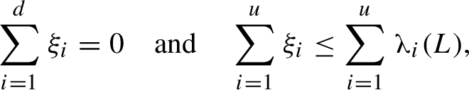
does there exist a conservative Anosov diffeomorphism f homotopic (and hence topologically conjugate) to
 $F_L$
such that
$F_L$
such that
 $\boldsymbol {\unicode{x3bb} }(f) = (\xi _{1}, \ldots , \xi _{d})$
?
$\boldsymbol {\unicode{x3bb} }(f) = (\xi _{1}, \ldots , \xi _{d})$
?
Regularity of f may vary but it does not seem likely that the answer depends on regularity, at least above
 $C^1$
(it may be more challenging to make some exponents equal in regularity above
$C^1$
(it may be more challenging to make some exponents equal in regularity above
 $C^1$
).
$C^1$
).
For
 $d=2$
(and so
$d=2$
(and so
 $u=1$
), the problem reduces to the existence of Anosov diffeomorphisms on
$u=1$
), the problem reduces to the existence of Anosov diffeomorphisms on
 $\mathbb {T}^2$
with any positive value of metric entropy below the topological entropy. Here the answer is positive. It is not difficult to produce such examples even in the real-analytic category by a fairly straightforward global twist construction (see [Reference Bochi11]). The existence of
$\mathbb {T}^2$
with any positive value of metric entropy below the topological entropy. Here the answer is positive. It is not difficult to produce such examples even in the real-analytic category by a fairly straightforward global twist construction (see [Reference Bochi11]). The existence of
 $C^{\infty }$
examples also follows from our Theorem 1.5 below.
$C^{\infty }$
examples also follows from our Theorem 1.5 below.
In its weak version, that is, without considerations about homotopy, the flexibility problem is likely to have a positive solution.
Conjecture 1.4. (Weak flexibility—Anosov)
Given any list of non-zero numbers
 $\xi _{1} \ge \cdots \ge \xi _{d}$
such that
$\xi _{1} \ge \cdots \ge \xi _{d}$
such that
 $\sum _{i=1}^d\!\xi _i=0$
, there exists an Anosov diffeomorphism of
$\sum _{i=1}^d\!\xi _i=0$
, there exists an Anosov diffeomorphism of
 $\mathbb {T}^d$
such that
$\mathbb {T}^d$
such that
 $\boldsymbol {\unicode{x3bb} }(f) = (\xi _{1}, \ldots , \xi _{d})$
.
$\boldsymbol {\unicode{x3bb} }(f) = (\xi _{1}, \ldots , \xi _{d})$
.
The case of this conjecture with strict inequalities easily follows from our main result: see Corollary 1.6 below.
1.4 Dominated splittings
Given a diffeomorphism
 $f \colon M \to M$
, a
$f \colon M \to M$
, a
 $Df$
-invariant splitting
$Df$
-invariant splitting
 $T M = E_1 \oplus \cdots \oplus E_k$
into bundles of constant dimension is called dominated if each of the bundles dominates the next. This means that given a Riemannian metric, there exists
$T M = E_1 \oplus \cdots \oplus E_k$
into bundles of constant dimension is called dominated if each of the bundles dominates the next. This means that given a Riemannian metric, there exists
 $n_0 \ge 1$
such that for every
$n_0 \ge 1$
such that for every
 $x \in M$
and all unit vectors
$x \in M$
and all unit vectors
 $v_1 \in E_1(x)$
, …,
$v_1 \in E_1(x)$
, …,
 $v_k \in E_k(x)$
,
$v_k \in E_k(x)$
,
 $$ \begin{align} \| Df^{n_0}(x) v_1 \|> \| Df^{n_0}(x) v_2 \| > \cdots > \| Df^{n_0}(x) v_k \|. \end{align} $$
It is always possible to find an ‘adapted’ Riemannian metric for which
 ${n_0 = 1}$
: see [Reference Gourmelon23]. Dominated splittings are automatically continuous, and their existence is a
${n_0 = 1}$
: see [Reference Gourmelon23]. Dominated splittings are automatically continuous, and their existence is a
 $C^1$
-open condition; see e.g. [Reference Bonatti, Díaz and Viana14, §B.1] for these and other properties. We say that a dominated splitting is simple if all the sub-bundles
$C^1$
-open condition; see e.g. [Reference Bonatti, Díaz and Viana14, §B.1] for these and other properties. We say that a dominated splitting is simple if all the sub-bundles
 $E_j$
are one-dimensional (and so
$E_j$
are one-dimensional (and so
 $k=d$
). In this case, the Oseledets splitting coincides with
$k=d$
). In this case, the Oseledets splitting coincides with
 $E_1 \oplus \cdots \oplus E_d$
a.e., the Lyapunov spectrum is simple, and the Lyapunov exponents with respect to invariant volume m are given by integrals:
$E_1 \oplus \cdots \oplus E_d$
a.e., the Lyapunov spectrum is simple, and the Lyapunov exponents with respect to invariant volume m are given by integrals:

In particular, in the class of diffeomorphisms admitting a simple dominated splitting, the Lyapunov exponents depend continuously on the dynamics, and therefore, the flexibility analysis becomes more manageable. However, in the absence of domination, small perturbations (with respect to the
 $C^1$
topology) of the dynamics may have a large effect on the Lyapunov spectrum and even send all Lyapunov exponents to zero [Reference Bochi9, Reference Bochi and Viana13] (but the
$C^1$
topology) of the dynamics may have a large effect on the Lyapunov spectrum and even send all Lyapunov exponents to zero [Reference Bochi9, Reference Bochi and Viana13] (but the
 $C^2$
norm of such a perturbation generally explodes [Reference Liang, Marin and Yang31]).
$C^2$
norm of such a perturbation generally explodes [Reference Liang, Marin and Yang31]).
Existence of a dominated splitting also imposes restrictions on the topology of the manifold.
1.5 Formulation of results
Let us recall the classical notion of majorization, which has a wide range of applications (see e.g. [Reference Marshall, Olkin and Arnold32]; also see [Reference Bochi and Bonatti12] for another instance where majorization plays a role in the perturbation of Lyapunov exponents).
Suppose that
 $\boldsymbol {\xi } = (\xi _1,\ldots ,\xi _d)$
and
$\boldsymbol {\xi } = (\xi _1,\ldots ,\xi _d)$
and
 $\boldsymbol {\eta }=(\eta _1,\ldots ,\eta _d)$
are ordered vectors in
$\boldsymbol {\eta }=(\eta _1,\ldots ,\eta _d)$
are ordered vectors in
 $\mathbb {R}^d$
, in the sense that
$\mathbb {R}^d$
, in the sense that
 $\xi _1 \ge \cdots \ge \xi _d$
and
$\xi _1 \ge \cdots \ge \xi _d$
and
 $\eta _1 \ge \cdots \ge \eta _d$
. We say that
$\eta _1 \ge \cdots \ge \eta _d$
. We say that
 $\boldsymbol {\xi }$
majorizes
$\boldsymbol {\xi }$
majorizes
 $\boldsymbol {\eta }$
(or
$\boldsymbol {\eta }$
(or
 $\boldsymbol {\eta }$
is majorized by
$\boldsymbol {\eta }$
is majorized by
 $\boldsymbol {\xi }$
) if the following conditions hold:
$\boldsymbol {\xi }$
) if the following conditions hold:
 $$ \begin{align} \xi_1 + \cdots + \xi_j &\ge \eta_1 + \cdots + \eta_j \quad \text{for all } j \in \{1,\ldots, d-1\}, \text{ and} \end{align} $$
 $$ \begin{align} \xi_1 + \cdots + \xi_d &= \eta_1 + \cdots + \eta_d. \end{align} $$
This is denoted by
 $\boldsymbol {\xi } \succcurlyeq \boldsymbol {\eta }$
(or
$\boldsymbol {\xi } \succcurlyeq \boldsymbol {\eta }$
(or
 $\boldsymbol {\eta } \preccurlyeq \boldsymbol {\xi }$
), and defines a partial order among ordered vectors. If all the inequalities (1.7) are strict (and the equality (1.8) holds), then we say that
$\boldsymbol {\eta } \preccurlyeq \boldsymbol {\xi }$
), and defines a partial order among ordered vectors. If all the inequalities (1.7) are strict (and the equality (1.8) holds), then we say that
 $\boldsymbol {\xi }$
strictly majorizes
$\boldsymbol {\xi }$
strictly majorizes
 $\boldsymbol {\eta }$
(or
$\boldsymbol {\eta }$
(or
 $\boldsymbol {\eta }$
is strictly majorized by
$\boldsymbol {\eta }$
is strictly majorized by
 $\boldsymbol {\eta }$
), and denote this by
$\boldsymbol {\eta }$
), and denote this by
 $\boldsymbol {\xi } \succ \boldsymbol {\eta }$
(or
$\boldsymbol {\xi } \succ \boldsymbol {\eta }$
(or
 $\boldsymbol {\eta } \prec \boldsymbol {\xi }$
).
$\boldsymbol {\eta } \prec \boldsymbol {\xi }$
).
Intuitively,
 $\boldsymbol {\xi } \succcurlyeq \boldsymbol {\eta }$
means that the entries of
$\boldsymbol {\xi } \succcurlyeq \boldsymbol {\eta }$
means that the entries of
 $\boldsymbol {\eta }$
are obtained from those of
$\boldsymbol {\eta }$
are obtained from those of
 $\boldsymbol {\xi }$
by a process of ‘mixing’. Let us state this precisely: If
$\boldsymbol {\xi }$
by a process of ‘mixing’. Let us state this precisely: If
 $\boldsymbol {\xi }$
majorizes
$\boldsymbol {\xi }$
majorizes
 $\boldsymbol {\eta }$
then there exists a doubly-stochastic
$\boldsymbol {\eta }$
then there exists a doubly-stochastic
 $d\times d$
matrix P such that
$d\times d$
matrix P such that
 $\boldsymbol {\eta } = P \boldsymbol {\xi }$
; conversely, given an ordered vector
$\boldsymbol {\eta } = P \boldsymbol {\xi }$
; conversely, given an ordered vector
 $\boldsymbol {\xi }$
and a doubly-stochastic matrix P, the vector obtained by reordering the entries of
$\boldsymbol {\xi }$
and a doubly-stochastic matrix P, the vector obtained by reordering the entries of
 $P \boldsymbol {\xi }$
is majorized by
$P \boldsymbol {\xi }$
is majorized by
 $\boldsymbol {\xi }$
—see [Reference Marshall, Olkin and Arnold32, Theorem B.2].
$\boldsymbol {\xi }$
—see [Reference Marshall, Olkin and Arnold32, Theorem B.2].
We now state the main result of this paper. Recall that M is a smooth compact connected manifold of dimension
 $d \ge 2$
, and m is a smooth volume measure, normalized so that
$d \ge 2$
, and m is a smooth volume measure, normalized so that
 $m(M)=1$
; note that we do not assume that M is a torus (nor even an infranilmanifold). The unstable index of an Anosov diffeomorphism is the dimension of its unstable bundle.
$m(M)=1$
; note that we do not assume that M is a torus (nor even an infranilmanifold). The unstable index of an Anosov diffeomorphism is the dimension of its unstable bundle.
Theorem 1.5. Let
 $r\in \{2,3,\ldots ,\infty \}$
, and let
$r\in \{2,3,\ldots ,\infty \}$
, and let
 $f \in \mathrm {Diff}_m^r(M)$
be a conservative Anosov
$f \in \mathrm {Diff}_m^r(M)$
be a conservative Anosov
 $C^r$
-diffeomorphism with simple dominated splitting. Let
$C^r$
-diffeomorphism with simple dominated splitting. Let
 $\boldsymbol {\xi } \in \mathbb {R}^d$
be such that:
$\boldsymbol {\xi } \in \mathbb {R}^d$
be such that:
-
(a)
$\xi _1> \cdots > \xi _u > 0 > \xi _{u+1} > \cdots > \xi _d$
, where u is the unstable index of f; -
(b)
$\boldsymbol {\xi } \prec \boldsymbol {\unicode{x3bb} }(f)$
, that is,
$\boldsymbol {\xi }$
is strictly majorized by
$\boldsymbol {\unicode{x3bb} }(f)$
.


Then there is a continuous path
 $(f_t)_{t \in [0,1]}$
in
$(f_t)_{t \in [0,1]}$
in
 $\mathrm {Diff}_m^r(M)$
such that:
$\mathrm {Diff}_m^r(M)$
such that:
-
•
$f_0 = f$
; -
• each
$f_t$
is Anosov with simple dominated splitting; -
•
$\boldsymbol {\unicode{x3bb} }(f_1) = \boldsymbol {\xi }$
.


Corollary 1.6. (Anosov diffeomorphisms display all hyperbolic simple Lyapunov spectra)
Given any list of non-zero numbers
 $\xi _{1}> \cdots > \xi _{d}$
whose sum is equal to
$\xi _{1}> \cdots > \xi _{d}$
whose sum is equal to
 $0$
, there exists a conservative Anosov
$0$
, there exists a conservative Anosov
 $C^{\infty }$
diffeomorphism of
$C^{\infty }$
diffeomorphism of
 $\mathbb {T}^d$
with simple dominated splitting such that
$\mathbb {T}^d$
with simple dominated splitting such that
 $\boldsymbol {\unicode{x3bb} }(f) = (\xi _{1}, \ldots , \xi _{d})$
.
$\boldsymbol {\unicode{x3bb} }(f) = (\xi _{1}, \ldots , \xi _{d})$
.
Corollary 1.6 is obtained as follows: first, we take an Anosov linear automorphism whose spectrum is simple and ‘large’ with respect to the majorization partial order; then, Theorem 1.5 allows us to deform the linear automorphism and obtain a conservative Anosov diffeomorphism with the desired Lyapunov spectrum. (See §7.1 for full details.)
Note that as a consequence of Corollary 1.6, we obtain a positive solution of the general weak flexibility Conjecture 1.1 on tori for simple spectra: if the desired spectrum contains
 $0$
, then we just take the product
$0$
, then we just take the product
 $f = g \times R_{\theta }$
of an appropriate Anosov map g on
$f = g \times R_{\theta }$
of an appropriate Anosov map g on
 $\mathbb {T}^{d-1}$
and an irrational rotation
$\mathbb {T}^{d-1}$
and an irrational rotation
 $R_{\theta }$
on
$R_{\theta }$
on
 $\mathbb {T}$
; this f is ergodic because g is mixing.
$\mathbb {T}$
; this f is ergodic because g is mixing.
While condition (b) in Theorem 1.5 asks for strict majorization, there are specific situations where this requirement can be relaxed to ordinary majorization. This is demonstrated by the next theorem, which also shows that the majorization condition is indeed necessary.
Theorem 1.7. Let
 $F_L$
be an Anosov linear automorphism of
$F_L$
be an Anosov linear automorphism of
 $\mathbb {T}^3$
with simple Lyapunov spectrum and unstable index u. For any given
$\mathbb {T}^3$
with simple Lyapunov spectrum and unstable index u. For any given
 $\boldsymbol {\xi } = (\xi _1,\xi _2,\xi _3) \in \mathbb {R}^3$
, there exists an Anosov diffeomorphism
$\boldsymbol {\xi } = (\xi _1,\xi _2,\xi _3) \in \mathbb {R}^3$
, there exists an Anosov diffeomorphism
 $f \in \mathrm {Diff}_m^{\infty }(\mathbb {T}^3)$
homotopic (and hence topologically conjugate) to
$f \in \mathrm {Diff}_m^{\infty }(\mathbb {T}^3)$
homotopic (and hence topologically conjugate) to
 $F_L$
and with simple dominated splitting such that
$F_L$
and with simple dominated splitting such that
 $\boldsymbol {\unicode{x3bb} }(f) = \boldsymbol {\xi }$
if and only if
$\boldsymbol {\unicode{x3bb} }(f) = \boldsymbol {\xi }$
if and only if
 $$ \begin{align} \xi_1>\xi_2>\xi_3, \quad \xi_u>0>\xi_{u+1}, \quad \mathrm{and} \quad \boldsymbol{\xi} \preccurlyeq \boldsymbol{\unicode{x3bb}}(L). \end{align} $$
Furthermore, one can choose a homotopy between
 $F_L$
and f consisting of conservative smooth Anosov diffeomorphisms with simple dominated splitting.
$F_L$
and f consisting of conservative smooth Anosov diffeomorphisms with simple dominated splitting.
In
 $d=3$
, the condition
$d=3$
, the condition
 $\boldsymbol {\xi } \preccurlyeq \boldsymbol {\unicode{x3bb} }(L)$
is strictly stronger than the ‘entropy condition’ in equation (1.4). Therefore, if Problem 1.3 has a positive solution, it necessarily involves Anosov diffeomorphisms without a simple dominated splitting, even in the case of simple Lyapunov spectra. The existence of a single conservative Anosov diffeomorphism
$\boldsymbol {\xi } \preccurlyeq \boldsymbol {\unicode{x3bb} }(L)$
is strictly stronger than the ‘entropy condition’ in equation (1.4). Therefore, if Problem 1.3 has a positive solution, it necessarily involves Anosov diffeomorphisms without a simple dominated splitting, even in the case of simple Lyapunov spectra. The existence of a single conservative Anosov diffeomorphism
 $f \colon \mathbb {T}^3 \to \mathbb {T}^3$
whose spectrum
$f \colon \mathbb {T}^3 \to \mathbb {T}^3$
whose spectrum
 $\boldsymbol {\xi } = \boldsymbol {\unicode{x3bb} }(f)$
is not majorized by
$\boldsymbol {\xi } = \boldsymbol {\unicode{x3bb} }(f)$
is not majorized by
 $\boldsymbol {\unicode{x3bb} }(L)$
is already a very interesting question.
$\boldsymbol {\unicode{x3bb} }(L)$
is already a very interesting question.
Let us note that Hu, M. Jiang, and Y. Jiang [Reference Hu, Jiang and Jiang25] have constructed deformations of conservative Anosov diffeomorphisms and of conservative expanding endomorphisms having arbitrarily small metric entropy. In the case of diffeomorphisms with dominated splittings, their result follows from Theorem 1.5. Their construction is very different from ours.
1.6 Comments on the proofs
Let us summarize the ideas of the proof of Theorem 1.5. Motivated by the work of Shub and Wilkinson [Reference Shub and Wilkinson42], Baraviera and Bonatti [Reference Baraviera and Bonatti5] have proved the following ‘local flexibility’ result: given a conservative stably ergodic partially hyperbolic diffeomorphism, one can perturb it so that the sum of central Lyapunov exponents becomes different from zero. Their idea was to perturb the diffeomorphism on a small ball around a non-periodic point (so to avoid fast returns) by rotating on a center-unstable plane so that the central bundle borrows some expansion from the unstable bundle. Actually, their argument allows to slightly mix Lyapunov exponents in any pair of consecutive bundles in a dominated splitting, while the Lyapunov exponents in the other bundles move extremely little. So it is conceivable that with a sequence of Baraviera–Bonatti perturbations, one could mix Lyapunov exponents basically at will. Though this idea is ultimately correct, several difficulties need to be overcome to turn it into a proof of Theorem 1.5. First, how can we ensure that the effect of the perturbations is not too weak? Second, how can we obtain a prescribed Lyapunov spectrum exactly?
Let us discuss how to overcome the first difficulty. Instead of using a single ball as the support of a perturbation, we select several small balls whose union has a large first return time but non-negligible measure: this is done with a standard tower construction (in the style of [Reference Bochi9, Reference Bochi and Viana13], for instance). In each of these balls, one composes with the same ‘model’ perturbation of the identity that rotates the appropriate plane. However, this trick by itself is not sufficient to conclude. If the domination or the hyperbolicity gets weak, the rotations should be smaller and their effect on the Lyapunov exponents are also small. The solution is to select carefully not only the location of the balls but also their shape. This is done using a specially adapted Riemannian metric such that, on the one hand, domination and hyperbolicity are seen in a single iterate (as in [Reference Gourmelon23]), but on the other hand, for a large proportion of points with respect to the reference measure m, the rates of expansion on a single iterate with respect to the adapted metric are very close to the Lyapunov exponents. We only perform the perturbations on balls around those good points. In this way, we can ensure that the effect of the perturbation on the Lyapunov exponents is considerable. In this regard, we also remark that we have no bound for the
 $C^1$
size of the deformation
$C^1$
size of the deformation
 $(f_t)_{t \in [0,1]}$
that we eventually construct in Theorem 1.5. Therefore, we need to be careful with the quantifiers to ensure some effectiveness of the perturbation without knowing which diffeomorphism we are perturbing.
$(f_t)_{t \in [0,1]}$
that we eventually construct in Theorem 1.5. Therefore, we need to be careful with the quantifiers to ensure some effectiveness of the perturbation without knowing which diffeomorphism we are perturbing.
Concerning the second difficulty, we note that the type of perturbations sketched above always has some small ‘noisy’ effect on the Lyapunov exponents that cannot be made exactly zero (except if some of the invariant sub-bundles are smoothly integrable). To resolve this, we define our perturbations depending on several parameters, allowing us to move the Lyapunov spectrum in all directions. By topological reasons, this eventually permits us to obtain open sets of spectra. Now, to construct these multiparametric perturbations, in principle, one could try to compose several Baraviera–Bonatti-like perturbations that mix different pairs of Lyapunov exponents. This idea turns out to be impractical, essentially because one would need to consider adapted metrics and towers depending on parameters. Luckily, it is possible to define a new type of multiparametric model perturbation that includes Baraviera–Bonatti perturbations as a particular case, freeing us from the trouble of working separately with each pair of exponents.
Now let us outline the proof of Theorem 1.7. To manipulate, say, the first two Lyapunov exponents while keeping the third one unchanged, we follow the same strategy as in the proof of Theorem 1.5, but using Baraviera–Bonatti perturbations that preserve the center-unstable foliation. This is possible because we start with the automorphism
 $F_L$
for which this foliation is smooth. In the converse direction, suppose that f is a conservative Anosov diffeomorphism of
$F_L$
for which this foliation is smooth. In the converse direction, suppose that f is a conservative Anosov diffeomorphism of
 $\mathbb {T}^3$
homotopic to
$\mathbb {T}^3$
homotopic to
 $F_L$
whose Lyapunov spectrum is simple but is not majorized by the spectrum of L. For example, consider the case
$F_L$
whose Lyapunov spectrum is simple but is not majorized by the spectrum of L. For example, consider the case
 $u=2$
and
$u=2$
and
 $\unicode{x3bb} _1(f)>\unicode{x3bb} _1(L)$
. If f had a simple dominated splitting, then the exponential growth rate of the strong unstable foliation of f would be bigger than the corresponding rate for
$\unicode{x3bb} _1(f)>\unicode{x3bb} _1(L)$
. If f had a simple dominated splitting, then the exponential growth rate of the strong unstable foliation of f would be bigger than the corresponding rate for
 $F_L$
, and this would contradict the quasi-isometric property of this foliation obtained by Brin, Burago, and Ivanov [Reference Brin, Burago and Ivanov15].
$F_L$
, and this would contradict the quasi-isometric property of this foliation obtained by Brin, Burago, and Ivanov [Reference Brin, Burago and Ivanov15].
1.7 Further directions of research and other instances of the flexibility program
1.7.1 Extensions of our methods
Hyperbolicity is not fundamental to our constructions; as in Baraviera and Bonatti [Reference Baraviera and Bonatti5], domination is the important keyword. In fact, this perturbation method seems much more versatile, and should apply if domination is allowed to degenerate in a controlled way on a certain singular set, as is the case in [Reference Dolgopyat and Pesin18, Reference Katok26]. Therefore, the conjectures of §1.2 seem approachable, at least in some cases.
Let us briefly discuss what happens when we approach the boundary of the set of allowable spectra
 $\boldsymbol {\xi }$
in Theorem 1.5. We consider the principal case
$\boldsymbol {\xi }$
in Theorem 1.5. We consider the principal case
 $f=F_L$
. Let u be the unstable index of
$f=F_L$
. Let u be the unstable index of
 $F_L$
. Consider the set of
$F_L$
. Consider the set of
 $\boldsymbol {\xi }$
that meet conditions (a) and (b) in the theorem. There are three types of components of the boundary.
$\boldsymbol {\xi }$
that meet conditions (a) and (b) in the theorem. There are three types of components of the boundary.
-
(a)
$\xi _u=0$
or
$\xi _{u+1} = 0$
. One can carry our construction across either of those. The resulting map of course is not Anosov anymore but partially hyperbolic with a one-dimensional central bundle (a similar construction appears in [Reference Ponce and Tahzibi37], but starting with an automorphism
$F_L$
of
$\mathbb {T}^3$
whose central exponent is already close to
$0$
). -
(b)
$\sum _{i=1}^k\!\xi _i=\sum _{i=1}^k\!\unicode{x3bb} _i(L)$
for some
$k\in \{1,\ldots , d-1\}$
. Cases
$k=1$
and
$k=d-1$
are feasible: as in the proof of the ‘if’ part of Theorem 1.7, the perturbations preserve codimension-one
$F_L$
-invariant foliations. For other values of k, we get into difficulties: our construction is iterative, but after the first step, the foliation that needs to be preserved would no longer be smooth. -
(c)
$\xi _i=\xi _{i+1}$
for some
$i \in \{1,\ldots , d-1\}$
. Our construction degenerates because the amount of domination decreases and the Lyapunov metric explodes.


Related to the last point, to realize non-simple Lyapunov spectrum (e.g. to prove Conjecture 1.4), one should be able to manipulate Lyapunov exponents at least in some cases of non-simple dominated splittings. However, then formula (1.6) does not apply, so finer methods would be required.
1.7.2 Explicit constructions and bounds
As mentioned before, in dimension
 $2$
, there exists a simple construction of conservative Anosov diffeomorphisms with prescribed Lyapunov spectra. It would be interesting to have such explicit constructions on higher-dimensional tori as well.
$2$
, there exists a simple construction of conservative Anosov diffeomorphisms with prescribed Lyapunov spectra. It would be interesting to have such explicit constructions on higher-dimensional tori as well.
Here is an exciting general questionFootnote †: What would be the effect of bounds on the
 $C^r$
norms on the flexibility results? Our constructions are certainly very ‘expensive’ in terms of
$C^r$
norms on the flexibility results? Our constructions are certainly very ‘expensive’ in terms of
 $C^2$
norms, and probably in terms of
$C^2$
norms, and probably in terms of
 $C^1$
norms as well (because do not have estimates on the eccentricities of the Lyapunov balls).
$C^1$
norms as well (because do not have estimates on the eccentricities of the Lyapunov balls).
1.7.3 Other measures
In other settings, the invariant measure (or measures) one is interested in is not necessarily fixed in the class of dynamical systems under consideration, but varies with the dynamics itself. The prototypical example consists of equilibrium states of sufficiently hyperbolic dynamics with respect to relevant potentials. The flexibility paradigm then applies. See [Reference Erchenko19] for a result in this direction, where expanding maps on the circle are considered.
1.7.4 Symplectic systems
The problems that we have posed in the volume-preserving setting have symplectic counterparts, where symmetry of the spectrum appears as an extra requirement. It is plausible that our methods can be adapted to the symplectic setting, but not in a straightforward way.
1.7.5 Flows
Structural stability for flows does not imply topological conjugacy, so topological entropy becomes a free parameter even in the uniformly hyperbolic case. Thus, for conservative Anosov flows on three-dimensional manifolds, the basic flexibility problem involves the realization of arbitrary pairs of numbers as values for topological and metric entropy subject only to the variational inequality. This problem can be solved fairly easily for suspensions of
 $\mathbb {T}^2$
and unit tangent bundles of surfaces of genus
$\mathbb {T}^2$
and unit tangent bundles of surfaces of genus
 $g\ge 2$
using time changes of homogeneous models but becomes more interesting (probably still tractable) for exotic Anosov flows where homogeneous models are not available.
$g\ge 2$
using time changes of homogeneous models but becomes more interesting (probably still tractable) for exotic Anosov flows where homogeneous models are not available.
The problem becomes really interesting in the standard setting when one considers special classes of Anosov flows. The prime example here is provided by geodesic flows on compact surfaces of negative curvature. In this case, a natural normalization is available by fixing the total surface area. The variational inequality is strengthened by the conformal inequality [Reference Katok27] and possible values of the metric entropy
 $h_m$
and topological entropy
$h_m$
and topological entropy
 $h_{\mathrm {top}}$
for Riemannian metrics of negative non-constant curvature are restricted to:
$h_{\mathrm {top}}$
for Riemannian metrics of negative non-constant curvature are restricted to:
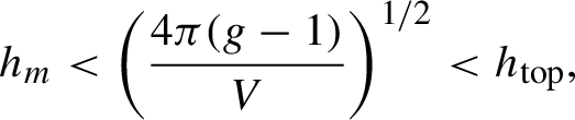 $$ \begin{align*} h_m<\bigg(\frac{4\pi(g-1)}{V}\bigg)^{{1}/{2}}<h_{\mathrm{top}}, \end{align*} $$
where g is the genus of the surface and V is its total area. For any constant curvature metric those inequalities become equalities. The fact that equality of the metric and topological entropy implies constant curvature is a prototype case of rigidity that is discussed below. The flexibility problem in this setting is solved in [Reference Erchenko and Katok20]. The solution uses methods which are totally different from those of the present work. For flexibility results where the conformal class is fixed (and also taking other invariant quantities into account), see [Reference Barthelmé and Erchenko7, Reference Barthelmé and Erchenko8]. More problems are posed in [Reference Erchenko and Katok20, §4] and [Reference Barthelmé and Erchenko8, §7].
The higher dimensional case is wide open. One of the difficulties of dealing with geodesic flows on higher dimensional negatively curved manifolds is that algebraic models have a non-simple Lyapunov spectrum (in fact, either one or two Lyapunov exponents are of the same sign and full splittings never exist).
1.7.6 Flexibility and rigidity
In the context of conservative smooth dynamical systems, the strongest natural equivalence relation is smooth conjugacy. For symplectic systems, it is similarly a symplectic conjugacy, for geodesic flows—isometry of the underlying metrics, and so on. A general phenomenon of rigidity in this context can be described as follows:
 $(\mathfrak {{R}})$
Values of finitely many invariants determine the system either locally, that is, in a certain neighborhood of a ‘model’, or globally within an a priori defined class of systems.
$(\mathfrak {{R}})$
Values of finitely many invariants determine the system either locally, that is, in a certain neighborhood of a ‘model’, or globally within an a priori defined class of systems.
The space of equivalence classes, at best, can be given some natural infinite-dimensional structure and, at worst, is ‘wild’. This is proven in a number of situations but, in general, it has to be viewed as a paradigmatic statement, not a theorem, and, beyond the
 $C^1$
case, almost every meaningful general question is open. Thus, rigidity should be quite rare because it should appear for very special values of invariants. (Nevertheless, for zero entropy systems, local rigidity of toral translations appears in the context of Kolmogorov–Arnold–Moser theory and global rigidity for circle diffeomorphisms with Diophantine rotation number. Those situations do not concern us here.)
$C^1$
case, almost every meaningful general question is open. Thus, rigidity should be quite rare because it should appear for very special values of invariants. (Nevertheless, for zero entropy systems, local rigidity of toral translations appears in the context of Kolmogorov–Arnold–Moser theory and global rigidity for circle diffeomorphisms with Diophantine rotation number. Those situations do not concern us here.)
A natural question in our context is whether particular values of Lyapunov exponents (for conservative systems, or symplectic systems, or geodesic flows) imply rigidity. In agreement with the general flexibility paradigm, one may expect this to happen at the extreme allowable values of exponents. This tends to be true in low dimension, not true in full generality, and probable in a number of interesting situations. Several recent results fit this pattern: see the papers [Reference Gogolev, Kalinin and Sadovskaya22, Reference Micena and Tahzibi33, Reference Saghin and Yang40] (concerning conservative Anosov diffeomorphisms, mostly) and [Reference Butler16, Reference Butler17] (concerning geodesic flows).
1.8 Organization of the paper
The rest of this paper is organized as follows. In §2, we state the technical Proposition 2.1, which is a local multiparametric version of Theorem 1.5, and we show how it implies the theorem. In §3, we construct the adapted metrics mentioned above. In §4, we use them to define damping perturbations; these are actually ‘large perturbations’, but we show that their results are still Anosov under the appropriate conditions. In §5, we define the local model of our multiparametric perturbations and perform some computations concerning those. In §6, we use the results of the previous sections and a tower construction to prove Proposition 2.1. In §7, we prove Theorem 1.7.
2 Reduction to a central proposition
Let
 $H := \{(\xi _1,\ldots ,\xi _d) \in \mathbb {R}^d\!\;\mathord {;}\; {\textstyle \sum } \xi _j = 0\}$
. Define a linear isomorphism
$H := \{(\xi _1,\ldots ,\xi _d) \in \mathbb {R}^d\!\;\mathord {;}\; {\textstyle \sum } \xi _j = 0\}$
. Define a linear isomorphism
 $T \colon H \to \mathbb {R}^{d-1}$
by:
$T \colon H \to \mathbb {R}^{d-1}$
by:
 $$ \begin{align} T ( \xi_1,\xi_2, \ldots, \xi_{d-1} , \xi_d ) := ( \xi_1, \xi_1 + \xi_2, \ldots, \xi_1 + \cdots + \xi_{d-1} ). \end{align} $$
Given an ergodic
 $f \in \mathrm {Diff}_m^r(M)$
, recall that
$f \in \mathrm {Diff}_m^r(M)$
, recall that
 $\boldsymbol {\unicode{x3bb} }(f)$
denotes the Lyapunov spectrum of f with respect to the volume measure m. We define
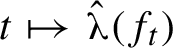
$\boldsymbol {\unicode{x3bb} }(f)$
denotes the Lyapunov spectrum of f with respect to the volume measure m. We define
 $\hat {\boldsymbol {\unicode{x3bb} }}(f) := T(\boldsymbol {\unicode{x3bb} }(f))$
, that is,
$\hat {\boldsymbol {\unicode{x3bb} }}(f) := T(\boldsymbol {\unicode{x3bb} }(f))$
, that is,
 $\hat {\boldsymbol {\unicode{x3bb} }}(f)$
is the vector whose jth entry
$\hat {\boldsymbol {\unicode{x3bb} }}(f)$
is the vector whose jth entry
 $\hat {\unicode{x3bb} }_j(f)$
is the sum of the j biggest Lyapunov exponents. This is a natural object to consider because
$\hat {\unicode{x3bb} }_j(f)$
is the sum of the j biggest Lyapunov exponents. This is a natural object to consider because
 $\hat {\unicode{x3bb} }_j(f)$
equals the top Lyapunov exponent of the j-fold exterior power of the derivative cocycle. It is also convenient to define
$\hat {\unicode{x3bb} }_j(f)$
equals the top Lyapunov exponent of the j-fold exterior power of the derivative cocycle. It is also convenient to define
 $\hat {\unicode{x3bb} }_0(f) := 0 =: \hat {\unicode{x3bb} }_d(f)$
. The fact that
$\hat {\unicode{x3bb} }_0(f) := 0 =: \hat {\unicode{x3bb} }_d(f)$
. The fact that
 $\unicode{x3bb} _1(f) \ge \cdots \ge \unicode{x3bb} _d(f)$
means that the function
$\unicode{x3bb} _1(f) \ge \cdots \ge \unicode{x3bb} _d(f)$
means that the function
 $j \in \{0,\ldots ,d\} \mapsto \hat {\unicode{x3bb} }_j(f)$
is concave: see Figure 1.
$j \in \{0,\ldots ,d\} \mapsto \hat {\unicode{x3bb} }_j(f)$
is concave: see Figure 1.


In this section, we state Proposition 2.1, which roughly says that we can perturb f to slightly lower the graph of
 $j \in \{0,\ldots ,d\} \mapsto \hat {\unicode{x3bb} }_j(f)$
and that different vertices of the graph can be moved somewhat independently. We also show how Proposition 2.1 implies the main theorem (Theorem 1.5).
$j \in \{0,\ldots ,d\} \mapsto \hat {\unicode{x3bb} }_j(f)$
and that different vertices of the graph can be moved somewhat independently. We also show how Proposition 2.1 implies the main theorem (Theorem 1.5).
Given
 $u \in \{1,2,\ldots ,d-1\}$
, define a ‘gap function’
$u \in \{1,2,\ldots ,d-1\}$
, define a ‘gap function’
 $\textsf {g}_u \colon \mathbb {R}^d \to \mathbb {R}$
by:
$\textsf {g}_u \colon \mathbb {R}^d \to \mathbb {R}$
by:
 $$ \begin{align} \textsf{g}_u(\xi_1,\ldots,\xi_d) := \min \{ \xi_1 - \xi_2, \xi_2 - \xi_3, \ldots, \xi_{d-1} - \xi_d , \ \xi_u, \ -\xi_{u+1} \} \,. \end{align} $$
Note that if f is a conservative Anosov diffeomorphism of unstable index u and admitting a simple dominated splitting, then
 $\textsf {g}_u(\boldsymbol {\unicode{x3bb} }(f))$
is strictly positive; indeed it is the minimal gap between the
$\textsf {g}_u(\boldsymbol {\unicode{x3bb} }(f))$
is strictly positive; indeed it is the minimal gap between the
 $d+1$
numbers
$d+1$
numbers
Proposition 2.1. (Central proposition)
Let
 $u \in \{1,2,\ldots ,d-1\}$
, and let
$u \in \{1,2,\ldots ,d-1\}$
, and let
 $a_1$
, … ,
$a_1$
, … ,
 $a_{d-1}$
,
$a_{d-1}$
,
 $\sigma $
, and
$\sigma $
, and
 $\delta _0$
be positive numbers. Then there exists
$\delta _0$
be positive numbers. Then there exists
 $\delta \in (0,\delta _0)$
so that the following holds.
$\delta \in (0,\delta _0)$
so that the following holds.
If
 $f \in \mathrm {Diff}_m^r(M)$
is a conservative Anosov diffeomorphism of unstable index u, admitting a simple dominated splitting, and such that
$f \in \mathrm {Diff}_m^r(M)$
is a conservative Anosov diffeomorphism of unstable index u, admitting a simple dominated splitting, and such that
 $\textsf {g}_u(\boldsymbol {\unicode{x3bb} }(f)) \ge \sigma $
, then there exists a continuous map
$\textsf {g}_u(\boldsymbol {\unicode{x3bb} }(f)) \ge \sigma $
, then there exists a continuous map
 $$ \begin{align*} t \in [0,1]^{d-1} \mapsto f_t \in \mathrm{Diff}_m^r(M), \end{align*} $$
where
 $f_{(0,\ldots ,0)} = f$
and for each
$f_{(0,\ldots ,0)} = f$
and for each
 $t = (t_1,\ldots ,t_{d-1}) \in [0,1]^{d-1}$
, the conservative diffeomorphism
$t = (t_1,\ldots ,t_{d-1}) \in [0,1]^{d-1}$
, the conservative diffeomorphism
 $f_t$
is Anosov of unstable index u, admits a simple dominated splitting, and, for each
$f_t$
is Anosov of unstable index u, admits a simple dominated splitting, and, for each
 $j \in \{1,\ldots ,d-1\}$
,
$j \in \{1,\ldots ,d-1\}$
,
 $$ \begin{align} \phantom{t_j = 1 \quad \Rightarrow\quad}\hat{\unicode{x3bb}}_j(f) - 4\delta a_j < \hat{\unicode{x3bb}}_j(f_t) < \hat{\unicode{x3bb}}_j(f) + \phantom{1}\delta a_j,\qquad\qquad\quad \end{align} $$
 $$ \begin{align} t_j = 0 \quad \Rightarrow\quad \hat{\unicode{x3bb}}_j(f) - \phantom{1}\delta a_j < \hat{\unicode{x3bb}}_j(f_t) < \hat{\unicode{x3bb}}_j(f) + \phantom{1}\delta a_j, \end{align} $$
 $$ \begin{align} t_j = 1 \quad\Rightarrow\quad \hat{\unicode{x3bb}}_j(f) - 4\delta a_j < \hat{\unicode{x3bb}}_j(f_t) < \hat{\unicode{x3bb}}_j(f) - 2\delta a_j. \end{align} $$
So the numbers
 $a_j$
allow us to move some of the summed exponents
$a_j$
allow us to move some of the summed exponents
 $\hat {\unicode{x3bb} }_j$
faster than others, but the overall movement is controlled by the scaling factor
$\hat {\unicode{x3bb} }_j$
faster than others, but the overall movement is controlled by the scaling factor
 $\delta $
. Let us emphasize that a main point of the proposition is that the dependence of
$\delta $
. Let us emphasize that a main point of the proposition is that the dependence of
 $\delta $
on f is only through u and
$\delta $
on f is only through u and
 $\sigma $
, and that is the key for the possible iteration of the proposition to obtain Theorem 1.5.
$\sigma $
, and that is the key for the possible iteration of the proposition to obtain Theorem 1.5.
The following consequence is intuitively obvious (see Figure 2).
Illustration of Proposition 2.1 for
 $d=3$
. The images of the edges of the square
$d=3$
. The images of the edges of the square
 $[0,1]^2$
under the map
$[0,1]^2$
under the map
 $t \mapsto \hat {\boldsymbol {\unicode{x3bb} }}(f_t)$
stay on the strips determined by conditions (2.4) and (2.5). Corollary 2.2 tells us that the image of this map is a set
$t \mapsto \hat {\boldsymbol {\unicode{x3bb} }}(f_t)$
stay on the strips determined by conditions (2.4) and (2.5). Corollary 2.2 tells us that the image of this map is a set
 $\Lambda $
that contains the small gray square and is contained in the big square.
$\Lambda $
that contains the small gray square and is contained in the big square.

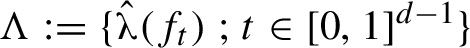
Corollary 2.2. In Proposition 2.1, the set
 $\Lambda := \{\hat {\boldsymbol {\unicode{x3bb} }}(f_t) \;\mathord {;}\; t \in [0,1]^{d-1} \}$
satisfies
$\Lambda := \{\hat {\boldsymbol {\unicode{x3bb} }}(f_t) \;\mathord {;}\; t \in [0,1]^{d-1} \}$
satisfies
 $$ \begin{align*} \prod_{j=1}^{d-1} \, [\hat{\unicode{x3bb}}_j(f) - 2\delta a_j, \, \hat{\unicode{x3bb}}_j(f) - \delta a_j] \, \, \subseteq \, \Lambda \, \subseteq \, \prod_{j=1}^{d-1} \, [\hat{\unicode{x3bb}}_j(f) - 4\delta a_j, \, \hat{\unicode{x3bb}}_j(f) + \delta a_j]. \end{align*} $$
The second inclusion comes from inequality (2.3). For the first one, we need the following topological fact.
Lemma 2.3. Let
 $\varphi = (\varphi _1,\ldots ,\varphi _{d-1}) \colon [-1,1]^{d-1} \to \mathbb {R}^{d-1}$
be a continuous map such that for every
$\varphi = (\varphi _1,\ldots ,\varphi _{d-1}) \colon [-1,1]^{d-1} \to \mathbb {R}^{d-1}$
be a continuous map such that for every
 $z = (z_1,\ldots ,z_{d-1}) \in [-1,1]^{d-1}$
and every
$z = (z_1,\ldots ,z_{d-1}) \in [-1,1]^{d-1}$
and every
 $j \in \{1,\ldots ,d-1\}$
,
$j \in \{1,\ldots ,d-1\}$
,
 $$ \begin{align*} \begin{gathered} z_j = -1 \quad \Rightarrow \quad \varphi_j(z) < -\tfrac{1}{3}, \\ z_j = \phantom{+}1 \quad \Rightarrow \quad \varphi_j(z)> \phantom{+}\tfrac{1}{3}. \end{gathered} \end{align*} $$
Then the image of
 $\varphi $
contains the cube
$\varphi $
contains the cube
 $[-\tfrac {1}{3},\tfrac {1}{3}]^{d-1}$
.
$[-\tfrac {1}{3},\tfrac {1}{3}]^{d-1}$
.
Proof of Corollary 2.2 Let
 $C := [-1,1]^{d-1}$
. Note that:
$C := [-1,1]^{d-1}$
. Note that:
 $$ \begin{align} \text{ for all } z \in \partial C, \text{the segment } [z,\varphi(z)] \text{ does not intersect the cube }\tfrac{1}{3}C. \end{align} $$
Consider the map
 $\psi \colon C \to \mathbb {R}^{d-1}$
that coincides with a rescaled version of
$\psi \colon C \to \mathbb {R}^{d-1}$
that coincides with a rescaled version of
 $\varphi $
on the subcube
$\varphi $
on the subcube
 $\tfrac {1}{2}C$
, and on the remaining shell, interpolates linearly between
$\tfrac {1}{2}C$
, and on the remaining shell, interpolates linearly between
 $\varphi |_{\partial C}$
and
$\varphi |_{\partial C}$
and
 $\mathrm {id}|_{\partial C}$
. More precisely, letting
$\mathrm {id}|_{\partial C}$
. More precisely, letting
 $\|\mathord {\cdot }\|_{\infty }$
denote the maximum norm in
$\|\mathord {\cdot }\|_{\infty }$
denote the maximum norm in
 $\mathbb {R}^{d-1}$
(whose unit closed ball is the cube C), we define:
$\mathbb {R}^{d-1}$
(whose unit closed ball is the cube C), we define:
 $$ \begin{align*} \psi(z) := \begin{cases} \varphi(2z) &\text{if }\|z\|_{\infty} \le 1/2;\\ 2(1-\|z\|_{\infty}) \varphi ( \|z\|_{\infty}^{-1} z) + (2-\|z\|_{\infty}^{-1}) z &\text{otherwise.} \end{cases} \end{align*} $$
In particular,
 $\psi $
coincides with the identity on the boundary
$\psi $
coincides with the identity on the boundary
 $\partial C$
.
$\partial C$
.
By contradiction, suppose that
 $\tfrac {1}{3}C \smallsetminus \varphi (C)$
contains a point w. Then it follows from observation (2.6) that the image of
$\tfrac {1}{3}C \smallsetminus \varphi (C)$
contains a point w. Then it follows from observation (2.6) that the image of
 $\psi $
does not contain w. Fix a retraction
$\psi $
does not contain w. Fix a retraction
 $\pi $
of
$\pi $
of
 $\mathbb {R}^{d-1}\smallsetminus \{w\}$
onto
$\mathbb {R}^{d-1}\smallsetminus \{w\}$
onto
 $\partial C$
. Then
$\partial C$
. Then
 $\pi \circ \psi $
is a retraction of the cube C onto its boundary. It is a known fact that no such map exists. This contradiction completes the proof of the lemma.
$\pi \circ \psi $
is a retraction of the cube C onto its boundary. It is a known fact that no such map exists. This contradiction completes the proof of the lemma.
Now Corollary 2.2 follows by an affine change of coordinates. Namely, consider the map:
 $$ \begin{align*} \varphi(z) := B ( \hat{\boldsymbol{\unicode{x3bb}}}(f_{A(z)}) ) \end{align*} $$
where
 $A = (A_1,\ldots ,A_{d-1})$
,
$A = (A_1,\ldots ,A_{d-1})$
,
 $B=(B_1,\ldots ,B_{d-1})$
are the maps:
$B=(B_1,\ldots ,B_{d-1})$
are the maps:
 $$ \begin{align*} A_j(z_1,\ldots,z_{d-1}) := \frac{1 - z_j}{2}, \quad B_j(\xi_1,\ldots,\xi_{d-1}):= 1 + \frac{2}{3} \, \frac{\xi_j-\hat{\unicode{x3bb}}_j(f)}{\delta a_j}. \end{align*} $$
By equation (2.4), if
 $z_j=1$
, then
$z_j=1$
, then
 $\tfrac {1}{3}<\varphi _j(z)<\tfrac {5}{3}$
, while by equation (2.5), if
$\tfrac {1}{3}<\varphi _j(z)<\tfrac {5}{3}$
, while by equation (2.5), if
 $z_j=-1$
, then
$z_j=-1$
, then
 $-\tfrac {5}{3}<\varphi _j(z)<-\tfrac {1}{3}$
. So we can apply Lemma 2.3 and conclude the proof of Corollary 2.2.
$-\tfrac {5}{3}<\varphi _j(z)<-\tfrac {1}{3}$
. So we can apply Lemma 2.3 and conclude the proof of Corollary 2.2.
Proof of Theorem 1.5 Let f and
 $\boldsymbol {\xi }$
be as in the statement of the theorem. Let
$\boldsymbol {\xi }$
be as in the statement of the theorem. Let
 $$ \begin{align*} \sigma := \tfrac{1}{2} \min \{ \textsf{g}_u(\boldsymbol{\unicode{x3bb}}(f)) , \textsf{g}_u(\boldsymbol{\xi}) \}. \end{align*} $$
Recalling equation (2.1), let
 $\hat {\boldsymbol {\xi }} := T(\boldsymbol {\xi })$
and
$\hat {\boldsymbol {\xi }} := T(\boldsymbol {\xi })$
and
 $(a_1, \ldots , a_{d-1}) := \hat {\boldsymbol {\unicode{x3bb} }}(f) - \hat {\boldsymbol {\xi }}$
. Because
$(a_1, \ldots , a_{d-1}) := \hat {\boldsymbol {\unicode{x3bb} }}(f) - \hat {\boldsymbol {\xi }}$
. Because
 $\boldsymbol {\unicode{x3bb} }(f)$
strictly majorizes
$\boldsymbol {\unicode{x3bb} }(f)$
strictly majorizes
 $\boldsymbol {\xi }$
, each
$\boldsymbol {\xi }$
, each
 $a_j$
is positive. The function
$a_j$
is positive. The function
 $\textsf {g}_u \circ T^{-1} \colon \mathbb {R}^{d-1} \to \mathbb {R}$
is concave (because it is the minimum of affine functions), and it follows that this function is
$\textsf {g}_u \circ T^{-1} \colon \mathbb {R}^{d-1} \to \mathbb {R}$
is concave (because it is the minimum of affine functions), and it follows that this function is
 $\ge 2\sigma $
on the segment
$\ge 2\sigma $
on the segment
 $[ \hat {\boldsymbol {\xi }} , \hat {\boldsymbol {\unicode{x3bb} }}(f)]$
. By continuity, we can find a small positive
$[ \hat {\boldsymbol {\xi }} , \hat {\boldsymbol {\unicode{x3bb} }}(f)]$
. By continuity, we can find a small positive
 $\delta _0 < 1$
such that the function
$\delta _0 < 1$
such that the function
 $\textsf {g}_u \circ T^{-1}$
is
$\textsf {g}_u \circ T^{-1}$
is
 $\ge \sigma $
on the following neighborhood of the segment (pictured in Figure 3):
$\ge \sigma $
on the following neighborhood of the segment (pictured in Figure 3):
 $$ \begin{align*} V := [ \hat{\boldsymbol{\xi}} , \hat{\boldsymbol{\unicode{x3bb}}}(f)] + \prod_{j=1}^{d-1} [ - 4\delta_0 a_j, \delta_0 a_j]. \end{align*} $$
Illustration of the proof of Theorem 1.5 with
 $d=3$
,
$d=3$
,
 $u=1$
. The function
$u=1$
. The function
 $\textsf {g}_u \circ T^{-1}$
is positive on the sector between the horizontal positive semi-axis and the diagonal. The gray region is the neighborhood V, and the marked points along the segment
$\textsf {g}_u \circ T^{-1}$
is positive on the sector between the horizontal positive semi-axis and the diagonal. The gray region is the neighborhood V, and the marked points along the segment
 $[ \hat {\boldsymbol {\xi }} , \hat {\boldsymbol {\unicode{x3bb} }}(f)]$
are the
$[ \hat {\boldsymbol {\xi }} , \hat {\boldsymbol {\unicode{x3bb} }}(f)]$
are the
 $\boldsymbol {\eta }_i$
values. For the first perturbation
$\boldsymbol {\eta }_i$
values. For the first perturbation
 $(g_{0,t})$
, the corresponding hatted Lyapunov vector
$(g_{0,t})$
, the corresponding hatted Lyapunov vector
 $\hat {\boldsymbol {\unicode{x3bb} }}(g_{0,t})$
stays inside the upper right rectangle and hits
$\hat {\boldsymbol {\unicode{x3bb} }}(g_{0,t})$
stays inside the upper right rectangle and hits
 $\boldsymbol {\eta }_1$
for some parameter
$\boldsymbol {\eta }_1$
for some parameter
 $t=t_0$
.
$t=t_0$
.

Let
 $\delta = \delta (a_1, \ldots , a_{d-1}, \sigma , \delta _0)$
be given by Proposition 2.1. Let
$\delta = \delta (a_1, \ldots , a_{d-1}, \sigma , \delta _0)$
be given by Proposition 2.1. Let
 $n := \lfloor \delta ^{-1} \rfloor $
; this is a positive integer because
$n := \lfloor \delta ^{-1} \rfloor $
; this is a positive integer because
 $0 < \delta < \delta _0 < 1$
. For each
$0 < \delta < \delta _0 < 1$
. For each
 $i \in \{0,1,\ldots ,n\}$
, let
$i \in \{0,1,\ldots ,n\}$
, let
 $$ \begin{align*} \boldsymbol{\eta}_i := \left(1-\frac{i}{n}\right)\hat{\boldsymbol{\unicode{x3bb}}}(f) + \frac{i}{n}\hat{\boldsymbol{\xi}}. \end{align*} $$
Note that
 $\tfrac {1}{n} \in [\delta , 2 \delta ]$
. Therefore, for each
$\tfrac {1}{n} \in [\delta , 2 \delta ]$
. Therefore, for each
 $i \in \{0,\ldots ,n-1\}$
,
$i \in \{0,\ldots ,n-1\}$
,
 $$ \begin{align} \boldsymbol{\eta}_{i+1} - \boldsymbol{\eta}_i \in \prod_{j=1}^{d-1} [- 2\delta a_j, - \delta a_j]. \end{align} $$
We now construct a continuous path
 $(f_s)_{s \in [0,1]}$
of conservative Anosov diffeomorphisms as follows. Applying Proposition 2.1 to the diffeomorphism
$(f_s)_{s \in [0,1]}$
of conservative Anosov diffeomorphisms as follows. Applying Proposition 2.1 to the diffeomorphism
 $f_0 := f$
, we obtain a certain family of Anosov diffeomorphisms
$f_0 := f$
, we obtain a certain family of Anosov diffeomorphisms
 $(g_{0,t})$
, where t runs in the cube
$(g_{0,t})$
, where t runs in the cube
 $[0,1]^{d-1}$
. Because
$[0,1]^{d-1}$
. Because
 $\hat {\boldsymbol {\unicode{x3bb} }}(f_0) = \boldsymbol {\eta }_0$
, by Corollary 2.2 and equation (2.7), there exists
$\hat {\boldsymbol {\unicode{x3bb} }}(f_0) = \boldsymbol {\eta }_0$
, by Corollary 2.2 and equation (2.7), there exists
 $t_0$
in the cube such that
$t_0$
in the cube such that
 $\hat {\boldsymbol {\unicode{x3bb} }}(g_{0,t_0}) = \boldsymbol {\eta }_1$
. Let
$\hat {\boldsymbol {\unicode{x3bb} }}(g_{0,t_0}) = \boldsymbol {\eta }_1$
. Let
 $f_{1/n} := g_{0,t_0}$
, and define
$f_{1/n} := g_{0,t_0}$
, and define
 $f_s$
for s in the interval
$f_s$
for s in the interval
 $[0,1/n]$
by
$[0,1/n]$
by
 $f_s := g_{0, n t_0 s}$
. Note that these diffeomorphisms obey the gap condition
$f_s := g_{0, n t_0 s}$
. Note that these diffeomorphisms obey the gap condition
 $\textsf {g}_u(\boldsymbol {\unicode{x3bb} }(f_s)) \ge \sigma $
. We continue recursively in the obvious way: we apply Proposition 2.1 and Corollary 2.2 to the diffeomorphism
$\textsf {g}_u(\boldsymbol {\unicode{x3bb} }(f_s)) \ge \sigma $
. We continue recursively in the obvious way: we apply Proposition 2.1 and Corollary 2.2 to the diffeomorphism
 $f_{1/n}$
, extend the family
$f_{1/n}$
, extend the family
 $f_t$
to the interval
$f_t$
to the interval
 $[1/n,2/n]$
, and so on. We end up defining a path
$[1/n,2/n]$
, and so on. We end up defining a path
 $(f_s)_{s \in [0,1]}$
of conservative Anosov diffeomorphisms of unstable index u admitting simple dominated splittings, such that
$(f_s)_{s \in [0,1]}$
of conservative Anosov diffeomorphisms of unstable index u admitting simple dominated splittings, such that
 $\hat {\boldsymbol {\unicode{x3bb} }}(f_{i/n}) = \boldsymbol {\eta }_i$
for each
$\hat {\boldsymbol {\unicode{x3bb} }}(f_{i/n}) = \boldsymbol {\eta }_i$
for each
 $i \in \{0,\ldots , n\}$
. In particular,
$i \in \{0,\ldots , n\}$
. In particular,
 $\hat {\boldsymbol {\unicode{x3bb} }}(f_1) = \hat {\boldsymbol {\xi }}$
, or equivalently,
$\hat {\boldsymbol {\unicode{x3bb} }}(f_1) = \hat {\boldsymbol {\xi }}$
, or equivalently,
 $\boldsymbol {\unicode{x3bb} }(f_1) = \boldsymbol {\xi }$
, as desired.
$\boldsymbol {\unicode{x3bb} }(f_1) = \boldsymbol {\xi }$
, as desired.
Remark 2.4. Prescribing paths of spectra
The proof of Theorem 1.5 can be easily adapted so that the path
 $(\boldsymbol {\unicode{x3bb} }(f_t))_{t\in [0,1]}$
is
$(\boldsymbol {\unicode{x3bb} }(f_t))_{t\in [0,1]}$
is
 $C^0$
-close to any given path from
$C^0$
-close to any given path from
 $\boldsymbol {\unicode{x3bb} }(f)$
to
$\boldsymbol {\unicode{x3bb} }(f)$
to
 $\boldsymbol {\xi }$
that satisfies property (a) and is monotone with respect to the majorization partial order.
$\boldsymbol {\xi }$
that satisfies property (a) and is monotone with respect to the majorization partial order.
In §§ 3 to 5, we establish several preliminary results which will be eventually used to prove the central proposition (Proposition 2.1) in §6.
3 Lyapunov metrics and charts
3.1 Lyapunov metrics
There are different ways to introduce Riemannian metrics that are suitable to study particular classes of hyperbolic dynamical systems. Such metrics are usually called Lyapunov or adapted metrics, and both terms are used in more than one meaning. For various versions of such Lyapunov metrics, see e.g. [Reference Barreira and Pesin6, Reference Gourmelon23, Reference Katok and Hasselblatt28]. Here we will construct a variant which specifically fits our setting.
Suppose that
 $f \in \mathrm {Diff}_m^r(M)$
is a conservative Anosov diffeomorphism admitting a simple dominated splitting
$f \in \mathrm {Diff}_m^r(M)$
is a conservative Anosov diffeomorphism admitting a simple dominated splitting
 $TM = E_1 \oplus \cdots \oplus E_d$
. Given a
$TM = E_1 \oplus \cdots \oplus E_d$
. Given a
 $C^0$
Riemannian metric
$C^0$
Riemannian metric
 $\mathopen {\langle {\kern -1.7pt} \langle }{\mathord {\cdot }, \mathord {\cdot }} \mathclose {\rangle {\kern -1.7pt} \rangle }$
, let
$\mathopen {\langle {\kern -1.7pt} \langle }{\mathord {\cdot }, \mathord {\cdot }} \mathclose {\rangle {\kern -1.7pt} \rangle }$
, let
 $\mathopen {| {\kern -1.5pt} | {\kern -1.5pt} |} {\mathord {\cdot }} \mathclose {| {\kern -1.5pt} | {\kern -1.5pt} |}$
denote the induced vector norm, and consider the expansion functions
$\mathopen {| {\kern -1.5pt} | {\kern -1.5pt} |} {\mathord {\cdot }} \mathclose {| {\kern -1.5pt} | {\kern -1.5pt} |}$
denote the induced vector norm, and consider the expansion functions
 $\chi _1$
, …,
$\chi _1$
, …,
 $\chi _d \colon M \to \mathbb {R}$
defined by
$\chi _d \colon M \to \mathbb {R}$
defined by
 $$ \begin{align} \chi_j(x) := \log \frac{\mathopen{| {\kern -1.5pt} | {\kern -1.5pt} |} {Df(x) v} \mathclose{| {\kern -1.5pt} | {\kern -1.5pt} |}}{\mathopen{| {\kern -1.5pt} | {\kern -1.5pt} |} {v} \mathclose{| {\kern -1.5pt} | {\kern -1.5pt} |}} \quad \text{for arbitrary nonzero } v\in E_j(x). \end{align} $$
It is clear that each
 $\chi _j$
is continuous and its integral is
$\chi _j$
is continuous and its integral is
 $\unicode{x3bb} _j(f)$
. We say that
$\unicode{x3bb} _j(f)$
. We say that
 $\mathopen {\langle {\kern -1.7pt} \langle }{\mathord {\cdot }, \mathord {\cdot }} \mathclose {\rangle {\kern -1.7pt} \rangle }$
is a Lyapunov metric if:
$\mathopen {\langle {\kern -1.7pt} \langle }{\mathord {\cdot }, \mathord {\cdot }} \mathclose {\rangle {\kern -1.7pt} \rangle }$
is a Lyapunov metric if:
-
• the bundles
$E_j$
are mutually orthogonal with respect to
$\mathopen {\langle {\kern -1.7pt} \langle }{\mathord {\cdot }, \mathord {\cdot }} \mathclose {\rangle {\kern -1.7pt} \rangle }$
; -
• the expansion functions satisfy, for every
$x \in M$
, (3.2)where u is the unstable index of f.
$$ \begin{align} \chi_1(x)> \chi_2(x) > \cdots > \chi_u(x) > 0 > \chi_{u+1}(x) > \cdots > \chi_d(x), \end{align} $$


Proposition 3.1. (Lyapunov metric with
$L^1$
estimate)

Let
 $f \in \mathrm {Diff}_m^r(M)$
be a conservative Anosov diffeomorphism admitting a simple dominated splitting. Furthermore, let
$f \in \mathrm {Diff}_m^r(M)$
be a conservative Anosov diffeomorphism admitting a simple dominated splitting. Furthermore, let
 $\varepsilon>0$
. Then there exists a Lyapunov metric such that each expansion function is
$\varepsilon>0$
. Then there exists a Lyapunov metric such that each expansion function is
 $L^1$
-close to a constant:
$L^1$
-close to a constant:

We could smoothen the metrics given by the proposition, but in that case we would lose the orthogonality of the bundles of the dominated splitting, which is convenient for our later calculations.
Proof of Proposition 3.1 We fix an arbitrary Riemannian metric on M. Consider the following continuous functions:
 $$ \begin{align*} \theta_j^{(n)} (x) := \log \frac{\| Df^n(x) v \|}{\|v\|} \quad \text{for arbitrary non-zero } v\in E_j(x). \end{align*} $$
For each j, the sequence above forms an additive cocycle with respect to the dynamics f.
By domination and hyperbolicity, if N is sufficiently large then
 $$ \begin{align} \text{for all}\ x \in M, \ \theta_{1}^{(N)}(x)> \cdots > \theta_u^{(N)}(x) > 0 > \theta_{u+1}^{(N)}(x) > \cdots > \theta_{d}^{(N)}(x). \end{align} $$
However, the functions
 $\theta _j^{(n)} / n$
converge m-a.e. to the constant
$\theta _j^{(n)} / n$
converge m-a.e. to the constant
 $\unicode{x3bb} _j(f)$
. So, increasing N if necessary, we assume that
$\unicode{x3bb} _j(f)$
. So, increasing N if necessary, we assume that
Now, for each
 $x \in M$
,
$x \in M$
,
 $j \in \{1,\ldots ,d\}$
, and
$j \in \{1,\ldots ,d\}$
, and
 $v \in E_j(x)$
, we let
$v \in E_j(x)$
, we let
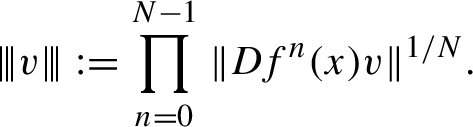 $$ \begin{align} \mathopen{| {\kern -1.5pt} | {\kern -1.5pt} |} {v} \mathclose{| {\kern -1.5pt} | {\kern -1.5pt} |} := \prod_{n=0}^{N-1} \| Df^n(x) v \|^{1/N}. \end{align} $$
This defines a norm on each one-dimensional bundle
 $E_j(x)$
. Consider the unique inner product on
$E_j(x)$
. Consider the unique inner product on
 $T_x M$
that makes those bundles orthogonal and whose induced norm agrees with the definition above.
$T_x M$
that makes those bundles orthogonal and whose induced norm agrees with the definition above.
If
 $v\in E_j(x)$
is non-zero then, by telescopic multiplication,
$v\in E_j(x)$
is non-zero then, by telescopic multiplication,
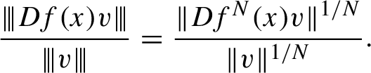 $$ \begin{align*} \frac{\mathopen{| {\kern -1.5pt} | {\kern -1.5pt} |} {Df(x) v} \mathclose{| {\kern -1.5pt} | {\kern -1.5pt} |}}{\mathopen{| {\kern -1.5pt} | {\kern -1.5pt} |} {v} \mathclose{| {\kern -1.5pt} | {\kern -1.5pt} |}} = \frac{\| Df^N(x) v \|^{1/N}}{\|v\|^{1/N}}. \end{align*} $$
This means that the expansion function
 $\chi _j$
defined by equation (3.1) equals
$\chi _j$
defined by equation (3.1) equals
 $\theta _j^{(N)}/N$
. Therefore, the desired properties shown by equations (3.2) and (3.3) are just those of equations (3.4) and (3.5).
$\theta _j^{(N)}/N$
. Therefore, the desired properties shown by equations (3.2) and (3.3) are just those of equations (3.4) and (3.5).
Remark 3.2. It follows from the proof that the Lyapunov metrics can be constructed so that the tempering property
 $|\chi _j \circ f - \chi _j| < \varepsilon $
also holds.
$|\chi _j \circ f - \chi _j| < \varepsilon $
also holds.
Remark 3.3. Our proof used that the bundles of the dominated splitting are one-dimensional, so that the geometric average defined by formula (3.6) defines a norm. If the bundles
 $E_j$
are higher dimensional, one can still adapt this trick by taking an appropriate notion of averaging on the symmetric space of inner products: see [Reference Bochi10, p. 1839].
$E_j$
are higher dimensional, one can still adapt this trick by taking an appropriate notion of averaging on the symmetric space of inner products: see [Reference Bochi10, p. 1839].
3.2 Lyapunov charts
Proposition 3.4. (Lyapunov charts)
Suppose that
 $f\in \mathrm {Diff}^r_m(M)$
is a conservative Anosov diffeomorphism of unstable index u admitting a simple dominated splitting
$f\in \mathrm {Diff}^r_m(M)$
is a conservative Anosov diffeomorphism of unstable index u admitting a simple dominated splitting
 $TM = E_1 \oplus \cdots \oplus E_d$
, and that
$TM = E_1 \oplus \cdots \oplus E_d$
, and that
 $\mathopen {\langle {\kern -1.7pt} \langle }{\mathord {\cdot }, \mathord {\cdot }} \mathclose {\rangle {\kern -1.7pt} \rangle }$
is a Lyapunov metric.
$\mathopen {\langle {\kern -1.7pt} \langle }{\mathord {\cdot }, \mathord {\cdot }} \mathclose {\rangle {\kern -1.7pt} \rangle }$
is a Lyapunov metric.
Then for all
 $x \in M$
, there exists a map
$x \in M$
, there exists a map
 $\Phi _x \colon B_0 \to M$
, where
$\Phi _x \colon B_0 \to M$
, where
 $B_0 \subset \mathbb {R}^d$
is a fixed closed ball centered at
$B_0 \subset \mathbb {R}^d$
is a fixed closed ball centered at
 $0$
, with the following properties:
$0$
, with the following properties:
-
(a)
$\Phi _x(0) = x$
; -
(b)
$\Phi _x$
is a smooth diffeomorphism onto its image; -
(c)
$\Phi _x$
has constant Jacobian, that is, the push-forward of Lebesgue measure on
$B_0$
equals the restriction of the measure m to
$\Phi _x(B_0)$
times a constant factor; -
(d) the derivative
$\mathcal {L}_x := D\Phi _x(0)$
takes the canonical basis
$\{e_1,\ldots ,e_d\}$
of
$\mathbb {R}^d$
to a basis
$\{\mathcal {L}_x(e_1), \ldots , \mathcal {L}_x(e_d)\}$
of
$T_x M$
which is orthonormal for the Lyapunov metric
$\mathopen {\langle {\kern -1.7pt} \langle }{\mathord {\cdot }, \mathord {\cdot }} \mathclose {\rangle {\kern -1.7pt} \rangle }_x$
and, moreover,
$\mathcal {L}_x(e_j) \in E_j(x)$
for each j.


Furthermore,
 $\{\Phi _x \;\mathord {;}\; x \in M\}$
is a relatively compact subset of
$\{\Phi _x \;\mathord {;}\; x \in M\}$
is a relatively compact subset of
 $C^{\infty }(B_0,M)$
.
$C^{\infty }(B_0,M)$
.
Proof As it is well known and elementary (see e.g. [Reference Kobayashi30, p. 6]), the manifold M admits a conservative atlas, that is, an atlas whose charts
 $F_i \colon U_i \subset \mathbb {R}^d \to M$
are such that the push-forward of Lebesgue measure on
$F_i \colon U_i \subset \mathbb {R}^d \to M$
are such that the push-forward of Lebesgue measure on
 $U_i$
coincides with the measure m restricted to
$U_i$
coincides with the measure m restricted to
 $F_i(U_i)$
. By compactness, we assume that this atlas is finite.
$F_i(U_i)$
. By compactness, we assume that this atlas is finite.
Now, given
 $x \in M$
, let
$x \in M$
, let
 $\mathcal {L}_x \colon \mathbb {R}^d \to T_x M$
be a linear isomorphism that sends the coordinate axes to the bundles
$\mathcal {L}_x \colon \mathbb {R}^d \to T_x M$
be a linear isomorphism that sends the coordinate axes to the bundles
 $E_{1}$
, …,
$E_{1}$
, …,
 $E_{d}$
, and such that the push-forward of the standard inner product is the Lyapunov metric
$E_{d}$
, and such that the push-forward of the standard inner product is the Lyapunov metric
 $\mathopen {\langle {\kern -1.7pt} \langle }{\mathord {\cdot }, \mathord {\cdot }} \mathclose {\rangle {\kern -1.7pt} \rangle }_x$
. Choose i such that
$\mathopen {\langle {\kern -1.7pt} \langle }{\mathord {\cdot }, \mathord {\cdot }} \mathclose {\rangle {\kern -1.7pt} \rangle }_x$
. Choose i such that
 $F_i(U_i) \ni x$
, and define
$F_i(U_i) \ni x$
, and define
 $$ \begin{align*} \Phi_x (z) := F_i ( F_i^{-1}(x) + (DF_i^{-1}(x) \circ \mathcal{L}_x) (z) ), \end{align*} $$
for every z in a sufficiently small closed ball
 $B_0 \subset \mathbb {R}^d$
around
$B_0 \subset \mathbb {R}^d$
around
 $0$
. It is clear that these maps have the asserted properties (a)–(d). Moreover, all their derivatives are uniformly bounded, so we obtain relative compactness of the family.
$0$
. It is clear that these maps have the asserted properties (a)–(d). Moreover, all their derivatives are uniformly bounded, so we obtain relative compactness of the family.
The maps
 $\Phi _x$
given by the proposition are called Lyapunov charts. Note that the derivative of f at an arbitrary point
$\Phi _x$
given by the proposition are called Lyapunov charts. Note that the derivative of f at an arbitrary point
 $x\in M$
can be diagonalized using the Lyapunov charts as follows:
$x\in M$
can be diagonalized using the Lyapunov charts as follows:
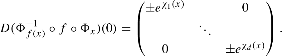 $$ \begin{align} D ( \Phi_{f(x)}^{-1} \circ f \circ \Phi_x) (0) = \begin{pmatrix} \pm e^{\chi_{1}(x)} & & 0 \\ & \ddots & \\ 0 & & \pm e^{\chi_{d}(x)} \end{pmatrix}. \end{align} $$
4 Damping perturbations
In this section, we define a certain type of perturbations
 $\tilde f$
of an Anosov diffeomorphism f, called damping perturbations. The idea comes from Baraviera and Bonatti [Reference Baraviera and Bonatti5] but, as one of the referees has pointed out to us, constructions of this type go back to Newhouse and Mañé.
$\tilde f$
of an Anosov diffeomorphism f, called damping perturbations. The idea comes from Baraviera and Bonatti [Reference Baraviera and Bonatti5] but, as one of the referees has pointed out to us, constructions of this type go back to Newhouse and Mañé.
Damping perturbations are actually ‘large perturbations’, in the sense that the
 $C^1$
or even the
$C^1$
or even the
 $C^0$
distance between
$C^0$
distance between
 $\tilde f$
and f may be large. However, the support of the perturbation, that is, the set
$\tilde f$
and f may be large. However, the support of the perturbation, that is, the set
 $Z := \{x \;\mathord {;}\; \tilde f(x) \neq f(x)\}$
is required to be ‘dynamically small’: the return times from Z to itself are not smaller than a large number N. On Z, we impose a transversality condition: essentially we want the spaces
$Z := \{x \;\mathord {;}\; \tilde f(x) \neq f(x)\}$
is required to be ‘dynamically small’: the return times from Z to itself are not smaller than a large number N. On Z, we impose a transversality condition: essentially we want the spaces
 $D\tilde {f}(x)E^{\mathrm {u}}(x)$
and
$D\tilde {f}(x)E^{\mathrm {u}}(x)$
and
 $D\tilde {f}(x)E^{\mathrm {s}}(x)$
to be transverse to
$D\tilde {f}(x)E^{\mathrm {s}}(x)$
to be transverse to
 $E^{\mathrm {s}}(\tilde {f}(x))$
and
$E^{\mathrm {s}}(\tilde {f}(x))$
and
 $E^{\mathrm {u}}(\tilde {f}(x))$
, respectively, where
$E^{\mathrm {u}}(\tilde {f}(x))$
, respectively, where
 $E^{\mathrm {u}}\oplus E^{\mathrm {s}}$
denotes the hyperbolic splitting of f. We show that if the least return time N is large enough, then the perturbed diffeomorphism
$E^{\mathrm {u}}\oplus E^{\mathrm {s}}$
denotes the hyperbolic splitting of f. We show that if the least return time N is large enough, then the perturbed diffeomorphism
 $\tilde {f}$
is still Anosov. Moreover, on the set Z, the new unstable bundle
$\tilde {f}$
is still Anosov. Moreover, on the set Z, the new unstable bundle
 $\tilde {E}^{\mathrm {u}}$
is close to the old one
$\tilde {E}^{\mathrm {u}}$
is close to the old one
 $E^{\mathrm {u}}$
, while on the set
$E^{\mathrm {u}}$
, while on the set
 $f(Z)$
, they can be far apart. As we go upwards in the tower with base Z, the bundle
$f(Z)$
, they can be far apart. As we go upwards in the tower with base Z, the bundle
 $\tilde {E}^{\mathrm {u}}$
is attracted by
$\tilde {E}^{\mathrm {u}}$
is attracted by
 $E^{\mathrm {u}}$
, so it suffers some ‘damping’ before returning to Z and getting ‘kicked’ again. See Figure 4. Actually, we work with Anosov diffeomorphisms with simple dominated splitting; we show that domination also persists under damping perturbations. Let us give precise statements.
$E^{\mathrm {u}}$
, so it suffers some ‘damping’ before returning to Z and getting ‘kicked’ again. See Figure 4. Actually, we work with Anosov diffeomorphisms with simple dominated splitting; we show that domination also persists under damping perturbations. Let us give precise statements.
A damping perturbation
 $\tilde f$
of an Anosov diffeomorphism
$\tilde f$
of an Anosov diffeomorphism
 $f\!.$

4.1 Definition of damping perturbations
Assume given a conservative Anosov diffeomorphism
 $f\in \mathrm {Diff}^r_m(M)$
of unstable index u and admitting a simple dominated splitting
$f\in \mathrm {Diff}^r_m(M)$
of unstable index u and admitting a simple dominated splitting
 $TM = E_1 \oplus \cdots \oplus E_d$
. Fix a Lyapunov metric
$TM = E_1 \oplus \cdots \oplus E_d$
. Fix a Lyapunov metric
 $\mathopen {\langle {\kern -1.7pt} \langle }{\mathord {\cdot }, \mathord {\cdot }} \mathclose {\rangle {\kern -1.7pt} \rangle }$
. Let us use the following notation:
$\mathopen {\langle {\kern -1.7pt} \langle }{\mathord {\cdot }, \mathord {\cdot }} \mathclose {\rangle {\kern -1.7pt} \rangle }$
. Let us use the following notation:
 $$ \begin{align} \boldsymbol{\chi}(x) := (\chi_1(x), \ldots, \chi_d(x)), \end{align} $$
where the
 $\chi _j$
terms are the expansion functions of equation (3.1). By definition of the Lyapunov metric,
$\chi _j$
terms are the expansion functions of equation (3.1). By definition of the Lyapunov metric,
 $\textsf {g}_u ( \boldsymbol {\chi }(x) )> 0$
for every
$\textsf {g}_u ( \boldsymbol {\chi }(x) )> 0$
for every
 $x \in M$
, where
$x \in M$
, where
 $\textsf {g}_u$
is the gap function of equation (2.2).
$\textsf {g}_u$
is the gap function of equation (2.2).
For each
 $x\in M$
, let
$x\in M$
, let
 $$ \begin{align} \mathcal{L}_x \colon \mathbb{R}^d \to T_x M \end{align} $$
be a linear map that takes the canonical basis
 $\{e_1,\ldots ,e_d\}$
of
$\{e_1,\ldots ,e_d\}$
of
 $\mathbb {R}^d$
to a basis
$\mathbb {R}^d$
to a basis
 $\{\mathcal {L}_x(e_1), \ldots , \mathcal {L}_x(e_d)\}$
of
$\{\mathcal {L}_x(e_1), \ldots , \mathcal {L}_x(e_d)\}$
of
 $T_x M$
that is orthonormal for the Lyapunov metric
$T_x M$
that is orthonormal for the Lyapunov metric
 $\mathopen {\langle {\kern -1.7pt} \langle }{\mathord {\cdot }, \mathord {\cdot }} \mathclose {\rangle {\kern -1.7pt} \rangle }_x$
and, moreover,
$\mathopen {\langle {\kern -1.7pt} \langle }{\mathord {\cdot }, \mathord {\cdot }} \mathclose {\rangle {\kern -1.7pt} \rangle }_x$
and, moreover,
 $\mathcal {L}_x(e_j) \in E_j(x)$
for each j. Note that the map
$\mathcal {L}_x(e_j) \in E_j(x)$
for each j. Note that the map
 $\mathcal {L}_x$
is unique modulo composing from the right by a matrix of the form
$\mathcal {L}_x$
is unique modulo composing from the right by a matrix of the form
 $\mathrm {diag}(\pm 1, \ldots , \pm 1)$
. Taking quotient by this finite group,
$\mathrm {diag}(\pm 1, \ldots , \pm 1)$
. Taking quotient by this finite group,
 $\mathcal {L}_x$
becomes unique and continuous.
$\mathcal {L}_x$
becomes unique and continuous.
For each
 $j \in \{1,\ldots ,d-1\}$
and
$j \in \{1,\ldots ,d-1\}$
and
 $\tau>0$
, we define the standard horizontal and vertical cones of index j and opening
$\tau>0$
, we define the standard horizontal and vertical cones of index j and opening
 $\tau $
as the following subsets of Euclidean space
$\tau $
as the following subsets of Euclidean space
 $\mathbb {R}^d$
:
$\mathbb {R}^d$
:
 $$ \begin{align} \mathcal{H}_j(\tau) &:= \{ (z_1,\ldots,z_d) \;\mathord{;}\; z_{j+1}^2 + \cdots + z_d^2 < \tau^2 (z_1^2 + \cdots + z_j^2) \} \cup \{0\}, \end{align} $$
 $$ \begin{align} \mathcal{V}_j(\tau) &:= \{ (z_1,\ldots,z_d) \;\mathord{;}\; z_1^2 + \ldots + z_j^2 < \tau^2 (z_{j+1}^2 + \ldots + z_d^2) \} \cup \{0\}. \end{align} $$
Then we define the following continuous fields of cones on the tangent bundle
 $TM$
:
$TM$
:
 $$ \begin{align*} \mathcal{H}_j(x,\tau) := \mathcal{L}_x (\mathcal{H}_j(\tau)), \quad \mathcal{V}_j(x,\tau) := \mathcal{L}_x (\mathcal{V}_j(\tau)). \end{align*} $$
By equation (3.7), we have the following invariance properties, for every
 $\tau>0$
:
$\tau>0$
:
 $$ \begin{align} Df(x) \mathcal{H}_j(x,\tau) &\subseteq \mathcal{H}_j(f(x), e^{-[\chi_j(x)-\chi_{j+1}(x)]} \tau), \end{align} $$
 $$ \begin{align} Df^{-1}(x)\mathcal{V}_j(x,\tau) &\subseteq \mathcal{V}_j(f^{-1}(x),e^{-[\chi_j(f^{-1}(x))-\chi_{j+1}(f^{-1}(x))]} \tau). \end{align} $$
Let
 $P^{\mathrm {u}}$
and
$P^{\mathrm {u}}$
and
 $P^{\mathrm {s}} : TM \to TM$
be the projections on the unstable and stable bundles of f, respectively, so that their sum is the identity.
$P^{\mathrm {s}} : TM \to TM$
be the projections on the unstable and stable bundles of f, respectively, so that their sum is the identity.
Fix numbers
 $\alpha> \beta >0$
,
$\alpha> \beta >0$
,
 $\kappa>0$
,
$\kappa>0$
,
 $\sigma> 0$
, and
$\sigma> 0$
, and
 $N \ge 2$
. We say that a diffeomorphism
$N \ge 2$
. We say that a diffeomorphism
 $\tilde f \in \mathrm {Diff}^r_m(M)$
is a
$\tilde f \in \mathrm {Diff}^r_m(M)$
is a
 $(\alpha ,\beta ,\kappa ,\sigma ,N)$
-damping perturbation of f with respect to the metric
$(\alpha ,\beta ,\kappa ,\sigma ,N)$
-damping perturbation of f with respect to the metric
 $\mathopen {\langle {\kern -1.7pt} \langle }{\mathord {\cdot }, \mathord {\cdot }} \mathclose {\rangle {\kern -1.7pt} \rangle }$
if the following conditions hold.
$\mathopen {\langle {\kern -1.7pt} \langle }{\mathord {\cdot }, \mathord {\cdot }} \mathclose {\rangle {\kern -1.7pt} \rangle }$
if the following conditions hold.
-
(i) For all
$x \in M$
and
$j \in \{1,\ldots ,d-1\}$
,
$$ \begin{align*} D\tilde{f}(x) \mathcal{H}_j(x,\beta) &\subseteq \mathcal{H}_j(\tilde{f}(x), \alpha), \\ D\tilde{f}^{-1}(x)\mathcal{V}_j(x,\beta) &\subseteq \mathcal{V}_j(\tilde{f}^{-1}(x),\alpha). \end{align*} $$
-
(ii) For all
$x \in M$
,
$$\begin{align*}\begin{aligned} v &\in \mathcal{H}_u(x,\beta) &&\Rightarrow &\mathopen{| {\kern -1.5pt} | {\kern -1.5pt} |} {P^{\mathrm{u}} \, D\tilde{f}(x) \, v} \mathclose{| {\kern -1.5pt} | {\kern -1.5pt} |} &\ge \kappa \, \mathopen{| {\kern -1.5pt} | {\kern -1.5pt} |} {P^{\mathrm{u}} \, v} \mathclose{| {\kern -1.5pt} | {\kern -1.5pt} |}, \\ v &\in \mathcal{V}_u(x,\beta) &&\Rightarrow &\mathopen{| {\kern -1.5pt} | {\kern -1.5pt} |} {P^{\mathrm{s}} \, D\tilde{f}^{-1}(x) \, v} \mathclose{| {\kern -1.5pt} | {\kern -1.5pt} |} &\ge \kappa \, \mathopen{| {\kern -1.5pt} | {\kern -1.5pt} |} {P^{\mathrm{s}} \, v} \mathclose{| {\kern -1.5pt} | {\kern -1.5pt} |}. \end{aligned} \end{align*}$$
-
(iii) Letting
the sets Z,
$$ \begin{align*} Z := \{x \in M \;\mathord{;}\; \tilde{f}(x) \neq f(x)\;\mbox{or}\; D\tilde{f}(x)\neq Df(x)\}, \end{align*} $$
$f(Z)$
, …,
$f^{N-1}(Z)$
have disjoint closures.
-
(iv) For all
$x \in Z$
, we have, in terms of notations (4.1) and (2.2):
$$ \begin{align*} \textsf{g}_u \bigg( \frac{1}{N-1} \sum_{n=1}^{N-1} \boldsymbol{\chi}(f^n x) \bigg) \ge \frac{\sigma}{2}, \quad \textsf{g}_u \bigg( \frac{1}{N-1} \sum_{n=-N-2}^{0} \boldsymbol{\chi}(f^n x) \bigg) \ge \frac{\sigma}{2}. \end{align*} $$


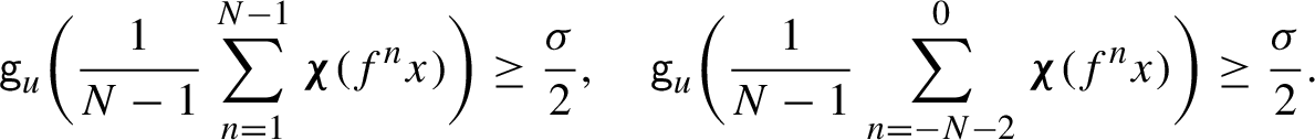
Note that the definition is symmetric under time-reversal, that is,
 $\tilde {f}^{-1}$
is a
$\tilde {f}^{-1}$
is a
 $(\alpha ,\beta ,\kappa ,\sigma ,N)$
-damping perturbation of
$(\alpha ,\beta ,\kappa ,\sigma ,N)$
-damping perturbation of
 $f^{-1}$
. Indeed,
$f^{-1}$
. Indeed,
 $\{x \in M \;\mathord {;}\; \tilde {f}^{-1}(x) \neq f^{-1}(x)\;\mbox {or}\;D \tilde {f}^{-1} (x) \neq Df^{-1}(x)\} = f(Z)$
.
$\{x \in M \;\mathord {;}\; \tilde {f}^{-1}(x) \neq f^{-1}(x)\;\mbox {or}\;D \tilde {f}^{-1} (x) \neq Df^{-1}(x)\} = f(Z)$
.
Remark 4.1. Note that condition (iv) is weaker than the condition
 $\textsf {g}_u \circ \boldsymbol {\chi } \ge {\sigma }/{2}$
, which is always satisfied in this paper. The reason why we insist in working with the more complicated condition (iv) is that it may be useful for future applications of our methods. Moreover, working with the stronger condition would not make the proof of Proposition 4.2 below any simpler.
$\textsf {g}_u \circ \boldsymbol {\chi } \ge {\sigma }/{2}$
, which is always satisfied in this paper. The reason why we insist in working with the more complicated condition (iv) is that it may be useful for future applications of our methods. Moreover, working with the stronger condition would not make the proof of Proposition 4.2 below any simpler.
4.2 Properties of damping perturbations
We will show that damping perturbations are still Anosov with simple dominated splitting, provided the ‘damping time’ N is large enough. It is important that the condition on N depends only on the other parameters
 $\alpha $
,
$\alpha $
,
 $\beta $
,
$\beta $
,
 $\kappa $
,
$\kappa $
,
 $\sigma $
(together with a parameter
$\sigma $
(together with a parameter
 $\gamma $
that controls the desired closeness between the new and the old spaces), but not on f itself. Furthermore, given the other parameters, the damping time N must be at least of the order
$\gamma $
that controls the desired closeness between the new and the old spaces), but not on f itself. Furthermore, given the other parameters, the damping time N must be at least of the order
 $1/\sigma $
. This should not come as a surprise, because Lyapunov exponents are inversely proportional to the time it takes to obtain a prescribed factor of expansion or contraction.
$1/\sigma $
. This should not come as a surprise, because Lyapunov exponents are inversely proportional to the time it takes to obtain a prescribed factor of expansion or contraction.
Given numbers
 $\alpha>\beta >\gamma >0$
,
$\alpha>\beta >\gamma >0$
,
 $\kappa>0$
, and
$\kappa>0$
, and
 $\sigma>0$
, let
$\sigma>0$
, let
 $$ \begin{align} N_0 := \bigg\lfloor \frac{2}{\sigma}\log(\max\{\kappa^{-1},\alpha\gamma^{-1}\})\bigg\rfloor + 2. \end{align} $$
Let
 $f\in \mathrm {Diff}^r_m(M)$
be a conservative Anosov diffeomorphism of unstable index u admitting a simple dominated splitting
$f\in \mathrm {Diff}^r_m(M)$
be a conservative Anosov diffeomorphism of unstable index u admitting a simple dominated splitting
 $TM = E_1 \oplus \cdots \oplus E_d$
, and fix a Lyapunov metric for f.
$TM = E_1 \oplus \cdots \oplus E_d$
, and fix a Lyapunov metric for f.
Proposition 4.2. Let
 $N \ge N_0$
and let
$N \ge N_0$
and let
 $\tilde f \in \mathrm {Diff}^r_m(M)$
be a
$\tilde f \in \mathrm {Diff}^r_m(M)$
be a
 $(\alpha ,\beta ,\kappa ,\sigma ,N)$
-damping perturbation of f with respect to the Lyapunov metric.
$(\alpha ,\beta ,\kappa ,\sigma ,N)$
-damping perturbation of f with respect to the Lyapunov metric.
Then
 $\tilde f$
is a conservative Anosov diffeomorphism of unstable index u, and it admits a simple dominated splitting
$\tilde f$
is a conservative Anosov diffeomorphism of unstable index u, and it admits a simple dominated splitting
 $\tilde E_1 \oplus \cdots \oplus \tilde E_d$
.
$\tilde E_1 \oplus \cdots \oplus \tilde E_d$
.
Moreover, letting
 $Z := \{x \in M \;\mathord {;}\; \tilde {f}(x) \neq f(x)\;\mbox {or}\; D\tilde {f}(x)\neq Df(x)\}$
, then for all
$Z := \{x \in M \;\mathord {;}\; \tilde {f}(x) \neq f(x)\;\mbox {or}\; D\tilde {f}(x)\neq Df(x)\}$
, then for all
 $x\in M$
and
$x\in M$
and
 $j \in \{1,\ldots ,d-1\}$
:
$j \in \{1,\ldots ,d-1\}$
:
-
(a)
$\tilde {E}_1(x) \oplus \cdots \oplus \tilde {E}_j(x)$
and
$E_{j+1}(x) \oplus \cdots \oplus E_d(x)$
are transverse, and if
$x \not \in \bigsqcup _{n=1}^{N-1} f^n(Z)$
, then
$\tilde {E}_1(x) \oplus \cdots \oplus \tilde {E}_j(x)\subset \mathcal {H}_j(x,\gamma )$
; -
(b)
$\tilde {E}_{j+1}(x) \oplus \cdots \oplus \tilde {E}_d(x)$
and
$E_1(x) \oplus \cdots \oplus E_j(x)$
are transverse, and if
$x \not \in \bigsqcup _{n=-N-2}^{0} f^n(Z)$
, then
$\tilde {E}_{j+1}(x) \oplus \cdots \oplus \tilde {E}_d(x)\subset \mathcal {V}_j(x,\gamma )$
.


Observe that
 $N_0 \ge 2$
and that
$N_0 \ge 2$
and that
 $$ \begin{align} e^{(N_0-1) \sigma/2}> \max\{\kappa^{-1} , \alpha \gamma^{-1} \}. \end{align} $$
The first step is to construct continuous fields of cones that are invariant with respect to the perturbation
 $\tilde f$
.
$\tilde f$
.
Lemma 4.3. For each
 $j \in \{1,\ldots ,d-1\}$
, there exists a continuous function
$j \in \{1,\ldots ,d-1\}$
, there exists a continuous function
 $\omega _j$
on M such that, for every
$\omega _j$
on M such that, for every
 $x \in M$
,
$x \in M$
,
-
(a)
$\gamma \le \omega _j(x) \le \alpha $
; -
(b)
$\omega _j(x) = \gamma $
if
$x \not \in \bigsqcup _{n=1}^{N-1} f^n(\bar Z)$
; -
(c)
$D\tilde f(x) \, \overline {\mathcal {H}_j(x,\omega _j(x))} \subset \mathcal {H}_j ( \tilde f(x), \omega _j(\tilde f(x)) )$
.


Proof of Proposition 4.2 Fix j. By equation (4.8), we can choose
 $\varepsilon>0$
such that
$\varepsilon>0$
such that
 $$ \begin{align*} \varepsilon < \inf_M (\chi_j - \chi_{j+1}) \quad \text{and} \quad \alpha e^{-(N-1)(\sigma/2-\varepsilon)}<\gamma. \end{align*} $$
Let
 $$ \begin{align*} A := \{ x \in M \;\mathord{;}\; D\tilde{f}(x) \, \overline{\mathcal{H}_j(x,\gamma)} \subset \mathcal{H}_j(\tilde{f}(x),\gamma) \}. \end{align*} $$
Then A is an open set and
 $A \cup Z = M$
. Let
$A \cup Z = M$
. Let
 $\rho _1 + \rho _2 = 1$
be a partition of unity subordinated to this open covering. Define the function
$\rho _1 + \rho _2 = 1$
be a partition of unity subordinated to this open covering. Define the function
 $\omega _j$
as follows:
$\omega _j$
as follows:
-
• if
$x \not \in \bigsqcup _{n=1}^{N-1} f^n(\bar Z)$
, then we let
$\omega _j(x) := \gamma $
; -
• if
$x \in f(Z) = \tilde {f}(Z)$
, then we let
$$ \begin{align*} \omega_j(x) := \gamma \rho_1(\tilde{f}^{-1}(x)) + \alpha \rho_2(\tilde{f}^{-1}(x)). \end{align*} $$
-
• if
$x \in f^n(Z)$
, where
$2 \le n \le N-1$
then, assuming
$\omega _j$
was already defined on
$f^{n-1}(Z)$
, we let
$$ \begin{align*} \omega_j(x) := \max \{ \gamma, \omega_j(f^{-1}(x)) e^{-\chi_j(f^{-1}(x)) +\chi_{j+1}(f^{-1}(x)) + \varepsilon} \}. \end{align*} $$


The function
 $\omega _j$
is continuous and has properties (a) and (b). Next we check property (c) case by case. First, consider
$\omega _j$
is continuous and has properties (a) and (b). Next we check property (c) case by case. First, consider
 $x \in Z$
.
$x \in Z$
.
-
• If
$x \in Z \cap A$
, then
$\omega _j(x) = \gamma $
and
$\omega _j(\tilde {f}(x)) \ge \gamma $
, so property (c) follows directly from the definition of A. -
• If
$x \in Z \smallsetminus A$
, then
$\omega _j(x) = \gamma < \beta $
and
$\omega _j(\tilde {f}(x)) = \alpha $
, so property (c) follows from condition (i) in the definition of damping perturbations.
Next we consider the cases where
 $x \not \in Z$
, and so
$x \not \in Z$
, and so
 $\tilde {f}(x) = f(x)$
and
$\tilde {f}(x) = f(x)$
and
 $D\tilde {f}(x) = Df(x)$
.
$D\tilde {f}(x) = Df(x)$
.
-
• If
$x \not \in \bigsqcup _{n=0}^{N-1} f^n(\bar Z)$
, then
$\omega _j(x) = \omega _j(f(x)) = \gamma $
, so property (c) follows from the invariance property (4.5). -
• If
$x \in f^n(Z)$
for some
$n \in \{1,\ldots ,N-2\}$
, then and so property (c) again follows from the invariance property (4.5).
$$ \begin{align*} \omega_j(f(x)) \ge \omega_j(x) e^{-\chi_j(x)+\chi_{j+1}(x)+\varepsilon}, \end{align*} $$
-
• Finally, if
$x \in f^{N-1}(Z)$
then, letting
$y := f^{-N+2}(x)$
, Using the fact that
$$ \begin{align*} \omega_j(x) = \max \bigg\{ \gamma, \omega_j(y) \exp \sum_{i=0}^{N-2} [-\chi_j(f^i(y))+\chi_{j+1}(f^i(y))+\varepsilon ] \bigg\}. \end{align*} $$
$\omega _j(y) \le \alpha $
, condition (iv) from the definition of damping perturbations, and the choice of
$\varepsilon $
, we obtain that
${\omega _j(x) = \gamma }$
. Of course,
$\omega _j(f(x))$
also equals
$\gamma $
, so property (c) again follows from the invariance property (4.5).


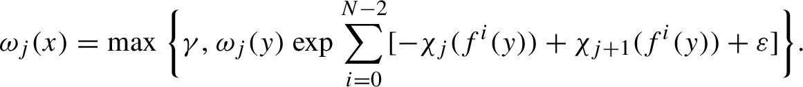


This completes the proof of lemma.
Property (c) from Lemma 4.3 means that for each j, the continuous cone field
 $\mathcal {C}_j(x) := \mathcal {H}_j(x,\omega _j(x))$
is strictly forward invariant. This implies that the diffeomorphism
$\mathcal {C}_j(x) := \mathcal {H}_j(x,\omega _j(x))$
is strictly forward invariant. This implies that the diffeomorphism
 $\tilde f$
has a simple dominated splitting
$\tilde f$
has a simple dominated splitting
 $\tilde E_1 \oplus \cdots \oplus \tilde E_d$
such that for all x and j, we have
$\tilde E_1 \oplus \cdots \oplus \tilde E_d$
such that for all x and j, we have
 $\tilde {E}_1(x) \oplus \cdots \oplus \tilde {E}_j(x) \subset \mathcal {C}_j(x)$
; see e.g. [Reference Sambarino41, Proposition 2.2]. In particular, conclusion (a) of Proposition 4.2 is satisfied. Because the definition of damping perturbations is symmetric under time-reversal, it follows that conclusion (b) is also satisfied.
$\tilde {E}_1(x) \oplus \cdots \oplus \tilde {E}_j(x) \subset \mathcal {C}_j(x)$
; see e.g. [Reference Sambarino41, Proposition 2.2]. In particular, conclusion (a) of Proposition 4.2 is satisfied. Because the definition of damping perturbations is symmetric under time-reversal, it follows that conclusion (b) is also satisfied.
Next, consider the sub-bundles:
 $$\begin{align*}\begin{aligned} E^{\mathrm{u}} &:= E_1 \oplus \cdots \oplus E_u, &\quad E^{\mathrm{s}} &:= E_{u+1} \oplus \cdots \oplus E_d, \\ \tilde E^{\mathrm{u}} &:= \tilde E_1 \oplus \cdots \oplus \tilde E_u, &\quad \tilde E^{\mathrm{s}} &:= \tilde E_{u+1} \oplus \cdots \oplus \tilde E_d. \end{aligned} \end{align*}$$
Let us check that the
 $D\tilde {f}$
-invariant splitting
$D\tilde {f}$
-invariant splitting
 $\tilde E^{\mathrm {u}} \oplus \tilde E^{\mathrm {s}}$
is uniformly hyperbolic.
$\tilde E^{\mathrm {u}} \oplus \tilde E^{\mathrm {s}}$
is uniformly hyperbolic.
Recall that
 $P^{\mathrm {u}} \colon TM \to TM$
denotes the projection onto
$P^{\mathrm {u}} \colon TM \to TM$
denotes the projection onto
 $E^{\mathrm {u}}$
with kernel
$E^{\mathrm {u}}$
with kernel
 $E^{\mathrm {s}}$
. Then, for every
$E^{\mathrm {s}}$
. Then, for every
 $x \in M$
and
$x \in M$
and
 $v \in T_x M$
,
$v \in T_x M$
,
 $$ \begin{align} \mathopen{| {\kern -1.5pt} | {\kern -1.5pt} |} {P^{\mathrm{u}} Df(x) \, v} \mathclose{| {\kern -1.5pt} | {\kern -1.5pt} |} \ge e^{\chi_u(x)} \mathopen{| {\kern -1.5pt} | {\kern -1.5pt} |} {P^{\mathrm{u}} v} \mathclose{| {\kern -1.5pt} | {\kern -1.5pt} |} \ge a_1 \mathopen{| {\kern -1.5pt} | {\kern -1.5pt} |} {P^{\mathrm{u}} v} \mathclose{| {\kern -1.5pt} | {\kern -1.5pt} |} , \end{align} $$
for some constant
 $a_1>1$
. Now consider
$a_1>1$
. Now consider
 $x \in Z$
and
$x \in Z$
and
 $v \in \mathcal {C}_u(x)$
; then,
$v \in \mathcal {C}_u(x)$
; then,
 $$ \begin{align*} \mathopen{| {\kern -1.5pt} | {\kern -1.5pt} |} {P^{\mathrm{u}} \, D\tilde{f}^N(x) v} \mathclose{| {\kern -1.5pt} | {\kern -1.5pt} |} &\ge \mathopen{| {\kern -1.5pt} | {\kern -1.5pt} |} {P^{\mathrm{u}} Df^{N-1}(\tilde{f}(x)) \, D\tilde{f}(x) \, v} \mathclose{| {\kern -1.5pt} | {\kern -1.5pt} |} \\ &\ge \exp\bigg[ \sum_{i=0}^{N-2} \chi_u(f^i(\tilde{f}(x))) \bigg] \mathopen{| {\kern -1.5pt} | {\kern -1.5pt} |} {P^{\mathrm{u}} D\tilde{f}(x) \, v} \mathclose{| {\kern -1.5pt} | {\kern -1.5pt} |} \\ &\ge e^{(N-1)\sigma/2} \mathopen{| {\kern -1.5pt} | {\kern -1.5pt} |} {P^{\mathrm{u}} D\tilde{f}(x) \, v} \mathclose{| {\kern -1.5pt} | {\kern -1.5pt} |} &\quad&\text{(by (iv))} \\ &\ge \kappa e^{(N-1)\sigma/2} \mathopen{| {\kern -1.5pt} | {\kern -1.5pt} |} {P^{\mathrm{u}} v} \mathclose{| {\kern -1.5pt} | {\kern -1.5pt} |} &\quad&\text{(by (ii))}. \end{align*} $$
Let
 $a_2 =: \kappa e^{(N-1)\sigma /2}$
, which, by inequality (4.8), is bigger than
$a_2 =: \kappa e^{(N-1)\sigma /2}$
, which, by inequality (4.8), is bigger than
 $1$
.
$1$
.
Let
 $a_3 := \min \{a_1,a_2^{1/N}\}> 1$
. We claim that there exists a constant
$a_3 := \min \{a_1,a_2^{1/N}\}> 1$
. We claim that there exists a constant
 $c> 0$
such that for all
$c> 0$
such that for all
 $x\in M$
,
$x\in M$
,
 $v \in \mathcal {C}_u(x)$
, and
$v \in \mathcal {C}_u(x)$
, and
 $n \ge 0$
,
$n \ge 0$
,
 $$ \begin{align} \mathopen{| {\kern -1.5pt} | {\kern -1.5pt} |} {P^{\mathrm{u}} \, D\tilde{f}^n(x) \, v} \mathclose{| {\kern -1.5pt} | {\kern -1.5pt} |} \ge c a_3^n \mathopen{| {\kern -1.5pt} | {\kern -1.5pt} |} {P^{\mathrm{u}} \, v} \mathclose{| {\kern -1.5pt} | {\kern -1.5pt} |}. \end{align} $$
Indeed, the inequality holds with
 $c=1$
if the segment of orbit
$c=1$
if the segment of orbit
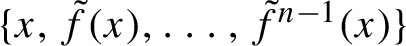 $\{x, \tilde {f}(x), \ldots , \tilde {f}^{n-1}(x)\}$
:
$\{x, \tilde {f}(x), \ldots , \tilde {f}^{n-1}(x)\}$
:
-
• either does not intersect Z;
-
• or, for each time it enters Z, it goes through the tower
$Z \sqcup f(Z) \sqcup \cdots \sqcup f^{N-1}(Z)$
completely.

In general, the segment may end inside the tower; in this case, its contribution is uniformly bounded, so we conclude that equation (4.10) holds for an appropriate value of c.
Next, note that for all
 $x\in M$
,
$x\in M$
,
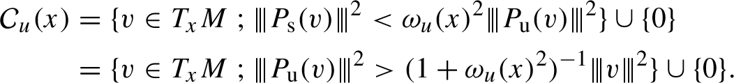 $$ \begin{align*} \mathcal{C}_u(x) &= \{ v \in T_x M \;\mathord{;}\; \mathopen{| {\kern -1.5pt} | {\kern -1.5pt} |} {P_{\mathrm{s}}(v)} \mathclose{| {\kern -1.5pt} | {\kern -1.5pt} |}^2 < \omega_u(x)^2 \mathopen{| {\kern -1.5pt} | {\kern -1.5pt} |} {P_{\mathrm{u}}(v)} \mathclose{| {\kern -1.5pt} | {\kern -1.5pt} |}^2 \} \cup \{0\} \\ &= \{ v \in T_x M \;\mathord{;}\; \mathopen{| {\kern -1.5pt} | {\kern -1.5pt} |} {P_{\mathrm{u}}(v)} \mathclose{| {\kern -1.5pt} | {\kern -1.5pt} |}^2> (1+\omega_u(x)^2)^{-1} \mathopen{| {\kern -1.5pt} | {\kern -1.5pt} |} {v} \mathclose{| {\kern -1.5pt} | {\kern -1.5pt} |}^2 \} \cup \{0\}. \end{align*} $$
By Lemma 4.3(a),
 $\omega _u(x) \le \alpha $
. Using equation (4.10), we conclude that for all
$\omega _u(x) \le \alpha $
. Using equation (4.10), we conclude that for all
 $v \in \mathcal {C}_u(x)$
and
$v \in \mathcal {C}_u(x)$
and
 $n \ge 0$
,
$n \ge 0$
,
 $$ \begin{align*} \mathopen{| {\kern -1.5pt} | {\kern -1.5pt} |} {D\tilde{f}^n(x) \, v} \mathclose{| {\kern -1.5pt} | {\kern -1.5pt} |} \ge \mathopen{| {\kern -1.5pt} | {\kern -1.5pt} |} {P^{\mathrm{u}} \, D\tilde{f}^n(x) \, v} \mathclose{| {\kern -1.5pt} | {\kern -1.5pt} |} \ge c a_3^n \mathopen{| {\kern -1.5pt} | {\kern -1.5pt} |} {P^{\mathrm{u}} \, v} \mathclose{| {\kern -1.5pt} | {\kern -1.5pt} |} \ge c (1+\alpha^2)^{-1/2} a_3^n \mathopen{| {\kern -1.5pt} | {\kern -1.5pt} |} {v} \mathclose{| {\kern -1.5pt} | {\kern -1.5pt} |}. \end{align*} $$
In particular, the bundle
 $\tilde E^{\mathrm {u}}$
is uniformly expanding. By symmetry, the bundle
$\tilde E^{\mathrm {u}}$
is uniformly expanding. By symmetry, the bundle
 $\tilde E^{\mathrm {s}}$
is uniformly contracting. This shows that
$\tilde E^{\mathrm {s}}$
is uniformly contracting. This shows that
 $\tilde f$
is an Anosov diffeomorphism of index u, completing the proof of Proposition 4.2.
$\tilde f$
is an Anosov diffeomorphism of index u, completing the proof of Proposition 4.2.
5 The model deformation
In this section, we define a special family of diffeomorphisms called the ‘model deformation’ that will be the basis for the construction in §6. We also establish a few properties of those maps.
Let
 $\| \mathord {\cdot } \|$
denote the Euclidean norm in
$\| \mathord {\cdot } \|$
denote the Euclidean norm in
 $\mathbb {R}^d$
, and let
$\mathbb {R}^d$
, and let
 $\mathbb {B} := \{z \;\mathord {;}\; \|z\| \le 1\}$
be the unit ball. Denote by m the Lebesgue measure on
$\mathbb {B} := \{z \;\mathord {;}\; \|z\| \le 1\}$
be the unit ball. Denote by m the Lebesgue measure on
 $\mathbb {R}^d$
. All the constructions in this section are in
$\mathbb {R}^d$
. All the constructions in this section are in
 $\mathbb {R}^d$
, so there is no risk of confusion with the volume measure on the manifold M.
$\mathbb {R}^d$
, so there is no risk of confusion with the volume measure on the manifold M.
Let
 $\mathrm {Diff}^{\infty }_m(\mathbb {B},\partial \mathbb {B})$
denote the set of all maps
$\mathrm {Diff}^{\infty }_m(\mathbb {B},\partial \mathbb {B})$
denote the set of all maps
 $h \colon \mathbb {B} \to \mathbb {B}$
that can be extended to volume-preserving
$h \colon \mathbb {B} \to \mathbb {B}$
that can be extended to volume-preserving
 $C^{\infty }$
-diffeomorphisms of
$C^{\infty }$
-diffeomorphisms of
 $\mathbb {R}^d$
that coincide with the identity outside
$\mathbb {R}^d$
that coincide with the identity outside
 $\mathbb {B}$
.
$\mathbb {B}$
.
For each
 $j \in \{1,\ldots ,d-1\}$
and
$j \in \{1,\ldots ,d-1\}$
and
 $\theta \in \mathbb {R}$
, let
$\theta \in \mathbb {R}$
, let
 $R^{(j)}_{\theta }$
be the orthogonal matrix that rotates the plane
$R^{(j)}_{\theta }$
be the orthogonal matrix that rotates the plane
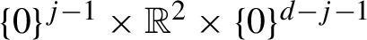 $\{0\}^{j-1} \times \mathbb {R}^2 \times \{0\}^{d-j-1}$
by angle
$\{0\}^{j-1} \times \mathbb {R}^2 \times \{0\}^{d-j-1}$
by angle
 $\theta $
and is the identity on its orthogonal complement, that is,
$\theta $
and is the identity on its orthogonal complement, that is,
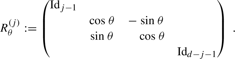 $$ \begin{align} R^{(j)}_{\theta} := \begin{pmatrix} \mathrm{Id}_{j-1} & & & \\ & \cos \theta & -\sin \theta & \\ & \sin \theta & \phantom{-}\cos \theta & \\ & & & \mathrm{Id}_{d-j-1} \end{pmatrix} \,. \end{align} $$
Fix a rotationally symmetric (that is only depending on the norm)
 $C^{\infty }$
-function
$C^{\infty }$
-function
 $\rho \colon \mathbb {R}^d \to \mathbb {R}$
which is not identically zero and is supported on
$\rho \colon \mathbb {R}^d \to \mathbb {R}$
which is not identically zero and is supported on
 $\mathbb {B}$
. For each
$\mathbb {B}$
. For each
 $j \in \{1,\ldots ,d-1\}$
and
$j \in \{1,\ldots ,d-1\}$
and
 $s \in \mathbb {R}$
, define
$s \in \mathbb {R}$
, define
 $h^{(j)}_s \in \mathrm {Diff}^{\infty }_m(\mathbb {B},\partial \mathbb {B})$
by
$h^{(j)}_s \in \mathrm {Diff}^{\infty }_m(\mathbb {B},\partial \mathbb {B})$
by
 $$ \begin{align} h^{(j)}_s(z) := R^{(j)}_{s \rho(z)} (z) \,; \end{align} $$
such a map is indeed conservative because it preserves the family of spheres with center at the origin and it acts on each of these as an orthonormal map. The diffeomorphisms
 $h^{(j)}_s$
will be called the elementary model deformations. See the figure in [p. 334].
$h^{(j)}_s$
will be called the elementary model deformations. See the figure in [p. 334].
For each
 $t = (t_1,\ldots ,t_{d-1}) \in \mathbb {R}^{d-1}$
, define
$t = (t_1,\ldots ,t_{d-1}) \in \mathbb {R}^{d-1}$
, define
 $h_t \in \mathrm {Diff}^{\infty }_m(\mathbb {B},\partial \mathbb {B})$
by
$h_t \in \mathrm {Diff}^{\infty }_m(\mathbb {B},\partial \mathbb {B})$
by
 $$ \begin{align} h_t := h^{(d-1)}_{t_{d-1}} \circ \cdots \circ h^{(1)}_{t_1}. \end{align} $$
This
 $d-1$
-parameter family of diffeomorphisms will be called the model deformation.
$d-1$
-parameter family of diffeomorphisms will be called the model deformation.
If
 $t \in \mathbb {R}^{d-1}$
is sufficiently close to
$t \in \mathbb {R}^{d-1}$
is sufficiently close to
 $(0,\ldots ,0)$
, then the diffeomorphism
$(0,\ldots ,0)$
, then the diffeomorphism
 $h_t$
is sufficiently
$h_t$
is sufficiently
 $C^1$
-close to the identity so that the following transversality condition holds: for all
$C^1$
-close to the identity so that the following transversality condition holds: for all
 $z \in \mathbb {B}$
and
$z \in \mathbb {B}$
and
 $j \in \{1,\ldots ,d-1\}$
,
$j \in \{1,\ldots ,d-1\}$
,
 $$ \begin{align} Dh_t(z) (\mathbb{R}^j \times \{0\}^{d-j}) &\text{ is transverse to } \{0\}^j \times \mathbb{R}^{d-j}. \end{align} $$
Adjusting
 $\rho $
if necessary, we assume from now on that every t in the unit cube
$\rho $
if necessary, we assume from now on that every t in the unit cube
 $[0,1]^{d-1}$
satisfies the transversality condition.
$[0,1]^{d-1}$
satisfies the transversality condition.
If A is any
 $d \times d$
matrix and I,
$d \times d$
matrix and I,
 $J \subseteq \{1,\ldots ,d\}$
are non-empty subsets of the same cardinality, let us denote by
$J \subseteq \{1,\ldots ,d\}$
are non-empty subsets of the same cardinality, let us denote by
 $A[I,J]$
the submatrix formed by the entries with row in I and column in J. Recall that the determinants of those matrices are called the minors of A; the kth principal minor corresponds to
$A[I,J]$
the submatrix formed by the entries with row in I and column in J. Recall that the determinants of those matrices are called the minors of A; the kth principal minor corresponds to
 $I = J = \{1,\ldots ,k\}$
, and is denoted by
$I = J = \{1,\ldots ,k\}$
, and is denoted by
 $\det \nolimits _k A$
.
$\det \nolimits _k A$
.
Note that the derivatives of the maps (5.2) have the following form (where asterisks are placeholders for unspecified entries):

Moreover, because these matrices have unit determinant, we conclude that their principal minors are
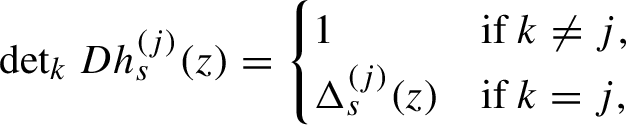 $$ \begin{align} \det\nolimits_k Dh_s^{(j)}(z) = \begin{cases} 1 &\text{if } k \neq j, \\ \Delta^{(j)}_s(z) &\text{if } k = j, \end{cases} \end{align} $$
where
 $\Delta ^{(j)}_s(z)$
is defined as the
$\Delta ^{(j)}_s(z)$
is defined as the
 $(j,j)$
-entry of the matrix
$(j,j)$
-entry of the matrix
 $Dh^{(j)}_s(z)$
, that is, the circled entry above.
$Dh^{(j)}_s(z)$
, that is, the circled entry above.
The matrices
 $Dh^{(j)}_s(z)$
have no common block triangular form, so the derivative of the composition (5.3) is intricate. Nevertheless, there is a simple expression for its principal minors.
$Dh^{(j)}_s(z)$
have no common block triangular form, so the derivative of the composition (5.3) is intricate. Nevertheless, there is a simple expression for its principal minors.
Lemma 5.1. For all
 $z \in \mathbb {B}$
,
$z \in \mathbb {B}$
,
 $t = (t_1,\ldots ,t_{d-1}) \in \mathbb {R}^{d-1}$
, and
$t = (t_1,\ldots ,t_{d-1}) \in \mathbb {R}^{d-1}$
, and
 $j \in \{1,\ldots ,d-1\}$
,
$j \in \{1,\ldots ,d-1\}$
,
 $$ \begin{align*} \det\nolimits_j Dh_t(z) = \Delta^{(j)}_{t_j} \circ h^{(j-1)}_{t_{j-1}} \circ \cdots \circ h^{(1)}_{t_1} (z). \end{align*} $$
Proof Fix z and t, and let
 $P := Dh_t(z)$
. Let
$P := Dh_t(z)$
. Let
 $z^{(0)} := z$
. For each
$z^{(0)} := z$
. For each
 $k \in \{1,\ldots , d-1\}$
, let
$k \in \{1,\ldots , d-1\}$
, let
 $z^{(k)} := h^{(k)}_{t_k} \circ \cdots \circ h^{(1)}_{t_1} (z)$
and
$z^{(k)} := h^{(k)}_{t_k} \circ \cdots \circ h^{(1)}_{t_1} (z)$
and
 $A_k := Dh^{(k)}_{t_k} (z^{(k-1)})$
. By the chain rule,
$A_k := Dh^{(k)}_{t_k} (z^{(k-1)})$
. By the chain rule,
 $P = A_{d-1} \cdots A_2 A_1$
.
$P = A_{d-1} \cdots A_2 A_1$
.
Fix
 $j \in \{1,\ldots ,d-1\}$
, and let
$j \in \{1,\ldots ,d-1\}$
, and let
 $J := \{1,\ldots ,j\}$
. We claim that if
$J := \{1,\ldots ,j\}$
. We claim that if
 $I \subset \{1,\ldots ,d\}$
has cardinality j and
$I \subset \{1,\ldots ,d\}$
has cardinality j and
 $I \neq J$
then:
$I \neq J$
then:
 $$ \begin{align} \det A_k [I,J] = 0\quad \text{for every } k &< j; \text{ and } \end{align} $$
 $$ \begin{align} \det A_k [J,I] = 0\quad \text{for every } k &> j. \end{align} $$
Indeed, for all
 $i>j$
, the row matrix
$i>j$
, the row matrix
 $A_k[\{i\},J]$
vanishes if
$A_k[\{i\},J]$
vanishes if
 $k<j$
, and the column matrix
$k<j$
, and the column matrix
 $A_k[J,\{i\}]$
vanishes if
$A_k[J,\{i\}]$
vanishes if
 $k>j$
.
$k>j$
.
By the Cauchy–Binet formula for the minors of a product,
 $$ \begin{align*} \det P[J,J] = \sum \det A_{d-1}[J,I_{d-2}] \cdots \det A_j [I_j,I_{j-1}] \cdots \det A_1 [I_1,J], \end{align*} $$
where the sum is over all
 $d-2$
-tuples
$d-2$
-tuples
 $(I_1,\ldots ,I_{d-2})$
of subsets of
$(I_1,\ldots ,I_{d-2})$
of subsets of
 $\{1,\ldots ,d\}$
of cardinality j. Consider a non-zero term of this sum. Using equation (5.6) recursively, we obtain
$\{1,\ldots ,d\}$
of cardinality j. Consider a non-zero term of this sum. Using equation (5.6) recursively, we obtain
 $J = I_1 = I_2 = \cdots = I_{j-1}$
. However, using equation (5.7) recursively, we obtain
$J = I_1 = I_2 = \cdots = I_{j-1}$
. However, using equation (5.7) recursively, we obtain
 $J = I_{d-2} = I_{d-3} = \cdots = I_j$
. Therefore, the sum contains a single non-zero term, which by equation (5.5) equals
$J = I_{d-2} = I_{d-3} = \cdots = I_j$
. Therefore, the sum contains a single non-zero term, which by equation (5.5) equals
 $\Delta ^{(j)}_{t_j}(z^{(j-1)})$
.
$\Delta ^{(j)}_{t_j}(z^{(j-1)})$
.
The transversality condition (5.4) is equivalent to the non-vanishing of the minors
 $\det \nolimits _j Dh_t(z)$
. When
$\det \nolimits _j Dh_t(z)$
. When
 $t=0$
, these minors equal
$t=0$
, these minors equal
 $1$
. So the minors are always strictly positive. In particular, by Lemma 5.1, the functions
$1$
. So the minors are always strictly positive. In particular, by Lemma 5.1, the functions
 $\Delta ^{(j)}_s$
are strictly positive for
$\Delta ^{(j)}_s$
are strictly positive for
 $s \in [0,1]$
. We will need information about the logarithms of these functions. By definition,
$s \in [0,1]$
. We will need information about the logarithms of these functions. By definition,
 $$ \begin{align*} \Delta^{(j)}_s(z_1,\ldots,z_d) = \frac{\partial}{\partial z_j} ( z_j \cos (s\rho(z)) - z_{j+1} \sin (s\rho(z)) ). \end{align*} $$
Because
 $\rho $
is rotationally symmetric,
$\rho $
is rotationally symmetric,
 $$ \begin{align*} \Delta^{(j)}_s (z_1,\ldots,z_d) = \Delta^{(1)}_s (z_j, z_{j+1}, \ldots, z_d, z_1, \ldots, z_{j-1}). \end{align*} $$
In particular, for each
 $s \in [0,1]$
, the integral
$s \in [0,1]$
, the integral
 $$ \begin{align} {\mathcal Q}(s) := - \frac{1}{m(\mathbb{B})} \int_{\mathbb{B}} \log \Delta^{(j)}_s \,\mathrm{d} m, \end{align} $$
is independent of j.
Lemma 5.2. For every
 $s \in [0,1]$
, we have
$s \in [0,1]$
, we have
 ${\mathcal Q}(s) \ge 0$
, with equality if and only if
${\mathcal Q}(s) \ge 0$
, with equality if and only if
 $s=0$
.
$s=0$
.
Proof Consider
 $j=1$
in equation (5.8). Then the lemma follows from Jensen inequality and a geometric argument: see [Reference Baraviera and Bonatti5, Lemma 1.2].
$j=1$
in equation (5.8). Then the lemma follows from Jensen inequality and a geometric argument: see [Reference Baraviera and Bonatti5, Lemma 1.2].
Because each
 $h^{(j)}_{t_j}$
is volume preserving, we obtain from equations (5.8) and Lemma 5.1 that
$h^{(j)}_{t_j}$
is volume preserving, we obtain from equations (5.8) and Lemma 5.1 that
 $$ \begin{align} \frac{1}{m(\mathbb{B})} \int_{\mathbb{B}} \log \det\nolimits_j Dh_t \,\mathrm{d} m = -{\mathcal Q}(t_j). \end{align} $$
This formula will be essential for our deformations of Lyapunov exponents: roughly speaking, it will allow us to move the summed exponents
![]() simultaneously and independently, as we will see in the next section.
simultaneously and independently, as we will see in the next section.
Let us discuss a few other features of the model deformation.
Recall the definitions (4.3) and (4.4) of standard cones in
 $\mathbb {R}^d$
. By the transversality assumption (5.4), if
$\mathbb {R}^d$
. By the transversality assumption (5.4), if
 $\alpha> 1$
is large enough and
$\alpha> 1$
is large enough and
 $\beta := \alpha ^{-1}$
, then for all
$\beta := \alpha ^{-1}$
, then for all
 $z \in \mathbb {B}$
,
$z \in \mathbb {B}$
,
 $t \in [0,1]^{d-1}$
, and
$t \in [0,1]^{d-1}$
, and
 $j \in \{1,\ldots ,d-1\}$
,
$j \in \{1,\ldots ,d-1\}$
,
 $$ \begin{align} Dh_t(z) \mathcal{H}_j(\beta) \subseteq \mathcal{H}_j(\alpha) \, \quad \text{and} \quad Dh_t^{-1}(z) \mathcal{V}_j(\beta) \subseteq \mathcal{V}_j(\alpha). \end{align} $$
In fact, the inclusions are equivalent to one another because the complement of a horizontal cone
 $\mathcal {H}_j(\tau )$
is (modulo sets of non-empty interior) a vertical cone
$\mathcal {H}_j(\tau )$
is (modulo sets of non-empty interior) a vertical cone
 $\mathcal {V}_j(\tau )$
. Let us fix these numbers
$\mathcal {V}_j(\tau )$
. Let us fix these numbers
 $\alpha> \beta > 0$
from now on.
$\alpha> \beta > 0$
from now on.
Let
 $P_j$
and
$P_j$
and
 $Q_j \colon \mathbb {R}^d \to \mathbb {R}^d$
be the projections on the spaces
$Q_j \colon \mathbb {R}^d \to \mathbb {R}^d$
be the projections on the spaces
 $\mathbb {R}^j \times \{0\}^{d-j}$
and
$\mathbb {R}^j \times \{0\}^{d-j}$
and
 $\{0\}^j \times \mathbb {R}^{d-j}$
, respectively. We fix
$\{0\}^j \times \mathbb {R}^{d-j}$
, respectively. We fix
 $\kappa> 0$
such that
$\kappa> 0$
such that
 $$ \begin{align} \left\{ \begin{array}{ccc} v \in \mathcal{H}_j(\beta) & \Rightarrow & \; \; \| P_j \, Dh_t(z) \, v \| \ge \kappa \, \|P_j \, v \|, \\ v \in \mathcal{V}_j(\beta) & \Rightarrow & \| Q_j \, Dh_t^{-1}(z) \, v \| \ge \kappa \, \|Q_j \, v\|. \end{array} \right. \end{align} $$
Let us recall a few facts about exterior powers. Let
 $\{e_1,\ldots ,e_d\}$
denote the canonical basis in
$\{e_1,\ldots ,e_d\}$
denote the canonical basis in
 $\mathbb {R}^d$
. Then, for each
$\mathbb {R}^d$
. Then, for each
 $k \in \{1,\ldots ,d\}$
,
$k \in \{1,\ldots ,d\}$
,
 $\mathsf {\Lambda }^k \mathbb {R}^d$
is a vector space with the canonical basis
$\mathsf {\Lambda }^k \mathbb {R}^d$
is a vector space with the canonical basis
 $\{e_{i_1} \wedge \cdots \wedge e_{i_k}\}_{i_1 < \cdots < i_k}$
. We endow
$\{e_{i_1} \wedge \cdots \wedge e_{i_k}\}_{i_1 < \cdots < i_k}$
. We endow
 $\mathsf {\Lambda }^k \mathbb {R}^d$
with the inner product that makes the canonical basis orthonormal. There is a wedge operation
$\mathsf {\Lambda }^k \mathbb {R}^d$
with the inner product that makes the canonical basis orthonormal. There is a wedge operation
 $(v,w) \in (\mathsf {\Lambda }^k \mathbb {R}^d) \times (\mathsf {\Lambda }^{\ell } \mathbb {R}^d) \mapsto v \wedge w \in \mathsf {\Lambda }^{k+\ell } \mathbb {R}^d$
which is associative, mutilinear, and skew-symmetric (that is,
$(v,w) \in (\mathsf {\Lambda }^k \mathbb {R}^d) \times (\mathsf {\Lambda }^{\ell } \mathbb {R}^d) \mapsto v \wedge w \in \mathsf {\Lambda }^{k+\ell } \mathbb {R}^d$
which is associative, mutilinear, and skew-symmetric (that is,
 $w \wedge v = (-1)^{k\ell } v \wedge w$
). Given a linear map
$w \wedge v = (-1)^{k\ell } v \wedge w$
). Given a linear map
 $A \colon \mathbb {R}^d \to \mathbb {R}^d$
, there are induced linear maps
$A \colon \mathbb {R}^d \to \mathbb {R}^d$
, there are induced linear maps
 $\mathsf {\Lambda }^k A \colon \mathsf {\Lambda }^k \mathbb {R}^d \to \mathsf {\Lambda }^k \mathbb {R}^d$
such that
$\mathsf {\Lambda }^k A \colon \mathsf {\Lambda }^k \mathbb {R}^d \to \mathsf {\Lambda }^k \mathbb {R}^d$
such that
 $(\mathsf {\Lambda }^k A) (e_{i_1} \wedge \cdots \wedge e_{i_k}) = Ae_{i_1} \wedge \cdots \wedge Ae_{i_k}$
. The entries of the matrix of the exterior power
$(\mathsf {\Lambda }^k A) (e_{i_1} \wedge \cdots \wedge e_{i_k}) = Ae_{i_1} \wedge \cdots \wedge Ae_{i_k}$
. The entries of the matrix of the exterior power
 $\mathsf {\Lambda }^k A$
with respect to the canonical basis are exactly the
$\mathsf {\Lambda }^k A$
with respect to the canonical basis are exactly the
 $k \times k$
minors of A; this is called the kth compound matrix of A. More precisely, if
$k \times k$
minors of A; this is called the kth compound matrix of A. More precisely, if
 $I=\{i_1<\cdots <i_k\}$
and
$I=\{i_1<\cdots <i_k\}$
and
 $J=\{j_1<\cdots <j_k\}$
, then
$J=\{j_1<\cdots <j_k\}$
, then
 $$ \begin{align*} \langle e_{i_1} \wedge \cdots \wedge e_{i_k} , \, (\mathsf{\Lambda}^k A)(e_{j_1} \wedge \cdots \wedge e_{j_k}) \rangle = \det A[I,J]. \end{align*} $$
So the Cauchy–Binet formula used before is nothing but the functoriality of the exterior powers, that is,
 $\mathsf {\Lambda }^k(AB) = (\mathsf {\Lambda }^k A)(\mathsf {\Lambda }^k B)$
. If A is an orthogonal linear map, then so is
$\mathsf {\Lambda }^k(AB) = (\mathsf {\Lambda }^k A)(\mathsf {\Lambda }^k B)$
. If A is an orthogonal linear map, then so is
 $\mathsf {\Lambda }^k A$
. Therefore, the inner product on
$\mathsf {\Lambda }^k A$
. Therefore, the inner product on
 $\mathsf {\Lambda }^k \mathbb {R}^d$
depends only on the inner product on
$\mathsf {\Lambda }^k \mathbb {R}^d$
depends only on the inner product on
 $\mathbb {R}^d$
and not on the choice of orthonormal basis; equivalently, the k-fold exterior power of an inner product space is an inner product space. From a more geometrical viewpoint, if
$\mathbb {R}^d$
and not on the choice of orthonormal basis; equivalently, the k-fold exterior power of an inner product space is an inner product space. From a more geometrical viewpoint, if
 $v_1$
, …,
$v_1$
, …,
 $v_k$
are vectors in
$v_k$
are vectors in
 $\mathbb {R}^d$
then the norm of
$\mathbb {R}^d$
then the norm of
 $v_1 \wedge \cdots \wedge v_k$
is the k-dimensional volume of the parallelepiped spanned by these vectors.
$v_1 \wedge \cdots \wedge v_k$
is the k-dimensional volume of the parallelepiped spanned by these vectors.
Coming back to the model deformation, let us note for later use that for any
 $\nu>0$
, there exists
$\nu>0$
, there exists
 $\gamma \in (0,\beta )$
such that for all
$\gamma \in (0,\beta )$
such that for all
 $z \in \mathbb {B}$
,
$z \in \mathbb {B}$
,
 $t \in [0,1]^{d-1}$
,
$t \in [0,1]^{d-1}$
,
 $j \in \{1,\ldots ,d-1\}$
and all linearly independent vectors
$j \in \{1,\ldots ,d-1\}$
and all linearly independent vectors
 $w_1$
, …,
$w_1$
, …,
 $w_j \in \mathcal {H}_j(\gamma )$
,
$w_j \in \mathcal {H}_j(\gamma )$
,
 $$ \begin{align} \bigg| \log \frac{\langle (\mathsf{\Lambda}^j Dh_t(z))(w_1 \wedge \cdots \wedge w_j) , e_1 \wedge \cdots \wedge e_j \rangle}{\langle w_1 \wedge \cdots \wedge w_j , e_1 \wedge \cdots \wedge e_j \rangle} - \log \det\nolimits_j Dh_t(z) \bigg| < \nu ; \end{align} $$
this statement includes the fact that the numerator and the denominator in the expression above are both non-zero and have the same sign.
6 Proof of the central proposition
We now assemble the material of the previous three sections to prove Proposition 2.1 (which, as we have seen, implies Theorem 1.5). Recall that we need to define a multiparametric perturbation
 $(f_t)$
of f whose Lyapunov exponents ‘spread out’ in a controlled way (see Figure 2). Our diffeomorphisms
$(f_t)$
of f whose Lyapunov exponents ‘spread out’ in a controlled way (see Figure 2). Our diffeomorphisms
 $f_t$
will be damping perturbations of the given f. Recall from §4.2 that the damping time N (that is, the minimal return time to the support of the perturbation) must be roughly proportional to
$f_t$
will be damping perturbations of the given f. Recall from §4.2 that the damping time N (that is, the minimal return time to the support of the perturbation) must be roughly proportional to
 $1/\sigma $
, where
$1/\sigma $
, where
 $\sigma $
is the bound on the gap. By preservation of the measure, the volume of the support of the perturbations cannot be larger than
$\sigma $
is the bound on the gap. By preservation of the measure, the volume of the support of the perturbations cannot be larger than
 $1/N \asymp \sigma $
. This upper bound can be essentially attained using the Rokhlin tower lemma to select convenient places to perturb. The actual maps
$1/N \asymp \sigma $
. This upper bound can be essentially attained using the Rokhlin tower lemma to select convenient places to perturb. The actual maps
 $f_t$
will be defined by inserting copies of our model deformations on many ‘Lyapunov balls’ (that is, balls with respect to the Lyapunov charts constructed in §3.2). Our preparations will ensure that such maps
$f_t$
will be defined by inserting copies of our model deformations on many ‘Lyapunov balls’ (that is, balls with respect to the Lyapunov charts constructed in §3.2). Our preparations will ensure that such maps
 $f_t$
are Anosov with simple dominated splittings
$f_t$
are Anosov with simple dominated splittings
 $E_{1,t} \oplus \cdots \oplus E_{d,t}$
, and what we are left to do is to estimate their Lyapunov exponents. It is convenient to work with the summed exponents
$E_{1,t} \oplus \cdots \oplus E_{d,t}$
, and what we are left to do is to estimate their Lyapunov exponents. It is convenient to work with the summed exponents
 $\hat {\unicode{x3bb} }_j(f_t)$
, which equal the average log of the expansion of j-dimensional volume along the invariant sub-bundle
$\hat {\unicode{x3bb} }_j(f_t)$
, which equal the average log of the expansion of j-dimensional volume along the invariant sub-bundle
 $E_{1,t} \oplus \cdots \oplus E_{j,t}$
. It boils down that, modulo a small error (arising from the lack of smooth integrability),
$E_{1,t} \oplus \cdots \oplus E_{j,t}$
. It boils down that, modulo a small error (arising from the lack of smooth integrability),
 $\hat {\unicode{x3bb} }_j(f_t)$
drops compared with the unperturbed
$\hat {\unicode{x3bb} }_j(f_t)$
drops compared with the unperturbed
 $\hat {\unicode{x3bb} }_j(f)$
, and the drop is proportional to two things (see equation (6.16)): the integrals (5.9) that control the basic effect of each model perturbation, and the total measure of the supports of the perturbations. The integrals are bounded by constants, and the measure of the support of the whole damping perturbation is, as explained above, of the order of
$\hat {\unicode{x3bb} }_j(f)$
, and the drop is proportional to two things (see equation (6.16)): the integrals (5.9) that control the basic effect of each model perturbation, and the total measure of the supports of the perturbations. The integrals are bounded by constants, and the measure of the support of the whole damping perturbation is, as explained above, of the order of
 $\sigma $
. So ultimately, we are able to move Lyapunov exponents by an amount that depends on the gap
$\sigma $
. So ultimately, we are able to move Lyapunov exponents by an amount that depends on the gap
 $\sigma $
but not on f itself, which is an essential feature of Proposition 2.1.
$\sigma $
but not on f itself, which is an essential feature of Proposition 2.1.
Proof of Proposition 2.1 Let
 $u \in \{1,\ldots ,d-1\}$
and
$u \in \{1,\ldots ,d-1\}$
and
 $a_1$
, …,
$a_1$
, …,
 $a_{d-1}$
,
$a_{d-1}$
,
 $\sigma $
,
$\sigma $
,
 $\delta _0> 0$
be given. Recall that
$\delta _0> 0$
be given. Recall that
 ${\mathcal Q}(s)$
denotes the quantity defined in equation (5.8), which is a continuous function of
${\mathcal Q}(s)$
denotes the quantity defined in equation (5.8), which is a continuous function of
 $s \in [0,1]$
, vanishes at
$s \in [0,1]$
, vanishes at
 $s=0$
, and is positive for
$s=0$
, and is positive for
 $s>0$
(by Lemma 5.2). Reducing
$s>0$
(by Lemma 5.2). Reducing
 $\delta _0$
if necessary, we may assume that
$\delta _0$
if necessary, we may assume that
 $$ \begin{align*} 3 \delta_0 \max\{a_1,\ldots,a_{d-1}\} \le {\mathcal Q}(1). \end{align*} $$
For each
 $j \in \{1,\ldots ,d-1\}$
, define
$j \in \{1,\ldots ,d-1\}$
, define
 $$ \begin{align} b_j := \text{ the least value in }[0,1] \text{ such that } {\mathcal Q}(b_j) = 3 \delta_0 a_j. \end{align} $$
We fix several other constants. Let
 $\alpha> \beta > 0$
be openings with property (5.10). Let
$\alpha> \beta > 0$
be openings with property (5.10). Let
 $\kappa> 0$
be a constant with property (5.11). Let
$\kappa> 0$
be a constant with property (5.11). Let
 $\nu := (\delta _0/2) \min \{a_1,\ldots ,a_{d-1}\}$
and take
$\nu := (\delta _0/2) \min \{a_1,\ldots ,a_{d-1}\}$
and take
 $\gamma \in (0,\beta )$
with property (5.12). Let
$\gamma \in (0,\beta )$
with property (5.12). Let
 $N := N_0(\alpha , \beta , \gamma , \kappa , \sigma )$
be given by equation (4.7). Let
$N := N_0(\alpha , \beta , \gamma , \kappa , \sigma )$
be given by equation (4.7). Let
 $\delta := \delta _0 / N$
; this will be the scaling factor as in the statement of Proposition 2.1. Choose a very small
$\delta := \delta _0 / N$
; this will be the scaling factor as in the statement of Proposition 2.1. Choose a very small
 $\varepsilon>0$
; this choice will be apparent at the end of the proof.
$\varepsilon>0$
; this choice will be apparent at the end of the proof.
Now let us pick
 $f \in \mathrm {Diff}_m^r(M)$
as in the statement of Proposition 2.1, that is, a conservative Anosov
$f \in \mathrm {Diff}_m^r(M)$
as in the statement of Proposition 2.1, that is, a conservative Anosov
 $C^r$
-diffeomorphism of unstable index u, admitting a simple dominated splitting, and such that
$C^r$
-diffeomorphism of unstable index u, admitting a simple dominated splitting, and such that
 $\textsf {g}_u(\boldsymbol {\unicode{x3bb} }(f)) \ge \sigma $
.
$\textsf {g}_u(\boldsymbol {\unicode{x3bb} }(f)) \ge \sigma $
.
We apply Proposition 3.1 and find a Lyapunov metric so that the associated expansion functions
 $\chi _1$
, …,
$\chi _1$
, …,
 $\chi _d$
obey the
$\chi _d$
obey the
 $L^1$
-estimate (3.3) with the chosen value of
$L^1$
-estimate (3.3) with the chosen value of
 $\varepsilon $
. Consider the sets
$\varepsilon $
. Consider the sets
By a trivial estimate (Markov’s inequality),
 $m(R_j) \le 2 \sigma ^{-1} \varepsilon $
. Thus, the open set
$m(R_j) \le 2 \sigma ^{-1} \varepsilon $
. Thus, the open set
 $$ \begin{align*} U := M \smallsetminus \bigcup_{j=1}^{d-1} \bigcup_{n=-N+1}^{N-1} f^n(R_j) \end{align*} $$
has measure
 $m(U)> 1 - 4 d N \sigma ^{-1}\varepsilon $
.
$m(U)> 1 - 4 d N \sigma ^{-1}\varepsilon $
.
By the Rokhlin lemma, there exists a measurable set
 $Z_1$
disjoint from
$Z_1$
disjoint from
 $f(Z_1)$
,
$f(Z_1)$
,
 $f^2(Z_1)$
, … ,
$f^2(Z_1)$
, … ,
 $f^{N-1}(Z_1)$
with measure
$f^{N-1}(Z_1)$
with measure
 $$ \begin{align*} m(Z_1)> \frac{1}{N} - \varepsilon. \end{align*} $$
Then
 $$ \begin{align*} m (Z_1 \cap U)> \frac{1}{N} - (1 + 4 d N \sigma^{-1}) \varepsilon. \end{align*} $$
Let
 $Z_2$
be a compact subset of
$Z_2$
be a compact subset of
 $Z_1 \cap U$
satisfying the same bound. Then take an open neighborhood
$Z_1 \cap U$
satisfying the same bound. Then take an open neighborhood
 $Z_3 \subseteq U$
of
$Z_3 \subseteq U$
of
 $Z_2$
that satisfies the same bound, and, moreover, is disjoint from
$Z_2$
that satisfies the same bound, and, moreover, is disjoint from
 $f(Z_3)$
,
$f(Z_3)$
,
 $f^2(Z_3)$
, …,
$f^2(Z_3)$
, …,
 $f^{N-1}(Z_3)$
.
$f^{N-1}(Z_3)$
.
Let
 $\Phi _x \colon B_0 \to M$
be the Lyapunov charts coming from Proposition 3.4; here,
$\Phi _x \colon B_0 \to M$
be the Lyapunov charts coming from Proposition 3.4; here,
 $B_0$
is a rescaling of the unit closed ball
$B_0$
is a rescaling of the unit closed ball
 $\mathbb {B}$
, that is,
$\mathbb {B}$
, that is,
 $B_0 = s_0 \mathbb {B}$
for some
$B_0 = s_0 \mathbb {B}$
for some
 $s_0>0$
. For every
$s_0>0$
. For every
 $x \in M$
and every
$x \in M$
and every
 $s \in (0,s_0]$
, let us define a Lyapunov ball as
$s \in (0,s_0]$
, let us define a Lyapunov ball as
 $$ \begin{align*} \mathcal{B}(x,s) := \Phi_x ( s \mathbb{B}). \end{align*} $$
Reducing
 $s_0$
if necessary, we assume that the following properties hold:
$s_0$
if necessary, we assume that the following properties hold:
 $$ \begin{align} y, y' \in \mathcal{B}(x,s) \ &\Rightarrow \ |\chi_j(y) - \chi_j(y')| < \varepsilon; \end{align} $$
 $$ \begin{align} y \in \mathcal{B}(x,s) \ &\Rightarrow \ \| D\Phi_x^{-1}(y) \mathcal{L}_y - \mathrm{Id} \| < \varepsilon; \end{align} $$
where
 $\mathcal {L}_y := D\Phi _y(0)$
.
$\mathcal {L}_y := D\Phi _y(0)$
.
Because the Lyapunov charts
 $\Phi _x$
form a relatively compact subset of
$\Phi _x$
form a relatively compact subset of
 $C^1(B_0,M)$
, the family of Lyapunov balls contained in the open set
$C^1(B_0,M)$
, the family of Lyapunov balls contained in the open set
 $Z_3$
forms a Vitali covering of
$Z_3$
forms a Vitali covering of
 $Z_3$
. Therefore, there exists a finite collection of disjoint Lyapunov balls
$Z_3$
. Therefore, there exists a finite collection of disjoint Lyapunov balls
 $\mathcal {B}(x_1,s_1)$
, … ,
$\mathcal {B}(x_1,s_1)$
, … ,
 $\mathcal {B}(x_p, s_p) \subseteq Z_3$
whose union
$\mathcal {B}(x_p, s_p) \subseteq Z_3$
whose union
 $Z_4$
has measure
$Z_4$
has measure
 $m(Z_4)> m(Z_3) - \varepsilon $
. To simplify notation, let
$m(Z_4)> m(Z_3) - \varepsilon $
. To simplify notation, let
 $\mathcal {B}_i := \mathcal {B}(x_i,s_i)$
and define
$\mathcal {B}_i := \mathcal {B}(x_i,s_i)$
and define
 $$ \begin{align} \Psi_i \colon \mathbb{B} \to M \quad \text{by} \Psi_i(z) := \Phi_{x_i}(s_i z); \end{align} $$
so
 $\Psi _i$
has constant Jacobian and image
$\Psi _i$
has constant Jacobian and image
 $\mathcal {B}_i$
.
$\mathcal {B}_i$
.
For each
 $t \in [0,1]^{d-1}$
, let us define
$t \in [0,1]^{d-1}$
, let us define
 $g_t \in \mathrm {Diff}_m^{\infty }(M)$
as follows:
$g_t \in \mathrm {Diff}_m^{\infty }(M)$
as follows:
 $g_t$
equals the identity outside of
$g_t$
equals the identity outside of
 $Z_4$
, and on each
$Z_4$
, and on each
 $\mathcal {B}_i$
it is defined as
$\mathcal {B}_i$
it is defined as
 $$ \begin{align} g_t := \Psi_i \circ h_{Bt} \circ \Psi_i^{-1}, \end{align} $$
where
 $B(t_1,\ldots ,t_{d-1}) := (b_1 t_1, \ldots , b_{d-1} t_{d-1})$
, and
$B(t_1,\ldots ,t_{d-1}) := (b_1 t_1, \ldots , b_{d-1} t_{d-1})$
, and
 $b_j$
comes from equation (6.1). The sought-after deformation of f is defined as
$b_j$
comes from equation (6.1). The sought-after deformation of f is defined as
 $$ \begin{align*} f_t := f \circ g_t \quad \text{for } t \in [0,1]^{d-1}. \end{align*} $$
We now need to check that the maps
 $f_t$
have the properties asserted in Proposition 2.1. As a first step, we show the following lemma.
$f_t$
have the properties asserted in Proposition 2.1. As a first step, we show the following lemma.
Lemma 6.1. Each
 $f_t$
is a
$f_t$
is a
 $(\alpha ,\beta ,\kappa ,\sigma ,N)$
-damping perturbation of f.
$(\alpha ,\beta ,\kappa ,\sigma ,N)$
-damping perturbation of f.
Proof Condition (i) in the definition of damping perturbations follows from the inclusions (5.10) and the fact that
 $Df$
(respectively
$Df$
(respectively
 $Df^{-1}$
) decreases the opening of horizontal (respectively vertical) cones: see equations (4.5), (4.6). Let us check condition (ii). If
$Df^{-1}$
) decreases the opening of horizontal (respectively vertical) cones: see equations (4.5), (4.6). Let us check condition (ii). If
 $v \in \mathcal {H}_u(x,\beta )$
then, using property (5.11),
$v \in \mathcal {H}_u(x,\beta )$
then, using property (5.11),
 $$ \begin{align*} \mathopen{| {\kern -1.5pt} | {\kern -1.5pt} |} {P^{\mathrm{u}} D\tilde{f}(x) \, v} \mathclose{| {\kern -1.5pt} | {\kern -1.5pt} |} = \mathopen{| {\kern -1.5pt} | {\kern -1.5pt} |} {P^{\mathrm{u}} Df(g_t x) \, Dg_t(x) \, v} \mathclose{| {\kern -1.5pt} | {\kern -1.5pt} |} \ge \mathopen{| {\kern -1.5pt} | {\kern -1.5pt} |} {P^{\mathrm{u}} Dg_t(x) \, v} \mathclose{| {\kern -1.5pt} | {\kern -1.5pt} |} \ge \kappa \, \mathopen{| {\kern -1.5pt} | {\kern -1.5pt} |} {P^{\mathrm{u}} v} \mathclose{| {\kern -1.5pt} | {\kern -1.5pt} |}, \end{align*} $$
while if
 $v \in \mathcal {V}_u(x,\beta )$
, then
$v \in \mathcal {V}_u(x,\beta )$
, then
 $D\tilde {f}^{-1} (x) \, v \in \mathcal {V}_u(\tilde {f}^{-1} (x) ,\beta )$
and so
$D\tilde {f}^{-1} (x) \, v \in \mathcal {V}_u(\tilde {f}^{-1} (x) ,\beta )$
and so
 $$ \begin{align*} \mathopen{| {\kern -1.5pt} | {\kern -1.5pt} |} {P^{\mathrm{s}} D\tilde{f}^{-1} (x) \, v} \mathclose{| {\kern -1.5pt} | {\kern -1.5pt} |} = \mathopen{| {\kern -1.5pt} | {\kern -1.5pt} |} {P^{\mathrm{s}} Dg_t^{-1}(\tilde{f}^{-1} (x)) D\tilde{f}^{-1} (x) \, v} \mathclose{| {\kern -1.5pt} | {\kern -1.5pt} |} \ge \kappa \, \mathopen{| {\kern -1.5pt} | {\kern -1.5pt} |} {P^{\mathrm{s}} D\tilde{f}^{-1} (x) \, v} \mathclose{| {\kern -1.5pt} | {\kern -1.5pt} |} \ge \kappa \, \mathopen{| {\kern -1.5pt} | {\kern -1.5pt} |} {P^{\mathrm{s}} v} \mathclose{| {\kern -1.5pt} | {\kern -1.5pt} |}. \end{align*} $$
Condition (iii) follows from the fact that the set
 $Z_4$
is disjoint from its
$Z_4$
is disjoint from its
 $N-1$
first iterates, while condition (iv) follows from the fact that
$N-1$
first iterates, while condition (iv) follows from the fact that
 $Z_4$
is contained in U.
$Z_4$
is contained in U.
Now Proposition 4.2 ensures that each
 $f_t$
is an Anosov diffeomorphism of unstable index u and admits a simple dominated splitting
$f_t$
is an Anosov diffeomorphism of unstable index u and admits a simple dominated splitting
 $TM = E_{1,t} \oplus \cdots \oplus E_{d,t}$
. Moreover, by part (a) of the proposition,
$TM = E_{1,t} \oplus \cdots \oplus E_{d,t}$
. Moreover, by part (a) of the proposition,
 $$ \begin{align} &E_{1,t}(x) \oplus \cdots \oplus E_{j,t}(x) \text{ is transverse to } E_{j+1}(x) \oplus \cdots \oplus E_d(x), \end{align} $$
 $$ \begin{align} &E_{1,t}(x) \oplus \cdots \oplus E_{j,t}(x) \subset \mathcal{H}_j( x, \gamma) \quad \text{if }x \in Z_4. \end{align} $$
The rest of the proof consists in estimating the summed Lyapunov exponents
 $\hat {\unicode{x3bb} }_j(f_t)$
.
$\hat {\unicode{x3bb} }_j(f_t)$
.
For each
 $x \in M$
and
$x \in M$
and
 $j \in \{1,\ldots ,d\}$
, let
$j \in \{1,\ldots ,d\}$
, let
 $v_j(x) := \mathcal {L}_x e_j$
, which is a vector that spans
$v_j(x) := \mathcal {L}_x e_j$
, which is a vector that spans
 $E_j(x)$
. Because these vectors form an orthonormal basis of
$E_j(x)$
. Because these vectors form an orthonormal basis of
 $T_x M$
, using the definition (3.1) of the expansion function
$T_x M$
, using the definition (3.1) of the expansion function
 $\chi _j$
, we obtain that for every vector
$\chi _j$
, we obtain that for every vector
 $w \in T_x M$
,
$w \in T_x M$
,
 $$ \begin{align} \mathopen{\langle {\kern -1.7pt} \langle}{Df(x) w, v_j(f(x))} \mathclose{\rangle {\kern -1.7pt} \rangle} = e^{\chi_j(x)} \mathopen{\langle {\kern -1.7pt} \langle}{w,v_j(x)} \mathclose{\rangle {\kern -1.7pt} \rangle}. \end{align} $$
In each exterior power of the tangent bundle, we consider the corresponding exterior power of the Lyapunov metric, denoting it by the same symbol. Let
 $$ \begin{align*} \hat{v}_{j}(x) := v_{1}(x) \wedge \cdots \wedge v_{j}(x) \in \mathsf{\Lambda}^j T_x M. \end{align*} $$
Note that for every
 $\hat {w} \in \mathsf {\Lambda }^j T_x M$
,
$\hat {w} \in \mathsf {\Lambda }^j T_x M$
,
 $$ \begin{align} \mathopen{\langle {\kern -1.7pt} \langle}{\mathsf{\Lambda}^j Df(x) \hat w, \hat{v}_j(f(x))} \mathclose{\rangle {\kern -1.7pt} \rangle} = e^{\chi_1(x) + \cdots + \chi_j(x)} \mathopen{\langle {\kern -1.7pt} \langle}{\hat w,\hat{v}_j(x)} \mathclose{\rangle {\kern -1.7pt} \rangle}. \end{align} $$
For each
 $x\in M$
,
$x\in M$
,
 $j \in \{1,\ldots ,d\}$
, and
$j \in \{1,\ldots ,d\}$
, and
 $t \in [0,1]^{d-1}$
, let us choose a vector
$t \in [0,1]^{d-1}$
, let us choose a vector
 $v_{j,t}(x)$
that spans
$v_{j,t}(x)$
that spans
 $E_{j,t}(x)$
in such a way that it depends continuously on t and equals
$E_{j,t}(x)$
in such a way that it depends continuously on t and equals
 $v_j(x)$
when
$v_j(x)$
when
 $t=0$
. Let
$t=0$
. Let
 $$ \begin{align*} \hat{v}_{j,t}(x) := v_{1,t}(x) \wedge \cdots \wedge v_{j,t}(x) \in \mathsf{\Lambda}^j T_x M. \end{align*} $$
Define the functions
 $$ \begin{align} \psi_{j,t}(x) := \frac{| \mathopen{\langle {\kern -1.7pt} \langle}{ \mathsf{\Lambda}^j Df_t(x) \, \hat v_{j,t}(x) , \hat v_j(f_t(x))} \mathclose{\rangle {\kern -1.7pt} \rangle} |} {\mathopen{\langle {\kern -1.7pt} \langle}{\hat v_{j,t}(x) , \hat v_j(x)} \mathclose{\rangle {\kern -1.7pt} \rangle}}. \end{align} $$
Note that the numerator and the denominator in this formula are both positive, thanks to equation (6.6).
Lemma 6.2. We have
 $\displaystyle \int _M \log \psi _{j,t} \,\mathrm {d} m = \hat {\unicode{x3bb} }_j(f_t)$
.
$\displaystyle \int _M \log \psi _{j,t} \,\mathrm {d} m = \hat {\unicode{x3bb} }_j(f_t)$
.
Proof The top Lyapunov exponent of the linear cocycle
 $\mathsf {\Lambda }^j Df_t$
equals
$\mathsf {\Lambda }^j Df_t$
equals
 $\hat {\unicode{x3bb} }_j(f_t)$
, has multiplicity
$\hat {\unicode{x3bb} }_j(f_t)$
, has multiplicity
 $1$
, and the corresponding Oseledets space at a regular point x is spanned by
$1$
, and the corresponding Oseledets space at a regular point x is spanned by
 $\hat v_{j,t}(x)$
(see [Reference Arnold3, Theorem 5.3.1]). In particular, the corresponding expansion function
$\hat v_{j,t}(x)$
(see [Reference Arnold3, Theorem 5.3.1]). In particular, the corresponding expansion function
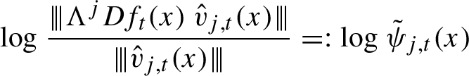 $$ \begin{align*} \log \frac {\mathopen{| {\kern -1.5pt} | {\kern -1.5pt} |} { \mathsf{\Lambda}^j Df_t(x) \, \hat v_{j,t}(x)} \mathclose{| {\kern -1.5pt} | {\kern -1.5pt} |}} {\mathopen{| {\kern -1.5pt} | {\kern -1.5pt} |} {\hat v_{j,t}(x)} \mathclose{| {\kern -1.5pt} | {\kern -1.5pt} |}} =: \log \tilde \psi_{j,t}(x) \end{align*} $$
has integral
 $\hat {\unicode{x3bb} }_j(f_t)$
. Furthermore,
$\hat {\unicode{x3bb} }_j(f_t)$
. Furthermore,
 $$ \begin{align*} \mathsf{\Lambda}^j Df_t(z) \, \hat v_{j,t}(x) = \pm \tilde \psi_{j,t}(x) \, \hat v_{j,t}(f_t(x)). \end{align*} $$
Substituting into equation (6.10), we see that the functions
 $\log \psi _{j,t}$
and
$\log \psi _{j,t}$
and
 $\log \tilde \psi _{j,t}$
are cohomologous. In particular, they have the same integral, proving the lemma.
$\log \tilde \psi _{j,t}$
are cohomologous. In particular, they have the same integral, proving the lemma.
Let us analyze the function
 $\log \psi _{j,t}$
to estimate its integral.
$\log \psi _{j,t}$
to estimate its integral.
Lemma 6.3. If
 $x \not \in Z_4$
, then
$x \not \in Z_4$
, then
 $\log \psi _{j,t}(x) = \chi _1(x) + \cdots + \chi _j(x)$
.
$\log \psi _{j,t}(x) = \chi _1(x) + \cdots + \chi _j(x)$
.
Proof If
 $x\notin Z_4$
, then
$x\notin Z_4$
, then
 $f_t=f$
on a neighborhood of x and so the lemma follows from equation (6.9).
$f_t=f$
on a neighborhood of x and so the lemma follows from equation (6.9).
However, on
 $Z_4 = \bigsqcup _i \mathcal {B}_i$
, we have the following estimate.
$Z_4 = \bigsqcup _i \mathcal {B}_i$
, we have the following estimate.
Lemma 6.4. If
 $x \in \mathcal {B}_i$
and
$x \in \mathcal {B}_i$
and
 $z := \Psi _i^{-1}(x)$
, then
$z := \Psi _i^{-1}(x)$
, then
 $$ \begin{align} | \log \psi_{j,t}(x) - [ \chi_1(x) + \cdots + \chi_j(x) + \log \det\nolimits_j Dh_{Bt}(z) ] | \le \nu + O(\varepsilon). \end{align} $$
Here and in what follows,
 $O(\varepsilon )$
stands for anything whose absolute value is bounded by
$O(\varepsilon )$
stands for anything whose absolute value is bounded by
 $\varepsilon $
times something depending on the numbers fixed at the beginning of the proof and on the model deformation.
$\varepsilon $
times something depending on the numbers fixed at the beginning of the proof and on the model deformation.
Proof Consider the case
 $j=1$
. Because
$j=1$
. Because
 $f_t = f \circ g_t$
,
$f_t = f \circ g_t$
,
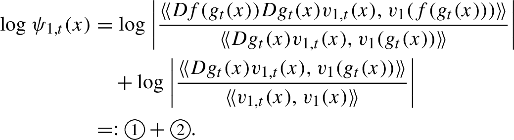
The first term is easy to estimate, using equations (6.8) and (6.2):
Consider x as fixed and denote
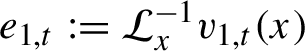 $e_{1,t} := \mathcal {L}_x^{-1} v_{1,t}(x)$
. Then
$e_{1,t} := \mathcal {L}_x^{-1} v_{1,t}(x)$
. Then
because
 $\mathcal {L}_x$
sends the Euclidean metric on
$\mathcal {L}_x$
sends the Euclidean metric on
 $\mathbb {R}^d$
to the Lyapunov metric at
$\mathbb {R}^d$
to the Lyapunov metric at
 $T_x M$
. Recall from equation (6.7) that
$T_x M$
. Recall from equation (6.7) that
 $v_{1,t}(x) \in \mathcal {H}_1(x,\gamma )$
, that is,
$v_{1,t}(x) \in \mathcal {H}_1(x,\gamma )$
, that is,
 $e_{1,t} \in \mathcal {H}_1(\gamma )$
. So the inner product
$e_{1,t} \in \mathcal {H}_1(\gamma )$
. So the inner product
is always positive (by continuity) and actually satisfies the bound:
Recall that
 $z := \Phi _i^{-1}(x)$
. By equation (5.12),
$z := \Phi _i^{-1}(x)$
. By equation (5.12),
 $\langle Dh_{Bt}(z) e_{1,t} , e_1 \rangle $
is positive and
$\langle Dh_{Bt}(z) e_{1,t} , e_1 \rangle $
is positive and
 $$ \begin{align} \bigg| \log \frac{\langle Dh_{Bt}(z) e_{1,t} , e_1 \rangle}{\langle e_{1,t} , e_1 \rangle} - \log \det\nolimits_1 Dh_{Bt}(z) \bigg| < \nu. \end{align} $$
Next, consider the quantity

Applying the chain rule,
 $$\begin{align*}\begin{array}{r@{\,}l@{\,}ll} Dg_t(x) &=& D\Psi_i(h_{Bt}(z)) \, Dh_{Bt}(z) \, D\Psi_i^{-1}(x) &\text{(by equation (6.5))} \\ &=& D\Phi_{x_i}(\Phi_{x_i}^{-1}(g_t(x))) \, Dh_{Bt}(z) \, D\Phi_{x_i}^{-1}(x) &\text{(by equation (6.4)).} \end{array} \end{align*}$$
Therefore,
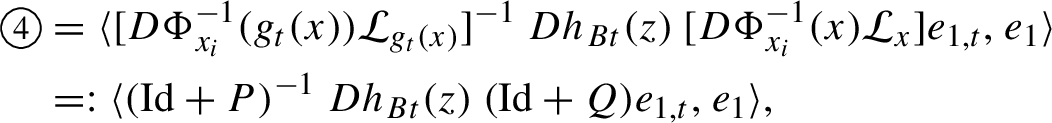
where, by equation (6.3), the linear maps
 $P, Q \colon \mathbb {R}^d \to \mathbb {R}^d$
satisfy
$P, Q \colon \mathbb {R}^d \to \mathbb {R}^d$
satisfy
 $\|P\|$
,
$\|P\|$
,
 $\|Q\| < \varepsilon $
. So
$\|Q\| < \varepsilon $
. So
and, in particular,
is positive. Now we can estimate
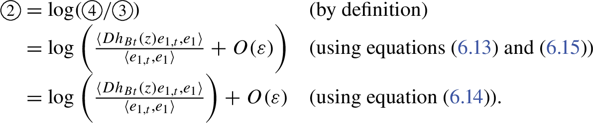
Combining this with equations (6.14) and (6.12), we obtain the desired estimate (6.11) for the case
 $j=1$
.
$j=1$
.
The proof for
 $j\ge 2$
follows exactly the same pattern, taking exterior powers, of course. The only point that deserves notice is that estimate (6.13) should be replaced by the following: if
$j\ge 2$
follows exactly the same pattern, taking exterior powers, of course. The only point that deserves notice is that estimate (6.13) should be replaced by the following: if
 $e_{j,t} := \mathcal {L}_x^{-1} v_{j,t}(x)$
, then
$e_{j,t} := \mathcal {L}_x^{-1} v_{j,t}(x)$
, then
 $$ \begin{align*} |\langle e_{1,t} \wedge \cdots \wedge e_{j,t}, e_1 \wedge \cdots \wedge e_j \rangle| \ge (1+\gamma^2)^{-j/2}\| e_{1,t} \wedge \cdots \wedge e_{j,t} \|. \end{align*} $$
Indeed, the orthogonal projection onto the space spanned by
 $e_1$
, …,
$e_1$
, …,
 $e_j$
cannot contract a vector in the cone
$e_j$
cannot contract a vector in the cone
 $\mathcal {H}_j(\gamma )$
by a factor smaller than
$\mathcal {H}_j(\gamma )$
by a factor smaller than
 $(1+\gamma ^2)^{-1/2}$
, and hence it cannot contract the volume of a j-dimensional parallelepiped in the cone by a factor smaller than
$(1+\gamma ^2)^{-1/2}$
, and hence it cannot contract the volume of a j-dimensional parallelepiped in the cone by a factor smaller than
 $(1+\gamma ^2)^{-j/2}$
.
$(1+\gamma ^2)^{-j/2}$
.
We obtain from equations (6.11) and (5.9) that for each Lyapunov ball
 $\mathcal {B}_i$
,
$\mathcal {B}_i$
,
 $$ \begin{align*} \bigg| \int_{\mathcal{B}_i} \log \psi_{j,t} \,\mathrm{d} m - \int_{\mathcal{B}_i} (\chi_1 + \cdots + \chi_j) \,\mathrm{d} m + {m(\mathcal{B}_i)} {\mathcal Q}(b_j t_j) \bigg| \le {m(\mathcal{B}_i)} \nu + O(\varepsilon). \end{align*} $$
This together with Lemmas 6.2 and 6.3 yields

Because
 $\nu \le \delta _0 a_j / 2$
and
$\nu \le \delta _0 a_j / 2$
and
 $1/N - m(Z_4) = O(\varepsilon )$
,
$1/N - m(Z_4) = O(\varepsilon )$
,

By the definition (6.1) of
 $b_j$
,
$b_j$
,
 $$ \begin{align*} {\mathcal Q}(0) = 0 \le {\mathcal Q}(b_j t_j) \le 3 \delta_0 a_j = {\mathcal Q}(b_j). \end{align*} $$
Combining these two pieces of information, and recalling that
 $\delta = \delta _0/N$
, we obtain
$\delta = \delta _0/N$
, we obtain
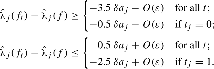
So a sufficiently small choice of
 $\varepsilon $
ensures that inequalities (2.3)–(2.5) are satisfied. Proposition 2.1 and, therefore, Theorem 1.5 are proved.
$\varepsilon $
ensures that inequalities (2.3)–(2.5) are satisfied. Proposition 2.1 and, therefore, Theorem 1.5 are proved.
7 Proof of additional results for tori
In this section, we prove two supplements to Theorem 1.5, namely Corollary 1.6 and Theorem 1.7.
7.1 Anosov diffeomorphisms display all hyperbolic simple Lyapunov spectra
To deduce Corollary 1.6 from Theorem 1.5, we need the following fact.
Lemma 7.1. Given integers
 $d>u>0$
, there exists an Anosov linear automorphism of
$d>u>0$
, there exists an Anosov linear automorphism of
 $\mathbb {T}^d$
with unstable index u and simple Lyapunov spectrum.
$\mathbb {T}^d$
with unstable index u and simple Lyapunov spectrum.
Proof We need to show the existence of a polynomial
 $P(x)$
with integer coefficients, leading term
$P(x)$
with integer coefficients, leading term
 $x^d$
, constant term
$x^d$
, constant term
 $\pm 1$
, whose roots are all real and simple, being u of them with modulus bigger than
$\pm 1$
, whose roots are all real and simple, being u of them with modulus bigger than
 $1$
and
$1$
and
 $d-u$
of them of modulus smaller than
$d-u$
of them of modulus smaller than
 $1$
. Then the companion matrix of
$1$
. Then the companion matrix of
 $P(x)$
will be an element
$P(x)$
will be an element
 $L \in \mathrm {GL}(d,\mathbb {Z})$
that induces an Anosov linear automorphism
$L \in \mathrm {GL}(d,\mathbb {Z})$
that induces an Anosov linear automorphism
 $F_L \colon \mathbb {T}^d \to \mathbb {T}^d$
with unstable index u and simple Lyapunov spectrum. Though the existence of such polynomials can be quickly deduced from Dirichlet’s unit theorem, we will provide a completely elementary proof. The idea comes from a proof of existence of Pisot–Vijayaraghavan numbers of arbitrary degree [Reference Vijayaraghavan43, Theorem 1].
$F_L \colon \mathbb {T}^d \to \mathbb {T}^d$
with unstable index u and simple Lyapunov spectrum. Though the existence of such polynomials can be quickly deduced from Dirichlet’s unit theorem, we will provide a completely elementary proof. The idea comes from a proof of existence of Pisot–Vijayaraghavan numbers of arbitrary degree [Reference Vijayaraghavan43, Theorem 1].
Fix integers
 $$ \begin{align*} a_1>\cdots>a_u>0>a_{u+1}>\cdots>a_d \end{align*} $$
whose sum is
 $0$
and such that
$0$
and such that
 $a_i-a_{i+1}\ge 2$
for each
$a_i-a_{i+1}\ge 2$
for each
 $i\in \{1,\ldots ,d-1\}$
. Let
$i\in \{1,\ldots ,d-1\}$
. Let
 $b \ge 3$
be another integer, and consider the polynomial
$b \ge 3$
be another integer, and consider the polynomial
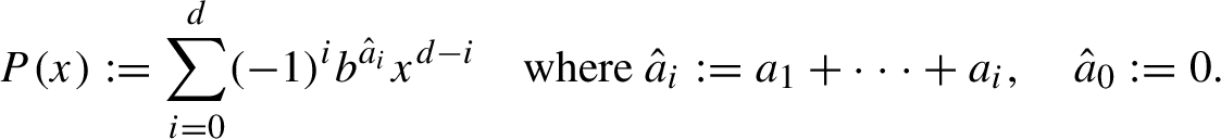 $$ \begin{align*} P(x) := \sum_{i=0}^d (-1)^i b^{\hat{a}_i} x^{d-i} \quad\text{where } \hat{a}_i := a_1+\cdots+a_i, \quad \hat{a}_0 := 0. \end{align*} $$
Note that
 $\hat {a}_i \ge 0$
for each i and so P has integer coefficients. Furthermore, P is monic and has constant term
$\hat {a}_i \ge 0$
for each i and so P has integer coefficients. Furthermore, P is monic and has constant term
 $(-1)^d$
.
$(-1)^d$
.
Let us locate the roots of P. We claim that, for all
 $n \in \mathbb {Z} \smallsetminus \{a_1,\ldots ,a_d\}$
,
$n \in \mathbb {Z} \smallsetminus \{a_1,\ldots ,a_d\}$
,
 $$ \begin{align} P(b^n) \text{ is non-zero and has the same sign as } \prod_{j=1}^d (n-a_j), \end{align} $$
and so, by the intermediate value theorem, P has
 $d-u$
simple roots on the interval
$d-u$
simple roots on the interval
 $(0,1)$
and u simple roots on the interval
$(0,1)$
and u simple roots on the interval
 $(1,+\infty )$
. To prove the claim, fix n and consider the expression:
$(1,+\infty )$
. To prove the claim, fix n and consider the expression:
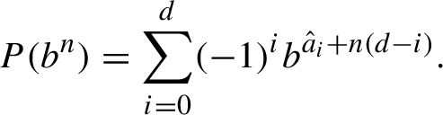 $$ \begin{align} P(b^n) = \sum_{i=0}^d (-1)^i b^{\hat{a}_i + n(d-i)}. \end{align} $$
The function
 $i \in \{0,\ldots ,d\} \mapsto \hat {a}_i + n(d-i)$
is integer-valued, strictly concave, and attains a maximum at
$i \in \{0,\ldots ,d\} \mapsto \hat {a}_i + n(d-i)$
is integer-valued, strictly concave, and attains a maximum at
 $i=k$
, where k is the number of negative factors in the product
$i=k$
, where k is the number of negative factors in the product
 $\prod _{j=1}^d (n-a_j)$
. Using that
$\prod _{j=1}^d (n-a_j)$
. Using that
 $2\sum _{j=1}^{\infty } b^{-j} \le 1$
, we see that the term corresponding to
$2\sum _{j=1}^{\infty } b^{-j} \le 1$
, we see that the term corresponding to
 $i=k$
in the right-hand side of equation (7.2) is bigger in absolute value than the sum of all other terms. So the sign of
$i=k$
in the right-hand side of equation (7.2) is bigger in absolute value than the sum of all other terms. So the sign of
 $P(b^n)$
is
$P(b^n)$
is
 $(-1)^k$
, thus proving equation (7.1).
$(-1)^k$
, thus proving equation (7.1).
Proof of Corollary 1.6 Consider non-zero numbers
 $\xi _{1}> \cdots > \xi _{d}$
whose sum is equal to
$\xi _{1}> \cdots > \xi _{d}$
whose sum is equal to
 $0$
, and let
$0$
, and let
 $\boldsymbol {\xi } := (\xi _1,\ldots ,\xi _d)$
. By Lemma 7.1, there exists an Anosov linear automorphism
$\boldsymbol {\xi } := (\xi _1,\ldots ,\xi _d)$
. By Lemma 7.1, there exists an Anosov linear automorphism
 $F_L \colon \mathbb {T}^d \to \mathbb {T}^d$
whose Lyapunov spectrum
$F_L \colon \mathbb {T}^d \to \mathbb {T}^d$
whose Lyapunov spectrum
 $\boldsymbol {\unicode{x3bb} }(L)$
is simple and has the same unstable index as
$\boldsymbol {\unicode{x3bb} }(L)$
is simple and has the same unstable index as
 $\boldsymbol {\xi }$
. If n is sufficiently large, then
$\boldsymbol {\xi }$
. If n is sufficiently large, then
 $\boldsymbol {\unicode{x3bb} }(L^n) = n \boldsymbol {\unicode{x3bb} }(L)$
strictly majorizes
$\boldsymbol {\unicode{x3bb} }(L^n) = n \boldsymbol {\unicode{x3bb} }(L)$
strictly majorizes
 $\boldsymbol {\xi }$
. Hence by Theorem 1.5, there exists a conservative Anosov
$\boldsymbol {\xi }$
. Hence by Theorem 1.5, there exists a conservative Anosov
 $C^{\infty }$
diffeomorphism
$C^{\infty }$
diffeomorphism
 $f \colon \mathbb {T}^d \to \mathbb {T}^d$
homotopic to
$f \colon \mathbb {T}^d \to \mathbb {T}^d$
homotopic to
 $F_{L^n}$
with simple dominated splitting and such that
$F_{L^n}$
with simple dominated splitting and such that
 $\boldsymbol {\unicode{x3bb} }(f) = \boldsymbol {\xi }$
, as we wanted to prove.
$\boldsymbol {\unicode{x3bb} }(f) = \boldsymbol {\xi }$
, as we wanted to prove.
7.2 Spectra of Anosov diffeomorphisms with simple dominated splitting on
$\mathbb {T}^3$

In this subsection, we prove Theorem 1.7. Fix a hyperbolic matrix
 $L \in \mathrm {GL}(3,\mathbb {Z})$
whose eigenvalues are all real and simple. So the induced automorphism
$L \in \mathrm {GL}(3,\mathbb {Z})$
whose eigenvalues are all real and simple. So the induced automorphism
 $F_L \colon \mathbb {T}^3 \to \mathbb {T}^3$
is Anosov and its Lyapunov spectrum is simple. Let
$F_L \colon \mathbb {T}^3 \to \mathbb {T}^3$
is Anosov and its Lyapunov spectrum is simple. Let
 $u \in \{1,2\}$
be its unstable index.
$u \in \{1,2\}$
be its unstable index.
Proof of the ‘only if’ part of Theorem 1.7 Let
 $f\in \mathrm {Diff}_m^{\infty }(\mathbb {T}^3)$
be an Anosov diffeomorphism homotopic to the automorphism
$f\in \mathrm {Diff}_m^{\infty }(\mathbb {T}^3)$
be an Anosov diffeomorphism homotopic to the automorphism
 $F_L$
, and admitting simple dominated splitting. Because f and
$F_L$
, and admitting simple dominated splitting. Because f and
 $F_L$
are topologically conjugate, they have the same unstable index u. Taking inverses if necessary, we can assume that
$F_L$
are topologically conjugate, they have the same unstable index u. Taking inverses if necessary, we can assume that
 $u=2$
. So the Lyapunov spectrum
$u=2$
. So the Lyapunov spectrum
 $\boldsymbol {\unicode{x3bb} }(f) = (\unicode{x3bb} _1(f),\unicode{x3bb} _2(f),\unicode{x3bb} _3(f))$
satisfies
$\boldsymbol {\unicode{x3bb} }(f) = (\unicode{x3bb} _1(f),\unicode{x3bb} _2(f),\unicode{x3bb} _3(f))$
satisfies
 $\unicode{x3bb} _1(f)>\unicode{x3bb} _2(f)>0>\unicode{x3bb} _3(f)$
. Let us show that
$\unicode{x3bb} _1(f)>\unicode{x3bb} _2(f)>0>\unicode{x3bb} _3(f)$
. Let us show that
 $\boldsymbol {\unicode{x3bb} }(f)$
is majorized by
$\boldsymbol {\unicode{x3bb} }(f)$
is majorized by
 $\boldsymbol {\unicode{x3bb} }(L)$
. As explained before, the inequality
$\boldsymbol {\unicode{x3bb} }(L)$
. As explained before, the inequality
 $\unicode{x3bb} _1(f)+\unicode{x3bb} _2(f) \le \unicode{x3bb} _1(L)+\unicode{x3bb} _2(L)$
is immediate: see equation (1.3). Therefore, we need to show that
$\unicode{x3bb} _1(f)+\unicode{x3bb} _2(f) \le \unicode{x3bb} _1(L)+\unicode{x3bb} _2(L)$
is immediate: see equation (1.3). Therefore, we need to show that
 $\unicode{x3bb} _1(f) \le \unicode{x3bb} _1(L)$
.
$\unicode{x3bb} _1(f) \le \unicode{x3bb} _1(L)$
.
Let
 $\tilde {f}$
be a lift of f to the universal covering
$\tilde {f}$
be a lift of f to the universal covering
 $\mathbb {R}^3$
. Because f is homotopic to
$\mathbb {R}^3$
. Because f is homotopic to
 $F_L$
, we have
$F_L$
, we have
 $\tilde {f} = L + \varphi $
for some
$\tilde {f} = L + \varphi $
for some
 $\mathbb {Z}^3$
-periodic map
$\mathbb {Z}^3$
-periodic map
 $\varphi \colon \mathbb {R}^3 \to \mathbb {R}^3$
. So, for every
$\varphi \colon \mathbb {R}^3 \to \mathbb {R}^3$
. So, for every
 $n \ge 0$
,
$n \ge 0$
,
 $$ \begin{align*} \tilde{f}^n = L^n + \sum_{k=0}^{n-1} L^k \circ \varphi \circ \tilde{f}^{n-1-k}. \end{align*} $$
Because
 $\varphi $
is bounded, it follows that there is a constant
$\varphi $
is bounded, it follows that there is a constant
 $C_1>0$
(independent of n) such that, for all x,
$C_1>0$
(independent of n) such that, for all x,
 $y \in \mathbb {R}^d$
with
$y \in \mathbb {R}^d$
with
 $\|x - y\| \le 1$
,
$\|x - y\| \le 1$
,
 $$ \begin{align*} \| \tilde{f}^n(x) - \tilde{f}^n(y) \| \le C_1 \sum_{k=0}^n \| L^k \|. \end{align*} $$
Because the top eigenvalue of the linear map L is simple, there is another constant
 $C_2>0$
such that
$C_2>0$
such that
 $\| L^k \| \le C_2 e^{k \unicode{x3bb} _1(L)}$
for all
$\| L^k \| \le C_2 e^{k \unicode{x3bb} _1(L)}$
for all
 $k \ge 0$
. In particular,
$k \ge 0$
. In particular,
where
 $C_3>0$
is another constant.
$C_3>0$
is another constant.
By [Reference Brin, Burago and Ivanov15, Theorem 1.3] (see also [Reference Potrie38, Corollary 7.7]), the strong unstable foliation in the universal covering is quasi-isometric; this means that there is a constant
 $C_4>0$
such that if
$C_4>0$
such that if
 $I \subset \mathbb {R}^3$
is a segment of strong unstable manifold, then its length, denoted by
$I \subset \mathbb {R}^3$
is a segment of strong unstable manifold, then its length, denoted by
 $\mathrm {len}(I)$
, can be bounded as
$\mathrm {len}(I)$
, can be bounded as
 $$ \begin{align*} \mathrm{len}(I) \le C_4\operatorname{\mathrm{diam}}(I)+C_4. \end{align*} $$
Hence, for every such a segment with
 $\operatorname {\mathrm {diam}}(I) \le 1$
, and every
$\operatorname {\mathrm {diam}}(I) \le 1$
, and every
 $n\geq 0$
,
$n\geq 0$
,
If follows from the next lemma that
 $\unicode{x3bb} _1(f) \le \unicode{x3bb} _1(L)$
, as we wanted to prove.
$\unicode{x3bb} _1(f) \le \unicode{x3bb} _1(L)$
, as we wanted to prove.
Lemma 7.2. For each
 $x\in \mathbb {T}^3$
, let
$x\in \mathbb {T}^3$
, let
 $W_x \subset \mathbb {T}^3$
be the segment of strong unstable leaf of length
$W_x \subset \mathbb {T}^3$
be the segment of strong unstable leaf of length
 $1$
for which x is a midpoint. Then, for m-almost every
$1$
for which x is a midpoint. Then, for m-almost every
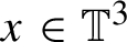 $x\in \mathbb {T}^3$
,
$x\in \mathbb {T}^3$
,

(See [Reference Saghin and Xia39] for related results.)
Proof Let
 $\ell $
denote a one-dimensional Hausdorff measure (that is, length) on
$\ell $
denote a one-dimensional Hausdorff measure (that is, length) on
 $\mathbb {T}^3$
. For every
$\mathbb {T}^3$
. For every
 $x\in \mathbb {T}^3$
,
$x\in \mathbb {T}^3$
,
 $$ \begin{align*} \ell(f^n(W_x)) = \int_{W_x} \| Df^n |_{E_1(y)} \| \,\mathrm{d} \ell(y). \end{align*} $$
Because
 $\ell (W_x) = 1$
, Jensen’s inequality yields:
$\ell (W_x) = 1$
, Jensen’s inequality yields:
 $$ \begin{align*} \log \ell(f^n(W_x)) \ge \int_{W_x} \log \| Df^n |_{E_1(y)} \| \,\mathrm{d} \ell(y). \end{align*} $$
Let R be the set of points
 $y\in \mathbb {T}^3$
for which
$y\in \mathbb {T}^3$
for which
 $\lim _{n\to \infty }({1}/{n}) \log \| Df^n |_{E_1(y)} \| = \unicode{x3bb} _1(f)$
; then
$\lim _{n\to \infty }({1}/{n}) \log \| Df^n |_{E_1(y)} \| = \unicode{x3bb} _1(f)$
; then
 $m(R)=1$
. By absolute continuity of the strong unstable foliation [Reference Pesin and Sinai36, Lemma 10], for m-almost every
$m(R)=1$
. By absolute continuity of the strong unstable foliation [Reference Pesin and Sinai36, Lemma 10], for m-almost every
 $x\in \mathbb {T}^3$
, we have
$x\in \mathbb {T}^3$
, we have
 $\ell (W_x\cap R) = 1$
. Therefore,
$\ell (W_x\cap R) = 1$
. Therefore,

Proof of the ‘if’ part of Theorem 1.7 Now we fix a vector
 $\boldsymbol {\xi } = (\xi _1,\xi _2,\xi _3)$
such that
$\boldsymbol {\xi } = (\xi _1,\xi _2,\xi _3)$
such that
 $\xi _1> \xi _2 >\xi _3$
,
$\xi _1> \xi _2 >\xi _3$
,
 $\xi _u>0>\xi _{u+1}$
, and
$\xi _u>0>\xi _{u+1}$
, and
 $\boldsymbol {\xi } \preccurlyeq \boldsymbol {\unicode{x3bb} }(L)$
. We want to find a smooth conservative Anosov diffeomorphism f homotopic to
$\boldsymbol {\xi } \preccurlyeq \boldsymbol {\unicode{x3bb} }(L)$
. We want to find a smooth conservative Anosov diffeomorphism f homotopic to
 $F_L$
, admitting a simple dominated splitting, and with spectrum
$F_L$
, admitting a simple dominated splitting, and with spectrum
 $\boldsymbol {\unicode{x3bb} }(f) = \boldsymbol {\xi }$
. If
$\boldsymbol {\unicode{x3bb} }(f) = \boldsymbol {\xi }$
. If
 $\boldsymbol {\xi }$
is strictly majorized by
$\boldsymbol {\xi }$
is strictly majorized by
 $\boldsymbol {\unicode{x3bb} }(L)$
, then the existence of f is guaranteed by Theorem 1.5. So let us assume that majorization is not strict, that is, either
$\boldsymbol {\unicode{x3bb} }(L)$
, then the existence of f is guaranteed by Theorem 1.5. So let us assume that majorization is not strict, that is, either
 $\xi _1=\unicode{x3bb} _1(L)$
or
$\xi _1=\unicode{x3bb} _1(L)$
or
 $\xi _1+\xi _2=\unicode{x3bb} _1(L)+\unicode{x3bb} _2(L)$
. We can assume that only one of these equalities is satisfied, because otherwise, we can simply take
$\xi _1+\xi _2=\unicode{x3bb} _1(L)+\unicode{x3bb} _2(L)$
. We can assume that only one of these equalities is satisfied, because otherwise, we can simply take
 $f=F_L$
.
$f=F_L$
.
Let
 $E^L_1$
,
$E^L_1$
,
 $E^L_2$
,
$E^L_2$
,
 $E^L_3$
denote the eigenspaces of L corresponding to the Lyapunov exponents
$E^L_3$
denote the eigenspaces of L corresponding to the Lyapunov exponents
 $\unicode{x3bb} _1(L)$
,
$\unicode{x3bb} _1(L)$
,
 $\unicode{x3bb} _2(L)$
,
$\unicode{x3bb} _2(L)$
,
 $\unicode{x3bb} _3(L)$
, respectively. In the case
$\unicode{x3bb} _3(L)$
, respectively. In the case
 $\xi _1=\unicode{x3bb} _1(L)$
, we shall perform the deformation in Theorem 1.5 in such a way that the foliation
$\xi _1=\unicode{x3bb} _1(L)$
, we shall perform the deformation in Theorem 1.5 in such a way that the foliation
 $\mathcal {F}^{23}$
parallel to
$\mathcal {F}^{23}$
parallel to
 $E^L_2\oplus E^L_3$
is preserved, while in the case
$E^L_2\oplus E^L_3$
is preserved, while in the case
 $\xi _1+\xi _2=\unicode{x3bb} _1(L)+\unicode{x3bb} _2(L)$
(or equivalently
$\xi _1+\xi _2=\unicode{x3bb} _1(L)+\unicode{x3bb} _2(L)$
(or equivalently
 $\unicode{x3bb} _3(f)=\unicode{x3bb} _3(L)$
), we shall do it in such a way that foliation
$\unicode{x3bb} _3(f)=\unicode{x3bb} _3(L)$
), we shall do it in such a way that foliation
 $\mathcal {F}^{12}$
parallel to
$\mathcal {F}^{12}$
parallel to
 $E^L_1\oplus E^L_2$
is preserved. Because both cases are dealt with similarly, we will concentrate on the second case, namely
$E^L_1\oplus E^L_2$
is preserved. Because both cases are dealt with similarly, we will concentrate on the second case, namely
 $\xi _3 = \unicode{x3bb} _3(L)$
.
$\xi _3 = \unicode{x3bb} _3(L)$
.
The following observation will make the argument simpler.
Lemma 7.3. Let f be a conservative Anosov diffeomorphism of
 $\mathbb {T}^3$
homotopic to
$\mathbb {T}^3$
homotopic to
 $F_L$
. If f preserves the foliation
$F_L$
. If f preserves the foliation
 $\mathcal {F}^{12}$
, then
$\mathcal {F}^{12}$
, then
 $\unicode{x3bb} _3(f)=\unicode{x3bb} _3(L)$
.
$\unicode{x3bb} _3(f)=\unicode{x3bb} _3(L)$
.
Proof Let
 $\tilde {f}$
be a lift of f to the universal covering
$\tilde {f}$
be a lift of f to the universal covering
 $\mathbb {R}^3$
. Because f is homotopic to
$\mathbb {R}^3$
. Because f is homotopic to
 $F_L$
, we have
$F_L$
, we have
 $\tilde {f} = L + \varphi $
for some
$\tilde {f} = L + \varphi $
for some
 $\mathbb {Z}^3$
-periodic map
$\mathbb {Z}^3$
-periodic map
 $\varphi $
. Let
$\varphi $
. Let
 $P_1$
,
$P_1$
,
 $P_2$
,
$P_2$
,
 $P_3$
be the projections associated to the splitting
$P_3$
be the projections associated to the splitting
 $\mathbb {R}^3=E_1^L\oplus E_2^L\oplus E_3^L$
. The fact that f preserves the foliation
$\mathbb {R}^3=E_1^L\oplus E_2^L\oplus E_3^L$
. The fact that f preserves the foliation
 $\mathcal {F}^{12}$
implies that
$\mathcal {F}^{12}$
implies that
 $\tilde {f}$
preserves the foliation
$\tilde {f}$
preserves the foliation
 $\widetilde {\mathcal {F}}^{12}$
of
$\widetilde {\mathcal {F}}^{12}$
of
 $\mathbb {R}^3$
along planes parallel to
$\mathbb {R}^3$
along planes parallel to
 $E_1^L\oplus E_2^L$
. For every
$E_1^L\oplus E_2^L$
. For every
 $x\in \mathbb {R}^3$
and every
$x\in \mathbb {R}^3$
and every
 $v\in E_1^L \oplus E_2^L$
, we have
$v\in E_1^L \oplus E_2^L$
, we have
 $P_3\circ \tilde {f}(x) = P_3\circ \tilde {f}(x+v)$
and therefore
$P_3\circ \tilde {f}(x) = P_3\circ \tilde {f}(x+v)$
and therefore
 $P_3\circ \varphi (x) = P_3\circ \varphi (x+v)$
. Because
$P_3\circ \varphi (x) = P_3\circ \varphi (x+v)$
. Because
 $F_L$
is a three-dimensional Anosov automorphism, the plane
$F_L$
is a three-dimensional Anosov automorphism, the plane
 $E_2^L\oplus E_3^L$
projects to a dense subset of
$E_2^L\oplus E_3^L$
projects to a dense subset of
 $\mathbb {T}^3$
, and because the map
$\mathbb {T}^3$
, and because the map
 $P_3 \circ \varphi $
is
$P_3 \circ \varphi $
is
 $\mathbb {Z}^3$
-periodic, it must be constant. So the derivative of f written with respect to the splitting
$\mathbb {Z}^3$
-periodic, it must be constant. So the derivative of f written with respect to the splitting
 $\mathbb {R}^3=E_1^L\oplus E_2^L\oplus E_3^L$
is necessarily of the form
$\mathbb {R}^3=E_1^L\oplus E_2^L\oplus E_3^L$
is necessarily of the form
Because
 $\tilde {f}$
is volume preserving, this implies that the absolute value of the determinant of
$\tilde {f}$
is volume preserving, this implies that the absolute value of the determinant of
 $D\tilde {f}$
restricted to
$D\tilde {f}$
restricted to
 $E_1^L\oplus E_2^L$
is everywhere constant
$E_1^L\oplus E_2^L$
is everywhere constant
 $e^{-\unicode{x3bb} _3(L)}$
. The same is true for
$e^{-\unicode{x3bb} _3(L)}$
. The same is true for
 $Df$
and hence
$Df$
and hence
 $\unicode{x3bb} _1(f) + \unicode{x3bb} _2(f) = -\unicode{x3bb} _3(L)$
, that is,
$\unicode{x3bb} _1(f) + \unicode{x3bb} _2(f) = -\unicode{x3bb} _3(L)$
, that is,
 $\unicode{x3bb} _3(f) = \unicode{x3bb} _3(L)$
(actually,
$\unicode{x3bb} _3(f) = \unicode{x3bb} _3(L)$
(actually,
 $\unicode{x3bb} _{3,\mu }(f)=\unicode{x3bb} _3(L)$
for any f-invariant probability measure
$\unicode{x3bb} _{3,\mu }(f)=\unicode{x3bb} _3(L)$
for any f-invariant probability measure
 $\mu $
, by the same proof).
$\mu $
, by the same proof).
Coming back to the proof of Theorem 1.7, we need a variation of the central proposition (Proposition 2.1) where all diffeomorphisms preserve the foliation
 $\mathcal {F}^{12}$
.
$\mathcal {F}^{12}$
.
Proposition 7.4. Let
 $a_1$
,
$a_1$
,
 $\sigma $
, and
$\sigma $
, and
 $\delta _0$
be positive numbers. Then, there exists
$\delta _0$
be positive numbers. Then, there exists
 $\delta \in (0,\delta _0)$
with the following properties.
$\delta \in (0,\delta _0)$
with the following properties.
Let
 $f\in \mathrm {Diff}_m^{\infty }(\mathbb {T}^3)$
be an Anosov diffeomorphism homotopic to
$f\in \mathrm {Diff}_m^{\infty }(\mathbb {T}^3)$
be an Anosov diffeomorphism homotopic to
 $F_L$
admitting a simple dominated splitting, and such that
$F_L$
admitting a simple dominated splitting, and such that
 $\textsf {g}_u(\boldsymbol {\unicode{x3bb} }(f)) \ge \sigma $
. In addition, assume that f preserves the foliation
$\textsf {g}_u(\boldsymbol {\unicode{x3bb} }(f)) \ge \sigma $
. In addition, assume that f preserves the foliation
 $\mathcal {F}^{12}$
(and so
$\mathcal {F}^{12}$
(and so
 $\unicode{x3bb} _3(f) = \unicode{x3bb} _3(L)$
, by Lemma 7.3). Then there exists a continuous map
$\unicode{x3bb} _3(f) = \unicode{x3bb} _3(L)$
, by Lemma 7.3). Then there exists a continuous map
 $$ \begin{align*} t \in [0,1] \mapsto f_t \in \mathrm{Diff}_m^{\infty}(\mathbb{T}^3), \end{align*} $$
where
 $f_0 = f$
and for each
$f_0 = f$
and for each
 $t \in [0,1]$
, the conservative diffeomorphism
$t \in [0,1]$
, the conservative diffeomorphism
 $f_t$
is Anosov, admits a simple dominated splitting, and its top Lyapunov exponent satisfies
$f_t$
is Anosov, admits a simple dominated splitting, and its top Lyapunov exponent satisfies
In addition, each
 $f_t$
preserves the foliation
$f_t$
preserves the foliation
 $\mathcal {F}^{12}$
(and so
$\mathcal {F}^{12}$
(and so
 $\unicode{x3bb} _3(f_t) = \unicode{x3bb} _3(L)$
, by Lemma 7.3).
$\unicode{x3bb} _3(f_t) = \unicode{x3bb} _3(L)$
, by Lemma 7.3).
Once this is established, we mimic the proof of Theorem 1.5; namely, we concatenate paths produced by the proposition and obtain a deformation of
 $F_L$
that ends with a diffeomorphism having Lyapunov spectrum equal to
$F_L$
that ends with a diffeomorphism having Lyapunov spectrum equal to
 $\boldsymbol {\xi }$
.
$\boldsymbol {\xi }$
.
To prove Proposition 7.4, we begin by modifying the construction of the Lyapunov charts in Proposition 3.4. Because we are working in the torus
 $\mathbb {T}^3 = \mathbb {R}^3/\mathbb {Z}^3$
, we can identify tangent spaces
$\mathbb {T}^3 = \mathbb {R}^3/\mathbb {Z}^3$
, we can identify tangent spaces
 $T_x\mathbb {T}^3$
with
$T_x\mathbb {T}^3$
with
 $\mathbb {R}^3$
. Let
$\mathbb {R}^3$
. Let
 $\pi \colon \mathbb {R}^3 \to \mathbb {T}^3$
be the quotient projection. For each
$\pi \colon \mathbb {R}^3 \to \mathbb {T}^3$
be the quotient projection. For each
 $x \in \mathbb {T}^3$
, let
$x \in \mathbb {T}^3$
, let
 $\mathcal {L}_x \colon \mathbb {R}^3 \to \mathbb {R}^3$
be a linear map that takes the canonical basis
$\mathcal {L}_x \colon \mathbb {R}^3 \to \mathbb {R}^3$
be a linear map that takes the canonical basis
 $\{e_1,e_2,e_3\}$
of
$\{e_1,e_2,e_3\}$
of
 $\mathbb {R}^3$
to a basis
$\mathbb {R}^3$
to a basis
 $\{\mathcal {L}_x(e_1), \mathcal {L}_x(e_2), \mathcal {L}_x(e_3)\}$
of
$\{\mathcal {L}_x(e_1), \mathcal {L}_x(e_2), \mathcal {L}_x(e_3)\}$
of
 $\mathbb {R}^3$
which is orthonormal for the Lyapunov metric
$\mathbb {R}^3$
which is orthonormal for the Lyapunov metric
 $\mathopen {\langle {\kern -1.7pt} \langle }{\mathord {\cdot }, \mathord {\cdot }} \mathclose {\rangle {\kern -1.7pt} \rangle }_x$
, and, moreover,
$\mathopen {\langle {\kern -1.7pt} \langle }{\mathord {\cdot }, \mathord {\cdot }} \mathclose {\rangle {\kern -1.7pt} \rangle }_x$
, and, moreover,
 $\mathcal {L}_x(e_j) \in E_j^f(x)$
for each j. Then we define the Lyapunov charts
$\mathcal {L}_x(e_j) \in E_j^f(x)$
for each j. Then we define the Lyapunov charts
 $$ \begin{align*} \Phi_x(z) := x + \pi (\mathcal{L}_x(z)). \end{align*} $$
These charts have all properties from Proposition 3.4 and the following additional one:
-
(e)
$\Phi _x$
is a foliated chart, that is, if
$z_1, z_2, z_3$
denote canonical coordinates in
$\mathbb {R}^3$
, then
$\Phi _x$
maps level sets of
$z_3$
(horizontal slices) into leaves of
$\mathcal {F}^{12}$
.


Indeed, the derivatives
 $D\Phi _x(z)$
are constant and equal to
$D\Phi _x(z)$
are constant and equal to
 $\mathcal {L}_x$
, and
$\mathcal {L}_x$
, and
 $\mathcal {L}_x$
maps the plane
$\mathcal {L}_x$
maps the plane
 $\mathbb {R} e_1 \oplus \mathbb {R} e_2$
to the plane
$\mathbb {R} e_1 \oplus \mathbb {R} e_2$
to the plane
 $E_1^f(x) \oplus E_2^f(x) = E_1^L \oplus E_2^L$
, which is tangent to
$E_1^f(x) \oplus E_2^f(x) = E_1^L \oplus E_2^L$
, which is tangent to
 $\mathcal {F}^{12}$
.
$\mathcal {F}^{12}$
.
Then we follow the proof of Proposition 2.1 (but with
 $a_2=0$
). To summarize, the deformation
$a_2=0$
). To summarize, the deformation
 $f_t$
of f is constructed as follows:
$f_t$
of f is constructed as follows:
-
• we select a disjoint family of Lyapunov balls
$\mathcal {B}_1, \ldots , \mathcal {B}_p$
; each ball
$\mathcal {B}_i$
equals
$\Phi _i(\mathbb {B})$
, where
$\mathbb {B}$
is the unit ball
$\mathbb {B}$
in
$\mathbb {R}^3$
and
$\Psi _i (z) = \Phi _{x_i}(s_i z)$
is a rescaled Lyapunov chart; -
• on each Lyapunov ball
$\mathcal {B}_i$
, the deformation is defined as
$f_t = f \circ g_t$
, where
$g_t = \Psi _i \circ h^{(1)}_{b_1 t} \circ \Psi _i^{-1}$
; here
$b_1>0$
is a constant and
$h^{(1)}_t$
is the first elementary model deformation.


Inspecting the equations (5.1), (5.2) that define the diffeomorphism
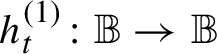 $h^{(1)}_t \colon \mathbb {B} \to \mathbb {B}$
, we immediately see that it preserves horizontal slices (that is, level sets of
$h^{(1)}_t \colon \mathbb {B} \to \mathbb {B}$
, we immediately see that it preserves horizontal slices (that is, level sets of
 $z_3$
). Because
$z_3$
). Because
 $\Psi _i$
maps horizontal slices into leaves of
$\Psi _i$
maps horizontal slices into leaves of
 $\mathcal {F}^{12}$
, the upshot is that each diffeomorphism
$\mathcal {F}^{12}$
, the upshot is that each diffeomorphism
 $f_t$
preserves the foliation
$f_t$
preserves the foliation
 $\mathcal {F}^{12}$
. This proves Proposition 7.4. As explained before, Theorem 1.7 follows.
$\mathcal {F}^{12}$
. This proves Proposition 7.4. As explained before, Theorem 1.7 follows.
Acknowledgements
We thank the referees for several corrections and suggestions that improved the readability of the paper. J.B. was partially supported by Fondecyt 1180371 and Conicyt PIA ACT172001. A.K. was partially supported by NSF Grant DMS 1602409. F.R.H. was partially supported by NSF 1500947. J.B. thanks the hospitality of Penn State University and Yeshiva University. The authors thank the hospitality of Mathematisches Forschungsinstitut Oberwolfach.


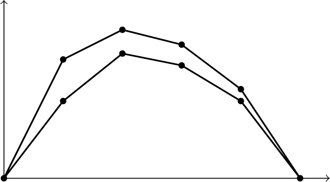


 Open access