





1. Introduction
In this work we study quasistatic approximations of time-inhomogeneous stochastic differential equations (SDEs) with multiplicative noise on $\mathbb{R}^n$
,
$\mathbb{R}^n$
,
 \begin{equation*} {\mathrm{d}} X_t = b(t,X_t)\,{\mathrm{d}} t + \sigma(t,X_t)\,{\mathrm{d}} W_t,\end{equation*}
driven by Brownian motion, $W_t$
. Specifically, for appropriate time-dependent observables h(t, x), we will obtain a quasistatic approximation
$W_t$
. Specifically, for appropriate time-dependent observables h(t, x), we will obtain a quasistatic approximation $\overline{h}^\mathrm{Q}_T$
to the time average
$\overline{h}^\mathrm{Q}_T$
to the time average
 \begin{equation} \overline{h}_T\,:\!=\,\frac{1}{T}\int_0^Th(t,X_t)\,{\mathrm{d}} t\end{equation}
and derive explicit non-asymptotic error bounds in two senses.
-
• We obtain probabilistic bounds on the deviation of $\overline{h}_T$
from
$\overline{h}^\mathrm{Q}_T$
, i.e. we derive concentration inequalities; see Theorems 2 and 3.
$\overline{h}_T$
from
$\overline{h}^\mathrm{Q}_T$
, i.e. we derive concentration inequalities; see Theorems 2 and 3. -
• We bound the difference between
$\mathbb{E}[\overline{h}_T]$
and
$\overline{h}^\mathrm{Q}_T$
; see Theorem 4 along with Corollaries 2 and 3. Our framework produces a quasistatic approximation of the form (2)where
\begin{equation} \overline{h}^\mathrm{Q}_{T}\,:\!=\,\frac{1}{T}\int_0^T\int h_t\,{\mathrm{d}}\widetilde\mu_t\,{\mathrm{d}} t, \end{equation}
$\widetilde{\mu}_t$
is an appropriate tilting of
$\mu_t$
(see Definition 2).


The term quasistatic approximation, which is commonly used in the physics literature, will mean the following in this work:
-
• All quantities involved in the approximations and error bounds that we derive are computed from the invariant distributions and functional inequalities for the time-homogeneous systems driven by
$b(t,\cdot)$
and
$\sigma(t,\cdot)$
for fixed t. -
• The approximation error will be small when the invariant distributions,
$\mu_t$
, of the time-homogeneous SDEs with drift
$b(t,\cdot)$
and diffusion
$\sigma(t,\cdot)$
(i.e. the instantaneous invariant distributions) change sufficiently slowly compared to the speed of convergence of each time-homogeneous system to
$\mu_t$
; this speed will be quantified by a parameter
$C_t$
that is small when the convergence to
$\mu_t$
is fast.


More precisely, by introducing a time-scaling parameter into the drift, diffusion, and observable, $b(\varepsilon t,\cdot)$
,
$b(\varepsilon t,\cdot)$
, $\sigma(\varepsilon t,\cdot)$
, and
$\sigma(\varepsilon t,\cdot)$
, and $h(\varepsilon t,\cdot)$
, and considering the time interval
$h(\varepsilon t,\cdot)$
, and considering the time interval $[0,T/\varepsilon]$
, our results imply concentration of the time averages (1) on an interval of width
$[0,T/\varepsilon]$
, our results imply concentration of the time averages (1) on an interval of width $O(\varepsilon\|C\|_\infty)$
around the quasistatic approximation (2), where
$O(\varepsilon\|C\|_\infty)$
around the quasistatic approximation (2), where $\|C\|_\infty\,:\!=\, \sup_tC_t$
. In this sense, the approximation error is determined by a competition between the rate of change of the invariant distributions, as measured by
$\|C\|_\infty\,:\!=\, \sup_tC_t$
. In this sense, the approximation error is determined by a competition between the rate of change of the invariant distributions, as measured by $\varepsilon$
, and the speed of convergence, as measured by
$\varepsilon$
, and the speed of convergence, as measured by $\|C\|_\infty$
; we will refer to the regime where
$\|C\|_\infty$
; we will refer to the regime where $\varepsilon\|C\|_\infty$
is small as the quasistatic regime and the limit as this quantity approaches zero will be called the quasistatic limit. Moreover, in the examples in Section 4 we show that the approximation error can approach zero as
$\varepsilon\|C\|_\infty$
is small as the quasistatic regime and the limit as this quantity approaches zero will be called the quasistatic limit. Moreover, in the examples in Section 4 we show that the approximation error can approach zero as $T\to\infty$
, even if the drift
$T\to\infty$
, even if the drift $b(t,\cdot)$
does not approach a time-invariant vector field as
$b(t,\cdot)$
does not approach a time-invariant vector field as $t\to\infty$
. Finally, we emphasize that our main theorems produce non-asymptotic bounds; the asymptotic results are presented simply to provide insight into the behavior of the non-asymptotic bounds.
$t\to\infty$
. Finally, we emphasize that our main theorems produce non-asymptotic bounds; the asymptotic results are presented simply to provide insight into the behavior of the non-asymptotic bounds.
1.1. Related works
Functional inequalities (e.g. Poincaré, $\log$
-Sobolev, F-Sobolev) have previously been used in a number of works to obtain concentration inequalities for time-homogeneous Markov processes [Reference Birrell and Rey-Bellet6, Reference Cattiaux and Guillin9, Reference Gao, Guillin and Wu14, Reference Wu25]. However, there is relatively little work on concentration inequalities for time-inhomogeneous systems. A key exception is [Reference Pepin22], which proved concentration of time averages around the exact mean for a class of non-stationary processes, including SDEs. In contrast, our work focuses specifically on the quasistatic regime and studies the deviation of time averages from a quasistatic approximation to the mean, as opposed to the exact mean; this quasistatic approximation has the advantage of being computationally tractable in situations where the exact mean under the time-inhomogeneous dynamics is not known. Our approach, which is complementary to that of [Reference Pepin22], also provides error bounds on the deviation between the exact mean and the quasistatic approximation (see Section 3.3). The methods developed here build on the work in [Reference Wu25], as we use
$\log$
-Sobolev, F-Sobolev) have previously been used in a number of works to obtain concentration inequalities for time-homogeneous Markov processes [Reference Birrell and Rey-Bellet6, Reference Cattiaux and Guillin9, Reference Gao, Guillin and Wu14, Reference Wu25]. However, there is relatively little work on concentration inequalities for time-inhomogeneous systems. A key exception is [Reference Pepin22], which proved concentration of time averages around the exact mean for a class of non-stationary processes, including SDEs. In contrast, our work focuses specifically on the quasistatic regime and studies the deviation of time averages from a quasistatic approximation to the mean, as opposed to the exact mean; this quasistatic approximation has the advantage of being computationally tractable in situations where the exact mean under the time-inhomogeneous dynamics is not known. Our approach, which is complementary to that of [Reference Pepin22], also provides error bounds on the deviation between the exact mean and the quasistatic approximation (see Section 3.3). The methods developed here build on the work in [Reference Wu25], as we use $\log$
-Sobolev inequalities to quantify the speed of convergence of the fixed-t time-homogeneous systems to their instantaneous invariant distributions,
$\log$
-Sobolev inequalities to quantify the speed of convergence of the fixed-t time-homogeneous systems to their instantaneous invariant distributions, $\mu_t$
; this tool will provide us with the parameters
$\mu_t$
; this tool will provide us with the parameters $C_t$
mentioned above and will be a key ingredient in our study of time-inhomogeneous systems in the quasistatic regime. Finally, we note that our bounds on the difference between the quasistatic approximation and the exact mean are reminiscent of the information-theoretic uncertainty quantification bounds from [Reference Birrell, Katsoulakis and Rey-Bellet4–Reference Birrell and Rey-Bellet6, Reference Chowdhary and Dupuis10, Reference Dupuis, Katsoulakis, Pantazis and Plechác12, Reference Dupuis, Katsoulakis, Pantazis and Rey-Bellet13, Reference Gourgoulias, Katsoulakis and Rey-Bellet15, Reference Gourgoulias, Katsoulakis, Rey-Bellet and Wang16, Reference Katsoulakis, Rey-Bellet and Wang20], though we do not explicitly rely on those techniques.
$C_t$
mentioned above and will be a key ingredient in our study of time-inhomogeneous systems in the quasistatic regime. Finally, we note that our bounds on the difference between the quasistatic approximation and the exact mean are reminiscent of the information-theoretic uncertainty quantification bounds from [Reference Birrell, Katsoulakis and Rey-Bellet4–Reference Birrell and Rey-Bellet6, Reference Chowdhary and Dupuis10, Reference Dupuis, Katsoulakis, Pantazis and Plechác12, Reference Dupuis, Katsoulakis, Pantazis and Rey-Bellet13, Reference Gourgoulias, Katsoulakis and Rey-Bellet15, Reference Gourgoulias, Katsoulakis, Rey-Bellet and Wang16, Reference Katsoulakis, Rey-Bellet and Wang20], though we do not explicitly rely on those techniques.
2. Bounding the moment-generating function in the quasistatic regime
Our method relies on bounding the moment-generating function (MGF) of the time-averaged observable $\overline{h}_T\,:\!=\,\frac{1}{T}\int_0^Th(t,X_t)\,{\mathrm{d}} t$
using only information from the family of time-homogeneous SDEs driven by
$\overline{h}_T\,:\!=\,\frac{1}{T}\int_0^Th(t,X_t)\,{\mathrm{d}} t$
using only information from the family of time-homogeneous SDEs driven by $b(t,\cdot)$
,
$b(t,\cdot)$
, $\sigma(t,\cdot)$
with t fixed. For the remainder of this paper we assume the SDE under consideration has the properties listed below. These properties can all be proven under rather standard assumptions on the drift and diffusion of the SDE; see Remark 1.
$\sigma(t,\cdot)$
with t fixed. For the remainder of this paper we assume the SDE under consideration has the properties listed below. These properties can all be proven under rather standard assumptions on the drift and diffusion of the SDE; see Remark 1.
Assumption 1. Let $W_t$
be an
$W_t$
be an $\mathbb{R}^m$
-valued Brownian motion and, for a given initial condition
$\mathbb{R}^m$
-valued Brownian motion and, for a given initial condition $\xi$
at time s, suppose we have a solution
$\xi$
at time s, suppose we have a solution $X_t^{s,\xi}$
to the following SDE on
$X_t^{s,\xi}$
to the following SDE on $\mathbb{R}^n$
:
$\mathbb{R}^n$
:
 \begin{equation} {\mathrm{d}} X_t^{s,\xi} = b\big(t,X_t^{s,\xi}\big)\,{\mathrm{d}} t + \sigma\big(t,X_t^{s,\xi}\big)\,{\mathrm{d}} W_t, \qquad X^{s,\xi}_s=\xi, \end{equation}
where b(t, x) and $\sigma(t,\,x)$
are continuous in (t, x) and are polynomially bounded in x uniformly for t in compact intervals. We assume the solutions have the following properties.
$\sigma(t,\,x)$
are continuous in (t, x) and are polynomially bounded in x uniformly for t in compact intervals. We assume the solutions have the following properties.
-
(i) Let
$h\in C^\infty_\mathrm{c}(\mathbb{R}^{1+n})$
(smooth functions with compact support) and
$f\in C^\infty_\mathrm{c}(\mathbb{R}^n)$
. We assume the Feynman–Kac formula holds, i.e. that, for all
$T>0$
, (4)is
\begin{equation} u_T(t,\,x) \,:\!=\, \mathbb{E}\bigg[f(X^{t,x}_T)\exp\bigg(\int_t^Th(s,X_s^{t,x})\,{\mathrm{d}} s\bigg)\bigg], \quad x\in\mathbb{R}^n, \,0\leq t\leq T, \end{equation}
$C^{1,2}$
in (t, x) and is a classical solution to the partial differential equation (PDE) (5)where
\begin{equation} \partial_t u_T(t,\,x) = -A_t[u_T(t,\cdot)](x) - h(t,\,x)u_T(t,\,x), \qquad u_T(T,x)=f(x), \end{equation}
$A_t$
is the generator of the SDE, Moreover, we assume that, for all
\begin{equation*} A_t[g](y) \,:\!=\, \sum_ib^i(t,y)\partial_ig(y) + \frac{1}{2}\sum_{i,j,k}\sigma^i_k(t,y)\sigma^j_k(t,y)\partial_{i}\partial_j g(y). \end{equation*}
$T>0$
,
$\partial_t u_T$
,
$D_x u_T$
, and
$D_x^2 u_T$
are polynomially bounded in x uniformly in
$t\in[0,T]$
.
-
(ii) We assume that, for initial conditions
$\xi\in L^p$
,
$p\geq 1$
, we have (6)
\begin{equation} \mathbb{E}\Big[\sup_{0\leq t\leq T}\|X_t^{0,\xi}\|^p\Big]<\infty. \end{equation}
-
(iii) We assume the distributions satisfy the following Markov property. Define
$\nu_\xi=\xi_\#\mathbb{P}$
,
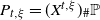
$P_{t,x}=(X^{t,x})_\#\mathbb{P}$
, and
$P_{t,\xi}=(X^{t,\xi})_\#\mathbb{P}$
(the latter two are distributions on the space of continuous paths), where
$Y_\#P\,:\!=\, P(Y^{-1}(\!\cdot\!))$
denotes the pushforward of a probability measure P by a measurable map Y. Given these definitions, we assume that (7)
\begin{equation} {\mathrm{d}} P_{t,\xi} = {\mathrm{d}} P_{t,x}\nu_\xi({\mathrm{d}} x). \end{equation}
-
(iv) We assume that, for every
$t\geq 0$
, the time-homogeneous SDE with drift
$b(t,\cdot)$
and diffusion
$\sigma(t,\cdot)$
has an invariant distribution
$\mu_t$
that satisfies-
(a)
$\mu_t$
has density
$\rho_t>0$
with respect to Lebesgue measure on
$\mathbb{R}^n$
. -
(b)
$\rho_t$
decays exponentially in x, uniformly for t in compact intervals. -
(c)
$\rho_t$
is
$C^1$
in t with
$\partial_t\log(\rho_t)$
polynomially bounded in x, uniformly for t in compact intervals.
-





Remark 1. The fact that every $C^{1,2}$
solution to (5) which is polynomially bounded in x, uniformly in
$C^{1,2}$
solution to (5) which is polynomially bounded in x, uniformly in $t\in[0,T]$
, can be written in the form (4) is proven, e.g. in [Reference Karatzas and Shreve19, Chapter 5, Theorem 7.6]. The existence of solutions to (5) with the required properties can be proven by PDE techniques under a variety of assumptions; a version that suffices for our purposes can be found in [Reference Krylov and Priola21, Theorem 2.8 and Corollary 4.2] (note that, after multiplying
$t\in[0,T]$
, can be written in the form (4) is proven, e.g. in [Reference Karatzas and Shreve19, Chapter 5, Theorem 7.6]. The existence of solutions to (5) with the required properties can be proven by PDE techniques under a variety of assumptions; a version that suffices for our purposes can be found in [Reference Krylov and Priola21, Theorem 2.8 and Corollary 4.2] (note that, after multiplying $u_T(t,\,x)$
by
$u_T(t,\,x)$
by ${\mathrm{e}}^{c(T-t)}$
for appropriate
${\mathrm{e}}^{c(T-t)}$
for appropriate $c\in\mathbb{R}$
, we can assume that
$c\in\mathbb{R}$
, we can assume that $\sup h<0$
in (5)). Equations (6) and (7) follow from standard assumptions that guarantee the existence and uniqueness of solutions to (3); see, e.g., [Reference Ikeda and Watanabe18, Reference Karatzas and Shreve19]. For instance, if b and
$\sup h<0$
in (5)). Equations (6) and (7) follow from standard assumptions that guarantee the existence and uniqueness of solutions to (3); see, e.g., [Reference Ikeda and Watanabe18, Reference Karatzas and Shreve19]. For instance, if b and $\sigma$
are continuous in (t, x) and are Lipschitz in x uniformly in t,
$\sigma$
are continuous in (t, x) and are Lipschitz in x uniformly in t, $\sigma$
is bounded, and
$\sigma$
is bounded, and $\sigma\sigma^T$
is uniformly elliptic, then properties (i), (ii), and (iii) of Assumption 1 all hold. In the examples studied in Section 4, where the drift is a gradient, property (iv) is straightforward to check by using the explicit formula for the time-t invariant distribution in terms of the potential.
$\sigma\sigma^T$
is uniformly elliptic, then properties (i), (ii), and (iii) of Assumption 1 all hold. In the examples studied in Section 4, where the drift is a gradient, property (iv) is straightforward to check by using the explicit formula for the time-t invariant distribution in terms of the potential.
Given the above assumptions, our analysis starts with the following bound on the MGF of $\overline{h}_T$
, i.e. on the Feynman–Kac semigroup. In this result, and elsewhere, we use the notation
$\overline{h}_T$
, i.e. on the Feynman–Kac semigroup. In this result, and elsewhere, we use the notation $h_t\,:\!=\, h(t,\cdot)$
.
$h_t\,:\!=\, h(t,\cdot)$
.
Lemma 1. Under Assumption 1, let $h\in C^\infty_\mathrm{c}(\mathbb{R}^{1+n})$
(smooth functions with compact support) and define
$h\in C^\infty_\mathrm{c}(\mathbb{R}^{1+n})$
(smooth functions with compact support) and define $u_T(t,\,x) \,:\!=\, \mathbb{E}\big[\!\exp\big(\int_t^T h(s, X_s^{t,x})\,{\mathrm{d}} s\big)\big]$
. We have
$u_T(t,\,x) \,:\!=\, \mathbb{E}\big[\!\exp\big(\int_t^T h(s, X_s^{t,x})\,{\mathrm{d}} s\big)\big]$
. We have
 \begin{equation} \|u_T(t,\cdot)\|_{L^2(\mu_t)}\leq\exp\bigg(\int_t^T \Lambda_s\,{\mathrm{d}} s\bigg) \end{equation}
for $0\leq t\leq T$
, where
$0\leq t\leq T$
, where
 \begin{equation} \Lambda_t \,:\!=\, \sup\bigg\{\int A_t[g]g\,{\mathrm{d}}\mu_t + \int\bigg(h_t-\frac{1}{2}\partial_t\log(\rho_t)\bigg)g^2\,{\mathrm{d}}\mu_t \colon g\in C^2_\mathrm{pb}(\mathbb{R}^n),\,\|g\|_{L^2(\mu_t)}=1\bigg\} \end{equation}
and $C^2_\mathrm{pb}(\mathbb{R}^n)$
denotes the set of
$C^2_\mathrm{pb}(\mathbb{R}^n)$
denotes the set of $C^2$
real-valued functions on
$C^2$
real-valued functions on $\mathbb{R}^n$
whose zeroth, first, and second derivatives are polynomially bounded. In addition,
$\mathbb{R}^n$
whose zeroth, first, and second derivatives are polynomially bounded. In addition, $t\mapsto\Lambda_t$
is lower semicontinuous (LSC) and bounded below on compact time intervals.
$t\mapsto\Lambda_t$
is lower semicontinuous (LSC) and bounded below on compact time intervals.
Proof. First, we write
 \begin{align*} \Lambda_t &\,= \sup\big\{\Phi_t[g] \colon g\in C^2_\mathrm{pb}(\mathbb{R}^n),\, g\text{ is not Lebesgue-almost surely }0\big\},\\ \Phi_t[g] & \,:\!=\, \int A_t[g]g\,{\mathrm{d}}\mu_t/\|g\|_{L^2(\mu_t)}^2 + \int\bigg(h_t-\frac{1}{2}\partial_t\log(\rho_t)\bigg)g^2\,{\mathrm{d}}\mu_t/\|g\|_{L^2(\mu_t)}^2. \end{align*}
Note that the polynomial-boundedness properties of $g\in C^2_\mathrm{pb}(\mathbb{R}^n)$
, b, and
$g\in C^2_\mathrm{pb}(\mathbb{R}^n)$
, b, and $\sigma$
, together with the exponential decay of the density
$\sigma$
, together with the exponential decay of the density $\rho_t$
and polynomial boundedness of
$\rho_t$
and polynomial boundedness of $\partial_t\log\rho_t$
(see Assumption 1) imply that
$\partial_t\log\rho_t$
(see Assumption 1) imply that $\Phi_t[g]$
is continuous in t via the dominated convergence theorem. Therefore
$\Phi_t[g]$
is continuous in t via the dominated convergence theorem. Therefore $\Lambda_t$
is LSC in t. Taking
$\Lambda_t$
is LSC in t. Taking $g=1$
we see that
$g=1$
we see that $\Lambda_t \geq \int h_t\,{\mathrm{d}}\mu_t - \frac{1}{2}\int\partial_t\log(\rho_t)\,{\mathrm{d}}\mu_t$
. Assumption 1(iv) together with the dominated convergence theorem imply the familiar fact that the expectation of the score function vanishes:
$\Lambda_t \geq \int h_t\,{\mathrm{d}}\mu_t - \frac{1}{2}\int\partial_t\log(\rho_t)\,{\mathrm{d}}\mu_t$
. Assumption 1(iv) together with the dominated convergence theorem imply the familiar fact that the expectation of the score function vanishes:
 \begin{equation} \int\partial_t\log(\rho_t)\,{\mathrm{d}}\mu_t = 0. \end{equation}
Therefore, on a compact time interval $t\in[0,T]$
we have
$t\in[0,T]$
we have
 \begin{equation} \Lambda_t \geq \int h_t\,{\mathrm{d}}\mu_t \geq \inf_{[0,T]\times\mathbb{R}^n}h > -\infty. \end{equation}
Together, these properties imply that the integral on the right-hand side of (8) exists in $(\!-\!\infty,\infty]$
.
$(\!-\!\infty,\infty]$
.
Now let $f\in C^\infty_\mathrm{c}(\mathbb{R}^n)$
and define
$f\in C^\infty_\mathrm{c}(\mathbb{R}^n)$
and define $u^f_T(t,\,x) \,:\!=\, \mathbb{E}\big[f(X^{t,x}_T)\exp\big(\int_t^T h(s, X_s^{t,x})\,{\mathrm{d}} s\big)\big]$
. Note that
$u^f_T(t,\,x) \,:\!=\, \mathbb{E}\big[f(X^{t,x}_T)\exp\big(\int_t^T h(s, X_s^{t,x})\,{\mathrm{d}} s\big)\big]$
. Note that $u_T^f$
is bounded. We will prove that
$u_T^f$
is bounded. We will prove that
 \begin{equation} \big\|u^f_T(t,\cdot)\big\|_{L^2(\mu_t)} \leq \|f\|_{L^2(\mu_T)}\exp\bigg(\int_t^T\Lambda_s\,{\mathrm{d}} s\bigg). \end{equation}
The claimed upper bound (8) will then follow by letting $f_j$
be a sequence of smooth bump functions that increase to 1 and then using the monotone convergence theorem to compute the limit as
$f_j$
be a sequence of smooth bump functions that increase to 1 and then using the monotone convergence theorem to compute the limit as $j\to\infty$
.
$j\to\infty$
.
To prove (12), suppose that $t<T$
,
$t<T$
,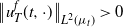 $\big\|u^f_T(t,\cdot)\big\|_{L^2(\mu_t)}>0$
, and
$\big\|u^f_T(t,\cdot)\big\|_{L^2(\mu_t)}>0$
, and $\int_t^T\Lambda_s\,{\mathrm{d}} s$
is finite (the other cases are trivial). By Assumption 1 (i), the Feynman–Kac formula (5) gives
$\int_t^T\Lambda_s\,{\mathrm{d}} s$
is finite (the other cases are trivial). By Assumption 1 (i), the Feynman–Kac formula (5) gives
 \begin{equation*} \partial_t u^f_T(t,\,x) = -A_t\big[u^f_T(t,\cdot)\big](x)-h(t,\,x) u^f_T(t,\,x), \qquad u^f_T(T,x) = f(x), \end{equation*}
where $u^f_T(t,\,x)$
is
$u^f_T(t,\,x)$
is $C^{1,2}$
in (t, x) with first derivative in t and first and second derivatives in x being polynomially bounded in x, uniformly in
$C^{1,2}$
in (t, x) with first derivative in t and first and second derivatives in x being polynomially bounded in x, uniformly in $t\in[0,T]$
; in particular,
$t\in[0,T]$
; in particular,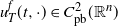 $u^f_T(t,\cdot)\in C^2_\mathrm{pb}(\mathbb{R}^n)$
for all
$u^f_T(t,\cdot)\in C^2_\mathrm{pb}(\mathbb{R}^n)$
for all $t\in[0,T]$
. Combining this with the exponential decay of
$t\in[0,T]$
. Combining this with the exponential decay of $\rho_t$
and the polynomial boundedness of b,
$\rho_t$
and the polynomial boundedness of b, $\sigma$
, and
$\sigma$
, and $\partial_t\log(\rho_t)$
from Assumption 1, we can use the dominated convergence theorem to compute
$\partial_t\log(\rho_t)$
from Assumption 1, we can use the dominated convergence theorem to compute
 \begin{align} \frac{{\mathrm{d}}}{{\mathrm{d}} t}\big\|u^f_T(t,\cdot)\big\|^2_{L^2(\mu_t)} & = \int\partial_t\big(u^f_T(t,\,x)^2 \rho_t(x)\big)\,{\mathrm{d}} x \notag \\ & = -2\bigg(\int A_t\big[u^f_T(t,\cdot)\big](x)u^f_T(t,\,x)\mu_t({\mathrm{d}} x) \notag \\ &\quad\quad + \int\bigg(h(t,\,x) - \frac{1}{2}\partial_t\log(\rho_t(x))\bigg)\big(u^f_T(t,\,x)\big)^2\mu_t({\mathrm{d}} x)\bigg) \notag \\ & \geq -2\Lambda_t\big\|u^f_T(t,\cdot)\big\|^2_{L^2(\mu_t)}. \end{align}
This lower bound on the derivative together with the terminal condition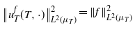 $\big\|u^f_T(T,\cdot)\big\|^2_{L^2(\mu_T)}{}=\|f\|^2_{L^2(\mu_T)}$
implies a bound on
$\big\|u^f_T(T,\cdot)\big\|^2_{L^2(\mu_T)}{}=\|f\|^2_{L^2(\mu_T)}$
implies a bound on $\big\|u^f_T(t,\cdot)\big\|^2_{L^2(\mu_t)}$
for
$\big\|u^f_T(t,\cdot)\big\|^2_{L^2(\mu_t)}$
for $t\in[0,T]$
. More specifically, define
$t\in[0,T]$
. More specifically, define $F(t)\,:\!=\,\big\|u^f_T(T-t,\cdot)\big\|^2_{L^2(\mu_{T-t})}$
. Then
$F(t)\,:\!=\,\big\|u^f_T(T-t,\cdot)\big\|^2_{L^2(\mu_{T-t})}$
. Then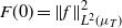 $F(0)=\|f\|^2_{L^2(\mu_T)}$
and (13) implies
$F(0)=\|f\|^2_{L^2(\mu_T)}$
and (13) implies $F^\prime(t)\leq 2\Lambda_{T-t}F(t)$
,
$F^\prime(t)\leq 2\Lambda_{T-t}F(t)$
, $0\leq t\leq T$
. Therefore we can use Grönwall’s inequality to obtain the bound
$0\leq t\leq T$
. Therefore we can use Grönwall’s inequality to obtain the bound $F(t) \leq F(0)\exp\big(2\int_0^t\Lambda_{T-s}\,{\mathrm{d}} s\big)$
. After changing variables and taking the square root, we arrive at the claimed result (12). This completes the proof.
$F(t) \leq F(0)\exp\big(2\int_0^t\Lambda_{T-s}\,{\mathrm{d}} s\big)$
. After changing variables and taking the square root, we arrive at the claimed result (12). This completes the proof.
Note that the bound in Lemma 1 is quasistatic in nature, as it depends on the SDE only through the generators $A_t$
and invariant distributions
$A_t$
and invariant distributions $\mu_t$
of the time-homogeneous systems obtained by fixing t, as seen in the definition (9) of
$\mu_t$
of the time-homogeneous systems obtained by fixing t, as seen in the definition (9) of $\Lambda_t$
. For each t, bounding
$\Lambda_t$
. For each t, bounding $\Lambda_t$
is equivalent to a functional inequality for the Feynman–Kac semigroup with potential
$\Lambda_t$
is equivalent to a functional inequality for the Feynman–Kac semigroup with potential $U_t=h_t-\frac{1}{2}\partial_t\!\log(\rho_t)$
[Reference Cattiaux and Guillin9, Reference Gao, Guillin and Wu14, Reference Wu25]. In particular, here we focus on
$U_t=h_t-\frac{1}{2}\partial_t\!\log(\rho_t)$
[Reference Cattiaux and Guillin9, Reference Gao, Guillin and Wu14, Reference Wu25]. In particular, here we focus on $\log$
-Sobolev inequalities [Reference Bakry1–Reference Bakry, Gentil and Ledoux3, Reference Carlen and Loss8, Reference Gross17, Reference Rothaus23] due to their ability to produce non-vacuous concentration inequalities for unbounded potentials. This is crucial for our purposes as
$\log$
-Sobolev inequalities [Reference Bakry1–Reference Bakry, Gentil and Ledoux3, Reference Carlen and Loss8, Reference Gross17, Reference Rothaus23] due to their ability to produce non-vacuous concentration inequalities for unbounded potentials. This is crucial for our purposes as $\partial_t\log(\rho_t)$
is very often unbounded; see the examples in Section 4.
$\partial_t\log(\rho_t)$
is very often unbounded; see the examples in Section 4.
Definition 1. The generator $A_t$
will be said to satisfy a
$A_t$
will be said to satisfy a $\log$
-Sobolev inequality with parameter
$\log$
-Sobolev inequality with parameter $C_t>0$
if
$C_t>0$
if
 \begin{equation} \int g^2\log(g^2)\,d\mu_t \leq -C_t\int A_t[g]g\,{\mathrm{d}}\mu_t \text{ for all } g\in C^2_\mathrm{pb}(\mathbb{R}^n) \text{ with } \|g\|_{L^2(\mu_t)}=1, \end{equation}
where we again let $C^2_\mathrm{pb}(\mathbb{R}^n)$
denote the set of
$C^2_\mathrm{pb}(\mathbb{R}^n)$
denote the set of $C^2$
real-valued functions on
$C^2$
real-valued functions on $\mathbb{R}^n$
whose zeroth, first, and second derivatives are polynomially bounded. As a shorthand, we will say that
$\mathbb{R}^n$
whose zeroth, first, and second derivatives are polynomially bounded. As a shorthand, we will say that $A_t$
is
$A_t$
is $C_t$
-
$C_t$
- $\log$
-Sobolev.
$\log$
-Sobolev.
Remark 2. For instance, if the drift is a gradient, $b(t,\,x)=-\nabla_xV(t,\,x)$
, and the noise is additive then a lower bound on the Hessian,
$b(t,\,x)=-\nabla_xV(t,\,x)$
, and the noise is additive then a lower bound on the Hessian, $D_x^2V_t(x)\geq 2C_t^{-1}I$
for some
$D_x^2V_t(x)\geq 2C_t^{-1}I$
for some $C_t>0$
, implies a
$C_t>0$
, implies a $\log$
-Sobolev inequality for
$\log$
-Sobolev inequality for $A_t$
with constant
$A_t$
with constant $C_t$
[Reference Bakry and Emery2]. Furthermore, we also obtain a
$C_t$
[Reference Bakry and Emery2]. Furthermore, we also obtain a $\log$
-Sobolev inequality when a bounded perturbation is added to such a potential; see, e.g., [Reference Bakry, Gentil and Ledoux3, Proposition 5.1.6].
$\log$
-Sobolev inequality when a bounded perturbation is added to such a potential; see, e.g., [Reference Bakry, Gentil and Ledoux3, Proposition 5.1.6].
Under Assumption 1, the integrals in (14) exist due to the polynomial boundedness and decay properties of b, $\sigma$
, and
$\sigma$
, and $\rho_t$
. The value of
$\rho_t$
. The value of $C_t$
can be viewed as bounding the speed of convergence to the invariant measure
$C_t$
can be viewed as bounding the speed of convergence to the invariant measure $\mu_t$
of the corresponding time-homogeneous system, with smaller
$\mu_t$
of the corresponding time-homogeneous system, with smaller $C_t$
implying faster convergence. Note that some authors define
$C_t$
implying faster convergence. Note that some authors define $\log$
-Sobolev inequalities in terms of the reciprocal of our parameter
$\log$
-Sobolev inequalities in terms of the reciprocal of our parameter $C_t$
and/or with an explicit factor of 2. In this work we follow the definition from, e.g., [Reference Wu25].
$C_t$
and/or with an explicit factor of 2. In this work we follow the definition from, e.g., [Reference Wu25].
We will use $\log$
-Sobolev inequalities to further refine the MGF bound from Lemma 1, thereby obtaining a form that is more computationally tractable. We work under the following additional assumptions on the observable and the generator. In particular, by truncating and taking limits we will be able to eliminate the smoothness and compact support assumptions on h that were made in Lemma 1 and extend the result to an appropriate class of unbounded observables h.
$\log$
-Sobolev inequalities to further refine the MGF bound from Lemma 1, thereby obtaining a form that is more computationally tractable. We work under the following additional assumptions on the observable and the generator. In particular, by truncating and taking limits we will be able to eliminate the smoothness and compact support assumptions on h that were made in Lemma 1 and extend the result to an appropriate class of unbounded observables h.
Assumption 2. Let $T\in(0,\infty)$
and, in addition to Assumption 1, assume the following:
$T\in(0,\infty)$
and, in addition to Assumption 1, assume the following:
-
(i) Let
$h\colon[0,\infty)\times\mathbb{R}^n\to\mathbb{R}$
be continuous and polynomially bounded in
$x\in\mathbb{R}^n$
uniformly in
$t\in[0,T]$
. -
(ii) For all
$t\in[0,T]$
, suppose the generator
$A_t$
satisfies the
$\log$
-Sobolev inequality (14) with parameter
$C_t$
, and
$t\mapsto C_t$
is measurable. -
(iii) Suppose that
$\exp\big\{{-}\frac12{C_t}\partial_t\log(\rho_t)\big\}\in L^1(\mu_t)$
for all
$t\in[0,T]$
, and
\begin{equation*} C_t^{-1}\log\bigg(\int\exp\bigg\{{-}\frac{C_t}{2}\partial_t\log(\rho_t)\bigg\}\,{\mathrm{d}}\mu_t\bigg) \in L^1([0,T],{\mathrm{d}} t). \end{equation*}
-
(iv) Assume the distribution of the initial condition,
$\xi$
, satisfies
$\nu_\xi\ll \mu_0$
with
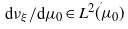
${{\mathrm{d}}\nu_\xi}/{{\mathrm{d}}\mu_0}{}\in L^2(\mu_0)$
.






Theorem 1. Under Assumption 2 we have the following bound on the MGF:
 \begin{multline} \mathbb{E}\bigg[\exp\bigg(\int_0^{T} h(t,X^{0,\xi}_t)\,{\mathrm{d}} t\bigg)\bigg] \\ \leq \bigg\|\frac{{\mathrm{d}}\nu_\xi}{{\mathrm{d}}\mu_0}\bigg\|_{L^2(\mu_0)} \exp\bigg(\int_0^TC_t^{-1}\log\bigg(\int\exp\bigg\{C_t\bigg(h_t-\frac{1}{2}\partial_t\log(\rho_t)\bigg)\bigg\}\, {\mathrm{d}}\mu_t\bigg)dt\bigg). \end{multline}
Proof. The polynomial bounds on h from Assumption 2(i) together with the assumptions on $\rho_t$
from Assumption 1(iv) imply that
$\rho_t$
from Assumption 1(iv) imply that $h_t,\partial_t\log(\rho_t)\in L^1(\mu_t)$
for all t and
$h_t,\partial_t\log(\rho_t)\in L^1(\mu_t)$
for all t and $\sup_{t\in[0,T]}\big|\int h_t\,{\mathrm{d}}\mu_t\big|<\infty$
. Non-negativity of centered cumulant-generating functions implies that
$\sup_{t\in[0,T]}\big|\int h_t\,{\mathrm{d}}\mu_t\big|<\infty$
. Non-negativity of centered cumulant-generating functions implies that $C_t^{-1}\log\big(\int\exp\big\{C_t(h_t-\frac{1}{2}\partial_t\log(\rho_t))\big\}\,{\mathrm{d}}\mu_t\big)$
is bounded below by
$C_t^{-1}\log\big(\int\exp\big\{C_t(h_t-\frac{1}{2}\partial_t\log(\rho_t))\big\}\,{\mathrm{d}}\mu_t\big)$
is bounded below by $\int h_t\,{\mathrm{d}}\mu_t$
and therefore the right-hand side of (15) is well defined and valued in
$\int h_t\,{\mathrm{d}}\mu_t$
and therefore the right-hand side of (15) is well defined and valued in $(0,\infty]$
; the claim is trivial if the right-hand side is infinite, therefore in the remainder of the proof we can, without loss of generality, assume that
$(0,\infty]$
; the claim is trivial if the right-hand side is infinite, therefore in the remainder of the proof we can, without loss of generality, assume that
 \begin{equation} C_t^{-1}\log\bigg(\int\exp\bigg\{C_t\bigg(h_t-\frac{1}{2}\partial_t\log(\rho_t)\bigg)\bigg\}\, {\mathrm{d}}\mu_t\bigg) \in L^1([0,T],{\mathrm{d}} t). \end{equation}
To prove (15), first suppose that $h\in C^\infty_\mathrm{c}(\mathbb{R}^{1+n})$
. Using Assumption 1(iii), Assumption 2(iv), and Lemma 1 we can compute
$h\in C^\infty_\mathrm{c}(\mathbb{R}^{1+n})$
. Using Assumption 1(iii), Assumption 2(iv), and Lemma 1 we can compute
 \begin{align} \mathbb{E}\bigg[\exp\bigg(\int_0^{T}h(t,X^{0,\xi}_t)\,{\mathrm{d}} t\bigg)\bigg] & = \int\mathbb{E}\bigg[\exp\bigg(\int_0^{T}h(t,X^{0,x}_t)\,{\mathrm{d}} t\bigg)\bigg]\,\nu_\xi({\mathrm{d}} x) \notag \\ & \leq \bigg\|\frac{{\mathrm{d}}\nu_\xi}{{\mathrm{d}}\mu_0}\bigg\|_{L^2(\mu_0)}\|u_T(0,\cdot)\|_{L^2(\mu_0)} \notag \\ & \leq \bigg\|\frac{{\mathrm{d}}\nu_\xi}{{\mathrm{d}}\mu_0}\bigg\|_{L^2(\mu_0)}\exp\bigg(\int_0^T\Lambda_t\,{\mathrm{d}} t\bigg), \end{align}
where $\Lambda_t$
was defined in (9). Using the
$\Lambda_t$
was defined in (9). Using the $\log$
-Sobolev inequality from Assumption 2(ii), we can bound
$\log$
-Sobolev inequality from Assumption 2(ii), we can bound
 \begin{align} \Lambda_t & \leq \sup\bigg\{{-}C_t^{-1}\int g^2\log(g^2)\,{\mathrm{d}}\mu_t + \int\bigg(h_t-\frac{1}{2}\partial_t\log(\rho_t)\bigg)g^2\,{\mathrm{d}}\mu_t \notag \\ & \qquad\qquad \colon g \in C^2_\mathrm{pb}(\mathbb{R}^n),\,\|g\|_{L^2(\mu_t)}=1\bigg\} \notag \\ & = C_t^{-1}\sup\bigg\{\int C_t\bigg(h_t-\frac{1}{2}\partial_t\log(\rho_t)\bigg)g^2\,{\mathrm{d}}\mu_t - \text{KL}(g^2{\mathrm{d}}\mu_t\|\mu_t) \notag \\ & \qquad\qquad\qquad \colon g \in C^2_\mathrm{pb}(\mathbb{R}^n),\,\|g\|_{L^2(\mu_t)}=1\bigg\}, \end{align}
where KL denotes the KL-divergence, i.e. relative entropy; note that $g\in C^2_\mathrm{pb}(\mathbb{R}^n)$
with
$g\in C^2_\mathrm{pb}(\mathbb{R}^n)$
with $\|g\|_{L^2(\mu_t)}=1$
implies
$\|g\|_{L^2(\mu_t)}=1$
implies $\text{KL}(g^2\,{\mathrm{d}}\mu_t\|\mu_t)<\infty$
, due to Assumption 1(iv). Next, we use the Gibbs variational principle (i.e. the convex conjugate of the KL divergence; see [Reference Dupuis11, Proposition 4.5.1]), which implies that if k is a real-valued measurable function that is bounded below and Q a probability measure (both on
$\text{KL}(g^2\,{\mathrm{d}}\mu_t\|\mu_t)<\infty$
, due to Assumption 1(iv). Next, we use the Gibbs variational principle (i.e. the convex conjugate of the KL divergence; see [Reference Dupuis11, Proposition 4.5.1]), which implies that if k is a real-valued measurable function that is bounded below and Q a probability measure (both on $\mathbb{R}^n$
) then
$\mathbb{R}^n$
) then
 \begin{equation*} \sup_{\nu:\text{KL}(\nu\|Q)<\infty}\bigg\{\int k\,{\mathrm{d}}\nu - \text{KL}(\nu\|Q)\bigg\} = \log\bigg(\int{\mathrm{e}}^{k}\,{\mathrm{d}} Q\bigg). \end{equation*}
Applying this to $k_m\,:\!=\,\max\big\{C_t\big(h_t-\frac{1}{2}\partial_t\log(\rho_t)\big),-m\big\}$
,
$k_m\,:\!=\,\max\big\{C_t\big(h_t-\frac{1}{2}\partial_t\log(\rho_t)\big),-m\big\}$
, $m\in\mathbb{Z}^+$
, and
$m\in\mathbb{Z}^+$
, and $Q=\mu_t$
we find
$Q=\mu_t$
we find
 \begin{align*} \int C_t\bigg(h_t-\frac{1}{2}\partial_t\log(\rho_t)\bigg)g^2\,{\mathrm{d}}\mu_t - \text{KL}(g^2\,{\mathrm{d}}\mu_t\|\mu_t) & \leq \int k_mg^2\,{\mathrm{d}}\mu_t - \text{KL}(g^2\,{\mathrm{d}}\mu_t\|\mu_t) \\ & \leq \log\bigg(\int{\mathrm{e}}^{k_m}\,{\mathrm{d}}\mu_t\bigg) \end{align*}
for all $m\in\mathbb{Z}^+$
and all
$m\in\mathbb{Z}^+$
and all $g\in C^2_\mathrm{pb}(\mathbb{R}^n)$
that satisfy
$g\in C^2_\mathrm{pb}(\mathbb{R}^n)$
that satisfy $\|g\|_{L^2(\mu_t)}=1$
. Therefore, we can compute
$\|g\|_{L^2(\mu_t)}=1$
. Therefore, we can compute
 \begin{multline} \int C_t\bigg(h_t-\frac{1}{2}\partial_t\log(\rho_t)\bigg)g^2\,{\mathrm{d}}\mu_t - \text{KL}(g^2\,{\mathrm{d}}\mu_t\|\mu_t) \\ \leq \liminf_{m\to\infty}\log\bigg(\int{\mathrm{e}}^{k_m}\,{\mathrm{d}}\mu_t\bigg) \leq \log\bigg(\int\exp\bigg(C_t\bigg(h_t-\frac{1}{2}\partial_t\log(\rho_t)\bigg)\bigg)\,{\mathrm{d}}\mu_t\bigg). \end{multline}
To obtain the second inequality in (19), note that it is trivial if $\exp\big(C_t\big(h_t-\frac{1}{2}\partial_t\log(\rho_t)\big)\big){}\not\in L^1(\mu_t)$
and otherwise it follows by combining the pointwise limit
$\exp\big(C_t\big(h_t-\frac{1}{2}\partial_t\log(\rho_t)\big)\big){}\not\in L^1(\mu_t)$
and otherwise it follows by combining the pointwise limit $\lim_{m\to\infty}k_m=C_t\big(h_t-\frac{1}{2}\partial_t\log(\rho_t)\big)$
, the bound
$\lim_{m\to\infty}k_m=C_t\big(h_t-\frac{1}{2}\partial_t\log(\rho_t)\big)$
, the bound ${\mathrm{e}}^{k_m} \leq 1+\exp\big(C_t\big(h_t-\frac{1}{2}\partial_t\log(\rho_t)\big)\big)$
, and the dominated convergence theorem.
${\mathrm{e}}^{k_m} \leq 1+\exp\big(C_t\big(h_t-\frac{1}{2}\partial_t\log(\rho_t)\big)\big)$
, and the dominated convergence theorem.
The bounds (19) and (18) together imply that
 \begin{equation*} \Lambda_t \leq C_t^{-1}\log\bigg(\int\exp\bigg(C_t\bigg(h_t-\frac{1}{2}\partial_t\!\log(\rho_t)\bigg)\bigg)\, {\mathrm{d}}\mu_t\bigg). \end{equation*}
Further combining this with (17), we obtain
 \begin{multline} \mathbb{E}\bigg[\exp\bigg(\int_0^Th\big(t,X^{0,\xi}_t\big)\,{\mathrm{d}} t\bigg)\bigg] \\ \leq \bigg\|\frac{{\mathrm{d}}\nu_\xi}{{\mathrm{d}}\mu_0}\bigg\|_{L^2(\mu_0)} \exp\bigg(\int_0^TC_t^{-1}\log\bigg(\int\exp\bigg\{C_t\bigg(h_t-\frac{1}{2}\partial_t\log(\rho_t)\bigg)\bigg\}\, {\mathrm{d}}\mu_t\bigg)\,{\mathrm{d}} t\bigg). \end{multline}
This proves the claim for $h\in C^\infty_\mathrm{c}(\mathbb{R}^{1+n})$
.
$h\in C^\infty_\mathrm{c}(\mathbb{R}^{1+n})$
.
Now suppose $h\in C_\mathrm{b}(\mathbb{R}^{1+n})$
(bounded and continuous functions). Combining the density of
$h\in C_\mathrm{b}(\mathbb{R}^{1+n})$
(bounded and continuous functions). Combining the density of $C_\mathrm{c}^\infty(\mathbb{R}^{1+n})$
in
$C_\mathrm{c}^\infty(\mathbb{R}^{1+n})$
in $C_\mathrm{c}(\mathbb{R}^{1+n})$
(in the uniform norm) with the use of a sequence of continuous bump functions, we can construct a sequence
$C_\mathrm{c}(\mathbb{R}^{1+n})$
(in the uniform norm) with the use of a sequence of continuous bump functions, we can construct a sequence $h_j\in C^\infty_\mathrm{c}(\mathbb{R}^{1+n})$
that converges pointwise to h and that satisfies
$h_j\in C^\infty_\mathrm{c}(\mathbb{R}^{1+n})$
that converges pointwise to h and that satisfies $\sup_j\|h_j\|_\infty<\infty$
. Therefore we can use the dominated convergence theorem, as justified by Assumption 2 (iii) and the uniform boundedness of the
$\sup_j\|h_j\|_\infty<\infty$
. Therefore we can use the dominated convergence theorem, as justified by Assumption 2 (iii) and the uniform boundedness of the $h_j$
, to compute
$h_j$
, to compute
 \begin{align*} & \mathbb{E}\bigg[\exp\bigg(\int_0^Th\big(t,X^{0,\xi}_t\big)\,{\mathrm{d}} t\bigg)\bigg] \\ & \qquad = \lim_{j\to\infty}\mathbb{E}\bigg[\exp\bigg(\int_0^Th_j\big(t,X^{0,\xi}_t\big)\,{\mathrm{d}} t\bigg)\bigg] \\ & \qquad \leq \lim_{j\to\infty} \bigg\|\frac{{\mathrm{d}}\nu_\xi}{{\mathrm{d}}\mu_0}\bigg\|_{L^2(\mu_0)} \exp\bigg(\int_0^TC_t^{-1}\log\bigg(\int\exp\bigg\{C_t\bigg((h_{j})_t - \frac{1}{2}\partial_t\log(\rho_t)\bigg)\bigg\}\,{\mathrm{d}}\mu_t\bigg)\,{\mathrm{d}} t\bigg) \\ & \qquad = \bigg\|\frac{{\mathrm{d}}\nu_\xi}{{\mathrm{d}}\mu_0}\bigg\|_{L^2(\mu_0)} \exp\bigg(\int_0^TC_t^{-1}\log\bigg(\int\exp\bigg\{C_t\bigg(h_{t} - \frac{1}{2}\partial_t\log(\rho_t)\bigg)\bigg\}\,{\mathrm{d}}\mu_t\bigg)\,{\mathrm{d}} t\bigg). \end{align*}
This proves the claim for $h\in C_\mathrm{b}(\mathbb{R}^{1+n})$
.
$h\in C_\mathrm{b}(\mathbb{R}^{1+n})$
.
Finally, let h be as in Assumption 2(i), i.e. $h\,:\,[0,\infty)\times\mathbb{R}^n\to\mathbb{R}$
is continuous and polynomially bounded in
$h\,:\,[0,\infty)\times\mathbb{R}^n\to\mathbb{R}$
is continuous and polynomially bounded in $x\in\mathbb{R}^n$
uniformly in
$x\in\mathbb{R}^n$
uniformly in $t\in[0,T]$
. Clearly, we can extend it to be continuous on
$t\in[0,T]$
. Clearly, we can extend it to be continuous on $\mathbb{R}^{1+n}$
. For
$\mathbb{R}^{1+n}$
. For $\ell,m\in\mathbb{Z}^+$
, define
$\ell,m\in\mathbb{Z}^+$
, define $h_{\ell,m} \,:\!=\,- \ell \mathbf{1}_{h<-\ell}+h\mathbf{1}_{-\ell\leq h\leq m}+m\mathbf{1}_{h>m}$
. Then
$h_{\ell,m} \,:\!=\,- \ell \mathbf{1}_{h<-\ell}+h\mathbf{1}_{-\ell\leq h\leq m}+m\mathbf{1}_{h>m}$
. Then $h_{\ell,m}\in C_\mathrm{b}(\mathbb{R}^{1+n})$
and we have the pointwise limits
$h_{\ell,m}\in C_\mathrm{b}(\mathbb{R}^{1+n})$
and we have the pointwise limits $\lim_{\ell\to\infty}h_{\ell,m}=h_{\infty,m}\,:\!=\, h\mathbf{1}_{h\leq m}+m\mathbf{1}_{h>m}$
and
$\lim_{\ell\to\infty}h_{\ell,m}=h_{\infty,m}\,:\!=\, h\mathbf{1}_{h\leq m}+m\mathbf{1}_{h>m}$
and $\lim_{m\to\infty}h_{\infty,m}=h$
, where
$\lim_{m\to\infty}h_{\infty,m}=h$
, where $h_{\infty,m}\leq h_{\infty,m+1}$
for all m. We also have the bounds
$h_{\infty,m}\leq h_{\infty,m+1}$
for all m. We also have the bounds $|h_{\ell,m}|\leq |h|$
and
$|h_{\ell,m}|\leq |h|$
and $|h_{\infty,m}|\leq |h|$
. Together with the continuity of
$|h_{\infty,m}|\leq |h|$
. Together with the continuity of $X_t^{0,\xi}$
in t and the dominated convergence theorem, these imply the pointwise limits
$X_t^{0,\xi}$
in t and the dominated convergence theorem, these imply the pointwise limits
 \begin{align*} \lim_{m\to\infty}\int_0^T h_{\infty,m}\big(t,X_t^{0,\xi}\big)\,{\mathrm{d}} t & = \int_0^T h\big(t,X_t^{0,\xi}\big)\,{\mathrm{d}} t, \\ \lim_{\ell\to\infty}\int_0^Th_{\ell,m}\big(t,X^{0,\xi}_t\big)\,{\mathrm{d}} t & = \int_0^Th_{\infty,m}\big(t,X^{0,\xi}_t\big)\,{\mathrm{d}} t. \end{align*}
Next, we can use the monotone convergence theorem and then the dominated convergence theorem to obtain
 \begin{align*} \mathbb{E}\bigg[\exp\bigg(\int_0^Th\big(t,X^{0,\xi}_t\big)\,{\mathrm{d}} t\bigg)\bigg] & = \lim_{m\to\infty}\mathbb{E}\bigg[\exp\bigg(\int_0^Th_{\infty,m}\big(t,X^{0,\xi}_t\big)\,{\mathrm{d}} t\bigg)\bigg] \\ & = \lim_{m\to\infty}\lim_{\ell\to\infty}\mathbb{E}\bigg[\exp\bigg( \int_0^Th_{\ell,m}\big(t,X^{0,\xi}_t\big)\,{\mathrm{d}} t\bigg)\bigg]\,. \end{align*}
We have already proved the result (15) for observables in $C_\mathrm{b}(\mathbb{R}^{1+n})$
, so by applying it to
$C_\mathrm{b}(\mathbb{R}^{1+n})$
, so by applying it to $h_{\ell,m}$
and then using the dominated convergence theorem, which is justified by Assumption 2(iii) along with (16), we can compute
$h_{\ell,m}$
and then using the dominated convergence theorem, which is justified by Assumption 2(iii) along with (16), we can compute
 \begin{align*} \mathbb{E}&\bigg[\exp\bigg(\int_0^Th\big(t,X^{0,\xi}_t\big)\,{\mathrm{d}} t\bigg)\bigg] \\ \leq &\bigg\|\frac{{\mathrm{d}}\nu_\xi}{{\mathrm{d}}\mu_0}\bigg\|_{L^2(\mu_0)} \liminf_{m\to\infty}\lim_{\ell\to\infty}\exp\bigg(\!\int_0^TC_t^{-1}\log\bigg(\!\int\!\exp\bigg\{C_t\bigg((h_{\ell,m})_{t}-\frac{1}{2}\partial_t\log(\rho_t)\bigg)\bigg\}\,{\mathrm{d}}\mu_t\bigg)\, {\mathrm{d}} t\bigg) \\ = &\bigg\|\frac{{\mathrm{d}}\nu_\xi}{{\mathrm{d}}\mu_0}\bigg\|_{L^2(\mu_0)} \liminf_{m\to\infty}\exp\bigg(\!\int_0^TC_t^{-1}\log\bigg(\!\int\!\exp\bigg\{ C_t\bigg((h_{\infty,m})_{t}-\frac{1}{2}\partial_t\log(\rho_t)\bigg)\bigg\}\,{\mathrm{d}}\mu_t\bigg)\,{\mathrm{d}} t\bigg) \\ \leq &\bigg\|\frac{{\mathrm{d}}\nu_\xi}{{\mathrm{d}}\mu_0}\bigg\|_{L^2(\mu_0)}\exp\bigg(\!\int_0^TC_t^{-1}\log\bigg(\!\int\!\exp\bigg\{C_t\bigg(h_{t}-\frac{1}{2}\partial_t\log(\rho_t)\bigg)\bigg\}\, {\mathrm{d}}\mu_t\bigg)\,{\mathrm{d}} t\bigg), \end{align*}
where in the last line we simply bounded $h_{\infty,m}$
above by h. This completes the proof.
$h_{\infty,m}$
above by h. This completes the proof.
3. Quasistatic approximation to time averages
In this section we use Theorem 1 to obtain a concentration inequality for time-averaged observables. Specifically, we will show concentration on an interval whose width decreases to zero in the quasistatic limit. To help in understanding the behavior of the bound, we write it in terms of the cumulant-generating function (CGF) under an appropriate tilting $\widetilde\mu_t$
of
$\widetilde\mu_t$
of $\mu_t$
, which also naturally leads to quasistatic approximations,
$\mu_t$
, which also naturally leads to quasistatic approximations, $\overline{h}^\mathrm{Q}_{T}$
, to the time averages (1).
$\overline{h}^\mathrm{Q}_{T}$
, to the time averages (1).
Definition 2. Define
 \begin{equation} \widetilde{Z}_t \,:\!=\, \int\exp\bigg\{{-}\frac{C_t}{2}\partial_t\log(\rho_t)\bigg\}d\mu_t, \qquad {\mathrm{d}}\widetilde\mu_t \,:\!=\, \exp\bigg\{-\frac{C_t}{2}\partial_t\log(\rho_t)\bigg\}\,{\mathrm{d}}\mu_t/\widetilde{Z}_t, \end{equation}
and
 \begin{equation} \overline{h}^\mathrm{Q}_{T} \,:\!=\, \frac{1}{T}\int_0^T\int h_t\,{\mathrm{d}}\widetilde\mu_t{\mathrm{d}} t. \end{equation}
Note that Assumption 2(iii) implies that $\widetilde{Z}_t$
is finite and
$\widetilde{Z}_t$
is finite and $\widetilde\mu_t$
is a probability measure for all
$\widetilde\mu_t$
is a probability measure for all $t\in[0,T]$
. Also note that Jensen’s inequality together with (10) implies
$t\in[0,T]$
. Also note that Jensen’s inequality together with (10) implies $\log(\widetilde{Z}_t)\geq 0$
.
$\log(\widetilde{Z}_t)\geq 0$
.
Remark 3. To obtain effective bounds on $\widetilde{Z}_t$
in the quasistatic regime, it is crucial that we leverage (10), i.e. the fact that the expected value of the score (with respect to
$\widetilde{Z}_t$
in the quasistatic regime, it is crucial that we leverage (10), i.e. the fact that the expected value of the score (with respect to $\mu_t$
) equals zero. With this in mind, it can be useful to rewrite (21) via Taylor’s formula with integral remainder,
$\mu_t$
) equals zero. With this in mind, it can be useful to rewrite (21) via Taylor’s formula with integral remainder,
 \begin{equation} \widetilde{Z}_t = 1 + \frac{C_t^2}{4}\int_0^1(1-r) \int\exp\bigg\{{-}r\frac{C_t}{2}\partial_t\log(\rho_t)\bigg\}(\partial_t\log(\rho_t))^2\,{\mathrm{d}}\mu_t\,{\mathrm{d}} r, \end{equation}
where we used (10) to conclude that the degree-1 term vanishes. See also the calculations in (31), (33), and (42).
We are now ready to use the MGF bound from Theorem 1 to obtain a concentration inequality via the standard Chernoff bound method. Initially we let the center of the interval be arbitrary, but in Section 3.1.2 we compute the optimal value by minimizing the upper bound on a two-sided concentration inequality; the optimizer will then be our quasistatic approximation to the time-averaged observable.
Lemma 2. Under Assumption 2, for all $v\in L^1([0,T],{\mathrm{d}} t)$
and all
$v\in L^1([0,T],{\mathrm{d}} t)$
and all $\delta>0$
we have
$\delta>0$
we have
 \begin{align} & \mathbb{P}\bigg(\frac{1}{T}\int_0^T h\big(t,X_t^{0,\xi}\big)\,{\mathrm{d}} t - \frac{1}{T}\int_0^Tv_t\,{\mathrm{d}} t\geq\delta\bigg) \notag \\ & \leq \bigg\|\frac{{\mathrm{d}}\nu_\xi}{{\mathrm{d}}\mu_0}\bigg\|_{L^2(\mu_0)} \exp\bigg(\int_0^T C_t^{-1}\log(\widetilde{Z}_t)\,{\mathrm{d}} t \notag \\ & \qquad\qquad\qquad\qquad + T\inf_{\lambda>0}\bigg\{{-}\lambda\delta + \frac{1}{T}\int_0^T C_t^{-1}\log\bigg(\int{\mathrm{e}}^{\lambda C_t(h_t-v_t)}\,{\mathrm{d}}\widetilde\mu_t\bigg)\,{\mathrm{d}} t\bigg\}\bigg), \end{align}
where $\widetilde{Z}_t$
and
$\widetilde{Z}_t$
and $\widetilde\mu_t$
are defined in (21).
$\widetilde\mu_t$
are defined in (21).
Proof. Letting $v\,:\!=\, ({1}/{T})\int_0^T v_t\,{\mathrm{d}} t$
, a standard Chernoff bound computation (see, e.g., [Reference Boucheron, Lugosi and Massart7]) implies that
$v\,:\!=\, ({1}/{T})\int_0^T v_t\,{\mathrm{d}} t$
, a standard Chernoff bound computation (see, e.g., [Reference Boucheron, Lugosi and Massart7]) implies that
 \begin{equation*} \mathbb{P}\bigg(\frac{1}{T}\int_0^Th\big(t,X_t^{0,\xi}\big)\,{\mathrm{d}} t - v \geq \delta\bigg) \leq \inf_{\lambda>0}{\mathrm{e}}^{-\lambda T(\delta+v)}\mathbb{E}\bigg[\exp\bigg(\lambda\int_0^T h\big(t,X_t^{0,\xi}\big)\,{\mathrm{d}} t\bigg)\bigg]. \end{equation*}
The observables $\lambda h$
satisfy the assumptions required by Theorem 1, therefore we can use the MGF bound (15) to obtain
$\lambda h$
satisfy the assumptions required by Theorem 1, therefore we can use the MGF bound (15) to obtain
 \begin{align} & \mathbb{P}\bigg(\frac{1}{T}\int_0^T h\big(t,X_t^{0,\xi}\big)\,{\mathrm{d}} t - v \geq \delta\bigg) \notag \\ & \leq \bigg\|\frac{{\mathrm{d}}\nu_\xi}{{\mathrm{d}}\mu_0}\bigg\|_{L^2(\mu_0)}\inf_{\lambda>0}\bigg\{{\mathrm{e}}^{-\lambda T(\delta+v)} \notag \\ & \qquad\qquad\qquad\qquad \times \exp\bigg(\int_0^TC_t^{-1}\log\bigg(\int\exp\bigg\{C_t\bigg(\lambda h_t - \frac{1}{2}\partial_t\log(\rho_t)\bigg)\bigg\}\,{\mathrm{d}}\mu_t\bigg)\,{\mathrm{d}} t\bigg)\bigg\}. \end{align}
Recalling that Assumption 2(iii) implies that $\widetilde{Z}_t$
is finite and
$\widetilde{Z}_t$
is finite and $\widetilde\mu_t$
is a probability measure for all
$\widetilde\mu_t$
is a probability measure for all $t\in[0,T]$
, we can rewrite the right-hand side of (25) in terms of
$t\in[0,T]$
, we can rewrite the right-hand side of (25) in terms of $\widetilde{\mu}_t$
to arrive at the claimed result.
$\widetilde{\mu}_t$
to arrive at the claimed result.
Note that the right-hand side of (24) involves the CGF of $C_t h_t$
under the tilted measures
$C_t h_t$
under the tilted measures $\widetilde\mu_t$
, which can be further bounded under various assumptions on the tail behavior. Specifically, in the next two subsections we consider the cases of sub-Gaussian and Bernstein bounds. Writing the bound in terms of
$\widetilde\mu_t$
, which can be further bounded under various assumptions on the tail behavior. Specifically, in the next two subsections we consider the cases of sub-Gaussian and Bernstein bounds. Writing the bound in terms of $\widetilde{\mu}_t$
also suggests that the center for the concentration inequality should be the time-averaged expectation of
$\widetilde{\mu}_t$
also suggests that the center for the concentration inequality should be the time-averaged expectation of $h_t$
under
$h_t$
under $\widetilde\mu_t$
(in order to center the CGF), which is precisely
$\widetilde\mu_t$
(in order to center the CGF), which is precisely $\overline{h}^\mathrm{Q}_{T}$
as defined in (22). As part of the sub-Gaussian calculation in Section 3.1 we show that this is indeed the optimal center in an appropriate sense.
$\overline{h}^\mathrm{Q}_{T}$
as defined in (22). As part of the sub-Gaussian calculation in Section 3.1 we show that this is indeed the optimal center in an appropriate sense.
Alternatively, at the cost of looser bounds, we can obtain a result expressed in terms of the CGF under $\mu_t$
, thus allowing us to use tail-bounds, e.g. sub-Gaussian or Bernstein, with respect to
$\mu_t$
, thus allowing us to use tail-bounds, e.g. sub-Gaussian or Bernstein, with respect to $\mu_t$
instead of
$\mu_t$
instead of $\widetilde{\mu}_t$
. In some cases this can simplify the calculations, though we emphasize that the resulting bounds are looser.
$\widetilde{\mu}_t$
. In some cases this can simplify the calculations, though we emphasize that the resulting bounds are looser.
Corollary 1. Under Assumption 2, if $(2C_t)^{-1}\log\big(\int{\mathrm{e}}^{-C_t\partial_t\log(\rho_t)}\,{\mathrm{d}}\mu_t\big) \in L^1([0,T],{\mathrm{d}} t)$
then, for all
$(2C_t)^{-1}\log\big(\int{\mathrm{e}}^{-C_t\partial_t\log(\rho_t)}\,{\mathrm{d}}\mu_t\big) \in L^1([0,T],{\mathrm{d}} t)$
then, for all $v\in L^1([0,T],{\mathrm{d}} t)$
and all
$v\in L^1([0,T],{\mathrm{d}} t)$
and all $\delta>0$
, we have
$\delta>0$
, we have
 \begin{align} & \mathbb{P}\bigg(\frac{1}{T}\int_0^T h\big(t,X_t^{0,\xi}\big)\,{\mathrm{d}} t - \frac{1}{T}\int_0^Tv_t\,{\mathrm{d}} t\geq\delta\bigg) \notag \\ & \leq \bigg\|\frac{{\mathrm{d}}\nu_\xi}{{\mathrm{d}}\mu_0}\bigg\|_{L^2(\mu_0)}\exp\bigg( \int_0^T(2C_t)^{-1}\log\bigg(\int{\mathrm{e}}^{-C_t\partial_t\log(\rho_t)}\,{\mathrm{d}}\mu_t\bigg)\,{\mathrm{d}} t \notag \\ & \qquad\qquad\qquad\qquad\quad + T\inf_{\lambda>0}\bigg\{{-}\lambda\delta + \frac{1}{T}\int_0^T(2C_t)^{-1}\log\bigg(\int{\mathrm{e}}^{2\lambda C_t(h_t-v_t)}\,{\mathrm{d}}\mu_t\bigg)\,{\mathrm{d}} t\bigg\}\bigg). \end{align}
Proof. Starting from (25), use the Cauchy–Schwarz inequality to obtain the bound
 \begin{equation*} \int{\mathrm{e}}^{\lambda C_t(h_t-v_t)}{\mathrm{e}}^{-C_t\partial_t\log(\rho_t)/2}\,{\mathrm{d}}\mu_t \leq \bigg(\int{\mathrm{e}}^{2\lambda C_t(h_t-v_t)}\,{\mathrm{d}}\mu_t\bigg)^{1/2}\bigg(\int{\mathrm{e}}^{-C_t\partial_t\log(\rho_t)}\,{\mathrm{d}}\mu_t\bigg)^{1/2} \end{equation*}
and then simplify.
Remark 4. Bounds on the MGF $\int\exp\big\{\lambda(h_t-\int h_t\,{\mathrm{d}}\mu_t)\big\}\,{\mathrm{d}}{\mu}_t$
can be used to simplify (26) in the same manner that bounds on
$\int\exp\big\{\lambda(h_t-\int h_t\,{\mathrm{d}}\mu_t)\big\}\,{\mathrm{d}}{\mu}_t$
can be used to simplify (26) in the same manner that bounds on $\int\exp\big\{\lambda(h_t-\int h_t\,{\mathrm{d}}\widetilde{\mu}_t)\big\}\,{\mathrm{d}}{\widetilde{\mu}}_t$
will be used in Sections 3.1 and 3.2 to simplify (24) (with
$\int\exp\big\{\lambda(h_t-\int h_t\,{\mathrm{d}}\widetilde{\mu}_t)\big\}\,{\mathrm{d}}{\widetilde{\mu}}_t$
will be used in Sections 3.1 and 3.2 to simplify (24) (with $v_t=\int h_t\,{\mathrm{d}}\widetilde{\mu}_t$
). The resulting concentration inequalities have essentially the same form, but with
$v_t=\int h_t\,{\mathrm{d}}\widetilde{\mu}_t$
). The resulting concentration inequalities have essentially the same form, but with $\overline{h}_T^\mathrm{Q}$
replaced by
$\overline{h}_T^\mathrm{Q}$
replaced by $({1}/{T})\int_0^T\int h_t\,{\mathrm{d}}\mu_t\,{\mathrm{d}} t$
and then
$({1}/{T})\int_0^T\int h_t\,{\mathrm{d}}\mu_t\,{\mathrm{d}} t$
and then $C_t$
replaced everywhere by
$C_t$
replaced everywhere by $2C_t$
, including in
$2C_t$
, including in $\widetilde{Z}_t$
. Note that this replacement can cause
$\widetilde{Z}_t$
. Note that this replacement can cause $\widetilde{Z}_t$
(see (21)) to become infinite when it would otherwise have been finite, hence this strategy does not always result in nontrivial bounds. However, when it is applicable it can sometimes simplify the analysis, as we demonstrate in Section 4 for Lipschitz observables.
$\widetilde{Z}_t$
(see (21)) to become infinite when it would otherwise have been finite, hence this strategy does not always result in nontrivial bounds. However, when it is applicable it can sometimes simplify the analysis, as we demonstrate in Section 4 for Lipschitz observables.
3.1. Sub-Gaussian
$h_t$

We now simplify (24) under the assumption of sub-Gaussian MGF bounds.
Theorem 2. In addition to Assumption 2, assume that for every $t\in [0,T]$
,
$t\in [0,T]$
, $h_t$
is sub-Gaussian with respect to
$h_t$
is sub-Gaussian with respect to $\widetilde\mu_t$
with sub-Gaussian parameter
$\widetilde\mu_t$
with sub-Gaussian parameter $\tilde{\sigma}_t\in(0,\infty)$
, and that
$\tilde{\sigma}_t\in(0,\infty)$
, and that $\int h_t\,{\mathrm{d}}\widetilde\mu_t,\tilde{\sigma}^2_tC_t\in L^1([0,T],{\mathrm{d}} t)$
. Then, recalling the definitions in (22) of
$\int h_t\,{\mathrm{d}}\widetilde\mu_t,\tilde{\sigma}^2_tC_t\in L^1([0,T],{\mathrm{d}} t)$
. Then, recalling the definitions in (22) of $\overline{h}^\mathrm{Q}_{T}$
and in (21) of
$\overline{h}^\mathrm{Q}_{T}$
and in (21) of $\widetilde{Z}_t$
, for all
$\widetilde{Z}_t$
, for all $\delta>0$
we have
$\delta>0$
we have
 \begin{align}& \mathbb{P}\bigg(\frac{1}{T}\int_0^T h\big(t,X_t^{0,\xi}\big)\,{\mathrm{d}} t - \overline{h}^\mathrm{Q}_{T}\geq\delta\bigg) \leq \bigg\|\frac{{\mathrm{d}}\nu_\xi}{{\mathrm{d}}\mu_0}\bigg\|_{L^2(\mu_0)} \exp\bigg({-}\frac{T}{2\beta_T}({\delta^2}-q_T^2)\bigg),\end{align}
 \begin{align}& q_{T} \,:\!=\, \bigg(\frac{2}{T}\int_0^T\tilde{\sigma}_t^2C_t\,{\mathrm{d}} t \frac{1}{T}\int_0^T C_t^{-1}\log(\widetilde{Z}_t)\,{\mathrm{d}} t\bigg)^{1/2}, \qquad \beta_T \,:\!=\, \frac{1}{T}\int_0^T\tilde{\sigma}_t^2C_t\,{\mathrm{d}} t.\end{align}
Remark 5. If the observable h satisfies the requirements of Theorem 2 then so does $-h$
. Therefore, we can obtain two-sided concentration inequalities in the usual manner, by applying this result to both h and
$-h$
. Therefore, we can obtain two-sided concentration inequalities in the usual manner, by applying this result to both h and $-h$
and then using a union bound. A similar remark applies to Theorem 3.
$-h$
and then using a union bound. A similar remark applies to Theorem 3.
Proof of Theorem 2. By definition, the sub-Gaussian assumption implies $h_t\in L^1(\widetilde\mu_t)$
and
$h_t\in L^1(\widetilde\mu_t)$
and
 \begin{equation} \int\exp\bigg\{\lambda\bigg(h_t-\int h_t\,{\mathrm{d}}\widetilde\mu_t\bigg)\bigg\}\,{\mathrm{d}}\widetilde{\mu}_t \leq {\mathrm{e}}^{\tilde{\sigma}_t^2\lambda^2/2} \end{equation}
for all $\lambda\in\mathbb{R}$
,
$\lambda\in\mathbb{R}$
, $t\in[0,T]$
. Using Lemma 2 along with (29), for
$t\in[0,T]$
. Using Lemma 2 along with (29), for $v\in L^1([0,T],{\mathrm{d}} t)$
we can compute
$v\in L^1([0,T],{\mathrm{d}} t)$
we can compute
 \begin{align} & \mathbb{P}\bigg(\frac{1}{T}\int_0^T h\big(t,X_t^{0,\xi}\big)\,{\mathrm{d}} t - \frac{1}{T}\int_0^Tv_t\,{\mathrm{d}} t\geq\delta\bigg) \notag \\ & \leq a_0\exp\bigg(\int_0^T C_t^{-1}\log(\widetilde{Z}_t)\,{\mathrm{d}} t \notag \\ & \quad + T\inf_{\lambda>0}\bigg\{{-}\lambda\delta + \frac{1}{T}\int_0^T\bigg(\tilde{\sigma}_t^2C_t\lambda^2/2 + \lambda\bigg(\int h_t\,{\mathrm{d}}\widetilde\mu_t-v_t\bigg)\bigg)\,{\mathrm{d}} t\bigg\}\bigg) \notag \\ & = a_0\exp\bigg(\int_0^TC_t^{-1}\log(\widetilde{Z}_t)\,{\mathrm{d}} t - T\frac{\big(\delta-\big(\overline{h}^\mathrm{Q}_{T}-({1}/{T})\int_0^Tv_t\,{\mathrm{d}} t\big)\big)^2} {2({1}/{T})\int_0^T\tilde{\sigma}_t^2C_t\,{\mathrm{d}} t} \mathbf{1}_{\delta\geq\overline{h}^\mathrm{Q}_{T}-({1}/{T})\int_0^Tv_t{\mathrm{d}} t}\bigg), \end{align}
where $a_0 \,:\!=\, \|{{\mathrm{d}}\nu_\xi}/{{\mathrm{d}}\mu_0}\|_{L^2(\mu_0)}$
. Letting
$a_0 \,:\!=\, \|{{\mathrm{d}}\nu_\xi}/{{\mathrm{d}}\mu_0}\|_{L^2(\mu_0)}$
. Letting $v_t=\int h_t\,{\mathrm{d}}\widetilde{\mu}_t$
and simplifying, we arrive at the claimed result.
$v_t=\int h_t\,{\mathrm{d}}\widetilde{\mu}_t$
and simplifying, we arrive at the claimed result.
3.1.1. Behavior in the quasistatic regime.
Supposing that the assumptions required by Theorem 2 hold for all $T>0$
, we can gain intuition regarding the concentration inequality (27) by noting that its right-hand side converges to 0 as
$T>0$
, we can gain intuition regarding the concentration inequality (27) by noting that its right-hand side converges to 0 as $T\to\infty$
whenever
$T\to\infty$
whenever $\delta>\limsup_{T\to\infty} q_T$
and
$\delta>\limsup_{T\to\infty} q_T$
and $\limsup_{T\to\infty}({1}/{T})\int_0^T\tilde{\sigma}_t^2C_t\,{\mathrm{d}} t<\infty$
. Therefore, in such cases, as
$\limsup_{T\to\infty}({1}/{T})\int_0^T\tilde{\sigma}_t^2C_t\,{\mathrm{d}} t<\infty$
. Therefore, in such cases, as $T\to\infty$
the time averages concentrate on any interval centered at
$T\to\infty$
the time averages concentrate on any interval centered at $\overline{h}^\mathrm{Q}_{T}$
with radius greater than
$\overline{h}^\mathrm{Q}_{T}$
with radius greater than $\limsup_{T\to\infty}q_{T}$
. This radius can be viewed as a measure of the quasistatic-approximation error and therefore the quasistatic regime can be identified with the regime where
$\limsup_{T\to\infty}q_{T}$
. This radius can be viewed as a measure of the quasistatic-approximation error and therefore the quasistatic regime can be identified with the regime where $\limsup_{T\to\infty}q_{T}$
is small. In particular, if
$\limsup_{T\to\infty}q_{T}$
is small. In particular, if $\lim_{T\to\infty}q_T= 0$
then the difference between
$\lim_{T\to\infty}q_T= 0$
then the difference between $\overline{h}_T$
and
$\overline{h}_T$
and $\overline{h}^\mathrm{Q}_{T}$
converges to zero in probability as
$\overline{h}^\mathrm{Q}_{T}$
converges to zero in probability as $T\to\infty$
.
$T\to\infty$
.
We can gain further insight into the quasistatic-approximation error, as measured by $q_T$
, by rescaling the time according to
$q_T$
, by rescaling the time according to $b(\varepsilon t,\cdot)$
,
$b(\varepsilon t,\cdot)$
, $\sigma(\varepsilon t,\cdot)$
,
$\sigma(\varepsilon t,\cdot)$
, $h(\varepsilon t,\cdot)$
, and expanding in
$h(\varepsilon t,\cdot)$
, and expanding in $\varepsilon$
; the following computations can easily be made rigorous by assuming the requisite integrability conditions, but we omit those details. We consider these systems over the time interval
$\varepsilon$
; the following computations can easily be made rigorous by assuming the requisite integrability conditions, but we omit those details. We consider these systems over the time interval $[0,T/\varepsilon]$
, which corresponds to the same set of instantaneous invariant distributions, only traversed at a slower and slower rate as
$[0,T/\varepsilon]$
, which corresponds to the same set of instantaneous invariant distributions, only traversed at a slower and slower rate as $\varepsilon\to 0^+$
. More specifically, at time
$\varepsilon\to 0^+$
. More specifically, at time $t\in[0,T/\varepsilon]$
the instantaneous invariant distribution of the time-rescaled system is
$t\in[0,T/\varepsilon]$
the instantaneous invariant distribution of the time-rescaled system is $\mu_{\varepsilon t}$
, which has density
$\mu_{\varepsilon t}$
, which has density $\rho_{\varepsilon t}$
, and the generator of the corresponding time-homogeneous system is
$\rho_{\varepsilon t}$
, and the generator of the corresponding time-homogeneous system is $A_{\varepsilon t}$
, which satisfies a
$A_{\varepsilon t}$
, which satisfies a $\log$
-Sobolev inequality with constant
$\log$
-Sobolev inequality with constant $C_{\varepsilon t}$
. The resulting tilted distribution at time t, obtained in accordance with Definition 2, is therefore given by
$C_{\varepsilon t}$
. The resulting tilted distribution at time t, obtained in accordance with Definition 2, is therefore given by $\widetilde{\mu}_{\varepsilon,\varepsilon t}$
, where
$\widetilde{\mu}_{\varepsilon,\varepsilon t}$
, where
 \begin{equation*} {\mathrm{d}}\widetilde{\mu}_{\varepsilon,s} \,:\!=\, \frac{{\mathrm{e}}^{-{\varepsilon C_{s}}\partial_s\log(\rho_s)/2}\,{\mathrm{d}}\mu_{s}} {\int{\mathrm{e}}^{-{\varepsilon C_{s}}\partial_s\log(\rho_s)/2}\,{\mathrm{d}}\mu_{s}}.\end{equation*}
Note the explicit presence of $\varepsilon$
in the exponents, which comes from the time-derivative of the density,
$\varepsilon$
in the exponents, which comes from the time-derivative of the density, $\rho_{\varepsilon t}$
; all other
$\rho_{\varepsilon t}$
; all other $\varepsilon$
-dependence derives from the evaluation at
$\varepsilon$
-dependence derives from the evaluation at $s=\varepsilon t$
. To simplify the following discussion, here we will strengthen the sub-Gaussian assumption (29) to be uniform over a range of
$s=\varepsilon t$
. To simplify the following discussion, here we will strengthen the sub-Gaussian assumption (29) to be uniform over a range of $\varepsilon$
. Specifically, we assume that
$\varepsilon$
. Specifically, we assume that $\int\exp\big\{\lambda\big(h_s-\int h_s\,{\mathrm{d}}\widetilde\mu_{\varepsilon,s}\big)\big\}\,{\mathrm{d}}\widetilde{\mu}_{\varepsilon,s} \leq{\mathrm{e}}^{\tilde{\sigma}_s^2\lambda^2/2}$
for all
$\int\exp\big\{\lambda\big(h_s-\int h_s\,{\mathrm{d}}\widetilde\mu_{\varepsilon,s}\big)\big\}\,{\mathrm{d}}\widetilde{\mu}_{\varepsilon,s} \leq{\mathrm{e}}^{\tilde{\sigma}_s^2\lambda^2/2}$
for all $\lambda\in\mathbb{R}$
,
$\lambda\in\mathbb{R}$
, $\varepsilon\in(0,1]$
,
$\varepsilon\in(0,1]$
, $s\geq 0$
; (29) corresponds to
$s\geq 0$
; (29) corresponds to $\varepsilon=1$
. Denoting the interval widths (28) for the rescaled systems at the time
$\varepsilon=1$
. Denoting the interval widths (28) for the rescaled systems at the time $T/\varepsilon$
by
$T/\varepsilon$
by $q_{\varepsilon,T/\varepsilon}$
, we can compute
$q_{\varepsilon,T/\varepsilon}$
, we can compute


where we have denoted the Fisher information by $\mathcal{I}_t$
; to obtain (31) and (32), we used (10), i.e. that the expectation of the score is zero. The above calculation shows that the quasistatic approximation has an error of
$\mathcal{I}_t$
; to obtain (31) and (32), we used (10), i.e. that the expectation of the score is zero. The above calculation shows that the quasistatic approximation has an error of $O(\varepsilon)$
as
$O(\varepsilon)$
as $\varepsilon\to 0^+$
. Moreover, if
$\varepsilon\to 0^+$
. Moreover, if $\|C\|_\infty\,:\!=\, \sup_tC_t$
is finite then we can use (23) with
$\|C\|_\infty\,:\!=\, \sup_tC_t$
is finite then we can use (23) with $\varepsilon C_t$
in place of
$\varepsilon C_t$
in place of $C_t$
to obtain the non-asymptotic bound
$C_t$
to obtain the non-asymptotic bound
 \begin{align} & q_{\varepsilon,T/\varepsilon} \notag \\ & = \bigg(\frac{2}{T}\int_0^{T}\tilde{\sigma}_{t}^2C_{t}\,{\mathrm{d}} t\bigg)^{1/2} \notag \\ & \quad \times \bigg(\frac{1}{T}\int_0^{T}C_{t}^{-1}\log\bigg(1+\frac{\varepsilon^2C_t^2}{4}\int_0^1(1-r)\int{\mathrm{e}}^{-r\frac{\varepsilon C_t}{2}\partial_t\log\rho_t}(\partial_t\log(\rho_t))^2\,{\mathrm{d}}\mu_t\,{\mathrm{d}} r\bigg)\,{\mathrm{d}} t\bigg)^{1/2} \notag \\ & \leq \frac{\varepsilon\|C\|_\infty}{2}\bigg(\frac{1}{T}\int_0^{T}\tilde{\sigma}_{t}^2\,{\mathrm{d}} t\bigg)^{1/2} \bigg(\frac{1}{T}\int_0^{T}\int{\mathrm{e}}^{\frac{\varepsilon \|C\|_\infty}{2}|\partial_t\log\rho_t|}(\partial_t\log(\rho_t))^2\, {\mathrm{d}}\mu_t\,{\mathrm{d}} t\bigg)^{1/2} \notag \\ & = O(\varepsilon\|C\|_\infty) \quad \text{ as } \varepsilon\|C\|_\infty\to 0, \end{align}
provided that the integrals are finite. From this we see that the error depends on a competition between $\varepsilon$
, which measures the rate of change of the invariant distributions, and
$\varepsilon$
, which measures the rate of change of the invariant distributions, and $\|C\|_\infty$
, which becomes smaller as the speed of convergence to the instantaneous invariant distributions increases. The quasistatic approximation will be accurate as long as the product of these quantities is sufficiently small; this justifies the informal discussion in Section 1.
$\|C\|_\infty$
, which becomes smaller as the speed of convergence to the instantaneous invariant distributions increases. The quasistatic approximation will be accurate as long as the product of these quantities is sufficiently small; this justifies the informal discussion in Section 1.
3.1.2. Optimal quasistatic approximation.
The calculations in the proof of Theorem 2 can also be used to show that $\overline{h}^\mathrm{Q}_{T}$
is the optimal quasistatic approximation in a certain sense. More specifically, applying (30) to
$\overline{h}^\mathrm{Q}_{T}$
is the optimal quasistatic approximation in a certain sense. More specifically, applying (30) to $\pm h$
and
$\pm h$
and $\pm v_t$
and then using a union bound we obtain the two-sided concentration inequality
$\pm v_t$
and then using a union bound we obtain the two-sided concentration inequality
 \begin{align} & \mathbb{P}\bigg(\bigg|\frac{1}{T}\int_0^T h\big(t,X_t^{0,\xi}\big)\,{\mathrm{d}} t - v\bigg| \geq \delta\bigg) \notag \\ & \qquad\leq a_0\exp\bigg\{\int_0^T C_t^{-1}\log(\widetilde{Z}_t)\,{\mathrm{d}} t\bigg\} \notag \\ & \qquad\quad \times \bigg[\exp\bigg({-}T\frac{\big(\delta-\big(({1}/{T})\int_0^T\int h_t\,{\mathrm{d}}\widetilde\mu_t\,{\mathrm{d}} t-v\big)\big)^2} {({2}/{T})\int_0^T\tilde{\sigma}_t^2C_t\,{\mathrm{d}} t} \mathbf{1}_{\delta\geq(({1}/{T})\int_0^T\int h_t{\mathrm{d}}\widetilde\mu_t{\mathrm{d}} t-v)}\bigg) \notag \\ & \qquad\qquad\quad + \exp\bigg({-}T\frac{\big(\delta+\big(({1}/{T})\int_0^T\int h_t\,{\mathrm{d}}\widetilde\mu_t\,{\mathrm{d}} t-v\big)\big)^2} {({2}/{T})\int_0^T\tilde{\sigma}_t^2C_t\,{\mathrm{d}} t} \mathbf{1}_{\delta\geq-(({1}/{T})\int_0^T\int h_t{\mathrm{d}}\widetilde\mu_t{\mathrm{d}} t-v)}\bigg)\bigg],\end{align}
where $v \,:\!=\, ({1}/{T})\int_0^Tv_t\,{\mathrm{d}} t$
. We use (34) to derive the optimal center for the concentration inequality by requiring that, in the regime of large T, the right-hand side of the two-sided bound be minimized. Operating somewhat informally, i.e. ignoring the questions of convergence of the time averages in (34) as
$v \,:\!=\, ({1}/{T})\int_0^Tv_t\,{\mathrm{d}} t$
. We use (34) to derive the optimal center for the concentration inequality by requiring that, in the regime of large T, the right-hand side of the two-sided bound be minimized. Operating somewhat informally, i.e. ignoring the questions of convergence of the time averages in (34) as $T\to\infty$
, our goal is therefore to find the v that minimizes
$T\to\infty$
, our goal is therefore to find the v that minimizes
 \begin{equation*} g_T(w-v) \,:\!=\, \exp\big({-}T(\delta-(w-v))^2\mathbf{1}_{\delta\geq w-v}\big) + \exp\big({-}T(\delta+(w-v))^2\mathbf{1}_{\delta\geq-(w-v)}\big)\end{equation*}
when T is large. Clearly the minimizing v must make both indicator functions equal 1, otherwise $g_T(w-v)\geq 1> g_T(0)$
for large enough T. Therefore, changing variables to
$g_T(w-v)\geq 1> g_T(0)$
for large enough T. Therefore, changing variables to $z=w-v$
, we need to solve
$z=w-v$
, we need to solve $\min_{z\in\mathbb{R}:|z|\leq\delta}\big\{{\mathrm{e}}^{-T(\delta-z)^2}+{\mathrm{e}}^{-T(\delta+z)^2}\big\}$
. The derivative of the objective is
$\min_{z\in\mathbb{R}:|z|\leq\delta}\big\{{\mathrm{e}}^{-T(\delta-z)^2}+{\mathrm{e}}^{-T(\delta+z)^2}\big\}$
. The derivative of the objective is
 \begin{equation*} \partial_z\big({\mathrm{e}}^{-T(\delta-z)^2} + {\mathrm{e}}^{-T(\delta+z)^2}\big) = 2T(\delta-z){\mathrm{e}}^{-T(\delta-z)^2} - 2T(\delta+z){\mathrm{e}}^{-T(\delta+z)^2},\end{equation*}
which is zero at $z=0$
, and
$z=0$
, and
 \begin{equation*} \partial_z^2\big({\mathrm{e}}^{-T(\delta-z)^2} + {\mathrm{e}}^{-T(\delta+z)^2}\big) = 2T(2T(\delta-z)^2-1){\mathrm{e}}^{-T(\delta-z)^2} + 2T(2T(z+\delta)^2-1){\mathrm{e}}^{-T(z+\delta)^2}.\end{equation*}
Therefore the second derivative is positive unless $T(z\pm \delta)^2\leq \frac12$
, in which case
$T(z\pm \delta)^2\leq \frac12$
, in which case $g_T(z)\geq {\mathrm{e}}^{-1/2}> 2{\mathrm{e}}^{-T\delta^2}=g_T(0)$
for large T. This proves that the minimum occurs at
$g_T(z)\geq {\mathrm{e}}^{-1/2}> 2{\mathrm{e}}^{-T\delta^2}=g_T(0)$
for large T. This proves that the minimum occurs at $z=0$
, i.e. when
$z=0$
, i.e. when $v=w$
. From this we see that the optimal center for the concentration inequality (34) in the quasistatic regime is obtained when
$v=w$
. From this we see that the optimal center for the concentration inequality (34) in the quasistatic regime is obtained when $v_t=\int h_t\,{\mathrm{d}}\widetilde{\mu}_t$
for all t, i.e.
$v_t=\int h_t\,{\mathrm{d}}\widetilde{\mu}_t$
for all t, i.e. $v=\overline{h}^\mathrm{Q}_{T}$
, where the latter was defined in (22).
$v=\overline{h}^\mathrm{Q}_{T}$
, where the latter was defined in (22).
3.2. Bernstein bound
We also consider the case where each $h_t$
satisfies a Bernstein MGF bound
$h_t$
satisfies a Bernstein MGF bound
 \begin{equation} \int\exp\bigg\{\lambda(h_t-\int h_t\,{\mathrm{d}}\widetilde\mu_t)\bigg\}\,{\mathrm{d}}\widetilde\mu_t \leq \exp\bigg(\frac{\tilde{\sigma}_t^2\lambda^2}{2(1-|\lambda|\tilde{b}_t)}\bigg) \quad \text{for } |\lambda|<\frac{1}{\tilde{b}_t}\end{equation}
for some $\tilde{\sigma}_t,\tilde{b}_t\in(0,\infty)$
; note that (35) is equivalent to
$\tilde{\sigma}_t,\tilde{b}_t\in(0,\infty)$
; note that (35) is equivalent to $h_t$
being sub-exponential with respect to
$h_t$
being sub-exponential with respect to $\widetilde{\mu}_t$
[Reference Boucheron, Lugosi and Massart7]. Such a bound can be be deduced from Bernstein’s condition (see, e.g., [Reference Wainwright24, Proposition 2.10]),
$\widetilde{\mu}_t$
[Reference Boucheron, Lugosi and Massart7]. Such a bound can be be deduced from Bernstein’s condition (see, e.g., [Reference Wainwright24, Proposition 2.10]),
 \begin{equation} \int\bigg|h_t-\int h_t\,{\mathrm{d}}\widetilde\mu_t\bigg|^{k}\,{\mathrm{d}}\widetilde\mu_t \leq \frac{1}{2}k!\tilde{\sigma}_t^2\tilde{b}_t^{k-2}, \quad k\in\mathbb{Z},\,k\geq 2.\end{equation}
Combining (35) with Lemma 2 we obtain the following result.
Theorem 3. In addition to Assumption 2, assume that for every $t\in[0,T]$
,
$t\in[0,T]$
, $h_t\in L^1(\widetilde{\mu}_t)$
and
$h_t\in L^1(\widetilde{\mu}_t)$
and $h_t$
satisfies the Bernstein MGF bound (35) with respect to
$h_t$
satisfies the Bernstein MGF bound (35) with respect to $\widetilde\mu_t$
. Assume there exists
$\widetilde\mu_t$
. Assume there exists $K_T\in(0,\infty)$
such that
$K_T\in(0,\infty)$
such that $C_t\tilde{b}_t\leq K_T$
for all
$C_t\tilde{b}_t\leq K_T$
for all $t\in[0,T]$
and assume that
$t\in[0,T]$
and assume that $\int h_t{\mathrm{d}}\widetilde\mu_t\in L^1([0,T],{\mathrm{d}} t)$
and
$\int h_t{\mathrm{d}}\widetilde\mu_t\in L^1([0,T],{\mathrm{d}} t)$
and $\tilde{\sigma}_t^2C_t\in L^1([0,T],{\mathrm{d}} t)$
. Then, for all
$\tilde{\sigma}_t^2C_t\in L^1([0,T],{\mathrm{d}} t)$
. Then, for all $\delta>0$
we obtain the concentration inequality
$\delta>0$
we obtain the concentration inequality
 \begin{equation} \mathbb{P}\bigg(\frac{1}{T}\int_0^T h(t,X_t^{0,\xi})\,{\mathrm{d}} t - \overline{h}^\mathrm{Q}_{T} \geq \delta\bigg) \leq \bigg\|\frac{{\mathrm{d}}\nu_\xi}{{\mathrm{d}}\mu_0}\bigg\|_{L^2(\mu_0)}\exp\bigg({-}\frac{T}{2\beta_T}(D_T(\delta)-q_T^2)\bigg), \end{equation}
where $\overline{h}^\mathrm{Q}_{T}$
is again defined via (22),
$\overline{h}^\mathrm{Q}_{T}$
is again defined via (22), $q_T$
and
$q_T$
and $\beta_T$
are defined via (28) (now with
$\beta_T$
are defined via (28) (now with $\tilde{\sigma}_t$
from the Bernstein MGF bound), and
$\tilde{\sigma}_t$
from the Bernstein MGF bound), and
 \begin{align} D_T(\delta) & \,:\!=\, \frac{2\beta_T}{K_T}\bigg(1-\sqrt{\frac{\beta_T/(2\delta K_T)}{1+\beta_T/(2\delta K_T)}}\bigg) \bigg(\delta-\frac{\beta_T}{2K_T}(\sqrt{1+2\delta K_T/\beta_T}-1)\bigg) \notag \\ & = \delta^2 + O(\delta^3). \end{align}
Remark 6. To leading order in $\delta$
, (37) agrees with the sub-Gaussian bound (27) and therefore the Bernstein and sub-Gaussian concentration inequalities have similar interpretations in the quasistatic regime and when
$\delta$
, (37) agrees with the sub-Gaussian bound (27) and therefore the Bernstein and sub-Gaussian concentration inequalities have similar interpretations in the quasistatic regime and when $\delta$
is small; see (31) and the surrounding discussion. In particular, the size of
$\delta$
is small; see (31) and the surrounding discussion. In particular, the size of $q_T$
can still be thought of as a measure of the quasistatic-approximation error in the Bernstein case.
$q_T$
can still be thought of as a measure of the quasistatic-approximation error in the Bernstein case.
Proof of Theorem 3. Combining Lemma 2 with the Bernstein bound (35), we have
 \begin{align*} & \mathbb{P}\bigg(\frac{1}{T}\int_0^T h(t,X_t^{0,\xi})\,{\mathrm{d}} t - \overline{h}^\mathrm{Q}_{T} \geq \delta\bigg) \\ & \leq \bigg\|\frac{{\mathrm{d}}\nu_\xi}{{\mathrm{d}}\mu_0}\bigg\|_{L^2(\mu_0)} \exp\bigg(\int_0^T C_t^{-1}\log(\widetilde{Z}_t)\,{\mathrm{d}} t \\ & \quad + T\inf_{0<\lambda<1/K_T}\bigg\{{-}\lambda\delta + \frac{1}{T}\int_0^T C_t^{-1}\log\bigg(\int{\mathrm{exp}}\bigg\{ \lambda C_t\bigg(h_t-\int h_t\,{\mathrm{d}}\widetilde{\mu}_t\bigg)\bigg\}\,{\mathrm{d}}\widetilde\mu_t\bigg)\, {\mathrm{d}} t\bigg\}\bigg) \\ & \leq \bigg\|\frac{{\mathrm{d}}\nu_\xi}{{\mathrm{d}}\mu_0}\bigg\|_{L^2(\mu_0)} \exp\bigg(\int_0^TC_t^{-1}\log(\widetilde{Z}_t)\,{\mathrm{d}} t + T\inf_{0<\lambda<1/K_T}\bigg\{{-}\lambda\delta + \frac{\lambda^2\beta_T}{2(1-\lambda K_T)}\bigg\}\bigg). \end{align*}
The optimization problem
 \begin{equation*} \inf_{\lambda\in(0,1/K_T)}\bigg\{{-}\lambda\delta+\frac{\beta_T\lambda^2}{2(1-\lambda K_T)}\bigg\} \end{equation*}
can be evaluated by noting that its objective has positive second derivative on $0<\lambda<1/K_T$
and so the minimum is achieved at the unique critical point
$0<\lambda<1/K_T$
and so the minimum is achieved at the unique critical point
 \begin{equation*} \lambda_* = \frac{1}{K_T}\bigg(1-\sqrt{\frac{\beta_T}{\beta_T+2\delta K_T}}\bigg) \in (0,1/K_T). \end{equation*}
This implies that
 \begin{multline*} \inf_{0<\lambda<1/K_T}\bigg\{{-}\lambda\delta+\frac{\beta_T\lambda^2}{2(1-\lambda K_T)}\bigg\} \\ = -\frac{1}{K_T}\Bigg(1-\sqrt{\frac{\beta_T/(2\delta K_T)}{1+\beta_T/(2\delta K_T)}}\Bigg) \bigg(\delta-\frac{\beta_T}{2K_T}(\sqrt{1+2\delta K_T/\beta_T}-1)\bigg) = -\frac{D_T(\delta)}{2\beta_T}. \end{multline*}
It is straightforward to expand this in $\delta$
, and we find (38). This completes the proof.
$\delta$
, and we find (38). This completes the proof.
3.3. Bound on the expectation of time averages
We can also use the MGF bound from Theorem 1 to show that the expected value of $({1}/{T})\int_0^T h(t,X_t^{0,\xi})\,{\mathrm{d}} t$
is close to
$({1}/{T})\int_0^T h(t,X_t^{0,\xi})\,{\mathrm{d}} t$
is close to $\overline{h}^\mathrm{Q}_{T}$
in the quasistatic regime. This follows from an application of the following standard lemma, whose proof is a straightforward application of Jensen’s inequality.
$\overline{h}^\mathrm{Q}_{T}$
in the quasistatic regime. This follows from an application of the following standard lemma, whose proof is a straightforward application of Jensen’s inequality.
Lemma 3. Suppose X is a real-valued random variable with finite mean, and $\psi\colon\mathbb{R}\to({-}\infty,\infty]$
is such that
$\psi\colon\mathbb{R}\to({-}\infty,\infty]$
is such that $\mathbb{E}[{\mathrm{e}}^{\lambda X}]\leq{\mathrm{e}}^{\psi(\lambda)}$
for all
$\mathbb{E}[{\mathrm{e}}^{\lambda X}]\leq{\mathrm{e}}^{\psi(\lambda)}$
for all $\lambda\in\mathbb{R}$
. Then
$\lambda\in\mathbb{R}$
. Then $\pm\mathbb{E}[X] \leq \inf_{\lambda>0}\lambda^{-1}\psi(\pm\lambda)$
.
$\pm\mathbb{E}[X] \leq \inf_{\lambda>0}\lambda^{-1}\psi(\pm\lambda)$
.
Theorem 4. In addition to Assumption 2, suppose the initial condition $\xi$
satisfies
$\xi$
satisfies $\mathbb{E}[\|\xi\|^p]<\infty$
for all
$\mathbb{E}[\|\xi\|^p]<\infty$
for all $p\geq 1$
. Then, recalling the definitions of
$p\geq 1$
. Then, recalling the definitions of $\widetilde{Z}_t$
and
$\widetilde{Z}_t$
and $\widetilde{\mu}_t$
from (21), we have
$\widetilde{\mu}_t$
from (21), we have
 \begin{align} \pm\mathbb{E}\bigg[\frac{1}{T}\int_0^Th(t,X_t^{0,\xi})\,{\mathrm{d}} t\bigg] \leq \inf_{\lambda>0}\bigg\{\lambda^{-1}\frac{1}{T}\int_0^TC_t^{-1}\log\bigg(\int{\mathrm{e}}^{\pm\lambda C_th_t}\, {\mathrm{d}}\widetilde\mu_t\bigg)\,{\mathrm{d}} t + \lambda^{-1}R_T\bigg\},\\[-32pt]\nonumber \end{align}
 \begin{align} R_{T} \,:\!=\, \frac{1}{T}\log\bigg\|\frac{{\mathrm{d}}\nu_\xi}{{\mathrm{d}}\mu_0}\bigg\|_{L^2(\mu_0)} + \frac{1}{T}\int_0^TC_t^{-1}\log(\widetilde{Z}_t)\,{\mathrm{d}} t.\\[-8pt]\nonumber \end{align}
Proof. Start from (15) applied to $\lambda h$
for
$\lambda h$
for $\lambda\in\mathbb{R}$
:
$\lambda\in\mathbb{R}$
:
 \begin{multline*} \mathbb{E}\bigg[\exp\bigg(\lambda\int_0^Th(t,X^{0,\xi}_t)\,{\mathrm{d}} t\bigg)\bigg] \\ \leq \exp\bigg(\log\bigg\|\frac{{\mathrm{d}}\nu_\xi}{{\mathrm{d}}\mu_0}\bigg\|_{L^2(\mu_0)} + \int_0^TC_t^{-1}\log\bigg(\int\exp\bigg\{C_t\bigg(\lambda h_t-\frac{1}{2}\partial_t\log(\rho_t)\bigg)\bigg\}\, {\mathrm{d}}\mu_t\bigg)\,{\mathrm{d}} t\bigg). \end{multline*}
We have assumed that $\mathbb{E}[\|\xi\|^p]<\infty$
for all p and that h(t, x) is polynomially bounded in x uniformly in
$\mathbb{E}[\|\xi\|^p]<\infty$
for all p and that h(t, x) is polynomially bounded in x uniformly in $t\in[0,T]$
; therefore, there exists
$t\in[0,T]$
; therefore, there exists $p\geq 1$
,
$p\geq 1$
, $D_T>0$
such that
$D_T>0$
such that
 \begin{equation*} \mathbb{E}\bigg[\bigg|\int_0^Th(t,X_t^{0,\xi})\,{\mathrm{d}} t\bigg|\bigg] \leq \mathbb{E}\big[TD_T\big(1+\sup_{0\leq t\leq T}\big\|X_t^{0,\xi}\big\|^p\big)\big] < \infty, \end{equation*}
where the finiteness of the expected value follows from Assumption 1(ii). Having proven the integrability of the time averages, we can now use Lemma 3 and then divide both sides by T to obtain the claimed result.
Remark 7. Similarly to Corollary 1, we can derive a variant of Theorem 4 that allows us to utilize MGF bounds relative to $\mu_t$
instead of
$\mu_t$
instead of $\widetilde{\mu}_t$
. We omit the details.
$\widetilde{\mu}_t$
. We omit the details.
The bound in (39) has a form that is reminiscent of the information-theoretic uncertainty quantification methods developed in [Reference Birrell, Katsoulakis and Rey-Bellet4–Reference Birrell and Rey-Bellet6, Reference Chowdhary and Dupuis10, Reference Dupuis, Katsoulakis, Pantazis and Plechác12, Reference Dupuis, Katsoulakis, Pantazis and Rey-Bellet13, Reference Gourgoulias, Katsoulakis and Rey-Bellet15, Reference Gourgoulias, Katsoulakis, Rey-Bellet and Wang16, Reference Katsoulakis, Rey-Bellet and Wang20], though the approach used here is distinct. As with the concentration inequalities in Section 3, we can show that $\overline{h}^\mathrm{Q}_{T}$
is again a natural quasistatic approximation to the time averages, this time in the sense of approximating the expected value. Specifically, expanding the right-hand side of (39) to second order in
$\overline{h}^\mathrm{Q}_{T}$
is again a natural quasistatic approximation to the time averages, this time in the sense of approximating the expected value. Specifically, expanding the right-hand side of (39) to second order in $\lambda$
yields
$\lambda$
yields
 \begin{equation} \Delta_T \,:\!=\, \bigg|\mathbb{E}\bigg[\frac{1}{T}\int_0^Th(t,X_t^{0,\xi})\,{\mathrm{d}} t\bigg] - \overline{h}^\mathrm{Q}_{T}\bigg| \leq \bigg({\frac{2R_{T}}{T}\int_0^T C_t{\text{Var}}_{\widetilde\mu_t}[h_t]\,{\mathrm{d}} t}\bigg)^{1/2} + O(R_{T}),\end{equation}
where ${\text{Var}}_{\widetilde\mu_t}$
denotes the variance with respect to the distribution
${\text{Var}}_{\widetilde\mu_t}$
denotes the variance with respect to the distribution $\widetilde\mu_t$
. The right-hand side of (41) approaches zero in the quasistatic limit, which here corresponds to
$\widetilde\mu_t$
. The right-hand side of (41) approaches zero in the quasistatic limit, which here corresponds to $R_{T}\to 0$
, and therefore
$R_{T}\to 0$
, and therefore $\overline{h}^\mathrm{Q}_{T}$
once again provides a natural quasistatic approximation to the expected time average; note that
$\overline{h}^\mathrm{Q}_{T}$
once again provides a natural quasistatic approximation to the expected time average; note that $R_T$
is related to
$R_T$
is related to $q_T$
(28) by
$q_T$
(28) by $\beta_TR_T = q_{T}^2/2 + ({\beta_T}/{T})\log\|{{\mathrm{d}}\nu_\xi}/{{\mathrm{d}}\mu_0}\|_{L^2(\mu_0)}$
and so, in most cases of interest, we have
$\beta_TR_T = q_{T}^2/2 + ({\beta_T}/{T})\log\|{{\mathrm{d}}\nu_\xi}/{{\mathrm{d}}\mu_0}\|_{L^2(\mu_0)}$
and so, in most cases of interest, we have $q_T\to 0$
if and only if
$q_T\to 0$
if and only if $R_T\to 0$
.
$R_T\to 0$
.
If we again introduce the time rescaling $b(\varepsilon t,\cdot)$
,
$b(\varepsilon t,\cdot)$
, $\sigma(\varepsilon t,\cdot)$
,
$\sigma(\varepsilon t,\cdot)$
, $h(\varepsilon t,\cdot)$
and consider the corresponding systems over the time interval
$h(\varepsilon t,\cdot)$
and consider the corresponding systems over the time interval $[0,T/\varepsilon]$
, then, denoting (40) by
$[0,T/\varepsilon]$
, then, denoting (40) by $R_{\varepsilon,T/\varepsilon}$
for this family of systems, we have the expansion
$R_{\varepsilon,T/\varepsilon}$
for this family of systems, we have the expansion
 \begin{align} R_{\varepsilon,T/\varepsilon} & = \frac{\varepsilon}{T}\log\bigg\|\frac{{\mathrm{d}}\nu_\xi}{{\mathrm{d}}\mu_0}\bigg\|_{L^2(\mu_0)} + \frac{\varepsilon}{T}\int_0^{T/\varepsilon}C_{\varepsilon t}^{-1} \log\bigg(\int\exp\bigg\{{-}\frac{\varepsilon}{2}C_{\varepsilon t}\partial_s|_{s=\varepsilon t}\log\rho_s\bigg\}\, {\mathrm{d}}\mu_{\varepsilon t}\bigg)\,{\mathrm{d}} t \notag \\ & = \frac{\varepsilon}{T}\log\bigg\|\frac{{\mathrm{d}}\nu_\xi}{{\mathrm{d}}\mu_0}\bigg\|_{L^2(\mu_0)} + \frac{\varepsilon^2}{8}\frac{1}{T}\int_0^{T}C_t\mathcal{I}_t\,{\mathrm{d}} t + O(\varepsilon^3), \end{align}
where we again let $\mathcal{I}_t$
denote the Fisher information (32). For simplicity, if we consider the case where
$\mathcal{I}_t$
denote the Fisher information (32). For simplicity, if we consider the case where $\nu_\xi=\mu_0$
then this implies the following expansion of the approximation error (41):
$\nu_\xi=\mu_0$
then this implies the following expansion of the approximation error (41):
 \begin{equation*} \Delta_{\varepsilon,T/\varepsilon} \leq \frac{\varepsilon}{2}\bigg({\frac{1}{T}\int_0^{T}C_t{\text{Var}}_{\mu_t}[h_t]\,{\mathrm{d}} t \frac{1}{T}\int_0^{T}C_t\mathcal{I}_t\,{\mathrm{d}} t}\bigg)^{1/2} + O(\varepsilon^2).\end{equation*}
The leading-order term is $O(\varepsilon\|C\|_\infty)$
, which shows that the quasistatic-approximation error again involves the same competition between
$O(\varepsilon\|C\|_\infty)$
, which shows that the quasistatic-approximation error again involves the same competition between $\varepsilon$
and
$\varepsilon$
and $\|C\|_\infty$
that was observed in Section 3.1.1.
$\|C\|_\infty$
that was observed in Section 3.1.1.
We can obtain simplified non-asymptotic bounds on (39) in the sub-Gaussian and sub-exponential cases. The expansion (42) can then similarly be used to understand their behavior in the quasistatic limit.
Corollary 2. In addition to Assumption 2, assume that for every $t\in [0,T]$
,
$t\in [0,T]$
, $h_t$
is sub-Gaussian with respect to
$h_t$
is sub-Gaussian with respect to $\widetilde\mu_t$
with sub-Gaussian parameter
$\widetilde\mu_t$
with sub-Gaussian parameter $\tilde{\sigma}_t\in(0,\infty)$
, and that
$\tilde{\sigma}_t\in(0,\infty)$
, and that $\tilde{\sigma}^2_tC_t,\int h_t\,{\mathrm{d}}\widetilde\mu_t\in L^1([0,T],{\mathrm{d}} t)$
. Also assume that the initial condition
$\tilde{\sigma}^2_tC_t,\int h_t\,{\mathrm{d}}\widetilde\mu_t\in L^1([0,T],{\mathrm{d}} t)$
. Also assume that the initial condition $\xi$
satisfies
$\xi$
satisfies $\mathbb{E}[\|\xi\|^p]<\infty$
for all
$\mathbb{E}[\|\xi\|^p]<\infty$
for all $p\geq 1$
. Then
$p\geq 1$
. Then
 \begin{equation*} \bigg|\mathbb{E}\bigg[\frac{1}{T}\int_0^Th(t,X_t^{0,\xi})\,{\mathrm{d}} t\bigg] - \overline{h}^\mathrm{Q}_{T}\bigg| \leq \bigg({\frac{2R_T}{T}\int_0^T\tilde{\sigma}_t^2C_t\,{\mathrm{d}} t}\bigg)^{1/2}, \end{equation*}
where $\overline{h}^\mathrm{Q}_{T}$
is defined in (22) and
$\overline{h}^\mathrm{Q}_{T}$
is defined in (22) and $R_T$
is defined in (40).
$R_T$
is defined in (40).
Proof. The sub-Gaussian assumption implies that $h_t\in L^1(\widetilde\mu_t)$
and
$h_t\in L^1(\widetilde\mu_t)$
and
 \begin{equation*} \log\bigg(\int{\mathrm{e}}^{\pm\lambda C_th_t}\,{\mathrm{d}}\widetilde\mu_t\bigg) \leq \frac{\tilde{\sigma}_t^2C_t^2\lambda^2}{2} \pm \lambda C_t\int h_t\,{\mathrm{d}}\widetilde\mu_t \end{equation*}
for all $\lambda>0$
. Combining this with (39), we find that
$\lambda>0$
. Combining this with (39), we find that
 \begin{equation*} \pm\bigg(\mathbb{E}\bigg[\frac{1}{T}\int_0^Th(t,X_t^{0,\xi})\,{\mathrm{d}} t\bigg] - \frac{1}{T}\int_0^T\int h_t\,{\mathrm{d}}\widetilde\mu_t\,{\mathrm{d}} t\bigg) \leq \inf_{\lambda>0}\bigg\{\frac{\lambda}{2T}\int_0^T\tilde{\sigma}_t^2C_t\,{\mathrm{d}} t + \lambda^{-1}R_T\bigg\}. \end{equation*}
This optimization problem can be solved explicitly to obtain the claimed result.
Corollary 3. In addition to Assumption 2, assume that, for every $t\in[0,T]$
,
$t\in[0,T]$
, $h_t\in L^1(\widetilde\mu_t)$
and
$h_t\in L^1(\widetilde\mu_t)$
and $h_t$
satisfies the Bernstein MGF bound (35), and assume that there exists
$h_t$
satisfies the Bernstein MGF bound (35), and assume that there exists $K_T\in(0,\infty)$
such that
$K_T\in(0,\infty)$
such that $C_t\tilde{b}_t\leq K_T$
for all
$C_t\tilde{b}_t\leq K_T$
for all $t\in[0,T]$
. Suppose
$t\in[0,T]$
. Suppose $\tilde{\sigma}_t^2C_t,\int h_t\,{\mathrm{d}}\widetilde\mu_t\in L^1([0,T],{\mathrm{d}} t)$
, and that the initial condition
$\tilde{\sigma}_t^2C_t,\int h_t\,{\mathrm{d}}\widetilde\mu_t\in L^1([0,T],{\mathrm{d}} t)$
, and that the initial condition $\xi$
satisfies
$\xi$
satisfies $\mathbb{E}[\|\xi\|^p]<\infty$
for all
$\mathbb{E}[\|\xi\|^p]<\infty$
for all $p\geq 1$
. Then
$p\geq 1$
. Then
 \begin{equation*} \bigg|\mathbb{E}\bigg[\frac{1}{T}\int_0^Th(t,X_t^{0,\xi})\,{\mathrm{d}} t\bigg] - \overline{h}_T^\mathrm{Q}\bigg| \leq \bigg({\frac{2R_T}{T}\int_0^T\tilde{\sigma}_t^2C_t\,{\mathrm{d}} t}\bigg)^{1/2} + K_TR_T, \end{equation*}
where $\overline{h}^\mathrm{Q}_{T}$
is defined in (22) and
$\overline{h}^\mathrm{Q}_{T}$
is defined in (22) and $R_T$
is defined in (40).
$R_T$
is defined in (40).
Proof. Using the Bernstein MGF bound (35) together with the assumption $C_t\tilde{b}_t\leq K_T$
, for all
$C_t\tilde{b}_t\leq K_T$
, for all $0<\lambda<1/K_T$
we find
$0<\lambda<1/K_T$
we find
 \begin{equation*} \log\bigg(\int{\mathrm{e}}^{\pm \lambda C_th_t}\,{\mathrm{d}}\widetilde\mu_t\bigg) \leq \frac{\tilde{\sigma}_t^2C_t^2\lambda^2}{2(1-C_t\tilde{b}_t\lambda)} \pm \lambda C_t\int h_t\,{\mathrm{d}}\widetilde\mu_t \leq \frac{\tilde{\sigma}_t^2C_t^2\lambda^2}{2(1-K_T\lambda)} \pm \lambda C_t\int h_t\,{\mathrm{d}}\widetilde\mu_t. \end{equation*}
Combining this with (39) gives
 \begin{equation*} \pm \mathbb{E}\bigg[\frac{1}{T}\int_0^Th(t,X_t^{0,\xi})\,{\mathrm{d}} t\bigg] \leq \pm \overline{h}^\mathrm{Q}_T + \inf_{\lambda\in(0,1/K_T)}\Bigg\{ \frac{(\lambda/{T})\int_0^T\tilde{\sigma}_t^2C_t\,{\mathrm{d}} t}{2(1-K_T\lambda)} + \lambda^{-1}R_T\Bigg\}. \end{equation*}
This optimization problem can be solved explicitly to obtain the claimed result.
4. Overdamped Langevin dynamics in a time-dependent potential
In this section we will use our results to study overdamped Langevin dynamics on $\mathbb{R}^n$
in a time-dependent potential of the form
$\mathbb{R}^n$
in a time-dependent potential of the form
 \begin{equation} {\mathrm{d}} X_t = -\nabla_xV(t,X_t)\,{\mathrm{d}} t + \sigma\,{\mathrm{d}} W_t, \qquad V(t,\,x) \,:\!=\, U(x-y(t)),\end{equation}
where $\sigma>0$
is a scalar and we assume the time-dependent translation y(t) is
$\sigma>0$
is a scalar and we assume the time-dependent translation y(t) is $C^1$
with uniformly bounded derivative,
$C^1$
with uniformly bounded derivative, $\|y^\prime\|_\infty<\infty$
; without loss of generality we also assume
$\|y^\prime\|_\infty<\infty$
; without loss of generality we also assume $y(0)=0$
. See Remark 1 for sufficient conditions that ensure solutions to (43) satisfy the requirements of Assumption 1.
$y(0)=0$
. See Remark 1 for sufficient conditions that ensure solutions to (43) satisfy the requirements of Assumption 1.
The stationary distribution of the corresponding time-homogeneous dynamics at fixed t is given by
 \begin{equation} {\mathrm{d}}\mu_t = Z^{-1}{\mathrm{e}}^{-2\sigma^{-2}V(t,\,x)}\,{\mathrm{d}} x, \qquad Z \,:\!=\, \int{\mathrm{e}}^{-2\sigma^{-2}U(x)}\,{\mathrm{d}} x.\end{equation}
We emphasize that the normalization constant, Z, does not depend on t, as the time-dependent translation of the potential can be removed by a change of variables in the integral. The score function is given by
 \begin{equation} \partial_t\log(\rho_t(x)) = \partial_t\log(Z^{-1}{\mathrm{e}}^{-2\sigma^{-2}V(t,\,x)}) = 2\sigma^{-2}(\nabla U)(x-y(t)) \cdot y^\prime(t).\end{equation}
Note that the score is unbounded, even for a simple quadratic potential (i.e. time-inhomogenous Ornstein–Uhlenbeck processes). This underscores the importance of our use of $\log$
-Sobolev inequalities in Theorem 1, on which all our subsequent results rely.
$\log$
-Sobolev inequalities in Theorem 1, on which all our subsequent results rely.
Assuming the time-homogeneous system with $t=0$
is C-
$t=0$
is C- $\log$
-Sobolev for some
$\log$
-Sobolev for some $C>0$
(see Remark 2 for an example of sufficient conditions), the fact that
$C>0$
(see Remark 2 for an example of sufficient conditions), the fact that $V(t,\cdot)$
is obtained by translating U implies that the fixed-t systems are C-
$V(t,\cdot)$
is obtained by translating U implies that the fixed-t systems are C- $\log$
-Sobolev at every time t. Therefore, we can use (23) to compute
$\log$
-Sobolev at every time t. Therefore, we can use (23) to compute
 \begin{align} &\frac{1}{T}\int_0^T C_t^{-1}\log(\widetilde{Z}_t)\,{\mathrm{d}} t \notag \\ & = \frac{1}{T}\int_0^TC^{-1}\log\bigg(1+\frac{C^2}{4}\int_0^1(1-r)\int{\mathrm{e}}^{-rC\partial_t\log(\rho_t)/2} (\partial_t\log(\rho_t))^2\,{\mathrm{d}}\mu_t\,{\mathrm{d}} r\bigg)\,{\mathrm{d}} t \notag \\ & \leq \frac{C}{\sigma^{4}}\frac{1}{T}\int_0^T\|y^\prime(t)\|^2\,{\mathrm{d}} t \int\|(\nabla U)(x)\|^2\bigg(\int_0^1(1-r){\mathrm{e}}^{rC\sigma^{-2}\|y^\prime\|_\infty\|\nabla U(x)\|}\,{\mathrm{d}} r\bigg) \frac{{\mathrm{e}}^{-2\sigma^{-2}U(x)}}{Z}\,{\mathrm{d}} x. \end{align}
Note that this bound separates the time dependence and spatial dependence; the effect of time inhomogeneity is captured by the time-average of $\|y^\prime(t)\|^2$
and the integral over x is an expectation with respect to
$\|y^\prime(t)\|^2$
and the integral over x is an expectation with respect to ${\mathrm{d}}\mu_0 = Z^{-1}{{\mathrm{e}}^{-2\sigma^{-2}U(x)}}\,{\mathrm{d}} x$
. Integrability does not present a problem in (44) or (46) for appropriate confining potentials and an explicit upper bound can be obtained if, e.g., we have bounds of the form
${\mathrm{d}}\mu_0 = Z^{-1}{{\mathrm{e}}^{-2\sigma^{-2}U(x)}}\,{\mathrm{d}} x$
. Integrability does not present a problem in (44) or (46) for appropriate confining potentials and an explicit upper bound can be obtained if, e.g., we have bounds of the form
 \begin{equation} U(x) \geq c_0 + c_1\|x\|^p, \qquad \|\nabla U(x)\| \leq \tilde{c}_0 + \tilde{c}_1\|x\|^{p-1}\end{equation}
for some $p\geq 1$
,
$p\geq 1$
, $c_0\in\mathbb{R}$
,
$c_0\in\mathbb{R}$
, $c_1>0$
, and
$c_1>0$
, and $\tilde{c}_0,\tilde{c}_1\geq 0$
; here we will assume this to be the case for
$\tilde{c}_0,\tilde{c}_1\geq 0$
; here we will assume this to be the case for $p=2$
. Also note that an explicit upper bound on
$p=2$
. Also note that an explicit upper bound on $Z^{-1}$
can be obtained if we assume a polynomial upper bound on U.
$Z^{-1}$
can be obtained if we assume a polynomial upper bound on U.
Equation (46) provides an upper bound on the second of the two key integrals that contribute to the quasistatic-approximation error, $q_T$
(28). The first of the integrals in (28) depends on the choice of observable,
$q_T$
(28). The first of the integrals in (28) depends on the choice of observable, $h_t$
, and its tail behavior. Here we consider several important subcases:
$h_t$
, and its tail behavior. Here we consider several important subcases:
-
(i) Bounded observables: If
$h_t$
is bounded for every t then Hoeffding’s lemma (see, e.g., [Reference Wainwright24, Exercise 2.4]) implies that
$h_t$
is sub-Gaussian with respect to
$\widetilde{\mu}_t$
with parameter
$\tilde{\sigma}_t=\|h_t\|_\infty$
. -
(ii) Lipschitz observables: Next, consider the case where
$h_t$
is
$L_t$
-Lipschitz for every t. In this case, we will demonstrate how sub-Gaussian MGF bounds with respect to
$\mu_t$
can be combined with Corollary 1 to bound the quasistatic error, as described in Remark 4. Denote by
$\Gamma(g)\,:\!=\,\frac{1}{2}\sigma^2 \|\nabla g\|^2$
the squared field operator for the time-homogeneous process at any fixed time t. The Lipschitz assumption implies that
$\Gamma(h_t)\leq \frac{1}{2}\sigma^2 L_t^2$
$\mu_t$
-almost surely. As noted above, the generator
$A_t$
is C-
$\log$
-Sobolev for every t, hence we can combine these facts with, e.g., [Reference Bakry, Gentil and Ledoux3, Theorem 5.4.1], to conclude that
$h_t$
is sub-Gaussian with respect to
$\mu_t$
, with parameter
$\tilde{\sigma}_t={\sigma L_t C^{1/2}}/{2}$
. -
(iii) Quadratically bounded observables: For our last class of examples, we consider observables that are neither bounded nor Lipschitz. Specifically, we consider observables satisfying a quadratic bound of the form
$|h_t(x)|\leq \tilde{a}_t\|x-y(t)\|^2$
, where
$\tilde{a}_t$
is bounded in t. Recalling the assumed quadratic lower bound on the potential and linear bound on its gradient (47) (with
$p=2$
), we can expect Bernstein-type (i.e. sub-exponential) MGF bounds (35) for quadratically bounded observables. Thus, our goal is to obtain moment bounds of the form in (36). To that end, for
$k\in\mathbb{Z}^+$
,
$k\geq 2$
, and any
$\eta\in (0,\sqrt{2c_1})$
, we compute where we used that
\begin{align*} & \int\bigg|h_t - \int h_t\,{\mathrm{d}}\widetilde{\mu}_t\bigg|^k\,{\mathrm{d}}\widetilde{\mu}_t \leq 2^k\int|h_t|^k\,{\mathrm{d}}\widetilde{\mu}_t \leq (2\tilde{a}_t)^k\int\|x-y(t)\|^{2k}\,{\mathrm{d}}\widetilde{\mu}_t(x) \\ & \qquad \leq (2\tilde{a}_t)^kZ^{-1}\int\|x\|^{2k}{\mathrm{e}}^{-C\sigma^{-2}\nabla U(x)\cdot y^\prime(t)}{\mathrm{e}}^{-2\sigma^{-2}U(x)}\,{\mathrm{d}} x \\ & \qquad\leq (2\tilde{a}_t)^kZ^{-1}\int\|x\|^{2k}{\mathrm{e}}^{C\sigma^{-2}(\tilde{c}_0+\tilde{c_1}\|x\|)\|y^\prime\|_\infty} {\mathrm{e}}^{-2\sigma^{-2}( c_0+c_1\|x\|^2)}\,{\mathrm{d}} x \\ & \qquad \leq (2\tilde{a}_t)^kZ^{-1}\exp\bigg\{\sigma^{-2}\bigg(C\|y^\prime\|_\infty \bigg(\tilde{c}_0 + C\tilde{c_1}^2\frac{\|y^\prime\|_\infty}{4\eta^2}\bigg) - 2c_0\bigg)\bigg\} \\ & \qquad\quad \times \int\|x\|^{2k}\exp\bigg\{{-}2c_1\sigma^{-2}\bigg(1-\frac{\eta^2}{2c_1}\bigg) \|x\|^2\bigg\}\,{\mathrm{d}} x, \end{align*}
$cd\leq \eta^2c^2+d^2/(4\eta^2)$
for all
$c,d\in\mathbb{R}$
. To obtain an upper bound in the Bernstein form (36), we evaluate the integral in terms of the gamma function and then use For
\begin{equation*} \frac{\Gamma(k+n/2)}{\Gamma(n/2)} = \prod_{j=0}^{k-1}(j+n/2) \leq \begin{cases} (n/2)^kk! & \text{ if } n\geq 2, \\ k! & \text{ if } n=1. \end{cases} \end{equation*}
$n\geq 2$
, this implies that (48)where
\begin{equation} \int\bigg|h_t-\int h_t\,{\mathrm{d}}\widetilde\mu_t\bigg|^{k}\,{\mathrm{d}}\widetilde\mu_t \leq \frac{1}{2}k!\tilde{\sigma}_t^2\tilde{b}_t^{k-2}, \quad k\in\mathbb{Z},\,k\geq 2, \end{equation}
For
\begin{align*} \tilde{\sigma}_t^2 & = 2Z^{-1}n^2\pi^{n/2}\tilde{a}_t^2\bigg(2c_1\sigma^{-2}\bigg(1-\frac{\eta^2}{2c_1}\bigg)\bigg)^{-(2+n/2)} \\ & \quad \times \exp\bigg\{\sigma^{-2}\bigg(C\|y^\prime\|_\infty\bigg(\tilde{c}_0 + \frac{C\tilde{c_1}^2\|y^\prime\|_\infty}{4\eta^2}\bigg) - 2c_0\bigg)\bigg\}, \\ \tilde{b}_t & = \frac{n\tilde{a}_t}{2c_1\sigma^{-2}(1-\eta^2/(2c_1))}. \end{align*}
$n=1$
, (48) holds after multiplying both
$\tilde{\sigma}_t$
and
$\tilde{b}_t$
by 2.











In cases (i) and (iii), the quasistatic error (see Theorems 2 and 3 respectively) can be bounded as follows:
 \begin{align} q_T & \leq \frac{\sqrt{2}C}{\sigma^{2}}\bigg(\frac{1}{T}\int_0^T\tilde{\sigma}_t^2\,{\mathrm{d}} t \frac{1}{T}\int_0^T\|y^\prime(t)\|^2\,{\mathrm{d}} t\bigg)^{1/2} \notag \\ & \quad \times \bigg(\int\|(\nabla U)(x)\|^2\bigg(\int_0^1(1-r){\mathrm{e}}^{r\sigma^{-2}C\|y^\prime\|_\infty\|\nabla U(x)\|}\, {\mathrm{d}} r\bigg)\frac{{\mathrm{e}}^{-2\sigma^{-2}U(x)}}{Z}\,{\mathrm{d}} x\bigg)^{1/2}, \end{align}
while in the second case we simply replace C with 2C in (49) (see Remark 4). If we further assume that $\limsup_{T\to\infty}({1}/{T})\int_0^T\tilde{\sigma}_t^2\,{\mathrm{d}} t<\infty$
and that
$\limsup_{T\to\infty}({1}/{T})\int_0^T\tilde{\sigma}_t^2\,{\mathrm{d}} t<\infty$
and that $\|y^\prime(t)\|=O(t^{-\alpha})$
as
$\|y^\prime(t)\|=O(t^{-\alpha})$
as $t\to\infty$
for some
$t\to\infty$
for some $\alpha>0$
then we obtain
$\alpha>0$
then we obtain
 \begin{equation*} q_T = \begin{cases} O(\sqrt{\log(T)/T}) & \text{ if } \alpha = \dfrac{1}{2} \\[8pt] O(1/T^{\min\{\alpha,1/2\}}) & \text{ if } \alpha \neq \dfrac{1}{2} \end{cases}\quad \text{ as } T\to\infty.\end{equation*}
More generally, if $\|y^\prime(t)\|\to 0$
as
$\|y^\prime(t)\|\to 0$
as $t\to\infty$
then
$t\to\infty$
then $\lim_{T\to \infty} q_T=0$
and also
$\lim_{T\to \infty} q_T=0$
and also $\lim_{T\to \infty}R_T=0$
(i.e. the quasistatic error vanishes) and hence, combined with Theorems 2 and 3, and Corollaries 2 and 3, we obtain
$\lim_{T\to \infty}R_T=0$
(i.e. the quasistatic error vanishes) and hence, combined with Theorems 2 and 3, and Corollaries 2 and 3, we obtain $\big|\overline{h}_T-\overline{h}^\mathrm{Q}_T\big|\to 0$
in probability as
$\big|\overline{h}_T-\overline{h}^\mathrm{Q}_T\big|\to 0$
in probability as $T\to\infty$
and
$T\to\infty$
and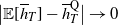 $\big|\mathbb{E}[\overline{h}_T]-\overline{h}^\mathrm{Q}_T\big|\to 0$
as
$\big|\mathbb{E}[\overline{h}_T]-\overline{h}^\mathrm{Q}_T\big|\to 0$
as $T\to\infty$
. We emphasize that, for the quasistatic error to vanish in the limit as
$T\to\infty$
. We emphasize that, for the quasistatic error to vanish in the limit as $T\to\infty$
it is not necessary for the potentials V(t, x) to approach some time-independent
$T\to\infty$
it is not necessary for the potentials V(t, x) to approach some time-independent $V_\infty(x)$
as
$V_\infty(x)$
as $t\to\infty$
, i.e. for y(t) to approach a constant.
$t\to\infty$
, i.e. for y(t) to approach a constant.
In contrast, if $\|y^\prime(t)\|$
does not decay in t (e.g. the location of the potential oscillates at a constant frequency or escapes to infinity at a constant rate) then we generally find a non-zero quasistatic-approximation error that persists in the limit
$\|y^\prime(t)\|$
does not decay in t (e.g. the location of the potential oscillates at a constant frequency or escapes to infinity at a constant rate) then we generally find a non-zero quasistatic-approximation error that persists in the limit $T\to\infty$
. Equation (49) shows that the error is
$T\to\infty$
. Equation (49) shows that the error is $O(C\|y^\prime\|_\infty)$
; this matches the behavior observed in (33), with
$O(C\|y^\prime\|_\infty)$
; this matches the behavior observed in (33), with $\|y^\prime\|_\infty$
replacing
$\|y^\prime\|_\infty$
replacing $\varepsilon$
as a measure of the rate of change of the instantaneous stationary distributions, and also matches the intuitive discussion of the quasistatic regime in Section 1.
$\varepsilon$
as a measure of the rate of change of the instantaneous stationary distributions, and also matches the intuitive discussion of the quasistatic regime in Section 1.
Acknowledgement
The author is grateful for the comments and suggestions of the referees, which led to substantial improvements in this manuscript.
Funding information
There are no funding bodies to thank relating to the creation of this article.
Competing interests
There were no competing interests to declare which arose during the preparation or publication process of this article.

 Open access

