


Non-technical Summary
Scientists often use morphological traits to figure out how fossil species are related. A popular method to do this assumes each trait changes on its own, even though many traits can be linked. This study used computer simulations to see how much this assumption affects the results. The researchers found that even when traits are connected or change at different rates, the method still does a good job figuring out the species tree. However, it can make mistakes in estimating how fast the traits changed over time. Some improved models help fix these errors. Overall, the study shows that current methods work well for figuring out relationships among species using morphological traits.
Introduction
Phylogenetic inference is essential for answering various questions in evolutionary biology. Despite the tremendous amount of genomic data available, morphological characters remain the primary or sole information to infer phylogenies of fossil taxa and to study deep-time divergence (Lee and Palci Reference Lee and Palci2015; Donoghue and Yang Reference Donoghue and Yang2016). Discrete characters are the main type of data and are traditionally analyzed under maximum parsimony. In recent years, model-based methods, including maximum likelihood and Bayesian inference, have been shown to have comparable or better performance in inferring phylogenies (Wright and Hillis Reference Wright and Hillis2014; O’Reilly et al. Reference O’Reilly, Puttick, Parry, Tanner, Tarver, Fleming, Pisani and Donoghue2016, Reference O’Reilly, Puttick, Pisani and Donoghue2018; Brown et al. Reference Brown, Parins-Fukuchi, Stull, Vargas and Smith2017; Puttick et al. Reference Puttick, O’Reilly, Tanner, Fleming, Clark, Holloway and Lozano-Fernandez2017, Reference Puttick, O’Reilly, Pisani and Donoghue2019; Smith Reference Smith2019; Keating et al. Reference Keating, Sansom, Sutton, Knight and Garwood2020). Among these methods, characters are treated as independent features. The simplest model for discrete characters is the Mk model (Lewis Reference Lewis2001), in which the rates of changes among the k states are equal. The most frequently used Mkv model (with suffix “v”; Lewis Reference Lewis2001) is a variant that accounts for the ascertainment bias of coding only variable characters.
Correlation among characters has long been recognized. One classical example is the tail-presence and tail-color problem (Maddison Reference Maddison1993), because the two characters are logically dependent. Several algorithmic solutions have been proposed to handle such cases, under either parsimony- or model-based criteria (Brazeau et al. Reference Brazeau, Guillerme and Smith2019; Goloboff et al. Reference Goloboff, Laet, Ríos-Tamayo and Szumik2021; Hopkins and St. John Reference Hopkins and St. John2021; Tarasov Reference Tarasov2023). Another example is that some characters are functionally or developmentally dependent (Beaulieu and Donoghue Reference Beaulieu and Donoghue2013; Leslie et al. Reference Leslie, Beaulieu, Crane, Knopf and Donoghue2015; Billet and Bardin Reference Billet and Bardin2019). This study mainly deals with the latter but also covers the former if the inapplicable states are governed by a hidden process (Tarasov Reference Tarasov2021). In general, correlated discrete characters can be modeled by a Markov chain with rates among states as parameters (Pagel Reference Pagel1994; Pagel and Meade Reference Pagel and Meade2006). However, such a model is typically employed in phylogenetic comparative methods to study the evolution of two or three characters given fixed trees (Pagel et al. Reference Pagel, Meade and Barker2004; Pagel and Meade Reference Pagel and Meade2006; Beaulieu and Donoghue Reference Beaulieu and Donoghue2013; Billet and Bardin Reference Billet and Bardin2019), but is rarely used for inference of phylogenetic trees, as the number of parameters grows so dramatically with the number of characters and the model quickly becomes unidentifiable. Instead, all inference methods (parsimony, maximum likelihood, and Bayesian) typically assume all the characters are independent (Felsenstein Reference Felsenstein1985a).
Simulation studies have shown that Bayesian inference assuming character independence outperforms parsimony-based solutions in the case of logical dependence (Simões et al. Reference Simões, Vernygora, de Medeiros and Wright2022). However, no study so far has investigated how the Bayesian method performs in the general case of character dependence. Previous simulations used the simplest Mkv model for inference (Wright and Hillis Reference Wright and Hillis2014; O’Reilly et al. Reference O’Reilly, Puttick, Parry, Tanner, Tarver, Fleming, Pisani and Donoghue2016, Reference O’Reilly, Puttick, Pisani and Donoghue2018; Puttick et al. Reference Puttick, O’Reilly, Tanner, Fleming, Clark, Holloway and Lozano-Fernandez2017, Reference Puttick, O’Reilly, Pisani and Donoghue2019; Smith Reference Smith2019; Keating et al. Reference Keating, Sansom, Sutton, Knight and Garwood2020), thus rate heterogeneity in state changes and across characters was not considered. Those studies also focused on non-clock (unrooted) trees. Herein we perform computer simulations to study the performance of Bayesian inference assuming character independence, with data simulated under either independent or dependent evolution under various conditions of evolutionary rate heterogeneity. We perform both non-clock and tip-dating analyses, and in the latter case, fossil ages are used and the results are dated (rooted) timetrees (Pyron Reference Pyron2011; Ronquist et al. Reference Ronquist, Klopfstein, Vilhelmsen, Schulmeister, Murray and Rasnitsyn2012a; Zhang et al. Reference Zhang, Stadler, Klopfstein, Heath and Ronquist2016).
Methods
Markov Models
In general, discrete character evolution can be modeled by a Markov chain with a Q-matrix specifying the rates of changes (Pagel Reference Pagel1994). We first describe the model for a single binary character, then the models for a doublet and a triplet of correlated binary characters. For simplicity, we do not further consider correlation of four or more characters, or characters with more than two states.
For a binary character, the changes between states 0 and 1 are determined by this instantaneous rate matrix
 $$ {Q}_1=\unicode{x03BB} \left[\begin{array}{cc}-{\unicode{x03C0}}_1& {\unicode{x03C0}}_1\\ {}{\unicode{x03C0}}_0& -{\unicode{x03C0}}_0\end{array}\right], $$
and the transition probability matrix is
 $$ P(t)=\left[\;\begin{array}{cc}{\unicode{x03C0}}_0+{\unicode{x03C0}}_1{\mathrm{e}}^{-\unicode{x03BB} t}& {\unicode{x03C0}}_1-{\unicode{x03C0}}_1{\mathrm{e}}^{-\unicode{x03BB} t}\\ {}{\unicode{x03C0}}_0-{\unicode{x03C0}}_0{\mathrm{e}}^{-\unicode{x03BB} t}& {\unicode{x03C0}}_1+{\unicode{x03C0}}_0{\mathrm{e}}^{-\unicode{x03BB} t}\end{array}\right]. $$
This model extends the Mk model (Lewis [Reference Lewis2001], in which π0 = π1 = 0.5), allowing the equilibrium state frequencies to vary (Ronquist and Huelsenbeck Reference Ronquist and Huelsenbeck2003; Klopfstein et al. Reference Klopfstein, Vilhelmsen and Ronquist2015; Wright et al. Reference Wright, Lloyd and Hillis2016) and is a two-state variate of the F81 model (Felsenstein Reference Felsenstein1981). It has two free parameters (λ and π0). The average rate of change is 2λπ0π1. Because λ and t are multiplied together in the transition probability matrix, they are not identifiable without further assumptions about the time and/or the rate.
For a doublet of binary characters, the general model for the four state pairs, 00, 01, 10 and 11, is introduced with eight free parameters (Pagel Reference Pagel1994). The model is not necessarily time reversible, and the Q-matrix may have complex eigenvalues and eigenvectors. For mathematical convenience, we reparametrize the Q-matrix as
 $$ {Q}_2=\left[\begin{array}{cccc}\cdot & {a\unicode{x03C0}}_2& {b\unicode{x03C0}}_3& 0\\ {}{a\unicode{x03C0}}_1& \cdot & 0& {c\unicode{x03C0}}_4\\ {}{b\unicode{x03C0}}_1& 0& \cdot & {d\unicode{x03C0}}_4\\ {}0& {c\unicode{x03C0}}_2& {d\unicode{x03C0}}_3& \cdot \end{array}\right]=\left[\begin{array}{cccc}\cdot & a& b& 0\\ {}a& \cdot & 0& c\\ {}b& 0& \cdot & d\\ {}0& c& d& \cdot \end{array}\right]\left[\begin{array}{cccc}{\unicode{x03C0}}_1& 0& 0& 0\\ {}0& {\unicode{x03C0}}_2& 0& 0\\ {}0& 0& {\unicode{x03C0}}_3& 0\\ {}0& 0& 0& {\unicode{x03C0}}_4\end{array}\right], $$
with {a, b, c, d} as the exchangeability rates and π = {π1, π2, π3, π4} as the equilibrium state frequencies for the four state pairs. The model is then time-reversible with seven free parameters. This can be viewed as a special case of the GTR model (Tavaré Reference Tavaré1986; Yang Reference Yang1994a). Setting q 12 = q 34, q 13 = q 24, q 21 = q 43, and q 31 = q 42 results in independent evolution with four parameters (π is derived from {a, b, c, d}), and will be equivalent to the Mk model by further constraining a = b = c = d (as few as one free parameter).
Similarly, we can use this rate matrix,
 $$ {Q}_3=\left[\begin{array}{cccccccc}\cdot & a& b& 0& i& 0& 0& 0\\ {}a& \cdot & 0& c& 0& j& 0& 0\\ {}b& 0& \cdot & d& 0& 0& k& 0\\ {}0& c& d& \cdot & 0& 0& 0& l\\ {}i& 0& 0& 0& \cdot & e& f& 0\\ {}0& j& 0& 0& e& \cdot & 0& g\\ {}0& 0& k& 0& f& 0& \cdot & h\\ {}0& 0& 0& l& 0& g& h& \cdot \end{array}\right]\left[\begin{array}{cccccccc}{\unicode{x03C0}}_1& 0& 0& 0& 0& 0& 0& 0\\ {}0& {\unicode{x03C0}}_2& 0& 0& 0& 0& 0& 0\\ {}0& 0& {\unicode{x03C0}}_3& 0& 0& 0& 0& 0\\ {}0& 0& 0& {\unicode{x03C0}}_4& 0& 0& 0& 0\\ {}0& 0& 0& 0& {\unicode{x03C0}}_5& 0& 0& 0\\ {}0& 0& 0& 0& 0& {\unicode{x03C0}}_6& 0& 0\\ {}0& 0& 0& 0& 0& 0& {\unicode{x03C0}}_7& 0\\ {}0& 0& 0& 0& 0& 0& 0& {\unicode{x03C0}}_8\end{array}\right], $$
for a triplet of binary characters with eight states, 000, 001, 010, 011, 100, 101, 110 and 111. Simultaneous changes of two or three states are negligible, so that their rates are zero. The model has 19 free parameters. The average rate is −∑ iπ iqii, where qii is the i th diagonal element in the Q-matrix.
Simulation Procedure
We first generated variable timetrees from a birth–death process using TreeSim in R (Stadler Reference Stadler2011) with a birth rate of 5.0 and a death rate of 4.0, conditioned on a root age of 1.0. The ages are on a relative scale and can be arbitrarily rescaled depending on the chosen time unit. From the trees simulated, we kept 100 trees with no more than 50 tips to make sure the data size is manageable. We simply treated the extinct tips as fossils, without further sampling fossils along the tree. The distribution of tree lengths and the numbers of extant and extinct tips are shown in Figure 1.
The distribution of tree length (A) and the numbers of extant and extinct tips (B) of the simulated trees.

For each tree, we then simulated evolution of discrete morphological characters along the tree under various models and settings (Table 1). The general procedure was generating the exponential waiting times and using the jump chain given the Q-matrix (Yang Reference Yang2014: section 12.5.4). This is particularly useful when the transition probability matrix is hard to derive. The starting state at the root was randomly drawn from the equilibrium frequencies (π). Only variable characters were kept at the tips referring to empirical practices.
Models and settings used in the simulations and inferences. See “Methods” for the explanations of the symbols.

For independent binary characters, the simplest model is fixing π0 = π1 = 0.5 (referred to as M2v herein) for all characters, representing homogeneous evolution. To introduce heterogeneity in character states, we drew π0 from a uniform distribution independently for each character and let π1 = 1 − π0 (the F81-alike extension, referred to as F2v herein). We rescaled Q 1 so that the average rate per character (i.e., the base clock rate) is 1.0, such that the branch lengths in the tree are measured by distance. To further introduce heterogeneity along time, each branch length for each character was multiplied by a relative rate r independently drawn from a lognormal distribution with mean 1.0 and variance 4.0, representing the most heterogeneous case (referred as “no common mechanism” [NCM]; Tuffley and Steel Reference Tuffley and Steel1997). We recorded a moderate size of 200 variable characters in the data matrix in each replicate of the three settings.
We used the rate matrix Q 2 to simulate pairs of binary characters (referred as G4v herein). We drew {a, b, c, d} and {π1, π2, π3, π4} from a symmetric Dirichlet distribution with parameter 10 (representing slight correlation) or 1.0 (severe correlation) for each doublet. We rescaled Q 2 to have an average rate of 2.0 (per character rate being 1.0). To further have heterogeneous evolutionary rates, each branch length for each doublet is multiplied by an independent relative rate r as we did previously. We recorded 200 characters (i.e., 100 doublets) and ensured that all characters were variable in the data matrix.
Similarly, with three settings, we rescaled Q 3 to have an average rate of 3.0 (per character rate being 1.0), and simulated triplets of binary characters (referred as G8v). We recorded 201 variable binary characters (i.e., 67 triplets) but discarded the last character, so that we still had 200 characters in the data matrix. Considering that many empirical datasets are much smaller, we repeated the simulations under the same procedure with 50 variable correlated characters.
Phylogenetic Inference
Each data matrix was analyzed using the Bayesian phylogenetic inference software MrBayes 3.2.7 (Ronquist et al. Reference Ronquist, Teslenko, van der Mark, Ayres, Darling, Höhna, Larget, Liu, Suchard and Huelsenbeck2012b). All characters were treated as independent, no matter how they were simulated. They were also treated as a single partition, meaning the branch lengths are shared by all characters (referred to as “common mechanism”; Tuffley and Steel Reference Tuffley and Steel1997). This setting reflects the practice in most empirical analyses.
MrBayes supports both the M2v and F2v models. The M2v model has no free parameter other than the tree topology and branch lengths, while the F2v model has an extra parameter, π0, which is averaged using a discretized symmetric beta prior with parameter α (Wright et al. Reference Wright, Lloyd and Hillis2016). We used an exponential hyperprior with mean 1.0 (Exp(1)) for α by default. For datasets simulated under NCM, we partially accommodated rate variation among characters using a discrete gamma distribution (Yang Reference Yang1994b) (F2v+G; Table 1).
The non-clock analyses used the morphological data only and the branch lengths were measured by distance. As we simulated timetrees with both extant and extinct tips, we further incorporated the tip ages in another round of tip-dating analyses, so that we could disentangle the times and clock rates. The tip ages were assigned their true values assuming they are perfectly known. We specified diffuse Exp(1) prior for the root age and mean clock rate, used constant-rate fossilized birth–death prior (Stadler Reference Stadler2010) for the timetree and independent lognormal relaxed clock (Drummond et al. Reference Drummond, Ho, Phillips and Rambaut2006) for the evolutionary rate variation, following common practices.
For each inference, two independent Markov chain Monte Carlo runs were executed each for 8 million generations with sampling frequency of 200. The beginning 35% of samples were discarded as burn-in, and the rest of the samples from the two runs were combined after checking consistency. We made sure the average standard deviation of split frequencies was below 0.02, and the effective sample sizes were all greater than 100. In rare cases, we had to resume the analysis or double the chain length until these criteria were satisfied. The posterior tree samples were summarized as a 50% majority-rule consensus tree.
Missing Data
The main procedure involves no missing data. We also repeated the analyses with 50% missing states in the extinct taxa and 10% missing in the extant taxa, mimicking the observation in empirical datasets. Specifically, we replaced each state by a question mark in the data matrix with the corresponding probability (i.e., 0.1 for extant and 0.5 for extinct taxa). Such replacement was performed randomly on the generated binary characters rather than on the doublets or triplets.
Tree Distance Metrics
We employed both the Quartet (Estabrook et al. Reference Estabrook, McMorris and Meacham1985) and Mutual Clustering Information (MCI; Smith Reference Smith2020) metrics for comparing the inferred tree with the true tree generating the data. The MCI metric is a generalized Robinson-Foulds (RF) distance metric (Robinson and Foulds Reference Robinson and Foulds1981) that is information based and less saturated; thus it is recommended over the RF metric (Smith Reference Smith2020). The Quartet metric also has several advantages over the RF metric and is also recommended (Smith Reference Smith2019).
Both distance metrics conflate accuracy and precision (Keating et al. Reference Keating, Sansom, Sutton, Knight and Garwood2020). Thus, we also calculated the Strict Joint Assertion (SJA, which is the number of quartets that are resolved identically in both trees over that resolved either identically or differently in both trees; Estabrook et al. Reference Estabrook, McMorris and Meacham1985) as a measure of accuracy, and the percentage of resolved internal branches (the number of internal branches in the estimated consensus tree over that in the true tree) as precision.
The quartet-related metrics are calculated using the package Quartet in R (Smith Reference Smith2019) and the MCI metric is using TreeDist in R (Smith Reference Smith2020).
Results
We aim to investigate the performance of Bayesian phylogenetic inference using the M2v and F2v models by comparing the inferred tree with the true tree simulating the data. The Quartet and MCI metrics measure the topological differences, and the tree lengths in non-clock analyses and tree heights in tip-dating analyses represent the branch-length estimates.
We first look at the results from data without missing states. The first two scenarios represent rate homogeneous evolution, and the models used in the inference can match that in the simulation, in which M2v is a special case of F2v. They are the best-case scenarios and act as a baseline. The results do show that the topologies and branch lengths are inferred with good accuracy (Figs. 2A–D, 3A–D, cases 1, 2). For the following four scenarios, the rates in the Q-matrix are quite similar, as they were generated from a Dirichlet distribution with parameter 10. As a result, the performance of the Bayesian inference is almost the same as when there is no rate variation (Figs. 2A–D, 3A–D, cases 3–6).
Tree distance metrics (Quartet and Mutual Clustering Information [MCI]) comparing the inferred tree with the true tree generating the data. Each violin plot contains 100 replicates. The left four panels show the results of non-clock analyses (A, C, E, G), while the right four panels show the results of tip-dating analyses (B, D, F, H). Panels labeled “w/ missing” (E–H) indicate scenarios with missing data. The numbers on the x-axis correspond to the following experiments (simulation model vs. inference model): 1, M2v–vs–M2v; 2, M2v–vs–F2v; 3, G4v(α = 10)–vs–M2v; 4, G4v(α = 10)–vs–F2v; 5, G8v(α = 10)–vs–M2v; 6, G8v(α = 10)–vs–F2v; 7, F2v(α = 1)–vs–M2v; 8, F2v(α = 1)–vs–F2v; 9, G4v(α = 1)–vs–M2v; 10, G4v(α = 1)–vs–F2v; 11, G8v(α = 1)–vs–M2v; 12, G8v(α = 1)–vs–F2v; 13, F2v(α = 1, v = 4)–vs–M2v; 14, F2v(α = 1, v = 4)–vs–F2v; 15, G4v(α = 1, v = 4)–vs–M2v; 16, G4v(α = 1, v = 4)–vs–F2v; 17, G8v(α = 1, v = 4)–vs–M2v; 18, G8v(α = 1, v = 4)–vs–F2v.

Relative bias (posterior mean minus the true value, then divided by the true value) and relative width of credibility interval (CI) (95% CI width divided by the true value) for each of the following experiments (simulation model vs. inference model): 1, M2v–vs–M2v; 2, M2v–vs–F2v; 3, G4v(α = 10)–vs–M2v; 4, G4v(α = 10)–vs–F2v; 5, G8v(α = 10)–vs–M2v; 6, G8v(α = 10)–vs–F2v; 7, F2v(α = 1)–vs–M2v; 8, F2v(α = 1)–vs–F2v; 9, G4v(α = 1)–vs–M2v; 10, G4v(α = 1)–vs–F2v; 11, G8v(α = 1)–vs–M2v; 12, G8v(α = 1)–vs–F2v; 13, F2v(α = 1, v = 4)–vs–M2v; 14, F2v(α = 1, v = 4)–vs–F2v; 15, G4v(α = 1, v = 4)–vs–M2v; 16, G4v(α = 1, v = 4)–vs–F2v; 17, G8v(α = 1, v = 4)–vs–M2v; 18, G8v(α = 1, v = 4)–vs–F2v. Each violin plot contains 100 replicates. The left four panels show the tree lengths from non-clock analyses (A, C, E, G), while the right four panels show the tree heights from tip-dating analyses (B, D, F, H). Panels labeled “w/ missing” (E–H) indicate scenarios with missing data.
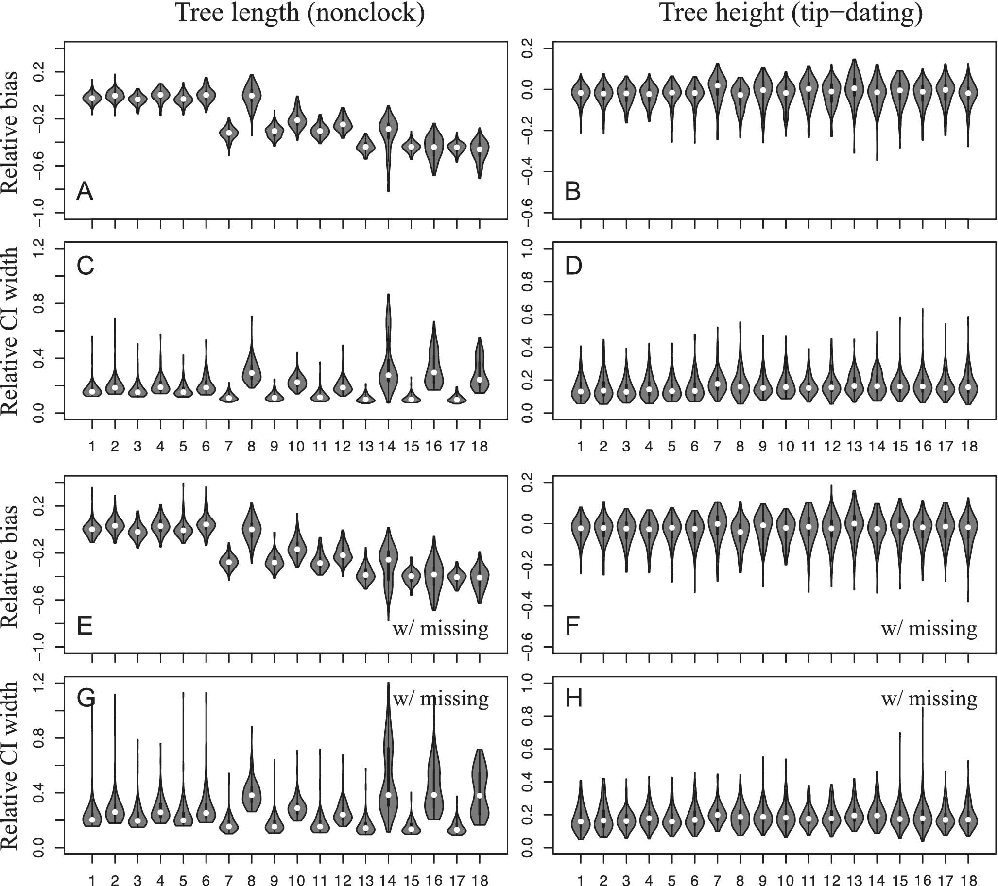
The hardest situation appears to be when the data were simulated under F2v and each character has its own stationary frequencies (π0 and π1). The M2v model certainly does not account for this, resulting in larger tree distances (Fig. 2A–D, case 7) and underestimated tree lengths (Fig. 3A, case 7). In the tip-dating analyses, the tree height estimates are barely affected (Fig. 3B, case 7), but the clock rate is underestimated (Fig. 4A, case 7). The inference model of F2v is supposed to match the simulation condition; however, we did not estimate individual frequencies for each character due to identifiability issues. Instead, we averaged π0 (and π1 = 1 − π0) using a discretized symmetric beta distribution (Wright et al. Reference Wright, Lloyd and Hillis2016). This strategy can correct the bias of tree-length or clock-rate estimates (Figs. 3A, 4A, case 8), but results in similar tree distances as using the M2v model (Fig. 2A–D, case 8). Having a further look at the accuracy (SJA) and precision (tree resolution) metrics, we find that the larger tree distances under M2v are largely contributed by decreased accuracy (Supplementary Figs. S1, S2, case 1 vs. case 7), whereas those under F2v are largely contributed by decreased precision (Supplementary Figs. S1, S2, case 2 vs. case 8).
Relative bias (posterior mean minus the true value, then divided by the true value) and relative width of credibility interval (CI) (95% CI width divided by the true value) of the base clock rate for each of the following experiments (simulation model vs. inference model): 1, M2v–vs–M2v; 2, M2v–vs–F2v; 3, G4v(α = 10)–vs–M2v; 4, G4v(α = 10)–vs–F2v; 5, G8v(α = 10)–vs–M2v; 6, G8v(α = 10)–vs–F2v; 7, F2v(α = 1)–vs–M2v; 8, F2v(α = 1)–vs–F2v; 9, G4v(α = 1)–vs–M2v; 10, G4v(α = 1)–vs–F2v; 11, G8v(α = 1)–vs–M2v; 12, G8v(α = 1)–vs–F2v; 13, F2v(α = 1, v = 4)–vs–M2v; 14, F2v(α = 1, v = 4)–vs–F2v; 15, G4v(α = 1, v = 4)–vs–M2v; 16, G4v(α = 1, v = 4)–vs–F2v; 17, G8v(α = 1, v = 4)–vs–M2v; 18, G8v(α = 1, v = 4)–vs–F2v. Each violin plot contains 100 replicates. The left two panels are scenarios without missing data (A and C), while the right two panels labeled with “w/ missing” (B and D) indicate scenarios with missing data.

Surprisingly, severe correlation in each pair or triplet of characters does not increase but instead decreases the tree distances (Fig. 2A–D, cases 9–12), although they still present higher distances than the homogeneous ones (Fig. 2A–D, cases 1–6). This results from both slightly increased accuracy and precision (Supplementary Figs. S1, S2, cases 7–12), likely because the rate heterogeneity for each character in these settings is slightly lower than that under independent evolution, which is reflected in the estimates of the shape parameter of the symmetric beta distribution (Supplementary Material, log files). Having more correlated characters (three vs. two) makes almost no difference in how the inference results are affected. Using the F2v model in inference cannot match the simulation models, but it is still helpful in slightly correcting the bias of underestimating tree length (Fig. 3A, cases 9–12) or clock rate (Fig. 4A, cases 9–12).
The most heterogeneous scenarios involve rate heterogeneity both among characters and across branches (NCM). However, using the simplest M2v model as well as the F2v model can achieve comparable performance as when there is no rate heterogeneity for inference of tree topology (Fig. 2A–D, cases 13–18, Supplementary Figs. S1, S2, cases 13–18). Evolutionary rate heterogeneity across branches appears to retain strong phylogenetic signal in the data. On the other hand, branch-length or clock-rate estimates are more biased, with M2v showing the most severe underestimation and narrowest credibility interval (CI) width (Figs. 3A, 4A, cases 13–18).
Empirical data typically contain many missing states. When 50% of states in the fossil taxa and 10% in the extant taxa are missing on average, we observe similar patterns as when there is no missing state, with decreased precision but similar accuracy (Figs. 2E–H, 3E–H, 4B, D, Supplementary Figs. S3, S4). In other words, missing data mostly result in more unresolved nodes in the trees and larger CIs of the tree lengths, but for the resolved part of the tree, the accuracy is similar to that when there is no missing data. Similar patterns are also observed when the number of characters is much smaller (50 vs. 200), with largely decreased precision and slightly decreased accuracy (Supplementary Fig. S5).
Discussion
The Bayesian method has been demonstrated to have good accuracy when data were generated under either common or no common mechanisms (Wright and Hillis Reference Wright and Hillis2014; O’Reilly et al. Reference O’Reilly, Puttick, Parry, Tanner, Tarver, Fleming, Pisani and Donoghue2016, Reference O’Reilly, Puttick, Pisani and Donoghue2018; Puttick et al. Reference Puttick, O’Reilly, Tanner, Fleming, Clark, Holloway and Lozano-Fernandez2017, Reference Puttick, O’Reilly, Pisani and Donoghue2019; Smith Reference Smith2019; Keating et al. Reference Keating, Sansom, Sutton, Knight and Garwood2020). We moved one step further and introduced character correlation in the simulations. Both the non-clock and tip-dating analyses suggest that Bayesian inference assuming character independence does not mislead the inference of tree topology when character correlation and rate heterogeneity are present. This is quite reassuring, as correlation and NCM have been argued to be quite common in morphological characters, and model-based methods are blamed for not accounting for these (Goloboff et al. Reference Goloboff, Torres and Arias2018, Reference Goloboff, Pittman, Pol and Xu2019).
However, when the interest is the branch lengths, they can be biased toward underestimation when evolutionary rate variation is high among characters and along branches. Such variation can be modeled by general Markov processes in theory, but they are typically not practical in inference. Unlike molecular sequences where the same nucleotide across sites has the same biological meaning, morphological characters coded as 0, for example, have different meanings among characters; thus using one parameter for all the 0s would be pointless, whereas unlinking all of them would result in too many parameters. The best strategy so far has been using the F2v model, in which the state frequencies are averaged analogous to averaging the site rates (Wright et al. Reference Wright, Lloyd and Hillis2016). According to our simulation results, it is recommended over the M2v model in all the scenarios we have tested. However, the F2v model only accounts for rate variation among character states. To further account for rate variation along branches, we could subdivide the data into multiple partitions (e.g., according to the anatomical regions) and infer independent evolutionary rates for each partition (e.g., using unlinked clock models; Lee Reference Lee2016; Zhang and Wang Reference Zhang and Wang2019). Bear in mind, though, we should keep enough (probably at least dozens of) characters in each partition to avoid overparameterization, especially when the data contain a large portion of missing states. Alternatively, a new method has been developed to account for rate variation both across characters and along branches by switching the rates among different rate regimes (Khakurel and Höhna Reference Khakurel and Höhna2025).
In the tip-dating analyses, we fixed the fossil ages to their true values. Hence the inferred tree heights (root ages) are reliable in all different conditions. This implies that incorporating accurate fossil information is crucial for dating divergence times, even when the morphological evolutionary model is mis-specified (Klopfstein et al. Reference Klopfstein, Ryer, Coiro and Spasojevic2019). In practice, however, uncertainties in fossil ages and prior for the timetree (root age in particular) are likely to decrease the accuracy (Barido-Sottani et al. Reference Barido-Sottani, Aguirre-Fernández, Hopkins, Stadler and Warnock2019; Luo et al. Reference Luo, Duchêne, Zhang, Zhu and Ho2019). Depending on the data and models, the situation can become rather complicated (Simões et al. Reference Simões, Caldwell and Pierce2020; May et al. Reference May, Contreras, Sundue, Nagalingum, Looy and Rothfels2021). Optimistically, when the timetree is presumably reliable, evolutionary rate estimates could be refined using subsequent comparative methods for the characters of interest under more complex models (Pennell et al. Reference Pennell, Eastman, Slater, Brown, Uyeda, FitzJohn, Alfaro and Harmon2014; Revell Reference Revell2024).
We only considered correlated discrete morphological characters in this study. It is worth noting that there is a large body of literature for correlated continuous traits. The evolution of the traits is typically modeled by a Brownian motion (BM) (Felsenstein Reference Felsenstein1973, Reference Felsenstein1985b; Freckleton Reference Freckleton2012) or an Ornstein–Uhlenbeck (OU) process (Uhlenbeck and Ornstein Reference Uhlenbeck and Ornstein1930; Felsenstein Reference Felsenstein1988; Hansen Reference Hansen1997; Butler and King Reference Butler and King2004), and trait correlations are described by the variance–covariance matrix in the model. Relative to this, the threshold model (Wright Reference Wright1934; Felsenstein Reference Felsenstein2005) is a promising alternative for correlated discrete characters, in which the observed discrete states depend on whether the underlying continuous trait (called liability) is above a threshold value. Although the BM and OU models have been well studied mathematically, practical implementations for phylogenetic inference are sparse (Álvarez-Carretero et al. Reference Álvarez-Carretero, Goswami, Yang and dos Reis2019; Hassler et al. Reference Hassler, Magee, Zhang, Baele, Lemey, Ji, Fourment and Suchard2022; Zhang et al. Reference Zhang, Drummond and Mendes2023). The main reason is that these models are parameter-rich, and developing efficient computational methods is technically challenging. Thus, it appears to be an important area for further improvement.
Conclusion
Our results demonstrate that Bayesian inference of phylogenetic trees is remarkably robust to violations of the character independence assumption. Topological inference remains accurate across a range of realistic evolutionary scenarios, including strong correlation and substantial evolutionary rate heterogeneity among morphological characters. However, our analyses also reveal that branch lengths or clock rates may be systematically underestimated under simpler models when rate variation is present. To mitigate this, we recommend using models that average over character-state frequencies (e.g., F2v) and, when feasible, incorporating rate variation across partitions.
While this study focuses on discrete morphological characters, future work should extend to continuous trait and threshold models that more directly account for trait correlations. Overall, our findings support the continued and expanded use of Bayesian methods in morphological phylogenetics and call for methodological innovations to improve branch-length estimation under complex evolutionary processes.
Acknowledgments
This research was supported by the National Key Research and Development Program of China (2023YFF0804502 to C.Z.) and the National Natural Science Foundation of China (42172006 to C.Z.).
Author Contribution
C.Z. designed the study and led the analyses. X.L. performed the simulations. C.Z. led the interpretation of the results and writing of the manuscript. X.L. and C.Z. revised the manuscript and gave final approval for publication.
Competing Interests
The authors declare no competing interests.
Data Availability Statement
Electronic Supplementary Material is available from the GitHub Digital Repository: https://github.com/zhangchicool/morphSim.


 Open access