


1. Introduction
Combined shear-driven and Rayleigh–Taylor (RT) turbulence occurs in mixing layers when the overlying stream is more dense than the underlying one. This configuration results in a complex flow, in which the turbulent mixing process is driven by both shear and buoyancy forces. Examples of such a flow can be found in the natural environment, e.g. in the ocean or the atmosphere (Turner Reference Turner1979), as well as in industrial processes, e.g. combustion chambers (Nagata & Komori Reference Nagata and Komori2000) and inertial confined fusion targets (Atzeni & Meyer-ter Vehn Reference Atzeni and Meyer-ter Vehn2004). The two pertinent phenomena, RT and shear-driven turbulence, have been widely studied independently. The RT turbulence phenomenology was originally introduced by Chertkov (Reference Chertkov2003) and has been recently reviewed by Boffetta & Mazzino (Reference Boffetta and Mazzino2017). By shear-driven turbulence, here we refer to shear turbulent mixing layers (see Pope (Reference Pope2001), chap. 5, § 5.4.2 for a complete overview).
Only a few works have investigated the compound effect of shear and buoyancy in the mixing of two fluids. In this context, most of the past research was devoted to analysis of the instability phase, referred to as RT/Kelvin–Helmholtz instability (RTKHI), especially in plasma physics (Satyanarayana et al. Reference Satyanarayana, Guzdar, Huba and Ossakow1984; Finn Reference Finn1993; Shumlak & Roderick Reference Shumlak and Roderick1998) but also in classical fluid flows (Olson et al. Reference Olson, Larsson, Lele and Cook2011). The major result of this research is that, while a linear stability analysis predicts that adding an arbitrary shear velocity to an RT configuration will increase the perturbation growth rate, if early nonlinear effects are taken into account, the shear can lead to a decrease of the growth rate or, in extremis, to a suppression of the RTKHI (Shumlak & Roderick Reference Shumlak and Roderick1998; Olson et al. Reference Olson, Larsson, Lele and Cook2011).
Focusing on the fully developed turbulent phase, Snider & Andrews (Reference Snider and Andrews1994) performed an experimental study in a water channel, in which an unstable thermal stratification is combined with a mean shear. The authors inferred that this problem is governed by two different types of transition: one from laminar flow to self-similar turbulence, and the other from shear-driven to buoyancy-driven mixing. Focusing on the latter, the authors identified as a suitable parameter for distinguishing between these two distinct mixing regimes the (negative) bulk Richardson number  $Ri = - h g {\Delta \rho } / (\rho {\Delta U}^2)$ (where $h$ is mixing layer thickness, ${\Delta \rho }$ and $\rho$ are the density difference and the reference density, respectively, ${\Delta U}$ is the shear velocity and $g$ is the gravitational acceleration). However, their estimate for the transitional Richardson number spans a wide range, from $-5$ to $-11$. Moreover, the transition to turbulence seemed to always occur in the RT regime, and it was not possible to clearly identify the shear-dominated phase. More recent experiments performed in a gas tunnel focused on the later time of the instability phase (Akula, Andrews & Ranjan Reference Akula, Andrews and Ranjan2013; Akula et al. Reference Akula, Suchandra, Mikhaeil and Ranjan2017). The authors identified two distinct mixing regimes through analysis of the mixing layer growth rate, which is expected to be constant for shear-dominated turbulence (Pope Reference Pope2001, constant velocity) and linear for RT turbulence (Boffetta & Mazzino Reference Boffetta and Mazzino2017, constant acceleration). Again, the bulk Richardson number was chosen to be the parameter for identifying the transition from the shear to the RT regime. The transitional $Ri$ was shown to be within the range $(-2.5,-1.5)$ in Akula et al. (Reference Akula, Andrews and Ranjan2013) and $(-2.5,-0.8)$ in Akula et al. (Reference Akula, Suchandra, Mikhaeil and Ranjan2017). However, the range of investigated stratification levels is completely different from that in Snider & Andrews (Reference Snider and Andrews1994), which might suggest that the transitional Richardson number depends on the stratification level. Moreover, the value of $Ri$ depends sensitively on the definition of the mixing layer thickness $h$.
$h$.
The complexity of the transition from shear-dominated to RT turbulence motivated investigators to devise low-order Reynolds-averaged turbulence models to adequately describe it. Within this context, Morgan, Schilling & Hartland (Reference Morgan, Schilling and Hartland2018) recently proposed a two-length-scale turbulence model to describe compound shear and RT mixing. Within this framework, the bulk Richardson number is again employed to quantify the relative strength of shear and buoyancy forces.
Despite the effort devoted to this research, only a few of the aforementioned works clearly capture a shear-driven, fully developed turbulent regime, because the investigated shear velocity Reynolds numbers are usually smaller or comparable to those needed for this regime to manifest. In fact, the focus of Akula et al. (Reference Akula, Andrews and Ranjan2013, Reference Akula, Suchandra, Mikhaeil and Ranjan2017) and Snider & Andrews (Reference Snider and Andrews1994) was always stated to be on the (at most) later stage of the instability phase; this is highlighted by the reference time chosen to scale the phenomena ( $\sqrt {2 \rho H /(\Delta \rho g)}$), which is suitable for quantifying the advancement of the RT instability only. Another critical point regarding the previously mentioned works concerns the so-called early nonlinear phase of the RT instability (Waddell, Niederhaus & Jacobs Reference Waddell, Niederhaus and Jacobs2001; Celani et al. Reference Celani, Mazzino, Muratore-Ginanneschi and Vozella2009). During the weakly nonlinear phase of the RT instability, the perturbation growth rate is expected to be constant. Because of this, distinguishing between the early nonlinear RT and the shear-driven turbulence is extremely challenging, especially in laboratory experiments, where a large separation between the time/space at which the transition to turbulence occurs and the time/space at which the transition from shear-dominated to RT turbulence occurs is hard to achieve. Moreover, small-scale quantities (such as the spatial velocity gradient), which could provide suitable indicators of the dominant flow regime, are difficult to access experimentally.
In this work, we investigate the fully developed turbulence arising in unstable stratified mixing layers. Our aim is to (i) clarify in which conditions a transition from shear-dominated to RT turbulence can occur and (ii) provide a phenomenological theory valid for a shear to RT transition where the shear-dominated turbulence is already developed from early times. Finally, we validate our theory against direct numerical simulations of a turbulent temporal mixing layer compounded with an unstable temperature stratification.
2. Phenomenological theory
In the following, we present a phenomenological theory that describes the transition from shear-driven to RT turbulence in a temporal mixing layer, for the case where the flow is already turbulent during the shear-dominated regime. Our theory leads to the identification of a cross-over time, which distinguishes between the shear-dominated and the RT regimes. We assume that the fluid motion is governed by the Navier–Stokes equations with the Boussinesq approximation, i.e. density variations are neglected for inertial effects, while they are still significant in the gravitational term:
 \begin{gather} \frac{\partial \boldsymbol{u}}{\partial t} + \boldsymbol{u} \boldsymbol{\cdot} \boldsymbol{\nabla} \boldsymbol{u} ={-} \frac{1}{\rho_0} \boldsymbol{\nabla} p + \nu \nabla^2 \boldsymbol{u} + \beta g \theta \boldsymbol{e}_3, \end{gather}
 \begin{gather} \boldsymbol{\nabla} \boldsymbol{\cdot} \boldsymbol{u} = 0, \end{gather}
where  $\boldsymbol {u} = (u,v,w)$ is the fluid velocity in the streamwise, spanwise and wall-normal directions, respectively, $\theta$ is the relative temperature, $\beta$ is the thermal expansion coefficient, $g$ is the gravitational acceleration and $\nabla ^2$ is the Laplace operator. The relative temperature is a scalar field that must satisfy the following advection–diffusion equation:
 \begin{equation} \frac{\partial \theta}{\partial t} + \boldsymbol{u} \boldsymbol{\cdot} \boldsymbol{\nabla} \theta = \kappa \nabla^2 \theta, \end{equation}
where  $\kappa$ is the thermal diffusivity.
We consider the case of a temporal turbulent mixing layer. Note that a temporal mixing layer is a limit of the spatial mixing layer for which the ratio between the shear velocity  $\Delta U$ (the velocity difference between the two streams) and the mean convective velocity $U_C$ (the mean velocity of the two streams) is much less than unity. In such a limit, the flow becomes statistically one-dimensional for an observer travelling in the streamwise direction at the mean convective velocity (Pope Reference Pope2001, chap. 5, § 5.4.2). Such a flow was experimentally observed to hold for a velocity ratio of at least $0.60$ between the two streams (Bell & Mehta Reference Bell and Mehta1990), and was numerically reproduced using periodic boundary conditions in the streamwise direction (Rogers & Moser Reference Rogers and Moser1994). We assume that the Reynolds number is large enough such that the flow is dominated by large-scale quantities only and the present turbulent state is independent of the initial perturbation and of viscosity. Moreover, we assume that at early times the turbulence is shear-dominated, so that the balance of the Navier–Stokes equation at large scale dictates that the first term on the left-hand side of (2.1) is balanced by the nonlinear term:
 \begin{equation} \frac{u_L}{t} \sim \frac{u_L^2}{h(t)}, \end{equation}
where  $u_L$ is the large-scale velocity magnitude and $h(t)$ is the integral scale that we identify with a measure of the mixing layer thickness. If we assume $u_L \sim \Delta U > 0$ (as is the case for shear-driven turbulence), the well-known linear law for the growth of the mixing layer thickness is thus obtained:
 \begin{equation} h(t) = S \Delta U t. \end{equation}
The proportionality constant  $S$ has been measured both experimentally and numerically, and ranges from $0.06$ to $0.11$ (Pope Reference Pope2001). Let us now assume that the flow is gravitationally unstable, i.e. the density of the upper layer is greater than the density of the underlying one. The large-scale balance becomes
 \begin{equation} \underbrace{\frac{\partial \boldsymbol{u}}{\partial t}}_{u_L/t} + \underbrace{\boldsymbol{u} \boldsymbol{\cdot} \boldsymbol{\nabla} \boldsymbol{u}}_{u_L^2/h(t)} = \cdots+ \underbrace{\beta g \theta \boldsymbol{e}_3}_{\beta g \Delta \theta}, \end{equation}
where  ${\Delta \theta }$ is the constant temperature difference between the two streams and the dots on the right-hand side represent the subleading terms. If shear turbulence develops at an early time, it must initially dominate with the scaling of (2.5). The order of magnitude of the inertial term decreases as $t^{-1}$, and it therefore follows from (2.6) that, sooner or later, the constant on the right-hand side must dominate. This happens when
 \begin{equation} t \simeq t_{c} \simeq \frac{\Delta U}{\beta g {\Delta \theta}}. \end{equation}
For  $t \gg t_{c}$ the buoyancy term becomes dominant; thus, given that always $h(t) \sim u_L \, t$, the terms on the left-hand side balance the buoyancy term such that
 \begin{equation} \frac{u_L}{t} \sim \beta g {\Delta \theta}, \end{equation}
from which one can estimate the large-scale velocity as  $u_L \sim \beta g {\Delta \theta } t$. One can thus obtain the typical RT turbulence law for the mixing layer thickness as $h(t) \sim u_L t$, namely,
 \begin{equation} h(t) = \alpha \beta g {\Delta \theta} t^2, \end{equation}
where  $\alpha$ has been measured both experimentally and numerically, and ranges from $0.03$ to $0.07$ (Boffetta & Mazzino Reference Boffetta and Mazzino2017).
The same analysis can be conducted from an alternative point of view. Assuming that shear initially dominates turbulent mixing, the governing parameters are  $\Delta U$ and $t$, and in this phase self-similarity leads to $h(t) \sim \Delta U t$. The ratio between the buoyancy and inertial forces is described by the bulk Richardson number $Ri = \beta g {\Delta \theta } h(t) / \Delta U^2$. By imposing $Ri = 1$, one obtains $t_c = t|_{Ri = 1} = \Delta U / (\beta g {\Delta \theta })$. For later times, the only relevant factors are $\beta g {\Delta \theta }$ and $t$, so that the self-similarity of the flow implies $h(t) \sim \beta g {\Delta \theta } t^2$ and $u_L = \sqrt {\beta g {\Delta \theta } h(t)}$, which represents the free-fall velocity.
When studying this flow configuration, past research focused on traditional non-dimensional quantities, namely, the large-scale Reynolds number  $Re = u_L h(t) / \nu$, the Rayleigh number $Ra = \beta g {\Delta \theta } h(t)^3 / ( \nu k )$ and the Richardson number $Ri = \beta g {\Delta \theta } h(t) / {\Delta U}^2$. All these parameters are time-dependent and are thus not suitable for describing the overall behaviour of the system given a set of dimensional flow parameters (initial conditions, boundary conditions and fluid properties). By considering the functional relation between dimensional quantities, namely, $h = f(\Delta U, \beta g {\Delta \theta }, k, \nu , t)$, in light of our phenomenological theory, we apply the Buckingham- $\varPi$ theorem using ${\Delta U}$ and $t_c$ as characteristic scales, and reduce the problem to the following relation between non-dimensional quantities:
 \begin{equation} \frac{h}{h_c} = \hat{f} \left(Re_c, \, \frac{\nu}{\kappa}, \, \frac{t}{t_c} \right), \end{equation}
where  $t_c$ is the cross-over time defined in the previous section, $h_c = {\Delta U} t_c$ is the order of magnitude of the corresponding turbulent mixing layer cross-over thickness (assuming shear scaling from early times), $Re_c = {\Delta U} h_c / \nu$ is the large-scale Reynolds number at transition and $Pr = \nu / \kappa$ is the Prandtl number. The non-dimensional mixing layer thickness, $h/h_c$, coincides with the bulk Richardson number:
 \begin{equation} \frac{h(t)}{h_c} = \frac{h(t)}{t_c \Delta U} = \frac{h(t) \beta g {\Delta \theta}}{{\Delta U}^2} = \frac{h(t) {\Delta \rho} g}{\rho {\Delta U}^2} = Ri, \end{equation}
because  $\beta {\Delta \theta } = {\Delta \rho }/\rho$. Note that in the Boussinesq approximation $\Delta \rho / \rho = 2 A$, where $A$ is the Atwood number.
The classical mixing layer thickness Reynolds number can be expressed as  $Re = Re_c \, Ri$, while the Rayleigh number is $Ra = Re_c \, Pr \, Ri$. In contrast to the standard approach, in our formulation $Ri$ is the dependent variable. We can therefore formulate the problem in terms of the following non-dimensional variables:
 \begin{equation} t^* = \frac{t}{t_c}, \quad \boldsymbol{x}^* = \frac{\boldsymbol{x}}{h_c}, \quad \boldsymbol{u}^* = \frac{\boldsymbol{u}}{\Delta U}, \quad p^* = \frac{p}{\rho_0 {\Delta U} ^2}, \quad \theta^* = \frac{\theta}{{\Delta \theta}}, \end{equation}
which transform the momentum equation (2.1), continuity equation (2.2) and scalar transport equation (2.3) to
 \begin{gather} \frac{\partial \boldsymbol{u}^*}{\partial t^*} + \boldsymbol{u}^* \boldsymbol{\cdot} \boldsymbol{\nabla} \boldsymbol{u}^* ={-} \boldsymbol{\nabla} p^* + \frac{1}{Re_c} \nabla^2 \boldsymbol{u}^* + \theta^* \boldsymbol{e}_3, \end{gather}
 \begin{gather} \boldsymbol{\nabla} \boldsymbol{\cdot} \boldsymbol{u}^* = 0, \end{gather}
 \begin{gather} \frac{\partial \theta^*}{\partial t^*} + \boldsymbol{u}^* \boldsymbol{\cdot} \boldsymbol{\nabla} \theta^* = \frac{1}{Re_c \, Pr} \nabla^2 \theta^*. \end{gather}
A critical aspect that we clarify with our theory concerns the existence of the shear-dominated turbulent phase. By assuming that the shear initially dominates, we assert that our theory holds under the condition that the turbulence is already fully developed in the shear-driven regime. The reason why this is a necessary condition lies in the fact that our theory requires the global flow behaviour to be governed from early times by large-scale flow parameters only, i.e. to be independent of the viscous scales. Considering (2.10), this condition requires that the cross-over Reynolds number  $Re_c$ be much larger than the shear-driven transition-to-turbulence Reynolds number, $Re_s$. The latter is the Reynolds number at which the mixing layer reaches a fully developed turbulent state in the absence of stratification. The value of $Re_s$ is documented to depend on various factors, namely: (i) the velocity ratio, (ii) the density ratio, (iii) the initial shear-layer profile and in particular (iv) the shape and nature of the instability. It can vary over a wide range (3000–17 000) (Bernal & Roshko Reference Bernal and Roshko1986; Koochesfahani & Dimotakis Reference Koochesfahani and Dimotakis1986). In the case of uniform density, the temporal mixing layer limit is the one for which the shear-driven transition-to-turbulence Reynolds number is generally smaller (Breidenthal Reference Breidenthal1981), so that, in our case, we can in principle rely on the lower limit.
3. Direct numerical simulations
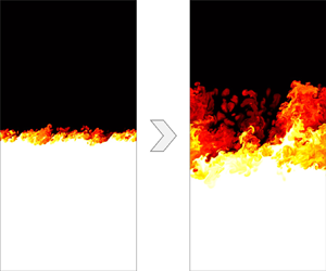
The temporal mixing layer is simulated by imposing periodic boundary conditions in the streamwise and spanwise directions, while a free-slip condition is imposed on the lower and upper walls. The streamwise velocity profile and the scalar concentration field are initialised with step functions  $u = \Delta U\, \textrm{sign} (z) / 2$ (Rogers & Moser Reference Rogers and Moser1994) and $\theta = {\Delta \theta }/2 (\textrm {sign} (z) + 1 )$), respectively. Equations (2.1), (2.2) and (2.3) are solved with a fourth-order-accurate finite-volume spatial discretisation scheme and a third-order Adams–Bashforth scheme for time integration (Verstappen & Veldman Reference Verstappen and Veldman2003; Craske & van Reeuwijk Reference Craske and van Reeuwijk2015). We fixed $Pr = \nu / \kappa = 1$ for all the simulations. We also fixed $\Delta U = 1$ and ${\Delta \theta } = 1$, and changed the control parameter $Re_c$ to act on the kinematic viscosity $\nu$ and on the coefficient $\beta$. As shown in § 2, $Re_c$ is indeed the only control parameter for this problem. We checked a posteriori that a sufficiently wide range of $t/t_c$ were explored, in order to be certain to observe the transition between shear-dominated and RT turbulence. In addition to the non-dimensional parameters discussed in § 2, table 1 also lists the ratio $t_c/t_0$, where $t_0$ is the time at which the mixing layer would reach a developed turbulent state in the absence of stratification, i.e. $\beta = 0$. In particular, $t_0$ is the time at which the following two conditions are met: (i) $Re_{\lambda } \geq 50$ and (ii) a $\sim k^{-5/3}$ spectrum with at least one decade of wavenumber separation being visible. The first three most stratified simulations ( $SL1$, $SL2$ and $SL3$) were initialised with laminar initial conditions. In these cases, the cross-over Reynolds number is small, so that the transition to turbulence is triggered directly by RT. The time $t_0$ required for shear-dominated transition to turbulence to occur was evaluated by performing a simulation with no buoyancy ( $SNB$) and the same viscosity as in $SL1$, $SL2$ and $SL3$. For the three less stratified cases $ST4$, $ST5$ and $ST6$, $Re_c$ is significantly higher, meaning that the transition to turbulence is expected to occur earlier than the transition from shear to RT turbulence. In these cases we decided to switch on the buoyancy term at $t_0$, that is, when the turbulence has already developed because of shear. This is equivalent to initialising the simulations with an already shear-triggered turbulent flow. This precaution, which can be realised in numerical simulations only, ensures shear-dominated turbulence at $t_0$, avoiding, at the same time, the ambiguity between shear turbulent mixing and early nonlinear RT instability, which characterised the previous experiments conducted with comparable shear and buoyancy forcing. The latter reasoning allows us to overcome the problem of having moderately high shear Reynolds numbers, which imposes both experimental-facility limitations and constraints on the computational power requirements of direct numerical simulations. Table 1 also lists the ratio between the total simulation time $t_{end}$ and the cross-over time $t_c$, showing that all the simulations reach the buoyancy-dominated phase.
Simulation parameters:  $L_i$ and $N_i$ denote the size and the number of grid points along the $i$th direction, respectively; $Re_c$ is the Reynolds number corresponding to the cross-over time; $t_0$ is the time at which the flow with shear only would reach a fully developed turbulent state (i.e. $Re_{\lambda } \geq 50$ and a clear scale separation in the turbulent spectra); $t_c$ is the cross-over time as predicted by (2.7); $t_{end}$ is the total time of each simulation.

4. Results and discussion
To check the tendency of the flow to attain asymptotically the RT-like structure, we rely on the following argument: consider the Nusselt number  $Nu = \langle w' \theta ' \rangle h(t) / ( k {\Delta \theta } )$, i.e. the ratio between the total turbulent scalar transport and the diffusive transport (the angled brackets indicate the average within the mixing layer), and the Reynolds number $Re = u_L h(t) / \nu$. By assuming RT-like scaling $u_L = \beta g \theta t$ and $h \sim \beta g {\Delta \theta } t^2$, we obtain the following relations:
 \begin{equation} Nu \sim Ra^{1/2}Pr^{1/2}, \qquad Re \sim Ra^{1/2}Pr^{{-}1/2}, \end{equation}
where  $Ra = \beta g {\Delta \theta } {h(t)}^3 / ( \nu \kappa )$ is the Rayleigh number (a dimensionless measure of the density difference). This state is sometimes referred to as the ultimate state of convection in the case of Rayleigh–Bénard (RB) convection (Kraichnan Reference Kraichnan1962); it is expected to appear at very large Rayleigh numbers, when boundary layers break down and the scalar and momentum mixing is driven by large-scale contributions (Lohse & Toschi Reference Lohse and Toschi2003). While this regime hardly emerges in RB turbulence because of the important role played by the boundaries, in RT configurations it is clearly manifest (Boffetta et al. Reference Boffetta, De Lillo, Mazzino and Vozella2012). Thus, these scaling laws are a good method for checking the tendency of the flow to reach RT turbulence. From here on, we consider the temperature integral thickness $h_{\theta } = \int _{-\infty }^{+\infty } 4 \theta (1-\theta )\,\textrm {d}z$ (Vladimirova & Chertkov Reference Vladimirova and Chertkov2009) as a proxy for the mixing layer thickness $h(t)$. We chose this quantity instead of the momentum thickness (which is usually employed in mixing layer theory) because the latter is suitable for shear mixing layers only, while the temperature thickness is still suitable for quantifying the mixing width in both limits. We recall that in our simulations, the Prandtl number $Pr = \kappa /\nu$ is fixed at $1$. Figure 1 shows clearly that all the simulated cases converge asymptotically to the scaling $(Nu,Re) \sim Ra^{1/2}$, regardless of the initial stratification.
Ultimate state scaling as a check for the turbulence to reach the buoyancy-dominated regime: (a)  $Nu$ vs $Ra$; (b) $Re$ vs $Ra$;
$Ra$;  $Pr$ is fixed at $1$.
$1$.

Different characteristic quantities of the flow can be analysed to discern between shear- and buoyancy-driven turbulence. The most direct way to quantitatively check the validity of our theory is to analyse the turbulent kinetic energy ( $tke$) balance. We chose the integral $tke$ balance (integrated over the wall-normal direction), because this does not depend on the definition of the mixing layer thickness $h(t)$. The $tke$ integral balance is written
 \begin{equation} \frac{\partial E}{\partial t} + \varepsilon = \mathcal{P}_{B} + \mathcal{P}_G, \end{equation}
where  $E = \int _{-\infty }^{+\infty } (\overline {\boldsymbol {u}' \boldsymbol {\cdot } \boldsymbol {u}'})^2/2 \, \mathrm {d}z$ is the $tke$ per unit mass, $\varepsilon = \nu \int _{-\infty }^{+\infty } \overline {( \boldsymbol {\nabla } \boldsymbol {u}' )^2}\,\mathrm {d}z$ is the viscous dissipation, $\mathcal {P}_{B} = \beta g \int _{-\infty }^{+\infty } \overline {w' \theta '}\,\mathrm {d}z$ is the buoyancy production and $\mathcal {P}_{G} = - \int _{-\infty }^{+\infty } \overline {w' u'} \partial _z \bar {u}\,\mathrm {d}z$ is the gradient production; the overline represents the horizontal average. Initially, when shear dominates ( $t < t_c$), $tke$ is mainly produced by $\mathcal {P}_{G}$, i.e. the ratio between the buoyancy and the shear production is smaller than unity. In this phase, the gradient production balances the dissipation rate ( ${\partial E}/{\partial t} + \varepsilon \sim \mathcal {P}_G$). For later times, buoyancy overcomes shear, i.e. the dissipation rate is balanced by buoyancy as in pure RT turbulence ( ${\partial E}/{\partial t} + \varepsilon \sim \mathcal {P}_{B}$). In more detail, when $t < t_c$, we expect that $u_L \sim \Delta U$ and $h(t) \sim \Delta U t$ for both $\mathcal {P}_{B}$ and $\mathcal {P}_G$. Indeed, the buoyancy production term is expected to be passively transported by the shear velocity without any relevant influence of the buoyancy force. For later times, we expect the variation of the streamwise mean velocity to be shear-dominated, i.e. $\partial \bar {u}/\partial z \sim \Delta U / h(t)$. The latter assertion is reasonable, because in temporal mixing layers $(\bar {v},\bar {w}) = (0,0)$, while in pure RT turbulence $\bar {u} = 0$. The streamwise mean velocity derivative is thus expected to be mostly affected by the shear velocity scale. Concerning the wall-normal turbulent flux, we assume that $u' \sim \Delta U$ and $w'\sim \beta g \Delta \theta$, such that $\overline {u' w'}$ scales as ${\Delta U} ( \beta g {\Delta \theta } ) t$, i.e. the Reynolds stress tensor remains anisotropic for longer times. We found this to agree well with our data (inset of figure 2a). Note that this is not the case for pure RT turbulence, in which the mean shear is absent. The scale of variation of the mean streamwise velocity can be identified using any measure of the mixing layer thickness. However, it is not needed to derive the scaling of $\mathcal {P}_G$, because it drops out after integration along the wall-normal direction. Consequently, we obtain the following scalings for the shear and buoyancy $tke$ production:
 \begin{equation} \mathcal{P}_{G} \sim \begin{cases} {\Delta U}^3 & \text{if }t \ll t_c,\\ \left( \beta g {\Delta \theta} \right) {\Delta U}^2 t & \text{if }t \gg t_c,\\ \end{cases} \quad \mathcal{P}_{B} \sim \begin{cases} \left(\beta g {\Delta \theta}\right) {\Delta U}^2 t & \text{if }t \ll t_c,\\ \left( \beta g {\Delta \theta} \right)^3 t^3 & \text{if }t \gg t_c,\\ \end{cases} \end{equation}
which implies that the flux Richardson number  $Ri_f = \mathcal {P}_{B}/\mathcal {P}_{G} \sim t$ for $t \ll t_c$ and ${\mathcal {P}_{B}/ \mathcal {P}_{G} \sim t^2}$ for $t \gg t_c$. Figure 2(a) shows that our phenomenological prediction reasonably matches the data in the limits of $t \ll t_c$ and $t \gg t_c$. As predicted, the shear-dominated phase clearly appears only in $ST4$, $ST5$ and $ST6$, for which $Re_c$ is high, and thus the transition from laminar to self-similar turbulence is shear-dominated. In the strongly stratified cases ( $SL1$, $SL2$ and $SL3$), the shear-dominated turbulence is suppressed, because the buoyancy term already prevails during the transition to turbulence (low $Re_c$). A noteworthy consideration is that, considering even the simulations in which the shear-driven turbulence is inhibited, the flux-Richardson number scaling still holds when considering only the turbulent phase.
Temporal scalings of the turbulent kinetic energy: (a) ratio between the buoyancy and gradient  $tke$ production (i.e. the flux Richardson number $Ri_f$) integrated over the wall-normal direction, with the inset showing the scaling of $\overline {u'w'}$ at the centreline; energy spectra normalised with the (b) shear and (c) RT scalings for all the simulations (see (4.4)); the line thickness is proportional to the non-dimensional time.

Another argument relies on the temporal scaling of the energy spectra. By considering  $K41$ inertial scaling (Kolmogorov Reference Kolmogorov1941, Reference Kolmogorov1962; Obukhov Reference Obukhov1941a, Reference Obukhovb, Reference Obukhov1962), one can derive two different scaling behaviours for the second-order structure function or, equivalently, the energy spectra. In terms of energy spectra, RT and shear turbulence are expected to scale equally with the wavenumber $k$, but differently with time (see Boffetta & Mazzino (Reference Boffetta and Mazzino2017) for a complete discussion on the energy spectra temporal scaling in three-dimensional RT turbulence). Simple power counting leads to the following spectral scalings:
 \begin{equation} E(k) \sim \begin{cases} \Delta U^{4/3} t^{{-}2/3} k^{{-}5/3} & \text{if }t \ll t_c,\\ \left( \beta g {\Delta \theta} \right)^{4/3} t^{2/3} k^{{-}5/3} & \text{if }t \gg t_c,\end{cases} \end{equation}
Figure 2(b,c) shows that shear/RT scaling holds for early/late times, respectively. Indeed, all the curves tend to stabilise on RT-like spectra for later non-dimensional times (thick line), and the shear scaling holds for early non-dimensional times (thin line), while becoming unreliable for later non-dimensional times (thicker line).
Finally, the two regimes can also be distinguished by analysing the bulk Richardson number  $h(t)/h_c$ and the mixing layer growth rate $\delta h(t) / \delta t$. In the shear-dominated phase a linear spreading of the mixing layer is expected, while when buoyancy prevails the mixing region grows quadratically. In other words, the mixing layer growth rate is expected to be constant in the shear-dominated phase and linear in the RT phase. Despite the fact that this method is the one usually adopted to distinguish between the two regimes, it often does not provide clear evidence of the dominance of shear over buoyancy, and vice versa. The reason is that the tendency of the mixing layer to grow linearly or quadratically is not a direct measure of the predominance of one forcing over the other, but only a consequence, that is, not directly causally correlated to the phenomena (in support of this argument, one may consider the early nonlinear phase of RT). Figure 3(a) shows that, as expected, $Ri$ grows linearly for $t \ll t_c$ and quadratically for $t \gg t_c$. Figure 3(b) shows $\delta h(t) / \delta t$ for $ST4$, $ST5$ and $ST6$, where an initial constant-like behaviour, which becomes linear near $t = t_c$ is appreciable, while $SL1$, $SL2$ and $SL3$ show only a linear trend, meaning that the shear-dominated turbulent phase is suppressed. The inset of figure 3(b), shows the growth rate in linear space for $ST4$, $ST5$ and $ST6$, highlighting the transitional phase between shear-dominated and RT turbulence.
Bulk Richardson number (a) and bulk Richardson number growth rate (b); the inset shows  $ST4$, $ST5$ and $ST6$ in linear space; note that the bulk Richardson number growth rate is a non-dimensional measure of the mixing layer thickness growth rate, because $h_{\theta }$ is proportional to $Ri$.
$Ri$.

Having shown that the cross-over time  $t_c$ correctly scales the bulk and the flux Richardson numbers, one may be interested in the exact value of the non-dimensional time at which the transition effectively occurs, $t/t_c|_T$. To estimate $t/t_c|_T$ we adopt the following procedure for $Ri$,
$Ri$,  $Ri_f$ and $t_c \delta {Ri}/ {\delta t}$. Firstly, we fit the phenomenological asymptotic predictions for $t \ll t_c$ and $t \gg t_c$ into the early and late-time data of $Ri$,
$Ri$,  $Ri_f$ and $t_c \delta {Ri}/ {\delta t}$. This is done systematically, by increasing the distance from $t/t_c = 1$ until the constant fitting coefficients no longer change. Then, the transitional time is estimated as the intersection between the two fitted asymptotic laws. For instance, by considering the bulk Richardson number, we expect $Ri = b_{shear} \, ( t/t_c )^1$ at early times and $Ri = b_{RT} \, ( t/t_c )^2$ for later times; $b_{shear}$ and $b_{RT}$ are evaluated using the aforementioned fitting procedure, and the transitional time is obtained as $t/t_c|_T = b_{shear}/b_{RT}$. Table 2 lists the values of $t/t_c|_T$ for each of the considered observables, together with their corresponding values at each of the transitional times. We report also the value of the gradient Richardson number evaluated at the centreline ( $Ri_g = (-{g}/{\rho } {\partial \bar {\rho }}/{\partial z}) / ({\partial \bar {u}}/{\partial z})^2$ at $z = 0$) and the corresponding transitional time.
Transitional time for each observable and the corresponding Richardson numbers. Column one lists the transition times  $t/t_c|_T$ for the bulk, gradient (at the centreline), increment and flux Richardson numbers. Columns two to four list the values of $Ri$,
$Ri$,  $Ri_f (z=0)$ and $Ri_g$ at the corresponding transitional time in column one.

We frame our results in the context of past research. By analysing the results of Akula et al. (Reference Akula, Andrews and Ranjan2013, Reference Akula, Suchandra, Mikhaeil and Ranjan2017), we evaluate the control parameter  $Re_c$ to identify experiments that are likely to include a shear-dominated turbulent regime. A notable case is experiment $A2S2$, in which $Re_c \simeq 17\,000$. Akula et al. (Reference Akula, Suchandra, Mikhaeil and Ranjan2017) evaluated the transitional location by analysing the mixing layer growth rate and then estimated $Ri_g$ at the centreline at that location. We can thus compare their value of $Ri_g$ at the transition with line three, column four of table 2: Akula et al. (Reference Akula, Suchandra, Mikhaeil and Ranjan2017) obtained $Ri_g = 0.17$ in experiment $A2S2$, which is almost equal to our estimate ( $Ri_g = 0.18$). Again, considering the mixing layer growth rate, experiment $A2S2$ transitions from shear-dominated to RT turbulence at $t/t_c|_T = 2.09$, which is close to the value $2.47$ listed in table 2 (column one, line three). This further confirms that the cross-over time $t_c$ correctly predicts the transition from shear- to buoyancy-dominated turbulence for sufficiently high $Re_c$ (turbulence already developed in the shear-dominated phase). Moreover, $t_c$ is shown to correctly scale the time even when the shear-dominated phase is suppressed, provided that only the fully developed turbulent phase is considered.
5. Concluding remarks
In this work, we have systematically analysed the problem of transition from shear-dominated to Boussinesq RT turbulence through theory and the use of direct numerical simulations. Our phenomenological approach allows us to predict a cross-over time  $t_c \simeq \Delta U / ( \beta g {\Delta \theta } )$ at which an initially shear-dominated turbulent flow transitions to RT turbulence. The direct numerical simulations confirmed the validity of our theory, in particular in terms of the flux Richardson number, a direct measure of which factor dominates the turbulence (buoyancy or shear). Moreover, using the Buckingham- $\varPi$ theorem, we clarified in which conditions the shear-dominated turbulence is suppressed (low values of $Re_c$). This latter aspect is particularly noteworthy, because it highlights the fact that only when the turbulence is fully developed at early times is it reasonable to expect the flow to show universal behaviour (i.e. the transition at a unique non-dimensional time).
In § 4, we derived a scaling law for the flux Richardson number that is in good agreement with the data. This follows from the non-trivial scaling  $\overline {u'w'} \sim \Delta U ( \beta g \theta ) t$, i.e. that the Reynolds stress tensor remains anisotropic also for longer times. This scaling is expected to have implications for turbulence modelling, because in pure RT turbulence $\overline {u'w'}$ is always equal to zero. For instance, it follows from our framework that the eddy viscosity is not constant in time and should feature an explicit dependence on the growing impact of stratification also for later times when the unstable stratification dominates the turbulence.
At the end of § 4 we framed our work in the context of past research. By comparing our results with the experiment of Akula et al. (Reference Akula, Suchandra, Mikhaeil and Ranjan2017), we observe that at large  $Re_c$, there may be a well-defined value of $t/t_c|_T$ (approximately 2.5) as well as of the transitional gradient Richardson number (approximately $0.18$). In other words, while for small values of $Re_c$ we expect a more complex dependency of $t/t_c|_T$ and $Ri_g(t/t_c|_T,z=0)$ on the control parameter $Re_c$ (and eventually on the nature of the perturbation), at finite but large $Re_c$ a unique and universal value of $t/t_c|_T$ (or $Ri_g(t/t_c|_T,z=0)$) may exist. This fact is crucial, given that the Reynolds numbers are usually large in many natural environments as well as in industrial applications. The detailed study of this aspect is left to future work.
Acknowledgements
J.P.M. and M.v.R. acknowledge the financial support of the Engineering and Physical Sciences Research Council (EPSRC) through grant EP/R042640/1. M.H. and S.B. acknowledge financial support from the DFG priority program SPP 1881 Turbulent Superstructures under Grant No. HO5519/1-2. A.M. acknowledges the financial support from the Compagnia di San Paolo, Project MINIERA No. I34I20000380007, and from the Project PoC – BUYT MAIH, No. C36I20000140006.
Declaration of interests
The authors report no conflict of interest.


 Open access