2.1. Structural governing equations

A sinusoidal heaving motion: $y_c(t)=h\sin (\kappa t)$ is imposed at the centre of the elliptic foil (figure 1b). Here, $y_c(t)$ is the instantaneous position of the centre of a foil in the non-dimensional form, $t$ being the time non-dimensionalised by $c/U_{\infty }$ (where $U_{\infty }$ is the free-stream velocity); $h$ and $\kappa$ denote the non-dimensional heaving amplitude and frequency, respectively. All the quantities throughout this paper are non-dimensionalised, considering $c$ and $U_{\infty }$ as the reference length and velocity scales, respectively. The flexible tail portion (marked ‘II’ in figure 1a) is modelled as an inextensible filament that is allowed to undergo a passive oscillation. In the non-dimensional form, the governing equation of the tail motion is given by

(2.1)\begin{equation} \beta\,\frac{\partial^2\boldsymbol{X}}{\partial t^2}=\frac{\partial}{\partial s}\left(T_s\,\frac{\partial\boldsymbol{X}}{\partial s}\right)-\frac{\partial^2}{\partial s^2}\left(\gamma\,\frac{\partial^2\boldsymbol{X}}{\partial s^2}\right)+\beta\, Fr\,\frac{\boldsymbol{g}}{{g}}+\boldsymbol{F}, \end{equation}

where, $s$ denotes the arc length, $\boldsymbol {X}=(X(s,t),Y(s,t))$ is the position of the filament, $T_s$ is the tension coefficient along the filament, $\gamma$ is the bending rigidity, and $\boldsymbol {F}$ indicates the fluid force acting on the filament. These non-dimensional quantities are obtained by using characteristic scales $\rho _f U_{\infty }^2$ for the fluid force, $\rho _f U_{\infty }^2 c$ for the tension coefficient, and $\rho _f U_{\infty }^2 c^3$ for the bending rigidity. The mass ratio is defined as $\beta ={\rho _s t_h}/{\rho _f c}$, where $\rho _s$ and $\rho _f$ are the solid and fluid densities, respectively; $t_h$ ($= 0.02c$) is the thickness of the tail structure; $Fr={{g} c}/{U_{\infty }^2}$ is the Froude number, with ${g}=|\boldsymbol {g}|$ being gravitational force. It is to be noted that the gravity term is included here in the structural governing equations alone, solely for the validation of the present solver against the available literature. However, it is not considered for the present fluid–structure interaction (FSI) simulations throughout the study, following the work of Zhu, He & Zhang (Reference Zhu, He and Zhang2014). In order to maintain a constant length of the tail, the inextensibility condition is implemented as

(2.2)\begin{equation} \frac{\partial \boldsymbol{X}}{\partial s}\boldsymbol{\cdot}\frac{\partial \boldsymbol{X}}{\partial s} = 1. \end{equation}

In (2.1), $\gamma$ is assumed to be constant. Here, $T_s$ is a function of both $s$ and $t$, hence $T_s$ is determined by substituting the inextensibility constraint (2.2) in (2.1). This results in a Poisson equation for $T_s$:

(2.3) \begin{align} \frac{\partial \boldsymbol{X}}{\partial s}\boldsymbol{\cdot}\frac{\partial^2}{\partial s^2}\left(T_s\,\frac{\partial \boldsymbol{X}}{\partial s}\right) = \frac{\beta}{2}\,\frac{\partial^2}{\partial t^2}\left(\frac{\partial \boldsymbol{X}}{\partial s}\boldsymbol{\cdot}\frac{\partial \boldsymbol{X}}{\partial s}\right)-\beta\, \frac{\partial^2\boldsymbol{X}}{\partial t\,\partial s}\boldsymbol{\cdot}\frac{\partial^2\boldsymbol{X}}{\partial t\,\partial s}-\frac{\partial \boldsymbol{X}}{\partial s}\boldsymbol{\cdot}\frac{\partial}{\partial s}\left(\boldsymbol{F}_b+\boldsymbol{F}\right), \end{align}

where $\boldsymbol {F}_b=-({\partial ^2}/{\partial s^2})(\gamma ({\partial ^2\boldsymbol {X}}/{\partial s^2}))$ denotes the bending force. For more details of the formulation of the above equations, one can refer to the work of Huang, Shin & Sung (Reference Huang, Shin and Sung2007). Note that the non-dimensional reference scales used in this work are different to what was used by Huang et al. (Reference Huang, Shin and Sung2007).

At $t = 0$, the leading edge of the elliptic foil lies at the origin, with the tail at rest in the horizontal position. The boundary conditions for the aft-tail are as follows: at the free end $(s=1.3c)$,

(2.4)\begin{equation} T_s=0, \quad \frac{\partial^2 \boldsymbol{X}}{\partial s^2}=(0,0), \quad \frac{\partial^3 \boldsymbol{X}}{\partial s^3}=(0,0), \end{equation}

and at the fixed end $(s=c)$,

(2.5)\begin{equation} \boldsymbol{X}=\boldsymbol{X}_0,\quad \frac{\partial \boldsymbol{X}}{\partial s}=(1,0), \end{equation}

where $\boldsymbol {X}_0=(c,y_c(t))$ is the position of the leading edge of the aft-tail. Equations (2.1) and (2.3) are solved using a finite difference technique (Huang et al. Reference Huang, Shin and Sung2007). In order to perform the finite difference discretisation for the structural equations, the flexible filament is divided into $N$ solid elements, each having width $\Delta s$ and thickness $t_h$, as shown in figure 2.

Figure 2.

(a) Schematic sketch of the flexible filament structure along with the background Eulerian mesh. (b) Spatial discretisation strategy of the filament.

2.2. Flow solver

In the present IBM solver framework, a momentum forcing $\boldsymbol {f}$ is applied throughout the solid domain to enforce the no-slip, no-penetration boundary condition exactly on the solid boundary (Majumdar et al. Reference Majumdar, Bose and Sarkar2020a). In order to ensure rigorous mass conservation across the immersed boundary, a source/sink term $q$ is added to the continuity equation. Hence the flow governing equations take the form

(2.6)\begin{gather} \frac{\partial \boldsymbol{u}}{\partial t}+\boldsymbol{\nabla} \boldsymbol{\cdot} \left(\boldsymbol{uu}\right)={-}\boldsymbol{\nabla} p+\frac{1}{Re}\,\nabla^2\boldsymbol{u}+\boldsymbol{f}, \end{gather}

(2.7)\begin{gather} \boldsymbol{\nabla}\boldsymbol{\cdot}\boldsymbol{u}-q=0. \end{gather}

Here, $\boldsymbol {u}$ denotes the flow velocity vector non-dimensionalised by $U_\infty$, $p$ is the pressure non-dimensionalised by $\rho _f U_\infty ^2$, and the Reynolds number is $Re = {U_\infty c}/{\nu }$. Equations (2.6) and (2.7) are solved on a background Eulerian grid using a finite-volume-based semi-implicit fractional step method. The diffusion term is discretised using the second-order Crank–Nicolson method, and Adams–Bashforth discretisation is used for the convection term. At every time step, the velocity is corrected using a pseudo-pressure-correction term. Note that for a grid cell entirely in the fluid domain, which has none of the cell faces inside the solid domain, $\boldsymbol {f}$ and $q$ are considered to be zero. For grid locations inside the solid domain, they take non-zero values. Further details of the flow solver can be found in Kim, Kim & Choi (Reference Kim, Kim and Choi2001), Lee & Choi (Reference Lee and Choi2015) and Majumdar et al. (Reference Majumdar, Bose and Sarkar2020a).

The fluid force acting on each solid element is calculated using (Lee et al. Reference Lee, Kim, Choi and Yang2011)

(2.8)\begin{equation} \boldsymbol{F} = \int_{\Delta V_i} \left(\frac{\partial \boldsymbol{u}}{\partial t} + \boldsymbol{\nabla}\boldsymbol{\cdot}\left(\boldsymbol{uu}\right) \right) \,{\rm d}V - \int_{\Delta V_i} \boldsymbol{f} \,{\rm d}V, \end{equation}

where $\Delta V_i$ denotes the control volume of each solid element. In figure 2, $\boldsymbol {X}_i$ shows the centre of a typical solid element, and the region bounded by $PQRS$ indicates the corresponding control volume. The present formulation requires the size of the Eulerian grid near the solid domain to be much smaller than a solid element, ensuring a sufficient number of fluid cells within a solid element (figure 2a), minimising the error involved in computing the volume integrals. The overall lift and drag coefficients, $C_L$ and $C_D$, respectively, are evaluated by performing the integration given in (2.8) over the entire solid domain. Further details can be found in the studies of Lee & Choi (Reference Lee and Choi2015) and Majumdar et al. (Reference Majumdar, Bose and Sarkar2020a).

The present FSI framework consists of a partitioned weak coupling strategy. In this approach, the flow governing equations are solved to get the flow field around the body at every time step, and the aerodynamic loads acting on the body are evaluated. These loads are then supplied to the structural solver to compute the position/shape of the body for the next time step, and the flow field is then solved with the modified position/shape of the structure. Thus at every time step, the flow and the structural solvers exchange information in a staggered manner.

2.3. Convergence study

Schematic representations of the rectangular computational domain and the non-uniform structured Cartesian mesh used in this study are shown in figures 1(b) and 3, respectively. The mesh size is uniform in the near-body region and then increases gradually towards the outer boundaries. The size of the flow domain is chosen to be sufficiently large so that the boundary effects are redundant. A Dirichlet-type boundary condition is applied at the inlet, a slip boundary condition is implemented at the upper and lower boundaries, and a Neumann-type boundary condition is employed at the outlet. A total of $1520$ Lagrangian markers are used to represent the solid surface. The optimum size of the discretised element for the flexible tail structure to solve the structural equations has been selected after performing a convergence study with the following parametric combination: $h=0.25$, $\kappa = 4.0$, $\gamma =0.1$, $\beta =1.0$, $Fr=0.0$, $\boldsymbol {g}/{g}=(0,0)$ and $Re=300$. Three different sizes of the structural element, $\Delta s = 0.05,0.02,0.005$, have been considered. The structural element length independence test is performed with $\Delta x=\Delta y=0.005$ and $\Delta t = 0.0004$. The corresponding time histories of the free-end tip deflection of the flexible aft-tail ($Y_{te}$) are compared in figure 4. The results obtained for $\Delta s = 0.02$ and $0.005$ are seen to be in very good agreement with each other. Therefore, the element size for the discretisation of the flexible tail structure is considered to be $0.02$ for the rest of the simulations in the present study.

Figure 3.

Meshing strategy: (a) Cartesian grid, (b) zoomed section of the background grid around the foil with a flexible tail, and (c) uniform mesh grid near the body.

Figure 4.

Convergence study for the number of elements considered for the trailing edge.

The flow domain is discretised into a mesh consisting of $N_x \times N_y$ grid points, where $N_x$ and $N_y$ indicate the numbers of Cartesian grid points along the streamwise and transverse directions, respectively. Four different meshes, Grid-1, Grid-2, Grid-3 and Grid-4, respectively having minimum grid sizes $\Delta x=\Delta y=0.01$, $\Delta x=\Delta y=0.008$, $\Delta x=\Delta y=0.005$ and $\Delta x=\Delta y=0.002$, are considered. The corresponding total numbers of grid points $N_x \times N_y$ are $546 \times 748$, $614 \times 840$, $800 \times 1080$ and $1440 \times 1860$. The structural element size and time step are kept at $\Delta s = 0.02$ and $\Delta t = 0.0004$, respectively. The aerodynamic load coefficients obtained from these four grids are compared in figure 5. Time evolutions of $C_L$ and $C_D$ obtained from Grid-3 match closely with those obtained from Grid-4. Therefore, Grid-3 is chosen for all further simulations.

Figure 5.

Grid convergence study: (a) lift coefficient, and (b) drag coefficient.

To test the time convergence, four different time steps are considered: $\Delta t=0.001$, $0.0007$, $0.0004$ and $0.0001$ at $\Delta s = 0.02$ and $\Delta x=\Delta y=0.005$. The corresponding $C_L$ and $C_D$ time histories are compared in figures 6(a) and 6(b), respectively. The results obtained for $\Delta t=0.0004$ and $0.0001$ are seen to be in very good agreement with each other. Therefore, the time step $\Delta t=0.0004$ is selected for the rest of the computations.

Figure 6.

Time step convergence study: (a) lift coefficient, and (b) drag coefficient.

2.4. Validation of the FSI solver

An extensive qualitative and quantitative validation of the flow solver has been presented by the authors in their recent study (Majumdar et al. Reference Majumdar, Bose and Sarkar2020a), and therefore is not repeated here for the sake of brevity. Instead, the validation results for the structural response and the coupled FSI response are presented in two stages: first, the structural solver is validated, and next, the validation of the coupled FSI solver is presented using structural displacement as well as flow-field and aerodynamic loads. For validating the structural solver alone, a flexible filament hanging under the gravitational force is considered in the absence of any ambient fluid. The time history of the free-end displacement of the filament ($Y_{te}$) obtained from the present solver is compared with the results presented by Huang et al. (Reference Huang, Shin and Sung2007) in figure 7(a). A close match between these results confirms the capability of the structural solver.

Figure 7.

Validation of the present solver set-up in terms of the free-end tip displacement: (a) for a flexible filament hanging under the gravitational force in the absence of ambient fluid at $\gamma = 0.01$, $Fr = 10$, $\boldsymbol {g}/{g}=(1,0)$, $L = 1$ and $N = 100$; and (b) for the FSI behaviour of a flexible filament in the presence of upstream flow at $Re=200$, $\gamma =0.0015$, $\beta =1.5$, $Fr=0.5$, $\boldsymbol {g}/{g}=(1,0)$, $L=1.0$ and $N=100$. Parametric symbols follow the definitions given by Huang et al. Reference Huang, Shin and Sung2007.

The coupled FSI solver is validated first by simulating the interaction of a flexible filament with the surrounding free stream at $Re=200$. Figure 7(b) shows a comparison of the time history of $Y_{te}$ obtained from present solver with the results from the works of Huang et al. (Reference Huang, Shin and Sung2007) and Lee & Choi (Reference Lee and Choi2015). The $C_L$ and $C_D$ time histories are also compared with the results presented by Lee & Choi (Reference Lee and Choi2015) in figures 8(a) and 8(b), respectively. It is evident from figures 7(b) and 8 that the present FSI results are in very good agreement with these earlier published data, establishing the validity of the current FSI solver. A qualitative comparison of the instantaneous flow-field data with that presented by Lee & Choi (Reference Lee and Choi2015) is also given in figure 9. A close match between the two further confirms the efficacy of the present in-house FSI solver.

Figure 8.

Validation of the present solver set-up in terms of the aerodynamic loads: (a) lift coefficient and (b) drag coefficient time histories of a flexible filament undergoing FSI with the surrounding free stream at $Re=200$, $\gamma =0.0015$, $\beta =1.5$, $Fr=0.5$, $\boldsymbol {g}/{g}=(1,0)$, $L=1.0$ and $N=100$.

Figure 9.

Comparison of vorticity fields between that from Lee & Choi (Reference Lee and Choi2015) (a–d) and the present simulation (e–h) of a flexible filament undergoing FSI with the surrounding free stream at $Re=200$, $\gamma =0.0015$, $\beta =1.5$, $Fr=0.5$, $\boldsymbol {g}/{g}=(1,0)$, $L=1.0$ and $N=100$. Permission for reproducing the figures from Lee & Choi (Reference Lee and Choi2015) has been obtained from the publisher.

To add further quantitative validation, the flow past a NACA0015 aerofoil with a flexible aft-tail, a configuration similar to the present study, is simulated and compared with the computational results of Wu et al. (Reference Wu, Wu, Tian, Zhao and Li2015). The Reynolds number is $Re=1100$, and the foil undergoes an active pitching and an induced heaving motion. Results from the present simulations are compared with Wu et al. (Reference Wu, Wu, Tian, Zhao and Li2015), in terms of instantaneous lift coefficient $C_L$ and its root-mean-square values, $(C_L)_{rms}$, in figures 10(a) and 10(b), respectively. The present simulations corroborate well with Wu et al. (Reference Wu, Wu, Tian, Zhao and Li2015), providing further quantitative validation in the concerned Reynolds number regime.

Figure 10.

(a) Comparison of lift coefficient $C_L$ for $\theta _m=20^{\circ }$, $m_t^*=5$, $\omega ^*=0.4$ and $f^*=0.15$. (b) Root-mean-square values of lift coefficient $(C_L)_{rms}$ with the work of Wu et al. (Reference Wu, Wu, Tian, Zhao and Li2015) at $Re=1100$. Parametric symbols follow the definitions given by Wu et al. (Reference Wu, Wu, Tian, Zhao and Li2015).

The present solver has also been used to compare with the experimental results of Heathcote & Gursul (Reference Heathcote and Gursul2007b), where jet-switching was studied in detail. Heathcote & Gursul (Reference Heathcote and Gursul2007b) considered a rigid teardrop foil with a flexible tail having length of two times the chord of the rigid foil, under quiescent flow conditions. The same configuration with the same level of flexibility has been used in the present validation simulations under quiescent flow conditions. Due to the limitations of the numerical schemes and algorithms used in the current IBM solver, the simulations were run at a lower $Re_f= f_s c^2/\nu =300$, whereas in the experiments, the value of $Re_f$ was $16\,200$. This comparison is presented to establish the capability of the FSI solver in capturing the jet-switching phenomenon. Figure 11 shows the qualitative comparison of the wake patterns. It is seen from figures 11(a,c) and figures 11(b,d) that the jet-switching phenomenon is captured properly under the quiescent flow. For quantitative comparison, the vortex core locations of the counter-clockwise and clockwise vortices are shown in figures 12(a) and 12(b) together with the results of Heathcote & Gursul (Reference Heathcote and Gursul2007b), and an overall agreement is observed in the time window considered. The temporal evolution of the flow field corresponding to figure 11 is presented in supplementary movie 5 available at https://doi.org/10.1017/jfm.2022.591.

Figure 11.

Comparison of the velocity vector field for two representative flapping cycles, showing the jet-switching phenomenon under quiescent flow conditions: (a,c) experimental results reported by Heathcote & Gursul (Reference Heathcote and Gursul2007b), and (b,d) simulation results; $h=0.194$ and $b/c=1.13\times 10^{-3}$. Note that the parametric symbols follow the definitions given by Heathcote & Gursul (Reference Heathcote and Gursul2007b), equivalent to $\gamma =0.496$. Permission for reproducing the figures from Heathcote & Gursul (Reference Heathcote and Gursul2007b) has been obtained from the publisher.

Figure 12.

Comparison of vortex core location in chord lengths obtained from the present simulation and the experimental work of Heathcote & Gursul (Reference Heathcote and Gursul2007b); $h=0.194$ and $b/c=1.13\times 10^{-3}$. Note that the parametric symbols follow the definitions given by Heathcote & Gursul (Reference Heathcote and Gursul2007b), equivalent to $\gamma =0.496$: (a) counter-clockwise vortex, and (b) clockwise vortex.

3.1. $\kappa h=1.0$: reverse Kármán wake with mild deflection (periodic dynamics)

At this $\kappa h$, the trailing wake exhibits a reverse Kármán vortex street with a small downward deflection with $\varTheta \approx -0.1^\circ$, as shown in figure 14 in terms of the instantaneous vorticity and velocity magnitude contours. Time variation of $\varTheta$ is presented in figure 15(a). A mild dominance of downward deflecting couple $\boldsymbol {B}\unicode{x2013}\boldsymbol {C}$, indicated by the $U_{ dipole}$-ratio less than unity (figure 15b), is able to direct the wake towards the downward direction. In figure 14, the vortex structures repeat in the consecutive flapping cycles due to the periodic nature of the flow field, resulting in a periodic $C_D$ time history as shown in figure 16(a). The closed-loop behaviour of the phase portrait in the reconstructed phase space (figure 16b), the dominant frequency peak corresponding to twice the heaving frequency accompanied by super harmonics in the frequency spectra (figure 16c), and the wavelet spectra with a narrow frequency band (figure 16d), all confirm the periodic dynamics.

Figure 14.

For $\kappa h=1.0$, rigid tail: instantaneous vorticity (top) and velocity magnitude (bottom) contours depicting a reverse Kármán wake with mild downward deflection. Note that the same contour levels have been used throughout the paper for all the vorticity and velocity contour plots, and are therefore not repeated hereafter.

Figure 15.

For $\kappa h=1.0$, rigid tail: (a) wake deflection angle, (b) quantitative measures associated with the vortex system. Dominant effect of the downward deflecting vortex couple $\boldsymbol {B}\unicode{x2013}\boldsymbol {C}$ results in negative deflecting angle.

Figure 16.

For $\kappa h=1.0$, rigid tail, time series analysis of $C_D$ indicates periodic dynamics: (a) time history, (b) reconstructed phase portrait, (c) frequency spectra (where PSD denotes power spectral density), and (d) wavelet transform.

Due to flow periodicity, the same vortex couple $\boldsymbol {B}\unicode{x2013}\boldsymbol {C}$ remains dominant throughout, leading to a downward deflected wake for all time; see figure 15(a). The minor variation in the $\varTheta$ time history can be attributed to the small changes observed in the $\xi$-ratio, while the $\varGamma _{ avg}$-ratio remains almost constant; see figure 15(b). These results are also quite similar to our earlier results for a rigid heaving system without any aft-tail (Majumdar et al. Reference Majumdar, Bose and Sarkar2020b).

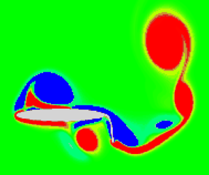
3.2. $\kappa h=1.2$: mild jet-switching (quasi-periodic dynamics)

With an increase in $\kappa h$, the magnitude of the wake deflection angle increases, and a jet-switching behaviour is seen to take place around $\kappa h = 1.2$; see figure 17. Figure 18(a) shows that $\varTheta$ changes its sign from positive to negative and vice versa, multiple times. The modulating oscillation in the $C_D$ time history (figure 19a) represents the quasi-periodic behaviour of the flow field, which can be confirmed from the corresponding reconstructed phase space showing a toroidal portrait; see figure 19(b). The presence of quasi-periodicity can be proven further by the frequency spectra, which comprise two incommensurate frequencies, $f_1=1.27$ and $f_2=0.61$, along with other non-harmonic peaks that are in a linear combination of these two; see figure 19(c). These incommensurate frequency bands are also visible in the wavelet spectra (figure 19d). The quasi-periodic wake interactions trigger jet-switching by inducing small changes in vortex strengths and vortex core locations in different cycles (Majumdar et al. Reference Majumdar, Bose and Sarkar2020b). As a result, the distances between the wake vortices change, leading to alternate dominance of upward and downward deflecting couples through the ‘vortex pairing’ process. The alternate dominance of the symmetry-breaking couples is depicted in terms of the variation in $U_{ dipole}$-ratio in figure 18(b). The dominant symmetry-breaking couple, while convecting downstream, pulls the fluid behind it, forcing the mean jet to deflect in the direction of its self-induced velocity (Godoy-Diana et al. Reference Godoy-Diana, Marais, Aider and Wesfreid2009). The subsequent vortices follow the path dictated by the dominant couple, resulting in a deflected street. As the relative dominance shifts alternately between the upward deflecting $\boldsymbol {A}\unicode{x2013}\boldsymbol {B}$ and downward deflecting $\boldsymbol {B}\unicode{x2013}\boldsymbol {C}$, they force the vortex street to switch the deflection direction alternately.

Figure 17.

For $\kappa h=1.2$, rigid tail: instantaneous vorticity (top) and velocity magnitude (bottom) contours showing mild jet-switching.

Figure 18.

For $\kappa h=1.2$, rigid tail: (a) wake deflection angle, (b) quantitative measures associated with the vortex system. Alternate dominance of the upward and downward deflecting vortex couples leads to jet-switching.

Figure 19.

For $\kappa h=1.2$, rigid tail, time series analysis of $C_D$ indicates quasi-periodic dynamics: (a) time history, (b) reconstructed phase portrait, (c) frequency spectra, and (d) wavelet transform.

3.3. $\kappa h=1.5$: prominent jet-switching with higher deflection angles (dynamical state of intermittency)

As $\kappa h$ is increased further to $1.5$, the jet-switching phenomenon becomes more prominent and the vortex street fluctuates with higher deflection angles compared to the previous case; see figure 20. The rapidity of switching also increases notably in this regime. The augmentation of jet-switching is triggered by strong intermittent perturbations from the primary LEV and its subsequent interactions with the TEV (as is discussed later in this subsection). As a result, the quasi-periodic pattern gets intermittently laden with irregular windows of chaotic bursts. In the nonlinear dynamics literature, such temporal patterns in which the system alternates irregularly between the states of quasi-periodicity and chaos are known as type-II intermittency (Hilborn et al. Reference Hilborn2000). The $C_D$ time history in figure 21(a) shows two such typical chaotic windows (marked by rectangular boxes $B_1$ and $B_2$) in between the quasi-periodic modulations. Note that the reconstructed phase space (figure 21b) and the frequency spectra (figure 21c) are unable to capture the properties of these intermittent behaviours, and reflect an average quasi-periodic behaviour instead. However, the temporal evolution of the frequency content presented in the wavelet spectra (figure 21d) captures clearly the intermittency behaviour through the sporadic bursts of broadband frequencies. The recurrence plot in figure 22 also identifies the two different dynamical states (quasi-periodic and chaotic) present in the system. The quasi-periodic state is characterised by the unequally spaced lines parallel to the main diagonal, whereas the short and broken lines along with isolated points (marked by windows $B_1$ and $B_2$ in figure 22) are representative of the chaotic state.

Figure 20.

Rigid tail configuration; variation in the wake deflection angle.

Figure 21.

For $\kappa h=1.5$, rigid tail, time series analysis of $C_D$ during type-II intermittency: (a) time history, (b) reconstructed phase portrait, (c) frequency spectra, and (d) wavelet transform.

Figure 22.

For $\kappa h=1.5$, rigid tail: recurrence plot of $C_D$ (depicting intermittency).

Recall that in the quasi-periodic regime, jet-switching started through the process of alternate dominance of upward and downward deflecting couples. The marginal shifts in the positions of the wake vortices was instrumental in flipping this dominance, and the LEVs had no direct contribution in jet-switching. However, during the state of intermittency, LEVs become important in the switching process through LEV–TEV interactions as the chaotic bursts provide strong perturbations in the near-field region. This results in the formation of strong symmetry-breaking couples at the trailing edge. A similar near-field behaviour was also observed by Bose et al. (Reference Bose, Gupta and Sarkar2021) for a no-tail configuration. For the present case, figure 23 shows the evolution of the primary LEVs ($\boldsymbol {L1}\unicode{x2013}\boldsymbol {L16}$) tracked for eight consecutive flapping cycles during the chaotic window $B_1$. The snapshots are presented for the same phases of the cycles, and they are chosen during the ends of upstrokes and downstrokes. The primary LEVs are named differently for different flapping cycles in figure 23 as their strengths and locations differ from one cycle to another during the chaotic window. Towards the end of the upstrokes, aperiodic leading-edge separation is observed that leads to shedding of vortex couples of different strengths at different cycles, either from the leading edge ($\boldsymbol {C1}$) or from the mid-surface ($\boldsymbol {C2}$). Shedding of leading-edge couples from the lower surface is hindered during a few cycles by the circumnavigation of another couple on the upper surface (e.g. see $\boldsymbol {L5}$ at $t/T = 113.25$ in figure 23a). This aperiodic growth and convection of the LEVs affect their subsequent interactions with the TEVs considerably.

Figure 23.

For $\kappa h=1.5$, rigid tail: LEV behaviour during the aperiodic window $B_1$ towards the end of (a) upstrokes and (b) downstrokes.

In order to understand the role of intermittency in enhancing jet-switching, the chronology of vortex interactions from five consecutive cycles ($112{\rm th}$ to $116{\rm th}$) during chaotic window $B_1$ is presented in figure 24. In the $112{\rm th}$ cycle, leading-edge couple $\boldsymbol {C1}$ interacts with the nascent TEVs, $\boldsymbol {T1}$ and $\boldsymbol {T2}$, which were produced during consecutive half-strokes. Consequently, $\boldsymbol {T1}$ is not able to convect away but it stays close to $\boldsymbol {T2}$, which ensures a local dominance of downward deflecting couple $\boldsymbol {T2}\unicode{x2013}\boldsymbol {T1}$ (similar to couple $\boldsymbol {B}\unicode{x2013}\boldsymbol {C}$ of figure 13b). A similar set of events takes place during the $115{\rm th}$ cycle as well, where $\boldsymbol {C2}$ influences the shedding of $\boldsymbol {T3}$ and $\boldsymbol {T4}$, resulting eventually in the dominance of downward deflecting $\boldsymbol {T4}\unicode{x2013}\boldsymbol {T3}$ (at $t/T = 116$ in figure 24t). Thus during the chaotic bursts in the intermittency regime, the primary LEV structures (say, $\boldsymbol {C1}$ or $\boldsymbol {C2}$) influence directly the shedding and convection of the TEVs (say, $\boldsymbol {T1}$ and $\boldsymbol {T2}$, or $\boldsymbol {T3}$ and $\boldsymbol {T4}$) through LEV–TEV interactions. This provides an additional impetus towards the formation of the symmetry-breaking couples, resulting in higher deflection angles and enhancement of the jet-switching process. Our previous studies (Majumdar et al. Reference Majumdar, Bose and Sarkar2020b; Bose et al. Reference Bose, Gupta and Sarkar2021) and the present findings confirm that the LEV shedding and its subsequent interactions with the TEV are instrumental in the formation of the symmetry-breaking couples at the trailing edge, leading to vigorous jet-switching.

Figure 24.

For $\kappa h=1.5$, rigid tail: instantaneous vorticity contours during $112{\rm th}$ to $116{\rm th}$ cycles.

Note that the deflection angles reported in the present study, during the prominent jet-switching at $\kappa h = 1.5$, are smaller comparatively ($<15^{\circ }$) than that reported in the experimental results of Heathcote & Gursul (Reference Heathcote and Gursul2007b). This can be attributed possibly to the lower $Re$ regime considered here, which is at least two orders of magnitude lower than that of the above-mentioned experimental study. Liang et al. (Reference Liang, Ou, Premasuthan, Jameson and Wang2011) and Zheng & Wei (Reference Zheng and Wei2012) have shown that the wake deflection angle varies considerably with $Re$, and a decrease in $Re$ results in a decrease in deflection angle as well. Besides, in the experiments with rigid and flexible teardrop foils under quiescent flow, Heathcote & Gursul (Reference Heathcote and Gursul2007b) observed the deflection angle to be higher than uniform inflow cases. Thus use of uniform free stream in the present simulations could also be another possible reason for encountering smaller angles compared to Heathcote & Gursul (Reference Heathcote and Gursul2007b).

4.1. Flexibility level I: deflected wake pattern associated with quasi-periodic dynamics

In contrast to the rigid tail configuration, the tail with flexibility level I ($\gamma =0.1$) exhibits a downward deflected reverse Kármán street without any switching (figure 25a). In this case, the $C_D$ time history reflects distinct quasi-periodic dynamics without any trace of intermittency (figure 26a). The corresponding reconstructed phase space depicts a well-developed toroidal portrait without any irregularities, which confirms the state to be pure quasi-periodic (figure 26b). The corresponding frequency spectrum is comprised of two incommensurate frequencies ($f_1=1.27$ and $f_2=0.87$), with other peaks being their linear combinations, which is again indicative of quasi-periodicity (figure 26c). The existence of these two incommensurate frequencies in the form of two narrow bands is also evident from the scalogram of the $C_D$ time history in figure 26(d). Quasi-periodicity is also visible from the recurrence plot presented in figure 27, showing unequally spaced lines parallel to the main diagonal. To establish the presence of quasi-periodicity through a direct flow-field quantity, correlation coefficients $\rho (t)$ of the vorticity field are estimated. For details of the formulation of $\rho (t)$, please refer to our earlier study, Badrinath et al. (Reference Badrinath, Bose and Sarkar2017). The variation of the maximum $\rho (t)$ between $0.5$ to $1$ confirms the fact that the flow structures do not exactly repeat, nor are they completely different in consecutive cycles (figure 25b), which points to a quasi-periodic scenario. The details of the flow-field behaviour responsible for this change in the dynamics, in comparison to the rigid case, will be discussed in §§ 4.3 and 4.4.

Figure 25.

For $\kappa h=1.5$, flexibility level I: (a) downward deflected vortex street, and (b) vorticity correlation.

Figure 26.

For $\kappa h=1.5$, flexibility level I, time series analysis of $C_D$ indicates quasi-periodic dynamics: (a) time history, (b) reconstructed phase portrait, (c) frequency spectra, and (d) wavelet transform.

Figure 27.

For $\kappa h=1.5$, flexibility level I: recurrence plot of $C_D$.

4.2. Flexibility level II: symmetric reverse Kármán wake with periodic dynamics

As the flexibility increases to level II, the trailing wake shows a reverse Kármán street without any switching or even any strong deflection (figure 28a). Contrary to both the cases of rigid and flexibility level I, the flow-field aperiodicity disappears in level II, and the wake vortices repeat almost exactly in consecutive cycles. Detailed flow-field comparisons are presented in §§ 4.3 and 4.4. The corresponding $C_D$ time history has no modulations in its amplitude (figure 29a), and instead of a toroidal shape, two distinct closed loops in the reconstructed phase space are seen. The latter represent a period-2 signature; see figure 29(b). The frequency spectra (figure 29c) and the wavelet spectra (figure 29d) highlight a dominant frequency peak along with the subharmonics and superharmonics only. The uniformly spaced continuous lines parallel to the main diagonal in the recurrence plot as shown in figure 30 are characteristic of a periodic signal too. Also, the maximum correlation coefficient ($\rho$) of the vorticity field remains unity, which establishes the periodicity of the flow field (figure 28b).

Figure 28.

For $\kappa h=1.5$, flexibility level II: (a) mildly deflected wake, and (b) vorticity correlation.

Figure 29.

For $\kappa h=1.5$, flexibility level II, time series analysis of $C_D$ indicates periodic dynamics: (a) time history, (b) reconstructed phase portrait, (c) frequency spectra, and (d) wavelet transform.

Figure 30.

For $\kappa h=1.5$, flexibility level II: recurrence plot of $C_D$.

4.3. Difference in the wake deflection characteristics between the rigid and flexible configurations

It is evident that the flow topology as well as the dynamical states undergoes a significant change as flexibility is introduced in the system, and as the flexibility increases, the trailing wake becomes more organised. The vigorous jet-switching at $\kappa h = 1.5$ seen for the rigid configuration is suppressed completely, and the trailing wake returns to a periodic reverse Kármán street at the higher flexibility level.

The instantaneous vorticity and velocity magnitude contours depicting the deflection angles of the jet at a few chosen cycles corresponding to the rigid and flexible tail configurations are compared in figure 31. The continuous temporal evolution of the flow fields for the respective cases are presented in supplementary movies 1, 2 and 3. Here, vigorous jet-switching with high deflection angles is observed for the rigid case. A downward deflected wake with $\varTheta =-2.6$ is seen at $t/T=104.0$, the deflection direction changes with time and the shed vortices start to move upwards, giving an upward deflected wake with $\varTheta =4.2$ at $t/T=110.0$ (figures 31a–d). Such switchings between downward and upward directions continue to take place for the rigid case (see at $t/T=119.0$ with $\varTheta =-6.6$, and at $t/T=126.0$ with $\varTheta =3.4$) . However, this gets inhibited with the introduction of flexibility, and at flexibility level I, the wake deflection direction no longer switches. It remains downward deflected for all time, with small time-dependent changes in its deflection angle (see figures 31e–h). With flexibility increasing to level II, the wake gets more regularised. It reorganises into a periodic reverse Kármán pattern with a very small deflection angle (figures 31i–l). The jet-switching and its inhibition at different flexibility levels reflect directly on the aerodynamic loads as well. This has been presented in terms of period-average lift coefficient in § 3 of the supplementary material.

Figure 31.

For $\kappa h=1.5$, comparison of instantaneous vorticity fields and corresponding velocity magnitude contours for (a–d) rigid tail, (e–h) flexibility level I, and (i–l) flexibility level II.

The flip in the relative dominance of the upward and downward deflecting couples is responsible for the manifestation of jet-switching, and the $\xi$-ratio is the primary factor dictating the dominance of the symmetry-breaking couples (Majumdar et al. Reference Majumdar, Bose and Sarkar2020b). Three representative cycles, at $t/T=108, 116,126$, are chosen to compare the $\xi$-ratios for rigid and flexible configurations in figure 32. The complete time evolution of the $\xi$-ratio is presented later, in figure 33(c). For the rigid tail, the $\xi$-ratio of $\boldsymbol {A}\unicode{x2013}\boldsymbol {B}$ to $\boldsymbol {B}\unicode{x2013}\boldsymbol {C}$ is seen to be less than unity ($\xi _{AB}/\xi _{BC}=0.82$) at $t/T = 108$. Hence $\boldsymbol {A}\unicode{x2013}\boldsymbol {B}$ forms the dominant couple, and this induces an upward jet that maintains the upward deflected wake subsequently (figures 32a,d,g). However, at $t/T=116.0$, the $\xi$-ratio becomes $1.24$, and the dominance is transferred to $\boldsymbol {B}\unicode{x2013}\boldsymbol {C}$, which induces a downward jet causing the subsequently shed vortices to follow a downward deflected path (see at $t/T=116.0$ in figures 32a,d,g). At $t/T=126.0$, the $\xi$-ratio again becomes less than 1, indicating the dominance of upward deflecting $\boldsymbol {A}\unicode{x2013}\boldsymbol {B}$ that gives way to another switching. The same was confirmed from the velocity magnitude contour plots in figures 31(a–d) as well.

Figure 32.

For $\kappa h=1.5$, comparison of trailing-wake patterns showing the $\xi -$ratio for (a,d,g) rigid tail, (b,e,h) flexibility level I, and (c, f,i) flexibility level II.

Figure 33.

For $\kappa h=1.5$, variation of: (a) deflection angle, (b) dipole velocity ratio, (c) distance ratio, and (d) average circulation ratio, for different aft-tail configurations.

The corresponding $\xi$-ratio for flexibility level I remains more than unity at all times with a varying magnitude, causing the wake to remain downward deflected, with the angle of deflection varying with time (figures 32b,e,h). Since the $\xi$-ratio remains always greater than 1, $\boldsymbol {B}\unicode{x2013}\boldsymbol {C}$ is able to maintain its continuous dominance to pull the wake downwards at every cycle; see figures 32(b,e,h). As an outcome, the phenomenon of jet-switching gets suppressed. At flexibility level II, the $\xi$-ratio remains almost constant and quite close to unity ($\approx 0.9$), facilitating the upward deflecting couple $\boldsymbol {A}\unicode{x2013}\boldsymbol {B}$ to maintain a small dominance forever. This results in an almost symmetric (with a negligible upward deflection) stable reverse Kármán street, as shown in figures 32(c, f,i).

The results can also be visualised quantitatively through a comparison of the time histories of different measures, as shown in figure 33. For the rigid tail, $\varTheta$ crosses the zero mark multiple times, indicating multiple switchings; see figure 33(a). For flexibility level I, $\varTheta$ varies with time but never changes its sign; hence jet-switching is absent and the wake stays downward deflected for all time. For flexibility level II, $\varTheta$ remains nearly constant with time with a very small positive value close to zero, representative of a vortex street having a mild upward deflection. The temporal evolution of $U_{{dipole}}$-ratio, $\xi$-ratio and $\varGamma _{{avg}}$-ratio are shown in figures 33(b), 33(c) and 33(d), respectively. The $\xi$-ratio, and therefore the $U_{{dipole}}$-ratio, undergoes significant modulations around unity for the rigid case, leading to frequent shifts in the dominance of the symmetry-breaking couples that get manifested as vigorous switching. Note that the variation of the $\varGamma _{{avg}}$-ratio is relatively lesser, signifying its unimportant role in jet-switching. For flexibility level I, the fluctuations in $\xi$-ratio and $U_{{dipole}}$-ratio are seen to stay always above and below unity, respectively, as no change takes place in the deflection direction. With the increase in flexibility to level II, the fluctuations in these measures come down significantly as the wake gets reorganised into an almost symmetric reverse Kármán pattern.

4.4. Underlying vortex interaction mechanisms

From the above results, flexibility emerges as a crucial system parameter that can be manipulated to alter the dynamics as well as suppress the phenomenon of jet-switching. The near-field vortex interactions that lead to this suppression are examined in this subsection. It is important to understand the mechanism of change in the dominance and formation of the symmetry-breaking couples under the flexible tail configurations. In this regard, the chronology of vortex interactions during a typical flapping cycle is presented for flexibility levels I and II in figure 34. For flexibility level I, LEV $\boldsymbol {L1}^*$ initially sheds as a couple having a strong CCW and a fragile CW component at the start of the upstroke (see at $t/T=110.125$ in figure 34a). Subsequently, the weaker CW component gets convected away, and the stronger CCW counterpart reattaches on the lower surface around the mid-chord, and gives rise to couple $\boldsymbol {C1}^*$ (see at $t/T=110.375$ in figure 34a). In the next half-cycle, $\boldsymbol {C1}^*$ is shed from the lower surface and interacts with the CW TEV $\boldsymbol {T1}^*$, forming eventually a dominant downward deflected symmetry-breaking couple. The CW LEV $\boldsymbol {L2}^*$ does not shed from the foil (see $t/T=110.625$ to $110.75$ in figure 34b), but remains attached to the upper surface near the leading-edge and gets flattened gradually over the body ($t/T=110.875$ to $111.0$ in figure 34b). Note that $\boldsymbol {L2}^*$ does not participate in any interactions with the TEV. Therefore, the LEV–TEV interaction takes place asymmetrically and only at the lower surface of the foil. The asymmetric LEV–TEV interactions prevent a full reversal of the deflection direction, as only a downward deflected symmetry-breaking couple forms at every cycle. As the associated dynamical state is quasi-periodic, the strength of this couple varies from one cycle to another, resulting in a time-varying $\varTheta$ behaviour (figure 33a).

Figure 34.

For $\kappa h = 1.5$, comparison of near-field vortex interactions at the $111{\rm th}$ cycle: (a) first half-cycle, (b) second half-cycle; each left-hand column shows flexibility level I, and each right-hand column shows flexibility level II.

As the flexibility increases to level II, the flow becomes more regularised, and the vortex interactions become symmetric between the upper and lower surfaces. Unlike level I, in this case an isolated CCW LEV, $\boldsymbol {L1}^**$, is formed, which stays close to the lower surface of the foil. However, similar to flexibility level I, $\boldsymbol {L1}^**$ forms couple $\boldsymbol {C1}^**$ with a shear layer vortex while convecting towards the trailing edge. The strength of $\boldsymbol {C1}^**$ is considerably lower than that of $\boldsymbol {C1}^*$ in the level I case, and it remains very close to the surface while moving downstream. Subsequently, $\boldsymbol {C1}^**$ interacts with the highly deformed tail structure and gets trapped near it, preventing the couple from interacting directly with the TEV $\boldsymbol {T2}^**$. Similar events occur on the upper surface in the following half-cycle as well, where LEV $\boldsymbol {L2}^**$ forms couple $\boldsymbol {C2}^**$. Similar to $\boldsymbol {C1}^**$, $\boldsymbol {C2}^**$ also does not get a chance to interact with the TEV due to its interaction with the highly deformed tail. The large bending of the flexible aft-tail inhibits the LEVs from interacting with the shed TEVs directly, thus preventing the formation of the symmetry-breaking couples that are the main agencies behind jet-switching. As a result, the near-wake vortices get well organised and finally settle into a near symmetric reverse Kármán wake through the merging of the same-signed vortices.

4.5. Flexible deformation of the aft-tail leading to suppression of jet-switching

Deformation of the flexible tail alters the interactions of the near-field vortices that decides the fate of the overall far-wake pattern. The deflection envelope and the phase plot of the tail-tip are shown in figure 35. The flexible tail acts as an inextensible cantilever beam clamped at the trailing edge of the foil. At flexibility level I, the tail is seen to bend predominantly in its first mode shape, as presented in figure 35(a). At flexibility level II, it exhibits mixed-mode oscillations involving both first and second modes with a significantly higher amplitude (figure 35c). In both these cases, the tip of the tail exhibits a ‘figure-of-eight’ motion (figures 35b,d). The phase portrait corresponding to level I in figure 35(b) is clearly indicative of a quasi-periodic dynamics, and this is triggered by the structure's coupled interactions with the quasi-periodic flow dynamics (presented in § 4.1). The flexibility level II case shows two distinct loops, representative of a period-2 dynamics (§ 4.2). Note that the flexible bending of the tail is influenced primarily by the trailing-edge separation in both the cases. However, the mild bending seen for level I does not prevent the LEV and the secondary vortices from interacting with the TEV. This gives way to the formation of the primary symmetry-breaking couple. At level II, the tail bends severely and even goes in the backward direction, taking an arch-like shape at the extreme positions. This highly deformed shape traps the LEVs and prevents the LEV–TEV interactions. Therefore, the resulting wake shape is dictated by the shedding of the strong TEVs, and the spatial symmetry of the wake is more or less retained.

Figure 35.

For $\kappa h=1.5$, deflection envelopes and phase portraits for the tip displacement of the flexible tail for flexibility level I (a,b) and flexibility level II (c,d). (a) Mode shape structure for flexibility level I. (b) Phase plot of the free end of the trailing edge for flexibility level I. (c) Mode shape structure for flexibility level II. (d) Phase plot of the free end of the trailing edge for flexibility level II.

The pressure coefficient ($C_P$) contours are compared in figure 36 for the three different tail configurations at the end of upstroke and downstroke of a typical cycle ($t/T=110.25$ and $110.75$, respectively). For the rigid tail case, a large low-pressure zone is seen to be present near the leading edge. This is followed by a high-pressure zone extended up to the trailing end of the tail along the lower surface, at the beginning of the upstroke. This creates a strong adverse pressure gradient. Also, a reverse flow is observed close to the leading edge; see figure 36(a), where the velocity field is marked by the arrows. A strong CCW LEV ($\boldsymbol {L2}$) gets shed due to the strong adverse pressure gradient, and, it interacts with the TEV subsequently to result in the formation of a symmetry-breaking couple. A similar strong low-pressure zone followed by a high-pressure zone on the upper surface of the foil is observed during the end of the downstroke (see figure 36d). Therefore, separation of the LEVs ($\boldsymbol {L2}$ and $\boldsymbol {L10}$, corresponding to figure 23) takes place from both upper and lower surfaces. This in turn results in the formation of upward and downward deflected symmetry-breaking couples. As discussed in the previous subsection, these symmetry-breaking couples are responsible for triggering jet-switching in case of the rigid configuration. In contrast, for flexibility level I, separation of the CCW LEV ($\boldsymbol {L1}^*$) takes place only during the upstroke. Due to a high adverse pressure gradient, counter-clockwise LEVs are formed and separated at the lower surface during the upstroke. But the flow on the upper surface remains smooth, as indicated by the unidirectional vector field (figure 36(b) at $t/T=110.25$). During the downstroke, a reverse flow is observed along both the surfaces, and the CW LEV ($\boldsymbol {L2}^*$) in the upper surface does not get separated but circumnavigates the leading edge to traverse in the lower surface. So LEV–TEV interaction occurs only along the lower surface in every cycle. Hence the trailing wake remains deflected in the same direction always – though, depending on the strengths of the LEV and the TEV, the magnitude of the deflection angle changes as was presented in § 4.1. For level II, the low- and high-pressure zones get reduced significantly due to the severe deformation of the tail; see figures 36(c, f). Furthermore, the downstream low-pressure zone comes much closer to the foil, increasing the suction. This pulls the upstream fluid at a faster rate as indicated by the longer lengths of the arrows. Therefore, the LEVs $(\boldsymbol {L1}^**$ and $\boldsymbol {L2}^**)$ do not get sufficient time to grow and separate. Instead, the LEVs stay close to the body, roll over the surface, and get trapped eventually in the vicinity of the flexible tail. No shedding of them happens during the upstroke or the downstroke. The flow remains almost periodic, without the formation of any symmetry-breaking couples, thereby inhibiting the jet-switching process.

Figure 36.

For $\kappa h=1.5$, comparison of pressure coefficient $(C_P)$ contours during the end of (a–c) upstroke ($t/T=110.25$) and (d–f) downstroke ($t/T=110.75$), for (a,d) rigid tail, (b,e) flexibility level I, and (c, f) flexibility level II. Lengths of arrows indicate the magnitude of the velocity vector field.

4.6. Effect of the aft-tail length $(L_t)$ on the flow-field dynamics

The results presented so far have been able to identify tail flexibility as a potential instrument for inhibiting jet-switching, by following the flow-field interactions systematically and interlinking them with the associated nonlinear dynamical states. In the earlier subsections, interactions of the near-field vortices have been investigated, and the corresponding nonlinear dynamical states were established using different qualitative and quantitative flow-field measures, and time series tools. The flow mechanisms of flexibility influencing directly the formation of symmetry-breaking couples, which dictate the wake deflection characteristics and play a pivotal role in triggering jet-switching (Godoy-Diana et al. Reference Godoy-Diana, Marais, Aider and Wesfreid2009; Zheng & Wei Reference Zheng and Wei2012; Majumdar et al. Reference Majumdar, Bose and Sarkar2020b), were also highlighted. It is worth noting that in the previous subsections, the length of the flexible tail was kept constant, and the non-dimensional bending rigidity has been varied to increase the flexibility. However, one can change the degree of flexibility by changing the aft-tail length as well, keeping the non-dimensional bending rigidity fixed (which is not a function of the length in any implicit manner). The effect of aft-tail length on the wake dynamics is not clear from the existing literature and is of interest to the present subsection. The present results obtained so far in this direction indicate that the tail length, being another crucial parameter to govern the flexibility level of the system, can play an important role in regularising a non-periodic wake. Therefore, both the non-dimensional bending rigidity and the aft-tail length can be considered as alternative choices for benefiting the design of engineering devices, ensuring a periodic wake to maximise the aerodynamic efficiency.

Here, results are presented for a typical case of aft-tail length of $L_t=0.38c$, for $\gamma = 0.1$ and $\kappa h=1.5$. As was shown in § 4.1, the wake deflected downwards with quasi-periodic dynamics for $L_t=0.3c$. But as $L_t$ is increased to $0.38c$, the wake turns periodic, as can be confirmed by the $C_D$ time history shown in figure 37(a), which represents a completely periodic response with no amplitude modulation. The closed loop in the corresponding reconstructed phase space, dominant frequency peak with subharmonics and superharmonics in the frequency spectra, and narrow bands of harmonic frequencies in the wavelet spectra, further establish the periodic dynamics; see figures 37(b), 37(c) and 37(d), respectively. The instantaneous vorticity contours for three consecutive cycles ($111{\rm th}$–$113{\rm th}$) are presented in figure 38. The flow field is seen to be repeating exactly from one cycle to another, confirming the periodicity of the wake. In contrast to the tail length $L_t=0.3c$, the vortices are regularised, and the wake can be characterised by a reverse Kármán street with very mild upward deflection ($\varTheta =1.65^{\circ }$) at $L_t=0.38$; see figures 39(a,b). The periodic nature of the flow field is confirmed further quantitatively from the vorticity correlation plot where the maximum value of ${\rho }$ reaches unity in every cycle; see figure 39(c). Here, $\varTheta$ remains nearly constant with time, with a small positive value representative of the vortex street having a mild deflection (figure 40a). A slight dominance of upward deflecting couple $\boldsymbol {A}\unicode{x2013}\boldsymbol {B}$ can be visualised through the temporal evolution of $U_{{dipole}}$-ratio, $\xi$-ratio and $\varGamma _{{avg}}$-ratio presented in figure 40(b). The $\xi$-ratio and $U_{{dipole}}$-ratio are always below and above unity, respectively, and remain constant in every cycle. Therefore, the couple $\boldsymbol {A}\unicode{x2013}\boldsymbol {B}$ always remains dominant, resulting in a slightly upward-looking wake. The continuous temporal evolution of the flow field for the present case is presented in supplementary movie 4.

Figure 37.

Changed tail length: $\kappa h=1.5$, $\gamma = 0.1$, aft-tail length $L_t=0.38c$. Time series analysis of $C_D$ indicates periodic dynamics: (a) time history, (b) reconstructed phase portrait, (c) frequency spectra, and (d) wavelet transform.

Figure 38.

Changed tail length: $\kappa h=1.5$, $\gamma = 0.1$, aft-tail length $L_t=0.38c$. Instantaneous vorticity contours during $111{\rm th}$–$113{\rm th}$ cycles.

Figure 39.

Changed tail length: $\kappa h=1.5$, $\gamma = 0.1$, aft-tail length $L_t=0.38c$. (a) Instantaneous vorticity and (b) velocity magnitude, contours depicting reverse Kármán wake with mild upward deflection; and (c) vorticity correlation.

Figure 40.

Changed tail length: $\kappa h=1.5$, $\gamma = 0.1$, aft-tail length $L_t=0.38c$. (a) Wake deflection angle and (b) quantitative measures associated with the vortex system. Dominant effect of the upward deflecting vortex couple $\boldsymbol {A}\unicode{x2013}\boldsymbol {B}$ results in a positive deflection angle.

The deflection envelope and the corresponding phase plot of the tail-tip are presented in figure 41. The tail bends with a little asymmetry and shows mostly a first-mode oscillation profile. The mechanism by which the tail influences the near field can be understood better from the $C_P$ contour during the end of upstroke and downstroke as shown in figure 42. The downstream low-pressure zone created by the deflection of the tail sucks the upstream fluid at a faster rate, as indicated by the longer lengths of the arrows. Hence the LEVs do not get sufficient time to grow and separate, instead getting trapped in the vicinity of the tail, similar to flexibility level II as was shown in § 4.5. The flow remains periodic without the formation of any symmetry-breaking couples, thereby inhibiting jet-switching and maintaining periodicity. This also evidently underlines the role of the length of the tail in influencing the dynamical transitions of the system. Therefore, an appropriate selection of the aft-tail length and bending rigidity inhibits the aperiodicity in the flow field. To the best of the authors’ knowledge, the effect of aft-tail length in inhibiting the jet-switching and regularising the flow field has not yet been taken up adequately in the existing literature. Note that design of flapping devices based on natural flyers/swimmers would like to avoid aperiodicity to propel efficiently by exploiting the combination of the length of flapping appendages and the wing/fin morphology. The present results contribute towards that by adding insights on the role of flexibility in suppressing the switching and inhibiting aperiodicity in the wake. Currently, the authors are studying the effect of a flexible aft-tail in delaying the onset of aperiodicity at higher values of $\kappa h$.

Figure 41.

Changed tail length: $\kappa h=1.5$, $\gamma = 0.1$, aft-tail length $L_t=0.38c$, (a) Deflection envelopes, mode shape structure. (b) Phase plot of the tail-tip of the flexible tail.

Figure 42.

Changed tail length: $\kappa h=1.5$, $\gamma = 0.1$, aft-tail length $L_t=0.38c$. Pressure coefficient $(C_P)$ contours during the end of (a) upstroke ($t/T=110.25$), and (b) downstroke ($t/T=110.75$).