


1 Introduction
In this article, we study splicing maps between braid varieties, generalizing the constructions of [Reference Gorsky, Kim, Scroggin and Simental17, Reference Gorsky and Scroggin18].
1.1 Splicing braid varieties
We consider the positive braid monoid
 $\mathrm {Br}^{+}_{k}$
. For an element
$\mathrm {Br}^{+}_{k}$
. For an element
 $\beta \in \mathrm {Br}^{+}_{k}$
, the braid variety
$\beta \in \mathrm {Br}^{+}_{k}$
, the braid variety
 $X(\beta )$
is a smooth affine algebraic variety defined in terms of configurations of complete flags in the k-dimensional space
$X(\beta )$
is a smooth affine algebraic variety defined in terms of configurations of complete flags in the k-dimensional space
 $\mathbb {C}^k$
, see Section 4 for a precise definition. In recent years, braid varieties have gained considerable attention due to their connections to character varieties, Legendrian link invariants, cluster algebras, and link homology. Additionally, many classical varieties appearing in geometric representation theory, such as open Richardson varieties or double Bruhat cells, are isomorphic to braid varieties.
$\mathbb {C}^k$
, see Section 4 for a precise definition. In recent years, braid varieties have gained considerable attention due to their connections to character varieties, Legendrian link invariants, cluster algebras, and link homology. Additionally, many classical varieties appearing in geometric representation theory, such as open Richardson varieties or double Bruhat cells, are isomorphic to braid varieties.
From now on, we will assume that
 $\beta $
contains a reduced expression for the longest element
$\beta $
contains a reduced expression for the longest element
 $w_0\in S_k$
as a (not necessarily consecutive) subword (by [Reference Casals, Gorsky, Gorsky, Le, Shen and Simental2, Lemma 3.4], this is without loss of generality). We consider a decomposition
$w_0\in S_k$
as a (not necessarily consecutive) subword (by [Reference Casals, Gorsky, Gorsky, Le, Shen and Simental2, Lemma 3.4], this is without loss of generality). We consider a decomposition
 $\beta = \beta ^1\beta ^2$
of
$\beta = \beta ^1\beta ^2$
of
 $\beta $
as a product of positive braids. A splicing map is an open embedding
$\beta $
as a product of positive braids. A splicing map is an open embedding
 $$\begin{align*}X\left(\widetilde{\beta}^1\right) \times X\left(\widetilde{\beta}^2\right) \to X(\beta), \end{align*}$$
where
 $\widetilde {\beta }^1$
and
$\widetilde {\beta }^1$
and
 $\widetilde {\beta }^2$
are braids explicitly determined by
$\widetilde {\beta }^2$
are braids explicitly determined by
 $\beta ^1$
and
$\beta ^1$
and
 $\beta ^2$
and some auxiliary data from the splicing map. Motivated by their applications to the study of the Khovanov–Rozansky homology of torus links, splicing maps are studied by the first and third authors in [Reference Gorsky and Scroggin18, Reference Scroggin25] in the special case of the top positroid variety in the Grassmannian
$\beta ^2$
and some auxiliary data from the splicing map. Motivated by their applications to the study of the Khovanov–Rozansky homology of torus links, splicing maps are studied by the first and third authors in [Reference Gorsky and Scroggin18, Reference Scroggin25] in the special case of the top positroid variety in the Grassmannian
 $\mathrm {Gr}(k,n)$
. This construction was later generalized by the authors in [Reference Gorsky, Kim, Scroggin and Simental17] to the case of skew shaped positroids, that is, those positroids that are open in the Grassmannian Richardson variety that contains them. In a different guise, another example of a splicing map is given by [Reference Eberhardt and Stroppel6, Definition 3.1], where these maps are used to construct a convolution product on the compactly supported cohomology of Grassmannian Richardson varieties. Our first construction is a common generalization of these.
$\mathrm {Gr}(k,n)$
. This construction was later generalized by the authors in [Reference Gorsky, Kim, Scroggin and Simental17] to the case of skew shaped positroids, that is, those positroids that are open in the Grassmannian Richardson variety that contains them. In a different guise, another example of a splicing map is given by [Reference Eberhardt and Stroppel6, Definition 3.1], where these maps are used to construct a convolution product on the compactly supported cohomology of Grassmannian Richardson varieties. Our first construction is a common generalization of these.
Assume that
 $\beta = \sigma _{i_1}\dots \sigma _{i_r}$
, where
$\beta = \sigma _{i_1}\dots \sigma _{i_r}$
, where
 $\sigma _1, \dots , \sigma _{k-1}$
are the usual simple generators of the positive braid monoid
$\sigma _1, \dots , \sigma _{k-1}$
are the usual simple generators of the positive braid monoid
 $\mathrm {Br}^{+}_{k}$
. For an element
$\mathrm {Br}^{+}_{k}$
. For an element
 $u \in S_k$
, we denote by
$u \in S_k$
, we denote by
 $\underline {u} \in \mathrm {Br}_{k}^{+}$
its braid lift of minimal length. For each
$\underline {u} \in \mathrm {Br}_{k}^{+}$
its braid lift of minimal length. For each
 $r_1 = 1, \dots , r$
, we let
$r_1 = 1, \dots , r$
, we let
 $\beta ^1 = \beta ^1(r_1) = \sigma _{i_1}\dots \sigma _{i_{r_1}}$
and
$\beta ^1 = \beta ^1(r_1) = \sigma _{i_1}\dots \sigma _{i_{r_1}}$
and
 $\beta ^2 = \beta ^2(r_1) = \sigma _{i_{r_1+1}}\dots \sigma _{i_r}$
, so that
$\beta ^2 = \beta ^2(r_1) = \sigma _{i_{r_1+1}}\dots \sigma _{i_r}$
, so that
 $\beta = \beta ^1\beta ^2$
. For each element
$\beta = \beta ^1\beta ^2$
. For each element
 $w \in S_k$
, we define a principal open set
$w \in S_k$
, we define a principal open set
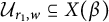 $\mathcal {U}_{r_1,w} \subseteq X(\beta )$
(see (5.1)) and prove the following.
$\mathcal {U}_{r_1,w} \subseteq X(\beta )$
(see (5.1)) and prove the following.
Theorem 1.1 For each
 $r_1 = 1, \dots , r$
and
$r_1 = 1, \dots , r$
and
 $w \in S_k$
, we have an isomorphism of algebraic varieties
$w \in S_k$
, we have an isomorphism of algebraic varieties
 $$ \begin{align} \Psi_{r_1, w}: X\left(\underline{(w^{-1}w_0)}\beta^1\right) \times X\left(\beta^2\underline{w}\right) \xrightarrow{\cong} \mathcal{U}_{r_1,w}, \end{align} $$
where
 $w_0$
is the longest element of
$w_0$
is the longest element of
 $S_k$
.
$S_k$
.
Remark 1.2 For simplicity, we choose to state and prove all the results in this article only in type A. However, it is not hard to see from the proof (see Section 5 below) that Theorem 1.1 holds in arbitrary type.
More precisely, the braid variety
 $X(\beta )$
is defined via chains of flags with specified relative positions, and the open set
$X(\beta )$
is defined via chains of flags with specified relative positions, and the open set
 $\mathcal {U}_{r_1, w}$
is given by the condition that the
$\mathcal {U}_{r_1, w}$
is given by the condition that the
 $r_1$
-th flag is transverse to the coordinate flag
$r_1$
-th flag is transverse to the coordinate flag
 $\mathcal {F}(w_0w)$
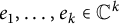
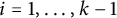
. Schematically, the inverse
$\mathcal {F}(w_0w)$
. Schematically, the inverse
 $\Phi _{r_1, w}$
of the map
$\Phi _{r_1, w}$
of the map
 $\Psi _{r_1, w}$
is given as follows:
$\Psi _{r_1, w}$
is given as follows:

In (1.2), the flags on the bottom row are all coordinate flags, and their successive relative positions spell a reduced word for
 $w_0$
. If
$w_0$
. If
 $\mathcal {F}^{r_1}$
is transverse to
$\mathcal {F}^{r_1}$
is transverse to
 $\mathcal {F}(w_0w)$
, then the blue part of the diagram belongs, up to an overall shift, to
$\mathcal {F}(w_0w)$
, then the blue part of the diagram belongs, up to an overall shift, to
 $X\left (\left (\underline {w^{-1}w_0}\right )\beta ^1\right )$
. Similarly, the red part of (1.2) belongs to
$X\left (\left (\underline {w^{-1}w_0}\right )\beta ^1\right )$
. Similarly, the red part of (1.2) belongs to
 $X\left (\beta ^2\underline {w}\right )$
.
$X\left (\beta ^2\underline {w}\right )$
.
Note that it may be that
 $\mathcal {U}_{r_1,w} = \emptyset $
, in which case the product on the left of (1.1) is also empty. This phenomenon can be easily understood using the notion of the Demazure product (see Section 2). The open set
$\mathcal {U}_{r_1,w} = \emptyset $
, in which case the product on the left of (1.1) is also empty. This phenomenon can be easily understood using the notion of the Demazure product (see Section 2). The open set
 $\mathcal {U}_{r_1,w}$
is not empty precisely when both Demazure products
$\mathcal {U}_{r_1,w}$
is not empty precisely when both Demazure products
 $\delta \left (\underline {(w^{-1}w_0})\beta ^1\right )$
and
$\delta \left (\underline {(w^{-1}w_0})\beta ^1\right )$
and
 $\delta \left (\beta ^2\underline {w}\right )$
are equal to
$\delta \left (\beta ^2\underline {w}\right )$
are equal to
 $w_0$
.
$w_0$
.
One advantage of the maps (1.1) is that, for fixed
 $r_1 = 1, \dots , r,$
we have
$r_1 = 1, \dots , r,$
we have
 $$\begin{align*}\bigcup_{w \in S_k}\mathcal{U}_{r_1,w} = X(\beta), \end{align*}$$
that is, the sets
 $\mathcal {U}_{r_1,w}$
form a cover of
$\mathcal {U}_{r_1,w}$
form a cover of
 $X(\beta )$
by open subsets which are themselves isomorphic to products of braid varieties for simpler braids.
$X(\beta )$
by open subsets which are themselves isomorphic to products of braid varieties for simpler braids.
A disadvantage is that the properties of the map (1.1) remain mysterious at the moment, especially those regarding the relationship between (1.1) and the cluster structure on
 $X(\beta )$
constructed in [Reference Casals, Gorsky, Gorsky, Le, Shen and Simental2, Reference Galashin, Lam and Sherman-Bennett12, Reference Galashin, Lam, Sherman-Bennett and Speyer13]. The following surprising inequality is an easy consequence of Theorem 1.1 (see Remark 5.8).
$X(\beta )$
constructed in [Reference Casals, Gorsky, Gorsky, Le, Shen and Simental2, Reference Galashin, Lam and Sherman-Bennett12, Reference Galashin, Lam, Sherman-Bennett and Speyer13]. The following surprising inequality is an easy consequence of Theorem 1.1 (see Remark 5.8).
Corollary 1.3 Let
 $f, f_1,f_2$
denote the numbers of frozen variables for
$f, f_1,f_2$
denote the numbers of frozen variables for
 $X(\beta ),X (\underline {(w^{-1}w_0)}\beta ^1)$
and
$X(\beta ),X (\underline {(w^{-1}w_0)}\beta ^1)$
and
 $X\left (\beta ^2\underline {w}\right )$
, respectively. Then we have an inequality
$X\left (\beta ^2\underline {w}\right )$
, respectively. Then we have an inequality
 $$ \begin{align} f_1+f_2\ge f. \end{align} $$
More precisely, we formulate the following conjecture relating the cluster structures.
Conjecture 1.4 For each
 $r_1 = 1, \dots , r$
and
$r_1 = 1, \dots , r$
and
 $w \in S_k$
such that
$w \in S_k$
such that
 $\mathcal {U}_{r_1,w} \not = \emptyset $
, there exists a seed
$\mathcal {U}_{r_1,w} \not = \emptyset $
, there exists a seed
 $\Sigma = (Q, \mathbf {x})$
in
$\Sigma = (Q, \mathbf {x})$
in
 $\mathbb {C}[X(\beta )]$
with cluster variables
$\mathbb {C}[X(\beta )]$
with cluster variables
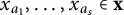 $x_{a_1}, \dots , x_{a_s} \in \mathbf {x}$
such that:
$x_{a_1}, \dots , x_{a_s} \in \mathbf {x}$
such that:
-
(a) The open set
 $\mathcal {U}_{r_1,w}$
is the common non-vanishing locus of
$x_{a_1}, \dots , x_{a_s}$
.
$\mathcal {U}_{r_1,w}$
is the common non-vanishing locus of
$x_{a_1}, \dots , x_{a_s}$
. -
(b) The variety
$\mathcal {U}_{r_1,w}$
is the cluster variety associated with the seed obtained from
$\Sigma $
upon freezing the cluster variables
$x_{a_1}, \dots , x_{a_s}$
. -
(c) The map (1.1) is a quasi-cluster isomorphism.


In particular, Conjecture 1.4(b) ensures that
 $\mathcal {U}_{r_1,w}$
is a cluster chart in
$\mathcal {U}_{r_1,w}$
is a cluster chart in
 $X(\beta )$
in the sense of Muller [Reference Muller23]. The open set
$X(\beta )$
in the sense of Muller [Reference Muller23]. The open set
 $\mathcal {U}_{r_1,w}$
is defined in
$\mathcal {U}_{r_1,w}$
is defined in
 $X(\beta )$
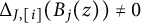
by the non-vanishing of minors
$X(\beta )$
by the non-vanishing of minors
 $\Delta _{ww_0[i],[i]}(M_{r_1}), i=1,\ldots ,k,$
where
$\Delta _{ww_0[i],[i]}(M_{r_1}), i=1,\ldots ,k,$
where
 $M_{r_1}$
is a certain matrix related to the flag
$M_{r_1}$
is a certain matrix related to the flag
 $\mathcal {F}^{r_1}$
in (1.2). Conjecture 1.4(b) then implies that these minors are cluster monomials in the seed
$\mathcal {F}^{r_1}$
in (1.2). Conjecture 1.4(b) then implies that these minors are cluster monomials in the seed
 $\Sigma $
, and their irreducible factors (up to monomials in frozen variables) are precisely
$\Sigma $
, and their irreducible factors (up to monomials in frozen variables) are precisely
 $x_{a_1}, \dots , x_{a_s}$
. The number s of cluster variables that one needs to freeze in Conjecture 1.4 equals
$x_{a_1}, \dots , x_{a_s}$
. The number s of cluster variables that one needs to freeze in Conjecture 1.4 equals
 $$ \begin{align*}s=f_1+f_2-f, \end{align*} $$
which is nonnegative by Corollary 1.3. See Sections 5.2 and 5.3 for more details and examples. Also, see Lemma 5.7 for more details and dependencies between (a) and (c).
1.2 Splicing open Richardson varieties
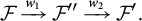
Open Richardson varieties are smooth, affine subvarieties of the flag variety, given by specifying relative positions with respect to the standard flag and the antistandard flag (see Section 5.3 for details). For
 $v \leq w \in S_k$
, the open Richardson variety is
$v \leq w \in S_k$
, the open Richardson variety is
 $$\begin{align*}R(v,w) := \{\mathcal{F} \in \mathcal{F}\ell(k) \mid \mathcal{F}^{\mathrm{std}} \xrightarrow{w} \mathcal{F} \xrightarrow{v^{-1}w_0} \mathcal{F}^{\mathrm{ant}}\}, \end{align*}$$
see Section 2 for details on relative position and unexplained notation. It is known, see, for example, [Reference Casals, Gorsky, Gorsky, Le, Shen and Simental2, Reference Galashin, Lam and Sherman-Bennett12, Reference Galashin, Lam, Sherman-Bennett and Speyer13] and Section 5.3 below, that open Richardson varieties are special cases of braid varieties. Specializing Theorem 1.1 to this setting, we obtain the following result.
Theorem 1.5 For
 $u \leq v \leq w \in S_k$
, define the set
$u \leq v \leq w \in S_k$
, define the set
 $$\begin{align*}\mathcal{U}_{u,v,w} := \left\{\mathcal{F} \in R(u,w) \mid \mathcal{F} \xrightarrow{w_0} \mathcal{F}(vw_0)\right\}. \end{align*}$$
Then,
 $\mathcal {U}_{u,v,w}$
is principal open in
$\mathcal {U}_{u,v,w}$
is principal open in
 $R(u,w)$
and
$R(u,w)$
and
 $$ \begin{align} \mathcal{U}_{u,v,w} \cong R(u,v) \times R(v,w). \end{align} $$
Note that Theorem 1.5 implies that, if
 $f_{v,w}$
denotes the number of frozen variables in
$f_{v,w}$
denotes the number of frozen variables in
 $R(v,w)$
, then we have the inequality
$R(v,w)$
, then we have the inequality
 $f_{u,v} + f_{v,w} \geq f_{u, w}$
. The problem of finding a combinatorial rule to compute the quantity
$f_{u,v} + f_{v,w} \geq f_{u, w}$
. The problem of finding a combinatorial rule to compute the quantity
 $f_{v,w}$
is an interesting one. In Section 5.3, we apply Theorem 1.5 to this problem. In particular, we find that
$f_{v,w}$
is an interesting one. In Section 5.3, we apply Theorem 1.5 to this problem. In particular, we find that
 $\max \{f_{v,w} \mid v \leq w \in S_k\} - k+1$
grows at least linearly in k (see Remark 5.18).
$\max \{f_{v,w} \mid v \leq w \in S_k\} - k+1$
grows at least linearly in k (see Remark 5.18).
We can identify
 $R(u,w)$
with a locally closed subset of the affine space
$R(u,w)$
with a locally closed subset of the affine space
 $\mathbb {C}^{\ell (w)}$
, by identifying an explicit matrix form of all flags
$\mathbb {C}^{\ell (w)}$
, by identifying an explicit matrix form of all flags
 $\mathcal {F}$
such that
$\mathcal {F}$
such that
 $\mathcal {F}^{\mathrm {std}} \xrightarrow {w} \mathcal {F}$
. It is a hard problem to determine which minors are cluster monomials. If true, Conjecture 1.4 applied to the Richardson setting would imply that, for every
$\mathcal {F}^{\mathrm {std}} \xrightarrow {w} \mathcal {F}$
. It is a hard problem to determine which minors are cluster monomials. If true, Conjecture 1.4 applied to the Richardson setting would imply that, for every
 $u \leq v \leq w$
, the minors
$u \leq v \leq w$
, the minors
 $\Delta _{v[i], [i]}$
are cluster monomials in
$\Delta _{v[i], [i]}$
are cluster monomials in
 $R(u,w)$
for all
$R(u,w)$
for all
 $i = 1, \dots , k$
. Note that it was recently shown in [Reference Mészáros, Musiker, Sherman-Bennett and Vidinas22, Theorem C] that for open positroid varieties in the Grassmannian
$i = 1, \dots , k$
. Note that it was recently shown in [Reference Mészáros, Musiker, Sherman-Bennett and Vidinas22, Theorem C] that for open positroid varieties in the Grassmannian
 $\mathrm {Gr}(r,k)$
all nonzero Plücker coordinates are cluster monomials. Viewed in the Richardson setting, the Plücker coordinates correspond to minors of the form
$\mathrm {Gr}(r,k)$
all nonzero Plücker coordinates are cluster monomials. Viewed in the Richardson setting, the Plücker coordinates correspond to minors of the form
 $\Delta _{I, [r]}$
, where
$\Delta _{I, [r]}$
, where
 $I \subseteq [k]$
is an r-element set.
$I \subseteq [k]$
is an r-element set.
One can also iterate Theorem 1.5 to obtain the following.
Corollary 1.6 Suppose that
 $u = v_0 < v_1 < v_2 < \cdots < v_{\ell } = w$
is a maximal chain from u to w in the Bruhat poset. Let
$u = v_0 < v_1 < v_2 < \cdots < v_{\ell } = w$
is a maximal chain from u to w in the Bruhat poset. Let
 $\sigma \in S_{\ell -1}$
be a permutation specifying an order in which to apply the splicing isomorphisms (1.4). Then we have an open embedding
$\sigma \in S_{\ell -1}$
be a permutation specifying an order in which to apply the splicing isomorphisms (1.4). Then we have an open embedding
 $$ \begin{align} \iota_{\sigma}: (\mathbb{C}^{\times})^{\ell}\simeq R(v_0,v_1)\times R(v_1,v_2)\times \cdots \times R(v_{\ell-1},v_{\ell})\hookrightarrow R(u,w). \end{align} $$
Here, we used the fact that one-dimensional Richardson varieties
 $R(v_{i-1},v_i)$
are isomorphic to
$R(v_{i-1},v_i)$
are isomorphic to
 $\mathbb {C}^{\times }$
. If true, Conjecture 1.4 would imply that all tori (1.5) are cluster tori in
$\mathbb {C}^{\times }$
. If true, Conjecture 1.4 would imply that all tori (1.5) are cluster tori in
 $R(u,w)$
.
$R(u,w)$
.
Remark 1.7 We note that (the image of) the embedding (1.5) depends on the permutation
 $\sigma $
and not just on the maximal Bruhat chain. As an example, consider the chain
$\sigma $
and not just on the maximal Bruhat chain. As an example, consider the chain
 $$\begin{align*}v_0 = e < v_1 = s_1 < v_2 = s_1s_2 < v_3 = s_1s_2s_1. \end{align*}$$
The Richardson variety
 $R(v_0, v_3)$
can be identified with
$R(v_0, v_3)$
can be identified with
 $\{(x,y,z) \in \mathbb {C}^3 \mid y \neq 0, xz - y \neq 0\}$
via the map
$\{(x,y,z) \in \mathbb {C}^3 \mid y \neq 0, xz - y \neq 0\}$
via the map
 $$\begin{align*}(x,y,z) \mapsto \begin{pmatrix} y & -z & 1 \\ x & -1 & 0 \\ 1 & 0 & 0 \end{pmatrix}. \end{align*}$$
Consider the case when the permutation
 $\sigma $
is the identity, so first we are splicing at
$\sigma $
is the identity, so first we are splicing at
 $v_1$
and consider the open set
$v_1$
and consider the open set
 $\mathcal {U}_{v_0, v_1, v_3} \cong R(v_0, v_1) \times R(v_1, v_3)$
. By Proposition 5.12 and Lemma 2.7(a), this open set is
$\mathcal {U}_{v_0, v_1, v_3} \cong R(v_0, v_1) \times R(v_1, v_3)$
. By Proposition 5.12 and Lemma 2.7(a), this open set is
 $\{z \neq 0\}$
. Note that
$\{z \neq 0\}$
. Note that
 $R(v_1, v_3)$
is already a torus, so in this case, we have that the image of
$R(v_1, v_3)$
is already a torus, so in this case, we have that the image of
 $\iota _{\sigma }$
is
$\iota _{\sigma }$
is
 $\{z \neq 0\}$
.
$\{z \neq 0\}$
.
Now assume that
 $\sigma \in S_2$
is not the identity, so that we first splice at
$\sigma \in S_2$
is not the identity, so that we first splice at
 $v_2$
and consider the open set
$v_2$
and consider the open set
 $\mathcal {U}_{v_0, v_2, v_3}$
. Similarly to the previous paragraph, the set
$\mathcal {U}_{v_0, v_2, v_3}$
. Similarly to the previous paragraph, the set
 $\mathcal {U}_{v_0, v_2, v_3}$
is given by
$\mathcal {U}_{v_0, v_2, v_3}$
is given by
 $\{x \neq 0\}$
, so in this case, the image of
$\{x \neq 0\}$
, so in this case, the image of
 $\iota _{\sigma }$
is
$\iota _{\sigma }$
is
 $\{x \neq 0\}$
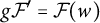
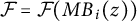
. We remark that
$\{x \neq 0\}$
. We remark that
 $\{x \neq 0\}$
and
$\{x \neq 0\}$
and
 $\{z \neq 0\}$
are precisely the cluster tori in the cluster structure on
$\{z \neq 0\}$
are precisely the cluster tori in the cluster structure on
 $R(v_0, v_3)$
with the following initial seed:
$R(v_0, v_3)$
with the following initial seed:
1.3 Splicing double Bott–Samelson varieties
While we do not have a proof of Conjecture 1.4 in full generality, in some cases, we are able to prove it, namely, those cases where we start with a double Bott–Samelson variety. For each positive braid
 $\beta \in \mathrm {Br}^{+}_{k}$
, the double Bott–Samelson variety
$\beta \in \mathrm {Br}^{+}_{k}$
, the double Bott–Samelson variety
 $\mathrm {BS}(\beta )$
is defined as a space of flag configurations dictated by the braid
$\mathrm {BS}(\beta )$
is defined as a space of flag configurations dictated by the braid
 $\beta $
in a way similar to, but subtly different from, the definition of a braid variety. In fact, we have isomorphisms
$\beta $
in a way similar to, but subtly different from, the definition of a braid variety. In fact, we have isomorphisms
 $$ \begin{align} \varphi_1: \mathrm{BS}(\beta) \to X(\beta\Delta), \qquad \varphi_2: \mathrm{BS}(\beta) \to X(\Delta\beta), \end{align} $$
where
 $\Delta $
is a positive braid lift of the longest element
$\Delta $
is a positive braid lift of the longest element
 $w_0 \in S_k$
. Double Bott–Samelson varieties were introduced by Elek and Lu in [Reference Elek and Jiang-Hua7], and a cluster structure on them was studied in [Reference Goodearl and Yakimov15, Reference Shen and Weng26]. Given a braid decomposition
$w_0 \in S_k$
. Double Bott–Samelson varieties were introduced by Elek and Lu in [Reference Elek and Jiang-Hua7], and a cluster structure on them was studied in [Reference Goodearl and Yakimov15, Reference Shen and Weng26]. Given a braid decomposition
 $\beta = \beta ^1\beta ^2$
as above, we define an open set
$\beta = \beta ^1\beta ^2$
as above, we define an open set
 $\mathcal {U}_{r_1}=\mathcal {U}(\beta ^1, \beta ^2) \subseteq \mathrm {BS}(\beta )$
and show the following.
$\mathcal {U}_{r_1}=\mathcal {U}(\beta ^1, \beta ^2) \subseteq \mathrm {BS}(\beta )$
and show the following.
Theorem 1.8 Let
 $\beta = \beta ^1\beta ^2 \in \mathrm {Br}^{+}_{k}$
be a positive braid. Then, we have an isomorphism:
$\beta = \beta ^1\beta ^2 \in \mathrm {Br}^{+}_{k}$
be a positive braid. Then, we have an isomorphism:
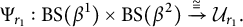 $$ \begin{align} \Psi_{r_1}: \mathrm{BS}(\beta^1) \times \mathrm{BS}(\beta^2) \xrightarrow{\cong} \mathcal{U}_{r_1}. \end{align} $$
Moreover, the map (1.7) and the open set
 $\mathcal {U}_{r_1}$
satisfy the properties predicted by Conjecture 1.4.
$\mathcal {U}_{r_1}$
satisfy the properties predicted by Conjecture 1.4.
We remark that, upon some identifications made possible by (1.6), the map (1.7) is a special case of the maps (1.1). Recall that we denote by
 $\Phi _{r_1, w}$
the inverse to
$\Phi _{r_1, w}$
the inverse to
 $\Psi _{r_1, w}$
. Similarly, denote by
$\Psi _{r_1, w}$
. Similarly, denote by
 $\Phi _{r_1}$
the inverse to
$\Phi _{r_1}$
the inverse to
 $\Psi _{r_1}$
from (1.7).
$\Psi _{r_1}$
from (1.7).
Theorem 1.9 Let
 $\beta = \beta ^1\beta ^2$
be a positive braid. The following diagrams commute:
$\beta = \beta ^1\beta ^2$
be a positive braid. The following diagrams commute:


Here
 $\varphi _1,\varphi _2$
are isomorphisms from (1.6).
$\varphi _1,\varphi _2$
are isomorphisms from (1.6).
We visually describe the splicing map in the following example, but leave the technical details needed to verify that the map is a quasi-cluster isomorphism to Example 6.10.
Example 1.10 Consider
, where
and
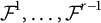
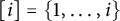
are as indicated by colors. We have the quiver
 $Q_{\beta }$
:
$Q_{\beta }$
:

The open set
 $\mathcal {U}_{r_1}$
is the cluster variety corresponding to the following quiver, which is obtained by freezing the vertices
$\mathcal {U}_{r_1}$
is the cluster variety corresponding to the following quiver, which is obtained by freezing the vertices
 $6, 7$
, and
$6, 7$
, and
 $9$
. Note that these are the vertices on the right of the rightmost appearance of a crossing in
$9$
. Note that these are the vertices on the right of the rightmost appearance of a crossing in
 ${\color {blue} \beta ^1}$
.
${\color {blue} \beta ^1}$
.

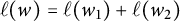
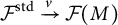
On the other hand, the product
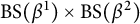 $\mathrm {BS}(\beta ^1) \times \mathrm {BS}(\beta ^2)$
is the cluster variety corresponding to the disjoint union of the quivers
$\mathrm {BS}(\beta ^1) \times \mathrm {BS}(\beta ^2)$
is the cluster variety corresponding to the disjoint union of the quivers
 $Q_{\beta ^1}$
and
$Q_{\beta ^1}$
and
 $Q_{\beta ^2}$
:
$Q_{\beta ^2}$
:

1.4 Connections to other work
The splicing maps for double Bott–Samelson varieties are predicted by results in link homology. In particular, the work of Trinh [Reference Trinh27] relates the equivariant Borel–Moore homology of
 $\mathrm {BS}(\beta )$
(together with the weight filtration) to the Khovanov–Rozansky homology
$\mathrm {BS}(\beta )$
(together with the weight filtration) to the Khovanov–Rozansky homology
 $\mathrm {HHH}^{a=0}(\beta )$
. The corresponding multiplication maps in link homology
$\mathrm {HHH}^{a=0}(\beta )$
. The corresponding multiplication maps in link homology
 $$ \begin{align*}\mathrm{HHH}^{a=0}(\beta^1)\otimes \mathrm{HHH}^{a=0}(\beta^2)\to \mathrm{HHH}^{a=0}(\beta^1\beta^2) \end{align*} $$
are well known and very useful (see, e.g., [Reference Gorsky and Hogancamp16] and the references therein).
More generally, the equivariant Borel–Moore homology (again with the weight filtration) of the variety
 $X(\beta )$
is related to the Khovanov–Rozansky homology
$X(\beta )$
is related to the Khovanov–Rozansky homology
 $\mathrm {HHH}^{a = 0}(\beta \Delta ^{-1})$
. In the setting of Theorem 1.1, note that the braid
$\mathrm {HHH}^{a = 0}(\beta \Delta ^{-1})$
. In the setting of Theorem 1.1, note that the braid
 $$\begin{align*}\left(\Delta^{-1}\underline{w^{-1}w_0}\beta^1\right) \cdot \left(\beta^2\underline{w}\Delta^{-1}\right) \end{align*}$$
is conjugate to
 $\beta ^1\beta ^2\Delta ^{-1}$
, so they represent the same link. Thus, we have a map in link homology
$\beta ^1\beta ^2\Delta ^{-1}$
, so they represent the same link. Thus, we have a map in link homology
 $$ \begin{align*}\mathrm{HHH}^{a = 0}\left(\Delta^{-1}\underline{w^{-1}w_0}\beta^1\right)\otimes \mathrm{HHH}^{a = 0}\left(\beta^2\underline{w}\Delta^{-1}\right)\to \mathrm{HHH}^{a = 0}\left(\beta^1\beta^2\Delta^{-1}\right), \end{align*} $$
which suggests the splicing map
 $X\left (\underline {w^{-1}w_0}\beta ^1\right ) \times X\left (\beta ^2\underline {w}\right ) \to X\left (\beta ^1\beta ^2\right )$
as in (1.1).
$X\left (\underline {w^{-1}w_0}\beta ^1\right ) \times X\left (\beta ^2\underline {w}\right ) \to X\left (\beta ^1\beta ^2\right )$
as in (1.1).
Another motivation for splicing maps comes from [Reference Eberhardt and Stroppel6] that studies homology of (parabolic) open Richardson varieties. Let
 $u,v$
be two permutations in
$u,v$
be two permutations in
 $S_k$
such that
$S_k$
such that
 $u\le v$
in Bruhat order. As mentioned above, the open Richardson variety
$u\le v$
in Bruhat order. As mentioned above, the open Richardson variety
 $R(u,v)$
is isomorphic to a certain braid variety:
$R(u,v)$
is isomorphic to a certain braid variety:
 $$ \begin{align*}R(u,v)\simeq X\left(\underline{v}\cdot \underline{u^{-1}w_0}\right). \end{align*} $$
It is known that compactly supported cohomology of
 $R(u,v)$
is closely related to the
$R(u,v)$
is closely related to the
 $\mathrm {Ext}$
group between the Verma modules in the category
$\mathrm {Ext}$
group between the Verma modules in the category
 $\mathcal {O}$
for
$\mathcal {O}$
for
 $\mathfrak {gl}_k$
:
$\mathfrak {gl}_k$
:
 $$ \begin{align} H^*_c(R(u,v))\simeq \mathrm{Ext}_{\mathcal{O}}^*(\Delta_u,\Delta_v). \end{align} $$
The homological grading and the weight filtration on the left-hand side correspond to two gradings on the right-hand side (see [Reference Eberhardt and Stroppel6, Theorem 12.5], [Reference Galashin and Lam11], and the references therein).
Given
 $u\le v\le w$
in
$u\le v\le w$
in
 $S_k$
, [Reference Eberhardt and Stroppel6, Section 3] constructs a rational map
$S_k$
, [Reference Eberhardt and Stroppel6, Section 3] constructs a rational map
 $$ \begin{align} R(u,v)\times R(v,w)\to R(u,w), \end{align} $$
which corresponds under (1.8) to compositions of extensions
 $$ \begin{align*}\mathrm{Ext}_{\mathcal{O}}^*(\Delta_u,\Delta_v)\otimes \mathrm{Ext}_{\mathcal{O}}^*(\Delta_v,\Delta_w)\rightarrow \mathrm{Ext}_{\mathcal{O}}^*(\Delta_u,\Delta_w), \end{align*} $$
see [Reference Eberhardt and Stroppel6, Corollary 3.3]. This can be compared with Theorem 1.5, however we do not know whether our maps coincide with those of [Reference Eberhardt and Stroppel6] and plan to investigate this in the future.
1.5 Organization of the article
Sections 2–4 are mostly preparatory: in Section 2, we give the necessary background on relative positions of flags and its relation to matrix minors. In Section 3, we recall the definition of cluster algebras and quasi-cluster isomorphisms. We define braid and double Bott–Samelson varieties in Section 4. In particular, in Section 4.3, we give details on the cluster structure on braid and double Bott–Samelson varieties obtained in [Reference Casals, Gorsky, Gorsky, Le, Shen and Simental2, Reference Galashin, Lam and Sherman-Bennett12, Reference Galashin, Lam, Sherman-Bennett and Speyer13, Reference Shen and Weng26].
The technical heart of the article is Section 5. In Section 5.1, we define the open sets
 $\mathcal {U}_{r_1, w}$
, see (5.1), and prove Theorem 1.1 as Theorem 5.2. In Section 5.2, we elaborate on the conjectural properties of the splicing map (1.1), giving a more precise version of Conjecture 1.4 as Conjecture 5.6. We elaborate on the relations between the different parts of this conjecture, and show a weaker version of the conjecture for the case
$\mathcal {U}_{r_1, w}$
, see (5.1), and prove Theorem 1.1 as Theorem 5.2. In Section 5.2, we elaborate on the conjectural properties of the splicing map (1.1), giving a more precise version of Conjecture 1.4 as Conjecture 5.6. We elaborate on the relations between the different parts of this conjecture, and show a weaker version of the conjecture for the case
 $w = w_0$
, and illustrate this with examples. Finally, in Section 5.3, we specialize the map (1.1) to the case of open Richardson varieties and prove Theorem 1.5.
$w = w_0$
, and illustrate this with examples. Finally, in Section 5.3, we specialize the map (1.1) to the case of open Richardson varieties and prove Theorem 1.5.
In Section 6, we deal with the case of double Bott–Samelson varieties. We show Theorem 1.8 in two parts: first, in Theorem 6.1, we construct the map (1.7) and show that it is an isomorphism; second, we study the cluster-theoretic properties of (1.7) in Section 6.4, showing the second part of Theorem 1.8 as Theorem 6.9. Finally, Theorem 1.9 is proved as Lemmas 6.4 and 6.5.
1.6 Notations
For a tuple of matrices
 $(A_1,\ldots ,A_k)$
and a matrix M, we write
$(A_1,\ldots ,A_k)$
and a matrix M, we write
 $M(A_1,\ldots ,A_k)=(MA_1,\ldots ,MA_k)$
. Similarly, given a tuple of flags
$M(A_1,\ldots ,A_k)=(MA_1,\ldots ,MA_k)$
. Similarly, given a tuple of flags
 $(\mathcal {F}^1,\ldots ,\mathcal {F}^k)$
and a matrix M, we write
$(\mathcal {F}^1,\ldots ,\mathcal {F}^k)$
and a matrix M, we write
 $M(\mathcal {F}^1,\ldots ,\mathcal {F}^k)=(M\mathcal {F}^1,\ldots ,M\mathcal {F}^k)$
.
$M(\mathcal {F}^1,\ldots ,\mathcal {F}^k)=(M\mathcal {F}^1,\ldots ,M\mathcal {F}^k)$
.
2 Background
We recall some standard facts we will use throughout the article, in the way setting up notation and conventions.
2.1 Braids and Demazure product
We will work with the positive braid monoid on k strands
 $\mathrm {Br}_k^{+}$
:
$\mathrm {Br}_k^{+}$
:
 $$\begin{align*}\mathrm{Br}_k^{+} = \left\langle \sigma_1, \dots, \sigma_{k-1} \mid \sigma_i\sigma_j = \sigma_j\sigma_i \; \text{if} \; |i-j|>1, \ \sigma_i\sigma_{i+1}\sigma_i = \sigma_{i+1}\sigma_i\sigma_{i+1}, i = 1, \dots, k-2\right\rangle. \end{align*}$$
We have a surjective homomorphism
 $\pi : \mathrm {Br}_k^{+} \to S_k$
given by
$\pi : \mathrm {Br}_k^{+} \to S_k$
given by
 $\pi (\sigma _i) = s_i$
, where
$\pi (\sigma _i) = s_i$
, where
 $s_1, \dots , s_{k-1}$
are the simple transpositions in the symmetric group
$s_1, \dots , s_{k-1}$
are the simple transpositions in the symmetric group
 $S_k$
. We also have the Demazure product
$S_k$
. We also have the Demazure product
 $\delta : \mathrm {Br}_k^{+} \to S_k$
, defined inductively by
$\delta : \mathrm {Br}_k^{+} \to S_k$
, defined inductively by
 $$ \begin{align} \delta(e) = e, \; \delta(\beta\sigma_i) = \begin{cases} \delta(\beta)s_i & \text{if} \; \delta(\beta)s_i> \delta(\beta) \\ \delta(\beta) & \text{else}. \end{cases} \end{align} $$
Note that, as opposed to
 $\pi $
, the Demazure product
$\pi $
, the Demazure product
 $\delta $
is not a morphism of monoids. If
$\delta $
is not a morphism of monoids. If
 $w \in S_k$
, we denote by
$w \in S_k$
, we denote by
 $\underline {w} \in \mathrm {Br}_k^{+}$
the unique lift of minimal length (either under the projection
$\underline {w} \in \mathrm {Br}_k^{+}$
the unique lift of minimal length (either under the projection
 $\pi $
or the Demazure product
$\pi $
or the Demazure product
 $\delta $
) of w to
$\delta $
) of w to
 $\mathrm {Br}_k^{+}$
. We will denote by
$\mathrm {Br}_k^{+}$
. We will denote by
 $w_0 \in S_k$
the longest element, and its lift
$w_0 \in S_k$
the longest element, and its lift
 $\underline {w_0}$
will be denoted by
$\underline {w_0}$
will be denoted by
 $\Delta $
. If
$\Delta $
. If
 $v, w \in S_k$
, we define their Demazure product by
$v, w \in S_k$
, we define their Demazure product by
 $$ \begin{align} v \star w := \delta(\underline{v}\cdot\underline{w}). \end{align} $$
We finish this section with the following result.
Lemma 2.1 Let
 $v, w \in S_k$
. The following are equivalent:
$v, w \in S_k$
. The following are equivalent:
-
(a)
$v \star w = w_0$
. -
(b)
$v \geq w_0w^{-1}$
in Bruhat order. -
(c)
$w \geq v^{-1}w_0$
in Bruhat oder.


Proof We show that (a) implies (b). First, we remark that the Demazure product
 $\delta (\beta )$
is the longest reduced word contained in
$\delta (\beta )$
is the longest reduced word contained in
 $\beta $
. Definition (2.1) is a greedy method to compute it – another equally effective greedy method is to read the word
$\beta $
. Definition (2.1) is a greedy method to compute it – another equally effective greedy method is to read the word
 $\beta $
in the opposite direction. That being said, we have
$\beta $
in the opposite direction. That being said, we have
 $v \star w = s_{i_1}\dots s_{i_k}w$
, where
$v \star w = s_{i_1}\dots s_{i_k}w$
, where
 $\sigma _{i_1}\dots \sigma _{i_k}$
is a reduced subexpression of
$\sigma _{i_1}\dots \sigma _{i_k}$
is a reduced subexpression of
 $\underline {v}$
. If
$\underline {v}$
. If
 $v \star w = w_0$
, then
$v \star w = w_0$
, then
 $s_{i_1}\dots s_{i_k} = w_0w^{-1}$
, so
$s_{i_1}\dots s_{i_k} = w_0w^{-1}$
, so
 $v \geq w_0w^{-1}$
as needed. Now, we show that (b) implies (a). If
$v \geq w_0w^{-1}$
as needed. Now, we show that (b) implies (a). If
 $\underline {w_0w^{-1}}$
appears as a reduced subexpression in
$\underline {w_0w^{-1}}$
appears as a reduced subexpression in
 $\underline {v}$
, then a reduced subexpression for
$\underline {v}$
, then a reduced subexpression for
 $w_0$
appears as a subexpression in
$w_0$
appears as a subexpression in
 $\underline {v}\dots \underline {w}$
, and we obtain
$\underline {v}\dots \underline {w}$
, and we obtain
 $v \star w = w_0$
. This proves that (a) and (b) are equivalent. The equivalence between (a) and (c) is proved similarly.
$v \star w = w_0$
. This proves that (a) and (b) are equivalent. The equivalence between (a) and (c) is proved similarly.
2.2 Flags and relative position
We will denote by
 $\mathcal {F}\ell _k$
the variety of complete flags in the k-dimensional complex vector space
$\mathcal {F}\ell _k$
the variety of complete flags in the k-dimensional complex vector space
 $\mathbb {C}^k$
. For a matrix
$\mathbb {C}^k$
. For a matrix
 $M \in \mathrm {GL}(k)$
with columns
$M \in \mathrm {GL}(k)$
with columns
 $m_1, \dots , m_k \in \mathbb {C}^k$
, we define the flag
$m_1, \dots , m_k \in \mathbb {C}^k$
, we define the flag
 $$\begin{align*}\mathcal{F}(M) = \left(\{0\} \subseteq \langle m_1 \rangle \subseteq \langle m_1,m_2 \rangle \subseteq \cdots \subseteq \langle m_1, \dots, m_{k-1} \rangle \subseteq \langle m_1, \dots, m_k \rangle = \mathbb{C}^k\right). \end{align*}$$
The assignment
 $M \mapsto \mathcal {F}(M)$
gives rise to the usual identification
$M \mapsto \mathcal {F}(M)$
gives rise to the usual identification
 $\mathcal {F}\ell _k = \mathrm {GL}(k)/\mathsf {B}(k)$
, where
$\mathcal {F}\ell _k = \mathrm {GL}(k)/\mathsf {B}(k)$
, where
 $\mathsf {B}(k) \subseteq \mathrm {GL}(k)$
is the subgroup of upper triangular matrices. Note that the group
$\mathsf {B}(k) \subseteq \mathrm {GL}(k)$
is the subgroup of upper triangular matrices. Note that the group
 $\mathrm {GL}(k)$
acts on
$\mathrm {GL}(k)$
acts on
 $\mathcal {F}\ell _k$
by multiplication on the left, or, equivalently,
$\mathcal {F}\ell _k$
by multiplication on the left, or, equivalently,
 $$\begin{align*}g.(\{0\} \subseteq F_1 \subseteq \cdots \subseteq F_{k-1} \subseteq \mathbb{C}^k) = (\{0\} \subseteq g(F_1) \subseteq \cdots \subseteq g(F_{k-1}) \subseteq \mathbb{C}^k), \end{align*}$$
so that
 $g.\mathcal {F}(M) = \mathcal {F}(gM)$
.
$g.\mathcal {F}(M) = \mathcal {F}(gM)$
.
We will denote by
 $e_1, \dots , e_k \in \mathbb {C}^k$
the usual standard basis. Given an element
$e_1, \dots , e_k \in \mathbb {C}^k$
the usual standard basis. Given an element
 $w \in S_k$
, we define the coordinate flag
$w \in S_k$
, we define the coordinate flag
 $$\begin{align*}\mathcal{F}(w) := (\{0\} \subseteq \langle e_{w(1)} \rangle \subseteq \langle e_{w(1)}, e_{w(2)} \rangle \subseteq \cdots \subseteq \langle e_{w(1)}, \dots, e_{w(k-1)} \rangle \subseteq \mathbb{C}^k), \end{align*}$$
in particular, we have the standard and antistandard flags:
 $$\begin{align*}\mathcal{F}^{\mathrm{std}} := \mathcal{F}(e), \qquad \mathcal{F}^{\mathrm{ant}} := \mathcal{F}(w_0). \end{align*}$$
We say that two flags
 $\mathcal {F}$
and
$\mathcal {F}$
and
 $\mathcal {F}'$
are in (relative) position
$\mathcal {F}'$
are in (relative) position
 $w \in S_k$
, and write
$w \in S_k$
, and write
 $\mathcal {F} \xrightarrow {w} \mathcal {F}'$
if there exists
$\mathcal {F} \xrightarrow {w} \mathcal {F}'$
if there exists
 $g \in \mathrm {GL}(k)$
such that
$g \in \mathrm {GL}(k)$
such that
 $g\mathcal {F} = \mathcal {F}^{\mathrm {std}}$
and
$g\mathcal {F} = \mathcal {F}^{\mathrm {std}}$
and
 $g\mathcal {F}' = \mathcal {F}(w)$
. Such g is uniquely defined up to left multiplication by an element of
$g\mathcal {F}' = \mathcal {F}(w)$
. Such g is uniquely defined up to left multiplication by an element of
 $\mathsf {B}(k) \cap w\mathsf {B}(k)w^{-1}$
.
$\mathsf {B}(k) \cap w\mathsf {B}(k)w^{-1}$
.
Note that given two flags
 $\mathcal {F}, \mathcal {F}' \in \mathcal {F}\ell _k$
, there exists a unique
$\mathcal {F}, \mathcal {F}' \in \mathcal {F}\ell _k$
, there exists a unique
 $w \in S_k$
such that
$w \in S_k$
such that
 $\mathcal {F} \xrightarrow {w} \mathcal {F}'$
, and such w is determined by
$\mathcal {F} \xrightarrow {w} \mathcal {F}'$
, and such w is determined by
 $$\begin{align*}\dim(F_i \cap F^{\prime}_j) = \#\left(\{1, \dots, i\}\cap\{w(1), \dots, w(j)\}\right). \end{align*}$$
In particular,
 $$\begin{align*}\mathcal{F} \xrightarrow{s_i} \mathcal{F}' \; \text{if and only if} \; F_i \neq F^{\prime}_i \; \text{and} \; F_j = F^{\prime}_j \; \text{for} \; j \neq i. \end{align*}$$
Relative position of flags is closely related to the Bruhat decomposition of the group
 $\mathrm {GL}(k)$
:
$\mathrm {GL}(k)$
:
 $$\begin{align*}\mathrm{GL}(k) = \bigsqcup_{w \in S_k} \mathsf{B}(k)w\mathsf{B}(k). \end{align*}$$
Indeed, note that if
 $M, M' \in \mathrm {GL}(k),$
then
$M, M' \in \mathrm {GL}(k),$
then
 $\mathcal {F}(M) \xrightarrow {w} \mathcal {F}(M')$
if and only if there exist upper triangular matrices
$\mathcal {F}(M) \xrightarrow {w} \mathcal {F}(M')$
if and only if there exist upper triangular matrices
 $U_1, U_2 \in \mathsf {B}(k)$
and
$U_1, U_2 \in \mathsf {B}(k)$
and
 $g \in \mathrm {GL}(k)$
such that
$g \in \mathrm {GL}(k)$
such that
 $gM = U_1, gM' = wU_2$
, and this is in turn equivalent to
$gM = U_1, gM' = wU_2$
, and this is in turn equivalent to
 $M^{-1}M' \in \mathsf {B}(k)w\mathsf {B}(k).$
The Bruhat decomposition satisfies the following multiplicative property. If
$M^{-1}M' \in \mathsf {B}(k)w\mathsf {B}(k).$
The Bruhat decomposition satisfies the following multiplicative property. If
 $w \in S_k$
and
$w \in S_k$
and
 $i = 1, \dots , k-1$
, we have
$i = 1, \dots , k-1$
, we have
 $$ \begin{align} (\mathsf{B} w \mathsf{B})(\mathsf{B} s_i\mathsf{B}) = \begin{cases} \mathsf{B} ws_i\mathsf{B} & \; \text{if} \; \ell(ws_i)> \ell(w), \\ (\mathsf{B} ws_i\mathsf{B})\sqcup (\mathsf{B} w \mathsf{B}) & \text{else}.\end{cases} \end{align} $$
This implies the following standard lemma that we will use repeatedly. For a proof, see, for example, [Reference Casals, Gorsky, Gorsky, Le, Shen and Simental2, Lemma 3.2].
Lemma 2.2 Let
 $\mathcal {F}, \mathcal {F}' \in \mathcal {F}\ell _k$
and
$\mathcal {F}, \mathcal {F}' \in \mathcal {F}\ell _k$
and
 $w \in S_k$
. The following are equivalent:
$w \in S_k$
. The following are equivalent:
-
(1)
$\mathcal {F} \xrightarrow {w} \mathcal {F}'$
. -
(2) There exist a reduced decomposition
$w = s_{i_1}\dots s_{i_r}$
and flags
$\mathcal {F}^1, \dots , \mathcal {F}^{r-1}$
such that
$$\begin{align*}\mathcal{F} \xrightarrow{s_{i_1}} \mathcal{F}^1 \xrightarrow{s_{i_2}} \dots \xrightarrow{s_{i_{r-1}}} \mathcal{F}^{r-1} \xrightarrow{s_{i_r}} \mathcal{F}'. \end{align*}$$
-
(3) For any reduced decomposition
$w = s_{i_1}\dots s_{i_r}$
there exist flags
$\mathcal {F}^1, \dots , \mathcal {F}^{r-1}$
such that
$$\begin{align*}\mathcal{F} \xrightarrow{s_{i_1}} \mathcal{F}^1 \xrightarrow{s_{i_2}} \dots \xrightarrow{s_{i_{r-1}}} \mathcal{F}^{r-1} \xrightarrow{s_{i_r}} \mathcal{F}'. \end{align*}$$


Moreover, given a reduced decomposition of
 $w,$
the flags
$w,$
the flags
 $\mathcal {F}^1, \dots , \mathcal {F}^{r-1}$
in (3) are unique.
$\mathcal {F}^1, \dots , \mathcal {F}^{r-1}$
in (3) are unique.
The set
 $\Gamma _w$
of pairs of flags
$\Gamma _w$
of pairs of flags
 $(\mathcal {F},\mathcal {F}')$
such that
$(\mathcal {F},\mathcal {F}')$
such that
 $\mathcal {F}\xrightarrow {w}\mathcal {F}'$
is a locally closed subvariety of
$\mathcal {F}\xrightarrow {w}\mathcal {F}'$
is a locally closed subvariety of
 $\mathcal {F}\ell _k\times \mathcal {F}\ell _k$
. The intermediate flags
$\mathcal {F}\ell _k\times \mathcal {F}\ell _k$
. The intermediate flags
 $\mathcal {F}^1,\ldots ,\mathcal {F}^r$
depend on
$\mathcal {F}^1,\ldots ,\mathcal {F}^r$
depend on
 $(\mathcal {F},\mathcal {F}')$
algebraically, that is, define
$(\mathcal {F},\mathcal {F}')$
algebraically, that is, define
 $(r-1)$
regular maps from
$(r-1)$
regular maps from
 $\Gamma _w$
to
$\Gamma _w$
to
 $\mathcal {F}\ell _k$
.
$\mathcal {F}\ell _k$
.
Corollary 2.3
(a) Suppose that
 $w=w_1w_2$
, where
$w=w_1w_2$
, where
 $w,w_1,w_2\in S_k$
, and
$w,w_1,w_2\in S_k$
, and
 $\ell (w)=\ell (w_1)+\ell (w_2)$
. Then
$\ell (w)=\ell (w_1)+\ell (w_2)$
. Then
 $\mathcal {F}\xrightarrow {w}\mathcal {F}'$
if and only if there exists a flag
$\mathcal {F}\xrightarrow {w}\mathcal {F}'$
if and only if there exists a flag
 $\mathcal {F}"$
such that
$\mathcal {F}"$
such that
 $$ \begin{align*}\mathcal{F}\xrightarrow{w_1}\mathcal{F}"\xrightarrow{w_2}\mathcal{F}'. \end{align*} $$
In this case,
 $\mathcal {F}"$
is unique.
$\mathcal {F}"$
is unique.
(b) Assume that we have
 $\mathcal {F} \xrightarrow {w_1} \mathcal {F}' \xrightarrow {w_2} \mathcal {F}"$
. Then,
$\mathcal {F} \xrightarrow {w_1} \mathcal {F}' \xrightarrow {w_2} \mathcal {F}"$
. Then,
 $\mathcal {F} \xrightarrow {w} \mathcal {F}"$
with
$\mathcal {F} \xrightarrow {w} \mathcal {F}"$
with
 $w \leq w_1\star w_2$
, where
$w \leq w_1\star w_2$
, where
 $w_1\star w_2$
is defined by (2.2).
$w_1\star w_2$
is defined by (2.2).
Proof Part (a) is immediate from Lemma 2.2. For part (b), assume
 $\mathcal {F} = \mathcal {F}(M)$
,
$\mathcal {F} = \mathcal {F}(M)$
,
 $\mathcal {F}' = \mathcal {F}(M'),$
and
$\mathcal {F}' = \mathcal {F}(M'),$
and
 $\mathcal {F}" = \mathcal {F}(M")$
. So we have
$\mathcal {F}" = \mathcal {F}(M")$
. So we have
 $M^{-1}M' \in \mathsf {B} w_1\mathsf {B}$
and
$M^{-1}M' \in \mathsf {B} w_1\mathsf {B}$
and
 $(M')^{-1}M" \in \mathsf {B} w_2\mathsf {B}$
. Now,
$(M')^{-1}M" \in \mathsf {B} w_2\mathsf {B}$
. Now,
 $M^{-1}M" \in (\mathsf {B} w_1\mathsf {B})(\mathsf {B} w_2\mathsf {B})$
and the result follows from (2.3).
$M^{-1}M" \in (\mathsf {B} w_1\mathsf {B})(\mathsf {B} w_2\mathsf {B})$
and the result follows from (2.3).
2.3 Transverse flags
We will say that two flags
 $\mathcal {F}$
and
$\mathcal {F}$
and
 $\mathcal {F}'$
are transverse and write
$\mathcal {F}'$
are transverse and write
 $\mathcal {F} \pitchfork \mathcal {F}'$
if
$\mathcal {F} \pitchfork \mathcal {F}'$
if
 $\mathcal {F} \xrightarrow {w_0} \mathcal {F}'$
. Note that
$\mathcal {F} \xrightarrow {w_0} \mathcal {F}'$
. Note that
 $$\begin{align*}\mathcal{F} \pitchfork \mathcal{F}' \; \text{if and only if} \; F_i \cap F^{\prime}_{k-i} = \{0\} \; \text{for all} \; i, \; \text{if and only if} \; F_i + F^{\prime}_{k-i} = \mathbb{C}^k \; \text{for all} \; i. \end{align*}$$
Lemma 2.4 Let M be a nonsingular matrix and
 $w \in S_k$
. Then,
$w \in S_k$
. Then,
 $\mathcal {F}(M) \pitchfork \mathcal {F}(w)$
if and only if the matrix M admits a decomposition of the form
$\mathcal {F}(M) \pitchfork \mathcal {F}(w)$
if and only if the matrix M admits a decomposition of the form
 $$\begin{align*}M = ww_0LU, \end{align*}$$
where L is lower-triangular and U is upper-triangular. Such decomposition is unique upon requiring that L has
 $1$
’s on the diagonal.
$1$
’s on the diagonal.
Proof We have that
 $\mathcal {F}(M) \pitchfork \mathcal {F}(w)$
if and only if there exists an element
$\mathcal {F}(M) \pitchfork \mathcal {F}(w)$
if and only if there exists an element
 $g \in \mathrm {GL}(k)$
such that
$g \in \mathrm {GL}(k)$
such that
 $gM \in \mathsf {B}$
and
$gM \in \mathsf {B}$
and
 $gw \in w_0\mathsf {B}$
. If such an element exists, then for some
$gw \in w_0\mathsf {B}$
. If such an element exists, then for some
 $U_1,U_2\in \mathsf {B,}$
we get
$U_1,U_2\in \mathsf {B,}$
we get
 $g = w_0U_1w^{-1}$
and
$g = w_0U_1w^{-1}$
and
 $M = g^{-1}U_2 = (w_0U_1w^{-1})^{-1}U_2 = wU_1^{-1}w_0U_2 = ww_0(w_0U_1^{-1}w_0)U_2$
, so such a decomposition of M exists with
$M = g^{-1}U_2 = (w_0U_1w^{-1})^{-1}U_2 = wU_1^{-1}w_0U_2 = ww_0(w_0U_1^{-1}w_0)U_2$
, so such a decomposition of M exists with
 $L=w_0U_1^{-1}w_0$
. Conversely, if
$L=w_0U_1^{-1}w_0$
. Conversely, if
 $M = ww_0LU,$
then setting
$M = ww_0LU,$
then setting
 $g = L^{-1}w_0w^{-1}$
we have that
$g = L^{-1}w_0w^{-1}$
we have that
 $gM = U \in \mathsf {B}$
and
$gM = U \in \mathsf {B}$
and
 $gw = L^{-1}w_0 \in w_0\mathsf {B}$
. Finally, the uniqueness claim follows from the uniqueness of the LU-decomposition.
$gw = L^{-1}w_0 \in w_0\mathsf {B}$
. Finally, the uniqueness claim follows from the uniqueness of the LU-decomposition.
2.4 Braid matrices
For
 $i = 1, \dots , k-1$
and a formal variable
$i = 1, \dots , k-1$
and a formal variable
 $z,$
we define the matrix
$z,$
we define the matrix
 $B_i(z)$
to be
$B_i(z)$
to be
 $$\begin{align*}B_i(z) = \begin{pmatrix}1&\cdots&&&\ldots&0\\ \vdots&\ddots&&&&\vdots\\ 0&\cdots&z&-1&\cdots&0\\ 0&\cdots&1&0&\cdots&0\\ \vdots&&&&\ddots&\vdots\\ 0&\cdots&&&\cdots&1\end{pmatrix}, \end{align*}$$
where the non-identity part of
 $B_i(z)$
is located in the i-th and
$B_i(z)$
is located in the i-th and
 $(i+1)$
-st row and columns.
$(i+1)$
-st row and columns.
The matrix
 $B_i(z)$
is important for us due to the following well-known (and easy) lemma.
$B_i(z)$
is important for us due to the following well-known (and easy) lemma.
Lemma 2.5 Let
 $M \in \mathrm {GL}(n)$
be a nondegenerate matrix and let
$M \in \mathrm {GL}(n)$
be a nondegenerate matrix and let
 $i = 1, \dots , n-1.$
Then,
$i = 1, \dots , n-1.$
Then,
 $\mathcal {F} \xrightarrow {s_i} \mathcal {F}(M)$
if and only if there exists a (necessarily unique)
$\mathcal {F} \xrightarrow {s_i} \mathcal {F}(M)$
if and only if there exists a (necessarily unique)
 $z \in \mathbb {C}$
such that
$z \in \mathbb {C}$
such that
 $\mathcal {F} = \mathcal {F}(MB_i(z))$
.
$\mathcal {F} = \mathcal {F}(MB_i(z))$
.
The following lemma is also easy to check (see [Reference Casals, Gorsky, Gorsky, Le, Shen and Simental2, Corollary 3.9] and [Reference Casals, Gorsky, Gorsky and Simental4, Lemma 2.20]).
Lemma 2.6 If U is an upper-triangular matrix and
 $z\in \mathbb {C,}$
then there exist unique upper-triangular matrix
$z\in \mathbb {C,}$
then there exist unique upper-triangular matrix
 $U'$
and
$U'$
and
 $z'\in \mathbb {C}$
such that
$z'\in \mathbb {C}$
such that
 $$ \begin{align*}UB_i(z)=B_i(z')U'. \end{align*} $$
Furthermore, the diagonal entries of
 $U'$
are permuted from the ones of U by
$U'$
are permuted from the ones of U by
 $s_i$
.
$s_i$
.
2.5 Minors
We use notation
 $[i]=\{1,\ldots ,i\}$
and
$[i]=\{1,\ldots ,i\}$
and
 $u[i]=\{u(1),\ldots ,u(i)\}$
for
$u[i]=\{u(1),\ldots ,u(i)\}$
for
 $u\in S_k$
. If
$u\in S_k$
. If
 $I, J \subseteq [k]$
are sets of the same cardinality and
$I, J \subseteq [k]$
are sets of the same cardinality and
 $M \in \mathrm {GL}(k)$
, we denote by
$M \in \mathrm {GL}(k)$
, we denote by
 $\Delta _{I, J}(M)$
the determinant of the
$\Delta _{I, J}(M)$
the determinant of the
 $|I| \times |J|$
-submatrix of M obtained by deleting the rows (resp. columns) not belonging to I (resp. J). For
$|I| \times |J|$
-submatrix of M obtained by deleting the rows (resp. columns) not belonging to I (resp. J). For
 $i = 1, \dots , k$
, we have the principal minor
$i = 1, \dots , k$
, we have the principal minor
 $$ \begin{align} \Delta_{i}(M) := \Delta_{[i], [i]}(M), \end{align} $$
that is,
 $\Delta _{i}(M)$
is the determinant of the upper-left justified
$\Delta _{i}(M)$
is the determinant of the upper-left justified
 $i \times i$
-submatrix of M. Thus, for example,
$i \times i$
-submatrix of M. Thus, for example,
 $\Delta _1(M) = m_{11}$
and
$\Delta _1(M) = m_{11}$
and
 $\Delta _k(M) = \det (M)$
. It is a classical result that a matrix admits an
$\Delta _k(M) = \det (M)$
. It is a classical result that a matrix admits an
 $LU$
decomposition if and only if all its principal minors are nonzero.
$LU$
decomposition if and only if all its principal minors are nonzero.
More generally, we have the following.
Lemma 2.7
a) For
 $w \in S_k$
and
$w \in S_k$
and
 $M \in \mathrm {GL}(k),$
we have that
$M \in \mathrm {GL}(k),$
we have that
 $\mathcal {F}(M) \pitchfork \mathcal {F}(w)$
if and only if the minors
$\mathcal {F}(M) \pitchfork \mathcal {F}(w)$
if and only if the minors
 $$\begin{align*}\Delta_{ww_0[i], [i]}(M) = (-1)^{\ell(w)}\Delta_{[i],[i]}(w_0w^{-1}M) \end{align*}$$
are nonzero for all
 $i = 1, \dots , k$
.
$i = 1, \dots , k$
.
b) If
 $\mathcal {F}^{\mathrm {std}} \xrightarrow {w} \mathcal {F}(M)$
, then the minors
$\mathcal {F}^{\mathrm {std}} \xrightarrow {w} \mathcal {F}(M)$
, then the minors
 $\Delta _{w[i], [i]}(M)$
are nonzero for
$\Delta _{w[i], [i]}(M)$
are nonzero for
 $i = 1, \dots , k$
.
$i = 1, \dots , k$
.
c) If
 $\Delta _{w[i], [i]}(M) \neq 0$
for every
$\Delta _{w[i], [i]}(M) \neq 0$
for every
 $i = 1, \dots , k$
, and
$i = 1, \dots , k$
, and
 $\mathcal {F}^{\mathrm {std}} \xrightarrow {v} \mathcal {F}(M)$
, then
$\mathcal {F}^{\mathrm {std}} \xrightarrow {v} \mathcal {F}(M)$
, then
 $v \not < w$
.
$v \not < w$
.
Proof Part (a) follows from Lemma 2.4 and (2.4).
For part (b), observe that the condition
 $\mathcal {F}^{\mathrm {std}} \xrightarrow {w} \mathcal {F}(M)$
implies
$\mathcal {F}^{\mathrm {std}} \xrightarrow {w} \mathcal {F}(M)$
implies
 $$\begin{align*}\mathcal{F}(ww_0)\xrightarrow{w_0w^{-1}} \mathcal{F}^{\mathrm{std}} \xrightarrow{w} \mathcal{F}(M) \end{align*}$$
so by Corollary 2.3(a), we get
 $\mathcal {F}(ww_0) \pitchfork \mathcal {F}(M)$
. Now, the statement follows from (a).
$\mathcal {F}(ww_0) \pitchfork \mathcal {F}(M)$
. Now, the statement follows from (a).
For part (c), we have that
 $\mathcal {F}(ww_0)\pitchfork \mathcal {F}(M)$
and
$\mathcal {F}(ww_0)\pitchfork \mathcal {F}(M)$
and
 $\mathcal {F}(ww_0) \xrightarrow {w_0w^{-1}} \mathcal {F}^{\mathrm {std}} \xrightarrow {v} \mathcal {F}(M)$
. By Corollary 2.3(b) and using the fact that
$\mathcal {F}(ww_0) \xrightarrow {w_0w^{-1}} \mathcal {F}^{\mathrm {std}} \xrightarrow {v} \mathcal {F}(M)$
. By Corollary 2.3(b) and using the fact that
 $w_0$
is the longest element in
$w_0$
is the longest element in
 $S_k$
, we have
$S_k$
, we have
 $w_0 = (w_0w^{-1}) \star v$
. But if
$w_0 = (w_0w^{-1}) \star v$
. But if
 $v < w,$
then
$v < w,$
then
 $(w_0w^{-1}) \star v < w_0$
, so we obtain
$(w_0w^{-1}) \star v < w_0$
, so we obtain
 $v \not < w$
.
$v \not < w$
.
Definition 2.8 For
 $w \in S_k$
, we define the subset
$w \in S_k$
, we define the subset
 $$\begin{align*}\mathcal{U}(w) := \{\mathcal{F} \in \mathcal{F}\ell_k \mid \mathcal{F} \pitchfork \mathcal{F}(w)\} \subseteq \mathcal{F}\ell_k. \end{align*}$$
Lemma 2.9 For all
 $w \in S_k$
, the subset
$w \in S_k$
, the subset
 $\mathcal {U}(w)$
is open in
$\mathcal {U}(w)$
is open in
 $\mathcal {F}\ell _k$
and moreover
$\mathcal {F}\ell _k$
and moreover
 $$\begin{align*}\mathcal{F}\ell_k = \bigcup_{w \in S_k}\mathcal{U}(w). \end{align*}$$
Proof By Lemma 2.7,
 $\mathcal {U}(w)$
is given by the nonvanishing of the minors
$\mathcal {U}(w)$
is given by the nonvanishing of the minors
 $\Delta _{ww_0[i], [i]}$
,
$\Delta _{ww_0[i], [i]}$
,
 $i = 1, \dots , k$
, so it is clearly open in
$i = 1, \dots , k$
, so it is clearly open in
 $\mathcal {F}\ell _k$
. Now, consider a flag
$\mathcal {F}\ell _k$
. Now, consider a flag
 $\mathcal {F} = \mathcal {F}(M) \in \mathcal {F}\ell _k$
, and pick any element
$\mathcal {F} = \mathcal {F}(M) \in \mathcal {F}\ell _k$
, and pick any element
 $v \in S_k$
. We have
$v \in S_k$
. We have
 $\mathcal {F}(M) \xrightarrow {w_1} \mathcal {F}(v)$
for some
$\mathcal {F}(M) \xrightarrow {w_1} \mathcal {F}(v)$
for some
 $w_1 \in S_k$
, and let
$w_1 \in S_k$
, and let
 $w_0 = w_1w_2$
be a length-additive decomposition. We get
$w_0 = w_1w_2$
be a length-additive decomposition. We get
 $$ \begin{align*}\mathcal{F}(M)\xrightarrow{w_1}\mathcal{F}(v)\xrightarrow{w_2}\mathcal{F}(vw_2) \end{align*} $$
and by Corollary 2.3(a), this implies that
 $\mathcal {F}(M) \xrightarrow {w_0} \mathcal {F}(vw_2)$
, that is,
$\mathcal {F}(M) \xrightarrow {w_0} \mathcal {F}(vw_2)$
, that is,
 $\mathcal {F}(M) \in \mathcal {U}(vw_2)$
.
$\mathcal {F}(M) \in \mathcal {U}(vw_2)$
.
Lemma 2.10 Let
 $M \in \mathfrak {gl}(k)$
. Let
$M \in \mathfrak {gl}(k)$
. Let
 $i, j = 1, \dots , k-1$
and assume
$i, j = 1, \dots , k-1$
and assume
 $i \neq j$
. Let
$i \neq j$
. Let
 $I \subseteq [k]$
be a set with
$I \subseteq [k]$
be a set with
 $|I| = i$
. Then,
$|I| = i$
. Then,
 $\Delta _{I,[i]}(MB_j(z)) = \Delta _{I,[i]}(M)$
.
$\Delta _{I,[i]}(MB_j(z)) = \Delta _{I,[i]}(M)$
.
Proof By the Cauchy–Binet formula,
 $$\begin{align*}\Delta_i(MB_j(z)) = \sum_{\substack{J \subseteq [k] \\ |J| = i}} \Delta_{I, J}(M)\Delta_{J, [i]}(B_j(z)). \end{align*}$$
Since
 $i \neq j$
, we have that
$i \neq j$
, we have that
 $\Delta _{J, [i]}(B_j(z)) \neq 0$
if and only if
$\Delta _{J, [i]}(B_j(z)) \neq 0$
if and only if
 $J = [i]$
, in which case
$J = [i]$
, in which case
 $\Delta _{[i], [i]}(B_j(z)) = 1$
. Thus,
$\Delta _{[i], [i]}(B_j(z)) = 1$
. Thus,
 $$\begin{align*}\Delta_{I,[i]}(MB_j(z)) = \Delta_{I,[i]}(M)\Delta_{[i], [i]}(B_j(z)) = \Delta_{I,[i]}(M). \end{align*}$$
3 Cluster algebras
3.1 Definition
We recall the definition of a cluster algebra [Reference Fomin and Zelevinsky8]. For this article, we will only need to restrict ourselves to the skew-symmetric case.
An ice quiver Q is a quiver with finite vertex set
 $Q_0$
, that is, a finite directed graph with which we allow multiple edges between vertices but no loops nor directed two cycles. We specify that a special subset
$Q_0$
, that is, a finite directed graph with which we allow multiple edges between vertices but no loops nor directed two cycles. We specify that a special subset
 $Q_0^{f}$
of the vertices of Q is declared to be frozen whereas an element in
$Q_0^{f}$
of the vertices of Q is declared to be frozen whereas an element in
 $Q_0 \setminus Q_0^{f}$
is declared to be mutable.
$Q_0 \setminus Q_0^{f}$
is declared to be mutable.
Given that Q is an ice quiver, with
 $|Q_0| = n+m$
, where we distinguish n vertices as mutable and m vertices as frozen. We consider a field
$|Q_0| = n+m$
, where we distinguish n vertices as mutable and m vertices as frozen. We consider a field
 $\mathcal {F}$
of transcendence degree
$\mathcal {F}$
of transcendence degree
 $n+m$
over
$n+m$
over
 $\mathbb {C}$
. A seed
$\mathbb {C}$
. A seed
 $\Sigma = (Q, \mathbf {x})$
consists of:
$\Sigma = (Q, \mathbf {x})$
consists of:
-
(1) the ice quiver Q, and
-
(2) a set
$\mathbf {x} = \{x_i \mid i \in Q_0\}$
that is a transcendental basis for
$\mathcal {F}$
, that is,
$\mathcal {F} = \mathbb {C}(x_i \mid i \in Q_0)$
. We say that
$\mathbf {x}$
is the set of cluster variables of
$\Sigma $
.


Given a seed
 $\Sigma = (Q, \mathbf {x})$
and a mutable vertex
$\Sigma = (Q, \mathbf {x})$
and a mutable vertex
 $k \in Q_0$
, the mutation of
$k \in Q_0$
, the mutation of
 $\Sigma $
in the direction k is the seed
$\Sigma $
in the direction k is the seed
 $\mu _k(\Sigma ) = (\mu _k(Q), \mu _k(\mathbf {x})),$
where:
$\mu _k(\Sigma ) = (\mu _k(Q), \mu _k(\mathbf {x})),$
where:
-
(1)
$\mu _k(\mathbf {x}) = (\mathbf {x}\setminus \{x_k\})\cup \{x^{\prime }_k\}$
, where
$x^{\prime }_k \in \mathcal {F}$
is defined by
$$\begin{align*}x_kx_k' = \prod_{i \to k}x_i + \prod_{k \to j}x_j. \end{align*}$$
-
(2)
$\mu _k(Q)$
has the same vertex set as Q, but the arrows change via the following three-step procedure:-
(a) Reverse all arrows incident with k.
-
(b) For any pair of arrows
$i \to k \to j$
in Q, create a new arrow
$i \to j$
. -
(c) If the previous two steps have created any
$2$
-cycles, then remove the arrows which form a maximal collection of disjoint
$2$
-cycles.
-


We call two seeds
 $\Sigma $
and
$\Sigma $
and
 $\Sigma '$
mutation equivalent if there is a finite sequence of mutations from one seed to the other. Mutation at a fixed vertex k is an involutive operation and therefore, mutation equivalence is well-defined. We will denote by
$\Sigma '$
mutation equivalent if there is a finite sequence of mutations from one seed to the other. Mutation at a fixed vertex k is an involutive operation and therefore, mutation equivalence is well-defined. We will denote by
 $\mathsf {mut}(\Sigma )$
the set of all seeds which are mutation equivalent to
$\mathsf {mut}(\Sigma )$
the set of all seeds which are mutation equivalent to
 $\Sigma $
.
$\Sigma $
.
Definition 3.1 Let
 $\Sigma $
be a seed. The cluster algebra
$\Sigma $
be a seed. The cluster algebra
 $A(\Sigma )$
is the subalgebra of the field
$A(\Sigma )$
is the subalgebra of the field
 $\mathcal {F}$
generated by the sets of cluster variables in all seeds mutation equivalent to
$\mathcal {F}$
generated by the sets of cluster variables in all seeds mutation equivalent to
 $\Sigma $
, as well as by
$\Sigma $
, as well as by
 $x_{k}^{-1}$
for
$x_{k}^{-1}$
for
 $k \in Q_0^{f}$
. We say that a commutative algebra A admits a cluster structure if there exists a seed
$k \in Q_0^{f}$
. We say that a commutative algebra A admits a cluster structure if there exists a seed
 $\Sigma $
such that
$\Sigma $
such that
 $A \cong A(\Sigma )$
. Similarly, we say that an affine algebraic variety X admits a cluster structure if the coordinate algebra
$A \cong A(\Sigma )$
. Similarly, we say that an affine algebraic variety X admits a cluster structure if the coordinate algebra
 $\mathbb {C}[X]$
admits a cluster structure.
$\mathbb {C}[X]$
admits a cluster structure.
3.2 Quasi-cluster morphisms
It is possible that there exist two non-mutation equivalent seeds
 $\Sigma ,\Sigma '$
such that
$\Sigma ,\Sigma '$
such that
 $A(\Sigma )\cong A\cong A(\Sigma ')$
, that is, the cluster structures for a commutative algebra A are generally not unique.
$A(\Sigma )\cong A\cong A(\Sigma ')$
, that is, the cluster structures for a commutative algebra A are generally not unique.
Example 3.2 Let Q be the quiver
 $$ \begin{align*}{\color{blue}{a}} \to 1 \to {\color{blue} {b}},\end{align*} $$
where the frozen vertices are shown in blue. Let
 $x_a, x_1, x_b$
be the corresponding cluster variables, then the associated cluster algebra
$x_a, x_1, x_b$
be the corresponding cluster variables, then the associated cluster algebra
 $A(\Sigma )$
is defined as
$A(\Sigma )$
is defined as
 $$\begin{align*}A(\Sigma) = \mathbb{C}[x_1, x_1', x_a^{\pm 1}, x_b^{\pm 1}]/(x_1x_1' = x_a + x_b). \end{align*}$$
Now, let
 $Q'$
be the quiver
$Q'$
be the quiver
 $$ \begin{align*}{\color{blue}{a}} \to 1 \qquad {\color{blue} {b.}}\end{align*} $$
Let
 $y_a, y_1, y_b$
be the corresponding cluster variables, then
$y_a, y_1, y_b$
be the corresponding cluster variables, then
 $A(\Sigma ')$
is
$A(\Sigma ')$
is
 $$\begin{align*}A(\Sigma') = \mathbb{C}[y_1, y_1', y_a^{\pm 1}, y_b^{\pm 1}]/(y_1y_1' = 1 + y_a). \end{align*}$$
Although these quivers are not mutation equivalent, there is an isomorphism between their cluster algebras given by the assignment
 $y_1 \mapsto x_1x_b^{-1}, y_a \mapsto x_ax_b^{-1}$
,
$y_1 \mapsto x_1x_b^{-1}, y_a \mapsto x_ax_b^{-1}$
,
 $y_b \mapsto x_b$
, and
$y_b \mapsto x_b$
, and
 $y^{\prime }_1 \mapsto x^{\prime }_1$
.
$y^{\prime }_1 \mapsto x^{\prime }_1$
.
Let
 $A(\Sigma )$
and
$A(\Sigma )$
and
 $A(\Sigma ')$
be the cluster algebras associated with the seeds
$A(\Sigma ')$
be the cluster algebras associated with the seeds
 $\Sigma $
and
$\Sigma $
and
 $\Sigma '$
, respectively. As demonstrated in Example 3.2, the algebras
$\Sigma '$
, respectively. As demonstrated in Example 3.2, the algebras
 $A(\Sigma )$
and
$A(\Sigma )$
and
 $A(\Sigma ')$
may be isomorphic even if the seeds
$A(\Sigma ')$
may be isomorphic even if the seeds
 $\Sigma $
and
$\Sigma $
and
 $\Sigma '$
are not mutation equivalent. Following Fraser [Reference Fraser9], see also [Reference Lam and Speyer21, Section 5.2], we define an interesting class of morphisms between cluster algebras of perhaps non-mutation-equivalent seeds.
$\Sigma '$
are not mutation equivalent. Following Fraser [Reference Fraser9], see also [Reference Lam and Speyer21, Section 5.2], we define an interesting class of morphisms between cluster algebras of perhaps non-mutation-equivalent seeds.
Given a seed
 $\Sigma $
and a mutable vertex i, we define the exchange ratio
$\Sigma $
and a mutable vertex i, we define the exchange ratio
 $\widehat {y}_i$
as the ratio
$\widehat {y}_i$
as the ratio
 $$ \begin{align*}\widehat{y}_i=\dfrac{\prod_{j\rightarrow i}x_j^{\#\{j\rightarrow i\}}}{\prod_{i\rightarrow j}x_j^{\#\{i\rightarrow j\}}}.\end{align*} $$
Definition 3.3 [Reference Fraser9, Reference Fraser and Sherman-Bennett10]
Let
 $A(\Sigma )$
and
$A(\Sigma )$
and
 $A(\Sigma ')$
be cluster algebras of rank
$A(\Sigma ')$
be cluster algebras of rank
 $n+m$
, each with m frozen variables. Let
$n+m$
, each with m frozen variables. Let
 $\mathbf {x} = \{x_1, \dots , x_{n+m}\}$
be the cluster variables of
$\mathbf {x} = \{x_1, \dots , x_{n+m}\}$
be the cluster variables of
 $\Sigma $
, and
$\Sigma $
, and
 $\mathbf {x} = \{x^{\prime }_1, \dots x^{\prime }_{n+m}\}$
be the cluster variables of
$\mathbf {x} = \{x^{\prime }_1, \dots x^{\prime }_{n+m}\}$
be the cluster variables of
 $\Sigma '$
. A quasi-cluster isomorphism is an algebra isomorphism
$\Sigma '$
. A quasi-cluster isomorphism is an algebra isomorphism
 $f: A(\Sigma ) \to A(\Sigma ')$
satisfying the following conditions:
$f: A(\Sigma ) \to A(\Sigma ')$
satisfying the following conditions:
-
(1) For each frozen variable
$x_j \in \mathbf {x}$
,
$f(x_j)$
is a Laurent monomial in the frozen variables of
$\mathbf {x}'$
. -
(2) For each mutable variable
$x_i \in \mathbf {x}$
,
$f(x_i)$
coincides with
$x^{\prime }_i$
, up to multiplication by a Laurent monomial in the frozen variables of
$\mathbf {x}'$
. -
(3) The exchange ratios are preserved, that is, for each mutable variable
$x_i$
of
$\Sigma $
,
$f(\widehat {y}_i) = \widehat {y}^{\prime }_i$
.


Remark 3.4 By [Reference Fraser9, Corollary 4.5], if a quasi-cluster isomorphism as in Definition 3.3 exists, then the mutable parts of the quivers Q and
 $Q'$
coincide, that is, the quivers Q and
$Q'$
coincide, that is, the quivers Q and
 $Q'$
coincide after deleting all frozen variables (and arrows incident to them). See also [Reference Lam and Speyer21, Section 5.2].
$Q'$
coincide after deleting all frozen variables (and arrows incident to them). See also [Reference Lam and Speyer21, Section 5.2].
One can check that the map in Example 3.2 is a quasi-cluster isomorphism. We remark that if properties (1)–(3) are stable under mutations, that is, if (1)–(3) hold for two seeds
 $\Sigma , \Sigma '$
, then it also holds for
$\Sigma , \Sigma '$
, then it also holds for
 $\mu _i(\Sigma ), \mu _i(\Sigma ')$
for every mutable vertex i (see [Reference Lam and Speyer21, Section 5.2]). While a quasi-cluster isomorphism
$\mu _i(\Sigma ), \mu _i(\Sigma ')$
for every mutable vertex i (see [Reference Lam and Speyer21, Section 5.2]). While a quasi-cluster isomorphism
 $f: A(\Sigma ) \to A(\Sigma ')$
does not send cluster variables to cluster variables, it does preserve all the cluster-theoretic geometric information such as cluster tori, and induces an isomorphism between upper cluster algebras (see [Reference Castronovo, Gorsky, Simental and Speyer5, Section 2.4]).
$f: A(\Sigma ) \to A(\Sigma ')$
does not send cluster variables to cluster variables, it does preserve all the cluster-theoretic geometric information such as cluster tori, and induces an isomorphism between upper cluster algebras (see [Reference Castronovo, Gorsky, Simental and Speyer5, Section 2.4]).
To finish this section, let us see how quasi-cluster morphisms can be obtained from maps between exchange matrices. For this, let us first observe that the information of an ice quiver Q with n mutable vertices
 $1, \dots , n$
and m frozen ones
$1, \dots , n$
and m frozen ones
 $n+1, \dots , n+m$
can be codified into an extended exchange matrix, that is, an
$n+1, \dots , n+m$
can be codified into an extended exchange matrix, that is, an
 $(n+m) \times n$
-matrix
$(n+m) \times n$
-matrix
 $\widetilde {B}$
, defined by
$\widetilde {B}$
, defined by
 $$\begin{align*}\widetilde{b}_{i,j} = \#\{\text{arrows} \; i \to j\} - \#\{\text{arrows} \; j \to i\}. \end{align*}$$
Note that the top part (formed by the first n rows) of
 $\widetilde {B}$
is a skew-symmetric matrix B, called the principal part of
$\widetilde {B}$
is a skew-symmetric matrix B, called the principal part of
 $\widetilde {B}$
.
$\widetilde {B}$
.
Lemma 3.5 [Reference Lam and Speyer21, Theorem 5.7]
Let
 $\Sigma = (Q, \mathbf {x}), \Sigma ' = (Q', \mathbf {z})$
be two seeds, both with n mutable and m frozen variables, and extended exchange matrices
$\Sigma = (Q, \mathbf {x}), \Sigma ' = (Q', \mathbf {z})$
be two seeds, both with n mutable and m frozen variables, and extended exchange matrices
 $\widetilde {B}, \widetilde {B}'$
. Assume that there exists an
$\widetilde {B}, \widetilde {B}'$
. Assume that there exists an
 $(n+m)\times (n+m)$
integer matrix R of block triangular form
$(n+m)\times (n+m)$
integer matrix R of block triangular form
 $$ \begin{align} R = \begin{pmatrix} \mathbf{1}_n & 0 \\ P & Q \end{pmatrix} \end{align} $$
such that
 $R\widetilde {B} = \widetilde {B}'$
. If
$R\widetilde {B} = \widetilde {B}'$
. If
 $\det (Q) = \pm 1$
, then the assignment
$\det (Q) = \pm 1$
, then the assignment
 $$ \begin{align} \Phi(x_j) = \prod_{i = 1}^{n+m}z_{i}^{r_{i,j}} \end{align} $$
extends to a quasi-cluster isomorphism
 $\Phi : A(\Sigma ) \to A(\Sigma ')$
. Moreover, if
$\Phi : A(\Sigma ) \to A(\Sigma ')$
. Moreover, if
 $\Phi : A(\Sigma ) \to A(\Sigma ')$
is a quasi-cluster isomorphism, then there exists a seed
$\Phi : A(\Sigma ) \to A(\Sigma ')$
is a quasi-cluster isomorphism, then there exists a seed
 $\Sigma "$
mutation equivalent to
$\Sigma "$
mutation equivalent to
 $\Sigma '$
and a matrix R of the form (3.1) such that
$\Sigma '$
and a matrix R of the form (3.1) such that
 $R\widetilde {B} = \widetilde {B}"$
and the quasi-cluster isomorphism is given by (3.2).
$R\widetilde {B} = \widetilde {B}"$
and the quasi-cluster isomorphism is given by (3.2).
4 Braid and double Bott–Samelson varieties
In this section, we recall the definition of the braid variety, both via configurations of flags and as an affine variety given by an explicit set of equations.
4.1 Definition via flags
Recall that
 $\mathrm {Br}_k^{+}$
is the positive braid monoid on k strands, with generators
$\mathrm {Br}_k^{+}$
is the positive braid monoid on k strands, with generators
 $\sigma _{1}, \dots , \sigma _{k-1}$
.
$\sigma _{1}, \dots , \sigma _{k-1}$
.
Definition 4.1 Let
 $\beta = \sigma _{i_1}\dots \sigma _{i_r} \in \mathrm {Br}^{+}_{k}$
be a positive braid. The braid variety
$\beta = \sigma _{i_1}\dots \sigma _{i_r} \in \mathrm {Br}^{+}_{k}$
be a positive braid. The braid variety
 $X(\beta )$
is the variety consisting of
$X(\beta )$
is the variety consisting of
 $(r+1)$
-tuples of flags
$(r+1)$
-tuples of flags
 $(\mathcal {F}^0, \dots , \mathcal {F}^{r})$
satisfying the following relative position conditions:
$(\mathcal {F}^0, \dots , \mathcal {F}^{r})$
satisfying the following relative position conditions:
-
(1)
$\mathcal {F}^0 = \mathcal {F}^{\mathrm {std}}$
and
$\mathcal {F}^r = \mathcal {F}^{\mathrm {ant}}$
. -
(2) For every
$j = 1, \dots , r$
,
$\mathcal {F}^{j-1} \xrightarrow {s_{i_j}} \mathcal {F}^{j}$
.


Let us remark that, up to a canonical isomorphism,
 $X(\beta )$
depends only on the braid
$X(\beta )$
depends only on the braid
 $\beta $
and not on its presentation as a product of generators, this follows from Lemma 2.2. We also remark that
$\beta $
and not on its presentation as a product of generators, this follows from Lemma 2.2. We also remark that
 $X(\beta )$
is nonempty if and only if we have
$X(\beta )$
is nonempty if and only if we have
 $\delta (\beta ) = w_0$
, in which case
$\delta (\beta ) = w_0$
, in which case
 $X(\beta )$
is a smooth, affine algebraic variety of dimension
$X(\beta )$
is a smooth, affine algebraic variety of dimension
 $r - \binom {k}{2} = r-\ell (w_0)$
(see [Reference Casals, Gorsky, Gorsky, Le, Shen and Simental2, Reference Casals, Gorsky, Gorsky and Simental3]).
$r - \binom {k}{2} = r-\ell (w_0)$
(see [Reference Casals, Gorsky, Gorsky, Le, Shen and Simental2, Reference Casals, Gorsky, Gorsky and Simental3]).
Remark 4.2 We could define the braid variety by replacing condition (1) of Definition 4.1 by
 $\mathcal {F}^0 = \mathcal {F}^{\mathrm {std}}$
and
$\mathcal {F}^0 = \mathcal {F}^{\mathrm {std}}$
and
 $\mathcal {F}^{r} = \mathcal {F}(\delta (\beta ))$
. With this definition, we always have that
$\mathcal {F}^{r} = \mathcal {F}(\delta (\beta ))$
. With this definition, we always have that
 $X(\beta )$
is affine, smooth, nonempty and of dimension
$X(\beta )$
is affine, smooth, nonempty and of dimension
 $r - \ell (\delta (\beta ))$
. However, by [Reference Casals, Gorsky, Gorsky, Le, Shen and Simental2, Lemma 3.4], we lose no generality by assuming that
$r - \ell (\delta (\beta ))$
. However, by [Reference Casals, Gorsky, Gorsky, Le, Shen and Simental2, Lemma 3.4], we lose no generality by assuming that
 $\delta (\beta ) = w_0$
. We will always assume that
$\delta (\beta ) = w_0$
. We will always assume that
 $\delta (\beta ) = w_0$
.
$\delta (\beta ) = w_0$
.
Definition 4.3 Let
 $\beta = \sigma _{i_1}\dots \sigma _{i_r} \in \mathrm {Br}^{+}_{k}$
be a positive braid. The double Bott–Samelson variety
$\beta = \sigma _{i_1}\dots \sigma _{i_r} \in \mathrm {Br}^{+}_{k}$
be a positive braid. The double Bott–Samelson variety
 $\mathrm {BS}(\beta )$
is the variety consisting of
$\mathrm {BS}(\beta )$
is the variety consisting of
 $(r+1)$
-tuples of flags
$(r+1)$
-tuples of flags
 $(\mathcal {F}^0, \dots , \mathcal {F}^{r})$
satisfying the following relative position conditions:
$(\mathcal {F}^0, \dots , \mathcal {F}^{r})$
satisfying the following relative position conditions:
-
(1)
$\mathcal {F}^0 = \mathcal {F}^{\mathrm {std}}$
and
$\mathcal {F}^r \pitchfork \mathcal {F}^{\mathrm {ant}}$
. -
(2) For every
$j = 1, \dots , r$
,
$\mathcal {F}^{j-1} \xrightarrow {s_{i_j}} \mathcal {F}^{j}$
.


Note that the definitions of
 $X(\beta )$
and
$X(\beta )$
and
 $\mathrm {BS}(\beta )$
are superficially very similar, with the crucial difference that in
$\mathrm {BS}(\beta )$
are superficially very similar, with the crucial difference that in
 $X(\beta )$
we require
$X(\beta )$
we require
 $\mathcal {F}^{r} = \mathcal {F}^{\mathrm {ant}}$
and in
$\mathcal {F}^{r} = \mathcal {F}^{\mathrm {ant}}$
and in
 $\mathrm {BS}(\beta )$
we require
$\mathrm {BS}(\beta )$
we require
 $\mathcal {F}^{r} \pitchfork \mathcal {F}^{\mathrm {ant}}$
. We can, nevertheless, realize every double Bott–Samelson variety as a braid variety in at least two different ways.
$\mathcal {F}^{r} \pitchfork \mathcal {F}^{\mathrm {ant}}$
. We can, nevertheless, realize every double Bott–Samelson variety as a braid variety in at least two different ways.
Lemma 4.4 We have isomorphisms
 $$\begin{align*}\varphi_1: \mathrm{BS}(\beta) \to X(\beta\Delta), \qquad \varphi_2: \mathrm{BS}(\beta) \to X(\Delta\beta). \end{align*}$$
Proof If we have a chain of flags
 $(\mathcal {F}^0, \dots , \mathcal {F}^r) \in \mathrm {BS}(\beta )$
then, since
$(\mathcal {F}^0, \dots , \mathcal {F}^r) \in \mathrm {BS}(\beta )$
then, since
 $\mathcal {F}^r \pitchfork \mathcal {F}(w_0)$
by Lemma 2.2, there exists a unique chain
$\mathcal {F}^r \pitchfork \mathcal {F}(w_0)$
by Lemma 2.2, there exists a unique chain
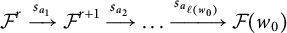 $\mathcal {F}^r \xrightarrow {s_{a_1}} \mathcal {F}^{r+1} \xrightarrow {s_{a_2}} \dots \xrightarrow {s_{a_{\ell (w_0)}}} \mathcal {F}(w_0)$
, where
$\mathcal {F}^r \xrightarrow {s_{a_1}} \mathcal {F}^{r+1} \xrightarrow {s_{a_2}} \dots \xrightarrow {s_{a_{\ell (w_0)}}} \mathcal {F}(w_0)$
, where
 $\Delta = \sigma _{a_1}\dots \sigma _{a_{\ell (w_0)}}$
, so setting
$\Delta = \sigma _{a_1}\dots \sigma _{a_{\ell (w_0)}}$
, so setting
 $\varphi _1(\mathcal {F}^0, \dots , \mathcal {F}^r)=(\mathcal {F}^0, \dots , \mathcal {F}^r, \mathcal {F}^{r+1}, \dots , \mathcal {F}(w_0))$
we obtain an element of
$\varphi _1(\mathcal {F}^0, \dots , \mathcal {F}^r)=(\mathcal {F}^0, \dots , \mathcal {F}^r, \mathcal {F}^{r+1}, \dots , \mathcal {F}(w_0))$
we obtain an element of
 $X(\beta \Delta )$
. Conversely, if
$X(\beta \Delta )$
. Conversely, if
 $(\mathcal {F}^0, \dots , \mathcal {F}^{r}, \mathcal {F}^{r+1}, \dots , \mathcal {F}(w_0)) \in X(\beta \Delta )$
, it is easy to see that
$(\mathcal {F}^0, \dots , \mathcal {F}^{r}, \mathcal {F}^{r+1}, \dots , \mathcal {F}(w_0)) \in X(\beta \Delta )$
, it is easy to see that
 $(\mathcal {F}^0, \dots , \mathcal {F}^{r}) \in \mathrm {BS}(\beta )$
, so
$(\mathcal {F}^0, \dots , \mathcal {F}^{r}) \in \mathrm {BS}(\beta )$
, so
 $\varphi _1$
is an isomorphism.
$\varphi _1$
is an isomorphism.
Let us now construct the map
 $\varphi _2^{-1}: X(\Delta \beta ) \to \mathrm {BS}(\beta )$
. Take an element
$\varphi _2^{-1}: X(\Delta \beta ) \to \mathrm {BS}(\beta )$
. Take an element
 $$\begin{align*}\left(\mathcal{F}^0, \dots, \mathcal{F}^{\ell(w_0)}, \mathcal{F}^{\ell(w_0)+1}, \dots, \mathcal{F}^{\ell(w_0) + r} = \mathcal{F}(w_0)\right) \in X(\Delta\beta).\end{align*}$$
Note that
 $\mathcal {F}^{\ell (w_0)} \in \mathsf {B} w_0 \mathsf {B}/\mathsf {B}$
, so it is of the form
$\mathcal {F}^{\ell (w_0)} \in \mathsf {B} w_0 \mathsf {B}/\mathsf {B}$
, so it is of the form
 $\mathcal {F}(U_1w_0U_2)$
, where
$\mathcal {F}(U_1w_0U_2)$
, where
 $U_1, U_2$
are upper triangular and
$U_1, U_2$
are upper triangular and
 $U_1$
is unique provided it has
$U_1$
is unique provided it has
 $1$
’s on the diagonal. Now consider the sequence of flags
$1$
’s on the diagonal. Now consider the sequence of flags
 $$ \begin{align} w_0U_1^{-1}\left(\mathcal{F}^{\ell(w_0)}, \dots, \mathcal{F}^{\ell(w_0) + r}\right). \end{align} $$
Note that
 $$ \begin{align*}w_0U_1^{-1}\mathcal{F}^{\ell(w_0) + r}=w_0U_1^{-1}\mathcal{F}(w_0)\pitchfork \mathcal{F}^{\mathrm{ant}} \end{align*} $$
so (4.1) defines a point in
 $\mathrm {BS}(\beta )$
, and we define it to be
$\mathrm {BS}(\beta )$
, and we define it to be
 $\varphi _2^{-1}(\mathcal {F}^0, \dots , \mathcal {F}^{\ell (w_0)+r})$
.
$\varphi _2^{-1}(\mathcal {F}^0, \dots , \mathcal {F}^{\ell (w_0)+r})$
.
To construct the map
 $\varphi _2$
, take an element
$\varphi _2$
, take an element
 $(\mathcal {F}^0, \dots , \mathcal {F}^r) \in \mathrm {BS}(\beta )$
. Since
$(\mathcal {F}^0, \dots , \mathcal {F}^r) \in \mathrm {BS}(\beta )$
. Since
 $\mathcal {F}^r \pitchfork \mathcal {F}(w_0)$
, we have
$\mathcal {F}^r \pitchfork \mathcal {F}(w_0)$
, we have
 $\mathcal {F}^r = \mathcal {F}((w_0V_1w_0)V_2)$
, where
$\mathcal {F}^r = \mathcal {F}((w_0V_1w_0)V_2)$
, where
 $V_1$
,
$V_1$
,
 $V_2$
are upper triangular and
$V_2$
are upper triangular and
 $V_1$
is unique provided it has
$V_1$
is unique provided it has
 $1$
’s on the diagonal. Note that
$1$
’s on the diagonal. Note that
 $V_1^{-1}w_0\mathcal {F}^r = \mathcal {F}(w_0V_2) = \mathcal {F}(w_0)$
, and that
$V_1^{-1}w_0\mathcal {F}^r = \mathcal {F}(w_0V_2) = \mathcal {F}(w_0)$
, and that
 $\mathcal {F}^{\mathrm {std}} \xrightarrow {w_0} V_1^{-1}w_0\mathcal {F}^0$
. So there exist unique flags
$\mathcal {F}^{\mathrm {std}} \xrightarrow {w_0} V_1^{-1}w_0\mathcal {F}^0$
. So there exist unique flags
 $\widetilde {\mathcal {F}}^{1}, \dots , \widetilde {\mathcal {F}}^{\ell (w_0) - 1}$
so that
$\widetilde {\mathcal {F}}^{1}, \dots , \widetilde {\mathcal {F}}^{\ell (w_0) - 1}$
so that
 $$\begin{align*}\varphi_2(\mathcal{F}^0, \dots, \mathcal{F}^r) = \left(\mathcal{F}^{\mathrm{std}}, \widetilde{\mathcal{F}}^{1}, \dots, \widetilde{\mathcal{F}}^{\ell(w_0) - 1}, V_1^{-1}w_0\mathcal{F}^0, \dots, V_1^{-1}w_0\mathcal{F}^{r}\right) \in X(\Delta\beta). \end{align*}$$
It is straightforward to see that
 $\varphi _2$
and
$\varphi _2$
and
 $\varphi _2^{-1}$
are indeed inverse maps.
$\varphi _2^{-1}$
are indeed inverse maps.
4.2 Definition via equations
For a positive braid
 $\beta = \sigma _{i_1}\dots \sigma _{i_r}$
, define the matrix
$\beta = \sigma _{i_1}\dots \sigma _{i_r}$
, define the matrix
 $$\begin{align*}B_{\beta}(z_1, \dots, z_r) = B_{i_1}(z_1)\dots B_{i_r}(z_r). \end{align*}$$
This allows us to present the braid variety
 $X(\beta )$
explicitly via equations.
$X(\beta )$
explicitly via equations.
Corollary 4.5 Let
 $\beta =\sigma _{i_1}\dots \sigma _{i_r}$
be a braid, and assume the Demazure product is
$\beta =\sigma _{i_1}\dots \sigma _{i_r}$
be a braid, and assume the Demazure product is
 $\delta (\beta ) = w_0$
. Then
$\delta (\beta ) = w_0$
. Then
 $$ \begin{align*}X(\beta)=\{(z_1,\ldots,z_r):w_0B_{\beta}(z_1,\ldots,z_r)\ \text{is upper-triangular}\}. \end{align*} $$
Indeed, given
 $(z_1, \dots , z_r)$
, by Lemma 2.5, one gets the sequence of flags
$(z_1, \dots , z_r)$
, by Lemma 2.5, one gets the sequence of flags
 $\mathcal {F}^0 = \mathcal {F}^{\mathrm {std}}$
,
$\mathcal {F}^0 = \mathcal {F}^{\mathrm {std}}$
,
 $\mathcal {F}^1 = \mathcal {F}(B_{i_1}(z_1))$
,
$\mathcal {F}^1 = \mathcal {F}(B_{i_1}(z_1))$
,
 $\mathcal {F}^2 = \mathcal {F}(B_{i_1}(z_1)B_{i_2}(z_2)),$
and so on. To obtain a similar description for the double Bott–Samelson variety
$\mathcal {F}^2 = \mathcal {F}(B_{i_1}(z_1)B_{i_2}(z_2)),$
and so on. To obtain a similar description for the double Bott–Samelson variety
 $\mathrm {BS}(\beta )$
, we use Lemma 2.4.
$\mathrm {BS}(\beta )$
, we use Lemma 2.4.
Corollary 4.6 Let
 $\beta $
be a positive braid. The double Bott–Samelson variety is
$\beta $
be a positive braid. The double Bott–Samelson variety is
 $$\begin{align*}\mathrm{BS}(\beta) = \{(z_1, \dots, z_r) \in \mathbb{C}^r \mid B_{\beta}(z_1, \dots, z_r) \; \text{admits an LU decomposition}\}. \end{align*}$$
Equivalently, using principal minors we have
 $$\begin{align*}\mathrm{BS}(\beta) = \{ (z_1, \dots, z_r)\in \mathbb{C}^r \mid \Delta_{[i],[i]}(B_{\beta}(z)) \neq 0 \; \text{for every} \; i = 1, \dots, k\} \end{align*}$$
so that
 $\mathrm {BS}(\beta )$
is a principal open subvariety of
$\mathrm {BS}(\beta )$
is a principal open subvariety of
 $\mathbb {C}^r$
. If
$\mathbb {C}^r$
. If
 $w \in S_k$
, then
$w \in S_k$
, then
 $\mathrm {BS}(\underline {w})$
coincides with the double Bruhat cell of w, that is, the open Richardson variety
$\mathrm {BS}(\underline {w})$
coincides with the double Bruhat cell of w, that is, the open Richardson variety
 $R(e,w)$
.
$R(e,w)$
.
The following lemmas give some useful examples of explicit braid matrices.
Lemma 4.7 Consider the partial Coxeter element
 $\mathbf {c}(i) = \sigma _{k-1}\dots \sigma _{k-i}$
. Then,
$\mathbf {c}(i) = \sigma _{k-1}\dots \sigma _{k-i}$
. Then,
 $$\begin{align*}B_{\mathbf{c}(i)}(z_1, \dots, z_i) = \begin{pmatrix} \mathbf{1}_{(k-i-1) \times (k-i-1)} & \mathbf{0}_{(k-i-1) \times 1} & \mathbf{0}_{(k-i-1) \times 1} & \dots & \mathbf{0}_{(k-i-1) \times 1} \\ \mathbf{0}_{1\times (k-i-1)} & z_i & -1 & \dots & 0 \\ \mathbf{0}_{1 \times(k-i-1)} & z_{i-1} & 0 & \dots & 0 \\ \vdots & \vdots & \vdots & \ddots & \vdots \\ {\mathbf{0}_{1 \times (k-i-1)}} & z_1 & 0 & \dots & -1 \\ {\mathbf{0}}_{1 \times (k- i-1)} & 1 & 0 & \dots & 0 \end{pmatrix}, \end{align*}$$
where
 $\mathbf {1}_{(k-i-1) \times (k-i-1)}$
is the identity matrix of size
$\mathbf {1}_{(k-i-1) \times (k-i-1)}$
is the identity matrix of size
 $k-i-1$
,
$k-i-1$
,
 $\mathbf {0}_{1 \times (k-i-1)}$
is the row vector of size
$\mathbf {0}_{1 \times (k-i-1)}$
is the row vector of size
 $k-i-1$
with only
$k-i-1$
with only
 $0$
’s, and similarly for
$0$
’s, and similarly for
 $\mathbf {0}_{(k-i-1) \times 1}$
.
$\mathbf {0}_{(k-i-1) \times 1}$
.
Proof By induction on i, the case
 $i = 1$
is simply the definition of the braid matrix
$i = 1$
is simply the definition of the braid matrix
 $B_{k-1}(z_1)$
and the induction step is a simple computation.
$B_{k-1}(z_1)$
and the induction step is a simple computation.
The next result is analogous to [Reference Casals, Gorsky, Gorsky and Simental4, Equation (2.5)] and can be shown by induction using Lemma 4.7 above.
Lemma 4.8 Consider the braid word
 $\Delta = (\sigma _{k-1}\dots \sigma _1)(\sigma _{k-1}\dots \sigma _2)\dots (\sigma _{k-1}\sigma _{k-2})\sigma _{k-1}$
. Then,
$\Delta = (\sigma _{k-1}\dots \sigma _1)(\sigma _{k-1}\dots \sigma _2)\dots (\sigma _{k-1}\sigma _{k-2})\sigma _{k-1}$
. Then,
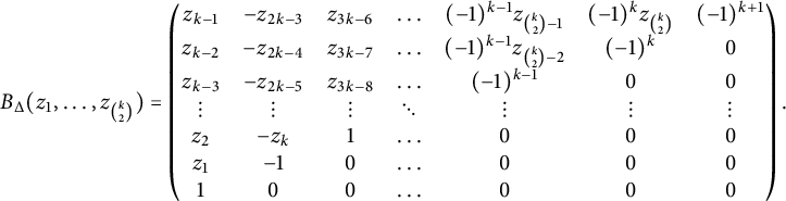 $$ \begin{align} B_{\Delta}(z_1, \dots, z_{\binom{k}{2}}) = \begin{pmatrix} z_{k-1} & -z_{2k-3} & z_{3k-6} & \dots & (-1)^{k-1}z_{\binom{k}{2} - 1} & (-1)^{k}z_{\binom{k}{2}} & (-1)^{k+1} \\ z_{k-2} & -z_{2k-4} & z_{3k-7} & \dots & (-1)^{k-1}z_{\binom{k}{2} - 2} & (-1)^{k} & 0 \\ z_{k-3} & -z_{2k-5} & z_{3k-8} & \dots & (-1)^{k-1} & 0 & 0 \\ \vdots & \vdots & \vdots & \ddots & \vdots & \vdots & \vdots \\ z_{2} & -z_{k} & 1 & \dots & 0 & 0 & 0 \\ z_{1} & -1 & 0 & \dots & 0 & 0 & 0 \\ 1 & 0 & 0 & \dots & 0 & 0 & 0 \end{pmatrix}. \end{align} $$
In particular,
 $w_0B_{\Delta }(z_1, \dots , z_{\binom {k}{2}})$
is a lower-triangular matrix, and
$w_0B_{\Delta }(z_1, \dots , z_{\binom {k}{2}})$
is a lower-triangular matrix, and
 $B_{\Delta }(z_1, \dots , z_{\binom {k}{2}})w_0$
is an upper-triangular matrix.
$B_{\Delta }(z_1, \dots , z_{\binom {k}{2}})w_0$
is an upper-triangular matrix.
Lemma 4.9 Let
 $(z_1, \dots , z_r) \in X(\beta )$
and let
$(z_1, \dots , z_r) \in X(\beta )$
and let
 $\widetilde {\Delta }$
be any braid of length
$\widetilde {\Delta }$
be any braid of length
 $\ell (w_0)$
such that
$\ell (w_0)$
such that
 $\pi (\widetilde {\Delta }) = w_0$
. Assume
$\pi (\widetilde {\Delta }) = w_0$
. Assume
 $\delta (\beta ) = w_0$
. Then, there exist unique functions
$\delta (\beta ) = w_0$
. Then, there exist unique functions
 $y_1, \dots , y_{\ell (w_0)} \in \mathbb {C}[X(\beta )]$
such that the matrix
$y_1, \dots , y_{\ell (w_0)} \in \mathbb {C}[X(\beta )]$
such that the matrix
 $$\begin{align*}B_{\beta}(z_1, \dots, z_r)B_{\widetilde{\Delta}}(y_1 \dots, y_{\ell(w_0)}) \end{align*}$$
is diagonal.
Proof Since any two reduced expressions for
 $w_0$
are related by braid moves, it is enough to prove this for a single reduced braid lift
$w_0$
are related by braid moves, it is enough to prove this for a single reduced braid lift
 $\widetilde {\Delta }$
of
$\widetilde {\Delta }$
of
 $w_0$
. For
$w_0$
. For
 $$ \begin{align*}\widetilde{\Delta} = (\sigma_{k-1}\dots \sigma_1)(\sigma_{k-1}\dots \sigma_2)(\sigma_{k-1}\sigma_{k-2})(\sigma_{k-1}),\end{align*} $$
this follows immediately from Lemma 4.8.
We can obtain a description in coordinates of the isomorphism
 $\varphi _2: \mathrm {BS}(\beta ) \to X(\Delta \beta )$
.
$\varphi _2: \mathrm {BS}(\beta ) \to X(\Delta \beta )$
.
Corollary 4.10 There exist unique functions
 $p_1, \dots , p_{\ell (w_0)} \in \mathbb {C}[\mathrm {BS}(\beta )]$
such that the map
$p_1, \dots , p_{\ell (w_0)} \in \mathbb {C}[\mathrm {BS}(\beta )]$
such that the map
 $$\begin{align*}\varphi_2: \mathrm{BS}(\beta) \to X(\Delta\beta), \qquad \varphi_2(z_1, \dots, z_r) = \left(p_1, \dots, p_{\ell(w_0)}, z_1, \dots, z_r\right) \end{align*}$$
is an isomorphism.
Proof If
 $(z_1, \dots , z_r) \in \mathrm {BS}(\beta )$
, then the braid matrix
$(z_1, \dots , z_r) \in \mathrm {BS}(\beta )$
, then the braid matrix
 $B_{\beta }(z_1, \dots , z_r)$
admits an LU decomposition, say
$B_{\beta }(z_1, \dots , z_r)$
admits an LU decomposition, say
 $B_{\beta }(z_1, \dots , z_r) = LU$
, equivalently,
$B_{\beta }(z_1, \dots , z_r) = LU$
, equivalently,
 $w_0L^{-1}B_{\beta }(z_1, \dots , z_r) = w_0U$
. By Lemma 4.8, we can find unique functions
$w_0L^{-1}B_{\beta }(z_1, \dots , z_r) = w_0U$
. By Lemma 4.8, we can find unique functions
 $p_1, \dots , p_{\ell (w_0)}$
such that
$p_1, \dots , p_{\ell (w_0)}$
such that
 $w_0L^{-1} = B_{\Delta }(p_1, \dots , p_{\ell (w_0)})$
and
$w_0L^{-1} = B_{\Delta }(p_1, \dots , p_{\ell (w_0)})$
and
 $\varphi _2: \mathrm {BS}(\beta ) \to X(\Delta \beta )$
is well-defined.
$\varphi _2: \mathrm {BS}(\beta ) \to X(\Delta \beta )$
is well-defined.
Note that the inverse map is given by
 $$\begin{align*}\varphi_2^{-1}(z_1, \dots, z_{\ell(w_0)}, z_{\ell(w_0)+1}, \dots, z_{\ell(w_0)+r}) = (z_{\ell(w_0)+1}, \dots, z_{\ell(w_0)+r}).\end{align*}$$
Indeed, if
 $B_{\Delta }(z_1, \dots , z_{\ell (w_0)})B_{\beta }(z_{\ell (w_0)+1}, \dots , z_{\ell (w_0)+r}) = w_0U_1$
for some upper triangular matrix
$B_{\Delta }(z_1, \dots , z_{\ell (w_0)})B_{\beta }(z_{\ell (w_0)+1}, \dots , z_{\ell (w_0)+r}) = w_0U_1$
for some upper triangular matrix
 $U_1$
, then
$U_1$
, then
 $B_{\beta }(z_{\ell (w_0)+1}, \dots , z_{\ell (w_0)+r}) = B_{\Delta }^{-1}(z_1,\dots , z_{\ell (w_0)})w_0U_1$
, which has an LU-decomposition by Lemma 4.8. It is straightforward to verify that
$B_{\beta }(z_{\ell (w_0)+1}, \dots , z_{\ell (w_0)+r}) = B_{\Delta }^{-1}(z_1,\dots , z_{\ell (w_0)})w_0U_1$
, which has an LU-decomposition by Lemma 4.8. It is straightforward to verify that
 $\varphi _2, \varphi _2^{-1}$
are indeed inverses of each other.
$\varphi _2, \varphi _2^{-1}$
are indeed inverses of each other.
4.3 Cluster structure
Let us now describe the cluster structure on braid varieties obtained in [Reference Casals, Gorsky, Gorsky, Le, Shen and Simental2] (see also [Reference Galashin, Lam and Sherman-Bennett12, Reference Galashin, Lam, Sherman-Bennett and Speyer13]). This cluster structure generalizes the one obtained for double Bott–Samelson varieties in [Reference Shen and Weng26], that we will also describe.
4.3.1 Cluster structure on braid varieties: Variables
We will define an initial cluster
 $\mathbf {x}_{X(\beta )}$
first by means of its non-vanishing locus. For each
$\mathbf {x}_{X(\beta )}$
first by means of its non-vanishing locus. For each
 $m = 1, \dots , r$
, let
$m = 1, \dots , r$
, let
 $\beta _{m} = \sigma _{i_1}\dots \sigma _{i_m}$
, so that
$\beta _{m} = \sigma _{i_1}\dots \sigma _{i_m}$
, so that
 $\beta _{r} = \beta $
.
$\beta _{r} = \beta $
.
Definition 4.11 The left-to-right inductive torus (also known as Deodhar torus)
 $\vec {\mathbb {T}}_{\beta } \subseteq X(\beta )$
consists of those elements
$\vec {\mathbb {T}}_{\beta } \subseteq X(\beta )$
consists of those elements
 $(\mathcal {F}^0 = \mathcal {F}^{\mathrm {std}}, \mathcal {F}^1, \dots , \mathcal {F}^r = \mathcal {F}^{\mathrm {ant}})$
such that
$(\mathcal {F}^0 = \mathcal {F}^{\mathrm {std}}, \mathcal {F}^1, \dots , \mathcal {F}^r = \mathcal {F}^{\mathrm {ant}})$
such that
 $$\begin{align*}\mathcal{F}^{0} \xrightarrow{\delta(\beta_{m})} \mathcal{F}^m \end{align*}$$
for all
 $m = 1, \dots , r$
.
$m = 1, \dots , r$
.
We can give a system of coordinates on
 $\vec {\mathbb {T}}_{\beta }$
as follows.
$\vec {\mathbb {T}}_{\beta }$
as follows.
Lemma 4.12 [Reference Galashin, Lam and Sherman-Bennett12, Proposition 2.12]
The torus
 $\vec {\mathbb {T}}_{\beta }$
is given by the non-vanishing of the minors
$\vec {\mathbb {T}}_{\beta }$
is given by the non-vanishing of the minors
 $$ \begin{align} \Delta_{\delta(\beta_{m})[i_m], [i_m]}\left(B_{\beta_{m}}\!\left(z_1, \dots, z_m\right)\right). \end{align} $$
Proof If
 $(z_1, \dots , z_r) \in \vec {\mathbb {T}}_{\beta }$
, then all minors (4.3) are nonzero by Lemma 2.7(b). Conversely, assume all minors (4.3) are nonzero. We show by induction on m that
$(z_1, \dots , z_r) \in \vec {\mathbb {T}}_{\beta }$
, then all minors (4.3) are nonzero by Lemma 2.7(b). Conversely, assume all minors (4.3) are nonzero. We show by induction on m that
 $\mathcal {F}^{\mathrm {std}} \xrightarrow {\delta (\beta _m)} \mathcal {F}(B_{\beta _m}(z_1, \dots , z_m))$
. The base of induction is
$\mathcal {F}^{\mathrm {std}} \xrightarrow {\delta (\beta _m)} \mathcal {F}(B_{\beta _m}(z_1, \dots , z_m))$
. The base of induction is
 $m = 0$
, where
$m = 0$
, where
 $\beta _m$
is the identity braid and
$\beta _m$
is the identity braid and
 $B_{\beta _m}(z_1,\dots , z_m)$
is the identity matrix. For brevity, we will denote
$B_{\beta _m}(z_1,\dots , z_m)$
is the identity matrix. For brevity, we will denote
 $\mathcal {F}^m := \mathcal {F}(B_{\beta _m}(z_1, \dots , z_m))$
.
$\mathcal {F}^m := \mathcal {F}(B_{\beta _m}(z_1, \dots , z_m))$
.
Assume
 $\mathcal {F}^0 \xrightarrow {\delta (\beta _m)}\mathcal {F}^m$
. Note that we have
$\mathcal {F}^0 \xrightarrow {\delta (\beta _m)}\mathcal {F}^m$
. Note that we have
 $$\begin{align*}\mathcal{F}^{0} \xrightarrow{\delta(\beta_m)} \mathcal{F}^m \xrightarrow{s_{i_{m+1}}} \mathcal{F}^{m+1}. \end{align*}$$
If
 $\delta (\beta _{m+1}) = \delta (\beta _m)s_{i_{m+1}}$
, then using Corollary 2.3(a), we obtain
$\delta (\beta _{m+1}) = \delta (\beta _m)s_{i_{m+1}}$
, then using Corollary 2.3(a), we obtain
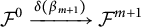 $\mathcal {F}^0 \xrightarrow {\delta (\beta _{m+1})} \mathcal {F}^{m+1}$
, as needed. If, on the other hand,
$\mathcal {F}^0 \xrightarrow {\delta (\beta _{m+1})} \mathcal {F}^{m+1}$
, as needed. If, on the other hand,
 $\delta (\beta _{m+1}) = \delta (\beta _m),$
then using Corollary 2.3(b), we have that
$\delta (\beta _{m+1}) = \delta (\beta _m),$
then using Corollary 2.3(b), we have that
 $\mathcal {F}^{0} \xrightarrow {v} \mathcal {F}^{m+1}$
with
$\mathcal {F}^{0} \xrightarrow {v} \mathcal {F}^{m+1}$
with
 $v \leq \delta (\beta _m)\star s_{i_{m+1}} = \delta (\beta _{m})$
. Thus, by Lemma 2.7(c), to conclude that
$v \leq \delta (\beta _m)\star s_{i_{m+1}} = \delta (\beta _{m})$
. Thus, by Lemma 2.7(c), to conclude that
 $v = \delta (\beta _m) = \delta (\beta _{m+1})$
, it is enough to show that
$v = \delta (\beta _m) = \delta (\beta _{m+1})$
, it is enough to show that
 $\Delta _{\delta (\beta _{m})[j], [j]}\!\left (B_{\beta _{m}}(z_1, \dots , z_m)B_{s_{i_{m+1}}}(z_{m+1})\right )$
is nonzero for all
$\Delta _{\delta (\beta _{m})[j], [j]}\!\left (B_{\beta _{m}}(z_1, \dots , z_m)B_{s_{i_{m+1}}}(z_{m+1})\right )$
is nonzero for all
 $j = 1, \dots , k$
. But by Lemma 2.10, if
$j = 1, \dots , k$
. But by Lemma 2.10, if
 $j \neq i_{m+1}$
, then
$j \neq i_{m+1}$
, then
 $$\begin{align*}\Delta_{\delta(\beta_{m})[j], [j]}\!\left(B_{\beta_{m}}(z_1, \dots, z_m)B_{s_{i_{m+1}}}(z_{m+1})\right) = \Delta_{\delta(\beta_{m})[j], [j]}\!\left(B_{\beta_{m}}(z_1, \dots, z_m)\right) \neq 0, \end{align*}$$
where the last inequality follows from the induction assumption. If
 $j = i_{m+1}$
, it is our assumption that
$j = i_{m+1}$
, it is our assumption that
 $\Delta _{\delta (\beta _{m})[i_{m+1}], [i_{m+1}]}\!\left (B_{\beta _{m}}(z_1, \dots , z_m)B_{s_{i_{m+1}}}(z_{m+1})\right ) \neq 0$
, and the result follows.
$\Delta _{\delta (\beta _{m})[i_{m+1}], [i_{m+1}]}\!\left (B_{\beta _{m}}(z_1, \dots , z_m)B_{s_{i_{m+1}}}(z_{m+1})\right ) \neq 0$
, and the result follows.
One might then expect that the minors (4.3) are the cluster variables in an initial seed for
 $X(\beta )$
. However, this does not work because in general (4.3) is not an irreducible polynomial in
$X(\beta )$
. However, this does not work because in general (4.3) is not an irreducible polynomial in
 $z_1, \dots , z_m$
. However, the irreducible factors of (4.3) are in fact the cluster variables defining the torus
$z_1, \dots , z_m$
. However, the irreducible factors of (4.3) are in fact the cluster variables defining the torus
 $\vec {\mathbb {T}}_{\beta }$
and the minors (4.3) are cluster monomials. Moreover, one can obtain (4.3) from the cluster variables in an upper uni-triangular fashion, and we only need to consider the minors (4.3) for those m so that
$\vec {\mathbb {T}}_{\beta }$
and the minors (4.3) are cluster monomials. Moreover, one can obtain (4.3) from the cluster variables in an upper uni-triangular fashion, and we only need to consider the minors (4.3) for those m so that
 $\delta (\beta _{m}) = \delta (\beta _{m-1})$
. To summarize, for each
$\delta (\beta _{m}) = \delta (\beta _{m-1})$
. To summarize, for each
 $m = 1, \dots , r$
such that
$m = 1, \dots , r$
such that
 $\delta (\beta _{m}) = \delta (\beta _{m-1})$
, the minor (4.3) has a unique irreducible factor that has not appeared in such a minor for a smaller index, this irreducible factor appears with multiplicity one, and it is a cluster variable. See [Reference Casals, Gorsky, Gorsky, Le, Shen and Simental2, Reference Galashin, Lam and Sherman-Bennett12, Reference Galashin, Lam, Sherman-Bennett and Speyer13] and also [Reference Ingermanson19] for details.
$\delta (\beta _{m}) = \delta (\beta _{m-1})$
, the minor (4.3) has a unique irreducible factor that has not appeared in such a minor for a smaller index, this irreducible factor appears with multiplicity one, and it is a cluster variable. See [Reference Casals, Gorsky, Gorsky, Le, Shen and Simental2, Reference Galashin, Lam and Sherman-Bennett12, Reference Galashin, Lam, Sherman-Bennett and Speyer13] and also [Reference Ingermanson19] for details.
The quiver Q forming a seed with the cluster described above can be obtained using the Lusztig cycles in the left-to-right inductive weave of
 $\beta $
. Since we will not need this level of detail we will not go into it, and instead refer the reader to [Reference Casals, Gorsky, Gorsky, Le, Shen and Simental2, Section 4].
$\beta $
. Since we will not need this level of detail we will not go into it, and instead refer the reader to [Reference Casals, Gorsky, Gorsky, Le, Shen and Simental2, Section 4].
4.3.2 Cluster structure on double Bott–Samelson varieties: Variables
We use the isomorphism
 $\varphi _2: \mathrm {BS}(\beta ) \to X(\Delta \beta )$
from Lemma 4.4 in order to translate the cluster structure on
$\varphi _2: \mathrm {BS}(\beta ) \to X(\Delta \beta )$
from Lemma 4.4 in order to translate the cluster structure on
 $X(\Delta \beta )$
described above to
$X(\Delta \beta )$
described above to
 $\mathrm {BS}(\beta )$
. We remark that the resulting cluster structure is the one obtained by Shen and Weng in [Reference Shen and Weng26], which predates the construction of cluster structures on general braid varieties (see [Reference Casals, Gorsky, Gorsky, Le, Shen and Simental2, Section 4.8 and Proposition 4.20]).
$\mathrm {BS}(\beta )$
. We remark that the resulting cluster structure is the one obtained by Shen and Weng in [Reference Shen and Weng26], which predates the construction of cluster structures on general braid varieties (see [Reference Casals, Gorsky, Gorsky, Le, Shen and Simental2, Section 4.8 and Proposition 4.20]).
First, we make some simplifications. By Corollary 4.10, we have that
 $\varphi _2$
sends
$\varphi _2$
sends
 $(z_1, \dots , z_r)$
to
$(z_1, \dots , z_r)$
to
 $(p_1, \dots , p_{\ell (w_0)}, z_1, \dots , z_r)$
, where
$(p_1, \dots , p_{\ell (w_0)}, z_1, \dots , z_r)$
, where
 $\mathbf {p}=\{p_1, \dots , p_{\ell (w_0)}\}$
are uniquely defined functions of
$\mathbf {p}=\{p_1, \dots , p_{\ell (w_0)}\}$
are uniquely defined functions of
 $\mathbf {z}=\{z_1, \dots , z_r\}$
.
$\mathbf {z}=\{z_1, \dots , z_r\}$
.
Second,
 $\delta ((\Delta \beta )_{m}) = \delta ((\Delta \beta )_{m-1})$
if and only if
$\delta ((\Delta \beta )_{m}) = \delta ((\Delta \beta )_{m-1})$
if and only if
 $m> \ell (w_0)$
, and in this case, the Demazure product is precisely
$m> \ell (w_0)$
, and in this case, the Demazure product is precisely
 $w_0$
. We denote
$w_0$
. We denote
 $j=m-\ell (w_0)$
, so that the m-th letter in
$j=m-\ell (w_0)$
, so that the m-th letter in
 $\Delta \beta $
is
$\Delta \beta $
is
 $i_{j}$
.
$i_{j}$
.
Therefore, the cluster variables are the irreducible factors of
 $$\begin{align*}\Delta_{w_0[i_j], [i_j]}\left(B_{(\Delta\beta)_{m}}\left(p_1, \dots, p_{\ell(w_0)},z_1, \dots, z_j\right)\right), \qquad j = 1, \dots, \ell(\beta). \end{align*}$$
Note, however, that
 $$\begin{align*}\begin{array}{r@{\,}l} \Delta_{w_0[i_j],[i_j]}\left(B_{(\Delta\beta)_{m}}\!\left(\mathbf{p},z_1, \dots, z_j\right)\right) = & \Delta_{w_0[i_j], [i_j]} \left(B_{\Delta}(\mathbf{p})B_{\beta_{j}}\!\left(z_{1}, \dots, z_j\right)\right) \\ = & \Delta_{w_0[i_j], [i_j]}\left(w_0L(\mathbf{p})B_{\beta_{j}}\!\left(z_{1}, \dots, z_j\right)\right) \\ = & \Delta_{[i_j], [i_j]}\left(L(\mathbf{p})B_{\beta_{j}}\!\left(z_{1}, \dots, z_j\right)\right) \\ = & \Delta_{[i_j], [i_j]}\left(B_{\beta_{j}}\!\left(z_{1}, \dots, z_j\right)\right), \end{array} \end{align*}$$
where we have used that
 $L(\mathbf {p})$
is lower triangular with
$L(\mathbf {p})$
is lower triangular with
 $1$
’s on the diagonal, and Lemma 4.8. We conclude that the cluster variables in
$1$
’s on the diagonal, and Lemma 4.8. We conclude that the cluster variables in
 $\mathrm {BS}(\beta )$
are the irreducible factors of
$\mathrm {BS}(\beta )$
are the irreducible factors of
 $$ \begin{align} x_j := \Delta_{[i_j],[i_j]}(B_{\beta_{j}}(z_1, \dots, z_j)). \end{align} $$
However, by [Reference Shen and Weng26, Lemma 3.30], the function
 $x_j$
is already irreducible. We summarize the previous discussion in the following result.
$x_j$
is already irreducible. We summarize the previous discussion in the following result.
Lemma 4.13 [Reference Shen and Weng26]
The cluster variables in
 $\mathrm {BS}(\beta )$
are as in (4.4), with
$\mathrm {BS}(\beta )$
are as in (4.4), with
 $j = 1, \dots , r$
.
$j = 1, \dots , r$
.
Since
 $\Delta _{[i],[i]}(U) \neq 0$
for any matrix
$\Delta _{[i],[i]}(U) \neq 0$
for any matrix
 $U \in \mathsf {B}(k)$
and any
$U \in \mathsf {B}(k)$
and any
 $i = 1, \dots , k$
, we immediately obtain the following.
$i = 1, \dots , k$
, we immediately obtain the following.
Corollary 4.14 The common nonvanishing locus of
 $x_j, j = 1, \dots , r$
, is
$x_j, j = 1, \dots , r$
, is
 $$\begin{align*}\vec{\mathbb{T}}_{\Delta\beta}=\left\{(\mathcal{F}^0, \mathcal{F}^1, \dots, \mathcal{F}^r) \in \mathrm{BS}(\beta) \mid \mathcal{F}^{i} \pitchfork \mathcal{F}(w_0) \; \text{for all} \; i\right\}. \end{align*}$$
For
 $s = 1, \dots , k-1$
, let
$s = 1, \dots , k-1$
, let
 $\mathrm {last}(s)$
be such that
$\mathrm {last}(s)$
be such that
 $i_{\mathrm {last}(s)} = s$
and
$i_{\mathrm {last}(s)} = s$
and
 $i_j \neq s$
for
$i_j \neq s$
for
 $j> \mathrm {last}(s)$
. In words,
$j> \mathrm {last}(s)$
. In words,
 $\mathrm {last}(s)$
is the position of the rightmost appearance of
$\mathrm {last}(s)$
is the position of the rightmost appearance of
 $\sigma _s$
in
$\sigma _s$
in
 $\beta $
. If s does not appear in
$\beta $
. If s does not appear in
 $\beta $
, we define
$\beta $
, we define
 $\mathrm {last}(s)$
to be a formal symbol
$\mathrm {last}(s)$
to be a formal symbol
 $\oslash $
. If
$\oslash $
. If
 $\mathrm {last}(s) \neq \oslash ,$
then by Lemma 2.10, we have
$\mathrm {last}(s) \neq \oslash ,$
then by Lemma 2.10, we have
 $$\begin{align*}x_{\mathrm{last}(s)} = \Delta_{[s],[s]}(B_{\beta_{\mathrm{last}(s)}}(z_1, \dots, z_{\mathrm{last}(s)})) = \Delta_{[s],[s]}(B_{\beta}(z_1, \dots, z_r)), \end{align*}$$
so that, by the definition of
 $\mathrm {BS}(\beta )$
,
$\mathrm {BS}(\beta )$
,
 $x_{\mathrm {last}(s)}$
is invertible in
$x_{\mathrm {last}(s)}$
is invertible in
 $\mathbb {C}[\mathrm {BS}(\beta )]$
. In fact, the frozen variables in
$\mathbb {C}[\mathrm {BS}(\beta )]$
. In fact, the frozen variables in
 $\mathrm {BS}(\beta )$
are
$\mathrm {BS}(\beta )$
are
 $\{x_{\mathrm {last}(s)} \mid s = 1, \dots , k-1, \mathrm {last}(s) \neq \oslash \}$
. For convenience and future use, we set
$\{x_{\mathrm {last}(s)} \mid s = 1, \dots , k-1, \mathrm {last}(s) \neq \oslash \}$
. For convenience and future use, we set
 $x_{\oslash } = 1$
.
$x_{\oslash } = 1$
.
Let us describe the frozen variables in terms of the LU-decomposition of
 $B_{\beta }(z_1, \dots , z_r)$
. Let
$B_{\beta }(z_1, \dots , z_r)$
. Let
 $B_{\beta }(z_1, \dots , z_r) = LU$
, where L has
$B_{\beta }(z_1, \dots , z_r) = LU$
, where L has
 $1$
’s in the diagonal and the diagonal of U is
$1$
’s in the diagonal and the diagonal of U is
 $\mathrm {diag}(u_1, \dots , u_k)$
, where each
$\mathrm {diag}(u_1, \dots , u_k)$
, where each
 $u_i \in \mathbb {C}[\mathrm {BS}(\beta )]$
is a function on
$u_i \in \mathbb {C}[\mathrm {BS}(\beta )]$
is a function on
 $\mathrm {BS}(\beta )$
. Note that
$\mathrm {BS}(\beta )$
. Note that
 $$\begin{align*}\det(B_{\beta}(z_1, \dots, z_r)) = 1 = u_1\dots u_k\end{align*}$$
so that each
 $u_i$
is a unit in
$u_i$
is a unit in
 $\mathbb {C}[\mathrm {BS}(\beta )]$
and, moreover,
$\mathbb {C}[\mathrm {BS}(\beta )]$
and, moreover,
 $$ \begin{align} x_{\mathrm{last}(s)} = \Delta_{[s],[s]}(B_{\beta}(z_1, \dots, z_r)) = u_1\dots u_s. \end{align} $$
Expressing u’s in terms of the frozen variables, we have
 $u_1 = x_{\mathrm {last}(1)}$
,
$u_1 = x_{\mathrm {last}(1)}$
,
 $u_s = x_{\mathrm {last}(s)}x_{\mathrm {last}(s-1)}^{-1}$
for
$u_s = x_{\mathrm {last}(s)}x_{\mathrm {last}(s-1)}^{-1}$
for
 $s = 2, \dots , k-1$
and
$s = 2, \dots , k-1$
and
 $u_k = u_1^{-1}\dots u_{k-1}^{-1} = x_{\mathrm {last}(k-1)}^{-1}$
.
$u_k = u_1^{-1}\dots u_{k-1}^{-1} = x_{\mathrm {last}(k-1)}^{-1}$
.
4.3.3 Cluster structure on double Bott–Samelson varieties: Quiver
Next, we describe the quiver for double Bott–Samelson variety
 $\mathrm {BS}(\beta )$
.
$\mathrm {BS}(\beta )$
.
The quiver
 $Q_{\beta }$
can be read directly from the braid diagram of
$Q_{\beta }$
can be read directly from the braid diagram of
 $\beta $
drawn horizontally. The vertices of
$\beta $
drawn horizontally. The vertices of
 $Q_{\beta }$
are in bijection with the connected components of
$Q_{\beta }$
are in bijection with the connected components of
 $\mathbb {R}^2$
minus the braid diagram of
$\mathbb {R}^2$
minus the braid diagram of
 $\beta $
which are bounded on the left: each connected component corresponds to the crossing directly to its left. Around each crossing, we have the following configuration of half arrows
$\beta $
which are bounded on the left: each connected component corresponds to the crossing directly to its left. Around each crossing, we have the following configuration of half arrows

which produces a quiver that possibly has oriented
 $2$
-cycles, and the quiver
$2$
-cycles, and the quiver
 $Q_{\beta }$
is obtained after removing a maximal collection of disjoint oriented
$Q_{\beta }$
is obtained after removing a maximal collection of disjoint oriented
 $2$
-cycles.
$2$
-cycles.
To see that half arrows add up to an integer number of arrows, it is useful to rephrase the construction of
 $Q_{\beta }$
. The vertices of the quiver are in bijection with the letters of
$Q_{\beta }$
. The vertices of the quiver are in bijection with the letters of
 $\beta $
. Let us say that the vertex j has color i and write
$\beta $
. Let us say that the vertex j has color i and write
 $\mathrm {clr}(j)=i$
if
$\mathrm {clr}(j)=i$
if
 $i_j = i$
. The arrows in
$i_j = i$
. The arrows in
 $Q_{\beta }$
are of two types: mixed (between vertices of different colors) and unmixed (between vertices of the same color).
$Q_{\beta }$
are of two types: mixed (between vertices of different colors) and unmixed (between vertices of the same color).
If
 $j_1 < j_2$
are vertices of the same color, then there is an unmixed arrow
$j_1 < j_2$
are vertices of the same color, then there is an unmixed arrow
 $j_1 \to j_2$
if and only if there does not exist
$j_1 \to j_2$
if and only if there does not exist
 $j_1 < k < j_2$
of the same color as
$j_1 < k < j_2$
of the same color as
 $j_1, j_2$
. Put it more succinctly: there is an unmixed arrow pointing right between two consecutive appearances of the same color. These are all the unmixed arrows.
$j_1, j_2$
. Put it more succinctly: there is an unmixed arrow pointing right between two consecutive appearances of the same color. These are all the unmixed arrows.

Let us now describe the mixed arrows. Assume
 $j_1 < j_2$
have different colors. If there is a mixed arrow
$j_1 < j_2$
have different colors. If there is a mixed arrow
 $j_2 \to j_1$
, then
$j_2 \to j_1$
, then
 $\mathrm {clr}(j_2) = \mathrm {clr}(j_1) \pm 1$
. Now, let us say that
$\mathrm {clr}(j_2) = \mathrm {clr}(j_1) \pm 1$
. Now, let us say that
 $j_1 < j_2$
and
$j_1 < j_2$
and
 $\mathrm {clr}(j_2) = \mathrm {clr}(j_1) \pm 1$
. Then, there is an arrow
$\mathrm {clr}(j_2) = \mathrm {clr}(j_1) \pm 1$
. Then, there is an arrow
 $j_2 \to j_1$
if and only if there exists
$j_2 \to j_1$
if and only if there exists
 $j_1 < j_2 < j^{\prime }_1$
such that:
$j_1 < j_2 < j^{\prime }_1$
such that:
-
•
$\mathrm {clr}(j_1) = \mathrm {clr}(j^{\prime }_1)$
and, moreover,
$j_1$
and
$j^{\prime }_1$
are consecutive appearances of this color; -
• there does not exist
$j_2 < k < j^{\prime }_1$
of the same color as
$j_2$
.


Finally, the frozen vertices are
 $\{\mathrm {last}(k) | k = 1, \dots , n-1\}$
.
$\{\mathrm {last}(k) | k = 1, \dots , n-1\}$
.
5 Splicing braid varieties
5.1 The splicing map
We now describe splicing maps for general braid varieties. Let us fix the braid
 $\beta =\sigma _{i_1}\dots \sigma _{i_r}$
. Furthermore, let
$\beta =\sigma _{i_1}\dots \sigma _{i_r}$
. Furthermore, let
 $\beta ^1=\sigma _{i_1}\dots \sigma _{i_{r_1}}$
and
$\beta ^1=\sigma _{i_1}\dots \sigma _{i_{r_1}}$
and
 $\beta ^2=\sigma _{i_{r_1+1}}\dots \sigma _{i_r}$
so that
$\beta ^2=\sigma _{i_{r_1+1}}\dots \sigma _{i_r}$
so that
 $\beta =\beta ^1\beta ^2$
. For fixed
$\beta =\beta ^1\beta ^2$
. For fixed
 $w \in S_k$
, we consider the subset
$w \in S_k$
, we consider the subset
 $$ \begin{align} \mathcal{U}_{r_1,w}(\beta) := \left\{\left(\mathcal{F}^0, \dots, \mathcal{F}^r\right) \in X(\beta) \mid \mathcal{F}^{r_1} \pitchfork \mathcal{F}(w_0w)\right\}. \end{align} $$
By Lemma 2.9,
 $\mathcal {U}_{r_1, w} \subseteq X(\beta )$
is open and
$\mathcal {U}_{r_1, w} \subseteq X(\beta )$
is open and
 $$\begin{align*}X(\beta) = \bigcup_{w \in S_k}\mathcal{U}_{r_1, w}. \end{align*}$$
Note, however, that for a fixed
 $w \in S_k$
, the open set
$w \in S_k$
, the open set
 $\mathcal {U}_{r_1, w}$
may be empty. Below, we will obtain necessary and sufficient conditions for
$\mathcal {U}_{r_1, w}$
may be empty. Below, we will obtain necessary and sufficient conditions for
 $\mathcal {U}_{r_1,w}(\beta )$
to be nonempty (see Corollary 5.5). Assume for the time being that
$\mathcal {U}_{r_1,w}(\beta )$
to be nonempty (see Corollary 5.5). Assume for the time being that
 $\mathcal {U}_{r_1,w}(\beta ) \not = \emptyset $
and let
$\mathcal {U}_{r_1,w}(\beta ) \not = \emptyset $
and let
 $(\mathcal {F}^{0}, \dots , \mathcal {F}^r) \in \mathcal {U}_{r_1,w}(\beta )$
. We fix a reduced expression for
$(\mathcal {F}^{0}, \dots , \mathcal {F}^r) \in \mathcal {U}_{r_1,w}(\beta )$
. We fix a reduced expression for
 $w_0$
that has a reduced word for w as a prefix:
$w_0$
that has a reduced word for w as a prefix:
 $$ \begin{align} w_0 = s_{a_1}\dots s_{a_{\ell(w_0)}},\quad w = s_{a_1}\dots s_{a_{\ell(w)}.} \end{align} $$
By Lemma 2.2, there exists a unique collection of flags (all of them coordinate flags)
 $\widetilde {\mathcal {F}}^1, \dots , \widetilde {\mathcal {F}}^{\ell (w_0)} = \mathcal {F}^{\mathrm {std}}$
so that
$\widetilde {\mathcal {F}}^1, \dots , \widetilde {\mathcal {F}}^{\ell (w_0)} = \mathcal {F}^{\mathrm {std}}$
so that
 $\widetilde {\mathcal {F}}^{\ell (w)}=\mathcal {F}(w_0w)$
and we have the following configuration of flags:
$\widetilde {\mathcal {F}}^{\ell (w)}=\mathcal {F}(w_0w)$
and we have the following configuration of flags:

In particular,
 $\widetilde {\mathcal {F}}^{\ell (w)}=\mathcal {F}(w_0w)$
. Since
$\widetilde {\mathcal {F}}^{\ell (w)}=\mathcal {F}(w_0w)$
. Since
 $\mathcal {F}^{r_1} \pitchfork \mathcal {F}(w_0w)$
, there exist
$\mathcal {F}^{r_1} \pitchfork \mathcal {F}(w_0w)$
, there exist
-
(1)
$g_1 \in \mathrm {GL}(k)$
such that
$g_1\mathcal {F}^{r_1} = \mathcal {F}^{\mathrm {ant}}$
,
$g_1\mathcal {F}(w_0w) = \mathcal {F}^{\mathrm {std}}$
. -
(2)
$g_2 \in \mathrm {GL}(k)$
such that
$g_2\mathcal {F}^{r_1} = \mathcal {F}^{\mathrm {std}}$
,
$g_2\mathcal {F}(w_0w) = \mathcal {F}^{\mathrm {ant}}$
.


Remark 5.1 Given that
 $\mathsf {B}\cap w_0\mathsf {B} w_0$
is the subgroup of diagonal matrices, the elements
$\mathsf {B}\cap w_0\mathsf {B} w_0$
is the subgroup of diagonal matrices, the elements
 $g_1, g_2$
are unique up to multiplication on the left by a diagonal matrix. We will clarify this ambiguity in the course of the proof of Theorem 5.2 below.
$g_1, g_2$
are unique up to multiplication on the left by a diagonal matrix. We will clarify this ambiguity in the course of the proof of Theorem 5.2 below.
Now, we define
 $$ \begin{align} \Phi^1\left(\mathcal{F}^0, \dots, \mathcal{F}^r\right) = g_1\left(\mathcal{F}(w_0w), \dots, \mathcal{F}_{\mathrm{std}}, \mathcal{F}^1, \dots, \mathcal{F}^{r_1}\right) \in X\left(\underline{w^{-1}w_0}\beta^1\right), \end{align} $$
 $$ \begin{align} \Phi^2\left(\mathcal{F}^0, \dots, \mathcal{F}^r\right) = g_2\left(\mathcal{F}^{r_1}, \mathcal{F}^{r_1+1}, \dots, \mathcal{F}^{r}, \widetilde{\mathcal{F}}^{1}, \dots, \mathcal{F}(w_0w)\right) \in X\left(\beta^2\underline{w}\right). \end{align} $$
Schematically, and up to the translation by
 $g_1$
and
$g_1$
and
 $g_2$
, the maps
$g_2$
, the maps
 $\Phi _1$
and
$\Phi _1$
and
 $\Phi _2$
are defined as follows:
$\Phi _2$
are defined as follows:

Theorem 5.2 The map
 $\Phi _{r_1, w} = (\Phi ^1, \Phi ^2): \mathcal {U}_{r_1,w}(\beta ) \to X\left (\underline {w^{-1}w_0}\beta ^1\right ) \times X\left (\beta ^2\underline {w}\right )$
is an isomorphism of algebraic varieties.
$\Phi _{r_1, w} = (\Phi ^1, \Phi ^2): \mathcal {U}_{r_1,w}(\beta ) \to X\left (\underline {w^{-1}w_0}\beta ^1\right ) \times X\left (\beta ^2\underline {w}\right )$
is an isomorphism of algebraic varieties.
Proof We break down the proof in several steps. In what follows, we fix the reduced expression (5.2) for
 $w_0$
. Let
$w_0$
. Let
 $y_1, \dots , y_{\ell (w_0)} \in \mathbb {C}[X(\beta )]$
be the functions constructed in Lemma 4.9 for the lift
$y_1, \dots , y_{\ell (w_0)} \in \mathbb {C}[X(\beta )]$
be the functions constructed in Lemma 4.9 for the lift
 $\underline {w_0}$
. We denote
$\underline {w_0}$
. We denote
 $\mathbf {y}=\{y_1, \dots , y_{\ell (w_0)}\}$
and
$\mathbf {y}=\{y_1, \dots , y_{\ell (w_0)}\}$
and
 $$ \begin{align*}\mathbf{y}^L=\{y_{\ell(w)+1}, \dots, y_{\ell(w_0)}\},\ \mathbf{y}^R=\{y_{1}, \dots, y_{\ell(w)}\}.\end{align*} $$
Also, if
 $\mathbf {z} = (z_1, \dots , z_r) \in X(\beta ),$
we will set
$\mathbf {z} = (z_1, \dots , z_r) \in X(\beta ),$
we will set
 $$ \begin{align*}\mathbf{z}^L=\{z_{1}, \dots, z_{r_1}\},\ \mathbf{z}^R=\{z_{r_1+1}, \dots, z_{r}\},\end{align*} $$
and
 $M = M(\mathbf {z}^L) = B_{\beta ^1}(z_1, \dots , z_{r_1})$
. Note that, by definition,
$M = M(\mathbf {z}^L) = B_{\beta ^1}(z_1, \dots , z_{r_1})$
. Note that, by definition,
 $\mathbf {z} \in \mathcal {U}_{r_1, w}(\beta )$
if and only if
$\mathbf {z} \in \mathcal {U}_{r_1, w}(\beta )$
if and only if
 $\mathcal {F}(M(\mathbf {z}^L)) \pitchfork \mathcal {F}(w_0w)$
. Also,
$\mathcal {F}(M(\mathbf {z}^L)) \pitchfork \mathcal {F}(w_0w)$
. Also,
 $MB_{\beta ^2}(\mathbf {z}^R)=B_{\beta }(\mathbf {z})$
.
$MB_{\beta ^2}(\mathbf {z}^R)=B_{\beta }(\mathbf {z})$
.
In the course of defining the maps
 $\Phi ^1, \Phi ^2$
, we glossed over the fact that the elements
$\Phi ^1, \Phi ^2$
, we glossed over the fact that the elements
 $g_1, g_2$
are only defined up to left multiplication by a diagonal matrix. Thus, in the first two steps, we carefully choose
$g_1, g_2$
are only defined up to left multiplication by a diagonal matrix. Thus, in the first two steps, we carefully choose
 $g_1$
and
$g_1$
and
 $g_2$
.
$g_2$
.
Step 1: Explicit construction of the map
 $\Phi ^2$
. Assume
$\Phi ^2$
. Assume
 $\mathbf {z} \in \mathcal {U}_{r_1, w}(\beta )$
. By Lemma 2.4, M admits a decomposition
$\mathbf {z} \in \mathcal {U}_{r_1, w}(\beta )$
. By Lemma 2.4, M admits a decomposition
 $$ \begin{align} M=M(\mathbf{z}^L) = (w_0ww_0)L(\mathbf{z})U(\mathbf{z})=(w_0ww_0)LU, \end{align} $$
where
 $L=L(\mathbf {z})$
is lower-triangular with
$L=L(\mathbf {z})$
is lower-triangular with
 $1$
’s on the diagonal and
$1$
’s on the diagonal and
 $U=U(\mathbf {z})$
is upper-triangular. Note that the entries of
$U=U(\mathbf {z})$
is upper-triangular. Note that the entries of
 $L(\mathbf {z})$
and
$L(\mathbf {z})$
and
 $U(\mathbf {z})$
are rational functions on
$U(\mathbf {z})$
are rational functions on
 $\mathbb {C}[X(\beta )],$
which are regular on
$\mathbb {C}[X(\beta )],$
which are regular on
 $\mathcal {U}_{r_1,w}(\beta )$
. Now, we consider the sequence of matrices
$\mathcal {U}_{r_1,w}(\beta )$
. Now, we consider the sequence of matrices
 $$ \begin{align} M\left(I, B_{i_{r_1+1}}\left(z_{r_1+1}\right), \dots, B_{\beta^2}\left(\mathbf{z}^R\right), B_{\beta^2}\left(\mathbf{z}^R\right)B_{a_1}(y_1), \dots, B_{\beta^2}\left(\mathbf{z}^R\right)B_{\underline{w}}\left(\mathbf{y}^R\right)\right), \end{align} $$
which projects to the flags on the red part of the diagram (5.5). Multiplying these matrices on the left by
 $((w_0ww_0)L(\mathbf {z}))^{-1},$
we obtain the sequence of matrices
$((w_0ww_0)L(\mathbf {z}))^{-1},$
we obtain the sequence of matrices
 $$ \begin{align} U\left(I, B_{i_{r_1+1}}\left(z_{r_1+1}\right), \dots, B_{\beta^2}\left(\mathbf{z}^R\right), B_{\beta^2}\left(\mathbf{z}^R\right)B_{a_1}(y_1), \dots, B_{\beta^2}\left(\mathbf{z}^R\right)B_{\underline{w}}\left(\mathbf{y}^R\right)\right), \end{align} $$
where
 $U = U(\mathbf {z})$
as in (5.6). Since
$U = U(\mathbf {z})$
as in (5.6). Since
 $\mathcal {F}(B_{\beta }\left (\mathbf {z}\right )B_{\underline {w}}(\mathbf {y}^R)) = \mathcal {F}(w_0w)$
, we have that there exists an upper triangular matrix
$\mathcal {F}(B_{\beta }\left (\mathbf {z}\right )B_{\underline {w}}(\mathbf {y}^R)) = \mathcal {F}(w_0w)$
, we have that there exists an upper triangular matrix
 $U_1$
such that
$U_1$
such that
 $$ \begin{align*}B_{\beta}\left(\mathbf{z}\right)B_{\underline{w}}(\mathbf{y}^R)=MB_{\beta^2}\left(\mathbf{z}^R\right)B_{\underline{w}}\left(\mathbf{y}^R\right) =w_0wU_1,\end{align*} $$
so that
 $UB_{\beta ^2}\left (\mathbf {z}^R\right )B_{\underline {w}}\left (\mathbf {y}^R\right ) = L^{-1}w_0U_1 \in w_0\mathsf {B}$
, that is,
$UB_{\beta ^2}\left (\mathbf {z}^R\right )B_{\underline {w}}\left (\mathbf {y}^R\right ) = L^{-1}w_0U_1 \in w_0\mathsf {B}$
, that is,
 $\mathcal {F}(UB_{\beta ^2}\left (\mathbf {z}^R\right )B_{\underline {w}}\left (\mathbf {y}^R\right )) = \mathcal {F}(w_0)$
and the projection of (5.8) to the flag variety defines an element of
$\mathcal {F}(UB_{\beta ^2}\left (\mathbf {z}^R\right )B_{\underline {w}}\left (\mathbf {y}^R\right )) = \mathcal {F}(w_0)$
and the projection of (5.8) to the flag variety defines an element of
 $X(\beta ^2\underline {w})$
, that we define to be
$X(\beta ^2\underline {w})$
, that we define to be
 $\Phi ^2$
. Note that the element
$\Phi ^2$
. Note that the element
 $g_2$
from (5.4) (see also Remark 5.1) is precisely
$g_2$
from (5.4) (see also Remark 5.1) is precisely
 $$ \begin{align} g_2=((w_0ww_0)L(\mathbf{z}))^{-1}. \end{align} $$
In coordinates, we “slide the matrix U to the right” using Lemma 2.6 to obtain regular functions
 $\widetilde {\mathbf {z}^R}=\{\widetilde {z}_{r_1}, \widetilde {z}_{r_1+1}, \dots , \widetilde {z}_r\},\widetilde {\mathbf {y}^R}=\{ \widetilde {y}_1, \dots , \widetilde {y}_{\ell (w)}\}$
on
$\widetilde {\mathbf {z}^R}=\{\widetilde {z}_{r_1}, \widetilde {z}_{r_1+1}, \dots , \widetilde {z}_r\},\widetilde {\mathbf {y}^R}=\{ \widetilde {y}_1, \dots , \widetilde {y}_{\ell (w)}\}$
on
 $U_{r_1,w}$
such that
$U_{r_1,w}$
such that
 $$ \begin{align*}UB_{\beta^2}\left(\mathbf{z}^R\right)B_{\underline{w}}\left(\mathbf{y}^R\right)=B_{\beta^2\underline{w}}\left(\widetilde{\mathbf{z}^R},\widetilde{\mathbf{y}^R}\right)U' \end{align*} $$
and we define
 $\Phi ^2(\mathbf {z}) = \left (\widetilde {z}_{r_1+1}, \dots , \widetilde {z}_r, \widetilde {y}_1, \dots , \widetilde {y}_{r_1}\right ) \in X\left (\beta ^2\underline {w}\right )$
.
$\Phi ^2(\mathbf {z}) = \left (\widetilde {z}_{r_1+1}, \dots , \widetilde {z}_r, \widetilde {y}_1, \dots , \widetilde {y}_{r_1}\right ) \in X\left (\beta ^2\underline {w}\right )$
.
Step 2: Explicit construction of the map
 $\Phi ^1$
. The map
$\Phi ^1$
. The map
 $\Phi ^1$
is constructed analogously to
$\Phi ^1$
is constructed analogously to
 $\Phi ^2$
, as follows. We now consider the sequence of matrices
$\Phi ^2$
, as follows. We now consider the sequence of matrices
 $$ \begin{align} \left(B_{\beta}(\mathbf{z})B_{\underline{w}}(\mathbf{y}^R), \dots, B_{\beta}(\mathbf{z})B_{\underline{w_0}}(\mathbf{y}) = U_2 | B_{i_1}(z_1), \dots, M\right) \end{align} $$
that project down to the flags in the blue part of the diagram (5.5). The vertical line indicates the fact that, while the flags
 $\mathcal {F}^{\mathrm {std}}$
on the left extreme of (5.5) are equal, the matrix
$\mathcal {F}^{\mathrm {std}}$
on the left extreme of (5.5) are equal, the matrix
 $B_{\beta }(\mathbf {z})B_{\underline {w_0}}(\mathbf {y})$
does not need to be the identity matrix; we only know that
$B_{\beta }(\mathbf {z})B_{\underline {w_0}}(\mathbf {y})$
does not need to be the identity matrix; we only know that
 $B_{\beta }(\mathbf {z})B_{\underline {w_0}}(\mathbf {y})$
is an upper triangular matrix
$B_{\beta }(\mathbf {z})B_{\underline {w_0}}(\mathbf {y})$
is an upper triangular matrix
 $U_2$
. In order to circumvent this problem, we write the matrices
$U_2$
. In order to circumvent this problem, we write the matrices
 $\left (B_{i_1}(z_1), \dots , B_{\beta ^1}(\mathbf {z}^L) = M\right )$
as
$\left (B_{i_1}(z_1), \dots , B_{\beta ^1}(\mathbf {z}^L) = M\right )$
as
 $U_2U_2^{-1}\left (B_{i_1}(z_1), \dots , B_{\beta ^1}(\mathbf {z}^L)\right )$
and slide the upper triangular matrix
$U_2U_2^{-1}\left (B_{i_1}(z_1), \dots , B_{\beta ^1}(\mathbf {z}^L)\right )$
and slide the upper triangular matrix
 $U_2^{-1}$
to the right, so we obtain regular functions
$U_2^{-1}$
to the right, so we obtain regular functions
 $\mathbf {z}^{\prime {L}}=\{z^{\prime }_1, \dots , z^{\prime }_{r_1}\}$
on
$\mathbf {z}^{\prime {L}}=\{z^{\prime }_1, \dots , z^{\prime }_{r_1}\}$
on
 $\mathcal {U}_{r_1, w}(\beta )$
so that the sequence of matrices
$\mathcal {U}_{r_1, w}(\beta )$
so that the sequence of matrices
 $$ \begin{align} \left(B_{\beta}(\mathbf{z})B_{\underline{w}}(\mathbf{y}^R), \dots, B_{\beta}(\mathbf{z})B_{\underline{w_0}}(\mathbf{y}) = U_2, U_2B_{i_1}(z^{\prime}_1), \dots, U_2B_{\beta^1}(\mathbf{z}^{\prime{L}})\right) \end{align} $$
project to the same flags as the sequence (5.10). Note that
 $U_2B_{\beta ^1}(\mathbf {z}^{\prime {L}}) = M(\mathbf {z})U_3(\mathbf {z})$
, where
$U_2B_{\beta ^1}(\mathbf {z}^{\prime {L}}) = M(\mathbf {z})U_3(\mathbf {z})$
, where
 $U_3(\mathbf {z})$
is an upper triangular matrix, so we have a decomposition
$U_3(\mathbf {z})$
is an upper triangular matrix, so we have a decomposition
 $$ \begin{align} U_2B_{\beta^1}(z^{\prime}_1, \dots, z^{\prime}_{r_1}) = (w_0ww_0)L(\mathbf{z})U(\mathbf{z})U_3(\mathbf{z}), \end{align} $$
where the matrix
 $L(\mathbf {z})$
is the same as in the decomposition (5.6). So we can multiply all matrices in the sequence (5.11) by
$L(\mathbf {z})$
is the same as in the decomposition (5.6). So we can multiply all matrices in the sequence (5.11) by
 $w_0((w_0ww_0)L(\mathbf {z}))^{-1}$
and now we proceed as in Step 1. Note that the element
$w_0((w_0ww_0)L(\mathbf {z}))^{-1}$
and now we proceed as in Step 1. Note that the element
 $g_1$
from (5.3) (see also Remark 5.1) is given by
$g_1$
from (5.3) (see also Remark 5.1) is given by
 $$ \begin{align} g_1=w_0((w_0ww_0)L(\mathbf{z}))^{-1}. \end{align} $$
Steps
 $1$
and
$1$
and
 $2$
show that
$2$
show that
 $\Phi _{r_1,w}$
is indeed a regular map. Note that, if
$\Phi _{r_1,w}$
is indeed a regular map. Note that, if
 $g_1$
and
$g_1$
and
 $g_2$
denote the translating elements as in (5.3) and (5.4), we obtain that
$g_2$
denote the translating elements as in (5.3) and (5.4), we obtain that
 $g_2 = w_0g_1$
.
$g_2 = w_0g_1$
.
Step 3. Construction of
 $\Phi _{r_1,w}^{-1}$
. Let us construct the map
$\Phi _{r_1,w}^{-1}$
. Let us construct the map
 $\Phi _{r_1,w}^{-1}$
. For this, we take
$\Phi _{r_1,w}^{-1}$
. For this, we take
 $$\begin{align*}\mathcal{F} = \left(\mathcal{F}^0 = \mathcal{F}^{\mathrm{std}}, \mathcal{F}^1, \dots, \mathcal{F}^{\ell(w^{-1}w_0) + \ell(\beta^1)} = \mathcal{F}^{\mathrm{ant}}\right) \in X\left(\underline{w^{-1}w_0}\beta^1\right), \end{align*}$$
 $$\begin{align*}\mathcal{G} = \left(\mathcal{G}^0 = \mathcal{F}^{\mathrm{std}}, \mathcal{G}^1, \dots, \mathcal{G}^{\ell(\beta^2)+ \ell(w)} = \mathcal{F}^{\mathrm{ant}}\right) \in X\left(\beta^2\underline{w}\right), \end{align*}$$
and arrange these flags as follows:

Since
 $\underline {w_{}}\cdot \underline {w^{-1}w_0}$
is a reduced lift of the longest element
$\underline {w_{}}\cdot \underline {w^{-1}w_0}$
is a reduced lift of the longest element
 $w_0$
, we see (moving on the orange and then teal parts of (5.14)) that the flags
$w_0$
, we see (moving on the orange and then teal parts of (5.14)) that the flags
 $w_0\mathcal {G}^{\ell (\beta ^2)}$
and
$w_0\mathcal {G}^{\ell (\beta ^2)}$
and
 $\mathcal {F}^{\ell (w^{-1}w_0)+1}$
are transverse. So we can find
$\mathcal {F}^{\ell (w^{-1}w_0)+1}$
are transverse. So we can find
 $g \in \mathrm {GL}(k)$
such that
$g \in \mathrm {GL}(k)$
such that
 $g\mathcal {F}^{\ell (w^{-1}w_0)+1} = \mathcal {F}^{\mathrm {std}}$
and
$g\mathcal {F}^{\ell (w^{-1}w_0)+1} = \mathcal {F}^{\mathrm {std}}$
and
 $gw_0\mathcal {G}^{\ell (\beta ^2)} = \mathcal {F}^{\mathrm {ant}}$
. Translating all the flags in (5.14) by g, we see that:
$gw_0\mathcal {G}^{\ell (\beta ^2)} = \mathcal {F}^{\mathrm {ant}}$
. Translating all the flags in (5.14) by g, we see that:
-
(1) The flags on the top row constitute an element of
$X(\beta ^1\beta ^2) = X(\beta )$
. -
(2) Since
$g\mathcal {F}^{\ell ({w^{-1}w_0})+1} = \mathcal {F}^{\mathrm {std}}$
,
$gw_0\mathcal {G}^{\ell (\beta ^2)} = \mathcal {F}^{\mathrm {ant}}$
, and
$\underline {w_{}}\cdot \underline {w^{-1}w_0}$
is a reduced lift of
$w_0$
, the translations by g of all the flags in the bottom row are coordinate flags, so the flag
$g\mathcal {F}^{\mathrm {std}}$
is
$\mathcal {F}(w_0w)$
and
$g\mathcal {F}^{\mathrm {ant}} \pitchfork g\mathcal {F}^{\mathrm {std}} = \mathcal {F}(w_0w)$
, that is, the element of
$X(\beta )$
obtained in (1) belongs to
$\mathcal {U}_{r_1,w}(\beta )$
.


It only remains to specify the element
 $g \in \mathrm {GL}(k)$
uniquely, as it is only defined up to multiplication on the left by a diagonal matrix. For this, we specify concrete matrices that project to the flags in (5.14). For the flags in
$g \in \mathrm {GL}(k)$
uniquely, as it is only defined up to multiplication on the left by a diagonal matrix. For this, we specify concrete matrices that project to the flags in (5.14). For the flags in
 $\mathcal {F}$
, these are the braid matrices
$\mathcal {F}$
, these are the braid matrices
 $B_{i_1}(z_1), \dots , B_{\beta ^1}(z_1, \dots , z_{r_1}) = w_0V$
, while the matrices for the flags in
$B_{i_1}(z_1), \dots , B_{\beta ^1}(z_1, \dots , z_{r_1}) = w_0V$
, while the matrices for the flags in
 $\mathcal {G}$
are the braid matrices translated by the upper triangular matrix V. Once we have specified
$\mathcal {G}$
are the braid matrices translated by the upper triangular matrix V. Once we have specified
 $M_1$
and
$M_1$
and
 $M_2$
such that
$M_2$
such that
 $\mathcal {F}^{\ell (w^{-1}w_0)+1} = \mathcal {F}(M_1)$
and
$\mathcal {F}^{\ell (w^{-1}w_0)+1} = \mathcal {F}(M_1)$
and
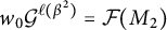 $w_0\mathcal {G}^{\ell (\beta ^2)} = \mathcal {F}(M_2)$
, the fact that
$w_0\mathcal {G}^{\ell (\beta ^2)} = \mathcal {F}(M_2)$
, the fact that
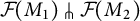 $\mathcal {F}(M_1) \pitchfork \mathcal {F}(M_2)$
means that
$\mathcal {F}(M_1) \pitchfork \mathcal {F}(M_2)$
means that
 $M_2^{-1}M_1$
belongs to
$M_2^{-1}M_1$
belongs to
 $\mathsf {B} w_0 \mathsf {B}$
and thus there exists a unique decomposition
$\mathsf {B} w_0 \mathsf {B}$
and thus there exists a unique decomposition
 $M_2^{-1}M_1 = U'w_0V'$
with
$M_2^{-1}M_1 = U'w_0V'$
with
 $U'$
unipotent. We then take
$U'$
unipotent. We then take
 $g = w_0(U')^{-1}M_2^{-1}$
. We leave details to the reader.
$g = w_0(U')^{-1}M_2^{-1}$
. We leave details to the reader.
Remark 5.3 The proof of Theorem 5.2 can be simplified by taking a slightly different realization of the braid variety
 $X(\beta )$
using weighted flags as in [Reference Galashin, Lam and Sherman-Bennett12, Reference Galashin, Lam, Sherman-Bennett and Speyer13] (see also [Reference Casals, Galashin, Gorsky, Shen, Sherman-Bennett and Simental1]). Let
$X(\beta )$
using weighted flags as in [Reference Galashin, Lam and Sherman-Bennett12, Reference Galashin, Lam, Sherman-Bennett and Speyer13] (see also [Reference Casals, Galashin, Gorsky, Shen, Sherman-Bennett and Simental1]). Let
 $\mathsf {U} \subseteq \mathrm {GL}(k)$
be the subgroup of upper uni-triangular matrices. A weighted flag is an element of
$\mathsf {U} \subseteq \mathrm {GL}(k)$
be the subgroup of upper uni-triangular matrices. A weighted flag is an element of
 $\mathrm {GL}(k)/\mathsf {U}$
. Two weighted flags
$\mathrm {GL}(k)/\mathsf {U}$
. Two weighted flags
 $h\mathsf {U}$
and
$h\mathsf {U}$
and
 $h'\mathsf {U}$
are said to be in strong relative position
$h'\mathsf {U}$
are said to be in strong relative position
 $w \in S_k$
if there exists
$w \in S_k$
if there exists
 $g \in \mathrm {GL}(k)$
such that
$g \in \mathrm {GL}(k)$
such that
 $g(h\mathsf {U}) = \mathsf {U}$
and
$g(h\mathsf {U}) = \mathsf {U}$
and
 $g(h'\mathsf {U}) = w\mathsf {U}$
. We denote this by
$g(h'\mathsf {U}) = w\mathsf {U}$
. We denote this by
 $h\mathsf {U} \xrightarrow {w} h'\mathsf {U}$
. Similarly,
$h\mathsf {U} \xrightarrow {w} h'\mathsf {U}$
. Similarly,
 $h\mathsf {U}$
and
$h\mathsf {U}$
and
 $h'\mathsf {U}$
are said to be in weak relative position
$h'\mathsf {U}$
are said to be in weak relative position
 $w \in S_k$
if there exist
$w \in S_k$
if there exist
 $g \in \mathrm {GL}(k)$
and a diagonal matrix t such that
$g \in \mathrm {GL}(k)$
and a diagonal matrix t such that
 $g(h\mathsf {U}) = \mathsf {U}$
and
$g(h\mathsf {U}) = \mathsf {U}$
and
 $g(h'\mathsf {U}) = tw\mathsf {U}$
. We denote this relation by
$g(h'\mathsf {U}) = tw\mathsf {U}$
. We denote this relation by
 $h\mathsf {U} \buildrel w \over \dashrightarrow h'\mathsf {U}$
. Given a braid
$h\mathsf {U} \buildrel w \over \dashrightarrow h'\mathsf {U}$
. Given a braid
 $\beta = \sigma _{i_1}\dots \sigma _{i_r}$
, we then have an isomorphism
$\beta = \sigma _{i_1}\dots \sigma _{i_r}$
, we then have an isomorphism
 $$\begin{align*}X(\beta) \cong \left\{h_0\mathsf{U} \xrightarrow{s_{i_1}} h_1\mathsf{U} \xrightarrow{s_{i_2}} \dots \xrightarrow{s_{i_r}} h_r\mathsf{U} \buildrel w_0 \over \dashrightarrow h_0\mathsf{U}\right\}/\mathrm{GL}(k), \end{align*}$$
where
 $\mathrm {GL}(k)$
acts diagonally on all weighted flags
$\mathrm {GL}(k)$
acts diagonally on all weighted flags
 $h_1\mathsf {U}, \dots , h_r\mathsf {U}$
. The set
$h_1\mathsf {U}, \dots , h_r\mathsf {U}$
. The set
 $\mathcal {U}_{r_1, w}(\beta )$
is then defined to consist of those chains of weighted flags such that
$\mathcal {U}_{r_1, w}(\beta )$
is then defined to consist of those chains of weighted flags such that
 $h_{r_1}\mathsf {U} \buildrel w_0 \over \dashrightarrow w_0w\mathsf {U}$
. An advantage of working with weighted flags is that, since
$h_{r_1}\mathsf {U} \buildrel w_0 \over \dashrightarrow w_0w\mathsf {U}$
. An advantage of working with weighted flags is that, since
 $\mathsf {U} \cap (w_0\mathsf {B} w_0) = \{\mathbf {1}\}$
, now we have uniqueness of the translating element in all the arguments used above.
$\mathsf {U} \cap (w_0\mathsf {B} w_0) = \{\mathbf {1}\}$
, now we have uniqueness of the translating element in all the arguments used above.
Remark 5.4 A priori, the construction of the map
 $\Phi _{r_1,w}$
depends on the choice of the reduced expression (5.2). However, one can check that different choices of the reduced expression lead to, essentially, the same map. More precisely, if we have two reduced expressions
$\Phi _{r_1,w}$
depends on the choice of the reduced expression (5.2). However, one can check that different choices of the reduced expression lead to, essentially, the same map. More precisely, if we have two reduced expressions
 $\underline {w}$
,
$\underline {w}$
,
 $\underline {w}'$
of w, choose reduced expressions
$\underline {w}'$
of w, choose reduced expressions
 $\underline {w_0}, \underline {w_0}'$
that contain
$\underline {w_0}, \underline {w_0}'$
that contain
 $\underline {w}, \underline {w}'$
as a prefix, respectively. We have canonical isomorphisms
$\underline {w}, \underline {w}'$
as a prefix, respectively. We have canonical isomorphisms
 $X(\beta ^2\underline {w}) \to X (\beta ^2\underline {w}' )$
and
$X(\beta ^2\underline {w}) \to X (\beta ^2\underline {w}' )$
and
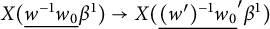 $X (\underline {w^{-1}w_0}\beta ^1 ) \to X (\underline {(w')^{-1}w_0}'\beta ^1 )$
such that the following diagram commutes:
$X (\underline {w^{-1}w_0}\beta ^1 ) \to X (\underline {(w')^{-1}w_0}'\beta ^1 )$
such that the following diagram commutes:

In particular, the flags in the bottom part of the diagram (5.14) are determined (for a given reduced expression (5.2)) by
 $\mathcal {F}^{\ell (w^{-1}w_0)+1}$
and
$\mathcal {F}^{\ell (w^{-1}w_0)+1}$
and
 $w_0\mathcal {G}^{\ell (\beta ^2)}.$
Furthermore, the element g is completely determined by these two flags.
$w_0\mathcal {G}^{\ell (\beta ^2)}.$
Furthermore, the element g is completely determined by these two flags.
From Theorem 5.2 and its proof, we obtain the following result.
Corollary 5.5 The open set
 $\mathcal {U}_{r_1, w}(\beta ) \subseteq X(\beta )$
is nonempty if and only if
$\mathcal {U}_{r_1, w}(\beta ) \subseteq X(\beta )$
is nonempty if and only if
 $$ \begin{align*}\delta\left(\underline{w^{-1}w_0}\beta^1\right) = w_0 =\delta\left(\beta^2\underline{w}\right).\end{align*} $$
By Lemma 2.1, this happens if and only if
 $\delta (\beta ^1) \geq w_0ww_0$
and
$\delta (\beta ^1) \geq w_0ww_0$
and
 $\delta (\beta ^2) \geq w_0w^{-1}$
.
$\delta (\beta ^2) \geq w_0w^{-1}$
.
5.2 Conjectural properties
We conjecture that the set
 $\mathcal {U}_{r_1, w}(\beta )$
and the map
$\mathcal {U}_{r_1, w}(\beta )$
and the map
 $\Phi _{r_1,w}=\Phi _1 \times \Phi _2$
satisfy various desirable cluster-theoretic properties. To state this conjecture precisely, we need some notation. If Q is an ice quiver, we denote by
$\Phi _{r_1,w}=\Phi _1 \times \Phi _2$
satisfy various desirable cluster-theoretic properties. To state this conjecture precisely, we need some notation. If Q is an ice quiver, we denote by
 $Q^{\mathrm {uf}}$
the quiver obtained by deleting the frozen vertices and all arrows adjacent to them. We also denote by
$Q^{\mathrm {uf}}$
the quiver obtained by deleting the frozen vertices and all arrows adjacent to them. We also denote by
 $Q_1$
the ice quiver from the cluster structure on
$Q_1$
the ice quiver from the cluster structure on
 $\mathbb {C} [X(\underline {w^{-1}w_0}\beta ^1)]$
, and by
$\mathbb {C} [X(\underline {w^{-1}w_0}\beta ^1)]$
, and by
 $Q_2$
the ice quiver associated with
$Q_2$
the ice quiver associated with
 $\mathbb {C} [X (\beta ^2\underline {w} ) ]$
.
$\mathbb {C} [X (\beta ^2\underline {w} ) ]$
.
Conjecture 5.6 Assume
 $\mathcal {U}_{r_1, w}(\beta )$
is nonempty, and consider the cluster structure on
$\mathcal {U}_{r_1, w}(\beta )$
is nonempty, and consider the cluster structure on
 $\mathbb {C}[X(\beta )]$
from Section 4.3. There exists a seed
$\mathbb {C}[X(\beta )]$
from Section 4.3. There exists a seed
 $\Sigma = (Q, \mathbf {x})$
satisfying the following properties:
$\Sigma = (Q, \mathbf {x})$
satisfying the following properties:
-
(1) There exist cluster variables
$x_{a_1}, \dots , x_{a_s} \in \mathbf {x}$
such that
$\mathcal {U}_{r_1, w}(\beta )$
is the common nonvanishing locus of
$x_{a_1}, \dots , x_{a_s}$
. -
(2) The variety
$\mathcal {U}_{r_1, w}(\beta )$
admits a cluster structure, and an initial seed
$\widehat {\Sigma } = \left (\widehat {Q}, \widehat {\mathbf {x}}\right )$
is given by freezing the variables
$x_{a_1}, \dots , x_{a_s}$
in the seed
$\Sigma = (Q, \mathbf {x})$
. -
(3) The quiver
$\widehat {Q}^{\mathrm {uf}}$
is mutation equivalent to the disjoint union of the quivers
$Q_1^{\mathrm {uf} }$
and
$Q_2^{\mathrm {uf}}$
. -
(4) Note that the variety
$X\left (\underline {w^{-1}w_0}\beta ^1\right ) \times X\left (\beta ^2\underline {w}\right )$
admits a natural product cluster structure. Then, the map
$\Phi _{r_1,w}: \mathcal {U}_{r_1, w}(\beta ) \to X\left (\underline {w^{-1}w_0}\beta ^1\right ) \times X\left (\beta ^2\underline {w}\right )$
is a quasi-cluster isomorphism.


The items (1)–(4) in Conjecture 5.6 are not independent.
Lemma 5.7 Assume (1) of Conjecture 5.6 holds. Then, we have that (4)
 $\Rightarrow $
(3)
$\Rightarrow $
(3)
 $\Rightarrow $
(2). Moreover, (3) implies that the cluster structures on
$\Rightarrow $
(2). Moreover, (3) implies that the cluster structures on
 $X\left (\underline {w^{-1}w_0}\beta ^1\right ) \times X\left (\beta ^2\underline {w}\right )$
and
$X\left (\underline {w^{-1}w_0}\beta ^1\right ) \times X\left (\beta ^2\underline {w}\right )$
and
 $\mathcal {U}_{r_1, w}(\beta )$
are abstractly quasi-cluster isomorphic (but it does not guarantee that the map
$\mathcal {U}_{r_1, w}(\beta )$
are abstractly quasi-cluster isomorphic (but it does not guarantee that the map
 $\Phi _{r_1,w}$
is a quasi-cluster isomorphism).
$\Phi _{r_1,w}$
is a quasi-cluster isomorphism).
Proof Assume (1). Quasi-cluster isomorphisms do not affect the mutable part of the cluster structure, see Remark 3.4, so (4) implies (3).
Assume (3) holds. By [Reference Casals, Gorsky, Gorsky, Le, Shen and Simental2, Theorem 7.13], the cluster structures on
 $\mathbb {C}[X(\underline {w^{-1}w_0}\beta ^1]$
and
$\mathbb {C}[X(\underline {w^{-1}w_0}\beta ^1]$
and
 $\mathbb {C}[X(\beta ^2\underline {w})]$
are locally acyclic, so the cluster structure given by the seed
$\mathbb {C}[X(\beta ^2\underline {w})]$
are locally acyclic, so the cluster structure given by the seed
 $\widehat {\Sigma }$
is also locally acyclic (see [Reference Muller23, Proposition 3.10]). From here, (2) follows from Lemma 3.4 and Theorem 4.1 in [Reference Muller23].
$\widehat {\Sigma }$
is also locally acyclic (see [Reference Muller23, Proposition 3.10]). From here, (2) follows from Lemma 3.4 and Theorem 4.1 in [Reference Muller23].
Let us show that, in the presence of (1), (3) already implies that the cluster structures on
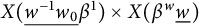 $X(\underline {w^{-1}w_0}\beta ^1) \times X(\beta ^w\underline {w}_{})$
and
$X(\underline {w^{-1}w_0}\beta ^1) \times X(\beta ^w\underline {w}_{})$
and
 $\mathcal {U}_{r_1, w}(\beta )$
are quasi-cluster isomorphic. For this, we use exchange matrices and Lemma 3.5 above. We have the following extended exchange matrices:
$\mathcal {U}_{r_1, w}(\beta )$
are quasi-cluster isomorphic. For this, we use exchange matrices and Lemma 3.5 above. We have the following extended exchange matrices:
-
•
$\widetilde {B} = \begin {pmatrix} B \\ \hline C\end {pmatrix}$
, the extended exchange matrix for the cluster structure on
$X(\beta )$
. By (1) and (2), the extended exchange matrix
$\widetilde {B}^{\circ }$
for the cluster structure on
$\mathcal {U}_{r_1, \beta }$
is given by deleting some columns on
$\widetilde {B}$
and freezing (moving to the bottom) the corresponding rows. By [Reference Casals, Gorsky, Gorsky, Le, Shen and Simental2, Corollary 8.5], the exchange matrix
$\widetilde {B}$
has really full rank, meaning that its rows span
$\mathbb {Z}^{n}$
, where n is the number of mutable variables in
$X(\beta )$
. Note that it follows that
$\widetilde {B}^{\circ }$
has really full rank as well. -
•
$\widetilde {B}_1 = \begin {pmatrix} B_1 \\ \hline C_1\end {pmatrix}$
, the extended exchange matrix for the cluster structure on
$X(\underline {w^{-1}w_0}\beta ^1)$
. We also have the extended exchange matrix
$\widetilde {B}_2$
for the cluster structure on
$X(\beta ^2\underline {w_{}})$
. Note that the extended exchange matrix for the cluster structure on the product variety
$X(\underline {w^{-1}w_0}\beta ^1) \times X(\beta ^2\underline {w})$
has the form
$$\begin{align*}\widetilde{B}^{\times} = \begin{pmatrix} B_1 & 0 \\ 0 & B_2 \\ \hline C_1 & 0 \\ 0 & C_2 \end{pmatrix}. \end{align*}$$


Note that by (3), we can assume that, maybe after mutations, the matrix
 $\widetilde {B}^{\circ }$
has the following form:
$\widetilde {B}^{\circ }$
has the following form:
 $$\begin{align*}\widetilde{B}^{\circ} = \begin{pmatrix} B_1 & 0 \\ 0 & B_2 \\ \hline C_{11} & C_{12} \\ C_{21} & C_{22} \end{pmatrix}. \end{align*}$$
And our job is to produce a matrix R as in Lemma 3.5 such that
 $R\widetilde {B}^{\times } = \widetilde {B}^{\circ }$
. We consider first the following matrices:
$R\widetilde {B}^{\times } = \widetilde {B}^{\circ }$
. We consider first the following matrices:
 $$\begin{align*}\widetilde{B}_{1}^{\times} := \begin{pmatrix} B_1 \\ 0 \\ \hline C_1 \\ 0\end{pmatrix}, \qquad \widetilde{B}_1^{\circ} = \begin{pmatrix} B_1 \\ 0 \\ \hline C_{11} \\ C_{12} \end{pmatrix}. \end{align*}$$
Since
 $\widetilde {B}_1$
has really full rank, the same is true for
$\widetilde {B}_1$
has really full rank, the same is true for
 $\widetilde {B}_1^{\times }$
. So we can express the rows of
$\widetilde {B}_1^{\times }$
. So we can express the rows of
 $C_{11}$
and
$C_{11}$
and
 $C_{12}$
as an integer linear combination of the rows of
$C_{12}$
as an integer linear combination of the rows of
 $B_1$
and
$B_1$
and
 $C_1$
. This means that we can find a matrix
$C_1$
. This means that we can find a matrix
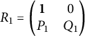 $R_1 = \begin {pmatrix} \mathbf {1} & 0 \\ P_1 & Q_1\end {pmatrix}$
so that
$R_1 = \begin {pmatrix} \mathbf {1} & 0 \\ P_1 & Q_1\end {pmatrix}$
so that
 $R_1\widetilde {B}_1^{\times } = \widetilde {B_1}^{\circ }$
. Note that
$R_1\widetilde {B}_1^{\times } = \widetilde {B_1}^{\circ }$
. Note that
 $Q_1$
is invertible over
$Q_1$
is invertible over
 $\mathbb {Z}$
, since the matrix
$\mathbb {Z}$
, since the matrix
 $\widetilde {B}_1^{\circ }$
has really full rank. Similarly, we can find
$\widetilde {B}_1^{\circ }$
has really full rank. Similarly, we can find
 $R_2 = \begin {pmatrix} \mathbf {1} & 0 \\ P_2 & Q_2\end {pmatrix}$
such that
$R_2 = \begin {pmatrix} \mathbf {1} & 0 \\ P_2 & Q_2\end {pmatrix}$
such that
 $R_2\widetilde {B}_2^{\times } = \widetilde {B}_2^{\circ }$
. It is now easy to see that
$R_2\widetilde {B}_2^{\times } = \widetilde {B}_2^{\circ }$
. It is now easy to see that
 $$\begin{align*}R = \begin{pmatrix} \mathbf{1} & 0 & 0 & 0 \\ 0 & \mathbf{1} & 0 & 0 \\ P_1 & 0 & Q_1 & 0 \\ 0 & P_2 & 0 & Q_2\end{pmatrix} \end{align*}$$
satisfies the required properties.
Remark 5.8 Let
 $f, f_1,f_2$
denote the numbers of frozen variables for
$f, f_1,f_2$
denote the numbers of frozen variables for
 $X(\beta ),X (\underline {w^{-1}w_0}\beta ^1 )$
and
$X(\beta ),X (\underline {w^{-1}w_0}\beta ^1 )$
and
 $X(\beta ^2\underline {w} )$
, respectively. By [Reference Geiss, Leclerc and Schröer14, Theorem 1.3], the group
$X(\beta ^2\underline {w} )$
, respectively. By [Reference Geiss, Leclerc and Schröer14, Theorem 1.3], the group
 $\mathbb {C}[X]^{\times }$
of global invertible functions on a cluster variety X is an abelian group generated by monomials in frozens and nonzero scalars. In particular, the number of frozen variables does not depend on a choice of a seed and is an invariant of a cluster variety. Theorem 5.2 and the inclusion
$\mathbb {C}[X]^{\times }$
of global invertible functions on a cluster variety X is an abelian group generated by monomials in frozens and nonzero scalars. In particular, the number of frozen variables does not depend on a choice of a seed and is an invariant of a cluster variety. Theorem 5.2 and the inclusion
 $$ \begin{align*}\mathbb{C}[X(\beta)]^{\times}\hookrightarrow \mathbb{C}[\mathcal{U}_{r_1,w}]^{\times} \end{align*} $$
imply the inequality
 $$ \begin{align} f_1+f_2\ge f. \end{align} $$
Assuming Conjecture 5.6, we can compute the number s of cluster variables
 $x_{a_1},\ldots ,x_{a_s}$
that need to be frozen in (1) or (2). By comparing the number of frozen variables for
$x_{a_1},\ldots ,x_{a_s}$
that need to be frozen in (1) or (2). By comparing the number of frozen variables for
 $\mathcal {U}_{r_1,w}(\beta )$
and their image under
$\mathcal {U}_{r_1,w}(\beta )$
and their image under
 $\Phi _{r_1,w}$
, we arrive at the equation
$\Phi _{r_1,w}$
, we arrive at the equation
 $ f+s=f_1+f_2, $
so
$ f+s=f_1+f_2, $
so
 $$\begin{align*}s = f_1+f_2-f. \end{align*}$$
We can verify (1)–(3) of Conjecture 5.6 in the extreme cases of
 $w = e$
and
$w = e$
and
 $w = w_0$
.
$w = w_0$
.
Proposition 5.9 Assume
 $w = e$
or
$w = e$
or
 $w = w_0$
. Then, (1)–(3) of Conjecture 5.6 hold.
$w = w_0$
. Then, (1)–(3) of Conjecture 5.6 hold.
Proof Assume
 $w = w_0$
, so that
$w = w_0$
, so that
 $\mathcal {U}_{r_1, w_0}(\beta )$
is given by the condition that
$\mathcal {U}_{r_1, w_0}(\beta )$
is given by the condition that
 $\mathcal {F}^{r_1}$
is transverse to
$\mathcal {F}^{r_1}$
is transverse to
 $\mathcal {F}^{\mathrm {std}}$
, and
$\mathcal {F}^{\mathrm {std}}$
, and
 $\mathcal {U}_{r_1, w_0}(\beta )$
is nonempty if and only if
$\mathcal {U}_{r_1, w_0}(\beta )$
is nonempty if and only if
 $\delta (\beta ^1) = w_0$
. In this case, the seed
$\delta (\beta ^1) = w_0$
. In this case, the seed
 $\Sigma $
predicted by Conjecture 5.6 is the left-to-right inductive seed, whose corresponding cluster torus is precisely the Deodhar torus
$\Sigma $
predicted by Conjecture 5.6 is the left-to-right inductive seed, whose corresponding cluster torus is precisely the Deodhar torus
 $\vec {\mathbb {T}}_{\beta }$
. It follows from [Reference Casals, Gorsky, Gorsky, Le, Shen and Simental2, Section 7.1] that a cluster variable
$\vec {\mathbb {T}}_{\beta }$
. It follows from [Reference Casals, Gorsky, Gorsky, Le, Shen and Simental2, Section 7.1] that a cluster variable
 $x_{a}$
is nowhere vanishing on
$x_{a}$
is nowhere vanishing on
 $\mathcal {U}_{r_1, w_0}(\beta )$
if and only if the Lusztig cycle associated with
$\mathcal {U}_{r_1, w_0}(\beta )$
if and only if the Lusztig cycle associated with
 $x_a$
intersects the horizontal slice of the inductive weave right after obtaining
$x_a$
intersects the horizontal slice of the inductive weave right after obtaining
 $\delta (\beta ^1) = w_0$
, and that these are the cluster variables predicted by Conjecture 5.6(1). By construction, cf. [Reference Casals, Gorsky, Gorsky, Le, Shen and Simental2, Section 4] the mutable part of the quiver obtained after freezing these cluster variables is equal to the disjoint union of the mutable parts of the quivers
$\delta (\beta ^1) = w_0$
, and that these are the cluster variables predicted by Conjecture 5.6(1). By construction, cf. [Reference Casals, Gorsky, Gorsky, Le, Shen and Simental2, Section 4] the mutable part of the quiver obtained after freezing these cluster variables is equal to the disjoint union of the mutable parts of the quivers
 $Q_1$
and
$Q_1$
and
 $Q_2$
, so (3) is valid and by Lemma 5.7(2) also holds. Moreover, again by Lemma 5.7, the cluster structures on
$Q_2$
, so (3) is valid and by Lemma 5.7(2) also holds. Moreover, again by Lemma 5.7, the cluster structures on
 $\mathcal {U}_{r_1, w_0}$
and
$\mathcal {U}_{r_1, w_0}$
and
 $X(\beta ^1) \times X(\beta ^2w_0)$
are abstractly quasi-cluster isomorphic. The case
$X(\beta ^1) \times X(\beta ^2w_0)$
are abstractly quasi-cluster isomorphic. The case
 $w = e$
is similar, taking the right-to-left inductive weave instead.
$w = e$
is similar, taking the right-to-left inductive weave instead.
Example 5.10 Consider the braid word
 $\beta = \sigma _2\sigma _1\sigma _3\sigma _2\sigma _2\sigma _3\sigma _1\sigma _2\sigma _2\sigma _1\sigma _3\sigma _2$
, that was considered in [Reference Casals, Gorsky, Gorsky, Le, Shen and Simental2, Section 11.4]. As explained in loc. cit., for the left-to-right inductive seed, we have the cluster variables
$\beta = \sigma _2\sigma _1\sigma _3\sigma _2\sigma _2\sigma _3\sigma _1\sigma _2\sigma _2\sigma _1\sigma _3\sigma _2$
, that was considered in [Reference Casals, Gorsky, Gorsky, Le, Shen and Simental2, Section 11.4]. As explained in loc. cit., for the left-to-right inductive seed, we have the cluster variables
 $$ \begin{align*} &x_1=z_5,\;\, x_2=-z_6z_7 + z_5z_8,\;\, x_3=-z_6z_7z_9+z_5z_8z_9-z_5, \;\, x_4=-z_6z_9 + z_5z_{10},\;\, \\ & x_5=-z_7z_9 + z_5z_{11},\end{align*} $$
 $$ \begin{align*}x_6= z_6z_7z_{10}z_{11} - z_5z_8z_{10}z_{11} - z_6z_7z_9z_{12} + z_5z_8z_9z_{12} - z_8z_9 + z_7z_{10} + z_6z_{11} - z_5z_{12} + 1,\end{align*} $$
the variables
 $x_4, x_5, x_6$
are frozen and the quiver Q is
$x_4, x_5, x_6$
are frozen and the quiver Q is

Let us take
 $r_1 = 9$
, so that
$r_1 = 9$
, so that
 $\beta ^1 = \sigma _2\sigma _1\sigma _3\sigma _2\sigma _2\sigma _3\sigma _1\sigma _2\sigma _2$
and
$\beta ^1 = \sigma _2\sigma _1\sigma _3\sigma _2\sigma _2\sigma _3\sigma _1\sigma _2\sigma _2$
and
 $\beta ^2 = \sigma _1\sigma _3\sigma _2$
, and
$\beta ^2 = \sigma _1\sigma _3\sigma _2$
, and
 $w = w_0$
, so that
$w = w_0$
, so that
 $\mathcal {U}_{9, w_0}(\beta )$
is given by the condition that
$\mathcal {U}_{9, w_0}(\beta )$
is given by the condition that
 $\mathcal {F}^9$
is transverse to
$\mathcal {F}^9$
is transverse to
 $\mathcal {F}^{\mathrm {std}}$
. The flag
$\mathcal {F}^{\mathrm {std}}$
. The flag
 $\mathcal {F}^9$
is the flag associated with the matrix
$\mathcal {F}^9$
is the flag associated with the matrix
 $B_{\beta ^1}(z_1, \dots , z_9)$
:
$B_{\beta ^1}(z_1, \dots , z_9)$
:
 $$ \begin{align} \begin{pmatrix} -z_4z_5+z_2z_7+1 & z_4z_6z_9 - z_2z_8z_9 + z_2 & -z_4z_6+z_2z_8 & -z_4 \\ -z_3z_5+z_1z_7 & z_3z_6z_9-z_1z_8z_9+z_1+z_9 & -z_3z_6 + z_1z_8 -1 & -z_3 \\ z_7 & -z_8z_9 + 1 & z_8 & 0 \\ z_5 & -z_6z_9 & z_6 & 1 \end{pmatrix}. \end{align} $$
So
 $\mathcal {F}^9$
is transverse to
$\mathcal {F}^9$
is transverse to
 $\mathcal {F}^{\mathrm {std}}$
if and only if the lower-left justified minors of (5.16) are nonzero. These are
$\mathcal {F}^{\mathrm {std}}$
if and only if the lower-left justified minors of (5.16) are nonzero. These are
 $$\begin{align*}\begin{vmatrix} z_5 \end{vmatrix} = x_1, \quad \begin{vmatrix}z_7 & -z_8z_9+1 \\ z_5 & -z_6z_9\end{vmatrix} = x_3,\end{align*}$$
 $$\begin{align*}\begin{vmatrix} -z_3z_5+z_1z_7 & z_3z_6z_9-z_1z_8z_9+z_1+z_9 & -z_3z_6 + z_1z_8 -1 \\ z_7 & -z_8z_9 + 1 & z_8 \\ z_5 & -z_6z_9 & z_6 \end{vmatrix} = x_1, \end{align*}$$
so that
 $\mathcal {U}_{9, w_0}(\beta )$
is the cluster variety associated with the seed
$\mathcal {U}_{9, w_0}(\beta )$
is the cluster variety associated with the seed

Note that the top row of this seed is isomorphic to a seed for
 $X(\beta ^1)$
, while the bottom part of the seed is isomorphic to a seed for
$X(\beta ^1)$
, while the bottom part of the seed is isomorphic to a seed for
 $X(\underline {w_0}\beta ^2)$
, so (1)–(3) of Conjecture 5.6 hold.
$X(\underline {w_0}\beta ^2)$
, so (1)–(3) of Conjecture 5.6 hold.
Combinatorially, splicing amounts to cutting the left-to-right inductive weave along the dotted line in Figure 1.
The left-to-right inductive weave for the braid
 $\beta = \sigma _2\sigma _1\sigma _3\sigma _2\sigma _2\sigma _3\sigma _1\sigma _2\sigma _2\sigma _1\sigma _3\sigma _2$
. Taking
$\beta = \sigma _2\sigma _1\sigma _3\sigma _2\sigma _2\sigma _3\sigma _1\sigma _2\sigma _2\sigma _1\sigma _3\sigma _2$
. Taking
 $r_1 = 9$
, the part of the weave above the dotted line is an inductive weave for
$r_1 = 9$
, the part of the weave above the dotted line is an inductive weave for
 $\beta ^1$
, while the part of the weave below the dotted line is an inductive weave for
$\beta ^1$
, while the part of the weave below the dotted line is an inductive weave for
 $\underline {w_0}\beta ^2$
, and the braid varieties
$\underline {w_0}\beta ^2$
, and the braid varieties
 $X(\underline {w_0}\beta ^2)$
and
$X(\underline {w_0}\beta ^2)$
and
 $X(\beta ^2\underline {w_0})$
are quasi-cluster isomorphic.
$X(\beta ^2\underline {w_0})$
are quasi-cluster isomorphic.
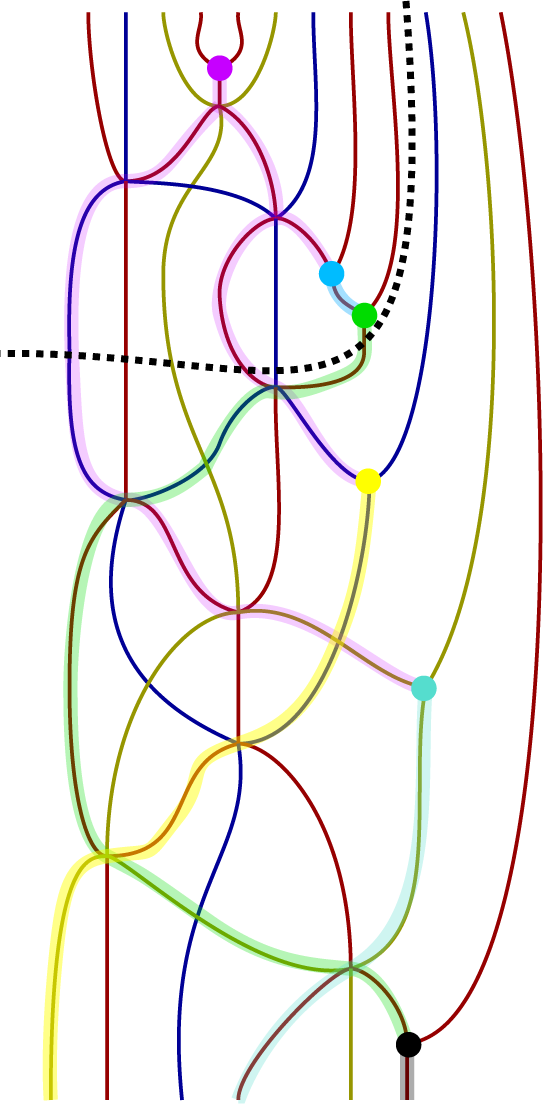
Example 5.11 Now consider the braid word
 $\beta = \sigma _2\sigma _1\sigma _3\sigma _2\sigma _2\sigma _3\sigma _1\sigma _1\sigma _2\sigma _3\sigma _2\sigma _2\sigma _3\sigma _2\sigma _1$
. The quiver for the left-to-right inductive weave is
$\beta = \sigma _2\sigma _1\sigma _3\sigma _2\sigma _2\sigma _3\sigma _1\sigma _1\sigma _2\sigma _3\sigma _2\sigma _2\sigma _3\sigma _2\sigma _1$
. The quiver for the left-to-right inductive weave is

and the extended exchange matrix is
 $$ \begin{align} \widetilde{B} = \begin{pmatrix} 0 & 0 & 0 & 1 & 0 & 0 \\ 0 & 0 & 0 & 0 & 0 & 0 \\ 0 & 0 & 0 & -1 & 1 & 0 \\ -1 & 0 & 1 & 0 & 0 & -1 \\ 0 & 0 & -1 & 0 & 0 & 1 \\ 0 & 0 & 0 & 1 & -1 & 0 \\ \hline 0 & 0 & 0 & -1 & 0 & 1 \\ 1 & 1 & 0 & 0 & 0 & -1\\ -1 & -1 & 0 & 0 & 0 & 0 \end{pmatrix}. \end{align} $$
Now, let us take
 $r = 11$
. The flag
$r = 11$
. The flag
 $\mathcal {F}^{11}$
is associated with the matrix
$\mathcal {F}^{11}$
is associated with the matrix
 $B_{\beta _{11}}(z_1, \dots , z_{11})$
, and a computation (using, e.g., Sage) shows that the lower-left justified minors of this matrix are
$B_{\beta _{11}}(z_1, \dots , z_{11})$
, and a computation (using, e.g., Sage) shows that the lower-left justified minors of this matrix are
 $$\begin{align*}x_1x_2, \qquad x_5, \qquad x_4, \qquad 1. \end{align*}$$
So that the cluster structure on the open set
 $\mathcal {U}_{11,e}$
is obtained by freezing the cluster variables
$\mathcal {U}_{11,e}$
is obtained by freezing the cluster variables
 $x_1, x_2, x_4, x_5$
. Note that there are no arrows between
$x_1, x_2, x_4, x_5$
. Note that there are no arrows between
 $x_3$
and
$x_3$
and
 $x_6$
, so the mutable part of the quiver indeed becomes disconnected after freezing.
$x_6$
, so the mutable part of the quiver indeed becomes disconnected after freezing.
Freezing the corresponding rows, and deleting the corresponding columns, in (5.17), we obtain the following extended exchange matrix:

On the other hand, the extended exchange matrices for the cluster structures on
 $X(\beta ^1)$
,
$X(\beta ^1)$
,
 $X(\Delta \beta ^2)$
, and
$X(\Delta \beta ^2)$
, and
 $X(\beta ^1) \times X(\Delta \beta ^2)$
are, respectively:
$X(\beta ^1) \times X(\Delta \beta ^2)$
are, respectively:
 $$\begin{align*}\widetilde{B}_1 = \begin{pmatrix} 0 \\ \hline 0 \\ 0 \\ 1 \\ -1\end{pmatrix}, \qquad \widetilde{B}_2 = \begin{pmatrix} 0 \\ \hline 1 \\ -1 \\ 0 \end{pmatrix}, \qquad \widetilde{B}^{\times} = \begin{pmatrix} 0 & 0 \\ 0 & 0 \\ \hline 0 & 0 \\ 0 & 0 \\ 1 & 0 \\ -1 & 0 \\ 0 & 1 \\ 0 & -1 \\ 0 & 0\end{pmatrix}. \end{align*}$$
We verify that
 $\widetilde {B}^{\circ }$
and
$\widetilde {B}^{\circ }$
and
 $\widetilde {B}^{\times }$
define quasi-cluster equivalent cluster structures. Following the strategy of Lemma 3.5, we need to find a
$\widetilde {B}^{\times }$
define quasi-cluster equivalent cluster structures. Following the strategy of Lemma 3.5, we need to find a
 $9 \times 9$
invertible integer matrix R of the form
$9 \times 9$
invertible integer matrix R of the form
 $R = \begin {pmatrix} \mathbf {1}_{2} & 0 \\ P & Q\end {pmatrix}$
such that
$R = \begin {pmatrix} \mathbf {1}_{2} & 0 \\ P & Q\end {pmatrix}$
such that
 $R\widetilde {B}^{\circ } = \widetilde {B}^{\times }$
. It is easy to see that taking
$R\widetilde {B}^{\circ } = \widetilde {B}^{\times }$
. It is easy to see that taking
 $P = 0$
and
$P = 0$
and
 $$\begin{align*}Q = \begin{pmatrix} 1 & 0 & 0 & 0 & 0 & 0 & 0 \\ 0 & 1 & 0 & 0 & 0 & 0 & 0 \\ 0 & 0 & 1 & 0 & 1 & 0 & 0 \\ 0 & 0 & 0 & 1 & 0 & 1 & 0 \\ 0 & 0 & 0 & 0 & 1 & 0 & 0 \\ 0 & 0 & 0 & 0 & 0 & 1 & 0 \\ 0 & 0 & 0 & 0 & 0 & 0 & 1 \end{pmatrix} \end{align*}$$
works. Note, however, that the induced quasi-cluster isomorphism preserves the mutable variables
 $x_3, x_6$
, so it is unlikely to coincide with the isomorphism
$x_3, x_6$
, so it is unlikely to coincide with the isomorphism
 $\Phi _{11, e}$
.
$\Phi _{11, e}$
.
5.3 Open Richardson varieties
We apply our results to the setting of open Richardson varieties in the flag variety. Recall that if
 $u \leq w \in S_k$
are permutations, the open Richardson variety is
$u \leq w \in S_k$
are permutations, the open Richardson variety is
 $$\begin{align*}R(u, w) := \left\{\mathcal{F} \in \mathcal{F}\ell_k \mid \mathcal{F}^{\mathrm{std}} \xrightarrow{w} \mathcal{F} \xrightarrow{u^{-1}w_0}\mathcal{F}^{\mathrm{ant}}\right\}. \end{align*}$$
The variety
 $R(u,w)$
is nonempty provided
$R(u,w)$
is nonempty provided
 $u \leq w$
, in which case it is an affine, smooth variety of dimension
$u \leq w$
, in which case it is an affine, smooth variety of dimension
 $\ell (w) - \ell (u)$
. In fact, we have an isomorphism
$\ell (w) - \ell (u)$
. In fact, we have an isomorphism
 $$ \begin{align} X\left(\underline{w_{}}\cdot\underline{u^{-1}w_0}\right) \to R(u, w), \end{align} $$
which takes a sequence of flags
 $(\mathcal {F}^0 = \mathcal {F}^{\mathrm {std}}, \mathcal {F}^1, \dots , \mathcal {F}^{\mathrm {ant}})$
to the flag
$(\mathcal {F}^0 = \mathcal {F}^{\mathrm {std}}, \mathcal {F}^1, \dots , \mathcal {F}^{\mathrm {ant}})$
to the flag
 $\mathcal {F}^{\ell (w)}$
(cf. [Reference Casals, Gorsky, Gorsky, Le, Shen and Simental2, Theorem 3.14]).
$\mathcal {F}^{\ell (w)}$
(cf. [Reference Casals, Gorsky, Gorsky, Le, Shen and Simental2, Theorem 3.14]).
Proposition 5.12 Let
 $u \leq v \leq w \in S_k$
. Then, there exists an open embedding
$u \leq v \leq w \in S_k$
. Then, there exists an open embedding
 $$ \begin{align} \Psi_{u, v, w}: R(u,v) \times R(v,w) \to R(u,w) \end{align} $$
whose image is the set
 $$ \begin{align} \mathcal{U}_{u, v, w} = \{\mathcal{F} \in R(u, w) \mid \mathcal{F}\pitchfork \mathcal{F}(vw_0)\}. \end{align} $$
Moreover, if
 $u, v, w \in S_k$
are permutations so that
$u, v, w \in S_k$
are permutations so that
 $\mathcal {U}_{u, v, w}$
is nonempty, then
$\mathcal {U}_{u, v, w}$
is nonempty, then
 $u \leq v \leq w$
.
$u \leq v \leq w$
.
Proof We use the isomorphism (5.19) together with a special case of the maps from Theorem 5.2, so we work with the variety
 $X\left (\underline {w_{}}\cdot \underline {u^{-1}w_0}\right ) \cong R(u,w)$
. In the setting of Section 5.1, we set
$X\left (\underline {w_{}}\cdot \underline {u^{-1}w_0}\right ) \cong R(u,w)$
. In the setting of Section 5.1, we set
 $r_1 = \ell (w)$
, so that
$r_1 = \ell (w)$
, so that
 $\beta ^1 = \underline {w}$
and
$\beta ^1 = \underline {w}$
and
 $\beta ^2 = \underline {u^{-1}w_0}$
. Consider
$\beta ^2 = \underline {u^{-1}w_0}$
. Consider
 $v^{\ast } := w_0vw_0$
. Then,
$v^{\ast } := w_0vw_0$
. Then,
 $$\begin{align*}\mathcal{U}_{r_1, v{^{\ast}}} = \left\{\left(\mathcal{F}^0 = \mathcal{F}^{\mathrm{std}}, \dots, \mathcal{F}^{\mathrm{ant}}\right) \in X\left(\underline{w_{}}\cdot\underline{u^{-1}w_0}\right) \mid \mathcal{F}^{\ell(w)} \pitchfork \mathcal{F}\left(w_0v^{\ast}\right)\right\} \end{align*}$$
maps isomorphically onto
 $\mathcal {U}_{u, v, w}$
upon the isomorphism
$\mathcal {U}_{u, v, w}$
upon the isomorphism
 $X\left (\underline {w_{}}\cdot \underline {u^{-1}w_0}\right ) \cong R(u,w)$
. On the other hand, by Theorem 5.2, we have
$X\left (\underline {w_{}}\cdot \underline {u^{-1}w_0}\right ) \cong R(u,w)$
. On the other hand, by Theorem 5.2, we have
 $$\begin{align*}\mathcal{U}_{r_1, v^{\ast}} \cong X\left(\underline{(v^{\ast})^{-1}w_0}\cdot \underline{w_{}^{}}\right) \times X\left(\underline{u^{-1}w_0^{}}\cdot\underline{v^{\ast}_{}}\right). \end{align*}$$
Using cyclic rotation isomorphisms (see [Reference Casals, Gorsky, Gorsky, Le, Shen and Simental2, Section 5.5]), we moreover have
 $$ \begin{align*}X\left(\underline{u^{-1}w_0^{}}\cdot \underline{v^{\ast}_{}}\right) \cong X\left(\underline{v_{}}\cdot\underline{u^{-1}w_0}\right) \cong R(u,v),\end{align*} $$
while
 $$ \begin{align*}X\left(\underline{(v^{\ast})^{-1}w_0}\cdot \underline{w_{}^{}}\right) \cong X\left(\underline{w_{}}\cdot\underline{v^{-1}w_0}\right) \cong R(v,w).\end{align*} $$
So
 $\mathcal {U}_{r_1, v^{\ast }} \cong R(u, v) \times R(v,w)$
and we obtain the embedding (5.20). The last claim of the statement of the proposition follows from Corollary 5.5.
$\mathcal {U}_{r_1, v^{\ast }} \cong R(u, v) \times R(v,w)$
and we obtain the embedding (5.20). The last claim of the statement of the proposition follows from Corollary 5.5.
Remark 5.13 In [Reference Eberhardt and Stroppel6, Definition 3.1], an open embedding
 $R(u,v) \times R(v,w) \to R(u,w)$
is obtained. We do not know if it coincides with the map constructed in Proposition 5.12.
$R(u,v) \times R(v,w) \to R(u,w)$
is obtained. We do not know if it coincides with the map constructed in Proposition 5.12.
Remark 5.14 Note that if
 $\beta = \beta ^1\beta ^2$
, with
$\beta = \beta ^1\beta ^2$
, with
 $\beta ^1$
and
$\beta ^1$
and
 $\beta ^2$
both reduced words, then the condition
$\beta ^2$
both reduced words, then the condition
 $\delta (\beta ) = w_0$
forces
$\delta (\beta ) = w_0$
forces
 $\beta ^1 = \underline {w}$
and
$\beta ^1 = \underline {w}$
and
 $\beta ^2 = \underline {v^{-1}w_0}$
for some
$\beta ^2 = \underline {v^{-1}w_0}$
for some
 $v \leq w$
. Thus, any splicing map with
$v \leq w$
. Thus, any splicing map with
 $\beta ^1$
and
$\beta ^1$
and
 $\beta ^2$
both reduced is equivalent to one of the form (5.20).
$\beta ^2$
both reduced is equivalent to one of the form (5.20).
We can use Proposition 5.12 to give a (non-explicit) formula for the number of frozen variables on Richardson varieties. For
 $v \leq w$
, write
$v \leq w$
, write
 $f_{v,w}$
for the number of frozen variables on the Richardson variety
$f_{v,w}$
for the number of frozen variables on the Richardson variety
 $R(v,w)$
.
$R(v,w)$
.
Corollary 5.15 Let
 $v \leq w \in S_k$
. Let
$v \leq w \in S_k$
. Let
 $s_{v,w}$
be the number of distinct irreducible factors appearing in the minors
$s_{v,w}$
be the number of distinct irreducible factors appearing in the minors
 $\Delta _{v[i], [i]}(B_{\underline {w}}(z_1, \dots , z_{\ell (w)}))$
which are not themselves principal minors of the matrix
$\Delta _{v[i], [i]}(B_{\underline {w}}(z_1, \dots , z_{\ell (w)}))$
which are not themselves principal minors of the matrix
 $B_{\underline {w}}(z_1, \dots , z_{\ell (w)})$
. Then,
$B_{\underline {w}}(z_1, \dots , z_{\ell (w)})$
. Then,
 $$ \begin{align} f_{v,w} = f_{ e,w} - f_{e,v} + s_{v,w}. \end{align} $$
Proof We have an embedding
 $R(e,v) \times R(v,w) \to R(e,w)$
whose image is the set
$R(e,v) \times R(v,w) \to R(e,w)$
whose image is the set
 $\mathcal {U}_{e,v,w}$
of flags
$\mathcal {U}_{e,v,w}$
of flags
 $\mathcal {F} \in R(e,w)$
that are transverse to
$\mathcal {F} \in R(e,w)$
that are transverse to
 $\mathcal {F}(vw_0)$
. The set of all flags in
$\mathcal {F}(vw_0)$
. The set of all flags in
 $R(e,w)$
is parameterized by those matrices
$R(e,w)$
is parameterized by those matrices
 $B_{\underline {w}}(z_1, \dots , z_{\ell (w)})$
with nonvanishing principal minors, and a flag
$B_{\underline {w}}(z_1, \dots , z_{\ell (w)})$
with nonvanishing principal minors, and a flag
 $B_{\underline {w}}(z_1, \dots , z_{\ell (w)})$
is transverse to
$B_{\underline {w}}(z_1, \dots , z_{\ell (w)})$
is transverse to
 $\mathcal {F}(w_0v)$
if and only if
$\mathcal {F}(w_0v)$
if and only if
 $\Delta _{v[i],[i]}(B_{\underline {w}}(z_1, \dots , z_{\ell (w)})$
is nonzero for every
$\Delta _{v[i],[i]}(B_{\underline {w}}(z_1, \dots , z_{\ell (w)})$
is nonzero for every
 $i = 1, \dots , k$
(cf. Lemma 2.7(a)). So
$i = 1, \dots , k$
(cf. Lemma 2.7(a)). So
 $s_{v,w}$
is precisely the number of irreducible elements in
$s_{v,w}$
is precisely the number of irreducible elements in
 $\mathbb {C}[R(e,w)]$
that we have to localize in order to obtain
$\mathbb {C}[R(e,w)]$
that we have to localize in order to obtain
 $\mathbb {C}[\mathcal {U}_{e,v,w}]$
and we get
$\mathbb {C}[\mathcal {U}_{e,v,w}]$
and we get
 $$\begin{align*}f_{e,v} + f_{v,w} = f_{e,w} + s_{v,w}, \end{align*}$$
which proves the result.
Remark 5.16 For
 $w \in S_k$
, the number
$w \in S_k$
, the number
 $f_{e,w}$
is simply the number of different simple generators of
$f_{e,w}$
is simply the number of different simple generators of
 $S_k$
appearing in one (equivalently, any) reduced expression for w. So by (5.22), the computation of
$S_k$
appearing in one (equivalently, any) reduced expression for w. So by (5.22), the computation of
 $f_{v,w}$
is equivalent to that of
$f_{v,w}$
is equivalent to that of
 $s_{v,w}$
, which still remains a challenging problem.
$s_{v,w}$
, which still remains a challenging problem.
Example 5.17 Let us consider
 $k = 4$
,
$k = 4$
,
 $v = s_2$
, and
$v = s_2$
, and
 $w = s_3s_2s_1s_2s_3$
. We have
$w = s_3s_2s_1s_2s_3$
. We have
 $$\begin{align*}B_{\underline{w}}(z_1, \dots, z_5) = \begin{pmatrix} z_3 & -z_4 & z_5 & -1 \\ z_2 & -1 & 0 & 0 \\ z_1 & 0 & -1 & 0 \\ 1 & 0 & 0 & 0 \end{pmatrix}. \end{align*}$$
Note that
 $v[i] \neq [i]$
if and only if
$v[i] \neq [i]$
if and only if
 $i = 2$
, so we only need to check the irreducible factors of
$i = 2$
, so we only need to check the irreducible factors of
 $\Delta _{[1,3],[1,2]}(B_{\underline {w}}(z_1, \dots , z_5)) = z_1z_4$
. Neither
$\Delta _{[1,3],[1,2]}(B_{\underline {w}}(z_1, \dots , z_5)) = z_1z_4$
. Neither
 $z_1$
nor
$z_1$
nor
 $z_4$
is a principal minor, so we obtain
$z_4$
is a principal minor, so we obtain
 $s_{v,w} = 2$
and
$s_{v,w} = 2$
and
 $f_{v,w} = 3 - 1 + 2 = 4$
. Since
$f_{v,w} = 3 - 1 + 2 = 4$
. Since
 $\dim (R(v,w)) = 4$
, we obtain that
$\dim (R(v,w)) = 4$
, we obtain that
 $R(v,w) \cong (\mathbb {C}^{\times })^{4}$
is a four-dimensional torus. The left-to-right inductive initial seed for the cluster structure on
$R(v,w) \cong (\mathbb {C}^{\times })^{4}$
is a four-dimensional torus. The left-to-right inductive initial seed for the cluster structure on
 $R(e,w)$
is
$R(e,w)$
is
Note that mutating at
 $z_2$
we obtain
$z_2$
we obtain
 $z_2' = z_4$
, so there is a seed in
$z_2' = z_4$
, so there is a seed in
 $R(e,w)$
with mutable variables
$R(e,w)$
with mutable variables
 $z_1, z_4$
.
$z_1, z_4$
.
Remark 5.18 Note that Corollary 5.15 is the easiest to apply when v is a simple transposition
 $s_i$
: in this case, we only need to find irreducible factors of a single minor
$s_i$
: in this case, we only need to find irreducible factors of a single minor
 $\Delta _{s_i[i], [i]}$
, since
$\Delta _{s_i[i], [i]}$
, since
 $\Delta _{s_i[j], [j]}$
is a principal minor for
$\Delta _{s_i[j], [j]}$
is a principal minor for
 $j \neq i$
.
$j \neq i$
.
Example 5.17 can be generalized as follows. Let
 $k = 2i$
, and let
$k = 2i$
, and let
 $w = [k, 2, 3, \dots , k-1, 1]$
, that is, w is the transposition
$w = [k, 2, 3, \dots , k-1, 1]$
, that is, w is the transposition
 $(1k)$
. Let
$(1k)$
. Let
 $v = s_2s_4\dots s_{k-2}$
. Up to signs in the pivotal
$v = s_2s_4\dots s_{k-2}$
. Up to signs in the pivotal
 $1$
’s, the matrix
$1$
’s, the matrix
 $B_{\underline {w}}$
has the following form:
$B_{\underline {w}}$
has the following form:
 $$\begin{align*}B_{\underline{w}} = \begin{pmatrix} p_{k-1} & p_{k} & p_{k+1} & \dots & p_{2k-3} & 1 \\ p_{k-2} & 1 & 0 & \dots & 0 & 0 \\ p_{k-3} & 0 & 1 & \dots & 0 & 0 \\ \vdots & \vdots & \vdots & \ddots & \vdots & \vdots \\ p_1 & 0 & 0 & \dots & 1 & 0 \\ 1 & 0 & 0 & \dots & 0 & 0\end{pmatrix}, \end{align*}$$
where
 $p_1, \dots , p_{2k-3}$
are irreducible polynomials in the z-variables. Among the minors
$p_1, \dots , p_{2k-3}$
are irreducible polynomials in the z-variables. Among the minors
 $\Delta _{v[j], [j]}$
, the ones that are not already principal minors are (up to signs)
$\Delta _{v[j], [j]}$
, the ones that are not already principal minors are (up to signs)
 $$\begin{align*}\Delta_{v[2], [2]} = p_{k-3}p_{k}, \; \Delta_{v[4], [4]} = p_{k-5}p_{k+2}, \dots, \Delta_{v[2(i-1)], [2(i-1)]}= p_1p_{2k-2}, \end{align*}$$
so each of these minors contributes with two irreducible factors. It follows that the number of frozen variables in
 $R(v,w)$
is
$R(v,w)$
is
 $$\begin{align*}f_{v,w} = k-1 - (i-1) +2(i-1) = k-1 + i-1 = k-1+\frac{k}{2} - 1, \end{align*}$$
which coincides with
 $\dim (R(v,w))$
. In particular,
$\dim (R(v,w))$
. In particular,
 $R(v,w)$
is a torus.
$R(v,w)$
is a torus.
Remark 5.19 For
 $u, v \in S_k$
with
$u, v \in S_k$
with
 $u \leq v$
, let
$u \leq v$
, let
 $f_{u,v}$
denote the number of frozen variables in the cluster structure on
$f_{u,v}$
denote the number of frozen variables in the cluster structure on
 $R(u,v)$
. By (5.15), we have the inequality
$R(u,v)$
. By (5.15), we have the inequality
 $$ \begin{align} f_{u,v} + f_{v,w} \geq f_{u,w}. \end{align} $$
In forthcoming work of the second author [Reference Kim20],
 $f_{u,v}$
is shown to be equal to the coefficient of the second highest degree of the so-called R-polynomial
$f_{u,v}$
is shown to be equal to the coefficient of the second highest degree of the so-called R-polynomial
 $\mathrm {R}_{u,v}(q)$
associated with the pair
$\mathrm {R}_{u,v}(q)$
associated with the pair
 $(u,v)$
which has interesting combinatorial interpretations (cf. [Reference Patimo24]). In particular, [Reference Kim20] provides an alternative combinatorial proof of (5.23).
$(u,v)$
which has interesting combinatorial interpretations (cf. [Reference Patimo24]). In particular, [Reference Kim20] provides an alternative combinatorial proof of (5.23).
Note that all the results so far in this section have been independent of the validity of Conjecture 5.6. The next result explores the consequences of Conjecture 5.6 in the Richardson setting.
Proposition 5.20 Assume Conjecture 5.6 holds. Then, for every
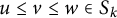 $u \leq v \leq w \in S_k$
and every
$u \leq v \leq w \in S_k$
and every
 $i = 1, \dots , k$
, the minors
$i = 1, \dots , k$
, the minors
 $\Delta _{v[i], [i]}$
are cluster monomials in
$\Delta _{v[i], [i]}$
are cluster monomials in
 $R(u,w)$
. Moreover, there exists a single cluster
$R(u,w)$
. Moreover, there exists a single cluster
 $\mathbf {x}$
so that all said minors are cluster monomials
$\mathbf {x}$
so that all said minors are cluster monomials
 $\mathbf {x}$
.
$\mathbf {x}$
.
Note that, fixing u and w,
 $\mathbf {x}$
may depend on the permutation v.
$\mathbf {x}$
may depend on the permutation v.
Proof If Conjecture 5.6(1) holds, then there exists a cluster
 $\mathbf {x}$
and cluster variables
$\mathbf {x}$
and cluster variables
 $x_{a_1}, \dots , x_{a_s} \in \mathbf {x}$
such that
$x_{a_1}, \dots , x_{a_s} \in \mathbf {x}$
such that
 $\mathcal {U}_{u,v,w}$
is the non-vanishing locus of
$\mathcal {U}_{u,v,w}$
is the non-vanishing locus of
 $x_{a_1}\dots x_{a_s}$
. Moreover, if Conjecture 5.6(2) holds, then
$x_{a_1}\dots x_{a_s}$
. Moreover, if Conjecture 5.6(2) holds, then
 $\mathcal {U}_{u,v,w}$
admits a cluster structure whose frozen variables are the frozen variables in
$\mathcal {U}_{u,v,w}$
admits a cluster structure whose frozen variables are the frozen variables in
 $R(u,w)$
, plus the variables
$R(u,w)$
, plus the variables
 $x_{a_1}, \dots x_{a_s}$
.
$x_{a_1}, \dots x_{a_s}$
.
Now, by Lemma 2.7(a), for every
 $i = 1, \dots , k$
, the minor
$i = 1, \dots , k$
, the minor
 $\Delta _{v[i], [i]}$
is nowhere vanishing on
$\Delta _{v[i], [i]}$
is nowhere vanishing on
 $\mathcal {U}_{u, v, w}$
. Thus, by [Reference Geiss, Leclerc and Schröer14, Theorem 2.2], the restriction
$\mathcal {U}_{u, v, w}$
. Thus, by [Reference Geiss, Leclerc and Schröer14, Theorem 2.2], the restriction
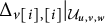 $\Delta _{v[i], [i]}|_{\mathcal {U}_{u,v,w}}$
is a monomial on the frozen variables of
$\Delta _{v[i], [i]}|_{\mathcal {U}_{u,v,w}}$
is a monomial on the frozen variables of
 $\mathcal {U}_{u,v,w}$
that, as we have seen, are frozen variables of
$\mathcal {U}_{u,v,w}$
that, as we have seen, are frozen variables of
 $R(u,w)$
plus some cluster variables in
$R(u,w)$
plus some cluster variables in
 $\mathbf {x}$
. Now,
$\mathbf {x}$
. Now,
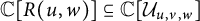 $\mathbb {C}[R(u,w)] \subseteq \mathbb {C}[\mathcal {U}_{u,v,w}]$
and the function
$\mathbb {C}[R(u,w)] \subseteq \mathbb {C}[\mathcal {U}_{u,v,w}]$
and the function
 $\Delta _{v[i], [i]}$
is regular on
$\Delta _{v[i], [i]}$
is regular on
 $R(u,w)$
. Since
$R(u,w)$
. Since
 $\Delta _{v[i],[i]}$
is a cluster monomial on
$\Delta _{v[i],[i]}$
is a cluster monomial on
 $\mathcal {U}_{u,v,w}$
, it is also a cluster monomial on
$\mathcal {U}_{u,v,w}$
, it is also a cluster monomial on
 $R(u,w)$
.
$R(u,w)$
.
In the remainder of the article, we will construct splicing maps satisfying all the properties of Conjecture 5.6 in the special case of double Bott–Samelson varieties.
6 Splicing double Bott–Samelson varieties
6.1 Setup
Let
 $\beta $
be a positive braid, and assume we have a decomposition
$\beta $
be a positive braid, and assume we have a decomposition
 $\beta = \beta ^1\beta ^2$
, where
$\beta = \beta ^1\beta ^2$
, where
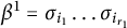 $\beta ^1 = \sigma _{i_1}\dots \sigma _{i_{r_1}}$
and
$\beta ^1 = \sigma _{i_1}\dots \sigma _{i_{r_1}}$
and
 $\beta ^2 = \sigma _{i_{r_1 + 1}}\dots \sigma _{i_r}$
. For each
$\beta ^2 = \sigma _{i_{r_1 + 1}}\dots \sigma _{i_r}$
. For each
 $s = 1, \dots , k-1$
, let
$s = 1, \dots , k-1$
, let
 $\mathrm {last}^1(s) \in \{1, \dots , r_1\}$
be such that
$\mathrm {last}^1(s) \in \{1, \dots , r_1\}$
be such that
 $i_{\mathrm {last}^1(s)} = s$
, and
$i_{\mathrm {last}^1(s)} = s$
, and
 $i_j \neq s$
for
$i_j \neq s$
for
 $\mathrm {last}^1(s) < j \leq r_1$
, that is,
$\mathrm {last}^1(s) < j \leq r_1$
, that is,
 $\mathrm {last}^1(s)$
is the rightmost appearance of
$\mathrm {last}^1(s)$
is the rightmost appearance of
 $\sigma _s$
in
$\sigma _s$
in
 $\beta ^1$
. We will consider the cluster variable
$\beta ^1$
. We will consider the cluster variable
 $x_{\mathrm {last}^1(s)} \in \mathbb {C}[X(\beta )]$
. If
$x_{\mathrm {last}^1(s)} \in \mathbb {C}[X(\beta )]$
. If
 $\sigma _s$
does not appear in
$\sigma _s$
does not appear in
 $\beta ^1$
, we will simply set
$\beta ^1$
, we will simply set
 $x_{\mathrm {last}^1(s)} = 1$
.
$x_{\mathrm {last}^1(s)} = 1$
.
6.2 Splicing
In the setup of Section 6.1, we have the following result.
Theorem 6.1 Let
 $\mathcal {U}_{r_1}(\beta ) \subseteq \mathrm {BS}(\beta )$
be the locus where none of the cluster variables
$\mathcal {U}_{r_1}(\beta ) \subseteq \mathrm {BS}(\beta )$
be the locus where none of the cluster variables
 $x_{\mathrm {last}^1(s)}$
vanish for
$x_{\mathrm {last}^1(s)}$
vanish for
 $s = 1, \dots , k-1$
. Then:
$s = 1, \dots , k-1$
. Then:
-
(1) We have
$(z_1, \dots , z_r) \in \mathcal {U}_{r_1}(\beta )$
if and only if
$(z_1, \dots , z_{r_1}) \in \mathrm {BS}\left (\beta ^1\right )$
. -
(2) We have an isomorphism of algebraic varieties
$$\begin{align*}\Phi_{r_1}: \mathcal{U}_{r_1}(\beta) \buildrel \cong \over \longrightarrow \mathrm{BS}\left(\beta^1\right) \times \mathrm{BS}\left(\beta^2\right). \end{align*}$$


Proof Let
 $(z_1, \dots , z_r) \in \mathcal {U}_{r_1}(\beta )$
. By Lemma 2.10 for
$(z_1, \dots , z_r) \in \mathcal {U}_{r_1}(\beta )$
. By Lemma 2.10 for
 $s = 1, \dots , k-1,$
we have
$s = 1, \dots , k-1,$
we have
 $$\begin{align*}\Delta_{s}(B_{\beta^1}(z_1, \dots, z_{r_1})) = x_{\mathrm{last}^1(s)} \end{align*}$$
so that the condition
 $(z_1, \dots , z_r) \in \mathcal {U}_{r_1}(\beta )$
is equivalent to
$(z_1, \dots , z_r) \in \mathcal {U}_{r_1}(\beta )$
is equivalent to
 $\Delta _{s}(B_{\beta ^1}(z_1, \dots , z_{r_1}))\neq 0$
for all s which is equivalent to
$\Delta _{s}(B_{\beta ^1}(z_1, \dots , z_{r_1}))\neq 0$
for all s which is equivalent to
 $(z_1, \dots , z_{r_1}) \in \mathrm {BS}\left (\beta ^1\right )$
. Now, since
$(z_1, \dots , z_{r_1}) \in \mathrm {BS}\left (\beta ^1\right )$
. Now, since
 $(z_1, \dots , z_{r_1}) \in \mathrm {BS}\left (\beta ^1\right ),$
we have an LU-decomposition
$(z_1, \dots , z_{r_1}) \in \mathrm {BS}\left (\beta ^1\right ),$
we have an LU-decomposition
 $$\begin{align*}B_{\beta^1}(z_1, \dots, z_{r_1}) = L_1U_1, \end{align*}$$
where
 $L_1$
has
$L_1$
has
 $1$
’s on the diagonal. Since
$1$
’s on the diagonal. Since
 $(z_1, \dots , z_r) \in \mathrm {BS}(\beta ),$
we also have an LU-decomposition
$(z_1, \dots , z_r) \in \mathrm {BS}(\beta ),$
we also have an LU-decomposition
 $B_{\beta }(z_1, \dots , z_r) = LU$
. Thus, we obtain
$B_{\beta }(z_1, \dots , z_r) = LU$
. Thus, we obtain
 $$ \begin{align} L_1U_1B_{\beta^2}(z_{r_1 + 1}, \dots, z_r) = LU. \end{align} $$
Now, by Lemma 2.6, we can write
 $$ \begin{align} U_1B_{\beta^2}(z_{r_1+1}, \dots, z_r) = B_{\beta^2}(z^{\prime}_{r_1+1}, \dots, z^{\prime}_r)U_1' \end{align} $$
for some change of variables
 $z^{\prime }_{r_1+1}, \dots , z^{\prime }_r$
. It follows from (6.1) that
$z^{\prime }_{r_1+1}, \dots , z^{\prime }_r$
. It follows from (6.1) that
 $(z^{\prime }_{r_1+1}, \dots , z^{\prime }_{r}) \in \mathrm {BS}\!\left (\beta ^2\right )$
. The map
$(z^{\prime }_{r_1+1}, \dots , z^{\prime }_{r}) \in \mathrm {BS}\!\left (\beta ^2\right )$
. The map
 $\Phi _{r_1}: (z_1, \dots , z_{r_1}, z_{r_1+1}, \dots , z_r) \mapsto ((z_1, \dots , z_{r_1}), (z^{\prime }_{r_1+1}, \dots , z^{\prime }_r))$
gives the desired isomorphism.
$\Phi _{r_1}: (z_1, \dots , z_{r_1}, z_{r_1+1}, \dots , z_r) \mapsto ((z_1, \dots , z_{r_1}), (z^{\prime }_{r_1+1}, \dots , z^{\prime }_r))$
gives the desired isomorphism.
To construct the inverse map, suppose that we are given
 $((z_1, \dots , z_{r_1}), $
 $ (z^{\prime }_{r_1+1}, \dots , z^{\prime }_r))$
such that
$ (z^{\prime }_{r_1+1}, \dots , z^{\prime }_r))$
such that
 $B_{\beta ^1}(z_1,\ldots ,z_{r_1})=L_1U_1$
and
$B_{\beta ^1}(z_1,\ldots ,z_{r_1})=L_1U_1$
and
 $B_{\beta ^2}(z^{\prime }_{r_1+1}, \dots , z^{\prime }_r)=L_2U_2$
. As above, the matrices
$B_{\beta ^2}(z^{\prime }_{r_1+1}, \dots , z^{\prime }_r)=L_2U_2$
. As above, the matrices
 $L_1,L_2$
are lower-triangular with 1 on diagonal and
$L_1,L_2$
are lower-triangular with 1 on diagonal and
 $U_1,U_2$
are upper triangular, all these matrices are uniquely determined by
$U_1,U_2$
are upper triangular, all these matrices are uniquely determined by
 $((z_1, \dots , z_{r_1}), (z^{\prime }_{r_1+1}, \dots , z^{\prime }_r))$
.
$((z_1, \dots , z_{r_1}), (z^{\prime }_{r_1+1}, \dots , z^{\prime }_r))$
.
By (6.2), there exist
 $(z_{r_1+1},\ldots ,z_{r})$
and an upper-triangular matrix
$(z_{r_1+1},\ldots ,z_{r})$
and an upper-triangular matrix
 $U^{\prime \prime }_1$
such that
$U^{\prime \prime }_1$
such that
 $$ \begin{align*}U_1^{-1}B_{\beta^2}(z^{\prime}_{r_1+1}, \dots, z^{\prime}_r)= B_{\beta^2}(z_{r_1+1}, \dots, z_r)U_1", \end{align*} $$
which implies
 $$ \begin{align*}B_{\beta^2}(z^{\prime}_{r_1+1}, \dots, z^{\prime}_r)(U^{\prime\prime}_1)^{-1}= U_1B_{\beta^2}(z_{r_1+1}, \dots, z_r). \end{align*} $$
This determines the inverse map. We can check that the result lands in
 $\mathrm {BS}(\beta )$
:
$\mathrm {BS}(\beta )$
:
 $$ \begin{align*}B_{\beta}(z_1,\ldots,z_r)=B_{\beta^1}(z_1,\ldots,z_{r_1})B_{\beta^2}(z_{r_1+1}, \dots, z_r)=L_1U_1B_{\beta^2}(z_{r_1+1}, \dots, z_r)= \end{align*} $$
 $$ \begin{align*}L_1B_{\beta^2}(z^{\prime}_{r_1+1}, \dots, z^{\prime}_r)(U^{\prime\prime}_1)^{-1}=L_1L_2U_2(U^{\prime\prime}_1)^{-1}=LU, \end{align*} $$
where
 $L=L_1L_2$
and
$L=L_1L_2$
and
 $U=U_2(U^{\prime \prime }_1)^{-1}$
.
$U=U_2(U^{\prime \prime }_1)^{-1}$
.
Remark 6.2 We constructed the map
 $\Phi _{r_1}$
using coordinates since we will need this in order to show cluster-theoretic properties of
$\Phi _{r_1}$
using coordinates since we will need this in order to show cluster-theoretic properties of
 $\Phi _{r_1}$
. It is useful, however, to have a more conceptual understanding of it using flags (cf. Section 6.3 below). Note that
$\Phi _{r_1}$
. It is useful, however, to have a more conceptual understanding of it using flags (cf. Section 6.3 below). Note that
 $\mathcal {U}_{r_1}(\beta )$
is the locus of elements
$\mathcal {U}_{r_1}(\beta )$
is the locus of elements
 $(\mathcal {F}^0, \dots , \mathcal {F}^r) \in \mathrm {BS}(\beta )$
such that
$(\mathcal {F}^0, \dots , \mathcal {F}^r) \in \mathrm {BS}(\beta )$
such that
 $\mathcal {F}^{r_1} \pitchfork \mathcal {F}(w_0)$
. In particular,
$\mathcal {F}^{r_1} \pitchfork \mathcal {F}(w_0)$
. In particular,
 $\mathcal {F}^{r_1} = \mathcal {F}(L_1U_1)$
, and
$\mathcal {F}^{r_1} = \mathcal {F}(L_1U_1)$
, and
 $L_1$
is uniquely determined provided it has
$L_1$
is uniquely determined provided it has
 $1$
’s on the diagonal. Then,
$1$
’s on the diagonal. Then,
 $$\begin{align*}\Phi_{r_1}\left(\mathcal{F}^0, \dots, \mathcal{F}^r\right) = \left(\left(\mathcal{F}^0, \dots, \mathcal{F}^{r_1}\right), L_1^{-1}\left(\mathcal{F}^{r_1}, \mathcal{F}^{r_1+1}, \dots, \mathcal{F}^r\right)\right) \in \mathrm{BS}\left(\beta^1\right) \times \mathrm{BS}\left(\beta^2\right). \end{align*}$$
Let
 $\Sigma _{\beta }$
be the left inductive seed on
$\Sigma _{\beta }$
be the left inductive seed on
 $\mathrm {BS}(\beta )$
as described in Section 4.3, and let
$\mathrm {BS}(\beta )$
as described in Section 4.3, and let
 $\widehat {\Sigma }_{\beta }$
be the seed obtained upon freezing the variables
$\widehat {\Sigma }_{\beta }$
be the seed obtained upon freezing the variables
 $x_{\mathrm {last}^1(s)}$
,
$x_{\mathrm {last}^1(s)}$
,
 $s = 1, \dots , k-1$
. The following lemma says that the set
$s = 1, \dots , k-1$
. The following lemma says that the set
 $\mathcal {U}_{r_1}(\beta )$
together with the cluster variables
$\mathcal {U}_{r_1}(\beta )$
together with the cluster variables
 $x_{\mathrm {last}^1(s)}$
satisfy the properties (1)–(3) of Conjecture 5.6.
$x_{\mathrm {last}^1(s)}$
satisfy the properties (1)–(3) of Conjecture 5.6.
Lemma 6.3 We have
 $A(\widehat {\Sigma }_{\beta }) \cong \mathbb {C}[\mathcal {U}_{r_1}(\beta )]$
.
$A(\widehat {\Sigma }_{\beta }) \cong \mathbb {C}[\mathcal {U}_{r_1}(\beta )]$
.


6.3 Comparison to braid variety splicing
It is natural to ask whether the map
 $\Phi _{r_1}$
constructed in Theorem 6.1 is compatible with the braid variety splicing from Theorem 5.2. Recall the isomorphisms
$\Phi _{r_1}$
constructed in Theorem 6.1 is compatible with the braid variety splicing from Theorem 5.2. Recall the isomorphisms
 $$ \begin{align*}\varphi_1:\mathrm{BS}(\beta)\to X(\beta\Delta),\quad \varphi_2:\mathrm{BS}(\beta)\to X(\Delta\beta) \end{align*} $$
from Lemma 4.4. We have the following results.
Lemma 6.4 Let
 $\beta = \beta ^1\beta ^2$
be a positive braid. The following diagram commutes:
$\beta = \beta ^1\beta ^2$
be a positive braid. The following diagram commutes:

Proof Let
 $(\mathcal {F}^0, \dots , \mathcal {F}^r) \in \mathcal {U}_{r_1}$
, so that
$(\mathcal {F}^0, \dots , \mathcal {F}^r) \in \mathcal {U}_{r_1}$
, so that
 $\varphi _1(\mathcal {F}^0, \dots , \mathcal {F}^r) = (\mathcal {F}^0, \dots , \mathcal {F}^r, \widetilde {\mathcal {F}}^{r+1}, \dots ,$
 $\widetilde {\mathcal {F}}^{r+\ell (w_0)})$
, where
$\widetilde {\mathcal {F}}^{r+\ell (w_0)})$
, where
 $\widetilde {\mathcal {F}}^{r+1}, \dots , \mathcal {F}^{r+\ell (w_0)}$
are uniquely determined. Note that both
$\widetilde {\mathcal {F}}^{r+1}, \dots , \mathcal {F}^{r+\ell (w_0)}$
are uniquely determined. Note that both
 $\mathcal {U}_{r_1}$
and
$\mathcal {U}_{r_1}$
and
 $\mathcal {U}_{r_1,e}$
are defined by
$\mathcal {U}_{r_1,e}$
are defined by
 $\mathcal {F}^{r_1}\pitchfork \mathcal {F}(w_0)$
, that is, the isomorphism
$\mathcal {F}^{r_1}\pitchfork \mathcal {F}(w_0)$
, that is, the isomorphism
 $\varphi _1$
identifies
$\varphi _1$
identifies
 $\mathcal {U}_{r_1}$
with
$\mathcal {U}_{r_1}$
with
 $\mathcal {U}_{r_1, e}$
.
$\mathcal {U}_{r_1, e}$
.
Let us write
 $\mathcal {F}^{r_1} = \mathcal {F}(L_1U_1)$
, where
$\mathcal {F}^{r_1} = \mathcal {F}(L_1U_1)$
, where
 $L_1$
is uniquely determined by the condition that it has
$L_1$
is uniquely determined by the condition that it has
 $1$
’s on the diagonal. Then,
$1$
’s on the diagonal. Then,
 $$ \begin{align} \begin{array}{r@{\,}l} (\varphi_2 \times \varphi_1)\circ\Phi_{r_1}(\mathcal{F}^0, \dots, \mathcal{F}^r) &= \left(\varphi_2\left(\mathcal{F}^0, \dots, \mathcal{F}^{r_1}\right), \varphi_1\left(L_1^{-1}\mathcal{F}^{r_1}, \dots, L_1^{-1}\mathcal{F}^{r}\right)\right) \\ &= \bigg(\left(\mathcal{G}^0, \dots, \mathcal{G}^{\ell(w_0)-1}, w_0L_1^{-1}\mathcal{F}^0, \dots, w_0L_1^{-1}\mathcal{F}^{r_1}\right), \\ &\quad \left(L_1^{-1}\mathcal{F}^{r_1}, \dots, L_1^{-1}\mathcal{F}^{r}, \widetilde{\mathcal{G}}^1, \dots, \widetilde{\mathcal{G}}^{\ell(w_0)}\right)\bigg), \end{array} \end{align} $$
where the flags
 $\mathcal {G}^{0} = \mathcal {F}^{\mathrm {std}}, \dots , \mathcal {G}^{\ell (w_0)-1}$
and
$\mathcal {G}^{0} = \mathcal {F}^{\mathrm {std}}, \dots , \mathcal {G}^{\ell (w_0)-1}$
and
 $\widetilde {\mathcal {G}}^{1}, \dots , \widetilde {\mathcal {G}}^{\ell (w_0)} = \mathcal {F}^{\mathrm {ant}}$
are uniquely determined. Indeed, to compute
$\widetilde {\mathcal {G}}^{1}, \dots , \widetilde {\mathcal {G}}^{\ell (w_0)} = \mathcal {F}^{\mathrm {ant}}$
are uniquely determined. Indeed, to compute
 $\varphi _2(\mathcal {F}^0, \dots , \mathcal {F}^{r_1})$
by Lemma 4.4, we first write
$\varphi _2(\mathcal {F}^0, \dots , \mathcal {F}^{r_1})$
by Lemma 4.4, we first write
 $\mathcal {F}^{r_1}=\mathcal {F}(L_1U_1)=\mathcal {F}((w_0U'w_0)U_1),$
where
$\mathcal {F}^{r_1}=\mathcal {F}(L_1U_1)=\mathcal {F}((w_0U'w_0)U_1),$
where
 $U'=w_0L_1w_0$
. Then
$U'=w_0L_1w_0$
. Then
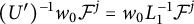 $(U')^{-1}w_0\mathcal {F}^j=w_0L_1^{-1}\mathcal {F}^j$
for
$(U')^{-1}w_0\mathcal {F}^j=w_0L_1^{-1}\mathcal {F}^j$
for
 $j=0,\ldots ,r_1$
.
$j=0,\ldots ,r_1$
.
Now, we have to compare (6.3) with
 $\Phi _{r_{1},e}(\mathcal {F}^0, \dots , \mathcal {F}^{r}, \widetilde {\mathcal {F}}^{r+1}, \dots , \widetilde {\mathcal {F}}^{r + \ell (w_0)})$
. First, we factor
$\Phi _{r_{1},e}(\mathcal {F}^0, \dots , \mathcal {F}^{r}, \widetilde {\mathcal {F}}^{r+1}, \dots , \widetilde {\mathcal {F}}^{r + \ell (w_0)})$
. First, we factor
 $\beta \Delta =\beta ^1(\beta ^2\Delta )$
. To get the
$\beta \Delta =\beta ^1(\beta ^2\Delta )$
. To get the
 $X(\beta ^2\Delta )$
component, we need to find an element
$X(\beta ^2\Delta )$
component, we need to find an element
 $g_2$
so that simultaneously
$g_2$
so that simultaneously
 $g_2\mathcal {F}^{r_1} = \mathcal {F}^{\mathrm {std}}$
and
$g_2\mathcal {F}^{r_1} = \mathcal {F}^{\mathrm {std}}$
and
 $g_2\widetilde {\mathcal {F}}^{r+\ell (w_0)} = \mathcal {F}^{\mathrm {ant}}$
. By (5.9), we get
$g_2\widetilde {\mathcal {F}}^{r+\ell (w_0)} = \mathcal {F}^{\mathrm {ant}}$
. By (5.9), we get
 $g_2 = L_1^{-1}$
and thus
$g_2 = L_1^{-1}$
and thus
 $$ \begin{align*}\Phi^2\left(\mathcal{F}^0, \dots, \mathcal{F}^{r}, \widetilde{\mathcal{F}}^{r+1}, \dots, \widetilde{\mathcal{F}}^{r + \ell(w_0)}\right)= g_2\left(\mathcal{F}^{r_1}, \mathcal{F}^{r_1+1}, \dots, \mathcal{F}^{r}, \widetilde{\mathcal{F}}^{r+1}, \dots, \widetilde{\mathcal{F}}^{r+\ell(w_0)}\right)\end{align*} $$
 $$ \begin{align*}=\left(L_1^{-1}\mathcal{F}^{r_1}, \dots, L_1^{-1}\mathcal{F}^{r}, \widetilde{\mathcal{G}}^1, \dots, \widetilde{\mathcal{G}}^{\ell(w_0)}\right)=\varphi_2\circ \Phi_{r_1}(\mathcal{F}^0,\ldots,\mathcal{F}^r) \end{align*} $$
by the uniqueness of the flags
 $\widetilde {\mathcal {G}}^1, \dots , \widetilde {\mathcal {G}}^{\ell (w_0)}$
.
$\widetilde {\mathcal {G}}^1, \dots , \widetilde {\mathcal {G}}^{\ell (w_0)}$
.
Let us now examine the
 $X(\Delta \beta ^1)$
component of
$X(\Delta \beta ^1)$
component of
 $\Phi _{r_{1},e}(\mathcal {F}^0, \dots , \mathcal {F}^{r}, \widetilde {\mathcal {F}}^{r+1}, \dots , \widetilde {\mathcal {F}}^{r+\ell (w_0)})$
. For this, we obtain a unique sequence of flags going from
$\Phi _{r_{1},e}(\mathcal {F}^0, \dots , \mathcal {F}^{r}, \widetilde {\mathcal {F}}^{r+1}, \dots , \widetilde {\mathcal {F}}^{r+\ell (w_0)})$
. For this, we obtain a unique sequence of flags going from
 $\widetilde {\mathcal {F}}^{r+\ell (w_0)} = \mathcal {F}^{\mathrm {ant}}$
to
$\widetilde {\mathcal {F}}^{r+\ell (w_0)} = \mathcal {F}^{\mathrm {ant}}$
to
 $\mathcal {F}^{\mathrm {std}}$
using the letters in
$\mathcal {F}^{\mathrm {std}}$
using the letters in
 $\Delta $
, say
$\Delta $
, say
 $\widehat {\mathcal {F}}^{1}, \dots , \widehat {\mathcal {F}}^{\ell (w_0)-1}$
and choose
$\widehat {\mathcal {F}}^{1}, \dots , \widehat {\mathcal {F}}^{\ell (w_0)-1}$
and choose
 $g_1=w_0L_1^{-1}$
by (5.13). Then
$g_1=w_0L_1^{-1}$
by (5.13). Then
 $$ \begin{align*}\Phi^1\left(\mathcal{F}^0, \dots, \mathcal{F}^{r}, \widetilde{\mathcal{F}}^{r+1}, \dots, \widetilde{\mathcal{F}}^{r+\ell(w_0)}\right)= g_1\left(\mathcal{F}^{r+\ell(w_0)}, \widehat{\mathcal{F}}^{1}, \dots, \widehat{\mathcal{F}}^{\ell(w_0)-1}, \mathcal{F}^{0}, \dots, \mathcal{F}^{r_1}\right) \end{align*} $$
 $$ \begin{align*}=\left(\mathcal{G}^0, \dots, \mathcal{G}^{\ell(w_0)-1}, w_0L_1^{-1}\mathcal{F}^0, \dots, w_0L_1^{-1}\mathcal{F}^{r_1}\right)=\varphi_1\circ \Phi_{r_1}(\mathcal{F}^0,\ldots,\mathcal{F}^r) \end{align*} $$
by the uniqueness of the flags
 $\mathcal {G}^0,\ldots ,\mathcal {G}^{\ell (w_0)-1}$
. This finishes the proof.
$\mathcal {G}^0,\ldots ,\mathcal {G}^{\ell (w_0)-1}$
. This finishes the proof.
Lemma 6.5 Let
 $\beta = \beta ^1\beta ^2$
be a positive braid. The following diagram commutes:
$\beta = \beta ^1\beta ^2$
be a positive braid. The following diagram commutes:

Note that at the bottom we use factorization
 $\Delta \beta =(\Delta \beta ^1)\beta ^2$
and
$\Delta \beta =(\Delta \beta ^1)\beta ^2$
and
 $w=w_0$
.
$w=w_0$
.
Proof The composition
 $(\varphi _2\times \varphi _1)\circ \Phi _{r_1}$
is unchanged, so we need to compute the composition
$(\varphi _2\times \varphi _1)\circ \Phi _{r_1}$
is unchanged, so we need to compute the composition
 $\Phi _{r_1+\ell (w_0),w_0}\circ \varphi _2$
and compare it with (6.3). We follow the notations
$\Phi _{r_1+\ell (w_0),w_0}\circ \varphi _2$
and compare it with (6.3). We follow the notations
 $\mathcal {F}^{r_1}=\mathcal {F}(L_1U_1)$
from Lemma 6.4.
$\mathcal {F}^{r_1}=\mathcal {F}(L_1U_1)$
from Lemma 6.4.
Given
 $(\mathcal {F}^0,\ldots ,\mathcal {F}^r)\in \mathrm {BS}(\beta )$
, we have
$(\mathcal {F}^0,\ldots ,\mathcal {F}^r)\in \mathrm {BS}(\beta )$
, we have
 $\mathcal {F}^r=\mathcal {F}(L'U'),$
where
$\mathcal {F}^r=\mathcal {F}(L'U'),$
where
 $L'$
is unique provided that it has 1’s on diagonal. Then, by Lemma 4.4, we get
$L'$
is unique provided that it has 1’s on diagonal. Then, by Lemma 4.4, we get
 $$ \begin{align*}\varphi_2(\mathcal{F}^0,\ldots,\mathcal{F}^r)=\left(\mathcal{F}^{\mathrm{std}},\ldots,\widetilde{\mathcal{F}}^{\ell(w_0)-1},w_0(L')^{-1}\mathcal{F}^0,\ldots,w_0(L')^{-1}\mathcal{F}^r\right). \end{align*} $$
Next, we look at the
 $(\ell (w)+r_1)$
-st flag:
$(\ell (w)+r_1)$
-st flag:
 $$ \begin{align*}w_0(L')^{-1}\mathcal{F}^{r_1}=w_0(L')^{-1}\mathcal{F}(L_1U_1)=\mathcal{F}(M),\quad M=w_0(L')^{-1}L_1U_1. \end{align*} $$
Next, according to (5.6), we need to write:
 $M=w_0LU$
so that
$M=w_0LU$
so that
 $L=(L')^{-1}L_1$
and
$L=(L')^{-1}L_1$
and
 $U=U_1$
. By (5.9) and (5.13), we compute
$U=U_1$
. By (5.9) and (5.13), we compute
 $$ \begin{align*}g_2=(w_0L)^{-1}=L_1^{-1}L'w_0,\ g_1=w_0L_1^{-1}L'w_0 \end{align*} $$
and
 $$ \begin{align*}g_2(w_0(L')^{-1}\mathcal{F}^j)=L_1^{-1}\mathcal{F}^j,\ g_1(w_0(L')^{-1}\mathcal{F}^j)=w_0L_1^{-1}\mathcal{F}^j. \end{align*} $$
Finally, by (5.3) and (5.4), we get
 $$ \begin{align*}\Phi^1\left(\mathcal{F}^{\mathrm{std}},\ldots,\widetilde{\mathcal{F}}^{\ell(w_0)-1},w_0(L')^{-1}\mathcal{F}^0,\ldots,w_0(L')^{-1}\mathcal{F}^r\right)= \end{align*} $$
 $$ \begin{align*}g_1\left(\mathcal{F}^{\mathrm{std}},\ldots,\widetilde{\mathcal{F}}^{\ell(w_0)-1},w_0(L')^{-1}\mathcal{F}^0,\ldots,w_0(L')^{-1}\mathcal{F}^{r_1}\right)= \end{align*} $$
 $$ \begin{align*}\left(\mathcal{G}^0,\ldots,\mathcal{G}^{\ell(w_0)-1},w_0L_1^{-1}\mathcal{F}^0,\ldots,w_0L_1^{-1}\mathcal{F}^{r_1}\right), \end{align*} $$
and
 $$ \begin{align*}\Phi^2\left(\mathcal{F}^{\mathrm{std}},\ldots,\widetilde{\mathcal{F}}^{\ell(w_0)-1},w_0(L')^{-1}\mathcal{F}^0,\ldots,w_0(L')^{-1}\mathcal{F}^r\right)= \end{align*} $$
 $$ \begin{align*}g_2\left(w_0(L')^{-1}\mathcal{F}^{r_1},\ldots,w_0(L')^{-1}\mathcal{F}^r,\widehat{\mathcal{F}^1},\ldots,\widehat{\mathcal{F}}^{\ell(w_0)}\right)= \end{align*} $$
 $$ \begin{align*}\left(L_1^{-1}\mathcal{F}^r_1,\ldots,L_1^{-1}\mathcal{F}^{r},\widetilde{\mathcal{G}}^1,\ldots,\widetilde{\mathcal{G}}^{\ell(w_0)}\right) \end{align*} $$
by the uniqueness of the flags
 $\mathcal {G},\widetilde {\mathcal {G}}$
. Therefore,
$\mathcal {G},\widetilde {\mathcal {G}}$
. Therefore,
 $\Phi _{r_1+\ell (w_0),w_0}\circ \varphi _2(\mathcal {F}^0,\ldots ,\mathcal {F}^r)$
is also given by (6.3).
$\Phi _{r_1+\ell (w_0),w_0}\circ \varphi _2(\mathcal {F}^0,\ldots ,\mathcal {F}^r)$
is also given by (6.3).
In [Reference Gorsky, Kim, Scroggin and Simental17] we defined a subclass of open positroid varieties
 $S^{\circ ,1}_{\lambda /\mu }\subset \mathrm {Gr}(k,n)$
called skew shaped positroids and labeled by skew Young diagrams
$S^{\circ ,1}_{\lambda /\mu }\subset \mathrm {Gr}(k,n)$
called skew shaped positroids and labeled by skew Young diagrams
 $\lambda /\mu $
. By [Reference Gorsky, Kim, Scroggin and Simental17, Theorem 3.5.13], we have an isomorphism
$\lambda /\mu $
. By [Reference Gorsky, Kim, Scroggin and Simental17, Theorem 3.5.13], we have an isomorphism
 $$ \begin{align*}S^{\circ,1}_{\lambda/\mu}\simeq X(\Delta\beta)\simeq \mathrm{BS}(\beta), \end{align*} $$
where
 $\beta $
is a certain k-strand braid determined by
$\beta $
is a certain k-strand braid determined by
 $\lambda /\mu $
.
$\lambda /\mu $
.
We also considered cutting the diagram
 $\lambda /\mu $
into two skew diagrams
$\lambda /\mu $
into two skew diagrams
 $\lambda ^{a,L}/\mu ^{a,L}$
and
$\lambda ^{a,L}/\mu ^{a,L}$
and
 $\lambda ^{a,R}/\mu ^{a,R}$
. These correspond to braids
$\lambda ^{a,R}/\mu ^{a,R}$
. These correspond to braids
 $\beta _L$
and
$\beta _L$
and
 $\beta _R$
and we showed that in fact
$\beta _R$
and we showed that in fact
 $\beta =\beta _L\beta _R$
. Then we defined a splicing map
$\beta =\beta _L\beta _R$
. Then we defined a splicing map
 $$ \begin{align*}S^{\circ,1}_{\lambda^L/\mu^L}\times S^{\circ,1}_{\lambda^R/\mu^R}\to \mathcal{U}_a\subset S^{\circ,1}_{\lambda/\mu} \end{align*} $$
or equivalently
 $$ \begin{align} X(\Delta\beta_L)\times X(\Delta\beta_R)\to \mathcal{U}_a\subset X(\Delta\beta). \end{align} $$
Here,
 $\mathcal {U}_a$
is a certain open subset in
$\mathcal {U}_a$
is a certain open subset in
 $S^{\circ ,1}_{\lambda /\mu }$
. By [Reference Gorsky, Kim, Scroggin and Simental17, Theorem 5.6.1], the map (6.4) is a quasi-cluster equivalence. We invite the reader to explore more combinatorial and linear-algebraic properties of the map (6.4) in [Reference Gorsky, Kim, Scroggin and Simental17].
$S^{\circ ,1}_{\lambda /\mu }$
. By [Reference Gorsky, Kim, Scroggin and Simental17, Theorem 5.6.1], the map (6.4) is a quasi-cluster equivalence. We invite the reader to explore more combinatorial and linear-algebraic properties of the map (6.4) in [Reference Gorsky, Kim, Scroggin and Simental17].
We claim that the map (6.4) agrees with the map
 $\Phi _r$
from Theorem 6.1 in this special case. We focus on [Reference Gorsky, Kim, Scroggin and Simental17, Definition 5.2.1]. The braid variety
$\Phi _r$
from Theorem 6.1 in this special case. We focus on [Reference Gorsky, Kim, Scroggin and Simental17, Definition 5.2.1]. The braid variety
 $X(\Delta \beta )$
parameterizes chains of (framed) flags
$X(\Delta \beta )$
parameterizes chains of (framed) flags
 $$ \begin{align*}\Omega=\left[\mathcal{F}^{W}\stackrel{\Delta}{\dashrightarrow}\mathcal{F}^{W^{\mathrm{op}}}\stackrel{\beta_{L}}{\dashrightarrow}\mathcal{F}^a\stackrel{\beta_{R}}{\dashrightarrow}\mathcal{F}^0\right], \end{align*} $$
see [Reference Gorsky, Kim, Scroggin and Simental17] for unexplained notations. Such a chain belongs to
 $\mathcal {U}_a$
if and only if
$\mathcal {U}_a$
if and only if
 $\mathcal {F}^a\pitchfork \mathcal {F}^W$
. In this case, the splicing map sends
$\mathcal {F}^a\pitchfork \mathcal {F}^W$
. In this case, the splicing map sends
 $\Omega $
to
$\Omega $
to
 $$ \begin{align*}\Omega^L=\left[\mathcal{F}^{W}\stackrel{\Delta}{\dashrightarrow}\mathcal{F}^{W^{\mathrm{op}}}\stackrel{\beta_{L}}{\dashrightarrow}\mathcal{F}^a\right],\quad \Omega^R=\left[\mathcal{F}^{W}\stackrel{\Delta}{\dashrightarrow}\mathcal{F}^{a}\stackrel{\beta_{R}}{\dashrightarrow}\mathcal{F}^0\right]. \end{align*} $$
We can identify these with points in
 $X(\Delta \beta _L)$
and
$X(\Delta \beta _L)$
and
 $X(\Delta \beta _R),$
respectively, up to multiplication by some
$X(\Delta \beta _R),$
respectively, up to multiplication by some
 $g\in \mathrm {GL}(k)$
. Similarly to Lemmas 6.4 and 6.5, this agrees with
$g\in \mathrm {GL}(k)$
. Similarly to Lemmas 6.4 and 6.5, this agrees with
 $\Phi _{r_1}$
after applying the isomorphism
$\Phi _{r_1}$
after applying the isomorphism
 $X(\Delta \beta _R)\simeq X(\beta _R\Delta )$
.
$X(\Delta \beta _R)\simeq X(\beta _R\Delta )$
.
6.4 Cluster-theoretic properties of the map
$\Phi _{r_1}$

By Lemma 6.3, the algebra
 $\mathbb {C}[\mathcal {U}_{r_1}(\beta )]$
admits a natural cluster structure. We then examine the cluster-theoretic properties of the map
$\mathbb {C}[\mathcal {U}_{r_1}(\beta )]$
admits a natural cluster structure. We then examine the cluster-theoretic properties of the map
 $\Phi _{r_1}$
. We consider the pullback
$\Phi _{r_1}$
. We consider the pullback
 $$\begin{align*}\Phi_{r_1}^{\ast}: \mathbb{C}\!\left[\mathrm{BS}(\beta^1) \times \mathrm{BS}(\beta^2)\right] \to \mathbb{C}[\mathcal{U}_{r_1}(\beta)] \end{align*}$$
that is an isomorphism of algebras. We will denote the coordinates on
 $\mathrm {BS}(\beta ^1)$
by
$\mathrm {BS}(\beta ^1)$
by
 $z_1, \dots , z_{r_1}$
and the coordinates on
$z_1, \dots , z_{r_1}$
and the coordinates on
 $\mathrm {BS}(\beta ^2)$
by
$\mathrm {BS}(\beta ^2)$
by
 $z_{r_1+1}, \dots , z_r$
. Then the isomorphism
$z_{r_1+1}, \dots , z_r$
. Then the isomorphism
 $\Phi _{r_1}^{\ast }$
is determined by
$\Phi _{r_1}^{\ast }$
is determined by
 $$ \begin{align} \Phi^{\ast}_{r_1}(z_j) = z_j, j = 1, \dots, r_1, \qquad \Phi^{\ast}_{r_1\textbf{}}(z_j) = z^{\prime}_j, j = r_1+1, \dots, r, \end{align} $$
where
 $z^{\prime }_{r_1+1}, \dots , z^{\prime }_r$
are determined by (6.2).
$z^{\prime }_{r_1+1}, \dots , z^{\prime }_r$
are determined by (6.2).
On
 $\mathbb {C}[\mathcal {U}_{r_1}(\beta )]$
we have the cluster algebra structure obtained in Lemma 6.3. Since this comes comes from the open embedding
$\mathbb {C}[\mathcal {U}_{r_1}(\beta )]$
we have the cluster algebra structure obtained in Lemma 6.3. Since this comes comes from the open embedding
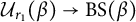 $\mathcal {U}_{r_1}(\beta ) \to \mathrm {BS}(\beta )$
, we call this the open cluster structure on
$\mathcal {U}_{r_1}(\beta ) \to \mathrm {BS}(\beta )$
, we call this the open cluster structure on
 $\mathcal {U}_{r_1}(\beta )$
, with quiver
$\mathcal {U}_{r_1}(\beta )$
, with quiver
 $Q^{\circ }_{\beta }$
. The quiver
$Q^{\circ }_{\beta }$
. The quiver
 $Q^{\circ }_{\beta }$
is obtained from the quiver
$Q^{\circ }_{\beta }$
is obtained from the quiver
 $Q_{\beta }$
by freezing the vertices corresponding to the rightmost appearance of a crossing in
$Q_{\beta }$
by freezing the vertices corresponding to the rightmost appearance of a crossing in
 $\beta ^1$
.
$\beta ^1$
.
On the other hand, on
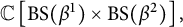 $\mathbb {C}\left [\mathrm {BS}(\beta ^1) \times \mathrm {BS}(\beta ^2)\right ],$
we have a natural cluster structure, with cluster variables
$\mathbb {C}\left [\mathrm {BS}(\beta ^1) \times \mathrm {BS}(\beta ^2)\right ],$
we have a natural cluster structure, with cluster variables
 $x^{(1)}_1, \dots , x^{(1)}_{r_1}$
(coming from
$x^{(1)}_1, \dots , x^{(1)}_{r_1}$
(coming from
 $\mathrm {BS}(\beta ^1)$
) and
$\mathrm {BS}(\beta ^1)$
) and
 $x^{(2)}{r_1+1}, \dots , x^{(2)}{r}$
(coming from
$x^{(2)}{r_1+1}, \dots , x^{(2)}{r}$
(coming from
 $\mathrm {BS}(\beta ^2)$
). Thus, we obtain a cluster structure on
$\mathrm {BS}(\beta ^2)$
). Thus, we obtain a cluster structure on
 $\mathbb {C}[\mathcal {U}_{r_1}(\beta )]$
, with cluster variables being
$\mathbb {C}[\mathcal {U}_{r_1}(\beta )]$
, with cluster variables being
 $\Phi _{r_1}^{\ast }\left (x^{(1)}_{j}\right )$
,
$\Phi _{r_1}^{\ast }\left (x^{(1)}_{j}\right )$
,
 $\Phi _{r_1}^{\ast }\left (x^{(2)}{\ell }\right )$
,
$\Phi _{r_1}^{\ast }\left (x^{(2)}{\ell }\right )$
,
 $j = 1, \dots , r_1, \ell = r_{1}+1, \dots , r$
. We call this the product cluster structure on
$j = 1, \dots , r_1, \ell = r_{1}+1, \dots , r$
. We call this the product cluster structure on
 $\mathbb {C}[\mathcal {U}_{r_1}(\beta )]$
. We denote by
$\mathbb {C}[\mathcal {U}_{r_1}(\beta )]$
. We denote by
 $\widehat {Q}_{\beta }$
the quiver corresponding to this product cluster structure: it is simply the disjoint union of the quivers
$\widehat {Q}_{\beta }$
the quiver corresponding to this product cluster structure: it is simply the disjoint union of the quivers
 $Q_{\beta ^1}$
and
$Q_{\beta ^1}$
and
 $Q_{\beta ^2}$
.
$Q_{\beta ^2}$
.
Our goal is to relate the open and the product cluster structures. We start with some useful notations and definitions.
Definition 6.6 Let
 $B_{\beta ^1}(z_1,\ldots ,z_{r_1})=L_1U_1$
as above. We denote the diagonal elements of
$B_{\beta ^1}(z_1,\ldots ,z_{r_1})=L_1U_1$
as above. We denote the diagonal elements of
 $U_1$
by
$U_1$
by
 $\left (u^{(1)}_1, \dots , u^{(1)}_k\right )$
.
$\left (u^{(1)}_1, \dots , u^{(1)}_k\right )$
.
Recall that, by (4.5), all
 $u^{(1)}_j$
are cluster monomials in the frozen variables
$u^{(1)}_j$
are cluster monomials in the frozen variables
 $x_{\mathrm {last}^1(s)}$
,
$x_{\mathrm {last}^1(s)}$
,
 $s = 1, \dots , k-1$
. We can combine these to build more cluster monomials.
$s = 1, \dots , k-1$
. We can combine these to build more cluster monomials.
Definition 6.7 For
 $l=r_1+1,\ldots ,r,$
we define
$l=r_1+1,\ldots ,r,$
we define
 $$ \begin{align} m_\ell = \prod_{t = 1}^{i_\ell}\left(u^{(1)}_{s_{i_{r_1+1}}\dots s_{i_\ell}(t)}\right)^{-1}. \end{align} $$
Let us interpret this pictorially. Draw the braid
 $\beta ^2$
and look at the
$\beta ^2$
and look at the
 $\ell -r_1$
-th crossing, counting from left to right. Right after this crossing, look at the bottom
$\ell -r_1$
-th crossing, counting from left to right. Right after this crossing, look at the bottom
 $i_\ell $
-strands, and follow them to the left. The end labels of the strands are precisely the subindices of the
$i_\ell $
-strands, and follow them to the left. The end labels of the strands are precisely the subindices of the
 $u^{(1)}$
-factors appearing in (6.6). See Figure 2 for an example.
$u^{(1)}$
-factors appearing in (6.6). See Figure 2 for an example.
The monomial
 $m_{r_1+6}$
equals
$m_{r_1+6}$
equals
 $\left (u^{(1)}_{3}u^{(1)}_5u^{(1)}_1\right )^{-1}$
.
$\left (u^{(1)}_{3}u^{(1)}_5u^{(1)}_1\right )^{-1}$
.

Lemma 6.8 Under the isomorphism
 $\Phi _{r_1}^{\ast }: \mathbb {C}\left [\mathrm {BS}(\beta ^1) \times \mathrm {BS}(\beta ^2)\right ] \to \mathbb {C}[\mathcal {U}_{r_1}(\beta )],$
we have:
$\Phi _{r_1}^{\ast }: \mathbb {C}\left [\mathrm {BS}(\beta ^1) \times \mathrm {BS}(\beta ^2)\right ] \to \mathbb {C}[\mathcal {U}_{r_1}(\beta )],$
we have:
-
(1)
$\Phi _{r_1}^{\ast }\left (x^{(1)}_j\right ) = x_j$
for
$j = 1, \dots , r_1$
. -
(2)
$\Phi _{r_1}^{\ast }\left (x^{(2)}\ell \right ) = m_\ell x_\ell $
for
$\ell = r_1 + 1, \dots , r$
, where
$m_\ell $
is given by (6.6).


Proof By (6.5), we have
 $$\begin{align*}\Phi_{r_1}^{\ast}\left(x^{(1)}_j\right) = \Phi_{r_1}^{\ast}\left(\Delta_{i_j}\!\left(B_{\beta^1_j}(z_1, \dots, z_j)\right)\right) = \Delta_{i_j}\!\left(B_{\beta_j}(z_1, \dots, z_j)\right) = x_j, \end{align*}$$
where
 $j = 1, \dots , r_1$
. On the other hand, if
$j = 1, \dots , r_1$
. On the other hand, if
 $\ell = r_1+1, \dots , r,$
we have
$\ell = r_1+1, \dots , r,$
we have
 $$\begin{align*}\Phi_{r_1}^{\ast}\left(x^{(2)}\ell\right) = \Phi_{r_1}^{\ast}\left(\Delta_{i_\ell}\! \left(B_{\beta^2_{\ell-r_1}}(z_{r_1+1}, \dots, z_\ell)\right)\right) = \Delta_{i_\ell}\!\left(B_{\beta^2_{\ell-r_1}}(z^{\prime}_{r_1+1}, \dots, z^{\prime}_\ell)\right) \end{align*}$$
and our job is to compare this to
 $x_\ell = \Delta _{i_\ell }\!\left (B_{\beta _\ell }(z_1, \dots , z_\ell )\right )$
. Note however that
$x_\ell = \Delta _{i_\ell }\!\left (B_{\beta _\ell }(z_1, \dots , z_\ell )\right )$
. Note however that
 $$\begin{align*}\begin{array}{r@{\;}l} x_\ell = \Delta_{i_\ell}\!\left(B_{\beta_\ell}(z_1, \dots, z_\ell)\right) = & \Delta_{i_\ell}\!\left(B_{\beta^1}(z_1, \dots, z_{r_1})B_{\beta^2_{\ell-r_1}}\!(z_{r_1+1}, \dots, z_{\ell})\right) \\ = & \Delta_{i_\ell}\!\left(L_1U_1B_{\beta^2_{\ell-r_1}}(z_{r_1+1}, \dots, z_\ell)\right) \\ = & \Delta_{i_\ell}\!\left(L_1\right)\Delta_{i_\ell}\left(U_1B_{\beta^2_{\ell-r_1}}(z_{r_1+1}, \dots, z_\ell)\right) \\ = & \Delta_{i_\ell}\!\left(U_1B_{\beta^2_{\ell-r_1}}(z_{r_1+1}, \dots, z_\ell)\right) \\ = & \Delta_{i_\ell}\!\left(B_{\beta^2_{\ell-r_1}}(z_{r_1+1}', \dots, z^{\prime}_\ell)U_1'\right) \\ = & \Delta_{i_\ell}\!\left(B_{\beta^2_{\ell-r_1}}(z^{\prime}_{r_1+1}, \dots, z^{\prime}_{\ell})\right)\Delta_{i_\ell}(U_1') \\ = & \Phi_{r_1}^{\ast}\!\left(x^{(2)}\ell\right)\Delta_{i_\ell}(U_1'), \end{array} \end{align*}$$
where we have used the Cauchy–Binet formula in the fourth and seventh equalities, and the fact that
 $L_1$
is uni-triangular in the fifth equality. Since
$L_1$
is uni-triangular in the fifth equality. Since
 $U^{\prime }_1$
is upper triangular, its
$U^{\prime }_1$
is upper triangular, its
 $i_\ell $
-th principal minor is just the product of the upper left
$i_\ell $
-th principal minor is just the product of the upper left
 $i_\ell $
-entries of the diagonal of
$i_\ell $
-entries of the diagonal of
 $U^{\prime }_1$
. By Lemma 2.6, these coincide with the corresponding entries of
$U^{\prime }_1$
. By Lemma 2.6, these coincide with the corresponding entries of
 $U_1$
up to permutation by
$U_1$
up to permutation by
 $\pi (\beta ^2_{\ell -r_1})=s_{i_{r_1+1}}\dots s_{i_{\ell }}$
. So
$\pi (\beta ^2_{\ell -r_1})=s_{i_{r_1+1}}\dots s_{i_{\ell }}$
. So
 $$ \begin{align*}\Delta_{i_\ell}(U_1')=m_\ell^{-1},\quad x_{\ell}=\Phi_{r_1}^{\ast}\left(x^{(2)}\ell\right)m_{\ell}^{-1} \end{align*} $$
and the result follows.
We are now ready to prove the following result.
Theorem 6.9 The product and the open cluster structures on
 $\mathcal {U}_{r_1}(\beta )$
are quasi-cluster equivalent.
$\mathcal {U}_{r_1}(\beta )$
are quasi-cluster equivalent.
Proof The fact that the cluster variables in both structures differ by monomials in frozens follows directly from Lemma 6.8. Now, we need to verify that the exchange ratios in both cluster structures agree. The mutable cluster variables in both cluster structures are indexed by
 $\mathrm {Mut} := \{1, \dots , r\}\setminus \{\mathrm {last}^1(s), \mathrm {last}(s) \mid s = 1, \dots , k-1\}$
.
$\mathrm {Mut} := \{1, \dots , r\}\setminus \{\mathrm {last}^1(s), \mathrm {last}(s) \mid s = 1, \dots , k-1\}$
.
Let us take
 $j \in \mathrm {Mut}$
such that
$j \in \mathrm {Mut}$
such that
 $j \leq r_1$
. We claim that if
$j \leq r_1$
. We claim that if
 $x_s$
is adjacent to
$x_s$
is adjacent to
 $x_j$
, then
$x_j$
, then
 $s \leq r_1$
. We have two cases. If s and j are the same color (i.e.,
$s \leq r_1$
. We have two cases. If s and j are the same color (i.e.,
 $i_s = i_j$
), then either
$i_s = i_j$
), then either
 $s \leq j \leq r_1$
, or
$s \leq j \leq r_1$
, or
 $j < s \leq \mathrm {last}^1(i_j) \leq r_1$
, where the last equation follows since there cannot be
$j < s \leq \mathrm {last}^1(i_j) \leq r_1$
, where the last equation follows since there cannot be
 $j < t < s$
with
$j < t < s$
with
 $i_j = i_t$
and,
$i_j = i_t$
and,
 $x_j$
being mutable, j cannot be the last appearance of
$x_j$
being mutable, j cannot be the last appearance of
 $i_j$
in
$i_j$
in
 $\beta ^1$
. Now assume s and j are not of the same color. If there is an arrow
$\beta ^1$
. Now assume s and j are not of the same color. If there is an arrow
 $j \to s,$
then
$j \to s,$
then
 $s \leq j \leq r_1$
, so we assume that there is an arrow
$s \leq j \leq r_1$
, so we assume that there is an arrow
 $s \to j$
. So s must be strictly between j and
$s \to j$
. So s must be strictly between j and
 $\mathrm {last}^1(j) \leq r_1$
. Thus,
$\mathrm {last}^1(j) \leq r_1$
. Thus,
 $s \leq r_1$
and we have proven our claim. By Lemma 6.8(1), the exchange ratio associated with the cluster variable
$s \leq r_1$
and we have proven our claim. By Lemma 6.8(1), the exchange ratio associated with the cluster variable
 $x_j$
in the open structure coincides with the exchange ratio associated with
$x_j$
in the open structure coincides with the exchange ratio associated with
 $\Phi _{r_1}^{\ast }\left (x^{(1)}_j\right )$
in the product structure.
$\Phi _{r_1}^{\ast }\left (x^{(1)}_j\right )$
in the product structure.
Now, we take
 $\ell \in \mathrm {Mut}$
with
$\ell \in \mathrm {Mut}$
with
 $r_1 < \ell $
. Our goal is to show that the exchange ratio associated with
$r_1 < \ell $
. Our goal is to show that the exchange ratio associated with
 $x_\ell $
in the open structure coincides with the exchange ratio of
$x_\ell $
in the open structure coincides with the exchange ratio of
 $\Phi _{r_1}^{\ast }\left (x^{(2)}\ell \right )$
in the product structure. Since
$\Phi _{r_1}^{\ast }\left (x^{(2)}\ell \right )$
in the product structure. Since
 $x_\ell $
is not frozen, there exists
$x_\ell $
is not frozen, there exists
 $\ell < \ell ' \leq r$
such that
$\ell < \ell ' \leq r$
such that
 $\mathrm {clr}(\ell ) = \mathrm {clr}(\ell ')$
. In particular, we have an arrow
$\mathrm {clr}(\ell ) = \mathrm {clr}(\ell ')$
. In particular, we have an arrow
 $\ell \to \ell '$
both in
$\ell \to \ell '$
both in
 $\widehat {Q}_{\beta }$
and in
$\widehat {Q}_{\beta }$
and in
 $Q_{\beta ^1}\sqcup Q_{\beta ^2}$
. We have several cases.
$Q_{\beta ^1}\sqcup Q_{\beta ^2}$
. We have several cases.
Case 1. The quiver
 $Q^{\circ }_{\beta }$
locally around
$Q^{\circ }_{\beta }$
locally around
 $\ell $
looks as follows:
$\ell $
looks as follows:

Since
 $\ell "$
is not frozen in
$\ell "$
is not frozen in
 $Q^{\circ }_{\beta }$
, we have
$Q^{\circ }_{\beta }$
, we have
 $r_1 < \ell "$
, so that both arrows also belong to
$r_1 < \ell "$
, so that both arrows also belong to
 $\widehat {Q}_{\beta }$
. So we have to show that
$\widehat {Q}_{\beta }$
. So we have to show that
 $x_{\ell '}/x_{\ell "} = \Phi _{r_1}^{\ast }\left (x^{(2)}{\ell '}\right )/\Phi _{r_1}^{\ast }\left (x^{(2)}{\ell "}\right )$
. By Lemma 6.8, this is equivalent to showing that
$x_{\ell '}/x_{\ell "} = \Phi _{r_1}^{\ast }\left (x^{(2)}{\ell '}\right )/\Phi _{r_1}^{\ast }\left (x^{(2)}{\ell "}\right )$
. By Lemma 6.8, this is equivalent to showing that
 $m_{\ell '} = m_{\ell "}$
. Note that there are no crossings of color
$m_{\ell '} = m_{\ell "}$
. Note that there are no crossings of color
 $\mathrm {clr}(\ell ) \pm 1$
between any of the three crossings depicted on the figure, as otherwise the quiver
$\mathrm {clr}(\ell ) \pm 1$
between any of the three crossings depicted on the figure, as otherwise the quiver
 $Q^{\circ }_{\beta }$
would have more arrows incident to either
$Q^{\circ }_{\beta }$
would have more arrows incident to either
 $\ell $
or
$\ell $
or
 $\ell "$
. It then follows from (6.6) that both
$\ell "$
. It then follows from (6.6) that both
 $m_{\ell '}$
and
$m_{\ell '}$
and
 $m_{\ell "}$
are equal to
$m_{\ell "}$
are equal to
 $\prod _{i \leq i_{\ell }}\left (u^{(1)}_{s_{i_{r_1+1}}\dots s_{i_{\ell "}}(i)}\right )^{-1}$
.
$\prod _{i \leq i_{\ell }}\left (u^{(1)}_{s_{i_{r_1+1}}\dots s_{i_{\ell "}}(i)}\right )^{-1}$
.
Case 2. The quiver
 $Q_{\beta ^1}\sqcup Q_{\beta ^2}$
locally around
$Q_{\beta ^1}\sqcup Q_{\beta ^2}$
locally around
 $\ell $
looks as follows:
$\ell $
looks as follows:

So that the quiver
 $Q^{\circ }_{\beta }$
locally around
$Q^{\circ }_{\beta }$
locally around
 $\ell $
simply looks as
$\ell $
simply looks as
 $\ell " \to \ell \to \ell '$
, and
$\ell " \to \ell \to \ell '$
, and
 $\ell " = \mathrm {last}^1(\mathrm {clr}(\ell ))$
, so that
$\ell " = \mathrm {last}^1(\mathrm {clr}(\ell ))$
, so that
 $\ell "$
is frozen. The exchange ratio in the product cluster structure is then simply
$\ell "$
is frozen. The exchange ratio in the product cluster structure is then simply
 $\Phi _{r_1}^{\ast }\left (x^{(2)}{\ell '}\right ) = m_{\ell '}x_{\ell '}$
. But
$\Phi _{r_1}^{\ast }\left (x^{(2)}{\ell '}\right ) = m_{\ell '}x_{\ell '}$
. But
 $m_{\ell '} = \left (u_1\dots u_{\mathrm {last}^1(\mathrm {clr}(\ell ))}\right )^{-1} = x_{\mathrm {last}^1(\mathrm {clr}(\ell ))}^{-1} = x_{\ell "}^{-1}$
and the result follows.
$m_{\ell '} = \left (u_1\dots u_{\mathrm {last}^1(\mathrm {clr}(\ell ))}\right )^{-1} = x_{\mathrm {last}^1(\mathrm {clr}(\ell ))}^{-1} = x_{\ell "}^{-1}$
and the result follows.
If the quiver
 $Q^{\circ }_{\beta }$
looks
$Q^{\circ }_{\beta }$
looks
 $\ell \to \ell '$
locally around
$\ell \to \ell '$
locally around
 $\ell $
, then
$\ell $
, then
 $$ \begin{align*}x_{\mathrm{last}^1(\mathrm{clr}(\ell))} = 1 = \left(u_1\dots u_{\mathrm{last}^1(\mathrm{clr}(\ell))}\right)^{-1} = m_{\ell'},\end{align*} $$
so this case is similar.
Case 3. The quiver
 $Q^{\circ }_{\beta }$
locally around
$Q^{\circ }_{\beta }$
locally around
 $\ell $
looks as follows:
$\ell $
looks as follows:

So we must show that
 $m_{\ell '}m_{j} = m_{\ell "}m_{j'}$
. This follows easily from the pictorial interpretation of (6.6). Let us color the strands contributing to a monomial
$m_{\ell '}m_{j} = m_{\ell "}m_{j'}$
. This follows easily from the pictorial interpretation of (6.6). Let us color the strands contributing to a monomial
 $m_{i}$
with the same color as i in the picture below:
$m_{i}$
with the same color as i in the picture below:

Note that we have used that there is no crossing of color
 $\mathrm {clr}(j')$
between
$\mathrm {clr}(j')$
between
 $j'$
and
$j'$
and
 $\ell '$
, no crossing of color
$\ell '$
, no crossing of color
 $\mathrm {clr}(\ell ) - 1$
and no crossing of color
$\mathrm {clr}(\ell ) - 1$
and no crossing of color
 $\mathrm {clr}(j)$
between j and
$\mathrm {clr}(j)$
between j and
 $\ell $
. Note that every u factor appearing in
$\ell $
. Note that every u factor appearing in
 $m_{\ell '}m_{j}$
cancels with one appearing in
$m_{\ell '}m_{j}$
cancels with one appearing in
 $m_{\ell "}m_{j'}$
and vice versa, so the result follows.
$m_{\ell "}m_{j'}$
and vice versa, so the result follows.
The case when
 $\ell " < r_1$
(so that the quiver
$\ell " < r_1$
(so that the quiver
 $Q_{\beta ^2}$
does not have the vertex
$Q_{\beta ^2}$
does not have the vertex
 $\ell "$
above, and
$\ell "$
above, and
 $\ell '$
becomes frozen in
$\ell '$
becomes frozen in
 $Q^{\circ }_{\beta }$
) is similar, after noticing that in this case
$Q^{\circ }_{\beta }$
) is similar, after noticing that in this case
 $\mathrm {last}^1 (\mathrm {clr}(\ell )) = \ell "$
.
$\mathrm {last}^1 (\mathrm {clr}(\ell )) = \ell "$
.
We note that when the quiver locally looks like a horizontal reflection, we obtain a similar result.
Case 4. The quiver
 $Q^{\circ }_{\beta }$
locally around
$Q^{\circ }_{\beta }$
locally around
 $\ell $
looks as follows:
$\ell $
looks as follows:

In this case, we need to prove that
 $$\begin{align*}m_{\ell"}m_{j'}m_{t'} = m_{\ell'}m_{j}m_{t}, \end{align*}$$
or, equivalently, that
 $$\begin{align*}\frac{m_{j'}m_{t'}}{m_{\ell'}} = \frac{m_{j}m_{t}}{m_{\ell"}}. \end{align*}$$
Let
 $i = \mathrm {clr}(\ell )$
and consider the truncation of the braid
$i = \mathrm {clr}(\ell )$
and consider the truncation of the braid
 $\beta ^{2}$
on the dashed vertical line as depicted above. Let
$\beta ^{2}$
on the dashed vertical line as depicted above. Let
 $\tau $
be the resulting permutation. Then
$\tau $
be the resulting permutation. Then
 $$ \begin{align} \frac{m_{j'}m_{t'}}{m_{\ell'}} = \prod_{s \leq i}\left(u^{(1)}_{\tau^{-1}(s)}\right)^{-1}. \end{align} $$
Now consider the truncation of the braid
 $\beta ^{2}$
on the red dashed vertical line below:
$\beta ^{2}$
on the red dashed vertical line below:

and let
 $\tau _1$
be the resulting permutation. Since there are no crossings of color
$\tau _1$
be the resulting permutation. Since there are no crossings of color
 $i = \mathrm {clr}(\ell )$
between
$i = \mathrm {clr}(\ell )$
between
 $\ell $
and
$\ell $
and
 $\ell '$
, we have that (6.7) can be rewritten as
$\ell '$
, we have that (6.7) can be rewritten as
 $$\begin{align*}\frac{m_{j'}m_{t'}}{m_{\ell'}} = \left(u^{(1)}_{\tau_1^{-1}(i+1)}\right)^{-1}\prod_{s < i}\left(u^{(1)}_{\tau_1^{-1}(s)}\right)^{-1}. \end{align*}$$
Which can easily seen to be
 $\frac {m_jm_{t}}{m_{\ell "}}$
and the result follows. Variations of this case (where, e.g., the t-crossing belongs to
$\frac {m_jm_{t}}{m_{\ell "}}$
and the result follows. Variations of this case (where, e.g., the t-crossing belongs to
 $\beta ^{1}$
) are proved similarly.
$\beta ^{1}$
) are proved similarly.
We now show that Example 1.10 given in the introduction is a quasi-cluster isomorphism.
Example 6.10 Recall Example 1.10. We verify the preservation of exchange ratios at each one of the vertices
 $10$
–
$10$
–
 $13$
. Note that the preservation of exchange ratios at the mutable vertices
$13$
. Note that the preservation of exchange ratios at the mutable vertices
 $1$
–
$1$
–
 $8$
is immediate by construction. To lighten the notation, we denote
$8$
is immediate by construction. To lighten the notation, we denote
 $x_k' = \Phi _{r_1}^{\ast }\left (x_k^{(2)}\right )$
.
$x_k' = \Phi _{r_1}^{\ast }\left (x_k^{(2)}\right )$
.
-
• Vertex 10: In the open cluster structure, the exchange ratio is
$\displaystyle {\frac {x_6x_{13}}{x_{7}x_{14}}}$
. In the product cluster structure, this exchange ratio is
$\displaystyle {\frac {x^{\prime }_{13}}{x^{\prime }_{14}}}$
. According to Lemma 6.8, we have
$x^{\prime }_{14} = \left (u^{(1)}_{2}u^{(1)}_{3}u^{(1)}_{4}\right )^{-1}x_{14}$
and
$x^{\prime }_{13} = \left (u^{(1)}_{2}u^{(1)}_{4}\right )^{-1}x_{13}$
. Now, we note that
$\displaystyle {\frac {x_6}{x_7}} = \frac {u^{(1)}_3u^{(1)}_2u^{(1)}_1}{u^{(1)}_2u^{(1)}_1} = u^{(1)}_3$
, which shows the desired equality. -
• Vertex 11: In the open cluster structure, the exchange ratio is
$\displaystyle {\frac {x_7x_{12}}{x_9x_{13}}}$
while in the product cluster structure, the exchange ratio is simply
$\displaystyle {\frac {x^{\prime }_{12}}{x^{\prime }_{13}}}$
. Now, according to Lemma 6.8, and it remains to notice that
$$\begin{align*}x^{\prime}_{12} = \left(u^{(1)}_{4}\right)^{-1}x_{12}, \qquad x^{\prime}_{13} = \left(u^{(1)}_{4}u^{(1)}_{2}\right)^{-1}x_{13}, \qquad \text{so that} \qquad \frac{x^{\prime}_{12}}{x^{\prime}_{13}} = u^{(1)}_2\frac{x_{12}}{x_{13}} \end{align*}$$
$\displaystyle {\frac {x_{7}}{x_{9}} = \frac {u^{(1)}_1u^{(1)}_2}{u^{(1)}_1} = u^{(1)}_2}$
.
-
• Vertex 12: In the open cluster structure, the exchange ratio is
$\displaystyle {\frac {x_9x_{15}}{x_{11}x_{16}}}$
and in the product cluster structure, it is
$\displaystyle {\frac {x^{\prime }_{15}}{x^{\prime }_{11}x^{\prime }_{16}}}$
. Now,
$$\begin{align*}\frac{x^{\prime}_{15}}{x^{\prime}_{11}x^{\prime}_{16}} = \frac{\left(u^{(1)}_3u^{(1)}_4\right)^{-1}x_{15}}{\left(u^{(1)}_4u^{(1)}_1\right)^{-1}x_{11}\left(u^{(1)}_3\right)^{-1}x_{16}} = \frac{u^{(1)}_1 x_{15}}{x_{11}x_{16}} = \frac{x_9x_{15}}{x_{11}x_{16}}. \end{align*}$$
-
• Vertex 13: We must verify that
$\displaystyle {\frac {x_{11}x_{14}}{x_{10}x_{15}}}$
coincides with
$\displaystyle {\frac {x^{\prime }_{11}x^{\prime }_{14}}{x^{\prime }_{10}x^{\prime }_{15}}}$
:
$$\begin{align*}\frac{x^{\prime}_{11}x^{\prime}_{14}}{x^{\prime}_{10}x^{\prime}_{15}} = \frac{\left(u^{(1)}_4u^{(1)}_1\right)^{-1}x_{11}\left(u^{(1)}_{2}u^{(1)}_{3}u^{(1)}_{4}\right)^{-1}x_{14}}{\left(u^{(1)}_{4}u^{(1)}_{2}u^{(1)}_{1}\right)^{-1}x_{10}{\left(u^{(1)}_3u^{(1)}_4\right)^{-1}x_{15}}} = \frac{x_{11}x_{14}}{x_{10}x_{15}}. \end{align*}$$


Acknowledgements
The authors would like to thank Roger Casals, Mikhail Gorsky, Thomas Lam, Melissa Sherman-Bennett, David Speyer, Catharina Stroppel, and Daping Weng for the useful discussions.


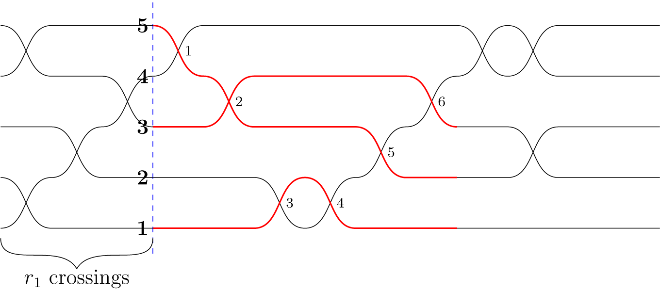


 Open access