







1 Introduction
Hele-Shaw cells are made by two parallel, transparent plates, which are separated by a gap that – ideally – is infinitesimal. Under this condition, any flow established inside the gap can reproduce a Stokes flow. This property makes Hele-Shaw cells widely used to visualise and analyse experimentally different types of flow instances. We focus here on the use of Hele-Shaw cells to investigate flows driven by the differential gravity force acting on fluids of different density, which are initially set in an unstable configuration. This type of experiment is particularly important for a number of applications, since it is simple and can, under certain assumptions, reproduce important features of Darcy flows in porous media. Specifically, we refer to the instance of fluid saturated porous media, in which a heavier fluid sits on top of a lighter fluid. In this instance (for certain density differences), the fluid flow is dominated by convection; this type of flow was examined by Saffman & Taylor (Reference Saffman and Taylor1958), who also introduced the concept that the flow inside a porous media can be experimentally reproduced employing a Hele-Shaw cell.
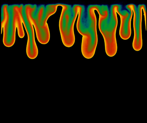
In this paper, we examine the process of solute convection in Rayleigh–Bénard-like flows in Hele-Shaw cells, with the following set-up: the cell is filled with pure fluid, i.e. solute is initially not present, and the concentration of solute is kept constant along the top boundary of the domain. Since the density of the fluid is larger at the top wall, the system is unstable and, with time, tiny instabilities of the density interface grow into finger-like structures, which eventually develop convective currents. This configuration is of crucial importance to investigate geophysical subsurface flows such as water contamination (LeBlanc Reference LeBlanc1984; Van Der Molen & Ommen Reference Van Der Molen and Ommen1988), petroleum migration (Simmons, Fenstemaker & Sharp Jr Reference Simmons, Fenstemaker and Sharp2001), carbon sequestration (Huppert & Neufeld Reference Huppert and Neufeld2014; Emami-Meybodi et al.
Reference Emami-Meybodi, Hassanzadeh, Green and Ennis-King2015) and sea ice formation (Wettlaufer, Worster & Huppert Reference Wettlaufer, Worster and Huppert1997; Feltham et al.
Reference Feltham, Untersteiner, Wettlaufer and Worster2006). The main dimensionless governing parameter of the flow is the Rayleigh–Darcy number ( $Ra$
), which stands for an inverse diffusivity, or for the relative strength of convection to diffusion (Slim Reference Slim2014), and is defined as
$Ra$
), which stands for an inverse diffusivity, or for the relative strength of convection to diffusion (Slim Reference Slim2014), and is defined as
 $$\begin{eqnarray}Ra=\frac{g\unicode[STIX]{x0394}\unicode[STIX]{x1D70C}_{s}^{\ast }(b^{\ast })^{2}H^{\ast }}{12\unicode[STIX]{x1D707}D},\end{eqnarray}$$
where, $\unicode[STIX]{x0394}\unicode[STIX]{x1D70C}_{s}^{\ast }$
is the density difference between the solute-saturated fluid and the pure fluid,
$\unicode[STIX]{x0394}\unicode[STIX]{x1D70C}_{s}^{\ast }$
is the density difference between the solute-saturated fluid and the pure fluid, $g$
is the acceleration due to gravity,
$g$
is the acceleration due to gravity, $b^{\ast }$
is the cell gap thickness,
$b^{\ast }$
is the cell gap thickness, $H^{\ast }$
is the cell height,
$H^{\ast }$
is the cell height, $D$
is the molecular diffusion coefficient and
$D$
is the molecular diffusion coefficient and $\unicode[STIX]{x1D707}$
is the dynamic viscosity. This system is analysed in terms of solute dissolution rate
$\unicode[STIX]{x1D707}$
is the dynamic viscosity. This system is analysed in terms of solute dissolution rate $F(t)$
, i.e. the amount of solute dissolved per unit of area and time. Based on the time evolution of
$F(t)$
, i.e. the amount of solute dissolved per unit of area and time. Based on the time evolution of $F(t)$
, three different flow phases can be defined: (i) the flow is initially controlled by diffusion; then (ii) an unstable layer builds up at the upper boundary and convective finger-like structures form and control the evolution of the system; and finally (iii) shutdown of convection takes place (Hewitt, Neufeld & Lister Reference Hewitt, Neufeld and Lister2013; Slim Reference Slim2014).
$F(t)$
, three different flow phases can be defined: (i) the flow is initially controlled by diffusion; then (ii) an unstable layer builds up at the upper boundary and convective finger-like structures form and control the evolution of the system; and finally (iii) shutdown of convection takes place (Hewitt, Neufeld & Lister Reference Hewitt, Neufeld and Lister2013; Slim Reference Slim2014).
Two-dimensional Darcy simulations have shown that, during the convection dominated phase, the solute dissolution rate is independent of the Rayleigh–Darcy number (Pau et al.
Reference Pau, Bell, Pruess, Almgren, Lijewski and Zhang2010; Hewitt et al.
Reference Hewitt, Neufeld and Lister2013; Slim Reference Slim2014). Noteworthy though, experiments in Hele-Shaw cells have shown that the quantity $F(t)$
exhibits weak dependence on
$F(t)$
exhibits weak dependence on $Ra$
(Backhaus, Turitsyn & Ecke Reference Backhaus, Turitsyn and Ecke2011; Tsai, Riesing & Stone Reference Tsai, Riesing and Stone2013). Therefore, in an attempt to unravel this discrepancy, Hidalgo et al. (Reference Hidalgo, Fe, Cueto-Felgueroso and Juanes2012) investigated numerically the time-dependent dissolution process in fluids characterised by concentration-dependent viscosity and non-monotonic density-concentration curves; they concluded that the
$Ra$
(Backhaus, Turitsyn & Ecke Reference Backhaus, Turitsyn and Ecke2011; Tsai, Riesing & Stone Reference Tsai, Riesing and Stone2013). Therefore, in an attempt to unravel this discrepancy, Hidalgo et al. (Reference Hidalgo, Fe, Cueto-Felgueroso and Juanes2012) investigated numerically the time-dependent dissolution process in fluids characterised by concentration-dependent viscosity and non-monotonic density-concentration curves; they concluded that the $Ra$
-dependent character of the dissolution flux observed experimentally is not motivated by these two causes. Subsequent studies investigated the influence of the geometry of the domain on the features of the flow. In particular, with the aid of perturbation techniques and numerical simulations, Letelier, Mujica & Ortega (Reference Letelier, Mujica and Ortega2019) investigated the effect of the combined action of the Rayleigh–Darcy number and the anisotropy ratio
$Ra$
-dependent character of the dissolution flux observed experimentally is not motivated by these two causes. Subsequent studies investigated the influence of the geometry of the domain on the features of the flow. In particular, with the aid of perturbation techniques and numerical simulations, Letelier, Mujica & Ortega (Reference Letelier, Mujica and Ortega2019) investigated the effect of the combined action of the Rayleigh–Darcy number and the anisotropy ratio $\unicode[STIX]{x1D716}=b^{\ast }/\sqrt{12}H^{\ast }$
. In accordance with the value of the parameter
$\unicode[STIX]{x1D716}=b^{\ast }/\sqrt{12}H^{\ast }$
. In accordance with the value of the parameter $\unicode[STIX]{x1D716}^{2}Ra$
, they have been able to identify three flow configurations: (i) Darcy regime (
$\unicode[STIX]{x1D716}^{2}Ra$
, they have been able to identify three flow configurations: (i) Darcy regime ( $\unicode[STIX]{x1D716}^{2}Ra\rightarrow 0$
), where the flow is two-dimensional and well described by Darcy simulations; (ii) Hele-Shaw regime (
$\unicode[STIX]{x1D716}^{2}Ra\rightarrow 0$
), where the flow is two-dimensional and well described by Darcy simulations; (ii) Hele-Shaw regime ( $\unicode[STIX]{x1D716}^{2}Ra\ll 1$
), where the flow is still two-dimensional but influenced by gap-induced dispersion; and (iii) three-dimensional regime (
$\unicode[STIX]{x1D716}^{2}Ra\ll 1$
), where the flow is still two-dimensional but influenced by gap-induced dispersion; and (iii) three-dimensional regime ( $\unicode[STIX]{x1D716}^{2}Ra\gg 1$
), when the effects of the third dimension become non-negligible.
$\unicode[STIX]{x1D716}^{2}Ra\gg 1$
), when the effects of the third dimension become non-negligible.
The object of this work is to provide experimental ground to these recent findings, with a further ambitious attempt of reconciling the different scaling laws of the solute dissolution rate available from the literature. To explore a wide range of the parameter space $\unicode[STIX]{x1D716}^{2}Ra$
, we will use a Hele-Shaw cell with variable gap and variable height in a Rayleigh–Bénard-like set-up.
$\unicode[STIX]{x1D716}^{2}Ra$
, we will use a Hele-Shaw cell with variable gap and variable height in a Rayleigh–Bénard-like set-up.
2 Methodology
We consider a rectangular domain initially filled with pure fluid. Solute concentration is kept constant at the top wall, whereas other boundaries are impermeable with respect to fluid and solute fluxes. This set-up is defined as Rayleigh–Bénard-like or a one-sided configuration (Hewitt et al.
Reference Hewitt, Neufeld and Lister2013; De Paoli, Zonta & Soldati Reference De Paoli, Zonta and Soldati2016). For different Rayleigh–Darcy numbers, we measured the mean solute dissolution rate by keeping the same fluid and solute ( $\unicode[STIX]{x0394}\unicode[STIX]{x1D70C}_{s}^{\ast }$
,
$\unicode[STIX]{x0394}\unicode[STIX]{x1D70C}_{s}^{\ast }$
, $D$
and
$D$
and $\unicode[STIX]{x1D707}$
are constant), but varying the geometry of the cell (gap width,
$\unicode[STIX]{x1D707}$
are constant), but varying the geometry of the cell (gap width, $b^{\ast }$
, and domain height,
$b^{\ast }$
, and domain height, $H^{\ast }$
).
$H^{\ast }$
).
The apparatus is sketched in figure 1(a) and consists of two parallel acrylic plates (thickness 30 mm), having width of 200 mm and height of 370 mm, separated by a gap $b^{\ast }\in [0.15;1.00]~\text{mm}$
. Except the top wall, fluid layer boundaries are defined by rubber seals, which confine the fluid between the plates and avoid leakages. The cell width is kept constant and equal to
$b^{\ast }\in [0.15;1.00]~\text{mm}$
. Except the top wall, fluid layer boundaries are defined by rubber seals, which confine the fluid between the plates and avoid leakages. The cell width is kept constant and equal to $L^{\ast }=160~\text{mm}$
, whereas the cell height is varied using different gaskets so that
$L^{\ast }=160~\text{mm}$
, whereas the cell height is varied using different gaskets so that $H^{\ast }\in [104;343]~\text{mm}$
. The material used for the gaskets is a high-quality impermeable rubber (Klinger–Sil C–4400) worked with high-precision CNC machines. The fluid domain, with explicit indication of the dimensions, coordinate system and boundary conditions, is shown in figure 1(b). The plates are held in place with the aid of screws. To obtain a desired value of gap thickness and to ensure its uniformity over the cell, metal shims are placed in the gap and the same torque is applied to all the screws. Along the top wall lies a steel mesh (40 μm grid size) which contains the dye powder.
$H^{\ast }\in [104;343]~\text{mm}$
. The material used for the gaskets is a high-quality impermeable rubber (Klinger–Sil C–4400) worked with high-precision CNC machines. The fluid domain, with explicit indication of the dimensions, coordinate system and boundary conditions, is shown in figure 1(b). The plates are held in place with the aid of screws. To obtain a desired value of gap thickness and to ensure its uniformity over the cell, metal shims are placed in the gap and the same torque is applied to all the screws. Along the top wall lies a steel mesh (40 μm grid size) which contains the dye powder.
Sketch of the experimental set-up adopted. (a) Side view of the apparatus with indication of the main components. (b) Domain with explicit indication of dimensions, coordinate system and boundary conditions.

Jafari-Raad & Hassanzadeh (Reference Jafari-Raad and Hassanzadeh2015) observed that some discrepancies between experiments and simulations may occur due to the nature of the fluids adopted. For instance, Methanol and Ethylene-Glycol (known as MEG) and Propylene-Glycol (PPG), often used in experimental studies, are characterised by a non-monotonic variation of the fluid density with respect to solute concentration. In contrast, most of the numerical studies considered a much simpler linear dependency of density and concentration. To neglect the effect of the fluid properties, we chose two fluids marked by a linear density-concentration profile: an aqueous solution of potassium permanganate (KMnO4) to mimic the heavy fluid (high solute concentration) and water to mimic the light fluid (low solute concentration). Viscosity and diffusion are assumed constant and equal to $\unicode[STIX]{x1D707}=9.2\times 10^{-4}~\text{Pa}~\text{s}$
and
$\unicode[STIX]{x1D707}=9.2\times 10^{-4}~\text{Pa}~\text{s}$
and $D=1.65\times 10^{-9}~\text{m}^{2}~\text{s}^{-1}$
, respectively (Slim et al.
Reference Slim, Bandi, Miller and Mahadevan2013). With these fluids, a linear behaviour of the mixture density
$D=1.65\times 10^{-9}~\text{m}^{2}~\text{s}^{-1}$
, respectively (Slim et al.
Reference Slim, Bandi, Miller and Mahadevan2013). With these fluids, a linear behaviour of the mixture density $\unicode[STIX]{x1D70C}^{\ast }$
as a function of the solute concentration
$\unicode[STIX]{x1D70C}^{\ast }$
as a function of the solute concentration $C^{\ast }$
is obtained, i.e.
$C^{\ast }$
is obtained, i.e.
 $$\begin{eqnarray}\unicode[STIX]{x1D70C}^{\ast }=\unicode[STIX]{x1D70C}_{s}^{\ast }\left[1+\frac{\unicode[STIX]{x0394}\unicode[STIX]{x1D70C}_{s}^{\ast }}{\unicode[STIX]{x1D70C}_{s}^{\ast }C_{s}^{\ast }}(C^{\ast }-C_{s}^{\ast })\right],\end{eqnarray}$$
where, $\unicode[STIX]{x1D70C}_{s}^{\ast }$
is the density of the saturated solution,
$\unicode[STIX]{x1D70C}_{s}^{\ast }$
is the density of the saturated solution, $C_{s}^{\ast }=48~\text{kg}~\text{m}^{-3}$
is the effective saturation value of concentration and
$C_{s}^{\ast }=48~\text{kg}~\text{m}^{-3}$
is the effective saturation value of concentration and $\unicode[STIX]{x0394}\unicode[STIX]{x1D70C}_{s}^{\ast }$
is the density difference between a saturated solution and pure water. A discussion on the mixture density as a function of the solute concentration can be found in appendix A. Since water density is sensitive to temperature, although we run experiments in the temperature range 20–25 °C, for the sake of precision
$\unicode[STIX]{x0394}\unicode[STIX]{x1D70C}_{s}^{\ast }$
is the density difference between a saturated solution and pure water. A discussion on the mixture density as a function of the solute concentration can be found in appendix A. Since water density is sensitive to temperature, although we run experiments in the temperature range 20–25 °C, for the sake of precision $\unicode[STIX]{x1D70C}_{s}^{\ast }$
and
$\unicode[STIX]{x1D70C}_{s}^{\ast }$
and $\unicode[STIX]{x0394}\unicode[STIX]{x1D70C}_{s}^{\ast }$
are estimated in each experiment by the correlations of Novotný & Söhnel (Reference Novotný and Söhnel1988). With this set-up, we obtained
$\unicode[STIX]{x0394}\unicode[STIX]{x1D70C}_{s}^{\ast }$
are estimated in each experiment by the correlations of Novotný & Söhnel (Reference Novotný and Söhnel1988). With this set-up, we obtained $Ra\in [4.8\times 10^{4};7.0\times 10^{6}]$
.
$Ra\in [4.8\times 10^{4};7.0\times 10^{6}]$
.
We reconstruct solute concentration fields from light intensity maps (Slim et al.
Reference Slim, Bandi, Miller and Mahadevan2013; Ching, Chen & Tsai Reference Ching, Chen and Tsai2017). The accuracy of the concentration reconstruction process is sensitive to the local value of the mass fraction (Slim et al.
Reference Slim, Bandi, Miller and Mahadevan2013); in particular, the error may be significant (a few per cent) in regions of the domain that are characterised by high values of solute concentration. However, regions of high solute concentration are limited to the top of the domain, with an overall extension of less than 5 %, similar to previous experimental campaigns (Slim et al.
Reference Slim, Bandi, Miller and Mahadevan2013; Alipour & De Paoli Reference Alipour and De Paoli2019). Grains of potassium permanganate (diameter greater than 200 μm) are poured onto the grid. Afterwards, water is injected from two channels located at the bottom of the cell with the aid of a syringe pump. The fluid level is increased up to the upper boundary and the pump is shut down. This moment is considered as the beginning of the experiment ( $t^{\ast }=0$
). After water injection, the solute dissolves and a fluid layer denser than water forms below the grid: the heavy mixture layer thickens, becomes unstable and the finger-like structures form (Slim Reference Slim2014). We use a Canon 1300D camera equipped with 18–55 mm lenses to record the evolution of the flow, with resolution and acquisition rate corresponding to
$t^{\ast }=0$
). After water injection, the solute dissolves and a fluid layer denser than water forms below the grid: the heavy mixture layer thickens, becomes unstable and the finger-like structures form (Slim Reference Slim2014). We use a Canon 1300D camera equipped with 18–55 mm lenses to record the evolution of the flow, with resolution and acquisition rate corresponding to $3456\times 5184~\text{pixel}$
and 1 f.p.s., respectively. The system is illuminated from the back side with a tuneable LED-based system: the tension applied to the LEDs is adjusted to maximise the sensitivity of the apparatus. Since the gap thickness has a significant effect on the colour of the mixture, the calibration is repeated for each value of
$3456\times 5184~\text{pixel}$
and 1 f.p.s., respectively. The system is illuminated from the back side with a tuneable LED-based system: the tension applied to the LEDs is adjusted to maximise the sensitivity of the apparatus. Since the gap thickness has a significant effect on the colour of the mixture, the calibration is repeated for each value of $b^{\ast }$
. Given the light intensity distribution (camera images), the concentration field is finally reconstructed (Slim et al.
Reference Slim, Bandi, Miller and Mahadevan2013). Experimental results are the average of three experiments in the same configuration. A summary of all experimental parameters investigated can be found in table 1.
$b^{\ast }$
. Given the light intensity distribution (camera images), the concentration field is finally reconstructed (Slim et al.
Reference Slim, Bandi, Miller and Mahadevan2013). Experimental results are the average of three experiments in the same configuration. A summary of all experimental parameters investigated can be found in table 1.
Summary of all experiments performed. The Rayleigh–Darcy number is defined as $Ra=g\unicode[STIX]{x0394}\unicode[STIX]{x1D70C}_{s}^{\ast }(b^{\ast })^{2}H^{\ast }/(12\unicode[STIX]{x1D707}D)$
, where
$Ra=g\unicode[STIX]{x0394}\unicode[STIX]{x1D70C}_{s}^{\ast }(b^{\ast })^{2}H^{\ast }/(12\unicode[STIX]{x1D707}D)$
, where $\unicode[STIX]{x0394}\unicode[STIX]{x1D70C}_{s}^{\ast }=38.1~\text{kg}~\text{m}^{-3}$
,
$\unicode[STIX]{x0394}\unicode[STIX]{x1D70C}_{s}^{\ast }=38.1~\text{kg}~\text{m}^{-3}$
, $\unicode[STIX]{x1D707}=9.2\times 10^{-4}~\text{Pa}~\text{s}$
and
$\unicode[STIX]{x1D707}=9.2\times 10^{-4}~\text{Pa}~\text{s}$
and $D=1.65\times 10^{-9}~\text{m}^{2}~\text{s}^{-1}$
. Experiments are grouped by gap thickness,
$D=1.65\times 10^{-9}~\text{m}^{2}~\text{s}^{-1}$
. Experiments are grouped by gap thickness, $b^{\ast }$
. Flux measurements reported are the average of three experiments.
$b^{\ast }$
. Flux measurements reported are the average of three experiments.

To present the results in dimensionless form, we set the buoyancy velocity
 $$\begin{eqnarray}{\mathcal{W}}^{\ast }=\frac{g\unicode[STIX]{x0394}\unicode[STIX]{x1D70C}_{s}^{\ast }(b^{\ast })^{2}}{12\unicode[STIX]{x1D707}}\end{eqnarray}$$
as the reference velocity scale, whereas lengths and time are scaled with ${\mathcal{L}}^{\ast }=D/{\mathcal{W}}^{\ast }$
and
${\mathcal{L}}^{\ast }=D/{\mathcal{W}}^{\ast }$
and ${\mathcal{L}}^{\ast }/{\mathcal{W}}^{\ast }$
, respectively. Concentration is made dimensionless with respect to
${\mathcal{L}}^{\ast }/{\mathcal{W}}^{\ast }$
, respectively. Concentration is made dimensionless with respect to $C_{s}^{\ast }$
(for further details on the dimensionless set of variables, see Slim (Reference Slim2014)). The absence of the superscript * is used here to refer to dimensionless variables. The most relevant global observable for the present system is the averaged dimensionless dissolution rate
$C_{s}^{\ast }$
(for further details on the dimensionless set of variables, see Slim (Reference Slim2014)). The absence of the superscript * is used here to refer to dimensionless variables. The most relevant global observable for the present system is the averaged dimensionless dissolution rate $F(t)$
. This observable, which represents the amount of solute dissolved per unit of area and time, is customarily computed in numerical simulations as
$F(t)$
. This observable, which represents the amount of solute dissolved per unit of area and time, is customarily computed in numerical simulations as $F(t)=1/L\int _{0}^{L}\unicode[STIX]{x2202}_{z}C(x,z)|_{z=H}\,\text{d}x$
. However, in experiments, the concentration gradients, especially at the top of the domain, are very sensitive to the concentration values as reconstructed from the pixels’ intensity. Therefore, we compute
$F(t)=1/L\int _{0}^{L}\unicode[STIX]{x2202}_{z}C(x,z)|_{z=H}\,\text{d}x$
. However, in experiments, the concentration gradients, especially at the top of the domain, are very sensitive to the concentration values as reconstructed from the pixels’ intensity. Therefore, we compute $F(t)$
starting from the cumulative indicator represented by the dimensionless mass of solute contained in the domain per unit of depth,
$F(t)$
starting from the cumulative indicator represented by the dimensionless mass of solute contained in the domain per unit of depth, $m(t)=\int _{0}^{L}\int _{0}^{H}C\,\text{d}x\,\text{d}z$
, obtaining (Ching et al.
Reference Ching, Chen and Tsai2017)
$m(t)=\int _{0}^{L}\int _{0}^{H}C\,\text{d}x\,\text{d}z$
, obtaining (Ching et al.
Reference Ching, Chen and Tsai2017)
 $$\begin{eqnarray}F(t)=\frac{1}{L}\frac{\text{d}m(t)}{\text{d}t}.\end{eqnarray}$$
Numerical and experimental investigations have shown that, with respect to the dissolution process, three regimes may be identified: diffusion-driven, convection-dominated (or constant flux) and shutdown of convection. We refer to Slim (Reference Slim2014) for a thorough description of the entire dissolution dynamics.
3 Results and discussion
In this section we will assess potential consequences of the assumption of Darcy flow by examining the role of the cell width when it is used as the parameter to increase the Rayleigh–Darcy number. However, it is instrumental in our analysis to examine the behaviour of dissolution flux in time for cases in which the Darcy flow assumptions can be safely applied (we will demonstrate this later). For experimental convenience, we will examine the solute flux behaviour for different Rayleigh–Darcy numbers: for this assessment, we increase $Ra$
by increasing the domain height
$Ra$
by increasing the domain height $H^{\ast }$
, as from (1.1), but fixing the gap thickness to
$H^{\ast }$
, as from (1.1), but fixing the gap thickness to $b^{\ast }=0.30~\text{mm}$
. The evolution of the dimensionless time-dependent dissolution rate,
$b^{\ast }=0.30~\text{mm}$
. The evolution of the dimensionless time-dependent dissolution rate, $F(t)$
, computed as in (2.3), is shown in figure 2. The line at
$F(t)$
, computed as in (2.3), is shown in figure 2. The line at $Ra=6.3\times 10^{5}$
is black as a reference for later discussion. It is apparent from the plateaux exhibited by the different experiments that a constant flux regime is found and it is later followed by a shutdown regime. The value of the plateau is similar for all the different cases and appears independent of
$Ra=6.3\times 10^{5}$
is black as a reference for later discussion. It is apparent from the plateaux exhibited by the different experiments that a constant flux regime is found and it is later followed by a shutdown regime. The value of the plateau is similar for all the different cases and appears independent of $Ra$
. This behaviour was found also, with quantitatively similar results, by a number of numerical studies performed under Darcy flow assumptions (Pau et al.
Reference Pau, Bell, Pruess, Almgren, Lijewski and Zhang2010; Hidalgo et al.
Reference Hidalgo, Fe, Cueto-Felgueroso and Juanes2012; Slim Reference Slim2014; De Paoli, Zonta & Soldati Reference De Paoli, Zonta and Soldati2017; Amooie, Soltanian & Moortgat Reference Amooie, Soltanian and Moortgat2018; Wen et al.
Reference Wen, Akhbari, Zhang and Hesse2018a
).
$Ra$
. This behaviour was found also, with quantitatively similar results, by a number of numerical studies performed under Darcy flow assumptions (Pau et al.
Reference Pau, Bell, Pruess, Almgren, Lijewski and Zhang2010; Hidalgo et al.
Reference Hidalgo, Fe, Cueto-Felgueroso and Juanes2012; Slim Reference Slim2014; De Paoli, Zonta & Soldati Reference De Paoli, Zonta and Soldati2017; Amooie, Soltanian & Moortgat Reference Amooie, Soltanian and Moortgat2018; Wen et al.
Reference Wen, Akhbari, Zhang and Hesse2018a
).
Time-dependent dimensionless dissolution rate $F(t)$
for different Rayleigh–Darcy numbers, as indicated in the figure. All experiments refer to the same gap thickness (
$F(t)$
for different Rayleigh–Darcy numbers, as indicated in the figure. All experiments refer to the same gap thickness ( $b^{\ast }=0.30~\text{mm}$
), whereas
$b^{\ast }=0.30~\text{mm}$
), whereas $H^{\ast }$
varies. It is apparent here that a constant flux regime is found and it is later followed by a shutdown regime. The black line at
$H^{\ast }$
varies. It is apparent here that a constant flux regime is found and it is later followed by a shutdown regime. The black line at $Ra=6.3\times 10^{5}$
corresponds to the experiment shown in figure 3(a). The time-averaged value of the dissolution rate during the constant flux regime, averaged over three experiments, is reported in figure 4(a) (red squares).
$Ra=6.3\times 10^{5}$
corresponds to the experiment shown in figure 3(a). The time-averaged value of the dissolution rate during the constant flux regime, averaged over three experiments, is reported in figure 4(a) (red squares).

Effect of the gap thickness on the flow. Concentration fields are reported for (a) $b^{\ast }=0.30~\text{mm}$
(
$b^{\ast }=0.30~\text{mm}$
( $Ra=6.3\times 10^{5}$
), (b)
$Ra=6.3\times 10^{5}$
), (b) $b^{\ast }=0.50~\text{mm}$
(
$b^{\ast }=0.50~\text{mm}$
( $Ra=1.8\times 10^{6}$
), (c)
$Ra=1.8\times 10^{6}$
), (c) $b^{\ast }=0.80~\text{mm}$
(
$b^{\ast }=0.80~\text{mm}$
( $Ra=4.5\times 10^{6}$
) and (d)
$Ra=4.5\times 10^{6}$
) and (d) $b^{\ast }=1.0~\text{mm}$
(
$b^{\ast }=1.0~\text{mm}$
( $Ra=7.0\times 10^{6}$
). Larger gap thicknesses correspond to stronger effects of dispersion. When gap thickness is increased, the shape of the fingers is less defined and the concentration gradients across the interface of the fingers reduce.
$Ra=7.0\times 10^{6}$
). Larger gap thicknesses correspond to stronger effects of dispersion. When gap thickness is increased, the shape of the fingers is less defined and the concentration gradients across the interface of the fingers reduce.

To focus now on the role of the domain gap, $b^{\ast }$
, we consider experiments performed in a cell with constant domain height
$b^{\ast }$
, we consider experiments performed in a cell with constant domain height $H^{\ast }=343~\text{mm}$
, and variable gap thickness
$H^{\ast }=343~\text{mm}$
, and variable gap thickness $b^{\ast }$
. Four snapshots of the solute concentration are shown in figure 3, and correspond to four different cases of increasing gap width (
$b^{\ast }$
. Four snapshots of the solute concentration are shown in figure 3, and correspond to four different cases of increasing gap width ( $b^{\ast }=0.30$
, 0.50, 0.80 and
$b^{\ast }=0.30$
, 0.50, 0.80 and $1.00~\text{mm}$
), i.e. of increasing
$1.00~\text{mm}$
), i.e. of increasing $Ra$
; the experiment shown in figure 3(a) corresponds to the black line in figure 2. The four snapshots of figure 3 are taken at the time at which fingers have impinged on the lower boundary. This time precedes the end of the different plateaux in figure 2, just before the beginning of the shutdown phase. While in figure 3(a) sharp concentration gradients (highlighted by the pronounced colour gradients) are noticeable, we observe from figure 3(b–d) that increasing
$Ra$
; the experiment shown in figure 3(a) corresponds to the black line in figure 2. The four snapshots of figure 3 are taken at the time at which fingers have impinged on the lower boundary. This time precedes the end of the different plateaux in figure 2, just before the beginning of the shutdown phase. While in figure 3(a) sharp concentration gradients (highlighted by the pronounced colour gradients) are noticeable, we observe from figure 3(b–d) that increasing $Ra$
via increasing the gap width corresponds to a smoothing of the concentration gradients, and fingers appear progressively less and less coherent. Responsible for this smoothing of the concentration gradients is the shear (or hydrodynamic) dispersion (Taylor Reference Taylor1953), which occurs when a velocity profile advects scalar species at different streamwise velocity. Increasing the gap width corresponds to a decrease of the resistance experienced by the fluid flowing down the cell and, for the same driving force (i.e. density difference) we should expect a larger solute flux, since the convective velocity
$Ra$
via increasing the gap width corresponds to a smoothing of the concentration gradients, and fingers appear progressively less and less coherent. Responsible for this smoothing of the concentration gradients is the shear (or hydrodynamic) dispersion (Taylor Reference Taylor1953), which occurs when a velocity profile advects scalar species at different streamwise velocity. Increasing the gap width corresponds to a decrease of the resistance experienced by the fluid flowing down the cell and, for the same driving force (i.e. density difference) we should expect a larger solute flux, since the convective velocity ${\mathcal{W}}^{\ast }$
scales with
${\mathcal{W}}^{\ast }$
scales with $(b^{\ast })^{2}$
, see (2.2). However, since the hydrodynamic dispersion varies with the velocity gradient of the Poiseuille flow profile, which scales as
$(b^{\ast })^{2}$
, see (2.2). However, since the hydrodynamic dispersion varies with the velocity gradient of the Poiseuille flow profile, which scales as ${\mathcal{W}}^{\ast }/b^{\ast }\sim b^{\ast }$
, increasing the gap width produces an interplay between convective velocity and hydrodynamic dispersion; in this way, the flow in the cell can be influenced by the three-dimensional spurious effects, which can prevent the application of the Darcy flow hypothesis to analyse the flow features. This will be further discussed later in this section.
${\mathcal{W}}^{\ast }/b^{\ast }\sim b^{\ast }$
, increasing the gap width produces an interplay between convective velocity and hydrodynamic dispersion; in this way, the flow in the cell can be influenced by the three-dimensional spurious effects, which can prevent the application of the Darcy flow hypothesis to analyse the flow features. This will be further discussed later in this section.
(a) Time-averaged dissolution rate, $\langle F\rangle$
, as a function of the Rayleigh–Darcy number,
$\langle F\rangle$
, as a function of the Rayleigh–Darcy number, $Ra$
. Here,
$Ra$
. Here, $Ra$
is changed varying gap thickness
$Ra$
is changed varying gap thickness $b^{\ast }$
and domain height
$b^{\ast }$
and domain height $H^{\ast }$
. A difference in the behaviour of
$H^{\ast }$
. A difference in the behaviour of $\langle F\rangle$
is observed between low and high values of the gap thickness. (b) Low-thickness experiments, corresponding to three values of thickness
$\langle F\rangle$
is observed between low and high values of the gap thickness. (b) Low-thickness experiments, corresponding to three values of thickness $b^{\ast }$
, and six values of the domain height
$b^{\ast }$
, and six values of the domain height $H^{\ast }=104~\text{mm}$
, 132 mm, 164 mm, 201 mm, 236 mm and 343 mm. Sherwood number is shown as a function of the Rayleigh–Darcy number. Results are fitted within the same value of the gap thickness. Best fitting functions
$H^{\ast }=104~\text{mm}$
, 132 mm, 164 mm, 201 mm, 236 mm and 343 mm. Sherwood number is shown as a function of the Rayleigh–Darcy number. Results are fitted within the same value of the gap thickness. Best fitting functions $Sh=\unicode[STIX]{x1D6FD}Ra^{\unicode[STIX]{x1D6FC}}$
computed for constant
$Sh=\unicode[STIX]{x1D6FD}Ra^{\unicode[STIX]{x1D6FC}}$
computed for constant $b^{\ast }$
are shown as dashed lines. Scaling exponents found via data fitting and limited to each subdataset are also reported. The curve corresponding to the exponent found in numerical simulations,
$b^{\ast }$
are shown as dashed lines. Scaling exponents found via data fitting and limited to each subdataset are also reported. The curve corresponding to the exponent found in numerical simulations, $\unicode[STIX]{x1D6FC}=1$
, is also shown (solid line).
$\unicode[STIX]{x1D6FC}=1$
, is also shown (solid line).

To fully appreciate the important role of hydrodynamic dispersion on this type of experiment, we present in figure 4 a global view of all our measurements of $\langle F\rangle$
, which is the time average of the solute flux
$\langle F\rangle$
, which is the time average of the solute flux $F(t)$
during the constant flux regime. We underline here that Letelier et al. (Reference Letelier, Mujica and Ortega2019) used the scalar dissipation rate rather than
$F(t)$
during the constant flux regime. We underline here that Letelier et al. (Reference Letelier, Mujica and Ortega2019) used the scalar dissipation rate rather than $\langle F\rangle$
, but as discussed by De Paoli et al. (Reference De Paoli, Giurgiu, Zonta and Soldati2019), for the present configuration,
$\langle F\rangle$
, but as discussed by De Paoli et al. (Reference De Paoli, Giurgiu, Zonta and Soldati2019), for the present configuration, $\langle F\rangle$
is equivalent to the mean scalar dissipation rate. In figure 4(a), we present
$\langle F\rangle$
is equivalent to the mean scalar dissipation rate. In figure 4(a), we present $\langle F\rangle$
as a function of
$\langle F\rangle$
as a function of $Ra$
, which is varied both by changing
$Ra$
, which is varied both by changing $H^{\ast }$
and
$H^{\ast }$
and $b^{\ast }$
, see (1.1). The figure shows five datasets, corresponding to five values of
$b^{\ast }$
, see (1.1). The figure shows five datasets, corresponding to five values of $b^{\ast }$
. We can observe that data corresponding to small values of
$b^{\ast }$
. We can observe that data corresponding to small values of $b^{\ast }$
(
$b^{\ast }$
( ${\leqslant}0.50~\text{mm}$
) have a distinctly different behaviour from those obtained for the two larger values of
${\leqslant}0.50~\text{mm}$
) have a distinctly different behaviour from those obtained for the two larger values of $b^{\ast }$
. In particular, for
$b^{\ast }$
. In particular, for $b^{\ast }=0.80~\text{mm}$
and 1.00 mm, corresponding to a decrease of resistance to the flow, there is an important decrease of
$b^{\ast }=0.80~\text{mm}$
and 1.00 mm, corresponding to a decrease of resistance to the flow, there is an important decrease of $\langle F\rangle$
, while hypothetical two-dimensional simulations would give a constant
$\langle F\rangle$
, while hypothetical two-dimensional simulations would give a constant $\langle F\rangle$
. The case of the reported strong reduction of
$\langle F\rangle$
. The case of the reported strong reduction of $\langle F\rangle$
in our experiments may be interpreted as the combined action of spurious transversal solute fluxes in the Hele-Shaw cell, which produce the dispersion effects as discussed by Letelier et al. (Reference Letelier, Mujica and Ortega2019), and the transition towards to the three-dimensional flow regime. Numerical simulations can replicate a perfect two-dimensional situation and therefore will be used here to benchmark and analyse our data in the limit of small thicknesses. Numerical simulations are commonly analysed in terms of the Sherwood number,
$\langle F\rangle$
in our experiments may be interpreted as the combined action of spurious transversal solute fluxes in the Hele-Shaw cell, which produce the dispersion effects as discussed by Letelier et al. (Reference Letelier, Mujica and Ortega2019), and the transition towards to the three-dimensional flow regime. Numerical simulations can replicate a perfect two-dimensional situation and therefore will be used here to benchmark and analyse our data in the limit of small thicknesses. Numerical simulations are commonly analysed in terms of the Sherwood number, $Sh=\langle F\rangle Ra$
which, in the instance of heat transfer problems, is called the Nusselt number. In the papers by Slim (Reference Slim2014) and Wen et al. (Reference Wen, Akhbari, Zhang and Hesse2018a
), a linear scaling was found for the Sherwood number as
$Sh=\langle F\rangle Ra$
which, in the instance of heat transfer problems, is called the Nusselt number. In the papers by Slim (Reference Slim2014) and Wen et al. (Reference Wen, Akhbari, Zhang and Hesse2018a
), a linear scaling was found for the Sherwood number as $Sh=\unicode[STIX]{x1D6FD}Ra^{\unicode[STIX]{x1D6FC}}$
with
$Sh=\unicode[STIX]{x1D6FD}Ra^{\unicode[STIX]{x1D6FC}}$
with $\unicode[STIX]{x1D6FC}=1$
and
$\unicode[STIX]{x1D6FC}=1$
and $\unicode[STIX]{x1D6FD}=0.017$
. Similarly, a linear scaling is obtained by Hidalgo et al. (Reference Hidalgo, Fe, Cueto-Felgueroso and Juanes2012) and Amooie et al. (Reference Amooie, Soltanian and Moortgat2018). With the aim of emphasising the effect of the experimental parameters on
$\unicode[STIX]{x1D6FD}=0.017$
. Similarly, a linear scaling is obtained by Hidalgo et al. (Reference Hidalgo, Fe, Cueto-Felgueroso and Juanes2012) and Amooie et al. (Reference Amooie, Soltanian and Moortgat2018). With the aim of emphasising the effect of the experimental parameters on $Sh$
, in figure 4(b) we show the behaviour of the Sherwood number as a function of
$Sh$
, in figure 4(b) we show the behaviour of the Sherwood number as a function of $Ra$
in the following way: we grouped the data into subdatasets of six experiments obtained for the same gap, and for each subdataset,
$Ra$
in the following way: we grouped the data into subdatasets of six experiments obtained for the same gap, and for each subdataset, $Ra$
was varied by changing only the domain height
$Ra$
was varied by changing only the domain height $H^{\ast }$
. In figure 4(b), the scaling exponents found via data fitting and limited to each subdataset are also reported: the value of the exponents is in very good agreement with those found in the literature, which are summarised in table 2. To find best fit power laws, a regression model is applied on the data in the form
$H^{\ast }$
. In figure 4(b), the scaling exponents found via data fitting and limited to each subdataset are also reported: the value of the exponents is in very good agreement with those found in the literature, which are summarised in table 2. To find best fit power laws, a regression model is applied on the data in the form $\log Sh=\unicode[STIX]{x1D6FC}\log Ra+\log \unicode[STIX]{x1D6FD}$
.
$\log Sh=\unicode[STIX]{x1D6FC}\log Ra+\log \unicode[STIX]{x1D6FD}$
.
Time-averaged dissolution rate, $\langle F\rangle$
, as a function of the Rayleigh–Darcy number,
$\langle F\rangle$
, as a function of the Rayleigh–Darcy number, $Ra$
. Experiments for all the values of height considered,
$Ra$
. Experiments for all the values of height considered, $H^{\ast }$
, and small thicknesses (
$H^{\ast }$
, and small thicknesses ( $b^{\ast }=0.15$
, 0.30 and 0.50 mm) are shown. Best fitting functions
$b^{\ast }=0.15$
, 0.30 and 0.50 mm) are shown. Best fitting functions $\langle F\rangle \sim Ra^{\unicode[STIX]{x1D6FC}-1}$
computed for constant
$\langle F\rangle \sim Ra^{\unicode[STIX]{x1D6FC}-1}$
computed for constant $H^{\ast }$
are shown as dashed lines. Scaling exponents found via data fitting and limited to each value of domain height are also reported. The curve corresponding to the mean value of best fit exponents,
$H^{\ast }$
are shown as dashed lines. Scaling exponents found via data fitting and limited to each value of domain height are also reported. The curve corresponding to the mean value of best fit exponents, $\unicode[STIX]{x1D6FC}=0.85$
, is also shown (solid line).
$\unicode[STIX]{x1D6FC}=0.85$
, is also shown (solid line).

Summary of scaling exponents, $\unicode[STIX]{x1D6FC}$
of equation
$\unicode[STIX]{x1D6FC}$
of equation $Sh=\unicode[STIX]{x1D6FD}Ra^{\unicode[STIX]{x1D6FC}}$
, as found in previous numerical and experimental works. We consider here only experiments performed in Hele-Shaw cells and two-dimensional Darcy simulations in homogeneous and isotropic porous media. In the experimental works, an aqueous solution of PPG has been used. In the numerical works, different discretisation techniques have been adopted. The range of Rayleigh–Darcy numbers considered is also reported.
$Sh=\unicode[STIX]{x1D6FD}Ra^{\unicode[STIX]{x1D6FC}}$
, as found in previous numerical and experimental works. We consider here only experiments performed in Hele-Shaw cells and two-dimensional Darcy simulations in homogeneous and isotropic porous media. In the experimental works, an aqueous solution of PPG has been used. In the numerical works, different discretisation techniques have been adopted. The range of Rayleigh–Darcy numbers considered is also reported.

If we compare now our situation to previous experimental campaigns, we observe that Backhaus et al. (Reference Backhaus, Turitsyn and Ecke2011) and Tsai et al. (Reference Tsai, Riesing and Stone2013) report $\unicode[STIX]{x1D6FC}=0.80$
and 0.76, respectively. In both papers
$\unicode[STIX]{x1D6FC}=0.80$
and 0.76, respectively. In both papers $\unicode[STIX]{x1D6FC}$
was identified as a best fit exponent on the entire dataset, but while Tsai et al. (Reference Tsai, Riesing and Stone2013) varied
$\unicode[STIX]{x1D6FC}$
was identified as a best fit exponent on the entire dataset, but while Tsai et al. (Reference Tsai, Riesing and Stone2013) varied $b^{\ast }$
only, Backhaus et al. (Reference Backhaus, Turitsyn and Ecke2011) varied both
$b^{\ast }$
only, Backhaus et al. (Reference Backhaus, Turitsyn and Ecke2011) varied both $b^{\ast }$
and
$b^{\ast }$
and $H^{\ast }$
. To emphasise clearly the effect of changing
$H^{\ast }$
. To emphasise clearly the effect of changing $b^{\ast }$
and
$b^{\ast }$
and $H^{\ast }$
on our data, in figure 5 we show the behaviour
$H^{\ast }$
on our data, in figure 5 we show the behaviour $\langle F\rangle$
as a function of
$\langle F\rangle$
as a function of $Ra$
and we find the best fit exponents
$Ra$
and we find the best fit exponents $\unicode[STIX]{x1D6FC}$
on different subdatasets which, this time, group data points with the same
$\unicode[STIX]{x1D6FC}$
on different subdatasets which, this time, group data points with the same $H^{\ast }$
. We plot
$H^{\ast }$
. We plot $\langle F\rangle$
rather than
$\langle F\rangle$
rather than $Sh$
because effects emerge in a more evident manner, and therefore we now look for the scaling
$Sh$
because effects emerge in a more evident manner, and therefore we now look for the scaling
 $$\begin{eqnarray}\langle F\rangle =\frac{Sh}{Ra}\sim Ra^{\unicode[STIX]{x1D6FC}-1}.\end{eqnarray}$$
As shown clearly by the value of the slopes reported in figure 5, in this case we find values for $\unicode[STIX]{x1D6FC}\approx 0.85$
, much closer to those obtained in previous experiments by Backhaus et al. (Reference Backhaus, Turitsyn and Ecke2011) and Tsai et al. (Reference Tsai, Riesing and Stone2013). It seems therefore clear that the scaling of
$\unicode[STIX]{x1D6FC}\approx 0.85$
, much closer to those obtained in previous experiments by Backhaus et al. (Reference Backhaus, Turitsyn and Ecke2011) and Tsai et al. (Reference Tsai, Riesing and Stone2013). It seems therefore clear that the scaling of $\unicode[STIX]{x1D6FC}$
found in previous experimental works includes also some effect of the spurious transversal currents.
$\unicode[STIX]{x1D6FC}$
found in previous experimental works includes also some effect of the spurious transversal currents.
Time-averaged dissolution rate, $\langle F\rangle$
is here reported. Experiments are grouped by gap thickness
$\langle F\rangle$
is here reported. Experiments are grouped by gap thickness $b^{\ast }$
. (a) Here,
$b^{\ast }$
. (a) Here, $\langle F\rangle$
is shown as a function of the anisotropy ratio,
$\langle F\rangle$
is shown as a function of the anisotropy ratio, $\unicode[STIX]{x1D716}$
. Results are grouped by regime as Hele-Shaw and three-dimensional regime. Here, (b)
$\unicode[STIX]{x1D716}$
. Results are grouped by regime as Hele-Shaw and three-dimensional regime. Here, (b) $\langle F\rangle$
is shown as a function of
$\langle F\rangle$
is shown as a function of $\unicode[STIX]{x1D716}^{2}Ra$
. In this case, the regime classification is more evident. A drop of the dissolution rate is observed in correspondence of
$\unicode[STIX]{x1D716}^{2}Ra$
. In this case, the regime classification is more evident. A drop of the dissolution rate is observed in correspondence of $\unicode[STIX]{x1D716}^{2}Ra=1$
, where the transition from Hele-Shaw flow to three-dimensional flow occurs. The Darcy regime, which represents a theoretical limit for the experiments and corresponds to
$\unicode[STIX]{x1D716}^{2}Ra=1$
, where the transition from Hele-Shaw flow to three-dimensional flow occurs. The Darcy regime, which represents a theoretical limit for the experiments and corresponds to $\unicode[STIX]{x1D716}^{2}Ra\rightarrow 0$
, is also indicated.
$\unicode[STIX]{x1D716}^{2}Ra\rightarrow 0$
, is also indicated.

To analyse in detail, and also in an effort to quantify the influence of the geometry of the Hele-Shaw cell, which is crucial for the evolution of the flow, we use the cell anisotropy ratio, $\unicode[STIX]{x1D716}=b^{\ast }/\sqrt{12}H^{\ast }$
, which scales as the ratio of the characteristic time of transverse diffusion,
$\unicode[STIX]{x1D716}=b^{\ast }/\sqrt{12}H^{\ast }$
, which scales as the ratio of the characteristic time of transverse diffusion, $(b^{\ast })^{2}/D$
, to the longitudinal advection time,
$(b^{\ast })^{2}/D$
, to the longitudinal advection time, $H^{\ast }/{\hat{w}}^{\ast }$
, being
$H^{\ast }/{\hat{w}}^{\ast }$
, being ${\hat{w}}^{\ast }$
the vertical velocity averaged across the gap
${\hat{w}}^{\ast }$
the vertical velocity averaged across the gap $b^{\ast }$
(see Bae, Beta & Bodenschatz Reference Bae, Beta and Bodenschatz2009; Kirby Reference Kirby2010). The behaviour of
$b^{\ast }$
(see Bae, Beta & Bodenschatz Reference Bae, Beta and Bodenschatz2009; Kirby Reference Kirby2010). The behaviour of $\langle F\rangle$
as a function of the anisotropy ratio is shown in figure 6(a). As discussed by Letelier et al. (Reference Letelier, Mujica and Ortega2019), a Hele-Shaw cell behaves as a two-dimensional domain only in the limit of
$\langle F\rangle$
as a function of the anisotropy ratio is shown in figure 6(a). As discussed by Letelier et al. (Reference Letelier, Mujica and Ortega2019), a Hele-Shaw cell behaves as a two-dimensional domain only in the limit of $\unicode[STIX]{x1D716}\rightarrow 0$
, which is also the limit for Darcy flow. Indeed, an increase of the gap width produces an increase of vertical velocity, while the characteristic diffusion time scale remains unchanged. Since diffusion is responsible for the homogenisation of the solute distribution in the wall-normal direction, we cannot assume that the solute concentration is uniform across the gap. An increase of
$\unicode[STIX]{x1D716}\rightarrow 0$
, which is also the limit for Darcy flow. Indeed, an increase of the gap width produces an increase of vertical velocity, while the characteristic diffusion time scale remains unchanged. Since diffusion is responsible for the homogenisation of the solute distribution in the wall-normal direction, we cannot assume that the solute concentration is uniform across the gap. An increase of $\unicode[STIX]{x1D716}$
implies the occurrence of transverse effects which will lead the behaviour of the cell to Hele-Shaw regime and further to three-dimensional regime as proposed by Letelier et al. (Reference Letelier, Mujica and Ortega2019). The application of their classification to our data emerges very clearly from figure 6(b), where we plot
$\unicode[STIX]{x1D716}$
implies the occurrence of transverse effects which will lead the behaviour of the cell to Hele-Shaw regime and further to three-dimensional regime as proposed by Letelier et al. (Reference Letelier, Mujica and Ortega2019). The application of their classification to our data emerges very clearly from figure 6(b), where we plot $\langle F\rangle$
as a function of the dimensionless number
$\langle F\rangle$
as a function of the dimensionless number $\unicode[STIX]{x1D716}^{2}Ra$
: if
$\unicode[STIX]{x1D716}^{2}Ra$
: if $\unicode[STIX]{x1D716}^{2}Ra$
is small, the cell behaviour is closer to the Darcy flow behaviour, whereas if
$\unicode[STIX]{x1D716}^{2}Ra$
is small, the cell behaviour is closer to the Darcy flow behaviour, whereas if $\unicode[STIX]{x1D716}^{2}Ra$
is large the flow exhibits three-dimensional effects which cannot be described with the Darcy equations, and can cause discrepancies of the scaling exponents. This is perhaps rather obvious, but it is here quantified precisely via experiments for the first time. We observe a drop of
$\unicode[STIX]{x1D716}^{2}Ra$
is large the flow exhibits three-dimensional effects which cannot be described with the Darcy equations, and can cause discrepancies of the scaling exponents. This is perhaps rather obvious, but it is here quantified precisely via experiments for the first time. We observe a drop of $\langle F\rangle$
after the threshold
$\langle F\rangle$
after the threshold $\unicode[STIX]{x1D716}^{2}Ra=1$
, which represents the threshold value identified theoretically for the transition to the three-dimensional flow (Letelier et al.
Reference Letelier, Mujica and Ortega2019). Our current dataset does not allow us to investigate whether there is a sharp or a smooth transition in correspondence of
$\unicode[STIX]{x1D716}^{2}Ra=1$
, which represents the threshold value identified theoretically for the transition to the three-dimensional flow (Letelier et al.
Reference Letelier, Mujica and Ortega2019). Our current dataset does not allow us to investigate whether there is a sharp or a smooth transition in correspondence of $\unicode[STIX]{x1D716}^{2}Ra=1$
. We can, however, confirm that the transition to the three-dimensional regime occurs for the subdatasets
$\unicode[STIX]{x1D716}^{2}Ra=1$
. We can, however, confirm that the transition to the three-dimensional regime occurs for the subdatasets $b^{\ast }=0.80$
and 1.00 mm, corresponding to
$b^{\ast }=0.80$
and 1.00 mm, corresponding to $\unicode[STIX]{x1D716}^{2}Ra\gg 1$
. These results provide a further assessment of the gap-induced dispersion effects, which represent one of the possible differences in the flow behaviour observed numerically and experimentally. Clearly, a transition of the cell behaviour from Hele-Shaw to three-dimensional regime, will require using the full Navier–Stokes equation set rather than a Darcy model (plus corrective terms) to analyse the flow. From the experimental viewpoint, a satisfactory analysis of full three-dimensional regime would require further observations in the out-of-plane direction. Phenomena like multiple finger in the thickness of the cell could not, otherwise, be accurately quantified.
$\unicode[STIX]{x1D716}^{2}Ra\gg 1$
. These results provide a further assessment of the gap-induced dispersion effects, which represent one of the possible differences in the flow behaviour observed numerically and experimentally. Clearly, a transition of the cell behaviour from Hele-Shaw to three-dimensional regime, will require using the full Navier–Stokes equation set rather than a Darcy model (plus corrective terms) to analyse the flow. From the experimental viewpoint, a satisfactory analysis of full three-dimensional regime would require further observations in the out-of-plane direction. Phenomena like multiple finger in the thickness of the cell could not, otherwise, be accurately quantified.
(a) Concentration field over a small portion of the domain. The solid, black line identifies the position of the interface between the solute-rich mixture (aqueous solution of KMnO4) and the pure fluid (water). The dashed line shows the position of the averaged fingertip, identified as the value of $z^{\ast }$
at which
$z^{\ast }$
at which $C^{\ast }/C_{s}^{\ast }=1/50$
, and with indication of the fingertip velocity,
$C^{\ast }/C_{s}^{\ast }=1/50$
, and with indication of the fingertip velocity, $w_{f}^{\ast }$
(vectors). (b) Horizontally averaged concentration profile (black, solid line) used to identify the fingertip position. (c) Gap-based Reynolds number,
$w_{f}^{\ast }$
(vectors). (b) Horizontally averaged concentration profile (black, solid line) used to identify the fingertip position. (c) Gap-based Reynolds number, $Re$
, estimated for all the experiments considered; when
$Re$
, estimated for all the experiments considered; when $Re\leqslant 1$
the system is in the Hele-Shaw regime, the transition to the three-dimensional flow occurs for
$Re\leqslant 1$
the system is in the Hele-Shaw regime, the transition to the three-dimensional flow occurs for $Re\gg 1$
.
$Re\gg 1$
.

The effect of inertia in the Hele-Shaw regime was examined theoretically by Letelier et al. (Reference Letelier, Mujica and Ortega2019), who proposed to add extra terms to the Darcy model. In our experiments, these extra terms scale as $\unicode[STIX]{x1D716}^{2}Ra/Sc$
, where
$\unicode[STIX]{x1D716}^{2}Ra/Sc$
, where $Sc$
is the Schmidt number, i.e. the ratio of momentum to mass diffusivity, and is defined here as
$Sc$
is the Schmidt number, i.e. the ratio of momentum to mass diffusivity, and is defined here as $Sc=\unicode[STIX]{x1D707}/\unicode[STIX]{x1D70C}D$
. We have that in our experiments
$Sc=\unicode[STIX]{x1D707}/\unicode[STIX]{x1D70C}D$
. We have that in our experiments $Sc\sim O(10^{3})$
. Since inertial terms are multiplied by the coefficient
$Sc\sim O(10^{3})$
. Since inertial terms are multiplied by the coefficient $\unicode[STIX]{x1D716}^{2}Ra/Sc$
(Letelier et al.
Reference Letelier, Mujica and Ortega2019), we can neglect these terms when
$\unicode[STIX]{x1D716}^{2}Ra/Sc$
(Letelier et al.
Reference Letelier, Mujica and Ortega2019), we can neglect these terms when $\unicode[STIX]{x1D716}^{2}Ra\leqslant 1$
, which in our experimental dataset corresponds to
$\unicode[STIX]{x1D716}^{2}Ra\leqslant 1$
, which in our experimental dataset corresponds to $b^{\ast }\leqslant 0.50~\text{mm}$
. Our aim here is to evaluate the Reynolds number
$b^{\ast }\leqslant 0.50~\text{mm}$
. Our aim here is to evaluate the Reynolds number $Re$
to confirm the predictions of Letelier et al. (Reference Letelier, Mujica and Ortega2019). In this context, we assume as velocity scale
$Re$
to confirm the predictions of Letelier et al. (Reference Letelier, Mujica and Ortega2019). In this context, we assume as velocity scale $\langle w_{f}^{\ast }\rangle$
, defined as the mean value during the constant flux regime of the average fingertip velocity
$\langle w_{f}^{\ast }\rangle$
, defined as the mean value during the constant flux regime of the average fingertip velocity $w_{f}^{\ast }$
, as sketched in figure 7(a), and we compute the Reynolds number
$w_{f}^{\ast }$
, as sketched in figure 7(a), and we compute the Reynolds number $Re$
as follows:
$Re$
as follows:
 $$\begin{eqnarray}Re=\frac{\unicode[STIX]{x1D70C}_{s}^{\ast }\langle w_{f}^{\ast }\rangle b^{\ast }}{\unicode[STIX]{x1D707}}.\end{eqnarray}$$
To find $w_{f}^{\ast }$
we use the horizontally averaged concentration profile
$w_{f}^{\ast }$
we use the horizontally averaged concentration profile
 $$\begin{eqnarray}\overline{C^{\ast }}(z^{\ast },t^{\ast })=\frac{1}{L^{\ast }}\int _{0}^{L^{\ast }}C^{\ast }(x^{\ast },z^{\ast },t^{\ast })\,\text{d}x^{\ast }.\end{eqnarray}$$
We customarily set the location of the average fingertip as the vertical coordinate $z^{\ast }$
of the cell where
$z^{\ast }$
of the cell where
 $$\begin{eqnarray}\overline{C^{\ast }}(z^{\ast },t^{\ast })/C_{s}^{\ast }=1/50,\end{eqnarray}$$
as illustrated in figure 7(b). In figure 7(c) we report the values of $Re$
for our dataset. We can observe that the Reynolds number
$Re$
for our dataset. We can observe that the Reynolds number $Re$
increases for increasing the cell gap width,
$Re$
increases for increasing the cell gap width, $b^{\ast }$
. The smallest gap-width experiments (
$b^{\ast }$
. The smallest gap-width experiments ( $b^{\ast }=0.15~\text{mm}$
) give a value of
$b^{\ast }=0.15~\text{mm}$
) give a value of $Re$
lower than
$Re$
lower than $10^{-1}$
, which is a good experimental approximation of Darcy flow conditions. For
$10^{-1}$
, which is a good experimental approximation of Darcy flow conditions. For $Re\leqslant 1$
(i.e.
$Re\leqslant 1$
(i.e. $b^{\ast }\leqslant 0.50~\text{mm}$
) inertial effects are of the same order of viscous effects. However, we have shown via detailed analysis of the dissolution rate that these experiments are in the Hele-Shaw regime. This indicates that the Reynolds number is not sufficient for the evaluation of inertia, and a detailed analysis of the local flow velocities may be required. Finally, for the larger gap-width experiments
$b^{\ast }\leqslant 0.50~\text{mm}$
) inertial effects are of the same order of viscous effects. However, we have shown via detailed analysis of the dissolution rate that these experiments are in the Hele-Shaw regime. This indicates that the Reynolds number is not sufficient for the evaluation of inertia, and a detailed analysis of the local flow velocities may be required. Finally, for the larger gap-width experiments $Re\gg 1$
(i.e.
$Re\gg 1$
(i.e. $b^{\ast }\geqslant 0.80~\text{mm}$
), where three-dimensional effects are important, we can observe that also inertial effects are becoming important, with
$b^{\ast }\geqslant 0.80~\text{mm}$
), where three-dimensional effects are important, we can observe that also inertial effects are becoming important, with $Re$
value of the order of 10.
$Re$
value of the order of 10.
4 Conclusions
In this work, we investigate experimentally the problem of solute convection in Hele-Shaw cells in Rayleigh–Bénard-like configuration. The solute dynamics is governed by the complex interplay of convection, diffusion and dispersion. The flow is controlled by two dimensionless parameters: the Rayleigh–Darcy number, $Ra$
, which measures the relative importance of convection and diffusion, and the anisotropy ratio,
$Ra$
, which measures the relative importance of convection and diffusion, and the anisotropy ratio, $\unicode[STIX]{x1D716}$
, proportional to the cell thickness-to-height ratio. On the basis of accurate measurements of the concentration field, we examined the occurrence of non-Darcy effects and their influence on the dissolution dynamics. Following the classification proposed by Letelier et al. (Reference Letelier, Mujica and Ortega2019), based on the value of the dimensionless parameter
$\unicode[STIX]{x1D716}$
, proportional to the cell thickness-to-height ratio. On the basis of accurate measurements of the concentration field, we examined the occurrence of non-Darcy effects and their influence on the dissolution dynamics. Following the classification proposed by Letelier et al. (Reference Letelier, Mujica and Ortega2019), based on the value of the dimensionless parameter $\unicode[STIX]{x1D716}^{2}Ra$
, we can experimentally confirm the existence of three different flow regimes: (i) Darcy regime, for
$\unicode[STIX]{x1D716}^{2}Ra$
, we can experimentally confirm the existence of three different flow regimes: (i) Darcy regime, for $\unicode[STIX]{x1D716}^{2}Ra\rightarrow 0$
, the flow is two-dimensional and is well described by a Darcy model; (ii) Hele-Shaw regime, the effect of non-Darcy terms is crucial for
$\unicode[STIX]{x1D716}^{2}Ra\rightarrow 0$
, the flow is two-dimensional and is well described by a Darcy model; (ii) Hele-Shaw regime, the effect of non-Darcy terms is crucial for $0<\unicode[STIX]{x1D716}^{2}Ra<1$
, when dispersion effects are responsible for the
$0<\unicode[STIX]{x1D716}^{2}Ra<1$
, when dispersion effects are responsible for the $Ra$
-dependent behaviour of the dissolution rate; (iii) three-dimensional regime, at last, for
$Ra$
-dependent behaviour of the dissolution rate; (iii) three-dimensional regime, at last, for $\unicode[STIX]{x1D716}^{2}Ra\geqslant 1$
, the flow has a three-dimensional character. On the basis of this analysis, we have also been able to reconcile the
$\unicode[STIX]{x1D716}^{2}Ra\geqslant 1$
, the flow has a three-dimensional character. On the basis of this analysis, we have also been able to reconcile the $Ra$
-dependent behaviour of the mean dissolution rate reportedly observed in previous experiments, and we have been able to attribute this dependency on
$Ra$
-dependent behaviour of the mean dissolution rate reportedly observed in previous experiments, and we have been able to attribute this dependency on $Ra$
to spurious three-dimensional effects.
$Ra$
to spurious three-dimensional effects.
Present results can also have implications for porous media flows. To investigate the effect of a porous structure on solute convection, more complicated experiments use Hele-Shaw cells: the porous matrix is usually mimicked by glass beads, which fill the cell gap that in this case is of the order of few centimetres. Experimental investigations in Rayleigh–Bénard-like configuration indicate that, as well as in the Hele-Shaw apparatus, also in this case there is a regime dominated by convection in which the solute dissolution rate is constant, and the time-averaged dissolution rate scales as ${\sim}Ra^{\unicode[STIX]{x1D6FC}-1}$
, with
${\sim}Ra^{\unicode[STIX]{x1D6FC}-1}$
, with $0<\unicode[STIX]{x1D6FC}<1$
(Neufeld et al.
Reference Neufeld, Hesse, Riaz, Hallworth, Tchelepi and Huppert2010). In a recent work, Liang et al. (Reference Liang, Wen, Hesse and DiCarlo2018) investigated experimentally the effect of solute redistribution induced by the beads. Tortuosity of the flow paths as well as friction with the solid surface of the porous matrix makes the fluid and the solute advected by the fluid follow sinuous pathways. This process, defined as mechanical dispersion, causes additional mechanical mixing and dilution effects and was identified as responsible for the
$0<\unicode[STIX]{x1D6FC}<1$
(Neufeld et al.
Reference Neufeld, Hesse, Riaz, Hallworth, Tchelepi and Huppert2010). In a recent work, Liang et al. (Reference Liang, Wen, Hesse and DiCarlo2018) investigated experimentally the effect of solute redistribution induced by the beads. Tortuosity of the flow paths as well as friction with the solid surface of the porous matrix makes the fluid and the solute advected by the fluid follow sinuous pathways. This process, defined as mechanical dispersion, causes additional mechanical mixing and dilution effects and was identified as responsible for the $Ra$
-dependent behaviour of the dissolution rate (Liang et al.
Reference Liang, Wen, Hesse and DiCarlo2018). This conclusion is also supported by simulations performed including the effect of mechanical dispersion (Wen et al.
Reference Wen, Chang and Hesse2018b
). The effect of mechanical dispersion in porous media shares some similarities with the Taylor hydrodynamic dispersion induced by the presence of the walls in Hele-Shaw cells. Although different in nature (e.g. strict two-dimensionality of the Hele-Shaw cell and tortuosity of flow paths in porous media), the Hele-Shaw cell is a good analogy for flows in homogenous and isotropic porous media provided that
$Ra$
-dependent behaviour of the dissolution rate (Liang et al.
Reference Liang, Wen, Hesse and DiCarlo2018). This conclusion is also supported by simulations performed including the effect of mechanical dispersion (Wen et al.
Reference Wen, Chang and Hesse2018b
). The effect of mechanical dispersion in porous media shares some similarities with the Taylor hydrodynamic dispersion induced by the presence of the walls in Hele-Shaw cells. Although different in nature (e.g. strict two-dimensionality of the Hele-Shaw cell and tortuosity of flow paths in porous media), the Hele-Shaw cell is a good analogy for flows in homogenous and isotropic porous media provided that $\unicode[STIX]{x1D716}^{2}Ra\rightarrow 0$
, and can be used for the verification of closure models for Darcy flows (Nield & Bejan Reference Nield and Bejan2013).
$\unicode[STIX]{x1D716}^{2}Ra\rightarrow 0$
, and can be used for the verification of closure models for Darcy flows (Nield & Bejan Reference Nield and Bejan2013).
Acknowledgements
We are grateful to the anonymous referees for insightful comments and suggestions. The authors would like to thank Mr W. Jandl and Mr F. Neuwirth for invaluable help with the experimental work. M.A. is supported by the scholarship number S3 1619942002 from Fondo Sociale Europeo (FSE) – Friuli-Venezia Giulia.
Declaration of interests
The authors report no conflict of interest.
Appendix A
The density of an aqueous solution of potassium permanganate and water, $\unicode[STIX]{x1D70C}^{\ast }$
, is a nonlinear function of fluid temperature,
$\unicode[STIX]{x1D70C}^{\ast }$
, is a nonlinear function of fluid temperature, $T^{\ast }$
, and solute concentration,
$T^{\ast }$
, and solute concentration, $C^{\ast }$
(Novotný & Söhnel Reference Novotný and Söhnel1988). However, we show here that, in the range of values of
$C^{\ast }$
(Novotný & Söhnel Reference Novotný and Söhnel1988). However, we show here that, in the range of values of $C^{\ast }$
and
$C^{\ast }$
and $T^{\ast }$
considered in the present work, the behaviour of the function
$T^{\ast }$
considered in the present work, the behaviour of the function $\unicode[STIX]{x1D70C}^{\ast }(C^{\ast },T^{\ast })$
for a given
$\unicode[STIX]{x1D70C}^{\ast }(C^{\ast },T^{\ast })$
for a given $T^{\ast }$
is nearly linear.
$T^{\ast }$
is nearly linear.
Density difference between aqueous solutions of KMnO4 and water (symbols) as a function of KMnO4 concentration at constant temperature ( $T^{\ast }=23\,^{\circ }\text{C}$
,
$T^{\ast }=23\,^{\circ }\text{C}$
, $\unicode[STIX]{x1D70C}^{\ast }(0)=997.54~\text{kg}~\text{m}^{-3}$
). The linear function defined by (2.1) (solid line) approximates very well the correlation proposed by Novotný & Söhnel (Reference Novotný and Söhnel1988) (symbols) in the range of values of interest.
$\unicode[STIX]{x1D70C}^{\ast }(0)=997.54~\text{kg}~\text{m}^{-3}$
). The linear function defined by (2.1) (solid line) approximates very well the correlation proposed by Novotný & Söhnel (Reference Novotný and Söhnel1988) (symbols) in the range of values of interest.

The fluid temperature is measured before fluid injection and after the experiment. Since we find a variation lower or equal to 0. 2 °C, we compute mixture density $\unicode[STIX]{x1D70C}^{\ast }(C^{\ast },T^{\ast })$
assuming that the temperature of the fluid is constant during the experiment. From the empirical correlation proposed by Novotný & Söhnel (Reference Novotný and Söhnel1988), we have that
$\unicode[STIX]{x1D70C}^{\ast }(C^{\ast },T^{\ast })$
assuming that the temperature of the fluid is constant during the experiment. From the empirical correlation proposed by Novotný & Söhnel (Reference Novotný and Söhnel1988), we have that
 $$\begin{eqnarray}\unicode[STIX]{x1D70C}^{\ast }=A_{0}(T^{\ast })+C^{\ast }A_{1}(T^{\ast })+(C^{\ast })^{3/2}A_{2}(T^{\ast }),\end{eqnarray}$$
where $A_{0}(T^{\ast })$
,
$A_{0}(T^{\ast })$
, $A_{1}(T^{\ast })$
and
$A_{1}(T^{\ast })$
and $A_{2}(T^{\ast })$
are functions of the temperature
$A_{2}(T^{\ast })$
are functions of the temperature $T^{\ast }$
. In figure 8, the value of the density difference between solution (concentration
$T^{\ast }$
. In figure 8, the value of the density difference between solution (concentration $C^{\ast }$
) and pure water is shown as a function of the solute concentration (symbols) for
$C^{\ast }$
) and pure water is shown as a function of the solute concentration (symbols) for $T^{\ast }=23\,^{\circ }\text{C}$
. The linear function corresponding to (2.1) (solid line) fits very well the correlation proposed by Novotný & Söhnel (Reference Novotný and Söhnel1988) in the range of values of interest.
$T^{\ast }=23\,^{\circ }\text{C}$
. The linear function corresponding to (2.1) (solid line) fits very well the correlation proposed by Novotný & Söhnel (Reference Novotný and Söhnel1988) in the range of values of interest.


 Open access

