


1. Introduction
Fluid flow influenced by body forces such as buoyancy or electromagnetic forces, or fictitious forces such as the Coriolis force, is ubiquitous in nature. Such convective motion of fluids occurs, for example, in the interstellar medium, in the interior of stars and planets such as the Earth, and in the Earth's atmosphere and its oceans. It is also of great importance for manifold technical applications, ranging from the design of cooking utensils and drag measurements in wind tunnels to the construction of hydroelectric power plants or the development of nuclear fusion reactors. The study of the dynamics (i.e. the fundamental laws and the resulting system behaviour) of convective fluid flow is thus essential to many branches of science and industry, including astrophysics, plasma physics, geophysics, meteorology, aerospace engineering and industrial design. Moreover, it is also a fundamental subject of research on its own, being addressed using theoretical, numerical and experimental methods.
In this work we consider the idealised problem of thermal convection in a non-rotating full sphere with uniform internal heat generation and homogeneous boundary conditions (of either Dirichlet or Neumann type). We adopt the Boussinesq approximation, all material properties to be constant, except for the density occurring in the buoyancy force. In this set-up, the fluid is incompressible and subject to a buoyancy force, to dissipative viscous forces and to inertial interactions. In addition, there is thermal dissipation in the system, and heat is both conducted and advected with the fluid. Convection ensues if the internal heating exceeds a certain threshold to overcome the inhibiting dissipation.
This configuration can be characterised by only two non-dimensional control parameters: the Prandtl number  $Pr$, being the ratio of the viscous and thermal diffusivities, and the Rayleigh number
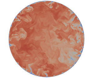
  $Ra$, the ratio of the buoyancy and the viscous force, multiplied by the Prandtl number. The Rayleigh number thus characterises the strength of the thermal forcing in the system. Both control parameters will be defined in § 2. Figure 1 shows a snapshot from a numerical simulation, visualising the temperature field inside the sphere at $Ra=5\times 10^9$ and $Pr=1$. It is evident that the temperature field exhibits small spatial scales, indicating that the corresponding flow field is turbulent.
Snapshot of the total temperature at a Rayleigh number of  $Ra=5\times 10^9$, a Prandtl number of $Pr=1$, with fixed temperature and stress-free boundary conditions.

The problem of thermal convection in a non-rotating full sphere has received remarkably little attention so far. The linear stability problem, i.e. the problem of establishing the threshold beyond which convection ensues, was studied by Jeffreys & Bland (Reference Jeffreys and Bland1951), Chandrasekhar (Reference Chandrasekhar1952) and Backus (Reference Backus1955), and predictions for the linear onset of convection (for fixed temperature boundaries) are summarised in Chandrasekhar (Reference Chandrasekhar1961). Later, Baldwin (Reference Baldwin1967) and Hsui, Turcotte & Torrance (Reference Hsui, Turcotte and Torrance1972) considered weakly nonlinear approximations in order to investigate the nonlinear effects very close to the onset of convection. However, no numerical study of this problem has ever been conducted to our knowledge.
The spherical geometry is of obvious relevance for convection in the interior of stars and planets, and indeed, numerous studies pertaining to convection in the full sphere in this context exist (see e.g. Guervilly & Cardin Reference Guervilly and Cardin2016; Kaplan et al. Reference Kaplan, Schaeffer, Vidal and Cardin2017; Lin & Jackson Reference Lin and Jackson2021). Convection in stars and planets is, however, generally strongly influenced by the effects of both rotation and magnetic fields, and the dynamics considered in these studies is therefore fundamentally different to the problem at hand.
Another related problem is convection in an (infinite) plane layer that is heated from below and cooled from above. This configuration is also known as classical Rayleigh–Bénard convection, and an abundance of literature on theory, numerical modelling and experiments exists for this problem (summarised, for example, in Manneville Reference Manneville, Mutabazi, Wesfreid and Guyon2006; Ahlers, Großmann & Lohse Reference Ahlers, Großmann and Lohse2009). The difference between Rayleigh–Bénard convection and convection in the non-rotating full sphere is mainly in the domain geometry and the nature of thermal forcing.
The main objective of this work is to characterise the fluid flow and the temperature field resulting from the internally heated, non-rotating full sphere configuration. We are interested in the resulting system behaviour for the different combinations of homogeneous boundary conditions and for a wide range of values of the control parameters  $Ra$ and $Pr$. The methods used for this characterisation depend on the values of the parameters and the nature of the resulting system behaviour.
At and near the onset of convection, the equations of motion (or their stability) can be investigated analytically. Because an exact analysis of the equations at finite flow amplitudes is not possible, we then resort to numerical simulations. At low to intermediate forcing, we analyse the time dependence and the spatial patterns of the ensuing convection. In addition, we also examine the large-scale behaviour through globally averaged quantities such as the kinetic energy density and non-dimensional diagnostics like the Reynolds number  $Re$, a measure of the vigour of the flow, and the Nusselt number $Nu$, a measure of the strength of advective heat transfer in the system. We further describe and study secondary bifurcations that occur at finite forcing, and the different flow regimes that develop depending on $Pr$. Where possible, we also issue some analytical or heuristic remarks on the nature of these secondary instabilities.
At sufficiently high forcing, the system transitions to turbulence. A classic problem in thermal convection is the scaling of the vigour of the flow (represented by the Reynolds number) and of the advective heat transfer (represented by the Nusselt number) with the Rayleigh number  $Ra$ and the Prandtl number $Pr$ at high forcing. To our knowledge, such scalings cannot be directly inferred from the nonlinear equations of motion (although techniques to establish rigorous bounds for such asymptotic scalings exist; see e.g. Fantuzzi, Arslan & Wynn Reference Fantuzzi, Arslan and Wynn2022), and therefore, scalings have been suggested on the basis of heuristic physical considerations, in particular for Rayleigh–Bénard convection. We adapt one such scaling prediction to the problem at hand. In addition, we also investigate the partition of the kinetic energy into its toroidal and poloidal components (based on a decomposition of the flow field introduced in § 2), and the thickness of the thermal boundary layers.
2. Problem formulation and governing equations
2.1. Problem setting and equations of motion
We consider a non-rotating full sphere of radius  $r_0$ and assume uniform and steady internal heating, characterised by a constant source term $S$ denoting the associated change of temperature. The fluid in the sphere is subject to the linear self-gravity $g=g_0r/r_0$ of a sphere of constant density, where $g_0$ represents the gravitational acceleration at $r=r_0$. We adopt the Boussinesq approximation, assuming all material properties except the density to be constant. The density is assumed to vary linearly with temperature (with an associated thermal expansion coefficient $\alpha$), and its variations are only considered in the buoyancy force and disregarded elsewhere. The dynamics of the system are governed by conservation of mass, energy and momentum. Under the Boussinesq approximation, these conditions can be expressed by the following equations in dimensional form (Chandrasekhar Reference Chandrasekhar1961):
 \begin{gather} \nabla^* \boldsymbol{\cdot} \boldsymbol u^* =0 , \end{gather}
 \begin{gather}\frac{\partial T^*}{\partial t^*} + \boldsymbol u^* \boldsymbol{\cdot} \nabla^* T^* = S +\kappa \nabla^{*^2} T^* , \end{gather}
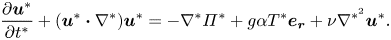 \begin{gather}\frac{\partial \boldsymbol u^*}{\partial t^*}+(\boldsymbol u^* \boldsymbol{\cdot} \nabla^*) \boldsymbol u^* ={-} \nabla^* \varPi^* + g\alpha T^* \boldsymbol{e_r}+ \nu \nabla^{*^2} \boldsymbol u^* . \end{gather}
Here  $\boldsymbol u^*$ denotes the flow field, $T^*$ is the total temperature field, $\varPi ^*:=-{p}/{\rho }$ is the ratio of the pressure and the (constant) density; $\alpha$ is the thermal expansion coefficient, $\nu$ denotes the kinematic viscosity and $\kappa$ is the thermal diffusivity. We non-dimensionalise the system using the radius $r_0$ as the length scale, $\beta r_0^2$ as the temperature scale (where $\beta = S/(3\kappa )$) and the viscous diffusion time $r_0^2/\nu$ as the time scale. In non-dimensional form, the equations of motion can then be expressed as
 \begin{gather} \boldsymbol{\nabla} \boldsymbol{\cdot} \boldsymbol u =0 , \end{gather}
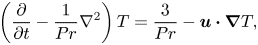 \begin{gather}\left(\frac{\partial }{\partial t}-\frac{1}{Pr} \nabla^2\right) T = \frac{3}{Pr} - \boldsymbol u \boldsymbol{\cdot} \boldsymbol{\nabla} T , \end{gather}
 \begin{gather}\left(\frac{\partial }{\partial t} + (\boldsymbol u \boldsymbol{\cdot} \boldsymbol{\nabla}) \right)\boldsymbol u ={-} \boldsymbol{\nabla} \varPi + \frac{Ra}{Pr} r T \boldsymbol{e_r}+ \nabla^2 \boldsymbol u , \end{gather}
where  $\varPi$ denotes a reduced pressure and the non-dimensional parameters $Ra$ and $Pr$ are defined as
 \begin{gather} Ra=\frac{g_0 \alpha \beta r_0^5}{\nu \kappa}, \end{gather}
 \begin{gather}Pr=\frac{\nu}{\kappa}, \end{gather}
where  $Ra$ and $Pr$ are the Rayleigh and Prandtl number, respectively, constituting the control parameters of the system. The Prandtl number is the ratio of viscous to thermal diffusivity and the Rayleigh number is the ratio of buoyant to viscous forces multiplied by the Prandtl number, thus representing a measure of the strength of the thermal forcing.
In the absence of fluid motion, heat transfer is solely by conduction. The purely conductive background temperature profile can be obtained by directly integrating the steady-state, purely conductive form of (2.5) given by
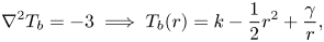 \begin{equation} \nabla^2 T_b ={-}3 \implies T_b(r) = k - \frac{1}{2}r^2 + \frac{\gamma}{r}, \end{equation}
with integration constants  $k$ and $\gamma$. The condition $T_b(0)<+\infty$ implies that $\gamma =0$ and we choose $k$ such that $T_b(1)=0$, yielding
 \begin{equation} T_b(r) = \tfrac{1}{2}(1-r^2). \end{equation}
Instead of considering (2.4)–(2.6), we can now consider perturbation equations from the steady, purely conductive and hydrostatic background state. We define the perturbations in pressure, temperature and velocity as  ${\rm \pi} = \varPi - \varPi _b$, $\varTheta = T -T_b$ and $u$ (since $u_b=0$), and since the background temperature and hydrostatic pressure satisfy
 \begin{gather} \nabla^2 T_b ={-}3, \end{gather}
 \begin{gather}\boldsymbol{\nabla} \varPi_b = \frac{Ra}{Pr}rT_b \boldsymbol{e_r}, \end{gather}
the evolution equations for the perturbations can be expressed as
 \begin{gather} \boldsymbol{\nabla} \boldsymbol{\cdot} \boldsymbol u =0 , \end{gather}
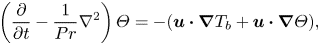 \begin{gather}\left(\frac{\partial }{\partial t}-\frac{1}{Pr} \nabla^2 \right) \varTheta ={-}( \boldsymbol u \boldsymbol{\cdot} \boldsymbol{\nabla} T_b + \boldsymbol u \boldsymbol{\cdot} \boldsymbol{\nabla} \varTheta ) , \end{gather}
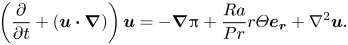 \begin{gather}\left(\frac{\partial }{\partial t} + (\boldsymbol u \boldsymbol{\cdot} \boldsymbol{\nabla}) \right)\boldsymbol u ={-} \boldsymbol{\nabla} {\rm \pi}+ \frac{Ra}{Pr} r \varTheta \boldsymbol{e_r}+ \nabla^2 \boldsymbol u. \end{gather}
Since only  $\boldsymbol {\nabla } T_b$ and not $T_b$ enters (2.13)–(2.15), it is evident that the choice of $k$ in (2.9) has no dynamic significance for the perturbation equations. We shall be concerned with examining (2.13)–(2.15) analytically and numerically. We note that the problem at hand is spherically symmetric (i.e. there is no preferred Cartesian axis that exists, for example, in rotating fluids), but it is not isotropic, due to gravity and the background temperature gradient acting solely in the radial direction.
2.2. Toroidal–poloidal decomposition and boundary conditions
Since the velocity field  $\boldsymbol {u}$ is solenoidal (see (2.13)), it can be represented by just two scalar functions (rather than three vector components). In spherical coordinates, this toroidal–poloidal or Mie representation can be written as (see e.g. Backus Reference Backus1986)
 \begin{equation} \boldsymbol u = \boldsymbol T + \boldsymbol P = \boldsymbol{\nabla} \times (\boldsymbol{r}{\mathcal{T}} ) + \boldsymbol{\nabla} \times (\boldsymbol{\nabla} \times (\boldsymbol{r}{\mathcal{P}} )), \end{equation}
where  $\boldsymbol T$ and $\boldsymbol P$ are the toroidal and poloidal field components and ${\mathcal {T}}(\boldsymbol {r)}$ and ${\mathcal {P}}(\boldsymbol {r})$ are called the toroidal and poloidal scalars, respectively. The toroidal field $\boldsymbol T$ does not have a radial component, while the poloidal field $\boldsymbol P$ has all three spherical components.
The equations of motion (2.13)–(2.15) can be recast as evolution equations for the temperature perturbation  $\varTheta$ and the toroidal and poloidal scalars ${\mathcal {T}}$ and ${\mathcal {P}}$ by virtue of using the toroidal–poloidal representation (2.16). Such equations are obtained by calculating $\boldsymbol {r} \boldsymbol {\cdot } \boldsymbol {\nabla }\, \times\, $(2.15) and $\boldsymbol {r} \boldsymbol {\cdot } \boldsymbol {\nabla } \times ( \boldsymbol {\nabla }\, \times\, $(2.15)) and complementing them by (2.14) to yield
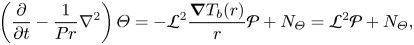 \begin{gather} \left(\frac{\partial}{\partial t}- \frac{1}{Pr}\nabla^2\right)\varTheta={-} {\mathcal{L}}^2 \frac{\boldsymbol{\nabla} T_b(r)}{r}{\mathcal{P}}+N_{\varTheta} = {\mathcal{L}}^2{\mathcal{P}} + N_{\varTheta}, \end{gather}
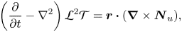 \begin{gather}\left(\frac{\partial}{\partial t}-\nabla^2\right){\mathcal{L}}^2 {\mathcal{T}}=\boldsymbol{r}\boldsymbol{\cdot} ( \boldsymbol{\nabla} \times \boldsymbol N_u ), \end{gather}
 \begin{gather}\nabla^2\left(\frac{\partial}{\partial t}-\nabla^2\right){\mathcal{L}}^2 {\mathcal{P}}= \frac{Ra}{Pr}{\mathcal{L}}^2\varTheta + \boldsymbol{r}\boldsymbol{\cdot}( \boldsymbol{\nabla} \times (\boldsymbol{\nabla} \times \boldsymbol N_u )), \end{gather}
where
 \begin{equation} {\mathcal{L}}^2 ({\cdot}) ={-} r^2 \nabla^2({\cdot}) + \frac{\partial}{\partial r}\left( r^2 \frac{\partial({\cdot})}{\partial r} \right) \end{equation}
is the angular momentum operator and
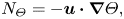 \begin{gather} N_{\varTheta}={-}\boldsymbol u \boldsymbol{\cdot} \boldsymbol{\nabla} \varTheta , \end{gather}
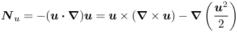 \begin{gather}\boldsymbol N_u={-}(\boldsymbol u \boldsymbol{\cdot} \boldsymbol{\nabla})\boldsymbol u= \boldsymbol u \times (\boldsymbol{\nabla} \times \boldsymbol u)- \boldsymbol{\nabla} \left(\frac{\boldsymbol u^2}{2}\right) \end{gather}
are the nonlinear interaction terms. Equations (2.17)–(2.19) now represent three scalar equations fully describing the dynamics of the convective system. We note that by only considering the curl (or double curl) of the Navier–Stokes equation in order to obtain (2.18) and (2.19), the pressure no longer appears in the system (2.17)–(2.19). The pressure therefore is not a dynamic variable in this problem.
The system (2.17)–(2.19) must be complemented by boundary conditions. As the thermal boundary condition, we consider homogeneous fixed temperature boundaries and we assume that the velocity field obeys either stress-free or no-slip boundary conditions.
These conditions read
 \begin{gather} \varTheta|_{r=1}=0 \ \ \mathrm{fixed\ temperature}, \end{gather}
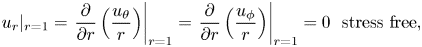 \begin{gather}u_r|_{r=1}=\left.\frac{\partial}{\partial r}\left( \frac{u_{\theta}}{r}\right)\right|_{r=1}=\left.\frac{\partial}{\partial r}\left( \frac{u_{\phi}}{r}\right)\right|_{r=1}=0 \ \ {{\rm stress\ free}}, \end{gather}
 \begin{gather}u_r|_{r=1}=u_{\theta}|_{r=1}=u_{\phi}|_{r=1}=0 \ \ {{{\rm no\ slip}}}. \end{gather}
The velocity boundary conditions (2.24) and (2.25) can be converted to conditions for the toroidal and poloidal scalar to read (see e.g. Hollerbach Reference Hollerbach2000):
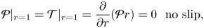 \begin{gather} {\mathcal{P}}|_{r=1}={\mathcal{T}}|_{r=1}=\frac{\partial}{\partial r}({\mathcal{P}}r) =0 \ \ {{\rm no\ slip}} , \end{gather}
 \begin{gather}{\mathcal{P}}|_{r=1} = \left.\frac{\partial}{\partial r} \left( \frac{{\mathcal{T}}}{r}\right)\right|_{r=1}= \left.\frac{\partial}{\partial r}\left( \frac{1}{r^2} \frac{\partial}{\partial r}( {\mathcal{P}}r)\right)\right|_{r=1} = 0 \ {{\rm stress\ free}}. \end{gather}
3. Numerical method and diagnostics
3.1. Spatial discretisation: spectral expansion
In our direct numerical simulations (DNS) we calculate solutions to (2.17)–(2.19) subject to boundary conditions (2.23) and either (2.27) or (2.26) using the quasi-inverse convection code (QuICC). The QuICC is a fully spectral framework for computational fluid dynamics and magnetohydrodynamics in Cartesian and spherical geometries, supporting both spherical shells and full spheres. In a full sphere geometry, it utilises spherical harmonics as basis functions for the expansion in the horizontal direction and Jones–Worland polynomials (introduced in Worland Reference Worland2004 and Livermore, Jones & Worland Reference Livermore, Jones and Worland2007) in the radial direction. We give a brief description of the methodology for the full sphere, which has been used for the numerical calculations in this work.
The expansion of the scalar functions ( $\varTheta, {\mathcal {T}}$ and ${\mathcal {P}}$) in the full sphere is
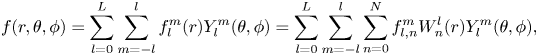 \begin{equation} f(r,\theta,\phi)=\sum_{l=0}^L \sum_{m={-}l}^l f_l^m(r)Y_l^m(\theta,\phi)= \sum_{l=0}^L \sum_{m={-}l}^l \sum_{n=0}^N f_{l,n}^m W_n^l(r) Y_l^m(\theta,\phi), \end{equation}
where  $Y_l^m(\theta,\phi )$ denotes spherical harmonics, $W_n^l(r)$ are the Jones–Worland polynomials and $f$ represents any of the three scalar functions. Below, we refer to the toroidal and poloidal vector modes $\boldsymbol {T}_l^m$ and $\boldsymbol {S}_l^m$ corresponding to ${\mathcal {T}}_l^m(r)$ and ${\mathcal {P}}_l^m(r)$ (Bullard & Gellman Reference Bullard and Gellman1954).
The QuICC supports different truncation schemes. For the numerical calculations in this work, a uniform truncation was employed for expression (3.1) in which the radial sum in  $n$ is truncated at the same $N$ for all $(l,m)$.
The radial expansion in the full sphere domain is complicated by the fact that the origin presents an artificial singularity in spherical coordinates. Provided that a spherical harmonic expansion is employed, requiring infinite differentiability at the origin imposes the following constraint on the functional form of the radial expansion (see e.g. Lewis & Bellan Reference Lewis and Bellan1990):
 \begin{equation} f_l^m(r)\sim r^lg_n(r^2)\sim r^l(\alpha_0 + \alpha_1 r^2 + \alpha_2 r^4 + \cdots). \end{equation}
Here  $g_n(r^2)$ is a smooth and even polynomial. One set of basis functions that satisfies this condition by construction are the Jones–Worland polynomials, a class of modified one-sided Jacobi polynomials defined as
 \begin{equation} W_n^l(r)\sim r^lP_n^{({-}1/2,l-1/2)}(2r^2-1), \end{equation}
where  $P_n^{(\alpha,\beta )}(x)$ are Jacobi polynomials (Worland Reference Worland2004). We note that different choices of $\alpha$ and $\beta$ have been considered by Lecoanet et al. (Reference Lecoanet, Vasil, Burns, Brown and Oishi2019) (although it should be noted that their approach is slightly different, for example, by not using the toroidal–poloidal decomposition). If suitably normalised, Jones–Worland polynomials satisfy the following orthonormality relation for a fixed spherical harmonic degree $l$:
$l$:
 \begin{equation} \int_0^1 \frac{1}{\sqrt{1-r^2}}W_n^l(r)W_{n'}^l(r)\,{\rm d}r=\delta_{nn'}. \end{equation}
Jones-Worland polynomials exhibit fast convergence and oscillate within an asymptotically uniform envelope as  $n\rightarrow \infty$ (Livermore et al. Reference Livermore, Jones and Worland2007). The factor $r^l$ damps these polynomials near the origin, rendering them close to zero for large $l$ over large parts of the radius. Thus, at the origin, only low $l$ harmonics contribute significantly to the spectral expansion.
3.2. Matrices, nonlinear terms and treatment of boundary conditions
The QuICC uses a non-interpolating spectral approach, generating equations for the spectral coefficients by forming the weak-form equations, i.e. multiplying the equations by the basis functions and integrating according to the orthogonality relations of spherical harmonics and Jones–Worland polynomials (see relation (3.4)). The eigenfunction property and orthogonality of spherical harmonics can immediately be exploited to yield
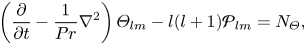 \begin{gather} \left(\frac{\partial}{\partial t}- \frac{1}{Pr}\nabla^2\right)\varTheta_{lm}-l(l+1){\mathcal{P}}_{lm}= N_{\varTheta}, \end{gather}
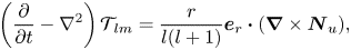 \begin{gather}\left(\frac{\partial}{\partial t}-\nabla^2\right) {\mathcal{T}}_{lm}=\frac{r}{l(l+1)}\boldsymbol e_r \boldsymbol{\cdot} ( \boldsymbol{\nabla} \times \boldsymbol N_u ), \end{gather}
 \begin{gather}\nabla^2\left(\frac{\partial}{\partial t}-\nabla^2\right) {\mathcal{P}}_{lm}-\frac{Ra}{Pr}\varTheta_{lm}=\frac{r}{l(l+1)}\boldsymbol e_r \boldsymbol{\cdot}( \boldsymbol{\nabla} \times (\boldsymbol{\nabla} \times \boldsymbol N_u ) ), \end{gather}
from (2.17)–(2.19). The remaining radial linear differential operators are generally dense, but are recast in terms of sparse banded matrices by virtue of the quasi-inverse technique due to Julien & Watson (Reference Julien and Watson2009). The boundary conditions can either be imposed by a Tau method, i.e. incorporating corresponding Tau lines into the linear operator on the left-hand side, or by using a Galerkin basis. For the numerical results in this work, the Tau method was used.
The nonlinear terms on the right-hand side are calculated in physical space at every time step in order to avoid computing large convolution sums in spectral space and the result is then projected back into spectral space. Therefore, a forward and a backward transform between spectral and physical space have to be calculated at every time step, necessitating efficient spherical harmonics and Jones–Worland transforms. In QuICC, the Fourier transform part of the spherical harmonics transform is performed using fast Fourier transform (FFT), and the projection integrals for the associated Legendre transform are calculated by Gauss–Legendre quadrature. The radial projection integrals for the Jones–Worland transform are computed by Gauss–Chebyshev quadrature and read
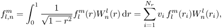 \begin{equation} f_{l,n}^m= \int_0^1 \frac{1}{\sqrt{1-r^2}}f_l^m(r) W_n^l(r)\,{\rm d}r = \sum_{i=1}^{N_r} v_i\, f_l^m(r_i) W_n^l(r_i), \end{equation}
where the quadrature nodes are the Chebyshev nodes  $r_i=\cos (({{\rm \pi} }/{4})({(2i-1)}/{N_r}))$ independently of $l$, the weights are the Chebyshev weights $v_i={{\rm \pi} }/{2N_r}$ and for a radial truncation $N$ and spherical harmonic truncation $L$,
$L$,  $N_r=\frac {3}{2}N+\frac {3}{4}L+1$ is chosen (Marti & Jackson Reference Marti and Jackson2016). As for the associated Legendre polynomials, the evaluation of the Jones–Worland polynomials is conducted by a three-term recurrence relation (see e.g. Livermore et al. Reference Livermore, Jones and Worland2007).
Recently, efforts have been made to develop both radial and horizontal (i.e. spherical-surface) transform algorithms that are partially based on FFT (see in particular Marti & Jackson (Reference Marti and Jackson2021) for the Jones–Worland transform) and to implement these on graphics processing units (GPUs) (D. Tolmachev, personal communication).
3.3. Time stepping and parallelisation
Time integration in QuICC is performed in spectral space using either an implicit–explicit Runge–Kutta scheme (for the present numerical study, the second-order algorithm IMEXRKCB2 due to Cavaglieri & Bewley (Reference Cavaglieri and Bewley2015) was employed) or a predictor–corrector scheme. The diffusion terms are treated implicitly while all other terms are treated explicitly. An adaptive time stepping scheme based on a Courant–Friedrichs–Lewy (CFL)-type physical stability condition has been implemented, ensuring that the time step is equal to the minimum of the following radial and horizontal CFL-constrained time steps:
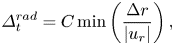 \begin{gather} \varDelta_t^{rad}=C\min\left( \frac{\Delta r}{ | u_r | }\right), \end{gather}
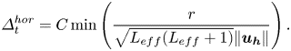 \begin{gather}\varDelta_t^{hor}=C\min \left(\frac{r}{\sqrt{L_{eff}(L_{eff}+1)}\| \boldsymbol{u_{h}}\|} \right) . \end{gather}
Here  $C$ is a safety factor, $\Delta r$ is the local radial grid spacing, $\boldsymbol {u_{h}}$ is the horizontal (i.e. spherical-surface) part of the velocity and $r/\sqrt {L_{eff}(L_{eff}+1)}$ is the effective local horizontal resolution of spherical harmonics. This effective resolution takes into account the fact that the Jones–Worland polynomials are close to zero near the origin for large $l$, thus suppressing the oscillatory behaviour of the spherical harmonics. The zeros of the Jones–Worland polynomials close to the origin are taken as a heuristic measure of the resolving power, and $L_{eff}$ is determined from an approximate expression for the location of the leading zero of the Jones–Worland polynomial $W_n^l(r)$ near zero (Marti & Jackson Reference Marti and Jackson2016).
Splitting algorithms and communication structures have been developed in order to achieve high performance through efficient parallelisation (in particular by minimising communication between computing units; see Marti Reference Marti2012; Marti & Jackson Reference Marti and Jackson2016). The code has been benchmarked, including for the case of rotating thermal convection (see Marti et al. Reference Marti2014).
3.4. Diagnostics
For the analysis of our numerical results, we employ certain key global diagnostics. One of these primary diagnostics is the kinetic energy density. It is defined as
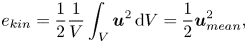 \begin{equation} e_{kin}= \frac{1}{2}\frac{1}{V}\int_V \boldsymbol{u}^2 \,{\rm d}V=\frac{1}{2}\boldsymbol{u}_{mean}^2, \end{equation}
where  $V={4{\rm \pi} }/{3}$ is the non-dimensional volume of the spherical domain. We subsequently refer to the respective toroidal and poloidal contributions to the kinetic energy as $e_{kin,tor.}$ and $e_{kin, pol.}$. These are respectively defined as
 \begin{gather} e_{kin,tor.}:= \frac{1}{2V} \sum_{l=0}^L \sum_{m={-}l}^l \int_{0}^1 | \sqrt{l(l+1)} {\mathcal{T}}_l^m(r) |^2 r^2 \,{\rm d}r , \end{gather}
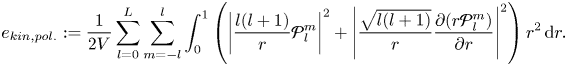 \begin{gather}e_{kin, pol.}:= \frac{1}{2V}\sum_{l=0}^L \sum_{m={-}l}^l \int_{0}^1 \left( \left| \frac{l(l+1)}{r}{\mathcal{P}}_l^m \right|^2 + \left| \frac{\sqrt{l(l+1)}}{r} \frac{\partial (r{\mathcal{P}}_l^m )}{\partial r} \right |^2 \right)r^2 \,{\rm d}r. \end{gather}
The thermal energy is similarly defined as
 \begin{equation} e_{therm.}= \frac{1}{2}\frac{1}{V}\int_V \varTheta^2 \,{\rm d}V=\frac{1}{2}\varTheta_{mean}^2 = \frac{1}{2V}\sum_{l=0}^L \sum_{m={-}l}^l \int_{0}^1 | \varTheta_l^m |^2 r^2 \,{\rm d}r . \end{equation}
The Reynolds number  $Re$ is the ratio of inertial to viscous forces, constituting a measure for the vigour of convection. Using the chosen non-dimensionalisation, it can be expressed as
 \begin{equation} Re=\frac{ | \boldsymbol{u}_{mean}^\ast | r_0}{\nu}= | \boldsymbol{u}_{mean} |=\sqrt{2 e_{kin}}. \end{equation}
 The Nusselt number  $Nu$ is the ratio of total heat transfer to purely conductive heat transfer defined as
 \begin{equation} Nu= \frac{h r_0}{ \kappa \rho c_p}, \end{equation}
where  $h$ is the heat transfer coefficient corresponding to the total heat transfer and $c_p$ is the specific heat capacity. We measure the Nusselt number indirectly by the temperature drop at the origin, following Guervilly & Cardin (Reference Guervilly and Cardin2016):
 \begin{equation} Nu=\frac{T_b(0)}{T(0)}. \end{equation}
The convective turnover time is the ratio of the characteristic length scale to the characteristic velocity, thus providing a measure of the time required for a full convection cycle of the flow within the system. In non-dimensional form, this reads
 \begin{equation} \tau=\frac{1}{2\sqrt{e_{kin}}}=\frac{1}{Re}. \end{equation}
The number of convective turnover cycles in a simulation run is then given by
 \begin{equation} \frac{t_{run}}{\tau}=t_{run}Re, \end{equation}
where  $t_{run}$ is the non-dimensional run time of the simulation.
For our series of simulations, the initial states for simulations at a given thermal forcing are taken to be the resulting solutions from the previous simulation at lower  $Ra$.
$Ra$.
4. Results
4.1. Nonlinear stability analysis
In thermal convection the linear stability analysis of the purely conductive state at rest yields a threshold in parameter space beyond which infinitesimal perturbations to the purely conductive state will grow and convection will ensue. For the problem at hand, this threshold is a critical Rayleigh number  $Ra_c$ depending on the boundary conditions but not on the Prandtl number, as in Rayleigh–Bénard convection. In addition, the onset of convection in the full sphere is known to be stationary (Chandrasekhar Reference Chandrasekhar1961). Using this, and considering (2.5) and $\boldsymbol r \boldsymbol {\cdot } (\boldsymbol {\nabla } \times (\boldsymbol {\nabla } \,\times\, $(2.6))), the linear stability system is given by
 \begin{gather} \frac{1}{Pr} \nabla^2 \varTheta ={-} u_rr , \end{gather}
 \begin{gather}\nabla^4 ( ru_r ) = \frac{Ra}{Pr} {\mathcal{L}}^2 \varTheta , \end{gather}
where we used that  $\boldsymbol r \boldsymbol {\cdot } \nabla ^2 \boldsymbol u = \nabla ^2 (\boldsymbol {r} \boldsymbol {\cdot } \boldsymbol u)$ if $\boldsymbol {\nabla } \boldsymbol {\cdot } \boldsymbol u =0$. The critical Rayleigh numbers resulting from this system are $Ra_c=3091.2$ for stress-free boundaries and $Ra_c=8040.0$ for no-slip boundaries, and the onset mode in both cases is purely poloidal and has a spherical harmonic degree $l=1$ (Chandrasekhar Reference Chandrasekhar1961).
The linear stability system (4.1)–(4.2) is an eigenvalue problem for  $Ra$ and implies that for Rayleigh numbers larger than the smallest eigenvalue (i.e. the critical Rayleigh number $Ra_c$), perturbations to the purely conductive state at rest will grow. It does, however, not imply that this background state is the only attractor below $Ra_c$. In principle, it is conceivable that finite amplitude subcritical convection might be sustained below $Ra_c$ (e.g. by the nonlinear interactions), as indeed has been observed numerically in the problem of rotating thermal convection in the full sphere (Guervilly & Cardin Reference Guervilly and Cardin2016; Kaplan et al. Reference Kaplan, Schaeffer, Vidal and Cardin2017), or for wall modes in magnetoconvection in Cartesian geometry (see e.g. McCormack et al. Reference McCormack, Teimurazov, Shishkina and Linkmann2023; Bhattacharya et al. Reference Bhattacharya, Boeck, Krasnov and Schumacher2024). The global stability of an attractor such as the purely conductive background state can, for example, be demonstrated by constructing a suitable Lyapunov functional, i.e. a non-negative functional of the state variables whose time derivative is non-positive. In fluid dynamics, usually Lyapunov functionals that are quadratic in the state variables are considered in order to facilitate in particular the calculation of their time derivative. This approach is known as the energy method and has been applied to different problems in fluid dynamics (see e.g. Joseph Reference Joseph1966; Straughan Reference Straughan2004; Goluskin Reference Goluskin2015). We now apply the energy method to the problem at hand.
We consider an energy functional of the form
 \begin{equation} E(\boldsymbol{u}(t), \varTheta(t))=\frac{1}{2}\int_V\left(\frac{Pr}{Ra} | \boldsymbol u|^2+ \varTheta^2\right){\rm d}V, \end{equation}
where  $V$ denotes the full sphere domain. We note that additional parameters are sometimes introduced in the definition of the energy functional (see e.g. Goluskin Reference Goluskin2015), but as we demonstrate, definition (4.3) yields the equivalence of the energy stability system and the linear stability system and, thus, provides the optimal bound on the energy stability Rayleigh number $Ra_E$.
Sufficient conditions for the global stability of the purely conductive background state (and, thus, for it being the only attractor) are then (Goluskin Reference Goluskin2015)
 \begin{gather} E(\boldsymbol{u}(t), \varTheta(t))\geq0 \quad {\rm and}\quad E(\boldsymbol{u}(t), \varTheta(t))=0 \quad \mathrm{if} \ \boldsymbol{u}=\varTheta=0 , \end{gather}
 \begin{gather}\frac{{\rm d}}{{\rm d}t}E(\boldsymbol{u}(t), \varTheta(t))\leq0 \quad {\rm and}\quad \frac{{\rm d}}{{\rm d}t}E(\boldsymbol{u}(t), \varTheta(t))=0 \quad\mathrm{if} \boldsymbol{u}=\varTheta=0 , \end{gather}
for all times  $t$. If the inequalities (4.4) and (4.5) are strict, the static background is also globally asymptotically stable and, thus, the only attractor in the system.
Condition (4.4) is evidently true for all  $t$, since $E(\boldsymbol {u}(t), \varTheta (t))$ is a quadratic functional. Regarding condition (4.5), we need to consider the time derivative of $E(\boldsymbol {u}(t), \varTheta (t))$. In the case of no-slip boundary conditions, differentiation of $E(\boldsymbol {u}(t), \varTheta (t))$ and inserting the equations of motion (2.14) and (2.15) leads to
 \begin{equation} \frac{{\rm d} E}{{\rm d}t}= \int_{V}2 r\varTheta u_r - \left(\frac{Pr}{Ra}| \boldsymbol{\nabla} \times \boldsymbol u|^2+\frac{1}{Pr}| \boldsymbol{\nabla} \varTheta |^2\right){\rm d}V. \end{equation}
Calculus of variations on the critical case  ${{\rm d} E}/{{\rm d}t}=0$ then yields a sufficient condition for (4.5) to be satisfied. The highest value of $Ra$ for which (4.5) is true for all $t$ can be obtained from the system of equations given by
 \begin{align} &\delta \frac{{\rm d}}{{\rm d}t}E(t)\stackrel{!}=0 \Longleftrightarrow \frac{{\rm d}}{{\rm d} \epsilon} \left( 2\int_{V} r (\varTheta + \epsilon T_h)( u_r+ \epsilon h_r)\,{\rm d}V\right.\nonumber\\ &\qquad \left.\left.-\int_{V} \frac{Pr}{Ra}(\boldsymbol{\nabla} \times (\boldsymbol u + \epsilon \boldsymbol h))^2+\frac{1}{Pr}( \boldsymbol{\nabla} (\varTheta+\epsilon T_h) )^2 \,{\rm d}V\right)\right|_{\epsilon =0}\nonumber\\ &\quad =\int_{V} T_h \left(\frac{2}{Pr} \nabla^2 \varTheta +2r u_r\right){\rm d}V +\int_{V} \boldsymbol h \boldsymbol{\cdot} \left(\frac{2Pr}{Ra} \nabla^2 \boldsymbol u - \boldsymbol{\nabla} {\rm \pi}+ 2 r \varTheta \boldsymbol e_r \right){\rm d}V \stackrel{!}=0, \end{align}
where  $\boldsymbol h, T_h$ are arbitrary, regular variations, the incompressibility condition was introduced as a Lagrange multiplier and several vector calculus identities were used. We note that in the case of stress-free boundary conditions, (4.6) is not valid, and we are thus unable to formulate a corresponding variational problem.
Since  $T_h$ and $\boldsymbol h$ are arbitrary and independent, the integrands themselves must vanish. This leads to the following system of equations:
 \begin{gather} \frac{1}{Pr} \nabla^2 \varTheta +r u_r=0, \end{gather}
 \begin{gather}\frac{Pr}{Ra} \nabla^2 \boldsymbol u - \frac{1}{2}\boldsymbol{\nabla} {\rm \pi}+ r \varTheta \boldsymbol e_r =0. \end{gather}
Equations (4.8)–(4.9) again constitute an eigenvalue problem for  $Ra$ with an associated smallest eigenvalue $Ra_E$, implying that for $Ra< Ra_E$, the strict inequality in condition (4.5) is satisfied and that thus the purely conductive background state is globally asymptotically stable and the only attractor. Computing $\boldsymbol r \boldsymbol {\cdot } (\boldsymbol {\nabla } \times (\boldsymbol {\nabla } \,\times\, $(4.9))) analogously to the linear stability analysis produces the following system:
 \begin{gather} \frac{1}{Pr} \nabla^2 \varTheta +r u_r=0, \end{gather}
 \begin{gather}-\frac{Pr}{Ra} \nabla^4 (ru_r) + {\mathcal{L}}^2 \varTheta =0 . \end{gather}
This is equivalent to the system (4.1)–(4.2), thus leading to the same critical Rayleigh number. We thus conclude that in the case of no-slip boundary conditions, subcritical convection cannot occur, since  $Ra_{E}=Ra_c$, i.e. the critical Rayleigh number for global, nonlinear stability and for linear stability align. The analysis remains inconclusive, however, in the case of stress-free boundary conditions, since the presence of additional boundary terms precludes the formulation of a variational problem of the form (4.7) and, therefore, the energy method does not yield a threshold value for global stability.
4.2. Convection at  $Pr=1$

In this section we present results for convection up to very high Rayleigh numbers for a fixed temperature and both stress-free and no-slip boundary conditions. In particular, we examine the scalings of the strength of heat advection (characterised by  $Nu$) and the vigour of the flow (characterised by $Re$) with the Rayleigh number and propose a theory for the scaling of $Nu$. We also report on the standard deviation of the global diagnostics in turbulent solutions, the partitioning of kinetic energy into toroidal and poloidal modes and the scaling of the thermal boundary layer. Parameters and key diagnostics of all simulations can be found in the supplementary material available at https://doi.org/10.1017/jfm.2024.1187.
4.2.1. Global diagnostics
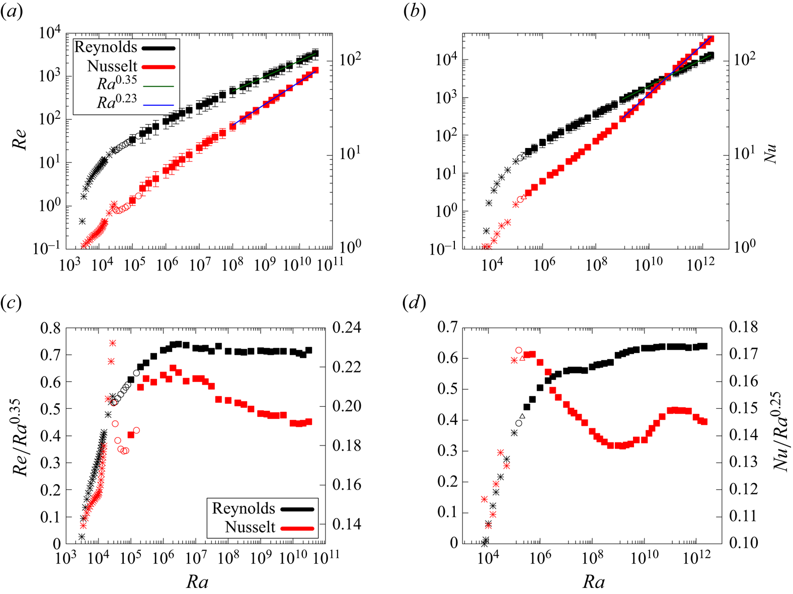
Figure 2 shows the Reynolds and Nusselt numbers as functions of  $Ra$ at $Pr=1$ for a fixed temperature and both stress-free and no-slip boundary conditions. For stress-free boundaries, we computed results up to $Ra=3\times 10^{10}\approx 10^7Ra_{c,SF}$ and, for no-slip conditions, we obtained results up to $Ra=2\times 10^{12}\approx 2.5\times 10^8 Ra_{c,NS}$. For both boundary conditions, we were thus able to investigate the system behaviour over several orders of magnitude of thermal forcing, up to highly turbulent solutions.
Nusselt (red) and Reynolds (black) numbers at  $Pr=1$ for fixed temperature, (a,c) stress-free and (b,d) no-slip boundary conditions. Plots (a,b) show power law fits of $Re$ and $Nu$ and (c,d) are compensated plots of $Re$ and $Nu$. The symbols represent distinct dynamical regimes: stars denote the purely poloidal steady-state regime, open circles the toroidal–poloidal steady-state regime, open triangles signify the vacillating regime and filled squares stand for turbulent solutions. Results for the vacillating and turbulent regimes are obtained as time averages, and the error bars represent the standard deviation around the mean in the time series.
Above the onset of convection, the system is initially in a purely poloidal steady-state state that is dominated by the poloidal  $\boldsymbol {S}_1^0$ onset mode for both velocity boundary conditions (denoted by crosses in figure 2). Eventually, this regime becomes unstable and toroidal flow sets in, generated by the nonlinear interactions. The resulting toroidal–poloidal state is still time independent (denoted by open circles). In the case of stress-free boundary conditions, the onset of toroidal flow is associated with $Nu$ decreasing with increasing $Ra$ over a certain range of $Ra$. For no-slip boundaries, we then observe a multi-frequency, time dependent but sub-turbulent solution (termed ‘vacillating’ and denoted by the open triangle). Turbulence ultimately sets in at $Ra=10^5$ for stress-free boundary conditions (with an intermediate toroidal–poloidal steady-state solution at $Ra=1.5\times 10^5$) and at $Ra=3\times 10^5$. For stress-free boundary conditions, the behaviour at low forcing and in particular the onset of toroidal flow has also been investigated (authors' unpublished observations).
In the turbulent regime, the global diagnostics fluctuate chaotically in time. For our analysis of the scaling of the Reynolds and Nusselt numbers with  $Ra$, we calculated the mean $\mu$ and the standard deviation $\sigma$ around the mean $\mu$ of the time series of the respective diagnostic. At very high $Ra$, the transients are generally very short, but also difficult to distinguish from the turbulent states. For all simulations, we discarded the first ten convective turnover times and performed time averages over the remaining run time. The minimum time averaging window of $33.3$ turnover cycles was reached for $Ra=3\times 10^{10}$ with stress-free boundaries. For most simulations, however, the averaging was performed over a window of hundreds of turnover times.
Scaling predictions for  $Nu$ and $Re$ and the control parameters $Ra$ and $Pr$ are often assumed to follow power laws of the form
 \begin{gather} Nu \sim Ra^{\gamma_{Nu}}Pr^{\alpha_{Nu}}, \end{gather}
 \begin{gather}Re \sim Ra^{\gamma_{Re}}Pr^{\alpha_{Re}}. \end{gather}
Noting that  $Pr=1$, we performed power law fits on the results obtained at high $Ra$ and obtained scaling exponents of $\gamma _{Re}=0.35$, $\gamma _{Nu}=0.23$ for stress-free boundaries (fit performed between $10^8\leq Ra \leq 3\times 10^{10}$) and $\gamma _{Re}=0.35$, $\gamma _{Nu}=0.25$ for no-slip boundaries (fit performed between $2\times 10^8\leq Ra \leq 2\times 10^{12}$). In figure 2(c,d) we present compensated plots of the Reynolds and Nusselt numbers for both boundaries. We scale the Reynolds number by $Ra^{0.35}$ and the Nusselt number by $Ra^{0.25}$. While the Reynolds number compensation is based purely on the empirically determined scaling exponents, we present a theory for the $Nu\sim Ra^{0.25}$ scaling below. Figure 2(c) shows that the Reynolds number scaling for stress-free boundaries is very robust, the scaling exponent $\gamma _{Re}=0.35$ is reached at roughly $Ra=10^7$ and does not change significantly at higher forcing. Although we determined a scaling exponent of $\gamma _{Nu}=0.23$, the Nusselt number scaling seems to converge to the scaling of $Nu\sim Ra^{0.25}$ for stress-free boundaries. In the case of no-slip boundaries displayed in figure 2(d), the Reynolds number scaling is again quite robust, with the scaling exponent being almost stationary beyond $Ra=10^9$. The plot of the compensated Nusselt number is more difficult to interpret, because it changes non-monotonically. However, considering that these variations are not very large and that the power law fit over more than three orders of magnitude of $Ra$ yields $\gamma _{Nu}=0.25$, we feel confident about this scaling.
Figure 3 displays the relative standard deviation (RSD)  $\sigma /\mu$ for stress-free and no-slip boundaries as a percentage. This gives us a measure of the relative amplitude of the fluctuation of the diagnostics around the mean in time. For the steady-state solutions, this fluctuation is evidently vanishing, but for the time-varying solutions (i.e. for both the vacillating and the turbulent solutions that we observe), it grows up to roughly $18.3\,\%$ of the mean of the Nusselt number with stress-free boundaries and $8.1\,\%$ of the mean of the Reynolds number for no-slip boundaries.
Relative standard deviation percentages  $\sigma /\mu$ of the Reynolds (black) and Nusselt (red) numbers as functions of $Ra$ for fixed temperature and both (a) stress-free and (b) no-slip boundary conditions. Symbols again denote the distinct dynamical regimes.

As the system transitions to turbulence, the RSDs initially increase. For stress-free boundary conditions, a maximum of approximately  $16.1\,\%$ is reached at $Ra=2\times 10^5$ for fluctuations in $Re$, and a maximum of $18.1\,\%$ is reached at $Ra=5\times 10^5$ for fluctuations in $Nu$. Beyond these maxima, the RSDs generally decrease with $Ra$ (although they vary non-monotonically), and at least the RSD for $Re$ seems to level off at around $8\,\%$.
For no-slip boundary conditions, the behaviour is similar: after the onset of time dependence with the vacillating states, and also beyond the transition to turbulence, the RSDs initially grow, reaching maxima of  $8.1\,\%$ at $Ra=5\times 10^6$ for fluctuations in $Re$ and $7\,\%$ at $Ra=5\times 10^6$ for fluctuations in $Nu$. Beyond these maxima, the RSDs decrease, reaching approximately $3.5\,\%$ for fluctuations in $Nu$ and $5\,\%$ for fluctuations in $Re$ at $Ra=10^{12}$. Relative standard deviations are observed to be smaller for no-slip boundaries than for stress-free boundaries.
As the Rayleigh number is increased, both the buoyancy force and consequently the nonlinear interactions driving the toroidal motion (and generating small-scale poloidal motion as well) increase in amplitude, generally leading into an increase in both the poloidal and the toroidal kinetic energy, and possibly affecting the partition of kinetic energy between the two flow components. Figure 4 shows the ratio of the toroidal to poloidal kinetic energy of the resulting solutions as a function of  $Ra$ for both stress-free and no-slip boundary conditions.
Ratio of toroidal to poloidal kinetic energy at  $Pr=1$ with fixed temperature and (a) stress-free and (b) no-slip boundary conditions.

For stress-free boundary conditions, displayed in figure 4(a), the ratio of toroidal to poloidal kinetic energy initially decreases from a maximum value of  $0.59$ in the turbulent range, having risen sharply at the onset of toroidal motion. It reaches a minimum of $0.4$ at $1.5\times 10^7$ and then increases again, reaching $0.55$ at $Ra=3\times 10^{10}$, the highest forcing for which results were obtained.
The results show a similar trend for no-slip conditions, displayed in figure 4(b): beyond the transition to turbulence (at which the ratio attains a maximum value of  $0.29$ at $Ra=3\times 10^5$), the ratio initially decreases, reaching a minimum of $0.19$ at $Ra=3\times 10^6$. It then increases again, and seems to level off beyond $Ra=10^{11}$ at just below $0.5$, reaching $0.48$ at $Ra=2\times 10^{12}$. At the present time, we do not have an (asymptotic) theoretical model for the ratio of toroidal to poloidal kinetic energy.
4.2.2. Thermal boundary layer scaling
As the Rayleigh number is increased, the stronger convection produces a progressively more well-mixed interior, leading to the bulk of the sphere approaching an isothermal state. The fixed temperature boundary condition, however, forces the temperature to drop to zero at the boundary and, thus, induces a thermal boundary layer in the solutions. Figure 5(a) shows a snapshot of the total temperature  $T$ on a slice at $Ra=10^{10}$ with fixed temperature and stress-free boundary conditions, and spherical-surface averaged instantaneous temperature profiles at various $Ra$ for stress-free and no-slip boundary conditions are displayed in figure 5(c,d). The spherical-surface averaged temperature is defined as
 \begin{equation} T_{hor.avg.}(r) = \frac{1}{V}\int_{\varOmega} T(r,\theta,\phi) \,{\rm d}\varOmega = \frac{1}{V} T_0^0(r) = \frac{1}{V}(T_b(r) + \varTheta_0^0(r)), \end{equation}
where the integral is over the spherical surface  $\varOmega$ at radius $r$ and the second equality holds due to the orthogonality of spherical harmonics on the surface of the sphere $\varOmega$. The spherical-surface averaged temperature is therefore fully represented by the radially symmetric contribution $\varTheta _0^0$. Both the visualisation and the temperature profiles illustrate that the bulk becomes increasingly well mixed and isothermal and that the range of the radius over which the temperature drops to zero (i.e. the thermal boundary layer thickness) becomes smaller as $Ra$ is increased. Some of the instantaneous spherical-surface averaged temperature profiles (e.g. the profile obtained at $Ra=10^6$ for no-slip boundary conditions; see figure 5b) intriguingly also exhibit an adverse, outward radial temperature gradient, corresponding to at least instantaneous outward heat conduction in the system.
(a) Snapshot of the total temperature  $T$ on a slice at $Ra=10^{10}$ with fixed temperature and stress-free boundary conditions, (b) instantaneous spherical-surface averaged velocity and temperature profiles at $Ra=10^6$ for fixed temperature and no-slip boundary conditions. A clear adverse temperature gradient is shown in black; spherical-surface averaged toroidal velocity is shown in red, spherical-surface averaged poloidal velocity is shown in green, illustrating that there is significant flow through the origin. Bottom row shows instantaneous spherical-surface averaged temperature profiles for fixed temperature and (c) stress-free and (d) no-slip boundary conditions on a logarithmic temperature scale at various $Ra$, illustrating the thermal boundary layer.

Figure 5(b) also shows spherical-surface averaged toroidal and poloidal velocity profiles. These are defined as
 \begin{equation} | u_{rms, tor./pol}(r) | = \sqrt{\frac{1}{V}\int_{\varOmega} |\boldsymbol{u}_{tor./pol}(r,\theta,\phi)}|^2 \,{\rm d}\varOmega, \end{equation}
such that
 \begin{equation} \frac{1}{2}\int_0^1| u_{rms, tor./pol}(r) |^2 r^2 \,{\rm d}r = e_{kin,tor./pol.}. \end{equation}
The spherical-surface averaged velocity profiles illustrate that while the poloidal motion vanishes at the origin and is strongest at a radius of roughly  $r=0.57$, there is strong poloidal flow through and close to the origin.
There are several ways to define the thermal boundary layer and its extent. We choose a criterion based on the spherical-surface averaged radial temperature gradient. We define the extent of the thermal boundary layer as the radius  $r_\lambda$ at which
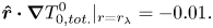 \begin{equation} \boldsymbol{\hat{r}}\boldsymbol{\cdot}\boldsymbol{\nabla} T_{0,tot.}^0 |_{r=r_\lambda}={-}0.01. \end{equation}
This definition is ad hoc, but given the monotonic decrease of the gradient near the boundary, it is well defined and consistent. Figure 6(a) shows the spherical-surface averaged total temperature, temperature perturbation and temperature gradient near the boundary for a highly turbulent state. Because of the conservation of energy, the outward radial heat flux must balance the internal heat production in the time average, and therefore, the spherical-surface averaged temperature gradient satisfies
 \begin{equation} \overline{\boldsymbol{\nabla} T}|_{r=1}={-}1, \end{equation}
where  $\bar {\cdot }$ denotes the time average. We emphasise that this holds in spite of the fact that no boundary condition is explicitly imposed on the heat flux. We observe that the instantaneous temperature gradient profiles also assume values close to $-1$.
$-1$.
(a) Instantaneous spherical-surface averaged total temperature, temperature perturbation and temperature gradient at  $Ra=3\times 10^{10}$ near the outer boundary and (b) time-averaged thermal boundary layer thickness $\lambda$ as a function of the thermal forcing. For both (a) and (b), fixed temperature and stress-free boundary conditions were imposed.

Figure 6(b) shows the time-averaged thermal boundary layer thickness measured according to definition (4.17) for fixed temperature and stress-free boundaries in the highly turbulent regime. The results show a scaling of
 \begin{equation} \lambda\sim Ra^{{-}0.23}\sim Nu^{{-}1}, \end{equation}
with the  $Nu\sim Ra^{0.23}$ scaling displayed in figure 2(a). This inverse scaling of the boundary layer thickness with the Nusselt number is consistent with a purely conductive boundary layer (Plumley & Julien Reference Plumley and Julien2019).
4.2.3. Howard–Malkus-type Nusselt number scaling prediction
As the boundary layer thickness decreases, the effect of curvature becomes asymptotically negligible. The boundary layer can thus be viewed as a Rayleigh–Bénard system with a temperature at the top of  $T_{top}=0$ and a bottom temperature of $T_{bot}=T_{bulk}\approx T(0)$. We employ this picture of the thermal boundary layer as a nested Rayleigh–Bénard system being heated from the bottom with $T_{bot}=T_{bulk}\approx T(0)$ and cooled from the top with $T_{top}=0$ (visualised in figure 7) in order to formulate an asymptotic scaling prediction for the Nusselt number similar to the one posited by Malkus (Reference Malkus1954) and Howard (Reference Howard1963). For very high $Ra$, the boundary layer representing the throttle for heat transfer in the system asymptotically resembles a nested Rayleigh–Bénard system of layer height $\lambda$ whose Rayleigh number is then given as (see e.g. Chandrasekhar Reference Chandrasekhar1961)
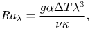 \begin{equation} Ra_{\lambda}=\frac{g\alpha\Delta T \lambda^3}{\nu\kappa}, \end{equation}
where  $\Delta T = T_{bulk}-T(r=1)$. Since the boundary layer becomes asymptotically thin, we take the gravity $g$ within the boundary layer to be constant at $g_0$. The temperature drop between the lower and upper boundary is given by
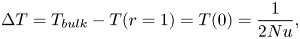 \begin{equation} \Delta T = T_{bulk}-T(r=1)=T(0)=\frac{1}{2Nu}, \end{equation}
where we used our definition of  $Nu$ (3.17) of the Nusselt number. Inserting this into the definition of the Rayleigh number for the boundary layer (4.20) yields
 \begin{equation} Ra_{\lambda}=\frac{Ra Nu^{{-}1} }{2\beta r_0^2}\left(\frac{\lambda}{r_0}\right)^3. \end{equation}
Following Howard (Reference Howard1963), we now assume that the boundary layer is marginally stable, meaning that
 \begin{equation} Ra_{\lambda}=Ra_c={\rm const.}\implies \lambda \sim \left(\frac{Ra}{Nu}\right)^{{-}1/3}, \end{equation}
where the constant depends on the velocity boundary condition. The heat transferred through the boundary layer must balance the internal heat production on time average. If we further assume that the boundary layer is purely conductive, we must have
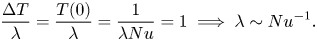 \begin{equation} \frac{\Delta T}{\lambda}=\frac{T(0)}{\lambda}=\frac{1}{\lambda Nu}=1 \implies \lambda \sim Nu^{{-}1}. \end{equation}
Equations (4.23) and (4.24) then imply together that
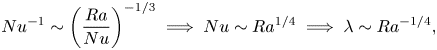 \begin{equation} Nu^{{-}1}\sim \left( \frac{Ra}{Nu} \right)^{{-}1/3} \implies Nu \sim Ra^{1/4} \implies \lambda \sim Ra^{{-}1/4}, \end{equation}
i.e. a scaling exponent of  $\gamma _{Nu}=1/4$. We note that this scaling prediction does not depend on the velocity boundary condition. Indeed, we observe scaling exponents at or close to $\gamma _{Nu}=1/4$ for both stress-free and no-slip boundaries (see figure 2a,b), and we also observe a scaling of the thermal boundary thickness $\lambda$ that is close to the predicted scaling (see figure 6b and relation (4.19)).
Sketch of the thermal boundary layer of thickness  $\lambda$ as a Rayleigh–Bénard system, being cooled from the bottom with the bulk temperature $T_{bulk}\approx T(0)$ and cooled from the top with $T_{top}=0$.
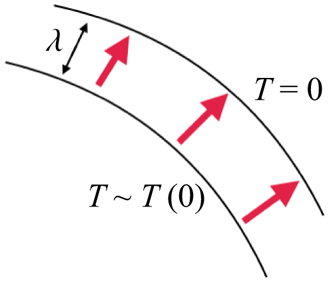
4.3. Prandtl number dependence at low to intermediate forcing
As we have seen above, for the problem at hand, the onset of convection is independent of the Prandtl number  $Pr$, and so is the threshold for global stability established through the energy method. At any given thermal forcing above the critical Rayleigh number, however, the nature of the convection, i.e. the kinetic energy, potential flow patterns, the time dependence, the heat transfer and all other characteristics will in general depend on $Pr$. In this section we thus aim to provide a characterisation of the system behaviour at low to intermediate $Ra$ at different $Pr$ for a fixed temperature and stress-free boundary conditions. We choose stress-free boundaries because they lead to stronger nonlinear interactions at given $Ra$ and $Pr$, which are at the core of the phenomena that we observe at intermediate forcing.
In our study we find five distinct convective regimes characterised primarily by their spatial structure and distinct flow patterns, their time dependence, their spatial and temporal coherence, the absence or presence of toroidal flow as well as the relative contributions of the toroidal and poloidal components to the flow field. In particular, we observe the dependence on  $Pr$ of both the Rayleigh number at which toroidal flow sets in and the characteristics of the toroidal modes excited by nonlinear inertial interactions at supercritical $Ra$.
$Ra$.
We first present a regime diagram and discuss the global diagnostics, and then we describe the five regimes individually.
4.3.1. Regime diagram
In our study of Prandtl number dependence at low forcing, we perform simulations at six different values of  $Pr$ in the range $0.1\leq Pr \leq 30$, spanning $2.5$ decades. We vary $Ra$ as $Ra_c=3091.2\leq Ra\leq 3\times 10^5$, spanning roughly two decades. In total, we observe five distinct dynamic regimes, and the corresponding regime diagram is displayed in figure 8.
Regime diagram in  $Ra-Pr$-parameter space at low forcing for fixed temperature and stress-free boundary conditions. The symbols again represent distinct dynamical regimes: stars indicate the purely poloidal steady-state regime, open squares the oscillatory regime, open circles the toroidal–poloidal steady-state regime, filled circles the bursting regime and filled squares the turbulent regime. Colours indicate the value of $Pr$. Regime boundaries are merely sketched.

As mentioned in § 4.1, the critical Rayleigh number  $Ra_c$ obtained from linear stability analysis at which convection sets in is independent of $Pr$, and so is the critical spherical harmonic degree $l=1$. For all $Pr$ investigated in this study, there is a range of $Ra$ above the onset of convection over which the resulting solutions are purely poloidal, steady state and dominated by the onset mode $\boldsymbol {S}_1^0$. If the forcing is increased, the purely poloidal solutions become unstable and toroidal motion sets in. Both the Rayleigh number at which toroidal flow sets in and the nature of the resulting state (e.g. its time dependence and energy spectra) depend on $Pr$. In general, it is the case that the lower $Pr$, the less supercritical the Rayleigh number at which the onset of toroidal motion occurs. For small $Pr$, buoyancy and thermal dissipation are large (cf. (2.14) and (2.15)), leading to solutions near the onset of convection with high kinetic energy and, thus, strong nonlinear interactions that generate toroidal flow at comparatively small $Ra$. Regarding the time dependence of the resulting solutions, we observe an oscillatory regime for $Pr<1$, at $Pr=1$ we find a toroidal–poloidal steady-state solution and, for $Pr>1$, we find bursting solutions.
As the Rayleigh number is increased further, the nonlinear interactions become stronger and additional modes are excited. At some point then, the resulting solutions lose their spatial and temporal coherence and transition to turbulence. In particular, such solutions exhibit small length scales and fluctuations on short time scales. The Rayleigh number at which this transition to turbulence occurs depends on  $Pr$, and the corresponding heuristic explanation is the same as for the onset of toroidal motion: the nonlinear interactions are stronger for smaller $Pr$ at a given forcing $Ra$ and, thus, the lower $Pr$, the lower the Rayleigh number at which the transition to turbulence occurs.
Beyond this qualitative argument, we currently do not have a theory for the scaling of regime boundaries, both regarding the onset of toroidal flow and the transition to turbulence. We emphasise that the regime boundaries displayed in figure 8 are merely sketched and that further simulations would need to be run in order to establish them more firmly.
The main diagnostics  $Re$,
$Re$,  $Nu$ and the averaged kinetic energy density as functions of the thermal forcing $Ra$ at different $Pr$ ranging between $0.1 < Pr< 30$ are shown in figure 9. For all $Pr$, convection commences with the purely poloidal onset mode and ultimately transitions to a turbulent state. However, the vigour of convection, the strength of heat advection, the nature of the intermediate convective regimes and the locations of regime transitions depend very strongly on $Pr$, as is the case in other convective systems like the plane layer system (see e.g. Krishnamurti Reference Krishnamurti1973; Goluskin et al. Reference Goluskin, Johnston, Flierl and Spiegel2014).
(a) Reynolds number, (b) Nusselt number and (c) averaged kinetic energy density as functions of  $Ra$ for different $Pr$. The symbols represent distinct dynamical regimes as above.

A general trend is that at lower  $Pr$ the flow is more vigorous (i.e. has higher $Re$) at a given $Ra$ as shown in figure 9(a). For $Pr<1$, lower $Pr$ leads to lower heat advection, as displayed in figure 9(b). For $Pr>1$, however, the correlation between $Nu$ and $Pr$ is not clear, and the obtained values at $Pr=3$, 10, 30 are similar to one another. Such a non-monotonic variation of the Nusselt number with $Pr$ has also been observed in an experimental study of Rayleigh–Bénard convection by Belmonte, Tilgner & Libchaber (Reference Belmonte, Tilgner and Libchaber1994) and in thermal convection in non-rotating spherical shells (Tilgner Reference Tilgner1996). Schmalzl, Breuer & Hansen (Reference Schmalzl, Breuer and Hansen2002) similarly report two distinct scalings of $Nu$ with $Pr$ for numerical simulations of Rayleigh–Bénard convection with stress-free boundary conditions, with the transition at $Pr=1$, and an associated significant change of the character of the flow at $Pr=1$.
Heuristically, the general trend in  $Re$ is again due to the increased strength of the nonlinear interactions at lower $Pr$, causing more vigorous flow. The greater effectiveness of heat conduction at lower $Pr$ and the excitation of modes that do not contribute to heat advection by the stronger nonlinear interactions at lower $Pr$ might explain the trend in $Nu$ for $Pr<1$. The dependence of $Nu$ on $Pr$ seems to qualitatively change at $Pr=1$, and we are unaware of a corresponding theory.
Figure 10(a) shows the Reynolds number collapsed onto  $RePr$, the Péclet number for heat transport. The Péclet number is the ratio of the rate of heat advection to the rate of heat diffusion. In spite of the dynamically distinct flow regimes, the Reynolds number for different $Pr$ can be collapsed reasonably well onto $RePr$, although there is still considerable scatter of, for example, up to a factor of 2 at $Ra=3\times 10^5$. This indicates that the system solutions organise themselves such that they have a Péclet number of a similar magnitude independent of $Pr$. However, the Péclet number $RePr$ is not the best possible collapse of the data. Best fit estimates for our results yield scaling exponents of $\gamma _{Re}=0.44, \alpha _{Re}=-0.89$ for the power law relations between the control parameters $Ra$ and $Pr$ and $Re$ given by (4.13). The collapse corresponding to this best fit estimate is shown in figure 10(b).
(a) Plot of  $RePr$ as a function of $Ra$ at different $Pr$. The Reynolds number at different $Pr$ can be collapsed reasonably well onto $RePr$, a Péclet number. (b) The best fit collapse with $RePr^{0.89}$.
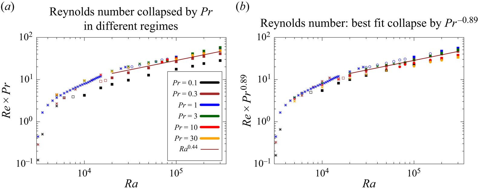
For all surveyed  $Pr$ except for $Pr=3$, we observe that $Nu$ drops at the onset of toroidal flow (see figure 9b). This is heuristically plausible, since the additional toroidal motion does not contribute to the radial advective heat transfer. For the case of $Pr=1$ and the decrease of $Nu$ with increasing $Ra$ beyond the onset of toroidal flow, this effect was observed (authors' unpublished observations). At the present time, we do not have an explanation as to why at $Pr=3$ there seems to be no intermediate regime between the purely poloidal onset regime and the turbulent regime and why, consequently, a similar kink in the $Nu$ slope and the non-monotonic change with $Ra$ are absent.
In total, we can identify five distinct convective regimes that we describe in the following. The different sub-turbulent regimes are sufficiently distinct, such that they can clearly be distinguished through the analysis of the time evolution of their diagnostics. We provide some examples in which the transitions between regimes are clearly visible. The situation is more complex, however, near the transition to the turbulent regime. In some instances, spatial or temporal coherence is lost to a certain degree, and so the classification has to be made on the assessment whether the character of the convective behaviour is determined rather by the coherent structures or by turbulent patterns. Again, we provide an example of this below.
4.3.2. Purely poloidal steady-state regime
Sufficiently close to the onset of convection, the flow is purely poloidal and dominated by the time-independent onset mode  $\boldsymbol {S}_1^0$ for all $Pr$. In this regime, no poloidal flow is being generated through the nonlinear interactions. An exact analysis of the domain of stability of this regime has not been possible so far, but the existence of a class of poloidal modes whose nonlinear interactions do not generate any toroidal flow can be demonstrated (authors' unpublished observations).
As the Rayleigh number is increased, higher modes are excited, but the flow remains largely dominated by the  $l=1$ modes. This is illustrated by the kinetic energy $l$ spectrum in figure 11. At some forcing (depending on $Pr$), the purely poloidal solutions become unstable and toroidal flow sets in. For lower $Pr$, the stability threshold for the onset of toroidal flow is at lower $Ra$.
$Ra$.
Instantaneous kinetic energy  $l$ spectra at $Pr=1$ for different Rayleigh numbers.
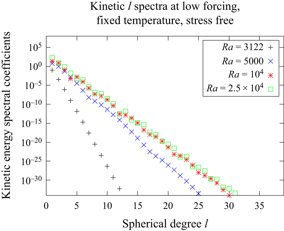
We emphasise again that the case of  $Pr=3$ is special: the purely poloidal regime is stable up to (at least) $Ra=7\times 10^4$, and then gives way to turbulent solutions without going through an intermediate regime.
4.3.3. Oscillatory regime
We observe oscillatory solutions in which the global diagnostics oscillate with a single fixed frequency for low  $Pr$, i.e. $Pr=0.1$, $0.3$, and only in a small range of $Ra$. The transition from the purely poloidal steady-state regime to this time-periodic regime with a toroidal flow component occurs via a metastable state, as can be seen in figure 12(a). This time series of the diagnostics at $Ra=6\times 10^3$, $Pr=10^{-1}$ is an example of a regime transition from one regime to another that is clearly visible in the time evolution. After the usual initial transient, the system first seems to settle in the purely poloidal steady-state regime. However, both the total kinetic energy density and the Nusselt number decrease while the toroidal contribution to the kinetic energy grows exponentially.
(a) Time evolution of the main diagnostics kinetic energy density and the Nusselt number displaying the transition from a metastable state and (b) the oscillatory behaviour of the main diagnostics at  $Ra=6\times 10^3$, $Pr=0.1$.
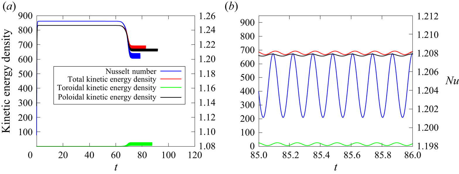
Figure 12(b) illustrates that the oscillations of the Nusselt number and the poloidal kinetic energy are roughly in phase. This is to be expected, as heat advection should be strong whenever the poloidal flow and, thus, the radial velocity is strong. The poloidal and toroidal kinetic energies are not in phase, indicating a periodic exchange of energy between the two flow components. The time-averaged relative contribution of the toroidal flow component to the total kinetic energy at  $Ra=6\times 10^3$, $Pr=10^{-1}$ is $2.4\,\%$. An animation of the evolution of the magnitude of velocity at $Ra=6\times 10^3$, $Pr=10^{-1}$, illustrating the oscillatory regime, can be found in the supplementary material.
Over the small range of  $Ra$ in which the oscillatory regime exists, the frequency of the oscillations increases, $Re$ slightly increases with $Ra$ and $Nu$ slightly decreases with $Ra$; see figure 9. The relative contribution of the toroidal flow also grows with $Ra$. As $Ra$ is increased further, the oscillatory solutions become unstable and the system transitions to turbulence.
4.3.4. Toroidal–poloidal steady-state regime
For  $Pr=1$ (and only for a Prandtl number of unity), we observe a transition from the purely poloidal steady-state regime to a toroidal–poloidal steady-state solution. It extends from the onset of toroidal flow at $Ra=3\times 10^4$, $Pr=1$ up to at least $Ra=8\times 10^4$, $Pr=1$. As the Rayleigh number is increased, higher-order modes become excited increasingly. At $Ra=10^5$, $Pr=1$, we observe the transition to a turbulent state, but at $Ra=1.5\times 10^5$, $Pr=1$, we find that the system attains a toroidal–poloidal steady state again. All solutions with $Ra>1.5\times 10^5$, $Pr=1$ are then turbulent.
4.3.5. Bursting regime
For  $Pr=10$, $30$, we observe yet another type of convective regime after the onset of toroidal flow that occurs at $Ra=7\times 10^4$ at $Pr=10$ in our study. Here, after an initial transient, the system settles into a regime where heat advection and toroidal flow exhibit bursts that leave a characteristic signature in the time series of the diagnostics. An example of this is given in figure 13. There are long quiescent phases in which the toroidal kinetic energy decreases down to $e_{kin,tor.}\approx 10^{-18}$ as illustrated in figure 13(b). The poloidal kinetic energy and Nusselt number decrease in parallel, but settle at much larger values corresponding to the fundamental poloidal modes specified in table 1 and then appear quasi-static during the quiescent phase. The poloidal and toroidal kinetic energies then start to increase again (with the exponential growth of the toroidal kinetic energy being particularly noticeable), culminating ultimately in a burst of peaks of stronger kinetic energy than during the quiescent phases. The Nusselt number initially drops before the occurrence of the burst and then also steeply increases. During each burst, the diagnostics vary in time according to a fixed pattern, with the kinetic energies and the Nusselt number forming several distinct spikes before the next quiescent phase sets in.
Time evolution of the global diagnostics at  $Ra=7\times 10^4$, $Pr=10$, using (a) a linear scale and (b) a logarithmic scale for the kinetic energy. The system exhibits regular convective bursts with a fixed signature in time.
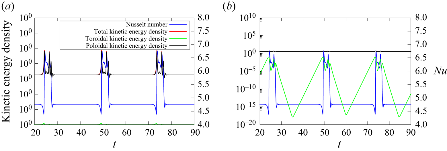
Relative contribution of the first five spherical harmonic modes to the kinetic energy of two consecutive quiescent phases at  $Ra=7\times 10^4$, $Pr=10$. The toroidal kinetic energy is vanishing during these quiescent phases. Kinetic energy seems to be shifted between the $\boldsymbol {S}_2^2$ mode and the axisymmetric $\boldsymbol {S}_2^0$ mode by the bursts, while the contribution of the $\boldsymbol {S}_2^1$ mode does not change significantly.
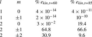
Such bursting convection has been observed, for example, in the case of two-dimensional planar convection (see e.g. Garcia et al. Reference Garcia, Bian, Paulsen, Benkadda and Rypdal2003; Goluskin et al. Reference Goluskin, Johnston, Flierl and Spiegel2014) and the corresponding physical interpretation has been discussed (see Leboeuf, Charlton & Carreras Reference Leboeuf, Charlton and Carreras1993; Garcia et al. Reference Garcia, Bian, Naulin, Nielsen and Rasmussen2006; Goluskin et al. Reference Goluskin, Johnston, Flierl and Spiegel2014). The central idea is that the mean horizontal flow component (corresponding to the toroidal motion in our case) inhibits heat advection, leading to the dispersion of convective structures, with the most slowly decaying mode surviving the longest. This is what is observed as a quiescent phase. At sufficiently large  $Ra$ however, this configuration is highly unstable and so once the horizontal flow component suppressing the convective instability has decayed sufficiently, convection sets in again, causing the vertical flow component (corresponding to the poloidal flow in our case) and, thus, the Nusselt number to increase. The nonlinear interactions then transfer the associated kinetic energy to the horizontal toroidal flow, and a burst is observed. The excited toroidal motion in turn inhibits the very convective structures that drive it and, thus, ends the burst and a new quiescent phase begins. The suggested cyclic burst mechanism is sketched in figure 14.
Sketch of the suggested cyclic burst mechanism: toroidal flow is generated by nonlinear interactions, but it inhibits and disperses the (mostly poloidal) convective structures that drive it, leading to a quiescent-bursting cycle.
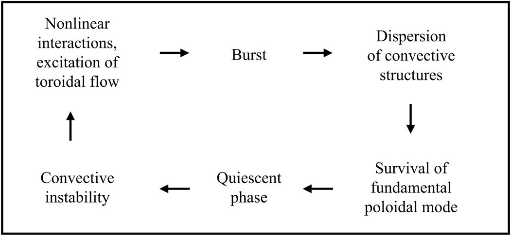
We believe that despite some differences to the numerical observations in two-dimensional planar convection (e.g. the share of kinetic energy in the toroidal flow we observe is generally much smaller compared with that contained in the mean shearing motion observed by Goluskin et al. Reference Goluskin, Johnston, Flierl and Spiegel2014), a mechanism of the kind that is sketched in figure 14 causes these convective bursts both in the planar convection and in the three-dimensional simulations in the full sphere.
However, the situation is more complicated than the sketch (figure 14) suggests, because we observe that the system does in fact not always return to the same fundamental flow state during the quiescent phases. Instead, it alternates between two different virtually purely poloidal states with the same kinetic energy, being separated by the bursts. The kinetic energy contained in the first spherical harmonic modes of the two different quiescent states attained during two consecutive quiescent phases is given in table 1. During the quiescent phases (sampled at time  $t=60$), $95.7\,\%$ of the kinetic energy is contained in just the $\boldsymbol {S}_2^1$ and $\boldsymbol {S}_2^2$ modes. Unlike this first state, the other solutions (sampled at time $t=85$) also have a significant contribution from the axisymmetric $\boldsymbol {S}_2^0$ mode. During this phase, $95.6\,\%$ of the kinetic energy is in the $\boldsymbol {S}_2^0$, $\boldsymbol {S}_2^1$ and $\boldsymbol {S}_2^2$ quadrupolar modes. The relative contribution of $\boldsymbol {S}_2^1$ remains largely unchanged between the quiescent phases, suggesting an exchange of energy between the $\boldsymbol {S}_2^0$ and $\boldsymbol {S}_2^2$ modes during the bursts. The different flow states corresponding to these two solutions are visualised in figure 15. An animation of the evolution of the magnitude of velocity at $Ra=8\times 10^4$, $Pr=10$ showing a burst can be found in the supplementary material.
Snapshots of the magnitude of velocity  $| \boldsymbol {u}|$ on a meridional slice at (a) $t=60$ and (b) $t=80$, corresponding to two consecutive quiescent phases of the bursting solution at $Ra=7\times 10^4$, $Pr=10$. The red arrow of the coordinate system points in the direction of $\boldsymbol {e}_z$, the green arrow in the direction of $\boldsymbol {e}_x$ and $\boldsymbol {e}_y$ points into the plane. The two consecutive quiescent phases have the same globally averaged kinetic energy and are both dominated by the quadrupolar $l=2$ modes, but differ precise contributions of the spherical harmonic modes.
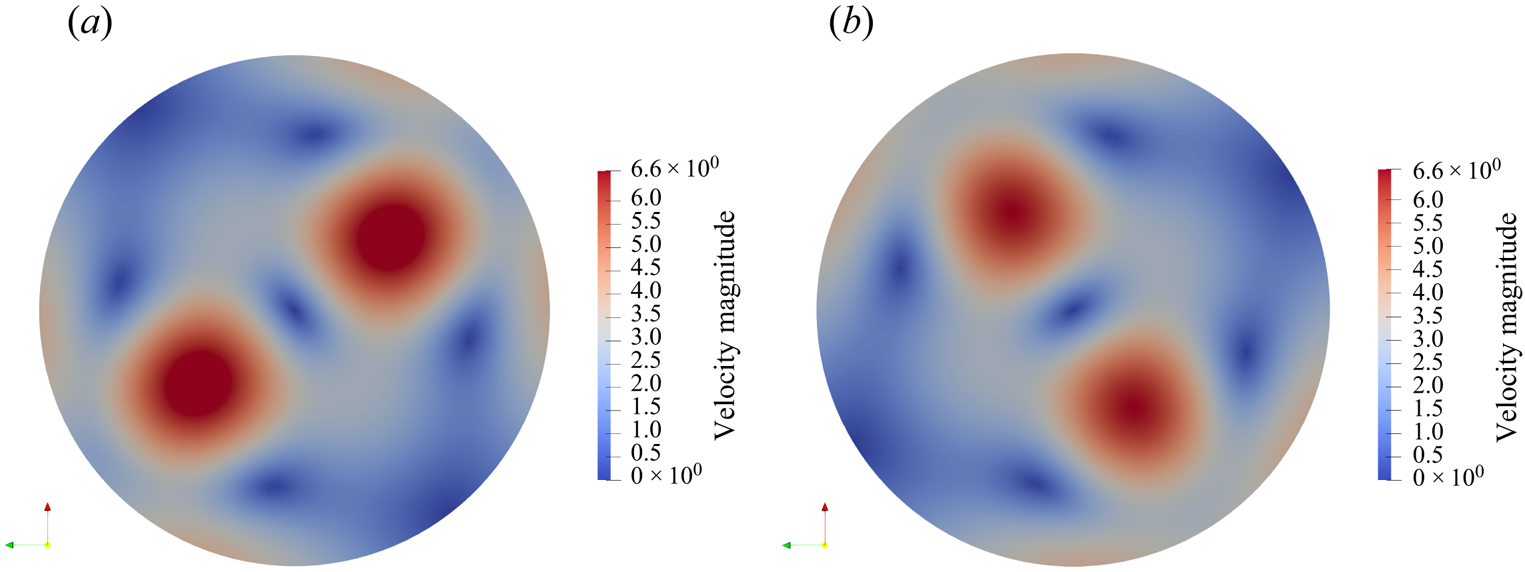
As  $Ra$ is increased, the quiescent phases become shorter and the signature of the bursts becomes simpler. Near the transition to the turbulent regime, the temporal coherence is gradually lost, as can be seen in figure 16. This is an example of a time series of the diagnostics that contains features both from the bursting regime, a sub-turbulent regime, as well as from the turbulent regime. It was still classified as belonging to the bursting regime because the time evolution is primarily characterised by the bursts and not by the deviations from the bursting behaviour. At some $Ra$, the solutions lose all spatial and temporal coherence and clearly transition to turbulence.
Time evolution of the averaged kinetic energy density and the Nusselt number at  $Ra=1.5\times 10^5$, $Pr=10$. This state was classified as belonging to the bursting regime, although there are instances when the temporal coherence is transiently lost and then recovered.
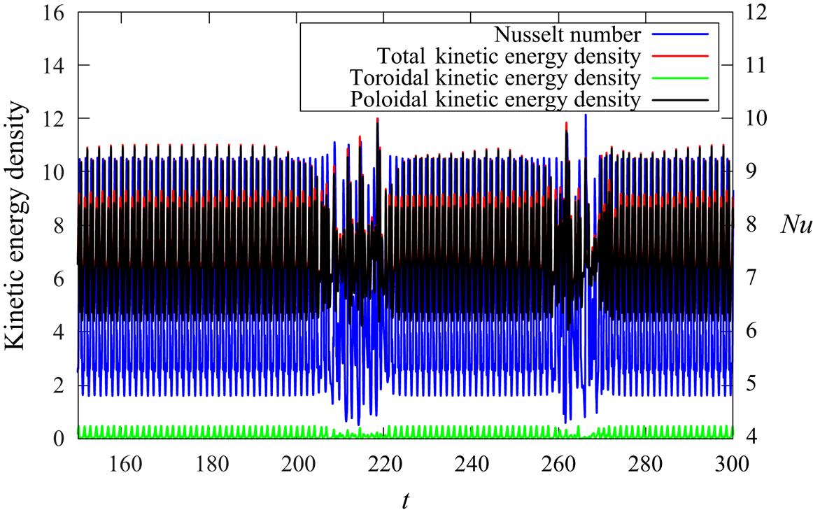
4.3.6. Turbulent regime
For all  $Pr$ and at sufficiently high $Ra$, the states attained by the system lose spatial and temporal coherence and become turbulent. Figure 17(a) shows an example of the time evolution of the diagnostics in this regime. All diagnostics now vary without any coherent time dependence. The snapshot of the velocity shown in figure 17(b) shows smaller-scale structures and the loss of any spatial coherence or symmetry. However, the observed spatial features are not extremely small scale compared with the size of the domain, possibly being an effect of the forcing being still only about $100Ra_c$, as opposed to the turbulent states observed at very high forcing discussed in § 4.2. An animation of the evolution of the temperature field in a highly turbulent simulation at $Ra=5\times 10^9$, $Pr=1$ can be found in the supplementary material.
(a) Time evolution of the main diagnostics and (b) a snapshot of the absolute velocity on a slice at  $Ra=3\times 10^5$, $Pr=0.1$, (c) instantaneous kinetic energy $l$ spectra for different $Pr$ at $Ra=3\times 10^5$, (d) instantaneous kinetic energy $l$ spectra compensated by the Kolmogorov scaling $l^{-5/3}$ for different $Pr$ at $Ra=3\times 10^5$, and (e) instantaneous thermal energy $l$ spectra for different $Pr$ at $Ra=3\times 10^5$.
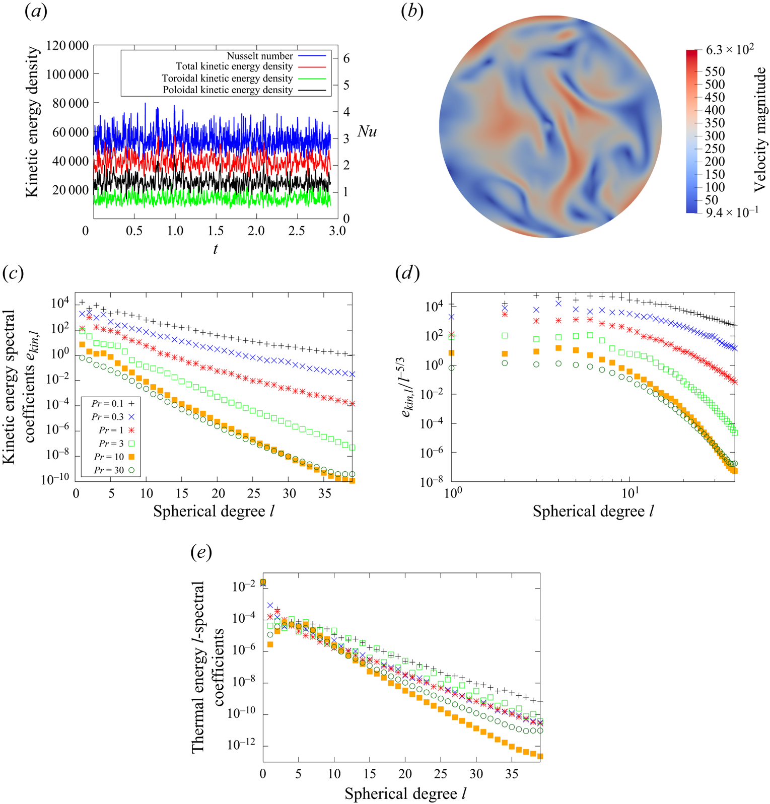
Figure 17(c) shows kinetic energy  $l$ spectra for the different values of $Pr$ at $Ra=3\times 10^5$, i.e. at a forcing at which the solutions are turbulent for all surveyed $Pr$. The general trend is that the kinetic energy spectra become steeper as $Pr$ is increased. This is heuristically plausible, since high $Pr$ corresponds to strong viscous dissipation compared with, for example, the buoyant thermal forcing, becoming then significant not only on small but also on intermediate length scales. Our observation is in agreement with previous studies of the Prandtl number dependence of energy spectra in Rayleigh–Bénard convection (Bhattacharya, Verma & Samtaney Reference Bhattacharya, Verma and Samtaney2021).
Figure 17(d) shows these kinetic  $l$ spectra compensated by $l^{-5/3}$. This scaling corresponds to the well-known universal scaling postulated for the inertial subrange by Kolmogorov (Reference Kolmogorov1941) (with the spherical harmonic degree asymptotically corresponding to the Fourier wavenumber $k$ for large $l$). We observe that for each $Pr$, there is a range of $l$ over which the compensated spectrum does not vary strongly (e.g. the range $2 \leq l \leq 4$ for $Pr=30$) and over which thus the Kolmogorov scaling $l^{-5/3}$ approximately holds. Beyond these ranges, the spectra decrease more strongly with $l$ than $l^{-5/3}$, which according to the theory of Kolmogorov (Reference Kolmogorov1941) is due to the dominance of dissipation over inertia at these scales. The ranges over which the Kolmogorov scaling seems to hold appear to extend up to higher $l$ for lower $Pr$, reflecting the higher kinetic energies and, thus, the stronger inertia at those scales for lower $Pr$. We note, however, that especially for high $Pr$, the Reynolds numbers of the associated turbulent solutions are still relatively low (see figure 9a).
In figure 17 (e) the corresponding thermal energy  $l$ spectra for the surveyed values of $Pr$ are displayed for the turbulent solutions at $Ra=3\times 10^5$. All of these spectra are clearly dominated by the contribution from the $l=0$ modes. For higher $l$, there is not a clear dependence of the thermal energy spectral coefficients on $Pr$ for a given $l$. At least for $l>20$, the coefficients of the solutions at $Pr=10,30$ are the lowest for a given $l$ (with the coefficients of the solution at $Pr=10$ being the lowest) and those at $Pr=0.1$ are the highest. A detailed investigation of the dependence of the thermal energy spectra on $Pr$ is the subject of future work.
Figure 18(a) shows a kinetic energy  $l$ spectrum at $Ra=3\times 10^{10}$ (the largest Rayleigh number for which results were computed) and a $l^{-5/3}$ scaling for comparison. This highly turbulent solution with a Reynolds number of $Re=3.3\times 10^3$ is still dominated by modes of low spherical harmonic degree, i.e. by large length scales. In particular, the largest contribution still comes from $l=1$, the degree of the onset mode. In addition, we find that in the range $10 \leq l \leq 80$, the spectrum indeed decays approximately as the Kolmogorov scaling $l^{-5/3}$, and faster than this for $l>80$. Figure 18(b) shows an $l$ spectrum of thermal energy at $Ra=3\times 10^{10}$. Similarly to the kinetic energy spectrum, the thermal energy $l$ spectrum is dominated by the low $l$ modes, and we also observe a steeper slope of the spectrum beyond roughly $l=80$, consistent with strong thermal diffusion at the small length scales. We note, however, that in the inertial subrange, the scaling of the temperature $l$ spectrum is less steep than a $l^{-5/3}$ scaling. The investigation of the scaling of the thermal energy is also subject for future work.
(a) Kinetic energy  $l$ spectrum at $Ra=3\times 10^{10}$, $Pr=1$. (b) Thermal energy $l$ spectrum at $Ra=3\times 10^{10}$, $Pr=1$. Kolmogorov scaling $l^{-5/3}$ for comparison.
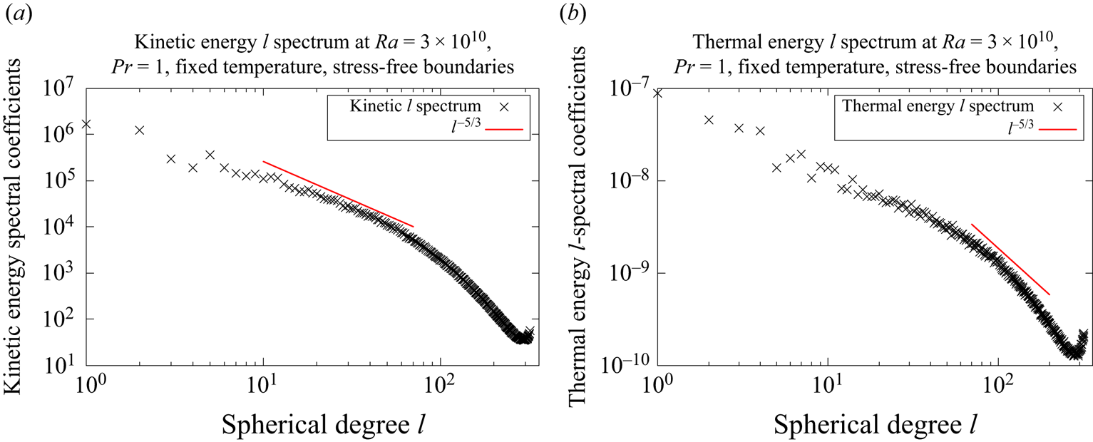
5. Conclusion
In this work we investigated the problem of thermal convection in an internally heated, non-rotating full sphere. We characterised the fluid flow and heat transfer depending on the boundary conditions and the non-dimensional control parameters  $Ra$ and $Pr$ in this configuration, employing both analytical methods and DNS computed with the fully spectral code QuICC.
We first applied the energy method for nonlinear stability to the problem at hand. We described the formalism to establish global nonlinear stability by the energy method, and then demonstrated that in the case of no-slip boundary conditions, linear and nonlinear stability coincide. This implies that the purely conductive state is globally nonlinearly stable below the Rayleigh number for the onset of convection and that subcritical convection is thus impossible for no-slip boundary conditions. The situation remains inconclusive for stress-free boundaries, since boundary terms preclude the formulation of a corresponding variational problem in the energy method.
We proceeded by presenting results for high-Rayleigh-number convection at  $Pr=1$ and for a fixed temperature and both stress-free and no-slip boundary conditions. We computed results up to $Ra=3\times 10^{10}\approx 10^7Ra_c$ for stress-free boundaries and up to $Ra=2\times 10^{12}\approx 2.5\times 10^8Ra_c$ for no-slip boundaries. For the two boundary conditions, we obtained power law scaling exponents of $\gamma _{Nu,SF}=0.23$ and $\gamma _{Re,SF}=0.35$ for stress-free boundaries and $\gamma _{Nu,NS}=0.25$ and $\gamma _{Re,NS}=0.35$ for no-slip boundaries for the scaling of $Nu$ and $Re$ with $Ra$, respectively. We analysed the change of the RSD with the thermal forcing and observed that it decreases with increasing $Ra$. In addition, we examined the toroidal–poloidal partition of the kinetic energy and found that its change with $Ra$ varies significantly between the configurations with stress-free and those with no-slip boundaries. For very high $Ra$, however, we find $E_{kin., tor.}/E_{kin., pol}\approx 0.5$ for both types of velocity boundary conditions. The thermal boundary layer thickness was measured to scale as $\lambda \sim Ra^{-0.23}\sim Nu^{-1}$ for stress-free boundaries, which is consistent with a purely conductive boundary layer. We then adapted the classical scaling argument due Malkus (Reference Malkus1954) and Howard (Reference Howard1963) assuming purely conductive and marginally stable boundary layers to the internally heated full sphere configuration. Using our definition of the Nusselt number, we obtained a scaling prediction of $Nu\sim Ra^{1/4}$, which is consistent with the numerically established scalings.
Finally, we discussed results of a study of the Prandtl number dependence of the system at low to intermediate forcing and with a fixed temperature and stress-free boundary conditions. We computed results for  $0.1\leq Pr \leq 30$ and up to roughly $100Ra_c$, observing five distinct convective regimes in total. We first presented a regime diagram and then discussed the dependence of the global diagnostics on $Ra$ and $Pr$. We observed that the Reynolds number scales roughly inversely with $Pr$ (with a measured power law scaling exponent of $\alpha _{Re}=-0.89$). Results obtained at different $Pr$ can thus reasonably be collapsed onto $RePr$, a type of Péclet number. For $Pr<1$, a lower $Pr$ leads to lower $Nu$, but for $Pr>1$, $Nu$ seems almost independent of $Pr$. We then proceeded to describe the distinct convective regimes individually, focusing on their respective flow patterns, spectral content and time dependence. For the bursting regime, we put forward an interpretation of its distinctive time dependence as the toroidal flow component inhibiting the convective structures by which it is driven, analogous to the analysis of bursting regimes in the plane layer geometry in Garcia et al. (Reference Garcia, Bian, Naulin, Nielsen and Rasmussen2006) and Goluskin et al. (Reference Goluskin, Johnston, Flierl and Spiegel2014).
Supplementary materials and movies
Supplementary materials and movies are available at https://doi.org/10.1017/jfm.2024.1187.
Acknowledgements
We thank J. Luo and G. Castiglioni for valuable input at various points of this research, and F. Burmann for stress testing QuICC to its limits. C. Guervilly made suggestions that helped to clarify some aspects of this work, for which we are grateful.
Funding
We are grateful for funding from the European Research Council (agreement 833848-UEMHP) under the Horizon 2020 programme. This work was partially supported by a grant from the Simons Foundation to A. J. to enable participation in the programme ‘Frontiers in dynamo theory’ at the Isaac Newton Institute, Cambridge, UK. Computing provision was from a grant from the Swiss National Supercomputer Centre (CSCS) under project s1111, for which we are very grateful.
Declaration of interests
The authors report no conflict of interest.


 Open access