


1. Introduction
Hydromagnetic dynamo action is the commonly accepted source of sustained magnetic fields in stars and planets. In this mechanism, a convective system with an electrically conducting fluid can amplify a small magnetic field and continuously convert the kinetic energy of the fluid to magnetic energy, to sustain the field against Joule dissipation. This self-exciting dynamo action can be facilitated due to the presence of rotation leading to large-scale organized fields (Moffatt & Dormy Reference Moffatt and Dormy2019). The most familiar example of such a rotating convection-driven dynamo is the Earth's outer core, where the dynamo mechanism originating from the turbulent motions of electrically conducting liquid iron in the Earth's outer core forms the sustained dipole dominant geomagnetic field (Roberts & King Reference Roberts and King2013). Thermal convection in rotating dynamos, both in plane layer (Stellmach & Hansen Reference Stellmach and Hansen2004; Tilgner Reference Tilgner2012) and spherical (Glatzmaiers & Roberts Reference Glatzmaiers and Roberts1995; Christensen & Wicht Reference Christensen and Wicht2015) geometries, has been extensively investigated to understand their force balance, nature of magnetohydrodynamic turbulence and magnetic field behaviour. Another aspect of fundamental importance is the heat transfer to diagnose the global transport properties of such systems. Convective heat transfer through the atmosphere decides the weather, climate, planetary and stellar energetics, their evolution (Schmitz & Tilgner Reference Schmitz and Tilgner2009) and the generation of magnetic fields from planetary cores (Nimmo Reference Nimmo2015). However, heat transport in self-excited rotating dynamos is yet to be explored.
Dynamics of flow and heat transfer in thermal convection with rotation and magnetic field depends on four governing non-dimensional numbers: (i) the Rayleigh number ( $Ra$) representing the thermal forcing, (ii) the Ekman number ( $E$) signifying the ratio of the viscous force to the Coriolis force, (iii) the thermal Prandtl number ( $Pr$) and (iv) the magnetic Prandtl number ( $Pr_m$); $Pr$ and $Pr_m$ are fluid properties as defined in (2.5a–d). These four numbers decide the global characteristics of the system, indicated by (a) the magnetic Reynolds number ( $Re_m = u_{{rms}}d/\lambda$, where $u_{rms}$ and $d$ are the characteristic velocity and length scales, whereas $\lambda$ is the magnetic diffusivity), characterizing the dominance of electromagnetic induction over ohmic diffusion of the magnetic field, (b) the Nusselt number ( $Nu$) representing non-dimensional heat transfer (see (2.11)) and (c) the Elsasser number ( $\varLambda =\sigma B_{rms}^{2}/\rho \varOmega$, where $\sigma$ is the electrical conductivity, $B_{rms}$ is the characteristics magnetic field strength, $\rho$ is the density and $\varOmega$ is the rotation rate), depicting the ratio of the Lorentz and the Coriolis forces.
Based on the behaviour of the magnetic field with varying  $Re_m$, thermal convection with rotation and a magnetic field can be broadly classified into two categories: (i) rotating magnetoconvection (RMC) at low magnetic Reynolds number ( $Re_m\xrightarrow {}0$) and (ii) dynamo convection (DC) for moderate to high values $Re_m\geqslant O(10)$. For RMC, the system cannot self-induce or sustain a magnetic field, and therefore the magnetic field has to be imposed externally. As the self-induced magnetic field remains small with respect to the imposed field, linear analysis may be used to predict the critical value of Rayleigh number ( $Ra_c$) at the onset of convection (Chandrasekhar Reference Chandrasekhar1961). Moreover, liquid metals (e.g. mercury, sodium, gallium), having large magnetic diffusivities $(\lambda \xrightarrow {}O(10^{6}\unicode{x2013}10^{7}))$ are used to conduct RMC experiments at low $Re_m$. Strong rotation in any convective system restricts convection, attributed to the Taylor–Proudman constraint imposed by the Coriolis force, which inhibits changes along the axis of rotation. Linear theory of RMC (Chandrasekhar Reference Chandrasekhar1961) suggests that the magnetic field can relax the Taylor–Proudman constraint to enhance convection, known as the ‘magnetorelaxation’ process. These theoretical predictions have been verified by experiments (Nakagawa Reference Nakagawa1957, Reference Nakagawa1959; Aurnou & Olson Reference Aurnou and Olson2001). Eltayeb (Reference Eltayeb1972) performed an extensive linear analysis of RMC in the asymptotic limits of large rotation rate ( $E\xrightarrow {}0$) with large imposed field strength for various boundary conditions, orientations of the external magnetic field and rotation. Later, the linear theory was extended to allow for finite-amplitude modes considering that the dominant modes contribute most of the heat transport (Stevenson Reference Stevenson1979). In RMC, the action of the Lorentz force on the flow can lead to enhanced heat transfer (King & Aurnou Reference King and Aurnou2015) as compared with non-magnetic rotating convection (RC). The highest enhancement occurs when the Lorentz force due to the magnetic field and the Coriolis force due to rotation balance each other, as found in the experiment of King & Aurnou (Reference King and Aurnou2015). This global balance, known as the ‘magnetostrophic’ state, is characterized by an Elsasser number of order unity, $\varLambda \approx O(1)$.
Challenges in producing dynamo action in laboratory experiments (Plumley & Julien Reference Plumley and Julien2019) mean that the studies on turbulent DC depend primarily on numerical simulations. Self-exciting dynamo simulations at moderate values of magnetic Reynolds number  $(Re_m = 243{-}346)$ in a spherical shell model performed by Yadav et al. (Reference Yadav, Gastine, Christensen, Wolk and Poppenhaeger2016) revealed a fundamentally different force balance compared with the experimental results of King & Aurnou (Reference King and Aurnou2015). In such ‘geodynamo’ simulations that attempt to model the Earth's outer core, the primary force balance is ‘geostrophic’ between Coriolis and pressure forces, whereas the magnetic, the Archimedean (buoyancy) and the Coriolis forces (MAC) constitute a lower order of magnitude (quasi-geostrophic, QG) balance (Davidson Reference Davidson2013; Aubert Reference Aubert2019; Schwaiger, Gastine & Aubert Reference Schwaiger, Gastine and Aubert2019). Interestingly, Yadav et al. (Reference Yadav, Gastine, Christensen, Wolk and Poppenhaeger2016) also reported a similar heat transfer enhancement as found in the RMC experiments of King & Aurnou (Reference King and Aurnou2015), irrespective of very different force balance and parameter regime.
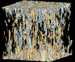
The present study explores the heat transfer behaviour in DC with a plane layer geometry using direct numerical simulations (DNS). This is the simplest possible model of DC in a rotating layer of an electrically conducting fluid between two parallel plates, heated from the bottom and cooled from the top (see figure 1a). Using this model, Jones & Roberts (Reference Jones and Roberts2000) investigated the effect of  $Ra$,
$Ra$,  $E$ and $Pr_m$ on the growth and saturation of the magnetic field and the global force balance while neglecting inertial effects at large Prandtl numbers ( $Pr\xrightarrow {}\infty$). The dynamo was found to saturate at $\varLambda \approx O(1)$. At moderate values of magnetic Reynolds number, $Re_m\approx O(10^{2})$ a simple model of DC was proposed. Rotvig & Jones (Reference Rotvig and Jones2002) studied DC in the range $E=10^{-4}\unicode{x2013}10^{-5}$ and reported a MAC balance in the bulk with $\varLambda \approx O(10)$. Rapidly rotating ( $E=2\times 10^{-4}\unicode{x2013}10^{-6}$), weakly nonlinear DC was explored by Stellmach & Hansen (Reference Stellmach and Hansen2004). They reported time-dependent flow with cyclic variation between small- and large-scale magnetic fields. Interestingly, dynamo action was found to exist even below the critical Rayleigh number for the onset of non-magnetic convection ( $Ra_c$), indicating subcritical dynamo action. Cattaneo & Hughes (Reference Cattaneo and Hughes2006) analysed the $\alpha$-effect (a mechanism of large-scale field generation from small scales due to the helical nature of the flow in DC Moffatt & Dormy Reference Moffatt and Dormy2019) and reported small-scale dynamos with a diffusively controlled $\alpha$-effect, without any indication of large-scale field generation. A transition between small-scale and large-scale field generation was found by Tilgner (Reference Tilgner2012, Reference Tilgner2014) with separate scaling laws for the magnetic energy. The transition occurs at $Re_mE^{1/3}=13.5$, below which the magnetic field generation is dependent on flow helicity. Equipartition of energies is observed above the transition point where the field stretching process at high $Re_m$ generates small-scale fields independent of flow helicity. Guervilly, Hughes & Jones (Reference Guervilly, Hughes and Jones2015) demonstrated the existence of large-scale vortices in DC that can lead to large-scale field generation, which is of great interest for astrophysical dynamos. These vortices reduced the heat transfer efficiency. However, for high $Re_m$, generation of a small-scale magnetic field suppresses the formation of such vortices (Guervilly, Hughes & Jones Reference Guervilly, Hughes and Jones2017). Calkins et al. (Reference Calkins, Julien, Tobias and Aurnou2015) investigated asymptotically reduced DC models with a leading-order QG balance. Four distinct QG dynamo regimes have been identified with varying dynamics and magnetic to kinetic energy density ratios (Calkins Reference Calkins2018). Extension to non-Boussinesq convection was investigated by Käpylä, Korpi & Brandenburg (Reference Käpylä, Korpi and Brandenburg2009) and Favier & Bushby (Reference Favier and Bushby2013).
Plane layer dynamo driven by convection of an electrically conducting fluid.

The heat transport behaviour in plane layer DC remains almost unexplored. In this geometry, two distinct regions of convection can be identified: the boundary layer region near the plates with high velocity and temperature gradients (Ekman and thermal boundary layers) and a well-mixed ‘bulk’ regime in the interior where gradients are much smaller. Heat transfer scaling of dynamos without rotation has been found to be identical to non-rotating, non-magnetic Rayleigh Bénard convection (Yan, Tobias & Calkins Reference Yan, Tobias and Calkins2021), where heat transfer is known to be constrained by the boundary layer dynamics (Plumley & Julien Reference Plumley and Julien2019). Conversely, heat transfer in non-magnetic RC is constrained by the bulk, although it can be significantly altered by the boundary layer dynamics (Stellmach et al. Reference Stellmach, Lischper, Julien, Vasil, Cheng, Ribeiro, King and Aurnou2014). Even without considering the viscous boundary layer, Stellmach & Hansen (Reference Stellmach and Hansen2004) found enhanced heat transfer in weakly nonlinear convection in a rapidly rotating dynamo. They attributed this increased heat transport to the increased length scale of convection due to the presence of a strong magnetic field. However, the variation of heat transfer with thermal forcing in a rotating dynamo remains unknown. Also, to the best of our knowledge, no studies report the role of the boundary layer in the heat transfer behaviour in rotating DC. We perform a systematic study, unprecedented in the previous investigations, in a plane layer geometry to investigate the boundary layer dynamics of dynamos and its implications on the heat transfer behaviour.
2. Method
2.1. Governing equations and numerical details
We consider DC in a three-dimensional Cartesian layer of an incompressible, electrically conducting, Boussinesq fluid. The layer of depth  $d$ is kept between two parallel plates with temperature difference $\Delta T$ where the lower plate is hotter (see figure 1). The system is rotating about the vertical with an angular velocity $\varOmega$. The fluid properties are density ( $\rho$), kinematic viscosity ( $\nu$), thermal diffusivity ( $\kappa$), magnetic permeability ( $\mu$), electrical conductivity ( $\sigma$), adiabatic volume expansion coefficient ( $\alpha$) and the magnetic diffusivity ( $\lambda$). The layer depth $d$ is the length scale, free-fall velocity, $u_f=\sqrt {g\alpha \Delta T d}$, is the velocity scale where g is the acceleration due to gravity, $\sqrt {\rho \mu }u_f$ is the magnetic field scale and the temperature drop across the layer, $\Delta T$ is the temperature scale assumed for non-dimensionalizing the governing equations (Iyer et al. Reference Iyer, Scheel, Schumacher and Sreenivasan2020). The non-dimensional equations for the velocity field $\boldsymbol {u}$, temperature field $\theta$ and magnetic field $\boldsymbol {B}$, take the following form:
 $$\begin{gather} \frac{\partial u_j}{\partial x_j}= \frac{\partial B_j}{\partial x_j}=0, \end{gather}$$
 $$\begin{gather}\frac{\partial u_i}{\partial t}+ u_j\frac{\partial u_i}{\partial x_j}={-}\frac{\partial p}{\partial x_i}+ \frac{2}{E}\sqrt{\frac{Pr}{Ra}}\epsilon_{ij3} u_j\widehat{e_3}+ B_j\frac{\partial B_i}{\partial x_j}+ \theta\delta_{i3}+ \sqrt{\frac{Pr}{Ra}}\frac{\partial^{2} u_{i}}{\partial x_j\partial x_j}, \end{gather}$$
 $$\begin{gather}\frac{\partial \theta}{\partial t}+ u_j\frac{\partial \theta}{\partial x_j}= \frac{1}{\sqrt{RaPr}}\frac{\partial^{2}\theta}{\partial x_j\partial x_j}, \end{gather}$$
 $$\begin{gather}\frac{\partial B_i}{\partial t}+ u_j\frac{\partial B_i}{\partial x_j}= B_j\frac{\partial u_i}{\partial x_j}+ \sqrt{\frac{Pr}{Ra}}\frac{1}{Pr_m}\frac{\partial^{2} B_{i}}{\partial x_j\partial x_j}. \end{gather}$$
The non-dimensional parameters appearing in (2.2)–(2.4) are defined below
 \begin{equation} Ra=\frac{g\alpha\Delta T d^{3}}{\kappa\nu},\quad E=\frac{\nu}{\varOmega d^{2}},\quad Pr=\frac{\nu}{\kappa},\quad Pr_m=\frac{\nu}{\lambda}. \end{equation}
 In the horizontal directions ( $x_{1},x_{2}$) periodic boundary conditions are applied. In the vertical direction ( $x_3$), the velocity boundary conditions are no slip and impenetrable. As we aim to study the effect of the boundary layer dynamics on DC, the no-slip boundary condition is the natural choice (Jones & Roberts Reference Jones and Roberts2000; Stellmach et al. Reference Stellmach, Lischper, Julien, Vasil, Cheng, Ribeiro, King and Aurnou2014). Although corresponding results for a free-slip boundary condition are also presented, we discuss the results for the no-slip boundary condition unless stated otherwise. Therefore,
 \begin{equation} u_{1}=u_{2}=u_{3}=0 \quad \textrm{at} \ x_{3}={\pm} 1/2. \end{equation}
An unstable temperature gradient is maintained by imposing isothermal boundary conditions
 \begin{equation} \theta=1 \ \textrm{at} \ x_{3}={-}1/2, \quad \theta=0 \ \textrm{at} \ x_{3}=1/2. \end{equation}
For the magnetic field, either perfectly conducting or perfectly insulating boundary conditions can be implemented. The insulating boundary condition is commonly applied in spherical shell geometries for geodynamo simulations (Christensen & Wicht Reference Christensen and Wicht2015; Yadav et al. Reference Yadav, Gastine, Christensen, Wolk and Poppenhaeger2016). However, for plane layer geometries, a perfectly conducting boundary condition is commonly used (Tilgner Reference Tilgner2012; Guervilly et al. Reference Guervilly, Hughes and Jones2015; Hughes & Cattaneo Reference Hughes and Cattaneo2019) because it enables comparison with the theoretical studies (Stellmach & Hansen Reference Stellmach and Hansen2004). Laboratory set-ups for RMC (King & Aurnou Reference King and Aurnou2015) and dynamos (Monchaux et al. Reference Monchaux2007) also use conducting materials as containers of liquid metals are commonly used to conduct experiments. Thus, perfectly conducting boundary condition are implemented in the present study such that
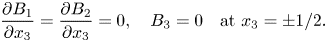 \begin{equation} \frac{\partial B_{1}}{\partial x_{3}}=\frac{\partial B_{2}}{\partial x_{3}}=0,\quad B_{3}=0 \quad \textrm{at} \ x_{3}={\pm} 1/2. \end{equation}
The governing equations are solved in a cubic domain with unit side length, using the finite difference method (Bakhuis et al. Reference Bakhuis, Ostilla-Mónico, Van Der Poel, Erwin, Verzicco and Lohse2018) in a staggered grid arrangement. The scalar quantities (pressure and temperature) are stored at the cell centres whereas, velocity and magnetic field components are stored at the cell faces. Second-order central difference is used for spatial discretization. The projection method is used to calculate the divergence-free velocity field where the pressure Poisson equation is solved using a parallel multigrid algorithm. Similarly, an elliptic divergence cleaning algorithm is employed to keep the magnetic field solenoidal (Brackbill & Barnes Reference Brackbill and Barnes1980). An explicit third-order Runge–Kutta method is used for time advancement except for the diffusion terms, which are solved implicitly using the Crank–Nicolson method (Pham, Sarkar & Brucker Reference Pham, Sarkar and Brucker2009; Brucker & Sarkar Reference Brucker and Sarkar2010). The solver has been validated extensively for numerous DNS of stratified turbulent flows (Pal, de Stadler & Sarkar Reference Pal, de Stadler and Sarkar2013; Pal & Sarkar Reference Pal and Sarkar2015; Pal & Chalamalla Reference Pal and Chalamalla2020).
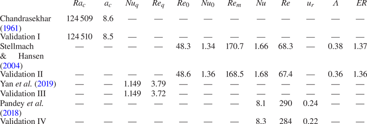
Validation of our numerical solver is performed by replicating the results from the following literature: (i) critical Rayleigh number and wavenumber ( $Ra_c$ and $a_c$) at the onset of magnetoconvection with imposed field strength $Q=\sigma B^{2}d^{2}/\rho \nu =10^{4}$ predicted from linear theory (Chandrasekhar Reference Chandrasekhar1961), (ii) RC simulations of Stellmach & Hansen (Reference Stellmach and Hansen2004) at $Ra=1.4\times 10^{7}$, $E=5\times 10^{-5}$ and $Pr=1$, along with DC simulation results for $Pr_m=2.5$ with free-slip boundary conditions, (iii) DNS results of quasi-static magnetoconvection (Yan et al. Reference Yan, Calkins, Maffei, Julien, Tobias and Marti2019) at $Q=10^{4}$ and $Ra=1.3\times 10^{5}$ and (iv) DNS of Rayleigh Bénard convection at $Ra=10^{6}$ and $Pr=0.7$ as reported by Pandey et al. (Reference Pandey, Scheel and Schumacher2018). Our results are in good agreement with these earlier studies, as demonstrated in table 1.
Results from the three test runs to reproduce results from the literature: (i) linear magnetoconvection theory (Chandrasekhar Reference Chandrasekhar1961), (ii) RC and DC simulations of Stellmach & Hansen (Reference Stellmach and Hansen2004), (iii) DNS results of quasi-static magnetoconvection (Yan et al. Reference Yan, Calkins, Maffei, Julien, Tobias and Marti2019) and (iv) DNS of Rayleigh Bénard convection (Pandey, Scheel & Schumacher Reference Pandey, Scheel and Schumacher2018). Subscripts ‘0’ and  $q$ are used to represent non-magnetic RC and quasi-static magnetoconvection results, respectively. Here, $u_r=\langle u_iu_i\rangle _{\mathcal {V},t}$, where $\langle \cdot \rangle _{\mathcal {V},t}$ denotes a volume and time averaged value. The magnetic to kinetic energy ratio is represented by $ER$.
$ER$.
2.2. Problem set-up
Dynamical balances and heat transport are studied at constant rotation rate and constant fluid properties with variation in thermal forcing. The thermal forcing here is represented by the convective supercriticality  $\mathcal {R}=Ra/Ra_c$, where $Ra_c=19.15E^{-4/3}$ is the minimum required value of $Ra$ to start RC for vanishingly small Ekman numbers $E\xrightarrow {}0$ (King, Stellmach & Aurnou Reference King, Stellmach and Aurnou2012; Kunnen Reference Kunnen2021). We have used a higher prefactor for free-slip boundaries, where $Ra_c=21.91E^{-4/3}$, following Chandrasekhar (Reference Chandrasekhar1961). We choose the values of $\mathcal {R}=2,2.5,3,4,5,10,20$, Ekman number $E=10^{-6}$ and the Prandtl numbers $Pr=Pr_m=1$ for the present simulations. To elucidate the effect of the magnetic field, we perform two simulations at each value of $\mathcal {R}$: DC and RC. It should be noted here that the critical Rayleigh number for the onset of DC remains unknown (Plumley & Julien Reference Plumley and Julien2019). Hence, we use the same value of $Ra_c$ for both DC and RC simulations following Stellmach & Hansen (Reference Stellmach and Hansen2004).
In the horizontal directions ( $x_1$ and $x_2$) $1024$ uniform grid points are used, whereas in the vertical direction ( $x_3$) we have used $256$ non-uniform grid points. Grid clustering near the walls is performed to ensure a minimum of four grid points inside the Ekman layer with the spacing, $\Delta x_{3}=4.8\times 10^{-4}$ at the wall. The clustering function has been used for this purpose is given in (2.9).
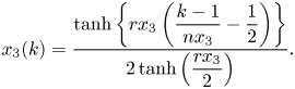 \begin{equation} x_3(k)=\frac{\tanh\left\{rx_3\left(\dfrac{k-1}{nx_3}-\dfrac{1}{2}\right)\right\}}{2 \tanh\left(\dfrac{rx_3}{2}\right)}. \end{equation}
Here,  $k$ is the grid index, $nx_3$ is the number of grid divisions in $x_3$ and
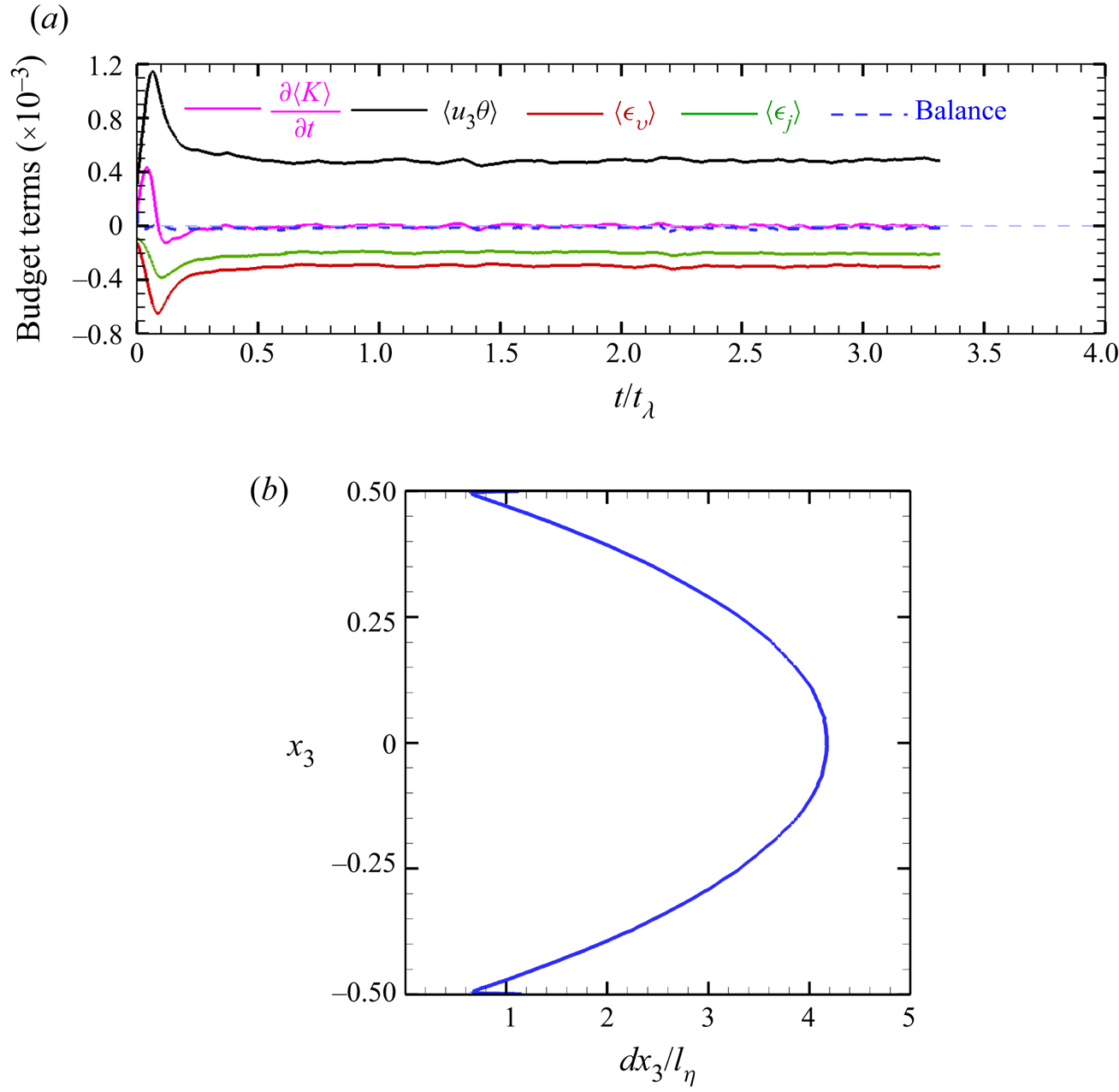
  $rx_3$ is the stretching factor which is fine tuned to resolve the boundary layers. Our aim is to explain the optimal heat transfer characteristics in a plane layer dynamo using turbulence resolving simulations. Capturing the boundary layer dynamics in these simulations is imperative for understanding the enhanced heat transfer phenomenon, and requires a grid that can resolve the smallest dissipative scales (Shishkina et al. Reference Shishkina, Stevens, Grossmann and Lohse2010). An appropriate resolution should achieve a balance of the stringent turbulent kinetic energy (t.k.e.) budget given in (2.10) (Pal & Chalamalla Reference Pal and Chalamalla2020)
 \begin{equation} \frac{{\rm d}\langle K \rangle}{{\rm d}t}= \langle u_{3}\theta \rangle-\langle \epsilon_{v} \rangle-\langle \epsilon_{j} \rangle. \end{equation}
 The time evolution of the terms in (2.10) are presented for DC at  $\mathcal {R}=20$ in figure 2(a). Here, the volume-averaged balance depicts generation of kinetic energy from the vertical buoyancy flux $\langle u_{3}\theta \rangle$, balanced by viscous and Joule dissipation, $\langle \epsilon _{v} \rangle$ and $\langle \epsilon _{j} \rangle$, respectively, acting as sinks of energy (see (2.11) for the definition of these terms). The balance term, signifying the difference between the left- and right-hand sides of (2.10), remains two orders of magnitude smaller than the leading-order terms for all the simulations. Additionally, the vertical grid spacing, normalized by the non-dimensional Kolmogorov scale, $l_\eta =(1/\overline {\epsilon _v})^{1/4}(Pr/Ra)^{3/8}$, as estimated from the horizontally averaged dissipation, is plotted in figure 2(b). The value of this quantity remains close to unity near the wall, indicating appropriate wall resolution. In the horizontal directions, $\Delta x_i/l_{\eta,min}\approx 2.66$, where $l_{\eta,min}$ is the minimum Kolmogorov scale in the domain. It should be noted that, $\Delta x_i/l_{\eta,min}\leqslant 2\unicode{x2013}4$ should be sufficient for accurate estimation of second-order moments in DNS of turbulent flows (Brucker & Sarkar Reference Brucker and Sarkar2010). The grid resolution used in this study, has been selected after subsequent grid refinements such that the kinetic and magnetic energies are sufficiently dissipated, and the t.k.e. budget closure is maintained. Therefore, the present simulations, albeit computationally expensive, can capture the smallest scales in the flow, especially near the walls, and therefore successfully resolve the boundary layer dynamics. The simulation details and global diagnostic parameters are summarized in table 2.
(a) Volume-averaged budget of turbulent kinetic energy at  $\mathcal {R}=20$. The time evolution of volume-averaged terms in (2.10) is presented. Here, the balance term signifies the difference between the left- and right-hand sides of the equation. (b) Vertical variation of grid spacing ( $dx_3$) normalized by the Kolmogorov scale ( $l_{\eta }$) as estimated from the horizontally averaged dissipation.
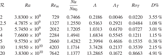
Statistics of the DC simulations with no-slip boundary conditions at  $E=10^{-6}$, $Pr=Pr_m=1$.
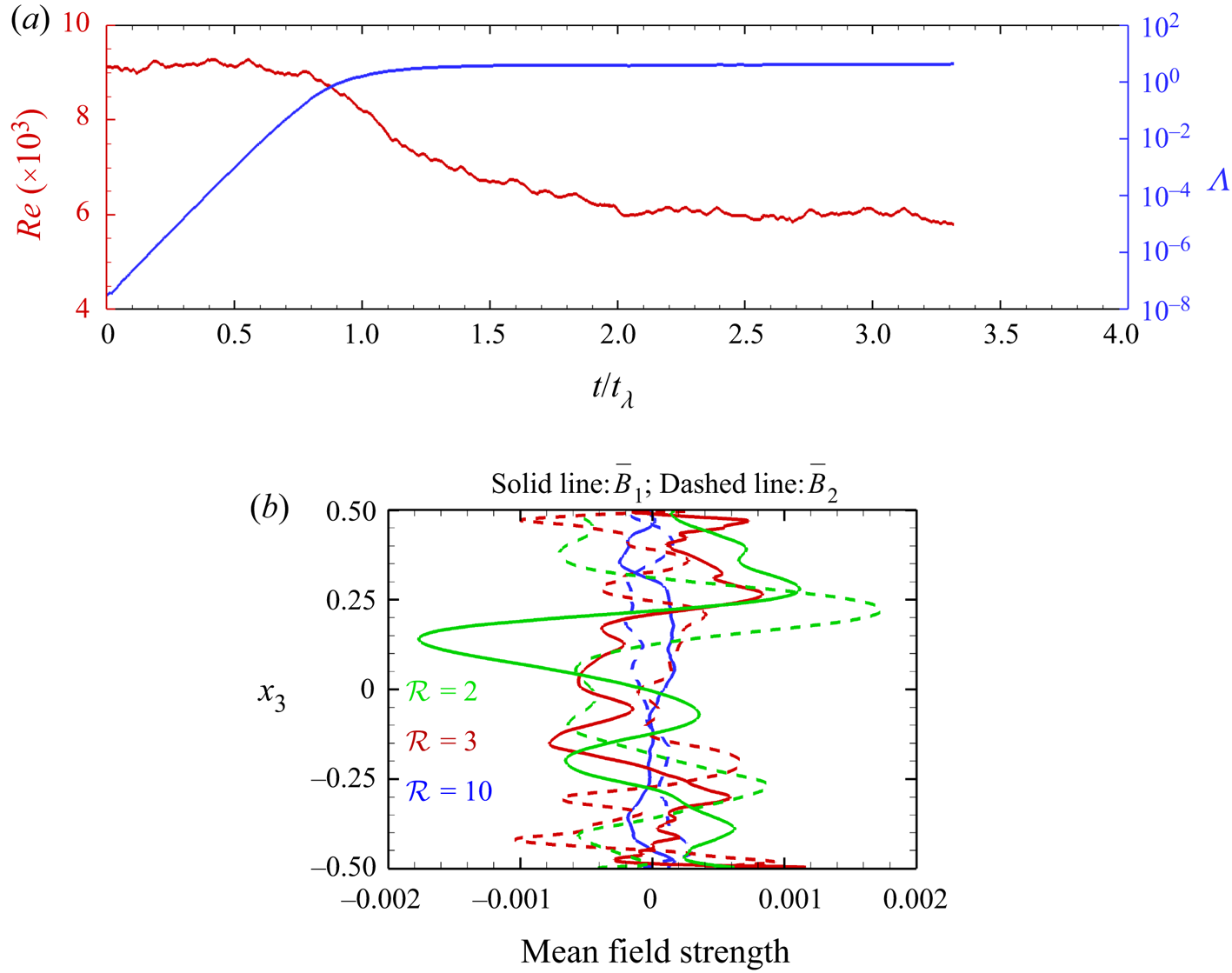
We start the DC simulations at  $\mathcal {R}=20$, by introducing a small magnetic perturbation in a statistically steady RC simulation, as shown in figure 3(a). The magnetic field shows an exponential growth over approximately one free decay time scale ( $t_\lambda =d^{2}/\lambda$) before it saturates. The decrease in Reynolds number ( $Re=Re_m/Pr_m$), signifies decrease in turbulence due to dynamo action at $\mathcal {R}=20$. Simulations at lower values of $\mathcal {R}$ are started using the data of higher $\mathcal {R}$ as the initial condition to save computational time. The mean magnetic field is calculated to outline the behaviour of the dynamos, by averaging the field over horizontal planes. This horizontal averaging of any quantity $\phi$ is denoted by an overbar in the following discussion, with $\bar {\phi }$ denoting the mean and $\phi _{rms}$ representing the root mean square (r.m.s.) field. The vertical variation of the mean horizontal magnetic fields ( $\bar {B}_{1}$ and $\bar {B}_{2}$) is depicted in figure 3(b). It should be noted here that the vertical component of the mean magnetic field ( $\bar {B}_{3}$) is zero everywhere by the definition of averages and solenoidal field conditions. Thus the mean field remains horizontal. However, as we show later in figure 10(b), the vertical component of the r.m.s. field ( ${b}_{3,rms}$) is non-zero except at the walls. We observe a one order of magnitude drop in the mean-field strength (figure 3b) with increasing $\mathcal {R}$ signifying a transition from large-scale to small-scale dynamo action. The magnetic Reynolds number (based on the horizontal scale of convective cells, Tilgner Reference Tilgner2012) varies as $Re_mE^{1/3}\approx 7\unicode{x2013}76$ in the range $\mathcal {R}=2\unicode{x2013}20$ in our simulations. A similar transition in dynamos is reported to occur at $Re_mE^{1/3}=13.5$ (Tilgner Reference Tilgner2012, Reference Tilgner2014) which lies in the range $\mathcal {R}=2.5\unicode{x2013}3$ our simulations.
(a) Time evolution of Reynolds number and Elsasser number for DC at  $\mathcal {R}=20$. (b) Vertical variation of mean magnetic fields for different $\mathcal {R}$.
In the following discussion, the DC and RC simulations are compared in terms of their heat transfer and turbulence properties. Heat transfer is represented by the Nusselt number ( $Nu$), defined as the total heat to conductive heat transferred from the bottom plate to the top plate. The intensity of turbulence is characterized by the t.k.e. ( $K$), whereas the viscous and the Joule dissipation signify the conversion of kinetic and magnetic energy to internal energy via the action of viscous and magnetic diffusion, respectively,
 \begin{equation} \left.\begin{gathered} Nu=\frac{qd}{k\Delta T}=1+\sqrt{RaPr}\langle u_3\theta\rangle, \quad \langle K \rangle=\left\langle{\frac{1}{2}u_{i}u_{i}}\right\rangle ,\\ \langle \epsilon _{v} \rangle=\sqrt{\frac{Pr}{Ra}}\left \langle\frac{\partial u_{i}}{\partial x_j}\frac{\partial u_{i}}{\partial x_j}\right\rangle, \quad \langle \epsilon _{j} \rangle=\sqrt{\frac{Pr}{Ra}}\frac{1}{Pr_m} \left\langle\frac{\partial b_{i}}{\partial x_j}\frac{\partial b_{i}}{\partial x_j}\right\rangle. \end{gathered}\right\} \end{equation}
Here,  $\langle \cdot \rangle$ denotes average over the entire volume. The volume-averaged total heat flux and vertical buoyant energy flux are denoted by $q$ and $\langle u_3\theta \rangle$. Subscript ‘0’ is used to represent the properties without a magnetic field (RC cases). All the statistical quantities presented in this paper are averaged in time for at least 100 free-fall time units ( $d/u_f$), when the turbulent flow becomes statistically stationary in our simulations.
3. Result
We begin the analysis by comparing our simulation results for DC and RC in terms of their global heat transfer and turbulence properties. In figure 4, the ratio of the Nusselt number for DC to RC ( $Nu/Nu_{0}$) is plotted with respect to the convective supercriticality ( $\mathcal {R}$). The dynamo action associated with the magnetic field results in increased heat transfer for DC, except at $\mathcal {R}=2$. Maximum enhancement occurs at $\mathcal {R}=3$ where the heat transfer of DC is more than $70\,\%$ as compared with RC. The experiment in a rotating cylinder by King & Aurnou (Reference King and Aurnou2015) and the geodynamo simulation in a spherical shell model by Yadav et al. (Reference Yadav, Gastine, Christensen, Wolk and Poppenhaeger2016) have reported a similar heat transfer enhancement peak. However, this optimum heat transfer enhancement owing to dynamo action is a novel finding for a plane layer dynamo. Interestingly, the peak in heat transfer is found to occur at $\varLambda \approx 1$ (see table 2), similar to the RMC experiments of King & Aurnou (Reference King and Aurnou2015) and the geodynamo simulation of Yadav et al. (Reference Yadav, Gastine, Christensen, Wolk and Poppenhaeger2016). When the Lorentz force is of similar magnitude to the Coriolis force, the global magnetorelaxation process should enhance heat transport in RMC (King & Aurnou Reference King and Aurnou2015). However, this leading-order magnetostrophic balance for $\varLambda =O(1)$ may not represent the primary balance in DC (Soderlund et al. Reference Soderlund, Sheyko, King and Aurnou2015; Aurnou & King Reference Aurnou and King2017; Calkins Reference Calkins2018). The traditional definition of the Elsasser number( $\varLambda =\sigma B_{rms}^{2}/\rho \varOmega$) gives a correct ratio of the Lorentz and the Coriolis forces only for small $Re_m\leqslant O(1)$, which is not valid for a dynamo (Soderlund et al. Reference Soderlund, Sheyko, King and Aurnou2015; Aurnou & King Reference Aurnou and King2017). As the global force balance reported in the simulation (Yadav et al. Reference Yadav, Gastine, Christensen, Wolk and Poppenhaeger2016) is geostrophic, not magnetostrophic, a similar magnetorelaxation process to that reported in the RMC experiment of King & Aurnou (Reference King and Aurnou2015) may not be the reason for heat transfer enhancement in the DC simulations of Yadav et al. (Reference Yadav, Gastine, Christensen, Wolk and Poppenhaeger2016). The present study indicates a local increase in the Lorentz force near the top and bottom plates signifying the importance of the thermal boundary layer dynamics for the heat transfer enhancement in dynamo simulations, instead of any global force balance.
Ratio of Nusselt number, t.k.e., viscous dissipation and Joule dissipation as a function of convective supercriticality. Subscript ‘0’ is used to represent non-magnetic simulation.
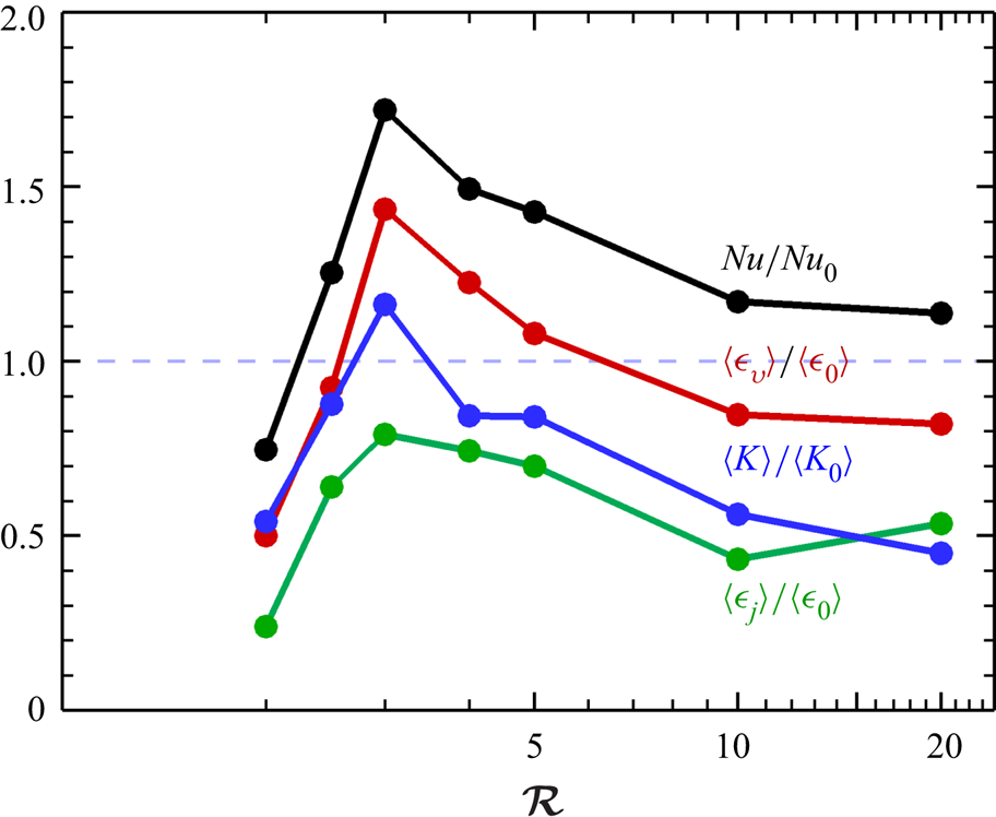
The global statistics of the underlying turbulent motion are shown in figure 4 to understand the heat transfer enhancement phenomenon. We observe that the ratio of the t.k.e. of the DC simulations to the RC simulations,  $\langle K \rangle /\langle K_{0} \rangle$, achieves a maximum at $\mathcal {R}=3$, indicating higher turbulence intensity in DC as compared with RC. We further confirm this enhanced turbulence activity by showing the variation of the ratio of viscous dissipation, $\langle \epsilon _{v}\rangle /\langle \epsilon _{0}\rangle$, in figure 4. A similar peak in the dissipation ratio for $\mathcal {R}=3$ is observed. Additionally, the part of kinetic energy converted into magnetic energy dissipates via Joule dissipation. The normalized Joule dissipation of magnetic energy, $\langle \epsilon _{j}\rangle /\langle \epsilon _{0}\rangle$, manifests a similar peak. It should be noted here that the overall energy balance leads to the exact relation $(Nu-1)/\sqrt {RaPr}=\langle \epsilon _v\rangle +\langle \epsilon _j\rangle$, between the Nusselt number and the dissipation mechanisms present in the dynamo. Therefore, we can expect the appearance of similar peaks in these quantities. These observations confirm increased turbulence for $\mathcal {R} = 3$ that promotes mixing and scalar transport, resulting in heat transfer enhancement.
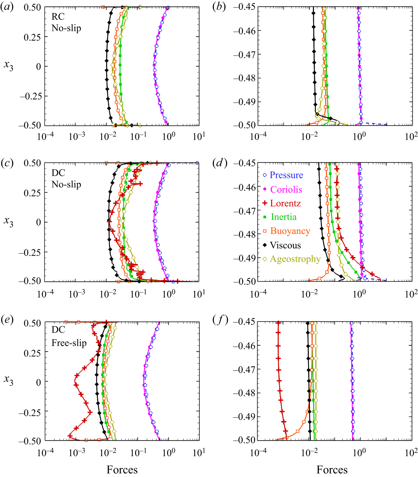
To explore the possible reasons for this increased turbulence and heat transfer enhancement, we can compare the vertical variation of forces in figure 5 for DC and RC with both no-slip and free-slip boundary conditions at  $\mathcal {R}=3$. The forces are calculated from the r.m.s. values of the terms in the momentum equation (2.2) by averaging over horizontal planes (Yan et al. Reference Yan, Tobias and Calkins2021). The leading-order geostrophic balance between pressure and the Coriolis forces are apparent for all cases, as shown in figures 5(a), 5(c) and 5(e). Geostrophic balance is known to be the characteristic of strong RC (King et al. Reference King, Stellmach and Aurnou2012). Small departures from this balance due to the other forces make QG convection (even turbulence) possible in such flows, making these other forces important for the dynamics. Buoyancy, viscous and inertia constitute the QG force balance in RC at $\mathcal {R}=3$ (see figure 5a). Although the viscous diffusion term is smallest in the bulk, it increases near the Ekman layer at the bottom plate, as shown in figure 5(b), and dominates the QG balance. For the no-slip boundary condition, the velocities are zero at the wall, which results in an increase in the pressure force at the walls (figure 5b,d). In figure 5 the difference between the horizontal Coriolis and pressure forces is termed as ageostrophy. For the non-magnetic simulations the ageostrophic component is primarily balanced by buoyancy and inertial forces in the bulk, whereas the same balanced by the viscous forces near the boundary, as the geostrophic balance breaks down near the Ekman layer. Moreover, for dynamo simulations with a no-slip condition, Lorentz force plays a significant role in balancing the ageostrophic component, whereas for free-slip cases buoyancy and inertia balance the same with a sub-dominant role played the Lorentz force. In figure 5(c), the Lorentz force, which is at least one order of magnitude smaller than the Coriolis force in the bulk, decreases from the wall towards the centre of the domain, reaching a minimum. Therefore, the global magnetostrophic balance between the Lorentz and the Coriolis forces, as found in the previous RMC experiment (King & Aurnou Reference King and Aurnou2015), may not be the reason for the heat transfer enhancement in the present DC simulations. A closer look near the bottom plate for DC at $\mathcal {R}=3$ reveals a different dynamical behaviour in figure 5(d). Here, the Lorentz force increases nearly three orders of magnitude from its value at the centre of the domain to become the dominant force at the wall. This increase in the Lorentz force near the wall can attenuate the turbulence suppressing effect of the Coriolis force, resulting in enhanced turbulence, mixing and heat transfer. We also observe a similar increase in the Lorentz force near the boundary for $\mathcal {R}=2.5,4$ and 5 (figures not shown). Apart from a dissimilar vertical variation, the Lorentz force for the free-slip boundary condition case (figure 5e) is one order of magnitude smaller compared with the no-slip boundary condition case (figure 5c). Furthermore, no enhancement in the Lorentz force is observed for the free-slip boundary condition case near the wall (see figure 5f).
Vertical variation of forces at  $\mathcal {R}=3$ for (a,b) no-slip RC, (c,d) no-slip DC and (e, f) free-slip DC. The horizontally averaged force distribution is shown in the bulk (a,c,e) and near the bottom plate (b,d, f). The ageostrophy is defined by the difference between the r.m.s. horizontal Coriolis and pressure forces.
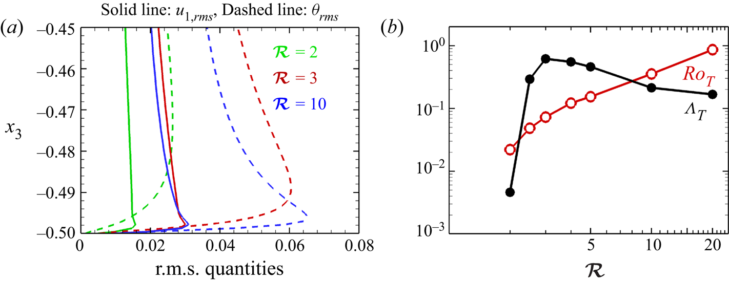
Further analysis of the boundary layer characteristics can be made to assess the relative magnitudes of the Lorentz and the Coriolis forces near the walls. The variation of the r.m.s. horizontal velocity ( $u_{1,rms}$), and the r.m.s. temperature ( $\theta _{rms}$) in the vertical direction near the bottom plate is shown in figure 6(a) for DC cases at $\mathcal {R}=2,3\ \textrm {and} 10$. Here, we can define the Ekman boundary layer (EBL) and thermal boundary layer (TBL) as the regions adjacent to the plates where viscous diffusion and thermal diffusion are important. In strong RC, heat is transported by columnar structures, and plumes that are formed due to the instability of the TBL (King et al. Reference King, Stellmach and Aurnou2012). The heat transfer characteristics of such systems depend on the relative thickness of the two layers (King et al. Reference King, Stellmach, Noir, Hansen and Aurnou2009, Reference King, Stellmach and Aurnou2012). The distance of the peaks in the r.m.s. horizontal velocity and temperature from the bottom boundary can be used to estimate the EBL and TBL thicknesses ( $\delta _{E}$ and $\delta _{T}$) respectively from figure 6(a) (King et al. Reference King, Stellmach, Noir, Hansen and Aurnou2009). If $\delta _{T}>\delta _{E}$, the strong Coriolis force stabilizes the thermal layer, impeding the formation of plumes and thereby restricting heat transfer (King et al. Reference King, Stellmach and Aurnou2012). The TBL thickness is higher than the Ekman layer for the DC cases as demonstrated in figure 6(a). Similar observations are true for RC cases (figure not shown), indicating a strong stabilizing effect of the Coriolis force in all simulations. To determine the effect of the Lorentz force in DC cases, we define a local Elsasser number ( $\varLambda _{T}$) at the edge of TBL that measures the ratio of the Lorentz and the Coriolis forces at this location. We emphasize here that this Elsasser number is computed directly from the r.m.s. magnitudes of the forces (see figure 5), not from the traditional definition ( $\varLambda$). The variation of $\varLambda _{T}$ with $\mathcal {R}$ at the TBL edge near the bottom boundary is shown in figure 6(b). The two forces can be seen to be of the same order of magnitude near the edge of the TBL for $\mathcal {R}=2.5,3,4$ and 5. The local Elsasser number also achieves a maximum at $\mathcal {R}=3$, similar to the Nusselt number ratio (see figure 4), indicating a correlation between the increase in the Lorentz force and the heat transport behaviour. The increase in the Lorentz force at the TBL effectively mitigates the stabilizing effect of the Coriolis force and can be seen as a local magnetorelaxation of the Taylor–Proudman constraint, resulting in enhanced turbulence and heat transport. Although the inertial force, represented by the Rossby number ( $Ro_T$, the ratio of inertia to Coriolis force) in figure 6(b) also increases near the wall, the monotonically increasing trend does not correlate with the heat transfer behaviour.
(a) Horizontal r.m.s. velocity (solid lines) and temperature profiles (dashed lines) near wall for DC cases, (b) variation of local Elsasser number and the Rossby number at the thermal boundary layer edge with convective supercriticality.
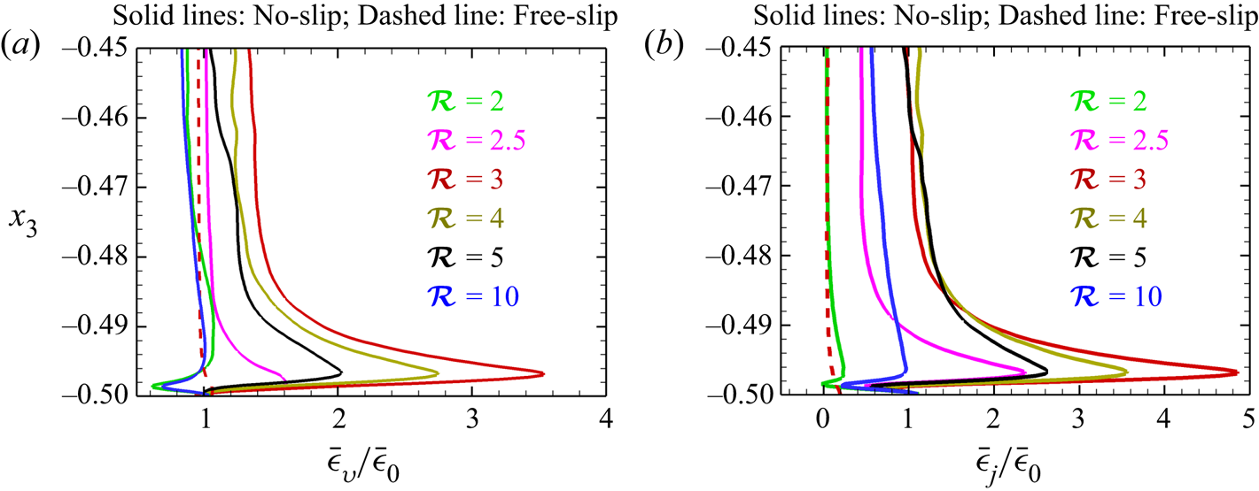
To corroborate the local magnetorelaxation process, and enhancement in turbulence, we show the vertical variation of the viscous dissipation ratio ( $\bar {\epsilon }_{v}/\bar {\epsilon }_{0}$) near the bottom wall in figure 7(a). This dissipation ratio is computed after averaging the dissipation for DC, and RC simulations over the horizontal directions. We observe an increase in viscous dissipation for $\mathcal {R}=2.5,3,4$ and 5, near the bottom boundary, suggesting an increase in turbulence near the walls because of the local magnetorelaxation. This enhancement in viscous dissipation is highest for $\mathcal {R}=3$, indicating higher turbulence intensity among all the other cases. Similar enhancement in Joule dissipation can also be observed in figure 7(b). However, no such enhancement in viscous and Joule dissipation is found at $\mathcal {R} = 3$ for free-slip boundary condition (dashed lines).
Vertical variation of (a) viscous dissipation ratio and (b) Joule dissipation ratio near the bottom plate for DC cases with no-slip (solid lines) and free-slip (dashed line) boundary conditions.
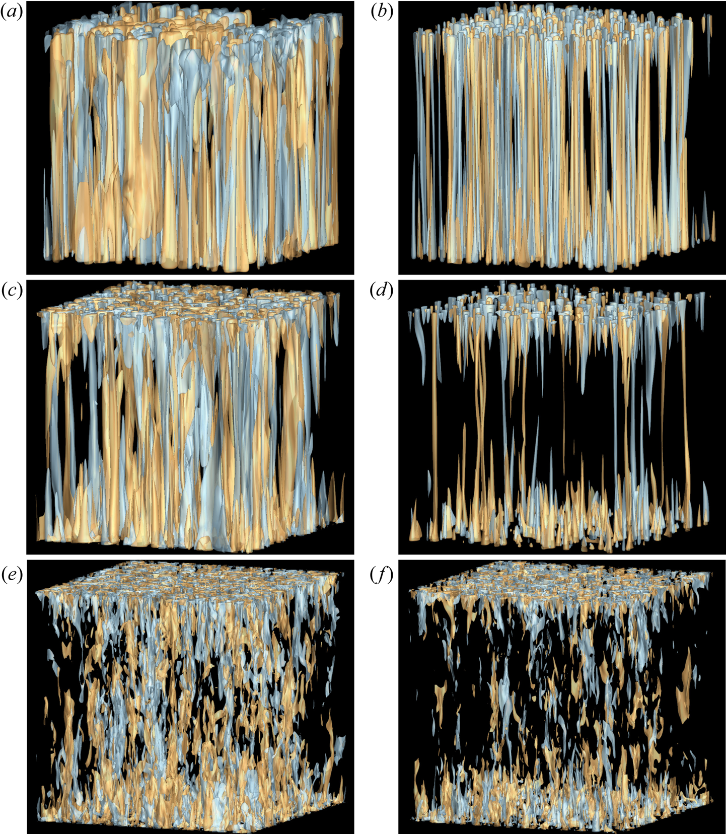
Isosurfaces of temperature perturbation for DC (a,c,e) and RC (b,d, f) are shown in figure 8 to provide visualizations of the thermal structures. The horizontally averaged temperature variation is subtracted from the instantaneous temperature field to compute these temperature perturbations. For RC, the flow morphology changes from columnar cells at  $\mathcal {R}=2$ (figure 8b) to plumes at $\mathcal {R}=3$ (figure 8d) to geostrophic turbulence dominating at larger thermal forcing at $\mathcal {R}=10$ (figure 8f). The transition of flow morphology from columnar cells to plumes occurs at $RaE^{4/3}\sim 22$ whereas the transition from plumes to geostrophic turbulence happens at $RaE^{4/3}\sim 55$ (Julien et al. Reference Julien, Rubio, Grooms and Knobloch2012; Nieves, Rubio & Julien Reference Nieves, Rubio and Julien2014). For the present RC simulations at $\mathcal {R}=2,3 \textrm {and}\ 10$, the values of $RaE^{4/3}=15.2,22.8\ \textrm {and}\ 76$, agree well with the predictions of this transition regime. Thick columnar convection cells with larger horizontal scales are observed for DC at $\mathcal {R}=2$ in figure 8(a), due to higher effective viscosity in the presence of a magnetic field (Chandrasekhar Reference Chandrasekhar1961). The temperature perturbation field at $\mathcal {R}=3$ constitutes both columnar structures and plumes, as shown in figures 8(c) and 8(d). Compared with RC in figure 8(d), DC at $\mathcal {R}=3$ (figure 8c) is more populated by columnar structures and plumes. This increased population of columnar structures and plumes is expected due to the local magnetorelaxation phenomenon near the TBL, as reported in figures 6 and 7. The upwards (downwards) motion of the hot (cold) plumes from the bottom (top) wall towards the bulk transport momentum and thermal energy to increase turbulence and heat transport, as depicted in figure 4. The horizontal distortion of the thermal structures in figure 8(c) also indicates the relaxation of the Taylor–Proudman constraint due to the magnetic field. Convection at $\mathcal {R}=10$ occurs in the geostrophic turbulence regime, as apparent from figure 8(e, f) with more turbulence and abundant small-scale structures as compared with lower $\mathcal {R}$ cases.
Isosurfaces of temperature perturbation for DC (a,c,e) and RC cases (b,d, f). Hot (orange) and cold (blue) columnar and plume structures are visualized by isosurface values  ${\pm }0.03$ for $\mathcal {R}=2$ (a,b), ${\pm }0.07$ for $\mathcal {R}=3$ (c,d) and ${\pm }0.07$ $\mathcal {R}=10$ (e, f).
We now look into the reason for the enhancement of the Lorentz force at the thermal boundary layer for DC at  $\mathcal {R}=3$ with a no-slip boundary condition (figure 5d). A quarter of the horizontal plane inside the thermal boundary layer $x_{3}=-0.495$ is plotted in figure 9 to depict the instantaneous vertical vorticity ( $\omega _{3}$). The section surrounded by the black dashed line in the vorticity contour plot (figure 9a) is focused on in figures 9(b), 9(c) and 9(d) to show the magnetic field strength in the $x_{1}$-direction (i.e. $b_{1}$, superimposed with magnetic field lines), the viscous dissipation and the Lorentz force magnitude, respectively. Comparison of the vorticity and the dissipation contours (figure 9a,c) exhibits the interaction among vortices that leads to shear layers with intense dissipation around the core of the vortices. The magnetic field lines are observed to concentrate around the edges of these vortices (figure 9b). This behaviour of the magnetic field can be understood from the flux expulsion mechanism (Weiss Reference Weiss1966; Gilbert, Mason & Tobias Reference Gilbert, Mason and Tobias2016), where magnetic field lines are advected towards the edges of a vortex. This tendency of the field lines to gather around the vortical plumes leads to the dynamical alignment of the small-scale vortex filaments and the magnetic field lines, which is a known feature of strongly turbulent dynamos (Tobias, Cattaneo & Boldyrev Reference Tobias, Cattaneo and Boldyrev2012; Aubert Reference Aubert2019). These magnetic field lines around the vortices are stretched due to shear, leading to the amplification of the magnetic field, hence resulting in a localized increase (figure 9d) in the Lorentz force.
Instantaneous snapshots for horizontal planes of (a) vertical vorticity, (b) vertical vorticity superimposed with magnetic field lines, (c) viscous dissipation and (d) Lorentz force magnitude. A quarter of the plane is plotted inside the TBL ( $x_{3}=-0.495$) for no-slip DC simulation with $\mathcal {R}=3$ in (a). The section marked by the black dashed line in (a) is enhanced in (b–d).
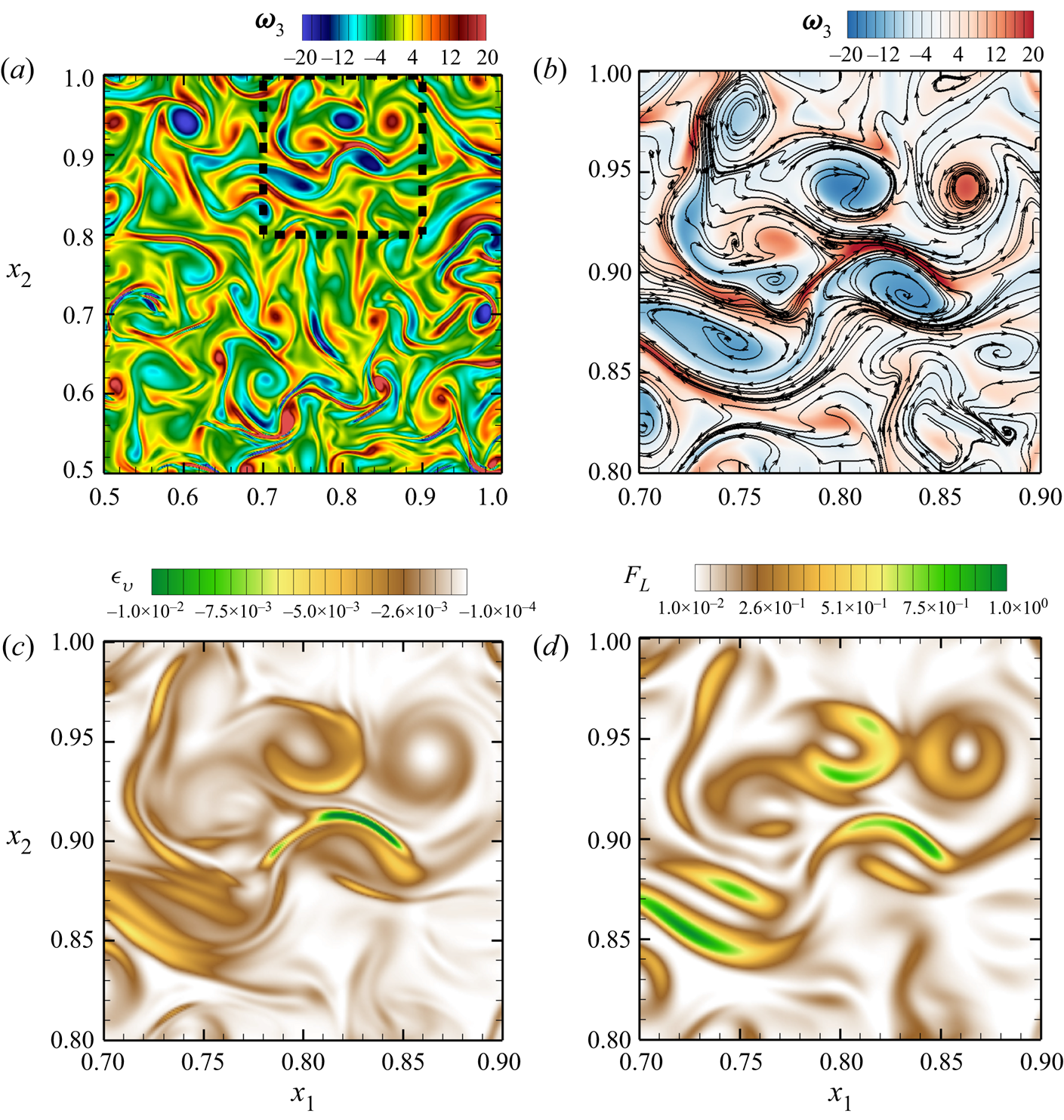
Interestingly, the dynamo behaviours for DC at  $\mathcal {R}=3$ with no-slip and free-slip boundary conditions are found to be very different. In figure 10(a) the strength of the vortices (represented by the horizontally averaged enstrophy, $1/2\ \overline {\omega _{i}\omega _{i}}$) is an order of magnitude higher near the walls for the no-slip boundary condition case as compared with the free-slip boundary condition case. This increase may be attributed to Ekman pumping (Hopfinger & Van Heijst Reference Hopfinger and Van Heijst1993). Apart from higher vertical r.m.s. magnetic field strength ( $b_{3,rms}$), an amplification in the horizontal magnetic field strength in the $x_{1}$ direction ( $b_{1,rms}$) is also observed near the wall for the case with the no-slip boundary condition in comparison with the case with the free-slip boundary condition (see figure 10b). Because of higher enstrophy, the stretching of magnetic field lines by these vortices, and consequently the increase in the Lorentz force near the walls, is higher with no-slip boundary conditions as compared with free-slip boundary conditions (figure 5d, f). This increase in Lorentz force leads to magnetorelaxation in the TBL that promotes turbulence and heat transfer enhancement. We do not observe such enhancement in heat transport with free-slip boundary conditions. It should be noted here that, for perfectly conducting boundaries, the r.m.s. magnetic field has to become parallel to the plates with $b_{3,rms}\xrightarrow {}0$ near the walls (figure 10b). As the field cannot escape the boundaries, a build-up of Lorentz force can be expected (St Pierre Reference St Pierre1993). Investigations with insulated wall boundary conditions will be carried out in the future to check whether this mechanism is exclusive to the present combination of boundary conditions.
Comparison of results for DC at  $\mathcal {R}=3$ between no-slip and free-slip conditions: (a) enstrophy and (b) r.m.s. field strength. Vertical variations are presented after averaging all quantities in the horizontal planes.
4. Conclusions
We have performed turbulence resolving simulations of the plane layer dynamo. Our study reveals the presence of an optimum thermal forcing at which heat transfer in DC is most efficient compared with RC. The novelty of this investigation is in reporting that a local increase in the Lorentz force at the TBL edge (figure 5d) is the cause of this enhanced heat transport instead of a global balance between the Lorentz and the Coriolis forces. This local increase in the Lorentz force mitigates the turbulence suppression by the Coriolis force, and can be viewed as local magnetorelaxation at the TBL. This local magnetorelaxation phenomenon results in an increase in the population of plumes and columnar structures (figure 8c) that increases the intensity of turbulence and kinetic energy dissipation, especially near the walls (figure 7). We also demonstrate that the stretching of the magnetic field lines around the vortices near the wall is the reason for this enhanced Lorentz force in the TBL (figure 9). Therefore, the present simulations reveal that capturing the boundary layer dynamics is imperative for understanding the heat transfer characteristics in DC, and therefore further investigation of the near-wall behaviour of dynamos is warranted.
It should be reiterated here that the traditional definition of the Elsasser number,  $\varLambda$, is unsuitable for dynamo simulations (Soderlund et al. Reference Soderlund, Sheyko, King and Aurnou2015; Aurnou & King Reference Aurnou and King2017; Calkins Reference Calkins2018). The Elsasser number in a dynamo simulation is not an input parameter that can be externally controlled, unlike in low $Re_m$ magnetoconvection experiments. Therefore, in this study, we chose to plot the heat transfer variation against $\mathcal {R}$, which is more common for heat transfer studies of scaling laws of convection with or without rotation or a magnetic field (Plumley & Julien Reference Plumley and Julien2019). The enhancement of heat transfer at lower values of $\mathcal {R}$ indicates a change of scaling law in strong RC due to the dynamo action. This parameter choice will help in designing future experiments to facilitate the search for heat transfer scaling laws for DC.
Funding
We gratefully acknowledge the support of the Science and Engineering Research Board, Government of India grant no. SERB/ME/2020318. We also want to thank the Office of Research and Development, Indian Institute of Technology Kanpur for the financial support through grant no. IITK/ME/2019194. The support and the resources provided by PARAM Sanganak under the National Supercomputing Mission, Government of India at the Indian Institute of Technology, Kanpur are gratefully acknowledged. We would also like to thank the anonymous referees whose helpful suggestions improved the quality of this paper.
Declaration of interests
The authors report no conflict of interest.
Author contributions
The authors contributed equally to analysing data and reaching conclusions, and in writing the paper.


 Open access