














1 Introduction
The kinetic framework is a general paradigm that aims to extend Boltzmann’s kinetic theory for dilute gases to other types of microscopic interacting systems. This approach has been highly informative, and became a cornerstone of the theory of nonequilibrium statistical mechanics for a large body of systems [Reference Spohn43, Reference Spohn44]. In the context of nonlinear dispersive waves, this framework was initiated in the first half of the past century [Reference Peierls41] and developed into what is now called wave turbulence theory [Reference Zakharov, L’vov and Falkovich51, Reference Nazarenko39]. There, waves of different frequencies interact nonlinearly at the microscopic level, and the goal is to extract an effective macroscopic picture of how the energy densities of the system evolve.
The description of such an effective evolution comes via the wave kinetic equation (WKE), which is the analogue of Boltzmann’s equation for nonlinear wave systems [Reference Spohn46]. Such kinetic equations have been derived at a formal level for many systems of physical interest (nonlinear Schrödinger (NLS) and nonlinear wave (NLW) equations, water waves, plasma models, lattice crystal dynamics, etc.; compare [Reference Nazarenko39] for a textbook treatment) and are used extensively in applications (thermal conductivity in crystals [Reference Spohn45], ocean forecasting [Reference Janssen31, Reference Burns49], and more). This kinetic description is conjectured to appear in the limit where the number of (locally interacting) waves goes to infinity and an appropriate measure of the interaction strength goes to zero (weak nonlinearityFootnote 1 ). In such kinetic limits, the total energy of the whole system often diverges.
The fundamental mathematical question here, which also has direct consequences for the physical theory, is to provide a rigorous justification of such wave kinetic equations starting from the microscopic dynamics given by the nonlinear dispersive model at hand. The importance of such an endeavour stems from the fact that it allows an understanding of the exact regimes and the limitations of the kinetic theory, which has long been a matter of scientific interest (see [Reference Denissenko, Lukaschuk and Nazarenko20, Reference Aubourg, Campagne, Peureux, Ardhuin, Sommeria, Viboud and Mordant1]). A few mathematical investigations have recently been devoted to studying problems in this spirit [Reference Faou23, Reference Buckmaster, Germain, Hani and Shatah7, Reference Lukkarinen and Spohn35], yielding some partial results and useful insights.
This manuscript continues the investigation initiated in [Reference Buckmaster, Germain, Hani and Shatah7], aimed at providing a rigorous justification of the wave kinetic equation corresponding to the nonlinear Schrödinger equation,
 $$ \begin{align*} i \partial_t v - \Delta v + \left\lvert v\right\rvert^{2} v=0. \end{align*} $$
As we shall explain later, the sign of the nonlinearity has no effect on the kinetic description, so we choose the defocussing sign for concreteness. The natural setup for the problem is to start with a spatial domain given by a torus ${\mathbb T}^d_L$
of size L, which approaches infinity in the thermodynamic limit we seek. This torus can be rational or irrational, which amounts to rescaling the Laplacian into
${\mathbb T}^d_L$
of size L, which approaches infinity in the thermodynamic limit we seek. This torus can be rational or irrational, which amounts to rescaling the Laplacian into
 $$ \begin{align*} \Delta_{\beta} \mathrel{\mathop:}= \frac{1}{2\pi} \sum\limits_{i=1}^d \beta_i \partial_i^2, \qquad \beta \mathrel{\mathop:}= (\beta_1,\dots,\beta_d)\in [1,2]^d, \end{align*} $$
and taking the spatial domain to be the standard torus of size L, namely ${\mathbb T}^d_L=[0,L]^d$
with periodic boundary conditions. With this normalisation, an irrational torus would correspond to taking the
${\mathbb T}^d_L=[0,L]^d$
with periodic boundary conditions. With this normalisation, an irrational torus would correspond to taking the $\beta _j$
to be rationally independent. Our results cover both cases, and in part of them
$\beta _j$
to be rationally independent. Our results cover both cases, and in part of them $\beta $
is assumed to be generic – that is, avoiding a set of Lebesgue measure
$\beta $
is assumed to be generic – that is, avoiding a set of Lebesgue measure $0$
.
$0$
.
The strength of the nonlinearity is related to the characteristic size $\lambda $
of the initial data (say in the conserved
$\lambda $
of the initial data (say in the conserved $L^2$
space). Adopting the ansatz
$L^2$
space). Adopting the ansatz $v=\lambda u$
, we arrive at the following equation:
$v=\lambda u$
, we arrive at the following equation:
 $$ \begin{align} \begin{cases} i \partial_t u - \Delta_{\beta} u + \lambda^{2} \left\lvert u\right\rvert^{2} u=0, \quad x\in \mathbb{T}_L^d = [0,L]^d, \\ u(0,x) = u_{\text{in}}(x). \end{cases} \end{align} $$
The kinetic description of the long-time behaviour is akin to a law of large numbers, and therefore one has to start with a random distribution of the initial data. Heuristically, a randomly distributed, $L^{2}$
-normalised field would (with high probability) have a roughly uniform spatial distribution, and consequently an
$L^{2}$
-normalised field would (with high probability) have a roughly uniform spatial distribution, and consequently an $L_x^{\infty }$
norm
$L_x^{\infty }$
norm $\sim L^{-d/2}$
. This makes the strength of the nonlinearity in (NLS) comparable to
$\sim L^{-d/2}$
. This makes the strength of the nonlinearity in (NLS) comparable to $\lambda ^2 L^{-d}$
(at least initiallyFootnote
2
), which motivates us to introduce the quantity
$\lambda ^2 L^{-d}$
(at least initiallyFootnote
2
), which motivates us to introduce the quantity
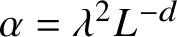
 $$ \begin{align*} \alpha=\lambda^2L^{-d} \end{align*} $$
and phrase the results in terms of $\alpha $
instead of
$\alpha $
instead of $\lambda $
. The kinetic conjecture states that at sufficiently long time scales, the effective dynamics of the Fourier-space mass density
$\lambda $
. The kinetic conjecture states that at sufficiently long time scales, the effective dynamics of the Fourier-space mass density $\mathbb E \left \lvert \widehat u(t, k)\right \rvert ^2 \left (k \in \mathbb Z^d_L=L^{-1}\mathbb Z^d\right )$
is well approximated – in the limit of large L and vanishing
$\mathbb E \left \lvert \widehat u(t, k)\right \rvert ^2 \left (k \in \mathbb Z^d_L=L^{-1}\mathbb Z^d\right )$
is well approximated – in the limit of large L and vanishing $\alpha $
– by an appropriately scaled solution
$\alpha $
– by an appropriately scaled solution $n(t, \xi )$
of the following WKE:
$n(t, \xi )$
of the following WKE:
 $$ \begin{align} \partial_t n(t, \xi) &={\mathcal K}\left(n(t, \cdot)\right), \nonumber \\ {\mathcal K}(\phi)(\xi)&:= \int_{\substack{\left(\xi_1, \xi_2, \xi_3\right)\in {\mathbb R}^{3d} \\ \xi_1-\xi_2+\xi_3=\xi}} \phi \phi_1 \phi_2 \phi_3\left(\frac{1}{\phi}-\frac{1}{\phi_1}+\frac{1}{\phi_2}-\frac{1}{\phi_3}\right)\delta_{{\mathbb R}}\left(\left\lvert\xi_1\right\rvert_{\beta}^2-\left\lvert\xi_2\right\rvert_{\beta}^2+\left\lvert\xi_3\right\rvert_{\beta}^2-\left\lvert\xi\right\rvert_{\beta}^2\right) d\xi_1 d\xi_2 d\xi_3, \end{align} $$
where we used the shorthand notations $\phi _j:=\phi \left (\xi _j\right )$
and
$\phi _j:=\phi \left (\xi _j\right )$
and $\left \lvert \xi \right \rvert ^2_{\beta }=\sum _{j=1}^d \beta _j \left (\xi ^{\left (j\right )}\right )^2$
for
$\left \lvert \xi \right \rvert ^2_{\beta }=\sum _{j=1}^d \beta _j \left (\xi ^{\left (j\right )}\right )^2$
for $\xi =\left (\xi ^{(1)},\cdots ,\xi ^{(d)}\right )$
. More precisely, one expects this approximation to hold at the kinetic timescale
$\xi =\left (\xi ^{(1)},\cdots ,\xi ^{(d)}\right )$
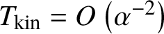
. More precisely, one expects this approximation to hold at the kinetic timescale $T_{\mathrm {kin}}\sim \alpha ^{-2}=\frac {L^{2d}}{\lambda ^4}$
, in the sense that
$T_{\mathrm {kin}}\sim \alpha ^{-2}=\frac {L^{2d}}{\lambda ^4}$
, in the sense that
 $$ \begin{align} \mathbb E \left\lvert\widehat u(t, k)\right\rvert^2 \approx n\left(\frac{t}{T_{\mathrm{kin}}}, k\right) \quad \text{as } L\to \infty, \alpha \to 0. \end{align} $$
Of course, for such an approximation to hold at time $t=0$
, one has to start with a well-prepared initial distribution for
$t=0$
, one has to start with a well-prepared initial distribution for $\widehat u_{\text {in}}(k)$
as follows: denoting by
$\widehat u_{\text {in}}(k)$
as follows: denoting by $n_{\text {in}}$
the initial data for (WKE), we assume
$n_{\text {in}}$
the initial data for (WKE), we assume
 $$ \begin{align} \widehat u_{\mathrm{in}}(k)=\sqrt{n_{\text{in}}(k)} \eta_{k}(\omega), \end{align} $$
where $\eta _{k}(\omega )$
are mean-
$\eta _{k}(\omega )$
are mean- $0$
complex random variables satisfying
$0$
complex random variables satisfying $\mathbb E \left \lvert \eta _k\right \rvert ^2=1$
. In what follows,
$\mathbb E \left \lvert \eta _k\right \rvert ^2=1$
. In what follows, $\eta _k(\omega )$
will be independent, identically distributed complex random variables, such that the law of each
$\eta _k(\omega )$
will be independent, identically distributed complex random variables, such that the law of each $\eta _k$
is either the normalised complex Gaussian or the uniform distribution on the unit circle
$\eta _k$
is either the normalised complex Gaussian or the uniform distribution on the unit circle $\lvert z\rvert =1$
.
$\lvert z\rvert =1$
.
Before stating our results, it is worth remarking on the regime of data and solutions covered by this kinetic picture in comparison to previously studied and well-understood regimes in the nonlinear dispersive literature. For this, let us look back at the (pre-ansatz) NLS solution v, whose conserved energy is given by
 $$ \begin{align*} {\mathcal E}[v]:=\int_{{\mathbb T}^d_L} \frac{1}{2}\left\lvert\nabla v\right\rvert^2 +\frac{1}{4}\left\lvert v\right\rvert^4 \mathrm{d}x. \end{align*} $$
We are dealing with solutions having an $L^{\infty }$
-norm of
$L^{\infty }$
-norm of $O\left (\sqrt \alpha \right )$
(with high probability) and whose total mass is
$O\left (\sqrt \alpha \right )$
(with high probability) and whose total mass is $O\left (\alpha L^d\right )$
, in a regime where
$O\left (\alpha L^d\right )$
, in a regime where $\alpha $
is vanishingly small and L is asymptotically large. These bounds on the solutions are true initially, as we have already explained, and will be propagated in our proof. In particular, the mass and energy are very large and will diverge in this kinetic limit, as is common in taking thermodynamic limits [Reference Ruelle42, Reference Minlos37]. Moreover, the potential part of the energy is dominated by the kinetic part – the former of size
$\alpha $
is vanishingly small and L is asymptotically large. These bounds on the solutions are true initially, as we have already explained, and will be propagated in our proof. In particular, the mass and energy are very large and will diverge in this kinetic limit, as is common in taking thermodynamic limits [Reference Ruelle42, Reference Minlos37]. Moreover, the potential part of the energy is dominated by the kinetic part – the former of size $O\left (\alpha ^3 L^d\right )$
and the latter of size
$O\left (\alpha ^3 L^d\right )$
and the latter of size $O\left (\alpha L^d\right )$
– which explains why there is no distinction between the defocussing and focussing nonlinearities in the kinetic limit. It would be interesting to see how the kinetic framework can be extended to regimes of solutions which are sensitive to the sign of the nonlinearity; this has been investigated in the physics literature (e.g., [Reference Dyachenko, Newell, Pushkarev and Zakharov22, Reference Fitzmaurice, Gurarie, McCaughan and Woyczynski25, Reference Zakharov, Korotkevich, Pushkarev and Resio50]).
$O\left (\alpha L^d\right )$
– which explains why there is no distinction between the defocussing and focussing nonlinearities in the kinetic limit. It would be interesting to see how the kinetic framework can be extended to regimes of solutions which are sensitive to the sign of the nonlinearity; this has been investigated in the physics literature (e.g., [Reference Dyachenko, Newell, Pushkarev and Zakharov22, Reference Fitzmaurice, Gurarie, McCaughan and Woyczynski25, Reference Zakharov, Korotkevich, Pushkarev and Resio50]).
1.1 Statement of the results
It is not a priori clear how the limits $L\to \infty $
and
$L\to \infty $
and $\alpha \to 0$
need to be taken for formula (1.1) to hold or whether there is an additional scaling law (between
$\alpha \to 0$
need to be taken for formula (1.1) to hold or whether there is an additional scaling law (between $\alpha $
and L) that needs to be satisfied in the limit. In comparison, such scaling laws are imposed in the rigorous derivation of Boltzmann’s equation [Reference Lanford34, Reference Cercignani, Illner and Pulvirenti10, Reference Gallagher, Saint-Raymond and Texier26], which is derived in the so-called Boltzmann–Grad limit [Reference Grad27]: namely, the number N of particles goes to
$\alpha $
and L) that needs to be satisfied in the limit. In comparison, such scaling laws are imposed in the rigorous derivation of Boltzmann’s equation [Reference Lanford34, Reference Cercignani, Illner and Pulvirenti10, Reference Gallagher, Saint-Raymond and Texier26], which is derived in the so-called Boltzmann–Grad limit [Reference Grad27]: namely, the number N of particles goes to $\infty $
while their radius r goes to
$\infty $
while their radius r goes to $0$
in such a way that
$0$
in such a way that $Nr^{d-1}\sim O(1)$
. To the best of our knowledge, this central point has not been adequately addressed in the wave-turbulence literature.
$Nr^{d-1}\sim O(1)$
. To the best of our knowledge, this central point has not been adequately addressed in the wave-turbulence literature.
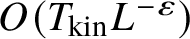
Our results seem to suggest some key differences depending on the chosen scaling law. Roughly speaking, we identify two special scaling laws for which we are able to justify the approximation (1.1) up to time scales $L^{-\varepsilon } T_{\text {kin}}$
for any arbitrarily small
$L^{-\varepsilon } T_{\text {kin}}$
for any arbitrarily small $\varepsilon>0$
. For other scaling laws, we identify significant absolute divergences in the power-series expansion for
$\varepsilon>0$
. For other scaling laws, we identify significant absolute divergences in the power-series expansion for $\mathbb E \left \lvert \widehat u(t, k)\right \rvert ^2$
at much earlier times. We can therefore only justify this approximation at such shorter times (which are still better than those in [Reference Buckmaster, Germain, Hani and Shatah7]). In these cases, whether or not formula (1.1) holds up to time scales
$\mathbb E \left \lvert \widehat u(t, k)\right \rvert ^2$
at much earlier times. We can therefore only justify this approximation at such shorter times (which are still better than those in [Reference Buckmaster, Germain, Hani and Shatah7]). In these cases, whether or not formula (1.1) holds up to time scales $L^{-\varepsilon } T_{\text {kin}}$
depends on whether such series converge conditionally instead of absolutely, and thus would require new methods and ideas, as we explain later.
$L^{-\varepsilon } T_{\text {kin}}$
depends on whether such series converge conditionally instead of absolutely, and thus would require new methods and ideas, as we explain later.
We start by identifying the two favourable scaling laws. We use the notation $\sigma +$
for any numerical constant
$\sigma +$
for any numerical constant $\sigma $
(e.g.,
$\sigma $
(e.g., $\sigma =-\varepsilon $
or
$\sigma =-\varepsilon $
or $\sigma =-1-\frac {\varepsilon }{2}$
, where
$\sigma =-1-\frac {\varepsilon }{2}$
, where $\varepsilon $
is as in Theorem 1.1) to denote a constant that is strictly larger than and sufficiently close to
$\varepsilon $
is as in Theorem 1.1) to denote a constant that is strictly larger than and sufficiently close to $\sigma $
.
$\sigma $
.
Theorem 1.1. Set $d\geq 2$
and let
$d\geq 2$
and let $\beta \in [1,2]^d$
be arbitrary. Suppose that
$\beta \in [1,2]^d$
be arbitrary. Suppose that $n_{\mathrm {in}} \in {\mathcal S}\left ({\mathbb R}^d \to [0, \infty )\right )$
is SchwartzFootnote
3
and
$n_{\mathrm {in}} \in {\mathcal S}\left ({\mathbb R}^d \to [0, \infty )\right )$
is SchwartzFootnote
3
and $\eta _{k}(\omega )$
are independent, identically distributed complex random variables, such that the law of each
$\eta _{k}(\omega )$
are independent, identically distributed complex random variables, such that the law of each $\eta _k$
is either complex Gaussian with mean
$\eta _k$
is either complex Gaussian with mean $0$
and variance
$0$
and variance $1$
or the uniform distribution on the unit circle
$1$
or the uniform distribution on the unit circle $\lvert z\rvert =1$
. Assume well-prepared initial data
$\lvert z\rvert =1$
. Assume well-prepared initial data $u_{\mathrm {in}}$
for (NLS) as in equation (1.2).
$u_{\mathrm {in}}$
for (NLS) as in equation (1.2).
Fix $0<\varepsilon <1$
(in most interesting cases
$0<\varepsilon <1$
(in most interesting cases $\varepsilon $
will be small); recall that
$\varepsilon $
will be small); recall that $\lambda $
and L are the parameters in (NLS) and let
$\lambda $
and L are the parameters in (NLS) and let $\alpha =\lambda ^2L^{-d}$
be the characteristic strength of the nonlinearity. If
$\alpha =\lambda ^2L^{-d}$
be the characteristic strength of the nonlinearity. If $\alpha $
has the scaling law
$\alpha $
has the scaling law $\alpha \sim L^{(-\varepsilon )+}$
or
$\alpha \sim L^{(-\varepsilon )+}$
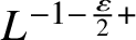
or $\alpha \sim L^{\left (-1-\frac {\varepsilon }{2}\right )+}$
, then we have
$\alpha \sim L^{\left (-1-\frac {\varepsilon }{2}\right )+}$
, then we have
 $$ \begin{align} \mathbb E \left\lvert\widehat u(t, k)\right\rvert^2 =n_{\mathrm{in}}(k)+\frac{t}{T_{\mathrm{kin}}}{\mathcal K}(n_{\mathrm{in}})(k)+o_{\ell^{\infty}_k}\left(\frac{t}{T_{\mathrm {kin}}}\right)_{L \to \infty} \end{align} $$
for all $L^{0+} \leq t \leq L^{-\varepsilon } T_{\mathrm {kin}}$
, where
$L^{0+} \leq t \leq L^{-\varepsilon } T_{\mathrm {kin}}$
, where $T_{\mathrm {kin}}=\alpha ^{-2}/2$
,
$T_{\mathrm {kin}}=\alpha ^{-2}/2$
, ${\mathcal K}$
is defined in (WKE) and
${\mathcal K}$
is defined in (WKE) and $o_{\ell ^{\infty }_k}\left (\frac {t}{T_{\mathrm {kin}}}\right )_{L \to \infty }$
is a quantity that is bounded in
$o_{\ell ^{\infty }_k}\left (\frac {t}{T_{\mathrm {kin}}}\right )_{L \to \infty }$
is a quantity that is bounded in $\ell ^{\infty }_k$
by
$\ell ^{\infty }_k$
by $L^{-\theta } \frac {t}{T_{\mathrm {kin}}}$
for some
$L^{-\theta } \frac {t}{T_{\mathrm {kin}}}$
for some $\theta>0$
.
$\theta>0$
.
We remark that in the time interval of the approximation we have been discussing, the right hand sides of formulas (1.1) and (1.3) are equivalent. Also note that any type of scaling law of the form $\alpha \sim L^{-s}$
gives an upper bound of
$\alpha \sim L^{-s}$
gives an upper bound of $t\leq L^{-\varepsilon }T_{\mathrm {kin}}\sim L^{2s-\varepsilon }$
for the times considered. Consequently, for the two scaling laws in Theorem 1.1, the time t always satisfies
$t\leq L^{-\varepsilon }T_{\mathrm {kin}}\sim L^{2s-\varepsilon }$
for the times considered. Consequently, for the two scaling laws in Theorem 1.1, the time t always satisfies $t\ll L^{2}$
, and it is for this reason that the rationality type of the torus is not relevant. As will be clear later, no similar results can hold for
$t\ll L^{2}$
, and it is for this reason that the rationality type of the torus is not relevant. As will be clear later, no similar results can hold for $t\gg L^2$
in the case of a rational torus,Footnote
4
as this would require rational quadratic forms to be equidistributed on scales
$t\gg L^2$
in the case of a rational torus,Footnote
4
as this would require rational quadratic forms to be equidistributed on scales $\ll 1$
, which is impossible. However, if the aspect ratios
$\ll 1$
, which is impossible. However, if the aspect ratios $\beta $
are assumed to be generically irrational, then one can access equidistribution scales that are as small as
$\beta $
are assumed to be generically irrational, then one can access equidistribution scales that are as small as $L^{-d+1}$
for the resulting irrational quadratic forms [Reference Bourgain4, Reference Buckmaster, Germain, Hani and Shatah7]. This allows us to consider scaling laws for which
$L^{-d+1}$
for the resulting irrational quadratic forms [Reference Bourgain4, Reference Buckmaster, Germain, Hani and Shatah7]. This allows us to consider scaling laws for which $T_{\mathrm {kin}}$
can be as big as
$T_{\mathrm {kin}}$
can be as big as $L^{d-}$
on generically irrational tori.
$L^{d-}$
on generically irrational tori.
Remark 1.2. Strictly speaking, in evaluating equation (1.3) one has to first ensure the existence of the solution u. This is guaranteed if $d\in \{2,3,4\}$
(when (NLS) is
$d\in \{2,3,4\}$
(when (NLS) is $H^1$
-critical or subcritical). When
$H^1$
-critical or subcritical). When $d\geq 5$
we shall interpret equation (1.3) such that the expectation is taken only when the long-time smooth solution u exists. Moreover, from our proof it follows that the probability that this existence fails is at most
$d\geq 5$
we shall interpret equation (1.3) such that the expectation is taken only when the long-time smooth solution u exists. Moreover, from our proof it follows that the probability that this existence fails is at most $O\left (e^{-L^{\theta }}\right )$
, which quickly becomes negligible when
$O\left (e^{-L^{\theta }}\right )$
, which quickly becomes negligible when $L\to \infty $
.
$L\to \infty $
.
The following theorem covers general scaling laws, including the ones that can only be accessed for the generically irrational torus. By a simple calculation of exponents, we can see that it implies Theorem 1.1.
Theorem 1.3. With the same assumptions as in Theorem 1.1, we impose the following conditions on $(\alpha , L, T)$
for some
$(\alpha , L, T)$
for some $\delta>0$
:
$\delta>0$
:
 $$ \begin{align}T\leq \begin{cases}L^{2-\delta}&\text{if }\beta_i\text{ is arbitrary},\\ L^{d-\delta}&\text{if }\beta_i\text{ is generic}, \end{cases} \qquad\alpha\leq \begin{cases} L^{-\delta}T^{-1}&\text{if }T \leq L,\\ L^{-1-\delta}&\text{if }L\leq T\leq L^2,\\ L^{1-\delta}T^{-1}&\text{if } T\geq L^2. \end{cases} \end{align} $$
Then formula (1.3) holds for all $L^{\delta } \leq t \leq T$
.
$L^{\delta } \leq t \leq T$
.
It is best to read this theorem in terms of the $\left (\log _L \left (\alpha ^{-1}\right ),\log _L T\right )$
plot in Figure 1. The kinetic conjecture corresponds to justifying the approximation in formula (1.1) up to time scales
$\left (\log _L \left (\alpha ^{-1}\right ),\log _L T\right )$
plot in Figure 1. The kinetic conjecture corresponds to justifying the approximation in formula (1.1) up to time scales $T\lesssim T_{\mathrm {kin}}=\alpha ^{-2}$
. As we shall explain later, the time scale
$T\lesssim T_{\mathrm {kin}}=\alpha ^{-2}$
. As we shall explain later, the time scale $T\sim T_{\mathrm {kin}}$
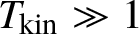
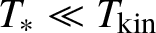
represents a critical scale for the problem from a probabilistic point of view. This is depicted by the red line in the figure, and the region below this line corresponds to a probabilistically subcritical regime (see Section 1.2.1). The shaded blue region corresponds to the
$T\sim T_{\mathrm {kin}}$
represents a critical scale for the problem from a probabilistic point of view. This is depicted by the red line in the figure, and the region below this line corresponds to a probabilistically subcritical regime (see Section 1.2.1). The shaded blue region corresponds to the $(\alpha , T)$
region in Theorem 1.3, neglecting
$(\alpha , T)$
region in Theorem 1.3, neglecting $\delta $
losses. This region touches the line
$\delta $
losses. This region touches the line $T=\alpha ^{-2}$
at the two points corresponding to
$T=\alpha ^{-2}$
at the two points corresponding to $\left (\alpha ^{-1}, T\right )=(1, 1)$
and
$\left (\alpha ^{-1}, T\right )=(1, 1)$
and $\left (L, L^2\right )$
, whereas the two scaling laws of Theorem 1.1, where
$\left (L, L^2\right )$
, whereas the two scaling laws of Theorem 1.1, where $\left (\alpha ^{-1},T\right )\sim (L^{\varepsilon -},L^{\varepsilon -})$
and
$\left (\alpha ^{-1},T\right )\sim (L^{\varepsilon -},L^{\varepsilon -})$
and $\left (\alpha ^{-1},T\right )\sim \left (L^{1+\frac {\varepsilon }{2}-},L^{2-}\right )$
, approach these two points when
$\left (\alpha ^{-1},T\right )\sim \left (L^{1+\frac {\varepsilon }{2}-},L^{2-}\right )$
, approach these two points when $\varepsilon $
is small.
$\varepsilon $
is small.
Admissible range for $(\alpha , L, T)$
in the
$(\alpha , L, T)$
in the $\left (\log _L \left (\alpha ^{-1}\right ),\log _L T\right )$
plot when
$\left (\log _L \left (\alpha ^{-1}\right ),\log _L T\right )$
plot when $d\geq 3$
. The coloured region is the range of Theorem 1.3 (up to
$d\geq 3$
. The coloured region is the range of Theorem 1.3 (up to $\varepsilon $
endpoint accuracy). The red line denotes the case when
$\varepsilon $
endpoint accuracy). The red line denotes the case when $T=T_{\mathrm {kin}}=\alpha ^{-2}$
, which our coloured region touches at two points corresponding to
$T=T_{\mathrm {kin}}=\alpha ^{-2}$
, which our coloured region touches at two points corresponding to $T\sim 1$
and
$T\sim 1$
and $T\sim L^{2}$
.
$T\sim L^{2}$
.

These results rely on a diagrammatic expansion of the NLS solution in Feynman diagrams akin to a Taylor expansion. The shaded blue region depicting the result of Theorem 1.3 corresponds to the cases when such a diagrammatic expansion is absolutely convergent for very large L. In the complementary region between the blue region and the line $T=T_{\text {kin}}$
, we show that some (arbitrarily high-degree) terms of this expansion do not converge to
$T=T_{\text {kin}}$
, we show that some (arbitrarily high-degree) terms of this expansion do not converge to $0$
as their degree goes to
$0$
as their degree goes to $\infty $
, which means that the diagrammatic expansion cannot converge absolutely in this region. Therefore, the only way for the kinetic conjecture to be true in the scaling regimes not included in Theorem 1.1 is for those terms to exhibit a highly nontrivial cancellation, which would make the series converge conditionally but not absolutely.
$\infty $
, which means that the diagrammatic expansion cannot converge absolutely in this region. Therefore, the only way for the kinetic conjecture to be true in the scaling regimes not included in Theorem 1.1 is for those terms to exhibit a highly nontrivial cancellation, which would make the series converge conditionally but not absolutely.
Finally, we remark on the restriction in formula (1.4). The upper bounds on T on the left are necessary from number-theoretic considerations: indeed, if $T\gg L^2$
for a rational torus, or if
$T\gg L^2$
for a rational torus, or if $T\gg L^d$
for an irrational one, the exact resonances of the NLS equation dominate the quasi-resonant interactions that lead to the kinetic wave equation. One should therefore not expect the kinetic description to hold in those ranges of T (see Lemma 3.2 and Section 4). The second set of restrictions in formula (1.4) correspond exactly to the requirement that the size of the Feynman diagrams of degree n can be bounded by
$T\gg L^d$
for an irrational one, the exact resonances of the NLS equation dominate the quasi-resonant interactions that lead to the kinetic wave equation. One should therefore not expect the kinetic description to hold in those ranges of T (see Lemma 3.2 and Section 4). The second set of restrictions in formula (1.4) correspond exactly to the requirement that the size of the Feynman diagrams of degree n can be bounded by $\rho ^n$
with some
$\rho ^n$
with some $\rho \ll 1$
. In fact, if one aims only at proving existence with high probability (not caring about the asymptotics of
$\rho \ll 1$
. In fact, if one aims only at proving existence with high probability (not caring about the asymptotics of $\mathbb {E}\left \lvert \widehat {u}(t,k)\right \rvert ^2$
), then the restrictions on the left of formula (1.4) will not be necessary, and one obtains control for longer times. See also the following remark:
$\mathbb {E}\left \lvert \widehat {u}(t,k)\right \rvert ^2$
), then the restrictions on the left of formula (1.4) will not be necessary, and one obtains control for longer times. See also the following remark:
Remark 1.4 Admissible scaling laws
The foregoing restrictions on T impose the limits of the admissible scaling laws, in which $\alpha \to 0$
and
$\alpha \to 0$
and $L \to \infty $
, for which the kinetic description of the long-time dynamics can appear. Indeed, since
$L \to \infty $
, for which the kinetic description of the long-time dynamics can appear. Indeed, since $T_{\mathrm {kin}}=\alpha ^{-2}$
, then the necessary (up to
$T_{\mathrm {kin}}=\alpha ^{-2}$
, then the necessary (up to $L^{\delta }$
factors) restrictions
$L^{\delta }$
factors) restrictions $T\ll L^{2-\delta }$
(resp.,
$T\ll L^{2-\delta }$
(resp., $T\ll L^{d-\delta }$
) on the rational (resp., irrational) torus already mentioned imply that one should only expect the previous kinetic description in the regime where
$T\ll L^{d-\delta }$
) on the rational (resp., irrational) torus already mentioned imply that one should only expect the previous kinetic description in the regime where $\alpha \gtrsim L^{-1}$
(resp.,
$\alpha \gtrsim L^{-1}$
(resp., $\gtrsim L^{-d/2}$
). In other words, the kinetic description requires the nonlinearity to be weak, but not too weak! In the complementary regime of very weak nonlinearity, the exact resonances of the equation dominate the quasi-resonances – a regime referred to as discrete wave turbulence (see [Reference L’vov and Nazarenko36, Reference Kartashova32, Reference Nazarenko39]), in which different effective equations, like the (CR) equation in [Reference Faou, Germain and Hani24, Reference Buckmaster, Germain, Hani and Shatah6], can arise.
$\gtrsim L^{-d/2}$
). In other words, the kinetic description requires the nonlinearity to be weak, but not too weak! In the complementary regime of very weak nonlinearity, the exact resonances of the equation dominate the quasi-resonances – a regime referred to as discrete wave turbulence (see [Reference L’vov and Nazarenko36, Reference Kartashova32, Reference Nazarenko39]), in which different effective equations, like the (CR) equation in [Reference Faou, Germain and Hani24, Reference Buckmaster, Germain, Hani and Shatah6], can arise.
1.2 Ideas of the proof
As Theorem 1.1 is a consequence of Theorem 1.3, we will focus on Theorem 1.3. The proof of Theorem 1.3 contains three components: ( $1$
) a long-time well-posedness result, where we expand the solution to (NLS) into Feynman diagrams for sufficiently long time, up to a well-controlled error term; (
$1$
) a long-time well-posedness result, where we expand the solution to (NLS) into Feynman diagrams for sufficiently long time, up to a well-controlled error term; ( $2$
) computation of
$2$
) computation of $\mathbb E\left \lvert \widehat u_k(t)\right \rvert ^2 \left (k \in \mathbb Z^d_L\right )$
using this expansion, where we identify the leading terms and control the remainders; and (
$\mathbb E\left \lvert \widehat u_k(t)\right \rvert ^2 \left (k \in \mathbb Z^d_L\right )$
using this expansion, where we identify the leading terms and control the remainders; and ( $3$
) a number-theoretic result that justifies the large box approximation, where we pass from the sums appearing in the expansion in the previous component to the integral appearing on the right-hand side of (WKE).
$3$
) a number-theoretic result that justifies the large box approximation, where we pass from the sums appearing in the expansion in the previous component to the integral appearing on the right-hand side of (WKE).
The main novelty of this work is in the first component, which is the hardest. The second component follows similar lines to those in [Reference Buckmaster, Germain, Hani and Shatah7]. Regarding the third component, the main novelty of this work is to complement the number-theoretic results in [Reference Buckmaster, Germain, Hani and Shatah7] (which dealt only with the generically irrational torus) by the cases of general tori (in the admissible range of time $T\ll L^2$
). This provides an essentially full (up to
$T\ll L^2$
). This provides an essentially full (up to $L^{\varepsilon }$
losses) understanding of the number-theoretic issues arising in wave-turbulence derivations for (NLS). Therefore, we will limit this introductory discussion to the first component.
$L^{\varepsilon }$
losses) understanding of the number-theoretic issues arising in wave-turbulence derivations for (NLS). Therefore, we will limit this introductory discussion to the first component.
1.2.1 The scheme and probabilistic criticality
Though technically involved, the basic idea of the long-time well-posedness argument is in fact quite simple. Starting from (NLS) with initial data of equation (1.2), we write the solution as
 $$ \begin{align} u=u^{(0)}+\cdots+u^{(N)}+\mathcal R_{N+1}, \end{align} $$
where $u^{(0)}=e^{-it\Delta _{\beta }}u_{\mathrm {in}}$
is the linear evolution,
$u^{(0)}=e^{-it\Delta _{\beta }}u_{\mathrm {in}}$
is the linear evolution, $u^{(n)}$
are iterated self-interactions of the linear solution
$u^{(n)}$
are iterated self-interactions of the linear solution $u^{(0)}$
that appear in a formal expansion of u and
$u^{(0)}$
that appear in a formal expansion of u and $\mathcal R_{N+1}$
is a sufficiently regular remainder term.
$\mathcal R_{N+1}$
is a sufficiently regular remainder term.
Since $u^{(0)}$
is a linear combination of independent random variables, and each
$u^{(0)}$
is a linear combination of independent random variables, and each $u^{(n)}$
is a multilinear combination, each of them will behave strictly better (both linearly and nonlinearly) than its deterministic analogue (i.e., with all
$u^{(n)}$
is a multilinear combination, each of them will behave strictly better (both linearly and nonlinearly) than its deterministic analogue (i.e., with all $\eta _k=1$
). This is due to the well-known large deviation estimates, which yield a ‘square root’ gain coming from randomness, akin to the central limit theorem (for instance,
$\eta _k=1$
). This is due to the well-known large deviation estimates, which yield a ‘square root’ gain coming from randomness, akin to the central limit theorem (for instance, $\left \lVert u_{\mathrm {in}}\right \rVert _{L^{\infty }}$
is bounded by
$\left \lVert u_{\mathrm {in}}\right \rVert _{L^{\infty }}$
is bounded by $L^{-d/2}\cdot \left \lVert u_{\mathrm {in}}\right \rVert _{L^2}$
in the probabilistic setting, as opposed to
$L^{-d/2}\cdot \left \lVert u_{\mathrm {in}}\right \rVert _{L^2}$
in the probabilistic setting, as opposed to $1\cdot \left \lVert u_{\mathrm {in}}\right \rVert _{L^2}$
deterministically by Sobolev embedding, assuming compact Fourier support). This gain leads to a new notion of criticality for the problem, which can be definedFootnote
5
as the edge of the regime of
$1\cdot \left \lVert u_{\mathrm {in}}\right \rVert _{L^2}$
deterministically by Sobolev embedding, assuming compact Fourier support). This gain leads to a new notion of criticality for the problem, which can be definedFootnote
5
as the edge of the regime of $(\alpha , T)$
for which the iterate
$(\alpha , T)$
for which the iterate $u^{(1)}$
is better bounded than the iterate
$u^{(1)}$
is better bounded than the iterate $u^{(0)}$
. It is not hard to see that
$u^{(0)}$
. It is not hard to see that $u^{(1)}$
can have size up to
$u^{(1)}$
can have size up to $O(\alpha\sqrt{T})$
(in appropriate norms), compared to the
$O(\alpha\sqrt{T})$
(in appropriate norms), compared to the $O(1)$
size of
$O(1)$
size of $u^{(0)}$
(see, e.g., formula (2.25) for
$u^{(0)}$
(see, e.g., formula (2.25) for $n=1$
). This justifies the notion that
$n=1$
). This justifies the notion that $T\sim T_{\mathrm {kin}}=\alpha ^{-2}$
corresponds to probabilistically critical scaling, whereas the time scales
$T\sim T_{\mathrm {kin}}=\alpha ^{-2}$
corresponds to probabilistically critical scaling, whereas the time scales $T\ll T_{\mathrm {kin}}$
are subcritical.Footnote
6
$T\ll T_{\mathrm {kin}}$
are subcritical.Footnote
6
As it happens, a certain notion of criticality might not capture all the subtleties of the problem. As we shall see, some higher-order iterates $u^{(n)}$
will not be better bounded than
$u^{(n)}$
will not be better bounded than $u^{(n-1)}$
in the full subcritical range
$u^{(n-1)}$
in the full subcritical range $T\ll \alpha ^{-2}$
we have postulated, but instead only in a subregion thereof. This is what defines our admissible blue region in Figure 1.
$T\ll \alpha ^{-2}$
we have postulated, but instead only in a subregion thereof. This is what defines our admissible blue region in Figure 1.
We should mention that the idea of using the gain from randomness goes back to Bourgain [Reference Bourgain3] (in the random-data setting) and to Da Prato and Debussche [Reference Da Prato and Debussche14] (later, in the stochastic PDE setting). They first noticed that the ansatz $u=u^{(0)}+\mathcal R$
allows one to put the remainder
$u=u^{(0)}+\mathcal R$
allows one to put the remainder $\mathcal R$
in a higher regularity space than the linear term
$\mathcal R$
in a higher regularity space than the linear term $u^{(0)}$
. This idea has since been applied to many different situations (see, e.g., [Reference Bourgain and Bulut5, Reference Burq and Tzvetkov8, Reference Colliander and Oh11, Reference Deng15, Reference Dodson, Lührmann and Mendelson21, Reference Kenig and Mendelson33, Reference Nahmod and Staffilani38]), though most of these works either involve only the first-order expansion (i.e.,
$u^{(0)}$
. This idea has since been applied to many different situations (see, e.g., [Reference Bourgain and Bulut5, Reference Burq and Tzvetkov8, Reference Colliander and Oh11, Reference Deng15, Reference Dodson, Lührmann and Mendelson21, Reference Kenig and Mendelson33, Reference Nahmod and Staffilani38]), though most of these works either involve only the first-order expansion (i.e., $N=0$
) or involve higher-order expansions with only suboptimal bounds (e.g., [Reference Bényi, Oh and Pocovnicu2]). To the best of our knowledge, the present paper is the first work where the sharp bounds for these
$N=0$
) or involve higher-order expansions with only suboptimal bounds (e.g., [Reference Bényi, Oh and Pocovnicu2]). To the best of our knowledge, the present paper is the first work where the sharp bounds for these $u^{(j)}$
terms are obtained to arbitrarily high order (at least in the dispersive setting).
$u^{(j)}$
terms are obtained to arbitrarily high order (at least in the dispersive setting).
Remark 1.5. There are two main reasons why the high-order expansion (1.5) gives the sharp time of control, in contrast to previous works. The first is that we are able to obtain sharp estimates for the terms $u^{(j)}$
with arbitrarily high order, which were not known previously due to the combinatorial complexity associated with trees (see Section 1.2.2).
$u^{(j)}$
with arbitrarily high order, which were not known previously due to the combinatorial complexity associated with trees (see Section 1.2.2).
The second reason is more intrinsic. In higher-order versions of the original Bourgain–Da Prato–Debussche approach, it usually stops improving in regularity beyond a certain point, due to the presence of the high-low interactions (heuristically, the gain of powers of low frequency does not transform to the gain in regularity). This is a major difficulty in random-data theory, and in recent years a few methods have been developed to address it, including regularity structure [Reference Hairer29], para-controlled calculus [Reference Gubinelli, Imkeller and Perkowski28] and random averaging operators [Reference Deng, Nahmod and Yue18]. Fortunately, in the current problem this issue is absent, since the well-prepared initial data (1.2) bound the high-frequency components (where $\lvert k\rvert \sim 1$
) and low-frequency components (where
$\lvert k\rvert \sim 1$
) and low-frequency components (where $\left \lvert k\right \rvert \sim L^{-1}$
) uniformly, so the high-low interaction is simply controlled in the same way as the high-high interaction, allowing one to gain regularity indefinitely as the order increases.
$\left \lvert k\right \rvert \sim L^{-1}$
) uniformly, so the high-low interaction is simply controlled in the same way as the high-high interaction, allowing one to gain regularity indefinitely as the order increases.
1.2.2 Sharp estimates of Feynman trees
We start with the estimate for $u^{(n)}$
. As is standard with the cubic nonlinear Schrödinger equation, we first perform the Wick ordering by defining
$u^{(n)}$
. As is standard with the cubic nonlinear Schrödinger equation, we first perform the Wick ordering by defining

Note that $M_0$
is essentially the mass which is conserved. Now w satisfies the renormalised equation
$M_0$
is essentially the mass which is conserved. Now w satisfies the renormalised equation

and $\left \lvert \widehat {w_k}(t)\right \rvert ^2=\left \lvert \widehat {u_k}(t)\right \rvert ^2$
. This gets rid of the worst resonant term, which would otherwise lead to a suboptimal time scale.
$\left \lvert \widehat {w_k}(t)\right \rvert ^2=\left \lvert \widehat {u_k}(t)\right \rvert ^2$
. This gets rid of the worst resonant term, which would otherwise lead to a suboptimal time scale.
Let $w^{(n)}$
be the nth-order iteration of the nonlinearity in equation (1.6), corresponding to the
$w^{(n)}$
be the nth-order iteration of the nonlinearity in equation (1.6), corresponding to the $u^{(n)}$
in equation (1.5). Since this nonlinearity is cubic, by induction it is easy to see that
$u^{(n)}$
in equation (1.5). Since this nonlinearity is cubic, by induction it is easy to see that $w^{(n)}$
can be written (say, in Fourier space) as a linear combination of termsFootnote
7
$w^{(n)}$
can be written (say, in Fourier space) as a linear combination of termsFootnote
7 $\mathcal J_{\mathcal{T}\,}$
, where
$\mathcal J_{\mathcal{T}\,}$
, where $\mathcal{T}\,$
runs over all ternary trees with exactly n branching nodes (we will say it has scale
$\mathcal{T}\,$
runs over all ternary trees with exactly n branching nodes (we will say it has scale $\mathfrak s(\mathcal{T}\,\,)=n$
). After some further reductions, the estimate for
$\mathfrak s(\mathcal{T}\,\,)=n$
). After some further reductions, the estimate for $\mathcal J_{\mathcal{T}\,}$
can be reduced to the estimate for terms of the form
$\mathcal J_{\mathcal{T}\,}$
can be reduced to the estimate for terms of the form
 $$ \begin{align} \Sigma_k:=\sum_{\left(k_1,\ldots,k_{2n+1}\right)\in S}\eta_{k_1}^{\pm}\cdots \eta_{k_{2n+1}}^{\pm}, \qquad \left(\eta_k^+,\eta_k^{-}\right):=\left(\eta_k(\omega), \overline{\eta_k}(\omega)\right), \end{align} $$
where $\eta _k(\omega )$
is as in equation (1.2),
$\eta _k(\omega )$
is as in equation (1.2), $(k_1,\ldots ,k_{2n+1})\in \left (\mathbb {Z}_L^d\right )^{2n+1}$
, S is a suitable finite subset of
$(k_1,\ldots ,k_{2n+1})\in \left (\mathbb {Z}_L^d\right )^{2n+1}$
, S is a suitable finite subset of $\left (\mathbb {Z}_L^d\right )^{2n+1}$
and the
$\left (\mathbb {Z}_L^d\right )^{2n+1}$
and the $(2n+1)$
subscripts correspond to the
$(2n+1)$
subscripts correspond to the $(2n+1)$
leaves of
$(2n+1)$
leaves of $\mathcal{T}\,$
(see Definition 2.2 and Figure 2).Footnote
8
$\mathcal{T}\,$
(see Definition 2.2 and Figure 2).Footnote
8
On the left, a node $\mathfrak n$
with its three children
$\mathfrak n$
with its three children $\mathfrak n_1, \mathfrak n_2, \mathfrak n_3$
, with signs
$\mathfrak n_1, \mathfrak n_2, \mathfrak n_3$
, with signs $\iota _1=\iota _3=\iota =-\iota _2$
. On the right, a tree of scale
$\iota _1=\iota _3=\iota =-\iota _2$
. On the right, a tree of scale $4$
$4$ $(\mathfrak s(\mathcal{T}\,\,)=4)$
with root
$(\mathfrak s(\mathcal{T}\,\,)=4)$
with root $\mathfrak r$
, four branching nodes (
$\mathfrak r$
, four branching nodes ( $\mathfrak r, \mathfrak n_1, \mathfrak n_2, \mathfrak n_3$
) and
$\mathfrak r, \mathfrak n_1, \mathfrak n_2, \mathfrak n_3$
) and $l=9$
leaves, along with their signatures.
$l=9$
leaves, along with their signatures.

To estimate $\Sigma _k$
defined in formaul (1.7) we invoke the standard large deviation estimate (see Lemma 3.1), which essentially asserts that
$\Sigma _k$
defined in formaul (1.7) we invoke the standard large deviation estimate (see Lemma 3.1), which essentially asserts that $\left \lvert \Sigma _k\right \rvert \lesssim (\#S)^{1/2}$
with overwhelming probability, provided that there is no pairing in
$\left \lvert \Sigma _k\right \rvert \lesssim (\#S)^{1/2}$
with overwhelming probability, provided that there is no pairing in $(k_1,\ldots ,k_{2n+1})$
, where a pairing
$(k_1,\ldots ,k_{2n+1})$
, where a pairing $\left (k_i,k_j\right )$
means
$\left (k_i,k_j\right )$
means $k_i=k_j$
and the signs of
$k_i=k_j$
and the signs of $\eta _{k_i}$
and
$\eta _{k_i}$
and $\eta _{k_j}$
in formula (1.7) are opposites. Moreover, in the case of a pairing
$\eta _{k_j}$
in formula (1.7) are opposites. Moreover, in the case of a pairing $\left (k_i,k_j\right )$
we can essentially replace
$\left (k_i,k_j\right )$
we can essentially replace $\eta _{k_i}^{\pm } \eta _{k_j}^{\pm }=\left \lvert \eta _{k_i}\right \rvert ^2\approx 1$
, so in general we can bound, with overwhelming probability,
$\eta _{k_i}^{\pm } \eta _{k_j}^{\pm }=\left \lvert \eta _{k_i}\right \rvert ^2\approx 1$
, so in general we can bound, with overwhelming probability,
 $$ \begin{align*} \left\lvert\Sigma_k\right\rvert^2\lesssim\sum_{\left(\text{unpaired }k_i\right)}\left(\sum_{\substack{\left(\text{paired }k_i\right):\\ \left(k_1,\ldots,k_{2n+1}\right)\in S}}1\right)^2\lesssim\sum_{\left(k_1,\ldots,k_{2n+1}\right)\in S}1\cdot\sup_{\left(\text{unpaired }k_i\right)}\sum_{\substack{\left(\text{paired }k_i\right):\\ \left(k_1,\ldots,k_{2n+1}\right)\in S}}1. \end{align*} $$
It thus suffices to bound the number of choices for $(k_1,\ldots ,k_{2n+1})$
given the pairings, as well as the number of choices for the paired
$(k_1,\ldots ,k_{2n+1})$
given the pairings, as well as the number of choices for the paired $k_j$
s given the unpaired
$k_j$
s given the unpaired $k_j$
s.
$k_j$
s.
In the no-pairing case, such counting bounds are easy to prove, since the set S is well adapted to the tree structure of $\mathcal{T}\,$
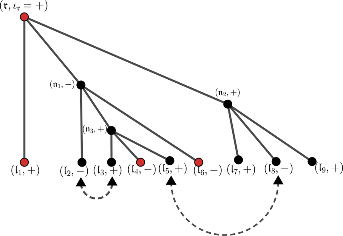
; what makes the counting nontrivial is the pairings, especially those between leaves that are far away or from different levels (see Figure 3, where a pairing is depicted by an extra link between the two leaves). Nevertheless, we have developed a counting algorithm that specifically deals with the given pairing structure of
$\mathcal{T}\,$
; what makes the counting nontrivial is the pairings, especially those between leaves that are far away or from different levels (see Figure 3, where a pairing is depicted by an extra link between the two leaves). Nevertheless, we have developed a counting algorithm that specifically deals with the given pairing structure of $\mathcal{T}\,$
and ultimately leads to sharp counting bounds and consequently sharp bounds for
$\mathcal{T}\,$
and ultimately leads to sharp counting bounds and consequently sharp bounds for $\Sigma _k$
(see Proposition 3.5).
$\Sigma _k$
(see Proposition 3.5).
A paired tree with two pairings $(p=2)$
. The set
$(p=2)$
. The set ${\mathcal S}$
of single leaves is
${\mathcal S}$
of single leaves is $\{\mathfrak l_1,\mathfrak l_4,\mathfrak l_6,\mathfrak l_7,\mathfrak l_9 \}$
. The subset
$\{\mathfrak l_1,\mathfrak l_4,\mathfrak l_6,\mathfrak l_7,\mathfrak l_9 \}$
. The subset $\mathcal R\subset \mathcal {S}\cup \{\mathfrak {r}\}$
of red-coloured vertices is
$\mathcal R\subset \mathcal {S}\cup \{\mathfrak {r}\}$
of red-coloured vertices is $\{\mathfrak r, \mathfrak l_1,\mathfrak l_4,\mathfrak l_6\}$
. Here
$\{\mathfrak r, \mathfrak l_1,\mathfrak l_4,\mathfrak l_6\}$
. Here $(l, p, r)=(9, 2, 4)$
. A strongly admissible assignment with respect to this pairing, colouring and a certain fixed choice of the red modes
$(l, p, r)=(9, 2, 4)$
. A strongly admissible assignment with respect to this pairing, colouring and a certain fixed choice of the red modes $\left (k_{\mathfrak r},k_{\mathfrak l_4},k_{\mathfrak l_6}\right )$
corresponds to having the modes
$\left (k_{\mathfrak r},k_{\mathfrak l_4},k_{\mathfrak l_6}\right )$
corresponds to having the modes $k_{\mathfrak l_2}=k_{\mathfrak l_3}$
,
$k_{\mathfrak l_2}=k_{\mathfrak l_3}$
, $k_{\mathfrak l_5}=k_{\mathfrak l_8}$
and
$k_{\mathfrak l_5}=k_{\mathfrak l_8}$
and $\lvert k_{\mathfrak l}\rvert \leq L^{\theta }$
for all the uncoloured leaves. The rest of the modes are determined according to Definition 2.2.
$\lvert k_{\mathfrak l}\rvert \leq L^{\theta }$
for all the uncoloured leaves. The rest of the modes are determined according to Definition 2.2.
1.2.3 An $\ell ^2$
operator norm bound
$\ell ^2$
operator norm bound

In contrast to the tree terms $\mathcal J_{\mathcal{T}\,}$
, the remainder term
$\mathcal J_{\mathcal{T}\,}$
, the remainder term $\mathcal R_{N+1}$
has no explicit random structure. Indeed, the only way it feels the ‘chaos’ of the initial data is through the equation it satisfies, which in integral form and spatial Fourier variables looks like
$\mathcal R_{N+1}$
has no explicit random structure. Indeed, the only way it feels the ‘chaos’ of the initial data is through the equation it satisfies, which in integral form and spatial Fourier variables looks like
 $$ \begin{align*}\mathcal R_{N+1}=\mathcal J_{\sim N}+\mathcal L(\mathcal R_{N+1}) +\mathcal Q(\mathcal R_{N+1})+\mathcal C(\mathcal R_{N+1}), \end{align*} $$
where $\mathcal J_{\sim N}$
is a sum of Feynman trees
$\mathcal J_{\sim N}$
is a sum of Feynman trees $\mathcal J_{\mathcal{T}\,}$
(already described) of scale
$\mathcal J_{\mathcal{T}\,}$
(already described) of scale $\mathfrak s (\mathcal{T}\,\,)\sim N$
, and
$\mathfrak s (\mathcal{T}\,\,)\sim N$
, and $\mathcal L$
,
$\mathcal L$
, $\mathcal Q$
and
$\mathcal Q$
and $\mathcal C$
are, respectively, linear, bilinear and trilinear operator in
$\mathcal C$
are, respectively, linear, bilinear and trilinear operator in $\mathcal R_{N+1}$
. The main point here is that one would like to propagate the estimates on
$\mathcal R_{N+1}$
. The main point here is that one would like to propagate the estimates on $\mathcal J_{\sim N}$
to
$\mathcal J_{\sim N}$
to $\mathcal R_{N+1}$
itself; this is how we make rigorous the so-called ‘propagation of chaos or quasi-Gaussianity’ claims that are often adopted in formal derivations. In another aspect, qualitative results on propagation of quasi-Gaussianity, in the form of absolute continuity of measures, have been obtained in some cases (with different settings) by exploiting almost-conservation laws (e.g., [Reference Tzvetkov48]).
$\mathcal R_{N+1}$
itself; this is how we make rigorous the so-called ‘propagation of chaos or quasi-Gaussianity’ claims that are often adopted in formal derivations. In another aspect, qualitative results on propagation of quasi-Gaussianity, in the form of absolute continuity of measures, have been obtained in some cases (with different settings) by exploiting almost-conservation laws (e.g., [Reference Tzvetkov48]).
Since we are bootstrapping a smallness estimate on $\mathcal R_{N+1}$
, any quadratic and cubic form of
$\mathcal R_{N+1}$
, any quadratic and cubic form of $\mathcal R_{N+1}$
will be easily bounded. It therefore suffices to propagate the bound for the term
$\mathcal R_{N+1}$
will be easily bounded. It therefore suffices to propagate the bound for the term $\mathcal L(\mathcal R_{N+1})$
, which reduces to bounding the
$\mathcal L(\mathcal R_{N+1})$
, which reduces to bounding the $\ell ^2\to \ell ^2$
operator norm for the linear operator
$\ell ^2\to \ell ^2$
operator norm for the linear operator $\mathcal L$
. By definition, the operator
$\mathcal L$
. By definition, the operator $\mathcal L$
will have the form
$\mathcal L$
will have the form $v\mapsto \mathcal {IW}\left (\mathcal J_{\mathcal{T}\,_1}, \mathcal J_{\mathcal{T}\,_2}, v\right )$
, where
$v\mapsto \mathcal {IW}\left (\mathcal J_{\mathcal{T}\,_1}, \mathcal J_{\mathcal{T}\,_2}, v\right )$
, where $\mathcal {I}$
is the Duhamel operator,
$\mathcal {I}$
is the Duhamel operator, $\mathcal {W}$
is the trilinear form coming from the cubic nonlinearity and
$\mathcal {W}$
is the trilinear form coming from the cubic nonlinearity and $\mathcal J_{\mathcal{T}\,_1}, \mathcal J_{\mathcal{T}\,_2}$
are trees of scale
$\mathcal J_{\mathcal{T}\,_1}, \mathcal J_{\mathcal{T}\,_2}$
are trees of scale $\leq N$
; thus in Fourier space it can be viewed as a matrix with random coefficients. The key to obtaining the sharp estimate for
$\leq N$
; thus in Fourier space it can be viewed as a matrix with random coefficients. The key to obtaining the sharp estimate for $\mathcal L$
is then to exploit the cancellation coming from this randomness, and the most efficient way to do this is via the
$\mathcal L$
is then to exploit the cancellation coming from this randomness, and the most efficient way to do this is via the $TT^*$
method.
$TT^*$
method.
In fact, the idea of applying the $TT^*$
method to random matrices has already been used by Bourgain [Reference Bourgain3]. In that paper one is still far above (probabilistic) criticality, so applying the
$TT^*$
method to random matrices has already been used by Bourgain [Reference Bourgain3]. In that paper one is still far above (probabilistic) criticality, so applying the $TT^*$
method once already gives adequate control. In the present case, however, we are aiming at obtaining sharp estimates, so applying
$TT^*$
method once already gives adequate control. In the present case, however, we are aiming at obtaining sharp estimates, so applying $TT^*$
once will not be sufficient.
$TT^*$
once will not be sufficient.
The solution is thus to apply $TT^*$
sufficiently many times (say,
$TT^*$
sufficiently many times (say, $D\gg 1$
), which leads to the analysis of the kernel of the operator
$D\gg 1$
), which leads to the analysis of the kernel of the operator $(\mathcal L\mathcal L^*)^D$
. At first sight this kernel seems to be a complicated multilinear expression which is difficult to handle; nevertheless, we make one key observation, namely that this kernel can essentially be recast in the form of formula (1.7) for some large auxiliary tree
$(\mathcal L\mathcal L^*)^D$
. At first sight this kernel seems to be a complicated multilinear expression which is difficult to handle; nevertheless, we make one key observation, namely that this kernel can essentially be recast in the form of formula (1.7) for some large auxiliary tree $\mathcal{T}\,=\mathcal{T}\;^D$
, which is obtained from a single root node by attaching copies of the trees
$\mathcal{T}\,=\mathcal{T}\;^D$
, which is obtained from a single root node by attaching copies of the trees $\mathcal{T}\,_1$
and
$\mathcal{T}\,_1$
and $\mathcal{T}\,_2$
successively a total of
$\mathcal{T}\,_2$
successively a total of $2D$
times (see Figure 4). With this observation, the arguments in the previous section then lead to sharp bounds of the kernel of
$2D$
times (see Figure 4). With this observation, the arguments in the previous section then lead to sharp bounds of the kernel of $(\mathcal L\mathcal L^*)^D$
, up to some loss that is a power of L independent of D; taking the
$(\mathcal L\mathcal L^*)^D$
, up to some loss that is a power of L independent of D; taking the $1/(2D)$
power and choosing D sufficiently large makes this power negligible and implies the sharp bound for the operator norm of
$1/(2D)$
power and choosing D sufficiently large makes this power negligible and implies the sharp bound for the operator norm of $\mathcal L$
(see Section 3.3).
$\mathcal L$
(see Section 3.3).
Construction of the tree $\mathcal{T}\,^D$
by successive plantings of trees
$\mathcal{T}\,^D$
by successive plantings of trees $\mathcal{T}\,_1$
and
$\mathcal{T}\,_1$
and $\mathcal{T}\,_2$
onto the first two nodes of a ternary tree, starting with a root
$\mathcal{T}\,_2$
onto the first two nodes of a ternary tree, starting with a root $\mathfrak r$
and stopping after
$\mathfrak r$
and stopping after $2D$
steps, leaving a leaf node
$2D$
steps, leaving a leaf node $\mathfrak r'$
. In the figure,
$\mathfrak r'$
. In the figure, $D=2$
.
$D=2$
.

1.2.4 Sharpness of estimates
We remark that the estimates we prove for $\mathcal J_{\mathcal{T}\,}$
are sharp up to some finite power of L (independent of
$\mathcal J_{\mathcal{T}\,}$
are sharp up to some finite power of L (independent of $\mathcal{T}\,$
). More precisely, from Proposition 2.5 we know that for any ternary tree
$\mathcal{T}\,$
). More precisely, from Proposition 2.5 we know that for any ternary tree $\mathcal{T}\,$
of scale n and possible pairing structure (see Definition 3.3), with overwhelming probability,
$\mathcal{T}\,$
of scale n and possible pairing structure (see Definition 3.3), with overwhelming probability,
 $$ \begin{align}\sup_k\left\lVert(\mathcal J_{\mathcal{T}})_k\right\rVert_{h^{b}}\leq L^{0+}\rho^n, \end{align} $$
where $\rho $
is some quantity depending on
$\rho $
is some quantity depending on $\alpha $
, L and T (see formula (2.24)), k is the spatial Fourier variable and
$\alpha $
, L and T (see formula (2.24)), k is the spatial Fourier variable and $h^b$
is a time-Sobolev norm defined in equation (2.22); on the other hand, we will show that that for some particular choice of trees
$h^b$
is a time-Sobolev norm defined in equation (2.22); on the other hand, we will show that that for some particular choice of trees $\mathcal{T}\,$
of scale n and some particular choice of pairings, with high probability,
$\mathcal{T}\,$
of scale n and some particular choice of pairings, with high probability,
 $$ \begin{align}\sup_k\left\lVert(\mathcal J_{\mathcal{T}})_k\right\rVert_{h^{b}}\geq L^{-d}\rho^n. \end{align} $$
The timescale T of Theorem 1.3 is the largest that makes $\rho \ll 1$
; thus if one wants to go beyond T in cases other than Theorem 1.1, it would be necessary to address the divergence of formula (1.9) with
$\rho \ll 1$
; thus if one wants to go beyond T in cases other than Theorem 1.1, it would be necessary to address the divergence of formula (1.9) with $\rho \gg 1$
by exploiting the cancellation between different tree terms or different pairing choices (see Section 3.4).
$\rho \gg 1$
by exploiting the cancellation between different tree terms or different pairing choices (see Section 3.4).
1.2.5 Discussions
Shortly after the completion of this paper, work of Collot and Germain [Reference Collot and Germain12] was announced that studies the same problem, but only in the rational-torus setting. In the language of this paper, their result corresponds to the validity of equation (1.3) for $L\leq t\leq L^{2-\delta }$
, under the assumption
$L\leq t\leq L^{2-\delta }$
, under the assumption $\alpha \leq L^{-1-\delta }$
. This is a special case of Theorem 1.3, essentially corresponding to the rectangle below the horizontal line
$\alpha \leq L^{-1-\delta }$
. This is a special case of Theorem 1.3, essentially corresponding to the rectangle below the horizontal line $\log _LT=2$
and to the right of the vertical line
$\log _LT=2$
and to the right of the vertical line $\log _L\left (\alpha ^{-1}\right )=1$
in Figure 1. We also mention later work by the same authors [Reference Collot and Germain13], where they consider a generic nonrectangular torus (as opposed to the rectangular tori here and in [Reference Collot and Germain12]) and prove the existence of solutions (but without justifying equation (1.3)) up to time
$\log _L\left (\alpha ^{-1}\right )=1$
in Figure 1. We also mention later work by the same authors [Reference Collot and Germain13], where they consider a generic nonrectangular torus (as opposed to the rectangular tori here and in [Reference Collot and Germain12]) and prove the existence of solutions (but without justifying equation (1.3)) up to time $t\leq L^{-\delta }T_{\mathrm {kin}}$
for a wider range of power laws between
$t\leq L^{-\delta }T_{\mathrm {kin}}$
for a wider range of power laws between $\alpha $
and L.
$\alpha $
and L.
While the present paper was being peer-reviewed, we submitted new work to arXiv [Reference Deng and Hani16], in which we provide the first full derivation of (WKE) from (NLS). Those results reach the kinetic time scale $t=\tau \cdot T_{\mathrm {kin}}$
, where
$t=\tau \cdot T_{\mathrm {kin}}$
, where $\tau $
is independent of L (compared to Theorem 1.1 here, where
$\tau $
is independent of L (compared to Theorem 1.1 here, where $\tau \leq L^{-\varepsilon }$
), for the scaling law
$\tau \leq L^{-\varepsilon }$
), for the scaling law $\alpha \sim L^{-1}$
on generic (irrational) rectangular tori and the scaling laws
$\alpha \sim L^{-1}$
on generic (irrational) rectangular tori and the scaling laws $\alpha \sim L^{-\gamma }$
(where
$\alpha \sim L^{-\gamma }$
(where $\gamma <1$
and is close to
$\gamma <1$
and is close to $1$
) on arbitrary rectangular tori.
$1$
) on arbitrary rectangular tori.
Shortly after completing [Reference Deng and Hani16], we received a preprint of a forthcoming deep work by Staffilani and Tran [Reference Staffilani and Tran47]. It concerns a high-dimensional (on $\mathbb {T}^d$
for
$\mathbb {T}^d$
for $d\geq 14$
) KdV equation under a time-dependent Stratonovich stochastic forcing, which effectively randomises the phases without injecting energy into the system. The authors derive the corresponding wave kinetic equation up to the kinetic time scale, for the scaling law
$d\geq 14$
) KdV equation under a time-dependent Stratonovich stochastic forcing, which effectively randomises the phases without injecting energy into the system. The authors derive the corresponding wave kinetic equation up to the kinetic time scale, for the scaling law $\alpha \sim L^{-0}$
(i.e., first taking
$\alpha \sim L^{-0}$
(i.e., first taking $L\to \infty $
and then taking
$L\to \infty $
and then taking $\alpha \to 0$
). They also prove a conditional result without such forcing, where the condition is verified for some particular initial densities converging to the equilibrium state (stationary solution to the wave kinetic equation) in the limit.
$\alpha \to 0$
). They also prove a conditional result without such forcing, where the condition is verified for some particular initial densities converging to the equilibrium state (stationary solution to the wave kinetic equation) in the limit.
1.3 Organisation of the paper
In Section 2 we explain the diagrammatic expansion of the solution into Feynman trees, and state the a priori estimates on such trees and remainder terms, which yield the long-time existence of such expansions. Section 3 is devoted to the proof of those a priori estimates. In Section 4 we prove the main theorems already mentioned, and in Section 5 we prove the necessary number-theoretic results that allow us to replace the highly oscillating Riemann sums by integrals.
1.4 Notation
Most notation will be standard. Let $z^+=z$
and
$z^+=z$
and $z^-=\overline {z}$
. Define
$z^-=\overline {z}$
. Define $\left \lvert k\right \rvert _{\beta }$
by
$\left \lvert k\right \rvert _{\beta }$
by $\left \lvert k\right \rvert _{\beta }^2=\beta _1k_1^2+\cdots +\beta _dk_d^2$
for
$\left \lvert k\right \rvert _{\beta }^2=\beta _1k_1^2+\cdots +\beta _dk_d^2$
for $k=(k_1,\ldots ,k_d)$
. The spatial Fourier series of a function
$k=(k_1,\ldots ,k_d)$
. The spatial Fourier series of a function $u: {\mathbb T}_L^d \to \mathbb C$
is defined on
$u: {\mathbb T}_L^d \to \mathbb C$
is defined on $\mathbb Z^d_L:=L^{-1}\mathbb Z^{d}$
by
$\mathbb Z^d_L:=L^{-1}\mathbb Z^{d}$
by
 $$ \begin{align} \widehat{u}_k=\int_{{\mathbb T}^d_L} u(x) e^{-2\pi i k\cdot x},\quad \text{so that}\quad u(x)=\frac{1}{L^d}\sum_{k \in \mathbb Z^d_L} \widehat{u}_k e^{2\pi i k\cdot x}. \end{align} $$
The temporal Fourier transform is defined by
 $$ \begin{align*} \widetilde{f}(\tau)=\int_{\mathbb{R}}e^{-2\pi it\tau}f(t)\mathrm{d}t. \end{align*} $$
Let $\delta>0$
be fixed throughout the paper. Let N, s and
$\delta>0$
be fixed throughout the paper. Let N, s and $b>\frac {1}{2}$
be fixed, such that N and s are large enough and
$b>\frac {1}{2}$
be fixed, such that N and s are large enough and $b-\frac {1}{2}$
is small enough, depending on d and
$b-\frac {1}{2}$
is small enough, depending on d and $\delta $
. The quantity C will denote any large absolute constant, not dependent on
$\delta $
. The quantity C will denote any large absolute constant, not dependent on $\big(N,s,b-\frac {1}{2}\big)$
, and
$\big(N,s,b-\frac {1}{2}\big)$
, and $\theta $
will denote any small positive constant, which is dependent on
$\theta $
will denote any small positive constant, which is dependent on $\big(N,s,b-\frac {1}{2}\big)$
; these may change from line to line. The symbols
$\big(N,s,b-\frac {1}{2}\big)$
; these may change from line to line. The symbols $O(\cdot )$
,
$O(\cdot )$
, $\lesssim $
and so on will have their usual meanings, with implicit constants depending on
$\lesssim $
and so on will have their usual meanings, with implicit constants depending on $\theta $
. Let L be large enough depending on all these implicit constants. If some statement S involving
$\theta $
. Let L be large enough depending on all these implicit constants. If some statement S involving $\omega $
is true with probability
$\omega $
is true with probability $\geq 1-Ke^{-L^{\theta }}$
for some constant K (depending on
$\geq 1-Ke^{-L^{\theta }}$
for some constant K (depending on $\theta $
), then we say this statement S is L-certain.
$\theta $
), then we say this statement S is L-certain.
When a function depends on many variables, we may use notations like
 $$ \begin{align*} f=f\left(x_i:i\in A,\,y_j:1\leq j\leq m\right) \end{align*} $$
to denote a function f of variables $(x_i:i\in A)$
and
$(x_i:i\in A)$
and $y_1,\ldots ,y_m$
.
$y_1,\ldots ,y_m$
.
2 Tree expansions and long-time existence
2.1 First reductions
Let $\widehat {u}_k(t)$
be the Fourier coefficients of
$\widehat {u}_k(t)$
be the Fourier coefficients of $u(t)$
, as in equation (1.10). Then with
$u(t)$
, as in equation (1.10). Then with $c_k(t):= e^{2\pi i\left \lvert k\right \rvert _{\beta }^2t} \widehat u_k(t)=\left (\mathcal F_{{\mathbb T}^d_L} e^{-it\Delta _{\beta }} u\right )(k)$
, we arrive at the following equation for the Fourier modes:
$c_k(t):= e^{2\pi i\left \lvert k\right \rvert _{\beta }^2t} \widehat u_k(t)=\left (\mathcal F_{{\mathbb T}^d_L} e^{-it\Delta _{\beta }} u\right )(k)$
, we arrive at the following equation for the Fourier modes:
 $$ \begin{align} \begin{cases} i \dot{c_k} = \left(\frac{\lambda}{L^{d}}\right)^{2} \sum\limits_{\substack{\left(k_1,k_2,k_{3}\right) \in \left(\mathbb{Z}^d_L\right)^3 \\ k - k_1 + k_2 -k_3 = 0}} c_{k_1}\overline{c_{k_2}} c_{k_3} e^{2\pi i \Omega\left(k_1,k_2,k_3,k\right)t} \\[1.5em] c_k(0) = (c_k)_{\mathrm{in}}=\widehat u_k(0), \end{cases} \end{align} $$
where $ \Omega (k_1,k_2,k_3,k) =\left \lvert k_1\right \rvert _{\beta }^2-\left \lvert k_2\right \rvert _{\beta }^2+\left \lvert k_3\right \rvert _{\beta }^2-\left \lvert k\right \rvert _{\beta }^2. $
Note that the sum can be written as
$ \Omega (k_1,k_2,k_3,k) =\left \lvert k_1\right \rvert _{\beta }^2-\left \lvert k_2\right \rvert _{\beta }^2+\left \lvert k_3\right \rvert _{\beta }^2-\left \lvert k\right \rvert _{\beta }^2. $
Note that the sum can be written as
 $$ \begin{align*}\sum\limits_{\substack{\left(k_1,k_2, k_{3}\right) \in \left(\mathbb{Z}^d_L\right)^3 \\ k - k_1 + k_2 -k_3 = 0}}=2\sum_{k_1=k}-\sum_{k_1=k_2=k_3} +\sum_{k_1, k_3\neq k}, \end{align*} $$
which, defining $M=\sum _{k_3} \left \lvert c_{k_3}\right \rvert ^2$
(which is conserved), allows us to write
$M=\sum _{k_3} \left \lvert c_{k_3}\right \rvert ^2$
(which is conserved), allows us to write
 $$ \begin{align*} i \dot{c_k} = \left(\frac{\lambda}{L^{d}}\right)^{2} \left(2M c_k -\left\lvert c_k\right\rvert^2c_k+ \sum\limits_{\left(k_1,k_2, k_{3}\right)}^{\times} c_{k_1}\overline{c_{k_2}} c_{k_3} e^{2\pi i \Omega\left(k_1,k_2,k_3,k\right)t}\right). \end{align*} $$
Here and later, $\sum ^{\times }$
represents summation under the conditions
$\sum ^{\times }$
represents summation under the conditions $k_j\in \mathbb {Z}_L^d$
,
$k_j\in \mathbb {Z}_L^d$
, $k_1-k_2+k_3=k$
and
$k_1-k_2+k_3=k$
and $k\not \in \{k_1,k_3\}$
. Introducing
$k\not \in \{k_1,k_3\}$
. Introducing $b_k(t)=c_k(t)e^{-2i\left (L^{-d}\lambda \right )^{2}Mt}$
, we arrive at the following equation for
$b_k(t)=c_k(t)e^{-2i\left (L^{-d}\lambda \right )^{2}Mt}$
, we arrive at the following equation for $b_k(t)$
:
$b_k(t)$
:
 $$ \begin{align} \begin{cases} i \dot{b_k} = \left(\frac{\lambda}{L^{d}}\right)^{2} \left( -\left\lvert b_k\right\rvert^2b_k+ \sum\limits_{\left(k_1,k_2, k_{3}\right)}^{\times} b_{k_1}\overline{b_{k_2}} b_{k_3} e^{2\pi i \Omega\left(k_1,k_2,k_3,k\right)t}\right)\\[1.5em] b_k(0) = (b_k)_{\mathrm{in}}=\widehat u_k(0). \end{cases} \end{align} $$
In Theorem 1.3 we will be studying the solution $u(t)$
, or equivalently the sequence
$u(t)$
, or equivalently the sequence $(b_k(t))_{k \in \mathbb Z^d_L}$
, on a time interval
$(b_k(t))_{k \in \mathbb Z^d_L}$
, on a time interval $[0,T]$
. It will be convenient, to simplify some notation later, to work on the unit time interval
$[0,T]$
. It will be convenient, to simplify some notation later, to work on the unit time interval $[0,1]$
. For this we introduce the final ansatz
$[0,1]$
. For this we introduce the final ansatz
 $$ \begin{align*} a_k(t)=b_k(Tt), \end{align*} $$
which satisfies the equation
 $$ \begin{align} \begin{cases} i \dot{a_k} = \left(\frac{\alpha T}{L^{d}}\right) \left( -\left\lvert a_k\right\rvert^2a_k+ \sum\limits_{\left(k_1,k_2, k_{3}\right)}^{\times} a_{k_1}\overline{a_{k_2}} a_{k_3} e^{2\pi i T\Omega\left(k_1,k_2,k_3,k\right)t}\right)\\[1.5em] a_k(0) =(a_k)_{\mathrm{in}}=\widehat u_k(0). \end{cases} \end{align} $$
Here we have also used the relation $\alpha =\lambda ^2L^{-d}$
. Recall the well-prepared initial data (1.2), which transform into the initial data for
$\alpha =\lambda ^2L^{-d}$
. Recall the well-prepared initial data (1.2), which transform into the initial data for $a_k$
:
$a_k$
:
 $$ \begin{align} (a_k)_{\mathrm{in}}=\sqrt{n_{\mathrm{in}}} \cdot\eta_{k}(\omega), \end{align} $$
where $\eta _{k}(\omega )$
are the same as in equation (1.2).
$\eta _{k}(\omega )$
are the same as in equation (1.2).
2.2 The tree expansion
Let $\boldsymbol a(t) =(a_k(t))_{k \in \mathbb Z^d_L}$
and
$\boldsymbol a(t) =(a_k(t))_{k \in \mathbb Z^d_L}$
and $\boldsymbol {a}_{\mathrm {in}} =\boldsymbol a(0)$
. Let
$\boldsymbol {a}_{\mathrm {in}} =\boldsymbol a(0)$
. Let $J=[0,1]$
; we will fix a smooth compactly supported cutoff function
$J=[0,1]$
; we will fix a smooth compactly supported cutoff function $\chi $
such that
$\chi $
such that $\chi \equiv 1$
on J. Then by equation (2.3), we know that for
$\chi \equiv 1$
on J. Then by equation (2.3), we know that for $t\in J$
we have
$t\in J$
we have
 $$ \begin{align}\boldsymbol{a}(t)=\chi(t)\boldsymbol{a}_{\mathrm{in}}+\mathcal{IW}(\boldsymbol a, \boldsymbol a, \boldsymbol a)(t),\end{align} $$
where the Duhamel term is defined by
 $$ \begin{align} \mathcal{I}F(t)=\chi(t)\int_0^t\chi(t')F(t')\mathrm{d}t', \end{align} $$
 $$ \begin{align} \mathcal{W}(\boldsymbol b, \boldsymbol c , \boldsymbol d)_k(t):=-\frac{i\alpha T}{L^{d}}\left( -\left(b_{k}\overline{c_{k}}d_{k}\right)(t)+ \sum\limits_{\left(k_1,k_2, k_{3}\right)}^{\times} \left(b_{k_1}\overline{c_{k_2}} d_{k_3}\right)(t) e^{2\pi i T\Omega\left(k_1,k_2,k_3,k\right)t}\right). \end{align} $$
Since we will only be studying $\boldsymbol {a}$
for
$\boldsymbol {a}$
for $t\in J$
, from now on we will replace
$t\in J$
, from now on we will replace $\boldsymbol {a}$
by the solution to equation (2.5) for
$\boldsymbol {a}$
by the solution to equation (2.5) for $t\in \mathbb {R}$
(the existence and uniqueness of the latter will be clear from a proof to follow). We will be analysing the temporal Fourier transform of this (extended)
$t\in \mathbb {R}$
(the existence and uniqueness of the latter will be clear from a proof to follow). We will be analysing the temporal Fourier transform of this (extended) $\boldsymbol {a}$
, so let us first record a formula for
$\boldsymbol {a}$
, so let us first record a formula for $\mathcal {I}$
on the Fourier side:
$\mathcal {I}$
on the Fourier side:
Lemma 2.1. Let $\mathcal {I}$
be defined as in equation (2.6), and recall that
$\mathcal {I}$
be defined as in equation (2.6), and recall that $\widetilde {G}$
means the temporal Fourier transform of G; then we have
$\widetilde {G}$
means the temporal Fourier transform of G; then we have
 $$ \begin{align}\widetilde{\mathcal{I}F}(\tau)=\int_{\mathbb{R}}(I_0+I_1)(\tau,\sigma)\widetilde{F}(\sigma)\mathrm{d}\sigma,\qquad\left\lvert\partial_{\tau,\sigma}^aI_d(\tau,\sigma)\right\rvert\lesssim_{a,A}\frac{1}{\left\langle \tau-d\sigma\right\rangle^A}\frac{1}{\langle\sigma\rangle}.\end{align} $$
Proof. See [Reference Deng, Nahmod and Yue17].
Now define $\mathcal J_n$
recursively by
$\mathcal J_n$
recursively by
 $$ \begin{align} \begin{array}{ll} \mathcal J_0(t)&=\chi(t)\cdot\boldsymbol{a}_{\mathrm{in}},\\ \mathcal J_n(t)&=\displaystyle\sum_{n_1+n_2+n_3=n-1}\mathcal{IW}\left(\mathcal J_{n_1},\mathcal J_{n_2},\mathcal J_{n_3}\right)(t), \end{array} \end{align} $$
and define
 $$ \begin{align}\mathcal J_{\leq N}=\sum_{n\leq N}\mathcal J_{n},\qquad \mathcal{R}_{N+1}=\boldsymbol{a}-\mathcal J_{\leq N}.\end{align} $$
By plugging in equation (2.5), we get that $\mathcal R_{N+1}$
satisfies the equation
$\mathcal R_{N+1}$
satisfies the equation
 $$ \begin{align}\mathcal R_{N+1}=\mathcal J_{\sim N}+\mathcal L(\mathcal R_{N+1}) +\mathcal Q(\mathcal R_{N+1})+\mathcal C(\mathcal R_{N+1}), \end{align} $$
where the relevant terms are defined as
 $$ \begin{align} \mathcal J_{\sim N}&:=\sum_{\substack{n_1, n_2, n_3\leq N\\ n_1+n_2+n_3\geq N}} \mathcal{IW}\left(\mathcal J_{n_1},\mathcal J_{n_2},\mathcal J_{n_3}\right), \end{align} $$
 $$ \begin{align} \mathcal L(v)&:=\sum_{n_1,n_2\leq N}\left(2\mathcal{IW}\left(\mathcal J_{n_1}, \mathcal J_{n_2}, v\right)+\mathcal{IW}\left(\mathcal J_{n_1}, v, \mathcal J_{n_2}\right)\right), \end{align} $$
 $$ \begin{align} \mathcal Q(v)&:=\sum_{n_1\leq N}\left(2\mathcal{IW}\left(v,v, \mathcal J_{n_1}\right)+\mathcal{IW}\left(v, \mathcal J_{n_1}, v\right)\right), \end{align} $$
 $$ \begin{align} \mathcal C(v)&:=\mathcal{IW}(v, v, v). \end{align} $$
Next we will derive a formula for the time Fourier transform of $\mathcal J_n$
; for this we need some preparation regarding multilinear forms associated with ternary trees.
$\mathcal J_n$
; for this we need some preparation regarding multilinear forms associated with ternary trees.
Definition 2.2.
-
1. Let
$\mathcal{T}~$
be a ternary tree. We use
$\mathcal {L}$
to denote the set of leaves and l their number,
$\mathcal {N}=\mathcal{T}\,\backslash \mathcal L$
the set of branching nodes and n their number, and
$\mathfrak {r} \in \mathcal N$
the root node. The scale of a ternary tree
$\mathcal{T}\,$
is defined as
$\mathfrak s(\mathcal{T}\,\,)=n$
(the number of branching nodes).Footnote
9
A tree of scale n has
$l=2n+1$
leaves and a total of
$3n+1$
vertices. -
2. (Signs on a tree) For each node
$\mathfrak {n}\in \mathcal {N}$
, let its children from left to right be
$\mathfrak {n}_1$
,
$\mathfrak {n}_2$
,
$\mathfrak {n}_3$
. We fix the sign
$\iota _{\mathfrak {n}}\in \{\pm \}$
as follows: first
$\iota _{\mathfrak {r}}=+$
, then for any node
$\mathfrak {n}\in \mathcal {N}$
, define
$\iota _{\mathfrak {n}_1}=\iota _{\mathfrak {n}_3}=\iota _{\mathfrak {n}}$
and
$\iota _{\mathfrak {n}_2}=-\iota _{\mathfrak {n}}$
. -
3. (Admissible assignments) Suppose we assign to each
$\mathfrak {n}\in \mathcal{T}\,$
an element
$k_{\mathfrak {n}}\in \mathbb {Z}_L^d$
. We say such an assignment
$(k_{\mathfrak {n}}:\mathfrak {n}\in \mathcal{T}\,\,)$
is admissible if for any
$\mathfrak {n}\in \mathcal {N}$
we have
$k_{\mathfrak {n}}=k_{\mathfrak {n}_1}-k_{\mathfrak {n}_2}+k_{\mathfrak {n}_3}$
and either
$k_{\mathfrak {n}}\not \in \left \{k_{\mathfrak {n}_1},k_{\mathfrak {n}_3}\right \}$
or
$k_{\mathfrak {n}}=k_{\mathfrak {n}_1}=k_{\mathfrak {n}_2}=k_{\mathfrak {n}_3}$
. Clearly an admissible assignment is completely determined by the values of
$k_{\mathfrak {l}}$
for
$\mathfrak {l}\in \mathcal {L}$
. For any assignment, we denote
$\Omega _{\mathfrak {n}}:=\Omega \left (k_{\mathfrak {n}_1},k_{\mathfrak {n}_2},k_{\mathfrak {n}_3},k_{\mathfrak {n}}\right )$
. Suppose we also fixFootnote
10
$d_{\mathfrak {n}}\in \{0,1\}$
for each
$\mathfrak {n}\in \mathcal {N}$
; then we can define
$q_{\mathfrak {n}}$
for each
$\mathfrak {n}\in \mathcal{T}\,$
inductively by (2.16)
$$ \begin{align} q_{\mathfrak{n}}=0\text{ if }\mathfrak{n}\in\mathcal L\quad\text{or}\quad q_{\mathfrak{n}}=d_{\mathfrak{n}_1}q_{\mathfrak{n}_1}-d_{\mathfrak{n}_2}q_{\mathfrak{n}_2}+d_{\mathfrak{n}_3}q_{\mathfrak{n}_3}+\Omega_{\mathfrak{n}}\text{ if }\mathfrak{n}\in\mathcal{N}.\end{align} $$


Proposition 2.3. For each ternary tree $\mathcal{T}\,$
, define
$\mathcal{T}\,$
, define $\mathcal J_{\mathcal{T}\,}$
inductively by
$\mathcal J_{\mathcal{T}\,}$
inductively by
 $$ \begin{align} \mathcal J_{\bullet}(t)=\chi(t)\cdot\boldsymbol{a}_{\mathrm{in}},\qquad \mathcal J_{\mathcal{T}}(t)=\mathcal{IW}\left(\mathcal J_{\mathcal{T}_1},\mathcal J_{\mathcal{T}_2},\mathcal J_{\mathcal{T}_3}\right)(t), \end{align} $$
where $\bullet $
represents the tree with a single node and
$\bullet $
represents the tree with a single node and $\mathcal{T}\,_1$
,
$\mathcal{T}\,_1$
, $\mathcal{T}\,_2$
,
$\mathcal{T}\,_2$
, $\mathcal{T}\,_3$
are the subtrees rooted at the three children of the root node of
$\mathcal{T}\,_3$
are the subtrees rooted at the three children of the root node of $\mathcal{T}\,$
. Then we have
$\mathcal{T}\,$
. Then we have
 $$ \begin{align}\mathcal J_n=\sum_{\mathfrak s(\mathcal{T}\,\,)=n}\mathcal J_{\mathcal{T}}. \end{align} $$
Moreover, for any $\mathcal{T}\,$
of scale
$\mathcal{T}\,$
of scale $\mathfrak s(\mathcal{T}\,\,)=n$
we have the formula
$\mathfrak s(\mathcal{T}\,\,)=n$
we have the formula
 $$ \begin{align} \left(\widetilde{\mathcal J_{\mathcal{T}}}\right)_{k}(\tau)=\left(\frac{\alpha T}{L^{d}}\right)^n\sum_{\left(k_{\mathfrak{n}}:\mathfrak{n}\in\mathcal{T}\right)}\mathcal{K}_{\mathcal{T}}(\tau,k_{\mathfrak{n}}:\mathfrak{n}\in\mathcal{T}\,\,)\prod_{\mathfrak{l}\in\mathcal L}\sqrt{n_{\mathrm{in}}(k_{\mathfrak{l}})}\cdot\prod_{\mathfrak{l}\in\mathcal L}\left[\eta_{k_{\mathfrak{l}}}(\omega)\right]^{\iota_{\mathfrak{l}}}, \end{align} $$
where the sum is taken over all admissible assignments $(k_{\mathfrak {n}}:\mathfrak {n}\in \mathcal{T}\,\,)$
such that
$(k_{\mathfrak {n}}:\mathfrak {n}\in \mathcal{T}\,\,)$
such that $k_{\mathfrak {r}}=k$
, and the function
$k_{\mathfrak {r}}=k$
, and the function $\mathcal {K}=\mathcal {K}_{\mathcal{T}\,}(\tau ,k_{\mathfrak {n}}:\mathfrak {n}\in \mathcal{T}\,\,)$
satisfies
$\mathcal {K}=\mathcal {K}_{\mathcal{T}\,}(\tau ,k_{\mathfrak {n}}:\mathfrak {n}\in \mathcal{T}\,\,)$
satisfies
 $$ \begin{align}\left\lvert\partial_{\tau}^a\mathcal{K}\right\rvert\lesssim_{a,A}\sum_{\left(d_{\mathfrak{n}}:\mathfrak{n}\in\mathcal{N}\right)}\left\langle \tau-Td_{\mathrm{r}}q_{\mathrm{r}}\right\rangle^{-A}\cdot\prod_{\mathfrak{n}\in\mathcal{N}}\left\langle Tq_{\mathfrak{n}}\right\rangle^{-1}, \end{align} $$
where $q_{\mathfrak {n}}$
is defined in equation (2.16).
$q_{\mathfrak {n}}$
is defined in equation (2.16).
Proof. First, equation (2.18) follows from the definitions in equations (2.9) and (2.17) and an easy induction. We now prove formulas (2.19) and (2.20) inductively, noting also that $(a_k)_{\mathrm {in}}=\sqrt {n_{\mathrm {in}}(k)}\cdot \eta _k(\omega )$
. For
$(a_k)_{\mathrm {in}}=\sqrt {n_{\mathrm {in}}(k)}\cdot \eta _k(\omega )$
. For $\mathcal{T}\,=\bullet $
, equation (2.19) follows from equation (2.17) with
$\mathcal{T}\,=\bullet $
, equation (2.19) follows from equation (2.17) with $\mathcal {K}_{\mathcal{T}\,}(\tau ,k_{\mathfrak {r}})=\widetilde {\chi }(\tau )$
that satisfies formula (2.20). Now suppose formulas (2.19) and (2.20) are true for smaller trees; then by formulas (2.7) and (2.17) and Lemma 2.1, up to unimportant coefficients, we can write
$\mathcal {K}_{\mathcal{T}\,}(\tau ,k_{\mathfrak {r}})=\widetilde {\chi }(\tau )$
that satisfies formula (2.20). Now suppose formulas (2.19) and (2.20) are true for smaller trees; then by formulas (2.7) and (2.17) and Lemma 2.1, up to unimportant coefficients, we can write
 $$ \begin{align*}\left(\widetilde{\mathcal J_{\mathcal{T}}}\right)_{k}(\tau)=\frac{i\alpha T}{L^{d}}\sum_{d\in\{0,1\}}\sum_{\left(k_1,k_2,k_3\right)}^*\int_{\mathbb{R}^3}I_d(\tau,\sigma)\prod_{j=1}^3\left[\left(\widetilde{\mathcal J_{\mathcal{T}_j}}\right)_{k_j}\left(\tau_j\right)\right]^{\iota_j}\mathrm{d}\tau_j,\end{align*} $$
where $\sum ^*$
represents summation under the conditions
$\sum ^*$
represents summation under the conditions $k_j\in \mathbb {Z}_L^d$
,
$k_j\in \mathbb {Z}_L^d$
, $k_1-k_2+k_3=k$
and either
$k_1-k_2+k_3=k$
and either $k\not \in \{k_1,k_3\}$
or
$k\not \in \{k_1,k_3\}$
or $k=k_1=k_2=k_3$
, the signs
$k=k_1=k_2=k_3$
, the signs $(\iota _1,\iota _2,\iota _3)=(+,-,+)$
, and
$(\iota _1,\iota _2,\iota _3)=(+,-,+)$
, and $\sigma =\tau _1-\tau _2+\tau _3+T\Omega (k_1,k_2,k_3,k)$
. Now applying the induction hypothesis, we can write
$\sigma =\tau _1-\tau _2+\tau _3+T\Omega (k_1,k_2,k_3,k)$
. Now applying the induction hypothesis, we can write $\left (\widetilde {\mathcal J_{\mathcal{T}\,}}\right )_{k}(\tau )$
in the form of equation (2.19) with the function
$\left (\widetilde {\mathcal J_{\mathcal{T}\,}}\right )_{k}(\tau )$
in the form of equation (2.19) with the function
 $$ \begin{align}\mathcal{K}_{\mathcal{T}}(\tau,k_{\mathfrak{n}}:\mathfrak{n}\in\mathcal{T}\,\,)=\sum_{d\in\{0,1\}}\int_{\mathbb{R}^3}I_d(\tau,\tau_1-\tau_2+\tau_3+T\Omega_{\mathfrak{r}})\prod_{j=1}^3\left[\mathcal{K}_{\mathcal{T}_j}\left(\tau_j,k_{\mathfrak{n}}:\mathfrak{n}\in\mathcal{T}_j\right)\right]^{\iota_j}\mathrm{d}\tau_j, \end{align} $$
where $\mathfrak {r}$
is the root of
$\mathfrak {r}$
is the root of $\mathcal{T}\,$
with children
$\mathcal{T}\,$
with children $\mathfrak {r}_1,\mathfrak {r}_2,\mathfrak {r}_3$
and
$\mathfrak {r}_1,\mathfrak {r}_2,\mathfrak {r}_3$
and $\mathcal{T}\,_j$
is the subtree rooted at
$\mathcal{T}\,_j$
is the subtree rooted at $\mathfrak {r}_j$
.
$\mathfrak {r}_j$
.
It then suffices to prove that $\mathcal {K}_{\mathcal{T}\,}$
defined by equation (2.21) satisfies formula (2.20). By the induction hypothesis, we may fix a choice
$\mathcal {K}_{\mathcal{T}\,}$
defined by equation (2.21) satisfies formula (2.20). By the induction hypothesis, we may fix a choice $d_{\mathfrak {n}}$
for each nonleaf node
$d_{\mathfrak {n}}$
for each nonleaf node $\mathfrak {n}$
of each
$\mathfrak {n}$
of each $\mathcal{T}\,_j$
, and let
$\mathcal{T}\,_j$
, and let $d_{\mathfrak {r}}=d$
. Then plugging formula (2.20) into equation (2.21), we get
$d_{\mathfrak {r}}=d$
. Then plugging formula (2.20) into equation (2.21), we get
 $$ \begin{align*}\left\lvert\partial_{\tau}^a\mathcal{K}_{\mathcal{T}}\right\rvert \lesssim_{a,A}\prod_{\mathfrak{r}\neq\mathfrak{n}\in\mathcal{N}}\frac{1}{\langle T q_{\mathfrak{n}}\rangle}\int_{\mathbb{R}^3}\frac{1}{\left\langle\tau\!-\!d(\tau_1\!-\!\tau_2+\tau_3+T\Omega_{\mathfrak{r}})\right\rangle^A}\frac{1}{\langle \tau_1\!-\!\tau_2+\tau_3+T\Omega_{\mathfrak{r}}\rangle}\prod_{j=1}^3\frac{\mathrm{d}\tau_j}{\left\langle\tau_j\!-\!Td_{\mathfrak{r}_j}q_{\mathfrak{r}_j}\right\rangle^A},\end{align*} $$
which upon integration in $\tau _j$
gives equation (2.20). This completes the proof.
$\tau _j$
gives equation (2.20). This completes the proof.
2.3 Statement of main estimates
Define the $h^b$
space by
$h^b$
space by
 $$ \begin{align} \lVert a(t)\rVert_{h^{b}} = \left(\int_{{\mathbb R}} \left\langle \tau \right\rangle^{2b}\left\lvert\widetilde{a}(\tau)\right\rvert^2 d\tau\right)^{\frac12}, \end{align} $$
and similarly the $h^{s,b}$
space for
$h^{s,b}$
space for $\boldsymbol a(t)=(a_k(t))_{k \in \mathbb Z^d_L}$
by
$\boldsymbol a(t)=(a_k(t))_{k \in \mathbb Z^d_L}$
by
 $$ \begin{align} \lVert\boldsymbol a\rVert_{h^{s,b}} = \left(L^{-d}\sum_{k \in \mathbb Z^d_L}\int_{{\mathbb R}} \left\langle \tau \right\rangle^{2b}\left\langle k\right\rangle^{2s}\left\lvert\widetilde{a}_k(\tau)\right\rvert^2 d\tau\right)^{\frac12}. \end{align} $$
We shall estimate the solution u in an appropriately rescaled $X^{s, b}$
space, which is equivalent to estimating the sequence
$X^{s, b}$
space, which is equivalent to estimating the sequence $\boldsymbol a(t)=\left (a_k(t)\right )_{k \in \mathbb Z^d_L}$
in the space
$\boldsymbol a(t)=\left (a_k(t)\right )_{k \in \mathbb Z^d_L}$
in the space $h^{s, b}$
. Define the quantity
$h^{s, b}$
. Define the quantity
 $$ \begin{align}\rho:= \begin{cases} \alpha T&\text{if }1\leq T\leq L,\\ \alpha L&\text{if }L\leq T\leq L^2,\\ \alpha TL^{-1}&\text{if } T\geq L^2\text{ and }\beta_i\text{ is generic}. \end{cases}\end{align} $$
By the definition of $\delta>0$
in formula (1.4), we can verify that
$\delta>0$
in formula (1.4), we can verify that $\alpha T^{1/2}\leq \rho \leq L^{-\delta }$
.
$\alpha T^{1/2}\leq \rho \leq L^{-\delta }$
.
Proposition 2.4 Well-posedness bounds
Let $\rho $
be defined as in formula (2.24); then L-certainly, for all
$\rho $
be defined as in formula (2.24); then L-certainly, for all $1\leq n\leq 3N$
, we have
$1\leq n\leq 3N$
, we have
 $$ \begin{align}\sup_k\left\langle k\right\rangle^{2s}\left\lVert(\mathcal{J}_n)_k\right\rVert_{h^{b}}\leq L^{\theta+C\left(b-\frac{1}{2}\right)}\rho^{n-1}\left(\alpha T^{\frac{1}{2}}\right)\leq L^{\theta+C\left(b-\frac{1}{2}\right)}\rho^{n}, \end{align} $$
 $$ \begin{align}\left\lVert\mathcal{R}_{N+1}\right\rVert_{h^{s,b}}\leq \rho^{N}. \end{align} $$
Proposition 2.4 follows from the following two bounds, which will be proved in Section 3:
Proposition 2.5 Bounds of tree terms
We have, L-certainly, that
 $$ \begin{align}\sup_k\left\langle k\right\rangle^{2s}\left\lVert(\mathcal{J}_{\mathcal{T}})_k\right\rVert_{h^{b}}\leq L^{\theta+C\left(b-\frac{1}{2}\right)}\rho^{n-1}\left(\alpha T^{\frac{1}{2}}\right)\leq L^{\theta+C\left(b-\frac{1}{2}\right)}\rho^{n} \end{align} $$
for any ternary tree of depth n, where $0\leq n\leq 3N$
.
$0\leq n\leq 3N$
.
Proposition 2.6 An operator norm bound
We have, L-certainly, that for any trees $\mathcal{T}\,_1,\mathcal{T}\,_2$
with
$\mathcal{T}\,_1,\mathcal{T}\,_2$
with $\left \lvert \mathcal{T}\,_j\right \rvert =3n_j+1$
and
$\left \lvert \mathcal{T}\,_j\right \rvert =3n_j+1$
and $0\leq n_1,n_2\leq N$
, the operators
$0\leq n_1,n_2\leq N$
, the operators
 $$ \begin{align}\mathcal{P}_+:v\mapsto\mathcal{IW}\left(\mathcal J_{\mathcal{T}_1},\mathcal J_{\mathcal{T}_2},v\right)\quad\text{and}\quad \mathcal{P}_-:v\mapsto\mathcal{IW}\left(\mathcal J_{\mathcal{T}_1},v,\mathcal J_{\mathcal{T}_2}\right)\end{align} $$
satisfy the bounds
 $$ \begin{align}\left\lVert\mathcal{P}_{\pm}\right\rVert_{h^{s,b}\to h^{s,b}}\leq L^{\theta}\rho^{n_1+n_2+\frac{1}{2}}. \end{align} $$
Remark 2.7. The bound (2.29) is a result of the probabilistic subcriticality of the problem. Similar bounds are also used in recent work by the first author, Nahmod and Yue [Reference Deng, Nahmod and Yue19] to get sharp probabilistic local well-posedness of nonlinear Schrödinger equations. The proof in both cases relies on high-order $TT^*$
arguments, although in [Reference Deng, Nahmod and Yue19] one needs to use the more sophisticated tensor norms due to the different ansatz caused by the inhomogeneity of initial data.
$TT^*$
arguments, although in [Reference Deng, Nahmod and Yue19] one needs to use the more sophisticated tensor norms due to the different ansatz caused by the inhomogeneity of initial data.
Proof of Proposition 2.4 (assuming Propositions 2.5 and 2.6)
Assume we have already excluded an exceptional set of probability $\lesssim e^{-L^{\theta }}$
. The bound (2.25) follows directly from formulas (2.18) and (2.27); it remains to bound
$\lesssim e^{-L^{\theta }}$
. The bound (2.25) follows directly from formulas (2.18) and (2.27); it remains to bound $\mathcal {R}_{N+1}$
. Recall that
$\mathcal {R}_{N+1}$
. Recall that $\mathcal {R}_{N+1}$
satisfies equation (2.11), so it suffices to prove that the mapping
$\mathcal {R}_{N+1}$
satisfies equation (2.11), so it suffices to prove that the mapping
 $$ \begin{align*}v\mapsto \mathcal J_{\sim N}+\mathcal L(v)+\mathcal Q(v)+\mathcal C(v)\end{align*} $$
is a contraction mapping from the set $\mathcal {Z}=\left \{v:\left \lVert v\right \rVert _{h^{s,b}}\leq \rho ^{N}\right \}$
to itself. We will prove only that it maps
$\mathcal {Z}=\left \{v:\left \lVert v\right \rVert _{h^{s,b}}\leq \rho ^{N}\right \}$
to itself. We will prove only that it maps $\mathcal {Z}$
into
$\mathcal {Z}$
into $\mathcal {Z}$
, as the contraction part follows in a similar way. Now suppose
$\mathcal {Z}$
, as the contraction part follows in a similar way. Now suppose $\left \lVert v\right \rVert _{h^{s,b}}\leq \rho ^N$
; then by formulas (2.18) and (2.27), we have
$\left \lVert v\right \rVert _{h^{s,b}}\leq \rho ^N$
; then by formulas (2.18) and (2.27), we have
 $$ \begin{align*} \left\lVert\mathcal J_{\sim N}\right\rVert_{h^{s,b}}^2\sim L^{-d}\sum_{k\in\mathbb{Z}_L^d}\left\langle k\right\rangle^{2s}\left\lVert(\mathcal J_{\sim N})_k\right\rVert_{h^b}^2\lesssim \left(L^{\theta+C\left(b-\frac{1}{2}\right)}\rho^{N+1}\right)^2\cdot L^{-d}\sum_{k\in\mathbb{Z}_L^d}\left\langle k\right\rangle^{-2s}\ll\rho^{2N},\end{align*} $$
so $\left \lVert \mathcal J_{\sim N}\right \rVert _{h^{s,b}}\ll \rho ^N$
. Next we may use formula (2.29) to bound
$\left \lVert \mathcal J_{\sim N}\right \rVert _{h^{s,b}}\ll \rho ^N$
. Next we may use formula (2.29) to bound
 $$ \begin{align*}\left\lVert\mathcal L(v)\right\rVert_{h^{s,b}}\leq L^{\theta}\rho^{\frac{1}{2}}\cdot\left\lVert v\right\rVert_{h^{s,b}}\leq L^{\theta}\rho^{\frac{1}{2}}\cdot \rho^N\ll\rho^N.\end{align*} $$
As for the terms $\mathcal Q(v)$
and
$\mathcal Q(v)$
and $\mathcal C(v)$
, we apply the simple bound
$\mathcal C(v)$
, we apply the simple bound
 $$ \begin{align} &\left\lVert\mathcal{IW}(u,v,w)\right\rVert_{h^{s,b}}\lesssim\left\lVert\mathcal{IW} (u,v,w)\right\rVert_{h^{s,1}}\lesssim\left\lVert\mathcal{IW}(u,v,w)\right\rVert_{h^{s,0}}+ \left\lVert\partial_t\mathcal{IW}(u,v,w)\right\rVert_{h^{s,0}}\nonumber\\ &\quad \lesssim\frac{\alpha T}{L^{d}}\sum_{\mathrm{cyc}}\left\lVert u\right\rVert_{h^{s,0}}\left\lVert v_k(t)\right\rVert_{\ell_k^1L_t^{\infty}}\left\lVert w_k(t)\right\rVert_{\ell_k^1L_t^{\infty}}\lesssim \alpha TL^d\left\lVert u\right\rVert_{h^{s,b}}\left\lVert v\right\rVert_{h^{s,b}}\left\lVert w\right\rVert_{h^{s,b}} \end{align} $$
(which easily follows from formula (2.7)), where $\sum _{\mathrm {cyc}}$
means summing in permutations of
$\sum _{\mathrm {cyc}}$
means summing in permutations of $(u,v,w)$
. As
$(u,v,w)$
. As $\alpha T\leq L^{d}$
, we conclude (also using Proposition 2.5) that
$\alpha T\leq L^{d}$
, we conclude (also using Proposition 2.5) that
 $$ \begin{align*}\left\lVert\mathcal Q(v)\right\rVert_{h^{s,b}}+\left\lVert\mathcal C(v)\right\rVert_{h^{s,b}}\lesssim \alpha TL^{\theta+d+C\left(b-\frac{1}{2}\right)}\rho^{2N}\ll\rho^N,\end{align*} $$
since $\rho \leq L^{-\delta }$
and
$\rho \leq L^{-\delta }$
and $N\gg \delta ^{-1}$
. This completes the proof.
$N\gg \delta ^{-1}$
. This completes the proof.
3 Proof of main estimates
In this section we prove Propositions 2.5 and 2.6.
3.1 Large deviation and basic counting estimates
We start by making some preparations, namely the large deviation and counting estimates that will be used repeatedly in the proof later.
Lemma 3.1. Let $\{\eta _k(\omega )\}$
be independent, identically distributed complex random variables, such that the law of each
$\{\eta _k(\omega )\}$
be independent, identically distributed complex random variables, such that the law of each $\eta _k$
is either Gaussian with mean
$\eta _k$
is either Gaussian with mean $0$
and variance
$0$
and variance $1$
or the uniform distribution on the unit circle. Let
$1$
or the uniform distribution on the unit circle. Let $F=F(\omega )$
be defined by
$F=F(\omega )$
be defined by
 $$ \begin{align}F(\omega)=\sum_{k_1,\ldots,k_n}a_{k_1\cdots k_n}\prod_{j=1}^n\eta_{k_j}^{\iota_j}, \end{align} $$
where $a_{k_1\cdots k_n}$
are constants; then F can be divided into finitely many terms, and for each term there is a choice of
$a_{k_1\cdots k_n}$
are constants; then F can be divided into finitely many terms, and for each term there is a choice of $X=\left \{i_1,\ldots ,i_p\right \}$
and
$X=\left \{i_1,\ldots ,i_p\right \}$
and $Y=\left \{j_1,\ldots ,j_p\right \}$
, which are two disjoint subsets of
$Y=\left \{j_1,\ldots ,j_p\right \}$
, which are two disjoint subsets of $\{1,2,\ldots ,n\}$
, such that
$\{1,2,\ldots ,n\}$
, such that
 $$ \begin{align}\mathbb{P}\left(\lvert F(\omega)\rvert\geq A\cdot M^{\frac{1}{2}}\right)\leq Ce^{-cA^{\frac{2}{n}}} \end{align} $$
holds with
 $$ \begin{align}M=\sum_{\left(k_{\ell}\right):\ell\not\in X\cup Y}\left(\sum_{\text{pairing }\left(k_{i_s},k_{j_s}\right):1\leq s\leq p}\left\lvert a_{k_1\cdots k_n}\right\rvert\right)^2, \end{align} $$
where a pairing $\left (k_{i},k_{j}\right )$
means
$\left (k_{i},k_{j}\right )$
means $\left (\iota _i+\iota _j,\iota _ik_i+\iota _jk_j\right )=0$
.
$\left (\iota _i+\iota _j,\iota _ik_i+\iota _jk_j\right )=0$
.
Proof. First assume $\eta _k$
is Gaussian. Then by the standard hypercontractivity estimate for an Ornstein–Uhlenbeck semigroup (see, e.g., [Reference Oh and Thomann40]), we know that formula (3.2) holds with M replaced by
$\eta _k$
is Gaussian. Then by the standard hypercontractivity estimate for an Ornstein–Uhlenbeck semigroup (see, e.g., [Reference Oh and Thomann40]), we know that formula (3.2) holds with M replaced by $\mathbb {E}\left \lvert F(\omega )\right \rvert ^2$
. Now to estimate
$\mathbb {E}\left \lvert F(\omega )\right \rvert ^2$
. Now to estimate $\mathbb {E}\left \lvert F(\omega )\right \rvert ^2$
, by dividing the sum (3.1) into finitely many terms and rearranging the subscripts, we may assume in a monomial of equation (3.1) that
$\mathbb {E}\left \lvert F(\omega )\right \rvert ^2$
, by dividing the sum (3.1) into finitely many terms and rearranging the subscripts, we may assume in a monomial of equation (3.1) that
 $$ \begin{align}k_{1}=\cdots=k_{j_1}, k_{j_1+1}=\cdots=k_{j_2},\cdots,k_{j_{r-1}+1}=\cdots=k_{j_r},\quad 1\leq j_1<\cdots <j_r=n, \end{align} $$
and the $k_{j_s}$
are different for
$k_{j_s}$
are different for $1\leq s\leq r$
. Such a monomial has the form
$1\leq s\leq r$
. Such a monomial has the form
 $$ \begin{align*}\prod_{s=1}^r\eta_{k_{j_s}}^{b_s}\left(\overline{\eta_{k_{j_s}}}\right)^{c_s},\qquad b_s+c_s=j_s-j_{s-1}\ (j_0=0),\end{align*} $$
where the factors for different s are independent. We may also assume $b_s=c_s$
for
$b_s=c_s$
for $1\leq s\leq q$
and
$1\leq s\leq q$
and $b_s\neq c_s$
for
$b_s\neq c_s$
for $q+1\leq s\leq r$
, and for
$q+1\leq s\leq r$
, and for $1\leq j\leq j_q$
we may assume
$1\leq j\leq j_q$
we may assume $\iota _j$
has the same sign as
$\iota _j$
has the same sign as $(-1)^j$
. Then we can further rewrite this monomial as a linear combination of
$(-1)^j$
. Then we can further rewrite this monomial as a linear combination of
 $$ \begin{align*}\prod_{s=1}^pb_s!\prod_{s=p+1}^q\left(\left\lvert\eta_{k_{j_s}}\right\rvert^{2b_s}-b_s!\right)\prod_{s=q+1}^r\eta_{k_{j_s}}^{b_s}\left(\overline{\eta_{k_{j_s}}}\right)^{c_s}\end{align*} $$
for $1\leq p\leq q$
. Therefore,
$1\leq p\leq q$
. Therefore, $F(\omega )$
is a finite linear combination of expressions of the form
$F(\omega )$
is a finite linear combination of expressions of the form
 $$ \begin{align*}\sum_{k_{j_1},\ldots,k_{j_r}}a_{k_{j_1},\ldots,k_{j_1},\ldots,k_{j_r},\ldots k_{j_r}}\prod_{s=1}^pb_s!\prod_{s=p+1}^q\left(\left\lvert\eta_{k_{j_s}}\right\rvert^{2b_s}-b_s!\right)\prod_{s=q+1}^r\eta_{k_{j_s}}^{b_s}\left(\overline{\eta_{k_{j_s}}}\right)^{c_s}.\end{align*} $$
Due to independence and the fact that $\mathbb {E}\left (\left \lvert \eta \right \rvert ^{2b}-b!\right )=\mathbb {E}\left (\eta ^b\left (\overline {\eta }\right )^c\right )=0$
for a normalised Gaussian
$\mathbb {E}\left (\left \lvert \eta \right \rvert ^{2b}-b!\right )=\mathbb {E}\left (\eta ^b\left (\overline {\eta }\right )^c\right )=0$
for a normalised Gaussian $\eta $
and
$\eta $
and $b\neq c$
, we conclude that
$b\neq c$
, we conclude that
 $$ \begin{align}\mathbb{E}\left\lvert F(\omega)\right\rvert^2\lesssim\sum_{k_{j_{p+1}},\ldots, k_{j_r}}\left(\sum_{k_{j_1},\ldots,k_{j_p}}\left\lvert a_{k_{j_1},\ldots,k_{j_1},\ldots,k_{j_r},\ldots k_{j_r}}\right\rvert\right)^2, \end{align} $$
which is bounded by the right-hand side of equation (3.3), by choosing $X=\left \{1,3,\ldots ,j_p-1\right \}$
and
$X=\left \{1,3,\ldots ,j_p-1\right \}$
and $Y=\left \{2,4,\ldots ,j_p\right \}$
, as under our assumptions
$Y=\left \{2,4,\ldots ,j_p\right \}$
, as under our assumptions $(k_{2i-1},k_{2i})$
is a pairing for
$(k_{2i-1},k_{2i})$
is a pairing for $2i\leq j_p$
.
$2i\leq j_p$
.
Now assume $\eta _k$
is uniformly distributed on the unit circle. Let
$\eta _k$
is uniformly distributed on the unit circle. Let $\{g_k(\omega )\}$
be independent, identically distributed normalised Gaussians as in the first part, and consider the random variable
$\{g_k(\omega )\}$
be independent, identically distributed normalised Gaussians as in the first part, and consider the random variable
 $$ \begin{align*}H(\omega)=\sum_{k_1,\ldots,k_n}\left\lvert a_{k_1\cdots k_n}\right\rvert\prod_{j=1}^ng_{k_j}^{\iota_j}.\end{align*} $$
We can calculate
 $$ \begin{align}\mathbb{E}\left(\left\lvert F(\omega)\right\rvert^{2q}\right)=\sum_{\left(k_j^i,\ell_j^i\right)}\prod_{i=1}^qa_{k_1^i\cdots k_n^i}\overline{a_{\ell_1^i\cdots\ell_n^i}}\mathbb{E}\left(\prod_{i=1}^q\prod_{j=1}^n\eta_{k_j^i}^{\iota_j}\overline{\eta_{\ell_j^i}^{\iota_j}}\right), \end{align} $$
where $1\leq i\leq q$
and
$1\leq i\leq q$
and $1\leq j\leq n$
, and similarly for H,
$1\leq j\leq n$
, and similarly for H,
 $$ \begin{align}\mathbb{E}\left(\left\lvert H(\omega)\right\rvert^{2q}\right)=\sum_{\left(k_j^i,\ell_j^i\right)}\prod_{i=1}^q\left\lvert a_{k_1^i\cdots k_n^i}\right\rvert\left\lvert a_{\ell_1^i\cdots\ell_n^i}\right\rvert\mathbb{E}\left(\prod_{i=1}^q\prod_{j=1}^ng_{k_j^i}^{\iota_j}\overline{g_{\ell_j^i}^{\iota_j}}\right). \end{align} $$
The point is that we always have
 $$ \begin{align*}\left\lvert\mathbb{E}\left(\prod_{i=1}^q\prod_{j=1}^r\eta_{k_j^i}^{\iota_j}\overline{\eta_{\ell_j^i}^{\iota_j}}\right)\right\rvert\leq \mathrm{Re}\mathbb{E}\left(\prod_{i=1}^q\prod_{j=1}^rg_{k_j^i}^{\iota_j}\overline{g_{\ell_j^i}^{\iota_j}}\right).\end{align*} $$
In fact, in order for either side to be nonzero, for any particular k we must have
 $$ \begin{gather*}\#\left\{(i,j):k_j^i=k,\iota_j=+\right\}+\#\left\{(i,j):\ell_j^i=k,\iota_j=-\right\}\\=\#\left\{(i,j):k_j^i=k,\iota_j=-\right\}+\#\left\{(i,j):\ell_j^i=k,\iota_j=+\right\}. \end{gather*} $$
Let both be equal to m; then by independence, the factor that the $\eta _k^{\pm }$
s contribute to the expectation on the left-hand side will be
$\eta _k^{\pm }$
s contribute to the expectation on the left-hand side will be $\mathbb {E}\left \lvert \eta _k\right \rvert ^{2m}=1$
, while for the right-hand side it will be
$\mathbb {E}\left \lvert \eta _k\right \rvert ^{2m}=1$
, while for the right-hand side it will be $\mathbb {E}\left \lvert g_k\right \rvert ^{2m}=m!\geq 1$
.
$\mathbb {E}\left \lvert g_k\right \rvert ^{2m}=m!\geq 1$
.
This implies that $\mathbb {E}\left (\left \lvert F\right \rvert ^{2q}\right )\leq \mathbb {E}\left (\left \lvert H\right \rvert ^{2q}\right )$
for any positive integer q; since formula (3.2) holds for H, we have
$\mathbb {E}\left (\left \lvert F\right \rvert ^{2q}\right )\leq \mathbb {E}\left (\left \lvert H\right \rvert ^{2q}\right )$
for any positive integer q; since formula (3.2) holds for H, we have
 $$ \begin{align*}\mathbb{E}\left(\left\lvert H\right\rvert^{2q}\right)\leq (Cq)^{nq}M^q\end{align*} $$
with an absolute constant C. This gives an upper bound for $\mathbb {E}\left (\left \lvert F\right \rvert ^{2q}\right )$
, and by Chebyshev inequality, we deduce formula (3.2) for F.
$\mathbb {E}\left (\left \lvert F\right \rvert ^{2q}\right )$
, and by Chebyshev inequality, we deduce formula (3.2) for F.
Lemma 3.2. Let $\beta =(\beta _1,\ldots ,\beta _d)\in [1,2]^d$
and
$\beta =(\beta _1,\ldots ,\beta _d)\in [1,2]^d$
and $0<T\leq L^d$
. Assume that
$0<T\leq L^d$
. Assume that $\beta $
is generic for
$\beta $
is generic for $T\geq L^{2}$
. Then, uniformly in
$T\geq L^{2}$
. Then, uniformly in $(k,a,b,c)\in \left (\mathbb {Z}_L^d\right )^4$
and
$(k,a,b,c)\in \left (\mathbb {Z}_L^d\right )^4$
and $m\in \mathbb {R}$
, the sets
$m\in \mathbb {R}$
, the sets
 $$ \begin{align} S_3=&\bigg\{(x,y,z)\in \left(\mathbb{Z}_L^d\right)^3:x-y+z=k,\ \left\lvert\left\lvert x\right\rvert_{\beta}^2-\left\lvert y\right\rvert_{\beta}^2+\left\lvert z\right\rvert_{\beta}^2-\left\lvert k\right\rvert_{\beta}^2-m\right\rvert\leq T^{-1},\nonumber \\ &\quad\quad\quad\quad\quad \left\lvert x-a\right\rvert\leq L^{\theta},\ \left\lvert y-b\right\rvert\leq L^{\theta},\ \left\lvert z-c\right\rvert\leq L^{\theta} \text{ and }k\not\in\{x,z\}\bigg\}, \end{align} $$
 $$ \begin{align} S_2&=\bigg\{(x,y)\in\left(\mathbb{Z}_L^d\right)^3:x\pm y=k,\ \left\lvert\left\lvert x\right\rvert_{\beta}^2\pm\left\lvert y\right\rvert_{\beta}^2-\left\lvert k\right\rvert_{\beta}^2-m\right\rvert\leq T^{-1},\nonumber \\ &\quad\quad\quad\quad\quad\left\lvert x-a\right\rvert\leq L^{\theta},\ \left\lvert y-b\right\rvert\leq L^{\theta} \text{ and }x\neq y\text{ if the sign }\pm\text{ is }-\bigg\} \end{align} $$
satisfy the bounds
 $$ \begin{align}\#S_3\lesssim L^{2d+\theta}T^{-1},\qquad \#S_2\lesssim \begin{cases}L^{d+\theta}&\text{if }T\leq L,\\ L^{d+1+\theta}T^{-1}&\text{if }T\in\left[L,L^2\right],\\ L^{d-1+\theta}&\text{if }T\geq L^{2}\text{ and }\beta_i\text{ is generic}, \end{cases} \end{align} $$
where in the first inequality of formula (3.10) we also assume $\left \lvert k\right \rvert ,\left \lvert a\right \rvert ,\left \lvert b\right \rvert \leq L^{\theta }$
.
$\left \lvert k\right \rvert ,\left \lvert a\right \rvert ,\left \lvert b\right \rvert \leq L^{\theta }$
.
Moreover, with $\rho $
defined as in formula (2.24), we have
$\rho $
defined as in formula (2.24), we have
 $$ \begin{align}\max\left((\#S_3)^{\frac{1}{2}},\#S_2\right)\leq L^{\theta} Q,\qquad Q:=\frac{L^d\rho}{\alpha T}, \end{align} $$
without any assumption on $(k,a,b)$
.
$(k,a,b)$
.
Proof. We first consider $S_3$
. Let
$S_3$
. Let $k-x=p$
and
$k-x=p$
and $k-z=q$
; then we may write
$k-z=q$
; then we may write $p=\left (L^{-1}u_1,\ldots , L^{-1}u_d\right )$
and similarly for q, where each
$p=\left (L^{-1}u_1,\ldots , L^{-1}u_d\right )$
and similarly for q, where each $u_i$
and
$u_i$
and $v_i$
is an integer and belongs to a fixed interval of length
$v_i$
is an integer and belongs to a fixed interval of length $O\left (L^{1+\theta }\right )$
. Moreover, from
$O\left (L^{1+\theta }\right )$
. Moreover, from $(x,y,z)\in S_3$
we deduce that
$(x,y,z)\in S_3$
we deduce that
 $$ \begin{align*}\left|\sum_{i=1}^d\beta_iu_iv_i+\frac{L^2m}{2}\right|\leq\frac{L^2T^{-1}}{2}.\end{align*} $$
We may assume $u_iv_i=0$
for
$u_iv_i=0$
for $1\leq i\leq r$
, and
$1\leq i\leq r$
, and $\sigma _i:=u_iv_i\neq 0$
for
$\sigma _i:=u_iv_i\neq 0$
for $r+1\leq i\leq d$
; then the number of choices for
$r+1\leq i\leq d$
; then the number of choices for $(u_i,v_i:1\leq i\leq r)$
is
$(u_i,v_i:1\leq i\leq r)$
is $O\left (L^{r+\theta }\right )$
. It is known (see [Reference Deng, Nahmod and Yue17, Reference Deng, Nahmod and Yue18]) that given
$O\left (L^{r+\theta }\right )$
. It is known (see [Reference Deng, Nahmod and Yue17, Reference Deng, Nahmod and Yue18]) that given $\sigma \neq 0$
, the number of integer pairs
$\sigma \neq 0$
, the number of integer pairs $(u,v)$
such that u and v each belongs to an interval of length
$(u,v)$
such that u and v each belongs to an interval of length $O\left (L^{1+\theta }\right )$
and
$O\left (L^{1+\theta }\right )$
and $uv=\sigma $
is
$uv=\sigma $
is $O\left (L^{\theta }\right )$
. Therefore, if
$O\left (L^{\theta }\right )$
. Therefore, if $\left \lvert k\right \rvert ,\left \lvert a\right \rvert ,\left \lvert b\right \rvert \leq L^{\theta }$
, then
$\left \lvert k\right \rvert ,\left \lvert a\right \rvert ,\left \lvert b\right \rvert \leq L^{\theta }$
, then $\#S_3$
is bounded by
$\#S_3$
is bounded by $O\left (L^{r+\theta }\right )$
times the number of choices for
$O\left (L^{r+\theta }\right )$
times the number of choices for $(\sigma _{r+1},\ldots ,\sigma _d)$
that satisfy
$(\sigma _{r+1},\ldots ,\sigma _d)$
that satisfy
 $$ \begin{align}\left\lvert\sigma_j\right\rvert\leq L^{2+\theta}\ (r+1\leq j\leq d),\qquad \sum_{j=r+1}^d\beta_i\sigma_i=-\frac{L^2m}{2}+O\left(L^2T^{-1}\right).\end{align} $$
Using the assumption $T\leq L^{d}$
, it suffices to show that the number of choices for
$T\leq L^{d}$
, it suffices to show that the number of choices for $(\sigma _{r+1},\ldots ,\sigma _d)$
satisfying formula (3.12) is at most
$(\sigma _{r+1},\ldots ,\sigma _d)$
satisfying formula (3.12) is at most $O\left (1+L^{2(d-r)+\theta }T^{-1}\right )$
. This latter bound is trivial if
$O\left (1+L^{2(d-r)+\theta }T^{-1}\right )$
. This latter bound is trivial if $d-r=1$
or
$d-r=1$
or $L^2T^{-1}\geq 1$
, so we may assume
$L^2T^{-1}\geq 1$
, so we may assume $d-r\geq 2$
,
$d-r\geq 2$
, $T\geq L^{2}$
and
$T\geq L^{2}$
and $\beta _i$
is generic. It is well known in Diophantine approximation (see, e.g., [Reference Cassels9]) that for generic
$\beta _i$
is generic. It is well known in Diophantine approximation (see, e.g., [Reference Cassels9]) that for generic $\beta _i$
we have
$\beta _i$
we have
 $$ \begin{align*}\left\lvert\sum_{i=r+1}^d\beta_i\eta_i\right\rvert\gtrsim\left(\max_{r+1\leq i\leq d}\left\langle\eta_i\right\rangle\right)^{-(d-r-1)-\theta}\quad\text{if }\eta_i\text{ are not all }0,\end{align*} $$
so the distance between any two points $(\sigma _i:r+1\leq i\leq d)$
and
$(\sigma _i:r+1\leq i\leq d)$
and $(\sigma _i':r+1\leq i\leq d)$
satisfying formula (3.12) is at least
$(\sigma _i':r+1\leq i\leq d)$
satisfying formula (3.12) is at least $\left (L^2T^{-1}\right )^{-\frac {1}{d-r-1}-\theta }$
. Since all these points belong to a box which has size
$\left (L^2T^{-1}\right )^{-\frac {1}{d-r-1}-\theta }$
. Since all these points belong to a box which has size $O(1)$
in one direction and size
$O(1)$
in one direction and size $O\left (L^{2+\theta }\right )$
in other orthogonal directions, we deduce that the number of solutions to formula (3.12) is at most
$O\left (L^{2+\theta }\right )$
in other orthogonal directions, we deduce that the number of solutions to formula (3.12) is at most $1+L^{\theta } L^{2(d-r-1)}L^2T^{-1}$
, as desired.
$1+L^{\theta } L^{2(d-r-1)}L^2T^{-1}$
, as desired.
Next, without any assumption on $(k,a,b)$
, we need to prove formula (3.11). By definition (2.24) we can check that
$(k,a,b)$
, we need to prove formula (3.11). By definition (2.24) we can check that $Q^2\geq L^{2d}\left (\min \left (T,L^2\right )\right )^{-1}$
, so it suffices to prove the first inequality of formula (3.10), assuming
$Q^2\geq L^{2d}\left (\min \left (T,L^2\right )\right )^{-1}$
, so it suffices to prove the first inequality of formula (3.10), assuming $T\leq L^2$
. But this again follows from formula (3.12), noting that now
$T\leq L^2$
. But this again follows from formula (3.12), noting that now $\left \lvert \sigma _j\right \rvert \leq L^{2+\theta }$
is no longer true, but each
$\left \lvert \sigma _j\right \rvert \leq L^{2+\theta }$
is no longer true, but each $\sigma _j$
still has at most
$\sigma _j$
still has at most $L^{2+\theta }$
possible values.
$L^{2+\theta }$
possible values.
Finally we consider $S_2$
, which is much easier. In fact, formula (3.11) follows from formula (3.10), so we only need to prove the latter. Now if
$S_2$
, which is much easier. In fact, formula (3.11) follows from formula (3.10), so we only need to prove the latter. Now if $T\leq L$
, we trivially have
$T\leq L$
, we trivially have $\#S_2\leq L^{d+\theta }$
, as y will be fixed once x is; if
$\#S_2\leq L^{d+\theta }$
, as y will be fixed once x is; if $T\geq L$
, then we may assume
$T\geq L$
, then we may assume $x_d-y_d\neq 0$
if the sign
$x_d-y_d\neq 0$
if the sign $\pm $
is
$\pm $
is $-$
, and then fix the first coordinates
$-$
, and then fix the first coordinates $x_j (1\leq j\leq d-1)$
and hence
$x_j (1\leq j\leq d-1)$
and hence $y_j (1\leq j\leq d-1)$
. Then we have that
$y_j (1\leq j\leq d-1)$
. Then we have that $x_d\pm y_d$
is fixed, and
$x_d\pm y_d$
is fixed, and $x_d^2\pm y_d^2$
belongs to a fixed interval of length
$x_d^2\pm y_d^2$
belongs to a fixed interval of length $O\left (T^{-1}\right )$
. Since
$O\left (T^{-1}\right )$
. Since $x_d,y_d\in L^{-1}\mathbb {Z}$
, we know that
$x_d,y_d\in L^{-1}\mathbb {Z}$
, we know that $x_d$
has at most
$x_d$
has at most $1+L^2T^{-1}$
choices, which implies what we want to prove.
$1+L^2T^{-1}$
choices, which implies what we want to prove.
3.2 Bounds for
$\mathcal {J}_n$

In this section we prove Proposition 2.5. We will need to extend the notion of ternary trees to paired, coloured ternary trees:
Definition 3.3 Tree pairings and colourings
Let $\mathcal{T}\,$
be a ternary tree as in Definition 2.2. We will pair some of the leaves of
$\mathcal{T}\,$
be a ternary tree as in Definition 2.2. We will pair some of the leaves of $\mathcal{T}\,$
such that each leaf belongs to at most one pair. The two leaves in a pair are called partners of each other, and the unpaired leaves are called single. We assume
$\mathcal{T}\,$
such that each leaf belongs to at most one pair. The two leaves in a pair are called partners of each other, and the unpaired leaves are called single. We assume $\iota _{\mathfrak {l}}+\iota _{\mathfrak {l}'}=0$
for any pair
$\iota _{\mathfrak {l}}+\iota _{\mathfrak {l}'}=0$
for any pair $(\mathfrak {l},\mathfrak {l}')$
. The set of single leaves is denoted
$(\mathfrak {l},\mathfrak {l}')$
. The set of single leaves is denoted $\mathcal {S}$
. The number of pairs is denoted by p, so that
$\mathcal {S}$
. The number of pairs is denoted by p, so that $\lvert {\mathcal S}\rvert =l-2p$
. Moreover, we assume that some nodes in
$\lvert {\mathcal S}\rvert =l-2p$
. Moreover, we assume that some nodes in $\mathcal {S}\cup \{\mathfrak {r}\}$
are coloured red, and let
$\mathcal {S}\cup \{\mathfrak {r}\}$
are coloured red, and let $\mathcal R$
be the set of red nodes. We shall denote
$\mathcal R$
be the set of red nodes. We shall denote $r=\lvert \mathcal R\rvert $
.
$r=\lvert \mathcal R\rvert $
.
We shall use red colouring to denote that the frequency assignments to the corresponding red vertex are fixed in the counting process. We also introduce the following definition:
Definition 3.4 Strong admissibility
Suppose we fix $n_{\mathfrak {m}}\in \mathbb {Z}_L^d$
for each
$n_{\mathfrak {m}}\in \mathbb {Z}_L^d$
for each $\mathfrak {m}\in \mathcal R$
. An assignment
$\mathfrak {m}\in \mathcal R$
. An assignment $(k_{\mathfrak {n}}:\mathfrak {n}\in \mathcal{T}\,\,)$
is called strongly admissible with respect to the given pairing, colouring and
$(k_{\mathfrak {n}}:\mathfrak {n}\in \mathcal{T}\,\,)$
is called strongly admissible with respect to the given pairing, colouring and $(n_{\mathfrak {m}}:\mathfrak {m}\in \mathcal R)$
if it is admissible in the sense of Definition 2.2, and
$(n_{\mathfrak {m}}:\mathfrak {m}\in \mathcal R)$
if it is admissible in the sense of Definition 2.2, and
 $$ \begin{align}k_{\mathfrak{m}}=n_{\mathfrak{m}}\ \forall \mathfrak{m}\in\mathcal R,\qquad \lvert k_{\mathfrak{l}}\rvert\leq L^{\theta}\ \forall \mathfrak{l}\in\mathcal L,\qquad k_{\mathfrak{l}}=k_{\mathfrak{l}'}\ \forall \text{ pairs of leaves } (\mathfrak{l},\mathfrak{l}'). \end{align} $$
The key to the proof of Proposition 2.5 is the following combinatorial counting bound:
Proposition 3.5. Let $\mathcal{T}\,$
be a paired and coloured ternary tree such that
$\mathcal{T}\,$
be a paired and coloured ternary tree such that $\mathcal R\neq \varnothing $
, and let
$\mathcal R\neq \varnothing $
, and let $(n_{\mathfrak {m}}:\mathfrak {m}\in \mathcal R)$
be fixed. We also fix
$(n_{\mathfrak {m}}:\mathfrak {m}\in \mathcal R)$
be fixed. We also fix $\sigma _{\mathfrak {n}}\in \mathbb {R}$
for each
$\sigma _{\mathfrak {n}}\in \mathbb {R}$
for each $\mathfrak {n}\in \mathcal {N}$
. Let
$\mathfrak {n}\in \mathcal {N}$
. Let $l=\lvert \mathcal L\rvert $
be the total number of leaves, p be the number of pairs and
$l=\lvert \mathcal L\rvert $
be the total number of leaves, p be the number of pairs and $r=\lvert \mathcal R\rvert $
be the number of red nodes. Then the number of strongly admissible assignments
$r=\lvert \mathcal R\rvert $
be the number of red nodes. Then the number of strongly admissible assignments $(k_{\mathfrak {n}}:\mathfrak {n}\in \mathcal{T}\,\,)$
which also satisfy
$(k_{\mathfrak {n}}:\mathfrak {n}\in \mathcal{T}\,\,)$
which also satisfy
 $$ \begin{align}\lvert\Omega_{\mathfrak{n}}-\sigma_{\mathfrak{n}}\rvert\leq T^{-1}\ \forall \mathfrak{n}\in\mathcal{N} \end{align} $$
is – recalling Q defined in formula (3.11) – bounded by
 $$ \begin{align}M\leq \begin{cases} L^{\theta} Q^{l-p-r}&\text{if }\mathcal R\neq\mathcal{S}\cup\{\mathfrak{r}\},\\ L^{\theta} Q^{l-p-r+1}&\text{if } \mathcal R=\mathcal{S}\cup\{\mathfrak{r}\}. \end{cases} \end{align} $$
Proof. We proceed by induction. The base cases directly follow from formula (3.11). Now suppose the desired bound holds for all smaller trees, and consider $\mathcal{T}\,$
. Let
$\mathcal{T}\,$
. Let $\mathfrak {r}_1,\mathfrak {r}_2,\mathfrak {r}_3$
be the children of the root node
$\mathfrak {r}_1,\mathfrak {r}_2,\mathfrak {r}_3$
be the children of the root node $\mathfrak {r}$
and
$\mathfrak {r}$
and $\mathcal{T}\,_j$
be the subtree rooted at
$\mathcal{T}\,_j$
be the subtree rooted at $\mathfrak {r}_j$
. Let
$\mathfrak {r}_j$
. Let $l_j$
be the number of leaves in
$l_j$
be the number of leaves in $\mathcal{T}\,_j$
,
$\mathcal{T}\,_j$
, $p_j$
the number of pairs within
$p_j$
the number of pairs within $\mathcal{T}\,_j$
and
$\mathcal{T}\,_j$
and $p_{ij}$
the number of pairings between
$p_{ij}$
the number of pairings between $\mathcal{T}\,_i$
and
$\mathcal{T}\,_i$
and $\mathcal{T}\,_j$
, and let
$\mathcal{T}\,_j$
, and let $r_j=\left \lvert \mathcal {R}\cap \mathcal{T}\,_j\right \rvert $
; then we have
$r_j=\left \lvert \mathcal {R}\cap \mathcal{T}\,_j\right \rvert $
; then we have
 $$ \begin{align*}l=l_1+l_2+l_3,\qquad p=p_1+p_2+p_3+p_{12}+p_{13}+p_{23},\qquad r=r_1+r_2+r_3+\mathbf{1}_{\mathfrak{r}\in\mathcal R}.\end{align*} $$
Also note that $\lvert k_{\mathfrak {n}}\rvert \lesssim L^{\theta }$
for all
$\lvert k_{\mathfrak {n}}\rvert \lesssim L^{\theta }$
for all $\mathfrak {n}\in \mathcal{T}\,$
.
$\mathfrak {n}\in \mathcal{T}\,$
.
The proof will be completely algorithmic, with the discussion of a lot of cases. The general strategy is to perform the following four operations, which we refer to as $\mathcal {O}_j (0\leq j\leq 3)$
, in a suitable order. Here in operation
$\mathcal {O}_j (0\leq j\leq 3)$
, in a suitable order. Here in operation $\mathcal {O}_0$
we apply formula (3.11) to count the number of choices for the values among
$\mathcal {O}_0$
we apply formula (3.11) to count the number of choices for the values among $\left \{k_{\mathfrak {r}},k_{\mathfrak {r}_1},k_{\mathfrak {r}_2},k_{\mathfrak {r}_2}\right \}$
that are not already fixed (this step may be trivial if three of these four vectors are already fixed –i.e., coloured – or if one of them is already fixed and
$\left \{k_{\mathfrak {r}},k_{\mathfrak {r}_1},k_{\mathfrak {r}_2},k_{\mathfrak {r}_2}\right \}$
that are not already fixed (this step may be trivial if three of these four vectors are already fixed –i.e., coloured – or if one of them is already fixed and $k_{\mathfrak {r}}=k_{\mathfrak {r}_1}=k_{\mathfrak {r}_2}=k_{\mathfrak {r}_3}$
). In operations
$k_{\mathfrak {r}}=k_{\mathfrak {r}_1}=k_{\mathfrak {r}_2}=k_{\mathfrak {r}_3}$
). In operations $\mathcal {O}_j (1\leq j\leq 3)$
, we apply the induction hypothesis to one of the subtrees
$\mathcal {O}_j (1\leq j\leq 3)$
, we apply the induction hypothesis to one of the subtrees $\mathcal{T}\,_j$
and count the number of choices for
$\mathcal{T}\,_j$
and count the number of choices for $\left (k_{\mathfrak {n}}:\mathfrak {n}\in \mathcal{T}\,_j\right )$
. Let the number of choices associated with
$\left (k_{\mathfrak {n}}:\mathfrak {n}\in \mathcal{T}\,_j\right )$
. Let the number of choices associated with $\mathcal {O}_j (0\leq j\leq 3)$
be
$\mathcal {O}_j (0\leq j\leq 3)$
be $M_j$
, with superscripts indicating different cases. In the whole process we may colour new nodes
$M_j$
, with superscripts indicating different cases. In the whole process we may colour new nodes $\mathfrak {n}$
red if
$\mathfrak {n}$
red if $k_{\mathfrak {n}}$
is already fixed during the previous operations, namely when
$k_{\mathfrak {n}}$
is already fixed during the previous operations, namely when $\mathfrak {n}=\mathfrak {r}$
and we have performed
$\mathfrak {n}=\mathfrak {r}$
and we have performed $\mathcal {O}_0$
before, when
$\mathcal {O}_0$
before, when $\mathfrak {n}=\mathfrak {r}_j$
and we have performed
$\mathfrak {n}=\mathfrak {r}_j$
and we have performed $\mathcal {O}_0$
or
$\mathcal {O}_0$
or $\mathcal {O}_j$
before or when
$\mathcal {O}_j$
before or when $\mathfrak {n}$
is a leaf that has a partner in
$\mathfrak {n}$
is a leaf that has a partner in $\mathcal{T}\,_j$
and we have performed
$\mathcal{T}\,_j$
and we have performed $\mathcal {O}_j$
before.
$\mathcal {O}_j$
before.
(1) Suppose $\mathfrak {r}\not \in \mathcal R$
; then we may assume that there is a red leaf from
$\mathfrak {r}\not \in \mathcal R$
; then we may assume that there is a red leaf from $\mathcal{T}\,_1$
.Footnote
11
We first perform
$\mathcal{T}\,_1$
.Footnote
11
We first perform $\mathcal {O}_1$
and get a factor
$\mathcal {O}_1$
and get a factor
 $$ \begin{align*}M_1^{(1)}:= L^{\theta} Q^{l_1-p_1-r_1}.\end{align*} $$
Now $\mathfrak {r}_1$
is coloured red, as is any leaf in
$\mathfrak {r}_1$
is coloured red, as is any leaf in $\mathcal{T}\,_2\cup \mathcal{T}\,_3$
which has a partner in
$\mathcal{T}\,_2\cup \mathcal{T}\,_3$
which has a partner in $\mathcal{T}\,_1$
. There are then two cases.
$\mathcal{T}\,_1$
. There are then two cases.
(1.1) Suppose now there is a leaf in $\mathcal{T}\,_2\cup \mathcal{T}\,_3$
, say from
$\mathcal{T}\,_2\cup \mathcal{T}\,_3$
, say from $\mathcal{T}\,_2$
, that is red. Then we perform
$\mathcal{T}\,_2$
, that is red. Then we perform $\mathcal {O}_2$
and get a factor
$\mathcal {O}_2$
and get a factor
 $$ \begin{align*}M_2^{(1.1)}:=L^{\theta} Q^{l_2-p_2-r_2-p_{12}}.\end{align*} $$
Now $\mathfrak {r}_2$
is coloured red, as is any leaf of
$\mathfrak {r}_2$
is coloured red, as is any leaf of $\mathcal{T}\,_3$
which has a partner in
$\mathcal{T}\,_3$
which has a partner in $\mathcal{T}\,_2$
. There are again two cases.
$\mathcal{T}\,_2$
. There are again two cases.
(1.1.1) Suppose now there is a red leaf in $\mathcal{T}\,_3$
; then we perform
$\mathcal{T}\,_3$
; then we perform $\mathcal {O}_3$
and get a factor
$\mathcal {O}_3$
and get a factor
 $$ \begin{align*}M_3^{(1.1.1)}:=L^{\theta} Q^{l_3-p_3-r_3-p_{13}-p_{23}},\end{align*} $$
then colour $\mathfrak {r}_3$
red and apply
$\mathfrak {r}_3$
red and apply $\mathcal {O}_0$
to get a factor
$\mathcal {O}_0$
to get a factor $M_0^{(1.1.1)}:=1$
. Thus
$M_0^{(1.1.1)}:=1$
. Thus
 $$ \begin{align*}M\leq M_1^{(1)}M_2^{(1.1)}M_3^{(1.1.1)}M_0^{(1.1.1)}=L^{l-p-r+\theta},\end{align*} $$
which is what we need.
(1.1.2) Suppose after step (1.1) there is no red leaf in $\mathcal{T}\,_3$
; then
$\mathcal{T}\,_3$
; then $r_3=p_{13}=p_{23}=0$
. We perform
$r_3=p_{13}=p_{23}=0$
. We perform $\mathcal {O}_0$
and get a factor
$\mathcal {O}_0$
and get a factor $M_0^{(1.1.2)}:=L^{\theta } Q^{1}$
(perhaps with slightly enlarged
$M_0^{(1.1.2)}:=L^{\theta } Q^{1}$
(perhaps with slightly enlarged $\theta $
; the same applies later). Now we may colour
$\theta $
; the same applies later). Now we may colour $\mathfrak {r}_3$
red and perform
$\mathfrak {r}_3$
red and perform $\mathcal {O}_3$
to get a factor
$\mathcal {O}_3$
to get a factor
 $$ \begin{align*}M_3^{(1.1.2)}:=L^{\theta} Q^{l_3-p_3-1}.\end{align*} $$
Thus
 $$ \begin{align*}M\leq M_1^{(1)}M_2^{(1.1)}M_0^{(1.1.2)}M_3^{(1.1.2)}=L^{\theta} Q^{l-p-r},\end{align*} $$
which is what we need.
(1.2) Now suppose that after step (1) there is no red leaf in $\mathcal{T}\,_2\cup \mathcal{T}\,_3$
; then
$\mathcal{T}\,_2\cup \mathcal{T}\,_3$
; then $r_2=r_3=p_{12}=p_{13}=0$
. There are two cases.
$r_2=r_3=p_{12}=p_{13}=0$
. There are two cases.
(1.2.1) Suppose there is a single leaf in $\mathcal{T}\,_2\cup \mathcal{T}\,_3$
, say from
$\mathcal{T}\,_2\cup \mathcal{T}\,_3$
, say from $\mathcal{T}\,_2$
. Then we will perform
$\mathcal{T}\,_2$
. Then we will perform $\mathcal {O}_0$
and get a factor
$\mathcal {O}_0$
and get a factor $M_0^{(1.2.1)}:=L^{\theta } Q^{2}$
. Now we may colour
$M_0^{(1.2.1)}:=L^{\theta } Q^{2}$
. Now we may colour $\mathfrak {r}_2$
and
$\mathfrak {r}_2$
and $\mathfrak {r}_3$
red and perform
$\mathfrak {r}_3$
red and perform $\mathcal {O}_3$
to get a factor
$\mathcal {O}_3$
to get a factor
 $$ \begin{align*}M_3^{(1.2.1)}:=L^{\theta} Q^{l_3-p_3-1}.\end{align*} $$
Now any leaf of $\mathcal{T}\,_2$
which has a partner in
$\mathcal{T}\,_2$
which has a partner in $\mathcal{T}\,_3$
is coloured red, so we may perform
$\mathcal{T}\,_3$
is coloured red, so we may perform $\mathcal {O}_2$
and get a factor
$\mathcal {O}_2$
and get a factor
 $$ \begin{align*}M_2^{(1.2.1)}:=L^{\theta} Q^{l_2-p_2-p_{23}-1}.\end{align*} $$
Thus
 $$ \begin{align*}M\leq M_1^{(1)}M_0^{(1.2.1)}M_3^{(1.2.1)}M_2^{(1.2.1)}=L^{\theta} Q^{l-p-r},\end{align*} $$
which is what we need.
(1.2.2) Suppose there is no single leaf in $\mathcal{T}\,_2\cup \mathcal{T}\,_3$
; then all leaves in
$\mathcal{T}\,_2\cup \mathcal{T}\,_3$
; then all leaves in $\mathcal{T}\,_2\cup \mathcal{T}\,_3$
are paired to one another, which implies that
$\mathcal{T}\,_2\cup \mathcal{T}\,_3$
are paired to one another, which implies that $k_{\mathfrak {r}_2}=k_{\mathfrak {r}_3}$
and that
$k_{\mathfrak {r}_2}=k_{\mathfrak {r}_3}$
and that $\mathfrak {r}_2$
and
$\mathfrak {r}_2$
and $\mathfrak {r}_3$
have opposite signs, and hence by the admissibility condition we must have
$\mathfrak {r}_3$
have opposite signs, and hence by the admissibility condition we must have $k_{\mathfrak {r}}=k_{\mathfrak {r}_1}=k_{\mathfrak {r}_2}=k_{\mathfrak {r}_3}$
. This allows us to perform
$k_{\mathfrak {r}}=k_{\mathfrak {r}_1}=k_{\mathfrak {r}_2}=k_{\mathfrak {r}_3}$
. This allows us to perform $\mathcal {O}_0$
and colour
$\mathcal {O}_0$
and colour $\mathfrak {r}_2$
and
$\mathfrak {r}_2$
and $\mathfrak {r}_3$
red with
$\mathfrak {r}_3$
red with $M_0^{(1.2.2)}:=1$
, then perform
$M_0^{(1.2.2)}:=1$
, then perform $\mathcal {O}_3$
and colour red any leaf of
$\mathcal {O}_3$
and colour red any leaf of $\mathcal{T}\,_2$
which has a partner in
$\mathcal{T}\,_2$
which has a partner in $\mathcal{T}\,_3$
, then perform
$\mathcal{T}\,_3$
, then perform $\mathcal {O}_2$
(for which we use the second bound in formula (3.15)). This leads to the factors
$\mathcal {O}_2$
(for which we use the second bound in formula (3.15)). This leads to the factors
 $$ \begin{align*}M_3^{(1.2.2)}:=L^{\theta} Q^{l_3-p_3-1},\qquad M_2^{(1.2.2)}\leq L^{\theta} Q^{l_2-p_2-p_{23}-1+1},\end{align*} $$
and thus
 $$ \begin{align*}M\leq M_1^{(1)}M_0^{(1,2,2)}M_3^{(1.2.2)}M_2^{(1.2.2)}=L^{\theta} Q^{l-p-r-1},\end{align*} $$
which is better than what we need.
(2) Now suppose $\mathfrak {r}\in \mathcal R$
; then
$\mathfrak {r}\in \mathcal R$
; then $r=r_1+r_2+r_3+1$
. There are two cases.
$r=r_1+r_2+r_3+1$
. There are two cases.
(2.1) Suppose there is one single leaf that is not red, say from $\mathcal{T}\,_1$
. There are again two cases.
$\mathcal{T}\,_1$
. There are again two cases.
(2.1.1) Suppose there is a red leaf in $\mathcal{T}\,_2\cup \mathcal{T}\,_3$
, say
$\mathcal{T}\,_2\cup \mathcal{T}\,_3$
, say $\mathcal{T}\,_2$
. Then we perform
$\mathcal{T}\,_2$
. Then we perform $\mathcal {O}_2$
and get a factor
$\mathcal {O}_2$
and get a factor
 $$ \begin{align*}M_2^{(2.1.1)}:=L^{\theta} Q^{l_2-p_2-r_2}.\end{align*} $$
We now colour red $\mathfrak {r}_2$
and any leaf in
$\mathfrak {r}_2$
and any leaf in $\mathcal{T}\,_1\cup \mathcal{T}\,_3$
which has a partner in
$\mathcal{T}\,_1\cup \mathcal{T}\,_3$
which has a partner in $\mathcal{T}\,_2$
. There are a further two cases.
$\mathcal{T}\,_2$
. There are a further two cases.
(2.1.1.1) Suppose now there is a red leaf in $\mathcal{T}\,_3$
; then we perform
$\mathcal{T}\,_3$
; then we perform $\mathcal {O}_3$
and get a factor
$\mathcal {O}_3$
and get a factor
 $$ \begin{align*}M_3^{(2.1.1.1)}:= L^{\theta} Q^{l_3-p_3-r_3-p_{23}}.\end{align*} $$
Now we perform $\mathcal {O}_0$
and get a factor
$\mathcal {O}_0$
and get a factor $M_0^{(2.1.1.1)}:=1$
, then colour red
$M_0^{(2.1.1.1)}:=1$
, then colour red $\mathfrak {r}_1$
as well as any leaf of
$\mathfrak {r}_1$
as well as any leaf of $\mathcal{T}\,_1$
which has a partner in
$\mathcal{T}\,_1$
which has a partner in $\mathcal{T}\,_3$
, and perform
$\mathcal{T}\,_3$
, and perform $\mathcal {O}_1$
to get a factor
$\mathcal {O}_1$
to get a factor
 $$ \begin{align*}M_1^{(2.1.1.1)}:=L^{\theta} Q^{l_1-p_1-r_1-p_{12}-p_{13}-1}.\end{align*} $$
Thus
 $$ \begin{align*}M\leq M_2^{(2.1.1)}M_3^{(2.1.1.1)}M_0^{(2.1.1.1)}M_{1}^{(2.1.1.1)}=L^{\theta} Q^{l-p-r},\end{align*} $$
which is what we need.
(2.1.1.2) Suppose after step (2.1.1) there is no red leaf in $\mathcal{T}\,_3$
; then
$\mathcal{T}\,_3$
; then $r_3=p_{23}=0$
. We perform
$r_3=p_{23}=0$
. We perform $\mathcal {O}_0$
and get a factor
$\mathcal {O}_0$
and get a factor $M_0^{(2.1.1.2)}:=L^{\theta } Q^{1}$
. Then we colour
$M_0^{(2.1.1.2)}:=L^{\theta } Q^{1}$
. Then we colour $\mathfrak {r}_1$
and
$\mathfrak {r}_1$
and $\mathfrak {r}_3$
red and perform
$\mathfrak {r}_3$
red and perform $\mathcal {O}_3$
to get a factor
$\mathcal {O}_3$
to get a factor
 $$ \begin{align*}M_3^{(2.1.1.2)}:=L^{\theta} Q^{l_3-p_3-1}.\end{align*} $$
Finally we colour red any leaf of $\mathcal{T}\,_1$
which has a partner in
$\mathcal{T}\,_1$
which has a partner in $\mathcal{T}\,_3$
, and perform
$\mathcal{T}\,_3$
, and perform $\mathcal {O}_1$
to get a factor
$\mathcal {O}_1$
to get a factor
 $$ \begin{align*}M_1^{(2.1.1.2)}:=L^{\theta} Q^{l_1-p_1-r_1-p_{12}-p_{13}-1}.\end{align*} $$
Thus
 $$ \begin{align*}M\leq M_2^{(2.1.1)}M_0^{(2.1.1.2)}M_3^{(2.1.1.2)}M_{1}^{(2.1.1.2)}=L^{\theta} Q^{l-p-r},\end{align*} $$
which is what we need.
(2.1.2) Suppose in the beginning there is no red leaf in $\mathcal{T}\,_2\cup \mathcal{T}\,_3$
; then
$\mathcal{T}\,_2\cup \mathcal{T}\,_3$
; then $r_2=r_3=0$
. There are again two cases.
$r_2=r_3=0$
. There are again two cases.
(2.1.2.1) Suppose there is a leaf in $\mathcal{T}\,_2\cup \mathcal{T}\,_3$
, say from
$\mathcal{T}\,_2\cup \mathcal{T}\,_3$
, say from $\mathcal{T}\,_2$
, that is either single or paired with a leaf in
$\mathcal{T}\,_2$
, that is either single or paired with a leaf in $\mathcal{T}\,_1$
. Then we perform
$\mathcal{T}\,_1$
. Then we perform $\mathcal {O}_0$
and get a factor
$\mathcal {O}_0$
and get a factor $M_0^{(2.1.2.1)}:=L^{\theta } Q^{2}$
. After this we colour
$M_0^{(2.1.2.1)}:=L^{\theta } Q^{2}$
. After this we colour $\mathfrak {r}_1,\mathfrak {r}_2,\mathfrak {r}_3$
red and perform
$\mathfrak {r}_1,\mathfrak {r}_2,\mathfrak {r}_3$
red and perform $\mathcal {O}_3$
to get a factor
$\mathcal {O}_3$
to get a factor
 $$ \begin{align*}M_3^{(2.1.2.1)}:= L^{\theta} Q^{l_3-p_3-1}.\end{align*} $$
We then colour red any leaf of $\mathcal{T}\,_1$
and
$\mathcal{T}\,_1$
and $\mathcal{T}\,_2$
which has a partner in
$\mathcal{T}\,_2$
which has a partner in $\mathcal{T}\,_3$
, and perform
$\mathcal{T}\,_3$
, and perform $\mathcal {O}_2$
to get a factor
$\mathcal {O}_2$
to get a factor
 $$ \begin{align*}M_2^{(2.1.2.1)}:= L^{\theta} Q^{l_2-p_2-p_{23}-1}.\end{align*} $$
Finally we colour red any leaf of $\mathcal{T}\,_1$
which has a partner in
$\mathcal{T}\,_1$
which has a partner in $\mathcal{T}\,_2$
, and perform
$\mathcal{T}\,_2$
, and perform $\mathcal {O}_1$
to get a factor
$\mathcal {O}_1$
to get a factor
 $$ \begin{align*}M_{1}^{(2.1.2.1)}:= L^{\theta} Q^{l_1-p_1-r_1-p_{12}-p_{13}-1}.\end{align*} $$
Thus
 $$ \begin{align*}M\leq M_0^{(2.1.2.1)}M_3^{(2.1.2.1)}M_2^{(2.1.2.1)}M_{1}^{(2.1.2.1)}=L^{\theta} Q^{l-p-r},\end{align*} $$
which is what we need.
(2.1.2.2) Suppose there is no leaf in $\mathcal{T}\,_2\cup \mathcal{T}\,_3$
that is either single or paired with a leaf in
$\mathcal{T}\,_2\cup \mathcal{T}\,_3$
that is either single or paired with a leaf in $\mathcal{T}\,_1$
; then in the same way as in case (1.2.2), we must have
$\mathcal{T}\,_1$
; then in the same way as in case (1.2.2), we must have $k_{\mathfrak {r}}=k_{\mathfrak {r}_1}=k_{\mathfrak {r}_2}=k_{\mathfrak {r}_3}$
. Moreover, we have
$k_{\mathfrak {r}}=k_{\mathfrak {r}_1}=k_{\mathfrak {r}_2}=k_{\mathfrak {r}_3}$
. Moreover, we have $p_{12}=p_{13}=0$
. Then we perform
$p_{12}=p_{13}=0$
. Then we perform $\mathcal {O}_0$
and get a factor
$\mathcal {O}_0$
and get a factor $M_0^{(2.1.2.2)}:=1$
. After this we colour
$M_0^{(2.1.2.2)}:=1$
. After this we colour $\mathfrak {r}_1,\mathfrak {r}_2,\mathfrak {r}_3$
red and perform
$\mathfrak {r}_1,\mathfrak {r}_2,\mathfrak {r}_3$
red and perform $\mathcal {O}_3$
to get a factor
$\mathcal {O}_3$
to get a factor
 $$ \begin{align*}M_3^{(2.1.2.2)}:= L^{\theta} Q^{l_3-p_3-1}.\end{align*} $$
We then colour red any leaf of $\mathcal{T}\,_2$
which has a partner in
$\mathcal{T}\,_2$
which has a partner in $\mathcal{T}\,_3$
and perform
$\mathcal{T}\,_3$
and perform $\mathcal {O}_2$
to get a factor
$\mathcal {O}_2$
to get a factor
 $$ \begin{align*}M_2^{(2.1.2.2)}\leq L^{\theta} Q^{l_2-p_2-p_{23}-1+1}.\end{align*} $$
Finally, we perform $\mathcal {O}_1$
, again using the second part of estimate (3.15), to get a factor
$\mathcal {O}_1$
, again using the second part of estimate (3.15), to get a factor
 $$ \begin{align*}M_{1}^{(2.1.2.2)}:= L^{\theta} Q^{l_1-p_1-r_1-1}.\end{align*} $$
Thus
 $$ \begin{align*}M\leq M_0^{(2.1.2.2)}M_3^{(2.1.2.2)}M_2^{(2.1.2.2)}M_{1}^{(2.1.2.2)}=L^{\theta} Q^{l-p-r-1},\end{align*} $$
which is better than what we need.
(2.2) Now suppose that in the beginning all single leaves are red – that is, $\mathcal R=\mathcal {S}\cup \{\mathfrak {r}\}$
. Then we can argue in exactly the same way as in case (2.1), except that in the last step where we perform
$\mathcal R=\mathcal {S}\cup \{\mathfrak {r}\}$
. Then we can argue in exactly the same way as in case (2.1), except that in the last step where we perform $\mathcal {O}_1$
, it may happen that the root
$\mathcal {O}_1$
, it may happen that the root $\mathfrak {r}_1$
as well as all leaves of
$\mathfrak {r}_1$
as well as all leaves of $\mathcal{T}\,_1$
are red at that time, so we lose one power of Q in view of the weaker bound from the induction hypothesis. However, since
$\mathcal{T}\,_1$
are red at that time, so we lose one power of Q in view of the weaker bound from the induction hypothesis. However, since $\mathcal R=\mathcal {S}\cup \{\mathfrak {r}\}$
, we are in fact allowed to lose this power, so we can still close the inductive step, in the same way as in case (2.1). This completes the proof.
$\mathcal R=\mathcal {S}\cup \{\mathfrak {r}\}$
, we are in fact allowed to lose this power, so we can still close the inductive step, in the same way as in case (2.1). This completes the proof.
Corollary 3.6. In Proposition 3.5, suppose $\mathcal {R}=\{\mathfrak {r}\}$
. Then formula (3.15) can be improved to
$\mathcal {R}=\{\mathfrak {r}\}$
. Then formula (3.15) can be improved to
 $$ \begin{align}M\leq L^{\theta} Q^{l-p-3}L^{2d}T^{-1}. \end{align} $$
Proof. In the proof of Proposition 3.5, we are now in case (2.1.2). In each subcase, either (2.1.2.1) or (2.1.2.2), we perform the operation $\mathcal {O}_0$
first. In case (2.1.2.1), by formula (3.10) – noting that the extra conditions are satisfied – we can replace the bound
$\mathcal {O}_0$
first. In case (2.1.2.1), by formula (3.10) – noting that the extra conditions are satisfied – we can replace the bound $M_0^{(2.1.2.1)}$
by
$M_0^{(2.1.2.1)}$
by $M_0':= L^{\theta } L^{2d}T^{-1}$
, so we get
$M_0':= L^{\theta } L^{2d}T^{-1}$
, so we get
 $$ \begin{align*}M\leq M_0'M_3^{(2.1.2.1)}M_2^{(2.1.2.1)}M_{1}^{(2.1.2.1)}=L^{\theta} Q^{l-p-3}L^{2d}T^{-1}.\end{align*} $$
In case (2.1.2.2) we get an improvement: we have $M\leq L^{\theta } Q^{l-p-2}$
, which also implies formula (3.16), since we can check
$M\leq L^{\theta } Q^{l-p-2}$
, which also implies formula (3.16), since we can check $Q\leq L^{2d}T^{-1}\leq Q^2$
by definition.
$Q\leq L^{2d}T^{-1}\leq Q^2$
by definition.
Now we are ready to prove Proposition 2.5.
Proof of Proposition 2.5. We start with equation (2.19). Let $\lvert \mathcal{T}\,\rvert =3n+1$
. Due to the rapid decay of
$\lvert \mathcal{T}\,\rvert =3n+1$
. Due to the rapid decay of $\sqrt {n_{\mathrm {in}}}$
, we may assume in the summation that
$\sqrt {n_{\mathrm {in}}}$
, we may assume in the summation that $\lvert k_{\mathfrak {l}}\rvert \leq L^{\theta }$
for any
$\lvert k_{\mathfrak {l}}\rvert \leq L^{\theta }$
for any $\mathfrak {l}\in \mathcal L$
, and so
$\mathfrak {l}\in \mathcal L$
, and so $\lvert k\rvert \leq L^{\theta }$
also. For any fixed value of
$\lvert k\rvert \leq L^{\theta }$
also. For any fixed value of $\tau $
, we may apply Lemma 3.1 to the L-certain estimate
$\tau $
, we may apply Lemma 3.1 to the L-certain estimate $\left (\widetilde {\mathcal J_{\mathcal{T}\,}}\right )_k(\tau )$
. Namely, L-certainly, we have, for some choice of pairing and with colouring
$\left (\widetilde {\mathcal J_{\mathcal{T}\,}}\right )_k(\tau )$
. Namely, L-certainly, we have, for some choice of pairing and with colouring $\mathcal R=\{\mathfrak {r}\}$
and
$\mathcal R=\{\mathfrak {r}\}$
and $n_{\mathfrak {r}}=k$
,
$n_{\mathfrak {r}}=k$
,
 $$ \begin{align}\left\langle k\right\rangle^{4s}\left\lvert\left(\widetilde{\mathcal J_{\mathcal{T}}}\right)_k(\tau)\right\rvert^2\leq L^{\theta}\left(\frac{\alpha T}{L^{d}}\right)^{2n}\sum_{\left(k_{\mathfrak{l}}:\mathfrak{l}\in\mathcal{S}\right)}\left[\sum_{\left(k_{\mathfrak{l}}:\mathfrak{l}\in\mathcal L\backslash\mathcal{S}\right)}^{**}\left\lvert\mathcal{K}_{\mathcal{T}}(\tau,k_{\mathfrak{n}}:\mathfrak{n}\in\mathcal{T}\,\,)\right\rvert\right]^2, \end{align} $$
where $\sum ^{**}$
represents summation under the condition that the unique admissible assignment determined by
$\sum ^{**}$
represents summation under the condition that the unique admissible assignment determined by $(k_{\mathfrak {l}}:\mathfrak {l}\in \mathcal {S})$
and
$(k_{\mathfrak {l}}:\mathfrak {l}\in \mathcal {S})$
and $(k_{\mathfrak {l}}:\mathfrak {l}\in \mathcal L\backslash \mathcal {S})$
is strongly admissible. Next we would like to assume formula (3.17) for all
$(k_{\mathfrak {l}}:\mathfrak {l}\in \mathcal L\backslash \mathcal {S})$
is strongly admissible. Next we would like to assume formula (3.17) for all $\tau $
, which can be done by the following trick. First, due to the decay factor in formula (2.20) and the assumption
$\tau $
, which can be done by the following trick. First, due to the decay factor in formula (2.20) and the assumption $\lvert k_{\mathfrak {l}}\rvert \leq L^{\theta }$
, we may assume
$\lvert k_{\mathfrak {l}}\rvert \leq L^{\theta }$
, we may assume $\lvert \tau \rvert \leq L^{d+\theta }$
; moreover, choosing a large power D, we may divide the interval
$\lvert \tau \rvert \leq L^{d+\theta }$
; moreover, choosing a large power D, we may divide the interval $\left [-L^{\theta },L^{\theta }\right ]$
into subintervals of length
$\left [-L^{\theta },L^{\theta }\right ]$
into subintervals of length $L^{-D}$
and pick one point
$L^{-D}$
and pick one point $\tau _j$
from each interval. Due to the differentiability of
$\tau _j$
from each interval. Due to the differentiability of $\mathcal {K}_{\mathcal{T}\,}$
(see formula (2.20)), we can bound the difference
$\mathcal {K}_{\mathcal{T}\,}$
(see formula (2.20)), we can bound the difference
 $$ \begin{align*}\left\lvert\mathcal{K}_{\mathcal{T}}(\tau,k_{\mathfrak{n}}:\mathfrak{n}\in\mathcal{T}\,\,)-\mathcal{K}_{\mathcal{T}}\left(\tau_j,k_{\mathfrak{n}}:\mathfrak{n}\in\mathcal{T}\,\right)\right\rvert\end{align*} $$
by a large negative power of L, provided $\tau $
is in the same interval as
$\tau $
is in the same interval as $\tau _j$
. Therefore, as long as formula (3.17) is true for each
$\tau _j$
. Therefore, as long as formula (3.17) is true for each $\tau _j$
, we can assume it is true for each
$\tau _j$
, we can assume it is true for each $\tau $
up to negligible errors. Since the number of
$\tau $
up to negligible errors. Since the number of $\tau _j$
s is at most
$\tau _j$
s is at most $O\left (L^{2D}\right )$
and formula (3.17) holds L-certainly for each fixed
$O\left (L^{2D}\right )$
and formula (3.17) holds L-certainly for each fixed $\tau _j$
, we conclude that, L-certainly, formula (3.17) holds for all
$\tau _j$
, we conclude that, L-certainly, formula (3.17) holds for all $\tau $
.
$\tau $
.
Now, by expanding the square in formula (3.17), it suffices to bound the quantity
 $$ \begin{align*}\int_{\mathbb{R}}\left\langle\tau\right\rangle^{2b}\sum_{\left(k_{\mathfrak{l}}:\mathfrak{l}\in\mathcal{S}\right)}\sum_{\left(k_{\mathfrak{l}}:\mathfrak{l}\in\mathcal L\backslash\mathcal{S}\right)}^{**}\sum_{\left(k_{\mathfrak{l}}':\mathfrak{l}\in\mathcal L\backslash\mathcal{S}\right)}^{**'}\left\lvert\mathcal{K}_{\mathcal{T}}(\tau,k_{\mathfrak{n}}:\mathfrak{n}\in\mathcal{T}\,\,)\right\rvert\cdot\left\lvert\mathcal{K}_{\mathcal{T}}\left(\tau,k_{\mathfrak{n}}':\mathfrak{n}\in\mathcal{T}\right)\right\rvert\mathrm{d}\tau,\end{align*} $$
where $(k_{\mathfrak {n}}:\mathfrak {n}\in \mathcal{T}\,\,)$
is the unique admissible assignment determined by
$(k_{\mathfrak {n}}:\mathfrak {n}\in \mathcal{T}\,\,)$
is the unique admissible assignment determined by $(k_{\mathfrak {l}}:\mathfrak {l}\in \mathcal L)$
and
$(k_{\mathfrak {l}}:\mathfrak {l}\in \mathcal L)$
and $(k_{\mathfrak {l}}:\mathfrak {l}\in \mathcal L\backslash \mathcal {S})$
, and
$(k_{\mathfrak {l}}:\mathfrak {l}\in \mathcal L\backslash \mathcal {S})$
, and $\left (k_{\mathfrak {n}}':\mathfrak {n}\in \mathcal{T}\,\right )$
is the one determined by
$\left (k_{\mathfrak {n}}':\mathfrak {n}\in \mathcal{T}\,\right )$
is the one determined by $(k_{\mathfrak {l}}:\mathfrak {l}\in \mathcal L)$
and
$(k_{\mathfrak {l}}:\mathfrak {l}\in \mathcal L)$
and $\left (k_{\mathfrak {l}}':\mathfrak {l}\in \mathcal L\backslash \mathcal {S}\right )$
. The conditions in the summations
$\left (k_{\mathfrak {l}}':\mathfrak {l}\in \mathcal L\backslash \mathcal {S}\right )$
. The conditions in the summations $\sum ^{**}$
and
$\sum ^{**}$
and $\sum ^{**'}$
correspond to these two assignments being strongly admissible. By formula (2.20), we have (for some choice of
$\sum ^{**'}$
correspond to these two assignments being strongly admissible. By formula (2.20), we have (for some choice of $d_{\mathfrak {n}}$
)
$d_{\mathfrak {n}}$
)
 $$ \begin{align*}&\left\langle\tau\right\rangle^{2b}\left\lvert\mathcal{K}_{\mathcal{T}}(\tau,k_{\mathfrak{n}}:\mathfrak{n}\in\mathcal{T}\,\,)\right\rvert\cdot\left\lvert\mathcal{K}_{\mathcal{T}}\left(\tau,k_{\mathfrak{n}}':\mathfrak{n}\in\mathcal{T}\right)\right\rvert\\ &\quad\lesssim\left\langle\tau\right\rangle^{2b}\left\langle \tau-Td_{\mathfrak{r}}q_{\mathfrak{r}}\right\rangle^{-10}\left\langle \tau-Td_{\mathfrak{r}}q_{\mathfrak{r}}'\right\rangle^{-10}\prod_{\mathfrak{n}\in\mathcal{N}}\left\langle Tq_{\mathfrak{n}}\right\rangle^{-1}\left\langle Tq_{\mathfrak{n}}'\right\rangle^{-1},\end{align*} $$
where $q_{\mathfrak {n}}$
and
$q_{\mathfrak {n}}$
and $q_{\mathfrak {n}}'$
are defined from the assignments
$q_{\mathfrak {n}}'$
are defined from the assignments $(k_{\mathfrak {n}})$
and
$(k_{\mathfrak {n}})$
and $\left (k_{\mathfrak {n}}'\right )$
, respectively, via equation (2.16). Thus the integral in
$\left (k_{\mathfrak {n}}'\right )$
, respectively, via equation (2.16). Thus the integral in $\tau $
gives
$\tau $
gives
 $$ \begin{align*}\max\left(\langle Tq_{\mathfrak{r}}\rangle,\left\langle Tq_{\mathfrak{r}}'\right\rangle\right)^{-2+2b}\left\langle T\left(q_{\mathfrak{r}}-q_{\mathfrak{r}}'\right)\right\rangle^{-5}\prod_{\mathfrak{r}\neq\mathfrak{n}\in\mathcal{N}}\left\langle Tq_{\mathfrak{n}}\right\rangle^{-1}\left\langle Tq_{\mathfrak{n}}'\right\rangle^{-1},\end{align*} $$
and it suffices to bound
 $$ \begin{align*}\sum_{\left(k_{\mathfrak{l}}:\mathfrak{l}\in\mathcal{S}\right)}\sum_{\left(k_{\mathfrak{l}}:\mathfrak{l}\in\mathcal L\backslash\mathcal{S}\right)}^{**}\sum_{\left(k_{\mathfrak{l}}':\mathfrak{l}\in\mathcal L\backslash\mathcal{S}\right)}^{**'}\max\left(\langle Tq_{\mathfrak{r}}\rangle,\left\langle Tq_{\mathfrak{r}}'\right\rangle\right)^{-2+2b}\left\langle T\left(q_{\mathfrak{r}}-q_{\mathfrak{r}}'\right)\right\rangle^{-5}\prod_{\mathfrak{r}\neq\mathfrak{n}\in\mathcal{N}}\left\langle Tq_{\mathfrak{n}}\right\rangle^{-1}\left\langle Tq_{\mathfrak{n}}'\right\rangle^{-1}.\end{align*} $$
Since all the qs are bounded by $L^{\theta }$
, and
$L^{\theta }$
, and $T\leq L^d$
, we may fix the integer parts of each
$T\leq L^d$
, we may fix the integer parts of each $Tq_{\mathfrak {n}}$
and
$Tq_{\mathfrak {n}}$
and $Tq_{\mathfrak {n}}'$
for each
$Tq_{\mathfrak {n}}'$
for each $\mathfrak {n}\in \mathcal {N}$
, and reduce the foregoing sum to a counting bound, at the price of losing a power
$\mathfrak {n}\in \mathcal {N}$
, and reduce the foregoing sum to a counting bound, at the price of losing a power $L^{C\left (b-\frac {1}{2}\right )}$
. Now by definition (2.16), each
$L^{C\left (b-\frac {1}{2}\right )}$
. Now by definition (2.16), each $q_{\mathfrak {n}}$
is a linear combination of
$q_{\mathfrak {n}}$
is a linear combination of $\Omega _{\mathfrak {n}}$
s, and conversely, each
$\Omega _{\mathfrak {n}}$
s, and conversely, each $\Omega _{\mathfrak {n}}$
is a linear combination of
$\Omega _{\mathfrak {n}}$
is a linear combination of $q_{\mathfrak {n}}$
s. So once the integer parts of each
$q_{\mathfrak {n}}$
s. So once the integer parts of each $Tq_{\mathfrak {n}}$
and
$Tq_{\mathfrak {n}}$
and $Tq_{\mathfrak {n}}'$
are fixed, we have also fixed
$Tq_{\mathfrak {n}}'$
are fixed, we have also fixed $\sigma _{\mathfrak {n}}\in \mathbb {R}$
and
$\sigma _{\mathfrak {n}}\in \mathbb {R}$
and $\sigma _{\mathfrak {n}}'\in \mathbb {R}$
, such that
$\sigma _{\mathfrak {n}}'\in \mathbb {R}$
, such that
 $$ \begin{align}\lvert\Omega_{\mathfrak{n}}-\sigma_{\mathfrak{n}}\rvert\leq T^{-1},\qquad \left\lvert\Omega_{\mathfrak{n}}'-\sigma_{\mathfrak{n}}'\right\rvert\leq T^{-1}.\end{align} $$
Therefore we are reduced to counting the number of $(k_{\mathfrak {l}}:\mathfrak {l}\in \mathcal {S})$
,
$(k_{\mathfrak {l}}:\mathfrak {l}\in \mathcal {S})$
, $(k_{\mathfrak {l}}:\mathfrak {l}\in \mathcal L\backslash \mathcal {S})$
and
$(k_{\mathfrak {l}}:\mathfrak {l}\in \mathcal L\backslash \mathcal {S})$
and $\left (k_{\mathfrak {l}}':\mathfrak {l}\in \mathcal L\backslash \mathcal {S}\right )$
such that the assignments
$\left (k_{\mathfrak {l}}':\mathfrak {l}\in \mathcal L\backslash \mathcal {S}\right )$
such that the assignments $(k_{\mathfrak {n}})$
and
$(k_{\mathfrak {n}})$
and $\left (k_{\mathfrak {n}}'\right )$
are both strongly admissible and satisfy formula (3.18). Now let
$\left (k_{\mathfrak {n}}'\right )$
are both strongly admissible and satisfy formula (3.18). Now let $\lvert \mathcal L\rvert =l=2n+1$
and p be the number of pairs; then
$\lvert \mathcal L\rvert =l=2n+1$
and p be the number of pairs; then $\lvert \mathcal {S}\rvert =2n+1-2p$
. First we count the number of choices for
$\lvert \mathcal {S}\rvert =2n+1-2p$
. First we count the number of choices for $(k_{\mathfrak {l}}:\mathfrak {l}\in \mathcal {S})$
and
$(k_{\mathfrak {l}}:\mathfrak {l}\in \mathcal {S})$
and $(k_{\mathfrak {l}}:\mathfrak {l}\in \mathcal L\backslash \mathcal {S})$
, where we apply Corollary 3.6 with
$(k_{\mathfrak {l}}:\mathfrak {l}\in \mathcal L\backslash \mathcal {S})$
, where we apply Corollary 3.6 with $\mathcal R=\{\mathfrak {r}\}$
and get the factor
$\mathcal R=\{\mathfrak {r}\}$
and get the factor $M:=L^{\theta } Q^{2n-p-2}L^{2d}T^{-1}$
; then, with
$M:=L^{\theta } Q^{2n-p-2}L^{2d}T^{-1}$
; then, with $k_{\mathfrak {l}}$
fixed for all
$k_{\mathfrak {l}}$
fixed for all $\mathfrak {l}\in \mathcal {S}$
, we count the number of choices for
$\mathfrak {l}\in \mathcal {S}$
, we count the number of choices for $\left (k_{\mathfrak {l}}':\mathfrak {l}\in \mathcal L\backslash \mathcal {S}\right )$
by applying Proposition 3.5 with
$\left (k_{\mathfrak {l}}':\mathfrak {l}\in \mathcal L\backslash \mathcal {S}\right )$
by applying Proposition 3.5 with $\mathcal R=\mathcal {S}\cup \{\mathfrak {r}\}$
and get the factor
$\mathcal R=\mathcal {S}\cup \{\mathfrak {r}\}$
and get the factor $M':= L^{\theta }Q^p$
. In the end we have, L-certainly,
$M':= L^{\theta }Q^p$
. In the end we have, L-certainly,
 $$ \begin{align*}\sup_k\left\langle k\right\rangle^{4s}\left\lvert\left(\widetilde{\mathcal J_{\mathcal{T}}}\right)_k(\tau)\right\rvert^2 & \leq L^{\theta+C\left(b-\frac{1}{2}\right)}\left(\frac{\alpha T}{L^{d}}\right)^{2n}MM'\\ & \leq L^{\theta+C\left(b-\frac{1}{2}\right)}\left(\frac{\alpha T}{L^{d}}\right)^{2n}Q^{2n-2}L^{2d}T^{-1}=L^{\theta+C\left(b-\frac{1}{2}\right)}\rho^{2n-2}\left(\alpha^2T\right)\end{align*} $$
by the definition of Q in formula (3.11), as desired.
3.3 Bounds for
$\mathcal {P}_{\pm }$

In this section we prove Proposition 2.6. The proofs for both $\mathcal {P}_{\pm }$
are similar, so we consider only
$\mathcal {P}_{\pm }$
are similar, so we consider only $\mathcal {P}_+$
.
$\mathcal {P}_+$
.
Proof of Proposition 2.6. There are three steps.
Step 1: First reductions. We start with some simple observations. The operator $\mathcal {P}_+(v)=\mathcal {IW}\left (\mathcal J_{\mathcal{T}\,_1},\mathcal J_{\mathcal{T}\,_2},v\right )$
, where
$\mathcal {P}_+(v)=\mathcal {IW}\left (\mathcal J_{\mathcal{T}\,_1},\mathcal J_{\mathcal{T}\,_2},v\right )$
, where $\mathcal {I}$
and
$\mathcal {I}$
and $\mathcal {W}$
are defined in formulas (2.6) and (2.7). Now in formula (2.7) we may assume
$\mathcal {W}$
are defined in formulas (2.6) and (2.7). Now in formula (2.7) we may assume $\lvert k_1\rvert ,\lvert k_2\rvert \leq L^{\theta }$
, for the same reason as in the proof of Proposition 2.5. We thus have
$\lvert k_1\rvert ,\lvert k_2\rvert \leq L^{\theta }$
, for the same reason as in the proof of Proposition 2.5. We thus have
 $$ \begin{align*}L^{-\theta}\leq\frac{\left\langle k\right\rangle^s}{\left\langle k_3\right\rangle^s}\leq L^{\theta},\end{align*} $$
so instead of $h^{s,b}$
bounds we only need to consider
$h^{s,b}$
bounds we only need to consider $h^{0,b}$
bounds. Next notice that if
$h^{0,b}$
bounds. Next notice that if $\mathcal {I}$
is defined by equation (2.6) and
$\mathcal {I}$
is defined by equation (2.6) and $\mathcal {I}_1$
is defined by
$\mathcal {I}_1$
is defined by $\mathcal {I}_1F=\chi \cdot (\mathrm {sgn}*(\chi \cdot F))$
, then we have the identity
$\mathcal {I}_1F=\chi \cdot (\mathrm {sgn}*(\chi \cdot F))$
, then we have the identity $2\mathcal {I}F(t)=\mathcal {I}_1F(t)-\chi (t)\mathcal {I}_1F(0)$
, so for
$2\mathcal {I}F(t)=\mathcal {I}_1F(t)-\chi (t)\mathcal {I}_1F(0)$
, so for $b>\frac {1}{2}$
we have
$b>\frac {1}{2}$
we have $\left \lVert \mathcal {I}F\right \rVert _{h^{s,b}}\lesssim \left \lVert \mathcal {I}_1F\right \rVert _{h^{s,b}}$
. Therefore, in estimating
$\left \lVert \mathcal {I}F\right \rVert _{h^{s,b}}\lesssim \left \lVert \mathcal {I}_1F\right \rVert _{h^{s,b}}$
. Therefore, in estimating $\mathcal {P}_+$
we may replace the operator G that appears in the formula for
$\mathcal {P}_+$
we may replace the operator G that appears in the formula for $\mathcal {I}$
by
$\mathcal {I}$
by $\mathcal {I}_1$
. The advantage is that
$\mathcal {I}_1$
. The advantage is that $\mathcal {I}_1$
has a formula
$\mathcal {I}_1$
has a formula
 $$ \begin{align*}\widetilde{\mathcal{I}_1F}(\tau)=\int_{\mathbb{R}}I_1(\tau,\sigma)\widetilde{F}(\sigma)\mathrm{d}\sigma,\end{align*} $$
where $I_1$
is as in Lemma 2.1, so we may get rid of the
$I_1$
is as in Lemma 2.1, so we may get rid of the $I_0$
term. From now on we will stick to the renewed definition of
$I_0$
term. From now on we will stick to the renewed definition of $\mathcal {I}$
. Next, by Proposition 2.5 we have the trivial bound
$\mathcal {I}$
. Next, by Proposition 2.5 we have the trivial bound
 $$ \begin{align*} &\left\lVert\mathcal{P}_+v\right\rVert_{h^{0,1}} \sim\left\lVert\mathcal{P}_+v\right\rVert_{\ell_k^2L_t^2}+\left\lVert\partial_t\mathcal{P}_+v\right\rVert_{\ell_k^2L_t^2}\\ \lesssim&\left\lVert v\right\rVert_{\ell_k^2L_t^2}\cdot\frac{\alpha T}{L^{d}}\sum_{k_1,k_2}\left\lVert\left(\mathcal J_{\mathcal{T}_1}\right)_{k_1}\right\rVert_{L_t^{\infty}}\left\lVert\left(\mathcal J_{\mathcal{T}_2}\right)_{k_2}\right\rVert_{L_t^{\infty}}\lesssim\alpha TL^{d+\theta+C\left(b-\frac{1}{2}\right)}\rho^{n_1+n_2} \cdot\left\lVert v\right\rVert_{h^{0,0}}. \end{align*} $$
Note also that $\alpha T\leq L^{d}$
and
$\alpha T\leq L^{d}$
and $\rho \leq L^{-\varepsilon }$
, so by interpolation it suffices to L-certainly bound the
$\rho \leq L^{-\varepsilon }$
, so by interpolation it suffices to L-certainly bound the $h^{0,b}\to h^{0,1-b}$
norm of (the renewed version of)
$h^{0,b}\to h^{0,1-b}$
norm of (the renewed version of) $\mathcal {P}_+$
by
$\mathcal {P}_+$
by $L^{\theta }\rho ^{n_1+n_2+1}$
.
$L^{\theta }\rho ^{n_1+n_2+1}$
.
Now, using Lemma 2.1 and noticing that the bound (2.8) is symmetric in $\sigma $
and
$\sigma $
and $\tau $
, we have the formula
$\tau $
, we have the formula
 $$ \begin{align} \left(\widetilde{\mathcal{P}_+v}\right)_k(\tau)=\frac{i\alpha T}{L^{d}}\left\langle\tau\right\rangle^{-1} &\sum_{\left(m_1,m_2,k'\right)}^*\int_{\mathbb{R}^3}J\left(\tau,\sigma_1-\sigma_2+ \tau'+T\Omega(m_1,m_2,k',k)\right)\nonumber\\ &\times\left(\widetilde{\mathcal J_{\mathcal{T}_1}}\right)_{m_1}(\sigma_1)\overline{\left(\widetilde{\mathcal J_{\mathcal{T}_2}}\right)_{m_2}(\sigma_2)}\cdot\widetilde{v}_{k'}(\tau')\mathrm{d}\sigma_1\mathrm{d}\sigma_2\mathrm{d}\tau', \end{align} $$
where $J=J(\tau ,\eta )$
and all its derivatives are bounded by
$J=J(\tau ,\eta )$
and all its derivatives are bounded by $\left \langle \tau -\eta \right \rangle ^{-10}$
. By elementary estimates we have
$\left \langle \tau -\eta \right \rangle ^{-10}$
. By elementary estimates we have
 $$ \begin{align}\left\lVert\widetilde{w}_{k}(\tau)\right\rVert_{L_{\tau}^1\ell_k^2}\lesssim\left\lVert\left\langle \tau\right\rangle^b\widetilde{w}_{k}(\tau)\right\rVert_{\ell_k^2L_{\tau}^2},\qquad\left\lVert\left\langle\tau\right\rangle^{1-b}\left\langle\tau\right\rangle^{-1}w_k(\tau)\right\rVert_{\ell_k^2L_{\tau}^2}\lesssim \left\lVert\widetilde{w}_{k}(\tau)\right\rVert_{L_{\tau}^{\infty}\ell_k^2},\end{align} $$
and thus it suffices to L-certainly bound the $\ell ^2\to \ell ^2$
norm of the operator
$\ell ^2\to \ell ^2$
norm of the operator
 $$ \begin{align} \mathcal{X}:(\mathcal{X}v)_k=\frac{\alpha T}{L^{d}} \sum_{\left(m_1,m_2,k'\right)}^*v_{k'}\cdot\int_{\mathbb{R}^2} &J \left(\tau,\sigma_1-\sigma_2+\tau'+T\Omega(m_1,m_2,k',k)\right)\nonumber\\ &\times \left(\widetilde{\mathcal J_{\mathcal{T}_1}}\right)_{m_1}(\sigma_1)\overline{\left(\widetilde{\mathcal J_{\mathcal{T}_2}}\right)_{m_2}(\sigma_2)}\mathrm{d}\sigma_1\mathrm{d}\sigma_2 \end{align} $$
uniformly in $\tau $
and
$\tau $
and $\tau '$
.
$\tau '$
.
Step 2: Second reductions. At this point we apply similar arguments as in the proof of Proposition 2.5. Namely, we first restrict $\lvert \tau \rvert ,\lvert \tau '\rvert \leq L^{\theta ^{-1}}$
(otherwise we can gain a power of either
$\lvert \tau \rvert ,\lvert \tau '\rvert \leq L^{\theta ^{-1}}$
(otherwise we can gain a power of either $\lvert \tau \rvert ^{\frac {1}{2}\left (b-\frac {1}{2}\right )}$
or
$\lvert \tau \rvert ^{\frac {1}{2}\left (b-\frac {1}{2}\right )}$
or $\lvert \tau '\rvert ^{\frac {1}{2}\left (b-\frac {1}{2}\right )}$
from the extra room when applying formula (3.20), which turns into a large power of L and closes the whole estimate), and then divide this interval into subintervals of length
$\lvert \tau '\rvert ^{\frac {1}{2}\left (b-\frac {1}{2}\right )}$
from the extra room when applying formula (3.20), which turns into a large power of L and closes the whole estimate), and then divide this interval into subintervals of length $L^{-\theta ^{-1}}$
and apply differentiability to reduce to
$L^{-\theta ^{-1}}$
and apply differentiability to reduce to $O\left (L^{C\theta ^{-1}}\right )$
choices of
$O\left (L^{C\theta ^{-1}}\right )$
choices of $(\tau ,\tau ')$
. Therefore, it suffices to fix
$(\tau ,\tau ')$
. Therefore, it suffices to fix $\tau $
and
$\tau $
and $\tau '$
and L-certainly bound
$\tau '$
and L-certainly bound $\left \lVert \mathcal {X}\right \rVert _{\ell ^2\to \ell ^2}$
. Let
$\left \lVert \mathcal {X}\right \rVert _{\ell ^2\to \ell ^2}$
. Let $\tau -\tau '=\zeta $
be fixed.
$\tau -\tau '=\zeta $
be fixed.
Now use equation (2.19) for the $\mathcal J_{\mathcal{T}\,_j}$
factors, assuming also
$\mathcal J_{\mathcal{T}\,_j}$
factors, assuming also $\left \lvert k_{\mathfrak {l}}\right \rvert \leq L^{\theta }$
in each tree, and integrate in
$\left \lvert k_{\mathfrak {l}}\right \rvert \leq L^{\theta }$
in each tree, and integrate in $(\sigma _1,\sigma _2)$
. This leads to further reduced expression for
$(\sigma _1,\sigma _2)$
. This leads to further reduced expression for $\mathcal {X}$
, which can be described as follows. First let the tree
$\mathcal {X}$
, which can be described as follows. First let the tree $\mathcal{T}\,$
be defined such that its root is
$\mathcal{T}\,$
be defined such that its root is $\mathfrak {r}$
and three subtrees from left to right are
$\mathfrak {r}$
and three subtrees from left to right are $\mathcal{T}\,_1$
,
$\mathcal{T}\,_1$
, $\mathcal{T}\,_2$
and a single node
$\mathcal{T}\,_2$
and a single node $\mathfrak {r}'$
. Then we have
$\mathfrak {r}'$
. Then we have
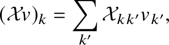 $$ \begin{align*}(\mathcal{X}v)_k=\sum_{k'}\mathcal{X}_{kk'}v_{k'},\end{align*} $$
where the matrix coefficients are given by
 $$ \begin{align*}\mathcal{X}_{kk'}=\left(\frac{\alpha T}{L^{d}}\right)^{n_1+n_2+1}\sum_{\left(k_{\mathfrak{n}}:\mathfrak{n}\in\mathcal{T}\right)}\mathcal{K}\left(\left\lvert k\right\rvert_{\beta}^2-\left\lvert k'\right\rvert_{\beta}^2,\ k_{\mathfrak{l}}:\mathfrak{r}'\neq\mathfrak{l}\in\mathcal L\right)\cdot\frac{1}{\left\langle Tq_{\mathfrak{r}}-\zeta\right\rangle^5}\prod_{\mathfrak{n}\in\mathcal{N}\setminus \{\mathfrak{r}\}}\frac{1}{\langle Tq_{\mathfrak{n}}\rangle}\prod_{\mathfrak{l}\in\mathcal L\setminus \{\mathfrak{r}'\}}\eta_{k_{\mathfrak{l}}}^{\iota_{\mathfrak{l}}},\end{align*} $$
where the sum is taken over all admissible assignments $(k_{\mathfrak {n}}:\mathfrak {n}\in \mathcal{T}\,\,)$
which satisfy
$(k_{\mathfrak {n}}:\mathfrak {n}\in \mathcal{T}\,\,)$
which satisfy $k_{\mathfrak {r}}=k$
,
$k_{\mathfrak {r}}=k$
, $k_{\mathfrak {r}'}=k'$
and
$k_{\mathfrak {r}'}=k'$
and $\left \lvert k_{\mathfrak {n}}\right \rvert \leq L^{\theta }$
for
$\left \lvert k_{\mathfrak {n}}\right \rvert \leq L^{\theta }$
for $\mathfrak {n}\not \in \{\mathfrak {r},\mathfrak {r}'\}$
, and the coefficient satisfies
$\mathfrak {n}\not \in \{\mathfrak {r},\mathfrak {r}'\}$
, and the coefficient satisfies $\left \lvert \mathcal {K}\right \rvert \leq L^{\theta }$
and
$\left \lvert \mathcal {K}\right \rvert \leq L^{\theta }$
and $\left \lvert \partial \mathcal {K}\right \rvert \leq L^{\theta } T$
. Moreover, we observe that
$\left \lvert \partial \mathcal {K}\right \rvert \leq L^{\theta } T$
. Moreover, we observe that $\mathcal {K}$
and
$\mathcal {K}$
and $q_{\mathfrak r}$
depend on the variables
$q_{\mathfrak r}$
depend on the variables $k_{\mathfrak {r}}=k$
and
$k_{\mathfrak {r}}=k$
and $k_{\mathfrak {r}'}=k'$
only through the quantity
$k_{\mathfrak {r}'}=k'$
only through the quantity $\left \lvert k\right \rvert _{\beta }^2-\left \lvert k'\right \rvert _{\beta }^2$
.
$\left \lvert k\right \rvert _{\beta }^2-\left \lvert k'\right \rvert _{\beta }^2$
.
Next we argue in the same way as in the proof of Proposition 2.5 and fix the integer parts of $Tq_{\mathfrak {n}}$
for
$Tq_{\mathfrak {n}}$
for $\mathfrak {n}\in \mathcal {N}\setminus \{\mathfrak {r}\}$
, as well as the integer part of
$\mathfrak {n}\in \mathcal {N}\setminus \{\mathfrak {r}\}$
, as well as the integer part of $Tq_{\mathfrak {r}}-\zeta $
, at a cost of
$Tq_{\mathfrak {r}}-\zeta $
, at a cost of $(\log L)^{O(1)}$
. All these can be assumed to be
$(\log L)^{O(1)}$
. All these can be assumed to be $\leq L^{\theta ^{-1}}$
due to the decay
$\leq L^{\theta ^{-1}}$
due to the decay $\left \langle Tq_{\mathfrak {r}}-\zeta \right \rangle ^{-5}$
and the bounds on
$\left \langle Tq_{\mathfrak {r}}-\zeta \right \rangle ^{-5}$
and the bounds on $\tau $
and
$\tau $
and $\tau '$
. This is equivalent to fixing some real numbers
$\tau '$
. This is equivalent to fixing some real numbers $\sigma _{\mathfrak {n}}=O\left (L^{\theta ^{-1}}\right )$
and requiring the assignment
$\sigma _{\mathfrak {n}}=O\left (L^{\theta ^{-1}}\right )$
and requiring the assignment $(k_{\mathfrak {n}}:\mathfrak {n}\in \mathcal{T}\,\,)$
to satisfy
$(k_{\mathfrak {n}}:\mathfrak {n}\in \mathcal{T}\,\,)$
to satisfy $\lvert \Omega _{\mathfrak {n}}-\sigma _{\mathfrak {n}}\rvert \leq T^{-1}$
for each
$\lvert \Omega _{\mathfrak {n}}-\sigma _{\mathfrak {n}}\rvert \leq T^{-1}$
for each $\mathfrak {n}\in \mathcal {N}$
. Let this final operator, obtained by all the previous reductions, be
$\mathfrak {n}\in \mathcal {N}$
. Let this final operator, obtained by all the previous reductions, be $\mathcal {G}$
. Schematically, the operator
$\mathcal {G}$
. Schematically, the operator $\mathcal {G}$
can be viewed as ‘attaching’ two trees
$\mathcal {G}$
can be viewed as ‘attaching’ two trees $\mathcal{T}\,_1$
and
$\mathcal{T}\,_1$
and $\mathcal{T}\,_2$
to a single node
$\mathcal{T}\,_2$
to a single node $\mathfrak {r}'$
.
$\mathfrak {r}'$
.
Step 3: The high-order $\mathcal {G}\mathcal {G}^*$
argument. For this, we consider the adjoint operator
$\mathcal {G}\mathcal {G}^*$
argument. For this, we consider the adjoint operator $\mathcal {G}^*$
. A similar argument gives a formula for
$\mathcal {G}^*$
. A similar argument gives a formula for $\mathcal {G}^*$
, which is associated with a tree
$\mathcal {G}^*$
, which is associated with a tree $\mathcal{T}\,^*$
formed by attaching the two trees
$\mathcal{T}\,^*$
formed by attaching the two trees $\mathcal{T}\,_2$
and
$\mathcal{T}\,_2$
and $\mathcal{T}\,_1$
(with
$\mathcal{T}\,_1$
(with $\mathcal{T}\,_2$
on the left of
$\mathcal{T}\,_2$
on the left of $\mathcal{T}\,_1$
) to a single node
$\mathcal{T}\,_1$
) to a single node $\mathfrak {r}'$
, in the same way that
$\mathfrak {r}'$
, in the same way that $\mathcal {G}$
is associated with
$\mathcal {G}$
is associated with $\mathcal{T}\,$
. Given a large positive integer D, we will consider
$\mathcal{T}\,$
. Given a large positive integer D, we will consider $(\mathcal {G}\mathcal {G}^*)^{D}$
, which is associated with a tree
$(\mathcal {G}\mathcal {G}^*)^{D}$
, which is associated with a tree $\mathcal{T}\,^D$
. The precise description is as follows.
$\mathcal{T}\,^D$
. The precise description is as follows.
First, $\mathcal{T}\,^D$
is a tree with root node
$\mathcal{T}\,^D$
is a tree with root node $\mathfrak {r}_0=\mathfrak {r}$
, and its first two subtrees (from the left) are
$\mathfrak {r}_0=\mathfrak {r}$
, and its first two subtrees (from the left) are $\mathcal{T}\,_1$
and
$\mathcal{T}\,_1$
and $\mathcal{T}\,_2$
. The third subtree has root
$\mathcal{T}\,_2$
. The third subtree has root $\mathfrak {r}_1$
, and its first two subtrees (from the left) are
$\mathfrak {r}_1$
, and its first two subtrees (from the left) are $\mathcal{T}\,_2$
and
$\mathcal{T}\,_2$
and $\mathcal{T}\,_1$
. The third subtree has root
$\mathcal{T}\,_1$
. The third subtree has root $\mathfrak {r}_2$
, and its first two subtrees (from the left) are
$\mathfrak {r}_2$
, and its first two subtrees (from the left) are $\mathcal{T}\,_1$
and
$\mathcal{T}\,_1$
and $\mathcal{T}\,_2$
, and so on. This process repeats and eventually stops at
$\mathcal{T}\,_2$
, and so on. This process repeats and eventually stops at $\mathfrak {r}_{2D}=\mathfrak {r}'$
, which is a single node, finishing the construction of
$\mathfrak {r}_{2D}=\mathfrak {r}'$
, which is a single node, finishing the construction of $\mathcal{T}\,^D$
. As usual, denote by
$\mathcal{T}\,^D$
. As usual, denote by $\mathcal L^D$
and
$\mathcal L^D$
and $\mathcal N^D$
the set of leaves and branching nodes, respectively. Then the kernel of
$\mathcal N^D$
the set of leaves and branching nodes, respectively. Then the kernel of $(\mathcal {G}\mathcal {G}^*)^{D}$
is given by
$(\mathcal {G}\mathcal {G}^*)^{D}$
is given by
 $$ \begin{align} \left((\mathcal{G}\mathcal{G}^*)^{D}\right)_{kk'}=\sum_{\left(k_{\mathfrak{n}}:\mathfrak{n}\in\mathcal{T}^D\right)}\mathcal{K}^{(D)}&\left(\left\lvert k_{\mathfrak{r}_j}\right\rvert_{\beta}^2-\left\lvert k_{\mathfrak{r}_{j+1}}\right\rvert_{\beta}^2:0\leq j\leq 2D-1,\ k_{\mathfrak{l}}:\mathfrak{r}'\neq\mathfrak{l}\in\mathcal L^D\right)\nonumber\\ &\quad\quad\quad\quad\quad\quad\times\left(\frac{\alpha T}{L^{d}}\right)^{2D\left(n_1+n_2+1\right)}\prod_{\mathfrak{r}'\neq\mathfrak{l}\in\mathcal L^D}\eta_{k_{\mathfrak{l}}}^{\iota_{\mathfrak{l}}}, \end{align} $$
where $\left \lvert \mathcal {K}^{(D)}\right \rvert \leq L^{\theta }$
and
$\left \lvert \mathcal {K}^{(D)}\right \rvert \leq L^{\theta }$
and $\left \lvert \partial \mathcal {K}^{(D)}\right \rvert \leq L^{\theta } T$
, and the sum is taken over all admissible assignments
$\left \lvert \partial \mathcal {K}^{(D)}\right \rvert \leq L^{\theta } T$
, and the sum is taken over all admissible assignments $\left (k_{\mathfrak {n}}:\mathfrak {n}\in \mathcal{T}\,^D\right )$
that satisfy
$\left (k_{\mathfrak {n}}:\mathfrak {n}\in \mathcal{T}\,^D\right )$
that satisfy $(k_{\mathfrak {r}},k_{\mathfrak {r}'})=(k,k')$
,
$(k_{\mathfrak {r}},k_{\mathfrak {r}'})=(k,k')$
, $\lvert k_{\mathfrak {l}}\rvert \leq L^{\theta }$
for
$\lvert k_{\mathfrak {l}}\rvert \leq L^{\theta }$
for $\mathfrak {r}'\neq \mathfrak {l}\in \mathcal L$
and
$\mathfrak {r}'\neq \mathfrak {l}\in \mathcal L$
and $\lvert \Omega _{\mathfrak {n}}-\sigma _{\mathfrak {n}}\rvert \leq T^{-1}$
for
$\lvert \Omega _{\mathfrak {n}}-\sigma _{\mathfrak {n}}\rvert \leq T^{-1}$
for $\mathfrak {n}\in \mathcal {N}^D$
, where
$\mathfrak {n}\in \mathcal {N}^D$
, where $\sigma _{\mathfrak {n}}=O\left (L^{\theta ^{-1}}\right )$
are fixed. Moreover,
$\sigma _{\mathfrak {n}}=O\left (L^{\theta ^{-1}}\right )$
are fixed. Moreover, $\mathcal {K}^{(D)}$
depends on the variables
$\mathcal {K}^{(D)}$
depends on the variables $k_{\mathfrak {r}}=k$
and
$k_{\mathfrak {r}}=k$
and $k_{\mathfrak {r}'}=k'$
only through the quantities
$k_{\mathfrak {r}'}=k'$
only through the quantities $\left \lvert k_{\mathfrak {r}_j}\right \rvert _{\beta }^2-\left \lvert k_{\mathfrak {r}_{j+1}}\right \rvert _{\beta }^2$
for
$\left \lvert k_{\mathfrak {r}_j}\right \rvert _{\beta }^2-\left \lvert k_{\mathfrak {r}_{j+1}}\right \rvert _{\beta }^2$
for $0\leq j\leq 2D-1$
.
$0\leq j\leq 2D-1$
.
Now note that each $\left ((\mathcal {G}\mathcal {G}^*)^{D}\right )_{kk'}$
is an explicit multilinear Gaussian expression. Since for fixed k (or
$\left ((\mathcal {G}\mathcal {G}^*)^{D}\right )_{kk'}$
is an explicit multilinear Gaussian expression. Since for fixed k (or $k'$
) the number of choices for
$k'$
) the number of choices for $k'$
(or k) is
$k'$
(or k) is $O\left (L^{d+\theta }\right )$
, by Schur’s estimate we know
$O\left (L^{d+\theta }\right )$
, by Schur’s estimate we know
 $$ \begin{align*} \left\lVert(\mathcal{G}\mathcal{G}^*)^{D}\right\rVert_{\ell^2\to\ell^2}\lesssim L^{d+\theta}\sup_{k,k'}\left\lvert\left((\mathcal{G}\mathcal{G}^*)^{D}\right)_{kk'}\right\rvert. \end{align*} $$
So it suffices to L-certainly bound $\left \lvert \left ((\mathcal {G}\mathcal {G}^*)^{D}\right )_{kk'}\right \rvert $
uniformly in k and
$\left \lvert \left ((\mathcal {G}\mathcal {G}^*)^{D}\right )_{kk'}\right \rvert $
uniformly in k and $k'$
. We first consider this estimate with fixed
$k'$
. We first consider this estimate with fixed $(k,k')$
. Applying Lemma 3.1, we can fix some pairings of
$(k,k')$
. Applying Lemma 3.1, we can fix some pairings of $\mathcal{T}\,^D$
and the set
$\mathcal{T}\,^D$
and the set $\mathcal {S}^D$
of single leaves, and argue as in the proof of Proposition 2.5 to conclude L-certainly that
$\mathcal {S}^D$
of single leaves, and argue as in the proof of Proposition 2.5 to conclude L-certainly that
 $$ \begin{align*} \left\lvert\left((\mathcal{G}\mathcal{G}^*)^{D}\right)_{kk'}\right\rvert^2\lesssim L^{\theta}\left(\frac{\alpha T}{L^{d}}\right)^{4D\left(n_1+n_2+1\right)}\sum_{\left(k_{\mathfrak{l}}:\mathfrak{l}\in\mathcal{S}^D\right)}\sum_{\left(k_{\mathfrak{l}}:\mathfrak{l}\in\mathcal L^D\backslash\mathcal{S}^D\right)}^{**}\sum_{\left(k_{\mathfrak{l}'}:\mathfrak{l}\in\mathcal L^D\backslash\mathcal{S}^D\right)}^{**'}1, \end{align*} $$
where the condition for summation, as in the proof of Proposition 2.5, is that the unique admissible assignment $\left (k_{\mathfrak {n}}:\mathfrak {n}\in \mathcal{T}\,^D\right )$
determined by
$\left (k_{\mathfrak {n}}:\mathfrak {n}\in \mathcal{T}\,^D\right )$
determined by $\left (k_{\mathfrak {l}}:\mathfrak {l}\in \mathcal {S}^D\right )$
and
$\left (k_{\mathfrak {l}}:\mathfrak {l}\in \mathcal {S}^D\right )$
and $\left (k_{\mathfrak {l}}:\mathfrak {l}\in \mathcal L^D\backslash \mathcal {S}^D\right )$
satisfies all the conditions already listed, and the same happens for
$\left (k_{\mathfrak {l}}:\mathfrak {l}\in \mathcal L^D\backslash \mathcal {S}^D\right )$
satisfies all the conditions already listed, and the same happens for $\left (k_{\mathfrak {n}}':\mathfrak {n}\in \mathcal{T}\,^D\right )$
corresponding to
$\left (k_{\mathfrak {n}}':\mathfrak {n}\in \mathcal{T}\,^D\right )$
corresponding to $\left (k_{\mathfrak {l}}:\mathfrak {l}\in \mathcal {S}^D\right )$
and
$\left (k_{\mathfrak {l}}:\mathfrak {l}\in \mathcal {S}^D\right )$
and $\left (k_{\mathfrak {l}}':\mathfrak {l}\in \mathcal L^D\backslash \mathcal {S}^D\right )$
. We know that
$\left (k_{\mathfrak {l}}':\mathfrak {l}\in \mathcal L^D\backslash \mathcal {S}^D\right )$
. We know that $\mathcal{T}\,^D$
is a tree of scale
$\mathcal{T}\,^D$
is a tree of scale $2D(n_1+n_2+1)$
,, and so
$2D(n_1+n_2+1)$
,, and so $\left \lvert \mathcal L^D\right \rvert =4D(n_1+n_2+1)+1$
; let the number of pairings be p, and then
$\left \lvert \mathcal L^D\right \rvert =4D(n_1+n_2+1)+1$
; let the number of pairings be p, and then $\left \lvert \mathcal {S}^D\right \rvert =4D(n_1+n_2+1)-2p$
. By Proposition 3.5 we can bound the number of choicesFootnote
12
for
$\left \lvert \mathcal {S}^D\right \rvert =4D(n_1+n_2+1)-2p$
. By Proposition 3.5 we can bound the number of choicesFootnote
12
for $\left (k_{\mathfrak {l}}:\mathfrak {l}\in \mathcal {S}^D\right )$
and
$\left (k_{\mathfrak {l}}:\mathfrak {l}\in \mathcal {S}^D\right )$
and $\left (k_{\mathfrak {l}}':\mathfrak {l}\in \mathcal L^D\backslash \mathcal {S}^D\right )$
by
$\left (k_{\mathfrak {l}}':\mathfrak {l}\in \mathcal L^D\backslash \mathcal {S}^D\right )$
by $M=L^{\theta } Q^{4D\left (n_1+n_2+1\right )-p}$
, and bound the number of choices for
$M=L^{\theta } Q^{4D\left (n_1+n_2+1\right )-p}$
, and bound the number of choices for $\left (k_{\mathfrak {l}}':\mathfrak {l}\in \mathcal L^D\backslash \mathcal {S}^D\right )$
given
$\left (k_{\mathfrak {l}}':\mathfrak {l}\in \mathcal L^D\backslash \mathcal {S}^D\right )$
given $\left (k_{\mathfrak {l}}:\mathfrak {l}\in \mathcal {S}^D\right )$
by
$\left (k_{\mathfrak {l}}:\mathfrak {l}\in \mathcal {S}^D\right )$
by $M'=L^{\theta } Q^{p}$
. In the end, for any fixed
$M'=L^{\theta } Q^{p}$
. In the end, for any fixed $(k,k')$
, we have that L-certainly,
$(k,k')$
, we have that L-certainly,
 $$ \begin{align*} L^{d+\theta}\sup_{k,k'}\left\lvert\left((\mathcal{G}\mathcal{G}^*)^{D}\right)_{kk'}\right\rvert\leq L^{d+\theta}\left(\frac{\alpha T}{L^{d}}\right)^{2D\left(n_1+n_2+1\right)}\left(MM'\right)^{1/2}\leq L^{d+\theta}\rho^{2D\left(n_1+n_2+1\right)}. \end{align*} $$
Finally we need to L-certainly make this bound uniform in all choices of $(k,k')$
. This is not obvious, since we impose no upper bound on
$(k,k')$
. This is not obvious, since we impose no upper bound on $\lvert k\rvert $
and
$\lvert k\rvert $
and $\lvert k'\rvert $
, so the number of exceptional sets we remove in the L-certain condition could presumably be infinite. However, note that the coefficient
$\lvert k'\rvert $
, so the number of exceptional sets we remove in the L-certain condition could presumably be infinite. However, note that the coefficient $\boldsymbol {\mathcal {K}}$
depends on k and
$\boldsymbol {\mathcal {K}}$
depends on k and $k'$
only through the quantities
$k'$
only through the quantities $\left \lvert k\right \rvert _{\beta }^2-\left \lvert k_{\mathfrak {r}_{j}}\right \rvert _{\beta }^2$
. Let
$\left \lvert k\right \rvert _{\beta }^2-\left \lvert k_{\mathfrak {r}_{j}}\right \rvert _{\beta }^2$
. Let $\mathcal {D}=\mathcal L\backslash \{\mathfrak {r'}\}$
; then
$\mathcal {D}=\mathcal L\backslash \{\mathfrak {r'}\}$
; then $\lvert k_{\mathfrak {l}}\rvert \leq L^{\theta }$
for
$\lvert k_{\mathfrak {l}}\rvert \leq L^{\theta }$
for $\mathfrak {l}\in \mathcal {D}$
, and the condition for summation creates the restriction that
$\mathfrak {l}\in \mathcal {D}$
, and the condition for summation creates the restriction that $\left \lvert \left \lvert k\right \rvert _{\beta }^2-\left \lvert k_{\mathfrak {r}_{j}}\right \rvert _{\beta }^2\right \rvert \leq L^{\theta ^{-1}}$
. The reduction from infinitely many possibilities for k (and hence
$\left \lvert \left \lvert k\right \rvert _{\beta }^2-\left \lvert k_{\mathfrak {r}_{j}}\right \rvert _{\beta }^2\right \rvert \leq L^{\theta ^{-1}}$
. The reduction from infinitely many possibilities for k (and hence $k'$
) to finitely many is done by invoking the following result, whose proof will be left to the end:
$k'$
) to finitely many is done by invoking the following result, whose proof will be left to the end:
Claim 3.7. Let $k\in \mathbb {Z}_L^d$
, and consider the function
$k\in \mathbb {Z}_L^d$
, and consider the function
 $$ \begin{align*}f_{(k)}:m\mapsto \left\lvert k\right\rvert_{\beta}^2-\left\lvert k+m\right\rvert_{\beta}^2,\qquad \mathrm{Dom}\left(f_{(k)}\right)=\left\{m\in\mathbb{Z}_L^d:\lvert m\rvert\leq L^{\theta},\left\lvert\left\lvert k\right\rvert_{\beta}^2-\left\lvert k+m\right\rvert_{\beta}^2\right\rvert\leq L^{\theta^{-1}}\right\}.\end{align*} $$
Then there exist finitely many functions $f_1,\ldots ,f_A$
, where
$f_1,\ldots ,f_A$
, where $A\leq L^{C\theta ^{-1}}$
, such that for any
$A\leq L^{C\theta ^{-1}}$
, such that for any $k\in \mathbb {Z}_L^d$
there exists
$k\in \mathbb {Z}_L^d$
there exists $1\leq j\leq A$
such that
$1\leq j\leq A$
such that $\left \lvert f_{(k)}-f_j\right \rvert \leq L^{-\theta ^{-1}}$
on
$\left \lvert f_{(k)}-f_j\right \rvert \leq L^{-\theta ^{-1}}$
on $\mathrm {Dom}\left (f_{(k)}\right )$
.
$\mathrm {Dom}\left (f_{(k)}\right )$
.
Remark 3.8. We may view Claim 3.7 as a ‘finiteness’ or ‘compactness’ lemma. Similar results are also used in [Reference Deng, Nahmod and Yue18] and [Reference Deng, Nahmod and Yue19] for similar purposes.
Now it is not hard to see that Claim 3.7 allows us to obtain a bound of the form proved that is uniform in $(k,k')$
, after removing at most
$(k,k')$
, after removing at most $O\left (L^{C\theta ^{-1}}\right )$
exceptional sets, each with probability
$O\left (L^{C\theta ^{-1}}\right )$
exceptional sets, each with probability $\lesssim e^{-L^{\theta }}$
. This then implies
$\lesssim e^{-L^{\theta }}$
. This then implies
 $$ \begin{align*}\left\lVert(\mathcal{G}\mathcal{G}^*)^{D}\right\rVert_{\ell^2\to\ell^2}\lesssim L^{d+\theta}\rho^{2D\left(n_1+n_2+1\right)},\end{align*} $$
hence
 $$ \begin{align*}\left\lVert\mathcal{G}\right\rVert_{\ell^2\to\ell^2}\lesssim L^{\frac{d+\theta}{2D}}\rho^{n_1+n_2+1}.\end{align*} $$
By fixing D to be a sufficiently large positive integer, we deduce the correct operator bound for $\mathcal {G}$
, and hence for
$\mathcal {G}$
, and hence for $\mathcal {X}$
and
$\mathcal {X}$
and $\mathcal {P}_+$
. This completes the proof of Proposition 2.6.
$\mathcal {P}_+$
. This completes the proof of Proposition 2.6.
Proof of Claim 3.7. We will prove the result for any linear function $g(m)=x\cdot m+X$
, where
$g(m)=x\cdot m+X$
, where $x\in \mathbb {R}^d$
and
$x\in \mathbb {R}^d$
and $X\in \mathbb {R}$
are arbitrary. We may also assume
$X\in \mathbb {R}$
are arbitrary. We may also assume $m\in \mathbb {Z}^d$
instead of
$m\in \mathbb {Z}^d$
instead of $\mathbb {Z}_L^d$
; the domain
$\mathbb {Z}_L^d$
; the domain $\mathrm {Dom}(g)$
will then be the set E of m such that
$\mathrm {Dom}(g)$
will then be the set E of m such that $\lvert m\rvert \leq L^{1+\theta }$
and
$\lvert m\rvert \leq L^{1+\theta }$
and $\lvert g(m)\rvert \leq L^{2+\theta ^{-1}}$
.
$\lvert g(m)\rvert \leq L^{2+\theta ^{-1}}$
.
Let the affine dimension $\dim (E)=r\leq d$
; then E contains a maximal affine independent set
$\dim (E)=r\leq d$
; then E contains a maximal affine independent set $\left \{q_j:0\leq j\leq r\right \}$
. The number of choices for these
$\left \{q_j:0\leq j\leq r\right \}$
. The number of choices for these $q_j$
is at most
$q_j$
is at most $L^{d+1}$
, so we may fix them. Let
$L^{d+1}$
, so we may fix them. Let $\mathcal L$
be the primitive lattice generated by
$\mathcal L$
be the primitive lattice generated by $\left \{q_j-q_0:1\leq j\leq r\right \}$
, and fix a reduced basis
$\left \{q_j-q_0:1\leq j\leq r\right \}$
, and fix a reduced basis $\left \{\ell _j:1\leq j\leq r\right \}$
of
$\left \{\ell _j:1\leq j\leq r\right \}$
of $\mathcal L$
. For any
$\mathcal L$
. For any $m\in E$
there is a unique integer vector
$m\in E$
there is a unique integer vector $k=(k_1,\ldots ,k_r)\in \mathbb {Z}^r$
such that
$k=(k_1,\ldots ,k_r)\in \mathbb {Z}^r$
such that $\lvert k\rvert \lesssim L^{1+\theta }$
,
$\lvert k\rvert \lesssim L^{1+\theta }$
, $m-q_0=k_1\ell _1+\cdots +k_r\ell _r$
, and as a linear function we can write
$m-q_0=k_1\ell _1+\cdots +k_r\ell _r$
, and as a linear function we can write $g(m)=y\cdot k+Y$
, where
$g(m)=y\cdot k+Y$
, where $y\in \mathbb {R}^r$
and
$y\in \mathbb {R}^r$
and $Y=g(q_0)\in \mathbb {R}$
.
$Y=g(q_0)\in \mathbb {R}$
.
Now let the $k\in \mathbb {Z}^r$
corresponding to
$k\in \mathbb {Z}^r$
corresponding to $m=q_j$
be
$m=q_j$
be $k^{\left (j\right )}$
, where
$k^{\left (j\right )}$
, where $1\leq j\leq r$
; then since
$1\leq j\leq r$
; then since $q_0\in E$
and
$q_0\in E$
and $q_j\in E$
, we conclude that
$q_j\in E$
, we conclude that $\left \lvert y\cdot k^{\left (j\right )}\right \rvert \leq L^{3+\theta ^{-1}}$
. As the
$\left \lvert y\cdot k^{\left (j\right )}\right \rvert \leq L^{3+\theta ^{-1}}$
. As the $k^{\left (j\right )}$
are linear independent integer vectors in
$k^{\left (j\right )}$
are linear independent integer vectors in $\mathbb {Z}^r$
with norm bounded by
$\mathbb {Z}^r$
with norm bounded by $L^{1+\theta }$
, we conclude that
$L^{1+\theta }$
, we conclude that $\lvert y\rvert \leq L^{C+\theta ^{-1}}$
, and consequently
$\lvert y\rvert \leq L^{C+\theta ^{-1}}$
, and consequently $\lvert Y\rvert \leq L^{C+\theta ^{-1}}$
. We may then approximate
$\lvert Y\rvert \leq L^{C+\theta ^{-1}}$
. We may then approximate $g(m)$
for
$g(m)$
for $m\in E$
by
$m\in E$
by $y_j\cdot k+Y_j$
, where
$y_j\cdot k+Y_j$
, where $y_j$
and
$y_j$
and $Y_j$
are one of the
$Y_j$
are one of the $L^{C\theta ^{-1}}$
choices that approximate y and Y up to error
$L^{C\theta ^{-1}}$
choices that approximate y and Y up to error $L^{-\theta ^{-1}}$
, and choose
$L^{-\theta ^{-1}}$
, and choose $g_{\left (j\right )}=y_j\cdot k+Y_j$
.
$g_{\left (j\right )}=y_j\cdot k+Y_j$
.
3.4 The worst terms
In this section we exhibit terms $\mathcal J_{\mathcal{T}}~$
that satisfy the lower bound (1.9). These are the terms corresponding to trees
$\mathcal J_{\mathcal{T}}~$
that satisfy the lower bound (1.9). These are the terms corresponding to trees $\mathcal{T}~$
and pairings (see Remark 3.9) as shown in Figure 5, where
$\mathcal{T}~$
and pairings (see Remark 3.9) as shown in Figure 5, where $\mathcal{T}~$
is formed from a single node by successively attaching two leaf nodes, and the ‘left’ node attached at each step is paired with the ‘right’ node attached in the next step. Let the scale
$\mathcal{T}~$
is formed from a single node by successively attaching two leaf nodes, and the ‘left’ node attached at each step is paired with the ‘right’ node attached in the next step. Let the scale $\mathfrak s(\mathcal{T}\,\,)=r$
; then
$\mathfrak s(\mathcal{T}\,\,)=r$
; then $\mathcal{T}\,$
has exactly
$\mathcal{T}\,$
has exactly $r-1$
pairings. For simplicity we will consider the rational case
$r-1$
pairings. For simplicity we will consider the rational case $\beta _j=1$
and
$\beta _j=1$
and $T\leq L^{2-\delta }$
; the irrational case is similar.
$T\leq L^{2-\delta }$
; the irrational case is similar.
A tree of scale $\mathfrak s (\mathcal{T}\,\,)=6$
and
$\mathfrak s (\mathcal{T}\,\,)=6$
and $p=6-1=5$
pairings. The pairings force
$p=6-1=5$
pairings. The pairings force $\lvert y-z\rvert =\lvert n_5-\ell _5\rvert =\lvert n_4-\ell _4\rvert =\cdots =\lvert k-x\rvert $
.
$\lvert y-z\rvert =\lvert n_5-\ell _5\rvert =\lvert n_4-\ell _4\rvert =\cdots =\lvert k-x\rvert $
.

Here it is more convenient to work with the time variable t (instead of its Fourier dual $\tau $
). To show formula (1.9), since
$\tau $
). To show formula (1.9), since $b>1/2$
, we just need to bound
$b>1/2$
, we just need to bound $(\mathcal J_{\mathcal{T}\,})_k(t)$
from below for some k and some
$(\mathcal J_{\mathcal{T}\,})_k(t)$
from below for some k and some $t\in [0,1]$
; moreover, since
$t\in [0,1]$
; moreover, since $\chi \equiv 1$
on
$\chi \equiv 1$
on $[0,1]$
, and using the recursive definition (2.17), we can write
$[0,1]$
, and using the recursive definition (2.17), we can write
 $$ \begin{align}(\mathcal J_{\mathcal{T}})_k(t)=\left(\frac{\alpha T}{L^d}\right)^r\sum_{x-y+z=k}\left(\sum_{\ell_1,\ldots,\ell_{r-1}}\mathcal{B}\cdot\prod_{j=1}^{r-1}n_{\mathrm{in}}(\ell_j)\left\lvert\eta_{\ell_j}\right\rvert^2\right)\cdot \eta_x\overline{\eta_y}\eta_z \cdot \sqrt{n_{\mathrm{in}}(x)n_{\mathrm{in}}(y)n_{\mathrm{in}}(z)}, \end{align} $$
where (due to admissibility) the variables in the summation satisfy
 $$ \begin{align*}k-x=n_1-\ell_1=n_2-\ell_2=\cdots=n_{r-1}-\ell_{r-1}=y-z:=q\end{align*} $$
and the coefficient $\mathcal {B}$
is given by
$\mathcal {B}$
is given by
 $$ \begin{align}\mathcal{B}=\int_{t>t_1>\cdots >t_r>0}e^{2\pi iT\left(t_1\Omega_1+\cdots +t_r\Omega_r\right)}\mathrm{d}t_1\cdots\mathrm{d}t_r, \end{align} $$
with $\Omega _j$
being the resonance factors, namely
$\Omega _j$
being the resonance factors, namely
 $$ \begin{align*}\Omega_1=2q\cdot(k-n_1),\Omega_2=2q\cdot(n_1-n_2),\ldots,\Omega_{r-1}=2q\cdot(n_{r-2}-n_{r-1}),\Omega_r=2q\cdot(n_{r-1}-z).\end{align*} $$
In equation (3.23) we may replace $\left \lvert \eta _{\ell _j}\right \rvert ^2$
by 1, so the factor in the big parentheses, which we denote by
$\left \lvert \eta _{\ell _j}\right \rvert ^2$
by 1, so the factor in the big parentheses, which we denote by $\mathcal {A}_{kxyz}$
, involves no randomness. Therefore, with high probability,
$\mathcal {A}_{kxyz}$
, involves no randomness. Therefore, with high probability,
 $$ \begin{align*}\left\lvert(\mathcal J_{\mathcal{T}})_k(t)\right\rvert^2\sim\left(\frac{\alpha T}{L^d}\right)^{2r}\sum_{x-y+z=k}\left\lvert\mathcal{A}_{kxyz}\right\rvert^2.\end{align*} $$
In the sum, we may fix $q\in \mathbb {Z}_L^d$
with
$q\in \mathbb {Z}_L^d$
with $0<\lvert q\rvert \lesssim L^{-1}$
, which has
$0<\lvert q\rvert \lesssim L^{-1}$
, which has $O(1)$
choices, and write
$O(1)$
choices, and write
 $$ \begin{align*} \mathcal{A}_{kxyz}&=\int_{t>t_1>\cdots >t_r>0}e^{4\pi iTq\cdot\left[t_1\left(k-q\right)+t_r\left(q-z\right)\right]}\\ &\quad\quad\quad\times\left[\sum_{\ell_1,\ldots,\ell_{r-1}}e^{4\pi iT \left[\left(t_2-t_1\right)q\cdot \ell_1+\cdots +\left(t_r-t_{r-1}\right)q\cdot\ell_{r-1}\right]}\prod_{j=1}^{r-1}n_{\mathrm{in}}\left(\ell_j\right)\right]\mathrm{d}t_1\cdots\mathrm{d}t_r. \end{align*} $$
By Poisson summation, and noticing that $\left \lvert Tt_jq\right \rvert \lesssim L^{1-\delta }$
, we conclude that up to constants,
$\left \lvert Tt_jq\right \rvert \lesssim L^{1-\delta }$
, we conclude that up to constants,
 $$ \begin{align*} \sum_{\ell_1,\ldots,\ell_{r-1}}e^{4\pi iT \left[\left(t_2-t_1\right)q\cdot \ell_1+\cdots +\left(t_r-t_{r-1}\right)q \cdot\ell_{r-1}\right]} \prod_{j=1}^{r-1}n_{\mathrm{in}}\left(\ell_j\right)=L^{(r-1)d} \prod_{j=1}^{r-1}\widehat{n_{\mathrm{in}}}\left(Tq\left(t_{j+1}-t_j\right)\right)+O\left(L^{-\infty}\right). \end{align*} $$
By making change of variables $s_j=t_{j}-t_{j+1} (1\leq j\leq r-1)$
and
$s_j=t_{j}-t_{j+1} (1\leq j\leq r-1)$
and $s_0=t-t_1$
,
$s_0=t-t_1$
, $s_r=t_r$
, we can reduce to
$s_r=t_r$
, we can reduce to
 $$ \begin{align*} \mathcal{A}_{kxyz}\approx L^{(r-1)d}\int_{s_0+\cdots +s_{r}=t} e^{4\pi iT\left[\left(t-s_0\right)q\cdot\left(k-q\right)+s_rq\cdot\left(q-z\right)\right]}\prod_{j=1}^{r-1}\widehat{n_{\mathrm{in}}}\left(Tqs_j\right)\mathrm{d}s_1\cdots\mathrm{d}s_r. \end{align*} $$
By choosing some particular $(k,q,z)$
, we may assume
$(k,q,z)$
, we may assume $q\cdot (k-q)=q\cdot (q-z)=0$
, and if we also choose
$q\cdot (k-q)=q\cdot (q-z)=0$
, and if we also choose $n_{\mathrm {in}}$
such that
$n_{\mathrm {in}}$
such that $\widehat {n_{\mathrm {in}}}$
is positive, say
$\widehat {n_{\mathrm {in}}}$
is positive, say $n_{\mathrm {in}}(k)=e^{-\left \lvert k\right \rvert ^2}$
, and
$n_{\mathrm {in}}(k)=e^{-\left \lvert k\right \rvert ^2}$
, and $t=\min \left (1,LT^{-1}\right )$
, then we have
$t=\min \left (1,LT^{-1}\right )$
, then we have
 $$ \begin{align*} \left\lvert\mathcal{A}_{kxyz}\right\rvert\sim L^{\left(r-1\right)d}\min\left(1,LT^{-1}\right)^{r}, \end{align*} $$
and hence, with high probability,
 $$ \begin{align*} \sup_{k,t}\left\lvert(\mathcal J_{\mathcal{T}})_k(t)\right\rvert\gtrsim L^{-d}\min(\alpha T,\alpha L)^r=L^{-d}\rho^r \end{align*} $$
for any fixed r – thus formula (1.9).
Remark 3.9. Here, strictly speaking, we are further decomposing $\mathcal J_{\mathcal{T}\,}$
into the sum of terms
$\mathcal J_{\mathcal{T}\,}$
into the sum of terms $\mathcal J_{\mathcal{T}\,,\mathcal {P}}$
, where
$\mathcal J_{\mathcal{T}\,,\mathcal {P}}$
, where $\mathcal {P}$
represents the pairing structure of
$\mathcal {P}$
represents the pairing structure of $\mathcal{T}\,$
. In the proof of Proposition 2.5, we are actually making the same decomposition (by identifying the set of pairings) and proving the same bound for each
$\mathcal{T}\,$
. In the proof of Proposition 2.5, we are actually making the same decomposition (by identifying the set of pairings) and proving the same bound for each $\mathcal J_{\mathcal{T}\,,\mathcal {P}}$
. On the other hand, the example here shows that individual terms
$\mathcal J_{\mathcal{T}\,,\mathcal {P}}$
. On the other hand, the example here shows that individual terms $\mathcal J_{\mathcal{T}\,,\mathcal {P}}$
can be very large in absolute value. Thus to get any improvement on the results of this paper, one would need to explore the subtle cancellations between the
$\mathcal J_{\mathcal{T}\,,\mathcal {P}}$
can be very large in absolute value. Thus to get any improvement on the results of this paper, one would need to explore the subtle cancellations between the $\mathcal J_{\mathcal{T}\,,\mathcal {P}}$
terms with different
$\mathcal J_{\mathcal{T}\,,\mathcal {P}}$
terms with different $\mathcal{T}\,$
or different
$\mathcal{T}\,$
or different $\mathcal {P}$
.
$\mathcal {P}$
.
4 Proof of the main theorem
In this section we prove Theorem 1.3 (which also implies Theorem 1.1). Since we may alter the value of T, in proving Theorem 1.3 we may restrict to the case $T/2\leq t\leq T$
.
$T/2\leq t\leq T$
.
First note that $\mathbb E\left \lvert \widehat u(k, t)\right \rvert ^2=\mathbb E \left \lvert a_k(s)\right \rvert ^2$
, where
$\mathbb E\left \lvert \widehat u(k, t)\right \rvert ^2=\mathbb E \left \lvert a_k(s)\right \rvert ^2$
, where $s:=\frac {t}{T} \in [1/2,1]$
. By mass conservation, we have
$s:=\frac {t}{T} \in [1/2,1]$
. By mass conservation, we have $L^{-d/2}\sum _{k \in \mathbb Z^d_L}\left \lvert a_k\right \rvert ^2=O(1)$
and hence
$L^{-d/2}\sum _{k \in \mathbb Z^d_L}\left \lvert a_k\right \rvert ^2=O(1)$
and hence $\left \lVert a_k\right \rVert _{\ell ^{\infty }}\lesssim L^{d/2}$
. Therefore, if we denote by
$\left \lVert a_k\right \rVert _{\ell ^{\infty }}\lesssim L^{d/2}$
. Therefore, if we denote by $\Gamma $
the intersection of all the L-certain events in Propositions 2.4 and 2.5, we have, for
$\Gamma $
the intersection of all the L-certain events in Propositions 2.4 and 2.5, we have, for $0\leq s \leq 1$
(denoting by
$0\leq s \leq 1$
(denoting by $\mathbb E_{\Gamma } G= \mathbb E \mathbf 1_{\Gamma } G$
),
$\mathbb E_{\Gamma } G= \mathbb E \mathbf 1_{\Gamma } G$
),
 $$ \begin{align}\mathbb E\left\lvert\widehat u(k, Ts)\right\rvert^2&=\mathbb{E}_{\Gamma}\left[\left\lvert(\mathcal J_0)_k(s)\right\rvert^2+\left\lvert(\mathcal J_1)_k(s)\right\rvert^2+2\mathrm{Re}\overline{(\mathcal J_0)_k(s)}(\mathcal J_1)_k(s)+2\mathrm{Re}\overline{(\mathcal J_0)_k(s)}(\mathcal J_2)_k(s)\right]\nonumber\\&\quad+\sum_{3\leq n\leq N}2\mathbb{E}_{\Gamma}\mathrm{Re}\overline{(\mathcal J_0)_k(s)}(\mathcal J_n)_k(s)+\sum_{1\leq n_1,n_2\leq N;n_1+n_2\geq 3}\mathbb{E}_{\Gamma}\overline{\left(\mathcal J_{n_1}\right)_k(s)}\left(\mathcal J_{n_2}\right)_k(s)\nonumber\\&\quad+\sum_{n\leq N}2\mathbb{E}_{\Gamma}\mathrm{Re}\overline{(\mathcal R_{N+1})_k(s)}(\mathcal J_n)_k(s)+\mathbb{E}_{\Gamma}\left\lvert(\mathcal R_{N+1})_k(s)\right\rvert^2+O\left(e^{-L^{\theta}}\right). \end{align} $$
By using Proposition 2.4, we can bound the last three terms by
 $$ \begin{align*} \left\lvert\mathbb{E}_{\Gamma}\overline{\left(\mathcal J_{n_1}\right)_k(s)}\left(\mathcal J_{n_2}\right)_k(s)\right\rvert &\leq L^{\theta +c\left(b-1/2\right)}\rho^{n_1+n_2-2}\left(\alpha^2T\right)\leq L^{-\delta}/10\frac{T}{T_{\mathrm{kin}}},\\ \left\lvert\mathbb{E}_{\Gamma}\mathrm{Re}\overline{(\mathcal R_{N+1})_k(s)}(\mathcal J_n)_k(s)\right\rvert &+\mathbb{E}_{\Gamma}\left\lvert(\mathcal R_{N+1})_k(s)\right\rvert^2\leq L^{\theta+C\left(b-1/2\right)}\rho^N\leq L^{-10d}. \end{align*} $$
As with the first term on the second line of equation (4.1), since $(\mathcal J_0)_k(s)=\chi (t)\sqrt {n_{\mathrm {in}}}\cdot \eta _k(\omega )$
, by direct calculations and similar arguments as in the proof of Proposition 2.5 we can bound, for any tree
$(\mathcal J_0)_k(s)=\chi (t)\sqrt {n_{\mathrm {in}}}\cdot \eta _k(\omega )$
, by direct calculations and similar arguments as in the proof of Proposition 2.5 we can bound, for any tree $\mathcal{T}\,$
with
$\mathcal{T}\,$
with $\mathfrak s (\mathcal{T}\,\,)=n$
,
$\mathfrak s (\mathcal{T}\,\,)=n$
,
 $$ \begin{align*} \left\lvert\mathbb{E}\overline{(\mathcal J_0)_k(s)}(\mathcal J_{\mathcal{T}})_k(s)\right\rvert\leq L^{\theta}\left(\frac{\alpha T}{L^{d}}\right)^nM, \end{align*} $$
where M is the quantity estimated in Proposition 3.5 (i.e., the number of strongly admissible assignments satisfying formula (3.14)), with all but one leaf of $\mathcal{T}~$
being paired, and
$\mathcal{T}~$
being paired, and $\mathcal {R}=\{\mathfrak {r}\}$
. By Corollary 3.6 we have
$\mathcal {R}=\{\mathfrak {r}\}$
. By Corollary 3.6 we have
 $$ \begin{align*} \left\lvert\mathbb{E}\overline{(\mathcal J_0)_k(s)}(\mathcal J_{\mathcal{T}})_k(s)\right\rvert\leq L^{\theta}\left(\frac{\alpha T}{L^{d}}\right)^nQ^{n-2}L^{2d}T^{-1}\leq L^{\theta}\rho^{n-2}\left(\alpha^2T\right)\leq L^{-\delta}/10\frac{T}{T_{\mathrm{kin}}}. \end{align*} $$
It then suffices to calculate the main term, which is the first line of equation (4.1). Up to an error of size $O\left (e^{-L^{\theta }}\right )$
, we can replace
$O\left (e^{-L^{\theta }}\right )$
, we can replace $\mathbb {E}_{\Gamma }$
by
$\mathbb {E}_{\Gamma }$
by $\mathbb {E}$
; also, we can easily show that
$\mathbb {E}$
; also, we can easily show that $\mathrm {Re}\,\mathbb {E}\overline {(\mathcal J_0)_k(s)}(\mathcal J_1)_k(s)=0$
. For
$\mathrm {Re}\,\mathbb {E}\overline {(\mathcal J_0)_k(s)}(\mathcal J_1)_k(s)=0$
. For $\lvert s\rvert \leq 1$
, clearly
$\lvert s\rvert \leq 1$
, clearly $\mathbb {E}\left \lvert (\mathcal J_0)_k(s)\right \rvert ^2=n_{\mathrm {in}}$
; as for the other two terms, namely
$\mathbb {E}\left \lvert (\mathcal J_0)_k(s)\right \rvert ^2=n_{\mathrm {in}}$
; as for the other two terms, namely $\mathbb {E}\left \lvert (\mathcal J_1)_k(s)\right \rvert ^2$
and
$\mathbb {E}\left \lvert (\mathcal J_1)_k(s)\right \rvert ^2$
and $2\mathbb {E}\mathrm {Re}\overline {(\mathcal J_0)_k(s)}(\mathcal J_2)_k(s)$
, we compute as follows: Recall that
$2\mathbb {E}\mathrm {Re}\overline {(\mathcal J_0)_k(s)}(\mathcal J_2)_k(s)$
, we compute as follows: Recall that $(a_{\mathrm {in}})_{k}=\sqrt {n_{\mathrm {in}}(k)}\eta _k(\omega )$
and
$(a_{\mathrm {in}})_{k}=\sqrt {n_{\mathrm {in}}(k)}\eta _k(\omega )$
and
 $$ \begin{align*} (\mathcal J_1)_k(s)=-\frac{\alpha T}{L^{d}} &\left[\sum_{\left(k_1, k_2, k_3\right); \Omega\neq 0}^{\times} (a_{\mathrm{in}})_{k_1}\overline{(a_{\mathrm{in}})_{k_2}}(a_{\mathrm{in}})_{k_3} \frac{e^{2\pi iT\Omega s}-1}{2\pi T\Omega}\right.\\ &\quad\quad\quad\left.+is \sum_{\left(k_1, k_2, k_3\right); \Omega= 0}^{\times} (a_{\mathrm{in}})_{k_1}\overline{(a_{\mathrm{in}})_{k_2}}(a_{\mathrm{in}})_{k_3} -is \left\lvert(a_{\mathrm{in}})_{k}\right\rvert^2(a_{\mathrm{in}})_{k} \right], \end{align*} $$
and therefore we have
 $$ \begin{align*} \mathbb{E}\left\lvert(\mathcal J_1)_k(t)\right\rvert^2&=\frac{\alpha^2s^2T^2}{L^{2d}}\left[\sum_{\left(k_1, k_2, k_3\right); \Omega\neq 0}^{\times} 2(n_{\mathrm{in}})_{k_1}\overline{(n_{\mathrm{in}})_{k_2}}(n_{\mathrm{in}})_{k_3} \left\lvert\frac{\sin \pi \Omega Ts}{\pi \Omega Ts}\right\rvert^2\right.\\ & \left. \quad+ \sum_{\left(k_1, k_2, k_3\right); \Omega= 0}^{\times} (n_{\mathrm{in}})_{k_1}\overline{(n_{\mathrm{in}})_{k_2}}(n_{\mathrm{in}})_{k_3} + \left\lvert(n_{\mathrm{in}})_{k}\right\rvert^2(n_{\mathrm{in}})_{k} \right] \\ &=2\frac{\alpha^2t^2}{L^{2d}}\sum_{\left(k_1, k_2, k_3\right); \Omega\neq 0}^{\times} (n_{\mathrm{in}})_{k_1}\overline{(n_{\mathrm{in}})_{k_2}}(n_{\mathrm{in}})_{k_3} \left\lvert\frac{\sin \pi \Omega t}{\pi \Omega t}\right\rvert^2 +O\left(\frac{T}{T_{\mathrm {kin}}}L^{-\delta}\right), \end{align*} $$
where we used $T<L^{2d-\delta }$
for the third term and estimated the second term by
$T<L^{2d-\delta }$
for the third term and estimated the second term by $L^{2d-2+\theta }$
for general
$L^{2d-2+\theta }$
for general $\beta _j$
and by
$\beta _j$
and by $L^{d+\theta }$
if
$L^{d+\theta }$
if $\beta _j$
are irrational (e.g., using Lemma 3.2 with
$\beta _j$
are irrational (e.g., using Lemma 3.2 with $m=0$
and
$m=0$
and $T=L^2$
and
$T=L^2$
and $L^d$
, respectively).
$L^d$
, respectively).
A similar computation for $2\mathbb {E}\mathrm {Re}\overline {(\mathcal J_0)_k(s)}(\mathcal J_2)_k(s)$
(see [Reference Buckmaster, Germain, Hani and Shatah7]) gives
$2\mathbb {E}\mathrm {Re}\overline {(\mathcal J_0)_k(s)}(\mathcal J_2)_k(s)$
(see [Reference Buckmaster, Germain, Hani and Shatah7]) gives
 $$ \begin{align*} \mathbb{E}\left[\left\lvert(\mathcal J_1)_k(t)\right\rvert^2+2\mathrm{Re}\overline{(\mathcal J_0)_k(t)}(\mathcal J_2)_k(t)\right]=\frac{2\alpha^2t^2}{L^{2d}}\cdot\mathscr{S}_{t}(n_{\mathrm{in}}) +O\left(\frac{T}{T_{\mathrm{kin}}}L^{-\delta}\right), \end{align*} $$
where
 $$ \begin{align} {\mathscr S}_t(\phi):=\sum\limits_{\substack{k_i\in\mathbb{Z}_L^d\\ k-k_1+k_2-k_3=0}}\phi_k \phi_{k_1} \phi_{k_2} \phi_{k_3} \left[ \frac{1}{\phi_k} - \frac{1}{\phi_{k_1}} + \frac{1}{\phi_{k_2}} - \frac{1}{\phi_{k_3}} \right] \left\lvert \frac{\sin\left(\pi t\Omega\left(\vec k\right)\right)}{\pi t \Omega\left(\vec k\right)} \right\rvert^2, \end{align} $$
with $\Omega \left (\vec k\right )=\Omega (k,k_1,k_2,k_3)=\left \lvert k_1\right \rvert _{\beta }^2-\left \lvert k_2\right \rvert _{\beta }^2+\left \lvert k_3\right \rvert _{\beta }^2-\left \lvert k\right \rvert _{\beta }^2$
. Therefore, we conclude that
$\Omega \left (\vec k\right )=\Omega (k,k_1,k_2,k_3)=\left \lvert k_1\right \rvert _{\beta }^2-\left \lvert k_2\right \rvert _{\beta }^2+\left \lvert k_3\right \rvert _{\beta }^2-\left \lvert k\right \rvert _{\beta }^2$
. Therefore, we conclude that
 $$ \begin{align*} \mathbb{E}\left\lvert\widehat{u} (k,t)\right\rvert^2=n_{\mathrm{in}}+ \frac{2\alpha^2t^2}{L^{2d}} \mathscr{S}_{t}(n_{\mathrm{in}})+O \left(\frac{T}{T_{\mathrm {kin}}} L^{-\delta/10}\right). \end{align*} $$
In the following section, we derive the asymptotic formula for the sum ${\mathscr S}_t$
– namely, we show that
${\mathscr S}_t$
– namely, we show that ${\mathscr S}_t(\phi )=\mathscr K_t(\phi )+O\left (t^{-1}L^{2d-\theta }\right )$
for some
${\mathscr S}_t(\phi )=\mathscr K_t(\phi )+O\left (t^{-1}L^{2d-\theta }\right )$
for some $\theta>0$
, where
$\theta>0$
, where $\mathscr K_t$
is given by
$\mathscr K_t$
is given by
 $$ \begin{align} {\mathscr K}_t(\phi)&:=L^{2d} \int_{\xi_1-\xi_2+\xi_3=\xi }\phi(\xi) \phi(\xi_1) \phi(\xi_2) \phi(\xi_3) \left[ \frac{1}{\phi(\xi)} - \frac{1}{\phi(\xi_1)} + \frac{1}{\phi(\xi_2)} - \frac{1}{\phi(\xi_3)} \right]\nonumber\\ &\quad{}\times \left\lvert\frac{\sin\left(\pi t\Omega\left(\vec \xi\right)\right)}{\pi t\Omega\left(\vec \xi\right)} \right\rvert^2 d\xi_1 d\xi_2 d\xi_3. \end{align} $$
Finally, the proof is complete by using the fact that for a smooth function f,
 $$ \begin{align*} \qquad\qquad t \int \left\lvert \frac{\sin(\pi t x)}{\pi t x} \right\rvert^2 f(x)\mathrm{d}x = f(0) + O\left(t^{-1}\right).\end{align*} $$
5 Number-theoretic results
The purpose of this section is to prove the asymptotic formula for $\mathscr {S}_t$
defined in formula (4.2). The sum
$\mathscr {S}_t$
defined in formula (4.2). The sum $\mathscr {S}_t$
should be regarded as a Riemann sum that approximates the integral
$\mathscr {S}_t$
should be regarded as a Riemann sum that approximates the integral $\mathscr K_t$
in formula (4.3). However, this approximation is far from trivial, because of the highly oscillating factor
$\mathscr K_t$
in formula (4.3). However, this approximation is far from trivial, because of the highly oscillating factor $\left \lvert \frac {\sin \left (\pi t\Omega \left (\vec \xi \right )\right )}{\pi t\Omega \left (\vec \xi \right )} \right |{}^2$
, which makes the problem intimately related to the equidistribution properties of the values of the quadratic form
$\left \lvert \frac {\sin \left (\pi t\Omega \left (\vec \xi \right )\right )}{\pi t\Omega \left (\vec \xi \right )} \right |{}^2$
, which makes the problem intimately related to the equidistribution properties of the values of the quadratic form $\Omega $
.
$\Omega $
.
Theorem 5.1. Set $\phi \in {\mathcal S}\left ({\mathbb R}^d\right )$
with
$\phi \in {\mathcal S}\left ({\mathbb R}^d\right )$
with $d\geq 3$
. For any
$d\geq 3$
. For any $\delta>0$
, there exists
$\delta>0$
, there exists $\theta>0$
such that the asymptotic holds:
$\theta>0$
such that the asymptotic holds:
-
1. (General tori) For any
$\beta _i\in [1, 2]^d$
and any
$t< L^{2-\delta }$
,
$$ \begin{align*} {\mathscr S}_t=\mathscr K_t +O\left(L^{2d-\theta} t^{-1}\right). \end{align*} $$
-
2. (Generic tori) For generic
$\beta _i\in [1, 2]^d$
and any
$t< L^{d-\delta }$
,
$$ \begin{align*}{\mathscr S}_t=\mathscr K_t +O\left(L^{2d-\theta} t^{-1}\right). \end{align*} $$


It is not hard to see that $\mathscr K_t=O\left (L^{2d}\right )t^{-1}$
, which justifies the sufficiency of the error-term bound.
$\mathscr K_t=O\left (L^{2d}\right )t^{-1}$
, which justifies the sufficiency of the error-term bound.
Remark 5.2. It is interesting that in the case of the rational torus for which $\beta _j=1$
, this asymptotic ceases to be true at the end point
$\beta _j=1$
, this asymptotic ceases to be true at the end point $t=L^2$
. This corresponds to
$t=L^2$
. This corresponds to $\mu =1$
in formula (5.1), whose asymptotic was studied in [Reference Faou, Germain and Hani24, Reference Buckmaster, Germain, Hani and Shatah6] and yields a logarithmic divergence when
$\mu =1$
in formula (5.1), whose asymptotic was studied in [Reference Faou, Germain and Hani24, Reference Buckmaster, Germain, Hani and Shatah6] and yields a logarithmic divergence when $d=2$
and a different multiplicative constant for
$d=2$
and a different multiplicative constant for $d\geq 3$
compared to the asymptotic in our theorem.
$d\geq 3$
compared to the asymptotic in our theorem.
Proof of Theorem 5.1. The proof of part (2) is contained in [Reference Buckmaster, Germain, Hani and Shatah7], we will focus only on the first part, which is less sophisticated. To simplify the notation, we will drop the subscript t from ${\mathscr S}_t$
and
${\mathscr S}_t$
and $\mathscr K_t$
. We use a refinement of [Reference Buckmaster, Germain, Hani and Shatah7] which basically covers the case
$\mathscr K_t$
. We use a refinement of [Reference Buckmaster, Germain, Hani and Shatah7] which basically covers the case $t<L^{1-\delta }$
. First, observe that
$t<L^{1-\delta }$
. First, observe that $\Omega \left (\vec k\right )=-2\mathcal Q (k_1-k,k_3-k)$
, where
$\Omega \left (\vec k\right )=-2\mathcal Q (k_1-k,k_3-k)$
, where $\mathcal Q(x,y):=\sum _{j=1}^d \beta _j x_j y_j$
. Therefore, changing variables
$\mathcal Q(x,y):=\sum _{j=1}^d \beta _j x_j y_j$
. Therefore, changing variables $N_1=L(k_1-k)\in \mathbb Z^d$
and
$N_1=L(k_1-k)\in \mathbb Z^d$
and $N_2=L(k_3-k)\in \mathbb Z^d$
, we write the sum
$N_2=L(k_3-k)\in \mathbb Z^d$
, we write the sum ${\mathscr S}$
in the form
${\mathscr S}$
in the form
 $$ \begin{align} {\mathscr S}=\sum_{N=\left(N_1, N_2\right)\in \mathbb Z^{2d}}W\left(\frac{N}{L}\right) g(4\mu \mathcal Q(N)), \quad g(x):=\left\lvert\frac{\sin \pi x}{\pi x}\right\rvert^2, \quad \mu:=\frac12 tL^{-2}<L^{-\delta}, \end{align} $$
where $W\in {\mathcal S}\left ({\mathbb R}^{2d}\right )$
. Thus we have
$W\in {\mathcal S}\left ({\mathbb R}^{2d}\right )$
. Thus we have
 $$ \begin{align} \mathscr K=L^{2d}\int_{\left(z_1, z_2\right) \in {\mathbb R}^{2d}} W(z_1, z_2) g(4\mu z_1 \cdot z_2) dz_1 dz_2. \end{align} $$
Step 1: Truncating in N. We first notice that the main contribution of the sum ${\mathscr S}$
(resp., the integral
${\mathscr S}$
(resp., the integral $\mathscr K$
) comes from the region
$\mathscr K$
) comes from the region $|N|\lesssim L^{1+\delta _1} \left (\text {resp., }\lvert (\xi _1, \xi _2)\rvert \lesssim L^{\delta _1}\right )$
, where
$|N|\lesssim L^{1+\delta _1} \left (\text {resp., }\lvert (\xi _1, \xi _2)\rvert \lesssim L^{\delta _1}\right )$
, where $\delta _1=\frac {\delta }{100}$
. This uses the fact that W is a Schwartz function with sufficient decay. We can therefore without loss of generality include in the sum
$\delta _1=\frac {\delta }{100}$
. This uses the fact that W is a Schwartz function with sufficient decay. We can therefore without loss of generality include in the sum ${\mathscr S}$
(resp., the integral
${\mathscr S}$
(resp., the integral ${\mathcal K}$
) a factor
${\mathcal K}$
) a factor $\chi \left (\frac {N}{L^{1+\delta _1}}\right ) \left (\text {resp., }\chi \left (\frac {z}{L^{1+\delta _1}}\right )\right )$
, where
$\chi \left (\frac {N}{L^{1+\delta _1}}\right ) \left (\text {resp., }\chi \left (\frac {z}{L^{1+\delta _1}}\right )\right )$
, where $\chi \in C_c^{\infty }\left ({\mathbb R}^d\right )$
is 1 on the unit ball
$\chi \in C_c^{\infty }\left ({\mathbb R}^d\right )$
is 1 on the unit ball $B\left (0, \frac {1}{10}\right )$
and vanishes outside
$B\left (0, \frac {1}{10}\right )$
and vanishes outside $B\left (0, \frac {2}{10}\right )$
.
$B\left (0, \frac {2}{10}\right )$
.
Step 2: Isolating the main term. We now use the fact that the Fourier transform of g is given by the tent function $\widehat g(x)=1-\lvert x\rvert $
on the interval
$\widehat g(x)=1-\lvert x\rvert $
on the interval $[-1,1]$
and vanishes otherwise to write (using the notation
$[-1,1]$
and vanishes otherwise to write (using the notation $e(x):=e^{2\pi i x}$
)
$e(x):=e^{2\pi i x}$
)
 $$ \begin{align*} {\mathscr S}=&\sum_{N=\left(N_1, N_2\right)\in \mathbb Z^{2d}}W\left(\frac{N}{L}\right) \chi\left(\frac{N}{L^{1+\delta_1}}\right) \int_{-1}^1 \widehat g(\tau) e(4\mu \tau \mathcal Q(N)) d\tau\\ =&\mu^{-1}\sum_{N=\left(N_1, N_2\right)\in \mathbb Z^{2d}}W\left(\frac{N}{L}\right) \chi\left(\frac{N}{L^{1+\delta_1}}\right) \int_{-\mu}^{\mu} \widehat g\left(\frac{\tau}{\mu}\right) e(4 \tau \mathcal Q(N)) d\tau\\ =&{\mathscr S}_A+{\mathscr S}_B, \end{align*} $$
where A is the contribution of $\lvert \tau \rvert \leq L^{-1-\delta _1}$
and B is the contribution of the complementary region, which could be empty if
$\lvert \tau \rvert \leq L^{-1-\delta _1}$
and B is the contribution of the complementary region, which could be empty if $\mu <L^{-1-\delta _1}$
, in which case we assume
$\mu <L^{-1-\delta _1}$
, in which case we assume $B=0$
. This decomposition can be understood as the analogue of the classical minor versus major arc splitting in the circle method. For the major arc
$B=0$
. This decomposition can be understood as the analogue of the classical minor versus major arc splitting in the circle method. For the major arc ${\mathscr S}_A$
, we use Poisson summation to replace the sum in N by an integral which will give the needed asymptotic up to acceptable errors:
${\mathscr S}_A$
, we use Poisson summation to replace the sum in N by an integral which will give the needed asymptotic up to acceptable errors:
 $$ \begin{align*} {\mathscr S}_A&=\mu^{-1} \int_{\lvert\tau\rvert\leq \min\left(\mu, L^{-1-\delta_1}\right)}\widehat g\left(\frac{\tau}{\mu}\right) \sum_{c\in \mathbb Z^{2d}}\int_{z\in {\mathbb R}^{2d}} W\left(\frac{z}{L}\right)\chi\left(\frac{z}{L^{1+\delta_1}}\right)e(4 \tau \mathcal Q(z)-c\cdot z) dz d\tau\\ &=\mu^{-1} L^{2d}\int_{\lvert\tau\rvert\leq \min\left(\mu, L^{-1-\delta_1}\right)}\widehat g\left(\frac{\tau}{\mu}\right) \int_{z\in {\mathbb R}^{2d}} W(z)\chi\left(\frac{z}{L^{\delta_1}}\right)e\left(4 \tau L^2 \mathcal Q(z)\right) dz d\tau\\ & \quad +\mu^{-1} L^{2d} \int_{\lvert\tau\rvert\leq \min\left(\mu, L^{-1-\delta_1}\right)}\widehat g\left(\frac{\tau}{\mu}\right) \sum_{\substack{c\in \mathbb Z^{2d}\\c\neq 0}}\int_{z\in {\mathbb R}^{2d}} W(z)\chi\left(\frac{z}{L^{\delta_1}}\right)e\left(4 \tau L^2 \mathcal Q(z)-Lc\cdot z\right) dz d\tau\\ &=\mu^{-1} L^{2d}\int_{\lvert\tau\rvert\leq \mu}\widehat g\left(\frac{\tau}{\mu}\right) \int_{z\in {\mathbb R}^{2d}} W(z)\chi\left(\frac{z}{L^{\delta_1}}\right)e\left(4 \tau L^2 \mathcal Q(z)\right) dz d\tau\\ & \quad +\mu^{-1} L^{2d}\int_{ \min\left(\mu, L^{-1-\delta_1}\right)<\lvert\tau\rvert\leq \mu}\widehat g\left(\frac{\tau}{\mu}\right) \int_{z\in {\mathbb R}^{2d}} W(z)\chi\left(\frac{z}{L^{\delta_1}}\right)e\left(4 \tau L^2\mathcal Q(z)\right) dz d\tau\\\ & \quad +\mu^{-1} L^{2d}\int_{\lvert\tau\rvert\leq \min\left(\mu, L^{-1-\delta_1}\right)}\widehat g\left(\frac{\tau}{\mu}\right) \sum_{\substack{c\in \mathbb Z^{2d}\\c\neq 0}}\int_{z\in {\mathbb R}^{2d}} W(z)\chi\left(\frac{z}{L^{\delta_1}}\right)e\left(4 \tau L^2 \mathcal Q(z)-Lc\cdot z\right) dz d\tau\\ &=\mathscr K +{\mathscr S}_{A1}+{\mathscr S}_{A2}, \end{align*} $$
where ${\mathscr S}_{A1}$
and
${\mathscr S}_{A1}$
and ${\mathscr S}_{A2}$
are respectively the second and third terms in the second-to-last equality.
${\mathscr S}_{A2}$
are respectively the second and third terms in the second-to-last equality.
The remainder of the proof is to show that ${\mathscr S}_{A1}, {\mathscr S}_{A2}$
and
${\mathscr S}_{A1}, {\mathscr S}_{A2}$
and ${\mathscr S}_{B}$
are error terms.
${\mathscr S}_{B}$
are error terms.
Step 3: Showing that ${\mathscr S}_{A1}$
and
${\mathscr S}_{A1}$
and ${\mathscr S}_{A2}$
are error terms. To estimate
${\mathscr S}_{A2}$
are error terms. To estimate ${\mathscr S}_{A1}$
, we use the stationary phase estimate
${\mathscr S}_{A1}$
, we use the stationary phase estimate
 $$ \begin{align*}\left\lvert\int_{z\in {\mathbb R}^{2d}} W(z)\chi\left(\frac{z}{L^{\delta_1}}\right)e\left(4 \tau L^2\mathcal Q(z)\right) dz\right\rvert \lesssim \left(\tau L^2\right)^{-d}\end{align*} $$
and the fact that the term is only nonzero if $\mu> L^{-1-\delta _1}$
to bound
$\mu> L^{-1-\delta _1}$
to bound
 $$ \begin{align*}\left\lvert{\mathscr S}_{A1}\right\rvert\lesssim \mu^{-1}\int_{ L^{-1-\delta_1} <\lvert\tau\rvert\leq \mu}\left\lvert\widehat g\left(\frac{\tau}{\mu}\right)\right\rvert \left\lvert\tau\right\rvert^{-d} d\tau\lesssim \mu^{-1}L^{\left(1+\delta_1\right)\left(d-1\right)}=t^{-1}L^{d+1 +\delta_1\left(d-1\right)}\ll L^{2d-\delta}t^{-1}. \end{align*} $$
For ${\mathscr S}_{A2}$
, we use nonstationary phase techniques relying on the fact that the phase function
${\mathscr S}_{A2}$
, we use nonstationary phase techniques relying on the fact that the phase function $\Phi (z)=4\tau L^2 \mathcal Q(z) -Lc\cdot z$
satisfies
$\Phi (z)=4\tau L^2 \mathcal Q(z) -Lc\cdot z$
satisfies $\left \lvert \nabla _z \Phi (z)\right \rvert =\lvert L(4\tau L (z_2, z_1)-c)\rvert \gtrsim L\lvert c\rvert $
for
$\left \lvert \nabla _z \Phi (z)\right \rvert =\lvert L(4\tau L (z_2, z_1)-c)\rvert \gtrsim L\lvert c\rvert $
for $c\neq 0$
, since
$c\neq 0$
, since $\lvert z\rvert \leq \frac {L^{\delta _1}}{5}$
. Therefore, one can integrate by parts in z sufficiently many times and show that
$\lvert z\rvert \leq \frac {L^{\delta _1}}{5}$
. Therefore, one can integrate by parts in z sufficiently many times and show that $\left \lvert {\mathscr S}_{A1}\right \rvert \ll L^{2d-\delta }t^{-1}$
as well.
$\left \lvert {\mathscr S}_{A1}\right \rvert \ll L^{2d-\delta }t^{-1}$
as well.
Step 4: Showing that ${\mathscr S}_{B}$
is an error term. Here we assume without loss of generality that
${\mathscr S}_{B}$
is an error term. Here we assume without loss of generality that $L^{-1-\delta _1} <\mu \leq L^{-\delta }$
(otherwise
$L^{-1-\delta _1} <\mu \leq L^{-\delta }$
(otherwise ${\mathscr S}_{B}=0$
). Therefore,
${\mathscr S}_{B}=0$
). Therefore,
 $$ \begin{align*}{\mathscr S}_{B}=\mu^{-1}\int_{L^{-1-\delta_1}<\lvert\tau\rvert\leq \mu} \widehat g\left(\frac{\tau}{\mu}\right)F(\tau) d\tau, \quad F(\tau)=\sum_{N=\left(N_1, N_2\right)\in \mathbb Z^{2d}}W\left(\frac{N}{L}\right) \chi\left(\frac{N}{L^{1+\delta_1}}\right) e\left(4 \tau \mathcal Q(N)\right). \end{align*} $$
Recall that $\mathcal Q(N)=\sum _{j=1}^d\beta _j (N_1)_j(N_2)_j$
, so we perform the following change of variables:
$\mathcal Q(N)=\sum _{j=1}^d\beta _j (N_1)_j(N_2)_j$
, so we perform the following change of variables:
 $$ \begin{align*}(N_1)_j=\frac{p_j+q_j}{2}, \qquad (N_2)_j=\frac{p_j-q_j}{2}, \qquad p_j=q_j\pmod{2}. \end{align*} $$
Therefore, the sum in $(N_1)_j, (N_2)_j \in \mathbb Z^{2}$
becomes a sum
$(N_1)_j, (N_2)_j \in \mathbb Z^{2}$
becomes a sum
 $$ \begin{align*}\sum_{\left(p_j, q_j\right)\in \mathbb Z^{2}} -\sum_{p_j \in 2\mathbb Z, q_j \in \mathbb Z}-\sum_{p_j \in \mathbb Z, q_j \in 2\mathbb Z} +2\sum_{\left(p_j, q_j\right)\in 2\mathbb Z^{2}}. \end{align*} $$
We will estimate the contribution of the first sum, and it will be obvious from the proof that the other sums are estimated similarly. Also, by symmetry, we only need to consider the sums for which $p_j, q_j \geq 0$
, which reduces us to
$p_j, q_j \geq 0$
, which reduces us to
 $$ \begin{align*}F(\tau)=\sum_{\substack{p_j, q_j\geq 0 \\ j=1, \ldots, d}} \widetilde W\left(\frac{(p,q)}{L}\right) \widetilde \chi\left(\frac{(p,q)}{L^{1+\delta_1}}\right)\prod_{j=1}^de\left(\tau \beta_j p_j^2\right)e\left(-\tau \beta_j q_j^2\right). \end{align*} $$
Let $G(s, n)=\sum _{p=0}^ne\left (s p^2\right )$
be the Gauss sum, and abusing notation, also denote by
$G(s, n)=\sum _{p=0}^ne\left (s p^2\right )$
be the Gauss sum, and abusing notation, also denote by $G(s, x)=G(s, [x])$
for
$G(s, x)=G(s, [x])$
for $x\in {\mathbb R}$
, where
$x\in {\mathbb R}$
, where $[x]$
is the floor function. Then
$[x]$
is the floor function. Then
 $$ \begin{align*} F(\tau)=\int_{\substack{x_j,y_j\geq 0\\j=1, \ldots, d}}\widetilde W\left(\frac{(x,y)}{L}\right) \widetilde \chi\left(\frac{(x,y)}{L^{1+\delta_1}}\right)\prod_{j=1}^d G'\left(\tau\beta_j, x_j\right)G'\left(\tau\beta_j, y_j\right). \end{align*} $$
Integrating by parts in all the variables (or equivalently, performing an Abel summation), one obtains
 $$ \begin{align*} F(\tau)=\int_{\substack{x_j,y_j\geq 0\\j=1, \ldots, d}}\partial_{x_1}\cdots \partial_{y_d}\widetilde W\left(\frac{(x,y)}{L}\right) \widetilde \chi\left(\frac{(x,y)}{L^{1+\delta_1}}\right)\prod_{j=1}^d G\left(\tau\beta_j, x_j\right)G\left(\tau\beta_j, y_j\right) +\text{l.o.t.}, \end{align*} $$
where ‘l.o.t.’ is lower-order terms that can be bounded is a similar or simpler way than the main term. Here and in what follows, $\partial _{x_1}\cdots \partial _{y_d}\widetilde W\left (\frac {(x,y)}{L}\right )$
is understood as
$\partial _{x_1}\cdots \partial _{y_d}\widetilde W\left (\frac {(x,y)}{L}\right )$
is understood as $\partial _{x_1}\cdots \partial _{y_d}\left (\widetilde W\left (\frac {(x,y)}{L}\right )\right )$
.
$\partial _{x_1}\cdots \partial _{y_d}\left (\widetilde W\left (\frac {(x,y)}{L}\right )\right )$
.
We now recall the Gauss sum estimate for $G(s, n)$
: let
$G(s, n)$
: let $0\leq a<q\leq n$
be integers such that
$0\leq a<q\leq n$
be integers such that $(a, q)=1$
and
$(a, q)=1$
and $\left \lvert s-\frac {a}{q}\right \rvert <\frac {1}{qn}$
(for any s and n, such a pair exists by Dirichlet’s approximation theorem); then
$\left \lvert s-\frac {a}{q}\right \rvert <\frac {1}{qn}$
(for any s and n, such a pair exists by Dirichlet’s approximation theorem); then
 $$ \begin{align*} \lvert G(s, n)\rvert\leq \frac{n}{\sqrt q \left(1+n\left\lVert s-\frac{a}{q}\right\rVert^{1/2}\right)}\leq \frac{n}{\sqrt q}.\end{align*} $$
Here $s=\tau \beta _j$
, with
$s=\tau \beta _j$
, with $\tau \in \left [L^{-1-\delta _1}, L^{-\delta }\right ]$
,
$\tau \in \left [L^{-1-\delta _1}, L^{-\delta }\right ]$
, $\beta _j \in [1,2]$
. This means that either
$\beta _j \in [1,2]$
. This means that either $\lvert n\rvert <L^{2\delta }$
or
$\lvert n\rvert <L^{2\delta }$
or $\frac {a}{q}\lesssim L^{-\delta }$ $(\Rightarrow q\gtrsim L^{\delta })$
, and in either case we get
$(\Rightarrow q\gtrsim L^{\delta })$
, and in either case we get $\lvert G(s, n)\rvert \lesssim L^{\left (1+\delta _1-\frac {\delta }{2}\right )}$
, since
$\lvert G(s, n)\rvert \lesssim L^{\left (1+\delta _1-\frac {\delta }{2}\right )}$
, since $\lvert n\rvert \lesssim L^{1+\delta _1}$
(note that this argument works when
$\lvert n\rvert \lesssim L^{1+\delta _1}$
(note that this argument works when $a>0$
; if
$a>0$
; if $a=0$
we have the better bound
$a=0$
we have the better bound $\lvert G(s,n)\rvert \lesssim \left \lvert s\right \rvert ^{-1/2}\leq L^{2/3}$
).
$\lvert G(s,n)\rvert \lesssim \left \lvert s\right \rvert ^{-1/2}\leq L^{2/3}$
).
As a result, we have
 $$ \begin{align*} \lvert F(\tau)\rvert &\lesssim L^{\left(1+\delta_1-\frac{\delta}{2}\right)(2d-4)}\int_{\substack{x_j,y_j\geq 0\\j=1, \ldots, d}}\left\lvert\partial_{x_1}\cdots \partial_{y_d}\widetilde W \left(\frac{(x,y)}{L}\right) \widetilde \chi\left(\frac{(x,y)}{L^{1+\delta_1}}\right) \right\rvert \\ &\quad{}\times\prod_{j=1}^2 \left\lvert G\left(\tau\beta_j, \left[x_j\right]\right)\right\rvert\left\lvert G\left(\tau\beta_j, \left[y_j\right]\right)\right\rvert. \end{align*} $$
This gives
 $$ \begin{align*}\left\lvert{\mathscr S}_{B}\right\rvert &\lesssim L^{\left(1+\delta_1-\frac{\delta}{2}\right)(2d-4)}\mu^{-1} \int_{\substack{x_j,y_j\geq 0\\j=1, \ldots, d}}\left\lvert\partial_{x_1}\cdots \partial_{y_d}\widetilde W\left(\frac{(x,y)}{L}\right) \widetilde \chi\left(\frac{(x,y)}{L^{1+\delta_1}}\right) \right\rvert\\ &\quad{}\times \int_{\lvert\tau\rvert\leq \mu}\prod_{j=1}^2 \left\lvert G\left(\tau\beta_j, \left[x_j\right]\right)\right\rvert\left\lvert G\left(\tau\beta_j, \left[y_j\right]\right)\right\rvert d\tau. \end{align*} $$
Now using Hua’s lemma (compare [Reference Iwaniec and Kowalski30]), we have $\left \lVert G\left (\tau , n_j\right )\right \rVert _{L^4\left [0, 1\right ]}\lesssim n_j^{1/2+\delta _1}\lesssim L^{\left (1+\delta _1\right )\left (\frac {1}{2}+\delta _1\right )}$
, which gives
$\left \lVert G\left (\tau , n_j\right )\right \rVert _{L^4\left [0, 1\right ]}\lesssim n_j^{1/2+\delta _1}\lesssim L^{\left (1+\delta _1\right )\left (\frac {1}{2}+\delta _1\right )}$
, which gives
 $$ \begin{align*}\left\lvert{\mathscr S}_{B}\right\rvert\lesssim L^{\left(1+\delta_1-\frac{\delta}{2}\right)(2d-4)}\mu^{-1} L^{\left(1+\delta_1\right)\left(2+4\delta_1\right)}=L^{2d}t^{-1}L^{-\delta(d-2)+\delta_1\left(2d-2+4\delta_1\right)}\ll L^{2d-\theta}t^{-1}, \end{align*} $$
provided that $\theta <\min \left (1, \frac {(d-2)\delta }{2d}\right )$
and recalling that
$\theta <\min \left (1, \frac {(d-2)\delta }{2d}\right )$
and recalling that $\delta _1=\frac {\delta }{100}$
.
$\delta _1=\frac {\delta }{100}$
.
Acknowledgements
The authors would like to thank Andrea Nahmod, Sergey Nazarenko and Jalal Shatah for illuminating discussions. They also thank the anonymous referee for valuable suggestions that helped improve the exposition.
Conflict of Interest
None.
Financial support
The first author was supported by NSF grant DMS 1900251. The second author was supported by NSF grants DMS-1852749 and DMS-1654692, a Sloan Fellowship and the Simons Collaboration Grant on Wave Turbulence. The results of this work were announced on 1 November, 2019, at a Simons Collaboration Grant meeting.


 Open access

