Proof. Let $\lambda = \lambda _{d_E,d_I,d_R}$ . Integrating (2.14) both sides, we obtain

(3.1) \begin{equation} \begin{cases} 0 = \int _\Omega ({-}\sigma \varphi _E + \alpha \varphi _R - \lambda \varphi _E)\\[2pt] 0= \int _\Omega ({-}\gamma \varphi _I + \sigma \varphi _E - \lambda \varphi _I)\\[2pt] 0 = \int _\Omega ({-}\alpha \varphi _R + \gamma \varphi _I -\lambda \varphi _R). \end{cases} \end{equation}

Add up the equations in (3.1) to get

\begin{equation*} \lambda \int _\Omega (\varphi _E + \varphi _I + \varphi _R) = 0. \end{equation*}

Since $\varphi _E, \varphi _I, \varphi _R$ are all positive, then $\int _\Omega (\varphi _E + \varphi _I + \varphi _R)$ is positive and so $\lambda = 0$ . So $\text{(i)}$ holds.

Observe that since $ \lambda _{d_E,d_I,d_R}=0$ , then $(E,I,R)$ solves (2.29) if and only if it is an eigenvector associated with $\lambda _{d_E,d_I,d_R}$ . Therefore, recalling that $ \lambda _{d_E,d_I,d_R}$ is a simple eigenvalue, then any solution of (2.29) is of the form $(E,I,R)=\kappa (\varphi _E,\varphi _I,\varphi _R)$ for some $\kappa \in \mathbb{R}$ . But, adding up the first three equations of (2.14) yields that

\begin{equation*} \begin{cases} 0=\Delta (d_E\varphi _E+d_I\varphi _I+d_R\varphi _R) & x\in \Omega ,\\ 0=\partial _{\boldsymbol{n}}(d_E\varphi _E+d_I\varphi _I+d_R\varphi _R) & x\in \partial \Omega . \end{cases} \end{equation*}

We deduce that there is a positive constant $c_*\gt 0$ such that $d_E\varphi _E+d_I\varphi _I+d_R\varphi _R=c_*$ . Therefore,

(3.2) \begin{equation} (\tilde {E}^*,\tilde {I}^*,\tilde {R}^*)\,:\!=\,\frac {1}{c_*}(\varphi _E,\varphi _I,\varphi _R) \end{equation}

is the unique positive solution of (2.29) satisfying (2.30). Hence, $\text{(ii)}$ holds.

Proof of Proposition 2.10. $\textrm {(i)}$ Taking $\beta =n\beta _1$ in (2.10), and let $\mu ^*_{n}$ be the principal eigenvalue of the weighted eigenvalue problem (2.10). By the uniqueness of $\mu ^*$ , we have that $\mu ^*_1=n\mu ^*_n$ . Hence, by (2.11), it holds that $\mathcal{R}_0^{(n)}=n\mathcal{R}_0^{(1)}$ for all $n\gt 0$ .

$\textrm {(ii)}$ Assume that $\sigma =n\sigma _1$ for $n\gt 0$ . Let $\mu ^{*,n}$ denote the principal eigenvalue of (2.10). Let $(\Phi ^n,\Psi ^n)$ be a positive eigenfunction associated with $\mu ^{*,n}$ . Then, setting $(\tilde {\Phi }^n,\tilde {\Psi }^n)=(\Phi ^n,\frac {\Psi ^n}{n})$ , it holds that

\begin{equation*} \begin{cases} 0=\frac {d_E}{n}\Delta \tilde {\Phi }^n-\sigma _1\tilde {\Phi }^n+\mu ^{*,n}\beta \tilde {\Psi }^n & x\in \Omega ,\\ 0=d_I\Delta \tilde {\Psi }^n+\sigma _1\tilde {\Phi }^n-\gamma \tilde {\Psi }^n & x\in \Omega ,\\ 0=\partial _{\boldsymbol{n}}\tilde {\Phi }^n=\partial _{\boldsymbol{n}}\tilde {\Psi }_n & x\in \partial \Omega ,\\ \tilde {\Phi }^n\gt 0,\quad \tilde {\Psi }^n\gt 0 & x\in \bar {\Omega }. \end{cases} \end{equation*}

Then, ${\mu }^{*,n}$ is the principal eigenvalue of the weighted eigenvalue problem (2.10) with $\sigma$ replaced with $\sigma _1$ and $d_E$ replaced with $\frac {d_E}{n}$ , respectively. Hence, by (2.11) and Proposition 2.9- $\textrm {(i)}$ , we have that

\begin{equation*} \lim _{n\to \infty }\tilde {\mathcal{R}}_0^{(n)}=\lim _{n\to \infty }\frac {N}{|\Omega |{\mu }^{*,n}}=\frac {N}{|\Omega |}\mathcal{R}(d_I,\gamma ,\beta ), \end{equation*}

and

\begin{equation*} \lim _{n\to 0^+}\tilde {\mathcal{R}}^{(n)}_0=\lim _{n\to 0^+}\frac {N}{|\Omega |{\mu }^{*,n}}=\frac {N}{|\Omega |}\frac {\int _{\Omega }\beta (\gamma -d_I\Delta )^{-1}(\sigma _1)dx}{\int _{\Omega }\sigma _1dx}. \end{equation*}

Proof of Proposition 2.12.Let $(\varphi _E,\varphi _I,\varphi _R)$ be the positive eigenfunction associated with $\lambda _{d_E,d_I,d_R}$ satisfying $\max _{x\in \bar {\Omega }}(\varphi _E(x)+\varphi _{I}(x)+\varphi _R(x))=1$ . Define

\begin{equation*} \xi \,:\!=\,d_E\varphi _E+d_I\varphi _I+d_R\varphi _R, \end{equation*}

then

\begin{equation*} 0=\Delta \xi , \quad x\in \Omega ;\quad 0=\partial _{\boldsymbol{n}}\xi ,\quad x\in \partial \Omega . \end{equation*}

This shows that $\xi$ is constant. So, setting $ \tilde {\varphi }_E=\frac {\varphi _E}{\xi }$ , $\tilde {\varphi }_I=\frac {\varphi _I}{\xi }$ , and $\tilde {\varphi }_R=\frac {\varphi _R}{\xi }$ , it holds that

(3.3) \begin{equation} \tilde {\varphi }_E=\frac {1}{d_E}\big(1-d_I\tilde {\varphi }_I-d_R\tilde {\varphi }_R\big)\gt 0 \end{equation}

(3.4) \begin{equation} \begin{cases} 0=d_E(d_I\Delta \tilde {\varphi }_I-\gamma \tilde {\varphi }_I)+\sigma (1-d_I\tilde {\varphi }_I-d_R\tilde {\varphi }_R) & x\in \Omega ,\\ 0=d_R\Delta \tilde {\varphi }_R-\alpha \tilde {\varphi }_R+\gamma \tilde {\varphi }_I & x\in \Omega ,\\ 0=\partial _{\boldsymbol{n}}\tilde {\varphi }_I=\partial _{\boldsymbol{n}}\tilde {\varphi }_R & x\in \partial \Omega , \end{cases} \end{equation}

and

\begin{equation*} N_*\,:\!=\,\int _{\Omega }\frac {\alpha }{\beta }\frac {\tilde {\varphi }_R}{\tilde {\varphi }_I}, \end{equation*}

where $N_*$ is defined by (2.20).

$\textrm {(i)}$ We first find the profiles of $(\tilde {\varphi }_I,\tilde {\varphi }_R)$ as $d_R\to 0$ . Since by (3.3), $\|\sigma (1-d_I\tilde {\varphi }_I-d_R\tilde {\varphi }_R)\|_{\infty }\le \|\sigma \|_{\infty }$ , then by the regularity theory for elliptic equations, we have that $\sup _{d_R\gt 0}\|\tilde {\varphi }_I\|_{C^{1+\nu }(\bar {\Omega })}\lt \infty$ . So, the set $\{\tilde {\varphi }_{I} \,:\, d_R\gt 0\}$ is relatively compact in $C^1(\bar {\Omega })$ . Let $\tilde {\varphi }^0_I$ be a limit point of $\{\tilde {\varphi }_{I} \,:\, d_R\gt 0\}$ in $C^1(\bar {\Omega })$ as $d_R\to 0$ . After passing to a subsequence, we may suppose that $\|\tilde {\varphi }_I-\tilde {\varphi }_I^0\|_{C^1(\bar {\Omega })}\to 0$ as $d_R\to 0$ . Hence, apply the singular perturbation theory for elliptic equations, it follows from the second equation of (3.4) that $\|\tilde {\varphi }_R-\frac {\gamma }{\alpha }\tilde {\varphi }_I^0\|_{\infty }\to 0$ as $d_R\to 0$ . This, in turn, implies that $d_R\|\tilde {\varphi }_R\|_{\infty }\to 0$ as $d_R\to 0$ . This along with the regularity theory for elliptic equations apply to the first equation of (3.4) implies that $\tilde {\varphi }^0_I\in C^2(\bar {\Omega })$ and is a classical solution of

(3.5) \begin{equation} \begin{cases} 0=d_E\big(d_I\Delta \tilde {\varphi }_I^0-\gamma \tilde {\varphi }_I^0\big)+\sigma \big(1-d_I\tilde {\varphi }_I^0\big) & x\in \Omega ,\\ 0=\partial _{\boldsymbol{n}}\tilde {\varphi }_I^0 & x\in \partial \Omega . \end{cases} \end{equation}

However, it is clear that (3.5) has a unique classical solution. Therefore, $\tilde {\varphi }_I^0$ is independent of the chosen subsequence. Consequently, 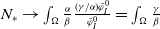$N_*\to \int _{\Omega }\frac {\alpha }{\beta }\frac {(\gamma /\alpha )\tilde {\varphi }_I^0}{\tilde {\varphi }_I^0}=\int _{\Omega }\frac {\gamma }{\beta }$ as $d_R\to 0$ .

$\textrm {(ii)}$ By the proper modifications of the arguments employed in the proof of $\textrm {(i)}$ , we can show that $\|\tilde {\varphi }_R- \tilde {\varphi }_R^*\|_{C^1(\bar {\Omega })}\to 0$ and $\|\tilde {\varphi }_I-\frac {\sigma (1-d_{R}\tilde {\varphi }_{R}^*)}{\gamma d_{E}}\|_{\infty }\to 0$ as $d_I\to 0$ where $\tilde {\varphi }_{R}^*$ is the unique positive solution of (2.32). Hence, $N_*\to \int _{\Omega }\frac {\gamma }{\beta }\frac {d_E\alpha \tilde {\varphi }_R^*}{{\sigma }(1-d_R\tilde {\varphi }_R^*)}$ as $d_I\to 0$ . If $\frac {\alpha }{\sigma }$ is a constant function, then $\tilde {\varphi }_{R}^*$ is also a constant function and $\frac {d_{E}\alpha \tilde {\varphi }_{R}^*}{\sigma (1-d_{R}\tilde {\varphi }_{R}^*)}=1$ . Therefore, $N_*\to \int _{\Omega }\gamma /\beta$ as $d_I\to 0$ .

$\textrm {(iii)}$ The result can also be obtained by a proper modification of the arguments of the proof of $\textrm {(i)}$ . Hence, we omit the details.

Proof. Fix $1\le p\lt \frac {n}{(n-2)_+}$ . Then, $\frac {n}{2}(1-\frac {1}{p})\lt 1$ . Next, thanks to the variation of constant formula,

(4.3) \begin{equation} I(t)=e^{d_It(\Delta -a_0)}I_0+\int _0^te^{d_I(t-s)(\Delta -a_0)}(\sigma E(s)-(\gamma -{a_0}{d_I})I(s))ds,\quad \forall \ t\gt 0. \end{equation}

Hence, thanks to the positivity of the $C_0$ -semigroup $\{e^{t\Delta }\}_{t\ge 0}$ , the fact that $\gamma \ge d_Ia_0$ , and the positivity of $E$ and $I$ , we get

\begin{equation*} 0\le I(t)\le e^{d_It(\Delta -a_0)}I_0+\|\sigma \|_{\infty }\int _0^te^{d_I(t-s)(\Delta -a_0)} E(s)ds,\quad \forall \ t\gt 0. \end{equation*}

This, along with (4.1), the triangle inequality, and the Minkowski’s inequality, yields

(4.4) \begin{align*} \|I(t)\|_{L^p(\Omega )}&\le \left \| e^{d_It(\Delta -a_0)}I_0+\|\sigma \|_{\infty }\int _0^te^{d_I(t-s)(\Delta -a_0)} E(s)ds\right \|_{L^p(\Omega )} \nonumber\\ & \le \left \| e^{d_It(\Delta -a_0)}I_0\right \|_{L^p(\Omega )}+\|\sigma \|_{\infty }\int _0^t\left \|e^{d_I(t-s)(\Delta -a_0)} E(s)\right \|_{L^p(\Omega )}ds \nonumber\\& \le \frac {C\big(1+(d_It)^{-\frac {n}{2}(1-\frac {1}{p})}\big)}{e^{a_0d_It}}\|I_0\|_{L^1(\Omega )}+C\|\sigma \|_{\infty }\int _{0}^t\frac {\big(1+(d_I(t-s))^{-\frac {n}{2}(1-\frac {1}{p})}\big)}{e^{a_0d_I(t-s)}}\|E(s)\|_{L^1(\Omega )}ds \nonumber \\ & \le CN\big(1+(d_It)^{-\frac {n}{2}(1-\frac {1}{p})}\big)e^{-a_0d_It}+CN\|\sigma \|_{\infty }\int _{0}^t\big(1+(d_I(t-s))^{-\frac {n}{2}(1-\frac {1}{p})}\big)e^{-a_0d_I(t-s)}ds \nonumber\\ & \le CN\big(1+(d_It)^{-\frac {n}{2}(1-\frac {1}{p})}\big)e^{-a_0d_It}+CN\|\sigma \|_{\infty }\int _{0}^{\infty }\big(1+(d_Is)^{-\frac {n}{2}(1-\frac {1}{p})}\big)e^{-d_Ia_0s}ds \nonumber\\ & =\frac {CN\big(1+(d_It)^{-\frac {n}{2}(1-\frac {1}{p})}\big)}{e^{a_0d_It}}+\frac {CN\|\sigma \|_{\infty }}{d_Ia_0}\left(1+a_0^{\frac {n}{2}(1-\frac {1}{p})}\Gamma \left(1-\frac {n}{2}\left(1-\frac {1}{p}\right)\right)\right) \quad t\gt 0, \end{align*}

where $\Gamma$ is the Gamma function. Similarly, noting that

(4.5) \begin{align} 0\le S(t)=& e^{d_St(\Delta -a_0)}S_0+\int _0^te^{d_S(t-s)(\Delta -a_0)}(\alpha R(s)+{a_0}{d_S}S(s)-\beta SI(s))ds \nonumber\\ \le & e^{d_St(\Delta -a_0)}S_0+\int _0^te^{d_S(t-s)(\Delta -a_0)}(\alpha R(s)+{a_0}{d_S}S(s))ds, \end{align}

and $\|\alpha R(t)+{a_0}{d_S} S(t)\|_{L^1(\Omega )}\le 2\|\alpha \|_{\infty }N$ for all $t\ge 0$ , we can proceed as above to obtain

\begin{equation*} \|S(t)\|_{L^p(\Omega )}\le CN\big(1+(d_St)^{-\frac {n}{2}(1-\frac {1}{p})}\big)e^{-d_Sa_0t}+\frac {2CN\|\alpha \|_{\infty }}{d_Sa_0}\left(1+(d_Sa_0)^{\frac {n}{2}\left(1-\frac {1}{p}\right)}\Gamma \left(1-\frac {n}{2}\left(1-\frac {1}{p}\right)\right)\right) \!\!\quad t\gt 0, \end{equation*}

which completes the proof of the result.

Proof. Fix $1\le p_1\lt \frac {n}{(n-2)_+}$ and $p_1\le p_2\lt \frac {np_1}{(n-2p_1)_+}$ . By (4.2), there is $\tilde {M}_{1,p_1}$ , independent of initial data and $N$ such that

(4.7) \begin{equation} \max \big \{ \|I(t)\|_{L^{p_1}(\Omega )},\|S(t)\|_{L^{p_1}(\Omega )}\big \}\le N\tilde {M}_{1,p_1}\quad \forall \ t\gt 1. \end{equation}

By the variation of constant formula,

(4.8) \begin{align} R(t+1) & = e^{d_Rt(\Delta -a_0)}R(1)+\int _0^te^{d_R(t-s)(\Delta -a_0)} (\gamma I(1+s))ds\nonumber\\ & -\int _0^te^{d_R(t-s)(\Delta -a_0)}((\alpha -{a_0}{d_R})R(1+s))ds\nonumber\\ & \le e^{d_Rt(\Delta -a_0)}R(1)+\int _0^te^{d_R(t-s)(\Delta -a_0)} (\gamma I(1+s))ds\quad t\gt 0. \end{align}

Hence, thanks to (4.7), (4.1), and Minkowski’s inequality,

\begin{align*} &\|R(1+t)\|_{L^{p_2}(\Omega )}\\ \le & \left \|e^{d_Rt(\Delta -a_0)}R(1)\right \|_{L^{p_2}(\Omega )}+\int _0^t\left \|e^{d_R(t-s)(\Delta -a_0)} (\gamma I(1+s))\right \|_{L^{p_2}(\Omega )}ds\\ \le & C\big(1+(d_Rt)^{-\frac {n}{2}(1-\frac {1}{p_2})}\big)e^{-a_0d_Rt}\|R(1)\|_{L^1(\Omega )}\\ &+C\|\gamma \|_{\infty }\int _0^{t}\big(1+(d_R(t-s))^{-\frac {n}{2}(\frac {1}{p_1}-\frac {1}{p_2})}\big)e^{-a_0d_R(t-s)}\|I(1+s)\|_{L^{p_1(\Omega )}}ds\\ \le & CN\big(1+(d_Rt)^{-\frac {n}{2}(1-\frac {1}{p_2})}\big)e^{-a_0d_Rt}+CN\tilde {M}_{1,p_1}\|\gamma \|_{\infty }\int _0^{t}\frac {\big(1+(d_R(t-s))^{-\frac {n}{2}(\frac {1}{p_1}-\frac {1}{p_2})}\big)}{e^{a_0d_R(t-s)}}ds,\\ \le & \frac {CN\big(1+(d_Rt)^{-\frac {n}{2}(1-\frac {1}{p_2})}\big)}{e^{a_0d_Rt}}+\frac {CN\tilde {M}_{1,p_1}\|\gamma \|_{\infty }}{d_Ra_0}\left(1+a_0^{\frac {n}{2}(\frac {1}{p_1}-\frac {1}{p_2})}\Gamma \left(1-\frac {n}{2}\left(\frac {1}{p_1}-\frac {1}{p_2}\right)\right)\right)\quad t\gt 0. \end{align*}

Next, since (4.5) and (4.7) hold, we can proceed as above to derive similar estimates for $\|S(t)\|_{L^{p_2}(\Omega )}$ .

Proof. Since $n\in \{1,\cdots ,5\}$ , then $ \max \{\frac {n}{4},1\}\lt \frac {n}{(n-2)_+}$ . So, we can first choose

\begin{equation*}\max \left\{\frac {n}{4},1\right\}\lt p_1\lt \frac {n}{(n-2)_+}.\end{equation*}

Next, we select $p_2$ as follows:

Case 1. $\frac {n}{2}\le p_1$ , that is $(n-2p_1)_+=0$ . In this case we fix any $p_2\gt \max \{n, p_1\}$ .

Case 2. $\frac {n}{2}\gt p_1$ . In this case, we have

\begin{equation*} \frac {np_1}{n-2p_1}-\frac {n}{2}=\frac {n(4p_1-n)}{2(n-2p_1)}\gt 0. \end{equation*}

So, we have $p_1\lt \frac {n}{2}\lt \frac {np_1}{n-2p_1}$ . We can then choose $\frac {n}{2}\lt p_2\lt \frac {np_1}{n-2p_1}$ .

In both cases, we have $\max \{\frac {n}{2},p_1\}\lt p_2\lt \frac {np_1}{(n-2p_1)_+}$ . So, by (4.6), there is ${M}_2\gt 0$ , independent of $N$ and initial data, such that

\begin{equation*} \max \left \{\|R(t)\|_{L^{p_2}(\Omega )},\|S(t)\|_{L^{p_2}(\Omega )}\right \}\le N{M}_2\quad \forall \,\ t\ge 2. \end{equation*}

Therefore, by (4.1) and (4.5), we have that

\begin{align*} S(t+2)\le & \|e^{d_St(\Delta -a_0)}S(2)\|_{{\infty }}+\int _0^{t}\|e^{d_S(t-s)(\Delta -a_0)}(\alpha R(2+s)+{a_0}{d_S}S(2+s))\|_{\infty }ds\\ \le & C\big (1+(d_{S}t)^{-\frac {n}{2p_2}}\big )e^{-a_0d_St}\|S(2)\|_{L^{p_2}(\Omega )}\\ &+C\int _0^{t}\big (1+(d_S(t-s))^{-\frac {n}{2p_2}}\big )e^{-a_0d_S(t-s)}\|\alpha R(2+s)+{a_0}{d_S}S(2+s)\|_{L^{p_2}(\Omega )}ds\\ \le & CN{M}_2\big(\big (1+(d_St)^{-\frac {n}{2p_2}}\big )e^{-a_0d_St}+2\|\alpha \|_{\infty }\int _0^t\big (1+(d_S(t-s))^{-\frac {n}{2p_2}}\big )e^{-a_0d_S(t-s)}ds\big) \\ \le & CN{M}_2\left (\big (1+(d_St)^{-\frac {n}{2p_2}}\big )e^{-a_0d_St}+\frac {2\|\alpha \|_{\infty }}{d_Sa_0}\left(1+a_0^{\frac {n}{2p_2}}\Gamma \left(1-\frac {n}{2p_2}\right)\right)\right )\quad \forall \ t\gt 0, \end{align*}

which yields the desired result.

Proof. Let $M_{\infty }$ as in (4.9). We proceed in five steps.

Step 1. Fix $1\le p\lt \frac {n}{(n-2)_+}$ so that $\frac {n}{2}(1-\frac {1}{p})\lt 1$ . We claim that there is $\tilde {M}_{1,p}\gt 0$ , independent of initial data and $N$ such that

(4.11) \begin{equation} \|E(t)\|_{L^p(\Omega )}\le N^2\tilde {M}_{1,p}\quad \forall \ t\ge 4. \end{equation}

Indeed, thanks to the variation of constant formula, and the positivity of $\{e^{t(\Delta -a_0)}\}_{t\gt 0},$ we have

(4.12) \begin{align} E(t+3) & = e^{d_Et(\Delta -a_0)}E(3)+\int _0^te^{d_E(t-s)(\Delta -a_0)}(\beta S(s+3)I(s+3)-(\sigma -{a_0}{d_E})E(s+3))ds\nonumber\\& \le e^{d_Et(\Delta -a_0)}E(3)+NM_{\infty }\|\beta \|_{\infty }\int _0^te^{d_E(t-s)(\Delta -a_0)}I(s+3)ds\quad t\gt 0. \end{align}

Therefore, by the similar arguments leading to (4.4), we get

\begin{equation*} \|E(t+3)\|_{L^p(\Omega )}\le \frac {CN\big(1+(d_Et)^{-\frac {n}{2}(1-\frac {1}{p})}\big)}{e^{a_0d_Et}}+\frac {CN^2M_{\infty }\|\beta \|_{\infty }}{d_Ea_0}\left(1+a_0^{\frac {n}{2}(1-\frac {1}{p})}\Gamma \left(1-\frac {n}{2}\left(1-\frac {1}{p}\right)\right)\right) \quad t\gt 0. \end{equation*}

Therefore, there is a positive number $\tilde {M}_{1,p}$ , independent of $N$ and initial data such that (4.11) holds.

Step 2. Fix $1\le p_1\lt \frac {n}{(n-2)_+}$ and $p_1\lt p_2\lt \frac {np_1}{(n-2p_1)_+}$ . Since (4.11) holds, we can proceed as in (4.2) to establish that there is $\tilde {M}_{2,p_1,p_2}\gt 0$ independent of $N$ and initial data such that

(4.13) \begin{equation} \|I(t)\|_{L^{p_2}(\Omega )}\le N^2\tilde {M}_{1,p_1,p_2}\quad \forall \ t\ge 5. \end{equation}

Step 3. Here, we fix $p_1$ and $p_2$ as in the proof of Lemma 4.3. Then, thanks to (4.9), (4.11), and (4.12), we can proceed as in the proof of (4.9) to show the existence of $\tilde {M}_{2}\gt 0$ , independent of $N$ and initial data, such that

(4.14) \begin{equation} \|E(t)\|_{\infty }\le N^{3}\tilde {M}_2\quad \forall \ t\ge 6. \end{equation}

Step 4. Here we derive the estimates on $\|I(t)\|_{\infty }$ . To this end, thanks to (4.14) and the third equation of (1.3), we have

\begin{equation*} \begin{cases} \partial _tI\le d_I\Delta I +\|\sigma \|_{\infty }N^3\tilde {M}_2-\gamma _{\min }I, & x\in \Omega ,\ t\gt {6},\\ 0=\partial _{\boldsymbol{n}}I, & x\in \partial \Omega ,\ t\gt {6}. \end{cases} \end{equation*}

We can now invoke the comparison principle for parabolic equations to conclude that

\begin{equation*} \|I(t)\|_{\infty }\le \frac {\|\sigma \|_{\infty }N^3\tilde {M}_2}{\gamma _{\min }}+\left (\|I(6,\cdot )\|_{\infty }-\frac {\|\sigma \|_{\infty }N^3\tilde {M}_2}{\gamma _{\min }}\right )e^{-\gamma _{\min }(t-6)}, \quad \forall \, t \gt 6. \end{equation*}

Consequently,

(4.15) \begin{equation} \limsup _{t\to \infty }\|I(t)\|_{\infty }\le \frac {\|\sigma \|_{\infty }N^3\tilde {M}_2}{\gamma _{\min }}. \end{equation}

Step 5. Here we derive the estimate on $\|R(t)\|_{\infty }$ . From (4.15) and the fourth equation of (1.3), for every $\varepsilon \gt 0$ , there is $t_{\varepsilon }\gt 0$ such that

\begin{equation*} \begin{cases} \partial _t R \leq d_R\Delta R + (1+\varepsilon )\frac {\|\gamma \|_{\infty }\|\sigma \|_{\infty }N^3\tilde {M}_2}{\gamma _{\min }} - \alpha _{\min }R, & x\in \Omega ,\ t \gt t_{\varepsilon },\\ 0 = \partial _{\boldsymbol{n}}R, & x\in \partial \Omega ,\ t \gt t_{\varepsilon }. \end{cases} \end{equation*}

We can now invoke the comparison principle for parabolic equations, and proceed by the similar arguments leading to (4.15) to conclude that

\begin{equation*} \limsup _{t\to \infty } \|R(t)\|_{\infty }\le (1+\varepsilon )\frac {\|\gamma \|_{\infty }\|\sigma \|_{\infty }N^3\tilde {M}_2}{\gamma _{\min }\alpha _{\min }} \quad \forall \,\ \varepsilon \gt 0. \end{equation*}

Letting $\varepsilon \to 0$ , we get

\begin{equation*} \limsup _{t\to \infty }\|R(t)\|_{\infty }\le \frac {\|\gamma \|_{\infty }\|\sigma \|_{\infty }N^3\tilde {M}_2}{\gamma _{\min }\alpha _{\min }}. \end{equation*}

This, along with (4.14) and (4.15), yields (4.10).

Proof. Suppose that $d_E=d_S$ . Fix $ 0\lt \tau _1\lt \frac {1}{2}\frac {\min \{1,d_{\min }\}}{(\|\sigma \|_{\infty }+\|\gamma \|_{\infty }+\|\alpha \|_{\infty })}$ where $d_{\min }=\min \{d_S,d_R,d_I\}$ . Since $\tau _1\gt 0$ , by the Harnack’s inequality for parabolic equations [Reference Húska15, Theorem 2.5], there is $c_{\tau _1}\gt 0$ such that

\begin{equation*} \|e^{t\Delta }u_0\|_{\infty }\le c_{\tau _1}\min _{x\in \bar {\Omega }}(e^{t\Delta }u_0)(x)\quad \forall \ t\ge \tau _1,\quad u_0\in C^{+}(\bar {\Omega }), \end{equation*}

where $\{e^{t\Delta }\}_{t\ge 0}$ denotes the heat $C_0$ -semigroup subject to the homogeneous Neumann boundary conditions on $\partial \Omega$ . From this point, we proceed in two steps.

Step 1. In this step, we prove global boundedness. To this end, let $(S(t,x),E(t,x),I(t,x),R(t,x))$ be a classical solution of (1.3) with positive initial data. For every $T \ge T_1\,:\!=\,\frac {\tau _1}{d_{\min }}$ , define

\begin{equation*} M_T=\max _{0\le t\le T}(\|S(t)\|_{\infty }+\|E(t)\|_{\infty }+\|I(t)\|_{\infty }+\|R(t)\|_{\infty }). \end{equation*}

We claim that

(4.17) \begin{equation} M_{T}\le \max \Bigg \{M_{T_1}, \frac {\frac {(\|S_0+E_0\|_{\infty }+\|I_0\|_{\infty }+\|R_0\|_{\infty })}{e^{\tau _1a_0}}+\frac {c_{\tau _1}N}{|\Omega |a_0d_{\min }}(\|\sigma \|_{\infty }+\|\gamma \|_{\infty }+\|\alpha \|_{\infty })}{1-{\frac {\tau _1}{d_{\min }}}(\|\sigma \|_{\infty }+\|\gamma \|_{\infty }+\|\alpha \|_{\infty })}\Bigg \}\quad \forall \,\, T\ge T_1. \end{equation}

Thanks to the first equations in (4.5) and (4.12),

(4.18) \begin{align} S(t)+E(t) & = e^{td_S(\Delta -a_0)}(E_0+S_0)+\int _{0}^te^{(t-s)d_S(\Delta -a_0)}(\alpha R(s)+{a_0}{d_S}S(s)-(\sigma -{a_0}{d_S})E(s))\,\text{d}s \nonumber\\ & \le e^{-td_Sa_0}\|E_0+S_0\|_{\infty }+\|\alpha \|_{\infty }\int _{0}^te^{(t-s)d_S(\Delta -a_0)}( R(s)+S(s))\,\text{d}s\nonumber\\ & = e^{-td_Sa_0}\|E_0+S_0\|_{\infty }+\|\alpha \|_{\infty }\int _{0}^{t-{\frac {\tau _1}{d_S}}}e^{(t-s)d_S(\Delta -a_0)}( R(s)+S(s))\,\text{d}s\nonumber\\ &+\|\alpha \|_{\infty }\int _{t-{\frac {\tau _1}{d_S}}}^{t}e^{(t-s)d_S(\Delta -a_0)}( R(s)+S(s))\,\text{d}s\nonumber\\ & \le e^{-td_Sa_0}\|E_0+S_0\|_{\infty }+c_{\tau _1}\|\alpha \|_{\infty }\int _{0}^{t-{\frac {\tau _1}{d_S}}}e^{-(t-s)d_Sa_0}(e^{(t-s)d_S\Delta }( R(s)+S(s)))_{\min }\,\text{d}s\nonumber\\ & +\|\alpha \|_{\infty }\int _{t-{\frac {\tau _1}{d_S}}}^{t}e^{-(t-s)d_Sa_0}\|e^{(t-s)d_S\Delta }( R(s)+S(s))\|_{\infty }\,\text{d}s\nonumber\\ & \le e^{-td_Sa_0}\|E_0+S_0\|_{\infty }+\frac {c_{\tau _1}\|\alpha \|_{\infty }}{|\Omega |}\int _{0}^{t-{\frac {\tau _1}{d_S}}}e^{-(t-s)d_Sa_0}\|e^{(t-s)d_S\Delta }( R(s)+S(s))\|_{L^1(\Omega )}\,\text{d}s\nonumber\\ & +\|\alpha \|_{\infty }M_T\int _{t-{\frac {\tau _1}{d_S}}}^{t}e^{-(t-s)d_Sa_0}\,\text{d}s\nonumber\\ & \le e^{-ta_0d_S}\|E_0+S_0\|_{\infty }+\frac {c_{\tau _1}N\|\alpha \|_{\infty }}{|\Omega |}\int _{0}^{t-{\frac {\tau _1}{d_S}}}e^{-(t-s)a_0d_S}\,\text{d}s+{\frac {\tau _1}{d_S}}\|\alpha \|_{\infty }M_T\nonumber\\[4pt] & \le e^{-ta_0d_S}\|E_0+S_0\|_{\infty }+\frac {c_{\tau _1}N\|\alpha \|_{\infty }}{|\Omega |a_0d_S}+{\frac {\tau _1}{d_S}}\|\alpha \|_{\infty }M_T \quad {\frac {\tau _1}{d_S}}\lt t\lt T. \end{align}

Similarly, thanks to the variation of constant formula, (4.3) and (4.8), we can proceed as above to establish that

(4.19) \begin{equation} I(t)\le e^{-td_Ia_0}\|I_0\|_{\infty }+\frac {c_{\tau _1}N\|\sigma \|_{\infty }}{|\Omega |a_0d_I}+{\frac {\tau _1}{d_I}}\|\sigma \|_{\infty }M_T \quad {\frac {\tau _1}{d_I}}\lt t\lt T \end{equation}

and

(4.20) \begin{equation} R(t)\le e^{-td_Ra_0}\|R_0\|_{\infty }+\frac {c_{\tau _1}N\|\gamma \|_{\infty }}{|\Omega |d_Ra_0}+{\frac {\tau _1}{d_R}}\|\gamma \|_{\infty }M_T \quad {\frac {\tau _1}{d_R}}\lt t\lt T. \end{equation}

Adding up side by side inequalities (4.18), (4.19) and (4.20), we get

(4.21) \begin{equation} (S+E+I+R)(t)\le \frac {(\|S_0+E_0\|_{\infty }+\|I_0\|_{\infty }+\|R_0\|_{\infty })}{e^{ta_0d_{\min }}}+\left(\frac {c_{\tau _1}N}{|\Omega |a_0d_{\min }}+{\frac {\tau _1M_T}{d_{\min }}}\right)(\|\sigma \|_{\infty }+\|\gamma \|_{\infty }+\|\alpha \|_{\infty }) \end{equation}

for all $T_1\lt t\lt T$ . Hence

\begin{equation*} M_T\le \max \left\{ M_{T_1},\frac {(\|S_0+E_0\|_{\infty }+\|I_0\|_{\infty }+\|R_0\|_{\infty })}{e^{\tau _1a_0}}+\left(\frac {c_{\tau _1}N}{|\Omega |a_0d_{\min }}+{\frac {\tau _1M_T}{d_{\min }}}\right)(\|\sigma \|_{\infty }+\|\gamma \|_{\infty }+\|\alpha \|_{\infty })\right\}, \end{equation*}

from which (4.17) follows.

Step 2. We complete the proof of (4.16) here. Indeed, set

\begin{equation*} A=\limsup _{t\to \infty }\|S(t)+E(t)+I(t)+R(t)\|_{\infty }. \end{equation*}

By Step 1, we know that $A\lt \infty$ . Next, by the definition of the $\limsup$ , for every $\varepsilon \gt 0$ there is $t_{\varepsilon }\gg \tau _1$ such that

\begin{equation*} \|S(t)+E(t)+I(t)+R(t)\|_{\infty }\le A+\varepsilon \quad \forall \ t\gt t_{\varepsilon }. \end{equation*}

This, along with (4.21), yields for every $t\gt \frac {\tau _1}{d_{\min }}$ ,

\begin{align*} \|S(t+t_{\varepsilon })+E(t+t_{\varepsilon })+I(t+t_{\varepsilon })+R(t+t_{\varepsilon })\|_{\infty }\le &\frac {(\|S(t_{\varepsilon })+E(t_{\varepsilon })\|_{\infty }+\|I(t_{\varepsilon })\|_{\infty }+\|R(t_{\varepsilon })\|_{\infty })}{e^{ta_0d_{\min }}}\\ &+\left(\frac {c_{\tau _1}N}{|\Omega |a_0d_{\min }}+\frac {\tau _1(A+\varepsilon )}{{d_{\min }}}\right)(\|\sigma \|_{\infty }+\|\gamma \|_{\infty }+\|\alpha \|_{\infty }). \end{align*}

Taking $\limsup$ as $t\to \infty$ , we obtain that

\begin{equation*} A\le \left(\frac {c_{\tau _1}N}{|\Omega |a_0d_{\min }}+{\frac {\tau _1}{d_{\min }}}(A+\varepsilon )\right)(\|\sigma \|_{\infty }+\|\gamma \|_{\infty }+\|\alpha \|_{\infty }). \end{equation*}

Finally, letting $\varepsilon \to 0^+$ in the last inequality, we get

\begin{equation*}A\le \frac {c_{\tau _1}(\|\sigma \|_{\infty }+\|\gamma \|_{\infty }+\|\alpha \|_{\infty })}{|\Omega |a_0({d_{\min }}-\tau _1(\|\sigma \|_{\infty }+\|\gamma \|_{\infty }+\|\alpha \|_{\infty }))}N. \end{equation*}

Taking $M_*=\frac {c_{\tau _1}(\|\sigma \|_{\infty }+\|\gamma \|_{\infty }+\|\alpha \|_{\infty })}{|\Omega |a_0({d_{\min }}-\tau _1(\|\sigma \|_{\infty }+\|\gamma \|_{\infty }+\|\alpha \|_{\infty }))}$ , the result follows.

Proof of Theorem 2.2.Collecting Lemmas 4.3–4.5, the result follows.

Proof. Since the principle eigenvalue $\lambda ^l$ is single, it follows from standard regularity theory of principal eigenvalue that $\lambda ^l$ is continuously differentiable $l\gt 0$ , and the mapping $l\mapsto (\psi _E^l,\psi _I^l)\in [C^2(\overline {\Omega })]^2$ is also continuously differentiable (see [Reference Hess14, Lemma 15.1, Chapter 2]). Denoting by $\sigma ^l\,:\!=\,\frac {d\lambda ^l}{dl}$ , $\psi _E^{'}\,:\!=\,\partial _l\psi _E^l$ and $\psi _I^{'}\,:\!=\,\partial _l\psi _I^l$ , it follows from (5.3) that

(5.7) \begin{equation} \begin{cases} \sigma ^l\psi _E^l+\lambda ^l\psi _E^{'}=d_E\Delta \psi _E^{'}-\sigma \psi _E^{'}+l\beta \psi _I^{'}+\beta \psi _I^l & x\in \Omega ,\\ \sigma ^l\psi _I^l+\lambda ^l\psi _I^{'}=d_I\Delta \psi _{I}^{'}-\gamma \psi _{I}^{'}+\sigma \psi _{E}^{'} & x\in \Omega ,\\ 0=\partial _{\boldsymbol{n}}\psi _{E}^{'}=\partial _{\boldsymbol{n}}\psi _{I}^{'} & x\in \partial \Omega . \end{cases} \end{equation}

Now, let $(\psi _E^*,\psi _I^*)$ be the positive eigenfunction satisfying $\|\psi _E^*+\psi _I^*\|_{\infty }=1$ of the adjoint problem of (5.3), that is $(\psi _E^*,\psi _I^*)$ solves

(5.8) \begin{equation} \begin{cases} \lambda ^l\psi _E^*=d_E\Delta \psi _E^*-\sigma \psi _E^*+\sigma \psi _I^* & x\in \Omega ,\\ \lambda ^l\psi _I^*=d_I\Delta \psi _I^*-\gamma \psi _I^*+l\beta \psi _E^* & x\in \Omega ,\\ 0=\partial _{\boldsymbol{n}}\psi _E^*=\partial _{\boldsymbol{n}}\psi _I^* & x\in \partial \Omega . \end{cases} \end{equation}

Multiply the first equations of (5.7) and (5.8) by $\psi _E^*$ and $\psi _E^{'}$ , respectively, then integrate by parts the resulting equations, then take the difference to obtain

(5.9) \begin{equation} \sigma ^l\int _{\Omega }\psi _E^*\psi _E^l=l\int _{\Omega }\beta \psi _I^{'}\psi _E^*+\int _{\Omega }\beta \psi _{E}^*\psi _I^l-\int _{\Omega }\sigma \psi _I^*\psi _E^{'}. \end{equation}

Similarly, multiplying the second equations of (5.7) and (5.8) by $\psi _I^*$ and $\psi _I^{'}$ , respectively, integrate by parts the resulting equations, and then take the difference to obtain

(5.10) \begin{equation} \sigma ^l\int _{\Omega }\psi _I^l\psi _I^*=\int _{\Omega }\sigma \psi _E^{'}\psi _I^*-l\int _{\Omega }\beta \psi _E^*\psi _I^{'}. \end{equation}

Now, taking the sum of (5.9) and (5.10) yields

\begin{equation*} \frac {d\lambda ^l}{dl}=\sigma ^l=\frac {\int _{\Omega }\beta \psi _E^*\psi _I^l}{\int _{\Omega }\big(\psi _E^l\psi _E^*+\psi _I^l\psi _I^*\big)}\gt 0 \end{equation*}

since $\beta \ge , \not \equiv 0$ and $\psi _I^l,\psi _I^*,\psi _E^l,\psi _E^*\gt 0$ . This shows that $\lambda ^l$ is strictly increasing. Next, clearly, $\lambda ^l$ is continuous on $[0,\infty )$ where $\lambda ^0$ is the maximal eigenvalue of (5.3) when $l=0$ . Observe that $\lambda ^0\lt 0$ . Indeed, let $(\psi _E^0,\psi _I^0)$ be a nonnegative eigenfunction associated with $\lambda ^0$ . If $\psi ^0_E\equiv 0$ , then $\lambda ^0$ is an eigenvalue of the single species elliptic equation

(5.11) \begin{equation} \begin{cases} \lambda ^0\varphi =d_I\Delta \varphi -\gamma \varphi & x\in \Omega ,\\ 0=\partial _{\boldsymbol{n}}\varphi & x\in \Omega . \end{cases} \end{equation}

Hence, it follows from Lemma 3.2 that $\lambda ^0\le \lambda (d_I,-\gamma )\le -\gamma _{\min }\lt 0$ . On the other hand, if $\|\varphi _E^0\|_{\infty }\gt 0$ , then $\lambda ^0$ is an eigenvalue of (5.11) with $d_I$ and $\gamma$ replaced with $d_E$ and $\sigma .$ Hence, by Lemma 3.2 again, we have $\lambda ^0\le \lambda (d_E,-\sigma )\le -\sigma _{\min }\lt 0$ . Therefore, we always have $\lim _{l\to 0^+}\lambda ^l=\lambda ^0\lt 0$ .

Note that we can apply [Reference Cantrell, Cosner and Martinez4, Proposition 3] to conclude that $\lambda ^l/\sqrt {l}\to \max _{x\in \bar {\Omega }}\sqrt {\beta (x)\sigma (x)}$ as $l\to \infty$ .

Finally, noting that $\lambda ^{\mu ^*}=0$ , where $\mu ^*$ is the principal eigenvalue of (2.10), the conclusion follows from the strict monotonicity of $\lambda ^l$ in $l\gt 0$ .

Proof. Suppose that $(\tilde {E}^l,\tilde {I}^l,\tilde {R}^l)$ is a classical solution of (5.1) with $\tilde {E}^l\ge , \not \equiv 0$ . It follows from the second equation of (5.1), the fact that $\gamma _{\min }\gt 0$ , and the strong maximum principle principle for elliptic equations that $\tilde {I}^l\gt 0$ on $\overline {\Omega }$ . This, in turn, thanks the third equation of (5.1), the fact that $\alpha _{\min }\gt 0$ , and the strong maximum principle principle that $\tilde {R}^l\gt 0$ on $\overline {\Omega }$ . Next, set $S^{l}=l(1-d_E\tilde {E}^l-d_I\tilde {I}^l-d_R\tilde {R}^l)$ . Then, ${S}^l$ satisfies

(5.12) \begin{equation} \begin{cases} 0=\frac {1}{l}\Delta S^{l}+\alpha \tilde {R}^l-\beta \tilde {I}^{l}{S}^l & x\in \Omega ,\\ 0=\partial _{\boldsymbol{n}}{S}^l & x\in \partial \Omega . \end{cases} \end{equation}

As a result, since $(\alpha \tilde {R}^l)_{\min }\gt 0$ and $(\beta \tilde {I}^l)_{\min }\gt 0$ , we employ the strong maximum principle principle for elliptic equations to deduce that ${S}^l_{\min }\gt 0$ . Therefore, observing that $\tilde {E}^l$ is a classical solution of

\begin{equation*} \begin{cases} 0=d_E\Delta \tilde {E}^l+\beta S^l\tilde {I}^l-\sigma \tilde {E}^l & x\in \Omega ,\\ 0=\partial _{\boldsymbol{n}}\tilde {E}^l & x\in \partial \Omega , \end{cases} \end{equation*}

with $\sigma _{\min }\gt 0$ and $(\beta S^l\tilde {I}^l)_{\min }\gt 0$ , we employ again the strong maximum principle principle for elliptic equations to obtain that $\tilde {E}^l\gt 0$ on $\overline {\Omega }$ , which completes the proof of the lemma.

Proof. Let $(\tilde {E}^l,\tilde {I}^{l},\tilde {R}^l)$ be a sequence of positive solution of (5.1) for $l\gt \mu ^*$ . Observe that

(5.13) \begin{equation} \|\tilde {E}^l\|_{\infty }\le \frac {1}{d_E},\,\, \|\tilde {I}^l\|_{\infty }\le \frac {1}{d_I}\quad \text{and}\quad \|\tilde {R}^l\|_{\infty }\le \frac {1}{d_R} \quad \forall \ l\gt \mu ^*, \end{equation}

since $1\gt d_E\tilde {E}^l+d_I\tilde {I}^l+d_R\tilde {R}^l$ . Therefore,

\begin{equation*} \|\Delta \tilde {I}^l \|_{\infty }\le \frac {1}{d_I}\|\gamma \tilde {I}^l-\sigma \tilde {E}^l\|_{\infty }\le \frac {1}{d_I}\left(\frac {\|\gamma \|_{\infty }}{d_I}+\frac {\|\sigma \|_{\infty }}{d_E}\right)\quad \forall \ l\gt \mu ^* \end{equation*}

and

\begin{equation*} \|\Delta \tilde {R}^l \|_{\infty }\le \frac {1}{d_R}\|\gamma \tilde {I}^l-\alpha \tilde {R}^l\|_{\infty }\le \frac {1}{d_R}\left(\frac {\|\gamma \|_{\infty }}{d_I}+\frac {\|\alpha \|_{\infty }}{d_R}\right)\quad \forall \ l\gt \mu ^*. \end{equation*}

Hence, after passing to a subsequence, we employ the Sobolev compact embedding of $W^{2,p}(\Omega )$ in $C^1(\overline {}\Omega )$ for $p\gg n$ , to deduce that there exist nonnegative functions ${I}^*,{R}^*\in C^{1}(\overline {\Omega })$ such that

(5.14) \begin{equation} \lim _{l\to \infty }\|\tilde {I}^l-{I}^*\|_{C^1(\overline {\Omega })}=0 \quad \text{and}\quad \lim _{l\to \infty }\|\tilde {R}^l-{R}^*\|_{C^1(\overline {\Omega })}=0. \end{equation}

Furthermore, thanks to the third equation of (5.1) and the regularity theory for elliptic equations, we have that ${R}^*\in C^2(\overline {\Omega })$ and solves (in the classical sense)

(5.15) \begin{equation} \begin{cases} 0=d_R\Delta {R}^*-\alpha {R}^*+\gamma {I}^* & x\in \Omega ,\\ 0=\partial _{\boldsymbol{n}}{R}^* & x\in \partial \Omega . \end{cases} \end{equation}

Moreover, since $\sup _{l\gt \mu ^*}\|\tilde {E}^l\|_{\infty }\lt \infty$ by (5.13), it follows from the Banach-Alaoglu Theorem that, after passing to a furtehr subsequence, there is ${E}^*\in L^{\infty }(\Omega )$ such that $\tilde {E}^l\to {E}^*$ as $l\to \infty$ in the weak-star topology of $L^{\infty }(\Omega )$ . Therefore, it follows from the second equation of (5.1) and the $L^p$ - regularity theory for elliptic equations that ${I}^*\in W^{2,p}(\Omega )$ for every $p\gt 1$ and is a weak solution of

(5.16) \begin{equation} \begin{cases} 0=d_I\Delta {I}^*-\gamma {I}^*+\sigma {E}^* & x\in \Omega \\ 0=\partial _{\boldsymbol{n}}{I}^* & x\in \partial \Omega . \end{cases} \end{equation}

Note that ${E}^*\ge 0$ almost everywhere since $\tilde {E}^l\gt 0$ for all $l\gt \mu ^*$ .

Next, observe from (5.1) that

\begin{equation*} \begin{cases} 0\ge d_{E}\Delta \tilde {E}^l+l\beta _{\min }\big(1-\|d_{I}\tilde {I}^l+d_R\tilde {R}^l\|_{\infty }\big)\tilde {I}^l-\big(\sigma _{\max }+l\beta _{\max } d_E\|\tilde {I}^l\|_{\infty }\big)\tilde {E}^l & x\in \Omega ,\\ 0\ge d_{I}\Delta \tilde {I}^l +\sigma _{\min }\tilde {E}^l -\gamma _{\max }\tilde {I}^l & x\in \Omega ,\\ 0=\partial _{\boldsymbol{n}}\tilde {E}^l=\partial _{\boldsymbol{n}}\tilde {I}^l & x\in \partial \Omega . \end{cases} \end{equation*}

Hence, it follows as in (5.4) that

\begin{align*} 0\ge & \frac {1}{2}\bigg [\sqrt {4\big(l\beta _{\min }\big(1{-}\|d_{I}\tilde {I}^l+d_R\tilde {R}^l\|_{\infty }\big)\sigma _{\min }-\big(\sigma _{\max }+l\beta _{\max } d_E\|\tilde {I}^l\|_{\infty }\big)\gamma _{\max }\big)+\big(\big(\sigma _{\max }{+}l\beta _{\max } d_E\|\tilde {I}^l\|_{\infty }\big)+\gamma _{\max }\big)^2}\\ &-\big(\big(\sigma _{\max }+l\beta _{\max } d_E\|\tilde {I}^l\|_{\infty }\big)+\gamma _{\max }\big)\bigg ]. \end{align*}

Equivalently,

\begin{equation*} 0\ge l\beta _{\min }\big(1-\|d_{I}\tilde {I}^l+d_R\tilde {R}^l\|_{\infty }\big)\sigma _{\min }-\big(\sigma _{\max }+l\beta _{\max } d_E\|\tilde {I}^l\|_{\infty }\big)\gamma _{\max }, \end{equation*}

which gives

\begin{equation*} \frac {\beta _{\max }}{\sigma _{\min }\beta _{\min }} d_E\|{\tilde I}^l\|_{\infty }\gamma _{\max }+\frac {\sigma _{\max }\gamma _{\max }}{l\sigma _{\min }\beta _{\min }}+\|d_{I}{\tilde I}+d_R{\tilde R}^l\|_{\infty }\ge 1 . \end{equation*}

Letting $l\to \infty$ in the last inequality yields

(5.17) \begin{equation} 1\le \frac {d_E\beta _{\max }\gamma _{\max }}{\sigma _{\min }\beta _{\min }} \|{I}^*\|_{\infty }+\|d_{I}{I}^*+d_R{R}^*\|_{\infty } \le \left(\frac {d_E\beta _{\max }\gamma _{\max }}{\sigma _{\min }\beta _{\min }}+d_E\right)\|I^*\|_{\infty }+d_R\|R^*\|_{\infty }. \end{equation}

However, observe from (5.15) and the maximum principle for elliptic equations that

\begin{equation*} \|{R}^*\|_{\infty }\le \Big \|\frac {\gamma }{\alpha }\Big \|_{\infty }\|{I}^*\|_{\infty }. \end{equation*}

Hence, it follows from (5.17) that $\|{I}^*\|_{\infty }\gt 0$ . It then follows from the strong maximum principle principle and (5.15) and (5.16) that

(5.18) \begin{equation} {I}^*\gt 0\quad \text{and}\quad {R}^*\gt 0\quad \text{on}\ \overline {\Omega }. \end{equation}

Now, observing that

\begin{equation*} \begin{cases} 0=\frac {1}{l}\Delta S^l+\alpha \tilde {R}^l-\beta \tilde {I}^lS^l & x\in \Omega ,\\[3pt] 0=\partial _{\boldsymbol{n}}S^l & x\in \partial \Omega , \end{cases} \end{equation*}

we infer to the singular perturbation arguments to conclude that

(5.19) \begin{equation} S^l\to \frac {\alpha }{\beta }\frac {{R}^*}{{I}^*} \quad \text{as}\ {l\to \infty }\quad \text{uniformly on}\ \ \overline {\Omega }. \end{equation}

Therefore, rewriting (5.1) as

(5.20) \begin{equation} \begin{cases} 0=d_E\Delta \tilde {E}+\beta S^l\tilde {I}-\sigma \tilde {E} & x\in \Omega ,\\ 0=d_I\Delta \tilde {I}+\sigma \tilde {E}-\gamma \tilde {I} & x\in \Omega ,\\ 0=d_R\Delta \tilde {R}+\gamma \tilde {I}-\alpha \tilde {R} & x\in \Omega ,\\ 0=\partial _{\boldsymbol{n}}\tilde {E}=\partial _{\boldsymbol{n}}\tilde {I}=\partial _{\boldsymbol{n}}\tilde {R} & x\in \partial \Omega . \end{cases} \end{equation}

Then, by regularity theory for elliptic equations, we can invoke (5.1), (5.15), (5.16), and (5.19) to conclude that $({E}^*,{I}^*,{R}^*)$ is a positive classical solution of (2.29) and $(\tilde {E}^l,\tilde {I}^l,\tilde {R}^l)\to ({E}^*,{I}^*,{R}^*)$ as $l\to \infty$ in $C^1({\overline {\Omega }})$ . Finally, recalling that

\begin{equation*} 1=\frac {1}{l}S^l+d_E\tilde {E}^l+d_I\tilde {I}^l+d_R\tilde {R}, \end{equation*}

then as $l\to \infty$ , since (5.19) holds, we conclude that $({E}^*,{I}^*,{R}^*)$ also satisfies (2.30). Hence, by Proposition 3.1, $({E}^*,{I}^*,{R}^*)=(\tilde {E}^*,\tilde {I}^*,\tilde {R}^*)$ .

Proof. Thanks to Lemma 5.3, it is enough to show that for every $ k\gt 0$ , there is $ \eta _k\gt 0$ such that

(5.22) \begin{equation} \min _{x\in \overline {\Omega }}\min \{\tilde {E}^l(x),\tilde {I}^l(x),\tilde {R}^l(x)\}\ge \eta _k, \end{equation}

whenever $l\in [l^*,l^*+k]$ and $(\tilde {E}^l,\tilde {I}^l,\tilde {R}^l)$ is a positive classical solution of (5.1). We proceed by contradiction to establish that (5.22) holds. So, suppose that there is some $k\gt 0$ such that there exist a sequence $\{l_m\}_{m\ge 1}\subset [l^*,l^*+k]$ and positive classical solutions $(\tilde {E}^{l_m},\tilde {I}^{l_m},\tilde {R}^{l_m})$ of (5.1) for each $l=l_m$ satisfying

(5.23) \begin{equation} \lim _{m\to \infty } \min _{x\in \overline {\Omega }}\min \{\tilde {E}^{l_m}(x),\tilde {I}^{l_m}(x),\tilde {R}^{l_m}(x)\}=0. \end{equation}

Since $(\tilde {E}^{l_m},\tilde {I}^{l_m},\tilde {R}^{l_m})$ is uniformly bounded, then after passing to a subsequence, by the regularity theory for elliptic equations, we may suppose that there exist $l^{\infty }\in [l^*,l^*+k]$ and a nonnegative classical solution $(\tilde {E}^{\infty },\tilde {I}^{\infty },\tilde {R}^{\infty })$ of (5.1) with $l=l^{\infty }$ such that $(\tilde {E}^{l_m},\tilde {I}^{l_m},\tilde {R}^{l_m})\to (\tilde {E}^{\infty },\tilde {I}^{\infty },\tilde {R}^{\infty })$ as $m\to \infty$ in $C^{1}(\overline {\Omega })$ . Note from (5.23) that $\min _{x\in \overline {\Omega }}\min \{\tilde {E}^{\infty }(x),\tilde {I}^{\infty }(x),\tilde {R}^{\infty }(x)\} =0$ . Hence, by Lemma 5.2, we must have that $\tilde {E}^{\infty }=\tilde {I}^{\infty }=\tilde {R}^{\infty }\equiv 0$ . This implies that

(5.24) \begin{equation} \lim _{m\to \infty }\big(\|\tilde {E}^{l_m}\|_{\infty }+\|\tilde {I}^{l_m}\|_{\infty }+\|\tilde {R}^{l_m}\|_{\infty }\big)=0. \end{equation}

Now, set $\hat {E}^{l_m}\,:\!=\,\frac {\tilde {E}^{l_m}}{\|\tilde {E}^{l_m}\|_{\infty }}$ , $\hat {I}^{l_m}\,:\!=\,\frac {\tilde {I}^{l_m}}{\|\tilde {E}^{l_m}\|_{\infty }}$ , and $\hat {R}^{l_m}\,:\!=\,\frac {\tilde {R}^{l_m}}{\|\tilde {E}^{l_m}\|_{\infty }}$ for all $m\ge 1$ . Observe that $(\hat {E}^{l_m},\hat {I}^{l_m},\hat {R}^{l_m})$ is a classical solution of

\begin{equation*} \begin{cases} 0=d_{E}\Delta \hat {E}^{l_m}+l_m\beta \big(1-d_E\tilde {E}^{l_m}-d_{I}\tilde {I}{l_m}-d_R\tilde {R}^{l_m}\big)\hat {I}^{l_m}-\sigma \hat {E}^{l_m} & x\in \Omega ,\\ 0=d_{I}\Delta \hat {I}^{l_m} +\sigma \hat {E}^{l_m} -\gamma \hat {I}^{l_m} & x\in \Omega ,\\ 0= d_{R}\Delta \hat {R}^{l_m}+\gamma \hat {I}^{l_m}-\alpha \hat {R}^{l_m} & x\in \Omega ,\\ 0=\partial _{\boldsymbol{n}}\tilde {E}^{l_m}=\partial _{\boldsymbol{n}}\tilde {I}^{l_m}=\partial _{\boldsymbol{n}}\tilde {R}^{l_m} & x\in \partial \Omega , \end{cases} \end{equation*}

and satisfies

\begin{equation*} \|\hat {E}^{l_m}\|_{\infty }=1,\quad \|\hat {I}^{l_m}\|_{\infty }\le \Big \|\frac {\sigma }{\gamma }\hat {E}^{l_m}\|_{\infty }\le \Big \|\frac {\sigma }{\gamma }\|_{\infty }, \quad \text{and}\quad \|\hat {R}^{l_m}\|_{\infty }\le \Big \|\frac {\gamma }{\alpha }\hat {I}^{l_m}\|_{\infty }\le \Big \|\frac {\gamma }{\alpha }\|_{\infty }\quad \forall \ m\ge 1. \end{equation*}

Hence, since (5.24) holds, we can employ the regularity theory for elliptic equations, to conclude that, if possible after passing to a further subsequence, there exist a nonnegative function $(\hat {E}^{\infty },\hat {I}^{\infty },\hat {R}^{\infty })$ satisfying $\|\hat {E}^{\infty }\|_{\infty }=1$ and

\begin{equation*} \begin{cases} 0=d_{E}\Delta \hat {E}^{\infty }+l^{\infty }\beta \hat {I}^{\infty }-\sigma \hat {E}^{\infty } & x\in \Omega ,\\ 0=d_{I}\Delta \hat {I}^{\infty } +\sigma \hat {E}^{\infty } -\gamma \hat {I}^{\infty } & x\in \Omega ,\\ 0= d_{R}\Delta \hat {R}^{\infty }+\gamma \hat {I}^{\infty }-\alpha \hat {R}^{\infty } & x\in \Omega ,\\ 0=\partial _{\boldsymbol{n}}\hat {E}^{\infty }=\partial _{\boldsymbol{n}}\hat {I}^{\infty }=\partial _{\boldsymbol{n}}\hat {R}^{\infty } & x\in \partial \Omega , \end{cases} \end{equation*}

such that $(\hat {E}^{l_m},\hat {I}^{l_m},\hat {R}^{l_m})\to (\hat {E}^{\infty },\hat {I}^{\infty },\hat {R}^{\infty })$ as $m\to \infty$ in $C^{1}(\overline {\Omega })$ . Since $\hat {E}^{\infty }\ge , \not \equiv 0$ , it then follows from the similar arguments as in the proof of Lemma 5.2 that $\hat {E}^{\infty }\gt 0$ , $\hat {I}^{\infty }\gt 0$ , and $\hat {R}^{\infty }\gt 0$ on $\overline {\Omega }$ . This shows that $\lambda ^{l^{\infty }}=0$ , which is not possible in view of Lemma 5.1 since $l^{\infty }\gt \mu ^*$ . Therefore, (5.22) must hold, which complete the proof of the lemma.

Proof. If $l=0$ , it follows from the first equation of (5.1) that $\tilde {E}\equiv 0$ for any solution $(\tilde {E},\tilde {I},\tilde {R})$ of (5.1), which gives the desired result. Next, fix $0\lt l\le \mu ^*$ . Note if $ (\tilde {E},\tilde {I},\tilde {R})$ is a positive solution of (5.1), then by the monotonicity of the principal eigenvalue with repect to parameters, we must have that the principal eigenvalue $\lambda ^{l}$ of (5.3) is positive, which contradicts with Lemma 5.1. Hence, the result follows.

Proof. By Lemma 5.2, we have that $\|\tilde {E}^n\|_{\infty }\lt \frac {1}{d_E}$ , $\|\tilde {I}^n\|_{\infty }\le \frac {1}{d_I}$ , and $\|\tilde {R}^n\|_{\infty }\le \frac {1}{d_R}$ for all $n\ge 1$ . Hence, possibly after passing to a subsequence, we can apply the regularity theory for elliptic equations to conclude that there is $(\tilde {E}^*,\tilde {I}^*,\tilde {R}^*)\in [C^2(\Omega )]^3\cap [C^+(\bar {\Omega })]^3$ such that $\|\tilde {E}^n-\tilde {E}^*\|_{\infty }+\|\tilde {I}^n-\tilde {I}^*\|_{\infty }+\|\tilde {R}^n-\tilde {R}^*\|_{\infty }\to 0$ as $n\to \infty$ . Moreover, $(\tilde {E}^*,\tilde {I}^*,\tilde {R}^*)$ is a classical solution of (5.1) for $l=\mu ^*$ . Hence, by Lemma 5.5, we must have that $(\tilde {E}^*,\tilde {I}^*,\tilde {R}^*)=(0,0,0)$ .

Proof. $\textrm {(i)}$ It is apparent that $\kappa$ satisfies

\begin{equation*} \begin{cases} 0 = \Delta \kappa , \quad x\in \Omega ,\\ 0 = \partial _{\boldsymbol{n}} \kappa , \quad x\in \partial \Omega . \end{cases} \end{equation*}

Therefore, $\kappa$ is a constant function. By dividing (5.27) by $\kappa$ , we obtain (5.29). Lastly, using $S = \kappa \tilde {S} = \frac {\kappa }{d_S}(1 - d_E\tilde {E} - d_I\tilde {I} - d_R\tilde {R})$ , a direct computation shows that $ (\tilde {E},\tilde {I},\tilde {R})$ solves (5.1) with $l=\frac {\kappa }{d_S}$ .

$\textrm {(ii)}$ By Lemma 5.2, we have that $ S^l=l(1-d_E\tilde {E}-d_I\tilde {I}-d_R\tilde {R})\gt 0$ . It now follows by inspection that $(S^{l},E^{l},I^{l},R^{l})$ is an EE solution of (1.3).

Proof. We distinguish two cases.

Case 1. Here we assume that $d_E\int _{\Omega }\tilde {E}^{l}+d_I\int _{\Omega }\tilde {I}^l+d_R\int _{\Omega }\tilde {R}^{l}\le \frac {|\Omega |}{2}$ . In this case, we have

\begin{equation*} N=l\Bigg (|\Omega |-d_E\int _{\Omega }\tilde {E}^l-d_I\int _{\Omega }\tilde {I}^l-d_R\int _{\Omega }\tilde {R}^l\Bigg )+d_Sl\int _{\Omega }(\tilde {E}^l+\tilde {I}^l+\tilde {R}^l)\ge l\frac {|\Omega |}{2}, \end{equation*}

from which we get $l\le \frac {2N}{|\Omega |}$ .

Case 2. Here we assume that $d_E\int _{\Omega }\tilde {E}^{l}+d_I\int _{\Omega }\tilde {I}^l+d_R\int _{\Omega }\tilde {R}^{l}\ge \frac {|\Omega |}{2}$ . Then

\begin{align*} d_S\int _{\Omega }(\tilde {E}^l+\tilde {I}^l+\tilde {R}^l)\ge \min \Bigg\{\frac {d_S}{d_E},\frac {d_S}{d_I},\frac {d_S}{d_R}\Bigg\}\Bigg (d_E\int _{\Omega }\tilde {E}^{l}+d_I\int _{\Omega }\tilde {I}^l+d_R\int _{\Omega }\tilde {R}^{l}\Bigg )\ge \frac {|\Omega |}{2}\min \Bigg\{\frac {d_S}{d_E},\frac {d_S}{d_I},\frac {d_S}{d_R}\Bigg\}. \end{align*}

As a result, we get

\begin{equation*} N=l\Bigg (|\Omega |-d_E\int _{\Omega }\tilde {E}^l-d_I\int _{\Omega }\tilde {I}^l-d_R\int _{\Omega }\tilde {R}^l\Bigg )+d_Sl\int _{\Omega }(\tilde {E}^l+\tilde {I}^l+\tilde {R}^l)\ge l\frac {|\Omega |}{2}\min\Bigg \{\frac {d_S}{d_E},\frac {d_S}{d_I},\frac {d_S}{d_R}\Bigg\}, \end{equation*}

from which we get

\begin{equation*} l\le \frac {2N}{|\Omega |\min \left\{\frac {d_S}{d_E},\frac {d_S}{d_I},\frac {d_S}{d_R}\right\}}=\frac {2N}{|\Omega |}\max \left\{\frac {d_E}{d_S},\frac {d_I}{d_S},\frac {d_R}{d_S}\right\}. \end{equation*}

Combining both cases, we obtain $l\leq \frac {2N}{|\Omega |}\max \{1,\frac {d_E}{d_S},\frac {d_R}{d_S},\frac {d_I}{d_S}\}$ . This completes the proof of the lemma.

Proof of Theorem 2.3.The eigenvalue problem associated with the linearization of (1.3) at the DFE, $(\frac {N}{|\Omega |},0,0,0)$ , is given by

(6.1) \begin{equation} \begin{cases} \lambda \psi _1=d_S\Delta \psi _1 +\alpha \psi _4 -\frac {N}{|\Omega |}\beta \psi _3 & x\in \Omega ,\\ \lambda \psi _2=d_{E}\Delta \psi _2+\frac {N}{|\Omega |}\beta \psi _3-\sigma \psi _2 & x\in \Omega ,\\ \lambda \psi _3=d_{I}\Delta \psi _3 +\sigma \psi _2-\gamma \psi _3 & x\in \Omega ,\\ \lambda \psi _4=d_{R}\Delta \psi _4 +\gamma \psi _3-\alpha \psi _4 & x\in \Omega ,\\ 0=\partial _{\boldsymbol{n}}\psi _1=\partial _{\boldsymbol{n}}\psi _2=\partial _{\boldsymbol{n}}\psi _3=\partial _{\boldsymbol{n}}\psi _4 & x\in \partial \Omega ,\\ 0 = \int _\Omega (\psi _1+\psi _2+\psi _3+\psi _4). \end{cases} \end{equation}

We first take $\mathcal{R}_0 \lt 1$ . Suppose that $(\psi _1,\psi _2,\psi _3,\psi _4)$ solves (6.1) with at least one of $\psi _1,\psi _2,\psi _3,\psi _4$ not identically 0. We show that $\mathfrak{R}e(\lambda ) \lt 0$ . We proceed in two cases.

Case 1. Here, we suppose that $\psi _2 = \psi _3 \equiv 0$ . Then, $\psi _1$ and $\psi _4$ are not both 0 and (6.1) reduces to

(6.2) \begin{equation} \begin{cases} \lambda \psi _1=d_S\Delta \psi _1 +\alpha \psi _4& x\in \Omega ,\\ \lambda \psi _4=d_{R}\Delta \psi _4 -\alpha \psi _4& x\in \Omega ,\\ 0=\partial _{\boldsymbol{n}}\psi _1=\partial _{\boldsymbol{n}}\psi _4 & x\in \partial \Omega , \\ 0 = \int _\Omega (\psi _1+\psi _4). \end{cases} \end{equation}

Next, we distinguish two subcases: either $\psi _4\equiv 0$ or $\psi _4\not \equiv 0$ . If $\psi _4\equiv 0$ , then (6.2) reduces to

(6.3) \begin{equation} \begin{cases} \lambda \psi _1=d_S\Delta \psi _1& x\in \Omega ,\\ 0=\partial _{\boldsymbol{n}}\psi _1 & x\in \partial \Omega ,\\ 0 = \int _\Omega \psi _1 \quad \text{and}\quad \int _{\Omega }|\psi _1|\gt 0. \end{cases} \end{equation}

Hence, $\lambda$ is an eigenvalue of (3.6) with $d=d_S$ and $h\equiv 0$ . Thus $\lambda$ is real. Multiplying (6.3) by $\psi _1$ and integrating by parts yields

\begin{equation*} \lambda = -\frac {d_{S}\int _\Omega |\nabla \psi _1|^2}{\int _\Omega \psi _1^2}. \end{equation*}

Moreover, since $\int _\Omega \psi _1 = 0$ while $\int _\Omega \psi _1^2 \gt 0$ , then $\psi _1$ is not constant almost everywhere, and hence $\lambda \lt 0$ . Similarly, if $\psi _4\not \equiv 0$ , then by the second equation of (6.2), $\lambda$ is an eigenvalue of (3.6) with $d=d_R$ and $h=-\alpha$ . Thus $\lambda$ is real and by Lemma 3.2, we have that $\lambda =\lambda (d_R,-\alpha )\le -\alpha _{\min }\lt 0$ . Hence, in this case, we have $\mathfrak{R}e(\lambda )=\lambda \lt 0$ .

Case 2. In this case, we suppose that $\|\psi _2+\psi _3\|_{\infty }\gt 0$ . Hence, the second and third equations of (6.1) decouple to give

\begin{equation*} \begin{cases} \lambda \psi _2=d_{E}\Delta \psi _2+\frac {N}{|\Omega |}\beta \psi _3-\sigma \psi _2 & x\in \Omega ,\\ \lambda \psi _3=d_{I}\Delta \psi _3 +\sigma \psi _2-\gamma \psi _3 & x\in \Omega ,\\ 0=\partial _{\boldsymbol{n}}\psi _2=\partial _{\boldsymbol{n}}\psi _3 & x\in \partial \Omega ,\\ 0 = \int _\Omega (\psi _2+\psi _3), \end{cases} \end{equation*}

which yield that $\lambda$ is an eigenvalue of (5.3) with $l=l_0=\frac {N}{|\Omega |}$ . Therefore, we deduce from the Krein-Rutman theorem that

\begin{equation*} \mathfrak{R}e(\lambda )\le \lambda ^{l_0}. \end{equation*}

However, since $\mathcal{R}_0=\frac {N}{|\Omega |\mu ^*}\lt 1$ , then $\mu ^*\gt \frac {N}{|\Omega |}=l_0$ , which implies from Lemma 5.1 that $\lambda ^{l_0}\lt \lambda ^{\mu ^*}=0$ . Therefore, in this case as well, we get $\mathfrak{R}e(\lambda )\lt 0$ , which yields the desired result. This completes the proof of statement $\textrm {(i)}$ .

Next, we suppose that $\mathcal{R}_0\gt 1$ . We show that the DFE is linearly unstable. First, note that $l_0\,:\!=\,\frac {N}{|\Omega |}\gt \mu ^*$ since $\mathcal{R}_0\gt 1$ . Hence, by Lemma 5.1, $\lambda ^{l_0}\gt 0$ , where $\lambda ^{l_0}$ is the principal eigenvalue of (5.3) with $l=l_0$ . Let $(\psi _{2}^0,\psi _{3}^0)$ be a positive eigenvector associated with $\lambda ^{l_0}$ . Since $\lambda ^{l_0}\gt 0$ , then the densely defined linear operator $ \text{Dom}_{\infty }(\Delta )\ni u \mapsto (\lambda ^{l_0}+\alpha )u-d_R\Delta u\in C(\bar {\Omega })$ , where ${\textrm {Dom}}_{\infty }(\Delta )\,:\!=\,\{u\in \cap _{p\gt 1}W^{2,p}(\Omega ) \,:\, \partial _{\boldsymbol{n}}u=0\ \text{on}\ \partial \Omega \}$ , is invertible. Therefore, there is a unique $\psi _4^0\in {\textrm {Dom}}_{\infty }(\Delta )$ solving the fourth equation of (6.1) with $\lambda =\lambda ^{l_0}$ and $\psi _3=\psi _3^0$ . By the regularity theory for elliptic equations, we have that $\psi _4^0\in C^2(\bar {\Omega })$ . Again, since $\lambda ^{l_0}\gt 0$ , then the densely defined linear operator $ {\textrm {Dom}}_{\infty }(\Delta ) \ni u \mapsto \lambda ^{l_0}u-d_S\Delta u\in C(\bar {\Omega })$ is invertible. Hence, there is a unique $\psi _1^0\in {\textrm {Dom}}_{\infty }(\Delta )$ solving the first equation of (6.1) for $\lambda =\lambda ^{l_0}$ and $(\psi _4,\psi _3)=(\psi _4^0,\psi _3^0)$ . Therefore, $(\psi _1^0,\psi _2^0,\psi _3^0,\psi _4^0)\ne (0,0,0,0)$ solves the first five equations of (6.1) for $\lambda =\lambda ^{l_0}\gt 0$ . Now, adding up all the first four equations of (6.1) and integrate by parts on $\Omega$ yields $\lambda ^{l_0}\int _{\Omega }(\psi _1^0+\psi _2^0+\psi _3^0+\psi _4^0)=\int _{\Omega }(d_S\Delta \psi _1^0+d_E\Delta \psi _2^0+d_I\Delta \psi _3^0+d_R\Delta \psi _4^0)=0$ , from which we derive that $\int _{\Omega }(\psi _1^0+\psi _2^0+\psi _3^0+\psi _4^0)=0$ . This shows that $(\frac {N}{|\Omega |},0,0,0)$ is linearly unstable.

Finally, assume that $\mathcal{R}_0\gt 1$ and that either of the hypotheses of Theorem2.2 holds, so that the system (1.3) is eventually bounded. Hence, $(\frac {N}{|\Omega |},0,0,0)$ is linearly unstable. As a result, the proof of the persistence of the disease and the existence of at least one EE solution when $\mathcal{R}_0\gt 1$ can be also established by appealing to the persistence theory in population dynamics as in the proofs of [Reference Song, Lou and Xiao37, Theorem 1.1-(ii)] or [Reference Cui, Lam and Lou9, Theorem 1.1-(b)]. Since the arguments here are standard, then it will be omitted, which completes the proof of statement $\text{(ii)}$ .

Proof of Theorem 2.4.Let $M\gt 0$ be as in (2.6) and $\mu ^*$ be the principal eigenvalue of the weighted eigenvalue problem (2.10). Let $N_0\gt 0$ be the unique positive number satisfying

(6.4) \begin{equation} 2MN_0\big(1+N_0^2\big)\,:\!=\,\mu ^*. \end{equation}

Now, we fix $0\lt N\lt N_0$ and let $(S,E,I,R)(t,x)$ be a classical solution of (1.3). Thanks to (2.6), there is $T_1\gt 0$ such that

(6.5) \begin{equation} \|S(t,\cdot )+E(t,\cdot )+I(t,\cdot )+R(t,\cdot )\|_{\infty }\le 2MN(1+N^2)\quad \forall \ t\geq T_1. \end{equation}

Hence, from the second and third equations of (1.3), we have that

(6.6) \begin{equation} \begin{cases} \partial _tE\le d_{E}\Delta E - \sigma (x)E+2MN(1+N^2)\beta (x)I & x\in \Omega ,\ t\gt T_1,\\ \partial _tI=d_{I}\Delta I +\sigma (x) E-\gamma (x)I & x\in \Omega ,\ t\gt T_1,\\ 0=\partial _{\boldsymbol{n}}E=\partial _{\boldsymbol{n}}I & x\in \partial \Omega , \ t\gt T_1. \end{cases} \end{equation}

Since $0\lt N\lt N_0$ , it follows from (6.4) that

(6.7) \begin{equation} 2MN(1+N^2)\lt \mu ^*. \end{equation}

Hence, since $\mu ^*$ is the principal eigenvalue of the weighted eigenvalue problem (2.10), then by the monotonicity of the principal eigenvalue with respect to parameters, we have that the principal eigenvalue, say $\lambda _N$ , of the system of cooperative equations

(6.8) \begin{equation} \begin{cases} \lambda \varphi = d_{E}\varphi - \sigma (x)\varphi +2MN(1+N^2)\beta (x)\psi & x\in \Omega ,\\ \lambda \psi =d_{I}\Delta \psi +\sigma (x) \varphi -\gamma (x)\psi & x\in \Omega ,\\ 0=\partial _{\boldsymbol{n}}\varphi =\partial _{\boldsymbol{n}}\psi & x\in \partial \Omega , \end{cases} \end{equation}

is less than zero. Let $(\varphi _N,\psi _N)$ be the principal eigenvector associated with $\lambda _N$ satisfying

(6.9) \begin{equation} \min _{x\in \bar {\Omega }}\min \{\varphi _N(x),\psi _N(x)\}=1. \end{equation}

Then, since $(\varphi _N,\psi _N)$ solves (6.8), we have that

\begin{equation*} (\bar {E}(t,x),\bar {I}(t,x))\,:\!=\,2MN(1+N^2)e^{\lambda _N(t-T_1)}(\varphi _N(x),\psi _N(x))\quad t\ge T_1,\ x\in \bar {\Omega }, \end{equation*}

is a super-solution of (6.6). Note from (6.4) and (6.9) that $(\bar {E}(T_1,\cdot ),\bar {I}(T_1,\cdot ))\ge (E(T_1,\cdot ),I(T_1,\cdot ))$ . Hence, by the comparison principle for cooperative systems, we have that

\begin{equation*} (E(t,\cdot ),I(t,\cdot ))\le (\bar {E}(t,\cdot ),\bar {I}(t,\cdot ))\quad \forall \ t\gt T_1, \end{equation*}

where the inequality holds componentwise. Recalling that $\lambda _N\lt 0$ , then

(6.10) \begin{equation} \|E(t,\cdot )\|_{\infty }+\|I(t,\cdot )\|_{\infty }\le 2MN(1+N^2)e^{\lambda _N(t-T_1)}(\|\varphi _N\|_{\infty }+\|\psi _N\|_{\infty })\to 0\quad \text{as}\quad t\to \infty . \end{equation}

This along with the fourth equation of (1.3) implies that

(6.11) \begin{equation} \|R(t,\cdot )\|_{\infty }\to 0 \quad \text{as}\ t\to \infty . \end{equation}

By (6.10) and (6.11),

(6.12) \begin{equation} \int _{\Omega }S=N-\int _{\Omega }(E(t)+I(t)+R(t))\to N\quad \text{as}\quad t\to \infty . \end{equation}

Finally, thanks to (6.10)–(6.12), we can employ standard perturbation arguments to the first equation of (1.3) to deduce that $\|S(t,\cdot )-\frac {N}{|\Omega |}\|_{\infty }\to 0$ as $t\to \infty$ .

Finally, assume that $d_S=d_E=d_I=d_R$ . Then, by (2.4), for all $\varepsilon \gt 0$ , there is $t_{\varepsilon }\gt 0$ such that

(6.13) \begin{equation} \|S(t,\cdot )+E(t,\cdot )+I(t,\cdot )+R(t,\cdot )\|_{\infty }\lt \frac {(1+\varepsilon )}{|\Omega |}N. \end{equation}

So, if $0\lt N\lt N_0=|\Omega |\mu ^*$ , and we fix $0\lt \varepsilon \ll \frac {N_0-N}{N}$ , we have

(6.14) \begin{equation} \frac {(1+\varepsilon )}{|\Omega |}N\lt \mu ^*. \end{equation}

Note that (6.13) is similar to (6.5), while (6.14) is similar to (6.7). Thus, we can proceed as in the above to obtain that $\|S(t,\cdot )-\frac {N}{|\Omega |}\|_{\infty }\to 0$ and $\|E(t,\cdot )+I(t,\cdot )+R(t,\cdot )\|_{\infty }\to 0$ as $t\to \infty$ .

Proof of Theorem 2.5. $\textrm {(i)}$ Suppose that $\mathcal{R}_0\gt 1$ , that is $N\gt \mu ^*|\Omega |$ . Let $\Gamma ^+\subset \mathbb{R}^+\times [C^1(\overline {\Omega })]^3$ be the unbounded connected branch of nonnegative solutions of (5.1) satisfying (5.25) and (5.26) given by Theorem5.7. Note by Theorem5.7, ${\textbf {u}}\in [C^{++}(\bar {\Omega })]^3$ whenever $l\gt \mu ^*$ and $(l,{\textbf {u}})\in \Gamma ^+$ . Define the continuous map $\mathcal{N}\ :\ \Gamma ^+\to [0,\infty )$ by

(6.15) \begin{equation} \mathcal{N}(l,{\textbf {u}})=l\int _{\Omega }[(1-d_Eu_1-d_Iu_2-d_Ru_3)+d_S(u_1+u_2+u_3)]\quad \forall \ (l,{\textbf {u}})\in \Gamma ^+. \end{equation}

Clearly, $\mathcal{N}$ is a continuous function and $\mathcal{N}(\mu ^*,{\textbf {0}})=|\Omega |\mu ^*$ . Given any sequence $\{(l^n,{\textbf {u}}^n)\}_{n\ge 1}$ of elements of $\Gamma ^+$ with $l^n\to \infty$ as $n\to \infty$ , it follows from Lemma 5.3 that $(u_1^n,u_2^n,u_3^n)\to (\tilde {E}^*,\tilde {I}^*,\tilde {R}^*)$ as $n\to \infty$ in $C^1({\overline {\Omega }})$ and $l(1-d_Eu_1^n-d_Iu_2^n-d_Ru_3^n)\to \frac {\alpha }{\beta }\frac {\tilde {R}^*}{\tilde {I}^*}$ as $n\to \infty$ in $C(\overline {\Omega })$ , where $(\tilde {E}^*,\tilde {I}^*,\tilde {R}^*)$ is the unique positive classical solution of (2.29) satisfying (2.30) as given by Proposition 3.1. Hence, $\mathcal{N}(l^n,{\textbf {u}}^n)\to \infty$ as $n\to \infty$ . This shows that $\mathcal{N}$ is not bounded above. Recalling that $\mathcal{N}(\Gamma ^+)$ is also an interval as the image of a connected set under a continuous map, we get that $[\mu ^*,\infty )\subset \mathcal{N}(\Gamma ^+)$ . Hence, given $N\gt \mu ^*|\Omega |$ , or equivalently $\mathcal{R}_0\gt 1$ , there is $(l,{\textbf {u}}^l)\in \Gamma ^+$ with $l\gt \mu ^*$ such that $\mathcal{N}(l,{\textbf {u}}^l)=N$ . This along with Lemma 5.8 shows that system (1.3) has at least one EE solution whenever $\mathcal{R}_0\gt 1$ .

$\textrm {(ii)}$ For the nonexistence, note that from Lemmas 5.5 and 5.8-(i) that if $(S,E,I,R)$ is an EE solution, then

\begin{equation*} \frac {\kappa }{d_S}\gt \mu ^*=\frac {N}{|\Omega |\mathcal{R}_0}. \end{equation*}

On the other hand, by (5.27),

\begin{align*} \frac {\kappa }{d_S}|\Omega |&=\int _{\Omega }S+\frac {d_E}{d_S}\int _{\Omega }E+\frac {d_I}{d_S}\int _{\Omega }I+\frac {d_R}{d_S}\int _{\Omega }R\\[4pt] &= N-\int _{\Omega }(E+I+R)+\frac {d_E}{d_S}\int _{\Omega }E+\frac {d_I}{d_S}\int _{\Omega }I+\frac {d_R}{d_S}\int _{\Omega }R\\[4pt] &=N+\left(\frac {d_E}{d_S}-1\right)\int _{\Omega }E+\left(\frac {d_I}{d_S}-1\right)\int _{\Omega }I+\left(\frac {d_R}{d_S}-1\right)\int _{\Omega }R\\[4pt] & \le \left(1+\left(\frac {d_E}{d_S}-1\right)_++\left(\frac {d_I}{d_S}-1\right)_++\left(\frac {d_R}{d_S}-1\right)_+\right)N. \end{align*}

Therefore,

\begin{equation*}\frac {N}{|\Omega |\mathcal{R}_0}\lt \frac {N}{|\Omega |}\left(1+\left(\frac {d_E}{d_S}-1\right)_++\left(\frac {d_I}{d_S}-1\right)_++\left(\frac {d_R}{d_S}-1\right)_+\right), \end{equation*}

which implies that $\mathcal{R}_0\gt \frac {1}{1+\big (\frac {d_E}{d_S}-1\big )_++\big (\frac {d_I}{d_S}-1\big )_++\big (\frac {d_R}{d_S}-1\big )_+}$ . Hence, system (1.3) has no EE solution if $\mathcal{R}_0\le \frac {1}{1+\big (\frac {d_E}{d_S}-1\big )_++\big (\frac {d_I}{d_S}-1\big )_++\big (\frac {d_R}{d_S}-1\big )_+}$ .

Proof of Theorem 2.7.Fix $d_I\gt 0$ , $d_E\gt 0$ , and $d_R\gt 0$ . Let $(\varphi _E,\varphi _I,\varphi _R)$ be the unique positive eigenvector of (2.14) associated with $\lambda _{d_E,d_I,d_R}$ satisfying $\max _{x\in \bar {\Omega }}(\varphi _{E}(x)+\varphi _{I}(x)+\varphi _{R}(x))=1$ . Assume (2.15) holds. Fix $\mathcal{R}_0\in (\mathcal{R}_1^*,1)$ . Since $\mathcal{R}_0=\frac {N}{|\Omega |\mu ^*}$ , we must have that

(6.16) \begin{equation} \int _{\Omega }\frac {\alpha }{\beta }\frac {\varphi _R}{\varphi _{I}}\lt {N}\lt \mu ^*|\Omega |. \end{equation}

Let $\Gamma ^+$ be as in Theorem5.7. Then, by Lemma 5.3, it holds that

(6.17) \begin{equation} \lim _{l\to \infty , (l,{\textbf {u}})\in \Gamma ^+}\|l(1-d_Eu_1-d_Iu_2-d_Ru_2)-\frac {\alpha }{\beta }\frac {\varphi _{R}}{\varphi _{I}}\|_{\infty }=0. \end{equation}

Hence, since (6.16) holds, there exist $l_0\gg \mu ^*$ and $0\lt \varepsilon _0\ll 1$ such that

(6.18) \begin{equation} M_0\,:\!=\,\sup _{l\ge l_0, (l,{\textbf {u}})\in \Gamma ^+}\int _{\Omega }l(1-d_Eu_1-d_Iu_2-d_Ru_2)\lt (1-\varepsilon _0)N\lt N. \end{equation}

Define

(6.19) \begin{equation} d_S^*\,:\!=\,\frac {((1-\varepsilon _0)N-M_0)}{l_0\left(\frac {1}{d_E}+\frac {1}{d_I}+\frac {1}{d_R}\right)|\Omega |}. \end{equation}

Fix $0\lt d_S\lt d_S^*$ and let $\mathcal{N}$ be the function introduced in (6.15). For every ${\textbf {u}}\in [C^{++}(\bar {\Omega })]^3$ satisfying $(l_0,{\textbf {u}})\in \Gamma ^+$ , we have

\begin{align*} \mathcal{N}(l_0,{\textbf {u}})=&\int _{\Omega }l_0(1-d_{E}u_1-d_Iu_2-d_Ru_3)+l_0d_S\int _{\Omega }(u_1+u_2+u_3)\\[3pt] \le & M_0+d_Sl_0|\Omega |\left(\frac {1}{d_E}+\frac {1}{d_I}+\frac {1}{d_R}\right)\\[3pt] \lt &M_0+d_S^*l_0|\Omega |\left(\frac {1}{d_E}+\frac {1}{d_I}+\frac {1}{d_R}\right)=(1-\varepsilon _0)N. \end{align*}

This shows that

(6.20) \begin{equation} N_0\,:\!=\,\sup _{(l_0,{\textbf {u}})\in \Gamma ^+}\mathcal{N}(l_0,{\textbf {u}})\le (1-\varepsilon _0)N\lt N. \end{equation}

Since the set $\Gamma _{1}^+\,:\!=\,\{(l,{\textbf {u}})\in \Gamma ^+ \,:\, l\ge l_0\}$ is connected, then $\mathcal{N}(\Gamma _1^+)$ is an interval. Recalling that $\mathcal{N}(l^n,{\textbf {u}}^n) \to \infty$ as $n\to \infty$ for any sequence $(l^n,{\textbf {u}}^n)\in \Gamma ^+$ with $l^n\to \infty$ as $n\to \infty$ (see Lemma 5.3), we conclude from (6.20) that

\begin{equation*} N\in (N_0,\infty )\subset \mathcal{N}(\Gamma _1^+). \end{equation*}

Thus there is $l_1\gt l_0$ and ${\textbf {u}}^{l_1}\gt 0$ such that $(l_1,{\textbf {u}}^{l_1})\in \Gamma _1^+$ and $\mathcal{N}(l_1,{\textbf {u}}^{l_1})=N$ . Therefore, by Lemma 5.8- $\textrm {(ii)}$ ,

\begin{equation*}(S_1,E_1,I_1,R_1)\,:\!=\,\big(l_1\big(1-d_Eu_1^{l_1}-d_Iu_2^{l_1}-d_Ru_3^{l_1}\big),d_Sl_1u_1^{l_1},d_Sl_1u_2^{l_1},d_Sl_1u_3^{l_1}\big)\end{equation*}

is an EE solution of (1.3).

Note also that the set $\Gamma _2^+\,:\!=\,\{(l,{\textbf {u}})\in \Gamma ^+ \,:\, \mu ^*\le l\le l_0\}$ is a connected set, and hence $\mathcal{N}(\Gamma _2^+)$ is an interval. Since $\mathcal{N}(\mu ^*,{\textbf {0}})=\mu ^*|\Omega |$ and (6.20) holds, we have that $N\in (N_0,\mu ^*|\Omega |)\subset \mathcal{N}(\Gamma _2^+)$ . Thus, there is $l_2\in (\mu ^*,l_0)$ and $ {\textbf {u}}^{l_2}\gt 0$ such that $(l_2,{\textbf {u}}^{l_2})\in \Gamma _2^+$ satisfying $\mathcal{N}(l_2,{\textbf {u}}^{l_2})=N$ . Therefore, by Lemma 5.8- $\textrm {(ii)}$ ,

\begin{equation*}(S_2,E_2,I_2,R_2)\,:\!=\,\big(l_2\big(1-d_Eu_1^{l_2}-d_Iu_2^{l_2}-d_Ru_3^{l_2}\big),d_Sl_2u_1^{l_2},d_Sl_2u_2^{l_2},d_Sl_2u_3^{l_2}\big)\end{equation*}

is an EE solution of (1.3). Finally, we claim that

(6.21) \begin{equation} (S_1,E_1,I_1,R_1)\ne (S_2,E_2,I_2,R_2). \end{equation}

If this was false, then we must have $(d_Sl_1u_1^{l_1},d_Sl_1u_2^{l_1},d_Sl_1u_3^{l_1}) =(d_Sl_2u_1^{l_2},d_Sl_2u_2^{l_2},d_Sl_2u_3^{l_2})$ which in turn yields

\begin{equation*} S_1-S_2=l_1-l_2\gt 0, \end{equation*}

which is a contradiction. Therefore, (6.21) holds, which completes the proof of the theorem.

Proof of Theorem 2.11. $\text{(i)}$ Fix $d_I\gt 0$ , $d_R\gt 0$ , and $d_E\gt 0$ . Suppose that $\mathcal{R}_0\ne 1$ and assume that for some $d_0\gt 0$ , system (1.3) has at least one EE solution $(S,E,I,R)$ for every $0\lt d_S\le d_0$ . Set $\kappa =d_SS+d_EE+d_II+d_RR$ as in (5.27), and let $(\tilde {E},\tilde {I},\tilde {R})$ be defined by (5.28). Then, by Lemma 5.8, $(\tilde {E},\tilde {I},\tilde {R})$ satisfies (5.29) and (5.1) with $l=\frac {\kappa }{d_S}$ .

$\textrm {(i-1)}$ Assume that $N\lt \int _{\Omega }\frac {\alpha }{\beta }\frac {\varphi _R}{\varphi _{I}}$ . We claim that

(7.1) \begin{equation} \limsup _{d_S\to 0}\frac {\kappa }{d_S}\lt \infty . \end{equation}

Suppose to the contrary that (7.1) is false. Without loss of generality, after passing to a subsequence, we may suppose that

(7.2) \begin{equation} \lim _{d_S\to 0}\frac {\kappa }{d_S}=\infty . \end{equation}

Then, by Lemma 5.3, if possible after passing to a subsequence, $(\tilde {E},\tilde {I},\tilde {R})\to (\tilde {E}^*,\tilde {I}^*,\tilde {R}^*)$ as $d_S\to 0$ uniformly in $C^{1}(\overline {\Omega })$ where $(\tilde {E}^*,\tilde {I}^*,\tilde {R}^*)$ is the unique positive classical solution of (2.29) satisfying (2.30) and

(7.3) \begin{equation} S\to \frac {\alpha }{\beta }\frac {\tilde {R}^*}{\tilde {I^*}}\quad \text{as}\quad d_S\to 0\quad \text{uniformly on } \ \overline {\Omega }. \end{equation}

However, since

\begin{equation*} N=\int _{\Omega }S+\int _{\Omega }({E}+{I}+{R})\gt \int _{\Omega }S, \end{equation*}

then letting $d_S\to 0$ in this inequality yields $N\ge \int _{\Omega }\frac {\alpha }{\beta }\frac {\tilde {R}^*}{\tilde {I}^*}$ . But, by (3.2), there is a positive constant $c_*\gt 0$ such that $(\tilde {E}^*,\tilde {I}^*,\tilde {R}^*)=\frac {1}{c_*}(\varphi _{E},\varphi _I,\varphi _R)$ , which implies that $ \int _{\Omega }\frac {\alpha }{\beta }\frac {\tilde {R}^*}{\tilde {I}^*}=\int _{\Omega }\frac {\alpha }{\beta }\frac {\varphi _{R}}{\varphi _{I}}$ . So, we have established that $N\ge \int _{\Omega }\frac {\alpha }{\beta }\frac {\tilde {R}^*}{\tilde {I}^*}=\int _{\Omega }\frac {\alpha }{\beta }\frac {\varphi _{R}}{\varphi _{I}}$ , which contradicts our initial assumption on $N$ . Hence, (7.1) holds. This implies that there is some positive constant $C=C(d_E,d_R,d_I)$ such that (2.21) holds.