1. Introduction
With the rapid advance of intelligent and automated agriculture, high-resolution mapping and high-precision navigation have become the core enablers for the stable operation of smart agricultural machinery in complex field scenarios [Reference Liu, Yang, Liu, Du, Li, Li, Chen, Zhu and Song1]. Accurate terrain reconstruction and spatial modeling of crop distribution are essential for precision farming management, automated harvesting, and optimal resource allocation [Reference Yang, Xing, Xing, Deng and Xi2]. Nevertheless, conventional remote sensing exhibits pronounced limitations in near-ground perception. Its spatiotemporal resolution and real-time capability fail to meet the demands of fine-grained agricultural tasks. Specifically, in densely vegetated farmland, existing remote-sensing data rarely deliver the centimeter-level environmental details required for field operations [Reference Shao, Han, Jia, Shi, Wang, Song and Hu3]. Addressing this bottleneck, simultaneous localization and mapping (SLAM) demonstrates distinct advantages. By concurrently estimating ego-pose and constructing an environmental map, SLAM provides agricultural robotic systems with high-accuracy positional references and environmental representations, thereby establishing a reliable foundation for precision spraying, autonomous harvesting, and other fine-scale field operations [Reference Liu, Xu, Liu, Li, Yang, Tang, Pan and Xing4, Reference Qu, Qiu, Li, Guo and Li5].
Based on sensor modality, SLAM systems can be classified into vision-based V-SLAM- and LiDAR-based L-SLAM. V-SLAM estimates pose by processing RGB image sequences and is characterized by low hardware cost and high integration, yet its robustness is degraded by variable illumination in typical agricultural scenes [Reference Li, Yu and Fei6]. Conversely, L-SLAM exploits high-precision 3D point clouds acquired by LiDAR for matching and optimization, maintaining consistent accuracy under diverse illumination and weather conditions [Reference Wang, Tang, Zhou, Xiao and a. Duan7], and has thus become the preferred solution for complex agricultural environments.
Accurate pose estimation and consistent map construction constitute the core challenges of SLAM, and the overall performance of L-SLAM heavily relies on the efficiency and robustness of point cloud registration algorithms [Reference Vizzo, Guadagnino, Mersch, Wiesmann, Behley and Stachniss8]. Among existing approaches, feature-based registration methods (e.g., LOAM [Reference Zhang and Singh9], LeGO-LOAM [Reference Shan and Englot10], and their variants [Reference Wang, Wang, Chen and Xie11–Reference Wang, Wang and Xie13]) have become mainstream by extracting key geometric features such as edge and planar points from point clouds, achieving a favorable trade-off between computational efficiency and estimation accuracy. Nevertheless, these methods are highly sensitive to the richness and discriminability of environmental features. In scenarios with sparse or highly repetitive structures, they are prone to mismatches, leading to degraded pose estimation or even state divergence [Reference Guo, Zhu and Chen14, Reference Melvin, Wang and Yazdani15]. To address this, research has primarily progressed in two directions: (1) enhancing feature distinctiveness by incorporating auxiliary information such as intensity [Reference Wang, Wang and Xie13] and curvature [Reference Choi, Chae, Jeung, Kim, Cho and Kim16] and (2) implementing multi-sensor fusion strategies, particularly tightly coupling LiDAR with inertial measurement unit (IMU) [Reference Shen, Lin, Sun, Ouyang, Shi and Sun17], such as LIO-SAM [Reference Shan, Englot, Meyers, Wang, Ratti and Rus18] and FAST-LIO2 [Reference Xu, Cai, He, Lin and Zhang19]. This integration results in LiDAR–inertial odometry (LIO), which leverages high-frequency short-term motion constraints from IMU to improve system robustness. These approaches have achieved notable progress in general scenarios and partially alleviated issues related to feature degradation and motion discontinuity.
However, in complex agricultural environments, these solutions still face significant challenges. First, the prevalence of highly repetitive spatial structures, such as orderly arranged fruit trees and uniform furrows, hinders the establishment of stable and discriminative constraints, even with feature enhancement. Consequently, existing studies often resort to feature extraction strategies tailored to specific crop types, which, while effective in localized scenarios, exhibit limited cross-scene adaptability given the substantial diversity in crop species and planting patterns [Reference Kim, Deb and Cappelleri20]. Second, during operations on loose soil or uneven terrain, agricultural robots frequently encounter jolts and slippage, inducing significant and non-stationary changes in sensor noise characteristics. Notably, most existing LiDAR–IMU fusion methods assume fixed noise parameters, a static modeling approach ill-suited to the dynamically varying noise profiles encountered in agricultural tasks. This mismatch in fusion weights can undermine the stability and long-term accuracy of state estimation [Reference Hong, Ma, Li, Shao, Huang, Zeng and Chen21].
Therefore, this paper proposes an L-SLAM framework tailored to complex agricultural robotic operations, with contributions in feature modeling and noise estimation. First, a curved-voxel (CV) [Reference Park, Wang, Lim and Kang22] representation that fuses intensity and geometric structure is introduced to enhance registration stability in environments with repetitive structures. Second, a time-varying recursive noise estimator is devised to jointly model the noise characteristics of the LiDAR odometry (LO) and the IMU, thereby improving the system’s adaptability to terrain disturbances and dynamic uncertainties. The main contributions of this paper are as follows:
-
(1) A robust L-SLAM architecture is proposed to counteract feature degradation caused by repetitive structures and dynamic sensor noise in agriculture, significantly improving mapping accuracy and operational stability in typical farmland and orchard scenarios.
-
(2) An intensity–geometry joint probability model based on CV is constructed. Point features are transformed into spatial features, and the distribution-to-distribution normal-distributions transform (D2D-NDT) algorithm [Reference Guo, Zhu and Chen14] is employed to minimize the joint probability distance, thereby enhancing matching accuracy in feature-degraded environments.
-
(3) A maximum a posteriori (MAP)-based time-varying recursive noise estimator is designed. Employing a dual-filter architecture [Reference Gao, Li, Zhou and Li23] enables adaptive modeling and joint recursive optimization of LO and IMU noise parameters, strengthening pose estimation accuracy and robustness under complex agricultural terrain.
2. Related work
2.1. Feature enhancement methods in L-SLAM
Traditional feature-based point cloud registration schemes, typified by LOAM [Reference Zhang and Singh9], typically estimate inter-frame motion by extracting and matching key geometric features such as edge and planar points. The efficacy of these methods is highly dependent on the richness and discriminability of environmental features [Reference Wang, Zhou and Duan24]. To enhance the distinctiveness of geometric features in sparse or structurally repetitive scenarios, researchers have incorporated auxiliary information such as LiDAR intensity and curvature, while also refining feature description strategies [Reference Xu, Li, Wei, Tang and Chen25]. For instance, Wang et al. [Reference Wang, Wang and Xie13] proposed intensity-SLAM, which integrates intensity information into the optimization process to improve feature discrimination. Guo et al. [Reference Guo, Zhu and Chen14] supplemented and reinforced sparse geometric features by fusing intensity data, thereby enhancing overall feature quality. Zhang et al. [Reference Zhang, Zhang, Qian, Li and Cao26] further introduced an adaptive geometry–intensity weighting strategy to jointly model multimodal information during feature extraction. Choi et al. [Reference Choi, Chae, Jeung, Kim, Cho and Kim16] employed local quadric surface modeling and optimized the registration process using a symmetric error function, bolstering system robustness in weak-feature environments.
In agricultural robotics applications, researchers have further tailored feature extraction and matching strategies by leveraging structural priors specific to farming environments. For example, Kim et al. [Reference Kim, Deb and Cappelleri20] developed P-AgSLAM, a dual-LiDAR framework for cornfields, which extracts geometric features of corn stalks as stable landmarks to achieve reliable localization in row-crop settings. Xia et al. [Reference Xia, Lei, Pan, Chen, Zhang and Lyu27] targeted trellised orchard scenarios, utilizing the trellis structure as a stable matching target in conjunction with the NDT for point cloud registration. Aguiar et al. [Reference Aguiar, Santos, Sobreira, Boaventura-Cunha and Sousa28] achieved high-precision localization in vineyards by integrating point features with half-plane features. Teng et al. [Reference Teng, Zhang, Yamane, Kogoshi, Yoshida, Ota and Nakagawa29] proposed an adaptive mapping module that employs a consistency filtering mechanism to retain only stable points for matching, achieving centimeter-level accuracy in heavily occluded environments.
Although these methods have improved the adaptability of L-SLAM in agricultural settings to some extent, their feature enhancement strategies remain largely confined to point-level or localized geometric refinements. In environments characterized by large-scale repetitive structures, such as orderly crop rows and uniform furrows, point clouds still exhibit high similarity at the macro-structural level, making it difficult to establish stable and globally consistent geometric constraints [Reference Xiong, Zhang, Gao, Wang, Liu, Qu, Guo, Shen and Li30]. Moreover, approaches reliant on specific crop morphologies or man-made structures, while effective in targeted scenarios, exhibit strong dependencies on crop type and environmental layout, limiting their generalizability across diverse agricultural contexts. Departing from these methods, this paper adopts a spatial structure modeling perspective by representing local point clouds using CV [Reference Park, Wang, Lim and Kang22], thereby providing a more stable and generalizable feature representation for repetitive structural environments.
2.2. Noise modeling method based on LiDAR-IMU fusion in L-SLAM
Although feature enhancement improves accuracy to a certain extent, LiDAR alone still suffers from inherent limitations in temporal resolution and short-term motion constraints. To address this, contemporary L-SLAM systems widely adopt LiDAR–IMU multi-sensor fusion strategies, leveraging high-frequency inertial measurements from the IMU to provide short-term motion priors for pose estimation, thereby enhancing system continuity and robustness [Reference Wang, Liu, Yang and Gao31]. Relevant approaches primarily fall into two categories: factor graph optimization and Kalman filtering. Factor graph-based methods, exemplified by LIO-SAM [Reference Shan, Englot, Meyers, Wang, Ratti and Rus18], flexibly model LiDAR and IMU observations as constraint factors and jointly optimize them within a sliding window or global framework, offering advantages in modeling flexibility and global consistency [Reference Li, Zhang, Zhang, Yuan, Liu and Wu32]. These methods have been extensively applied in agricultural scenarios. For instance, Hong et al. [Reference Hong, Ma, Li, Shao, Huang, Zeng and Chen21] proposed a hierarchically coupled LiDAR–IMU system that achieves high-precision localization and mapping in orchard environments through the synergistic design of factor graph optimization and a geometric observer. Rincon et al. [Reference Rapado-Rincon and Kootstra33] incorporated trunk observation factors into the factor graph, reducing localization error to less than 0.18 m in apple and pear orchard datasets. Kim et al. [Reference Kim, Lee and Lee34] further improved the stability of localization and mapping results in agricultural settings by introducing a dynamic weight allocation mechanism based on covariance analysis into the factor graph. Gong et al. [Reference Gong, Gao, Sun, Zhang, Lin, Zhang, Li and Liu35] developed a confidence region optimization algorithm to tightly couple LiDAR, IMU, and ultrasonic data within a factor graph framework, achieving high-precision localization in indoor plant factories.
In contrast, Kalman filtering-based methods typically employ an error-state model to realize tight coupling of LiDAR and IMU data through recursive updates, offering high computational efficiency and real-time performance. Representative methods include FAST-LIO2 [Reference Xu, Cai, He, Lin and Zhang19] and LIO-EKF [Reference Wu, Guadagnino, Wiesmann, Klingbeil, Stachniss and Kuhlmann36]. This category of methods has also seen widespread application in agricultural robotics. For example, Huang et al. [Reference Huang, Yang, Cao, Li, He and Feng37] integrated ground constraints and loop closure detection into the FAST-LIO2 framework to achieve robust pose estimation in complex greenhouse environments. Yu et al. [Reference Yu, Li, Dai, Pan and Xu38] utilized an unscented Kalman filter to fuse LiDAR and IMU observations, improving localization accuracy and system robustness in typical agricultural scenarios such as farm roads. Hoang et al. [Reference Hoang and Kim39] proposed an odometry solution for autonomous agricultural machinery by first estimating IMU attitude precisely using an error-state Kalman filter and then integrating it into a multi-sensor fusion pipeline.
However, regardless of whether a factor graph or Kalman filtering approach is adopted, existing studies commonly treat sensor noise covariances as static or empirically determined constants [Reference Wang, Tang, Zhou, Xiao and a. Duan7]. In agricultural operational environments characterized by significant terrain undulations and complex wheel–terrain interactions, sensor noise often exhibits pronounced time-varying and nonstationary characteristics. Conventional static noise modeling approaches fail to accurately capture these variations, which can lead to mismatched fusion weights and degraded estimation performance. Departing from the static assumptions regarding noise statistics in existing methods, this study introduces an online recursive noise estimation mechanism to adaptively update the noise model, specifically addressing the time-varying noise properties prevalent in agricultural settings.
3. Methodology
3.1. System overview
This paper proposes an L-SLAM system tailored for agricultural environments, with the overall architecture illustrated in Figure 1. The system primarily takes LiDAR and IMU data as inputs and synergistically integrates a spatial feature enhancement module with a noise-state joint optimization module to output high-precision pose estimates and mapping results. For spatial feature modeling, the system constructs an intensity-geometry joint probabilistic model using CV [Reference Park, Wang, Lim and Kang22], transforming point features into spatial features. Subsequently, the D2D-NDT [Reference Guo, Zhu and Chen14] is employed to minimize the distribution distance between the current frame and the local map, yielding LO results. In the joint noise-state optimization stage, a time-varying recursive noise estimator dynamically models the noise parameters of both the LO and IMU. This is coupled with a dual-filter architecture to jointly optimize the system state and noise parameters, thereby enhancing the overall accuracy and robustness of the system.
System overview.

3.2. Spatial feature modeling for repetitive structure
To address the feature matching challenges arising from highly repetitive structures in agricultural environments, an intensity–geometry joint probability model based on CV [Reference Park, Wang, Lim and Kang22] is proposed. This model enhances point cloud discriminability within structures exhibiting similar geometric shapes and spatial distributions, suppressing mismatches and improving the accuracy and robustness of LO registration.
To accurately characterize local geometric properties of farmland scenes, the system first partitions the point cloud space using a volume of interest (VOI). The physical domain of a VOI is defined as
 \begin{equation} V_{t}=\left\{p_{k}| p_{k}\in P_{t},\rho _{k}\lt L_{\max },h_{\min }\lt z_{k}\lt h_{\max }\right\} \end{equation}
where
 $p_{k}$
represents points within the VOI of the current frame
$p_{k}$
represents points within the VOI of the current frame
 $P_{t}$
, and
$P_{t}$
, and
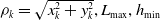 $\rho _{k}=\sqrt{{x}_{k}^{2}+{y}_{k}^{2}} , L_{\max } , h_{\min }$
and
$\rho _{k}=\sqrt{{x}_{k}^{2}+{y}_{k}^{2}} , L_{\max } , h_{\min }$
and
 $h_{\max }$
are constants defining the VOI’s radial and elevation boundaries.
$h_{\max }$
are constants defining the VOI’s radial and elevation boundaries.
Next, intensity information is introduced as a complementary dimension to eliminate matching ambiguities arising from highly similar geometric structures. The LiDAR intensity value
 $I$
is determined by
$I$
is determined by
 \begin{equation} I=\frac{P_{r}}{P_{e}}=\eta \frac{\rho \cos \alpha }{R^{2}} \end{equation}
where
 $P_{e}$
denotes the laser transmission power,
$P_{e}$
denotes the laser transmission power,
 $P_{r}$
represents the received signal energy,
$P_{r}$
represents the received signal energy,
 $\eta$
is a device-specific constant,
$\eta$
is a device-specific constant,
 $\rho$
is the material reflectivity,
$\rho$
is the material reflectivity,
 $R$
is the distance between LiDAR and object surface, and
$R$
is the distance between LiDAR and object surface, and
 $\alpha$
is the incidence angle between the laser beam and surface normal.
$\alpha$
is the incidence angle between the laser beam and surface normal.
However, in agricultural scenes, severe incident angle variations on foliage and furrows, render raw intensities unreliable. We address this limitation by employing a geometry-based intensity correction method [Reference Wang, Wang and Xie13]. For any given point
 $p\in R^{3}$
, we use its neighboring points
$p\in R^{3}$
, we use its neighboring points
 $p_{1}$
and
$p_{1}$
and
 $p_{2}$
to compute the local normal vector, subsequently deriving the incidence angle for intensity correction. This process enables a more accurate representation of crop or soil surface properties.
$p_{2}$
to compute the local normal vector, subsequently deriving the incidence angle for intensity correction. This process enables a more accurate representation of crop or soil surface properties.
 \begin{align} n &=\frac{\left(p-p_{1}\right)\times \left(p-p_{2}\right)}{\left| p-p_{1}\right| \cdot \left| p-p_{2}\right| } \\[-8pt]\nonumber \end{align}
 \begin{align} \cos \alpha &=\frac{p^{T}\cdot n}{\left| p\right| } \end{align}
To accommodate the within-row point density variation (dense near, sparse far), we employ a distance threshold instead of a point-count threshold [Reference Chang, Zhang, Huang, Hu, Ding and Qin40]. We construct a viewpoint-invariant evaluation function for both roughness and intensity distribution, which scales the geometric relationship between a point
 $p_{i}$
and the points
$p_{i}$
and the points
 $p_{i-n}$
and
$p_{i-n}$
and
 $p_{i+n}$
adjacent to it on either side. This function is defined as
$p_{i+n}$
adjacent to it on either side. This function is defined as
 \begin{align} {\sigma }_{i}^{c} &=\frac{1}{N_{i}}{\sum }_{n=1}^{N_{i}}\frac{\delta d\left|\left|\left(p_{i+n}-p_{i}\right)-\left(p_{i-n}-p_{i}\right)\right|\right|}{\min \left(\left|\left|\left(p_{i+n}-p_{i}\right)\right|\right|,\left|\left|\left(p_{i-n}-p_{i}\right)\right|\right|\right)} \\[-8pt]\nonumber \end{align}
 \begin{align} {\sigma }_{i}^{I} &=\frac{1}{N_{i}}{\sum }_{n=1}^{N_{i}}\frac{\delta d\left|\left|\left(\eta _{i+n}-\eta _{i}\right)-\left(\eta _{i-n}-\eta _{i}\right)\right|\right|}{\min \left(\left|\left|\left(\eta _{i+n}-\eta _{i}\right)\right|\right|,\left|\left|\left(\eta _{i-n}-\eta _{i}\right)\right|\right|\right)} \end{align}
where
 $\eta _{i}$
represents the corrected intensity threshold. Furthermore,
$\eta _{i}$
represents the corrected intensity threshold. Furthermore,
 $N_{i}$
denotes the number of neighboring points on each side, which is calculated as
$N_{i}$
denotes the number of neighboring points on each side, which is calculated as
 \begin{align} {N}_{i}^{L} &=\underset{n\gt 0}{\min \left(n\right)}\,s.t.\,\left|\left|\left(p_{i-n}-p_{i}\right)\right|\right|\geq \delta d \\[-8pt]\nonumber \end{align}
 \begin{align} {N}_{i}^{R} &=\underset{n\gt 0}{\min \left(n\right)}\,s.t.\,\left|\left|\left(p_{i+n}-p_{i}\right)\right|\right|\geq \delta d \\[-8pt]\nonumber \end{align}
 \begin{align} N_{i} &=\max \left({N}_{i}^{L},{N}_{i}^{R}\right) \\[8pt] \nonumber \end{align}
Subsequently, we adopt a weighted fusion method for feature extraction, where
 $\omega ^{c}$
and
$\omega ^{c}$
and
 $\omega ^{I}$
represent the weights of geometric and intensity distributions, respectively. During each scan, edge and plane features are selected from regions with larger and smaller
$\omega ^{I}$
represent the weights of geometric and intensity distributions, respectively. During each scan, edge and plane features are selected from regions with larger and smaller
 $\sigma _{i}$
:
$\sigma _{i}$
:
 \begin{equation} \sigma _{i}=\omega ^{c}\cdot {\sigma }_{i}^{c}+\omega ^{I}\cdot {\sigma }_{i}^{I} \end{equation}
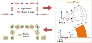
As shown in Figure 2, the core procedure for transforming point features into spatial features constructs an intensity–geometry joint probability model within CV. This process begins by mapping the point cloud space
 $V_{t}$
to a spherical coordinate system. Subsequently, the point cloud is partitioned into CVs based on distance, angular resolution, and sparsity.
$V_{t}$
to a spherical coordinate system. Subsequently, the point cloud is partitioned into CVs based on distance, angular resolution, and sparsity.
Schematic of spatial feature modeling.

The polar coordinate system
 $P(\rho ,\theta ,\phi )$
of a CV comprises radial distance, azimuth angle, and polar angle. Taking the
$P(\rho ,\theta ,\phi )$
of a CV comprises radial distance, azimuth angle, and polar angle. Taking the
 $m,n,o$
voxel as an example, it is defined as:
$m,n,o$
voxel as an example, it is defined as:
 \begin{align} \begin{array}{l} CV_{m,n,o} =\{P(\rho ,\theta ,\phi )=| {\unicode[Arial]{x0394}} \rho \cdot \left(m-1\right)\leq \rho \lt {\unicode[Arial]{x0394}} \rho \cdot m,\\[2pt] \qquad\qquad {\unicode[Arial]{x0394}} \theta \cdot \left(n-1\right)\leq \theta \lt {\unicode[Arial]{x0394}} \theta \cdot n,\\[2pt] \qquad\qquad {\unicode[Arial]{x0394}} \phi \cdot \left(o-1\right)\leq \phi \lt {\unicode[Arial]{x0394}} \phi \cdot o\} \end{array} \end{align}
where
 ${\unicode[Arial]{x0394}} \rho , {\unicode[Arial]{x0394}} \theta$
and
${\unicode[Arial]{x0394}} \rho , {\unicode[Arial]{x0394}} \theta$
and
 ${\unicode[Arial]{x0394}} \phi$
represent the incremental units adjusted based on point cloud sparsity and distance.
${\unicode[Arial]{x0394}} \phi$
represent the incremental units adjusted based on point cloud sparsity and distance.
It is important to identify the
 $CV_{m,n,o| i}$
containing the feature point
$CV_{m,n,o| i}$
containing the feature point
 $p_{i}$
in order to establish matching constraints for local structural information. For brevity, indices
$p_{i}$
in order to establish matching constraints for local structural information. For brevity, indices
 $i$
and
$i$
and
 $j$
hereafter are used to denote
$j$
hereafter are used to denote
 $m,n,o| i$
and
$m,n,o| i$
and
 $m,n,o| j$
, respectively.
$m,n,o| j$
, respectively.
The point cloud within a CV is assumed to follow a Gaussian distribution
 $N(\mu _{i},\sum _{i})$
, where the probability density parameters are computed as
$N(\mu _{i},\sum _{i})$
, where the probability density parameters are computed as
 \begin{align} \mu _{i} &=\frac{1}{\left| CV_{i}\right| }\sum _{p_{i}\in CV_{i}}PI_{i} \\[-8pt]\nonumber \end{align}
 \begin{align} {\sum}_{i} &=\frac{1}{\left| CV_{i}\right| -1}\sum _{p_{i}\in CV_{i}}\left(PI_{i}-\mu _{i}\right)\left(PI_{i}-\mu _{i}\right)^{T} \end{align}
where
 $\mu _{i}$
is the mean vector,
$\mu _{i}$
is the mean vector,
 $\sum _{i}$
is the covariance matrix, and
$\sum _{i}$
is the covariance matrix, and
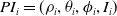 $PI_{i}=(\rho _{i},\theta _{i},\phi _{i},I_{i})$
encodes the joint statistical properties of spatial geometry and intensity, elevating a single point feature to a spatial descriptor that represents local structure.
$PI_{i}=(\rho _{i},\theta _{i},\phi _{i},I_{i})$
encodes the joint statistical properties of spatial geometry and intensity, elevating a single point feature to a spatial descriptor that represents local structure.
The matching of local structural information is achieved using the D2D-NDT [Reference Guo, Zhu and Chen14] method to minimize the joint probability distribution distance between the current frame and the local map. The optimization objective is given below:
 \begin{equation} f_{d2d}=\sum _{CV_{i}}\sum _{CV_{j}}-d_{1}\exp \left(-\frac{d_{2}}{2}{\mu }_{ij}^{T}\left(R^{T}\sum _{i}R+\sum _{j}\right)^{-1}\mu _{ij}\right) \end{equation}
where
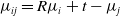 $\mu _{ij}=R\mu _{i}+t-\mu _{j}$
and
$\mu _{ij}=R\mu _{i}+t-\mu _{j}$
and
 $d_{1} , d_{2}$
are regularization factors.
$d_{1} , d_{2}$
are regularization factors.
Iterative optimization is used to align the local structural information, and the resulting LO serves as input for the subsequent state estimation layer.
3.3. Noise–state joint optimization via recursive estimation
To counteract the pronounced time-varying and non-stationary noise characteristics of multi-source sensors caused by severe terrain vibrations and wheel slip during operation in unstructured farmland, a time-varying recursive noise estimator is devised. Its objective is to estimate the noise statistics of the LO and the IMU under dynamic motion conditions in real time. Coupled with this estimator, a dual-filter architecture jointly propagates and refines both noise parameters and system states through recursive inference, thereby markedly improving pose-estimation accuracy and robustness in agricultural environments.
The system model consists of state-observation equations. The state vector is defined as follows:
 \begin{equation} x_{k}= \big[\begin{array}{llll} p_{k} &\quad \varphi _{k} &\quad v_{k} &\quad w_{k} \end{array}\big]^{T} \end{equation}
where
 $p_{k}$
and
$p_{k}$
and
 $\varphi _{k}$
denote position and orientation, respectively, and
$\varphi _{k}$
denote position and orientation, respectively, and
 $v_{k}$
and
$v_{k}$
and
 $w_{k}$
represent linear and angular velocities, respectively.
$w_{k}$
represent linear and angular velocities, respectively.
The state transition and observation equations are
 \begin{align} \hat{x}_{k} &=F_{k}\hat{x}_{k-1}+B_{k}u_{k}+w_{k} \\[-8pt]\nonumber \end{align}
 \begin{align} \qquad z_{k} &=H_{k}\hat{x}_{k}+v_{k} \end{align}
where
 $F_{k}$
is the state transition matrix,
$F_{k}$
is the state transition matrix,
 $B_{k}$
is the control input matrix,
$B_{k}$
is the control input matrix,
 $u_{k}$
is the control input, and
$u_{k}$
is the control input, and
 $w_{k}$
and
$w_{k}$
and
 $v_{k}$
denote the process and observation noise, respectively.
$v_{k}$
denote the process and observation noise, respectively.
Position and orientation updates are derived from velocities as follows:
 \begin{equation} \left[\begin{array}{l} p\\[2pt] \varphi \end{array}\right]=\left[\begin{array}{l} p+R\left(\varphi \right)v{\unicode[Arial]{x0394}} t\\[2pt] \varphi +J\left(\varphi \right)w{\unicode[Arial]{x0394}} t \end{array}\right] \end{equation}
where
 $R(\varphi )\in SO(3)$
is the rotation matrix,
$R(\varphi )\in SO(3)$
is the rotation matrix,
 $J(\varphi )$
is the Jacobian mapping relating angular velocity to Euler derivatives, and
$J(\varphi )$
is the Jacobian mapping relating angular velocity to Euler derivatives, and
 ${\unicode[Arial]{x0394}} t$
is the sampling interval.
${\unicode[Arial]{x0394}} t$
is the sampling interval.
The joint observation model
 $Z_{k}=[\begin{array}{ll} Z_{L} & Z_{I} \end{array}]^{T}$
combines LO and IMU. Velocity is used instead of pose as the observation metric, based on the EKF-LOAM [Reference Junior, Rezende, Miranda, Fernandes, Azpurua, Neto, Pessin and Freitas41] principles.
$Z_{k}=[\begin{array}{ll} Z_{L} & Z_{I} \end{array}]^{T}$
combines LO and IMU. Velocity is used instead of pose as the observation metric, based on the EKF-LOAM [Reference Junior, Rezende, Miranda, Fernandes, Azpurua, Neto, Pessin and Freitas41] principles.
The linear velocity
 $v_{L}$
and angular velocity
$v_{L}$
and angular velocity
 $w_{L}$
are obtained from the LO as:
$w_{L}$
are obtained from the LO as:
 \begin{align} Z_{L} &=\big[\begin{array}{l@{\quad}l} v_{L} & w_{L} \end{array}\big]^{T} \\[-8pt]\nonumber \end{align}
 \begin{align} \left[\begin{array}{l} v_{L}\\ w_{L} \end{array}\right] &=\left[\begin{array}{l@{\quad}l} R\left(\varphi _{L}\right) & o _{3\times 3}\\ o _{3\times 3} & J\left(\varphi _{L}\right) \end{array}\right]\left[\begin{array}{l} \Delta p_{L}\\ \Delta \varphi _{L} \end{array}\right]\frac{1}{{\unicode[Arial]{x0394}} t_{L}} \\[8pt] \nonumber \end{align}
where
 ${\unicode[Arial]{x0394}} p$
and
${\unicode[Arial]{x0394}} p$
and
 ${\unicode[Arial]{x0394}} \varphi$
represent the position and direction changes in LO, respectively.
${\unicode[Arial]{x0394}} \varphi$
represent the position and direction changes in LO, respectively.
The angular velocity
 $w_{I}$
is measured from the IMU as
$w_{I}$
is measured from the IMU as
 \begin{equation} Z_{I}=w_{I} \end{equation}
Traditional fusion schemes assume constant noise covariances, but in complex agricultural scenes, the noise characteristics of LO and IMU exhibit significant heterogeneity. If fixed parameters are directly used, it will cause fusion weight mismatch and state estimation divergence problems. To address this, an MAP time-varying recursive noise estimator is formulated. The associated noise parameters are defined as:
 \begin{align} &\qquad \qquad \qquad w_{k} =\frac{1}{k}{\sum }_{j=1}^{k}\left[\hat{x}_{j,k}-F_{j-1}\hat{x}_{j-1,k}\right] \\[-10pt]\nonumber \end{align}
 \begin{align} & \qquad \qquad \qquad \quad v_{k} =\frac{1}{k}{\sum }_{j=1}^{k}\left[Z_{j}-H_{j}\hat{x}_{j,k}\right] \\[-10pt]\nonumber \end{align}
 \begin{align} &Q_{k} =Cov\big[w_{k},w_{j}\big]=\frac{1}{k}{\sum }_{j=1}^{k}\left[\hat{x}_{j,k}-F_{j-1}\hat{x}_{j-1,k}-w\right]\left[\hat{x}_{j,k}-F_{j-1}\hat{x}_{j-1,k}-w\right]^{T} \\[-10pt]\nonumber \end{align}
 \begin{align} &\qquad \qquad R_{k} =Cov\big[v_{k},v_{j}\big]=\frac{1}{k}{\sum }_{j=1}^{k}\left[z_{j}-H_{j}\hat{x}_{j,k}-r\right]\left[z_{j}-H_{j}\hat{x}_{j,k}-v\right]^{T} \end{align}
where
 $w_{k}$
and
$w_{k}$
and
 $v_{k}$
are the process and observation noise, respectively, and
$v_{k}$
are the process and observation noise, respectively, and
 $Q_{k}$
and
$Q_{k}$
and
 $R_{k}$
are the process and observation noise covariance, respectively.
$R_{k}$
are the process and observation noise covariance, respectively.
However, the noise parameters contain complex multi-step smoothing terms, such as
 $\hat{x}_{j-1,k}$
and
$\hat{x}_{j-1,k}$
and
 $\hat{x}_{j,k}$
, which make it difficult to achieve recursive computation. To address this issue, we adopt a single-step smoothing approximation of
$\hat{x}_{j,k}$
, which make it difficult to achieve recursive computation. To address this issue, we adopt a single-step smoothing approximation of
 $\hat{x}_{j-1,j}\approx \hat{x}_{j-1,k} , \hat{x}_{j,j}\approx \hat{x}_{j,k}$
, thereby obtaining
$\hat{x}_{j-1,j}\approx \hat{x}_{j-1,k} , \hat{x}_{j,j}\approx \hat{x}_{j,k}$
, thereby obtaining
 \begin{align} &\qquad \qquad \qquad w_{k} =\frac{1}{k}\sum \limits_{j=1}^{k}\left[\hat{x}_{j,j}-F_{j-1}\hat{x}_{j-1,j}\right] \\[-24pt]\nonumber \end{align}
 \begin{align} &Q_{k} =\frac{1}{k}\sum \limits_{j=1}^{k}\left[\hat{x}_{j,j}-F_{j-1}\hat{x}_{j-1,j}-w\right]\left[\hat{x}_{j,j}-F_{j-1}\hat{x}_{j-1,j}-w\right]^{T} \\[-24pt]\nonumber \end{align}
 \begin{align} &\qquad \qquad \qquad \quad v_{k} =\frac{1}{k}\sum \limits_{j=1}^{k}\left[Z_{j}-H_{j}\hat{x}_{j,j}\right] \\[-24pt]\nonumber \end{align}
 \begin{align} &\qquad R_{k} =\frac{1}{k}\sum \limits_{j=1}^{k}\left[z_{j}-H_{j}\hat{x}_{j,j}-v\right]\left[z_{j}-H_{j}\hat{x}_{j,j}-v\right]^{T} \end{align}
The noise estimator is effectively integrated into the system by using the dual-filter structure proposed by Gao et al. [Reference Gao, Li, Zhou and Li23]. This structure consists of two parts: noise estimation propagation and state estimation correction. The former obtains the single-step smoothed value
 $\hat{x}_{k-1,k}$
of the propagating noise estimates based on the
$\hat{x}_{k-1,k}$
of the propagating noise estimates based on the
 $k-1$
step estimate
$k-1$
step estimate
 $\hat{x}_{k-1,k-1}$
and the
$\hat{x}_{k-1,k-1}$
and the
 $k$
step innovation
$k$
step innovation
 $\overline{\varepsilon }_{k}$
as follows:
$\overline{\varepsilon }_{k}$
as follows:
 \begin{align} &\quad \quad \overline{x}_{k,k-1} =F_{k-1}\hat{x}_{k-1,k-1}+w_{k-1} \\[-10pt]\nonumber \end{align}
 \begin{align} &\qquad \quad \overline{\varepsilon }_{k} =z_{k}-H_{k}\overline{x}_{k,k-1}-v_{k} \\[-10pt]\nonumber \end{align}
 \begin{align} &\quad \quad P_{k,k-1} =F_{k-1}P_{k-1}{F}_{k-1}^{T}+Q_{k-1} \\[-10pt]\nonumber \end{align}
 \begin{align} &\overline{K}_{k} =P_{k-1}{F}_{k-1}^{T}{H}_{k}^{T}\left(H_{k}P_{k,k-1}{H}_{k}^{T}+R_{k}\right)^{-1} \\[-10pt]\nonumber \end{align}
 \begin{align} &\quad \quad \hat{x}_{k-1,k} =\hat{x}_{k-1,k-1}+\overline{K}_{k}\overline{\varepsilon }_{k} \\[8pt] \nonumber \end{align}
The latter corrects the state estimate
 $\hat{x}_{k-1,k}$
using the single-step smoothed value
$\hat{x}_{k-1,k}$
using the single-step smoothed value
 $\hat{x}_{k,k}$
as
$\hat{x}_{k,k}$
as
 \begin{align} &\qquad \quad \hat{x}_{k,k-1} =F_{k-1}\hat{x}_{k-1,k}+w_{k-1} \\[-10pt]\nonumber \end{align}
 \begin{align} &\qquad \quad \varepsilon _{k} =z_{k}-H_{k}\hat{x}_{k,k-1}-v_{k} \\[-10pt]\nonumber \end{align}
 \begin{align}& K_{k} =P_{k,k-1}{H}_{k}^{T}\left(H_{k}P_{k,k-1}{H}_{k}^{T}+R_{k}\right)^{-1} \\[-8pt]\nonumber \end{align}
 \begin{align} &\qquad \qquad \hat{x}_{k,k} =\hat{x}_{k,k-1}+K_{k}\varepsilon _{k} \\[-10pt]\nonumber \end{align}
 \begin{align} &\qquad \quad P_{k} =\left(I-K_{k}H_{k}\right)P_{k,k-1} \end{align}
The noise estimator can be redefined according to the dual-filter structure, expressed in (40) and (41) as follows:
 \begin{align} &\qquad \qquad \quad \hat{x}_{j,j}-F_{j-1}\hat{x}_{j-1,j} =K_{j}\varepsilon _{j}+w_{j-1} \\[-8pt]\nonumber \end{align}
 \begin{align} &Z_{j}-H_{j}\hat{x}_{j,j} =Z_{j}-H_{j}\left(\hat{x}_{j,j-1}+K_{j}\varepsilon _{j}\right) =\left(I-H_{j}K_{j}\right)\varepsilon _{j}+v_{j} \end{align}
Furthermore, an exponentially weighted fading mechanism combined with a dynamic-window strategy is introduced to accurately capture the time-varying nature of sensor noise. Specifically, the exponential weighting term is defined as
 \begin{equation} \alpha ^{k}=\frac{\beta }{N_{k}+1} \end{equation}
where
 $\alpha ^{k}$
is the exponential weighting term,
$\alpha ^{k}$
is the exponential weighting term,
 $\beta$
is a constant term, and
$\beta$
is a constant term, and
 $N_{k}$
is the window size. The term
$N_{k}$
is the window size. The term
 $\alpha ^{k}$
is adjusted according to
$\alpha ^{k}$
is adjusted according to
 $N_{k}$
: when
$N_{k}$
: when
 $N_{k}$
is small,
$N_{k}$
is small,
 $\alpha ^{k}$
is larger, giving higher weight to recent data; when
$\alpha ^{k}$
is larger, giving higher weight to recent data; when
 $N_{k}$
is large,
$N_{k}$
is large,
 $\alpha ^{k}$
is smaller, which allows more historical data to be considered.
$\alpha ^{k}$
is smaller, which allows more historical data to be considered.
The window size
 $N_{k}$
is adjusted based on
$N_{k}$
is adjusted based on
 ${\sigma _{k}}^{2}$
, which is the variance of the innovation sequence within the window. This process is represented by the following equations:
${\sigma _{k}}^{2}$
, which is the variance of the innovation sequence within the window. This process is represented by the following equations:
 \begin{align} {\sigma }_{k}^{2} =\frac{1}{N_{k}}{\sum }_{i=k-N_{k}+1}^{k}\left(\varepsilon _{i}-\overline{\varepsilon }_{k}\right)^{2} \\[-8pt]\nonumber \end{align}
 \begin{align} N_{k} =N_{k-1}+\gamma \left({\sigma _{k}}^{2}-\overline{\sigma }^{2}\right) \end{align}
where
 ${\sigma _{k}}^{2}$
reflects the noise fluctuation in the current window. Furthermore,
${\sigma _{k}}^{2}$
reflects the noise fluctuation in the current window. Furthermore,
 $\varepsilon _{i}$
represents the
$\varepsilon _{i}$
represents the
 $i$
-th innovation value,
$i$
-th innovation value,
 $\overline{\varepsilon }_{k}$
is the mean of the innovation sequence within the window,
$\overline{\varepsilon }_{k}$
is the mean of the innovation sequence within the window,
 $\overline{\sigma }^{2}$
is the historical mean variance, and
$\overline{\sigma }^{2}$
is the historical mean variance, and
 $\gamma$
is a tuning factor.
$\gamma$
is a tuning factor.
In the presence of severe noise fluctuations, the window size is increased to improve the smoothness of the estimation results. When the noise stabilizes, the window size is reduced to ensure the system’s real-time responsiveness.
Thus, the final noise estimator is defined as
 \begin{align} &\qquad \qquad \qquad w_{k} =w_{k-1}+\alpha ^{k}\left[K_{j}\varepsilon _{j}+w_{j-1}\right] \\[-8pt] \nonumber \end{align}
 \begin{align} &\qquad \qquad Q_{k} =\left(1-\alpha ^{k}\right)Q_{k-1}+\alpha ^{k}\left[K_{j}\varepsilon _{j}{\varepsilon }_{j}^{T}{K}_{j}^{T}\right] \\[-8pt] \nonumber \end{align}
 \begin{align} &\qquad \qquad \quad v_{k} =v_{k-1}+\alpha ^{k}\left[\left(I-H_{j}K_{j}\right)\varepsilon _{j}+v_{j}\right] \\[-8pt] \nonumber \end{align}
 \begin{align} &R_{k} =\left(1-\alpha ^{k}\right)R_{k-1}+\alpha ^{k}\left[\left(I-H_{j}K_{j}\right)\varepsilon _{j}{\varepsilon }_{j}^{T}\left(I-H_{j}K_{j}\right)^{T}\right] \\[8pt] \nonumber \end{align}
4. Experiments
4.1. Experimental setup
To evaluate the proposed method, experiments are conducted along two dimensions: generalizability and agricultural adaptability. General performance is assessed on public datasets (KITTI [Reference Geiger, Lenz and Urtasun42], NCLT [Reference Carlevaris-Bianco, Ushani and Eustice43]), while task-oriented functionality is validated in both simulated agricultural environments (Gazebo) and real-world farmland. Evaluation metrics include relative translational error (RTE) and relative rotational error (RRE) as quantitative baselines [Reference Sturm, Engelhard, Endres, Burgard and Cremers44], and qualitative analysis is carried out in combination with the generated point cloud maps. RTE and RRE, established metrics in the SLAM domain, quantify the discrepancies between the estimated relative pose transformations and the ground truth over a time interval
 ${\unicode[Arial]{x0394}}$
. For a given time
${\unicode[Arial]{x0394}}$
. For a given time
 $i$
, the relative pose transformation error
$i$
, the relative pose transformation error
 $E_{i}$
is defined as:
$E_{i}$
is defined as:
 \begin{equation} E_{i}=\left({Q}_{i}^{-1}Q_{i+{\unicode[Arial]{x0394}} }\right)^{-1}\left({P}_{i}^{-1}P_{i+{\unicode[Arial]{x0394}} }\right) \end{equation}
where
 $Q$
denotes the ground truth pose sequence and
$Q$
denotes the ground truth pose sequence and
 $P$
the estimated pose sequence.
$P$
the estimated pose sequence.
Subsequently, RTE and RRE are calculated as:
 \begin{align} RTE_{i} =\left|\left|\textit{trans}\left(E_{i}\right)\right|\right| \\[-8pt]\nonumber \end{align}
 \begin{align} RRE_{i} =\angle \left(rot\left(E_{i}\right)\right) \end{align}
where
 $\textit{trans}(E_{i})$
extracts the translational vector from
$\textit{trans}(E_{i})$
extracts the translational vector from
 $E_{i}$
, and
$E_{i}$
, and
 $\angle (rot(E_{i}))$
converts the rotational matrix extracted from
$\angle (rot(E_{i}))$
converts the rotational matrix extracted from
 $E_{i}$
into an angular representation.
$E_{i}$
into an angular representation.
In agricultural scenes, row spacing is adopted as the core agronomic structural indicator. Row spacing, a key spatial parameter in agricultural remote sensing and agronomic mapping, directly reflects the consistency and precision of inter-row crop distribution. By quantifying the structural fidelity of the reconstructed map, this metric evaluates SLAM’s potential for remote sensing detail supplementation. Computation proceeds as follows: after orthographic projection of the reconstructed cloud, crop centers are extracted and trunk centerlines are fitted, and the Euclidean distance between adjacent plants is calculated and compared with ground truth.
In terms of hardware configuration, the public dataset and Gazebo experiments are executed on a notebook with an Intel Core i7-12700H CPU and 32 GB RAM under Ubuntu 20.04, with ROS Noetic. Real-field experiments employ an agricultural transport robot equipped with an LS-C16 LiDAR, and centimeter-level ground truth is obtained via RTK (as shown in Figure 3).
Experimental platform.

4.2. Generalization validation on public datasets
To evaluate the generalization performance of the proposed method under different environmental conditions, this paper conducts experimental validation using the widely recognized KITTI [Reference Geiger, Lenz and Urtasun42] and NCLT [Reference Carlevaris-Bianco, Ushani and Eustice43] datasets in the SLAM community. The KITTI dataset, a classic benchmark in autonomous driving, was collected from real urban environments and features rich structured roads and buildings, alongside geometrically sparse regions such as highways. It is well-suited for assessing system robustness under feature-degraded conditions. The NCLT dataset, a long-term large-scale collection from a campus environment, exhibits significant temporal spans and seasonal variations, thereby effectively testing the consistency and stability of SLAM systems during prolonged operation. The selection of these two representative public datasets for comparative experiments aims to systematically verify the generalization capability of the proposed method on standard benchmark datasets, demonstrating that its core design is not an overfitting optimization tailored to specific environments. Moreover, the geometric monotony and feature sparsity issues present in these datasets share intrinsic similarities with the feature degradation caused by orderly crop rows in agricultural environments, thereby providing empirical support for its applicability in farming scenarios.
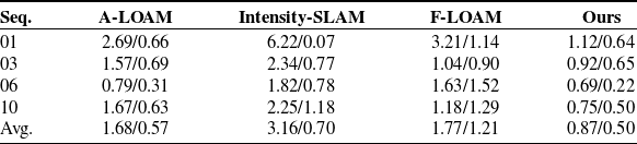
The evaluation first focuses on the KITTI dataset. Two representative scenario types are selected: (1) feature-sparse highway sequences (01, 10) with large scale topology and (2) complex urban sequences (03, 06) containing wide streets and multiple corner obstacles. Since the KITTI dataset used in this experiment only provides LiDAR data, the spatial feature modeling module of the proposed method is exclusively enabled to validate its effectiveness in pure LO tasks. Three representative state-of-the-art pure LO methods are selected as baselines for comparison. A-LOAM [Reference Zhang and Singh9], an efficient implementation of the LOAM framework, is employed as a baseline method due to its stable performance, which relies on matching extracted edge and planar points. F-LOAM [Reference Wang, Wang, Chen and Xie11] adopts a pure scan-to-map framework, directly registering each point cloud frame to a local map to achieve higher computational efficiency while maintaining accuracy. Intensity-SLAM [Reference Wang, Wang and Xie13] leverages both geometric features and point cloud intensity information to enhance robustness in complex environments.
Table I shows the pose estimation results obtained by different methods. The results demonstrate that by constructing a joint probabilistic model based on CV, which transforms traditional point features into spatial features, the localization accuracy of the system is significantly improved. Across the four sequences, the average RTE and RRE are reduced to 0.87% and 0.50°/100 m, respectively. This represents a 48.2% improvement in translation accuracy and a 14% improvement in rotation accuracy compared to the second-best method, A-LOAM, thereby further validating the effectiveness of the proposed method in enhancing LO precision. F-LOAM achieves translation accuracy comparable to A-LOAM, but its rotation error is considerably higher than that of other methods. This indicates that while the scan-to-map framework can improve computational efficiency, it exhibits limited capability in estimating high-frequency rotational motions, making it susceptible to error accumulation. In contrast, Intensity-SLAM shows a larger translation error, as its performance heavily relies on the consistency of environmental intensity features. In outdoor scenarios affected by varying illumination, the reliability of intensity features diminishes, consequently degrading localization accuracy.
Relative pose errors on the KITTI dataset.

Note that the performance is presented in the “A/B” format, where “A” and “B” represent the RTE (%) and °/100 m, respectively.
Mapping results are shown in Figure 4(a–d). The proposed method produces complete and continuous point cloud maps under all tested conditions, accurately reconstructing spatial structure. Even in geometrically sparse regions (e.g., flat highway sections), the system maintains stable mapping quality without discernible drift. Figure 4(e–h) presents the trajectory estimation outcomes of different methods. The trajectory obtained through spatial feature registration aligns most closely with the ground truth, exhibiting substantially lower errors compared to the baseline methods. In contrast, the trajectories generated by other methods display varying degrees of drift in feature-sparse regions. Particularly, Intensity-SLAM suffers from severe drift in Sequence 01, leading to a complete system failure.
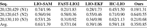
Relative pose errors on the NCLT dataset.

Note that the performance is presented in the “A/B” format, where “A” and “B” represent the RTE (%) and °/100 m, respectively.
Mapping and trajectory results on the KITTI. (a–d) Mapping results on Seq. 01, 03, 06, and 10, (e–h) corresponding trajectory results.

Subsequently, the complete system (integrating both LiDAR and IMU data) is validated on the NCLT dataset. Four representative LIO methods are selected as baselines for comparison: LIO-SAM, a classic factor graph-based optimization method; FAST-LIO2 [Reference Xu, Cai, He, Lin and Zhang19] and LIO-EKF [Reference Wu, Guadagnino, Wiesmann, Klingbeil, Stachniss and Kuhlmann36], which are representative methods under the Kalman filtering framework; and HC-LIO [Reference Hong, Ma, Li, Shao, Huang, Zeng and Chen21], a method specifically designed for agricultural operational environments. It should be noted that pure LO methods are excluded from this comparison, as they cannot operate effectively on this dataset. The pose estimation results of these methods are summarized in Table II. The proposed complete system achieves the best performance across most sequences, with average RTE and RRE controlled at 0.35% and 0.85°/100 m, respectively. LIO-EKF and FAST-LIO2 exhibit comparable overall performance, demonstrating high accuracy and stability in translation estimation, though their rotation estimation accuracy is relatively limited. In contrast, leveraging the noise-state joint optimization mechanism, the proposed method significantly enhances the system’s ability to constrain rotational motion, resulting in more stable and improved pose estimation accuracy. HC-LIO outperforms LIO-SAM, but both methods lag notably behind the filter-based approaches. This outcome indicates that in large-scale, long-term operational scenarios like NCLT, factor graph-based methods face greater challenges in terms of real-time performance and consistency. Moreover, while HC-LIO is tailored for agricultural environments, its cross-domain adaptability in general scenarios remains limited, further highlighting the advantages of the proposed method in terms of cross-scene applicability.
Figure 5 shows the mapping and trajectory results on the NCLT dataset. From Figure 5(a–c), it can be seen that the proposed full system reconstructs large-scale scene details, including street layouts and vegetation distributions. The trajectory results in Figure 5(d–f) show that the proposed method consistently achieves high trajectory accuracy across all test sequences, with estimated trajectories aligning most closely with the ground truth. In contrast, the baseline methods exhibit more pronounced trajectory errors in certain sequences.
Mapping and trajectory results on the NCLT. (a)–(c) Mapping results on Seq. N1, N2, and N3, (d)–(f) corresponding trajectory results.

To quantify the joint optimization effect of the proposed time-varying recursive noise estimator and the dual-filter architecture, a comparative experiment was conducted on sequence N3 against a conventional EKF baseline. Error statistics are shown in Figure 6. The joint optimization confines absolute position error in the XY plane to 0.89 m and keeps heading error within 1.02°, both significantly outperforming the EKF. The error traces reveal pronounced fluctuations for the EKF in local regions, whereas the adaptive adjustment of noise parameters by the recursive estimator effectively suppresses these fluctuations, yielding superior stability and reliability in pose estimation.
Error statistics. (a) Translation error, (b) rotation error.

Collectively, the public dataset results demonstrate that the proposed spatial feature modeling and joint noise–state optimization framework is fully transferable across scenarios. Although originally designed to address structural degradation and nonstationary noise in agriculture, the technical framework confers universal advantages in complex environments.
Simulated and real agricultural scenes. (a) Simulated agricultural scene, (b) real agricultural scene.

4.3. Agricultural scene validation
To comprehensively evaluate performance in agricultural contexts, experiments were conducted in both simulated and real-world scenes. As shown in Figure 7, both environments contain regularly spaced, highly repetitive crop rows and feature complex, undulating terrain, providing stringent tests of scene adaptability.
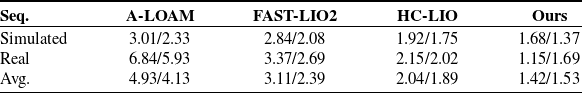
Relative pose errors on the agricultural scenes.

Note that the performance is presented in the “A/B” format, where “A” and “B” represent the RTE (%) and °/100 m, respectively.
Mapping and trajectory results on the simulated agricultural scenes. (a) Mapping result, (b) trajectory result.

Mapping and trajectory results on the real agricultural scenes. (a) Mapping result, (b) trajectory result.

The proposed system is compared with three representative methods: A-LOAM [Reference Zhang and Singh9], a pure LO method; FAST-LIO2 [Reference Xu, Cai, He, Lin and Zhang19], a representative LIO method (both of which performed well in the generalizability validation); and HC-LIO [Reference Hong, Ma, Li, Shao, Huang, Zeng and Chen21], a method specifically designed for agricultural scenarios. The pose estimation results are summarized in Table III. The results show that the proposed system achieves average RTE and RRE values of 1.42% and 1.53°/100 m, respectively, significantly outperforming all baseline methods. In the simulation environment, A-LOAM and FAST-LIO2 exhibit comparable accuracy, indicating that the IMU noise is in an ideal state under these conditions, and the primary factor limiting system accuracy is the feature extraction and registration performance of the LO. Under these conditions, both the proposed method and HC-LIO achieve better localization accuracy than A-LOAM and FAST-LIO2 by improving their feature extraction and matching strategies. However, the spatial feature modeling approach proposed more effectively characterizes the geometric structures of regularly arranged crops in agricultural environments, resulting in superior localization accuracy compared to HC-LIO. In real agricultural scenarios, the accuracy of A-LOAM decreases significantly. In contrast, all LIO methods that fuse IMU data outperform A-LOAM, demonstrating that a single sensor is insufficient to meet high-precision localization requirements in complex real-world environments. Specifically, by integrating spatial feature modeling with noise-state joint optimization, the proposed method achieves a 43.6% improvement in RTE and a 10.6% improvement in RRE over the second-best method, HC-LIO, highlighting its significant advantages. As a SLAM method specifically tailored for agricultural environments, HC-LIO outperforms the general-purpose FAST-LIO2 in this scenario through its hierarchical coupling design, which further underscores the necessity of developing targeted algorithms to address the unique challenges of agricultural settings.
Figures 8 and 9 show the mapping and trajectory results for the simulated and real scenes, respectively. The proposed method constructs maps that preserve geometric fidelity and spatial continuity, accurately reproducing agricultural scene structures and providing reliable data for subsequent precision operations. Regarding trajectory results, in the simulation environment, A-LOAM and FAST-LIO2 exhibit multiple minor drifts in structurally repetitive areas. Although HC-LIO shows significantly better trajectory stability than these methods, it still presents slight deviations at certain turning points. In the real-world scenario, the trajectory drift of A-LOAM is considerably more severe. While both FAST-LIO2 and HC-LIO maintain a certain level of trajectory accuracy, their trajectories are noticeably affected by the rugged terrain, exhibiting pronounced “zigzag” fluctuations. HC-LIO shows smaller fluctuation amplitudes, reflecting the advantages of its scenario-specific design. In contrast, the proposed method demonstrates superior stability in both scenarios, with its trajectory closely matching the ground truth, thereby fully validating its strong adaptability in complex agricultural environments.
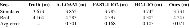
Further, row spacing is extracted from the generated maps (shown in Figure 10) as an agronomic metric to verify the proposed system’s value for near-ground remote sensing supplementation. The estimation results of row spacing are shown in Table IV. The mean row spacing values extracted by the proposed method are 3.731 and 4.247 m, respectively, with estimation errors controlled within 0.071 m, which is the closest to the measured ground truth. In contrast, the estimates obtained by other methods exhibit varying levels of deviation. Figure 11 further shows the distribution statistics of row spacing estimation errors for each method. The proposed method achieves the lowest median error and the narrowest interquartile range, indicating that its estimation results are not only highly accurate overall but also exhibit low fluctuation and excellent stability. HC-LIO shows a lower median error and a narrower distribution range compared to A-LOAM and FAST-LIO2, which is consistent with its superior localization accuracy and confirms the effectiveness of its design tailored for agricultural environments.
Row-spacing estimation results on the agricultural scenes.

Row-spacing estimation in agricultural scenes.

Statistical distribution of row-spacing estimation error.

These results demonstrate that general-purpose methods such as A-LOAM and FAST-LIO2 struggle to reconstruct agronomic structures in a stable manner. Although HC-LIO effectively enhances performance in agricultural scenarios, its accuracy and stability still fall short of the proposed method. The proposed system not only provides high-precision localization and mapping capabilities to support precision agriculture operations but also, through stable and accurate map reconstruction, delivers high-resolution, quantifiable supplementary information on the near-ground 3D structure of crop structures, which are often difficult for conventional remote sensing systems to resolve.
5. Conclusion
This paper proposes a robust L-SLAM system that integrates spatial feature modeling with noise-state joint optimization to address the repetitive structures, severe terrain disturbances, and non-stationary sensor noise prevalent in agricultural environments. To improve registration stability in structurally redundant scenes, the system employs a CV-based joint probability model that fuses intensity and geometric information. For pose estimation under dynamic and uncertain conditions, a time-varying recursive noise modeling scheme is introduced within an MAP optimization framework, further enhanced by a dual-filter architecture that jointly refines states and noise parameters. Experimental validation on public datasets demonstrates the generalizability of the proposed method. Comparative experiments in both simulated and real-world agricultural environments further confirm the system’s significant advantages in localization accuracy, mapping quality, and the ability to reconstruct agronomic structures.
However, the proposed method has certain limitations. Its superior performance largely depends on the presence of discernible macro-geometric structures in the environment; in extremely sparse and unstructured scenarios, the system’s constraint capability may diminish. Moreover, the complex models introduced to achieve high precision and strong adaptability impose higher computational demands. Future work will focus on developing lightweight models and acceleration algorithms to enhance real-time performance on embedded platforms, and to explore enhancement strategies for extremely unstructured environments, thereby advancing the large-scale application of SLAM systems in precision agriculture.
Author contribution
Ziyang Wang: Writing original draft, Validation, Investigation, Methodology. Wenfu Tong: Visualization, Investigation, Supervision. Haibo Zhou: Writing review & editing, Methodology. Mingjun Li: Supervision, Investigation. Xiaozhuo Wang: Writing review & editing. Biyao Cheng: Writing review & editing, Methodology.
Financial support
This work was supported in part by National Natural Science Foundation of China (No. U24B2051), Changsha Major Science and Technology Open Competition Project (kq2503005) and Natural Science Foundation of Hunan Province (No. 2023JJ30694).
Competing interests
The authors declare that they have no known competing financial interests or personal relationships that could have appeared to influence the work reported in this paper.
Ethical approval
This article does not involve human or animal participation or data; therefore, ethics approval is not applicable.
Declaration of generative AI and AI-assisted technologies in the writing process
During the preparation of this work, the authors used ChatGPT in order to translate and polish this article. After using this tool, the authors reviewed and edited the content as needed and take full responsibility for the content of the publication.