2. Rethinking persistence in the global economy

We seek a theory that answers, at the very least, the central cross-sectional question of economic history: what explains the distribution, ${\cal M}$, of the social and economic development or wellbeing of nations today.Footnote ³ Such a theory is necessarily time-dependent because the wellbeing of a nation evolves over time. And, being time-dependent, the same theory must be consistent with the longitudinal evidence. We first quantify what we mean by wellbeing, and then we characterize the time evolution of ${\cal M}$.

Though per capita production (GDP), or the closely related per capita national income (GNI), are frequently used as measures of national wealth, neither one may be taken seriously as a stand-alone proxy for wellbeing. For instance, thanks to $13k per capita in oil revenue, the per capita 2015 GNI of Equatorial Guinea is $21k, putting it on par with Argentina in the third decile from the top (United Nations, 2019). However, that near-equivalence masks a 19-year difference in life expectancy. Surpassing GDP, GNI, and other purely or narrowly economic measures of wellbeing, the human development index (HDI) combines the logarithm of GNI with life expectancy (at birth) and measures of education offered and achieved. On HDI's 0–1 scale where the standard deviation is 0.156, Equatorial Guinea (0.59) is comparable to Ghana (0.58), despite the GNI of the former being nearly six times that of the latter, and much much lower than that of Argentina (0.84). ${\cal M}$, the distribution of HDI in 2015, is shown in Figure 1A and is tabulated in an online appendix.

Figure 1.

Characteristics of HDI. (A) The multimodal distribution of HDI in 2015. (B) Trajectories of the mean and standard deviation of the distribution (1870–2015). The gray bands delineate 99% confidence intervals of exponential fits to the raw data. (C) ${\cal P}( t )$, the correlation of the distribution to itself at an earlier time. Smaller black dots, t < 30, are UN data. The larger black dots are Escosura's. The gray band delineates 99.9% confidence intervals of a decaying exponential fit. The slow decay of ${\cal P}( t )$ informs us that, after accounting for its mean and standard deviation, the distribution shown in (A) is materially constant on a time scale of a century.

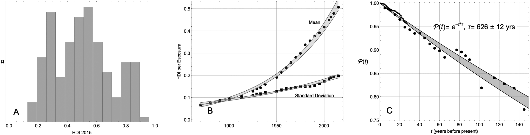
Beyond this snapshot of the present, the UN provides annual estimates of HDI (for up to 192 nations) dating back to 1990 when it pioneered the concept. Leandro Prados de la Escosura (Reference de la Escosura2019) provides assessments for 164 nations at roughly 10-year intervals going back to 1870. We ask, how does ${\cal M}( t )$ vary as we look backward in time? Were today's rich also rich in the past, and likewise the poor? North intimated as much when he characterized the explanation of the persistence of those disparities as one of the two central challenges of economic history?Footnote ⁴ Although a vast literature is devoted to the matter of the disparities, the problem of documenting and explaining their persistence has received little attention.

To quantify the evolution of the distribution ${\cal M}$, we compute its Pearson correlation to itself at earlier times t. We call this autocorrelation the persistence, ${\cal P}( t )$. The Pearson correlation of two distributions is independent of their mean and variance. The autocorrelation function thus tells us about the stability of relative position within the distribution. Figure 1C shows that ${\cal P}( t )$ decays steadily and slowly, permitting us to write ${\cal P}( t ) = e^{{-}t/\tau }$ where τ = 626  ± 12 years. The implied decay rate is about 15% per century. On a time scale of half a millennium the rich stay rich and the poor stay poor relative to others, with few exceptions.

The growth of the global economy and its inequalities are obvious and the subject of innumerable studies. That the disparities of wellbeing are persistent in relative terms, as just noted, is not obvious. Nor does it invalidate those other studies. During the same 145-year span over which the distribution ${\cal M}( t )$ has changed very little as measured by ${\cal P}( t )$, its mean and standard deviation have changed enormously; see Figure 1B. They are well approximated by exponentials with time constants of 69 and 148 years, respectively. Development economics entangles two different phenomena: (1) the persistence of the distribution of wealth; and (2) the trajectories of its mean and of its variance. Theory must account for both. Here, we focus our attention on the former. The latter must be the subject of a separate inquiry.

Whether or not one is inclined to extrapolate beyond the 145-year time span of this dataset, it must be acknowledged that the pronounced persistence across the late 19th and 20th centuries obtains in the face of decolonization, two world wars, the coming and going of Fascism and much of Communism, the rise of Asia's Tigers, and the rise of the oil economy, each a vector of profound institutional change. How could it be that the rules of the game are changing so much and yet the distributional outcome of the game has changed so little?

3. The paradigm in crisis

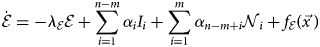
The persistence described above is a boundary condition by which any theory of economic history is constrained. No static theory of the present can say anything about meeting such a condition, for the simple reason that a static theory is a temporal point estimate. For all their claims to be rooted in game theory's dynamics, and the assertion that institutions rule, the mathematical foundations of widely cited papers of the NIE (e.g. Acemoglu et al., Reference Acemoglu, Johnson and Robinson2002; Rodrik et al., Reference Rodrik, Subramanian and Trebbi2004) are of the form ${\cal E}^k = \sum _ic_ix_i^k$, where ${\cal E}^k$ is a measure of economic performance of nation k, the $x_i^k$ are various factors or independent variables evaluated on nation k, and the c _i are constants or parameters to be determined. As such, those studies are no more than static factor analytics as described in Society, Politics, & Economic Development (Adelman and Morris, Reference Adelman and Morris1972), and commonly known today as linear regression. In that form, the NIE is a theory that cannot grapple with history, and not having done so, it suffers from a particularly grave form of omitted variable bias.

North's definition of institutions as humanly devised formal and informal constraints makes no mention of time, yet he was well aware of the fact that the informal constraints tend to be long-standing and the formal ones tend to be fairly recent. Williamson articulates this in a four-level hierarchy of institutions, distinguishing one from another on the basis of the time scale of their evolution (Reference Williamson2000: 597). Those that evolve most slowly, on a time scale of 100 to 1,000 years, e.g. customs, traditions, norms, and religion, he assigns to a level he calls Embeddedness, labeling it L1. Real actors are embedded in society where social convention constrains agency more narrowly than rational choice alone would suggest (Granovetter, Reference Granovetter1985; Williamson, Reference Williamson2000: 596). L2, the level of Institutional Environment is the realm of North's rules of the game, especially institutions establishing property rights codified in governing bodies, the judiciary, and other bureaucracies. These evolve on a time scale of 10–100 years. L3 is the level of Governance, transpiring within 1–10 years, and L4 – Resource Allocation and Employment – operates continuously. This hierarchy, and some of its implications as spelled out by Gerard Roland (Reference Roland2004), begins to zero in on the dynamics which must be part of any theory of development.

However, Roland and Williamson remain firmly wedded to the paradigm of game theory and its stipulated rules. Game theory is indeed dynamic as required of a mathematical theory of economic history that must contend with the boundary condition of persistence. But it is a wedding in name only, as there has been no issue in the form of an actual testable theory. Williamson, invoking Kenneth Arrow, offered this hopeful perspective: ‘The NIE has progressed not by advancing an overarching theory but by uncovering and explicating the microanalytic features … and by piling block upon block until the cumulative value cannot be denied’ (Reference Williamson2000: 596). In other words, the NIE would find by induction what it has not found by deduction. Two decades on, there is no evidence that the inductive method converges.

Finally, North opens Institutions, Institutional Change and Economic Performance with his slogan, ‘Institutions are the rules of the game’, and then goes on to make the case for the coevolution, that is, for the influence of an economy on its institutions and vice versa. But is it possible that institutions are both the rules of the game and one of its coevolutionary outcomes? It may be possible, but Greif notes that ‘classical game theory provides an inadequate analytical framework for studying institutional dynamics’ (Reference Greif2006: 10), by which he means coevolution. The authors of ‘Institutions Rule’ answer the same question by including the influence of the economy on institutions in a key figure, while downplaying it the text, and disabling it altogether in their system of equations (Rodrik et al., Reference Rodrik, Subramanian and Trebbi2004: 134). In Alston et al.'s much heralded 2018 summary of the NIE,Footnote ⁵ Economic Performance is understood as an outcome pure and simple, with ‘institutions and norms [taken] as given’ (Reference Alston, Alston, Mueller and Nonnenmacher2018: 12). This formulation excludes the possibility of coevolution. Although North viewed coevolution as integral, it seems to contradict his best remembered phrase. Game theory as presently understood is incapable of modeling it, and in contemporary scholarship it is minimized and or ignored outright.

If, as we argue, the paradigm that institutions are the rules of the game is fraught with paradox; and if, as explained above, persistence in the global economy makes the premise of the paradigm implausible; and if one of the field's pre-eminent game theorists reports that game theory is not up to the task, why does the paradigm persist?

In a 1969 monograph, the American philosopher David Lewis emphasized that precedent, not superiority, is at the heart of adherence to convention, a term which we could use interchangeably with paradigm (Reference Lewis2002: 35-41). When it comes to frameworks for solving time-dependent problems, there is a more highly developed alternative to game theory that is, owing to convention, deployed by almost no institutional economists or economic historians. That alternative is called dynamical systems theory – an amalgam of differential equations, linear algebra, perturbation theory, and other computational methods. It has been successfully deployed in celestial mechanics, cardiology, and population dynamics, to name a few disciplines on a long list. Its rich and fruitful 300-year history suggests that the pre-eminence of game theory in the NIE is neither essential, nor, in the face of its inability to solve the central challenges of economic history, warranted.

If we are no longer constrained by precedent to think of institutions as rules, how might we think of them? A university is indisputably an institution, though not indisputably a constraint. And though institutions are, obviously to economists, the rules of the game of development, they are not the rules of the game of development to financiers or shopkeepers who, seeking to build inventory to meet growth's demands, understand that ‘Cash is King!’ Cash is a source of economic growth, suggesting by analogy that institutions are not humanly devised constraints that reduce uncertainty, but rather humanly devised sources of economic growth. By this logic, a university is an economically productive investment, one that turns dollars into historians, legislators, doctors, and inventors, for instance, whose skills and commitment enable the day-to-day functioning of society. Such a definition is well-suited to dynamical systems theory, and in the next section we employ it to construct a new theory of an economy and its institutions.

4. r-Theory

North defined an institution as a humanly devised constraint that reduces uncertainty and transaction costs, thereby promoting growth. Simplifying, let an institution be the source itself, for instance a network of roads, a university campus and its faculty and staff, or a judiciary with its attendant courthouses, personnel, law-making bodies, and law schools.Footnote ⁶ Let r ^k be the real economy of a nation k, consisting of its performance, ${\cal E}^k$, for instance the logarithm of per capita income, and its many institutions, I ^k. Expressed as a vector, we have $r^k = ( {{\cal E}^k, \;I_1^k , \;\ldots , \;I_n^k } )$. Because institutions promote growth, for every $I_i^k$ there will be a corresponding contribution to the growth of ${\cal E}^k$, that is, to its time rate of change, ${\dot{\cal E}}{}^k$. Assuming linearity – an assumption that can be lifted if warranted by the evidence – that contribution is of the form $\alpha _iI_i^k$.Footnote ⁷

The constant α _i couples an entity of type I to an entity of type ${\cal E}$, and as such, we call α _i a coupling constant. The coupling constants are universals by assumption; they are not state-specific and do not carry the superscript k. If we can demonstrate that our theory and its models have verisimilitude then we will have some confidence in the merit of this assumption. If not, we must amend it. For ease of reading from here on, we drop the state-specifying superscript, k, from the notation of those variables that do carry them, for instance I and ${\cal E}$.

A larger economy needs more roads to support its traffic, more universities to train its highly skilled citizens, and a bigger judiciary to adjudicate its disputes. Thus, just as institutions promote economic growth, the economy promotes institutional growth. An expression for $\dot{I}_i$, the time rate of change of the i^th institution, must therefore include a term of the form $\beta _i{\cal E}$, where β _i is also a coupling constant. Similarly, a Ministry of Industry and Technology, call it I_j, may seek to promote growth in a network managed by the Department of Roads, call it I_i, so $\dot{I}_i$ may be expected to include cross-institutional couplings of the form γ _ijI _j. These couplings and cross-couplings give us the coevolution that North envisioned but game theory has not integrated. Our framework builds it in but does not prejudge its import. After solving the system and comparing the solutions to the real world we might find that the coevolutionary contributions are negligible.

Our definition specifies institutions in terms of their function, their propensity to generate growth, and not in terms of their form. In this framework, the measure of an institution is not whether, for instance, it is a network of roads or a network of canals, but whether the network works to deliver goods and drive $\dot{{\cal E}}$.Footnote ⁸ Thus there are multiple paths of institutional development that lead to the same economic outcome. The rules paradigm, on the other hand, defines institutions in terms of their form, as if in the form itself lies the secret of success.Footnote ⁹

The economy is situated in an environment, $\vec{x}$, exemplified by climate, geography, natural resources, neighboring states, and so forth. The environment stimulates or retards growth, too. We express its contributions to $\dot{{\cal E}}$ and $\dot{I}_i$ as forcing functions $f_{\cal E}( \vec{x} \,)$ and $f_I( \vec{x} \,)$.Footnote ¹⁰ With the forcing functions over environment variables standing in for what North called the standard constraints of economics, and with the couplings capturing his evocation of an incremental evolution of the economy and its institutions, it would seem that we have everything necessary for a theory of that evolution. Though the implied theory is easily solved, it is unstable. Every state becomes more prosperous than Norway or more impoverished than Somalia. To put it another way, the implied theory predicts a world with no middle. However, the world as we know it has a middle, as is easily seen by examination of the distribution of HDIs in Figure 1A. The implied theory fails by reason of verisimilitude.Footnote ¹¹

This failure might be seen as a reason to lift the assumption of linearity, or to consider higher order derivative terms, or even to invoke complex adaptive systems, but the failure is one of omission not of lower order math.Footnote ¹² This simple model misses decay. In the real world, roads get overgrown and become impassable if not maintained. Things fall apart. Metaphorically, the same happens to bureaucracies, universities, or judiciaries. In short, institutions are subject to degradative processes, equivalent in the material world to drag. Similarly, economic performance suffers the friction of transaction costs, the dissipative strain of sustaining its bureaucracies, and of corruption, points emphasized by North (Reference North1990, 12). In addition, that performance is burdened by the caring for young or elderly dependents, a point made by Smith in the opening pages of The Wealth of Nations (Reference Smith1999: 3). We posit that drag on $\dot{I}_i$ is of the form −λ _iI _i, and that the corresponding contribution to $\dot{{\cal E}}$ is $-\lambda _{\cal E}{\cal E}$. From the structure of these terms, it is evident that the λs have units of inverse time; thus they set the time scale of the system's evolution.

From this description we get equation (1), a set of coupled differential equations (also known as a dynamical system) describing the coevolution of a real economy constrained by its environment $\vec{x}$.Footnote ¹³ Λ is a square matrix (of n + 1 dimensions) comprised of coupling and drag constants. $f( \vec{x} \,)$ is an n + 1-dimensional vector of forcing functions over the environmental variables:

(1)$$\dot{r} = {\rm \Lambda }r + f( {\vec{x}} \,) \quad {\rm given}\;{\rm \Lambda } = \left({\matrix{ {-\lambda_{\cal E}} & {\alpha_1} & {\alpha_2} & \cdots & {\alpha_n} \cr {\beta_1} & {-\lambda_1} & {\gamma_{12}} & \cdots & {\gamma_{1n}} \cr {\beta_2} & {\gamma_{21}} & {-\lambda_2} & \cdots & {\gamma_{2n}} \cr \vdots & \vdots & \vdots & \ddots & \vdots \cr {\beta_n} & {\gamma_{n1}} & {\gamma_{n2}} & \ldots & {-\lambda_n} \cr } } \right)$$

The drag terms, $-\lambda _{\cal E}{\cal E}$ and −λ _iI _i, are necessarily in opposition to ${\cal E}$ and I, so the λs are necessarily positive. The coupling constants are, by construction, positive if they promote growth, negative if they retard it, or negligible if they are inconsequential. This very general formulation has (n + 1)² free parameters and is unlikely to yield interpretable findings without severe pruning.

Although the economy stimulates the growth of roads, it is by no means true that the economy stimulates the growth of all institutions. Take, for instance, incest, a set of social norms governing family structure. Ancient in origin, commonly found across the globe, and having survived all manners of economic change, the cultural traditions surrounding incest are manifestly impervious to the economy, to other institutions, and to $\vec{x}$. Norms such as these, call them ${\cal N}_i$, do not coevolve, that is $\dot{{\cal N}}_i\cong 0.$ Nevertheless, they may influence economic performance or other institutions.

Let ${\cal N}$ be a vector of m different norms. Examine $\dot{{\cal E}}$, the first component of $\dot{r}$ in equation (1), by expanding the product Λr. We get

$$\dot{{\cal E}} = {-}\lambda _{\cal E}{\cal E} + \mathop \sum \limits_{i = 1}^{n-m} \alpha _iI_i + \mathop \sum \limits_{i = 1}^m \alpha _{n-m + i}{\cal N}_i + f_{\cal E}( {\vec{x}} \,) $$

The second sum is a constant because the individual ${\cal N}_i$ are constant. Absorbing it into $f_{\cal E}$, we rewrite the latter as $f_{\cal E}( {\vec{x},\ {\cal N}} )$. If climate is conceptually synonymous with the environmental variables $\vec{x}$, then social climate is conceptually synonymous with ${\cal N}$. This echoes Grafstein's observation that ‘[Institutional] structuring of alternatives can be a brute fact of life for those who live within them, much as physical situations can be brute facts of life for everyone at large’ (Reference Grafstein1992: 4). The same logic applies to the other non-normative components of r, giving us equation (2), or what we call r-theory, where the dimensionality of Λ has been reduced to from n + 1 to n + 1 − m by virtue of the pruning of m norms:

(2)$$\dot{r} = {\rm \Lambda }r + f( {\vec{x},\ {\cal N}} ) $$

The paradox of informal constraints is an expression of the fact that norms matter more than North and Williamson and other peers of the NIE expected that they should matter, though neither North nor Williamson was specific about which norms matter. By the derivation of equation (2) we see that it is the relative constancy of norms, or the fact that they do not coevolve with the economy, that puts them on a par with the brute facts of the physical environment. Thus r-theory resolves the paradox of informal constraints, and it does so without having specified which norms matter. Norms are culture, and it is beyond the scope of this paper to give cultural analysis its due.Footnote ¹⁴

In the language of Williamson's four-level hierarchy, the vector of norms ${\cal N}$corresponds to his L1 or embedded institutions. The remaining institutions, the non-normative I _i, belong on the other rungs of his hierarchy in accordance with their time scale of evolution. Even if there were only one institution in each of L2, L3, and L4, the implied Λ would have 16 free parameters. From the modeling, that is to say practical perspective, 16 might as well be infinity, so further pruning is called for.

We order the remaining institutions such that α _i > α _i+1, that is, in descending order of their constructive influence on $\dot{{\cal E}}$, and we retain the strongest. Smith noted that roads and canals ‘are upon their account the greatest of all improvements’ (Reference Smith1999: 251). By analogy, we deploy the term 'infrastructure' and the symbol ${\cal I}$ to refer to the vector of the most productive of the non-normative I _i.

What does infrastructure have to do with North's institutions as we know them, specifically with formal institutions? Property rights, integral to the NIE, are words on a page without the physical infrastructure in which to litigate and enforce them, and without the concomitant infrastructure needed to train litigators and enforcers. A state's stated commitment to the health of its citizens is only aspirational without the physical infrastructure of hospitals, credentialed training, and so forth, ad infinitum. When formal rules are instantiated, they become infrastructure that grows alongside the economy.

In the same spirit in which we ordered the I _i by descending α _i, we order the ${\cal I}_i$ such that β _i > β _i+1; that is, in descending order of the strength of the coupling of economic performance into institutional growth. Again, transportation networks are candidates for topping this list. Retaining only the largest of these, ${\cal I}_1$, and dropping its subscript, we obtain $r = ( {{\cal E}, \;{\cal I}} )$ and Λ reduces to the first matrix in equation (3):

(3)$${\rm \Lambda } = \left({\matrix{ {-\lambda_{\cal E}} & \alpha \cr \beta & {-\lambda_{\cal I}} \cr } } \right)\to {\rm \Lambda } = \lambda \left({\matrix{ {-1} & \alpha \cr \alpha & {-1} \cr } } \right)$$

Without loss of generality, we may equate the couplings and eliminate β. Furthermore, though the inverse time constants, $\lambda _{\cal E}$ and $\lambda _{\cal I}$, are explicitly different, we know from lived experience that institutional and economic decay times are comparable, both on the order of a generation. Accordingly, we may express Λ in terms of a single inverse time constant and a single dimensionless coupling constant, giving us the second matrix in equation (3) wherein the number of free parameters has been reduced from (n + 1)² to 2.

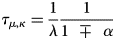
Equation (3) is a compact representation of two coupled equations for $\dot{{\cal E}}$ and $\dot{{\cal I}}$. The substitutions $\mu = {\cal I} + {\cal E}$ and $\kappa = {\cal I}-{\cal E}$ decouples them. After rearrangements, we get equation (4), where $f_\mu$ and $f_\kappa$ are the sum and difference of the drive terms for $\dot{{\cal E}}$ and $\dot{{\cal I}}$. The pre-factors, $\lambda ( {1\mp \alpha } )$, are the system's inverse time constants:

(4)$$\eqalign{ \dot{\mu } = & -\lambda ( {1-\alpha } ) \mu + f_\mu ( {\vec{x}, \;{\rm {\cal N}}} ) \cr \dot{\kappa } = & -\lambda ( {1 + \alpha } ) \kappa + f_\kappa ( {\vec{x}, \;{\cal N}} ) } $$

$$\tau _{\mu , \kappa } = \displaystyle{1 \over \lambda }\displaystyle{1 \over {1\;\mp \;\alpha }}$$

The solutions to Equation (4) describe exponential motion or flow of a nation's r in the coordinate system of the real economy, ${\cal R} = ( {{\cal E}, \;{\cal I}} )$.Footnote ¹⁵ In ${\cal R}$, $\mu = {\cal I} + {\cal E}$ points northeast and $\kappa = {\rm {\cal I}}-{\rm {\cal E}}$ is its perpendicular. For any and all initial conditions, a state progresses toward a stable fixed point r ₀ if 0 < α < 1. If α ≥ 1, the state exhibits exponentially unbounded growth in the positive or negative μ-direction. A world described by α > 1 would have no states occupying the middle and is not the world as we know it. Therefore 0 < α < 1. An example of each is illustrated in Figure 2.

Figure 2.

Flow in ${\cal R}$ as described by r-theory. The fixed point at the center is stable if α = 0.5 and unstable if α = 1.5.

r-Theory predicts, not that a state does not move in ${\cal R}$, but rather that it returns to its fixed point r₀ in ${\cal R}$ after the vicissitudes of history cause it to move away from that fixed point. As the vicissitudes of history are never ending, our dynamical system may be near and trending toward equilibrium, though not necessarily in equilibrium. This is a property of many dynamical systems, for instance a pendulum with friction which returns to equilibrium following displacement by never ending transient forces, e.g. gusts of air, vibrations of its pivot, and so forth.

The locus of the fixed point, which is state-specific and carries an implied superscript k, is obtained from equation (4) by setting the left-hand sides to zero, and is given in equation (5):

(5)$$r_0 = ( {\mu_0, \ \kappa_0} ) = \left({\displaystyle{{\,f_\mu ( {\vec{x},\ {\rm {\cal N}}} ) } \over {\lambda ( {1-\alpha } ) }}, \;\displaystyle{{\,f_\kappa ( {\vec{x},\ {\rm {\cal N}}} ) } \over {\lambda ( {1 + \alpha } ) }}} \right)$$

The vector arguments of the forcing functions $f_\mu$ and $f_\kappa$ are the non-coevolving sources of economic and institutional growth.Footnote ¹⁶ Supposing that these functions are linear in the vector components, a supposition that may be lifted if shown to be false, then μ ₀ is a linear combination of the vector components, or in our preferred phrasing, a superposition of sources. A comparable reading applies to κ ₀.

We will now use $\tau _\mu$ to estimate α. Suppose that the annual cost of developing and supporting productive infrastructure is equal to tax revenue. Over the past 20 years, OECD tax revenues have averaged about 1/3 of national income, from which we infer λ = 0.33. On the other hand, Generally Accepted Accounting Principles tell us to depreciate buildings – which we equate with infrastructure in general – over 33 years, implying λ = 0.03 per year. Let their geometric mean serve as our estimate, or λ = ~0.10 per year. Public or private investments in the real economy, r, are intentional, not accidental. If they are to be fruitful within the tenure of a politician or a private investor, then the longer of the two relaxation times, $\tau _\mu$, must be less than a generation, roughly 15 years. Solving for α according to the definition of $\tau _\mu$, we get α ≤ 0.36.Footnote ¹⁷

The coupling and damping are universals, constants for all states, whereas the values of the environmental variables and the norms are state-specific. Being that those state-specific terms are materially constant over centuries, equation (5) predicts that distribution of r ₀ for all states k will, once achieved, persist for centuries. Furthermore, the short time scales implied by λ tell us that the global economy is not merely on approach to equilibrium, but is in fact very close to equilibrium. This is consistent with ${\cal P}( t )$ as described in section 2, and it contradicts NIE orthodoxy as summarized by Acemoglu and Robinson: ‘Although cultural and geographical factors may also matter for economic performance, differences in economic institutions are the major source of cross-country differences in economic growth and prosperity’ (Reference Acemoglu, Robinson, Wittman and Weingast2008: 2). The contradiction is not surprising given that NIE orthodoxy does not account for the boundary condition imposed by ${\cal P}( t )$.

To the extent that HDI approximates μ, the centuries-long persistence of its global distribution is predicted (or explained) by r-theory subject to 0 < α < 1. Per our reading of equation (5), μ is a superposition of the sources, that is, the components of $\vec{x}$ and${\rm \;{\cal N}}$. To the extent that these sources are geospatially correlated – meaning that the state-specific values of the sources at two states k and k′ are more likely to be similar if k and k′ are geographically near – the superposition of those sources will be geospatially correlated. Climate is an exemplar of geospatial correlation, and thus r-theory tells us μ must exhibit large geospatial correlations. The geospatial correlations of wealth are large, readily observed, and have been the subject of a millennia-long conversation initiated by Aristotle and joined by such luminaries as Ibn Khaldun, Montesquieu, and others, though they have never been satisfactorily explained. Recently, Dell et al. observe that hot countries tend to be poor, except for those which are rich in oil, and cold countries tend to be rich, except for those which are rich in Communism (Reference Dell, Jones and Olken2012: 70). We observe further that countries at high elevation tend to be poorer than their lower elevation neighbors.

A different but equivalent way of visualizing this two-dimensional r-theory is with a flowchart. In Figure 3, information flows from sources $\vec{x}$ and${\rm \;{\cal N}}$ to the dynamically coupled $\dot{{\cal I}}$ and $\dot{{\cal E}}$. These come to equilibrium, meaning $\dot{{\cal E}} = 0$ and $\dot{{\cal I}} = 0$, on a time scale governed by 1/λ and the coupling constant α. Being that there are no information flows into $\vec{x}$ or into ${\cal N}$, this flowchart is a causal diagram per causal inference theory (Pearl and Mackenzie, Reference Pearl and Mackenzie2018).

Figure 3.

Environmental variables $\vec{x}$ and the norms ${\cal N}$ drive the system. They are sources of infrastructural and economic growth. Clockwise from the right in the loop, ${\cal I}$ couples to $\dot{{\cal E}}$. Then, $\dot{{\cal E}}$ leads to more ${\cal E}$, but ${\cal E}$ damps $\dot{{\cal E}}$ by way of $\lambda _{\cal E}$ and hence the counterclockwise arrow. Coevolution moves around and around until such time as $\dot{{\cal E}} = \dot{{\cal I}} = 0$ and equilibrium is achieved at $r_0 = ( {\cal E}_0, \;{\cal I}_0)$ as determined by the sources, the coupling, and the damping. Were it not for positive damping and suitable coupling, the system would be unstable and the streamlines (shown within the loop) would veer off to infinity along the main diagonal.

Neither ${\cal I}$ nor ${\cal E}$ is the cause of the other. ${\cal I}$-type institutions, those institutions that look like infrastructure and seem to map onto the NIE's formal constraints, are not the rules of the game. Together they are caused by, and they achieve an equilibrium whose level is set by the sources $\vec{x}$ and ${\cal N}$. By virtue of their slow rate of change, these sources are, effectively, state variables, or the rules of the game.Footnote ¹⁸ This is a restatement of r-theory's resolution of the paradox of informal constraints.

Returning to HDI as a first approximation of μ, its persistence tells us that the global distribution of wealth (for all states k) is and has been close to equilibrium for a very long time. Consequently, a contemporary measurement of r (for a particular state k) can be expected to be close to its equilibrium value, a fact we will make use of later when we model μ.

Using equation (5), the specification of the locus of r ₀ for a single state, let us contemplate the ratio of variances of the distribution of r ₀ for all states. It is the product of two terms, as below:

$$\displaystyle{{\sigma _\mu ^2 } \over {\sigma _\kappa ^2 }} = \displaystyle{{{( {1 + \alpha } ) }^2} \over {{( {1-\alpha } ) }^2}} \times \displaystyle{{\sigma _{\,f_\mu }^2 } \over {\sigma _{\,f_\kappa }^2 }}$$

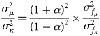
The first term is a constant. At the coupling's upper bound, α = 0.36, and the constant takes on its maximum value, 4.5. The second term depends on the forcing functions of $\dot{\mu }$ and $\dot{\kappa }$, and is greater than 1 so long as the forcing functions of $\dot{{\cal I}}$ and $\dot{{\cal E}}$ are positively correlated. If that is the case, as seems likely, then $\sigma _\mu ^2 /\sigma _\kappa ^2 > 4.5$, and r-theory forecasts that the distribution will lie principally in the μ-direction, or the northeast-pointing diagonal in ${\cal R} = ( {{\cal E}, \;{\cal I}} ).$ As such, r-theory predicts that ${\cal E}$ and ${\cal I}$ are highly correlated. Is that forecast borne out?

Indeed it is, as shown in Figure 4, where we plot the log of income against a measure of health care and education infrastructure taken from the UN, both in standardized or z-scored units. The long-observed correlation between institutions and economic performance is the foundation of the argument that institutions are the rules of the game, but r-theory tells us that the correlation arises from the workings of a dynamical system in near equilibrium, not by causation running from institutions to the economy. The standard causal interpretation of that correlation – as in Hall and Jones (Reference Hall and Jones1999), Acemoglu et al. (2002), and Rodrik et al. (Reference Rodrik, Subramanian and Trebbi2004) – is erroneous. The observed ratio of variances is 13.0, substantially greater than our estimate of 4.5. This is consistent with our estimate of α ≤ 0.36 and with a large positive of correlation of the forcing functions for $\dot{{\cal I}}$ and $\dot{{\cal E}}$.

Figure 4.

Distribution of $r^k = ( {{\cal E}^k, \;{\cal I}^k} )$ for 189 states indexed by k, where the state-specific ${\cal I}$ is constructed from UN-provided measures of health care and educational infrastructure, and ${\cal E}$ = log GNI. $\mu ^k = {\cal E}^k + {\cal I}^k$, the projection of r ^k along the μ-diagonal, is, apart from being cast in different units, practically indistinguishable from HDI.

The simple fact that $\sigma _\mu ^2 \gg \sigma _\kappa ^2$ tells us that the principal measure of a nation's real economy r is neither ${\cal I}$ nor ${\cal E}$, but μ, their sum. In turn, North's central challenge of modeling the economic performance of nations is mistargeted. The better target is economic performance plus its accompanying productive infrastructure. The equilibrium value, μ₀, is made larger by low damping and strong coupling both of which are constants, by state-specific good fortune in the form of favorable climate, geography, and natural resources, and by social norms that permit the exploitation of the aforesaid.Footnote ¹⁹ Norms that close a society off from external innovation, or that fail to reward internal innovation, are more likely than not to be present in low μ societies. This observation conjures up Granovetter's theorizing about the importance of strong weak ties (Reference Granovetter1973).

Before we move on to the objective of economic history, that is, to modeling ${\cal M}$, the distribution of wellbeing μ, we must move beyond our first approximation of μ, HDI. The infrastructure in Figure 4 is the first principal component of life expectancy at birth and two measures of education, all provided by the UN. These are necessary but insufficient, as we expect transportation, judicial, and other governance infrastructure will coevolve with ${\cal E}$, too. To the initial pool of three measures, we add the 6 Worldwide Governance Indicators from the World Bank (2018). These are Voice and Accountability; Political Stability and Lack of Violence; Government Effectiveness; Regulatory Quality; Rule of Law; and Control of Corruption. The first principal component of the combined set of nine gives us a new estimate of ${\cal I}$ whose correlation with the previously estimated one is 0.89.Footnote ²⁰ Combining this with ${\cal E}$, we get a refined estimate of μ, one in the spirit of Amartya Sen's Development as Freedom (Reference Sen1999). Its correlation with HDI is 0.93. Also, the ratio of variances in the μ- and κ-directions is 10.0, still consistent with α ≤ 0.36. Figure 5 is the distribution ${\cal M}$, with dark regions being low μ and light regions high. Geospatial correlations are self-evident. N.B., in the z-scored units of Figure 4, ${\cal E}$ and ${\cal I}$ range, roughly, from -2 to +2. The range of μ, their sum, is roughly -4 to 4.

Figure 5.

${\cal M}$, the global distribution of μ. Dark regions are low μ and light regions are high.

Let us summarize. Institutions are humanly devised sources of economic growth. Some coevolve with the economy, for instance the physical infrastructure of governance, commerce, education, and health; and others do not, for instance social norms. A dynamical systems formulation predicts an equilibrium or persistent solution in which state-specific norms, climate, geography, and other environmental factors determine state outcomes. This explains the observed persistence of the distribution of HDI while resolving the paradox of informal constraints. Furthermore, it explains the observed correlation of economic performance and institutions in terms of coevolutionary dynamics rather than causation. Subject to state-specific factors, two universal model parameters, λ and α, define the equilibrium. The first describes the decay rate of infrastructure, λ ≅ 0.1 per year, and the second describes the symmetric coupling of institutions into economic growth and the economy into institutional growth. Together, α and λ set the time scale, $\tau _\mu$, for the return on (or coupling of) infrastructure investments into the real economy. Rational actors will invest their own or other people's money in infrastructure that couples strongly to economic growth, so α can be expected to be large. But as α → 1, $\tau _\mu \to \infty$, per equation (4). Therefore, we can expect rational actors to invest in that infrastructure whose return is seen, not infinitely far off in the future, but in their tenure, implying an upper bound of α ≅ 0.36, which is consistent with real-world observations.

5. A naïve model of the wealth of nations

As explained above, r-theory tells us that though ${\cal E}$ is the preferred measure of economists, $\mu = {\cal I} + {\cal E}$ is the proper scalar measure of a nation's development,Footnote ²¹ and also that the time constants for coevolutionary equilibration are a few decades or less. Consequently, states can be expected to be close to their equilibrium values, or r ≈ r ₀ where r ₀ is given by equation (5). Therefore, an explanation of the distribution of the wealth of nations lies in the expression for μ ₀ in that same equation, which we now proceed to approximate using a model selection protocol described below. Because the components of $\vec{x}$ and ${\cal N}$ must be, for the most part, persistent, and the fast-changing terms of microeconomics are not persistent, the results of this modeling effort clarify the limits to the reconciliation of micro and macroeconomics.

A model, as we use the term, is a linear function of independent variables drawn from a list of candidate x _i and ${\cal N}_i$. The choice of variables is controversial, but evident geospatial correlations in ${\cal M}$ suggest at least these four: climate, geography, Communism, and oil. As proxies for climate we use insolation (Rose, Reference Rose2020), mean monthly high temperature,Footnote ²² aridity and potential evapo-transpiration (PET),Footnote ²³ and the absolute value of latitude.Footnote ²⁴ For geography, we use mean elevation and a measure of ruggedness (Nunn and Puga, Reference Nunn and Puga2012). For Communism and oil, we use, respectively, the duration of Communist rule and the logarithm of per capita natural resource revenue (NRR)in excess of extraction costs (World Bank, 2011).

Choosing one or none of the climate variables, one or none of the geographic variables, and one, none or both of the Communism and natural resources variables, there are 72 different models. Model selection ranks them on the basis of an objective criterion. The Bayes Information Criterion (BIC) assesses the extent to which the data, usually called the evidence, favors the model, usually referred to as a scientific theory. Included in that assessment is a penalty for model complexity as measured by the number of model parameters. It is well suited to and widely used in model selection (Kass and Raftery, Reference Kass and Raftery1995; Raftery, Reference Raftery1995). The optimal model is that one whose BIC is lower than all others. BIC differences of more than 10 are dispositive, but differences of less than 6 are moot.Footnote ²⁵ Whether the optimal model is good or useful is a topic for discussion after its identification.

Model selection is no better than its independent variables, and is no less vulnerable to omitted variable bias (OVB) than any modeling endeavor. Geospatially correlated residuals indicate a missing variable with geopspatial significance. In our case, the dependent variable, μ, has strong geospatial correlations.Footnote ²⁶ We introduce here a new method to assess OVB by exploiting those correlations in the residuals, δ.

Let I′ be the log of a geospatially weighted covariance of residuals, $\mathop \sum \delta _i\delta _jw_{ij}$, wherein the w _ij are 1 if states i and j share a border and 0 otherwise. I′ attains its maximum value for the null model, in which case δ = μ. Adding model complexity serves to reduce δ. If the model is very good, and δ is very small, then I′ may become so small as to be indistinguishable from what one would expect from randomness. Normalizing I′ such that its maximum value is 0, and drawing on an analysis (not shown) of randomized datasets, we state that a model has greater than 50% probability of being free of OVB only if ${I}^{\prime} < \;{I}^{\prime}_{50} = {-}2.88$. If ${I}^{\prime} > {I}^{\prime}_{50}$, we say that the model is naïve.

A graphical summary of the model selection is provided in Figure 6. The cluster of gray points in the vicinity of I′ = 0 and BIC = 740 represent 1-, 2-, and 3-variable models having no climate variable. Their explained variance, R ², indicated by the labels, is small. The large difference in BIC between models with and without climate informs us of the essentiality of climate as an explanatory variable in economic history. Black points are those whose climate variable is PET. The four-sided polygon in the lower left is the BIC-minimum, a four-variable model, ${\cal M}_4$. Its 13-point separation (in BIC) from its closest competitor informs us of its clear superiority to all others.

Figure 6.

Model selection: a graphical summary of the model selection process described in the text. Each point represents one of the 72 models and is labeled by its corresponding explained variance, R ². Those clustered in the upper right hand corner lack a climate variable. Black signifies that the climate variable is PET. Horizontal lines are labeled by their corresponding I′ confidence levels. The black four-sided polygon is the optimal model, ${\cal M}_4$, summarized in Table 1. I′ of ${\cal M}_4$ exceeds ${I}^{\prime}_{50}$ so it is a naïve model and is very likely to suffer from OVB.

The import of the four selected variables of ${\cal M}_4$ is summarized in Table 1, in which negative numbers are parenthesized. The first four columns are self-explanatory. The fifth column, labeled 'oomph' per McCloskey and Ziliak (Reference McCloskey and Ziliak1996), is the product of the parameter estimate and twice the standard deviation of the variable in the global dataset. It is informative of the aggregate impace of the variable. As noted earlier, μ ranges from -4 to 4. The oomph associated with PET, 3.54, is nearly half the total range, so climate matters quite a lot. Entries in the final column are the percentage change in GNI per unit change in the independent variable. We compute it as follows. μ is 95% correlated with ${\cal E} = {\rm log}\;GNI.$ To a high degree of approximation, then, we may write ${\rm \Delta }{\cal E} = 0.595{\rm \Delta }\mu$. For a +1 °C change in PET, the corresponding change in μ is −0.17. The change in log GNI is therefore −0.104, corresponding to a percentage change in GNI of −9.9% per ^°C. This is more or less in agreement with Dell et al. (Reference Dell, Jones and Olken2012) who estimate 8.2% for materially the same parameter. By this method of analysis, ${\cal M}_4$ tells us that the penalty for Communist rule is just less than 17% GNI per decade. Also, there is no resource curse in this linear model, but owing to the exponential dependence of GNI on μ, low μ states are predicted to make less of a given resource surfeit than high μ states.

Table 1.

${\cal M}_4$ summary

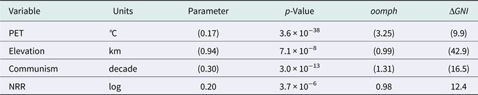
${\cal M}_4$'s explained variance, R ² = 0.65, is gratifyingly high for such a compact model. Though it is the best of all models drawn from this variable set, it remains a naïve model because ${I}^{\prime} > {I}^{\prime}_{50}$. It is imprudent, therefore, to draw firm conclusions about this model selection's choice of elevation over ruggedness, or PET over the other climate variables, or the magnitude of any coefficient in ${\cal M}_4$.Footnote ²⁷

As a final test, we ask how well ${\cal M}_4$ conforms to the boundary condition set by the observed persistence, ${\cal P}( {100} ) = 0.85$. We estimate ${\cal M}_4$ in 1920 by zeroing out the Communism and natural resource terms. Computing the corresponding autocorrelation function, we obtain ${\cal P}( {100} ) = 0.91$. This is a bit high, but ${\cal M}_4$ is naïve, and our estimate of ${\cal M}_4$ in 1920 does not take into account the substantial relative movement of East Asian countries within the distribution. We must, therefore, be cautious before reading too much into agreement or disagreement with expectations. Nevertheless, the combination of nearly immutable climate and geography are, by far, the dominant determinants of development. However, this is true only within the context of ${\cal M}_4$ whose imperfections are already noted. Whether or to what extent this generalizes to better models, it is premature to say.

${\cal M}_4$ is an application of r-theory. It is our long-term goal to use models to understand history, to explain not only the present and the recent past, but also a deeper historical past and even to inform policy. But a naïve model cannot be the basis for any such understanding. North and Williamson observe that norms matter, though paradoxically, norms matter more than the Nobelists could account for. Granovetter and Solow suggest that unaccounted for norms explain a large part of the discrepancy between rational choice and the choices people make. Yet, apart from Communism, ${\cal M}_4$ has no norms in it. The elucidation of relevant norms is the next step in this project, but as noted earlier, it is beyond the scope of this paper to give such important matters their due. Nevertheless, this naïve model bodes well for non-naïve models, in particular ones with norms in them, when we or others discover them.Footnote ²⁸

The paradox of informal constraints was recognized by Williamson and North as a threat to the dreamt-of program whereby price theory and its rules would explain the wealth of nations. r-Theory resolves the paradox and quantifies the real peril. Because R ² = 0.65 for the provably naive ${\cal M}_4$, and because nearly 92% of R ² originates in climate, geography, and oil,Footnote ²⁹ nearly 59% of the explained variance of the wealth of nations is not attributable to institutional rules as envisioned by Coase, North, Williamson, AJR, RST, Mokyr, Greif, and others, to name a few. This gap – between what the microeconomics of rules can tell us and the actual macroeconomics of the wealth of nations – is not something that has been or could have been predicted. Theory and observation generate this result. Both are required.

6. Summary

Institutional economics has advanced the idea that institutions matter and that their role in economic development is one of the rules that reduce uncertainty and lower transaction costs to the benefit of the economy. In the limit then, a microeconomic price theory rooted in institutions as rules is the principal determinant of macroeconomic and macrosocial outcomes. The boldest claims, for instance that institutions rule and that institutions are the rules of the game are sloganeering, not demonstration. In everyday experience, as well as in much social science, good institutions – that is those that make social life functional – are as much an output as they are an input.

Nor is this the only problem. The enterprise of the NIE at once acknowledges and yet fails to grapple with a paradox at its center. Articulated by North and seconded by Williamson, the paradox is the perplexing pervasiveness of the influence of informal constraints on long-term economic development. In addition, the enterprise has failed to answer the central challenges posed by North, those being the explanation of the disparities of the wealth of nations and of their persistence. Indeed, in the case of persistence, there has been little effort to even measure it. Furthermore, though they have claimed institutional change as the key ingredient that would explain economic history, a testable theory of institutional change is nowhere to be found. We assert that these matters are evidence of a discipline in crisis: of a discipline ensnared by the rules of its own game, what Kuhn calls a paradigm, and which in this instance is the paradigm of institutions as rules.

Abandoning institutions as rules in favor of institutions as sources of growth, and abandoning rules-based game theory in favor of dynamical systems theory, we construct a coevolutionary theory of institutional and economic change. Impossible to solve in its most general form, we simplify and approximate, paring down its complexity to an absolute minimum, arriving at a two-dimensional r-theory which is easily solved. Similar to the NIE, we consider two species of institutions, but rather than distinguish between types on the basis of their being formal or informal, we speciate on the basis of their coevolution with the economy. Those institutions that coevolve we call infrastructure, and those that don't we call norms. Though this taxonomy is less complex than Williamson's, the results generated here do not indicate that it is an oversimplification.

r-Theory's solutions tell us that ‘institutions are the rules of the game’ is a spurious correlation. When institutions coevolve with income, as they do, and as North said they would, then income and institutions are correlated, as they are. As such, income is not the proper measure of the real economy. Rather, that measure is income plus coevolving institutions, or what we call μ and we equate with wellbeing or development. The UN makes the same case, though it does so on moral grounds.

Does r-theory advance answers to North's central challenges? Yes. First, r-theory tells us that outcomes, μ, are determined by factors that are as persistent and as disparate as the global distribution of climate and cultural norms. Consequently, the distribution of outcomes must be persistent, and if they are disparate, then persistently disparate. Incidentally, because our norms map to North's and Williamson's informal constraints, this resolves the paradox of informal constraints.

Second, r-theory gives us a framework for explaining the disparities in the wealth of nations. Here, we construct ${\cal M}_4$, an admittedly simplistic, quantifiably naive, four-variable, global model (N = 177, R ² = 0.65), and we show that it is consistent with the long-term persistence of the distribution of HDI. But ${\cal M}_4$ is not yet a worthy tool for analyzing economic history. Given that it eschews norms, whose pervasive influence on long-term development has been noted by North, Williamson, Solow, and Granovetter, it seems more than likely to us that identifying which norms matter is the key to moving beyond ${\cal M}_4$ to a non-naïve model that answers the central question of economic history, that is, why the haves have and the have-nots have not.

It remains at this point premature to venture fully what variables will comprise a better, more complex model of global macroeconomic and macrosocial performance. What can be said without hesitation following the presentation of r-theory and the simple dynamical systems equations which define its moving parts, is that there is no such thing in this world as being rich in money alone. The set of places on Earth where incomes are high but people die young, or which have state-of-the-art transport systems but terrible education, or where good governance and the rule of law stand alongside low trust and political repression, is the null set. These facets of the experience of wealth are no more separable than the faces of a cube. Nor is it an accident that we find them working hand in hand in the historical past and in the world today. The imperative of life is to live, and those factors just named are examples of humanly devised systems that facilitate our lives on Earth. Individually and collectively, we do what is necessary – whether that is learning from the past, borrowing from our neighbors, or inventing the future – to satisfy the imperative. r-Theory explains both the system and its mechanisms that yield long, prosperous, lives beneath an umbrella of good governance.