


1. Introduction
A fluid flow is an input–output system, where infinitesimally small entities, like fluid drops, enter and leave a credit buffer non-instantaneously, subject to randomly varying rates determined by some stochastic sense. These stochastic fluid models are commonly used to represent communication networks that handle a continuous data stream, which is instrumental in the analysis and development of scheduling and routing algorithms. Among fluid flow systems, Markov-modulated fluid queues have drawn a lot of attention in various contexts of system modeling, such as congestion control of high-speed data networks (Elwalid and Mitra [Reference Elwalid and Mitra12]), statistical multiplexers in ATM networks (Ren and Kobayashi [Reference Ren and Kobayashi26]), traffic shaper for an on-off sources (Adan and Resing [Reference Adan and Resing1]), Transmission Control Protocol ( transmission control protocol) modeling in communication systems (van Foreest et al. [Reference van Foreest, Mandjes and Scheinhardt33]), buffer storage in manufacturing systems (Aggarwal et al. [Reference Aggarwal, Gautam, Kumar and Greaves2]), peer to peer file sharing process (Kumar et al. [Reference Kumar, Liu and Ross18]), single-wave length optical buffer (Kankaya and Akar [Reference Kankaya and Akar15]), rechargeable batteries in smart mobile phones (Jones et al. [Reference Jones, Harrison, Harder and Field14]) and energy harvesting IoT system (Tunc and Akar [Reference Tunc and Akar32]). For a comprehensive review of results and the widespread applications on fluid queues, we refer the readers to the outstanding survey papers by Kulkarni [Reference Kulkarni and Dshalalow17] and Scheinhardt [Reference Scheinhardt27], the monographs by Schwartz [Reference Schwartz28] and Gautam [Reference Gautam13], and the references therein.
In the literature, fluid queues have been long analyzed analytically by exploring various techniques based on their applications to determine stationary performance indices, such as the distribution, moments of the fluid content, system throughput and busy period. For instance, Virtamo and Norros [Reference Virtamo and Norros36] analyzed a fluid flow model modulated by an  $M/M/1$ queue using a spectral-decomposition method. The busy period for the buffer content has been carried out in Boxma and Dumas [Reference Boxma and Dumas4], where the fluid commodity is fed by $N$ independent on/off sources. Parthasarathy et al. [Reference Parthasarathy, Vijayashree and Lenin24] have discussed the stationary buffer content distribution of the fluid flow system regulated by the $M/M/1$ queue, exploring a continued fraction technique. Li et al. [Reference Li, Liu and Shang20] have investigated a fluid flow content driven by the $M/G/1$ queue and derived the Laplace transform (LT) of the stationary distribution of the buffer content by making use of the supplementary variable technique. Mao et al. [Reference Mao, Wang and Tian22] have studied a fluid queueing system controlled by a non-Markovian queue with multiple exponential vacations, and evaluated the mean fluid content in the buffer. Xu et al. [Reference Xu, Geng, Liu and Guo40] have determined the distribution of fluid level in the buffer modulated by the $M/M/c$ queue with working vacation adopting the matrix analytic technique. Vijayashree and Anjuka [Reference Vijayashree and Anjuka34] have researched a fluid flow system controlled by the $M/M/1$ queue with working vacations and obtained the stationary distribution of the buffer occupancy along with the average fluid level. Subsequently, a study on the stationary analysis of a fluid occupancy in the buffer regulated by the $M/M/1$ queue subject to catastrophic failures and repairs is proposed by Vijayshree and Anjuka [Reference Vijayashree and Anjuka35] using the probability generating function technique. Later, the mean of the fluid content in the credit buffer and the probability of an empty buffer have been computed for a fluid level in a storage device fed by the $PH/M/1$ queue through the matrix geometric method in Xu and Wang [Reference Xu and Wang41]. In Ammar [Reference Ammar3], the stationary performance characteristics of the amount of fluid in the buffer under catastrophic failures in random environments have been studied. El-Baz et al. [Reference El-Baz, Tarabia and Darwiesh10] have considered a Markov fluid flow model modulated by the $M/M/1/N$ queue. For this system, the stationary distribution of the buffer occupancy in the storage facility, along with the various performance descriptors, is presented by exploring the spectral properties of the tridiagonal matrices. Nikhil et al. [Reference Nikhil., Telek and Deepak23] have analyzed an $M/M/1/N$ queueing system in which the server draws energy from a battery while serving customers. When the battery is depleted, the server takes a random length vacation. The authors modeled the battery’s energy level as a fluid in an infinite-capacity buffer and derived the steady-state vector density of the fluid level and the mean fluid level.
In the queueing literature, double-ended queues are widely studied and have diverse applications, including in computer science, perishable inventory and organ allocation systems. A double-ended queueing system can be viewed as the state of the bilateral birth–death processes with constant birth and death rates (one-dimensional random walk in continuous time) on the whole set of integers. Double-ended queues are often employed as stochastic systems for queueing models characterized by flows of two classes of agents, that is, customers and servers. When there is a customer and a server in the system, the match between the request and service occurs, and then they both leave the system immediately. Clearly, there cannot be a non-zero number of customers and servers simultaneously in the system (see Srivastava and Kashyap [Reference Srivastava and Kashyap30]).
Double-ended queues arise in many practical applications to real-life systems, such as passenger-taxi service systems, buyers and sellers in a common market, assembly systems, organ transplant systems and communication network systems, to name a few. For example, Kashyap [Reference Kashyap16] discussed the passenger-taxi queuing system as a double-ended queue with limited space. Under the assumptions that the arrival processes of taxis and passengers are Poisson processes, he has derived the analytic results for the steady-state distribution of the system state. Sharma and Nair [Reference Sharma and Nair29] used the matrix theory to analyze the transient behavior of a double-ended Markovian queue. Takahashi et al. [Reference Takahashi, Osawa and Fujisawa31] considered a double-ended queue consisting of two buffers with finite capacities where tokens arrive as distinct input flows and are stored in the buffers. For such a system, they have determined the throughput of the system and the loss probabilities of each type of token. Subsequently, Conolly et al. [Reference Conolly, Parthasarathy and Selvaraju7] studied the impact of impatience behavior primarily in the context of a double-ended queue under the assumption of Poisson arrivals, independent exponential distribution for service times and reneging mechanisms. Elalouf et al. [Reference Elalouf, Perlman and Yechiali11] have obtained the steady-state probabilities of a double-ended queueing system that incorporated two independent streams: a stream of randomly arriving patients needing transplantation, and a stream of randomly arriving kidneys. Diamant and Baron [Reference Diamant and Baron9] have analyzed a double-ended queue with priority and impatient customers and derived the exact expressions for the stationary queue length distribution and several key performance characteristics. Lee et al. [Reference Lee, Liu, Liu and Zhang19] have proposed a time-varying double-ended queueing model to study optimal control of the production system. Liu et al. [Reference Liu, Li, Chang and Zhang21] have examined three block-structured double-ended queues under two Poisson arrival processes, considering customer impatience. In such models, the system stability, the stationary queue length distribution and the average sojourn times have been investigated.
Consequently, previous studies reveal that extensive research has been conducted on fluid flow systems in which the modulating (foreground) process is either a classical queue with finite or infinite waiting capacity, a queue incorporating various vacation policies or a queue subject to catastrophic failures. In contrast, only a limited number of studies have addressed the analysis of fluid content in a credit buffer driven by a double-ended queue or a one-dimensional random walk in continuous time. In recent years, fluid flow processes driven by double-ended queues have attracted increasing attention due to their relevance and applications in modern communication networks and inventory management systems. For instance, Wu and He [Reference Wu and He37] analyzed a multi-layer Markov-modulated fluid flow (MMFF) process for a double-ended queue with finite discrete abandonment times. They developed computational techniques to evaluate key queueing metrics, such as age processes, abandonment probabilities, waiting times and queue lengths on both sides of the system. Subsequently, Wu et al. [Reference Wu, He and Ereuary38] have employed a multi-layer MMFF process to analyze a double-ended queueing model characterized by batch Markovian arrival processes and finite discrete abandonment times, in the context of a vaccine inventory system. They have derived the stationary distribution of the queue length and evaluated various system performance metrics. Of late, Xu et al. [Reference Xu, Su and Shen39] have analyzed a fluid model of a bilateral matching queue with time-varying arrivals to both the task and worker queue. They have characterized the fluid content in the credit buffer under general impatience-time distributions for tasks and work. However, in fluid flow processes driven by double-ended queues without catastrophic failure, algorithmic and computational methods, as well as fluid flow rate simulations, have been used to quantify the fluid level in the buffer.
In the present article, we analyze analytically, for the first time, a versatile stochastic fluid flow system governed by a double-ended queue (bilateral birth–death process) in continuous time, which is prone to catastrophic failures and non-negligible repair times. When a catastrophe occurs, all customers currently in the double-ended queue are removed from the system and lost. Such catastrophes may result from severe technological failures, such as power outages or network virus attacks, which cause system breakdowns and force all customers to abandon the service system (see Chao [Reference Chao5]). Specifically, the catastrophes may occur, no matter whether the regulated system is either in an active or an idle state. Investigating the performance of such a fluid flow system becomes particularly interesting and challenging in the context of a double-ended queue. These observations motivate us, in this article, to investigate a fluid flow system regulated by a double-ended queue subject to catastrophic failure and non-zero repair times. By employing an effective analytical technique, we derive explicit closed-form expressions for the stationary probability density function (PDF) and the corresponding cumulative distribution function (CDF) of the fluid content in the credit buffer under the stability condition in a direct and elegant manner. We subsequently obtain several vital performance indices that are both novel and distinct from those reported in the existing literature on fluid flow queuing models. Therefore, our analytic results will provide researchers with a deeper understanding of the fluid particle occupancy system under investigation. Additionally, the derivation of several key performance metrics for the present fluid flow system offers valuable engineering guidelines for designing networks. In the sequel, we use the terms double-ended queue and bilateral birth–death process interchangeably.
The proposed fluid flow process, governed by a double-ended queue subject to catastrophic failures and subsequent repairs, naturally arises in a production line–storage system in which a continuous commodity (fluid) accumulates in a storage buffer at constant rates determined by the operational status of the driving system. In particular, we consider a production line-storage system involving two distinct types of raw materials, denoted by A and B, arriving from two different sources and entering their respective infinite-capacity buffer queues. These materials must be matched to form a fluid-type commodity. Specifically, the two raw materials act as complementary inputs for a single fluid-type production process, which is subsequently transferred to a fluid credit buffer. Consequently, the raw materials A and B cannot coexist simultaneously in the double-ended (bilateral) queue.
Let  $N(t)$ be the net inventory position of two raw materials relative to each other in the bilateral queue when the system is in active (up) mode. Whenever a catastrophic event occurs, all raw materials in the bilateral queue are flushed out, and the system enters the failure state $F$ and undergoes repair. For $t \geq 0$, the state space of $N(t)$ is given by $S=\left\{F\right\} \cup \{\cdots,-3,-2,-1,0,1,2,3,\cdots\}$. Consequently, $N(t) \gt 0$ indicates a surplus of raw material A, $N(t) \lt 0$ indicates a surplus of raw material B and $N(t)=0$ corresponds to an empty or balanced bilateral queue. The fluid-type commodity $U(t)$ represents finished production accumulated in a storage buffer, which is produced when raw materials A and B are both available, matched instantaneously and transferred to a fluid credit buffer.
Accordingly, during the active period, the production line operates normally, and the finished product is continuously transferred to an infinite fluid credit buffer at a constant rate  $r \gt 0$. In contrast, during the repair period, the production line is halted due to a catastrophic failure, and the fluid commodity is depleted from the credit buffer at a constant rate $r_0 \lt 0$, as long as the buffer remains non-empty. Clearly, while the production line is under repair, neither raw material A nor B is consumed; all materials in the bilateral queue expire, resulting in $N(t)=0$. Nevertheless, the fluid-type commodity accumulated during the active mode remains in the credit buffer and is depleted at a constant rate $r_0$ while the system is under repair. The system discussed above can be effectively applied to analyze performance measures of composite production line/service systems with fluid-type commodities, such as 3D printing or chemical production systems.
The present article is structured as follows. Section 2 describes the mathematical model in detail and establishes the stability condition of the fluid occupancy in the buffer for the system under investigation. Section 3 determines the stationary partial CDFs of the fluid level in the buffer and the status of the server in the driven double-ended queue by employing the continued fraction technique. In Section 4, explicit closed-form analytic expressions for the PDF and the corresponding CDF of the fluid level in the credit buffer are presented in the stationary regime. Several interesting and essential performance characteristics of the fluid stored in the reservoir are discussed in Section 5. We have also provided graphical numerical results in Section 6 to illustrate the impact of various parameters on the system’s performance measures. Finally, in Section 7, we summarize and interpret the results.
2. Problem description and equilibrium condition
We consider a versatile fluid flow queueing model consisting of infinitely large buffer capacity driven by a system performing a bilateral birth–death process in continuous-time on the whole set of integers subject to catastrophic failures and repairs. Let  $\left\{N(t); t\geq0\right\}$ be the position of the driven bilateral birth–death process at time $t$. The bilateral birth–death system moves along the real axis such that $\lambda$ is the rate of movement to the right and $\mu$ is the rate of movement to the left. This bilateral birth–death process $\left\{N(t) ; t\geq0\right\}$ is also said to be a double-ended queueing system (see Conolly [Reference Conolly6]) with birth rate $\lambda$ and death rate $\mu$; in small interval of time $(t, t+\Delta t)$, $\Delta t \gt 0$, a birth occurs with probability $\lambda\Delta t+o(\Delta t)$; a death occurs with probability $\mu\Delta t+o(\Delta t)$. It is evident that in this small time interval $(t, t+\Delta t)$, neither a birth nor a death takes place with probability $1-(\lambda+\mu)\Delta{t}+o(\Delta{t})$.
Apart from birth and death processes on the whole set of integers, catastrophes occur in the system according to a Poisson process with rate  $\nu$, that is, the catastrophe occurs at the bilateral birth–death process in the small time interval $(t, t+\Delta{t})$ with probability $\nu\Delta{t}+o(\Delta{t})$. Whenever a catastrophe occurs in the system, the system goes into the failure state $F$, that is, the bilateral birth–death process is subject to catastrophic failure. The repair times of the failed system are independent and exponentially distributed random variables with mean $\eta^{-1}$. As soon as a repair of the system is completed, the bilateral birth–death process returns to state zero and begins to work again (“up” state).
Consequently,  $\left\{N(t); \; t\geq0\right\}$ can be identified as the state of the driven double-ended queue/bilateral birth–death process subject to catastrophic failures and followed by non-negligible repair times. Thus, we treat the driven system as a continuous-time with discrete-state space random process whose state space is $S=\left\{F\right\}\cup\mathbb{Z},\; \text{where}\; \mathbb{Z}= \left\{\ldots,-3,-2-1, 0, 1, 2, \ldots\right\}$. We denote by $I(t)$, the status of the driven queueing system at time $t$ described above, such that
 \begin{equation*}
I(t)=\left\{
\begin{array}{ll}
1, & \hbox{if the driven system is in up/active mode,} \\
0, & \hbox{if the driven system is under repair/failure mode.}
\end{array}
\right.
\end{equation*}
\begin{equation*}
I(t)=\left\{
\begin{array}{ll}
1, & \hbox{if the driven system is in up/active mode,} \\
0, & \hbox{if the driven system is under repair/failure mode.}
\end{array}
\right.
\end{equation*} Thus, the resulting system can be modeled as a two-dimensional process  $\left\{(I(t), N(t)): \; t\geq0\right\}$ which constitutes a continuous-time Markov chain (CTMC) with state space given by $E=\left\{(0,F) \right\}\cup \left\{(1,n); \; n = 0, \pm1, \pm2, \ldots \right\}$. The flow diagram describing the driven bilateral birth–death process with catastrophes and repairs is depicted in Figure 1.
Rate diagram of the driven system.

For this underlying driven bilateral birth–death process with parameters  $\lambda \gt 0, \mu \gt 0, \nu \gt 0$ and $\eta \gt 0$, let $\left\{\tilde{\pi}_{n}; n=0,\pm1, \pm 2,\ldots\right\}$ be the steady-state probability distributions that the system is in state $(1,n)$ when it is in working mode (“up”/active period) and $\tilde{Q}$ be the probability that the system is in state $(0,F)$ when it is in failure mode (repair period). These steady-state probability distributions are obtained from Di Crescenzo et al. [Reference Di Crescenzo, Giorno, Krishna Kumar and Nobile8] as
 \begin{equation}
\begin{split}
\tilde{Q} &= \displaystyle\frac{\nu}{\eta+\nu}, \\
\tilde{\pi}_{0} &= (1-\tilde{Q})\displaystyle\frac{\nu}{\sqrt{(\lambda+\mu+\nu)^2-4\lambda\mu}}, \\
\tilde{\pi}_{n} &= \left[\displaystyle\frac{(\lambda+\mu+\nu)-\sqrt{(\lambda+\mu+\nu)^2-4\lambda\mu}}{2\mu}\right]^{n}\tilde{\pi}_{0},\quad n=1,2,3,\ldots, \\
\tilde{\pi}_{-n} &= \left[\displaystyle\frac{(\lambda+\mu+\nu)-\sqrt{(\lambda+\mu+\nu)^2-4\lambda\mu}}{2\lambda}\right]^{n}\tilde{\pi}_{0}, \quad n=1,2,3,\ldots\; .
\end{split}
\end{equation}
\begin{equation}
\begin{split}
\tilde{Q} &= \displaystyle\frac{\nu}{\eta+\nu}, \\
\tilde{\pi}_{0} &= (1-\tilde{Q})\displaystyle\frac{\nu}{\sqrt{(\lambda+\mu+\nu)^2-4\lambda\mu}}, \\
\tilde{\pi}_{n} &= \left[\displaystyle\frac{(\lambda+\mu+\nu)-\sqrt{(\lambda+\mu+\nu)^2-4\lambda\mu}}{2\mu}\right]^{n}\tilde{\pi}_{0},\quad n=1,2,3,\ldots, \\
\tilde{\pi}_{-n} &= \left[\displaystyle\frac{(\lambda+\mu+\nu)-\sqrt{(\lambda+\mu+\nu)^2-4\lambda\mu}}{2\lambda}\right]^{n}\tilde{\pi}_{0}, \quad n=1,2,3,\ldots\; .
\end{split}
\end{equation} We will now investigate a fluid queuing system with an infinite credit buffer where the input and output rates of fluid drops are regulated by the bilateral birth–death process prone to catastrophic failures and non-negligible repair times. The fluid drops accumulate in the buffer and are processed on a first-come first-served basis: Fluid drop arriving at time  $t$ will be removed from the buffer only when all fluid drops that arrived before time $t$ have been removed. Let $\left\{U(t); t\geq0\right\}$ represent the amount of fluid drops residing in the credit buffer at time $t$, which is driven by the two-dimensional Markovian process $\left\{(I(t), N(t)); t\geq0\right\}$. During the active period, ( $I(t)=1$), of driven system, the fluid drops accumulate in the credit buffer at a constant input rate $r \gt 0$, whereas the fluid drops/contents deplete during the repair period, ( $I(t)=0$), of the system at a constant leaking rate $r_{0} \lt 0$ as long as the fluid content in the credit buffer is non-empty. Consequently, $\left\{U(t); t\geq0\right\}$ is a non-negative random process, and the evaluation of the fluid content $U(t)$ at time $t$ in the credit buffer can be described by the equation:
 \begin{equation}
\frac{dU(t)}{dt}=\left\{
\begin{array}{ll}
0, & for~U(t)=0, (I(t), N(t))=(0,F) \\
r_{0}, & for~U(t) \gt 0, (I(t), N(t))=(0,F) \\
r, & for~U(t) \gt 0, (I(t), N(t))=(1,n),n=0,\pm1, \pm2,\ldots\;.
\end{array}
\right.
\end{equation}
\begin{equation}
\frac{dU(t)}{dt}=\left\{
\begin{array}{ll}
0, & for~U(t)=0, (I(t), N(t))=(0,F) \\
r_{0}, & for~U(t) \gt 0, (I(t), N(t))=(0,F) \\
r, & for~U(t) \gt 0, (I(t), N(t))=(1,n),n=0,\pm1, \pm2,\ldots\;.
\end{array}
\right.
\end{equation} It is not hard to see that the three-dimensional process  $\left\{\left(U(t), I(t), N(t)\right); t\geq0\right\}$ is an irreducible and positive recurrent continuous time Markov process, and hence it possesses a unique stationary distribution under the appropriate stability condition.
As the fluid contents in the credit buffer vary dynamically, the net effective rate of the fluid must remain negative to ensure the stability of the process in the long run. To this end, using (2.1), the mean drift of the fluid contents in the credit buffer can be calculated as
 \begin{equation*}
d=r_{0}\;\tilde{Q}+r\displaystyle\sum_{k=-\infty}^{\infty}\tilde{\pi}_{k}=\frac{r_{0}\; \nu+r \eta}{\eta+\nu}.
\end{equation*}
\begin{equation*}
d=r_{0}\;\tilde{Q}+r\displaystyle\sum_{k=-\infty}^{\infty}\tilde{\pi}_{k}=\frac{r_{0}\; \nu+r \eta}{\eta+\nu}.
\end{equation*}Hence, the fluid flow queueing system is stable if and only if
 \begin{equation}
\nu \gt 0,\quad\eta \gt 0\quad\text{and}\quad d=\displaystyle\frac{r_{0}\;\nu+r\eta}{\eta+\nu} \lt 0
\end{equation}
\begin{equation}
\nu \gt 0,\quad\eta \gt 0\quad\text{and}\quad d=\displaystyle\frac{r_{0}\;\nu+r\eta}{\eta+\nu} \lt 0
\end{equation} (see Kulkarni [Reference Kulkarni and Dshalalow17]). Henceforth, we shall assume throughout this article that the system is stable, so that the limiting distribution of the trivariate process  $\left\{(U(t), I(t), N(t)); t\geq0\right\}$ exists.
3. Partial cumulative probability distribution functions of fluid content
In this section, we focus our attention on determining the stationary partial probability distribution of the fluid contents in the credit buffer under the stability condition (2.3).
In what follows, we now define the partial CDFs of fluid contents at time  $t$ as
 \begin{eqnarray*}
Q(u,t) &=& P\left\{U(t)\leq u, I(t)=0, N(t)=F\right\},\quad t\geq0,\; u\geq0, \\
F_{n}(u,t) &=& P\left\{U(t)\leq u, I(t)=1, N(t)=n \right\}, \quad t\geq0,\; u\geq0,\; n=0,\pm1, \pm2,\ldots\; .
\end{eqnarray*}
\begin{eqnarray*}
Q(u,t) &=& P\left\{U(t)\leq u, I(t)=0, N(t)=F\right\},\quad t\geq0,\; u\geq0, \\
F_{n}(u,t) &=& P\left\{U(t)\leq u, I(t)=1, N(t)=n \right\}, \quad t\geq0,\; u\geq0,\; n=0,\pm1, \pm2,\ldots\; .
\end{eqnarray*} By simple probability arguments, it is not hard to show that the sequence  $\left\{Q(u,t), F_{n}(u,t), n\in\mathbb{Z}\right\}$ satisfies the following Kolmogorov forward equations:
 \begin{equation}
r_{0}\;\frac{\partial Q(u,t)}{\partial u}+\frac{\partial Q(u,t)}{\partial t} = -\eta\; Q(u,t)+\nu\displaystyle\sum_{n=-\infty}^{\infty}F_{n}(u,t),
\end{equation}
\begin{equation}
r_{0}\;\frac{\partial Q(u,t)}{\partial u}+\frac{\partial Q(u,t)}{\partial t} = -\eta\; Q(u,t)+\nu\displaystyle\sum_{n=-\infty}^{\infty}F_{n}(u,t),
\end{equation} \begin{equation}
r\frac{\partial F_{0}(u,t)}{\partial u}+\frac{\partial F_{0}(u,t)}{\partial t} =-(\nu+\lambda+\mu)F_{0}(u,t)+\mu\; F_{1}(u,t)+\lambda\; F_{-1}(u,t)+\eta\; Q(u,t),
\end{equation}
\begin{equation}
r\frac{\partial F_{0}(u,t)}{\partial u}+\frac{\partial F_{0}(u,t)}{\partial t} =-(\nu+\lambda+\mu)F_{0}(u,t)+\mu\; F_{1}(u,t)+\lambda\; F_{-1}(u,t)+\eta\; Q(u,t),
\end{equation} \begin{equation}
r\frac{\partial F_{n}(u,t)}{\partial u}+\frac{\partial F_{n}(u,t)}{\partial t} = -(\nu+\lambda+\mu)F_{n}(u,t)+\lambda\; F_{n-1}(u,t)+\mu\; F_{n+1}(u,t),\, n=1,2,3,\ldots,
\end{equation}
\begin{equation}
r\frac{\partial F_{n}(u,t)}{\partial u}+\frac{\partial F_{n}(u,t)}{\partial t} = -(\nu+\lambda+\mu)F_{n}(u,t)+\lambda\; F_{n-1}(u,t)+\mu\; F_{n+1}(u,t),\, n=1,2,3,\ldots,
\end{equation} \begin{equation}
r\frac{\partial F_{-n}(u,t)}{\partial u}+\frac{\partial F_{-n}(u,t)}{\partial t} = -(\nu+\lambda+\mu)F_{-n}(u,t)+\lambda\;F_{-n-1}(u,t)+\mu\; F_{-n+1}(u,t),\, n=1,2,3,\ldots\;.
\end{equation}
\begin{equation}
r\frac{\partial F_{-n}(u,t)}{\partial u}+\frac{\partial F_{-n}(u,t)}{\partial t} = -(\nu+\lambda+\mu)F_{-n}(u,t)+\lambda\;F_{-n-1}(u,t)+\mu\; F_{-n+1}(u,t),\, n=1,2,3,\ldots\;.
\end{equation} Under the equilibrium condition (2.3), the Markov process  $\left\{(U(t), I(t), N(t));t\geq0\right\}$ is stable and its stationary joint distribution is denoted by $P(U,I,N)=\displaystyle{\lim_{t\rightarrow\infty}} P(U(t), I(t), N(t))$, where $U$ represents the stationary fluid contents in the buffer.
Thus, the corresponding limiting partial cumulative distributions are denoted by
 \begin{equation*}
Q{(u)}=\displaystyle{\lim_{t\rightarrow\infty}Q(u,t)}=P(U\leq u, I=F, N=0)
\end{equation*}
\begin{equation*}
Q{(u)}=\displaystyle{\lim_{t\rightarrow\infty}Q(u,t)}=P(U\leq u, I=F, N=0)
\end{equation*}and
 \begin{equation*}
F_{n}(u)=\displaystyle\lim_{t\rightarrow\infty}F_{n}(u,t)=P(U\leq u, I=1, N=n),\quad n=0,\pm1, \pm2,\ldots,
\end{equation*}
\begin{equation*}
F_{n}(u)=\displaystyle\lim_{t\rightarrow\infty}F_{n}(u,t)=P(U\leq u, I=1, N=n),\quad n=0,\pm1, \pm2,\ldots,
\end{equation*}which are independent of the initial state of the system. Now, taking the limit as  $t\rightarrow\infty$, Eqs. (3.1)–(3.4) are reduced to a system of ordinary differential equations given as
 \begin{equation}
r_{0}\frac{dQ(u)}{du} =-\eta\; Q(u)+\nu\sum_{n=-\infty}^{\infty}F_{n}(u),\quad\quad\quad\quad\quad\quad\quad\qquad\qquad\qquad\quad\,\,\,\,\,\,\,\,\,\,
\end{equation}
\begin{equation}
r_{0}\frac{dQ(u)}{du} =-\eta\; Q(u)+\nu\sum_{n=-\infty}^{\infty}F_{n}(u),\quad\quad\quad\quad\quad\quad\quad\qquad\qquad\qquad\quad\,\,\,\,\,\,\,\,\,\,
\end{equation} \begin{equation}
r\frac{dF_{0}(u)}{du} = -(\nu+\lambda+\mu)\;F_{0}(u)+\mu\; F_{1}(u)+\lambda\; F_{-1}(u)+\eta\; Q(u),\qquad\qquad\,\,\,\,
\end{equation}
\begin{equation}
r\frac{dF_{0}(u)}{du} = -(\nu+\lambda+\mu)\;F_{0}(u)+\mu\; F_{1}(u)+\lambda\; F_{-1}(u)+\eta\; Q(u),\qquad\qquad\,\,\,\,
\end{equation} \begin{equation}
r\frac{dF_{n}(u)}{du} = -(\nu+\lambda+\mu)\;F_{n}(u)+\lambda\; F_{n-1}(u)+\mu\; F_{n+1}(u),\, n=1,2,3,\ldots,\,\,\,\,\,\,
\end{equation}
\begin{equation}
r\frac{dF_{n}(u)}{du} = -(\nu+\lambda+\mu)\;F_{n}(u)+\lambda\; F_{n-1}(u)+\mu\; F_{n+1}(u),\, n=1,2,3,\ldots,\,\,\,\,\,\,
\end{equation} \begin{equation}
r\frac{dF_{-n}(u)}{du} = -(\nu+\lambda+\mu)\;F_{-n}(u)+\lambda\; F_{-n-1}(u)+\mu\; F_{-n+1}(u),\, n=1,2,3,\ldots,
\end{equation}
\begin{equation}
r\frac{dF_{-n}(u)}{du} = -(\nu+\lambda+\mu)\;F_{-n}(u)+\lambda\; F_{-n-1}(u)+\mu\; F_{-n+1}(u),\, n=1,2,3,\ldots,
\end{equation}with the boundary conditions
 \begin{equation*}
F_{\pm n}(0)=0,\; n=1,2,3,\ldots,
\end{equation*}
\begin{equation*}
F_{\pm n}(0)=0,\; n=1,2,3,\ldots,
\end{equation*}and
 \begin{eqnarray}
Q(0)=a,\; \text{where ‘a’ is undetermined constant.}\end{eqnarray}
\begin{eqnarray}
Q(0)=a,\; \text{where ‘a’ is undetermined constant.}\end{eqnarray} The condition  $Q(0)=a$ means that with probability “ $a$”,
$a$”,  $0 \lt a \lt 1$, the buffer content of fluid drops is empty and the net input rate is zero, when the driven bilateral birth–death process/double-end queue is under repair.
In the sequel, let  $f^{\ast}(s)=\int_{0}^{\infty}e^{-su}f(u)\;du$ be the LT of the function $f(u)$. Applying the LTs to Eqs. (3.5)–(3.8), and rearranging the terms lead to
 \begin{equation}
Q^{\ast}(s)=\displaystyle\frac{a}{(s+\frac{\eta}{r_{0}})}+\frac{\frac{\nu}{r_{0}}}{(s+\frac{\eta}{r_{0}})}\left[F_{0}^{\ast}(s)+\sum_{n=1}^{\infty}F_{n}^{\ast}(s)+\sum_{n=1}^{\infty}F_{-n}^{\ast}(s)\right],
\end{equation}
\begin{equation}
Q^{\ast}(s)=\displaystyle\frac{a}{(s+\frac{\eta}{r_{0}})}+\frac{\frac{\nu}{r_{0}}}{(s+\frac{\eta}{r_{0}})}\left[F_{0}^{\ast}(s)+\sum_{n=1}^{\infty}F_{n}^{\ast}(s)+\sum_{n=1}^{\infty}F_{-n}^{\ast}(s)\right],
\end{equation} \begin{equation}
(sr+\nu+\lambda+\mu)F_{0}^{\ast}(s)=\mu\; F_{1}^{\ast}(s)+\lambda\; F_{-1}^{\ast}(s)+\eta\;Q^{\ast}(s),\qquad\qquad\,
\end{equation}
\begin{equation}
(sr+\nu+\lambda+\mu)F_{0}^{\ast}(s)=\mu\; F_{1}^{\ast}(s)+\lambda\; F_{-1}^{\ast}(s)+\eta\;Q^{\ast}(s),\qquad\qquad\,
\end{equation} \begin{equation}
(sr+\nu+\lambda+\mu)F_{n}^{\ast}(s)=\lambda\; F_{n-1}^{\ast}(s)+\mu\; F_{n+1}^{\ast}(s),\;\; n=1,2,3,\ldots,\,\,\,
\end{equation}
\begin{equation}
(sr+\nu+\lambda+\mu)F_{n}^{\ast}(s)=\lambda\; F_{n-1}^{\ast}(s)+\mu\; F_{n+1}^{\ast}(s),\;\; n=1,2,3,\ldots,\,\,\,
\end{equation} \begin{equation}
(sr+\nu+\lambda+\mu)F_{-n}^{\ast}(s)=\lambda\; F_{-n-1}^{\ast}(s)+\mu\; F_{-n+1}^{\ast}(s),\;\; n=1,2,3,\ldots,
\end{equation}
\begin{equation}
(sr+\nu+\lambda+\mu)F_{-n}^{\ast}(s)=\lambda\; F_{-n-1}^{\ast}(s)+\mu\; F_{-n+1}^{\ast}(s),\;\; n=1,2,3,\ldots,
\end{equation}where we have used the boundary conditions (3.9).
We can write (3.12) as the forward system of a recurrence relation
 \begin{equation}
\displaystyle\frac{F_{n}^{\ast}(s)}{F_{n-1}^{\ast}(s)}=\frac{\lambda}{[sr+\nu+\lambda+\mu]-\mu\;\displaystyle\frac{F_{n+1}^{\ast}(s)}{F_{n}^{\ast}(s)}},\;\; n=1,2,3,\ldots\;.
\end{equation}
\begin{equation}
\displaystyle\frac{F_{n}^{\ast}(s)}{F_{n-1}^{\ast}(s)}=\frac{\lambda}{[sr+\nu+\lambda+\mu]-\mu\;\displaystyle\frac{F_{n+1}^{\ast}(s)}{F_{n}^{\ast}(s)}},\;\; n=1,2,3,\ldots\;.
\end{equation}By iterative operation, the above produces the continued fraction
 \begin{equation}
\displaystyle\frac{F_{n}^{\ast}(s)}{F_{n-1}^{\ast}(s)}=\displaystyle\frac{\lambda}{[sr+\nu+\lambda+\mu]-\displaystyle\frac{\lambda\mu}{[sr+\nu+\lambda+\mu]-\displaystyle\frac{\lambda\mu}{[sr+\nu+\lambda+\mu]-\displaystyle\frac{\lambda\mu}{[sr+\nu+\lambda+\mu]-\cdots.}}}}
\end{equation}
\begin{equation}
\displaystyle\frac{F_{n}^{\ast}(s)}{F_{n-1}^{\ast}(s)}=\displaystyle\frac{\lambda}{[sr+\nu+\lambda+\mu]-\displaystyle\frac{\lambda\mu}{[sr+\nu+\lambda+\mu]-\displaystyle\frac{\lambda\mu}{[sr+\nu+\lambda+\mu]-\displaystyle\frac{\lambda\mu}{[sr+\nu+\lambda+\mu]-\cdots.}}}}
\end{equation}We write the above as
 \begin{equation}
\displaystyle\frac{F_{n}^{\ast}(s)}{F_{n-1}^{\ast}(s)}=\displaystyle\frac{\lambda}{[sr+\nu+\lambda+\mu]-\phi(s)}
\end{equation}
\begin{equation}
\displaystyle\frac{F_{n}^{\ast}(s)}{F_{n-1}^{\ast}(s)}=\displaystyle\frac{\lambda}{[sr+\nu+\lambda+\mu]-\phi(s)}
\end{equation}where
 \begin{equation*}
\phi(s)=\displaystyle\frac{\lambda\mu}{[sr+\nu+\lambda+\mu]-\displaystyle\frac{\lambda\mu}{[sr+\nu+\lambda+\mu]-\displaystyle\frac{\lambda\mu}{[sr+\nu+\lambda+\mu]-\displaystyle\frac{\lambda\mu}{[sr+\nu+\lambda+\mu]-\cdots}}}}
\end{equation*}
\begin{equation*}
\phi(s)=\displaystyle\frac{\lambda\mu}{[sr+\nu+\lambda+\mu]-\displaystyle\frac{\lambda\mu}{[sr+\nu+\lambda+\mu]-\displaystyle\frac{\lambda\mu}{[sr+\nu+\lambda+\mu]-\displaystyle\frac{\lambda\mu}{[sr+\nu+\lambda+\mu]-\cdots}}}}
\end{equation*}so that
 \begin{equation}
\phi(s)=\displaystyle\frac{\displaystyle\frac{\lambda\mu}{r}}{[s+\displaystyle\frac{\nu+\lambda+\mu}{r}]-\displaystyle\frac{\phi(s)}{r}}.
\end{equation}
\begin{equation}
\phi(s)=\displaystyle\frac{\displaystyle\frac{\lambda\mu}{r}}{[s+\displaystyle\frac{\nu+\lambda+\mu}{r}]-\displaystyle\frac{\phi(s)}{r}}.
\end{equation} Thus,  $\phi(s)$ satisfies the quadratic equation
 \begin{equation}
\displaystyle\frac{\phi^{2}(s)}{r}-\left[s+\displaystyle\frac{\nu+\lambda+\mu}{r}\right]\phi(s)+\displaystyle\frac{\lambda\mu}{r}=0.
\end{equation}
\begin{equation}
\displaystyle\frac{\phi^{2}(s)}{r}-\left[s+\displaystyle\frac{\nu+\lambda+\mu}{r}\right]\phi(s)+\displaystyle\frac{\lambda\mu}{r}=0.
\end{equation} For  $s \gt 0$, there exist two positive solutions to (3.18) which are obtained as
 \begin{equation}
\phi_{+}(s),\; \phi_{-}(s)=\displaystyle\frac{\left[s+\displaystyle\frac{\nu+\lambda+\mu}{r}\right]\pm\sqrt{\left[s+\displaystyle\frac{\nu+\lambda+\mu}{r}\right]^2-\displaystyle\frac{4\lambda\mu}{r^2}}}{\displaystyle\frac{2}{r}}.
\end{equation}
\begin{equation}
\phi_{+}(s),\; \phi_{-}(s)=\displaystyle\frac{\left[s+\displaystyle\frac{\nu+\lambda+\mu}{r}\right]\pm\sqrt{\left[s+\displaystyle\frac{\nu+\lambda+\mu}{r}\right]^2-\displaystyle\frac{4\lambda\mu}{r^2}}}{\displaystyle\frac{2}{r}}.
\end{equation} Note that  $\phi(+\infty)=0$ is a necessary condition for $\phi(s)$ to be the LT of the probability distribution function of a random variable (see Prabhu [Reference Prabhu25]). Clearly, only $\phi_{-}(s)$ fulfills the required conditions, and it is the minimal positive unique solution of (3.18). Accordingly, we adopt the minimal positive solution $\phi_-(s)$ of the continued fraction for subsequent analysis.
Substituting the expression for  $\phi_-(s)$ into $\phi(s)$ in (3.16), we get
 \begin{equation*}
\displaystyle\frac{F_{n}^{\ast}(s)}{F_{n-1}^{\ast}(s)}=\displaystyle\frac{\displaystyle\frac{\lambda}{r}}{\left[s+\displaystyle\frac{\nu+\lambda+\mu}{r}\right]-\left\{\displaystyle\frac{\left[s+\displaystyle\frac{\nu+\lambda+\mu}{r}\right]-\sqrt{\left[s+\displaystyle\frac{\nu+\lambda+\mu}{r}\right]^2-\displaystyle\frac{4\lambda\mu}{r^2}}}{2}\right\}},\, n=1,2,3,\ldots\;.
\end{equation*}
\begin{equation*}
\displaystyle\frac{F_{n}^{\ast}(s)}{F_{n-1}^{\ast}(s)}=\displaystyle\frac{\displaystyle\frac{\lambda}{r}}{\left[s+\displaystyle\frac{\nu+\lambda+\mu}{r}\right]-\left\{\displaystyle\frac{\left[s+\displaystyle\frac{\nu+\lambda+\mu}{r}\right]-\sqrt{\left[s+\displaystyle\frac{\nu+\lambda+\mu}{r}\right]^2-\displaystyle\frac{4\lambda\mu}{r^2}}}{2}\right\}},\, n=1,2,3,\ldots\;.
\end{equation*}whence
 \begin{equation}
F_{n}^{\ast}(s)=\left(\displaystyle\frac{\beta}{\alpha}\right)\left\{\left[s+\displaystyle\frac{\nu+\lambda+\mu}{r}\right]-\sqrt{\left[s+\displaystyle\frac{\nu+\lambda+\mu}{r}\right]^2-\alpha^2}\right\}F_{n-1}^{\ast}(s),\;\;n=1,2,3,\ldots,
\end{equation}
\begin{equation}
F_{n}^{\ast}(s)=\left(\displaystyle\frac{\beta}{\alpha}\right)\left\{\left[s+\displaystyle\frac{\nu+\lambda+\mu}{r}\right]-\sqrt{\left[s+\displaystyle\frac{\nu+\lambda+\mu}{r}\right]^2-\alpha^2}\right\}F_{n-1}^{\ast}(s),\;\;n=1,2,3,\ldots,
\end{equation}where  $\alpha=\displaystyle\frac{2\sqrt{\lambda\mu}}{r}$ and $\beta=\sqrt{\displaystyle\frac{\lambda}{\mu}}$.
Iterating (3.20), we have
 \begin{equation}
F_{n}^{\ast}(s)=\left(\displaystyle\frac{\beta}{\alpha}\right)^{n}\left[\left(s+\displaystyle\frac{\nu+\lambda+\mu}{r}\right)-\sqrt{\left(s+\displaystyle\frac{\nu+\lambda+\mu}{r}\right)^2-\alpha^2}\right]^{n}F_{0}^{\ast}(s),\;n=1,2,3,\ldots\;.
\end{equation}
\begin{equation}
F_{n}^{\ast}(s)=\left(\displaystyle\frac{\beta}{\alpha}\right)^{n}\left[\left(s+\displaystyle\frac{\nu+\lambda+\mu}{r}\right)-\sqrt{\left(s+\displaystyle\frac{\nu+\lambda+\mu}{r}\right)^2-\alpha^2}\right]^{n}F_{0}^{\ast}(s),\;n=1,2,3,\ldots\;.
\end{equation}Using a similar approach, we find from (3.13) that
 \begin{equation}
F_{-n}^{\ast}(s)=\displaystyle\frac{\left[\left(s+\displaystyle\frac{\nu+\lambda+\mu}{r}\right)-\sqrt{\left(s+\displaystyle\frac{\nu+\lambda+\mu}{r}\right)^2-\alpha^2}\right]^{n}}{(\alpha\beta)^{n}}\;F_{0}^{\ast}(s),\; \;n=1,2,3,\ldots\;.
\end{equation}
\begin{equation}
F_{-n}^{\ast}(s)=\displaystyle\frac{\left[\left(s+\displaystyle\frac{\nu+\lambda+\mu}{r}\right)-\sqrt{\left(s+\displaystyle\frac{\nu+\lambda+\mu}{r}\right)^2-\alpha^2}\right]^{n}}{(\alpha\beta)^{n}}\;F_{0}^{\ast}(s),\; \;n=1,2,3,\ldots\;.
\end{equation}Consequently, it is observed from (3.21) and (3.22) that
 \begin{equation}
\begin{aligned}
\displaystyle\sum_{n=1}^{\infty}F_{n}^{\ast}(s) &= \displaystyle\frac{\displaystyle\frac{\phi_{-}(s)}{\mu}}{\left[1-\displaystyle\frac{\phi_{-}(s)}{\mu}\right]}F_{0}^{\ast}(s), \quad\text{and}\quad & \displaystyle\sum_{n=1}^{\infty}F_{-n}^{\ast}(s) &=\displaystyle\frac{\displaystyle\frac{\phi_{-}(s)}{\lambda}}{\left[1-\displaystyle\frac{\phi_{-}(s)}{\lambda}\right]}F_{0}^{\ast}(s)
\end{aligned}
\end{equation}
\begin{equation}
\begin{aligned}
\displaystyle\sum_{n=1}^{\infty}F_{n}^{\ast}(s) &= \displaystyle\frac{\displaystyle\frac{\phi_{-}(s)}{\mu}}{\left[1-\displaystyle\frac{\phi_{-}(s)}{\mu}\right]}F_{0}^{\ast}(s), \quad\text{and}\quad & \displaystyle\sum_{n=1}^{\infty}F_{-n}^{\ast}(s) &=\displaystyle\frac{\displaystyle\frac{\phi_{-}(s)}{\lambda}}{\left[1-\displaystyle\frac{\phi_{-}(s)}{\lambda}\right]}F_{0}^{\ast}(s)
\end{aligned}
\end{equation}where  $\phi_-(s)$ is given in (3.19).
Next, by making use of (3.21) and (3.22) in (3.10), we obtain
 \begin{align}
Q^{\ast}(s)=\displaystyle\frac{a}{s+\displaystyle\frac{\eta}{r_{0}}}+\displaystyle\frac{\displaystyle\frac{\nu}{r_{0}}}{s+\displaystyle\frac{\eta}{r_0}}F_{0}^{\ast}(s) \left\{\displaystyle\frac{1}{1-\left(\displaystyle\frac{\beta}{\alpha}\right)\left[\left(s+\displaystyle\frac{\nu+\lambda+\mu}{r}\right)-\sqrt{\left(s+\displaystyle\frac{\nu+\lambda+\mu}{r}\right)^2-\alpha^2}\right]}\right\}\nonumber\\
+\displaystyle\frac{\displaystyle\frac{\nu}{r_{0}}}{s+\displaystyle\frac{\eta}{r_0}}F_{0}^{\ast}(s) \left\{\frac{\displaystyle\frac{1}{\alpha\beta}\left[\left(s+\displaystyle\frac{\nu+\lambda+\mu}{r}\right)-\sqrt{\left(s+\displaystyle\frac{\nu+\lambda+\mu}{r}\right)^2-\alpha^2}\right]}{1-\displaystyle\frac{\left(s+\displaystyle\frac{\nu+\lambda+\mu}{r}\right)-\sqrt{\left(s+\displaystyle\frac{\nu+\lambda+\mu}{r}\right)^2-\alpha^2}}{\alpha\beta}}\right\}.\end{align}
\begin{align}
Q^{\ast}(s)=\displaystyle\frac{a}{s+\displaystyle\frac{\eta}{r_{0}}}+\displaystyle\frac{\displaystyle\frac{\nu}{r_{0}}}{s+\displaystyle\frac{\eta}{r_0}}F_{0}^{\ast}(s) \left\{\displaystyle\frac{1}{1-\left(\displaystyle\frac{\beta}{\alpha}\right)\left[\left(s+\displaystyle\frac{\nu+\lambda+\mu}{r}\right)-\sqrt{\left(s+\displaystyle\frac{\nu+\lambda+\mu}{r}\right)^2-\alpha^2}\right]}\right\}\nonumber\\
+\displaystyle\frac{\displaystyle\frac{\nu}{r_{0}}}{s+\displaystyle\frac{\eta}{r_0}}F_{0}^{\ast}(s) \left\{\frac{\displaystyle\frac{1}{\alpha\beta}\left[\left(s+\displaystyle\frac{\nu+\lambda+\mu}{r}\right)-\sqrt{\left(s+\displaystyle\frac{\nu+\lambda+\mu}{r}\right)^2-\alpha^2}\right]}{1-\displaystyle\frac{\left(s+\displaystyle\frac{\nu+\lambda+\mu}{r}\right)-\sqrt{\left(s+\displaystyle\frac{\nu+\lambda+\mu}{r}\right)^2-\alpha^2}}{\alpha\beta}}\right\}.\end{align}The above can be succinctly written as
 \begin{equation}
Q^{\ast}(s)=\displaystyle\frac{a}{s+\displaystyle\frac{\eta}{r_{0}}}+\displaystyle\frac{\displaystyle\frac{\nu}{r_{0}}}{\left(s+\displaystyle\frac{\eta}{r_{0}}\right)}\frac{F_{0}^{\ast}(s)}{\left(1-\displaystyle\frac{\phi_{-}(s)}{\mu}\right)}+\frac{\displaystyle\frac{\nu}{r_{0}}}{\left(s+\displaystyle\frac{\eta}{r_{0}}\right)}\displaystyle\frac{\displaystyle\frac{\phi_{-}(s)}{\lambda}F_{0}^{\ast}(s)}{\left(1-\displaystyle\frac{\phi_{-}(s)}{\lambda}\right)},
\end{equation}
\begin{equation}
Q^{\ast}(s)=\displaystyle\frac{a}{s+\displaystyle\frac{\eta}{r_{0}}}+\displaystyle\frac{\displaystyle\frac{\nu}{r_{0}}}{\left(s+\displaystyle\frac{\eta}{r_{0}}\right)}\frac{F_{0}^{\ast}(s)}{\left(1-\displaystyle\frac{\phi_{-}(s)}{\mu}\right)}+\frac{\displaystyle\frac{\nu}{r_{0}}}{\left(s+\displaystyle\frac{\eta}{r_{0}}\right)}\displaystyle\frac{\displaystyle\frac{\phi_{-}(s)}{\lambda}F_{0}^{\ast}(s)}{\left(1-\displaystyle\frac{\phi_{-}(s)}{\lambda}\right)},
\end{equation}where (3.19) has been used in the above. Substitution of (3.21), (3.22) for  $n=1$ and (3.24) in (3.11) gives
 \begin{multline*}
F_{0}^{\ast}(s)\left\{\left[\sqrt{\left(s+\displaystyle\frac{\nu+\lambda+\mu}{r}\right)^2-\alpha^2}\right]\right.\\
\left.
-\displaystyle\frac{\displaystyle\frac{\eta\nu}{r_{0}\;r}}{\left(s+\displaystyle\frac{\eta}{r_{0}}\right)}\left\{\displaystyle\frac{\left(\displaystyle\frac{\beta}{\alpha}\right)\left[\left(s+\displaystyle\frac{\nu+\lambda+\mu}{r}\right)-\sqrt{\left(s+\displaystyle\frac{\nu+\lambda+\mu}{r}\right)^2-\alpha^2}\right]}{1-\left(\displaystyle\frac{\beta}{\alpha}\right)\left[\left(s+\displaystyle\frac{\nu+\lambda+\mu}{r}\right)-\sqrt{\left(s+\displaystyle\frac{\nu+\lambda+\mu}{r}\right)^2-\alpha^2}\right]}\right.\right.\\
\left.\left.+\displaystyle\left(1-\left[\displaystyle\frac{\left(s+\displaystyle\frac{\nu+\lambda+\mu}{r}\right)-\sqrt{\left(s+\displaystyle\frac{\nu+\lambda+\mu}{r}\right)^2-\alpha^2}}{\alpha\beta}\right]\right)^{-1}\right\}\right\}=\displaystyle\frac{\displaystyle\;a\;\frac{\eta}{r}}{s+\displaystyle\frac{\eta}{r_{0}}}.
\end{multline*}
\begin{multline*}
F_{0}^{\ast}(s)\left\{\left[\sqrt{\left(s+\displaystyle\frac{\nu+\lambda+\mu}{r}\right)^2-\alpha^2}\right]\right.\\
\left.
-\displaystyle\frac{\displaystyle\frac{\eta\nu}{r_{0}\;r}}{\left(s+\displaystyle\frac{\eta}{r_{0}}\right)}\left\{\displaystyle\frac{\left(\displaystyle\frac{\beta}{\alpha}\right)\left[\left(s+\displaystyle\frac{\nu+\lambda+\mu}{r}\right)-\sqrt{\left(s+\displaystyle\frac{\nu+\lambda+\mu}{r}\right)^2-\alpha^2}\right]}{1-\left(\displaystyle\frac{\beta}{\alpha}\right)\left[\left(s+\displaystyle\frac{\nu+\lambda+\mu}{r}\right)-\sqrt{\left(s+\displaystyle\frac{\nu+\lambda+\mu}{r}\right)^2-\alpha^2}\right]}\right.\right.\\
\left.\left.+\displaystyle\left(1-\left[\displaystyle\frac{\left(s+\displaystyle\frac{\nu+\lambda+\mu}{r}\right)-\sqrt{\left(s+\displaystyle\frac{\nu+\lambda+\mu}{r}\right)^2-\alpha^2}}{\alpha\beta}\right]\right)^{-1}\right\}\right\}=\displaystyle\frac{\displaystyle\;a\;\frac{\eta}{r}}{s+\displaystyle\frac{\eta}{r_{0}}}.
\end{multline*} Now, the above equation can be expressed in terms of  $\phi_{-}(s)$ as
 \begin{equation}
\left\{\left[\sqrt{\left(s+\displaystyle\frac{\nu+\lambda+\mu}{r}\right)^2-\alpha^2}\right]-\displaystyle\frac{\displaystyle\frac{\nu}{r}\frac{\eta}{r_{0}}}{\left(s+\displaystyle\frac{\eta}{r_{0}}\right)}
\left[\displaystyle\frac{\displaystyle\frac{1}{r}\left(\lambda\mu-\phi^2_{-}(s)\right)}{\displaystyle\frac{\phi_{-}^{2}(s)}{r}\;-\displaystyle\frac{(\lambda+\mu)}{r}\phi_{-}(r)+\displaystyle\frac{\lambda\mu}{r}}\right]\right\}F_{0}^{\ast}(s)
\end{equation}
\begin{equation}
\left\{\left[\sqrt{\left(s+\displaystyle\frac{\nu+\lambda+\mu}{r}\right)^2-\alpha^2}\right]-\displaystyle\frac{\displaystyle\frac{\nu}{r}\frac{\eta}{r_{0}}}{\left(s+\displaystyle\frac{\eta}{r_{0}}\right)}
\left[\displaystyle\frac{\displaystyle\frac{1}{r}\left(\lambda\mu-\phi^2_{-}(s)\right)}{\displaystyle\frac{\phi_{-}^{2}(s)}{r}\;-\displaystyle\frac{(\lambda+\mu)}{r}\phi_{-}(r)+\displaystyle\frac{\lambda\mu}{r}}\right]\right\}F_{0}^{\ast}(s)
\end{equation} \begin{equation*}
=\displaystyle\frac{a\;\displaystyle\frac{\eta}{r}}{\left(s+\displaystyle\frac{\eta}{r_{0}}\right)},
\end{equation*}
\begin{equation*}
=\displaystyle\frac{a\;\displaystyle\frac{\eta}{r}}{\left(s+\displaystyle\frac{\eta}{r_{0}}\right)},
\end{equation*}which results in
 \begin{equation}
F_{0}^{\ast}(s)\left\{\left[\sqrt{\left(s+\displaystyle\frac{\nu+\lambda+\mu}{r}\right)^2-\alpha^2}\right]-\displaystyle\frac{\displaystyle\frac{\nu}{r}\frac{\eta}{r_{0}}}{\left(s+\displaystyle\frac{\eta}{r_{0}}\right)}\right.
\end{equation}
\begin{equation}
F_{0}^{\ast}(s)\left\{\left[\sqrt{\left(s+\displaystyle\frac{\nu+\lambda+\mu}{r}\right)^2-\alpha^2}\right]-\displaystyle\frac{\displaystyle\frac{\nu}{r}\frac{\eta}{r_{0}}}{\left(s+\displaystyle\frac{\eta}{r_{0}}\right)}\right.
\end{equation} \begin{equation*}
\times \left.\left[\displaystyle\frac{\displaystyle\frac{2\lambda\mu}{r}-\left[\displaystyle\frac{\phi_{-}^{2}(s)}{r}-\left(s+\displaystyle\frac{\nu+\lambda+\mu}{r}\right)\phi_{-}(s)+\displaystyle\frac{\lambda\mu}{r}\right]-\left(s+\displaystyle\frac{\nu+\lambda+\mu}{r}\right)\phi_{-}(s)}{\dfrac{\phi_{-}^{2}(s)}{r}-\left(s+\displaystyle\frac{\nu+\lambda+\mu}{r}\right)\phi_{-}(s)+\displaystyle\frac{\lambda\mu}{r}+\left(s+\displaystyle\frac{\nu}{r}\right)\phi_{-}(s)}\right]\right\}
\end{equation*}
\begin{equation*}
\times \left.\left[\displaystyle\frac{\displaystyle\frac{2\lambda\mu}{r}-\left[\displaystyle\frac{\phi_{-}^{2}(s)}{r}-\left(s+\displaystyle\frac{\nu+\lambda+\mu}{r}\right)\phi_{-}(s)+\displaystyle\frac{\lambda\mu}{r}\right]-\left(s+\displaystyle\frac{\nu+\lambda+\mu}{r}\right)\phi_{-}(s)}{\dfrac{\phi_{-}^{2}(s)}{r}-\left(s+\displaystyle\frac{\nu+\lambda+\mu}{r}\right)\phi_{-}(s)+\displaystyle\frac{\lambda\mu}{r}+\left(s+\displaystyle\frac{\nu}{r}\right)\phi_{-}(s)}\right]\right\}
\end{equation*} \begin{equation*}
=\displaystyle\frac{a\;\displaystyle\frac{\eta}{r}}{\left(s+\displaystyle\frac{\eta}{r_{0}}\right)}.
\end{equation*}
\begin{equation*}
=\displaystyle\frac{a\;\displaystyle\frac{\eta}{r}}{\left(s+\displaystyle\frac{\eta}{r_{0}}\right)}.
\end{equation*}Now, by making use of (3.18) in (3.27), it follows immediately that
 \begin{multline*}
\left\{\left[\sqrt{\left(s+\displaystyle\frac{\nu+\lambda+\mu}{r}\right)^2-\alpha^2}\right]-\displaystyle\frac{\displaystyle\frac{\nu}{r}\displaystyle\frac{\eta}{r_0}}{\left(s+\displaystyle\frac{\eta}{r_0}\right)\left(s+\displaystyle\frac{\nu}{r}\right)}\left[\displaystyle\frac{r\alpha^2}{2\phi_{-}(s)}-\left(s+\displaystyle\frac{\nu+\lambda+\mu}{r}\right)\right]\right\}F_{0}^{\ast}(s) \\
=\displaystyle\frac{a\; \displaystyle\frac{\eta}{r}}{\left(s+\displaystyle\frac{\eta}{r_{0}}\right)}.\qquad\qquad\qquad\qquad
\end{multline*}
\begin{multline*}
\left\{\left[\sqrt{\left(s+\displaystyle\frac{\nu+\lambda+\mu}{r}\right)^2-\alpha^2}\right]-\displaystyle\frac{\displaystyle\frac{\nu}{r}\displaystyle\frac{\eta}{r_0}}{\left(s+\displaystyle\frac{\eta}{r_0}\right)\left(s+\displaystyle\frac{\nu}{r}\right)}\left[\displaystyle\frac{r\alpha^2}{2\phi_{-}(s)}-\left(s+\displaystyle\frac{\nu+\lambda+\mu}{r}\right)\right]\right\}F_{0}^{\ast}(s) \\
=\displaystyle\frac{a\; \displaystyle\frac{\eta}{r}}{\left(s+\displaystyle\frac{\eta}{r_{0}}\right)}.\qquad\qquad\qquad\qquad
\end{multline*} Substituting the expression for  $\phi_{-}(s)$ from (3.19) leads to
 \begin{equation}
F_{0}^{\ast}(s)=\displaystyle\frac{a\;\displaystyle\frac{\eta}{r}\left(s+\displaystyle\frac{\nu}{r}\right)}{s\left(s+\displaystyle\frac{\eta}{r_{0}}+\displaystyle\frac{\nu}{r}\right)\left[\sqrt{\left(s+\displaystyle\frac{\nu+\lambda+\mu}{r}\right)^2-\alpha^2}\right]}.
\end{equation}
\begin{equation}
F_{0}^{\ast}(s)=\displaystyle\frac{a\;\displaystyle\frac{\eta}{r}\left(s+\displaystyle\frac{\nu}{r}\right)}{s\left(s+\displaystyle\frac{\eta}{r_{0}}+\displaystyle\frac{\nu}{r}\right)\left[\sqrt{\left(s+\displaystyle\frac{\nu+\lambda+\mu}{r}\right)^2-\alpha^2}\right]}.
\end{equation}Resolving (3.28) by the partial fraction expansions, it can be shown that
 \begin{equation}
F_{0}^{\ast}(s)= a\;\displaystyle\frac{\eta}{r}\left\{\displaystyle\frac{\displaystyle\frac{\nu}{r}}{\left(\displaystyle\frac{\eta}{r_0}+\displaystyle\frac{\nu}{r}\right)}\displaystyle\frac{1}{s\sqrt{\left(s+\displaystyle\frac{\nu+\lambda+\mu}{r}\right)^2-\alpha^2}}\right.
\end{equation}
\begin{equation}
F_{0}^{\ast}(s)= a\;\displaystyle\frac{\eta}{r}\left\{\displaystyle\frac{\displaystyle\frac{\nu}{r}}{\left(\displaystyle\frac{\eta}{r_0}+\displaystyle\frac{\nu}{r}\right)}\displaystyle\frac{1}{s\sqrt{\left(s+\displaystyle\frac{\nu+\lambda+\mu}{r}\right)^2-\alpha^2}}\right.
\end{equation} \begin{equation*}
\left.+\;\displaystyle\frac{\displaystyle\frac{\eta}{r_0}}{\left(\displaystyle\frac{\eta}{r_{0}}+\displaystyle\frac{\nu}{r}\right)}\displaystyle\frac{1}{\left(s+\displaystyle\frac{\eta}{r_{0}}+\displaystyle\frac{\nu}{r}\right)\sqrt{\left(s+\displaystyle\frac{\nu+\lambda+\mu}{r}\right)^2-\alpha^2}}\right\}.
\end{equation*}
\begin{equation*}
\left.+\;\displaystyle\frac{\displaystyle\frac{\eta}{r_0}}{\left(\displaystyle\frac{\eta}{r_{0}}+\displaystyle\frac{\nu}{r}\right)}\displaystyle\frac{1}{\left(s+\displaystyle\frac{\eta}{r_{0}}+\displaystyle\frac{\nu}{r}\right)\sqrt{\left(s+\displaystyle\frac{\nu+\lambda+\mu}{r}\right)^2-\alpha^2}}\right\}.
\end{equation*} Upon Laplace inversions of (3.29), (3.21), (3.22) and (3.10), the explicit analytic expressions for the partial CDFs of the fluid contents  $u\geq0$ in the stationary regime are calculated, respectively, as
 \begin{eqnarray}F_{0}(u) &=& \displaystyle\dfrac{\frac{a\;\eta}{r}}{\left(\displaystyle\frac{\eta}{r_{0}}+\displaystyle\frac{\nu}{r}\right)}\left\{\displaystyle\frac{\nu}{r}\int_{0}^{u}I_{0}(\alpha x) \; e^{-\;\left(\dfrac{\nu+\lambda+\mu}{r}\right)x}\;dx \right. \nonumber\\
&& \qquad\qquad\left.+\displaystyle\frac{\eta}{r_{0}}\int_{0}^{u}I_{0}(\alpha x) \; e^{-\;\left(\dfrac{\nu+\lambda+\mu}{r}\right)x}
\displaystyle{ e^{-\left(\dfrac{\eta}{r_{0}}+\dfrac{\nu}{r}\right)(u-x)}\;dx}\right\},\end{eqnarray}
\begin{eqnarray}F_{0}(u) &=& \displaystyle\dfrac{\frac{a\;\eta}{r}}{\left(\displaystyle\frac{\eta}{r_{0}}+\displaystyle\frac{\nu}{r}\right)}\left\{\displaystyle\frac{\nu}{r}\int_{0}^{u}I_{0}(\alpha x) \; e^{-\;\left(\dfrac{\nu+\lambda+\mu}{r}\right)x}\;dx \right. \nonumber\\
&& \qquad\qquad\left.+\displaystyle\frac{\eta}{r_{0}}\int_{0}^{u}I_{0}(\alpha x) \; e^{-\;\left(\dfrac{\nu+\lambda+\mu}{r}\right)x}
\displaystyle{ e^{-\left(\dfrac{\eta}{r_{0}}+\dfrac{\nu}{r}\right)(u-x)}\;dx}\right\},\end{eqnarray} \begin{equation}
F_{n}(u) = \displaystyle\int_{0}^{u}F_{0}(x)\;n\;\beta^{n}\;e^{-\left(\frac{\nu+\lambda+\mu}{r}\right)(u-x)}\;\displaystyle\frac{I_{n}(\alpha(u-x))}{(u-x)}\;dx,\, n=1,2,3,\ldots,
\end{equation}
\begin{equation}
F_{n}(u) = \displaystyle\int_{0}^{u}F_{0}(x)\;n\;\beta^{n}\;e^{-\left(\frac{\nu+\lambda+\mu}{r}\right)(u-x)}\;\displaystyle\frac{I_{n}(\alpha(u-x))}{(u-x)}\;dx,\, n=1,2,3,\ldots,
\end{equation} \begin{equation}
F_{-n}(u) =\displaystyle\int_{0}^{u}F_{0}(x)\;n\;\beta^{-n}e^{-\left(\frac{\nu+\lambda+\mu}{r}\right)(u-x)}\;\displaystyle\frac{I_{n}(\alpha(u-x))}{(u-x)}\;dx,\, n=1,2,3,\ldots
\end{equation}
\begin{equation}
F_{-n}(u) =\displaystyle\int_{0}^{u}F_{0}(x)\;n\;\beta^{-n}e^{-\left(\frac{\nu+\lambda+\mu}{r}\right)(u-x)}\;\displaystyle\frac{I_{n}(\alpha(u-x))}{(u-x)}\;dx,\, n=1,2,3,\ldots
\end{equation}and
 \begin{equation}
Q(u)=a\;e^{-\displaystyle{\frac{\eta}{r_{0}}u}}+\displaystyle\int_{0}^{u}F_{0}(x)\;\frac{\nu}{r_{0}}\;e^{\displaystyle-\frac{\eta}{r_{0}}(u-x)}\;dx+\displaystyle\int_{0}^{u}\sum_{n=1}^{\infty}F_{n}(x)\;\frac{\nu}{r_{0}}\;e^{\displaystyle{-\frac{\eta}{r_{0}}(u-x)}}\;dx
\end{equation}
\begin{equation}
Q(u)=a\;e^{-\displaystyle{\frac{\eta}{r_{0}}u}}+\displaystyle\int_{0}^{u}F_{0}(x)\;\frac{\nu}{r_{0}}\;e^{\displaystyle-\frac{\eta}{r_{0}}(u-x)}\;dx+\displaystyle\int_{0}^{u}\sum_{n=1}^{\infty}F_{n}(x)\;\frac{\nu}{r_{0}}\;e^{\displaystyle{-\frac{\eta}{r_{0}}(u-x)}}\;dx
\end{equation} \begin{equation*}
\qquad\qquad\qquad\qquad\qquad\qquad\qquad\qquad\qquad+\displaystyle\int_{0}^{u}\sum_{n=1}^{\infty}F_{-n}(x)\;\frac{\nu}{r_{0}}\;e^{\displaystyle{-\frac{\eta}{r_{0}}(u-x)}}\;dx,
\end{equation*}
\begin{equation*}
\qquad\qquad\qquad\qquad\qquad\qquad\qquad\qquad\qquad+\displaystyle\int_{0}^{u}\sum_{n=1}^{\infty}F_{-n}(x)\;\frac{\nu}{r_{0}}\;e^{\displaystyle{-\frac{\eta}{r_{0}}(u-x)}}\;dx,
\end{equation*} where  $I_{0}(x)$ is the modified Bessel function of the first kind of order zero.
Hence, (3.30)–(3.33) completely determine all the stationary partial CDFs of fluid contents in the credit buffer regulated by the bilateral birth–death process/double-ended queue with catastrophic failure and repair processes.
Remark 1. Let us denote by  $F_{n}(u, \lambda, \mu)$ the right-hand side of (3.31). Then, it can be seen that the symmetry property
 \begin{equation*}
F_{n}(u,\lambda,\mu)=F_{-n}(u,\mu,\lambda)\; for\; u\geq0,\;\; n=\pm1, \pm2,\ldots\;.
\end{equation*}
\begin{equation*}
F_{n}(u,\lambda,\mu)=F_{-n}(u,\mu,\lambda)\; for\; u\geq0,\;\; n=\pm1, \pm2,\ldots\;.
\end{equation*}In addition,
 \begin{equation*}
F_{n}(u, \lambda,\mu)=\left(\displaystyle\frac{\lambda}{\mu}\right)^{n}F_{-n}(u,\lambda, \mu)\; \text{for }\; u\geq0,\;\; n=1,2,3,\ldots\;.
\end{equation*}
\begin{equation*}
F_{n}(u, \lambda,\mu)=\left(\displaystyle\frac{\lambda}{\mu}\right)^{n}F_{-n}(u,\lambda, \mu)\; \text{for }\; u\geq0,\;\; n=1,2,3,\ldots\;.
\end{equation*}Remark 2. It is not hard to verify that
 \begin{eqnarray*}
\displaystyle\lim_{u\rightarrow\infty}Q(u)=\displaystyle\lim_{s \rightarrow0}s \;Q^{\ast}(s)= \tilde{Q}, \\
\displaystyle\lim_{u\rightarrow\infty}F_{0}(u)=\displaystyle\lim_{s\rightarrow0}s\;F_{0}^{\ast}(s)=\tilde{\pi}_{0},
\end{eqnarray*}
\begin{eqnarray*}
\displaystyle\lim_{u\rightarrow\infty}Q(u)=\displaystyle\lim_{s \rightarrow0}s \;Q^{\ast}(s)= \tilde{Q}, \\
\displaystyle\lim_{u\rightarrow\infty}F_{0}(u)=\displaystyle\lim_{s\rightarrow0}s\;F_{0}^{\ast}(s)=\tilde{\pi}_{0},
\end{eqnarray*} \begin{eqnarray*}
\displaystyle\lim_{u\rightarrow\infty}F_{n}(u)=\displaystyle\lim_{s\rightarrow0}s\;F_{n}^{\ast}(s)=\tilde{\pi}_{n} ,\;\;n=1,2,3,\ldots, \\
\displaystyle\lim_{u\rightarrow\infty}F_{-n}(u)=\displaystyle\lim_{s\rightarrow0}s\;F_{-n}^{\ast}(s)=\tilde{\pi}_{-n},\;n=1,2,3,\ldots
\end{eqnarray*}
\begin{eqnarray*}
\displaystyle\lim_{u\rightarrow\infty}F_{n}(u)=\displaystyle\lim_{s\rightarrow0}s\;F_{n}^{\ast}(s)=\tilde{\pi}_{n} ,\;\;n=1,2,3,\ldots, \\
\displaystyle\lim_{u\rightarrow\infty}F_{-n}(u)=\displaystyle\lim_{s\rightarrow0}s\;F_{-n}^{\ast}(s)=\tilde{\pi}_{-n},\;n=1,2,3,\ldots
\end{eqnarray*}which are the limiting probability distributions of the driven system given in (2.1).
4. Cumulative distribution of fluid content in the buffer
In the present section, we study the CDF of the fluid content level in the buffer when the system is under steady state.
To this end, let  $H(u)=\displaystyle\lim_{t\rightarrow\infty}P(U(t)\leq u)$, $u\geq0$, denote the stationary CDF of the buffer contents and $H^{\ast}(s)$ be its LT. In what follows, the stationary CDF of the fluid contents in the buffer under the stability condition (2.3) is defined as
 \begin{equation*}
H(u)=Q(u)+\sum_{n=-\infty}^{\infty}F_{n}(u)
\end{equation*}
\begin{equation*}
H(u)=Q(u)+\sum_{n=-\infty}^{\infty}F_{n}(u)
\end{equation*}and hence the LT  $H^{\ast}(s)$ of the CDF $H(u)$ is obtained as
 \begin{equation}
H^{\ast}(s)=Q^{\ast}(s)+F_{0}^{\ast}(s)+\sum_{n=1}^{\infty}F_{n}^{\ast}(s)+\sum_{n=1}^{\infty}F_{-n}^{\ast}(s).
\end{equation}
\begin{equation}
H^{\ast}(s)=Q^{\ast}(s)+F_{0}^{\ast}(s)+\sum_{n=1}^{\infty}F_{n}^{\ast}(s)+\sum_{n=1}^{\infty}F_{-n}^{\ast}(s).
\end{equation}Plugging the results of (3.23) and (3.25) into (4.1) and rearranging the resulting expression, it follows that
 \begin{equation}
H^{\ast}(s)=\displaystyle\frac{a}{\left(s+\displaystyle\frac{\eta}{r_{0}}\right)}+\displaystyle\frac{\displaystyle\frac{\nu}{r_{0}}}{\left(s+\displaystyle\frac{\eta}{r_{0}}\right)}\displaystyle\frac{F_{0}^{\ast}(s)}{\left(1-\displaystyle\frac{\phi_{-}(s)}{\mu}\right)}+\displaystyle\frac{F_{0}^{\ast}(s)}{\left(1-\displaystyle\frac{\phi_{-}(s)}{\lambda}\right)}
\end{equation}
\begin{equation}
H^{\ast}(s)=\displaystyle\frac{a}{\left(s+\displaystyle\frac{\eta}{r_{0}}\right)}+\displaystyle\frac{\displaystyle\frac{\nu}{r_{0}}}{\left(s+\displaystyle\frac{\eta}{r_{0}}\right)}\displaystyle\frac{F_{0}^{\ast}(s)}{\left(1-\displaystyle\frac{\phi_{-}(s)}{\mu}\right)}+\displaystyle\frac{F_{0}^{\ast}(s)}{\left(1-\displaystyle\frac{\phi_{-}(s)}{\lambda}\right)}
\end{equation} \begin{equation*}
\qquad\qquad\qquad\qquad\,+\displaystyle\frac{\nu}{r_{0}}\displaystyle\frac{F_{0}^{\ast}(s)}{\left(s+\displaystyle\frac{\eta}{r_{0}}\right)}\displaystyle\frac{\displaystyle\frac{\phi_{-}(s)}{\lambda}}{\left(1-\displaystyle\frac{\phi_{-}(s)}{\lambda}\right)}+\displaystyle\frac{F_{0}^{\ast}(s)\;\displaystyle\frac{\phi_{-}(s)}{\mu}}{\left(1-\displaystyle\frac{\phi_{-}(s)}{\mu}\right)},
\end{equation*}
\begin{equation*}
\qquad\qquad\qquad\qquad\,+\displaystyle\frac{\nu}{r_{0}}\displaystyle\frac{F_{0}^{\ast}(s)}{\left(s+\displaystyle\frac{\eta}{r_{0}}\right)}\displaystyle\frac{\displaystyle\frac{\phi_{-}(s)}{\lambda}}{\left(1-\displaystyle\frac{\phi_{-}(s)}{\lambda}\right)}+\displaystyle\frac{F_{0}^{\ast}(s)\;\displaystyle\frac{\phi_{-}(s)}{\mu}}{\left(1-\displaystyle\frac{\phi_{-}(s)}{\mu}\right)},
\end{equation*}which simplifies to
 \begin{equation}
H^{\ast}(s)=\displaystyle\frac{a}{\left(s+\displaystyle\frac{\eta}{r_{0}}\right)}+\left[\displaystyle\frac{\displaystyle\frac{\nu}{r_{0}}}{s+\displaystyle\frac{\eta}{r_{0}}}+1\right]F_{0}^{\ast}(s)\left[\displaystyle\frac{\lambda\mu-\phi_{-}^{2}(s)}{\phi_{-}^{2}(s)-(\lambda+\mu)\phi_{-}(s)+\lambda\mu}\right].
\end{equation}
\begin{equation}
H^{\ast}(s)=\displaystyle\frac{a}{\left(s+\displaystyle\frac{\eta}{r_{0}}\right)}+\left[\displaystyle\frac{\displaystyle\frac{\nu}{r_{0}}}{s+\displaystyle\frac{\eta}{r_{0}}}+1\right]F_{0}^{\ast}(s)\left[\displaystyle\frac{\lambda\mu-\phi_{-}^{2}(s)}{\phi_{-}^{2}(s)-(\lambda+\mu)\phi_{-}(s)+\lambda\mu}\right].
\end{equation}As before, (4.3) can be cast into the following form:
 \begin{equation}
H^{\ast}(s)=\displaystyle\frac{a}{\left(s+\displaystyle\frac{\eta}{r_{0}}\right)}+\left[1+\displaystyle\frac{\displaystyle\frac{\nu}{r_{0}}}{\left(s+\displaystyle\frac{\eta}{r_{0}}\right)}\right]F_{0}^{\ast}(s)\qquad\qquad\qquad\qquad\qquad\qquad\qquad
\end{equation}
\begin{equation}
H^{\ast}(s)=\displaystyle\frac{a}{\left(s+\displaystyle\frac{\eta}{r_{0}}\right)}+\left[1+\displaystyle\frac{\displaystyle\frac{\nu}{r_{0}}}{\left(s+\displaystyle\frac{\eta}{r_{0}}\right)}\right]F_{0}^{\ast}(s)\qquad\qquad\qquad\qquad\qquad\qquad\qquad
\end{equation} \begin{equation*}
\left\{\displaystyle\frac{\displaystyle\frac{2\lambda\mu}{r}-\left(s+\displaystyle\frac{\nu+\lambda+\mu}{r}\right)\phi_{-}(s)-\left[\dfrac{\phi_{-}^{2}(s)}{r}-\left(s+\displaystyle\frac{\nu+\lambda+\mu}{r}\right)\phi_{-}(s)+\displaystyle\frac{\lambda\mu}{r}\right]}{\left[\displaystyle\frac{\phi_{-}^{2}(s)}{r}-\left(s+\displaystyle\frac{\nu+\lambda+\mu}{r}\right)\phi_{-}(s)+\displaystyle\frac{\lambda\mu}{r}\right]+\left(s+\displaystyle\frac{\nu}{r}\right)\phi_{-}(s)}\right\}.
\end{equation*}
\begin{equation*}
\left\{\displaystyle\frac{\displaystyle\frac{2\lambda\mu}{r}-\left(s+\displaystyle\frac{\nu+\lambda+\mu}{r}\right)\phi_{-}(s)-\left[\dfrac{\phi_{-}^{2}(s)}{r}-\left(s+\displaystyle\frac{\nu+\lambda+\mu}{r}\right)\phi_{-}(s)+\displaystyle\frac{\lambda\mu}{r}\right]}{\left[\displaystyle\frac{\phi_{-}^{2}(s)}{r}-\left(s+\displaystyle\frac{\nu+\lambda+\mu}{r}\right)\phi_{-}(s)+\displaystyle\frac{\lambda\mu}{r}\right]+\left(s+\displaystyle\frac{\nu}{r}\right)\phi_{-}(s)}\right\}.
\end{equation*}By virtue of (3.18), the above simplifies to
 \begin{equation}
H^{\ast}(s)=\displaystyle\frac{a}{\left(s+\displaystyle\frac{\eta}{r_{0}}\right)}+\displaystyle\frac{\displaystyle\frac{\nu}{r_{0}}}{\left(s+\displaystyle\frac{\eta}{r_{0}}\right)\left(s+\displaystyle\frac{\nu}{r}\right)}\left[\displaystyle\frac{\displaystyle\frac{r}{2}\alpha^2}{\phi_{-}(s)}-\left(s+\displaystyle\frac{\nu+\lambda+\mu}{r}\right)\right]F_{0}^{\ast}(s)
\end{equation}
\begin{equation}
H^{\ast}(s)=\displaystyle\frac{a}{\left(s+\displaystyle\frac{\eta}{r_{0}}\right)}+\displaystyle\frac{\displaystyle\frac{\nu}{r_{0}}}{\left(s+\displaystyle\frac{\eta}{r_{0}}\right)\left(s+\displaystyle\frac{\nu}{r}\right)}\left[\displaystyle\frac{\displaystyle\frac{r}{2}\alpha^2}{\phi_{-}(s)}-\left(s+\displaystyle\frac{\nu+\lambda+\mu}{r}\right)\right]F_{0}^{\ast}(s)
\end{equation} \begin{equation*}
\qquad\qquad+\displaystyle\frac{1}{\left(s+\displaystyle\frac{\nu}{r}\right)}\left[\displaystyle\frac{\displaystyle\frac{r}{2}\alpha^2}{\phi_{-}(s)}-\left(s+\displaystyle\frac{\nu+\lambda+\mu}{r}\right)\right]F_{0}^{\ast}(s).
\end{equation*}
\begin{equation*}
\qquad\qquad+\displaystyle\frac{1}{\left(s+\displaystyle\frac{\nu}{r}\right)}\left[\displaystyle\frac{\displaystyle\frac{r}{2}\alpha^2}{\phi_{-}(s)}-\left(s+\displaystyle\frac{\nu+\lambda+\mu}{r}\right)\right]F_{0}^{\ast}(s).
\end{equation*}Next, by making use of (3.19) and (3.28) in (4.5), we obtain the LT of CDF of the fluid drops/contents in the credit buffer given by
 \begin{equation}
H^{\ast}(s)=a\left\{\displaystyle\frac{1}{\left(s+\displaystyle\frac{\eta}{r_{0}}\right)}+\displaystyle\frac{\displaystyle\frac{\nu}{r}\displaystyle\frac{\eta}{r_{0}}}{s\left(s+\displaystyle\frac{\eta}{r_{0}}\right)\left(s+\displaystyle\frac{\eta}{r_{0}}+\displaystyle\frac{\nu}{r}\right)}+\displaystyle\frac{\displaystyle\frac{\eta}{r}}{s\left(s+\displaystyle\frac{\eta}{r_{0}}+\displaystyle\frac{\nu}{r}\right)}\right\}.
\end{equation}
\begin{equation}
H^{\ast}(s)=a\left\{\displaystyle\frac{1}{\left(s+\displaystyle\frac{\eta}{r_{0}}\right)}+\displaystyle\frac{\displaystyle\frac{\nu}{r}\displaystyle\frac{\eta}{r_{0}}}{s\left(s+\displaystyle\frac{\eta}{r_{0}}\right)\left(s+\displaystyle\frac{\eta}{r_{0}}+\displaystyle\frac{\nu}{r}\right)}+\displaystyle\frac{\displaystyle\frac{\eta}{r}}{s\left(s+\displaystyle\frac{\eta}{r_{0}}+\displaystyle\frac{\nu}{r}\right)}\right\}.
\end{equation} Next, for any  $s \gt 0$, the Laplace–Stieltjes transform (LST), $\hat{H}(s)$, of the stationary fluid contents in the credit buffer is determined as
 \begin{equation}
\hat{H}(s)=sH^{\ast}(s)=a\left\{\displaystyle\frac{s}{\left(s+\displaystyle\frac{\eta}{r_{0}}\right)}+\displaystyle\frac{\displaystyle\frac{\nu}{r}\displaystyle\frac{\eta}{r_{0}}}{\left(s+\displaystyle\frac{\eta}{r_{0}}\right)\left(s+\displaystyle\frac{\eta}{r_{0}}+\displaystyle\frac{\nu}{r}\right)}+\displaystyle\frac{\displaystyle\frac{\eta}{r}}{\left(s+\displaystyle\frac{\eta}{r_{0}}+\displaystyle\frac{\nu}{r}\right)}\right\}.
\end{equation}
\begin{equation}
\hat{H}(s)=sH^{\ast}(s)=a\left\{\displaystyle\frac{s}{\left(s+\displaystyle\frac{\eta}{r_{0}}\right)}+\displaystyle\frac{\displaystyle\frac{\nu}{r}\displaystyle\frac{\eta}{r_{0}}}{\left(s+\displaystyle\frac{\eta}{r_{0}}\right)\left(s+\displaystyle\frac{\eta}{r_{0}}+\displaystyle\frac{\nu}{r}\right)}+\displaystyle\frac{\displaystyle\frac{\eta}{r}}{\left(s+\displaystyle\frac{\eta}{r_{0}}+\displaystyle\frac{\nu}{r}\right)}\right\}.
\end{equation} Finally, the probability “ $a$” of the empty buffer content while the driven system is under repair can be computed by invoking the property of the LST, namely $\hat{H}(0+)=1$. By letting the limit as $s\rightarrow0+$ on both sides of (4.7) and collecting the terms, we get
 \begin{equation}
a=\displaystyle\frac{r}{\eta+\nu}\left[\displaystyle\frac{\eta}{r_{0}}+\displaystyle\frac{\nu}{r}\right],
\end{equation}
\begin{equation}
a=\displaystyle\frac{r}{\eta+\nu}\left[\displaystyle\frac{\eta}{r_{0}}+\displaystyle\frac{\nu}{r}\right],
\end{equation}which represents the probability that the buffer is empty while the driven double-ended queueing server is under repair. It follows from (4.7) and (4.8) that the LST of the stationary distribution function of the fluid drops accumulated in the credit buffer is
 \begin{equation}
\hat{H}(s)=\displaystyle\frac{r}{\eta+\nu}\left[\displaystyle\frac{\eta}{r_{0}}+\displaystyle\frac{\nu}{r}\right]\left\{1-\displaystyle\frac{\displaystyle\frac{\eta}{r_{0}}}{\left(s+\displaystyle\frac{\eta}{r_{0}}+\displaystyle\frac{\nu}{r}\right)}+\displaystyle\frac{\displaystyle\frac{\eta}{r}}{\left(s+\displaystyle\frac{\eta}{r_{0}}+\displaystyle\frac{\nu}{r}\right)}\right\}.
\end{equation}
\begin{equation}
\hat{H}(s)=\displaystyle\frac{r}{\eta+\nu}\left[\displaystyle\frac{\eta}{r_{0}}+\displaystyle\frac{\nu}{r}\right]\left\{1-\displaystyle\frac{\displaystyle\frac{\eta}{r_{0}}}{\left(s+\displaystyle\frac{\eta}{r_{0}}+\displaystyle\frac{\nu}{r}\right)}+\displaystyle\frac{\displaystyle\frac{\eta}{r}}{\left(s+\displaystyle\frac{\eta}{r_{0}}+\displaystyle\frac{\nu}{r}\right)}\right\}.
\end{equation} The inverse transform of the above yields an explicit closed-form expression for the stationary PDF,  $h(u)$, of the fluid drops/contents in the credit buffer for $u \gt 0$ as
 \begin{equation}
h(u)=\displaystyle\frac{r}{\eta+\nu}\left[\displaystyle\frac{\eta}{r_{0}}+\displaystyle\frac{\nu}{r}\right]\left\{\delta(u)+\eta\left(\displaystyle\frac{1}{r}-\displaystyle\frac{1}{r_{0}}\right)\; e^{-\displaystyle{\left(\frac{\eta}{r_{0}}+\frac{\nu}{r}\right)u}}\right\}
\end{equation}
\begin{equation}
h(u)=\displaystyle\frac{r}{\eta+\nu}\left[\displaystyle\frac{\eta}{r_{0}}+\displaystyle\frac{\nu}{r}\right]\left\{\delta(u)+\eta\left(\displaystyle\frac{1}{r}-\displaystyle\frac{1}{r_{0}}\right)\; e^{-\displaystyle{\left(\frac{\eta}{r_{0}}+\frac{\nu}{r}\right)u}}\right\}
\end{equation}where  $\delta(u)$ is the Dirac delta function. That is, the stationary PDF $h(u)$ can be expressed as a mixture of discrete and continuous components.
As a result, the stationary CDF,  $H(u)=P(U\leq u)=\int_{0}^{u}h(v)dv$ of the fluid contents can be computed as
 \begin{equation}
H(u)=1-\frac{\eta}{\eta+\nu}\left(1-\displaystyle\frac{r}{r_{0}}\right)e^{-\displaystyle{\left(\frac{\eta}{r_{0}}+\frac{\nu}{r}\right)u}},\;\; u\geq0
\end{equation}
\begin{equation}
H(u)=1-\frac{\eta}{\eta+\nu}\left(1-\displaystyle\frac{r}{r_{0}}\right)e^{-\displaystyle{\left(\frac{\eta}{r_{0}}+\frac{\nu}{r}\right)u}},\;\; u\geq0
\end{equation}and
 \begin{equation*}
H(0)=1-\dfrac{\eta}{\eta+\nu}\left(1-\dfrac{r}{r_0}\right).
\end{equation*}
\begin{equation*}
H(0)=1-\dfrac{\eta}{\eta+\nu}\left(1-\dfrac{r}{r_0}\right).
\end{equation*}Besides, the conditional tail probability of the fluid occupancy given that the buffer is non-empty is
 \begin{equation}
P\left(U \gt u\big{|}U \gt 0\right)=\displaystyle\frac{1-H(u)}{1-H(0)}=e^{\displaystyle{-\left(\frac{\eta}{r_{0}}+\frac{\nu}{r}\right)u}},\;\; u \gt 0.
\end{equation}
\begin{equation}
P\left(U \gt u\big{|}U \gt 0\right)=\displaystyle\frac{1-H(u)}{1-H(0)}=e^{\displaystyle{-\left(\frac{\eta}{r_{0}}+\frac{\nu}{r}\right)u}},\;\; u \gt 0.
\end{equation} Interestingly, the closed-form analytical expressions reveal that the stationary distributions of the fluid content are independent of the bilateral birth–death rates  $(\lambda,\mu)$.
Remark 3. Certainly, one can verify that  $\int_{0+}^{\infty}h(u)\;du=1$. This means that $h(u)$ for $u \gt 0$ in (4.10) is a legitimate PDF of the fluid contents.
Remark 4. It is seen that the average outflow from the system as
 \begin{equation*}
(-r_{0})\left[\tilde{Q}-H(0)\right]=\displaystyle\frac{\eta}{\eta+\nu}\;r
\end{equation*}
\begin{equation*}
(-r_{0})\left[\tilde{Q}-H(0)\right]=\displaystyle\frac{\eta}{\eta+\nu}\;r
\end{equation*}which is equal to the average inflow  $r\displaystyle{\sum_{n=-\infty}^{\infty}\tilde{\pi}_{k}}=[1-\tilde{Q}]r$ into the system where the steady-state probabilities $\tilde{Q}$ and $\tilde{\pi}_{n}$, $n=0,\pm1,\pm2,\ldots$, are given in (2.1). In other words, the fluid passes through the buffer uninterrupted, and hence the average outflow from the system is the same as the average inflow into the system.
5. Performance metrics
We will now study significant system characteristics of the fluid contents in the credit buffer, such as the buffer that is not empty, the throughput, the average values of buffer contents and the expected sojourn time in the stationary regime.
(1) The probability that the credit buffer is non-empty as
 \begin{equation*}
P_{\text{NEB}}\equiv P(U \gt 0)=1-H(0)=\displaystyle\frac{\eta r}{\eta+\nu}\left[\frac{1}{r}-\frac{1}{r_{0}}\right].
\end{equation*}
\begin{equation*}
P_{\text{NEB}}\equiv P(U \gt 0)=1-H(0)=\displaystyle\frac{\eta r}{\eta+\nu}\left[\frac{1}{r}-\frac{1}{r_{0}}\right].
\end{equation*}(2) The throughput,
$T_{\text{Fluid}}$, of the fluid drops in the fluid credit buffer is determined by
\begin{eqnarray*}
T_{\text{Fluid}}&=&\text{Output rate}\times P(U \gt 0)\nonumber\\
&=&(-r_{0})[1-H(0)]=\displaystyle\frac{\eta}{\eta+\nu}\left[r-r_{0}\right].
\end{eqnarray*}(3) The average inflow rate,
$\Lambda_{I}$, of the fluid contents
$U$ is
\begin{equation*}
\Lambda_{I}=[1-\tilde{Q}]r=\displaystyle{\frac{r}{1+\frac{\nu}{\eta}}}.
\end{equation*}(4) The
$k$-th moment of the fluid content
$U$ in the buffer is
\begin{equation*}
E(U^{k})=\displaystyle\int_{0}^{\infty}u^{k}\;h(u)\;du=\displaystyle\frac{k!\displaystyle\frac{\eta}{\eta+\nu}\left[1-\displaystyle\frac{r}{r_{0}}\right]}{\left[\displaystyle\frac{\eta}{r_{0}}+\displaystyle\frac{\nu}{r}\right]^{k}}, \, k=1,2,3,\ldots\;.
\end{equation*}Specifically, the mean
$\mathrm{E}(U)$ and the second moment
$\mathrm{E}(U^2)$ of
$U$, respectively, are computed as
\begin{equation*}
\begin{aligned}
E(U) &= \displaystyle\frac{\displaystyle\frac{\eta}{\eta+\nu}\left[1-\displaystyle\frac{r}{r_{0}}\right]}{\left[\displaystyle\frac{\eta}{r_{0}}+\displaystyle\frac{\nu}{r}\right]} \quad\text{and}\quad & E(U^2) &=\displaystyle\frac{\displaystyle\frac{2\eta}{\eta+\nu}\left[1-\displaystyle\frac{r}{r_{0}}\right]}{\left[\displaystyle\frac{\eta}{r_{0}}+\displaystyle\frac{\nu}{r}\right]^2}.
\end{aligned}
\end{equation*}(5) The variance
$\mathrm{Var}(U)$ of
$U$ can be found by
and the squared coefficient of variation (SCV) of the fluid contents
\begin{align*}
\mathrm{Var}(U)&=\mathrm{E}(U^2)-\mathrm{E}(U)^2 \nonumber\\
&=\displaystyle\frac{\displaystyle\frac{\eta}{\eta+\nu}\left[1-\displaystyle\frac{r}{r_{0}}\right]}{\left[\displaystyle\frac{\eta}{r_{0}}+\displaystyle\frac{\nu}{r}\right]^2}\left\{\displaystyle\frac{2\nu+\eta\left(1+\displaystyle\frac{r}{r_{0}}\right)}{\eta+\nu}\right\}
\end{align*}
$U$ in the buffer is
\begin{equation*}
\text{SCV}=\displaystyle\frac{\mathrm{Var}(U)}{(\mathrm{E}(U))^2}=\displaystyle\frac{\displaystyle\frac{2\nu}{\eta}+\left[1+\displaystyle\frac{r}{r_{0}}\right]}{\left[1-\displaystyle\frac{r}{r_{0}}\right]}.
\end{equation*}(6) The average sojourn/transfer time
$E(W)$ for the fluid drops in the fluid flow system, using the Little’s formula, is calculated by
\begin{equation*}
\mathrm{E}(W)=\displaystyle\frac{E(U)}{\Lambda_{I}}=\displaystyle\frac{\left[\displaystyle\frac{1}{r}-\displaystyle\frac{1}{r_{0}}\right]}{\left[\displaystyle\frac{\eta}{r_{0}}+\displaystyle\frac{\nu}{r}\right]}.
\end{equation*}(7) Finally, the conditional expectations (proof is omitted for brevity)
and
\begin{equation*}\mathrm{E}(U\big{|}\;\text{Driven Queueing System is in Active State})=\displaystyle\frac{1}{\left[\displaystyle\frac{\eta}{r_{0}}+\displaystyle\frac{\nu}{r}\right]}\end{equation*}
\begin{equation*}\mathrm{E}(U\big{|}\;\text{Driven Queueing System is Under Repair})=\displaystyle\frac{-\displaystyle\frac{r}{r_{0}}}{\displaystyle\frac{\nu}{\eta}\left[\displaystyle\frac{\eta}{r_{0}}+\displaystyle\frac{\nu}{r}\right]}.\end{equation*}


6. Illustrative numerical examples
In this section, we use some selected probability descriptors and average measures determined previously to gain deeper insight into the proposed fluid flow queueing system through numerical illustrations. To this end, numerical results are presented in the form of three-dimensional graphs, and several interesting features can be gleaned from these graphs. Of course, in all the numerical studies below, the chosen parametric values satisfy the ergodic condition (2.3), that is,  $d \lt 0$.
We now look at the effects of the system parameters,  $\lambda, \mu, \nu, \eta, r$ and $r_0$ on the probability, $P_{NEB}$, that the buffer is non-empty with respect to fluid drops in Figure 2(a) and (b). We plot in Figure 2(a) the measure $P_{NEB}$ versus input rate $r$ and depletion rate $r_0$ for the repair rate $\eta=4,6$ and 8 of the driven queue by taking the other parameters $(\lambda, \mu, \nu)=(4,6,2)$. The results show that all three surfaces of $P_{NEB}$ increase gradually for increasing values of $r$. This phenomenon can be intuitively explained as follows. When the input rate of the fluid flow rises, more fluid drops will accumulate in the buffer, and hence the non-empty buffer probability grows with $r$. Further, Figure 2(a) reveals that all three surfaces increase at a slower rate while the absolute values of $r_0$ decrease. This is because when the depletion rate of fluid drops decreases, the buffer content will also increase moderately. In addition, for a fixed value of $(r, r_0)$, the surfaces of descriptor $P_{NEB}$ appear to be increasing functions of $\eta$. This event is due to the fact that the larger $\eta$ results in a shorter mean repair time $\frac{1}{\eta}$ leading to a large amount of fluid drop flows to the credit buffer during the active period of the driven queue. So, the buffer occupancy will be high.
By setting  $(\lambda, \mu, \eta)=(4,6,4)$, Figure 2(b) exhibits the behavior of the descriptor $P_{NEB}$ as a function of $r$ when $r_0$ is fixed, as well as a function of $r_0$ when $r$ is fixed, for the catastrophic rate $\nu=2,5$ and 8. Most of the observations related to the descriptor $P_{NEB}$ with respect to both $r$ and $r_0$ established in Figure 2(a) hold good here. However, for a fixed $(r, r_0)$, the plots in Figure 2(b) show that the surfaces of $P_{NEB}$ decrease for increasing values of $\nu$ of the driven queue. This is because while $\nu$ increases, the active period of the driven queue is terminated frequently, which causes the interruption of the input to the buffer. As a result, fluid drops in the buffer drain out at a constant rate $r_0$ during the repair period; consequently, the probability of the buffer being non-empty decreases.
We now keep  $(\lambda, \mu, \nu)=(4,6,2)$ and sketch three surfaces corresponding to the system throughput $T_{Fluid}$ in Figure 3(a) as functions of $r$ and $r_0$ for $\eta=4,6$ and 8. Evidently, the surfaces of $T_{Fluid}$ exhibit a linearly increasing trend as the absolute values of $r_0$ increase. We also notice that the measure, $T_{Fluid}$, increases significantly as the increase in $r$. Besides, it is observed that the surface for $\eta=8$ is higher as compared to the surfaces of $\eta=4$ and $\eta=6$ for a fixed value of $(r, r_0)$. The possible explanation for this phenomenon is that the larger $\eta$ results in a shorter mean repair time $\frac{1}{\eta}$ leading to a large amount of fluid drops flow into the credit buffer during the active period of the queue; hence, the system throughput $T_{Fluid}$ increases in $\eta$. For $(\lambda, \mu, \eta)=(4,6,4)$, we can infer from Figure 3(b) that the trend of the surfaces corresponding to $\nu=2,5$ and 8 behaves very similarly to those discussed in Figure 3(a) for varying values of $r$ and $r_0$. But, in this scenario, the surface for $\nu=2$ case appears to be at the highest level as compared to the surfaces with respect to $\nu=5$ and $\nu=8$ cases. This trend agrees with our intuitive expectation.
Our next set of numerical illustrations demonstrates the variation of the average transfer time,  $E(W)$, of the fluid drops for various values of the system parameters in the stationary regime. The results are presented in Figure 4(a) and (b). For the fixed parametric values $(\lambda, \mu, \nu)=(4, 6, 2)$, the impacts of both $r$ and $r_0$ on $E(W)$ corresponding to $\eta=4, \eta=6$ and $\eta=8$ are reported in Figure 4(a). Observe that the surfaces of $E(W)$ with respect to $\eta=4$ and $\eta=6$ increase moderately with $r$. Whereas the surface of $E(W)$ corresponding to $\eta=8$ increases rapidly by increasing the input rate $r$, since in this case the buffer experiences a highly loaded system, the transfer times drastically increase. On the other hand, the surfaces of $E(W)$ increase at a slower rate as the absolute values of $r_0$ decrease. This is because, if there is a low rate for depletion of the fluid drops, the buffer experiences a minor increase in the buffer occupancy, resulting in relatively longer flow transfer times. Next, Figure 4(b) displays the trend of the surfaces of $E(W)$ versus both $r$ and $r_0$ for $\nu=2, 5$ and 8 by taking $(\lambda, \mu, \eta)=(4,6,4)$. As a result, while the values of $r$ increase, all three surfaces of $E(W)$ increase. Moreover, the surface for $\nu=2$ increases more rapidly with $r$ compared to the surfaces corresponding to $\nu=5$ and $\nu=8$. However, the surfaces of $E(W)$ corresponding to $\nu=2, \nu=5$ and $\nu=8$ increase insignificantly by decreasing the absolute values of $r_0$ for a fixed value of $r$.
$r$.
We now turn our attention to analyzing the impact of the system parameters on PDF,  $h(u)$, $(u \gt 0),$ of the fluid occupancy in the buffer under the equilibrium condition in Figure 5(a)–(d). For the chosen parametric values $(\lambda, \mu, \eta, r_0)=(4,6,2,-5)$, the three surfaces of $h(u)$ corresponding to the catastrophic rate $\nu=2,5$ and 8 are plotted as functions of $u$ and $r$ in Figure 5(a). It is clearly seen that, for each $\nu$, the surfaces drastically decrease and eventually approach zero while the values of $u$ increase, whereas they gradually increase for increasing values of $r$, as is expected. Now, by setting $(\lambda, \mu, \eta, r)=(4, 6,4, 0.5)$, the surfaces of the PDF $h(u)$ versus both $u$ and $r_0$ for $\nu=2,5$ and 8 are sketched in Figure 5(b). Referring to this figure, one can see, not surprisingly, that all three surfaces of $h(u)$ corresponding to each catastrophic rate $\nu$ decrease drastically and approach zero as $u$ increases. Conversely, as observed earlier, the surfaces of $h(u)$ for each $\nu$ increase gradually as the absolute value of $r_0$ decreases for a fixed value of $u$. Next, in the scenario $\eta=4,6$ and 8, we study the characteristic of PDF $h(u)$ by varying both $u$ and $r_0$ for $(\lambda, \mu, \nu, r)=(4, 6, 2, 0.5)$ in Figure 5(c). A quick examination of this figure shows the anticipated behavior that all three surfaces decrease drastically while $u$ is increased. However, for a fixed $u$, the surfaces are not significantly affected by the values of $r_0$. Additionally, the surface for $\eta=8$ appears to be at the highest level when compared to the surfaces of $\eta=4$ and $\eta=6$. Now, Figure 5(d) demonstrates the influence of the values of $u$ and $r$ on the PDF $h(u)$ by keeping the parametric values $(\lambda, \mu, \nu, r_0)=(4,6,2,-5)$. Looking at this figure, it is noticed under these circumstances also that the surfaces of $h(u)$ for $\eta=4,6$ and 8 decrease drastically as the values of $u$ increase, whereas they are insignificant with respect to $r$. It is quite interesting to observe from Figure 5(a)–(d) that the densities are more concentrated on the left of the interval $(0,\infty)$. This phenomenon is due to the negative drift of the fluid flow system, that is, $d \lt 0$.
In the proposed fluid flow system, the CDF,  $H(u)$, $(u\geq 0)$, of the fluid occupancy in the credit buffer is of great interest. To study the influence of the system parameters on $H(u)$, a few numerical experiments are performed. To this end, we now discuss the impact of the varying values of $u$ and $r$ on $H(u)$ in Figure 6(a) for three repair rates $\eta=4,6$ and 8 of the driven queue by considering $(\lambda, \mu, \nu, r_0)=(4,6,2,-5)$. Evidently, it indicates that the surfaces increase steeply in the lower range of $u$ and then flatten to become almost constant for higher values of $u$. It is noteworthy to mention that the surfaces take values in the range $(0,1]$, which is consistent with the probabilistic interpretation of the distribution function. Additionally, the surface for $\eta=8$ attains its saturation level earlier, whereas there is an onset delay in the attainment of the saturation level in the other cases, $\eta =4$ and $\eta=6$, for increasing values of $u$. On the other hand, all three surfaces are not significantly affected by the values of $r$ for each fixed value of $(u,\eta)$. Figure 6(b) describes the characteristics of the CDF $H(u)$ as functions of $u$ and $r_0$ for $\eta=4,6$ and 8 by setting the parametric values $(\lambda, \mu, \nu, r)=(4,6,2,0.5)$. It is seen that the surfaces of $H(u)$ grow in a concave manner with $u$ and then converge to one for larger values of $u$. As before, the surface for $\eta=8$ attains its saturation level much earlier for increasing values of $u$, while compared to the other cases, $\eta=4$ and $\eta=6$. But, all three surfaces are fairly insensitive to the values of $r_0$ for each fixed value of $(u, \eta)$.
In Figure 6(c), we depict the three surfaces of CDF  $H(u)$ relating to $\nu=2,5$ and 8 as functions of $u$ when $r$ is fixed as well as functions of $r$ when $u$ is fixed for $(\lambda, \mu, \eta, r_0)=(4,6,4,-5)$. Here too, we see that the surfaces grow in a concave fashion in the lower range of $u$, and then they converge to one while $u$ becomes large. In this setting also, the surfaces of $H(u)$ take values in the range $(0,1]$. This behavior agrees with our intuition. Moreover, the surfaces corresponding to $\nu=2$, $\nu=5$ and $\nu=8$ increase gradually when $r$ decreases for a fixed value of $u$. Indeed, the surface for $\nu=8$ attains its maximum rapidly compared to the other cases, $\nu=2$ and $\nu=5$, for a fixed value of $(u,r)$, as is to be expected. Next, plotting the CDF $H(u)$ as functions of $u$ and $r_0$ results in the trend of surfaces in Figure 6(d) for $\nu=2,5$ and 8 and the chosen parametric values $(\lambda, \mu, \eta, r)=(4,6,4,0.5)$. Upon examination, in the scenario, the resulting surfaces exhibit the increasing trend with $u$, and further, they converge to one for large values of $u$. As is expected, the surface of $\nu=2$ appears to be the lowest level, the surface of $\nu=8$ seems to be at the highest level and the surface of $\nu=5$ remains in between them. Further, Figure 6(d) displays that the trends of the surfaces of $H(u)$ are very similar to the behavior of the surfaces in Figure 6(c) with respect to $r_0$ for $\nu=2,5$ and 8. In fact, the most notable feature is that the values of $u$ have a greater effect on all three surfaces of $H(u)$ than the absolute values of $r_0$.
Lastly, Figure 6(e) demonstrates the ordering of the three surfaces of CDF  $H(u)$ in the stationary regime for $u=0.001, 0.002$ and 0.003 as functions of both $r$ and $r_0$ by assuming the other parametric values $(\lambda, \mu, \nu, \eta)=(4, 6, 2, 4)$. It is not hard to see that the surfaces of $H(u)$ reveal a concave shape for a decrease in the absolute values of $r_0$ as well as an increase in the values of $r$. Indeed, the surfaces show increasing functions of $u$ and that increment for each surface with respect to $u$ is more apparent for fixed $(r, r_0)$.
7. Conclusion and further research
In the foregoing research, we conducted a detailed analytical investigation of a fluid flow system regulated by a double-ended queue subject to catastrophic failure and recovery mechanisms. The presence of a driven double-ended queue results in strong coupling among the system dynamics, whereas catastrophic events lead to sudden distribution in the driven queue and thereby the fluid inflow to the buffer, substantially complicating the analytical treatment. To overcome these challenges, the continued fraction technique was employed effectively, yielding a tractable analytical result of the underlying fluid flow systems. A rigorous stability condition for the proposed fluid queueing system was established, providing a precise characterization of the parameter regime under which a stationary distribution exists. Based on the stability constraint, explicit closed-form analytical expressions for the stationary PDF and CDF of the fluid occupancy in the credit buffer were derived. The availability of such explicit descriptors constitutes a key technical contribution, as closed-form stationary distributions are rarely attainable for fluid flow systems with double-ended queue interaction and catastrophic interruptions. Surprisingly, the stationary distribution of the fluid content did not depend on the bilateral birth–death rates  $(\lambda,\mu)$. In light of these results, several key performance metrics, such as the moments of the fluid content in the credit buffer, the throughput of fluid drops and the average sojourn time of the fluid drops, were analytically characterized. These measures offer valuable insight into buffer utilization, congestion tendencies and the system’s resilience to catastrophic failures. Furthermore, graphical illustrations were presented to demonstrate the sensitivity of the performance descriptors of the fluid flow system to variations in the system parameter, therebyhighlighting fundamental trade-offs between efficiency and robustness.
‘As directions for future research, it would be of significant interest to extend the present framework to fluid flow dynamic systems governed by the Ehrenfest queueing system, which would introduce additional layers of interaction and realism. Another challenging yet impactful extension is the consideration of non-exponential distributions for the regulated system. While such generalizations would substantially broaden the applicability of the model, they also pose considerable analytical challenges and may require advanced analytic approaches such as the matrix-analytic method or the supplementary variable technique. These extensions are therefore left for future investigation.
Acknowledgments
The authors are grateful to the anonymous referees and associate editor for their critical reading of the manuscript, fruitful suggestions and constructive comments that have improved the presentation and quality of this manuscript.
Funding statement
The authors declare that no funds, grants, or other support were received during the preparation of this manuscript.
Conflict of interest
The authors declare that they have no conflict of interest regarding the publication of this paper.
Author contributions
All authors have contributed equally.
Supplementary material
To view supplementary material for this article, please visit https://doi.org/10.1017/S026996482610028X.


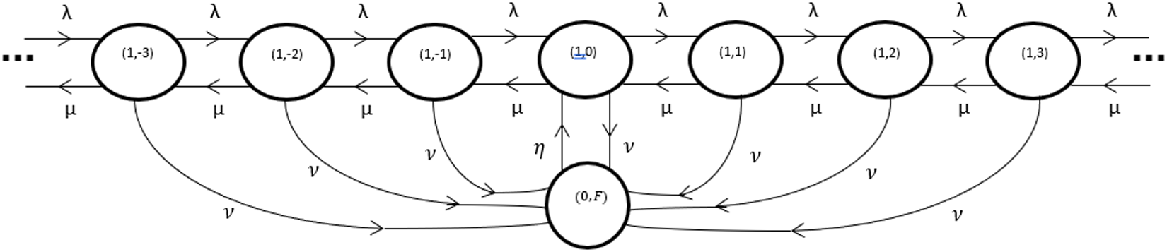


 Open access