


1. Introduction
In comparison to traditional serial robots with rigid links, cable-driven robots, which replace rigid linkages with cables, provide several advantages. The utilization of cables significantly reduces weight and allows for the deployment of extended lengths without substantially increasing the robot’s overall mass [Reference Korayem and Bamdad1, Reference Korayem, Bamdad. and Bayat2]. Therefore, the end-effector (EE) of a cable-driven parallel robot (CDPR) can reach high accelerations and velocities, enabling it to operate effectively within a large workspace [Reference Tho and Thinh3, Reference Amare, Zi, Qian, Du and Ge4]. Meanwhile, cables are flexible, and they can only bear tension but not compression. Consequently, n-DOF CDPRs should contain a minimum n + 1 cables to entirely constrain and control the EE. For n cables CDPRs, another actuator can be used to maintain tension in cables [Reference Liu, Mei, Wang and Guo5]. As an example, a pneumatic muscle could play the role of spinal cord in the biologically inspired cable robot to imitate the human neck [Reference Zhao, Zi and Qian6]. Also, a dynamic trajectory optimization method for a CDPR that has a rigid linkage that passes through singular orientations is investigated [Reference Xiang, Li and Jiang7]. Ensuring positive cable forces imposes a major issue in CDPR control and trajectory planning [Reference Shang, Xie, Zhang, Cong and Li8–Reference Jiang, Barnett and Gosselin10].
Trajectory optimization methods in the optimal control theory (OCP) fall into two main classes: direct and indirect approaches. Direct methods derive Pontryagin conditions and numerically solve the resulting boundary-value problems, offering accuracy but requiring precise initial guesses. In contrast, direct methods discretize the problem upfront using nonlinear programming (NLP) methods. While direct methods may yield slightly suboptimal trajectories, they offer larger convergence regions, making them advantageous for robotics applications [Reference Bordalba, Schoels, Ros, Porta and Diehl11]. The direct collocation (DC) method offers a powerful solution for trajectory optimization [Reference Hargraves and Paris12], yielding dynamically accurate trajectories in robotics. However, they may introduce significant kinodynamic errors in constrained mechanical systems [Reference Bordalba, Schoels, Ros, Porta and Diehl11]. For CDPRs, achieving optimal trajectory involves adapting either direct or indirect methods while ensuring cable forces remain tensile [Reference Behzadipour and Khajepour13–Reference Bamdad15]. This article focuses on collocation methods, a type of direct approach known for speed and effectiveness. Unlike indirect methods, which rely on explicit integrators or shooting methods, collocation methods use spline approximations to discretize dynamic constraints, making them efficient and versatile [Reference Betts16–Reference Kolathaya, Guffey, Sinnet and Ames18]. The pseudo-spectral technique, another direct method, transforms the OCP into a discrete constrained problem. GPOPS-II relies on the Radau pseudo-spectral scheme [Reference Patterson and Rao19], which has been applied in various robotic motion planning scenarios [Reference Campbell and Kunkel20]. This approach approximates the state and control using interpolating polynomials, with the nodes being the roots of orthogonal polynomials.
The hybrid CDPR developed in this study features a centrally mounted pneumatic cylinder that applies an upward support force to the EE, helping maintain consistent cable tension during operation. Achieving consistent robot behavior that closely follows the planned trajectory is essential for accurate execution on real hardware [Reference Bamdad15].
While DC methods excel in dynamic accuracy, ensuring kinematic precision on the cable-constrained robotic system remains underexplored. Discretization errors can lead to unrealistic trajectories that are challenging to stabilize with a controller because these robots may impose complex constraints on the state vector, confining trajectories to nonlinear manifolds within larger ambient spaces [Reference Bordalba, Schoels, Ros, Porta and Diehl11].
Cable robots, with their intricate cable tensions, pose unique challenges in trajectory planning due to their inability to push. This work mainly delves into the DC method besides GPOPS-II to tackle trajectory planning challenges for CDPRs, aiming to overcome limitations associated with initial guess dependency and local minima. GPOPS-II was selected as the comparison benchmark because it is a widely recognized and extensively validated tool for solving complex trajectory optimization problems using pseudo-spectral methods. Its high-level abstraction, adaptive mesh refinement, and ability to handle large-scale constrained NLP problems make it a suitable and rigorous baseline for benchmarking. GPOPS-II implements the collocation technique by the pseudo-spectral method to solve OCP for nonlinear systems. By a new class of variable-order Legendre-Gauss-Radau quadrature orthogonal collocation polynomials, the continuous-time OCP is converted to an NLP. A distinctive characteristic of GPOPS-II is the adaptive mesh refinement that defines the number of mesh intervals and the degree of the approximating polynomial to obtain a definite accuracy. As stated, GPOPS-II approximates both control and state variables that translate the OCP into an NLP of dimension for each (k = 1,2,…, N-1) interval. The limitations of the OCP solution using GPOPS-II include the need to express dynamic equations of motion explicitly to avoid doubling the system dimension. While GPOPS-II offers automatic mesh refinement and supports algebraic constraints, developing gradients, Hessian, and Jacobian matrices require the use of automatic differentiation.
The robot’s performance has been a subject of particular interest, with the tension distribution being a key factor. A positive tension must be considered for each cable to keep control of the CDPR [Reference Ueland, Sauder and Skjetne21]. In the previous research of the authors, although the subject of positive cable tension to maintain control of the cable robot was considered [Reference Badrikouhi and Bamdad22], the issue of cable tension management was neglected. This issue, which leads to the uniform distribution of forces in cables, is considered in this research. Minimizing the rate of change of tension reduces abrupt changes in cable forces, ensuring continuous and smooth tension profiles. Cable tension management is formed along with the definition of the appropriate objective function, and altogether, the cost of the CDPR’s control effort should be acceptable. This strategy ensures physically feasible motions and allows for the practical implementation of algorithms.
The paper construction is as follows. In Section 2, we delve into two distinct approaches, DC and the pseudo-spectral method. Section 3 serves as an introduction to the CDPR, featuring a central spine, where we also address the kinematic and dynamic formulation. Section 4 is dedicated to presenting our problem statement. In Section 5, we delve into the discussion of simulation results, employing both the DC and GPOPS-II methods. This section also encompasses a comparative analysis of the DC results concerning minimum-force and minimum-force-rate, aiding in the selection of a more pertinent cost function. Section 6 offers a comprehensive explanation of our experimental platform. Here, we present a comparative evaluation between the simulation and experimental outcomes. Finally, in Section 7, we conclude this paper by summarizing our key findings and contributions.
2. General formulations
The trajectory optimization is formulated using DC, discretizing dynamics and constraints into a nonlinear program. A tailored DC solver with defined tolerances ensures efficient and accurate convergence. To support solver performance, a linear initial guess is employed, providing a smooth and feasible starting point for optimization.
2.1. Direct collocation
Generally, the dynamic equation of the CDPR can be modeled by $\dot{\mathbf{x}}(t)=\mathbf{f}(\mathbf{x}(t),\mathbf{u}(t))$
, that x ∈ R
n and u ∈ R
m signifies the vector of state and control variables. Analytical Methods rely on mathematical formulations and closed-form solutions, which often lead to deterministic and computationally efficient results when the problem structure is well-defined. In the trajectory optimization problem, a finite-time u(t), ∀t ∈ [0, T] is searched, such that a given objective function J is minimized,
$\dot{\mathbf{x}}(t)=\mathbf{f}(\mathbf{x}(t),\mathbf{u}(t))$
, that x ∈ R
n and u ∈ R
m signifies the vector of state and control variables. Analytical Methods rely on mathematical formulations and closed-form solutions, which often lead to deterministic and computationally efficient results when the problem structure is well-defined. In the trajectory optimization problem, a finite-time u(t), ∀t ∈ [0, T] is searched, such that a given objective function J is minimized,
 \begin{equation} \begin{array}{l} \underset{\mathbf{x}(t),\mathbf{u}(t)}{\text{minimize }}J(\mathbf{x}(t),\mathbf{u}(t))=\int _{0}^{T}\phi \left(\mathbf{x}(t),\mathbf{u}(t),t\right)\\[4pt] \text{subject to} \left\{\begin{array}{l} \dot{\mathbf{x}}(t)=\mathbf{f}\left(\mathbf{x}(t),\mathbf{u}(t)\right)\\[4pt] \mathbf{h}\left(\mathbf{x}(t),\mathbf{u}(t)\right)= 0,\mathbf{g}\left(\mathbf{x}(t),\mathbf{u}(t)\right)\leq 0 \end{array}\right. \end{array} \end{equation}
that h and g are formulated as the equality and inequality constraints, and the cost function is $\varPhi$
. DC transforms this continuous problem into a discretized problem with a finite number of variables. All approaches divide the phase duration (time) into N -1 segments, 0 = t
1
< t
2
<…<t
N
= T where the points are denoted as a node, mesh, or grid point N. We use x
k
= x(t
k
) to designate the state variable at a node k. Indicating the input control at a node by u
k
= u(t
k
), a discrete-time dynamic system is described as x (k + 1) =f(x (k), u (k), k). We collocate dynamic modeling via the trapezoidal approximation to discretize
$\varPhi$
. DC transforms this continuous problem into a discretized problem with a finite number of variables. All approaches divide the phase duration (time) into N -1 segments, 0 = t
1
< t
2
<…<t
N
= T where the points are denoted as a node, mesh, or grid point N. We use x
k
= x(t
k
) to designate the state variable at a node k. Indicating the input control at a node by u
k
= u(t
k
), a discrete-time dynamic system is described as x (k + 1) =f(x (k), u (k), k). We collocate dynamic modeling via the trapezoidal approximation to discretize $\dot{\mathrm{x}} = \mathrm{f}(\mathrm{x,\ u}, t) $
. Using trapezoidal quadrature simplifies (1) into an NLP form:
$\dot{\mathrm{x}} = \mathrm{f}(\mathrm{x,\ u}, t) $
. Using trapezoidal quadrature simplifies (1) into an NLP form:
 \begin{equation} \begin{aligned} \text{minimize}_{\textrm{x}(k),\,\textrm{u}(k)} \quad & J(\textrm{x}(k),\textrm{u}(k)) = \sum_{k=1}^{N} \phi\big(x(k),u(k)\big) \\[6pt] \text{subject to} & \left\{ \begin{aligned} \textrm{x}_{k+1} - \textrm{x}_k &= \frac{h}{2}\left(\textrm{f}_k + \textrm{f}_{k+1}\right), \quad (k = 1,2,\ldots,N-1) \\[6pt] \textrm{h}\big(x(k),\textrm{u}(k)\big) &= 0, \quad g\big(x(k),u(k)\big) \le 0 \\[6pt] h &= (t_N - t_1)/(N - 1) \end{aligned} \right. \end{aligned} \end{equation}
2.2. Proposed solver
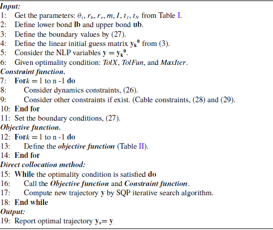
The challenge in the DC method for trajectory planning in constrained robotic systems is the discretization errors. These errors can cause the trajectories to drift away from the implicitly-defined manifold of the system’s constraints [Reference Bordalba, Schoels, Ros, Porta and Diehl11]. The Sequential Quadratic Programming (SQP) algorithm is designed for the DC problem. SQP effectively manages complex constraints, and by solving a series of quadratic subproblems, SQP iteratively refines the trajectory, reducing discretization errors and keeping the motion physically consistent. SQP’s approach ensures minimizing drift and high accuracy in the final trajectory, which aligns well with the structure of DC in CDPRs. Its ability to exploit second-order information ensures faster convergence and higher accuracy compared to gradient-free or population-based methods [Reference Di, Vincenzo, Zoppi and Caro23]. First, the tolerances of the stopping criteria and optimality conditions are determined. Three stopping criteria are defined. The norm of (x k – x k + 1), which is the size of the variation of x k in each step, is considered as TolX. The iterations continue until the number of solver iterations reaches MaxIter. The SQP iterations terminate if (x k – x k + 1) is minor than TolX. The DC problem will be resolved upon |J (x k ) – J (x k + 1)| < TolFun, whereas a change in the cost function during a step is TolFun.
Next, a linear initial guess is selected to improve convergence and reduce solution time as:
 \begin{equation}y_k^0 = y_1 + \frac{k-1}{N-1}(y_N - y_1), \quad (k = 1,2,\ldots,N) \end{equation}
where y k 0 is the initial guess and y 1 and y N are the initial and final values. Optimization variables are bounded based on the physical constraints of joint variables and actuator forces. Hence, for y k = (x k,u k), it is supposed to be a lower bound l b and upper bound u b for each state and control y k as l b < y k < u b .
3. CDPR with central spine
The CAD model is presented in Figure 1, which features 3 degrees of freedom: the rotation about the X-axis (pitch), the rotation about the Y-axis (roll), and the vertical motion along the Z-axis (heave). The spine produces a force between the base and the EE to keep all the cables in tension. The pneumatic cylinder is settled and fixed at point O to the base platform. In the proposed CDPR architecture, the actuation system is spatially considered to be in an optimized cable routing and minimize cable interference. The stepper motors and associated winch mechanisms are mounted on an intermediate support structure located between the fixed base and the moving EE platform. This reduces the effective cable span, which serves two primary purposes: (1) it reduces the likelihood of cable interference or entanglement, where a central spin occupies the core workspace volume and could intersect with the cable routing path, and (2) it minimizes the deflection and vibration caused by long unsupported cable lengths.
CAD model of the designed 3-DOF CDPR.

CDPR kinematic diagram [Reference Badrikouhi and Bamdad22].

The EE is connected at P m to the cylinder by a 2-DOF universal joint. Thus, 3 degrees of freedom are constrained: the EE rotation about the Z-axis (yaw), the forward/backward movement (surge), and the left/right movement (sway). Since the positive tension in cables is essential, the cylinder is applied as an extra actuator to improve the tensionability of the cables. It also eliminates the EE’s normal weight force. The cylinder enables the EE to move up and down, while the cables guide rotational movement. Additionally, the universal joint angle within the CDPR workspace is designed to minimize the overall required actuator torque, while the spine serves to obviate the necessity for robust cable winches.
3.1. Kinematics
To the kinematic analysis of the CDPR, the fixed reference frame A: XYZ, and the moving frame B: xyz attached to the moving platform at point P
m
are considered. The EE coordinate x is defined as [z α $ \beta $
]
T
, where z signifies the end position of the pneumatic cylinder, α is the EE pitch angle, and the EE roll angle is denoted as β. Thus, the joint coordinate is q = [l
1
l
2
l
3
d]
T
, in which l
i
is the length of cable i, and the spine translation along Z is defined as d. Since the cylinder is fixed to the base platform at point O, z = d, where d
0
is the primary height of the cylinder. Per the CDPR schematic diagram in Figure 2, P
i (i = 1,2,3) and S
i
(i = 1,2,3) are the cable attachment points. The base radius is defined as r
b
, and θ
i
is the angle between the right-hand side of X and OS
i;
thus, S
i
=[r
b
cosθ
i,
r
b
sinθ
i,
h
0
]. The stepper motors are positioned at h
0
to avoid a clash between the cables and the spine. To calculate the cable length:
$ \beta $
]
T
, where z signifies the end position of the pneumatic cylinder, α is the EE pitch angle, and the EE roll angle is denoted as β. Thus, the joint coordinate is q = [l
1
l
2
l
3
d]
T
, in which l
i
is the length of cable i, and the spine translation along Z is defined as d. Since the cylinder is fixed to the base platform at point O, z = d, where d
0
is the primary height of the cylinder. Per the CDPR schematic diagram in Figure 2, P
i (i = 1,2,3) and S
i
(i = 1,2,3) are the cable attachment points. The base radius is defined as r
b
, and θ
i
is the angle between the right-hand side of X and OS
i;
thus, S
i
=[r
b
cosθ
i,
r
b
sinθ
i,
h
0
]. The stepper motors are positioned at h
0
to avoid a clash between the cables and the spine. To calculate the cable length:
 \begin{equation} \mathbf{O}\mathbf{S}_{i}+\mathbf{S}_{i}\mathbf{P}_{i}=\mathbf{O}\mathbf{P}_{i}\rightarrow l_{i}\mathbf{=}\| \mathbf{S}_{i}\mathbf{P}_{i}\| \mathbf{=}\| \mathbf{O}\mathbf{P}_{i}\mathbf{-}\mathbf{O}\mathbf{S}_{i}\| (i=1,2,3) \end{equation}
OS
i
is a constant. Also, OP
i
= d
0
+z+P
m
P
i
, in which z = z
K and d
0 = d
0
K. For P
m
P
i
, we have P
m
P
i
= R
PR
P
m
P
i
)
mov
. R
PR
= R
y( $\beta$
)R
x(α) is the EE pitch-roll rotation matrix relative to the base platform. P
m
P
i
)
mov
is the vector from the attachment point of EE and cylinder to the end corner of the EE. The vector P
m
P
i
)
mov
is defined in the moving coordinate frame {B} as donated by the subscript. Consequently, the inverse kinematic model could be expressed as:
$\beta$
)R
x(α) is the EE pitch-roll rotation matrix relative to the base platform. P
m
P
i
)
mov
is the vector from the attachment point of EE and cylinder to the end corner of the EE. The vector P
m
P
i
)
mov
is defined in the moving coordinate frame {B} as donated by the subscript. Consequently, the inverse kinematic model could be expressed as:
 \begin{equation} z=d,\,\,l_{i}=\| \mathbf{d}_{0}+\mathbf{z}+\mathbf{R}_{\mathbf{PR}}\mathbf{P}_{m}\mathbf{P}_{i}-\mathbf{O}\mathbf{S}_{\mathbf{i}}\| (i=1,2,3) \end{equation}
Then, to calculate the Jacobian, the velocity loop closure is used. The Jacobian is calculated as $ \dot{\mathbf{q}} = \mathbf{J}_x \,\dot{\mathbf{x}} $
, in which the Jacobian is J
x
,
$ \dot{\mathbf{q}} = \mathbf{J}_x \,\dot{\mathbf{x}} $
, in which the Jacobian is J
x
, $\dot{\mathbf{q}} = \left[ \dot{l}_1 \;\; \dot{l}_2 \;\; \dot{l}_3 \;\; \dot{d} \right]^{T} $
is the velocity vector of the joints, and
$\dot{\mathbf{q}} = \left[ \dot{l}_1 \;\; \dot{l}_2 \;\; \dot{l}_3 \;\; \dot{d} \right]^{T} $
is the velocity vector of the joints, and $\dot{\mathbf{x}} = \left[ \dot{z} \;\; \dot{\alpha} \;\; \dot{\beta} \right]^{T} $
presents the EE velocity, whereas the unit vector of a fixed frame A is I, J, K, and the unit vector of a moving frame B is i, j, k. Thus, we consider:
$\dot{\mathbf{x}} = \left[ \dot{z} \;\; \dot{\alpha} \;\; \dot{\beta} \right]^{T} $
presents the EE velocity, whereas the unit vector of a fixed frame A is I, J, K, and the unit vector of a moving frame B is i, j, k. Thus, we consider:
 \begin{equation} \mathbf{O}\mathbf{P}_{m}\mathbf{+}\mathbf{P}_{m}\mathbf{P}_{i}\mathbf{=}\mathbf{O}\mathbf{S}_{i}\mathbf{+}\mathbf{S}_{i}\mathbf{P}_{i} \end{equation}
We differentiate from each term of (6). For a prismatic joint, the vector $ \left({d\,OP_m}/{dt} \right)_{\text{fix}} = \dot{z}\,\mathbf{K} $
is represented in the fixed reference frame {A}. By considering the EE pitch-roll rotation, (7) is obtained.
$ \left({d\,OP_m}/{dt} \right)_{\text{fix}} = \dot{z}\,\mathbf{K} $
is represented in the fixed reference frame {A}. By considering the EE pitch-roll rotation, (7) is obtained.
 \begin{equation} (d\,\mathbf{P}_{m} \mathbf{P}_{i}/dt)_{\mathbf{fix}}=\boldsymbol{\Omega} \times \mathbf{P}_{m}\mathbf{P}_{i} \end{equation}
To calculate the $\boldsymbol{\Omega}$
, first, the R
PR
is written as:
$\boldsymbol{\Omega}$
, first, the R
PR
is written as:
 \begin{equation} \mathbf{R} = \begin{bmatrix} r_{11} &\quad r_{12} &\quad r_{13} \\ r_{21} &\quad r_{22} &\quad r_{23} \\ r_{31} &\quad r_{32} &\quad r_{33} \end{bmatrix} = \begin{bmatrix} \cos\beta &\quad \sin\beta \sin\alpha &\quad \sin\beta \cos\alpha \\ 0 &\quad \cos\alpha &\quad -\sin\alpha \\ -\sin\beta &\quad \cos\beta \sin\alpha &\quad \cos\beta \cos\alpha \end{bmatrix} \end{equation}
where r
ij
denotes the (i, j) components of the corresponding rotation matrix, and to derive the EE angular velocity $\boldsymbol{\Omega }=[\Omega_{x}\,\,\Omega_{y}\,\,\Omega_{z}]^{T}$
, the following three independent equations are extracted [Reference Taghirad24].
$\boldsymbol{\Omega }=[\Omega_{x}\,\,\Omega_{y}\,\,\Omega_{z}]^{T}$
, the following three independent equations are extracted [Reference Taghirad24].
 \begin{align}\Omega_{x} & =\dot{r}_{31}r_{21}+\dot{r}_{32}r_{22}+\dot{r}_{33}r_{23}=\cos \beta \,\dot{\alpha }\nonumber\\\Omega_{y} & =\dot{r}_{11}r_{31}+\dot{r}_{12}r_{32}+\dot{r}_{13}r_{33}=\dot{\beta }\nonumber\\\Omega_{z} & =\dot{r}_{21}r_{11}+\dot{r}_{22}r_{12}+\dot{r}_{23}r_{13}=-\sin \beta \,\dot{\alpha } \end{align}
Since OS
i
is constant, $ \left( \frac{d\,OS_i}{dt} \right)_{\text{fix}} = 0 $
and from (5), the direction of the cable length li is computed by s
i
from (10):
$ \left( \frac{d\,OS_i}{dt} \right)_{\text{fix}} = 0 $
and from (5), the direction of the cable length li is computed by s
i
from (10):
 \begin{equation} \mathbf{s}_{i}=\mathbf{S}_{i}\mathbf{P}_{i}/l_{i}\overset{}{\rightarrow }\mathbf{S}_{i}\mathbf{P}_{i}\mathbf{=}l_{i}\mathbf{s}_{i} \end{equation}
Since the cables do not rotate around themselves, angular velocity $ \boldsymbol{\Omega}_{l_i} $
is perpendicular to s
i,
and we have:
$ \boldsymbol{\Omega}_{l_i} $
is perpendicular to s
i,
and we have:
 \begin{equation} d(l_{i}\mathbf{s}_{i})/dt=\dot{l}_{i}\mathbf{s}_{i}+\boldsymbol{\Omega }_{{l_{i}}}\times l_{i}\mathbf{s}_{i} \end{equation}
From differentiation of (6), (12) is obtained:
 \begin{equation}\dot{z}K + \boldsymbol{\Omega} \times P_m P_i = \dot{l}_{s_i} + \boldsymbol{\Omega}_{l_i} \times l_{s_i} \end{equation}
To get an expression for Jacobian, multiply both sides of (12) by the dot-product of s i :
 \begin{equation} \dot{z}\mathbf{K}\cdot \mathbf{s}_{i}+(\boldsymbol{\Omega }\times \mathbf{P}_{m}\mathbf{P}_{i})\cdot \mathbf{s}_{i}=\dot{l}_{i}\mathbf{s}_{i}\cdot \mathbf{s}_{i}+(\boldsymbol{\Omega }_{{l_{i}}}\times l_{i}\mathbf{s}_{i})\cdot \mathbf{s}_{i} \end{equation}
Since the angular velocity $\boldsymbol{\Omega }_{{l_{i}}}$
is perpendicular to s
i
, the last term of (13) becomes zero and for the sake of brevity, we assume in notation that P
m
P
i
= E
i
. Hence:
$\boldsymbol{\Omega }_{{l_{i}}}$
is perpendicular to s
i
, the last term of (13) becomes zero and for the sake of brevity, we assume in notation that P
m
P
i
= E
i
. Hence:
 \begin{equation} \dot{z}\mathbf{K}.\mathbf{s}_{i}+(\boldsymbol{\Omega }\times \mathbf{E}_{i}).\,\mathbf{s}_{i}=\dot{l}_{i} \end{equation}
Rewriting (14) for all the limbs by factoring the velocity terms considering $\boldsymbol{\Omega }=\cos \beta \,\dot{\alpha }\mathbf{I}+\dot{\beta }\mathbf{J}-\sin \beta \,\dot{\alpha }\mathbf{K}$
results in:
$\boldsymbol{\Omega }=\cos \beta \,\dot{\alpha }\mathbf{I}+\dot{\beta }\mathbf{J}-\sin \beta \,\dot{\alpha }\mathbf{K}$
results in:
 \begin{align} \dot{z}\mathbf{K}.\mathbf{s}_{i}+\cos \beta \,\dot{\alpha }(\mathbf{I}\times \mathbf{E}_{i}).\mathbf{s}_{i}+\dot{\beta }(\mathbf{J}\times \mathbf{E}_{i}).\mathbf{s}_{i}-\sin \beta \,\dot{\alpha }(\mathbf{K}\times \mathbf{E}_{i}).\mathbf{s}_{i}&=\dot{l}\\[-10pt]\nonumber \end{align}
 \begin{align} \left[\left.\mathbf{K}.\mathbf{s}_{i}\right| \left.\cos \beta \left(\mathbf{I}\times \mathbf{E}_{i}\right).\mathbf{s}_{i}-\sin \beta \left(\mathbf{K}\times \mathbf{E}_{i}\right).\mathbf{s}_{i}\right| \left(\mathbf{J}\times \mathbf{E}_{i}\right).\mathbf{s}_{i}\right]\left[\dot{z}\dot{\alpha }\dot{\beta }\right]^{T}&=\dot{l}_{i} \end{align}
From (5), $\dot{z} = \dot{d} $
and using (15) for i = 1, 2, 3, CDPR Jacobian matrix J
x
can be derived as:
$\dot{z} = \dot{d} $
and using (15) for i = 1, 2, 3, CDPR Jacobian matrix J
x
can be derived as:
 \begin{equation}\mathbf{J}_{\mathbf{x}}\mathit{=}\left[\!\left.\begin{array}{l} \mathbf{K}\mathit{.}\mathbf{s}_{1}\\\mathbf{K}\mathit{.}\mathbf{s}_{2}\\ \mathbf{K}\mathit{.}\mathbf{s}_{3}\\ \ \ 1 \end{array}\!\right | \right.\left.\!\begin{array}{l} \cos \beta\!\left(\mathbf{I}\times \mathbf{E}_{1}\right)\!.\mathbf{s}_{1}-\sin \beta\!\left(\mathbf{K}\times \mathbf{E}_{1}\right)\!.\mathbf{s}_{1}\\\cos \beta\!\left(\mathbf{I}\times \mathbf{E}_{2}\right)\!.\mathbf{s}_{2}-\sin \beta\!\left(\mathbf{K}\times \mathbf{E}_{2}\right)\!.\mathbf{s}_{2}\\\cos \beta\!\left(\mathbf{I}\times \mathbf{E}_{3}\right)\!.\mathbf{s}_{3}-\sin\beta\!\left(\mathbf{K}\times \mathbf{E}_{3}\right)\!.\mathbf{s}_{3}\\\qquad\qquad\qquad\quad 0 \end{array}\!\right|\! \left.\begin{array}{l} \left(\mathbf{J}\mathit{\times }\mathbf{E}_{1}\right)\!\mathit{.}\mathbf{s}_{1}\\ \left(\mathbf{J}\mathit{\times }\mathbf{E}_{2}\right)\mathit{.}\mathbf{s}_{2}\\ \left(\mathbf{J}\mathit{\times }\mathbf{E}_{3}\right)\mathit{.}\mathbf{s}_{3}\\ \qquad 0 \end{array}\!\right] \end{equation}
3.2. Dynamic
The dynamic model of the CDPR is formulated using the Lagrangian approach, leading to the following expression:
 \begin{equation} \frac{d}{dt}\left(\frac{\partial L}{\partial \dot{q}_{k}}\right)-\frac{\partial L}{\partial q_{k}}=Q_{k},\,\,\,\,Q_{k}=\sum _{i=1}^{N}F_{i}^{*}\cdot \frac{\partial r_{i}}{\partial q_{k}} \end{equation}
The kinetic and potential energies of the robot are derived in terms of the discussed generalized coordinate [Reference Korayem, Najafi and Bamdad25]. Lagrangian function L and the generalized force Q
k
are linked to the generalized coordinate q
k
= [z, α, $\beta$
] that describes the system’s configuration.
$\beta$
] that describes the system’s configuration.
Following that, F
i
* is the effective force exerted on mass m
i
with the position vector r
i
. It is assumed that the friction and mass of the cables are ignored. The actuator force vector is defined as τ= $[T_{\textit{1}}\ \ T_{\textit{2}}\ \ T_{\textit{3}}\ \ F_{n}]^ T$
, where T
i
denotes the tension in the i-th cable and F
n
represents the vertical (normal) force generated by the central spine actuator (refer to Figure 3). Accordingly, the Lagrangian L for the EE (with mass m and moment of inertia I) is formulated as:
$[T_{\textit{1}}\ \ T_{\textit{2}}\ \ T_{\textit{3}}\ \ F_{n}]^ T$
, where T
i
denotes the tension in the i-th cable and F
n
represents the vertical (normal) force generated by the central spine actuator (refer to Figure 3). Accordingly, the Lagrangian L for the EE (with mass m and moment of inertia I) is formulated as:
 \begin{equation} L=\frac{1}{2}m\mathbf{V}_{C}^{2}+\frac{1}{2}\mathbf{I}\boldsymbol{\Omega }^{2}-mgh_{C}=\frac{1}{2}m\!\left(V_{C_{x}}^{2}+V_{C_{y}}^{2}+V_{C_{z}}^{2}\right)+\frac{1}{2}\left(I_{x}\Omega_{x}^{2}+I_{y}\Omega_{y}^{2}+I_{z}\Omega_{z}^{2}\right)-mgh_{C} \end{equation}
Designed spine mechanism and corresponding free body diagram.

The angular velocity vector Ω is computed using (9). The EE center position and its velocity V c , as defined in (19), are obtained as follows:
 \begin{align}&\qquad\quad \mathbf{r}_{C}=[0\ 0\ d_{0}+z]^{T}+\mathbf{R}[0\ 0\ l_{C}]^{T}=[l_{C}\cos \alpha \sin \beta -l_{C}\sin\ \alpha\ d_{0}+\,\textrm{z}\,+l_{C}\cos\ \alpha \cos \beta ]^{T} \end{align}
 \begin{align}& \mathbf{V}_{C}=\frac{d\mathbf{r}_{C}}{dt}=\left[l_{C}\left(-\dot{\alpha }\sin \alpha \sin \beta +\dot{\beta }\cos \beta \cos \alpha \right)-l_{C}\dot{\alpha }\cos \alpha \dot{\textrm{z}}+l_{C}\left(-\dot{\alpha }\sin \alpha \cos \beta -\dot{\beta }\sin \beta \cos \alpha \right)\right]^{T} \end{align}
where l C is illustrated in Figure 3. Also, h C , the height from the base, are given by:
 \begin{equation} h_{C}=d_{0}+\textrm{z}+l_{C}\cos \alpha \cos \beta \end{equation}
By substituting (9) and (20–22) into (19), the Lagrangian of the CDPR can be derived as follows:
 \begin{align} L&=(m((l_{C}\dot{\alpha }\sin \alpha \sin \beta -l_{C}\dot{\beta }\cos \alpha \cos \beta )^{2}+(l_{C}\dot{\alpha }\cos \beta \sin \alpha -\dot{z}+l_{C}\dot{\beta }\cos \alpha \sin \beta )^{2}\nonumber\\&\quad +{l_{C}}^{2}\dot{\alpha }^{2}\cos ^{2}\alpha ))/2 +(I_{y}\dot{\beta }^{2})/2+(I_{x}\dot{\alpha }^{2}\cos ^{2}\beta )/2+(I_{z}\dot{\alpha }^{2}\sin ^{2}\beta )/2-mg(\textrm{z}+d_{0}+l_{C}\cos \alpha \cos \beta ) \end{align}
The Lagrangian is formed, and for each generalized coordinate, Lagrange equation is required to be applied. Next, an overview of how generalized force Q
k
is defined and integrated into the Lagrangian dynamics is presented in Appendix A. It is essential for deriving the equations of motion that govern system behavior. By specifying L from (23) and Q
k
from (A.4), and substituting these terms in (18), closed-form dynamic including mass matrix M $\in \boldsymbol{R}^{\mathbf{3}\times \mathbf{3}}$
, Coriolis and centrifugal vector C
$\in \boldsymbol{R}^{\mathbf{3}\times \mathbf{3}}$
, Coriolis and centrifugal vector C $\in \boldsymbol{R}^{\mathbf{3}\times \mathbf{1}}$
, and gravity vector G
$\in \boldsymbol{R}^{\mathbf{3}\times \mathbf{1}}$
, and gravity vector G $\in \boldsymbol{R}^{\mathbf{3}\times \mathbf{1}}$
could be generated:
$\in \boldsymbol{R}^{\mathbf{3}\times \mathbf{1}}$
could be generated:
 \begin{align} &\mathbf{M}\ddot{\mathbf{x}}+\mathbf{C}+\mathbf{G}=\mathbf{Q}\nonumber\\& \ddot{\mathbf{x}}=\mathbf{M}^{-1}(\mathbf{Q}-\mathbf{G}-\mathbf{C})=\mathbf{A}\nonumber\\& \mathbf{A}=[A_{1}\ A_{2}\ A_{3}]^{T} \end{align}
The detailed formulations of M, C, and G are provided in Appendix B. The state space form of dynamic equations is expressed in (25):
 \begin{align} \dot{\mathbf{x}} & =\mathbf{f}(\mathbf{x}\,,\,\mathbf{u},\,\,t)\nonumber\\ \mathbf{x} & =[z,\dot{z},\alpha ,\dot{\alpha },\beta ,\dot{\beta }]^{T}=[x_{1},x_{2},\ldots ,x_{6}]^{T}\nonumber\\ \mathbf{f} & =[x_{2},A_{1},x_{4},A_{2},x_{6},A_{3}]^{T}=[\,f_{1},f_{2},\ldots ,f_{6}]^{T} \end{align}
4. Problem statement
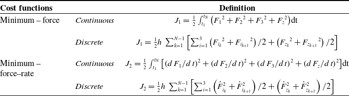
In this section, we initially examine the dynamic equation of motion and the associated objective functions, which are discretized using the trapezoidal approximation method. We’ve chosen to focus on two specific cost functions: minimum-force and minimum-force-rate. Selecting the minimum-force criterion serves the goal of reducing the control effort exerted on the actuators. Conversely, opting for the minimum-force-rate criterion aims to minimize abrupt force variations, particularly in the cable forces. This approach fosters the creation of smoothly evolving and symmetrical forces within the actuators, ultimately facilitating the generation of a well-suited and seamless trajectory.
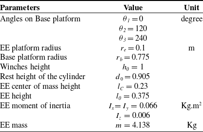
The discretized dynamic equation of motion is detailed as equality constraints. Furthermore, the section outlines essential inequality constraints pertaining to the maintenance of cable forces in a tensile state while avoiding significant fluctuations. Due to trajectory optimization, the DC method must be adapted with the CDPR, considering the kinematics and dynamics in Section 3. In Table I, the CDPR parameters are presented.
The parameters of the CDPR

Thus, the optimization variables, including states and controls, are $ \mathbf{y}_k = [ z_k,\; \dot{z}_k,\; \alpha_k,\; \dot{\alpha}_k,\; \beta_k,\; \dot{\beta}_k, F_{1k},\; F_{2k},\; F_{3k},\; F_{zk} ] $
in which k = 1, 2, …, N. The variables that should be optimized based on the cost function are y = (y
1
, y
2
, …, y
N
)
T
. Hereby, the trajectory planning problem is to detect y in all nodes, considering constraints and boundary conditions.
$ \mathbf{y}_k = [ z_k,\; \dot{z}_k,\; \alpha_k,\; \dot{\alpha}_k,\; \beta_k,\; \dot{\beta}_k, F_{1k},\; F_{2k},\; F_{3k},\; F_{zk} ] $
in which k = 1, 2, …, N. The variables that should be optimized based on the cost function are y = (y
1
, y
2
, …, y
N
)
T
. Hereby, the trajectory planning problem is to detect y in all nodes, considering constraints and boundary conditions.
This problem is prescribed with force and force-rate in the cost functions. Also, it demands a modification of the actuation to ensure a smooth response. Researchers regularly investigate the cable force objective function in a quadratic form of first-order constraints. Then the SQP algorithm [Reference Pott, Bruckmann and Mikelsons26] can be used to solve this issue. The constraints in this study entail maintaining positive tension and avoiding excessive fluctuation in the cable tension through more complex objective functions, which distinguishes it from previous research. The tensionability constraints effectively confine the cable robot states within a nonlinear manifold. However, due to potential transcription errors, trajectories may inadvertently deviate from this manifold.
The objective functions

Table II explains the cost function and the trapezoidal approximation in discretizing. For minimum-force-rate, the smoothness of the cable tensions is considered directly in the cost function, and there is no need for this constraint. From (25) and using (2), the dynamic is discretized, thus it is designated as equality constraints:
 \begin{equation} \begin{array}{l} \text{minimize}\,\,\,J\\ \text{subject}\,\textrm{to}\,\colon x_{{i_{k+1}}}-x_{{i_{k}}}-\dfrac{h}{2}\left(f_{{i_{k}}}+f_{{i_{k+1}}}\right)=0\left\{\begin{array}{l} \left(i=1,2,\ldots ,6\right)\\[3pt] \left(k=1,2,\ldots ,N-1\right) \end{array}\right. \end{array} \end{equation}
The boundary conditions are considered as the second set of constraints:
 \begin{equation} \begin{array}{l} z_{1}=0\,\textrm{m}\,,\,\,\,\,\,\,\dot{z}_{1}=0\ \textrm{m}/\textrm{s}\,,\,\,\,\,\,\,z_{N}=0.12\textrm{m}\,,\,\,\,\,\,\,\,\,\,\,\dot{z}_{N}=0\ \textrm{m}/\textrm{s}\\ \alpha _{1}=0\,\textrm{rad},\,\,\,\dot{\alpha }_{1}=0\ \textrm{rad}/\textrm{s},\,\,\,\alpha _{N}=-0.1\,\textrm{rad},\,\,\,\,\,\,\,\dot{\alpha }_{N} = 0\ \textrm{rad}/\textrm{s}\\ \beta _{1}=0\,\textrm{rad},\,\,\,\dot{\beta }_{1}=0\ \textrm{rad}/\textrm{s},\,\,\,\,\beta _{N}=-0.1\,\textrm{rad},\,\,\,\,\,\,\dot{\beta }_{N}=0\ \textrm{rad}/\textrm{s} \end{array} \end{equation}
Therefore, the discrete form of dynamic equations (26) and the boundary conditions (27) are considered as equality constraints. The primary inequality constraint is to ensure positive tension in cables with the minimum force F allow throughout the trajectory; failure to do so would disrupt the robot’s performance.
 \begin{equation} F_{ik} \ge F_{\text{allow}} \; \quad \left\{ \begin{aligned} (i &= 1,2,3 ) \\ (k &= 1,2,\ldots,N) \end{aligned} \right. \end{equation}
When utilizing the minimum-force cost function, it becomes essential to regulate substantial variations in cable tensions to maintain their smoothness. Therefore, an additional set of constraints is introduced to mitigate this issue. These inequality constraints related to cable tensions are comprehensively discussed in Section 5.
 \begin{equation}\left| \frac{F_{ik+1} - F_{ik}}{h} \right| \le F_{\text{allow}}\end{equation}
This problem could be solved by the SQP method represented in Figure 4(a).
(a) Direct collocation algorithm, (b) Movement comparison for the spine position and EE rotations.

5. Simulation results
5.1. Verification of the dynamic modeling
Solving the state space equation in (25) yields the robot’s motion, capturing how the dynamics evolve over time. To validate the dynamic modeling, a 3D model was constructed using ADAMS. The simulation was set up to determine EE motion under actuator forces in the cable parallel mechanism. The computer used has a Core i5 CPU M-480@ 2.67 GHz. Sinusoidal actuator forces were applied for verification, considering the exerted forces on EE by the cylinder and cables:
 \begin{equation} \left\{\begin{array}{l} T_{1}=0.45\sin\!\left(\pi t\right),\textrm{unit}\colon \textrm{N}\\ T_{2}=0.5\sin\!\left(\pi t\right),\textrm{unit}\colon \textrm{N}\\ T_{3}=0.45\sin\!\left(\pi t\right),\textrm{unit}\colon \textrm{N}\\ F_{z}=9.806\times 4.138+1.5\sin\!\left(\pi t\right),\textrm{unit}\colon \textrm{N} \end{array}\right.0\leq t\leq 1,\textrm{unit}\colon s \end{equation}
Under the assumed actuator forces in (30), the EE angle, angular velocity, and prismatic actuator displacement are derived using MATLAB. The simulation starts at t
1
= 0 and stops at t
N
= 1s. Furthermore, F
allow
is considered 2N and $| \dot{F}_{\textit{allow}}| \leq 10$
N/s. The results are juxtaposed with the simulations conducted using ADAMS in Figure 4.
$| \dot{F}_{\textit{allow}}| \leq 10$
N/s. The results are juxtaposed with the simulations conducted using ADAMS in Figure 4.
Direct collocation trajectory planning of a CDPR

Considering the physical constraints of the pneumatic actuator, its stroke is limited to a range of 0 to 0.5 m, with a corresponding velocity bound of −1 to 1 m/s. The boundary values are expressed in (27). The universal joint introduces angular constraints, where the joint angles α and β are restricted to the interval [−π/3, π/3] radians. To promote smooth and stable motion, the angular velocities are likewise constrained within [−π/3, π/3] rad/s. In order to maintain continuous cable tension throughout the trajectory, the allowable cable forces are constrained within the range of 2 N (minimum) to 100 N (maximum), ensuring positive tension and avoiding slack conditions. Also, for the pneumatic actuator, F zk lies between 0 and 100N. Therefore lb= [0 -1 -π/3 -π /3 -π /3 -π /3 2 2 2 0] and ub= [0.5 1 π/3 π /3 π /3 π /3 100 100 100 100].
5.2. Comparing direct collocation and GPOPS-II
We compare the DC algorithm with GPOPS-II for trajectory planning, both relying on the same optimality condition: TolX = TolFun = 10-2, and MaxIter = 104. For the minimum force-rate problem, DC converges to the optimal solution for 24 nodes, but GPOPS-II arrives at the suboptimal solution for 22 nodes. Our analytical approach converges more quickly for smooth and differentiable problems compared to evolutionary algorithms. In Figure 5(c), for the GPOPS-II solution, as the time increases, the linear actuation may change suddenly for adaptation to the cable forces and tension reduction due to trajectory planning. The result shows that the sudden change of linear actuation leads to violent vibration and significant changes in cable tensions.
Results for minimum–force-rate cost function: DC solutions on the left and, GPOPS-II solutions on the right. (a, b) generalized coordinates. (c, d) generalized forces.

Given the inclusion of a pneumatic cylinder, minimizing drift from the trajectory becomes crucial. The pneumatic cylinder exerts a normal force to maintain cable tension, and any abrupt changes in force can lead to significant deviations from the desired path. In this state, the maximum tension of cable one generated by trajectory planning exceeds 20 N, 10 times its initial value, which is unacceptable. It is shown that DC generates a reasonable joint position trajectory and actuator forces due to its ability to handle nonlinear constraints and nonlinear objective functions in (25) and (29), efficiently. Moreover, the trajectory planning with minimum-force and minimum-force-rate cost functions is compared in Figure 6. We provide a more detailed description of our approach to managing abrupt cable force changes.
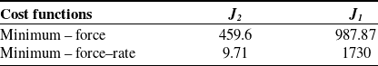
From Figure 6(b) left and Figure 5(b) right, although drastic changes are restrained compared to GPOPS-II, force changes are still seen in F 1 and F 3 . Note that, when it is used with minimum-force, in cable 1, there is a significant change in force (about 6 N in half a second). By changing the scenario, the minimum-force-rate problem is applied. Comparing Figure 6(b) right and Figure 6(b) left, it is illustrated that cable force changes have fallen effectively. In Table III, a comparison of two objective functions is presented, observed during a simulation comprising 24 nodes. The analysis reveals that by opting for the minimum-force-rate criterion instead of the minimum-force criterion, the total sum of squared robot actuator forces experienced a modest increase of only 70%, but on the other hand, more than 4,000% smoother internal forces.
With a pneumatic cylinder in the system, minimizing jerky motions is crucial. Abrupt actuator forces can cause significant deviations from the desired path, making smooth actuation essential for control and stability. The result shows that the actuator force-rate experiences a substantial reduction, decreasing by more than 46 times. As a result, both the tension rate in the cables and the force-rate in the cylinder have effectively decreased, enabling the generation of continuous tensions for CDPR. In light of this, to promote continuous tension, it is advisable to substitute the minimum-force cost function with the minimum-force-rate objective function.
6. Experimental study
6.1. Experimental set-up
To validate the feasibility of optimal trajectories using the proposed algorithm, a test bed is constructed. The developed experimental set-up is shown in Figure 7. In the winch-driven actuation system, each cable is tensioned using a 2-phase 24V DC stepping motor with a holding torque of 12.8 Nm, which refers to the maximum static torque the motor can exert without losing steps —1.8-degree step angle—when energized but not rotating.
To provide compressed air, a storage tank is in line with the compressor. The air compressor works at 230V AC with 2.5 hp and gives a 116 PSI maximum pressure. Two 24V DC VPPE Festo valves control the Festo cylinder, DNC-125-500-PPV-A. Arduino ATmega2560 (Figure 8) controls the stepper motors and VPPE valves. Also, a 48V power supply powers the stepper motor, and a 24V power supply powers the VPPE Festo valves. The complete electrical schematic is illustrated in Figure 8. All electronic components of the CDPR—including the Arduino ATmega2560, power supplies, motor drivers, and peripheral control boards—are integrated within a centralized electrical panel. The stepper motors are driven by Kinko’s 2CM880 drivers. An IR Sharp sensor is employed to measure the displacement of the pneumatic cylinder and is interfaced directly with the microcontroller. The Arduino ATmega2560, despite its limited computational resources and lack of hardware-level parallelism, was employed for real-time control of the CDPR. To ensure smooth and synchronized motor actuation across all three axes, an efficient control strategy based on interrupt-driven timers and feedforward execution of precomputed waypoints was implemented. This minimized computational load during operation while maintaining acceptable timing precision. Additionally, an Arduino Nano with an onboard gyroscope was mounted on the EE to provide orientation feedback to the main microcontroller. Both were programmed using the Arduino IDE, and sensor data was relayed to a host PC for acquisition and processing.
Comparison of results for objective functions.

Comparing kinematic and kinetic variables for DC solutions: minimum–force on the left and, minimum–force–rate on the right. (a) End-effector’s angles and end position of the cylinder. (b) Cable tensions.

General overview of experimental set-up.

Electrical drawing.

6.2. Comparison of experimental and simulation results
The EE angular velocity and the cylinder force are calculated from the simulation data by the minimum-force-rate objective function. Experimental results demonstrate that regulating sudden variations in cable forces led to significantly smoother EE motion. The stepper motor angular velocities are computed using the system Jacobian, and along with the cylinder force, these are provided as control inputs to the CDPR via the Arduino ATmega 2,560 board, enabling the robot’s motion. A gyroscope sensor sends the CDPR pitch and roll angle. Also, the IR Sharp sensor records the end position of the prismatic actuator.
The input data utilized for the CDPR is generated independently using the two trajectory planning approaches—GPOPS-II and the proposed DC method. These inputs include the desired EE trajectories, cable tension profiles, and actuator commands required to realize the planned motion. A comparative overview of these input datasets for both methods is illustrated in Figure 9, highlighting the distinctions in the resulting reference trajectories and control effort distributions. This comparison forms the basis for subsequent experimental validation, enabling a direct assessment of how the planned trajectories from each method translate into real system performance.
Comparison of input profiles for the CDPR generated using the minimum–force-rate cost function. The left column corresponds to the proposed DC method, while the right column shows the GPOPS-II results. Subplots (a)–(b) depict the angular velocities of the three stepper motors, and (c)–(d) illustrate the corresponding spine actuation forces.

Figure 10 shows the CDPR orientation and position in the experiment and its comparison with the numerical results for the two methods, GPOPS-II and DC. High variations in force rates can introduce oscillations in the cables, leading to dynamic instability. A smooth force rate minimizes cable vibrations, preserving structural integrity and reducing undesired oscillations. Furthermore, smooth tension variations improve the performance of feedback controllers by reducing control effort and enabling more precise trajectory tracking.
Comparison of simulation and experimental results for the minimum–force-rate cost function. DC solutions are shown on the left and GPOPS-II solutions on the right. The plots illustrate the end-effector orientation angles (α, β), vertical position (z), and corresponding tracking errors.

Upon comparing the experimental and simulation outcomes, discrepancies become evident in trajectory tracking. A rapid change in force causes cables to go slack or experience excessive tension, leading to nonlinear discontinuities in the system dynamics. It’s worth noting that measurement inaccuracies could also contribute to these errors. The proposed actuators’ commands ensure cables remain under tension without violating constraints. Nevertheless, it’s noteworthy that, on the whole, the simulation results align favorably with the experimental data.
In this context, error signifies the disparity between the experimental results and the simulated values. Specifically, the most significant tracking deviation occurs along the vertical Z direction, where the maximum positional error reaches approximately 1.0 cm for the proposed DC method and 1.1 cm for the GPOPS-II trajectory. Furthermore, the maximum angular deviation in the EE orientation for angles α and $\beta $
is observed to be around 1° for the DC-based trajectory and 1.7° for the GPOPS-II trajectory. These results indicate that the DC method achieves slightly higher accuracy and smoother tracking performance, particularly in maintaining orientation consistency and minimizing vertical displacement errors. The model assumes an ideal universal joint and disregards factors such as the EE thickness, the cylinder dynamics, the cable mass, and the friction.
$\beta $
is observed to be around 1° for the DC-based trajectory and 1.7° for the GPOPS-II trajectory. These results indicate that the DC method achieves slightly higher accuracy and smoother tracking performance, particularly in maintaining orientation consistency and minimizing vertical displacement errors. The model assumes an ideal universal joint and disregards factors such as the EE thickness, the cylinder dynamics, the cable mass, and the friction.
7. Conclusion
The generation of algorithms for trajectory optimization is a critical aspect of the manipulation of CDPRs. Incorporating various equality and inequality constraints, including the regulation of cable tensions during trajectory planning, introduces significant complexity into the optimization problem. This study focuses on optimizing cable forces and addressing constraints related to the central spine. Existing trajectory optimization methods struggle to handle cable force constraints, which impose nonlinear dynamics on the problem space. Even minor errors can lead to trajectory deviations, resulting in unrealistic robot behavior and challenging control implementation. To address these issues, this article presents a method that minimizes dynamic errors in trajectories by selecting an appropriate objective function. Simulations using a minimum-force objective function revealed high force variations in certain cables. To mitigate this, minimizing force rates was proposed to achieve smoother trajectories, reduce numerical sensitivity to discretization errors, and preserve physical feasibility even under coarse discretization. Generally, the use of stepper motors is expected to affect trajectory tracking due to their discrete actuation and torque limitations at high speeds. In this study, angular velocity inputs were constrained within safe operating limits, and the use of a force-rate minimization objective yielded smoother trajectories. This reduced abrupt force variations and enabled reliable execution without stalling or step loss. Experimental results confirmed accurate and consistent tracking performance using stepper-driven CDPR hardware.
Despite the benefits, some undesirable effects of the minimum-force objective function were observed. To ensure trajectory continuity and smoothness, the cost function was refined to prioritize smoother internal actuation forces. As demonstrated in Table III, replacing the minimum-force objective function with a minimum-force-rate objective effectively generates continuous tension rates in CDPRs. This approach reduces the total actuator force-rate by over 46 times, while only incurring a 70% increase in the minimum-force cost, which is negligible. The design of the SQP algorithm, combined with a linear initial guess, enables the DC method to produce accurate, efficient, and optimal solutions. The linear initial guess between the boundary values of each state and control variable is considered in (3). The quality of the initial guess significantly influences trajectory optimization performance, as supported by comparative results against the GPOPS-II technique.
A dedicated testbed was developed to validate the theoretical outcomes against experimental data. While the dynamic model adopted in this work provides accuracy, it does not account for universal joint clearance, cable mass, cylinder dynamics, or component friction. Experimental results confirm the feasibility and smoothness of the proposed trajectory. The angular velocity inputs to the stepper motors remained within operational limits, and the resulting trajectory fit comfortably within the CDPR’s workspace, demonstrating its practical viability.
The experimental system employed open-loop control of stepper motors with a native resolution of 200 steps per revolution with inherent positioning uncertainty, but this effect was minimized through systematic calibration and signal filtering. Future iterations will integrate high-precision external sensing modalities to enhance measurement fidelity and support closed-loop control strategies. Additionally, the dynamic model fidelity can be improved in future work by incorporating cable mass and friction effects to reduce simulation–experiment discrepancies and enhance the accuracy of trajectory tracking and actuator force estimation in the CDPR system.
Author contributions
MB (SUT) carried out the visualization and investigation. MB (UNSW) acquired funding and provided supervision. Both authors, MB (SUT) and MB (UNSW), jointly contributed to study design, hardware development, methodology, and writing – review and editing.
Financial support
This research received no specific grant from any funding agency, commercial or not-for-profit sectors.
Competing interest
The authors declare no conflicts of interest exist.
Ethical standards
Not applicable.
Use of AI
AI tools were not used in the research or writing of this paper.
Appendix A
This appendix provides a detailed explanation of the generalized forces used in the development of the system’s dynamic model via the Lagrangian method. The cable directions, s i is obtained from (10), and the cylinder force s n , is in K direction. Hence, the actuator forces are defined as:
 \begin{equation} \mathbf{T}_{i}=T_{i}\mathbf{s}_{i}=T_{i}\,\mathbf{l}_{i}/l_{i}(i=1,2,3),\,\mathbf{F}_{\mathbf{z}}=F_{n}\mathbf{s}_{n}=F_{n}\mathbf{K} \end{equation}
where:
 \begin{equation*} \mathbf{l}_{1}=\left[\begin{array}{c} r_{b}-r_{e}\cos \beta -l_{0}\cos \alpha \sin \beta \\[5pt] \,\,\,\,\,\,\,\,\,\,\,\,\,\,\,\,\,\,\,\,\,\,\,\,\,\,\,\,\,\,\,\,\,l_{0}\sin \alpha \\[5pt] h_{0}-z-d_{0}+r_{e}\sin \beta -l_{0}\cos \alpha \cos \beta \end{array}\right] \end{equation*}
 \begin{equation*} \mathbf{l}_{2}=\left[\begin{array}{c} -r_{b}/2+r_{e}\cos \beta /2-l_{0}\cos \alpha \sin \beta -\sqrt{3}r_{e}\sin \alpha \sin \beta /2\\[5pt] l_{0}\sin \alpha +\sqrt{3}r_{b}/2-\sqrt{3}r_{e}\cos \alpha /2\\[5pt] h_{0}-z-d_{0}-r_{e}\sin \beta /2-l_{0}\cos \alpha \cos \beta -\sqrt{3}r_{e}\cos \beta \sin \alpha /2 \end{array}\right] \end{equation*}
 \begin{equation*} \mathbf{l}_{3}=\left[\begin{array}{c} -r_{b}/2+r_{e}\cos \beta /2-l_{0}\cos \alpha \sin \beta +\sqrt{3}r_{e}\sin \alpha \sin \beta /2\\[5pt] l_{0}\sin \alpha -\sqrt{3}r_{b}/2+\sqrt{3}r_{e}\cos \alpha /2\\[5pt] h_{0}-z-d_{0}-r_{e}\sin \beta /2-l_{0}\cos \alpha \cos \beta +\sqrt{3}r_{e}\cos \beta \sin \alpha /2 \end{array}\right] \end{equation*}
The position vectors of the cable forces are obtained as:
 \begin{equation} \,\mathbf{r}_{{T_{i}}}=[0\ 0\ d_{0}+z]^{T}+\mathbf{R}\times \mathbf{E}_{i})_{mov}\,(i=1,2,3) \end{equation}
where: $\mathbf{r}_{T_1} = \begin{bmatrix} 0 & 0 & z + d_0 \end{bmatrix}^{T} + \mathbf{R} \begin{bmatrix} r_e & 0 & l_0 \end{bmatrix}^{T} = \begin{bmatrix} r_e \cos\beta + l_0 \cos\alpha \sin\beta \\ -\,l_0 \sin\alpha \\ z + d_0 - r_e \sin\beta + l_0 \cos\alpha \cos\beta \end{bmatrix}$

and finally:
 \begin{equation} \mathbf{r}_{{F_{z}}}=[00d_{0}+z]^{T} \end{equation}
Therefore, for generalized coordinates α, $\beta$
and z, the generalized forces can be obtained by:
$\beta$
and z, the generalized forces can be obtained by:
 \begin{align} Q_{\alpha } & =\mathbf{T}_{1}\cdot \dfrac{\partial \mathbf{r}_{{T_{1}}}}{\partial \alpha }+\mathbf{T}_{2}\cdot \dfrac{\partial \mathbf{r}_{{T_{2}}}}{\partial \alpha }+\mathbf{T}_{3}\cdot \dfrac{\partial \mathbf{r}_{{T_{3}}}}{\partial \alpha }+\mathbf{F}_{z}\cdot \dfrac{\partial \mathbf{r}_{{F_{z}}}}{\partial \alpha }\nonumber\\[10pt] Q_{\beta } & =\mathbf{T}_{1}\cdot \dfrac{\partial \mathbf{r}_{{T_{1}}}}{\partial \beta }+\mathbf{T}_{2}\cdot \dfrac{\partial \mathbf{r}_{{T_{2}}}}{\partial \beta }+\mathbf{T}_{3}\cdot \dfrac{\partial \mathbf{r}_{{T_{3}}}}{\partial \beta }+\mathbf{F}_{z}\cdot \dfrac{\partial \mathbf{r}_{{F_{z}}}}{\partial \beta }\nonumber\\[10pt] Q_{z} & =\mathbf{T}_{1}\cdot \dfrac{\partial \mathbf{r}_{{T_{1}}}}{\partial z}+\mathbf{T}_{2}\cdot \dfrac{\partial \mathbf{r}_{{T_{2}}}}{\partial z}+\mathbf{T}_{3}\cdot \dfrac{\partial \mathbf{r}_{{T_{3}}}}{\partial z}+\mathbf{F}_{z}\cdot \dfrac{\partial \mathbf{r}_{{F_{z}}}}{\partial z} \end{align}
Appendix B
The detailed formulations of closed-form dynamic including mass matrix M, mass matrix $\boldsymbol{M} \in \boldsymbol{R}^{3\times 3}$
, Coriolis and centrifugal vector
$\boldsymbol{M} \in \boldsymbol{R}^{3\times 3}$
, Coriolis and centrifugal vector $\boldsymbol{C} \in \boldsymbol{R}^{3\times 1}$
,
$\boldsymbol{C} \in \boldsymbol{R}^{3\times 1}$
, $\boldsymbol{Q} \in \boldsymbol{R}^{3\times 1}$
, and gravity vector
$\boldsymbol{Q} \in \boldsymbol{R}^{3\times 1}$
, and gravity vector $\boldsymbol{G} \in \boldsymbol{R}^{3\times 1}$
is generated here:
$\boldsymbol{G} \in \boldsymbol{R}^{3\times 1}$
is generated here:
 \begin{equation} \mathbf{M}\ddot{\mathbf{x}}+\mathbf{C}+\mathbf{G}=\mathbf{Q} \end{equation}
where:
 \begin{align} \mathbf{x}&=[z\,\,\,\alpha \,\,\,\beta ]^{T}\\[-10pt]\nonumber \end{align}
 \begin{align} \mathbf{M}&=\left[\begin{array}{l@{\quad}l@{\quad}l} m_{11} & m_{12}& m_{13}\\ m_{21}& m_{22} & m_{23}\\ m_{31} & m_{32} & m_{33} \end{array}\right] \end{align}
where:
 \begin{equation*} m_{11}=-ml_{c}\cos \beta \sin \alpha \end{equation*}
 \begin{equation*} m_{12}=m{l_{c}}^{2}+I_{x}cos^{2}\beta +I_{z}sin^{2}\beta \end{equation*}
 \begin{equation*} m_{13}=0 \end{equation*}
 \begin{equation*}m_{21}=-ml_{c}\cos \alpha \sin \beta\end{equation*}
 \begin{equation*}m_{22}=0\end{equation*}
 \begin{equation*}m_{23}=m{l_{c}}^{2}cos^{2}\alpha +I_{y}\end{equation*}
 \begin{equation*} m_{31}=m \end{equation*}
 \begin{equation*}m_{32}=-ml_{c}\cos \beta \sin \alpha\end{equation*}
 \begin{equation*} m_{33}=-ml_{c}\cos \alpha \sin \beta \end{equation*}
 \begin{equation} \mathbf{G} = [g_{1}\ g_{2}\ g_{3}]^{T}\end{equation}
where:
 \begin{equation*}g_{1}=-mgl_{c}\cos \beta \sin \alpha\end{equation*}
 \begin{equation*}g_{2}=-mgl_{c}\cos \alpha \sin \beta\end{equation*}
 \begin{equation*}g_{3}=mg\end{equation*}
 \begin{equation} \mathbf{C}=[c_{1}\ c_{2}\ c_{3}]^{T} \end{equation}
where:
 \begin{equation*} c_{1}=m{l_{c}}^{2}\dot{\beta }^{2}sin(2\alpha)/2-I_{x}\dot{\alpha }\dot{\beta }sin(2\beta)+I_{z}\dot{\alpha }\dot{\beta }sin(2\beta)-ml_{c}\dot{\alpha }\dot{z}\mathit{\cos }\mathit{\alpha }cos\beta \end{equation*}
 \begin{equation*} c_{2}=I_{x}\dot{\alpha }^{2}sin(2\beta )/2-I_{z}\dot{\alpha }^{2}sin(2\beta )/2-ml_{c}\textit{zcos}\mathit{\alpha }sin\beta -m{l_{c}}^{2}\dot{\alpha }\dot{\beta }sin(2\alpha )-ml_{c}\dot{\beta }\dot{z}\mathit{\cos }\mathit{\alpha }cos\beta \end{equation*}
 \begin{equation*} c_{3}=-m(2\dot{\alpha }^{2}l_{c}\mathit{\cos }\mathit{\alpha }cos\beta -4l_{c}\dot{\alpha }\dot{\beta }\mathit{\sin }\mathit{\alpha }sin\beta +2\dot{\beta }^{2}l_{c}\mathit{\cos }\mathit{\alpha }cos\beta )/2 \end{equation*}
 \begin{equation} \mathbf{Q}=[q_{1}\ q_{2}\ q_{3}]^{T} \end{equation}
The components $q_{1}$
and
$q_{1}$
and $q_{2}$
are omitted to avoid displaying lengthy expressions; only
$q_{2}$
are omitted to avoid displaying lengthy expressions; only $q_{3}$
is presented in full detail to illustrate the formulation:
$q_{3}$
is presented in full detail to illustrate the formulation:
 \begin{align*} q_{3}&=F_{n} - (T_{1}(d_{0} - h_{0} + z - r_{e}sin\beta + l_{0}\mathit{\cos }\mathit{\alpha }cos\beta ))/((d_{0} - h_{0} + z - r_{e}sin\beta \nonumber\\&\quad +l_{0}\mathit{\cos }\mathit{\alpha }cos\beta )^{2}+{l_{0}}^{2}sin^{2}\alpha +(r_{e}cos\beta -r_{b}+l_{0}\mathit{\cos }\mathit{\alpha }sin\beta )^{2})^{(1/2)}-(T_{2}(d_{0}-h_{0}+z+(r_{e}sin\beta )/2 \nonumber \\&\quad +l_{0}\mathit{\cos }\mathit{\alpha }cos\beta +(\sqrt{3}r_{e}\mathit{\cos }\mathit{\beta }sin\alpha )/2))/((l_{0}sin\alpha +(\sqrt{3}r_{b})/2-(\sqrt{3}r_{e}cos\alpha )/2)^{2} \nonumber \\&\quad +(r_{b}/2-(r_{e}cos\beta )/2+l_{0}\mathit{\cos }\mathit{\alpha }sin\beta +(\sqrt{3}r_{e}\mathit{\sin }\mathit{\alpha }sin\beta )/2)^{2}+ (d_{0} - h_{0} + z + r_{e}sin\beta /2 \nonumber \\&\quad + l_{0}\mathit{\cos }\mathit{\alpha }cos\beta +(\sqrt{3}r_{e}\mathit{\cos }\mathit{\beta }sin\alpha )/2)^{2})^{(1/2)}-(T_{3}(d_{0}-h_{0}+z+(r_{e}sin\beta )/2+l_{0}\mathit{\cos }\mathit{\alpha }cos\beta \nonumber \\&\quad -(\sqrt{3}r_{e}\mathit{\cos }\mathit{\beta }sin\alpha )/2))/((l_{0}sin\alpha -(\sqrt{3}r_{b})/2+(\sqrt{3}r_{e}cos\alpha )/2)^{2}+(r_{b}/2-(r_{e}cos\beta )/2+l_{0}\mathit{\cos }\mathit{\alpha }sin\beta \nonumber \\&\quad -(\sqrt{3}r_{e}\mathit{\sin }\mathit{\alpha }sin\beta )/2)^{2}+(d_{0} - h_{0} + z + r_{e}sin\beta /2 + l_{0}\mathit{\cos }\mathit{\alpha }cos\beta -(\sqrt{3}r_{e}\mathit{\cos }\mathit{\beta }sin\alpha )/2)^{2})^{(1/2)} \end{align*}


 Open access