




1. Introduction
In the seminal article [Reference TaelmanTae12], Taelman proved an analogue of the analytic class number formula for Drinfeld modules. He stated that ‘it should be possible to formulate and prove an equivariant version’ of this formula (cf. Remark 10 in [Reference TaelmanTae12]).
Let $\ell$
be a prime number and let q be a power of
$\ell$
be a prime number and let q be a power of $\ell$
. Let k be a finite separable extension of the rational function field
$\ell$
. Let k be a finite separable extension of the rational function field ${\mathbb F}_q(t)$
. Let K be a finite Galois extension of k with group
${\mathbb F}_q(t)$
. Let K be a finite Galois extension of k with group $G:=\mathrm{Gal}(K/k)$
.
$G:=\mathrm{Gal}(K/k)$
.
Let E be a Drinfeld ${\mathbb F}_q[t]$
-module defined over the ring of integers
${\mathbb F}_q[t]$
-module defined over the ring of integers $\mathcal O_k$
of k. We may then also regard E as being defined over
$\mathcal O_k$
of k. We may then also regard E as being defined over $\mathcal O_K$
, and G obviously acts on the
$\mathcal O_K$
, and G obviously acts on the ${\mathbb F}_q[t]$
-modules
${\mathbb F}_q[t]$
-modules $\mathcal O_K$
and
$\mathcal O_K$
and $E(\mathcal O_K)$
. The exponential map of E is Galois-equivariant and this fact implies that G acts naturally on the
$E(\mathcal O_K)$
. The exponential map of E is Galois-equivariant and this fact implies that G acts naturally on the ${\mathbb F}_q[t]$
-modules
${\mathbb F}_q[t]$
-modules $\mathbb U(E/\mathcal O_K)$
and
$\mathbb U(E/\mathcal O_K)$
and $H(E/\mathcal O_K)$
that are studied by Taelman [Reference TaelmanTae10] as respective analogues for
$H(E/\mathcal O_K)$
that are studied by Taelman [Reference TaelmanTae10] as respective analogues for $E/\mathcal O_K$
of the unit group and of the ideal class group of the ring of integers of a global field.
$E/\mathcal O_K$
of the unit group and of the ideal class group of the ring of integers of a global field.
An equivariant, or ‘refined’, version of Taelman’s class number formula for $(E,K/k)$
should encode the action of G on these arithmetic
$(E,K/k)$
should encode the action of G on these arithmetic ${\mathbb F}_q[t]$
-modules. In the main result of this article, Theorem 2.17, we prove such a formula, which specialises to recover Taelman’s for
${\mathbb F}_q[t]$
-modules. In the main result of this article, Theorem 2.17, we prove such a formula, which specialises to recover Taelman’s for $K=k$
.
$K=k$
.
In the case that the Galois group G of $K/k$
is abelian, a refined class number formula has recently been obtained by Ferrara, Green, Higgins and Popescu [Reference Ferrara, Green, Higgins and PopescuFGH+22], who refer to it as an ‘equivariant Tamagawa number formula’. Our formula also specialises to recover it for such abelian extensions.
$K/k$
is abelian, a refined class number formula has recently been obtained by Ferrara, Green, Higgins and Popescu [Reference Ferrara, Green, Higgins and PopescuFGH+22], who refer to it as an ‘equivariant Tamagawa number formula’. Our formula also specialises to recover it for such abelian extensions.
In the following, we set $A:={\mathbb F}_q[t]$
,
$A:={\mathbb F}_q[t]$
, $\mathcal F:={\mathbb F}_q(t)$
and
$\mathcal F:={\mathbb F}_q(t)$
and $\mathcal F_\infty:={\mathbb F}_q(\!(t^{-1})\!)$
, the completion of
$\mathcal F_\infty:={\mathbb F}_q(\!(t^{-1})\!)$
, the completion of $\mathcal F$
at the place at infinity (i.e. of uniformiser
$\mathcal F$
at the place at infinity (i.e. of uniformiser $t^{-1}$
). We interpret our given Drinfeld A-module
$t^{-1}$
). We interpret our given Drinfeld A-module $E/\mathcal O_k$
as a functor that assigns
$E/\mathcal O_k$
as a functor that assigns $\mathcal O_k[G]$
-modules M a new A-action, thus a new A[G]-module structure E(M).
$\mathcal O_k[G]$
-modules M a new A-action, thus a new A[G]-module structure E(M).
1.1 The refined trace formula
1.1.1 Characteristic classes
Taelman interprets the special L-value of $E/\mathcal O_K$
as an Euler product whose factors compare the characteristic polynomials of the finite A-modules
$E/\mathcal O_K$
as an Euler product whose factors compare the characteristic polynomials of the finite A-modules $\mathcal O_K/\mathfrak{p}$
and
$\mathcal O_K/\mathfrak{p}$
and $E(\mathcal O_K/\mathfrak{p})$
, as
$E(\mathcal O_K/\mathfrak{p})$
, as $\mathfrak{p}$
runs through the maximal ideals of
$\mathfrak{p}$
runs through the maximal ideals of $\mathcal O_K$
.
$\mathcal O_K$
.
At the moment there is, however, no suitable notion of ‘reduced determinant’ or ‘reduced norm’ over general group rings in positive characteristic (but see also § 1.3 below for a more detailed discussion of this issue).
As a key component of our approach and a generalisation of the notion of characteristic polynomial we are led to define, for suitable finite A[G]-modules M, the ‘characteristic class’ $c_G(M)$
of M to be the class of the automorphism
$c_G(M)$
of M to be the class of the automorphism
 $$(t\otimes 1)-(1\otimes t)$$
of $\mathcal F_\infty[G]\otimes_{{\mathbb F}_q[G]}M$
, regarded as an element of the Whitehead group
$\mathcal F_\infty[G]\otimes_{{\mathbb F}_q[G]}M$
, regarded as an element of the Whitehead group $K_1(\mathcal F_\infty[G])$
of the group ring
$K_1(\mathcal F_\infty[G])$
of the group ring $\mathcal F_\infty[G]$
(see Definition 2.4 for details).
$\mathcal F_\infty[G]$
(see Definition 2.4 for details).
We observe that if G is abelian, then the determinant of the characteristic class of M is simply a generator of the Fitting ideal of M in A[G] while, if $\ell$
does not divide
$\ell$
does not divide $|G|$
, then its reduced norm is a generator of the non-commutative Fitting invariant of M, as defined by Nickel [Reference NickelNic10] or by Burns and Sano [Reference Burns and SanoBS25] (see Lemma 3.10).
$|G|$
, then its reduced norm is a generator of the non-commutative Fitting invariant of M, as defined by Nickel [Reference NickelNic10] or by Burns and Sano [Reference Burns and SanoBS25] (see Lemma 3.10).
In the general case, characteristic classes allow us to define equivariant special L-values for $(E,K/k)$
as Euler products in the abelian group
$(E,K/k)$
as Euler products in the abelian group $K_1(\mathcal F_\infty[G])$
.
$K_1(\mathcal F_\infty[G])$
.
1.1.2 Convergence and the trace formula
As an essential intermediate result towards the proof of his main theorem, Taelman proves a ‘trace formula’ in $\mathcal F_\infty^\times$
for the Euler products that arise from global ‘nuclear’ automorphisms (see [Reference TaelmanTae12, Theorem 3]). This result is a generalisation of the trace formula of Anderson [Reference AndersonAnd00].
$\mathcal F_\infty^\times$
for the Euler products that arise from global ‘nuclear’ automorphisms (see [Reference TaelmanTae12, Theorem 3]). This result is a generalisation of the trace formula of Anderson [Reference AndersonAnd00].
As a special case, Taelman deduces the convergence in $\mathcal F_\infty^\times$
of the special L-value of E to the (infinite-dimensional) determinant of a certain global action defined by E.
$\mathcal F_\infty^\times$
of the special L-value of E to the (infinite-dimensional) determinant of a certain global action defined by E.
We endow $K_1(\mathcal F_\infty[G])$
with the quotient topology of the natural group topology in
$K_1(\mathcal F_\infty[G])$
with the quotient topology of the natural group topology in $\mathcal F_\infty[G]^\times$
and prove a refined trace formula in this topological group (see Theorem 5.5). As far as we are aware, the idea of studying the convergence of Euler products directly in an algebraic K-group is completely new.
$\mathcal F_\infty[G]^\times$
and prove a refined trace formula in this topological group (see Theorem 5.5). As far as we are aware, the idea of studying the convergence of Euler products directly in an algebraic K-group is completely new.
In Corollary 5.6 we then deduce a convergence formula for the special L-values for $(E,K/k)$
. For
$(E,K/k)$
. For $K=k$
, this result corresponds to Taelman’s via the determinant map
$K=k$
, this result corresponds to Taelman’s via the determinant map $K_1(\mathcal F_\infty)\cong \mathcal F_\infty^\times$
. More generally, if G is abelian, then it corresponds via the determinant
$K_1(\mathcal F_\infty)\cong \mathcal F_\infty^\times$
. More generally, if G is abelian, then it corresponds via the determinant $K_1(\mathcal F_\infty[G])\cong \mathcal F_\infty[G]^\times$
to [Reference Ferrara, Green, Higgins and PopescuFGH+22, Corollary 3.0.3]. One should thus think of the refined trace formula as a direct relation between the relevant A[G]-actions.
$K_1(\mathcal F_\infty[G])\cong \mathcal F_\infty[G]^\times$
to [Reference Ferrara, Green, Higgins and PopescuFGH+22, Corollary 3.0.3]. One should thus think of the refined trace formula as a direct relation between the relevant A[G]-actions.
As a key step towards the refined trace formula, we prove a topological extension of the structural result [Reference Fukaya and KatoFK06, Proposition 1.5.1] of Fukaya and Kato for Whitehead groups of adic rings (see Proposition 4.4).
1.2 The refined class number formula
1.2.1 The lattice of units and the class group
In [Reference TaelmanTae10], Taelman studies the kernel $\mathbb U(E/\mathcal O_K)$
and the cokernel
$\mathbb U(E/\mathcal O_K)$
and the cokernel $H(E/\mathcal O_K)$
of the exponential map
$H(E/\mathcal O_K)$
of the exponential map
 \begin{equation}K_\infty\longrightarrow E(K_\infty)/E(\mathcal O_K)\end{equation}
of E. Here we have set $K_\infty:=\mathcal F_\infty\otimes_{\mathcal F}K$
. He proves that
$K_\infty:=\mathcal F_\infty\otimes_{\mathcal F}K$
. He proves that $\mathbb U(E/\mathcal O_K)$
is a finitely generated A-submodule of
$\mathbb U(E/\mathcal O_K)$
is a finitely generated A-submodule of $K_\infty$
, while
$K_\infty$
, while $H(E/\mathcal O_K)$
is a finite A-module.
$H(E/\mathcal O_K)$
is a finite A-module.
As an equivariant version of these results, we prove in Theorem 6.19 that appropriate modifications of (1.1), which we refer to as ‘complexes of units’ for $(E,K/k)$
, are perfect complexes of A[G]-modules; that is, isomorphic in the derived category to a bounded complex of finitely generated, projective modules.
$(E,K/k)$
, are perfect complexes of A[G]-modules; that is, isomorphic in the derived category to a bounded complex of finitely generated, projective modules.
1.2.2 The refined Euler characteristic of the complex of units
Taelman’s class number formula for $E/\mathcal O_K$
in [Reference TaelmanTae12] states that the ratio of co-volumes in
$E/\mathcal O_K$
in [Reference TaelmanTae12] states that the ratio of co-volumes in $\mathcal F_\infty^\times$
of the A-lattices
$\mathcal F_\infty^\times$
of the A-lattices $\mathcal O_K$
and
$\mathcal O_K$
and $\mathbb U(E/\mathcal O_K)$
, multiplied by the characteristic polynomial of
$\mathbb U(E/\mathcal O_K)$
, multiplied by the characteristic polynomial of $H(E/\mathcal O_K)$
, coincides with the special L-value of
$H(E/\mathcal O_K)$
, coincides with the special L-value of $E/\mathcal O_K$
. To be more precise, this first term is defined through the determinant that measures the relative positions of
$E/\mathcal O_K$
. To be more precise, this first term is defined through the determinant that measures the relative positions of $\mathcal O_K$
and
$\mathcal O_K$
and $\mathbb U(E/\mathcal O_K)$
in
$\mathbb U(E/\mathcal O_K)$
in $K_\infty$
, but see also Remarks 8 and 14 in [Reference TaelmanTae12].
$K_\infty$
, but see also Remarks 8 and 14 in [Reference TaelmanTae12].
Our main result, the refined class number formula for $(E,K/k)$
(see Theorem A, and Theorem 2.17 for a precise version thereof), compares the special L-value for
$(E,K/k)$
(see Theorem A, and Theorem 2.17 for a precise version thereof), compares the special L-value for $(E,K/k)$
to the refined Euler characteristic of the complex of units for
$(E,K/k)$
to the refined Euler characteristic of the complex of units for $(E,K/k)$
. Specifically, we consider the image of the special L-value for
$(E,K/k)$
. Specifically, we consider the image of the special L-value for $(E,K/k)$
under the canonical homomorphism
$(E,K/k)$
under the canonical homomorphism
 $$K_1(\mathcal F_\infty[G])\,\longrightarrow \,K_0(A[G],\mathcal F_\infty[G])$$
to the relative algebraic $K_0$
-group of the ring inclusion
$K_0$
-group of the ring inclusion $A[G]\subset\mathcal F_\infty[G]$
(see Remark 2.19 for the explicit definition of this homomorphism).
$A[G]\subset\mathcal F_\infty[G]$
(see Remark 2.19 for the explicit definition of this homomorphism).
Relative $K_0$
-groups of inclusions of group rings are by now regarded as the natural environment for equivariant special L-value formulas (see e.g. [Reference BurnsBur11, Reference BurnsBur15, Reference Burns and FlachBF01, Reference Burns and KakdeBK25, Reference Coates, Fukaya, Kato, Sujatha and VenjakobCFK+05, Reference KakdeKak13, Reference Ritter and WeissRW11]). In particular,
$K_0$
-groups of inclusions of group rings are by now regarded as the natural environment for equivariant special L-value formulas (see e.g. [Reference BurnsBur11, Reference BurnsBur15, Reference Burns and FlachBF01, Reference Burns and KakdeBK25, Reference Coates, Fukaya, Kato, Sujatha and VenjakobCFK+05, Reference KakdeKak13, Reference Ritter and WeissRW11]). In particular, $K_0(A[G],\mathcal F_\infty[G])$
is the natural environment for the refined Euler characteristic of a pair
$K_0(A[G],\mathcal F_\infty[G])$
is the natural environment for the refined Euler characteristic of a pair $(C,\mu)$
comprising a perfect complex C of A[G]-modules (that satisfies an additional condition as in Definition 2.8) and an
$(C,\mu)$
comprising a perfect complex C of A[G]-modules (that satisfies an additional condition as in Definition 2.8) and an $\mathcal F_\infty$
-trivialisation
$\mathcal F_\infty$
-trivialisation $\mu$
of C (in the sense of [Reference Burns and Macias CastilloBMC14, 2.3.2]). The adjective ‘refined’ refers here to the fact that the refined Euler characteristic of
$\mu$
of C (in the sense of [Reference Burns and Macias CastilloBMC14, 2.3.2]). The adjective ‘refined’ refers here to the fact that the refined Euler characteristic of $(C,\mu)$
maps to the classical Euler characteristic of C in the Grothendiek group
$(C,\mu)$
maps to the classical Euler characteristic of C in the Grothendiek group $K_0(A[G])$
.
$K_0(A[G])$
.
Such refined Euler characteristics can be defined by mimicking the use of Deligne’s determinant functor (with values in the category of virtual objects) that is made by Breuning and Burns in [Reference Breuning and BurnsBB05] (see Remark 2.11). They provide a conceptual and general interpretation of the ratios of co-volumes that occur in [Reference TaelmanTae12, Reference Ferrara, Green, Higgins and PopescuFGH+22].
For simplicity, we use instead a completely explicit definition in the special case of interest for this article (see Definition 2.9). In particular, other than to state Theorem A, we do not use the term ‘trivialisation’ in the rest of this article.
Our refined class number formula (Theorems A and 2.17) specialises to recover the equivariant Tamagawa number formula of Ferrara et al. [Reference Ferrara, Green, Higgins and PopescuFGH+22] for abelian extensions, and thus also Taelman’s main result in [Reference TaelmanTae12] for $K=k$
(see Remark 2.19, and Remark 6.7 for further details).
$K=k$
(see Remark 2.19, and Remark 6.7 for further details).
1.2.3 Taming modules
In the above discussion we have referred to special L-values and to complexes of units for $(E,K/k)$
, both in plural, so as to avoid mentioning a specific technical issue, which we now address explicitly to state Theorem A.
$(E,K/k)$
, both in plural, so as to avoid mentioning a specific technical issue, which we now address explicitly to state Theorem A.
By Noether’s theorem, $\mathcal O_K$
is projective as an
$\mathcal O_K$
is projective as an $\mathcal O_k[G]$
-module if and only if the ring extension
$\mathcal O_k[G]$
-module if and only if the ring extension $\mathcal O_K/\mathcal O_k$
is tamely ramified. In fact, given a maximal ideal
$\mathcal O_K/\mathcal O_k$
is tamely ramified. In fact, given a maximal ideal $\mathfrak{p}$
of
$\mathfrak{p}$
of $\mathcal O_k$
, the quotient
$\mathcal O_k$
, the quotient $\mathcal O_K/\mathfrak{p}\mathcal O_K$
is
$\mathcal O_K/\mathfrak{p}\mathcal O_K$
is ${\mathbb F}_q[G]$
-projective if and only if
${\mathbb F}_q[G]$
-projective if and only if $\mathfrak{p}$
is tamely ramified in
$\mathfrak{p}$
is tamely ramified in $K/k$
, but the notion of characteristic class only suits finite A[G]-modules that are
$K/k$
, but the notion of characteristic class only suits finite A[G]-modules that are ${\mathbb F}_q[G]$
-projective.
${\mathbb F}_q[G]$
-projective.
In a similar way, it follows easily from Noether’s theorem that if $\mathcal O_K/\mathcal O_k$
is not tamely ramified, then the complex of A[G]-modules (1.1) cannot itself be perfect.
$\mathcal O_K/\mathcal O_k$
is not tamely ramified, then the complex of A[G]-modules (1.1) cannot itself be perfect.
To get around these technical difficulties, we use the notion of ‘taming module’ introduced by Ferrara et al. [Reference Ferrara, Green, Higgins and PopescuFGH+22, Definition 1.3.2]. Although it is discussed in the abelian setting in [Reference Ferrara, Green, Higgins and PopescuFGH+22], taming modules $\mathcal M$
exist for general Galois extensions
$\mathcal M$
exist for general Galois extensions $K/k$
(see Definition 2.13 and Remark 2.14), with the following basic properties:
$K/k$
(see Definition 2.13 and Remark 2.14), with the following basic properties:
-
– $\mathcal M$
is a projective A[G]-submodule of
$\mathcal O_K$
with finite index; and
$\mathcal M$
is a projective A[G]-submodule of
$\mathcal O_K$
with finite index; and -
– for each maximal ideal
$\mathfrak{p}$
of
$\mathcal O_k$
, the
${\mathbb F}_q[G]$
-module
$\mathcal M/\mathfrak{p}\mathcal M$
is free with whenever
$$\mathcal M/\mathfrak{p}\mathcal M=\mathcal O_K/\mathfrak{p}\mathcal O_K$$
$\mathfrak{p}$
is tamely ramified in
$K/k$
.


In fact, if $\mathcal O_K/\mathcal O_k$
is tamely ramified, then the only taming module for
$\mathcal O_K/\mathcal O_k$
is tamely ramified, then the only taming module for $K/k$
is
$K/k$
is $\mathcal M=\mathcal O_K$
.
$\mathcal M=\mathcal O_K$
.
For a given taming module $\mathcal M$
, one can thus define a K-theoretic Euler factor at a wildly ramified prime
$\mathcal M$
, one can thus define a K-theoretic Euler factor at a wildly ramified prime $\mathfrak{p}$
of
$\mathfrak{p}$
of $\mathcal O_k$
as the difference between the characteristic classes
$\mathcal O_k$
as the difference between the characteristic classes $c_G(\mathcal M/\mathfrak{p}\mathcal M)$
and
$c_G(\mathcal M/\mathfrak{p}\mathcal M)$
and $c_G(E(\mathcal M/\mathfrak{p}\mathcal M))$
of the A[G]-modules
$c_G(E(\mathcal M/\mathfrak{p}\mathcal M))$
of the A[G]-modules $\mathcal M/\mathfrak{p}\mathcal M$
and
$\mathcal M/\mathfrak{p}\mathcal M$
and $E(\mathcal M/\mathfrak{p}\mathcal M)$
. Regarding
$E(\mathcal M/\mathfrak{p}\mathcal M)$
. Regarding $\mathcal M$
as fixed, we are thus led to define the ‘
$\mathcal M$
as fixed, we are thus led to define the ‘ $\mathcal M$
-modified L-value’
$\mathcal M$
-modified L-value’ $\Theta^{\mathcal M}_{E,K/k}$
of
$\Theta^{\mathcal M}_{E,K/k}$
of $(E,K/k)$
as the corresponding Euler product, which converges in
$(E,K/k)$
as the corresponding Euler product, which converges in $K_1(\mathcal F_\infty[G])$
(Corollary 5.6) as a consequence of our refined trace formula (Theorem 5.5).
$K_1(\mathcal F_\infty[G])$
(Corollary 5.6) as a consequence of our refined trace formula (Theorem 5.5).
In a similar way, for our fixed $\mathcal M$
, we define the ‘
$\mathcal M$
, we define the ‘ $\mathcal M$
-modified complex of units’ of
$\mathcal M$
-modified complex of units’ of $(E,K/k)$
to be the complex
$(E,K/k)$
to be the complex $C^{\mathcal M}_{E,K/k}$
of A[G]-modules
$C^{\mathcal M}_{E,K/k}$
of A[G]-modules
 $$K_\infty\,\xrightarrow{(\exp _E,0)}\,(E(K_\infty)/E(\mathcal M)) \oplus \mathcal M,$$
with the first term in degree one and $\exp _E$
induced by the exponential map of E.
$\exp _E$
induced by the exponential map of E.
Our main result, Theorem 2.17, may then be roughly stated as follows.
Theorem A. Let E be a Drinfeld module defined over $\mathcal O_k$
and let
$\mathcal O_k$
and let $\mathcal M$
be a taming module for
$\mathcal M$
be a taming module for $K/k$
. Then the following claims are valid.
$K/k$
. Then the following claims are valid.
-
(1) The infinite product
converges to a unique element of
$$\Theta^{\mathcal M}_{E,K/k}:=\prod_{\mathfrak{p}\in\textrm{MSpec}(\mathcal O_k)}(c_G(\mathcal M/\mathfrak{p}\mathcal M)\cdot c_G(E(\mathcal M/\mathfrak{p}\mathcal M))^{-1})$$
$K_1(\mathcal F_\infty[G])$
.
-
(2) The complex of A[G]-modules
$C^{\mathcal M}_{E,K/k}$
is perfect. -
(3) The canonical image of
$\Theta^{\mathcal M}_{E,K/k}$
in
$K_0(A[G],\mathcal F_\infty[G])$
is equal to the inverse of the refined Euler characteristic of the pair
$(C^{\mathcal M}_{E,K/k},\mu)$
, where
$\mu$
is the
$\mathcal F_\infty$
-trivialisation of
$C^{\mathcal M}_{E,K/k}$
induced by the inclusions
$\mathcal M\subseteq\mathcal O_K\subset K_\infty$
.






See also Remark 2.18 and Corollary 5.6 for further details on claim (1), and Remark 2.21 and Theorem 6.19 for further details on claim (2).
Although both sides of the equality in claim (3) depend on the given choice of $\mathcal M$
, the equality itself is a priori independent of the choice of taming module.
$\mathcal M$
, the equality itself is a priori independent of the choice of taming module.
We also refer the reader to Remark 6.2.4 in [Reference Ferrara, Green, Higgins and PopescuFGH+22] for a discussion of the analogy between the above instances of $\mathcal M$
-modification and the T-modifications that have been commonplace in the study of equivariant special Artin L-values for global fields since the work of Gross [Reference GrossGro88] and of Rubin [Reference RubinRub96]. We simply recall that such T-modifications are necessary in order to circumvent certain technical difficulties associated with the presence of roots of unity.
$\mathcal M$
-modification and the T-modifications that have been commonplace in the study of equivariant special Artin L-values for global fields since the work of Gross [Reference GrossGro88] and of Rubin [Reference RubinRub96]. We simply recall that such T-modifications are necessary in order to circumvent certain technical difficulties associated with the presence of roots of unity.
1.3 A construction of non-abelian Stickelberger elements
In this section we discuss some explicit consequences of our main result (Theorems A and 2.17).
By Maschke’s theorem, the group rings $\mathcal F[G]$
and
$\mathcal F[G]$
and $\mathcal F_\infty[G]$
are semisimple if and only if the characteristic
$\mathcal F_\infty[G]$
are semisimple if and only if the characteristic $\ell$
does not divide the degree of the extension
$\ell$
does not divide the degree of the extension $K/k$
. The theory of reduced norms is often restricted to semisimple rings in the literature.
$K/k$
. The theory of reduced norms is often restricted to semisimple rings in the literature.
More generally, given a finite group G, it is also a classical result (see Proposition 3.1) that group rings for G in characteristic $\ell$
decompose as finite direct sums of matrix rings over commutative rings if and only if G has an abelian
$\ell$
decompose as finite direct sums of matrix rings over commutative rings if and only if G has an abelian $\ell$
-Sylow subgroup and a normal
$\ell$
-Sylow subgroup and a normal $\ell$
-complement, if and only if
$\ell$
-complement, if and only if $\ell$
does not divide the order of the commutator subgroup of G. Over such group rings, it is still possible to define a well-behaved notion of reduced determinant that recovers semisimple reduced norms, as well as determinants in the abelian case (see Definition 3.5).
$\ell$
does not divide the order of the commutator subgroup of G. Over such group rings, it is still possible to define a well-behaved notion of reduced determinant that recovers semisimple reduced norms, as well as determinants in the abelian case (see Definition 3.5).
In the rest of § 1.3, we assume that $\ell$
does not divide the degree of K over the maximal abelian subextension of k in K. For any Drinfeld module
$\ell$
does not divide the degree of K over the maximal abelian subextension of k in K. For any Drinfeld module $E/\mathcal O_k$
and any taming module
$E/\mathcal O_k$
and any taming module $\mathcal M$
for
$\mathcal M$
for $K/k$
, we then define the ‘
$K/k$
, we then define the ‘ $\mathcal M$
-modified Stickelberger element’ of
$\mathcal M$
-modified Stickelberger element’ of $(E,K/k)$
as the reduced determinant of the
$(E,K/k)$
as the reduced determinant of the $\mathcal M$
-modified L-value,
$\mathcal M$
-modified L-value,
 $$\theta^{\mathcal M}_{E,K/k} := \mathrm{Nrd}_{\mathcal F_\infty[G]} (\Theta^{\mathcal M}_{E,K/k} ) \in Z(\mathcal F_\infty[G])^\times.$$
Here, $Z(\mathcal F_\infty[G])^\times$
denotes the unit group of the centre
$Z(\mathcal F_\infty[G])^\times$
denotes the unit group of the centre $Z(\mathcal F_\infty[G])$
of
$Z(\mathcal F_\infty[G])$
of $\mathcal F_\infty[G]$
.
$\mathcal F_\infty[G]$
.
Reduced determinants also allow us to define non-commutative Fitting ideals over A[G], in a manner that is compatible with the constructions of Nickel [Reference NickelNic10], Johnston and Nickel [Reference Johnston and NickelJN13] and Burns and Sano [Reference Burns and SanoBS25] for orders in semisimple algebras (see Definition 3.5).
As a consequence of Theorem 2.17, we then derive in Theorem 3.15 that suitable normalisations of $\theta^{\mathcal M}_{E,K/k}$
belong to the non-commutative Fitting ideal of the ‘
$\theta^{\mathcal M}_{E,K/k}$
belong to the non-commutative Fitting ideal of the ‘ $\mathcal M$
-modified Taelman class group’
$\mathcal M$
-modified Taelman class group’
 $$H(E/\mathcal M) := \textrm{cok} (K_\infty\,\xrightarrow{\exp _E}\, E(K_\infty)/E(\mathcal M) )$$
of $(E,K/k)$
. More precisely, we define a subset
$(E,K/k)$
. More precisely, we define a subset $\mathcal{R}$
of
$\mathcal{R}$
of $Z(\mathcal F_\infty[G])$
for which
$Z(\mathcal F_\infty[G])$
for which
 \begin{align*}Z(A[G])\cdot\theta^{\mathcal M}_{E,K/k}\cdot\mathcal{R} &\subseteq\textrm{Fit}_{A[G]}(H(E/\mathcal M))\\ &\subseteq \textrm{Fit}_{A[G]}(H(E/\mathcal O_K))\\&\subseteq \mathrm{Ann}_{Z(A[G])}(H(E/\mathcal O_K))\end{align*}
as ideals in the centre Z(A[G]) of A[G]. Let us note that $\theta^{\mathcal M}_{E,K/k}$
is typically transcendental, and that
$\theta^{\mathcal M}_{E,K/k}$
is typically transcendental, and that $\mathcal{R}$
is amenable to computation and always non-trivial (see Remark 3.18 and § 3.2.2).
$\mathcal{R}$
is amenable to computation and always non-trivial (see Remark 3.18 and § 3.2.2).
For any finite abelian extension $K/k$
and any Drinfeld module
$K/k$
and any Drinfeld module $E/\mathcal O_k$
, Theorem 3.15 recovers the ‘refined Brumer–Stark theorem for Drinfeld modules’ [Reference Ferrara, Green, Higgins and PopescuFGH+22, Theorem 1.5.5] of Ferrara et al. (see Remark 3.16).
$E/\mathcal O_k$
, Theorem 3.15 recovers the ‘refined Brumer–Stark theorem for Drinfeld modules’ [Reference Ferrara, Green, Higgins and PopescuFGH+22, Theorem 1.5.5] of Ferrara et al. (see Remark 3.16).
For any finite Galois extension $K/k$
of degree not divisible by
$K/k$
of degree not divisible by $\ell$
and any Drinfeld module
$\ell$
and any Drinfeld module $E/\mathcal O_k$
, one necessarily has
$E/\mathcal O_k$
, one necessarily has $\mathcal M=\mathcal O_K$
(so we may drop the superscript
$\mathcal M=\mathcal O_K$
(so we may drop the superscript $\mathcal M$
) and, as Corollary 3.21 to Theorem 3.15, we prove the equality of Z(A[G])-ideals
$\mathcal M$
) and, as Corollary 3.21 to Theorem 3.15, we prove the equality of Z(A[G])-ideals
 $$Z(A[G])\cdot\theta_{E,K/k}\cdot\mathcal{R}=\textrm{Fit}_{A[G]}(H(E/\mathcal O_K)).$$
This equality is a vast non-abelian generalisation of Theorem A of Anglès and Taelman in [Reference Anglès and TaelmanAT15] (see Remark 3.22).
The question of how to construct non-abelian Stickelberger elements in completely general finite Galois extensions $K/k$
remains open. We will return to it in future work.
$K/k$
remains open. We will return to it in future work.
1.4 Structure of the article
In § 2 we introduce characteristic classes and refined Euler characteristics and we state Theorem 2.17. In § 3 we introduce reduced determinants and non-commutative Fitting ideals and we state Theorem 3.15 and Corollary 3.21. In § 4 we prove a topological extension of a result of Fukaya and Kato for Whitehead groups and we use it to associate a suitable class to nuclear automorphisms. In § 5 we prove the refined trace formula and we apply it to derive the convergence of the special L-values. In § 6 we prove Theorem 2.17 and in § 7 we prove Theorem 3.15.
2. The refined class number formula
In this section we state our main result. We fix a prime number $\ell$
and a power q of
$\ell$
and a power q of $\ell$
. We set
$\ell$
. We set $A:={\mathbb F}_q[t]$
,
$A:={\mathbb F}_q[t]$
, $\mathcal F:={\mathbb F}_q(t)$
and
$\mathcal F:={\mathbb F}_q(t)$
and $\mathcal F_\infty:={\mathbb F}_q(\!(t^{-1})\!)$
. For any field extension
$\mathcal F_\infty:={\mathbb F}_q(\!(t^{-1})\!)$
. For any field extension $L/\mathcal F$
and A-module M, we set
$L/\mathcal F$
and A-module M, we set $M_L:=L\otimes_A M$
and use identical notation for homomorphisms.
$M_L:=L\otimes_A M$
and use identical notation for homomorphisms.
2.1 Characteristic classes
We first define the notion of characteristic classes in Whitehead groups.
2.1.1.
Unless otherwise specified, we regard all rings R as unital and all R-modules as left R-modules. We write Z(R) for their centre, $R^\times$
for their unit group and
$R^\times$
for their unit group and $K_1(R)$
for their Whitehead group.
$K_1(R)$
for their Whitehead group.
We recall that, in addition to its interpretation as the abelianisation of $\textrm{GL}(R)$
, the latter group is the
$\textrm{GL}(R)$
, the latter group is the $K_1$
-group of the category of finitely generated, projective R-modules (cf. [Reference SwanSwa78, Reference Curtis and ReinerCR87]). We write
$K_1$
-group of the category of finitely generated, projective R-modules (cf. [Reference SwanSwa78, Reference Curtis and ReinerCR87]). We write $[P,\phi]$
, or simply
$[P,\phi]$
, or simply $[\phi]$
when P is clear from the context, for the class of an automorphism
$[\phi]$
when P is clear from the context, for the class of an automorphism $\phi$
of a finitely generated projective R-module P. We always use multiplicative notation for
$\phi$
of a finitely generated projective R-module P. We always use multiplicative notation for $K_1$
-groups.
$K_1$
-groups.
A ring is said to be semilocal if the quotient by its Jacobson radical is a semisimple Artinian ring. If R is semilocal, then Bass’s theorem implies that the canonical group homomorphism $R^\times\to K_1(R)$
is surjective (see [Reference Curtis and ReinerCR87, Vol. II, Theorem 40.31]).
$R^\times\to K_1(R)$
is surjective (see [Reference Curtis and ReinerCR87, Vol. II, Theorem 40.31]).
If R is a semilocal topological ring, we endow $R^\times$
with the group topology induced by the injection
$R^\times$
with the group topology induced by the injection
 \[ R^\times\longrightarrow R\times R \]
that maps $u\in R^\times$
to
$u\in R^\times$
to $(u,u^{-1})$
. We then endow the quotient
$(u,u^{-1})$
. We then endow the quotient $K_1(R)$
of
$K_1(R)$
of $R^\times$
with the corresponding group topology. In general, this topology need not be Hausdorff, even if R is. In Proposition 4.4 below we prove that if R is an adic ring in the sense of [Reference Fukaya and KatoFK06], then
$R^\times$
with the corresponding group topology. In general, this topology need not be Hausdorff, even if R is. In Proposition 4.4 below we prove that if R is an adic ring in the sense of [Reference Fukaya and KatoFK06], then $K_1(R)$
is in fact a profinite abelian group.
$K_1(R)$
is in fact a profinite abelian group.
Lemma 2.1. Let $\beta:\Lambda\to S$
be an injective, continuous and open homomorphism between semilocal topological rings. Then the restriction
$\beta:\Lambda\to S$
be an injective, continuous and open homomorphism between semilocal topological rings. Then the restriction $\gamma:\Lambda^\times\to S^\times$
of
$\gamma:\Lambda^\times\to S^\times$
of $\beta$
, and the map
$\beta$
, and the map $\delta:K_1(\Lambda)\to K_1(S)$
induced by
$\delta:K_1(\Lambda)\to K_1(S)$
induced by $\beta$
, are both continuous and open. In particular,
$\beta$
, are both continuous and open. In particular, $\textrm{im}(\delta)$
is a clopen subgroup of
$\textrm{im}(\delta)$
is a clopen subgroup of $K_1(S)$
.
$K_1(S)$
.
Proof. We write $\iota_1$
,
$\iota_1$
, $\iota_2$
for the respective continuous injections
$\iota_2$
for the respective continuous injections $\Lambda^\times\to\Lambda\times\Lambda$
and
$\Lambda^\times\to\Lambda\times\Lambda$
and $S^\times\to S\times S$
that map u to
$S^\times\to S\times S$
that map u to $(u,u^{-1})$
, note that
$(u,u^{-1})$
, note that $\iota_2\circ\gamma=(\beta\times\beta)\circ\iota_1$
and fix open subsets
$\iota_2\circ\gamma=(\beta\times\beta)\circ\iota_1$
and fix open subsets $U_1,U_2$
of
$U_1,U_2$
of $\Lambda$
and
$\Lambda$
and $V_1,V_2$
of S. Then
$V_1,V_2$
of S. Then $\gamma$
is continuous because
$\gamma$
is continuous because
 $$\gamma^{-1}(\iota_2^{-1}(V_1\times V_2))=\iota_1^{-1}((\beta\times\beta)^{-1}(V_1\times V_2))=\iota_1^{-1}(\beta^{-1}(V_1)\times\beta^{-1}(V_2))$$
is open. In addition, $\gamma$
is open because the following image is open:
$\gamma$
is open because the following image is open:
 \begin{align*}\gamma(\iota_1^{-1}(U_1\times U_2))&=\{\beta(\lambda):\lambda\in\Lambda^\times, \lambda\in U_1, \lambda^{-1}\in U_2\}\\&=\{s\in(S^\times\cap\beta(U_1)): s^{-1}\in(S^\times\cap\beta(U_2))\}\\&=\{s\in S^\times:s\in\beta(U_1),s^{-1}\in\beta(U_2)\}\\&=\iota_2^{-1}(\beta(U_1)\times\beta(U_2)).\end{align*}
Here the second equality is valid because, if $s=\beta(u_1)\in S^\times$
with
$s=\beta(u_1)\in S^\times$
with $s^{-1}=\beta(u_2)$
and with
$s^{-1}=\beta(u_2)$
and with $u_i\in U_i$
, then
$u_i\in U_i$
, then $1=\beta(u_1u_2)$
so, since
$1=\beta(u_1u_2)$
so, since $\beta$
is injective,
$\beta$
is injective, $u_1$
belongs to
$u_1$
belongs to $\Lambda^\times$
with
$\Lambda^\times$
with $u_1^{-1}=u_2$
.
$u_1^{-1}=u_2$
.
We next write $\pi_1$
,
$\pi_1$
, $\pi_2$
for the respective surjections
$\pi_2$
for the respective surjections $\Lambda^\times\to K_1(\Lambda)$
and
$\Lambda^\times\to K_1(\Lambda)$
and $S^\times\to K_1(S)$
, recall that they are continuous and open, note that
$S^\times\to K_1(S)$
, recall that they are continuous and open, note that $\delta\circ\pi_1=\pi_2\circ\gamma$
and fix open subsets U of
$\delta\circ\pi_1=\pi_2\circ\gamma$
and fix open subsets U of $K_1(\Lambda)$
and V of
$K_1(\Lambda)$
and V of $K_1(S)$
. Then
$K_1(S)$
. Then $\delta$
is continuous because
$\delta$
is continuous because
 $$\delta^{-1}(V)=\pi_1(\gamma^{-1}(\pi_2^{-1}(V)))$$
is open, and $\delta$
is open because the following image is also open:
$\delta$
is open because the following image is also open:
 $$\delta(U)=\delta(\pi_1(\pi_1^{-1}(U)))=\pi_2(\gamma(\pi_1^{-1}(U))).$$
2.1.2.
We next recall some useful facts concerning group rings. Let G be a finite group. A G-module M is said to be G-cohomologically trivial, or G-c.t., if the Tate cohomology groups of M vanish in all degrees and with respect to all subgroups of G.
Lemma 2.2.
-
(i) If S is a Dedekind domain (or a field), then an S[G]-module is projective if and only if it is S-projective and G-c.t.
-
(ii) If
$T/S$
is an extension of fields and M,N are finitely generated S[G]-modules, then
$M\cong N$
if and only if
$T\otimes_S M\cong T\otimes_S N$
over T[G]. -
(iii) If S is a discrete valuation ring with quotient field T and M,N are finitely generated, projective S[G]-modules, then
$M\cong N$
if and only if
$T\otimes_S M\cong T\otimes_S N$
over T[G].





Proof. To prove claim (i) we note that a free S[G]-module $\bigoplus_{I}S[G]\cong\bigoplus_I(S\otimes_{\mathbb Z}\mathbb Z[G])\cong(\bigoplus_I S)\otimes_{\mathbb Z}\mathbb Z[G]$
is G-induced. Now, a projective S[G]-module is clearly S-projective and, since it is a direct summand in a free S[G]-module, it is relatively projective as a G-module (cf. [Reference SerreSer79, Ch. VIII, 1]) and thus G-c.t. by [Reference SerreSer79, Ch. IX, §3, Examples].
$\bigoplus_{I}S[G]\cong\bigoplus_I(S\otimes_{\mathbb Z}\mathbb Z[G])\cong(\bigoplus_I S)\otimes_{\mathbb Z}\mathbb Z[G]$
is G-induced. Now, a projective S[G]-module is clearly S-projective and, since it is a direct summand in a free S[G]-module, it is relatively projective as a G-module (cf. [Reference SerreSer79, Ch. VIII, 1]) and thus G-c.t. by [Reference SerreSer79, Ch. IX, §3, Examples].
For the converse implication, we follow the proof of [Reference ChinburgChi94, Proposition 4.1.b] to reduce it to the case [Reference ChinburgChi94, Proposition 4.1.a] of fields. Alternatively, one could also deduce claim (i) from [Reference ChinburgChi94, Proposition 4.1.b].
We let N be an S[G]-module that is S-projective and G-c.t. By [Reference SerreSer77, Example 14.2, p. 120], it suffices to fix an arbitrary maximal ideal $\mathfrak{p}$
of S and prove that the
$\mathfrak{p}$
of S and prove that the $(S/\mathfrak{p})[G]$
-module
$(S/\mathfrak{p})[G]$
-module $N/\mathfrak{p} N$
is projective. We fix
$N/\mathfrak{p} N$
is projective. We fix $\mathfrak{p}$
and a uniformiser
$\mathfrak{p}$
and a uniformiser $\pi$
such that
$\pi$
such that $\mathfrak{p} S_{(\mathfrak{p})}=\pi S_{(\mathfrak{p})}$
and set
$\mathfrak{p} S_{(\mathfrak{p})}=\pi S_{(\mathfrak{p})}$
and set $P:=S_{(\mathfrak{p})}\otimes_S N$
. Then P is
$P:=S_{(\mathfrak{p})}\otimes_S N$
. Then P is $S_{(\mathfrak{p})}$
-projective (in fact, free) and, since Tate cohomology commutes with localisation, also G-c.t. In addition,
$S_{(\mathfrak{p})}$
-projective (in fact, free) and, since Tate cohomology commutes with localisation, also G-c.t. In addition,
 $$N/\mathfrak{p} N\cong (S/\mathfrak{p}) \otimes_S N\cong(S_{(\mathfrak{p})}/\mathfrak{p} S_{(\mathfrak{p})}) \otimes_S N\cong(S_{(\mathfrak{p})}/\pi S_{(\mathfrak{p})}) \otimes_{S_{(\mathfrak{p})}} P\cong P/\pi P.$$
Thus, the exactness of $0\to P\stackrel{\pi}{\to}P\to P/\pi P\to 0$
implies that
$0\to P\stackrel{\pi}{\to}P\to P/\pi P\to 0$
implies that $N/\mathfrak{p} N$
is G-c.t. Since
$N/\mathfrak{p} N$
is G-c.t. Since $S/\mathfrak{p}$
is a field,
$S/\mathfrak{p}$
is a field, $N/\mathfrak{p} N$
is
$N/\mathfrak{p} N$
is $(S/\mathfrak{p})[G]$
-projective by [Reference ChinburgChi94, Proposition 4.1.a], as required.
$(S/\mathfrak{p})[G]$
-projective by [Reference ChinburgChi94, Proposition 4.1.a], as required.
Claim (ii) is the Noether–Deuring theorem (cf. [Reference Curtis and ReinerCR87, Vol. I., §6, p. 139, Example 6] or [Reference LamLam01, (19.25)]) and claim (iii) is Swan’s theorem (cf. [Reference Curtis and ReinerCR87, Vol. I, Theorem 32.1]).
2.1.3.
In this section we fix an arbitrary finite group G and associate a characteristic class in the (topological) group $K_1(\mathcal F[G])$
to a natural family of A[G]-modules.
$K_1(\mathcal F[G])$
to a natural family of A[G]-modules.
For a finite A[G]-module M, we consider the finitely generated A[G]-module
 $$M':=A[G]\otimes_{{\mathbb F}_q[G]}M$$
with $t(h\otimes m)=th\otimes m$
for
$t(h\otimes m)=th\otimes m$
for $h\in A[G]$
and
$h\in A[G]$
and $m\in M$
. We then define
$m\in M$
. We then define $\tau_M\in\mathrm{End}_{A[G]}(M')$
by setting
$\tau_M\in\mathrm{End}_{A[G]}(M')$
by setting
 $$\tau_M(h\otimes m):=(th\otimes m)-(h\otimes t\cdot m).$$
By [Reference Curtis and ReinerCR87, Vol. II, (43.4)], $\tau_M$
has the following useful property.
$\tau_M$
has the following useful property.
Lemma 2.3. Let M be a finite A[G]-module. Then there is an exact sequence
 $$0\to M'\stackrel{\tau_M}{\longrightarrow}M'\longrightarrow M\to 0.$$
In particular, the scalar extension $\tau_{M,\mathcal F}$
of
$\tau_{M,\mathcal F}$
of $\tau_M$
belongs to
$\tau_M$
belongs to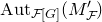 $\mathrm{Aut}_{\mathcal F[G]}(M'_{\mathcal F})$
.
$\mathrm{Aut}_{\mathcal F[G]}(M'_{\mathcal F})$
.
Definition 2.4. Let G be a finite group. Let M be an A[G]-module that is both finite and G-c.t. The characteristic class of M is the element
 $$c_G(M):=[M'_{\mathcal F},\tau_{M,\mathcal F}]$$
of $K_1(\mathcal F[G])$
. By abuse of notation, we identify
$K_1(\mathcal F[G])$
. By abuse of notation, we identify $c_G(M)$
with its image
$c_G(M)$
with its image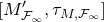 $[M'_{\mathcal F_\infty},\tau_{M,\mathcal F_\infty}]$
in
$[M'_{\mathcal F_\infty},\tau_{M,\mathcal F_\infty}]$
in $K_1(\mathcal F_\infty[G])$
.
$K_1(\mathcal F_\infty[G])$
.
Remarks 2.5.
-
(i) An
${\mathbb F}_q[G]$
-module that is G-c.t. is
${\mathbb F}_q[G]$
-projective (by Lemma 2.2(i)). Thus,
$M'_{\mathcal F}$
is
$\mathcal F[G]$
-projective. -
(ii) If G is abelian, then the determinant of
$\tau_M\in\mathrm{End}_{A[G]}(M')$
is a generator of the Fitting ideal of M in A[G]. In fact, it is the ‘monic’ generator in the sense of [Reference Ferrara, Green, Higgins and PopescuFGH+22, Remark A.3.3]. -
(iii) See also Lemma 3.10 below for a similar explicit relationship between characteristic classes and non-commutative Fitting ideals.



Characteristic classes are multiplicative, in the following sense.
Lemma 2.6. If $0\to L\to M\to N\to 0$
is a short exact sequence of A[G]-modules, two of which are finite and G-c.t., then so is the third, and one has
$0\to L\to M\to N\to 0$
is a short exact sequence of A[G]-modules, two of which are finite and G-c.t., then so is the third, and one has $c_G(M)=c_G(L)\cdot c_G(N)$
. In particular, characteristic classes are well-defined on isomorphism classes of A[G]-modules (that are finite and G-c.t.), and commute with finite direct products.
$c_G(M)=c_G(L)\cdot c_G(N)$
. In particular, characteristic classes are well-defined on isomorphism classes of A[G]-modules (that are finite and G-c.t.), and commute with finite direct products.
Proof. It is clear that the third module is finite and G-c.t. Since $A[G]={\mathbb F}_q[G][t]$
is a flat
$A[G]={\mathbb F}_q[G][t]$
is a flat ${\mathbb F}_q[G]$
-module, we obtain a short exact sequence
${\mathbb F}_q[G]$
-module, we obtain a short exact sequence $0\to L'\xrightarrow{1\otimes\alpha}M'\xrightarrow{1\otimes\beta}N'\to 0$
, where we have denoted by
$0\to L'\xrightarrow{1\otimes\alpha}M'\xrightarrow{1\otimes\beta}N'\to 0$
, where we have denoted by $\alpha,\beta$
the given A[G]-homomorphisms.
$\alpha,\beta$
the given A[G]-homomorphisms.
Now, for any $h\in A[G]$
and
$h\in A[G]$
and $l\in L$
, one has
$l\in L$
, one has
 $$(1\otimes\alpha)(\tau_L(h\otimes l))=(th\otimes\alpha(l))-(h\otimes\alpha(t\cdot l))=(th\otimes\alpha(l))-(h\otimes t\cdot\alpha(l))=\tau_M((1\otimes\alpha)(h\otimes l))$$
and, similarly, for any $m\in M$
, one has
$m\in M$
, one has $(1\otimes\beta)(\tau_M(h\otimes m))=\tau_N((1\otimes\beta)(h\otimes m))$
. The equality
$(1\otimes\beta)(\tau_M(h\otimes m))=\tau_N((1\otimes\beta)(h\otimes m))$
. The equality $c_G(M)=c_G(L)\cdot c_G(N)$
thus follows directly from the definition of
$c_G(M)=c_G(L)\cdot c_G(N)$
thus follows directly from the definition of $K_1(\mathcal F[G])$
(cf. [Reference Curtis and ReinerCR87, Vol. II, Definition 38.28] or [Reference SwanSwa78, Chapter 13]).
$K_1(\mathcal F[G])$
(cf. [Reference Curtis and ReinerCR87, Vol. II, Definition 38.28] or [Reference SwanSwa78, Chapter 13]).
Characteristic classes also satisfy the following base-change property.
Lemma 2.7. Let H be a subgroup of G and let N be an A[H]-module that is both finite and H-c.t. Let M be the A[G]-module ${\mathbb F}_q[G]\otimes_{{\mathbb F}_q[H]}N$
, with
${\mathbb F}_q[G]\otimes_{{\mathbb F}_q[H]}N$
, with $tg(x\otimes n)=g x\otimes t\cdot n$
for each
$tg(x\otimes n)=g x\otimes t\cdot n$
for each $g\in G$
,
$g\in G$
, $x\in {\mathbb F}_q[G]$
and
$x\in {\mathbb F}_q[G]$
and $n\in N$
.
$n\in N$
.
Then M is both finite and G-c.t. and in $K_1(\mathcal F[G])$
one has
$K_1(\mathcal F[G])$
one has $\iota_H(c_H(N)) = c_G(M)$
, where
$\iota_H(c_H(N)) = c_G(M)$
, where $\iota_H$
is the canonical homomorphism
$\iota_H$
is the canonical homomorphism $K_1(\mathcal F[H])\to K_1(\mathcal F[G])$
.
$K_1(\mathcal F[H])\to K_1(\mathcal F[G])$
.
Proof. It is clear that M is finite and, applying Lemma 2.2(i) twice, we find that N is ${\mathbb F}_q[H]$
-projective, so M is
${\mathbb F}_q[H]$
-projective, so M is ${\mathbb F}_q[G]$
-projective and M is G-c.t.
${\mathbb F}_q[G]$
-projective and M is G-c.t.
We now consider the following commutative diagram of A[G]-modules.

Here, $\phi$
and
$\phi$
and $\psi$
are the canonical isomorphisms and, for
$\psi$
are the canonical isomorphisms and, for $x\in A[G]$
and
$x\in A[G]$
and $n\in N$
, we set
$n\in N$
, we set
 $$\sigma(x\otimes n) := (tx\otimes n)-(x\otimes t\cdot n).$$
The commutativity of the diagram is straightforward to verify, and implies that
 \begin{align*}\iota_H(c_H(N))=\iota_H([N'_{\mathcal F},\tau_{N,\mathcal F}])&=[(A[G]\otimes_{A[H]}N')_{\mathcal F},(1\otimes\tau_{N})_{\mathcal F}]\\&=[(A[G]\otimes_{{\mathbb F}_q[H]}N)_{\mathcal F},\sigma_{\mathcal F}]=[M'_{\mathcal F},\tau_{M,\mathcal F}]=c_G(M).\end{align*}
2.2 Refined Euler characteristics
Let G be a finite group. In this section we define refined Euler characteristics in the relative algebraic $K_0$
-group
$K_0$
-group $K_0(A[G],\mathcal F_\infty[G])$
of the ring inclusion
$K_0(A[G],\mathcal F_\infty[G])$
of the ring inclusion $A[G]\subset\mathcal F_\infty[G]$
(cf. [Reference SwanSwa78, Reference Curtis and ReinerCR87]). Elements of this group are equivalence classes
$A[G]\subset\mathcal F_\infty[G]$
(cf. [Reference SwanSwa78, Reference Curtis and ReinerCR87]). Elements of this group are equivalence classes $[P,\phi,Q]$
of triples comprising finitely generated projective A[G]-modules P,Q and an isomorphism of
$[P,\phi,Q]$
of triples comprising finitely generated projective A[G]-modules P,Q and an isomorphism of $\mathcal F_\infty[G]$
-modules
$\mathcal F_\infty[G]$
-modules $\phi:P_{\mathcal F_\infty}\cong Q_{\mathcal F_\infty}$
. We always use additive notation for
$\phi:P_{\mathcal F_\infty}\cong Q_{\mathcal F_\infty}$
. We always use additive notation for $K_0$
-groups.
$K_0$
-groups.
We write $D^{\mathrm{p}}(A[G])$
for the full triangulated subcategory of the derived category D(A[G]) comprising complexes that are perfect. We recall that an object of D(A[G]) is said to be perfect if it is isomorphic (in D(A[G])) to a bounded complex of finitely generated, projective modules.
$D^{\mathrm{p}}(A[G])$
for the full triangulated subcategory of the derived category D(A[G]) comprising complexes that are perfect. We recall that an object of D(A[G]) is said to be perfect if it is isomorphic (in D(A[G])) to a bounded complex of finitely generated, projective modules.
Definition 2.8. We write $D^{\mathrm{p,c}}(A[G],\mathcal F_\infty)$
for the full subcategory of
$D^{\mathrm{p,c}}(A[G],\mathcal F_\infty)$
for the full subcategory of $D^{\mathrm{p}}(A[G])$
comprising complexes C with the property that
$D^{\mathrm{p}}(A[G])$
comprising complexes C with the property that $H^n(C)_{\mathcal F_\infty}$
is a (finitely generated) projective
$H^n(C)_{\mathcal F_\infty}$
is a (finitely generated) projective $\mathcal F_\infty[G]$
-module for every
$\mathcal F_\infty[G]$
-module for every $n\in\mathbb Z$
. (Here, ‘c’ stands for cohomology.)
$n\in\mathbb Z$
. (Here, ‘c’ stands for cohomology.)
Definition 2.9. Let C be an object of $D^{\mathrm{p,c}}(A[G],\mathcal F_\infty)$
that is isomorphic (in D(A[G])) to a complex of the form
$D^{\mathrm{p,c}}(A[G],\mathcal F_\infty)$
that is isomorphic (in D(A[G])) to a complex of the form
 \begin{equation}P^1\stackrel{d}{\longrightarrow} P^2\end{equation}
with the first term in degree one, where both $P^1$
and
$P^1$
and $P^2$
are finitely generated, projective A[G]-modules. Assume also given an isomorphism of
$P^2$
are finitely generated, projective A[G]-modules. Assume also given an isomorphism of $\mathcal F_\infty[G]$
-modules
$\mathcal F_\infty[G]$
-modules
 $$\lambda:H^{2}(C)_{\mathcal F_\infty}\longrightarrow H^{1}(C)_{\mathcal F_\infty}.$$
The refined Euler characteristic of the pair $(C,\lambda)$
is the element
$(C,\lambda)$
is the element
 $$\chi_{G}(C,\lambda) := -[P^1,\gamma,P^2]$$
of $K_0(A[G],\mathcal F_\infty[G])$
, where
$K_0(A[G],\mathcal F_\infty[G])$
, where $\gamma$
is the composite isomorphism of
$\gamma$
is the composite isomorphism of $\mathcal F_\infty[G]$
-modules
$\mathcal F_\infty[G]$
-modules
 $$P^1_{\mathcal F_\infty}\stackrel{\iota_1}{\longrightarrow}\textrm{im}(d_{\mathcal F_\infty})\oplus H^1(C)_{\mathcal F_\infty}\xrightarrow{\mathrm{id}\oplus\lambda^{-1}}\textrm{im}(d_{\mathcal F_\infty})\oplus H^2(C)_{\mathcal F_\infty}\xrightarrow{\iota_2^{-1}}P^2_{\mathcal F_\infty},$$
for an arbitrary choice of splittings $\iota_1$
and
$\iota_1$
and $\iota_2$
of the respective short exact sequences
$\iota_2$
of the respective short exact sequences
 \begin{align*}0\to H^1(C)_{\mathcal F_\infty}&\longrightarrow P^1_{\mathcal F_\infty}\xrightarrow{d_{\mathcal F_\infty}}\textrm{im}(d_{\mathcal F_\infty})\to 0,\\0\to \textrm{im}(d_{\mathcal F_\infty})&\longrightarrow P^2_{\mathcal F_\infty}\longrightarrow H^2(C)_{\mathcal F_\infty}\to 0.\end{align*}
We note that Definition 2.8 ensures that the second sequence splits and combines with Lemma 2.2(i) to imply that $\textrm{im}(d_{\mathcal F_\infty})$
is projective, so the first sequence splits. In addition, strictly speaking, we have denoted
$\textrm{im}(d_{\mathcal F_\infty})$
is projective, so the first sequence splits. In addition, strictly speaking, we have denoted $\iota_1:P^1_{\mathcal F_\infty}\to\textrm{im}(d_{\mathcal F_\infty})\oplus H^1(C)_{\mathcal F_\infty}$
and
$\iota_1:P^1_{\mathcal F_\infty}\to\textrm{im}(d_{\mathcal F_\infty})\oplus H^1(C)_{\mathcal F_\infty}$
and $\iota_2:P^2_{\mathcal F_\infty}\to\textrm{im}(d_{\mathcal F_\infty})\oplus H^2(C)_{\mathcal F_\infty}$
the isomorphisms induced by arbitrary choices of such splittings.
$\iota_2:P^2_{\mathcal F_\infty}\to\textrm{im}(d_{\mathcal F_\infty})\oplus H^2(C)_{\mathcal F_\infty}$
the isomorphisms induced by arbitrary choices of such splittings.
Remark 2.10. It is straightforward to prove directly (or to deduce from general arguments due to Burns [Reference BurnsBur04]) that $\chi_{G}(C,\lambda)$
does not depend on the choice of representative of C of the form (2.1) or on the choice of splittings
$\chi_{G}(C,\lambda)$
does not depend on the choice of representative of C of the form (2.1) or on the choice of splittings $\iota_1,\iota_2$
.
$\iota_1,\iota_2$
.
Remark 2.11. After restricting consideration to the subcategory $D^{\mathrm{p,c}}(A[G],\mathcal F_\infty)$
of
$D^{\mathrm{p,c}}(A[G],\mathcal F_\infty)$
of $D^{\mathrm{p}}(A[G])$
, one may mimic the use of Deligne’s universal determinant functors [Reference DeligneDel87] that is made by Breuning and Burns in [Reference Breuning and BurnsBB05, Definition 5.5] (even though
$D^{\mathrm{p}}(A[G])$
, one may mimic the use of Deligne’s universal determinant functors [Reference DeligneDel87] that is made by Breuning and Burns in [Reference Breuning and BurnsBB05, Definition 5.5] (even though $\mathcal F_\infty[G]$
is not, in general, a regular ring).
$\mathcal F_\infty[G]$
is not, in general, a regular ring).
In this way, to any pair $(C,\lambda)$
, with C in
$(C,\lambda)$
, with C in $D^{\mathrm{p,c}}(A[G],\mathcal F_\infty)$
and with
$D^{\mathrm{p,c}}(A[G],\mathcal F_\infty)$
and with
 $$\lambda:H^{\mathrm{ev}}(C)_{\mathcal F_\infty}\,\xrightarrow{\sim}\,H^{\mathrm{od}}(C)_{\mathcal F_\infty}$$
an isomorphism of $\mathcal F_\infty[G]$
-modules, one associates a refined Euler characteristic in
$\mathcal F_\infty[G]$
-modules, one associates a refined Euler characteristic in $K_0(A[G],\mathcal F_\infty[G])$
. Here we have written
$K_0(A[G],\mathcal F_\infty[G])$
. Here we have written $H^{\mathrm{ev}}(C)$
and
$H^{\mathrm{ev}}(C)$
and $H^{\mathrm{od}}(C)$
for the direct sum of the even and of the odd degree cohomology of C, respectively. This more general construction specialises to recover Definition 2.9.
$H^{\mathrm{od}}(C)$
for the direct sum of the even and of the odd degree cohomology of C, respectively. This more general construction specialises to recover Definition 2.9.
2.3 Statement of the refined class number formula
In this section we state our main result. Let k be a finite separable extension of $\mathcal F={\mathbb F}_q(t)$
and let K be a finite Galois extension of k with group
$\mathcal F={\mathbb F}_q(t)$
and let K be a finite Galois extension of k with group $G:=\mathrm{ Gal}(K/k)$
.
$G:=\mathrm{ Gal}(K/k)$
.
We endow $\mathcal F_\infty$
with the
$\mathcal F_\infty$
with the $t^{-1}$
-adic absolute value, and
$t^{-1}$
-adic absolute value, and $\mathcal F_\infty[G]=\prod_{g\in G}(\mathcal F_\infty g)$
with the supremum norm. Using the ring isomorphism
$\mathcal F_\infty[G]=\prod_{g\in G}(\mathcal F_\infty g)$
with the supremum norm. Using the ring isomorphism $\mathcal F_\infty[G]\cong{\mathbb F}_q[G](\!(t^{-1})\!)$
to define a function
$\mathcal F_\infty[G]\cong{\mathbb F}_q[G](\!(t^{-1})\!)$
to define a function $V:(\mathcal F_\infty[G]\setminus\{0\})\to\mathbb Z$
by
$V:(\mathcal F_\infty[G]\setminus\{0\})\to\mathbb Z$
by $V(\sum_{i\geq N}r_it^{-i}):=N$
for
$V(\sum_{i\geq N}r_it^{-i}):=N$
for $r_i\in{\mathbb F}_q[G]$
with
$r_i\in{\mathbb F}_q[G]$
with $r_N\neq 0$
, one finds that the norm of
$r_N\neq 0$
, one finds that the norm of $0\neq f=\sum_{g\in G}f_gg\in\mathcal F_\infty[G]$
with
$0\neq f=\sum_{g\in G}f_gg\in\mathcal F_\infty[G]$
with $f_g\in\mathcal F_\infty$
is computed as
$f_g\in\mathcal F_\infty$
is computed as
 $${\max}_{g\in G}\{|f_g|\}={\max}_{g\in G}\{q^{-v_\infty(f_g)}\}=q^{-\min_{g\in G}\{v_\infty(f_g)\}}=q^{-V(f)}.$$
One easily verifies that this is a (sub-multiplicative) ring norm. The ring topology it induces is, in fact, the unique topology making $\mathcal F_\infty[G]$
a Hausdorff
$\mathcal F_\infty[G]$
a Hausdorff $\mathcal F_\infty$
-vector space.
$\mathcal F_\infty$
-vector space.
We set $K_\infty:=\mathcal F_\infty\otimes_{\mathcal F} K$
, a free topological
$K_\infty:=\mathcal F_\infty\otimes_{\mathcal F} K$
, a free topological $\mathcal F_\infty[G]$
-module of rank
$\mathcal F_\infty[G]$
-module of rank $[k:\mathcal F]$
. We say that a finitely generated A[G]-submodule M of
$[k:\mathcal F]$
. We say that a finitely generated A[G]-submodule M of $K_\infty$
is an ‘A[G]-lattice in
$K_\infty$
is an ‘A[G]-lattice in $K_\infty$
’ if the canonical map
$K_\infty$
’ if the canonical map $M_{\mathcal F_\infty}\to K_\infty$
is bijective. An A[G]-submodule of
$M_{\mathcal F_\infty}\to K_\infty$
is bijective. An A[G]-submodule of $K_\infty$
that is A-free of finite rank is an A[G]-lattice if and only if it is discrete and co-compact in
$K_\infty$
that is A-free of finite rank is an A[G]-lattice if and only if it is discrete and co-compact in $K_\infty$
(cf. [Reference DebryDeb16, Proposition 1.6]).
$K_\infty$
(cf. [Reference DebryDeb16, Proposition 1.6]).
Remark 2.12. Claims (ii) and (iii) of Lemma 2.2 combine to imply that any projective A[G]-lattice M in $K_\infty$
is locally free of constant local rank
$K_\infty$
is locally free of constant local rank $n:=[k:\mathcal F]$
, i.e. that
$n:=[k:\mathcal F]$
, i.e. that $A_{(P)}\otimes_A M\cong A_{(P)}[G]^{n}$
for every prime P of A.
$A_{(P)}\otimes_A M\cong A_{(P)}[G]^{n}$
for every prime P of A.
2.3.1.
For any commutative ${\mathbb F}_q$
-algebra
${\mathbb F}_q$
-algebra $\mathcal O$
, we denote by
$\mathcal O$
, we denote by $\tau$
the qth-power Frobenius of
$\tau$
the qth-power Frobenius of $\mathcal O$
, that is, the endomorphism of
$\mathcal O$
, that is, the endomorphism of $\mathcal O$
given by
$\mathcal O$
given by $\tau(x)=x^q$
. The twisted polynomial ring
$\tau(x)=x^q$
. The twisted polynomial ring $\mathcal O\{\tau\}$
, with commutation relation
$\mathcal O\{\tau\}$
, with commutation relation $\tau\cdot x=x^q\cdot\tau$
, acts on any commutative
$\tau\cdot x=x^q\cdot\tau$
, acts on any commutative $\mathcal O$
-algebra.
$\mathcal O$
-algebra.
Let E be a Drinfeld module defined over the integral closure $\mathcal O_k$
of A in k. We interpret E as a functor, from the category of
$\mathcal O_k$
of A in k. We interpret E as a functor, from the category of $\mathcal O_k\{\tau\}[G]$
-modules to the category of A[G]-modules, induced by a given
$\mathcal O_k\{\tau\}[G]$
-modules to the category of A[G]-modules, induced by a given ${\mathbb F}_q$
-algebra morphism
${\mathbb F}_q$
-algebra morphism $\phi_E:A\to\mathcal O_{k}\{\tau\}$
. (In this article, we only ever consider Drinfeld A-modules for
$\phi_E:A\to\mathcal O_{k}\{\tau\}$
. (In this article, we only ever consider Drinfeld A-modules for $A:={\mathbb F}_q[t]$
and defined over
$A:={\mathbb F}_q[t]$
and defined over $\mathcal O_k$
.)
$\mathcal O_k$
.)
The exponential power series of E defines a homomorphism of A[G]-modules
 $$\exp _E:K_\infty\to E(K_\infty).$$
The main result of Taelman in [Reference TaelmanTae10] implies both that $\exp ^{-1}_E(E(\mathcal O_K))$
is an A[G]-lattice in
$\exp ^{-1}_E(E(\mathcal O_K))$
is an A[G]-lattice in $K_\infty$
and that the A[G]-module
$K_\infty$
and that the A[G]-module
 $$H(E/\mathcal O_K):=\frac{E(K_\infty)}{E(\mathcal O_K)+\exp _E(K_\infty)}$$
is finite. The former assertion is an analogue of Dirichlet’s theorem for the preimage under the archimedean exponential of the units of a number field. The analogy between $H(E/\mathcal O_K)$
and class groups is more elaborate, but see Remark 6 in [Reference TaelmanTae10].
$H(E/\mathcal O_K)$
and class groups is more elaborate, but see Remark 6 in [Reference TaelmanTae10].
2.3.2.
We now use the notion of ‘taming module’, introduced by Ferrara et al. in [Reference Ferrara, Green, Higgins and PopescuFGH+22, Definition 1.3.2].
Definition 2.13. A taming module for $K/k$
is an
$K/k$
is an $\mathcal O_k\{\tau\}[G]$
-submodule
$\mathcal O_k\{\tau\}[G]$
-submodule $\mathcal M$
of
$\mathcal M$
of $\mathcal O_K$
that is
$\mathcal O_K$
that is $\mathcal O_k[G]$
-projective and such that the quotient
$\mathcal O_k[G]$
-projective and such that the quotient $\mathcal O_K/\mathcal M$
is finite and only supported at prime ideals of
$\mathcal O_K/\mathcal M$
is finite and only supported at prime ideals of $\mathcal O_k$
which are wildly ramified in
$\mathcal O_k$
which are wildly ramified in $K/k$
.
$K/k$
.
Remark 2.14. Taming modules $\mathcal M$
for
$\mathcal M$
for $K/k$
exist and, in fact, are
$K/k$
exist and, in fact, are $\mathcal O_k[G]$
locally free, of constant local rank 1. These claims follow from Proposition A.2.4 in [Reference Ferrara, Green, Higgins and PopescuFGH+22], upon replacing the use of Corollary A.1.7(3) by Swan’s theorem, as stated in Lemma 2.2(iii). Indeed, set
$\mathcal O_k[G]$
locally free, of constant local rank 1. These claims follow from Proposition A.2.4 in [Reference Ferrara, Green, Higgins and PopescuFGH+22], upon replacing the use of Corollary A.1.7(3) by Swan’s theorem, as stated in Lemma 2.2(iii). Indeed, set $\mathcal{R}:=\mathcal O_k$
and
$\mathcal{R}:=\mathcal O_k$
and $\mathcal{S}:=\mathcal O_K$
. Then, if
$\mathcal{S}:=\mathcal O_K$
. Then, if $v\in\textrm{MSpec}(\mathcal{R})$
is tamely ramified in
$v\in\textrm{MSpec}(\mathcal{R})$
is tamely ramified in $K/k$
, the fact that
$K/k$
, the fact that $\mathcal{S}_{(v)}\cong\mathcal{R}_{(v)}[G]$
, used in [Reference Ferrara, Green, Higgins and PopescuFGH+22], follows by Swan’s theorem from the isomorphism of k[G]-modules
$\mathcal{S}_{(v)}\cong\mathcal{R}_{(v)}[G]$
, used in [Reference Ferrara, Green, Higgins and PopescuFGH+22], follows by Swan’s theorem from the isomorphism of k[G]-modules $k\otimes_{\mathcal{R}_{(v)}}\mathcal{S}_{(v)}\cong K\cong k[G]\cong k\otimes_{\mathcal{R}_{(v)}}\mathcal{R}_{(v)}[G]$
.
$k\otimes_{\mathcal{R}_{(v)}}\mathcal{S}_{(v)}\cong K\cong k[G]\cong k\otimes_{\mathcal{R}_{(v)}}\mathcal{R}_{(v)}[G]$
.
In particular, for any taming module $\mathcal M$
for
$\mathcal M$
for $K/k$
and for every
$K/k$
and for every $\mathfrak{p}\in\textrm{MSpec}(\mathcal O_k)$
, the finite
$\mathfrak{p}\in\textrm{MSpec}(\mathcal O_k)$
, the finite ${\mathbb F}_q[G]$
-module
${\mathbb F}_q[G]$
-module $\mathcal M/\mathfrak{p}\mathcal M$
is free, thus also G-c.t. (by Lemma 2.2(i)), and the characteristic classes
$\mathcal M/\mathfrak{p}\mathcal M$
is free, thus also G-c.t. (by Lemma 2.2(i)), and the characteristic classes $c_G(\mathcal M/\mathfrak{p}\mathcal M)$
and
$c_G(\mathcal M/\mathfrak{p}\mathcal M)$
and $c_G(E(\mathcal M/\mathfrak{p}\mathcal M))$
are well-defined.
$c_G(E(\mathcal M/\mathfrak{p}\mathcal M))$
are well-defined.
Definition 2.15. We fix a taming module $\mathcal M$
for
$\mathcal M$
for $K/k$
.
$K/k$
.
-
(i) The
$\mathcal M$
-modified complex of units of
$(E,K/k)$
is the complex
$C^{\mathcal M}_{E,K/k}$
of A[G]-modules with the first term placed in degree one.
$$K_\infty\,\,\xrightarrow{(\exp _E,0)}\,\,(E(K_\infty)/E(\mathcal M))\,\oplus\,\mathcal M$$
-
(ii) The
$\mathcal M$
-modified Taelman class group of
$(E,K/k)$
is the A[G]-module
$$H(E/\mathcal M):=\frac{E(K_\infty)}{E(\mathcal M)+\exp _E(K_\infty)}.$$


Remark 2.16. The term ‘complex of units’ is taken from [Reference MornevMor18]. It is clear that
 $$H^j(C^{\mathcal M}_{E,K/k})=\begin{cases}\exp ^{-1}_E(E(\mathcal M)), & j=1,\\H(E/\mathcal M)\oplus\mathcal M, & j=2,\\0, & j\neq 1,2,\end{cases}$$
that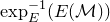 $\exp ^{-1}_E(E(\mathcal M))$
is an A[G]-lattice in
$\exp ^{-1}_E(E(\mathcal M))$
is an A[G]-lattice in $K_\infty$
and that
$K_\infty$
and that $H(E/\mathcal M)$
is finite. We denote by
$H(E/\mathcal M)$
is finite. We denote by $\lambda^{\mathcal M}_{E,K/k}$
the isomorphism
$\lambda^{\mathcal M}_{E,K/k}$
the isomorphism
 \begin{equation*}H^1(C^{\mathcal M}_{E,K/k})_{\mathcal F_\infty}=\exp ^{-1}_E(E(\mathcal M))_{\mathcal F_\infty}= K_\infty\cong\,(\mathcal O_K)_{\mathcal F_\infty}=\mathcal M_{\mathcal F_\infty}= H^2(C^{\mathcal M}_{E,K/k})_{\mathcal F_\infty},\end{equation*}
and by $\lambda^{\mathcal M,-1}_{E,K/k}$
its inverse (which is thus induced by the inclusions
$\lambda^{\mathcal M,-1}_{E,K/k}$
its inverse (which is thus induced by the inclusions $\mathcal M\subseteq\mathcal O_K\subset K\subset K_\infty$
, as claimed in Theorem A(3)).
$\mathcal M\subseteq\mathcal O_K\subset K\subset K_\infty$
, as claimed in Theorem A(3)).
2.3.3.
We may now state the main result of this article. We recall that, since $\mathcal F_\infty[G]$
is naturally a semilocal topological ring,
$\mathcal F_\infty[G]$
is naturally a semilocal topological ring, $K_1(\mathcal F_\infty[G])$
is a topological abelian group, and we also use the canonical connecting homomorphism
$K_1(\mathcal F_\infty[G])$
is a topological abelian group, and we also use the canonical connecting homomorphism
 \begin{equation*}\partial_G:K_1(\mathcal F_\infty[G])\to K_0(A[G],\mathcal F_\infty[G]).\end{equation*}
Theorem 2.17. Let K be a finite Galois extension of k and let E be a Drinfeld module over $\mathcal O_k$
. Let
$\mathcal O_k$
. Let $\mathcal M$
be a taming module for
$\mathcal M$
be a taming module for $K/k$
.
$K/k$
.
Then the complex $C^{\mathcal M}_{E,K/k}$
belongs to the category
$C^{\mathcal M}_{E,K/k}$
belongs to the category $D^{\mathrm{p,c}}(A[G],\mathcal F_\infty)$
, the infinite product
$D^{\mathrm{p,c}}(A[G],\mathcal F_\infty)$
, the infinite product
 $$\Theta^{\mathcal M}_{E,K/k}:=\prod_{\mathfrak{p}\in\textrm{MSpec}(\mathcal O_k)}(c_G(\mathcal M/\mathfrak{p}\mathcal M)\cdot c_G(E(\mathcal M/\mathfrak{p}\mathcal M))^{-1})$$
converges to a unique element of $K_1(\mathcal F_\infty[G])$
and, in
$K_1(\mathcal F_\infty[G])$
and, in $K_0(A[G],\mathcal F_\infty[G])$
, one has
$K_0(A[G],\mathcal F_\infty[G])$
, one has
 \begin{equation}\partial_G(\Theta^{\mathcal M}_{E,K/k}) = -\chi_{G}(C^{\mathcal M}_{E,K/k},\lambda^{\mathcal M,-1}_{E,K/k}).\end{equation}
The proof of Theorem 2.17 is given in § 6.
Remark 2.18. By convergence of a countable, ordered infinite product in the topological abelian group $K_1(\mathcal F_\infty[G])$
, we mean that the sequence of partial products converges. In Corollary 5.6 (see also Corollary 4.9(ii)) we prove that, for any given order on the countable set
$K_1(\mathcal F_\infty[G])$
, we mean that the sequence of partial products converges. In Corollary 5.6 (see also Corollary 4.9(ii)) we prove that, for any given order on the countable set $\textrm{MSpec}(\mathcal O_k)$
, the infinite product in Theorem 2.17 converges to a unique element
$\textrm{MSpec}(\mathcal O_k)$
, the infinite product in Theorem 2.17 converges to a unique element $\Theta^{\mathcal M}_{E,K/k}$
of
$\Theta^{\mathcal M}_{E,K/k}$
of $K_1(\mathcal F_\infty[G])$
and, moreover, that this limit element
$K_1(\mathcal F_\infty[G])$
and, moreover, that this limit element $\Theta^{\mathcal M}_{E,K/k}$
is independent of the given order on
$\Theta^{\mathcal M}_{E,K/k}$
is independent of the given order on $\textrm{MSpec}(\mathcal O_k)$
.
$\textrm{MSpec}(\mathcal O_k)$
.
Remark 2.19. The map $\partial_G$
is defined by the equality
$\partial_G$
is defined by the equality $\partial_G([\mathcal F_\infty[G]^n, \phi]):=[A[G]^n,\phi,A[G]^n]$
for any
$\partial_G([\mathcal F_\infty[G]^n, \phi]):=[A[G]^n,\phi,A[G]^n]$
for any $n\geq 1$
and any automorphism
$n\geq 1$
and any automorphism $\phi$
of
$\phi$
of $\mathcal F_\infty[G]^n$
, and fits in the exact localisation sequence
$\mathcal F_\infty[G]^n$
, and fits in the exact localisation sequence
 $$K_1(A[G])\longrightarrow K_1(\mathcal F_\infty[G])\stackrel{\partial_G}{\longrightarrow}K_0(A[G],\mathcal F_\infty[G]).$$
Although $\partial_G$
need not be surjective, the equality (2.2) takes place in the subgroup
$\partial_G$
need not be surjective, the equality (2.2) takes place in the subgroup
 $$\textrm{im}(\partial_G)\cong K_1(\mathcal F_\infty[G])/\textrm{im}(K_1(A[G])).$$
Now, if G is abelian, then taking determinants over $\mathcal F_\infty[G]$
induces an isomorphism
$\mathcal F_\infty[G]$
induces an isomorphism
 $$\textrm{im}(\partial_G)\cong \mathcal F_\infty[G]^\times/A[G]^\times$$
and [Reference Ferrara, Green, Higgins and PopescuFGH+22, Proposition A.3.4] shows that there is a decomposition
 $$\mathcal F_\infty[G]^\times\cong\mathcal F_\infty[G]^+\times A[G]^\times.$$
Here, $\mathcal F_\infty[G]^+$
is the subgroup of ‘monic elements’ of
$\mathcal F_\infty[G]^+$
is the subgroup of ‘monic elements’ of $\mathcal F_\infty[G]^\times$
in which their ‘equivariant Tamagawa number formula for Drinfeld modules’ (Theorem 1.5.1 in [Reference Ferrara, Green, Higgins and PopescuFGH+22]) takes place.
$\mathcal F_\infty[G]^\times$
in which their ‘equivariant Tamagawa number formula for Drinfeld modules’ (Theorem 1.5.1 in [Reference Ferrara, Green, Higgins and PopescuFGH+22]) takes place.
Our proof of Theorem 2.17 makes clear that, for abelian extensions $K/k$
and under this identification of
$K/k$
and under this identification of $\textrm{im}(\partial_G)$
with
$\textrm{im}(\partial_G)$
with $\mathcal F_\infty[G]^+$
, the equality (2.2) specialises to recover the equivariant Tamagawa number formula of [Reference Ferrara, Green, Higgins and PopescuFGH+22]; see Remark 6.7 below for details. In particular, (2.2) also specialises to recover Taelman’s class number formula [Reference TaelmanTae12, Theorem A] in the case
$\mathcal F_\infty[G]^+$
, the equality (2.2) specialises to recover the equivariant Tamagawa number formula of [Reference Ferrara, Green, Higgins and PopescuFGH+22]; see Remark 6.7 below for details. In particular, (2.2) also specialises to recover Taelman’s class number formula [Reference TaelmanTae12, Theorem A] in the case $K=k$
.
$K=k$
.
Remark 2.20. It is straightforward to show that the validity of the equality (2.2) is a priori independent of the choice of taming module $\mathcal M$
. As further discussed in [Reference Ferrara, Green, Higgins and PopescuFGH+22, Remark 6.2.4], one should think of the above
$\mathcal M$
. As further discussed in [Reference Ferrara, Green, Higgins and PopescuFGH+22, Remark 6.2.4], one should think of the above $\mathcal M$
-modifications as analogous to the usual T-modifications in the study of equivariant special Artin L-values for global fields.
$\mathcal M$
-modifications as analogous to the usual T-modifications in the study of equivariant special Artin L-values for global fields.
Remark 2.21. We actually prove that the complex $C^{\mathcal M}_{E,K/k}$
belongs to the category
$C^{\mathcal M}_{E,K/k}$
belongs to the category $D^{\mathrm{p,c}}(A[G],\mathcal F_\infty)$
and has a representative of the form (2.1). For
$D^{\mathrm{p,c}}(A[G],\mathcal F_\infty)$
and has a representative of the form (2.1). For $K=k$
, this fact specialises to recover the main result of [Reference TaelmanTae10].
$K=k$
, this fact specialises to recover the main result of [Reference TaelmanTae10].
Remark 2.22. The statement of Theorem 2.17 generalises in the obvious manner to abelian t-modules E defined over $\mathcal O_k$
, and our proof may be extended to this general setting. To avoid obscuring the main ideas of the present article, the details of this generalisation of Theorem 2.17 will be presented in a separate note. For now we recall that, under the assumption that the Galois group G is abelian, Green and Popescu have recently proved an equivariant Tamagawa number formula for abelian t-modules [Reference Green and PopescuGP25, Theorem 1.32] and Beaumont has proved an equivariant class formula for z-deformations of t-modules [Reference BeaumontBea23, Theorem 1.2].
$\mathcal O_k$
, and our proof may be extended to this general setting. To avoid obscuring the main ideas of the present article, the details of this generalisation of Theorem 2.17 will be presented in a separate note. For now we recall that, under the assumption that the Galois group G is abelian, Green and Popescu have recently proved an equivariant Tamagawa number formula for abelian t-modules [Reference Green and PopescuGP25, Theorem 1.32] and Beaumont has proved an equivariant class formula for z-deformations of t-modules [Reference BeaumontBea23, Theorem 1.2].
Example 2.23. We consider the Carlitz module $E=C$
, defined by the morphism
$E=C$
, defined by the morphism $\phi_C:A\to \mathcal O_k\{\tau\}$
given by
$\phi_C:A\to \mathcal O_k\{\tau\}$
given by $\phi_C(t):=t+\tau$
. Given a prime
$\phi_C(t):=t+\tau$
. Given a prime $\mathfrak{p}\in\textrm{MSpec}(\mathcal O_k)$
that is tamely ramified in
$\mathfrak{p}\in\textrm{MSpec}(\mathcal O_k)$
that is tamely ramified in $K/k$
, we show that the Euler factor
$K/k$
, we show that the Euler factor
 $$c_G(\mathcal M/\mathfrak{p}\mathcal M)\cdot c_G(C(\mathcal M/\mathfrak{p}\mathcal M))^{-1}=c_G(\mathcal O_K/\mathfrak{p}\mathcal O_K)\cdot c_G(C(\mathcal O_K/\mathfrak{p}\mathcal O_K))^{-1}$$
of $\Theta^{\mathcal M}_{C,K/k}$
at
$\Theta^{\mathcal M}_{C,K/k}$
at $\mathfrak{p}$
is equal in
$\mathfrak{p}$
is equal in $K_1(\mathcal F[G])$
to
$K_1(\mathcal F[G])$
to $[1-(N\mathfrak{p})^{-1}\textrm{Fr}_{\mathfrak{p}}\cdot e_{I_{\mathfrak{p}}}]^{-1}$
. Here,
$[1-(N\mathfrak{p})^{-1}\textrm{Fr}_{\mathfrak{p}}\cdot e_{I_{\mathfrak{p}}}]^{-1}$
. Here, $I_{\mathfrak{p}}$
and
$I_{\mathfrak{p}}$
and $\textrm{Fr}_{\mathfrak{p}}$
denote the restriction to G of an inertia group and Frobenius automorphism for
$\textrm{Fr}_{\mathfrak{p}}$
denote the restriction to G of an inertia group and Frobenius automorphism for $\mathfrak{p}$
, respectively; we use the idempotent
$\mathfrak{p}$
, respectively; we use the idempotent $e_{I_{\mathfrak{p}}}:=|I_{\mathfrak{p}}|^{-1}\sum_{g\in I_{\mathfrak{p}}}g$
of A[G]; and the monic element
$e_{I_{\mathfrak{p}}}:=|I_{\mathfrak{p}}|^{-1}\sum_{g\in I_{\mathfrak{p}}}g$
of A[G]; and the monic element $N\mathfrak{p}$
of A is defined by the equality
$N\mathfrak{p}$
of A is defined by the equality $\bar{\mathfrak{p}}^{f_{\mathfrak{p}}}=N\mathfrak{p}\cdot A$
, where
$\bar{\mathfrak{p}}^{f_{\mathfrak{p}}}=N\mathfrak{p}\cdot A$
, where $\bar{\mathfrak{p}}$
denotes the restriction of
$\bar{\mathfrak{p}}$
denotes the restriction of $\mathfrak{p}$
and
$\mathfrak{p}$
and $f_{\mathfrak{p}}:=[\mathcal O_k/\mathfrak{p}:A/\bar{\mathfrak{p}}]$
. A corresponding interpretation of Euler factors of
$f_{\mathfrak{p}}:=[\mathcal O_k/\mathfrak{p}:A/\bar{\mathfrak{p}}]$
. A corresponding interpretation of Euler factors of $\Theta^{\mathcal M}_{E,K/k}$
for general Drinfeld modules E will be proved in forthcoming work.
$\Theta^{\mathcal M}_{E,K/k}$
for general Drinfeld modules E will be proved in forthcoming work.
We regard the tamely ramified prime $\mathfrak{p}$
as fixed and first claim that
$\mathfrak{p}$
as fixed and first claim that
 \begin{equation}c_G(\mathcal O_K/\mathfrak{p}\mathcal O_K)=[N\mathfrak{p}].\end{equation}
We set $\kappa_{\bar{\mathfrak{p}}}:=A/\bar{\mathfrak{p}}$
and write P for the monic generator of
$\kappa_{\bar{\mathfrak{p}}}:=A/\bar{\mathfrak{p}}$
and write P for the monic generator of $\bar{\mathfrak{p}}$
. We fix a prime
$\bar{\mathfrak{p}}$
. We fix a prime $\mathfrak{q}$
of K above
$\mathfrak{q}$
of K above $\mathfrak{p}$
, with completion
$\mathfrak{p}$
, with completion $K_{\mathfrak{q}}\supset\mathcal O_{K_{\mathfrak{q}}}$
and decomposition subgroup
$K_{\mathfrak{q}}\supset\mathcal O_{K_{\mathfrak{q}}}$
and decomposition subgroup $G_{\mathfrak{p}}$
in G. Then
$G_{\mathfrak{p}}$
in G. Then
 \begin{align*}&\mathcal O_K/\mathfrak{p}\mathcal O_K\cong{\mathbb F}_q[G]\otimes_{{\mathbb F}_q[G_{\mathfrak{p}}]}\mathcal O_{K_{\mathfrak{q}}}/\mathfrak{p}\mathcal O_{K_{\mathfrak{q}}}\cong{\mathbb F}_q[G]\otimes_{{\mathbb F}_q[G_{\mathfrak{p}}]}(\mathcal O_{k}/\mathfrak{p})[G_{\mathfrak{p}}]\\&\quad \cong {\mathbb F}_q[G]\otimes_{{\mathbb F}_q[G_{\mathfrak{p}}]}(\kappa_{\bar{\mathfrak{p}}}^{f_{\mathfrak{p}}})[G_{\mathfrak{p}}]\cong{\mathbb F}_q[G]\otimes_{{\mathbb F}_q[G_{\mathfrak{p}}]}(\kappa_{\bar{\mathfrak{p}}}[G_{\mathfrak{p}}])^{f_{\mathfrak{p}}}\cong({\mathbb F}_q[G]\otimes_{{\mathbb F}_q[G_{\mathfrak{p}}]}\kappa_{\bar{\mathfrak{p}}}[G_{\mathfrak{p}}])^{f_{\mathfrak{p}}}.\end{align*}
Thus, Lemmas 2.6 and 2.7 imply that (2.3) is valid if $c_{G_{\mathfrak{p}}}{(\kappa_{\bar{\mathfrak{p}}}[G_{\mathfrak{p}}])}=[P]$
in
$c_{G_{\mathfrak{p}}}{(\kappa_{\bar{\mathfrak{p}}}[G_{\mathfrak{p}}])}=[P]$
in $K_1(\mathcal F[G_{\mathfrak{p}}])$
.
$K_1(\mathcal F[G_{\mathfrak{p}}])$
.
By definition, the left-hand side of the latter equality is the class of the action of $(t\otimes 1)-(1\otimes t)$
on
$(t\otimes 1)-(1\otimes t)$
on $\mathcal F[G_{\mathfrak{p}}]\otimes_{{\mathbb F}_q[G_{\mathfrak{p}}]}\kappa_{\bar{\mathfrak{p}}}[G_{\mathfrak{p}}]$
. To compute this action we write d for the degree of
$\mathcal F[G_{\mathfrak{p}}]\otimes_{{\mathbb F}_q[G_{\mathfrak{p}}]}\kappa_{\bar{\mathfrak{p}}}[G_{\mathfrak{p}}]$
. To compute this action we write d for the degree of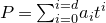 $P={\sum}_{i=0}^{i=d}a_it^{i}$
and use the
$P={\sum}_{i=0}^{i=d}a_it^{i}$
and use the $A[G_{\mathfrak{p}}]$
-basis
$A[G_{\mathfrak{p}}]$
-basis $\{1\otimes t^{i}:0\leq i\leq d-1\}$
of
$\{1\otimes t^{i}:0\leq i\leq d-1\}$
of $A[G_{\mathfrak{p}}]\otimes_{{\mathbb F}_q[G_{\mathfrak{p}}]}\kappa_{\bar{\mathfrak{p}}}[G_{\mathfrak{p}}]$
. Then the matrix of
$A[G_{\mathfrak{p}}]\otimes_{{\mathbb F}_q[G_{\mathfrak{p}}]}\kappa_{\bar{\mathfrak{p}}}[G_{\mathfrak{p}}]$
. Then the matrix of $(t\otimes 1)-(1\otimes t)$
is given by
$(t\otimes 1)-(1\otimes t)$
is given by
 \begin{equation*}M_\tau:=\begin{bmatrix}t &\quad -1 &\quad 0 &\quad 0 &\quad \cdots &\quad 0 &\quad 0\\0 &\quad t &\quad -1 &\quad 0 &\quad \cdots &\quad 0 &\quad 0\\0 &\quad 0 &\quad t &\quad -1 &\quad \cdots &\quad 0 &\quad 0\\0 &\quad 0 &\quad 0 &\quad t &\quad \ddots &\quad 0 &\quad 0\\\vdots &\quad \vdots &\quad \vdots &\quad \ddots &\quad \ddots &\quad \vdots &\quad \vdots\\0 &\quad 0 &\quad 0 &\quad 0 &\quad \cdots &\quad t &\quad -1\\a_0 &\quad a_1 &\quad a_2 &\quad a_3 &\quad \cdots &\quad a_{d-2} &\quad (a_{d-1}+t)\end{bmatrix}.\end{equation*}
But it is straightforward to verify that $M_\tau$
is equal, up to multiplication by elementary matrices in
$M_\tau$
is equal, up to multiplication by elementary matrices in $M_d(\mathcal F)$
, to the diagonal matrix
$M_d(\mathcal F)$
, to the diagonal matrix $D_P:=\mathrm{diag}(1,1,\ldots,1,P)$
. Thus,
$D_P:=\mathrm{diag}(1,1,\ldots,1,P)$
. Thus, $c_{G_{\mathfrak{p}}}(\kappa_{\bar{\mathfrak{p}}}[G_{\mathfrak{p}}])=[M_\tau]=[D_P]=[P]$
, as required to prove (2.3).
$c_{G_{\mathfrak{p}}}(\kappa_{\bar{\mathfrak{p}}}[G_{\mathfrak{p}}])=[M_\tau]=[D_P]=[P]$
, as required to prove (2.3).
We next claim that
 \begin{equation}c_G(C(\mathcal O_K/\mathfrak{p}\mathcal O_K))=[N\mathfrak{p}-\textrm{Fr}_{\mathfrak{p}}\cdot e_{I_{\mathfrak{p}}}].\end{equation}
We assume, as we may, that $I_{\mathfrak{p}}\subseteq G_{\mathfrak{p}}$
and
$I_{\mathfrak{p}}\subseteq G_{\mathfrak{p}}$
and $\textrm{Fr}_{\mathfrak{p}}\in G_{\mathfrak{p}}$
, and we set
$\textrm{Fr}_{\mathfrak{p}}\in G_{\mathfrak{p}}$
, and we set $e:=|I_{\mathfrak{p}}|$
,
$e:=|I_{\mathfrak{p}}|$
, $M:=K^{I_{\mathfrak{p}}}$
,
$M:=K^{I_{\mathfrak{p}}}$
, $L:=K^{G_{\mathfrak{p}}}$
,
$L:=K^{G_{\mathfrak{p}}}$
, $J_{\mathfrak{p}}:=G_{\mathfrak{p}}/I_{\mathfrak{p}}$
,
$J_{\mathfrak{p}}:=G_{\mathfrak{p}}/I_{\mathfrak{p}}$
, $\mathfrak{q}_M:=\mathfrak{q}\cap\mathcal O_M$
,
$\mathfrak{q}_M:=\mathfrak{q}\cap\mathcal O_M$
, $\mathfrak{q}_L:=\mathfrak{q}\cap\mathcal O_L$
and
$\mathfrak{q}_L:=\mathfrak{q}\cap\mathcal O_L$
and $e'_{I_{\mathfrak{p}}}=1-e_{I_{\mathfrak{p}}}$
. We note that
$e'_{I_{\mathfrak{p}}}=1-e_{I_{\mathfrak{p}}}$
. We note that $\mathcal O_{K_{\mathfrak{q}}}\cong\mathcal O_{L_{\mathfrak{q}_L}}[G_{\mathfrak{p}}]$
is
$\mathcal O_{K_{\mathfrak{q}}}\cong\mathcal O_{L_{\mathfrak{q}_L}}[G_{\mathfrak{p}}]$
is $G_{\mathfrak{p}}$
-c.t. by Lemma 2.2(i), that
$G_{\mathfrak{p}}$
-c.t. by Lemma 2.2(i), that $\mathfrak{q}^{a}\mathcal O_{K_{\mathfrak{q}}}\cong\mathcal O_{K_{\mathfrak{q}}}$
for any
$\mathfrak{q}^{a}\mathcal O_{K_{\mathfrak{q}}}\cong\mathcal O_{K_{\mathfrak{q}}}$
for any $a\geq 0$
, and thus that
$a\geq 0$
, and thus that $\mathfrak{q}^{a}/\mathfrak{q}^{b}\cong\mathfrak{q}^{a}\mathcal O_{K_{\mathfrak{q}}}/\mathfrak{q}^{b}\mathcal O_{K_{\mathfrak{q}}}$
is
$\mathfrak{q}^{a}/\mathfrak{q}^{b}\cong\mathfrak{q}^{a}\mathcal O_{K_{\mathfrak{q}}}/\mathfrak{q}^{b}\mathcal O_{K_{\mathfrak{q}}}$
is $G_{\mathfrak{p}}$
-c.t. for any
$G_{\mathfrak{p}}$
-c.t. for any $b\geq a\geq 0$
.
$b\geq a\geq 0$
.
Since $C(\mathcal O_K/\mathfrak{p}\mathcal O_K)\cong{\mathbb F}_q[G]\otimes_{{\mathbb F}_q[G_{\mathfrak{p}}]}C(\mathcal O_{K}/\mathfrak{q}^{e})$
and
$C(\mathcal O_K/\mathfrak{p}\mathcal O_K)\cong{\mathbb F}_q[G]\otimes_{{\mathbb F}_q[G_{\mathfrak{p}}]}C(\mathcal O_{K}/\mathfrak{q}^{e})$
and
 $$N\mathfrak{p}-\textrm{Fr}_{\mathfrak{p}}\cdot e_{I_{\mathfrak{p}}}=(e_{I_{\mathfrak{p}}}(N\mathfrak{p}-\textrm{Fr}_{\mathfrak{p}})+e'_{I_{\mathfrak{p}}})\cdot(e_{I_{\mathfrak{p}}}+e'_{I_{\mathfrak{p}}}N\mathfrak{p}),$$
to deduce (2.4) from Lemmas 2.6 and 2.7, it is enough to show that
 \begin{equation}c_{G_{\mathfrak{p}}}(C(\mathcal O_K/\mathfrak{q}))=[e_{I_{\mathfrak{p}}}(N\mathfrak{p}-\textrm{Fr}_{\mathfrak{p}})+e'_{I_{\mathfrak{p}}}] \quad\text{and}\quad c_{G_{\mathfrak{p}}}(C(\mathfrak{q}/\mathfrak{q}^{e}))=[e_{I_{\mathfrak{p}}}+e'_{I_{\mathfrak{p}}}N\mathfrak{p}].\end{equation}
To consider the first equality, we note that $J_{\mathfrak{p}}$
is abelian (in fact, cyclic) and apply [Reference Ferrara, Green, Higgins and PopescuFGH+22, Proposition A.5.1(3)] to the extension
$J_{\mathfrak{p}}$
is abelian (in fact, cyclic) and apply [Reference Ferrara, Green, Higgins and PopescuFGH+22, Proposition A.5.1(3)] to the extension $M/L$
and the unramified prime
$M/L$
and the unramified prime $\mathfrak{q}_L$
. Together with Proposition A.4.1 in [Reference Ferrara, Green, Higgins and PopescuFGH+22] (or with Lemma 3.10 below), this gives
$\mathfrak{q}_L$
. Together with Proposition A.4.1 in [Reference Ferrara, Green, Higgins and PopescuFGH+22] (or with Lemma 3.10 below), this gives $\det _{\mathcal F[J_{\mathfrak{p}}]}(c_{J_{\mathfrak{p}}}(C(\mathcal O_M/\mathfrak{q}_L\mathcal O_M)))=N\mathfrak{p}-\textrm{Fr}_{\mathfrak{p}}I_{\mathfrak{p}}$
in
$\det _{\mathcal F[J_{\mathfrak{p}}]}(c_{J_{\mathfrak{p}}}(C(\mathcal O_M/\mathfrak{q}_L\mathcal O_M)))=N\mathfrak{p}-\textrm{Fr}_{\mathfrak{p}}I_{\mathfrak{p}}$
in $\mathcal F[J_{\mathfrak{p}}]^\times$
. We abbreviate
$\mathcal F[J_{\mathfrak{p}}]^\times$
. We abbreviate $\tau_M$
for
$\tau_M$
for $M=C(\mathcal O_K/\mathfrak{q})$
to
$M=C(\mathcal O_K/\mathfrak{q})$
to $\tau$
. Then, since
$\tau$
. Then, since $I_{\mathfrak{p}}$
acts trivially on
$I_{\mathfrak{p}}$
acts trivially on
 $$\mathcal O_K/\mathfrak{q}\cong\mathcal O_M/\mathfrak{q}_M=\mathcal O_M/\mathfrak{q}_L\mathcal O_M,$$
it follows that $c_{G_{\mathfrak{p}}}(C(\mathcal O_K/\mathfrak{q}))=[C(\mathcal O_K/\mathfrak{q})'_{\mathcal F},\tau_{\mathcal F}]$
is mapped to
$c_{G_{\mathfrak{p}}}(C(\mathcal O_K/\mathfrak{q}))=[C(\mathcal O_K/\mathfrak{q})'_{\mathcal F},\tau_{\mathcal F}]$
is mapped to
 \begin{align*}&(\det _{\mathcal F[J_{\mathfrak{p}}]}([\mathcal F[J_{\mathfrak{p}}]\otimes_{\mathcal F[G_{\mathfrak{p}}]}C(\mathcal O_K/\mathfrak{q})'_{\mathcal F},1\otimes\tau_{\mathcal F}]),1)\\&\quad = (\det _{\mathcal F[J_{\mathfrak{p}}]}([\mathcal F[J_{\mathfrak{p}}]\otimes_{{\mathbb F}_q[J_{\mathfrak{p}}]}C(\mathcal O_M/\mathfrak{q}_L\mathcal O_M),\tau_{\mathcal F}]),1)=(N\mathfrak{p}-\textrm{Fr}_{\mathfrak{p}}I_{\mathfrak{p}},1)\end{align*}
under the composite isomorphism
 \begin{align*}K_1(\mathcal F[G_{\mathfrak{p}}])\cong&\, K_1(e_{I_{\mathfrak{p}}}\mathcal F[G_{\mathfrak{p}}])\times K_1(e'_{I_{\mathfrak{p}}}\mathcal F[G_{\mathfrak{p}}])\cong K_1(\mathcal F[J_{\mathfrak{p}}])\times K_1(e'_{I_{\mathfrak{p}}}\mathcal F[G_{\mathfrak{p}}])\\ \stackrel{\det }{\cong}&\,\mathcal F[J_{\mathfrak{p}}]^\times\times K_1(e'_{I_{\mathfrak{p}}}\mathcal F[G_{\mathfrak{p}}]).\end{align*}
Since the same is true of $[e_{I_{\mathfrak{p}}}(N\mathfrak{p}-\textrm{Fr}_{\mathfrak{p}})+e'_{I_{\mathfrak{p}}}]$
, the first equality in (2.5) is valid.
$[e_{I_{\mathfrak{p}}}(N\mathfrak{p}-\textrm{Fr}_{\mathfrak{p}})+e'_{I_{\mathfrak{p}}}]$
, the first equality in (2.5) is valid.
To consider the second equality in (2.5), we note that for all $n\geq 1$
,
$n\geq 1$
, $x\in\mathfrak{q}^n$
and
$x\in\mathfrak{q}^n$
and $a\in A$
,
$a\in A$
, $(\phi_C(a))(x)$
is congruent to ax modulo
$(\phi_C(a))(x)$
is congruent to ax modulo $\mathfrak{q}^{qn}$
. In particular,
$\mathfrak{q}^{qn}$
. In particular, $C(\mathfrak{q}^n/\mathfrak{q}^{n+1})\cong\mathfrak{q}^n/\mathfrak{q}^{n+1}$
so, by induction on e, one can deduce from Lemma 2.6 that
$C(\mathfrak{q}^n/\mathfrak{q}^{n+1})\cong\mathfrak{q}^n/\mathfrak{q}^{n+1}$
so, by induction on e, one can deduce from Lemma 2.6 that $c_{G_{\mathfrak{p}}}(C(\mathfrak{q}/\mathfrak{q}^{e}))=c_{G_{\mathfrak{p}}}(\mathfrak{q}/\mathfrak{q}^{e})$
.
$c_{G_{\mathfrak{p}}}(C(\mathfrak{q}/\mathfrak{q}^{e}))=c_{G_{\mathfrak{p}}}(\mathfrak{q}/\mathfrak{q}^{e})$
.
To compute $c_{G_{\mathfrak{p}}}(\mathfrak{q}/\mathfrak{q}^{e})$
we note that
$c_{G_{\mathfrak{p}}}(\mathfrak{q}/\mathfrak{q}^{e})$
we note that $\mathcal O_K/\mathfrak{q}^{e}=\mathcal O_K/\mathfrak{q}_L\mathcal O_K\cong(\mathcal O_L/\mathfrak{q}_L)[G_{\mathfrak{p}}]$
and that
$\mathcal O_K/\mathfrak{q}^{e}=\mathcal O_K/\mathfrak{q}_L\mathcal O_K\cong(\mathcal O_L/\mathfrak{q}_L)[G_{\mathfrak{p}}]$
and that $e_{I_{\mathfrak{p}}}(\mathcal O_K/\mathfrak{q}^{e})\cong(\mathcal O_L/\mathfrak{q}_L)[J_{\mathfrak{p}}]$
surjects onto
$e_{I_{\mathfrak{p}}}(\mathcal O_K/\mathfrak{q}^{e})\cong(\mathcal O_L/\mathfrak{q}_L)[J_{\mathfrak{p}}]$
surjects onto $e_{I_{\mathfrak{p}}}(\mathcal O_K/\mathfrak{q})=\mathcal O_K/\mathfrak{q}$
. Since the latter two
$e_{I_{\mathfrak{p}}}(\mathcal O_K/\mathfrak{q})=\mathcal O_K/\mathfrak{q}$
. Since the latter two $(\mathcal O_L/\mathfrak{q}_L)$
-spaces have dimension
$(\mathcal O_L/\mathfrak{q}_L)$
-spaces have dimension $|J_{\mathfrak{p}}|$
, in fact we have
$|J_{\mathfrak{p}}|$
, in fact we have
 $$\mathcal O_K/\mathfrak{q}\cong e_{I_{\mathfrak{p}}}(\mathcal O_L/\mathfrak{q}_L)[G_{\mathfrak{p}}]=e_{I_{\mathfrak{p}}}(\mathcal O_k/\mathfrak{p})[G_{\mathfrak{p}}]\cong(e_{I_{\mathfrak{p}}}\kappa_{\bar{\mathfrak{p}}}[G_{\mathfrak{p}}])^{f_{\mathfrak{p}}}.$$
Now, (2.3) applied to the extension $K/L$
gives
$K/L$
gives $c_{G_{\mathfrak{p}}}(\mathcal O_K/\mathfrak{q}^{e})=c_{G_{\mathfrak{p}}}(\mathcal O_K/\mathfrak{q}_L\mathcal O_K)=[N\mathfrak{p}]$
. Set
$c_{G_{\mathfrak{p}}}(\mathcal O_K/\mathfrak{q}^{e})=c_{G_{\mathfrak{p}}}(\mathcal O_K/\mathfrak{q}_L\mathcal O_K)=[N\mathfrak{p}]$
. Set $\kappa:=\kappa_{\bar{\mathfrak{p}}}[G_{\mathfrak{p}}]$
and
$\kappa:=\kappa_{\bar{\mathfrak{p}}}[G_{\mathfrak{p}}]$
and $f:=f_{\mathfrak{p}}$
. Writing
$f:=f_{\mathfrak{p}}$
. Writing $I_d$
for the identity matrix, the argument used to prove (2.3) shows that
$I_d$
for the identity matrix, the argument used to prove (2.3) shows that
 \begin{align*}c_{G_{\mathfrak{p}}}(e_{I_{\mathfrak{p}}}\kappa)&= [(e_{I_{\mathfrak{p}}}\kappa)'_{\mathcal F},\tau_{e_{I_{\mathfrak{p}}}\kappa,\mathcal F}]=[(e_{I_{\mathfrak{p}}}\kappa)'_{\mathcal F},\tau_{e_{I_{\mathfrak{p}}}\kappa,\mathcal F}]\cdot[(e'_{I_{\mathfrak{p}}}\kappa)'_{\mathcal F},1]\\&= [\kappa'_{\mathcal F},e_{I_{\mathfrak{p}}}\tau_{\kappa,\mathcal F}\oplus e'_{I_{\mathfrak{p}}}\mathrm{id}_{\kappa'_{\mathcal F}}]=[e_{I_{\mathfrak{p}}}M_\tau+e'_{I_{\mathfrak{p}}}I_d],\end{align*}
and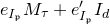 $e_{I_{\mathfrak{p}}}M_\tau+e'_{I_{\mathfrak{p}}}I_d$
is equal, up to multiplication by elementary matrices in
$e_{I_{\mathfrak{p}}}M_\tau+e'_{I_{\mathfrak{p}}}I_d$
is equal, up to multiplication by elementary matrices in $M_d(\mathcal F[G_{\mathfrak{p}}])$
, to the diagonal matrix
$M_d(\mathcal F[G_{\mathfrak{p}}])$
, to the diagonal matrix $D'_P:=\mathrm{ diag}(1,1,\ldots,1,e_{I_{\mathfrak{p}}}P+e'_{I_{\mathfrak{p}}})$
. Using Lemma 2.6, we have
$D'_P:=\mathrm{ diag}(1,1,\ldots,1,e_{I_{\mathfrak{p}}}P+e'_{I_{\mathfrak{p}}})$
. Using Lemma 2.6, we have
 $$c_{G_{\mathfrak{p}}}(\mathcal O_K/\mathfrak{q})=c_{G_{\mathfrak{p}}}(e_{I_{\mathfrak{p}}}\kappa)^{f}=[e_{I_{\mathfrak{p}}}M_\tau+e'_{I_{\mathfrak{p}}}I_d]^{f}=[D'_P]^{f}=[e_{I_{\mathfrak{p}}}P+e'_{I_{\mathfrak{p}}}]^{f}=[e_{I_{\mathfrak{p}}}N\mathfrak{p}+e'_{I_{\mathfrak{p}}}].$$
The second equality in (2.5) now follows from Lemma 2.6 as
 \begin{align*}c_{G_{\mathfrak{p}}}(C(\mathfrak{q}/\mathfrak{q}^{e})) &=c_{G_{\mathfrak{p}}}(\mathfrak{q}/\mathfrak{q}^{e}) = c_{G_{\mathfrak{p}}}(\mathcal O_K/\mathfrak{q}^{e})\cdot c_{G_{\mathfrak{p}}}(\mathcal O_K/\mathfrak{q})^{-1} =[N\mathfrak{p}]\cdot[e_{I_{\mathfrak{p}}}N\mathfrak{p}+e'_{I_{\mathfrak{p}}}]^{-1}\\ &= [e_{I_{\mathfrak{p}}}+e'_{I_{\mathfrak{p}}}N\mathfrak{p}].\end{align*}
Finally, (2.3) and (2.4) combine to give our claim
 $$c_G(\mathcal O_K/\mathfrak{p}\mathcal O_K)\cdot c_G(C(\mathcal O_K/\mathfrak{p}\mathcal O_K))^{-1}=[N\mathfrak{p}]\cdot [N\mathfrak{p}-\textrm{Fr}_{\mathfrak{p}}\cdot e_{I_{\mathfrak{p}}}]^{-1}=[1-(N\mathfrak{p})^{-1}\textrm{Fr}_{\mathfrak{p}}\cdot e_{I_{\mathfrak{p}}}]^{-1}.$$
3. A construction of non-abelian Stickelberger elements
In this section, we restrict attention to finite Galois extensions $K/k$
with the property that the corresponding group rings decompose as finite direct sums of matrix rings over commutative rings. In this setting, we will construct non-abelian Stickelberger elements for Drinfeld modules and state their relations to the Galois module structure of Taelman class groups, that are encoded within Theorem 2.17.
$K/k$
with the property that the corresponding group rings decompose as finite direct sums of matrix rings over commutative rings. In this setting, we will construct non-abelian Stickelberger elements for Drinfeld modules and state their relations to the Galois module structure of Taelman class groups, that are encoded within Theorem 2.17.
In particular, we obtain generalisations of the ‘refined Brumer–Stark theorem for Drinfeld modules’ [Reference Ferrara, Green, Higgins and PopescuFGH+22, Theorem 1.5.5] of Ferrara et al. and of Theorem A of Anglès and Taelman in [Reference Anglès and TaelmanAT15].
In the general case, even defining suitable notions of reduced determinants and of non-commutative Fitting ideals will require new and rather involved algebraic techniques. We will return to these problems in future work.
3.1 Reduced determinants and non-commutative Fitting ideals
We fix a finite group G with the property that $\ell$
does not divide the order of the commutator subgroup G’ of G. Equivalently, G has an abelian
$\ell$
does not divide the order of the commutator subgroup G’ of G. Equivalently, G has an abelian $\ell$
-Sylow subgroup L and a normal
$\ell$
-Sylow subgroup L and a normal $\ell$
-complement N, and thus admits a semidirect product decomposition
$\ell$
-complement N, and thus admits a semidirect product decomposition
 \begin{equation}G\cong N\rtimes L.\end{equation}
(Indeed, if $\ell\nmid|G'|$
, then any
$\ell\nmid|G'|$
, then any $\ell$
-Sylow subgroup L is isomorphic to the direct factor
$\ell$
-Sylow subgroup L is isomorphic to the direct factor $LG'/G'$
of the abelian group
$LG'/G'$
of the abelian group $G/G'$
, and the
$G/G'$
, and the $\ell$
-complement
$\ell$
-complement $\ker(G\to G/G'\to LG'/G')$
is normal. Conversely, G’ must be contained in N, so
$\ker(G\to G/G'\to LG'/G')$
is normal. Conversely, G’ must be contained in N, so $\ell\nmid|G'|$
.)
$\ell\nmid|G'|$
.)
3.1.1.
If F is an algebraically closed field of characteristic $\ell$
, then the proof of [Reference PassmanPas77, Part 2, § 6, Lemma 1.10, pp. 231–233] gives a canonical decomposition of F[G] as a finite direct sum of matrix rings over commutative F-algebras. DeMeyer and Janusz [Reference DeMeyer and JanuszDJ83, Theorem 3.1] then use this fact to prove that for any field F of characteristic
$\ell$
, then the proof of [Reference PassmanPas77, Part 2, § 6, Lemma 1.10, pp. 231–233] gives a canonical decomposition of F[G] as a finite direct sum of matrix rings over commutative F-algebras. DeMeyer and Janusz [Reference DeMeyer and JanuszDJ83, Theorem 3.1] then use this fact to prove that for any field F of characteristic $\ell$
, F[G] is an Azumaya algebra. However, their proof is non-constructive, in that it does not provide information on how to decompose F[G] as a sum of matrix rings.
$\ell$
, F[G] is an Azumaya algebra. However, their proof is non-constructive, in that it does not provide information on how to decompose F[G] as a sum of matrix rings.
In this section, we explain how to extend the argument of [Reference PassmanPas77, Part 2, § 6, Lemma 1.10, pp. 231–233] to give a corresponding canonical decomposition of ${\mathbb F}_\ell[G]$
.
${\mathbb F}_\ell[G]$
.
We fix a decomposition (3.1) of G. Then G acts on the set of central primitive idempotents of ${\mathbb F}_\ell[N]$
by conjugation. Let
${\mathbb F}_\ell[N]$
by conjugation. Let $\{\mathcal O_i:1\leq i\leq m\}$
be the set of orbits of this action. For each i, fix an element
$\{\mathcal O_i:1\leq i\leq m\}$
be the set of orbits of this action. For each i, fix an element $e_i\in\mathcal O_i$
. Then the Wedderburn decomposition of
$e_i\in\mathcal O_i$
. Then the Wedderburn decomposition of $e_i{\mathbb F}_\ell[N]$
is of the form
$e_i{\mathbb F}_\ell[N]$
is of the form
 \begin{equation}e_i{\mathbb F}_\ell[N]\cong M_{m_i}({\mathbb F}_\ell(i))\end{equation}
for some $m_i\in\mathbb N$
and some finite field extension
$m_i\in\mathbb N$
and some finite field extension ${\mathbb F}_\ell(i)/{\mathbb F}_\ell$
(note that
${\mathbb F}_\ell(i)/{\mathbb F}_\ell$
(note that ${\mathbb F}_\ell(i)$
is indeed a field by Wedderburn’s little theorem). We also define an abelian
${\mathbb F}_\ell(i)$
is indeed a field by Wedderburn’s little theorem). We also define an abelian $\ell$
-group
$\ell$
-group
 $$L_i:=\{\lambda\in L:\lambda e_i \lambda^{-1}=e_i\},$$
the centraliser of $e_i$
in L.
$e_i$
in L.
Proposition 3.1. There is a canonical isomorphism
 $${\mathbb F}_\ell[G]\cong \bigoplus _{i=1}^{i=m}M_{m_i\cdot|\mathcal O_i|}({\mathbb F}_\ell(i)[L_i]).$$
Remark 3.2. Given an index $1\leq i\leq m$
, different choices of idempotent
$1\leq i\leq m$
, different choices of idempotent $e_i\in\mathcal O_i$
give rise to canonically isomorphic summands
$e_i\in\mathcal O_i$
give rise to canonically isomorphic summands $M_{m_i\cdot|\mathcal O_i|}({\mathbb F}_\ell(i)[L_i])$
. The summand corresponding to the orbit
$M_{m_i\cdot|\mathcal O_i|}({\mathbb F}_\ell(i)[L_i])$
. The summand corresponding to the orbit $\{e_N\}$
for
$\{e_N\}$
for $e_N:=|N|^{-1}\sum_{\nu\in N}\nu$
is
$e_N:=|N|^{-1}\sum_{\nu\in N}\nu$
is $M_{1}({\mathbb F}_\ell[L])={\mathbb F}_\ell[L]$
. If
$M_{1}({\mathbb F}_\ell[L])={\mathbb F}_\ell[L]$
. If $\ell\nmid|G|$
, Proposition 3.1 recovers the Wedderburn decomposition
$\ell\nmid|G|$
, Proposition 3.1 recovers the Wedderburn decomposition ${\mathbb F}_\ell[G]={\mathbb F}_\ell[N]\cong \bigoplus _{i=1}^{i=m}M_{m_i}({\mathbb F}_\ell(i))$
. If G is abelian, it simply gives
${\mathbb F}_\ell[G]={\mathbb F}_\ell[N]\cong \bigoplus _{i=1}^{i=m}M_{m_i}({\mathbb F}_\ell(i))$
. If G is abelian, it simply gives ${\mathbb F}_\ell[G]={\mathbb F}_\ell[N][L]\cong \bigoplus _{i=1}^{i=m}{\mathbb F}_\ell(i)[L]$
.
${\mathbb F}_\ell[G]={\mathbb F}_\ell[N][L]\cong \bigoplus _{i=1}^{i=m}{\mathbb F}_\ell(i)[L]$
.
In the rest of § 3.1.1, we prove Proposition 3.1. For each $1\leq i\leq m$
we set
$1\leq i\leq m$
we set $f_i:=\sum_{e\in\mathcal O_i}e\in{\mathbb F}_\ell[N]$
and observe that this idempotent is central in
$f_i:=\sum_{e\in\mathcal O_i}e\in{\mathbb F}_\ell[N]$
and observe that this idempotent is central in ${\mathbb F}_\ell[G]$
. Since
${\mathbb F}_\ell[G]$
. Since $\sum_{i=1}^{i=m}f_i=1$
, we have
$\sum_{i=1}^{i=m}f_i=1$
, we have
 \begin{equation}{\mathbb F}_\ell[G] = \bigoplus _{i=1}^{i=m}f_i{\mathbb F}_\ell[G].\end{equation}
We next fix i and let
 $$G_i:=\{g\in G:ge_ig^{-1}=e_i\}\supseteq N$$
be the centraliser of $e_i$
in G. We then apply [Reference PassmanPas77, Part 2, § 6, Lemma 1.7, pp. 228–229] to G, with H taken to be N, K taken to be
$e_i$
in G. We then apply [Reference PassmanPas77, Part 2, § 6, Lemma 1.7, pp. 228–229] to G, with H taken to be N, K taken to be ${\mathbb F}_\ell$
,
${\mathbb F}_\ell$
, $e_1$
taken to be
$e_1$
taken to be $e_i$
and e taken to be
$e_i$
and e taken to be $f_i$
, to obtain the following result.
$f_i$
, to obtain the following result.
Lemma 3.3. There is a canonical isomorphism
 $$M_{|\mathcal O_i|}(e_i{\mathbb F}_\ell[G_i])\cong f_i{\mathbb F}_\ell[G]$$
that maps a matrix $(s_{kj})_{1\leq k,j\leq |\mathcal O_i|}$
to
$(s_{kj})_{1\leq k,j\leq |\mathcal O_i|}$
to $\sum_{1\leq k,j\leq |\mathcal O_i|}s_{kj}(g_k^{-1}e_ig_j)$
, where the elements
$\sum_{1\leq k,j\leq |\mathcal O_i|}s_{kj}(g_k^{-1}e_ig_j)$
, where the elements $g_l\in G$
are chosen so that
$g_l\in G$
are chosen so that $g_1=1$
and
$g_1=1$
and
 $$\mathcal O_i=\{g_l^{-1}e_ig_l:1\leq l\leq|\mathcal O_i|\}.$$
The proof of Proposition 3.1 is now completed upon combining (3.3) with Lemma 3.3 and with the following result.
Lemma 3.4. The isomorphism (3.2) induces a canonical isomorphism (see (3.4))
 $$e_i{\mathbb F}_\ell[G_i]\cong M_{m_i}({\mathbb F}_\ell(i)[L_i]).$$
Proof. Because $e_i$
is a central idempotent of
$e_i$
is a central idempotent of ${\mathbb F}_\ell[G_i]$
,
${\mathbb F}_\ell[G_i]$
, $R:=e_i{\mathbb F}_\ell[G_i]$
is a ring with identity element
$R:=e_i{\mathbb F}_\ell[G_i]$
is a ring with identity element $e_i$
and with
$e_i$
and with

Let $E_{kj}$
be the matrix with 1 in position (k,j) and zeros elsewhere, and let
$E_{kj}$
be the matrix with 1 in position (k,j) and zeros elsewhere, and let $\{e_{kj}\}_{1\leq k,j\leq m_i}\subseteq e_i{\mathbb F}_\ell[N]$
be their preimages through (3.2). We note that
$\{e_{kj}\}_{1\leq k,j\leq m_i}\subseteq e_i{\mathbb F}_\ell[N]$
be their preimages through (3.2). We note that $e_{11}e_i=e_{11}$
, and hence that
$e_{11}e_i=e_{11}$
, and hence that $e_{11}Re_{11}=e_{11}(e_i{\mathbb F}_\ell[G_i])e_{11}=e_{11}{\mathbb F}_\ell[G_i]e_{11}$
. Because
$e_{11}Re_{11}=e_{11}(e_i{\mathbb F}_\ell[G_i])e_{11}=e_{11}{\mathbb F}_\ell[G_i]e_{11}$
. Because
 $$e_{kj}e_{ab}=\begin{cases}0, & j\neq a,\\e_{kb}, & j=a,\end{cases}$$
and $e_i=e_{11}+\cdots+e_{m_i m_i}$
, [Reference PassmanPas77, Part 2, §6, Lemma 1.5, p. 227] shows that the map
$e_i=e_{11}+\cdots+e_{m_i m_i}$
, [Reference PassmanPas77, Part 2, §6, Lemma 1.5, p. 227] shows that the map
 \begin{align}M_{m_i}(e_{11}{\mathbb F}_\ell[G_i]e_{11})=M_{m_i}(e_{11}Re_{11})&\cong R=e_i{\mathbb F}_\ell[G_i],\\\notag(s_{kj})_{1\leq k,j\leq m_i}&\mapsto{\sum}_{1\leq k,j\leq m_i}s_{kj}e_{kj}\end{align}
is a ring isomorphism. Therefore, it suffices to show that $e_{11}{\mathbb F}_\ell[G_i]e_{11}\cong{\mathbb F}_\ell(i)[L_i]$
.
$e_{11}{\mathbb F}_\ell[G_i]e_{11}\cong{\mathbb F}_\ell(i)[L_i]$
.
Next we observe that the map $L_i=G_i\cap L\to G_i\to G_i/N$
is bijective. Then, the argument used to prove [Reference PassmanPas77, Part 2, § 6, Lemma 1.8, pp. 229–230], with G taken to be
$L_i=G_i\cap L\to G_i\to G_i/N$
is bijective. Then, the argument used to prove [Reference PassmanPas77, Part 2, § 6, Lemma 1.8, pp. 229–230], with G taken to be $G_i$
, H taken to be N and e taken to be
$G_i$
, H taken to be N and e taken to be $e_i$
, shows that
$e_i$
, shows that $e_{11}{\mathbb F}_\ell[G_i]e_{11}$
is a twisted group ring, in the sense of [Reference PassmanPas77, Part 1, § 2], of the group
$e_{11}{\mathbb F}_\ell[G_i]e_{11}$
is a twisted group ring, in the sense of [Reference PassmanPas77, Part 1, § 2], of the group $L_i$
over the field
$L_i$
over the field

Indeed, although, for a given group G, normal subgroup H, field K and idempotent $e\in K[H]$
central in K[G], the statement of this result assumes that
$e\in K[H]$
central in K[G], the statement of this result assumes that $eK[H]\cong M_m(K)$
for some m, and the relevant argument then shows that
$eK[H]\cong M_m(K)$
for some m, and the relevant argument then shows that $e_{11}K[G]e_{11}$
is a twisted group ring of
$e_{11}K[G]e_{11}$
is a twisted group ring of $G/H$
over
$G/H$
over $e_{11}K[H]e_{11}=e_{11}(eK[H])e_{11}\cong E_{11}(M_m(K))E_{11}\cong K$
, every step works in an identical manner upon using the isomorphism (3.2) instead.
$e_{11}K[H]e_{11}=e_{11}(eK[H])e_{11}\cong E_{11}(M_m(K))E_{11}\cong K$
, every step works in an identical manner upon using the isomorphism (3.2) instead.
To finally complete the proof of the lemma, we now recall that $L_i$
is an
$L_i$
is an $\ell$
-group and
$\ell$
-group and ${\mathbb F}_\ell(i)$
is a perfect field. Thus, [Reference PassmanPas77, Part 1, § 2, Lemma 2.10, p. 20] implies that any twisted group ring of
${\mathbb F}_\ell(i)$
is a perfect field. Thus, [Reference PassmanPas77, Part 1, § 2, Lemma 2.10, p. 20] implies that any twisted group ring of $L_i$
over
$L_i$
over ${\mathbb F}_\ell(i)$
is necessarily equal to the group ring
${\mathbb F}_\ell(i)$
is necessarily equal to the group ring ${\mathbb F}_\ell(i)[L_i]$
.
${\mathbb F}_\ell(i)[L_i]$
.
3.1.2.
We now fix a commutative (and associative) $\mathbb{F}_\ell$
-algebra B and, in the notation of Proposition 3.1, for each index
$\mathbb{F}_\ell$
-algebra B and, in the notation of Proposition 3.1, for each index $1\leq i\leq m$
, we define a commutative B-algebra
$1\leq i\leq m$
, we define a commutative B-algebra
 $$R_i:=B \otimes_{\mathbb{F}_\ell}{\mathbb F}_\ell(i)[L_i].$$
We note that $R_i$
is finitely generated as a B-module. Setting also
$R_i$
is finitely generated as a B-module. Setting also $n_i:=m_i\cdot|\mathcal O_i|$
, from Proposition 3.1 we then derive a canonical decomposition
$n_i:=m_i\cdot|\mathcal O_i|$
, from Proposition 3.1 we then derive a canonical decomposition
 \begin{equation}B[G]\cong \bigoplus_{i=1}^m M_{n_i}(R_i).\end{equation}
From this we derive a decomposition $Z(B[G])\cong\bigoplus_{i=1}^m R_i$
and, for any
$Z(B[G])\cong\bigoplus_{i=1}^m R_i$
and, for any $a,b\geq 1$
, also
$a,b\geq 1$
, also
 $$M_{a\times b}(B[G])\,\cong \bigoplus_{i=1}^m M_{(n_i\cdot a)\times (n_i\cdot b)}(R_i).$$
For any element x of either of the above rings, let us write $x_i$
for the i-component of its image on the right-hand side. We denote by
$x_i$
for the i-component of its image on the right-hand side. We denote by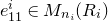 $e_{11}^{i}\in M_{n_i}(R_i)$
the matrix with 1 in position (1, 1) and zeros elsewhere, and regard it as an element of B[G] through (3.5).
$e_{11}^{i}\in M_{n_i}(R_i)$
the matrix with 1 in position (1, 1) and zeros elsewhere, and regard it as an element of B[G] through (3.5).
We may now provide definitions of reduced determinants and of non-commutative Fitting ideals, for the latter of which we follow [Reference Johnston and NickelJN13, Definition 1].
Definition 3.5.
-
(i) Let H be a square matrix over B[G]. The reduced determinant of H is
$$\textrm{Nrd}_{B[G]}(H) := (\det _{R_i}(H_i))_{1\leq i\leq m} \in Z(B[G]).$$
-
(ii) Let M be a finitely presented B[G]-module. The non-commutative Fitting ideal of M is the ideal of Z(B[G]) given by
$$\textrm{Fit}_{B[G]}(M) :=\bigoplus_{i=1}^m\textrm{Fit}_{R_i}(e_{11}^{i}M).$$


Remark 3.6. If each $n_i$
is equal to 1, these recover the usual definitions of determinants and of Fitting ideals over
$n_i$
is equal to 1, these recover the usual definitions of determinants and of Fitting ideals over $\bigoplus_{i=1}^mR_i=B[G]$
. We have chosen the notation
$\bigoplus_{i=1}^mR_i=B[G]$
. We have chosen the notation $\textrm{Nrd}_{B[G]}$
to emphasise the fact that, if B is a field and
$\textrm{Nrd}_{B[G]}$
to emphasise the fact that, if B is a field and $\ell\nmid|G|$
, so that
$\ell\nmid|G|$
, so that $G=N$
, then reduced determinants also coincide with the usual reduced norms over the semisimple ring B[N]. We also refer the reader to [Reference Johnston and NickelJN13, Theorem 2.2, Propositions 2.4 and 3.4] for the basic properties of non-commutative Fitting ideals.
$G=N$
, then reduced determinants also coincide with the usual reduced norms over the semisimple ring B[N]. We also refer the reader to [Reference Johnston and NickelJN13, Theorem 2.2, Propositions 2.4 and 3.4] for the basic properties of non-commutative Fitting ideals.
Remark 3.7. Let P be a finitely generated, projective B[G]-module, and let $\Phi$
be a B[G]-endomorphism of P. Then the reduced determinant
$\Phi$
be a B[G]-endomorphism of P. Then the reduced determinant
 $$\textrm{Nrd}_{B[G]}(\Phi) := \textrm{Nrd}_{B[G]}(H(\Phi\oplus\mathrm{id}_Q)) \in Z(B[G])$$
of $\Phi$
is easily seen to be independent of the choice of B[G]-module Q with the property that
$\Phi$
is easily seen to be independent of the choice of B[G]-module Q with the property that $P\oplus Q$
is free of finite rank, as well as of the choice of B[G]-basis with respect to which the matrix
$P\oplus Q$
is free of finite rank, as well as of the choice of B[G]-basis with respect to which the matrix $H(\Phi\oplus\mathrm{id}_Q)$
of the endomorphism
$H(\Phi\oplus\mathrm{id}_Q)$
of the endomorphism $\Phi\oplus\mathrm{id}_Q$
of
$\Phi\oplus\mathrm{id}_Q$
of $P\oplus Q$
is computed.
$P\oplus Q$
is computed.
Given $B'\supseteq B$
, the compatibility of the respective decompositions of the form (3.5) implies that
$B'\supseteq B$
, the compatibility of the respective decompositions of the form (3.5) implies that $\textrm{Nrd}_{B'[G]}(B'\otimes_B \Phi)=\textrm{Nrd}_{B[G]}(\Phi)$
. Non-commutative Fitting ideals satisfy an analogous base-change property (cf. [Reference Johnston and NickelJN13, Theorem 2.2(vii)]).
$\textrm{Nrd}_{B'[G]}(B'\otimes_B \Phi)=\textrm{Nrd}_{B[G]}(\Phi)$
. Non-commutative Fitting ideals satisfy an analogous base-change property (cf. [Reference Johnston and NickelJN13, Theorem 2.2(vii)]).
In the next result, we set $SK_1(R_i):=\{x\in K_1(R_i) \mid \det _{R_i}(x)=1\}$
.
$SK_1(R_i):=\{x\in K_1(R_i) \mid \det _{R_i}(x)=1\}$
.
Lemma 3.8. Taking reduced determinants induces a split short exact sequence of abelian groups
 $$1\to\bigoplus_{i=1}^m SK_1(R_i)\longrightarrow K_1(B[G])\xrightarrow{\textrm{Nrd}_{B[G]}} Z(B[G])^\times\to 1.$$
If B is a (commutative) local ring, then the first term vanishes and $\textrm{Nrd}_{B[G]}$
is an isomorphism.
$\textrm{Nrd}_{B[G]}$
is an isomorphism.
Proof. It suffices to prove the case $m=1$
. In this case, the first claim follows from the Morita equivalence between
$m=1$
. In this case, the first claim follows from the Morita equivalence between $B[G]\cong M_{n_1}(R_1)$
and
$B[G]\cong M_{n_1}(R_1)$
and $R_1$
and the second claim from Proposition 5.28 in Volume I and Proposition 45.12 in Volume II of [Reference Curtis and ReinerCR87].
$R_1$
and the second claim from Proposition 5.28 in Volume I and Proposition 45.12 in Volume II of [Reference Curtis and ReinerCR87].
Lemma 3.9. Let $Z(\mathcal F_\infty[G])^\times\subseteq\mathcal F_\infty[G]^\times$
have the subspace topology. Then the isomorphism
$Z(\mathcal F_\infty[G])^\times\subseteq\mathcal F_\infty[G]^\times$
have the subspace topology. Then the isomorphism $\textrm{Nrd}_{\mathcal F_\infty[G]}:K_1(\mathcal F_\infty[G])\to Z(\mathcal F_\infty[G])^\times$
is continuous.
$\textrm{Nrd}_{\mathcal F_\infty[G]}:K_1(\mathcal F_\infty[G])\to Z(\mathcal F_\infty[G])^\times$
is continuous.
Proof. Each $R_i:=\mathcal F_\infty\otimes_{\mathbb{F}_\ell}{\mathbb F}_\ell(i)[L_i]$
is a finite-dimensional
$R_i:=\mathcal F_\infty\otimes_{\mathbb{F}_\ell}{\mathbb F}_\ell(i)[L_i]$
is a finite-dimensional $\mathcal F_\infty$
-space, and so is the right-hand side of (3.5). We endow it with the supremum ring norm, which defines the unique Hausdorff
$\mathcal F_\infty$
-space, and so is the right-hand side of (3.5). We endow it with the supremum ring norm, which defines the unique Hausdorff $\mathcal F_\infty$
-space topology. Since
$\mathcal F_\infty$
-space topology. Since $\mathcal F_\infty[G]$
is also a Hausdorff
$\mathcal F_\infty[G]$
is also a Hausdorff $\mathcal F_\infty$
-space, the ring isomorphism (3.5) is an isomorphism of topological rings. The same claim is true of the restriction
$\mathcal F_\infty$
-space, the ring isomorphism (3.5) is an isomorphism of topological rings. The same claim is true of the restriction $Z(\mathcal F_\infty[G])\cong\bigoplus_{i=1}^m R_i$
of (3.5). The respective induced maps
$Z(\mathcal F_\infty[G])\cong\bigoplus_{i=1}^m R_i$
of (3.5). The respective induced maps $\mathcal F_\infty[G]^\times\cong\bigoplus_{i=1}^m \textrm{GL}_{n_i}(R_i)$
and
$\mathcal F_\infty[G]^\times\cong\bigoplus_{i=1}^m \textrm{GL}_{n_i}(R_i)$
and $Z(\mathcal F_\infty[G])^\times\cong\bigoplus_{i=1}^m R_i^\times$
are isomorphisms of topological groups.
$Z(\mathcal F_\infty[G])^\times\cong\bigoplus_{i=1}^m R_i^\times$
are isomorphisms of topological groups.
Now, for each i, $\det _{R_i}:\textrm{GL}_{n_i}(R_i)\to R_i^\times$
is continuous, since it may be computed through sums and products on the topological ring
$\det _{R_i}:\textrm{GL}_{n_i}(R_i)\to R_i^\times$
is continuous, since it may be computed through sums and products on the topological ring $R_i$
. Thus,
$R_i$
. Thus, $\bigoplus_{i=1}^m \det _{R_i}:\mathcal F_\infty[G]^\times\to Z(\mathcal F_\infty[G])^\times$
is continuous. Since the latter map factors as the composition of
$\bigoplus_{i=1}^m \det _{R_i}:\mathcal F_\infty[G]^\times\to Z(\mathcal F_\infty[G])^\times$
is continuous. Since the latter map factors as the composition of $\textrm{Nrd}_{\mathcal F_\infty[G]}$
with the open quotient map
$\textrm{Nrd}_{\mathcal F_\infty[G]}$
with the open quotient map $\mathcal F_\infty[G]^\times\to K_1(\mathcal F_\infty[G])$
,
$\mathcal F_\infty[G]^\times\to K_1(\mathcal F_\infty[G])$
, $\textrm{Nrd}_{\mathcal F_\infty[G]}$
is continuous, as claimed.
$\textrm{Nrd}_{\mathcal F_\infty[G]}$
is continuous, as claimed.
We make explicit the relationship between non-commutative Fitting ideals and characteristic classes.
Lemma 3.10. Let M be an A[G]-module that is both finite and G-c.t. Then
 $$\textrm{Fit}_{A[G]}(M)=Z(A[G])\cdot\mathrm{Nrd}_{\mathcal F[G]}(c_G(M)).$$
In particular, $\mathrm{Nrd}_{\mathcal F[G]}(c_G(M))$
belongs to Z(A[G]) and
$\mathrm{Nrd}_{\mathcal F[G]}(c_G(M))$
belongs to Z(A[G]) and $\textrm{Fit}_{A[G]}(M)$
is principal.
$\textrm{Fit}_{A[G]}(M)$
is principal.
Proof. The A[G]-module M’ is finitely generated and projective (by Lemma 2.2(i)), so we may and do fix an A[G]-module Q with the property that $M'\oplus Q$
is free of finite rank, say n. By Lemma 2.3, there is then a short exact sequence
$M'\oplus Q$
is free of finite rank, say n. By Lemma 2.3, there is then a short exact sequence
 $$0\to M'\oplus Q\xrightarrow{\tau_M\oplus\mathrm{id}}M'\oplus Q\longrightarrow M\to 0.$$
Writing $(\tau_M\oplus\mathrm{id})_i$
for the endomorphism of
$(\tau_M\oplus\mathrm{id})_i$
for the endomorphism of $M_{n_i}(R_i)^{n}$
induced by the restriction of
$M_{n_i}(R_i)^{n}$
induced by the restriction of $\tau_M\oplus\mathrm{id}$
and an arbitrary choice of A[G]-basis of
$\tau_M\oplus\mathrm{id}$
and an arbitrary choice of A[G]-basis of $M'\oplus Q$
, we then find that
$M'\oplus Q$
, we then find that
 \begin{align*}\textrm{Fit}_{A[G]}(M)&= \bigoplus _{i=1}^m(R_i\cdot\det _{R_i}(e^{i}_{11}(\tau_M\oplus\mathrm{id})))\\&= \bigoplus _{i=1}^m(R_i\cdot\det _{R_i}((\tau_M\oplus\mathrm{id})_i))\\&= Z(A[G])\cdot\mathrm{Nrd}_{\mathcal F[G]}([(M'\oplus Q)_{\mathcal F},(\tau_M\oplus\mathrm{id})_{\mathcal F}])\\&= Z(A[G])\cdot\mathrm{Nrd}_{\mathcal F[G]}(c_G(M)).\end{align*}
Here, the second equality holds by [Reference Johnston and NickelJN13, Lemma 2.3].
One may finally deduce the following explicit relationship between non-commutative Fitting ideals and refined Euler characteristics. Since we do not use it in the following, we omit the proof.
Corollary 3.11. Let M be an A[G]-module that is both finite and G-c.t. Then an element x of $Z(\mathcal F_\infty[G])^\times$
satisfies
$Z(\mathcal F_\infty[G])^\times$
satisfies
 \begin{equation*}\partial_{G}(\textrm{Nrd}_{\mathcal F_\infty[G]}^{-1}(x)) = -\chi_{G}(M[-2],0)\end{equation*}
in $K_0(A[G],\mathcal F_\infty[G])$
if and only if it belongs to Z(A[G]) and generates
$K_0(A[G],\mathcal F_\infty[G])$
if and only if it belongs to Z(A[G]) and generates $\textrm{Fit}_{A[G]}(M)$
.
$\textrm{Fit}_{A[G]}(M)$
.
3.2 Galois structure of Taelman class groups
In this section we consider finite Galois extensions $K/k$
that satisfy the following.
$K/k$
that satisfy the following.
Assumption 3.12. The prime number $\ell$
does not divide the degree of K over the maximal abelian subextension of k in K.
$\ell$
does not divide the degree of K over the maximal abelian subextension of k in K.
The Galois group $G:=\textrm{Gal}(K/k)$
then admits a decomposition of the form (3.1), which induces (compatible) decompositions (3.5) for the group rings A[G] and
$G:=\textrm{Gal}(K/k)$
then admits a decomposition of the form (3.1), which induces (compatible) decompositions (3.5) for the group rings A[G] and $\mathcal F_\infty[G]$
.
$\mathcal F_\infty[G]$
.
Example 3.13. Let $\ell=q=2$
and
$\ell=q=2$
and $k=\mathbb{F}_2(t)$
, and let
$k=\mathbb{F}_2(t)$
, and let $D/\mathbb{F}_2[t]$
be the Drinfeld module defined by the morphism
$D/\mathbb{F}_2[t]$
be the Drinfeld module defined by the morphism $\phi_D:\mathbb{F}_2[t]\to\mathbb{F}_2[t]\{\tau\}$
given by
$\phi_D:\mathbb{F}_2[t]\to\mathbb{F}_2[t]\{\tau\}$
given by $\phi_D(t):=t+\tau+\tau^2$
. Then the extension
$\phi_D(t):=t+\tau+\tau^2$
. Then the extension $K_{D,t}:=k(D[t])$
generated by the t-torsion points on D is Galois with
$K_{D,t}:=k(D[t])$
generated by the t-torsion points on D is Galois with $\mathrm{Gal}(K_{D,t}/k)\cong S_3$
, so
$\mathrm{Gal}(K_{D,t}/k)\cong S_3$
, so $K_{D,t}$
has degree 3 over the maximal abelian subextension of k in
$K_{D,t}$
has degree 3 over the maximal abelian subextension of k in $K_{D,t}$
(cf. [Reference PapikianPap23, Example 3.5.6]).
$K_{D,t}$
(cf. [Reference PapikianPap23, Example 3.5.6]).
3.2.1.
We now fix a Drinfeld module $E/\mathcal O_k$
and a taming module
$E/\mathcal O_k$
and a taming module $\mathcal M$
for
$\mathcal M$
for $K/k$
.
$K/k$
.
Definition 3.14. The $\mathcal M$
-modified Stickelberger element of
$\mathcal M$
-modified Stickelberger element of $(E,K/k)$
is
$(E,K/k)$
is
 $$\theta^{\mathcal M}_{E,K/k} := \mathrm{Nrd}_{\mathcal F_\infty[G]}(\Theta^{\mathcal M}_{E,K/k}) \in Z(\mathcal F_\infty[G])^\times.$$
We set $\mathbb U_{E,K}^{\mathcal M}:=\exp ^{-1}_E(E(\mathcal M))$
.
$\mathbb U_{E,K}^{\mathcal M}:=\exp ^{-1}_E(E(\mathcal M))$
.
Theorem 3.15. Let $M^1$
be any projective A[G]-lattice in
$M^1$
be any projective A[G]-lattice in $K_\infty$
that contains
$K_\infty$
that contains $\mathbb U_{E,K}^{\mathcal M}$
and fits into an exact commutative diagram as in claim (i) of Theorem 6.4 below.
$\mathbb U_{E,K}^{\mathcal M}$
and fits into an exact commutative diagram as in claim (i) of Theorem 6.4 below.
Then the set
 \begin{equation}\{\theta^{\mathcal M}_{E,K/k}\cdot \mathrm{Nrd}_{\mathcal F_\infty[G]}(\psi_{\mathcal F_\infty}\circ \lambda^{\mathcal M,-1}_{E,K/k})\mid \psi\in\textrm{Hom}_{A[G]}(M^1,\mathcal M)\}\end{equation}
is contained in Z(A[G]) and moreover is contained in the Z(A[G])-ideal $\textrm{Fit}_{A[G]}(H(E/\mathcal M))$
.
$\textrm{Fit}_{A[G]}(H(E/\mathcal M))$
.
In particular, the set (3.6) is also contained in the ideals $\mathrm{Ann}_{Z(A[G])}(H(E/\mathcal M))$
,
$\mathrm{Ann}_{Z(A[G])}(H(E/\mathcal M))$
, $\textrm{Fit}_{A[G]}(H(E/\mathcal O_K))$
and
$\textrm{Fit}_{A[G]}(H(E/\mathcal O_K))$
and $\mathrm{Ann}_{Z(A[G])}(H(E/\mathcal O_K))$
of Z(A[G]).
$\mathrm{Ann}_{Z(A[G])}(H(E/\mathcal O_K))$
of Z(A[G]).
Remark 3.16. Fix any finite abelian extension K of k, any Drinfeld module $E/\mathcal O_k$
and any taming module
$E/\mathcal O_k$
and any taming module $\mathcal M$
for
$\mathcal M$
for $K/k$
. Then, by construction, any ‘
$K/k$
. Then, by construction, any ‘ $E(K_\infty)/E(\mathcal M)$
-admissible’ A[G]-lattice as in the ‘refined Brumer–Stark theorem for Drinfeld modules’ of [Reference Ferrara, Green, Higgins and PopescuFGH+22, Theorem 1.5.5] fits into an exact commutative diagram as in claim (i) of Theorem 6.4 below. See Lemma 6.6 for the details.
$E(K_\infty)/E(\mathcal M)$
-admissible’ A[G]-lattice as in the ‘refined Brumer–Stark theorem for Drinfeld modules’ of [Reference Ferrara, Green, Higgins and PopescuFGH+22, Theorem 1.5.5] fits into an exact commutative diagram as in claim (i) of Theorem 6.4 below. See Lemma 6.6 for the details.
For any such abelian extension, Theorem 3.15 therefore specialises to recover the refined Brumer–Stark theorem of [Reference Ferrara, Green, Higgins and PopescuFGH+22]. Indeed, $\textrm{Nrd}_{\mathcal F_\infty[G]}:K_1(\mathcal F_\infty[G])\cong Z(\mathcal F_\infty[G])^\times$
is given by taking determinants if G is abelian and, as explained in Remark 6.7 below,
$\textrm{Nrd}_{\mathcal F_\infty[G]}:K_1(\mathcal F_\infty[G])\cong Z(\mathcal F_\infty[G])^\times$
is given by taking determinants if G is abelian and, as explained in Remark 6.7 below, $\theta^{\mathcal M}_{E,K/k}$
coincides with the element
$\theta^{\mathcal M}_{E,K/k}$
coincides with the element $\Theta_{K/k}^{E,\mathcal M}(0)$
defined in [Reference Ferrara, Green, Higgins and PopescuFGH+22, p. 2221].
$\Theta_{K/k}^{E,\mathcal M}(0)$
defined in [Reference Ferrara, Green, Higgins and PopescuFGH+22, p. 2221].
Meanwhile, $M^1$
may be taken to be a free A[G]-lattice (of rank
$M^1$
may be taken to be a free A[G]-lattice (of rank $n:=[k:\mathcal F]$
) by Theorem 6.4. In this case, the factor
$n:=[k:\mathcal F]$
) by Theorem 6.4. In this case, the factor $[\mathcal M:M^1]_G^{-1}$
(as in Definition 4.1.4 of [Reference Ferrara, Green, Higgins and PopescuFGH+22]) is given by
$[\mathcal M:M^1]_G^{-1}$
(as in Definition 4.1.4 of [Reference Ferrara, Green, Higgins and PopescuFGH+22]) is given by $\det (Y)\cdot\mathrm{Nrd}_{\mathcal F[G]}(c_G(\mathcal N/\mathcal M))$
, where
$\det (Y)\cdot\mathrm{Nrd}_{\mathcal F[G]}(c_G(\mathcal N/\mathcal M))$
, where $\mathcal N$
is an arbitrary free A[G]-lattice in
$\mathcal N$
is an arbitrary free A[G]-lattice in $K_\infty$
that contains
$K_\infty$
that contains $\mathcal M$
and
$\mathcal M$
and $Y\in\mathrm{ GL}_n(\mathcal F_\infty[G])$
is the transition matrix between arbitrary A[G]-bases
$Y\in\mathrm{ GL}_n(\mathcal F_\infty[G])$
is the transition matrix between arbitrary A[G]-bases $(e_i)_{1\leq i\leq n}$
of
$(e_i)_{1\leq i\leq n}$
of $M^1$
and
$M^1$
and $(e'_i)_{1\leq i\leq n}$
of
$(e'_i)_{1\leq i\leq n}$
of $\mathcal N$
. To express this factor in the form
$\mathcal N$
. To express this factor in the form $\mathrm{Nrd}_{\mathcal F_\infty[G]}(\psi_{\mathcal F_\infty}\circ \lambda^{\mathcal M,-1}_{E,K/k})$
, one can define
$\mathrm{Nrd}_{\mathcal F_\infty[G]}(\psi_{\mathcal F_\infty}\circ \lambda^{\mathcal M,-1}_{E,K/k})$
, one can define $\psi:M^1\to\mathcal M$
as mapping a basis element
$\psi:M^1\to\mathcal M$
as mapping a basis element $e_i$
to
$e_i$
to $\mathrm{ Nrd}_{\mathcal F[G]}(c_G(\mathcal N/\mathcal M))\cdot e'_i$
; indeed, by Lemma 3.10,
$\mathrm{ Nrd}_{\mathcal F[G]}(c_G(\mathcal N/\mathcal M))\cdot e'_i$
; indeed, by Lemma 3.10, $\mathrm{Nrd}_{\mathcal F[G]}(c_G(\mathcal N/\mathcal M))$
is a generator of the (classical) Fitting ideal
$\mathrm{Nrd}_{\mathcal F[G]}(c_G(\mathcal N/\mathcal M))$
is a generator of the (classical) Fitting ideal $\textrm{Fit}_{A[G]}(\mathcal N/\mathcal M)\subseteq\mathrm{Ann}_{A[G]}(\mathcal N/\mathcal M)$
, so the latter term belongs to
$\textrm{Fit}_{A[G]}(\mathcal N/\mathcal M)\subseteq\mathrm{Ann}_{A[G]}(\mathcal N/\mathcal M)$
, so the latter term belongs to $\mathcal M$
.
$\mathcal M$
.
Remark 3.17. Fix $M^1$
as in Theorem 3.15 and abbreviate the Z(A[G])-ideal generated by (3.6) to
$M^1$
as in Theorem 3.15 and abbreviate the Z(A[G])-ideal generated by (3.6) to $I(M^1)$
. Then, in fact, we prove that
$I(M^1)$
. Then, in fact, we prove that
 \begin{equation}\textrm{Fit}_{A[G]}(M^1/\mathbb U_{E,K}^{\mathcal M})\cdot\textrm{Fit}_{A[G]}(H(E/\mathcal M))\subseteq I(M^1)\subseteq \textrm{Fit}_{A[G]}(H(E/\mathcal M)).\end{equation}
Remark 3.18. By Remark 2.12, any A[G]-modules $M^1$
and
$M^1$
and $\mathcal M$
in Theorem 3.15 are locally free of rank equal to
$\mathcal M$
in Theorem 3.15 are locally free of rank equal to $[k:\mathcal F]$
. For every injective
$[k:\mathcal F]$
. For every injective $\psi$
, the reduced determinant in (3.6) is invertible in
$\psi$
, the reduced determinant in (3.6) is invertible in $Z(\mathcal F_\infty[G])$
. Moreover, the set (3.6) is amenable to explicit computation in examples.
$Z(\mathcal F_\infty[G])$
. Moreover, the set (3.6) is amenable to explicit computation in examples.
The proof of Theorem 3.15 (and Remark 3.17) is given in § 7.
3.2.2.
In this section we make the result of Theorem 3.15 explicit in some special cases.
Remark 3.19. To construct an element of the set (3.6), we assume that $K/k$
satisfies Assumption 3.12 and also, for simplicity, is tamely ramified at all maximal ideals of
$K/k$
satisfies Assumption 3.12 and also, for simplicity, is tamely ramified at all maximal ideals of $\mathcal O_k$
. We set
$\mathcal O_k$
. We set $n:=[k:\mathcal F]$
, omit
$n:=[k:\mathcal F]$
, omit $\mathcal M=\mathcal O_K$
from all notation and fix the following data.
$\mathcal M=\mathcal O_K$
from all notation and fix the following data.
-
– A free A[G]-lattice L in
$K_\infty$
containing
$\mathbb U_{E,K}$
and a basis
$\underline{b}=\{b_j\}_{1\leq j\leq n}$
of L. -
– An element
$a\in A\setminus\{0\}$
that annihilates
$H(E/\mathcal O_K)$
. -
– An n-tuple
$\underline{\alpha}=(\alpha_i)_{1\leq i\leq n}$
in
$\mathcal O_K$
.







We set $c_j:=a^{-1}\cdot b_j\in L_{\mathcal F}$
and
$c_j:=a^{-1}\cdot b_j\in L_{\mathcal F}$
and $\underline{c}:=\{c_j\}_{1\leq j\leq n}$
. We then set
$\underline{c}:=\{c_j\}_{1\leq j\leq n}$
. We then set $R_{\underline{c},\underline{\alpha}}^{E}:=(r_{i,j})_{1\leq i,j\leq n}$
in
$R_{\underline{c},\underline{\alpha}}^{E}:=(r_{i,j})_{1\leq i,j\leq n}$
in $M_n(\mathcal F_\infty[G])$
, where
$M_n(\mathcal F_\infty[G])$
, where $r_{i,j}\in\mathcal F_\infty[G]$
is the unique element defined by the equality
$r_{i,j}\in\mathcal F_\infty[G]$
is the unique element defined by the equality
 $$1\otimes\alpha_i = \sum_{j=1}^{j=n}r_{i,j}\cdot c_j$$
in $(\mathcal O_K)_{\mathcal F_\infty}\cong K_\infty= L_{\mathcal F_\infty}=\bigoplus_{j=1}^{j=n}\mathcal F_\infty[G]\cdot b_j=\bigoplus_{j=1}^{j=n}\mathcal F_\infty[G]\cdot c_j$
.
$(\mathcal O_K)_{\mathcal F_\infty}\cong K_\infty= L_{\mathcal F_\infty}=\bigoplus_{j=1}^{j=n}\mathcal F_\infty[G]\cdot b_j=\bigoplus_{j=1}^{j=n}\mathcal F_\infty[G]\cdot c_j$
.
By the argument of [Reference Ferrara, Green, Higgins and PopescuFGH+22, Proposition 4.2.3], the free A[G]-lattice $M^1:=\bigoplus_{j=1}^{j=n}A[G]\cdot c_j$
contains
$M^1:=\bigoplus_{j=1}^{j=n}A[G]\cdot c_j$
contains $\mathbb U_{E,K}$
and fits into an exact commutative diagram as in claim (i) of Theorem 6.4 below. We define
$\mathbb U_{E,K}$
and fits into an exact commutative diagram as in claim (i) of Theorem 6.4 below. We define $\psi\in\textrm{Hom}_{A[G]}(M^1,\mathcal O_K)$
by setting
$\psi\in\textrm{Hom}_{A[G]}(M^1,\mathcal O_K)$
by setting $\psi(c_i):=\alpha_i$
for each i. Then
$\psi(c_i):=\alpha_i$
for each i. Then
 $$(\lambda_{E,K/k}^{-1}\circ\psi_{\mathcal F_\infty})(c_i)=\lambda_{E,K/k}^{-1}(\alpha_i)=\sum_{j=1}^{j=n}r_{i,j}\cdot c_j$$
so
 $$\mathrm{Nrd}_{\mathcal F_\infty[G]}(\psi_{\mathcal F_\infty}\circ \lambda^{-1}_{E,K/k})=\mathrm{Nrd}_{\mathcal F_\infty[G]}(\lambda_{E,K/k}^{-1}\circ\psi_{\mathcal F_\infty})=\mathrm{ Nrd}_{\mathcal F_\infty[G]}(R_{\underline{c},\underline{\alpha}}^{E}).$$
By Theorem 3.15, the product $\theta_{E,K/k}\cdot\mathrm{Nrd}_{\mathcal F_\infty[G]}(R_{\underline{c},\underline{\alpha}}^{E})$
belongs to
$\theta_{E,K/k}\cdot\mathrm{Nrd}_{\mathcal F_\infty[G]}(R_{\underline{c},\underline{\alpha}}^{E})$
belongs to $\textrm{Fit}_{A[G]}(H(E/\mathcal O_K))$
.
$\textrm{Fit}_{A[G]}(H(E/\mathcal O_K))$
.
Example 3.20. We assume the notation and hypotheses of Remark 3.19 and also the notation of Example 2.23. In particular, we consider the Carlitz module $E=C$
, defined by the morphism
$E=C$
, defined by the morphism $\phi_C:A\to \mathcal O_k\{\tau\}$
with
$\phi_C:A\to \mathcal O_k\{\tau\}$
with $\phi_C(t):=t+\tau$
. Then the computation of Euler factors given in Example 2.23 combines with Lemma 3.9 to give the equality
$\phi_C(t):=t+\tau$
. Then the computation of Euler factors given in Example 2.23 combines with Lemma 3.9 to give the equality
 \begin{align*}\theta_{C,K/k}&=\textrm{Nrd}_{\mathcal F_\infty[G]}\bigg(\prod_{\mathfrak{p}\in\textrm{MSpec}(\mathcal O_k)}c_G(\mathcal O_K/\mathfrak{p}\mathcal O_K)\cdot c_G(C(\mathcal O_K/\mathfrak{p}\mathcal O_K))^{-1}\bigg)\\&=\prod _{\mathfrak{p}\in\textrm{MSpec}(\mathcal O_k)}\mathrm{Nrd}_{\mathcal F[G]}(1-(N\mathfrak{p})^{-1}\textrm{Fr}_{\mathfrak{p}}\cdot e_{I_{\mathfrak{p}}})^{-1}\end{align*}
in $Z(\mathcal F_\infty[G])^\times$
. Therefore, by Theorem 3.15,
$Z(\mathcal F_\infty[G])^\times$
. Therefore, by Theorem 3.15,
 \begin{equation*}\bigg(\prod_{\mathfrak{p}\in\textrm{MSpec}(\mathcal O_k)}\mathrm{Nrd}_{\mathcal F[G]}(1-(N\mathfrak{p})^{-1}\textrm{Fr}_{\mathfrak{p}}\cdot e_{I_{\mathfrak{p}}})^{-1}\bigg)\cdot\mathrm{Nrd}_{\mathcal F_\infty[G]}(R_{\underline{c},\underline{\alpha}}^C)\in\textrm{Fit}_{A[G]}(H(C/\mathcal O_K)).\end{equation*}
3.2.3.
In the special case of finite Galois extensions K of k of degree not divisible by $\ell$
, one has
$\ell$
, one has $\mathcal M=\mathcal O_K$
and may also take
$\mathcal M=\mathcal O_K$
and may also take $M^1=\mathbb U_{E,K}^{\mathcal O_K}=\exp ^{-1}_E(E(\mathcal O_K))$
. For such extensions, we thus immediately derive from (3.7) the following explicit equality.
$M^1=\mathbb U_{E,K}^{\mathcal O_K}=\exp ^{-1}_E(E(\mathcal O_K))$
. For such extensions, we thus immediately derive from (3.7) the following explicit equality.
Corollary 3.21. Let $K/k$
be a finite Galois extension of degree not divisible by
$K/k$
be a finite Galois extension of degree not divisible by $\ell$
and let
$\ell$
and let $E/\mathcal O_k$
be a Drinfeld module. Then
$E/\mathcal O_k$
be a Drinfeld module. Then
 $$Z(A[G])\cdot \{\theta^{\mathcal O_K}_{E,K/k}\cdot \mathrm{Nrd}_{\mathcal F_\infty[G]}(\varphi_{\mathcal F_\infty}\circ \lambda^{\mathcal O_K,-1}_{E,K/k}) \mid \varphi\in\textrm{Hom}_{A[G]}(\exp ^{-1}_E(E(\mathcal O_K)),\mathcal O_K)\}$$
is equal to $\textrm{Fit}_{A[G]}(H(E/\mathcal O_K))$
.
$\textrm{Fit}_{A[G]}(H(E/\mathcal O_K))$
.
Remark 3.22. Corollary 3.21 constitutes a non-abelian generalisation of Theorem A of Anglès and Taelman in [Reference Anglès and TaelmanAT15], who considered the case where $k={\mathbb F}_q(t)$
,
$k={\mathbb F}_q(t)$
, $E=C$
is the Carlitz module and
$E=C$
is the Carlitz module and $K={\mathbb F}_q(t)(C[P])$
is the extension generated by the P-torsion points on the Carlitz module, for some prime P of A. Note that this extension is abelian and of degree congruent to
$K={\mathbb F}_q(t)(C[P])$
is the extension generated by the P-torsion points on the Carlitz module, for some prime P of A. Note that this extension is abelian and of degree congruent to $-1$
modulo q.
$-1$
modulo q.
Indeed, in the setting of [Reference Anglès and TaelmanAT15] it is straightforward to deduce from Corollary 3.21 the equality of A[G]-lattices
 $$\theta^{\mathcal O_K}_{C,K/{\mathbb F}_q(t)}\cdot\mathcal O_K = \textrm{Fit}_{A[G]}(H(C/\mathcal O_K))\cdot \exp _C^{-1}(C(\mathcal O_K)).$$
4. Nuclear automorphisms
In [Reference TaelmanTae12, § 2], Taelman adapted Anderson’s ‘trace calculus’ from [Reference AndersonAnd00, § 2] to develop a theory of determinants for ‘nuclear endomorphisms’ of infinite-dimensional ${\mathbb F}_q$
vector spaces. Later, given a finite abelian group
${\mathbb F}_q$
vector spaces. Later, given a finite abelian group $\mathcal{A}$
, Ferrara et al. [Reference Ferrara, Green, Higgins and PopescuFGH+22, § 2] extended Taelman’s theory to consider
$\mathcal{A}$
, Ferrara et al. [Reference Ferrara, Green, Higgins and PopescuFGH+22, § 2] extended Taelman’s theory to consider $\mathcal{A}$
-equivariant determinants for nuclear endomorphisms of topological, projective
$\mathcal{A}$
-equivariant determinants for nuclear endomorphisms of topological, projective ${\mathbb F}_q[\mathcal{A}]$
-modules.
${\mathbb F}_q[\mathcal{A}]$
-modules.
Since we do not have an appropriate notion of reduced determinant over the general group rings we wish to work with, we instead associate appropriate classes in Whitehead groups to nuclear automorphisms.
4.1 Whitehead groups of adic rings
4.1.1.
We follow Fukaya and Kato [Reference Fukaya and KatoFK06, § 1.4] in defining a notion of adic ring.
Definition 4.1. Fix a prime $\ell$
. A ring
$\ell$
. A ring $\Lambda$
is adic if there is a two-sided ideal I of
$\Lambda$
is adic if there is a two-sided ideal I of $\Lambda$
such that
$\Lambda$
such that $\Lambda/I^n$
is finite of
$\Lambda/I^n$
is finite of $\ell$
-power order for each
$\ell$
-power order for each $n\geq 1$
, and the map
$n\geq 1$
, and the map
 $$\Lambda\longrightarrow{{\varprojlim}}_{n\geq 1}\Lambda/I^n$$
is bijective.
Remark 4.2. Every adic ring $\Lambda$
is semilocal, and we regard it as a topological ring, endowed with the profinite topology. Then
$\Lambda$
is semilocal, and we regard it as a topological ring, endowed with the profinite topology. Then $K_1(\Lambda)$
is a topological group, as in § 2.1.1. This topology on
$K_1(\Lambda)$
is a topological group, as in § 2.1.1. This topology on $\Lambda$
(and thus on
$\Lambda$
(and thus on $K_1(\Lambda)$
) is independent of the choice of I; for example, fundamental systems of neighbourhoods of zero are given by the powers of the Jacobson radical (by the proof of [Reference Fukaya and KatoFK06, Lemma 1.4.4(1)]), by the left ideals of finite index (by [Reference Ribes and ZalesskiiRZ13, Lemma 5.1.1(b)] for
$K_1(\Lambda)$
) is independent of the choice of I; for example, fundamental systems of neighbourhoods of zero are given by the powers of the Jacobson radical (by the proof of [Reference Fukaya and KatoFK06, Lemma 1.4.4(1)]), by the left ideals of finite index (by [Reference Ribes and ZalesskiiRZ13, Lemma 5.1.1(b)] for $M=\Lambda$
) or by the two-sided ideals of finite index (by [Reference Fukaya and KatoFK06, § 1.4.5]).
$M=\Lambda$
) or by the two-sided ideals of finite index (by [Reference Fukaya and KatoFK06, § 1.4.5]).
Example 4.3. For any finite ring R of $\ell$
-power order, the power series ring
$\ell$
-power order, the power series ring $R[\![Z]\!]$
in a formal variable Z is adic (one can take I to be generated by Z). Another example of an adic ring is the completed group ring
$R[\![Z]\!]$
in a formal variable Z is adic (one can take I to be generated by Z). Another example of an adic ring is the completed group ring $\mathcal O[\![\mathcal{G}]\!]$
for the valuation ring
$\mathcal O[\![\mathcal{G}]\!]$
for the valuation ring $\mathcal O$
of a finite extension of
$\mathcal O$
of a finite extension of $\mathbb Q_\ell$
and a profinite group
$\mathbb Q_\ell$
and a profinite group $\mathcal{G}$
that has a topologically finitely generated pro-
$\mathcal{G}$
that has a topologically finitely generated pro- $\ell$
open normal subgroup (see [Reference Fukaya and KatoFK06, §1.4.2]).
$\ell$
open normal subgroup (see [Reference Fukaya and KatoFK06, §1.4.2]).
In this section we prove the following extension of [Reference Fukaya and KatoFK06, Proposition 1.5.1].
Proposition 4.4. Let $\Lambda$
be an adic ring and let I be any ideal as in Definition 4.1. Then the canonical homomorphism
$\Lambda$
be an adic ring and let I be any ideal as in Definition 4.1. Then the canonical homomorphism
 \begin{equation}K_1(\Lambda)\longrightarrow{\varprojlim}_{n\geq 1}K_1(\Lambda/I^n)\end{equation}
is an isomorphism of topological groups.
Remark 4.5. We recall again that for a semilocal ring R, the map $R^\times\to K_1(R)$
is surjective. In particular, for any finite ring R, the abelian group
$R^\times\to K_1(R)$
is surjective. In particular, for any finite ring R, the abelian group $K_1(R)$
is finite, so we regard the right-hand side of (4.1) as a profinite group. Proposition 4.4 thus implies that
$K_1(R)$
is finite, so we regard the right-hand side of (4.1) as a profinite group. Proposition 4.4 thus implies that $K_1(\Lambda)$
is a profinite abelian group, and in particular is a Hausdorff space.
$K_1(\Lambda)$
is a profinite abelian group, and in particular is a Hausdorff space.

4.1.2.
This section is devoted to the proof of Proposition 4.4. We fix an ideal I as in Definition 4.1 and write J for the Jacobson radical of $\Lambda$
. Note that we have inclusions
$\Lambda$
. Note that we have inclusions $I\subseteq J$
and
$I\subseteq J$
and $1+I\subseteq 1+J\subseteq\Lambda^\times$
and that, in addition, the finiteness of
$1+I\subseteq 1+J\subseteq\Lambda^\times$
and that, in addition, the finiteness of $\Lambda/I$
implies that
$\Lambda/I$
implies that $J^m\subseteq I$
for some
$J^m\subseteq I$
for some $m\geq1$
. In the following, we fix such an m.
$m\geq1$
. In the following, we fix such an m.
Lemma 4.7. For each $k\geq 1$
, the maps
$k\geq 1$
, the maps
 $$K_1(\Lambda/J^{mk})\to K_1(\Lambda/I^k)\quad\text{and}\quad K_1(\Lambda/I^k) \to K_1(\Lambda/J^k)$$
are both surjective.
Proof. The result follows readily from the definition of Whitehead groups after we ensure that, for every $n\geq 1$
, the maps
$n\geq 1$
, the maps
 $$\mathrm{\textrm{GL}}_n(\Lambda/J^{mk})\to \mathrm{\textrm{GL}}_n(\Lambda/I^k)\quad\text{and}\quad \mathrm{\textrm{GL}}_n(\Lambda/I^k) \to \mathrm{\textrm{GL}}_n(\Lambda/J^k)$$
are both surjective.
A two-sided ideal H in a ring R is radical if $1+H\subseteq R^\times$
. Since both
$1+H\subseteq R^\times$
. Since both $I^k$
and
$I^k$
and $J^k$
are radical in
$J^k$
are radical in $\Lambda$
, the ideal
$\Lambda$
, the ideal $I^k/J^{mk}$
is radical in
$I^k/J^{mk}$
is radical in $\Lambda/J^{mk}$
and the ideal
$\Lambda/J^{mk}$
and the ideal $J^k/I^k$
is radical in
$J^k/I^k$
is radical in $\Lambda/I^k$
. The required surjectivities follow from these facts as in [Reference WeibelWei13, Exercise I.1.12].
$\Lambda/I^k$
. The required surjectivities follow from these facts as in [Reference WeibelWei13, Exercise I.1.12].
Noting that the quotient rings occurring in Lemma 4.7 are finite, and thus so are their $K_1$
-groups (by Remark 4.5), we deduce that the induced limit maps
$K_1$
-groups (by Remark 4.5), we deduce that the induced limit maps
 $$\alpha:{\varprojlim}_{k\geq 1}K_1(\Lambda/J^{mk})\to {\varprojlim}_{k\geq 1}K_1(\Lambda/I^k),\quad\beta:{\varprojlim}_{k\geq 1}K_1(\Lambda/I^k) \to {\varprojlim}_{k\geq 1}K_1(\Lambda/J^k)$$
are both surjective. Since the composition $\beta\circ\alpha$
is itself bijective, we then deduce that so are both
$\beta\circ\alpha$
is itself bijective, we then deduce that so are both $\alpha$
and
$\alpha$
and $\beta$
.
$\beta$
.
We may finally apply the result [Reference Fukaya and KatoFK06, Proposition 1.5.1] of Fukaya and Kato, which states that the map
 $$K_1(\Lambda)\longrightarrow{\varprojlim}_{n\geq 1}K_1(\Lambda/J^n)$$
is bijective. Noting that this map is the composition of the map (4.1) with $\beta$
, we have now shown that the map (4.1) is an isomorphism of abelian groups.
$\beta$
, we have now shown that the map (4.1) is an isomorphism of abelian groups.
It remains to show that (4.1) is, in fact, an isomorphism of topological groups. In order to do so, we require the following fact, which is straightforward to prove.
Lemma 4.8. The map $\Lambda^\times\longrightarrow\varprojlim_{n\geq 1}(\Lambda/I^n)^\times$
is an isomorphism of topological groups.
$\Lambda^\times\longrightarrow\varprojlim_{n\geq 1}(\Lambda/I^n)^\times$
is an isomorphism of topological groups.
We now denote by $\rho_n$
each map
$\rho_n$
each map $(\Lambda/I^n)^\times\to K_1(\Lambda/I^n)$
, write
$(\Lambda/I^n)^\times\to K_1(\Lambda/I^n)$
, write $\rho$
for their limit and consider the following commutative square, in which the horizontal arrows are bijective and the vertical arrows are surjective.
$\rho$
for their limit and consider the following commutative square, in which the horizontal arrows are bijective and the vertical arrows are surjective.

The vertical arrow on the left is both continuous and open, by definition of the topological group $K_1(\Lambda)$
. As for
$K_1(\Lambda)$
. As for $\rho$
, it coincides with the composite map
$\rho$
, it coincides with the composite map
 $${\varprojlim}_{n\geq 1}(\Lambda/I^n)^\times\longrightarrow({\varprojlim}_{n\geq 1}(\Lambda/I^n)^\times)/({\varprojlim}_{n\geq 1}\ker(\rho_n))\cong{\varprojlim}_{n\geq 1}K_1(\Lambda/I^n).$$
Here, the isomorphism is of topological groups by [Reference BourbakiBou71, III.59, Corollary 3]. Therefore, $\rho$
is also continuous and open.
$\rho$
is also continuous and open.
These facts, together with Lemma 4.8 and the commutativity of (4.2), imply that the map (4.1) is an isomorphism of topological groups, as claimed in Proposition 4.4.
4.1.3.
The following consequence of Proposition 4.4 will be useful in our study of infinite products. In claim (i), given an adic ring $\Lambda$
, an ideal I as in Definition 4.1 and
$\Lambda$
, an ideal I as in Definition 4.1 and $n\in\mathbb N$
, we write
$n\in\mathbb N$
, we write $\pi_{I^n}$
for the map
$\pi_{I^n}$
for the map $K_1(\Lambda)\to K_1(\Lambda/I^n)$
.
$K_1(\Lambda)\to K_1(\Lambda/I^n)$
.
Corollary 4.9. Let $\Lambda$
be an adic ring. Let
$\Lambda$
be an adic ring. Let $(x_i)_{i\in\mathbb N}$
be a sequence in
$(x_i)_{i\in\mathbb N}$
be a sequence in $K_1(\Lambda)$
.
$K_1(\Lambda)$
.
-
(1) The sequence
$(\prod_{i=1}^{i=j}x_i)_{j\in\mathbb N}$
converges in
$K_1(\Lambda)$
if and only if, for any I as in Definition 4.1, and every
$n\in\mathbb N$
,
$\pi_{I^n}(x_i)=1$
for all but finitely many indices
$i\in\mathbb N$
. -
(2) Let
$\beta:\Lambda\to S$
be an injective, continuous and open homomorphism into a semilocal topological ring S. Let
$\delta:K_1(\Lambda)\to K_1(S)$
be the map induced by
$\beta$
. Assume that
$\ker(\delta)$
is closed in
$K_1(\Lambda)$
.If the sequence
$(\prod_{i=1}^{i=j}x_i)_{j\in\mathbb N}$
converges in
$K_1(\Lambda)$
, then the sequence
$(\prod_{i=1}^{i=j}\delta(x_i))_{j\in\mathbb N}$
converges in
$K_1(S)$
, and:-
(a) it converges to a unique element
$\prod_{i\in\mathbb N}\delta(x_i)$
of
$K_1(S)$
; -
(b) for any bijection
$\sigma:\mathbb N\to\mathbb N$
, one has
$\prod_{i\in\mathbb N}\delta(x_{\sigma(i)})=\prod_{i\in\mathbb N}\delta(x_i)$
; and -
(c)
$\prod_{i\in\mathbb N}\delta(x_i)=\delta(\prod_{i\in\mathbb N}x_i)$
.
-










Proof. We first prove claim (i), and also claim (ii) in the special case that $\beta$
is the identity
$\beta$
is the identity $\Lambda\to\Lambda$
.
$\Lambda\to\Lambda$
.
We fix I. Given $n\in\mathbb N$
, since
$n\in\mathbb N$
, since $K_1(\Lambda/I^n)$
is a (finite) discrete space, the sequence
$K_1(\Lambda/I^n)$
is a (finite) discrete space, the sequence $(\prod_{i=1}^{i=j}\pi_{I^n}(x_i))_{j\in\mathbb N}$
converges if and only if
$(\prod_{i=1}^{i=j}\pi_{I^n}(x_i))_{j\in\mathbb N}$
converges if and only if $\pi_{I^n}(x_i)=1$
forall but finitely many indices
$\pi_{I^n}(x_i)=1$
forall but finitely many indices $i\in\mathbb N$
. Thus, the latter condition is valid for every
$i\in\mathbb N$
. Thus, the latter condition is valid for every $n\in\mathbb N$
if and only if the sequence
$n\in\mathbb N$
if and only if the sequence $((\prod_{i=1}^{i=j}\pi_{I^n}(x_i))_{j\in\mathbb N})_{n\in\mathbb N}$
converges in
$((\prod_{i=1}^{i=j}\pi_{I^n}(x_i))_{j\in\mathbb N})_{n\in\mathbb N}$
converges in $\prod_{n\in\mathbb N}K_1(\Lambda/I^n)$
, in which case it converges to a family of finite products
$\prod_{n\in\mathbb N}K_1(\Lambda/I^n)$
, in which case it converges to a family of finite products $(\prod_{i=1}^{i=B_n}\pi_{I^n}(x_i))_{n\in\mathbb N}$
, for some
$(\prod_{i=1}^{i=B_n}\pi_{I^n}(x_i))_{n\in\mathbb N}$
, for some $B_n\in\mathbb N$
. Such a family of finite products is obviously unique, belongs to
$B_n\in\mathbb N$
. Such a family of finite products is obviously unique, belongs to $\varprojlim_{n\in\mathbb N}K_1(\Lambda/I^n)$
and is invariant under reordering of the indices i (as in claim (ii)(b)). By Proposition 4.4, both claim (i), and also claim (ii) in the special case
$\varprojlim_{n\in\mathbb N}K_1(\Lambda/I^n)$
and is invariant under reordering of the indices i (as in claim (ii)(b)). By Proposition 4.4, both claim (i), and also claim (ii) in the special case $\beta=\mathrm{id}_\Lambda$
, are valid (with claim (ii)(c) being trivial).
$\beta=\mathrm{id}_\Lambda$
, are valid (with claim (ii)(c) being trivial).
In the general case, $\delta$
is continuous and open by Lemma 2.1 so, by [Reference BourbakiBou71, III.16, Proposition 24], it induces an isomorphism of topological groups
$\delta$
is continuous and open by Lemma 2.1 so, by [Reference BourbakiBou71, III.16, Proposition 24], it induces an isomorphism of topological groups $K_1(\Lambda)/\ker(\delta)\cong\textrm{im}(\delta)$
. If
$K_1(\Lambda)/\ker(\delta)\cong\textrm{im}(\delta)$
. If $\ker(\delta)$
is assumed to be closed in the profinite abelian group
$\ker(\delta)$
is assumed to be closed in the profinite abelian group $K_1(\Lambda)$
, then it would follow that
$K_1(\Lambda)$
, then it would follow that $\textrm{im}(\delta)$
is a Hausdorff subspace of
$\textrm{im}(\delta)$
is a Hausdorff subspace of $K_1(S)$
.
$K_1(S)$
.
Even without this assumption, the continuity of $\delta$
implies that if the sequence
$\delta$
implies that if the sequence $(\prod_{i=1}^{i=j}x_i)_{j\in\mathbb N}$
converges to
$(\prod_{i=1}^{i=j}x_i)_{j\in\mathbb N}$
converges to $\prod_{i\in\mathbb N}x_i$
in
$\prod_{i\in\mathbb N}x_i$
in $K_1(\Lambda)$
, then the sequence
$K_1(\Lambda)$
, then the sequence
 \begin{equation*}\bigg(\prod _{i=1}^{i=j}\delta(x_i)\!\bigg)_{\!\!j\in\mathbb N}=\bigg(\!\delta\bigg(\prod _{i=1}^{i=j}x_i\!\bigg)\!\!\bigg)_{\!\!j\in\mathbb N}\end{equation*}
converges to $\delta(\prod_{i\in\mathbb N}x_i)$
in
$\delta(\prod_{i\in\mathbb N}x_i)$
in $\textrm{im}(\delta)$
. It therefore also converges to
$\textrm{im}(\delta)$
. It therefore also converges to $\delta(\prod_{i\in\mathbb N}x_i)$
in
$\delta(\prod_{i\in\mathbb N}x_i)$
in $K_1(S)$
.
$K_1(S)$
.
Assuming now that $\ker(\delta)$
is closed,
$\ker(\delta)$
is closed, $\textrm{im}(\delta)$
is closed in
$\textrm{im}(\delta)$
is closed in $K_1(S)$
by Lemma 2.1 and
$K_1(S)$
by Lemma 2.1 and $\textrm{im}(\delta)$
is Hausdorff, so the limit
$\textrm{im}(\delta)$
is Hausdorff, so the limit $\prod_{i\in\mathbb N}\delta(x_i):=\delta(\prod_{i\in\mathbb N}x_i)$
is indeed unique in
$\prod_{i\in\mathbb N}\delta(x_i):=\delta(\prod_{i\in\mathbb N}x_i)$
is indeed unique in $K_1(S)$
.
$K_1(S)$
.
It only remains to prove claim (ii)(b), which now follows from the case $\delta=\mathrm{id}_\Lambda$
since
$\delta=\mathrm{id}_\Lambda$
since $\prod_{i\in\mathbb N}\delta(x_{\sigma(i)}):=\delta(\prod_{i\in\mathbb N}x_{\sigma(i)})=\delta(\prod_{i\in\mathbb N}x_i)=:\prod_{i\in\mathbb N}\delta(x_i)$
.
$\prod_{i\in\mathbb N}\delta(x_{\sigma(i)}):=\delta(\prod_{i\in\mathbb N}x_{\sigma(i)})=\delta(\prod_{i\in\mathbb N}x_i)=:\prod_{i\in\mathbb N}\delta(x_i)$
.
4.2 Nuclear automorphisms in Whitehead groups
Let G be a finite group. The power series ring
 $$\Lambda:={\mathbb F}_q[G][\![Z]\!]$$
over $R:={\mathbb F}_q[G]$
is adic, with respect to
$R:={\mathbb F}_q[G]$
is adic, with respect to $\ell$
and to the ideal I generated by Z.
$\ell$
and to the ideal I generated by Z.
In this section we use Proposition 4.4 to associate a class in $K_1(\Lambda)$
to ‘nuclear
$K_1(\Lambda)$
to ‘nuclear $\Lambda$
-automorphisms’ of R-modules.
$\Lambda$
-automorphisms’ of R-modules.
4.2.1.
In order to define a suitable notion of nuclear $\Lambda$
-automorphism, we first follow [Reference Ferrara, Green, Higgins and PopescuFGH+22, Definition 2.1.1] in fixing the following data
$\Lambda$
-automorphism, we first follow [Reference Ferrara, Green, Higgins and PopescuFGH+22, Definition 2.1.1] in fixing the following data $(V,\mathcal U)$
:
$(V,\mathcal U)$
:
-
– a compact topological R-projective module V;
-
– a decreasing sequence
$\mathcal U=\{U_i\}_{i\geq 1}$
of R-projective submodules of V that forms a basis of open neighbourhoods of 0 in V.

Remark 4.10. By Lemma 2.2(i), an R-module is projective if and only if it is G-c.t. In particular, any quotient of projective R-modules is projective.
Definition 4.11. A continuous R-endomorphism $\varphi$
of V is locally contracting if there is
$\varphi$
of V is locally contracting if there is $M\geq 1$
such that
$M\geq 1$
such that $\varphi(U_i)\subseteq U_{i+1}$
for all
$\varphi(U_i)\subseteq U_{i+1}$
for all $i\geq M$
. Then
$i\geq M$
. Then $U_M$
is a nucleus for
$U_M$
is a nucleus for $\varphi$
.
$\varphi$
.
Remarks 4.12
-
(i) Any finite family of locally contracting endomorphisms of V has a common nucleus.
-
(ii) If
$\varphi$
and
$\psi$
are locally contracting then so are the sum
$\varphi+\psi$
and composition
$\varphi\psi$
.


Remark 4.13. If V is a finitely generated, projective R-module, then we always take $U_i=0$
for
$U_i=0$
for $i\geq 1$
, so that every continuous endomorphism of V is locally contracting.
$i\geq 1$
, so that every continuous endomorphism of V is locally contracting.
In applications of the general theory to Drinfeld module actions in § 5, we are interested in the following type of example.
Example 4.14. If V is also a topological R[Z]-module, with respect to the Z-adic topology on R[Z], and W is an open submodule of V that is R-projective and has no Z-torsion, one may take $U_i=Z^{i}\cdot W$
. In this case, the action on V of any polynomial without constant term in R[Z] is locally contracting.
$U_i=Z^{i}\cdot W$
. In this case, the action on V of any polynomial without constant term in R[Z] is locally contracting.
If, in this setting, V is also an $R[Z]\{\tau\}$
-module and W is a submodule, then the action of
$R[Z]\{\tau\}$
-module and W is a submodule, then the action of $\tau$
is locally contracting, since
$\tau$
is locally contracting, since $\tau\cdot U_i=\tau Z^{i}\cdot W=Z^{iq}\tau\cdot W\subseteq Z^{iq}\cdot W=U_{iq}$
.
$\tau\cdot U_i=\tau Z^{i}\cdot W=Z^{iq}\tau\cdot W\subseteq Z^{iq}\cdot W=U_{iq}$
.
4.2.2.
We may now define nuclear $\Lambda$
-automorphism, with respect to our fixed
$\Lambda$
-automorphism, with respect to our fixed $(V,\mathcal U)$
.
$(V,\mathcal U)$
.
Definition 4.15. A nuclear $\Lambda$
-automorphism of
$\Lambda$
-automorphism of $(V,\mathcal U)$
is a sequence
$(V,\mathcal U)$
is a sequence $\Phi=(\varphi_j)_{j\geq 1}$
of continuous, locally contracting R-endomorphisms of V. We write
$\Phi=(\varphi_j)_{j\geq 1}$
of continuous, locally contracting R-endomorphisms of V. We write
 $$\tilde\varphi_j:=\begin{cases}\mathrm{id}_V & \text{if }j=0,\\\varphi_j & \text{if }j\neq 0,\end{cases}$$
and then denote by $1+\Phi$
the sequence
$1+\Phi$
the sequence $(\tilde\varphi_j)_{j\geq 0}$
.
$(\tilde\varphi_j)_{j\geq 0}$
.
For any R-module M and any $N\geq 1$
, we set
$N\geq 1$
, we set $M_N:=(\Lambda/Z^N)\otimes_R M$
.
$M_N:=(\Lambda/Z^N)\otimes_R M$
.
Lemma 4.16. Fix a nuclear $\Lambda$
-automorphism
$\Lambda$
-automorphism $\Phi=(\varphi_j)_{j\geq 1}$
of
$\Phi=(\varphi_j)_{j\geq 1}$
of $(V,\mathcal U)$
, an integer
$(V,\mathcal U)$
, an integer $N\geq 1$
and a common nucleus
$N\geq 1$
and a common nucleus $U\in\mathcal U$
for
$U\in\mathcal U$
for $\varphi_1,\ldots,\varphi_{N-1}$
. Then the
$\varphi_1,\ldots,\varphi_{N-1}$
. Then the $\Lambda/Z^N$
-endomorphism
$\Lambda/Z^N$
-endomorphism
 \begin{equation*}(1+\Phi)_N:=\sum_{j=0}^{j=N-1}(Z^j\otimes\tilde\varphi_j):(V/U)_N\longrightarrow (V/U)_N\end{equation*}
is bijective and its class $[1+\Phi]_N$
in
$[1+\Phi]_N$
in $K_1(\Lambda/Z^N)$
is independent of the choice of
$K_1(\Lambda/Z^N)$
is independent of the choice of $U\in\mathcal U$
.
$U\in\mathcal U$
.
Proof. We can write the inverse of $(1+\Phi)_N$
explicitly using the standard recursive formulae for inverses of power series. For any R-endomorphisms
$(1+\Phi)_N$
explicitly using the standard recursive formulae for inverses of power series. For any R-endomorphisms $\psi_0,\ldots,\psi_{N-1}$
of
$\psi_0,\ldots,\psi_{N-1}$
of $V/U$
, one has the following equality of
$V/U$
, one has the following equality of $\Lambda/Z^N$
-endomorphisms of
$\Lambda/Z^N$
-endomorphisms of $(V/U)_N$
:
$(V/U)_N$
:
 $$(1+\Phi)_N\circ \sum_{j=0}^{j=N-1}(Z^j\otimes \psi_j) = \sum_{k=0}^{k=N-1}\bigg(Z^k \otimes \bigg(\sum_{j=0}^{j=k}\tilde\varphi_j \psi_{k-j}\bigg)\bigg).$$
For $\psi_0 = \mathrm{id}_{V/U}$
and
$\psi_0 = \mathrm{id}_{V/U}$
and $\psi_k = - {\sum}_{j=1}^{j=k}\tilde\varphi_j \psi_{k-j}$
for
$\psi_k = - {\sum}_{j=1}^{j=k}\tilde\varphi_j \psi_{k-j}$
for $k\gt0$
, one indeed has
$k\gt0$
, one indeed has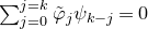 $\sum_{j=0}^{j=k}\tilde\varphi_j \psi_{k-j} = 0$
.
$\sum_{j=0}^{j=k}\tilde\varphi_j \psi_{k-j} = 0$
.
Now assume given common nuclei U, W for $\varphi_1,\ldots,\varphi_{N-1}$
in
$\varphi_1,\ldots,\varphi_{N-1}$
in $\mathcal U$
and assume without loss of generality that
$\mathcal U$
and assume without loss of generality that $U \subset W$
, so there is a descending chain
$U \subset W$
, so there is a descending chain
 \begin{equation*} W = U_J \supset U_{J+1} \supset \cdots \supset U_M = U.\end{equation*}
Consider the short exact sequences of finitely generated, projective $\Lambda/Z^N$
-modules
$\Lambda/Z^N$
-modules

Since $(1+\Phi)_N$
defines automorphisms of each of these modules, in
$(1+\Phi)_N$
defines automorphisms of each of these modules, in $K_1(\Lambda/Z^N)$
one has
$K_1(\Lambda/Z^N)$
one has
 $$[(V/U)_N,(1+\Phi)_N] = [(V/W)_N,(1+\Phi)_N]\cdot\prod _{i=J}^{i=M-1}[(U_i/U_{i+1})_N,(1+\Phi)_N].$$
However, $(1+\Phi)_N$
is the identity map on each of the modules
$(1+\Phi)_N$
is the identity map on each of the modules $(U_i/U_{i+1})_N$
, so the class of
$(U_i/U_{i+1})_N$
, so the class of $(1+\Phi)_N$
does not depend on whether it is computed with respect to U or W.
$(1+\Phi)_N$
does not depend on whether it is computed with respect to U or W.
Remark 4.17. In the notation of Lemma 4.16, if $N\,\geq\, 2$
, then
$N\,\geq\, 2$
, then $[1\,+\,\Phi]_{N-1}\,=\,[(V/U)_{N-1},\sum_{j=0}^{j=N-2}(Z^j\otimes\tilde\varphi_j)]\in K_1(\Lambda/Z^{N-1})$
is the image of
$[1\,+\,\Phi]_{N-1}\,=\,[(V/U)_{N-1},\sum_{j=0}^{j=N-2}(Z^j\otimes\tilde\varphi_j)]\in K_1(\Lambda/Z^{N-1})$
is the image of $[1+\Phi]_N\in K_1(\Lambda/Z^N)$
.
$[1+\Phi]_N\in K_1(\Lambda/Z^N)$
.
Definition 4.18. For a nuclear $\Lambda$
-automorphism
$\Lambda$
-automorphism $\Phi$
of
$\Phi$
of $(V,\mathcal U)$
, we use Proposition 4.4, Lemma 4.16 and Remark 4.17 to define the power series class of
$(V,\mathcal U)$
, we use Proposition 4.4, Lemma 4.16 and Remark 4.17 to define the power series class of $\Phi$
in
$\Phi$
in $K_1(\Lambda)$
to be
$K_1(\Lambda)$
to be
 $$[1+\Phi]=[1+\Phi\mid V]:=([1+\Phi]_N)_{N\geq 1}.$$
Remark 4.19. Definitions 4.11 and 4.15 only make sense with respect to a fixed V and $\mathcal U$
, and the same is true for Definition 4.18. Even though the notation
$\mathcal U$
, and the same is true for Definition 4.18. Even though the notation $[1+\Phi]$
omits the choice of both V and
$[1+\Phi]$
omits the choice of both V and $\mathcal U$
and the notation
$\mathcal U$
and the notation $[1+\Phi\mid V]$
omits the choice of
$[1+\Phi\mid V]$
omits the choice of $\mathcal U$
, we always specify the R-module V on which the components of
$\mathcal U$
, we always specify the R-module V on which the components of $\Phi$
act, and the sequence
$\Phi$
act, and the sequence $\mathcal U$
with respect to which (they are locally contracting and) the power series class of
$\mathcal U$
with respect to which (they are locally contracting and) the power series class of $\Phi$
is taken to be computed (via choices of common nuclei
$\Phi$
is taken to be computed (via choices of common nuclei $U\in\mathcal U$
in Lemma 4.16).
$U\in\mathcal U$
in Lemma 4.16).
Remark 4.20. If V is a finitely generated, projective R-module, then since $U_i=0$
for each i by Remark 4.13,
$U_i=0$
for each i by Remark 4.13, $[1+\Phi\mid V]$
is simply the class in
$[1+\Phi\mid V]$
is simply the class in $K_1(\Lambda)$
of the
$K_1(\Lambda)$
of the $\Lambda$
-automorphism
$\Lambda$
-automorphism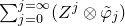 $\sum_{j=0}^{j=\infty}(Z^j\otimes\tilde\varphi_j)$
of the finitely generated, projective
$\sum_{j=0}^{j=\infty}(Z^j\otimes\tilde\varphi_j)$
of the finitely generated, projective $\Lambda$
-module
$\Lambda$
-module $\Lambda\otimes_R V=\varprojlim_{N\geq 1}V_N$
.
$\Lambda\otimes_R V=\varprojlim_{N\geq 1}V_N$
.
Remark 4.21. Let $V^1$
be a closed R-projective submodule of V. Set
$V^1$
be a closed R-projective submodule of V. Set $V^2=V/V^1$
,
$V^2=V/V^1$
, $\mathcal U^1=\{U_i^1\}$
with
$\mathcal U^1=\{U_i^1\}$
with $U_i^1:=U_i \cap V^1$
and
$U_i^1:=U_i \cap V^1$
and $\mathcal U^2=\{U_i^2\}$
, where
$\mathcal U^2=\{U_i^2\}$
, where $U_i^2$
denotes the image of
$U_i^2$
denotes the image of $U_i$
in
$U_i$
in $V^2$
. Let
$V^2$
. Let $\{a,b\}=\{1,2\}$
.
$\{a,b\}=\{1,2\}$
.
If each R-module $U_i^{a}$
is projective and
$U_i^{a}$
is projective and $\Phi$
is a nuclear
$\Phi$
is a nuclear $\Lambda$
-automorphism of
$\Lambda$
-automorphism of $(V,\mathcal U)$
that induces a well-defined nuclear
$(V,\mathcal U)$
that induces a well-defined nuclear $\Lambda$
-automorphism of
$\Lambda$
-automorphism of $(V^{a},\mathcal U^{a})$
, then
$(V^{a},\mathcal U^{a})$
, then $\Phi$
also induces a nuclear
$\Phi$
also induces a nuclear $\Lambda$
-automorphism of
$\Lambda$
-automorphism of $(V^b,\mathcal U^b)$
and, computing the respective power series classes with respect to
$(V^b,\mathcal U^b)$
and, computing the respective power series classes with respect to $\mathcal U$
,
$\mathcal U$
, $\mathcal U^1$
and
$\mathcal U^1$
and $\mathcal U^2$
, one has
$\mathcal U^2$
, one has
 \begin{equation*}[1+ \Phi \mid V ] = [1+\Phi \mid V^{1}]\cdot[1+\Phi \mid V^2].\end{equation*}
Remark 4.22. Given nuclear $\Lambda$
-automorphisms
$\Lambda$
-automorphisms $\Phi=(\varphi_j)_{j\geq 1}$
and
$\Phi=(\varphi_j)_{j\geq 1}$
and $\Psi=(\psi_j)_{j\geq 1}$
of
$\Psi=(\psi_j)_{j\geq 1}$
of $(V,\mathcal U)$
, the sequence
$(V,\mathcal U)$
, the sequence
 $$(1+\Phi)(1+\Psi)-1 := \bigg(\varphi_j+\psi_j+\sum_{i=1}^{i=j-1}\varphi_i\psi_{j-i}\bigg)_{\!\!j\geq 1}$$
is a nuclear $\Lambda$
-automorphism of
$\Lambda$
-automorphism of $(V,\mathcal U)$
, and one has
$(V,\mathcal U)$
, and one has
 $$[1+(1+\Phi)(1+\Psi)-1] = [1+\Phi]\cdot[1+\Psi].$$
4.2.3.
Nuclear automorphisms comprising a single non-trivial term play an important role in the following.
Definition 4.23. For a continuous, locally contracting R-endomorphism $\varphi$
of V and
$\varphi$
of V and $m\geq 1$
, we set
$m\geq 1$
, we set $[1-\varphi_m]_N=[1+\Phi]_N$
for
$[1-\varphi_m]_N=[1+\Phi]_N$
for $N\geq 1$
and
$N\geq 1$
and $[1-\varphi_m]=[1+\Phi]$
, for
$[1-\varphi_m]=[1+\Phi]$
, for $\Phi=(\varphi_j)$
with
$\Phi=(\varphi_j)$
with
 $$\varphi_j:=\begin{cases}-\varphi & \text{if }j=m,\\0 & \text{if }j\neq m.\end{cases}$$
The following result extends [Reference TaelmanTae12, Theorem 2] to our setting.
Proposition 4.24. Assume we are given continuous R-endomorphisms $\alpha,\varphi$
of V with the following properties.
$\alpha,\varphi$
of V with the following properties.
-
(a) The continuous R-endomorphism
$\alpha$
is surjective. -
(b) Both of the compositions
$\varphi\alpha$
and
$\alpha\varphi$
are locally contracting, and there is a common nucleus
$U_a\in\mathcal U$
for them with for some
$$\varphi(U_a)\subseteq U_{a+b}\quad\text{and}\quad \alpha(U_{a+b})\subseteq U_a$$
$b\geq 1$
.


Then, for every $m\geq 1$
, one has
$m\geq 1$
, one has
 $$[1-(\varphi\alpha)_m] = [1-(\alpha\varphi)_m].$$
Proof. We first note that, since V and $U_a$
are R-projective, the exact sequences
$U_a$
are R-projective, the exact sequences
 $$0\to\ker(\alpha)\to V\xrightarrow{\alpha}V\to 0 \quad\text{and}\quad 0\to\ker(\alpha)\to\alpha^{-1}(U_a)\xrightarrow{\alpha}U_a\to 0$$
imply that the R-module $\alpha^{-1}(U_a)\cong\ker(\alpha)\oplus U_a$
is projective. Remark 4.10 then implies that the quotients
$\alpha^{-1}(U_a)\cong\ker(\alpha)\oplus U_a$
is projective. Remark 4.10 then implies that the quotients $\alpha^{-1}(U_a)/U_{a+b}$
and
$\alpha^{-1}(U_a)/U_{a+b}$
and $V/\alpha^{-1}(U_a)$
are R-projective.
$V/\alpha^{-1}(U_a)$
are R-projective.
For each $m,N\geq 1$
, one then has
$m,N\geq 1$
, one then has
 \begin{align*}[1-(\varphi\alpha)_m]_N&=[(V/U_{a+b})_N,1-(Z^m\otimes\varphi\alpha)]\\&=[(V/U_{a+b})_N,1-(Z^m\otimes\varphi\alpha)]\cdot[(\alpha^{-1}(U_a)/U_{a+b})_N,1-(Z^m\otimes\varphi\alpha)]^{-1}\\&=[(V/\alpha^{-1}(U_a))_N,1-(Z^m\otimes\varphi\alpha)].\end{align*}
The claimed equality now follows from the commutativity of the following square of $\Lambda/Z^N$
-modules with bijective horizontal arrows.
$\Lambda/Z^N$
-modules with bijective horizontal arrows.

5. The refined trace formula
Taelman’s trace formula [Reference TaelmanTae12, Theorem 3] provides an interpretation of Euler products associated to nuclear automorphisms, as a single determinant for their action on a compact (but not finitely generated) module over the formal power series ring ${\mathbb F}_q[\![Z]\!]$
.
${\mathbb F}_q[\![Z]\!]$
.
In this section we fix notation and setting as in Theorem 2.17 and prove a refined trace formula in the Whitehead group $K_1({\mathbb F}_q[G][\![Z]\!])$
. This formula provides an interpretation of K-theoretic Euler products as a single power series class of nuclear automorphisms, as introduced in Definition 4.18.
$K_1({\mathbb F}_q[G][\![Z]\!])$
. This formula provides an interpretation of K-theoretic Euler products as a single power series class of nuclear automorphisms, as introduced in Definition 4.18.
In particular, our trace formula will imply that the Euler product $\Theta_{E,K/k}^{\mathcal M}$
occurring in Theorem 2.17 converges to the element of
$\Theta_{E,K/k}^{\mathcal M}$
occurring in Theorem 2.17 converges to the element of $K_1(\mathcal F_\infty[G])$
obtained as the evaluation
$K_1(\mathcal F_\infty[G])$
obtained as the evaluation
 \begin{equation*}\textrm{ev}_{t^{-1}}:K_1(\Lambda)\longrightarrow K_1(R(\!(Z)\!))\xrightarrow{Z\mapsto t^{-1}}K_1(R(\!(t^{-1})\!))=K_1(\mathcal F_\infty[G])\end{equation*}
of a given power series class in $K_1(\Lambda)$
. Here, and in the following, we continue to abbreviate
$K_1(\Lambda)$
. Here, and in the following, we continue to abbreviate ${\mathbb F}_q[G][\![Z]\!]$
to
${\mathbb F}_q[G][\![Z]\!]$
to $\Lambda$
and
$\Lambda$
and ${\mathbb F}_q[G]$
to R.
${\mathbb F}_q[G]$
to R.
Before proceeding, we note that $\Lambda$
is the closed unit ball in the ultrametric space
$\Lambda$
is the closed unit ball in the ultrametric space $R(\!(Z)\!)$
and is thus an open subspace. By Lemma 2.1,
$R(\!(Z)\!)$
and is thus an open subspace. By Lemma 2.1, $\textrm{ev}_{t^{-1}}$
is continuous and open. To apply Corollary 4.9(ii) to the inclusion
$\textrm{ev}_{t^{-1}}$
is continuous and open. To apply Corollary 4.9(ii) to the inclusion $\Lambda\subset R(\!(Z)\!)\cong\mathcal F_\infty[G]$
, we use the following result, which is proved in § 6.2 below.
$\Lambda\subset R(\!(Z)\!)\cong\mathcal F_\infty[G]$
, we use the following result, which is proved in § 6.2 below.
Proposition 5.1. The map $\textrm{ev}_{t^{-1}}$
is injective.
$\textrm{ev}_{t^{-1}}$
is injective.
In particular, $\ker(\textrm{ev}_{t^{-1}})=\{1\}$
is closed in the profinite group
$\ker(\textrm{ev}_{t^{-1}})=\{1\}$
is closed in the profinite group $K_1(\Lambda)$
.
$K_1(\Lambda)$
.
5.1 The compact module
In this section we review the construction of an arithmetic family of pairs $(V_S^{\mathcal M},\mathcal U)$
as in § 4.2.1 given in [Reference Ferrara, Green, Higgins and PopescuFGH+22]. The refined trace formula of § 5.2 applies to a class of nuclear automorphisms of such pairs.
$(V_S^{\mathcal M},\mathcal U)$
as in § 4.2.1 given in [Reference Ferrara, Green, Higgins and PopescuFGH+22]. The refined trace formula of § 5.2 applies to a class of nuclear automorphisms of such pairs.
We fix a finite set S of places of k containing the set $S^\infty_k$
of places above the place at infinity of
$S^\infty_k$
of places above the place at infinity of $\mathcal F$
, as well as a taming module
$\mathcal F$
, as well as a taming module $\mathcal M$
for
$\mathcal M$
for $K/k$
.
$K/k$
.
For each $v\in S$
we define a G-module
$v\in S$
we define a G-module $K_v:=\prod _{w\mid v}K_w$
, with w running over the places of K that divide v. We endow
$K_v:=\prod _{w\mid v}K_w$
, with w running over the places of K that divide v. We endow $K_v$
with the supremum of the norms on each
$K_v$
with the supremum of the norms on each $K_w$
. If
$K_w$
. If $v\in S^\infty_k$
, respectively
$v\in S^\infty_k$
, respectively $v\in S\setminus S^\infty_k$
, we assume that
$v\in S\setminus S^\infty_k$
, we assume that $t^{-1}$
, respectively a uniformiser of
$t^{-1}$
, respectively a uniformiser of $k_v$
, has norm
$k_v$
, has norm $q^{-1}$
in
$q^{-1}$
in $K_v$
. We then define
$K_v$
. We then define $\mathcal O_{k,S}[G]\{\tau\}$
-modules
$\mathcal O_{k,S}[G]\{\tau\}$
-modules
 $$K_S:=\prod _{v\in S}K_v \quad\text{and}\quad \mathcal M_S:=\mathcal O_{k,S}\otimes_{\mathcal O_k}\mathcal M,$$
where $\mathcal O_{k,S}$
is the ring of S-integers in k. We endow
$\mathcal O_{k,S}$
is the ring of S-integers in k. We endow $K_S$
with the supremum norm. Embedding
$K_S$
with the supremum norm. Embedding $\mathcal M_S$
into
$\mathcal M_S$
into $K_S$
diagonally, we obtain an
$K_S$
diagonally, we obtain an $\mathcal O_{k,S}[G]\{\tau\}$
-module
$\mathcal O_{k,S}[G]\{\tau\}$
-module
 $$V_S^{\mathcal M}:=K_S/\mathcal M_S.$$
We note that $\mathcal M_S$
is discrete in
$\mathcal M_S$
is discrete in $K_S$
, because
$K_S$
, because $\mathcal O_{k,S}\otimes_{\mathcal O_k}\mathcal O_K$
is. We write
$\mathcal O_{k,S}\otimes_{\mathcal O_k}\mathcal O_K$
is. We write $\varpi$
for the projection
$\varpi$
for the projection $K_S\to V_S^{\mathcal M}$
.
$K_S\to V_S^{\mathcal M}$
.
Remark 5.2. For each $v\in S\setminus S^\infty_k$
, we fix a uniformiser
$v\in S\setminus S^\infty_k$
, we fix a uniformiser $\pi_v$
of
$\pi_v$
of $k_v$
. For each
$k_v$
. For each $v\in S$
, we endow
$v\in S$
, we endow $K_v$
with the following action of R[Z]:
$K_v$
with the following action of R[Z]:
 $$Z\cdot x:=\begin{cases}t^{-1}x, & v\in S^\infty_k,\\\pi_vx, & v\notin S^\infty_k.\end{cases}$$
Then $\mathcal M_S$
is an R[Z]-submodule of
$\mathcal M_S$
is an R[Z]-submodule of $K_S$
and
$K_S$
and $V_S^{\mathcal M}$
becomes a topological R[Z]-module.
$V_S^{\mathcal M}$
becomes a topological R[Z]-module.
Let $\{\mathcal{W}_v\}_{v\in S}$
be a family of open, R-projective
$\{\mathcal{W}_v\}_{v\in S}$
be a family of open, R-projective $\mathcal O_{k_v}[G]\{\tau\}$
-submodules of
$\mathcal O_{k_v}[G]\{\tau\}$
-submodules of $K_v$
with the property that for each v,
$K_v$
with the property that for each v, $\{Z^{i}\cdot\mathcal{W}_v\}_{i\geq 0}$
is a basis of open neighbourhoods of zero in
$\{Z^{i}\cdot\mathcal{W}_v\}_{i\geq 0}$
is a basis of open neighbourhoods of zero in $K_v$
. Then, since
$K_v$
. Then, since $\mathcal M_S$
is discrete, there is
$\mathcal M_S$
is discrete, there is $B\in\mathbb N$
with the property that
$B\in\mathbb N$
with the property that $(\prod_{v\in S}Z^B\cdot\mathcal{W}_v)\cap\mathcal M_S=\{0\}$
in
$(\prod_{v\in S}Z^B\cdot\mathcal{W}_v)\cap\mathcal M_S=\{0\}$
in $K_S$
. Rescaling to
$K_S$
. Rescaling to $W_v:=Z^B\cdot\mathcal{W}_v$
, we may define an open R[Z]-submodule that is R-projective and has no Z-torsion by setting
$W_v:=Z^B\cdot\mathcal{W}_v$
, we may define an open R[Z]-submodule that is R-projective and has no Z-torsion by setting
 \begin{equation}W=\varpi\bigg(\prod _{v\in S}W_v\bigg)\subseteq V_S^{\mathcal M}.\end{equation}
Any such choice of family $\{\mathcal{W}_v\}_{v\in S}$
thus defines data
$\{\mathcal{W}_v\}_{v\in S}$
thus defines data $U_i:=Z^{i}\cdot W$
as in Example 4.14.
$U_i:=Z^{i}\cdot W$
as in Example 4.14.
Definition 5.3. We write $\mathcal O_{k,S}\{\tau\}\tau$
for the subset of
$\mathcal O_{k,S}\{\tau\}\tau$
for the subset of $\mathcal O_{k,S}\{\tau\}$
comprising polynomials in
$\mathcal O_{k,S}\{\tau\}$
comprising polynomials in $\tau$
with constant term 0. We then denote the set of sequences in
$\tau$
with constant term 0. We then denote the set of sequences in $\mathcal O_{k,S}\{\tau\}\tau$
by
$\mathcal O_{k,S}\{\tau\}\tau$
by $\langle\tau\rangle:=\prod _{j\geq 1}\mathcal O_{k,S}\{\tau\}\tau$
. In the following, we interpret any element of
$\langle\tau\rangle:=\prod _{j\geq 1}\mathcal O_{k,S}\{\tau\}\tau$
. In the following, we interpret any element of $\mathcal O_{k,S}\{\tau\}\tau$
as a continuous R-endomorphism of
$\mathcal O_{k,S}\{\tau\}\tau$
as a continuous R-endomorphism of $V_S^{\mathcal M}$
via its own left-action.
$V_S^{\mathcal M}$
via its own left-action.
The next result is essentially proved by Ferrara et al. [Reference Ferrara, Green, Higgins and PopescuFGH+22].
Proposition 5.4. The R-module $V_S^{\mathcal M}$
is compact and projective, and there is a (non-empty) family
$V_S^{\mathcal M}$
is compact and projective, and there is a (non-empty) family $\mathcal T_S^{\mathcal M}$
of sequences of R-submodules of
$\mathcal T_S^{\mathcal M}$
of sequences of R-submodules of $V_S^{\mathcal M}$
with the following properties.
$V_S^{\mathcal M}$
with the following properties.
-
(i) Each sequence in
$\mathcal T_S^{\mathcal M}$
is of the form
$\{Z^{i}\cdot W\}_{i\geq 1}$
for some R-projective submodule W of
$V_S^{\mathcal M}$
as in (5.1). In addition, there exists
$a_W\in\mathbb N$
with the property that for large enough i, where
$$Z^{a_W+i}\cdot\varpi(B_{K_S})\subseteq Z^{i}\cdot W\subseteq Z^{i}\cdot\varpi(B_{K_S})$$
$B_{K_S}$
denotes the closed unit ball in
$K_S$
.
-
(ii) Any element of
$\mathcal O_{k,S}\{\tau\}\tau$
is locally contracting with respect to any pair
$(V_S^{\mathcal M},\mathcal U)$
with
$\mathcal U$
in
$\mathcal T^{\mathcal M}_S$
. -
(iii) If
$\Phi$
is a sequence in
$\langle\tau\rangle$
, the power series class
$[1+\Phi\mid V_S^{\mathcal M}]$
of
$\Phi$
in
$K_1(\Lambda)$
is independent of the sequence in
$\mathcal T_S^{\mathcal M}$
with respect to which it is computed. -
(iv) Let
$\mathfrak{p}_0$
be a place of k that is not in S and set
$S':=S\cup\{\mathfrak{p}_0\}$
. Then, for any
$\Phi$
in
$\langle\tau\rangle$
, computing the power series classes on the left-hand side with respect to sequences in
$\mathcal T^{\mathcal M}_{S'}$
and in
$\mathcal T^{\mathcal M}_S$
, respectively (and the right-hand side as in Remark 4.13), one has
$$[1+\Phi\mid V_{S'}^{\mathcal M}]\cdot[1+\Phi\mid V_S^{\mathcal M}]^{-1}=[1+\Phi\mid \mathcal M/\mathfrak{p}_0\mathcal M].$$





Proof. Since all the above claims follow in a straightforward manner from arguments in [Reference Ferrara, Green, Higgins and PopescuFGH+22], we limit ourselves to providing a sketch of the proof.
The fact that $K_S$
is a projective R-module follows upon combining the normal basis theorem with Shapiro’s lemma. The fact that the R-module
$K_S$
is a projective R-module follows upon combining the normal basis theorem with Shapiro’s lemma. The fact that the R-module $V_S^{\mathcal M}$
is compact and projective then follows directly from the properties of taming modules.
$V_S^{\mathcal M}$
is compact and projective then follows directly from the properties of taming modules.
We then let $\mathcal T_S^{\mathcal M}$
comprise any sequences
$\mathcal T_S^{\mathcal M}$
comprise any sequences $\mathcal U$
constructed as in [Reference Ferrara, Green, Higgins and PopescuFGH+22, 2.3.2]. Any such sequences satisfy the first statement of claim (i) by construction, the second statement of claim (i) by the argument in Corollary A.2.5 (see also (5.1.1)) of [Reference Ferrara, Green, Higgins and PopescuFGH+22], and then also claim (ii) by the argument in Lemma 2.3.3 of [Reference Ferrara, Green, Higgins and PopescuFGH+22] (or of Example 4.14).
$\mathcal U$
constructed as in [Reference Ferrara, Green, Higgins and PopescuFGH+22, 2.3.2]. Any such sequences satisfy the first statement of claim (i) by construction, the second statement of claim (i) by the argument in Corollary A.2.5 (see also (5.1.1)) of [Reference Ferrara, Green, Higgins and PopescuFGH+22], and then also claim (ii) by the argument in Lemma 2.3.3 of [Reference Ferrara, Green, Higgins and PopescuFGH+22] (or of Example 4.14).
To prove claim (iii), we fix $\Phi=(\varphi_j)_{j\geq 1}$
in
$\Phi=(\varphi_j)_{j\geq 1}$
in $\langle\tau\rangle$
, as well as sequences
$\langle\tau\rangle$
, as well as sequences $\mathcal U=\{U_i\}_{i\geq 1}$
and
$\mathcal U=\{U_i\}_{i\geq 1}$
and $\mathcal U'=\{U_i'\}_{i\geq 1}$
in
$\mathcal U'=\{U_i'\}_{i\geq 1}$
in $\mathcal T_S^{\mathcal M}$
, and an integer
$\mathcal T_S^{\mathcal M}$
, and an integer $N\geq 1$
. It is enough to show that, in
$N\geq 1$
. It is enough to show that, in $K_1(\Lambda/Z^N),$
one has
$K_1(\Lambda/Z^N),$
one has
 $$[(V_S^{\mathcal M}/U_i)_N,(1+\Phi)_N] = [(V_S^{\mathcal M}/U'_k)_N,(1+\Phi)_N]$$
for some common nuclei $U_i$
and
$U_i$
and $U'_k$
for
$U'_k$
for $\varphi_1,\ldots,\varphi_{N-1}$
. But the argument of Lemma 2.3.10 of [Reference Ferrara, Green, Higgins and PopescuFGH+22] shows that there exist common nuclei
$\varphi_1,\ldots,\varphi_{N-1}$
. But the argument of Lemma 2.3.10 of [Reference Ferrara, Green, Higgins and PopescuFGH+22] shows that there exist common nuclei $U_i$
and
$U_i$
and $U'_k$
with
$U'_k$
with
 $$U_i\supset U'_k\quad\text{and}\quad \varphi_j(U_i)\subset U'_k\quad\text{for every }j\lt N.$$
Using this choice of nuclei, we find the required equality
 \begin{align*}[(V_S^{\mathcal M}/U'_k)_N,(1+\Phi)_N]&=[(V_S^{\mathcal M}/U_i)_N,(1+\Phi)_N]\cdot[(U_i/U'_k)_N,(1+\Phi)_N]\\&=[(V_S^{\mathcal M}/U_i)_N,(1+\Phi)_N].\end{align*}
To prove claim (iv), we write $\mathcal O_{\mathfrak{p}_0}$
for the valuation ring of the completion of k at
$\mathcal O_{\mathfrak{p}_0}$
for the valuation ring of the completion of k at $\mathfrak{p}_0$
and
$\mathfrak{p}_0$
and $\mathcal M_{\mathfrak{p}_0}:=\mathcal O_{\mathfrak{p}_0}\otimes_{\mathcal O_k}\mathcal M$
for the
$\mathcal M_{\mathfrak{p}_0}:=\mathcal O_{\mathfrak{p}_0}\otimes_{\mathcal O_k}\mathcal M$
for the $\mathfrak{p}_0$
-adic completion of
$\mathfrak{p}_0$
-adic completion of $\mathcal M$
. Then the proof of Lemma 3.0.1 of [Reference Ferrara, Green, Higgins and PopescuFGH+22] gives a short exact sequence of compact
$\mathcal M$
. Then the proof of Lemma 3.0.1 of [Reference Ferrara, Green, Higgins and PopescuFGH+22] gives a short exact sequence of compact $\mathcal O_{k,S}[G]\{\tau\}$
-modules
$\mathcal O_{k,S}[G]\{\tau\}$
-modules

and a sequence $\mathcal U'=\{U'_i\}_{i\geq 1}$
in
$\mathcal U'=\{U'_i\}_{i\geq 1}$
in $\mathcal T^{\mathcal M}_{S'}$
with the property that
$\mathcal T^{\mathcal M}_{S'}$
with the property that $\psi^{-1}(U'_i)=\mathfrak{p}_0^{i}\cdot\mathcal M_{\mathfrak{p}_0}$
and that
$\psi^{-1}(U'_i)=\mathfrak{p}_0^{i}\cdot\mathcal M_{\mathfrak{p}_0}$
and that $\{\eta(U_i')\}_{i\geq 1}$
belongs to
$\{\eta(U_i')\}_{i\geq 1}$
belongs to $\mathcal T^{\mathcal M}_S$
.
$\mathcal T^{\mathcal M}_S$
.
By Remark 4.21, one then finds that
 $$[1+\Phi\mid V_{S'}^{\mathcal M}]\cdot[1+\Phi\mid V_S^{\mathcal M}]^{-1}=[1+\Phi\mid \mathcal M_{\mathfrak{p}_0}],$$
computing the power series class on the right-hand side with respect to the sequence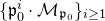 $\{\mathfrak{p}_0^{i}\cdot\mathcal M_{\mathfrak{p}_0}\}_{i\geq 1}$
. The claimed equality is thus valid because
$\{\mathfrak{p}_0^{i}\cdot\mathcal M_{\mathfrak{p}_0}\}_{i\geq 1}$
. The claimed equality is thus valid because $\mathfrak{p}_0\cdot\mathcal M_{\mathfrak{p}_0}$
is a common nucleus for the action of all
$\mathfrak{p}_0\cdot\mathcal M_{\mathfrak{p}_0}$
is a common nucleus for the action of all $\varphi_j\in \mathcal O_{k,S}\{\tau\}\tau$
on
$\varphi_j\in \mathcal O_{k,S}\{\tau\}\tau$
on $\mathcal M_{\mathfrak{p}_0}$
, by the argument of Example 4.14.
$\mathcal M_{\mathfrak{p}_0}$
, by the argument of Example 4.14.
5.2 The trace formula and convergence of the L-value
We may now state our refined trace formula for nuclear $\Lambda$
-automorphisms in
$\Lambda$
-automorphisms in $\langle\tau\rangle$
(see Definition 5.3). This result constitutes a non-abelian generalisation of [Reference Ferrara, Green, Higgins and PopescuFGH+22, Theorem 3.0.2].
$\langle\tau\rangle$
(see Definition 5.3). This result constitutes a non-abelian generalisation of [Reference Ferrara, Green, Higgins and PopescuFGH+22, Theorem 3.0.2].
Theorem 5.5. Let S be a finite set of places of k containing $S^\infty_k$
and let
$S^\infty_k$
and let $\mathcal M$
be a taming module for
$\mathcal M$
be a taming module for $K/k$
. Then for each nuclear
$K/k$
. Then for each nuclear $\Lambda$
-automorphism
$\Lambda$
-automorphism $\Phi$
of
$\Phi$
of $V_S^{\mathcal M}$
in the set
$V_S^{\mathcal M}$
in the set $\langle\tau\rangle$
, the S-truncated Euler product
$\langle\tau\rangle$
, the S-truncated Euler product
 $$\prod _{\mathfrak{p}\notin S}[1+\Phi\mid \mathcal M/\mathfrak{p}\mathcal M]$$
converges in $K_1(\Lambda)$
to the inverse of the power series class
$K_1(\Lambda)$
to the inverse of the power series class $[1+\Phi\mid V_S^{\mathcal M}]$
, computed with respect to any sequence in
$[1+\Phi\mid V_S^{\mathcal M}]$
, computed with respect to any sequence in $\mathcal T_S^{\mathcal M}$
. This limit is unique in
$\mathcal T_S^{\mathcal M}$
. This limit is unique in $K_1(\Lambda)$
and, moreover, is independent of the order of the Euler factors.
$K_1(\Lambda)$
and, moreover, is independent of the order of the Euler factors.
Before proving Theorem 5.5, we state its consequence for $\Theta_{E,K/k}^{\mathcal M}$
. Set
$\Theta_{E,K/k}^{\mathcal M}$
. Set $V_\infty^{\mathcal M}:=V_{S^\infty_k}^{\mathcal M}$
.
$V_\infty^{\mathcal M}:=V_{S^\infty_k}^{\mathcal M}$
.
Corollary 5.6. Let $\mathcal M$
be a taming module for
$\mathcal M$
be a taming module for $K/k$
. Then the Euler product
$K/k$
. Then the Euler product $\Theta_{E,K/k}^{\mathcal M}$
converges in
$\Theta_{E,K/k}^{\mathcal M}$
converges in $K_1(\mathcal F_\infty[G])$
to
$K_1(\mathcal F_\infty[G])$
to
 $$\textrm{ev}_{t^{-1}}([1+\Phi_E\mid V_\infty^{\mathcal M}]),$$
where $\Phi_E=(\varphi_{j,E})_{j\geq 1}$
with
$\Phi_E=(\varphi_{j,E})_{j\geq 1}$
with $\varphi_{j,E}=(t-\phi_E(t))t^{j-1}$
. This limit is unique in
$\varphi_{j,E}=(t-\phi_E(t))t^{j-1}$
. This limit is unique in $K_1(\mathcal F_\infty[G])$
and, moreover, is independent of the order of the Euler factors.
$K_1(\mathcal F_\infty[G])$
and, moreover, is independent of the order of the Euler factors.
Proof. We recall that $\textrm{MSpec}(\mathcal O_k)$
is a countable set. We fix an order and, for each
$\textrm{MSpec}(\mathcal O_k)$
is a countable set. We fix an order and, for each $i\in\mathbb N$
, write
$i\in\mathbb N$
, write $x_i\in K_1(\Lambda)$
for
$x_i\in K_1(\Lambda)$
for $[1+\Phi\mid \mathcal M/\mathfrak{p}_i\mathcal M]$
. Theorem 5.5 implies that the sequence of partial products
$[1+\Phi\mid \mathcal M/\mathfrak{p}_i\mathcal M]$
. Theorem 5.5 implies that the sequence of partial products $(\prod_{i=1}^{i=j}x_i)_{j\in\mathbb N}$
converges in
$(\prod_{i=1}^{i=j}x_i)_{j\in\mathbb N}$
converges in $K_1(\Lambda)$
to (a unique limit)
$K_1(\Lambda)$
to (a unique limit) $\prod_{i\in\mathbb N}x_i=[1+\Phi\mid V_\infty^{\mathcal M}]$
(independent of the chosen order).
$\prod_{i\in\mathbb N}x_i=[1+\Phi\mid V_\infty^{\mathcal M}]$
(independent of the chosen order).
By Proposition 5.1 and Corollary 4.9(ii), it follows that the sequence of partial products $(\prod_{i=1}^{i=j}\textrm{ev}_{t^{-1}}(x_i))_{j\in\mathbb N}$
converges in
$(\prod_{i=1}^{i=j}\textrm{ev}_{t^{-1}}(x_i))_{j\in\mathbb N}$
converges in $K_1(\mathcal F_\infty[G])$
to a unique limit that is independent of the chosen order, and is moreover equal to
$K_1(\mathcal F_\infty[G])$
to a unique limit that is independent of the chosen order, and is moreover equal to $\textrm{ev}_{t^{-1}}([1+\Phi\mid V_\infty^{\mathcal M}])$
. Given these facts, it is enough to show that, for any
$\textrm{ev}_{t^{-1}}([1+\Phi\mid V_\infty^{\mathcal M}])$
. Given these facts, it is enough to show that, for any $\mathfrak{p}\notin S^\infty_k$
, one has
$\mathfrak{p}\notin S^\infty_k$
, one has
 \begin{equation}\textrm{ev}_{t^{-1}}([1+\Phi_E\mid \mathcal M/\mathfrak{p}\mathcal M])=c_G(\mathcal M/\mathfrak{p}\mathcal M)^{-1}\cdot c_G(E(\mathcal M/\mathfrak{p}\mathcal M))\end{equation}
in $K_1(\mathcal F_\infty[G])$
. We fix such a place
$K_1(\mathcal F_\infty[G])$
. We fix such a place $\mathfrak{p}$
.
$\mathfrak{p}$
.
Now, a direct computation (as in the proof of Lemma 4.16) gives, for each $N\geq 2$
, the following equality of continuous
$N\geq 2$
, the following equality of continuous $\Lambda/Z^N$
-automorphisms of
$\Lambda/Z^N$
-automorphisms of $(\mathcal M/\mathfrak{p}\mathcal M)_N$
:
$(\mathcal M/\mathfrak{p}\mathcal M)_N$
:
 \begin{equation}(\textrm{id}-(Z\otimes t))^{-1} \circ (\textrm{id}-(Z\otimes\phi_E(t)))=\textrm{id}+\sum_{j=1}^{j=N-1}(Z^j\otimes\varphi_{j,E}).\end{equation}
We set $(\mathcal M/\mathfrak{p}\mathcal M)_\Lambda:=\Lambda\otimes_{R}\mathcal M/\mathfrak{p}\mathcal M$
. Writing
$(\mathcal M/\mathfrak{p}\mathcal M)_\Lambda:=\Lambda\otimes_{R}\mathcal M/\mathfrak{p}\mathcal M$
. Writing
 $$\alpha_t:=\textrm{id}-(Z\otimes t)\quad \text{and}\quad \alpha_{\phi_E(t)}:=\textrm{id}-(Z\otimes\phi_E(t))$$
for the respective $\Lambda$
-automorphisms of the finitely generated, projective module
$\Lambda$
-automorphisms of the finitely generated, projective module $(\mathcal M/\mathfrak{p}\mathcal M)_\Lambda$
, we thus find that
$(\mathcal M/\mathfrak{p}\mathcal M)_\Lambda$
, we thus find that
 $$[1+\Phi_E\mid \mathcal M/\mathfrak{p}\mathcal M]=[(\mathcal M/\mathfrak{p}\mathcal M)_\Lambda,\,\alpha_t]^{-1}\cdot[(\mathcal M/\mathfrak{p}\mathcal M)_\Lambda,\,\alpha_{\phi_E(t)}]$$
in $K_1(\Lambda)$
. Using the notation of Lemma 2.3, this equality implies that
$K_1(\Lambda)$
. Using the notation of Lemma 2.3, this equality implies that
 \begin{align*}&\textrm{ev}_{t^{-1}}([1+\Phi_E\mid \mathcal M/\mathfrak{p}\mathcal M])\\&\quad=[(\mathcal M/\mathfrak{p}\mathcal M)'_{\mathcal F_\infty},\,\textrm{id}-(t^{-1}\otimes t)]^{-1}\cdot[(\mathcal M/\mathfrak{p}\mathcal M)'_{\mathcal F_\infty},\,\textrm{id}-(t^{-1}\otimes\phi_E(t))]\\&\quad=[(\mathcal M/\mathfrak{p}\mathcal M)'_{\mathcal F_\infty},\,(t\otimes\textrm{id})-(\textrm{id}\otimes t)]^{-1}\cdot[(\mathcal M/\mathfrak{p}\mathcal M)'_{\mathcal F_\infty},\,(t\otimes\textrm{id})-(\textrm{id}\otimes\phi_E(t))]\\&\quad=c_G(\mathcal M/\mathfrak{p}\mathcal M)^{-1}\cdot c_G(E(\mathcal M/\mathfrak{p}\mathcal M))\end{align*}
in $K_1(\mathcal F_\infty[G])$
. We have now verified the required equality (5.2).
$K_1(\mathcal F_\infty[G])$
. We have now verified the required equality (5.2).
In the rest of this section we prove Theorem 5.5, by adapting the proofs of [Reference TaelmanTae12, Theorem 3] and [Reference Ferrara, Green, Higgins and PopescuFGH+22, Theorem 3.0.2]. We recall again that $\textrm{MSpec}(\mathcal O_k)$
is a countable set.
$\textrm{MSpec}(\mathcal O_k)$
is a countable set.
We fix $N\geq 1$
. By (the proof of) Corollary 4.9(i), it is enough to prove that
$N\geq 1$
. By (the proof of) Corollary 4.9(i), it is enough to prove that
 $$\prod _{\mathfrak{p}\notin S}[(1+\Phi)_N\mid (\mathcal M/\mathfrak{p}\mathcal M)_N]$$
converges in $K_1(\Lambda/Z^N)$
to the inverse of
$K_1(\Lambda/Z^N)$
to the inverse of $[1+\Phi\mid V_S^{\mathcal M}]_N$
, computed with respect to any sequence in
$[1+\Phi\mid V_S^{\mathcal M}]_N$
, computed with respect to any sequence in $\mathcal T_S^{\mathcal M}$
.
$\mathcal T_S^{\mathcal M}$
.
We write $\Phi=(\varphi_j)_{j\geq 1}$
and fix
$\Phi=(\varphi_j)_{j\geq 1}$
and fix $D \gt N\cdot\mathrm{max}_{j\lt N}\{\deg_\tau(\varphi_j)\}$
. We then also set
$D \gt N\cdot\mathrm{max}_{j\lt N}\{\deg_\tau(\varphi_j)\}$
. We then also set
 $$T := S\cup\{\mathfrak{p}\in\textrm{MSpec}(\mathcal O_{k,S}) \mid [\mathcal O_{k,S}/\mathfrak{p}:{\mathbb F}_q]\lt D\}.$$
We note that the set T is finite. By Proposition 5.4(iv), it hence suffices to prove that
 \begin{equation}\prod _{\mathfrak{p}\notin T}[(1+\Phi)_N\mid (\mathcal M/\mathfrak{p}\mathcal M)_N]\end{equation}
converges in $K_1(\Lambda/Z^N)$
to the inverse of
$K_1(\Lambda/Z^N)$
to the inverse of $[1+\Phi\mid V_T^{\mathcal M}]_N$
, computed with respect to any sequence in
$[1+\Phi\mid V_T^{\mathcal M}]_N$
, computed with respect to any sequence in $\mathcal T_T^{\mathcal M}$
. In fact, we claim that every factor in the product (5.4) is trivial, and so is
$\mathcal T_T^{\mathcal M}$
. In fact, we claim that every factor in the product (5.4) is trivial, and so is $[1+\Phi\mid V_T^{\mathcal M}]_N$
.
$[1+\Phi\mid V_T^{\mathcal M}]_N$
.
Now the argument of [Reference TaelmanTae12, Theorem 3] (which relies on a trick due to Anderson [Reference AndersonAnd00, Proposition 9]), together with the multiplicativity property in Remark 4.22, reduces these claims to showing that
 \begin{equation}[1-((s\tau^d)\alpha)_m\mid\mathcal M/\mathfrak{p}\mathcal M] = [1-(\alpha(s\tau^d))_m\mid \mathcal M/\mathfrak{p}\mathcal M]\end{equation}
and
 \begin{equation}[1-((s\tau^d)\alpha)_m\mid V_T^{\mathcal M}] = [1-(\alpha(s\tau^d))_m\mid V_T^{\mathcal M}]\end{equation}
for $\mathfrak{p}\notin T$
, any
$\mathfrak{p}\notin T$
, any $\alpha,s\in\mathcal O_{k,T}$
and any
$\alpha,s\in\mathcal O_{k,T}$
and any $d,m\geq 1$
.
$d,m\geq 1$
.
To prove (5.5), we recall from Remark 2.14 that $\mathcal M$
is a locally free
$\mathcal M$
is a locally free $\mathcal O_k[G]$
-module of constant local rank 1. Therefore,
$\mathcal O_k[G]$
-module of constant local rank 1. Therefore,
 $$\frac{\mathcal M}{\mathfrak{p}\mathcal M}\cong\frac{\mathcal M_{(\mathfrak{p})}}{\mathfrak{p}\mathcal M_{(\mathfrak{p})}}\cong\frac{\mathcal O_{k,(\mathfrak{p})}[G]}{\mathfrak{p}\mathcal O_{k,(\mathfrak{p})}[G]}\cong\left(\frac{\mathcal O_{k,(\mathfrak{p})}}{\mathfrak{p}\mathcal O_{k,(\mathfrak{p})}}\right)[G]\cong\left(\frac{\mathcal O_{k,T}}{\mathfrak{p}\mathcal O_{k,T}}\right)[G].$$
Thus, if $\alpha$
belongs to
$\alpha$
belongs to $\mathfrak{p}\mathcal O_{k,T}$
, then both of the endomorphisms
$\mathfrak{p}\mathcal O_{k,T}$
, then both of the endomorphisms $(s\tau^d)\alpha$
and
$(s\tau^d)\alpha$
and $\alpha(s\tau^d)$
of
$\alpha(s\tau^d)$
of $\mathcal M/\mathfrak{p}\mathcal M$
are trivial, so that both sides of (5.5) are trivial. On the other hand, if
$\mathcal M/\mathfrak{p}\mathcal M$
are trivial, so that both sides of (5.5) are trivial. On the other hand, if $\alpha\notin\mathfrak{p}\mathcal O_{k,T}$
, then its action defines an automorphism of
$\alpha\notin\mathfrak{p}\mathcal O_{k,T}$
, then its action defines an automorphism of $\mathcal M/\mathfrak{p}\mathcal M$
, so (5.5) follows from Proposition 4.24 applied to
$\mathcal M/\mathfrak{p}\mathcal M$
, so (5.5) follows from Proposition 4.24 applied to $V=\mathcal M/\mathfrak{p}\mathcal M$
,
$V=\mathcal M/\mathfrak{p}\mathcal M$
, $\alpha=\alpha$
and
$\alpha=\alpha$
and $\varphi=s\tau^d$
.
$\varphi=s\tau^d$
.
To deduce (5.6) from Proposition 4.24, we must fix $\mathcal U=\{Z^{i}W\}_{i\geq 1}$
in
$\mathcal U=\{Z^{i}W\}_{i\geq 1}$
in $\mathcal T_T^{\mathcal M}$
and, after noting that
$\mathcal T_T^{\mathcal M}$
and, after noting that $(s\tau^d)\alpha$
and
$(s\tau^d)\alpha$
and $\alpha(s\tau^d)$
are both locally contracting with respect to any such choice (by Proposition 5.4(ii)), show that they have a common nucleus
$\alpha(s\tau^d)$
are both locally contracting with respect to any such choice (by Proposition 5.4(ii)), show that they have a common nucleus $Z^{a}W$
which satisfies
$Z^{a}W$
which satisfies
 \begin{equation}(s\tau^d)(Z^{a}W)\subseteq Z^{a+b}W\quad\text{and}\quad \alpha(Z^{a+b}W)\subseteq Z^{a}W\end{equation}
for some b. We abuse notation to write v for the normalised valuation at a place $v\in T$
, and set
$v\in T$
, and set
 $$e_v:=\begin{cases}v(t^{-1}), & v\in S_k^\infty,\\1, & v\in T\setminus S_k^\infty.\end{cases}$$
We then fix a common nucleus $Z^{a}W$
for
$Z^{a}W$
for $(s\tau^d)\alpha$
and
$(s\tau^d)\alpha$
and $\alpha(s\tau^d)$
, with a large enough that
$\alpha(s\tau^d)$
, with a large enough that
 $$b := \min_{v\in T}\left\{a+\frac{v(s)}{e_v}\right\}\geq \max\left\{1, \mathrm{max}_{v\in T}\left\{-\frac{v(\alpha)}{e_v}\right\}\right\}.$$
We recall from (5.1) that we may fix a decomposition $W=\prod_{v\in T}W_v$
, where each
$W=\prod_{v\in T}W_v$
, where each $W_v$
is an
$W_v$
is an $\mathcal O_{k_v}[G]\{\tau\}$
-module. For any
$\mathcal O_{k_v}[G]\{\tau\}$
-module. For any $x=(x_v)\in W$
, one then has
$x=(x_v)\in W$
, one then has
 $$s\tau^d(Z^{a}x)=((st^{-2a}t^{-(aq^d-2a)}\tau^d(x_v))_{v\in S_k^\infty},(s\pi_u^{2a}\pi_u^{aq^d-2a}\tau^d(x_u))_{u\in T\setminus S_k^\infty}).$$
Since we have inequalities
 $$v(st^{-2a})=v(s)+2av(t^{-1})\geq (a+b)v(t^{-1}), \quad u(s\pi_u^{2a})=u(s)+2a\geq a+b$$
and $aq^d\geq 2a$
, the first inclusion of (5.7) is valid.
$aq^d\geq 2a$
, the first inclusion of (5.7) is valid.
For $x=(x_v)\in W$
one also has
$x=(x_v)\in W$
one also has
 $$\alpha(Z^{a+b}x)=Z^{a}((\alpha t^{-b}x_v)_{v\in S_k^\infty},(\alpha\pi_u^{b}x_u)_{u\in T\setminus S_k^\infty}).$$
Since $v(\alpha t^{-b})=v(\alpha)+bv(t^{-1})\geq 0$
and
$v(\alpha t^{-b})=v(\alpha)+bv(t^{-1})\geq 0$
and $u(\alpha\pi_u^{b})=u(\alpha)+b\geq 0$
, the second inclusion of (5.7) is also valid.
$u(\alpha\pi_u^{b})=u(\alpha)+b\geq 0$
, the second inclusion of (5.7) is also valid.
We finally note that by Corollary 4.9(ii), applied to the identity map $\Lambda\to\Lambda$
, the limit
$\Lambda\to\Lambda$
, the limit $[1+\Phi\mid V_S^{\mathcal M}]$
is unique in
$[1+\Phi\mid V_S^{\mathcal M}]$
is unique in $K_1(\Lambda)$
and independent of the order of the Euler factors. This completes the proof of Theorem 5.5.
$K_1(\Lambda)$
and independent of the order of the Euler factors. This completes the proof of Theorem 5.5.
6. The proof of Theorem 2.17
Before proceeding to prove Theorem 2.17, we find it convenient to introduce the following general notion of K-theoretic Fitting classes.
Definition 6.1. Let G be a finite group. Let M be an A[G]-module that is both finite and G-c.t. The K-theoretic Fitting class of M in $K_0(A[G],\mathcal F_\infty[G])$
is
$K_0(A[G],\mathcal F_\infty[G])$
is
 $$\textrm{KFit}_G(M):=\partial_G(c_G(M)).$$
Remark 6.2. In fact, $\textrm{KFit}_G(M)$
can also be regarded as the image of
$\textrm{KFit}_G(M)$
can also be regarded as the image of $c_G(M)$
in
$c_G(M)$
in $K_0(A[G],\mathcal F[G])$
. We note that
$K_0(A[G],\mathcal F[G])$
. We note that $\partial_G$
factors through the injective map
$\partial_G$
factors through the injective map $K_0(A[G],\mathcal F[G])\to K_0(A[G],\mathcal F_\infty[G])$
.
$K_0(A[G],\mathcal F[G])\to K_0(A[G],\mathcal F_\infty[G])$
.
The following result justifies our terminology.
Lemma 6.3. Let M be an A[G]-module that is both finite and G-c.t. Let
 \begin{equation}0\to P\xrightarrow{\alpha}Q\to M\to0\end{equation}
be a short exact sequence of A[G]-modules, in which both P and Q are finitely generated and projective. Then, in $K_0(A[G],\mathcal F[G])$
, one has
$K_0(A[G],\mathcal F[G])$
, one has
 $$[P,\alpha_{\mathcal F},Q] = \textrm{KFit}_G(M).$$
Proof. As observed in Remark 6.2, throughout this proof we may, and do, regard $\textrm{KFit}_G(M)$
as an element of
$\textrm{KFit}_G(M)$
as an element of $K_0(A[G],\mathcal F[G])$
. We also abuse notation and write
$K_0(A[G],\mathcal F[G])$
. We also abuse notation and write $\partial_G$
for the canonical map
$\partial_G$
for the canonical map $K_1(\mathcal F[G])\to K_0(A[G],\mathcal F[G])$
.
$K_1(\mathcal F[G])\to K_0(A[G],\mathcal F[G])$
.
Let $\mathcal{C}$
be the category of finite A[G]-modules that admit a projective presentation of the form (6.1). There is an isomorphism from the Grothendieck group
$\mathcal{C}$
be the category of finite A[G]-modules that admit a projective presentation of the form (6.1). There is an isomorphism from the Grothendieck group $K_0(\mathcal{C})$
of
$K_0(\mathcal{C})$
of $\mathcal{C}$
to
$\mathcal{C}$
to $K_0(A[G],\mathcal F[G])$
that maps [M] to
$K_0(A[G],\mathcal F[G])$
that maps [M] to $[P,\alpha_{\mathcal F},Q]$
(cf. [Reference Curtis and ReinerCR87, Vol. II, Remark 40.19, Lemma 40.10]). In particular,
$[P,\alpha_{\mathcal F},Q]$
(cf. [Reference Curtis and ReinerCR87, Vol. II, Remark 40.19, Lemma 40.10]). In particular, $[P,\alpha_{\mathcal F},Q]$
depends only on the isomorphism class of M.
$[P,\alpha_{\mathcal F},Q]$
depends only on the isomorphism class of M.
Since Lemma 2.3 gives a projective presentation of the form (6.1), we find that
 $$[P,\alpha_{\mathcal F},Q]=[M',\tau_{M,\mathcal F},M']=\partial_G([M'_{\mathcal F},\tau_{M,\mathcal F}])=\partial_G(c_G(M))=\textrm{KFit}_G(M).$$
6.1 Computation through an auxiliary lattice
To deduce Theorem 2.17 from Corollary 5.6, for a fixed taming module $\mathcal M$
for
$\mathcal M$
for $K/k$
, we must compute
$K/k$
, we must compute $[1+\Phi_E\mid V_\infty^{\mathcal M}]$
in
$[1+\Phi_E\mid V_\infty^{\mathcal M}]$
in $K_1({\mathbb F}_q[G][\![Z]\!])$
. Here,
$K_1({\mathbb F}_q[G][\![Z]\!])$
. Here, $\Phi_E=(\varphi_{j,E})_{j\geq 1}$
, with
$\Phi_E=(\varphi_{j,E})_{j\geq 1}$
, with $\varphi_{j,E}=(t-\phi_E(t))t^{j-1}$
and the power series class is computed with respect to an arbitrary choice of sequence in
$\varphi_{j,E}=(t-\phi_E(t))t^{j-1}$
and the power series class is computed with respect to an arbitrary choice of sequence in $\mathcal T_{S_k^\infty}^{\mathcal M}$
.
$\mathcal T_{S_k^\infty}^{\mathcal M}$
.
We set $R:={\mathbb F}_q[G]$
,
$R:={\mathbb F}_q[G]$
, $\Lambda:=R[\![Z]\!]$
,
$\Lambda:=R[\![Z]\!]$
, $V_E:=E(K_\infty)/E(\mathcal M)$
,
$V_E:=E(K_\infty)/E(\mathcal M)$
, $\mathbb{U}:=\exp ^{-1}_E(E(\mathcal M))$
and
$\mathbb{U}:=\exp ^{-1}_E(E(\mathcal M))$
and $H:=H(E/\mathcal M)$
. By abuse of notation, we denote by
$H:=H(E/\mathcal M)$
. By abuse of notation, we denote by $\exp _E$
the map
$\exp _E$
the map
 $$K_\infty/\mathbb U\longrightarrow V_E$$
induced by the exponential of E. In this section we prove the next intermediate result.
Theorem 6.4. The following claims are valid.
-
(i) There exists a free A[G]-lattice
$M^1$
in
$K_\infty$
that contains
$\mathbb U$
, and an exact commutative diagram of A[G]-modules of the following form, in which the first row and second column are canonical. -
(ii) For any A[G]-modules
$M^1$
,
$M^2$
as in claim (i), in
$K_0(A[G],\mathcal F_\infty[G])$
one has Here we identify
$$\partial_G(\Theta^{\mathcal M}_{E,K/k}) = \bigl[M^1,\lambda,\mathcal M\bigr]+\textrm{KFit}_G(M^2).$$
$\lambda=\lambda^{\mathcal M}_{E,K/k}$
with the isomorphism
$M^1_{\mathcal F_\infty}=\mathbb U_{\mathcal F_\infty}\xrightarrow{\lambda}\mathcal M_{\mathcal F_\infty}$
, and
$M^2$
is G-c.t. by the exactness of the second row of the diagram.







Remark 6.5. In fact, claim (ii) of Theorem 6.4 remains valid for any projective A[G]-lattice $M^1$
as in claim (i) (even if it is not free) and associated A[G]-module
$M^1$
as in claim (i) (even if it is not free) and associated A[G]-module $M^2$
.
$M^2$
.
To prove Theorem 6.4, we first note that the A-module $K_\infty/\mathbb{U}$
is divisible, and we fix an A-module section
$K_\infty/\mathbb{U}$
is divisible, and we fix an A-module section $s:H\hookrightarrow V_E$
to the tautological surjection.
$s:H\hookrightarrow V_E$
to the tautological surjection.
The construction of A[G]-modules $M^1$
,
$M^1$
, $M^2$
as in claim (i) of Theorem 6.4 then follows directly from the following adaptation of the result [Reference Ferrara, Green, Higgins and PopescuFGH+22, Proposition 4.2.3], applied to the exact sequence
$M^2$
as in claim (i) of Theorem 6.4 then follows directly from the following adaptation of the result [Reference Ferrara, Green, Higgins and PopescuFGH+22, Proposition 4.2.3], applied to the exact sequence
 $$0\to K_\infty/\mathbb U\xrightarrow{\exp _E}V_E\longrightarrow H\to 0.$$
Lemma 6.6. Fix an exact sequence of topological A[G]-modules of the form
 $$0\to K_\infty/L\stackrel{\iota}{\to}V\to\mathcal H\to 0,$$
where L is an A[G]-lattice in $K_\infty$
, V is compact and R-projective and
$K_\infty$
, V is compact and R-projective and $\mathcal H$
is finite. Fix an A-module section
$\mathcal H$
is finite. Fix an A-module section $s:\mathcal H\hookrightarrow V$
to this sequence. Then the following claims are valid.
$s:\mathcal H\hookrightarrow V$
to this sequence. Then the following claims are valid.
-
(i) There exists a free A[G]-lattice
$M^1$
in
$K_\infty$
that contains L and with the property that
$M^2:=\iota(M^1/L)\oplus s(\mathcal H)$
is an A[G]-submodule of V. -
(ii) For
$M^1$
as in claim (i), there is an exact commutative diagram of A[G]-modules. -
(iii) Set
$L_0:=L$
and let
$\{L_i\}_{1\leq i\leq m}$
be a finite set of A[G]-lattices in
$K_\infty$
, with the property that the union
$\bigcup_{i=0}^{i=m}L_i$
is contained in a common A[G]-lattice in
$K_\infty$
. Then, in claim (i),
$M^1$
may be chosen so that
$\bigcup_{i=0}^{i=m}L_i\subseteq M^1$
.





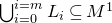
Proof. Claims (i) and (iii) follow directly from the approach of [Reference Ferrara, Green, Higgins and PopescuFGH+22, Proposition 4.2.3, Remark 4.2.4]. For later use, we note that the G-action on $V=\iota(K_\infty/L)\oplus s(\mathcal H)$
is
$V=\iota(K_\infty/L)\oplus s(\mathcal H)$
is
 \begin{equation}g\cdot(\iota(\lambda),s(h))=(\iota(g\lambda)+a_{g,h},b_{g,h})=(\iota(g\lambda)+a_{g,h},s(gh))\end{equation}
for any $\lambda\in K_\infty/L$
,
$\lambda\in K_\infty/L$
, $h\in\mathcal H$
and
$h\in\mathcal H$
and $g\in G$
, where
$g\in G$
, where $(a_{g,h},b_{g,h}):=g\cdot(0,s(h))$
and we have also used the fact that
$(a_{g,h},b_{g,h}):=g\cdot(0,s(h))$
and we have also used the fact that $b_{g,h}$
is necessarily equal to s(gh).
$b_{g,h}$
is necessarily equal to s(gh).
Now, from the explicit definition of $M^2$
, we derive an exact commutative diagram of A[G]-modules.
$M^2$
, we derive an exact commutative diagram of A[G]-modules.

Since the first two columns of this diagram induce the identity map on $\mathcal H$
, the arrow in the third column must be bijective by the snake lemma, and it is therefore straightforward to modify the second row to obtain the diagram in claim (ii).
$\mathcal H$
, the arrow in the third column must be bijective by the snake lemma, and it is therefore straightforward to modify the second row to obtain the diagram in claim (ii).
Remark 6.7. If $K/k$
is abelian, then the main result [Reference Ferrara, Green, Higgins and PopescuFGH+22, Theorem 1.5.1] of Ferrara et al. follows directly from Theorem 6.4.
$K/k$
is abelian, then the main result [Reference Ferrara, Green, Higgins and PopescuFGH+22, Theorem 1.5.1] of Ferrara et al. follows directly from Theorem 6.4.
Indeed, as in Remark 2.19 and since G is abelian, taking determinants over $\mathcal F_\infty[G]$
induces an isomorphism
$\mathcal F_\infty[G]$
induces an isomorphism
 $$\textrm{im}(\partial_G)\cong K_1(\mathcal F_\infty[G])/\textrm{im}(K_1(A[G]))\cong\mathcal F_\infty[G]^\times/A[G]^\times\cong\mathcal F_\infty[G]^+,$$
with the last map as in [Reference Ferrara, Green, Higgins and PopescuFGH+22, Definition A.3.2, Proposition A.3.4, Corollary A.3.6]. In addition, by Proposition A.4.1 in [Reference Ferrara, Green, Higgins and PopescuFGH+22] (or by Lemma 3.10 in this special abelian case), the determinant of the characteristic class $c_G(M)$
of any suitable module M is equal to its ‘A[G]-size’
$c_G(M)$
of any suitable module M is equal to its ‘A[G]-size’ $|M|_G$
, as in Definition 1.2.4 or Definition A.4.2 of [Reference Ferrara, Green, Higgins and PopescuFGH+22]. Therefore, using also that taking determinants is continuous (as a special case of Lemma 3.9),
$|M|_G$
, as in Definition 1.2.4 or Definition A.4.2 of [Reference Ferrara, Green, Higgins and PopescuFGH+22]. Therefore, using also that taking determinants is continuous (as a special case of Lemma 3.9), $\partial_G(\Theta^{\mathcal M}_{E,K/k})$
maps to
$\partial_G(\Theta^{\mathcal M}_{E,K/k})$
maps to
 \begin{align*}&\prod _{\mathfrak{p}\in\textrm{MSpec}(\mathcal O_k)}\det _{\mathcal F_\infty[G]}(c_G(\mathcal M/\mathfrak{p}\mathcal M)\cdot c_G(E(\mathcal M/\mathfrak{p}\mathcal M))^{-1})\\&\quad = \prod _{\mathfrak{p}\in\textrm{MSpec}(\mathcal O_k)}|\mathcal M/\mathfrak{p}\mathcal M|_G\cdot |E(\mathcal M/\mathfrak{p}\mathcal M)|_G^{-1},\end{align*}
which recovers the definition of $\Theta_{K/k}^{E,\mathcal M}(0)\in\mathcal F_\infty[G]^+$
from [Reference Ferrara, Green, Higgins and PopescuFGH+22, p. 2221].
$\Theta_{K/k}^{E,\mathcal M}(0)\in\mathcal F_\infty[G]^+$
from [Reference Ferrara, Green, Higgins and PopescuFGH+22, p. 2221].
It thus suffices to observe that taking determinants maps the sum $[M^1,\lambda,\mathcal M]+\textrm{KFit}_G(M^2)$
to the ‘ratio of volumes’
$[M^1,\lambda,\mathcal M]+\textrm{KFit}_G(M^2)$
to the ‘ratio of volumes’ $\mathrm{Vol}(V_E)/\mathrm{Vol}(K_\infty/\mathcal M)$
of [Reference Ferrara, Green, Higgins and PopescuFGH+22, Theorem 1.5.1]. On the one hand, for any free A[G]-lattice
$\mathrm{Vol}(V_E)/\mathrm{Vol}(K_\infty/\mathcal M)$
of [Reference Ferrara, Green, Higgins and PopescuFGH+22, Theorem 1.5.1]. On the one hand, for any free A[G]-lattice $\mathcal N$
in
$\mathcal N$
in $K_\infty$
that contains
$K_\infty$
that contains $\mathcal M$
, the former sum is the image under
$\mathcal M$
, the former sum is the image under $\partial_G$
of the product
$\partial_G$
of the product
 $$c_G(M^2)\cdot[X]\cdot c_G(\mathcal N/\mathcal M)^{-1},$$
where $X\in\mathrm{GL}_n(\mathcal F_\infty[G])$
is the transition matrix between arbitrary A[G]-bases of
$X\in\mathrm{GL}_n(\mathcal F_\infty[G])$
is the transition matrix between arbitrary A[G]-bases of $\mathcal N$
and of
$\mathcal N$
and of $M^1$
, respectively. The claimed observation is now clear because, on the other hand, taking
$M^1$
, respectively. The claimed observation is now clear because, on the other hand, taking $\Lambda_0$
to be
$\Lambda_0$
to be $\mathcal M$
in Definition 4.2.6 of [Reference Ferrara, Green, Higgins and PopescuFGH+22],
$\mathcal M$
in Definition 4.2.6 of [Reference Ferrara, Green, Higgins and PopescuFGH+22], $\mathrm{Vol}(K_\infty/\mathcal M)=1$
, while
$\mathrm{Vol}(K_\infty/\mathcal M)=1$
, while $\mathrm{ Vol}(V_E)$
is computed (taking
$\mathrm{ Vol}(V_E)$
is computed (taking $\Lambda'$
to be
$\Lambda'$
to be $M^1$
, so that
$M^1$
, so that $\Lambda'/\Lambda\times s(H)=M^2$
) as
$\Lambda'/\Lambda\times s(H)=M^2$
) as
 $$|M^2|_G\cdot[M^1:\mathcal M]_G^{-1}=|M^2|_G\cdot\det (X^{-1})^{-1}\cdot|\mathcal N/\mathcal M|_G^{-1}=|M^2|_G\cdot\det (X)\cdot|\mathcal N/\mathcal M|_G^{-1},$$
with the factor $[M^1:\mathcal M]_G$
and the first equality given by Definition 4.1.4 in [Reference Ferrara, Green, Higgins and PopescuFGH+22].
$[M^1:\mathcal M]_G$
and the first equality given by Definition 4.1.4 in [Reference Ferrara, Green, Higgins and PopescuFGH+22].
In the rest of § 6.1 we prove Theorem 6.4(ii). We fix A[G]-modules $M^1$
and
$M^1$
and
 $$M^2:=\exp _E(M^1/\mathbb{U})\oplus s(H)$$
as in claim (i), and proceed to compute the class $[1+\Phi_E\mid V_\infty^{\mathcal M}]$
. To do so we first construct, for each natural number N, approximations
$[1+\Phi_E\mid V_\infty^{\mathcal M}]$
. To do so we first construct, for each natural number N, approximations $M^1_N$
and
$M^1_N$
and $M^2_N$
of
$M^2_N$
of $M^1$
and
$M^1$
and $M^2$
that are related to the taming module
$M^2$
that are related to the taming module $\mathcal M$
.
$\mathcal M$
.
We set $n:=[k:\mathcal F]$
, recall that
$n:=[k:\mathcal F]$
, recall that $K_\infty\cong\mathcal F_\infty[G]^n$
and fix an
$K_\infty\cong\mathcal F_\infty[G]^n$
and fix an $\mathcal F_\infty[G]$
-basis
$\mathcal F_\infty[G]$
-basis $b_\bullet$
of
$b_\bullet$
of $K_\infty$
. We use this basis to interpret any
$K_\infty$
. We use this basis to interpret any $\sigma\in\mathrm{GL}_n(\mathcal F_\infty[G])$
as an automorphism of
$\sigma\in\mathrm{GL}_n(\mathcal F_\infty[G])$
as an automorphism of $K_\infty$
.
$K_\infty$
.
We fix a free A[G]-lattice $\mathcal N$
in
$\mathcal N$
in $K_\infty$
containing
$K_\infty$
containing $\mathcal M$
and A[G]-bases
$\mathcal M$
and A[G]-bases $\textbf{e}$
and
$\textbf{e}$
and $\textbf{e}'$
of
$\textbf{e}'$
of $\mathcal N$
and of
$\mathcal N$
and of $M^1$
and write
$M^1$
and write $X\in\mathrm{GL}_n(\mathcal F_\infty[G])$
for the transition matrix between
$X\in\mathrm{GL}_n(\mathcal F_\infty[G])$
for the transition matrix between $\textbf{e}'$
and
$\textbf{e}'$
and $\textbf{e}$
.
$\textbf{e}$
.
Endowing $M_n(\mathcal F_\infty[G])=M_n(R(\!(t^{-1})\!))$
with its
$M_n(\mathcal F_\infty[G])=M_n(R(\!(t^{-1})\!))$
with its $t^{-1}$
-adic topology,
$t^{-1}$
-adic topology, $\textrm{GL}_n(\mathcal F_\infty[G])$
is an open subset and
$\textrm{GL}_n(\mathcal F_\infty[G])$
is an open subset and $(\{\mathrm{Id}_n+t^{-N}\mathrm{M}_n(R[\![t^{-1}]\!])\})_{N\geq 0}$
is a basis of open neighbourhoods of
$(\{\mathrm{Id}_n+t^{-N}\mathrm{M}_n(R[\![t^{-1}]\!])\})_{N\geq 0}$
is a basis of open neighbourhoods of $\mathrm{Id}_n$
in
$\mathrm{Id}_n$
in $\textrm{GL}_n(\mathcal F_\infty[G])$
. It is also straightforward to see that
$\textrm{GL}_n(\mathcal F_\infty[G])$
. It is also straightforward to see that $M_n(\mathcal F[G])=M_n(R(t))$
is dense in
$M_n(\mathcal F[G])=M_n(R(t))$
is dense in $M_n(\mathcal F_\infty[G])$
and that
$M_n(\mathcal F_\infty[G])$
and that $\textrm{GL}_n(\mathcal F[G])=M_n(\mathcal F[G])\cap\textrm{GL}_n(\mathcal F_\infty[G])$
. These facts imply that
$\textrm{GL}_n(\mathcal F[G])=M_n(\mathcal F[G])\cap\textrm{GL}_n(\mathcal F_\infty[G])$
. These facts imply that $\textrm{GL}_n(\mathcal F[G])$
is dense in
$\textrm{GL}_n(\mathcal F[G])$
is dense in $\textrm{GL}_n(\mathcal F_\infty[G])$
and, in particular, that the intersection
$\textrm{GL}_n(\mathcal F_\infty[G])$
and, in particular, that the intersection
 $$\textrm{GL}_n(\mathcal F[G])\cap \{(\mathrm{Id}_n+t^{-N}\mathrm{M}_n(R[\![t^{-1}]\!]))\cdot X^{-1}\}$$
is non-empty for every natural number N. We thus may and do fix a matrix
 $$\sigma_N \in \{\mathrm{Id}_n+t^{-2N}\mathrm{M}_n(R[\![t^{-1}]\!])\}$$
such that $X\cdot\sigma_N^{-1}$
belongs to
$X\cdot\sigma_N^{-1}$
belongs to $\textrm{GL}_n(\mathcal F[G])$
. This property then implies that the free A[G]-lattices
$\textrm{GL}_n(\mathcal F[G])$
. This property then implies that the free A[G]-lattices $\sigma_N(M^1)$
and
$\sigma_N(M^1)$
and $\mathcal N$
are contained in a common A[G]-lattice in
$\mathcal N$
are contained in a common A[G]-lattice in $K_\infty$
.
$K_\infty$
.
For each N we also fix a push-out $(\pi_N:V_E\to\Pi_N,\iota_N:K_\infty/\sigma_N(\mathbb{U})\to\Pi_N)$
of
$(\pi_N:V_E\to\Pi_N,\iota_N:K_\infty/\sigma_N(\mathbb{U})\to\Pi_N)$
of $(\exp_E:K_\infty/\mathbb U\to V_E,\sigma_N:K_\infty/\mathbb U\to K_\infty/\sigma_N(\mathbb{U}))$
. Then
$(\exp_E:K_\infty/\mathbb U\to V_E,\sigma_N:K_\infty/\mathbb U\to K_\infty/\sigma_N(\mathbb{U}))$
. Then $\pi_N$
is bijective and
$\pi_N$
is bijective and $\iota_N$
is injective (because
$\iota_N$
is injective (because $\sigma_N$
is bijective and
$\sigma_N$
is bijective and $\exp_E$
is injective), so we derive the following exact commutative diagram with bijective vertical arrows.
$\exp_E$
is injective), so we derive the following exact commutative diagram with bijective vertical arrows.

We write $s_N$
for the composition
$s_N$
for the composition
 $$H\stackrel{s}{\hookrightarrow}V_E\stackrel{\pi_N}{\cong}\Pi_N,$$
which is then an A-module section to the lower row of (6.3).
Applying Lemma 6.6 to $s_N$
, to the lower row of the diagram (6.3) and to the finite set of free A[G]-lattices
$s_N$
, to the lower row of the diagram (6.3) and to the finite set of free A[G]-lattices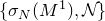 $\{\sigma_N(M^1),\mathcal N\}$
we deduce, for each natural number N, the existence of a free A[G]-lattice
$\{\sigma_N(M^1),\mathcal N\}$
we deduce, for each natural number N, the existence of a free A[G]-lattice $M^1_N$
with
$M^1_N$
with
 $$\sigma_N(\mathbb U)\cup\mathcal M\subseteq\sigma_N(M^1)\cup\mathcal N\subseteq M^1_N$$
and with the property that
 $$M^2_N:=\iota_N(M^1_N/\sigma_N(\mathbb U))\oplus s_N(H)$$
is an A[G]-submodule of $\Pi_N$
that fits in an exact commutative diagram.
$\Pi_N$
that fits in an exact commutative diagram.

Regarding this data as fixed, we now obtain the following intermediate computation of the class $[1+\Phi_E\mid V_\infty^{\mathcal M}]$
.
$[1+\Phi_E\mid V_\infty^{\mathcal M}]$
.
Lemma 6.8. For every large enough natural number N, in $K_1(\Lambda/Z^N)$
one has
$K_1(\Lambda/Z^N)$
one has
 $$[1+\Phi_E\mid V_\infty^{\mathcal M}]_N = [(M^1_N/\mathcal M)_N,\,1-(Z\otimes t)]^{-1}\cdot[(M^2_N)_N,\,1-(Z\otimes t)].$$
Proof. We first recall that any quotient of projective R-modules is also R-projective (see Remark 4.10). We fix an open, projective R-submodule Q of $K_\infty$
as in Lemma 6.9 below. In particular,
$K_\infty$
as in Lemma 6.9 below. In particular, $K_\infty=M_N^1\oplus Q$
. We also fix, as we may, an R-splitting
$K_\infty=M_N^1\oplus Q$
. We also fix, as we may, an R-splitting $\varpi:\Pi_N\cong M_N^2\oplus (K_\infty/M^1_N)$
of the second row of the diagram (6.4).
$\varpi:\Pi_N\cong M_N^2\oplus (K_\infty/M^1_N)$
of the second row of the diagram (6.4).
Then $\pi_N:V_E\cong\Pi_N$
induces an isomorphism of R-modules
$\pi_N:V_E\cong\Pi_N$
induces an isomorphism of R-modules
 $$\tilde\pi:(M^1_N/\mathcal M)\oplus Q= V_\infty^{\mathcal M}= V_E\cong\Pi_N\cong M_N^2\oplus (K_\infty/M^1_N)= M_N^2\oplus Q.$$
We now write $B_{K_\infty}$
for the closed unit ball in
$B_{K_\infty}$
for the closed unit ball in $K_\infty$
. Then our choice of
$K_\infty$
. Then our choice of $\sigma_N$
combines with [Reference Ferrara, Green, Higgins and PopescuFGH+22, Proposition 5.1.3] to imply that for every large enough natural number j, one has
$\sigma_N$
combines with [Reference Ferrara, Green, Higgins and PopescuFGH+22, Proposition 5.1.3] to imply that for every large enough natural number j, one has
 \begin{equation}\tilde\pi(t^{-j}B_{K_\infty})=t^{-j}B_{K_\infty}\quad\text{and}\quad (\tilde\pi^{-1}-1)(t^{-j}B_{K_\infty})\subseteq t^{-(j+2N)}B_{K_\infty}.\end{equation}
In particular, if j is also large enough that $t^{-j}B_{K_\infty}\subseteq Q$
, the R-isomorphism
$t^{-j}B_{K_\infty}\subseteq Q$
, the R-isomorphism $\tilde\pi$
induces an R-isomorphism
$\tilde\pi$
induces an R-isomorphism
 $$(M^1_N/\mathcal M)\oplus (Q/t^{-j}B_{K_\infty})\cong M_N^2\oplus (Q/t^{-j}B_{K_\infty}).$$
Thus, by the cancellation theorem [Reference LamLam01, 20.12] (and Lemma 6.9), there exists a (non-canonical) R-isomorphism $\beta:M_N^1/\mathcal M\cong M_N^2$
. We then consider the R-isomorphism
$\beta:M_N^1/\mathcal M\cong M_N^2$
. We then consider the R-isomorphism
 $$\delta:=\beta\oplus\mathrm{id}_Q:(M^1_N/\mathcal M)\oplus Q\cong M_N^2\oplus Q.$$
We next recall that the power series class $[1+\Phi_E\mid V_\infty^{\mathcal M}]$
is computed with respect to the sequence
$[1+\Phi_E\mid V_\infty^{\mathcal M}]$
is computed with respect to the sequence $\{t^{-i}W\}_{i\geq 1}$
in
$\{t^{-i}W\}_{i\geq 1}$
in $\mathcal T_{S_k^\infty}^{\mathcal M}$
, for some R-projective, open, torsion-free-
$\mathcal T_{S_k^\infty}^{\mathcal M}$
, for some R-projective, open, torsion-free- $R[t^{-1}]$
-submodule W of
$R[t^{-1}]$
-submodule W of $V_\infty^{\mathcal M}$
of the form (5.1), which we now regard as fixed.
$V_\infty^{\mathcal M}$
of the form (5.1), which we now regard as fixed.
We first use the factorisation (5.3) to compute that
 \begin{equation*}[1+\Phi_E\mid V_\infty^{\mathcal M}]_N=\left[\frac{1-(Z\otimes\varpi t\varpi^{-1})}{1-(Z\otimes\tilde\pi t\tilde\pi^{-1})}\mid M_N^2\oplus Q\right]_N,\end{equation*}
with the right-hand side computed with respect to a common nucleus in $\{\tilde\pi(t^{-i}W)\}_{i\geq 1}$
.
$\{\tilde\pi(t^{-i}W)\}_{i\geq 1}$
.
On the other hand, one has
 \begin{align*}\left[\frac{1-(Z\otimes\varpi t\varpi^{-1})}{1-(Z\otimes\delta t\delta^{-1})}\,\bigg|\, M_N^2\oplus Q\right]_N&=\left[\frac{1-(Z\otimes t)}{1-(Z\otimes\beta t\beta^{-1})}\,\bigg|\, M_N^2\right]_N\cdot \left[\frac{1-(Z\otimes t)}{1-(Z\otimes t)}\,\bigg|\, Q\right]_N \\[4pt]&=\left[\frac{1-(Z\otimes t)}{1-(Z\otimes\beta t\beta^{-1})}\,\bigg|\, M_N^2\right]_N \\[4pt]&=[(M^1_N/\mathcal M)_N,1-(Z\otimes t)]^{-1}\cdot[(M^2_N)_N,1-(Z\otimes t)].\end{align*}
It therefore only remains to prove that the element
 $$\left[\frac{1-(Z\otimes\delta t\delta^{-1})}{1-(Z\otimes\tilde\pi t\tilde\pi^{-1})}\,\bigg|\, M_N^2\oplus Q\right]_N=\left[\frac{1-(Z\otimes\tilde\pi^{-1}\delta t\delta^{-1}\tilde\pi)}{1-(Z\otimes t)}\,\bigg|\, V_\infty^{\mathcal M}\right]_N$$
of $K_1(\Lambda/Z^N)$
is trivial or equivalently, in the notation of Definition 4.23 (
$K_1(\Lambda/Z^N)$
is trivial or equivalently, in the notation of Definition 4.23 ( $m=1$
), that
$m=1$
), that
 $$[1-(\tilde\pi^{-1}\delta t\delta^{-1}\tilde\pi)_1\mid V_\infty^{\mathcal M}]_N=[1-t_1\mid V_\infty^{\mathcal M}]_N.$$
We set $\psi:=(\tilde\pi^{-1}\delta)-1$
and
$\psi:=(\tilde\pi^{-1}\delta)-1$
and $\alpha:=t(\delta^{-1}\tilde\pi)$
. Then, by Taelman’s argument in [Reference TaelmanTae12, Corollary 1], it suffices to show that
$\alpha:=t(\delta^{-1}\tilde\pi)$
. Then, by Taelman’s argument in [Reference TaelmanTae12, Corollary 1], it suffices to show that
 $$[1-(\varphi\alpha)_1]_N = [1-(\alpha\varphi)_1]_N,$$
where $\varphi$
is a composition of, say,
$\varphi$
is a composition of, say, $n\lt N$
endomorphisms in the set
$n\lt N$
endomorphisms in the set $\{\alpha,\psi\}$
, with
$\{\alpha,\psi\}$
, with $\psi$
occurring at least once. In order to do so, we proceed to show that such an
$\psi$
occurring at least once. In order to do so, we proceed to show that such an $\alpha$
and
$\alpha$
and $\varphi$
satisfy the hypotheses of Proposition 4.24.
$\varphi$
satisfy the hypotheses of Proposition 4.24.
The map $\alpha$
is surjective, since both
$\alpha$
is surjective, since both $\delta$
and
$\delta$
and $\tilde\pi$
are bijective while
$\tilde\pi$
are bijective while $V_\infty^{\mathcal M}$
is A-divisible.
$V_\infty^{\mathcal M}$
is A-divisible.
To consider hypothesis (b) of Proposition 4.24, we use the integer $a_W$
in Proposition 5.4(i), which we recall is independent of N. We thus may and do assume that
$a_W$
in Proposition 5.4(i), which we recall is independent of N. We thus may and do assume that $N \geq 2 a_W$
, and we also fix a natural number i large enough that for every
$N \geq 2 a_W$
, and we also fix a natural number i large enough that for every $j\geq i-N$
, (6.5) is valid and also
$j\geq i-N$
, (6.5) is valid and also $t^{-j}B_{K_\infty}\subseteq Q$
, so
$t^{-j}B_{K_\infty}\subseteq Q$
, so $\delta$
restricts to the identity map on
$\delta$
restricts to the identity map on $t^{-j}B_{K_\infty}$
.
$t^{-j}B_{K_\infty}$
.
In this case, one has
 \begin{equation*}\varphi\alpha(t^{-i}W)\subseteq\varphi\alpha(t^{-i}B_{K_\infty})=\varphi(t^{-(i-1)}B_{K_\infty})\subseteq t^{-(i-n+2N)}B_{K_\infty}\subseteq t^{-(i+a_W+1)}B_{K_\infty} \subseteq t^{-(i+1)}W\end{equation*}
and, similarly,
 $$\alpha\varphi(t^{-i}W)\subseteq \alpha\varphi(t^{-i}B_{K_\infty})\subseteq t^{-(i-n+2N)}B_{K_\infty}\subseteq t^{-(i+a_W+1)}B_{K_\infty} \subseteq t^{-(i+1)}W.$$
Thus, both $\varphi\alpha$
and
$\varphi\alpha$
and $\alpha\varphi$
are locally contracting, with common nucleus
$\alpha\varphi$
are locally contracting, with common nucleus $t^{-i}W$
. In fact, the same arguments as above also show that
$t^{-i}W$
. In fact, the same arguments as above also show that
 $$\alpha(t^{-(i+a_W+1)}W)\subseteq\alpha(t^{-(i+a_W+1)}B_{K_\infty})\subseteq t^{-(i+a_W)}B_{K_\infty}\subseteq t^{-i}W$$
and
 $$\varphi(t^{-i}W)\subseteq\varphi(t^{-i}B_{K_\infty})\subseteq t^{-(i+2N-n+1)}B_{K_\infty} \subseteq t^{-(i+N-a_W+2)}W \subseteq t^{-(i+a_W+1)}W.$$
Hypothesis (b) of Proposition 4.24 is thus satisfied with $b=a_W+1$
. This completes the proof of the lemma.
$b=a_W+1$
. This completes the proof of the lemma.
Lemma 6.9. Let M be a free A[G]-lattice in $K_\infty$
. There is an open, projective R-submodule Q of
$K_\infty$
. There is an open, projective R-submodule Q of $K_\infty$
with the property that
$K_\infty$
with the property that $K_\infty=M\oplus Q$
. In addition, if
$K_\infty=M\oplus Q$
. In addition, if $j\in\mathbb N$
is such that
$j\in\mathbb N$
is such that $t^{-j}B_{K_\infty}\subseteq Q$
(with
$t^{-j}B_{K_\infty}\subseteq Q$
(with $B_{K_\infty}$
the closed unit ball in
$B_{K_\infty}$
the closed unit ball in $K_\infty$
), then
$K_\infty$
), then $Q/t^{-j}B_{K_\infty}$
is finite.
$Q/t^{-j}B_{K_\infty}$
is finite.
Proof. We recall that $\mathcal F_\infty$
decomposes as an
$\mathcal F_\infty$
decomposes as an ${\mathbb F}_q$
-space as
${\mathbb F}_q$
-space as $A\oplus t^{-1}{\mathbb F}_q[\![t^{-1}]\!]$
, with the second summand open in
$A\oplus t^{-1}{\mathbb F}_q[\![t^{-1}]\!]$
, with the second summand open in $\mathcal F_\infty$
. Let
$\mathcal F_\infty$
. Let $\mathbf{b}=\{b_1, \ldots, b_n\}$
be a basis of M. Then
$\mathbf{b}=\{b_1, \ldots, b_n\}$
be a basis of M. Then $Q :=\bigoplus_{i=1}^n t^{-1}{\mathbb F}_q[\![t^{-1}]\!][G]b_i=\bigoplus_{i=1}^n t^{-1}R[\![t^{-1}]\!]b_i$
is open in
$Q :=\bigoplus_{i=1}^n t^{-1}{\mathbb F}_q[\![t^{-1}]\!][G]b_i=\bigoplus_{i=1}^n t^{-1}R[\![t^{-1}]\!]b_i$
is open in $K_\infty$
because each summand gives the R-decomposition
$K_\infty$
because each summand gives the R-decomposition $K_\infty=M\oplus Q$
, and is R-projective by Remark 4.10.
$K_\infty=M\oplus Q$
, and is R-projective by Remark 4.10.
To prove the second claim it suffices to observe that there is $a\geq 0$
with
$a\geq 0$
with $t^{-a}Q\subseteq B_{K_\infty}$
, since then
$t^{-a}Q\subseteq B_{K_\infty}$
, since then $t^{-(a+j)}Q\subseteq t^{-j}B_{K_\infty}\subseteq Q$
and
$t^{-(a+j)}Q\subseteq t^{-j}B_{K_\infty}\subseteq Q$
and $Q/t^{-(a+j)}Q$
is finite. Indeed, since the norm of
$Q/t^{-(a+j)}Q$
is finite. Indeed, since the norm of $t^{-1}$
is normalised to be
$t^{-1}$
is normalised to be $q^{-1}$
, this is true whenever
$q^{-1}$
, this is true whenever $q^{a}$
is greater than the norms of all elements in the given basis
$q^{a}$
is greater than the norms of all elements in the given basis $\mathbf{b}$
.
$\mathbf{b}$
.
Returning to the proof of claim (ii) of Theorem 6.4, for each $N\in\mathbb N$
, we write
$N\in\mathbb N$
, we write
 $$\tilde\sigma_N \in \{\mathrm{Id}_n+Z^{2N}M_n(\Lambda)\}$$
for the image of $\sigma_N$
. Then, in order to relate the right-hand side of the equality in claim (ii) of Theorem 6.4 to the right-hand side of the equality in Lemma 6.8, we require the following intermediate result.
$\sigma_N$
. Then, in order to relate the right-hand side of the equality in claim (ii) of Theorem 6.4 to the right-hand side of the equality in Lemma 6.8, we require the following intermediate result.
Lemma 6.10. Fix $N_0\in\mathbb N$
. Then, in
$N_0\in\mathbb N$
. Then, in $K_0(A[G],\mathcal F_\infty[G])$
, one has
$K_0(A[G],\mathcal F_\infty[G])$
, one has
 $$[M^1,\lambda,\mathcal M]+\textrm{KFit}_G(M^2)=(\partial_G\circ\mathrm{ev}_{t^{-1}})\bigg([\tilde\sigma_{N_0}]^{-1}\cdot\frac{[\Lambda\otimes_RM^2_{N_0},\,1-(Z\otimes t)]}{[\Lambda\otimes_R M^1_{N_0}/\mathcal M,\,1-(Z\otimes t)]}\bigg).$$
Proof. To compute the right-hand side of the claimed equality we recall from the proof of Lemma 6.8 that there is an isomorphism of R-modules $\beta:M^1_{N_0}/\mathcal M \cong M^2_{N_0}$
. Thus,
$\beta:M^1_{N_0}/\mathcal M \cong M^2_{N_0}$
. Thus,
 \begin{align*}&\textrm{ev}_{t^{-1}}\bigg(\frac{[\Lambda\otimes_RM^2_{N_0},1-(Z\otimes t)]}{[\Lambda\otimes_R M^1_{N_0}/\mathcal M,1-(Z\otimes t)]}\bigg)\\[5pt]&\quad =\textrm{ev}_{t^{-1}}\bigg(\frac{[\Lambda\otimes_RM^2_{N_0},1-(Z\otimes t)]}{[\Lambda\otimes_R M^2_{N_0},1-(Z\otimes \beta t\beta^{-1})]}\bigg)\\[5pt]&\quad =\frac{[\mathcal F_\infty[G]\otimes_R M^2_{N_0},t\otimes1]}{[\mathcal F_\infty[G]\otimes_R M^2_{N_0},t\otimes 1]}\cdot\frac{[\mathcal F_\infty[G]\otimes_R M^2_{N_0},1-(t^{-1}\otimes t)]}{[\mathcal F_\infty[G]\otimes_R M^2_{N_0},1-(t^{-1}\otimes \beta t\beta^{-1})]}\\[5pt]&\quad =\frac{[\mathcal F_\infty[G]\otimes_R M^2_{N_0},(t\otimes1)-(1\otimes t)]}{[\mathcal F_\infty[G]\otimes_R M^2_{N_0},(t\otimes 1)-(1\otimes \beta t\beta^{-1})]}\\[5pt]&\quad =\frac{[\mathcal F_\infty[G]\otimes_R M^2_{N_0},(t\otimes 1)-(1\otimes t)]}{[\mathcal F_\infty[G]\otimes_R M^1_{N_0}/\mathcal M,(t\otimes 1)-(1\otimes t)]}=\frac{c_G(M^2_{N_0})}{c_G(M^1_{N_0}/\mathcal M)}.\end{align*}
Since also
 $$(\partial_G\circ\mathrm{ev}_{t^{-1}})([\tilde\sigma_{N_0}])=\partial_G([K_\infty,\sigma_{N_0}])=\partial_G([\mathcal F_\infty[G]\otimes_{A[G]}M^1,\sigma_{N_0}])=[M^1,\sigma_{N_0},M^1]$$
by definition of $\partial_G$
(or by [Reference SwanSwa78, Lemma 15.7], but note that there is a typo in this result, where [(P, f, P)] should read [(P, g, P)]), we find that the right-hand side of the claimed equality is equal to
$\partial_G$
(or by [Reference SwanSwa78, Lemma 15.7], but note that there is a typo in this result, where [(P, f, P)] should read [(P, g, P)]), we find that the right-hand side of the claimed equality is equal to
 $$-[M^1,\sigma_{N_0},M^1]+\textrm{KFit}_G(M^2_{N_0})-\textrm{KFit}_G(M^1_{N_0}/\mathcal M).$$
Applying Lemma 6.3 to the exact sequences
 $$0\longrightarrow\mathcal M\longrightarrow M^1_{N_0}\longrightarrow M^1_{N_0}/\mathcal M\to 0$$
and
 $$0\to M^1\xrightarrow{\sigma_{N_0}}M^1_{N_0}\longrightarrow M^1_{N_0}/\sigma_{N_0}(M^1)\to 0,$$
we also find that
 \begin{align*}[M^1,\lambda,\mathcal M]+[M^1,\sigma_{N_0},M^1]+\textrm{KFit}_G(M^1_{N_0}/\mathcal M)&= [M^1,\lambda,M^1_{N_0}]+[M^1,\sigma_{N_0},M^1]\\&=[M^1,\sigma_{N_0},M^1_{N_0}]\\&=\textrm{KFit}_G(M^1_{N_0}/\sigma_{N_0}(M^1)).\end{align*}
It therefore suffices to prove that
 \begin{equation}\textrm{KFit}_G(M^1_{N_0}/\sigma_{N_0}(M^1))=\textrm{KFit}_G(M^2_{N_0})-\textrm{KFit}_G(M^2).\end{equation}
In order to do so, we define a map
 $$\mu:M^2=\exp_E(M^1/\mathbb U)\oplus s(H)\longrightarrow \iota_{N_0}(M^1_{N_0}/\sigma_{N_0}(\mathbb U))\oplus (\pi_{N_0}\circ s)(H)=M^2_{N_0}$$
by setting
 $$\mu(\exp_E(\bar m),s(h)):=(\iota_{N_0}(\overline{\sigma_{N_0}(m)}),\pi_{N_0}(s(h)))$$
for $m\in M^1$
and
$m\in M^1$
and $h\in H$
. Here,
$h\in H$
. Here, $\iota_{N_0},\pi_{N_0}$
are as in the push-out diagram (6.3).
$\iota_{N_0},\pi_{N_0}$
are as in the push-out diagram (6.3).
Using the commutativity of (6.3) and (6.4) and the explicit G-action (6.2) on the modules $M^2$
and
$M^2$
and $M^2_{N_0}$
, it is straightforward to verify that
$M^2_{N_0}$
, it is straightforward to verify that $\mu$
is a well-defined, injective A[G]-module homomorphism that makes the following exact diagram commute.
$\mu$
is a well-defined, injective A[G]-module homomorphism that makes the following exact diagram commute.

By the snake lemma, we find that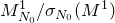 $M^1_{N_0}/\sigma_{N_0}(M^1)$
is isomorphic to
$M^1_{N_0}/\sigma_{N_0}(M^1)$
is isomorphic to $\textrm{cok}(\mu)$
and therefore (by Lemma 2.6) also that
$\textrm{cok}(\mu)$
and therefore (by Lemma 2.6) also that
 $$\textrm{KFit}_G(M^1_{N_0}/\sigma_{N_0}(M^1))=\textrm{KFit}_G(\textrm{cok}(\mu))=\textrm{KFit}_G(M^2_{N_0})-\textrm{KFit}_G(M^2).$$
We have now proved the equality (6.6) and thus completed the proof.
In order to complete the proof of Theorem 6.4, we now require certain K-theoretical results.
Lemma 6.11. The canonical map $K_1(\Lambda)\to K_0(R,\Lambda)$
is surjective, and the isomorphism in Proposition 4.4 induces an isomorphism of abelian groups
$K_1(\Lambda)\to K_0(R,\Lambda)$
is surjective, and the isomorphism in Proposition 4.4 induces an isomorphism of abelian groups
 \begin{equation*}K_0(R,\Lambda)\cong {\varprojlim}_{N\in\mathbb N}K_0(R,\Lambda/Z^N).\end{equation*}
Proof. The composite map $R\subset\Lambda\to\Lambda/Z$
is an isomorphism of rings. From this fact, it is straightforward to verify that the group
$R\subset\Lambda\to\Lambda/Z$
is an isomorphism of rings. From this fact, it is straightforward to verify that the group $K_0(R,\Lambda/Z)$
is trivial. Since the canonical map
$K_0(R,\Lambda/Z)$
is trivial. Since the canonical map $K_0(R,\Lambda)\to K_0(R)$
factors through
$K_0(R,\Lambda)\to K_0(R)$
factors through $K_0(R,\Lambda/Z)$
, it must be the zero map. The exactness of the localisation sequence [Reference SwanSwa78, Theorem 15.5] then proves the first claim.
$K_0(R,\Lambda/Z)$
, it must be the zero map. The exactness of the localisation sequence [Reference SwanSwa78, Theorem 15.5] then proves the first claim.
For each $N\in\mathbb N$
, the canonical map
$N\in\mathbb N$
, the canonical map $K_0(R,\Lambda/Z^N)\to K_0(R)$
also factors through
$K_0(R,\Lambda/Z^N)\to K_0(R)$
also factors through $K_0(R,\Lambda/Z)$
, so the same argument proves that the canonical map
$K_0(R,\Lambda/Z)$
, so the same argument proves that the canonical map $K_1(\Lambda/Z^N)\to K_0(R,\Lambda/Z^N)$
is surjective. We therefore have an exact sequence
$K_1(\Lambda/Z^N)\to K_0(R,\Lambda/Z^N)$
is surjective. We therefore have an exact sequence
 $$K_1(R)\to K_1(\Lambda)\to K_0(R,\Lambda)\to 0$$
and, for each N, setting
 $$K_1(R)_N:=\textrm{im}(K_1(R)\to K_1(\Lambda/Z^N)),$$
also an exact sequence of finite abelian groups
 $$0\to K_1(R)_N\to K_1(\Lambda/Z^N)\to K_0(R,\Lambda/Z^N)\to 0.$$
Now, the map $K_1(R)\to\varprojlim_{N\in\mathbb N}K_1(R)_N$
is surjective. Therefore, the result follows from applying the snake lemma to the following exact commutative diagram.
$K_1(R)\to\varprojlim_{N\in\mathbb N}K_1(R)_N$
is surjective. Therefore, the result follows from applying the snake lemma to the following exact commutative diagram.

We also require the next K-theoretic result, which will be proved in § 6.2 below.
Proposition 6.12. The canonical map
 $$\textrm{ev}_{t^{-1}}^0:K_0(R,\Lambda)\to K_0(R[Z^{-1}],R(\!(Z)\!))\xrightarrow{Z\mapsto t^{-1}}K_0(A[G],\mathcal F_\infty[G])$$
is injective.
We next observe that there is a canonical commutative square as follows.

For each $N\in\mathbb N$
, we set
$N\in\mathbb N$
, we set
 $$Y'(N):=[\tilde\sigma_{N}]^{-1}\cdot\frac{[\Lambda\otimes_R M^2_{N},\,1-(Z\otimes t)]}{[\Lambda\otimes_R M^1_{N}/\mathcal M,\,1-(Z\otimes t)]}\in K_1(\Lambda).$$
By Lemma 6.10 and the commutativity of (6.7),
 $$\textrm{ev}_{t^{-1}}^0(\widehat\partial_G(Y'(N))) = (\partial_G\circ\textrm{ev}_{t^{-1}})(Y'(N))= [M^1,\lambda,\mathcal M ]+\textrm{KFit}_G(M^2).$$
In particular, Proposition 6.12 implies that the preimage $Y:=\widehat\partial_G(Y'(N))\in K_0(R,\Lambda)$
of the right-hand side under
$Y:=\widehat\partial_G(Y'(N))\in K_0(R,\Lambda)$
of the right-hand side under $\textrm{ev}_{t^{-1}}^0$
is independent of
$\textrm{ev}_{t^{-1}}^0$
is independent of $N\in\mathbb N$
.
$N\in\mathbb N$
.
Now, Corollary 5.6 combines with the commutativity of (6.7) to reduce the proof of the equality in claim (ii) of Theorem 6.4 to proving that
 \begin{equation}\widehat\partial_G([1+\Phi_E\mid V_\infty^{\mathcal M}]) = Y.\end{equation}
In turn, by Lemma 6.11, the equality (6.8) will be valid if and only if its projection to $K_0(R,\Lambda/Z^N)$
is valid for every
$K_0(R,\Lambda/Z^N)$
is valid for every $N\in\mathbb N$
, if and only if its projection to
$N\in\mathbb N$
, if and only if its projection to $K_0(R,\Lambda/Z^N)$
is valid for every large enough
$K_0(R,\Lambda/Z^N)$
is valid for every large enough $N\in\mathbb N$
. We may thus fix
$N\in\mathbb N$
. We may thus fix $N_0\in\mathbb N$
, large enough that Lemma 6.8 applies to
$N_0\in\mathbb N$
, large enough that Lemma 6.8 applies to $N=N_0$
, and proceed to verify that the projection to
$N=N_0$
, and proceed to verify that the projection to $K_0(R,\Lambda/Z^{N_0})$
of the equality (6.8) is valid.
$K_0(R,\Lambda/Z^{N_0})$
of the equality (6.8) is valid.
Using now the equality $Y=\widehat\partial_G(Y'(N_0))$
and the commutativity of the following square, it suffices to show that the image of
$Y=\widehat\partial_G(Y'(N_0))$
and the commutativity of the following square, it suffices to show that the image of $Y'(N_0)$
in
$Y'(N_0)$
in $K_1(\Lambda/Z^{N_0})$
is equal to
$K_1(\Lambda/Z^{N_0})$
is equal to $[1+\Phi_E\mid V_\infty^{\mathcal M}]_{N_0}$
.
$[1+\Phi_E\mid V_\infty^{\mathcal M}]_{N_0}$
.

But, by choice of $\sigma_{N_0}$
, the image in
$\sigma_{N_0}$
, the image in $K_1(\Lambda/Z^{N_0})$
of
$K_1(\Lambda/Z^{N_0})$
of $[\tilde\sigma_{N_0}]$
is trivial, and hence the image of
$[\tilde\sigma_{N_0}]$
is trivial, and hence the image of $Y'(N_0)$
in
$Y'(N_0)$
in $K_1(\Lambda/Z^{N_0})$
is equal to
$K_1(\Lambda/Z^{N_0})$
is equal to
 $$\frac{[(M^2_{N_0})_{N_0},\,1-(Z\otimes t)]}{[(M^1_{N_0}/\mathcal M)_{N_0},\,1-(Z\otimes t)]}.$$
The proof of Theorem 6.4 is now completed by simply applying Lemma 6.8 to $N=N_0$
.
$N=N_0$
.
6.2 The proofs of Propositions 5.1 and 6.12
We are grateful to Oliver Braunling for his advice regarding the argument that we present in this section.
We set $R:={\mathbb F}_q[G]$
,
$R:={\mathbb F}_q[G]$
, $\Lambda:=R[\![Z]\!]$
,
$\Lambda:=R[\![Z]\!]$
, $\Pi:=R[Z^{-1}]$
and
$\Pi:=R[Z^{-1}]$
and $\mathcal L:=R(\!(Z)\!)$
. By [Reference SwanSwa78, Theorem 15.5] and Lemma 6.11, we have the following exact commutative diagram of abelian groups.
$\mathcal L:=R(\!(Z)\!)$
. By [Reference SwanSwa78, Theorem 15.5] and Lemma 6.11, we have the following exact commutative diagram of abelian groups.

The claims of Propositions 5.1 and 6.12 are then equivalent to the following.
Proposition 6.13. The maps $\delta$
and
$\delta$
and $\varepsilon$
are both injective.
$\varepsilon$
are both injective.
In the rest of this section, we prove Proposition 6.13. At the outset, we fix notation for the following canonical maps:
 \begin{gather*}\beta':K_1(R)\to K_1(R[Z]),\quad \theta:K_1(R[Z])\to K_1(R[Z,Z^{-1}]),\quad \iota:K_1(R[Z])\to K_1(\Lambda),\\\theta':K_1(\Pi)\to K_1(R[Z,Z^{-1}]),\quad\lambda:K_1(R[Z,Z^{-1}])\to K_1(\mathcal L).\end{gather*}
We then observe the following relations:
 \begin{equation}\alpha=\iota\circ\beta',\quad \gamma=\lambda\circ\theta', \quad \delta\circ\iota=\lambda\circ\theta.\end{equation}
6.2.1.
Before proving Proposition 6.13, we adapt several useful results from [Reference WeibelWei13].
The set $S:=\{Z^j \mid j\geq 0\}$
is a central, multiplicatively closed subset of non-zero divisors in both of the rings R[Z] and
$S:=\{Z^j \mid j\geq 0\}$
is a central, multiplicatively closed subset of non-zero divisors in both of the rings R[Z] and $\Lambda$
.
$\Lambda$
.
We write H(R[Z]), respectively $H(\Lambda)$
, for the category of R[Z]-modules, respectively
$H(\Lambda)$
, for the category of R[Z]-modules, respectively $\Lambda$
-modules, that admit a finite resolution by finitely generated projective R[Z]-modules, respectively
$\Lambda$
-modules, that admit a finite resolution by finitely generated projective R[Z]-modules, respectively $\Lambda$
-modules. We then write
$\Lambda$
-modules. We then write $H_S(R[Z])$
and
$H_S(R[Z])$
and $H_S(\Lambda)$
for their respective exact subcategories comprising S-torsion modules. The following result extends the commutative square
$H_S(\Lambda)$
for their respective exact subcategories comprising S-torsion modules. The following result extends the commutative square $\delta\circ\iota=\lambda\circ\theta$
from (6.9) to the
$\delta\circ\iota=\lambda\circ\theta$
from (6.9) to the $K_0$
-groups of these categories.
$K_0$
-groups of these categories.
Proposition 6.14. There is a commutative diagram of abelian groups as follows, with exact rows in which $\zeta_0$
is bijective.
$\zeta_0$
is bijective.

In particular, $\delta$
is injective, as claimed in Proposition 6.13.
$\delta$
is injective, as claimed in Proposition 6.13.
Proof. We first claim that there is the following exact commutative diagram of abelian groups in which $\zeta_0$
and
$\zeta_0$
and $\zeta_1$
are induced by the scalar extension functor, which is exact by Proposition 6.15 below.
$\zeta_1$
are induced by the scalar extension functor, which is exact by Proposition 6.15 below.

After noting that the localisations $S^{-1}R[Z]$
and
$S^{-1}R[Z]$
and $S^{-1}\Lambda$
identify with
$S^{-1}\Lambda$
identify with $R[Z^{-1},Z]$
and with
$R[Z^{-1},Z]$
and with $\mathcal L$
, respectively, [Reference WeibelWei13, Theorem V.7.1] gives the exactness of both rows. The naturality of these exact localisation sequences with respect to the scalar extension from R[Z] to
$\mathcal L$
, respectively, [Reference WeibelWei13, Theorem V.7.1] gives the exactness of both rows. The naturality of these exact localisation sequences with respect to the scalar extension from R[Z] to $\Lambda$
is implicitly stated in [Reference WeibelWei13, Proposition V.7.5(2)], but we proceed to give a direct argument instead.
$\Lambda$
is implicitly stated in [Reference WeibelWei13, Proposition V.7.5(2)], but we proceed to give a direct argument instead.
To first consider the right-hand square, we use the explicit description of the connecting homomorphisms $\mu$
,
$\mu$
, $\nu$
from [Reference WeibelWei13, Corollary III.3.1.1]. Every element of
$\nu$
from [Reference WeibelWei13, Corollary III.3.1.1]. Every element of $K_1(R[Z^{-1},Z])$
may be represented by a pair
$K_1(R[Z^{-1},Z])$
may be represented by a pair $[R[Z^{-1},Z]^n,s^{-1}\otimes_{R[Z]}\alpha]$
, where s is an element of S and
$[R[Z^{-1},Z]^n,s^{-1}\otimes_{R[Z]}\alpha]$
, where s is an element of S and $\alpha$
is an injective endomorphism of
$\alpha$
is an injective endomorphism of $R[Z]^n$
with the property that
$R[Z]^n$
with the property that $R[Z^{-1},Z]\otimes_{R[Z]}\textrm{cok}(\alpha)$
vanishes. One then has
$R[Z^{-1},Z]\otimes_{R[Z]}\textrm{cok}(\alpha)$
vanishes. One then has
 \begin{align*}(\zeta_0\circ\mu)([R[Z^{-1},Z]^n,s^{-1}\otimes_{R[Z]}\alpha])&=\zeta_0([\textrm{cok}(\alpha)]\cdot[R[Z]/sR[Z]]^{-n})\\&=[\Lambda\otimes_{R[Z]}\textrm{cok}(\alpha)]\cdot[\Lambda\otimes_{R[Z]}(R[Z]/sR[Z])]^{-n}\\&=[\textrm{cok}(\Lambda\otimes_{R[Z]}\alpha)]\cdot[\Lambda/s\Lambda]^{-n}\\&=\nu([\mathcal L^n,s^{-1}\otimes_\Lambda(\Lambda\otimes_{R[Z]}\alpha)])\\&=(\nu\circ\lambda)([R[Z^{-1},Z]^n,s^{-1}\otimes_{R[Z]}\alpha]).\end{align*}
To next consider the left-hand square, we write $\mathcal P(R[Z])$
, respectively
$\mathcal P(R[Z])$
, respectively $\mathcal P(\Lambda)$
, for the category of finitely generated, projective R[Z]-modules, respectively
$\mathcal P(\Lambda)$
, for the category of finitely generated, projective R[Z]-modules, respectively $\Lambda$
-modules. Then the canonical maps
$\Lambda$
-modules. Then the canonical maps $\eta$
and
$\eta$
and $\kappa$
decompose as
$\kappa$
decompose as $\eta=\eta_1^{-1}\circ\eta_2$
and
$\eta=\eta_1^{-1}\circ\eta_2$
and $\kappa=\kappa_1^{-1}\circ\kappa_2$
, where
$\kappa=\kappa_1^{-1}\circ\kappa_2$
, where $\eta_1,\eta_2,\kappa_1,\kappa_2$
are respectively induced by the inclusions of categories
$\eta_1,\eta_2,\kappa_1,\kappa_2$
are respectively induced by the inclusions of categories $\mathcal P(R[Z])\to H(R[Z])$
,
$\mathcal P(R[Z])\to H(R[Z])$
, $H_S(R[Z])\to H(R[Z])$
,
$H_S(R[Z])\to H(R[Z])$
, $\mathcal P(\Lambda)\to H(\Lambda)$
and
$\mathcal P(\Lambda)\to H(\Lambda)$
and $H_S(\Lambda)\to H(\Lambda)$
(see the proof of [Reference WeibelWei13, Lemma V.7.4]). In these decompositions we have also used the fact that
$H_S(\Lambda)\to H(\Lambda)$
(see the proof of [Reference WeibelWei13, Lemma V.7.4]). In these decompositions we have also used the fact that $\eta_1$
and
$\eta_1$
and $\kappa_1$
are bijective, by [Reference WeibelWei13, Theorem V.3.2]. Using also the fact that the scalar extension functor
$\kappa_1$
are bijective, by [Reference WeibelWei13, Theorem V.3.2]. Using also the fact that the scalar extension functor $H(R[Z])\to H(\Lambda)$
is exact by Lemma 6.16, and thus induces a map
$H(R[Z])\to H(\Lambda)$
is exact by Lemma 6.16, and thus induces a map $\zeta'$
on
$\zeta'$
on $K_1$
-groups, the definition of the maps
$K_1$
-groups, the definition of the maps $\eta_1,\eta_2,\kappa_1,\kappa_2$
implies the commutativity of the following diagram.
$\eta_1,\eta_2,\kappa_1,\kappa_2$
implies the commutativity of the following diagram.

The commutativity $\kappa\circ\zeta_1=\kappa_1^{-1}\circ\kappa_2\circ\zeta_1=\kappa_1^{-1}\circ\zeta'\circ\eta_2=\iota\circ\eta_1^{-1}\circ\eta_2=\iota\circ\eta$
of the left-hand square thus follows from that of the last displayed diagram.
$\kappa\circ\zeta_1=\kappa_1^{-1}\circ\kappa_2\circ\zeta_1=\kappa_1^{-1}\circ\zeta'\circ\eta_2=\iota\circ\eta_1^{-1}\circ\eta_2=\iota\circ\eta$
of the left-hand square thus follows from that of the last displayed diagram.
We next observe that $\zeta_0$
and
$\zeta_0$
and $\zeta_1$
are bijective, by Proposition 6.15 below.
$\zeta_1$
are bijective, by Proposition 6.15 below.
We finally observe that $\theta$
is injective by [Reference WeibelWei13, Corollary III.3.5.5]. It only remains to show that
$\theta$
is injective by [Reference WeibelWei13, Corollary III.3.5.5]. It only remains to show that $\delta$
is also injective. But
$\delta$
is also injective. But $\eta$
must be the trivial map and
$\eta$
must be the trivial map and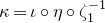 $\kappa=\iota\circ\eta\circ\zeta_1^{-1}$
, so
$\kappa=\iota\circ\eta\circ\zeta_1^{-1}$
, so $\kappa$
must also be the trivial map, hence
$\kappa$
must also be the trivial map, hence $\ker(\delta)=\textrm{im}(\kappa)=1$
, as required.
$\ker(\delta)=\textrm{im}(\kappa)=1$
, as required.
Proposition 6.15. The scalar extension functor is an exact equivalence of categories $H_S(R[Z])\to H_S(\Lambda)$
, whose inverse is the forgetful functor.
$H_S(R[Z])\to H_S(\Lambda)$
, whose inverse is the forgetful functor.
Proof. Exactness follows from Lemma 6.16 below. Equivalence is a special case of the general result [Reference WeibelWei13, Proposition V.7.5(1)] but, for the sake of clarity and simplicity, we sketch here a more direct and explicit proof instead. We implicitly use Lemma 2.2(i) for both $S={\mathbb F}_q[Z]$
and
$S={\mathbb F}_q[Z]$
and $S={\mathbb F}_q[\![Z]\!]$
.
$S={\mathbb F}_q[\![Z]\!]$
.
Since we only consider S-torsion modules, the inverse of the scalar extension functor is the forgetful functor, provided that it is a well-defined functor $H_S(\Lambda)\to H_S(R[Z])$
. We fix an object M of
$H_S(\Lambda)\to H_S(R[Z])$
. We fix an object M of $H_S(\Lambda)$
and show that M also belongs to
$H_S(\Lambda)$
and show that M also belongs to $H_S(R[Z])$
.
$H_S(R[Z])$
.
Now, M is necessarily finitely generated over R[Z]. The existence of a finite resolution by finitely generated projective $\Lambda$
-modules also implies that M is G-c.t.
$\Lambda$
-modules also implies that M is G-c.t.
We now fix a short exact sequence of finitely generated R[Z]-modules
 $$0\to\mathcal K\to P\to M\to 0$$
in which P is projective. Since both M and P are G-c.t., so must be $\mathcal K$
.
$\mathcal K$
.
Since ${\mathbb F}_q[Z]$
is a principal ideal domain,
${\mathbb F}_q[Z]$
is a principal ideal domain, $\mathcal K$
is also
$\mathcal K$
is also ${\mathbb F}_q[Z]$
-projective, so
${\mathbb F}_q[Z]$
-projective, so $\mathcal K$
must be R[Z]-projective. This proves that M belongs to
$\mathcal K$
must be R[Z]-projective. This proves that M belongs to $H_S(R[Z])$
, as required. (In fact, picking the projective resolution of Lemma 2.3, with Z for t, gives a direct proof.)
$H_S(R[Z])$
, as required. (In fact, picking the projective resolution of Lemma 2.3, with Z for t, gives a direct proof.)
Lemma 6.16. $\Lambda$
is a flat R[Z]-module.
$\Lambda$
is a flat R[Z]-module.
Proof. By the equivalence of parts (i) and (iv) in [Reference Grothendieck and RaynaudGR71, Exposé IV, § 5, p. 98, Theorem 5.6], it suffices to fix $n\in\mathbb N$
and show that
$n\in\mathbb N$
and show that $\Lambda\otimes_{R[Z]}(R[Z]/Z^nR[Z])$
is a flat
$\Lambda\otimes_{R[Z]}(R[Z]/Z^nR[Z])$
is a flat $R[Z]/Z^nR[Z]$
-module.
$R[Z]/Z^nR[Z]$
-module.
We consider the following commutative diagram of R[Z]-modules with exact rows.

We claim that both $f_3$
and
$f_3$
and $g_3$
are bijective, which implies that
$g_3$
are bijective, which implies that $\Lambda\otimes_{R[Z]}(R[Z]/Z^nR[Z])$
is a free
$\Lambda\otimes_{R[Z]}(R[Z]/Z^nR[Z])$
is a free $R[Z]/Z^nR[Z]$
-module of rank one, and in particular flat.
$R[Z]/Z^nR[Z]$
-module of rank one, and in particular flat.
Our claim follows from the snake lemma after observing that $g_1$
is surjective, that
$g_1$
is surjective, that $g_2$
is bijective, that
$g_2$
is bijective, that $f_2$
is injective and that the map
$f_2$
is injective and that the map
 $$\textrm{cok}(f_1)=(Z^n\Lambda)/(Z^nR[Z])\longrightarrow \Lambda/R[Z]=\textrm{cok}(f_2)$$
induced by $Z^n\Lambda\subset\Lambda$
is bijective.
$Z^n\Lambda\subset\Lambda$
is bijective.
We finally state [Reference WeibelWei13, Theorem III.3.6], translated to our multiplicative notation.
Proposition 6.17. The following sequence is exact:
 $$1\to K_1(R)\xrightarrow{(\beta,\beta')}K_1(\Pi)\oplus K_1(R[Z])\xrightarrow{(\theta'/\theta)} K_1(R[Z^{-1},Z]).$$
Here, $(\theta'/\theta)(y,w):=\theta'(y)\cdot\theta(w)^{-1}$
.
$(\theta'/\theta)(y,w):=\theta'(y)\cdot\theta(w)^{-1}$
.
6.2.2.
To complete the proof of Proposition 6.13, we finally prove that $\varepsilon$
is injective. We fix
$\varepsilon$
is injective. We fix $\rho\in\ker(\varepsilon)$
and, using Lemma 6.11, we fix
$\rho\in\ker(\varepsilon)$
and, using Lemma 6.11, we fix $x\in K_1(\Lambda)$
such that
$x\in K_1(\Lambda)$
such that $\widehat\partial(x)=\rho$
. Then
$\widehat\partial(x)=\rho$
. Then $0=\varepsilon(\rho)=\varepsilon(\widehat\partial(x))=\partial(\delta(x))$
, and we also fix
$0=\varepsilon(\rho)=\varepsilon(\widehat\partial(x))=\partial(\delta(x))$
, and we also fix $y\in K_1(\Pi)$
such that
$y\in K_1(\Pi)$
such that $\gamma(y)=\delta(x)$
.
$\gamma(y)=\delta(x)$
.
Lemma 6.18.
-
(i) In the notation of Proposition 6.17, there is
$w\in K_1(R[Z])$
with
$(y,w)\in\ker(\theta'/\theta)$
. -
(ii) For w as in claim (i), one has
$\iota(w)=x$
.



Proof. By Proposition 6.14, we have
 \begin{align*}\mu(\theta'(y))=\zeta_0^{-1}(\zeta_0(\mu(\theta'(y))))=\zeta_0^{-1}(\nu(\lambda(\theta'(y))))=\zeta_0^{-1}(\nu(\gamma(y)))&=\zeta_0^{-1}(\nu(\delta(x)))\\ &=\zeta_0^{-1}(0)=0.\end{align*}
In the third equality, we have used the second equality from (6.9). Thus, using Proposition 6.14 again, there is $w\in K_1(R[Z])$
such that
$w\in K_1(R[Z])$
such that $\theta(w)=\theta'(y)$
, i.e.
$\theta(w)=\theta'(y)$
, i.e. $(y,w)\in\ker(\theta'/\theta)$
.
$(y,w)\in\ker(\theta'/\theta)$
.
For w as in claim (i), we compute
 $$\delta(x\cdot\iota(w)^{-1})=\delta(x)\cdot\delta(\iota(w))^{-1}=\gamma(y)\cdot\lambda(\theta(w))^{-1}=\gamma(y)\cdot\lambda(\theta'(y))^{-1}=\gamma(y)\cdot\gamma(y)^{-1}=1.$$
In the second, respectively fourth, equality, we have used the third, respectively second, equality in (6.9). Since $\delta$
is injective by Proposition 6.14, we now deduce that
$\delta$
is injective by Proposition 6.14, we now deduce that $\iota(w)=x$
.
$\iota(w)=x$
.
We are ready to combine Lemma 6.18 with Proposition 6.17 in order to finally show that $\rho$
is trivial. Indeed, there is
$\rho$
is trivial. Indeed, there is $z\in K_1(R)$
such that
$z\in K_1(R)$
such that $\beta'(z)=w$
with
$\beta'(z)=w$
with $\iota(w)=x$
(and
$\iota(w)=x$
(and $\beta(z)=y$
). But then
$\beta(z)=y$
). But then
 $$\rho=\widehat\partial(x)=\widehat\partial(\iota(w))=\widehat\partial(\iota(\beta'(z)))=\widehat\partial(\alpha(z))=0.$$
In the fourth equality we have used the first equality from (6.9).
6.3 A finitely generated representative of the complex of units
In this section we prove that the complex $C^{\mathcal M}_{E,K/k}$
belongs to the category
$C^{\mathcal M}_{E,K/k}$
belongs to the category $D^{\mathrm{p,c}}(A[G],\mathcal F_\infty)$
, as claimed in Theorem 2.17. To do so we assume given a fixed taming module
$D^{\mathrm{p,c}}(A[G],\mathcal F_\infty)$
, as claimed in Theorem 2.17. To do so we assume given a fixed taming module $\mathcal M$
for
$\mathcal M$
for $K/k$
.
$K/k$
.
In the process we obtain a representative of $C^{\mathcal M}_{E,K/k}$
that is more amenable to the computation, in § 6.4, of the refined Euler characteristic of
$C^{\mathcal M}_{E,K/k}$
that is more amenable to the computation, in § 6.4, of the refined Euler characteristic of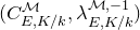 $(C^{\mathcal M}_{E,K/k},\lambda^{\mathcal M,-1}_{E,K/k})$
.
$(C^{\mathcal M}_{E,K/k},\lambda^{\mathcal M,-1}_{E,K/k})$
.
Theorem 6.19. Fix A[G]-modules $M^1$
and
$M^1$
and $M^2$
as in Theorem 6.4(i). Fix a pull-back square of A[G]-modules as follows, in which
$M^2$
as in Theorem 6.4(i). Fix a pull-back square of A[G]-modules as follows, in which $P^2$
is finitely generated and free,
$P^2$
is finitely generated and free, $\beta$
is surjective and
$\beta$
is surjective and $\exp _E^1$
denotes the restriction of
$\exp _E^1$
denotes the restriction of $\exp _E$
to
$\exp _E$
to $M^1$
.
$M^1$
.

Then $P^1$
is locally free of finite rank and the complex
$P^1$
is locally free of finite rank and the complex
 $$P^1\xrightarrow{(d,0)}P^2\oplus\mathcal M,$$
with the first term in degree one, is isomorphic in D(A[G]) to $C^{\mathcal M}_{E,K/k}$
. In particular,
$C^{\mathcal M}_{E,K/k}$
. In particular, $C^{\mathcal M}_{E,K/k}$
belongs to
$C^{\mathcal M}_{E,K/k}$
belongs to $D^{\mathrm{p,c}}(A[G],\mathcal F_\infty)$
, as claimed in Theorem 2.17.
$D^{\mathrm{p,c}}(A[G],\mathcal F_\infty)$
, as claimed in Theorem 2.17.
Proof. We first observe that the sequence
 \begin{equation}0\to P^1\xrightarrow{(d,\alpha)}P^2\oplus M^1\xrightarrow{\beta-\exp _E^1}M^2\to 0\end{equation}
is exact. Indeed, it is exact at the first two terms by [Reference Hilton and StammbachHS97, Lemma III.1.1], and exact at $M^2$
because
$M^2$
because $\beta$
is assumed to be surjective, and
$\beta$
is assumed to be surjective, and $\beta(\pi)=(\beta-\exp _E^1)(\pi,0)$
for all
$\beta(\pi)=(\beta-\exp _E^1)(\pi,0)$
for all $\pi\in P^2$
.
$\pi\in P^2$
.
We next recall that $M^1$
,
$M^1$
, $P^2$
(by Lemma 2.2(i)) and
$P^2$
(by Lemma 2.2(i)) and $M^2$
(by exactness of the second row of the diagram in Theorem 6.4) are G-c.t. By the exactness of (6.11),
$M^2$
(by exactness of the second row of the diagram in Theorem 6.4) are G-c.t. By the exactness of (6.11), $P^1$
is G-c.t., and also A-free of finite rank. Thus,
$P^1$
is G-c.t., and also A-free of finite rank. Thus, $P^1$
is finitely generated over A[G], and A[G]-projective by Lemma 2.2(i).
$P^1$
is finitely generated over A[G], and A[G]-projective by Lemma 2.2(i).
In fact, $P^1$
is locally free by Swan’s theorem (Lemma 2.2(iii)) because (6.11) induces an isomorphism
$P^1$
is locally free by Swan’s theorem (Lemma 2.2(iii)) because (6.11) induces an isomorphism $P^1_{\mathcal F}\cong(P^2\oplus M^1)_{\mathcal F}$
, and
$P^1_{\mathcal F}\cong(P^2\oplus M^1)_{\mathcal F}$
, and $P^2$
and
$P^2$
and $M^1$
are locally free.
$M^1$
are locally free.
We next set $\mathbb{U}:=\exp ^{-1}_E(E(\mathcal M))$
and
$\mathbb{U}:=\exp ^{-1}_E(E(\mathcal M))$
and $H:=H(E/\mathcal M)$
and we note that the fixed pull-back square (6.10) induces an exact commutative diagram of the following form.
$H:=H(E/\mathcal M)$
and we note that the fixed pull-back square (6.10) induces an exact commutative diagram of the following form.

We write $D^\bullet$
for the complex of A[G]-modules
$D^\bullet$
for the complex of A[G]-modules
 $$K_\infty \xrightarrow{\exp _E} E(K_\infty)/E(\mathcal M),$$ $M^\bullet$
for the complex
$M^\bullet$
for the complex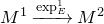 $M^1\xrightarrow{\mathrm{ exp}_E^1}M^2$
and
$M^1\xrightarrow{\mathrm{ exp}_E^1}M^2$
and $P^\bullet$
for the complex
$P^\bullet$
for the complex $P^1\stackrel{d}{\longrightarrow}P^2$
, in all cases with the first term placed in degree one.
$P^1\stackrel{d}{\longrightarrow}P^2$
, in all cases with the first term placed in degree one.
Then, since
 $$H^j(D^\bullet)=\begin{cases}\mathbb{U}, & j=1,\\H, & j=2,\\0, & j\neq 1,2,\end{cases}$$
these three complexes give rise to respective classes $\gamma_{D^\bullet}$
,
$\gamma_{D^\bullet}$
, $\gamma_{M^\bullet}$
and
$\gamma_{M^\bullet}$
and $\gamma_{P^\bullet}$
in the Yoneda Ext-group
$\gamma_{P^\bullet}$
in the Yoneda Ext-group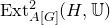 $\textrm{Ext}^2_{A[G]}(H,\mathbb{U})$
, with
$\textrm{Ext}^2_{A[G]}(H,\mathbb{U})$
, with $\gamma_{M^\bullet}=\gamma_{P^\bullet}$
via (6.12).
$\gamma_{M^\bullet}=\gamma_{P^\bullet}$
via (6.12).
To complete the proof of the theorem, after recalling Remark 2.16, it only remains to show that $D^\bullet\cong P^\bullet$
in D(A[G]). But, in order to prove that, in fact,
$D^\bullet\cong P^\bullet$
in D(A[G]). But, in order to prove that, in fact, $D^\bullet\cong M^\bullet\cong P^\bullet$
, it is enough to prove that
$D^\bullet\cong M^\bullet\cong P^\bullet$
, it is enough to prove that $\gamma_{D^\bullet}=\gamma_{M^\bullet}=\gamma_{P^\bullet}$
or, equivalently, that
$\gamma_{D^\bullet}=\gamma_{M^\bullet}=\gamma_{P^\bullet}$
or, equivalently, that $\gamma_{D^\bullet}=\gamma_{M^\bullet}$
.
$\gamma_{D^\bullet}=\gamma_{M^\bullet}$
.
For this we use the following canonical commutative triangle of abelian groups and denote by $\epsilon$
, respectively
$\epsilon$
, respectively $\epsilon'$
, the class in
$\epsilon'$
, the class in $\textrm{Ext}^1_{A[G]}(H,M^1/\mathbb{U})$
, respectively
$\textrm{Ext}^1_{A[G]}(H,M^1/\mathbb{U})$
, respectively $\textrm{Ext}^1_{A[G]}(H,K_\infty/\mathbb{U})$
, of the first, respectively second, column of the diagram in Theorem 6.4.
$\textrm{Ext}^1_{A[G]}(H,K_\infty/\mathbb{U})$
, of the first, respectively second, column of the diagram in Theorem 6.4.

Then, the left-hand square of the diagram in Theorem 6.4 is a push-out diagram by Lemma 6.21 below, which implies that $\iota(\epsilon)=\epsilon'$
. It follows that
$\iota(\epsilon)=\epsilon'$
. It follows that
 $$\gamma_{D^\bullet}=\delta'(\epsilon')=\delta'(\iota(\epsilon))=\delta(\epsilon)=\gamma_{M^\bullet},$$
where the first and last equalities follow, for example, from the general description of connecting homomorphisms given in [Reference Burns and FlachBF98, Lemma 3].
Remark 6.20. The proof of Theorem 6.19 uses that $M^1$
is locally free, but does not require it to be free. Thus, by Remark 2.12, it remains valid for any projective A[G]-lattice
$M^1$
is locally free, but does not require it to be free. Thus, by Remark 2.12, it remains valid for any projective A[G]-lattice $M^1$
as in Theorem 6.4(i) and associated A[G]-module
$M^1$
as in Theorem 6.4(i) and associated A[G]-module $M^2$
.
$M^2$
.
Lemma 6.21. The left-hand square of the diagram in Theorem 6.4 is a push-out.
Proof. This follows from the dual statement to [Reference Hilton and StammbachHS97, Lemma III.1.3], which is left as Exercise III.1.3 and used throughout [Reference Hilton and StammbachHS97], but not stated explicitly. To give a more direct argument, we write $\iota_1:M^1/\mathbb U\to K_\infty/\mathbb U$
,
$\iota_1:M^1/\mathbb U\to K_\infty/\mathbb U$
, $\iota_2:M^1/\mathbb U\to M^2$
,
$\iota_2:M^1/\mathbb U\to M^2$
, $\iota_3:M^2\to V_E$
,
$\iota_3:M^2\to V_E$
, $\pi_1:K_\infty/\mathbb U\to K_\infty/M^1$
and
$\pi_1:K_\infty/\mathbb U\to K_\infty/M^1$
and $\pi_3:V_E\to K_\infty/M^1$
for the corresponding arrows in the diagram. Then, by the dual statement to [Reference Hilton and StammbachHS97, Lemma III.1.1], or by Exercise II.9.2.(ii) in [Reference Hilton and StammbachHS97], the relevant square is a push-out diagram if and only if the sequence
$\pi_3:V_E\to K_\infty/M^1$
for the corresponding arrows in the diagram. Then, by the dual statement to [Reference Hilton and StammbachHS97, Lemma III.1.1], or by Exercise II.9.2.(ii) in [Reference Hilton and StammbachHS97], the relevant square is a push-out diagram if and only if the sequence
 $$(M^1/\mathbb U)\xrightarrow{(\iota_1,\iota_2)}(K_\infty/\mathbb U)\oplus M^2\xrightarrow{\exp_E-\,\iota_3}V_E\to 0$$
is exact. We proceed to prove this exactness claim.
Clearly, $\textrm{im}((\iota_1,\iota_2))\subseteq\ker(\exp_E-\,\iota_3)$
. For the converse, assume that
$\textrm{im}((\iota_1,\iota_2))\subseteq\ker(\exp_E-\,\iota_3)$
. For the converse, assume that $\exp_E(\kappa)=\iota_3(m)$
. Then
$\exp_E(\kappa)=\iota_3(m)$
. Then $\pi_1(\kappa)=\pi_3(\iota_3(m))=0$
, so there is
$\pi_1(\kappa)=\pi_3(\iota_3(m))=0$
, so there is $\mu\in M^1/\mathbb U$
with
$\mu\in M^1/\mathbb U$
with $\iota_1(\mu)=\kappa$
. Since then
$\iota_1(\mu)=\kappa$
. Since then $\iota_3(\iota_2(\mu))=\exp_E(\kappa)=\iota_3(m)$
and
$\iota_3(\iota_2(\mu))=\exp_E(\kappa)=\iota_3(m)$
and $\iota_3$
is injective, we also have
$\iota_3$
is injective, we also have $\iota_2(\mu)=m$
, as required.
$\iota_2(\mu)=m$
, as required.
It remains to show that $\exp_E-\,\iota_3$
is surjective. Let
$\exp_E-\,\iota_3$
is surjective. Let $v\in V_E$
and fix
$v\in V_E$
and fix $\kappa\in K_\infty/\mathbb U$
such that
$\kappa\in K_\infty/\mathbb U$
such that $\pi_1(\kappa)=\pi_3(v)$
. Then
$\pi_1(\kappa)=\pi_3(v)$
. Then $\pi_3(\exp_E(\kappa)-v)=\pi_1(\kappa)-\pi_1(\kappa)=0$
, so there is
$\pi_3(\exp_E(\kappa)-v)=\pi_1(\kappa)-\pi_1(\kappa)=0$
, so there is $m\in M^2$
with
$m\in M^2$
with $\iota_3(m)=\exp_E(\kappa)-v$
, which means that
$\iota_3(m)=\exp_E(\kappa)-v$
, which means that $v=\exp_E(\kappa)-\iota_3(m)$
, as required.
$v=\exp_E(\kappa)-\iota_3(m)$
, as required.
6.4 Completion of the proof of Theorem 2.17
We fix a pull-back square (6.10) as in Theorem 6.19. By this result and Definition 2.9, $\chi_{G}(C^{\mathcal M}_{E,K/k},\lambda^{\mathcal M,-1}_{E,K/k})$
is equal to
$\chi_{G}(C^{\mathcal M}_{E,K/k},\lambda^{\mathcal M,-1}_{E,K/k})$
is equal to $-[P^1,\gamma,P^2\oplus\mathcal M]$
, where
$-[P^1,\gamma,P^2\oplus\mathcal M]$
, where $\gamma$
denotes the composite isomorphism of
$\gamma$
denotes the composite isomorphism of $\mathcal F_\infty[G]$
-modules
$\mathcal F_\infty[G]$
-modules
 $$P^1_{\mathcal F_\infty}\xrightarrow{(d,\alpha)_{\mathcal F_\infty}}P^2_{\mathcal F_\infty}\oplus M^1_{\mathcal F_\infty}\xrightarrow{\mathrm{id}\oplus\lambda}P^2_{\mathcal F_\infty}\oplus\mathcal M_{\mathcal F_\infty}.$$
By Theorem 6.4(ii), it is therefore enough to show that
 $$[P^1,\gamma,P^2\oplus\mathcal M] = [M^1,\lambda,\mathcal M]+\textrm{KFit}_G(M^2)$$
or, equivalently, that
 \begin{equation}[P^1,(d,\alpha)_{\mathcal F_\infty},P^2\oplus M^1] = \textrm{KFit}_G(M^2).\end{equation}
The latter equality is, in turn, a direct consequence of Lemma 6.3, applied to the short exact sequence of A[G]-modules (6.11). This completes the proof of Theorem 2.17.
7. The proof of Theorem 3.15
In this section we fix a finite Galois extension $K/k$
with the property that
$K/k$
with the property that $G=\textrm{Gal}(K/k)$
admits a decomposition of the form (3.1) (i.e.
$G=\textrm{Gal}(K/k)$
admits a decomposition of the form (3.1) (i.e. $\ell$
does not divide the order of the commutator subgroup of G).
$\ell$
does not divide the order of the commutator subgroup of G).
We then fix a Drinfeld module $E/\mathcal O_k$
and a taming module
$E/\mathcal O_k$
and a taming module $\mathcal M$
for
$\mathcal M$
for $K/k$
. We set
$K/k$
. We set $\mathbb U:=\exp ^{-1}_E(E(\mathcal M))$
and
$\mathbb U:=\exp ^{-1}_E(E(\mathcal M))$
and $H:=H(E/\mathcal M)$
.
$H:=H(E/\mathcal M)$
.
Since H naturally surjects onto $H(E/\mathcal O_K)$
, the final claim of Theorem 3.15 follows directly upon combining the first claim with [Reference Johnston and NickelJN13, Theorem 2.2(ii) and (iii)].
$H(E/\mathcal O_K)$
, the final claim of Theorem 3.15 follows directly upon combining the first claim with [Reference Johnston and NickelJN13, Theorem 2.2(ii) and (iii)].
We now fix a projective A[G]-lattice $M^1$
as in Theorem 6.4(i), as well as a corresponding A[G]-module
$M^1$
as in Theorem 6.4(i), as well as a corresponding A[G]-module $M^2$
and, by abuse of notation, we again identify
$M^2$
and, by abuse of notation, we again identify $\lambda=\lambda^{\mathcal M}_{E,K/k}$
with the isomorphism
$\lambda=\lambda^{\mathcal M}_{E,K/k}$
with the isomorphism $M^1_{\mathcal F_\infty}=\mathbb U_{\mathcal F_\infty}\stackrel{\lambda}{\longrightarrow}\mathcal M_{\mathcal F_\infty}$
.
$M^1_{\mathcal F_\infty}=\mathbb U_{\mathcal F_\infty}\stackrel{\lambda}{\longrightarrow}\mathcal M_{\mathcal F_\infty}$
.
Now, since $M^2$
surjects onto H, and by applying [Reference Johnston and NickelJN13, Theorem 2.2(iii)], the proof of the first claim of Theorem 3.15 is reduced to showing that
$M^2$
surjects onto H, and by applying [Reference Johnston and NickelJN13, Theorem 2.2(iii)], the proof of the first claim of Theorem 3.15 is reduced to showing that
 \begin{equation}Z(A[G])\cdot\{\theta^{\mathcal M}_{E,K/k}\cdot R(\psi)\mid\psi\in\textrm{Hom}_{A[G]}(M^1,\mathcal M)\}=\textrm{Fit}_{A[G]}(M^2),\end{equation}
where the left-hand side denotes the Z(A[G])-submodule of $Z(\mathcal F_\infty[G])$
generated by the given subset, and we have put
$Z(\mathcal F_\infty[G])$
generated by the given subset, and we have put
 \begin{equation} R(\psi) := \mathrm{Nrd}_{\mathcal F_\infty[G]}(\psi_{\mathcal F_\infty}\circ\lambda^{-1}).\end{equation}
We also note in passing that the equality (7.1), in combination with [Reference Johnston and NickelJN13, Theorem 2.2(v)], justifies the claim made in Remark 3.17.
In order to now verify the equality (7.1), since non-commutative Fitting ideals commute with localisation (by [Reference Johnston and NickelJN13, Theorem 2.2(vii)]), it is enough to show that, for every maximal ideal P of A, one has
 \begin{align}&Z(A_{(P)}[G])\cdot\{\theta_{E,K/k}^{\mathcal M}\cdot R(\psi) \mid \psi\in\textrm{Hom}_{A_{(P)}[G]}(A_{(P)}\otimes_A M^1,A_{(P)}\otimes_A\mathcal M)\}\nonumber\\&\quad =\textrm{Fit}_{A_{(P)}[G]}(A_{(P)}\otimes_A M^2),\end{align}
where the left-hand side denotes the $Z(A_{(P)}[G])$
-submodule of
$Z(A_{(P)}[G])$
-submodule of $Z(\mathcal F_\infty[G])$
generated by the given subset, and with
$Z(\mathcal F_\infty[G])$
generated by the given subset, and with $R(\psi)$
defined exactly as in (7.2).
$R(\psi)$
defined exactly as in (7.2).
We thus fix a maximal ideal P of A, set $\mathfrak B_P:=A_{(P)}[G]$
and, for every A[G]-module M, also
$\mathfrak B_P:=A_{(P)}[G]$
and, for every A[G]-module M, also $M_P:=A_{(P)}\otimes_A M$
. We now proceed to verify the equality (7.3).
$M_P:=A_{(P)}\otimes_A M$
. We now proceed to verify the equality (7.3).
By Remark 2.12, the A[G]-modules $\mathcal M$
and
$\mathcal M$
and $M^1$
are both locally free of rank equal to
$M^1$
are both locally free of rank equal to $[k:\mathcal F]$
. We thus may and do fix an isomorphism
$[k:\mathcal F]$
. We thus may and do fix an isomorphism $\phi:M^1_P\cong\mathcal M_P$
and observe that for any
$\phi:M^1_P\cong\mathcal M_P$
and observe that for any $\psi$
as in (7.3), the difference
$\psi$
as in (7.3), the difference
 $$R(\psi)\cdot R(\phi)^{-1} = \textrm{Nrd}_{\mathcal F_\infty[G]}((\psi\circ\phi^{-1})_{\mathcal F_\infty}) = \textrm{Nrd}_{\mathfrak B_P}(\psi\circ\phi^{-1})$$
belongs to $Z(\mathfrak B_P)$
. To verify (7.3), it therefore suffices to prove that
$Z(\mathfrak B_P)$
. To verify (7.3), it therefore suffices to prove that
 \begin{equation}Z(\mathfrak B_P)\cdot\theta_{E,K/k}^{\mathcal M}\cdot R(\phi)=\textrm{Fit}_{\mathfrak B_P}(M^2_P).\end{equation}
We fix a pull-back square (6.10) as in Theorem 6.19 and abbreviate the map $(d,\alpha)$
in the sequence (6.11) to h. We use the following canonical commutative triangle of abelian groups.
$(d,\alpha)$
in the sequence (6.11) to h. We use the following canonical commutative triangle of abelian groups.

Then Theorem 2.17, via Theorem 6.4(ii) and the equality (6.13), implies that
 \begin{align*}\partial_{G,P}([h_{\mathcal F_\infty}])&=\iota_P(\textrm{KFit}_G(M^2))\\&=\partial_{G,P}(\Theta^{\mathcal M}_{E,K/k})-[M^1_P,\lambda,\mathcal M_P]\\&=\partial_{G,P}(\Theta^{\mathcal M}_{E,K/k})+[\mathcal M_P,\lambda^{-1},M^1_P]+[M^1_P,\phi_{\mathcal F_\infty},\mathcal M_P]\\&=\partial_{G,P}(\Theta^{\mathcal M}_{E,K/k})+[\mathcal M_P,\phi_{\mathcal F_\infty}\circ\lambda^{-1},\mathcal M_P]\\&=\partial_{G,P}(\Theta^{\mathcal M}_{E,K/k}\cdot [\phi_{\mathcal F_\infty}\circ\lambda^{-1}]).\end{align*}
Now, since
 $$\textrm{Nrd}_{\mathcal F_\infty[G]}(\ker(\partial_{G,P}))=\textrm{Nrd}_{\mathcal F_\infty[G]}(\textrm{im}(K_1(\mathfrak B_P)))=\textrm{Nrd}_{\mathfrak B_P}(K_1(\mathfrak B_P))=Z(\mathfrak B_P)^\times,$$
with the last equality by Lemma 3.8, we deduce the required equality (7.4) because
 $$Z(\mathfrak B_P)\cdot\theta_{E,K/k}^{\mathcal M}\cdot R(\phi)=Z(\mathfrak B_P)\cdot \textrm{Nrd}_{\mathcal F_\infty[G]}([h_{\mathcal F_\infty}])=\textrm{Fit}_{\mathfrak B_P}(M^2_P).$$
Here, the last equality holds by [Reference Johnston and NickelJN13, Proposition 3.4].
This completes the proof of Theorem 3.15.
Acknowledgements
The authors are very grateful to Oliver Braunling for his generous and helpful advice regarding the proof of Proposition 6.12 that we present in § 6.2. They are also very grateful to Carlos de Vera Piquero for his interest in this project and for actively and frequently participating in pertinent discussions. They also thank Bruno Anglès, Francesc Bars, Dominik Bullach, José Ignacio Burgos Gil, David Burns, Alexandre Daoud, Andrei Jaikin-Zapirain, Henri Johnston, Donghyeok Lim, Maxim Mornev, Cristian Popescu and Lenny Taelman for many helpful discussions and correspondence, and an anonymous referee for their careful reading, and their generous comments and suggestions, that helped improve the article.
Conflicts of interest
None.
Financial support
The first author acknowledges support from the Grant CA1/RSUE/2021-00623 funded by the Spanish Ministry of Universities, the Recovery, Transformation and Resilience Plan and Universidad Autónoma de Madrid; and from the Deutsche Forschungsgemeinschaft (DFG, German Research Foundation) under Germany’s Excellence Strategy – EXC-2047/1 – 390685813. The second author acknowledges support for this article as part of Grants CEX2023-001347-S, PID2022-142024NB-I00 and CNS2023-145167 funded by MICIU/AEI/10.13039/501100011033.
Journal information
Compositio Mathematica is owned by the Foundation Compositio Mathematica and published by the London Mathematical Society in partnership with Cambridge University Press. All surplus income from the publication of Compositio Mathematica is returned to mathematics and higher education through the charitable activities of the Foundation, the London Mathematical Society and Cambridge University Press.


 Open access

