


1 Introduction
In the present work, we investigate the following stochastic semilinear parabolic problem
 \begin{equation}\frac{\partial u}{\partial t} =\Delta u+ \frac{\lambda}{\left(1-u\right)^2 }+\kappa\cdot \;\mbox{noise term}, \quad x\in D,\; t>0, \end{equation}
 \begin{equation} \mathcal{B}u=\beta_c, \quad x\in {\partial} D,\; t>0, \end{equation}
 \begin{equation} 0\leq u(x,0)=u_0(x)<1, \quad x \in D, \end{equation}
together with some of its variations rise a mathematical interest. Moreover, $\lambda$
and
$\lambda$
and $\kappa$
are given positive constants, and D is a bounded subset of
$\kappa$
are given positive constants, and D is a bounded subset of $\mathbb{R}^d$
,
$\mathbb{R}^d$
, $d=1,2,3$
with smooth boundary. In addition,
$d=1,2,3$
with smooth boundary. In addition, $\beta_c$
might be a positive or zero constant whilst the boundary operator
$\beta_c$
might be a positive or zero constant whilst the boundary operator $\mathcal{B}$
gives rise to Robin boundary conditions, that is
$\mathcal{B}$
gives rise to Robin boundary conditions, that is $\mathcal{B}u:=\frac{\partial u}{ \partial \nu} + \beta u $
, for some positive constant
$\mathcal{B}u:=\frac{\partial u}{ \partial \nu} + \beta u $
, for some positive constant $\beta$
.
$\beta$
.
We remark that, by setting $\beta\to \infty$
and
$\beta\to \infty$
and $\beta_c=0,$
we obtain Dirichlet boundary conditions. On the other hand, for
$\beta_c=0,$
we obtain Dirichlet boundary conditions. On the other hand, for $0<\beta< \infty$
and
$0<\beta< \infty$
and $\beta_c=0$
(homogeneous) Robin boundary conditions arise. The case of nonhomogeneous Robin boundary conditions, that is when
$\beta_c=0$
(homogeneous) Robin boundary conditions arise. The case of nonhomogeneous Robin boundary conditions, that is when $\beta_c> 0,$
is also considered which has a significant theoretical interest as well. For the noise term in (1.1a), we consider two alternative cases. Initially, we consider a multiplicative noise, reflecting the fact of the occurrence of possible fluctuations into the physical parameters of the MEMS device (see Section 2) of the form
$\beta_c> 0,$
is also considered which has a significant theoretical interest as well. For the noise term in (1.1a), we consider two alternative cases. Initially, we consider a multiplicative noise, reflecting the fact of the occurrence of possible fluctuations into the physical parameters of the MEMS device (see Section 2) of the form $\kappa (1-u) \partial_t W(x,t).$
The term
$\kappa (1-u) \partial_t W(x,t).$
The term $\partial_t W(x,t)$
denotes by convention the formal time derivative of a real valued Wiener process W(x, t) on a stochastic basis
$\partial_t W(x,t)$
denotes by convention the formal time derivative of a real valued Wiener process W(x, t) on a stochastic basis $\{ \Omega, \,{\mathcal F}, \,{\mathcal F}_t,\,\mathbb{P} \}$
with filtration
$\{ \Omega, \,{\mathcal F}, \,{\mathcal F}_t,\,\mathbb{P} \}$
with filtration $\left({\mathcal F}_t\right)_{t\in[0,T]};$
W(x, t) is defined rigorously in Section 3. On the other hand, the adopted approach in Section 5 is only applicable for the case of a multiplicative noise of the form
$\left({\mathcal F}_t\right)_{t\in[0,T]};$
W(x, t) is defined rigorously in Section 3. On the other hand, the adopted approach in Section 5 is only applicable for the case of a multiplicative noise of the form $\kappa(1-u) d B_t,$
where
$\kappa(1-u) d B_t,$
where $B_t$
stands for the one-dimensional Brownian motion, again defined on the stochastic basis
$B_t$
stands for the one-dimensional Brownian motion, again defined on the stochastic basis $\{ \Omega, \,{\mathcal F}, \,{\mathcal F}_t,\,\mathbb{P} \}$
.
$\{ \Omega, \,{\mathcal F}, \,{\mathcal F}_t,\,\mathbb{P} \}$
.
Notably, towards the limit $\kappa \to 0+$
problem (1.1) is reduced to its deterministic version,
$\kappa \to 0+$
problem (1.1) is reduced to its deterministic version,
 \begin{equation}\frac{\partial u}{\partial t}=\Delta u+ \frac{\lambda}{\left(1-u\right)^2 }, \quad x\in D,\; t>0, , \end{equation}
 \begin{equation}\mathcal{B}u=0, \quad x\in {\partial} D,\; t>0, , \end{equation}
 \begin{equation} 0\leq u(x,0)=u_0(x)<1, \quad x \in D, \end{equation}
which, for homogeneous boundary conditions, has been extensively studied in [Reference Esposito, Ghoussoub and Guo15, Reference Flores, Mercado, Pelesko and Smyth16, Reference Ghoussoub and Guo22, Reference Kavallaris, Miyasita and Suzuki28, Reference Kavallaris and Suzuki32]. For hyperbolic modifications of the deterministic variation of (1.1), an interested reader can check [Reference Flores17, Reference Guo23, Reference Kavallaris, Lacey, Nikolopoulos and Tzanetis30]. Finally, non-local alterations of parabolic and hyperbolic problems arising in MEMS technology are treated in [Reference Drosinou, Kavallaris and Nikolopoulos12, Reference Duong and Zaag14, 19, Reference Guo, Kavallaris, Wang and Yu21, 20, Reference Kavallaris, Lacey, Nikolopoulos and Tzanetis29, 31, Reference Kavallaris and Suzuki32, 41, Reference Miyasita42, Reference Miyasita43].
Due to the presence of the term $f (u):=\frac{1}{(1-u)^2}$
in (1.2a), the occurrence of a singular behaviour, called quenching, is observed when
$f (u):=\frac{1}{(1-u)^2}$
in (1.2a), the occurrence of a singular behaviour, called quenching, is observed when $\max_{x\in \overline{D}}u\to 1.$
Such a singular behaviour is closely associated with the mechanical phenomenon of touching down. It is worth investigating whether the stochastic problem (1.1) can perform analogous singular (quenching) behaviour. Indeed, the main purpose of the current paper is twofold: first to examine the circumstances under which quenching occurs for the stochastic problem (1.1), which is actually a stochastic perturbation of (1.1) derived by a random perturbation of the tuning parameter
$\max_{x\in \overline{D}}u\to 1.$
Such a singular behaviour is closely associated with the mechanical phenomenon of touching down. It is worth investigating whether the stochastic problem (1.1) can perform analogous singular (quenching) behaviour. Indeed, the main purpose of the current paper is twofold: first to examine the circumstances under which quenching occurs for the stochastic problem (1.1), which is actually a stochastic perturbation of (1.1) derived by a random perturbation of the tuning parameter $\lambda,$
cf. Section 2. Secondly, we intend to obtain, using both analytical and numerical methods, estimates of the probability of quenching as well as of the quenching time which is actually a random variable. Apart from its practical importance, such a consideration has its own theoretical importance in the context of singular stochastic PDEs (SPDEs).
$\lambda,$
cf. Section 2. Secondly, we intend to obtain, using both analytical and numerical methods, estimates of the probability of quenching as well as of the quenching time which is actually a random variable. Apart from its practical importance, such a consideration has its own theoretical importance in the context of singular stochastic PDEs (SPDEs).
The structure of the current work is as follows. In the next section, a derivation of the stochastic model (1.1) is delivered. In Section 3, we provide the main mathematical tools from the field of stochastic calculus used through the manuscript as well as give the main concepts of solutions for the stochastic problem (1.1) and its considered variations. Section 4 deals with the local existence of (1.1), for a general space-time noise, whilst in Section 5, we appeal to the key properties of exponential functionals of Brownian motion $B_t$
to derive estimates of the quenching time as well as estimates of the quenching probability for stochastic problem (1.1) and some of its variations. As far as we know, this is the first time in the literature of SPDEs where such an approach is used for MEMS nonlinearities. A numerical approach is delivered in Section 6, again for a general space-time noise, which verifies through various numerical experiments the analytical results of the previous sections for nonhomogeneous conditions. Furthermore, the numerical study also provides quenching results for the case of homogeneous boundary conditions, which is not treated via the analysis of Section 5. The current work closes with discussion of the importance of the obtained results in Section 7.
$B_t$
to derive estimates of the quenching time as well as estimates of the quenching probability for stochastic problem (1.1) and some of its variations. As far as we know, this is the first time in the literature of SPDEs where such an approach is used for MEMS nonlinearities. A numerical approach is delivered in Section 6, again for a general space-time noise, which verifies through various numerical experiments the analytical results of the previous sections for nonhomogeneous conditions. Furthermore, the numerical study also provides quenching results for the case of homogeneous boundary conditions, which is not treated via the analysis of Section 5. The current work closes with discussion of the importance of the obtained results in Section 7.
2 The mathematical model
Our main motivation for investigating problem (1.1) is its close connection with the operation of some electrostatic actuated MEMS. By the term ‘MEMS’, we more precisely refer to precision devices which combine both mechanical processes with electrical circuits. MEMS devices range in size from millimetres down to microns and involve precision mechanical components which can be constructed using semiconductor manufacturing technologies. Indeed, the last decade various electrostatic actuated MEMS have been developed and used in a wide variety of devices applied as sensors and have fluid-mechanical, optical, radio frequency (RF), data storage, and biotechnology applications. Interesting examples of microdevices of this kind include microphones, temperature sensors, RF switches, resonators, accelerometers, micromirrors, micropumps, microvalves, data storage devices etc., [Reference Kavallaris and Suzuki32, Reference Pelesko and Bernstein49, Reference Younis54].
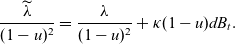
The key part of such a electrostatic actuated MEMS device usually consists of an elastic plate (or membrane) suspended above a rigid ground one. Regularly, the elastic plate is held fixed at two ends whilst the other two edges remain free to move, see Figure 1.
Schematic representation of a MEMS device
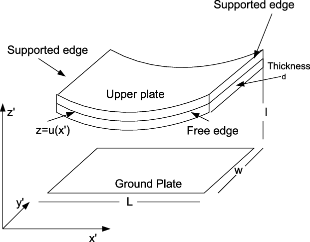
When a potential difference V is applied between the elastic membrane and the rigid ground plate, then a deflection of the membrane towards the plate is observed. Assuming now that the width d of the gap, between the membrane and the bottom plate, is small compared to the device length L, then the deformation of the elastic membrane u, after proper scaling, can be described by the dimensionless equation
 \begin{eqnarray}\frac{\partial u}{\partial t}=\Delta u +\frac{\widetilde{\lambda}\, h(x,t)}{(1-u)^2},\quad x\in D,\; t>0, \end{eqnarray}
see [Reference Kavallaris and Suzuki32, Reference Pelesko and Bernstein49, Reference Pelesko and Triolo50]. Here the term h(x, t) describes the varying dielectric properties of the membrane and for some elastic materials can be taken to be constant; for simplicity henceforth, we assume that $h(x,t)\equiv 1,$
although the general case is again considered in Section 5. Moreover, the parameter
$h(x,t)\equiv 1,$
although the general case is again considered in Section 5. Moreover, the parameter $\lambda$
appearing in (2.1) equals to
$\lambda$
appearing in (2.1) equals to
 \begin{equation*}\widetilde{{\lambda}}=\frac{V^2 L^2 \varepsilon_0}{2\mathcal{T}\ell^3},\end{equation*}
and is actually the tuning parameter of the considered MEMS device. Note that $\mathcal{T}$
stands for the tension of the elastic membrane,
$\mathcal{T}$
stands for the tension of the elastic membrane, $\ell$
is the characteristic width of the gap between the membrane and the fixed ground plate (electrode), whilst
$\ell$
is the characteristic width of the gap between the membrane and the fixed ground plate (electrode), whilst $\varepsilon_0$
is the permittivity of free space. MEMS engineers are interested in identifying under which conditions the elastic membrane could touch the rigid plate, a mechanical phenomenon usually called touching down and could lead to the destruction of MEMS device. Touching down can be described via model (2.1) and occurs when the deformation u reaches the value
$\varepsilon_0$
is the permittivity of free space. MEMS engineers are interested in identifying under which conditions the elastic membrane could touch the rigid plate, a mechanical phenomenon usually called touching down and could lead to the destruction of MEMS device. Touching down can be described via model (2.1) and occurs when the deformation u reaches the value $1;$
such a situation in the mathematical literature is known as quenching (or extinction).
$1;$
such a situation in the mathematical literature is known as quenching (or extinction).
Experimental observations, see [Reference Mohd-Yasin, Nagel and Korman40, Reference Younis54], show a significant uncertainty regarding the values of V and $\mathcal{T}.$
More specifically, V fluctuates around an average value
$\mathcal{T}.$
More specifically, V fluctuates around an average value $V_0 $
(corresponding to some
$V_0 $
(corresponding to some ${\lambda}>0$
) inferring the parameter
${\lambda}>0$
) inferring the parameter $\widetilde{{\lambda}}={\lambda}+\sigma\, \eta(x,t)$
(or alternatively
$\widetilde{{\lambda}}={\lambda}+\sigma\, \eta(x,t)$
(or alternatively $\widetilde{{\lambda}}={\lambda}+\sigma\, \eta(t)$
if V fluctuates only in time). Note that
$\widetilde{{\lambda}}={\lambda}+\sigma\, \eta(t)$
if V fluctuates only in time). Note that $\sigma>0$
is a coefficient measuring the intensity of the fluctuation (noise term)
$\sigma>0$
is a coefficient measuring the intensity of the fluctuation (noise term) $\eta(x,t)$
(or
$\eta(x,t)$
(or $\eta(t).$
) Naturally, the coefficient
$\eta(t).$
) Naturally, the coefficient $\sigma$
depends on the deformation u (that is
$\sigma$
depends on the deformation u (that is $\sigma\equiv \sigma(u)$
), whereas a feasible choice for the noise could be a space-time white noise, that is
$\sigma\equiv \sigma(u)$
), whereas a feasible choice for the noise could be a space-time white noise, that is $\eta(x,t)=\partial_t W(x,t),$
and thus, we consider
$\eta(x,t)=\partial_t W(x,t),$
and thus, we consider $\widetilde{{\lambda}}={\lambda}+\sigma(u)\partial_t W(x,t).$
Alternatively, if the noise is chosen as
$\widetilde{{\lambda}}={\lambda}+\sigma(u)\partial_t W(x,t).$
Alternatively, if the noise is chosen as $\eta(t)=dB_t,$
where
$\eta(t)=dB_t,$
where $B_t$
is the standard one-dimensional Brownian motion, then we end up with
$B_t$
is the standard one-dimensional Brownian motion, then we end up with $\widetilde{{\lambda}}={\lambda}+\sigma(u) d B_t.$
It would be compelling, from the applications point of view, to investigate the impact of uncertainty on the phenomenon of touching down. Accordingly, it would be feasible to choose the diffusion coefficient $\sigma(u)$
as a power of the difference
$\sigma(u)$
as a power of the difference $1-u,$
that is
$1-u,$
that is $\sigma(u)=\kappa (1-u)^{\vartheta},$
measuring the distance to quenching (touching down), where
$\sigma(u)=\kappa (1-u)^{\vartheta},$
measuring the distance to quenching (touching down), where $\kappa$
is a positive constant with rather small values to guarantee the positivity of
$\kappa$
is a positive constant with rather small values to guarantee the positivity of $\lambda.$
Next, we choose $\theta=3$
to derive
$\theta=3$
to derive
 \begin{eqnarray*}\frac{\widetilde{\lambda}}{(1-u)^2}=\frac{\lambda}{(1-u)^2}+\kappa (1-u) \partial_t W\end{eqnarray*}
or alternatively
 \begin{eqnarray*}\frac{\widetilde{\lambda}}{(1-u)^2}=\frac{\lambda}{(1-u)^2}+\kappa (1-u) d B_t.\end{eqnarray*}
Thus, under some imposed uncertainty model (2.1) can be transformed to (1.1a). Notably, the choice $\theta=3$
is made since it leads to a linear type diffusion term for which case the local existence theory is well established for a general Lipschitz nonlinearity, cf [Reference Da Prato and Zabczyk8, Reference Kavallaris and Yan33], and [Reference Kavallaris27] for the non-Lipschitz nonlinearity
$\theta=3$
is made since it leads to a linear type diffusion term for which case the local existence theory is well established for a general Lipschitz nonlinearity, cf [Reference Da Prato and Zabczyk8, Reference Kavallaris and Yan33], and [Reference Kavallaris27] for the non-Lipschitz nonlinearity $(1-u)^{-2}.$
Also, for the case of a model with a general diffusion term
$(1-u)^{-2}.$
Also, for the case of a model with a general diffusion term
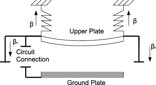
 $\sigma(u)$
the interested reader can check [Reference Kavallaris27]. When the two edges of the membrane are attached to a pair of torsional and translational springs, modelling a flexible nonideal support [Reference Drosinou, Kavallaris and Nikolopoulos12, Reference Younis54], see also Figure 2, then homogeneous boundary conditions of the form (1.1b), with
$\sigma(u)$
the interested reader can check [Reference Kavallaris27]. When the two edges of the membrane are attached to a pair of torsional and translational springs, modelling a flexible nonideal support [Reference Drosinou, Kavallaris and Nikolopoulos12, Reference Younis54], see also Figure 2, then homogeneous boundary conditions of the form (1.1b), with $\beta_c=0$
, are imposed together with the stochastic equation for the deformation u and complemented with initial condition (1.1c).
$\beta_c=0$
, are imposed together with the stochastic equation for the deformation u and complemented with initial condition (1.1c).
Schematic representation of a MEMS device with support nonideal and subject to external forces.
The case of having $\beta_c>0$
may arise as well with a configuration where the support or cantilever of MEMS devises might be nonideal and flexible. More specifically, considering the situation in which together with the spring force at the edges of the membrane we also have a significant external force opposite to the spring force, for example due to gravity, cf. [Reference Younis54]. The latter consideration would result in a boundary condition of the form
$\beta_c>0$
may arise as well with a configuration where the support or cantilever of MEMS devises might be nonideal and flexible. More specifically, considering the situation in which together with the spring force at the edges of the membrane we also have a significant external force opposite to the spring force, for example due to gravity, cf. [Reference Younis54]. The latter consideration would result in a boundary condition of the form $\frac{\partial u}{\partial \nu}= -\beta u + \beta_c$
where
$\frac{\partial u}{\partial \nu}= -\beta u + \beta_c$
where $\beta_c$
stands for this external force. For simplicity and without loss of generality, especially regarding the analysis in Section 5, we may take
$\beta_c$
stands for this external force. For simplicity and without loss of generality, especially regarding the analysis in Section 5, we may take $\beta_c$
to be of the same magnitude as
$\beta_c$
to be of the same magnitude as $\beta.$
Then, we end up with a nonhomogeneous boundary condition of the form
$\beta.$
Then, we end up with a nonhomogeneous boundary condition of the form $\frac{\partial u}{\partial \nu}= \beta(1- u )$
for some
$\frac{\partial u}{\partial \nu}= \beta(1- u )$
for some $ \beta>0$
.
$ \beta>0$
.
Notably, the mathematical model (1.1a), as a stochastic perturbation of (2.1), is built up to capture possible destructions due to the uncertainty in parameter measurements of the MEMS system. Thus, under these circumstances is more realistic compared to (2.1).
3 Preliminaries
The current Section is devoted to the introduction of the main mathematical concepts and tools from the field of stochastic calculus that will be used throughout the manuscript. Henceforth, C, K will denote positive constants whose values might change from line to line.
We first consider the stochastic basis $\{ \Omega, \,{\mathcal F}, \,{\mathcal F}_t,\,\mathbb{P} \}$
with filtration
$\{ \Omega, \,{\mathcal F}, \,{\mathcal F}_t,\,\mathbb{P} \}$
with filtration $\left({\mathcal F}_t\right)_{t\in[0,T]}.$
Next, take
$\left({\mathcal F}_t\right)_{t\in[0,T]}.$
Next, take $H:=L^2(D)$
and let also
$H:=L^2(D)$
and let also $Q \in \mathcal{L}_1(H)$
be a linear non-negative definite and symmetric operator which has an orthonormal basis
$Q \in \mathcal{L}_1(H)$
be a linear non-negative definite and symmetric operator which has an orthonormal basis $\chi_{j}(x) \in H, j=1,2, 3, \dots$
of eigenfunctions with corresponding eigenvalues
$\chi_{j}(x) \in H, j=1,2, 3, \dots$
of eigenfunctions with corresponding eigenvalues $ \gamma_{j} \geq 0, j=1, 2, 3, \dots$
such that
$ \gamma_{j} \geq 0, j=1, 2, 3, \dots$
such that $\text{Tr} (Q) = \sum_{j=1}^{\infty} \gamma_{j} <\infty;$
that is Q is of trace class. Then
$\text{Tr} (Q) = \sum_{j=1}^{\infty} \gamma_{j} <\infty;$
that is Q is of trace class. Then $W(\cdot,t)$
is a Q-Wiener process if and only if
$W(\cdot,t)$
is a Q-Wiener process if and only if
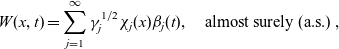 \begin{equation}W(x,t) = \sum_{j=1}^{\infty} \gamma_{j}^{1/2} \chi_{j}(x) \beta_{j}(t), \quad\mbox{almost surely (a.s.)}\;,\end{equation}
where $\beta_{j}(t)$
are independent and identically distributed (i.i.d)
$\beta_{j}(t)$
are independent and identically distributed (i.i.d) $\mathcal{F}_{t}$
-Brownian motions and the series converges in
$\mathcal{F}_{t}$
-Brownian motions and the series converges in $L^{2}({\Omega}, H),$
cf. [Reference Chow7]. It is worth noting that the eigenfunctions
$L^{2}({\Omega}, H),$
cf. [Reference Chow7]. It is worth noting that the eigenfunctions $\{ \chi_{j}(x) \}_{j=1}^{\infty}$
may be different from the eigenfunctions
$\{ \chi_{j}(x) \}_{j=1}^{\infty}$
may be different from the eigenfunctions $\{ \phi_{j}(x) \}_{j=1}^{\infty}$
of the elliptic operator
$\{ \phi_{j}(x) \}_{j=1}^{\infty}$
of the elliptic operator $ A=-\Delta:\mathcal{D} ( A)=W^{2,2}(D)\cap W^{1,2}(D)\subset H\to H$
associated with boundaries conditions of the form (1.1b) and is self-adjoint, positive definite with compact inverse. Note that the trace class operator Q is also a Hilbert-Schmidt operator and then we denote
$ A=-\Delta:\mathcal{D} ( A)=W^{2,2}(D)\cap W^{1,2}(D)\subset H\to H$
associated with boundaries conditions of the form (1.1b) and is self-adjoint, positive definite with compact inverse. Note that the trace class operator Q is also a Hilbert-Schmidt operator and then we denote $Q\in \mathcal{L}_2(H).$
For such an operator $Q\in \mathcal{L}_2(H)$
with
$Q\in \mathcal{L}_2(H)$
with $\text{Tr} (Q) <\infty$
, there exists a kernel q(x, y) such that
$\text{Tr} (Q) <\infty$
, there exists a kernel q(x, y) such that
 \begin{equation*}(Qu) (x) := \int_{D} q(x, y) u(y) \, dy, \quad\mbox{for any} \; x \in D, \; u \in H,\end{equation*}
see [Reference Chow7, p. 42-43] and [Reference Lord, Powell and Shardlow37, Definition 1.64]. The kernel q(x, y) is also called the covariance function of the Q-Wiener process W(x, t).
Let X be a Banach space endowed with the norm $\| \cdot \|_{X}$
we then define the following Hilbert space
$\| \cdot \|_{X}$
we then define the following Hilbert space
 \begin{equation*} L_{2}^{0}(H; X) =\left\{\pi \in L(H,X): \; \sum_{j=1}^{\infty} \| \pi Q^{1/2} (\phi_{j}) \|_{X}^{2} = \sum_{j=1}^{\infty} \gamma_{j} \| \pi (\phi_{j}) \|_{X}^{2} <\infty \right\},\end{equation*}
where L(H, X) denotes the space of all bounded operators from H to X. $ L_{2}^{0}(H; X)$
is equipped with the norm
$ L_{2}^{0}(H; X)$
is equipped with the norm $\| \pi \|_{L_{2}^{0}} = \Big ( \sum_{j=1}^{\infty} \gamma_{j} \| \pi (\phi_{j}) \|_{X}^{2} \Big )^{1/2}.$
For
$\| \pi \|_{L_{2}^{0}} = \Big ( \sum_{j=1}^{\infty} \gamma_{j} \| \pi (\phi_{j}) \|_{X}^{2} \Big )^{1/2}.$
For $\Psi: [0, T] \to L_{2}^{0} (H, X)$
, the stochastic integral
$\Psi: [0, T] \to L_{2}^{0} (H, X)$
, the stochastic integral $\int_{0}^{T} \Psi (t) \, d W(x,t)$
is well defined, [Reference Da Prato and Zabczyk8].
$\int_{0}^{T} \Psi (t) \, d W(x,t)$
is well defined, [Reference Da Prato and Zabczyk8].
For the case of a one-dimensional Brownian motion $B_t,$
we recall that Itô’s formula (see [Reference Klebaner35, Theorem 4.16 page 112]) entails
$B_t,$
we recall that Itô’s formula (see [Reference Klebaner35, Theorem 4.16 page 112]) entails
 \begin{eqnarray}F(B_t)-F(B_0)=\int_0^t F'(B_s)dB_s + \frac{1}{2} \int_0^t F''(B_s)ds,\end{eqnarray}
for any function $F\in C^2({\mathbb R}),$
which in differential form reads
$F\in C^2({\mathbb R}),$
which in differential form reads
 \begin{equation*}dF(B_t)=F'(B_t) dB_t+ \frac{1}{2} F''(B_t) dt.\end{equation*}
Closing the current section, we recall the integration by parts formula for stochastic processes. Indeed, if $X_t$
and
$X_t$
and $Y_t$
are Itô stochastic processes given by
$Y_t$
are Itô stochastic processes given by
 \begin{equation*}X_t=X_0+\int_0^t\Psi_s\,ds+\int_0^t \Phi_s \, dB_s\quad\mbox{and}\quad Y_t=Y_0+\int_0^t\tilde{\Psi}_s\,ds+\int_0^t \tilde{\Phi}_s \, dB_s\end{equation*}
then
 \begin{eqnarray}X_tY_t=X_0Y_0 + \int_0^t X_s dY_s +\int_0^t Y_sdX_s+\left[ X,Y\right]_t, \quad t\in[0,T],\end{eqnarray}
where the last term in (3.3) is the quadratic variation of $X_t, Y_t$
and is defined as
$X_t, Y_t$
and is defined as
 \begin{eqnarray}\left[ X,Y\right]_t:=\int_0^t \Phi_s \tilde{\Phi}_s\,ds,\end{eqnarray}
cf. [Reference Klebaner35, page 114].
4 Local Existence
According to the setting introduced to the previous section, then problem (1.1), for a space-time Wiener perturbation, can be written in the form of the following Itô problem
 \begin{equation}du_t=\left(\Delta u_t+\lambda f(u_t)\right)dt+\sigma( u_t) \partial_t W, \; x\in D, t>0, \end{equation}
 \begin{equation}0\leq u_0< 1, \quad\mbox{almost surely (a.s.)}, \end{equation}
where $f(v):=(1-v)^{-2}$
,
$f(v):=(1-v)^{-2}$
, $\sigma(v):=\kappa(1- v)$
and
$\sigma(v):=\kappa(1- v)$
and $W=W(x,t)$
is the space-time Wiener process defined by (3.1). The local existence theory is developed for this general model (4.1); the latter model is also used for the numerical study demonstrated in Section 6.
$W=W(x,t)$
is the space-time Wiener process defined by (3.1). The local existence theory is developed for this general model (4.1); the latter model is also used for the numerical study demonstrated in Section 6.
Note that, $\sigma: H\to \mathcal{L}_0^2$
satisfies a (global) Lipschitz condition whilst it can be easily checked that
$\sigma: H\to \mathcal{L}_0^2$
satisfies a (global) Lipschitz condition whilst it can be easily checked that $f:H\to H,$
does not satisfy a Lipschitz condition, but only locally.
$f:H\to H,$
does not satisfy a Lipschitz condition, but only locally.
Then, $u_t:=u(\cdot,t)$
can be interpreted as a predictable
$u_t:=u(\cdot,t)$
can be interpreted as a predictable $H-$
valued stochastic process. Next recalling that
$H-$
valued stochastic process. Next recalling that $A=- \Delta :\mathcal{D}(A)=W^{2,2}(D) \cap W^{1,2}(D) \subset H \rightarrow H$
then
$A=- \Delta :\mathcal{D}(A)=W^{2,2}(D) \cap W^{1,2}(D) \subset H \rightarrow H$
then $-A$
is a generator of an analytic semigroup
$-A$
is a generator of an analytic semigroup $\mathcal{G}(t)= e^{-tA}$
on
$\mathcal{G}(t)= e^{-tA}$
on $ H.$
Notably, if homogeneous Dirichlet boundary conditions are considered then
$ H.$
Notably, if homogeneous Dirichlet boundary conditions are considered then $\mathcal{D}(A)=W^{2,2}(D) \cap W_0^{1,2}(D)$
and again an analytic semigroup is generated by
$\mathcal{D}(A)=W^{2,2}(D) \cap W_0^{1,2}(D)$
and again an analytic semigroup is generated by $-A.$
$-A.$
If we set $z=1-u,$
then z satisfies
$z=1-u,$
then z satisfies
 \begin{equation}\frac{\partial z}{\partial t}=\Delta z-\frac{\lambda}{z^2 }-\kappa z \partial_t W, \; x\in D, t>0, \end{equation}
 \begin{equation} \mathcal{B}(1-z)=\beta_c\; \; x\in {\partial} D, t>0, \end{equation}
 \begin{equation} 0<z_0(x):=z(x,0)=1-u_0(x)=\xi(x)\leq 1, \quad x \in D. \end{equation}
In particular, if $u=0$
on
$u=0$
on $\Gamma_T$
this results in
$\Gamma_T$
this results in $z=1$
for condition (4.2b), or otherwise into
$z=1$
for condition (4.2b), or otherwise into $\frac{\partial z}{ \partial \nu} +\beta z=0$
if u satisfies the boundary condition
$\frac{\partial z}{ \partial \nu} +\beta z=0$
if u satisfies the boundary condition $\frac{\partial u}{ \partial \nu} =\beta (1-u)$
.
$\frac{\partial u}{ \partial \nu} =\beta (1-u)$
.
Accordingly, Itô problem (4.1) is written equivalently as follows:
 \begin{equation}dz_t=\left(\Delta z_t-\frac{\lambda}{z^2_t}\right)dt -\kappa z_t \partial_t W, \; x\in D, t>0, \end{equation}
 \begin{equation} 0<z_0=\xi\leq1,\; a.s.\quad x\in D\, . \end{equation}
In the sequel, we focus on the investigation of (4.3) and we only come back to (4.1) in Section 6 where its numerical investigation is delivered.
Definition 4.1 A stopping time $\tau: \Omega \to (0,\infty)$
with respect to the filtration
$\tau: \Omega \to (0,\infty)$
with respect to the filtration $\{\mathcal{F}_t, t\geq 0\}$
is a quenching time of a solution z of (4.3) if
$\{\mathcal{F}_t, t\geq 0\}$
is a quenching time of a solution z of (4.3) if
 \begin{eqnarray}\lim_{t\to \tau} \inf_{x\in D} \vert z(x,t)\vert=0, \quad\mbox{a.s. on the event}\quad \{\tau<\infty\},\end{eqnarray}
or equivalently
 \begin{eqnarray}\mathbb{P}\left[\inf_{(x,t) \in D\times [0,\tau)}\vert z(x,t)\vert >0\right]=1, \quad\mbox{a.s. on the event}\quad \{\tau<\infty\}.\end{eqnarray}
We will write $\tau=+\infty$
if
$\tau=+\infty$
if $\tau>t$
for all
$\tau>t$
for all $t>0.$
Below we introduce some concepts of solutions for problem (4.3) that will be used through the manuscript.
Definition 4.2 A predictable $H-$
valued stochastic process
$H-$
valued stochastic process $\{z_t: t \in [0,\tau)\}$
is called a weak solution of problem (4.3) if for any
$\{z_t: t \in [0,\tau)\}$
is called a weak solution of problem (4.3) if for any $v \in \mathcal{D}(A)$
and for any
$v \in \mathcal{D}(A)$
and for any $t \in [0,\tau),$
 \begin{equation}(z_t,v)=(z_0,v)+\int_0^t [-(z_s,Av)+(\lambda \widetilde{f}(z_s),v)] ds + \int_0^t (\widetilde{\sigma}(z_s) dW_s,v), \quad \mathbb{P}-a.s.,\end{equation}
where $\widetilde{f}(z):=-\frac{1}{z^2}$
and
$\widetilde{f}(z):=-\frac{1}{z^2}$
and $\widetilde{\sigma}(z)=-\kappa z.$
Furthermore,
$\widetilde{\sigma}(z)=-\kappa z.$
Furthermore, $(\cdot,\cdot)$
stands for the inner product into Hilbert space
$(\cdot,\cdot)$
stands for the inner product into Hilbert space $ H=L^2(D).$
Note that the stochastic integral
$ H=L^2(D).$
Note that the stochastic integral $\int_0^t (\widetilde{\sigma}(u_s) dW_s,v)$
is well defined, cf. [Reference Chow7, Theorem 2.4].
$\int_0^t (\widetilde{\sigma}(u_s) dW_s,v)$
is well defined, cf. [Reference Chow7, Theorem 2.4].
Definition 4.3 A predictable $ H-$
valued stochastic process
$ H-$
valued stochastic process $\{z_t: t \in [0,\tau)\}$
is called a mild solution of (4.3) if for any
$\{z_t: t \in [0,\tau)\}$
is called a mild solution of (4.3) if for any $t \in [0,\tau),$
there holds
$t \in [0,\tau),$
there holds
 \begin{equation}z_t=\mathcal{G}(t) z_0+\lambda \int_0^t \mathcal{G}(t-s) \widetilde{f}(z_s)ds +\int_0^t \mathcal{G}(t-s) \widetilde{\sigma}(z_s) dW_s, \quad \mathbb{P}-\mbox{a.s.}\quad\mbox{and a.e. in} \quad D.\end{equation}
Remark 4.4 It is evident from the above definitions that any solution of problem (4.3) ceases to exist as soon as it hits 0 almost surely for some $x\in D,$
cf. [Reference Mueller44, Reference Mueller and Khoshnevisan45, Reference Mueller and Pardoux46] Such a phenomenon, which is defined more rigorously in the next section, will be called quenching.
$x\in D,$
cf. [Reference Mueller44, Reference Mueller and Khoshnevisan45, Reference Mueller and Pardoux46] Such a phenomenon, which is defined more rigorously in the next section, will be called quenching.
Remark 4.5 Notably, any weak (variational) solution is a mild solution of (4.3) under the assumption of the local Lipschitz continuity of $\tilde{f},$
see [Reference Gyöngy and Rovira24]. Conversely, by appealing to a stochastic Fubini theorem, cf. [Reference Walsh51, Theorem 2.6], we get that any mild solution of (4.3) is also a weak solution. Indeed, the weak formulation (4.6) will be used in section 5 for the investigation of the quenching behaviour.
$\tilde{f},$
see [Reference Gyöngy and Rovira24]. Conversely, by appealing to a stochastic Fubini theorem, cf. [Reference Walsh51, Theorem 2.6], we get that any mild solution of (4.3) is also a weak solution. Indeed, the weak formulation (4.6) will be used in section 5 for the investigation of the quenching behaviour.
Existence and uniqueness of a solution for problem (4.3) is guaranteed by the following:
Theorem 4.6 For any initial data $z_0 \in L^2({\Omega},\mathcal{D}(A))$
such that
$z_0 \in L^2({\Omega},\mathcal{D}(A))$
such that $0<z_0\leq 1$
almost surely there exists
$0<z_0\leq 1$
almost surely there exists $T>0$
such that problem (4.3) has a unique mild solution in
$T>0$
such that problem (4.3) has a unique mild solution in $[0, T).$
Proof. The proof follows closely the approach developed in [Reference Mueller and Pardoux46] and so it is kept short. First, note that $\widetilde{f}$
is not (globally) Lipshcitz continuous, and thus, classical existence results, cf. [Reference Chow7, Theorem 6.5] or [Reference Da Prato and Zabczyk8, Theorem 7.5], are not applicable straight away to problem (4.3). To overcome this difficulty, we then define:
$\widetilde{f}$
is not (globally) Lipshcitz continuous, and thus, classical existence results, cf. [Reference Chow7, Theorem 6.5] or [Reference Da Prato and Zabczyk8, Theorem 7.5], are not applicable straight away to problem (4.3). To overcome this difficulty, we then define:
 \begin{equation*}\widetilde{f}_n(z):=\displaystyle-\frac{1}{(\max\{z,\frac{1}{n}\})^2},\end{equation*}
which is Lipschitz continuous and set $\tau_n$
be the first time t so that
$\tau_n$
be the first time t so that $\inf_{x\in D} |z(x,t)|\leq \frac{1}{n}.$
It is readily seen that
$\inf_{x\in D} |z(x,t)|\leq \frac{1}{n}.$
It is readily seen that $\{\tau_n\}_{n=1}^\infty$
is a decreasing sequence.
$\{\tau_n\}_{n=1}^\infty$
is a decreasing sequence.
Then by virtue of [Reference Chow7, Theorem 6.5] and [Reference Da Prato and Zabczyk8, Theorem 7.5] or using an approach introduced to [Reference Mueller44], we obtain that Itô problem
 \begin{eqnarray*}&& dz^n_t=\left(\Delta z^n_t+\widetilde{f}(z^n_t)dt\right) +\widetilde{\sigma}( z^n_t) \partial_t W, \; x\in D, t>0,\\[3pt] &&0<z^n_0=\xi\leq1,\; a.s.\; x\in D\, ,\end{eqnarray*}
has a unique mild solution
 \begin{eqnarray*} z^n_t=\mathcal{G}(t) z^n_0+\lambda \int_0^t \mathcal{G}(t-s) \widetilde{f}(z^n_s)ds +\int_0^t \mathcal{G}(t-s) \widetilde{\sigma}(z^n_s) dW_s\,, \end{eqnarray*}
for any $n=1,2,\dots,$
which also remains bounded within its existence interval.
$n=1,2,\dots,$
which also remains bounded within its existence interval.
However, since $\widetilde{f}(z)=-\frac{1}{z^2}$
for
$\widetilde{f}(z)=-\frac{1}{z^2}$
for $z\geq \frac{1}{n},$
it arises that
$z\geq \frac{1}{n},$
it arises that $z(x,t)=z^n(x,t)$
for
$z(x,t)=z^n(x,t)$
for $t\leq \tau_n$
where z is any solution of Itô problem (4.3). Set now
$t\leq \tau_n$
where z is any solution of Itô problem (4.3). Set now $T=\lim_{n\to \infty}\tau_n$
then
$T=\lim_{n\to \infty}\tau_n$
then $0<T<\infty$
since the initial data
$0<T<\infty$
since the initial data $z_0$
is strictly positive almost surely; hence, we infer existence and uniqueness of mild solution for (4.3) in the time interval
$z_0$
is strictly positive almost surely; hence, we infer existence and uniqueness of mild solution for (4.3) in the time interval $[0,T).$
Throughout the current work, the following variation of problem (4.1) is also investigated
 \begin{equation} du_t= \left( g(t) \Delta u_t+\lambda h(x,t) f(u_t)\right)dt+\kappa(t) (1-u_t) \partial_t W,\; x\in D, t>0, \end{equation}
 \begin{equation}0\leq u_0<1,\; a.s. \;x\in D, \end{equation}
where $g, \kappa: \mathbb{R}_+\rightarrow \mathbb{R}_+$
and
$g, \kappa: \mathbb{R}_+\rightarrow \mathbb{R}_+$
and $h: D\times \mathbb{R}_+ \rightarrow \mathbb{R}_+$
are continuous and bounded functions. It is also assumed that
$h: D\times \mathbb{R}_+ \rightarrow \mathbb{R}_+$
are continuous and bounded functions. It is also assumed that $g\in C^{1}(\mathbb{R}_+).$
Setting $z=1-u$
then z solves the following Itô problem
$z=1-u$
then z solves the following Itô problem
 \begin{equation} dz_t= \left( g(t) \Delta z_t-\lambda h(x,t) z_t^{-2}\right)dt-\kappa(t) z_t \partial_t W,\; x\in D, t>0, \end{equation}
 \begin{equation}0<z_0=\xi\leq1,\; a.s. \; x\in D. \end{equation}
Remarkably, under the given assumptions for g, cf. [Reference Sanz-Solé and Vuillermot48], then the Green’s function G associated with the deterministic problem
 \begin{eqnarray*}&&\zeta_t =g(t)\Delta \zeta, \quad \; x\in D, t>0,\\[5pt]&& \mathcal{B}(\zeta)=\beta_c , \quad \; x\in {\partial} D, t>0,\\[5pt] && 0\leq \zeta(x,0)=\zeta_0(x)<1, \quad x \in D,\end{eqnarray*}
exists and satisfies the growth conditions
 \begin{eqnarray}\left|\partial^m_x\partial^{\ell}_t G(x,t;y,s)\right|\leq c(t-s)^{-\frac{d+|m|+2\ell}{2}}\exp\left[-\frac{|x-y|^2}{t-s}\right],\end{eqnarray}
where $m= (m_1, . . .,m_d)\in \mathbb{N}^N, \ell \in \mathbb{N}$
and
$m= (m_1, . . .,m_d)\in \mathbb{N}^N, \ell \in \mathbb{N}$
and $|m|+2\ell\leq 2,\; |m|=\sum_{j=1}^N m_j.$
Then, we define the corresponding semigroup $\mathcal{E}(t)$
on
$\mathcal{E}(t)$
on $H=L^2(D)$
as follows
$H=L^2(D)$
as follows
 \begin{eqnarray}\mathcal{E}(t)w(x):=\int_D G(x,t;y,0)\,w(y)dy\quad\mbox{for any}\quad x\in D\quad\mbox{and}\quad t>0.\end{eqnarray}
A stopping time $\tau$
for problem (4.9) is defined again by (4.4) or via (4.5).
$\tau$
for problem (4.9) is defined again by (4.4) or via (4.5).
Next, we define the notion of weak and mild solutions for problem (4.9).
Definition 4.7 A predictable $ H-$
valued stochastic process
$ H-$
valued stochastic process $\{z_t: t \in [0,\tau)\}$
is called a weak solution of problem (4.9) if for any
$\{z_t: t \in [0,\tau)\}$
is called a weak solution of problem (4.9) if for any $v \in \mathcal{D}(A)$
and for any
$v \in \mathcal{D}(A)$
and for any $t \in [0,\tau)$
,
$t \in [0,\tau)$
,
 \begin{equation}(z_t,v)=(z_0,v)+\int_0^t [-g(s)(z_s,Av) + \lambda( h(\cdot,s) \widetilde{f}(z_s),v)] ds +\int_0^t ( \widetilde{\sigma}_1(z_s) dW_s,v), \quad \mathbb{P}-a.s. ,\end{equation}
where $ \widetilde{\sigma}_1(z):=-\kappa(t) z$
clearly satisfies a Lispchitz condition for
$ \widetilde{\sigma}_1(z):=-\kappa(t) z$
clearly satisfies a Lispchitz condition for $\kappa(t)$
bounded.
$\kappa(t)$
bounded.
Definition 4.8 A predictable $ H-$
valued stochastic process
$ H-$
valued stochastic process $\{z_t: t \in [0,\tau)\}$
is called a mild solution of (4.9) if for any
$\{z_t: t \in [0,\tau)\}$
is called a mild solution of (4.9) if for any $t \in [0,\tau),$
there holds
$t \in [0,\tau),$
there holds
 \begin{equation}z_t=\mathcal{E}(t) z_0 +\lambda \int_0^t \mathcal{E}(t-s) h(\cdot,s)\widetilde{f}(z_s)ds +\int_0^t \mathcal{E}(t-s) \widetilde{\sigma}_1(z_s) dW_s, \quad \mathbb{P}- \mbox{a.s.}\quad\mbox{ and a.e. in} \quad D\;.\end{equation}
Using an approach similar to Theorem 4.6, we guarantee the existence and uniqueness of a mild solution for the Itô problem (4.9). Such a solution is also proven to be a weak solution by virtue of a stochastic Fubini theorem, see also [Reference Walsh51]. Again any solution to (4.9) ceases to exist as soon as it hits the zero value.
It is worth noting that the more general problem
 \begin{eqnarray}&&dz_t=\left(\Delta z_t+f(z_t)\right)dt+\sigma(z_t) \partial_t W, \; x\in D, t>0,\end{eqnarray}
 \begin{eqnarray} && 0<z_0=\xi\leq1,\; a.s. \; x\in D\, , \end{eqnarray}
where $f(z)=\frac{1}{z^{\alpha}},\; \alpha>0$
and
$f(z)=\frac{1}{z^{\alpha}},\; \alpha>0$
and $c<|\sigma(z)|<C (1+|z|^\gamma)$
for
$c<|\sigma(z)|<C (1+|z|^\gamma)$
for $c, C>0$
and
$c, C>0$
and $\gamma\in(0,\frac{3}{2})$
is investigated by C. Mueller and his collaborators. In particular, it is shown, cf. [Reference Mueller and Khoshnevisan45, Reference Mueller and Pardoux46], that if
$\gamma\in(0,\frac{3}{2})$
is investigated by C. Mueller and his collaborators. In particular, it is shown, cf. [Reference Mueller and Khoshnevisan45, Reference Mueller and Pardoux46], that if $0<\alpha<3$
then the solution of Itô problem (4.14)-(4.15) hits 0 in finite time, that is a quenching phenomenon arises (see next section), with positive probability. Otherwise, if
$0<\alpha<3$
then the solution of Itô problem (4.14)-(4.15) hits 0 in finite time, that is a quenching phenomenon arises (see next section), with positive probability. Otherwise, if $\alpha\geq 3,$
cf. [Reference Mueller44, Reference Zambotti55], the solution of (4.14)-(4.15) remains strictly positive with probability 1 (almost surely).
$\alpha\geq 3,$
cf. [Reference Mueller44, Reference Zambotti55], the solution of (4.14)-(4.15) remains strictly positive with probability 1 (almost surely).
In the current work a similar problem to (4.14)-(4.15) is considered, see (4.3) where now $f(z)=-\frac{\lambda}{z^{2}}$
and
$f(z)=-\frac{\lambda}{z^{2}}$
and $\sigma(u)=-\kappa u$
for some
$\sigma(u)=-\kappa u$
for some $\lambda, \kappa>0.$
It is anticipated, according to the preceding results for problem (4.14)-(4.15), that since in that case
$\lambda, \kappa>0.$
It is anticipated, according to the preceding results for problem (4.14)-(4.15), that since in that case $\alpha=2$
(a value closely related with an application from MEMS industry) then the solution of (4.3) should hit zero with positive probability. In the following section, by applying some innovative approach we move one step further and improve the quenching results proven in [Reference Mueller and Khoshnevisan45, Reference Mueller and Pardoux46]. In particular, we provide estimates of the hitting to zero (quenching) probability not only for problem (4.3) but also for the nonautonomous problem (4.9). Furthermore, using numerical methods we also provide estimates of the quenching time. To the best of our knowledge, such results are novel in the literature and we expect them to be valuable both to mathematicians working on SPDEs as well as to MEMS engineers.
$\alpha=2$
(a value closely related with an application from MEMS industry) then the solution of (4.3) should hit zero with positive probability. In the following section, by applying some innovative approach we move one step further and improve the quenching results proven in [Reference Mueller and Khoshnevisan45, Reference Mueller and Pardoux46]. In particular, we provide estimates of the hitting to zero (quenching) probability not only for problem (4.3) but also for the nonautonomous problem (4.9). Furthermore, using numerical methods we also provide estimates of the quenching time. To the best of our knowledge, such results are novel in the literature and we expect them to be valuable both to mathematicians working on SPDEs as well as to MEMS engineers.
5 Estimation of Quenching Probability
In the current section, we focus on the case of a one-dimensional Brownian motion $B_t,$
since the adopted approach for the estimation of the quenching probability is straightforward in that special case. The implementation of this approach to the case of space-time Wiener process would be explored in a future work.
$B_t,$
since the adopted approach for the estimation of the quenching probability is straightforward in that special case. The implementation of this approach to the case of space-time Wiener process would be explored in a future work.
5.1 The basic model
In the sequel, we will first investigate the quenching behaviour of problem (4.3) but with one-dimensional Brownian motion $B_t,$
in place of space-time Wiener process W(x, t), whose solution can be expressed as an Itô process as follows
$B_t,$
in place of space-time Wiener process W(x, t), whose solution can be expressed as an Itô process as follows
 \begin{eqnarray}z_t=z_0-\kappa \int_0^t z_s dB_s+\int_0^t \left(\Delta z_s-\frac{{\lambda}}{z_s^2}\right)\,ds.\end{eqnarray}
Remarkably, the analysis that follows applies to the imposed homogeneous Robin boundary condition $\frac{\partial z_t}{\partial \nu}+\beta z_t =0$
which corresponds to the situation that a boundary condition (1.1b) is applied for
$\frac{\partial z_t}{\partial \nu}+\beta z_t =0$
which corresponds to the situation that a boundary condition (1.1b) is applied for $\beta_c>0$
. The nonhomogeneous Robin boundary condition, arising for
$\beta_c>0$
. The nonhomogeneous Robin boundary condition, arising for $\beta_c=0,$
is treated only numerically in section 6.
$\beta_c=0,$
is treated only numerically in section 6.
We define now the stochastic process
 \begin{equation} v_t:= e ^{\kappa B_t} z_t, \quad 0\leq t<\tau ,\end{equation}
cf.[Reference Dozzi and López-Mimbela9], where $\tau$
identifies a (random) stopping time, which is actually the quenching time for stochastic processes
$\tau$
identifies a (random) stopping time, which is actually the quenching time for stochastic processes $z_t$
as defined by (4.4). Relation (5.2) and the a.s. path continuity of
$z_t$
as defined by (4.4). Relation (5.2) and the a.s. path continuity of $B_t$
imply that
$B_t$
imply that $z_t$
and
$z_t$
and $v_t$
quench at the same time
$v_t$
quench at the same time $\tau,$
cf. [Reference Dozzi, Kolkovska and López-Mimbela10].
$\tau,$
cf. [Reference Dozzi, Kolkovska and López-Mimbela10].
Next, using Itô’s formula (3.2) for $F(u)=e^{\kappa u}$
we obtain
$F(u)=e^{\kappa u}$
we obtain
 \begin{eqnarray} e^{\kappa B_t} &=& e^{\kappa B_0} +\kappa \int_0^t e^{\kappa B_s}dB_s + \frac{\kappa ^2}{2} \int_0 ^t e^{\kappa B_s}ds \nonumber\\[3pt] &=& 1 +\kappa \int_0^t e^{\kappa B_s}dB_s + \frac{\kappa ^2}{2} \int_0 ^t e^{\kappa B_s}ds, \end{eqnarray}
since $B_0=0,$
or equivalently
$B_0=0,$
or equivalently
 \begin{equation}d(e^{\kappa B_t})=\kappa e^{\kappa B_t}dB_t+\frac{\kappa ^2}{2} e^{\kappa B_t}dt,\\\end{equation}
 \begin{equation*}v_0=e^{\kappa B_0}=1. \nonumber\end{equation*}
In the sequel, we use for simplicity the notation
 \begin{eqnarray*}z_t(\phi):=\int_D z_t \phi\,dx, \; t\geq 0,\end{eqnarray*}
for any function $\phi \in C^2(D).$
Then, problem (5.1), using also second Green’s formula, can be written in a weak formulation as follows
 \begin{eqnarray}z_t(\phi)= z_0(\phi)&+& \int_0^t \int_{\partial D} \left[ \frac{\partial z_s}{\partial \nu} \phi- z_s \frac{\partial \phi}{\partial \nu}\right ] d \sigma ds+ \int_0^t z_s(\Delta \phi)ds\nonumber\\[3pt]&-& \lambda \int_0^t z_s^{-2}(\phi) ds-\kappa \int_0^t z_s(\phi) dB_s,\end{eqnarray}
for some test function $\phi \in C^2(D),$
where
$\phi \in C^2(D),$
where
 \begin{eqnarray*}z^{-2}_s(\phi):=\int_D z^{-2}_s \phi\,dx.\end{eqnarray*}
Next, we take as a test function $\phi \in C^2(D)$
the solution of the eigenvalue problem
$\phi \in C^2(D)$
the solution of the eigenvalue problem
 \begin{eqnarray}&&-\Delta \phi =\lambda_1 \phi, \quad x \in D,\end{eqnarray}
 \begin{eqnarray}&&\frac{\partial \phi}{\partial \nu}+\beta \phi =0, \quad x \in \partial D,\end{eqnarray}
normalised as
 \begin{eqnarray}\int_{D} \phi(x)dx =1.\end{eqnarray}
Note that the principal eigenvalue $\lambda_1$
is positive for
$\lambda_1$
is positive for $\beta \neq 0,$
cf. [Reference Amann3, Theorem 4.3].
$\beta \neq 0,$
cf. [Reference Amann3, Theorem 4.3].
In particular, the boundary integral in (5.5) thanks to the applied homogeneous Robin-type boundary conditions gives
 \begin{equation*}\int_{\partial D} \left[\frac{\partial z_t}{\partial \nu} \phi -z_t \frac{\partial \phi}{\partial \nu}\right] d\sigma=\int_{\partial D }\left(-\beta z_t \phi + \beta z_t \phi\right) d \sigma=0,\end{equation*}
and thus, the weak formulation (5.5) reduces to
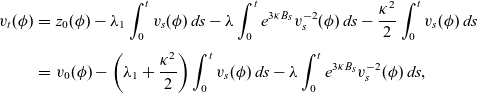
 \begin{eqnarray}z_t(\phi) = z_0(\phi) + \int_0^t z_s(\Delta \phi)\, ds - \lambda \int_0^t z_s^{-2}(\phi) ds-\kappa \int_0^t z_s(\phi) dB_s. \end{eqnarray}
Applying now the integration by parts formula (3.3) to the Itô process defined by (5.1) and (5.3) we have
 \begin{equation*}v_t=e^{\kappa B_t} z_t=e^{\kappa B_0} z_0+ \int_0^t e^{\kappa B_s} dz_s+ \int_0^t z_s de^{\kappa B_s}+\left[e^{\kappa B_s}, z_s \right](t), \end{equation*}
where the quadratic variation is given by
 \begin{eqnarray}\left[e^{\kappa B_s}, z_s \right](t) =-\kappa ^2\int_0^t e^{\kappa B_s}z_s\,ds, \quad t\geq 0,\end{eqnarray}
and thus
 \begin{eqnarray}v_t=z_0+ \int_0^t e^{\kappa B_s}dz_s+\int_0^t z_s de^{\kappa B_s} - \kappa ^2 \int_0^t e^{\kappa B_s}z_s\,ds.\end{eqnarray}
Next, multiplying (5.11) by $\phi$
and integrating over the domain D we obtain
$\phi$
and integrating over the domain D we obtain
 \begin{eqnarray}v_t(\phi) &=& z_0(\phi)+ \int_0^t e^{\kappa B_s}\left[\int_D \left(\Delta z_s-\lambda z_s^{-2} \right) \phi\, dx \right]\,ds- \kappa \int_0^t e^{\kappa B_s}z_s(\phi)\, dB_s\nonumber\\[3pt]&&+ \kappa \int_0^t e^{\kappa B_s}z_s(\phi)\, dB_s+ \frac{\kappa ^2}{2} \int_0^t e^{\kappa B_s}z_s(\phi)\,ds -\kappa ^2 \int_0^t e^{\kappa B_s} z_s(\phi)\,ds\nonumber\\[3pt]&=&z_0(\phi) + \int_0^t e^{\kappa B_s}\left[\int_D \left(\Delta z_s-\lambda z_s^{-2} \right) \phi\, dx \right]\,ds - \frac{\kappa ^2}{2} \int_0^t z_s(\phi) e^{\kappa B_s}ds \nonumber\\[3pt] &=& z_0(\phi) + \int_0^t e^{\kappa B_s} z_s(\Delta \phi)\, ds - \lambda\int_0^t e^{\kappa B_s} z_s^{-2}( \phi)\, ds - \frac{\kappa ^2}{2} \int_0^t z_s(\phi) e^{\kappa B_s}\, ds \nonumber\\[3pt] &=& z_0(\phi)- \lambda_1 \int_0^t e^{\kappa B_s} z_s(\phi)\, ds - \lambda\int_0^t e^{\kappa B_s} z_s^{-2}( \phi)\, ds - \frac{\kappa ^2}{2} \int_0^t e^{\kappa B_s} z_s(\phi)\, ds ,\end{eqnarray}
using also (4.3a) and (5.4) together with second Green’s identity and stochastic Fubini’s theorem, cf. [Reference Da Prato and Zabczyk8, Theorem 4.33].
Expressing (5.12) in terms of the $v_t,$
and since
$v_t,$
and since $z_t=v_t e^{-\kappa B_t},$
then thanks to (5.2) we infer
$z_t=v_t e^{-\kappa B_t},$
then thanks to (5.2) we infer
 \begin{eqnarray}v_t(\phi) &=& z_0(\phi)- \lambda_1 \int_0^tv_s(\phi)\, ds-\lambda \int_0^t e^{3\kappa B_s} v_s^{-2}(\phi)\,ds - \frac{\kappa ^2}{2} \int_0^t v_s(\phi)\,ds\nonumber\\[3pt] &=& v_0(\phi)- \left(\lambda_1+\frac{\kappa^2}{2}\right)\int_0^t v_s(\phi)\,ds-\lambda \int_0^t e^{3\kappa B_s} v_s^{-2}(\phi)\,ds,\quad\end{eqnarray}
taking also into account that $z_0(\phi)=v_0(\phi)$
due to (5.2).
$z_0(\phi)=v_0(\phi)$
due to (5.2).
Then, the differential form of (5.13) reads
 \begin{eqnarray} \frac{d v_t(\phi)}{dt}=- \left(\lambda_1+\frac{\kappa^2}{2}\right) v_t(\phi)-\lambda e^{3\kappa B_t} v_t^{-2}( \phi)\,\;t>0,\quad v_0(\phi)>0. \end{eqnarray}
By virtue of Jensen’s inequality, since $r(s)=s^{-2}, s>0$
is convex, and via (5.8) we have
$r(s)=s^{-2}, s>0$
is convex, and via (5.8) we have
 \begin{eqnarray*}v_t^{-2}(\phi)=\int_D v_t^{-2} \phi\, dx \geq \left( \int_D v_t \phi\, dx \right)^{-2}=(v_t(\phi))^{-2}\end{eqnarray*}
and thus (5.14) leads to the following differential inequality
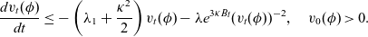 \begin{eqnarray*} \frac{d v_t(\phi)}{dt} \leq - \left(\lambda_1+\frac{\kappa^2}{2}\right) v_t(\phi) - \lambda e^{3\kappa B_t}(v_t(\phi))^{-2} , \quad v_0(\phi)>0.\end{eqnarray*}
By a standard comparison principle, we have that $v_t(\phi)\leq \mathcal{Y}(t)$
where
$v_t(\phi)\leq \mathcal{Y}(t)$
where $\mathcal{Y}(t)$
satisfies the following Bernoulli differential equation:
$\mathcal{Y}(t)$
satisfies the following Bernoulli differential equation:
 \begin{eqnarray*}\mathcal{Y}'(t)=- \left(\lambda_1+\frac{\kappa^2}{2}\right) \mathcal{Y}(t) -\lambda e^{3\kappa B_t} \mathcal{Y}^{-2}(t), \quad \mathcal{Y}_0=\mathcal{Y}(0)= v_0(\phi)>0,\end{eqnarray*}
and is given by
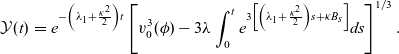 \begin{eqnarray}\mathcal{Y}(t)&=&e^{- \left(\lambda_1+\frac{\kappa^2}{2}\right) t} \left[v^3_0(\phi)-3\lambda \int_0^t e^{3\left[\left({\lambda}_1+\frac{\kappa^2}{2}\right)s+\kappa B_s\right]} ds \right]^{1/3}. \end{eqnarray}
Next, taking into account (5.15) we can define the stopping (quenching) time for $\mathcal{Y}(t)$
as
$\mathcal{Y}(t)$
as
 \begin{eqnarray*} \tau_1:=\inf \left\lbrace t\geq 0 \Big| \int_0^t e^{3\left[\left({\lambda}_1+\frac{\kappa^2}{2}\right)s +\kappa B_s\right]} ds \geq \frac{1}{3\lambda} v_0(\phi)^3 \right\rbrace, \end{eqnarray*}
and so it follows that $\mathcal{Y}(t)$
quenches) (hits to zero) in finite time on the event
$\mathcal{Y}(t)$
quenches) (hits to zero) in finite time on the event $\left\lbrace \tau_1 < + \infty \right\rbrace$
. The fact that
$\left\lbrace \tau_1 < + \infty \right\rbrace$
. The fact that $0\leq v_t(\phi)\leq \mathcal{Y}(t)$
implies that
$0\leq v_t(\phi)\leq \mathcal{Y}(t)$
implies that $\tau_1$
is an upper bound of the stopping (quenching) time
$\tau_1$
is an upper bound of the stopping (quenching) time $\tau$
for
$\tau$
for $v_t(\phi),$
hence the function
$v_t(\phi),$
hence the function
 \begin{equation*}t\mapsto\int_D e^{\kappa B_t} z_t(x)\phi(x)\,dx,\end{equation*}
quenches in finite time under the event $\left\lbrace \tau_1 < + \infty\right\rbrace.$
Using now (5.8) as well as the fact that
$\left\lbrace \tau_1 < + \infty\right\rbrace.$
Using now (5.8) as well as the fact that $t\mapsto e^{\kappa B_t}$
is bounded away from zero on
$t\mapsto e^{\kappa B_t}$
is bounded away from zero on $[0,\tau_1],$
since
$[0,\tau_1],$
since $\tau_1$
is finite (cf. (5.17) and (5.18) below), then we deduce that the function
$\tau_1$
is finite (cf. (5.17) and (5.18) below), then we deduce that the function $t\mapsto \inf_D z_t$
cannot stay away from zero on
$t\mapsto \inf_D z_t$
cannot stay away from zero on $[0,\tau_1]$
when
$[0,\tau_1]$
when $\tau_1<\infty.$
Consequently,
$\tau_1<\infty.$
Consequently, $z_t$
also quenches in finite time on the event
$z_t$
also quenches in finite time on the event $\left\lbrace \tau_1 < + \infty\right\rbrace$
and
$\left\lbrace \tau_1 < + \infty\right\rbrace$
and $\tau_1$
is an upper bound for the quenching time of
$\tau_1$
is an upper bound for the quenching time of $z_t.$
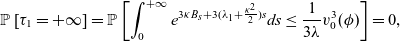
In the sequel, we are working towards the estimation of the probability of the event $\left\lbrace \tau_1 = + \infty\right\rbrace,$
so we have
$\left\lbrace \tau_1 = + \infty\right\rbrace,$
so we have
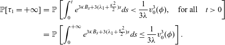 \begin{eqnarray} \mathbb{P}[\tau_1=+\infty]&=& \mathbb{P}\left[\int_0 ^t e^{3\kappa B_s+3(\lambda_1+\frac{\kappa ^2}{2})s} ds < \frac{1}{3\lambda}v^3_0(\phi), \quad \mbox{for all} \quad t>0 \right]\nonumber\\[3pt] &=&\mathbb{P}\left[\int_0 ^{+\infty} e^{3\kappa B_s+3(\lambda_1+\frac{\kappa ^2}{2})s} ds \leq \frac{1}{3\lambda}v^3_0(\phi) \right]. \end{eqnarray}
Then, by virtue of the law of the iterated logarithm for the Brownian motion $B_t,$
cf. [Reference Arcones4, Theorem 2.3] and [Reference Karatzas and Shreve25, Theorem 9.23], that is
$B_t,$
cf. [Reference Arcones4, Theorem 2.3] and [Reference Karatzas and Shreve25, Theorem 9.23], that is
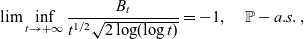 \begin{eqnarray}&&\lim \inf_{t \to + \infty} \frac{B_t}{t^{1/2} \sqrt{2 \log ( \log t)}}=-1, \quad \mathbb{P}- a.s.\; ,\end{eqnarray}
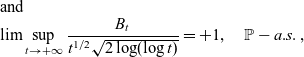 \begin{eqnarray}&&\mbox{and}{\nonumber}\\&&\lim \sup_{t \to +\infty} \frac{B_t}{t^{1/2} \sqrt{2 \log ( \log t)}}=+1, \quad \mathbb{P}- a.s.\; ,\end{eqnarray}
we deduce that for any sequence $t_n\to +\infty$
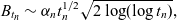 \begin{eqnarray*}B_{t_n} \sim \alpha_n t_n^{1/2} \sqrt{2 \log (\log t_n)},\end{eqnarray*}
with $\alpha_n\in[-1,1],$
and thus,
$\alpha_n\in[-1,1],$
and thus,
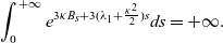 \begin{eqnarray*}\int_0^{+\infty} e^{3\kappa B_s+3(\lambda_1+\frac{\kappa ^2}{2})s}ds=+\infty.\end{eqnarray*}
The latter implies that
 \begin{eqnarray}\mathbb{P} \left[\tau_1=+ \infty \right]= \mathbb{P} \left[ \int_0 ^{+\infty} e^{3\kappa B_s+3(\lambda_1+\frac{\kappa ^2}{2})s}ds \leq \frac{1}{3\lambda} v^3_0(\phi) \right]=0,\nonumber\end{eqnarray}
and hence
 \begin{align}\mathbb{P}\left[\tau_1 <+\infty \right]= 1-\mathbb{P}[\tau_1=+\infty]=1-0=1.\end{align}
Therefore, $\mathcal{Y}(t)$
and consequently
$\mathcal{Y}(t)$
and consequently $ v_t(\phi)$
quenches a.s. which in turn implies that
$ v_t(\phi)$
quenches a.s. which in turn implies that $z_t(\phi)$
quenches a.s. as well. The latter entails, due also to (5.8), that
$z_t(\phi)$
quenches a.s. as well. The latter entails, due also to (5.8), that
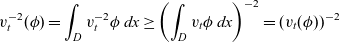
 \begin{eqnarray*}z_t(\phi)=\int_D z_t(x)\phi(x)\,dx\geq \inf_{x\in D}|z_t(x)| \end{eqnarray*}
and thus
 \begin{eqnarray*} \lim_{t\to \tau} \inf_{x\in D} \vert z_t(x)\vert=0, \quad\mbox{a.s. on}\quad \{\tau<\infty\} , \end{eqnarray*}
for some $\tau\leq \tau_1$
and independently of the initial condition
$\tau\leq \tau_1$
and independently of the initial condition $z_0$
and the parameter value
$z_0$
and the parameter value $\lambda.$
Thus, we have the following result.
$\lambda.$
Thus, we have the following result.
Theorem 5.1 The weak solution of problem (5.1), that is
 \begin{align*} dz_t=\left(\Delta z_t-\frac{\lambda}{z^2_t}\right)dt -\kappa z_t d B_t , \; x\in D, t>0, \\0<z_0=\xi\leq1,\; a.s.\quad x\in D\, , \end{align*}
quenches in finite time with probability one, that is almost surely, regardless the size of its initial condition as well as that of parameter $\lambda$
.
$\lambda$
.
Remark 5.2 The result of Theorem 5.1 shows that the impact of the noise for the dynamics of problem (5.1) is vital. In particular, the presence of the nonlinear term $f(z)={z}^{-2}$
forces the solution towards quenching almost surely. On the other hand, for the corresponding deterministic problem, that is when
$f(z)={z}^{-2}$
forces the solution towards quenching almost surely. On the other hand, for the corresponding deterministic problem, that is when $k=0,$
and for homogeneous boundary conditions then quenching occurs only either for large initial data or for large values of the parameter
$k=0,$
and for homogeneous boundary conditions then quenching occurs only either for large initial data or for large values of the parameter $\lambda,$
cf. [Reference Esposito, Ghoussoub and Guo15, Reference Kavallaris, Miyasita and Suzuki28, Reference Kavallaris and Suzuki32].
$\lambda,$
cf. [Reference Esposito, Ghoussoub and Guo15, Reference Kavallaris, Miyasita and Suzuki28, Reference Kavallaris and Suzuki32].
5.2 Introducing a regularising term into model (4.3)
A natural question that arises is: can model (4.3) be modified appropriately so its destructive quenching behaviour to be only limited in a certain range of parameters? To this end, we consider a model with a modified nonlinear drift term; indeed, the drift term $f(z)={z}^{-2},$
which is responsible for the almost surely quenching (cf. Remark 5.2), is now multiplied by
$f(z)={z}^{-2},$
which is responsible for the almost surely quenching (cf. Remark 5.2), is now multiplied by $e^{-3\gamma t}$
for some positive constant
$e^{-3\gamma t}$
for some positive constant $\gamma.$
Specifically, problem (4.3) is now modified to
 \begin{equation}dz_t=(\Delta z_t- \lambda e^{-3\gamma t}z_t^{-2})dt -\kappa z_t dB_t,\quad x\in D, \quad t>0, \end{equation}
 \begin{equation}\frac{\partial z_t}{\partial \nu}+ \beta z_t=0,\quad x\in \partial D, \quad t>0, \quad \beta, \kappa,\gamma >0, \end{equation}
 \begin{equation} 0<z_0(x)=z(x,0)\leq 1. \end{equation}
In the sequel, we proceed similarly as in the proof of Theorem 5.1, so we first set
 \begin{equation*}z_t(\phi):= \int_D z_t \phi\, dx\quad \mbox{and}\quad z_t^{-2}(\phi):=\int_D z^{-2}_t \phi dx,\end{equation*}
where $\phi$
again solves (5.6)-(5.8) and then by second Green’s identity we obtain
$\phi$
again solves (5.6)-(5.8) and then by second Green’s identity we obtain
 \begin{eqnarray}\Delta z_t(\phi)=z_t(\Delta \phi),\nonumber\end{eqnarray}
recalling that
 \begin{eqnarray*}z_t(\Delta \phi):=\int_D z_t \Delta \phi \,dx.\end{eqnarray*}
Then, the weak formulation of (5.2) is :
 \begin{eqnarray}z_t(\phi)=z_0(\phi) +\int_0^t z_s(\Delta \phi)ds- \int_0^t \lambda e^{-3\gamma t} z_s^{-2}(\phi)\, ds - \kappa \int_0^t z_s(\phi) dB_s,\;\; \mathbb{P}-\mbox{a.s.}\end{eqnarray}
We again consider the stochastic process $v_t=e^{\kappa B_t}z_t$
, for
$v_t=e^{\kappa B_t}z_t$
, for $ 0\leq t<\tau$
with
$ 0\leq t<\tau$
with $\tau$
being the stopping (quenching) time of stochastic process
$\tau$
being the stopping (quenching) time of stochastic process $z_t$
defined by (4.4). Next, using integration by parts formula, see also (3.3) and (3.4), for the stochastic processes
$z_t$
defined by (4.4). Next, using integration by parts formula, see also (3.3) and (3.4), for the stochastic processes
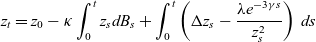 \begin{eqnarray*}z_t=z_0-\kappa \int_0^t z_s dB_s+\int_0^t \left(\Delta z_s-\frac{{\lambda} e^{-3\gamma s}}{z_s^2}\right)\,ds\end{eqnarray*}
and for $e^{\kappa B_t}$
given by (5.3), we obtain that
$e^{\kappa B_t}$
given by (5.3), we obtain that
 \begin{eqnarray}v_t(\phi)=v_0(\phi)+ \int_0^t e^{\kappa B_s} dz_s(\phi)+ \int_0^t z_s(\phi) d\left( e^{\kappa B_s} \right)+ \left[ e^{\kappa B_s},z_s(\phi)\right](t),\end{eqnarray}
where the quadratic variation, represented by the last term into (5.23), is given by (5.10).
Therefore, by virtue of (5.2), (5.22) and Itô’s formula, cf. (5.4), we obtain that
 \begin{eqnarray}v_t(\phi)=v_0(\phi)&+&\int_0^t v_s(\Delta \phi) ds -\lambda \int_0^t e^{3\kappa B_s} e^{-3\gamma s}v_s^{-2}(\phi)ds- \frac{\kappa ^2}{2} \int_0^t v_s(\phi)ds,\end{eqnarray}
taking also into account that $z_t=e^{-\kappa B_t}v_t.$
Notably, via (5.24) we deduce that $v_t(x)=v(x,t)$
is a weak solution of the following random Stochastic PDE (RPDE)
$v_t(x)=v(x,t)$
is a weak solution of the following random Stochastic PDE (RPDE)
 \begin{equation}\frac{\partial v}{\partial t} (x,t)= \Delta v(x,t)+ \left( \gamma- \frac{\kappa ^2}{2}\right) v(x,t)+\lambda e^{3\kappa B_t} v^{-2}(x,t),\quad x\in D, t>0, \end{equation}
 \begin{equation} \frac{\partial v(x,t)}{\partial \nu}+\beta v(x,t)=0,\quad\mbox{on}\quad x\in {\partial} D, t>0, \end{equation}
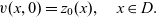 \begin{equation}v(x,0)=z_0(x),\quad x \in D. \end{equation}
Problem (5.2) should be understood pathwise, and its local existence, uniqueness and positivity of solution up to eventual quenching time can be derived by [Reference Friedman18, Theorem 9, Chapter 7].
Recalling that $\phi$
solves the eigenvalue problem (5.6)-(5.8) then equation (5.24) is reduced to
$\phi$
solves the eigenvalue problem (5.6)-(5.8) then equation (5.24) is reduced to
 \begin{eqnarray} v_t(\phi)=v_0(\phi)- (\lambda_1 +\frac{\kappa ^2}{2}) \int_0^t v_s(\phi) ds. -\lambda \int_0^t e^{-3(\gamma s-\kappa B_s)}\,v_s^{-2} (\phi)ds, \end{eqnarray}
or (cf. Subsection 5.1) in differential form
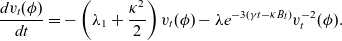 \begin{eqnarray} \frac{d v_t(\phi)}{dt}= - \left( \lambda_1 +\frac{\kappa ^2}{2} \right) v_t(\phi) - \lambda e^{-3(\gamma t-\kappa B_t)} v_t^{-2}(\phi). \nonumber \end{eqnarray}
Next, by virtue of Jensen’s inequality we deduce
 \begin{eqnarray} \frac{d v_t(\phi)}{dt} \leq - \left( \lambda_1 + \frac{\kappa ^2}{2} \right) v_t(\phi)- \lambda e^{-3(\gamma t-\kappa B_t)} (v_t(\phi))^{-2}, \quad v_0(\phi)>0. \nonumber \end{eqnarray}
By comparison, we get $v_t(\phi)\leq \Psi(t)$
where
$v_t(\phi)\leq \Psi(t)$
where $\Psi(t)$
satisfies the following Bernoulli differential equation
$\Psi(t)$
satisfies the following Bernoulli differential equation
 \begin{eqnarray} \Psi'(t)=- \left( \lambda_1 + \frac{\kappa ^2}{2} \right) \Psi(t)- \lambda e^{-3(\gamma t-\kappa B_t)} \Psi^{-2} (t), \quad \Psi_0= \Psi(0)=v_0(\phi)>0,\nonumber \end{eqnarray}
with solution
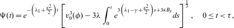 \begin{eqnarray} \Psi(t)=e^{ - \left( \lambda_1+\frac{\kappa ^2}{2} \right)t} \left[ v^3_0(\phi) - 3\lambda \int_0^t e^{ 3 \left( \lambda_1- \gamma+\frac{\kappa ^2}{2} \right)s+3 \kappa B_s} ds \right]^{\frac{1}{3}}, \quad 0\leq t < \tau, \nonumber \end{eqnarray}
with
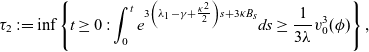 \begin{equation*}\tau_2:= \inf \left\lbrace t\geq 0 : \int_0^t e^{ 3 \left( \lambda_1- \gamma+ \frac{\kappa ^2}{2} \right)s+3 \kappa B_s} ds\geq \frac{1}{3\lambda}v^3_0(\phi) \right\rbrace,\end{equation*}
being the stopping time of $\Psi(t).$
It follows that $\Psi(t)$
hits 0 in finite time on the event
$\Psi(t)$
hits 0 in finite time on the event $\left\lbrace \tau_2 < +\infty \right\rbrace$
. Since
$\left\lbrace \tau_2 < +\infty \right\rbrace$
. Since $v_t(\phi)\leq \Psi(t),$
then
$v_t(\phi)\leq \Psi(t),$
then $\tau_2$
is an upper bound for the stopping (extinction) time
$\tau_2$
is an upper bound for the stopping (extinction) time $\tau$
of
$\tau$
of $v_t(\phi),$
which is also the stopping (quenching) time of
$v_t(\phi),$
which is also the stopping (quenching) time of $v_t$
and
$v_t$
and $z_t.$
More specifically, we have
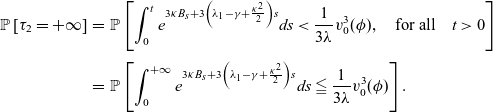 \begin{eqnarray} \mathbb{P}\left[\tau_2=+\infty \right]&=&\mathbb{P}\left[\int_0^t e^{3\kappa B_s+3 \left(\lambda_1- \gamma + \frac{\kappa ^2}{2}\right)s}ds < \frac{1}{3\lambda}v^3_0(\phi), \quad \mbox{for all} \quad t>0 \right]\nonumber\\[3pt] &=&\mathbb{P}\left[\int_0^{+\infty} e^{3\kappa B_s+3 \left(\lambda_1- \gamma + \frac{\kappa ^2}{2}\right)s}ds \leqq \frac{1}{3\lambda}v^3_0(\phi) \right]. \end{eqnarray}
Then, via the change of variables $s_1\mapsto \frac{ 9 \kappa^2 s}{4}$
and making use of the scaling property of
$s_1\mapsto \frac{ 9 \kappa^2 s}{4}$
and making use of the scaling property of $B_t$
we obtain
$B_t$
we obtain
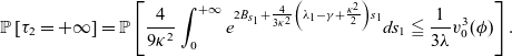 \begin{eqnarray} \mathbb{P}\left[\tau_2=+\infty \right]= \mathbb{P}\left[ \frac{4}{9 \kappa ^2 } \int_0^{+\infty} e^{2 B_{ s_1}+\frac{4}{3 \kappa^2}\left(\lambda_1- \gamma + \frac{\kappa ^2}{2}\right)s_1}ds_1 \leqq \frac{1}{3\lambda}v^3_0(\phi) \right].\end{eqnarray}
Setting $B^{(\mu)}_s:=B_s+\mu s$
, with
$B^{(\mu)}_s:=B_s+\mu s$
, with $\mu :=\frac{2}{3 \kappa^2}\left(\lambda_1- \gamma + \frac{\kappa ^2}{2}\right)$
then (5.28) reads
$\mu :=\frac{2}{3 \kappa^2}\left(\lambda_1- \gamma + \frac{\kappa ^2}{2}\right)$
then (5.28) reads
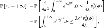 \begin{eqnarray} \mathbb{P}\left[\tau_2=+\infty \right]&&= \mathbb{P}\left[ \frac{4}{9 \kappa ^2 }\int_0^ {+\infty} e^ {2 B^{(\mu)}_s} ds \leq \frac{1}{3\lambda}v^3_0(\phi) \right]\nonumber\\[3pt] && = \mathbb{P}\left[\int_0^ {+\infty} e^ {2 B^{(\mu)}_s} ds \leq \frac {3 \kappa^2 v^3_0(\phi)} {4\lambda }\right],\end{eqnarray}
We now distinguish two cases:
-
(i) We first take $\gamma\geq \lambda_1+\frac{\kappa ^2}{2,}$
and thus, we have see [Reference Yor53, Chapter 6, Corollary 1.2], where
\begin{eqnarray}\int_0^{\infty} e^{2 B_s^{\mu}} ds\stackrel{\text{Law}}{=} \frac{1}{2 Z_{-\mu}}, \nonumber \end{eqnarray}
$Z_{-\mu}$
is a random variable with law
$\Gamma(-\mu),$
that is where
\begin{equation*}\mathbb{P}\left(Z_{-\mu} \in dy\right)=\frac{1}{\Gamma(-\mu)} e^{-y} y^{-\mu-1}\,dy,\end{equation*}
$\Gamma(\cdot)$
is the complete gamma function, cf. [Reference Abramowitz and Stegun1].
$\gamma\geq \lambda_1+\frac{\kappa ^2}{2,}$
and thus, we have see [Reference Yor53, Chapter 6, Corollary 1.2], where
\begin{eqnarray}\int_0^{\infty} e^{2 B_s^{\mu}} ds\stackrel{\text{Law}}{=} \frac{1}{2 Z_{-\mu}}, \nonumber \end{eqnarray}
$Z_{-\mu}$
is a random variable with law
$\Gamma(-\mu),$
that is where
\begin{equation*}\mathbb{P}\left(Z_{-\mu} \in dy\right)=\frac{1}{\Gamma(-\mu)} e^{-y} y^{-\mu-1}\,dy,\end{equation*}
$\Gamma(\cdot)$
is the complete gamma function, cf. [Reference Abramowitz and Stegun1].


Hence, (5.29) entails (see also [Reference Borodin and Salminen5, formula 1.104(1) page 264])
 \begin{eqnarray}&& \mathbb{P}\left[ \tau_2 = +\infty \right]= \mathbb{P}\left[ \frac{1}{2 Z_{-\mu}}\leq\frac{3 \kappa^2}{4\lambda}v^3_0(\phi) \right]= \mathbb{P}\left[ Z_{-\mu}\geq \frac{2\lambda } {3 \kappa^2 v^3_0(\phi)}\right]\nonumber\\ &&=1- \mathbb{P}\left[ Z_{-\mu}\leq \theta \right]=1-\frac{1}{\Gamma(-\mu)}\int_0^\theta e^{-y} y^{-\mu-1}\,dy,\end{eqnarray}
where $\theta:=\frac{2\lambda } {3 \kappa^2 v^3_0(\phi)}.$
Therefore,
 \begin{eqnarray*} \mathbb{P}\left[ \tau_2 <+\infty \right]=\mathbb{P}\left[ Z_{-\mu}\leq \theta \right]=\frac{1}{\Gamma(-\mu)}\int_0^\theta e^{-y} y^{-\mu-1}\,dy\end{eqnarray*}
and since $\tau<\tau_2,$
we have that
$\tau<\tau_2,$
we have that
 \begin{eqnarray} \mathbb{P}\left[ \tau <+\infty \right]\geq \frac{1}{\Gamma(-\mu)}\int_0^\theta e^{-y} y^{-\mu-1}\,dy. \end{eqnarray}
-
(ii) Next, we assume that
$\mu>0, $
that is
$\gamma< \lambda_1+\frac{\kappa ^2}{2}$
. Then using the law of the iterated logarithm, cf. (5.17) and (5.18), for
$B_t$
, we obtain hence via (5.27) we derive
\begin{eqnarray*}\int_0^{+\infty} e^{3\kappa B_s+3 \left(\lambda_1- \gamma + \frac{\kappa ^2}{2}\right)s}ds=+\infty, \end{eqnarray*}
and thus
\begin{eqnarray}\mathbb{P} \left[\tau_2=+ \infty \right]= \mathbb{P} \left[ \int_0 ^{+\infty} e^{3\kappa B_s+3(\lambda_1+\frac{\kappa ^2}{2})s}ds \leq \frac{1}{3\lambda} v^3_0(\phi) \right]=0 \nonumber \end{eqnarray}
\begin{eqnarray} \mathbb{P} \left[ \tau_2<+ \infty \right]=1-\mathbb{P} \left[\tau_2=+ \infty \right]=1. \nonumber \end{eqnarray}


Summarising the above, we have the following result
Theorem 5.3
-
(i) If
$\gamma\geq \lambda_1+ \frac{\kappa ^2}{2,}$
then the weak solution of problem (5.21) quenches in finite time with probability bounded below as shown in (5.31). -
(ii) In the complementary case when
$\gamma<\lambda_1+ \frac{\kappa ^2}{2}$
then the weak solution of problem (5.21) quenches in finite time almost surely.


Remark 5.4 Let us fix $\gamma$
and
$\gamma$
and $\kappa$
so that
$\kappa$
so that $\gamma- \frac{\kappa ^2}{2}>0.$
Then Theorem 5.3(ii) entails that quenching behaviour dominates when
$\gamma- \frac{\kappa ^2}{2}>0.$
Then Theorem 5.3(ii) entails that quenching behaviour dominates when ${\lambda}_1$
is rather big, a case that only occurs when the domain D is rather small.
${\lambda}_1$
is rather big, a case that only occurs when the domain D is rather small.
In Figure 3, an upper bound of the probability of global existence, provided by (5.30), is displayed with respect to the parameter $\lambda$
in Figure 3(a) and with respect to the parameter a in Figure 3(b). In that case, an initial condition of the form
$\lambda$
in Figure 3(a) and with respect to the parameter a in Figure 3(b). In that case, an initial condition of the form $z_0(x)=1-ax(1-x)$
is considered. Specifically, in Figure 3(a) we observe a decrease of the probability of global existence, as
$z_0(x)=1-ax(1-x)$
is considered. Specifically, in Figure 3(a) we observe a decrease of the probability of global existence, as $\lambda$
increases. Similarly, in Figure 3(b) again reducing the minimum of the initial condition results in decreasing the probability of global existence and this becomes more intense as
$\lambda$
increases. Similarly, in Figure 3(b) again reducing the minimum of the initial condition results in decreasing the probability of global existence and this becomes more intense as $\lambda$
increases.
$\lambda$
increases.
Besides, in Figure 4 the behaviour of the probability of the global existence, bounded above by the quantity defined in (5.31), is examined with respect to the parameter $\gamma$
and the noise amplitude
$\gamma$
and the noise amplitude $\kappa.$
In particular, the impact of parameter
$\kappa.$
In particular, the impact of parameter $\gamma,$
that is the coefficient of the regularising term, is displayed in Figure 4(a). Note that the condition
$\gamma,$
that is the coefficient of the regularising term, is displayed in Figure 4(a). Note that the condition $\gamma>\lambda_1+\kappa^2$
should be satisfied (here
$\gamma>\lambda_1+\kappa^2$
should be satisfied (here $\lambda_1=\pi^2$
and
$\lambda_1=\pi^2$
and $\kappa=1$
); then we observe a peak of the probability at the value
$\kappa=1$
); then we observe a peak of the probability at the value $\gamma = 13.77.$
Moreover, in Figure 4(b) the variation of that probability with respect to the parameter
$\gamma = 13.77.$
Moreover, in Figure 4(b) the variation of that probability with respect to the parameter $\kappa$
for various values of the parameter
$\kappa$
for various values of the parameter $\lambda$
is shown. In that case a similar peak is attained at the value
$\lambda$
is shown. In that case a similar peak is attained at the value $\kappa=1.084.$
Diagram of the probability $\mathbb{P}\left[\tau =+\infty \right]$
(a) with respect to the parameter
$\mathbb{P}\left[\tau =+\infty \right]$
(a) with respect to the parameter $\lambda $
, (b) with respect to the parameter a in the initial condition for various values of the parameter
$\lambda $
, (b) with respect to the parameter a in the initial condition for various values of the parameter $\lambda$
.
$\lambda$
.
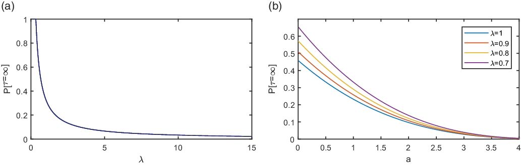
Diagram of the probability $\mathbb{P}\left[\tau =+\infty \right]$
for various values of the parameter
$\mathbb{P}\left[\tau =+\infty \right]$
for various values of the parameter $\lambda$
, (a) with respect to the parameter
$\lambda$
, (a) with respect to the parameter $\gamma $
, (b) with respect to the noise amplitude
$\gamma $
, (b) with respect to the noise amplitude $\kappa$
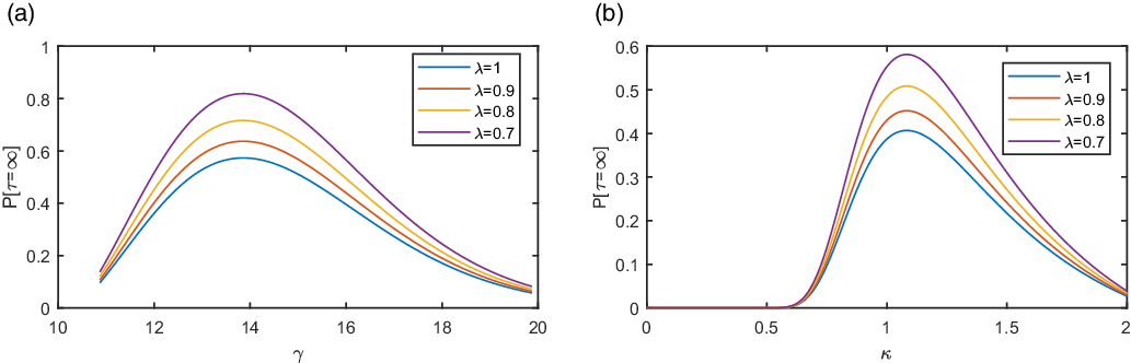
5.3 Model (4.9)
In the current Subsection, we investigate the probability of quenching for the solution of problem (4.9) where $g, \kappa_1: \mathbb{R}_+\rightarrow \mathbb{R}_+$
and
$g, \kappa_1: \mathbb{R}_+\rightarrow \mathbb{R}_+$
and $h: D\times \mathbb{R}_+ \rightarrow \mathbb{R}_+$
are continuous functions. Note that from mathematical modelling perspective the function g(t) represents the dispersion coefficient whilst h(x, t) describes the varying dielectric properties of the elastic membrane ([Reference Flores, Mercado, Pelesko and Smyth16]), cf. section 2.
$h: D\times \mathbb{R}_+ \rightarrow \mathbb{R}_+$
are continuous functions. Note that from mathematical modelling perspective the function g(t) represents the dispersion coefficient whilst h(x, t) describes the varying dielectric properties of the elastic membrane ([Reference Flores, Mercado, Pelesko and Smyth16]), cf. section 2.
Next, we define the stochastic process
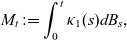 \begin{equation*}M_t:=\int_0^t \kappa_1(s)dB_s,\end{equation*}
and we set
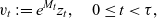 \begin{equation}v_t:= e^{M_t} z_t,\quad 0\leq t<\tau,\end{equation}
where again $\tau$
is the stopping (quenching) time of stochastic process
$\tau$
is the stopping (quenching) time of stochastic process $z_t$
determined by (4.4).
$z_t$
determined by (4.4).
In the sequel, we proceed as in [Reference Alvarez, Alfredo Lopez -Mimbela and Privault2]. Itô’s formula implies the semimartingale expansion
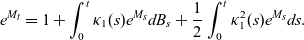 \begin{eqnarray}e^{M_t}=1+\int_0^t \kappa_1(s) e^{M_s} dB_s + \frac{1}{2} \int_0^t \kappa_1^2(s) e^{M_s} ds .\end{eqnarray}
By letting $z_t(\phi):= \int_D z_t \phi dx$
and
$z_t(\phi):= \int_D z_t \phi dx$
and $z_t^{-2}(\phi):=\int_D z^{-2}_t \phi dx,$
where again
$z_t^{-2}(\phi):=\int_D z^{-2}_t \phi dx,$
where again $\phi \in C^2(D)$
solves the eigenvalue problem (5.6)-(5.8), we have
$\phi \in C^2(D)$
solves the eigenvalue problem (5.6)-(5.8), we have
 \begin{eqnarray}z_t(\phi)= z_0(\phi)+ \int_0^t g(s) \Delta z_s(\phi) ds- \lambda\int_0^t h(x,s) z_s^{-2}(\phi) ds -\int_0^t \kappa_1(s) z_s(\phi)dB_s,\end{eqnarray} $\mathbb{P} - a.s.$
for all
$\mathbb{P} - a.s.$
for all $ t \in [0, \tau).$
Note also that for any fixed $\phi$
, the process
$\phi$
, the process $(z_t(\phi)1_{[0,\tau)}(t))_{t\in \mathbb{R}_+}$
is also a semimartingale. Moreover, using integration by parts formula, cf. (3.3) and (3.4), we get the weak formulation
$(z_t(\phi)1_{[0,\tau)}(t))_{t\in \mathbb{R}_+}$
is also a semimartingale. Moreover, using integration by parts formula, cf. (3.3) and (3.4), we get the weak formulation
 \begin{eqnarray}v_t(\phi) &=& e^{M_t} z_t(\phi) \nonumber \\&=&e^{M_0}z_0(\phi)+ \int_0^t e^{M_s} d(z_s(\phi))+\int_0^t z_s(\phi) d(e^{M_s}),+ \left[e^{M_t},z_t(\phi)\right],\,\end{eqnarray}
where the quadratic variation (see [Reference Mackevičius38, section 7.6, pg. 113]) is given by
 \begin{equation*}\left[e^{M_t}, z_t(\phi)\right](t):=- \int_0^t \kappa^2 _1 (s) e^{M_s}z_s(\phi) ds.\end{equation*}
Next, (5.35) in conjunction with (5.32), (5.33) and (5.34) yields
 \begin{eqnarray}v_t(\phi) &=& z_0(\phi) + \int_0^t e^{M_s} \left( g(s) \Delta z_s(\phi) -\lambda z_s^{-2}(h\phi) \right) ds \nonumber \\[3pt]&&\quad\quad \quad + \int_0^t e^{M_s} \kappa_1 (s) z_s(\phi) dB_s- \int_0^t e^{M_s} \kappa_1 (s) z_s(\phi) dB_s \nonumber \\[3pt]&& \quad\quad \quad + \frac{1}{2} \int_0^t \kappa_1 ^2 (s) e^{M_s} z_s(\phi) ds - \int_0^t \kappa^ 2_1(s) e^{M_s} z_s(\phi) ds \nonumber\\[3pt]&=& v_0(\phi) + \int_0^t g(s) v_s(\Delta \phi) ds - \lambda\int_0^t e^{3M_s} v_s^{-2}(h\phi) ds-\frac{1}{2} \int_0^t \kappa_1 ^2(s) v_s(\phi) ds\nonumber\\[3pt]&=& v_0(\phi) -\lambda_1\int_0^t g(s) v_s(\phi) ds-\lambda\int_0^t e^{3M_s} v_s^{-2}(h\phi) ds-\frac{1}{2} \int_0^t \kappa_1 ^2(s) v_s(\phi) ds ,\end{eqnarray}
where
 \begin{eqnarray*}v_s^{-2}(h\phi) :=\int_D v_s^{-2}(x) h(x,t) \phi(x)\,dx,\end{eqnarray*}
taking also into account that $z_0(\phi)= v_0(\phi)$
due to (5.32) as well as that
$z_0(\phi)= v_0(\phi)$
due to (5.32) as well as that $\Delta v_s (\phi)=v_s(\Delta \phi)=-\lambda_1 v_s(\phi)$
via Green’s second identity.
$\Delta v_s (\phi)=v_s(\Delta \phi)=-\lambda_1 v_s(\phi)$
via Green’s second identity.
Equation (5.36) can then be written in differential form as
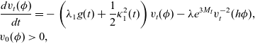 \begin{eqnarray*}&& \frac{d v_t(\phi)}{dt}=-\left(\lambda_1 g(t)+\frac{1}{2}\kappa_1^2(t)\right) v_t(\phi)-\lambda e^{3M_t} v_t^{-2}(h\phi),\\&& v_0(\phi)>0,\end{eqnarray*}
which by virtue of Jensen’s inequality infers
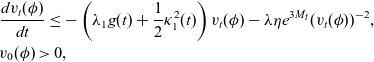 \begin{eqnarray*}&&\frac{d v_t(\phi)}{dt}\leq-\left(\lambda_1 g(t)+\frac{1}{2}\kappa_1^2(t)\right)v_t(\phi)-\lambda \eta e^{3M_t}(v_t(\phi))^{-2},\\&& v_0(\phi)>0,\end{eqnarray*}
where $\eta:=\max_{(x,s)\in \bar{D}\times [0,\tau]} h(x,s)>0$
and by means of a comparison argument we get
$\eta:=\max_{(x,s)\in \bar{D}\times [0,\tau]} h(x,s)>0$
and by means of a comparison argument we get
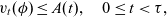 \begin{equation}v_t(\phi) \leq A(t), \quad 0\leq t<\tau ,\end{equation}
where now A(t) denotes the solution of the initial value problem
 \begin{eqnarray}A'(t)=-\left(\lambda_1 g(t)+\frac{1}{2}\kappa_1^2(t)\right) A(t)-\lambda \eta e^{3M_t} A^{-2}(t) , \; 0<t<\tau,\quad A_0=A(0)= v_0(\phi)>0, \nonumber\end{eqnarray}
with solution
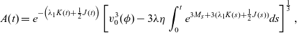 \begin{equation} A(t) =e^{-\left( \lambda_1 K(t) +\frac{1}{2} J(t)\right)} \left[ v^3_0(\phi)- 3 \lambda\eta \int_0^t e^{3M_s +3( \lambda_1 K(s) + \frac{1}{2}J(s))} ds \right]^{\frac{1}{3}}, \end{equation}
where $K(t):= \int_0^t g(s) ds$
and
$K(t):= \int_0^t g(s) ds$
and $J(t) : = \int_0^ t \kappa_1^2 (s) ds.$
The maximum existence (stopping) time $\tau_3$
of A(t) is then given by
$\tau_3$
of A(t) is then given by
 \begin{equation*} \tau_3:=\left\lbrace t\geq 0 : \int_0^t e^{3M_s + 3(\lambda_1 K(s) + \frac{1}{2}J(s))} ds \geq \frac{1}{3\lambda\eta} v^3_0(\phi) \right \rbrace, \end{equation*}
and actually A(t) quenches in finite time on the event $\left\lbrace \tau_3 < + \infty\right\rbrace.$
The fact that $0\leq v_t(\phi)\leq A(t)$
reveals that
$0\leq v_t(\phi)\leq A(t)$
reveals that $\tau_3$
is an upper bound of the stopping (extinction) time
$\tau_3$
is an upper bound of the stopping (extinction) time $\tau$
for
$\tau$
for $v_t(\phi);$
hence, the function
$v_t(\phi);$
hence, the function
 \begin{equation*}t\mapsto\int_D e^{M_t} z_t(x)\phi(x)\,dx,\end{equation*}
quenches in finite time under the event $\left\lbrace \tau_3< + \infty\right\rbrace.$
Using now (5.8) as well as the fact that
$\left\lbrace \tau_3< + \infty\right\rbrace.$
Using now (5.8) as well as the fact that $t\mapsto e^{M_t}$
is bounded below away from zero (cf. (5.17), (5.18) and the fact that
$t\mapsto e^{M_t}$
is bounded below away from zero (cf. (5.17), (5.18) and the fact that $\kappa_1(t)$
is bounded ) on
$\kappa_1(t)$
is bounded ) on $[0,\tau_3],$
once
$[0,\tau_3],$
once $\tau_3<\infty,$
then we deduce that the function
$\tau_3<\infty,$
then we deduce that the function $t\mapsto \inf_D z_t $
cannot stay away from zero on
$t\mapsto \inf_D z_t $
cannot stay away from zero on $[0,\tau_3]$
for
$[0,\tau_3]$
for $\tau_3<\infty.$
Therefore,
$\tau_3<\infty.$
Therefore, $z_t$
quenches in finite time on the event
$z_t$
quenches in finite time on the event $\left\lbrace \tau_3 < + \infty\right\rbrace$
and so
$\left\lbrace \tau_3 < + \infty\right\rbrace$
and so $\tau_3$
is an upper bound for the quenching time of
$\tau_3$
is an upper bound for the quenching time of $z_t$
.
$z_t$
.
Observe that $M_t= \int_0^t \kappa_1 (s) dB_s$
is a continuous martingale and so it can be written as
$M_t= \int_0^t \kappa_1 (s) dB_s$
is a continuous martingale and so it can be written as $M_t= B_{J(t)},$
where
$M_t= B_{J(t)},$
where $J(t)=[M](t)= \int_0^t \kappa^2 _1 (s) ds $
is the quadratic variation of
$J(t)=[M](t)= \int_0^t \kappa^2 _1 (s) ds $
is the quadratic variation of $M_t,$
cf. [Reference Karatzas and Shreve25, Theorem 4.6 page 174] and [Reference Revuz and Yor52, Theorems 1.6 and 1.7 in Chapter V], a result known as Dambis-Dubins-Schwarz theorem.
$M_t,$
cf. [Reference Karatzas and Shreve25, Theorem 4.6 page 174] and [Reference Revuz and Yor52, Theorems 1.6 and 1.7 in Chapter V], a result known as Dambis-Dubins-Schwarz theorem.
Set $\rho:=\frac{1}{3 \lambda \eta} v^3_0(\phi)$
then
$\rho:=\frac{1}{3 \lambda \eta} v^3_0(\phi)$
then
 \begin{eqnarray} \mathbb{P}(\tau_3=+ \infty) &=& \mathbb{P} \left( \int_0^t e^{3M_s + 3(\lambda_1 K(s)+ \frac{1}{2}J(s))} ds < \rho, \quad \mbox{for all} \quad t>0 \right) \nonumber\\ & =& \mathbb{P}\left( \int_0^{+\infty} e^ {3 B_{J(s)} + 3(\lambda_1 K(s)+ \frac{1}{2}J(s)) } ds \leq \rho\right) \nonumber \\ &=& \mathbb{P} \left( \int_0^{+\infty} \frac{1}{\kappa_1 ^2 (J^{-1} (s_1))} e^{3 B_{s_1}+3 \left( \lambda_1 K(J^{-1}(s_1))+\frac{1}{2} s_1 \right) } ds_1 \leq \rho \right), \end{eqnarray}
where $s_1:=J(s).$
At that point, we introduce the assumption that coefficients g(t) and $\kappa_1(t)$
satisfy: there exists some positive constant C such that
$\kappa_1(t)$
satisfy: there exists some positive constant C such that
 \begin{equation} \frac{1}{\kappa_1 ^2 (t)} e^{ 3\lambda_1\left( K(t) +\frac{1}{2}J(t) \right) } \geq C\quad\mbox{for any}\quad t\geq 0. \end{equation}
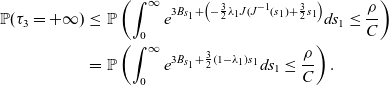 \begin{eqnarray} \mathbb{P}(\tau_3=+ \infty) &\leq& \mathbb{P} \left( \int_0^{\infty} e^{3 B_{s_1}+\left(-\frac{3}{2} \lambda_1 J(J^{-1}(s_1) + \frac{3}{2} s_1\right) } ds_1 \leq \frac{\rho}{ C} \right)\nonumber\\ &=& \mathbb{P} \left( \int_0^{\infty} e^{3 B_{s_1}+\frac{3}{2}\left( 1 -\lambda_1\right) s_1 } ds_1 \leq \frac{\rho}{ C} \right). \end{eqnarray}
Next, we introduce the change of variables $s_2\mapsto \left(\frac{3}{2} \right) ^2 s_1 ,$
and thus again via the scaling property of
$s_2\mapsto \left(\frac{3}{2} \right) ^2 s_1 ,$
and thus again via the scaling property of $B_t$
then (5.41) entails
$B_t$
then (5.41) entails
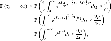 \begin{eqnarray} \mathbb{P}\left( \tau_3= + \infty \right) &\leq & \mathbb{P}\left( \frac{4}{9} \int_0^{\infty} e^{3 B_{\frac{4}{9} s_2}+\frac{3}{2}\left(1-\lambda_1\right) \frac{4}{9}s_2} ds_2 \leq \frac{\rho}{ C} \right) \nonumber \\&=& \mathbb{P} \left( \int_0^{\infty} e^{2 B_{s_2} +2\left(\frac{1-\lambda_1}{3}\right)s_2} ds_2 \leq \frac{9 \rho}{4 C} \right)\nonumber\\ &=&\mathbb{P}\left(\int_0^{+\infty} e^{2B_s^{(\mu)}} ds \leq \frac{9 \rho}{4 C} \right), \end{eqnarray}
where $\mu:= \frac{1-\lambda_1}{3}$
and
$\mu:= \frac{1-\lambda_1}{3}$
and $B_s^{(\mu)}:=B_s+\mu s.$
In the following, we distinguish the following cases:
-
(i) Initially, we assume that
$\mu<0,$
that is
$\lambda_1>1.$
Then by virtue of (5.42) and following the same reasoning as in Subsection 5.2, we obtain (5.43)cf. [Reference Yor53, Corollary 1.2 page 95].
\begin{align} \mathbb{P}( \tau_3= +\infty) &\leq \mathbb{P} \left( \frac{1}{2 Z_{-\mu}}\leq \frac{9 \rho}{4C}\right) \nonumber\\[3pt]&=1-\frac{1}{\Gamma(-\mu)} \int_0 ^{\frac{2C}{9 \rho}} y^{-\mu - 1} e^{-y} dy=\frac{1}{\Gamma(-\mu)} \int_{\frac{2C}{9 \rho}}^{\infty} y^{-\mu - 1} e^{-y} dy, \end{align}


Hence, from (5.43) we derive
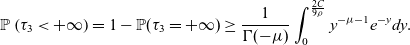 \begin{equation} \mathbb{P} \left( \tau_3< + \infty \right) =1 - \mathbb{P}( \tau_3= + \infty ) \geq \frac{1}{\Gamma(-\mu)} \int_0 ^{\frac{2C}{9 \rho}} y^{-\mu - 1} e^{-y} dy. \end{equation}
-
(ii) In the complimentary case
$\mu\geq 0,$
that is when
$\lambda_1\leq 1,$
then via the iterated logarithm law for
$B_s,$
cf. (5.17) and (5.18), we obtain and thus
\begin{equation*}\int_0^{+\infty} e^{2B_s^{(\mu)}} ds=+\infty\end{equation*}
The latter implies that
\begin{equation*} \mathbb{P}[\tau= +\infty]=\mathbb{P}\left(\int_0^{+\infty} e^{2B_s^{(\mu)}} ds \leq \frac{9 \rho}{4 C} \right)=0. \end{equation*}
and so in that case A(t) quenches a.s. independently of the initial condition
\begin{equation*} \mathbb{P}[ \tau < + \infty] = 1 - \mathbb{P}[\tau= +\infty]=1, \end{equation*}
$v_0$
and the parameter
$\lambda$
, which also entails that
$v_t$
and
$z_t$
quench as well.


Theorem 5.5 Assume that condition (5.40) holds true for the continuous positive functions $g(t), \kappa_1(t) >0.$
Then:
$g(t), \kappa_1(t) >0.$
Then:


Remark 5.6 Note that in the special case $g(t)=1,\kappa_1(t)=\kappa=$
constant and
$g(t)=1,\kappa_1(t)=\kappa=$
constant and $h(x,t)=1$
then via relation (5.39) we recover the result of Theorem 5.1.
$h(x,t)=1$
then via relation (5.39) we recover the result of Theorem 5.1.
Remark 5.7 Actually, Theorem 5.5 (ii) implies that when the diffusion coefficient g(t) is large enough, ensured by condition (5.40), then quenching behaviour dominates in the case of a rather big domain D. This might look to be counterintuitive to what has been pointed out in Remark 5.4 in the first place; however, it is in full agreement with the phenomenon observed in [Reference Kavallaris, Barreira and Madzvamuse34] where a strong reaction coefficient, enhanced there by the evolution of the moving domain, fights against the development of a singularity.
Remark 5.8 Note that since K(t) and J(t) are increasing functions we have
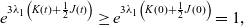 \begin{eqnarray*}e^{3\lambda_1\left( K(t)+\frac{1 }{2}J(t)\right)}\geq e^{3\lambda_1\left( K(0)+\frac{1 }{2}J(0)\right)}=1,\end{eqnarray*}
and thus condition (5.40) holds true provided that $\kappa_1(t)$
is bounded above, that is
$\kappa_1(t)$
is bounded above, that is $\sup_{(0,\infty)}\kappa_1(t)=L<\infty.$
In that case, we have that
$\sup_{(0,\infty)}\kappa_1(t)=L<\infty.$
In that case, we have that $C=\frac{1}{L^2}.$
Alternatively, if $\kappa_1(t)$
gets unbounded as
$\kappa_1(t)$
gets unbounded as $t\to \infty$
but satisfies the growth condition
$t\to \infty$
but satisfies the growth condition
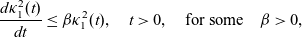 \begin{eqnarray*}\frac{d\kappa^2_1(t)}{dt}\leq \beta \kappa^2_1(t), \quad t>0,\quad\mbox{for some}\quad \beta>0,\end{eqnarray*}
then by virtue of L’ Hôpital’s rule we can show that
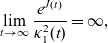 \begin{eqnarray*}\lim_{t\to\infty}\frac{e^{J(t)}}{\kappa_1^2(t)}=\infty,\end{eqnarray*}
and then using again the monotonicity of K(t) we derive (5.40) with $C=1.$
In relation to applications, it is of particular interest to simulate the stochastic process describing the operation of MEMS device and so to investigate under which circumstances it quenches. To this end, in the following section we present such a numerical algorithm together with various related simulations for problem (1.1).
6 Numerical Solution
6.1 Finite Elements approximation
In the current section, we present a numerical study of problem (1.1) in the one-dimensional case for the general case of a space-time Wiener process $W(x,t).$
Notably, our numerical approach could be easily implemented to the case of the standard Brownian motion
$W(x,t).$
Notably, our numerical approach could be easily implemented to the case of the standard Brownian motion $B_t.$
For that purpose, we apply a finite element semi-implicit Euler in time scheme, cf. [Reference Lord, Powell and Shardlow37]. The considered noise term is a multiplicative one and of the form
$B_t.$
For that purpose, we apply a finite element semi-implicit Euler in time scheme, cf. [Reference Lord, Powell and Shardlow37]. The considered noise term is a multiplicative one and of the form $\sigma(u)\,\partial_t W$
for
$\sigma(u)\,\partial_t W$
for $\sigma(u)=\kappa (1-u)$
with
$\sigma(u)=\kappa (1-u)$
with $\kappa>0$
. We also assume homogeneous Dirichlet boundary conditions at the points
$\kappa>0$
. We also assume homogeneous Dirichlet boundary conditions at the points $x=0,1,$
although some of the presented numerical experiments also concern homogeneous and nonhomogeneous Robin boundary conditions. A homogeneous Dirichlet boundary condition
$x=0,1,$
although some of the presented numerical experiments also concern homogeneous and nonhomogeneous Robin boundary conditions. A homogeneous Dirichlet boundary condition $u(0,t)=u(1,t)=0$
corresponds in having
$u(0,t)=u(1,t)=0$
corresponds in having $z=1$
at those points. Remarkably, this case is not actually covered by the analysis in section 5.
$z=1$
at those points. Remarkably, this case is not actually covered by the analysis in section 5.
We apply a discretisation in $[0,T]\times [0,1]$
,
$[0,T]\times [0,1]$
, $0\leq t\leq T$
,
$0\leq t\leq T$
, $0\leq x\leq 1$
with
$0\leq x\leq 1$
with $t_n=n\delta t$
,
$t_n=n\delta t$
, $\delta t=\left[{T}/{N}\right]$
for N the number of time steps and we also introduce the grid points in [0,1],
$\delta t=\left[{T}/{N}\right]$
for N the number of time steps and we also introduce the grid points in [0,1], $x_j = j\delta x$
, for
$x_j = j\delta x$
, for $\delta x = 1/M$
and
$\delta x = 1/M$
and $j = 0,1,\ldots, M$
.
$j = 0,1,\ldots, M$
.
Then, we proceed with a finite element approximation for problem (1.1). Let $\Phi_j$
,
$\Phi_j$
, $j=1,\ldots, M-1$
denote the standard linear
$j=1,\ldots, M-1$
denote the standard linear $B-$
splines on the interval
$B-$
splines on the interval $[0,\,1]$
that is
$[0,\,1]$
that is
 \begin{eqnarray}\Phi_j=\left\{\begin{array}{l@{\quad}l} \dfrac{x-x_{j-1}}{\delta x},&\quad x_{j-1}\leq x \leq x_j, \\ \\[-8pt]\dfrac{x_{j+1}\,-x}{\delta x},&\quad x_{j}\leq x \leq x_{j+1}, \\ \\[-8pt]0,&\quad \mbox{elsewhere in}\quad [0,\,1],\end{array} \right.\end{eqnarray}
for $j=1,2,\ldots,M-1$
. We then set
$j=1,2,\ldots,M-1$
. We then set $u(x,t)=\sum_{j=1}^{M-1} {a}_{u_j}(t) \Phi_j(x)$
,
$u(x,t)=\sum_{j=1}^{M-1} {a}_{u_j}(t) \Phi_j(x)$
, $t\geq 0$
,
$t\geq 0$
, $0\leq x\leq 1$
.
$0\leq x\leq 1$
.
Substituting the later expression for u into equation (1.1a) and applying the standard Galerkin method, that is multiplying with $\Phi_i$
, for
$\Phi_i$
, for $i=1,2,\ldots, M-1$
and integrating over
$i=1,2,\ldots, M-1$
and integrating over $[0,\,1]$
, we obtain a system of equations for the
$[0,\,1]$
, we obtain a system of equations for the ${a_{u_j} }$
’s as follows
${a_{u_j} }$
’s as follows
 \begin{eqnarray} \sum_{j=1}^{M-1} d{a}_{u_j} (t)<\Phi_j(x),\,\Phi_i(x)> &= & -\sum_{j=1}^{M-1} {a}_{x_j}(t)\langle\Phi^{\prime}_j(x),\,\Phi^{\prime}_i(y)\rangle \nonumber\\ &&+ \left\langle F\left(\sum_{j=1}^{M-1} {a}_{u_j}(t) \Phi_j(x)\right),\,\Phi_i(x)\right\rangle,\quad\quad \nonumber\\ &&+ \left\langle\sigma \left(\sum_{j=1}^{M-1} {a}_{u_j}(t) \Phi_j(x)\right) dW(x,t),\,\Phi_i(x)\right\rangle,\quad\quad\end{eqnarray}
where $<f,g>:=\int_0^1 f(x)g(x)dx$
and
$<f,g>:=\int_0^1 f(x)g(x)dx$
and $i=1,2,\ldots,M-1$
, and in our case
$i=1,2,\ldots,M-1$
, and in our case $F(s)=\frac{\lambda}{(1-s)^2}$
,
$F(s)=\frac{\lambda}{(1-s)^2}$
, $\sigma(s)=\kappa\,(1-s)$
.
$\sigma(s)=\kappa\,(1-s)$
.
Setting $a_u=[a_{u_1},\,a_{u_2},\ldots,a_{u_{M-1}}]^T$
the system of equations for the
$a_u=[a_{u_1},\,a_{u_2},\ldots,a_{u_{M-1}}]^T$
the system of equations for the ${a_u}$
’s take the form
${a_u}$
’s take the form
 \begin{eqnarray}A \, d{a}_u(t)&=&-B a_u(t) +b(t) + b_s(t),\nonumber\end{eqnarray}
for
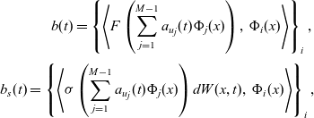 \begin{eqnarray*} b(t)=\left\{\left\langle F \left(\sum_{j=1}^{M-1} {a}_{u_j}(t) \Phi_j(x)\right),\,\Phi_i(x)\right\rangle\right\}_i, \nonumber\\[3pt]b_s(t)= \left\{\left\langle\sigma \left(\sum_{j=1}^{M-1} {a}_{u_j}(t) \Phi_j(x)\right) dW(x,t) ,\,\Phi_i(x)\right\rangle\right\}_i, \end{eqnarray*}
the latter coming from the corresponding Itô integral. Note also that $\partial_t W(x,t)\simeq \Delta W_h(x,t)=W_h(x,t+\delta t)-W_h(x,t)$
for
$\partial_t W(x,t)\simeq \Delta W_h(x,t)=W_h(x,t+\delta t)-W_h(x,t)$
for $W_h(x,t)$
the finite sum giving the discrete approximation of W(x, t).
$W_h(x,t)$
the finite sum giving the discrete approximation of W(x, t).
More specifically, the approximation $W_h$
, for a sample point x in [0,1], should have the form
$W_h$
, for a sample point x in [0,1], should have the form $W_h(x,t):=\sum_{j=1}^{M-1} \sqrt{q_j}\chi_j(x) \beta_j(t)$
. Additionally, in order to obtain the same sample path W(x, t) with different time steps we use the reference time step
$W_h(x,t):=\sum_{j=1}^{M-1} \sqrt{q_j}\chi_j(x) \beta_j(t)$
. Additionally, in order to obtain the same sample path W(x, t) with different time steps we use the reference time step $\delta t_{r}=T/(m N)$
,
$\delta t_{r}=T/(m N)$
, $m\in \mathbb{N}^+$
.
$m\in \mathbb{N}^+$
.
The increments over intervals of size $\delta t=m \delta t_{r}$
are given by
$\delta t=m \delta t_{r}$
are given by
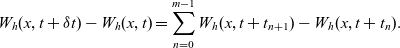 \begin{equation*}W_h(x,t+\delta t)-W_h(x,t)=\sum_{n=0}^{m-1} W_h(x,t+t_{n+1})-W_h(x,t+t_n). \end{equation*}
Moreover, we approximate the space-time white noise by taking
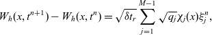 \begin{equation*}W_h(x,t^{n+1})-W_h(x,t^{n}) =\sqrt{\delta t_r}\sum_{j=1}^{ M-1}\sqrt{q_j}\chi_j(x)\xi_j^n,\end{equation*}
where $\xi_j^n:=( \beta_j(t_{n+1})-\beta_j(t_{n}))/\sqrt{\delta t_r}$
and
$\xi_j^n:=( \beta_j(t_{n+1})-\beta_j(t_{n}))/\sqrt{\delta t_r}$
and $\xi_j^n\sim N(0,1)$
are i.i.d. random variables for i.i.d. standard Brownian motions
$\xi_j^n\sim N(0,1)$
are i.i.d. random variables for i.i.d. standard Brownian motions $\beta_j(t)$
. Also, the eigenfunctions
$\beta_j(t)$
. Also, the eigenfunctions $\chi_j=\chi_j(x)=\sqrt{2}\sin\left( j\pi x\right)$
,
$\chi_j=\chi_j(x)=\sqrt{2}\sin\left( j\pi x\right)$
, $j\in\mathbb{N}^{+}$
are taken as a basis of
$j\in\mathbb{N}^{+}$
are taken as a basis of $L^2(0,1)$
and
$L^2(0,1)$
and $q_j^{\prime}s$
are chosen to be
$q_j^{\prime}s$
are chosen to be
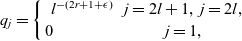 \begin{eqnarray} q_j=\left\{ \begin{array}{cc} l^{-(2r+1+\epsilon)} & j=2l+1, \, j=2l,\\ 0 \quad \quad \quad \quad & j=1, \end{array}\right. \end{eqnarray}
for $l\in \mathbb{N}$
, r being the regularity parameter,
$l\in \mathbb{N}$
, r being the regularity parameter, $0\ll \epsilon <1$
to obtain an
$0\ll \epsilon <1$
to obtain an $H_0^r(0,1)$
-valued process.
$H_0^r(0,1)$
-valued process.
We then apply a semi-implicit Euler method in time by taking
 \begin{equation*} A\, d{a}_u(t_{n})\simeq A\left({a_u^{n+1}-a_u^{n}}\right)/({\delta t})= -B a_u^{n+1} + b(t_{n})+b_s(t_n),\end{equation*}
or
 \begin{equation*}\left( A+\delta t B\right)a_u^{n+1} =a_u^{n}+ \delta t\, b(t_{n})+\delta t \, b_s(t_n),\end{equation*}
with the ${(M-1)\times(M-1)}$
matrices A, B having the form
${(M-1)\times(M-1)}$
matrices A, B having the form
 \begin{eqnarray}&& A=\delta x \left[\begin{array}{c@{\quad}c@{\quad}c@{\quad}c@{\quad}c} \dfrac23 & \dfrac16 & 0 & \ldots & 0 \\ \\[-8pt] \dfrac16 & \dfrac23 & \dfrac16 & \ldots & 0\\ \\[-8pt] 0 & 0 & \ddots & \ddots & 0\\ \\[-8pt] 0 & 0 & \ldots &\dfrac16 & \dfrac13\end{array} \right], \,B=\dfrac{1}{\delta y} \left[\begin{array}{c@{\quad}c@{\quad}c@{\quad}c@{\quad}c} 2 & -1 & 0 & \ldots & 0 \\ \\[-8pt] -1 & 2 & -1 & \ldots & 0\\ \\[-8pt] 0 & 0 & \ddots & \ddots & 0\\ \\[-8pt] 0 & 0 & \ldots &-1 & 2\end{array} \right], \, \nonumber \end{eqnarray}
 \begin{eqnarray}&& b^n= b(t_n)=\left\{\left\langle F \left(\sum_{j=0}^{M-1} {a}_{u_j}^n \Phi_j(x)\right),\,\Phi_i(x)\right\rangle\right\}_i, \nonumber \\&& b_s^n= b_s(t_n)= \left\{\left\langle\sigma \left(\sum_{j=0}^M {a}_{u_j}^n\Phi_j(x)\right) \Delta W_h^n,\,\Phi_i(x)\right\rangle\right\}_i \nonumber,\end{eqnarray}
for ${a}_{u_j}^n={a}_{u_j}(t_n)$
,
${a}_{u_j}^n={a}_{u_j}(t_n)$
, $i=1\ldots, M-1$
.
$i=1\ldots, M-1$
.
Finally, the corresponding algebraic system for the $a_u^n$
’s after some manipulation becomes
$a_u^n$
’s after some manipulation becomes
 \begin{eqnarray} a_u^{n+1}=\left(A+\delta t B \right)^{-1}\left[a_u^{n} + \delta t\, b^n+ \delta t\, b_s^n\right],\end{eqnarray}
for $ a_u^0$
being determined by the initial condition.
$ a_u^0$
being determined by the initial condition.
6.2 Simulations
Initially, we present a realisation of the numerical solution of problem (1.1) in Figure 5(a) for $\lambda=1$
,
$\lambda=1$
, $\kappa=1$
,
$\kappa=1$
, $r=0.1$
initial condition
$r=0.1$
initial condition $u(x,0)=c\,x(1-x)$
for
$u(x,0)=c\,x(1-x)$
for $c=0.1$
and homogeneous Dirichlet boundary conditions (
$c=0.1$
and homogeneous Dirichlet boundary conditions ( $\beta\to\infty$
,
$\beta\to\infty$
, $\beta_c=0$
). By this performed realisation the occurrence of quenching is evident. For a different realisation but for the same parameters in Figure 5(b) the maximum of the solution at each time step is plotted and again a similar quenching behaviour is observed.
$\beta_c=0$
). By this performed realisation the occurrence of quenching is evident. For a different realisation but for the same parameters in Figure 5(b) the maximum of the solution at each time step is plotted and again a similar quenching behaviour is observed.
(a) Realisation of the numerical solution of problem (1.1) for $\lambda=1$
,
$\lambda=1$
, $k=1$
,
$k=1$
, $M=102$
,
$M=102$
, $N=10^4$
,
$N=10^4$
, $r=0.1$
and initial condition
$r=0.1$
and initial condition $u(x,0)=c\,x(1-x)$
for
$u(x,0)=c\,x(1-x)$
for $c=0.1$
. (b) Plot of
$c=0.1$
. (b) Plot of $\|u(\cdot,t) \|_\infty$
from a different realisation but with the same parameter values.
$\|u(\cdot,t) \|_\infty$
from a different realisation but with the same parameter values.
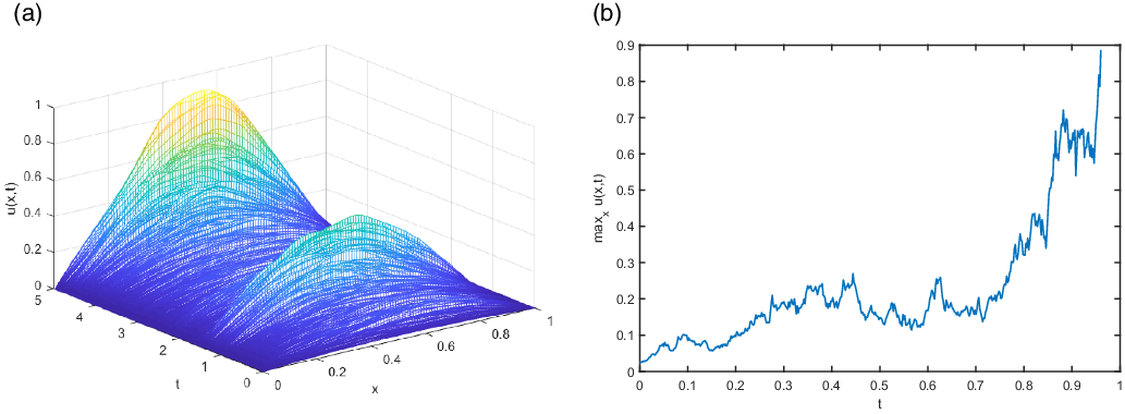
Next, in Figure 6(a) we observe the quenching behaviour of five realisations of the numerical solution of problem (1.1) for $\lambda=2$
. In an extra realisation depicted in Figure 6(b), the spatial distribution of the numerical solution at different time instants can be seen.
$\lambda=2$
. In an extra realisation depicted in Figure 6(b), the spatial distribution of the numerical solution at different time instants can be seen.
An interesting direction that is worth investigating is the derivation of estimates of the probability of quenching in a specific time interval [0, T] for some $T>0$
. It is known, cf. [Reference Kavallaris27], that for imposed Dirichlet boundary conditions, then the solution u will eventually quench in some finite time
$T>0$
. It is known, cf. [Reference Kavallaris27], that for imposed Dirichlet boundary conditions, then the solution u will eventually quench in some finite time $T_q$
for large enough values of the parameter
$T_q$
for large enough values of the parameter $\lambda$
or big enough initial data.
$\lambda$
or big enough initial data.
From the application point of view, an estimate of the probability that $T_q<T$
would be useful with respect to various values of the parameter
$T_q<T$
would be useful with respect to various values of the parameter $\lambda$
.
$\lambda$
.
In Table (T1), the results of such a numerical experiment are presented. In particular, implementing $N_R$
realisations then in the first column we print out the values of
$N_R$
realisations then in the first column we print out the values of $\lambda$
considered, whilst the second column contains the number of times that the solution quenched before the time T, whilst in the last two columns the mean
$\lambda$
considered, whilst the second column contains the number of times that the solution quenched before the time T, whilst in the last two columns the mean $m(T_q)$
and the variance
$m(T_q)$
and the variance $Var (T_q)$
of the quenching time respectively are given. More specifically, the quenching time
$Var (T_q)$
of the quenching time respectively are given. More specifically, the quenching time $T_q$
numerically is approximated as
$T_q$
numerically is approximated as $T_q\simeq t_m$
for
$T_q\simeq t_m$
for $t_m$
the maximum time step for which the condition
$t_m$
the maximum time step for which the condition $\max_j\left(u(x_j,t_m)\right)\leq 1-\varepsilon$
holds for a predefined small number
$\max_j\left(u(x_j,t_m)\right)\leq 1-\varepsilon$
holds for a predefined small number $\varepsilon$
. In the following simulations
$\varepsilon$
. In the following simulations $\varepsilon$
it is taken to be the machine tolerance, that is
$\varepsilon$
it is taken to be the machine tolerance, that is $\varepsilon=2.2204\, 10^{-16}$
. Note that for example in Figure 6 in the presented realisations, we have
$\varepsilon=2.2204\, 10^{-16}$
. Note that for example in Figure 6 in the presented realisations, we have $\max_j\left(u(x_j,t_m)\right)$
noticeably smaller than
$\max_j\left(u(x_j,t_m)\right)$
noticeably smaller than $1-\varepsilon$
whilst for the time step
$1-\varepsilon$
whilst for the time step $t_{m+1}$
the aforementioned condition is not satisfied. More accuracy in the estimation of the stopping time
$t_{m+1}$
the aforementioned condition is not satisfied. More accuracy in the estimation of the stopping time $t_m$
would require an adaptive time stepping numerical scheme. The rest of the parameters were taken to be the same as in the previous simulations but with
$t_m$
would require an adaptive time stepping numerical scheme. The rest of the parameters were taken to be the same as in the previous simulations but with $\kappa=0.1$
.
$\kappa=0.1$
.
Realisations of the numerical solution of problem (1.1) for $N_R=1000$
in the time interval
$N_R=1000$
in the time interval $[0,10].$
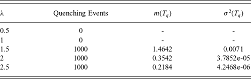
(a) Realisation of the $\|u(\cdot,t) \|_\infty$
of the numerical solution of problem (1.1) for
$\|u(\cdot,t) \|_\infty$
of the numerical solution of problem (1.1) for $\lambda=2$
,
$\lambda=2$
, $k=1$
,
$k=1$
, $M=102$
,
$M=102$
, $N=10^4$
,
$N=10^4$
, $r=0.1$
and initial condition
$r=0.1$
and initial condition $u(x,0)=c\,x(1-x)$
for
$u(x,0)=c\,x(1-x)$
for $c=0.1$
. (b) Plot of
$c=0.1$
. (b) Plot of $u(x,t_i) $
from a different realisation with the same parameter values at five time instants.
$u(x,t_i) $
from a different realisation with the same parameter values at five time instants.
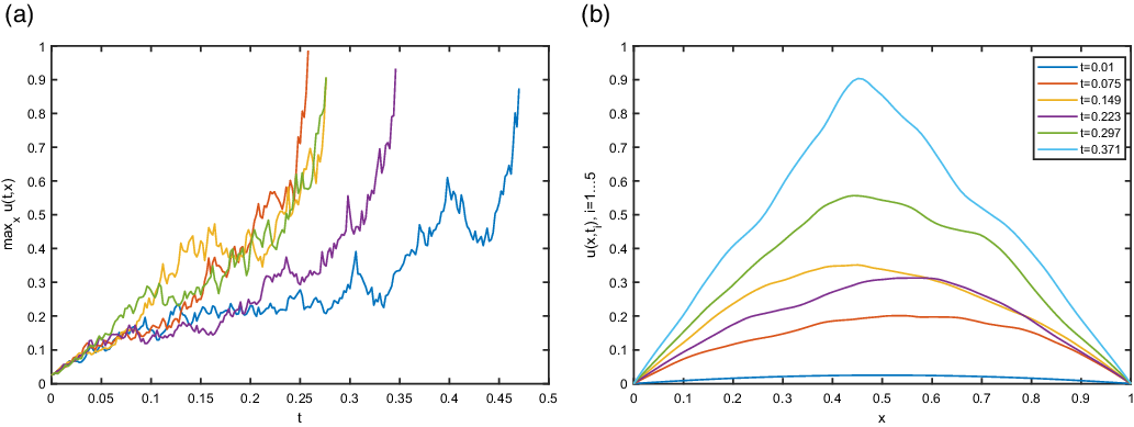
By the results in Table (T1), we observe that in a finite time interval the stochastic problem performs a dynamic behaviour which resembles that of the deterministic one. Specifically, increasing the value of $\lambda$
initially we have no quenching in this time interval whilst after
$\lambda$
initially we have no quenching in this time interval whilst after $\lambda>\lambda^*_{T}>1$
we have quenching almost surely at a time
$\lambda>\lambda^*_{T}>1$
we have quenching almost surely at a time $T_q$
with mean and variance decreasing with
$T_q$
with mean and variance decreasing with $\lambda$
.
$\lambda$
.
Additionally, we perform another experiment for simulation time $T=1$
and
$T=1$
and $\lambda=1.65,$
chosen in a
$\lambda=1.65,$
chosen in a ${\lambda}-$
range where the occurrence of quenching is not definite, and for a larger number of realisations
${\lambda}-$
range where the occurrence of quenching is not definite, and for a larger number of realisations $N_R=10^4$
, whilst the rest of the parameter values being kept the same as in Table (T1). Then, we obtain a numerical estimation for the probability of quenching equal to
$N_R=10^4$
, whilst the rest of the parameter values being kept the same as in Table (T1). Then, we obtain a numerical estimation for the probability of quenching equal to $ 0.3464$
with
$ 0.3464$
with $m(Tq)=0.3380$
and
$m(Tq)=0.3380$
and $Var(Tq)=0.2157.$
Next, we consider the case of nonhomogeneous boundary conditions of the form (1.1b) or equivalently (4.2b) with $\beta=\beta_c,$
since such a case is of particular interest in the light of the quenching results of section 5. It is sufficient for Robin-type boundary conditions to be satisfied in the weak sense, although they could even hold in the classical sense too, see [Reference Kavallaris and Yan33, Theorem 4.1]. A simulation implementing the previously described numerical algorithm for this particular case is presented in Figure 7(a). The presented realisation is for problem (1.1), and the parameters used here are
$\beta=\beta_c,$
since such a case is of particular interest in the light of the quenching results of section 5. It is sufficient for Robin-type boundary conditions to be satisfied in the weak sense, although they could even hold in the classical sense too, see [Reference Kavallaris and Yan33, Theorem 4.1]. A simulation implementing the previously described numerical algorithm for this particular case is presented in Figure 7(a). The presented realisation is for problem (1.1), and the parameters used here are $\lambda=0.3$
,
$\lambda=0.3$
, $k=1$
,
$k=1$
, $\beta=\beta_c=1.$
Also, in Figure 7(b) the quenching of
$\beta=\beta_c=1.$
Also, in Figure 7(b) the quenching of $||u(\cdot,t)||_{\infty}$
for one realisation is depicted.
$||u(\cdot,t)||_{\infty}$
for one realisation is depicted.
(a) Realisation of the numerical solution of problem (1.1) for $\lambda=0.3$
,
$\lambda=0.3$
, $\kappa=1$
,
$\kappa=1$
, $M=102$
,
$M=102$
, $N=10^4$
,
$N=10^4$
, $r=0.1$
, initial condition
$r=0.1$
, initial condition $u(x,0)=c\,x(1-x)$
for
$u(x,0)=c\,x(1-x)$
for $c=0.1$
and with
$c=0.1$
and with $\beta=\beta_c=1$
in the nonhomogeneous boundary condition. (b) Plot of
$\beta=\beta_c=1$
in the nonhomogeneous boundary condition. (b) Plot of $\|u(\cdot,t) \|_\infty$
. The quenching behaviour is apparent.
$\|u(\cdot,t) \|_\infty$
. The quenching behaviour is apparent.
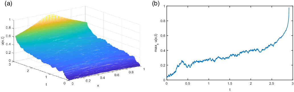
Similarly, in the next set of graphs in Figure 8(a) we display the quenching behaviour of five realisations of the numerical solution of problem (1.1) for $\lambda=0.3$
. In an extra realisation provided by Figure 8(b), the spatial distribution of the numerical solution at different time instants is presented.
$\lambda=0.3$
. In an extra realisation provided by Figure 8(b), the spatial distribution of the numerical solution at different time instants is presented.
(a) Realisation of the $\|u(\cdot,t) \|_\infty$
of the numerical solution of problem (1.1) for
$\|u(\cdot,t) \|_\infty$
of the numerical solution of problem (1.1) for $\lambda=2$
,
$\lambda=2$
, $\kappa=1$
,
$\kappa=1$
, $M=102$
,
$M=102$
, $N=10^4$
,
$N=10^4$
, $r=0.1$
and initial condition
$r=0.1$
and initial condition $u(x,0)=c\,x(1-x)$
for
$u(x,0)=c\,x(1-x)$
for $c=0.1$
. (b) Plot of
$c=0.1$
. (b) Plot of $u(x,t_i) $
from a different realisation with the same values of the parameters at five time instants.
$u(x,t_i) $
from a different realisation with the same values of the parameters at five time instants.
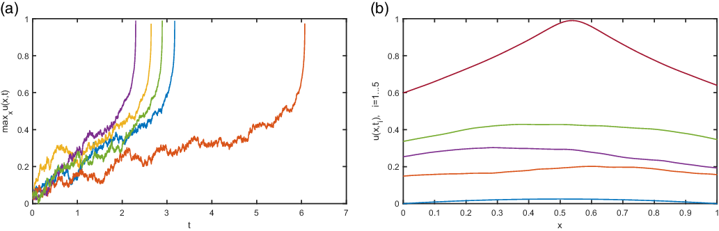
Additionally, in the following Table (T2) we present the results of such a numerical experiment. Indeed, implementing $N_R$
realisations we derive analogous results as in Table (T1).
$N_R$
realisations we derive analogous results as in Table (T1).
Realisations of the numerical solution of problem (1.1) in the case of nonhomogeneous Robin boundary conditions for $N_R=1000$
in the time interval
$N_R=1000$
in the time interval $[0,1].$
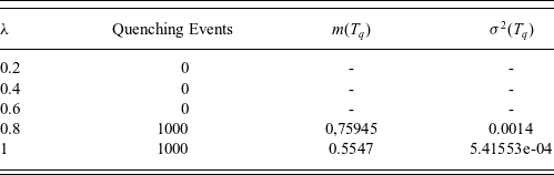
We notice a transition of the behaviour of the solution u around the value $\lambda\sim 0.7$
. So, in the next table, Table (T3), we focus around this value and point out a gradual increase of the number of quenching results as the parameter
$\lambda\sim 0.7$
. So, in the next table, Table (T3), we focus around this value and point out a gradual increase of the number of quenching results as the parameter $\lambda$
increases.
$\lambda$
increases.
Realisations of the numerical solution of problem (1.1) in the case of nonhomogeneous Robin boundary conditions for $N_R=1000$
in the time interval
$N_R=1000$
in the time interval $[0,1].$
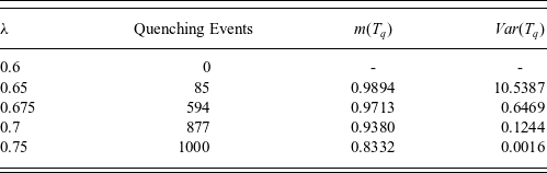
In the next set of experiments, we solve numerically problem (4.9). We choose the diffusion coefficient to be of the form $g=g(t)=c_0+c_1\cos(\omega t)$
, with
$g=g(t)=c_0+c_1\cos(\omega t)$
, with $c_0=1$
,
$c_0=1$
, $c_1=0.1$
,
$c_1=0.1$
, $\omega=10$
. We also consider a potential in the source term of the form
$\omega=10$
. We also consider a potential in the source term of the form $h(x)=x^b$
, for
$h(x)=x^b$
, for $b=\frac12$
. The results of these experiments are demonstrated in Table (T4).
$b=\frac12$
. The results of these experiments are demonstrated in Table (T4).
Realisations of the numerical solution of problem (4.9) in the case of nonhomogeneous Robin boundary conditions for $N_R=1000$
in the time interval
$N_R=1000$
in the time interval $[0,1].$
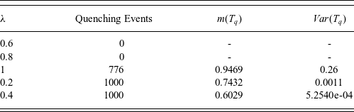
Moreover, focusing again around the value $\lambda\sim 1$
we can observe the transitional behaviour of the system in Table (T5) for
$\lambda\sim 1$
we can observe the transitional behaviour of the system in Table (T5) for $T=1.$
Realisations of the numerical solution of problem (4.9) in the case of nonhomogeneous Robin boundary conditions for $N_R=1000$
in the time interval
$N_R=1000$
in the time interval $[0,1].$
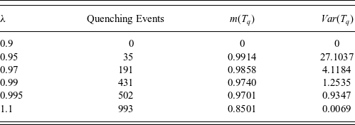
7 Discussion
In the current work, we demonstrate an investigation of a $d-$
dimensional,
$d-$
dimensional, $d=1,2,3,$
stochastic parabolic problem related to the modelling of an electrostatic MEMS device part of which is a membrane-rigid plate system. Firstly, the basic stochastic model is presented. Later, local existence and uniqueness of the basic stochastic
$d=1,2,3,$
stochastic parabolic problem related to the modelling of an electrostatic MEMS device part of which is a membrane-rigid plate system. Firstly, the basic stochastic model is presented. Later, local existence and uniqueness of the basic stochastic $u-$
problem (1.1), as well as of its main variations, and for general boundary conditions is discussed.
$u-$
problem (1.1), as well as of its main variations, and for general boundary conditions is discussed.
Next, and for a certain form of boundary conditions (cf. equation (4.2b)) it is shown that the solution of $z-$
problem (4.2) quenches almost surely regardless the chosen initial condition or the value of the tuning parameter
$z-$
problem (4.2) quenches almost surely regardless the chosen initial condition or the value of the tuning parameter $\lambda.$
This is actually a striking and counterintutive result; indeed for the corresponding deterministic problem, quenching occurs only if the parameter
$\lambda.$
This is actually a striking and counterintutive result; indeed for the corresponding deterministic problem, quenching occurs only if the parameter $\lambda$
or the initial data are large enough. To the best of our knowledge, this the first result of such kind derived in the context of semilinear SPDEs related to MEMS.
$\lambda$
or the initial data are large enough. To the best of our knowledge, this the first result of such kind derived in the context of semilinear SPDEs related to MEMS.
Furthermore, adding a regularising term into equation (4.2a), in the form of a modified nonlinear drift term, changes the dynamics of solution $z=1-u$
and we then obtain a dynamical behaviour resembling that of the deterministic problem. Moreover, in this particular case a lower estimate of the quenching probability is provided by formula (5.31).
$z=1-u$
and we then obtain a dynamical behaviour resembling that of the deterministic problem. Moreover, in this particular case a lower estimate of the quenching probability is provided by formula (5.31).
The case of including time-dependent coefficients related to dispersion and varying dielectric properties in the equation is tackled by a similar approach. Again, a lower bound for the quenching probability or quenching almost surely are derived, depending on the size of the first eigenvalue of the Laplacian operator associated with relevant boundary conditions.
We end our investigation by the implementation of a finite element numerical method, for the solution of the stochastic time-dependent problem in the one-dimensional case. We also provide a series of numerical experiments initially for the case of homogeneous Dirichlet boundary conditions (for the u-problem) and next for nonhomogeneous Robin conditions. In each case, we present various results estimating the quenching events in a specific time interval [0,T], which are of particular interest for MEMS practitioners.
Finally, we would like to point out that other kind of noise terms could be considered in the same context of MEMS applications. A more rough in time noise perturbation, realised via a fractional Brownian, is treated in a forthcoming paper, cf. [Reference Drosinou, Nikolopoulos, Matzavinos and Kavallaris13]. Indeed, such a consideration is linked with more irregular changes (including possible jumps in the values) of the features of MEMS device, as it is indicated in [Reference Mohd-Yasin, Nagel and Korman40]. Furthermore, the consideration of a more general continuous-time stochastic perturbation, like a Lévy noise, would be of considerable interest from mathematical as well as from applications point of view. In addition, the estimation of quenching probability for a space-time Wiener process, via the approach of Section 5, seems to be a challenging issue, since it requires a quite technical analysis, and thus, it will be treated in a future work.
Acknowledgement
The authors would like to thank the referees for the careful reading and valuable comments which led to improvements in our original manuscript. Dedicated to Professor Andrew A. Lacey on the occasion of his retirement.


 Open access