


1. Introduction
The present paper is concerned with the long-time asymptotic behaviour for the solution of the modified Camassa–Holm (mCH) equation [Reference Fuchssteiner26, Reference Olver and Rosenau42]
 \begin{align} &m_{t}+\left (m\left (u^{2}-u_{x}^{2}\right )\right )_{x}=0, \quad m=u-u_{xx}, \end{align}
with step-like initial data
 \begin{align} u(x,0)=u_0(x)\to \left \{ \begin{array}{l@{\quad}l} 1/c_+, &\ x\to +\infty, \\[5pt] 1/c_-, &\ x\to -\infty . \end{array}\right . \end{align}
The mCH (1.1) appeared in [Reference Fuchssteiner26] as a integrable equation proposed by Fuchssteiner and Fokas and first introduced by Camassa and Holm as a model for the unidirectional propagation of shallow-water waves [Reference Camassa and Holm8] (see also [Reference Constantin and Lannes15] for a rigorous justification in shallow-water approximation).
The mCH (1.1) bears some similarity to the celebrated Camassa–Holm (CH) equation
 \begin{align} &m_t+ (um )_x+ u_x m=0, \quad m=u-u_{x x}, \end{align}
due to the presence of the relation
 $m=u-u_{x x}$
. Different from the CH (1.3), the mCH (1.1) contains the cubic nonlinearity. In view of Fokas and Fuchssteiner [Reference Fuchssteiner and Fokas27], Olver and Rosenau [Reference Olver and Rosenau42], the CH (1.3) is obtained from the general method of tri-Hamiltonian duality to the bi-Hamiltonian representation of the Korteweg–de Vries equation, while this method applied to the modified Korteweg–de Vries equation yields the (1.1). Henceforth, the (1.1) was referred to the modified CH equation (see also [Reference Qiao43]). The CH (1.3) appeared in [Reference Fuchssteiner and Fokas27] as a integrable equation proposed by Fuchssteiner and Fokas and first introduced by Camassa and Holm as a model for the unidirectional propagation of shallow-water waves [Reference Camassa and Holm8] (see also [Reference Constantin and Lannes15] for a rigorous justification in shallow-water approximation). Therefore, the CH (1.3) has attracted considerable interest and studied extensively due to its rich mathematical structures and remarkable properties, such as peakon and multi-peakon solutions, bi-Hamiltonian structure, algebro-geometric solutions, wave-breaking phenomena [Reference Camassa and Holm8, Reference Constantin13, Reference Constantin and Escher14, Reference Constantin and Strauss16, Reference Eckhardt and Teschl21, Reference Mckean38].
$m=u-u_{x x}$
. Different from the CH (1.3), the mCH (1.1) contains the cubic nonlinearity. In view of Fokas and Fuchssteiner [Reference Fuchssteiner and Fokas27], Olver and Rosenau [Reference Olver and Rosenau42], the CH (1.3) is obtained from the general method of tri-Hamiltonian duality to the bi-Hamiltonian representation of the Korteweg–de Vries equation, while this method applied to the modified Korteweg–de Vries equation yields the (1.1). Henceforth, the (1.1) was referred to the modified CH equation (see also [Reference Qiao43]). The CH (1.3) appeared in [Reference Fuchssteiner and Fokas27] as a integrable equation proposed by Fuchssteiner and Fokas and first introduced by Camassa and Holm as a model for the unidirectional propagation of shallow-water waves [Reference Camassa and Holm8] (see also [Reference Constantin and Lannes15] for a rigorous justification in shallow-water approximation). Therefore, the CH (1.3) has attracted considerable interest and studied extensively due to its rich mathematical structures and remarkable properties, such as peakon and multi-peakon solutions, bi-Hamiltonian structure, algebro-geometric solutions, wave-breaking phenomena [Reference Camassa and Holm8, Reference Constantin13, Reference Constantin and Escher14, Reference Constantin and Strauss16, Reference Eckhardt and Teschl21, Reference Mckean38].
Applying the scaling transformation and taking parameter limit
 $\epsilon \to 0$
,
$\epsilon \to 0$
,
 \begin{align*} x\mapsto \epsilon x, t\mapsto \epsilon ^{-1}t, u\mapsto \epsilon ^2u, \end{align*}
the mCH (1.1) can be reduced a short pulse equation [Reference Schäfer and Wayne41]
 \begin{align*} &u_{xt}=u+\frac {1}{6}\left(u^3 \right)_{xx}. \end{align*}
More recently, the mCH (1.1) was considered as a model for the unidirectional propagation for shallow-water waves of mild amplitude over a flat bottom [Reference Chen, Hu and Liu12], where the solution
 $ u$
is related to the horizontal velocity at a specific water level. It is noted that the global smooth one-soliton solution of the mCH (1.1) with nonzero background data were obtained by using the RH method [Reference de Monvel, Karpenko and Shepelsky2]. On the other hand, the soliton of the mCH (1.1) with zero background data is a weak solution in the form of peaked wave. In addition, the quasi-periodic solutions with periodic background data were constructed by using algebro-geometric method [Reference Hou, Fan and Qiao31]. The wave-breaking and those peakons for the mCH (1.1) with zero background data were also investigated in [Reference Gui, Liu, Olver and Qu30]. The existence of the global peakon solutions and the large time asymptotic behaviour of these kind of non-smooth solitons were investigated in [Reference Chang and Szmigielski10]. It is known that the Cauchy problem associated with the mCH (1.1) is the locally well-posed in the Sobolev space
$ u$
is related to the horizontal velocity at a specific water level. It is noted that the global smooth one-soliton solution of the mCH (1.1) with nonzero background data were obtained by using the RH method [Reference de Monvel, Karpenko and Shepelsky2]. On the other hand, the soliton of the mCH (1.1) with zero background data is a weak solution in the form of peaked wave. In addition, the quasi-periodic solutions with periodic background data were constructed by using algebro-geometric method [Reference Hou, Fan and Qiao31]. The wave-breaking and those peakons for the mCH (1.1) with zero background data were also investigated in [Reference Gui, Liu, Olver and Qu30]. The existence of the global peakon solutions and the large time asymptotic behaviour of these kind of non-smooth solitons were investigated in [Reference Chang and Szmigielski10]. It is known that the Cauchy problem associated with the mCH (1.1) is the locally well-posed in the Sobolev space
 $ H^{s}(\mathbb{R}), s \gt 5/2$
[Reference Gui, Liu, Olver and Qu30]. Recently, the long-time asymptotic behaviour of the mCH (1.1) with linear dispersion term was established by using
$ H^{s}(\mathbb{R}), s \gt 5/2$
[Reference Gui, Liu, Olver and Qu30]. Recently, the long-time asymptotic behaviour of the mCH (1.1) with linear dispersion term was established by using
 $\bar \partial$
-steepest descent analysis in [Reference Yang and Fan46]. Based on the RH problem established in [Reference de Monvel, Karpenko and Shepelsky2], Boutet de Monvel et al. studied the long-time asymptotic behaviour of the mCH (1.1) under nonzero boundary conditions via nonlinear steepest descent method.
$\bar \partial$
-steepest descent analysis in [Reference Yang and Fan46]. Based on the RH problem established in [Reference de Monvel, Karpenko and Shepelsky2], Boutet de Monvel et al. studied the long-time asymptotic behaviour of the mCH (1.1) under nonzero boundary conditions via nonlinear steepest descent method.
Initial value problems for nonlinear evolution equations with step-like initial data have attracted much attention since the early 1970s [Reference Khruslov34]. The implementation of the rigorous asymptotic analysis to step-like initial value problems for integrable equations started in the paper [Reference Buckingham and Venakides7], which extended the methods from Deift, Venakides, and Zhou [Reference Deift, Venakides and Zhou17]. Since then, problems with step-like initial data have also been considered for a variety of integrable systems such as the KdV equation [Reference Egorova, Gladka, Kotlyarov and Teschl22], the focusing and defocusing NLS equations [Reference Biondini and Mantzavinos1, Reference de Monvel, Kotlyarov and Shepelsky4–Reference de Monvel, Lenells and Shepelsky6, Reference Fromm, Lenells and Quirchmayr25, Reference Jenkins32], the modified KdV equation [Reference Grava and Minakov29, Reference Kotlyarov and Minakov35] and Camassa–Holm equation [Reference Minakov39]. A wide range of important physical phenomena manifest themselves in the behaviour of solutions of such step-like initial value problems for large times, e.g., rarefaction waves [Reference Jenkins32], modulated waves [Reference Venakides, Deift and Oba45], elliptic waves [Reference de Monvel, Kotlyarov and Shepelsky4] and so on. The main feature in the long-time behaviour that distinguishes step-like initial conditions from decaying initial conditions is the formation of an oscillatory region that connects the different behaviour at
 $x\to \pm \infty$
of the solution. These oscillatory regions are typically described by elliptic or hyperelliptic modulated waves. Very recently, Karpenko, Shepelsky, and Teschl develop the RH formalism to the mCH (1.1) with step-like initial data (1.2) and give a representation for the solution of this problem in terms of the solution of an associated RH problem [Reference Karpenko, Shepelsky and Teschl33].
$x\to \pm \infty$
of the solution. These oscillatory regions are typically described by elliptic or hyperelliptic modulated waves. Very recently, Karpenko, Shepelsky, and Teschl develop the RH formalism to the mCH (1.1) with step-like initial data (1.2) and give a representation for the solution of this problem in terms of the solution of an associated RH problem [Reference Karpenko, Shepelsky and Teschl33].
1.1. Statement of results
The purpose of our present work is to investigate the long-time asymptotic behaviour of the mCH (1.1) with step-like initial data (1.2). Notice that under the transformation
 \begin{align} u(x,t)\mapsto c_- u(x,c_-^2t), \end{align}
 $c_- u(x,c_-^2t)$
is also a solution of the mCH (1.1), and the condition (1.2) becomes
$c_- u(x,c_-^2t)$
is also a solution of the mCH (1.1), and the condition (1.2) becomes
 \begin{align} u(x,0)=u_0(x)\to \left \{ \begin{array}{l@{\quad}l} 1/c, &\ x\to +\infty, \\[5pt] 1, &\ x\to -\infty, \end{array}\right . \end{align}
where
 $c=c_+/c_-$
. Therefore, without loss of generality, let
$c=c_+/c_-$
. Therefore, without loss of generality, let
 \begin{align} c_-=1,\qquad c_+=c\geq 1, \end{align}
in (1.2). For brevity, we will continue to adopt the notations
 $c_-$
and
$c_-$
and
 $c_+$
, but their exact values are given by (1.6).
$c_+$
, but their exact values are given by (1.6).
We find that the types of asymptotic expansions for the mCH (1.1) are closely related to the scope of two parameter
 $\xi =y/t$
and
$\xi =y/t$
and
 $c$
, where
$c$
, where
 $y$
is a new space variable defined by
$y$
is a new space variable defined by
 \begin{equation} y(x,t)=x+\int ^{x}_{-\infty } \left (m(s,t)-\frac {1}{c_-}\right ) ds. \end{equation}
So in our paper we adopt double coordinates
 $(\xi, c)$
to divide the upper half plane
$(\xi, c)$
to divide the upper half plane
 $\{(\xi, c)\,:\, \xi \in \mathbb{R}, c\gt 1\}$
into four different space-time regions (see Figure 1), in which we will present different leading order asymptotic approximations for the mCH (1.1) with step-like initial value (1.5). Our results are subject to the following assumption:
$\{(\xi, c)\,:\, \xi \in \mathbb{R}, c\gt 1\}$
into four different space-time regions (see Figure 1), in which we will present different leading order asymptotic approximations for the mCH (1.1) with step-like initial value (1.5). Our results are subject to the following assumption:
Asymptotic approximations of the mCH equation in different space-time-
 $(\xi, c)$
regions, where the Regions I ( yellow ) and II ( orange ) corresponding to genus-0, they are slow-decay and fast-decay background regions, respectively; The Regions III ( green ) and IV ( purple ) corresponding to genus-2 region, they are the first-type and second-type elliptic wave regions. Here,
$(\xi, c)$
regions, where the Regions I ( yellow ) and II ( orange ) corresponding to genus-0, they are slow-decay and fast-decay background regions, respectively; The Regions III ( green ) and IV ( purple ) corresponding to genus-2 region, they are the first-type and second-type elliptic wave regions. Here,
 $\xi _m$
is the critical condition that under the case of Region III, the stationary point of
$\xi _m$
is the critical condition that under the case of Region III, the stationary point of
 $g$
-function merges to
$g$
-function merges to
 $c$
. The Region I is a unit of three subregions. We use three shades of yellow to distinguish these three subregions. The Region III is a unit of two subregions, where we use two shades of green to distinguish it.
$c$
. The Region I is a unit of three subregions. We use three shades of yellow to distinguish these three subregions. The Region III is a unit of two subregions, where we use two shades of green to distinguish it.

Assumption 1.
The reflection coefficients defined by (2.16), associated to the initial data
 $u_0$
, are analytic on
$u_0$
, are analytic on
 $\mathbb{C}\setminus \left [{-}c,c\right ]$
.
$\mathbb{C}\setminus \left [{-}c,c\right ]$
.
This assumption is set similar to [Reference de Monvel, Lenells and Shepelsky5, Reference de Monvel, Lenells and Shepelsky6]. On one hand, the initial data are smooth and approaches to the backgrounds quickly enough such that the reflecting coefficients are meromorphic on
 $\mathbb{C}\setminus \left [{-}c,c\right ]$
. It is only made to simplify the proof and only affect the error order of the final asymptotic formulas in our main result. It allows us to avoid the technical work associated with the introduction of
$\mathbb{C}\setminus \left [{-}c,c\right ]$
. It is only made to simplify the proof and only affect the error order of the final asymptotic formulas in our main result. It allows us to avoid the technical work associated with the introduction of
 $\bar {\partial }$
-extensions of the jump matrices to perform the steepest descent analysis like in [Reference Yang and Fan46]. On the other hand, the assumption ensures that the initial data are ”no soliton” and generic, namely, the corresponding spectral problem has no eigenvalue and spectral singularity. Then the reflection coefficients defined by (2.16) have no poles. The combination of these two aspects results in the analyticity of the reflecting coefficients on
$\bar {\partial }$
-extensions of the jump matrices to perform the steepest descent analysis like in [Reference Yang and Fan46]. On the other hand, the assumption ensures that the initial data are ”no soliton” and generic, namely, the corresponding spectral problem has no eigenvalue and spectral singularity. Then the reflection coefficients defined by (2.16) have no poles. The combination of these two aspects results in the analyticity of the reflecting coefficients on
 $\mathbb{C}\setminus \left [{-}c,c\right ]$
.
$\mathbb{C}\setminus \left [{-}c,c\right ]$
.
Theorem 1.1.
Let
 $u(x,t)$
be the solution for the initial-value problem (1.1) and (1.5). Denote
$u(x,t)$
be the solution for the initial-value problem (1.1) and (1.5). Denote
 $\xi =y/t$
with
$\xi =y/t$
with
 $y$
defined in (1.7). As
$y$
defined in (1.7). As
 $t\to \infty$
, the long-time asymptotics of the mCH (1.1) are given as follows.
$t\to \infty$
, the long-time asymptotics of the mCH (1.1) are given as follows.
-
Region I: (i)
 $\ \{(\xi, c)\,\,:\ c\geq 1, \ \xi \lt 3/4\}$
; (ii)
$ \{(\xi, c)\,\,:\ 1\leq c\leq \lambda _1, \ 3/4\lt \xi \lt 1\}$
; (iii)
$\{(\xi, c)\,\,:\ 1\leq c\leq \lambda _1, \ 1\leq \xi \lt 3\},$
with
(1.8)whose branch is selected by
\begin{align} \lambda _1 \,:\!=\, \lambda _1(\xi )= \left (\dfrac {1-\sqrt {4\xi -3}}{1-\xi }\right ) ^{1/2}, \end{align}
$\lambda _1(1)=\sqrt {2}$
. It is a slow decay step-like background constant region with genus-0 and admits asymptotic expansion
(1.9)
\begin{align} &u(x,t)= {u(x(y,t),t)}= 1 +u^{(1)}(\xi ) t^{-\frac {1}{2}} +\mathcal{O}(t^{-1}), \end{align}
(1.10)where
\begin{align} & x=y-2I^1_{\delta }-2y^{(1)}(\xi )t^{-\frac {1}{2}}+\mathcal{O}(t^{-1}), \\[6pt] \nonumber \end{align}
$u^{(1)}$
defined in (7.2) comes from the parabolic cylinder function, and
$I^1_{\delta }$
,
$u^{(1)}$
and
$y^{(1)}$
are given in (3.3) and (7.3), respectively.
$\ \{(\xi, c)\,\,:\ c\geq 1, \ \xi \lt 3/4\}$
; (ii)
$ \{(\xi, c)\,\,:\ 1\leq c\leq \lambda _1, \ 3/4\lt \xi \lt 1\}$
; (iii)
$\{(\xi, c)\,\,:\ 1\leq c\leq \lambda _1, \ 1\leq \xi \lt 3\},$
with
(1.8)whose branch is selected by
\begin{align} \lambda _1 \,:\!=\, \lambda _1(\xi )= \left (\dfrac {1-\sqrt {4\xi -3}}{1-\xi }\right ) ^{1/2}, \end{align}
$\lambda _1(1)=\sqrt {2}$
. It is a slow decay step-like background constant region with genus-0 and admits asymptotic expansion
(1.9)
\begin{align} &u(x,t)= {u(x(y,t),t)}= 1 +u^{(1)}(\xi ) t^{-\frac {1}{2}} +\mathcal{O}(t^{-1}), \end{align}
(1.10)where
\begin{align} & x=y-2I^1_{\delta }-2y^{(1)}(\xi )t^{-\frac {1}{2}}+\mathcal{O}(t^{-1}), \\[6pt] \nonumber \end{align}
$u^{(1)}$
defined in (7.2) comes from the parabolic cylinder function, and
$I^1_{\delta }$
,
$u^{(1)}$
and
$y^{(1)}$
are given in (3.3) and (7.3), respectively.
-
Region II:
$\{(\xi, c)\,\,:\ \xi \gt 1+2/c,\ c\geq 1\}$
. It is a fast decay step-like background constant region with genus-0. We have asymptotic expansion (1.11)
\begin{align} & u(x,t)= {u(x(y,t),t)}= c^{-1} +\mathcal{O}(e^{-Ct}), \end{align}
(1.12)where
\begin{align} & x(y,t) =y-2\ln \left (\delta (\infty )e^{I_\delta ^1+ia(y,t)}\right ) +\mathcal{O}(e^{-Ct}), \\[6pt] \nonumber \end{align}
$a(y,t)=-\frac {i}{2}( c+1)y+\frac {it}{2}\left ( c^{-2} + c\right )$
,
$I_\delta ^1$
and
$\delta (\infty )$
are given in Proposition
5
and
$C$
is a positive constant.
-
Region III: Genus-2 elliptic wave region.
-
(i)
$\{(\xi, c)\,\,:\ c\gt \sqrt {2},\ 1\leq \xi \lt 1+2/c \}\cup \{(\xi, c)\,\,:\ 2\lt c,\ 1+\frac {2}{c^4}(c^2-2)\lt \xi \lt 1+\frac {2}{c}\}$
, we have asymptotic expansion
where
\begin{align*} & {u(x,t)= u(x(y,t),t)}=u^{(3)}(y,t;\,\xi )+t^{-1}\mathcal{E}(\xi ) +\mathcal{O}(t^{-2}),\\[3pt] &x(y,t)= y-2\ln \left ({-}ie^{-itg(\infty )+it(p^{(-)}_+-g_+)(0)}\delta _\infty (0)\delta _+(0)M_{12,+}^{mod}(0)\right )\\[3pt] &+2i\dfrac {H^{(0)}_{11}M_{12,+}^{mod}(0)+H^{(0)}_{12}M_{22,+}^{mod}(0)}{M_{12,+}^{mod}(0)}t^{-1} +\mathcal{O}(t^{-2}), \end{align*}
$u^{(3)}(y,t;\,\xi )$
is constructed by the Riemann theta function associated with the genus 2 Riemann surface shown in (7.5), and
$\mathcal{E}(\xi )$
given in (7.6) comes from the combined effect of the Riemann theta function and Airy Model.
$g(\infty )$
,
$M^{mod}$
,
$g(z)$
,
$\delta _\infty (0)$
,
$\delta _+(0)$
and
$H^{(0)}$
are shown in (5.5), (5.13), Proposition
6
,
7
, and
8
, respectively.
-
(ii)
$\{(\xi, c)\,:\,\sqrt {2}\lt c\lt 2,\ 1-\frac {2}{c^4}(2-c^2)\lt \xi \lt 1\}\cup \{(\xi, c)\,\,:\ \xi _m \lt \xi \lt 1,\ c\gt 2\}$
, we have asymptotic expansion
where
\begin{align*} & {u(x,t)= u(x(y,t),t)}=u^{(4)}(y,t;\,\xi )+t^{-1/2}\mathcal{E}(\xi ) +\mathcal{O}(t^{-1}),\\[3pt] &x(y,t)= y-2\ln \left ({-}ie^{-itg(\infty )+it(p^{(-)}_+-g_+)(0)}\delta _\infty (0)\delta _+(0)M_{12,+}^{mod}(0)\right )\\[3pt] &+2i\dfrac {H^{(0)}_{11}M_{12,+}^{mod}(0)+H^{(0)}_{12}M_{22,+}^{mod}(0)}{M_{12,+}^{mod}(0)}t^{-1/2} +\mathcal{O}(t^{-1}), \end{align*}
$u^{(4)}(y,t;\,\xi )$
,
$\mathcal{E}(\xi )$
, has same expansion as (7.5), (7.6) but the function
$\delta _\infty (0)$
,
$\delta _+(0)$
,
$H^{(0)}$
and
$H^{(1)}$
are shown in Proposition
9
and
11
, respectively.
$\xi _m$
is the critical velocity that the stationary points of the
$g$
-function given in Proposition
6
merges to
$c$
.
$\mathcal{E}(\xi )$
,
$H^{(0)}$
and
$H^{(1)}$
represent the contribution of the pairs of stationary points out of cut via parabolic cylinder model.
-
-
Region IV: Genus-2 elliptic wave region.
$\{\frac {3}{4}\lt \xi \lt \xi _m, 2\lt c\}$
, we have asymptotic expansion
where
\begin{align*} & {u(x,t)= u(x(y,t),t)}=u^{(5)}(y,t;\,\xi )+t^{-1}\mathcal{E}(\xi ) +\mathcal{O}(t^{-2}),\\[3pt] &x(y,t)=y-2\ln \left ({-}ie^{-itg(\infty )+it(p^{(-)}_+-g_+)(0)}\delta _\infty (0)\delta _+(0)M_{12,+}^{mod}(0)\right )\\[3pt] &+2i\dfrac {H^{(0)}_{11}M_{12,+}^{mod}(0)+H^{(0)}_{12}M_{22,+}^{mod}(0)}{M_{12,+}^{mod}(0)}t^{-1} +\mathcal{O}(t^{-2}). \end{align*}
$u^{(5)}(y,t;\,\xi )$
and
$\mathcal{E}(\xi )$
has same expansion as (7.5), (7.6) but the functions
$g(\infty )$
,
$g(z)$
,
$\delta _\infty (0)$
,
$\delta _+(0)$
,
$H^{(0)}$
,
$H^{(1)}$
and
$M^{mod}$
are shown in Proposition
12
,
13
, and
14
, formula (6.19), respectively.
$\mathcal{E}(\xi )$
,
$H^{(0)}$
and
$H^{(1)}$
represent the common contribution of two local Airy Model of two pairs of stationary points.


Remark 1.2. We divide the
 $(\xi, c)$
plane in four parts as shown in above theorem accounting to the
$(\xi, c)$
plane in four parts as shown in above theorem accounting to the
 $g$
-function appeared in the analysis. Although both Region III and Region IV are genus-2 regions, their
$g$
-function appeared in the analysis. Although both Region III and Region IV are genus-2 regions, their
 $g$
-functions have different expressions.
$g$
-functions have different expressions.
Remark 1.3. Region I and Region III are comprised of the union of two and three subregions, respectively. In Regions I and III, the subleading term of the asymptotic behaviour in these subregions are different, because these subregions have different number of stationary points. When
 $\xi \to 1_-$
, a pair of stationary points approaches to infinity while a pair of stationary points approaches to
$\xi \to 1_-$
, a pair of stationary points approaches to infinity while a pair of stationary points approaches to
 $\pm \sqrt {2}$
. We find that there is no transition region on the shared boundary
$\pm \sqrt {2}$
. We find that there is no transition region on the shared boundary
 $\xi =1$
in Region I. So does it on the shared boundary
$\xi =1$
in Region I. So does it on the shared boundary
 $\xi =1$
in Region III. But as
$\xi =1$
in Region III. But as
 $\xi \to 3/4$
, the stationary points will merge, which implies that the asymptotic behaviour may be expressed in terms of solutions of the second Painlevé equation. Our results also hold for
$\xi \to 3/4$
, the stationary points will merge, which implies that the asymptotic behaviour may be expressed in terms of solutions of the second Painlevé equation. Our results also hold for
 $c=1$
.
$c=1$
.
Remark 1.4. Our result also implies that
 $x/t=y/t+\mathcal{O}(t^{-1}).$
So the division of regions in the
$x/t=y/t+\mathcal{O}(t^{-1}).$
So the division of regions in the
 $(y, t)$
plane approximates to it on
$(y, t)$
plane approximates to it on
 $(x, t)$
plane as
$(x, t)$
plane as
 $t\to \infty$
.
$t\to \infty$
.
Compared with the works [Reference de Monvel, Karpenko and Shepelsky2, Reference de Monvel, Karpenko and Shepelsky3, Reference Karpenko, Shepelsky and Teschl33], our work has the following different features:
-
• Consider the mCH (1.1) with a nonzero boundary condition, Boutet de Monvel et al. in [Reference de Monvel, Karpenko and Shepelsky2] constructed its RH problem and exact solutions. Further they obtained long-time asymptotics of the solution by using Deift–Zhou steepest descent method [Reference de Monvel, Karpenko and Shepelsky3]. In our present work, we consider the mCH (1.1) with the step-like initial data condition (1.2), which can reduce the nonzero boundary condition as a special case of (1.2) by taking
$c=1$
. Moreover, our long-time asymptotics with the step-like initial data condition becomes more challenging than that [Reference de Monvel, Karpenko and Shepelsky3] which is only described by parabolic cylinder model. Our result requires a elliptic wave model in genus-2, the Airy function model and also the parabolic cylinder model. -
• In Ref. [Reference Karpenko, Shepelsky and Teschl33], though Karpenko et al. considered the mCH (1.1) with step-like initial data which is the same as ours, they only established its RH problem without consideration of long-time asymptotics. While we focus on its long-time asymptotic behaviours for different space-time regions on the whole
$(x,t)$
-plane.


1.2. Out line of the paper
Our paper is arranged as follows. In Section 2, we study the eigenfunctions and scattering data associated with step-like initial value (1.5). Further we analyse their analyticity, symmetries and asymptotic to construct the RH problem for
 $M(z)$
of step-like initial value problem, which will be used to analyse long-time asymptotics of the mCH equation in our paper. In Section 3 and Section 4, we construct the RH problem associated with the Regions I and II, further transform it into a model RH problem. In Sections 5 and 6, to analyse the RH problem in the regions III and IV, we introduce a
$M(z)$
of step-like initial value problem, which will be used to analyse long-time asymptotics of the mCH equation in our paper. In Section 3 and Section 4, we construct the RH problem associated with the Regions I and II, further transform it into a model RH problem. In Sections 5 and 6, to analyse the RH problem in the regions III and IV, we introduce a
 $g$
-function in genus two Riemann surface and transform the original RH problem to a RH problem
$g$
-function in genus two Riemann surface and transform the original RH problem to a RH problem
 $M^{(2)}(z)$
, which is further decomposed into a
$M^{(2)}(z)$
, which is further decomposed into a
 $M^{mod}(z)$
model problem and an inner local problems. The
$M^{mod}(z)$
model problem and an inner local problems. The
 $M^{mod}(z)$
contributes to the leading term of the asymptotics and is given by Riemann theta functions attached to a hyperelliptic Riemann surface in subsection 5.2.1 and subsection 6.3 in different region. Finally, in Section 7, we give the proof of Theorem1.1.
$M^{mod}(z)$
contributes to the leading term of the asymptotics and is given by Riemann theta functions attached to a hyperelliptic Riemann surface in subsection 5.2.1 and subsection 6.3 in different region. Finally, in Section 7, we give the proof of Theorem1.1.
2. Direct scattering and the RH problem
2.1. Spectral analysis on the lax pair
The mCH (1.1) admits the Lax pair [Reference de Monvel, Karpenko and Shepelsky2]
 \begin{equation} \Phi _x = X \Phi, \qquad \Phi _t =T \Phi, \end{equation}
where
 \begin{align} & X=\frac {1}{2}(izm\sigma _2-\sigma _3), \end{align}
 \begin{align} &T= \left(z^{-2}+\frac {u^2-u_x^2}{2} \right)\sigma _3-i \left(z^{-1} (u-u_x)+\frac {z}{2}\left(u^2-u_x^2 \right)m \right)\sigma _2 \\[6pt] \nonumber \end{align}
and
 $z\in \mathbb{C}$
is spectrum parameter. Here, we introduce the standard Pauli matrices
$z\in \mathbb{C}$
is spectrum parameter. Here, we introduce the standard Pauli matrices
 \begin{align*} \sigma _1= \left(\begin{array}{l@{\quad}l} 0&1\\[3pt]1&0\\[3pt] \end{array} \right),\quad \sigma _2= \left(\begin{array}{l@{\quad}l} 0&-i\\[3pt]i&0\\[3pt] \end{array} \right),\quad \sigma _3 = \left(\begin{array}{l@{\quad}l} 1&0\\[3pt]0&-1\\[3pt] \end{array} \right). \end{align*}
Since the Lax pair (2.1) admit spectral singularity at
 $z=\infty$
and
$z=\infty$
and
 $z=0$
, the asymptotic behaviour of the eigenfunction
$z=0$
, the asymptotic behaviour of the eigenfunction
 $\Phi$
as
$\Phi$
as
 $z\to \infty$
and
$z\to \infty$
and
 $z\to 0$
need to be controlled.
$z\to 0$
need to be controlled.
Case I.
 $z=\infty$
. For any real constant
$z=\infty$
. For any real constant
 $C\neq 0$
, we denote a matrix function relying on
$C\neq 0$
, we denote a matrix function relying on
 $C$
$C$
 \begin{equation} D_C(z)=\frac {1}{2}\left (\begin{array}{c@{\quad}c} \phi _C(z)+\phi _C(z)^{-1} & \phi _C(z)^{-1}-\phi _C(z)\\[3pt] \phi _C(z)^{-1}-\phi _C(z) & \phi _C(z)+\phi _C(z)^{-1} \end{array}\right ), \ \phi _C(z)=\left ( \frac {C+z}{C-z}\right ) ^{1/4}, \end{equation}
where
 $\phi _C(z)$
is analytic on
$\phi _C(z)$
is analytic on
 $\mathbb{C}\setminus \left [{-}C,C\right ]$
and the branch is chosen such that as
$\mathbb{C}\setminus \left [{-}C,C\right ]$
and the branch is chosen such that as
 $\ z\to \infty$
,
$\ z\to \infty$
,
 $ \phi _C(z)\sim e^{-\frac {i\pi }{4}}+\mathcal{O}(z^{-1}).$
Denote
$ \phi _C(z)\sim e^{-\frac {i\pi }{4}}+\mathcal{O}(z^{-1}).$
Denote
 \begin{align} {\lim _{z\to \infty } D_C(z)}=D_C(\infty )=\frac {\sqrt {2}}{2}(I+i\sigma _1), \end{align}
which is independent of
 $C$
. For convenience, we use the notation
$C$
. For convenience, we use the notation
 $f_\pm (z)$
of some function
$f_\pm (z)$
of some function
 $f$
to denote the boundary values of
$f$
to denote the boundary values of
 $f$
from the
$f$
from the
 $\pm$
sides of the oriented jump contours. We set the orientation of all curve on the real axis to be directed from the left to the right in this paper. From
$\pm$
sides of the oriented jump contours. We set the orientation of all curve on the real axis to be directed from the left to the right in this paper. From
 $\phi _{C,+}(z)=-i\phi _{C,-}(z)$
, it follows that
$\phi _{C,+}(z)=-i\phi _{C,-}(z)$
, it follows that
 \begin{align*} D_{C,+}(z)=i\sigma _1D_{C,-}(z), \ \ z\in \Sigma _+, \end{align*}
Under the initial value (1.5), we define two gauge transformations
 \begin{align} \Psi ^\pm (z;\,x,t)=D_{c_\pm }(z)\Phi (z;\,x,t), \end{align}
which satisfy the following Lax pair
 \begin{align} & \Psi _{x}^\pm = \left ({-}\frac {i}{2}m\sqrt {z^2-c_\pm ^2}\sigma _3+P^\pm \right )\Psi ^\pm, \end{align}
 \begin{align} & \Psi _{t}^\pm =\left (i\sqrt {z^2-c_\pm ^2}\left ( \dfrac {m(u^2-u_x^2)}{2}+\dfrac {1}{c_\pm z}\right ) \sigma _3+L^\pm \right )\Psi ^\pm, \end{align}
with
 \begin{align*} P^\pm \,:\!=\, &i\dfrac {c_\pm m-1}{2\sqrt {z^2-c_\pm ^2}}\left (c_\pm \sigma _3+iz\sigma _2\right ), \\[3pt] L^\pm \,:\!=\, &i\left ( \dfrac {c_\pm (u^2-u_x^2)(1-c_\pm m)}{2\sqrt {z^2-c_\pm ^2}}-\dfrac {u-1/c_\pm }{\sqrt {z^2-c_\pm ^2}}\right ) \sigma _3+\dfrac {u_x}{c_\pm }\sigma _1\\[3pt] &-\left ( \dfrac {z(u^2-u_x^2)(1-c_\pm m)}{2\sqrt {z^2-c_\pm ^2}}-\dfrac {c_\pm u-1}{z\sqrt {z^2-c_\pm ^2}}\right ) {\sigma _2,} \end{align*}
and the branch of the square root is chosen such that
 $\sqrt {z^2-c_\pm ^2}\sim ic_\pm$
,
$\sqrt {z^2-c_\pm ^2}\sim ic_\pm$
,
 $z\to 0$
in
$z\to 0$
in
 $\mathbb{C}^+$
, where
$\mathbb{C}^+$
, where
 $\mathbb{C}^\pm$
denote the upper/lower half complex plane and
$\mathbb{C}^\pm$
denote the upper/lower half complex plane and
 $c_\pm$
are exactly given in (1.6). For convenience, we denote
$c_\pm$
are exactly given in (1.6). For convenience, we denote
 $\Sigma _\pm =[{-}c_\pm, c_\pm ]$
as the branch cut of
$\Sigma _\pm =[{-}c_\pm, c_\pm ]$
as the branch cut of
 $\phi _{c_\pm }(z)$
.
$\phi _{c_\pm }(z)$
.
Furthermore, we introduce
 \begin{align} \mu ^\pm (z;\,x,t)=\Psi ^\pm (z;\,x,t)e^{itp^{(\pm )}(z)\sigma _3}, \end{align}
where
 $p^{(\pm )}(z)$
are defined by
$p^{(\pm )}(z)$
are defined by
 \begin{align} tp^{(\pm )}(z) \,:\!=\, tp^{(\pm )}(z;\,x,t)&=\dfrac {\sqrt {z^2-c_\pm ^2}}{2}\left ( \int _{\pm \infty }^{x}(m(s)-1/c_\pm )ds+\frac {x}{c_\pm }-\frac {2t}{c_\pm z^2}-\frac {t}{c_\pm ^3} \right ). \end{align}
In this paper, whenever convenient, we use
 $f(z)$
to denote
$f(z)$
to denote
 $f(z;\,x,t)$
to emphasise the dependence on
$f(z;\,x,t)$
to emphasise the dependence on
 $z$
. Then
$z$
. Then
 $\mu ^\pm (z;\,x,t)$
solve the two Volterra-type integral equations
$\mu ^\pm (z;\,x,t)$
solve the two Volterra-type integral equations
 \begin{equation} \mu ^\pm (z;\,x,t)=I+\int ^{x}_{\pm \infty }e^{\frac {i}{2}\hat {\sigma }_3\sqrt {z^2-c_\pm ^2}\int ^{s}_{x}m(v,t)dv}\left [ P^\pm (z;\,s,t) \mu ^\pm (z;\,s,t) \right ] ds. \end{equation}
It follows from (2.11) that the Jost functions
 $ \mu ^\pm (z) \,:\!=\, \mu ^\pm (z;\,x,t)$
admit two kinds of symmetries
$ \mu ^\pm (z) \,:\!=\, \mu ^\pm (z;\,x,t)$
admit two kinds of symmetries
 \begin{align*} \mu ^\pm (z)=\sigma _1\overline {\mu ^\pm (\bar {z})}\sigma _1=\sigma _2\overline {\mu ^\pm ({-}z)}\sigma _2^{-1}. \end{align*}
Again applying (2.11), it is accomplished that
 $ \det \mu ^\pm (z)=1,$
and
$ \det \mu ^\pm (z)=1,$
and
 \begin{align*} \mu ^\pm (z)\to I, \ z\to \infty .\end{align*}
Thus it appears that
 $\mu ^\pm (z)$
are analytical in
$\mu ^\pm (z)$
are analytical in
 $\mathbb{C}\setminus \Sigma _\pm$
, respectively. Let
$\mathbb{C}\setminus \Sigma _\pm$
, respectively. Let
 \begin{align} \tilde {\mu }^\pm (z;\,x,t) =D_{c_\pm }^{-1}(z)\mu ^\pm (z;\,x,t), \end{align}
then the Volterra-type integrals (2.11) about
 $\tilde {\mu }^\pm (z) \,:\!=\, \tilde {\mu }^\pm (z;\,x,t)$
are changed into
$\tilde {\mu }^\pm (z) \,:\!=\, \tilde {\mu }^\pm (z;\,x,t)$
are changed into
 \begin{align} \tilde {\mu }^\pm (z;\,x,t) =\,& D_{c_\pm }^{-1}(z) +\int ^{x}_{\pm \infty }D_{c_\pm }^{-1}(z)e^{\frac {i}{2}\sqrt {z^2-c_\pm ^2}\int ^{s}_{x}m(l,t)dl\hat {\sigma _3}} D_{c_\pm }(z)\nonumber \\[3pt] &\cdot \left (X(z;\,s,t)+ \frac {i}{2}m(s,t)\sqrt {z^2-c_\pm ^2}D_{c_\pm }(z)^{-1}\sigma _3D_{c_\pm }(z)\right ) \tilde {\mu }^\pm (z;\,s,t) ds, \end{align}
where
 $X$
is defined in (2.2). It follows from (2.13) that the Jost functions
$X$
is defined in (2.2). It follows from (2.13) that the Jost functions
 $\tilde {\mu }^\pm (z)$
have no more than
$\tilde {\mu }^\pm (z)$
have no more than
 $-\frac {1}{4}$
-weak singularity at
$-\frac {1}{4}$
-weak singularity at
 $z=\pm 1$
and
$z=\pm 1$
and
 $z=\pm c$
as
$z=\pm c$
as
 \begin{align*} \tilde {\mu }^\pm (z)=\mathcal{O}\big ((z\mp 1)^{-1/4}\big ), \quad \tilde {\mu }^\pm (z)=\mathcal{O}\big ((z\mp c)^{-1/4}\big ). \end{align*}
Since
 $D_{c_\pm }(z)^{-1}\Psi ^\pm (z;\,x,t)$
are two fundamental matrix solutions of the Lax pair (2.1), they are related by a scattering matrix function
$D_{c_\pm }(z)^{-1}\Psi ^\pm (z;\,x,t)$
are two fundamental matrix solutions of the Lax pair (2.1), they are related by a scattering matrix function
 $S(z)$
independent of
$S(z)$
independent of
 $x$
and
$x$
and
 $t$
$t$
 \begin{equation} D_{c_+}(z)^{-1}\Psi ^+(z;\,x,t)=D_{c_-}(z)^{-1}\Psi ^-(z;\,x,t)S(z), \end{equation}
 \begin{align*} S(z) =\left (\begin{array}{c@{\quad}c} s_{11}(z) &s_{12}(z) \\[4pt] s_{21}(z) & s_{22}(z) \end{array}\right ),\qquad \det S(z) =1. \end{align*}
Combining the transformations (2.9), (2.12) with the (2.14), it deduced that
 \begin{align} S(z)=e^{itp^{(-)}(z;\,x,t)\sigma _3}(\tilde {\mu }^-(z;\,x,t))^{-1}\tilde {\mu }^+(z;\,x,t)e^{-itp^{(+)}(z;\,x,t)\sigma _3}, \end{align}
which is analytic on
 $\mathbb{C}\setminus \Sigma _+$
. It also implies that the scattering matrix
$\mathbb{C}\setminus \Sigma _+$
. It also implies that the scattering matrix
 $S(z)$
has no more than
$S(z)$
has no more than
 $-\frac {1}{4}$
-weak singularity at
$-\frac {1}{4}$
-weak singularity at
 $z=\pm 1$
and
$z=\pm 1$
and
 $z=\pm c$
. On the other hand, it is also deduced that
$z=\pm c$
. On the other hand, it is also deduced that
 \begin{align*} S(z)\sim e^{\frac {1}{2}Hz\sigma _3 },\ \ z\to \infty, \end{align*}
where
 $H$
is a constant given by
$H$
is a constant given by
 \begin{align*}H= \left(1-\frac {1}{c}\right)x+\left(\frac {1}{c^3}-1\right)t+\int _{-\infty }^{x} \left(m(s,t)-1 \right)ds+\int _{x}^{+\infty } \left(m(s,t)-\frac {1}{c} \right)ds.\end{align*}
Define two reflecting coefficients by
 \begin{equation} r_1(z)=\frac {s_{21}(z)}{s_{11}(z)},\qquad r_2(z)=\frac {s_{12}(z)}{s_{22}(z)}. \end{equation}
As
 $z\to \pm c$
, they then admit asymptotic behaviour
$z\to \pm c$
, they then admit asymptotic behaviour
 $1-r_1(z)r_2(z)=\mathcal{O}((z\mp c)^{1/2}).$
To construct the RH problem, the jump of the Jost functions
 $\tilde {\mu }^\pm (z)$
on the cut
$\tilde {\mu }^\pm (z)$
on the cut
 $\Sigma _\pm$
need to be analysed in the following proposition under standard proof.
$\Sigma _\pm$
need to be analysed in the following proposition under standard proof.
Proposition 1.
The functions
 $\mu ^\pm$
,
$\mu ^\pm$
,
 $\tilde {\mu }^\pm$
,
$\tilde {\mu }^\pm$
,
 $S$
and the reflecting coefficients
$S$
and the reflecting coefficients
 $r_1$
,
$r_1$
,
 $r_2$
admit the jump relations
$r_2$
admit the jump relations
(i) For
 $z\in \Sigma _\pm$
,
$z\in \Sigma _\pm$
,
 \begin{align*} \mu ^\pm _+(z)=\sigma _1 \mu ^\pm _-(z)\sigma _1. \end{align*}
(ii) For
 $z\in \Sigma _-$
,
$z\in \Sigma _-$
,
 \begin{align*} & \tilde {\mu }^\pm _{11,+}(z)=-i \tilde {\mu }^\pm _{12,-}(z), \quad \tilde {\mu }^\pm _{21,+}(z)=-i \tilde {\mu }^\pm _{22,-}(z),\\[3pt] &s_{11,\pm }(z)=s_{22,\mp }(z), \quad s_{12,\pm }(z)=s_{21,\mp }(z), \quad {r_{1,\pm }(z)=r_{2,\mp }(z).} \end{align*}
(iii) For
 $z\in \Sigma _+\setminus \Sigma _-$
,
$z\in \Sigma _+\setminus \Sigma _-$
,
 $\tilde {\mu }^+(z)$
has same jump as above equation while
$\tilde {\mu }^+(z)$
has same jump as above equation while
 $\tilde {\mu }^-(z)$
has no jump. And
$\tilde {\mu }^-(z)$
has no jump. And
 \begin{align*} & s_{11,+}(z)=-is_{12,-}(z), \quad s_{21,+}(z)=-is_{22,-}(z), \quad {r_{1,\pm }(z)r_{2,\mp }(z)=1.} \end{align*}
(iv) For
 $z\in \mathbb{R}\setminus \Sigma _+$
,
$z\in \mathbb{R}\setminus \Sigma _+$
,
 \begin{align*} r_1(z)=\overline {r_2(z)}. \end{align*}
Under the Assumption1
 $r_1(z)$
and
$r_1(z)$
and
 $r_2(z)$
are analytic in
$r_2(z)$
are analytic in
 $\mathbb{C}\setminus \Sigma _+$
.
$\mathbb{C}\setminus \Sigma _+$
.
Case II:
 $z=0$
.
$z=0$
.
The Lax pair (2.7)–(2.8) is rewritten in the form
 \begin{align*} & \Psi ^{\pm }_x = -\frac {i\sqrt {z^2-c_\pm ^2}}{2c_\pm }\sigma _3\Psi ^\pm +P_0^\pm \Psi ^\pm, \\[3pt] & \Psi ^{\pm }_t =i\sqrt {z^2-c_\pm ^2}\left ( \dfrac {1}{2c_\pm ^3}+\dfrac {1}{c_\pm z^2}\right ) \sigma _3\Psi ^\pm +L_0^\pm \Psi ^\pm, \end{align*}
where
 $c_\pm$
are exactly given in (1.6) and
$c_\pm$
are exactly given in (1.6) and
 \begin{align*} P_0^\pm =&iz\dfrac {c_\pm m-1}{2c_\pm \sqrt {z^2-c_\pm ^2}}\left ( z\sigma _3+ic_\pm \sigma _2\right ),\\[3pt] L_0^\pm =&L_\pm +i\sqrt {z^2-c_\pm ^2}\left ( \dfrac {m(u^2-u_x^2)}{2}+\dfrac {1}{c_\pm z}-\dfrac {1}{2c_\pm ^3}+\dfrac {1}{c_\pm z^2}\right ) \sigma _3. \end{align*}
By making transformation
 \begin{align*} \mu ^\pm _0(z;\,x,t)&=\Psi _\pm (z;\,x,t) e^{iq^{(\pm )}(z;\,x,t)\sigma _3}, \quad \\[3pt] q^{(\pm )}(z;\,x,t)&=\frac {i\sqrt {z^2-c_\pm ^2}}{2c_\pm }\left [x-\left (\dfrac {1}{c_\pm ^2}+\dfrac {2}{ z^2} \right )t \right ], \end{align*}
 $\mu ^\pm _0(z) \,:\!=\, \mu ^\pm _0(z;\,x,t)$
admit a new Lax pair
$\mu ^\pm _0(z) \,:\!=\, \mu ^\pm _0(z;\,x,t)$
admit a new Lax pair
 \begin{align} & \mu ^{\pm }_{0,x} = -\frac {i\sqrt {z^2-c_\pm ^2}}{2c_\pm }[\sigma _3,\mu ^\pm _0]+P_0^\pm \mu ^\pm _0, \end{align}
 \begin{align} & \mu ^{\pm }_{0,t} =i\sqrt {z^2-c_\pm ^2}\left ( \dfrac {1}{2c_\pm ^3}+\dfrac {1}{c_\pm z^2}\right ) [\sigma _3,\mu ^\pm _0(z)]+L_0^\pm \mu ^\pm _0, \\[6pt] \nonumber \end{align}
which can be written into two Volterra type integrals
 \begin{align*} \mu ^\pm _0(z)=I+\int ^{x}_{\pm \infty }e^{\frac {i}{2c_\pm }\hat {\sigma }_3\sqrt {z^2-c_\pm ^2}(s-x)}\left [ P_0^\pm (z;\,s,t)\mu ^\pm _0(z;\,s,t) \right ] ds. \end{align*}
Taking
 $z=0$
in above integral equation implies
$z=0$
in above integral equation implies
 $\mu ^\pm _0(0)=I$
. Moreover, expanding
$\mu ^\pm _0(0)=I$
. Moreover, expanding
 $\mu ^\pm _0(z)$
at
$\mu ^\pm _0(z)$
at
 $z=0$
gives that
$z=0$
gives that
 \begin{align} \mu ^\pm _0(z)=I+\frac {z}{2}\left (\begin{array}{c@{\quad}c} 0 & \int _{\pm \infty }^x\left(m-\frac {1}{c_\pm }\right)e^{x-s}ds \\[3pt] -\int _{\pm \infty }^x\left(m-\frac {1}{c_\pm } \right)e^{s-x}ds & 0 \end{array}\right )+\mathcal{O}(z^2), \end{align}
which will be used to reconstruct the potential
 $u(x, t)$
.
$u(x, t)$
.
Because
 $\mu ^\pm _0e^{-iq^{(\pm )}\sigma _3}$
also admit Lax pair (2.7)–(2.8), there exist two matrix functions
$\mu ^\pm _0e^{-iq^{(\pm )}\sigma _3}$
also admit Lax pair (2.7)–(2.8), there exist two matrix functions
 $C_\pm (z)$
independent of
$C_\pm (z)$
independent of
 $x$
and
$x$
and
 $t$
such that
$t$
such that
 \begin{align} \mu ^\pm _0(z;\,x,t)e^{-iq^{(\pm )}(z;\,x,t)\sigma _3}C_\pm (z)=\mu ^\pm (z;\,x,t)e^{-itp^{(\pm )}(z;\,x,t)\sigma _3}. \end{align}
Since
 $q^{(\pm )}-tp^{(\pm )}=-\dfrac {1}{2}\sqrt {z^2-c_\pm ^2}\int _{\pm \infty }^x(m-1/c_\pm )ds,$
taking the limits
$q^{(\pm )}-tp^{(\pm )}=-\dfrac {1}{2}\sqrt {z^2-c_\pm ^2}\int _{\pm \infty }^x(m-1/c_\pm )ds,$
taking the limits
 $x\to \pm \infty$
, we obtain
$x\to \pm \infty$
, we obtain
 $C_\pm (z)\equiv I$
. Invoking (2.12) and
$C_\pm (z)\equiv I$
. Invoking (2.12) and
 $D_{c_\pm, +}(0)=i\sigma _1$
, it follows that
$D_{c_\pm, +}(0)=i\sigma _1$
, it follows that
 \begin{align} \tilde {\mu }^\pm _+(0)=-i\left (\begin{array}{c@{\quad}c} 0 & e^{i(q^{(\pm )}_+(0)-tp^{(\pm )}_+ (0))} \\[3pt] e^{-i(q^{(\pm )}_+(0)-tp^{(\pm )}_+ (0))} & 0 \end{array}\right ). \end{align}
Consequently, from (2.15) it follows that as
 $z\to 0 \in \mathbb{C}^+$
,
$z\to 0 \in \mathbb{C}^+$
,
 \begin{align} s_{11}(z)=e^{i(q^{(-)}_+-q^{(+)}_+) (0)}+\mathcal{O}(z^2),\ s_{22}(z)=e^{-i(q^{(-)}_+-q^{(+)}_+)(0)}+\mathcal{O}(z^2). \end{align}
2.2. Setting up a RH problem with step-like initial data
Define a sectionally analytical matrix
 \begin{equation} M(z) \,:\!=\, M(z;\,x,t)= {D_{c_-}(\infty )}\times \left \{ \begin{array}{l@{\quad}l} \left ( \tilde {\mu }^-_1 (z), \ \frac {\tilde {\mu }^+_2(z)}{s_{22}(z)}e^{it(p^{(+)}-p^{(-)})}\right ), &\text{as } z\in \mathbb{C}^+,\\[12pt] \left ( \frac {\tilde {\mu }^+_1(z)}{s_{11}(z)}e^{-it(p^{(+)}-p^{(-)})}, \ \tilde {\mu }^-_2(z)\right ), &\text{as }z\in \mathbb{C}^-,\\[3pt] \end{array}\right . \end{equation}
where
 $\tilde {\mu }^\pm _1 (z)$
and
$\tilde {\mu }^\pm _1 (z)$
and
 $\tilde {\mu }^\pm _2 (z)$
denote the first and second column of
$\tilde {\mu }^\pm _2 (z)$
denote the first and second column of
 $\tilde {\mu }^\pm (z)$
, respectively and
$\tilde {\mu }^\pm (z)$
, respectively and
 $D_{c_-}(\infty )$
is defined in (2.5).
$D_{c_-}(\infty )$
is defined in (2.5).
In order to construct the RH problem only depending explicitly on the scattering data, via the definition of the new scale
 $y(x, t)$
in (1.7), we define
$y(x, t)$
in (1.7), we define
 \begin{equation} N(z) \,:\!=\, N(z;\,y,t)= M(z;\,x(y,t),t). \end{equation}
Recall the notation
 $\xi =y/t$
and
$\xi =y/t$
and
 $c_-=1$
, then
$c_-=1$
, then
 $p^{(-)}$
defined in (2.10) can be rewrite as
$p^{(-)}$
defined in (2.10) can be rewrite as
 \begin{align*}p^{(-)}=\frac {\sqrt {z^2-1}}{2}\left (\xi -1-2z^{-2} \right ). \end{align*}
Then
 $ N(z)$
is a solution of the following RH problem.
$ N(z)$
is a solution of the following RH problem.
RH problem 1.
-
1. Analyticity:
$N(z)$
is meromorphic in
$\mathbb{C}\setminus \mathbb{R}$
; -
2. Symmetry:
$N(z)=\sigma _2N({-}z)\sigma _2^{-1}$
=
$\sigma _1\overline {N(\bar {z})}\sigma _1$
; -
3. Jump condition:
$N$
has continuous boundary values
$N_\pm (z)$
on
$\mathbb{R}$
and
(2.25)where
\begin{equation} N_+(z)=N_-(z)\tilde {V}(z),\qquad z \in \mathbb{R}, \end{equation}
\begin{align*} \tilde {V}(z)=\left \{ \begin{array}{l@{\quad}l} \left (\begin{array}{c@{\quad}c} 1 & r_2(z)e^{-2itp^{(-)}}\\[3pt] -r_1(z)e^{2itp^{(-)}} & 1-r_1r_2 \end{array}\right ), &\text{as } z\in \mathbb{R}\setminus \Sigma _+,\\[12pt] \left (\begin{array}{c@{\quad}c} 1 & r_{2,+}(z)e^{-2itp^{(-)}}\\[3pt] -r_{1,-}(z)e^{2itp^{(-)}} & 0 \end{array}\right ), &\text{as } z\in \Sigma _+\setminus \Sigma _-,\\[12pt] {-i\sigma _1}, &\text{as } z\in \Sigma _-. \end{array}\right . \end{align*}
-
4. Asymptotic behaviours:
$N(z) = I+\mathcal{O}(z^{-1}),\qquad z \rightarrow \infty$
; -
5. Singularity:
$N(z)$
has singularity at
$z=\pm 1$
with (2.26)
\begin{align} &N(z)\sim \left (\mathcal{O}\big ( (z\mp 1)^{-1/4}\big ), \mathcal{O}\big ( (z\mp 1)^{1/4}\big ) \right ), \ z\to \pm 1\text{ in }\mathbb{C}^+, \end{align}
(2.27)
\begin{align} &N(z)\sim \left (\mathcal{O}\big ( (z\mp 1)^{1/4}\big ), \mathcal{O}\big ( (z\mp 1)^{-1/4}\big ) \right ), \ z\to \pm 1\text{ in }\mathbb{C}^-. \\[6pt] \nonumber \end{align}


From (2.19), (2.20) and (2.22), it reveals that
 \begin{align} N(z)=&N_+(0)+N_1z+\mathcal{O}(z^2), \ \ z\to 0\in \mathbb{C}^+, \end{align}
where
 \begin{align*} N_+(0)=iD_{c_-}(\infty )\left (\begin{array}{c@{\quad}c} 0 & f_1 \\[3pt] f_1^{-1} & 0 \end{array}\right ),\ N_1=iD_{c_-}(\infty ) \left (\begin{array}{c@{\quad}c} f_2 & 0\\[3pt] 0 & f_3 \end{array}\right ) \end{align*}
with
 \begin{align*} f_1&=\exp \left \lbrace -\frac {1}{2}\int _{-\infty }^x(m-1)ds\right \rbrace, \ f_2=\frac {e^{\frac {1}{2}\int _{-\infty }^x(m-1)ds}}{2}\left ( \int _{-\infty }^x(m-1)e^{s-x}ds +1\right ),\\[3pt] f_3&=\frac {e^{-\frac {1}{2}\int _{-\infty }^x(m-1)ds}}{2c}\left (1-\int _{+\infty }^x(cm-1)e^{x-s}ds \right ). \end{align*}
Thus, via the definition of
 $y$
in (1.7), it follows that
$y$
in (1.7), it follows that
 \begin{equation} x(y,t)=y-2\ln \left ( i\sqrt {2}N_{21,+}(0)\right ). \end{equation}
Direct calculation shows that
 \begin{align} &-2\left (N_{12,+}(0)N_{1,11}+N_{21,+}(0)N_{1,22}\right )=f_1f_2+f_1^{-1}f_3\\[3pt] &=\frac {1}{2}\left (\int _{-\infty }^x(m-1)e^{s-x}ds-\int _{+\infty }^x(m-1/c)e^{x-s}ds +(1+c)/c\right ).\nonumber \end{align}
Taking
 $x\to +\infty$
and
$x\to +\infty$
and
 $x\to -\infty$
in above equation, respectively, and via the fact that
$x\to -\infty$
in above equation, respectively, and via the fact that
 $\underset {x\to -\infty }{\lim }m=1$
,
$\underset {x\to -\infty }{\lim }m=1$
,
 $\underset {x\to +\infty }{\lim }m=1/c$
, we arrive at that
$\underset {x\to +\infty }{\lim }m=1/c$
, we arrive at that
 \begin{align*} \underset {x\to +\infty }{\lim }(f_1f_2+f_1^{-1}f_3)=1/c\qquad \underset {x\to -\infty }{\lim }(f_1f_2+f_1^{-1}f_3)=1. \end{align*}
Via taking the derivative with respect to
 $x$
on (2.30), we obtain
$x$
on (2.30), we obtain
 \begin{align*}-2\left (N_{12,+}(0)N_{1,11}+N_{21,+}(0)N_{1,22}\right )+2\partial _x^2(N_{12,+}(0)N_{1,11}+N_{21,+}(0)N_{1,22})=m.\end{align*}
Therefore, we arrive at the following reconstruction formula
 \begin{align} &u(x,t)=-2(N_{12}(0)N_{1,11}+N_{21,+}(0)N_{1,22}), \end{align}
2.3. An almanac of jump matrix factorisations
The jump matrix
 $\tilde {V}(z)$
admits the following decomposition from the symmetry of the reflecting coefficients
$\tilde {V}(z)$
admits the following decomposition from the symmetry of the reflecting coefficients
 $r_1$
,
$r_1$
,
 $r_2$
in Proposition1, which will be used in the asymptotic analysis in the next section.
$r_2$
in Proposition1, which will be used in the asymptotic analysis in the next section.
On the interval
 $ \mathbb{R}\setminus \Sigma _+$
,
$ \mathbb{R}\setminus \Sigma _+$
,
 \begin{align} \tilde {V}(z)=&\left (\begin{array}{c@{\quad}c} 1 & 0\\[3pt] -r_1e^{2itp^{(-)}} & 1 \end{array}\right )\left (\begin{array}{c@{\quad}c} 1 & r_2e^{-2itp^{(-)}}\\[3pt] 0 & 1 \end{array}\right )\nonumber \\[3pt] =&\left (\begin{array}{c@{\quad}c} 1 &\frac { r_2e^{-2itp^{(-)}}}{1-r_1r_2}\\[3pt] 0 & 1 \end{array}\right )(1-r_1r_2)^{-\sigma _3}\left (\begin{array}{c@{\quad}c} 1 &0\\[3pt] \frac {-r_1e^{2itp^{(-)}}}{1-r_1r_2} & 1 \end{array}\right ). \\[6pt] \nonumber \end{align}
On the interval
 $ \Sigma _+\setminus \Sigma _-$
,
$ \Sigma _+\setminus \Sigma _-$
,
 \begin{align*} &\tilde {V}(z) =\left (\begin{array}{c@{\quad}c} 1 & 0\\[3pt] -r_{1,-}(z)e^{2itp^{(-)}} & 1 \end{array}\right )\left (\begin{array}{c@{\quad}c} 1 & r_{2,+}(z)e^{-2itp^{(-)}}\\[3pt] 0 & 1 \end{array}\right )\\[3pt] =&\left (\begin{array}{c@{\quad}c} 1 &\frac { r_{2,-}(z)e^{-2itp^{(-)}}}{1-r_{1,-}(z)r_{2,-}(z)}\\[3pt] 0 & 1 \end{array}\right )\left (\begin{array}{c@{\quad}c} 0 & \frac {r_{2,-}(z)}{e^{2itp^{(-)}}}\\[3pt] \frac {-e^{2itp^{(-)}}}{r_{2,-}(z)} & 0 \end{array}\right )\left (\begin{array}{c@{\quad}c} 1 &0\\[3pt] \frac {-r_{1,+}(z)e^{2itp^{(-)}}}{1-r_{1,+}(z)r_{2,+}(z)} & 1 \end{array}\right ). \end{align*}
On the interval
 $ \Sigma _-$
,
$ \Sigma _-$
,
 \begin{align*} &\tilde {V}(z) =-i\left (\begin{array}{c@{\quad}c} 1 & 0\\[3pt] -r_{1,-}(z)e^{2itp^{(-)}} & 1 \end{array}\right )\sigma _1\left (\begin{array}{c@{\quad}c} 1 & r_{2,+}(z)e^{-2itp^{(-)}}\\[3pt] 0 & 1 \end{array}\right ). \end{align*}
The long-time asymptotic of RH problem1 is affected by the growth or decay of the exponential function
 $e^{\pm 2itp^{(-)}}$
with
$e^{\pm 2itp^{(-)}}$
with
 \begin{align*}p^{(-)}=\frac {\sqrt {z^2-1}}{2}\left (\xi -1-2z^{-2} \right ),\ \partial _zp^{(-)}=\frac {1}{2\sqrt {z^2-1}z^3}\left [ \left ( \xi -1)z^4+2z^2-4 \right ) \right ]. \end{align*}
Thus, to obtain the long-time asymptotics, we need to analyse the real part of
 $ 2itp^{(-)}$
. We hope that after appropriately choosing triangular factorisations of the jump matrices and associated deformations of the original RH problem, the jumps remaining on
$ 2itp^{(-)}$
. We hope that after appropriately choosing triangular factorisations of the jump matrices and associated deformations of the original RH problem, the jumps remaining on
 $\mathbb{R}$
can become constant matrices (independent of
$\mathbb{R}$
can become constant matrices (independent of
 $z$
, but dependent on
$z$
, but dependent on
 $\xi$
and
$\xi$
and
 $c$
) of special structure or a jump matrices of solvable model, whereas the other jumps decay exponentially to the identity matrix. We introduce the g-function mechanism [Reference Deift, Venakides and Zhou17] to problems with step-like background in different regions. This mechanism is relevant when some entries of the jump matrix grow exponentially or oscillate as
$c$
) of special structure or a jump matrices of solvable model, whereas the other jumps decay exponentially to the identity matrix. We introduce the g-function mechanism [Reference Deift, Venakides and Zhou17] to problems with step-like background in different regions. This mechanism is relevant when some entries of the jump matrix grow exponentially or oscillate as
 $t\to \infty$
. The general idea consists in replacing the original phase function in the jump matrix. This new
$t\to \infty$
. The general idea consists in replacing the original phase function in the jump matrix. This new
 $g$
-function needs to be analytic on
$g$
-function needs to be analytic on
 $\mathbb{C}$
except some new cut (it is undetermined and do not must be
$\mathbb{C}$
except some new cut (it is undetermined and do not must be
 $\Sigma _\pm$
) and satisfies the above condition. Moreover, it must have same asymptotic properties as
$\Sigma _\pm$
) and satisfies the above condition. Moreover, it must have same asymptotic properties as
 $z\to \infty, \ 0\in \mathbb{C}^+$
as
$z\to \infty, \ 0\in \mathbb{C}^+$
as
 $p^{(-)}$
:
$p^{(-)}$
:
 \begin{align} &p^{(-)}=\frac {1-\xi }{2}z+\mathcal{O}(z^{-1}),\ \partial _zp^{(-)}=\frac {1-\xi }{2}+\mathcal{O}(z^{-2}),\ z\to \infty ; \end{align}
 \begin{align} &p^{(-)}=\frac {i}{z^2}-\frac {i\xi }{2}+\mathcal{O}(z),\ \partial _zp^{(-)}=\frac {-2i}{z^3}+\mathcal{O}(z),\ z\to 0\in \mathbb{C}^+. \\[6pt] \nonumber \end{align}
The structure of the limiting RH problem is such that the problem can be solved explicitly in terms of Riemann theta functions and Abel integrals on Riemann surfaces associated with the limiting RH problem [Reference Biondini and Mantzavinos1, Reference de Monvel, Kotlyarov and Shepelsky4–Reference Buckingham and Venakides7]. For different ranges of the parameter
 $\xi = y/t$
, different Riemann surfaces may appear.
$\xi = y/t$
, different Riemann surfaces may appear.
In the white region,
 $\mathrm{Im}[p^{(-)}]\gt 0$
, while in another region,
$\mathrm{Im}[p^{(-)}]\gt 0$
, while in another region,
 $\mathrm{Im}[p^{(-)}]\lt 0$
. (a)
$\mathrm{Im}[p^{(-)}]\lt 0$
. (a)
 $\xi \lt 3/4$
; (b)
$\xi \lt 3/4$
; (b)
 $3/4\lt \xi \lt 1$
; (c)
$3/4\lt \xi \lt 1$
; (c)
 $1\leq \xi \lt 3$
.
$1\leq \xi \lt 3$
.

Figure of curves
 $\Sigma _j$
and domains
$\Sigma _j$
and domains
 $\Omega _j$
,
$\Omega _j$
,
 $j=1,2,$
in the case of
$j=1,2,$
in the case of
 $\{(\xi, c)\,\,:\ \xi \lt 3/4\}$
.
$\{(\xi, c)\,\,:\ \xi \lt 3/4\}$
.

3. Region I: slow-decay background region
In this section, we will analyse the long-time asymptotics in the slow-decay background region. The signature table and stationary points of
 $p^{(-)}$
are shown in Figure 2.
$p^{(-)}$
are shown in Figure 2.
-
(a) For the case
$\xi \lt \frac {3}{4}$
, there is no stationary point on
$\mathbb{R}$
; -
(b) For the case
$3/4\lt \xi \lt 1$
, there are four stationary points
$ \pm \lambda _1$
and
$\pm \lambda _2$
on
$\mathbb{R}$
, where
$\lambda _1$
is defined in (1.8) and
$\lambda _2 \,:\!=\, \lambda _2(\xi )= \left (\dfrac {1+\sqrt {4\xi -3}}{1-\xi }\right )^{1/2}$
where
$\lambda _2(3/4)=2$
; -
(c) For the case
$1\leq \xi \lt 3$
, there are two stationary points
$ \pm \lambda _1$
on
$\mathbb{R}.$


Therefore, the Region I contains the following three different cases:
-
(i)
$\{(\xi, c)\,:\ \xi \lt 3/4\}$
; -
(ii)
$ \{(\xi, c)\,:\ 1\lt c\leq \lambda _1, \ 3/4\lt \xi \lt 1\}$
; -
(iii)
$\{(\xi, c)\,:\ 1\lt c\leq \lambda _1, \ 1\leq \xi \lt 3\}$
.


Specially, in the case (ii) and case (iii), it follows that
 $c\lt \lambda _1$
. In what follows, we introduce the curves
$c\lt \lambda _1$
. In what follows, we introduce the curves
 $\Sigma _j \,:\!=\, \Sigma _j(\xi, c)$
and domains
$\Sigma _j \,:\!=\, \Sigma _j(\xi, c)$
and domains
 $\Omega _j \,:\!=\, \Omega _j(\xi, c)$
,
$\Omega _j \,:\!=\, \Omega _j(\xi, c)$
,
 $j=1,2$
, relying on
$j=1,2$
, relying on
 $(\xi, c)$
, that is, it is different in cases
$(\xi, c)$
, that is, it is different in cases
 $(i)-(iii)$
. We will use the first decomposition of the jump matrix given in Subsection 2.3 on
$(i)-(iii)$
. We will use the first decomposition of the jump matrix given in Subsection 2.3 on
 $\Omega _1$
and
$\Omega _1$
and
 $\Sigma _1$
while use the second decomposition on
$\Sigma _1$
while use the second decomposition on
 $\Omega _2$
and
$\Omega _2$
and
 $\Sigma _2$
to open the jump on
$\Sigma _2$
to open the jump on
 $\mathbb{R}$
.
$\mathbb{R}$
.
(i) The case
 $\{(\xi, c)\,:\ \xi \lt 3/4\}$
. In this region, there has no stationary point. Define
$\{(\xi, c)\,:\ \xi \lt 3/4\}$
. In this region, there has no stationary point. Define
 \begin{align*} &\Sigma _1=e^{ i \psi }\mathbb{R}^+\cup e^{i ( \pi -\psi )}\mathbb{R}^+,\qquad \Sigma _2=\Omega _2=\emptyset, \\[3pt]\ \ &\Omega _1=\{ z\,:\ z=e^{ \phi i}l,\ l\in \mathbb{R},\ 0\lt \phi \lt \psi \} \cup \{ z\,:\ z=e^{\phi i}l,\ l\in \mathbb{R},\ \pi -\psi \lt \phi \lt \pi \}, \end{align*}
where
 $\phi$
is a small enough positive angle such that
$\phi$
is a small enough positive angle such that
 $\Omega _1$
is non-intersect with the curve Im
$\Omega _1$
is non-intersect with the curve Im
 $[p^{(-)}](z)=0$
as shown in Figure 3.
$[p^{(-)}](z)=0$
as shown in Figure 3.
(ii) The case
 $ \{(\xi, c)\,:\ 1\lt c\leq \lambda _1, \ 3/4\lt \xi \lt 1\}$
. Let curve
$ \{(\xi, c)\,:\ 1\lt c\leq \lambda _1, \ 3/4\lt \xi \lt 1\}$
. Let curve
 $\Sigma _{j}, j=1,2$
as Figure 4 shown. It also admits that
$\Sigma _{j}, j=1,2$
as Figure 4 shown. It also admits that
 $\Omega _j$
,
$\Omega _j$
,
 $j=1,2$
, is non-intersect with the curve Im
$j=1,2$
, is non-intersect with the curve Im
 $[p^{(-)}](z)=0$
.
$[p^{(-)}](z)=0$
.
(iii) The case
 $\{(\xi, c)\,:\ 1\lt c\leq \lambda _1, \ 1\leq \xi \lt 3\}$
. Let the curve
$\{(\xi, c)\,:\ 1\lt c\leq \lambda _1, \ 1\leq \xi \lt 3\}$
. Let the curve
 $\Sigma _{j}, j=1,2$
as Figure 5 showing. The only difference from the case (ii) is that there is only two stationary points
$\Sigma _{j}, j=1,2$
as Figure 5 showing. The only difference from the case (ii) is that there is only two stationary points
 $\pm \lambda _1$
.
$\pm \lambda _1$
.
Figure of curves
 $\Sigma _j$
and domains
$\Sigma _j$
and domains
 $\Omega _j$
,
$\Omega _j$
,
 $j=1,2,$
in the case of
$j=1,2,$
in the case of
 $ \{(\xi, c)\,\,:\ 1\lt c\leq \lambda _1, \ 3/4\lt \xi \lt 1\}$
.
$ \{(\xi, c)\,\,:\ 1\lt c\leq \lambda _1, \ 3/4\lt \xi \lt 1\}$
.

Figure of curves
 $\Sigma _j$
and domains
$\Sigma _j$
and domains
 $\Omega _j$
,
$\Omega _j$
,
 $j=1,2,$
in the case of
$j=1,2,$
in the case of
 $\{(\xi, c)\,:\ 1\lt c\leq \lambda _1, \ 1\leq \xi \lt 3\}$
.
$\{(\xi, c)\,:\ 1\lt c\leq \lambda _1, \ 1\leq \xi \lt 3\}$
.

To deal with the jump on
 $\mathbb{R}$
, we denote a interval
$\mathbb{R}$
, we denote a interval
 \begin{align} I(\xi )=\left \{ \begin{array}{l@{\quad}l} \emptyset, &\text{as } \xi \lt \frac {3}{4};\\[12pt] [{-}\lambda _2,-\lambda _1]\cup [\lambda _1,\lambda _2], &\text{as } \frac {3}{4}\lt \xi \lt 1;\\[12pt] (-\infty, -\lambda _1]\cup [\lambda _1,+\infty ) &\text{as } \xi \gt 1; \end{array}\right . \end{align}
and introduce an auxiliary function
 \begin{align} \delta (z) \,:\!=\, \delta (z;\,\xi, c)=\exp \left \{\frac {1}{2\pi i}\int _{I(\xi )}\dfrac {\log\!(1-r_1(s)r_2(s))}{s-z}ds \right \}, \end{align}
We give the properties about
 $\delta (z)$
as follow without proof.
$\delta (z)$
as follow without proof.
Proposition 2.
-
(a) As
$z\to 0\in \mathbb{C}^+$
,where
\begin{align*} \delta (z)=&\exp \left \lbrace I_{\delta }^1\right \rbrace \cdot \left ( 1+zI_{\delta }^2\right ) +\mathcal{O}(z^2), \end{align*}
(3.3)
\begin{align} I_{\delta }^1=&\frac {1}{2\pi i }\int _{I(\xi )}\dfrac {\log\!(1-r_1(s)r_2(s))}{s}ds,\\[3pt] I_{\delta }^2=&\frac {1}{2\pi i }\int _{I(\xi )}\dfrac {\log\!(1-r_1(s)r_2(s))}{s^2}ds;\nonumber \end{align}
-
(b)
$\delta _+(z)=\delta _-(z)(1-r_1r_2),\, \, z\in I(\xi ), \ \ \delta _-(z)=\delta _+(z),\ \ z\in \mathbb{R} \setminus I(\xi )$
; -
(c)
$\delta (z)\to 1$
, as
$z\to \infty \in \mathbb{C}\setminus I(\xi )$
. -
For the right endpoints
$\lambda$
of
$I(\xi )$
(
$\lambda$
may be
$-\lambda _1$
,
$+\lambda _2$
here), there exists an analytic function
$\delta _{\lambda }(z)$
on
$z\in U_{\lambda }\setminus I(\xi )$
which is continuous to the boundary such that for
$\nu \,:\!=\, \nu (z)=\log\!(1-r_1(z)r_2(z))/2\pi$
,(3.4)with
\begin{align} \delta (z)=\delta _{\lambda }(z)(z-\lambda )^{-i\nu (\lambda )}, \mathrm{arg}(z-\lambda )\in (-\pi, \pi ), \end{align}
\begin{align*} \left |\delta _{\lambda }(z)-\delta _{\lambda }(\lambda )\right |\lesssim \left |z-\lambda \right |. \end{align*}


Via the function
 $\delta$
given in (3.2), we define a new matrix-valued function,
$\delta$
given in (3.2), we define a new matrix-valued function,
 \begin{equation} M^{(1)}(z) \,:\!=\, M^{(1)}(z;\,\xi, c)= N(z;\,\xi, c)G(z;\,\xi, c)\delta ^{\sigma _3}(z;\,\xi, c), \end{equation}
where
 $G(z) \,:\!=\, G(z;\,\xi, c)$
is a piecewise matrix interpolation function
$G(z) \,:\!=\, G(z;\,\xi, c)$
is a piecewise matrix interpolation function
 \begin{align} {\begin{aligned} G(z)=\left (\begin{array}{c@{\quad}c} 1 & -r_2e^{-2itp^{(-)}}\\[3pt] 0 & 1 \end{array}\right )&, \ \text{ } z\in \Omega _1;\quad G(z)=\left (\begin{array}{c@{\quad}c} 1 & 0\\[3pt] -r_1e^{2itp^{(-)}} & 1 \end{array}\right ), \ \text{ } z\in \Omega _1^*;\\[3pt] G(z)= \left (\begin{array}{c@{\quad}c} 1 &0\\[3pt] \frac {r_1e^{2itp^{(-)}}}{1-r_1r_2} & 1 \end{array}\right )&,\ \text{ } z\in \Omega _2;\qquad G(z)= \left (\begin{array}{c@{\quad}c} 1 &\frac { r_2e^{-2itp^{(-)}}}{1-r_1r_2}\\[3pt] 0 & 1 \end{array}\right ),\ \text{as } z\in \Omega _2^*;\\[3pt] &G(z)= I\ \text{ } z \text{ in elsewhere}. \end{aligned} } \end{align}
Then
 $M^{(1)}$
satisfies the following RH problem.
$M^{(1)}$
satisfies the following RH problem.
RH problem 2.
-
1. Analyticity:
$M^{(1)}(z)$
is meromorphic in
$\mathbb{C}\setminus \Sigma ^{(1)}$
, where
(3.7)
\begin{equation} \Sigma ^{(1)} \,:\!=\, \Sigma ^{(1)}(\xi, c)= \left (\cup _{j=1}^2\Sigma _j(\xi, c)\cup \Sigma _j(\xi, c)^*\right )\cup \left [{-}1,1\right ] ; \end{equation}
-
2. Symmetry:
$M^{(1)}(z)=\sigma _2M^{(1)}({-}z)\sigma _2^{-1}$
=
$\sigma _1\overline {M^{(1)}(\bar {z})}\sigma _1$
; -
3. Jump condition:
$M^{(1)}$
has continuous boundary values
$M^{(1)}_\pm (z)$
on
$ \Sigma ^{(1)}$
and
(3.8)where
\begin{equation} M^{(1)}_+(z)=M^{(1)}_-(z)V^{(1)}(z),\qquad z \in \Sigma ^{(1)}, \end{equation}
\begin{align*} &V^{(1)}(z) = \left (\begin{array}{c@{\quad}c} 1 & r_2\delta ^{-2}e^{-2itp^{(-)}}\\[3pt] 0 & 1 \end{array}\right ), \text{ } z\in \Sigma _1;\quad V^{(1)}(z) = \left (\begin{array}{c@{\quad}c} 1 & 0\\[3pt] -r_1\delta ^2e^{2itp^{(-)}} & 1 \end{array}\right ), \text{ } z\in \Sigma _1^*;\\[3pt] &V^{(1)}(z) = \left (\begin{array}{c@{\quad}c} 1 &0\\[3pt] \frac {-r_1\delta ^2e^{2itp^{(-)}}}{1-r_1r_2} & 1 \end{array}\right ) \text{ } z\in \Sigma _2;\quad V^{(1)}(z) = \left (\begin{array}{c@{\quad}c} 1 &\frac { r_2\delta ^{-2}e^{-2itp^{(-)}}}{1-r_1r_2}\\[3pt] 0 & 1 \end{array}\right ), \text{ } z\in \Sigma _2^*;\\[3pt] &V^{(1)}(z) = {-i\sigma _1}, \text{ }z\in \Sigma _- \end{align*}
-
4. Asymptotic behaviours:
$M^{(1)}(z) = I+\mathcal{O}(z^{-1}),\qquad z \rightarrow \infty$
; -
5. Singularity:
$M^{(1)}(z)$
has at most fourth root singularities at
$z=\pm 1$
.


Denote
 $ U_{\pm \lambda _j}$
as a small neighbourhood of
$ U_{\pm \lambda _j}$
as a small neighbourhood of
 $\pm \lambda _j$
with
$\pm \lambda _j$
with
 $ U_{\pm \lambda _j}= \left \lbrace z\,:\,|z\pm \lambda _j|\leq \varrho \right \rbrace, $
where
$ U_{\pm \lambda _j}= \left \lbrace z\,:\,|z\pm \lambda _j|\leq \varrho \right \rbrace, $
where
 $\varrho$
is a small positive constant such that
$\varrho$
is a small positive constant such that
 $\varrho \lt \min \left \lbrace \frac {\lambda _1-c}{3}, \frac {\lambda _2-\lambda _1}{3} \right \rbrace$
.
$\varrho \lt \min \left \lbrace \frac {\lambda _1-c}{3}, \frac {\lambda _2-\lambda _1}{3} \right \rbrace$
.
In the case (i), because of the absence of stationary point,
 $U_{\pm \lambda _j}=\emptyset$
,
$U_{\pm \lambda _j}=\emptyset$
,
 $j=1,2$
, while in case (ii),
$j=1,2$
, while in case (ii),
 $U_{\pm \lambda _2}=\emptyset$
.
$U_{\pm \lambda _2}=\emptyset$
.
The jump matrix exponentially decays to the identity matrix
 $I$
as
$I$
as
 $t\to \infty$
away from stationary points, which inspires us to construct the solution
$t\to \infty$
away from stationary points, which inspires us to construct the solution
 $M^{(1)}(z)$
as follows
$M^{(1)}(z)$
as follows
 \begin{equation} M^{(1)}(z) =\left \{\begin{array}{l@{\quad}l} E(z;\,\xi, c)M^{mod1}(z;\,\xi, c), & z\notin U_{\pm \lambda _1}\cup U_{\pm \lambda _2},\\[4pt] E(z;\,\xi, c)M^{1,\pm }(z;\,\xi, c), &z\in U_{\pm \lambda _1},\\[4pt] E(z;\,\xi, c)M^{2,\pm }(z;\,\xi, c), &z\in U_{\pm \lambda _2}. \end{array}\right . \end{equation}
 $M^{mod1}$
is the global parametrix, which will be given later.
$M^{mod1}$
is the global parametrix, which will be given later.
 $E$
is the error function, whose existence is guaranteed by small norm theory in Subsection 3.2 and as
$E$
is the error function, whose existence is guaranteed by small norm theory in Subsection 3.2 and as
 $t\to \infty$
, its asymptotic expansion can be computed.
$t\to \infty$
, its asymptotic expansion can be computed.
 $M^{j,\pm }$
,
$M^{j,\pm }$
,
 $j=1,2$
are the local parametrixs. Each
$j=1,2$
are the local parametrixs. Each
 $M^{j,\pm }$
,
$M^{j,\pm }$
,
 $j=1,2$
admits jump
$j=1,2$
admits jump
 $V^{(1)}$
only on
$V^{(1)}$
only on
 $U_{\pm \lambda _j}$
, and satisfies that
$U_{\pm \lambda _j}$
, and satisfies that
 $M^{j,\pm }\to I$
, as
$M^{j,\pm }\to I$
, as
 $z\to \infty$
. They can be approximated by a model RH problem whose solution is constructed explicitly in terms of parabolic cylinder functions and appears frequently in the literature of long-time asymptotic calculations for integrable nonlinear waves [Reference Biondini and Mantzavinos1, Reference de Monvel, Kotlyarov and Shepelsky4–Reference de Monvel, Lenells and Shepelsky6, Reference Deift, Venakides and Zhou17–Reference Deift and Zhou20, Reference Yang and Fan46].
$z\to \infty$
. They can be approximated by a model RH problem whose solution is constructed explicitly in terms of parabolic cylinder functions and appears frequently in the literature of long-time asymptotic calculations for integrable nonlinear waves [Reference Biondini and Mantzavinos1, Reference de Monvel, Kotlyarov and Shepelsky4–Reference de Monvel, Lenells and Shepelsky6, Reference Deift, Venakides and Zhou17–Reference Deift and Zhou20, Reference Yang and Fan46].
Because of the symmetry
 $M^{(1)}(z)=\sigma _2M^{(1)}({-}z)\sigma _2^{-1}$
in RH problem2, the local RH problems should satisfy
$M^{(1)}(z)=\sigma _2M^{(1)}({-}z)\sigma _2^{-1}$
in RH problem2, the local RH problems should satisfy
 \begin{align*} M^{j,+}(z)=\sigma _2M^{j,-}({-}z)\sigma _2^{-1}, z\in U_{+\lambda _j}. \end{align*}
It is sufficient to consider
 $M^{2,+}$
and
$M^{2,+}$
and
 $M^{1,-}$
. Denote
$M^{1,-}$
. Denote
 $\zeta ^{j,\pm }=\sqrt {|2p^{(-)''}(\pm \lambda _j)|}(z\mp \lambda _j)$
as the local parameter in
$\zeta ^{j,\pm }=\sqrt {|2p^{(-)''}(\pm \lambda _j)|}(z\mp \lambda _j)$
as the local parameter in
 $U_{\pm \lambda _j}$
, and
$U_{\pm \lambda _j}$
, and
 \begin{align*} r_{+\lambda _2}=&r_2(\lambda _2)\delta _{+\lambda _2}(\lambda _2)e^{-2itp^{(-)}(\lambda _2)}(-2t p^{(-)''}(\lambda _2))^{2i\nu (\lambda _2)},\\[3pt] r_{-\lambda _1}=&r_2(-\lambda _1)\delta _{-\lambda _1}(-\lambda _1)e^{-2itp^{(-)}(-\lambda _1)}(-2tp^{(-)''}(-\lambda _1))^{2i\nu (\lambda _1)}. \end{align*}
The Assumption1 (analyticity) and (d) in the Proposition2 imply that in the corresponding neighbourhood,
 \begin{align*} \left |r_{-\lambda _1}-r_2(z)\delta _{-\lambda _1}^{-2}(z)\right |\lesssim \left |\zeta ^{1,-}\right |,\quad \left |r_{+\lambda _2}-r_2(z)\delta _{+\lambda _2}^{-2}(z)\right |\lesssim \left |\zeta ^{2,+}\right |, \end{align*}
which satisfies the conditions of Theorem A.1 in [Reference Krüger and Teschl36] thanks to
 \begin{align*}-2p^{(-)}=-2p^{(-)}(\pm \lambda _j)+(\zeta ^{j,\pm })^2+\mathcal{O}(\zeta ^{j,\pm })^3.\end{align*}
Thus,
 $M^{2,+}$
and
$M^{2,+}$
and
 $M^{1,-}$
are well approximated by
$M^{1,-}$
are well approximated by
 $P_1(\zeta ^{2,+};\,r_{+\lambda _2})$
and
$P_1(\zeta ^{2,+};\,r_{+\lambda _2})$
and
 $P_1(\zeta ^{1,-};\,r_{-\lambda _1})$
, respectively, which are defined in the Appendix B. As
$P_1(\zeta ^{1,-};\,r_{-\lambda _1})$
, respectively, which are defined in the Appendix B. As
 $t\to \infty$
, the asymptotics of
$t\to \infty$
, the asymptotics of
 $M^{j,\pm }(z) \,:\!=\, M^{j,\pm }(z;\,\xi, c)$
is given by the following proposition.
$M^{j,\pm }(z) \,:\!=\, M^{j,\pm }(z;\,\xi, c)$
is given by the following proposition.
Proposition 3.
For
 $z\in U_{\pm \lambda _j}\setminus \{\pm \lambda _j\}$
, we have
$z\in U_{\pm \lambda _j}\setminus \{\pm \lambda _j\}$
, we have
 \begin{align} M^{j,\pm }(z)=I+t^{-1/2} \frac {A_{j,\pm }(\xi )}{z\mp \lambda _j} +\mathcal{O}(t^{-1}),\ j=1,2, \end{align}
where
 \begin{align*} A_{j,\pm }(\xi )=\frac {1}{\sqrt {|2p^{(-)''}(\pm \lambda _j)|}} \left (\begin{array}{c@{\quad}c} 0 & \tilde {\beta }^{j,\pm }_{12}\\[3pt] \tilde {\beta }^{j,\pm }_{21} & 0 \end{array}\right ), \end{align*}
and
 $\tilde {\beta }^{j,\pm }_{21}\tilde {\beta }^{j,\pm }_{12}=-\nu (\lambda _j)$
with
$\tilde {\beta }^{j,\pm }_{21}\tilde {\beta }^{j,\pm }_{12}=-\nu (\lambda _j)$
with
 \begin{align*} \tilde {\beta }^{1,+}_{12}=\tilde {\beta }^{1,-}_{21}=\frac {\sqrt {2\pi }e^{\frac {1}{2}\pi \nu (\lambda _1)}e^{\frac {\pi i}{4} }}{r_{-\lambda _1}\Gamma (i\nu (\lambda _1))},\\[3pt] \tilde {\beta }^{2,-}_{12}=\tilde {\beta }^{2,+}_{21}=\frac {\sqrt {2\pi }e^{\frac {1}{2}\pi \nu (\lambda _2)}e^{\frac {\pi i}{4} }}{r_{+\lambda _2}\Gamma (i\nu (\lambda _2))}. \end{align*}
3.1. A model RH problem on cuts
The global parametrix
 $ M^{mod1}(z )$
is given by the following model RH problem:
$ M^{mod1}(z )$
is given by the following model RH problem:
RH problem 3.
-
1. Analyticity:
$ M^{mod1}(z )$
is holomorphic in
$\mathbb{C}\setminus \Sigma _-$
; -
2. Jump condition:
$M^{mod1}$
has continuous boundary values
$M^{mod1}_\pm (z)$
on
$\Sigma _-$
with
$M^{mod1}_+(z)=M^{mod1}_-(z)V^{mod1}(z),\ z \in \Sigma _-,$
where
(3.11)
\begin{equation} V^{mod1}(z)= {-i\sigma _1}, z\in \Sigma _-; \end{equation}
-
3. Asymptotic behaviours:
$M^{mod1}(z) = I+\mathcal{O}(z^{-1}),\qquad z \rightarrow \infty$
; -
4. Singularity:
$M^{mod1}(z)$
has at most fourth root singularities at
$z=\pm 1$
.


The solution of this model RH problem is given by
 \begin{align} M^{mod1}(z)=D_1(\infty )D_1(z)^{-1}, \end{align}
where
 $D_1$
is defined in (2.4). As
$D_1$
is defined in (2.4). As
 $z\to 0\in \mathbb{C}^+$
, it is adduced that
$z\to 0\in \mathbb{C}^+$
, it is adduced that
 \begin{equation} M^{mod1}(z)=\frac {1}{\sqrt {2}}\left (I-i\sigma _1\right )-\frac {zi}{2\sqrt {2}}\left (I+i\sigma _1\right )+\mathcal{O}(z^2). \end{equation}
3.2. The small norm RH problem for error function
In this subsection, we consider the error matrix-function
 $E(z) \,:\!=\, E(z;\,\xi, c)$
in this region.
$E(z) \,:\!=\, E(z;\,\xi, c)$
in this region.
RH problem 4.
-
1. Analyticity:
$E(z)$
is analytical in
$\mathbb{C}\setminus \Sigma ^{ E }$
, where
$\Sigma ^{ E }= \partial U \cup \left [ \Sigma ^{(1)}\setminus \left ( U \cup \Sigma _-\right ) \right ],$
with
$U\,:\!=\,U(\xi, c)=\cup _{j=1,2} U_{\pm \lambda _j}$
, and
$\partial U$
is the boundary of
$U$
; -
2. Asymptotic behaviours:
$E(z) \sim I+\mathcal{O}(z^{-1}),\qquad |z| \rightarrow \infty$
; -
3. Jump condition:
$E(z)$
has continuous boundary values
$E_\pm (z)$
on
$\Sigma ^{ E }$
satisfying
$E_+(z) = E_-(z)V^{E}(z),$
where the jump matrix
$V^{E}(z)$
is given by
(3.14)
\begin{equation} V^{ E }(z)=\left \{\begin{array}{l@{\quad}l@{\quad}l@{\quad}l} M^{mod1}(z)V^{(1)}(z)M^{mod1}(z)^{-1}, & z\in \Sigma ^{ E }\setminus \partial U,\\[4pt] M^{j,\pm }(z)M^{mod1}(z)^{-1}, & z\in \partial U, \end{array}\right . \end{equation}


Out of
 $U$
, the jump
$U$
, the jump
 $V^{ E }$
admits the following estimates
$V^{ E }$
admits the following estimates
 \begin{equation} \| V^{ E }-I\|_p\lesssim \exp \left \{-tK_p\right \}, z\in \Sigma ^{ E }\setminus U, \ p\in [1,\infty ], \end{equation}
for positive
 $K_p$
relying on
$K_p$
relying on
 $p$
. For
$p$
. For
 $z\in \partial U$
,
$z\in \partial U$
,
 $M^{mod1}(z)$
is bounded, so by (3.10), we find that
$M^{mod1}(z)$
is bounded, so by (3.10), we find that
 \begin{align} | V^{ E }(z)-I|&= \mathcal{O}(t^{-1/2}). \end{align}
Therefore, the existence and uniqueness of the RH problem4 is obtained via a small-norm RH problem [Reference Deift and Zhou18, Reference Deift and Zhou19]. According to Beals–Coifman theory, the solution of the RH problem4 can be given by
 \begin{equation} E(z)=I+\frac {1}{2\pi i}\int _{\Sigma ^{E}}\dfrac {\left ( I+\varpi (s)\right ) (V^{E}(s)-I)}{s-z}ds, \end{equation}
where the
 $\varpi \in L^\infty (\Sigma ^{E})$
is the unique solution of
$\varpi \in L^\infty (\Sigma ^{E})$
is the unique solution of
 $(1-C_E)\varpi =C_E\left (I \right ),$
and
$(1-C_E)\varpi =C_E\left (I \right ),$
and
 $C_E$
is a integral operator:
$C_E$
is a integral operator:
 $L^\infty (\Sigma ^{E})\to L^2(\Sigma ^{E})$
defined by
$L^\infty (\Sigma ^{E})\to L^2(\Sigma ^{E})$
defined by
 $ C_E(f)(z)=C_-\left ( \,f(V^{E}(z) -I)\right )$
with the usual Cauchy projection operator
$ C_E(f)(z)=C_-\left ( \,f(V^{E}(z) -I)\right )$
with the usual Cauchy projection operator
 $ C_-(f)(s)=\lim _{z\to \Sigma ^{E}_-}\frac {1}{2\pi i}\int _{\Sigma ^{E}}\dfrac {f(s)}{s-z}ds.$
In case (i), under the absence of
 $\lambda _j$
,
$\lambda _j$
,
 $j=1,2$
, it appears that
$j=1,2$
, it appears that
 \begin{equation} E(z)=I+\mathcal{O}(e^{-C(\xi, c)t}) \end{equation}
where
 $C(\xi, c)$
is a positive constant relying on
$C(\xi, c)$
is a positive constant relying on
 $\xi$
and
$\xi$
and
 $c$
. While in the case(ii) and (iii), the stationary points have contribution on
$c$
. While in the case(ii) and (iii), the stationary points have contribution on
 $t\to \infty$
. By (3.16), it adduced that
$t\to \infty$
. By (3.16), it adduced that
 \begin{equation} \| C_E\|\leq \| C_-\| \| V^{E}(z)-I\|_2 \lesssim \mathcal{O}(t^{-1/2}), \end{equation}
which implies that
 $1-C_E$
is invertible for sufficiently large
$1-C_E$
is invertible for sufficiently large
 $t$
. So
$t$
. So
 $\varpi$
exists and is unique. Besides,
$\varpi$
exists and is unique. Besides,
 \begin{equation} \| \varpi \|_{L^\infty (\Sigma ^{E})}\lesssim \dfrac {\| C_E\|}{1-\| C_E\|}\lesssim t^{-1/2}. \end{equation}
In order to reconstruct the solution
 $u(y,t)$
of (1.1), we need the asymptotic behaviour of
$u(y,t)$
of (1.1), we need the asymptotic behaviour of
 $E(z)$
as
$E(z)$
as
 $z\to 0\in \mathbb{C}^+$
and the long-time asymptotic behaviour of
$z\to 0\in \mathbb{C}^+$
and the long-time asymptotic behaviour of
 $E(0)$
.
$E(0)$
.
Proposition 4.
As
 $z\to 0\in \mathbb{C}^+$
, we have
$z\to 0\in \mathbb{C}^+$
, we have
 \begin{align} E(z)=E(0)+E_1z+\mathcal{O}(z^2), \end{align}
with long-time asymptotic behaviour
 \begin{equation} E(0)=I+t^{-1/2}H^{(0)}+\mathcal{O}(t^{-1}), \end{equation}
where
 \begin{align} H^{(0)}= &\sum _{ p=\pm \lambda _j,j=1,2 }\frac {M^{mod1}(p)A_{j,\pm }(\xi )M^{mod1}(p)^{-1}}{p}. \end{align}
Here
 $A_{j,\pm }(\xi )$
is given by (3.10). And
$A_{j,\pm }(\xi )$
is given by (3.10). And
 \begin{align*} E_1=\frac {1}{2\pi i}\int _{\Sigma ^{E}}\dfrac {\left ( I+\varpi (s)\right ) (V^{E}-I)}{s^2}ds= t^{-1/2}H^{(1)}+\mathcal{O}(t^{-1}), \end{align*}
where
 \begin{align} H^{(1)}= &\sum _{ p=\pm \lambda _j,j=1,2 }\frac {M^{mod}(p)A_{j,\pm }(\xi )M^{mod}(p)^{-1}}{p^2}. \end{align}
Proof. Substituting the long-time asymptotic behaviour of
 $V^{E}$
,
$V^{E}$
,
 $\varpi (s)$
and Proposition3 into
$\varpi (s)$
and Proposition3 into
 $2\pi i(E(0)-I)$
, it is found that
$2\pi i(E(0)-I)$
, it is found that
 \begin{align} &\int _{\Sigma ^{E}}\dfrac {\left ( I+\varpi (s)\right ) (V^{E}-I)}{s}ds\nonumber \\[3pt] &=\int _{\partial U}\dfrac { M^{mod1}(s)(M^{j,\pm }(s)-I)M^{mod1}(s)^{-1}}{s}ds+\mathcal{O}(t^{-1})\nonumber \\[3pt] &=t^{-1/2}\int _{\partial U}\dfrac { M^{mod1}(s)A_{j,\pm }(\xi )M^{mod1}(s)^{-1}}{s(z\mp \lambda _j)}ds+\mathcal{O}(t^{-1}). \end{align}
Then by residue theorem we finally arrive at the result.
4. Region II: fast-decay background region
The Region II is corresponding to the case
 $\{(\xi, c)\,:\ \xi \gt 1+2/c\}$
. In this case, we introduce a new scalar function
$\{(\xi, c)\,:\ \xi \gt 1+2/c\}$
. In this case, we introduce a new scalar function
 \begin{align} X(z)=\sqrt {z^2-c^2}, \quad \theta ^{(+)}(z)=X(z)\left ( \frac {\xi -1}{2}-\frac {1}{cz^2}\right ), \end{align}
where
 $X(z)$
is analytic on
$X(z)$
is analytic on
 $\mathbb{C}\setminus \Sigma _+$
and takes the single-valued analytic branch such that
$\mathbb{C}\setminus \Sigma _+$
and takes the single-valued analytic branch such that
 $X_+(z)\in i\mathbb{R}^+$
on
$X_+(z)\in i\mathbb{R}^+$
on
 $\Sigma _+$
. In this region of
$\Sigma _+$
. In this region of
 $\xi$
, we also define the stationary point of
$\xi$
, we also define the stationary point of
 $\theta ^{(+)}$
as
$\theta ^{(+)}$
as
 $\lambda _1=\sqrt {\frac {2}{c(\xi -1)}}\in (0,1)$
satisfying
$\lambda _1=\sqrt {\frac {2}{c(\xi -1)}}\in (0,1)$
satisfying
 \begin{align*}\frac {\xi -1}{2}-\frac {1}{c\lambda _1^2}=0.\end{align*}
Unlike Region I, the stationary point
 $\lambda _1$
is not the zero of
$\lambda _1$
is not the zero of
 $\partial _z\theta ^{(+)}=0$
.The sign of the imaginary part Im
$\partial _z\theta ^{(+)}=0$
.The sign of the imaginary part Im
 $[\theta ^{(+)}]$
is shown in Figure 6. Define the contour
$[\theta ^{(+)}]$
is shown in Figure 6. Define the contour
 $\Sigma _1$
and the region
$\Sigma _1$
and the region
 $\Omega _1$
as shown in Figure 6. Obviously,
$\Omega _1$
as shown in Figure 6. Obviously,
 \begin{align} &p^{(-)}-\theta ^{(+)}=\mathcal{O}\left (z^{-1}\right ), \text{ as }z\to \infty, \end{align}
 \begin{align} &p^{(-)}-\theta ^{(+)}=\frac {ci}{2}(\xi -1)+\frac {i}{2c^2}-\frac {i\xi }{2}+\mathcal{O}(z^2),\text{ as }z\to 0\in \mathbb{C}^+. \\[6pt] \nonumber \end{align}
So we can use
 $\theta ^{(+)}$
to replace
$\theta ^{(+)}$
to replace
 $p^{(-)}$
in the jump matrix. And we will utilise the factorisations of the jump matrix in Section 2.3 to deform the jump contours, so that the oscillating factor
$p^{(-)}$
in the jump matrix. And we will utilise the factorisations of the jump matrix in Section 2.3 to deform the jump contours, so that the oscillating factor
 $e^{\pm 2it\theta ^{(+)}}$
are decaying in corresponding region, respectively.
$e^{\pm 2it\theta ^{(+)}}$
are decaying in corresponding region, respectively.
The region
 $\Omega _2\cup \Omega _2^*$
and curve
$\Omega _2\cup \Omega _2^*$
and curve
 $\Sigma _2\cup \Sigma _2^*$
. In this case
$\Sigma _2\cup \Sigma _2^*$
. In this case
 $\{(\xi, c)\,:\ \xi \gt 1+2/c\}$
, Im
$\{(\xi, c)\,:\ \xi \gt 1+2/c\}$
, Im
 $[\theta ^{(+)}](z)\lt 0$
in yellow region while Im
$[\theta ^{(+)}](z)\lt 0$
in yellow region while Im
 $[\theta ^{(+)}](z)\gt 0$
in white region. And critical line
$[\theta ^{(+)}](z)\gt 0$
in white region. And critical line
 $ \text{Im }[\theta ^{(+)}](z)=0$
is black solid line.
$ \text{Im }[\theta ^{(+)}](z)=0$
is black solid line.

Similar to the above section, in this region of
 $\xi$
, we introduce a piecewise matrix interpolation function
$\xi$
, we introduce a piecewise matrix interpolation function
 \begin{equation} G(z)\,=\!:\, G(z;\,\xi, c)=\left \{ \begin{array}{l@{\quad}l} \left (\begin{array}{c@{\quad}c} 1 &0\\[3pt] \frac {r_1e^{2it\theta ^{(+)}}}{1-r_1r_2} & 1 \end{array}\right ), &\text{as } z\in \Omega _2;\\[12pt] \left (\begin{array}{c@{\quad}c} 1 &\frac { r_2e^{-2it\theta ^{(+)}}}{1-r_1r_2}\\[3pt] 0 & 1 \end{array}\right ), &\text{as } z\in \Omega _2^*;\\[3pt] I &\text{as } z \text{ in elsewhere}, \end{array}\right .. \end{equation}
Invoking that
 $1-r_1(\pm c)r_2(\pm c)=0$
, the matrix function
$1-r_1(\pm c)r_2(\pm c)=0$
, the matrix function
 $G(z)$
brings a new
$G(z)$
brings a new
 $-\frac {1}{4}$
-singularity on
$-\frac {1}{4}$
-singularity on
 $z=\pm c$
. To deal with the jump on
$z=\pm c$
. To deal with the jump on
 $\mathbb{R}$
, we introduce an auxiliary function
$\mathbb{R}$
, we introduce an auxiliary function
 $\delta (z) \,:\!=\, \delta (z;\,\xi, c)$
defined by
$\delta (z) \,:\!=\, \delta (z;\,\xi, c)$
defined by
 \begin{align} \log \delta (z)=&\frac {X(z)}{2\pi i}\left (\int _{-c}^{-1}+\int _{c}^{1} \right ) \dfrac {\log\! (ir_{2,-}(s))}{(s-z)X_+(s)}ds +\frac {X(z)}{2\pi i}\int _{\mathbb{R}\setminus \Sigma _+}\dfrac {\log\!(1-r_1(s)r_2(s))}{(s-z)X(s)}ds, \end{align}
which relies on
 $\xi$
and admits the following jump condition:
$\xi$
and admits the following jump condition:
 \begin{align*} &\delta _+(z)=\delta _-(z)(1-r_1r_2), \qquad z\in \mathbb{R}\setminus \Sigma _+;\\[3pt] &\delta _-(z)\delta _+(z)=ir_{2,-}(z), \qquad z\in \Sigma _+ \setminus \Sigma _-;\\[3pt] &\delta _-(z)\delta _+(z)=1, \qquad z\in \Sigma _-. \end{align*}
Then we have the following proposition
Proposition 5.
The scalar function
 $\delta (z)$
satisfies the following properties
$\delta (z)$
satisfies the following properties
-
(a)
$\delta (z)$
is analytic on
$\mathbb{C}\setminus \mathbb{R}$
; -
(b)
$\delta (z)$
has singularity at
$z=c,-c$
with
\begin{align*} \delta (z)=\mathcal{O}\left ( (z-p)^{\mp 1/4}\right ), \quad z\in \mathbb{C}^\pm \to p, \quad p=\pm c; \end{align*}
-
(c) As
$z\to \infty \in \mathbb{C}\setminus \mathbb{R}$
,
$\delta (z)$
has limit
$\delta (\infty )$
with
\begin{align*} \log \delta (\infty )=&-\frac {1}{2\pi i}\left (\int _{-c}^{-1}+\int _{c}^{1} \right ) \dfrac {\log \!(ir_{2,-}(s))}{X_+(s)}ds-\frac {1}{2\pi i}\int _{\mathbb{R}\setminus \Sigma _+}\dfrac {\log \!(1-r_1(s)r_2(s))}{X(s)}ds. \end{align*}
-
(d) As
$z\to 0\in \mathbb{C}^+$
,Here,
\begin{align*} \delta (z)=&\exp \left \lbrace I_{\delta }^1\right \rbrace \cdot \left ( 1+zI_{\delta }^2\right ) +\mathcal{O}(z^2) . \end{align*}
(4.6)
\begin{align} I_{\delta }^1=& \frac {c}{2\pi }\left (\int _{-c}^{-1}+\int _{c}^{1} \right ) \dfrac {\log\!(ir_{2,-}(s))}{sX_+(s)}ds+\frac {c}{2\pi }\int _{\mathbb{R}\setminus \Sigma _+}\dfrac {\log\!(1-r_1(s)r_2(s))}{sX(s)}ds, \end{align}
(4.7)
\begin{align} I_{\delta }^2=&\frac {c}{2\pi }\left (\int _{-c}^{-1}+\int _{c}^{1} \right ) \dfrac {\log\!(ir_{2,-}(s))}{s^2X_+(s)}ds+\frac {c}{2\pi }\int _{\mathbb{R}\setminus \Sigma _+}\dfrac {\log\!(1-r_1(s)r_2(s))}{s^2X(s)}ds. \\[6pt] \nonumber \end{align}


Proof. The proof of (a), (c) and (d) is trivial as [Reference Yang and Fan46]. And for (b), noting that the integral function
 $\frac {X(z)}{2\pi i}\left (\int _{-c}^{-1}+\int _{c}^{1} \right ) \dfrac {\log\!(ir_{2,-}(s))}{(s-z)X_+(s)}ds$
is bounded as
$\frac {X(z)}{2\pi i}\left (\int _{-c}^{-1}+\int _{c}^{1} \right ) \dfrac {\log\!(ir_{2,-}(s))}{(s-z)X_+(s)}ds$
is bounded as
 $z\to \pm c$
, it remains to estimate the second integral
$z\to \pm c$
, it remains to estimate the second integral
 $\frac {X(z)}{2\pi i}\int _{\mathbb{R}\setminus \Sigma _+}\dfrac {\log\!(1-r_1(s)r_2(s))}{(s-z)X(s)}ds$
. The proof is given by taking
$\frac {X(z)}{2\pi i}\int _{\mathbb{R}\setminus \Sigma _+}\dfrac {\log\!(1-r_1(s)r_2(s))}{(s-z)X(s)}ds$
. The proof is given by taking
 $z\to c$
as an example. There exists a constant
$z\to c$
as an example. There exists a constant
 $c_r$
such that as
$c_r$
such that as
 $c\lt s\to c$
 \begin{align*} \log\!(1-r_1r_2)=c_r+\frac {1}{2}\log\!(s-c)+\mathcal{O}\left ( (s-c)^{1/2}\right ) . \end{align*}
It follows from [Reference Muskhelishvili40] that as
 $z\to c$
for
$z\to c$
for
 $z\in \mathbb{C}^\pm$
 \begin{align*} \frac {X(z)}{2\pi i}\int _{\mathbb{R}\setminus \Sigma _+}\dfrac {c_r}{(s-z)X(s)}ds=\mathcal{O}(1). \end{align*}
On the other hand,
 \begin{align*} \frac {X(z)}{2\pi i}\int _{\mathbb{R}\setminus \Sigma _+}\dfrac {\frac {1}{2}\log\!(s-c)}{(s-z)X(s)}ds=\frac {1}{4}\log\!(z-c)+o(1), \end{align*}
from which we conclude the property (b).
Define a new transformation via (4.4), (4.5),
 \begin{align} M^{(1)}(z) \,:\!=\, M^{(1)}(z;\,\xi, c)=\delta (\infty )^{-\sigma _3}N(z)e^{it(p^{(-)}-\theta ^{(+)})\sigma _3}G(z)\delta (z)^{\sigma _3}, \end{align}
which has continuous boundary values
 $M^{(1)}_\pm (z)$
on
$M^{(1)}_\pm (z)$
on
 $\Sigma ^{(1)} \,:\!=\, \Sigma _+\cup \Sigma _2\cup \Sigma _2^*$
and
$\Sigma ^{(1)} \,:\!=\, \Sigma _+\cup \Sigma _2\cup \Sigma _2^*$
and
 \begin{equation} M^{(1)}_+(z)=M^{(1)}_-(z)V^{(1)}(z),\qquad z \in \Sigma ^{(1)}, \end{equation}
where
 \begin{equation} V^{(1)}(z)=\left \{ \begin{array}{l@{\quad}l} \left (\begin{array}{c@{\quad}c} 1 &0\\[3pt] \frac {-r_1\delta ^2e^{2it\theta ^{(+)}}}{1-r_1r_2} & 1 \end{array}\right ),&\text{as } z\in \Sigma _2,\\[14pt] \left (\begin{array}{c@{\quad}c} 1 &\frac { r_2\delta ^{-2}e^{-2it\theta ^{(+)}}}{1-r_1r_2}\\[3pt] 0 & 1 \end{array}\right ),&\text{as } z\in \Sigma _2^*,\\[14pt] -i\sigma _1, &\text{as } z\in \Sigma _+, \end{array}\right . \end{equation}
The jump matrix exponentially decays to the identity matrix
 $I$
as
$I$
as
 $t\to \infty$
on
$t\to \infty$
on
 $\Sigma _2\cup \Sigma _2^*$
, which finally leads to the model RH problem replaced
$\Sigma _2\cup \Sigma _2^*$
, which finally leads to the model RH problem replaced
 $1$
to
$1$
to
 $c$
in RH problem3 with solution
$c$
in RH problem3 with solution
 \begin{align} M^{modc}(z) \,:\!=\, D_c(\infty )D_c(z)^{-1}, \end{align}
where
 $D_c$
is defined in (2.4). As
$D_c$
is defined in (2.4). As
 $z\to 0\in \mathbb{C}^+$
, it is accomplished that
$z\to 0\in \mathbb{C}^+$
, it is accomplished that
 \begin{equation} M^{modc}(z)=\frac {1}{\sqrt {2}}\left (\begin{array}{c@{\quad}c} 1 & -i\\[3pt] -i & 1 \end{array}\right )-\frac {zi}{2\sqrt {2}c}\left (\begin{array}{c@{\quad}c} 1 & i\\[3pt] i & 1 \end{array}\right )+\mathcal{O}(z^2). \end{equation}
Consider the error function
 \begin{equation} E(z) \,:\!=\, E(z;\,\xi, c)=M^{(1)}(z)(M^{modc}(z))^{-1}, \end{equation}
which has jump matrix exponentially decaying to the identity matrix
 $I$
as
$I$
as
 $t\to \infty$
on
$t\to \infty$
on
 $\Sigma _2\cup \Sigma _2^*$
including
$\Sigma _2\cup \Sigma _2^*$
including
 $\pm 1$
. Then its existence and uniqueness can be shown by a small-norm RH problem with
$\pm 1$
. Then its existence and uniqueness can be shown by a small-norm RH problem with
 \begin{equation} E=I+\mathcal{O}(e^{-Ct}), \end{equation}
for some constant
 $C\gt 0$
.
$C\gt 0$
.
5. Region III: the first-type genus-2 elliptic wave region
In the Region III, we need to introduce a new g-function defined on genus 2 Riemann surface. Note that this region contains two cases
-
(i)
$ \{(\xi, c)\,:\ 2\lt c^2\lt 4,\ 1-\frac {2(c^2-2)}{c^4}\lt \xi \lt 1\}\cup \{(\xi, c)\,:\ c^2\gt 4,\ \xi _m\lt \xi \lt 1\}$
; -
(ii)
$\{(\xi, c)\,:\ c^2\lt 2,\ 1+\frac {2(2-c^2)}{c^4}\lt \xi \lt 1+2/c \}\cup \{(\xi, c)\,:\ c^2\gt 2,\ 1\leq \xi \lt 1+2/c \}$
.


In this two different cases, although has same expression,
 $g$
has different property. So after we proving the basic property of
$g$
has different property. So after we proving the basic property of
 $g$
, we will discuss this two different cases separately. Here,
$g$
, we will discuss this two different cases separately. Here,
 $\xi _m$
is the critical point of
$\xi _m$
is the critical point of
 $\xi$
that the stationary point
$\xi$
that the stationary point
 $z_2$
of the
$z_2$
of the
 $g$
-function given in Proposition6 in case (i) merge
$g$
-function given in Proposition6 in case (i) merge
 $c$
.
$c$
.
5.1. Constructing the
$g$
-function

To construct the g-function, we first introduce:
 \begin{align} Y(z) \,:\!=\, Y(z;\,z_0,c)=\left [\dfrac {z^2-z_0^2}{(z^2-1)(z^2-c^2)} \right ]^{1/2}, \end{align}
where
 $z_0\in (1,c)$
. Its branch cut is
$z_0\in (1,c)$
. Its branch cut is
 \begin{align} \Sigma _{mod}=[{-}c,-z_0]\cup \Sigma _-\cup [z_0,c]. \end{align}
and the branch of the square root is chosen such that
 $Y_+(z)\in i\mathbb{R}^+$
for
$Y_+(z)\in i\mathbb{R}^+$
for
 $z\in [z_0,c]$
. And d
$z\in [z_0,c]$
. And d
 $g$
is the derivative of g-function given as follows
$g$
is the derivative of g-function given as follows
 \begin{align} \text{d}g=\dfrac { Y(z)}{z^3}\left [ \frac {1-\xi }{2}z^4-\frac {c}{z_0}\left ( 1+\frac {1}{c^2}-\frac {1}{z_0^2}\right ) z^2+\frac {2c}{z_0}\right ] \text{d}z. \end{align}
Here,
 $\text{d}g$
is a meromorphic differential defined on the 2-genus Riemann surface
$\text{d}g$
is a meromorphic differential defined on the 2-genus Riemann surface
 $\mathcal{M}$
, which has real branch points
$\mathcal{M}$
, which has real branch points
 $\pm 1$
,
$\pm 1$
,
 $\pm c$
and
$\pm c$
and
 $\pm z_0$
with
$\pm z_0$
with
 $1\lt z_0\lt c$
. And the canonical homology basis
$1\lt z_0\lt c$
. And the canonical homology basis
 $\left \lbrace a_j,b_j \right \rbrace _{j=1}^2$
is shown in Figure 7. Simply calculation shows that
$\left \lbrace a_j,b_j \right \rbrace _{j=1}^2$
is shown in Figure 7. Simply calculation shows that
 \begin{align*} &\partial _zg-\partial _zp^{(-)}=\mathcal{O}( z^{-2}),\text{ as }z\to \infty ;\ \partial _zg-\partial _zp^{(-)}=\mathcal{O}(z),\text{ as }z\to 0\in \mathbb{C}^+. \end{align*}
Thus the g-function is given by
 \begin{align} g(z) \,:\!=\, g(z;\,\xi, c)=\int _{c}^{z}\text{d}g,\ \ z\in \mathbb{C}\setminus \Sigma _{mod}. \end{align}
The canonical homology basis
 $\lbrace a_j,b_j \rbrace _{j=1}^2$
of the genius 2 Riemann surface.
$\lbrace a_j,b_j \rbrace _{j=1}^2$
of the genius 2 Riemann surface.

Proposition 6.
There exists a real number
 $z_0=z_0(\xi, c)$
in
$z_0=z_0(\xi, c)$
in
 $(1,c)$
such that the function
$(1,c)$
such that the function
 $g(z)$
defined above has the following properties
$g(z)$
defined above has the following properties
-
(a) The
$a$
-period of
$g(z)$
is zero and the
$b$
-period of
$g(z)$
is real;
-
(b)
$g(z)$
satisfies the following jump conditions across
$\Sigma _+$
:where
\begin{align*} &g_-(z)+g_+(z)=0,\qquad z\in (z_0,c),\\[3pt] &g_-(z)-g_+(z)=0,\qquad z\in (1,z_0)\cup ({-}z_0,-1),\\[3pt] &g_-(z)+g_+(z)=B_1,\qquad z\in \Sigma _-,\\[3pt] &g_-(z)+g_+(z)=B_2,\qquad z\in (-c,-z_0), \end{align*}
$B_j=B_j(\xi, c)=\oint _{b_j}dg$
is real;
-
(c)
$g(z)$
has another stationary point
$z_1=z_1(\xi )\in (z_0,c)$
, which is one of the solutions of equation
$\frac {\xi -1}{2}z^4+\frac {c}{z_0}\left ( 1+\frac {1}{c^2}-\frac {1}{z_0^2}\right ) z^2-\frac {2c}{z_0}=0$
; -
(d) In Case (i), (ii) with
$c^2\gt 2$
,
$1\gt \xi$
,
$g(z)$
has another stationary point
$z_2=z_2(\xi )\in (c,+\infty )$
,
$z_2\gt z_1$
, which also is a solution of equation
$\frac {\xi -1}{2}z^4+\frac {c}{z_0}\left ( 1+\frac {1}{c^2}-\frac {1}{z_0^2}\right ) z^2-\frac {2c}{z_0}=0$
. When
$c\gt 2$
, as
$\xi \to \xi _m\lt 1-\frac {2(c^2-2)}{c^4}$
,
$z_2(\xi )$
decreases to
$c$
.


Proof. First, we give the existence of
 $z_0$
. From the symmetry of d
$z_0$
. From the symmetry of d
 $g$
, it is accomplished that
$g$
, it is accomplished that
 $a_2$
-period of
$a_2$
-period of
 $g(z)$
is zero. Rewrite the function
$g(z)$
is zero. Rewrite the function
 $ Y(z)$
as
$ Y(z)$
as
 $Y(z;\,z_0,c)$
. Let
$Y(z;\,z_0,c)$
. Let
 $F(s) \,:\!=\, F(s;\,\xi, c)$
be a function defined on
$F(s) \,:\!=\, F(s;\,\xi, c)$
be a function defined on
 $\mathbb{R}$
with
$\mathbb{R}$
with
 \begin{align*} F(s;\,\xi, c)=\int _{s}^{c}\frac {Y_+(z;s,c)}{z^3}\left [ \frac {\xi -1}{2}z^4+\frac {c}{s}\left ( 1+\frac {1}{c^2}-\frac {1}{s^2}\right ) z^2-\frac {2c}{s}\right ] \text{d}z. \end{align*}
Then it follows that
 $F(c)=0$
and
$F(c)=0$
and
 \begin{align*}F(1)=\int _{1}^{c}\frac {1}{z^3}\left [ \left (z^2-c^2 \right )^{-1/2}\right ] _+\left ( \frac {\xi -1}{2}z^4+\frac {z^2}{c}-2c\right ) \text{d}z=-\theta ^{(+)}_+(1),\end{align*}
with
 $\theta ^{(+)}$
defined in (4.1). And we calculate the
$\theta ^{(+)}$
defined in (4.1). And we calculate the
 $s$
-derivative of
$s$
-derivative of
 $F$
at
$F$
at
 $s=c$
,
$s=c$
,
 \begin{align*} \partial _sF(c)=-\frac {i}{c^3}\left (c^2-1\right )^{-1/2}\left ( \frac {\xi -1}{2}c^4+c^2-2\right ). \end{align*}
In the case
 $\xi \lt 1$
, obviously,
$\xi \lt 1$
, obviously,
 $F(1)\in i\mathbb{R}^-$
. Thus, when
$F(1)\in i\mathbb{R}^-$
. Thus, when
 $c^2\gt 2$
,
$c^2\gt 2$
,
 $\xi \gt -\frac {2(c^2-2)}{c^4}+1$
,
$\xi \gt -\frac {2(c^2-2)}{c^4}+1$
,
 $\partial _sF(c)\in i\mathbb{R}^-$
. And in the case
$\partial _sF(c)\in i\mathbb{R}^-$
. And in the case
 $1\leq \xi \lt \frac {2}{c}+1$
, from the property of
$1\leq \xi \lt \frac {2}{c}+1$
, from the property of
 $\theta ^{(+)}$
in above section, we have that
$\theta ^{(+)}$
in above section, we have that
 $F(1)\in i\mathbb{R}^+$
. While when
$F(1)\in i\mathbb{R}^+$
. While when
 $c^2\lt 2$
,
$c^2\lt 2$
,
 $1+\frac {2(2-c^2)}{c^4}\lt \xi \lt \frac {2}{c}+1$
and
$1+\frac {2(2-c^2)}{c^4}\lt \xi \lt \frac {2}{c}+1$
and
 $c^2\gt 2$
,
$c^2\gt 2$
,
 $1\leq \xi \lt \frac {2}{c}+1$
, it is adduced that
$1\leq \xi \lt \frac {2}{c}+1$
, it is adduced that
 $\partial _sF(c)\in i\mathbb{R}^+$
. So there must exist
$\partial _sF(c)\in i\mathbb{R}^+$
. So there must exist
 $z_0\in (1,c)$
, such that
$z_0\in (1,c)$
, such that
 $F(z_0)=0$
.
$F(z_0)=0$
.
Moreover, there exists
 $z_1\in (z_0,c)$
such that
$z_1\in (z_0,c)$
such that
 $f(z_1^2)=0$
with
$f(z_1^2)=0$
with
 \begin{align*}f(x)=\frac {\xi -1}{2}x^2+\frac {c}{z_0}\left ( 1+\frac {1}{c^2}-\frac {1}{z_0^2}\right ) x-\frac {2c}{z_0}.\end{align*}
By simply calculating the
 $a_1$
-period of
$a_1$
-period of
 $g(z)$
is zero and the both
$g(z)$
is zero and the both
 $b$
-period are real. Obviously,
$b$
-period are real. Obviously,
 $f(0)\lt 0$
. So in the
$f(0)\lt 0$
. So in the
 $\xi \gt 1$
case,
$\xi \gt 1$
case,
 $f(x)$
only has one zero
$f(x)$
only has one zero
 $z_1$
on
$z_1$
on
 $\mathbb{R}^+$
. And in the
$\mathbb{R}^+$
. And in the
 $\xi \lt 1$
case, we denote another real solution of
$\xi \lt 1$
case, we denote another real solution of
 $f(z)=0$
as
$f(z)=0$
as
 $z_2^2$
.
$z_2^2$
.
In addition, in the
 $\xi \lt 1$
case, simple calculation gives that
$\xi \lt 1$
case, simple calculation gives that
 \begin{align*} &\partial _s F(s;\,\xi )=-\int _{s}^{c}\frac {z(1-\xi )}{2\sqrt {(z^2-1)(z^2-c^2)(z^2-s^2)}s^3}(s^2-z_1^2)(s^2-z_2^2)dz,\\[3pt] &\partial _{ ( 1-\xi )/2} F(s;\,\xi )=\int _{s}^{c}\frac {z\sqrt {z^2-s^2}}{\sqrt {(z^2-1)(z^2-c^2)}}dz. \end{align*}
Thus, when
 $\xi$
decreases from
$\xi$
decreases from
 $1$
,
$1$
,
 $z_0(\xi )$
increases in
$z_0(\xi )$
increases in
 $(1,c)$
while
$(1,c)$
while
 $z_2$
as a solution of
$z_2$
as a solution of
 $f(x)=0$
decreases. When
$f(x)=0$
decreases. When
 $z_2$
merges with
$z_2$
merges with
 $c$
, we denote this critical condition as
$c$
, we denote this critical condition as
 $\xi _m$
.
$\xi _m$
.
Denote constant
 \begin{align} g(\infty )=\lim _{z\to \infty }g(z)-p^{(-)}(z). \end{align}
Next, because
 $g$
will have different sign table in
$g$
will have different sign table in
 $\xi \gt 1$
and
$\xi \gt 1$
and
 $\xi \lt 1$
, we will discuss
$\xi \lt 1$
, we will discuss
 $g$
-function separately in these two cases.
$g$
-function separately in these two cases.
5.2.
Opening the jump in the region
$1\leq \xi \lt +\infty$

In this region, we give the signature table of Im
 $[g]$
in Figure 8. Let the open domains
$[g]$
in Figure 8. Let the open domains
 $\Omega ^\pm _j$
be as in Figure 8. Now we use
$\Omega ^\pm _j$
be as in Figure 8. Now we use
 $g$
to replace
$g$
to replace
 $p^{(-)}$
in the exponential function. In this region of
$p^{(-)}$
in the exponential function. In this region of
 $(\xi, c)$
, we introduce a piecewise matrix interpolation function
$(\xi, c)$
, we introduce a piecewise matrix interpolation function
 $ G(z) \,:\!=\, G (z;\,\xi, c)$
with
$ G(z) \,:\!=\, G (z;\,\xi, c)$
with
 \begin{align} \begin{aligned} G(z)=&\left (\begin{array}{c@{\quad}c} 1 &0\\[3pt] \frac {r_1e^{2itg}}{1-r_1r_2} & 1 \end{array}\right ), \text{ } z\in \Omega _2;\quad G(z)= \left (\begin{array}{c@{\quad}c} 1 &\frac { r_2e^{-2itg}}{1-r_1r_2}\\[3pt] 0 & 1 \end{array}\right ), \text{ } z\in \Omega _2^*;\\[3pt] G(z)=&\left (\begin{array}{c@{\quad}c} 1 & -r_2e^{-2itg}\\[3pt] 0 & 1 \end{array}\right ), \text{ } z\in \Omega _1;\quad G(z)= \left (\begin{array}{c@{\quad}c} 1 & 0\\[3pt] -r_1e^{2itg} & 1 \end{array}\right ), \text{ } z\in \Omega _1^*;\\[3pt] G(z)&=I, \text{ } z \text{ in elsewhere}. \end{aligned} \end{align}
Same as above section,
 $ G (z)$
brings a new
$ G (z)$
brings a new
 $-\frac {1}{4}$
-singularity on
$-\frac {1}{4}$
-singularity on
 $z=\pm c$
. To open the jump contour
$z=\pm c$
. To open the jump contour
 $\mathbb{R}$
, we define
$\mathbb{R}$
, we define
 \begin{align*} \Sigma _2=&\left \lbrace z= -z_1+e^{\frac {3\pi i}{4}}\mathbb{R}^+\right \rbrace \cup \left \lbrace z= z_1+e^{\frac {\pi i}{4}}\mathbb{R}^+\right \rbrace, \\[3pt] \Sigma _1=&\left \lbrace z=-z_0+e^{\psi i}l,\ l\in (0,\frac {z_0-1}{2\cos \psi })\right \rbrace \cup \left \lbrace z=z_0+e^{(\pi -\psi ) i}l,\ l\in (0,\frac {z_0-1}{2\cos \psi })\right \rbrace \\[3pt] &\cup \left \lbrace z=1+e^{\psi i}l,\ l\in (0,\frac {z_0-1}{2\cos \psi })\right \rbrace \cup \left \lbrace z=-1+e^{(\pi -\psi ) i}l,\ l\in (0,\frac {z_0-1}{2\cos \psi })\right \rbrace, \end{align*}
where
 $ \psi \lt \pi /4$
is chosen as a small enough positive constant such that
$ \psi \lt \pi /4$
is chosen as a small enough positive constant such that
 $\Sigma _1$
is contained in the region of Im
$\Sigma _1$
is contained in the region of Im
 $[g]\gt 0$
.
$[g]\gt 0$
.
The opened jump contours
 $\Sigma ^{(1)}$
and opened domains
$\Sigma ^{(1)}$
and opened domains
 $\Omega _j\cup \Omega _j^*$
,
$\Omega _j\cup \Omega _j^*$
,
 $j=1,2$
. The yellow region means Im
$j=1,2$
. The yellow region means Im
 $[g]\lt 0$
, while white region means Im
$[g]\lt 0$
, while white region means Im
 $[g]\gt 0$
.
$[g]\gt 0$
.

We define a new matrix-valued function
 $M^{(1)}(z)$
,
$M^{(1)}(z)$
,
 \begin{equation} M^{(1)}(z) \,:\!=\, M^{(1)}(z;\,\xi, c)= e^{itg(\infty )\sigma _3}Ne^{it(p^{(-)}-g)\sigma _3} G, \end{equation}
which satisfies the following RH problem.
RH problem 5.
-
1. Analyticity:
$M^{(1)}(z)$
is meromorphic in
$\mathbb{C}\setminus \Sigma ^{(1)}$
, where
is shown Figure 8 ;
\begin{align*}\Sigma ^{(1)}= \left (\cup _{j=1}^2\Sigma _j \cup \Sigma _j^*\right )\cup \mathbb{R}\end{align*}
-
2. Symmetry:
$M^{(1)}(z)=\sigma _2M^{(1)}({-}z)\sigma _2^{-1}$
=
$\sigma _1\overline {M^{(1)}(\bar {z})}\sigma _1$
; -
3. Asymptotic behaviours:
$M^{(1)}(z) = I+\mathcal{O}(z^{-1}),\qquad z \rightarrow \infty$
; -
4. Singularity:
$M^{(1)}(z)$
has singularity at
$z=\pm 1,\pm c$
with:
\begin{align*} &M^{(1)}(z)\sim \mathcal{O}(z\mp 1)^{-1/4}, \ z\to \pm 1\text{ in }\mathbb{C}\setminus \Sigma ^{(1)},\\[3pt] &M^{(1)}(z)\sim \left (\mathcal{O}(1),\mathcal{O}(z\mp c)^{-1/2} \right ), \ z\to \pm c\text{ in }\mathbb{C}^+,\\[3pt] &M^{(1)}(z)\sim \left (\mathcal{O}(z\mp c)^{-1/2},\mathcal{O}(1) \right ), \ z\to \pm c\text{ in }\mathbb{C}^-. \end{align*}
-
5. Jump condition:
$M^{(1)}$
has continuous boundary values
$M^{(1)}_\pm (z)$
on the contour
$ \Sigma ^{(1)}$
with
$ M^{(1)}_+(z)=M^{(1)}_-(z)V^{(1)}(z),$
where
\begin{align*} V^{(1)}(z)&= \left (\begin{array}{c@{\quad}c} 1 & r_2e^{-2itg}\\[3pt] 0 & 1 \end{array}\right ), \text{ } z\in \Sigma _1;\quad V^{(1)}(z)= \left (\begin{array}{c@{\quad}c} 1 & 0\\[3pt] -r_1e^{2itg} & 1 \end{array}\right ), \text{ } z\in \Sigma _1^*;\\[3pt] V^{(1)}(z)&=\left (\begin{array}{c@{\quad}c} 1 &0\\[3pt] \frac {-r_1e^{2itg}}{1-r_1r_2} & 1 \end{array}\right ),\text{ } z\in \Sigma _2;\quad V^{(1)}(z)= \left (\begin{array}{c@{\quad}c} 1 &\frac { r_2e^{-2itg}}{1-r_1r_2}\\[3pt] 0 & 1 \end{array}\right ),\text{ } z\in \Sigma _2^*;\\[3pt] V^{(1)}(z)&= (1-r_1r_2)^{-\sigma _3}, \text{ } z\in \mathbb{R}\setminus \Sigma _+;\quad V^{(1)}(z)= \left (\begin{array}{c@{\quad}c} 0 & -ie^{-itB_1}\\[3pt] -ie^{itB_1} & 0 \end{array}\right ), \text{ } z\in \Sigma _-;\\[3pt] V^{(1)}(z)&= \left (\begin{array}{c@{\quad}c} 0 & r_{2,-}(z)e^{-itB_2}\\[3pt] -r_{1,+}(z)e^{itB_2} & 0 \end{array}\right ), \text{ } z\in [{-}c,-z_1];\\[3pt] V^{(1)}(z)&=\left (\begin{array}{c@{\quad}c} 0 & r_{2,-}(z)e^{-itB_2}\\[3pt] -r_{1,+}(z)e^{itB_2} & e^{it(g_{-}-g_+)} \end{array}\right ), \text{ } z\in [{-}z_1,-z_0];\\[3pt] V^{(1)}(z)&=\left (\begin{array}{c@{\quad}c} 0 & r_{2,-}(z)\\[3pt] -r_{1,+}(z) & e^{-2itg_+} \end{array}\right ), \text{ } z\in [z_0,z_1];\\[3pt] V^{(1)}(z)&= \left (\begin{array}{c@{\quad}c} 0 & r_{2,-}(z)\\[3pt] -r_{1,+}(z) & 0 \end{array}\right ), \text{ } z\in [z_1,c]; \end{align*}


To deal with the jump on
 $\mathbb{R}$
, we define
$\mathbb{R}$
, we define
 $Y_3(z)= (z^2-1)(z^2-c^2)Y(z),$
and
$Y_3(z)= (z^2-1)(z^2-c^2)Y(z),$
and
 $\delta (z;\,\xi, c) \,:\!=\, \delta (z)$
with
$\delta (z;\,\xi, c) \,:\!=\, \delta (z)$
with
 \begin{align} \log \delta (z)=&\frac {Y_3(z)}{2\pi i}\left [ \sum _{\pm }\mp \int _{\pm c}^{\pm z_0} \dfrac {\log\!(ir_{2,-}(s))-w_\pm }{(s-z)Y_{3,+}(s)}ds +\int _{\mathbb{R}\setminus \Sigma _+}\dfrac {\log\!(1-r_1(s)r_2(s))}{(s-z)Y_3(s)}ds\right ], \end{align}
where
 $w_\pm$
satisfy linear system as
$w_\pm$
satisfy linear system as
 \begin{align*} \left(\begin{array}{l@{\quad}l} \int _{-c}^{-z_0}\dfrac {ds}{Y_{3,+}(s)}&\int _{z_0}^{c}\dfrac {ds}{Y_{3,+}(s)}\\[3pt] \int _{-c}^{-z_0}\dfrac {sds}{Y_{3,+}(s)}&\int _{z_0}^{c}\dfrac {sds}{Y_{3,+}(s)}\\[3pt] \end{array} \right)\begin{pmatrix} w_-\\[3pt]w_+\\[3pt] \end{pmatrix}=\begin{pmatrix} \int _{\Sigma _+\setminus [{-}z_0,z_0]} \dfrac {\log\!(ir_{2,-}(s))}{Y_{3,+}(s)}ds+\int _{\mathbb{R}\setminus \Sigma _+}\dfrac {\log\!(1-r_1(s)r_2(s))}{Y_3(s)}ds\\[3pt] \int _{\Sigma _+\setminus [{-}z_0,z_0]} \dfrac {s\log\!(ir_{2,-}(s))}{Y_{3,+}(s)}ds+\int _{\mathbb{R}\setminus \Sigma _+}\dfrac {s\log\!(1-r_1(s)r_2(s))}{Y_3(s)}ds\\[3pt] \end{pmatrix}. \end{align*}
 $\delta (z)$
admits the following jump condition:
$\delta (z)$
admits the following jump condition:
 \begin{align*} &\delta _+(z)=\delta _-(z)(1-r_1(z)r_2(z)), \qquad z\in \mathbb{R}\setminus \Sigma _+;\\[3pt] &\delta _-(z)\delta _+(z)=ir_{2,-}(z)e^{-w_\pm }, \qquad \qquad z\in \mp [\pm c, \pm z_0];\\[3pt] &\delta _-(z)\delta _+(z)=1, \qquad \qquad z\in \Sigma _-. \end{align*}
By a similar way to Proposition5, we obtain the following proposition
Proposition 7.
The scalar function
 $\delta (z)$
satisfies the following properties
$\delta (z)$
satisfies the following properties
-
(a)
$\delta (z)$
is analytic on
$\mathbb{C}\setminus \left ( (-\infty, -z_0)\cup \Sigma _-\cup (z_0,\infty )\right )$
; -
(b)
$\delta (z)$
has singularity at
$z=\pm c$
with:
\begin{align*} \delta (z)=\mathcal{O}(z-p)^{\mp 1/4}, \quad z\in \mathbb{C}^\pm \to p, \quad p=\pm c. \end{align*}
-
(c) As
$z\to \infty \in \mathbb{C}$
,
$\delta (z)\sim \delta _\infty \,:\!=\, \delta _\infty (\xi, c)$
with
\begin{align*} \log \delta _\infty =&-\frac {1}{2\pi i}\left (\int _{-c}^{-z_0}+\int _{c}^{z_0} \right ) \dfrac {s^2\log\!(ir_{2,-}(s))}{Y_{3,+}(s)} ds-\frac {1}{2\pi i}\int _{\mathbb{R}\setminus \Sigma _+}\dfrac {s^2\log\!(1-r_1(s)r_2(s))}{Y_3(s)}ds. \end{align*}
-
(d) As
$z\to 0\in \mathbb{C}^+$
,where
\begin{align*} \delta (z)=&\delta _+(0)\left ( 1+\delta ^{(1)}z\right ) +\mathcal{O}(z^2), \end{align*}
\begin{align*} \delta ^{(1)}= \frac {cz_0}{2\pi }\left (\int _{-c}^{-z_0}+\int _{c}^{z_0} \right ) \dfrac {\log\!(ir_{2,-}(s))}{s^2Y_{3,+}(s)}ds +\frac {cz_0}{2\pi }\int _{\mathbb{R}\setminus \Sigma _+}\dfrac {\log\!(1-r_1(s)r_2(s))}{s^2Y_3(s)}ds. \end{align*}


By using
 $\delta (z)$
in (5.8), we define a new matrix function
$\delta (z)$
in (5.8), we define a new matrix function
 \begin{align} M^{(2)}(z;\,\xi, c) \,:\!=\, \delta _\infty (\xi, c)^{-\sigma _3}M^{(1)}(z;\,\xi, c)\delta (z;\,\xi, c)^{\sigma _3}, \end{align}
which then satisfies the following RH problem.
RH problem 6.
-
1. Analyticity:
$M^{(2)}(z)$
is meromorphic in
$\mathbb{C}\setminus \Sigma ^{(2)}$
with
$\Sigma ^{(2)}= \left (\cup _{j=1}^2\Sigma _j \cup \Sigma _j^*\right )\cup \Sigma _{mod}$
, where
$\Sigma _{mod}$
is given in (5.2); -
2. Symmetry:
$M^{(2)}(z)=\sigma _2M^{(2)}({-}z)\sigma _2^{-1}$
=
$\sigma _1\overline {M^{(2)}(\bar {z})}\sigma _1$
; -
3. Asymptotic behaviours:
$M^{(2)}(z) = I+\mathcal{O}(z^{-1}),\quad z \rightarrow \infty$
; -
4. Singularity:
$M^{(2)}(z)$
has at most fourth root singularities at
$z=\pm c$
; -
5. Jump condition:
$M^{(2)}$
has continuous boundary values
$M^{(2)}_\pm (z)$
on
$\Sigma ^{(2)}$
and
where
\begin{align*} M^{(2)}_+(z)=M^{(2)}_-(z)V^{(2)}(z),\qquad z \in \Sigma ^{(2)}, \end{align*}
\begin{align*} &V^{(2)}(z)= \left (\begin{array}{c@{\quad}c} 1 & r_2\delta ^{-2}e^{-2itg}\\[3pt] 0 & 1 \end{array}\right ), \text{ } z\in \Sigma _1;\quad V^{(2)}(z)= \left (\begin{array}{c@{\quad}c} 1 & 0\\[3pt] -r_1\delta ^2e^{2itg} & 1 \end{array}\right ), \text{ } z\in \Sigma _1^*;\\[3pt]&V^{(2)}(z)=\left (\begin{array}{c@{\quad}c} 1 &0\\[3pt] \frac {-r_1\delta ^2e^{2itg}}{1-r_1r_2} & 1 \end{array}\right ),\text{ } z\in \Sigma _2;\quad V^{(2)}(z)=\left (\begin{array}{c@{\quad}c} 1 &\frac { r_2\delta ^{-2}e^{-2itg}}{1-r_1r_2}\\[3pt] 0 & 1 \end{array}\right ),\text{ } z\in \Sigma _2^*;\\[3pt] &V^{(2)}(z)= \left (\begin{array}{c@{\quad}c} 0 & -ie^{-itB_2+w_-}\\[3pt] -ie^{itB_2-w_-} & 0 \end{array}\right ), \text{ } z\in [{-}c,-z_1];\quad V^{(2)}(z)=\left (\begin{array}{c@{\quad}c} 0 & -ie^{w_+}\\[3pt] -ie^{-w_+} & 0 \end{array}\right ), \text{ } z\in [z_1,c];\\[3pt] &V^{(2)}(z)= \left (\begin{array}{c@{\quad}c} 0 & -ie^{-itB_1}\\[3pt] -ie^{itB_1} & 0 \end{array}\right ), \text{ } z\in \Sigma _-;V^{(2)}(z)= \left (\begin{array}{c@{\quad}c} 0 & -ie^{w_+}\\[3pt] -ie^{-w_+} & \frac {\delta _-}{\delta _+}e^{-2itg_+} \end{array}\right ), \text{ } z\in [z_0,z_1];\\[3pt] &V^{(2)}(z)= \left (\begin{array}{c@{\quad}c} 0 & -ie^{-itB_2+w_-}\\[3pt] -ie^{itB_2-w_-} & \frac {\delta _-}{\delta _+}e^{itB_2}e^{-2itg_+} \end{array}\right ), \text{ } z\in [{-}z_1,-z_0]; \end{align*}


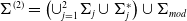


For
 $z\in \Sigma ^{(2)}\setminus \mathbb{R}$
, the jump
$z\in \Sigma ^{(2)}\setminus \mathbb{R}$
, the jump
 $V^{(2)}(z)$
exponentially approaches the identity matrix as
$V^{(2)}(z)$
exponentially approaches the identity matrix as
 $t\to \infty$
. So we expect to only consider the jump on
$t\to \infty$
. So we expect to only consider the jump on
 $\mathbb{R}$
. To arrive at this goal, in this case, we denote
$\mathbb{R}$
. To arrive at this goal, in this case, we denote
 $ U \,:\!=\, U(\xi, c)$
as the union set of neighbourhood of
$ U \,:\!=\, U(\xi, c)$
as the union set of neighbourhood of
 $\pm z_0$
:
$\pm z_0$
:
 \begin{equation} U=U_{+z_0}\cup U_{-z_0},\ U_{\pm z_0}= \left \lbrace z\,:\,|z\mp z_0|\leq \varrho \right \rbrace, \end{equation}
where
 $\varrho$
is a small positive constant such that
$\varrho$
is a small positive constant such that
 $\varrho \lt \min \left \lbrace \frac {z_0-1}{3}, \frac {z_1-z_0}{3} \right \rbrace$
. The stationary point
$\varrho \lt \min \left \lbrace \frac {z_0-1}{3}, \frac {z_1-z_0}{3} \right \rbrace$
. The stationary point
 $\pm z_1$
is on the cut with Im
$\pm z_1$
is on the cut with Im
 $[g_+](z_1)\lt 0$
, which means that the exponential function in
$[g_+](z_1)\lt 0$
, which means that the exponential function in
 $V^{(2)}(z)$
also decays exponentially on
$V^{(2)}(z)$
also decays exponentially on
 $\pm z_1$
. In fact, it is also decays exponentially on
$\pm z_1$
. In fact, it is also decays exponentially on
 $(z_0,z_1]\cup [{-}z_1,z_0)$
. So the contribution of
$(z_0,z_1]\cup [{-}z_1,z_0)$
. So the contribution of
 $\pm z_1$
is small as
$\pm z_1$
is small as
 $t\to \infty$
.
$t\to \infty$
.
Thus, the jump matrix
 $V^{(2)}(z)$
uniformly goes to
$V^{(2)}(z)$
uniformly goes to
 $I$
on
$I$
on
 $\Sigma ^{(2)}\setminus U$
. So outside
$\Sigma ^{(2)}\setminus U$
. So outside
 $U$
there is only exponentially small error (in
$U$
there is only exponentially small error (in
 $t$
) by completely ignoring the jump condition of
$t$
) by completely ignoring the jump condition of
 $M^{(2)}(z)$
. It enlightens us to construct the solution
$M^{(2)}(z)$
. It enlightens us to construct the solution
 $M^{(2)}(z)$
as follow
$M^{(2)}(z)$
as follow
 \begin{equation} M^{(2)}(z)=\left \{\begin{array}{l@{\quad}l} E(z;\,\xi, c)M^{mod}(z;\,\xi, c), & z\notin U_{\pm z_0},\\[3pt] E(z;\,\xi, c)M^{lo,+}(z;\,\xi, c), &z\in U_{+z_0},\\[3pt] E(z;\,\xi, c)M^{lo,-}(z;\,\xi, c), &z\in U_{-z_0},\\[3pt] \end{array}\right . \end{equation}
where
 $M^{mod}(z)$
is the model RH problem on the Riemann surface, which solution is given by theta function in Subsection 5.2.1.
$M^{mod}(z)$
is the model RH problem on the Riemann surface, which solution is given by theta function in Subsection 5.2.1.
 $M^{lo,\pm }(z)$
are local model of
$M^{lo,\pm }(z)$
are local model of
 $\pm z_0$
which solution can be expressed in terms of Airy functions shown in Subsection 5.2.2. And
$\pm z_0$
which solution can be expressed in terms of Airy functions shown in Subsection 5.2.2. And
 $E(z;\,\xi, c)$
is the error function, which will be discussed in subsection 5.2.3 by the small-norm RH problem theory.
$E(z;\,\xi, c)$
is the error function, which will be discussed in subsection 5.2.3 by the small-norm RH problem theory.
5.2.1. Model RH problem on Riemann surface
We consider the following model RH problem with its jump matrix on
 $\mathbb{R}$
.
$\mathbb{R}$
.
RH problem 7.
-
1. Analyticity:
$M^{mod}(z)$
is analytical in
$\mathbb{C}\setminus \Sigma _{mod}$
, where
$\Sigma _{mod}$
is given in (5.2); -
2. Asymptotic behaviours:
$M^{mod}(z) \sim I+\mathcal{O}(z^{-1}),\quad |z| \rightarrow \infty$
; -
3. Jump condition:
$M^{mod}(z)$
satisfies the jump relation
where the jump matrix
\begin{align*}M^{mod}_+(z)=M^{mod}_-(z)V^{mod}(z), \ \ \ z\in \Sigma _{mod},\end{align*}
$V^{mod}(z)$
is given by
(5.12)
\begin{equation} V^{mod}(z)=\left \{ \begin{array}{l@{\quad}l} \left (\begin{array}{c@{\quad}c} 0 & -ie^{-itB_2+w_-}\\[3pt] -ie^{itB_2-w_-} & 0 \end{array}\right ), &\text{as } z\in [{-}c,-z_0], \\[12pt] \left (\begin{array}{c@{\quad}c} 0 & -ie^{-itB_1}\\[3pt] -ie^{itB_1} & 0 \end{array}\right ), &\text{as } z\in \Sigma _-,\\[12pt] \left (\begin{array}{c@{\quad}c} 0 & -ie^{w_+}\\[3pt] -ie^{-w_+} & 0 \end{array}\right ), &\text{as } z\in [z_0,c]. \end{array}\right . \end{equation}
-
4. Singularity:
$M^{mod}(z)$
has at most fourth root singularities at
$z=\pm c,\ \pm 1,\ \pm z_0$
.


The solution
 $M^{mod}$
of the model RH problem can be specifically characterised by
$M^{mod}$
of the model RH problem can be specifically characterised by
 $\Theta$
function on the Riemann surface with genus-2. We define
$\Theta$
function on the Riemann surface with genus-2. We define
 \begin{align*} \mathcal{N}_1(z)=\frac {1}{2} \left (\kappa (z)+\kappa (z)^{-1}\right ),\ \mathcal{N}_2(z)= \frac {1}{2}\left (\kappa (z)^{-1}-\kappa (z)\right ), \end{align*}
where
 $\kappa (z)$
is analytic function for
$\kappa (z)$
is analytic function for
 $z\in \mathbb{C}\setminus \Sigma _{mod},$
 \begin{align*} \kappa (z)&=\left [ \frac {(z-c)(z-1)(z+z_0)}{(z-z_0)(z+1)(z+c)}\right ] ^{\frac {1}{4}}, \ \ \end{align*}
and its branch is fixed by requiring that
 $\kappa (z)=1+\mathcal{O}(z^{-2}), \ \ z\to \infty .$
Let
$\kappa (z)=1+\mathcal{O}(z^{-2}), \ \ z\to \infty .$
Let
 $\omega _i,\ i=1,2$
be the standard holomorphic differentials on the genus 2 Riemann surface
$\omega _i,\ i=1,2$
be the standard holomorphic differentials on the genus 2 Riemann surface
 $\mathcal{M}$
such that
$\mathcal{M}$
such that
 $\int _{a_i}\omega _j=\delta _{ij}$
,
$\int _{a_i}\omega _j=\delta _{ij}$
,
 $i,j=1,2$
. And denote its
$i,j=1,2$
. And denote its
 $b$
-period matrix
$b$
-period matrix
 $\tilde {B}=[\tilde {B}_{ij}]_{i,j=1,2}\in GL_2(\mathbb{C})$
, with
$\tilde {B}=[\tilde {B}_{ij}]_{i,j=1,2}\in GL_2(\mathbb{C})$
, with
 $\tilde {B}_{ij}=\oint _{b_j}\omega _i$
,
$\tilde {B}_{ij}=\oint _{b_j}\omega _i$
,
 $i,j=1,2$
. Define the Abel map
$i,j=1,2$
. Define the Abel map
 \begin{align*} \mathcal{A}\,:\,\mathcal{M}&\to \mathbb{C}^2/\tilde {B}M+N, \ \ M, N\in \mathbb{Z}^2,\\[3pt] P&\mapsto \left (\int _{1}^{P}\omega _1, \ \int _{1}^{P}\omega _2\right )^T. \end{align*}
The theta function
 $\Theta$
associated to
$\Theta$
associated to
 $\tilde {B}$
is defined by
$\tilde {B}$
is defined by
 \begin{align*} \Theta (\vec {u})=\sum _{\vec {l}\in \mathbb{Z}^g}\exp (\pi i\lt \tilde {B}\vec {l},\vec {l}\gt +2\pi i\lt \vec {l},\vec {u}\gt ) \end{align*}
with
 \begin{align*} \Theta (\vec {u}\pm e_j)&= \Theta (\vec {u}),\ \Theta (\vec {u}\pm \tilde {B}e_j)=\exp (\mp 2\pi iu_j-\pi i\tilde {B}_{jj})\Theta (\vec {u}). \end{align*}
Let
 $C=(-\frac {tB_1-w_+}{2\pi },-\frac {tB_2+i(w_{-}-w_+)}{2\pi })^T\in \mathbb{C}^2$
be a column vector. According to [Reference Fay23], there exists a constant
$C=(-\frac {tB_1-w_+}{2\pi },-\frac {tB_2+i(w_{-}-w_+)}{2\pi })^T\in \mathbb{C}^2$
be a column vector. According to [Reference Fay23], there exists a constant
 $\mathcal{K}\in \mathbb{C}^2$
such that
$\mathcal{K}\in \mathbb{C}^2$
such that
 $\Theta (\mathcal{A}(P)-\mathcal{K}),\ \Theta (\mathcal{A}(P)+\mathcal{K})$
have the same zeros as
$\Theta (\mathcal{A}(P)-\mathcal{K}),\ \Theta (\mathcal{A}(P)+\mathcal{K})$
have the same zeros as
 $\mathcal{N}_1(z)$
and
$\mathcal{N}_1(z)$
and
 $\mathcal{N}_2(z)$
, respectively. Define
$\mathcal{N}_2(z)$
, respectively. Define
 \begin{align} M^{mod}(z)= e^{\frac {w_+}{2}\hat {\sigma }_3} \left (\begin{array}{c@{\quad}c} N^{mod}_{11}(\infty )^{-1}\mathcal{N}_{1}N^{mod}_{11}(z)& N^{mod}_{11}(\infty )^{-1}\mathcal{N}_{2}N^{mod}_{12}(z)\\[10pt] N^{mod}_{22}(\infty )^{-1}\mathcal{N}_{2}N^{mod}_{21}(z)& N^{mod}_{22}(\infty )^{-1}\mathcal{N}_{1}N^{mod}_{22}(z)\\[3pt] \end{array}\right ), \end{align}
which is the solution of RH problem7, where
 \begin{align*} N^{mod}(z)= \left (\begin{array}{c@{\quad}c} \frac {\Theta (\mathcal{A}(z)-\mathcal{K}+C)}{\Theta (\mathcal{A}(z)-\mathcal{K})}& \frac {\Theta (-\mathcal{A}(z)-\mathcal{K}+C)}{\Theta (-\mathcal{A}(z)-\mathcal{K})}\\[10pt] \frac {\Theta (\mathcal{A}(z)+\mathcal{K}+C)}{\Theta (\mathcal{A}(z)+\mathcal{K})}& \frac {\Theta (-\mathcal{A}(z)+\mathcal{K}+C)}{\Theta (-\mathcal{A}(z)+\mathcal{K})}\\[3pt] \end{array}\right ),\ N^{mod}(\infty )=\lim _{z\to \infty } N^{mod}(z). \end{align*}
As
 $z\to 0\in \mathbb{C}^+$
, it follows that
$z\to 0\in \mathbb{C}^+$
, it follows that
 \begin{align*} M^{mod}(z)=M^{mod}_+(0)+M^{mod}_1z+\mathcal{O}(z^2), \end{align*}
where
 \begin{align*} &M^{mod}_+(0)= \frac {\sqrt {2}}{2} e^{\frac {w_+}{2}\hat {\sigma }_3}\left (\begin{array}{c@{\quad}c} N^{mod}_{11}(\infty )^{-1}N^{mod}_{11,+}(0)& -iN^{mod}_{11}(\infty )^{-1}N^{mod}_{12,+}(0)\\[10pt] -iN^{mod}_{22}(\infty )^{-1}N^{mod}_{21,+}(0)& N^{mod}_{22}(\infty )^{-1}N^{mod}_{22,+}(0)\\[3pt] \end{array}\right ),\\[3pt] &M^{mod}_1=\frac {\sqrt {2}}{2} \left (\begin{array}{c@{\quad}c}N^{mod}_{11}(\infty )^{-1}& 0\\[10pt] 0& N^{mod}_{22}(\infty )^{-1}\\[3pt] \end{array}\right )\\[3pt] & e^{\frac {w_+}{2}\hat {\sigma }_3}\left [\left (\begin{array}{c@{\quad}c} \partial _zN^{mod}_{11,+}(0)& -i \partial _zN^{mod}_{12,+}(0)\\[10pt] -i \partial _zN^{mod}_{21,+}(0)& \partial _zN^{mod}_{22,+}(0)\\[3pt] \end{array}\right )+ \left(1-\frac {1}{z_0}+\frac {1}{c} \right) \left (\begin{array}{c@{\quad}c} -iN^{mod}_{11,+}(0)& N^{mod}_{12,+}(0)\\[10pt] N^{mod}_{21,+}(0)& -iN^{mod}_{22,+}(0)\\[3pt] \end{array}\right )\right ]. \end{align*}
5.2.2. Localised RH problem near stationary points
Using local approximations, appropriate error estimates as well as higher-order asymptotics beyond the
 $\mathcal{O}(1)$
term can be derived. In this subsection, we only give the details of the model around
$\mathcal{O}(1)$
term can be derived. In this subsection, we only give the details of the model around
 $z_0$
. We consider
$z_0$
. We consider
 $M^{lo,+}(z)$
here as an example. First, we denote
$M^{lo,+}(z)$
here as an example. First, we denote
 $P(z_0)$
as the neighbourhood of
$P(z_0)$
as the neighbourhood of
 $z_0$
in the Riemann surface
$z_0$
in the Riemann surface
 $\mathcal{M}$
corresponding to
$\mathcal{M}$
corresponding to
 $dg$
. It is an analytic homeomorphism. It follows form the definition of d
$dg$
. It is an analytic homeomorphism. It follows form the definition of d
 $g$
in (5.1)–(5.3) that there exist a holomorphic function
$g$
in (5.1)–(5.3) that there exist a holomorphic function
 $f_+$
(we hope the subscript
$f_+$
(we hope the subscript
 $\pm$
indicates
$\pm$
indicates
 $\pm z_0$
) on
$\pm z_0$
) on
 $P(z_0)$
such that
$P(z_0)$
such that
 \begin{align*} g=-\frac {2i}{3}f_+^3. \end{align*}
Here, on the complex plane, because
 $g_+(z) \subset i\mathbb{R}^-$
when
$g_+(z) \subset i\mathbb{R}^-$
when
 $z\in \left ( z_0,c\right )$
, we can choose
$z\in \left ( z_0,c\right )$
, we can choose
 $f_+\in \mathbb{R}^+$
on
$f_+\in \mathbb{R}^+$
on
 $\left ( z_0,c\right ) \cap U_{+z_0}$
. Let
$\left ( z_0,c\right ) \cap U_{+z_0}$
. Let
 \begin{equation} \lambda _+=t^{\frac {2}{3}}f_+^2. \end{equation}
Because of
 $g_+(z)=-g_-(z)$
,
$g_+(z)=-g_-(z)$
,
 $\lambda _+ \,:\!=\, \lambda _+(z)$
is a holomorphic homeomorphism from
$\lambda _+ \,:\!=\, \lambda _+(z)$
is a holomorphic homeomorphism from
 $U_{+z_0}$
to a neighbourhood of zero and
$U_{+z_0}$
to a neighbourhood of zero and
 \begin{align*} \frac {4}{3}\lambda _+^{\frac {3}{2}}=2itg_+, \ \ z\in \left ( z_0,c\right ) \cap U_{+z_0}, \end{align*}
where the branch cut of
 $(\cdot )^{\frac {3}{2}}$
is chosen same as in the Airy model in the Appendix A.
$(\cdot )^{\frac {3}{2}}$
is chosen same as in the Airy model in the Appendix A.
From the definition of
 $\lambda _+$
, it follows that
$\lambda _+$
, it follows that
 \begin{eqnarray*} \frac {4}{3}\lambda _+^{\frac {3}{2}}=2itg,\ \ \text{Im}z\gt 0,\ \ \ \frac {4}{3}\lambda _+^{\frac {3}{2}}=-2itg,\ \ \text{Im}z\lt 0. \end{eqnarray*}
Then we explicitly define
 $M^{lo,+}(z)$
which should have the same jump condition with
$M^{lo,+}(z)$
which should have the same jump condition with
 $M^{(2)}(z)$
locally in
$M^{(2)}(z)$
locally in
 $U_{+z_0}$
as follow via the Airy parametrix. Similar to [Reference de Monvel, Lenells and Shepelsky6, Reference Fromm, Lenells and Quirchmayr25, Reference Grava and Minakov29], it is shown that
$U_{+z_0}$
as follow via the Airy parametrix. Similar to [Reference de Monvel, Lenells and Shepelsky6, Reference Fromm, Lenells and Quirchmayr25, Reference Grava and Minakov29], it is shown that
 \begin{align} M^{lo,+}(z)=\frac {\sqrt {2}}{2}M^{mod}H(z;\,z_0)^{-1}\left (I-i\sigma _1\right )\lambda _+^{\frac {\sigma _3}{4}}m^{Ai}(\lambda _+)H(z;\,z_0), \end{align}
where
 \begin{align*} H(z;\,z_0)=\left \{ \begin{array}{l@{\quad}l} \delta ^{\sigma _3}r_1^{\frac {\sigma _3}{2}},\quad z-z_0\in \mathbb{C}^+\cap U_{+z_0},\\[3pt] \sigma _3\sigma _1\delta ^{\sigma _3}r_2^{-\frac {\sigma _3}{2}}, \ z-z_0\in \mathbb{C}^-\cap U_{+z_0}. \end{array} \right . \end{align*}
Moreover, for convenience, denote
 \begin{align} F^+(z) \,:\!=\, F^+(z;\,\xi, c)=\frac {\sqrt {2}}{2}M^{mod}(z;\,\xi, c)H(z;\pm z_0)^{-1}\left (I-i\sigma _1\right )f_+^{\frac {1}{2}\sigma _3}, \end{align}
which thereby is an analytic and invertible function in
 $U_{+z_0}$
. Similarly,
$U_{+z_0}$
. Similarly,
 \begin{align} M^{lo,-}(z)=\frac {\sqrt {2}}{2}M^{mod}H(z;-z_0)^{-1}\left (I-i\sigma _1\right )\lambda _-^{\frac {\sigma _3}{4}}m^{Ai}(\lambda _-)H(z;-z_0). \end{align}
with
 \begin{align*} &H(z;-z_0)=\left \{ \begin{array}{l@{\quad}l} e^{\frac {itB_2}{2}\sigma _3}\sigma _3\delta ^{\sigma _3}r_1^{\frac {\sigma _3}{2}},& z-z_0\in \mathbb{C}^+\cap U_{-z_0},\\[3pt] e^{\frac {itB_2}{2}\sigma _3}\sigma _1\delta ^{\sigma _3}r_2^{-\frac {\sigma _3}{2}},& z-z_0\in \mathbb{C}^-\cap U_{-z_0}, \end{array} \right .\\[3pt] &g=-\frac {2i}{3}f_-^3+\frac {B_2}{2},\qquad \lambda _-=t^{\frac {2}{3}}f_-^2, \end{align*}
where
 $f_-\in \mathbb{R}+$
on
$f_-\in \mathbb{R}+$
on
 $z\in (-c,-z_0)\cap U_{-z_0}$
and
$z\in (-c,-z_0)\cap U_{-z_0}$
and
 \begin{align} F^- \,:\!=\, M^{mod}H(z;-z_0)^{-1}\left (I-i\sigma _1\right )\lambda _-^{\frac {\sigma _3}{4}} \end{align}
is an analytic and invertible function in
 $U_{-z_0}$
. Moreover, as
$U_{-z_0}$
. Moreover, as
 $z\to z_0$
in
$z\to z_0$
in
 $\mathbb{C}\setminus [z_0,c]$
,
$\mathbb{C}\setminus [z_0,c]$
,
 $\lambda _+$
has expansion
$\lambda _+$
has expansion
 \begin{align*} \lambda _+=(\tilde {A}_+)^{\frac {2}{3}}(z-z_0)+\frac {2\tilde {B}_+}{3\tilde {A}_+^{\frac {1}{3}}}(z-z_0)^2+\mathcal{O}((z-z_0)^3),\\[3pt] \lambda _-=(\tilde {A}_-)^{\frac {2}{3}}(z+z_0)+\frac {2\tilde {B}_-}{3\tilde {A}_-^{\frac {1}{3}}}(z+z_0)^2+\mathcal{O}((z+z_0)^3), \end{align*}
where
 \begin{align} \tilde {A}_+=&\frac {t}{2} \left (\frac {2z_0}{(z_0^2-1)(c^2-z_0^2)}\right )^{\frac {1}{2}}\left ( \frac {\xi -1}{2}z_0+\frac {c}{z_0^2}(1+\frac {1}{c^2})-\frac {3c}{z_0^4}\right ),\nonumber \\[6pt]\tilde {B}_+=&\frac {3t}{10}\left [{-}\frac {1}{2}(\frac {2z_0}{(z_0^2-1)(c^2-z_0^2)})^{-\frac {1}{2}}\frac {-7z_0^4+3(1+c^2)z_0^2+c^2}{(z_0^2-1)^2(c^2-z_0^2)^2} \left (\frac {\xi -1}{2}z_0+\frac {c}{z_0^2}\left(1+\frac {1}{c^2} \right)-\frac {3c}{z_0^4}\right )\right .\nonumber \\[4pt]&\left .+\left(\frac {2z_0}{(z_0^2-1)(c^2-z_0^2)}\right)^{\frac {1}{2}}\left(\frac {\xi -1}{2}-\frac {c}{z_0^3}\left(1+\frac {1}{c^2}-\frac {1}{z_0^2}\right)+\frac {6c}{z_0^5}\right)\right ],\nonumber \\[6pt]\tilde {A}_-=&-\frac {it}{2}\left (\frac {2z_0}{(z_0^2-1)(c^2-z_0^2)}\right )^{\frac {1}{2}}\left (-\frac {\xi -1}{2}z_0+\frac {c}{z_0^2}\left(1+\frac {1}{c^2}\right)-\frac {3c}{z_0^4}\right ),\nonumber \\[4pt]\tilde {B}_-=&\frac {3t}{10}\left [{-}\frac {i}{2}\left(\frac {2z_0}{(z_0^2-1)(c^2-z_0^2)}\right)^{-\frac {1}{2}}\frac {-7z_0^4+3(1+c^2)z_0^2+c^2}{(z_0^2-1)^2(c^2-z_0^2)^2} \left(-\frac {\xi -1}{2}z_0+\frac {c}{z_0^2}\left(1+\frac {1}{c^2} \right)-\frac {3c}{z_0^4} \right)\right .\nonumber \\[4pt] &\left .-i\left(\frac {2z_0}{(z_0^2-1)(c^2-z_0^2)}\right)^{\frac {1}{2}}\left(\frac {\xi -1}{2}+\frac {c}{z_0^3}\left(1+\frac {1}{c^2}-\frac {1}{z_0^2}\right)-\frac {6c}{z_0^5}\right)\right ]. \end{align}
5.2.3. The small norm RH problem for error function
In this subsection, we consider the error matrix-function
 $E(z) \,:\!=\, E(z;\,\xi, c)$
in this region.
$E(z) \,:\!=\, E(z;\,\xi, c)$
in this region.
RH problem 8.
-
1. Analyticity:
$E(z)$
is analytical in
$\mathbb{C}\setminus \Sigma ^{ E }$
, where
with
\begin{align*}\Sigma ^{ E }= \partial U\cup \left [ \Sigma ^{(2)}\setminus \left ( U\cup [{-}c,-z_1]\cup \Sigma _-\cup [z_1,c]\right ) \right ] \end{align*}
$U$
defined in (5.10);
-
2. Asymptotic behaviours:
$E(z) \sim I+\mathcal{O}(z^{-1}),\qquad |z| \rightarrow \infty$
; -
3. Jump condition:
$E(z)$
has continuous boundary values
$E_\pm (z)$
on
$\Sigma ^{E}$
satisfying
$E_+(z)=E_-(z)V^{ E }(z),$
where the jump matrix
$V^{E}(z)$
is given by
(5.20)which is shown in Figure 9 .
\begin{equation} V^{ E }(z)=\left \{\begin{array}{l@{\quad}l@{\quad}l@{\quad}l} M^{mod}(z)V^{(2)}(z)M^{mod}(z)^{-1}, & z\in \Sigma ^{ E }\setminus \partial U,\\[4pt] M^{lo,\pm }(z)M^{mod}(z)^{-1}, & z\in \partial U_{\pm z_0}, \end{array}\right . \end{equation}


By (5.15), (5.17) and (A.5), the jump matrix of above RH problem satisfies
 \begin{align*} \parallel V^{E}(z)-I\parallel _2 \lesssim \mathcal{O}(t^{-1}). \end{align*}
Similar to the discussion in Subsection 3.2, the RH problem8 admits a unique solution given by
 \begin{equation} E(z)=I+\frac {1}{2\pi i}\int _{\Sigma ^{ E }}\dfrac {\left ( I+\varpi (s)\right ) (V^{E}(s)-I)}{s-z}ds, \end{equation}
where the
 $\varpi \in L^\infty (\Sigma ^{ E })$
is the unique solution of
$\varpi \in L^\infty (\Sigma ^{ E })$
is the unique solution of
 $ (1-C_E)\varpi =C_E\left (I \right ).$
The jump contour
 $\Sigma ^{E}$
for the
$\Sigma ^{E}$
for the
 $E(z)$
. The red circles are
$E(z)$
. The red circles are
 $\partial U$
.
$\partial U$
.

In order to reconstruct the solution
 $u(y,t)$
of (1.1), we need the asymptotic behaviour of
$u(y,t)$
of (1.1), we need the asymptotic behaviour of
 $E(z)$
as
$E(z)$
as
 $z\to 0\in \mathbb{C}^+$
and the long-time asymptotic behaviour of
$z\to 0\in \mathbb{C}^+$
and the long-time asymptotic behaviour of
 $E(0)$
.
$E(0)$
.
Proposition 8.
As
 $z\to 0\in \mathbb{C}^+$
, we have
$z\to 0\in \mathbb{C}^+$
, we have
 \begin{align*} E(z)=E(0)+E_1z+\mathcal{O}(z^2), \end{align*}
with long-time asymptotic behaviour
 \begin{equation} E(0)=I+t^{-1}H^{(0)}+\mathcal{O}(t^{-2}). \end{equation}
And
 \begin{align*} H^{(0)} \,:\!=\, H^{(0)}(\xi, c)=&\sum _{ p=\pm z_0 }\partial _z\left (\frac {1 }{z}F^{\pm }\left (\begin{array}{c@{\quad}c} 0&-\frac {5i}{48}\tilde {A}_\pm ^{-\frac {4}{3}}\\[3pt] 0&0\\[3pt] \end{array}\right )(F^\pm )^{-1}\right )(p)\\[3pt] &+\sum _{ p=\pm z_0 }\frac {1 }{p}\left ( F^{\pm }\left (\begin{array}{c@{\quad}c} 0&\frac {5}{36}\tilde {B}_\pm \tilde {A}^{-\frac {7}{3}}_\pm \\[3pt] -\frac {7i}{48}\tilde {A}^{-\frac {2}{3}}_\pm &0\\[3pt] \end{array}\right )(F^\pm )^{-1}\right )(p). \end{align*}
Here,
 $\tilde {B}_\pm$
,
$\tilde {B}_\pm$
,
 $\tilde {A}_\pm$
are given in (5.19). And
$\tilde {A}_\pm$
are given in (5.19). And
 \begin{align*} E_1 \,:\!=\, E_1(\xi, c)=\frac {1}{2\pi i}\int _{\Sigma ^{E}}\dfrac {\left ( I+\varpi (s)\right ) (V^{ E }-I)}{s^2}ds, \end{align*}
satisfies long-time asymptotic behaviour condition
 \begin{equation} E_1=t^{-1}H^{(1)}+\mathcal{O}(t^{-2}), \end{equation}
where
 \begin{align*} H^{(1)} \,:\!=\, H^{(1)}(\xi, c)=&\sum _{ p=\pm z_0 }\partial _z\left (\frac {1 }{z^2}F^{\pm }\left (\begin{array}{c@{\quad}c} 0&-\frac {5i}{48}\tilde {A}_\pm ^{-\frac {4}{3}}\\[3pt] 0&0\\[3pt] \end{array}\right )(F^\pm )^{-1}\right )(p)\\[3pt] &+\sum _{ p=\pm z_0 }\frac {1 }{p^2}\left ( F^{\pm }\left (\begin{array}{c@{\quad}c} 0&\frac {5}{36}\tilde {B}_\pm \tilde {A}^{-\frac {7}{3}}_\pm \\[3pt] -\frac {7i}{48}\tilde {A}^{-\frac {2}{3}}_\pm &0\\[3pt] \end{array}\right )(F^\pm )^{-1}\right )(p). \end{align*}
Proof. By using expansion of
 $V^{ E }$
and
$V^{ E }$
and
 $\varpi (s)=\mathcal{O}(t^{-1})$
, we have
$\varpi (s)=\mathcal{O}(t^{-1})$
, we have
 \begin{align*} &\int _{\Sigma ^{E}}\dfrac {\left ( I+\varpi (s)\right ) (V^{E}-I)}{s}ds=\frac {1}{t}\int _{\partial U_{\pm z_0}}\dfrac { M^{mod}H(s;\pm z_0)^{-1} m^{Ai}_1H(s;\pm z_0)(M^{mod})^{-1}}{sf_\pm ^{3}}ds+\mathcal{O}(t^{-2}). \end{align*}
From the definition of
 $F^\pm$
in (5.16) and (5.18), we rewrite
$F^\pm$
in (5.16) and (5.18), we rewrite
 \begin{align*} M^{mod}H(s;\pm z_0)^{-1}& m^{Ai}_1H(s;\pm z_0)(M^{mod})^{-1}\\[3pt] &=\frac {1}{2}F^\pm f_\pm ^{-\frac {\sigma _3}{2}}\left (I+i\sigma _1\right )m^{Ai}_1\left (I-i\sigma _1\right )f_\pm ^{\frac {\sigma _3}{2}}(F^\pm )^{-1}. \end{align*}
Here, from (5.19) and
 $m^{Ai}_1$
in Appendix A, as
$m^{Ai}_1$
in Appendix A, as
 $z\to z_0\in \mathbb{C}^+$
, we have
$z\to z_0\in \mathbb{C}^+$
, we have
 \begin{align*} &\frac {1}{2}f_\pm ^{-3}f_\pm ^{-\frac {\sigma _3}{2}}\left (I+i\sigma _1\right )m^{Ai}_1\left (I-i\sigma _1\right )f_\pm ^{\frac {\sigma _3}{2}}=\\[3pt] &\frac {1}{(z\mp z_0)^2}\left (\begin{array}{c@{\quad}c} 0&-\frac {5i}{48}\tilde {A}_\pm ^{-\frac {4}{3}}\\[3pt] 0&0\\[3pt] \end{array}\right )+\frac {1}{(z\mp z_0)} \left (\begin{array}{c@{\quad}c} 0&\frac {5}{36}\tilde {B}_\pm \tilde {A}^{-\frac {7}{3}}_\pm \\[3pt] -\frac {7i}{48}\tilde {A}^{-\frac {2}{3}}_\pm &0\\[3pt] \end{array}\right )+\mathcal{O}(1). \end{align*}
Then by residue theorem, we finally arrive at the result.
5.3.
Opening the jump in the region
$3/4\lt \xi \lt 1$

This region includes two cases:
-
(1)
$\left \{ (\xi, c)\,:\,2\lt c^2\lt 4, 1-\frac {2(c^2-2)}{c^4} \lt \xi \lt 1\right \}$
; -
(2)
$\left \{(\xi, c)\,:\,c^2\gt 4, \xi _m\lt \xi \lt 1\right \}$
.


In both cases we introduce the same
 $g$
function by
$g$
function by
 \begin{align*} \text{d}g=\dfrac { Y(z)}{z^3}\left [ \frac {1-\xi }{2}z^4-\frac {c}{z_0}\left ( 1+\frac {1}{c^2}-\frac {1}{z_0^2}\right ) z^2+\frac {2c}{z_0}\right ] \text{d}z \end{align*}
which will have another zero on
 $\mathbb{R}$
except on cut. It means that
$\mathbb{R}$
except on cut. It means that
 $g$
has three pairs of stationary points on
$g$
has three pairs of stationary points on
 $\mathbb{R}$
, which will gives additional contribution as
$\mathbb{R}$
, which will gives additional contribution as
 $t\to \infty$
. The stationary points of
$t\to \infty$
. The stationary points of
 $g$
are
$g$
are
 $\pm z_0$
and the zeros of the equation
$\pm z_0$
and the zeros of the equation
 \begin{align*} \frac {1-\xi }{2}z^4-\frac {c}{z_0}\left ( 1+\frac {1}{c^2}-\frac {1}{z_0^2}\right ) z^2+\frac {2c}{z_0}=0. \end{align*}
It has two pairs of zeros on
 $\mathbb{R}$
:
$\mathbb{R}$
:
 $\pm z_1\in (z_0,c)$
,
$\pm z_1\in (z_0,c)$
,
 $\pm z_2$
. Note that,
$\pm z_2$
. Note that,
 $z_1^2z_2^2=\frac {4c}{z_0(1-\xi )}$
. For a given
$z_1^2z_2^2=\frac {4c}{z_0(1-\xi )}$
. For a given
 $c$
, when
$c$
, when
 $\xi$
decreases from
$\xi$
decreases from
 $1$
,
$1$
,
 $z_2$
as a function of
$z_2$
as a function of
 $\xi$
decreases from
$\xi$
decreases from
 $+\infty$
. We denote
$+\infty$
. We denote
 $\xi _m$
as the critical condition of
$\xi _m$
as the critical condition of
 $\xi$
that stationary point
$\xi$
that stationary point
 $z_2$
merge
$z_2$
merge
 $c$
. Under this case, the sign table of Im
$c$
. Under this case, the sign table of Im
 $g$
is shown in Figure 10.
$g$
is shown in Figure 10.
Similar to the above section, we define the contour
 $\Sigma _j$
and closed region
$\Sigma _j$
and closed region
 $\Omega _j$
relying on
$\Omega _j$
relying on
 $(\xi, c)$
as in Figure 10. Here the angle of
$(\xi, c)$
as in Figure 10. Here the angle of
 $\Sigma _j$
is a small enough positive constant such that
$\Sigma _j$
is a small enough positive constant such that
 $\Sigma _j,\ j=1,2$
are contained in the region of Im
$\Sigma _j,\ j=1,2$
are contained in the region of Im
 $g\gt 0$
.
$g\gt 0$
.
The domains
 $\Omega _j$
and curves
$\Omega _j$
and curves
 $\Sigma _j$
,
$\Sigma _j$
,
 $j=1,2$
. The yellow region means Im
$j=1,2$
. The yellow region means Im
 $[g](z)\lt 0$
while white region means Im
$[g](z)\lt 0$
while white region means Im
 $[g](z)\gt 0$
.
$[g](z)\gt 0$
.

In this region of
 $(\xi, c)$
, we introduce a piecewise matrix interpolation function
$(\xi, c)$
, we introduce a piecewise matrix interpolation function
 \begin{equation} G(z) \,:\!=\, G(z;\,\xi, c)=\left \{ \begin{array}{l@{\quad}l} \left (\begin{array}{c@{\quad}c} 1 & -r_2e^{-2itg}\\[3pt] 0 & 1 \end{array}\right ), &\text{as } z\in \Omega _1;\\[12pt] \left (\begin{array}{c@{\quad}c} 1 & 0\\[3pt] -r_1e^{2itg} & 1 \end{array}\right ), &\text{as } z\in \Omega _1^*;\\[3pt] \left (\begin{array}{c@{\quad}c} 1 &0\\[3pt] \frac {r_1e^{2itg}}{1-r_1r_2} & 1 \end{array}\right ), &\text{as } z\in \Omega _2;\\[12pt] \left (\begin{array}{c@{\quad}c} 1 &\frac { r_2e^{-2itg}}{1-r_1r_2}\\[3pt] 0 & 1 \end{array}\right ), &\text{as } z\in \Omega _2^*;\\[12pt] I &\text{as } z \text{ in elsewhere}, \end{array}\right .. \end{equation}
Same as above section,
 $ G (z)$
brings a new singularity. To deal with the jump on
$ G (z)$
brings a new singularity. To deal with the jump on
 $\mathbb{R}$
, we introduce an auxiliary function
$\mathbb{R}$
, we introduce an auxiliary function
 $\delta (z) \,:\!=\, \delta (z;\,\xi, c)$
. Define
$\delta (z) \,:\!=\, \delta (z;\,\xi, c)$
. Define
 $Y_3(z)= (z^2-1)(z^2-c^2)Y(z),$
and
$Y_3(z)= (z^2-1)(z^2-c^2)Y(z),$
and
 \begin{align*} \log \delta (z)=&\frac {Y_3(z)}{2\pi i}\sum _{\pm }\mp \int _{\pm c}^{\pm z_0} \dfrac {\log\!(ir_{2,-}(s))-w_\pm }{(s-z)Y_{3,+}(s)}ds +\frac {Y_3(z)}{2\pi i}\left ( \int _{-z_2}^{-c}+\int _{c}^{z_2}\right ) \dfrac {\log\!(1-r_1(s)r_2(s))}{(s-z)Y_3(s)}ds, \end{align*}
where
 \begin{align*} \begin{pmatrix} \int _{-c}^{-z_0}\dfrac {ds}{Y_{3,+}(s)}&\int _{z_0}^{c}\dfrac {ds}{Y_{3,+}(s)}\\[3pt] \int _{-c}^{-z_0}\dfrac {sds}{Y_{3,+}(s)}&\int _{z_0}^{c}\dfrac {sds}{Y_{3,+}(s)}\\[3pt] \end{pmatrix}\begin{pmatrix} w_-\\[3pt]w_+\\[3pt] \end{pmatrix}=\begin{pmatrix} \int _{\Sigma _+\setminus [{-}z_0,z_0]} \dfrac {\log\!(ir_{2,-}(s))}{Y_{3,+}(s)}ds+\int _{[{-}z_2,z_2]\setminus \Sigma _+}\dfrac {\log\!(1-r_1(s)r_2(s))}{Y_3(s)}ds\\[3pt] \int _{\Sigma _+\setminus [{-}z_0,z_0]} \dfrac {s\log\!(ir_{2,-}(s))}{Y_{3,+}(s)}ds+\int _{[{-}z_2,z_2]\setminus \Sigma _+}\dfrac {s\log\!(1-r_1(s)r_2(s))}{Y_3(s)}ds\\[3pt] \end{pmatrix}. \end{align*}
 $\delta (z)$
admits the following jump condition
$\delta (z)$
admits the following jump condition
 \begin{align*} &\delta _+(z)=\delta _-(z)(1-r_1r_2), \qquad z\in [{-}z_2,z_2]\setminus \Sigma _+;\\[3pt] &\delta _-(z)\delta _+(z)=ir_{2,-}(z)e^{-w_\pm }, \quad z\in \mp [\pm c, \pm z_0];\\[3pt] &\delta _-(z)\delta _+(z)=1, \qquad \qquad z\in \Sigma _-. \end{align*}
and the following proposition
Proposition 9.
The scalar function
 $\delta (z)$
satisfies the following properties
$\delta (z)$
satisfies the following properties
-
(a)
$\delta (z)$
is analytic on
$\mathbb{C}\setminus \left ( ({-}z_2,-z_0)\cup \Sigma _-\cup (z_0,z_2)\right )$
; -
(b)
$\delta (z)$
has singularity at
$z=\pm c$
with
(5.25)
\begin{align} \delta (z)=\mathcal{O}(z-p)^{\mp 1/4}, \quad z\in \mathbb{C}^\pm \setminus \mathbb{R} \to p, \quad p=c,-c. \end{align}
-
(c) As
$z\to \infty \in \mathbb{C}\setminus \mathbb{R}$
,
$\delta (z)\sim \delta _\infty$
with
\begin{align*} \log \delta _\infty =&-\frac {1}{2\pi i}\int _{\Sigma _+\setminus [{-}z_0,z_0]} \dfrac {s^2\log\!(ir_{2,-}(s))}{Y_{3,+}(s)} ds-\frac {1}{2\pi i}\int _{[{-}z_2,z_2]\setminus \Sigma _+}\dfrac {s^2\log\!(1-r_1(s)r_2(s))}{Y_3(s)}ds. \end{align*}
-
(d) As
$z\to 0\in \mathbb{C}^+$
,(5.26)where
\begin{align} \delta (z)=&\delta _+(0)\left ( 1+\delta ^{(1)}z\right ) +\mathcal{O}(z^2), \end{align}
\begin{align*} & \delta ^{(1)}= \frac {cz_0}{2\pi }\left (\int _{-c}^{-z_0}+\int _{z_0}^{c} \right ) \dfrac {\log\!(ir_{2,-}(s))}{s^2Y_{3,+}(s)}ds +\frac {cz_0}{2\pi }\left ( \int _{-z_2}^{-c}+\int _{c}^{z_2}\right )\dfrac {\log\!(1-r_1(s)r_2(s))}{s^2Y_3(s)}ds; \end{align*}
-
(e) For
$z_2$
, there exists an analytic function
$\delta _{+z_2}(z)$
on
$z\in U_{+z_2}\setminus (c,z_2)$
which is continuous to the boundary such that for
$\nu (z_2)= \frac {1}{2\pi }\log\!(1-r_1(z_2)r_2(z_2) )$
,


 \begin{align} \delta (z)= \delta _{\pm z_2}(z)(z-z_2)^{-i\nu (z_2)}, \quad \arg\!(z-z_2)\in (-\pi, \pi ), \end{align}
and
 \begin{align*} \left |\delta _{+z_2}(z)-\delta _{+z_2}(z_2)\right |\lesssim \left |z-z_2\right |. \end{align*}
Through
 $\delta (z)$
and
$\delta (z)$
and
 $G(z)$
, in this region of
$G(z)$
, in this region of
 $(\xi, c)$
, same as above subsection, we give series of transformations:
$(\xi, c)$
, same as above subsection, we give series of transformations:
 \begin{align*} N\overset {(5.7)}{\longrightarrow } M^{(1)} \overset {(5.9)}{\longrightarrow }M^{(2)}=\delta _\infty ^{-\sigma _3}e^{itg(\infty )\sigma _3}Ne^{it(p-_-g)\sigma _3}\delta ^{\sigma _3}, \end{align*}
which then satisfies the following RH problem.
RH problem 9.
-
1. Analyticity:
$M^{(2)}(z)$
is meromorphic in
$\mathbb{C}\setminus \Sigma ^{(2)}$
with
where
\begin{align*} \Sigma ^{(2)}=\cup _{j=1}^2\left (\Sigma _j\cup \Sigma _j^*\right ) \cup \Sigma _{mod}, \end{align*}
$\Sigma _{mod}$
is given in (5.2)
-
2. Symmetry:
$M^{(2)}(z)=\sigma _2M^{(2)}({-}z)\sigma _2^{-1}$
=
$\sigma _1\overline {M^{(2)}(\bar {z})}\sigma _1$
; -
3. Asymptotic behaviours:
$M^{(2)}(z) = I+\mathcal{O}(z^{-1}),\qquad z \rightarrow \infty$
; -
4. Jump condition:
$M^{(2)}$
has continuous boundary values
$M^{(2)}_\pm (z)$
on
$\Sigma ^{(2)}$
and
(5.28)where
\begin{equation} M^{(2)}_+(z)=M^{(2)}_-(z)V^{(2)}(z),\qquad z \in \Sigma ^{(2)}, \end{equation}
\begin{align*} &V^{(2)}(z)= \left (\begin{array}{c@{\quad}c} 1 & r_2\delta ^{-2}e^{-2itg}\\[3pt] 0 & 1 \end{array}\right ), \text{ } z\in \Sigma _1;\quad V^{(2)}(z)=\left (\begin{array}{c@{\quad}c} 1 & 0\\[3pt] -r_1\delta ^2e^{2itg} & 1 \end{array}\right ), \text{ } z\in \Sigma _1^*;\\[3pt] &V^{(2)}(z)=\left (\begin{array}{c@{\quad}c} 1 &0\\[3pt] \frac {-r_1\delta ^2e^{2itg}}{1-r_1r_2} & 1 \end{array}\right ),\text{ } z\in \Sigma _2;\quad V^{(2)}(z)=\left (\begin{array}{c@{\quad}c} 1 &\frac { r_2\delta ^{-2}e^{-2itg}}{1-r_1r_2}\\[3pt] 0 & 1 \end{array}\right ),\text{ } z\in \Sigma _2^*;\\[3pt] &V^{(2)}(z)= \left (\begin{array}{c@{\quad}c} 0 & -ie^{-itB_2+w_-}\\[3pt] -ie^{itB_2-w_-} & 0 \end{array}\right ), \text{ } z\in [{-}c,-z_1] ;\quad V^{(2)}(z)=\left (\begin{array}{c@{\quad}c} 0 & -ie^{w_+}\\[3pt] -ie^{-w_+} & 0 \end{array}\right ), \text{ } z\in [z_1,c] ;\\[3pt] &V^{(2)}(z)= \left (\begin{array}{c@{\quad}c} 0 & -ie^{-itB_1}\\[3pt] -ie^{itB_1} & 0 \end{array}\right ), \text{ } z\in \Sigma _-;\quad V^{(2)}(z)= \left (\begin{array}{c@{\quad}c} 0 & -ie^{w_+}\\[3pt] -ie^{-w_+} & \frac {\delta _-}{\delta _+}e^{-2itg_+} \end{array}\right ), \text{ } z\in [z_0,z_1];\\[3pt] &V^{(2)}(z)= \left (\begin{array}{c@{\quad}c} 0 & -ie^{-itB_2+w_-}\\[3pt] -ie^{itB_2-w_-} & \frac {\delta _-}{\delta _+}e^{itB_2}e^{-2itg_+} \end{array}\right ), \text{ } z\in [{-}z_1,-z_0] ; \end{align*}
-
5. Singularity:
$M^{(2)}(z)$
has at most fourth root singularities at
$z=\pm c,\ \pm 1$
.


Except the cut away from
 $\mathbb{R}$
, the jump
$\mathbb{R}$
, the jump
 $ {V}^{(2)}(z)$
exponentially approaches the identity matrix as
$ {V}^{(2)}(z)$
exponentially approaches the identity matrix as
 $t\to \infty$
. So we expect to only consider the jump on
$t\to \infty$
. So we expect to only consider the jump on
 $\mathbb{R}$
. However, different from above section, in this region,
$\mathbb{R}$
. However, different from above section, in this region,
 $g$
has another pair of stationary points on
$g$
has another pair of stationary points on
 $\mathbb{R}$
. So in this case, we denote
$\mathbb{R}$
. So in this case, we denote
 $ U \,:\!=\, U(\xi, c)$
as the union set of neighbourhood of
$ U \,:\!=\, U(\xi, c)$
as the union set of neighbourhood of
 $\pm z_0$
and
$\pm z_0$
and
 $\pm z_2$
 \begin{equation} U=U_{\pm z_0}\cup U_{\pm z_2},\ U_{\pm z_j}= \left \lbrace z\,:\,|z\mp z_j|\leq \varrho \right \rbrace, \ j=0,2. \end{equation}
Here,
 $\varrho$
is a small positive constant such that
$\varrho$
is a small positive constant such that
 $\varrho \lt \min \left \lbrace \frac {z_0-1}{3}, \frac {z_1-z_0}{3},\frac {z_2-c}{3},\epsilon \right \rbrace$
. Outside
$\varrho \lt \min \left \lbrace \frac {z_0-1}{3}, \frac {z_1-z_0}{3},\frac {z_2-c}{3},\epsilon \right \rbrace$
. Outside
 $U$
there is only exponentially small error (in
$U$
there is only exponentially small error (in
 $t$
) by completely ignoring the jump condition of
$t$
) by completely ignoring the jump condition of
 $M^{(2)}(z)$
. This proposition enlightens us to construct the solution
$M^{(2)}(z)$
. This proposition enlightens us to construct the solution
 $M^{(2)}(z)$
as follow
$M^{(2)}(z)$
as follow
 \begin{align*} M^{(2)}(z)= \left \{\begin{array}{l@{\quad}l} E(z;\,\xi, c)M^{mod}(z;\,\xi, c), & z\notin U,\\[4pt] E(z;\,\xi, c)M^{0,\pm }(z;\,\xi, c), &z\in U_{\pm z_0},\\[4pt] E(z;\,\xi, c)M^{mod}(z;\,\xi, c)M^{2,\pm }(z;\,\xi, c), &z\in U_{\pm z_2},\\[3pt] \end{array}\right . \end{align*}
where same as
 $M^{mod}(z;\,\xi, c)$
is the model RH problem on the Riemann surface, which solution is given by theta function in Subsection 5.2.1. The difference is
$M^{mod}(z;\,\xi, c)$
is the model RH problem on the Riemann surface, which solution is given by theta function in Subsection 5.2.1. The difference is
 $M^{j,\pm }(z;\,\xi, c)$
are local model of
$M^{j,\pm }(z;\,\xi, c)$
are local model of
 $\pm z_j$
,
$\pm z_j$
,
 $j=0,2$
. When
$j=0,2$
. When
 $j=2$
, its solution can be expressed in terms of parabolic cylinder parametrix. When
$j=2$
, its solution can be expressed in terms of parabolic cylinder parametrix. When
 $j=0$
, same as above subsection, its solution can be expressed in terms of Airy parametrix shown in Subsection 5.2.2. Its contribution will be higher-order term of the local parametrix of
$j=0$
, same as above subsection, its solution can be expressed in terms of Airy parametrix shown in Subsection 5.2.2. Its contribution will be higher-order term of the local parametrix of
 $M^{2,\pm }(z;\,\xi, c)$
Similar to discussion of the Proposition3 in the Section 3, let
 \begin{align*}\zeta ^{2,+}=2\sqrt {g''(\pm z_2)}(z\mp z_2),\ r_{+z_2}=r_2(+ z_2)\delta ^2_{+ z_2}(\pm z_2)e^{-2itg(\pm z_2)}(4tg''(\pm z_2))^{2i\nu (z_2)}.\end{align*}
One can find that
 $M^{2,+}(z)$
is well approximated by
$M^{2,+}(z)$
is well approximated by
 $P_1(\zeta ^{2,+};r_{z_2}^+)$
and
$P_1(\zeta ^{2,+};r_{z_2}^+)$
and
 $M^{2,+}(z)=\sigma _2M^{2,-}({-}z)\sigma _2^{-1}$
. Therefore, similar to the Proposition3, we give the approximation below.
$M^{2,+}(z)=\sigma _2M^{2,-}({-}z)\sigma _2^{-1}$
. Therefore, similar to the Proposition3, we give the approximation below.
Proposition 10.
 $M^{2,\pm }(z)$
admits the following asymptotic expansion
$M^{2,\pm }(z)$
admits the following asymptotic expansion
 \begin{align} M^{2,\pm }(z)=I+t^{-1/2} \frac {A_\pm (\xi )}{z\mp z_2} +\mathcal{O}(t^{-1}), \ \ t\to +\infty, \end{align}
where
 \begin{align} &A_\pm (\xi, c)=\frac {1}{2\sqrt {|g''(\pm z_2)|}} \left (\begin{array}{c@{\quad}c} 0 & \tilde {\beta }^\pm _{12}\\[3pt] \tilde {\beta }^\pm _{21} & 0 \end{array}\right ),\\[3pt] &\tilde {\beta }^-_{12}=\tilde {\beta }^+_{21}=\frac {\sqrt {2\pi }e^{\frac {\pi \nu (z_2)}{2}}e^{\frac {\pi i}{4} }}{r_{+z_2}\Gamma (i\nu (z_2))},\quad \tilde {\beta }^\pm _{21}\tilde {\beta }^\pm _{12}=-\nu (z_2),\nonumber \end{align}
where
 $\delta _{+z_2}$
and
$\delta _{+z_2}$
and
 $\nu (z_2)$
are defined in (5.27).
$\nu (z_2)$
are defined in (5.27).
5.3.1. The small norm RH problem for error function
In this subsection, we consider the error matrix-function
 $E(z) \,:\!=\, E(z;\,\xi, c)$
in this region.
$E(z) \,:\!=\, E(z;\,\xi, c)$
in this region.
RH problem 10.
-
1. Analyticity:
$E(z)$
is analytical in
$\mathbb{C}\setminus \Sigma ^{E}$
, where
\begin{align*}\Sigma ^{E}= \partial U\cup \left [ \Sigma ^{(2)}\setminus \left ( U\cup [{-}c,-z_1]\cup \Sigma _-\cup [z_1,c]\right ) \right ] ;\end{align*}
-
2. Asymptotic behaviours:
$E(z) \sim I+\mathcal{O}(z^{-1}),\qquad |z| \rightarrow \infty$
; -
3. Jump condition:
$E(z)$
has continuous limit
$E_\pm (z)$
on
$\Sigma ^{E}$
satisfying
$E_+(z)=E_-(z)V^{E}(z),$
where the jump matrix
$V^{E}(z)$
is given by
(5.32)which is shown in Figure 11 .
\begin{equation} V^{E}(z)=\left \{\begin{array}{l@{\quad}l@{\quad}l@{\quad}l} M^{mod}(z)V^{(2)}(z)M^{mod}(z)^{-1}, & z\in \Sigma ^{E}\setminus \partial U,\\[4pt] M^{lo,\pm }(z)M^{mod}(z)^{-1}, & z\in \partial U_{\pm z_0}, \\[4pt] M^{mod}(z)M^{2,\pm }(z)M^{mod}(z)^{-1}, & z\in \partial U_{\pm z_2}, \end{array}\right . \end{equation}


The jump contour
 $\Sigma ^{E}$
for the
$\Sigma ^{E}$
for the
 $E(z)$
. The red circles are
$E(z)$
. The red circles are
 $\partial U$
.
$\partial U$
.

Similar to the discussion in Section 3.2, the RH problem10 satisfies
 \begin{align} | V^{E}(z)-I|&= \mathcal{O}(t^{-1/2}). \end{align}
and admits a unique solution, which can be given by
 \begin{equation} E(z)=I+\frac {1}{2\pi i}\int _{\Sigma ^{ E }}\dfrac {\left ( I+\varpi (s)\right ) (V^{E}(s)-I)}{s-z}ds, \end{equation}
where the
 $\varpi \in L^\infty (\Sigma ^{ E })$
is the unique solution of the equation
$\varpi \in L^\infty (\Sigma ^{ E })$
is the unique solution of the equation
 $ (1-C_E)\varpi =C_E\left (I \right ).$
In order to reconstruct the solution
 $u(y,t)$
of (1.1), we need the asymptotic behaviour of
$u(y,t)$
of (1.1), we need the asymptotic behaviour of
 $E(z)$
as
$E(z)$
as
 $z\to 0\in \mathbb{C}^+$
and the long-time asymptotic behaviour of
$z\to 0\in \mathbb{C}^+$
and the long-time asymptotic behaviour of
 $E(0)$
, which is obtained from Proposition4.
$E(0)$
, which is obtained from Proposition4.
Proposition 11.
As
 $z\to 0\in \mathbb{C}^+$
, we have
$z\to 0\in \mathbb{C}^+$
, we have
 \begin{align} E(z)=E(0)+E_1z+\mathcal{O}(z^2), \end{align}
with long-time asymptotic behaviour
 \begin{equation} E(0)=I+t^{-1/2}H^{(0)}+\mathcal{O}(t^{-2}). \end{equation}
And
 \begin{align} H^{(0)} \,:\!=\, H^{(0)}(\xi, c)=&\sum _{ p=\pm z_2 }\frac {M^{mod}(p)A_\pm (\xi )M^{mod}(p)^{-1}}{p}. \end{align}
Here,
 $\tilde {B}_\pm$
,
$\tilde {B}_\pm$
,
 $\tilde {A}_\pm$
are shown in (5.19). And
$\tilde {A}_\pm$
are shown in (5.19). And
 \begin{equation} E_1=\frac {1}{2\pi i}\int _{\Sigma ^{E}}\dfrac {\left ( I+\varpi (s)\right ) (V^{E}-I)}{s^2}ds, \end{equation}
satisfies long-time asymptotic behaviour condition
 \begin{equation} E_1=t^{-1/2}H^{(1)}+\mathcal{O}(t^{-1}), \end{equation}
where
 \begin{align} H^{(1)} \,:\!=\, H^{(1)}(\xi, c)=&\sum _{ p=\pm z_2 }\frac {M^{mod}(p)A_\pm (\xi )M^{mod}(p)^{-1}}{p^2}. \end{align}
6. Region IV: the second-type genus-2 elliptic wave region
The Region IV is corresponding to the case
 $\frac {3}{4}\lt \xi \lt \xi _m$
,
$\frac {3}{4}\lt \xi \lt \xi _m$
,
 $c\gt 2$
. Here, as denoted in the above section,
$c\gt 2$
. Here, as denoted in the above section,
 $\xi _m$
is the critical condition that stationary point
$\xi _m$
is the critical condition that stationary point
 $z_2$
merge
$z_2$
merge
 $c$
. Similarly, we need to construct new g-functions defined on genus 2 Riemann surface which has real branch points
$c$
. Similarly, we need to construct new g-functions defined on genus 2 Riemann surface which has real branch points
 $\pm 1$
,
$\pm 1$
,
 $\pm z_1$
and
$\pm z_1$
and
 $\pm z_2$
with
$\pm z_2$
with
 $z_1\lt z_2$
. And the canonical homology basis
$z_1\lt z_2$
. And the canonical homology basis
 $\left \lbrace a_j,b_j \right \rbrace _{j=1}^2$
is shown in Figure 12.
$\left \lbrace a_j,b_j \right \rbrace _{j=1}^2$
is shown in Figure 12.
6.1.
Constructing the
$g$
-function

The canonical homology basis
 $\lbrace a_j,b_j \rbrace _{j=1}^2$
of the genius 2 Riemann surface.
$\lbrace a_j,b_j \rbrace _{j=1}^2$
of the genius 2 Riemann surface.

To construct the g-function, we introduce
 \begin{align} Z(z)=\left [\dfrac {(z^2-z_1^2)(z^2-z_2^2)}{(z^2-1)} \right ]^{1/2}, \end{align}
whose branch cut is
 \begin{align} \Sigma _{mod} \,:\!=\, \Sigma _{mod} (\xi, c)=[{-}z_2,-z_1]\cup \Sigma _-\cup [z_1,z_2], \end{align}
and the branch of the square root is chosen such that
 $Z_+(z)\in i\mathbb{R}^+$
for
$Z_+(z)\in i\mathbb{R}^+$
for
 $z\in [z_1,z_2]$
. And
$z\in [z_1,z_2]$
. And
 $z_1$
,
$z_1$
,
 $z_2$
admit:
$z_2$
admit:
 \begin{align} \frac {1-\xi }{2}=\frac {1}{z_1z_2}\left (1-\frac {1}{z_1^2} -\frac {1}{z_2^2}\right ) . \end{align}
Denote
 \begin{align} \text{d}g=\dfrac {Z(z)}{z^3}\left [ \frac {1-\xi }{2}z^2-\frac {2}{z_1z_2}\right ] \text{d}z. \end{align}
 $\text{d}g$
is a meromorphic differential defined on the 2-genus Riemann surface, with d
$\text{d}g$
is a meromorphic differential defined on the 2-genus Riemann surface, with d
 $g$
on the upper sheet and
$g$
on the upper sheet and
 $-$
d
$-$
d
 $g$
on the lower sheet. Similarly, the g-function is given by
$g$
on the lower sheet. Similarly, the g-function is given by
 \begin{align} g(z)=\int _{z_2}^{z}\text{d}g,\ z\in \mathbb{C}\setminus \Sigma _{mod}. \end{align}
The region of
 $\Omega _1\cup \Omega _1^*$
and the contour
$\Omega _1\cup \Omega _1^*$
and the contour
 $\Sigma _1\cup \Sigma _1^*$
. The shaded region means Im
$\Sigma _1\cup \Sigma _1^*$
. The shaded region means Im
 $[g](z)\lt 0$
, while white region means Im
$[g](z)\lt 0$
, while white region means Im
 $[g](z)\gt 0$
.
$[g](z)\gt 0$
.

Proposition 12.
There exist a pair of real numbers
 $z_1 \,:\!=\, z_1(\xi, c)$
,
$z_1 \,:\!=\, z_1(\xi, c)$
,
 $z_2 \,:\!=\, z_2(\xi, c)$
in
$z_2 \,:\!=\, z_2(\xi, c)$
in
 $(1,c)$
such that the function
$(1,c)$
such that the function
 $g(z)$
defined above has the following properties
$g(z)$
defined above has the following properties
-
(a) The
$a$
-period of
$g(z)$
is zero and the
$b$
-period of
$g(z)$
is in
$\mathbb{R}$
; -
(b) The sign of Im
$[g]$
has the same property in Figure 13
; -
(c)
$g(z)$
satisfies the following jump conditions across
$[{-}z_2,z_2]$
:here,
\begin{align*} &g_-(z)+g_+(z)=0,\qquad z\in (z_1,z_2),\\[3pt] &g_-(z)-g_+(z)=0,\qquad z\in (1,z_1)\cup ({-}z_1,-1),\\[3pt] &g_-(z)+g_+(z)=B_1,\qquad z\in (-1,1),\\[3pt] &g_-(z)+g_+(z)=B_2,\qquad z\in ({-}z_2,-z_1), \end{align*}
$B_j=B_j(\xi )=\oint _{b_j}dg$
is real;
-
(d)
$g(z)$
has another stationary point
$z_0=z_0(\xi )\in (z_1,z_2)$
, which is the solution of equation
$\frac {\xi -1}{2}z^2 - \frac {2}{z_1z_2}=0$
. -
(e) As
$\xi \to \xi _m$
, we have
$z_2\to c$
, while as
$\xi \to \frac {3}{4}$
,
$z_1, z_2\to 2$
.


Proof. Denote
 $\eta =-\frac {2}{z_1z_2}$
. Thus, (6.3) gives
$\eta =-\frac {2}{z_1z_2}$
. Thus, (6.3) gives
 \begin{align*} z_1^2+z_2^2=\frac {4}{\eta ^2}\left ( 1+\frac {1-\xi }{\eta }\right ) . \end{align*}
Then the
 $a_2$
-period of
$a_2$
-period of
 $g$
equals to zero if and only if
$g$
equals to zero if and only if
 $F(\eta, \xi )=0$
with
$F(\eta, \xi )=0$
with
 \begin{align*} F(\eta, \xi )=\int _{z_1}^{z_2}\dfrac {Z(z)}{z^3}\left [ \frac {1-\xi }{2}z^2-\frac {2}{z_1z_2}\right ] \text{d}z. \end{align*}
When
 $\xi =\frac {3}{4}$
,
$\xi =\frac {3}{4}$
,
 $F(\eta, \xi )=0$
has solution
$F(\eta, \xi )=0$
has solution
 $(-\frac {1}{2},\frac {3}{4})$
, and on the other end
$(-\frac {1}{2},\frac {3}{4})$
, and on the other end
 $\xi =\xi _m$
,
$\xi =\xi _m$
,
 $F(\eta, \xi )=0$
has solution as shown in Proposition6:
$F(\eta, \xi )=0$
has solution as shown in Proposition6:
 $(-\frac {2}{cz_0(\xi _m)},\xi _m)$
. And
$(-\frac {2}{cz_0(\xi _m)},\xi _m)$
. And
 \begin{align*} \partial _ \eta F(\eta, \xi )=\int _{z_1}^{z_2}\dfrac {z}{\sqrt {(z^2-1)(z^2-z_1^2)(z^2-z_2^2)}}\left [ 1+(1-\xi )\left (\frac {2}{\eta ^3}+\frac {2}{\eta ^4}(1-\xi ) \right ) \right ] \text{d}z. \end{align*}
Consider the function
 $f(x)=x^4+2(1-\xi )x+3(1-\xi )^2$
. It is noticed that (6.3) implies
$f(x)=x^4+2(1-\xi )x+3(1-\xi )^2$
. It is noticed that (6.3) implies
 $-\eta \gt 1-\xi$
, so simple calculation gives that
$-\eta \gt 1-\xi$
, so simple calculation gives that
 $f(\eta )\gt f(\xi -1)\gt 0$
. So
$f(\eta )\gt f(\xi -1)\gt 0$
. So
 $ \partial _ \eta F\neq 0$
, which gives the existence of solution
$ \partial _ \eta F\neq 0$
, which gives the existence of solution
 $\eta$
.
$\eta$
.
6.2. Opening the jump contour
Similar to the above section, we define the following contour
 $\Sigma _1$
and closed region
$\Sigma _1$
and closed region
 $\Omega _1$
relying on
$\Omega _1$
relying on
 $(\xi, c)$
as in Figure 13 to open the jump on
$(\xi, c)$
as in Figure 13 to open the jump on
 $\mathbb{R}$
. In this region of
$\mathbb{R}$
. In this region of
 $(\xi, c)$
, we introduce a piecewise matrix interpolation function
$(\xi, c)$
, we introduce a piecewise matrix interpolation function
 \begin{equation} G(z) \,:\!=\, G (z;\,\xi, c)=\left \{\begin{array}{l@{\quad}l} {\left ({\begin{array}{c@{\quad}c}1 & -r_2e^{-2itg}\\[3pt] 0 & 1\end{array}}\right )},&\text{as } z\in \Omega _1;\\[12pt] {\left ({\begin{array}{c@{\quad}c}1 & 0\\[3pt]-r_1e^{2itg} & 1\end{array}}\right )}, &\text{as } z\in \Omega _1^*;\\[3pt] I &\text{as } z \text{ in elsewhere}, \end{array}\right . \end{equation}
Same as above sections,
 $ G (z)$
brings a new singularity. To deal with the jump on
$ G (z)$
brings a new singularity. To deal with the jump on
 $\mathbb{R}$
, we give a introduction of an auxiliary function
$\mathbb{R}$
, we give a introduction of an auxiliary function
 $\delta (z) \,:\!=\, \delta (z;\,\xi, c)$
. Define
$\delta (z) \,:\!=\, \delta (z;\,\xi, c)$
. Define
 \begin{align} Z_3(z)=&(z^2-1)Z(z),\quad \log \delta (z)=\frac {Z_3(z)}{2\pi i}\sum _{\pm }\mp \int _{\pm z_2}^{\pm z_0} \dfrac {\log\!(ir_{2,-}(s))-w_\pm }{(s-z)Z_{3,+}(s)}ds. \end{align}
where
 $w_\pm$
satisfy linear system as
$w_\pm$
satisfy linear system as
 \begin{align*} \begin{pmatrix} \int _{-z_2}^{-z_0}\dfrac {ds}{Z_{3,+}(s)}&\int _{z_0}^{ z_2}\dfrac {ds}{Z_{3,+}(s)}\\[3pt] \int _{- z_2}^{-z_0}\dfrac {sds}{Z_{3,+}(s)}&\int _{z_0}^{ z_2}\dfrac {sds}{Z_{3,+}(s)}\\[3pt] \end{pmatrix}\begin{pmatrix} w_-\\[3pt]w_+\\[3pt] \end{pmatrix}=\begin{pmatrix} \int _{[{-}z_2,z_2]\setminus [{-}z_0,z_0]} \dfrac {\log\!(ir_{2,-}(s))}{Z_{3,+}(s)}ds\\[3pt] \int _{[{-}z_2,z_2]\setminus [{-}z_0,z_0]} \dfrac {s\log\!(ir_{2,-}(s))}{Z_{3,+}(s)}ds\\[3pt] \end{pmatrix}. \end{align*}
 $\delta (z)$
admits the following jump condition
$\delta (z)$
admits the following jump condition
 \begin{align*} \delta _-(z)\delta _+(z) & = ir_{2,-}e^{-w_-}, \qquad z\in [{-}z_2,z_2] \setminus [{-}z_1,z_1];\\[3pt] \delta _-(z)\delta _+(z) & = 1, \qquad \qquad\quad\ \ z \in \Sigma _-, \end{align*}
and the following proposition
Proposition 13.
The scalar function
 $\delta (z)$
satisfies the following properties
$\delta (z)$
satisfies the following properties
-
(a)
$\delta (z)$
is analytic on
$\mathbb{C}\setminus \Sigma _{mod}$
; -
(b)
$\delta (z)$
has singularity at
$z=c,-c$
with:
(6.8)
\begin{align} \delta (z)=\mathcal{O}\big ((z-p)^{\mp 1/4}\big ), \quad z\in \mathbb{C}^\pm \setminus \mathbb{R}\to p, \quad p=c, -c; \end{align}
-
(c) As
$z\to \infty \in \mathbb{C}\setminus \mathbb{R}$
,
$\delta (z)\sim \delta _\infty (z)$
with
$\delta _\infty$
defined by
\begin{align*} \log \delta _\infty =&-\frac {1}{2\pi i}\left (\int _{-z_2}^{-z_1}+\int _{z_1}^{z_2} \right ) \dfrac {s^2\log\!(ir_{2,-}(s))}{Z_{3,+}(s)} ds; \end{align*}
-
(d) As
$z\to 0\in \mathbb{C}^+$
,where
\begin{align*} \delta (z)=\delta _+(0)\left ( 1+\delta ^{(1)}z\right ) +\mathcal{O}(z^2), \end{align*}
\begin{align*} & \delta ^{(1)}= \frac {cz_1}{2\pi }\left (\int _{-z_2}^{-z_1}+\int _{z_2}^{z_1} \right ) \dfrac {\log\!(ir_{2,-}(s))}{s^2Z_{3,+}(s)}ds. \end{align*}


Through
 $\delta (z)$
and
$\delta (z)$
and
 $G(z)$
, in this region of
$G(z)$
, in this region of
 $(\xi, c)$
, same as above subsection, we give the same transformation in this case:
$(\xi, c)$
, same as above subsection, we give the same transformation in this case:
 \begin{align*} N(z)\overset {(5.7)}{\longrightarrow } M^{(1)}(z)\overset {(5.9)}{\longrightarrow } M^{(2)}(z)=\left \{\begin{array}{l@{\quad}l} E(z;\,\xi, c)M^{mod}(z;\,\xi, c) & z\notin U\\[3pt] E(z;\,\xi, c)M^{j,pm}(z;\,\xi, c) &z\in U_{\pm z_j},\ j=1,2,\\[3pt] \end{array}\right . \end{align*}
where
 $M^{mod}(z;\,\xi, c)$
is the model RH problem on the Riemann surface, which solution is given by theta function in Subsection 6.3. For
$M^{mod}(z;\,\xi, c)$
is the model RH problem on the Riemann surface, which solution is given by theta function in Subsection 6.3. For
 $j=1,2$
,
$j=1,2$
,
 $M^{j,pm}(z;\,\xi, c)$
are local model of
$M^{j,pm}(z;\,\xi, c)$
are local model of
 $\pm z_j$
which solution can be expressed in terms of Airy functions similarly in Subsection 5.2.2. And
$\pm z_j$
which solution can be expressed in terms of Airy functions similarly in Subsection 5.2.2. And
 $E(z;\,\xi, c)$
is the error function, which has jump contour in Figure 14, and it is similarly in subsection 5.2.3. We obtain its asymptotic property directly as follow
$E(z;\,\xi, c)$
is the error function, which has jump contour in Figure 14, and it is similarly in subsection 5.2.3. We obtain its asymptotic property directly as follow
The jump contour
 $\Sigma ^{E}$
for the
$\Sigma ^{E}$
for the
 $E(z;\,\xi, c)$
. The red circles are
$E(z;\,\xi, c)$
. The red circles are
 $\partial U$
.
$\partial U$
.

Proposition 14.
As
 $z\to 0\in \mathbb{C}^+$
, we have
$z\to 0\in \mathbb{C}^+$
, we have
 \begin{align} E(z;\,\xi, c)=E(0)+E_1z+\mathcal{O}(z^2), \end{align}
with long-time asymptotic behaviour
 \begin{equation} E(0)=I+t^{-1}H^{(0)}+\mathcal{O}(t^{-2}). \end{equation}
And
 \begin{align*} H^{(0)} \,:\!=\, H^{(0)}(\xi, c)=&\sum _{ p=\pm z_j,j=1,2 }\partial _z\left (\frac {1 }{z}F^{\pm }\left (\begin{array}{c@{\quad}c} 0&-\frac {5i}{48}[\tilde {A}^j_\pm ]^{-\frac {4}{3}}\\[3pt] 0&0\\[3pt] \end{array}\right )(F^\pm )^{-1}\right )(p) \\[3pt] &+\sum _{ p=\pm z_j,j=1,2}\frac {1 }{p}\left ( F^{\pm }\left (\begin{array}{c@{\quad}c} 0&\frac {5}{36}\tilde {B}^{\kern1pt j}_\pm [\tilde {A}_\pm ^j]^{-\frac {7}{3}}\\[3pt] -\frac {7i}{48}[\tilde {A}_\pm ^j]^{-\frac {2}{3}}&0\\[3pt] \end{array}\right )(F^\pm )^{-1}\right )(p), \end{align*}
where
 $\tilde {B}^{\kern1pt j}_\pm$
and
$\tilde {B}^{\kern1pt j}_\pm$
and
 $\tilde {A}^j_\pm$
are shown in (6.14). Further,
$\tilde {A}^j_\pm$
are shown in (6.14). Further,
 $E_1$
admits the following asymptotic expansion
$E_1$
admits the following asymptotic expansion
 \begin{equation} E_1=t^{-1}H^{(1)}+\mathcal{O}(t^{-2}), \end{equation}
where
 \begin{align*} H^{(1)} \,:\!=\, H^{(1)}(\xi, c)=&\sum _{ p=\pm z_j,j=1,2 }\partial _z\left (\frac {1 }{z^2}F^{\pm }\left (\begin{array}{c@{\quad}c} 0&-\frac {5i}{48}[\tilde {A}_\pm ^j]^{-\frac {4}{3}}\\[3pt] 0&0\\[3pt] \end{array}\right )(F^\pm )^{-1}\right )(p)\\[3pt] &+\sum _{ p=\pm z_j,j=1,2}\frac {1 }{p^2}\left ( F^{\pm }\left (\begin{array}{c@{\quad}c} 0&\frac {5}{36}\tilde {B}^j_\pm [\tilde {A}_\pm ^j]^{-\frac {7}{3}}\\[3pt] -\frac {7i}{48}[\tilde {A}^j_\pm ]^{-\frac {2}{3}}&0\\[3pt] \end{array}\right )(F^\pm )^{-1}\right )(p). \end{align*}
Here we denote
 \begin{align} &F^\pm (z) \,:\!=\, M^{mod}H(z;\pm z_0)^{-1}N^{-1}f_\pm ^{\frac {\sigma _3}{2}}, \end{align}
 \begin{align} &\frac {3}{2}itg(z)=\tilde {A}_{+}^1(z-z_1)^{3/2}+\tilde {B}_{+}^1(z-z_1)^2+\mathcal{O}((z-z_1)^{5/2}), \\[6pt] \nonumber \end{align}
where the definition of the square root is mapping
 $\mathbb{R}^+$
to
$\mathbb{R}^+$
to
 $\mathbb{R}^+$
, and
$\mathbb{R}^+$
, and
 $\tilde {A}^1_-,\tilde {B}_-^1,\tilde {A}^2_+,\tilde {B}_+^2,\tilde {A}^2_-,\tilde {B}_-^2$
are as the similar definition on
$\tilde {A}^1_-,\tilde {B}_-^1,\tilde {A}^2_+,\tilde {B}_+^2,\tilde {A}^2_-,\tilde {B}_-^2$
are as the similar definition on
 $-z_1,z_2,-z_2$
, respectively.
$-z_1,z_2,-z_2$
, respectively.
 \begin{align} \tilde {A}^1_+=&\frac {t}{2}\left ( \frac {2z_1(z_2^2-z_1^2)}{(z_1^2-1)}\right ) ^{\frac {1}{2}}\left ( \frac {1-\xi }{z_1}-\frac {4}{z_1^4z_2}\right ), \\[3pt] \tilde {B}_+^1=&\frac {3t}{10}\left ( \frac {2z_1(z_2^2-z_1^2)}{(z_1^2-1)}\right ) ^{\frac {1}{2}} \left [ -\frac {1-\xi }{z_1^2}+\frac {12}{z_1^5z_2}+ \left (\frac {1-\xi }{z_1}-\frac {4}{z_1^4z_2}\right )\left (\frac {1}{4z_1}+\frac {z_1}{z_1^2-z_2^2}-\frac {2z_1}{z_1^2-1}\right )\right ],\nonumber \\[3pt] \tilde {A}^2_+=&\frac {it}{2}\left ( \frac {2z_2(z_2^2-z_1^2)}{(z_2^2-1)}\right ) ^{\frac {1}{2}}\left ( \frac {1-\xi }{z_2}-\frac {4}{z_1z_2^4}\right ), \nonumber \\[3pt] \tilde {B}_+^2=&\frac {3it}{10}\left ( \frac {2z_1(z_2^2-z_1^2)}{(z_2^2-1)}\right ) ^{\frac {1}{2}} \left [ -\frac {1-\xi }{z_2^2}+\frac {12}{z_1z_2^5}+ \left (\frac {1-\xi }{z_2}-\frac {4}{z_1z_2^4}\right )\left (\frac {1}{4z_2}+\frac {z_2}{z_2^2-z_1^2}-\frac {2z_2}{z_2^2-1}\right )\right ],\nonumber \\[3pt] \tilde {A}^1_-=&- i \tilde {A}^1_+, \ \ \ \tilde {B}_-^1=i\tilde {B}_+^1, \ \ \tilde {A}^2_-= i \tilde {A}^2_+, \ \ \ \tilde {B}_-^2=-i\tilde {B}_+^2.\nonumber \end{align}
6.3. Model RH problem on Riemann surface
Similarly to Subsection 5.2.1, we arrive at the following model RH problem
RH problem 11.
-
1. Analyticity:
$M^{mod}(z)$
is analytical in
$\mathbb{C}\setminus \Sigma _{mod}$
with
$\Sigma _{mod}$
defined in (6.2). -
2. Asymptotic behaviours:
$M^{mod}(z) \sim I+\mathcal{O}(z^{-1}),\qquad |z| \rightarrow \infty$
; -
3. Jump condition:
$M^{mod}(z)$
satisfies the jump relation
where the jump matrix
\begin{align*}M^{mod}_+(z)=M^{mod}_-(z)V^{mod}(z), \ \ \ z\in \Sigma _{mod},\end{align*}
$V^{mod}(z)$
is given by
(6.15)
\begin{equation} V^{mod}(z)=\left \{ \begin{array}{l@{\quad}l} \left (\begin{array}{c@{\quad}c} 0 & -ie^{-itB_2+w_-}\\[3pt] -ie^{itB_2-w_-} & 0 \end{array}\right ), &\text{as } z\in [{-}z_2,-z_1], \\[12pt] \left (\begin{array}{c@{\quad}c} 0 & -ie^{-itB_1}\\[3pt] -ie^{itB_1} & 0 \end{array}\right ), &\text{as } z\in \Sigma _-,\\[12pt] \left (\begin{array}{c@{\quad}c} 0 & -ie^{w_+}\\[3pt] -ie^{-w_+} & 0 \end{array}\right ), &\text{as } z\in [z_1,z_2]; \end{array}\right . \end{equation}
-
4. Singularity:
$M^{mod}(z)$
has at most fourth root singularities at
$z=\pm z_2,\ \pm 1,\ \pm z_1$
.


 $M^{mod}$
can be derived by the
$M^{mod}$
can be derived by the
 $\Theta$
function on the Riemann surface of genus 2. To construct the model RH problem
$\Theta$
function on the Riemann surface of genus 2. To construct the model RH problem
 $M^{mod}$
, we further let for
$M^{mod}$
, we further let for
 $z\in \mathbb{C}\setminus \Sigma _{mod},$
 \begin{align*} \kappa (z)&=\left [ \frac {(z-z_2)(z-1)(z+z_1)}{(z-z_1)(z+1)(z+z_2)}\right ] ^{\frac {1}{4}}, \ \mathcal{N}_1(z)=\frac {1}{2}(\kappa +\kappa ^{-1}),\mathcal{N}_2(z)=\frac {1}{2}(\kappa ^{-1}-\kappa ), \end{align*}
where the branch of the forth root is chosen such that
 $ \kappa (z)=1+\mathcal{O}(z^{-1}),z\to \infty .$
Let
$ \kappa (z)=1+\mathcal{O}(z^{-1}),z\to \infty .$
Let
 $\omega _i$
denote the standard holomorphic differentials on this genus-2 Riemann surface
$\omega _i$
denote the standard holomorphic differentials on this genus-2 Riemann surface
 $\mathcal{M}$
such that
$\mathcal{M}$
such that
 $\int _{a_i}\omega _j=\delta _{ij}$
,
$\int _{a_i}\omega _j=\delta _{ij}$
,
 $i,j=1,2$
. Denote matrix
$i,j=1,2$
. Denote matrix
 $\tilde {B}\in GL_2(\mathbb{C})$
,
$\tilde {B}\in GL_2(\mathbb{C})$
,
 $\tilde {B}_{ij}=\oint _{b_j}\omega _i$
,
$\tilde {B}_{ij}=\oint _{b_j}\omega _i$
,
 $i,j=1,2$
. Considering the Abel map
$i,j=1,2$
. Considering the Abel map
 \begin{align} \mathcal{A}\,:\,\mathcal{M}&\to \mathbb{C}^2/\tilde {B}M+N,M,N\in \mathbb{Z}^2 \end{align}
 \begin{align} P&\mapsto \left (\int _{c}^{P}\omega _i\right )_{i=1}^2, \end{align}
and the
 $\Theta$
function
$\Theta$
function
 \begin{align} \Theta (\vec {u})=\sum _{\vec {l}\in \mathbb{Z}^g}\exp (\pi i\lt \tilde {B}\vec {l},\vec {l}\gt +2\pi i\lt \vec {l},\vec {u}\gt ) \end{align}
Let
 $C=(-\frac {tB_1-iw_+}{2\pi },-\frac {tB_2+i(w_{-}-w_+)}{2\pi })^T\in \mathbb{C}^2$
be a column vector. Then there exists a constant
$C=(-\frac {tB_1-iw_+}{2\pi },-\frac {tB_2+i(w_{-}-w_+)}{2\pi })^T\in \mathbb{C}^2$
be a column vector. Then there exists a constant
 $\mathcal{K}\in \mathbb{C}^2$
such that
$\mathcal{K}\in \mathbb{C}^2$
such that
 $\Theta (\mathcal{A}(P)-K),\ \Theta (\mathcal{A}(P)+K)$
have the same zeros as
$\Theta (\mathcal{A}(P)-K),\ \Theta (\mathcal{A}(P)+K)$
have the same zeros as
 $\mathcal{N}_{11}$
and
$\mathcal{N}_{11}$
and
 $\mathcal{N}_{12}$
, respectively. Then
$\mathcal{N}_{12}$
, respectively. Then
 \begin{align} M^{mod}(z)&= \frac {1}{2}e^{\frac {w_+}{2}\hat {\sigma }_3}\textrm {diag} \left ( \frac {\Theta (\mathcal{A}(\infty )-K)}{\Theta (\mathcal{A}(\infty )-K+C)}, \frac {\Theta (\mathcal{A}(\infty )-K)}{\Theta (\mathcal{A}(\infty )-K-C)} \right ) \left (\begin{array}{c@{\quad}c} \mathcal{N}_{1}N^{mod}_{11}& \mathcal{N}_{2}N^{mod}_{12}\\[10pt] \mathcal{N}_{2}N^{mod}_{21}& \mathcal{N}_{1}N^{mod}_{22}\\[3pt] \end{array}\right ), \end{align}
is the solution of RH problem11, where
 \begin{align*} N^{mod}(z)= \left (\begin{array}{c@{\quad}c} \frac {\Theta (\mathcal{A}(z)-\mathcal{K}+C)}{\Theta (\mathcal{A}(z)-\mathcal{K})}& \frac {\Theta (-\mathcal{A}(z)-\mathcal{K}+C)}{\Theta (-\mathcal{A}(z)-\mathcal{K})}\\[10pt] \frac {\Theta (\mathcal{A}(z)+\mathcal{K}+C)}{\Theta (\mathcal{A}(z)+\mathcal{K})}& \frac {\Theta (-\mathcal{A}(z)+\mathcal{K}+C)}{\Theta (-\mathcal{A}(z)+\mathcal{K})}\\[3pt] \end{array}\right ), \end{align*}
As
 $z\to 0\in \mathbb{C}^+$
, it follows that
$z\to 0\in \mathbb{C}^+$
, it follows that
 \begin{align} M^{mod}(z)=M^{mod}_+(0)+M^{mod}_1z+\mathcal{O}(z^2). \end{align}
7. Long-time asymptotics for the mCH equation
In this section, we give the proof of Theorem1.1.
For the region I, we have a sequence of transformations for
 $z$
in a small neighbourhood of
$z$
in a small neighbourhood of
 $0$
$0$
 \begin{align} N(z)\overset {(3.5)}{\longrightarrow }M^{(1)}(z)\overset {(3.9)}{\longrightarrow } E(z)M^{mod1}(z). \end{align}
Together with the definition of
 $G$
in (3.6), Propositions2 and 4, it is adduced that as
$G$
in (3.6), Propositions2 and 4, it is adduced that as
 $z\to 0$
in
$z\to 0$
in
 $\mathbb{C}^+,$
 \begin{align*} N(z)=&E(z)M^{mod1}(z)\delta ^{-\sigma _3}G(z)^{-1} =(I+H^{(0)}t^{-\frac {1}{2}})M^{mod1}_+(0)\exp (-I_{\delta }^1\sigma _3)\\[3pt] &+\frac {z}{2\sqrt {2}}\left (\left ( I-i\sigma _1\right )e^{-I_{\delta }^1\sigma _3}+\left ( iI-\sigma _1\right )e^{-I_{\delta }^1\sigma _3}I_{\delta }^2\sigma _3\right ) \\[3pt] &+\frac {zt^{-\frac {1}{2}}}{2\sqrt {2}}H^{(0)}\left (\left ( \sigma _1-iI\right )e^{-I_{\delta }^1\sigma _3}-\left ( I-i\sigma _1\right )e^{-I_{\delta }^1\sigma _3}I_{\delta }^2\sigma _3\right ) \\[3pt] &+\frac {zt^{-\frac {1}{2}}}{2\sqrt {2}}H^{(1)}\left ( I-i\sigma _1\right )e^{-I_{\delta }^1\sigma _3}+\mathcal{O}(z^2)+\mathcal{O}(t^{-1}), \end{align*}
where the
 $I^1_{\delta }$
and
$I^1_{\delta }$
and
 $I^2_{\delta }$
,
$I^2_{\delta }$
,
 $H^{(0)}$
and
$H^{(0)}$
and
 $H^{(1)}$
are given by (3.3), Proposition4, respectively. Substituting above estimates into reconstruction formula (2.29) and (2.31) leads to the result in (1.9) and (1.10) with
$H^{(1)}$
are given by (3.3), Proposition4, respectively. Substituting above estimates into reconstruction formula (2.29) and (2.31) leads to the result in (1.9) and (1.10) with
 \begin{align} u^{(1)}(\xi )=&-(1+iI_\delta ^2) H_{22}^{(0)}-2i(H_{21}^{(0)}+H_{12}^{(0)})-(1-iI_\delta ^2)H_{11}^{(0)}\nonumber \\[3pt] &-H_{21}^{(1)}-H_{12}^{(1)}-iH_{11}^{(1)}-iH_{22}^{(1)} \end{align}
 \begin{align} y^{(1)} (\xi )=&H^{(0)}_{11}-H^{(0)}_{21}i. \\[6pt] \nonumber \end{align}
For the region II, we have done the sequence of transformations for
 $z$
in a small neighbourhood of
$z$
in a small neighbourhood of
 $0$
$0$
 \begin{align} N(z)\overset {(4.8)}{\longrightarrow }M^{(1)}(z)\overset {(4.13)}{\longrightarrow } E(z)M^{modc}(z). \end{align}
To reconstruct
 $u(x,t)$
by using (2.31), we take
$u(x,t)$
by using (2.31), we take
 $z\to 0$
in
$z\to 0$
in
 $\mathbb{C}^+$
of
$\mathbb{C}^+$
of
 $N$
. Together with Proposition5, (4.3), (4.4), (4.12) and (4.14), we obtain that
$N$
. Together with Proposition5, (4.3), (4.4), (4.12) and (4.14), we obtain that
 \begin{align*} &N(z)=\delta (\infty )^{\sigma _3}E(z)M^{modc}(z)\delta (z)^{-\sigma _3}G(z)^{-1}e^{-it(p^{(-)}-\theta ^{(+)})\sigma _3}\\[3pt] =&\delta (\infty )^{\sigma _3}\left (\frac {1}{\sqrt {2}}(I-i\sigma _1)-\frac {zi}{2\sqrt {2}c}(I+i\sigma _1)\right )e^{-I_\delta ^1\sigma _3}(I-I_\delta ^2\sigma _3z)e^{-it(p^{(-)}_+-\theta ^{(+)}_+)(0)\sigma _3}\\[3pt] &+\mathcal{O}(t^{-2})+\mathcal{O}(z^2) \end{align*}
Substituting above estimates into (2.29) and (2.31) leads to the result in (1.11) and (1.12).
For the regions III and IV, their solving processes are similar. Therefore, we take
 $\xi \gt 1$
part of region III as an example to give the proof. For
$\xi \gt 1$
part of region III as an example to give the proof. For
 $z$
in a small neighbourhood of
$z$
in a small neighbourhood of
 $0$
, we have done a sequence of transformations of RH problem
$0$
, we have done a sequence of transformations of RH problem
 \begin{align*} N(z)\overset {(5.7)}{\longrightarrow } M^{(1)}(z) \overset {(5.9)}{\longrightarrow }M^{(2)} (z)\overset {(5.11)}{\longrightarrow } E(z)M^{mod}(z). \end{align*}
Taking
 $z\to 0$
in
$z\to 0$
in
 $\mathbb{C}^+$
, from the asymptotic expansion of
$\mathbb{C}^+$
, from the asymptotic expansion of
 $g$
in (5.5), Proposition6, 7 and equations (5.6), (5.13), it follows that
$g$
in (5.5), Proposition6, 7 and equations (5.6), (5.13), it follows that
 \begin{align*} N(z)=&e^{-itg(\infty )\sigma _3}\delta _\infty (z)^{\sigma _3}E(z)M^{mod}(z)\delta (z)^{-\sigma _3} G (z)^{-1}e^{-it(p^{(-)}-g)\sigma _3}\\[3pt] =&e^{-itg(\infty )\sigma _3}\delta _\infty (0)^{\sigma _3}M^{mod}_+(0)\delta _+(0)^{-\sigma _3}e^{-it(p^{(-)}_+-g_+)(0)\sigma _3}\\[3pt] &+t^{-1}e^{-itg(\infty )\sigma _3}\delta _\infty (0)^{\sigma _3}H^{(0)}M^{mod}_+(0)\delta _+(0)^{-\sigma _3}e^{-it(p^{(-)}_+-g_+)(0)\sigma _3}\\[3pt] &+ze^{-itg(\infty )\sigma _3}\delta _\infty (0)^{\sigma _3}\left ( \delta _\infty ^{(1)}\sigma _3M_+^{mod}(0)\delta _+(0)^{-\sigma _3}+M^{mod}_1\delta _+(0)^{-\sigma _3}\right .\\[3pt] &\left .-M_+^{mod}(0)\delta _+(0)^{-\sigma _3}\delta ^{(1)}\sigma _3\right )e^{-it(p^{(-)}_+-g_+)(0)\sigma _3} \\[3pt] &+zt^{-1}e^{-itg(\infty )\sigma _3}\delta _\infty (0)^{\sigma _3}H^{(1)}M^{mod}_+(0)\delta _+(0)^{-\sigma _3}e^{-it(p^{(-)}_+-g_+)(0)\sigma _3} +\mathcal{O}(t^{-2})+\mathcal{O}(z^2). \end{align*}
Substituting above equation into (2.29) and (2.31) leads to
 \begin{align*} u(x,t)=&u(y(x,t),t)=u^{(3)}(y,t;\,\xi )+t^{-1}\mathcal{E}(\xi ) +\mathcal{O}(t^{-2}), \end{align*}
where
 \begin{align} &u^{(3)}(y,t;\,\xi )= -e^{-2itg(\infty )}\delta _\infty (0)^2M_{12,+}^{mod}(0)\left [ \left (\delta _\infty ^{(1)}-\delta ^{(1)}\right )M_{11,+}^{mod}(0)+M_{1,11}^{mod}\right ] \nonumber \\[3pt] &-e^{2itg(\infty )}\delta _\infty (0)^{-2}M_{12,+}^{mod}(0)^{-1} \left [ \left (\delta ^{(1)}-\delta _\infty ^{(1)}\right ) M_{22,+}^{mod}(0)+M_{1,22}^{mod} \right ], \end{align}
and
 \begin{align} \mathcal{E}&(\xi )= - e^{-2itg(\infty )}\delta _\infty (0)^2 M_{12,+}^{mod}(0)\left [H^{(1)}_{11}M_{11,+}^{mod}(0)+H^{(1)}_{12}M_{21,+}^{mod}(0) \right ] \nonumber \\[3pt] -&e^{-2itg(\infty )}\delta _\infty (0)^2\left ( H^{(0)}_{11}M_{12,+}^{mod}(0)+H^{(0)}_{12}M_{22,+}^{mod}(0)\right ) \nonumber \\[3pt] &\times \left [ \left (\delta _\infty ^{(1)}-\delta ^{(1)}\right )M_{11,+}^{mod}(0)+M_{1,11}^{mod}\right ] \nonumber \\[3pt] -&e^{2itg(\infty )}\delta _\infty (0)^{-2}\dfrac {H^{(1)}_{21}M_{12,+}^{mod}(0)+H^{(1)}_{22}M_{22,+}^{mod}(0)}{M_{12,+}^{mod}(0)} \nonumber \\[3pt] +&e^{2itg(\infty )}\delta _\infty (0)^{-2}\dfrac {H^{(0)}_{11}M_{12,+}^{mod}(0)+H^{(0)}_{12}M_{22,+}^{mod}(0)}{M_{12,+}^{mod}(0)^2} \nonumber \\[3pt] & \times \left [ \left (\delta ^{(1)}-\delta _\infty ^{(1)}\right ) M_{22,+}^{mod}(0)+M_{1,22}^{mod} \right ] . \end{align}
Moreover, it is accomplished that
 \begin{align} x(y,t)=&y-2\ln \left (-ie^{-itg(\infty )+it(p^{(-)}-g)(0)}\delta _\infty (0)\delta _+(0)M_{12,+}^{mod}(0)\right )\nonumber \\[3pt] &+2i\dfrac {H^{(0)}_{11}M_{12,+}^{mod}(0)+H^{(0)}_{12}M_{22,+}^{mod}(0)}{M_{12,+}^{mod}(0)}t^{-1} +\mathcal{O}(t^{-2}), \end{align}
where
 $H^{(0)}$
and
$H^{(0)}$
and
 $H^{(1)}$
is in Proposition8 and 11 corresponding to different case of
$H^{(1)}$
is in Proposition8 and 11 corresponding to different case of
 $\xi \gt 1$
and
$\xi \gt 1$
and
 $\xi \lt 1$
parts of region III. Finally, by summarising the above results, we present our main Theorem1.1 in this paper.
$\xi \lt 1$
parts of region III. Finally, by summarising the above results, we present our main Theorem1.1 in this paper.
Acknowledgements
The authors are grateful to the anonymous reviewers for their careful reading of the manuscript, as well as their insightful comments and suggestions.
Financial support
The work of Fan was partially supported by NSFC under grants 12271104. The work of Yang was partially supported by Innovation Center for Mathematical Analysis of Fluid and Chemotaxis (Chongqing University).
Competing interests
The authors have no conflicts to disclose.
Data availability statement
No data was used for the research described in the article.
Appendix A. The RH model for Airy function
In this appendix, we recall the standard model RH problem of Airy function [Reference de Monvel, Lenells and Shepelsky6], which has been used in our paper. Let
 $\Gamma =\Gamma _1\cup \Gamma _2\cup \Gamma _3\cup \Gamma _4 \subset \mathbb{C}$
be the rays
$\Gamma =\Gamma _1\cup \Gamma _2\cup \Gamma _3\cup \Gamma _4 \subset \mathbb{C}$
be the rays
 \begin{eqnarray*} \Gamma _1 \,:\!=\, \{ze^{\frac {2i\pi }{3}}\,:\,z\in \mathbb{R}^+\},\ \Gamma _2 \,:\!=\, \{z\,:\,z\in \mathbb{R}^-\},\ \Gamma _3 \,:\!=\, \{ze^{\frac {4i\pi }{3}}\,:\,z\in \mathbb{R}^+\},\ \Gamma _4 \,:\!=\, \{z\,:\,z\in \mathbb{R}^+\}. \end{eqnarray*}
The corresponding open sectors are given as follows
 \begin{align} S_1 & =\{z\,:\arg z\in (0, {2\pi }/{3})\}, S_2=\{z\,:\arg z\in ( {2\pi }/{3},\pi )\}, \end{align}
 \begin{align} S_3R =\{z\,:\arg z\in (\pi, {4\pi }/{3})\}, S_4=\{z\,:\arg z\in ( {4\pi }/{3},2\pi )\}. \\[6pt] \nonumber \end{align}
Let
 $\chi =e^{\frac {2i\pi }{3}}$
and the function
$\chi =e^{\frac {2i\pi }{3}}$
and the function
 $m^{Ai}(z)$
for
$m^{Ai}(z)$
for
 $z\in \mathbb{C}\setminus \Gamma$
by
$z\in \mathbb{C}\setminus \Gamma$
by
 \begin{align} m^{Ai}(z)=\mathcal{A}(z)\times \left \{\begin{array}{l@{\quad}l@{\quad}l} e^{\frac {2}{3}z^{\frac {3}{2}}\sigma _3}, &z\in S_1\cup S_4,\\[3pt] \left (\begin{array}{c@{\quad}c} 1 & 0\\[3pt] -1 & 1 \end{array}\right )e^{\frac {2}{3}z^{\frac {3}{2}}\sigma _3}, &z\in S_2,\\[3pt] \left (\begin{array}{c@{\quad}c} 1 & 0\\[3pt] 1 & 1 \end{array}\right )e^{\frac {2}{3}z^{\frac {3}{2}}\sigma _3}, &z\in S_3, \end{array}\right . \end{align}
where
 \begin{align} \mathcal{A}(z)=\left \{\begin{array}{l@{\quad}l} \left (\begin{array}{c@{\quad}c} \text{Ai}(z) & \text{Ai}(\chi ^2z)\\[3pt] \text{Ai}'(z) & \chi ^2\text{Ai}'(\chi ^2z) \end{array}\right )e^{-\frac {\pi }{6}\sigma _3}, &\text{Im}z\gt 0,\\[3pt] \left (\begin{array}{c@{\quad}c} \text{Ai}(z) & -\chi ^2\text{Ai}(\chi z)\\[3pt] \text{Ai}'(z) & -\text{Ai}'(\chi z) \end{array}\right )e^{-\frac {\pi }{6}\sigma _3}, &\text{Im}z\lt 0,\\[3pt] \end{array}\right . \end{align}
and
 $\text{Ai}(z)$
is Airy function. In addition,
$\text{Ai}(z)$
is Airy function. In addition,
 $m^{Ai}\,:\,\mathbb{C}\setminus \Gamma \to \mathbb{C}^{2\times 2}$
is a matrix valued analytic function and satisfies the jump condition
$m^{Ai}\,:\,\mathbb{C}\setminus \Gamma \to \mathbb{C}^{2\times 2}$
is a matrix valued analytic function and satisfies the jump condition
 \begin{align*}m^{Ai}_{+}(z)=m^{Ai}_-(z)v^{\kern1pt Ai}(z),\end{align*}
where
 \begin{align*} v^{Ai}({z})=\left \{\begin{array}{l@{\quad}l@{\quad}l} \left (\begin{array}{c@{\quad}c} 1 & 0\\[3pt] -e^{\frac {4}{3}z^{\frac {3}{2}}} & 1 \end{array}\right ), &z\in \Gamma _1\cup \Gamma _3,\\[10pt] \left (\begin{array}{c@{\quad}c} 0 & -1\\[3pt] 1 & 0 \end{array}\right ), &z\in \Gamma _2,\\[10pt] \left (\begin{array}{c@{\quad}c} 1 & -e^{\frac {4}{3}z^{\frac {3}{2}}}\\[3pt] 0& 1 \end{array}\right ), &z\in \Gamma _4.\\[3pt] \end{array}\right . \end{align*}
The asymptotic behaviour of
 $m^{Ai}(z)$
as
$m^{Ai}(z)$
as
 $z\to \infty$
is
$z\to \infty$
is
 \begin{equation} \frac {\sqrt {2}}{2}\left (I-i\sigma _1\right )z^{\frac {\sigma _3}{4}}m^{Ai}(z)=I+\sum _{j=1}^{\infty }\frac {m_j^{Ai}}{z^{\frac {3j}{2}}}, \end{equation}
where
 \begin{align} &m^{Ai}_j=\frac {e^{\frac {i\pi }{4}}}{2}\left (I-i\sigma _1\right )\left (\begin{array}{c@{\quad}c} 1&0\\[3pt] 0&-i\\[3pt] \end{array}\right )(\frac {3}{2})^{j} \left (\begin{array}{c@{\quad}c} ({-}1)^{\kern 1pt j}u_j&u_j\\[3pt] -({-}1)^{\kern 1pt j}v_j&v_j\\[3pt] \end{array}\right )e^{-\frac {i\pi }{4}\sigma _3},\\[3pt] &u_j=\frac {(2j+1)(2j+3)\ldots (6j-1)}{(216)^{\kern1pt j}j!},\ v_j=\frac {6j+1}{1-6j}u_j.\nonumber \end{align}
Appendix B. The RH model for parabolic cylinder function
RH problem 12.
For any non-zero complex constant
 $|r_0|\lt 1,\ \nu (r_0)=\frac {1}{2\pi }\log \left (1-|r_0|^2\right )$
, small positive angle
$|r_0|\lt 1,\ \nu (r_0)=\frac {1}{2\pi }\log \left (1-|r_0|^2\right )$
, small positive angle
 $0\lt \varkappa \lt \frac {\pi }{4}$
, find a holomorphic function
$0\lt \varkappa \lt \frac {\pi }{4}$
, find a holomorphic function
 $P_1(\zeta;\,r_0)$
on
$P_1(\zeta;\,r_0)$
on
 $\zeta \in \mathbb{C}\setminus \cup _{k=1}^4\Sigma _k$
,
$\zeta \in \mathbb{C}\setminus \cup _{k=1}^4\Sigma _k$
,
 $\Sigma _1=e^{i\varkappa }\mathbb{R}^+$
,
$\Sigma _1=e^{i\varkappa }\mathbb{R}^+$
,
 $\Sigma _2=e^{-i\varkappa }\mathbb{R}^-$
,
$\Sigma _2=e^{-i\varkappa }\mathbb{R}^-$
,
 $\Sigma _3=e^{i\varkappa }\mathbb{R}^-$
,
$\Sigma _3=e^{i\varkappa }\mathbb{R}^-$
,
 $\Sigma _4=e^{-i\varkappa }\mathbb{R}^+$
oriented as Figure 15
, satisfying the following conditions:
$\Sigma _4=e^{-i\varkappa }\mathbb{R}^+$
oriented as Figure 15
, satisfying the following conditions:
(i)
 $P_1(\zeta;\,r_0)=I+\mathcal{O}(\frac {1}{\zeta }), \zeta \to \infty .$
(ii) On
 $\zeta \in \Sigma _k$
,
$\zeta \in \Sigma _k$
,
 $ P_{1,+}(\zeta;\,r_0)=P_{1,-}(\zeta;\,r_0)V_1^{pc}(\zeta;\,r_0),$
where
$ P_{1,+}(\zeta;\,r_0)=P_{1,-}(\zeta;\,r_0)V_1^{pc}(\zeta;\,r_0),$
where
 \begin{align} V_1^{pc}(\zeta;\,r_0)=\left \{\begin{array}{l@{\quad}l} \left (\begin{array}{c@{\quad}c} 1& r_0\zeta ^{2i\nu (r_0)}e^{\frac {i}{2}\zeta ^2}\\[3pt] 0&1 \end{array}\right ),& \zeta \in \Sigma _1,\\[12pt] \left (\begin{array}{c@{\quad}c} 1 & 0\\[3pt] -\frac {\bar {r}_{0}}{1-|r_{0}|^2}\zeta ^{-2i\nu (r_0)}e^{-\frac {i}{2}\zeta ^2} & 1 \end{array}\right ), & \zeta \in \Sigma _2,\\[12pt] \left (\begin{array}{c@{\quad}c} 1 & \frac {r_{0}}{1-|r_{0}|^2}\zeta ^{2i\nu (r_0)}e^{\frac {i}{2}\zeta ^2}\\[3pt] 0 & 1 \end{array}\right ), & \zeta \in \Sigma _3,\\[12pt] \left (\begin{array}{c@{\quad}c} 1 & 0\\[3pt] -\bar {r}_0\zeta ^{-2i\nu (r_0)}e^{-\frac {i}{2}\zeta ^2} & 1 \end{array}\right ), & \zeta \in \Sigma _4, \end{array}\right . \end{align}
where the branch of the logarithmic function is chosen such that
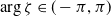 $\arg \zeta \in (-\pi, \pi )$
.
$\arg \zeta \in (-\pi, \pi )$
.
Orient of
 $\Sigma _k,k=1,2,3,4$
.
$\Sigma _k,k=1,2,3,4$
.

For any complex constant
 $a$
,
$a$
,
 $D_a(\zeta )$
denotes the parabolic cylinder function which satisfies the Weber’s equation
$D_a(\zeta )$
denotes the parabolic cylinder function which satisfies the Weber’s equation
 \begin{align} D_{a,\zeta \zeta }+\left (-\frac {\zeta ^2}{4}+a+\frac {1}{2}\right )D_a=0, \end{align}
with large
 $\zeta$
behaviour
$\zeta$
behaviour
 \begin{align} D_a(\zeta )\sim \left \{\begin{array}{l@{\quad}l@{\quad}l} \zeta ^ae^{-\frac {\zeta ^2}{4}}, &-\frac {3\pi }{4}\lt \arg \zeta \lt \frac {3\pi }{4},\\[3pt] \zeta ^ae^{-\frac {\zeta ^2}{4}}-\frac {\sqrt {2\pi }}{\Gamma (-a)}e^{ia\pi }\zeta ^{-a-1}e^{\frac {\zeta ^2}{4}},&\frac {\pi }{4}\lt \arg \zeta \lt \frac {5\pi }{4},\\[3pt] \zeta ^ae^{-\frac {\zeta ^2}{4}}-\frac {\sqrt {2\pi }}{\Gamma (-a)}e^{-ia\pi }\zeta ^{-a-1}e^{\frac {\zeta ^2}{4}},&-\frac {5\pi }{4}\lt \arg \zeta \lt -\frac {\pi }{4}. \end{array}\right . \end{align}
The unique solution of RH problem12 is given by
 \begin{align} P_1(\zeta;\,r_0)=\Phi _1(\zeta;\,r_0)S_1(\zeta;\,r_0)\zeta ^{-i\nu (r_0)\sigma _3}e^{-\frac {i\zeta ^2}{4}\sigma _3}, \end{align}
where
 \begin{align*} & \Phi _1=\left (\begin{array}{c@{\quad}c} e^{\frac {-\pi \nu }{4}}D_{i\nu }(\zeta e^{-\frac {i\pi }{4}}) & -\frac {i\nu }{\beta _{21}}e^{\frac {3\pi (\nu -i)}{4}}D_{-i\nu -1}(\zeta e^{-\frac {3i\pi }{4}}) \\[3pt] \frac {i\nu }{\beta _{12}}e^{\frac {-\pi (\nu +i)}{4}}D_{i\nu -1}(\zeta e^{-\frac {i\pi }{4}}) & e^{\frac {3\pi \nu }{4}}D_{-i\nu }(\zeta e^{-\frac {3i\pi }{4}}) \end{array}\right ), &\text{Im}\zeta \gt 0,\\[3pt] &\Phi _1=\left (\begin{array}{c@{\quad}c} e^{\frac {3\pi \nu }{4}}D_{i\nu }(\zeta e^{\frac {3i\pi }{4}}) & -\frac {i\nu }{\beta _{21}}e^{\frac {\pi (-\nu +i)}{4}}D_{-i\nu -1}(\zeta e^{\frac {i\pi }{4}}) \\[3pt] \frac {i\nu }{\beta _{12}}e^{\frac {3\pi (\nu +i)}{4}}D_{i\nu -1}(\zeta e^{\frac {3i\pi }{4}}) & e^{\frac {\pi \nu }{4}}D_{i\nu }(\zeta e^{\frac {i\pi }{4}}) \end{array}\right ), &\text{Im}\zeta \lt 0,\\[3pt] &\Phi _1\sim \zeta ^{i\nu (r_0)\sigma _3}e^{\frac {i\zeta ^2}{4}\sigma _3}, \zeta \to \infty, \end{align*}
with
 $ \beta _{21}=\frac {\sqrt {2\pi }e^{\frac {\pi \nu }{2}+\frac {i\pi }{4}}}{r_0\Gamma (i\nu )},\ \beta _{12}= -\frac {\nu (r_0)}{\beta _{21}}$
and
$ \beta _{21}=\frac {\sqrt {2\pi }e^{\frac {\pi \nu }{2}+\frac {i\pi }{4}}}{r_0\Gamma (i\nu )},\ \beta _{12}= -\frac {\nu (r_0)}{\beta _{21}}$
and
 \begin{align*} &S_1=\left (\begin{array}{c@{\quad}c} 1& r_0\\[3pt] 0&1 \end{array}\right ), 0\lt \arg \zeta \lt \varkappa, \ S_1=\left (\begin{array}{c@{\quad}c} 1 & 0\\[3pt] -\frac {\bar {r}_{0}}{1-|r_{0}|^2} & 1 \end{array}\right ), \pi -\varkappa \lt \arg \zeta \lt \pi, \\[3pt] &S_1=\left (\begin{array}{c@{\quad}c} 1 & \frac {r_{0}}{1-|r_{0}|^2}\\[3pt] 0 & 1 \end{array}\right ), \pi \lt \arg \zeta \lt \pi +\varkappa, \ S_1=\left (\begin{array}{c@{\quad}c} 1 & 0\\[3pt] -\bar {r}_0 & 1 \end{array}\right ), 2\pi -\varkappa \lt \arg \zeta \lt 2\pi, \\[3pt] &S_1=I, \arg \zeta \in \left (\varkappa, \pi -\varkappa \right )\cup \left (\pi +\varkappa, 2\pi -\varkappa \right ). \end{align*}
Moreover, the solution
 $P_1(\zeta;\,r_0)$
satisfies
$P_1(\zeta;\,r_0)$
satisfies
 \begin{align*}P_1(\zeta;\,r_0)=I+\frac {P^{(1)}_1(r_0)}{\zeta }+\mathcal{O}(\frac {1}{\zeta ^2}), \zeta \to \infty, \end{align*}
where
 \begin{align*} P^{(1)}_1(r_0)=\left (\begin{array}{c@{\quad}c} 0&\beta _{12}\\[3pt] \beta _{21}&0\\[3pt] \end{array}\right ). \end{align*}


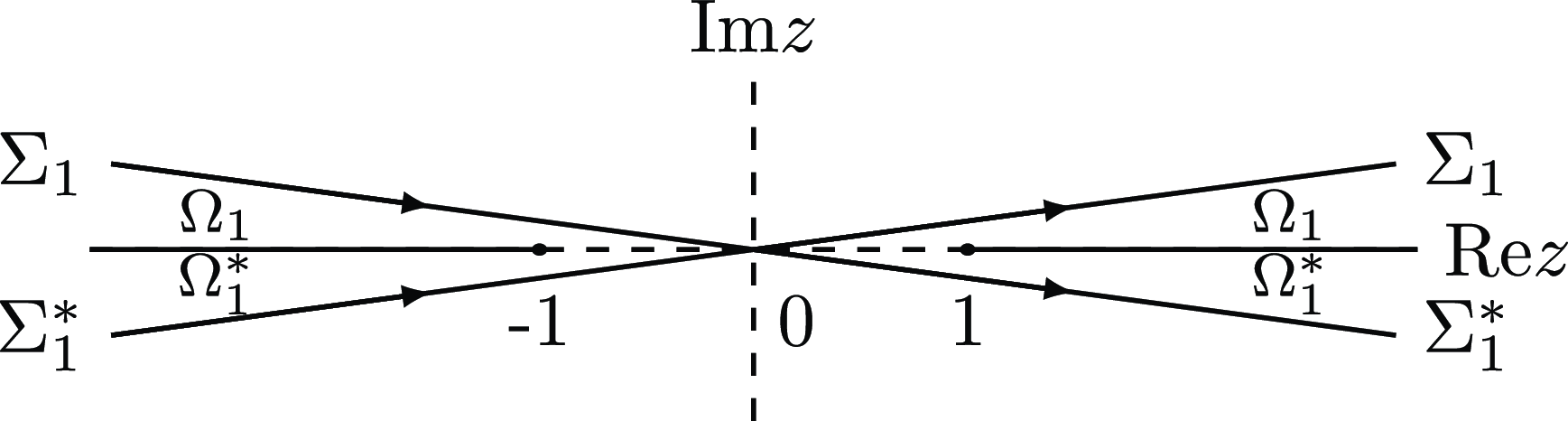


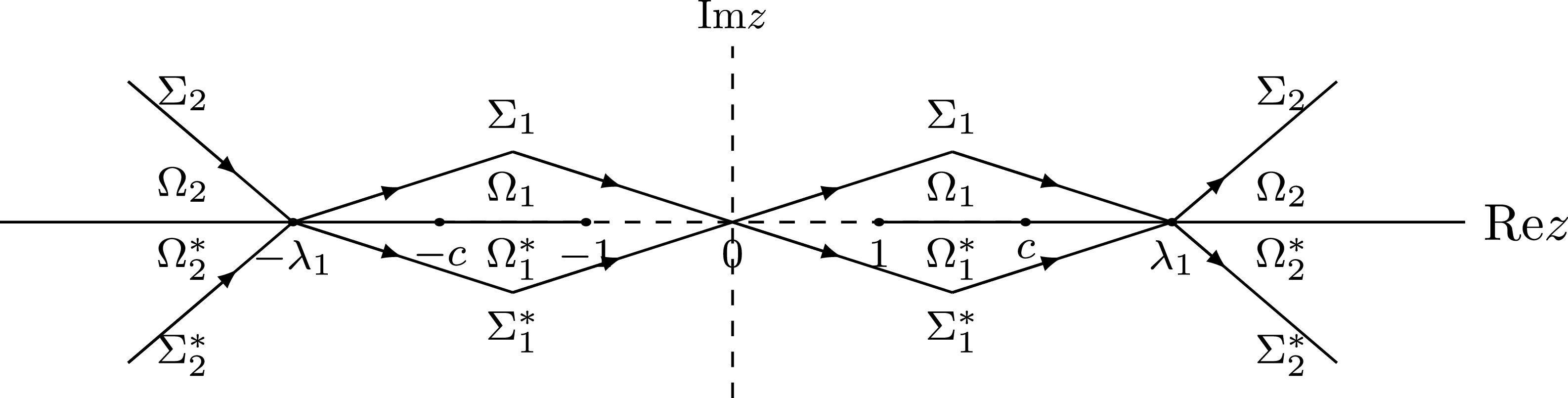


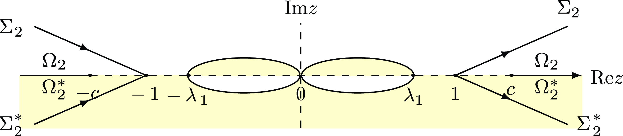


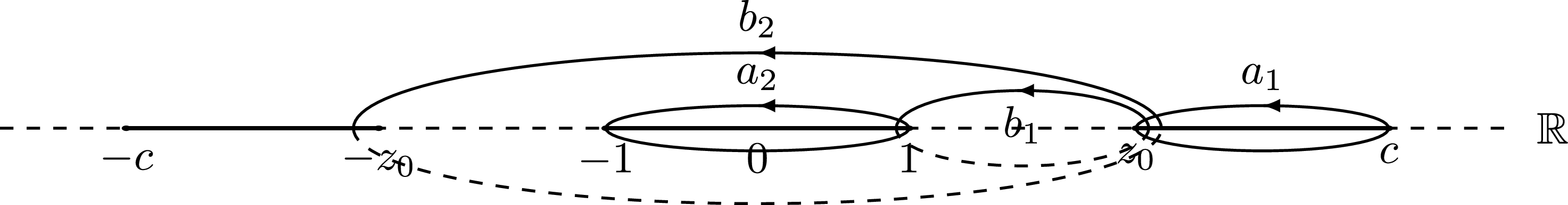


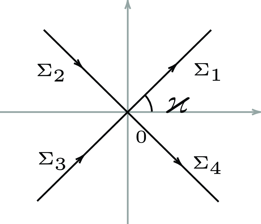


 Open access