


1. Introduction
Viscous fingering (Saffman & Taylor Reference Saffman and Taylor1958; Homsy Reference Homsy1987) occurs when a less viscous fluid displaces a more viscous fluid inside porous media. First discovered in oil recovery processes, viscous fingering has been studied extensively as a premier example of a pattern-forming system whose fundamental physics has aided our understanding of solidification and other growth phenomena (Couder Reference Couder2000). Viscous fingering is driven by the viscosity difference between the two fluids, while the interfacial tension
 $\gamma$
stabilises the system, setting the critical wavelength that scales as
$\gamma$
stabilises the system, setting the critical wavelength that scales as
 $\gamma ^{1/2}$
(Chuoke, Van Meurs & Van Der Poel Reference Chuoke, van Meurs and van der Poel1959; Park, Gorell & Homsy Reference Park, Gorell and Homsy1984; Park & Homsy Reference Park and Homsy1984). In the limit of zero interfacial tension, the instability between the two fluids is mediated by thermal diffusion characterised by the Péclet number Pe, the ratio of flow advection to diffusion. For relatively small pore-scale Pe where diffusion homogenises the flow within the pore, viscous fingering can be described by a depth-averaged two-dimensional (2-D) model (Tan & Homsy Reference Tan and Homsy1986; Booth Reference Booth2010; Nijjer, Hewitt & Neufeld Reference Nijjer, Hewitt and Neufeld2018). In such systems, thermal diffusion determines the mixing region width and sets the wavelength of instability (Wooding Reference Wooding1962; Hickernell & Yortsos Reference Hickernell and Yortsos1986; Yortsos & Salin Reference Yortsos and Salin2006; Booth Reference Booth2010; Nijjer et al. Reference Nijjer, Hewitt and Neufeld2018).
$\gamma ^{1/2}$
(Chuoke, Van Meurs & Van Der Poel Reference Chuoke, van Meurs and van der Poel1959; Park, Gorell & Homsy Reference Park, Gorell and Homsy1984; Park & Homsy Reference Park and Homsy1984). In the limit of zero interfacial tension, the instability between the two fluids is mediated by thermal diffusion characterised by the Péclet number Pe, the ratio of flow advection to diffusion. For relatively small pore-scale Pe where diffusion homogenises the flow within the pore, viscous fingering can be described by a depth-averaged two-dimensional (2-D) model (Tan & Homsy Reference Tan and Homsy1986; Booth Reference Booth2010; Nijjer, Hewitt & Neufeld Reference Nijjer, Hewitt and Neufeld2018). In such systems, thermal diffusion determines the mixing region width and sets the wavelength of instability (Wooding Reference Wooding1962; Hickernell & Yortsos Reference Hickernell and Yortsos1986; Yortsos & Salin Reference Yortsos and Salin2006; Booth Reference Booth2010; Nijjer et al. Reference Nijjer, Hewitt and Neufeld2018).
In this paper, we uncover a new mechanism of wavelength selection of viscous fingering in the limit of zero interfacial tension and
 ${{Pe}}\rightarrow \infty$
, with the use of a 2-D suspension. We experimentally inject clear oil into the mixture of the same oil and non-colloidal particles inside a rectangular Hele-Shaw cell, whose gap thickness is comparable to the particle diameter. The inclusion of the particles in the oil increases the effective viscosity of the mixture (Einstein Reference Einstein1906; Brady Reference Brady1983) and generates the necessary condition for viscous fingering. Despite the absence of thermal diffusion, our experiments reveal a striking similarity to 2-D viscous fingering with miscible liquids at low Pe (Tan & Homsy Reference Tan and Homsy1986). The invading oil is shown to finger into the suspension, and the characteristic finger width gradually widens over time. This behaviour is a complete departure from the suppression of fingering that is observed when a clear oil invades the suspension inside the channel with a large gap (Luo, Chen & Lee Reference Luo, Chen and Lee2020).
${{Pe}}\rightarrow \infty$
, with the use of a 2-D suspension. We experimentally inject clear oil into the mixture of the same oil and non-colloidal particles inside a rectangular Hele-Shaw cell, whose gap thickness is comparable to the particle diameter. The inclusion of the particles in the oil increases the effective viscosity of the mixture (Einstein Reference Einstein1906; Brady Reference Brady1983) and generates the necessary condition for viscous fingering. Despite the absence of thermal diffusion, our experiments reveal a striking similarity to 2-D viscous fingering with miscible liquids at low Pe (Tan & Homsy Reference Tan and Homsy1986). The invading oil is shown to finger into the suspension, and the characteristic finger width gradually widens over time. This behaviour is a complete departure from the suppression of fingering that is observed when a clear oil invades the suspension inside the channel with a large gap (Luo, Chen & Lee Reference Luo, Chen and Lee2020).
The key feature responsible for this surprising phenomenon is the channel confinement that causes the flow disturbance by each particle to behave as a long-range dipole. Such non-equilibrium many-body systems with slowly decaying disturbances have been shown to exhibit complex collective dynamics, including hydrodynamic fluctuations of 2-D uniform suspension flows (Desreumaux et al. Reference Desreumaux, Caussin, Jeanneret, Lauga and Bartolo2013), and clustering of magnetically driven micro-rollers (Driscoll et al. Reference Driscoll, Delmotte, Youssef, Sacanna, Donev and Chaikin2017). To demonstrate this, we derive a coarse-grained model accounting for the dipolar interactions between particles, whose results correctly predict the development of gradually widening fingers even at
 ${{Pe}}\rightarrow \infty$
. Our model further reveals universal fingering dynamics that is independent of the initial particle concentration, which only sets the time-scale of the instability.
${{Pe}}\rightarrow \infty$
. Our model further reveals universal fingering dynamics that is independent of the initial particle concentration, which only sets the time-scale of the instability.
The paper is organised as follows. We introduce the experimental set-up and observations in § 2, while the formulation of the mathematical model is included in § 3. We discuss the model results and make the quantitative comparison with the experiments in § 4. In § 4.3, we uncover the physical origin of wavelength selection. Finally, we conclude the paper with the summary and discussion in § 5.
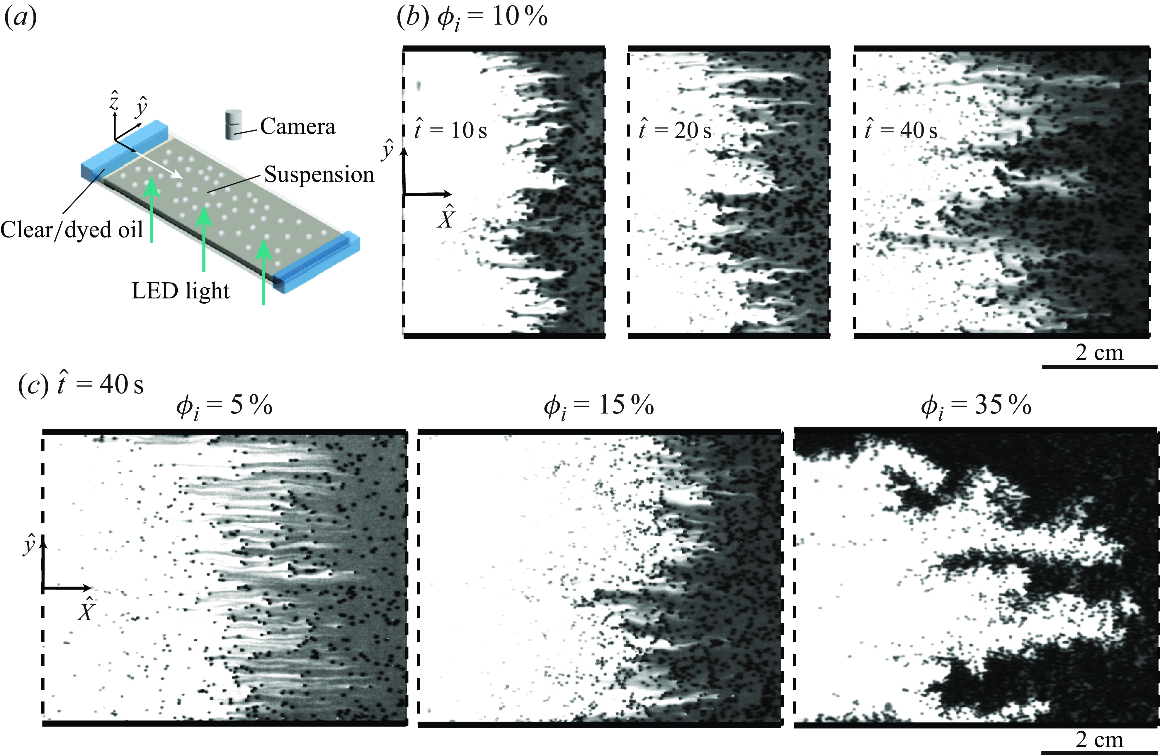
(a) Schematic of the experimental set-up: a 2-D Hele-Shaw cell consisting of two rectangular glass plates that are separated by a thin gap. The images of flow patterns are captured from above using a CMOS camera, as the clear oil invades the particle–oil mixture. (b) The time-sequential experimental images at
 $\phi _i = 10\, \%$
show the gradual widening of fingers over time in a single experiment. (c) The experimental images at
$\phi _i = 10\, \%$
show the gradual widening of fingers over time in a single experiment. (c) The experimental images at
 $\hat {t}=40\,{\textrm s}$
show the increase in the critical wavelength
$\hat {t}=40\,{\textrm s}$
show the increase in the critical wavelength
 $\lambda _c$
as the initial concentration
$\lambda _c$
as the initial concentration
 $\phi _i$
is increased:
$\phi _i$
is increased:
 $\phi _i=5\, \%$
,
$\phi _i=5\, \%$
,
 $15\, \%$
,
$15\, \%$
,
 $35\, \%$
. The solid line represents the location of the side wall.
$35\, \%$
. The solid line represents the location of the side wall.
2. Experiments
To induce viscous fingering with zero interfacial tension, we inject silicone oil (density
 $0.96 \, \textrm{kg m}^{-3}$
, dynamic viscosity
$0.96 \, \textrm{kg m}^{-3}$
, dynamic viscosity
 $\mu = 0.096 \, \textrm{Pa s}$
) into the mixture of the same oil and polyethylene particles with diameter
$\mu = 0.096 \, \textrm{Pa s}$
) into the mixture of the same oil and polyethylene particles with diameter
 $d= 0.625 \pm 0.4\,\textrm{mm}$
and density
$d= 0.625 \pm 0.4\,\textrm{mm}$
and density
 $\rho _p= 0.98 \,\textrm{g cm}^{-3}$
inside a rectangular Hele-Shaw cell. Since
$\rho _p= 0.98 \,\textrm{g cm}^{-3}$
inside a rectangular Hele-Shaw cell. Since
 ${{Pe}}\sim O(10^{10})$
, the thermal diffusion of the non-colloidal particles is negligible. As illustrated in figure 1(a), the Hele-Shaw cell comprises two glass plates with width
${{Pe}}\sim O(10^{10})$
, the thermal diffusion of the non-colloidal particles is negligible. As illustrated in figure 1(a), the Hele-Shaw cell comprises two glass plates with width
 $W= 60 \, \textrm{mm}$
separated by gap thickness
$W= 60 \, \textrm{mm}$
separated by gap thickness
 $b = 0.76 \pm 0.03 \, \textrm{mm}$
, such that
$b = 0.76 \pm 0.03 \, \textrm{mm}$
, such that
 $b/d\approx 1$
ensures the formation of a monolayer.
$b/d\approx 1$
ensures the formation of a monolayer.
In our experiments, we fix the oil flow rate to
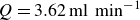 $Q = 3.62\, \textrm{ml min}^{-1}$
, and systematically vary the particle volume fractions
$Q = 3.62\, \textrm{ml min}^{-1}$
, and systematically vary the particle volume fractions
 $\phi _i$
or the corresponding average number densities
$\phi _i$
or the corresponding average number densities
 $\rho _i$
. Note that the average number density
$\rho _i$
. Note that the average number density
 $\rho _i$
is defined as the total number of particles over the area of the domain. Varying
$\rho _i$
is defined as the total number of particles over the area of the domain. Varying
 $\phi _i$
or
$\phi _i$
or
 $\rho _i$
is equivalent to varying the viscosity ratio between the suspension (defending fluid) and the clear oil (invading fluid); viscosity ratios greater than 1 are conducive to viscous fingering. We estimate the viscosity ratio of the current system based on the following empirical expression of the effective viscosity (Brady Reference Brady1983):
$\rho _i$
is equivalent to varying the viscosity ratio between the suspension (defending fluid) and the clear oil (invading fluid); viscosity ratios greater than 1 are conducive to viscous fingering. We estimate the viscosity ratio of the current system based on the following empirical expression of the effective viscosity (Brady Reference Brady1983):
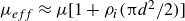 $\mu _{{eff}}\approx \mu [1 + \rho _i(\unicode{x03C0} d^2/2) ]$
, which is valid for a 2-D suspension in a dilute regime. The resultant viscosity ratios in the current experiments range from 1.2 to 1.8.
$\mu _{{eff}}\approx \mu [1 + \rho _i(\unicode{x03C0} d^2/2) ]$
, which is valid for a 2-D suspension in a dilute regime. The resultant viscosity ratios in the current experiments range from 1.2 to 1.8.
Successful experiments require generating a uniform suspension of
 $\phi _i$
and a relatively uniform front of invading oil. We include the detailed description of our experimental procedure in Appendix A. We conduct two complementary sets of experiments with and without dyeing the invading oil for the purposes of visualisation. The experiments in which we dye the invading oil allow us to directly visualise the miscible displacement pattern of the invading oil (see figure 1
b,c), while we track the motion of individual particle with corresponding high-resolution experiments with no dyed oil.
$\phi _i$
and a relatively uniform front of invading oil. We include the detailed description of our experimental procedure in Appendix A. We conduct two complementary sets of experiments with and without dyeing the invading oil for the purposes of visualisation. The experiments in which we dye the invading oil allow us to directly visualise the miscible displacement pattern of the invading oil (see figure 1
b,c), while we track the motion of individual particle with corresponding high-resolution experiments with no dyed oil.
The experimental images in figure 1 demonstrate two major observations from the experiments. First, the invading oil is observed to form fingers into the suspension for all
 $\phi _i$
or
$\phi _i$
or
 $\rho _i$
tested. Second, the characteristic finger width
$\rho _i$
tested. Second, the characteristic finger width
 $\lambda _c$
(as quantified in Appendix B) increases with both time and
$\lambda _c$
(as quantified in Appendix B) increases with both time and
 $\rho _i$
. The experimental images in figure 1(b) demonstrate coarsening of the finger width over time at
$\rho _i$
. The experimental images in figure 1(b) demonstrate coarsening of the finger width over time at
 $\phi _i=10\, \%$
(
$\phi _i=10\, \%$
(
 $\rho _i=0.48\,{\textrm{mm}}^{-2}$
), while at fixed time, fingers of the invading oil appear wider as
$\rho _i=0.48\,{\textrm{mm}}^{-2}$
), while at fixed time, fingers of the invading oil appear wider as
 $\rho _i$
is systematically increased from 5 % (
$\rho _i$
is systematically increased from 5 % (
 $\rho _i=0.17\,{\textrm{mm}}^{-2}$
) to 35 % (
$\rho _i=0.17\,{\textrm{mm}}^{-2}$
) to 35 % (
 $\rho _i=1.84\,{\textrm{mm}}^{-2}$
) in figure 1(c).
$\rho _i=1.84\,{\textrm{mm}}^{-2}$
) in figure 1(c).
The appearance of miscible fingering at all
 $\phi _i$
is a clear deviation from the recent series of studies on the displacement of miscible fluids at
$\phi _i$
is a clear deviation from the recent series of studies on the displacement of miscible fluids at
 ${{Pe}}\rightarrow \infty$
(Goyal & Meiburg Reference Goyal and Meiburg2006; Bischofberger, Ramachandran & Nagel Reference Bischofberger, Ramachandran and Nagel2014; Nijjer et al. Reference Nijjer, Hewitt and Neufeld2018; Videbæk & Nagel Reference Videbæk and Nagel2019; Videbæk Reference Videbæk2020). These studies show that the displacement of miscible fluids is stable at low viscosity ratios, including in the case of clear oil invading a suspension (Luo et al. Reference Luo, Chen and Lee2020). The cause of stable displacements is understood to be the development of a three-dimensional (3-D) structure inside the thin gap at
${{Pe}}\rightarrow \infty$
(Goyal & Meiburg Reference Goyal and Meiburg2006; Bischofberger, Ramachandran & Nagel Reference Bischofberger, Ramachandran and Nagel2014; Nijjer et al. Reference Nijjer, Hewitt and Neufeld2018; Videbæk & Nagel Reference Videbæk and Nagel2019; Videbæk Reference Videbæk2020). These studies show that the displacement of miscible fluids is stable at low viscosity ratios, including in the case of clear oil invading a suspension (Luo et al. Reference Luo, Chen and Lee2020). The cause of stable displacements is understood to be the development of a three-dimensional (3-D) structure inside the thin gap at
 ${{Pe}}\rightarrow \infty$
. Hence by working with highly confined particles whose dynamics can be modelled as quasi-2-D, the onset of fingering is no longer delayed even at low viscosity ratios. Here, we refer to the particles in a monolayer as being ‘highly confined’ by the channel walls. Yet the emergence of a finite wavelength that evolves with time and
${{Pe}}\rightarrow \infty$
. Hence by working with highly confined particles whose dynamics can be modelled as quasi-2-D, the onset of fingering is no longer delayed even at low viscosity ratios. Here, we refer to the particles in a monolayer as being ‘highly confined’ by the channel walls. Yet the emergence of a finite wavelength that evolves with time and
 $\phi _i$
speaks to the existence of an alternate wavelength selection mechanism, which we will rationalise with a minimal model.
$\phi _i$
speaks to the existence of an alternate wavelength selection mechanism, which we will rationalise with a minimal model.
3. Theoretical model
Given the simplicity of our experimental system with no interfacial tension and thermal diffusion, we hypothesise that the hydrodynamic interactions between the highly confined particles comprise both stabilising and destabilising effects, and thereby can describe the observed fingering phenomena. To demonstrate this, we develop a coarse-grained continuum model that takes into account pairwise interactions between particles immersed in the Stokes flow and the initial jump in particle concentrations.
We model our system comprising
 $N$
particles denoted with the index
$N$
particles denoted with the index
 $i\ (i = 1,\ldots, N)$
. Due to the friction of the bounding walls, a highly confined particle
$i\ (i = 1,\ldots, N)$
. Due to the friction of the bounding walls, a highly confined particle
 $i$
moves slower than the local oil flow, such that
$i$
moves slower than the local oil flow, such that
 ${\hat{\boldsymbol{v}}}_{p,i} = \kappa {\hat{\boldsymbol{v}}}$
, where
${\hat{\boldsymbol{v}}}_{p,i} = \kappa {\hat{\boldsymbol{v}}}$
, where
 ${\hat{\boldsymbol{v}}}_{p,i}$
and
${\hat{\boldsymbol{v}}}_{p,i}$
and
 ${\hat{\boldsymbol{v}}}$
are the in-plane velocities of the particle and suspending oil in the absence of the particle
${\hat{\boldsymbol{v}}}$
are the in-plane velocities of the particle and suspending oil in the absence of the particle
 $i$
, respectively. Here,
$i$
, respectively. Here,
 $\kappa \!\lt \! 1$
is an empirical constant whose value we determine by measuring the velocity of individual particles in dilute suspension experiments. The velocity difference between the particle and the fluid causes a dipolar disturbance to the suspending oil,
$\kappa \!\lt \! 1$
is an empirical constant whose value we determine by measuring the velocity of individual particles in dilute suspension experiments. The velocity difference between the particle and the fluid causes a dipolar disturbance to the suspending oil,
 ${\hat{\boldsymbol{v}}}^{{dip}}$
. The dipolar disturbance introduced at position
${\hat{\boldsymbol{v}}}^{{dip}}$
. The dipolar disturbance introduced at position
 ${\hat{\boldsymbol{r}}}$
by a particle at
${\hat{\boldsymbol{r}}}$
by a particle at
 ${\hat{\boldsymbol{r}}}'$
can be modelled as
${\hat{\boldsymbol{r}}}'$
can be modelled as
 ${\hat{\boldsymbol{v}}}^{{dip}}({\hat{\boldsymbol{r}}},{\hat{\boldsymbol{r}}}') = S\, {\hat{\boldsymbol{\nabla}}}(({\hat{\boldsymbol{r}}}-{\hat{\boldsymbol{r}}}')\boldsymbol{\cdot} \boldsymbol{e}_{\hat {X}}/\left |{\hat{\boldsymbol{r}}}-{\hat{\boldsymbol{r}}}'\right |^2)$
, where
${\hat{\boldsymbol{v}}}^{{dip}}({\hat{\boldsymbol{r}}},{\hat{\boldsymbol{r}}}') = S\, {\hat{\boldsymbol{\nabla}}}(({\hat{\boldsymbol{r}}}-{\hat{\boldsymbol{r}}}')\boldsymbol{\cdot} \boldsymbol{e}_{\hat {X}}/\left |{\hat{\boldsymbol{r}}}-{\hat{\boldsymbol{r}}}'\right |^2)$
, where
 $S$
represents the dipolar strength accounting for channel confinement and particle surface properties (Beatus et al. Reference Beatus, Tlusty and Bar-Ziv2006, Reference Beatus, Bar-Ziv and Tlusty2012), and
$S$
represents the dipolar strength accounting for channel confinement and particle surface properties (Beatus et al. Reference Beatus, Tlusty and Bar-Ziv2006, Reference Beatus, Bar-Ziv and Tlusty2012), and
 $\boldsymbol{e}_{\hat {X}}$
is the unit vector in the axial coordinate
$\boldsymbol{e}_{\hat {X}}$
is the unit vector in the axial coordinate
 $\hat {X}$
. The resultant streamlines of
$\hat {X}$
. The resultant streamlines of
 ${\hat{\boldsymbol{v}}}^{{dip}}$
are symmetric in the transverse direction and asymmetric in the flow direction. We assume that the dipolar disturbances between particles are pairwise additive, such that
${\hat{\boldsymbol{v}}}^{{dip}}$
are symmetric in the transverse direction and asymmetric in the flow direction. We assume that the dipolar disturbances between particles are pairwise additive, such that
 ${\hat{\boldsymbol{v}}}\!=\!{\hat{\boldsymbol{v}}}^\infty +\sum _{j\ne i}{\hat{\boldsymbol{v}}}^{{dip}}({\hat{\boldsymbol{r}}}_i,{\hat{\boldsymbol{r}}}_j)$
, where
${\hat{\boldsymbol{v}}}\!=\!{\hat{\boldsymbol{v}}}^\infty +\sum _{j\ne i}{\hat{\boldsymbol{v}}}^{{dip}}({\hat{\boldsymbol{r}}}_i,{\hat{\boldsymbol{r}}}_j)$
, where
 ${\hat{\boldsymbol{v}}}^\infty \!=\!\hat {v}^\infty \boldsymbol{e}_{\hat {X}}$
is the uniform background flow.
${\hat{\boldsymbol{v}}}^\infty \!=\!\hat {v}^\infty \boldsymbol{e}_{\hat {X}}$
is the uniform background flow.
Moving from the individual particle dynamics to a continuum description, we now derive an equation for the local number density
 $\rho ({\hat{\boldsymbol{r}}},\hat {t})$
based on mass conservation:
$\rho ({\hat{\boldsymbol{r}}},\hat {t})$
based on mass conservation:
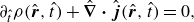 \begin{equation} \partial _{\hat {t}} \rho ({\hat{\boldsymbol{r}}},\hat {t}) + {\hat{\boldsymbol{\nabla}}} \boldsymbol{\cdot} {\hat{\boldsymbol{j}}}({\hat{\boldsymbol{r}}},\hat {t}) = 0, \end{equation}
where the local particle flux
 $\hat{\boldsymbol{\kern-2pt j}}({\hat{\boldsymbol{r}}},\hat {t})$
is derived using a conventional kinetic theory (Menzel Reference Menzel2012; Desreumaux et al. Reference Desreumaux, Caussin, Jeanneret, Lauga and Bartolo2013)
$\hat{\boldsymbol{\kern-2pt j}}({\hat{\boldsymbol{r}}},\hat {t})$
is derived using a conventional kinetic theory (Menzel Reference Menzel2012; Desreumaux et al. Reference Desreumaux, Caussin, Jeanneret, Lauga and Bartolo2013)
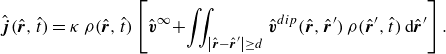 \begin{equation} {\hat{\boldsymbol{j}}}({\hat{\boldsymbol{r}}},\hat {t})=\kappa\, \rho ({\hat{\boldsymbol{r}}},\hat {t}) \left [{\hat{\boldsymbol{v}}}^{\infty }\!+\!\iint _{\left | {\hat{\boldsymbol{r}}} - {{\hat{\boldsymbol{r}}}'} \right | \ge d} {\hat{\boldsymbol{v}}}^{{dip}}({\hat{\boldsymbol{r}}},{\hat{\boldsymbol{r}}}')\, \rho ({\hat{\boldsymbol{r}}}',\hat {t})\,{\textrm d}{\hat{\boldsymbol{r}}}'\right ]. \end{equation}
The quadratic nonlinearity in (3.2) accounts for the pairwise interaction, and introducing the cut-off length in the integration ensures that the number density remains bounded. A similar continuum framework has been used previously to model the collective dynamics in systems comprising multiple bodies, such as magnetic rotors, sedimenting particles and droplet emulsions (Desreumaux et al. Reference Desreumaux, Caussin, Jeanneret, Lauga and Bartolo2013; Delmotte et al. Reference Delmotte, Driscoll, Chaikin and Donev2017; Sprinkle et al. Reference Sprinkle, Wilken, Karapetyan, Tanaka, Chen, Cruise, Delmotte, Driscoll, Chaikin and Donev2021).
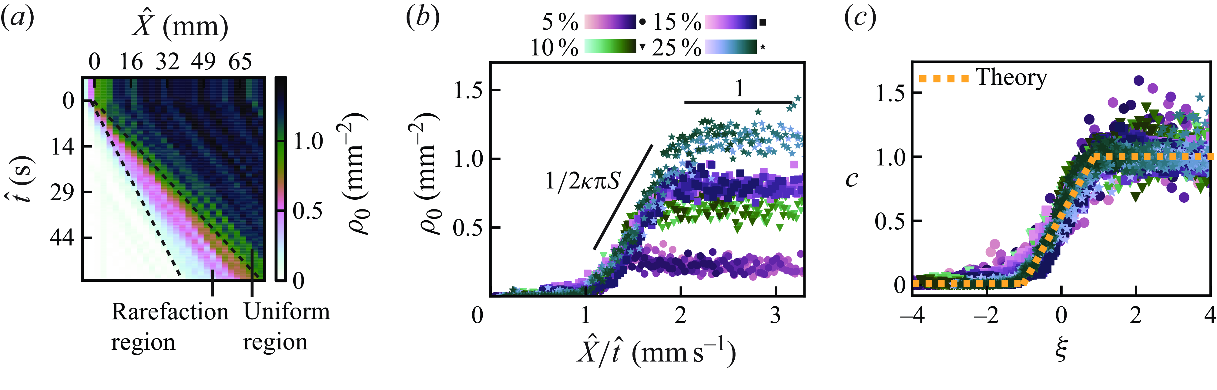
(a) Space–time diagram illustrating the number density
 $\rho _0$
measured and averaged over the channel width from an experiment at
$\rho _0$
measured and averaged over the channel width from an experiment at
 $\phi _i = 25\, \%$
or
$\phi _i = 25\, \%$
or
 $\rho _i = 1.13\,{\textrm{mm}}^{-2}$
. The colour scale indicates the local number density. The rarefaction region (bounded by dashed lines) is characterised by a gradual increase in
$\rho _i = 1.13\,{\textrm{mm}}^{-2}$
. The colour scale indicates the local number density. The rarefaction region (bounded by dashed lines) is characterised by a gradual increase in
 $\rho _0$
. (b) We plot
$\rho _0$
. (b) We plot
 $\rho _0$
measured from the experiments at
$\rho _0$
measured from the experiments at
 $\phi _i = 5\, \%, 10\, \%, 15\, \%, 25\, \%$
as a function of
$\phi _i = 5\, \%, 10\, \%, 15\, \%, 25\, \%$
as a function of
 $\hat {X}/\hat {t}$
, which reveals the self-similarity of our data and two distinct regions. The rarefaction region, exhibiting a positive slope, is influenced by the system’s confinement parameters (
$\hat {X}/\hat {t}$
, which reveals the self-similarity of our data and two distinct regions. The rarefaction region, exhibiting a positive slope, is influenced by the system’s confinement parameters (
 $\kappa$
and
$\kappa$
and
 $S$
), while the uniform region is set by
$S$
), while the uniform region is set by
 $\phi _i$
. The colour of each symbol corresponds to different values of
$\phi _i$
. The colour of each symbol corresponds to different values of
 $\phi _i$
, with the darker shade indicating later dimensional times (see the colourmaps in (b)). (c) The dimensionless number density profiles
$\phi _i$
, with the darker shade indicating later dimensional times (see the colourmaps in (b)). (c) The dimensionless number density profiles
 $c$
from all experiments collapse onto a single rarefaction solution curve, consistent with the predictions of the leading-order equation (dashed line).
$c$
from all experiments collapse onto a single rarefaction solution curve, consistent with the predictions of the leading-order equation (dashed line).
We move to a moving reference frame based on
 $\hat {x} = \hat {X} - \kappa ({\hat{v}}^{\infty } + \unicode{x03C0} S\rho _i)\hat {t}$
, where
$\hat {x} = \hat {X} - \kappa ({\hat{v}}^{\infty } + \unicode{x03C0} S\rho _i)\hat {t}$
, where
 $\hat {x}$
is the moving coordinate in the flow direction, while
$\hat {x}$
is the moving coordinate in the flow direction, while
 $\hat {y}$
corresponds to the coordinate in the transverse direction. We define
$\hat {y}$
corresponds to the coordinate in the transverse direction. We define
 $c\equiv \rho /\rho _i$
, and non-dimensionalise (3.1) based on the scales: length
$c\equiv \rho /\rho _i$
, and non-dimensionalise (3.1) based on the scales: length
 $d$
, velocity
$d$
, velocity
 $\kappa \unicode{x03C0} S \rho _i$
, and time
$\kappa \unicode{x03C0} S \rho _i$
, and time
 $d/(\kappa \unicode{x03C0} S \rho _i)$
. The dimensionless variables will be denoted without hats to clearly distinguish them from the dimensional variables. Notably, the average number density
$d/(\kappa \unicode{x03C0} S \rho _i)$
. The dimensionless variables will be denoted without hats to clearly distinguish them from the dimensional variables. Notably, the average number density
 $\rho _i$
sets the intrinsic speed of the system, and thereby the characteristic timescale.
$\rho _i$
sets the intrinsic speed of the system, and thereby the characteristic timescale.
The resultant dimensionless equation for
 $c$
is
$c$
is
 \begin{equation} \frac {\partial c}{\partial t} + \left (\frac {1}{\unicode{x03C0} } u_{d} -1\right )\frac {\partial c}{\partial x} + \frac {1}{\unicode{x03C0} } v_{d} \frac {\partial c}{\partial y} - \frac {1}{\unicode{x03C0} } c \int _{0}^{2\unicode{x03C0} } c(\boldsymbol{r} - \boldsymbol{n},t)\cos \theta \,{\textrm d}\theta = 0, \end{equation}
where
 $\boldsymbol{n} = (\cos \theta ,\sin \theta )$
, and
$\boldsymbol{n} = (\cos \theta ,\sin \theta )$
, and
 $u_{d}$
and
$u_{d}$
and
 $v_{d}$
are the summed dimensionless disturbance velocities in
$v_{d}$
are the summed dimensionless disturbance velocities in
 $x$
and
$x$
and
 $y$
, respectively:
$y$
, respectively:
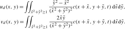 \begin{equation} \begin{aligned} u_{d}(x,y) = \iint _{\tilde {x}^2+\tilde {y}^2\ge 1} \frac {\tilde {y}^2-\tilde {x}^2}{(\tilde {x}^2+\tilde {y}^2)^2} c(x+\tilde {x},y+\tilde {y},t)\,{\textrm d}\tilde {x}{\textrm d}\tilde {y}, \\ v_{d}(x,y) = \iint _{\tilde {x}^2+\tilde {y}^2\ge 1} \frac {2\tilde {x}\tilde {y}}{(\tilde {x}^2+\tilde {y}^2)^2} c(x+\tilde {x},y+\tilde {y},t)\,{\textrm d}\tilde {x}{\textrm d}\tilde {y}. \end{aligned} \end{equation}
We include the detailed derivation of (3.3) and (3.4) in Appendix C.
Finally, to simulate the invasion of the clear oil into the uniform suspension, we subject (3.3) to the initial condition
 $c(x,y, t=0) ={\mathbb(1)}_{x\gt 0}.$
The dimensionless governing equation and initial condition for
$c(x,y, t=0) ={\mathbb(1)}_{x\gt 0}.$
The dimensionless governing equation and initial condition for
 $c$
are completely independent of the initial particle number density
$c$
are completely independent of the initial particle number density
 $\rho _i$
, which suggests the universal nature of the 2-D suspension in the current configuration. In other words, instead of solving the governing equation for varying parameters, such as
$\rho _i$
, which suggests the universal nature of the 2-D suspension in the current configuration. In other words, instead of solving the governing equation for varying parameters, such as
 $\rho _i$
and channel confinement, one only needs to obtain the solution to the dimensionless equation once and re-normalise the result to describe the invasion of clear oil into the 2-D suspension for different physical parameters.
$\rho _i$
and channel confinement, one only needs to obtain the solution to the dimensionless equation once and re-normalise the result to describe the invasion of clear oil into the 2-D suspension for different physical parameters.
4. Results
4.1. Rarefaction wave
To examine the stability of the system, we decompose
 $c$
into
$c$
into
 $c\!=\!c_0(x,t)+\delta\, c(x,y,t)$
, where
$c\!=\!c_0(x,t)+\delta\, c(x,y,t)$
, where
 $|c_0|\!\gg \!|\delta c|$
. Here,
$|c_0|\!\gg \!|\delta c|$
. Here,
 $c_0$
is the normalised particle number density at leading order that is uniform in
$c_0$
is the normalised particle number density at leading order that is uniform in
 $y$
. Based on this decomposition and the further assumption that
$y$
. Based on this decomposition and the further assumption that
 $c_0(x+\tilde x, t) \approx c_0(x,t) + \partial _x c_0(x,t)\, \tilde x$
for
$c_0(x+\tilde x, t) \approx c_0(x,t) + \partial _x c_0(x,t)\, \tilde x$
for
 $\tilde x \in [-1,1]$
(see Appendix D for details), we obtain the following equation for
$\tilde x \in [-1,1]$
(see Appendix D for details), we obtain the following equation for
 $c_0$
from (3.3):
$c_0$
from (3.3):
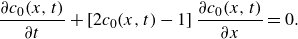 \begin{equation} \frac {\partial c_0(x,t)}{\partial t} + \left [2 c_0(x,t) - 1 \right ] \frac {\partial c_0(x,t)}{\partial x} = 0. \end{equation}
Equation (4.1) can be solved analytically via the method of characteristics, with the similarity variable
 $\xi \equiv x/t$
:
$\xi \equiv x/t$
:
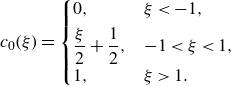 \begin{equation} c_0(\xi ) = \begin{cases} 0,& \xi \lt -1,\\[3pt] \dfrac {\xi }{2} + \dfrac {1}{2}, & -1 \lt \xi \lt 1, \\[3pt] 1, & \xi \gt 1. \end{cases} \end{equation}
This solution demonstrates the existence of an expanding rarefaction region that linearly connects the regions of clear oil (i.e.
 $c_0 = 0$
) and uniform suspension (i.e.
$c_0 = 0$
) and uniform suspension (i.e.
 $c_0 = 1$
).
$c_0 = 1$
).
To validate (4.2) experimentally, we quantify the particle number density averaged in the transverse direction,
 $\rho _0(\hat {X},\hat {t})$
, from our systematic experiments with clear oil. The high-resolution experiments allow us to track the positions of the individual particles inside the cell over the duration of the experiment. We convert the particle positions into
$\rho _0(\hat {X},\hat {t})$
, from our systematic experiments with clear oil. The high-resolution experiments allow us to track the positions of the individual particles inside the cell over the duration of the experiment. We convert the particle positions into
 $\rho _0(\hat {X},\hat {t})$
by averaging the number of particles inside a rectangular domain that is a few particle diameters wide. For
$\rho _0(\hat {X},\hat {t})$
by averaging the number of particles inside a rectangular domain that is a few particle diameters wide. For
 $\phi _i = 25\, \%$
or
$\phi _i = 25\, \%$
or
 $\rho _i = 1.13\,{\textrm{mm}}^{-2}$
, the plot of
$\rho _i = 1.13\,{\textrm{mm}}^{-2}$
, the plot of
 $\rho _0(\hat {X},\hat {t})$
in figure 2(a) clearly shows the emergence and expansion of the rarefaction region over which
$\rho _0(\hat {X},\hat {t})$
in figure 2(a) clearly shows the emergence and expansion of the rarefaction region over which
 $\rho _0(\hat {X},\hat {t})$
gradually increases from 0 to
$\rho _0(\hat {X},\hat {t})$
gradually increases from 0 to
 $\rho _i$
(bounded by dashed lines). We acknowledge that
$\rho _i$
(bounded by dashed lines). We acknowledge that
 $\rho _0$
shows some non-uniformities even in the uniform region, while its mean value matches
$\rho _0$
shows some non-uniformities even in the uniform region, while its mean value matches
 $\rho _i$
. Such non-uniformities are caused by the fluctuations that occur in the flow of a 2-D uniform suspension (Desreumaux et al. Reference Desreumaux, Caussin, Jeanneret, Lauga and Bartolo2013).
$\rho _i$
. Such non-uniformities are caused by the fluctuations that occur in the flow of a 2-D uniform suspension (Desreumaux et al. Reference Desreumaux, Caussin, Jeanneret, Lauga and Bartolo2013).
We plot
 $\rho _0$
as a function of
$\rho _0$
as a function of
 $\hat {X}/\hat {t}$
for different values of
$\hat {X}/\hat {t}$
for different values of
 $\rho _i$
in figure 2(b). Note that
$\rho _i$
in figure 2(b). Note that
 $\hat {X}/\hat {t} = \kappa \unicode{x03C0} S\rho _i(\xi +1)+\kappa {\hat{v}}^{\infty }$
based on our non-dimensionalisation. As predicted by our solution in (4.2),
$\hat {X}/\hat {t} = \kappa \unicode{x03C0} S\rho _i(\xi +1)+\kappa {\hat{v}}^{\infty }$
based on our non-dimensionalisation. As predicted by our solution in (4.2),
 $\rho _0(\hat {X},\hat {t})$
for given
$\rho _0(\hat {X},\hat {t})$
for given
 $\rho _i$
is shown to collapse across all time, experimentally validating the self-similar nature of the rarefaction region. Furthermore, the slope of the linear part of
$\rho _i$
is shown to collapse across all time, experimentally validating the self-similar nature of the rarefaction region. Furthermore, the slope of the linear part of
 $\rho _0(\hat {X}/\hat {t})$
corresponds to
$\rho _0(\hat {X}/\hat {t})$
corresponds to
 $1/(2\kappa \unicode{x03C0} S)$
, independent of
$1/(2\kappa \unicode{x03C0} S)$
, independent of
 $\rho _i$
. Once the dipolar strength
$\rho _i$
. Once the dipolar strength
 $S$
is determined experimentally (i.e.
$S$
is determined experimentally (i.e.
 $S\approx 0.178\,{\textrm{mm}}^3\,{\textrm s}^{-1}$
) from this slope, we set the dimensionless moving coordinate
$S\approx 0.178\,{\textrm{mm}}^3\,{\textrm s}^{-1}$
) from this slope, we set the dimensionless moving coordinate
 $x$
for each
$x$
for each
 $\rho _i$
. The resultant plot of
$\rho _i$
. The resultant plot of
 $\rho _0/\rho _i$
as a function of
$\rho _0/\rho _i$
as a function of
 $\xi =x/t$
shows a reasonable collapse for all experimental parameters in figure 2(c).
$\xi =x/t$
shows a reasonable collapse for all experimental parameters in figure 2(c).
4.2. Universal fingering growth
To probe the stability of the model system, we set
 $\delta\, c(x,y,t) \equiv 2\sum _{k=0}^\infty \tilde {c}_k(x,t)\cos {(k y)}$
with wavenumber
$\delta\, c(x,y,t) \equiv 2\sum _{k=0}^\infty \tilde {c}_k(x,t)\cos {(k y)}$
with wavenumber
 $k$
, and combine it with (3.3). Then with the subscript
$k$
, and combine it with (3.3). Then with the subscript
 $k$
omitted for brevity, we arrive at the following governing equation for
$k$
omitted for brevity, we arrive at the following governing equation for
 $\tilde {c}$
:
$\tilde {c}$
:
 \begin{equation} \begin{aligned}[b] 0 ={}& \frac {\partial \tilde {c}}{\partial t}-\frac {1}{\unicode{x03C0} }c_0\int _0^{2\unicode{x03C0} }\tilde {c}(x-\cos \theta )\cos {(-k\sin {\theta })}\cos {\theta }\,{\textrm d}\theta \\ &{}+ \frac {\partial \tilde {c}}{\partial x}\left [\frac {2}{\unicode{x03C0} }\int _{-1}^{+1}c_0(x+\tilde x)\sqrt {1-\tilde {x}^2}\,{\textrm d}\tilde x - 1\right ] -\frac {1}{\pi }\tilde {c}\int _0^{2\unicode{x03C0} }c_0(x-\cos {\theta })\cos {\theta }\,{\textrm d}\theta \\ &{}+\frac {1}{\pi }\frac {\partial c_0}{\partial x}\left [\int _1^{+\infty }\left [\tilde {c}(x+\tilde {x})+\tilde {c}(x-\tilde {x})\right ]I_1\,{\textrm d}\tilde {x} +\int _{-1}^{1}\tilde {c}(x+\tilde {x})I_2\,{\textrm d}\tilde {x}\right ], \end{aligned} \end{equation}
where
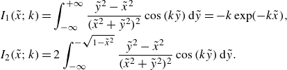 \begin{equation} \begin{aligned} I_1(\tilde {x};k) &= \int _{-\infty }^{+\infty } \frac {\tilde {y}^2-\tilde {x}^2}{(\tilde {x}^2+\tilde {y}^2)^2} \cos {(k\tilde {y})}\,{\textrm d}\tilde {y} = -k \exp (-k\tilde {x}), \\ I_2(\tilde {x};k) &= 2\int _{-\infty }^{-\sqrt {1-\tilde {x}^2}}\frac {\tilde {y}^2-\tilde {x}^2}{(\tilde {x}^2+\tilde {y}^2)^2} \cos {(k\tilde {y})}\,{\textrm d}\tilde {y}. \end{aligned} \end{equation}
Here,
 $I_1$
and
$I_1$
and
 $I_2$
constitute
$I_2$
constitute
 $u_{d}$
in the Fourier space, while
$u_{d}$
in the Fourier space, while
 $v_{d}\!=\!0$
owing to the symmetry of the disturbance flow (i.e.
$v_{d}\!=\!0$
owing to the symmetry of the disturbance flow (i.e.
 $\boldsymbol{v}^{{dip}}$
) and the uniformity of
$\boldsymbol{v}^{{dip}}$
) and the uniformity of
 $c_0$
in the
$c_0$
in the
 $y$
-direction. The detailed derivation of (4.3) and (4.4) has been included in Appendix E.
$y$
-direction. The detailed derivation of (4.3) and (4.4) has been included in Appendix E.
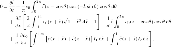
(a) The plot of the growth rate
 $\sigma$
versus the wavenumber
$\sigma$
versus the wavenumber
 $k$
. The growth rate varies non-monotonically with
$k$
. The growth rate varies non-monotonically with
 $k$
, and is positive across a range of wavenumbers. Over time, the critical wavenumber associated with the peak growth rate exhibits a decay. (b) The plot of the critical wavelength
$k$
, and is positive across a range of wavenumbers. Over time, the critical wavenumber associated with the peak growth rate exhibits a decay. (b) The plot of the critical wavelength
 $\lambda _c$
over dimensionless time
$\lambda _c$
over dimensionless time
 $t$
from the simulations and the experiments;
$t$
from the simulations and the experiments;
 $\lambda _c$
from the simulations increases over
$\lambda _c$
from the simulations increases over
 $t$
. Given the universality of the derived equation, the critical wavelengths from different experiments are expected to converge into a single curve upon non-dimensionalisation. The error bars associated with the experimental data reflect the spatial variability of finger widths in the rarefaction region for each experiment. (c) We include the experimental images from three experiments (
$t$
. Given the universality of the derived equation, the critical wavelengths from different experiments are expected to converge into a single curve upon non-dimensionalisation. The error bars associated with the experimental data reflect the spatial variability of finger widths in the rarefaction region for each experiment. (c) We include the experimental images from three experiments (
 $\phi _i=5\, \%,15\, \%,25\, \%$
) at
$\phi _i=5\, \%,15\, \%,25\, \%$
) at
 $t=12$
(or three separate dimensional times). The three images exhibit similar fingering patterns.
$t=12$
(or three separate dimensional times). The three images exhibit similar fingering patterns.
Using the upwind numerical scheme, we compute
 $\tilde c(x,t)$
from (4.3), by assuming a Gaussian function with a particle-scale width as the initial condition. Once
$\tilde c(x,t)$
from (4.3), by assuming a Gaussian function with a particle-scale width as the initial condition. Once
 $\tilde c(x,t)$
is known, we define the growth rate
$\tilde c(x,t)$
is known, we define the growth rate
 $\sigma$
based on the changes in the root mean square of
$\sigma$
based on the changes in the root mean square of
 $\tilde c(x,t)$
over the whole domain (Tan & Homsy Reference Tan and Homsy1986), or
$\tilde c(x,t)$
over the whole domain (Tan & Homsy Reference Tan and Homsy1986), or
 $\sigma \equiv \ln [M(t+\delta t)- M(t)]/\delta t$
, where
$\sigma \equiv \ln [M(t+\delta t)- M(t)]/\delta t$
, where
 $M(t)\equiv \Big[\int _{-L}^{L} [\tilde {c}(x,t)]^2 \,{\textrm d}x /(2L) \Big]^{1/2}$
, with the time step
$M(t)\equiv \Big[\int _{-L}^{L} [\tilde {c}(x,t)]^2 \,{\textrm d}x /(2L) \Big]^{1/2}$
, with the time step
 $\delta t$
and the domain size
$\delta t$
and the domain size
 $L$
. As shown in figure 3(a),
$L$
. As shown in figure 3(a),
 $\sigma$
varies non-monotonically with
$\sigma$
varies non-monotonically with
 $k$
and is positive for the intermediate values of
$k$
and is positive for the intermediate values of
 $k$
, while its overall magnitude decreases with time. In addition, the critical wavenumber
$k$
, while its overall magnitude decreases with time. In addition, the critical wavenumber
 $k_c$
at which
$k_c$
at which
 $\partial \sigma /\partial k = 0$
gradually decreases over time, which corresponds to an increase in the critical wavelength
$\partial \sigma /\partial k = 0$
gradually decreases over time, which corresponds to an increase in the critical wavelength
 $\lambda _c$
with time. Hence our minimal model with inter-particle dipolar interactions correctly predicts widening of the emergent fingers with time at all particle concentrations. Note that our choice of initial data guarantees that a sufficiently wide range of Fourier modes is covered, and our specific definition of
$\lambda _c$
with time. Hence our minimal model with inter-particle dipolar interactions correctly predicts widening of the emergent fingers with time at all particle concentrations. Note that our choice of initial data guarantees that a sufficiently wide range of Fourier modes is covered, and our specific definition of
 $\sigma$
does not influence the wavenumber selection, which has been confirmed through numerical tests.
$\sigma$
does not influence the wavenumber selection, which has been confirmed through numerical tests.
Furthermore, the behaviours of
 $\sigma (k;t)$
and
$\sigma (k;t)$
and
 $k_c$
mirror those found in viscous fingering between two miscible fluids for low
$k_c$
mirror those found in viscous fingering between two miscible fluids for low
 ${Pe}$
. Tan & Homsy (Reference Tan and Homsy1986) performed the stability analysis of the displacement of pure miscible liquids, and showed that thermal diffusion gradually increases the mixing region between the two fluids, which causes the finger width to widen over time. This striking similarity between our simulation results and the analysis by Tan & Homsy (Reference Tan and Homsy1986) suggests that dipolar interactions between highly confined particles display the stabilising effects that are comparable to thermal diffusion even at
${Pe}$
. Tan & Homsy (Reference Tan and Homsy1986) performed the stability analysis of the displacement of pure miscible liquids, and showed that thermal diffusion gradually increases the mixing region between the two fluids, which causes the finger width to widen over time. This striking similarity between our simulation results and the analysis by Tan & Homsy (Reference Tan and Homsy1986) suggests that dipolar interactions between highly confined particles display the stabilising effects that are comparable to thermal diffusion even at
 ${{Pe}}\rightarrow \infty$
.
${{Pe}}\rightarrow \infty$
.
However, distinct from Tan & Homsy (Reference Tan and Homsy1986), our current model is not explicitly governed by the external parameters (e.g.
 $Pe$
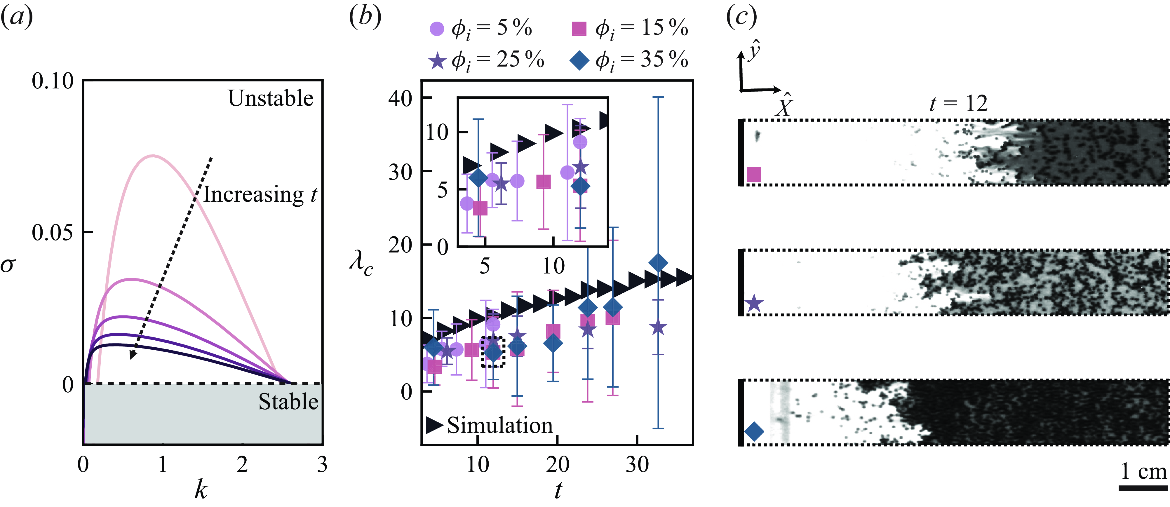
, viscosity ratios) that control the relative strength of stabilising and destabilising effects. Because the inter-particle dipolar interactions alone control the instability, the initial particle concentration drops out of the dimensionless equation, except to set the timescale of fingering. As the dimensionless time
$Pe$
, viscosity ratios) that control the relative strength of stabilising and destabilising effects. Because the inter-particle dipolar interactions alone control the instability, the initial particle concentration drops out of the dimensionless equation, except to set the timescale of fingering. As the dimensionless time
 $t$
has been normalised by
$t$
has been normalised by
 $\rho _i$
, our results indicate that the dimensional time
$\rho _i$
, our results indicate that the dimensional time
 $\hat {t}=td/(\kappa \unicode{x03C0} S\rho _i)$
that it takes for the finger width to reach the comparable size must decrease with increasing
$\hat {t}=td/(\kappa \unicode{x03C0} S\rho _i)$
that it takes for the finger width to reach the comparable size must decrease with increasing
 $\rho _i$
. Equivalently, at given dimensional time
$\rho _i$
. Equivalently, at given dimensional time
 $\hat {t}$
that corresponds to longer
$\hat {t}$
that corresponds to longer
 $t$
for larger
$t$
for larger
 $\rho _i$
, the emergent fingers are predicted to be wider as
$\rho _i$
, the emergent fingers are predicted to be wider as
 $\rho _i$
is increased, which is consistent with our experimental observations in figure 1(c).
$\rho _i$
is increased, which is consistent with our experimental observations in figure 1(c).
For more quantitative comparison, we obtain the critical wavelengths
 $\lambda _c$
from the experiments via image processing, which we describe in detail in Appendix B. We plot
$\lambda _c$
from the experiments via image processing, which we describe in detail in Appendix B. We plot
 $\lambda _c$
from the experiments as a function of
$\lambda _c$
from the experiments as a function of
 $t$
together with the numerical simulations in figure 3(b). Despite the scatter caused by the broad distribution of finger widths inside the rarefaction region, experimental
$t$
together with the numerical simulations in figure 3(b). Despite the scatter caused by the broad distribution of finger widths inside the rarefaction region, experimental
 $\lambda _c$
increases with
$\lambda _c$
increases with
 $t$
and shows a reasonable collapse across all particle concentrations. Furthermore, the images in figure 3(c) from three separate experiments (i.e.
$t$
and shows a reasonable collapse across all particle concentrations. Furthermore, the images in figure 3(c) from three separate experiments (i.e.
 $\phi _i=5\, \%,15\, \%,25\, \%$
) exhibit similar fingering patterns at given dimensionless time
$\phi _i=5\, \%,15\, \%,25\, \%$
) exhibit similar fingering patterns at given dimensionless time
 $t=12$
, which again qualitatively matches our model predictions.
$t=12$
, which again qualitatively matches our model predictions.
4.3. Mechanism of wavelength selection
In our system, both experimental observations and linear stability analysis demonstrate the simultaneous development of rarefaction and fingering regions. To further elucidate the mechanism of wavelength selection via dipolar interactions, we focus on the
 $\partial c_0/\partial x$
term in (4.3), which directly addresses the viscosity contrast between the invading (clear oil) and defending (2-D suspension) phases. This term separates the current model from the work of Desreumaux et al. (Reference Desreumaux, Caussin, Jeanneret, Lauga and Bartolo2013), who performed a stability analysis on the 2-D uniform suspension flow. Their analysis yielded hydrodynamic fluctuations but no growing instabilities, which confirms that the
$\partial c_0/\partial x$
term in (4.3), which directly addresses the viscosity contrast between the invading (clear oil) and defending (2-D suspension) phases. This term separates the current model from the work of Desreumaux et al. (Reference Desreumaux, Caussin, Jeanneret, Lauga and Bartolo2013), who performed a stability analysis on the 2-D uniform suspension flow. Their analysis yielded hydrodynamic fluctuations but no growing instabilities, which confirms that the
 $\partial c_0/\partial x$
term is indeed the key to viscous fingering. This choice is also confirmed by the ablation test included in Appendix F.
$\partial c_0/\partial x$
term is indeed the key to viscous fingering. This choice is also confirmed by the ablation test included in Appendix F.
By systematically analysing the effects of the
 $\partial c_0/\partial x$
term on critical wavelength selection in (4.3), we reduce the governing equation for
$\partial c_0/\partial x$
term on critical wavelength selection in (4.3), we reduce the governing equation for
 $\tilde {c}$
to
$\tilde {c}$
to
 \begin{equation} \frac {\partial \tilde {c}}{\partial t} +\frac {1}{\pi }\frac {\partial c_0}{\partial x}\int _1^{+\infty }\left [\tilde {c}(x+\tilde {x})+\tilde {c}(x-\tilde {x})\right ]I_1\,{\textrm d}\tilde {x} = 0. \end{equation}
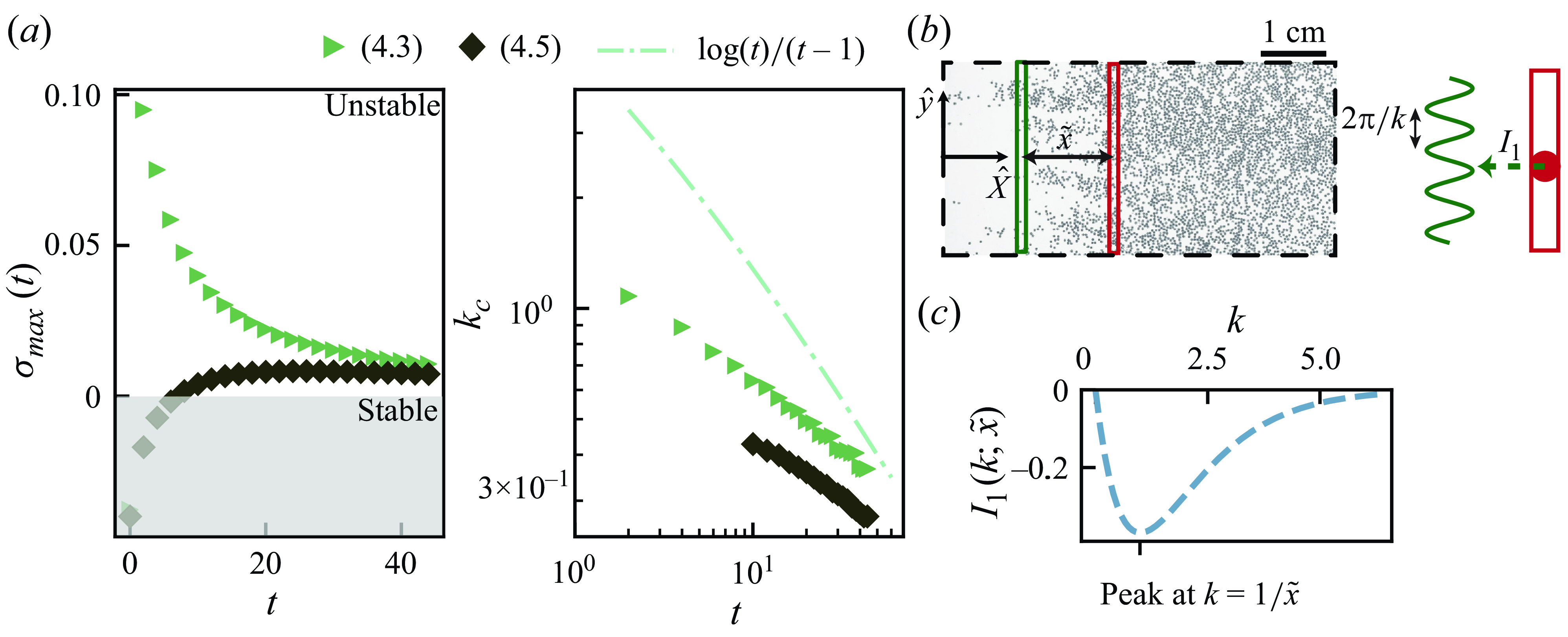
We plot the maximum
 $\sigma$
(i.e.
$\sigma$
(i.e.
 $\sigma _{{max}}$
) and
$\sigma _{{max}}$
) and
 $k_c$
from (4.5), and compare them to the results of the full governing equation in figure 4(a), which shows a qualitative match with the full solutions as
$k_c$
from (4.5), and compare them to the results of the full governing equation in figure 4(a), which shows a qualitative match with the full solutions as
 $t\rightarrow \infty$
.
$t\rightarrow \infty$
.
As illustrated in figure 4(b),
 $I_1(\tilde {x};k)$
captures the effects of a column of perturbed particles (green line) on a ‘test’ particle (red circle) separated by a distance
$I_1(\tilde {x};k)$
captures the effects of a column of perturbed particles (green line) on a ‘test’ particle (red circle) separated by a distance
 $\tilde {x}$
. As shown in figure 4(c), for given
$\tilde {x}$
. As shown in figure 4(c), for given
 $\tilde {x}$
,
$\tilde {x}$
,
 $I_1$
is negative across all
$I_1$
is negative across all
 $k$
, indicating that perturbing the green line will destabilise the test particle across all wavenumbers as long as
$k$
, indicating that perturbing the green line will destabilise the test particle across all wavenumbers as long as
 $\partial c_0/\partial x\gt 0$
. Additionally, for given
$\partial c_0/\partial x\gt 0$
. Additionally, for given
 $\tilde {x}$
, the magnitude of
$\tilde {x}$
, the magnitude of
 $I_1$
peaks at
$I_1$
peaks at
 $k=1/\tilde {x}$
, which implies that the perturbed green line selectively fosters the fastest-growing mode based on the separation distance.
$k=1/\tilde {x}$
, which implies that the perturbed green line selectively fosters the fastest-growing mode based on the separation distance.
(a) Comparative simulation results between the comprehensive model (4.3) and the simplified physical model (4.5). The simplified model initially fails to capture the system’s instability but converges to a similar constant maximum growth rate over long times. It also accurately predicts the broadening of the wavelength, or equivalently the decrease in
 $k_c$
, as observed in the full model. (b) To represent the physical meaning of
$k_c$
, as observed in the full model. (b) To represent the physical meaning of
 $I_1$
, we include the schematic of the perturbed line of particles (green curve) affecting a test particle (red circle) placed at a distance
$I_1$
, we include the schematic of the perturbed line of particles (green curve) affecting a test particle (red circle) placed at a distance
 $\tilde {x}$
away from it. (c) For given
$\tilde {x}$
away from it. (c) For given
 $\tilde {x}$
,
$\tilde {x}$
,
 $I_1$
is negative for all
$I_1$
is negative for all
 $k$
, and its magnitude reaches a maximum at
$k$
, and its magnitude reaches a maximum at
 $k=1/\tilde {x}$
. The wavenumber selection is influenced by the cumulative impact of all perturbed lines within the expanding rarefaction region.
$k=1/\tilde {x}$
. The wavenumber selection is influenced by the cumulative impact of all perturbed lines within the expanding rarefaction region.
As the product of
 $I_1$
and
$I_1$
and
 $\tilde {c}$
is integrated over
$\tilde {c}$
is integrated over
 $\tilde {x}$
in (4.5), the largest growing mode must be influenced by the size of the integration domain. The integration domain can be approximated as the rarefaction region, as our numerical solutions reveal that
$\tilde {x}$
in (4.5), the largest growing mode must be influenced by the size of the integration domain. The integration domain can be approximated as the rarefaction region, as our numerical solutions reveal that
 $\tilde {c}$
is mostly zero outside it. Finally, by assuming constant
$\tilde {c}$
is mostly zero outside it. Finally, by assuming constant
 $\tilde {c}$
for simplicity, we integrate
$\tilde {c}$
for simplicity, we integrate
 $I_1$
over the rarefaction region to obtain
$I_1$
over the rarefaction region to obtain
 $k_c\propto \log (t)/(t-1)$
. As shown in figure 4(a), this scaling decays more steeply with time compared to the full simulation results, which underscores the significance of accounting for the non-uniformity of
$k_c\propto \log (t)/(t-1)$
. As shown in figure 4(a), this scaling decays more steeply with time compared to the full simulation results, which underscores the significance of accounting for the non-uniformity of
 $\tilde {c}$
within the rarefaction region. Despite the deviation between the scaling and the numerical results, our simple analysis illustrates that the expanding rarefaction region is the key to qualitatively capturing the decay of
$\tilde {c}$
within the rarefaction region. Despite the deviation between the scaling and the numerical results, our simple analysis illustrates that the expanding rarefaction region is the key to qualitatively capturing the decay of
 $k_c$
, or the widening fingers, over time. The expanding rarefaction region parallels the growing mixing region between two miscible fluids, which explains the similarity between the
$k_c$
, or the widening fingers, over time. The expanding rarefaction region parallels the growing mixing region between two miscible fluids, which explains the similarity between the
 $x$
-component of the dipolar interactions and thermal diffusion that is responsible for generating the mixing region.
$x$
-component of the dipolar interactions and thermal diffusion that is responsible for generating the mixing region.
5. Conclusion
In this study, we experimentally demonstrate viscous fingering when pure oil displaces the mixture of the same oil and highly confined non-colloidal particles in the limit of zero interfacial tension and diffusion. In contrast to other studies of miscible displacements at
 ${{Pe}}\rightarrow \infty$
(Videbæk & Nagel Reference Videbæk and Nagel2019; Luo et al. Reference Luo, Chen and Lee2020; Videbæk Reference Videbæk2020), our experiments show that fingers form at all particle concentrations, as the channel confinement eliminates the 3-D structure inside the channel gap that suppresses viscous fingering of all wavelengths. Furthermore, despite having no thermal diffusion, we find that fingering behaviours in 2-D suspensions are strongly reminiscent of classic 2-D viscous fingering between two miscible fluids at low
${{Pe}}\rightarrow \infty$
(Videbæk & Nagel Reference Videbæk and Nagel2019; Luo et al. Reference Luo, Chen and Lee2020; Videbæk Reference Videbæk2020), our experiments show that fingers form at all particle concentrations, as the channel confinement eliminates the 3-D structure inside the channel gap that suppresses viscous fingering of all wavelengths. Furthermore, despite having no thermal diffusion, we find that fingering behaviours in 2-D suspensions are strongly reminiscent of classic 2-D viscous fingering between two miscible fluids at low
 $Pe$
.
$Pe$
.
To rationalise this fingering regime, we develop a minimal mathematical model that captures the hydrodynamic interactions between the highly confined particles. Overall, our model successfully demonstrates that the dominant source of instability lies in the
 $x$
-component of the dipolar interactions, initiating both the rarefaction wave and the subsequent instability along the
$x$
-component of the dipolar interactions, initiating both the rarefaction wave and the subsequent instability along the
 $y$
-direction. In addition, the expanding rarefaction region qualitatively takes on the role of ‘diffusion’, as it causes the critical finger width to widen over time. Because we do not have separate sources for fingering and stabilisation, our model is described by a universal equation that is independent of the particle concentration.
$y$
-direction. In addition, the expanding rarefaction region qualitatively takes on the role of ‘diffusion’, as it causes the critical finger width to widen over time. Because we do not have separate sources for fingering and stabilisation, our model is described by a universal equation that is independent of the particle concentration.
Our work combines viscous fingering with particle ensembles, which offers a new insight into harnessing instabilities to control the particle motion. For instance, strategically injecting the 2-D suspension to generate gradients in the particle concentration can lead to the shock or rarefaction waves and instabilities (Beatus, Tlusty & Bar-Ziv Reference Beatus, Tlusty and Bar-Ziv2009), which will alter the emergent behaviours of particles. In addition to the control of particles, we will extend our current analysis by including more relevant physics into the model, such as the effects of the side walls, and investigating the coupling between fingering patterns and hydrodynamic fluctuations, as observed by Desreumaux et al. (Reference Desreumaux, Caussin, Jeanneret, Lauga and Bartolo2013). Finally, another future direction of research includes investigating the effects of channel confinement on the miscible displacement of a suspension with pure oil. The previous experiments by Luo et al. (Reference Luo, Chen and Lee2020) demonstrated that the miscible displacement of a suspension in the continuum limit completely deviates from the present monolayer limit. Hence it would be of great interest to characterise the onset of viscous fingering as the channel confinement is systematically varied from continuum to the monolayer limit.
Supplementary movie
Supplementary movie is available at https://doi.org/10.1017/jfm.2025.402.
Acknowledgements
The authors would like to acknowledge Z. Wang for helpful discussions, and R. Bansal for his help with the experiments.
Funding
R.L., M.M., Z.H. and S.L. are partly funded by the National Science Foundation (DMR-2003706, EAR-2100493). L.W. is partly supported by NSF DMS-1846854.
Declaration of interests
The authors report no conflict of interest.
Appendix A. Experimental procedure
To study the interfacial instability between the suspension and the clear oil, it is essential to establish an undisturbed, flat interface prior to the invasion of the clear oil into the suspension. This is achieved through the use of two 3-D-printed flow-guiding structures attached to either end of the Hele-Shaw cell. A suspension is prepared and injected through the structure designated as the suspension inlet into the Hele-Shaw cell. The injection continues until the suspension reaches the periphery of the cell, adjacent to the second structure. Once the suspension has filled the cell to the desired location, the suspension inlet is sealed to prevent any further inflow of suspension.
Clear oil is then injected into the reservoir of the second structure, ensuring that it makes contact with the suspension without causing any disturbances to the established interface. The second structure comes with a circular opening on top, which allows air to vent out during initial oil injection. After the clear oil has been introduced, the circular opening (for releasing air) is sealed to maintain the integrity of the interface. With the circular opening sealed, the suspension inlet is reopened. Clear oil is injected again, this time invading the suspension and generating fingers. The displaced suspension is expelled through the suspension inlet, allowing for the observation of the interfacial instability as the clear oil advances.
Appendix B. Finger width measurements
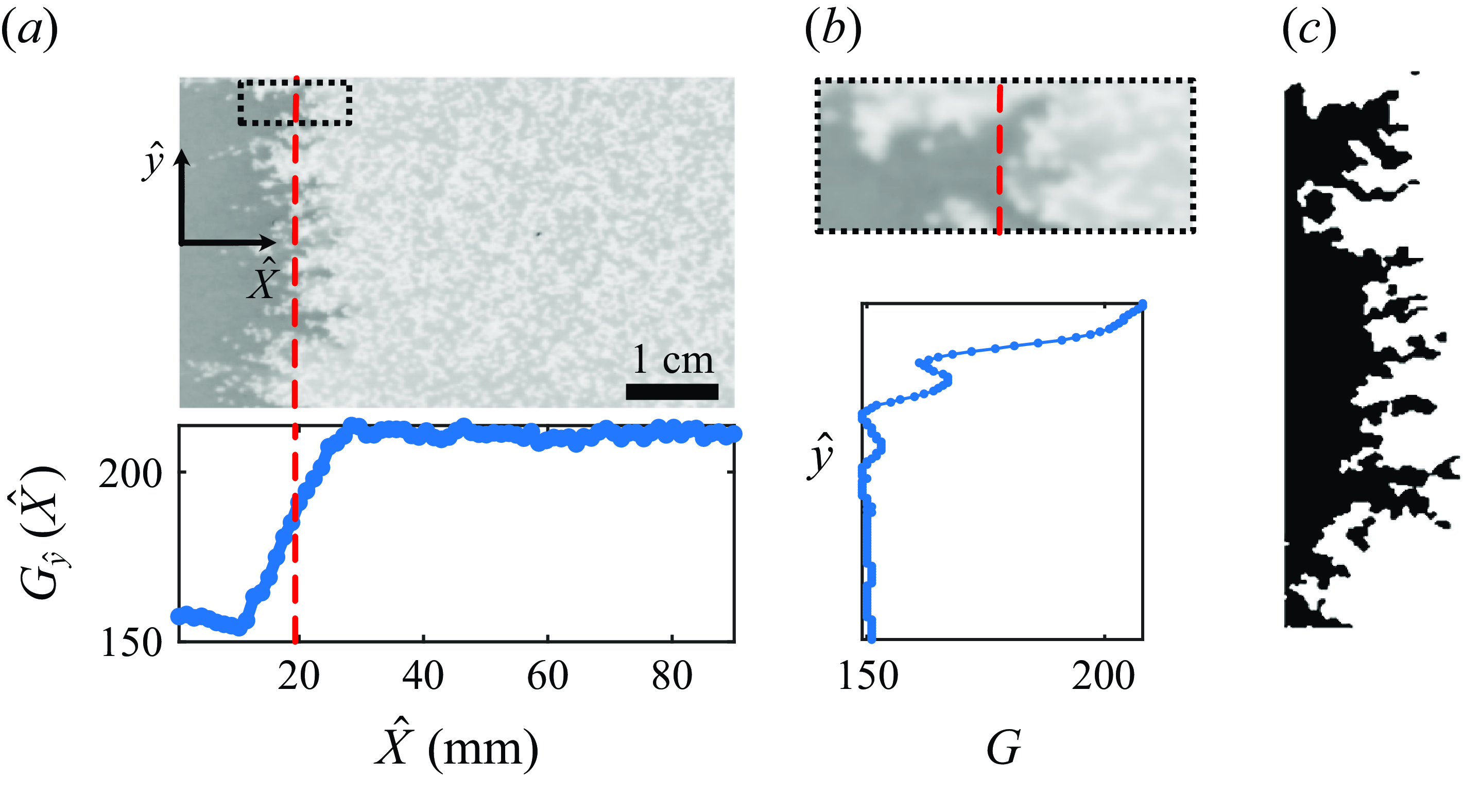
We employ a fluorescent dye to visualise the flow patterns as silicone oil is injected into the mixture of the same oil and polystyrene particles. The captured images are processed using the red channel filter, denoted as
 $ G(\hat {X},\hat {y})$
, to analyse the finger patterns (see figure 5
a). The analysis proceeds as follows.
$ G(\hat {X},\hat {y})$
, to analyse the finger patterns (see figure 5
a). The analysis proceeds as follows.
The rarefaction region is identified by calculating the
 $\hat {y}$
-averaged intensity (grey scale) of the red channel,
$\hat {y}$
-averaged intensity (grey scale) of the red channel,
 $ G_y(\hat {X})$
. The image is then cropped to focus on this region. As illustrated in figure 5(b), the intensity profile
$ G_y(\hat {X})$
. The image is then cropped to focus on this region. As illustrated in figure 5(b), the intensity profile
 $ G(\hat {y})$
along the centreline of the rarefaction region (red dashed line) reveals a distinct intensity variation, clearly demarcating the finger region. A fixed threshold is applied to the cropped image to extract the dyed oil region, resulting in a binary representation of the finger pattern (figure 5
c). This binary image highlights the spatial distribution of the dyed oil within the rarefaction region. The finger pattern exhibits non-uniformity in both the
$ G(\hat {y})$
along the centreline of the rarefaction region (red dashed line) reveals a distinct intensity variation, clearly demarcating the finger region. A fixed threshold is applied to the cropped image to extract the dyed oil region, resulting in a binary representation of the finger pattern (figure 5
c). This binary image highlights the spatial distribution of the dyed oil within the rarefaction region. The finger pattern exhibits non-uniformity in both the
 $\hat {X}$
- and
$\hat {X}$
- and
 $\hat {y}$
-directions. In the
$\hat {y}$
-directions. In the
 $\hat {X}$
-direction, the fingers are thinner near the front of the rarefaction region, and gradually widen towards the end. In the
$\hat {X}$
-direction, the fingers are thinner near the front of the rarefaction region, and gradually widen towards the end. In the
 $\hat {y}$
-direction, the width of the fingers varies due to the dynamic behaviour of the particles during injection. This non-uniformity is quantified by calculating the standard deviation of the finger width in the
$\hat {y}$
-direction, the width of the fingers varies due to the dynamic behaviour of the particles during injection. This non-uniformity is quantified by calculating the standard deviation of the finger width in the
 $\hat {y}$
-direction, providing a measure of the spatial variability in the pattern.
$\hat {y}$
-direction, providing a measure of the spatial variability in the pattern.
(a) The plot of the width-averaged intensity
 $G_y(\hat {X})$
as a function of
$G_y(\hat {X})$
as a function of
 $\hat {X}$
highlights the rarefaction region inside the cell. (b) We focus on the small region around the rarefaction region to highlight the variations of
$\hat {X}$
highlights the rarefaction region inside the cell. (b) We focus on the small region around the rarefaction region to highlight the variations of
 $G$
in
$G$
in
 $\hat {y}$
, corresponding to the emergent fingers. (c) We turn the original image into a binary image via thresholding (dyed oil in black), from which we extract
$\hat {y}$
, corresponding to the emergent fingers. (c) We turn the original image into a binary image via thresholding (dyed oil in black), from which we extract
 $\lambda _c$
.
$\lambda _c$
.
Appendix C. Derivation of (3.3) and (3.4)
The key to deriving (3.3) from (3.2) is the simplification
 $\boldsymbol{\nabla} \boldsymbol{\cdot} \boldsymbol{j}$
, where
$\boldsymbol{\nabla} \boldsymbol{\cdot} \boldsymbol{j}$
, where
 $\boldsymbol{j}$
is the dimensionless particle flux. Let us first introduce the relative position vector
$\boldsymbol{j}$
is the dimensionless particle flux. Let us first introduce the relative position vector
 $ {\tilde{\boldsymbol{r}}} = \boldsymbol{r}' - \boldsymbol{r}$
, where
$ {\tilde{\boldsymbol{r}}} = \boldsymbol{r}' - \boldsymbol{r}$
, where
 ${\tilde{\boldsymbol{r}}}$
denotes the displacement vector along the direction of the normal vector
${\tilde{\boldsymbol{r}}}$
denotes the displacement vector along the direction of the normal vector
 $\boldsymbol{n}$
, such that
$\boldsymbol{n}$
, such that
 ${\tilde{\boldsymbol{r}}} = (\tilde {x},\tilde {y})\boldsymbol{\cdot} \boldsymbol{n}$
. This definition is instrumental in simplifying the convection term and facilitating the physical interpretation of each term, as shown below:
${\tilde{\boldsymbol{r}}} = (\tilde {x},\tilde {y})\boldsymbol{\cdot} \boldsymbol{n}$
. This definition is instrumental in simplifying the convection term and facilitating the physical interpretation of each term, as shown below:
 \begin{equation} \begin{aligned}[b] \boldsymbol{\nabla} \boldsymbol{\cdot} \boldsymbol{j}(\boldsymbol{r},t) &= \boldsymbol{\nabla} \boldsymbol{\cdot} \left [ \iint _{\left | \boldsymbol{r} - \boldsymbol{r'} \right | \ge 1} c(\boldsymbol{r},t)\,\boldsymbol{v}^{{dip}}(\boldsymbol{r},\boldsymbol{r}')\, c(\boldsymbol{r}',t)\,\textrm {d}\boldsymbol{r}' \right ] \\ &= \boldsymbol{\nabla}c(\boldsymbol{r},t) \boldsymbol{\cdot} \iint _{\left | \boldsymbol{r} - \boldsymbol{r'} \right | \ge 1} \boldsymbol{v}^{{dip}}(\boldsymbol{r},\boldsymbol{r}')\, c(\boldsymbol{r}',t)\,\textrm {d}\boldsymbol{r}' + c(\boldsymbol{r},t)\, \boldsymbol{\nabla} \boldsymbol{\cdot} \\ & \quad\left [\iint _{\left | \boldsymbol{r} - \boldsymbol{r'} \right | \ge 1} \boldsymbol{v}^{{dip}}(\boldsymbol{r},\boldsymbol{r}')\, c(\boldsymbol{r}',t)\,\textrm {d}\boldsymbol{r}'\right ] \\ &=\frac {\partial c(\boldsymbol{r},t)}{\partial x}\iint _{\tilde {x}^2+\tilde {y}^2 \ge 1} \frac {\tilde {y}^2-\tilde {x}^2}{(\tilde {x}^2+\tilde {y}^2)^2} c(x+\tilde {x},y+\tilde {y},t) \,\textrm {d}\tilde {x}\textrm {d}{\tilde {y}} \\ &\quad{}+ \frac {\partial c(\boldsymbol{r},t)}{\partial y}\iint _{\tilde {x}^2+\tilde {y}^2 \ge 1} \frac {2\tilde {x}\tilde {y}}{(\tilde {x}^2+\tilde {y}^2)^2} c(x+\tilde {x},y+\tilde {y},t)\,\textrm {d}\tilde {x}\textrm {d}{\tilde {y}}-c(\boldsymbol{r},t) \\ & \quad\times \int _{0}^{2\unicode{x03C0} } c(\boldsymbol{r} - \boldsymbol{n},t)\cos \theta \,\textrm {d}\theta . \end{aligned} \end{equation}
Note that we have used the divergence theorem to simplify the following:
 \begin{equation} \begin{aligned}[b] \boldsymbol{\nabla} \boldsymbol{\cdot} \left [\iint _{\left | \boldsymbol{r} - \boldsymbol{r'} \right | \ge 1} \boldsymbol{v}^{{dip}}(\boldsymbol{r},\boldsymbol{r}')\, c(\boldsymbol{r}',t)\,\textrm {d}\boldsymbol{r}'\right ] =& \iint _{ | {\tilde{\boldsymbol{r}}}| \ge 1} \boldsymbol{\nabla}_{ {\tilde{\boldsymbol{r}}}} \boldsymbol{\cdot} [\boldsymbol{v}^{{dip}}(\boldsymbol{r},\boldsymbol{r}+ {\tilde{\boldsymbol{r}}})\, c(\boldsymbol{r}+ {\tilde{\boldsymbol{r}}},t)]\,\textrm {d} {\tilde{\boldsymbol{r}}} \\ =& -\int _{ | {\tilde{\boldsymbol{r}}}| = 1} \boldsymbol{v}^{{dip}}(\boldsymbol{r},\boldsymbol{r}+ {\tilde{\boldsymbol{r}}})\, c(\boldsymbol{r}+ {\tilde{\boldsymbol{r}}},t) \boldsymbol{\cdot} \boldsymbol{n}\,\textrm {d} {\tilde{\boldsymbol{r}}} \\ =& -\int _0^{2 \unicode{x03C0} } \boldsymbol{v}^{{dip}}(\boldsymbol{r},\boldsymbol{r}+ \boldsymbol{n}) \boldsymbol{\cdot} \hat n\, c(\boldsymbol{r}+\boldsymbol{n} ,t)\,\textrm {d}\theta \\ =& - \int _0^{2 \unicode{x03C0} } c(\boldsymbol{r}-\boldsymbol{n},t) \cos \theta \,\textrm {d}\theta \,. \end{aligned} \end{equation}
Inserting (C1) into the original conservation law leads to (3.3)–(3.4), which govern the evolution of particle concentration.
Another major step in deriving (3.3) is the coordinate transformation based on
 $\hat {x} = \hat {X} - \kappa ({\hat{v}}^{\infty } + \unicode{x03C0} S\rho _i)\hat {t}$
and non-dimensionalisation via
$\hat {x} = \hat {X} - \kappa ({\hat{v}}^{\infty } + \unicode{x03C0} S\rho _i)\hat {t}$
and non-dimensionalisation via
 $\hat {x} = xd$
,
$\hat {x} = xd$
,
 $\hat {t} = t ({d}/{\kappa \unicode{x03C0} S \rho _i})$
:
$\hat {t} = t ({d}/{\kappa \unicode{x03C0} S \rho _i})$
:
 \begin{equation} \begin{aligned} \frac {\partial \rho (\hat {X},\hat {y},\hat {t})}{\partial \hat {t}} &= \rho _i \frac {\partial c(\hat {X},\hat {y},\hat {t})}{\partial \hat {t}} \\ &= \rho _i \frac {\partial c(\hat {x},\hat {y},\hat {t})}{\partial \hat {x}} \frac {\partial \hat {x}}{\partial \hat {t}} + \rho _i \frac {\partial c(\hat {x},\hat {y},\hat {t})}{\partial \hat {t}} \\ &= \rho _i \frac {\partial c(\hat {x},\hat {y},\hat {t})}{\partial \hat {t}}-\kappa \unicode{x03C0} S\rho _i^2 \frac {\partial c(\hat {x},\hat {y},\hat {t})}{\partial \hat {x}} - \kappa {\hat{v}}^{\infty } \frac {\partial c(\hat {x},\hat {y},\hat {t})}{\partial \hat {x}} \\ &= \frac {\kappa \unicode{x03C0} S\rho _i^2}{d} \frac {\partial c(x,y,t)}{\partial t} - \frac {\kappa \unicode{x03C0} S\rho _i^2}{d} \frac {\partial c(x,y,t)}{\partial x} - \kappa {\hat{v}}^{\infty } \frac {\partial c(x,y,t)}{\partial x}. \end{aligned} \end{equation}
Appendix D. Derivation of (4.1)
The leading order equation is obtained from (3.3) by introducing decomposition
 $c\!=\!c_0(x,t)+\delta\, c(x,y,t)$
, where
$c\!=\!c_0(x,t)+\delta\, c(x,y,t)$
, where
 $|c_0|\!\gg \!|\delta c|$
, and keeping the terms with
$|c_0|\!\gg \!|\delta c|$
, and keeping the terms with
 $c_0$
,
$c_0$
,
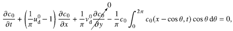
where
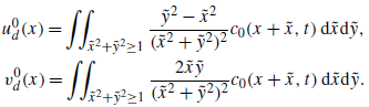 \begin{equation} \begin{aligned} u^0_{d}(x) = \iint _{\tilde {x}^2+\tilde {y}^2\ge 1} \frac {\tilde {y}^2-\tilde {x}^2}{(\tilde {x}^2+\tilde {y}^2)^2} c_0(x+\tilde {x},t)\,{\textrm d}\tilde {x}{\textrm d}\tilde {y}, \\ v^0_{d}(x) = \iint _{\tilde {x}^2+\tilde {y}^2\ge 1} \frac {2\tilde {x}\tilde {y}}{(\tilde {x}^2+\tilde {y}^2)^2} c_0(x+\tilde {x},t)\,{\textrm d}\tilde {x}{\textrm d}\tilde {y}. \end{aligned} \end{equation}
Here,
 $u^0_{d}(x)$
is further divided into four regions to compute the integral:
$u^0_{d}(x)$
is further divided into four regions to compute the integral:
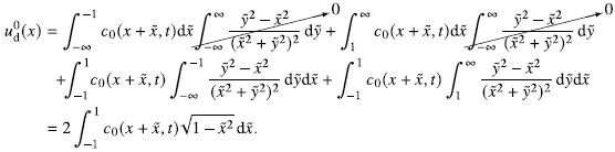
Now we apply the Taylor expansion of
 $c_0(x+\tilde x, t) \approx c_0(x,t) + \partial _x c_0(x,t) \tilde x$
to obtain
$c_0(x+\tilde x, t) \approx c_0(x,t) + \partial _x c_0(x,t) \tilde x$
to obtain
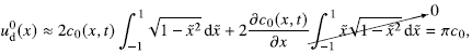
and
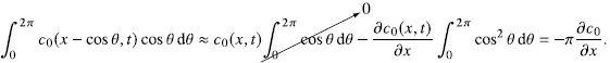
Appendix E. Derivation of (4.3) and (4.4)
The perturbation equation for
 $\delta\, c(x,y,t)$
is
$\delta\, c(x,y,t)$
is
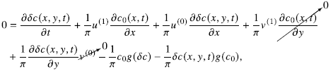
where
 $v^{(0)} = \iint _{\tilde {x}^2+\tilde {y}^2 \ge 1} ({2\tilde {x}\tilde {y}}/{(\tilde {x}^2+\tilde {y}^2)^2})\, c_0(x+\tilde {x},t) \,\textrm {d}\tilde {x}\textrm {d}{\tilde {y}}=0$
,
$v^{(0)} = \iint _{\tilde {x}^2+\tilde {y}^2 \ge 1} ({2\tilde {x}\tilde {y}}/{(\tilde {x}^2+\tilde {y}^2)^2})\, c_0(x+\tilde {x},t) \,\textrm {d}\tilde {x}\textrm {d}{\tilde {y}}=0$
,
 $g(c_0)= \int _{0}^{2\unicode{x03C0} } c_0(x - \cos \theta ,t)\cos \theta\, \textrm {d}\theta$
,
$g(c_0)= \int _{0}^{2\unicode{x03C0} } c_0(x - \cos \theta ,t)\cos \theta\, \textrm {d}\theta$
,
 $g(\delta c)= \int _{0}^{2\unicode{x03C0} } \delta\, c(\boldsymbol{r} - \boldsymbol{n},t)\cos \theta\, \textrm {d}\theta$
. Additionally,
$g(\delta c)= \int _{0}^{2\unicode{x03C0} } \delta\, c(\boldsymbol{r} - \boldsymbol{n},t)\cos \theta\, \textrm {d}\theta$
. Additionally,
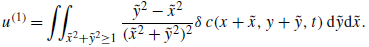 \begin{equation} u^{(1)} = \iint _{\tilde {x}^2+\tilde {y}^2 \ge 1} \frac {\tilde {y}^2-\tilde {x}^2}{(\tilde {x}^2+\tilde {y}^2)^2} \delta\, c(x+\tilde {x},y+\tilde {y},t)\,\textrm {d}{\tilde {y}}\textrm {d}{\tilde {x}}. \end{equation}
By setting
 $\delta\, c(x,y,t) \equiv 2\sum _k \tilde {c}(x,t) \cos {(k y)}$
with the wavenumber
$\delta\, c(x,y,t) \equiv 2\sum _k \tilde {c}(x,t) \cos {(k y)}$
with the wavenumber
 $k$
and plugging it into (E1), we rewrite the double integral in (E2) as
$k$
and plugging it into (E1), we rewrite the double integral in (E2) as
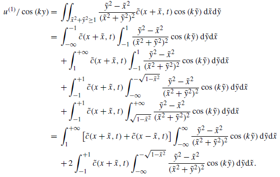 \begin{equation} \begin{aligned}[b] u^{(1)}/\cos {(k y)} ={}& \iint _{\tilde {x}^2+\tilde {y}^2 \ge 1} \frac {\tilde {y}^2-\tilde {x}^2}{(\tilde {x}^2+\tilde {y}^2)^2} \tilde {c}(x+\tilde {x},t)\cos {(k \tilde {y})}\,\textrm {d}\tilde {x}\textrm {d}{\tilde {y}} \\ ={}& \int _{-\infty }^{-1} \tilde {c}(x+\tilde x,t) \int _{-1}^{1} \frac {\tilde {y}^2-\tilde {x}^2}{(\tilde {x}^2+\tilde {y}^2)^2} \cos {(k \tilde {y})}\,\textrm {d}{\tilde {y}}\textrm {d}{\tilde {x}}\\ &{}+ \int _{1}^{+\infty } \tilde {c}(x+\tilde x,t) \int _{-1}^{1} \frac {\tilde {y}^2-\tilde {x}^2}{(\tilde {x}^2+\tilde {y}^2)^2} \cos {(k \tilde {y})}\,\textrm {d}{\tilde {y}}\textrm {d}{\tilde {x}}\\ &{}+ \int _{-1}^{+1} \tilde {c}(x+\tilde x,t) \int _{-\infty }^{-\sqrt {1-\tilde x^2}} \frac {\tilde {y}^2-\tilde {x}^2}{(\tilde {x}^2+\tilde {y}^2)^2} \cos {(k \tilde {y})}\,\textrm {d}{\tilde {y}}\textrm {d}{\tilde {x}}\\ &{}+ \int _{-1}^{+1} \tilde {c}(x+\tilde x,t) \int _{\sqrt {1-\tilde x^2}}^{+\infty } \frac {\tilde {y}^2-\tilde {x}^2}{(\tilde {x}^2+\tilde {y}^2)^2} \cos {(k \tilde {y})}\,\textrm {d}{\tilde {y}}\textrm {d}{\tilde {x}}\\ ={}& \int _{1}^{+\infty } \left [ \tilde {c}(x+\tilde x,t) + \tilde {c}(x-\tilde x,t) \right ] \int _{-\infty }^{\infty } \frac {\tilde {y}^2-\tilde {x}^2}{(\tilde {x}^2+\tilde {y}^2)^2} \cos {(k \tilde {y})}\,\textrm {d}{\tilde {y}}\textrm {d}{\tilde {x}}\\ &{}+ 2\int _{-1}^{+1} \tilde {c}(x+\tilde x,t) \int ^{-\sqrt {1-\tilde x^2}}_{-\infty } \frac {\tilde {y}^2-\tilde {x}^2}{(\tilde {x}^2+\tilde {y}^2)^2} \cos {(k \tilde {y})}\,\textrm {d}{\tilde {y}}\textrm {d}{\tilde {x}}. \end{aligned} \end{equation}
This expression reveals the cumulative impact of particles within the rarefaction zone (i.e.
 $\partial c_0/\partial x \neq 0$
) and sets our current model apart from the one for the uniform suspension described by Desreumaux et al. (Reference Desreumaux, Caussin, Jeanneret, Lauga and Bartolo2013).
$\partial c_0/\partial x \neq 0$
) and sets our current model apart from the one for the uniform suspension described by Desreumaux et al. (Reference Desreumaux, Caussin, Jeanneret, Lauga and Bartolo2013).
The maximum growth rate (
 $\sigma _{{max}}(t)$
) and critical wavenumber (
$\sigma _{{max}}(t)$
) and critical wavenumber (
 $k_c$
) over time based on versions 1, 2, 3 of (4.3).
$k_c$
) over time based on versions 1, 2, 3 of (4.3).
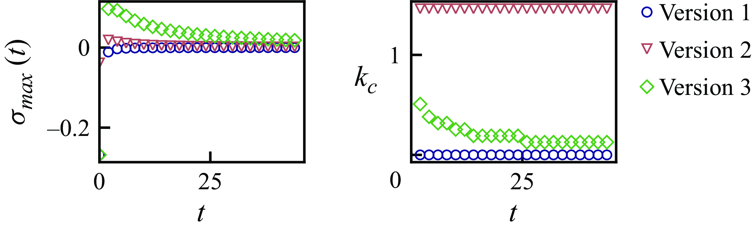
Appendix F. Ablation test
We conduct an ablation test by systematically deleting selected terms from (4.3), and numerically determining the maximum growth rate (
 $\sigma _{{max}}$
) and critical wavenumber (
$\sigma _{{max}}$
) and critical wavenumber (
 $k_c$
). We consider the following three versions of (4.3). Version 1 consists of all the terms of (4.3), except for the last two integral terms, which contain
$k_c$
). We consider the following three versions of (4.3). Version 1 consists of all the terms of (4.3), except for the last two integral terms, which contain
 $(1/\pi )\,\partial c_0/\partial x$
. This version of (4.3) is consistent with the model by Desreumaux et al. (Reference Desreumaux, Caussin, Jeanneret, Lauga and Bartolo2013) when
$(1/\pi )\,\partial c_0/\partial x$
. This version of (4.3) is consistent with the model by Desreumaux et al. (Reference Desreumaux, Caussin, Jeanneret, Lauga and Bartolo2013) when
 $c_0$
is constant. Version 2 is only missing
$c_0$
is constant. Version 2 is only missing
 $({1}/{\pi }) ({\partial c_0}/{\partial x}) \Big[\int _1^{+\infty } [\tilde {c}(x+\tilde {x})+\tilde {c}(x-\tilde {x}) ]I_1\,{\textrm d}\tilde {x} \Big]$
from (4.3), while version 3 does not contain
$({1}/{\pi }) ({\partial c_0}/{\partial x}) \Big[\int _1^{+\infty } [\tilde {c}(x+\tilde {x})+\tilde {c}(x-\tilde {x}) ]I_1\,{\textrm d}\tilde {x} \Big]$
from (4.3), while version 3 does not contain
 $({1}/{\pi }) ({\partial c_0}/{\partial x}) [\int _{-1}^{1}\tilde {c}(x+\tilde {x})I_2\,{\textrm d}\tilde {x} ]$
only. The plots in figure 6 demonstrate the importance of the term
$({1}/{\pi }) ({\partial c_0}/{\partial x}) [\int _{-1}^{1}\tilde {c}(x+\tilde {x})I_2\,{\textrm d}\tilde {x} ]$
only. The plots in figure 6 demonstrate the importance of the term
 $({1}/{\pi }) ({\partial c_0}/{\partial x}) \Big[\int _1^{+\infty } [\tilde {c}(x+\tilde {x})+\tilde {c}(x-\tilde {x}) \Big]I_1\,{\textrm d}\tilde {x} ]$
. Namely, only version 3 of the governing equation that retains this term shows the decay of
$({1}/{\pi }) ({\partial c_0}/{\partial x}) \Big[\int _1^{+\infty } [\tilde {c}(x+\tilde {x})+\tilde {c}(x-\tilde {x}) \Big]I_1\,{\textrm d}\tilde {x} ]$
. Namely, only version 3 of the governing equation that retains this term shows the decay of
 $k_c$
over time, which qualitatively matches the full numerical results from solving (4.3).
$k_c$
over time, which qualitatively matches the full numerical results from solving (4.3).


 Open access