





1 Introduction
Aerodynamic heating is a key issue in hypersonic flow research due to its strong relevance to the safety of ultra-high-speed flight. Accurate knowledge about where and why, and with what strength, strong heating peaks occur at the wall is of crucial importance to the performance and safety of hypersonic vehicles (Sivolella Reference Sivolella2014). Under real flight conditions, laminar-to-turbulence transition is one of the most important sources bringing about uncertain aerodynamic heating that might adversely impact a vehicle’s thermal protection system (TPS) (Berry et al. Reference Berry, Horvath, Greene, Kinder and Wang2006; Greene & Hamilton Reference Greene and Hamilton2006; McGinley et al. Reference McGinley, Berry, Kinder, Barnwell, Wang and Kirk2006). It is generally acknowledged that enhanced heat transfer is related to the evolution of flow disturbances and onset of turbulence, which in turn modifies the skin friction. Extensive studies have been performed using physical and numerical experiments as well as theoretical analyses (Hopkins & Inouye Reference Hopkins and Inouye1972; Brostmeyer & Nagamatsu Reference Brostmeyer and Nagamatsu1984; Horvath et al. Reference Horvath, Berry, Hollis, Chang and Singer2002; Wadhams et al. Reference Wadhams, Mundy, MacLean and Holden2008; Berridge et al. Reference Berridge, Chou, Ward, Steen, Gilbert, Juliano, Schneider and Gronvall2010; Franko & Lele Reference Franko and Lele2013). In fact, the region with a dramatic increase of skin friction and heat transfer (denoted herein as HT) is commonly identified as the onset of the turbulent state in experiments and numerical simulations.
An important mechanism in the transition process, absent in low Mach number flows, is the instability of dilatational, longitudinal waves (Emanuel Reference Emanuel1992; Gad-el-Hak Reference Gad-el-Hak1995), such as second- and higher instability modes, which was first identified based on linear stability analysis of hypersonic boundary layers (Mack Reference Mack1969). Those modes behave as acoustic waves reflecting between the solid wall and the sonic line in hypersonic boundary layers (Fedorov Reference Fedorov2011), and play an increasingly important role as the Mach number increases – as demonstrated in previous studies (Stetson & Kimmel Reference Stetson and Kimmel1992; Bountin, Shiplyuk & Sidorenko Reference Bountin, Shiplyuk, Sidorenko, Fasel and Saric2000; Fujii Reference Fujii2006; Hofferth et al. Reference Hofferth, Humble, Floryan and Saric2013; Zhang, Tang & Lee Reference Zhang, Tang and Lee2013; Casper, Beresh & Schneider Reference Casper, Beresh and Schneider2014; Sivasubramanian & Fasel Reference Sivasubramanian and Fasel2015; Zhang et al. Reference Zhang, Zhu, Chen, Yuan, Wu, Chen, Lee and Gad-el-Hak2015; Zhu et al. Reference Zhu, Zhang, Chen, Yuan, Wu, Chen, Lee and Gad-el-Hak2016). Recent investigations of hypersonic boundary layers have indicated the appearance of an additional peak in heat transfer (denoted herein as HS) within the transitional region, as well as a second rapid growth of heat transfer near the end of transition (HT). Schneider and his group (Berridge et al. Reference Berridge, Chou, Ward, Steen, Gilbert, Juliano, Schneider and Gronvall2010) were the first to observe this phenomenon on a Mach 6 flared cone under quiet flow conditions. Since 1998, this group has made significant contributions to re-establish a hypersonic quiet wind tunnel at Purdue University. They also pioneered the application of temperature-sensitive paint (TSP) in hypersonic experiments. In their TSP results published in 2010 (Berridge et al. Reference Berridge, Chou, Ward, Steen, Gilbert, Juliano, Schneider and Gronvall2010), hot streaks were found during the early stage of transition over a flared cone, corresponding to a peak value HS in the spanwise-averaged temperature. PCB® piezoelectric pressure sensors were also applied within that region, and indicated an appearance of second-mode instability. Sivasubramanian & Fasel (Reference Sivasubramanian and Fasel2015) used direct numerical simulations (DNS) to simulate the experiment of Berridge et al. (Reference Berridge, Chou, Ward, Steen, Gilbert, Juliano, Schneider and Gronvall2010). Streamwise hot streaks were also observed before the boundary layer became turbulent. Either spanwise-averaged heat transfer or that along a single streak exhibited both HS and HT along the streamwise direction. Note that the Stanton number at HS was twice that at HT, but the skin friction of the former was only half that of the latter, so that a new aerodynamic heating mechanism might be active. However, because the focus of Sivasubramanian & Fasel’s work was the fundamental resonance of second-mode instability, no explanation of HS has been presented in their paper.
The behaviour of hypersonic aerodynamic heating seems to rely on the types of instability mode. Based on DNS, Franko & Lele (Reference Franko and Lele2013) investigated the transition mechanisms of a $Ma=6$
planar hypersonic boundary layer. Three types of such mechanisms were identified, including first-mode oblique interaction, second-mode fundamental resonance and second-mode oblique interaction. For the first-mode oblique interaction mechanism, a distinct overshoot of heat transfer was observed near the end of the transitional region, HT, which was attributed to the generation of streamwise vortices and correspondingly increased wall shear stress. However, for the fundamental resonance dominated by two-dimensional second mode, an additional peak of heat transfer, HS, appeared where the second mode reached its maximum. The temperature values at HS are slightly higher than those at HT, while the associated skin friction of the former is no more than half of the latter. Franko & Lele (Reference Franko and Lele2013) stated that the appearance of HS was attributed to the second-mode evolution, but no physical explanation was given in terms of fundamental thermo-aerodynamics.
$Ma=6$
planar hypersonic boundary layer. Three types of such mechanisms were identified, including first-mode oblique interaction, second-mode fundamental resonance and second-mode oblique interaction. For the first-mode oblique interaction mechanism, a distinct overshoot of heat transfer was observed near the end of the transitional region, HT, which was attributed to the generation of streamwise vortices and correspondingly increased wall shear stress. However, for the fundamental resonance dominated by two-dimensional second mode, an additional peak of heat transfer, HS, appeared where the second mode reached its maximum. The temperature values at HS are slightly higher than those at HT, while the associated skin friction of the former is no more than half of the latter. Franko & Lele (Reference Franko and Lele2013) stated that the appearance of HS was attributed to the second-mode evolution, but no physical explanation was given in terms of fundamental thermo-aerodynamics.
Understanding the physics of second-mode instability is clearly important. By applying inviscid theory to compressible boundary layer stability, Mack (Reference Mack1969) found a family of neutral curves, denoted as second and higher modes, whenever the phase speed of the disturbances is subsonic relative to the free stream. As explained by Morkovin (Reference Morkovin1987) and later by Mack (Reference Mack1990), the inviscid solutions of these higher modes were consistent with the acoustic behaviour depicted by Lighthill’s equation. Mack (Reference Mack1990) suggested the terminology ‘acoustic modes’ to describe those modes because they were dominated by acoustic waves. When the waves reflected in an embedded region between the sonic line and solid wall, the flow was alternately compressed and expanded owing to the boundary condition at the sonic line. Not surprisingly, the consequent variations of density or velocity divergence could be captured experimentally using techniques such as schlieren or particle image velocimetry (PIV). Hofferth et al. (Reference Hofferth, Humble, Floryan and Saric2013) have applied a focused schlieren technique on a 0.5 m long, $5^{\circ }$
half-angle flared cone in their Mach 6 Quiet Wind Tunnel at Texas A&M University. The density variation caused by second-mode instability resulted in light intensity variations on the schlieren image, which were acquired by a high-bandwidth photo-detector. Using this technique, Hofferth et al. (Reference Hofferth, Humble, Floryan and Saric2013) determined the frequency and amplitude evolution of the second mode. Laurence, Wagner & Hannemann (Reference Laurence, Wagner and Hannemann2012, Reference Laurence, Wagner and Hannemann2016) investigated a 1.1 m long,
$5^{\circ }$
half-angle flared cone in their Mach 6 Quiet Wind Tunnel at Texas A&M University. The density variation caused by second-mode instability resulted in light intensity variations on the schlieren image, which were acquired by a high-bandwidth photo-detector. Using this technique, Hofferth et al. (Reference Hofferth, Humble, Floryan and Saric2013) determined the frequency and amplitude evolution of the second mode. Laurence, Wagner & Hannemann (Reference Laurence, Wagner and Hannemann2012, Reference Laurence, Wagner and Hannemann2016) investigated a 1.1 m long, $7^{\circ }$
half-angle cone in a free-piston-driven, reflected-shock wind tunnel under high-entropy conditions. Employing a 1000 W short-arc Xe lamp together with a camera at frame rates of up to 1 MHz, Laurence et al. (Reference Laurence, Wagner and Hannemann2012, Reference Laurence, Wagner and Hannemann2016) obtained schlieren images of typical ‘rope-like’ structures of the second mode. The intensity variation in the image manifested the density variation caused by the compression and expansion process inherent in the second-mode instability.
$7^{\circ }$
half-angle cone in a free-piston-driven, reflected-shock wind tunnel under high-entropy conditions. Employing a 1000 W short-arc Xe lamp together with a camera at frame rates of up to 1 MHz, Laurence et al. (Reference Laurence, Wagner and Hannemann2012, Reference Laurence, Wagner and Hannemann2016) obtained schlieren images of typical ‘rope-like’ structures of the second mode. The intensity variation in the image manifested the density variation caused by the compression and expansion process inherent in the second-mode instability.
Very recently, Zhang et al. (Reference Zhang, Zhu, Chen, Yuan, Wu, Chen, Lee and Gad-el-Hak2015) and Zhu et al. (Reference Zhu, Zhang, Chen, Yuan, Wu, Chen, Lee and Gad-el-Hak2016) have conducted two-dimensional PIV measurements, combined with PCB sensors, over a 0.26 m long, $5^{\circ }$
half-angle flared cone in the Mach 6 wind tunnel at Peking University. They found that the second-mode instability initially grew fast, reached its maximum and finally decayed to zero along the streamwise direction. However, low-frequency waves continued to grow until the boundary layer became turbulent. The PIV results clearly showed a strong compression and expansion process accompanying the evolution of second mode. The corresponding shear- and dilatation-induced viscous dissipation of energy were respectively evaluated; however, their connection to aerodynamic heating was not investigated. They then applied temperature-sensitive paint, as well as PCB sensors, to simultaneously measure both the surface-temperature distribution and the instability amplitude evolution. PIV measurements were also performed to evaluate the dissipation function of the flow. The recent work not only confirmed the previously observed heat-transfer peak HS that correlated with the second-mode-dominated instability evolution, but also revealed a new physical mechanism to promptly generate this heating impact and its strong connection to the instability evolution. For the first time, a direct relation was identified between the local heating peak HS before transition was completed and the second-mode-induced dilatation process. The new discovery has been published as a rapid communication (Zhu et al.
Reference Zhu, Chen, Wu, Chen, Lee and Gad-el-Hak2018), and soon after highlighted by Wolverton (Reference Wolverton2018) and Sun & Oran (Reference Sun and Oran2018) for its significant achievement from the physics perspective as well as in the engineering design of hypersonic flights.
$5^{\circ }$
half-angle flared cone in the Mach 6 wind tunnel at Peking University. They found that the second-mode instability initially grew fast, reached its maximum and finally decayed to zero along the streamwise direction. However, low-frequency waves continued to grow until the boundary layer became turbulent. The PIV results clearly showed a strong compression and expansion process accompanying the evolution of second mode. The corresponding shear- and dilatation-induced viscous dissipation of energy were respectively evaluated; however, their connection to aerodynamic heating was not investigated. They then applied temperature-sensitive paint, as well as PCB sensors, to simultaneously measure both the surface-temperature distribution and the instability amplitude evolution. PIV measurements were also performed to evaluate the dissipation function of the flow. The recent work not only confirmed the previously observed heat-transfer peak HS that correlated with the second-mode-dominated instability evolution, but also revealed a new physical mechanism to promptly generate this heating impact and its strong connection to the instability evolution. For the first time, a direct relation was identified between the local heating peak HS before transition was completed and the second-mode-induced dilatation process. The new discovery has been published as a rapid communication (Zhu et al.
Reference Zhu, Chen, Wu, Chen, Lee and Gad-el-Hak2018), and soon after highlighted by Wolverton (Reference Wolverton2018) and Sun & Oran (Reference Sun and Oran2018) for its significant achievement from the physics perspective as well as in the engineering design of hypersonic flights.
This paper is an expansion of the preliminary work reported in Zhu et al. (Reference Zhu, Chen, Wu, Chen, Lee and Gad-el-Hak2018), methodically providing more experimental and numerical evidence. Compared to the rapid communication, the present expanded manuscript describes an in-depth investigation of the newly discovered heating mechanism. The importance of pressure work in aerodynamic heating is particularly elucidated. A theoretical analysis of heat transfer is also described to explain the relationship between aerodynamic heating and surface-temperature distribution.
2 Experimental set-up
2.1 Facility and model
The experiments are carried out in a Mach 6 wind tunnel (M6QT) at Peking University (Zhang et al.
Reference Zhang, Tang and Lee2013; Tang Reference Tang2014; Zhang Reference Zhang2014; Zhang et al.
Reference Zhang, Zhu, Chen, Yuan, Wu, Chen, Lee and Gad-el-Hak2015; Zhu et al.
Reference Zhu, Zhang, Chen, Yuan, Wu, Chen, Lee and Gad-el-Hak2016), which at present is one of three operational hypersonic quiet wind tunnels in the world (Schneider Reference Schneider2013). The tunnel is of the open-jet configuration with nozzle exit diameter of 160 mm. Longitudinal suction can be applied upstream of the nozzle throat and the wind tunnel runs at quiet or noisy conditions with the suction valve open or closed, respectively. For the quiet condition, the turbulence level is below 0.2 %. Owing to low free-stream disturbances and the upper limit of unit Reynolds number for the quiet condition, natural transition does not occur up to the end of the present model. Therefore, to obtain a whole picture of the transition process in the present work, the wind tunnel runs at noisy condition with the suction valve closed. To avoid liquefying the air, the flow is pre-heated to a nominal stagnation temperature of 433 K. During the typical run time of 30 s, the stagnation pressure holds nearly constant with variation of less than 3 %. Four flow conditions with $Re_{unit}=5.4$
, 7.6, 9.7 and
$Re_{unit}=5.4$
, 7.6, 9.7 and $11.7\times 10^{6}~\text{m}^{-1}$
are investigated, where
$11.7\times 10^{6}~\text{m}^{-1}$
are investigated, where $Re_{unit}$
is the free-stream unit Reynolds number. As indicated in Zhu et al. (Reference Zhu, Zhang, Chen, Yuan, Wu, Chen, Lee and Gad-el-Hak2016), the stagnation temperature and normalized pitot pressure fluctuations of the free stream are, respectively, 433 K and 2.2 %.
$Re_{unit}$
is the free-stream unit Reynolds number. As indicated in Zhu et al. (Reference Zhu, Zhang, Chen, Yuan, Wu, Chen, Lee and Gad-el-Hak2016), the stagnation temperature and normalized pitot pressure fluctuations of the free stream are, respectively, 433 K and 2.2 %.
The model used in the present study is a flared, instability-enhanced cone, schematically shown in figure 1. The full length is $L=260$
mm. Its geometry consists of a
$L=260$
mm. Its geometry consists of a $5^{\circ }$
half-angle circular conical profile for the first 100 mm of axial distance, followed by a tangent flare of radius 931 mm until the base of the cone at the 260 mm axial position. The first 50 mm of length, which can be removed and replaced with an arbitrary nose-tip shape, is made of stainless steel. In this work, the tip is sharp with a nominal
$5^{\circ }$
half-angle circular conical profile for the first 100 mm of axial distance, followed by a tangent flare of radius 931 mm until the base of the cone at the 260 mm axial position. The first 50 mm of length, which can be removed and replaced with an arbitrary nose-tip shape, is made of stainless steel. In this work, the tip is sharp with a nominal $50~\unicode[STIX]{x03BC}\text{m}$
radius. The rest of the model is made of Bakelite. The origin of the coordinate is located at the cone tip, with
$50~\unicode[STIX]{x03BC}\text{m}$
radius. The rest of the model is made of Bakelite. The origin of the coordinate is located at the cone tip, with $x$
being the streamwise coordinate along the cone’s surface,
$x$
being the streamwise coordinate along the cone’s surface, $y$
the coordinate normal to that surface,
$y$
the coordinate normal to that surface, $z$
the transverse coordinate normal to the
$z$
the transverse coordinate normal to the $x$
–
$x$
– $y$
plane and
$y$
plane and $l$
the axial coordinate along the axis of the model.
$l$
the axial coordinate along the axis of the model.
(a) Schematic of the model; (b) temperature-sensitive paint sprayed over the model (left) and its intensity–temperature ratio at different streamwise locations (right). $I_{ref}$
, reference intensity;
$I_{ref}$
, reference intensity; $T_{ref}$
, reference temperature.
$T_{ref}$
, reference temperature.
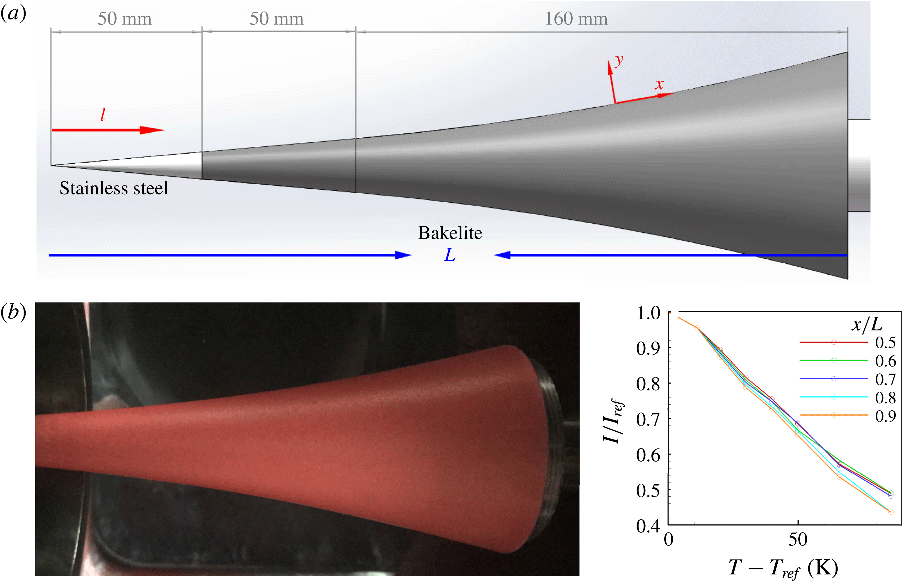
The cone is installed along the centreline of the nozzle with zero angle of attack. The tip is 50 mm deep into the nozzle exit. The length of the flow field that is not affected by the reflected Mach waves is more than 400 mm, which is long enough to embed the whole length of the model.
2.2 Fast-response surface pressure measurements
An array of surface-mounted PCB fast-response sensors is used to evaluate the evolution of instability waves in hypersonic wall-bounded flows (Fujii Reference Fujii2006; Zhang et al.
Reference Zhang, Tang and Lee2013, Reference Zhang, Zhu, Chen, Yuan, Wu, Chen, Lee and Gad-el-Hak2015; Zhu et al.
Reference Zhu, Zhang, Chen, Yuan, Wu, Chen, Lee and Gad-el-Hak2016). In this work, PCB 132A31 sensors are flush-mounted along one ray of the model, which is defined as the zero circumferential angle. The sensor is a piezoelectric quartz sensor with a flat frequency response between 11 KHz and 1 MHz. The diameter of the sensor head is 3.18 mm, but the effective sensing area is only approximately $0.581~\text{mm}^{2}$
. The signals of the PCB sensors are first processed by an ICP® signal conditioner and then recorded by Donghua 5939 data-acquisition system with a sample rate of 1 MHz and a duration of 100 ms.
$0.581~\text{mm}^{2}$
. The signals of the PCB sensors are first processed by an ICP® signal conditioner and then recorded by Donghua 5939 data-acquisition system with a sample rate of 1 MHz and a duration of 100 ms.
2.3 Temperature-sensitive paint
To investigate the surface-temperature distribution, fluorescent temperature-sensitive paint (TSP) (Liu & Sullivan Reference Liu and Sullivan2005) is painted all over the model surface (figure 1), with a thickness of less than 0.1 mm. The fluorescence is excited continuously by an LED light and recorded by a Photron FASTCAM CMOS high-speed camera with an image resolution of $1024\times 1024$
pixels and sample rate of 100 Hz. A Nikkor Micro 60 mm lens is mounted ahead of the camera using long-wavelength-pass filter to remove the LED light. The camera’s recording rate is 100 Hz, corresponding to an integral time of 10 ms on each complementary metal oxide semiconductor (CMOS) pixel. A black background image is sampled before recording and subtracted from each image.
$1024\times 1024$
pixels and sample rate of 100 Hz. A Nikkor Micro 60 mm lens is mounted ahead of the camera using long-wavelength-pass filter to remove the LED light. The camera’s recording rate is 100 Hz, corresponding to an integral time of 10 ms on each complementary metal oxide semiconductor (CMOS) pixel. A black background image is sampled before recording and subtracted from each image.
The model is first placed in a thermal bath to calibrate the TSP’s performance. Fluorescent images are then recorded through a quartz-glass window once the model reaches thermal equilibrium. Intensity ratios are then calculated under different temperatures to calibrate the TSP images and the results are depicted in figure 1.
The TSP’s response time is affected by a number of factors, including the fluorescence lifetime, the image exposure time and the paint’s heat lag time. The first two factors are $1~\unicode[STIX]{x03BC}\text{s}$
and 0.01 s, respectively. The last factor can be evaluated from
$1~\unicode[STIX]{x03BC}\text{s}$
and 0.01 s, respectively. The last factor can be evaluated from
 $$\begin{eqnarray}\displaystyle \unicode[STIX]{x1D70F}_{l}=\frac{\unicode[STIX]{x1D6FF}^{2}\unicode[STIX]{x1D70C}~C}{k}, & & \displaystyle\end{eqnarray}$$
where $\unicode[STIX]{x1D6FF}$
,
$\unicode[STIX]{x1D6FF}$
, $\unicode[STIX]{x1D70C}$
,
$\unicode[STIX]{x1D70C}$
, $C$
and
$C$
and $k$
are, respectively, the thickness, density, specific heat and thermal conductivity of the paint layer. For our TSP,
$k$
are, respectively, the thickness, density, specific heat and thermal conductivity of the paint layer. For our TSP, $\unicode[STIX]{x1D6FF}=0.1$
mm,
$\unicode[STIX]{x1D6FF}=0.1$
mm, $\unicode[STIX]{x1D70C}=1200~\text{kg}~\text{m}^{-3}$
,
$\unicode[STIX]{x1D70C}=1200~\text{kg}~\text{m}^{-3}$
, $C=1464~\text{J}~\text{kg}^{-1}~\text{K}^{-1}$
and
$C=1464~\text{J}~\text{kg}^{-1}~\text{K}^{-1}$
and $k=0.19~\text{W}~\text{m}^{-1}~\text{K}^{-1}$
. Thus, the heat lag time is estimated to be 0.1 s, which is considered to be the TSP’s response time.
$k=0.19~\text{W}~\text{m}^{-1}~\text{K}^{-1}$
. Thus, the heat lag time is estimated to be 0.1 s, which is considered to be the TSP’s response time.
2.4 Particle image velocimetry
Due to rapid developments in CCD cameras since the first application of PIV in hypersonic flows (Moraitis & Riethmuller Reference Moraitis and Riethmuller1988), this technique is now more commonly used in high-speed flows (Scarano Reference Scarano, Riethmuller and Scarano2005; Schrijer, Scarano & van Oudheusden Reference Schrijer, Scarano and van Oudheusden2006; Sahoo, Papageorge & Smits Reference Sahoo, Papageorge and Smits2010; Schreyer, Sahoo & Smits Reference Schreyer, Sahoo and Smits2011; Williams & Smits Reference Williams and Smits2012; Avallone et al. Reference Avallone, Ye, Schrijer, Scarano and Cardone2014). The key issues include the selection of seeding particles, their dispersion in the flow and the analysis of particle image recordings (Scarano Reference Scarano, Riethmuller and Scarano2005).
To seed the present flow, $\text{TiO}_{2}$
particles are applied for their high-temperature stability and high index of refraction. The nominal diameter of the selected particles is 90 nm. The particle tracking capability is assessed by Scarano (Reference Scarano, Riethmuller and Scarano2005) as the ratio
$\text{TiO}_{2}$
particles are applied for their high-temperature stability and high index of refraction. The nominal diameter of the selected particles is 90 nm. The particle tracking capability is assessed by Scarano (Reference Scarano, Riethmuller and Scarano2005) as the ratio
 $$\begin{eqnarray}\displaystyle \unicode[STIX]{x1D70F}=\frac{\unicode[STIX]{x1D70F}_{p}}{\unicode[STIX]{x1D70F}_{f}}, & & \displaystyle\end{eqnarray}$$
where $\unicode[STIX]{x1D70F}_{p}$
is the particle’s relaxation time as it passes through a velocity step (e.g. an oblique shock wave) from
$\unicode[STIX]{x1D70F}_{p}$
is the particle’s relaxation time as it passes through a velocity step (e.g. an oblique shock wave) from $u_{1}$
to
$u_{1}$
to $u_{2}$
, where
$u_{2}$
, where $u_{1}$
and
$u_{1}$
and $u_{2}$
are the initial and final velocities during a single particle’s displacement. The particle’s velocity is given by
$u_{2}$
are the initial and final velocities during a single particle’s displacement. The particle’s velocity is given by
 $$\begin{eqnarray}\displaystyle u(t)=u_{1}+(u_{2}-u_{1})\text{e}^{(-t/\unicode[STIX]{x1D70F}_{p})}, & & \displaystyle\end{eqnarray}$$
where $t$
is the time. The flow time scale
$t$
is the time. The flow time scale $\unicode[STIX]{x1D70F}_{f}$
is the slipping time of the flow, defined as
$\unicode[STIX]{x1D70F}_{f}$
is the slipping time of the flow, defined as
 $$\begin{eqnarray}\displaystyle \unicode[STIX]{x1D70F}_{f}=\text{d}l/\text{d}u, & & \displaystyle\end{eqnarray}$$
where $\text{d}u$
is the velocity spatial variation, and
$\text{d}u$
is the velocity spatial variation, and $\text{d}l$
is the distance for that variation.
$\text{d}l$
is the distance for that variation.
In the present work, $\unicode[STIX]{x1D70F}_{p}$
is assessed experimentally to be
$\unicode[STIX]{x1D70F}_{p}$
is assessed experimentally to be $2~\unicode[STIX]{x03BC}\text{s}$
(Tang Reference Tang2014). For a hypersonic boundary layer with thickness
$2~\unicode[STIX]{x03BC}\text{s}$
(Tang Reference Tang2014). For a hypersonic boundary layer with thickness $\unicode[STIX]{x1D6FF}$
,
$\unicode[STIX]{x1D6FF}$
, $\text{d}l$
is characterized by the wavelength of the second-mode wave
$\text{d}l$
is characterized by the wavelength of the second-mode wave $\unicode[STIX]{x1D706}$
, and
$\unicode[STIX]{x1D706}$
, and $\text{d}u$
is no more than 5 % of the free-stream velocity
$\text{d}u$
is no more than 5 % of the free-stream velocity $U_{\infty }$
(Stetson et al.
Reference Stetson, Thompson, Donaldson and Siler1983; Stetson & Kimmel Reference Stetson and Kimmel1992). Thus,
$U_{\infty }$
(Stetson et al.
Reference Stetson, Thompson, Donaldson and Siler1983; Stetson & Kimmel Reference Stetson and Kimmel1992). Thus, $\unicode[STIX]{x1D70F}_{f}\simeq \unicode[STIX]{x1D706}/(0.05U_{\infty })$
. In view of our experimental conditions,
$\unicode[STIX]{x1D70F}_{f}\simeq \unicode[STIX]{x1D706}/(0.05U_{\infty })$
. In view of our experimental conditions, $U_{\infty }=850~\text{m}~\text{s}^{-1}$
, and
$U_{\infty }=850~\text{m}~\text{s}^{-1}$
, and $\unicode[STIX]{x1D706}\simeq 2.5$
mm. Therefore,
$\unicode[STIX]{x1D706}\simeq 2.5$
mm. Therefore, $\unicode[STIX]{x1D70F}_{f}\simeq 58.5~\unicode[STIX]{x03BC}\text{s}$
, and
$\unicode[STIX]{x1D70F}_{f}\simeq 58.5~\unicode[STIX]{x03BC}\text{s}$
, and $\unicode[STIX]{x1D70F}\simeq 0.034$
. As discussed in Zhu et al. (Reference Zhu, Zhang, Chen, Yuan, Wu, Chen, Lee and Gad-el-Hak2016), the injection of PIV particles somewhat dampens the amplitude of the high-frequency second mode. Therefore, the velocity fluctuations below the sonic line are slightly decreased.
$\unicode[STIX]{x1D70F}\simeq 0.034$
. As discussed in Zhu et al. (Reference Zhu, Zhang, Chen, Yuan, Wu, Chen, Lee and Gad-el-Hak2016), the injection of PIV particles somewhat dampens the amplitude of the high-frequency second mode. Therefore, the velocity fluctuations below the sonic line are slightly decreased.
The particles are illuminated by a double-cavity Nd:YAG laser from Continuum, generating 6 ns duration light pulses at a wavelength of 532 nm, with a maximum energy of 2 J per pulse. The laser sheet is projected vertically from the top window of the test section and aligned with the cone’s top centreline. The light sheet’s thickness is 1 mm and width 100 mm. The time delay of the laser pulses is set at $1~\unicode[STIX]{x03BC}\text{s}$
and the sample rate is 2.5 Hz. The light scattered by the particles is viewed by a PCO SensiCam QE CCD camera from a side window, which is equipped with a Nikkor Micro 200 mm lens. The field of view is
$1~\unicode[STIX]{x03BC}\text{s}$
and the sample rate is 2.5 Hz. The light scattered by the particles is viewed by a PCO SensiCam QE CCD camera from a side window, which is equipped with a Nikkor Micro 200 mm lens. The field of view is $34\times 26~\text{mm}^{2}$
.
$34\times 26~\text{mm}^{2}$
.
The algorithm to evaluate the PIV images has been discussed by Zhu et al. (Reference Zhu, Yuan, Zhang and Lee2013). To conduct window correlation of the particle images, at least 10 particles are needed in each interrogation window (Adrian Reference Adrian1991). However, this is not always satisfied in laminar boundary layers. Furthermore, the low signal-to-noise ratio of particle images can decrease the $Q$
-value of the correlation peak, making it submerged in the noise, or provides wrong peaks. Therefore, only the images that satisfy both standards are selected.
$Q$
-value of the correlation peak, making it submerged in the noise, or provides wrong peaks. Therefore, only the images that satisfy both standards are selected.
Finally, to solve the problem of very large in-plane displacement and its gradient on the PIV images – commonly encountered in hypersonic boundary layers – we have developed an improved image-preprocessing method (Zhu et al.
Reference Zhu, Yuan, Zhang and Lee2013). PIV images are first rotated to make the wall boundary nearly horizontal. The evaluations start in $256\times 256$
pixel coarse samples and then
$256\times 256$
pixel coarse samples and then $128\times 128$
pixel medium samples to capture the mean displacement fields of the time series. With the mean results as reference, instantaneous recordings are then evaluated with
$128\times 128$
pixel medium samples to capture the mean displacement fields of the time series. With the mean results as reference, instantaneous recordings are then evaluated with $64\times 64$
pixel samples to resolve the fine structures in the boundary layer. Smaller samples are unavailable because of low particle density near the wall. Vectors are then post-processed by a global histogram filter and a
$64\times 64$
pixel samples to resolve the fine structures in the boundary layer. Smaller samples are unavailable because of low particle density near the wall. Vectors are then post-processed by a global histogram filter and a $Q$
-ratio of 2. Vectors could then be replaced if a second correlation peak proved to be suitable.
$Q$
-ratio of 2. Vectors could then be replaced if a second correlation peak proved to be suitable.
2.5 Rayleigh-scattering technique
The whole transition process is also investigated qualitatively using Rayleigh-scattering flow visualization (RSFV), which can offer clear information regarding the evolution of the structures in the boundary layer. This method was used by Smits & Lim (Reference Smits and Lim2000) and Auvity, Etz & Smits (Reference Auvity, Etz and Smits2001) to investigate various hypersonic flows. $\text{CO}_{2}$
gas is injected upstream of the test section. The mass injection rate of carbon dioxide is no more than 5 % of the free-stream flow. Owing to the very low static temperature of the hypersonic flow, the
$\text{CO}_{2}$
gas is injected upstream of the test section. The mass injection rate of carbon dioxide is no more than 5 % of the free-stream flow. Owing to the very low static temperature of the hypersonic flow, the $\text{CO}_{2}$
gas changes phase to become minute, solid particles in the free stream. The particles scatter when illuminated by the laser, so that this region is white on the grey-scale CCD image. The scattering is of the Rayleigh type because the particle diameters are much smaller than the laser wavelength. On the other hand, these
$\text{CO}_{2}$
gas changes phase to become minute, solid particles in the free stream. The particles scatter when illuminated by the laser, so that this region is white on the grey-scale CCD image. The scattering is of the Rayleigh type because the particle diameters are much smaller than the laser wavelength. On the other hand, these $\text{CO}_{2}$
particles sublimate to gas near the wall because of the relatively high temperature there. This region is black on the CCD image. The line distinguishing the white and black regions is the condensation line. The set-up of the light source and camera is the same as in the PIV, except that the camera operates in the single-frame mode.
$\text{CO}_{2}$
particles sublimate to gas near the wall because of the relatively high temperature there. This region is black on the CCD image. The line distinguishing the white and black regions is the condensation line. The set-up of the light source and camera is the same as in the PIV, except that the camera operates in the single-frame mode.
3 Theoretical and numerical approaches
3.1 Analysis based on parabolized stability equations
We seek solutions in the form
 $$\begin{eqnarray}\displaystyle \unicode[STIX]{x1D6F9}(x,y,\unicode[STIX]{x1D719},t)=\bar{\unicode[STIX]{x1D6F9}}(x,y)+\mathop{\sum }_{m,n}\hat{\unicode[STIX]{x1D6F9}}_{mn}(x,y)\exp \left(\text{i}\int _{0}^{x}\unicode[STIX]{x1D6FC}_{mn}\,\text{d}x-\text{i}\unicode[STIX]{x1D71B}_{m}t+\text{i}n\unicode[STIX]{x1D719}\right), & & \displaystyle\end{eqnarray}$$
where $x$
,
$x$
, $y$
and
$y$
and $\unicode[STIX]{x1D719}$
are body-oriented coordinates representing, respectively, streamwise, wall-normal and circumferential directions;
$\unicode[STIX]{x1D719}$
are body-oriented coordinates representing, respectively, streamwise, wall-normal and circumferential directions; $\bar{\unicode[STIX]{x1D6F9}}\equiv (\bar{\unicode[STIX]{x1D70C}},\bar{u},\bar{v},\bar{w},\bar{T})$
denotes the basic state;
$\bar{\unicode[STIX]{x1D6F9}}\equiv (\bar{\unicode[STIX]{x1D70C}},\bar{u},\bar{v},\bar{w},\bar{T})$
denotes the basic state; $\hat{\unicode[STIX]{x1D6F9}}_{mn}\equiv (\hat{\unicode[STIX]{x1D70C}},\hat{u} ,\hat{v},{\hat{w}},\hat{T})_{mn}$
is the shape function for the Fourier mode (
$\hat{\unicode[STIX]{x1D6F9}}_{mn}\equiv (\hat{\unicode[STIX]{x1D70C}},\hat{u} ,\hat{v},{\hat{w}},\hat{T})_{mn}$
is the shape function for the Fourier mode ( $m,n$
);
$m,n$
); $\unicode[STIX]{x1D6FC}_{mn}$
and
$\unicode[STIX]{x1D6FC}_{mn}$
and $\unicode[STIX]{x1D71B}_{m}$
are, respectively, the associated streamwise (complex) wavenumber and radian frequency. All variables are non-dimensionalized by the edge value of the mean flow. Finally,
$\unicode[STIX]{x1D71B}_{m}$
are, respectively, the associated streamwise (complex) wavenumber and radian frequency. All variables are non-dimensionalized by the edge value of the mean flow. Finally, $n$
is an integer called the azimuthal wavenumber, which represents the number of waves around the circumference of the cone. The mode shape,
$n$
is an integer called the azimuthal wavenumber, which represents the number of waves around the circumference of the cone. The mode shape, $\hat{\unicode[STIX]{x1D6F9}}_{mn}$
, is assumed to be a slowly varying function of the streamwise coordinate
$\hat{\unicode[STIX]{x1D6F9}}_{mn}$
, is assumed to be a slowly varying function of the streamwise coordinate $x$
, so that its second derivative with respect to
$x$
, so that its second derivative with respect to $x$
is negligible. Substituting (3.1) into the Navier–Stokes equations and subtracting the mean-flow equation yields the governing equations for the shape function of each mode
$x$
is negligible. Substituting (3.1) into the Navier–Stokes equations and subtracting the mean-flow equation yields the governing equations for the shape function of each mode $(m,n)$
:
$(m,n)$
:
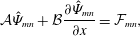 $$\begin{eqnarray}\displaystyle {\mathcal{A}}\hat{\unicode[STIX]{x1D6F9}}_{mn}+{\mathcal{B}}\frac{\unicode[STIX]{x2202}\hat{\unicode[STIX]{x1D6F9}}_{mn}}{\unicode[STIX]{x2202}x}={\mathcal{F}}_{mn}, & & \displaystyle\end{eqnarray}$$
where ${\mathcal{F}}_{mn}$
is the nonlinear forcing term, and expressions of the operators
${\mathcal{F}}_{mn}$
is the nonlinear forcing term, and expressions of the operators ${\mathcal{A}}$
and
${\mathcal{A}}$
and ${\mathcal{B}}$
can be seen in appendix A.
${\mathcal{B}}$
can be seen in appendix A.
The above system of equations is parabolic and thus requires boundary and initial conditions. The initial conditions are provided by the linear stability theory (LST). The boundary conditions are
 $$\begin{eqnarray}\displaystyle \hat{u} _{mn},\hat{v}_{mn},{\hat{w}}_{mn},\frac{\unicode[STIX]{x2202}\hat{T}_{mn}}{\unicode[STIX]{x2202}y}=0,\quad \text{at}~y=0~\text{and}~y=\infty , & & \displaystyle\end{eqnarray}$$
except for the mean-flow distortion, $\unicode[STIX]{x1D6F9}_{00}$
, where the infinity condition for the wall-normal velocity is replaced by
$\unicode[STIX]{x1D6F9}_{00}$
, where the infinity condition for the wall-normal velocity is replaced by
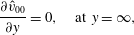 $$\begin{eqnarray}\displaystyle \frac{\unicode[STIX]{x2202}\hat{v}_{00}}{\unicode[STIX]{x2202}y}=0,\quad \text{at}~y=\infty , & & \displaystyle\end{eqnarray}$$
and the wall condition for the temperature is replaced by
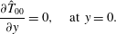 $$\begin{eqnarray}\displaystyle \frac{\unicode[STIX]{x2202}\hat{T}_{00}}{\unicode[STIX]{x2202}y}=0,\quad \text{at}~y=0. & & \displaystyle\end{eqnarray}$$
Equation (3.3) corresponds to no-slip boundary conditions for velocity and adiabatic wall ones for temperature disturbances at the wall. Equation (3.4) accounts for the boundary layer growth. Equation (3.5) is responsible for the wall heating in order to compare with the TSP measurements. The boundary conditions for density are implemented utilizing the continuity equation. Equation (3.2) is marched forward using the Euler backward scheme. The Vigneron technique is applied to avoid numerical instabilities caused by the residual ellipticity (Chang & Malik Reference Chang and Malik1994; Li & Malik Reference Li and Malik1996). Both the curvature effects and external pressure-gradient effects have been taken into account.
The wavenumber is updated at each station as follows:
 $$\begin{eqnarray}\displaystyle \unicode[STIX]{x1D6FC}^{new}=\unicode[STIX]{x1D6FC}^{old}-\text{i}\frac{1}{E}\int _{0}^{\infty }\bar{\unicode[STIX]{x1D70C}}\left(\hat{u} ^{\dagger }\frac{\unicode[STIX]{x2202}\hat{u} }{\unicode[STIX]{x2202}x}+\hat{v}^{\dagger }\frac{\unicode[STIX]{x2202}\hat{v}}{\unicode[STIX]{x2202}x}+{\hat{w}}^{\dagger }\frac{\unicode[STIX]{x2202}{\hat{w}}}{\unicode[STIX]{x2202}x}\right)\text{d}y, & & \displaystyle\end{eqnarray}$$
where
 $$\begin{eqnarray}\displaystyle E\equiv \int _{0}^{\infty }\bar{\unicode[STIX]{x1D70C}}(|\hat{u} |^{2}+|\hat{v}|^{2}+|{\hat{w}}|^{2})\,\text{d}y. & & \displaystyle\end{eqnarray}$$
Iteration continues until the largest change is less than $10^{-5}$
. A norm based on both kinetic and internal energy is also utilized, with which the parabolized stability equations (PSE) results have no distinct difference compared to the present ones.
$10^{-5}$
. A norm based on both kinetic and internal energy is also utilized, with which the parabolized stability equations (PSE) results have no distinct difference compared to the present ones.
In the present work, the mean flow for PSE calculations is obtained via an Euler boundary layer approach (Pruett & Chang Reference Pruett and Chang1998). The Euler equations are solved with FLUENT to obtain the inviscid flow field around the flared cone, and the non-similar boundary layer is then calculated using a spectral collocation method (Malik & Spall Reference Malik and Spall1991). An adiabatic wall condition is used.
In the PSE simulations, a planar second mode $(f_{2nd},n)$
, where
$(f_{2nd},n)$
, where $f_{2nd}=350$
kHz and
$f_{2nd}=350$
kHz and $n=0$
, with an initial amplitude (maximum of temperature root-mean-square, r.m.s.) of 5 %, is seeded at
$n=0$
, with an initial amplitude (maximum of temperature root-mean-square, r.m.s.) of 5 %, is seeded at $x=0.384L$
, which is the beginning of the flared region. The initial second-mode amplitude is chosen such that the second mode becomes saturated at approximately
$x=0.384L$
, which is the beginning of the flared region. The initial second-mode amplitude is chosen such that the second mode becomes saturated at approximately $x=0.65L$
, as observed in the experiments. In order to trigger early transition, an oblique low-frequency mode (
$x=0.65L$
, as observed in the experiments. In order to trigger early transition, an oblique low-frequency mode ( $f_{low},n$
), where
$f_{low},n$
), where $f_{low}=20$
kHz and
$f_{low}=20$
kHz and $n=50$
, with an amplitude of 0.1 % is also seeded. The initial mode shapes are provided by LST. The number of grid points along the wall-normal direction is 151. Four modes, the mean-flow distortion, the difference mode
$n=50$
, with an amplitude of 0.1 % is also seeded. The initial mode shapes are provided by LST. The number of grid points along the wall-normal direction is 151. Four modes, the mean-flow distortion, the difference mode $(f_{2nd}-f_{low},-n)$
, the summation mode
$(f_{2nd}-f_{low},-n)$
, the summation mode $(f_{2nd}+f_{low},n)$
and the harmonic
$(f_{2nd}+f_{low},n)$
and the harmonic $(2f_{2nd},0)$
, are directly triggered via nonlinear interactions. These four modes along with the two seeded modes further generate higher-order modes of which nine modes are included here:
$(2f_{2nd},0)$
, are directly triggered via nonlinear interactions. These four modes along with the two seeded modes further generate higher-order modes of which nine modes are included here: $(3f_{2nd},0)$
;
$(3f_{2nd},0)$
; $(4f_{2nd},0)$
;
$(4f_{2nd},0)$
; $(2f_{low},2n)$
;
$(2f_{low},2n)$
; $(2f_{2nd}+f_{low},n)$
;
$(2f_{2nd}+f_{low},n)$
; $(2f_{2nd}-f_{low},-n)$
;
$(2f_{2nd}-f_{low},-n)$
; $(2f_{2nd}+2f_{low},2n)$
;
$(2f_{2nd}+2f_{low},2n)$
; $(2f_{2nd}-2f_{low},-2n)$
;
$(2f_{2nd}-2f_{low},-2n)$
; $(f_{2nd}-2f_{low},-2n)$
;
$(f_{2nd}-2f_{low},-2n)$
; $(f_{2nd}+2f_{low},2n)$
.
$(f_{2nd}+2f_{low},2n)$
.
3.2 Direct numerical simulations
DNS has been performed on the supercomputer Tianhe-2 in the Guangzhou Supercomputing Centre. The basic laminar (steady) flow is first established including the bow shock and without any perturbation, and is then perturbed to obtain the time-dependent simulations of the transitional flow. The code Hoam-OpenCFD, developed by Li, Fu & Ma (Reference Li, Fu and Ma2008), is used in these simulations. In this code, the Navier–Stokes equations (see appendix B) are solved numerically using a high-order finite-difference method.
(i) Convection terms are split by using Steger–Warming splitting, and are discretized with a seventh-order weighted essentially non-oscillatory (WENO) scheme.
(ii) An eighth-order central finite-difference scheme is used for the viscous terms.
(iii) A third-order total-variation-diminishing type of Runge–Kutta method is used for time advance.
The computational domain of the unsteady (transition) simulations in the circumferential direction spans from the $0^{\circ }$
meridian plane to the
$0^{\circ }$
meridian plane to the $45^{\circ }$
plane. The mesh number (streamwise
$45^{\circ }$
plane. The mesh number (streamwise $\times$
wall normal
$\times$
wall normal $\times$
circumference) is
$\times$
circumference) is $4000\times 200\times 500$
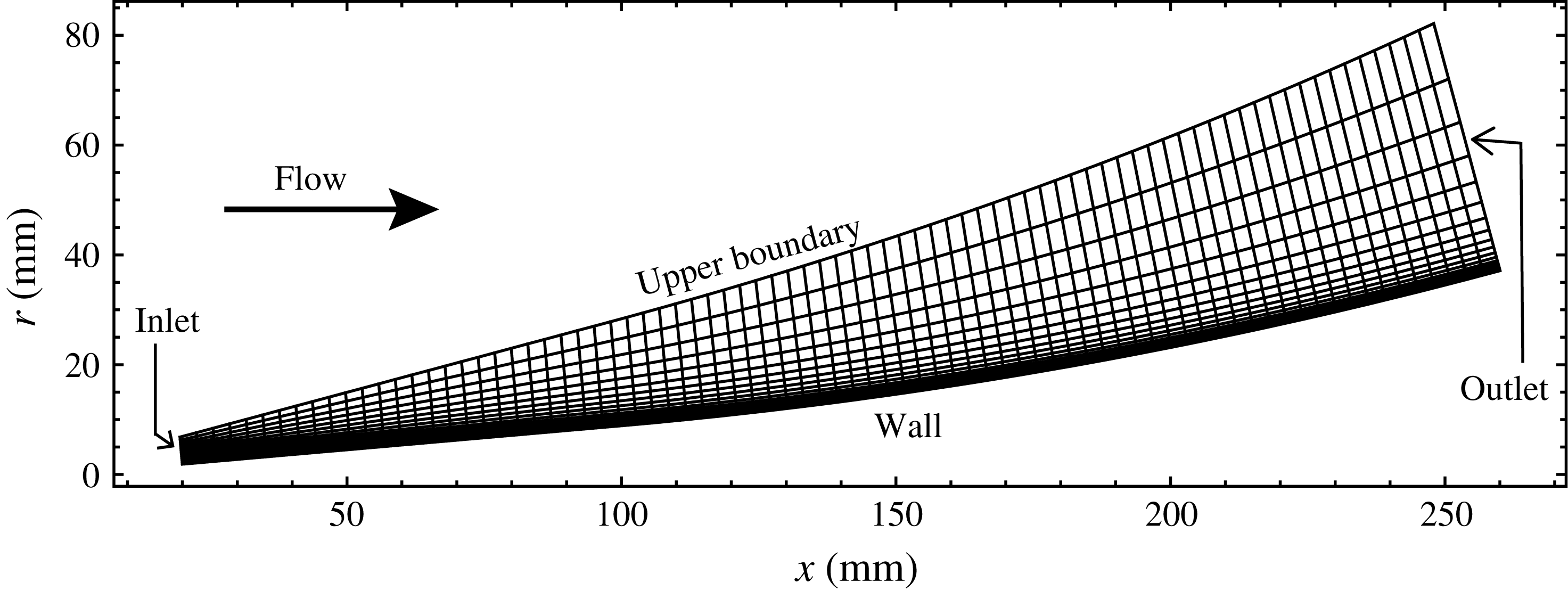
, as shown in figure 2. Both the curvature effects and external pressure-gradient effects have been taken into account. The boundary conditions for simulations of the unsteady flow are as follows.
$4000\times 200\times 500$
, as shown in figure 2. Both the curvature effects and external pressure-gradient effects have been taken into account. The boundary conditions for simulations of the unsteady flow are as follows.
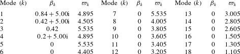
(i) For the inflow boundary and upper boundary, time-independent conditions are obtained from the steady-flow simulations. The upper boundary is perturbed by random velocity noise with maximum velocity fluctuations of 1 %. Meanwhile, eighteen modes, including first- and second-mode waves, are seeded at the inflow boundary in the form
(3.8)The amplitude $$\begin{eqnarray}\displaystyle \unicode[STIX]{x1D716}\mathop{\sum }_{k=1}^{18}\hat{\unicode[STIX]{x1D6F9}}_{k}(y)\exp (\text{i}\unicode[STIX]{x1D6FD}_{k}z-\text{i}\unicode[STIX]{x1D71B}_{k}t). & & \displaystyle\end{eqnarray}$$
$\unicode[STIX]{x1D716}$
, measured in terms of peak streamwise velocity fluctuations across the boundary layer, is equal to 1 % for each mode; the mode shapes,
$\hat{\unicode[STIX]{x1D6F9}}_{k}\equiv (\hat{\unicode[STIX]{x1D70C}},\hat{u} ,\hat{v},{\hat{w}},\hat{T})_{k}$
, are provided by LST;
$\unicode[STIX]{x1D6FD}_{k}$
and
$\unicode[STIX]{x1D71B}_{k}$
are, respectively, the corresponding spanwise wavenumber and radian frequency; and
$z$
is the spanwise coordinate in numerical space. The detailed parameters of the seeded modes are illustrated in table 1.
$$\begin{eqnarray}\displaystyle \unicode[STIX]{x1D716}\mathop{\sum }_{k=1}^{18}\hat{\unicode[STIX]{x1D6F9}}_{k}(y)\exp (\text{i}\unicode[STIX]{x1D6FD}_{k}z-\text{i}\unicode[STIX]{x1D71B}_{k}t). & & \displaystyle\end{eqnarray}$$
$\unicode[STIX]{x1D716}$
, measured in terms of peak streamwise velocity fluctuations across the boundary layer, is equal to 1 % for each mode; the mode shapes,
$\hat{\unicode[STIX]{x1D6F9}}_{k}\equiv (\hat{\unicode[STIX]{x1D70C}},\hat{u} ,\hat{v},{\hat{w}},\hat{T})_{k}$
, are provided by LST;
$\unicode[STIX]{x1D6FD}_{k}$
and
$\unicode[STIX]{x1D71B}_{k}$
are, respectively, the corresponding spanwise wavenumber and radian frequency; and
$z$
is the spanwise coordinate in numerical space. The detailed parameters of the seeded modes are illustrated in table 1.(ii) A non-reflecting boundary condition is used on the outflow boundary in the streamwise direction.
(iii) A periodic boundary is used in the circumference direction.
(iv) For the wall boundary, an adiabatic wall temperature together with the assumption
$\unicode[STIX]{x2202}p/\unicode[STIX]{x2202}y=0$
is used on the wall, and a second-order, one-side, finite-difference scheme is used to compute the wall pressure.(v) The boundary conditions for the upper side of the box are free-stream conditions, that is,
$u=\unicode[STIX]{x1D70C}=T=1$
while
$v=w=0$
.


Schematic of DNS grid for time-dependent simulations.
Eighteen modes seeded in the initial location.
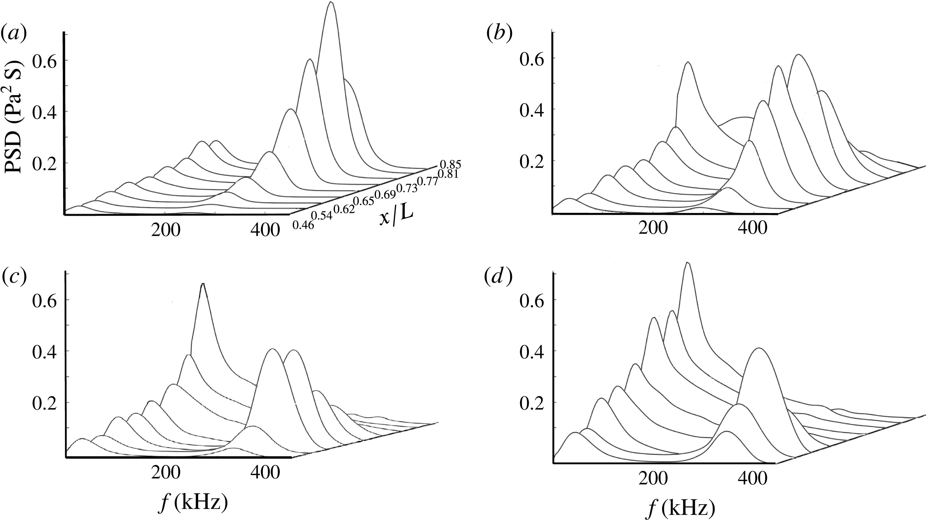
Streamwise developments of PCB frequency spectra at (a) $Re_{unit}=5.4\times 10^{6}~\text{m}^{-1}$
, (b)
$Re_{unit}=5.4\times 10^{6}~\text{m}^{-1}$
, (b) $Re_{unit}=7.6\times 10^{6}~\text{m}^{-1}$
, (c)
$Re_{unit}=7.6\times 10^{6}~\text{m}^{-1}$
, (c) $Re_{unit}=9.7\times 10^{6}~\text{m}^{-1}$
and (d)
$Re_{unit}=9.7\times 10^{6}~\text{m}^{-1}$
and (d) $Re_{unit}=11.7\times 10^{6}~\text{m}^{-1}$
.
$Re_{unit}=11.7\times 10^{6}~\text{m}^{-1}$
.
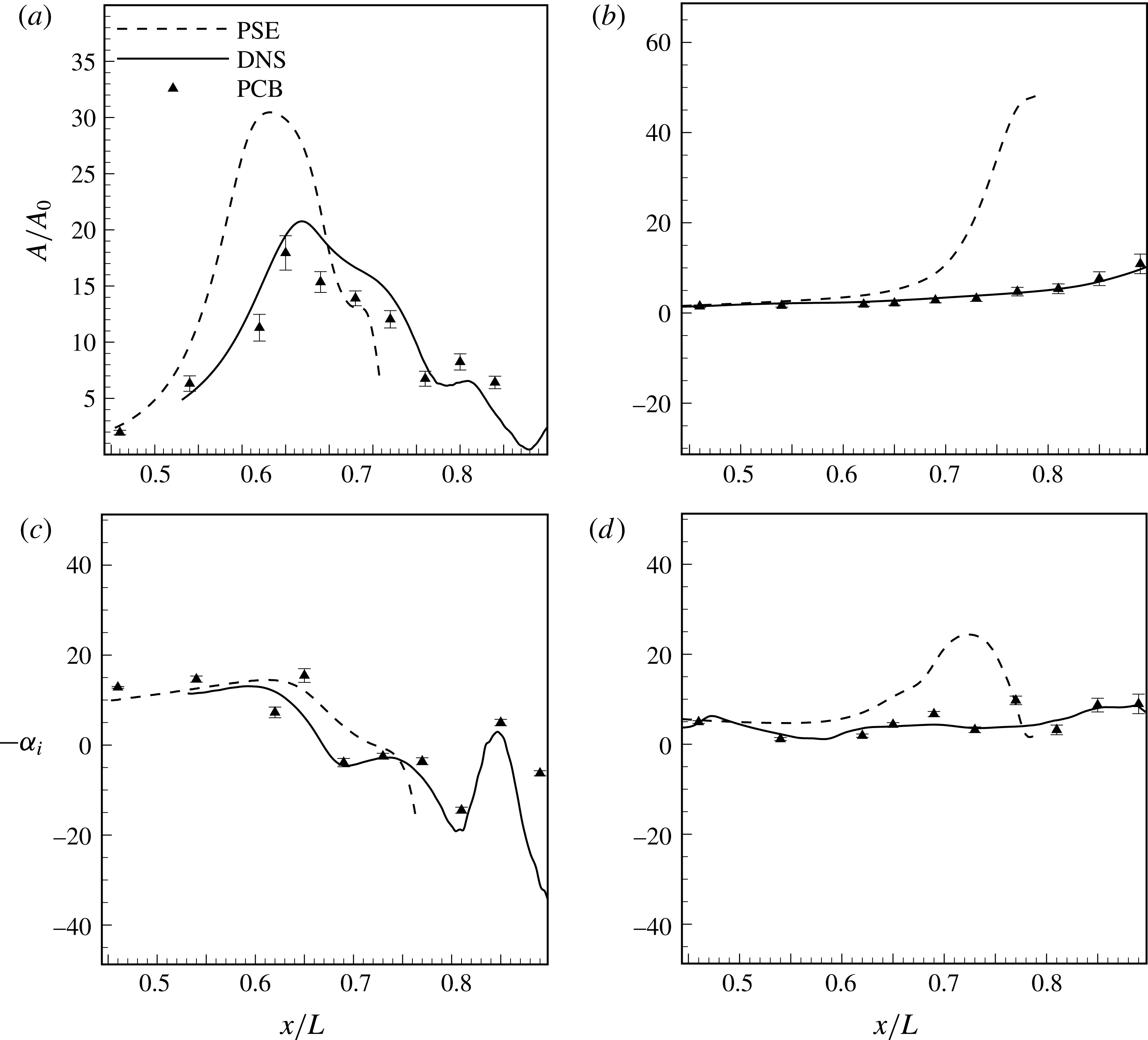
Comparison of instability amplitudes and streamwise growth ratios between PCB, PSE and DNS. $Re_{unit}=9.7\times 10^{6}~\text{m}^{-1}$
. (a,b) Second-mode instability; (c,d) low-frequency disturbances.
$Re_{unit}=9.7\times 10^{6}~\text{m}^{-1}$
. (a,b) Second-mode instability; (c,d) low-frequency disturbances.
TSP results of surface-temperature rise when the wind tunnel has run for 8 seconds from its start: (a) $Re_{unit}=5.4\times 10^{6}~\text{m}^{-1}$
, (b)
$Re_{unit}=5.4\times 10^{6}~\text{m}^{-1}$
, (b) $Re_{unit}=7.6\times 10^{6}~\text{m}^{-1}$
, (c)
$Re_{unit}=7.6\times 10^{6}~\text{m}^{-1}$
, (c) $Re_{unit}=9.7\times 10^{6}~\text{m}^{-1}$
and (d)
$Re_{unit}=9.7\times 10^{6}~\text{m}^{-1}$
and (d) $Re_{unit}=11.7\times 10^{6}~\text{m}^{-1}$
.
$Re_{unit}=11.7\times 10^{6}~\text{m}^{-1}$
.
4 Results and discussion
4.1 Instability evolution and surface-temperature rise
Power spectrum distributions (PSD) of PCB-measured time series are calculated. Their streamwise evolutions at different unit Reynolds numbers are shown in figure 3. Two peaks are clearly seen for each spectrum, respectively representing the second-mode instability at approximately 300–350 kHz and the low-frequency waves at approximately 20–30 kHz, consistent with previous studies (Zhang et al.
Reference Zhang, Tang and Lee2013; Zhu et al.
Reference Zhu, Zhang, Chen, Yuan, Wu, Chen, Lee and Gad-el-Hak2016; Chen, Zhu & Lee Reference Chen, Zhu and Lee2017). For the lowest unit Reynolds number, the second mode continuously grows until the end of the model whereas the low-frequency waves grow slowly. The amplitude of the latter is approximately 25 % that of the former. As $Re_{unit}$
increases to
$Re_{unit}$
increases to $7.6\times 10^{6}~\text{m}^{-1}$
, a saturation of second-mode amplitude occurs at
$7.6\times 10^{6}~\text{m}^{-1}$
, a saturation of second-mode amplitude occurs at $x/L=0.73$
. It then decays until the end of the model. Meanwhile, the low-frequency waves enjoy a faster growth, reaching a maximum value nearly the same as that of the second mode. As
$x/L=0.73$
. It then decays until the end of the model. Meanwhile, the low-frequency waves enjoy a faster growth, reaching a maximum value nearly the same as that of the second mode. As $Re_{unit}$
increases to
$Re_{unit}$
increases to $11.7\times 10^{6}~\text{m}^{-1}$
, the decay of the second mode is brought forward to
$11.7\times 10^{6}~\text{m}^{-1}$
, the decay of the second mode is brought forward to $x/L=0.65$
, whereas the growth of the low-frequency waves is further promoted. For the highest unit Reynolds number, the annihilation of the second mode is further brought forward. By contrast, the maximum value of the low-frequency waves is nearly three times that of the second mode.
$x/L=0.65$
, whereas the growth of the low-frequency waves is further promoted. For the highest unit Reynolds number, the annihilation of the second mode is further brought forward. By contrast, the maximum value of the low-frequency waves is nearly three times that of the second mode.
Comparison of instability growth is further made between PCB, PSE and DNS, as shown in figure 4. Herein, $-\unicode[STIX]{x1D6FC}_{i}$
represents the growth ratio, which can be calculated from the equation
$-\unicode[STIX]{x1D6FC}_{i}$
represents the growth ratio, which can be calculated from the equation
 $$\begin{eqnarray}\displaystyle -\unicode[STIX]{x1D6FC}_{i}=\ln (\text{d}A)/\text{d}x, & & \displaystyle\end{eqnarray}$$
where $A$
is the amplitude and
$A$
is the amplitude and $\unicode[STIX]{x1D6FC}_{i}$
is the imaginary part of the streamwise wavenumber
$\unicode[STIX]{x1D6FC}_{i}$
is the imaginary part of the streamwise wavenumber $\unicode[STIX]{x1D6FC}$
. As shown, DNS and PCB agree very well with each other whereas the PSE data, especially for low-frequency waves, are higher than the other two. As discussed by Chen et al. (Reference Chen, Zhu and Lee2017), one possible reason is that PSE purely considers the two fastest-growing modes whereas both the experiment and DNS involve a considerable level of random disturbance in the oncoming stream. The latter two growth ratios are integrative results of a wide spectrum. For example, although the present PSE has considered three-dimensional waves, only the mode (20, 50) with frequency of 20 kHz and circumferential wavenumber of 50 is seeded, which might not completely satisfy the complicated real flow condition. Despite this, the physical process depicted by PSE is substantially the same as the other two.
$\unicode[STIX]{x1D6FC}$
. As shown, DNS and PCB agree very well with each other whereas the PSE data, especially for low-frequency waves, are higher than the other two. As discussed by Chen et al. (Reference Chen, Zhu and Lee2017), one possible reason is that PSE purely considers the two fastest-growing modes whereas both the experiment and DNS involve a considerable level of random disturbance in the oncoming stream. The latter two growth ratios are integrative results of a wide spectrum. For example, although the present PSE has considered three-dimensional waves, only the mode (20, 50) with frequency of 20 kHz and circumferential wavenumber of 50 is seeded, which might not completely satisfy the complicated real flow condition. Despite this, the physical process depicted by PSE is substantially the same as the other two.
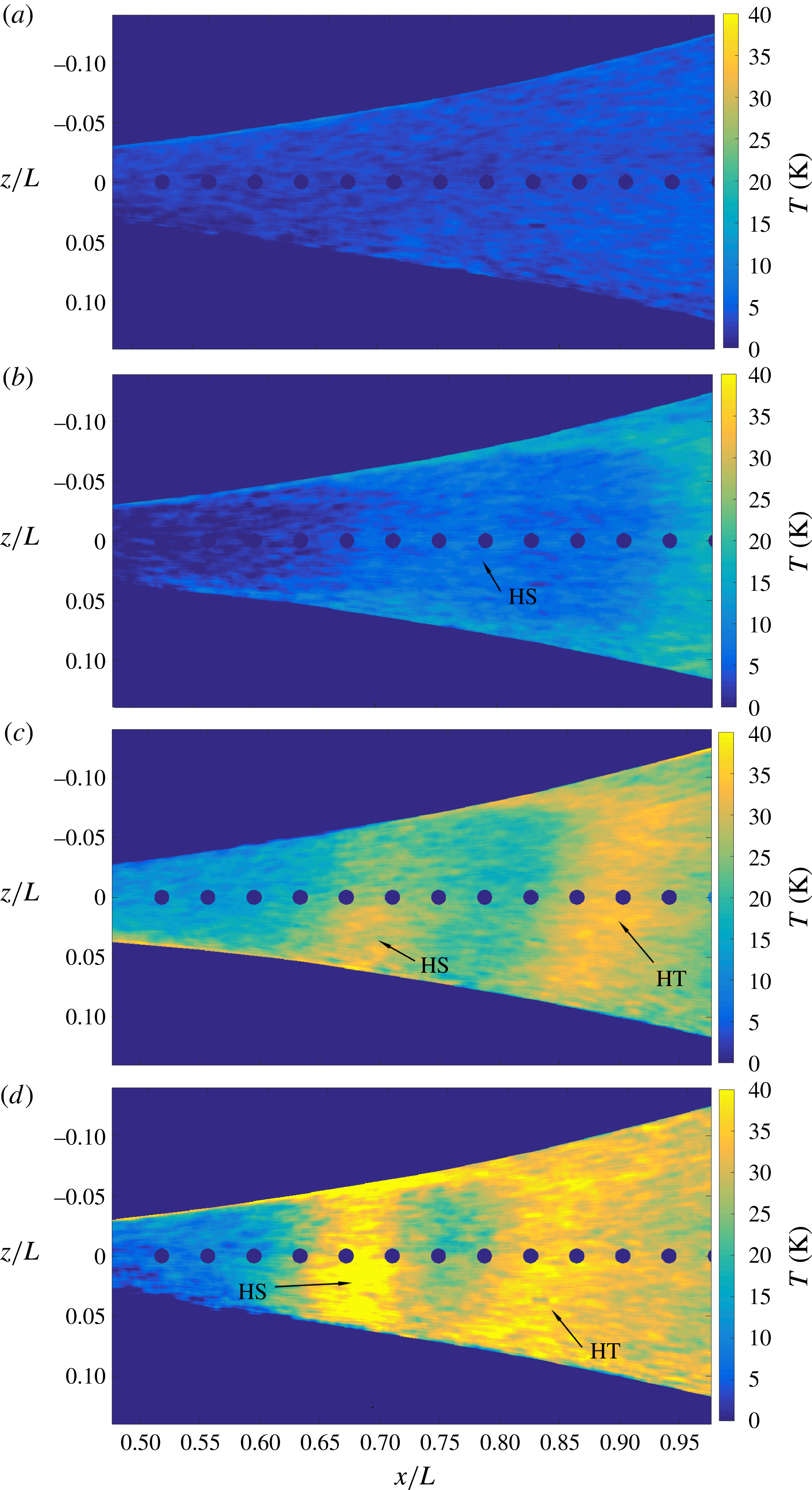
Surface-temperature distributions are then calculated from the TSP results. As shown in figure 5, increasing the unit Reynolds number greatly promotes the aerodynamic heating as well as the appearance of local hot spots (indicated as HS) in the streamwise direction. For $Re_{unit}=5.4\times 10^{6}~\text{m}^{-1}$
(figure 5
a), the temperature rises slowly to the end of the model. However, no prominent local peak is observed in the temperature rise distribution. As
$Re_{unit}=5.4\times 10^{6}~\text{m}^{-1}$
(figure 5
a), the temperature rises slowly to the end of the model. However, no prominent local peak is observed in the temperature rise distribution. As $Re_{unit}$
increases to
$Re_{unit}$
increases to $7.6\times 10^{6}~\text{m}^{-1}$
(figure 5
b), the aerodynamic heating becomes more pronounced, and a hot spot HS appears at
$7.6\times 10^{6}~\text{m}^{-1}$
(figure 5
b), the aerodynamic heating becomes more pronounced, and a hot spot HS appears at $x/L=0.79$
. As
$x/L=0.79$
. As $Re_{unit}$
increases to
$Re_{unit}$
increases to $9.7\times 10^{6}~\text{m}^{-1}$
(figure 5
c), the first hot spot HS is advanced to
$9.7\times 10^{6}~\text{m}^{-1}$
(figure 5
c), the first hot spot HS is advanced to $x/L=0.68$
with a new hot spot HT appearing at
$x/L=0.68$
with a new hot spot HT appearing at $x/L=0.89$
. The latter is related to the onset of turbulence at the end of the transition process (Berridge et al.
Reference Berridge, Chou, Ward, Steen, Gilbert, Juliano, Schneider and Gronvall2010; Franko & Lele Reference Franko and Lele2013; Sivasubramanian & Fasel Reference Sivasubramanian and Fasel2015). For the highest
$x/L=0.89$
. The latter is related to the onset of turbulence at the end of the transition process (Berridge et al.
Reference Berridge, Chou, Ward, Steen, Gilbert, Juliano, Schneider and Gronvall2010; Franko & Lele Reference Franko and Lele2013; Sivasubramanian & Fasel Reference Sivasubramanian and Fasel2015). For the highest $Re_{unit}$
(figure 5
d), the hot spot HS at
$Re_{unit}$
(figure 5
d), the hot spot HS at $x/L=0.68$
becomes stronger, with its peak value higher than that in HT. Streamwise streaks are also seen in the temperature rise distribution, consistent with the findings of Berridge et al. (Reference Berridge, Chou, Ward, Steen, Gilbert, Juliano, Schneider and Gronvall2010). The temperature value varies along the spanwise position, indicating the three-dimensional development of the boundary layer. HS might not be observed clearly if the temperature probes had been arranged at the valleys.
$x/L=0.68$
becomes stronger, with its peak value higher than that in HT. Streamwise streaks are also seen in the temperature rise distribution, consistent with the findings of Berridge et al. (Reference Berridge, Chou, Ward, Steen, Gilbert, Juliano, Schneider and Gronvall2010). The temperature value varies along the spanwise position, indicating the three-dimensional development of the boundary layer. HS might not be observed clearly if the temperature probes had been arranged at the valleys.
Evolution of second-mode and low-frequency waves arising from the PCB array at $\unicode[STIX]{x1D719}=0$
are compared with the TSP-measured surface-temperature rise along ten circumferential angles from
$\unicode[STIX]{x1D719}=0$
are compared with the TSP-measured surface-temperature rise along ten circumferential angles from $\unicode[STIX]{x1D719}=-18^{\circ }$
to
$\unicode[STIX]{x1D719}=-18^{\circ }$
to $18^{\circ }$
, as shown in figure 6. Temperatures within PCB sensors are evaluated by cubic-spline interpolation. It can be clearly seen that the appearance of HS is strongly correlated with that of the second-mode peak. For the lowest
$18^{\circ }$
, as shown in figure 6. Temperatures within PCB sensors are evaluated by cubic-spline interpolation. It can be clearly seen that the appearance of HS is strongly correlated with that of the second-mode peak. For the lowest $Re_{unit}$
(figure 6
a), the second mode grows until the end and no HS is found. For
$Re_{unit}$
(figure 6
a), the second mode grows until the end and no HS is found. For $Re_{unit}=7.6\times 10^{6}~\text{m}^{-1}$
(figure 6
b), the second-mode peak is located at
$Re_{unit}=7.6\times 10^{6}~\text{m}^{-1}$
(figure 6
b), the second-mode peak is located at $x/L=0.71$
, which is approximately 0.7
$x/L=0.71$
, which is approximately 0.7 $L$
ahead of HS. For
$L$
ahead of HS. For $Re_{unit}=9.7\times 10^{6}~\text{m}^{-1}$
(figure 6
c), the second-mode peak is located at
$Re_{unit}=9.7\times 10^{6}~\text{m}^{-1}$
(figure 6
c), the second-mode peak is located at $x/L=0.65$
, which is approximately 0.6–0.7
$x/L=0.65$
, which is approximately 0.6–0.7 $L$
ahead of HS. For the highest Reynolds number (figure 6
d), the distance between the second-mode peak and HS decreases to 0.3
$L$
ahead of HS. For the highest Reynolds number (figure 6
d), the distance between the second-mode peak and HS decreases to 0.3 $L$
. Comparison of instability evolutions and spanwise-averaged surface temperature is also made for PSE (figure 6
e) and DNS (figure 6
f). Correlations between the peak of the second mode and the hot spot HS are also observed.
$L$
. Comparison of instability evolutions and spanwise-averaged surface temperature is also made for PSE (figure 6
e) and DNS (figure 6
f). Correlations between the peak of the second mode and the hot spot HS are also observed.
Comparison of second-mode (red) and low-frequency waves (blue) with streamwise evolution of temperature at different spanwise angles (grey) and their spanwise average (green). Obtained from time-averaged PCB spectra and TSP results for (a) $Re_{unit}=5.4\times 10^{6}~\text{m}^{-1}$
, (b)
$Re_{unit}=5.4\times 10^{6}~\text{m}^{-1}$
, (b) $Re_{unit}=7.6\times 10^{6}~\text{m}^{-1}$
, (c)
$Re_{unit}=7.6\times 10^{6}~\text{m}^{-1}$
, (c) $Re_{unit}=9.7\times 10^{6}~\text{m}^{-1}$
and (d)
$Re_{unit}=9.7\times 10^{6}~\text{m}^{-1}$
and (d) $Re_{unit}=11.7\times 10^{6}~\text{m}^{-1}$
. Based on (e) DNS, and (f) PSE for
$Re_{unit}=11.7\times 10^{6}~\text{m}^{-1}$
. Based on (e) DNS, and (f) PSE for $Re_{unit}=9.7\times 10^{6}~\text{m}^{-1}$
. The subscripts
$Re_{unit}=9.7\times 10^{6}~\text{m}^{-1}$
. The subscripts $2nd$
and
$2nd$
and $lf$
respectively represent the second-mode and low-frequency waves.
$lf$
respectively represent the second-mode and low-frequency waves.
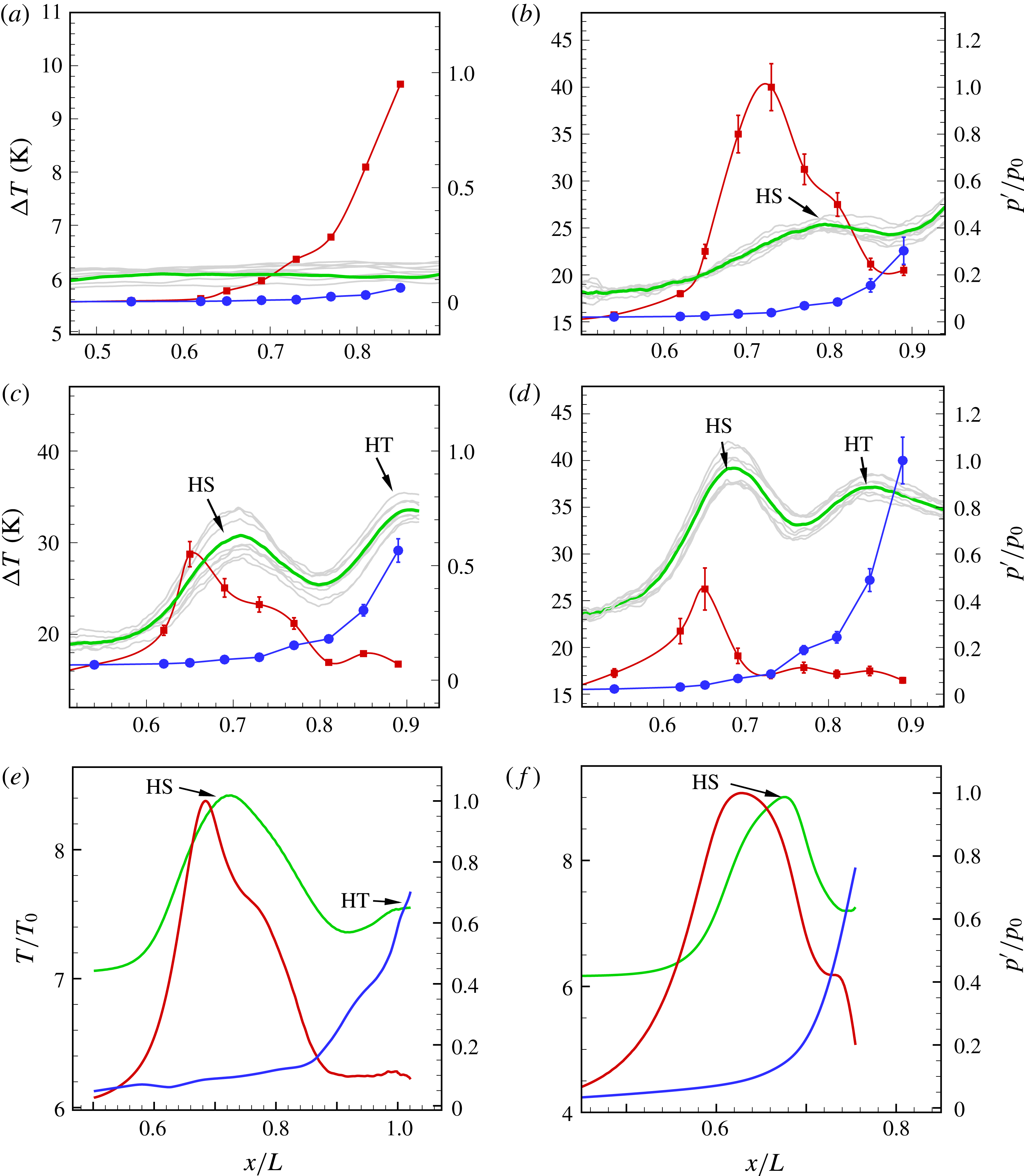
In general, as the unit Reynolds number increases, the second mode significantly decreases but HS quickly increases. This relationship seems logical because the aerodynamic heating should come from the dissipation of the flow mechanical energy. The heat production mechanism and its relationship with the flow structure near HS need to be further investigated.
4.2 Heat generation rate
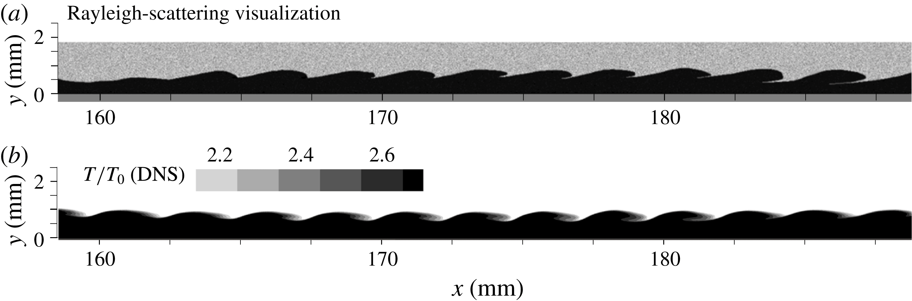
An RSFV picture of flow structures and the DNS-calculated temperature field near HS are both presented in figure 7. Such a comparison is reasonable because the RSFV actually reflects the temperature distribution in the field of view (Chen et al.
Reference Chen, Zhu and Lee2017). As shown, the boundary layer is initially laminar in the upstream region, but then regular rope-like structures appear at $x/L=0.55$
, which is typical of second-mode instability waves because their wavelength is twice the boundary layer thickness. The second-mode waves grow, saturate and finally decay to zero around
$x/L=0.55$
, which is typical of second-mode instability waves because their wavelength is twice the boundary layer thickness. The second-mode waves grow, saturate and finally decay to zero around $x/L=0.76$
. For experiments, the boundary layer becomes completely turbulent soon afterwards at approximately
$x/L=0.76$
. For experiments, the boundary layer becomes completely turbulent soon afterwards at approximately $x/L=0.85$
, whereas for DNS, onset of turbulence is delayed until nearly the end of the model (
$x/L=0.85$
, whereas for DNS, onset of turbulence is delayed until nearly the end of the model ( $x/L=1.0$
).
$x/L=1.0$
).
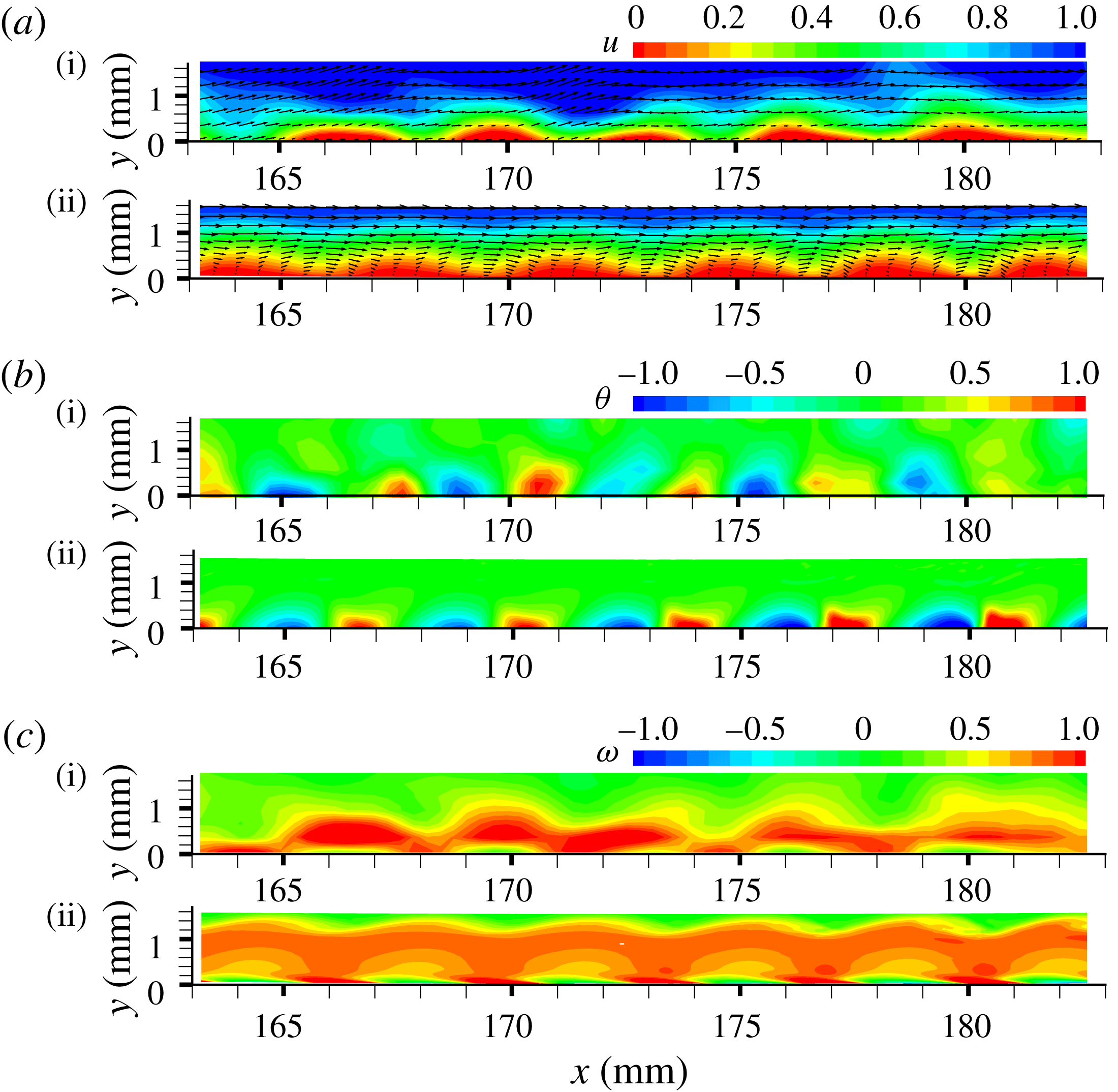
Figure 8 presents the instantaneous flow field near HS. The velocity magnitude normalized by the free-stream velocity, the dilatation $\unicode[STIX]{x1D714}^{2}$
and
$\unicode[STIX]{x1D714}^{2}$
and $\unicode[STIX]{x1D703}^{2}$
are presented in, respectively, (a), (b) and (c). Good agreement has been achieved between the PIV and DNS results. As shown, a strong compression–expansion process accompanies the evolution of the second-mode instability (figure 8
b), reflecting the acoustic nature of the latter (Mack Reference Mack1990). The vorticity distribution both near the wall and the critical layer are also modified due to viscous effects, creating periodic vortical waves in the boundary layer (figure 8
c). Such a mechanism has been discussed in detail in Zhu et al. (Reference Zhu, Zhang, Chen, Yuan, Wu, Chen, Lee and Gad-el-Hak2016).
$\unicode[STIX]{x1D703}^{2}$
are presented in, respectively, (a), (b) and (c). Good agreement has been achieved between the PIV and DNS results. As shown, a strong compression–expansion process accompanies the evolution of the second-mode instability (figure 8
b), reflecting the acoustic nature of the latter (Mack Reference Mack1990). The vorticity distribution both near the wall and the critical layer are also modified due to viscous effects, creating periodic vortical waves in the boundary layer (figure 8
c). Such a mechanism has been discussed in detail in Zhu et al. (Reference Zhu, Zhang, Chen, Yuan, Wu, Chen, Lee and Gad-el-Hak2016).
Time-averaged skin friction can then be calculated from PIV and DNS results. It would seem reasonable that the increase of wall skin friction due to the disturbance evolution is the major source of additional aerodynamic heating in the boundary layer. However, both for DNS and PIV (figure 9), the increase of skin friction at HS from laminar state is less than 15 % of that at HT, which cannot account for the enhanced heat transfer observed in figure 5. The inherent aerodynamic heating mechanism for HS needs to be further investigated.
The heat generation rate per unit volume can be explicitly split into contributions of vorticity $\unicode[STIX]{x1D714}$
and dilatation
$\unicode[STIX]{x1D714}$
and dilatation $\unicode[STIX]{x1D703}$
(Lele Reference Lele1994; Wu, Ma & Zhou Reference Wu, Ma and Zhou2006):
$\unicode[STIX]{x1D703}$
(Lele Reference Lele1994; Wu, Ma & Zhou Reference Wu, Ma and Zhou2006):
 $$\begin{eqnarray}\displaystyle q & = & \displaystyle w_{\unicode[STIX]{x1D703}1}+w_{\unicode[STIX]{x1D703}2}+w_{\unicode[STIX]{x1D714}}+\text{BI},\end{eqnarray}$$
 $$\begin{eqnarray}\displaystyle w_{\unicode[STIX]{x1D703}} & = & \displaystyle -p\unicode[STIX]{x1D703}+\unicode[STIX]{x1D707}^{\prime }\unicode[STIX]{x1D703}^{2},\end{eqnarray}$$
 $$\begin{eqnarray}\displaystyle w_{\unicode[STIX]{x1D714}} & = & \displaystyle \unicode[STIX]{x1D707}\unicode[STIX]{x1D714}^{2},\end{eqnarray}$$
where BI represents a boundary integral; $w_{\unicode[STIX]{x1D703}}$
and
$w_{\unicode[STIX]{x1D703}}$
and $w_{\unicode[STIX]{x1D714}}$
denote, respectively, the work done by dilatation and shear stress;
$w_{\unicode[STIX]{x1D714}}$
denote, respectively, the work done by dilatation and shear stress; $\unicode[STIX]{x1D707}^{\prime }=\unicode[STIX]{x1D707}_{b}+4\unicode[STIX]{x1D707}/3$
is the longitudinal viscosity, with
$\unicode[STIX]{x1D707}^{\prime }=\unicode[STIX]{x1D707}_{b}+4\unicode[STIX]{x1D707}/3$
is the longitudinal viscosity, with $\unicode[STIX]{x1D707}$
and
$\unicode[STIX]{x1D707}$
and $\unicode[STIX]{x1D707}_{b}$
being, respectively, the shear and bulk viscosities. As stated above, the work done by the wall skin friction, reflected in the term
$\unicode[STIX]{x1D707}_{b}$
being, respectively, the shear and bulk viscosities. As stated above, the work done by the wall skin friction, reflected in the term $w_{\unicode[STIX]{x1D714}}$
, is the major source of aerodynamic heating in low Mach number wall-bounded flows. For high Mach number flows, however, the term
$w_{\unicode[STIX]{x1D714}}$
, is the major source of aerodynamic heating in low Mach number wall-bounded flows. For high Mach number flows, however, the term $w_{\unicode[STIX]{x1D703}}$
, including both the pressure work and dilatational viscous dissipation, might be considerable. Its important role was recognized by Emanuel (Reference Emanuel1992) and Gad-el-Hak (Reference Gad-el-Hak1995). Associated dilatational viscous dissipation was highlighted in our previous work (Zhang et al.
Reference Zhang, Zhu, Chen, Yuan, Wu, Chen, Lee and Gad-el-Hak2015; Zhu et al.
Reference Zhu, Zhang, Chen, Yuan, Wu, Chen, Lee and Gad-el-Hak2016).
$w_{\unicode[STIX]{x1D703}}$
, including both the pressure work and dilatational viscous dissipation, might be considerable. Its important role was recognized by Emanuel (Reference Emanuel1992) and Gad-el-Hak (Reference Gad-el-Hak1995). Associated dilatational viscous dissipation was highlighted in our previous work (Zhang et al.
Reference Zhang, Zhu, Chen, Yuan, Wu, Chen, Lee and Gad-el-Hak2015; Zhu et al.
Reference Zhu, Zhang, Chen, Yuan, Wu, Chen, Lee and Gad-el-Hak2016).
(a) Snapshot of flow structures near HS region based on Rayleigh-scattering technique. (b) Temperature field calculated by DNS near HS region. $Re_{unit}=9.7\times 10^{6}~\text{m}^{-1}$
.
$Re_{unit}=9.7\times 10^{6}~\text{m}^{-1}$
.
Snapshot of (a) velocity, (b) dilatation and (c) $z$
-vorticity field in the
$z$
-vorticity field in the $x$
–
$x$
– $y$
plane near HS region. Based on (i) PIV results and (ii) DNS. The magnitudes are normalized by their respective maximum value.
$y$
plane near HS region. Based on (i) PIV results and (ii) DNS. The magnitudes are normalized by their respective maximum value.
Comparison of streamwise evolution of second-mode (red) and low-frequency waves (blue) with time-averaged skin friction coefficients (magenta) based on (a) DNS and (b) experiments. $Re_{unit}=9.7\times 10^{6}~\text{m}^{-1}$
. SM, second mode; LFW, low-frequency waves. V1 and V2 stand for, respectively, the PIV view range
$Re_{unit}=9.7\times 10^{6}~\text{m}^{-1}$
. SM, second mode; LFW, low-frequency waves. V1 and V2 stand for, respectively, the PIV view range $x\in [157,187]$
mm and [190, 220] mm.
$x\in [157,187]$
mm and [190, 220] mm.
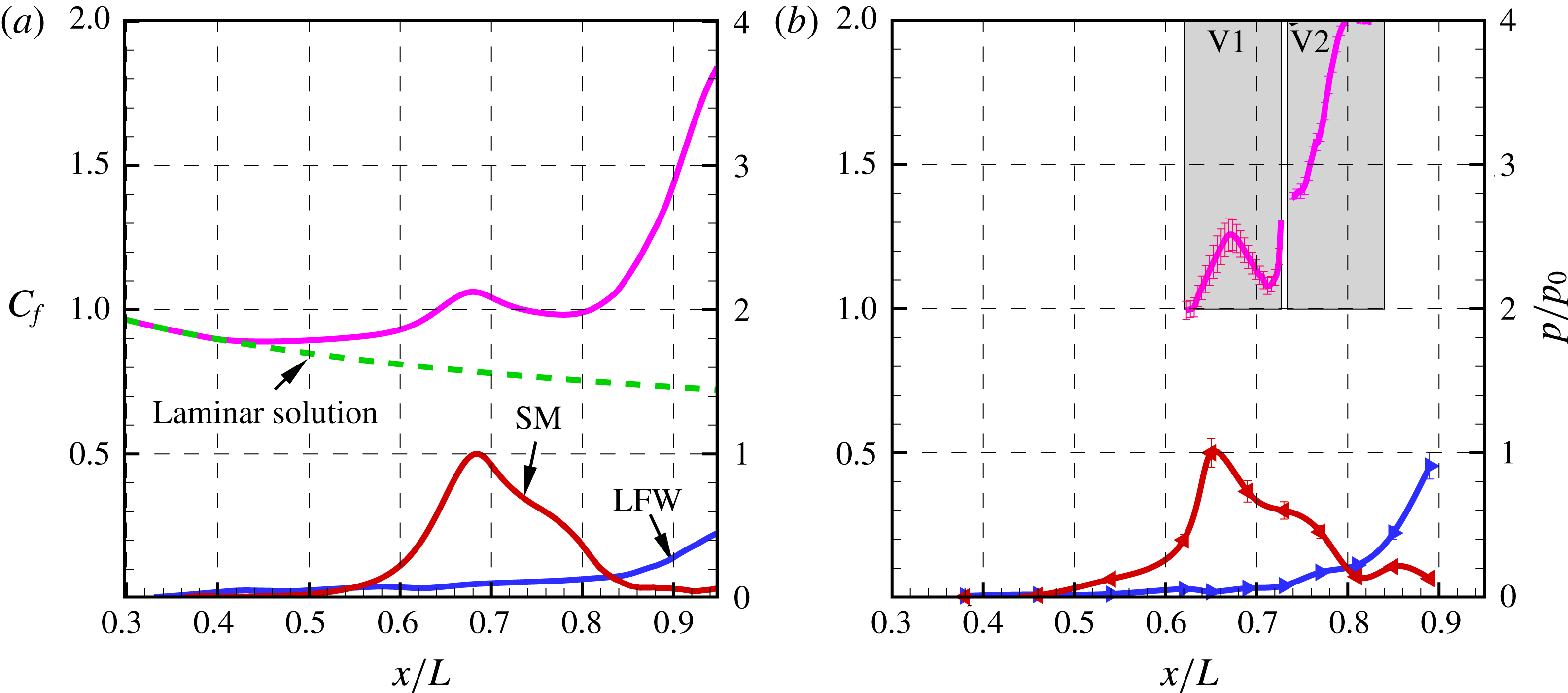
Because of their different natures, we further split $w_{\unicode[STIX]{x1D703}}$
into two parts:
$w_{\unicode[STIX]{x1D703}}$
into two parts:
 $$\begin{eqnarray}\displaystyle w_{\unicode[STIX]{x1D703}} & = & \displaystyle w_{\unicode[STIX]{x1D703}1}+w_{\unicode[STIX]{x1D703}2},\end{eqnarray}$$
 $$\begin{eqnarray}\displaystyle w_{\unicode[STIX]{x1D703}1} & = & \displaystyle -p\unicode[STIX]{x1D703},\end{eqnarray}$$
 $$\begin{eqnarray}\displaystyle w_{\unicode[STIX]{x1D703}2} & = & \displaystyle \unicode[STIX]{x1D707}^{\prime }\unicode[STIX]{x1D703}^{2}.\end{eqnarray}$$
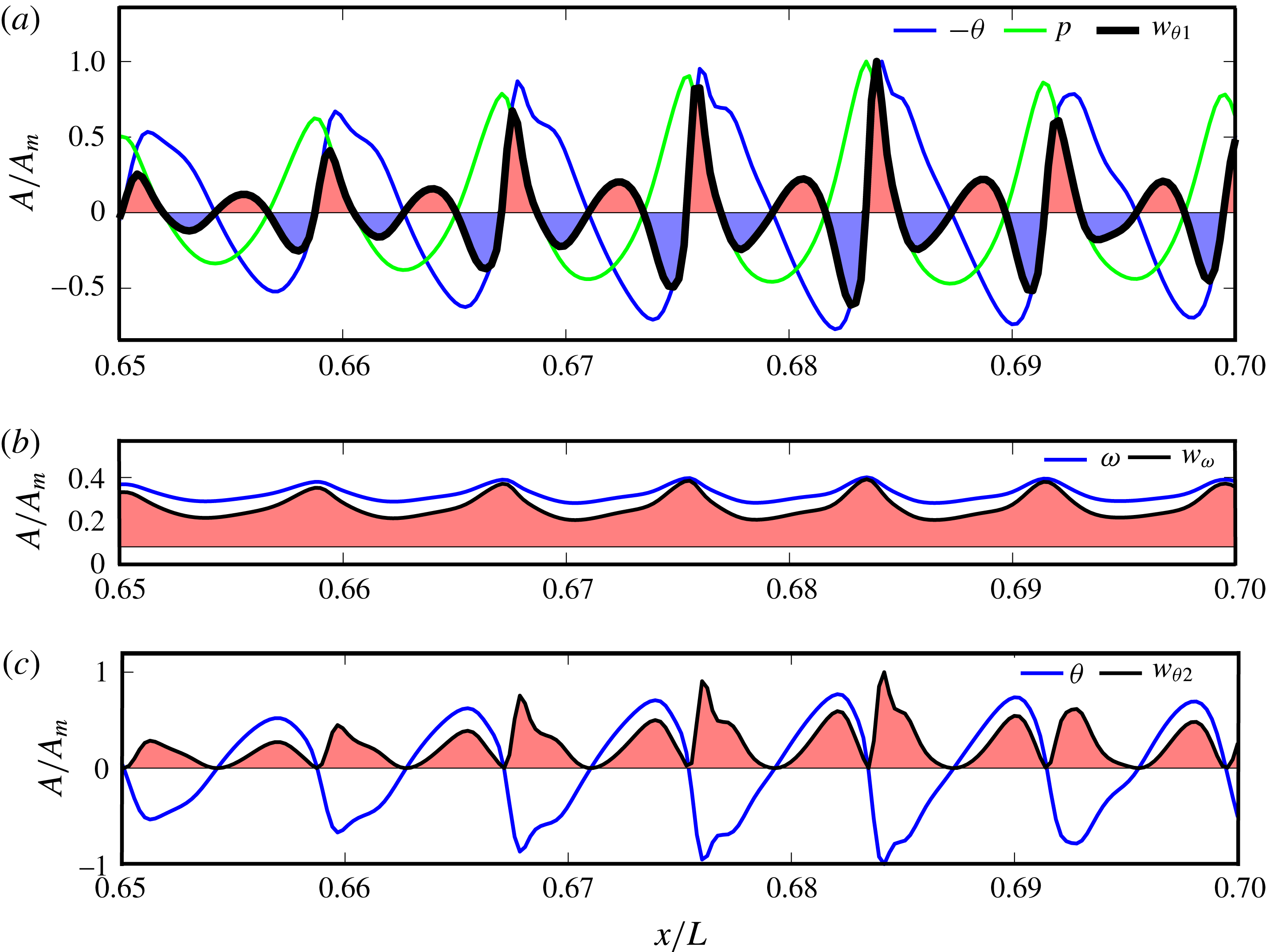
Figure 10 presents the instantaneous streamwise evolution of $w_{\unicode[STIX]{x1D703}1}$
,
$w_{\unicode[STIX]{x1D703}1}$
, $w_{\unicode[STIX]{x1D703}2}$
and
$w_{\unicode[STIX]{x1D703}2}$
and $w_{\unicode[STIX]{x1D714}}$
in the boundary layer near HS. As shown, the term
$w_{\unicode[STIX]{x1D714}}$
in the boundary layer near HS. As shown, the term $w_{\unicode[STIX]{x1D703}1}$
is alternatively positive and negative, representing an alternative creation and absorption of heat. Its time-averaged value not only depends on the amplitude of
$w_{\unicode[STIX]{x1D703}1}$
is alternatively positive and negative, representing an alternative creation and absorption of heat. Its time-averaged value not only depends on the amplitude of $p$
and
$p$
and $\unicode[STIX]{x1D703}$
, but also the phase angle between them. The terms
$\unicode[STIX]{x1D703}$
, but also the phase angle between them. The terms $w_{\unicode[STIX]{x1D703}2}$
and
$w_{\unicode[STIX]{x1D703}2}$
and $w_{\unicode[STIX]{x1D714}}$
are always positive because of their viscous dissipation nature. This means heat is created wherever the shear or dilatation process exists.
$w_{\unicode[STIX]{x1D714}}$
are always positive because of their viscous dissipation nature. This means heat is created wherever the shear or dilatation process exists.
Instantaneous streamwise evolution of the heating generation rate: (a) $w_{\unicode[STIX]{x1D703}1}=-p\unicode[STIX]{x1D703}$
, (b)
$w_{\unicode[STIX]{x1D703}1}=-p\unicode[STIX]{x1D703}$
, (b) $w_{\unicode[STIX]{x1D703}2}=\unicode[STIX]{x1D707}^{\prime }\unicode[STIX]{x1D703}^{2}$
and (c)
$w_{\unicode[STIX]{x1D703}2}=\unicode[STIX]{x1D707}^{\prime }\unicode[STIX]{x1D703}^{2}$
and (c) $w_{\unicode[STIX]{x1D714}}=\unicode[STIX]{x1D707}\unicode[STIX]{x1D714}^{2}$
at
$w_{\unicode[STIX]{x1D714}}=\unicode[STIX]{x1D707}\unicode[STIX]{x1D714}^{2}$
at $y/\unicode[STIX]{x1D6FF}=0.5$
, where
$y/\unicode[STIX]{x1D6FF}=0.5$
, where $\unicode[STIX]{x1D6FF}$
is the boundary layer thickness. Red and blue areas respectively stand for positive and negative heating generation rates. Values are normalized by their respective maximum value.
$\unicode[STIX]{x1D6FF}$
is the boundary layer thickness. Red and blue areas respectively stand for positive and negative heating generation rates. Values are normalized by their respective maximum value. $Re_{unit}=9.7\times 10^{6}~\text{m}^{-1}$
.
$Re_{unit}=9.7\times 10^{6}~\text{m}^{-1}$
.
We next evaluate the evolution of time-averaged $w_{\unicode[STIX]{x1D703}1}$
,
$w_{\unicode[STIX]{x1D703}1}$
, $w_{\unicode[STIX]{x1D703}1}$
and
$w_{\unicode[STIX]{x1D703}1}$
and $w_{\unicode[STIX]{x1D714}}$
in the flow field. Two problems are encountered, however. One is that
$w_{\unicode[STIX]{x1D714}}$
in the flow field. Two problems are encountered, however. One is that $w_{\unicode[STIX]{x1D703}1}$
is difficult to obtain experimentally because a simultaneous measurement of the instantaneous
$w_{\unicode[STIX]{x1D703}1}$
is difficult to obtain experimentally because a simultaneous measurement of the instantaneous $p$
- and
$p$
- and $\unicode[STIX]{x1D703}$
-field is far beyond the measurement capabilities available today for hypersonic flows. To solve this problem, we assumed that
$\unicode[STIX]{x1D703}$
-field is far beyond the measurement capabilities available today for hypersonic flows. To solve this problem, we assumed that $p$
is nearly constant in the boundary layer and
$p$
is nearly constant in the boundary layer and $w_{\unicode[STIX]{x1D703}1}$
is mainly created near the wall because
$w_{\unicode[STIX]{x1D703}1}$
is mainly created near the wall because $p$
and
$p$
and $\unicode[STIX]{x1D703}$
reach their maximum values there (Morkovin Reference Morkovin1987). Due to the no-slip condition, a balance between the normal and shear stress is achieved by
$\unicode[STIX]{x1D703}$
reach their maximum values there (Morkovin Reference Morkovin1987). Due to the no-slip condition, a balance between the normal and shear stress is achieved by
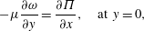 $$\begin{eqnarray}\displaystyle -\unicode[STIX]{x1D707}\frac{\unicode[STIX]{x2202}\unicode[STIX]{x1D714}}{\unicode[STIX]{x2202}y}=\frac{\unicode[STIX]{x2202}\unicode[STIX]{x1D6F1}}{\unicode[STIX]{x2202}x},\quad \text{at}~y=0, & & \displaystyle\end{eqnarray}$$
where $\unicode[STIX]{x1D6F1}=-p+\unicode[STIX]{x1D707}^{\prime }\unicode[STIX]{x1D703}$
. Then, the pressure at wall can be integrated as
$\unicode[STIX]{x1D6F1}=-p+\unicode[STIX]{x1D707}^{\prime }\unicode[STIX]{x1D703}$
. Then, the pressure at wall can be integrated as
 $$\begin{eqnarray}\displaystyle p=\unicode[STIX]{x1D707}^{\prime }\unicode[STIX]{x1D703}+\int \unicode[STIX]{x1D707}\frac{\unicode[STIX]{x2202}\unicode[STIX]{x1D714}}{\unicode[STIX]{x2202}y}\,\text{d}x,\quad \text{at}~y=0. & & \displaystyle\end{eqnarray}$$
The second problem is the exact value of $\unicode[STIX]{x1D707}_{b}$
. The dilatational dissipation for a gas arises from an internal molecular relaxation process, which is, of course, a dispersion of frequency. As interpreted by Landau & Lifshitz (Reference Landau and Lifshitz1959), the bulk viscosity that leads to attenuation of dilatational waves increases monotonically with frequency. A more accurate evaluation of the bulk viscosity coefficient in hypersonic boundary layers is necessary, which is an issue of crucial importance to the community. In this work, we use the most conservative evaluation as
$\unicode[STIX]{x1D707}_{b}$
. The dilatational dissipation for a gas arises from an internal molecular relaxation process, which is, of course, a dispersion of frequency. As interpreted by Landau & Lifshitz (Reference Landau and Lifshitz1959), the bulk viscosity that leads to attenuation of dilatational waves increases monotonically with frequency. A more accurate evaluation of the bulk viscosity coefficient in hypersonic boundary layers is necessary, which is an issue of crucial importance to the community. In this work, we use the most conservative evaluation as $\unicode[STIX]{x1D707}_{b}=2\unicode[STIX]{x1D707}/3$
for
$\unicode[STIX]{x1D707}_{b}=2\unicode[STIX]{x1D707}/3$
for $\text{N}_{2}$
gas at 430 K.
$\text{N}_{2}$
gas at 430 K.
Figures 11 and 12 present the time-averaged $w_{\unicode[STIX]{x1D703}1}$
,
$w_{\unicode[STIX]{x1D703}1}$
, $w_{\unicode[STIX]{x1D703}1}$
and
$w_{\unicode[STIX]{x1D703}1}$
and $w_{\unicode[STIX]{x1D714}}$
in the
$w_{\unicode[STIX]{x1D714}}$
in the $x$
–
$x$
– $y$
plane near HS and HT, respectively. The values are normalized by their respective maximum value. PIV and DNS results agree reasonably well, which validates our previous assumptions. For HS, the contribution to aerodynamic heating mainly comes from the dilatation process, especially
$y$
plane near HS and HT, respectively. The values are normalized by their respective maximum value. PIV and DNS results agree reasonably well, which validates our previous assumptions. For HS, the contribution to aerodynamic heating mainly comes from the dilatation process, especially $w_{\unicode[STIX]{x1D703}1}$
, rather than its shear counterpart
$w_{\unicode[STIX]{x1D703}1}$
, rather than its shear counterpart $w_{\unicode[STIX]{x1D714}}$
. The value of
$w_{\unicode[STIX]{x1D714}}$
. The value of $w_{\unicode[STIX]{x1D703}2}$
is also considerable in that region. The main energy of
$w_{\unicode[STIX]{x1D703}2}$
is also considerable in that region. The main energy of $w_{\unicode[STIX]{x1D703}1}$
and
$w_{\unicode[STIX]{x1D703}1}$
and $w_{\unicode[STIX]{x1D703}2}$
lies at the bottom of the boundary layer, because the dilatation process mainly exists beneath the sonic line. Some tiny negative regions of
$w_{\unicode[STIX]{x1D703}2}$
lies at the bottom of the boundary layer, because the dilatation process mainly exists beneath the sonic line. Some tiny negative regions of $w_{\unicode[STIX]{x1D703}1}$
are also seen in DNS, but not in PIV because the evaluated pressure there might be far from reality. For HT, the aerodynamic heating mainly comes from the fast increase of
$w_{\unicode[STIX]{x1D703}1}$
are also seen in DNS, but not in PIV because the evaluated pressure there might be far from reality. For HT, the aerodynamic heating mainly comes from the fast increase of $w_{\unicode[STIX]{x1D714}}$
very near the wall, which agrees well with the explanation given by Franko & Lele (Reference Franko and Lele2013) for HT in that ultimate transition process.
$w_{\unicode[STIX]{x1D714}}$
very near the wall, which agrees well with the explanation given by Franko & Lele (Reference Franko and Lele2013) for HT in that ultimate transition process.
Time-averaged distribution of (a) $w_{\unicode[STIX]{x1D703}1}=-p\unicode[STIX]{x1D703}$
, (b)
$w_{\unicode[STIX]{x1D703}1}=-p\unicode[STIX]{x1D703}$
, (b) $w_{\unicode[STIX]{x1D703}2}=\unicode[STIX]{x1D707}^{\prime }\unicode[STIX]{x1D703}^{2}$
and (c)
$w_{\unicode[STIX]{x1D703}2}=\unicode[STIX]{x1D707}^{\prime }\unicode[STIX]{x1D703}^{2}$
and (c) $w_{\unicode[STIX]{x1D714}}=\unicode[STIX]{x1D707}\unicode[STIX]{x1D714}^{2}$
in the
$w_{\unicode[STIX]{x1D714}}=\unicode[STIX]{x1D707}\unicode[STIX]{x1D714}^{2}$
in the $x$
–
$x$
– $y$
plane near HS. Based on (i) PIV and (ii) spanwise-averaged DNS results. Values are normalized by their maximum value.
$y$
plane near HS. Based on (i) PIV and (ii) spanwise-averaged DNS results. Values are normalized by their maximum value. $Re_{unit}=9.7\times 10^{6}~\text{m}^{-1}$
.
$Re_{unit}=9.7\times 10^{6}~\text{m}^{-1}$
.
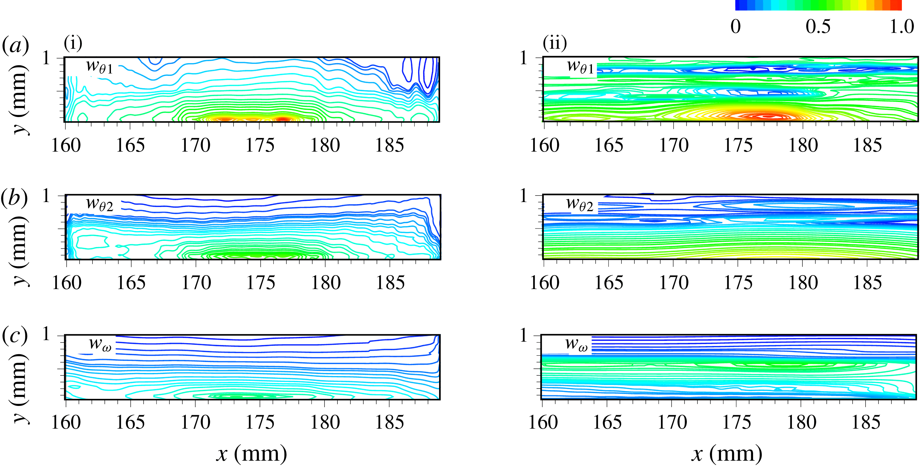
Time-averaged distribution of (a) $w_{\unicode[STIX]{x1D703}1}=-p\unicode[STIX]{x1D703}$
, (b)
$w_{\unicode[STIX]{x1D703}1}=-p\unicode[STIX]{x1D703}$
, (b) $w_{\unicode[STIX]{x1D703}2}=\unicode[STIX]{x1D707}^{\prime }\unicode[STIX]{x1D703}^{2}$
and (c)
$w_{\unicode[STIX]{x1D703}2}=\unicode[STIX]{x1D707}^{\prime }\unicode[STIX]{x1D703}^{2}$
and (c) $w_{\unicode[STIX]{x1D714}}=\unicode[STIX]{x1D707}\unicode[STIX]{x1D714}^{2}$
in the
$w_{\unicode[STIX]{x1D714}}=\unicode[STIX]{x1D707}\unicode[STIX]{x1D714}^{2}$
in the $x$
–
$x$
– $y$
plane near HT. Based on (i) PIV and (ii) spanwise-averaged DNS results. Values are normalized by their maximum value.
$y$
plane near HT. Based on (i) PIV and (ii) spanwise-averaged DNS results. Values are normalized by their maximum value. $Re_{unit}=9.7\times 10^{6}~\text{m}^{-1}$
.
$Re_{unit}=9.7\times 10^{6}~\text{m}^{-1}$
.
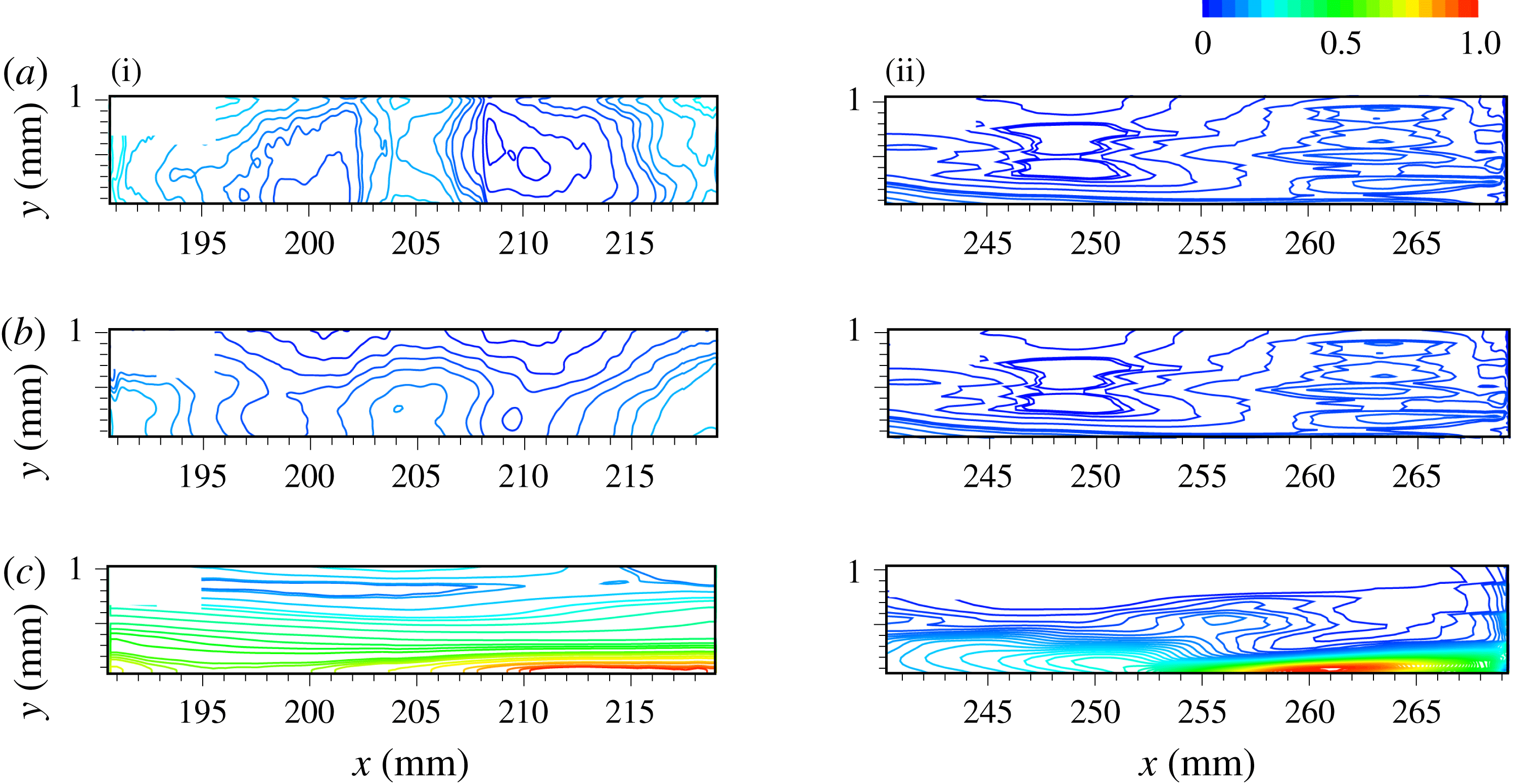
Comparison of streamwise evolution of second-mode (red) and low-frequency waves (blue) with heat generation rate. Based on (a) spanwise-averaged DNS and (b) experiments. Values are time-averaged along the normal direction. $w_{\unicode[STIX]{x1D703}1}=-p\unicode[STIX]{x1D703}$
(orange);
$w_{\unicode[STIX]{x1D703}1}=-p\unicode[STIX]{x1D703}$
(orange); $w_{\unicode[STIX]{x1D703}2}=\unicode[STIX]{x1D707}^{\prime }\unicode[STIX]{x1D703}^{2}$
(green);
$w_{\unicode[STIX]{x1D703}2}=\unicode[STIX]{x1D707}^{\prime }\unicode[STIX]{x1D703}^{2}$
(green); $w_{\unicode[STIX]{x1D714}}=\unicode[STIX]{x1D707}\unicode[STIX]{x1D714}^{2}$
(magenta).
$w_{\unicode[STIX]{x1D714}}=\unicode[STIX]{x1D707}\unicode[STIX]{x1D714}^{2}$
(magenta). $Re_{unit}=9.7\times 10^{6}~\text{m}^{-1}$
. SM, second mode; LFW, low-frequency waves. V1 and V2 stand for, respectively, the PIV view range
$Re_{unit}=9.7\times 10^{6}~\text{m}^{-1}$
. SM, second mode; LFW, low-frequency waves. V1 and V2 stand for, respectively, the PIV view range $x\in [157,187]$
mm and [190, 220] mm.
$x\in [157,187]$
mm and [190, 220] mm.
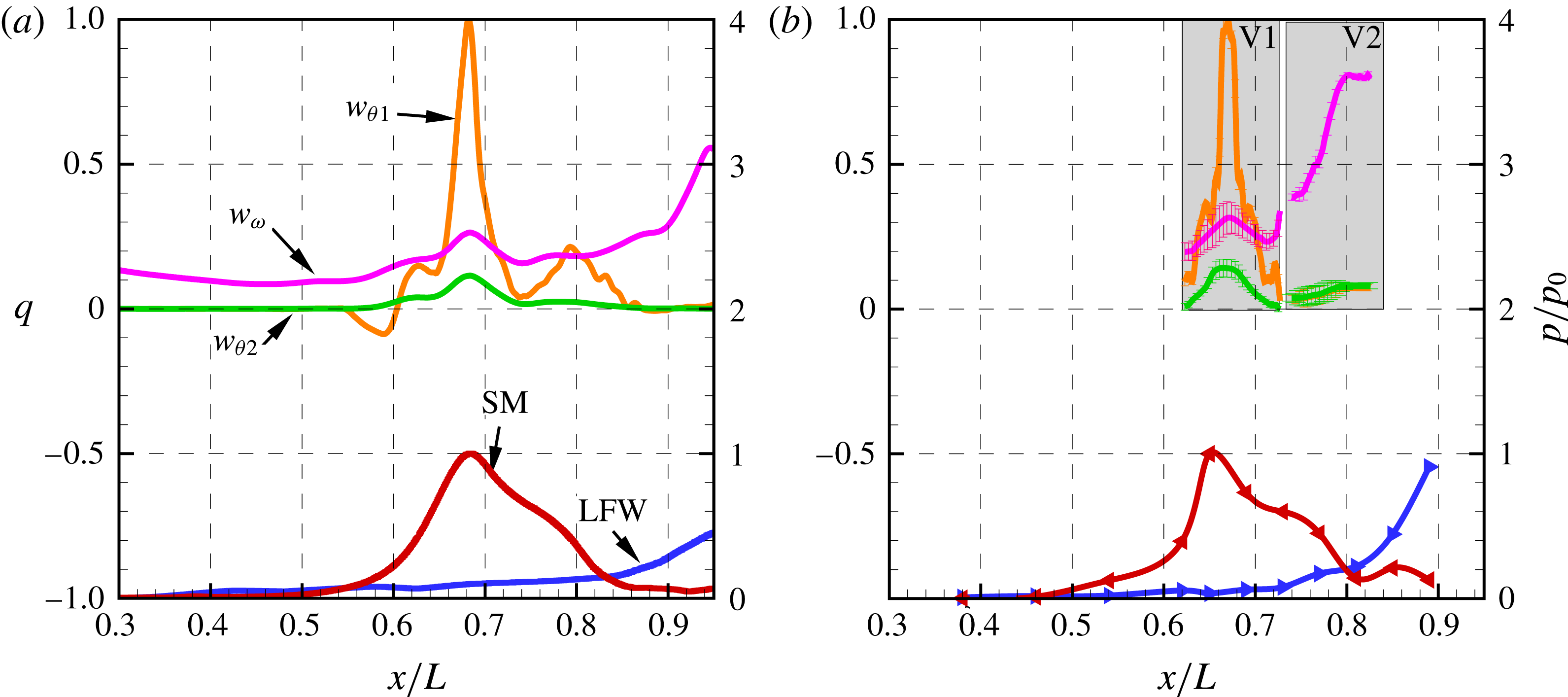
DNS results of surface distribution of (a) mean temperature and instantaneous heat generation rates. Including (b) $w_{\unicode[STIX]{x1D714}}=\unicode[STIX]{x1D707}\unicode[STIX]{x1D714}^{2}$
, (c)
$w_{\unicode[STIX]{x1D714}}=\unicode[STIX]{x1D707}\unicode[STIX]{x1D714}^{2}$
, (c) $w_{\unicode[STIX]{x1D703}1}=-p\unicode[STIX]{x1D703}$
and (d)
$w_{\unicode[STIX]{x1D703}1}=-p\unicode[STIX]{x1D703}$
and (d) $w_{\unicode[STIX]{x1D703}2}=\unicode[STIX]{x1D707}^{\prime }\unicode[STIX]{x1D703}^{2}$
. Each quantity is normalized by its maximum value.
$w_{\unicode[STIX]{x1D703}2}=\unicode[STIX]{x1D707}^{\prime }\unicode[STIX]{x1D703}^{2}$
. Each quantity is normalized by its maximum value.
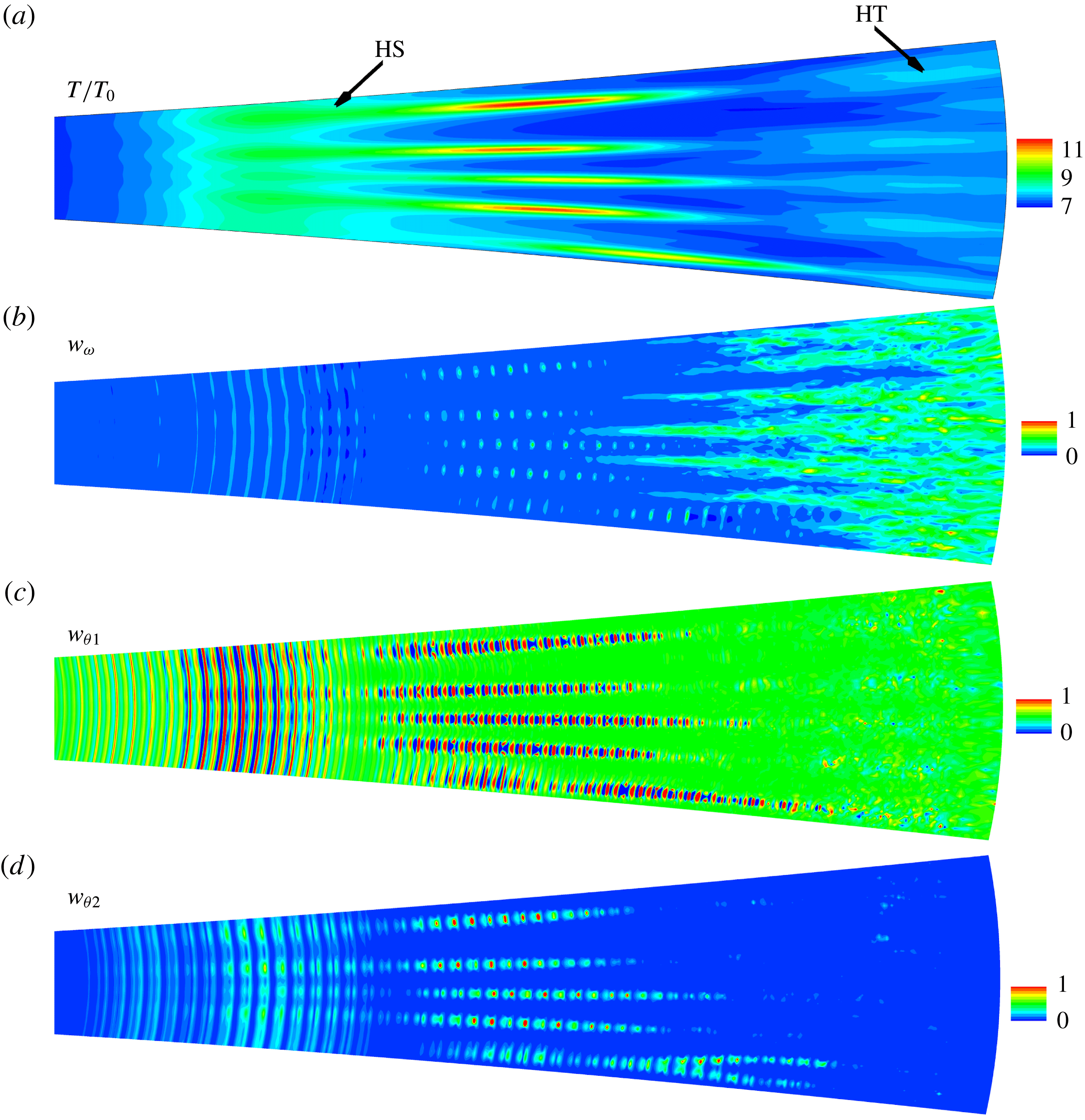
Streamwise evolution of heat generation rate at different spanwise angles near a hot streak, based on DNS. Values are averaged along the time and the normal direction in the boundary layer. $w_{\unicode[STIX]{x1D703}1}=-p\unicode[STIX]{x1D703}$
(orange);
$w_{\unicode[STIX]{x1D703}1}=-p\unicode[STIX]{x1D703}$
(orange); $w_{\unicode[STIX]{x1D703}2}=\unicode[STIX]{x1D707}^{\prime }\unicode[STIX]{x1D703}^{2}$
(green);
$w_{\unicode[STIX]{x1D703}2}=\unicode[STIX]{x1D707}^{\prime }\unicode[STIX]{x1D703}^{2}$
(green); $w_{\unicode[STIX]{x1D714}}=\unicode[STIX]{x1D707}\unicode[STIX]{x1D714}^{2}$
(magenta).
$w_{\unicode[STIX]{x1D714}}=\unicode[STIX]{x1D707}\unicode[STIX]{x1D714}^{2}$
(magenta). $Re_{unit}=9.7\times 10^{6}~\text{m}^{-1}$
.
$Re_{unit}=9.7\times 10^{6}~\text{m}^{-1}$
.
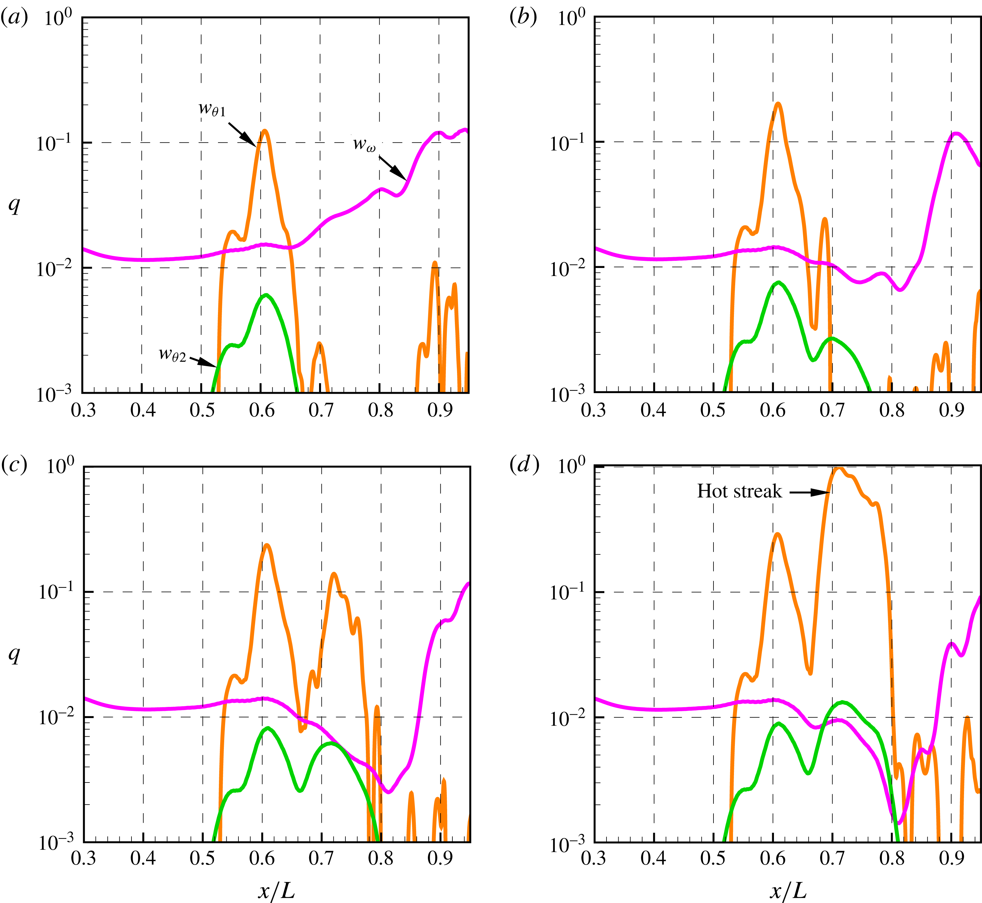
Time-averaged $w_{\unicode[STIX]{x1D703}1}$
,
$w_{\unicode[STIX]{x1D703}1}$
, $w_{\unicode[STIX]{x1D703}2}$
and
$w_{\unicode[STIX]{x1D703}2}$
and $w_{\unicode[STIX]{x1D714}}$
are then integrated along the
$w_{\unicode[STIX]{x1D714}}$
are then integrated along the $y$
-direction in the boundary layer and plotted in figure 10, as well as their correlation with the instability amplitudes. The values are normalized by their respective maxima. It is clearly seen both in PIV and DNS that the dilatation-induced heat at HS, mainly from
$y$
-direction in the boundary layer and plotted in figure 10, as well as their correlation with the instability amplitudes. The values are normalized by their respective maxima. It is clearly seen both in PIV and DNS that the dilatation-induced heat at HS, mainly from $w_{\unicode[STIX]{x1D703}1}$
, is more than five times that from
$w_{\unicode[STIX]{x1D703}1}$
, is more than five times that from $w_{\unicode[STIX]{x1D714}}$
. The value of the latter increases to nearly 75 % that of
$w_{\unicode[STIX]{x1D714}}$
. The value of the latter increases to nearly 75 % that of $w_{\unicode[STIX]{x1D703}1}$
at HS for PIV but only 52 % for DNS because transition is not completed in DNS. Note that low-frequency waves continuously grow until the end of the model because it belongs to a vortical instability, as discussed by Chen et al. (Reference Chen, Zhu and Lee2017). It benefits from the increasing shear stress after HS. One interesting phenomenon, shown in both DNS and PIV, is that unlike
$w_{\unicode[STIX]{x1D703}1}$
at HS for PIV but only 52 % for DNS because transition is not completed in DNS. Note that low-frequency waves continuously grow until the end of the model because it belongs to a vortical instability, as discussed by Chen et al. (Reference Chen, Zhu and Lee2017). It benefits from the increasing shear stress after HS. One interesting phenomenon, shown in both DNS and PIV, is that unlike $w_{\unicode[STIX]{x1D703}2}$
and
$w_{\unicode[STIX]{x1D703}2}$
and $w_{\unicode[STIX]{x1D714}}$
the peak width of
$w_{\unicode[STIX]{x1D714}}$
the peak width of $w_{\unicode[STIX]{x1D703}1}$
is much smaller than that of the second-mode amplitudes at HS. As stated earlier, this asynchrony reflects the fact the
$w_{\unicode[STIX]{x1D703}1}$
is much smaller than that of the second-mode amplitudes at HS. As stated earlier, this asynchrony reflects the fact the $w_{\unicode[STIX]{x1D703}}1$
-induced heating not only depends on the fluctuation amplitudes, but also the phase angle between them. The details of this mechanism will be discussed in future work.
$w_{\unicode[STIX]{x1D703}}1$
-induced heating not only depends on the fluctuation amplitudes, but also the phase angle between them. The details of this mechanism will be discussed in future work.
As introduced above, one important phenomenon observed in prior studies is streamwise hot streaks, which were not only identified in the experiments (Berridge et al.
Reference Berridge, Chou, Ward, Steen, Gilbert, Juliano, Schneider and Gronvall2010; Chou et al.
Reference Chou, Ward, Letterman, Luersen, Borg and Schneider2011; Chynoweth et al.
Reference Chynoweth, Ward, Henderson, Moraru, Greenwood, Abney and Schneider2014) but also in the DNS (Sivasubramanian & Fasel Reference Sivasubramanian and Fasel2015). However, such streaks are less clear in the present TSP results. One reason is that the noisy condition of the incoming stream makes the instantaneous spanwise flow structures rapidly vary in time. The effect of hot streaks is spanwise smoothed in the experimental data, as compared to DNS and PSE. To investigate this phenomenon accurately, we seed the most unstable spanwise wavenumber in the DNS so that those hot streaks are successfully repeated, as shown in figure 14(a). Figures 14(b), 14(c), and 14(d) show, respectively, the instantaneous $y$
-direction-averaged
$y$
-direction-averaged $w_{\unicode[STIX]{x1D703}1}$
,
$w_{\unicode[STIX]{x1D703}1}$
, $w_{\unicode[STIX]{x1D703}2}$
and
$w_{\unicode[STIX]{x1D703}2}$
and $w_{\unicode[STIX]{x1D714}}$
over the model surface. It can be seen that every streak is composed of second-mode waves, which is similar to the mechanism suggested by Lee & Wu (Reference Lee and Wu2008) (their figures 11 and 22) for incompressible flows. To verify the aerodynamic heating mechanism within these hot streaks,
$w_{\unicode[STIX]{x1D714}}$
over the model surface. It can be seen that every streak is composed of second-mode waves, which is similar to the mechanism suggested by Lee & Wu (Reference Lee and Wu2008) (their figures 11 and 22) for incompressible flows. To verify the aerodynamic heating mechanism within these hot streaks, $w_{\unicode[STIX]{x1D703}1}$
,
$w_{\unicode[STIX]{x1D703}1}$
, $w_{\unicode[STIX]{x1D703}2}$
and
$w_{\unicode[STIX]{x1D703}2}$
and $w_{\unicode[STIX]{x1D714}}$
are calculated at different circumferential positions, covering from one streak (
$w_{\unicode[STIX]{x1D714}}$
are calculated at different circumferential positions, covering from one streak ( $\unicode[STIX]{x1D719}=19^{\circ }$
) to its adjacent valley (
$\unicode[STIX]{x1D719}=19^{\circ }$
) to its adjacent valley ( $\unicode[STIX]{x1D719}=10^{\circ }$
), as shown in figure 15. No matter what the circumferential position is, the dilatation-induced
$\unicode[STIX]{x1D719}=10^{\circ }$
), as shown in figure 15. No matter what the circumferential position is, the dilatation-induced $w_{\unicode[STIX]{x1D703}}$
dominates the creation of aerodynamic heating. Especially along the streak, as shown in figure 15(d),
$w_{\unicode[STIX]{x1D703}}$
dominates the creation of aerodynamic heating. Especially along the streak, as shown in figure 15(d), $w_{\unicode[STIX]{x1D703}2}$
is larger than
$w_{\unicode[STIX]{x1D703}2}$
is larger than $w_{\unicode[STIX]{x1D714}}$
even if it is underestimated.
$w_{\unicode[STIX]{x1D714}}$
even if it is underestimated.
4.3 Heat transfer analysis
Theoretically, we may study the time-averaged surface-temperature distribution based on the steady-state energy equation
 $$\begin{eqnarray}\displaystyle \unicode[STIX]{x1D70C}C_{v}(\boldsymbol{u}\boldsymbol{\cdot }\unicode[STIX]{x1D735})T=-p\unicode[STIX]{x1D703}+\unicode[STIX]{x1D719}+\unicode[STIX]{x1D735}\boldsymbol{\cdot }(k\unicode[STIX]{x1D735}T), & & \displaystyle\end{eqnarray}$$
where $\unicode[STIX]{x1D70C}$
,
$\unicode[STIX]{x1D70C}$
, $C_{v}$
,
$C_{v}$
, $T$
,
$T$
, $p$
and
$p$
and $k$
are, respectively, the density, specific heat, temperature, pressure and thermal conductivity of the gas, and
$k$
are, respectively, the density, specific heat, temperature, pressure and thermal conductivity of the gas, and $\unicode[STIX]{x1D719}$
denotes the time-average of
$\unicode[STIX]{x1D719}$
denotes the time-average of $\unicode[STIX]{x1D6F7}$
. For two-dimensional flow near the wall, the equation can be simplified to
$\unicode[STIX]{x1D6F7}$
. For two-dimensional flow near the wall, the equation can be simplified to
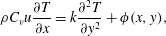 $$\begin{eqnarray}\displaystyle \unicode[STIX]{x1D70C}C_{v}u\frac{\unicode[STIX]{x2202}T}{\unicode[STIX]{x2202}x}=k\frac{\unicode[STIX]{x2202}^{2}T}{\unicode[STIX]{x2202}y^{2}}+\unicode[STIX]{x1D719}(x,y), & & \displaystyle\end{eqnarray}$$
where the three terms represent, respectively, heat convection in $x$
, conduction in
$x$
, conduction in $y$
and heat sources caused by dissipation. In order to integrate (4.11), we linearize this equation by replacing
$y$
and heat sources caused by dissipation. In order to integrate (4.11), we linearize this equation by replacing $u(y)$
with its mean value
$u(y)$
with its mean value $U$
, and assuming
$U$
, and assuming $C_{v}$
and
$C_{v}$
and $k$
to be constants. The boundary conditions at an adiabatic wall and far from the wall are
$k$
to be constants. The boundary conditions at an adiabatic wall and far from the wall are
 $$\begin{eqnarray}\displaystyle \frac{\unicode[STIX]{x2202}T}{\unicode[STIX]{x2202}y}=0,\quad \text{at}~y=0;\quad T=0,\quad \text{at}~y=\infty . & & \displaystyle\end{eqnarray}$$
The initial temperature profile at $x=0$
is assumed to be
$x=0$
is assumed to be $T_{0}(y)$
. The linearized problem can be solved using Laplace transformation, which yields the wall temperature
$T_{0}(y)$
. The linearized problem can be solved using Laplace transformation, which yields the wall temperature $T_{w}=T(x,0)$
:
$T_{w}=T(x,0)$
:
 $$\begin{eqnarray}\displaystyle T_{w} & = & \displaystyle T_{1}+T_{2},\end{eqnarray}$$
 $$\begin{eqnarray}\displaystyle T_{1} & = & \displaystyle \frac{2}{\sqrt{\unicode[STIX]{x03C0}}}\int _{0}^{\infty }T_{0}\left(2h\sqrt{\frac{kx}{C_{v}U}}\right)\text{e}^{-h^{2}}\,\text{d}h,\end{eqnarray}$$
 $$\begin{eqnarray}\displaystyle T_{2} & = & \displaystyle \frac{1}{\sqrt{\unicode[STIX]{x03C0}}}\int _{0}^{x}\int _{0}^{\infty }\unicode[STIX]{x1D719}\left(\unicode[STIX]{x1D70F},2h\sqrt{\frac{k(x-\unicode[STIX]{x1D70F})}{C_{v}U}}\right)\text{e}^{-h^{2}}\,\text{d}h\,\text{d}\unicode[STIX]{x1D70F}.\end{eqnarray}$$
Neglecting the variation of the heat source in the $y$
-direction,
$y$
-direction, $T_{2}$
can be further simplified to
$T_{2}$
can be further simplified to
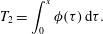 $$\begin{eqnarray}\displaystyle T_{2}=\int _{0}^{x}\unicode[STIX]{x1D719}(\unicode[STIX]{x1D70F})\,\text{d}\unicode[STIX]{x1D70F}. & & \displaystyle\end{eqnarray}$$
While $T_{1}$
represents the convection–conduction process without heat sources,
$T_{1}$
represents the convection–conduction process without heat sources, $T_{2}$
stands for the integration of heat sources along the streamwise direction. The
$T_{2}$
stands for the integration of heat sources along the streamwise direction. The $x$
-wise gradient of
$x$
-wise gradient of $T_{w}$
is given by that of
$T_{w}$
is given by that of $T_{1}$
and
$T_{1}$
and $T_{2}$
:
$T_{2}$
:
 $$\begin{eqnarray}\displaystyle \frac{\text{d}T_{1}}{\text{d}x} & = & \displaystyle \frac{4}{\sqrt{\unicode[STIX]{x03C0}}}\int _{0}^{\infty }\frac{\text{d}T_{0}}{\text{d}y}(h)h\sqrt{\frac{k}{xC_{v}U}}\text{e}^{-h^{2}}\,\text{d}h,\end{eqnarray}$$
 $$\begin{eqnarray}\displaystyle \frac{\text{d}T_{2}}{\text{d}x} & = & \displaystyle \unicode[STIX]{x1D719}(x).\end{eqnarray}$$
The sign of $\unicode[STIX]{x2202}T_{1}/\unicode[STIX]{x2202}x$
depends on the initial distribution of
$\unicode[STIX]{x2202}T_{1}/\unicode[STIX]{x2202}x$
depends on the initial distribution of $T_{0}(y)$
. For a hypersonic boundary layer,
$T_{0}(y)$
. For a hypersonic boundary layer, $\text{d}T_{0}/\text{d}y<0$
and
$\text{d}T_{0}/\text{d}y<0$
and $\text{d}^{2}T_{0}/\text{d}y^{2}<0$
, thus
$\text{d}^{2}T_{0}/\text{d}y^{2}<0$
, thus $\unicode[STIX]{x2202}T_{1}/\unicode[STIX]{x2202}x<0$
, which has the effect of cooling the wall, but its magnitude decreases with
$\unicode[STIX]{x2202}T_{1}/\unicode[STIX]{x2202}x<0$
, which has the effect of cooling the wall, but its magnitude decreases with $x$
. When
$x$
. When $\unicode[STIX]{x1D719}$
reaches its maximum value, it begins to decay although
$\unicode[STIX]{x1D719}$
reaches its maximum value, it begins to decay although $T_{2}$
still increases. Thus, if
$T_{2}$
still increases. Thus, if $\unicode[STIX]{x1D719}(x)$
decreases so rapidly that
$\unicode[STIX]{x1D719}(x)$
decreases so rapidly that
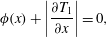 $$\begin{eqnarray}\displaystyle \unicode[STIX]{x1D719}(x)+\left|\frac{\unicode[STIX]{x2202}T_{1}}{\unicode[STIX]{x2202}x}\right|=0, & & \displaystyle\end{eqnarray}$$
at some downstream position, a peak value of $T$
occurs there and the position slightly shifts downstream relative to the
$T$
occurs there and the position slightly shifts downstream relative to the $\unicode[STIX]{x1D6F7}$
-peak.
$\unicode[STIX]{x1D6F7}$
-peak.
To verify (4.18), we compare the streamwise surface-temperature gradient and $q=w_{\unicode[STIX]{x1D703}1}+w_{\unicode[STIX]{x1D703}2}+w_{\unicode[STIX]{x1D714}}$
for
$q=w_{\unicode[STIX]{x1D703}1}+w_{\unicode[STIX]{x1D703}2}+w_{\unicode[STIX]{x1D714}}$
for $Re_{unit}=9.7\times 10^{6}~\text{m}^{-1}$
both from experiments and DNS, and second-mode instability amplitude for
$Re_{unit}=9.7\times 10^{6}~\text{m}^{-1}$
both from experiments and DNS, and second-mode instability amplitude for $Re_{unit}=7.6$
and
$Re_{unit}=7.6$
and $11.7\times 10^{6}~\text{m}^{-1}$
because no PIV data are available for the latter two. As shown in figure 16, the first peak positions of surface-temperature gradient agree well with that of
$11.7\times 10^{6}~\text{m}^{-1}$
because no PIV data are available for the latter two. As shown in figure 16, the first peak positions of surface-temperature gradient agree well with that of $q$
or second-mode amplitude, which justifies a posteriori the linearization of (4.11).
$q$
or second-mode amplitude, which justifies a posteriori the linearization of (4.11).
Comparison of streamwise evolution of surface-temperature gradient (green) with the second-mode (red) and low-frequency waves (blue) for (a) $Re_{unit}=7.6\times 10^{6}~\text{m}^{-1}$
and (b)
$Re_{unit}=7.6\times 10^{6}~\text{m}^{-1}$
and (b) $Re_{unit}=11.7\times 10^{6}~\text{m}^{-1}$
. Time-averaged heat generation rates (orange) for
$Re_{unit}=11.7\times 10^{6}~\text{m}^{-1}$
. Time-averaged heat generation rates (orange) for $Re_{unit}=9.7\times 10^{6}~\text{m}^{-1}$
based on (c) PIV and (d) DNS. Each quantity is normalized by its maximum.
$Re_{unit}=9.7\times 10^{6}~\text{m}^{-1}$
based on (c) PIV and (d) DNS. Each quantity is normalized by its maximum.
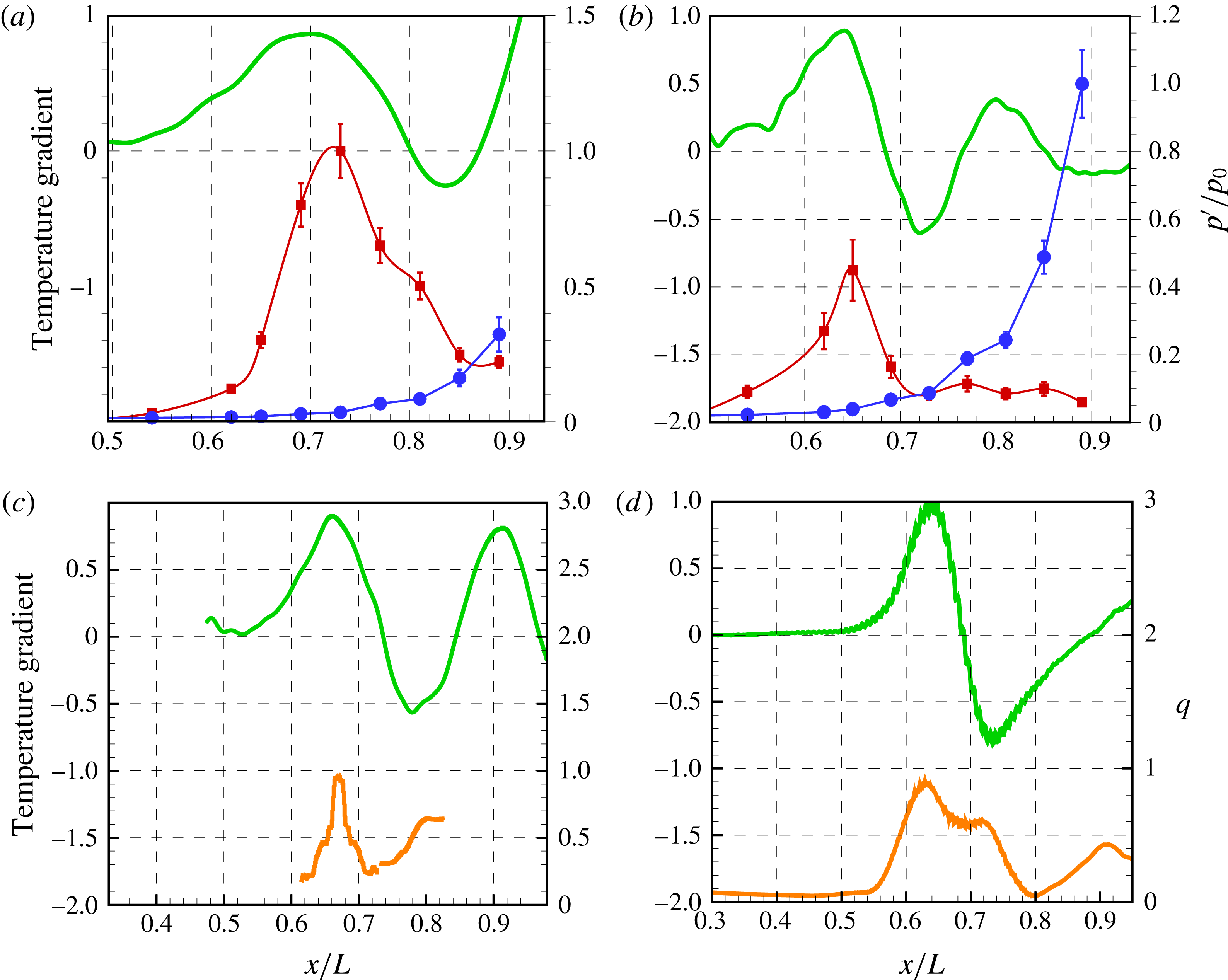
5 Conclusions
In this paper, a combined experimental, numerical and theoretical study of instability modes in a hypersonic boundary layer and their relevance to aerodynamic heating was conducted. The evolution of instabilities and wall temperature distributions were observed via physical and numerical experiments. The present study confirmed a previously observed heat-transfer peak that correlated with the second-mode-dominated transition process as well as revealing a new physical mechanism to promptly generate this heating impact. For the first time, our research identified a direct relation between the local temperature rise before transition was completed and the second-mode-induced dilatational heating.
By the joint use of TSP, PCB, Rayleigh-scattering and PIV techniques, the evolution of instability waves in a laminar hypersonic boundary layer and its relevance to aerodynamic heating were experimentally studied over a flared cone in the Peking University Mach 6 wind tunnel. Four unit Reynolds numbers, 5.4, 7.6, 9.7 and $11.7\times 10^{6}~\text{m}^{-1}$
, were investigated. PSE analysis and DNS were also conducted based on similar flow conditions. Several conclusions can be made as follows.
$11.7\times 10^{6}~\text{m}^{-1}$
, were investigated. PSE analysis and DNS were also conducted based on similar flow conditions. Several conclusions can be made as follows.
(i) Both the physical and numerical experiments showed that the evolution of a second mode brought about a local peak of surface-temperature HS that shifted slightly downstream. Increasing
$Re_{unit}$
promoted the strength of HS but led to a stronger dissipation of the second mode.(ii) The heat generation rate induced by the dilatation and shear processes (denoted as, respectively,
$w_{\unicode[STIX]{x1D703}}$
and
$w_{\unicode[STIX]{x1D714}}$
) were investigated. The second term included the pressure work
$w_{\unicode[STIX]{x1D703}1}$
and dilatation viscous dissipation
$w_{\unicode[STIX]{x1D703}2}$
. Different from the prevailing view for shear-induced heating, the aerodynamic heating in HS mainly arose from the high-frequency compression and expansion of fluid accompanying the second mode. The dilatation heating, especially
$w_{\unicode[STIX]{x1D703}1}$
, was more than five times its shear counterpart. In some regions, even the underestimated
$w_{\unicode[STIX]{x1D703}2}$
was larger than
$w_{\unicode[STIX]{x1D714}}$
.(iii) Based on a simplified two-dimensional, steady-state energy equation, heat transfer in the boundary layer and its effect on the surface temperature were analysed. Three factors were addressed, including streamwise heat convection, normal heat conduction and heat sources caused by viscous dissipation. The last factor heats the fluid passing through the source, resulting in a delay of surface-temperature rise in the streamwise direction. Such a mechanism was validated both by experiments and DNS, which explained why the peak of surface temperature shifted downstream compared to that of the second mode.


Two issues need to be further investigated in future work. First, a more accurate evaluation of the bulk viscosity coefficient in hypersonic boundary layers is necessary, which is an issue of crucial importance to the community. Second, since the phase angle between $p$
and
$p$
and $\unicode[STIX]{x1D703}$
has played an important role in
$\unicode[STIX]{x1D703}$
has played an important role in $w_{\unicode[STIX]{x1D703}1}$
, its detailed heating mechanism needs to be further clarified.
$w_{\unicode[STIX]{x1D703}1}$
, its detailed heating mechanism needs to be further clarified.
Acknowledgements
This research is supported by the National Natural Science Foundation of China under grants 11602005, 109103010062, 10921202, 11221061 and 11632002. This paper was also supported by NSF project ‘Physical Mechanisms of the Formation, Evolution and Interaction of Turbulence Structures’ (no. 91752000).
Appendix A. Details of the operators
${\mathcal{A}}$
and
${\mathcal{B}}$
in (3.2)


 $$\begin{eqnarray}\displaystyle A_{11}=vD1+\text{i}\unicode[STIX]{x1D6FC}u-\text{i}\unicode[STIX]{x1D714}+u_{x}+v_{y}+ug+v(h-\unicode[STIX]{x1D705}), & & \displaystyle\end{eqnarray}$$
 $$\begin{eqnarray}\displaystyle A_{12}=\text{i}\unicode[STIX]{x1D6FC}\unicode[STIX]{x1D70C}+\unicode[STIX]{x1D70C}_{x}+g\unicode[STIX]{x1D70C},\quad A_{13}=\unicode[STIX]{x1D70C}D1+\unicode[STIX]{x1D70C}_{y}+\unicode[STIX]{x1D70C}(h-\unicode[STIX]{x1D705}),\quad A_{14}=\text{i}\unicode[STIX]{x1D6FD}\unicode[STIX]{x1D70C},\quad A_{15}=0, & & \displaystyle \nonumber\\ \displaystyle & & \displaystyle\end{eqnarray}$$
 $$\begin{eqnarray}\displaystyle A_{21}=uu_{x}+vu_{y}+\frac{1}{\unicode[STIX]{x1D6FE}M^{2}}(\unicode[STIX]{x1D6FA}T_{x}+\text{i}\unicode[STIX]{x1D6FC}T)-\unicode[STIX]{x1D705}uv, & & \displaystyle\end{eqnarray}$$
 $$\begin{eqnarray}\displaystyle A_{22} & = & \displaystyle -\frac{\unicode[STIX]{x1D707}}{Re}D2+(\unicode[STIX]{x1D70C}v-\unicode[STIX]{x1D707}_{T}T_{y}/Re)D1+\unicode[STIX]{x1D70C}(u_{x}+\text{i}\unicode[STIX]{x1D6FC}u-\text{i}\unicode[STIX]{x1D714})\nonumber\\ \displaystyle & & \displaystyle +\,(\unicode[STIX]{x1D707}(L2\unicode[STIX]{x1D6FC}^{2}+\unicode[STIX]{x1D6FD}^{2}-L2g\unicode[STIX]{x1D6FC})-\unicode[STIX]{x1D707}_{T}T_{y}\unicode[STIX]{x1D705})/Re,\end{eqnarray}$$
 $$\begin{eqnarray}\displaystyle & \displaystyle A_{23}=-(\text{i}L1/Re\unicode[STIX]{x1D707}\unicode[STIX]{x1D6FC}+L0\unicode[STIX]{x1D707}_{T}T_{x}/Re)D1+\unicode[STIX]{x1D70C}u_{y}-\text{i}\unicode[STIX]{x1D6FC}/Re\unicode[STIX]{x1D707}_{T}T_{y}-\unicode[STIX]{x1D705}\unicode[STIX]{x1D70C}u, & \displaystyle\end{eqnarray}$$
 $$\begin{eqnarray}\displaystyle & \displaystyle A_{24}=\unicode[STIX]{x1D6FD}(-\text{i}\unicode[STIX]{x1D6FC}L1\unicode[STIX]{x1D707}-\text{i}\unicode[STIX]{x1D707}_{T}T_{x}L0+3\text{i}g\unicode[STIX]{x1D707})/Re, & \displaystyle\end{eqnarray}$$
 $$\begin{eqnarray}\displaystyle & \displaystyle A_{25}=-u_{y}\unicode[STIX]{x1D707}_{T}/ReD1+\frac{1}{\unicode[STIX]{x1D6FE}M^{2}}(\text{i}\unicode[STIX]{x1D6FC}\unicode[STIX]{x1D70C}+\unicode[STIX]{x1D6FA}\unicode[STIX]{x1D70C}_{x})-(\unicode[STIX]{x1D707}_{T}u_{yy}+u_{y}\unicode[STIX]{x1D707}_{TT}T_{y}-2\text{i}\unicode[STIX]{x1D6FC}\unicode[STIX]{x1D707}_{T}u_{x})/Re, & \displaystyle\end{eqnarray}$$
 $$\begin{eqnarray}\displaystyle & \displaystyle A_{31}=\frac{T}{\unicode[STIX]{x1D6FE}M^{2}}D1+\frac{T_{y}}{\unicode[STIX]{x1D6FE}M^{2}}+\unicode[STIX]{x1D705}u^{2}+vv_{y}, & \displaystyle\end{eqnarray}$$
 $$\begin{eqnarray}\displaystyle & \displaystyle A_{32}=-(\text{i}\unicode[STIX]{x1D6FC}+g)L1\unicode[STIX]{x1D707}/ReD1-(\text{i}\unicode[STIX]{x1D6FC}+g)\unicode[STIX]{x1D707}_{T}T_{y}L0/Re+2\unicode[STIX]{x1D70C}u\unicode[STIX]{x1D705}, & \displaystyle\end{eqnarray}$$
 $$\begin{eqnarray}\displaystyle A_{33} & = & \displaystyle -\frac{\unicode[STIX]{x1D707}}{Re}D2+(-L2\unicode[STIX]{x1D707}_{T}T_{y}/Re+\unicode[STIX]{x1D70C}v)D1+\unicode[STIX]{x1D70C}(\text{i}\unicode[STIX]{x1D6FC}u-\text{i}\unicode[STIX]{x1D714}+v_{y})\nonumber\\ \displaystyle & & \displaystyle +\,(\unicode[STIX]{x1D6FC}^{2}\unicode[STIX]{x1D707}+\unicode[STIX]{x1D6FD}^{2}\unicode[STIX]{x1D707}+L0\unicode[STIX]{x1D707}_{T}T_{y}(\unicode[STIX]{x1D705}-h)-\text{i}\unicode[STIX]{x1D6FC}g\unicode[STIX]{x1D707})/Re,\end{eqnarray}$$
 $$\begin{eqnarray}\displaystyle A_{34}=-L1\text{i}\unicode[STIX]{x1D6FD}\unicode[STIX]{x1D707}/ReD1-L0\text{i}\unicode[STIX]{x1D6FD}\unicode[STIX]{x1D707}_{T}T_{y}/Re, & & \displaystyle\end{eqnarray}$$
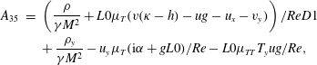 $$\begin{eqnarray}\displaystyle A_{35} & = & \displaystyle \left(\frac{\unicode[STIX]{x1D70C}}{\unicode[STIX]{x1D6FE}M^{2}}+L0\unicode[STIX]{x1D707}_{T}(v(\unicode[STIX]{x1D705}-h)-ug-u_{x}-v_{y})\right)/ReD1\nonumber\\ \displaystyle & & \displaystyle +\,\frac{\unicode[STIX]{x1D70C}_{y}}{\unicode[STIX]{x1D6FE}M^{2}}-u_{y}\unicode[STIX]{x1D707}_{T}(\text{i}\unicode[STIX]{x1D6FC}+gL0)/Re-L0\unicode[STIX]{x1D707}_{TT}T_{y}ug/Re,\end{eqnarray}$$
 $$\begin{eqnarray}\displaystyle A_{41}=\frac{\text{i}\unicode[STIX]{x1D6FD}T}{\unicode[STIX]{x1D6FE}M^{2}},\quad A_{42}=-\text{i}\unicode[STIX]{x1D6FD}\unicode[STIX]{x1D707}/Re(\text{i}\unicode[STIX]{x1D6FC}L1+(L0+4)g)-\text{i}\unicode[STIX]{x1D6FD}/Re\unicode[STIX]{x1D707}_{T}T_{x}, & & \displaystyle\end{eqnarray}$$
 $$\begin{eqnarray}\displaystyle A_{43}=-\text{i}\unicode[STIX]{x1D6FD}\unicode[STIX]{x1D707}/ReD1-\text{i}\unicode[STIX]{x1D6FD}\unicode[STIX]{x1D707}_{T}T_{y}/Re+\text{i}\unicode[STIX]{x1D6FD}\unicode[STIX]{x1D707}/Re(\unicode[STIX]{x1D705}L1-(L0+4)h), & & \displaystyle\end{eqnarray}$$
 $$\begin{eqnarray}\displaystyle A_{44} & = & \displaystyle -\unicode[STIX]{x1D707}/ReD2+(-\unicode[STIX]{x1D707}_{T}T_{y}/Re+\unicode[STIX]{x1D70C}v+\unicode[STIX]{x1D707}(\unicode[STIX]{x1D705}-h)/Re)D1\nonumber\\ \displaystyle & & \displaystyle +\,\unicode[STIX]{x1D70C}(\text{i}\unicode[STIX]{x1D6FC}u-\text{i}\unicode[STIX]{x1D714}+ug+vh)+(L2\unicode[STIX]{x1D707}\unicode[STIX]{x1D6FD}^{2}+\unicode[STIX]{x1D707}\unicode[STIX]{x1D6FC}^{2}+\unicode[STIX]{x1D707}_{T}T_{y}h+(g-\text{i}\unicode[STIX]{x1D6FC})\unicode[STIX]{x1D707}_{T}T_{x})/Re,\nonumber\\ \displaystyle & & \displaystyle\end{eqnarray}$$
 $$\begin{eqnarray}\displaystyle & \displaystyle A_{45}=\frac{\text{i}\unicode[STIX]{x1D6FD}\unicode[STIX]{x1D70C}}{\unicode[STIX]{x1D6FE}M^{2}}+(-\text{i}\unicode[STIX]{x1D6FD}L2\unicode[STIX]{x1D707}_{T}(gu+hv)+\text{i}L0\unicode[STIX]{x1D705}v\unicode[STIX]{x1D707}_{T})/Re-\text{i}\unicode[STIX]{x1D6FD}L0(u_{x}+v_{y})/Re, & \displaystyle\end{eqnarray}$$
 $$\begin{eqnarray}\displaystyle & \displaystyle A_{51}=(1/\unicode[STIX]{x1D6FE}-1)(vTD1-\text{i}\unicode[STIX]{x1D714}T)+uT_{x}+vT_{y}/\unicode[STIX]{x1D6FE}+(1/\unicode[STIX]{x1D6FE}-1)(\text{i}\unicode[STIX]{x1D6FC}uT+uT_{x}), & \displaystyle\end{eqnarray}$$
 $$\begin{eqnarray}\displaystyle A_{52} & = & \displaystyle -2(\unicode[STIX]{x1D6FE}-1)M^{2}/Re\unicode[STIX]{x1D707}(u_{y}+\unicode[STIX]{x1D705}u)D1+\unicode[STIX]{x1D70C}T_{x}\nonumber\\ \displaystyle & & \displaystyle -\,2(\unicode[STIX]{x1D6FE}-1)M^{2}/Re\unicode[STIX]{x1D707}(\unicode[STIX]{x1D705}u_{y}+\text{i}\unicode[STIX]{x1D6FC}guL0),\end{eqnarray}$$
 $$\begin{eqnarray}\displaystyle A_{53} & = & \displaystyle -2\text{i}\unicode[STIX]{x1D6FC}(\unicode[STIX]{x1D6FE}-1)M^{2}/Re\unicode[STIX]{x1D707}u_{y}+\unicode[STIX]{x1D70C}T_{y}+2(1-\unicode[STIX]{x1D6FE})M^{2}/Re(\unicode[STIX]{x1D707}L0(ug+u_{x})\nonumber\\ \displaystyle & & \displaystyle +\,L2\unicode[STIX]{x1D707}v_{y}+\unicode[STIX]{x1D707}L0(v(h-\unicode[STIX]{x1D705})+gu+u_{x})+\unicode[STIX]{x1D707}L2v_{y} )D1,\end{eqnarray}$$
 $$\begin{eqnarray}\displaystyle A_{54}=2\text{i}\unicode[STIX]{x1D6FD}\unicode[STIX]{x1D707}(1-\unicode[STIX]{x1D6FE})M^{2}/Re(L2ug+u_{x}L0+v_{y}L0), & & \displaystyle\end{eqnarray}$$
 $$\begin{eqnarray}\displaystyle A_{55} & = & \displaystyle -\unicode[STIX]{x1D707}/Re/PrD2-2/Pr/Re\unicode[STIX]{x1D707}_{T}T_{y}D1+v\unicode[STIX]{x1D70C}D1+(1/\unicode[STIX]{x1D6FE}-1)(\unicode[STIX]{x1D70C}_{y}v+rho_{x}u)\nonumber\\ \displaystyle & & \displaystyle +\,\unicode[STIX]{x1D707}/Re/Pr(\unicode[STIX]{x1D6FC}^{2}+\unicode[STIX]{x1D6FD}^{2})-mu_{T}T_{yy}/Pr/Re+(1-\unicode[STIX]{x1D6FE})M^{2}/Re\unicode[STIX]{x1D707}_{T}u_{y}^{2}\nonumber\\ \displaystyle & & \displaystyle -\,\text{i}\unicode[STIX]{x1D714}\unicode[STIX]{x1D70C}/\unicode[STIX]{x1D6FE}-mu_{TT}T_{y}^{2}/Re/Pr+(1/\unicode[STIX]{x1D6FE}-1)(u\unicode[STIX]{x1D70C}_{x}+\text{i}\unicode[STIX]{x1D6FC}\unicode[STIX]{x1D70C}u)+\text{i}\unicode[STIX]{x1D6FC}\unicode[STIX]{x1D70C}u,\end{eqnarray}$$
 $$\begin{eqnarray}\displaystyle B_{11}=u,\quad B_{12}=\unicode[STIX]{x1D70C},\quad B_{13}=B_{14}=B_{15}=0, & & \displaystyle\end{eqnarray}$$
 $$\begin{eqnarray}\displaystyle B_{21}=\unicode[STIX]{x1D6FA}T/\unicode[STIX]{x1D6FE}/M^{2},\quad B_{22}=\unicode[STIX]{x1D70C}u,\quad B_{23}=-\unicode[STIX]{x1D707}_{T}T_{y}/Re, & & \displaystyle\end{eqnarray}$$
 $$\begin{eqnarray}\displaystyle B_{24}=-i\unicode[STIX]{x1D6FD}L1\unicode[STIX]{x1D707}/Re,\quad B_{25}=\unicode[STIX]{x1D6FA}\unicode[STIX]{x1D70C}/\unicode[STIX]{x1D6FE}/M^{2}, & & \displaystyle\end{eqnarray}$$
 $$\begin{eqnarray}\displaystyle B_{31}=0,\quad B_{32}=-L0\unicode[STIX]{x1D707}_{T}T_{y}/Re,\quad B_{33}=\unicode[STIX]{x1D70C}u-2\text{i}\unicode[STIX]{x1D6FC}\unicode[STIX]{x1D707}/Re-\unicode[STIX]{x1D707}_{T}T_{x}/Re, & & \displaystyle\end{eqnarray}$$
 $$\begin{eqnarray}\displaystyle B_{34}=0,\quad B_{35}=-\unicode[STIX]{x1D707}_{T}u_{y}/Re, & & \displaystyle\end{eqnarray}$$
 $$\begin{eqnarray}\displaystyle B_{41}=0,\quad B_{42}=-\text{i}\unicode[STIX]{x1D6FD}L1\unicode[STIX]{x1D707}_{T}/Re,\quad B_{43}=0,\quad B_{44}=\unicode[STIX]{x1D70C}u,\quad B_{45}=0, & & \displaystyle\end{eqnarray}$$
 $$\begin{eqnarray}\displaystyle B_{51}=(1/\unicode[STIX]{x1D6FE}-1)uT,\quad B_{52}=-2(\unicode[STIX]{x1D6FE}-1)M^{2}/ReL2u_{x}\unicode[STIX]{x1D707}+L0(ug+vh), & & \displaystyle\end{eqnarray}$$
 $$\begin{eqnarray}\displaystyle B_{53}=-2(\unicode[STIX]{x1D6FE}-1)M^{2}/Re\unicode[STIX]{x1D707}u_{y},\quad B_{54}=0,\quad B_{55}=\unicode[STIX]{x1D70C}u/\unicode[STIX]{x1D6FE}. & & \displaystyle\end{eqnarray}$$
In the above, $D1=\unicode[STIX]{x2202}/\unicode[STIX]{x2202}y,D2=\unicode[STIX]{x2202}/\unicode[STIX]{x2202}y^{2},L0=-2/3,L1=1/3,L2=4/3$
;
$D1=\unicode[STIX]{x2202}/\unicode[STIX]{x2202}y,D2=\unicode[STIX]{x2202}/\unicode[STIX]{x2202}y^{2},L0=-2/3,L1=1/3,L2=4/3$
; $g,h,\unicode[STIX]{x1D705}$
are curvature terms. The subscript denotes the derivative. Note that the bar has been neglected in the mean-flow variables for simplicity.
$g,h,\unicode[STIX]{x1D705}$
are curvature terms. The subscript denotes the derivative. Note that the bar has been neglected in the mean-flow variables for simplicity.
Appendix B. Governing equations for DNS
 $$\begin{eqnarray}\displaystyle & \displaystyle \frac{\unicode[STIX]{x2202}}{\unicode[STIX]{x2202}t}\boldsymbol{U}+\frac{\unicode[STIX]{x2202}}{\unicode[STIX]{x2202}R}\boldsymbol{f}_{\mathbf{1}}+\frac{\unicode[STIX]{x2202}}{\unicode[STIX]{x2202}\unicode[STIX]{x1D703}}\boldsymbol{f}_{\mathbf{2}}+\frac{\unicode[STIX]{x2202}}{\unicode[STIX]{x2202}z}\boldsymbol{f}_{\mathbf{3}}+\boldsymbol{E}_{\boldsymbol{i}}=\frac{\unicode[STIX]{x2202}}{\unicode[STIX]{x2202}R}\boldsymbol{V}_{\mathbf{1}}+\frac{\unicode[STIX]{x2202}}{\unicode[STIX]{x2202}\unicode[STIX]{x1D703}}\boldsymbol{V}_{\mathbf{2}}+\frac{\unicode[STIX]{x2202}}{\unicode[STIX]{x2202}z}\boldsymbol{V}_{\mathbf{3}}+\boldsymbol{E}_{\unicode[STIX]{x1D742}}, & \displaystyle\end{eqnarray}$$
 $$\begin{eqnarray}\displaystyle & \displaystyle \boldsymbol{U}=R[\unicode[STIX]{x1D70C},\unicode[STIX]{x1D70C}u,\unicode[STIX]{x1D70C}v,\unicode[STIX]{x1D70C}w,E]^{\text{T}}, & \displaystyle\end{eqnarray}$$
 $$\begin{eqnarray}\displaystyle & \displaystyle \boldsymbol{f}_{\mathbf{1}}=R[\unicode[STIX]{x1D70C}u,\unicode[STIX]{x1D70C}u^{2}+p,\unicode[STIX]{x1D70C}uv,\unicode[STIX]{x1D70C}uw,u(E+p)]^{\text{T}}, & \displaystyle\end{eqnarray}$$
 $$\begin{eqnarray}\displaystyle & \displaystyle \boldsymbol{f}_{\mathbf{2}}=[\unicode[STIX]{x1D70C}v,\unicode[STIX]{x1D70C}vu+p,\unicode[STIX]{x1D70C}v^{2}+p,\unicode[STIX]{x1D70C}vw,v(E+p)]^{\text{T}}, & \displaystyle\end{eqnarray}$$
 $$\begin{eqnarray}\displaystyle & \displaystyle \boldsymbol{f}_{\mathbf{3}}=R[\unicode[STIX]{x1D70C}w,\unicode[STIX]{x1D70C}wu,\unicode[STIX]{x1D70C}wv,\unicode[STIX]{x1D70C}w^{2}+p,w(E+p)]^{\text{T}}, & \displaystyle\end{eqnarray}$$
 $$\begin{eqnarray}\displaystyle & \displaystyle \boldsymbol{E}_{\boldsymbol{i}}=[0,-\unicode[STIX]{x1D70C}v^{2}-p,\unicode[STIX]{x1D70C}uv,0,0]^{\text{T}}, & \displaystyle\end{eqnarray}$$
 $$\begin{eqnarray}\displaystyle & \displaystyle \boldsymbol{V}_{\mathbf{1}}=R\left[0,\unicode[STIX]{x1D70E}_{11},\unicode[STIX]{x1D70E}_{21},\unicode[STIX]{x1D70E}_{31},u\unicode[STIX]{x1D70E}_{11}+v\unicode[STIX]{x1D70E}_{21}+w\unicode[STIX]{x1D70E}_{31}+k\frac{\unicode[STIX]{x2202}T}{\unicode[STIX]{x2202}R}\right]^{\text{T}}, & \displaystyle\end{eqnarray}$$
 $$\begin{eqnarray}\displaystyle & \displaystyle \boldsymbol{V}_{\mathbf{2}}=\left[0,\unicode[STIX]{x1D70E}_{12},\unicode[STIX]{x1D70E}_{22},\unicode[STIX]{x1D70E}_{32},u\unicode[STIX]{x1D70E}_{12}+v\unicode[STIX]{x1D70E}_{22}+w\unicode[STIX]{x1D70E}_{32}+k\frac{1}{R}\frac{\unicode[STIX]{x2202}T}{\unicode[STIX]{x2202}\unicode[STIX]{x1D703}}\right]^{\text{T}}, & \displaystyle\end{eqnarray}$$
 $$\begin{eqnarray}\displaystyle & \displaystyle \boldsymbol{V}_{\mathbf{3}}=R\left[0,\unicode[STIX]{x1D70E}_{13},\unicode[STIX]{x1D70E}_{23},\unicode[STIX]{x1D70E}_{33},u\unicode[STIX]{x1D70E}_{13}+v\unicode[STIX]{x1D70E}_{23}+w\unicode[STIX]{x1D70E}_{33}+k\frac{\unicode[STIX]{x2202}T}{\unicode[STIX]{x2202}z}\right]^{\text{T}}, & \displaystyle\end{eqnarray}$$
 $$\begin{eqnarray}\displaystyle & \displaystyle \boldsymbol{E}_{\unicode[STIX]{x1D742}}=[0,-\unicode[STIX]{x1D70E}_{22},\unicode[STIX]{x1D70E}_{12},0,0]^{\text{T}}, & \displaystyle\end{eqnarray}$$
 $$\begin{eqnarray}\displaystyle \unicode[STIX]{x1D70E}_{11}=2\unicode[STIX]{x1D707}\frac{\unicode[STIX]{x2202}u}{\unicode[STIX]{x2202}R}-\frac{2}{3}\unicode[STIX]{x1D707}\,\text{div}(\boldsymbol{V}),\quad \unicode[STIX]{x1D70E}_{22}=2\unicode[STIX]{x1D707}\left[\frac{1}{R}\frac{\unicode[STIX]{x2202}v}{\unicode[STIX]{x2202}\unicode[STIX]{x1D703}}+\frac{u}{R}\right]-\frac{2}{3}\unicode[STIX]{x1D707}\,\text{div}(\boldsymbol{V}), & & \displaystyle\end{eqnarray}$$
 $$\begin{eqnarray}\displaystyle \unicode[STIX]{x1D70E}_{33}=2\unicode[STIX]{x1D707}\frac{\unicode[STIX]{x2202}w}{\unicode[STIX]{x2202}z}-\frac{2}{3}\unicode[STIX]{x1D707}\,\text{div}(\boldsymbol{V}),\quad \unicode[STIX]{x1D70E}_{12}=\unicode[STIX]{x1D707}\left[\frac{1}{R}\frac{\unicode[STIX]{x2202}u}{\unicode[STIX]{x2202}\unicode[STIX]{x1D703}}+\frac{\unicode[STIX]{x2202}v}{\unicode[STIX]{x2202}R}-\frac{v}{R}\right], & & \displaystyle\end{eqnarray}$$
 $$\begin{eqnarray}\displaystyle \unicode[STIX]{x1D70E}_{13}=\unicode[STIX]{x1D707}\left[\frac{\unicode[STIX]{x2202}u}{\unicode[STIX]{x2202}z}+\frac{\unicode[STIX]{x2202}w}{\unicode[STIX]{x2202}R}\right],\quad \unicode[STIX]{x1D70E}_{23}=\unicode[STIX]{x1D707}\left[\frac{\unicode[STIX]{x2202}v}{\unicode[STIX]{x2202}z}+\frac{1}{R}\frac{\unicode[STIX]{x2202}w}{\unicode[STIX]{x2202}\unicode[STIX]{x1D703}}\right]. & & \displaystyle\end{eqnarray}$$


 Open access

