1. Introduction
In recent years, reinforcement learning (RL) has emerged as an advanced method that outperforms traditional models by enabling more flexible, effective end-to-end control in complex systems, thereby reducing the dependency on highly specialized mathematical models. Its applicability extends across diverse domains such as robotics [Reference Han, Mulyana, Stankovic and Cheng10, Reference Hou, Tu, Gao, Dong, Zhai and Zhang12, Reference Ibarz, Tan, Finn, Kalakrishnan, Pastor and Levine15], gaming [Reference Schrittwieser, Antonoglou, Hubert, Simonyan, Sifre, Schmitt, Guez, Lockhart, Hassabis, Graepel, Lillicrap and Silver25, Reference Silver, Schrittwieser, Simonyan, Antonoglou, Huang, Guez, Hubert, Baker, Lai, Bolton, Chen, Lillicrap, Hui, Sifre, van den Driessche, Graepel and Hassabis26, Reference Ye, Chen, Zhang, Chen, Yuan, Liu, Chen, Liu, Qiu, Yu, Yin, Shi, Wang, Shi, Fu, Yang, Huang and Liu34], autonomous vehicles [Reference Feng, Sun, Yan, Zhu, Zou, Shen and Liu8, Reference Wu, Yang, Yang, Huang, He and Lv33], and large language models (LLM) [Reference Havrilla, Du, Raparthy, Nalmpantis, Dwivedi-Yu, Hambro, Sukhbaatar and Raileanu11, Reference Yuan, Yuan, Li, Dong, Tan and Zhou36]. Central to RL is the reward function, which directly shapes agent behavior. However, in real-world applications – particularly in robotics – designing reward functions that accurately reflect task objectives is notoriously difficult. Even subtle differences in reward design can cause significant divergence in learned behaviors [Reference Booth, Knox, Shah, Niekum, Stone and Allievi1], making this process both error-prone and labor-intensive.
To reduce the burden of manual reward design, recent work has explored using LLMs to automatically generate reward functions from task descriptions or behavioral specifications. A representative approach is EUREKA [Reference Ma, Liang, Wang, Huang, Bastani, Jayaraman, Zhu, Fan and Anandkumar23], which synthesizes dense reward functions in natural language or code. While scalable and domain-agnostic, this method faces key limitations: LLM outputs are stochastic and often misaligned with task goals – especially in long-horizon or safety-critical settings – and may contain syntactic or logical flaws that are difficult to detect. Moreover, LLM inference is costly and lacks formal guarantees on behavioral correctness.
To mitigate these issues, EUREKA augments LLM-generated rewards with a task-specific fitness function – a sparse trajectory-level metric (e.g., success rate, completion time, energy use) that retrospectively validates and refines rewards through reward reflection. While this improves robustness, the approach still fundamentally depends on the quality of LLM-generated rewards, which can be brittle, hard to verify, and difficult to generalize.
An alternative paradigm that bypasses the need for manually defined reward functions is preference-based reinforcement learning (PbRL) [Reference Christiano, Leike, Brown, Martic, Legg and Amodei6, Reference Lee, Smith, Dragan and Abbeel19, Reference Liang, Shu, Lee and Abbeel21], which learns a reward model (RM) from pairwise comparisons between trajectories. Rather than relying on absolute scalar rewards, PbRL infers implicit reward signals from expert or user preferences, enabling learning in tasks where rewards are difficult to specify but relative preferences are easier to express. This approach has been successfully applied across a range of domains, including robotic manipulation [Reference Hwang, Lee, Kee, Kim, Lee and Oh14, Reference Lee, Smith, Dragan and Abbeel19, Reference Lee, Smith and Abbeel20], navigation [Reference de Heuvel, Seiler and Bennewitz7, Reference Keselman, Shih, Hebert and Steinfeld17], traffic simulation [Reference Cao, Ivanovic, Xiao and Pavone3], and LLM alignment [Reference Casper, Davies, Shi, Gilbert, Scheurer, Rando, Freedman, Korbak, Lindner, Freire, Wang, Marks, Segerie, Carroll, Peng, Christoffersen, Damani, Slocum, Anwar, Siththaranjan, Nadeau, Michaud, Pfau, Krasheninnikov, Chen, Langosco, Hase, Biyik, Dragan, Krueger, Sadigh and Hadfield-Menell4, Reference Stiennon, Ouyang, Wu, Ziegler, Lowe, Voss, Radford, Amodei and Christiano28, Reference Zheng, Dou, Gao, Hua, Shen, Wang, Liu, Jin, Liu, Zhou, Xiong, Chen, Xi, Xu, Lai, Zhu, Chang, Yin, Weng, Cheng, Huang, Sun, Yan, Gui, Zhang, Qiu and Huang37, Reference Ziegler, Stiennon, Wu, Brown, Radford, Amodei, Christiano and Irving38].
Despite its promise, classical PbRL methods face several limitations. First, they often require a large number of preference queries to train a robust RM, leading to high feedback cost. Second, preference data can be noisy or inconsistent, especially when collected from non-experts or in complex long-horizon tasks. Third, conventional approaches do not fully exploit the structure or consistency inherent in trajectory-level preferences.
To address these challenges, recent research has focused on improving both sample efficiency and reward modeling fidelity. For example, B-Pref [Reference Lee, Smith, Dragan and Abbeel19] introduced standardized benchmarks for systematic evaluation, while PEBBLE [Reference Lee, Smith and Abbeel20] combined unsupervised exploration with preference relabeling to reduce query complexity. SURF [Reference Park, Seo, Shin, Lee, Abbeel and Lee24] incorporated semi-supervised learning and data augmentation, and MRN [Reference Liu, Bai, Du and Yang22] leveraged the performance of a Q-function on a labeled preference dataset to support reward learning, extracting more task-relevant information from human preferences. Active query selection has also been explored to prioritize informative comparisons [Reference Kong and Yang18]. RIME [Reference Cheng, Xiong, Dai, Miao, Lv and Wang5] employs generative adversarial networks to correct erroneous preferences. QPA [Reference Hu, Li, Zhan, Jia and Zhang13] mitigates query–policy misalignment by aligning preference queries with the policy’s visitation distribution through near-on-policy query selection and hybrid experience replay, thereby improving feedback efficiency and policy performance.
Recent methods exploit temporal and structural consistency in preferences. PRIOR [Reference Verma and Metcalf32] uses hindsight relabeling with Transformers to model long-horizon patterns, while sequential ranking [Reference Hwang, Lee, Kee, Kim, Lee and Oh14] leverages ordered comparisons to improve feedback efficiency. These advances make PbRL more scalable and robust.
Despite these advances, important limitations remain. Methods such as SURF [Reference Park, Seo, Shin, Lee, Abbeel and Lee24] rely on semi-supervised preference relabeling using a learned $Q$
-function; when
$Q$
-function; when $Q$
is inaccurate, pseudo-labels can propagate errors and destabilize reward learning. Credit assignment strategies like PRIOR [Reference Verma and Metcalf32] require auxiliary world models and attention mechanisms to estimate state importance, adding modeling complexity and tuning burden. Sequential ranking [Reference Hwang, Lee, Kee, Kim, Lee and Oh14] expands preference data by ordering existing pairs but does not explicitly exploit externally verifiable task outcomes. More broadly, current PbRL methods often overlook intrinsic task signals – such as trajectory outcomes or sparse success indicators – that are readily available yet underused. This omission limits the expressiveness and generalization of learned reward models, particularly in long-horizon or safety-critical domains, while human preference feedback remains noisy and costly due to intransitivity, fatigue, and cognitive load [Reference Swamy, Dann, Kidambi, Wu and Agarwal30].
$Q$
is inaccurate, pseudo-labels can propagate errors and destabilize reward learning. Credit assignment strategies like PRIOR [Reference Verma and Metcalf32] require auxiliary world models and attention mechanisms to estimate state importance, adding modeling complexity and tuning burden. Sequential ranking [Reference Hwang, Lee, Kee, Kim, Lee and Oh14] expands preference data by ordering existing pairs but does not explicitly exploit externally verifiable task outcomes. More broadly, current PbRL methods often overlook intrinsic task signals – such as trajectory outcomes or sparse success indicators – that are readily available yet underused. This omission limits the expressiveness and generalization of learned reward models, particularly in long-horizon or safety-critical domains, while human preference feedback remains noisy and costly due to intransitivity, fatigue, and cognitive load [Reference Swamy, Dann, Kidambi, Wu and Agarwal30].

Figure 1. Framework of STL-PbRL. In the original PbRL, the training of the RM (module 3) is driven by expert (human) feedback (module 1), which captures expert preferences for agent trajectories by directly influencing the reward system with preferred trajectory segments. STL-PbRL enhances this methodology by integrating a self-learning mechanism (Module 2), which autonomously analyzes the merits of trajectories using a fitness function. By comparing trajectories with high and low fitness values, it optimizes the Reward Model (RM), thereby improving the overall learning process.
In contrast, human learning is typically more structured and efficient, often following a two-stage process: (1) teacher-led instruction (TL), where learners absorb knowledge from an expert; and (2) self-learning (SL), where they compare their own outputs with reference answers to reinforce understanding and correct errors. This “school-based” paradigm offers robustness, adaptability, and a natural way to integrate both external feedback and intrinsic evaluation. Inspired by EUREKA’s reward reflection mechanism and this human-centric learning process, we propose a new framework: Self-Teacher-Learning Preference-based Reinforcement Learning (STL-PbRL), as illustrated in Figure 1. STL-PbRL augments traditional PbRL with a self-improvement module that leverages task-level fitness functions to autonomously refine the RM. Specifically, STL-PbRL operates in three progressive phases:
-
1. Teacher-Led (TL) phase: The RM is trained solely via human preferences, following conventional PbRL procedures.
-
2. Hybrid (TL + SL) phase: The agent jointly uses expert preferences and fitness-based self-evaluation to refine its RM.
-
3. Self-Learning (SL) phase: The agent independently improves the RM using only fitness-based comparisons between trajectories, eliminating the need for further human annotation.
This dual-mode framework balances the interpretability and task specificity of human supervision with the scalability and precision of fitness-based self-refinement. Our contributions are as follows:
-
• The SL module is designed to enhance the RM by dynamically refining its parameters in line with task objectives described by the Fitness Function. Our approach is pioneering in integrating sparse task-oriented reward information from task objectives into the PbRL’s RM, resulting in a more robust RM.
-
• Through rigorous mathematical derivation, we theoretically prove that the SL module ensures the convergence of the RM to the optimal fitness RM.
-
• The STL-PbRL framework has achieved state-of-the-art results in numerous experiments and has proven effective in reducing the substantial required feedback, enhancing the robustness of preference feedback, and supporting various PbRL algorithms like PEBBLE [Reference Lee, Smith and Abbeel20], SURF [Reference Park, Seo, Shin, Lee, Abbeel and Lee24], and MRN [Reference Liu, Bai, Du and Yang22].
2. Preliminaries
Reinforcement learning. In the classic RL paradigm [Reference Sutton and Barto29], the environment is modeled using a Markov decision process, defined by a tuple ( $S$
,
$S$
, $A$
,
$A$
, $R$
,
$R$
, $P$
,
$P$
, $\gamma$
). This tuple encompasses the state space
$\gamma$
). This tuple encompasses the state space $S$
, action space
$S$
, action space $A$
, reward function
$A$
, reward function $R$
, transition probabilities
$R$
, transition probabilities $P$
, and discount factor
$P$
, and discount factor $\gamma$
. The transition function
$\gamma$
. The transition function $P(s'|s, a)$
quantifies the likelihood of moving to the next state
$P(s'|s, a)$
quantifies the likelihood of moving to the next state $s'$
from state
$s'$
from state $s$
after taking action
$s$
after taking action $a$
, encapsulating the environment’s stochastic behavior. The reward function
$a$
, encapsulating the environment’s stochastic behavior. The reward function $r_t = R(s, a)$
specifies the reward received after acting
$r_t = R(s, a)$
specifies the reward received after acting $a$
in state
$a$
in state $s$
at time step
$s$
at time step $t$
. A policy
$t$
. A policy $\pi (a|s)$
directs the selection of actions based on the current state, aiming to optimize the cumulative expected return
$\pi (a|s)$
directs the selection of actions based on the current state, aiming to optimize the cumulative expected return $\mathcal{R}_{return}=\sum _{k=0}^\infty {\gamma ^kr_{t+k}}$
from a series of interactions within the environment.
$\mathcal{R}_{return}=\sum _{k=0}^\infty {\gamma ^kr_{t+k}}$
from a series of interactions within the environment.
Reinforcement learning from feedback. In the general PbRL [Reference Christiano, Leike, Brown, Martic, Legg and Amodei6], the RM supersedes traditional reward function design, aiming to align the learned reward parameter $\hat {r}_{\psi }$
with expert preferences. This paper refers to this process as the TL module. A segment
$\hat {r}_{\psi }$
with expert preferences. This paper refers to this process as the TL module. A segment $\sigma$
consists of a sequence of states and actions, represented as
$\sigma$
consists of a sequence of states and actions, represented as $(s_{t}, a_{t}, \ldots , s_{t+k}, a_{t+k})$
. This segment
$(s_{t}, a_{t}, \ldots , s_{t+k}, a_{t+k})$
. This segment $\sigma$
is sampled from a section of the complete trajectory
$\sigma$
is sampled from a section of the complete trajectory $\tau$
resulting from the agent’s interaction with the environment. Human experts provide preferences on pairs of segments (
$\tau$
resulting from the agent’s interaction with the environment. Human experts provide preferences on pairs of segments ( $\sigma ^0$
,
$\sigma ^0$
, $\sigma ^1$
) the RM offers. The preference
$\sigma ^1$
) the RM offers. The preference $y$
belongs to the set
$y$
belongs to the set $\{0,1,0.5,-1\}$
, representing preferences for segment 0 over segment 1, segment 1 over segment 0, equal preference for both segments, and an inability to compare the preferences, respectively. Using the Bradley-Terry model [Reference Bradley and Terry2], the preference predictor
$\{0,1,0.5,-1\}$
, representing preferences for segment 0 over segment 1, segment 1 over segment 0, equal preference for both segments, and an inability to compare the preferences, respectively. Using the Bradley-Terry model [Reference Bradley and Terry2], the preference predictor $P_{\hat {r}_\psi }$
constructed by the RM’s estimation
$P_{\hat {r}_\psi }$
constructed by the RM’s estimation $\hat {r}_{\psi }$
is formulated as follows:
$\hat {r}_{\psi }$
is formulated as follows:
 \begin{equation} \begin{aligned} P_{\hat {r}_\psi }\left[\sigma ^0 \succ \sigma ^1\right] = \frac {\exp \left (\sum _t \hat {r}_{\psi }(s_t^0, a_t^0)\right )}{\exp \left (\sum _t \hat {r}_{\psi }(s_t^0, a_t^0)\right )+\exp \left (\sum _t \hat {r}_{\psi }(s_t^1, a_t^1)\right )}, \end{aligned} \end{equation}
where $\sigma ^0 \succ \sigma ^1$
indicates that
$\sigma ^0 \succ \sigma ^1$
indicates that $\sigma ^0$
aligns more closely with the expectations of human experts than
$\sigma ^0$
aligns more closely with the expectations of human experts than $\sigma ^1$
. Learning about RM can be accomplished by minimizing the cross-entropy loss between predictions made by preference predictors and actual preferences expressed by experts.
$\sigma ^1$
. Learning about RM can be accomplished by minimizing the cross-entropy loss between predictions made by preference predictors and actual preferences expressed by experts.
 \begin{equation} \begin{aligned} \mathcal{L}_{\text{TL}}(\psi )= - \mathbb{E}_{(\sigma ^0, \sigma ^1, y) \sim D}\left[(1-y) \log P_{\hat {r}_\psi }\left[\sigma ^0 \succ \sigma ^1\right] + y \log P_{\hat {r}_\psi }\left[\sigma ^1 \succ \sigma ^0\right]\right]. \end{aligned} \end{equation}
This objective is termed the TL loss. By refining the RM by minimizing this loss, segments that better align with human preferences are rewarded with a higher cumulative score.
Feedback from simulated human teacher. To better evaluate the differences between various PbRL algorithms, we adopt the human teacher simulation approach from B-Pref [Reference Lee, Smith, Dragan and Abbeel19] for providing feedback. The simulated teacher is defined as
 \begin{equation} \begin{aligned} P\left(\sigma ^1 \succ \sigma ^0; \eta _{\text{stoc}}, \eta _{\text{myopic}}\right) = \frac {\exp \left (\eta _{\text{stoc}} \sum _{t=1}^{H} \eta _{\text{myopic}}^{H-t} r(s_t^1, a_t^1)\right )}{\exp \left (\eta _{\text{stoc}} \sum _{t=1}^{H} \eta _{\text{myopic}}^{H-t} r(s_t^1, a_t^1)\right ) + \exp \left (\eta _{\text{stoc}} \sum _{t=1}^{H} \eta _{\text{myopic}}^{H-t} r(s_t^0, a_t^0)\right )}, \end{aligned} \end{equation}
where $r(s, a)$
represents the ground truth reward for a given state-action pair. The parameter
$r(s, a)$
represents the ground truth reward for a given state-action pair. The parameter $\eta _{\text{stoc}} \in [0,\infty )$
represents the rationality of the teacher. A higher
$\eta _{\text{stoc}} \in [0,\infty )$
represents the rationality of the teacher. A higher $\eta _{\text{stoc}}$
results in more rational and deterministic decisions, whereas setting
$\eta _{\text{stoc}}$
results in more rational and deterministic decisions, whereas setting $\eta _{\text{stoc}} = 0$
leads to completely random choices. The parameter
$\eta _{\text{stoc}} = 0$
leads to completely random choices. The parameter $\eta _{\text{myopic}} \in (0,1]$
serves as a myopia discount factor. A smaller value for
$\eta _{\text{myopic}} \in (0,1]$
serves as a myopia discount factor. A smaller value for $\eta _{\text{myopic}}$
gives more importance to earlier state-action transitions, making the agent’s behavior less focused on future outcomes.
$\eta _{\text{myopic}}$
gives more importance to earlier state-action transitions, making the agent’s behavior less focused on future outcomes.
B-pref provides several simulations of human irrationality. To enable a fair comparison with existing approaches, we set both $\eta _{\text{stoc}}$
and
$\eta _{\text{stoc}}$
and $\eta _{\text{myopic}}$
to 1, yielding the simplified preference probability:
$\eta _{\text{myopic}}$
to 1, yielding the simplified preference probability:
 \begin{equation} P_{sim}\left(\sigma ^1 \succ \sigma ^0\right) = \frac {\exp \left (\sum _{t=1}^{H} r(s_t^1, a_t^1)\right )}{\exp \left (\sum _{t=1}^{H} r(s_t^1, a_t^1)\right ) + \exp \left (\sum _{t=1}^{H} r(s_t^0, a_t^0)\right )}. \end{equation}
Incorporating mistake probability in preferences. To simulate potential errors in human annotation, we incorporate a mistake probability $\epsilon$
into the labeling process. Specifically, the simulated teacher may flip the true preference label with probability
$\epsilon$
into the labeling process. Specifically, the simulated teacher may flip the true preference label with probability $\epsilon$
. Assuming that the teacher’s correct preference is
$\epsilon$
. Assuming that the teacher’s correct preference is $\sigma ^1 \succ \sigma ^0$
, the observed label
$\sigma ^1 \succ \sigma ^0$
, the observed label $\tilde {y}$
is given by:
$\tilde {y}$
is given by:
 \begin{equation} \tilde {y} = \begin{cases} 1, & \text{with probability } 1 - \epsilon \quad \text{(correct preference: } \sigma ^1 \succ \sigma ^0 \text{)}, \\ 0, & \text{with probability } \epsilon \quad \text{(mistaken label: } \sigma ^0 \succ \sigma ^1 \text{)}, \end{cases} \end{equation}
where $\tilde {y}$
is the observed preference label which may not reflect the true ranking due to annotator mistakes. This mechanism systematically evaluates the robustness of PbRL algorithms under noisy human feedback.
$\tilde {y}$
is the observed preference label which may not reflect the true ranking due to annotator mistakes. This mechanism systematically evaluates the robustness of PbRL algorithms under noisy human feedback.
Problem setting. In real-world RL tasks, designing a dense and informative reward function is often difficult, especially when task success is defined by high-level or sparse criteria. Instead of directly optimizing a handcrafted sparse reward, we aim to learn an RM that implicitly captures task success by aligning with a separate task-level evaluation, referred to as a fitness function. This process is known as RM optimization. We formalize this under the framework of the Reward Design Problem (RDP), originally proposed by ref. [Reference Singh, Lewis and Barto27] and adapted here to the program synthesis and structured task setting.
Definition 1 (RDP). An RDP is defined by a tuple $(M, \mathcal{R}_{\text{FS}}, \mathcal{A}_M, F)$
. Here,
$(M, \mathcal{R}_{\text{FS}}, \mathcal{A}_M, F)$
. Here, $M = (S, A, P)$
represents the environment or world model, where
$M = (S, A, P)$
represents the environment or world model, where $S$
is the state space,
$S$
is the state space, $A$
is the action space, and
$A$
is the action space, and $P(s'|s,a)$
is the transition function that determines the dynamics of the environment.
$P(s'|s,a)$
is the transition function that determines the dynamics of the environment. $\mathcal{R}_{\text{FS}}$
denotes the space of candidate reward functions, each mapping state-action pairs to scalar values. The function
$\mathcal{R}_{\text{FS}}$
denotes the space of candidate reward functions, each mapping state-action pairs to scalar values. The function $\mathcal{A}_M\;:\; \mathcal{R}_{\text{FS}} \rightarrow \Pi$
represents the learning algorithm, which maps a given reward function
$\mathcal{A}_M\;:\; \mathcal{R}_{\text{FS}} \rightarrow \Pi$
represents the learning algorithm, which maps a given reward function $R \in \mathcal{R}_{\text{FS}}$
to a resulting policy
$R \in \mathcal{R}_{\text{FS}}$
to a resulting policy $\pi \in \Pi$
via standard RL optimization. Each policy
$\pi \in \Pi$
via standard RL optimization. Each policy $\pi$
is a mapping from states to distributions over actions, i.e.,
$\pi$
is a mapping from states to distributions over actions, i.e., $\pi \;:\; S \rightarrow \Delta (A)$
.
$\pi \;:\; S \rightarrow \Delta (A)$
.
The fitness function $F\;:\; \Pi \rightarrow \mathbb{R}$
evaluates the overall task performance of a policy by aggregating high-level feedback. Specifically,
$F\;:\; \Pi \rightarrow \mathbb{R}$
evaluates the overall task performance of a policy by aggregating high-level feedback. Specifically, $F(\pi )$
is defined as the expected cumulative fitness value over trajectories generated by policy
$F(\pi )$
is defined as the expected cumulative fitness value over trajectories generated by policy $\pi$
, computed as
$\pi$
, computed as
 \begin{equation} F(\pi ) = \mathbb{E}_{\tau \sim \pi } \left [ \sum _t f(s_t, a_t) \right ], \end{equation}
where $f(s_t, a_t)$
is a task-level evaluation function that provides sparse but intuitive feedback reflecting task success. This function is typically easier to define than dense reward functions and may correspond to metrics such as the number of successful object manipulations, completion of multi-step tasks, or binary success conditions (e.g., whether a robot has successfully opened a door or collected trash in a target bin).
$f(s_t, a_t)$
is a task-level evaluation function that provides sparse but intuitive feedback reflecting task success. This function is typically easier to define than dense reward functions and may correspond to metrics such as the number of successful object manipulations, completion of multi-step tasks, or binary success conditions (e.g., whether a robot has successfully opened a door or collected trash in a target bin).
The objective in the RDP is to find a reward function $R^* \in \mathcal{R}_{\text{FS}}$
such that the resulting policy
$R^* \in \mathcal{R}_{\text{FS}}$
such that the resulting policy $\pi ^* = \mathcal{A}_M(R^*)$
maximizes the fitness score
$\pi ^* = \mathcal{A}_M(R^*)$
maximizes the fitness score $F(\pi ^*)$
:
$F(\pi ^*)$
:
 \begin{equation} R^* = \arg \max _{R \in \mathcal{R}_{\text{FS}}} F(\mathcal{A}_M(R)). \end{equation}
Reward model optimization problem. Instead of manually searching over the reward function space, we consider a parameterized RM $\hat {r}_\psi \;:\; S \times A \rightarrow \mathbb{R}$
, where
$\hat {r}_\psi \;:\; S \times A \rightarrow \mathbb{R}$
, where $\psi$
denotes learnable parameters (e.g., the weights of a neural network). The goal is to optimize
$\psi$
denotes learnable parameters (e.g., the weights of a neural network). The goal is to optimize $\psi$
such that the policy
$\psi$
such that the policy $\pi _{\hat {r}_\psi } = \mathcal{A}_M(\hat {r}_\psi )$
, trained using
$\pi _{\hat {r}_\psi } = \mathcal{A}_M(\hat {r}_\psi )$
, trained using $\hat {r}_\psi$
as the reward function, maximizes the high-level task fitness:
$\hat {r}_\psi$
as the reward function, maximizes the high-level task fitness:
 \begin{equation} \psi ^* = \arg \max _{\psi } F(\mathcal{A}_M(\hat {r}_\psi )). \end{equation}
This formulation shifts the burden of reward design to learning, enabling the discovery of RMs that align with desired outcomes, even in environments where explicit reward shaping is infeasible or misaligned. It serves as the foundation for many learning-from-feedback frameworks, including preference-based learning, inverse RL, and offline reward learning.
3. Proposed method
In this section, we formally introduce the STL-PbRL framework, which comprises two pivotal steps. The first step involves extracting advantageous and disadvantageous trajectories from agent-environment interactions. The second step focuses on learning from the advantageous trajectory buffer by comparing these trajectories against those stored in the disadvantageous trajectory buffer. The complete pseudocode for this process is provided in Appendix A.
3.1. Self-learning module
3.1.1. Trajectory classification and storage
The process of extracting advantageous and disadvantageous trajectories from agent-environment interactions and storing these trajectories in distinct buffers is presented in Algorithm1. Agents initiate their interaction with the environment from a starting state and continue until an episode concludes. Throughout this process, agents evaluate the trajectories based on predefined Fitness Function $F(\!\cdot\!)$
relevant to the task. For trajectories deemed advantageous (high
$F(\!\cdot\!)$
relevant to the task. For trajectories deemed advantageous (high $F(\tau )$
), agents store them in an advantageous buffer (
$F(\tau )$
), agents store them in an advantageous buffer ( $B_S$
), while those considered less favorable (low
$B_S$
), while those considered less favorable (low $F(\tau )$
) are stored in a disadvantageous buffer (
$F(\tau )$
) are stored in a disadvantageous buffer ( $B_F$
). These stored trajectories then play a crucial role in subsequent learning phases.
$B_F$
). These stored trajectories then play a crucial role in subsequent learning phases.
Algorithm 1 Trajectory Classification and Storage

3.1.2. Self-learning learning from trajectories
Learning the RM can be achieved by minimizing the cross-entropy loss between the predictions from the preference predictors and the preferences derived from the fitness value of trajectories.
 \begin{equation} \begin{aligned} \mathcal{L}_{\text{self-learning}}(\psi )= - \mathbb{E}_{(\sigma ^0 \sim \mathcal{B}_{S}, \sigma ^1 \sim \mathcal{B}_{F})}[\log P_{\hat {r}_\psi }[\sigma ^0 \succ \sigma ^1]]. \end{aligned} \end{equation}
This objective is articulated as the self-learning loss. By optimizing the RM to minimize this loss, trajectory segments that more accurately align with high fitness values are assigned greater cumulative rewards.
Equation (9) is derived as follows:
Assumption 1: There exists an optimal fitness RM ( $R^*$
) capable of guiding the training of an agent’s policy such that it consistently maximizes the associated fitness function, thereby achieving the highest possible performance in the given task.
$R^*$
) capable of guiding the training of an agent’s policy such that it consistently maximizes the associated fitness function, thereby achieving the highest possible performance in the given task.
 \begin{equation} \begin{aligned} R^* = \arg \max _{R^*} F(\mathcal{A}_M(R^*)). \end{aligned} \end{equation}
Assumption 2: Segments of trajectories that attain high fitness values are predicted to yield substantially greater values under the optimal fitness RM ( $R^*$
) than segments from trajectories characterized by low fitness values.
$R^*$
) than segments from trajectories characterized by low fitness values.
 \begin{equation} \begin{aligned} R^*(\sigma ^0 \sim \tau _0) \gg R^*(\sigma ^1 \sim \tau _1), \text{ if } F(\tau _0) \gt F(\tau _1). \end{aligned} \end{equation}
Derivation of Eq. (9). The optimization objective is to align the RM $\hat {r}_\psi$
with the optimal reward function
$\hat {r}_\psi$
with the optimal reward function $R^*$
by adjusting its predicted preference distribution
$R^*$
by adjusting its predicted preference distribution $P_{\hat {r}_\psi }$
to approximate
$P_{\hat {r}_\psi }$
to approximate $P_{R^*}$
. We focus on minimizing the cross-entropy between these two distributions to achieve this. The cross-entropy
$P_{R^*}$
. We focus on minimizing the cross-entropy between these two distributions to achieve this. The cross-entropy $H$
between the
$H$
between the $P_{\hat {r}_\psi }$
and
$P_{\hat {r}_\psi }$
and $P_{R^*}$
is given by:
$P_{R^*}$
is given by:
 \begin{align} H(P_{R^*}, P_{\hat {r}_{\psi }}) \nonumber &= -\sum _{(\sigma ^0 \sim \mathcal{B}_{S}, \sigma ^1 \sim \mathcal{B}_{F})} P_{R^*}[\sigma ^0 \succ \sigma ^1] \log P_{\hat {r}_{\psi }}[\sigma ^0 \succ \sigma ^1] \nonumber \\ &= -\sum \frac {\exp \left (\sum _t R^*(s_t^0, a_t^0)\right )}{\exp \left (\sum _t R^*(s_t^0, a_t^0)\right ) + \exp \left (\sum _t R^*(s_t^1, a_t^1)\right )} \nonumber \\ &\quad \times \log \frac {\exp \left (\sum _t \hat {r}_{\psi }(s_t^0, a_t^0)\right )}{\exp \left (\sum _t \hat {r}_{\psi }(s_t^0, a_t^0)\right ) + \exp \left (\sum _t \hat {r}_{\psi }(s_t^1, a_t^1)\right )}. \end{align}
Follow the Assumption 2 ( $R^*(\sigma ^0) \gg R^*(\sigma ^1)$
),
$R^*(\sigma ^0) \gg R^*(\sigma ^1)$
),
 \begin{equation} \begin{aligned} \frac {\exp \left (\sum _t R^*(s_t^0, a_t^0)\right )}{\exp \left (\sum _t R^*(s_t^0, a_t^0)\right )+\exp \left (\sum _t R^*(s_t^1, a_t^1)\right )} = \frac {\exp (R^*(\sigma ^0))}{\exp (R^*(\sigma ^0))+\exp (R^*(\sigma ^1))} \approx 1. \end{aligned} \end{equation}
Therefore, the cross-entropy $H$
could be rewritten as:
$H$
could be rewritten as:
 \begin{equation} \begin{aligned} H\left(P_{R^*}, P_{r_{\psi }}\right) &= -\sum \log \frac {\exp \left (\sum _t \hat {r}_{\psi }(s_t^0, a_t^0)\right )}{\exp \left (\sum _t \hat {r}_{\psi }(s_t^0, a_t^0)\right )+\exp \left (\sum _t \hat {r}_{\psi }(s_t^1, a_t^1)\right )} \\ &= -\sum \log P_{\hat {r}_{\psi }}\left[\sigma ^0 \succ \sigma ^1\right] \approx - \mathbb{E}_{(\sigma ^0 \sim \mathcal{B}_{S}, \sigma ^1 \sim \mathcal{B}_{F})}\left[\log P_{\hat {r}_\psi }[\sigma ^0 \succ \sigma ^1]\right]. \end{aligned} \end{equation}
As a result, Eq. (9) ensures that the $\hat {r}_\psi$
converges towards an accurate approximation
$\hat {r}_\psi$
converges towards an accurate approximation $R^*$
, leading to improved decision-making by the agent under the guided policy. Through this process, the learned RM of the agent progressively converges towards trajectories that fulfill the task objectives, facilitating the agent to increasingly perform tasks with greater accuracy and efficiency.
$R^*$
, leading to improved decision-making by the agent under the guided policy. Through this process, the learned RM of the agent progressively converges towards trajectories that fulfill the task objectives, facilitating the agent to increasingly perform tasks with greater accuracy and efficiency.
Why not directly optimize strategies using behavioral cloning on the collected trajectories. The agent collects trajectories through Section 3.1.1, filtered by a fitness function $ F(\tau )$
that ensures task-level success (e.g.,
$ F(\tau )$
that ensures task-level success (e.g., $ F(\tau ) \geq \delta$
). These trajectories often exhibit significant quality variation: some are smooth and efficient, while others are barely successful or exhibit erratic behaviors. This intrinsic quality of diversity makes BC unsuitable.
$ F(\tau ) \geq \delta$
). These trajectories often exhibit significant quality variation: some are smooth and efficient, while others are barely successful or exhibit erratic behaviors. This intrinsic quality of diversity makes BC unsuitable.
BC treats all trajectories that meet the fitness threshold equally and performs supervised action regression on the entire set. As a result, when using a unimodal policy representation, BC is prone to averaging over high- and low-quality actions. This leads to degraded behavior and a lack of alignment with the truly optimal motion patterns.
In contrast, self-learning incorporates a RM $ \hat {r}_\psi$
, trained via TL module. Although the agent initially collects all trajectories satisfying
$ \hat {r}_\psi$
, trained via TL module. Although the agent initially collects all trajectories satisfying $ F(\tau ) \geq \delta$
, the TL module introduces an implicit ranking among them by assigning higher reward values to more preferred behaviors:
$ F(\tau ) \geq \delta$
, the TL module introduces an implicit ranking among them by assigning higher reward values to more preferred behaviors:
 \begin{equation} \hat {r}_\psi (\tau _{\text{better}}) \gt \hat {r}_\psi (\tau _{\text{sub}}). \end{equation}
This preference-induced reward shaping creates a natural feedback loop: as the policy improves under the guidance of $ \hat {r}_\psi$
, the agent begins to collect trajectories that are not only successful but increasingly aligned with human preferences. Over time, the dataset becomes skewed toward higher-quality trajectories, leading to a monotonic improvement in the expected reward of newly collected data:
$ \hat {r}_\psi$
, the agent begins to collect trajectories that are not only successful but increasingly aligned with human preferences. Over time, the dataset becomes skewed toward higher-quality trajectories, leading to a monotonic improvement in the expected reward of newly collected data:
 \begin{equation} \mathbb{E}_{\tau \sim \pi ^{(t+1)}}[\hat {r}_\psi (\tau )] \gt \mathbb{E}_{\tau \sim \pi ^{(t)}}[\hat {r}_\psi (\tau )]. \end{equation}
This shift in data distribution enables self-learning to continually reinforce better behaviors, even without explicit action-level supervision. Consequently, unlike BC – which enforces strict action matching over a static set of suboptimal trajectories – self-learning leverages a RM that enables dynamic re-evaluation and exploitation of relatively better trajectories. In BC, the policy is trained to rigidly imitate the action in each state, which often causes premature convergence toward suboptimal behaviors embedded in the collected data. This hard alignment restricts the policy’s ability to deviate from low-quality actions, even when better alternatives exist. In contrast, self-learning utilizes preference-based reward correction to iteratively bias the data distribution toward higher-quality trajectories. As training progresses, the proportion of better trajectories increases due to feedback from the RM, allowing the policy to gradually shift toward more optimal behaviors through reinforcement rather than strict imitation.
3.2. STL-PbRL framework
The operation process of the STL-PbRL framework is divided into three phases:
Teacher-led (TL) phase. The agent learns solely through the TL module. During this phase, the agent interacts with the environment and collects data into the disadvantage buffer.
Hybrid (TL + SL) phase. Both TL and SL modules are simultaneously active, jointly facilitating the agent’s learning process. The agent collects data into both the advantageous and disadvantageous buffers and engages in self-learning by comparing data in these buffers, as detailed in Section 3.1.
Self-learning (SL) phase. Since the SL module has collected trajectories exhibiting sufficiently high performance, the TL mechanism ceases to function in this phase. The agent relies solely on the SL mechanism for further optimized learning.
4. Experiments
We have structured our experiments to explore the following research questions across two distinct environments, Meta-world [Reference Yu, Quillen, He, Julian, Hausman, Finn and Levine35] and DMControl [Reference Tunyasuvunakool, Muldal, Doron, Liu, Bohez, Merel, Erez, Lillicrap, Heess and dm_control31]:
-
• Does SL enhance the performance of PbRL algorithms? (Section 4.2)
-
• Can the STL-PbRL framework be applied effectively across various PbRL algorithms? (Section 4.3.1)
-
• Does STL-PbRL reduce the number of feedback required? (Section 4.3.2)
-
• Can STL-PbRL mitigate the impact of errors during preference selection? (Section 4.3.3)
-
• Does TL (expert preference feedback PbRL) learning play an effective role? (Section 4.3.4)
-
• What is the best way to integrate task-oriented information into PbRL algorithms? (Section 4.3.5)
-
• Can the policy be directly optimized through behavioral cloning instead of self-learning? (Section 4.3.6)
-
• Can STL-PbRL be effectively transferred from simulation to the real-world robot platform? (Section 4.3.7)
-
• Does SL significantly increase the computational complexity of PbRL algorithms? (Section 4.3.8)
4.1. Experimental settings
Baselines. Reward-based SAC, three classical PbRL algorithms, and the proposed SL-PbRL framework are used for comparison:
-
• SAC [Reference Haarnoja, Zhou, Abbeel and Levine9]: SAC is regarded as the benchmark algorithm due to its use of a ground-truth reward function, which is absent in preference-based RL. We include SAC in our evaluations as it serves as the foundational RL algorithm for PEBBLE.
-
• PEBBLE [Reference Lee, Smith and Abbeel20]: PEBBLE employs a preference-based RL approach that incorporates unsupervised exploration and the relabeling of rewards.
-
• SURF [Reference Park, Seo, Shin, Lee, Abbeel and Lee24]: SURF integrates temporal data augmentation and pseudo-labeling within a semi-supervised learning framework.
-
• MRN [Reference Liu, Bai, Du and Yang22]: MRN incorporates bi-level optimization to enhance reward learning by leveraging the performance insights of the Q-function.
-
• RIME [Reference Cheng, Xiong, Dai, Miao, Lv and Wang5]: RIME employs generative adversarial networks to correct erroneous preferences.
-
• QPA [Reference Hu, Li, Zhan, Jia and Zhang13]: QPA aligns preference queries with the policy’s visitation distribution via near-on-policy sampling and hybrid replay to enhance feedback efficiency.
-
• STL-PbRL: The proposed method, inspired by autonomous learning, utilizes information from task objectives to facilitate training. In the experiments discussed in this section, the STL-PbRL methodology is primarily implemented as an adaptation of the MRN algorithm, resulting in the modified version termed STL-MRN.
4.1.1. Simulation environments
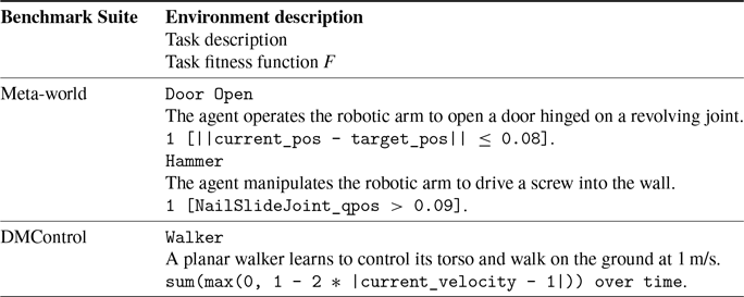
Six tasks from Meta-world and three tasks from DMControl were selected to evaluate the performance of the algorithms. The task description and related fitness functions of parts of environments are shown in Table I.
Table I. The specific details of parts of environments. || denotes the L2 norm and 1[] denotes the indicator function.

4.1.2. Implementation
To implement SAC, PEBBLE, SURF, and MRN, we utilize the publicly available repository of MRN [Reference Liu, Bai, Du and Yang22],Footnote
1
and RIME is implemented using their released code [Reference Cheng, Xiong, Dai, Miao, Lv and Wang5].Footnote
2
QPA is implemented based on its official repository [Reference Hu, Li, Zhan, Jia and Zhang13].Footnote
3
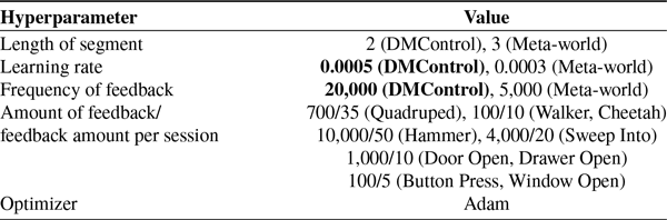
The hyperparameters for SAC, PEBBLE, SURF, and MRN are all derived from MRN, while those for RIME and QPA follow their respective official implementations. Our method introduces only one additional parameter: the self-learning update frequency $N_{self}$
, set to 5,000 for DMControl and 1,000 for Meta-world.
$N_{self}$
, set to 5,000 for DMControl and 1,000 for Meta-world.
We independently execute all algorithms five times for each task and report the mean and the standard deviation. Fitness values are used to evaluate Meta-world tasks and DMControl tasks. All experiments are conducted on the same machine equipped with an NVIDIA RTX 4,090 GPU and INTEL i9-14900KF CPU.
4.2. Results
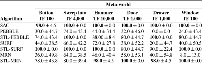
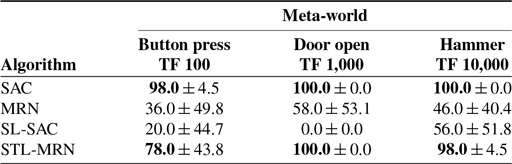
Meta-world tasks. Examples of the 6 continuous control tasks selected from Meta-world are detailed in Appendix B.2. These tasks, which involve robotic simulated manipulation skills of varying difficulties, have been chosen for our experiments due to their diverse challenges and applicability to real-world scenarios. Appendix B.2 comprehensively outlines each task’s specific details and description. Training curves depicting the performance of STL-MRN and various baseline algorithms on these Meta-world tasks are presented in Figure 2 and Table II.
Table II. Results on Meta-world tasks (mean $\pm$
std).
$\pm$
std).


Figure 2. Training curves on six continuous control tasks from Meta-world. The solid line and shaded regions denote the success rate’s mean and standard deviation across five runs.
PbRL is inherently designed for scenarios where the ground-truth reward function is unknown or difficult to specify, and learning must instead rely on human or proxy feedback. In such settings, algorithms like SAC – which directly access dense, stepwise ground-truth rewards – represent an idealized upper bound in terms of achievable performance. As shown in Figure 2 and Table II, SAC consistently attains the highest returns across most tasks due to the availability of globally accurate and continuous optimization signals. In contrast, PbRL methods must infer an implicit reward model from sparse pairwise preferences, which are often noisy and delayed. This indirect supervision requires iterative refinement through additional rollouts and feedback, resulting in slower convergence and occasionally lower asymptotic performance compared to SAC. Figure 2 also demonstrates that STL-MRN outperforms all other conventional PbRL algorithms in every environment tested. Indeed, under the STL-PbRL framework, all adapted algorithms – including STL-MRN, STL-PEBBLE, and STL-SURF – similarly surpass the performance of traditional PbRL algorithms. Detailed experimental results are shown in Section 4.3.1.
Notably, for the Hammer task (Figure 2(d)), the STL-PbRL algorithm consistently outperforms the baseline SAC algorithm. For the Window Open task, our algorithm achieved a 100% success rate using only 100 feedback instances. This superior performance of the STL-PbRL algorithm highlights its capability to learn a more effective RM that aligns better with the task objectives than the potentially suboptimal reward functions designed within traditional settings.
This advantage is particularly significant in complex environments where designing an ideal reward function can be challenging. The STL-PbRL framework demonstrates its robustness by not only adapting to the task’s intricacies but also by optimizing the learning process to focus on key performance indicators that are directly influenced by feedback. This approach ensures that the learning model is not solely dependent on predefined reward structures but is enhanced through iterative refinement based on actual performance outcomes.
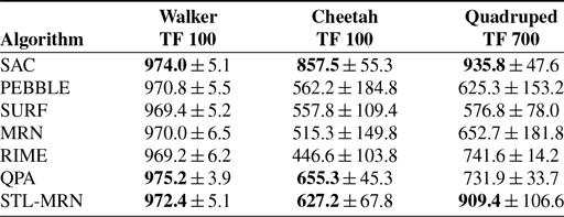
DMControl tasks. In the DMControl, three environments – Walker, Cheetah, and Quadruped – are utilized for testing. These tasks require the agent to maintain a specific speed. Appendix B.1 comprehensively outlines each task’s specific details and description.

Figure 3. Training curves on three continuous control tasks from DMControl. The solid line and shaded regions denote the episode target value mean and standard deviation across five runs.
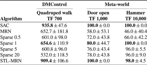
Figure 3 and Table III show the results of six methods on DMControl tasks. Although the SL-MRN algorithm shows improvements over other PbRL methods in the Cheetah and Quadruped environments, it does not perform as well in the Walker environment. This discrepancy can be attributed to the relative simplicity of the Walker task, which can be accomplished with only a few preference feedbacks. This phenomenon is also reflected in the section on the quantity of preference feedback (Section 4.3.2), indicating that self-learning does not provide significant enhancements when an ample amount of feedback is available. Despite this, the exceptional performance of the SL-MRN algorithm in the Cheetah and Quadruped environments demonstrates its effectiveness in tasks where simple reward functions are inadequate for modeling complex behaviors.
Table III. Results on DMControl tasks (mean $\pm$
std).
$\pm$
std).

4.3. Ablation study
4.3.1. Different PbRL algorithm
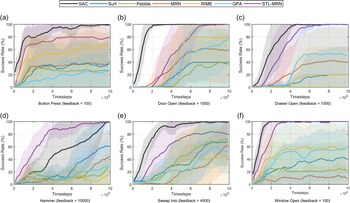
We comprehensively evaluated our STL-PbRL framework across six distinct Meta-world environments to assess its performance with various PbRL algorithms. The results, illustrated in Figure 4 and Table IV, clearly demonstrate the framework’s adaptability to different PbRL algorithms. The performance metrics show significant improvements over the original PbRL algorithms. These enhancements underscore the effectiveness of the STL-PbRL framework in optimizing the learning process and achieving higher performance benchmarks across a range of complex tasks in diverse simulation environments.
Table IV. STL-PbRL is applied in three different PbRL algorithms to verify its versatility.


Figure 4. STL-PbRL is applied in three different PbRL algorithms in the Button Press task to verify its versatility. The solid line and shaded regions denote the success rate’s mean and standard deviation across five runs.
4.3.2. Number of preference feedback
To evaluate whether the STL-PbRL algorithm can more effectively leverage self-learning capabilities to reduce the need for feedback, we conducted a series of experiments in the Meta-world environment with varying levels of feedback. Figure 5 effectively illustrates how our algorithm can better utilize a limited number of trajectories. Specifically, under conditions where feedback is minimal, with the total feedback number set at 100 and 400, traditional PbRL algorithms almost fail to enable agents to complete the specified tasks. In contrast, STL-PbRL provides the agents with a viable opportunity to accomplish the tasks. As the quantity of feedback increases, the performance gap between STL-PbRL and conventional PbRL narrows.

Figure 5. The impact of varying numbers of preference feedback (Feedback=100, 400, 700 & 1000) on Door Open task performance. The solid line and shaded regions denote the success rate’s mean and standard deviation across five runs.
4.3.3. Preference feedback mistake
In traditional PbRL algorithms such as PEBBLE, SURF, RUNE, and MRN, the accuracy of the feedback is crucial. When the quality of this feedback is poor, these algorithms struggle to perform effectively. In this section, we conduct experiments that compare MRN and STL-MRN with varying rates of feedback errors $\epsilon$
at 0%, 10%, and 20%. Figure 6 illustrates the impact of increasing the error rates in feedback on the performance of MRN and SL-MRN in different environments. The results indicate that both algorithms experience a decrease in accuracy as the error rate increases. However, STL-MRN demonstrates greater robustness to feedback errors, consistently achieving better outcomes. This enhanced resilience highlights STL-MRN’s ability to maintain performance integrity even when faced with suboptimal input, making it a more reliable choice in environments where the accuracy of feedback cannot be guaranteed.
$\epsilon$
at 0%, 10%, and 20%. Figure 6 illustrates the impact of increasing the error rates in feedback on the performance of MRN and SL-MRN in different environments. The results indicate that both algorithms experience a decrease in accuracy as the error rate increases. However, STL-MRN demonstrates greater robustness to feedback errors, consistently achieving better outcomes. This enhanced resilience highlights STL-MRN’s ability to maintain performance integrity even when faced with suboptimal input, making it a more reliable choice in environments where the accuracy of feedback cannot be guaranteed.
4.3.4. Self-learning only
Sections 3.1.2 and 4.3.3 demonstrate that the SL module more effectively approximates RM $\hat {r}_\psi$
to the optimal fitness RM
$\hat {r}_\psi$
to the optimal fitness RM $R^*$
compared to TL module. Consequently, we further examine the role of the TL module (expert preference feedback) by integrating the SL module with the SAC algorithm, resulting in the SL-SAC variant. Unlike the baseline SAC algorithm, which relies on a ground-truth reward function, SL-SAC utilizes only the rewards predicted by RM, which is exclusively optimized by the SL module using Eq. 9. Experimental results presented in Table V reveal that SL-SAC can achieve certain fitness values with the SL module alone. However, its performance falls short of that achieved by STL-MRN, suggesting that the TL module plays a crucial role within the STL-PbRL framework.
$R^*$
compared to TL module. Consequently, we further examine the role of the TL module (expert preference feedback) by integrating the SL module with the SAC algorithm, resulting in the SL-SAC variant. Unlike the baseline SAC algorithm, which relies on a ground-truth reward function, SL-SAC utilizes only the rewards predicted by RM, which is exclusively optimized by the SL module using Eq. 9. Experimental results presented in Table V reveal that SL-SAC can achieve certain fitness values with the SL module alone. However, its performance falls short of that achieved by STL-MRN, suggesting that the TL module plays a crucial role within the STL-PbRL framework.
Table V. Comparison of the impact of the TL module on the SL module. It is noted that MRN includes TL module but SAC does not.


Figure 6. The training curve for the impact of preference errors on STL-MRN, MRN, and RIME performance across different tasks.
4.3.5. PbRL with fitness function directly
We investigate the efficacy of integrating a fitness function with a preference-learned reward. We specifically use the fitness function with weights (W) of + 0.5, + 1, + 5, and + 20, which are directly combined with the $\hat {r}_\psi$
to optimize the agent’s strategy and Q-value. The reward is rewritten as
$\hat {r}_\psi$
to optimize the agent’s strategy and Q-value. The reward is rewritten as $r_t = \hat {r}_\psi (s_t,a_t)_{MRN} + W\times f(s_t,a_t)$
. Table VI demonstrates that our preference-based method outperformed algorithms that directly add the fitness function for reward augmentation. Additionally, Table VI reveals that varying the weight coefficients of different fitness functions significantly influences the outcomes. Notably, our method is insensitive to such coefficients by comparing trajectories solely based on their relative fitness values without the need for explicit definitions of weighting coefficients. This eliminates the necessity to design them, thereby simplifying the implementation and adaptation process.
$r_t = \hat {r}_\psi (s_t,a_t)_{MRN} + W\times f(s_t,a_t)$
. Table VI demonstrates that our preference-based method outperformed algorithms that directly add the fitness function for reward augmentation. Additionally, Table VI reveals that varying the weight coefficients of different fitness functions significantly influences the outcomes. Notably, our method is insensitive to such coefficients by comparing trajectories solely based on their relative fitness values without the need for explicit definitions of weighting coefficients. This eliminates the necessity to design them, thereby simplifying the implementation and adaptation process.
Table VI. MRN with fitness function directly.

Statistical significance. To assess the reliability of the reported improvements and account for the variance observed in MRN (Table VI), we conducted two-sample Welch’s t-tests on episodic returns across five random seeds. STL-MRN significantly outperforms MRN (t = $-2.72$
, p =
$-2.72$
, p = $0.032\lt 0.05$
), and its performance is not significantly different from SAC (t =
$0.032\lt 0.05$
), and its performance is not significantly different from SAC (t = $0.51$
, p =
$0.51$
, p = $0.63$
), indicating that the observed gains are statistically meaningful and approach the ground-truth reward upper bound.
$0.63$
), indicating that the observed gains are statistically meaningful and approach the ground-truth reward upper bound.
4.3.6. Behavior cloning as a replacement for self-learning
To examine whether the policy can be optimized solely through behavioral cloning (BC) on collected trajectories, we implemented a BC-MRN variant that replaces the self-learning stage with direct supervised regression on all successful rollouts. As shown in Table VII, BC-MRN performs substantially worse than STL-MRN across all tasks, despite using the same data filtered by the fitness function $F(\tau )$
. On average, STL-MRN achieves a 48% higher success rate than BC-MRN, and in some environments BC-MRN even degrades performance below the MRN baseline (e.g., Sweep Into: 20% vs. 64%; Drawer Open: 30% vs. 40%). This suggests that direct imitation conflicts with the reward model’s optimization objective – BC minimizes action-level regression loss, while MRN optimizes trajectory-level preferences – leading to misaligned gradients and unstable training. These results confirm the theoretical analysis in Section 3.1.2, showing that naive imitation of heterogeneous trajectories drives policy averaging and performance degradation, whereas STL-PbRL maintains consistent improvement through preference-based refinement.
$F(\tau )$
. On average, STL-MRN achieves a 48% higher success rate than BC-MRN, and in some environments BC-MRN even degrades performance below the MRN baseline (e.g., Sweep Into: 20% vs. 64%; Drawer Open: 30% vs. 40%). This suggests that direct imitation conflicts with the reward model’s optimization objective – BC minimizes action-level regression loss, while MRN optimizes trajectory-level preferences – leading to misaligned gradients and unstable training. These results confirm the theoretical analysis in Section 3.1.2, showing that naive imitation of heterogeneous trajectories drives policy averaging and performance degradation, whereas STL-PbRL maintains consistent improvement through preference-based refinement.
Table VII. Comparison between BC-MRN and STL-MRN on six Meta-world tasks.

4.3.7. Sim-to-real quadruped experiment
To further validate the applicability of STL-PbRL in real-world robotics, we conducted a sim-to-real experiment on the Unitree Go1 quadruped robot, following the setup of DAPPER [Reference Kadokawa, Frey, Miki, Matsubara and Hutter16]. The objective was to regulate the robot’s base height and body orientation during locomotion. Training was first performed in Isaac Gym using 1,000 preference feedback samples before deploying the learned policy to the physical robot. A detailed description of the training procedure, preference labeling strategy, and deployment setup is provided in Appendix C.
Two target configurations were considered: (1) maintaining a base height of $0.2$
m with level orientation, and (2) maintaining the same height while sustaining a
$0.2$
m with level orientation, and (2) maintaining the same height while sustaining a $30^\circ$
slope inclination. The reward model was trained using a combination of teacher-guided and self-learning preferences. The teacher preferences were derived from two task-specific reward terms: a height reward
$30^\circ$
slope inclination. The reward model was trained using a combination of teacher-guided and self-learning preferences. The teacher preferences were derived from two task-specific reward terms: a height reward $r_{\text{height}} = - (h_{\text{base}} - h_{\text{target}})^2$
that penalizes deviations from the desired base height, and an orientation reward
$r_{\text{height}} = - (h_{\text{base}} - h_{\text{target}})^2$
that penalizes deviations from the desired base height, and an orientation reward $r_{\text{ori}} = - \|\textbf{g}_{\text{proj}}\|_2^2$
that penalizes non-flat body orientations based on the projected gravity vector
$r_{\text{ori}} = - \|\textbf{g}_{\text{proj}}\|_2^2$
that penalizes non-flat body orientations based on the projected gravity vector $\textbf{g}_{\text{proj}}$
.
$\textbf{g}_{\text{proj}}$
.
In parallel, the self-learning preferences were computed from the robot’s geometric stability. For each of the four base corners $j \in \{\text{FL, FR, RL, RR}\}$
, the corner height was defined as
$j \in \{\text{FL, FR, RL, RR}\}$
, the corner height was defined as $h_j = h_{\text{base}} + x_j \sin \theta + y_j \sin \phi$
, where
$h_j = h_{\text{base}} + x_j \sin \theta + y_j \sin \phi$
, where $(x_j, y_j)$
are the corner coordinates and
$(x_j, y_j)$
are the corner coordinates and $(\theta , \phi )$
denote the roll and pitch angles of the base. The stability deviation was then measured as
$(\theta , \phi )$
denote the roll and pitch angles of the base. The stability deviation was then measured as $E = \tfrac {1}{4}\sum _j |h_j - h_j^*|$
, where
$E = \tfrac {1}{4}\sum _j |h_j - h_j^*|$
, where $h_j^*$
represents the desired corner height at the target configuration. The corresponding fitness function was defined as
$h_j^*$
represents the desired corner height at the target configuration. The corresponding fitness function was defined as $f(s_t,a_t) = -E$
.
$f(s_t,a_t) = -E$
.
This hybrid reward design enables the system to jointly leverage limited human supervision (via teacher-defined task rewards) and continuous self-learning (via geometric stability), effectively improving policy robustness in sim-to-real transfer.

Figure 7.
Real-world deployment of STL-PbRL on the Unitree Go1 quadruped. STL-PbRL successfully maintains the target base height and orientation (30 $^{\circ }$
inclination) through self-learning refinement. In contrast, baseline PbRL trained purely from pairwise preferences exhibits unstable posture and fails to achieve target alignment. (a) STL-PbRL (height=0.2 m, real), (b) PbRL (height=0.2 m, simulation), (c) STL-PbRL (slope=30
$^{\circ }$
inclination) through self-learning refinement. In contrast, baseline PbRL trained purely from pairwise preferences exhibits unstable posture and fails to achieve target alignment. (a) STL-PbRL (height=0.2 m, real), (b) PbRL (height=0.2 m, simulation), (c) STL-PbRL (slope=30 $^{\circ }$
, real), (d) PbRL (slope=30
$^{\circ }$
, real), (d) PbRL (slope=30 $^{\circ }$
, simulation).
$^{\circ }$
, simulation).
The results in Figure 7 confirm that STL-PbRL can be effectively transferred from simulation to real hardware. While conventional PbRL struggled to stabilize the robot in both flat and inclined settings, STL-PbRL achieved robust, consistent tracking of the desired base pose. This demonstrates that STL-PbRL not only improves feedback efficiency in simulation but also scales to real-world robotic control tasks.
4.3.8. Computational efficiency and complexity
Runtime analysis. To provide a clear comparison of computational cost, we measured the average wall-clock training time to convergence on the Meta-World door-open-v2 task (using NVIDIA RTX 4090 GPU and Intel i9-14900KF CPU, averaged over multiple random seeds). The results for the main baselines and their STL-enhanced variants are shown in Table VIII:
Table VIII. Average wall-clock training time (minutes:seconds) on Meta-world door-open-v2 and relative overhead of STL variants.

These empirical measurements show that incorporating the Self-Learning (SL) module introduces a modest runtime overhead of 14.6–15.1% across the evaluated PbRL baselines (with SURF showing a slightly lower relative increase in earlier runs, but consistent in the 6–15% range overall). This overhead primarily arises from additional self-learning trajectory sampling and pairwise comparison steps, but remains acceptable given the performance improvements demonstrated in the experiments.
The SL module reuses the existing reward model update mechanism without introducing new network training loops or frequent retraining, ensuring scalability. Overall, the added computational cost is low relative to the total training time and does not compromise deployment feasibility.
Memory analysis. The additional memory footprint of SL mainly comes from success/failure trajectory buffers and pairwise comparison buffers, adding less than $\textbf{20}\,\textrm{MB}$
of CPU memory in typical settings – negligible compared to standard replay buffers (hundreds of MB to several GB).
$\textbf{20}\,\textrm{MB}$
of CPU memory in typical settings – negligible compared to standard replay buffers (hundreds of MB to several GB).
Conclusion. Empirical results confirm that STL-PbRL incurs only 14.6–15.1% additional wall-clock time on representative tasks (Table VIII), providing a favorable trade-off between enhanced performance and computational efficiency.
5. Conclusion
This work presents STL-PbRL, a novel reinforcement learning framework that enhances feedback efficiency by integrating easily designed, task-oriented information. By optimizing the RM based on task objectives, STL-PbRL can be seamlessly integrated with other advanced PbRL algorithms to enhance feedback efficiency across various robotic simulation tasks. This integration reduces the amount of feedback required for training and demonstrates robust performance in the presence of feedback errors. We also confirm that the SL module is the most effective way to incorporate task objective information into the algorithm. We hope our method will inspire future research in PbRL and encourage the broader application of STL-PbRL in practical settings, enhancing its adaptability and effectiveness in real-world scenarios.
Limitations and future directions. A current limitation of STL-PbRL is its reliance on manually specified fitness functions to guide self-learning. While many task-oriented robotics benchmarks allow reasonably straightforward fitness definitions (e.g., distance to target, grasp success, or door opening angle), designing reliable signals can become non-trivial for highly complex or unstructured tasks. A promising direction is to first train a lightweight task success classifier from binary success/failure labels – data that are often easier to collect than dense rewards – to automatically infer task completion and provide a surrogate fitness signal. Another promising avenue is to leverage vision-language models (VLMs) to assess task outcomes: by conditioning on high-level textual goals and the final visual state of the robot or manipulated objects, VLMs can provide semantic judgments of success, reducing the need for hand-crafted metrics. Integrating such automatic evaluators could further broaden STL-PbRL’s applicability to diverse real-world tasks where manual fitness design is difficult.
Supplementary material
The supplementary material for this article can be found at https://doi.org/10.1017/S0263574726103300.
Acknowledgements
The authors used ChatGPT (GPT-5, OpenAI, accessed in November 2025) solely for language translation and editorial assistance to improve clarity. The authors verified all content for accuracy and take full responsibility for the final manuscript.
Financial support
This research received no specific grant from any funding agency, commercial, or not-for-profit sectors.
Competing interests
The authors declare no conflicts of interest exist.
Ethical approval
Not applicable.
Author contributions
HJ, ZP, and ZL conceived and designed the study. HJ conducted the experiments, data gathering, and analyses. HJ, WX, and LC wrote the article.
Appendix A. Self-teacher-learning PbRL framework
In this section, we present the detailed procedures of STL-PbRL in Algorithm2. As mentioned in the manuscript, our approach is adaptable to various algorithms, including PEBBLE [Reference Lee, Smith and Abbeel20], SURF [Reference Park, Seo, Shin, Lee, Abbeel and Lee24], and MRN [Reference Liu, Bai, Du and Yang22]. To elucidate our methodology without the encumbrance of supplementary algorithmic details, we focus here on the representative PbRL algorithm employed within the PEBBLE framework.
The RM is updated using supervised loss per K iterations, while the self-learning is performed per n iterations.
Algorithm 2 STL-PbRL(PEBBLE) Algorithm

Appendix B. Experimental details
B.1. DMControl
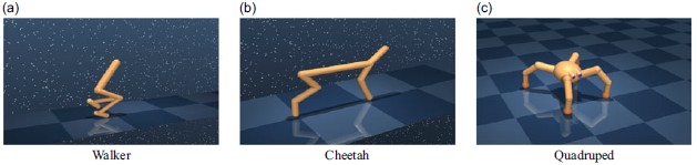
The locomotion tasks from DeepMind Control Suite (DMControl) [Reference Tunyasuvunakool, Muldal, Doron, Liu, Bohez, Merel, Erez, Lillicrap, Heess and dm_control31] used in our experiments are shown in Figure 8. The criteria of DMControl are shown in Table IX.
Table IX. Fitness function of DMControl.


Figure 8. DMControl environments.
Tasks description.
-
• Walker: A planar walker learns to control its torso and walk on the ground at 1 m/s.
-
• Cheetah: A planar biped learns to control its body and run on the ground at 10 m/s.
-
• Quadruped: A quadruped ant learns to control its body and limbs and walk on the ground at 5 m/s.
B.2. Meta-world
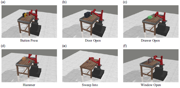
The simulated robotic manipulation tasks from Meta-world [Reference Yu, Quillen, He, Julian, Hausman, Finn and Levine35] used in our experiments are shown in Figure 9. The criteria of Meta-world are shown in Table X.

Figure 9. Meta-world environments. Each subfigure illustrates a distinct manipulation task.
Table X. Fitness function of Meta-world.

Tasks description.
-
• Hammer: The agent manipulates the robotic arm to drive a screw into the wall.
-
• Door open: The agent operates the robotic arm to open a door hinged on a revolving joint.
-
• Button press: The agent directs the robotic arm to press a button.
-
• Sweep into: The agent uses the robotic arm to sweep a ball into a designated hole.
-
• Drawer open: The agent guides the robotic arm to open a drawer.
-
• Window open: The agent maneuvers the robotic arm to open a window.
B.3. Implementation details
For SAC, the agent is provided the ground-truth reward function, and SAC serves as the upper bound of all methods. The detailed hyperparameters of SAC are shown in Table XI. For PEBBLE, SURF, and MRN, we adopt the hyperparameter settings from MRN as outlined in [Reference Liu, Bai, Du and Yang22], with a simplification applied to the parameters highlighted in bold in Tables XII, XIII, and XIV. The hyperparameters of RIME and QPA are summarized in Tables XV and XVI, respectively. Both methods adopt the hyperparameter settings reported in their original papers. This adjustment streamlines the parameter setup to enhance clarity and implementation efficiency in our experiments. The hyperparameter of SL-PbRL is shown in Table XVII.
Table XI. Hyperparameters of SAC.

Table XII. Hyperparameters of PEBBLE.

Table XIII. Hyperparameters of SURF.

Table XIV. Hyperparameters of MRN.

Table XV. Hyperparameters of RIME.

Table XVI. Hyperparameters of QPA.

Table XVII. Hyperparameters of STL-PbRL.

Appendix C. Real-world experiments
The locomotion experiments on the Unitree Go1 quadruped were conducted using the open-source unitree_rl_gym framework,Footnote 4 which is built upon the legged_gym reinforcement learning environment based on NVIDIA IsaacGym. During training, the policy was optimized in simulation and later evaluated at 50 Hz to predict target joint positions, which were tracked by individual joint-level PID controllers running at 400 Hz. All hyperparameters and simulation settings followed the standard configurations provided by prior Unitree benchmarks.
C.1. Task description
The Go1 task aimed to achieve two locomotion objectives:
-
1. Maintaining a nominal base height of 0.2 m with a level orientation while walking at commanded linear and angular velocities;
-
2. Sustaining the same nominal height while adapting to a 30 $^{\circ }$
inclined slope.
$^{\circ }$
inclined slope.

In parallel, the self-learning preferences were computed from the robot’s geometric stability. For each of the four base corners $j \in \{\text{FL}, \text{FR}, \text{RL}, \text{RR}\}$
, the instantaneous corner height was estimated as:
$j \in \{\text{FL}, \text{FR}, \text{RL}, \text{RR}\}$
, the instantaneous corner height was estimated as:
 \begin{equation*} h_j = h_{\text{base}} + x_j \sin \theta + y_j \sin \phi , \end{equation*}
where $(x_j, y_j)$
denote the local corner coordinates, and
$(x_j, y_j)$
denote the local corner coordinates, and $(\theta , \phi )$
represent the pitch and roll angles of the base, respectively. The target corner heights
$(\theta , \phi )$
represent the pitch and roll angles of the base, respectively. The target corner heights $h_j^*$
correspond to the desired base plane at 0.2 m height with a
$h_j^*$
correspond to the desired base plane at 0.2 m height with a $30^{\circ }$
forward inclination. The geometric stability deviation was then measured as:
$30^{\circ }$
forward inclination. The geometric stability deviation was then measured as:
 \begin{equation*} E = \frac {1}{4}\sum _{j} |h_j - h_j^{*}|, \end{equation*}
and the corresponding self-learning fitness function was defined as $f(s_t, a_t) = -E$
. This term provided a continuous preference signal for the reward model, complementing the scripted teacher that compared trajectories using predefined reward terms (e.g., base height and orientation).
$f(s_t, a_t) = -E$
. This term provided a continuous preference signal for the reward model, complementing the scripted teacher that compared trajectories using predefined reward terms (e.g., base height and orientation).
C.2. Reward composition
The total reward consisted of three parts:
 \begin{equation*} r_t = r_{\text{task}} + r_{\text{style}} + r_{\text{norm}}, \end{equation*}
where $r_{\text{task}}$
is the task-specific objective (velocity and stability tracking),
$r_{\text{task}}$
is the task-specific objective (velocity and stability tracking), $r_{\text{style}}$
comes from the preference-based reward model (teacher or self-learning), and
$r_{\text{style}}$
comes from the preference-based reward model (teacher or self-learning), and $r_{\text{norm}}$
includes regularization terms to encourage smooth and physically plausible motion. The detailed reward terms and their corresponding scales are listed in Table XVIII.
$r_{\text{norm}}$
includes regularization terms to encourage smooth and physically plausible motion. The detailed reward terms and their corresponding scales are listed in Table XVIII.
Table XVIII. Reward terms used in Go1 STL-PbRL training.

Table XIX. Domain randomization parameters.

C.3. Domain randomization
To improve sim-to-real transfer robustness, domain randomization was applied during training. The detailed parameter ranges are summarized in Table XIX.
C.4. STL-PbRL training procedure
The training followed a preference-based reinforcement learning loop. Rollout trajectories were first collected in parallel from the IsaacGym simulator. From the trajectory buffer, fixed-length segments were randomly sampled to form comparison pairs. For each pair $(\tau _A, \tau _B)$
, two preference sources were used:
$(\tau _A, \tau _B)$
, two preference sources were used:
-
• The scripted teacher evaluated trajectory quality via cumulative task rewards, primarily based on base height and orientation terms;
-
• The self-learning module computed geometric stability scores using the deviation metric
$E$
above.

The Reward Model (RM) was trained via cross-entropy loss to predict which segment was preferred, jointly incorporating teacher-guided and self-learning comparisons. The policy was then updated using the learned RM as a differentiable reward estimator, enabling continuous improvement beyond the fixed feedback budget of the teacher.