





1 Introduction
Motivated by the study of Yang–Mills equations on four-dimensional asymptotically locally Euclidean (ALE) spaces, Nakajima [Reference NakajimaNak94] used linear representations of quivers to construct new examples of noncompact hyperkähler varieties in arbitrary dimensions—the so-called Nakajima quiver varieties, which can be thought of as moduli spaces of these representations. This construction builds on a particular narrative threaded through the work of Gibbons and Hawking in type A [Reference Gibbons and HawkingGH79]; of Atiyah, Drinfel’d, Hitchin and Manin [Reference Atiyah, Hitchin, Drinfel’d and ManinAHDM78] when the underlying quiver is of type A, D or E; and of Kronheimer and Nakajima [Reference Kronheimer and NakajimaKN90] concerning Yang–Mills instantons over ALE gravitational instantons. The construction is also closely related to the McKay correspondence for finite subgroups of
$\text {SU }(2)$
 in the case where the underlying quiver is ADE.
Nakajima quiver varieties have been a mainstay in representation theory, in symplectic and complex algebraic geometry, and in mathematical physics. In foundational work [Reference NakajimaNak98], Nakajima connected the aforementioned quiver varieties to integrable highest-weight representations of simply laced Kac–Moody algebras. Specifically, these representations admit an interpretation within the homology ring of these varieties, and the Kac–Moody algebra acts in a certain way via Hecke-type correspondences defined with respect to Lagrangian subvarieties of products of quiver varieties. These subvarieties in turn provide generators for the algebra. At the same time, variation of stability parameters for the moduli problem, viewed either via geometric invariant theory or through symplectic reduction, is a means for resolving symplectic singularities [Reference Bellamy and SchedlerBS21]—this includes somewhat surprising cases such as where every resolution of a particular quotient singularity in four complex dimensions is realizable as a Nakajima quiver variety for a single quiver [Reference Bellamy, Craw, Rayan, Schedler and WeissBCR+24]. Furthermore, Nakajima quiver varieties are similar in crucial ways to moduli spaces of stable Higgs bundles: both are noncompact hyperkähler varieties equipped with an action by
$\mathbb {C}^\times $
 , although one is a finite-dimensional quotient (Nakajima) and the other is an infinite-dimensional one (Hitchin). The relation between them is explored from the vantage point of character varieties in [Reference Hausel, Letellier and Rodriguez-VillegasHLRV11], as well as in [Reference Fisher and RayanFR16, Reference Rayan and SchaposnikRS21] where Nakajima quiver varieties of star- and comet-shaped quivers are embedded into moduli spaces of meromorphic Higgs bundles, thereby eliciting a sub-integrable system of the Hitchin system for certain flag types.
A fundamental question concerns the behaviour of such quiver varieties when the linear representation data are generalized or ‘globalized’ to other types of representations, such as those valued in vector bundles over a fixed variety. This is already motivated in the literature. In [Reference HitchinHit87] there is the first study of fixed points of the
$\mathbb {C}^\times $
 -action on the moduli space of Higgs bundles on a Riemann surface X. Each fixed point is a Higgs bundle with a splitting of the underlying bundle for which the Higgs field has a strictly sub-diagonal matrix representation. As such, viewed through the lens of representation theory, the fixed points are representations of A-type quivers in the category of holomorphic bundles over X. Here, each vertex is assigned a holomorphic vector bundle
$E_i$
-action on the moduli space of Higgs bundles on a Riemann surface X. Each fixed point is a Higgs bundle with a splitting of the underlying bundle for which the Higgs field has a strictly sub-diagonal matrix representation. As such, viewed through the lens of representation theory, the fixed points are representations of A-type quivers in the category of holomorphic bundles over X. Here, each vertex is assigned a holomorphic vector bundle
$E_i$
 , and each edge is assigned a section
$\phi _i\in H^0(X,\operatorname {\mathrm {Hom}}(E_i,E_{i+1}))$
, and each edge is assigned a section
$\phi _i\in H^0(X,\operatorname {\mathrm {Hom}}(E_i,E_{i+1}))$
 . Such representations are often referred to as ‘holomorphic chains’. More generally (beyond A-type) they are referred to as quiver bundles. Such objects also appear as solutions to quiver vortex equations [Reference Álvarez-Cónsul and García-PradaAaCGP03], which themselves capture many well-known correspondences in that the existence of solutions is equivalent to the existence of connections satisfying certain curvature constraints. Some recent works on the physics side involving quiver bundles and emphasizing connections with higher-dimensional branes include [Reference Collinucci and SavelliCS15a, Reference Collinucci and SavelliCS15b, Reference Heckman, Hübner, Torres and ZhangHHTZ23].
This brings us to the goal of the present paper: to produce a variety parametrizing representations of double quivers by complex vector bundles. Such representations will be referred to as ‘Nakajima bundle representations’. In doing so, we construct objects similar to quiver bundles on a double quiver, called
$\overline {Q}$
 -bundles, and we provide a Hitchin–Kobayashi-type correspondence that identifies points in the moduli space of Nakajima representations with certain stable
$\overline {Q}$
-bundles, and we provide a Hitchin–Kobayashi-type correspondence that identifies points in the moduli space of Nakajima representations with certain stable
$\overline {Q}$
 -bundles. These representations differ from solutions of the quiver vortex equations described in [Reference Álvarez-Cónsul and García-PradaAaCGP03] in that the reverse edges appearing in the double quiver are represented by cohomology classes in the cotangent space of the original data. In this way we make use of the natural holomorphic symplectic structure on the representation space. The resulting objects can be thought of in two ways: providing a relative or global version of Nakajima quiver varieties on the surface X, or as the study of quiver bundles in a holomorphic symplectic context. Representations of double quivers in the category of vector bundles have appeared prior to the current work, having appeared for instance in [Reference SzendrőiSze08, Reference DiaconescuDia12] in the contexts of holomorphic D-branes, and local Donaldson–Thomas theory, respectively. These objects are also related to quasimaps [Reference Ciocan-Fontanine, Kim and MaulikCFKM14]. In these works there is no way to distinguish between a representation thought of as coming from a double quiver, or an ordinary quiver. In the present work, the two are clearly separated. To the knowledge of the authors, the approach and generality provided in the current work have not been emphasized in the literature. Moreover, the current work provides a basis-independent construction involving hermitian matrices (Lemma 13), starting from functions
$\psi ,\Psi $
-bundles. These representations differ from solutions of the quiver vortex equations described in [Reference Álvarez-Cónsul and García-PradaAaCGP03] in that the reverse edges appearing in the double quiver are represented by cohomology classes in the cotangent space of the original data. In this way we make use of the natural holomorphic symplectic structure on the representation space. The resulting objects can be thought of in two ways: providing a relative or global version of Nakajima quiver varieties on the surface X, or as the study of quiver bundles in a holomorphic symplectic context. Representations of double quivers in the category of vector bundles have appeared prior to the current work, having appeared for instance in [Reference SzendrőiSze08, Reference DiaconescuDia12] in the contexts of holomorphic D-branes, and local Donaldson–Thomas theory, respectively. These objects are also related to quasimaps [Reference Ciocan-Fontanine, Kim and MaulikCFKM14]. In these works there is no way to distinguish between a representation thought of as coming from a double quiver, or an ordinary quiver. In the present work, the two are clearly separated. To the knowledge of the authors, the approach and generality provided in the current work have not been emphasized in the literature. Moreover, the current work provides a basis-independent construction involving hermitian matrices (Lemma 13), starting from functions
$\psi ,\Psi $
 that are only
$C^1$
that are only
$C^1$
 -bounded rather than smooth.
We do note the parallel work of Azam and the third-named author [Reference Azam and RayanAR24] that develops similar ideas related to quiver bundles, but in a categorical context around moduli stacks with homotopy-theoretic applications in mind, as well as work of Minets [Reference MinetsMin20] in which a cohomological Hall algebra was constructed on the homology of certain moduli stacks of Higgs bundles by viewing it as a cotangent stack.
1.1 Set-up
Consider the quiver Q with a single vertex and no arrows. Upon fixing a rank r and degree d, a quiver bundle is a holomorphic vector bundle of rank r and degree d on X. By Narasimhan and Seshadri [Reference Narasimhan and SeshadriNS64], a stable holomorphic vector bundle on X is equivalent to a complex vector bundle E equipped with a hermitian connection A whose curvature satisfies the equation
$F_A =0$
 . One could then hope to recover the moduli space of stable bundles on X having rank r and degree d,
$\mathcal {N}_X(r,d)$
. One could then hope to recover the moduli space of stable bundles on X having rank r and degree d,
$\mathcal {N}_X(r,d)$
 , from representations of this quiver. With this in mind, the representation space for the quiver with a single vertex and no arrows is given by the space of connections
$\mathcal {A}(E)$
, from representations of this quiver. With this in mind, the representation space for the quiver with a single vertex and no arrows is given by the space of connections
$\mathcal {A}(E)$
 that are compatible with the hermitian metric on E. A variety parametrizing representations is then precisely the moduli space of hermitian Einstein connections.
Consider now the double quiver
$\overline {Q}$
 constructed from Q by adding an additional copy of each edge, whose orientation is reversed. Since there are no arrows to double,
$\overline {Q}$
constructed from Q by adding an additional copy of each edge, whose orientation is reversed. Since there are no arrows to double,
$\overline {Q}$
 coincides with the ordinary quiver Q. However, it still makes sense to ask what representations of
$\overline {Q}$
coincides with the ordinary quiver Q. However, it still makes sense to ask what representations of
$\overline {Q}$
 should be. The guiding principle for our approach is that in the construction of the Nakajima quiver variety, the representation space of the double quiver is the cotangent space of that of the original quiver. For the ordinary quiver, a representation is (equivalent to) a stable vector bundle on X. Deformations of stable bundles E are given by
$H^1(X,\operatorname {End}(E))$
should be. The guiding principle for our approach is that in the construction of the Nakajima quiver variety, the representation space of the double quiver is the cotangent space of that of the original quiver. For the ordinary quiver, a representation is (equivalent to) a stable vector bundle on X. Deformations of stable bundles E are given by
$H^1(X,\operatorname {End}(E))$
 , and so by Serre duality the cotangent directions are
$H^0(X,\operatorname {End}(E)\otimes K)$
, and so by Serre duality the cotangent directions are
$H^0(X,\operatorname {End}(E)\otimes K)$
 , where K is the canonical bundle of X. Thus, the cotangent space of the space of stable bundles consists of all pairs
$(E,\phi )$
, where K is the canonical bundle of X. Thus, the cotangent space of the space of stable bundles consists of all pairs
$(E,\phi )$
 where E is a stable holomorphic bundle and
$\phi $
where E is a stable holomorphic bundle and
$\phi $
 is a holomorphic
$\operatorname {End}(E)$
is a holomorphic
$\operatorname {End}(E)$
 -valued
$1$
-valued
$1$
 -form, in other words, a Higgs bundle.
For X of genus at least
$2$
 , Simpson [Reference SimpsonSim92] proved that a stable Higgs bundle on X admits a hermitian metric h such that the pair
$(A_h,\phi )$
, Simpson [Reference SimpsonSim92] proved that a stable Higgs bundle on X admits a hermitian metric h such that the pair
$(A_h,\phi )$
 , satisfies the Hitchin equations

where
$A_h$
 is the Chern connection associated to h and
$\Lambda :\Omega ^{i,j}(X,E)\to \Omega ^{i-1,j-1}(X,E)$
is the Chern connection associated to h and
$\Lambda :\Omega ^{i,j}(X,E)\to \Omega ^{i-1,j-1}(X,E)$
 is contraction with the symplectic form. The moduli space
$\mathcal {M}^{\text {Higgs}}_X(r,d)$
is contraction with the symplectic form. The moduli space
$\mathcal {M}^{\text {Higgs}}_X(r,d)$
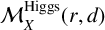 of Higgs bundles of rank r and degree d is a hyperkähler variety arising as a reduction of Equation (1-1).
In order to recover Simpson’s construction of
$\mathcal {M}^{\text {Higgs}}_X(r,d)$
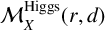 , a representation of the double quiver
$\overline {Q}$
, a representation of the double quiver
$\overline {Q}$
 should be a hermitian connection A and a section
$\phi \in \Omega ^{1,0}(X,\operatorname {End}(E))$
should be a hermitian connection A and a section
$\phi \in \Omega ^{1,0}(X,\operatorname {End}(E))$
 . With these data, the space of quiver representations satisfying Equation (1-1) up to equivalence recovers precisely the moduli space of Higgs bundles on
$\mathcal {M}_X^{\text {Higgs}}(r,d)$
. With these data, the space of quiver representations satisfying Equation (1-1) up to equivalence recovers precisely the moduli space of Higgs bundles on
$\mathcal {M}_X^{\text {Higgs}}(r,d)$
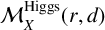 .
.
Now for a general quiver Q associate a bundle
$E_v$
 with hermitian connection
$A_v$
with hermitian connection
$A_v$
 to each vertex v. If
$a:v_i\rightarrow v_j$
to each vertex v. If
$a:v_i\rightarrow v_j$
 is an edge, we associate with it a bundle morphism
$x_a:E_{v_i}\rightarrow E_{v_j}$
is an edge, we associate with it a bundle morphism
$x_a:E_{v_i}\rightarrow E_{v_j}$
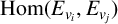
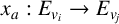 , which can be identified with a global section of
$\operatorname {\mathrm {Hom}}(E_{v_i},E_{v_j})$
, which can be identified with a global section of
$\operatorname {\mathrm {Hom}}(E_{v_i},E_{v_j})$
 on X. By taking the
$(0,1)$
on X. By taking the
$(0,1)$
 part of the connection, we get a holomorphic structure on
$E_i$
part of the connection, we get a holomorphic structure on
$E_i$
 allowing us to make sense of holomorphic sections. A section
$x\in \Omega ^0(X,\operatorname {\mathrm {Hom}}(E_{v_i},E_{v_j}))$
allowing us to make sense of holomorphic sections. A section
$x\in \Omega ^0(X,\operatorname {\mathrm {Hom}}(E_{v_i},E_{v_j}))$
 is holomorphic if it is holomorphic with respect to the operators
$\overline {\partial }_{A_{v_i}}$
is holomorphic if it is holomorphic with respect to the operators
$\overline {\partial }_{A_{v_i}}$
 and
$\overline {\partial }_{A_{v_j}}$
and
$\overline {\partial }_{A_{v_j}}$
 . In [Reference Álvarez-Cónsul and García-PradaAaCGP03] it was shown that there is a correspondence between representations satisfying the vortex equations and stable Q-sheaves. For the double quiver
$\overline {Q}$
. In [Reference Álvarez-Cónsul and García-PradaAaCGP03] it was shown that there is a correspondence between representations satisfying the vortex equations and stable Q-sheaves. For the double quiver
$\overline {Q}$
 , to capture the doubled information at the vertices, following the discussion above, in addition to the bundle E, we assign a section
$\phi \in \Omega ^{1,0}(X,\operatorname {End}(E))$
, to capture the doubled information at the vertices, following the discussion above, in addition to the bundle E, we assign a section
$\phi \in \Omega ^{1,0}(X,\operatorname {End}(E))$
 . For the reverse edges, assign a cohomology class
$y_a$
. For the reverse edges, assign a cohomology class
$y_a$
 that is Serre dual to
$x_a$
that is Serre dual to
$x_a$
 . Taking all equivalence classes of representations of a given quiver that satisfy the moment map conditions equations (2-1) and (2-2), produces a variety
$\mathcal {M}_{\overline {Q}}^{r,d}(\tau )$
. Taking all equivalence classes of representations of a given quiver that satisfy the moment map conditions equations (2-1) and (2-2), produces a variety
$\mathcal {M}_{\overline {Q}}^{r,d}(\tau )$
 we are calling a Nakajima bundle variety. These varieties are, in a sense, a global analogue of Nakajima quiver varieties.
1.2 Organization
The organization of this work is as follows. Sections 2–4 provide the theoretical framework and main results of the paper. Section 2 introduces the appropriate representations of double quivers and gives the construction of their moduli spaces, Nakajima bundle varieties. After constructing Nakajima bundle representations, Section 3 introduces the algebro-geometric counterpart
$\overline {Q}$
 -bundles. Stable
$\overline {Q}$
-bundles. Stable
$\overline {Q}$
 -bundles are shown to be in correspondence with representations that solve the moment map conditions in Section 4. With the general framework out of the way, Section 5 is devoted to a study of the infinitesimal deformations of a Nakajima bundle representation, combining the work of [Reference Gothen and KingGK05] for quiver bundles with that of [Reference BottacinBot00]. Section 6 briefly looks at representations of the framed
$A_1$
-bundles are shown to be in correspondence with representations that solve the moment map conditions in Section 4. With the general framework out of the way, Section 5 is devoted to a study of the infinitesimal deformations of a Nakajima bundle representation, combining the work of [Reference Gothen and KingGK05] for quiver bundles with that of [Reference BottacinBot00]. Section 6 briefly looks at representations of the framed
$A_1$
 -quiver. Finally, in Section 7 a
$\mathbb {C}^\times $
-quiver. Finally, in Section 7 a
$\mathbb {C}^\times $
 -action is described on Nakajima bundle varieties.
2 Nakajima bundle varieties
The present section defines the main object of the current paper, Nakajima bundle representations. These are representations of double quivers in which vertices are represented by hermitian vector bundles, and edges by cohomology classes valued in Hom-bundles. There is a hermitian action of the group
$\mathcal {G}=\prod _{v\in V}\text {Aut}(E_v)$
 on the space of all such representations. Symplectic reduction produces a moduli space
$\mathcal {M}^{r,d}_{\overline {Q}}(\tau )$
on the space of all such representations. Symplectic reduction produces a moduli space
$\mathcal {M}^{r,d}_{\overline {Q}}(\tau )$
 of Nakajima bundle representations.
A quiver Q consists of a tuple
$(Q_0,Q_1,h,t)$
 , where
$Q_0=\{v_0,\ldots , v_n\}$
, where
$Q_0=\{v_0,\ldots , v_n\}$
 is the set of vertices,
$Q_1=\{a:v_i\rightarrow v_j\}$
is the set of vertices,
$Q_1=\{a:v_i\rightarrow v_j\}$
 the set of edges, and
$h,t:Q_1\rightarrow Q_0$
the set of edges, and
$h,t:Q_1\rightarrow Q_0$
 are functions specifying the head and tail of each edge.
Given any quiver Q, the double quiver
$\overline {Q}$
 is a quiver whose sets of vertices and edges satisfy
$\overline {Q}_0 = Q_0$
is a quiver whose sets of vertices and edges satisfy
$\overline {Q}_0 = Q_0$
 and
$\overline {Q}_1 = Q_1 \sqcup -Q_1$
and
$\overline {Q}_1 = Q_1 \sqcup -Q_1$
 . Here
$-Q_1$
. Here
$-Q_1$
 consists of a copy of each element of
$Q_1$
consists of a copy of each element of
$Q_1$
 but with opposite orientation.
In order to define representations of a quiver, it is necessary to equip it with a label. Given a quiver Q, a label of Q is a pair
$(r,d)$
 where
$r=(r_v)_{v\in Q_0} \in \mathbb {N}^{\lvert Q_0\rvert }$
where
$r=(r_v)_{v\in Q_0} \in \mathbb {N}^{\lvert Q_0\rvert }$
 and
$d=(d_v)_{v\in Q_0}\in \mathbb {Z}^{\lvert Q_0\rvert }$
and
$d=(d_v)_{v\in Q_0}\in \mathbb {Z}^{\lvert Q_0\rvert }$
 . The data
$(r,d)$
. The data
$(r,d)$
 are referred to as the type of the representation.
Definition 1. Let
$\overline {Q}$
 be a double quiver with label
$(r,d)$
be a double quiver with label
$(r,d)$
 . For each
$v\in Q_0$
. For each
$v\in Q_0$
 , let
$E_v$
, let
$E_v$
 be a complex vector bundle over X of rank
$r_v$
be a complex vector bundle over X of rank
$r_v$
 and degree
$d_v$
and degree
$d_v$
 . A Nakajima bundle representation of
$\overline {Q}$
. A Nakajima bundle representation of
$\overline {Q}$
 is a collection
$(A,\phi ,x,y) = (A_v,\phi _v,x_a,y_a)$
is a collection
$(A,\phi ,x,y) = (A_v,\phi _v,x_a,y_a)$
 indexed by the vertices and edges of Q, consisting of the following objects: for every vertex,
$A_v$
indexed by the vertices and edges of Q, consisting of the following objects: for every vertex,
$A_v$
 is a connection on
$E_v$
is a connection on
$E_v$
 , and
$\phi _v\in \Omega ^{1,0}(X,\operatorname {End}(E_v))$
, and
$\phi _v\in \Omega ^{1,0}(X,\operatorname {End}(E_v))$
 , and for every edge,
$x_a\in \Omega ^0(X,\operatorname {\mathrm {Hom}}(E_{t(a)},E_{h(a)}))$
, and for every edge,
$x_a\in \Omega ^0(X,\operatorname {\mathrm {Hom}}(E_{t(a)},E_{h(a)}))$
 , and
$y_a\in \Omega ^{0,1}(X, \operatorname {\mathrm {Hom}}(E_{t(a)},E_{h(a)})\otimes K)$
, and
$y_a\in \Omega ^{0,1}(X, \operatorname {\mathrm {Hom}}(E_{t(a)},E_{h(a)})\otimes K)$
 such that
$\overline {\partial }x=0$
such that
$\overline {\partial }x=0$
 with respect to the connections
$A_{t(a)}$
with respect to the connections
$A_{t(a)}$
 and
$A_{h(a)}$
and
$A_{h(a)}$
 .
.
Let
$\mathcal {A}(E_v)$
 denote the space of unitary connections on
$E_v$
denote the space of unitary connections on
$E_v$
 . The space
$\text {Rep}(\overline {Q})$
. The space
$\text {Rep}(\overline {Q})$
 of Nakajima bundle representations of
$\overline {Q}$
of Nakajima bundle representations of
$\overline {Q}$
 is
$\text {Rep}(\overline {Q}) = \text {Rep}(Q_0) \oplus \text {Rep}(Q_1)$
is
$\text {Rep}(\overline {Q}) = \text {Rep}(Q_0) \oplus \text {Rep}(Q_1)$
 , where

and
$\text {Rep}(Q_1)$
 is the subset
$\ker (\overline {\partial })$
is the subset
$\ker (\overline {\partial })$
 of
of

At each vertex, the group  of unitary bundle automorphisms acts on
$E_v$
of unitary bundle automorphisms acts on
$E_v$
 , producing an action of
$\mathcal {G}=\prod _{v\in Q_0} \mathcal {G}_v$
, producing an action of
$\mathcal {G}=\prod _{v\in Q_0} \mathcal {G}_v$
 on
$\text {Rep}(\overline {Q})$
on
$\text {Rep}(\overline {Q})$
 :
:

In [Reference HitchinHit87] it was shown that the action of
$\mathcal {G}_v$
 on
$\mathcal {A}(E_v)\times \Omega ^{1,0}(X,\operatorname {End}(E_v))$
on
$\mathcal {A}(E_v)\times \Omega ^{1,0}(X,\operatorname {End}(E_v))$
 is Hamiltonian with real and complex moment maps given by Equation (1-1). This extends to the action of the product group
$\mathcal {G}$
is Hamiltonian with real and complex moment maps given by Equation (1-1). This extends to the action of the product group
$\mathcal {G}$
 on
$\text {Rep}(Q_0)$
on
$\text {Rep}(Q_0)$
 whose real and complex moment maps are
$\mu _{\mathbb {R}}^{\mathfrak {H}} =\bigoplus _{v\in Q_0}(\sqrt {-1}\Lambda F_{A_v}+[\phi _v,\phi _v^*])$
whose real and complex moment maps are
$\mu _{\mathbb {R}}^{\mathfrak {H}} =\bigoplus _{v\in Q_0}(\sqrt {-1}\Lambda F_{A_v}+[\phi _v,\phi _v^*])$
 and
$\mu _{\mathbb {C}}^{\mathfrak {H}} = \bigoplus _{v\in Q_0}\overline {\partial }_{E_v}\phi _v$
and
$\mu _{\mathbb {C}}^{\mathfrak {H}} = \bigoplus _{v\in Q_0}\overline {\partial }_{E_v}\phi _v$
 .
.
Consider the
$\mathcal {G}$
 -action on the space of edge representations
$\text {Rep}(\overline {Q}_1)$
-action on the space of edge representations
$\text {Rep}(\overline {Q}_1)$
 . For each
${a\in Q_1}$
. For each
${a\in Q_1}$
 let
$y_a^{\mathrm {harm}}$
let
$y_a^{\mathrm {harm}}$
 be the unique harmonic representative of the class
$y_a$
be the unique harmonic representative of the class
$y_a$
 . The representative
$y_a^{\mathrm {harm}}$
. The representative
$y_a^{\mathrm {harm}}$
 may be viewed as a twisted morphism
$E_{h(a)}\to E_{t(a)}\otimes \Omega ^{1,1}(X)$
may be viewed as a twisted morphism
$E_{h(a)}\to E_{t(a)}\otimes \Omega ^{1,1}(X)$
 . Using the metrics
$h_{h(a)}$
. Using the metrics
$h_{h(a)}$
 and
$h_{t(a)}$
and
$h_{t(a)}$
 on
$E_{h(a)}$
on
$E_{h(a)}$
 and
$E_{t(a)}$
and
$E_{t(a)}$
 respectively, there are adjoints
${x^{*h_a}:E_{h(a)}\to E_{t(a)}}$
respectively, there are adjoints
${x^{*h_a}:E_{h(a)}\to E_{t(a)}}$
 and
$(y_a^{\mathrm {harm}})^{*h_a}:E_{t(a)}\to E_{h(a)}\otimes \Omega ^{1,1}(X)$
and
$(y_a^{\mathrm {harm}})^{*h_a}:E_{t(a)}\to E_{h(a)}\otimes \Omega ^{1,1}(X)$
 . The proof of the following proposition is standard.
Proposition 2. The
$\mathcal {G}$
 -action is Hamiltonian with real and complex moment maps
$\mu _{\mathbb {R}},\mu _{\mathbb {C}}$
-action is Hamiltonian with real and complex moment maps
$\mu _{\mathbb {R}},\mu _{\mathbb {C}}$
 whose components at the vertex v are given by

and

Definition 3. Let
$\mathcal {Z}(\mathfrak {g})$
 denote the centre of
$\mathfrak {g}=\text {Lie}(\mathcal {G})$
denote the centre of
$\mathfrak {g}=\text {Lie}(\mathcal {G})$
 . For a fixed type
$(r,d),$
. For a fixed type
$(r,d),$
 and
$\tau = (\tau _{\mathbb {R}},\tau _{\mathbb {C}}) \in \mathcal {Z}(\mathfrak {g}) \oplus (\mathcal {Z}(\mathfrak {g})\otimes \mathbb {C})$
and
$\tau = (\tau _{\mathbb {R}},\tau _{\mathbb {C}}) \in \mathcal {Z}(\mathfrak {g}) \oplus (\mathcal {Z}(\mathfrak {g})\otimes \mathbb {C})$
 the Nakajima bundle variety at level
$\tau $
the Nakajima bundle variety at level
$\tau $
 ,
$\mathcal {M}_{\overline {Q}}^{r,d}(\tau )$
,
$\mathcal {M}_{\overline {Q}}^{r,d}(\tau )$
 is the moduli space of Nakajima quiver representations that are solutions of the equations


That is, it is the quotient

We close this section with a few remarks regarding the definition above.
Remark 4.
-
(1) For nonzero values of the parameter $\tau _{\mathbb {C}}$
 , the ‘Higgs fields’
$\phi _v$
are no longer holomorphic in general. Although the current work deals primarily with the
$\tau _{\mathbb {C}}=0$
case, it would be interesting to see what can be said in full generality.
, the ‘Higgs fields’
$\phi _v$
are no longer holomorphic in general. Although the current work deals primarily with the
$\tau _{\mathbb {C}}=0$
case, it would be interesting to see what can be said in full generality. -
(2) Upon restricting to a point $p\in X$
, a Nakajima bundle representation restricts to a linear representation of a quiver, having vertex set given by that of Q and edge set given by the edge set of
$\overline {Q}$
with a loop added at each vertex. These quivers have been referred to as tripled quivers and have appeared in [Reference McGerty and NevinsMN18], as well as in the context of Donaldson–Thomas theory [Reference MozgovoyMoz11]. -
(3) As is the case for Nakajima quiver varieties, the inclusion $\mu ^{-1}_{\mathbb {R}}(\tau ) \cap \mu ^{-1}_{\mathbb {C}}(0) \rightarrow \mu ^{-1}_{\mathbb {C}}(0)$
, followed by the quotient map
$\mu ^{-1}_{\mathbb {C}}(0)\rightarrow \mu ^{-1}_{\mathbb {C}}(0)//G$
, gives a map
${\mathcal {M}_{\overline {Q}}(\tau ) \rightarrow \mathcal {M}_{\overline {Q}}(0)}$
.





3
$\overline {Q}$
-bundles

The main purpose of this section is to define an alternative notion of a quiver bundle for a double quiver
$\overline {Q}$
 , which we refer to as
$\overline {Q}$
, which we refer to as
$\overline {Q}$
 -bundles, such that stable
$\overline {Q}$
-bundles, such that stable
$\overline {Q}$
 -bundles provide solutions to Equations (2-3) and (2-4). One of the main differences in the current work from that of previous correspondences, such as [Reference Álvarez-Cónsul and García-PradaAaCGP03], lies in the fact that the data associated to a reverse edge are given by a cohomology class in degree
$1$
-bundles provide solutions to Equations (2-3) and (2-4). One of the main differences in the current work from that of previous correspondences, such as [Reference Álvarez-Cónsul and García-PradaAaCGP03], lies in the fact that the data associated to a reverse edge are given by a cohomology class in degree
$1$
 rather than a true morphism of vector bundles. This is similar to the study of p-cohomology triples in [Reference Bradlow and García-PradaBGP95] and Higgs bundles on higher-dimensional varieties as in [Reference BottacinBot00].
Definition 5. Given a double quiver
$\overline {Q}$
 with label
$(r,d)$
with label
$(r,d)$
 , a
$\overline {Q}$
, a
$\overline {Q}$
 -bundle
$(E,\phi ,x,y)$
-bundle
$(E,\phi ,x,y)$
 over X is a collection
$(E_v,\phi _v,x_a,y_a)$
over X is a collection
$(E_v,\phi _v,x_a,y_a)$
 indexed by the vertices and edges of
$\overline {Q}$
indexed by the vertices and edges of
$\overline {Q}$
 , where
$E_v$
, where
$E_v$
 is a holomorphic vector bundle of rank
$r_v$
is a holomorphic vector bundle of rank
$r_v$
 and degree
$d_v$
and degree
$d_v$
 on X,
$\phi _v\in H^0(X,\operatorname {End}(E_v)\otimes K)$
on X,
$\phi _v\in H^0(X,\operatorname {End}(E_v)\otimes K)$
 ,
$x_a\in H^0(X,\operatorname {\mathrm {Hom}}(E_{t(a)},E_{h(a)}))$
,
$x_a\in H^0(X,\operatorname {\mathrm {Hom}}(E_{t(a)},E_{h(a)}))$
 , and
$y_a\in H^0(X,\operatorname {\mathrm {Hom}}(E_{t(a)},E_{h(a)}))^*$
, and
$y_a\in H^0(X,\operatorname {\mathrm {Hom}}(E_{t(a)},E_{h(a)}))^*$
 . A
$\overline {Q}$
. A
$\overline {Q}$
 -bundle
$(E,\phi ,x,y)$
-bundle
$(E,\phi ,x,y)$
 will be denoted by
$\mathcal {E}$
will be denoted by
$\mathcal {E}$
 when the context is clear.
A morphism of
$\overline {Q}$
 -bundles
$f:(E,\phi ,x,y)\rightarrow (E',\phi ',x',y')$
-bundles
$f:(E,\phi ,x,y)\rightarrow (E',\phi ',x',y')$
 , is a collection
$f_v:E_v \rightarrow E^{\prime }_v$
, is a collection
$f_v:E_v \rightarrow E^{\prime }_v$
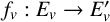 of bundle morphisms such that the induced morphisms on cohomology satisfy
$ f_{t(a)*}(y') = (f_{h(a)}\otimes 1_K)^*(y)$
of bundle morphisms such that the induced morphisms on cohomology satisfy
$ f_{t(a)*}(y') = (f_{h(a)}\otimes 1_K)^*(y)$
 , and the required squares commute for all v and a:

Definition 6. If
$(E,\phi ,x,y)$
 is a
$\overline {Q}$
is a
$\overline {Q}$
 -bundle, a
$\overline {Q}$
-bundle, a
$\overline {Q}$
 -sub-bundle consists of the data
$(E',\phi ',x',y')$
-sub-bundle consists of the data
$(E',\phi ',x',y')$
 where
$E^{\prime }_v\subseteq E_v$
where
$E^{\prime }_v\subseteq E_v$
 is a sub-bundle for all v, and such that the sections
$\phi _v,x_v,y_v$
is a sub-bundle for all v, and such that the sections
$\phi _v,x_v,y_v$
 agree with
$\phi ^{\prime }_v,x^{\prime }_v,y^{\prime }_v$
agree with
$\phi ^{\prime }_v,x^{\prime }_v,y^{\prime }_v$
 when restricted to the
$E^{\prime }_v$
when restricted to the
$E^{\prime }_v$
 . A
$\overline {Q}$
. A
$\overline {Q}$
 -subbundle will be referred to as a subbundle when the context is clear.
In order to identify
$\overline {Q}$
 -bundles with solutions to Equations (2-1) and (2-2), it is necessary to restrict to certain subsets of stable
$\overline {Q}$
-bundles with solutions to Equations (2-1) and (2-2), it is necessary to restrict to certain subsets of stable
$\overline {Q}$
 -bundles.
Definition 7. Let
$\mathcal {E}$
 be a
$\overline {Q}$
be a
$\overline {Q}$
 -bundle on X. For a tuple of real numbers
$\tau = (\tau _v)_{v\in Q_0}$
-bundle on X. For a tuple of real numbers
$\tau = (\tau _v)_{v\in Q_0}$
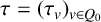 , define the degree and the
$\tau $
, define the degree and the
$\tau $
 -rank of
$\mathcal {E}$
-rank of
$\mathcal {E}$
 ,
,

The
$\tau $
 -slope of
$\mathcal {E}$
-slope of
$\mathcal {E}$
 , is then defined as

A
$\overline {Q}$
 -bundle
$\mathcal {E}$
-bundle
$\mathcal {E}$
 is semi-stable if for all subbundles
$\mathcal {E}'$
is semi-stable if for all subbundles
$\mathcal {E}'$
 , the slope satisfies
${\mu _\tau (\mathcal {E}') \leq \mu _\tau (\mathcal {E})}$
, the slope satisfies
${\mu _\tau (\mathcal {E}') \leq \mu _\tau (\mathcal {E})}$
 . It is said to be stable if the inequality is strict, and polystable if
$\mathcal {E}$
. It is said to be stable if the inequality is strict, and polystable if
$\mathcal {E}$
 is a direct sum of stable
$\overline {Q}$
is a direct sum of stable
$\overline {Q}$
 -bundles all of which have the same slope.
Remark 8.
-
(1) Given a constant $c\in \mathbb {R}$
, transforming the stability parameter
$\tau $
as
$\tau _v'=\tau _v +c$
has the effect of transforming the slope as
$\mu _{\tau '} = \mu _\tau -c$
. This does not change the stability condition, hence it is always possible to set
$\mu _\tau (\mathcal {E})=0$
, and proving stability amounts to showing
$\mu _\tau (\mathcal {E}')<0$
for all subbundles
$\mathcal {E}'$
. -
(2) The stability condition used here is not as general as that found in [Reference Álvarez-Cónsul and García-PradaAaCGP03], which depends on two stability parameters $(\sigma ,\tau )$
. However, it is expected that the current framework can be generalized without much difficulty.





Stable
$\overline {Q}$
 -bundles behave similarly to stable vector bundles. In particular, a standard proof as in [Reference KobayashiKob87, Corollary 5.7.12] shows the following proposition.
Proposition 9. If
$\mathcal {E}$
 is stable, then it is simple.
4 Stable
$\overline {Q}$
-bundles and Nakajima Representations

The ideas behind the correspondence of Nakajima quiver bundles with
$\overline {Q}$
 -bundles are not new, having been used to prove many related correspondences (see, for example, [Reference Uhlenbeck and YauUY86, Reference HitchinHit87, Reference SimpsonSim92, Reference Álvarez-Cónsul and García-PradaAaCGP03]). However, greater care is required in order to account for the higher cohomology classes that appear in the current setting. In order to do this, we work with the unique harmonic representatives
$y_a^{\mathrm {harm}}$
-bundles are not new, having been used to prove many related correspondences (see, for example, [Reference Uhlenbeck and YauUY86, Reference HitchinHit87, Reference SimpsonSim92, Reference Álvarez-Cónsul and García-PradaAaCGP03]). However, greater care is required in order to account for the higher cohomology classes that appear in the current setting. In order to do this, we work with the unique harmonic representatives
$y_a^{\mathrm {harm}}$
 of the classes
$y_a$
of the classes
$y_a$
 . This will reduce the problem to the correspondence for quiver bundles. The end result is the following correspondence relating stable
$\overline {Q}$
. This will reduce the problem to the correspondence for quiver bundles. The end result is the following correspondence relating stable
$\overline {Q}$
 -bundles with solutions of the moment map equations.
Proposition 10. Given a tuple of real numbers
$\tau =(\tau _v)_{v\in Q_0}$
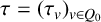 , a
$\overline {Q}$
, a
$\overline {Q}$
 -bundle
${\mathcal {E}=(E,\phi ,x,y)}$
-bundle
${\mathcal {E}=(E,\phi ,x,y)}$
 is
$\tau $
is
$\tau $
 -polystable if and only if it admits a hermitian metric h such that the Nakajima bundle representation
$\mathcal {R}=(A_h,\phi ,x,y^{\mathrm {harm}})$
-polystable if and only if it admits a hermitian metric h such that the Nakajima bundle representation
$\mathcal {R}=(A_h,\phi ,x,y^{\mathrm {harm}})$
 satisfies the moment map equations (2-3) and (2-4) for
$(\tau ,0)$
satisfies the moment map equations (2-3) and (2-4) for
$(\tau ,0)$
 .
.
One direction of the correspondence is a straightforward generalization of the argument in [Reference NakajimaNak94, Reference Álvarez-Cónsul and García-PradaAaCGP03].
Lemma 11. If
$(A,\phi ,x,y)$
 is a solution of the moment map equations, then the corresponding
$\overline {Q}$
is a solution of the moment map equations, then the corresponding
$\overline {Q}$
 -bundle
$(E,\phi ,x,y)$
-bundle
$(E,\phi ,x,y)$
 is polystable.
The remainder of this section is devoted to proving the second half of Proposition 10,
Lemma 12. If
$\mathcal {E}$
 is a
$\tau _{\mathbb {R}}$
is a
$\tau _{\mathbb {R}}$
 -polystable
$\overline {Q}$
-polystable
$\overline {Q}$
 bundle over a compact Riemann surface X such that
$\mu ^{\mathfrak {E}}_{\mathbb {C}}=0$
bundle over a compact Riemann surface X such that
$\mu ^{\mathfrak {E}}_{\mathbb {C}}=0$
 , then
$\mathcal {E}$
, then
$\mathcal {E}$
 admits a hermitian connection satisfying Equation (2-3).
4.1 Preliminaries
Fix a compact Riemann surface X, and a
$\overline {Q}$
 -bundle
$\mathcal {E}$
-bundle
$\mathcal {E}$
 such that
$\mu ^{\mathfrak {E}}_{\mathbb {C}}=0$
such that
$\mu ^{\mathfrak {E}}_{\mathbb {C}}=0$
 . For each
$v\in Q_0$
. For each
$v\in Q_0$
 , let
$\mathrm {Met}_v$
, let
$\mathrm {Met}_v$
 denote the space of hermitian metrics on the bundle
$E_v$
denote the space of hermitian metrics on the bundle
$E_v$
 . Fix a
$k_v\in \mathrm {Met}_v$
. Fix a
$k_v\in \mathrm {Met}_v$
 such that the metric on
$\mathrm {det}(E_v)$
such that the metric on
$\mathrm {det}(E_v)$
 induced by
$k_v$
induced by
$k_v$
 satisfies
$\sqrt {-1}F_{\text {det}(k_v)}=d_v$
satisfies
$\sqrt {-1}F_{\text {det}(k_v)}=d_v$
 . Given a metric
$h_v\in \mathrm {Met}_v$
. Given a metric
$h_v\in \mathrm {Met}_v$
 , denote the space of smooth
$h_v$
, denote the space of smooth
$h_v$
 -selfadjoint endomorphisms of
$E_v$
-selfadjoint endomorphisms of
$E_v$
 by
$S(h_v)$
by
$S(h_v)$
 . Any
$h_v\in \mathrm {Met}_v$
. Any
$h_v\in \mathrm {Met}_v$
 is related to
$k_v$
is related to
$k_v$
 through a section
$s_v\in S(k_v)$
through a section
$s_v\in S(k_v)$
 by
$h_v=k_v e^{s_v}$
by
$h_v=k_v e^{s_v}$
 . This notation extends to the direct sum
$E=\oplus E_v$
. This notation extends to the direct sum
$E=\oplus E_v$
 by dropping the mention of the vertex.
Recall that the adjoints of
$\phi _v$
 ,
$x_a$
,
$x_a$
 and
$y_a^{\mathrm {harm}}$
and
$y_a^{\mathrm {harm}}$
 depend on the choice of metrics
$h_v$
depend on the choice of metrics
$h_v$
 . This dependence will be denoted by
$\phi ^{*h},x^{*h}$
. This dependence will be denoted by
$\phi ^{*h},x^{*h}$
 and
$(y_a^{\mathrm {harm}})^{*h}$
and
$(y_a^{\mathrm {harm}})^{*h}$
 . If the operations are with respect to the fixed
$k_v$
. If the operations are with respect to the fixed
$k_v$
 , the operations will be denoted by
$x^*$
, the operations will be denoted by
$x^*$
 .
.
For each
$h\in \mathrm {Met}$
 , there is a metric
$h_a$
, there is a metric
$h_a$
 on
$\operatorname {\mathrm {Hom}}(E_{ta},E_{ha})$
on
$\operatorname {\mathrm {Hom}}(E_{ta},E_{ha})$
 for each
$a\in \overline {Q}_1$
for each
$a\in \overline {Q}_1$
 , given by
$(\zeta _a,\zeta _a')_{h_a} = \mathrm {tr}(\zeta _a \circ \zeta _a^{*h_a})$
, given by
$(\zeta _a,\zeta _a')_{h_a} = \mathrm {tr}(\zeta _a \circ \zeta _a^{*h_a})$
 . This gives a metric h on
$\bigoplus _a \operatorname {\mathrm {Hom}}(E_{ta},E_{ha})$
. This gives a metric h on
$\bigoplus _a \operatorname {\mathrm {Hom}}(E_{ta},E_{ha})$
 by
${(\zeta ,\zeta ') = \sum _a (\zeta _a,\zeta _a')_{h_a}}$
by
${(\zeta ,\zeta ') = \sum _a (\zeta _a,\zeta _a')_{h_a}}$
 , and the corresponding
$L^p$
, and the corresponding
$L^p$
 -inner products and norms are defined similarly.
Fix an integer
$p>2$
 . Let
$W^{p,2}S(k_v)$
. Let
$W^{p,2}S(k_v)$
 denote the Sobolev space of
$k_v$
denote the Sobolev space of
$k_v$
 -selfadjoint sections whose derivatives up to second order have finite
$L^p$
-selfadjoint sections whose derivatives up to second order have finite
$L^p$
 -norm, and
$\mathrm {Met}(W^{p,2}S(k_v)) = \{ k_v e^{s_v} : s_v \in W^{p,2}S(k_v)\}$
-norm, and
$\mathrm {Met}(W^{p,2}S(k_v)) = \{ k_v e^{s_v} : s_v \in W^{p,2}S(k_v)\}$
 . Given
$h =k e^s\in \mathrm {Met}(W^{p,2}S(k))$
. Given
$h =k e^s\in \mathrm {Met}(W^{p,2}S(k))$
 , define the h-adjoint of a section
$\xi $
, define the h-adjoint of a section
$\xi $
 by
$\xi ^{*_h}= e^{-s}\xi ^* e^s$
by
$\xi ^{*_h}= e^{-s}\xi ^* e^s$
 . Finally, define the connection
$A_{h_v}$
. Finally, define the connection
$A_{h_v}$
 by
by

with curvature
$F_{h_v} = F_{k_v} + \overline {\partial }_{E_v}(e^{-s_v}\partial _{k_v}(e^{s_v}))$
 .
.
For each vertex
$v\in Q_0$
 , let
$s_v\in S(k_v)$
, let
$s_v\in S(k_v)$
 . We consider the spectral resolution
$s_v= \sum _i \lambda _{v,i}P_{v,i}$
. We consider the spectral resolution
$s_v= \sum _i \lambda _{v,i}P_{v,i}$
 with selfadjoint projection
$P_{v,i}$
with selfadjoint projection
$P_{v,i}$
 . Let
$\psi :\mathbb {R}\to \mathbb {R}$
. Let
$\psi :\mathbb {R}\to \mathbb {R}$
 and
$\Psi :\mathbb {R}^2\to \mathbb {R}$
and
$\Psi :\mathbb {R}^2\to \mathbb {R}$
 be
$C^1$
be
$C^1$
 -bounded functions. We define fibrewise, and basis-independently,

for any
$T\in \operatorname {End}(E_v)$
 . These definitions remain valid even under eigenvalue multiplicities.
We let
$\Psi (s)$
 act on the data as bundle maps by

If
$\Psi (p,q)=\psi _1(p)\psi _2(q)$
 for functions
$\psi _1,\psi _2:\mathbb {R}\rightarrow \mathbb {R}$
for functions
$\psi _1,\psi _2:\mathbb {R}\rightarrow \mathbb {R}$
 , then

For any real number b, let
$W^{p,2}_bS(k) \subset W^{p,2}S(k)$
 be the closed subset of sections s with
$\lvert s\rvert \leq b$
be the closed subset of sections s with
$\lvert s\rvert \leq b$
 almost everywhere in X.
Lemma 13 (Surface case)
Assume
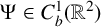
$\psi \in C^1_b(\mathbb {R})$
 and
$\Psi \in C^1_b(\mathbb {R}^2)$
and
$\Psi \in C^1_b(\mathbb {R}^2)$
 as above. If
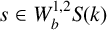
${s\in W^{1,2}_bS(k)}$
as above. If
${s\in W^{1,2}_bS(k)}$
 is selfadjoint, then for any
$q<\infty $
is selfadjoint, then for any
$q<\infty $
 the following assertions hold.
-
(1) $\psi (s)\in W^{1,2}S(k)$
with
$\|\psi (s)\|_{W^{1,2}}\le C\,(1+\|s\|_{W^{1,2}})$
. -
(2) For each vertex $v\in Q_0$
,
$\Psi (s_v)$
defines a bounded operator on
$\Omega ^0(\operatorname {End} E_v)$
and on
$\Omega ^{1,0}(\operatorname {End} E_v)$
; likewise on
$\Omega ^0(\operatorname {\mathrm {Hom}}(E_{t(a)},E_{h(a)}))$
and
$\Omega ^{0,1}(\operatorname {\mathrm {Hom}}(E_{h(a)},E_{t(a)})\!\otimes \!K)$
. -
(3) For every $q\leq 2$
, the actions in
$(2)$
extend continuously to
$\Psi (s):L^2\to L^q$
, with $$ \begin{align*} \|\Psi(s)[T]\|_{L^q} \leq C_{X,q} \|\psi_1\|_{C^1}\, \|\psi_2(s)\|_{C^1}( 1 + \|s\|_{W^{1,2}})^2 \|T\|_{L^2}. \end{align*} $$
-
(4) The actions in $(2)$
extend continuously to
$\Psi (s):L^2\to L^2$
with $$ \begin{align*} \|\Psi(s)[T]\|_{L^2} \leq \|\psi_1(s)\|_{L^\infty}\|\psi_2(s)\|_{L^\infty}\|T\|_{L^2}. \end{align*} $$













Proof. Since
$\psi \in C^1_b$
 ,
$\|\psi (\lambda _i)\|_{W^{1,2}} \leq C_i +C_i' \|\nabla \lambda _i\|^2_{L^2}$
,
$\|\psi (\lambda _i)\|_{W^{1,2}} \leq C_i +C_i' \|\nabla \lambda _i\|^2_{L^2}$
 . Then

From
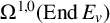
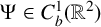
$\Psi \in C^1_b(\mathbb {R}^2)$
 ,
$(2)$
,
$(2)$
 is clear.
To see
$(3)$
 , when
$1/q=1/2 +2/p$
, when
$1/q=1/2 +2/p$
 ,
,

Since
$W^{1,2}$
 embeds into
$L^p$
embeds into
$L^p$
 for any
$p<\infty $
for any
$p<\infty $
 , the result follows from
$(1)$
, the result follows from
$(1)$
 .
.
Using the assumption that
$s\in W^{1,2}_b$
 ,
$\psi _1(s),\psi _2(s)\in W^{1,2}_b$
,
$\psi _1(s),\psi _2(s)\in W^{1,2}_b$
 as well. Then
$(4)$
as well. Then
$(4)$
 follows from Hölder’s inequality.
At this point, thinking of the tuple
$(E,\phi ,x,y^{\mathrm {harm}})$
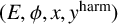 as a quiver bundle for the tripled quiver of Q, the majority of the proof is the same as that of Sections 3.3–3.7 of [Reference Álvarez-Cónsul and García-PradaAaCGP03]. The interested reader is encouraged to refer there for full details. First, construct a functional
$M_\tau $
as a quiver bundle for the tripled quiver of Q, the majority of the proof is the same as that of Sections 3.3–3.7 of [Reference Álvarez-Cónsul and García-PradaAaCGP03]. The interested reader is encouraged to refer there for full details. First, construct a functional
$M_\tau $
 on the space of metrics
$\mathrm {Met}(W^{p,2}S(k))$
on the space of metrics
$\mathrm {Met}(W^{p,2}S(k))$
 such that the metrics that minimize the functional provide solutions of the moment map equation. The existence of minimizing metrics is then shown to reduce to a particular inequality on
$M_\tau $
such that the metrics that minimize the functional provide solutions of the moment map equation. The existence of minimizing metrics is then shown to reduce to a particular inequality on
$M_\tau $
 . Finally, the regularity results of [Reference Uhlenbeck and YauUY86] are used to show that if this inequality is not satisfied, then there exists a filtration of the quiver bundle, which contradicts stability. To conclude it is necessary to relate the destabilizing quiver subbundles constructed in [Reference Álvarez-Cónsul and García-PradaAaCGP03] to subbundles of the
$\bar {Q}$
. Finally, the regularity results of [Reference Uhlenbeck and YauUY86] are used to show that if this inequality is not satisfied, then there exists a filtration of the quiver bundle, which contradicts stability. To conclude it is necessary to relate the destabilizing quiver subbundles constructed in [Reference Álvarez-Cónsul and García-PradaAaCGP03] to subbundles of the
$\bar {Q}$
 -bundle. This is accomplished by the following lemma, the proof of which is clear.
Lemma 14. Suppose
$(E,\phi ,x,y)$
 is a
$\overline {Q}$
is a
$\overline {Q}$
 -bundle. If
$(E',\phi ',x',y^{'\mathrm {harm}})$
-bundle. If
$(E',\phi ',x',y^{'\mathrm {harm}})$
 is a quiver subbundle of
$(E,\phi ,x,y^{\mathrm {harm}})$
is a quiver subbundle of
$(E,\phi ,x,y^{\mathrm {harm}})$
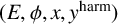 , then
$(E',\phi ',x',y')$
, then
$(E',\phi ',x',y')$
 is a
$\overline {Q}$
is a
$\overline {Q}$
 -subbundle of
$(E,\phi ,x,y)$
-subbundle of
$(E,\phi ,x,y)$
 .
.
5 Infinitesimal deformations
Let
$\mathcal {R}=(A_v,\phi _v,x_a,y_a)$
 be a representation of
$\overline {Q}$
be a representation of
$\overline {Q}$
 . In order to study deformations of
$\mathcal {R}$
. In order to study deformations of
$\mathcal {R}$
 , a complex
$C^\bullet (\mathcal {R})$
, a complex
$C^\bullet (\mathcal {R})$
 is constructed such that
$\mathbb {H}^1(C^\bullet (\mathcal {R}))$
is constructed such that
$\mathbb {H}^1(C^\bullet (\mathcal {R}))$
 corresponds to the infinitesimal deformations of
$\mathcal {R}$
corresponds to the infinitesimal deformations of
$\mathcal {R}$
 . The treatment of this section follows that of [Reference BottacinBot00] in the study of Higgs bundles on n-dimensional varieties. For the deformation theory of ordinary quiver bundles see [Reference Gothen and KingGK05]. Due to the growing number of indices in this section, in an effort to improve readability, for the remainder of this section the subscripts indicating vertices and edges are replaced with superscripts.
Let
$\mathcal {U}=\{U_i\}_{i\in I}$
 be a Čech cover of X. The cohomology classes
$(\phi ^v,x^a,y^a)$
be a Čech cover of X. The cohomology classes
$(\phi ^v,x^a,y^a)$
 defining the representation
$\mathcal {R}$
defining the representation
$\mathcal {R}$
 can be described in terms of Čech cocycles (
$\{\phi ^v_{i}\},\{x^a_i\},\{y^a_{ij}\})$
can be described in terms of Čech cocycles (
$\{\phi ^v_{i}\},\{x^a_i\},\{y^a_{ij}\})$
 .
.
For cocycles
$\{\alpha _{j_0,\ldots , j_p}^v\}_{v\in Q_0}\in \bigoplus _{v\in Q_0} C^p(\operatorname {End}(E^v))$
 define
$\{[\alpha ,x]_{j_0,\ldots , j_p}^a\}_{a\in Q_1} \in \bigoplus _{a\in Q_1} C^p(\operatorname {\mathrm {Hom}}(E^{t(a)},E^{h(a)}))$
define
$\{[\alpha ,x]_{j_0,\ldots , j_p}^a\}_{a\in Q_1} \in \bigoplus _{a\in Q_1} C^p(\operatorname {\mathrm {Hom}}(E^{t(a)},E^{h(a)}))$
 by
by

and similarly for
$[\alpha ,y]^a$
 and
$[\alpha ,\phi ]^v.$
and
$[\alpha ,\phi ]^v.$
 These define morphisms of Čech complexes

Putting these together, we define a map
![Direct sum over v in Q sub 0 of C super p (End(E super v)) maps via Psi to the direct sum over v in Q sub 0 of C super p (End(E super v) tensor K) plus the direct sum over a in Q sub 1 of [C super p (Hom(E^t(a), E^h(a))) plus C^p+1 (Hom(E^h(a), E^t(a)) tensor K)].](https://static.cambridge.org/binary/version/id/urn:cambridge.org:id:binary:20260707105544171-0955:S1446788726101542:S1446788726101542_eqnu18.png?pub-status=live)
by
$\Psi (f) = ([f,\phi ],[f,x],[f,y])$
 . Additionally, there exists a map
$\Phi $
. Additionally, there exists a map
$\Phi $
 from the codomain of
$\Psi $
from the codomain of
$\Psi $
 to
$\bigoplus _{v\in Q_0} C^{p+1}(\operatorname {End}(E^v)\otimes K)$
to
$\bigoplus _{v\in Q_0} C^{p+1}(\operatorname {End}(E^v)\otimes K)$
 given by

The desired complex of sheaves
$C^\bullet (\mathcal {R})$
 can be defined as follows. Let
$C^0(\mathcal {R}) = \bigoplus _{v\in Q_0} C^0(\operatorname {End}(E^v))$
can be defined as follows. Let
$C^0(\mathcal {R}) = \bigoplus _{v\in Q_0} C^0(\operatorname {End}(E^v))$
 , and for
$p=1,2$
, and for
$p=1,2$
 ,
,

with differentials
$d^0:C^0(\mathcal {R})\longrightarrow C^1(\mathcal {R})$
 given by
$d^0(f) = \big [\!\begin {smallmatrix}\delta \\ \Psi \end {smallmatrix}\!\big ]$
given by
$d^0(f) = \big [\!\begin {smallmatrix}\delta \\ \Psi \end {smallmatrix}\!\big ]$
 and
$d^1:C^1(\mathcal {R})\longrightarrow C^2(\mathcal {R})$
and
$d^1:C^1(\mathcal {R})\longrightarrow C^2(\mathcal {R})$
 by
by

Above,
$-\delta $
 is understood as taking in a triple of cocycles and applying minus the appropriate Čech differential to each.
Lemma 15. The first cohomology group
$\mathbb {H}^1(C^\bullet (\mathcal {R}))$
 does not depend on the choice of representatives for the
$y^a$
does not depend on the choice of representatives for the
$y^a$
 .
.
Proof. Without loss of generality we may assume Q consists of a pair of vertices connected by a single edge. Let
$(E^1,E^2,\phi ^1,\phi ^2,x,y)$
 be a
$\overline {Q}$
be a
$\overline {Q}$
 -bundle and
$y',y"$
-bundle and
$y',y"$
 two cocycles representing y. Write
$y" = y' +\delta \nu $
two cocycles representing y. Write
$y" = y' +\delta \nu $
 for
$\nu \in C^0(\operatorname {\mathrm {Hom}}(E^1,E^2)\otimes K)$
for
$\nu \in C^0(\operatorname {\mathrm {Hom}}(E^1,E^2)\otimes K)$
 . Denote by
$C^\bullet (\overline {Q},y')$
. Denote by
$C^\bullet (\overline {Q},y')$
 and
$C^\bullet (\overline {Q},y")$
and
$C^\bullet (\overline {Q},y")$
 the corresponding complexes. It is straightforward to check that the map

given by sending
$(\eta ^1,\eta ^2,\beta ^1,\beta ^2,\alpha ,\mu )$
 to
$(\eta ^1,\eta ^2,\beta ^1,\beta ^2,\alpha ,\mu +[\eta ,\nu ])$
to
$(\eta ^1,\eta ^2,\beta ^1,\beta ^2,\alpha ,\mu +[\eta ,\nu ])$
 is an isomorphism.
It is now not difficult to extend the proof of [Reference BottacinBot00, BR94] to arrive at the main result.
Theorem 16. The first cohomology
$\mathbb {H}^1(C^\bullet (\mathcal {R}))$
 corresponds to the set of infinitesimal deformations of the representation
$\mathcal {R}$
corresponds to the set of infinitesimal deformations of the representation
$\mathcal {R}$
 .
.
Proof. Given a vector bundle
$E^v$
 , a cohomology class
$\{\eta ^v_{ij}\}\in H^1(\operatorname {End}(E^v))$
, a cohomology class
$\{\eta ^v_{ij}\}\in H^1(\operatorname {End}(E^v))$
 uniquely determines a vector bundle
$E^v[\epsilon ]$
uniquely determines a vector bundle
$E^v[\epsilon ]$
 on
on ![X sub epsilon is defined as X times Spec C [epsilon] all over (epsilon-squared)](https://static.cambridge.org/binary/version/id/urn:cambridge.org:id:binary:20260707105544171-0955:S1446788726101542:S1446788726101542_inline345.png?pub-status=live) . The affine sets
. The affine sets ![U [epsilon] sub j is defined as U sub j times Spec C [epsilon] all over (epsilon-squared)](https://static.cambridge.org/binary/version/id/urn:cambridge.org:id:binary:20260707105544171-0955:S1446788726101542:S1446788726101542_inline346.png?pub-status=live) form a Čech cover of
$X_\epsilon $
form a Čech cover of
$X_\epsilon $
 .
.
Consider a deformation
$x^a[\epsilon ]:E^{t(a)}[\epsilon ] \longrightarrow E^{h(a)}[\epsilon ]$
 . This can be described by morphisms
$x^a[\epsilon ]_i: U^{t(a)}[\epsilon ]_i \longrightarrow U^{h(a)}[\epsilon ]_i$
. This can be described by morphisms
$x^a[\epsilon ]_i: U^{t(a)}[\epsilon ]_i \longrightarrow U^{h(a)}[\epsilon ]_i$
 that restrict to
$x^a$
that restrict to
$x^a$
 modulo
$\epsilon $
modulo
$\epsilon $
 and are compatible with the gluing isomorphisms
$1+\epsilon \eta ^v_{ij}$
and are compatible with the gluing isomorphisms
$1+\epsilon \eta ^v_{ij}$
 . Thus, we may write
$x^a[\epsilon ]_i = x^a +\epsilon \alpha _i^a$
. Thus, we may write
$x^a[\epsilon ]_i = x^a +\epsilon \alpha _i^a$
 for some
$\alpha ^a_i :U^{t(a)}_{i}\longrightarrow U^{h(a)}_{i}$
for some
$\alpha ^a_i :U^{t(a)}_{i}\longrightarrow U^{h(a)}_{i}$
 , and for each pair
$(i,j)$
, and for each pair
$(i,j)$
 , the following diagram commutes:
![Commutative diagram. Top-left U t(a) [epsilon] i j maps right via x^a [epsilon] i to U h(a) [epsilon] i j. Both map down via 1 + epsilon eta i j to identical terms below. Bottom-left U t(a) [epsilon] i j maps right via x^a [epsilon] j to U h(a) [epsilon] i j.](https://static.cambridge.org/binary/version/id/urn:cambridge.org:id:binary:20260707105544171-0955:S1446788726101542:S1446788726101542_eqnu23.png?pub-status=live)
Replacing the maps
$x^a[\epsilon ]_j$
 with
$x^a+\epsilon \alpha ^a_i$
with
$x^a+\epsilon \alpha ^a_i$
 , and using the fact that
$(1+\epsilon \eta _{ij}^v)^{-1} = 1-\epsilon \eta _{ij}^v$
, and using the fact that
$(1+\epsilon \eta _{ij}^v)^{-1} = 1-\epsilon \eta _{ij}^v$
 , the above diagram is equivalent to

A similar argument shows that

Now consider a deformation of
$y^a$
 , which can be described in terms of cocycles as
$y^a[\epsilon ]_{ij} = y^a + \epsilon \mu _{ij}^a$
, which can be described in terms of cocycles as
$y^a[\epsilon ]_{ij} = y^a + \epsilon \mu _{ij}^a$
 . Compatibility gives the condition

from which it follows that

Being a deformation of
$(\phi ^v,x^a,y^a)$
 , the data
$(\phi ^v[\epsilon ],x^a[\epsilon ],y^a[\epsilon ])$
, the data
$(\phi ^v[\epsilon ],x^a[\epsilon ],y^a[\epsilon ])$
 must solve the moment map equation. Explicitly, we must have that

Expanding the cocycles, and using the fact that
$(\phi ^v,x^a,y^a)$
 satisfy the moment map equation, the result follows.
Now let
$(\tilde {E}^{v}[\epsilon ],\tilde {\phi }^{v}[\epsilon ],\tilde {x}^{a}[\epsilon ], \tilde {y}^{a}[\epsilon ])$
 be a deformation that is isomorphic to
$(E^v[\epsilon ],\phi ^v[\epsilon ],x^a[\epsilon ], y^a[\epsilon ])$
be a deformation that is isomorphic to
$(E^v[\epsilon ],\phi ^v[\epsilon ],x^a[\epsilon ], y^a[\epsilon ])$
 , and corresponds to
$(\{\tilde {\eta }_{ij}^{v}\},\{\tilde {\beta }_i^{v}\},\{\tilde {\alpha }_i^{a}\},\{\tilde {\mu }_{ij}^{a}\})$
, and corresponds to
$(\{\tilde {\eta }_{ij}^{v}\},\{\tilde {\beta }_i^{v}\},\{\tilde {\alpha }_i^{a}\},\{\tilde {\mu }_{ij}^{a}\})$
 . Then it follows that
$\tilde {\eta }_{ij}^{v} = \eta _{ij}^v +(\lambda _j^v-\lambda _i^v)\lvert _{U_{ij}[\epsilon ]}$
. Then it follows that
$\tilde {\eta }_{ij}^{v} = \eta _{ij}^v +(\lambda _j^v-\lambda _i^v)\lvert _{U_{ij}[\epsilon ]}$
 , where
$\lambda ^v[\epsilon ] = 1 +\epsilon \lambda ^v$
, where
$\lambda ^v[\epsilon ] = 1 +\epsilon \lambda ^v$
 is the isomorphism
$E^{v'}[\epsilon ]\cong E^v[\epsilon ]$
is the isomorphism
$E^{v'}[\epsilon ]\cong E^v[\epsilon ]$
 . Moreover, the following diagram commutes:
![Commutative diagram: U t(a) [epsilon] i j maps via x^a [epsilon] to U h(a) [epsilon] i j. Vertical maps 1 + epsilon lambda t(a) and 1 + epsilon lambda h(a) lead to bottom row U t(a) [epsilon] i j mapping via x-tilde^a [epsilon] to U h(a) [epsilon] i j.](https://static.cambridge.org/binary/version/id/urn:cambridge.org:id:binary:20260707105544171-0955:S1446788726101542:S1446788726101542_eqnu29.png?pub-status=live)
from which we determine that
$\alpha _i^a - \tilde {\alpha }^{a}_i = [\lambda ,x]^a$
 . Similarly, it can be shown that
$\beta _i^v-\tilde {\beta }_i^{v} = [\lambda ,\phi ]^v$
. Similarly, it can be shown that
$\beta _i^v-\tilde {\beta }_i^{v} = [\lambda ,\phi ]^v$
 and
$\tilde {\mu }_{ij}^{a} =\mu _{ij}^a + [\lambda ,y]^a$
and
$\tilde {\mu }_{ij}^{a} =\mu _{ij}^a + [\lambda ,y]^a$
 . Thus, deformations correspond to cohomology classes in
$\mathbb {H}^1(C^\bullet (\mathcal {R}))$
. Thus, deformations correspond to cohomology classes in
$\mathbb {H}^1(C^\bullet (\mathcal {R}))$
 .
.
6
$\overline {Q}$
-bundles of type
$A_1$


We now consider framed quiver representations. Using the notation of [Reference GinzburgGin12], associated to any quiver Q, one can construct a new quiver
$Q^\heartsuit $
 , where
$Q^\heartsuit _0 = Q_0\sqcup Q_0$
, where
$Q^\heartsuit _0 = Q_0\sqcup Q_0$
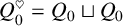 . The vertices in the second copy of
$Q_0$
. The vertices in the second copy of
$Q_0$
 are called the framing vertices and are denoted by
$w_i$
are called the framing vertices and are denoted by
$w_i$
 . The edge set
$Q^\heartsuit _1$
. The edge set
$Q^\heartsuit _1$
 consists of the edges of Q together with an edge
$v_i\rightarrow w_i$
consists of the edges of Q together with an edge
$v_i\rightarrow w_i$
 . A type vector for
$Q^\heartsuit $
. A type vector for
$Q^\heartsuit $
 is vector
$((v,d),(w,d_w))$
is vector
$((v,d),(w,d_w))$
 . Then a framed representation of
$\overline {Q}$
. Then a framed representation of
$\overline {Q}$
 is a representation of
$\overline {Q^\heartsuit }$
is a representation of
$\overline {Q^\heartsuit }$
 such that the data associated to the framing vertices is fixed. Thus, choosing a framing is equivalent to choosing an additional vector bundle
$W_v$
such that the data associated to the framing vertices is fixed. Thus, choosing a framing is equivalent to choosing an additional vector bundle
$W_v$
 of rank
$w_v$
of rank
$w_v$
 for each
$v\in Q_0$
for each
$v\in Q_0$
 .
.
Let
$Q^\heartsuit $
 be the framed
$A_1$
be the framed
$A_1$
 -quiver, pictured below with framing shown as a square vertex, and label
$((1,d),(n,0))$
-quiver, pictured below with framing shown as a square vertex, and label
$((1,d),(n,0))$
 for
$d>0$
for
$d>0$
 and
$n>1$
and
$n>1$
 :
:

In [Reference NakajimaNak94] it was shown that linear representations of
$\overline {Q^\heartsuit }$
 are isomorphic to cotangent spaces of Grassmannians.
Take
$X=\mathbb {P}^1$
 and
$\mathcal {O}^n$
and
$\mathcal {O}^n$
 as framing bundle. A framed Nakajima bundle representation of
$\overline {Q}$
as framing bundle. A framed Nakajima bundle representation of
$\overline {Q}$
 consists of a line bundle L on
$\mathbb {P}^1$
consists of a line bundle L on
$\mathbb {P}^1$
 , together with a pair
$x\in H^0(\mathbb {P}^1,\operatorname {\mathrm {Hom}}(\mathcal {O}^n,L))$
, together with a pair
$x\in H^0(\mathbb {P}^1,\operatorname {\mathrm {Hom}}(\mathcal {O}^n,L))$
 and
$y\in H^1(\mathbb {P}^1,\operatorname {\mathrm {Hom}}(L,\mathcal {O}^n)\otimes K) \cong H^0(\mathbb {P}^1,\operatorname {\mathrm {Hom}}(\mathcal {O}^n,L))^*$
and
$y\in H^1(\mathbb {P}^1,\operatorname {\mathrm {Hom}}(L,\mathcal {O}^n)\otimes K) \cong H^0(\mathbb {P}^1,\operatorname {\mathrm {Hom}}(\mathcal {O}^n,L))^*$
 . For
$\tau =(\tau _{\mathbb {R}},0)$
. For
$\tau =(\tau _{\mathbb {R}},0)$
 satisfying
${\tau _{\mathbb {R}}> d}$
satisfying
${\tau _{\mathbb {R}}> d}$
 , it follows from the real moment map that x must be surjective, hence it defines a rank
$1$
, it follows from the real moment map that x must be surjective, hence it defines a rank
$1$
 quotient bundle F of
$\mathcal {O}^n$
quotient bundle F of
$\mathcal {O}^n$
 having degree d. Moreover, from the complex moment map
$xy=0$
having degree d. Moreover, from the complex moment map
$xy=0$
 we see that
$yx \in H^1(\mathbb {P}^1,\operatorname {\mathrm {Hom}}(F,\text {ker}(x))\otimes K)$
we see that
$yx \in H^1(\mathbb {P}^1,\operatorname {\mathrm {Hom}}(F,\text {ker}(x))\otimes K)$
 . As shown in [Reference SernesiSer06], the tangent space at a point F in the Grassmannian can be identified with
$\operatorname {\mathrm {Hom}}_{\mathbb {P}^1}(F,\mathcal {O}^n/F)$
. As shown in [Reference SernesiSer06], the tangent space at a point F in the Grassmannian can be identified with
$\operatorname {\mathrm {Hom}}_{\mathbb {P}^1}(F,\mathcal {O}^n/F)$
 , so the map
$yx$
, so the map
$yx$
 lies in the cotangent space to the point defined by x. This describes a map from
$\mathcal {M}_{\overline {Q}}^{r,d}(\tau )$
lies in the cotangent space to the point defined by x. This describes a map from
$\mathcal {M}_{\overline {Q}}^{r,d}(\tau )$
 to
$T^*\text {Gr}^{d}(1,\mathcal {O}^n)$
to
$T^*\text {Gr}^{d}(1,\mathcal {O}^n)$
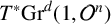 .
.
Conversely, assume that
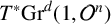
$(F,\Omega )$
 is a point in
$T^*\text {Gr}^{d}(1,\mathcal {O}^n)$
is a point in
$T^*\text {Gr}^{d}(1,\mathcal {O}^n)$
 . So
$q: \mathcal {O}^n \twoheadrightarrow F$
. So
$q: \mathcal {O}^n \twoheadrightarrow F$
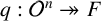 is a quotient bundle of
$\mathcal {O}^n$
is a quotient bundle of
$\mathcal {O}^n$
 having degree d and
$\Omega \in H^1(\mathbb {P}^1,\operatorname {\mathrm {Hom}}(F,\text {ker}(q))\otimes K)$
having degree d and
$\Omega \in H^1(\mathbb {P}^1,\operatorname {\mathrm {Hom}}(F,\text {ker}(q))\otimes K)$
 lies in the cotangent space at
$[q:\mathcal {O}^n \twoheadrightarrow F]$
lies in the cotangent space at
$[q:\mathcal {O}^n \twoheadrightarrow F]$
 . Consider the exact sequence

We may apply the functor
$\operatorname {\mathrm {Hom}}(F,-)\otimes K$
 to obtain a new short exact sequence

with the associated long exact sequence in cohomology

Since we are working over
$\mathbb {P}^1$
 , the
$H^0(\mathbb {P}^1,\operatorname {\mathrm {Hom}}(F,F)\otimes K)$
, the
$H^0(\mathbb {P}^1,\operatorname {\mathrm {Hom}}(F,F)\otimes K)$
 vanishes and so the map
$H^1(\mathbb {P}^1,\operatorname {\mathrm {Hom}}(F,\text {ker}(q))\otimes K) \longrightarrow H^1(\mathbb {P}^1,\operatorname {\mathrm {Hom}}(F,\mathcal {O}^n)\otimes K) $
vanishes and so the map
$H^1(\mathbb {P}^1,\operatorname {\mathrm {Hom}}(F,\text {ker}(q))\otimes K) \longrightarrow H^1(\mathbb {P}^1,\operatorname {\mathrm {Hom}}(F,\mathcal {O}^n)\otimes K) $
 is injective. Therefore, we can push forward
$\Omega $
is injective. Therefore, we can push forward
$\Omega $
 to get an element
$y\in H^1(\mathbb {P}^1,\operatorname {\mathrm {Hom}}(F,\mathcal {O}^n)\otimes K)$
to get an element
$y\in H^1(\mathbb {P}^1,\operatorname {\mathrm {Hom}}(F,\mathcal {O}^n)\otimes K)$
 . The complex moment map condition together with the above sequence implies that y is in the image of the map
$H^1(\mathbb {P}^1,\operatorname {\mathrm {Hom}}(F,\text {ker}(q))\otimes K) \longrightarrow H^1(\mathbb {P}^1,\operatorname {\mathrm {Hom}}(F,\mathcal {O}^n)\otimes K) $
. The complex moment map condition together with the above sequence implies that y is in the image of the map
$H^1(\mathbb {P}^1,\operatorname {\mathrm {Hom}}(F,\text {ker}(q))\otimes K) \longrightarrow H^1(\mathbb {P}^1,\operatorname {\mathrm {Hom}}(F,\mathcal {O}^n)\otimes K) $
 . This defines a map
$T^*\text {Gr}^d(1,\mathcal {O}^n)$
. This defines a map
$T^*\text {Gr}^d(1,\mathcal {O}^n)$
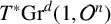 to
$\mathcal {M}_{\overline {Q}}^{r,d}(\tau )$
to
$\mathcal {M}_{\overline {Q}}^{r,d}(\tau )$
 . This describes an isomorphism between
$T^*\mathrm {Gr}^d(1,\mathcal {O}^n)$
. This describes an isomorphism between
$T^*\mathrm {Gr}^d(1,\mathcal {O}^n)$
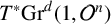 and
$\mathcal {M}_{\overline {Q}}^{r,d}(\tau )$
and
$\mathcal {M}_{\overline {Q}}^{r,d}(\tau )$
 .
.
When the genus of X is
$g\geq 1$
 , there exist nonzero sections of
$H^0(X,\operatorname {End}(L)\otimes K)$
, there exist nonzero sections of
$H^0(X,\operatorname {End}(L)\otimes K)$
 and so a representation includes a twisted endomorphism
$\phi $
and so a representation includes a twisted endomorphism
$\phi $
 . Thinking now in terms of stability, the
$\overline {Q}$
. Thinking now in terms of stability, the
$\overline {Q}$
 -bundle
$(L,\phi ,x,y)$
-bundle
$(L,\phi ,x,y)$
 is stable if and only if
$(L,\phi )$
is stable if and only if
$(L,\phi )$
 is a stable Higgs bundle of rank
$1$
is a stable Higgs bundle of rank
$1$
 , and x is surjective.
7
$\mathbb {C}^\times $
-action

In the presence of a suitable action of a torus
$\mathbb {T}$
 on a (possibly singular) variety X, the theory of Białynicki-Birula [Reference Białynicki-Birula.ByB73] establishes that the rational (co)homology of X is determined by the rational (co)homologies of the connected components of the fixed point set
$X^{\mathbb {T}}$
on a (possibly singular) variety X, the theory of Białynicki-Birula [Reference Białynicki-Birula.ByB73] establishes that the rational (co)homology of X is determined by the rational (co)homologies of the connected components of the fixed point set
$X^{\mathbb {T}}$
 . In this section we define a
$\mathbb {C}^\times $
. In this section we define a
$\mathbb {C}^\times $
 -action on Nakajima bundle varieties in an attempt to better understand the fixed points, and as a result the topology of
$\mathcal {M}_{\overline {Q}}^{r,d}(\tau )$
-action on Nakajima bundle varieties in an attempt to better understand the fixed points, and as a result the topology of
$\mathcal {M}_{\overline {Q}}^{r,d}(\tau )$
 . In general, even in the case of vector space representations, a full description of the fixed points is difficult. Therefore, we focus on the specific case of the framed
$A_1$
. In general, even in the case of vector space representations, a full description of the fixed points is difficult. Therefore, we focus on the specific case of the framed
$A_1$
 quiver.
Recall the
$\mathbb {C}^\times $
 -actions on the moduli space of Higgs bundles and on Nakajima quiver varieties that scale the cotangent directions. In the same way there is an action of
$\mathbb {C}^\times $
-actions on the moduli space of Higgs bundles and on Nakajima quiver varieties that scale the cotangent directions. In the same way there is an action of
$\mathbb {C}^\times $
 on
$\mathcal {M}_{\overline {Q}}^{r,d}(\tau )$
on
$\mathcal {M}_{\overline {Q}}^{r,d}(\tau )$
 that preserves the moment map conditions
$\mu _{\mathbb {R}}=\tau _{\mathbb {R}},\; \mu _{\mathbb {C}} = 0$
that preserves the moment map conditions
$\mu _{\mathbb {R}}=\tau _{\mathbb {R}},\; \mu _{\mathbb {C}} = 0$
 . If
$(E,\phi ,x,y)$
. If
$(E,\phi ,x,y)$
 is a
$\overline {Q}$
is a
$\overline {Q}$
 -bundle, the action of
$\lambda \in \mathbb {C}^\times $
-bundle, the action of
$\lambda \in \mathbb {C}^\times $
 is given by
$\lambda \cdot (E,\phi ,x,y) =(E,\lambda \phi ,x,\lambda y).$
is given by
$\lambda \cdot (E,\phi ,x,y) =(E,\lambda \phi ,x,\lambda y).$

For the remainder of this section, assume the genus of X is not
$1$
 . If
$(E,\phi ,x,y)$
. If
$(E,\phi ,x,y)$
 is a fixed point, there exists a one-parameter family of gauge transformations
$g_\lambda $
is a fixed point, there exists a one-parameter family of gauge transformations
$g_\lambda $
 such that

For each
$E_v\in Q_0$
 let
$E_v=\oplus _i E_v^{w_i}$
let
$E_v=\oplus _i E_v^{w_i}$
 be the weight decomposition of
$E_v$
be the weight decomposition of
$E_v$
 , in which
$\mathbb {C}^\times $
, in which
$\mathbb {C}^\times $
 acts on
$E_v^{w_i}$
acts on
$E_v^{w_i}$
 with weight
$w_i$
with weight
$w_i$
 . Being a fixed point of the action implies

We work with the specific example of the
$\mathbb {C}^\times $
 -action on
$\mathcal {M}_{\overline {Q}}^{r,d}(\tau )$
-action on
$\mathcal {M}_{\overline {Q}}^{r,d}(\tau )$
 , where Q is the framed
$A_1$
, where Q is the framed
$A_1$
 quiver. From the fixed-point equations, a point
$(\phi ,x,y)$
quiver. From the fixed-point equations, a point
$(\phi ,x,y)$
 is fixed if there exists a one-parameter subgroup
$g_\lambda $
is fixed if there exists a one-parameter subgroup
$g_\lambda $
 such that for all
$\lambda $
such that for all
$\lambda $
 we have

By stability, x is surjective, and therefore the only fixed points are of the form
$(0,x,0)$
 and the fixed-point set coincides with the
$\mathrm {Gr}^d(1,\mathcal {O}^n)$
and the fixed-point set coincides with the
$\mathrm {Gr}^d(1,\mathcal {O}^n)$
 .
.
Replace the framing vertex with an unframed vertex. We are interested in the action

Using the weight space decomposition of
$E_1,E_2$
 , it is straightforward to verify that the fixed points can be described as pairs of holomorphic chains given by the
$\phi _i:E_i^{w_i}\to E_i^{w_i-1}\otimes K$
, it is straightforward to verify that the fixed points can be described as pairs of holomorphic chains given by the
$\phi _i:E_i^{w_i}\to E_i^{w_i-1}\otimes K$
 , intertwined by the
$x^k$
, intertwined by the
$x^k$
 and
$y^k$
and
$y^k$
 data. Such a fixed point is shown in Figure 1. A more refined description, such as the length of the chains involved, will depend on stability and the topological type of the bundles
$E_1,E_2$
data. Such a fixed point is shown in Figure 1. A more refined description, such as the length of the chains involved, will depend on stability and the topological type of the bundles
$E_1,E_2$
 .
.
A fixed point for the
$\mathbb {C}^\times $
 -action on the unframed
$A_1$
-action on the unframed
$A_1$
 quiver.

If
$\lvert Q_0\rvert =n$
 , the action above can be generalized to an action of the product
$(\mathbb {C}^\times )^n$
, the action above can be generalized to an action of the product
$(\mathbb {C}^\times )^n$
 on
$\mathcal {M}_{\overline {Q}}^{r,d}(\tau )$
on
$\mathcal {M}_{\overline {Q}}^{r,d}(\tau )$
 . For
$\lambda = (\lambda _1,\ldots , \lambda _n)\in (\mathbb {C}^\times )^n$
. For
$\lambda = (\lambda _1,\ldots , \lambda _n)\in (\mathbb {C}^\times )^n$
 , the action scales
$\phi $
, the action scales
$\phi $
 by
$\lambda _v$
by
$\lambda _v$
 and y by
$\lambda _{t(a)}$
and y by
$\lambda _{t(a)}$
 .
.
A representation
$(A,\phi ,x,y)$
 is now a fixed point if there exists a homomorphism
$g:(\mathbb {C}^\times )^n\rightarrow \mathcal {G}$
is now a fixed point if there exists a homomorphism
$g:(\mathbb {C}^\times )^n\rightarrow \mathcal {G}$
 such that

From here, the same argument as for Higgs bundles shows that in order for
$\mathcal {E}= (E,\phi ,x,y)$
 to be a fixed point,
$\phi _v$
to be a fixed point,
$\phi _v$
 must be nilpotent for all v.
However, unlike in the case of ordinary Higgs bundles, the
$\phi _v$
 being nilpotent does not provide a sufficient condition for
$\mathcal {E}$
being nilpotent does not provide a sufficient condition for
$\mathcal {E}$
 to be fixed. As example, let
${\mathcal {E}=(E_1,E_2,\phi _1,\phi _2,x,y)}$
to be fixed. As example, let
${\mathcal {E}=(E_1,E_2,\phi _1,\phi _2,x,y)}$
 be a
$\overline {Q}$
be a
$\overline {Q}$
 -bundle on the unframed
$A_1$
-bundle on the unframed
$A_1$
 quiver. Suppose
${E_1\cong E_2\cong \mathcal {O}_X\oplus \mathcal {O}_X}$
quiver. Suppose
${E_1\cong E_2\cong \mathcal {O}_X\oplus \mathcal {O}_X}$
 and
and

Defining the nilpotent cone inside of
$\mathcal {M}_{\overline {Q}}(\tau )$
 to be those Nakajima representations with all Higgs fields
$\phi _v$
to be those Nakajima representations with all Higgs fields
$\phi _v$
 nilpotent, all fixed points for the torus action are constrained to live inside the nilpotent cone.
As the underlying quiver becomes more complicated and as the ranks and degrees involved grow larger, the analysis of the fixed points becomes markedly more difficult. In the absence of a systematic approach, the understanding of the fixed points of the action relies on a case-by-case approach. However, once this is accomplished, the Białynicki-Birula decomposition of
$\mathcal {M}_{\overline {Q}}^{r,d}(\tau )$
 in terms of the fixed-point sets should allow for a more complete understanding of the topology of Nakajima bundle varieties.
On a more speculative note, the fixed points of the
$\mathbb {C}^\times $
 -action on the moduli space of Higgs bundles play an important role in understanding both the Hitchin system and Nakajima quiver varieties. The Hitchin system leads to a proper morphism
${\mathcal {H}:\mathcal {M}^{\text {Higgs}}(X)\rightarrow \mathcal {B}}$
-action on the moduli space of Higgs bundles play an important role in understanding both the Hitchin system and Nakajima quiver varieties. The Hitchin system leads to a proper morphism
${\mathcal {H}:\mathcal {M}^{\text {Higgs}}(X)\rightarrow \mathcal {B}}$
 to an affine space
$\mathcal {B}$
to an affine space
$\mathcal {B}$
 , sending a Higgs field to the coefficients of its characteristic polynomial. The fixed points of the
$\mathbb {C}^\times $
, sending a Higgs field to the coefficients of its characteristic polynomial. The fixed points of the
$\mathbb {C}^\times $
 -action all reside in the nilpotent cone
$\mathcal {H}^{-1}(0)$
-action all reside in the nilpotent cone
$\mathcal {H}^{-1}(0)$
 of Higgs bundles
$(E,\phi )$
of Higgs bundles
$(E,\phi )$
 with nilpotent
$\phi $
with nilpotent
$\phi $
 . Given the presence of integrable systems on Nakajima quiver varieties [Reference Fisher and RayanFR16, Reference Rayan and SchaposnikRS21], as well as the similarities between Nakajima bundle varieties and Higgs moduli, the fixed points might facilitate a deeper understanding of the relationship between these systems.
Acknowledgments
The second-named author gratefully acknowledges support from the Simons Center for Geometry and Physics where important progress was made during the second Simons Math Summer Workshop (‘Moduli’) in July 2024. The second-named author was partially supported by an Ontario Graduate Scholarship and by the NSERC Discovery Grants of the other co-authors. The second- and third-named authors thank Mahmud Azam, Kuntal Banerjee, Eric Boulter, Robert Cornea, and Evan Sundbo for useful discussions, and all three authors acknowledge Eckhard Meinrenken and Nick Rozenblyum for helpful remarks and questions during the early stages of the work, as well as the anonymous referee for valuable feedback on earlier versions of this work.
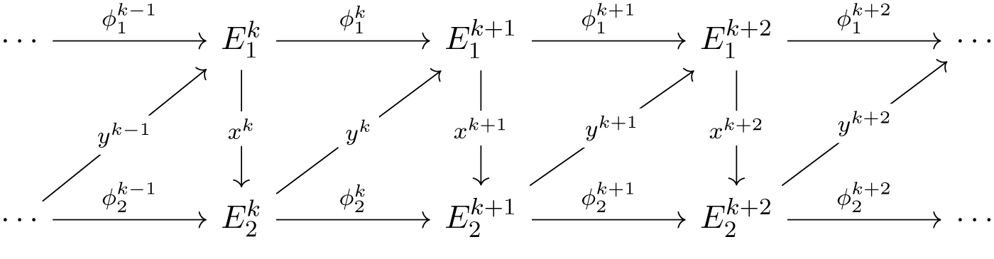


 Open access

