


1. Introduction
Robotic impedance control and stiffness control (and several of their variations) at the task-space level [Reference Villani, De Schutter, Sicilianoi and Khatib1–Reference Kao and Saldarriaga6] models the end-effector of the robot as a multidimensional mass-damper-spring system and has become a popular choice to control the dynamic behavior of a robotic manipulator physically interacting with its environment. A compliant behavior during interaction is desired for many robotic applications, in such a way that the contact forces and moments are within a preferred range and the motion of the end-effector is accurate. In order to perform according to a prescribed dynamic behavior based on the specific robotic task requirements, the impedance parameters of stiffness and damping need to be specified and should not be arbitrarily chosen [Reference Saldarriaga, Chakraborty and Kao7].
A serial robot manipulator with $n$
degrees of freedom (DOF) is said to be kinematically redundant if the dimension of the joint space is greater than the dimension of the task space
$n$
degrees of freedom (DOF) is said to be kinematically redundant if the dimension of the joint space is greater than the dimension of the task space $m$
, i.e.,
$m$
, i.e., $n\gt m$
. As a result of the redundancy, a desired pose (position and orientation) of the robot end-effector may have infinite possible joint configurations [Reference Siciliano, Sciavicco, Villani and Oriolo8]. In the context of impedance control, such redundancy will result in the zero-potential-energy (ZP) motions [Reference Kao and Saldarriaga9, Reference Saldarriaga and Kao10]. The ZP motions are the displacements of a redundant system in impedance control that minimize the potential energy due to the stiffness matrix. In ref. [Reference Saldarriaga and Kao10], the ZP motions of a redundant robot in impedance control were derived and experimentally validated using a 7-DOF Franka Emika Panda robot [Reference Haddadin, Parusel, Johannsmeier, Golz, Gabl, Walch, Sabaghian, Jähne, Hausperger and Haddadin11]. With the (
$n\gt m$
. As a result of the redundancy, a desired pose (position and orientation) of the robot end-effector may have infinite possible joint configurations [Reference Siciliano, Sciavicco, Villani and Oriolo8]. In the context of impedance control, such redundancy will result in the zero-potential-energy (ZP) motions [Reference Kao and Saldarriaga9, Reference Saldarriaga and Kao10]. The ZP motions are the displacements of a redundant system in impedance control that minimize the potential energy due to the stiffness matrix. In ref. [Reference Saldarriaga and Kao10], the ZP motions of a redundant robot in impedance control were derived and experimentally validated using a 7-DOF Franka Emika Panda robot [Reference Haddadin, Parusel, Johannsmeier, Golz, Gabl, Walch, Sabaghian, Jähne, Hausperger and Haddadin11]. With the ( $n-m$
) degrees of redundancy (DOR), a null-space control [Reference Khatib4, Reference Siciliano, Sciavicco, Villani and Oriolo8, Reference Tsuji, Jazidie and Kaneko12–Reference Dietrich, Ott and Albu-Schaffer14] can be applied to leverage the redundancy in impedance control.
$n-m$
) degrees of redundancy (DOR), a null-space control [Reference Khatib4, Reference Siciliano, Sciavicco, Villani and Oriolo8, Reference Tsuji, Jazidie and Kaneko12–Reference Dietrich, Ott and Albu-Schaffer14] can be applied to leverage the redundancy in impedance control.
In this paper, we present an analysis of the dynamic response of redundant robot manipulators under impedance control by applying the methodology of modal analysis originally proposed in ref. [Reference Kao and Saldarriaga9]. The modal analysis converts the coupled mass, damping, and stiffness matrices in the physical coordinates of the robot, after mapping them from the Cartesian space to the joint space, to modal coordinates where the matrices of impedance control are decoupled into independent modal coordinates. The expansion theorem stipulates that the dynamic response of the impedance control in the physical Cartesian space will be the linear combination of the modal responses, according to the expansion theorem [Reference Meirovitch15]. Consequently, the dynamic parameters of the independent modal coordinates, including the natural frequencies and damping ratios, will determine the responses in the physical space. This methodology of modal analysis provides a straightforward and useful tool to gain insights into the impedance control of redundant and non-redundant robot manipulators.
By using this analytical methodology, we will show that the results and the claims regarding null-space control and dynamic response of impedance control of a recent article [Reference Hermus, Lachner, Verdi and Hogan16] are not generally true, but is only valid based on the specially chosen parameters (and configuration). In addition, we conducted experiments to compare different choices for the parameters of the stiffness and damping matrices and their influence on dynamic responses based on theoretical analysis, considering different DOR. We also show preliminary results of a controller that can mitigate undesired overshoot in the transient responses of the null-space control using a switching strategy, based on the understanding of the dynamic behavior, afforded by the methodology.
The main contribution of this paper includes (1) a general formulation of the dynamics of redundant robotic manipulators performing primary and secondary impedance control tasks, based on an analytical solution, not trial and error, (2) a presentation of the physical insights into the modulation of the dynamic response by changing the primary and secondary stiffness and damping matrices, while considering null space control, for a prescribed trajectory of the end-effector, improving steady-state errors (a methodology for the robot at a given equilibrium configuration has been validated in ref. [Reference Saldarriaga, Chakraborty and Kao7]), we also demonstrated experimentally the general minimization of the kinetic energy when working with dynamically consistent projection matrices ( $\mathbf{W}=\mathbf{M}$
), and (3) a pilot study on the reduction in transient responses, when applying the dynamically consistent weighting matrix in the null-space control, through an empirical switching strategy using experimental data.
$\mathbf{W}=\mathbf{M}$
), and (3) a pilot study on the reduction in transient responses, when applying the dynamically consistent weighting matrix in the null-space control, through an empirical switching strategy using experimental data.
2. Related work
The methodology of modal analysis of impedance control for robotic manipulators was presented in ref. [Reference Kao and Saldarriaga9], with details in theoretical analysis and experimental results modulating the dynamic response of redundant robotic systems through stiffness and damping parameters. In order to provide the context, certain equations are presented in Section 3. The readers may want to consult [Reference Kao and Saldarriaga9] for a full treatment of the methodology.
Recent work has been published on the topic of tuning impedance parameters, such as [Reference Pollayil, Angelini, Xin, Mistry, Vijayakumar, Bicchi and Garabini17], where the authors deal with the reshaping of inertia, and several assumptions are made. Several encouraging results have been proposed using different approaches, such as learning [Reference Wu, Zhao, Tao and Ajoudani18–Reference Patino, Encalada-Davila, Sampietro, Tutiven, Saldarriaga and Kao21].
In addition, it is known that having redundant DOFs allows the robot to perform more than one task or objectives while satisfying different constraints [Reference Fiore, Meli, Ziese, Siciliano and Natale22] if the redundancy is resolved or managed in a proper manner, either analytically or by optimization methods [Reference Hoffman, Laurenzi, Muratore, Tsagarakis and Caldwell23].
2.1. Multiple redundancies and null-space control
In the case of a robot with 7 DOF, we can decide to describe the primary Cartesian impedance task with only 3 (translational) coordinates ( $m=3$
and
$m=3$
and $n-m=4$
). The null-space or secondary task will have up to four DOFs to satisfy or impose its corresponding motions.
$n-m=4$
). The null-space or secondary task will have up to four DOFs to satisfy or impose its corresponding motions.
In terms of the modal analysis of the redundant system [Reference Saldarriaga, Chakraborty and Kao7], this means that only three modes of motion will be specified for the primary task once all the ( $n-m$
) ZP modes are successively removed from the system [Reference Kao and Saldarriaga9].
$n-m$
) ZP modes are successively removed from the system [Reference Kao and Saldarriaga9].
As seen in a recent publication [Reference Hermus, Lachner, Verdi and Hogan16], without analysis or justification, for a given configuration $\mathbf{q}_0$
of a Kuka LBR manipulator, the Cartesian and null-space impedance parameters were chosen for both primary and secondary tasks, including stiffness and damping matrices, without considering inertia reshaping. One of the main claims from the authors of this paper [Reference Hermus, Lachner, Verdi and Hogan16] was that impedance superposition, or simply adding the impedance parameters without any null-space projection matrix, makes little or no difference when comparing the experimental results with those using statically and dynamically consistent null-space projection matrices, especially in cases of more than one redundant degree of freedom.
$\mathbf{q}_0$
of a Kuka LBR manipulator, the Cartesian and null-space impedance parameters were chosen for both primary and secondary tasks, including stiffness and damping matrices, without considering inertia reshaping. One of the main claims from the authors of this paper [Reference Hermus, Lachner, Verdi and Hogan16] was that impedance superposition, or simply adding the impedance parameters without any null-space projection matrix, makes little or no difference when comparing the experimental results with those using statically and dynamically consistent null-space projection matrices, especially in cases of more than one redundant degree of freedom.
We will present analysis in the following by applying the theoretical methodology [Reference Saldarriaga, Chakraborty and Kao7, Reference Kao and Saldarriaga9] to show that this claim is only true in special cases depending, among other things, on the chosen sets of parameters or robot configurations, and should not be held as generally valid. The methodology determines the modal natural frequencies ( $\omega _n$
) and damping ratios (
$\omega _n$
) and damping ratios ( $\zeta$
) in the modal space of impedance control, which determines the dynamic responses of the system in the physical space through a linear combination of the modal responses dictated by
$\zeta$
) in the modal space of impedance control, which determines the dynamic responses of the system in the physical space through a linear combination of the modal responses dictated by $\omega _n$
and
$\omega _n$
and $\zeta$
, as stipulated by the expansion theorem.
$\zeta$
, as stipulated by the expansion theorem.
By analyzing the results presented in ref. [Reference Hermus, Lachner, Verdi and Hogan16], the corresponding $\omega _n$
and
$\omega _n$
and $\zeta$
for the set of primary and secondary stiffness and damping values that the authors used for 3-DOF Cartesian impedance control (with 4 DOR) is compared in Table I with a dynamically consistent null-space projection matrix
$\zeta$
for the set of primary and secondary stiffness and damping values that the authors used for 3-DOF Cartesian impedance control (with 4 DOR) is compared in Table I with a dynamically consistent null-space projection matrix $\mathbf{W}=\mathbf{M}(\mathbf{q}_0)$
and superposition of impedances with
$\mathbf{W}=\mathbf{M}(\mathbf{q}_0)$
and superposition of impedances with $\mathbf{N}=\mathbf{I}$
, respectively.Footnote
1
From Table I, we observe that not all modes are well-damped and the modal
$\mathbf{N}=\mathbf{I}$
, respectively.Footnote
1
From Table I, we observe that not all modes are well-damped and the modal $\omega _n$
and
$\omega _n$
and $\zeta$
are nearly the same between the corresponding poles of both cases, due to the chosen impedance parameters. This explains the observation of almost identical behavior in the experimental results in ref. [Reference Hermus, Lachner, Verdi and Hogan16], although it is not because of the difference in the null-space controls.
$\zeta$
are nearly the same between the corresponding poles of both cases, due to the chosen impedance parameters. This explains the observation of almost identical behavior in the experimental results in ref. [Reference Hermus, Lachner, Verdi and Hogan16], although it is not because of the difference in the null-space controls.
Performing a similar comparison, now with 6-DOF Cartesian impedance control (1 DOR), using the same stiffness and damping values that the authors [Reference Hermus, Lachner, Verdi and Hogan16] used, we can find the results in Table II. We observed that the superposed (when $\mathbf{N}=\mathbf{I}$
) impedance parameters are changing the dynamics of the system (damping ratios) in a significant manner, especially in the dominant modes of
$\mathbf{N}=\mathbf{I}$
) impedance parameters are changing the dynamics of the system (damping ratios) in a significant manner, especially in the dominant modes of $\lambda _{3,4}$
,
$\lambda _{3,4}$
, $\lambda _{5,6}$
and
$\lambda _{5,6}$
and $\lambda _{7,8}$
, which explains the differences in the experimental results presented in ref. [Reference Hermus, Lachner, Verdi and Hogan16].
$\lambda _{7,8}$
, which explains the differences in the experimental results presented in ref. [Reference Hermus, Lachner, Verdi and Hogan16].
Comparison of modal $\omega _n$
and
$\omega _n$
and $\zeta$
of a 7-DOF Kuka robot with 4 degrees of redundancy, and
$\zeta$
of a 7-DOF Kuka robot with 4 degrees of redundancy, and $\mathbf{W}=\mathbf{M}$
or
$\mathbf{W}=\mathbf{M}$
or $\mathbf{N}=\mathbf{I}$
.
$\mathbf{N}=\mathbf{I}$
.

Table I. Long description
A table comparing modal and values of a 7-DOF Kuka robot with 4 degrees of redundancy, and or . The table has two cases, each with 7 columns and 2 rows. The columns are labeled with lambda subscripts and the rows are labeled with omega sub n and zeta. Case I: W equals M of q0 has values for lambda sub 1,2 to lambda sub 13,14. Case II: N equals I has values for lambda sub 1,2 to lambda sub 13,14. The values in the table show the comparison of modal and values for the two cases. Notable trends include the similarity in modal and values between the corresponding poles of both cases, indicating nearly identical behavior in experimental results.
In this paper, we will demonstrate how the experimental results and the selection of the parameters can lead to responses that are similar when having different choices of weighting matrix of the null-space control using a redundant robot, and explain in more detail the outcomes of responses. In general, we will show that the choice of different parameters and weighting matrix of the null-space control can affect the responses of redundant robotic manipulators in their corresponding primary and secondary tasks [Reference Kao and Saldarriaga9].
This paper is structured as follows. First, we present an abridged theoretical background of the methodology of modal analysis for impedance control in Section 3. After that, various experimental results using a 7-DOF Franka Emika Panda robot are presented in Section 4. This is followed by a switching strategy of null-space controls to reduce transient responses in Section 5.4. Discussion is presented in Section 5 with insights into the results using impedance control.
Comparison of modal $\omega _n$
and
$\omega _n$
and $\zeta$
of a 7-DOF Kuka robot with one degree of redundancy, and
$\zeta$
of a 7-DOF Kuka robot with one degree of redundancy, and $\mathbf{W}=\mathbf{M}$
or
$\mathbf{W}=\mathbf{M}$
or $\mathbf{N}=\mathbf{I}$
.
$\mathbf{N}=\mathbf{I}$
.

Table II. Long description
The table presents a comparison of modal values and damping ratios for a 7-DOF Kuka robot with four degrees of redundancy. It includes two cases, each with seven modal values and seven corresponding damping ratios. Case I shows values such as 1.61, 3.12, 4.72, 8.71, 18.2, 19.2, and 21.6 for the modal values, and 0.213, 0.157, 0.229, 0.0822, 0.175, 0.958, and 0.239 for the damping ratios. Case II shows values such as 1.58, 2.91, 4.53, 9.09, 19.3, 19.2, and 23.3 for the modal values, and 0.207, 0.151, 0.224, 0.121, 0.234, 0.959, and 0.289 for the damping ratios. The table highlights the differences in the dynamics of the system, particularly in the dominant modes.
3. Theoretical background
3.1. Redundancy resolution
Let $m \leq 6$
be the dimension of the task space of an
$m \leq 6$
be the dimension of the task space of an $n$
-DOF serial robot manipulator,
$n$
-DOF serial robot manipulator, $\mathbf{q} \in \mathbb{R}^n$
be the state vector of the joint angles, and
$\mathbf{q} \in \mathbb{R}^n$
be the state vector of the joint angles, and $\mathbf{x} \in \mathbb{R}^m$
be the state vector of the task space. The relation between the torques of the joints
$\mathbf{x} \in \mathbb{R}^m$
be the state vector of the task space. The relation between the torques of the joints $\boldsymbol{\tau }$
and the forces at the robot end-effector
$\boldsymbol{\tau }$
and the forces at the robot end-effector $\mathbf{f}$
is given by
$\mathbf{f}$
is given by $\boldsymbol{\tau }=\mathbf{J(\mathbf{q})}^T \mathbf{f}$
where
$\boldsymbol{\tau }=\mathbf{J(\mathbf{q})}^T \mathbf{f}$
where $\mathbf{J}(\mathbf{q}) \in \mathbb{R}^{m \times n}$
is the configuration-dependent Jacobian matrix which relates the vector of joint angle rates
$\mathbf{J}(\mathbf{q}) \in \mathbb{R}^{m \times n}$
is the configuration-dependent Jacobian matrix which relates the vector of joint angle rates $\dot {\mathbf{q}}$
of the manipulator to the end-effector pose rate
$\dot {\mathbf{q}}$
of the manipulator to the end-effector pose rate $\dot {\mathbf{x}}$
by
$\dot {\mathbf{x}}$
by $\dot {\mathbf{x}} = \mathbf{J} \dot {\mathbf{q}}$
. We will use
$\dot {\mathbf{x}} = \mathbf{J} \dot {\mathbf{q}}$
. We will use $\mathbf{J}$
to denote
$\mathbf{J}$
to denote $\mathbf{J(\mathbf{q})}$
hereafter.
$\mathbf{J(\mathbf{q})}$
hereafter.
For redundant manipulators where $n \gt m$
, we define
$n \gt m$
, we define $(n-m)$
as the degree of redundancy (DOR). The dimension of the null space of
$(n-m)$
as the degree of redundancy (DOR). The dimension of the null space of $\mathbf{J}$
is
$\mathbf{J}$
is $n-m$
. We can write
$n-m$
. We can write $\mathbf{f} = (\mathbf{J}^T)^+\boldsymbol{\tau }$
, where
$\mathbf{f} = (\mathbf{J}^T)^+\boldsymbol{\tau }$
, where $({\cdot})^+$
is the Penrose-Moore inverse, defined to render
$({\cdot})^+$
is the Penrose-Moore inverse, defined to render $\mathbf{J}\mathbf{J}^+=\mathbf{I}$
, and can be computed by
$\mathbf{J}\mathbf{J}^+=\mathbf{I}$
, and can be computed by
 \begin{equation} \mathbf{J}^{+}=\mathbf{W}^{-1} \mathbf{J}^T\left (\mathbf{J} \mathbf{W}^{-1} \mathbf{J}^T\right )^{-1} \end{equation}
where $\mathbf{W} \in \mathbb{R}^{n \times n}$
is an arbitrary weighting matrix. The matrices
$\mathbf{W} \in \mathbb{R}^{n \times n}$
is an arbitrary weighting matrix. The matrices $\mathbf{J}$
,
$\mathbf{J}$
, $\mathbf{J}^T$
, and
$\mathbf{J}^T$
, and $(\mathbf{J}^T)^+$
have at most a rank of
$(\mathbf{J}^T)^+$
have at most a rank of $m$
. The joint torque vectors in the null space of
$m$
. The joint torque vectors in the null space of $(\mathbf{J}^T)^+$
do not affect the wrench generated at the robot end-effector.
$(\mathbf{J}^T)^+$
do not affect the wrench generated at the robot end-effector.
The equation $\boldsymbol{\tau }=\mathbf{J}^T \mathbf{f}$
for redundant manipulators can include the null-space control, written as
$\boldsymbol{\tau }=\mathbf{J}^T \mathbf{f}$
for redundant manipulators can include the null-space control, written as
 \begin{equation} \boldsymbol{\tau }=\mathbf{J}^T \mathbf{f} + \mathbf{N}\boldsymbol{\tau }^* \end{equation}
where $\boldsymbol{\tau }^* \in \mathbb{R}^n$
is an arbitrary vector and
$\boldsymbol{\tau }^* \in \mathbb{R}^n$
is an arbitrary vector and $\mathbf{N} \in \mathbb{R}^{n \times n}$
is the null-space projection matrix of
$\mathbf{N} \in \mathbb{R}^{n \times n}$
is the null-space projection matrix of $(\mathbf{J}^T)^+$
, calculated by
$(\mathbf{J}^T)^+$
, calculated by
 \begin{equation} \mathbf{N}=\mathbf{I} - \mathbf{J}^T(\mathbf{J}^T)^+ \end{equation}
where $\mathbf{I}$
is a
$\mathbf{I}$
is a $n \times n$
identity matrix. Therefore, we can consider
$n \times n$
identity matrix. Therefore, we can consider $\mathbf{J}^T \mathbf{f}$
in Eq. (2) as a torque vector required to perform the primary task and
$\mathbf{J}^T \mathbf{f}$
in Eq. (2) as a torque vector required to perform the primary task and $\mathbf{N}\boldsymbol{\tau }^*$
as a torque vector required to perform a feasible secondary task
$\mathbf{N}\boldsymbol{\tau }^*$
as a torque vector required to perform a feasible secondary task $\boldsymbol{\tau }^*$
, but projected in the null space of the primary task. This term can also be modified to handle several simultaneous lower-priority tasks using successive or augmented methods without interfering with the primary task [Reference Dietrich, Ott and Albu-Schaffer14]. Note that since the secondary tasks are projected in the null space of the primary task, they are performed either fully or partially. From here on, we assume only two tasks, the primary and the secondary tasks, with their corresponding hierarchy, but it can include as many tasks as physically plausible.
$\boldsymbol{\tau }^*$
, but projected in the null space of the primary task. This term can also be modified to handle several simultaneous lower-priority tasks using successive or augmented methods without interfering with the primary task [Reference Dietrich, Ott and Albu-Schaffer14]. Note that since the secondary tasks are projected in the null space of the primary task, they are performed either fully or partially. From here on, we assume only two tasks, the primary and the secondary tasks, with their corresponding hierarchy, but it can include as many tasks as physically plausible.
In this paper, we consider three different cases of secondary control tasks in Eqs. (1) and (3): (i) dynamically consistent $\mathbf{W}=\mathbf{M}$
, (ii) statically consistent
$\mathbf{W}=\mathbf{M}$
, (ii) statically consistent $\mathbf{W}=\mathbf{I}$
, and (iii) superposition
$\mathbf{W}=\mathbf{I}$
, and (iii) superposition $\mathbf{N}=\mathbf{I}$
, where
$\mathbf{N}=\mathbf{I}$
, where $\mathbf{N}$
is independent of
$\mathbf{N}$
is independent of $\mathbf{J}$
and
$\mathbf{J}$
and $\mathbf{W}=\mathbf{0}$
.
$\mathbf{W}=\mathbf{0}$
.
3.2. Joint-space and task-space impedance control
Impedance control imposes mass-spring-damper behavior on the interaction between the robot and the environment, either in task space or joint space. Let’s consider the robot’s dynamic equations with $\boldsymbol{\tau }=\mathbf{M}_q \ddot {\mathbf{q}}+\mathbf{c}(\mathbf{q}, \dot {\mathbf{q}})+\mathbf{g}(\mathbf{q})+\boldsymbol{\tau }_{\mathrm{ext}}$
with
$\boldsymbol{\tau }=\mathbf{M}_q \ddot {\mathbf{q}}+\mathbf{c}(\mathbf{q}, \dot {\mathbf{q}})+\mathbf{g}(\mathbf{q})+\boldsymbol{\tau }_{\mathrm{ext}}$
with $\mathbf{M}_q$
being the mass matrix of the manipulator,
$\mathbf{M}_q$
being the mass matrix of the manipulator, $\mathbf{c}(\mathbf{q}, \dot {\mathbf{q}})$
a vector of Coriolis and Centripetal terms,
$\mathbf{c}(\mathbf{q}, \dot {\mathbf{q}})$
a vector of Coriolis and Centripetal terms, $\mathbf{g}(\mathbf{q})$
a vector of gravitational terms, and
$\mathbf{g}(\mathbf{q})$
a vector of gravitational terms, and $\boldsymbol{\tau }_{\mathrm{ext}}$
the joint torque. Let’s adopt the impedance control in the joint and task spaces as follows,
$\boldsymbol{\tau }_{\mathrm{ext}}$
the joint torque. Let’s adopt the impedance control in the joint and task spaces as follows,
 \begin{eqnarray} \mathbf{M}_{q} \ddot {\mathbf{q}}+\mathbf{C}_1\dot {\mathbf{q}}+\mathbf{K}_1\bar {\mathbf{q}}&=& \boldsymbol{\tau }_{\mathrm{ext}} \end{eqnarray}
 \begin{eqnarray} \boldsymbol{\Gamma }_{C} \ddot {\mathbf{x}}+\mathbf{C}_C\dot {\mathbf{x}}+\mathbf{K}_C\bar {\mathbf{x}} &=& \mathbf{f}_{\mathrm{ext}} \end{eqnarray}
where $\mathbf{M}_{q} \in \mathbb{R}^{n \times n}$
and
$\mathbf{M}_{q} \in \mathbb{R}^{n \times n}$
and $\mathbf{\Gamma }_{C} \in \mathbb{R}^{m \times m}$
are joint and task-space mass matrices, respectively,
$\mathbf{\Gamma }_{C} \in \mathbb{R}^{m \times m}$
are joint and task-space mass matrices, respectively, $\mathbf{C}_1 \in \mathbb{R}^{n \times n}$
and
$\mathbf{C}_1 \in \mathbb{R}^{n \times n}$
and $\mathbf{K}_1 \in \mathbb{R}^{n \times n}$
are the damping and stiffness matrices in joint space,
$\mathbf{K}_1 \in \mathbb{R}^{n \times n}$
are the damping and stiffness matrices in joint space, $\mathbf{C}_C \in \mathbb{R}^{m \times m}$
and
$\mathbf{C}_C \in \mathbb{R}^{m \times m}$
and $\mathbf{K}_C \in \mathbb{R}^{m \times m}$
are the damping and stiffness matrices in task space,
$\mathbf{K}_C \in \mathbb{R}^{m \times m}$
are the damping and stiffness matrices in task space, $\boldsymbol{\tau }_{\mathrm{ext}}$
is external torque at the joints, and
$\boldsymbol{\tau }_{\mathrm{ext}}$
is external torque at the joints, and $\mathbf{f}_{\mathrm{ext}}$
is external forces applied at the end-effector. The deviations
$\mathbf{f}_{\mathrm{ext}}$
is external forces applied at the end-effector. The deviations $\bar {\mathbf{q}} = (\mathbf{q}-\mathbf{q}_d)$
and
$\bar {\mathbf{q}} = (\mathbf{q}-\mathbf{q}_d)$
and $\bar {\mathbf{x}} = (\mathbf{x}-\mathbf{x}_d)$
are defined here, where
$\bar {\mathbf{x}} = (\mathbf{x}-\mathbf{x}_d)$
are defined here, where $\mathbf{q}_d$
and
$\mathbf{q}_d$
and $\mathbf{x}_d$
are the desired state vectors in the joint and task spaces. Note that
$\mathbf{x}_d$
are the desired state vectors in the joint and task spaces. Note that $\ddot {\bar {\mathbf{q}}}=\ddot {\mathbf{q}}$
and
$\ddot {\bar {\mathbf{q}}}=\ddot {\mathbf{q}}$
and $\dot {\bar {\mathbf{q}}}=\dot {\mathbf{q}}$
. The same applies to the state vector
$\dot {\bar {\mathbf{q}}}=\dot {\mathbf{q}}$
. The same applies to the state vector $\mathbf{x}$
.
$\mathbf{x}$
.
From the general definition of Jacobian, the stiffness and damping matrices in Eqs. (4) and (5) are made equivalent by the following equations [Reference Chen and Kao24, Reference Saldarriaga, Chakraborty, Kao, Asfour, Yoshida, Park, Christensen and Khatib25]
 \begin{align} {\mathbf{K}}_1&=\mathbf{J}^T\mathbf{K}_C\mathbf{J}+ \mathbf{K}_g +\mathbf{J}^T\mathbf{C}_C\dot {\mathbf{J}} \end{align}
 \begin{align} {\mathbf{C}}_1&=\mathbf{J}^T\mathbf{C}_C\mathbf{J} \end{align}
where $\mathbf{K}_g= [ (\tfrac {\partial \mathbf{J}^T}{\partial q_1}\mathbf{f} \,) (\tfrac {\partial \mathbf{J}^T}{\partial q_2}\mathbf{f} \,)\cdots ( {\partial \mathbf{J}^T}{\partial q_n}\mathbf{f} \,) ]$
is the matrix reflecting the changes in geometry under the presence of external forces when transforming between Cartesian and joint spaces [Reference Chen and Kao24], and
$\mathbf{K}_g= [ (\tfrac {\partial \mathbf{J}^T}{\partial q_1}\mathbf{f} \,) (\tfrac {\partial \mathbf{J}^T}{\partial q_2}\mathbf{f} \,)\cdots ( {\partial \mathbf{J}^T}{\partial q_n}\mathbf{f} \,) ]$
is the matrix reflecting the changes in geometry under the presence of external forces when transforming between Cartesian and joint spaces [Reference Chen and Kao24], and ${\mathbf{K}}_1$
and
${\mathbf{K}}_1$
and ${\mathbf{C}}_1$
are stiffness and damping matrices of the primary task mapped from the Cartesian space into the joint space.
${\mathbf{C}}_1$
are stiffness and damping matrices of the primary task mapped from the Cartesian space into the joint space.
The following torques are calculated to apply to the 7-DOF robot controller in the joint and task spaces, respectively [Reference Ficuciello, Villani and Siciliano26–Reference Stanisic and Fernandez30]Footnote 2
 \begin{equation} \boldsymbol{\tau }_q=\mathbf{K}_2 \left (\mathbf{q}-\mathbf{q}_d \right ) + \mathbf{C}_2 \dot {\mathbf{q}}+\mathbf{g}(\mathbf{q}) \end{equation}
 \begin{equation} \boldsymbol{\tau }_C=\mathbf{J}^T(\mathbf{q})\left (\mathbf{K}_C\left (\mathbf{x}-\mathbf{x}_d\right ) + \mathbf{C}_C \dot {\mathbf{x}}\right )+\mathbf{g}(\mathbf{q}) \end{equation}
The gravity compensation $\mathbf{g}(\mathbf{q})$
is provided by the control library of the Franka Emika Panda robot, and
$\mathbf{g}(\mathbf{q})$
is provided by the control library of the Franka Emika Panda robot, and $\mathbf{K}_2$
and
$\mathbf{K}_2$
and $\mathbf{C}_2$
are the joint stiffness and damping matrices of the secondary task. Consider the primary and secondary tasks defined in Eq. (2), the total torque is
$\mathbf{C}_2$
are the joint stiffness and damping matrices of the secondary task. Consider the primary and secondary tasks defined in Eq. (2), the total torque is
 \begin{equation} \boldsymbol{\tau } = \boldsymbol{\tau }_C + \mathbf{N}(\boldsymbol{\tau }_q - \mathbf{g}(\mathbf{q})) \end{equation}
where the null-space projection matrix $\mathbf{N}$
is given in Eq. (3).
$\mathbf{N}$
is given in Eq. (3).
Therefore, the control law in Eq. (10) can be rewritten as
 \begin{equation} \boldsymbol{\tau } = {\mathbf{K}}_q\left (\mathbf{q}-\mathbf{q}_d\right ) + {\mathbf{C}}_q \dot {\mathbf{q}}+\mathbf{g}(\mathbf{q}) \end{equation}
where ${\mathbf{K}}_q$
and
${\mathbf{K}}_q$
and ${\mathbf{C}}_q$
are
${\mathbf{C}}_q$
are $n\times n$
stiffness and damping matrices in the joint space, defined as
$n\times n$
stiffness and damping matrices in the joint space, defined as
 \begin{equation} {\mathbf{K}}_q = {\mathbf{K}}_1 + \mathbf{N} \mathbf{K}_2, \end{equation}
 \begin{equation} {\mathbf{C}}_q = {\mathbf{C}}_1 + \mathbf{N} \mathbf{C}_2. \end{equation}
By substituting the $\boldsymbol{\tau }$
in Eq. (11) into
$\boldsymbol{\tau }$
in Eq. (11) into $\boldsymbol{\tau }_{\mathrm{ext}}$
in the general equation of motion of a robot in the joint space, the impedance control can be analyzed and solved.
$\boldsymbol{\tau }_{\mathrm{ext}}$
in the general equation of motion of a robot in the joint space, the impedance control can be analyzed and solved.
3.3. Modulation of dynamic response through stiffness and damping in primary and secondary tasks
To obtain a desired dynamic behavior, we can use a closed-form solution that allows us to modulate the response through stiffness and damping [Reference Kao and Saldarriaga9]. This analytical tool gives us insights into how the parameters of the impedance controller affect the overall response based on the results of the modal natural frequencies and damping ratios.
Before solving systems with redundancy, we need to first remove the ZP motions and obtain the response for the remaining non-ZP (NZP) motions in the modal space [Reference Saldarriaga, Chakraborty and Kao7, Reference Kao and Saldarriaga9, Reference Saldarriaga and Kao10]. Next, we can obtain the dynamic responses of the entire system in the form of Eq. (4) by considering one or more tasks, as expressed by Eqs. (12) and (13), in the modal space using the following state-space equation of the linear system [Reference Kao and Saldarriaga9]
 \begin{equation} \dot {\mathbf{z}}(t)=\mathbf{A}\,\mathbf{z}(t)+\mathbf{B}\,\boldsymbol{\tau } \end{equation}
where $\mathbf{z} = [\bar {\mathbf{q}}^T,\dot {\bar {\mathbf{q}}}^T]^T \in \mathbb{R}^{2n}$
and
$\mathbf{z} = [\bar {\mathbf{q}}^T,\dot {\bar {\mathbf{q}}}^T]^T \in \mathbb{R}^{2n}$
and $\mathbf{A} \in \mathbb{R}^{2n \times 2n}$
and
$\mathbf{A} \in \mathbb{R}^{2n \times 2n}$
and $\mathbf{B} \in \mathbb{R}^{2n \times n}$
are given as
$\mathbf{B} \in \mathbb{R}^{2n \times n}$
are given as
 \begin{equation} \mathbf{A} = \begin{bmatrix} \mathbf{0} & \mathbf{I} \\ -\mathbf{M}^{-1}{\mathbf{K}_q} & -\mathbf{M}^{-1}{\mathbf{C}_q}\\ \end{bmatrix}\!, \, \mathbf{B}=\left [ \begin{array}{c} \mathbf{0}\\ \mathbf{M}^{-1} \end{array} \right ] \end{equation}
The solution of the linear system in Eq. (14) is
 \begin{eqnarray} \mathbf{z}(t) = \mathbf{X}e^{\mathbf{\Lambda }t}\mathbf{Y}^T\mathbf{z}(0) + \int _{0}^{t}\mathbf{X}e^{\mathbf{\Lambda }\xi }\mathbf{Y}^T\mathbf{B}\boldsymbol{\tau }(t-\xi )d\xi \end{eqnarray}
where $\mathbf{X}$
and
$\mathbf{X}$
and $\mathbf{Y}$
are matrices containing the right and left eigenvectors of the state-transition matrix
$\mathbf{Y}$
are matrices containing the right and left eigenvectors of the state-transition matrix $\mathbf{A}$
, respectively, and
$\mathbf{A}$
, respectively, and $\boldsymbol{\Lambda }$
is a diagonal matrix with the corresponding eigenvalues of
$\boldsymbol{\Lambda }$
is a diagonal matrix with the corresponding eigenvalues of $\mathbf{A}$
.
$\mathbf{A}$
.
By applying this methodology, we can solve the equations analytically for different values of impedance parameters to obtain a trend or insights into how the response is being affected, without trial and error. In addition, the methodology allows us to analyze and modulate the responses by taking into consideration all primary and secondary null-space tasks, with or without the ZP motions.
4. Experimental procedure and results
In this section, we will examine the effects of the null-space projection matrix and impedance parameters on the tasks performed by a redundant manipulator under different scenarios through theoretical analysis and experiments. Our general analytical methodology allows us to modulate the dynamic response of a robot, including redundant DOFs or secondary tasks. The Jacobian and mass matrices used in the analysis for all cases (with corresponding dimensions if DOR is $1$
or
$1$
or $4$
) are given in the Appendix. We will also illustrate with experimental results that the null-space control does play an important role in impedance control and cannot be readily dismissed generally, although such control may not be as influential in certain cases due to the choices of stiffness and damping metrics. Disregarding the null-space projection matrix
$4$
) are given in the Appendix. We will also illustrate with experimental results that the null-space control does play an important role in impedance control and cannot be readily dismissed generally, although such control may not be as influential in certain cases due to the choices of stiffness and damping metrics. Disregarding the null-space projection matrix $\mathbf{N}$
would not be fundamentally sound.
$\mathbf{N}$
would not be fundamentally sound.
The experimental setup imposes a circular Cartesian trajectory on the end-effector of the 7-DOF Panda robot under impedance control. We will see how different parameters modulate the dynamic response differently. We will impose a secondary joint impedance control law using a constant desired robot configuration, which will be the center of the circle $\mathbf{q}_c=[0.03, -0.41, -0.03,$ $-2.58, -0.01, 2.17, 0]^T$
. This generates conflicts with the primary circular trajectory task with joint torques attracting the end-effector towards the center of the circular path, in the absence of a null-space projection matrix. In the case of superposition of impedances (
$-2.58, -0.01, 2.17, 0]^T$
. This generates conflicts with the primary circular trajectory task with joint torques attracting the end-effector towards the center of the circular path, in the absence of a null-space projection matrix. In the case of superposition of impedances ( $\mathbf{N}=\mathbf{I}$
), such conflict may exist.
$\mathbf{N}=\mathbf{I}$
), such conflict may exist.
4.1. 7-DOF robot with one degree of redundancy
We first consider the case of the Cartesian impedance controller in the primary task with 6 DOFs ( $m=6$
). Since the Panda robot has 7 DOFs (
$m=6$
). Since the Panda robot has 7 DOFs ( $n=7$
), this leaves
$n=7$
), this leaves $(n-m)=1$
degree of redundancy for secondary null-space tasks of joint impedance control.
$(n-m)=1$
degree of redundancy for secondary null-space tasks of joint impedance control.
Experiments were conducted using the following matrices (all in SI units), obtained through the modal analysis, to trace a circular trajectory in the XY plane of a 12-cm radius. The weighting matrix $\mathbf{W}$
in Eq. (1) is the mass matrix
$\mathbf{W}$
in Eq. (1) is the mass matrix $\mathbf{M}$
.
$\mathbf{M}$
.
-
• $\mathbf{K}_C=$
diag
$(4000, 2000, 2000, 100, 100, 100)$
$\mathbf{K}_C=$
diag
$(4000, 2000, 2000, 100, 100, 100)$
-
•
$\mathbf{C}_C =$
diag
$(346.4, 124.3, 146.1, 1.35, 2.3, 0.26)$
-
•
$\mathbf{K}_2=$
30
$\mathbf{I}$
Footnote
3
-
•
$\mathbf{C}_2=$
diag
$(0.1, 0.1, 3.3, 0.1, 4, 0.1, 0.1)$




The corresponding natural frequencies and damping ratios in the modal space are listed in Table III.
Modal $\omega _n$
and
$\omega _n$
and $\zeta$
of a 7-DOF Panda robot for given Cartesian and secondary impedance parameters.
$\zeta$
of a 7-DOF Panda robot for given Cartesian and secondary impedance parameters.

Table III. Long description
The table presents the natural frequencies and damping ratios in the modal space for a 7-DOF Panda robot with specified Cartesian and secondary impedance parameters. It consists of three rows and seven columns. The first row contains the headers for the natural frequencies labeled as lambda subscript 12, lambda subscript 34, lambda subscript 56, lambda subscript 78, lambda subscript 910, lambda subscript 1112, and lambda subscript 1314. The second row, labeled as omega n, lists the values 2.7, 3.82, 4.1, 46.3, 2.6, 37.2, and 4.0. The third row, labeled as zeta, lists the values 0.594, 0.70, 0.59, 0.73, 1, 1, and 0.736. The table highlights the varying natural frequencies and damping ratios across different modes, with notable high values in the lambda subscript 78 and lambda subscript 1112 columns.
Experimental results of trajectories for a redundant robot with one DOR.

Figure 1. Long description
The image contains two graphs. The left graph shows circular trajectories of a robot with a radius of 12 centimeters. The trajectories are plotted for a period of 2 seconds. The graph compares modal analysis with arbitrary damping matrices, represented by different colored lines: black for modal, red for 1 over Kc, and blue for the square root of Kc. The intended circular path is shown as a black dashed line. The right graph displays the errors of different primary task damping matrices over time, with the same color scheme. The x-axis represents time in seconds, and the y-axis represents the error in position. The graphs illustrate how different damping matrices affect the robot’s trajectory and accuracy.
The eigenvalue pairs $\lambda _{9,10}$
and
$\lambda _{9,10}$
and $\lambda _{11,12}$
in Table III are overdamped and they are both on the real axis of the complex plane. Thus, there are two natural frequencies. The dominating (lower)
$\lambda _{11,12}$
in Table III are overdamped and they are both on the real axis of the complex plane. Thus, there are two natural frequencies. The dominating (lower) $\omega _n$
is listed in the table.
$\omega _n$
is listed in the table.
Next, we compare the experimental results of responses of the system using the damping matrix obtained through modal analysis versus arbitrarily chosen ones, such as $\mathbf{C}_C=\frac {1}{100}\mathbf{K}_C$
, and
$\mathbf{C}_C=\frac {1}{100}\mathbf{K}_C$
, and $\sqrt {\mathbf{K}_C}$
. The experimental results of trajectories of the parameters chosen by the modal analysis, as well as those chosen arbitrarily, are plotted for comparison in Figure 1(a). In the figure, the first two cycles are plotted with a period of 2 s. The intended circular path is plotted in black dashed line. A portion of the trajectory in the first quadrant is shown in zoom-in view for comparison. The norm of errors from the prescribed circular trajectory is plotted in Figure 1(b). When using proper damping from the modal analysis, the errors tend to stabilize or have a median value around zero. The mean error values for each response in Figure 1(b) are
$\sqrt {\mathbf{K}_C}$
. The experimental results of trajectories of the parameters chosen by the modal analysis, as well as those chosen arbitrarily, are plotted for comparison in Figure 1(a). In the figure, the first two cycles are plotted with a period of 2 s. The intended circular path is plotted in black dashed line. A portion of the trajectory in the first quadrant is shown in zoom-in view for comparison. The norm of errors from the prescribed circular trajectory is plotted in Figure 1(b). When using proper damping from the modal analysis, the errors tend to stabilize or have a median value around zero. The mean error values for each response in Figure 1(b) are $0.0002, -0.0049,$
and
$0.0002, -0.0049,$
and $-0.0041$
for the modal,
$-0.0041$
for the modal, $\frac {1}{100}\mathbf{K}_C$
, and
$\frac {1}{100}\mathbf{K}_C$
, and $\sqrt {\mathbf{K}_C}$
damping matrices, respectively. Several experiments with different radii were conducted with similar results.
$\sqrt {\mathbf{K}_C}$
damping matrices, respectively. Several experiments with different radii were conducted with similar results.
In addition to better trajectory following demonstrated in Figure 1(b), the control efforts of joints are analyzed and compared. The following observations are in order.
-
• The torques, or the control efforts, as a function of time, show that the modal analysis method performs better with smaller control efforts to achieve better trajectory following in all joints. A sample control effort of joint 2 is plotted in Figure 2 for illustration. In comparison, the control effort when applying appropriately chosen damping matrix using modal analysis is always smaller.
-
• The integration of control efforts over time is summarized in Table IV which indicates that the impedance control system using the modal analysis has considerably less integration of control efforts in joints 1 to 4 and 6, and are comparable in joints 5 and 7. Note that joint 7 is the joint of the end effector.
Comparison of torques of joint 2 when performing the trajectory following in Figure 1.

Figure 2. Long description
A line graph compares torques of joint 2 when performing the trajectory following, with three data lines labeled Modal, 1 over 100 K c, and square root of K c. The x axis represents time in seconds ranging from 0 to 6 seconds, and the y axis represents torque in Newton-meters ranging from negative 25 to positive 15. The Modal line fluctuates between negative 20 and positive 10 Newton-meters. The 1 over 100 K c line shows more pronounced oscillations, while the square root of K c line follows a similar pattern to the Modal line but with less amplitude. All values are approximated.
4.2. 7-DOF robot with multiple DOR
In this case, we consider only the three translational components of Cartesian impedance in the primary task with $m=3$
. The secondary impedance control in the joint space has
$m=3$
. The secondary impedance control in the joint space has $(n-m)=4$
DOR for the 7-DOF Panda robot.
$(n-m)=4$
DOR for the 7-DOF Panda robot.
Integration of joint torques over time for trajectory tracking in Figure 1.

Table IV. Long description
A table with seven columns and four rows comparing the integration of joint torques over time for trajectory tracking across different methods. The columns are labeled with tau subscript 1 through tau subscript 7, representing different joints. The rows are labeled as Modal, one over one hundred K subscript C, and square root of K subscript C. The table shows the values of joint torques for each method. For tau subscript 1, the values are 10.97 for Modal, 11.52 for one over one hundred K subscript C, and 11.64 for square root of K subscript C. For tau subscript 2, the values are 22.03 for Modal, 30.17 for one over one hundred K subscript C, and 26.39 for square root of K subscript C. For tau subscript 3, the values are 8.435 for Modal, 9.463 for one over one hundred K subscript C, and 9.752 for square root of K subscript C. For tau subscript 4, the values are 9.588 for Modal, 10.61 for one over one hundred K subscript C, and 10.64 for square root of K subscript C. For tau subscript 5, the values are 4.652 for Modal, 4.642 for one over one hundred K subscript C, and 4.859 for square root of K subscript C. For tau subscript 6, the values are 3.229 for Modal, 3.676 for one over one hundred K subscript C, and 4.548 for square root of K subscript C. For tau subscript 7, the values are 2.419 for Modal, 2.387 for one over one hundred K subscript C, and 2.952 for square root of K subscript C.
Experiments were conducted using the following matrices, obtained through modal analysis, to trace a circle of 12-cm radius using a weighting matrix $\mathbf{W}=\mathbf{M}$
. For the sake of comparison, we also include a case in which we chop off the rotational components of
$\mathbf{W}=\mathbf{M}$
. For the sake of comparison, we also include a case in which we chop off the rotational components of $\mathbf{C}_c$
directly from the previous case of 1 DOR.
$\mathbf{C}_c$
directly from the previous case of 1 DOR.
-
•
$\mathbf{K}_C=$
diag
$(4000, 2000, 2000)$
-
•
$\mathbf{C}_C =$
diag
$(54.75, 74, 150.8)$
-
•
$\mathbf{K}_2=$
30
$\mathbf{I}$
-
•
$\mathbf{C}_2=$
diag
$(1.75, 0.1, 2.2, 0.1, 1.06, 2, 0.22)$


The corresponding modal natural frequencies and damping ratios from the modal analysis are listed in Table V.
Modal $\omega _n$
and
$\omega _n$
and $\zeta$
of a 7-DOF Panda robot for given Cartesian and secondary impedance parameters.
$\zeta$
of a 7-DOF Panda robot for given Cartesian and secondary impedance parameters.

Table V. Long description
The table presents the modal natural frequencies and damping ratios for a 7-DOF Panda robot under specific Cartesian and secondary impedance parameters. It consists of three columns labeled lambda 12, lambda 34, lambda 56, lambda 78, lambda 910, lambda 1112, and lambda 1314, and two rows labeled omega n and zeta. The values in the table are as follows: Row 1: lambda 12, 3.52; lambda 34, 6.63; lambda 56, 7.0; lambda 78, 3.42; lambda 910, 3.97; lambda 1112, 6.88; lambda 1314, 30.1. Row 2: lambda 12, 0.646; lambda 34, 0.646; lambda 56, 0.808; lambda 78, 0.626; lambda 910, 0.782; lambda 1112, 0.788; lambda 1314, 0.826. The table provides a detailed comparison of the modal properties of the robot under the specified conditions.
The modal analysis must be conducted using four DOR, instead of chopping off the three rotational DOFs from the matrices. Simply removing rotational elements from previously modulated systems does not yield good results.
The experimental results of trajectories and errors are similar to those shown in the previous section and Figure 1. Several experiments with different radii were conducted with similar results also consistently showing greater control efforts when using several arbitrary damping matrices.
4.3. Dynamically and statically consistent projection matrices versus superposition of impedances
In this section, we study experimentally the responses by applying the dynamically and statically consistent projection matrices when $\mathbf{W=M}$
and
$\mathbf{W=M}$
and $\mathbf{W=I}$
, respectively, in Eq. (1) versus the superposition of the primary and secondary tasks when
$\mathbf{W=I}$
, respectively, in Eq. (1) versus the superposition of the primary and secondary tasks when $\mathbf{N=I}$
, for the case of 4 DOR and a radius of
$\mathbf{N=I}$
, for the case of 4 DOR and a radius of $5$
cm for the circular path. The following matrices are used.
$5$
cm for the circular path. The following matrices are used.
-
•
$\mathbf{K}_C=$
diag
$(4000, 2000, 2000)$
-
•
$\mathbf{C}_C =$
diag
$(50, 54, 162)$
-
•
$\mathbf{K}_2=$
30
$\mathbf{I}$
-
•
$\mathbf{C}_2=$
diag
$(0.1, 0.3, 3.87, 1, 1.06, 2.2, 0.2)$


The corresponding modal natural frequencies and damping ratios are listed in Table VI. The responses with different weighting matrix $\mathbf{W}$
and a case of superposition of impedances (when
$\mathbf{W}$
and a case of superposition of impedances (when $\mathbf{N=I}$
) are plotted in Figure 3 for comparison.
$\mathbf{N=I}$
) are plotted in Figure 3 for comparison.
Modal $\omega _n$
and
$\omega _n$
and $\zeta$
of a 7-DOF Panda robot for given Cartesian and secondary impedance parameters.
$\zeta$
of a 7-DOF Panda robot for given Cartesian and secondary impedance parameters.

Table VI. Long description
The table presents modal natural frequencies and damping ratios for a 7-DOF Panda robot under various impedance parameters. It consists of 4 rows and 8 columns. The columns are labeled with lambda subscripts ranging from lambda 1,2 to lambda 13,14 and the rows are labeled with omega n and zeta. The values in the table indicate the specific natural frequencies and damping ratios for each modal parameter. Notable trends include varying frequencies and damping ratios across different impedance settings, with some values significantly higher than others.
Experimental results of trajectories for a redundant robot with four DOR using different projection matrices.

Figure 3. Long description
The image contains two graphs. The left graph shows circular trajectories with a radius of five centimeters, comparing dynamically consistent and statically consistent null-space projection matrices. The trajectories are plotted for the first two cycles of motion, with the transient response in the solid black line representing only part of the first cycle. The right graph displays the errors of different null-space projection matrices over time, with the radius set to five centimeters. The errors are plotted for dynamically consistent, statically consistent, and no null-space projection matrix for the secondary task. The graphs use different line styles and colors to distinguish between the matrices: dashed red for W equals I, solid black for W equals M, and dash-dotted blue for N equals I. The x-axis of the left graph represents the X coordinate, and the y-axis represents the Y coordinate. The x-axis of the right graph represents time in seconds, and the y-axis represents the error. The graphs illustrate the performance and accuracy of different projection matrices in controlling the robot’s movements.
A few observations are in order.
-
1. The superposition of impedances (
$\mathbf{N}=\mathbf{I}$
), or simply adding the matrices without considering a null-space projection matrix
$\mathbf{N}$
of the secondary tasks, is not sound. As expected from theory, it significantly changes the dynamics of the system according to the parameters used. -
2. The dynamically consistent null-space projection matrix, with
$\mathbf{W=M}$
, generates a response with noticeable transient as shown in Figure 3(a) and (b) in black solid lines. These transients may not be suitable for most applications. This transient behavior was also observed and presented in ref. [Reference Dietrich, Ott and Albu-Schaffer14]. -
3. When the weighting matrix is chosen as the statically consistent projection with
$\mathbf{W=I}$
, the response does not have an initial transient response, although it is not as accurate when compared with the steady-state response of
$\mathbf{W=M}$
. -
4. Through the proposed modal methodology, we can reduce the transient through a different primary Cartesian damping matrix.Footnote 4 The corresponding modal
$\omega _n$
and
$\zeta$
are listed in Table VII. As expected, a matrix
$\mathbf{C}_c$
with higher damping generates a smaller transient response but a higher steady-state error. Nevertheless, the magnitudes of the transient, although reduced, are still too large to eliminate.


Modal $\omega _n$
and
$\omega _n$
and $\zeta$
of a 7-DOF Panda robot for given Cartesian and secondary impedance parameters.
$\zeta$
of a 7-DOF Panda robot for given Cartesian and secondary impedance parameters.

Table VII. Long description
The table presents modal and impedance parameters for a 7-DOF Panda robot, focusing on Cartesian and secondary impedance parameters. It consists of three columns labeled lambda subscript 12, lambda subscript 34, lambda subscript 56, lambda subscript 78, lambda subscript 910, lambda subscript 1112, and lambda subscript 1314, and three rows labeled omega subscript n and zeta. The values in the table indicate specific impedance parameters for different degrees of freedom of the robot. Notable trends include varying impedance values across different degrees of freedom, with some values significantly higher than others, suggesting differences in the robot’s response characteristics.
5. Discussion
In the following, we discuss several topics from both the theory and experiments of impedance control. Even though there are uncertainties in dynamic modeling and non-linearities, and it has been shown before that imperfections in the mass matrix term $\mathbf{M}(\mathbf{q})$
of the robot can affect the response when working with multiple tasks [Reference Di Lillo, Antonelli and Natale31, Reference Nakanishi, Cory, Mistry, Peters and Schaal32], the proposed methodology in impedance control is very effective and useful to understand the dynamic response of a robot system under impedance control. We observe consistent results for different radii of trajectory in experiments. The general modal methodology is theoretically sound, produces consistent results in experiments, and provides guidance to predict dynamic behavior using the damping ratios and natural frequencies in the modal space. More discussions in detail are in the following sections.
$\mathbf{M}(\mathbf{q})$
of the robot can affect the response when working with multiple tasks [Reference Di Lillo, Antonelli and Natale31, Reference Nakanishi, Cory, Mistry, Peters and Schaal32], the proposed methodology in impedance control is very effective and useful to understand the dynamic response of a robot system under impedance control. We observe consistent results for different radii of trajectory in experiments. The general modal methodology is theoretically sound, produces consistent results in experiments, and provides guidance to predict dynamic behavior using the damping ratios and natural frequencies in the modal space. More discussions in detail are in the following sections.
5.1. Methodology of modal analysis
Starting with an impedance control in the Cartesian space, the stiffness and damping matrices will lose rank when mapping to the joint space due to the redundancy of a 7-DOF Panda robot. For example, the matrices of impedance control, which are $6\times 6$
in the Cartesian space, will become
$6\times 6$
in the Cartesian space, will become $7\times 7$
after mapping to the joint space. This means that the matrices in the joint space will always lose rank and be singular, even though the matrices in the Cartesian space are full-rank and positive definite. Hence, the ZP mode(s) of motion of such singular matrices must be first removed in order to solve analytically the responses using the modal analysis [Reference Kao and Saldarriaga9, Reference Saldarriaga and Kao10]. When only translational impedance control in the Cartesian space is considered, there are four DOR, corresponding to four ZP modes, which must be removed successively [Reference Kao and Saldarriaga9].
$7\times 7$
after mapping to the joint space. This means that the matrices in the joint space will always lose rank and be singular, even though the matrices in the Cartesian space are full-rank and positive definite. Hence, the ZP mode(s) of motion of such singular matrices must be first removed in order to solve analytically the responses using the modal analysis [Reference Kao and Saldarriaga9, Reference Saldarriaga and Kao10]. When only translational impedance control in the Cartesian space is considered, there are four DOR, corresponding to four ZP modes, which must be removed successively [Reference Kao and Saldarriaga9].
By applying the modal methodology, we are able to modulate the dynamic responses. Results from different experiments in Section 4 illustrate how the null-space projection weighting matrix and different parameters affect the overall dynamic performance of the robot. Furthermore, our analytical tool provides us with insights into the dynamic response via $\omega _n$
and
$\omega _n$
and $\zeta$
in the modal space through the choice of parameters that can improve the dynamic response and stability.
$\zeta$
in the modal space through the choice of parameters that can improve the dynamic response and stability.
The experimental results shown in Figures 1, 2, and 3 represent typical responses of other trajectories although they were not presented in this paper due to space limitation and repetition of similar results.
5.2. Dynamically and statically consistent null-space weighting matrices
It is commonly known that a dynamically consistent projection matrix, with $\mathbf{W}=\mathbf{M}$
, allows for an optimization of the kinetic energy of the system, thereby producing no accelerations that affect the primary task [Reference Khatib4]. This is the advantage of a dynamically consistent null-space projection matrix. Despite the inaccuracy in modeling and nonlinear dynamic effects, the experimental results obtained using a Panda robot validate to a large extent this common knowledge, as shown in Figure 4. The response when applying the dynamic matrix,
$\mathbf{W}=\mathbf{M}$
, allows for an optimization of the kinetic energy of the system, thereby producing no accelerations that affect the primary task [Reference Khatib4]. This is the advantage of a dynamically consistent null-space projection matrix. Despite the inaccuracy in modeling and nonlinear dynamic effects, the experimental results obtained using a Panda robot validate to a large extent this common knowledge, as shown in Figure 4. The response when applying the dynamic matrix, $\mathbf{W}=\mathbf{M}$
, shows an initial transient response that settles down and becomes almost zero thereafter. In contrast, the static matrix,
$\mathbf{W}=\mathbf{M}$
, shows an initial transient response that settles down and becomes almost zero thereafter. In contrast, the static matrix, $\mathbf{W}=\mathbf{I}$
, shows a steady-state error from the intended zero value, although it displays no transient response in the beginning. The torque of joint 5,
$\mathbf{W}=\mathbf{I}$
, shows a steady-state error from the intended zero value, although it displays no transient response in the beginning. The torque of joint 5, $\tau _5$
, in an experiment, is plotted in Figure 4 for reference, although other joints exhibit similar behavior.
$\tau _5$
, in an experiment, is plotted in Figure 4 for reference, although other joints exhibit similar behavior.
Comparison of joint torques when applying the statically vs dynamically consistent projection matrices, in circular trajectories of radius $5$
cm.
$5$
cm.

Figure 4. Long description
A line graph compares joint torques using statically and dynamically consistent projection matrices in circular trajectories. The x-axis represents time in seconds, ranging from 0 to 4 seconds. The y-axis represents joint torque in Newton-meters, ranging from -3 to 3 Newton-meters. Two data lines are present: a red dashed line representing W equals I and a black solid line representing W equals M. The red dashed line shows a relatively stable trend around -1 Newton-meters with minor fluctuations. The black solid line exhibits significant oscillations initially, then stabilizes around 0 Newton-meters with minor fluctuations. All values are approximated.
5.3. Generalization of null-space matrix in ref. [Reference Hermus, Lachner, Verdi and Hogan16]
We have conducted experiments to compare the response of a redundant robot under impedance control and concluded that the null-space projection matrix does affect the outcomes of control and response with different selections of damping matrices. The generalization of the claim that the null-space control does not affect the response in ref. [Reference Hermus, Lachner, Verdi and Hogan16] appears to be an observation under specifically chosen parameters of stiffness and damping used in that paper, and cannot be generalized to all cases. Based on the results presented in this paper, with both theoretical analysis and experimental results, the null-space control does play an important role in impedance control for a redundant robot and cannot be neglected.
As shown in Figure 3(a), omitting a null space projector ( $\mathbf{N=I}$
) generates conflicts between the task hierarchy and large errors due to the nature of the secondary task. Regardless of the fact that it is a relatively small radius of
$\mathbf{N=I}$
) generates conflicts between the task hierarchy and large errors due to the nature of the secondary task. Regardless of the fact that it is a relatively small radius of $5$
cm, the projector plays an important role as expected from theory, although there is no transient in the response.
$5$
cm, the projector plays an important role as expected from theory, although there is no transient in the response.
Furthermore, when the static or dynamic weighting matrices are applied, the dynamic responses can be quite distinct, as shown in Figure 3(a) and (b) in Section 4.3. When $\mathbf{W=M}$
, the initial transient is very large but has a smaller steady-state error. When
$\mathbf{W=M}$
, the initial transient is very large but has a smaller steady-state error. When $\mathbf{W=I}$
, there is no initial transient, but it has a larger steady-state error when compared to the case with
$\mathbf{W=I}$
, there is no initial transient, but it has a larger steady-state error when compared to the case with $\mathbf{W=M}$
. When
$\mathbf{W=M}$
. When $\mathbf{N=I}$
(or
$\mathbf{N=I}$
(or $\mathbf{W=0}$
), the error is the largest among the three cases with larger steady-state error. Although this is prefaced by the application of the matrices determined through the modal methodology, the results are consistent with physical insights of the system and control in general. By choosing different stiffness and damping matrices, the results of the response may have different scales of error, but the general manifestation of impedance control still applies.
$\mathbf{W=0}$
), the error is the largest among the three cases with larger steady-state error. Although this is prefaced by the application of the matrices determined through the modal methodology, the results are consistent with physical insights of the system and control in general. By choosing different stiffness and damping matrices, the results of the response may have different scales of error, but the general manifestation of impedance control still applies.
5.4. Pilot study on the switching of null-space projection matrices after comparison of weights
As presented in Section 4.3, we were able to reduce the transient response by different choices of damping matrix to some extent, as illustrated in Table VII. However, the initial transient response when the dynamically consistent matrix, $\bf W=M$
, is used cannot be completely eliminated, based on the analysis and knowledge of the dynamics of the system by analytically modulating the response of the primary task. The presence of the transient response can be problematic in practical applications.
$\bf W=M$
, is used cannot be completely eliminated, based on the analysis and knowledge of the dynamics of the system by analytically modulating the response of the primary task. The presence of the transient response can be problematic in practical applications.
To this end, we conduct an analysis of the tracking error $e=(0.12-\sqrt {x^2+y^2+z^2})$
from the experiments at the radius
$e=(0.12-\sqrt {x^2+y^2+z^2})$
from the experiments at the radius $r=12$
cm within different time ranges. The results are tabulated in Table VIII.
$r=12$
cm within different time ranges. The results are tabulated in Table VIII.
Analysis of tracking errors in Figure 5(a) for $r=12\,\mathrm{cm}$
under different weighting matrices and time range.
$r=12\,\mathrm{cm}$
under different weighting matrices and time range.

Table VIII. Long description
The table presents an analysis of tracking errors in Figure 5(a) for different weighting matrices and time ranges. It consists of four rows and five columns. The columns are labeled as Time range (s), weighting, min. error, max. error, and average. The time ranges are (0, 6), (0.5, 6), (1.0, 6), and (1.5, 6) seconds. The weighting values are provided for each time range. The minimum error values range from 0.0046 to 0.013, the maximum error values range from 0.0031 to 0.017, and the average values range from 0.0001 to 0.0006. Notable trends include a general decrease in tracking error as the time range increases, with the smallest errors observed in the (1.5, 6) seconds range.
The results of analysis in Table VIII show stabilizing maximum and minimum values after the initial transient period within the first second (i.e., the first half period). After that, the values of errors stay consistent in statistical analysis. The four averages of errors in Table VIII for each weighting matrix have the statistical results shown in Table IX
Statistical analysis of the averages of errors.

Table IX. Long description
The table presents a statistical analysis of error averages for different weighting matrices. It includes four rows and four columns. The columns are labeled as weighting, min. ave., max. ave., std. dev., and mean. The rows provide data for two weighting matrices, W equals M and W equals I. For W equals M, the min. ave. is negative 0.0006, the max. ave. is 0.0001, the std. dev. is 0.000299, and the mean is negative 0.00023. For W equals I, the min. ave. is 0.0031, the max. ave. is 0.0035, the std. dev. is 0.000189, and the mean is 0.003225. The table highlights the differences in error averages and standard deviations for the two weighting matrices.
From the data, we observe that the mean value of errors when $\mathbf{W}=\mathbf{M}$
is nearly one order of magnitude smaller than that of
$\mathbf{W}=\mathbf{M}$
is nearly one order of magnitude smaller than that of $\mathbf{W}=\mathbf{I}$
. In addition, the standard deviation when
$\mathbf{W}=\mathbf{I}$
. In addition, the standard deviation when $\mathbf{W}=\mathbf{I}$
is smaller than that of
$\mathbf{W}=\mathbf{I}$
is smaller than that of $\mathbf{W}=\mathbf{M}$
, even though the mean of errors is nearly one order of magnitude larger. This indicates that the steady-state error when
$\mathbf{W}=\mathbf{M}$
, even though the mean of errors is nearly one order of magnitude larger. This indicates that the steady-state error when $\mathbf{W}=\mathbf{I}$
is consistently worse than that of
$\mathbf{W}=\mathbf{I}$
is consistently worse than that of $\mathbf{W}=\mathbf{M}$
. However, the max/min error of the initial transient is one order of magnitude higher when
$\mathbf{W}=\mathbf{M}$
. However, the max/min error of the initial transient is one order of magnitude higher when $\mathbf{W}=\mathbf{M}$
from Table VIII.
$\mathbf{W}=\mathbf{M}$
from Table VIII.
Based on the preceding data analysis as well as other experimental results using different radii, $r$
, and time ranges, we can infer that a switching strategy for impedance control can take advantage of a smaller steady-state error as
$r$
, and time ranges, we can infer that a switching strategy for impedance control can take advantage of a smaller steady-state error as $t\rightarrow \infty$
when
$t\rightarrow \infty$
when $\mathbf{W}=\mathbf{M}$
, while leveraging a desired small overshoot in the initial transient response afforded by
$\mathbf{W}=\mathbf{M}$
, while leveraging a desired small overshoot in the initial transient response afforded by $\mathbf{W}=\mathbf{I}$
at
$\mathbf{W}=\mathbf{I}$
at $t\approx 0$
. That is, we can apply the statically consistent
$t\approx 0$
. That is, we can apply the statically consistent $\mathbf{W}=\mathbf{I}$
in the beginning and then switch to the dynamic weighting of
$\mathbf{W}=\mathbf{I}$
in the beginning and then switch to the dynamic weighting of $\mathbf{W}=\mathbf{M}$
with a smaller steady-state error and better accuracy. The timing of this switch, however, should not be random nor arbitrary. Based on the analysis in Table VIII, the optimal time of switching for the experiments shown in this paper is at about 1.0 s when the max/min errors approach consistent values. Experimental results of the proposed switching strategy are shown for the case
$\mathbf{W}=\mathbf{M}$
with a smaller steady-state error and better accuracy. The timing of this switch, however, should not be random nor arbitrary. Based on the analysis in Table VIII, the optimal time of switching for the experiments shown in this paper is at about 1.0 s when the max/min errors approach consistent values. Experimental results of the proposed switching strategy are shown for the case $r=12$
cm.
$r=12$
cm.
Experimental results for different switching timings, and no switching (dynamically consistent weighting matrix only) along the desired path.

Figure 5. Long description
The image contains two graphs comparing switching timings and no switching in circular trajectories of radius 12 centimeters. The left graph shows switching timing at half cycle (t = 1 second) for a cycle period of T = 2 seconds versus no switching. The red-color dashed line represents no switching with W = M for the entire experiment, while the black line shows the result of employing the switching strategy. The right graph compares different switching timings of the switch strategy in control for a circular trajectory of period T = 2 seconds. The black line represents switching at 1.0 seconds, the red dashed line at 0.5 seconds, the blue dashed line at 1.5 seconds, and the black dotted line represents the desired path. An inset zooms in on a section of the graph for detailed comparison. All values are approximated.
5.4.1. Experimental study on the timing of the empirical switching strategy
An experimental study on the timing of the switching strategy, based on the preceding analysis in Section 5.4, is presented in Figure 5(a) with a comparison of trajectories of (i) switching at half cycle (at time $t=1.0$
sec for a period of cycle of
$t=1.0$
sec for a period of cycle of $T=2$
sec) and (ii) without switching. The red-color dashed line is without switching by using
$T=2$
sec) and (ii) without switching. The red-color dashed line is without switching by using $\bf W=M$
for the entire experiment, while the black line is the result of employing the switching strategy at half cycle. It is obvious that the ability to follow the desired circular trajectory is better by employing the empirical switching strategy, which results in less overshoot in the beginning and smaller steady-state error after the first cycle.
$\bf W=M$
for the entire experiment, while the black line is the result of employing the switching strategy at half cycle. It is obvious that the ability to follow the desired circular trajectory is better by employing the empirical switching strategy, which results in less overshoot in the beginning and smaller steady-state error after the first cycle.
Furthermore, we compare the switching strategy at different fractions of a cycle, including quarter, half, and three-quarters cycles. The results are plotted in Figure 5(b). When the switching is made at a quarter cycle ( $t=0.5$
seconds) as displayed in the red dashed line, the premature switching brings back the lingering overshoot when
$t=0.5$
seconds) as displayed in the red dashed line, the premature switching brings back the lingering overshoot when $\bf W=M$
, causing a poorer trajectory following. When the switching is made at three-quarters cycle (
$\bf W=M$
, causing a poorer trajectory following. When the switching is made at three-quarters cycle ( $t=1.5$
second), the steady-state error appears to be slightly worse than that of the results when switching at half cycle (
$t=1.5$
second), the steady-state error appears to be slightly worse than that of the results when switching at half cycle ( $t=1.0$
second) towards the end of one cycle, as illustrated by the experimental results in Figure 5(b), in which the black line for switching at 1.0 s coincides with the desired path, as can be seen more clearly in the zoom-in window towards the end of the cycle, with a steady-state error of nearly zero. By comparing the different switch timings, the timing of switching at half cycle produces the best results in transition and steady-state error.
$t=1.0$
second) towards the end of one cycle, as illustrated by the experimental results in Figure 5(b), in which the black line for switching at 1.0 s coincides with the desired path, as can be seen more clearly in the zoom-in window towards the end of the cycle, with a steady-state error of nearly zero. By comparing the different switch timings, the timing of switching at half cycle produces the best results in transition and steady-state error.
5.4.2. Control effort due to the timing of the empirical switching strategy
It is also important to study the control effort of different timings in the switching strategy. Figures 6(a) and (b) plot the experimental results of the torques of the two main joints of the Panda robot, $\tau _1$
and
$\tau _1$
and $\tau _2$
, in comparison with the control effort without switching. It is obvious from all three figures that the control efforts using
$\tau _2$
, in comparison with the control effort without switching. It is obvious from all three figures that the control efforts using $\bf W=M$
only are much larger than those with switching, as expected. When switching prematurely at a quarter cycle, the lingering effects of larger control effort can be observed in the red dashed lines in all the figures, although slightly smaller than those without switching. When comparing the torques at switch timing between half-cycle versus three-quarters cycle, we noticed a slightly larger control effort in torques when switching at half cycle, as displayed by the black lines. This is expected because of the correction made by using the dynamically consistent weighting matrix. However, the larger control efforts would dissipate and become nearly the same as the others, especially with very quick dissipation in
$\bf W=M$
only are much larger than those with switching, as expected. When switching prematurely at a quarter cycle, the lingering effects of larger control effort can be observed in the red dashed lines in all the figures, although slightly smaller than those without switching. When comparing the torques at switch timing between half-cycle versus three-quarters cycle, we noticed a slightly larger control effort in torques when switching at half cycle, as displayed by the black lines. This is expected because of the correction made by using the dynamically consistent weighting matrix. However, the larger control efforts would dissipate and become nearly the same as the others, especially with very quick dissipation in $\tau _1$
and
$\tau _1$
and $\tau _3$
.
$\tau _3$
.
Nevertheless, if the control effort is of important concern, switching at three-quarters cycle is more desirable than at half cycle, although it will come with a slightly larger steady-state error, as discussed in Section 5.4.1.
Torques from the experiments showing the different control efforts at joints 1 and 2 when applying different switching timings.

Figure 6. Long description
Two line graphs compare torques at joints 1 and 2 with different switching timings. The left graph shows torque at joint 1, while the right graph shows torque at joint 2. Each graph includes four lines representing different switching timings: at 1.0 seconds, 0.5 seconds, 1.5 seconds, and a scenario where W equals M only. The x-axis represents time in seconds, and the y-axis represents torque in Newton-meters. The lines fluctuate, indicating variations in torque over time for each switching timing. The legend identifies the different switching timings with distinct line styles and colors.
6. Conclusion and future work
Through the application of the modal method to modulate the dynamics of a redundant robot under impedance control, we elucidate how to improve the dynamic response by modulating modal frequencies and damping ratios through changing the parameter values of primary and secondary stiffness and damping matrices. The results were also experimentally validated.
We further confirm through experiments on a 7-DOF Panda robot that a null-space projection matrix of the null-space control cannot be randomly chosen nor neglected in a general impedance control. The analytical tool provides us with insights into the dynamic response via natural frequencies and damping ratios in the modal space through the choice of parameters of the stiffness and damping matrices.
An initial experimental study on the switching of the weighting matrices in the null-space projectors was performed. These experimental results motivate further exploration and validation of a general strategy for mitigating undesirable transient responses caused by null-space control, thereby enabling the integration of advantages from both weighting matrices. Such dynamic switching at proper timing will retain the advantages of minimum transient response, under a statically consistent weighting matrix, and smaller steady-state error, under a dynamically consistent weighting matrix.
Future work includes theoretical derivation of the switching strategy which can be informed by the results of empirical pilot study presented herein.
Author contributions
Carlos Saldarriaga and Imin Kao developed the theory and performed computations. Carlos Saldarriaga and Amin Fakhari conducted data gathering. All authors discussed the results and contributed to the final manuscript.
Financial support
This work was partially supported by the Beatriu de Pinós Postdoctoral Research grant 2023 BP 00183 from the Generalitat de Catalunya.
Competing interests
The authors declare no conflicts of interest exist.
Ethical approval
Not applicable.
Appendix
Jacobian $\mathbf{J}_5$
and
$\mathbf{J}_5$
and $\mathbf{J}_{12}$
and mass matrices
$\mathbf{J}_{12}$
and mass matrices $\mathbf{M}_5$
and
$\mathbf{M}_5$
and $\mathbf{M}_{12}$
of the Panda robot for starting configurations at radius
$\mathbf{M}_{12}$
of the Panda robot for starting configurations at radius $=5$
and radius
$=5$
and radius $=12$
cm, respectively, are as follows:
$=12$
cm, respectively, are as follows:
 \begin{align*} \mathbf{J}_5= \left [\begin{array}{ccccccc} -0.050 & 0.067 & -0.047 & 0.25 & -0.0034 & 0.10 & 0.0\\ 0.40 & 0.0017 & 0.39 & 0.046 & 0.038 & 0.0094 & 0.0\\ 0.0 & -0.40 & -0.015 & 0.45 & 0.0 & 0.088 & 0.0\\ 0.0 & -0.026 & -0.39 & 0.11 & 0.82 & 0.088 & 0.0\\ 0.0 & 0.99 & -0.010 & -0.99 & 0.072 & -0.99 & 0.0\\ 1.0 & 0.0 & 0.92 & 0.037 & -0.56 & 0.0 & -1.0 \end{array} \right ]\!, \end{align*}
 \begin{align*} \mathbf{J}_{12}= \left [\begin{array}{ccccccc} -0.12 & 0.067 & -0.11 & 0.24 & -0.0085 & 0.10 & 0.0\\ 0.40 & 0.006 & 0.40 & 0.099 & 0.037 & 0.024 & 0.0\\ 0.0 & -0.41 & -0.03 & 0.45 & 0.0 & 0.088 & 0.0\\ 0.0 & -0.089 & -0.35 & 0.27 & 0.80 & 0.22 & 0.0\\ 0.0 & 0.99 & -0.032 & -0.96 & 0.18 & -0.97 & 0.0\\ 1.0 & 0.0 & 0.93 & 0.069 & -0.57 & 0.0 & -1.0 \end{array} \right ]\!, \end{align*}
 \begin{align*} &\mathbf{M}_5= \\ &\left [\begin{array}{ccccccc} 0.60 & -0.054 & 0.60 & 0.0089 & -0.020 & 0.0003 & -0.0038\\ -0.054 & 1.26 & -0.039 & -0.51 & -0.0036 & -0.068 & 0.0006\\ 0.60 & -0.039 & 0.74 & -0.016 & -0.026 & -0.0028 & -0.0046\\ 0.0089 & -0.51 & -0.016 & 0.81 & 0.021 & 0.099 & -0.0006\\ -0.020 & -0.0036 & -0.026 & 0.021 & 0.0097 & 0.0001 & 0.0025\\ 0.0003 & -0.068 & -0.0028 & 0.099 & 0.0001 & 0.026 & -0.0004\\ -0.0038 & 0.0006 & -0.0046 & -0.0006 & 0.0025 & -0.0004 & 0.0013 \end{array} \right ]\!, \end{align*}
 \begin{align*} &\mathbf{M}_{12}=\\ &\left [\begin{array}{ccccccc} 0.64 & -0.10 & 0.66 & 0.0273 & -0.022 & -0.0008 & -0.0038\\ -0.10 & 1.3 & -0.063 & -0.53 & -0.0026 & -0.07 & 0.0004\\ 0.66 & -0.063 & 0.78 & -0.014 & -0.028 & -0.0061 & -0.0046\\ 0.027 & -0.53 & -0.014 & 0.81 & 0.020 & 0.099 & -0.0006\\ -0.020 & -0.0026 & -0.028 & 0.020 & 0.0096 & -0.0001 & 0.0026\\ -0.0008 & -0.07 & -0.0061 & 0.099 & -0.0001 & 0.026 & -0.0002\\ -0.0038 & 0.0004 & -0.0046 & -0.0006 & 0.0026 & -0.0002 & 0.0013 \end{array} \right ]\!. \end{align*}


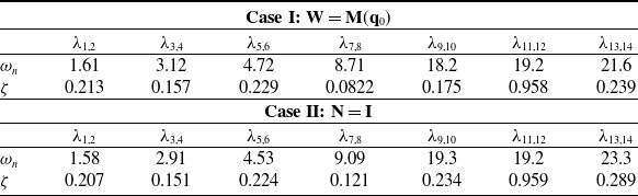
 ωn
ωn ζ
ζ W=M
W=M N=I
N=I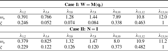
 ωn
ωn ζ
ζ W=M
W=M N=I
N=I
 ωn
ωn ζ
ζ



 ωn
ωn ζ
ζ
 ωn
ωn ζ
ζ

 ωn
ωn ζ
ζ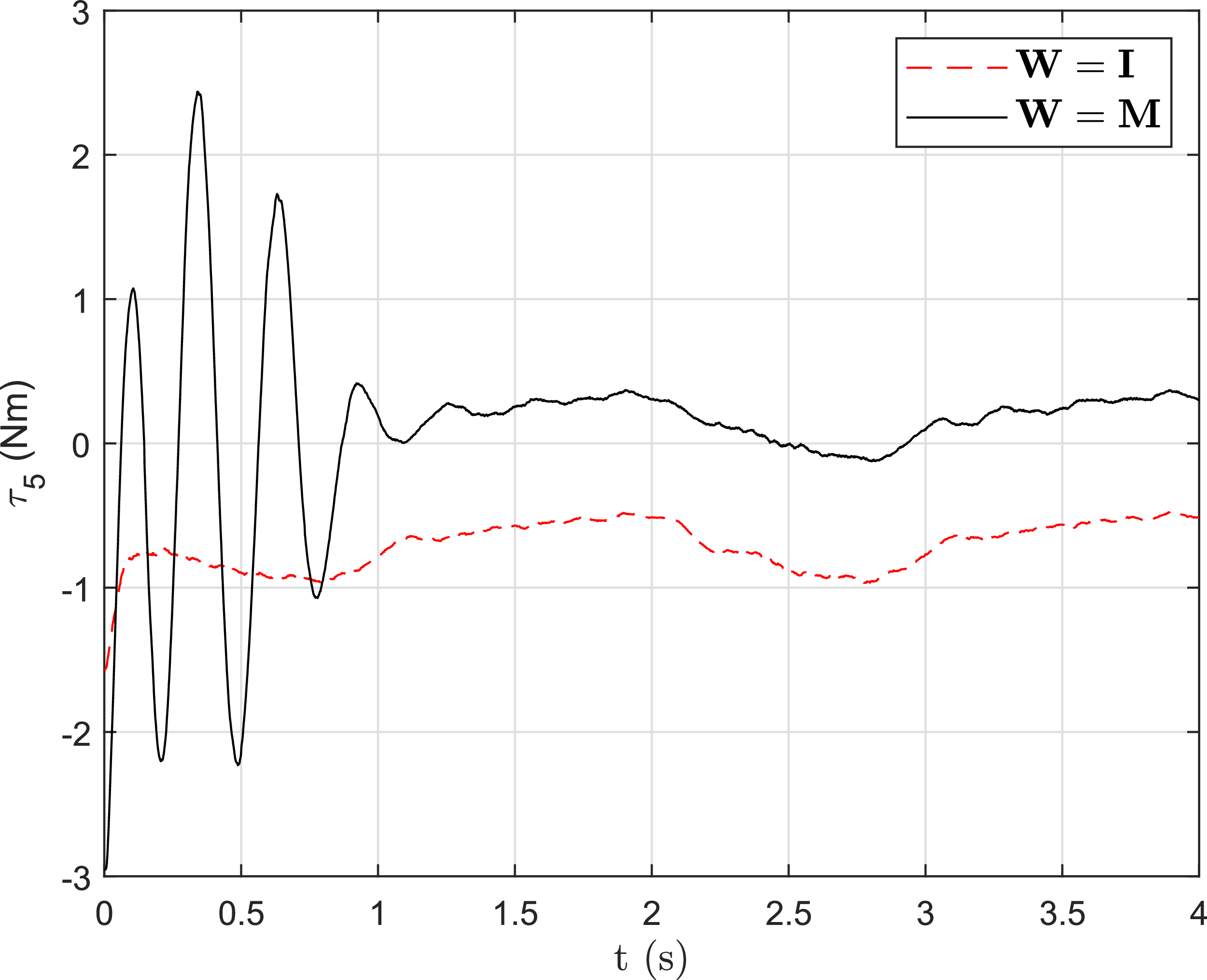
 5
5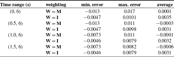
 r=12cm


 Open access

