1. Introduction
The rhythmic transverse vibration of a circular cylinder in a flow, and the whirls of fluid of opposite swirl alternately shed into the wake as this bluff body undergoes flow-induced vibration, are aesthetically beautiful and mesmerising to the observer. Although such flow-induced vibrations may have utility for energy harvesting, they also have the potential to cause destruction to engineering structures.
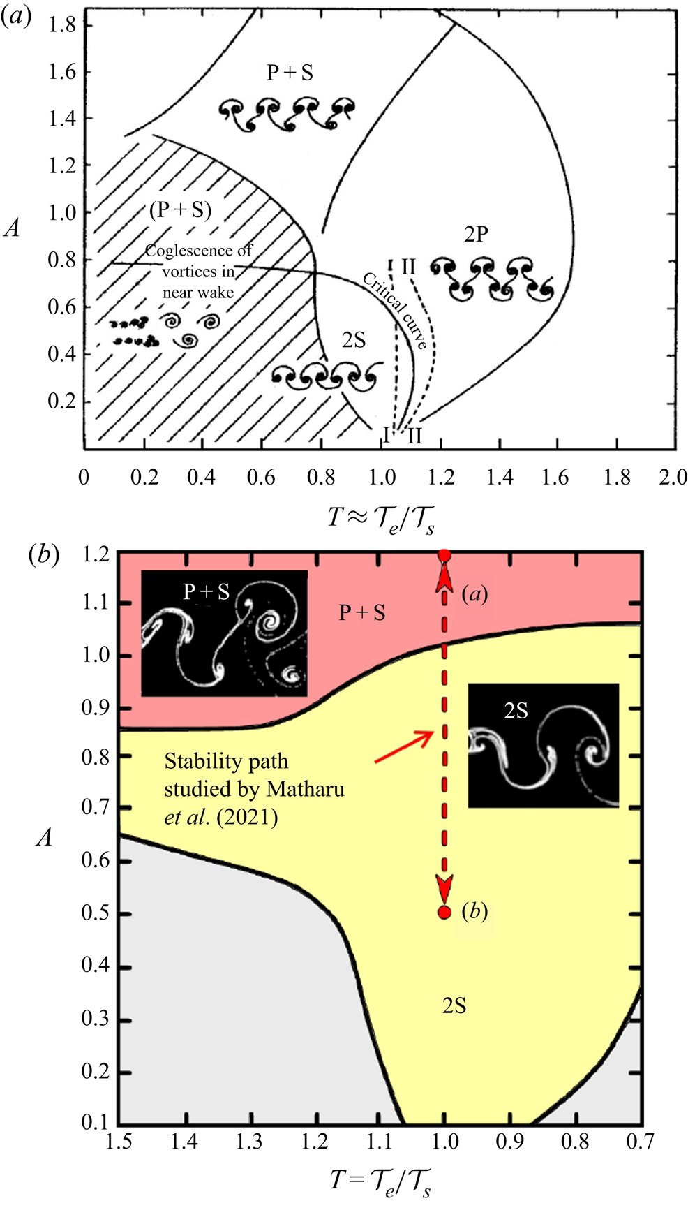
Applying forced vibrations to a cylinder at different frequencies and amplitudes can provide a strictly periodic flow that can mimic that due to flow-induced vibrations, as well as expanding the amplitude–frequency parameter space. A variety of vortex patterns, including two parallel rows of either single vortices of opposite spin (2S mode) or pairs of both spins (2P), or a row with single vortices of one spin and a parallel row of pairs of vortices with the opposite spin (P+S mode), have been observed in the pioneering studies of Williamson & Roshko (Reference Williamson and Roshko1988) and Williamson & Govardhan (Reference Williamson and Govardhan2004) in meticulous experiments using aluminium particles or dye as tracers (see figure 1a). These were later reproduced using time-dependent computational simulations by Leontini et al. (Reference Leontini, Stewart, Thompson and Hourigan2006) (see figure 1b).
What have not been understood are the precise details of the transition from 2S shedding to P+S shedding for a circular cylinder undergoing forced transverse oscillations. In particular, Matharu, Hazel & Heil (Reference Matharu, Hazel and Heil2021) examine two scenarios via which the transition might proceed. Scenario (i) is the evolution of a single solution that leads to quantifiable, discrete changes to the topology of the flow field, and scenario (ii) comprises bifurcations with additional solutions with distinct new features arising, disappearing or changing stability.
In the experiments of Williamson & Roshko (Reference Williamson and Roshko1988) and Williamson & Govardhan (Reference Williamson and Govardhan2004), and in the computational predictions of Leontini et al. (Reference Leontini, Stewart, Thompson and Hourigan2006), there appears a sharp discrete transition between the 2S mode and the P+S mode, which may at first glance suggest scenario (i). However,
by using an alternative computational technique that allows the capture of unstable solutions, Matharu et al. (Reference Matharu, Hazel and Heil2021) show that scenario (ii) underpins the transition. Matharu et al. (Reference Matharu, Hazel and Heil2021) consider this case for ‘moderate’ Reynolds number, based on cylinder diameter and upstream flow velocity, of 100 and less. In particular, the cases simulated previously by Leontini et al. (Reference Leontini, Stewart, Thompson and Hourigan2006) are considered for the particular case of forcing at the natural vortex shedding frequency (i.e. the Strouhal shedding frequency for a fixed circular cylinder) and varying the amplitude of oscillation. Leontini et al. (Reference Leontini, Stewart, Thompson and Hourigan2006) did not attempt to determine unstable solutions or regions of bistability. The parameter space explored by Leontini et al. (Reference Leontini, Stewart, Thompson and Hourigan2006) and the specific path of the stability study of Matharu et al. (Reference Matharu, Hazel and Heil2021) are shown in figure 1(b).
2. Overview
Matharu et al. (Reference Matharu, Hazel and Heil2021) investigate the nature of the transitions between the 2S and P+S modes in an elegant and rigorous approach. By employing a time-integration of the Navier–Stokes equations, they are able to reproduce the sharp jumps between modes found by the previous simulations of Leontini et al. (Reference Leontini, Stewart, Thompson and Hourigan2006) and experiments of Williamson & Roshko (Reference Williamson and Roshko1988) and Williamson & Govardhan (Reference Williamson and Govardhan2004). These solutions, however, reflect only stable solutions.
Through the clever use also of a numerical method based on space–time discretisation, Matharu et al. (Reference Matharu, Hazel and Heil2021) are able to track the evolution of wake structures along both stable and unstable branches. By mapping the magnitude of the symmetry-breaking perturbation,  $\epsilon$($A$), against the normalised amplitude of vibration, $A$, they are able clearly to distinguish the 2S mode ($\epsilon = 0$) and P+S mode ($\epsilon \neq 0$). The inferred stability of the various time-periodic solution branches was confirmed through time-integration of the Navier–Stokes equations.
An amalgam of some of the key results of Matharu et al. (Reference Matharu, Hazel and Heil2021) is shown in figure 2. The solutions above and below the horizontal axis are conjugate solutions – that is, the vortex pair can appear in the upper or lower row of vortices, depending on initial conditions.
At low vibration amplitudes $A$, the only solution is a stable 2S mode. As the amplitude increases, a subcritical pitchfork bifurcation (characterised by the square root growth of $\epsilon$) occurs at $A \approx 1.0855$, and two unstable conjugate branches then join stable conjugate P+S branches via a fold bifurcation at $A \approx 1.0680$. A small region of bistability occurs over this range of the unstable branches.
The transition is repeated when $A$ decreases from values larger than $\approx 1.5$, where a second subcritical pitchfork bifurcation occurs at $A \approx$ 1.316, leading to unstable conjugate branches joining the stable P+S conjugate branches at $A \approx 1.5$ via a fold bifurcation. A larger region of bistability exists over this range of unstable branches.
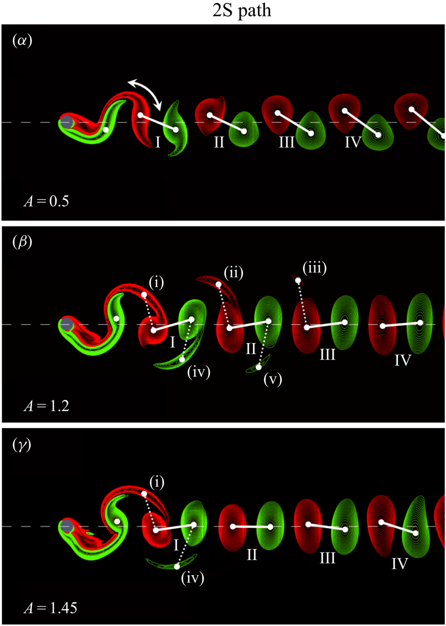
The question then remains as to the evolution of the vortex structures in the transition along the unstable branches joining the 2S and P+S modes. First, Matharu et al. (Reference Matharu, Hazel and Heil2021) show that by following the ‘2S path’ ($(\alpha )$–$(\gamma )$ in figure 2, i.e. $\epsilon = 0$), the 2S mode is maintained in both the stable and unstable branches. The wake structures corresponding to the points $(\alpha )$–$(\gamma )$ are shown in figure 3. Note, however, that at points $(\beta )$ and $(\gamma )$, the near-wakes in figures 3($\beta$)–3($\gamma$) show a weak secondary vorticity maximum associated with each shed vortex. These near-wake structures are reminiscent of a 2P wake mode. However, the evolution between the 2S and 2P occurs continuously and not via a bifurcation. These secondary vortices fade within a few wavelengths in the wake. It is interesting that Williamson & Roshko (Reference Williamson and Roshko1988), who mainly characterised the near wake, noted the 2P mode appeared for $Re \in (300,1000)$, but it was not detectable for $Re$ =100.
Second, tracking along the ‘P+S path’ (figure 2, points (a)–( f)) reveals the evolution of the wake between the 2S and the P+S modes – see figure 4 for the wake structures corresponding to the points (a)–( f). Of note is the gradual evolution along the unstable branches of the wake transition between modes 2S and P+S, with the second vortex in the pair fading away a short distance downstream. In experiments and time-dependent simulations, the transition between the two modes will appear as jumps between different stable branches.
As the Reynolds number is reduced from $Re=100$, the 2S and P+S branches disconnect to form isolated conjugate branches (isolas) of solutions at $Re \approx 82$. As $Re$ is further reduced, these isolas shrink but a bistable region remains. The isolas and P+S solutions finally disappear at $Re \approx 77.7$, with only the 2S solution remaining at lower $Re$. This process, evolution of the vorticity field around an isola, is discussed in detail in the article.
The animations available in the supplementary material for Matharu et al. (Reference Matharu, Hazel and Heil2021) at https://doi.org/10.1017/jfm.2021.358 show the above transitions with great clarity.
3. Future
The two-pronged approach of using complementary numerical schemes that elegantly produce bifurcation diagrams and uncover the evolution of the wake structure as the flow transitions between different modes provides a powerful tool for many other studies.
The effect of increasing Reynolds numbers would be of interest. The transition to three-dimensionality of this flow has been studied by Leontini, Thompson & Hourigan (Reference Leontini, Thompson and Hourigan2007), which provides a guide to the critical Reynolds numbers for two-dimensional studies to remain valid. In any case, soap film experiments maintain approximately two-dimensional flow fields in a physical setting (Yang, Masroor & Stremler Reference Yang, Masroor and Stremler2021); in addition, they produce two-dimensional base flows for the study of the genesis of three-dimensional structures. Williamson & Roshko (Reference Williamson and Roshko1988), in their figure 3(a), show an extended map of the synchronised regions to a limit of $A=5$, with other modes, such as 2P+2S, arising. This could provide fertile ground for new studies. The recent study of Matharu et al. (Reference Matharu, Hazel and Heil2021) focused on forcing amplitudes to a limit of $A=1.5$. At higher amplitudes, they state that they occasionally observed time-periodic solutions with larger periods. Extending their study to investigate the transition in such regimes would be most interesting. In addition, forcing frequencies other than those corresponding to the natural Strouhal number can produce different transitions, as may other body geometries, such as ellipses and airfoils.


1. Introduction
The rhythmic transverse vibration of a circular cylinder in a flow, and the whirls of fluid of opposite swirl alternately shed into the wake as this bluff body undergoes flow-induced vibration, are aesthetically beautiful and mesmerising to the observer. Although such flow-induced vibrations may have utility for energy harvesting, they also have the potential to cause destruction to engineering structures.
Applying forced vibrations to a cylinder at different frequencies and amplitudes can provide a strictly periodic flow that can mimic that due to flow-induced vibrations, as well as expanding the amplitude–frequency parameter space. A variety of vortex patterns, including two parallel rows of either single vortices of opposite spin (2S mode) or pairs of both spins (2P), or a row with single vortices of one spin and a parallel row of pairs of vortices with the opposite spin (P+S mode), have been observed in the pioneering studies of Williamson & Roshko (Reference Williamson and Roshko1988) and Williamson & Govardhan (Reference Williamson and Govardhan2004) in meticulous experiments using aluminium particles or dye as tracers (see figure 1a). These were later reproduced using time-dependent computational simulations by Leontini et al. (Reference Leontini, Stewart, Thompson and Hourigan2006) (see figure 1b).
Parameter map of normalised forcing amplitude, $A$, versus forcing period, $T_e$, showing different wake modes. (a) Adapted from Williamson & Roshko (Reference Williamson and Roshko1988) for $Re \in (300,1000)$. (b) Adapted from Matharu et al. (Reference Matharu, Hazel and Heil2021) and Leontini et al. (Reference Leontini, Stewart, Thompson and Hourigan2006).
What have not been understood are the precise details of the transition from 2S shedding to P+S shedding for a circular cylinder undergoing forced transverse oscillations. In particular, Matharu, Hazel & Heil (Reference Matharu, Hazel and Heil2021) examine two scenarios via which the transition might proceed. Scenario (i) is the evolution of a single solution that leads to quantifiable, discrete changes to the topology of the flow field, and scenario (ii) comprises bifurcations with additional solutions with distinct new features arising, disappearing or changing stability.
In the experiments of Williamson & Roshko (Reference Williamson and Roshko1988) and Williamson & Govardhan (Reference Williamson and Govardhan2004), and in the computational predictions of Leontini et al. (Reference Leontini, Stewart, Thompson and Hourigan2006), there appears a sharp discrete transition between the 2S mode and the P+S mode, which may at first glance suggest scenario (i). However, by using an alternative computational technique that allows the capture of unstable solutions, Matharu et al. (Reference Matharu, Hazel and Heil2021) show that scenario (ii) underpins the transition. Matharu et al. (Reference Matharu, Hazel and Heil2021) consider this case for ‘moderate’ Reynolds number, based on cylinder diameter and upstream flow velocity, of 100 and less. In particular, the cases simulated previously by Leontini et al. (Reference Leontini, Stewart, Thompson and Hourigan2006) are considered for the particular case of forcing at the natural vortex shedding frequency (i.e. the Strouhal shedding frequency for a fixed circular cylinder) and varying the amplitude of oscillation. Leontini et al. (Reference Leontini, Stewart, Thompson and Hourigan2006) did not attempt to determine unstable solutions or regions of bistability. The parameter space explored by Leontini et al. (Reference Leontini, Stewart, Thompson and Hourigan2006) and the specific path of the stability study of Matharu et al. (Reference Matharu, Hazel and Heil2021) are shown in figure 1(b).
2. Overview
Matharu et al. (Reference Matharu, Hazel and Heil2021) investigate the nature of the transitions between the 2S and P+S modes in an elegant and rigorous approach. By employing a time-integration of the Navier–Stokes equations, they are able to reproduce the sharp jumps between modes found by the previous simulations of Leontini et al. (Reference Leontini, Stewart, Thompson and Hourigan2006) and experiments of Williamson & Roshko (Reference Williamson and Roshko1988) and Williamson & Govardhan (Reference Williamson and Govardhan2004). These solutions, however, reflect only stable solutions.
Through the clever use also of a numerical method based on space–time discretisation, Matharu et al. (Reference Matharu, Hazel and Heil2021) are able to track the evolution of wake structures along both stable and unstable branches. By mapping the magnitude of the symmetry-breaking perturbation, $\epsilon$( $A$), against the normalised amplitude of vibration, $A$, they are able clearly to distinguish the 2S mode ( $\epsilon = 0$) and P+S mode ( $\epsilon \neq 0$). The inferred stability of the various time-periodic solution branches was confirmed through time-integration of the Navier–Stokes equations.
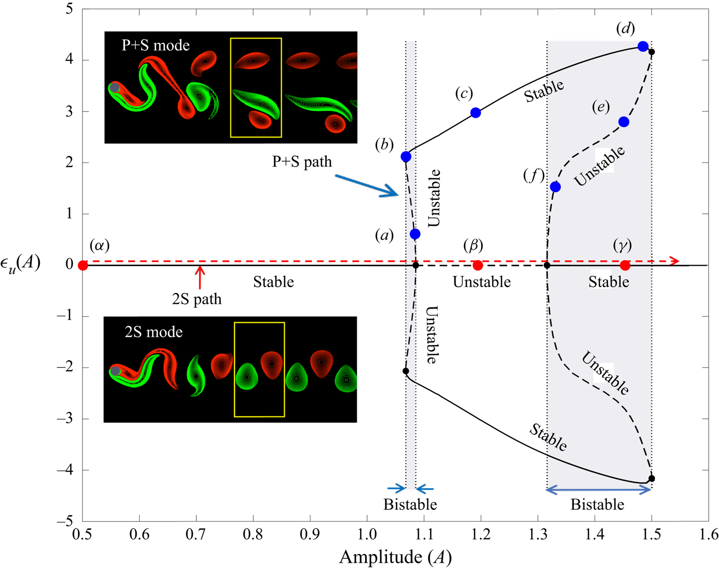
An amalgam of some of the key results of Matharu et al. (Reference Matharu, Hazel and Heil2021) is shown in figure 2. The solutions above and below the horizontal axis are conjugate solutions – that is, the vortex pair can appear in the upper or lower row of vortices, depending on initial conditions.
Bifurcation diagram, symmetry-breaking perturbation $\epsilon (A)$ versus normalised vibration amplitude $A$, showing regions of bistability and stable and unstable branches. The red markers and labels ( $\alpha$)–( $\gamma$) mark the path and parameter values linked to the vorticity snapshots in figure 3. The blue markers and labels (a)–( f) mark the path and parameter values linked to the vorticity snapshots in figure 4 (adapted from figures 1, 6, 7 and 8 of Matharu et al. Reference Matharu, Hazel and Heil2021).
At low vibration amplitudes $A$, the only solution is a stable 2S mode. As the amplitude increases, a subcritical pitchfork bifurcation (characterised by the square root growth of $\epsilon$) occurs at $A \approx 1.0855$, and two unstable conjugate branches then join stable conjugate P+S branches via a fold bifurcation at $A \approx 1.0680$. A small region of bistability occurs over this range of the unstable branches.
The transition is repeated when $A$ decreases from values larger than $\approx 1.5$, where a second subcritical pitchfork bifurcation occurs at $A \approx$ 1.316, leading to unstable conjugate branches joining the stable P+S conjugate branches at $A \approx 1.5$ via a fold bifurcation. A larger region of bistability exists over this range of unstable branches.
The question then remains as to the evolution of the vortex structures in the transition along the unstable branches joining the 2S and P+S modes. First, Matharu et al. (Reference Matharu, Hazel and Heil2021) show that by following the ‘2S path’ ( $(\alpha )$– $(\gamma )$ in figure 2, i.e. $\epsilon = 0$), the 2S mode is maintained in both the stable and unstable branches. The wake structures corresponding to the points $(\alpha )$– $(\gamma )$ are shown in figure 3. Note, however, that at points $(\beta )$ and $(\gamma )$, the near-wakes in figures 3( $\beta$)–3( $\gamma$) show a weak secondary vorticity maximum associated with each shed vortex. These near-wake structures are reminiscent of a 2P wake mode. However, the evolution between the 2S and 2P occurs continuously and not via a bifurcation. These secondary vortices fade within a few wavelengths in the wake. It is interesting that Williamson & Roshko (Reference Williamson and Roshko1988), who mainly characterised the near wake, noted the 2P mode appeared for $Re \in (300,1000)$, but it was not detectable for $Re$ =100.
Contours of the vorticity field at the points ( $\alpha$)–( $\gamma$) along the 2S path, as marked by red dots in figure 2. Adapted from figure 7 of Matharu et al. (Reference Matharu, Hazel and Heil2021).
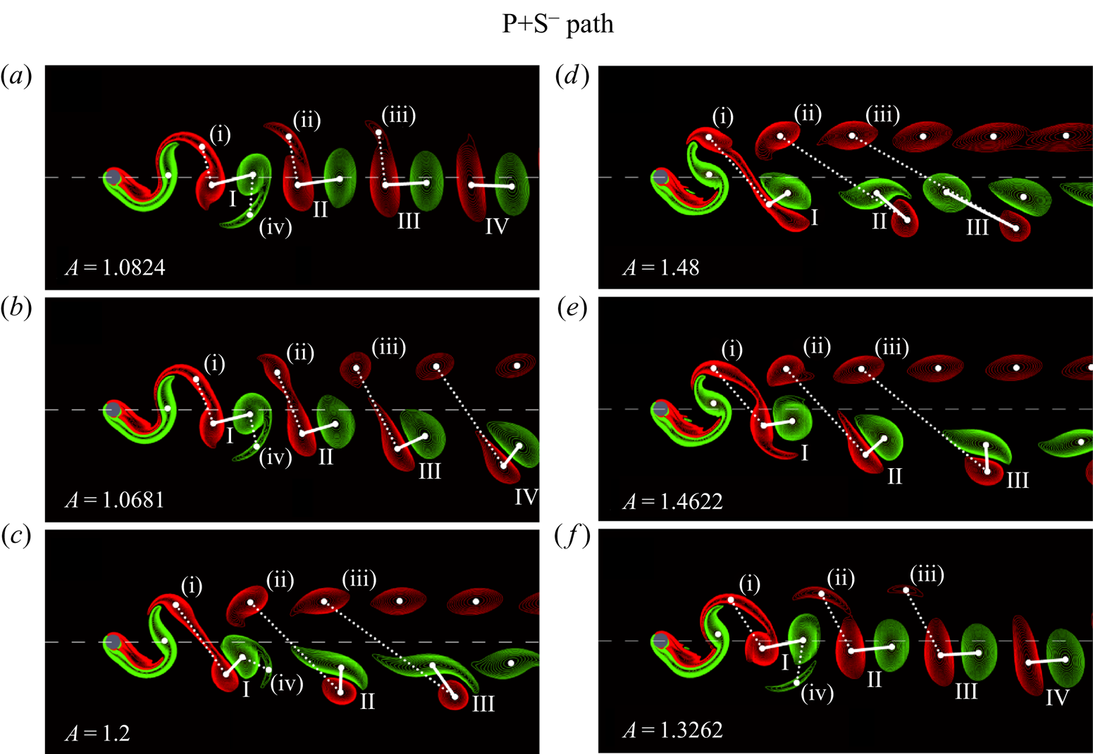
Second, tracking along the ‘P+S path’ (figure 2, points (a)–( f)) reveals the evolution of the wake between the 2S and the P+S modes – see figure 4 for the wake structures corresponding to the points (a)–( f). Of note is the gradual evolution along the unstable branches of the wake transition between modes 2S and P+S, with the second vortex in the pair fading away a short distance downstream. In experiments and time-dependent simulations, the transition between the two modes will appear as jumps between different stable branches.
Contours of the vorticity field at the points (a)–( f) along the P+S $^-$ path, as marked by blue dots in figure 2. Adapted from figure 8 of Matharu et al. (Reference Matharu, Hazel and Heil2021).
As the Reynolds number is reduced from $Re=100$, the 2S and P+S branches disconnect to form isolated conjugate branches (isolas) of solutions at $Re \approx 82$. As $Re$ is further reduced, these isolas shrink but a bistable region remains. The isolas and P+S solutions finally disappear at $Re \approx 77.7$, with only the 2S solution remaining at lower $Re$. This process, evolution of the vorticity field around an isola, is discussed in detail in the article.
The animations available in the supplementary material for Matharu et al. (Reference Matharu, Hazel and Heil2021) at https://doi.org/10.1017/jfm.2021.358 show the above transitions with great clarity.
3. Future
The two-pronged approach of using complementary numerical schemes that elegantly produce bifurcation diagrams and uncover the evolution of the wake structure as the flow transitions between different modes provides a powerful tool for many other studies.
The effect of increasing Reynolds numbers would be of interest. The transition to three-dimensionality of this flow has been studied by Leontini, Thompson & Hourigan (Reference Leontini, Thompson and Hourigan2007), which provides a guide to the critical Reynolds numbers for two-dimensional studies to remain valid. In any case, soap film experiments maintain approximately two-dimensional flow fields in a physical setting (Yang, Masroor & Stremler Reference Yang, Masroor and Stremler2021); in addition, they produce two-dimensional base flows for the study of the genesis of three-dimensional structures. Williamson & Roshko (Reference Williamson and Roshko1988), in their figure 3(a), show an extended map of the synchronised regions to a limit of $A=5$, with other modes, such as 2P+2S, arising. This could provide fertile ground for new studies. The recent study of Matharu et al. (Reference Matharu, Hazel and Heil2021) focused on forcing amplitudes to a limit of $A=1.5$. At higher amplitudes, they state that they occasionally observed time-periodic solutions with larger periods. Extending their study to investigate the transition in such regimes would be most interesting. In addition, forcing frequencies other than those corresponding to the natural Strouhal number can produce different transitions, as may other body geometries, such as ellipses and airfoils.
Declaration of interests
The author reports no conflict of interest.