


1 Introduction
Solutions of various complex systems and differential equations with multiple time scales are known to display critical transitions [Reference Kuehn41]. After a longer period of slow change, a critical transition corresponds to a large/drastic event happening on a fast scale. In more detail, we can characterise this mechanism [Reference Kuehn39, Reference Kuehn and Romano43] by several essential components. The typical dynamics of such systems display slow motion for long times. Yet, there is generically a slow drift towards a bifurcation point of the fast/layer subsystem. The critical transition is an abrupt change that happens on a fast timescale after the bifurcation point has been passed. Of course, it is of interest to study whether there are early warning signs to potentially anticipate a critical transition. One crucial mechanism to extract warning signs from data is to exploit the effect of critical slowing down, where the recovery of perturbations to the current state starts to slow as a bifurcation is approached. This behaviour can therefore be observed in real-life data by exploiting natural fluctuations caused by minor physical components, treated as stochastic perturbation effects and by measuring a stochastic observable, such as variance or autocorrelation [Reference Wiesenfeld65]. This approach has recently gained considerable popularity in various applications [Reference Scheffer, Bascompte and Brock58].
It is evident that in many complex systems with critical transitions, we should also take into account, beyond stochasticity, the spatial components. A prime example are applications in neuroscience, where it is apparent that larger-scale events, such as epileptic seizures, can be described by spatial stochastic systems with critical transitions [Reference McSharry, Smith and Tarassenko49, Reference Meisel and Kuehn50, Reference Mormann, Andrzejak, Elger and Lehnertz53]. Another example is electric power systems where critical transitions can lead to a failure of the whole system, such as voltage collapses [Reference Cotilla-Sanchez, Hines and Danforth14]. Other examples of complex systems with critical transitions occur in medical applications [Reference O’Regan and Drake55, Reference Venegas, Winkler and Musch63], economic applications [Reference May, Levin and Sugihara48] and environmental applications [Reference Alley, Marotzke and Nordhaus1, Reference Lenton46, Reference Scheffer, Carpenter, Foley, Folke and Walker59]. It becomes apparent that for each of these applications, a prediction and warning of a critical transition is desirable as it could enable the prevention of its occurrence or at least improve the adaptability to it. Yet, to make early warning sign theory reliable and avoid potential non-robust conclusions [Reference Dakos, Scheffer, van Nes, Brovkin, Petoukhov and Held17, Reference Ditlevsen and Johnsen20], a rigorous mathematical study of early warning sign theory is needed. There exists already a quite well-developed theory for warning signs of systems modeled by stochastic ordinary differential equations (SODE), for example in [Reference Crauel and Flandoli15, Reference Kuehn40]. However, there are still many open problems for systems modeled by stochastic partial differential equations (SPDE). For SPDEs, it is potentially even more crucial in comparison to SODEs to develop a mathematical theory as SPDEs model complex systems, where it is either extremely costly to obtain high-resolution experimental, or even simulation, data in many applications. Therefore, experimentally driven approaches have to be guided by rigorous mathematical analysis.
For our study, we follow the construction in [Reference Kuehn and Romano43], which considers differential equations of the form
 \begin{align} \begin{cases} \mathrm{d}u(x,t)=\left(F_1(x,p(t))u(x,t)+F_2(u(x,t),p(t))\right )\, \mathrm{d}t + \sigma \, \mathrm{d}W(t) \,, \\[3pt] \mathrm{d}p(t)= \epsilon G(u(x,t),p(t))\, \mathrm{d}t \,, \end{cases} \end{align}
with $(x,t) \in \mathcal{X} \times [0, \infty )$
for a connected set
$(x,t) \in \mathcal{X} \times [0, \infty )$
for a connected set $\mathcal{X}\subseteq \mathbb{R}^N$
with nonempty interior,
$\mathcal{X}\subseteq \mathbb{R}^N$
with nonempty interior, $u\,:\,\mathcal{X} \times [0, \infty )\to \mathbb{R}$
,
$u\,:\,\mathcal{X} \times [0, \infty )\to \mathbb{R}$
, $p\,:\, [0, \infty )\to \mathbb{R}$
and
$p\,:\, [0, \infty )\to \mathbb{R}$
and $N\in \mathbb{N}\,:\!=\,\{1,2,3,\ldots \}$
. Suppose that
$N\in \mathbb{N}\,:\!=\,\{1,2,3,\ldots \}$
. Suppose that $F_1$
is a linear operator and that
$F_1$
is a linear operator and that $F_2$
and
$F_2$
and $G$
are sufficiently smooth nonlinear maps. We assume
$G$
are sufficiently smooth nonlinear maps. We assume $\sigma \gt 0$
,
$\sigma \gt 0$
, $0\lt \epsilon \ll 1$
and with the notation
$0\lt \epsilon \ll 1$
and with the notation $W$
we refer to a
$W$
we refer to a $Q$
-Wiener process. The precise properties of the operator
$Q$
-Wiener process. The precise properties of the operator $Q$
are described further below. We denote
$Q$
are described further below. We denote $u(x,t)$
by
$u(x,t)$
by $u$
and
$u$
and $p(t)$
as
$p(t)$
as $p$
.
$p$
.
Suppose, for simplicity, that $F_2(0,p) = 0$
. Hence, we obtain for any
$F_2(0,p) = 0$
. Hence, we obtain for any $p$
the homogeneous steady state
$p$
the homogeneous steady state $u_{\ast }\equiv 0$
for the deterministic partial differential equation (PDE) corresponding to (1.1) with
$u_{\ast }\equiv 0$
for the deterministic partial differential equation (PDE) corresponding to (1.1) with $\sigma =0$
. To determine the local stability of
$\sigma =0$
. To determine the local stability of $u_{\ast } \equiv 0$
, we study the linear operator
$u_{\ast } \equiv 0$
, we study the linear operator
 \begin{align*} A(p) \,:\!=\, F_1 + \mathrm{D}_{u_{\ast }} F_2(0,p) \,, \end{align*}
where $\mathrm{D}_u$
is the Fréchet derivative of
$\mathrm{D}_u$
is the Fréchet derivative of $u$
on a suitable Banach space, which contains the solutions of (1.1) and which is described in full detail below.
$u$
on a suitable Banach space, which contains the solutions of (1.1) and which is described in full detail below.
Suppose that the spectrum of $A(p_0)$
is contained in
$A(p_0)$
is contained in $\{ z\,:\,\mathrm{Re}(z) \lt 0\}$
for fixed values
$\{ z\,:\,\mathrm{Re}(z) \lt 0\}$
for fixed values $p_0 \lt 0$
, whereas the spectrum has elements in
$p_0 \lt 0$
, whereas the spectrum has elements in $\{ z\,:\,\mathrm{Re}(z) \gt 0\}$
for fixed
$\{ z\,:\,\mathrm{Re}(z) \gt 0\}$
for fixed $p_0\gt 0$
. Therefore, the fast subsystem, given by taking the limit
$p_0\gt 0$
. Therefore, the fast subsystem, given by taking the limit $\epsilon =0$
, has a bifurcation point at
$\epsilon =0$
, has a bifurcation point at $p=0$
and in the full fast-slow system (1.1), with
$p=0$
and in the full fast-slow system (1.1), with $\epsilon \gt 0$
, the slow dynamics
$\epsilon \gt 0$
, the slow dynamics $\partial _t p = \epsilon G(0,p)$
can drive the system to the bifurcation point at
$\partial _t p = \epsilon G(0,p)$
can drive the system to the bifurcation point at $p=0$
and potentially induce a critical transition. For the case
$p=0$
and potentially induce a critical transition. For the case $\epsilon =0$
, the variable
$\epsilon =0$
, the variable $p$
becomes a parameter on which the motion of
$p$
becomes a parameter on which the motion of $u$
depends. More precisely, as
$u$
depends. More precisely, as $p$
is varying, it can cross the bifurcation threshold
$p$
is varying, it can cross the bifurcation threshold $p=0$
present in the fast PDE dynamics
$p=0$
present in the fast PDE dynamics $\partial _t u = F_1 u + F_2(u,p)$
. As of now, we consider for simplicity the case
$\partial _t u = F_1 u + F_2(u,p)$
. As of now, we consider for simplicity the case $\epsilon = 0$
and assume that
$\epsilon = 0$
and assume that $p$
is a parameter (see [Reference Gnann, Kuehn and Pein23] for steps towards a more abstract theory of fast-slow SPDEs). The problem studied is hence of the form of the fast system linearised at
$p$
is a parameter (see [Reference Gnann, Kuehn and Pein23] for steps towards a more abstract theory of fast-slow SPDEs). The problem studied is hence of the form of the fast system linearised at $u_\ast$
,
$u_\ast$
,
 \begin{align} \mathrm{d}U(x,t) = A(p) U(x,t) \, \mathrm{d}t + \sigma \, \mathrm{d}W(t) \, . \end{align}
For $p\ll 0$
and initial condition in
$p\ll 0$
and initial condition in $u_\ast$
, the dissipative linear term constrains the solution of such a system and the solution of (1.1) at
$u_\ast$
, the dissipative linear term constrains the solution of such a system and the solution of (1.1) at $\varepsilon =0$
in a neighbourhood of
$\varepsilon =0$
in a neighbourhood of $u_\ast$
with high probability. Therefore the two paths are expected to present a similar behaviour and variance [Reference Gowda and Kuehn24]. The observation of an early warning sign on the linearised system is therefore justified up to proximity to the bifurcation threshold. We discuss this problem setting initially
$u_\ast$
with high probability. Therefore the two paths are expected to present a similar behaviour and variance [Reference Gowda and Kuehn24]. The observation of an early warning sign on the linearised system is therefore justified up to proximity to the bifurcation threshold. We discuss this problem setting initially $A(p) = p \operatorname{I} + \operatorname{T}_f$
, where
$A(p) = p \operatorname{I} + \operatorname{T}_f$
, where $\operatorname{I}$
denotes the identity and
$\operatorname{I}$
denotes the identity and $\operatorname{T}_f$
is a multiplication operator associated to a function
$\operatorname{T}_f$
is a multiplication operator associated to a function $f\,:\,\mathcal{X} \to \mathbb{R}$
. Such a choice is directly motivated by the spectral theorem [Reference Hall25], which associates a multiplication operator with other operators with the same spectrum. For the precise technical set-up and assumptions made, we refer to Section 2. Generalisations to the choice of operator
$f\,:\,\mathcal{X} \to \mathbb{R}$
. Such a choice is directly motivated by the spectral theorem [Reference Hall25], which associates a multiplication operator with other operators with the same spectrum. For the precise technical set-up and assumptions made, we refer to Section 2. Generalisations to the choice of operator $A(p)$
are discussed in Section 5 and, from an applied perspective, in Section 7.
$A(p)$
are discussed in Section 5 and, from an applied perspective, in Section 7.
As mentioned above, prediction of critical transitions is very important in applications as it can help reduce, or even completely evade, its effects. This can be done by finding early warning signs [Reference Bernuzzi and Kuehn5, Reference Blumenthal, Engel and Neamtu7]. Our goal is to analyse the problem for early warning signs in the form of an increasing variance as the bifurcation point at $p=0$
is approached.
$p=0$
is approached.
This paper is structured as follows. In Section 2, we set up the problem and state our main results. In Section 3, we discuss the variance of the solutions of (1.2) for measurable functions $f$
that are defined on a one-dimensional space, i.e., assuming that
$f$
that are defined on a one-dimensional space, i.e., assuming that $N =1$
. We first focus on a specific tool function type and then generalise the obtained results to the case of more general analytic functions. In Section 4, we proceed with the study of the scalar product that defines the variance along certain directions in the space of square-integrable functions, with the domain of
$N =1$
. We first focus on a specific tool function type and then generalise the obtained results to the case of more general analytic functions. In Section 4, we proceed with the study of the scalar product that defines the variance along certain directions in the space of square-integrable functions, with the domain of $f$
in higher dimensions. While observing convergence as
$f$
in higher dimensions. While observing convergence as $p\to 0^-$
for
$p\to 0^-$
for $N\gt 1$
dimensions and
$N\gt 1$
dimensions and $f$
under certain assumptions, we further find an upper bound of divergence for analytic functions
$f$
under certain assumptions, we further find an upper bound of divergence for analytic functions $f$
on two- and three-dimensional domains. In Section 5, we discuss how our results are affected by relaxing certain assumptions and we provide examples of the effectiveness of the early warning-signs for different types of linear operators presented in the drift term of (1.2). In Section 6, we approximate (1.2) for one-, two- and three-dimensional spatial domains to obtain visual numerical representations and a cross-validation of the discussed theorems. Lastly, in Section 7, we provide examples of models employed in various research fields on which the early warning signs find application.
$f$
on two- and three-dimensional domains. In Section 5, we discuss how our results are affected by relaxing certain assumptions and we provide examples of the effectiveness of the early warning-signs for different types of linear operators presented in the drift term of (1.2). In Section 6, we approximate (1.2) for one-, two- and three-dimensional spatial domains to obtain visual numerical representations and a cross-validation of the discussed theorems. Lastly, in Section 7, we provide examples of models employed in various research fields on which the early warning signs find application.
2 Preliminaries
In this paper, we study the SPDE
 \begin{align} \begin{cases} \mathrm{d}u(x,t) = \left (f(x)+p\right )\; u(x,t) \, \mathrm{d}t + \sigma \mathrm{d}W(t)\\[3pt] u(\cdot, 0) = u_0 \end{cases} \end{align}
for $x\in \mathcal{X}$
,
$x\in \mathcal{X}$
, $t\gt 0$
and
$t\gt 0$
and $\mathcal{X}\subseteq \mathbb{R}^N$
a connected set with non-empty interior for
$\mathcal{X}\subseteq \mathbb{R}^N$
a connected set with non-empty interior for $N\in \mathbb{N}$
. The operator
$N\in \mathbb{N}$
. The operator $\operatorname{T}_f$
denotes the realisation in
$\operatorname{T}_f$
denotes the realisation in $L^2(\mathcal{X})$
of the multiplication operator for
$L^2(\mathcal{X})$
of the multiplication operator for $f$
, i.e.
$f$
, i.e.
 \begin{align*} \operatorname{T}_fu=fu\quad, \quad \mathcal{D}(\operatorname{T}_f)\,:\!=\,\left \{ u\;\;\mathrm{Lebesgue measurable}\;\Big |\; fu\in L^2(\mathcal{X}) \right \}\quad, \end{align*}
with $\mathcal{D}({\cdot})$
denoting the domain of an operator. We assume that the initial condition of the system satisfies
$\mathcal{D}({\cdot})$
denoting the domain of an operator. We assume that the initial condition of the system satisfies $u_0\in \mathcal{D}(\operatorname{T}_f)$
and
$u_0\in \mathcal{D}(\operatorname{T}_f)$
and $L^2(\mathcal{X})$
is the Hilbert space of square-integrable functions with the standard scalar product
$L^2(\mathcal{X})$
is the Hilbert space of square-integrable functions with the standard scalar product $\langle \cdot, \cdot \rangle$
. We denote as
$\langle \cdot, \cdot \rangle$
. We denote as $\mathcal{H}^{s}(\mathcal{X})$
the Hilbert Sobolev space of degree
$\mathcal{H}^{s}(\mathcal{X})$
the Hilbert Sobolev space of degree $s$
on
$s$
on $\mathcal{X}$
. We are going to assume that the Lebesgue measurable function
$\mathcal{X}$
. We are going to assume that the Lebesgue measurable function $f\,:\,\mathcal{X}\to \mathbb{R}$
satisfies
$f\,:\,\mathcal{X}\to \mathbb{R}$
satisfies
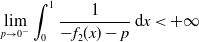
 \begin{align} f(x)\lt 0\; \;\forall x\in \mathcal{X}\setminus \{x_\ast \}, \quad \int _{\mathcal{X}} \frac{1}{|f(x)-p|} \mathrm{d}x\lt +\infty\ \mathrm{ for \, any} \, p\lt 0, {\rm{and}} \quad f(x_\ast )=0, \end{align}
for a point $x_\ast \in \mathcal{X}$
. Without loss of generality, i.e., up to a translation coordinate change in space, we can set
$x_\ast \in \mathcal{X}$
. Without loss of generality, i.e., up to a translation coordinate change in space, we can set $x_\ast =0$
, where
$x_\ast =0$
, where $0$
denotes the origin in
$0$
denotes the origin in $\mathbb{R}^N$
. We can then assume, again using a translation of space, that there exists
$\mathbb{R}^N$
. We can then assume, again using a translation of space, that there exists $\delta \gt 0$
such that
$\delta \gt 0$
such that $[0,\delta ]^N\subseteq \mathcal{X}$
. We assume also
$[0,\delta ]^N\subseteq \mathcal{X}$
. We assume also $\sigma \gt 0$
and
$\sigma \gt 0$
and $p\lt 0$
.
$p\lt 0$
.
The construction of the noise process $W$
and the existence of the solution follow from standard methods [Reference Da Prato and Zabczyk16] as follows. For fixed
$W$
and the existence of the solution follow from standard methods [Reference Da Prato and Zabczyk16] as follows. For fixed $T\gt 0$
, we consider the probability space
$T\gt 0$
, we consider the probability space $\left (\Omega, \mathcal{F}, \mathbb{P}\right )$
with
$\left (\Omega, \mathcal{F}, \mathbb{P}\right )$
with $\Omega$
the space of paths
$\Omega$
the space of paths $\{X(t)\}_{t\in [0,T]}$
such that
$\{X(t)\}_{t\in [0,T]}$
such that $X(t)\in L^2(\mathcal{X})$
for any
$X(t)\in L^2(\mathcal{X})$
for any $t\in [0,T]$
, for
$t\in [0,T]$
, for $\mathcal{F}$
the Borel
$\mathcal{F}$
the Borel $\sigma$
-algebra on
$\sigma$
-algebra on $\Omega$
and with
$\Omega$
and with $\mathbb{P}$
a Wiener measure induced by a Wiener process on
$\mathbb{P}$
a Wiener measure induced by a Wiener process on $[0,T]$
. To this probability space, we associate the natural filtration
$[0,T]$
. To this probability space, we associate the natural filtration $\mathcal{F}_t$
of
$\mathcal{F}_t$
of $\mathcal{F}$
with respect to a Wiener process for
$\mathcal{F}$
with respect to a Wiener process for $t\in [0,T]$
.
$t\in [0,T]$
.
We consider the non-negative operator $Q\,:\,L^2(\mathcal{X})\to L^2(\mathcal{X})$
with eigenvalues
$Q\,:\,L^2(\mathcal{X})\to L^2(\mathcal{X})$
with eigenvalues $\{q_k\}_{k\in \mathbb{N}}$
and eigenfunctions
$\{q_k\}_{k\in \mathbb{N}}$
and eigenfunctions $\{b_k\}_{k\in \mathbb{N}}$
. For
$\{b_k\}_{k\in \mathbb{N}}$
. For $Q$
assumed to be trace class, the stochastic process
$Q$
assumed to be trace class, the stochastic process $W$
is called
$W$
is called $Q$
-Wiener process if
$Q$
-Wiener process if
 \begin{align} W(t)=\sum _{i=1}^\infty \sqrt{q_i} b_i \beta ^i(t) \end{align}
holds for a family $\{\beta ^i\}_{i\in \mathbb{N}}$
of independent, identically distributed and
$\{\beta ^i\}_{i\in \mathbb{N}}$
of independent, identically distributed and $\mathcal{F}_t$
-adapted Brownian motions. Such series converges in
$\mathcal{F}_t$
-adapted Brownian motions. Such series converges in $L^2(\Omega, \mathcal{F},\mathbb{P})$
by [Reference Da Prato and Zabczyk16, Proposition 4.1]. Throughout the paper, we assume
$L^2(\Omega, \mathcal{F},\mathbb{P})$
by [Reference Da Prato and Zabczyk16, Proposition 4.1]. Throughout the paper, we assume $Q$
to be a self-adjoint bounded operator. In this case, there exists a larger space ([Reference Da Prato and Zabczyk16, Propositon 4.11]), denoted by
$Q$
to be a self-adjoint bounded operator. In this case, there exists a larger space ([Reference Da Prato and Zabczyk16, Propositon 4.11]), denoted by $H_1$
, on which
$H_1$
, on which $Q^{\frac{1}{2}} L^2(\mathcal{X})$
embeds through a Hilbert–Schmidt operator and such that the series in (2.3) converges in
$Q^{\frac{1}{2}} L^2(\mathcal{X})$
embeds through a Hilbert–Schmidt operator and such that the series in (2.3) converges in $L^2(\Omega, \mathcal{F},\mathbb{P};H_1)$
. The resulting stochastic process
$L^2(\Omega, \mathcal{F},\mathbb{P};H_1)$
. The resulting stochastic process $W$
is called a generalised Wiener process.
$W$
is called a generalised Wiener process.
Assuming $u_0$
to be
$u_0$
to be $\mathcal{F}_0$
-measurable, properties (2.2) imply that there exists a unique mild solution for the system (2.1) of the form
$\mathcal{F}_0$
-measurable, properties (2.2) imply that there exists a unique mild solution for the system (2.1) of the form
 \begin{align*} u(\cdot, t)=e^{\left (f({\cdot})+p\right )t}u_0+ \sigma \int _0^t e^{\left (f({\cdot})+p\right )(t-s)} \; \textrm{d}W(s)\quad, \end{align*}
with $t\gt 0$
, as stated by [Reference Da Prato and Zabczyk16, Theorem 5.4]. From [Reference Da Prato and Zabczyk16, Theorem 5.2], we can obtain the covariance operator of the mild solution of (2.1) as
$t\gt 0$
, as stated by [Reference Da Prato and Zabczyk16, Theorem 5.4]. From [Reference Da Prato and Zabczyk16, Theorem 5.2], we can obtain the covariance operator of the mild solution of (2.1) as
 \begin{align*} V(t)\,:\!=\, \sigma ^2 \int _0^t e^{\operatorname{T}_{f+p} s} Q e^{\operatorname{T}_{f+p} s} \;\textrm{d}s \end{align*}
for any $t\gt 0$
. We also define
$t\gt 0$
. We also define $V_\infty \,:\!=\,\underset{t\to \infty }{\lim } V(t)$
, which is the operator that is used to construct the discussed early warning signs, i.e., we are interested in the scaling laws that the covariance operator can exhibit as we vary the parameter
$V_\infty \,:\!=\,\underset{t\to \infty }{\lim } V(t)$
, which is the operator that is used to construct the discussed early warning signs, i.e., we are interested in the scaling laws that the covariance operator can exhibit as we vary the parameter $p$
towards the bifurcation point at
$p$
towards the bifurcation point at $p=0$
.
$p=0$
.
We employ the big theta notation [Reference Knuth35], $\Theta$
, in the limit to
$\Theta$
, in the limit to $0$
, i.e.
$0$
, i.e. $b_1=\Theta (b_2)$
if
$b_1=\Theta (b_2)$
if $\underset{s\to 0}{\lim } \frac{b_1(s)}{b_2(s)},\;\underset{s\to 0}{\lim } \frac{b_2(s)}{b_1(s)}\gt 0$
for
$\underset{s\to 0}{\lim } \frac{b_1(s)}{b_2(s)},\;\underset{s\to 0}{\lim } \frac{b_2(s)}{b_1(s)}\gt 0$
for $b_1$
and
$b_1$
and $b_2$
locally positive functions. The direction along which such a limit is approached is indicated by the space on which the parameter is defined.
$b_2$
locally positive functions. The direction along which such a limit is approached is indicated by the space on which the parameter is defined.
2.1 Results
We primarily set $Q=\operatorname{I}$
, the identity operator on
$Q=\operatorname{I}$
, the identity operator on $L^2(\mathcal{X})$
. The definition of
$L^2(\mathcal{X})$
. The definition of $V_\infty$
implies, through Fubini’s Theorem, that
$V_\infty$
implies, through Fubini’s Theorem, that
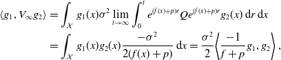 \begin{align} \langle g_1, V_\infty g_2\rangle &= \int _{\mathcal{X}} g_1(x) \sigma ^2 \lim _{t \to \infty } \int _0^t e^{(f(x)+p)r} Q e^{(f(x)+p)r} g_2(x) \, \mathrm{d}r \, \mathrm{d}x \\ & = \int _{\mathcal{X}} g_1(x)g_2(x) \frac{-\sigma ^2}{2(f(x)+p)} \, \mathrm{d}x =\dfrac{\sigma ^2}{2} \bigg \langle \frac{-1}{f+p} g_1, g_2 \bigg \rangle \,, \nonumber \end{align}
with $g_1, g_2 \in L^2(\mathcal{X})$
. We set
$g_1, g_2 \in L^2(\mathcal{X})$
. We set $g_1=g_2=g$
and, initially, we take
$g_1=g_2=g$
and, initially, we take $g=\unicode{x1D7D9}_{[0,\varepsilon ]^N}$
or
$g=\unicode{x1D7D9}_{[0,\varepsilon ]^N}$
or $g=\unicode{x1D7D9}_{[-\varepsilon, \varepsilon ]^N}$
for small enough
$g=\unicode{x1D7D9}_{[-\varepsilon, \varepsilon ]^N}$
for small enough $\varepsilon \gt 0$
. These indicator functions allow us to understand the scaling laws near the bifurcation point analytically as they are localised near the zero of
$\varepsilon \gt 0$
. These indicator functions allow us to understand the scaling laws near the bifurcation point analytically as they are localised near the zero of $f$
at
$f$
at $x_\ast =0$
. More general classes of test functions for the inner product with
$x_\ast =0$
. More general classes of test functions for the inner product with $V_\infty$
can then be treated in the usual way via approximation with simple functions.
$V_\infty$
can then be treated in the usual way via approximation with simple functions.
In Section 3, Theorem3.3 provides the scaling law of $\langle g, V_\infty g \rangle$
for
$\langle g, V_\infty g \rangle$
for $N=1$
and for an analytic function
$N=1$
and for an analytic function $f\,:\,\mathcal{X}\to \mathbb{R}$
. Similarly, in Section 4, Theorem4.5 and Theorem4.7 provide an upper bound for the rate of divergence of
$f\,:\,\mathcal{X}\to \mathbb{R}$
. Similarly, in Section 4, Theorem4.5 and Theorem4.7 provide an upper bound for the rate of divergence of $\langle g, V_\infty g \rangle$
for
$\langle g, V_\infty g \rangle$
for $N=2$
and
$N=2$
and $N=3$
respectively. Further, similar results are obtained under relaxed assumptions in Section 5 on
$N=3$
respectively. Further, similar results are obtained under relaxed assumptions in Section 5 on $g$
, the operator
$g$
, the operator $Q$
and the linear operator present in the drift component of (2.1). Moreover, Section 6 provides plots that cross-validate the stated conclusions through the implicit Euler–Maruyama method and computation of the integrals occurring in the mentioned theorems. Lastly, in Section 7, applications to the obtained results are examined.
$Q$
and the linear operator present in the drift component of (2.1). Moreover, Section 6 provides plots that cross-validate the stated conclusions through the implicit Euler–Maruyama method and computation of the integrals occurring in the mentioned theorems. Lastly, in Section 7, applications to the obtained results are examined.
3 One-dimensional case
In the current section, we assume $N=1$
and obtain a precise rate of divergence of the time-asymptotic variance of the solution of (2.1) for different types of functions
$N=1$
and obtain a precise rate of divergence of the time-asymptotic variance of the solution of (2.1) for different types of functions $f\,:\, \mathcal{X} \subseteq \mathbb{R} \to \mathbb{R}$
. Such a behaviour defines an early warning sign that precedes a bifurcation threshold of the system as
$f\,:\, \mathcal{X} \subseteq \mathbb{R} \to \mathbb{R}$
. Such a behaviour defines an early warning sign that precedes a bifurcation threshold of the system as $p$
approaches
$p$
approaches $0$
from below.
$0$
from below.
First, we choose a specific function type $f$
to analyse. Afterwards, we expand our analysis by considering general analytic functions and, lastly, we discuss an example in which
$f$
to analyse. Afterwards, we expand our analysis by considering general analytic functions and, lastly, we discuss an example in which $f$
is not analytic.
$f$
is not analytic.
3.1 Tool function
Consider the function $f_{\alpha }$
defined by
$f_{\alpha }$
defined by
 \begin{align} f_{\alpha }(x) \,:\!=\, - |x|^{\alpha } \quad \mathrm{ with } \alpha \gt 0 \end{align}
with $x$
in a neighbourhood of
$x$
in a neighbourhood of $x_\ast =0$
and such that (2.2) holds. This type of function is a useful tool for the study of system (2.1). Indeed, for
$x_\ast =0$
and such that (2.2) holds. This type of function is a useful tool for the study of system (2.1). Indeed, for $f$
such that there exist
$f$
such that there exist $c_1,c_2,\varepsilon \gt 0$
and
$c_1,c_2,\varepsilon \gt 0$
and
 \begin{align} c_1 f_\alpha (x)\leq f(x)\leq c_2 f_\alpha (x)\quad \quad \quad \forall x \in [{-}\varepsilon, \varepsilon ]\cap \mathcal{X}, \end{align}
we may transfer scaling laws obtained from the tool function directly to results for $f$
. We note that up to rescaling of the spatial variable, we can assume
$f$
. We note that up to rescaling of the spatial variable, we can assume $\varepsilon =1$
and that
$\varepsilon =1$
and that $[0,1]\subseteq \mathcal{X}$
. Hence, using
$[0,1]\subseteq \mathcal{X}$
. Hence, using $\operatorname{T}_{f_{\alpha }}$
to analyse the covariance operator and by (2.4) we obtain
$\operatorname{T}_{f_{\alpha }}$
to analyse the covariance operator and by (2.4) we obtain
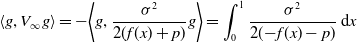 \begin{align*} \langle g, V_\infty g \rangle = - \bigg \langle g, \frac{\sigma ^{2}}{2(f(x)+p)}g \bigg \rangle = \int _{0}^{1} \frac{\sigma ^{2}}{ 2({-}f(x)-p)} \, \mathrm{d}x \end{align*}
and
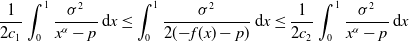 \begin{align} \frac{1}{2c_1}\int _{0}^{1} \frac{\sigma ^{2}}{ x^{\alpha }-p} \, \mathrm{d}x \leq \int _{0}^{1} \frac{\sigma ^{2}}{ 2({-}f(x)-p)} \, \mathrm{d}x \leq \frac{1}{2c_2}\int _{0}^{1} \frac{\sigma ^{2}}{ x^{\alpha }-p} \, \mathrm{d}x \end{align}
for $g(x)=\unicode{x1D7D9}_{[0,1]}$
and certain constants
$g(x)=\unicode{x1D7D9}_{[0,1]}$
and certain constants $c_1\geq 1\geq c_2$
.
$c_1\geq 1\geq c_2$
.
The following theorem describes the rate of divergence assumed by $\langle g, V_\infty g\rangle$
as
$\langle g, V_\infty g\rangle$
as $p\to 0^-$
for
$p\to 0^-$
for $f=f_\alpha$
.
$f=f_\alpha$
.
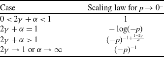
Theorem 3.1.
For $f=f_\alpha$
defined in (
3.1
),
$f=f_\alpha$
defined in (
3.1
), $Q=\operatorname{I}$
and
$Q=\operatorname{I}$
and $\varepsilon \gt 0$
, the time-asymptotic covariance
$\varepsilon \gt 0$
, the time-asymptotic covariance $V_\infty$
of the solution of (
2.1
) along
$V_\infty$
of the solution of (
2.1
) along $g(x)=\unicode{x1D7D9}_{[0,\varepsilon ]}$
,
$g(x)=\unicode{x1D7D9}_{[0,\varepsilon ]}$
, $\langle g, V_\infty g \rangle$
, presents scaling law, as
$\langle g, V_\infty g \rangle$
, presents scaling law, as $p\to 0^-$
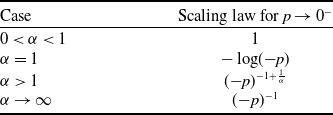
, described in Table 1.
$p\to 0^-$
, described in Table 1.
Scaling law of the time-asymptotic variance in dimension $N=1$
for the function
$N=1$
for the function $f=f_{\alpha }(x)$
and
$f=f_{\alpha }(x)$
and $g=\unicode{x1D7D9}_{[0,\varepsilon ]}$
Proof. The scaling law of $\langle g, V_\infty g \rangle$
for
$\langle g, V_\infty g \rangle$
for $p\to 0^-$
is equivalent to the one exhibited by
$p\to 0^-$
is equivalent to the one exhibited by $\int _{0}^{1} \frac{1}{x^{\alpha }-p} \, \mathrm{d}x$
, as described in (3.3). In such a limit in
$\int _{0}^{1} \frac{1}{x^{\alpha }-p} \, \mathrm{d}x$
, as described in (3.3). In such a limit in $p$
we obtain
$p$
we obtain
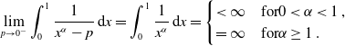 \begin{align*} \lim _{p \to 0^{-}} \int _{0}^{1} \frac{1}{x^{\alpha }-p} \, \mathrm{d}x = \int _{0}^{1} \frac{1}{x^{\alpha }} \, \mathrm{d}x = \begin{cases} \lt \infty &\mathrm{for } 0 \lt \alpha \lt 1 \,, \\ = \infty &\mathrm{for } \alpha \geq 1 \, . \end{cases} \end{align*}
For the case $\alpha = 1$
, by substituting
$\alpha = 1$
, by substituting $y = x - p$
we find that
$y = x - p$
we find that
 \begin{align*} \int _{0}^{1} \frac{1}{x - p} \, \mathrm{d}x = \int _{-p}^{1 - p} \frac{1}{y} \, \mathrm{d}y = \log\!(1 - p) - \log\!({-}p) = \Theta ({-}\log\!({-}p)) \quad \mathrm{ for } p \to 0^{-} \, . \end{align*}
We now consider the case $\alpha \gt 1$
. Through the substitution
$\alpha \gt 1$
. Through the substitution $y=x({-}p)^{-\frac{1}{\alpha }}$
we obtain
$y=x({-}p)^{-\frac{1}{\alpha }}$
we obtain
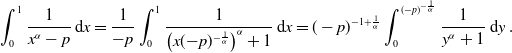 \begin{align} \int _{0}^{1} \frac{1}{x^{\alpha }-p} \, \mathrm{d}x = \frac{1}{-p} \int_{0}^{1} \frac{1}{\left (x({-}p)^{-\frac{1}{\alpha }}\right )^{\alpha }+1}\, \mathrm{d}x = (-p)^{-1 + \frac{1}{\alpha }} \int _{0}^{(-p)^{-\frac{1}{\alpha }}} \frac{1}{y^{\alpha }+1}\, \mathrm{d}y \, . \end{align}
Since $\alpha \gt 1$
, we find that
$\alpha \gt 1$
, we find that
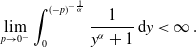 \begin{align} \lim _{p \to 0^{-}} \int _{0}^{ (-p)^{-\frac{1}{\alpha }}} \frac{1}{y^{\alpha }+1}\, \mathrm{d}y \lt \infty \, . \end{align}
Hence, taking the limit in $p$
to zero from below for the equation (3.4), we find divergence with the rate
$p$
to zero from below for the equation (3.4), we find divergence with the rate
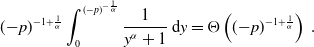 \begin{align*} ({-}p)^{-1 + \frac{1}{\alpha }} \int _{0}^{ (-p)^{-\frac{1}{\alpha }}} \frac{1}{y^{\alpha }+1}\, \mathrm{d}y = \Theta \left (({-}p)^{-1 +\frac{1}{\alpha }}\right )\, . \end{align*}
Further, we see that, for $\alpha$
approaching infinity, this expression is also well-defined with rate of divergence
$\alpha$
approaching infinity, this expression is also well-defined with rate of divergence $\Theta \!\left (\frac{1}{-p}\right )$
.
$\Theta \!\left (\frac{1}{-p}\right )$
.
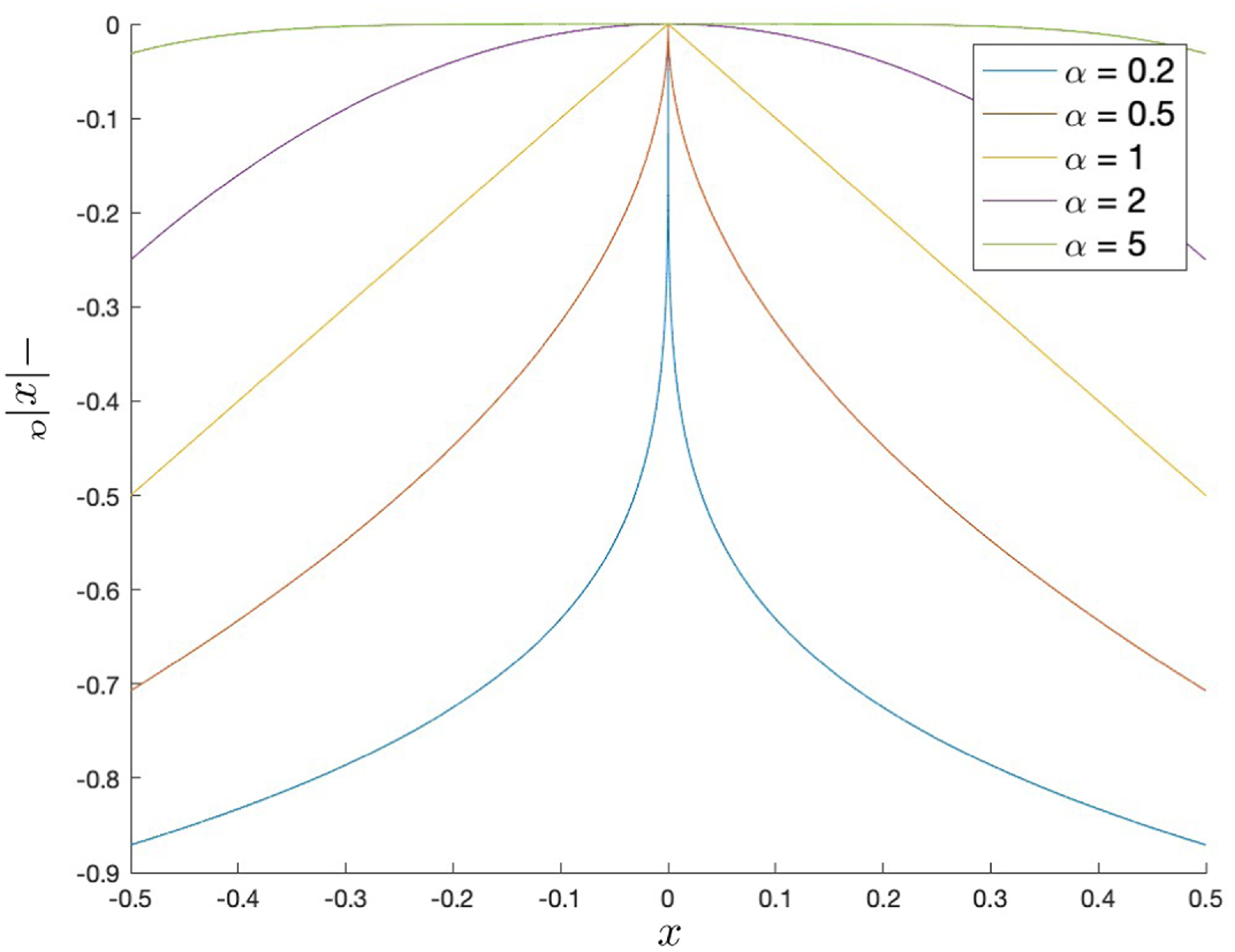
Plot of function $-|x|^{\alpha }$
for different choices of
$-|x|^{\alpha }$
for different choices of $\alpha$
. For
$\alpha$
. For $\alpha \gt 1$
, the function is
$\alpha \gt 1$
, the function is $C^1$
, with derivative equal to
$C^1$
, with derivative equal to $0$
at
$0$
at $x=0$
, therefore flat in
$x=0$
, therefore flat in $0$
. Conversely, for
$0$
. Conversely, for $\alpha \leq 1$
the function is steep at
$\alpha \leq 1$
the function is steep at $x=0$
.
$x=0$
.
Theorem3.1 states that, for the function $f_{\alpha }$
defined by (3.1) and
$f_{\alpha }$
defined by (3.1) and $0 \lt \alpha \lt 1$
, the time-asymptotic variance along
$0 \lt \alpha \lt 1$
, the time-asymptotic variance along $g$
is converging in the limit
$g$
is converging in the limit $p\to 0^-$
. Such function types
$p\to 0^-$
. Such function types $f_{\alpha }$
display a steep shape on
$f_{\alpha }$
display a steep shape on $0$
, as seen in Figure 1, given by the fact that their left and right first derivative assume infinite values. Alternatively, we observe that for
$0$
, as seen in Figure 1, given by the fact that their left and right first derivative assume infinite values. Alternatively, we observe that for $\alpha \geq 1$
, the time-asymptotic variance along
$\alpha \geq 1$
, the time-asymptotic variance along $g$
diverges, indicating that a divergence appears as the graph gets flatter and smoother, increasing
$g$
diverges, indicating that a divergence appears as the graph gets flatter and smoother, increasing $\alpha$
. The intuition behind such difference is given by the fact that, although the solution
$\alpha$
. The intuition behind such difference is given by the fact that, although the solution $u$
of (2.1) is less affected by the drift component on all
$u$
of (2.1) is less affected by the drift component on all $x\in \mathcal{X}$
as
$x\in \mathcal{X}$
as $p$
approaches
$p$
approaches $0$
, the only region in space on which
$0$
, the only region in space on which $u$
is solely driven by noise in the limit case is the set
$u$
is solely driven by noise in the limit case is the set $\{x_\ast =0\}$
. In particular, while the time-asymptotic variance of
$\{x_\ast =0\}$
. In particular, while the time-asymptotic variance of $u(x,\cdot )$
increases for all
$u(x,\cdot )$
increases for all $x\in \mathcal{X}$
, it presents divergence only on
$x\in \mathcal{X}$
, it presents divergence only on $x_\ast$
due to the fact that
$x_\ast$
due to the fact that $u(x_\ast, \cdot )$
is the solution of an Orstein–Uhlenbeck equation for any
$u(x_\ast, \cdot )$
is the solution of an Orstein–Uhlenbeck equation for any $p\leq 0$
. Analytically, it appears that for steep shapes of
$p\leq 0$
. Analytically, it appears that for steep shapes of $f_\alpha$
on
$f_\alpha$
on $x_\ast$
, the divergence of the time-asymptotic variance of
$x_\ast$
, the divergence of the time-asymptotic variance of $u(x_\ast, \cdot )$
does not affect
$u(x_\ast, \cdot )$
does not affect $\langle g, V_\infty g\rangle$
, as it is restricted by the dissipative effect of the drift component on
$\langle g, V_\infty g\rangle$
, as it is restricted by the dissipative effect of the drift component on $x\in (0,\varepsilon ]$
. Conversely, for smooth
$x\in (0,\varepsilon ]$
. Conversely, for smooth $f_\alpha$
on
$f_\alpha$
on $x_\ast$
, the dissipation induced by the multiplication operator on
$x_\ast$
, the dissipation induced by the multiplication operator on $u(x,\cdot )$
, for
$u(x,\cdot )$
, for $x\in (0,\varepsilon ]$
, is too weak to imply convergence of
$x\in (0,\varepsilon ]$
, is too weak to imply convergence of $\langle g, V_\infty g\rangle$
, but affects its rate of divergence. It is interesting to note that a similar scaling law behaviour, associated with the intermittency scaling law of an ODE dependent on a parameter near a non-smooth fold bifurcation, has been found in [Reference Kuehn38, Table 1].
$\langle g, V_\infty g\rangle$
, but affects its rate of divergence. It is interesting to note that a similar scaling law behaviour, associated with the intermittency scaling law of an ODE dependent on a parameter near a non-smooth fold bifurcation, has been found in [Reference Kuehn38, Table 1].
Remark 3.2.
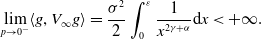
Under the assumptions of Theorem 3.1, the finite time $t\gt 0$
variance along a function
$t\gt 0$
variance along a function $g$
,
$g$
, $\langle g, V(t) g \rangle$
, converges for
$\langle g, V(t) g \rangle$
, converges for $p\to 0^-$
. Up to rescaling of
$p\to 0^-$
. Up to rescaling of $x$
, we fix
$x$
, we fix $\varepsilon =1$
and note that
$\varepsilon =1$
and note that
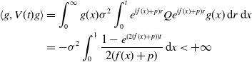 \begin{align*} \langle g, V(t) g \rangle &=\int _0^\infty g(x) \sigma ^2 \int _0^t e^{(f(x)+p)r} Q e^{(f(x)+p)r} g(x) \, \mathrm{d}r \, \mathrm{d}x \\ &= -\sigma ^2 \int _0^1 \frac{1-e^{(2(f(x)+p))t}}{2(f(x)+p)} \, \mathrm{d}x \lt +\infty \end{align*}
for any $p\leq 0$
. The growths of finite time variances are, therefore, early warning signs which are hard to observe in finite time series due to the fact that they increase as
$p\leq 0$
. The growths of finite time variances are, therefore, early warning signs which are hard to observe in finite time series due to the fact that they increase as $p$
approaches
$p$
approaches $0$
but do not diverge. For any fixed
$0$
but do not diverge. For any fixed $p\geq 0$
, longer times
$p\geq 0$
, longer times $t$
imply that the variance attains higher values.
$t$
imply that the variance attains higher values.
3.2 General analytic functions
We have found that $\langle g,V_\infty g \rangle$
converges for
$\langle g,V_\infty g \rangle$
converges for $\alpha \lt 1$
and diverges for
$\alpha \lt 1$
and diverges for $\alpha \geq 1$
, with corresponding rate of divergence, for the limit
$\alpha \geq 1$
, with corresponding rate of divergence, for the limit $p\to 0^-$
with the functions
$p\to 0^-$
with the functions $f_{\alpha }(x) = - |x|^{\alpha }$
and
$f_{\alpha }(x) = - |x|^{\alpha }$
and $g=\unicode{x1D7D9}_{[0,\varepsilon ]}$
. Our aim in this subsection is to generalise this result considerably. In particular, we now consider analytic functions
$g=\unicode{x1D7D9}_{[0,\varepsilon ]}$
. Our aim in this subsection is to generalise this result considerably. In particular, we now consider analytic functions $f$
such that (2.2) holds. Applying Taylor’s theorem and due to the fact that
$f$
such that (2.2) holds. Applying Taylor’s theorem and due to the fact that $f$
vanishes at
$f$
vanishes at $x_\ast =0$
, the function
$x_\ast =0$
, the function $f$
is of the form
$f$
is of the form
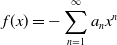 \begin{align*} f(x)= -\sum _{n=1}^{\infty }a_n x^{n} \end{align*}
for any $x\in \mathcal{X}$
and with coefficients
$x\in \mathcal{X}$
and with coefficients $\{a_n\}_{n\in \mathbb{N}}\subset \mathbb{R}$
such that (2.2) holds. Up to reparametrisation, we assume that
$\{a_n\}_{n\in \mathbb{N}}\subset \mathbb{R}$
such that (2.2) holds. Up to reparametrisation, we assume that $[0,\varepsilon ]\subseteq \mathcal{X}$
. The following theorem provides a scaling law, which can be used as an early warning sign, of the expression
$[0,\varepsilon ]\subseteq \mathcal{X}$
. The following theorem provides a scaling law, which can be used as an early warning sign, of the expression $\langle g, V_\infty g\rangle$
for an analytic
$\langle g, V_\infty g\rangle$
for an analytic $f$
and
$f$
and $g(x)=\unicode{x1D7D9}_{[0,\varepsilon ]}$
.
$g(x)=\unicode{x1D7D9}_{[0,\varepsilon ]}$
.
Theorem 3.3.
Set $f(x)=-\overset{\infty }{\underset{n=1}{\sum }}a_n x^{n}$
for all
$f(x)=-\overset{\infty }{\underset{n=1}{\sum }}a_n x^{n}$
for all $x \in \mathcal{X} \subseteq \mathbb{R}$
that satisfies (
2.2
),
$x \in \mathcal{X} \subseteq \mathbb{R}$
that satisfies (
2.2
), $\{a_n\}_{n\in \mathbb{N}}\subset \mathbb{R}$
and
$\{a_n\}_{n\in \mathbb{N}}\subset \mathbb{R}$
and $Q=\operatorname{I}$
. Let
$Q=\operatorname{I}$
. Let $m\in \mathbb{N}$
denote the index for which
$m\in \mathbb{N}$
denote the index for which $a_n = 0$
for any
$a_n = 0$
for any $n\in \{1,\dots, m-1\}$
and
$n\in \{1,\dots, m-1\}$
and $a_m\neq 0$
.Footnote
1
Then the time-asymptotic variance of the solution of (
2.1
) along
$a_m\neq 0$
.Footnote
1
Then the time-asymptotic variance of the solution of (
2.1
) along $g(x)=\unicode{x1D7D9}_{[0,\varepsilon ]}$
,
$g(x)=\unicode{x1D7D9}_{[0,\varepsilon ]}$
, $\langle g, V_\infty g \rangle$
, is characterised by the scaling law, as
$\langle g, V_\infty g \rangle$
, is characterised by the scaling law, as $p\to 0^-$
, described in Table 1, now depending on the value of
$p\to 0^-$
, described in Table 1, now depending on the value of $m=\alpha \gt 0$
.Footnote
2
$m=\alpha \gt 0$
.Footnote
2
Proof. As in the proof of Theorem3.1, up to rescaling of the variable $x$
, we can choose
$x$
, we can choose $\varepsilon =1$
. Analysing the variance along
$\varepsilon =1$
. Analysing the variance along $g$
, we obtain that
$g$
, we obtain that
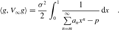 \begin{align} \langle g, V_\infty g \rangle &= \frac{\sigma ^2}{2} \int_{0}^{1} {\frac{1}{ \overset{\infty }{\underset{n=m}{\sum }}a_nx^n-p }}\, \mathrm{d}x \quad . \end{align}
For positive $x$
close to zero, the sum
$x$
close to zero, the sum $\overset{\infty }{\underset{n=1}{\sum }}a_nx^n$
is dominated by the leading term
$\overset{\infty }{\underset{n=1}{\sum }}a_nx^n$
is dominated by the leading term $a_m x^m$
, since
$a_m x^m$
, since
 \begin{align*} \lim _{x \to 0^{+}} \frac{\overset{\infty }{\underset{n=1}{\sum }}a_nx^n}{a_m x^m} = \lim _{x \to 0^{+}} \frac{\overset{\infty }{\underset{n=m}{\sum }}a_nx^n}{a_m x^m} = \lim _{x \to 0^{+}} \frac{a_m + \overset{\infty }{\underset{n=m+1}{\sum }}a_nx^{n-m}}{a_m} = 1 \;. \end{align*}
Therefore, there exists a constant $C \gt 1$
such that for any
$C \gt 1$
such that for any $x \in (0, 1]$
 \begin{align*} \frac{1}{C} a_m x^m \leq \overset{\infty }{\underset{n=1}{\sum }}a_nx^n \leq C a_m x^m \end{align*}
holds true. Hence, for (3.6) we obtain
 \begin{align*} \frac{\sigma ^2}{C} \int _0^{1} \frac{1}{a_m x^m - p}\, \mathrm{d}x \leq \sigma ^2 \int_0^{1} \frac{1}{\overset{\infty }{\underset{n=1}{\sum }}a_nx^n-p}\, \mathrm{d}x \leq C \sigma ^2 \int_0^{1} \frac{1}{a_m x^m - p}\, \mathrm{d}x \,. \end{align*}
This result is equivalent to (3.3), in the sense that it implies that the rate of divergence of $\langle g, V_\infty g \rangle$
is described in Table 1 with
$\langle g, V_\infty g \rangle$
is described in Table 1 with $m=\alpha$
.
$m=\alpha$
.
Remark 3.4.
In Theorem 3.3, we have considered bounded functions $g$
. Through similar methods as the proof of Theorem 3.1, a scaling law can be obtained for more general families of functions in
$g$
. Through similar methods as the proof of Theorem 3.1, a scaling law can be obtained for more general families of functions in $L^2(\mathcal{X})$
. For example, we consider
$L^2(\mathcal{X})$
. For example, we consider $\varepsilon \gt 0$
such that
$\varepsilon \gt 0$
such that $[0,\varepsilon ]\subseteq \mathcal{X}$
,
$[0,\varepsilon ]\subseteq \mathcal{X}$
, $g=x^{-\gamma } \unicode{x1D7D9}_{[0,\varepsilon ]}$
,
$g=x^{-\gamma } \unicode{x1D7D9}_{[0,\varepsilon ]}$
, $\gamma \lt \frac{1}{2}$
,
$\gamma \lt \frac{1}{2}$
, $f=\,f_\alpha$
and
$f=\,f_\alpha$
and $\alpha \gt 0$
, which yields
$\alpha \gt 0$
, which yields
 \begin{align*} \langle g, V_\infty g \rangle = \frac{\sigma ^2}{2}\int _0^\varepsilon \frac{1}{x^{2\gamma }} \frac{1}{x^\alpha -p} \textrm{d} x. \end{align*}
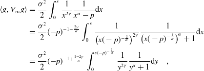
Hence, for $0\lt 2\gamma +\alpha \lt 1$
, we obtain
$0\lt 2\gamma +\alpha \lt 1$
, we obtain
 \begin{align*} \underset{p\to 0^-}{\lim }\langle g, V_\infty g \rangle = \frac{\sigma ^2}{2}\int _0^\varepsilon \frac{1}{x^{2\gamma +\alpha }} \textrm{d} x\lt +\infty . \end{align*}
Setting instead $2\gamma +\alpha \geq 1$
, we get
$2\gamma +\alpha \geq 1$
, we get
 \begin{align*} \langle g, V_\infty g \rangle &= \frac{\sigma ^2}{2}\int _0^\varepsilon \frac{1}{x^{2\gamma }} \frac{1}{x^\alpha -p} \textrm{d} x\\ &= \frac{\sigma ^2}{2}({-}p)^{-1-\frac{2\gamma }{\alpha }} \int_0^\varepsilon \frac{1}{\left (x (-p)^{-\frac{1}{\alpha }}\right )^{2\gamma }} \frac{1}{\left (x (-p)^{-\frac{1}{\alpha }}\right )^\alpha +1} \textrm{d} x\\ &= \frac{\sigma ^2}{2}({-}p)^{-1+\frac{1-2\gamma }{\alpha }}\int _0^{\varepsilon (-p)^{-\frac{1}{\alpha }}} \frac{1}{y^{2\gamma }} \frac{1}{y^\alpha +1} \textrm{d} y \quad, \end{align*}
for $y=x({-}p)^{-\frac{1}{\alpha }}$
. The scaling law for
$y=x({-}p)^{-\frac{1}{\alpha }}$
. The scaling law for $\langle g, V_\infty g \rangle$
in
$\langle g, V_\infty g \rangle$
in $p\to 0^-$
is summarised in Table 2. This result generalises the statement in [
Reference Kuehn and Romano43, Theorem 4.4] as an exact scaling law can be obtained for any analytic
$p\to 0^-$
is summarised in Table 2. This result generalises the statement in [
Reference Kuehn and Romano43, Theorem 4.4] as an exact scaling law can be obtained for any analytic $f$
that satisfies (
2.2
) and
$f$
that satisfies (
2.2
) and $g$
in a dense subset of
$g$
in a dense subset of $L^2(\mathcal{X})$
.
$L^2(\mathcal{X})$
.
Scaling law of the time-asymptotic variance in dimension $N=1$
for the function
$N=1$
for the function $f=f_{\alpha }(x)$
and
$f=f_{\alpha }(x)$
and $g=x^{-\gamma } \unicode{x1D7D9}_{[0,\varepsilon ]}$
Remark 3.5.
We found that the scaling law of the time-asymptotic variance, along an indicator function, of the solution of (
2.1
) is shown in Table 1 for every function $f$
that satisfies (
2.2
) and (
3.2
) for
$f$
that satisfies (
2.2
) and (
3.2
) for $\alpha \gt 0$
. Clearly, this does not include all possible functions
$\alpha \gt 0$
. Clearly, this does not include all possible functions $f$
. We take as an example the case in which there exists
$f$
. We take as an example the case in which there exists $\delta \geq 1$
such that
$\delta \geq 1$
such that $[{-}\delta, \delta ]\subseteq \mathcal{X}$
and functions
$[{-}\delta, \delta ]\subseteq \mathcal{X}$
and functions $f$
that converge at two different rates as
$f$
that converge at two different rates as $x$
approaches
$x$
approaches $0^-$
and
$0^-$
and $0^+$
. We consider
$0^+$
. We consider
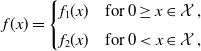 \begin{align*} f(x) = \begin{cases} f_1(x) & \mathrm{for }\; 0 \geq x \in \mathcal{X} \,, \\[3pt] f_2(x) & \mathrm{for }\; 0 \lt x \in \mathcal{X} \,, \\ \end{cases} \end{align*}
for smooth functions $f_1\,:\,\mathcal{X}\cap \mathbb{R}_{\leq 0}\rightarrow \mathbb{R}$
and
$f_1\,:\,\mathcal{X}\cap \mathbb{R}_{\leq 0}\rightarrow \mathbb{R}$
and $f_2\,:\,\mathcal{X}\cap \mathbb{R}_{\geq 0}\rightarrow \mathbb{R}$
and
$f_2\,:\,\mathcal{X}\cap \mathbb{R}_{\geq 0}\rightarrow \mathbb{R}$
and $f$
that satisfies (
2.2
). We assume
$f$
that satisfies (
2.2
). We assume $g(x)=\unicode{x1D7D9}_{[ -1, 1 ]}(x)$
and by (
2.4
) we get
$g(x)=\unicode{x1D7D9}_{[ -1, 1 ]}(x)$
and by (
2.4
) we get
 \begin{align} \langle g, V_\infty g \rangle = \int _{- 1}^{1} \frac{- \sigma ^2}{2(f(x)+p)} \, \mathrm{d}x = \frac{\sigma ^2}{2}\int _{-1}^{0} \frac{1}{-f_1(x)-p} \, \mathrm{d}x + \frac{\sigma ^2}{2}\int _{0}^{1} \frac{1}{-f_2(x)-p} \, \mathrm{d}x \, . \end{align}
We consider each summand separately and take the limit in $p$
to zero from below. If
$p$
to zero from below. If $\underset{x\rightarrow{0^+}}{\lim }\,f_2(x)\lt 0$
, then
$\underset{x\rightarrow{0^+}}{\lim }\,f_2(x)\lt 0$
, then
 \begin{align*} \lim _{p \to 0^{-}} \int _{0}^{1} \frac{1}{-f_2(x)-p} \, \mathrm{d}x\lt +\infty \end{align*}
and the scaling rate of $\langle g, V_\infty g \rangle$
is equivalent to the one given by
$\langle g, V_\infty g \rangle$
is equivalent to the one given by $\int _{-1}^{0} \frac{1}{-f_1(x)-p} \, \mathrm{d}x$
. Otherwise, it is dictated by the highest rate associated with the two summands. Such rates are shown in Table 1, assuming that
$\int _{-1}^{0} \frac{1}{-f_1(x)-p} \, \mathrm{d}x$
. Otherwise, it is dictated by the highest rate associated with the two summands. Such rates are shown in Table 1, assuming that $f_1$
and
$f_1$
and $f_2$
are analytic or that they have the same order of convergence to
$f_2$
are analytic or that they have the same order of convergence to $0$
as
$0$
as $f_\alpha$
for any
$f_\alpha$
for any $\alpha \gt 0$
.
$\alpha \gt 0$
.
4 Higher-dimensional cases
In the present section, we obtain upper bounds for the scaling of the time-asymptotic variance of the solutions of the system (2.1) along chosen functions $g$
. In this case, we consider
$g$
. In this case, we consider $N\gt 1$
, therefore assuming that the system (2.1) is studied in higher spatial dimensions. We find that, for certain functions
$N\gt 1$
, therefore assuming that the system (2.1) is studied in higher spatial dimensions. We find that, for certain functions $f\,:\,\mathcal{X}\subseteq \mathbb{R}^N\to \mathbb{R}$
, the early warning signs display convergence of the variance along the mentioned directions in the square-integrable function space,
$f\,:\,\mathcal{X}\subseteq \mathbb{R}^N\to \mathbb{R}$
, the early warning signs display convergence of the variance along the mentioned directions in the square-integrable function space, $L^2(\mathcal{X})$
.
$L^2(\mathcal{X})$
.
For the remainder of this section, we assume that $f$
is analytic and satisfies (2.2) for
$f$
is analytic and satisfies (2.2) for $x_\ast =0\in \mathcal{X}\subseteq \mathbb{R}^N$
. Hence,
$x_\ast =0\in \mathcal{X}\subseteq \mathbb{R}^N$
. Hence, $f$
is of the form
$f$
is of the form
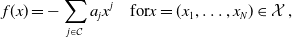 \begin{align} f(x) = - \sum _{j \in \mathcal{C}} a_j x^j \quad \mathrm{ for } x = (x_1, \dots, x_N)\in \mathcal{X}\,, \end{align}
where $j$
is a multi-index, i.e.,
$j$
is a multi-index, i.e., $x^j = \overset{N}{\underset{n=1}{\prod }} x_n^{i_n}$
with the collection
$x^j = \overset{N}{\underset{n=1}{\prod }} x_n^{i_n}$
with the collection $\mathcal{C}$
defined by the set
$\mathcal{C}$
defined by the set
 \begin{align*} \mathcal{C} = \left \{j = (i_1, \ldots, i_N) \in \left \{\mathbb{N}\cup \{0\}\right \}^N \right \}\, . \end{align*}
The coefficients $a_j$
are real-valued, and their signs satisfy (2.2) as discussed further in the paper. We assume that there exists
$a_j$
are real-valued, and their signs satisfy (2.2) as discussed further in the paper. We assume that there exists $\varepsilon \gt 0$
such that
$\varepsilon \gt 0$
such that $[0, \varepsilon ]^N\subseteq \mathcal{X}$
, up to rescaling of the space variable
$[0, \varepsilon ]^N\subseteq \mathcal{X}$
, up to rescaling of the space variable $x$
. Properties (2.2) imply that equation (2.4) holds, hence for
$x$
. Properties (2.2) imply that equation (2.4) holds, hence for $g(x) = \unicode{x1D7D9}_{[0, \varepsilon ]^N}(x)$
we find
$g(x) = \unicode{x1D7D9}_{[0, \varepsilon ]^N}(x)$
we find
 \begin{align*} \langle g, V_\infty g \rangle = \sigma ^2 \bigg \langle \frac{-1}{2(f+p)} g, g \bigg \rangle = \frac{\sigma ^2}{2} \int _0^\varepsilon \cdots \int _0^\varepsilon \frac{-1}{f(x)+p} \, \mathrm{d}x = \frac{\sigma ^2}{2} \int_0^\varepsilon \cdots \int_0^\varepsilon \frac{1}{\underset{j \in \mathcal{C}}{\sum }a_jx^j - p} \, \mathrm{d}x \;. \end{align*}
In the next proposition, we prove that for any $f$
in a dense subset of the analytic functions space that satisfies (2.2), the variance
$f$
in a dense subset of the analytic functions space that satisfies (2.2), the variance $\langle g, V_\infty g \rangle$
converges for
$\langle g, V_\infty g \rangle$
converges for $p\to 0^-$
.
$p\to 0^-$
.
Proposition 4.1.
Fix the dimension $N\gt 1$
, and set the indices
$N\gt 1$
, and set the indices $\{i_k \}_{k \in \{ 1, \ldots, N\}}$
as a permutation of
$\{i_k \}_{k \in \{ 1, \ldots, N\}}$
as a permutation of $\{ 1, \ldots, N\}$
. Furthermore, suppose that there exist two multi-indices
$\{ 1, \ldots, N\}$
. Furthermore, suppose that there exist two multi-indices $j_1,j_2\in \mathcal{C}$
such that
$j_1,j_2\in \mathcal{C}$
such that $a_{j_1}, a_{j_2} \gt 0$
and that each of these multi-indices corresponds to the multiplication of only one
$a_{j_1}, a_{j_2} \gt 0$
and that each of these multi-indices corresponds to the multiplication of only one $x_{i_1}$
, resp.
$x_{i_1}$
, resp. $x_{i_2}$
, meaning that
$x_{i_2}$
, meaning that $j_1$
, resp.
$j_1$
, resp. $j_2$
, has all elements equal to
$j_2$
, has all elements equal to $0$
with the exception of the component on the
$0$
with the exception of the component on the $i_1$
-th, resp.
$i_1$
-th, resp. $i_2$
-th, position which assumes value
$i_2$
-th, position which assumes value $1$
. Then it holds that
$1$
. Then it holds that
 \begin{align*} \lim _{p \to 0^{-}} \langle g, V_\infty g \rangle \lt \infty \end{align*}
for any $\varepsilon \gt 0$
and
$\varepsilon \gt 0$
and $g(x) = \unicode{x1D7D9}_{[0, \varepsilon ]^N}(x)$
.
$g(x) = \unicode{x1D7D9}_{[0, \varepsilon ]^N}(x)$
.
Proof. Without loss of generality, we assume that $j_1 = (1,0,0 \ldots )$
and
$j_1 = (1,0,0 \ldots )$
and $j_2 = (0,1,0 \ldots )$
. Then we obtain
$j_2 = (0,1,0 \ldots )$
. Then we obtain
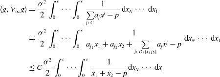 \begin{align*} \langle g, V_\infty g \rangle &= \frac{\sigma ^2}{2} \int_0^\varepsilon \cdots \int_0^\varepsilon \frac{1}{\underset{j \in \mathcal{C}}{\sum }a_jx^j - p}\, \mathrm{d}x_N \cdots \, \mathrm{d}x_1 \\ &= \frac{\sigma ^2}{2} \int_0^\varepsilon \cdots \int_0^\varepsilon \frac{1}{a_{j_1} x_1 + a_{j_2} x_2 + \underset{j \in \mathcal{C} \setminus \{j_1, j_2\}}{\sum }a_jx^j - p}\, \mathrm{d}x_N \cdots \, \mathrm{d}x_1 \\ &\leq C \frac{\sigma ^2}{2} \int _0^\varepsilon \cdots \int _0^\varepsilon \frac{1}{x_1 + x_2 -p} \mathrm{d}x_N \cdots \, \mathrm{d}x_1 \, \end{align*}
where the last inequality is satisfied by a constant $C\gt 0$
and follows from the values
$C\gt 0$
and follows from the values $a_{j_1}, a_{j_2} \gt 0 \gt p$
, the continuity of
$a_{j_1}, a_{j_2} \gt 0 \gt p$
, the continuity of $f$
and the compactness of the support of
$f$
and the compactness of the support of $g$
. This implies that
$g$
. This implies that
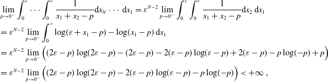 \begin{align*} & \lim _{p \to 0^{-}} \int _0^\varepsilon \cdots \int _0^\varepsilon \frac{1}{x_1 + x_2 - p} \mathrm{d}x_N \cdots \, \mathrm{d}x_1 = \varepsilon ^{N-2} \lim _{p \to 0^{-}} \int _0^\varepsilon \int _0^\varepsilon \frac{1}{x_1 + x_2 - p} \mathrm{d}x_2 \, \mathrm{d}x_1\\ &= \varepsilon ^{N-2} \lim _{p \to 0^{-}} \int _0^\varepsilon \log\!(\varepsilon +x_1 - p) - \log\!(x_1 -p) \, \mathrm{d}x_1 \\ &= \varepsilon ^{N-2} \lim _{p \to 0^{-}} \Big ( (2\varepsilon -p)\log\!(2\varepsilon -p)-(2\varepsilon -p) -2(\varepsilon -p)\log\!(\varepsilon -p)+2(\varepsilon -p) -p\log\!({-}p)+p \Big )\\ &= \varepsilon ^{N-2} \lim _{p \to 0^{-}} \Big ( (2\varepsilon -p)\log\!(2\varepsilon -p) -2(\varepsilon -p)\log\!(\varepsilon -p)-p\log\!({-}p) \Big )\lt +\infty \;, \end{align*}
which concludes the proof.
Example 4.2.
We study the trivial case in which we set $f$
in (
2.1
) to be
$f$
in (
2.1
) to be $f_\infty (x)\,:\!=\, 0$
for any
$f_\infty (x)\,:\!=\, 0$
for any $x$
in a neighbourhood of
$x$
in a neighbourhood of $x_\ast$
, in order to exclude it from the following computations. Whereas the function
$x_\ast$
, in order to exclude it from the following computations. Whereas the function $f_\infty$
does not satisfy the assumptions on the sign of
$f_\infty$
does not satisfy the assumptions on the sign of $f$
in (
2.2
), it provides an interesting and easy-to-study limit case. The time-asymptotic variance along the function
$f$
in (
2.2
), it provides an interesting and easy-to-study limit case. The time-asymptotic variance along the function $g = \unicode{x1D7D9}_{[0, \varepsilon ]^N}$
satisfies
$g = \unicode{x1D7D9}_{[0, \varepsilon ]^N}$
satisfies
 \begin{align*} &\langle g, V_\infty g \rangle = \frac{\sigma ^2}{2} \int _0^\varepsilon \dots \int _0^\varepsilon \frac{1}{f_\infty (x_1, \dots, x_N)-p}\, \mathrm{d}x_N \dots \, \mathrm{d}x_1 = \frac{\sigma ^2}{2} \int _0^\varepsilon \dots \int _0^\varepsilon \frac{1}{-p}\, \mathrm{d}x_N \dots \, \mathrm{d}x_1 = -\frac{\sigma ^2}{2p} \varepsilon ^N \, . \end{align*}
Taking the limit in $p$
, we obtain that
$p$
, we obtain that
 \begin{align*} \lim _{p\to 0^{-}} \langle g, V_\infty g \rangle = \lim _{p\to 0^{-}}-\frac{\sigma ^2}{2p} \varepsilon ^N= \infty \,. \end{align*}
Hence, we observe divergence with rate $\Theta \left ({-}p^{-1}\right )$
for
$\Theta \left ({-}p^{-1}\right )$
for $p$
approaching zero from below, if
$p$
approaching zero from below, if $f$
in (
2.1
) is, locally, equal to the null function.
$f$
in (
2.1
) is, locally, equal to the null function.
4.1 Upper bounds
In the remainder of this section, we find upper bounds for the scaling law of $\langle g, V_\infty g \rangle$
for the case in which the dimension
$\langle g, V_\infty g \rangle$
for the case in which the dimension $N$
of the domain of the function
$N$
of the domain of the function $f$
is larger than
$f$
is larger than $1$
. From the construction of
$1$
. From the construction of $f$
in (4.1), we define the set of multi-indices
$f$
in (4.1), we define the set of multi-indices
 \begin{align} \mathcal{C}^{+} \,:\!=\, \Big \{ j=(i_1,\dots, i_N)\in \mathcal{C} \Big | \; a_d=0\;\;\forall d=(d_1,\dots, d_N)\in \mathcal{C} \;\;\mathrm{s.t.}\;\; d_n\leq i_n\;\; \forall n\in \{1,\dots, N\} \;\;\mathrm{and}\;\; d\neq j\Big \}\;. \end{align}
The following lemma introduces an upper bound of $\langle g, V_\infty g \rangle$
as
$\langle g, V_\infty g \rangle$
as $p\to 0^-$
. The scaling law induced by this upper bound is studied further below.
$p\to 0^-$
. The scaling law induced by this upper bound is studied further below.
Lemma 4.3.
Set $f(x)= - \underset{j \in \mathcal{C}}{\sum }a_j x^j$
for all
$f(x)= - \underset{j \in \mathcal{C}}{\sum }a_j x^j$
for all $x \in \mathcal{X} \subseteq \mathbb{R}^N$
, that satisfies (
2.2
),
$x \in \mathcal{X} \subseteq \mathbb{R}^N$
, that satisfies (
2.2
), $\{a_j\}_{j\in \mathcal{C}}\subset \mathbb{R}$
,
$\{a_j\}_{j\in \mathcal{C}}\subset \mathbb{R}$
, $\varepsilon \gt 0$
and
$\varepsilon \gt 0$
and $Q=\operatorname{I}$
. Fix
$Q=\operatorname{I}$
. Fix $j_{\ast } \in \mathcal{C}^{+}$
, defined in (4.2). Then the time-asymptotic covariance of the solution of (
2.1
),
$j_{\ast } \in \mathcal{C}^{+}$
, defined in (4.2). Then the time-asymptotic covariance of the solution of (
2.1
), $V_\infty$
, satisfies,
$V_\infty$
, satisfies,
 \begin{align*} \langle g, V_\infty g \rangle \leq \Theta \left ( \int _0^\varepsilon \cdots \int _0^\varepsilon \frac{1}{a_{j_\ast } x^{j_\ast } -p} \, \mathrm{d}x_1 \dots \mathrm{d}x_N \right )\;, \end{align*}
for $g(x)=\unicode{x1D7D9}_{[0,\varepsilon ]^N}$
.
$g(x)=\unicode{x1D7D9}_{[0,\varepsilon ]^N}$
.
Proof. Since we assume $f$
to be negative in
$f$
to be negative in $\mathcal{X}\setminus \{0\}$
and we consider the bounded domain
$\mathcal{X}\setminus \{0\}$
and we consider the bounded domain $[0,\varepsilon ]^N$
, we know that
$[0,\varepsilon ]^N$
, we know that $a_j\gt 0$
for any
$a_j\gt 0$
for any $j\in \mathcal{C^+}$
. In particular, we note that for a constant
$j\in \mathcal{C^+}$
. In particular, we note that for a constant $1\gt C\gt 0$
, dependent on
$1\gt C\gt 0$
, dependent on $\varepsilon$
, and any
$\varepsilon$
, and any $x\in [0,\varepsilon ]^N$
, it holds
$x\in [0,\varepsilon ]^N$
, it holds
 \begin{align*} - f(x) = \sum _{j \in \mathcal{C}}a_j x^j \geq C \sum _{j \in \mathcal{C}^{+}}a_j x^j \geq C a_{j_{\ast }}x^{j_{\ast }} \end{align*}
for $j_{\ast } \in \mathcal{C}^{+}$
. Hence, we obtain
$j_{\ast } \in \mathcal{C}^{+}$
. Hence, we obtain
 \begin{align} \langle g, V_\infty g \rangle = \frac{\sigma ^2}{2} \int_{0}^\varepsilon \cdots \int_{0}^\varepsilon \frac{1}{\underset{j \in \mathcal{C}}{\sum } a_j x^{j} - p} \, \mathrm{d}x_1 \dots \mathrm{d}x_N \leq \frac{\sigma ^2}{2 C} \int _0^\varepsilon \cdots \int _0^\varepsilon \frac{1}{a_{j_\ast } x^{j_\ast } -p} \, \mathrm{d}x_1 \dots \mathrm{d}x_N \;. \end{align}
Without loss of generality and for simplicity, we assume for the remainder of the section that $a_{j_{\ast }} = \frac{\sigma ^2}{2} = 1$
.
$a_{j_{\ast }} = \frac{\sigma ^2}{2} = 1$
.
Remark 4.4.
In case the multi-index $j_\ast$
has
$j_\ast$
has $N\gt k\in \mathbb{N}\cup \{0\}$
indices with value
$N\gt k\in \mathbb{N}\cup \{0\}$
indices with value $0$
, the analysis on the upper bound in (4.3) can be reduced to the case of
$0$
, the analysis on the upper bound in (4.3) can be reduced to the case of $N-k$
spatial dimensions. In fact, assuming that
$N-k$
spatial dimensions. In fact, assuming that $j_\ast =(i_1,\dots, i_{N-k},0,\dots, 0)$
, we obtain
$j_\ast =(i_1,\dots, i_{N-k},0,\dots, 0)$
, we obtain
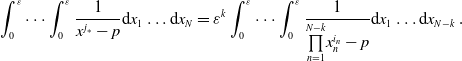 \begin{align*} \int _0^\varepsilon \cdots \int _0^\varepsilon \frac{1}{x^{j_\ast }-p} \mathrm{d}x_1\dots \mathrm{d}x_N =\varepsilon ^k \int_0^\varepsilon \cdots \int_0^\varepsilon \frac{1}{\overset{N-k}{\underset{n=1}{\prod }} x_n^{i_n}-p} \mathrm{d}x_1\dots \mathrm{d}x_{N-k}\;. \end{align*}
We note that the case $N=k$
contradicts the assumption
$N=k$
contradicts the assumption $f(x_\ast )=0$
and results in convergence of the upper bound as the bifurcation threshold is not reached for
$f(x_\ast )=0$
and results in convergence of the upper bound as the bifurcation threshold is not reached for $p\to 0^-$
.
$p\to 0^-$
.
As a consequence of Remark 4.4, we consider $j_\ast$
with no elements equal to
$j_\ast$
with no elements equal to $0$
in the remaining subsections.
$0$
in the remaining subsections.
4.2 Two dimensions
In this subsection, we find an upper bound for the scaling law of $\langle g, V_\infty g \rangle$
for
$\langle g, V_\infty g \rangle$
for $N=2$
. We therefore consider
$N=2$
. We therefore consider $j_\ast =(i_1,i_2)\in \mathbb{N}^2$
. In the following theorem, we outline how to obtain such upper bounds.
$j_\ast =(i_1,i_2)\in \mathbb{N}^2$
. In the following theorem, we outline how to obtain such upper bounds.
Theorem 4.5.
Set $f(x)= - \underset{j \in \mathcal{C}}{\sum }a_j x^j$
for all
$f(x)= - \underset{j \in \mathcal{C}}{\sum }a_j x^j$
for all $x \in \mathcal{X} \subseteq \mathbb{R}^2$
, that satisfies (
2.2
),
$x \in \mathcal{X} \subseteq \mathbb{R}^2$
, that satisfies (
2.2
), $\{a_j\}_{j\in \mathcal{C}}\subset \mathbb{R}$
,
$\{a_j\}_{j\in \mathcal{C}}\subset \mathbb{R}$
, $\varepsilon \gt 0$
and
$\varepsilon \gt 0$
and $Q=\operatorname{I}$
. Fix
$Q=\operatorname{I}$
. Fix $j_\ast =(i_1,i_2)\in \mathcal{C}^+$
with
$j_\ast =(i_1,i_2)\in \mathcal{C}^+$
with $i_1,i_2\gt 0$
. Then there exists an upper bound to the time-asymptotic variance of the solution of (
2.1
) along
$i_1,i_2\gt 0$
. Then there exists an upper bound to the time-asymptotic variance of the solution of (
2.1
) along $g(x)=\unicode{x1D7D9}_{[0,\varepsilon ]^2}$
,
$g(x)=\unicode{x1D7D9}_{[0,\varepsilon ]^2}$
, $\langle g, V_\infty g \rangle$
, and its rate as
$\langle g, V_\infty g \rangle$
, and its rate as $p\to 0^-$
is described in Table 3 in accordance to the value of
$p\to 0^-$
is described in Table 3 in accordance to the value of $i_1$
and
$i_1$
and $i_2$
.
$i_2$
.
Upper bounds to the scaling law of the time-asymptotic variance in dimension $N=2$
for different choices of indices
$N=2$
for different choices of indices $i_1, i_2$
, ordered for simplicity. We indicate as
$i_1, i_2$
, ordered for simplicity. We indicate as $\mathfrak{A}$
and
$\mathfrak{A}$
and $\mathfrak{B}$
two summands whose sum corresponds to the upper bound
$\mathfrak{B}$
two summands whose sum corresponds to the upper bound
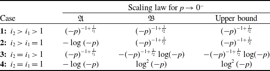
The proof of the theorem can be found in Appendix A. Overall, we have obtained an upper bound for an analytic function $f$
. In Table 3, we see that only the highest index
$f$
. In Table 3, we see that only the highest index $i_2$
directly affects the scaling law of the upper bound. However, its relation to the other index
$i_2$
directly affects the scaling law of the upper bound. However, its relation to the other index $i_1$
dictates the exact form. The limiting case for
$i_1$
dictates the exact form. The limiting case for $i_1,i_2\to \infty$
has been discussed in Example 4.2. Lastly, we note that our bound may not be sharp, as described in Proposition 4.1 and as shown in the next example. Figure 2 presents an intuition for the example
$i_1,i_2\to \infty$
has been discussed in Example 4.2. Lastly, we note that our bound may not be sharp, as described in Proposition 4.1 and as shown in the next example. Figure 2 presents an intuition for the example $j_\ast =(2,3)$
by illustrating the shapes of
$j_\ast =(2,3)$
by illustrating the shapes of $-x_1-x_2$
and
$-x_1-x_2$
and $-x_1^2 x_2^3$
, for
$-x_1^2 x_2^3$
, for $(x_1,x_2)\in [0,0.1]^2$
. Such functions can be assumed to be locally equal to
$(x_1,x_2)\in [0,0.1]^2$
. Such functions can be assumed to be locally equal to $f$
in Proposition 4.1 and Theorem4.5, respectively. As displayed, the first function has a unique root on
$f$
in Proposition 4.1 and Theorem4.5, respectively. As displayed, the first function has a unique root on $(0,0)$
, and the second is null on the set
$(0,0)$
, and the second is null on the set $(x_1,x_2)$
such that
$(x_1,x_2)$
such that $x_1=0$
or
$x_1=0$
or $x_2=0$
. The different dimensions that characterise such sets are the reason for the fact that the time-asymptotic variance on an indicator function
$x_2=0$
. The different dimensions that characterise such sets are the reason for the fact that the time-asymptotic variance on an indicator function $g$
,
$g$
, $\langle g, V_\infty g \rangle$
, presents different scaling laws in the limit
$\langle g, V_\infty g \rangle$
, presents different scaling laws in the limit $p\to 0^-$
. In particular, it converges in the first case and diverges with rate
$p\to 0^-$
. In particular, it converges in the first case and diverges with rate $({-}p)^{-\frac{2}{3}}$
in the second.Footnote
3
$({-}p)^{-\frac{2}{3}}$
in the second.Footnote
3
Illustration of functions $-x_1-x_2$
, in Figure a, and
$-x_1-x_2$
, in Figure a, and $-x_1^2 x_2^3$
, in Figure b, for
$-x_1^2 x_2^3$
, in Figure b, for $x_1,x_2\in [0,0.1]$
. We set an indicator function
$x_1,x_2\in [0,0.1]$
. We set an indicator function $g=\unicode{x1D7D9}_{[0,\varepsilon ]^2}$
, for
$g=\unicode{x1D7D9}_{[0,\varepsilon ]^2}$
, for $0\lt \varepsilon \leq 0.1$
. As discussed in Proposition 4.1 and in the proof of Theorem4.5, the time-asymptotic variance
$0\lt \varepsilon \leq 0.1$
. As discussed in Proposition 4.1 and in the proof of Theorem4.5, the time-asymptotic variance $\langle g, V_\infty g \rangle$
presents different scaling laws as
$\langle g, V_\infty g \rangle$
presents different scaling laws as $p\to 0^-$
under distinct assumptions of
$p\to 0^-$
under distinct assumptions of $f$
. For
$f$
. For $f$
set as in Figure a, the variance converges in the limit, whereas for
$f$
set as in Figure a, the variance converges in the limit, whereas for $f$
as displayed in Figure b, it diverges. We note that the choice of
$f$
as displayed in Figure b, it diverges. We note that the choice of $f$
in the Figure a presents only one value
$f$
in the Figure a presents only one value $x_\ast$
such that
$x_\ast$
such that $f(x_\ast )=0$
, in contrast with the second figure, for which
$f(x_\ast )=0$
, in contrast with the second figure, for which $f(x_1,x_2)=0$
for any
$f(x_1,x_2)=0$
for any $(x_1,x_2)$
such that
$(x_1,x_2)$
such that $x_1=0$
or
$x_1=0$
or $x_2=0$
. Such lines are displayed in the figure for comparison.
$x_2=0$
. Such lines are displayed in the figure for comparison.
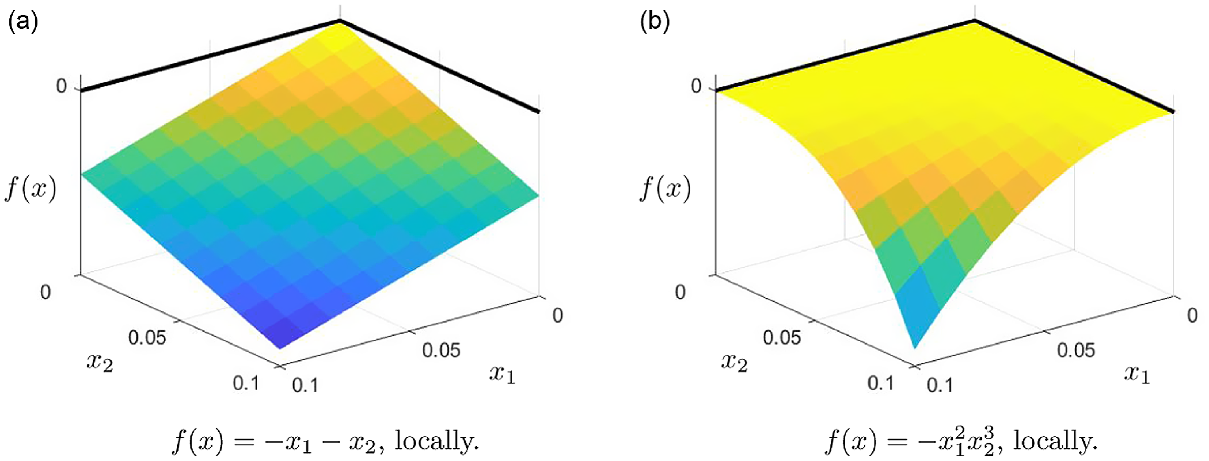
Example 4.6.
We consider the function $f$
such that it satisfies (
2.2
),
$f$
such that it satisfies (
2.2
), $[0,1]^2\subseteq \mathcal{X}$
and there exists
$[0,1]^2\subseteq \mathcal{X}$
and there exists $C\gt 0$
for which
$C\gt 0$
for which
 \begin{align*} C^{-1} \left ( - x_1^2-x_2^2 \right ) \leq f(x) \leq C \left ( - x_1^2-x_2^2 \right ) \,, \end{align*}
for $0\leq x_1,x_2 \leq 1$
. This implies that
$0\leq x_1,x_2 \leq 1$
. This implies that
 \begin{align*} \langle g, V_\infty g \rangle &\leq C^{-1} \int _{0}^1\int _0^1 \frac{1}{x_1^2+x_2^2-p} \, \mathrm{d}x_1 \, \mathrm{d}x_2 \leq C^{-1} \iint _{D} \frac{1}{x_1^2 + x_2^2 -p} \, \mathrm{d}x_1 \, \mathrm{d}x_2 \quad, \end{align*}
where $D$
denotes the circle of radius
$D$
denotes the circle of radius $\sqrt{2}$
centreed at the origin. We study then the integral in polar coordinates and obtain
$\sqrt{2}$
centreed at the origin. We study then the integral in polar coordinates and obtain
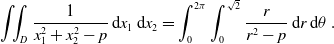 \begin{align*} \iint _{D} \frac{1}{x_1^2 + x_2^2 -p} \, \mathrm{d}x_1 \, \mathrm{d}x_2 = \int _0^{2 \pi } \int _{0}^{\sqrt{2} } \frac{r}{r^2 - p} \, \mathrm{d}r \, \mathrm{d} \theta \, . \end{align*}
Substituting $r^{\prime } = r^2 - p$
, we get
$r^{\prime } = r^2 - p$
, we get
 \begin{align*} &\int _0^{2 \pi } \int _{0}^{\sqrt{2} } \frac{r}{r^2 - p} \, \mathrm{d}r \, \mathrm{d} \theta = \frac{1}{2} \int _0^{2 \pi } \int _{-p}^{2 -p} \frac{1}{r^{\prime }} \, \mathrm{d}r^{\prime } \, \mathrm{d} \theta = \pi \Big ( \log\!(2 -p) - \log\!({-}p) \Big ) =\Theta \Big (- \log \left (-p \right ) \Big )\, . \end{align*}
A lower bound can be easily obtained through
 \begin{align*} \langle g, V_\infty g \rangle &\geq C \int _{0}^1\int _0^1 \frac{1}{x_1^2+x_2^2-p} \, \mathrm{d}x_1 \, \mathrm{d}x_2 \geq C \iint _{\tilde{D}} \frac{1}{x_1^2 + x_2^2 -p} \, \mathrm{d}x_1 \, \mathrm{d}x_2 =\Theta \Big (- \log \left (-p \right ) \Big ) \quad, \end{align*}
for $\tilde{D}=\left \{(x,y) \;\big |\; x^2+y^2\leq 1 \;,\; x,y\gt 0\right \}$
. Hence, we find divergence of
$\tilde{D}=\left \{(x,y) \;\big |\; x^2+y^2\leq 1 \;,\; x,y\gt 0\right \}$
. Hence, we find divergence of $\langle g,V_\infty g\rangle$
, for
$\langle g,V_\infty g\rangle$
, for $p$
approaching zero from below, of rate
$p$
approaching zero from below, of rate $\Theta \Big ({-}\log \left (-p \right ) \Big )$
, whereas the upper bounds in Theorem
4.5
assume scaling law
$\Theta \Big ({-}\log \left (-p \right ) \Big )$
, whereas the upper bounds in Theorem
4.5
assume scaling law $\Theta \left (({-}p)^{-\frac{1}{2}} \right )$
.
$\Theta \left (({-}p)^{-\frac{1}{2}} \right )$
.
4.3 Three dimensions
We now assume $N=3$
and therefore
$N=3$
and therefore $f\,:\,\mathcal{X}\subseteq \mathbb{R}^3\to \mathbb{R}$
and
$f\,:\,\mathcal{X}\subseteq \mathbb{R}^3\to \mathbb{R}$
and $g=\unicode{x1D7D9}_{[0,\varepsilon ]^3}$
. The following theorem provides an upper bound for the scaling law of the corresponding early warning sign
$g=\unicode{x1D7D9}_{[0,\varepsilon ]^3}$
. The following theorem provides an upper bound for the scaling law of the corresponding early warning sign $\langle g, V_\infty g \rangle$
.
$\langle g, V_\infty g \rangle$
.
Theorem 4.7.
Set $f(x)= - \underset{j \in \mathcal{C}}{\sum } a_j x^j$
for all
$f(x)= - \underset{j \in \mathcal{C}}{\sum } a_j x^j$
for all $x \in \mathcal{X} \subseteq \mathbb{R}^3$
that satisfies (
2.2
),
$x \in \mathcal{X} \subseteq \mathbb{R}^3$
that satisfies (
2.2
), $\{a_j\}_{j\in \mathcal{C}}\subset \mathbb{R}$
,
$\{a_j\}_{j\in \mathcal{C}}\subset \mathbb{R}$
, $\varepsilon \gt 0$
and
$\varepsilon \gt 0$
and $Q=\operatorname{I}$
. Fix
$Q=\operatorname{I}$
. Fix $j_\ast =(i_1,i_2,i_3)\in \mathcal{C}^+$
with
$j_\ast =(i_1,i_2,i_3)\in \mathcal{C}^+$
with $i_1,i_2, i_3\gt 0$
. Then there exists an upper bound to the time-asymptotic variance of the solution of (
2.1
) along
$i_1,i_2, i_3\gt 0$
. Then there exists an upper bound to the time-asymptotic variance of the solution of (
2.1
) along $g(x)=\unicode{x1D7D9}_{[0,\varepsilon ]^3}$
,
$g(x)=\unicode{x1D7D9}_{[0,\varepsilon ]^3}$
, $\langle g, V_\infty g \rangle$
, and it has a scaling law bound as
$\langle g, V_\infty g \rangle$
, and it has a scaling law bound as $p\to 0^-$
described in Table 4 depending upon the values of
$p\to 0^-$
described in Table 4 depending upon the values of $i_1$
,
$i_1$
, $i_2$
and
$i_2$
and $i_3$
.
$i_3$
.
Upper bounds to the scaling law of the time-asymptotic variance in dimension $N=3$
for different choices of indices
$N=3$
for different choices of indices $i_1, i_2$
and
$i_1, i_2$
and $i_3$
, ordered for simplicity. We denote as
$i_3$
, ordered for simplicity. We denote as $\mathfrak{C}$
and
$\mathfrak{C}$
and $\mathfrak{D}$
two values whose sum is the upper bound
$\mathfrak{D}$
two values whose sum is the upper bound
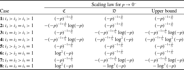
The theorem is proven in Appendix B. We observe that if $i_3$
is strictly greater than the other indices,
$i_3$
is strictly greater than the other indices, $i_1$
and
$i_1$
and $i_2$
, we find divergence with the upper bound
$i_2$
, we find divergence with the upper bound $\Theta \left (({-}p)^{-1 + \frac{1}{i_3}}\right )$
. If the highest index value is given by two of the indices, i.e.,
$\Theta \left (({-}p)^{-1 + \frac{1}{i_3}}\right )$
. If the highest index value is given by two of the indices, i.e., $i_3=i_2\gt i_1$
, then the upper bound to the scaling is
$i_3=i_2\gt i_1$
, then the upper bound to the scaling is $\Theta \left ({-}({-}p)^{-1 + \frac{1}{i_3}}\log\!({-}p)\right )$
. We see also that in the case all three indices are equal but greater than
$\Theta \left ({-}({-}p)^{-1 + \frac{1}{i_3}}\log\!({-}p)\right )$
. We see also that in the case all three indices are equal but greater than $1$
, i.e.,
$1$
, i.e., $i_3=i_2=i_1\gt 1$
, then the upper bound is
$i_3=i_2=i_1\gt 1$
, then the upper bound is $\Theta \left (({-}p)^{-1 + \frac{1}{i_3}}\log ^2({-}p)\right )$
. Lastly, setting all the indices equal to
$\Theta \left (({-}p)^{-1 + \frac{1}{i_3}}\log ^2({-}p)\right )$
. Lastly, setting all the indices equal to $1$
, the corresponding rate is
$1$
, the corresponding rate is $\Theta \left (-\log ^3({-}p)\right )$
. In Example 4.2, the limit case
$\Theta \left (-\log ^3({-}p)\right )$
. In Example 4.2, the limit case $i_1,i_2,i_3\to \infty$
is covered.
$i_1,i_2,i_3\to \infty$
is covered.
5 Generalisations and examples
5.1 Generalisations
We now generalise and discuss the main results obtained above, focusing on the impact of relaxing the hypotheses in Section 2. In particular, similar results to those presented in Theorems3.3, 4.5 and 4.7 can be obtained under slightly more general choices of functions $f, g$
and operator
$f, g$
and operator $Q$
. We also study the theorems for
$Q$
. We also study the theorems for $\operatorname{T}_f$
with complex spectrum. Lastly, we discuss the case in which different linear operators,
$\operatorname{T}_f$
with complex spectrum. Lastly, we discuss the case in which different linear operators, $A$
, with continuous spectrum are presented in the drift term of (2.1).
$A$
, with continuous spectrum are presented in the drift term of (2.1).
- $\blacktriangleright$
The condition of the uniqueness of
$x_\ast$
such that
$f(x_\ast )=0$
is required only in a local sense. In fact, we could assume the existence of
$\mathcal{Z}\subset \mathcal{X}$
for which any
$x\in \mathcal{Z}$
satisfies
$f(x)=0$
and
$\mathrm{dist} (x_\ast, x) \gt 0$
. Such a choice would trivially leave unchanged the scaling laws described in Theorems3.3, 4.5 and 4.7, for functions
$g$
such that the support of
$g$
has an empty intersection with
$\mathcal{Z}$
. The analytic behaviour of the non-positive function
$f$
presented in Theorems3.3, 4.5 and 4.7 can be assumed only in a neighbourhood of the roots of the function, while
$f$
satisfies the integrability condition in (2.2) and the sign properties previously described.
$\blacktriangleright$
The condition of the uniqueness of
$x_\ast$
such that
$f(x_\ast )=0$
is required only in a local sense. In fact, we could assume the existence of
$\mathcal{Z}\subset \mathcal{X}$
for which any
$x\in \mathcal{Z}$
satisfies
$f(x)=0$
and
$\mathrm{dist} (x_\ast, x) \gt 0$
. Such a choice would trivially leave unchanged the scaling laws described in Theorems3.3, 4.5 and 4.7, for functions
$g$
such that the support of
$g$
has an empty intersection with
$\mathcal{Z}$
. The analytic behaviour of the non-positive function
$f$
presented in Theorems3.3, 4.5 and 4.7 can be assumed only in a neighbourhood of the roots of the function, while
$f$
satisfies the integrability condition in (2.2) and the sign properties previously described. -
$\blacktriangleright$
In Theorems3.3, 4.5 and 4.7, the support of the function
$g$
is assumed to be
$[0,\varepsilon ]^N$
and
$g$
to be an indicator function, yet the scaling laws in Tables 1, 3 and 4 are applicable for a more general choice. First, similarly to Remark 3.5, the upper bounds described in Theorems4.5 and 4.7 can be shown to hold with
$g=\unicode{x1D7D9}_{[-\varepsilon, \varepsilon ]^N}$
, in the sense that the hypercube
$[-\varepsilon, \varepsilon ]^N\subseteq \mathcal{X}$
that describes the support of
$g$
can be split in
$2^N$
hypercubes on which such statements have been proven, up to reparametrisation and rescaling of the spatial variable
$x$
, and of which only the highest rate of divergence dictates the order assumed by the upper bound of
$\langle g, V_\infty g\rangle$
. The shape of the support can also be generalised. Set
$g=\unicode{x1D7D9}_{\mathcal{S}}$
for
$[-\varepsilon, \varepsilon ]^N\subseteq \mathcal{S}\subseteq \mathcal{X}$
, then the integralassumes an equivalent rate of divergence to the second summand on the right-hand side of the equation. That is implied by the fact that the first summand converges as
\begin{align*} \langle g, V_\infty g \rangle = \frac{\sigma ^2}{2} \int _{\mathcal{S}} \frac{-1}{f(x)+p} \, \mathrm{d}x = \frac{\sigma ^2}{2} \int _{\mathcal{S}\setminus [-\varepsilon, \varepsilon ]^N} \frac{-1}{f(x)+p} \, \mathrm{d}x + \frac{\sigma ^2}{2} \int _{[-\varepsilon, \varepsilon ]^N} \frac{-1}{f(x)+p} \, \mathrm{d}x \end{align*}
$p\to 0^-$
by construction. The scaling law is also unchanged under the assumption of
$g\in L^2(\mathcal{X})$
such that
$g$
and
$g^{-1}$
are bounded from above in a neighbourhood of
$x_\ast$
as, for any
$p\lt 0$
, it holdsfor a constant
\begin{align*} C^{-1} \frac{\sigma ^2}{2} \int _{\mathcal{S}} \frac{-1}{f(x)+p} \, \mathrm{d}x \leq \langle g, V_\infty g \rangle \leq C \frac{\sigma ^2}{2} \int _{\mathcal{S}} \frac{-1}{f(x)+p} \, \mathrm{d}x \;, \end{align*}
$C\gt 1$
depending on
$g$
and on the choice of
$\mathcal{S}$
. Lastly, assume
$g_1,g_2\in L^2(\mathcal{X})$
which are continuous in a neighbourhood
$\mathcal{S}$
of
$x_\ast$
and such that
$g_1,g_2,g_1^{-1}$
and
$g_2^{-1}$
are bounded from above in
$\mathcal{S}$
. We note that such a set of functions is dense in
$L^2(\mathcal{X})$
. For simplicity, we set
$g_1(x_\ast ) g_2(x_\ast )\gt 0$
. The scaling law of the scalar product in (2.4) can be obtained throughfor
\begin{align*} C^{-1} \frac{\sigma ^2}{2} \int _{\mathcal{S}} \frac{-1}{f(x)+p} \, \mathrm{d}x \leq \langle g_1, V_\infty g_2 \rangle \leq C \frac{\sigma ^2}{2} \int _{\mathcal{S}} \frac{-1}{f(x)+p} \, \mathrm{d}x \;, \end{align*}
$C\gt 1$
and any
$p$
close to
$0$
, thus enabling a study of the covariance operator
$V_\infty$
.
-
$\blacktriangleright$
A third generalisation of Theorems3.3, 4.5 and 4.7 is given by relaxing the assumptions for
$Q$
. We can assume
$Q$
and its inverse on
$L^2(\mathcal{X})$
,
$Q^{-1}$
, to have bounded eigenvalues from above. The covariance operator ([Reference Da Prato and Zabczyk16, Theorem 5.2]) takes the formHence, we get
\begin{align*} V_\infty = \sigma ^{2} \int _{0}^{\infty } e^{\tau (\operatorname{T}_f+p)} Q e^{\tau (\operatorname{T}_f+p)}\, \mathrm{d}\tau \;. \end{align*}
for any
\begin{align*} \langle g, V_\infty g \rangle &= \sigma ^2 \int _{0}^{\infty } \langle \sqrt{Q}e^{t(\operatorname{T}_f+p)}g, \sqrt{Q}e^{t (\operatorname{T}_f+p)}g \rangle \, \mathrm{d}t = \sigma ^2 \int _{0}^{\infty } \lVert \sqrt{Q}e^{t(\operatorname{T}_f+p)}g \rVert ^{2} \, \mathrm{d}t \;, \end{align*}
$g\in L^2(\mathcal{X})$
. Since we have assumed that
$Q$
and its inverse have bounded eigenvalues from above, the scalar product is also bounded from below and above, as we have(5.1)with
\begin{align} \inf _{n}{q_n \sigma ^2 \int _0^{\infty } \lVert e^{(\operatorname{T}_f+p)t}g \rVert ^{2} \, \mathrm{d}t} \leq \sigma ^2 \int _{0}^{\infty } \lVert \sqrt{Q}e^{(\operatorname{T}_f+p)t}g \rVert ^{2} \, \mathrm{d}t \leq \sup _n{q_n \sigma ^2 \int _0^{\infty } \lVert e^{(\operatorname{T}_f+p)t}g \rVert ^{2} \, \mathrm{d}t} \,, \end{align}
$\{q_n\}_{n\in \mathbb{N}}$
referring to the eigenvalues of
$Q$
. This implies that we have found an upper and lower bound for
$\langle g, V_\infty g \rangle$
whose scaling law is controlled in accordance with the results in Theorems3.3, 4.5 and 4.7. Therefore, the rate of divergence for the choices of
$f$
and
$g$
described in the theorems or in the previous generalisations is displayed in Tables 1, 3 and 4, in accordance to the value of dimension
$N\in \{1,2,3\}$
. Assuming instead
$Q$
to be bounded, the validity of the rates of the upper bound in Theorems4.5 and 4.7 is maintained as the second inequality in (5.1) holds.
-
$\blacktriangleright$
We now consider the case in which the spectrum of
$A = \operatorname{T}_f$
has complex values, i.e., we choose a function
$f\,:\, \mathcal{X} \subseteq \mathbb{R}^{N} \to \mathbb{C}$
and the solution of (2.1) as
$u\in L^2(\mathcal{X};\mathbb{C})$
. We suppose also that
$\mathrm{Re}(f)$
satisfies (2.2). The scalar product of the covariance operator takes then the formfor any
\begin{align*} \langle g, V_\infty g \rangle &= \int _{\mathcal{X}} \overline{g(x)} \int _{0}^{\infty } e^{(\overline{f(x)} + p) t} e^{(f(x) + p) t} g(x) \; \textrm{d}t \; \textrm{d}x = -\int _{\mathcal{X}} \lvert g(x) \rvert ^2 \frac{\sigma ^2}{2(\mathrm{Re}(f(x))+p)}\, \mathrm{d}x \, . \end{align*}
$g\in L^2(\mathcal{X};\mathbb{C})$
. Assuming that
$\mathrm{Re}(f(x))$
is analytic, we conclude that the rate of divergence, or its upper bound if
$N\gt 1$
, of the studied time-asymptotic variance along almost any
$g\in L^2(\mathcal{X};\mathbb{C})$
behaves equivalently to those indicated by Theorems3.3, 4.5 and 4.7 under the choices of real-valued functions
$\mathrm{Re}(f(x))$
, associated to the multiplication operator, and
$\lvert g(x)\rvert$
, as the direction along which the corresponding time-asymptotic variance is studied.
-
$\blacktriangleright$
Lastly, we study the system(5.2)for
\begin{align} \begin{cases} \mathrm{d}u(x,t) = \left (A+p\right )\; u(x,t) \, \mathrm{d}t + \sigma \mathrm{d}W(t)\\[4pt] u(\cdot, 0) = u_0 \end{cases} \end{align}
$A$
a linear self-adjoint operator in
$L^2(\mathcal{X})$
with non-positive spectrum. The spectral theorem [Reference Hall25, Theorem 10.10] implies the existence of a
$\sigma$
-finite measure space
$(\mathcal{X}_0,\mu )$
, a measurable function
$\tilde{f}\,:\,\mathcal{X}_0\to \mathbb{R}$
and a unitary map
$U\,:\,L^2(\mathcal{X})\to L^2(\mathcal{X}_0,\mu )$
such thatand
\begin{equation*} U(L^2(\mathcal {X}))=\left \{ \tilde {g}\in L^2(\mathcal {X}_0,\mu ) \; | \; \tilde {f}\tilde {g}\in L^2(\mathcal {X}_0,\mu ) \right \} \end{equation*}
for
\begin{equation*} U A U^{-1}=\operatorname {T}_{\tilde {f}} \;, \end{equation*}
$\operatorname{T}_{\tilde{f}}\,:\, L^2(\mathcal{X}_0,\mu ) \to L^2(\mathcal{X}_0,\mu )$
a multiplication operator for
$\tilde{f}$
. Assuming
$e^{A+p}$
to have finite trace, the time-asymptotic covariance operator for the solution of (5.2) isfor
\begin{align*} \langle g, V_\infty g \rangle &= \sigma ^2 \int _{0}^{\infty } \langle e^{2 t (A+p)} g, g\rangle \, \mathrm{d}t \;, \end{align*}
$Q=\operatorname{I}$
and
$g\in L^2(\mathcal{X})$
. Labelling
$\tilde{g}=U g$
we obtain through Fubini’s Theorem thatThe operators
\begin{align*} \langle g, V_\infty g \rangle &= \sigma ^2 \int _{0}^{\infty } \langle U^{-1} e^{2 t (\operatorname{T}_{\tilde{f}}+p)} U g, g\rangle \, \mathrm{d}t = \sigma ^2 \int _{0}^{\infty } \langle e^{2 t (\operatorname{T}_{\tilde{f}}+p)} \tilde{g}, \tilde{g} \rangle _{L^2(\mathcal{X}_0,\mu )} \, \mathrm{d}t \\ &= \int _{\mathcal{X}_0} \tilde{g}(x) \int _{0}^{\infty } e^{2 t (\tilde{f}(x) + p)} \tilde{g}(x)\; \textrm{d}t\; \textrm{d}\mu (x) = - \int _{\mathcal{X}_0} \tilde{g}(x)^2 \frac{\sigma ^2}{2(\tilde{f}(x)+p)}\, \mathrm{d}\mu (x) \, . \end{align*}
$A$
and
$\operatorname{T}_{\tilde{f}}$
have the same spectrum. We can assume that there exists an interval
$({-}\delta, 0]$
in the continuous spectrum of
$A$
, which yields that
$\mu (\{\tilde{f}=0\})=0$
and that there exists at least a point
$x_\ast \in \mathcal{X}_0$
such that
$\tilde{f}(x_\ast )=0$
. From the Stone–Weierstrass theorem, we know that, for
$g$
in a dense subset of
$L^2(\mathcal{X})$
, the associated
$\tilde{g}\in L^2(\mathcal{X}_0,\mu )$
assumes bounded and non-null values
$\mu$
-a.e. in a neighbourhood of each root
$x_\ast$
. The scaling law for the case
$N=1$
can be studied similarly to Remark 3.4, given insights about the measure
$\mu$
and assuming
$\tilde{f}$
analytic ([Reference Hall25]). Such an assumption is not restrictive for
$A$
bounded since such a condition implies that
$\tilde{f}$
is bounded [Reference Hall25, Theorem 7.20]. In fact, we fix
$x_\ast$
, a neighbourhood
$\mathcal{X}_1\subseteq \mathcal{X}_0$
and defineStone–Weierstrass Theorem states that
\begin{align*} S_p&=\{\tilde{f}\,:\,\mathcal{X}_1\to \mathbb{R} \;|\; \tilde{f}\;\mathrm{is polynomial}\;,\;\tilde{f}(x_\ast )=0\}\;,\\ S_a&=\{\tilde{f}\,:\,\mathcal{X}_1\to \mathbb{R} \;|\; \tilde{f}\;\mathrm{is analytic}\;,\;\tilde{f}(x_\ast )=0\}\;,\\ S_c&=\{\tilde{f}\,:\,\mathcal{X}_1\to \mathbb{R} \;|\; \tilde{f}\;\mathrm{is continuous}\;,\;\tilde{f}(x_\ast )=0\}\;,\\ S_b&=\{\tilde{f}\,:\,\mathcal{X}_1\to \mathbb{R} \;|\; \tilde{f}\;\mathrm{is bounded}\;,\;\tilde{f}(x_\ast )=0\}\;,\\ S_l&=\{\tilde{f}\,:\,\mathcal{X}_1\to \mathbb{R} \;|\; \tilde{f}\in L^2(\mathcal{X}_1)\;,\;\tilde{f}(x_\ast )=0\}\;. \end{align*}
$S_p$
, and thus
$S_a$
, is dense in
$S_c$
. Also,
$S_c$
is dense in
$S_l$
, and therefore in
$S_b$
. Hence, elements in
$S_a\cap \{\tilde{f}\,:\,\mathcal{X}_1\to \mathbb{R} \;|\; \tilde{f}(x)\lt 0 \;\mathrm{for}\;x\neq x_\ast \}$
can approximate functions in
$S_b\cap \{\tilde{f}\,:\,\mathcal{X}_1\to \mathbb{R} \;|\; \tilde{f}(x)\lt 0 \;\mathrm{for}\;x\neq x_\ast \}$
. Such sets of functions can be treated due to [Reference Hall25, Proposition 7.21].


5.2 Examples
In the current subsection, we provide general examples for the previously introduced generalisations. The focus is on different operators observed in Fourier space. Such a choice is also justified by their significance in applications, in particular for the widely studied differential operators [Reference Blumenthal, Engel and Neamtu7, Reference Rolland, Bouchet and Simonnet57]. Specific systems relevant to modelling real-life phenomena are described in Section 7.
Example 5.1.
Fix a non-positive function $f\,:\,\mathbb{R}\to \mathbb{R}$
that satisfies (
2.2
). Consider the linear operator
$f\,:\,\mathbb{R}\to \mathbb{R}$
that satisfies (
2.2
). Consider the linear operator $A\,:\,\mathcal{D}(A)\to L^2(\mathbb{R})$
such that for any
$A\,:\,\mathcal{D}(A)\to L^2(\mathbb{R})$
such that for any $g\in \mathcal{D}(A)$
it holds
$g\in \mathcal{D}(A)$
it holds
 \begin{align*} A g(x)=f\ast g(x) \quad, \quad \mathcal{D}(A)\,:\!=\,\left \{ g\;\;\mathrm{Lebesgue measurable}\;\Big |\; f \ast g\in L^2(\mathcal{X}) \right \}\quad, \end{align*}
where $\ast$
denotes convolution. We want to study the variance of the solution of the system (5.2) for
$\ast$
denotes convolution. We want to study the variance of the solution of the system (5.2) for $Q$
bounded with bounded inverse and
$Q$
bounded with bounded inverse and $u_0\in \mathcal{D}(A)$
. We define the Fourier transform
$u_0\in \mathcal{D}(A)$
. We define the Fourier transform $\mathcal{F}\,:\,L^2(\mathbb{R})\to L^2(\mathbb{R})$
, which is a unitary map. Assume
$\mathcal{F}\,:\,L^2(\mathbb{R})\to L^2(\mathbb{R})$
, which is a unitary map. Assume $g\in L^2(\mathbb{R})$
, then
$g\in L^2(\mathbb{R})$
, then
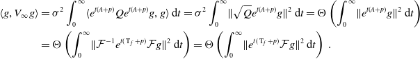 \begin{align*} \langle g, V_\infty g \rangle &= \sigma ^2 \int _{0}^{\infty } \langle e^{t (A+p)}Qe^{t (A+p)}g, g\rangle \, \mathrm{d}t = \sigma ^2 \int _{0}^{\infty } \lVert \sqrt{Q}e^{t(A+p)}g \rVert ^{2} \, \mathrm{d}t = \Theta \left ( \int _{0}^{\infty } \lVert e^{t(A+p)}g \rVert ^{2} \, \mathrm{d}t \right )\\ &= \Theta \left ( \int _{0}^{\infty } \lVert \mathcal{F}^{-1} e^{t(\operatorname{T}_f+p)} \mathcal{F} g \rVert ^{2} \, \mathrm{d}t \right ) = \Theta \left ( \int _{0}^{\infty } \lVert e^{t(\operatorname{T}_f+p)} \mathcal{F} g \rVert ^{2} \, \mathrm{d}t \right )\;. \end{align*}
The scaling law of the variance can thus be computed, or compared, through Theorem 3.1 for $f$
that satisfies (3.2) for
$f$
that satisfies (3.2) for $\alpha \gt 0$
and for
$\alpha \gt 0$
and for $g$
in a dense subset of
$g$
in a dense subset of $L^2(\mathbb{R})$
. As an example, we consider
$L^2(\mathbb{R})$
. As an example, we consider
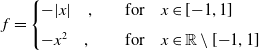 \begin{align*} f=\begin{cases} -\vert x\rvert \quad, \quad &\mathrm{for}\quad x\in [{-}1,1]\\[4pt] -x^2\quad, \quad &\mathrm{for}\quad x\in \mathbb{R}\setminus [{-}1,1] \end{cases} \end{align*}
and $g=\mathcal{F}^{-1}\unicode{x1D7D9}_{[-\varepsilon, \varepsilon ]}$
. The rate of divergence of the time-asymptotic variance is therefore
$g=\mathcal{F}^{-1}\unicode{x1D7D9}_{[-\varepsilon, \varepsilon ]}$
. The rate of divergence of the time-asymptotic variance is therefore $-\mathrm{log}({-}p)$
as
$-\mathrm{log}({-}p)$
as $p\to 0^-$
.
$p\to 0^-$
.
Example 5.2.
Consider the self-adjoint operator $A\,:\,\mathcal{H}^{2m}(\mathbb{R}) \to L^2(\mathbb{R})$
for
$A\,:\,\mathcal{H}^{2m}(\mathbb{R}) \to L^2(\mathbb{R})$
for $m\in \mathbb{N}$
such that
$m\in \mathbb{N}$
such that
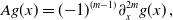 \begin{align*} A g(x) =({-}1)^{(m-1)} \partial _x^{2m} g(x) \;, \end{align*}
where $\partial _x$
denotes the weak derivative on
$\partial _x$
denotes the weak derivative on $\mathcal{H}^1(\mathbb{R})$
, and assume
$\mathcal{H}^1(\mathbb{R})$
, and assume $g\in \mathcal{H}^{2m}(\mathbb{R})$
. We want to study the variance of the solution of (5.2) for
$g\in \mathcal{H}^{2m}(\mathbb{R})$
. We want to study the variance of the solution of (5.2) for $u_0\in \mathcal{H}^{2m}(\mathbb{R})$
,
$u_0\in \mathcal{H}^{2m}(\mathbb{R})$
, $p\lt 0$
and
$p\lt 0$
and $Q$
a bounded operator with bounded inverse. For
$Q$
a bounded operator with bounded inverse. For $g\in \mathcal{H}^{2m}(\mathbb{R})$
and
$g\in \mathcal{H}^{2m}(\mathbb{R})$
and $f(k)=-k^{2m}$
for any
$f(k)=-k^{2m}$
for any $k\in \mathbb{R}$
, we find that
$k\in \mathbb{R}$
, we find that
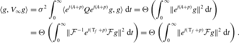 \begin{align*} \langle g, V_\infty g \rangle &= \sigma ^2 \int _{0}^{\infty } \langle e^{t (A+p)}Qe^{t (A+p)}g, g\rangle \, \mathrm{d}t = \Theta \left ( \int _{0}^{\infty } \lVert e^{t(A+p)}g \rVert ^{2} \, \mathrm{d}t \right )\\ &= \Theta \left ( \int _{0}^{\infty } \lVert \mathcal{F}^{-1} e^{t(\operatorname{T}_{f}+p)} \mathcal{F} g \rVert ^{2} \, \mathrm{d}t \right ) = \Theta \left ( \int _{0}^{\infty } \lVert e^{t(\operatorname{T}_f+p)} \mathcal{F} g \rVert ^{2} \, \mathrm{d}t \right ). \end{align*}
From Theorem 3.1, the scaling law as $p\to 0^-$
for
$p\to 0^-$
for $g$
in a dense subset of
$g$
in a dense subset of $\mathcal{H}^{2m}(\mathbb{R})$
is therefore
$\mathcal{H}^{2m}(\mathbb{R})$
is therefore $\Theta \left (p^{-1+\frac{1}{2m}} \right )$
.
$\Theta \left (p^{-1+\frac{1}{2m}} \right )$
.
Example 5.3.
We introduce the self-adjoint operator $A(p)\,:\,\mathcal{H}^2(\mathbb{R})\to L^2(\mathbb{R})$
such that
$A(p)\,:\,\mathcal{H}^2(\mathbb{R})\to L^2(\mathbb{R})$
such that $A(p)$
has negative spectrum for
$A(p)$
has negative spectrum for $p\lt 0$
. We assume the existence and uniqueness of
$p\lt 0$
. We assume the existence and uniqueness of $\lambda (p)$
, an isolated element in its spectrum that satisfies
$\lambda (p)$
, an isolated element in its spectrum that satisfies $\lambda (0)=0$
and is continuous in
$\lambda (0)=0$
and is continuous in $p$
. The spectrum is assumed to be purely absolutely continuous for any
$p$
. The spectrum is assumed to be purely absolutely continuous for any $p\leq 0$
and supported in
$p\leq 0$
and supported in $({-}\infty, \lambda (p)]$
. The mentioned assumptions are satisfied, for instance, by certain Schrödinger operators
$({-}\infty, \lambda (p)]$
. The mentioned assumptions are satisfied, for instance, by certain Schrödinger operators $A(p)=\Delta -v(p,\cdot )$
for a bounded real potential
$A(p)=\Delta -v(p,\cdot )$
for a bounded real potential $v(p,\cdot )$
with compact support for any
$v(p,\cdot )$
with compact support for any $p\leq 0$
[Reference Deift and Killip18]. For any
$p\leq 0$
[Reference Deift and Killip18]. For any $g\in L^2(\mathcal{X})$
,
$g\in L^2(\mathcal{X})$
, $p\leq 0$
and any continuous function
$p\leq 0$
and any continuous function $f$
, we define the absolutely continuous measure with respect to the Legesgue measure
$f$
, we define the absolutely continuous measure with respect to the Legesgue measure $\mu _{g,p}$
, such that
$\mu _{g,p}$
, such that
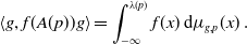 \begin{align*} \langle g, f(A(p)) g \rangle = \int _{-\infty }^{\lambda (p)} f(x)\, \mathrm{d}\mu _{g,p}(x) \, . \end{align*}
It follows that the time-asymptotic covariance operator associated with the solutions of
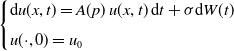 \begin{align*} \begin{cases} \mathrm{d}u(x,t) = A(p)\; u(x,t) \, \mathrm{d}t + \sigma \mathrm{d}W(t)\\[4pt] u(\cdot, 0) = u_0 \end{cases} \end{align*}
and $Q=I$
satisfies
$Q=I$
satisfies
 \begin{align*} \langle g, V_\infty g \rangle = \sigma ^2 \int _{-\infty }^{\lambda (p)} \int _0^\infty e^{2 t x} \,\mathrm{d}t \, \mathrm{d}\mu _{g,p}(x) = -\frac{\sigma ^2}{2} \int _{-\infty }^{\lambda (p)} \frac{1}{x} \, \mathrm{d}\mu _{g,p}(x) \;, \end{align*}
for any $p\lt 0$
. We introduce the Radon–Nikodym derivative
$p\lt 0$
. We introduce the Radon–Nikodym derivative $r_{g,p}(x)=\frac{\mathrm{d}\mu _{g,p}(x)}{\mathrm{d}x}$
. Under the assumption of continuity of
$r_{g,p}(x)=\frac{\mathrm{d}\mu _{g,p}(x)}{\mathrm{d}x}$
. Under the assumption of continuity of $r_{g,p}$
on
$r_{g,p}$
on $p$
, we obtain that
$p$
, we obtain that
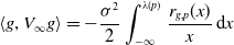 \begin{align*} \langle g, V_\infty g \rangle = -\frac{\sigma ^2}{2} \int _{-\infty }^{\lambda (p)} \frac{r_{g,p}(x)}{x} \, \mathrm{d}x \end{align*}
and the scaling law of the early warning sign.
Remark 5.4.
The early warning sign in the form of the divergence of the time-asymptotic variance of the solution of a linearised system (5.2) has been studied in the case of the linear non-positive self-adjoint operator $A$
with discrete spectrum [Reference Bernuzzi and Kuehn5, Reference Gowda and Kuehn24, Reference Kuehn and Romano43]. An example to such an operator is
$A$
with discrete spectrum [Reference Bernuzzi and Kuehn5, Reference Gowda and Kuehn24, Reference Kuehn and Romano43]. An example to such an operator is $\partial _{x}^2\,:\,\mathcal{H}^2([{-}L,L])\to L^2([{-}L,L])$
with Neumann boundary conditions. Its eigenvalues are known to be
$\partial _{x}^2\,:\,\mathcal{H}^2([{-}L,L])\to L^2([{-}L,L])$
with Neumann boundary conditions. Its eigenvalues are known to be $\left \{-\lambda _i\right \}_{i\in \mathbb{N}}$
for
$\left \{-\lambda _i\right \}_{i\in \mathbb{N}}$
for $\lambda _i=\left (\frac{i \pi }{L}\right )^2$
and corresponding eigenfunctions
$\lambda _i=\left (\frac{i \pi }{L}\right )^2$
and corresponding eigenfunctions $e_i({\cdot})\,:\!=\,\mathrm{cos}\left (\lambda _i \cdot \right )$
. For
$e_i({\cdot})\,:\!=\,\mathrm{cos}\left (\lambda _i \cdot \right )$
. For $g\in \mathcal{H}^2([{-}L,L])$
, the time-asymptotic variance of the solution of (5.2) is
$g\in \mathcal{H}^2([{-}L,L])$
, the time-asymptotic variance of the solution of (5.2) is
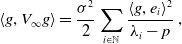 \begin{align} \langle g,V_\infty g\rangle = \frac{\sigma ^2}{2} \sum _{i\in \mathbb{N}} \frac{\langle g, e_i \rangle ^2}{\lambda _i-p}\;, \end{align}
which is proven in [Reference Bernuzzi and Kuehn5]. Under the assumption that the projection of $g$
along the most sensible eigenfunction
$g$
along the most sensible eigenfunction $e_i$
is not zero,
$e_i$
is not zero, $\langle g, e_i \rangle \neq 0$
, the rate of divergence of the variance is of order
$\langle g, e_i \rangle \neq 0$
, the rate of divergence of the variance is of order $\Theta \left (({-}p)^{-1}\right )$
as
$\Theta \left (({-}p)^{-1}\right )$
as $p\to 0^-$
, similar to the case
$p\to 0^-$
, similar to the case $\alpha \to \infty$
in Table 1.
$\alpha \to \infty$
in Table 1.
In the limit $L\to \infty$
, the spectrum of the operator
$L\to \infty$
, the spectrum of the operator $\partial _{x}^2\,:\,\mathcal{H}^2(\mathbb{R})\to L^2(\mathbb{R})$
is continuous and the rate of the divergence of time-asymptotic variance of the solution of the linearised system (5.2) can be obtained as described in Example 5.2
. In detail,
$\partial _{x}^2\,:\,\mathcal{H}^2(\mathbb{R})\to L^2(\mathbb{R})$
is continuous and the rate of the divergence of time-asymptotic variance of the solution of the linearised system (5.2) can be obtained as described in Example 5.2
. In detail,
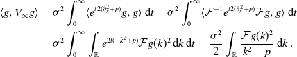 \begin{align} \langle g, V_\infty g \rangle &= \sigma ^2 \int _{0}^{\infty } \langle e^{t 2 (\partial _x^2+p)} g, g\rangle \, \mathrm{d}t = \sigma ^2 \int _{0}^{\infty } \langle \mathcal{F}^{-1} e^{t 2 (\partial _x^2+p)} \mathcal{F} g, g\rangle \, \mathrm{d}t \nonumber \\ &= \sigma ^2 \int _{0}^{\infty } \int _{\mathbb{R}} e^{2 t (-k^2+p)} \mathcal{F}g(k)^2 \, \mathrm{d}k \, \mathrm{d}t =\frac{\sigma ^2}{2} \int _{\mathbb{R}} \frac{\mathcal{F}g(k)^2}{k^2-p} \, \mathrm{d}k \;. \end{align}
We define the functions $d_k(x)=e^{-2 \pi \mathrm{i} k x}$
for
$d_k(x)=e^{-2 \pi \mathrm{i} k x}$
for $x,k\in \mathbb{R}$
and the imaginary unit
$x,k\in \mathbb{R}$
and the imaginary unit $\mathrm{i}$
. Under the assumption that
$\mathrm{i}$
. Under the assumption that $\mathcal{F}g$
assumes bounded non-zero values in a neighbourhood of
$\mathcal{F}g$
assumes bounded non-zero values in a neighbourhood of $k=0$
, i.e., the projections of function
$k=0$
, i.e., the projections of function $g$
along the most sensible functions in
$g$
along the most sensible functions in $\{d_k\}_{k\in \mathbb{R}}$
are bounded and non-zero, the rate of divergence of such variance is of order
$\{d_k\}_{k\in \mathbb{R}}$
are bounded and non-zero, the rate of divergence of such variance is of order $\Theta \left (({-}p)^{-\frac{1}{2}}\right )$
as proven in Example 5.2
.
$\Theta \left (({-}p)^{-\frac{1}{2}}\right )$
as proven in Example 5.2
.
Intuitively, the difference of the rates of (5.3) and (5.4) is implied by the different shape of the spectrum of $\partial _x^2$
for the finite or infinite value of
$\partial _x^2$
for the finite or infinite value of $L$
. In particular, as
$L$
. In particular, as $p$
crosses
$p$
crosses $0$
from below in the case
$0$
from below in the case $L\lt \infty$
, the solution of (5.2) is repelled by the linear term along
$L\lt \infty$
, the solution of (5.2) is repelled by the linear term along $e_0$
. Conversely, for
$e_0$
. Conversely, for $p\to 0^-$
in the case
$p\to 0^-$
in the case $L=\infty$
, the most unstable direction
$L=\infty$
, the most unstable direction $d_0$
, the constant function, is not in the domain of the operator.
$d_0$
, the constant function, is not in the domain of the operator.
6 Numerical simulations
In this section, we numerically investigate the analytic results from Sections 3 and 4 to gain more insight and also to obtain an outlook on how they can be relevant in a more applied setting. The numerical methods used and discussed follow the theory of [Reference Higham28] and [Reference Lord, Powell and Shardlow47].
We start by simulating a generalisation of the results obtained in Theorem3.1 for the one-dimensional case and the tool function $f_{\alpha }(x) = - |x|^{\alpha }$
on an interval for
$f_{\alpha }(x) = - |x|^{\alpha }$
on an interval for $\alpha \gt 0$
. In order to approximate the solution of the studied SPDE, we use the Euler–Maruyama method, which we introduce considering the differential equation
$\alpha \gt 0$
. In order to approximate the solution of the studied SPDE, we use the Euler–Maruyama method, which we introduce considering the differential equation
 \begin{align} \mathrm{d}u(x,t) = \left (f_\alpha (x)+p\right )\; u(x,t) \, \mathrm{d}t + \sigma \mathrm{d}W(t) \,, \quad u(\cdot, 0) = u_0\,, \quad 0 \leq t \leq T \,, \end{align}
for $\sigma, T\gt 0\gt p$
, initial condition
$\sigma, T\gt 0\gt p$
, initial condition $u_0\in L^2(\mathcal{X})$
and (boundary) conditions
$u_0\in L^2(\mathcal{X})$
and (boundary) conditions $f_\alpha u\in L^2(\mathcal{X})$
. We then discretise the time interval
$f_\alpha u\in L^2(\mathcal{X})$
. We then discretise the time interval $[0,T]$
by defining the time step
$[0,T]$
by defining the time step $\delta \texttt{t} = \frac{T}{\texttt{nt}}$
for a certain positive integer
$\delta \texttt{t} = \frac{T}{\texttt{nt}}$
for a certain positive integer $\texttt{nt}$
, to be the number of steps in time, and
$\texttt{nt}$
, to be the number of steps in time, and $ \tau _i\,:\!=\, i\; \delta \texttt{t}$
, the time passed after
$ \tau _i\,:\!=\, i\; \delta \texttt{t}$
, the time passed after $i$
time steps. Further, we discretise also the space interval
$i$
time steps. Further, we discretise also the space interval $\mathcal{X}=[{-}L, L]$
into its internal points
$\mathcal{X}=[{-}L, L]$
into its internal points $r_n=-L+2\frac{n}{\texttt{N}+1}L$
for
$r_n=-L+2\frac{n}{\texttt{N}+1}L$
for $n\in \{1,\dots, \texttt{N}\}$
, with
$n\in \{1,\dots, \texttt{N}\}$
, with $\texttt{N}$
being an integer that defines the number of mesh points. The numerical approximations of
$\texttt{N}$
being an integer that defines the number of mesh points. The numerical approximations of $u(\cdot, \tau _i)$
,
$u(\cdot, \tau _i)$
, $f_\alpha$
and
$f_\alpha$
and $W(\cdot, \tau _i)$
are labelled, respectively as
$W(\cdot, \tau _i)$
are labelled, respectively as $\texttt{u}_i, \texttt{f}_\alpha, \texttt{W}_i \in \mathbb{R}^{\texttt{N}+2}$
for any
$\texttt{u}_i, \texttt{f}_\alpha, \texttt{W}_i \in \mathbb{R}^{\texttt{N}+2}$
for any $i\in \{0,\dots, \texttt{nt}\}$
. Then, by the implicit Euler–Maruyama method, the numerical simulation takes the form
$i\in \{0,\dots, \texttt{nt}\}$
. Then, by the implicit Euler–Maruyama method, the numerical simulation takes the form
 \begin{align*} \texttt{u}_i = \texttt{u}_{i-1} + \left ( \texttt{f}_\alpha +p \right )\!\texttt{u}_{i} \delta \texttt{t} + \sigma (\texttt{W}_i - \texttt{W}_{i-1}) \,, \quad i = 1,2, \ldots, \texttt{nt} \end{align*}
which approximates the integral form of the SPDE. For fixed $i\in \{1,\ldots, \texttt{nt}\}$
, the term
$i\in \{1,\ldots, \texttt{nt}\}$
, the term $\texttt{W}_i - \texttt{W}_{i-1}$
can be expressed as
$\texttt{W}_i - \texttt{W}_{i-1}$
can be expressed as
 \begin{align*} \texttt{W}_i - \texttt{W}_{i-1}= \sqrt{\delta \texttt{t}} \sum _{m=1}^{M} \sqrt{q_m} W_i^{(m)}\texttt{b}_m \end{align*}
with $M\leq \texttt{N}$
being the number of directions in the space function on which the noise is taken numerically into account,
$M\leq \texttt{N}$
being the number of directions in the space function on which the noise is taken numerically into account, $\left \{W_i^{(m)}\right \}_{m\in \{1,\dots, M\}}$
a collection of independent standard Gaussian random variables and the randomly generated
$\left \{W_i^{(m)}\right \}_{m\in \{1,\dots, M\}}$
a collection of independent standard Gaussian random variables and the randomly generated $\left \{\left (q_m, \texttt{b}_m \right )\right \}_{m\in \{1,\dots, M\}}$
, which are, respectively, the first
$\left \{\left (q_m, \texttt{b}_m \right )\right \}_{m\in \{1,\dots, M\}}$
, which are, respectively, the first $M$
eigenvalues and approximations in
$M$
eigenvalues and approximations in $\mathbb{R}^{\texttt{N}+2}$
of the eigenfunctions of the covariance operator
$\mathbb{R}^{\texttt{N}+2}$
of the eigenfunctions of the covariance operator $Q$
of
$Q$
of $W$
in (6.1).Footnote
4
$W$
in (6.1).Footnote
4
We numerically simulate a generalisation of results from Theorem3.1, as described in Section 5, for the function $f_{\alpha }=- |x|^{\alpha }$
for
$f_{\alpha }=- |x|^{\alpha }$
for $\alpha \gt 0$
as defined by (3.1). We consider the case
$\alpha \gt 0$
as defined by (3.1). We consider the case $g(x)= \unicode{x1D7D9}_{[-\varepsilon, \varepsilon ]}$
for
$g(x)= \unicode{x1D7D9}_{[-\varepsilon, \varepsilon ]}$
for $\left |\left \{r_n\in [{-}\varepsilon, \varepsilon ]\;|\; n\in \{1,\dots, \texttt{N}\}\right \}\right |=M$
.Footnote
5
Further, we assume
$\left |\left \{r_n\in [{-}\varepsilon, \varepsilon ]\;|\; n\in \{1,\dots, \texttt{N}\}\right \}\right |=M$
.Footnote
5
Further, we assume $Q$
and its inverse
$Q$
and its inverse $Q^{-1}$
to be bounded operators. The fact that
$Q^{-1}$
to be bounded operators. The fact that $Q$
is not assumed to be the identity operator makes the random variables
$Q$
is not assumed to be the identity operator makes the random variables $u(x_1,t)$
and
$u(x_1,t)$
and $u(x_2,t)$
dependent for any
$u(x_2,t)$
dependent for any $x_1,x_2\in \mathcal{X}$
and
$x_1,x_2\in \mathcal{X}$
and $t\gt 0$
. Hence, the simulation of
$t\gt 0$
. Hence, the simulation of $u$
must be studied as an SPDE rather than a collection of SDEs on the resolution points. As described in Section 5, such a choice of
$u$
must be studied as an SPDE rather than a collection of SDEs on the resolution points. As described in Section 5, such a choice of $Q$
is expected to imply scaling laws, dependent on
$Q$
is expected to imply scaling laws, dependent on $\alpha$
, of the time-asymptotic variance as displayed in Table 1.
$\alpha$
, of the time-asymptotic variance as displayed in Table 1.
Log-log plot that describes the behaviour of $\langle g, V_\infty g \rangle$
as
$\langle g, V_\infty g \rangle$
as $p$
approaches
$p$
approaches $0^{-}$
in accordance to the choice of the tool function
$0^{-}$
in accordance to the choice of the tool function $f_{\alpha }$
. The circles are obtained as the mean value of
$f_{\alpha }$
. The circles are obtained as the mean value of $\log _{10}\!(\langle g, V_\infty g \rangle )$
given by 10 independent simulations. The shaded areas have a width equal to the numerical standard deviation. Lastly, the blue line has a slope equal to
$\log _{10}\!(\langle g, V_\infty g \rangle )$
given by 10 independent simulations. The shaded areas have a width equal to the numerical standard deviation. Lastly, the blue line has a slope equal to $-1$
and is provided as a reference for the scaling law. For
$-1$
and is provided as a reference for the scaling law. For $\alpha \geq 1$
, the expected slope from Theorem3.1 is shown close to
$\alpha \geq 1$
, the expected slope from Theorem3.1 is shown close to $p=10^{-5}$
. The convergence is visible for
$p=10^{-5}$
. The convergence is visible for $\alpha \lt 1$
until
$\alpha \lt 1$
until $p$
assumes small values. In fact, for small
$p$
assumes small values. In fact, for small $\texttt{N}$
, the log-log plot displays slope
$\texttt{N}$
, the log-log plot displays slope $-1$
induced by the divergence being only perceived on
$-1$
induced by the divergence being only perceived on $x=0$
and therefore leading to a behaviour similar to that of an OrnsteinUhlenbeck process [Reference Kuehn41].
$x=0$
and therefore leading to a behaviour similar to that of an OrnsteinUhlenbeck process [Reference Kuehn41].
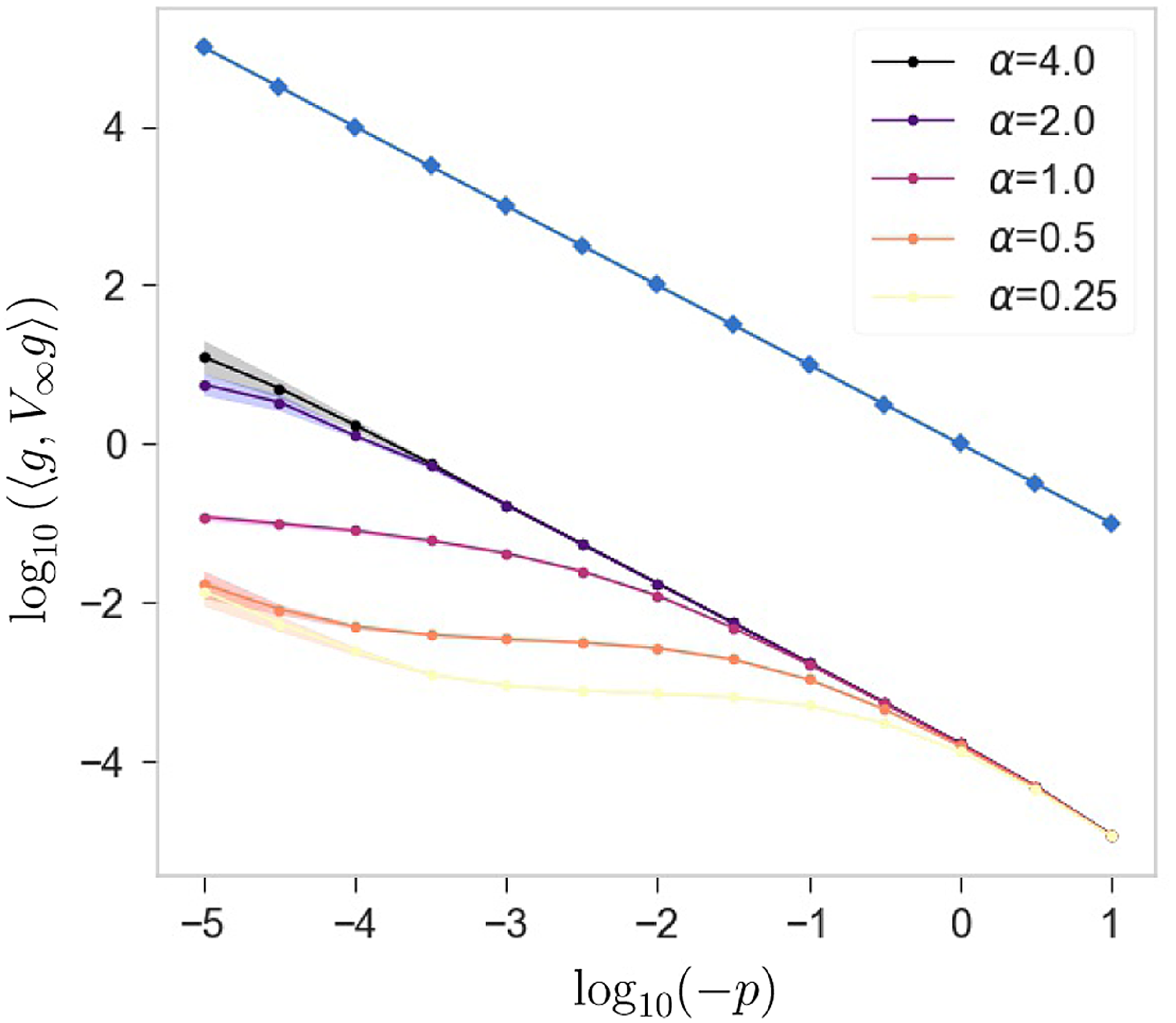
We simulate the projection $\langle u(\cdot, \tau _i), g \rangle$
with
$\langle u(\cdot, \tau _i), g \rangle$
with $\textrm{proj}_i=\underset{n:r_n\in [-\varepsilon, \varepsilon ]}{\sum } \texttt{u}_i(n)$
for any
$\textrm{proj}_i=\underset{n:r_n\in [-\varepsilon, \varepsilon ]}{\sum } \texttt{u}_i(n)$
for any $i\in \{1,\dots, \texttt{nt}\}$
. We approximate the behaviour of the scalar product that defines the variance along
$i\in \{1,\dots, \texttt{nt}\}$
. We approximate the behaviour of the scalar product that defines the variance along $g$
,
$g$
, $\langle g, V_\infty g \rangle$
, as the numerical variance in time
$\langle g, V_\infty g \rangle$
, as the numerical variance in time $i$
of
$i$
of $\textrm{proj}_i$
. The results are displayed as a log-log plot in Figure 3. As we are interested in the behaviour for
$\textrm{proj}_i$
. The results are displayed as a log-log plot in Figure 3. As we are interested in the behaviour for $p$
approaching zero from below, we focus on negative values of
$p$
approaching zero from below, we focus on negative values of $\log _{10}\!({-}p)$
. Validating the analytic results in Table 1, for
$\log _{10}\!({-}p)$
. Validating the analytic results in Table 1, for $\alpha \gt 1$
we observe
$\alpha \gt 1$
we observe $\log _{10}\!(\langle g, V_\infty g \rangle )$
to assume a negative slope of
$\log _{10}\!(\langle g, V_\infty g \rangle )$
to assume a negative slope of $-1 + \frac{1}{\alpha }$
as
$-1 + \frac{1}{\alpha }$
as $\log _{10}({-}p)$
approaches
$\log _{10}({-}p)$
approaches $-\infty$
. In the case
$-\infty$
. In the case $\alpha = 1$
, we expect a logarithmic divergence in the log-log plot as
$\alpha = 1$
, we expect a logarithmic divergence in the log-log plot as $\log _{10}({-}p)$
decreases. Lastly, we expect convergence for
$\log _{10}({-}p)$
decreases. Lastly, we expect convergence for $0\lt \alpha \lt 1$
, which is shown up to small values of
$0\lt \alpha \lt 1$
, which is shown up to small values of $p$
due to numerical errors.Footnote
6
$p$
due to numerical errors.Footnote
6
Next, we study the two-dimensional case and numerically simulate the asymptotic behaviour of the upper bound of $\langle g, V_\infty g \rangle$
as described in Theorem4.5. In particular, our goal is to illustrate the results analytically found for indices
$\langle g, V_\infty g \rangle$
as described in Theorem4.5. In particular, our goal is to illustrate the results analytically found for indices $i_1, i_2$
such that
$i_1, i_2$
such that $i_2 \geq i_1 \geq 1$
. For this case, we have found the scaling law of the upper bound as displayed in Table 3. We therefore compute the dependence of
$i_2 \geq i_1 \geq 1$
. For this case, we have found the scaling law of the upper bound as displayed in Table 3. We therefore compute the dependence of $\int _0^\varepsilon \int _0^\varepsilon \frac{1}{x_1^{i_1}x_2^{i_2}-p}\, \mathrm{d}x_1 \, \mathrm{d}x_2$
on
$\int _0^\varepsilon \int _0^\varepsilon \frac{1}{x_1^{i_1}x_2^{i_2}-p}\, \mathrm{d}x_1 \, \mathrm{d}x_2$
on $p\lt 0$
in a log-log plot.
$p\lt 0$
in a log-log plot.
The solid lines describe the scaling law of the upper bound for the two-dimensional problem, illustrated by $\log _{10}\!(\int _0^\varepsilon \int _0^\varepsilon \frac{1}{x^{j_{\ast }} - p}\, \mathrm{d}x)$
and decreasing
$\log _{10}\!(\int _0^\varepsilon \int _0^\varepsilon \frac{1}{x^{j_{\ast }} - p}\, \mathrm{d}x)$
and decreasing $\log _{10}({-}p)$
with
$\log _{10}({-}p)$
with $x = (x_1, x_2)$
and
$x = (x_1, x_2)$
and $j_\ast =(i_1,i_2)$
. The numbering of the cases refers to Table 3. The circle lines serve as comparison with the corresponding scaling law presented in the table as an argument of
$j_\ast =(i_1,i_2)$
. The numbering of the cases refers to Table 3. The circle lines serve as comparison with the corresponding scaling law presented in the table as an argument of $\mathrm{log}_{10}$
.
$\mathrm{log}_{10}$
.
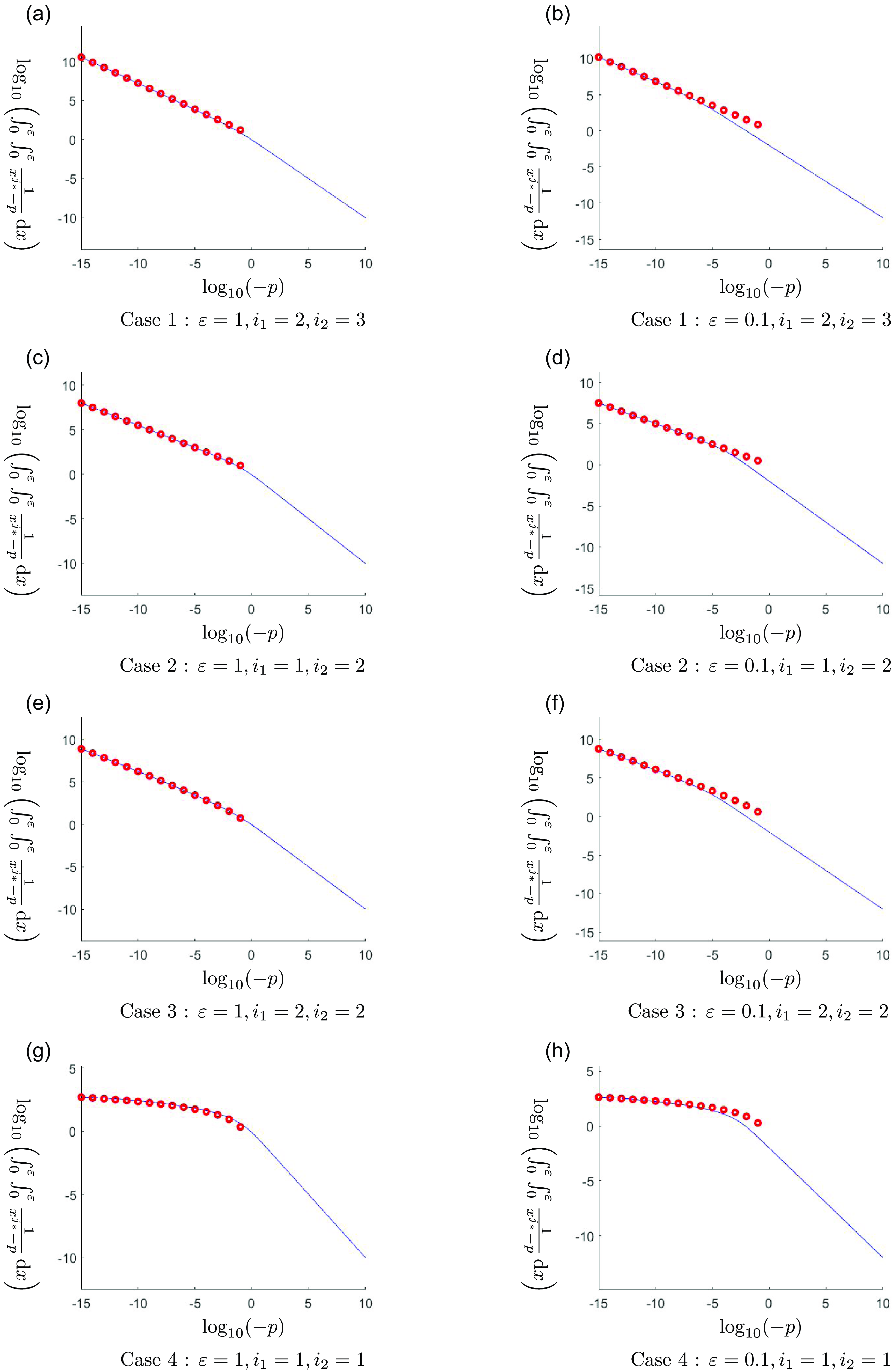
The subfigures shown in Figure 4 are obtained for different choices of $\varepsilon$
and of
$\varepsilon$
and of $i_2 \geq i_1 \geq 1$
. We see that the results are confirmed as the double integrals, displayed as solid lines, show a similar qualitative behaviour as the analytic result in Table 3, corresponding to the red circles, for small values of
$i_2 \geq i_1 \geq 1$
. We see that the results are confirmed as the double integrals, displayed as solid lines, show a similar qualitative behaviour as the analytic result in Table 3, corresponding to the red circles, for small values of $-p$
. In particular, in the Figure 4a, b, c and d, corresponding to Case
$-p$
. In particular, in the Figure 4a, b, c and d, corresponding to Case $1$
and Case
$1$
and Case $2$
of the table, we obtain a slope equal to
$2$
of the table, we obtain a slope equal to $-1+\frac{1}{i_2}$
. The red circles in Figure 4e and f, corresponding to Case
$-1+\frac{1}{i_2}$
. The red circles in Figure 4e and f, corresponding to Case $3$
, have values
$3$
, have values
 \begin{equation*}\mathrm{log}_{10}({-}p)\left(-1+\frac{1}{i_2}\right)+\mathrm{log}_{10}({-}\mathrm{log}_{10}({-}p))+c\end{equation*}
and the values in Figure 4g and h, corresponding to Case $4$
, are equal to
$4$
, are equal to
 \begin{equation*}2 \mathrm{log}_{10}({-}\mathrm{log}_{10}({-}p))+c\;,\end{equation*}
for different constants $c$
. Decreasing the parameter
$c$
. Decreasing the parameter $\varepsilon \gt 0$
appears to imply a decrease of the lowest threshold
$\varepsilon \gt 0$
appears to imply a decrease of the lowest threshold $q_c\gt 0$
such that for any
$q_c\gt 0$
such that for any $-p\gt q_c$
the slope of
$-p\gt q_c$
the slope of $\log _{10}\!\left (\int _0^\varepsilon \int _0^\varepsilon \frac{1}{x_1^{i_1} x_2^{i_2} - p}\, \mathrm{d}x_1 \mathrm{d}x_2 \right )$
in the log-log plot is approximately
$\log _{10}\!\left (\int _0^\varepsilon \int _0^\varepsilon \frac{1}{x_1^{i_1} x_2^{i_2} - p}\, \mathrm{d}x_1 \mathrm{d}x_2 \right )$
in the log-log plot is approximately $-1$
. Such a slope is implied by the fact that, for
$-1$
. Such a slope is implied by the fact that, for $p\ll 0$
, the values of
$p\ll 0$
, the values of $x_1^{i_1} x_2^{i_2} - p$
present the same order of distance from
$x_1^{i_1} x_2^{i_2} - p$
present the same order of distance from $0$
for any
$0$
for any $x_1,x_2\in [0,\varepsilon ]$
and, therefore, the early warning sign displays similar behaviour to those discussed in [Reference Bernuzzi and Kuehn5, Reference Gowda and Kuehn24, Reference Kuehn and Romano43] for such values of
$x_1,x_2\in [0,\varepsilon ]$
and, therefore, the early warning sign displays similar behaviour to those discussed in [Reference Bernuzzi and Kuehn5, Reference Gowda and Kuehn24, Reference Kuehn and Romano43] for such values of $p$
.
$p$
.
Lastly, we illustrate the results of Theorem4.7 by computing the values of $\int _0^\varepsilon \int _0^\varepsilon \int _0^\varepsilon \frac{1}{x_1^{i_1}x_2^{i_2}x_3^{i_3}-p}\, \mathrm{d}x_1 \, \mathrm{d}x_2 \, \mathrm{d}x_3$
on
$\int _0^\varepsilon \int _0^\varepsilon \int _0^\varepsilon \frac{1}{x_1^{i_1}x_2^{i_2}x_3^{i_3}-p}\, \mathrm{d}x_1 \, \mathrm{d}x_2 \, \mathrm{d}x_3$
on $p\lt 0$
in a log-log plot for different values of
$p\lt 0$
in a log-log plot for different values of $i_3 \geq i_2 \geq i_1 \geq 1$
. We then compare them to the corresponding scaling laws displayed in Table 4.
$i_3 \geq i_2 \geq i_1 \geq 1$
. We then compare them to the corresponding scaling laws displayed in Table 4.
The plots shown in Figure 5 are obtained for the fixed value $\varepsilon =1$
and of the exponents
$\varepsilon =1$
and of the exponents $i_3 \geq i_2 \geq i_1 \geq 1$
. The triple integral displays a similar qualitative behaviour as the analytic results in Table 4, again denoted by the red circles, for small values of
$i_3 \geq i_2 \geq i_1 \geq 1$
. The triple integral displays a similar qualitative behaviour as the analytic results in Table 4, again denoted by the red circles, for small values of $-p$
. In fact, in Figure 5a, b, e and f, corresponding to Case
$-p$
. In fact, in Figure 5a, b, e and f, corresponding to Case $1$
, Case
$1$
, Case $2$
, Case
$2$
, Case $5$
, and Case
$5$
, and Case $6$
of the mentioned table, they display a slope of value
$6$
of the mentioned table, they display a slope of value $-1+\frac{1}{i_3}$
. The red circles in Figure 5c and g, corresponding to Case
$-1+\frac{1}{i_3}$
. The red circles in Figure 5c and g, corresponding to Case $3$
and Case
$3$
and Case $7$
, have values
$7$
, have values
 \begin{equation*}\mathrm{log}_{10}({-}p)\left({-}1+\frac{1}{i_3}\right)+\mathrm{log}_{10}({-}\mathrm{log}_{10}({-}p))+c\;,\end{equation*}
for distinct constants $c$
. The red circles presented in Figure 5d, corresponding to Case
$c$
. The red circles presented in Figure 5d, corresponding to Case $4$
, are equal to
$4$
, are equal to
 \begin{equation*}\mathrm{log}_{10}({-}p)\left({-}1+\frac{1}{i_3}\right)+2 \mathrm{log}_{10}({-}\mathrm{log}_{10}({-}p))+c\end{equation*}
and those displayed in Figure 5h, corresponding to Case $8$
, are
$8$
, are
 \begin{equation*}3 \mathrm{log}_{10}({-}\mathrm{log}_{10}({-}p))+c\;,\end{equation*}
for a different constant $c$
each.
$c$
each.
The solid lines describe the scaling law of the upper bound for the three-dimensional problem illustrated by $\log _{10}\!(\int _0^\varepsilon \int _0^\varepsilon \int _0^\varepsilon \frac{1}{x^{j_{\ast }} - p}\, \mathrm{d}x)$
and decreasing
$\log _{10}\!(\int _0^\varepsilon \int _0^\varepsilon \int _0^\varepsilon \frac{1}{x^{j_{\ast }} - p}\, \mathrm{d}x)$
and decreasing $\log _{10}({-}p)$
with
$\log _{10}({-}p)$
with $x = (x_1, x_2,x_3)$
and
$x = (x_1, x_2,x_3)$
and $j_\ast =(i_1,i_2,i_3)$
. The numbering of cases refers to Table 4. The circle lines serve as comparison with the corresponding scaling law presented in the table as an argument of
$j_\ast =(i_1,i_2,i_3)$
. The numbering of cases refers to Table 4. The circle lines serve as comparison with the corresponding scaling law presented in the table as an argument of $\mathrm{log}_{10}$
.
$\mathrm{log}_{10}$
.
7 Applications
The early warning signs introduced in Theorems3.3, 4.5 and 4.7 can be applied to a wide range of applications. As described in Example 5.2, the study of reaction-diffusion equations can be achieved through Fourier transforms. In particular, we consider linearisations of reaction-diffusion systems in the form (1.2). For a distance $p$
to the bifurcation threshold, the solution of the linearised system on a stable solution
$p$
to the bifurcation threshold, the solution of the linearised system on a stable solution $u_\ast (p)$
behaves similarly to the solution of the original equation [Reference Gowda and Kuehn24]. This is implied by the fact that the solution remains in the basin of attraction in finite time with high probability due to the strong dissipative effect of the linear term until
$u_\ast (p)$
behaves similarly to the solution of the original equation [Reference Gowda and Kuehn24]. This is implied by the fact that the solution remains in the basin of attraction in finite time with high probability due to the strong dissipative effect of the linear term until $p$
has crossed the bifurcation point.
$p$
has crossed the bifurcation point.
The current section examines the relevance of our results to different models. Furthermore, their implementation in the prediction of real-life scenarios is discussed.
-
$\triangleright$
First, we introduce the Ginzburg–Landau, Allen–Cahn, or Chafee–Infante equation,in the domain
\begin{equation*} \textrm {d} u = \big (\partial _x^{2} u + p u - u^3\big ) \textrm {d}t \;, \end{equation*}
$\mathcal{X}=[{-}L,L]$
and Dirichlet boundary conditions. It finds applications in phase-ordering kinetic [Reference Bray8], quantum mechanics [Reference Faris and Jona-Lasinio22], and climate science [Reference Högele29]. The model is known to present a pitchfork supercritical bifurcation threshold at the parameter value
$p=0$
[Reference Chafee and Infante11]. The introduction of additive Gaussian noise is justified by the presence of lesser components in the physical model that can be treated as small stochastic perturbations [Reference Blumenthal, Engel and Neamtu7, Reference Rolland, Bouchet and Simonnet57]. We also consider the domain in the limit
$L\to \infty$
, in order to study large spaces. In such a limit, the spectrum of
$\partial _x^{2}$
is continuous and the only stable solution for
$p\lt 0$
is the null function
$u_\ast =0$
. The linearised system (1.2) is given with the drift operator(7.1)Example 5.2 implies that the time-asymptotic variance along almost any function
\begin{equation} A(p)=\partial _x^{2}+p\quad . \end{equation}
$g\in \mathcal{H}^2(\mathbb{R})$
yields a rate of divergence of order
$\Theta \left ((-p)^{\frac{1}{2}}\right )$
as
$p\to 0^-$
. In Figure 6a, a numerical approximation of the time-asymptotic variance of a solution of (5.2) for (7.1) is displayed. The observable is considered along
$g=\mathcal{F}^{-1}\unicode{x1D7D9}_{[-0.25,0.25]}$
and exhibits a slope of
$-\frac{1}{2}$
in a logarithmic scale, for
$p$
close to
$0$
.
-
$\triangleright$
We now consider the one-dimensional complex Ginzburg–Landau equation,for
\begin{equation*} \textrm {d} u = \big (\partial _{x}^{2} u + (p+\text {i} ) u -({-}1+\text {i} \; 0,1) \lvert u \rvert ^2 u - \lvert u \rvert ^4 u \big ) \textrm {d}t \;, \end{equation*}
$\mathrm{i}$
the imaginary unit and
$\lvert \cdot \rvert$
the absolute value, in the domain
$\mathcal{X}=[{-}L,L]$
and Neumann boundary conditions. Similar to its real counterpart, the introduction of white additive noise is justified by minor components in the system [Reference Hoshino, Inahama and Naganuma31]. For finite values of
$L$
, it is known that a supercritical Hopf bifurcation occurs at the stable solution
$u_\ast =0$
in the limit
$p\to 0^-$
[Reference Uecker62]. The assumption of the limit
$L\to +\infty$
follows from the observation of large domains in relevant applications and via the justification of the Ginzburg–Landau equation as an amplitude/modulation equation. The linearised system on
$u_\ast =0$
, (1.2) with linear operator(7.2)can be treated in Fourier space following Example 5.2 and the fourth generalisation in Section 5. In detail, for any
\begin{equation} A(p)=\partial _{x}^{2} + p + \mathrm{i} \;, \end{equation}
$g\in \mathcal{H}^2(\mathbb{R};\mathbb{C})$
it holdsThe time-asymptotic variance of the solution of the linearised system along almost any
\begin{align*} \langle g, V_\infty g \rangle &= \sigma ^2 \int _{0}^{\infty } \langle e^{t A(p)} e^{t A(p)^*}g, g\rangle \, \mathrm{d}t = \sigma ^2 \int _{0}^{\infty } \int _{\mathbb{R}} \overline{g(x)} e^{t (\partial _x^2 +p -\mathrm{i})} e^{t (\partial _x^2 +p +\mathrm{i})} g(x) \, \mathrm{d}x \; \mathrm{d}t\\ &= \sigma ^2 \int _{0}^{\infty } \lvert \lvert e^{t (\partial _x^2 +p)} g \rvert \rvert ^2 \, \mathrm{d}t = \sigma ^2 \int _{0}^{\infty } \lvert \lvert \mathcal{F}^{-1} e^{t (T_{-k^2} +p)} \mathcal{F} g \; \rvert \rvert ^2 \, \mathrm{d}t\\ &= \Theta \left (\int _{0}^{\infty } \lvert \lvert e^{t (T_{-k^2} +p)} \mathcal{F} g \; \rvert \rvert ^2 \, \mathrm{d}t \right ) = \Theta \left ({-}\int _{\mathbb{R}} \lvert \mathcal{F} g(k) \rvert ^2 \frac{1}{2({-}k^2+p)}\, \mathrm{d}k \right ) \;. \end{align*}
$g\in \mathcal{H}^2(\mathbb{R};\mathbb{C})$
is therefore characterised by rate
$\Theta \Big (\left (-p \right )^{-\frac{1}{2}} \Big )$
as
$p\to 0^-$
. In Figure 6b, an approximation of the observable along
$g=\mathcal{F}^{-1}\unicode{x1D7D9}_{[-0.25,0.25]}$
displays a slope of
$-\frac{1}{2}$
in a logarithmic scale, as
$p$
approaches
$0$
. An example of fields with which the complex Ginzburg–Landau equation is associated is the research on thin superconductors [Reference Milošević and Geurts52]. The stochastic non-linear Ginzburg–Landau equation in dimension
$N\gt 1$
is ill-defined in the classical sense under the assumption of perturbation by white noise and requires renormalisation; yet, note that the linearised SPDEs we work with here are always well-defined, even with space-time white noise. Assuming the covariance operator
$Q$
, in (2.3), such that a solution for such equation exists [Reference Da Prato and Zabczyk16, Theorems 5.20 and 7.13], an upper bound to the rate of divergence of the time-asymptotic variance of the solution of the linearised system can be obtained following Theorems4.5, 4.7 and the third generalisation in Section 5.
-
Figure 6.
A numerical approximation of the time-asymptotic variance of the solution of (5.2) along the function
$g$
is displayed for different models discussed in Section 7 in a log-log plot. The figures are obtained following the method in Section 6 in Fourier space, for
$T=10^4$
,
$\delta \texttt{t}=0.01$
and
$Q=\operatorname{I}$
. The red lines refer to the mean values of the observable for
$10$
sample solution, different for noise realisation. The areas have a width equal to double the corresponding numerical standard deviation. In Figure a, the drift term is described by (7.1); in Figure b, it is associated to (7.2); in Figure c to (7.3); in Figure d to (7.4); in Figure e to (7.5); in Figure f to (7.6). The respective functions
$g$
are introduced in Section 7. In blue, a line with a slope equal to
$-\frac{1}{2}$
is included as a comparison. In all figures, the lines appear to align for small values of
$p$
.
$\triangleright$
Another equation of interest is the (standard) one-dimensional Swift–Hohenberg equation [Reference Burke and Knobloch9, Reference Burke and Knobloch10, Reference Kao, Beaume and Knobloch34],with domain
\begin{equation*} \textrm {d} u = \big ({-}(1+\partial _x^{2})^2 u + p u - u^3\big ) \textrm {d}t \;, \end{equation*}
$\mathcal{X}=\mathbb{R}$
. Such a deterministic equation is known to display Turing bifurcations [Reference Hummel, Jelbart and Kuehn32, Reference Jelbart and Kuehn33]. We insert a white-noise term, meant to simulate the effect of minor physical components, in the system [Reference Hernández-Garcia, San Miguel, Toral and Vi27]; in fact, the stochastic Swift–Hohenberg equation has been studied very frequently already in the context of amplitude equations. The linearisation of such an SPDE on the trivial solution
$u_\ast (x)=0$
, for any
$x\in \mathbb{R}$
, takes the form of (5.2) with
$u_0\in \mathcal{H}^{4}(\mathbb{R})$
,
$Q=\operatorname{I}$
and
$A\,:\,\mathcal{H}^{4}(\mathbb{R}) \to L^2(\mathbb{R})$
such that(7.3)for any
\begin{align} A g(x) =-\left ( 1+\partial _x^{2} \right )^2 g(x) \;, \end{align}
$g\in \mathcal{H}^{4}(\mathbb{R})$
. Example 5.2 can easily be generalised on such self-adjoint linear differential operators through Theorem3.3. The scaling law of the variance of such a solution along
$g$
in a dense subset of
$\mathcal{H}^4(\mathbb{R})$
is given, therefore, bywith
\begin{align*} \langle g, V_\infty g \rangle &= \sigma ^2 \int _{0}^{\infty } \langle e^{t (A+p)} e^{t (A+p)}g, g\rangle \, \mathrm{d}t = \Theta \left ( \int _{0}^{\infty } \lVert e^{t(\operatorname{T}_f+p)} \mathcal{F} g \rVert ^{2} \, \mathrm{d}t \right )\;, \end{align*}
$f(k)=-\left ( 1-k^2 \right )^2$
for any
$k\in \mathbb{R}$
. From the Taylor expansion of
$f$
at
$k=\pm 1$
, it follows that the rate of divergence presents order
$\Theta \left (({-}p)^{-\frac{1}{2}} \right )$
. The time-asymptotic variance of the linearised model is displayed in red in the log-log plot in Figure 6c. As described in Section 5, the variance along
$g=\mathcal{F}^{-1} \unicode{x1D7D9}_{[0.75,1.25]}$
displays the rate of divergence
$\Theta \left (({-}p)^{-\frac{1}{2}}\right )$
as
$p\to 0^-$
. The Swift–Hohenberg equation on large or unbounded domains [Reference Blömker, Hairer and Pavliotis6] can be obtained from the Boussinesq approximation for fluid dynamics [Reference Swift and Hohenberg60]. In such an application, the ergodic theory states that the figure displays the rate of divergence of the time-asymptotic variance of the projection of the rescaled fluid velocity
$u$
on the function
$g$
up to the proximity to a bifurcation threshold. In particular, Theorem3.3 asserts that an equivalent order of divergence is assumed for
$g$
in a large set of indicator functions in
$L^2(\mathcal{X})$
. Therefore, it validates the study of the variance solely in bounded regions of space. As an example from [Reference Hariz, Bahloul and Cherbi26], another practical use of the corresponding early warning sign is the prediction of sudden changes in the electric field in crystal optical fibre resonators implied by the change of a bifurcation parameter. In this case, the generalised Swift–Hohenberg equation linearised on
$u_\ast =0$
yields(7.4)and the variable
\begin{equation} A =-\frac{\beta ^2}{4}+ \beta \partial _x^2 + \beta ^{\prime} \partial _x^3 - \partial _x^4 \end{equation}
$u$
represents the deviation of the electric field from its value at the bifurcation threshold. Upon consideration of the variational equation, i.e.,
$\beta ^{\prime}=0$
, the rate of the early warning sign can be obtained from Example 5.2. Set
$\beta \lt 0$
and
$g(x)= \mathcal{F}^{-1} \unicode{x1D7D9}_{[a,b]}$
for
$a\lt b$
, the scaling law of the time-asymptotic variance of the solution of the linearised system (1.2) on
$u_\ast =0$
along
$g$
is given bywith
\begin{align*} \langle g, V_\infty g \rangle &= \sigma ^2 \int _{0}^{\infty } \langle e^{t (A+p)} e^{t (A+p)}g, g\rangle \, \mathrm{d}t = \Theta \left ( \int _{0}^{\infty } \lVert e^{t(\operatorname{T}_f+p)} \mathcal{F} g \rVert ^{2} \, \mathrm{d}t \right )\;, \end{align*}
$f(k)=- k^2 (\beta +k^2)-\frac{\beta ^2}{4}$
for any
$k\in \mathbb{R}$
. The function
$f$
has multiple roots, and the corresponding equation presents an example of the first generalisation in Section 5. The values
$k_\ast =\pm \left (-\frac{\beta }{2}\right )^{\frac{1}{2}}$
are global maxima of
$f$
and solutions of order
$2$
. Therefore, the scaling law of the time-asymptotic variance of the solution of the linearised equation along
$g$
isfor
\begin{align*} \langle g, V_\infty g \rangle = \begin{cases} \Theta \left (({-}p)^{-\frac{1}{2}} \right ) \;\; &, \;\; \textrm{for} \;\; a\lt -\left (-\!\frac{\beta }{2}\right )^{\frac{1}{2}}\lt b \;\; \textrm{or} \;\; a\lt \left (-\frac{\beta }{2}\right )^{\frac{1}{2}}\lt b \;, \\ \Theta \left (1\right ) \;\; &, \;\; \textrm{otherwise} \;, \end{cases} \end{align*}
$p\to 0^-$
. In Figure 6d, the time-asymptotic variance of the solution of (5.2) along the function
$g=\mathcal{F}^{-1}\unicode{x1D7D9}_{\left [\left (-\frac{\beta }{2}\right )^{\frac{1}{2}}-0.25,\left (-\frac{\beta }{2}\right )^{\frac{1}{2}}+0.25\right ]}$
is displayed in red on logarithmic scale. Under the assumption
$\beta =-1$
, the variance appears to diverge with order
$\Theta \left (({-}p)^{-\frac{1}{2}} \right )$
in the limit
$p\to 0^-$
. Among other instances, the (standard) Swift–Hohenberg equation finds further applications in chemistry [Reference M’F, Métens, Borckmans and Dewel54] and in hydrodynamics [Reference Pomeau and Manneville56].
-
$\triangleright$
We also consider the application of Theorem3.3 to the standard two-dimensional Swift–Hohenberg equation. For more general versions whose linearisation presents a self-adjoint operator, Theorem4.5 and Example 5.2 provide an upper bound to the rate of the time-asymptotic variance of the solution of the linearised system. Such equations hold particular interest in the field of hydrodynamics as they enable a simulation of the Rayleigh–Bénard convection phenomena in non-Boussinesq fluids [Reference Swift and Hohenberg60, Reference Xi, Gunton and Vinals67] and of the Taylor–Couette flow [Reference Hohenberg and Swift30, Reference Pomeau and Manneville56]. A generalisation of the two-dimensional Swift–Hohenberg equation has also been employed in optics [Reference Lega, Moloney and Newell44, Reference Lega, Moloney and Newell45]. The standard two-dimensional Swift–Hohenberg equation can be studied similarly to its one-dimensional equivalent. It is of the formon domain
\begin{equation*} \textrm {d} u = \big ({-}(1+\partial _{x_1}^{2}+\partial _{x_2}^{2})^2 u + p u - u^3\big ) \textrm {d}t \;, \end{equation*}
$\mathcal{X}=\mathbb{R}^2$
. Again, we insert an additive noise component [Reference Hernández-Garcia, San Miguel, Toral and Vi27] and consider only the linearised SPDE along the deterministic stable solution
$u_\ast =0$
, which presents a valid approximation of the standard equation for values of the bifurcation parameter suitably distant to the bifurcation threshold. We set
$A\,:\,\mathcal{H}^{4}(\mathbb{R}^2) \to L^2(\mathbb{R}^2)$
as the Swift–Hohenberg operator on two spatial dimensions, i.e.,(7.5)for any
\begin{align} A g (x) = -\left ( 1+\partial _{x_1}^{2}+\partial _{x_2}^{2} \right )^2 g(x) \;, \end{align}
$g\in \mathcal{H}^{4}(\mathbb{R}^2)$
and
$x=(x_1,x_2)$
. We study the variance of the solution of (5.2) for
$u_0\in \mathcal{H}^{4}(\mathbb{R}^2)$
,
$p\lt 0$
and
$Q$
a bounded operator with bounded inverse. We consider
$g\in \mathcal{H}^{4}(\mathbb{R}^2)$
and
$f_i(k)=k_i$
for
$i\in \{1,2\}$
and
$k=(k_1,k_2)\in \mathbb{R}^2$
. Let
$\mathcal{F}$
denote the Fourier transform on
$L^2(\mathbb{R}^2)$
and
$\hat{g}=\mathcal{F} g$
. It follows thatWe know that the scaling law as
\begin{align*} \langle g, V_\infty g \rangle &= \sigma ^2 \int _{0}^{\infty } \langle e^{t (A+p)}Qe^{t (A+p)}g, g\rangle \, \mathrm{d}t = \Theta \left ( \int _{0}^{\infty } \lVert e^{t(A+p)}g \rVert ^{2} \, \mathrm{d}t \right )\\ &= \Theta \left ( \int_{0}^{\infty } \left \lVert \mathcal{F}^{-1} e^{t\left (\operatorname{T}_{-\left (1-f_1^2-f_2^2\right )^2}+p\right )} \mathcal{F} g \right \rVert ^{2} \, \mathrm{d}t \right ) = \Theta \left ( \int_{0}^{\infty } \left \lVert e^{t\left (\operatorname{T}_{-\left (1-f_1^2-f_2^2\right )^2}+p\right )} \hat{g} \right \rVert ^{2} \, \mathrm{d}t \right )\;. \end{align*}
$p\to 0^-$
of such a scalar product is equivalent for a dense set of functions
$g$
in
$\mathcal{H}^4(\mathbb{R}^2)$
. From such a set we can choose
$g$
such that
$\hat{g}=\unicode{x1D7D9}_D$
, where
$D$
denotes the circle of radius
$\sqrt{2}$
centreed at the origin in
$\mathbb{R}^2$
. Through Fubini’s Theorem, we can study the integral on polar spatial coordinates asIntroducing
\begin{align*} &\int _{0}^{\infty } \iint _D e^{t\left (-\left (1-k_1^2-k_2^2\right )^2+p\right )} \mathrm{d}k \, \mathrm{d}t =\iint _D \frac{1}{\left (1-k_1^2-k_2^2\right )^2-p} \mathrm{d}k =\int _0^{2\pi } \int _0^{\sqrt{2}} \frac{r}{\left (1-r^2\right )^2-p} \mathrm{d}r \, \mathrm{d}\theta \;. \end{align*}
$r^{\prime}=1-r^2$
and
$r^{\prime\prime}=r^{\prime}({-}p)^{-\frac{1}{2}}$
we can use the substitution method and obtainFigure 6e displays the time-asymptotic variance of a solution of (5.2) along a function
\begin{align*} &\int _0^{2\pi } \int _0^{\sqrt{2}} \frac{r}{\left (1-r^2\right )^2-p} \mathrm{d}r \, \mathrm{d}\theta = \pi \int _{-1}^1 \frac{1}{{r^{\prime}}^2-p} \mathrm{d}r^{\prime} = (-p)^{-\frac{1}{2}} \int _{-({-}p)^{-\frac{1}{2}}}^{(-p)^{-\frac{1}{2}}} \frac{1}{{r^{\prime\prime}}^2+1} \mathrm{d}r^{\prime\prime} = \Theta \left (({-}p)^{-\frac{1}{2}} \right )\;. \end{align*}
$g$
in red on a logarithmic scale. In such a case, we consider
$g=\mathcal{F}^{-1}\unicode{x1D7D9}_{\hat{D}}$
, for
$\hat{D}\subset \mathbb{R}^2$
such thatThe observable exhibits the scaling law
\begin{equation*} \hat {D}=\left \{(k_1,k_2)\in \mathbb {R}^2 \Big \lvert k_1=r\; \text {sin}(\theta ) \;, \; k_2=r\; \text {cos}(\theta )\;,\; r\in [0.75,1.25] \quad \text {and} \quad \theta \in \left [-\frac {\pi }{36},\frac {\pi }{36}\right ] \right \} \;. \end{equation*}
$\Theta \left (({-}p)^{-\frac{1}{2}}\right )$
as
$p$
approaches the bifurcation threshold.
-
$\triangleright$
Similarly to the previous application, we consider the three-dimensional Swift–Hohenberg equation. It is used in various applications, including hydrodynamics [Reference Hohenberg and Swift30, Reference Swift and Hohenberg60]. For solutions of generalised versions whose linearisation leads to a self-adjoint operator in the drift component, upper bounds to the time-asymptotic variance of the solution of the linearised equation can be obtained through Theorem4.7 and Example 5.2.
The standard three-dimensional Swift–Hohenberg equation is of the form
on domain
\begin{equation*} \textrm {d} u = \big (-(1+\partial _{x_1}^{2}+\partial _{x_2}^{2}+\partial _{x_3}^{2})^2 u + p u - u^3\big ) \textrm {d}t \;, \end{equation*}
$\mathcal{X}=\mathbb{R}^3$
. The linearised SPDE on
$u_\ast =0$
with additive Gaussian noise is characterised by the drift operator
$A\,:\,\mathcal{H}^{4}(\mathbb{R}^3) \to L^2(\mathbb{R}^3)$
of the form(7.6)for any
\begin{align} A g (x) = -\left ( 1+\partial _{x_1}^{2}+\partial _{x_2}^{2}+\partial _{x_3}^{2} \right )^2 g(x) \;, \end{align}
$g\in \mathcal{H}^{4}(\mathbb{R}^3)$
and
$x=(x_1,x_2,x_3)$
. We study the time-asymptotic variance of the solution of (5.2) for initial condition
$u_0\in \mathcal{H}^{4}(\mathbb{R}^3)$
,
$p\lt 0$
and
$Q$
a bounded operator with bounded inverse. We consider
$g\in \mathcal{H}^{4}(\mathbb{R}^3)$
and
$f_i(k)=k_i$
for
$i\in \{1,2,3\}$
and
$k=(k_1,k_2,k_3)\in \mathbb{R}^3$
. Again, let
$\mathcal{F}$
refer to the Fourier transform on
$L^2(\mathbb{R}^3)$
and
$\hat{g}=\mathcal{F} g$
. It follows thatWe know that the scaling law as
\begin{align*} \langle g, V_\infty g \rangle &= \sigma ^2 \int _{0}^{\infty } \langle e^{t (A+p)}Qe^{t (A+p)}g, g\rangle \, \mathrm{d}t = \Theta \left ( \int _{0}^{\infty } \lVert e^{t(A+p)}g \rVert ^{2} \, \mathrm{d}t \right )\\ &= \Theta \left ( \int_{0}^{\infty } \left \lVert \mathcal{F}^{-1} e^{t\left (\operatorname{T}_{-\left (1-f_1^2-f_2^2-f_3^2\right )^2}+p\right )} \mathcal{F} g \right \rVert ^{2} \, \mathrm{d}t \right ) = \Theta \left ( \int_{0}^{\infty } \left \lVert e^{t\left (\operatorname{T}_{-\left (1-f_1^2-f_2^2-f_3^2\right )^2}+p\right )} \hat{g} \right \rVert ^{2} \, \mathrm{d}t \right )\;. \end{align*}
$p\to 0^-$
of such scalar product is equivalent for a dense set of functions
$g$
in
$\mathcal{H}^4(\mathbb{R}^3)$
. From such set we can choose
$g$
such that
$\hat{g}=\unicode{x1D7D9}_S$
, where
$S$
denotes the sphere of radius
$\sqrt{2}$
centreed at the origin in
$\mathbb{R}^3$
. Through Fubini’s Theorem, we can study the integral on spherical spatial coordinates asFigure 6f displays the time-asymptotic variance of a solution of (5.2) along a function
\begin{align*} &\int _{0}^{\infty } \iiint _S e^{t\left (-\left (1-k_1^2-k_2^2-k_3^2\right )^2+p\right )} \mathrm{d}k \, \mathrm{d}t =\iiint _S \frac{1}{\left (1-k_1^2-k_2^2-k_3^2\right )^2-p} \mathrm{d}k \\ &=\int _0^\pi \int _0^{2\pi } \int _0^{\sqrt{2}} \frac{r^2 \textrm{sin}(\phi )}{\left (1-r^2\right )^2-p} \mathrm{d}r \, \mathrm{d}\theta \, \mathrm{d}\phi =4 \pi \int _0^{\sqrt{2}} \frac{r^2}{\left (1-r^2\right )^2-p} \mathrm{d}r = \Theta \left (({-}p)^{-\frac{1}{2}} \right ) \;. \end{align*}
$g$
in red on a logarithmic scale. We consider
$g=\mathcal{F}^{-1}\unicode{x1D7D9}_{\hat{S}}$
, for
$\hat{S}\subset \mathbb{R}^3$
such thatThe observable shows a slope of
\begin{align*} \hat{S}=\bigg \{(k_1,k_2)\in \mathbb{R}^2 \Big \lvert &k_1=r\; \mathrm{sin}(\theta ) \mathrm{sin}(\phi ) \;, \; k_2=r\; \mathrm{sin}(\theta ) \mathrm{cos}(\phi )\;, \; k_3=r\; \mathrm{cos}(\theta )\;,\\ &r\in [0.75,1.25] \quad \mathrm{and} \quad \theta, \phi \in \left [-\frac{\pi }{36},\frac{\pi }{36}\right ] \bigg \} \;. \end{align*}
$-\frac{1}{2}$
in logarithmic scale for
$p\to 0^-$
.
-
$\triangleright$
Yet another class of SPDEs arising in applications where our results apply are systems of reaction-diffusion equations that model various applications. A famous example is the (one-dimensional) FitzHugh–Nagumo model [Reference Asgari, Ghaemi and Mahjani2]. Among the applications to such a model is the study of activators and inhibitors in anisotropic systems [Reference Bär, Meron and Utzny4], with interest in fluid mechanics [Reference Kramer and Pesch37] and medicine [Reference Winfree66]. Recently, the inclusion of an additive stochastic term in the system and its reduced version, the Nagumo equation of the formwith
\begin{equation*} \textrm {d} u = \big (\Delta u + p u + u(1-u)(u-a) +v \big ) \textrm {d}t \end{equation*}
$\Delta$
the Laplace operator and
$v$
a space-heterogeneous term has been examined [Reference Cordoni and Di Persio12, Reference Cordoni and Persio13, Reference Eichinger, Gnann and Kuehn21, Reference Tuckwell61] along with the assumption of unbounded domains
$\mathcal{X}=\mathbb{R}$
[Reference Wang64]. As an example, the presence of noise is justified in the application of neurophysiology by the effect of random input current in neurons of synaptic or external nature [Reference Tuckwell61]. Under such assumptions, the reduced equation is of a generalised space-heterogeneous Ginzburg–Landau form, which can be treated similarly. In fact, Theorem3.3 provides the corresponding rate of the time-asymptotic variance of the solution of the linearised equation previous to a pitchfork [Reference Chafee and Infante11] or saddle-node [Reference Kuehn42] bifurcation. Given the stable solution
$u_\ast (p)$
, such an equation is of the form (1.2) and also gives a Schrödinger operatorThe dependence of
\begin{equation*} A(p) =\Delta + p - a + 2 (1+a) u_\ast (p) - 3 u_\ast (p)^2 \;. \end{equation*}
$u_\ast$
on
$p$
affects the spectrum of
$A(p)$
because it introduces heterogeneity in space. The scaling law is described analytically in Example 5.3. Unless
$u_\ast$
is a constant function,
$A(p)$
is not diagonalised in Fourier space, which leads to substantial additional numerical difficulties. Hence, we do not explore the numerical observation of the variance of a solution of the linearised model for
$u_\ast$
non-constant in this work and leave it for future work. For the case
$a=v(x)=u_\ast (x)=0$
for any
$x\in \mathbb{R}$
, we refer to Figure 6a, where the time-asymptotic variance along
$g=\unicode{x1D7D9}_{[-0.25,0.25]}$
displays a rate of divergence of order
$\Theta \left (({-}p)^{\frac{1}{2}}\right )$
as
$p$
approaches
$0$
.
-
$\triangleright$
As discussed in Section 5, the generalisations of Theorems3.3, 4.5 and 4.7 are not restricted to unbounded domains. This is the case for certain more complex models with linear operators
$A(p)$
, such as certain Schrödinger operators with electric and magnetic potentials [Reference Korotyaev and Saburova36]. We also note that, for large domains and
$N=1$
, the proximity of eigenvalues of differential operators with discrete spectrum, such as the Laplace operator, can delay the hyperbolic divergence of the early warning sign in reaction-diffusion equations discussed in Remark 5.4. An example of an application to such a case can be found in climate science in different two-dimensional ocean models, which display supercritical pitchfork and saddle-node bifurcations [Reference Baars, Viebahn, Mulder, Kuehn, Wubs and Dijkstra3, Reference Dijkstra and Molemaker19].


8 Conclusion and outlook
We have studied the time-asymptotic covariance operator of the system (2.1) along certain types of functions $g\in L^2(\mathcal{X})$
, i.e.,
$g\in L^2(\mathcal{X})$
, i.e., $\langle g, V_\infty g \rangle$
. Our results contribute to the study of early warning signs for the qualitative change that arises as the parameter
$\langle g, V_\infty g \rangle$
. Our results contribute to the study of early warning signs for the qualitative change that arises as the parameter $p\lt 0$
in (2.1) approaches
$p\lt 0$
in (2.1) approaches $0$
from below. A critical role for the behaviour of the early warning sign is given to the values assumed by the non-positive function
$0$
from below. A critical role for the behaviour of the early warning sign is given to the values assumed by the non-positive function $f\,:\,\mathcal{X}\subseteq \mathbb{R}^N\to \mathbb{R}$
, in (2.1), in the neighbourhood of one of its roots, labelled as
$f\,:\,\mathcal{X}\subseteq \mathbb{R}^N\to \mathbb{R}$
, in (2.1), in the neighbourhood of one of its roots, labelled as $x_\ast$
.
$x_\ast$
.
We have found sharp scaling laws for locally analytic functions $f$
on a one-dimensional domain by utilising the tool function
$f$
on a one-dimensional domain by utilising the tool function $f_{\alpha }(x)$
. For the two- and three-dimensional cases, we have studied the asymptotic behaviour of upper bounds of
$f_{\alpha }(x)$
. For the two- and three-dimensional cases, we have studied the asymptotic behaviour of upper bounds of $\langle g, V_\infty g \rangle$
. For general dimensions
$\langle g, V_\infty g \rangle$
. For general dimensions $N$
, we have found convergence in the variance for certain functions
$N$
, we have found convergence in the variance for certain functions $f$
. In these cases, the search for a finer early warning sign that provides more information might be useful.
$f$
. In these cases, the search for a finer early warning sign that provides more information might be useful.
Our results can be applied to a wide range of models in which critical transitions and bifurcations are present. A more detailed application of the theory is currently a work in progress for a large-scale model in climate science.
In future work, a novel route could be the study of similar early warning sign problems for different types of operators, such as linear differential operators that are not self-adjoint. Another promising research direction is to aim to determine weaker assumptions on the linear operators present in (5.2) or assuming unbounded $g$
on
$g$
on $x_\ast$
for
$x_\ast$
for $N\gt 1$
. The results for one-dimensional and higher-dimensional domains have been proven for analytic functions
$N\gt 1$
. The results for one-dimensional and higher-dimensional domains have been proven for analytic functions $f$
. A deeper discussion on multiplication operators with functions that do not behave locally like polynomials could be of further interest. Lastly, the results obtained in the paper, as tables listing rates, could be the basis for an induction method to extend the study to
$f$
. A deeper discussion on multiplication operators with functions that do not behave locally like polynomials could be of further interest. Lastly, the results obtained in the paper, as tables listing rates, could be the basis for an induction method to extend the study to $N\gt 3$
.
$N\gt 3$
.
Financial support
This project has received funding from the European Union’s Horizon 2020 research and innovation programme under Grant Agreement 956170.
Competing interest
The authors declare none.
Appendix A: Proof Theorem 4.5
The following proof justifies the description of the scaling law of the upper bound presented in Theorem4.5, and its results are summarised in Table 3. The proof is based upon a splitting of the upper bound into two summands, labeled as $\mathfrak{A}$
and
$\mathfrak{A}$
and $\mathfrak{B}$
, the first of which is studied similarly to the methods employed in the proof of Theorem3.1.
$\mathfrak{B}$
, the first of which is studied similarly to the methods employed in the proof of Theorem3.1.
Proof Theorem 4.5 Up to permutation of indices, we assume $i_2\geq i_1 \geq 1$
for simplicity. We also set
$i_2\geq i_1 \geq 1$
for simplicity. We also set $\varepsilon =1$
, up to rescaling of the space variable
$\varepsilon =1$
, up to rescaling of the space variable $x$
and subsequently of
$x$
and subsequently of $\mathcal{X}$
. Lemma 4.3 implies for a positive constant
$\mathcal{X}$
. Lemma 4.3 implies for a positive constant $C\gt 0$
that
$C\gt 0$
that
 \begin{align*} \langle g, V_\infty g \rangle &\leq \frac{1}{C} \int_{0}^{1} \int_{0}^{1} \frac{1}{x_1^{i_1}x_2^{i_2}-p} \, \mathrm{d}x_2 \mathrm{d}x_1 = \frac{-1}{C p} \int_0^1 \int_0^1 \frac{1}{\left (x_1({-}p)^{-\frac{1}{2 i_1}}\right )^{i_1} \left (x_2({-}p)^{-\frac{1}{2 i_2}} \right )^{i_2}+1} \, \mathrm{d}x_2 \mathrm{d}x_1 \, . \end{align*}
For convenience, we will write $q\,:\!=\,-p \gt 0$
. Through integration by substitution with
$q\,:\!=\,-p \gt 0$
. Through integration by substitution with $y_n\,:\!=\, x_nq^{-\frac{1}{2 i_n}}$
for
$y_n\,:\!=\, x_nq^{-\frac{1}{2 i_n}}$
for $n \in \{ 1,2\}$
we obtain
$n \in \{ 1,2\}$
we obtain
 \begin{align} \langle g, V_\infty g \rangle &\leq \frac{1}{Cq} \int_0^1 \int_0^1 \frac{1}{\left (x_1 q^{-\frac{1}{2 i_1}}\right )^{i_1} \left (x_2 q^{-\frac{1}{2 i_2}} \right )^{i_2}+1} \, \mathrm{d}y_2 \mathrm{d}y_1 \\ &= \frac{1}{C} q^{-1 + \frac{1}{2}\left (\frac{1}{i_1}+\frac{1}{i_2}\right )}\int _0^{ q^{-\frac{1}{2i_1}}}\int _0^{ q^{-\frac{1}{2i_2}}} \frac{1}{y_1^{ i_1}y_2^{i_2} +1} \, \mathrm{d}y_2 \, \mathrm{d} y_1 \,. \nonumber \end{align}
We evaluate the integral by substituting $z = \frac{1}{y_1^{i_1}y_2^{i_2} + 1}$
to get
$z = \frac{1}{y_1^{i_1}y_2^{i_2} + 1}$
to get
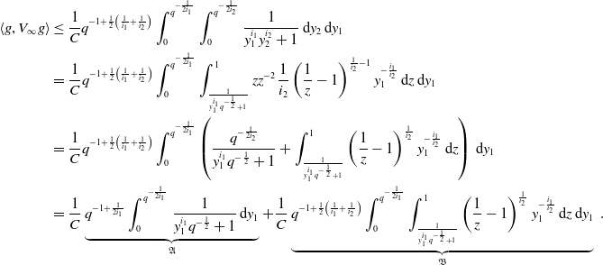 \begin{align} \langle g, V_\infty g \rangle &\leq \frac{1}{C} q^{-1 + \frac{1}{2}\left (\frac{1}{i_1}+\frac{1}{i_2}\right )}\int _0^{ q^{-\frac{1}{2i_1}}}\int _0^{ q^{-\frac{1}{2i_2}}} \frac{1}{y_1^{ i_1}y_2^{i_2} +1} \, \mathrm{d}y_2 \, \mathrm{d} y_1 \nonumber \\ &= \frac{1}{C} q^{-1 + \frac{1}{2}\left (\frac{1}{i_1}+\frac{1}{i_2}\right )} \int_0^{ q^{-\frac{1}{2i_1}}}\int _{ \frac{1}{y_1^{i_1} q^{-\frac{1}{2}}+1}}^{1} z z^{-2} \frac{1}{i_2} \left (\frac{1}{z}-1\right )^{\frac{1}{i_2} -1}y_1^{-\frac{i_1}{i_2}} \, \mathrm{d}z \, \mathrm{d}y_1\\ &= \frac{1}{C} q^{-1 + \frac{1}{2}\left (\frac{1}{i_1}+\frac{1}{i_2}\right )} \int_0^{ q^{-\frac{1}{2i_1}}} \left ( \frac{ q^{-\frac{1}{2i_2}}}{y_1^{i_1} q^{-\frac{1}{2}}+1}+ \int _{\frac{1}{y_1^{i_1} q^{-\frac{1}{2}}+1}}^1 \left ( \frac{1}{z} - 1 \right )^{\frac{1}{i_2}}y_1^{-\frac{i_1}{i_2}}\, \mathrm{d}z \right ) \, \mathrm{d}y_1 \nonumber \\ &= \frac{1}{C} \underbrace{ q^{-1 + \frac{1}{2 i_1}}\int _0^{ q^{-\frac{1}{2i_1}}} \frac{1}{y_1^{i_1} q^{-\frac{1}{2}}+1} \, \mathrm{d}y_1}_{\mathfrak{A}} + \frac{1}{C} \underbrace{q^{-1 + \frac{1}{2}\left (\frac{1}{i_1}+\frac{1}{i_2}\right )} \int_0^{ q^{-\frac{1}{2i_1}}}\int _{\frac{1}{y_1^{i_1} q^{-\frac{1}{2}}+1}}^1 \left ( \frac{1}{z} - 1 \right )^{\frac{1}{i_2}}y_1^{-\frac{i_1}{i_2}}\, \mathrm{d}z \, \mathrm{d}y_1}_{\mathfrak{B}} \, . \nonumber \end{align}
In the following, we first analyse $\mathfrak{A}$
before evaluating the order of divergence of
$\mathfrak{A}$
before evaluating the order of divergence of $\mathfrak{B}$
. Further, as seen above, the choice of
$\mathfrak{B}$
. Further, as seen above, the choice of $i_1$
and
$i_1$
and $i_2$
dictates the rate of the upper bound. Hence, we consider different cases corresponding to the choice of values of
$i_2$
dictates the rate of the upper bound. Hence, we consider different cases corresponding to the choice of values of $i_1$
and
$i_1$
and $i_2$
, whose numbering is displayed in Table 3.
$i_2$
, whose numbering is displayed in Table 3.
-
$\lozenge$
Scaling law of
$\boldsymbol{\mathfrak{A}}$
in Cases 1 and 3. Note that the order of
$\mathfrak{A}$
is independent of
$i_2$
, which simplifies the study of its scaling law. We start by discussing
$\mathfrak{A}$
for
$i_2 \geq i_1 \gt 1$
. Through the substitution
$y_1^{\prime} = y_1 q^{-\frac{1}{2i_1}}$
it follows thatAs already established in (3.5), the integral is converging for
\begin{align*} \mathfrak{A} = q^{-1 + \frac{1}{i_1}}{\int _0}^{q^{-\frac{1}{i_1}}} \frac{1}{y_{1}^{\prime i_1} +1} \, \mathrm{d}y^{\prime }_1 \; . \end{align*}
$p \to 0^{-}$
, and therefore we find a rate of divergence for the first summand given by(A3)for
\begin{align} \Theta \left ( ({-}p)^{-1 + \frac{1}{i_1}} \right ) \end{align}
$p \to 0^{-}$
and
$i_2 \geq i_1 \gt 1$
.
-
$\lozenge$
Scaling law of
$\boldsymbol{\mathfrak{A}}$
in Cases 2 and 4. Next, we consider
$\mathfrak{A}$
assuming that
$i_2 \geq i_1 = 1$
. Through the same substitutions present in the previous case, we getThis component diverges for
\begin{align*} \mathfrak{A} = \int _0^{q^{-1}} \frac{1}{y_1^{\prime} +1} \, \mathrm{d}y_1^{\prime} = \log \left ( q^{-1} +1 \right ) \;. \end{align*}
$q$
approaching zero from above. For
$i_2 \geq i_1 = 1$
, it follows that(A4)is the rate of divergence for
\begin{align} \Theta \left (\log \left (({-}p)^{-1}\right ) \right ) = \Theta \left ({-}\log \left (-p\right ) \right ) \end{align}
$p$
approaching zero from below.


-
$\lozenge$
Scaling law of
$\boldsymbol{\mathfrak{B}}$
in Case 1. We consider the case
$i_2 \gt i_1 \gt 1$
. In regard to
$\mathfrak{B}$
, our first goal is to switch integrals for more convenient computation. Through Fubini’s Theorem, we obtain(A5)By substitution with
\begin{align} \mathfrak{B} &= q^{-1 + \frac{1}{2}\left (\frac{1}{i_1}+\frac{1}{i_2}\right )} \int _{\frac{1}{ q^{-1}+1}}^1 \int _{\left (\frac{1}{z} -1\right )^{\frac{1}{i_1}} q^{\frac{1}{2i_1}}}^{ q^{-\frac{1}{2i_1}}} \left ( \frac{1}{z} - 1 \right )^{\frac{1}{i_2}} y_1^{-\frac{i_1}{i_2}}\, \mathrm{d}y_1 \, \mathrm{d}z \nonumber \\ &= q^{-1 + \frac{1}{2}\left (\frac{1}{i_1}+\frac{1}{i_2}\right )} \int_{\frac{1}{ q^{-1}+1}}^1 \left ( \frac{1}{z} - 1 \right )^{\frac{1}{i_2}} \left [ \frac{1}{\left (1- \frac{i_1}{i_2}\right )} y_1^{-\frac{i_1}{i_2}+1} \right ]_{\left ( \frac{1}{z} -1\right )^{\frac{1}{i_1}} q^{\frac{1}{2i_1}}}^{ q^{-\frac{1}{2i_1}}} \, \mathrm{d}z \\ & = \frac{q^{-1 + \frac{1}{2}\left (\frac{1}{i_1}+\frac{1}{i_2}\right )}}{1-\frac{i_1}{i_2}} \int _{\frac{1}{ q^{-1}+1}}^1 \left ( \frac{1}{z} - 1 \right )^{\frac{1}{i_2}} \left ( q^{\frac{1}{2i_2}-\frac{1}{2i_1}} - \left ( \frac{1}{z}-1 \right )^{\frac{1}{i_1} - \frac{1}{i_2}} q^{\frac{1}{2i_1}-\frac{1}{2i_2}} \right )\, \mathrm{d}z \nonumber \\ & = \Big (1-\frac{i_1}{i_2}\Big )^{-1} \Bigg ( q^{-1 + \frac{1}{i_2}} \int _{\frac{1}{ q^{-1}+1}}^1 \left ( \frac{1}{z} - 1 \right )^{\frac{1}{i_2}} \, \mathrm{d}z - q^{-1 + \frac{1}{i_1}} \int _{\frac{1}{ q^{-1}+1}}^1 \left ( \frac{1}{z}-1 \right )^{\frac{1}{i_1}} \, \mathrm{d}z \Bigg ) \; . \nonumber \end{align}
$z^{\prime } = \frac{1}{z}-1$
, we obtain(A6)Given
\begin{align} & \mathfrak{B} = \Big (1-\frac{i_1}{i_2}\Big )^{-1} \Bigg ( q^{-1 + \frac{1}{i_2}} \int _0^{ q^{-1}} \frac{z^{\prime \frac{1}{i_2}}}{(z^{\prime }+1)^2} \, \mathrm{d}z^{\prime} - q^{-1 + \frac{1}{i_1}} \int _0^{q^{-1}} \frac{z^{\prime \frac{1}{i_1}}}{(z^{\prime }+1)^2} \, \mathrm{d}z^{\prime} \Bigg ) \;. \end{align}
$i_2\gt i_1\gt 1$
, the integrals in (A6) can be uniformly bounded for any
$q\gt 0$
. Hence, we find that for
$\mathfrak{B}$
the rate of divergence is given byas
\begin{align*} \Theta \left ( q^{-1+\frac{1}{i_2}} \right ) - \Theta \left ( q^{-1+ \frac{1}{i_1}}\right ) = \Theta \left ( ({-}p)^{-1+\frac{1}{i_2}} \right ) - \Theta \left ( ({-}p)^{-1+ \frac{1}{i_1}}\right ) = \Theta \left ( ({-}p)^{-1+\frac{1}{i_2}} \right ) \end{align*}
$p$
approaches zero from below. From (A2), we get the rate of divergence of the upper bound asfor
\begin{align*} \Theta \left (({-}p)^{-1+ \frac{1}{i_1}}\right ) + \Theta \left (({-}p)^{-1+\frac{1}{i_2}}\right ) = \Theta \left (({-}p)^{-1+ \frac{1}{i_2}}\right )\, . \end{align*}
$i_2 \gt i_1 \gt 1$
.
-
$\lozenge$
Scaling law of
$\boldsymbol{\mathfrak{B}}$
in Case 2. We suppose now that
$i_2 \gt i_1 =1.$
We can follow the steps in the case above, up to (A6). We then note that(A7)Therefore, we obtain that
\begin{align} & \int _0^{ q^{-1}} \frac{z^{\prime}}{(z^{\prime }+1)^2} \, \mathrm{d}z^{\prime} =\log \left ( q^{-1}+1\right ) + \frac{1}{q^{-1}+1}-1 \;. \end{align}
$\mathfrak{B}$
diverges with ratefor
\begin{align*} \Theta \left ( ({-}p)^{-1 + \frac{1}{i_2}} \right ) - \Theta \left ( \log\!(({-}p)^{-1}) \right ) = \Theta \left ( ({-}p)^{-1 + \frac{1}{i_2}} \right ) \quad, \end{align*}
$p \to 0^{-}$
. Combining this result with equation (A4) we obtain for
$i_2 \gt i_1 =1$
an overall rate of divergence of order
\begin{align*} \Theta \left ({-}\log\!({-}p) \right ) + \Theta \left ( ({-}p)^{-1+\frac{1}{i_2}} \right ) = \Theta \left ( ({-}p)^{- 1 + \frac{1}{i_2}} \right )\,. \end{align*}
-
$\lozenge$
Scaling law of
$\boldsymbol{\mathfrak{B}}$
in Case 3. For the third case we consider
$\mathfrak{B}$
with
$i_2 = i_1 = i \gt 1$
, for which we getAgain, we substitute
\begin{align*} \mathfrak{B} &= q^{-1 + \frac{1}{i}} \int _{\frac{1}{ q^{-1}+1}}^1 \int _{\left (\frac{1}{z} -1\right )^{\frac{1}{i}} q^{\frac{1}{2i}}}^{ q^{-\frac{1}{2i}}} \left ( \frac{1}{z} - 1 \right )^{\frac{1}{i}} y_1^{-1}\, \mathrm{d}y_1 \, \mathrm{d}z \\ &= q^{-1 + \frac{1}{i}} \int _{\frac{1}{ q^{-1}+1}}^1 \left ( \frac{1}{z} - 1 \right )^{\frac{1}{i}} \left ( \log \left ( q^{-\frac{1}{2i}} \right ) - \log \left (\left (\frac{1}{z} -1 \right )^{\frac{1}{i}} q^{\frac{1}{2i}} \right ) \right )\, \mathrm{d}z \\ &= q^{-1 + \frac{1}{i}} \left ( - \frac{\log\!(q)}{i} \int _{\frac{1}{ q^{-1}+1}}^1 \left ( \frac{1}{z} - 1 \right )^{\frac{1}{i}} \, \mathrm{d}z - \frac{1}{i} \int _{\frac{1}{ q^{-1}+1}}^1 \left ( \frac{1}{z} - 1 \right )^{\frac{1}{i}} \log \left ( \frac{1}{z} - 1 \right )\, \mathrm{d}z\right ) \; . \end{align*}
$z^{\prime } = \frac{1}{z}-1$
to get(A8)The integrals in (A8) are uniformly bounded for any
\begin{align} \mathfrak{B} = q^{-1 + \frac{1}{i}} \left ( - \frac{\log\!(q)}{i}{\int _0}^{ q^{-1}} \frac{{z^{\prime}}^{\frac{1}{i}}}{(z^{\prime}+1)^2} \, \mathrm{d}z^{\prime} - \frac{1}{i}{\int _0}^{q^{-1}} \frac{{z^{\prime}}^{\frac{1}{i}} \log\!(z^{\prime})}{(z^{\prime}+1)^2} \, \mathrm{d}z^{\prime}\right ) \, . \end{align}
$q\gt 0$
due to
$i\gt 1$
. Equation (A8) implies that
$\mathfrak{B}$
assumes, in this case, rate of divergencefor
\begin{align*} \Theta \left ( -({-}p)^{-1+ \frac{1}{i}}\log\!({-}p) \right ) + \Theta \left ( ({-}p)^{-1 + \frac{1}{i}}\right ) = \Theta \left ({-}({-}p)^{-1+ \frac{1}{i}}\log\!({-}p) \right ) \end{align*}
$ p \to 0^{-}$
. From (A2) and (A3), we get that the rate of divergence of the upper bound is
\begin{align*} \Theta \left (({-}p)^{-1+\frac{1}{i}} \right ) + \Theta \left ({-}({-}p)^{-1+\frac{1}{i}}\log\!({-}p) \right ) = \Theta \left ({-}({-}p)^{-1+\frac{1}{i}}\log\!({-}p) \right )\, . \end{align*}
-
$\lozenge$
Scaling law of
$\boldsymbol{\mathfrak{B}}$
in Case 4. In the last case, we suppose that
$i_2 = i_1 =i=1$
. Hence, (A8) assumes the form(A9)We obtain therefore from (A9) and (C3), in Appendix C, that the two leading terms in
\begin{align} \mathfrak{B} &= - \log\!(q) \int _0^{ q^{-1}} \frac{z^{\prime}}{(z^{\prime}+1)^2} \, \mathrm{d}z^{\prime} - \int _0^{ q^{-1}} \frac{z^{\prime} \log\!(z^{\prime})}{(z^{\prime}+1)^2} \, \mathrm{d}z^{\prime}\\ &= - \log\!(q) \Bigg (\log\!( q^{-1}+1)+\frac{1}{ q^{-1}+1}-1\Bigg ) - \int _0^{ q^{-1}} \frac{z^{\prime} \log\!(z^{\prime})}{(z^{\prime}+1)^2} \, \mathrm{d}z^{\prime} \;. \nonumber \end{align}
$\mathfrak{B}$
diverge respectively as
$\log ^2(q)$
and as
$-\frac{1}{2}\log ^2(q)$
. Hence, we know that the divergence of
$\mathfrak{B}$
presents rateCombining such result with the rate of divergence of
\begin{align*} \Theta \left ( \log ^2({-}p) \right ) \quad \mathrm{for } p \to 0^{-} \, . \end{align*}
$\mathfrak{A}$
in (A4), we obtainas an overall upper bound for
\begin{align*} \Theta \left ({-}\log\!({-}p) \right ) + \Theta \left ( \log ^2({-}p) \right ) = \Theta \left ( \log ^2({-}p) \right ) \quad \mathrm{for } p \to 0^{-} \;, \end{align*}
$i_2 = i_1 = 1$
.


Appendix B: Proof Theorem4.7
The subsequent proof validates the description of the rate of divergence of the upper bound discussed in Theorem4.7 and in Table 4. The approach is similar to the one involved in the proof of Theorem4.5 as the upper bound is split into two summands, labeled $\mathfrak{C}$
and
$\mathfrak{C}$
and $\mathfrak{D}$
. The first summand is studied similarly to the upper bound in the stated proof for the two-dimensional case.
$\mathfrak{D}$
. The first summand is studied similarly to the upper bound in the stated proof for the two-dimensional case.
Proof Theorem 4.7 Lemma 4.3 implies that
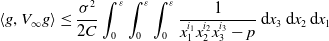 \begin{align*} \langle g, V_\infty g \rangle \leq \frac{\sigma ^2}{2C} \int _{0}^\varepsilon \int _{0}^\varepsilon \int _{0}^\varepsilon \frac{1}{x_1^{i_1} x_2^{i_2} x_3^{i_3}-p} \, \mathrm{d}x_3 \, \mathrm{d}x_2 \, \mathrm{d}x_1 \end{align*}
for a constant $C\gt 0$
and any
$C\gt 0$
and any $p\lt 0$
. As in the two-dimensional case, we make use of
$p\lt 0$
. As in the two-dimensional case, we make use of $q\,:\!=\,-p \gt 0$
and we fix
$q\,:\!=\,-p \gt 0$
and we fix $\varepsilon =1$
, up to rescaling of the spatial variable
$\varepsilon =1$
, up to rescaling of the spatial variable $x$
. Up to permutation of the indices we consider
$x$
. Up to permutation of the indices we consider $i_3\geq i_2 \geq i_1 \geq 1$
, thus excluding the cases described in Remark 4.4.
$i_3\geq i_2 \geq i_1 \geq 1$
, thus excluding the cases described in Remark 4.4.
We follow a similar computation of the integral as in Theorem4.5. First, we study it in the coordinates $y_n = x_nq^{-\frac{1}{3i_n}}$
for all
$y_n = x_nq^{-\frac{1}{3i_n}}$
for all $n \in \{1,2,3 \}$
and then we substitute
$n \in \{1,2,3 \}$
and then we substitute $y_3$
with
$y_3$
with $z = \frac{1}{y_1^{i_1}y_2^{i_2}y_3^{i_3}+1}$
to obtain
$z = \frac{1}{y_1^{i_1}y_2^{i_2}y_3^{i_3}+1}$
to obtain
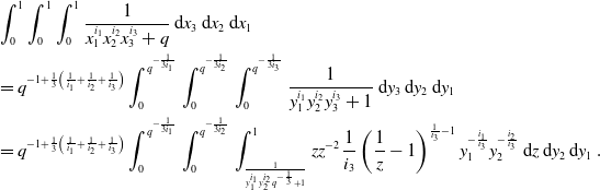 \begin{align*} & \int _{0}^1 \int _{0}^1 \int _{0}^1 \frac{1}{ x_1^{i_1} x_2^{i_2} x_3^{i_3}+q} \, \mathrm{d}x_3 \, \mathrm{d}x_2 \, \mathrm{d}x_1 \\ &=q^{-1 + \frac{1}{3}\left ( \frac{1}{i_1}+\frac{1}{i_2}+\frac{1}{i_3} \right )} \int _0^{ q^{-\frac{1}{3i_1}}} \int _0^{ q^{-\frac{1}{3i_2}}} \int _0^{ q^{-\frac{1}{3i_3}}} \frac{1}{y_1^{i_1}y_2^{i_2}y_3^{i_3}+1} \, \mathrm{d}y_3 \, \mathrm{d}y_2 \, \mathrm{d}y_1 \\ &= q^{-1 + \frac{1}{3} \left ( \frac{1}{i_1}+\frac{1}{i_2}+\frac{1}{i_3} \right )} \int_0^{ q^{-\frac{1}{3i_1}}} \int_0^{ q^{-\frac{1}{3i_2}}} \int _{\frac{1}{y_1^{i_1}y_2^{i_2} q^{-\frac{1}{3}}+1}}^1 z z^{-2} \frac{1}{i_3}\left ( \frac{1}{z}-1\right )^{\frac{1}{i_3}-1}y_1^{-\frac{i_1}{i_3}}y_2^{-\frac{i_2}{i_3}} \, \mathrm{d}z \, \mathrm{d}y_2 \, \mathrm{d}y_1 \, . \end{align*}
Through integration by parts on the inner integral, it follows that
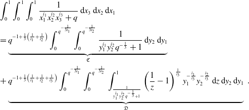 \begin{align} & \int _{0}^1 \int _{0}^1 \int _{0}^1 \frac{1}{ x_1^{i_1} x_2^{i_2} x_3^{i_3}+q} \, \mathrm{d}x_3 \, \mathrm{d}x_2 \, \mathrm{d}x_1 \nonumber \\ &=\underbrace{ q^{-1 + \frac{1}{3}\left (\frac{1}{i_1}+\frac{1}{i_2}\right )} \int _0^{ q^{-\frac{1}{3i_1}}} \int _0^{ q^{-\frac{1}{3i_2}}} \frac{1}{y_1^{i_1}y_2^{i_2} q^{-\frac{1}{3}}+1} \, \mathrm{d}y_2 \, \mathrm{d}y_1}_{\mathfrak{C}}\\ &+ \underbrace{q^{-1 + \frac{1}{3} \left ( \frac{1}{i_1}+\frac{1}{i_2}+\frac{1}{i_3} \right ) } \int_0^{ q^{-\frac{1}{3i_1}}} \int_0^{ q^{-\frac{1}{3i_2}}} \int _{\frac{1}{y_1^{i_1}y_2^{i_2} q^{- \frac{1}{3}}+1}}^{1} \left ( \frac{1}{z} - 1\right )^{\frac{1}{i_3}} y_1^{-\frac{i_1}{i_3}}y_2^{-\frac{i_2}{i_3}} \, \mathrm{d}z \, \mathrm{d}y_2 \, \mathrm{d}y_1}_{\mathfrak{D}} \,. \nonumber \end{align}
We study each summand independently as in Theorem4.5. Further, we distinguish between different choices of values for $i_n$
for
$i_n$
for $n \in \{ 1,2,3 \}$
. We find the scaling laws of
$n \in \{ 1,2,3 \}$
. We find the scaling laws of $\mathfrak{C}$
,
$\mathfrak{C}$
, $\mathfrak{D}$
, and the overall upper bound for each case. The numbering of the cases is reported in Table 4.
$\mathfrak{D}$
, and the overall upper bound for each case. The numbering of the cases is reported in Table 4.
-
$\lozenge$
Scaling law of
$\boldsymbol{\mathfrak{C}}$
in Cases 1–8. We assume
$i_1,i_2,i_3\gt 0$
. We change the variables in the integral with
$y_n^{\prime }=y_n q^{-\frac{1}{6i_n}}$
for
$n \in \{ 1, 2 \}$
to haveWe note that this expression is equivalent to the integral given by (A1), as
\begin{align*} & q^{-1 + \frac{1}{3} \left ( \frac{1}{i_1}+\frac{1}{i_2} \right ) } \int_0^{ q^{-\frac{1}{3i_1}}} \int_0^{ q^{-\frac{1}{3i_2}}} \frac{1}{\left (y_1 q^{- \frac{1}{6 i_1}} \right )^{i_1} \left (y_2 q^{- \frac{1}{6 i_2}} \right )^{i_2}+1}\, \mathrm{d}y_2 \, \mathrm{d}y_1 \\ &= q^{-1 + \frac{1}{2} \left (\frac{1}{i_1}+ \frac{1}{i_2} \right )} \int _0^{ q^{-\frac{1}{2i_1}}} \int _0^{ q^{-\frac{1}{2i_2}}} \frac{1}{y_1^{\prime i_1}y_2^{\prime i_2} + 1} \, . \end{align*}
$i_3$
does not affect such a rate of divergence. Hence, we have proven the divergence of
$\mathfrak{C}$
for different choices of
$i_1, i_2$
and that its corresponding rate is displayed in Table 3.


-
$\blacklozenge$
Scaling law of
$\boldsymbol{\mathfrak{D}}$
in Case 1. Next, we continue analyzing the component
$\mathfrak{D}$
of (B1). First, we assume that
$i_3 \gt i_2 \gt i_1 \gt 1$
. We change the order of integrals through Fubini’s Theorem, placing the integral on
$z$
in the outer position and obtaining(B2)Since
\begin{align} & q^{-1 + \frac{1}{3} \left ( \frac{1}{i_1}+\frac{1}{i_2}+\frac{1}{i_3} \right ) } \int_0^{ q^{-\frac{1}{3i_1}}} \int_0^{ q^{-\frac{1}{3i_2}}} \int _{\frac{1}{y_1^{i_1}y_2^{i_2} q^{- \frac{1}{3}}+1}}^{1} \left ( \frac{1}{z} - 1\right )^{\frac{1}{i_3}} y_1^{-\frac{i_1}{i_3}}y_2^{-\frac{i_2}{i_3}} \, \mathrm{d}z \, \mathrm{d}y_2 \, \mathrm{d}y_1\\ &= q^{-1 + \frac{1}{3} \left ( \frac{1}{i_1}+\frac{1}{i_2}+\frac{1}{i_3} \right )} \int _{\frac{1}{ q^{-1}+1}}^1 \int _{\left ( \frac{1}{z} - 1\right )^{\frac{1}{i_1}} q^{\frac{2}{3i_1}}}^{ q^{- \frac{1}{3i_1}}} \int _{\left ( \frac{1}{z} - 1\right )^{\frac{1}{i_2}} q^{\frac{1}{3i_2}}y_1^{-\frac{i_1}{i_2}}}^{ q^{-\frac{1}{3i_2}}} \left ( \frac{1}{z} - 1\right )^{\frac{1}{i_3}} y_1^{-\frac{i_1}{i_3}}y_2^{-\frac{i_2}{i_3}} \, \mathrm{d}y_2 \, \mathrm{d}y_1 \, \mathrm{d}z \,. \nonumber \end{align}
$i_3\gt i_2$
, it follows that
$\mathfrak{D}$
is equal to(B3)From
\begin{align} &\Big (-\frac{i_2}{i_3}+1\Big )^{-1} q^{-1 + \frac{1}{3} \left ( \frac{1}{i_1}+\frac{1}{i_2}+\frac{1}{i_3} \right )} \int _{\frac{1}{ q^{-1}+1}}^1 \int _{\left ( \frac{1}{z} - 1\right )^{\frac{1}{i_1}} q^{\frac{2}{3i_1}}}^{ q^{- \frac{1}{3i_1}}} \left ( \frac{1}{z} - 1\right )^{\frac{1}{i_3}} y_1^{-\frac{i_1}{i_3}} \left [y_2^{-\frac{i_2}{i_3}+1} \right ]_{y_2=\left ( \frac{1}{z} - 1\right )^{\frac{1}{i_2}} q^{\frac{1}{3i_2}}y_1^{-\frac{i_1}{i_2}}}^{ q^{-\frac{1}{3i_2}}} \, \mathrm{d}y_1 \, \mathrm{d}z \nonumber \\ &=\Big (-\frac{i_2}{i_3}+1\Big )^{-1} \underbrace{ q^{-1 + \frac{1}{3i_1} + \frac{2}{3i_3}} \int _{\frac{1}{ q^{-1}+1}}^1 \left ( \frac{1}{z} - 1\right )^{\frac{1}{i_3}} \int _{\left ( \frac{1}{z} - 1\right )^{\frac{1}{i_1}} q^{\frac{2}{3i_1}}}^{ q^{- \frac{1}{3i_1}}} y_1^{- \frac{i_1}{i_3}} \, \mathrm{d}y_1 \, \mathrm{d}z}_{\mathfrak{D}.\textrm{I}} \\ &- \Big (-\frac{i_2}{i_3}+1\Big )^{-1} \underbrace{ q^{-1 + \frac{1}{3i_1} + \frac{2}{3i_2}} \int _{\frac{1}{ q^{-1}+1}}^1 \left ( \frac{1}{z} - 1\right )^{\frac{1}{i_2}} \int _{\left ( \frac{1}{z} - 1\right )^{\frac{1}{i_1}} q^{\frac{2}{3i_1}}}^{q^{- \frac{1}{3i_1}}} y_1^{- \frac{i_1}{i_2}} \, \mathrm{d}y_1 \, \mathrm{d}z}_{\mathfrak{D}.\textrm{II}} \, . \nonumber \end{align}
$i_3\gt i_1$
, we know that
$\mathfrak{D}.\textrm{I}$
is equal to(B4)with
\begin{align} & \Big (-\frac{i_1}{i_3}+1\Big )^{-1} \Bigg ( q^{-1+\frac{1}{i_3}} \int _{\frac{1}{ q^{-1}+1}}^1 \left ( \frac{1}{z} - 1\right )^{\frac{1}{i_3}} \, \mathrm{d}z - q^{-1 + \frac{1}{i_1}} \int _{\frac{1}{ q^{-1}+1}}^1 \left ( \frac{1}{z} - 1\right )^{\frac{1}{i_1}} \, \mathrm{d}z\Bigg )\\ &= \Big (-\frac{i_1}{i_3}+1\Big )^{-1} \Bigg ( \underbrace{ q^{-1+\frac{1}{i_3}} \int _0^{ q^{-1}} \frac{{z^{\prime}}^{\frac{1}{i_3}}}{(z^{\prime}+1)^2} \, \mathrm{d}z^{\prime}}_{\mathfrak{D}.\textrm{I}.1} - \underbrace{ q^{-1 + \frac{1}{i_1}} \int _0^{ q^{-1}} \frac{{z^{\prime}}^{\frac{1}{i_1}}}{(z^{\prime}+1)^2} \, \mathrm{d}z^{\prime}}_{\mathfrak{D}.\textrm{I}.2} \Bigg ) \quad, \nonumber \end{align}
$z^{\prime } = \frac{1}{z} -1$
. Equivalently, since
$i_2\gt i_1$
, the summand
$\mathfrak{D}.\textrm{II}$
is equal toFor
\begin{align*} & \Big (-\frac{i_1}{i_2}+1\Big )^{-1} \Bigg ( \underbrace{ q^{-1+\frac{1}{i_2}} \int _0^{ q^{-1}} \frac{{z^{\prime}}^{\frac{1}{i_2}}}{(z^{\prime}+1)^2} \, \mathrm{d}z^{\prime}}_{\mathfrak{D}.\textrm{II}.1} - \underbrace{ q^{-1 + \frac{1}{i_1}} \int _0^{ q^{-1}} \frac{{z^{\prime}}^{\frac{1}{i_1}}}{(z^{\prime}+1)^2} \mathrm{d}z^{\prime}}_{\mathfrak{D}.\textrm{II}.2} \Bigg ) \, . \end{align*}
$i_1,i_2,i_3\gt 1$
, the integrals in
$\mathfrak{D}.\textrm{I}.1$
,
$\mathfrak{D}.\textrm{I}.2$
,
$\mathfrak{D}.\textrm{II}.1$
and
$\mathfrak{D}.\textrm{II}.2$
are uniformly bounded for any
$q\gt 0$
. Hence, the rate of divergence of
$\mathfrak{D}$
isCombining the rates of
\begin{align*} \Theta \left ( ({-}p)^{-1 + \frac{1}{i_3}} \right ) - \Theta \left ( ({-}p)^{-1 + \frac{1}{i_1}}\right ) - \Theta \left ( ({-}p)^{-1 + \frac{1}{i_2}}\right ) + \Theta \left ( ({-}p)^{-1 + \frac{1}{i_1}}\right ) = \Theta \left ( ({-}p)^{-1 + \frac{1}{i_3}} \right ) \, . \end{align*}
$\mathfrak{C}$
and
$\mathfrak{D}$
, we prove the divergence, for
$i_3 \gt i_2 \gt i_1 \gt 1$
, of the upper bound with scaling law
\begin{align*} \Theta \left ( ({-}p)^{-1+ \frac{1}{i_2}} \right ) + \Theta \left ( ({-}p)^{-1 + \frac{1}{i_3}} \right ) = \Theta \left ( ({-}p)^{-1 + \frac{1}{i_3}} \right ) \,. \end{align*}
-
$\blacklozenge$
Scaling law of
$\boldsymbol{\mathfrak{D}}$
in Case 2. Next, we consider the case
$i_3 \gt i_2 = i_1 = i \gt 1$
. We can follow the same argumentation of the previous case until (B4) and prove thatIn this case, summand
\begin{align*} \mathfrak{D}.\textrm{I} =\Big (-\frac{i}{i_3}+1\Big )^{-1} \Big ( \mathfrak{D}.\textrm{I}.1-\mathfrak{D}.\textrm{I}.2 \Big ) \;. \end{align*}
$\mathfrak{D}.\textrm{II}$
is equal to(B5)The integrals in
\begin{align} & q^{-1 + \frac{1}{i}} \int _{\frac{1}{ q^{-1}+1}}^1 \left ( \frac{1}{z} - 1\right )^{\frac{1}{i}} \int _{\left ( \frac{1}{z} - 1\right )^{\frac{1}{i}} q^{\frac{2}{3i}}}^{ q^{- \frac{1}{3i}}} y_1^{- 1} \, \mathrm{d}y_1 \, \mathrm{d}z \nonumber \\ &= - \frac{1}{i} q^{-1 + \frac{1}{i}} \int _{\frac{1}{ q^{-1}+1}}^1 \left ( \frac{1}{z} - 1\right )^{\frac{1}{i}} \Bigg ( \log\!(q) + \log \left ( \frac{1}{z} - 1\right ) \Bigg ) \mathrm{d}z \\ &= -\frac{1}{i} \underbrace{q^{-1 + \frac{1}{i}} \log\!(q) \int _0^{ q^{-1}} \frac{{z^{\prime}}^{\frac{1}{i}}}{(z^{\prime}+1)^2} \mathrm{d}z}_{\mathfrak{D}.\textrm{II}.3} -\frac{1}{i} \underbrace{q^{-1 + \frac{1}{i}} \int _0^{ q^{-1}} \frac{{z^{\prime}}^{\frac{1}{i}} \log\!(z^{\prime})}{(z^{\prime}+1)^2} \mathrm{d}z}_{\mathfrak{D}.\textrm{II}.4} \;. \nonumber \end{align}
$\mathfrak{D}.\textrm{II}.3$
and
$\mathfrak{D}.\textrm{II}.4$
are uniformly bounded for any
$q\gt 0$
, therefore the rate of divergence of
$\mathfrak{D}.\textrm{II}$
is
$\Theta \left ({-}({-}p)^{1+\frac{1}{i}}\log\!({-}p)\right )$
. The rate assumed by
$\mathfrak{D}$
isOverall, we find the rate of the upper bound in the case
\begin{align*} \Theta \left ( ({-}p)^{-1+\frac{1}{i_3}} \right ) -\Theta \left ({-} ({-}p)^{-1+ \frac{1}{i}} \log\!({-}p)\right ) = \Theta \left ( ({-}p)^{-1+ \frac{1}{i_3}} \right ) \;. \end{align*}
$i_3 \gt i_2 = i_1 \gt 1$
to be
\begin{align*} \Theta \left ({-}({-}p)^{-1+\frac{1}{i_2}} \log\!({-}p)\right ) + \Theta \left ( ({-}p)^{-1+ \frac{1}{i_3}} \right ) = \Theta \left ( ({-}p)^{-1+ \frac{1}{i_3}} \right ) \;. \end{align*}
-
$\blacklozenge$
Scaling law of
$\boldsymbol{\mathfrak{D}}$
in Case 3. Next, we consider the case
$i_3 = i_2 \gt i_1 \gt 1$
. We observe again equation (B2) and label
$i_3 = i_2 = i$
to obtain(B6)First we evaluate
\begin{align} & q^{-1 + \frac{1}{3} \left ( \frac{1}{i_1}+\frac{2}{i} \right )} \int _{\frac{1}{ q^{-1}+1}}^1 \int _{\left ( \frac{1}{z} - 1\right )^{\frac{1}{i_1}} q^{\frac{2}{3i_1}}}^{ q^{- \frac{1}{3i_1}}} \int _{\left ( \frac{1}{z} - 1\right )^{\frac{1}{i}} q^{\frac{1}{3i}}y_1^{-\frac{i_1}{i}}}^{ q^{-\frac{1}{3i}}} \left ( \frac{1}{z} - 1\right )^{\frac{1}{i}} y_1^{-\frac{i_1}{i}}y_2^{-1} \, \mathrm{d}y_2 \, \mathrm{d}y_1 \, \mathrm{d}z \nonumber \\ &= q^{-1 + \frac{1}{3} \left ( \frac{1}{i_1}+\frac{2}{i} \right )} \log \left ( q^{-\frac{1}{3i}} \right ) \int _{\frac{1}{ q^{-1}+1}}^1 \int _{\left ( \frac{1}{z} - 1\right )^{\frac{1}{i_1}} q^{\frac{2}{3i_1}}}^{ q^{- \frac{1}{3i_1}}} \left ( \frac{1}{z} - 1\right )^{\frac{1}{i}} y_1^{-\frac{i_1}{i}} \, \mathrm{d}y_1 \, \mathrm{d}z \nonumber \\ &- q^{-1 + \frac{1}{3} \left ( \frac{1}{i_1}+\frac{2}{i} \right )} \int _{\frac{1}{ q^{-1}+1}}^1 \int _{\left ( \frac{1}{z} - 1\right )^{\frac{1}{i_1}} q^{\frac{2}{3i_1}}}^{ q^{- \frac{1}{3i_1}}} \left ( \frac{1}{z} - 1\right )^{\frac{1}{i}} y_1^{-\frac{i_1}{i}} \log \left ( \left ( \frac{1}{z} - 1\right )^{\frac{1}{i}} q^{\frac{1}{3i}}y_1^{-\frac{i_1}{i}} \right ) \, \mathrm{d}y_1 \, \mathrm{d}z \\ &=- \frac{2}{3i} \underbrace{q^{-1 + \frac{1}{3} \left ( \frac{1}{i_1}+\frac{2}{i} \right )} \log \left (q \right ) \int _{\frac{1}{ q^{-1}+1}}^1 \int _{\left ( \frac{1}{z} - 1\right )^{\frac{1}{i_1}} q^{\frac{2}{3i_1}}}^{ q^{- \frac{1}{3i_1}}} \left ( \frac{1}{z} - 1\right )^{\frac{1}{i}} y_1^{-\frac{i_1}{i}} \, \mathrm{d}y_1 \, \mathrm{d}z}_{\mathfrak{D}.\textrm{III}} \nonumber \\ & - \frac{1}{i} \underbrace{q^{-1 + \frac{1}{3} \left ( \frac{1}{i_1}+\frac{2}{i} \right )} \int _{\frac{1}{ q^{-1}+1}}^1 \int _{\left ( \frac{1}{z} - 1\right )^{\frac{1}{i_1}} q^{\frac{2}{3i_1}}}^{ q^{- \frac{1}{3i_1}}} \left ( \frac{1}{z} - 1\right )^{\frac{1}{i}} \log \left ( \frac{1}{z} - 1 \right ) y_1^{-\frac{i_1}{i}} \, \mathrm{d}y_1 \, \mathrm{d}z}_{\mathfrak{D}.\textrm{IV}} \nonumber \\ & + \frac{i_1}{i} \underbrace{q^{-1 + \frac{1}{3} \left ( \frac{1}{i_1}+\frac{2}{i} \right )} \int _{\frac{1}{ q^{-1}+1}}^1 \int _{\left ( \frac{1}{z} - 1\right )^{\frac{1}{i_1}} q^{\frac{2}{3i_1}}}^{ q^{- \frac{1}{3i_1}}} \left ( \frac{1}{z} - 1\right )^{\frac{1}{i}} y_1^{-\frac{i_1}{i}} \log \left ( y_1 \right ) \, \mathrm{d}y_1 \, \mathrm{d}z}_{\mathfrak{D}.\textrm{V}} \; . \nonumber \end{align}
$\mathfrak{D}$
.III by integrating with respect to
$y_1$
. Since
$i\gt i_1$
, we get that
$\mathfrak{D}$
.III is equal to(B7)Since
\begin{align} &\Big (-\frac{i_1}{i}+1\Big )^{-1} \log\!(q) \Bigg ( q^{-1 + \frac{1}{i}} \int _{\frac{1}{ q^{-1}+1}}^1 \left ( \frac{1}{z} - 1\right )^{\frac{1}{i}} \, \mathrm{d}z - q^{-1 + \frac{1}{i_1}} \int _{\frac{1}{ q^{-1}+1}}^1 \left ( \frac{1}{z} - 1\right )^{\frac{1}{i_1}} \, \mathrm{d}z \Bigg ) \\ &= \Big (-\frac{i_1}{i}+1\Big )^{-1} \Bigg ( \underbrace{q^{-1 + \frac{1}{i}} \log\!(q) \int _0^{ q^{-1}} \frac{{z^{\prime}}^{\frac{1}{i}}}{(z^{\prime}+1)^2} \, \mathrm{d}z^{\prime}}_{\mathfrak{D}.\textrm{III}.1} - \underbrace{q^{-1 + \frac{1}{i_1}} \log\!(q) \int _0^{ q^{-1}} \frac{{z^{\prime}}^{\frac{1}{i_1}}}{(z^{\prime}+1)^2} \, \mathrm{d}z^{\prime}}_{\mathfrak{D}.\textrm{III}.2} \Bigg ) \;. \nonumber \end{align}
$i,i_1\gt 1$
, the integrals in
$\mathfrak{D}.\textrm{III}.1$
and in
$\mathfrak{D}.\textrm{III}.2$
are uniformly bounded for
$q\gt 0$
. The rate of divergence of
$\mathfrak{D}.\textrm{III}$
is therefore
$-\Theta \left ({-}q^{1-\frac{1}{i}}\log\!(q)\right )$
. Through a similar approach, we note that
$\mathfrak{D}.\textrm{IV}$
is equal toThe rate of divergence of
\begin{align*} \Big (-\frac{i_1}{i}+1\Big )^{-1} \Bigg ( \underbrace{ q^{-1 + \frac{1}{i}} \int _0^{ q^{-1}} \frac{{z^{\prime}}^{\frac{1}{i}} \log\!(z)}{(z^{\prime}+1)^2} \, \mathrm{d}z^{\prime}}_{\mathfrak{D}.\textrm{IV}.1} - \underbrace{ q^{-1 + \frac{1}{i_1}} \int _0^{ q^{-1}} \frac{{z^{\prime}}^{\frac{1}{i_1}} \log\!(z)}{(z^{\prime}+1)^2} \, \mathrm{d}z^{\prime}}_{\mathfrak{D}.\textrm{IV}.2} \Bigg ) \, . \end{align*}
$\mathfrak{D}.\textrm{IV}$
is
$\Theta \left (q^{1-\frac{1}{i}}\right )$
because the integrals in
$\mathfrak{D}.\textrm{IV}.1$
and
$\mathfrak{D}.\textrm{IV}.2$
are uniformly bounded for
$q\gt 0$
since
$i,i_1\gt 1$
. Lastly, through integration by parts we obtain that
$\mathfrak{D}.\textrm{V}$
is equal to(B8)The rate of divergence of
\begin{align} &\Big ({-}\frac{i_1}{i}+1\Big )^{-1} q^{-1 + \frac{1}{i}} \log \left (q^{-\frac{1}{3 i_1}}\right ) \int _{\frac{1}{ q^{-1}+1}}^1 \left ( \frac{1}{z} - 1\right )^{\frac{1}{i}} \, \mathrm{d}z \nonumber \\ & -\Big ({-}\frac{i_1}{i}+1\Big )^{-2} q^{-1 + \frac{1}{i}} \int _{\frac{1}{ q^{-1}+1}}^1 \left ( \frac{1}{z} - 1\right )^{\frac{1}{i}} \, \mathrm{d}z \nonumber \\ &- \Big ({-}\frac{i_1}{i}+1\Big )^{-1} q^{-1 + \frac{1}{i_1}} \int _{\frac{1}{ q^{-1}+1}}^1 \left ( \frac{1}{z} - 1\right )^{\frac{1}{i_1}} \log \left (\left ( \frac{1}{z} - 1\right )^{\frac{1}{i_1}} q^{\frac{2}{3i_1}}\right ) \, \mathrm{d}z \nonumber \\ &+ \Big ({-}\frac{i_1}{i}+1\Big )^{-2} q^{-1 + \frac{1}{i_1}} \int _{\frac{1}{ q^{-1}+1}}^1 \left ( \frac{1}{z} - 1\right )^{\frac{1}{i_1}} \, \mathrm{d}z\\ &=-\Big ({-}\frac{i_1}{i}+1\Big )^{-2} \underbrace{q^{-1 + \frac{1}{i}} \int _0^{ q^{-1}} \frac{{z^{\prime}}^{\frac{1}{i}}}{(z^{\prime}+1)^2} \, \mathrm{d}z^{\prime}}_{\mathfrak{D}.\textrm{V}.1} + \Big (-\frac{i_1}{i}+1\Big )^{-2} \underbrace{q^{-1 + \frac{1}{i_1}} \int _0^{ q^{-1}} \frac{{z^{\prime}}^{\frac{1}{i_1}}}{(z^{\prime}+1)^2} \, \mathrm{d}z^{\prime}}_{\mathfrak{D}.\textrm{V}.2} \nonumber \\ &-\Big ({-}\frac{i_1}{i}+1\Big )^{-1} \frac{1}{3i_1} \underbrace{q^{-1 + \frac{1}{i}} \log \left (q\right ) \int _0^{ q^{-1}} \frac{{z^{\prime}}^{\frac{1}{i}}}{(z^{\prime}+1)^2} \, \mathrm{d}z^{\prime}}_{\mathfrak{D}.\textrm{V}.3} - \Big (-\frac{i_1}{i}+1\Big )^{-1} \frac{2}{3i_1} \underbrace{q^{-1 + \frac{1}{i_1}} \log \left (q\right ) \int _0^{ q^{-1}} \frac{{z^{\prime}}^{\frac{1}{i_1}}}{(z^{\prime}+1)^2} \, \mathrm{d}z^{\prime}}_{\mathfrak{D}.\textrm{V}.4} \nonumber \\ &- \Big ({-}\frac{i_1}{i}+1\Big )^{-1} \frac{1}{i_1} \underbrace{q^{-1 + \frac{1}{i_1}} \int _0^{ q^{-1}} \frac{{z^{\prime}}^{\frac{1}{i_1}} \log\!(z^{\prime})}{(z^{\prime}+1)^2} \, \mathrm{d}z^{\prime}}_{\mathfrak{D}.\textrm{V}.5} \;. \nonumber \end{align}
$\mathfrak{D}.\textrm{V}$
is
$\Theta \left (-q^{-1+\frac{1}{i}}\log\!(q)\right )$
, since the integrals in (B8) are uniformly bounded for
$q\gt 0$
. Overall, the rate assumed by
$\mathfrak{D}$
isWe find the rate of divergence for the upper bound in the case
\begin{align*} \Theta \left (-q^{1-\frac{1}{i}} \log\!(q) \right ) - \Theta \left (q^{1-\frac{1}{i}}\right ) + \Theta \left (-q^{-1+\frac{1}{i}}\log\!(q)\right ) = \Theta \left (-q^{-1+\frac{1}{i}}\log\!(q)\right )\;. \end{align*}
$i_3 =i_2 \gt i_1 \gt 1$
given by
\begin{align*} &\Theta \left ( ({-}p)^{-1+ \frac{1}{i_2}} \right ) + \Theta \left ( -({-}p)^{-1 + \frac{1}{i_3}} \log\!({-}p) \right ) = \Theta \left (-({-}p)^{-1 + \frac{1}{i_3}} \log\!({-}p) \right ) \;. \end{align*}
-
$\blacklozenge$
Scaling law of
$\boldsymbol{\mathfrak{D}}$
in Case 4. We suppose now that
$i_3 = i_2 = i_1 \gt 1$
. We trace the previous case until equation (B6) and label
$i = i_3 = i_2 = i_1$
. Therefore,
$\mathfrak{D}.\textrm{III}$
is equal to(B9)Since
\begin{align} &q^{-1 + \frac{1}{i}} \log \left (q \right ) \int _{\frac{1}{ q^{-1}+1}}^1 \int _{\left ( \frac{1}{z} - 1\right )^{\frac{1}{i}} q^{\frac{2}{3i}}}^{ q^{- \frac{1}{3i}}} \left ( \frac{1}{z} - 1\right )^{\frac{1}{i}} y_1^{-1} \, \mathrm{d}y_1 \, \mathrm{d}z \nonumber \\ &= -\frac{1}{i} q^{-1 + \frac{1}{i}} \log \left (q \right ) \left ( \log\!(q) \int _{\frac{1}{ q^{-1}+1}}^1 \left ( \frac{1}{z} - 1\right )^{\frac{1}{i}} \, \mathrm{d}z + \int _{\frac{1}{ q^{-1}+1}}^1 \left ( \frac{1}{z} - 1\right )^{\frac{1}{i}} \log \left (\frac{1}{z} - 1\right ) \, \mathrm{d}z \right ) \\ &= -\frac{1}{i} \underbrace{q^{-1 + \frac{1}{i}} \log ^2\left (q \right ) \int _0^{q^{-1}} \frac{{z^{\prime}}^{\frac{1}{i}}}{(z^{\prime}+1)^2} \, \mathrm{d}z^{\prime}}_{\mathfrak{D}.\textrm{III}.3} -\frac{1}{i} \underbrace{q^{-1 + \frac{1}{i}} \log \left (q \right ) \int _0^{q^{-1}} \frac{{z^{\prime}}^{\frac{1}{i}}\log\!(z^{\prime})}{(z^{\prime}+1)^2} \, \mathrm{d}z}_{\mathfrak{D}.\textrm{III}.4} \;. \nonumber \end{align}
$i\gt 1$
, the integrals in the right-hand side of (B9) are uniformly bounded for any
$q\gt 0$
. Therefore the rate of divergence of
$\mathfrak{D}.\textrm{III}$
is
$-\Theta \left (q^{-1+\frac{1}{i}}\log ^2(q)\right )$
. Similarly, the summand
$\mathfrak{D}.\textrm{IV}$
assumes value(B10)Again, since
\begin{align} &q^{-1 + \frac{1}{i}} \int _{\frac{1}{ q^{-1}+1}}^1 \int _{\left ( \frac{1}{z} - 1\right )^{\frac{1}{i}} q^{\frac{2}{3i}}}^{ q^{- \frac{1}{3i}}} \left ( \frac{1}{z} - 1\right )^{\frac{1}{i}} \log \left ( \frac{1}{z} - 1 \right ) y_1^{-1} \, \mathrm{d}y_1 \, \mathrm{d}z \nonumber \\ &= -\frac{1}{i} q^{-1 + \frac{1}{i}} \left ( \log\!(q) \int _{\frac{1}{ q^{-1}+1}}^1 \left ( \frac{1}{z} - 1\right )^{\frac{1}{i}} \log \left ( \frac{1}{z} - 1 \right ) \, \mathrm{d}z + \int _{\frac{1}{ q^{-1}+1}}^1 \left ( \frac{1}{z} - 1\right )^{\frac{1}{i}} \log ^2\left (\frac{1}{z} - 1\right ) \, \mathrm{d}z \right ) \\ &= -\frac{1}{i} \underbrace{q^{-1 + \frac{1}{i}} \log\!(q) \int _0^{q^{-1}} \frac{{z^{\prime}}^{\frac{1}{i}}\log\!(z^{\prime})}{(z^{\prime}+1)^2} \, \mathrm{d}z^{\prime}}_{\mathfrak{D}.\textrm{IV}.3} -\frac{1}{i} \underbrace{q^{-1 + \frac{1}{i}} \int _0^{q^{-1}} \frac{{z^{\prime}}^{\frac{1}{i}}\log ^2(z^{\prime})}{(z^{\prime}+1)^2} \, \mathrm{d}z^{\prime}}_{\mathfrak{D}.\textrm{IV}.4} \;. \nonumber \end{align}
$i\gt 1$
, the integrals in the right-hand side of (B10) are uniformly bounded for any
$q\gt 0$
and the rate of divergence of
$\mathfrak{D}.\textrm{IV}$
is in this case
$\Theta \left (-q^{-1+\frac{1}{i}}\log\!(q)\right )$
. Lastly, the summand
$\mathfrak{D}.\textrm{V}$
is equal to(B11)Since
\begin{align} &q^{-1 + \frac{1}{i}} \int _{\frac{1}{ q^{-1}+1}}^1 \int _{\left ( \frac{1}{z} - 1\right )^{\frac{1}{i}} q^{\frac{2}{3i}}}^{ q^{- \frac{1}{3i}}} \left ( \frac{1}{z} - 1\right )^{\frac{1}{i}} y_1^{-1} \log \left ( y_1 \right ) \, \mathrm{d}y_1 \, \mathrm{d}z \nonumber \\ & =\frac{1}{2} q^{-1 + \frac{1}{i}} \log ^2(q^{-\frac{1}{3i}}) \int _{\frac{1}{ q^{-1}+1}}^1 \left ( \frac{1}{z} - 1\right )^{\frac{1}{i}} \, \mathrm{d}z - \frac{1}{2} q^{-1 + \frac{1}{i}} \int _{\frac{1}{ q^{-1}+1}}^1 \left ( \frac{1}{z} - 1\right )^{\frac{1}{i}} \log ^2\left ( \left ( \frac{1}{z} - 1\right )^{\frac{1}{i}} q^{\frac{2}{3i}} \right ) \, \mathrm{d}z \nonumber \\ &=-\frac{1}{6 i^2} q^{-1 + \frac{1}{i}} \log ^2(q) \int _{\frac{1}{ q^{-1}+1}}^1 \left ( \frac{1}{z} - 1\right )^{\frac{1}{i}} \, \mathrm{d}z -\frac{2}{3 i^2} q^{-1 + \frac{1}{i}} \log\!(q) \int _{\frac{1}{ q^{-1}+1}}^1 \left ( \frac{1}{z} - 1\right )^{\frac{1}{i}} \log \left ( \frac{1}{z} - 1\right ) \, \mathrm{d}z \nonumber \\ & -\frac{1}{2 i^2} q^{-1 + \frac{1}{i}} \int _{\frac{1}{ q^{-1}+1}}^1 \left ( \frac{1}{z} - 1\right )^{\frac{1}{i}} \log ^2\left ( \frac{1}{z} - 1\right ) \, \mathrm{d}z \\ &=-\frac{1}{6 i^2} \underbrace{q^{-1 + \frac{1}{i}} \log ^2(q) \int _0^{q^{-1}} \frac{{z^{\prime}}^{\frac{1}{i}}}{(z^{\prime}+1)^2} \, \mathrm{d}z^{\prime}}_{\mathfrak{D}.\textrm{V}.6} -\frac{2}{3 i^2} \underbrace{q^{-1 + \frac{1}{i}} \log\!(q) \int _0^{q^{-1}} \frac{{z^{\prime}}^{\frac{1}{i}}\log\!(z^{\prime})}{(z^{\prime}+1)^2} \, \mathrm{d}z^{\prime}}_{\mathfrak{D}.\textrm{V}.7} \nonumber \\ &-\frac{1}{2 i^2} \underbrace{q^{-1 + \frac{1}{i}} \int _0^{q^{-1}} \frac{{z^{\prime}}^{\frac{1}{i}}\log ^2(z^{\prime})}{(z^{\prime}+1)^2} \, \mathrm{d}z^{\prime}}_{\mathfrak{D}.\textrm{V}.8} \;. \nonumber \end{align}
$i\gt 1$
, the integrals in the right-hand side of (B11) are uniformly bounded for any
$q\gt 0$
and the rate of divergence of
$\mathfrak{D}.\textrm{V}$
is in this case
$-\Theta \left (q^{-1+\frac{1}{i}}\log ^2(q)\right )$
. Observing (B6), (B9) and (B11), we note that the leading terms of
$\mathfrak{D}$
are
$\frac{2}{3 i^2} \mathfrak{D}.\textrm{III}.3$
and
$-\frac{1}{6 i^2}\mathfrak{D}.\textrm{V}.6$
. Hence
$\mathfrak{D}$
is characterised by the same rate of divergence asCombining both summands
\begin{align*} \frac{2}{3 i^2} \mathfrak{D}.\textrm{III}.3 -\frac{1}{6 i^2}\mathfrak{D}.\textrm{V}.6 =\frac{1}{2 i^2} q^{-1 + \frac{1}{i}} \log ^2\left (q \right ) \int _0^{q^{-1}} \frac{{z^{\prime}}^{\frac{1}{i}}}{(z^{\prime}+1)^2} \, \mathrm{d}z^{\prime}=\Theta \left (q^{-1 + \frac{1}{i}} \log ^2\left (q \right ) \right ) \;. \end{align*}
$\mathfrak{C}$
and
$\mathfrak{D}$
, we obtain the rate of the upper bound asfor
\begin{align*} \Theta \left ( -({-}p)^{-1+ \frac{1}{i_2}} \log\!({-}p) \right ) + \Theta \left ( ({-}p)^{-1 + \frac{1}{i}} \log ^2 ({-}p) \right ) = \Theta \left ( ({-}p)^{-1+ \frac{1}{i}} \log ^2 ({-}p) \right ) \end{align*}
$i_3 = i_2 = i_1 \gt 1$
.
-
$\blacklozenge$
Scaling law of
$\boldsymbol{\mathfrak{D}}$
in Case 5. In the next case, we consider
$i_3 \gt i_2 \gt i_1 = 1$
. We can follow the same steps as in the computation of the scaling law of
$\mathfrak{D}$
in Case 1, but we note that the integrals in
$\mathfrak{D}.\textrm{I}.2$
and
$\mathfrak{D}.\textrm{II}.2$
diverge as
$\Theta \left (\log \left (q^{-1}\right )\right )$
due to (A7). The rate of divergence of
$\mathfrak{D}$
is thereforeand the rate of the upper bound in the case
\begin{align*} \Theta \left ( q^{-1 + \frac{1}{i_3}} \right ) - \Theta \left ( -\log \left (q\right )\right ) - \Theta \left ( q^{-1 + \frac{1}{i_2}}\right ) + \Theta \left ( -\log \left (q\right )\right ) = \Theta \left ( q^{-1 + \frac{1}{i_3}} \right ) \end{align*}
$i_3 \gt i_2 \gt i_1 = 1$
is
\begin{align*} \Theta \left ( ({-}p)^{-1+ \frac{1}{i_2}} \right ) + \Theta \left ( ({-}p)^{-1 + \frac{1}{i_3}} \right ) = \Theta \left ( ({-}p)^{-1 + \frac{1}{i_3}} \right ) \,. \end{align*}
-
$\blacklozenge$
Scaling law of
$\boldsymbol{\mathfrak{D}}$
in Case 6. We assume that
$i_3 \gt i_2 = i_1 = 1$
and proceed as in the previous case as we prove that the rate of divergence of
$\mathfrak{D}.\textrm{I}$
isWe can then follow the same approach as in the computation of the scaling law of
\begin{align*} \Theta \left ( q^{-1 + \frac{1}{i_3}} \right ) - \Theta \left ({-}\log\!(q)\right )= \Theta \left ( q^{-1 + \frac{1}{i_3}} \right ) \; . \end{align*}
$\mathfrak{D}$
in Case 2 and study the summands in (B5). Inserting
$i_2 = i_1 = i = 1$
, we know, from (A7), that the rate of divergence assumed by
$\mathfrak{D}.\textrm{II}.3$
is
$-\Theta \left (\log ^2(q) \right )$
. We also know, from (C1) in Appendix C, that the rate of
$\mathfrak{D}.\textrm{II}.4$
is
$\Theta \left ( \log ^2(q) \right )$
. Hence, we can state that
$\mathfrak{D}=\Theta \left ( q^{-1 + \frac{1}{i_3}} \right )$
, and in the case
$i_3 \gt i_2 = i_1 = 1$
that the rate of divergence of the upper bound is
\begin{align*} \Theta \left ( \log ^2 ({-}p)\right ) + \Theta \left ( ({-}p)^{-1+ \frac{1}{i_3}} \right ) = \Theta \left ( ({-}p)^{-1+ \frac{1}{i_3}} \right ) \, . \end{align*}
-
$\blacklozenge$
Scaling law of
$\boldsymbol{\mathfrak{D}}$
in Case 7. We now consider
$i_3 = i_2 \gt i_1 = 1$
. We follow the same approach employed in the computation of the scaling law of
$\mathfrak{D}$
in Case 3 and set
$i_3=i_2=i$
. We obtain that, due to (A7) and (C1),The rate of divergence of
\begin{alignat*}{4} &\mathfrak{D}.\textrm{III}.1=-\Theta \left ( -q^{1-\frac{1}{i}} \log \left (q\right )\right ) \quad &&, \quad \mathfrak{D}.\textrm{III}.2=-\Theta \left (\log ^2(q) \right ) \quad &&, \quad \mathfrak{D}.\textrm{IV}.1=\Theta \left ( q^{1-\frac{1}{i}} \right ) \quad &&, \\ &\mathfrak{D}.\textrm{IV}.2=\Theta \left ( \log ^2(q) \right ) \quad &&, \quad \mathfrak{D}.\textrm{V}.1=\Theta \left ( q^{1-\frac{1}{i}} \right ) \quad &&, \quad \mathfrak{D}.\textrm{V}.2=\Theta \left ( -\log \left (q\right ) \right ) \quad &&, \\ &\mathfrak{D}.\textrm{V}.3=-\Theta \left ( -q^{1-\frac{1}{i}} \log \left (q\right ) \right ) \quad &&, \quad \mathfrak{D}.\textrm{V}.4=-\Theta \left ( \log ^2\left (q\right ) \right ) \quad &&, \quad \mathfrak{D}.\textrm{V}.5=\Theta \left ( \log ^2\left (q\right ) \right ) \quad &&. \end{alignat*}
$\mathfrak{D}$
is henceCombining the results on the scaling law of
\begin{align*} &\Theta \left (- q^{1-\frac{1}{i}} \log\!(q)\right ) -\Theta \left (\log ^2(q) \right ) -\Theta \left ( q^{1-\frac{1}{i}} \right ) +\Theta \left (\log ^2(q) \right ) -\Theta \left (q^{1-\frac{1}{i}} \right )\\ &+\Theta \left ( -\log \left (q\right ) \right ) +\Theta \left (-q^{1-\frac{1}{i}} \log \left (q\right )\right ) +\Theta \left (\log ^2\left (q\right ) \right ) -\Theta \left (\log ^2\left (q\right ) \right ) =\Theta \left (-q^{1-\frac{1}{i}} \log \left (q\right )\right )\;. \end{align*}
$\mathfrak{C}$
and of
$\mathfrak{D}$
, we observe that the rate of divergence of the upper bound isfor
\begin{align*} &\Theta \left ( ({-}p)^{-1 + \frac{1}{i_2}} \right ) + \Theta \left (- ({-}p)^{-1+ \frac{1}{i_3}} \log\!({-}p) \right ) = \Theta \left ( -({-}p)^{-1+ \frac{1}{i_3}} \log\!({-}p) \right ) \;, \end{align*}
$i_3 = i_2 \gt i_1 = 1$
.
-
$\blacklozenge$
Scaling law of
$\boldsymbol{\mathfrak{D}}$
in Case 8. The last case for which we evaluate
$\mathfrak{D}$
assumes
$i_3 = i_2 = i_1 = 1$
. Following the same steps of the computation of the scaling law of
$\mathfrak{D}$
in Case 4, we obtain (B9), (B10) and (B11). We know, from (A7) and (C3) in Appendix C, that
$\mathfrak{D}.\textrm{III}.3$
,
$\mathfrak{D}.\textrm{IV}.4$
,
$\mathfrak{D}.\textrm{V}.6$
, and
$\mathfrak{D}.\textrm{V}.8$
diverge with rate
$\Theta \left (- \log ^3(q)\right )$
and that
$\mathfrak{D}.\textrm{III}.4$
,
$\mathfrak{D}.\textrm{IV}.3$
,
$\mathfrak{D}.\textrm{V}.7$
as
$-\Theta \left (- \log ^3(q)\right )$
. From (A7), (C2) and (C3), we get the rate of divergence of the summand
$\mathfrak{D}$
asConclusively, in the case
\begin{align*} &\frac{2}{3} \mathfrak{D}.\textrm{III}.3 + \frac{2}{3} \mathfrak{D}.\textrm{III}.4 + \mathfrak{D}.\textrm{IV}.3 + \mathfrak{D}.\textrm{IV}.4 - \frac{1}{6} \mathfrak{D}.\textrm{V}.6 - \frac{2}{3} \mathfrak{D}.\textrm{V}.7 - \frac{1}{2} \mathfrak{D}.\textrm{V}.8\\ &=\left (\frac{2}{3}-\frac{2}{3} \frac{1}{2} -\frac{1}{2}+\frac{1}{3} -\frac{1}{6}+\frac{2}{3} \frac{1}{2} -\frac{1}{2} \frac{1}{3} \right ) \Theta \left (- \log ^3(q)\right ) =\Theta \left (-\log ^3(q)\right ) \end{align*}
$i_3 = i_2 = i_1 = 1$
we find that
$\langle g, V_\infty g\rangle$
has an upper bound with rate of divergence
\begin{align*} \Theta \left ( \log ^2({-}p)\right ) + \Theta \left ({-}\log ^3 ({-}p) \right ) = \Theta \left ({-}\log ^3 ({-}p) \right ) \, . \end{align*}


Appendix C
For $q\gt 0$
and
$q\gt 0$
and $m\in \mathbb{N}\cup \{0\}$
,
$m\in \mathbb{N}\cup \{0\}$
,
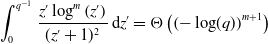 \begin{align} \int _0^{ q^{-1}}\frac{z^{\prime }\log ^m \left ( z^{\prime } \right )}{(z^{\prime }+1)^2} \, \mathrm{d}z^{\prime } = \Theta \left ( \left ({-}\log\!(q)\right )^{m+1}\right ) \end{align}
holds true by considering
 \begin{align*} \lim _{q \to 0^{+}}\int _{0}^{ q^{-1}} \frac{z^{\prime }\log ^m \left (z^{\prime }\right )}{(z^{\prime }+1)^2} \, \mathrm{d}z^{\prime } &= \int _{0}^{n} \frac{z^{\prime }\log ^m \left (z^{\prime }\right )}{(z^{\prime }+1)^2} \, \mathrm{d}z^{\prime } + \lim _{q \to 0^{+}}\int _{n}^{q^{-1}} \frac{z^{\prime }\log ^m \left (z^{\prime }\right )}{(z^{\prime }+1)^2} \, \mathrm{d}z^{\prime } \;, \end{align*}
with $n\gt 0$
. Whereas the first integral is finite for any finite
$n\gt 0$
. Whereas the first integral is finite for any finite $n\gt 0$
, we find that, in the limit
$n\gt 0$
, we find that, in the limit $z^{\prime }\to +\infty$
,
$z^{\prime }\to +\infty$
, $\frac{z^{\prime }\log ^m \left (z^{\prime } \right )}{(z^{\prime }+1)^2}$
behaves equivalently to
$\frac{z^{\prime }\log ^m \left (z^{\prime } \right )}{(z^{\prime }+1)^2}$
behaves equivalently to $\frac{\log ^m\left (z^{\prime }\right )}{z^{\prime }}$
since
$\frac{\log ^m\left (z^{\prime }\right )}{z^{\prime }}$
since
 \begin{align} \lim _{z^{\prime } \to \infty } \frac{(z^{\prime }+1)^{-2}z^{\prime }\log ^m \left (z^{\prime }\right )}{ z^{\prime -1} \log ^m \left ( z^{\prime } \right )} = 1 \quad . \end{align}
We then study the integral
 \begin{align*} &\int _{n}^{ q^{-1}} \frac{\log ^m \left ( z^{\prime } \right )}{z^{\prime }} \, \mathrm{d}z^{\prime } = \left [\frac{1}{m+1}\log ^{m+1}(z^{\prime })\right ]_n^{ q^{-1}} = \frac{1}{m+1}\log ^{m+1}( q^{-1})-\frac{1}{m+1}\log ^{m+1}(n)\;, \end{align*}
which concludes the proof.
Lastly, we note that
 \begin{align} \lim _{q \to 0^+} \frac{1}{\frac{1}{m+1}\log ^{m+1}( q^{-1})} \int _0^{ q^{-1}}\frac{z^{\prime }\log ^m \left ( z^{\prime } \right )}{(z^{\prime }+1)^2} \, \mathrm{d}z^{\prime } =1 \quad . \end{align}


 Open access