


1. Introduction
Atomisation simulations have progressed at an amazing rate, however, the topic is still far from mature. As we show in this paper, the prediction of the breakup of liquid masses in a typical large-speed flow is marred by vexing numerical effects and profound physical uncertainties. New developments, such as better codes, rapidly increasing processing power and new numerical methods are however poised to mitigate the difficulties. In this paper we investigate the pulsed jet, a paradigmatic case of atomising flow inspired by diesel engine jets, although we do not aim at solving a particular applied problem or even any experimental configuration, but rather to investigate the potential and limitations of direct numerical simulation (DNS) of an atomising flow, and in particular, the ability of such DNS to reveal physically relevant properties of the flow through statistically converged numerical approaches. The emphasis here is on statistical convergence, rather than ‘trajectory’ convergence, since only the former is conceivable in very complex, irregular flows.
The study of such convergence already has a long history, despite rapid progress. We review specifically the history of round-jet atomising simulations and we refer the reader to reviews on the general topic of atomisation and its simulation (Gorokhovski & Herrmann Reference Gorokhovski and Herrmann2008; Villermaux Reference Villermaux2020). The first attempts at testing the convergence of the probability distribution function (PDF) of droplet sizes were those of Herrmann (Reference Herrmann2011). His simulations of a round jet used a variant of the level-set method and showed that the number of small droplets in the PDF was underestimated by coarse-grid simulations. This can be understood by the fact the the level-set methods tend to eliminate small droplets by ‘evaporating’ them. On the other hand, volume-of-fluid (VOF) methods keep too many droplets in an intermediate range around the grid size $\varDelta$
, and in that range the PDF of droplet sizes is overestimated. This can be seen, for example, in a study of the convergence of the droplet-size distribution in the round jet by Pairetti et al. (Reference Pairetti, Damian, Nigro, Popinet and Zaleski2020) where coarse grids overestimate the number of large droplets.
$\varDelta$
, and in that range the PDF of droplet sizes is overestimated. This can be seen, for example, in a study of the convergence of the droplet-size distribution in the round jet by Pairetti et al. (Reference Pairetti, Damian, Nigro, Popinet and Zaleski2020) where coarse grids overestimate the number of large droplets.
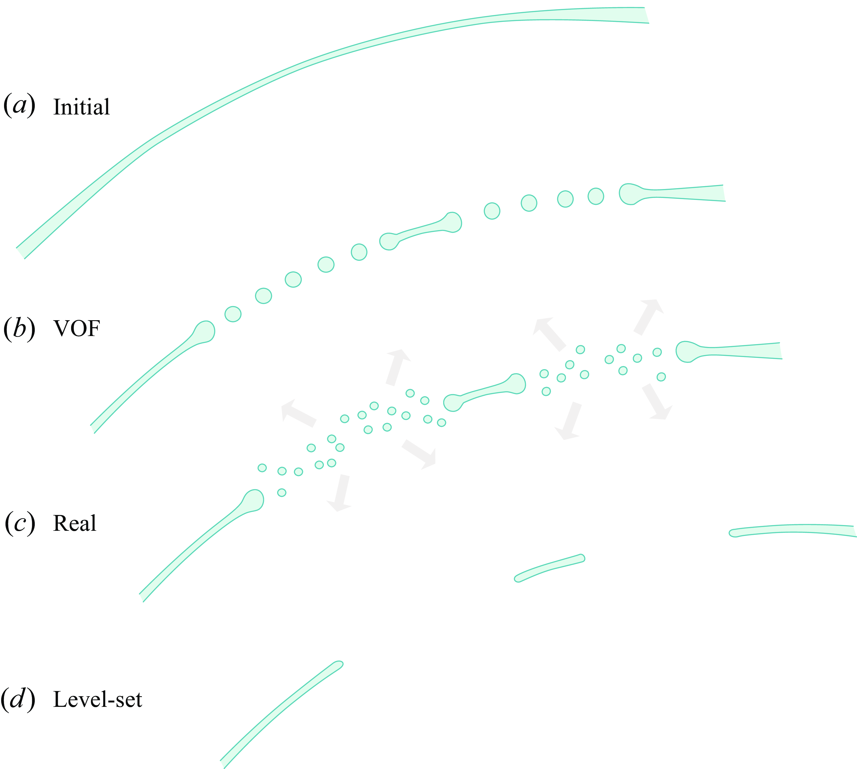
A graphical illustration of the contrasting effects of level-set and VOF methods on the droplet sizes in atomisation is shown on figure 1. Despite the inaccuracy of the distribution for small droplet diameters, both methods may converge as the grid is refined progressively. There is thus some hope that very large simulations will eventually produce converged distributions, a hope we want to explore in this paper.
An illustration of the outcomes for the numerical simulation of a thinning liquid sheet; panel (a) shows the initial configuration, before breakup. The other three images (b–d) show a schematic view of the outcome either in reality or in various types of numerical simulation. It is arbitrarily assumed that there are two breakup locations. Both the VOF and the level-set methods yield topology changes when the sheet thickness reaches the grid size. In (b) fragments larger than the grid size are obtained because of mass conservation in the VOF method. (c) In reality, the sheet thinning continues until much later than in the numerics, unless extremely fine grids are used. The final size of some of the droplets is then much smaller than in the VOF simulation. (d) The level-set or diffuse-interface methods on the other hand evaporate the thin parts of the sheet and loses much more mass.
The increase in two-phase round-jet grid resolution in time. The graph includes two simulations published only on the Gerris and Basilisk websites (and in other channels outside of academic journals) before 2017. The 2024 simulations are those reported in this paper.
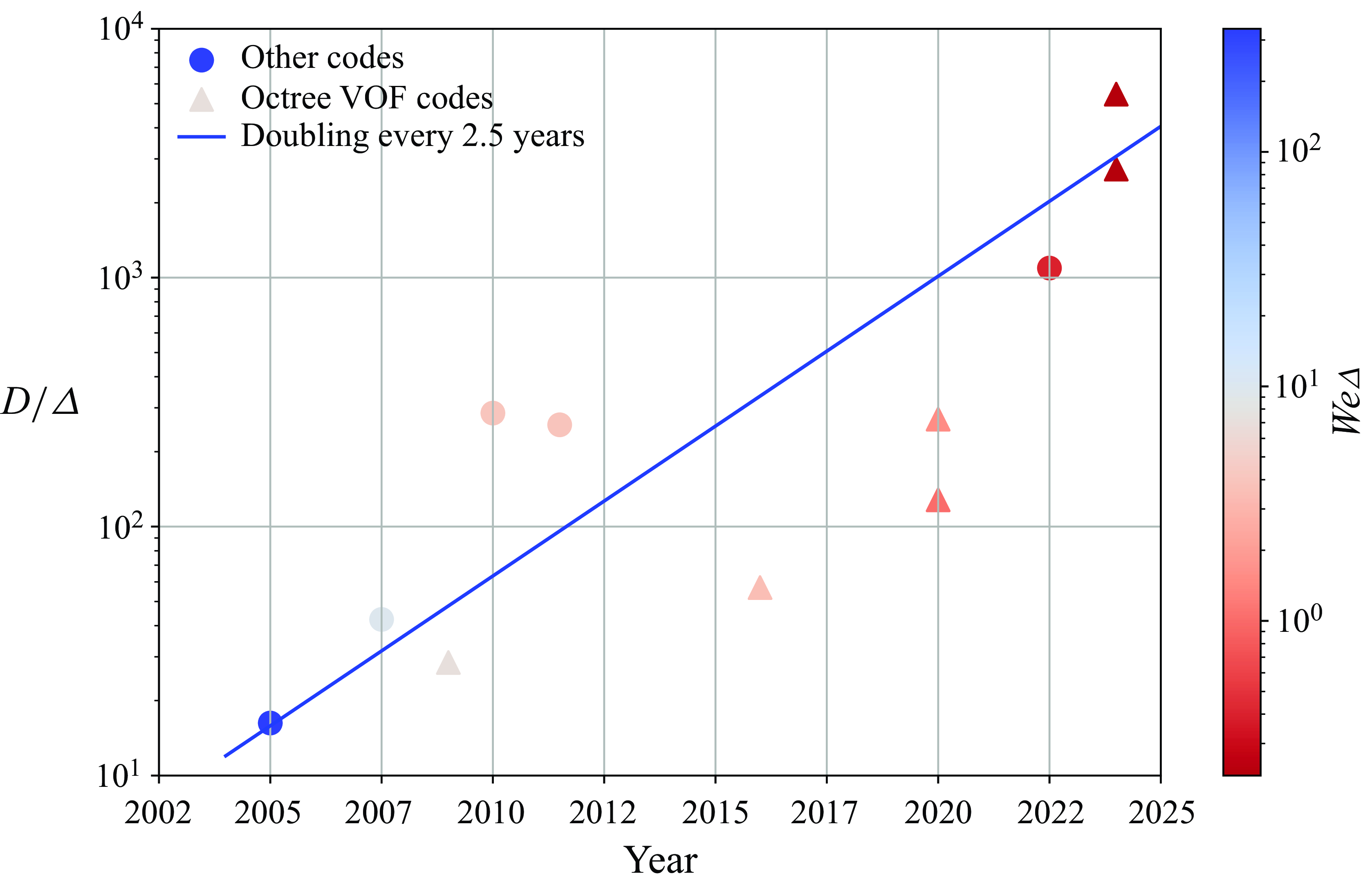
Aside from the two investigations cited above, very few studies address the issue of PDF convergence, despite detailed analyses of aspects of the flow. Perhaps the first round, single-jet atomisation simulation in the conditions of a diesel jet was that of Bianchi et al. (Reference Bianchi, Minelli, Scardovelli and Zaleski2007) using the VOF method, followed by more detailed simulations by Ménard et al. (Reference Ménard, Tanguy and Berlemont2007) using the combined level-set VOF method (CLSVOF). This was followed by other simulations using CLSVOF by Lebas et al. (Reference Lebas, Menard, Beau, Berlemont and Demoulin2009), Chesnel et al. (Reference Chesnel, Ménard, Réveillon and Demoulin2011) and Anez et al. (Reference Anez, Ahmed, Hecht, Duret, Reveillon and Demoulin2019) and by simulations using the VOF method (Fuster et al. Reference Fuster, Bagué, Boeck, Le Moyne, Leboissetier, Popinet, Ray, Scardovelli and Zaleski2009). The latter studied both the coaxial jet cases in the so-called ‘assisted atomisation’ set-up and the conical jet. For the conical jet, Fuster et al. (Reference Fuster, Bagué, Boeck, Le Moyne, Leboissetier, Popinet, Ray, Scardovelli and Zaleski2009) showed that the PDF changed drastically with grid resolution. The PDF never peaked as the droplet size was decreased towards the grid size. Until 2022, the most detailed (or highest-fidelity) published simulations of a round jet were performed by Shinjo & Umemura (Reference Shinjo and Umemura2010) using a combination of level-set and VOF techniques with a ratio of jet diameter to grid size of 286. These simulations, together with those of Herrmann (Reference Herrmann2011) are the two outliers above the trend line in figure 2. In addition to revealing a wealth of details about ligament and sheet formation, and the perforation of sheets, Shinjo & Umemura have also shown distributions of droplet sizes, but without investigating explicitly their convergence. As in earlier simulations of the round jet, the droplet-size distribution has a single maximum close to the small droplet end of the spectrum, almost at the grid size. Studies by Jarrahbashi & Sirignano (Reference Jarrahbashi and Sirignano2014) and Jarrahbashi et al. (Reference Jarrahbashi, Sirignano, Popov and Hussain2016) focused on a round, spatially periodic jet and analysed the effect of vortex dynamics on the development of instabilities along with the jet core. Studies by Zhang et al. (Reference Zhang, Popinet and Ling2020) and Pairetti et al. (Reference Pairetti, Damian, Nigro, Popinet and Zaleski2020) applied the VOF method with octree adaptive mesh refinement. As already mentioned, the latter paper investigated the distribution of droplet sizes showing some difficulties in reaching statistical convergence. Several authors including Torregrosa et al. (Reference Torregrosa, Payri, Salvador and Crialesi-Esposito2020) and Salvador et al. (Reference Salvador, Ruiz, Crialesi-Esposito and Blanquer2018) have focused on the effect of injection conditions and turbulence. Khanwale et al. (Reference Khanwale, Saurabh, Ishii, Sundar and Ganapathysubramanian2022) and Saurabh et al. (Reference Saurabh, Ishii, Khanwale, Sundar and Ganapathysubramanian2023), using a diffusive interface method with octree adaptive mesh refinement, obtained the most refined simulations published at the time of writing with a special treatment of the refinement in thin regions. It should be noted that all of the round-jet studies cited above involve a variety of physical parameters and grid resolutions, despite the fact that they share similarities, such as moderate density ratios and liquid Reynolds numbers (defined below) in a range $5000 \leqslant Re_l \leqslant 13\,400$
that are attainable by DNS for single-phase flow. For example, the two octree studies of Zhang et al. (Reference Zhang, Popinet and Ling2020) and Pairetti et al. (Reference Pairetti, Damian, Nigro, Popinet and Zaleski2020) have gas-based Weber numbers (defined below) of respectively 177 and 417. As a general rule, it is better to select relatively small density ratios, Reynolds and Weber numbers to increase the likelihood of reaching convergence in computation. In this work, we thus chose the parameters in the lower range of
$5000 \leqslant Re_l \leqslant 13\,400$
that are attainable by DNS for single-phase flow. For example, the two octree studies of Zhang et al. (Reference Zhang, Popinet and Ling2020) and Pairetti et al. (Reference Pairetti, Damian, Nigro, Popinet and Zaleski2020) have gas-based Weber numbers (defined below) of respectively 177 and 417. As a general rule, it is better to select relatively small density ratios, Reynolds and Weber numbers to increase the likelihood of reaching convergence in computation. In this work, we thus chose the parameters in the lower range of $Re$
,
$Re$
, $\textit{We}$
, as it correspondens to Weber number and density ratio for this type of flow. Similar attempts at obtaining convergence were realised in the simulations of Ling et al. (Reference Ling, Fuster, Zaleski and Tryggvason2017), investigating assisted quasi-planar atomisation after the experiment of Grenoble (Ben Rayana et al. Reference Ben Rayana, Cartellier and Hopfinger2006; Fuster et al. Reference Fuster, Matas, Marty, Popinet, Hoepffner, Cartellier and Zaleski2013). Ling et al. (Reference Ling, Fuster, Zaleski and Tryggvason2017) performed computations on four grids of increasing resolution. Despite the huge computational effort involved in that latter simulation, convergence was clearly not reached, both quantitatively as droplet-size distributions had a very narrow region of overlap, and qualitatively as clearly under-resolved structures in thin sheet-like regions were observed. One of our objectives in this work is to see what happens if ever finer grids are used, until very thin sheets are clearly resolved. In experiments as well as in some simulations it is clear that thin sheets are the site of weak spots (Lohse & Villermaux Reference Lohse and Villermaux2020). The presence of these weak spots as one of the mechanisms leading to atomisation forces the following somewhat sobering conclusion. Numerical simulations of diffuse-interface, level-set or VOF type can never be converged if thin sheets break or perforate only when they reach the grid size. Instead, a physical mechanism for weak spots or perforations must be present to nucleate holes in a manner independent of the numerics. Although such a mechanism may not be known yet, we suggest as a backstop procedure to define a critical sheet thickness
$\textit{We}$
, as it correspondens to Weber number and density ratio for this type of flow. Similar attempts at obtaining convergence were realised in the simulations of Ling et al. (Reference Ling, Fuster, Zaleski and Tryggvason2017), investigating assisted quasi-planar atomisation after the experiment of Grenoble (Ben Rayana et al. Reference Ben Rayana, Cartellier and Hopfinger2006; Fuster et al. Reference Fuster, Matas, Marty, Popinet, Hoepffner, Cartellier and Zaleski2013). Ling et al. (Reference Ling, Fuster, Zaleski and Tryggvason2017) performed computations on four grids of increasing resolution. Despite the huge computational effort involved in that latter simulation, convergence was clearly not reached, both quantitatively as droplet-size distributions had a very narrow region of overlap, and qualitatively as clearly under-resolved structures in thin sheet-like regions were observed. One of our objectives in this work is to see what happens if ever finer grids are used, until very thin sheets are clearly resolved. In experiments as well as in some simulations it is clear that thin sheets are the site of weak spots (Lohse & Villermaux Reference Lohse and Villermaux2020). The presence of these weak spots as one of the mechanisms leading to atomisation forces the following somewhat sobering conclusion. Numerical simulations of diffuse-interface, level-set or VOF type can never be converged if thin sheets break or perforate only when they reach the grid size. Instead, a physical mechanism for weak spots or perforations must be present to nucleate holes in a manner independent of the numerics. Although such a mechanism may not be known yet, we suggest as a backstop procedure to define a critical sheet thickness $h_c$
beyond which perforations occur with relatively high frequency, that is, at the rate of one or more perforations per connected thin sheet region. Chirco et al. (Reference Chirco, Maarek, Popinet and Zaleski2022) have called manifold death (MD) this procedure (this choice of words partially echoes that of Debrégeas et al. Reference Debrégeas, De Gennes and Brochard-Wyart1998). It should be noted that bags or membranes are observed at relatively low velocities in many atomisation configurations (droplets, jets etc.) and that at higher velocities, bags are not visible and perhaps non-existent. We note that the literature (Lasheras & Hopfinger Reference Lasheras and Hopfinger2000; Tolfts et al. Reference Tolfts, Deplus and Machicoane2023) distinguishes two kinds of atomisation, a bag or membrane-type atomisation at low Weber numbers and a fibre-type atomisation at high Weber numbers. The transition between the two behaviours was found by Reference Tolfts, Deplus and MachicoaneTolfts et al. (2023) to lie between
$h_c$
beyond which perforations occur with relatively high frequency, that is, at the rate of one or more perforations per connected thin sheet region. Chirco et al. (Reference Chirco, Maarek, Popinet and Zaleski2022) have called manifold death (MD) this procedure (this choice of words partially echoes that of Debrégeas et al. Reference Debrégeas, De Gennes and Brochard-Wyart1998). It should be noted that bags or membranes are observed at relatively low velocities in many atomisation configurations (droplets, jets etc.) and that at higher velocities, bags are not visible and perhaps non-existent. We note that the literature (Lasheras & Hopfinger Reference Lasheras and Hopfinger2000; Tolfts et al. Reference Tolfts, Deplus and Machicoane2023) distinguishes two kinds of atomisation, a bag or membrane-type atomisation at low Weber numbers and a fibre-type atomisation at high Weber numbers. The transition between the two behaviours was found by Reference Tolfts, Deplus and MachicoaneTolfts et al. (2023) to lie between $\textit{We}_g=70$
and
$\textit{We}_g=70$
and $\textit{We}_g=400$
. From the connection between thin sheets and the lack of statistical convergence one may conjecture that in the fibre-type regime statistical convergence could be achieved. This is however contradicted by the lack of convergence observed by Herrmann (Reference Herrmann2011) at
$\textit{We}_g=400$
. From the connection between thin sheets and the lack of statistical convergence one may conjecture that in the fibre-type regime statistical convergence could be achieved. This is however contradicted by the lack of convergence observed by Herrmann (Reference Herrmann2011) at $\textit{We}_g = 500$
. A definite answer to this argument may have to wait for a study similar to the one in this paper in the fibre-type regime, a study which would probably be even more expensive.
$\textit{We}_g = 500$
. A definite answer to this argument may have to wait for a study similar to the one in this paper in the fibre-type regime, a study which would probably be even more expensive.
In what follows we first describe the characteristics of our test case. We then describe our numerical method, including the MD procedure. Then we continue with our results that are both qualitative and quantitative. Qualitatively our results reveal new processes of numerical rupture. Quantitatively they allow an analysis of the droplet-size distributions or PDF. A discussion of the phenomenology of hole expansion in a thin sheet is given in Appendix A. We end with a conclusion including perspectives and discussion.
2. Mathematical model and numerical method
Our mathematical model is based on the mass and momentum conservation equations for incompressible and isothermal flow, i.e.
 \begin{equation} \nabla \cdot \textbf { u} = 0, \end{equation}
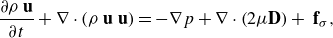 \begin{equation} \frac {\partial \rho \textbf { u}}{\partial t} + \nabla \cdot (\rho \textbf { u}\textbf { u}) = - \nabla p + \nabla \cdot \left (2\mu \mathbf {D}\right ) + \textbf { f}_\sigma , \end{equation}
where $\textbf { u}(\textbf { x},t)$
is the velocity field and
$\textbf { u}(\textbf { x},t)$
is the velocity field and $p(\textbf { x},t)$
is the pressure field. The tensor
$p(\textbf { x},t)$
is the pressure field. The tensor $\mathbf {D}$
is defined as
$\mathbf {D}$
is defined as $ ({1}/{2}) [\nabla \textbf { u} + (\nabla \textbf { u} )^T ]$
. The density and viscosity of the flow are noted as
$ ({1}/{2}) [\nabla \textbf { u} + (\nabla \textbf { u} )^T ]$
. The density and viscosity of the flow are noted as $\rho$
and
$\rho$
and $\mu$
, respectively. The last term on the right-hand side of the Navier–Stokes equation (2.2) represents the surface tension force
$\mu$
, respectively. The last term on the right-hand side of the Navier–Stokes equation (2.2) represents the surface tension force
 \begin{equation} \textbf { f}_\sigma = \sigma \kappa \textbf { n} \delta _s, \end{equation}
which depends on the surface tension $\sigma$
and the interface shape, particularly on its curvature
$\sigma$
and the interface shape, particularly on its curvature $\kappa$
and unit normal vector
$\kappa$
and unit normal vector $\textbf { n}$
. The Dirac distribution
$\textbf { n}$
. The Dirac distribution $\delta _s$
indicates that the force only acts at the free surface. We consider the phase distribution function
$\delta _s$
indicates that the force only acts at the free surface. We consider the phase distribution function $c(\textbf{x},t)$
that takes value unity in the reference phase and null outside of it. The transport equation for this function is
$c(\textbf{x},t)$
that takes value unity in the reference phase and null outside of it. The transport equation for this function is
 \begin{equation} \frac {\partial c}{\partial t} + \nabla \cdot (c\textbf { u})= c\,\nabla \cdot \textbf { u}. \end{equation}
In the context of incompressible flow, the right-hand side above is equal to zero. The $c$
function implicitly defines the interface at its discontinuity surface, defining also the
$c$
function implicitly defines the interface at its discontinuity surface, defining also the $\delta _s$
,
$\delta _s$
, $\textbf { n}$
and
$\textbf { n}$
and $\kappa$
fields, e.g.
$\kappa$
fields, e.g. $\nabla c = \textbf { n} \delta _s$
.
$\nabla c = \textbf { n} \delta _s$
.
The VOF method represents the evolution of $c$
using the piecewise linear interface capturing method of Hirt & Nichols (Reference Hirt and Nichols1981) and DeBar (Reference DeBar1974). In this context, the mean value of the colour function on a cell is
$c$
using the piecewise linear interface capturing method of Hirt & Nichols (Reference Hirt and Nichols1981) and DeBar (Reference DeBar1974). In this context, the mean value of the colour function on a cell is
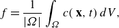 \begin{equation} f = \frac {1}{| \Omega | }\int _\Omega c(\textbf { x},t)\,{\rm d}V, \end{equation}
where $| \Omega |$
is the volume of the cell
$| \Omega |$
is the volume of the cell $\Omega$
. Then
$\Omega$
. Then $f$
is the volume fraction of the reference phase in the cell. The mixture properties of the cell may then be computed by arithmetic averages
$f$
is the volume fraction of the reference phase in the cell. The mixture properties of the cell may then be computed by arithmetic averages
 \begin{equation} \rho _\Omega = f \rho _l + (1 - f)\rho _g, \qquad \mu _\Omega = f\mu _l + (1 - f)\mu _g. \end{equation}
Spatial discretisation of the above equation is realised on a network of cubic cells obtained by a tree-like subdivision of an initial cubic cell of size $L_0$
. The subdivision is realised using a wavelet-based error estimate and is adapted dynamically as the simulation progresses. At all times the maximum subdivision level is a fixed number
$L_0$
. The subdivision is realised using a wavelet-based error estimate and is adapted dynamically as the simulation progresses. At all times the maximum subdivision level is a fixed number $\ell$
and the smallest grid size is
$\ell$
and the smallest grid size is
 \begin{equation} \varDelta _\ell = 2^{-\ell } {L_0}. \end{equation}
From now on, we consider the algebraic equations derived from applying the finite volume method on each cell. In this context, the approximate projection method by Chorin (Reference Chorin1968) can be used to solve the coupling between (2.1) and (2.2), considering that the velocity $\textbf { u}$
is staggered in time with respect to the volume fraction
$\textbf { u}$
is staggered in time with respect to the volume fraction $f$
and the pressure
$f$
and the pressure $p$
. The discrete set of equations can then be expressed as
$p$
. The discrete set of equations can then be expressed as
 \begin{equation} \frac {\rho \textbf { u}^{*} - \rho \textbf { u}^{n}}{\Delta t} + \nabla \cdot \left (\rho ^{n + \frac {1}{2}}\,\textbf { u}^{n+1/2}\textbf { u}^{n+1/2}\right ) = \nabla \cdot [\mu ^{n + \frac {1}{2}}(\mathbf {D}^n + \mathbf {D}^*)] + \textbf { f}_{\sigma }^{n+1/2}, \end{equation}
 \begin{equation} \nabla \cdot \left (\frac {\Delta t}{\rho ^{n+\frac {1}{2}}} \nabla p^{n + \frac {1}{2}}\right ) = \nabla \cdot \textbf { u}^*, \end{equation}
 \begin{equation} \textbf { u}^{n+1} = \textbf { u}^* - \frac {\Delta t}{\rho ^{n+\frac {1}{2}}} \nabla p^{n + \frac {1}{2}}. \end{equation}
In the above the expression, $\nabla \cdot (\rho ^{n + \frac {1}{2}}\,\textbf { u}^{n+1/2}\textbf { u}^{n+1/2} )$
must be interpreted as the use of a predictor–corrector scheme for advection of the velocity field. Both the predictor and the corrector use the Bell–Collela–Glaz scheme (Popinet Reference Popinet2003, Reference Popinet2009), and involve two projections. A full description of the predictor corrector scheme with projection is best found in the `literate’ source code at http://basilisk.fr/src/navier-stokes/centered.h. In addition to these equations,
$\nabla \cdot (\rho ^{n + \frac {1}{2}}\,\textbf { u}^{n+1/2}\textbf { u}^{n+1/2} )$
must be interpreted as the use of a predictor–corrector scheme for advection of the velocity field. Both the predictor and the corrector use the Bell–Collela–Glaz scheme (Popinet Reference Popinet2003, Reference Popinet2009), and involve two projections. A full description of the predictor corrector scheme with projection is best found in the `literate’ source code at http://basilisk.fr/src/navier-stokes/centered.h. In addition to these equations, $f$
is advanced in time using the split-volume-fraction advection scheme of Weymouth & Yue (Reference Weymouth and Yue2010). We use the semi-implicit Crank–Nicholson time stepping to compute the diffusive flux due to the viscous term in (2.8). An important aspect of the method is the numerical approximation of the surface tension force
$f$
is advanced in time using the split-volume-fraction advection scheme of Weymouth & Yue (Reference Weymouth and Yue2010). We use the semi-implicit Crank–Nicholson time stepping to compute the diffusive flux due to the viscous term in (2.8). An important aspect of the method is the numerical approximation of the surface tension force $\textbf { f}_{\sigma }$
. We use the continuous surface force well-balanced formulation
$\textbf { f}_{\sigma }$
. We use the continuous surface force well-balanced formulation $\textbf { f}_{\sigma } = \sigma \kappa \nabla c$
for (2.3), where we discretise
$\textbf { f}_{\sigma } = \sigma \kappa \nabla c$
for (2.3), where we discretise $\nabla c$
at cell faces with the same scheme employed to compute the pressure gradient
$\nabla c$
at cell faces with the same scheme employed to compute the pressure gradient $\nabla p$
. This is useful to reduce spurious currents provided curvature is accurately computed, as explained by Popinet (Reference Popinet2009, Reference Popinet2018). The interface curvature is computed using a complex method described in Popinet (Reference Popinet2009). When the grid resolution is sufficient, second-order stencils based on height functions are used to compute curvature. In some large-curvature cases the height functions are not defined and fits by quadratic functions are used instead. Equations (2.9) and (2.10) are the projection steps that will ensure continuity for the velocity field at time step
$\nabla p$
. This is useful to reduce spurious currents provided curvature is accurately computed, as explained by Popinet (Reference Popinet2009, Reference Popinet2018). The interface curvature is computed using a complex method described in Popinet (Reference Popinet2009). When the grid resolution is sufficient, second-order stencils based on height functions are used to compute curvature. In some large-curvature cases the height functions are not defined and fits by quadratic functions are used instead. Equations (2.9) and (2.10) are the projection steps that will ensure continuity for the velocity field at time step $n + 1$
. The mesh is adapted dynamically, by splitting the grid cells to eight smaller cells whenever the estimated local discretisation error exceeds a set threshold (see Appendix B). Details of the procedure can be found on the web site basilisk.fr and, in particular, in the documented free code available at http://basilisk.fr/src/examples/atomisation.c.
$n + 1$
. The mesh is adapted dynamically, by splitting the grid cells to eight smaller cells whenever the estimated local discretisation error exceeds a set threshold (see Appendix B). Details of the procedure can be found on the web site basilisk.fr and, in particular, in the documented free code available at http://basilisk.fr/src/examples/atomisation.c.
In all the data reported in this paper, the velocities are expressed in multiples of the jet velocity $U$
. All the numerical values for time are made dimensionless by
$U$
. All the numerical values for time are made dimensionless by $\tau _0 = L_0/(3 U)$
and all the reported lengths are made dimensionless by
$\tau _0 = L_0/(3 U)$
and all the reported lengths are made dimensionless by $L_0/3$
. However in the theoretical discussions the dimensional values are used unless otherwise indicated. To avoid confusion, we note with a
$L_0/3$
. However in the theoretical discussions the dimensional values are used unless otherwise indicated. To avoid confusion, we note with a $^*$
exponent the dimensionless values, so that
$^*$
exponent the dimensionless values, so that
 \begin{equation} t^* = t/\tau _0 \qquad x^* = 3 x / L_0 \qquad \varDelta ^* = 3 (2^{-\ell }). \end{equation}
In addition to the aforementioned model and procedure, we implement the MD procedure as described by Chirco et al. (Reference Chirco, Maarek, Popinet and Zaleski2022). This procedure involves the following two primary steps. (i) The identification of thin liquid sheets with a thickness of $h_c$
or less, achieved through a local integration of the characteristic function
$h_c$
or less, achieved through a local integration of the characteristic function $c$
. This integration results in the calculation of the signature of a quadratic form, based on the local main inertia moments. (ii) The creation of holes within the so identified thin sheets, using a probabilistic approach. This procedure is applied at a given frequency, defined by the user within this method. From a physical standpoint, this technique aligns with the weak spot model, wherein the likelihood of hole formation is exceedingly low for
$c$
. This integration results in the calculation of the signature of a quadratic form, based on the local main inertia moments. (ii) The creation of holes within the so identified thin sheets, using a probabilistic approach. This procedure is applied at a given frequency, defined by the user within this method. From a physical standpoint, this technique aligns with the weak spot model, wherein the likelihood of hole formation is exceedingly low for $h \gt h_c$
and substantially increases, rapidly approaching certainty, for
$h \gt h_c$
and substantially increases, rapidly approaching certainty, for $h \lt h_c$
. Note that this procedure distinguishes thin sheets from other shapes such as ligaments, only the thin sheets are detected and perforated. The specific implementation of the MD method we used is called the signature method. The complete MD code with the signature method can be accessed at http://basilisk.fr/sandbox/lchirco/signature.h. In the present case, hole punching is attempted every time interval of
$h \lt h_c$
. Note that this procedure distinguishes thin sheets from other shapes such as ligaments, only the thin sheets are detected and perforated. The specific implementation of the MD method we used is called the signature method. The complete MD code with the signature method can be accessed at http://basilisk.fr/sandbox/lchirco/signature.h. In the present case, hole punching is attempted every time interval of $\tau _m=0.01 \tau _0$
, that is, the raw dimensionless breakup frequency is
$\tau _m=0.01 \tau _0$
, that is, the raw dimensionless breakup frequency is $\tilde f_b^* = \tau _0/\tau _m = 100$
. At these instants
$\tilde f_b^* = \tau _0/\tau _m = 100$
. At these instants $N_b=200$
holes are attempted. We loosely term the pair of parameters
$N_b=200$
holes are attempted. We loosely term the pair of parameters $(\tilde f_b^* ,N_b)$
the breakup frequency. The breakup frequency chosen in this study is probably too high, as will appear in the discussion below. However, it is chosen to maintain the same parameters as in other studies, and possible improvements are discussed in the conclusion section. As we show in Appendix A, the characteristic time for sheet thinning is
$(\tilde f_b^* ,N_b)$
the breakup frequency. The breakup frequency chosen in this study is probably too high, as will appear in the discussion below. However, it is chosen to maintain the same parameters as in other studies, and possible improvements are discussed in the conclusion section. As we show in Appendix A, the characteristic time for sheet thinning is $\tau _c$
given by
$\tau _c$
given by
 \begin{equation} \tau _c = \frac D U \left ( \frac {\rho _l }{\rho _g} \right )^{1/2}, \end{equation}
where $D$
is the jet diameter. From the definition of these quantities, we can obtain the breakup attempt frequency in units of the sheet thinning characteristic time
$D$
is the jet diameter. From the definition of these quantities, we can obtain the breakup attempt frequency in units of the sheet thinning characteristic time $f_b = \tau _c/\tau _m$
, i.e.
$f_b = \tau _c/\tau _m$
, i.e.
 \begin{equation} f_b = \frac {3 \tilde f_b^* D}{L_0} \left ( \frac {\rho _l }{\rho _g} \right )^{1/2} , \end{equation}
that is, with the parameters of our simulation
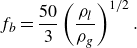 \begin{equation} f_b = \frac {50}{3} \left ( \frac {\rho _l }{\rho _g} \right )^{1/2} . \end{equation}
The numerical value is $f_b \simeq 87.9$
, ensuring that punching attempts are sufficiently frequent as not to `miss’ transient thinning sheets. It is large enough to eliminate numerical breakup events but is likely to be too high as discussed below.
$f_b \simeq 87.9$
, ensuring that punching attempts are sufficiently frequent as not to `miss’ transient thinning sheets. It is large enough to eliminate numerical breakup events but is likely to be too high as discussed below.
Using this numerical method, we analyse the atomisation of a circular jet injected at average velocity $U$
in a gas-filled cubical chamber of edge length
$U$
in a gas-filled cubical chamber of edge length $L_0$
. We consider incompressible, isothermal flow. The dimensionless groups most relevant for this problem are the gas-based Weber number, the liquid-based Reynolds number and the ratios
$L_0$
. We consider incompressible, isothermal flow. The dimensionless groups most relevant for this problem are the gas-based Weber number, the liquid-based Reynolds number and the ratios
 \begin{equation} We_g = \frac {\rho _g U^2 D}{\sigma }, \qquad {Re}_l = \frac {\rho _l U D}{\mu _l}, \qquad \rho ^* = \frac {\rho _l}{\rho _g}, \qquad \mu ^* = \frac {\mu _l}{\mu _g}, \qquad \frac {L_0}D, \end{equation}
where $\rho _l$
and
$\rho _l$
and $\rho _g$
are the densities of liquid and gas, respectively. The viscosity coefficients are noted by
$\rho _g$
are the densities of liquid and gas, respectively. The viscosity coefficients are noted by $\mu _l$
and
$\mu _l$
and $\mu _g$
, and
$\mu _g$
, and $\sigma$
is the surface tension coefficient. The boundary condition on the injection plane
$\sigma$
is the surface tension coefficient. The boundary condition on the injection plane $x = 0$
imposes the no-slip condition everywhere except on the liquid section (
$x = 0$
imposes the no-slip condition everywhere except on the liquid section ( ${y^2 + z^2} \lt D^2 / 4$
), where the injection velocity is
${y^2 + z^2} \lt D^2 / 4$
), where the injection velocity is
 \begin{equation} u_x(t) = U\,\left [ 1 + A_p\sin \left (\omega _{p} U t/D \right )\right ]. \end{equation}
On the remaining cube sides, we allow free outflow: $\partial _n \textbf { u}_\Gamma = 0$
and
$\partial _n \textbf { u}_\Gamma = 0$
and $p_\Gamma = 0$
.
$p_\Gamma = 0$
.
The dimensionless parameters of our simulation are given in table 1. These numbers are in the low range of the dimensionless numbers used in the above cited work. They are much smaller than the numbers of the spray G case of the engine combustion network (see Duke et al. Reference Duke2017) used by Zhang et al. (Reference Zhang, Popinet and Ling2020). The Reynolds number and density ratio are identical to those of Ménard et al. (Reference Ménard, Tanguy and Berlemont2007) and of the same order as those of Herrmann (Reference Herrmann2011). The equality of the gas and liquid Reynolds numbers stems from the fact that the viscosity and density ratios are equal, so the ratio of kinematic viscosities is one. However, while the moderate density ratio is realistic in the context of diesel jets, the viscosity ratio is not and would be much larger in a realistic set-up, which would lead to much larger values of ${Re}_g$
that are expensive to resolve by DNS. This motivates the choice of viscosity ratio. We note that the same choice of equal viscosity and density ratios and moderate
${Re}_g$
that are expensive to resolve by DNS. This motivates the choice of viscosity ratio. We note that the same choice of equal viscosity and density ratios and moderate $\textit{We}_g$
was made by Ling et al. (Reference Ling, Fuster, Zaleski and Tryggvason2017) who also studied atomisation and PDF convergence in a simplified set-up. The Reynolds number is somewhat larger than that of Shinjo & Umemura (Reference Shinjo and Umemura2010) while the gas Weber number
$\textit{We}_g$
was made by Ling et al. (Reference Ling, Fuster, Zaleski and Tryggvason2017) who also studied atomisation and PDF convergence in a simplified set-up. The Reynolds number is somewhat larger than that of Shinjo & Umemura (Reference Shinjo and Umemura2010) while the gas Weber number $\textit{We}_g$
is smaller than that of all the other papers in the literature. The rationale for selecting such a small Weber number is twofold. First the simplest prediction for the droplet size, based on the ratio of Bernoulli pressure
$\textit{We}_g$
is smaller than that of all the other papers in the literature. The rationale for selecting such a small Weber number is twofold. First the simplest prediction for the droplet size, based on the ratio of Bernoulli pressure $\rho _g U^2$
to surface tension, is
$\rho _g U^2$
to surface tension, is $d = D We_g^{-1}$
. Indeed if a purely inviscid flow with a velocity jump is considered, the cutoff wavelength for the Kelvin–Helmholtz instability scales as
$d = D We_g^{-1}$
. Indeed if a purely inviscid flow with a velocity jump is considered, the cutoff wavelength for the Kelvin–Helmholtz instability scales as $D We_g^{-1}$
. The wavelength thus obtained is a natural scale for the subsequent formation of sheets and ligaments. The number of grid points in the diameter of a droplet of this diameter
$D We_g^{-1}$
. The wavelength thus obtained is a natural scale for the subsequent formation of sheets and ligaments. The number of grid points in the diameter of a droplet of this diameter $d$
is then
$d$
is then $\textit{We}_\varDelta ^{-1}$
, where
$\textit{We}_\varDelta ^{-1}$
, where
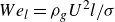 \begin{equation} \ {We}_l = {\rho _g U^2 l }/{\sigma } \end{equation}
is the Weber number based on length scale $l$
and
$l$
and $\varDelta$
is the grid size. Similarly,
$\varDelta$
is the grid size. Similarly,
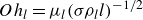 \begin{equation} \ {Oh}_l = \mu _l (\sigma \rho _l l)^{-1/2} \end{equation}
is the Ohnesorge number based on scale $l$
. The values of
$l$
. The values of $\textit{We}_\varDelta$
for two of the grids we use are given in table 2. We also give the value of the Ohnesorge numbers
$\textit{We}_\varDelta$
for two of the grids we use are given in table 2. We also give the value of the Ohnesorge numbers ${Oh}_{\varDelta }$
and
${Oh}_{\varDelta }$
and ${Oh}_{h_c}$
, which characterise the interplay of viscous and surface tension effects. In particular, they typify the regime of the Taylor–Culick rims (Song & Tryggvason Reference Song and Tryggvason1999; Savva & Bush Reference Savva and Bush2009) occurring at the edge of a sheet of thickness
${Oh}_{h_c}$
, which characterise the interplay of viscous and surface tension effects. In particular, they typify the regime of the Taylor–Culick rims (Song & Tryggvason Reference Song and Tryggvason1999; Savva & Bush Reference Savva and Bush2009) occurring at the edge of a sheet of thickness $\varDelta$
or
$\varDelta$
or $h_c$
. The
$h_c$
. The $Oh$
number of the thin sheets at the moment of hole formation is relatively large, implying a viscous Taylor–Culick flow and the absence of unsteady fragmentation as in Wang & Bourouiba (Reference Wang and Bourouiba2018) and Kant et al. (Reference Kant, Pairetti, Saade, Popinet, Zaleski and Lohse2023).
$Oh$
number of the thin sheets at the moment of hole formation is relatively large, implying a viscous Taylor–Culick flow and the absence of unsteady fragmentation as in Wang & Bourouiba (Reference Wang and Bourouiba2018) and Kant et al. (Reference Kant, Pairetti, Saade, Popinet, Zaleski and Lohse2023).
The dimensionless numbers characterising our simulation. The Reynolds number ${Re}_l$
based on the liquid is rather moderate. The density and viscosity ratios are identical, which implies that
${Re}_l$
based on the liquid is rather moderate. The density and viscosity ratios are identical, which implies that ${Re}_g = \ {Re}_l$
.
${Re}_g = \ {Re}_l$
.
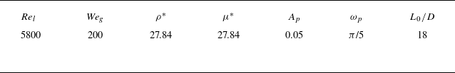
Characteristic numbers related to the grid size. The level $\ell$
is defined in (2.7).
$\ell$
is defined in (2.7).

Characteristic numbers based on the critical sheet thickness in our simulations. The MD level $m$
is defined in the text.
$m$
is defined in the text.

The second important consequence of selecting the relatively small value $\textit{We}_g =200$
is that it makes the simulation sit on the boundary between membrane type and fibre type defined in Lasheras & Hopfinger (Reference Lasheras and Hopfinger2000). Membrane type in that later paper refers to the formation of bags and sheets. Thus, the prevalence of thin sheets discussed in this paper may be less marked at higher Weber numbers, the sheets being replaced by fibres, and also less important at smaller Weber numbers where the flow may be less unstable.
$\textit{We}_g =200$
is that it makes the simulation sit on the boundary between membrane type and fibre type defined in Lasheras & Hopfinger (Reference Lasheras and Hopfinger2000). Membrane type in that later paper refers to the formation of bags and sheets. Thus, the prevalence of thin sheets discussed in this paper may be less marked at higher Weber numbers, the sheets being replaced by fibres, and also less important at smaller Weber numbers where the flow may be less unstable.
3. Results
3.1. Uncontrolled perforation: numerical sheet breakup
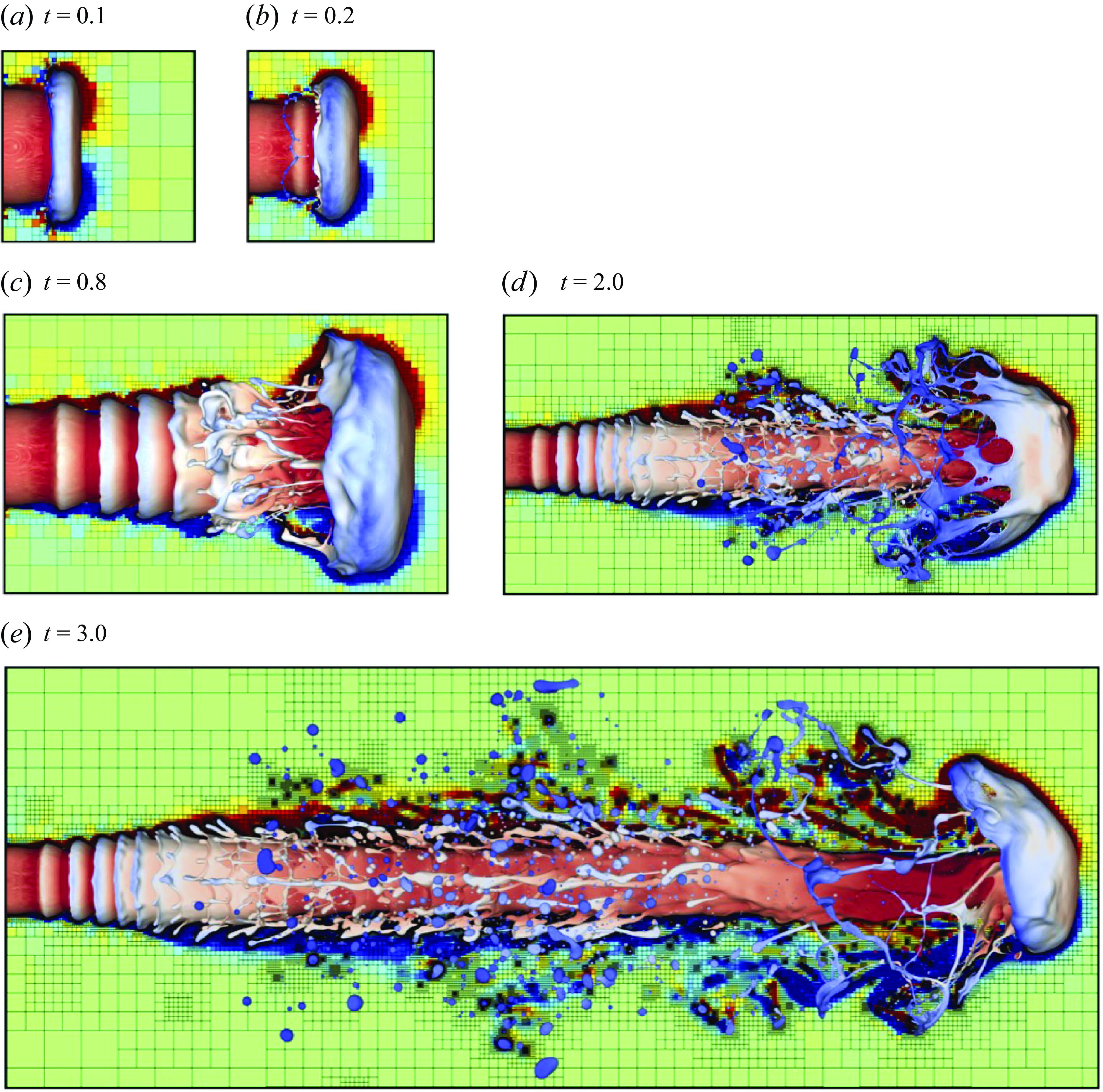
Figure 3 shows a global view of the jet evolution (see also supplementary movies 1–6 available at https://doi.org/10.1017/jfm.2025.218). The dynamics is initialised with a slightly penetrated jet at $t=0$
. At
$t=0$
. At $t=0.1$
, a mushroom-like structure starts rolling up. The annular structure stretches and extends in the form of a `corona flap’ that develops behind the mushroom head. A rim forms at the edge of this flap then detaches. It is visible at
$t=0.1$
, a mushroom-like structure starts rolling up. The annular structure stretches and extends in the form of a `corona flap’ that develops behind the mushroom head. A rim forms at the edge of this flap then detaches. It is visible at $t=0.2$
as a corrugated and partially fragmented annular ligament. As the jet evolves, pulsation results in a periodic series of corona flaps seen at
$t=0.2$
as a corrugated and partially fragmented annular ligament. As the jet evolves, pulsation results in a periodic series of corona flaps seen at $t=0.8$
. These flaps interact with the ligaments coming from the mushroom head. At
$t=0.8$
. These flaps interact with the ligaments coming from the mushroom head. At $t=2$
, the jet has evolved further and we can identify an interval in the core structure where the effect of pulsation is lost. Several mechanisms of droplet formation like sheet rupture, ligament breakup and their interactions with the jet core and corona flaps are seen. At
$t=2$
, the jet has evolved further and we can identify an interval in the core structure where the effect of pulsation is lost. Several mechanisms of droplet formation like sheet rupture, ligament breakup and their interactions with the jet core and corona flaps are seen. At $t=3$
, the jet is fully developed and we see long axial ligaments with a marked velocity gradient made visible by the colour change along the axis, circular ligaments, corona fingers merging and sheet rupture. A large number of droplets and ligaments are produced in the mushroom tip region. Most of the phenomena illustrated above are also observed with controlled perforation, except the initiation of sheet rupture and annular ligament detachment.
$t=3$
, the jet is fully developed and we see long axial ligaments with a marked velocity gradient made visible by the colour change along the axis, circular ligaments, corona fingers merging and sheet rupture. A large number of droplets and ligaments are produced in the mushroom tip region. Most of the phenomena illustrated above are also observed with controlled perforation, except the initiation of sheet rupture and annular ligament detachment.
The advancing pulsed jet at various time instants $t$
and level
$t$
and level $\ell =14$
. The fluid interface is coloured by the axial velocity and the background is coloured by the vorticity. The background also shows the mesh refinement. (a) The pulsed jet develops a mushroom head and a rim. In (b) the rim detaches. (c) Development of flaps coming from the sinusoidal pulsation. (d) A jet entering in a regime where the effect of pulsation is lost at the mushroom head. (e) A fully developed jet and a rich spectrum of droplets and ligaments. Since
$\ell =14$
. The fluid interface is coloured by the axial velocity and the background is coloured by the vorticity. The background also shows the mesh refinement. (a) The pulsed jet develops a mushroom head and a rim. In (b) the rim detaches. (c) Development of flaps coming from the sinusoidal pulsation. (d) A jet entering in a regime where the effect of pulsation is lost at the mushroom head. (e) A fully developed jet and a rich spectrum of droplets and ligaments. Since $Re_g$
is rather low at
$Re_g$
is rather low at $5800$
, there is relatively little vorticity away from the interface unlike in the case of Kant et al. (Reference Kant, Pairetti, Saade, Popinet, Zaleski and Lohse2023).
$5800$
, there is relatively little vorticity away from the interface unlike in the case of Kant et al. (Reference Kant, Pairetti, Saade, Popinet, Zaleski and Lohse2023).
View from the inlet at time $t=3.04$
showing the inner region of the central core liquid jet. Plot (a) is coloured by the curvature showing the encapsulation of gas bubbles identified by the negative curvature (blue) in the liquid core encircled in the black circle. The droplets have positive curvature (red). The entrained bubbles travel with the core jet velocity and could also result in the formation of a few compound droplets during atomisation or provide a physical breakup mechanism for thin sheets. Plot (b) is the same as (a) but coloured by the axial velocity. The simulation corresponds to level
$t=3.04$
showing the inner region of the central core liquid jet. Plot (a) is coloured by the curvature showing the encapsulation of gas bubbles identified by the negative curvature (blue) in the liquid core encircled in the black circle. The droplets have positive curvature (red). The entrained bubbles travel with the core jet velocity and could also result in the formation of a few compound droplets during atomisation or provide a physical breakup mechanism for thin sheets. Plot (b) is the same as (a) but coloured by the axial velocity. The simulation corresponds to level $\ell =14$
with the MD method applied at level
$\ell =14$
with the MD method applied at level $m=13$
.
$m=13$
.

Figure 4 shows a contrasting view of the jet with the camera direction aligned with the jet axis and the view positioned at the inlet. A full evolution of the jet, as seen from the inlet, is available in supplementary movie 6. In figure 4(a) the objects are coloured by curvature, so small droplets are red and small bubbles, with negative curvature, are blue. The bubbles have been trapped in the bulk or core of the jet or inside other liquid masses. The likely mechanism for the formation of a bubble is liquid mass collision, for example, droplets and wavelets of fluid mass impacting on the jet core. Many such droplet or ligament impacts are seen in supplementary movie 1. A surprising aspect of the display is the relatively large number of droplets and bubbles seen. In figure 4(b) the objects are coloured by axial velocity, as with supplementary movies 1 and 3. A further interesting aspect of this view is to show the large dispersion in the axial velocities of the droplets.
At this point in the exposition it may be useful to define the number distribution and the PDF and to recall the connection between the two. We consider a fixed instant of time $t_0$
. We partition the interval of droplet sizes
$t_0$
. We partition the interval of droplet sizes $(0,d_M)$
into a discrete set of
$(0,d_M)$
into a discrete set of $M$
intervals
$M$
intervals $[d_i, d_{i+1} = d_i + \delta _i]$
. The index
$[d_i, d_{i+1} = d_i + \delta _i]$
. The index $i$
varies from 0 to
$i$
varies from 0 to $i_m$
. The intervals are geometrically distributed, with
$i_m$
. The intervals are geometrically distributed, with $d_{i+1} = 1.047 d_i$
, so
$d_{i+1} = 1.047 d_i$
, so $\log(d_i)$
is evenly distributed in log space. The number of droplets with diameter in the interval
$\log(d_i)$
is evenly distributed in log space. The number of droplets with diameter in the interval $[d_i, d_i + \delta _i]$
is
$[d_i, d_i + \delta _i]$
is $n_{d,i} \delta _i$
. The PDF
$n_{d,i} \delta _i$
. The PDF $p(d)$
is proportional to the expected value
$p(d)$
is proportional to the expected value $\langle n_{d,i} \rangle$
as
$\langle n_{d,i} \rangle$
as
 \begin{equation} p(d_i) = \frac {1}{\mathcal N} \langle n_{d,i} \rangle , \end{equation}
where the normalising factor is
 \begin{equation} {\mathcal N} = \sum _{i=0}^{M} \langle n_{d,i} \rangle \delta _i. \end{equation}
We show two kinds of plots, one with the number $N(d_i)$
of droplets in each bin
$N(d_i)$
of droplets in each bin $i$
, that is,
$i$
, that is,
 \begin{equation} N(d_i) = n(d_i) \delta _i , \end{equation}
and the other with the PDF $p(d)$
. Because of the difference between the definitions of
$p(d)$
. Because of the difference between the definitions of $N$
(which is bin-size dependent) and
$N$
(which is bin-size dependent) and $n$
and
$n$
and $p$
(which are both bin-size independent), there is a scaling relation
$p$
(which are both bin-size independent), there is a scaling relation
 \begin{equation} N(d) \sim {\rm d} p(d) \sim {\rm d} n(d) \end{equation}
between the two distributions. (We note that in the literature both $n$
and
$n$
and $N$
are reported with the name ‘number distribution’.) The pulsed jet process is both deterministic (except for the random character of sheet perforations) and transient, so the value of
$N$
are reported with the name ‘number distribution’.) The pulsed jet process is both deterministic (except for the random character of sheet perforations) and transient, so the value of $n_{d,i}$
obtained at
$n_{d,i}$
obtained at $t=t_0$
in a simulation is well defined. The expected value
$t=t_0$
in a simulation is well defined. The expected value $\langle n_{d,i} \rangle$
differs very little from the numerically obtained value
$\langle n_{d,i} \rangle$
differs very little from the numerically obtained value $n_{d,i}$
. Moreover, in such a deterministic process no difference is expected between two realisations, that is, two identical simulations should yield identical droplet counts. On the other hand, in a jet with a random upstream injection condition instead of a pulsed injection condition, the simulation is not deterministic and the value of
$n_{d,i}$
. Moreover, in such a deterministic process no difference is expected between two realisations, that is, two identical simulations should yield identical droplet counts. On the other hand, in a jet with a random upstream injection condition instead of a pulsed injection condition, the simulation is not deterministic and the value of $n_{d,i}$
obtained in a simulation at some time
$n_{d,i}$
obtained in a simulation at some time $t$
is fluctuating. The transient nature of the jet is also important. In a steady-state simulation (which should be obtained some time after the jet starts flowing out of the simulation domain), initial perturbations are amplified chaotically and the system is again probabilistic. Thus, our pulsating initial condition simplifies somewhat the analysis by yielding a deterministic instead of a probabilistic number density.
$t$
is fluctuating. The transient nature of the jet is also important. In a steady-state simulation (which should be obtained some time after the jet starts flowing out of the simulation domain), initial perturbations are amplified chaotically and the system is again probabilistic. Thus, our pulsating initial condition simplifies somewhat the analysis by yielding a deterministic instead of a probabilistic number density.
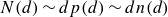
(a) The bubble size distribution for the image shown in figure 4. The number $N$
is defined in (3.3). (b) A 2-D histogram for the same image showing bubble size distribution on the transverse coordinates. The jet is advancing in the x direction, which is the axial direction. The solid white circle is the inlet region. The curly dotted white lines are drawn to highlight pale patches to indicate that some bubbles also exist outside the jet core, indicating possible compound drops.
$N$
is defined in (3.3). (b) A 2-D histogram for the same image showing bubble size distribution on the transverse coordinates. The jet is advancing in the x direction, which is the axial direction. The solid white circle is the inlet region. The curly dotted white lines are drawn to highlight pale patches to indicate that some bubbles also exist outside the jet core, indicating possible compound drops.
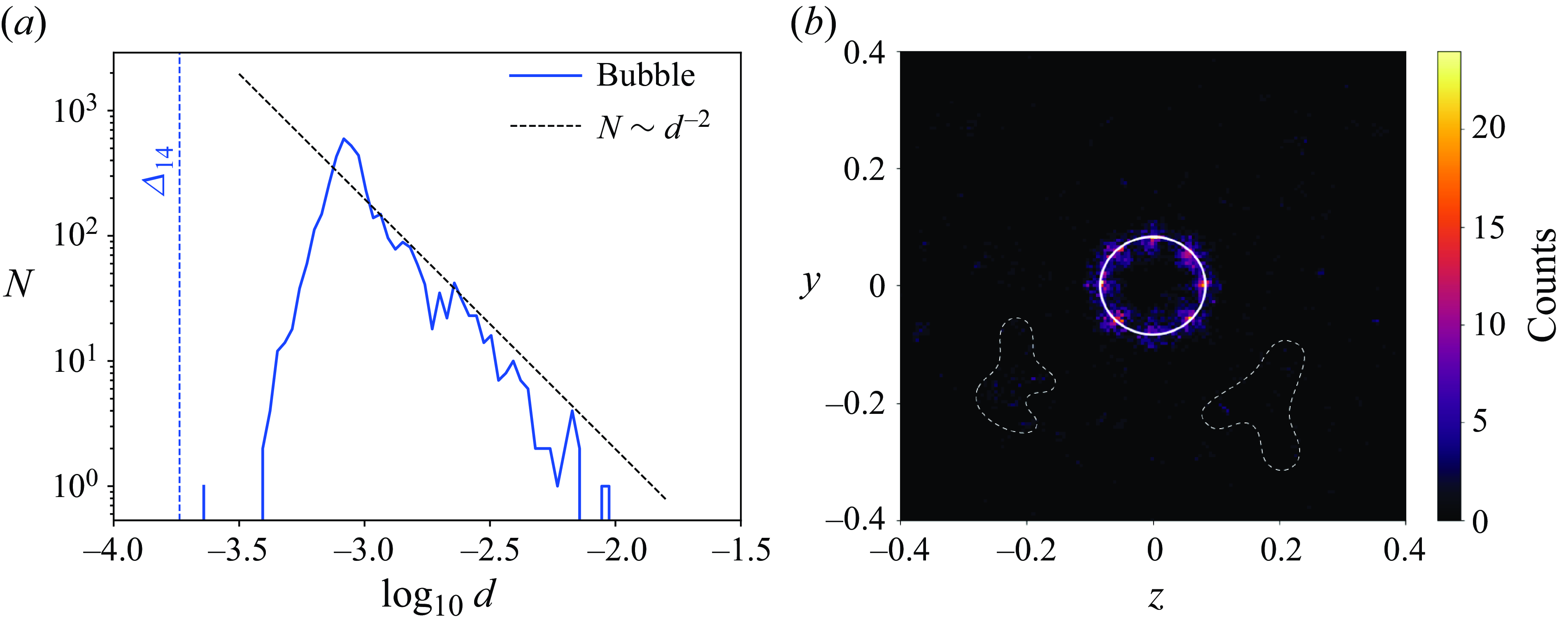
Figure 5 shows the number distribution of bubbles. The ordinate $N$
is the number
$N$
is the number $n_i$
of droplets defined in the text. We see that above the critical thickness, a distribution
$n_i$
of droplets defined in the text. We see that above the critical thickness, a distribution $N \sim r^{-\gamma }$
is seen. This distribution may have consequences in the sheet rupture and, hence, the droplet-size distribution. We have discussed the physical implications of bubble size distribution in Appendix A. In figure 5(b) we plot a two-dimensional (2-D) distribution of the bubble size on a y–z plane. The white circle represents the inlet. The plot shows that most of the bubbles are near the outer boundary of the jet core where we see wavelet interactions and drop impacts the most (figure 3(c) and supplementary movie 1). The distribution also shows eight characteristic high bubble-density zones. The occurrence of these zones and what decides their number is beyond the scope of the current paper. We also see some bubbles present outside the jet core encircled in dotted white lines. This indicates that we do have a relatively small number of compound droplets.
$N \sim r^{-\gamma }$
is seen. This distribution may have consequences in the sheet rupture and, hence, the droplet-size distribution. We have discussed the physical implications of bubble size distribution in Appendix A. In figure 5(b) we plot a two-dimensional (2-D) distribution of the bubble size on a y–z plane. The white circle represents the inlet. The plot shows that most of the bubbles are near the outer boundary of the jet core where we see wavelet interactions and drop impacts the most (figure 3(c) and supplementary movie 1). The distribution also shows eight characteristic high bubble-density zones. The occurrence of these zones and what decides their number is beyond the scope of the current paper. We also see some bubbles present outside the jet core encircled in dotted white lines. This indicates that we do have a relatively small number of compound droplets.
(a) The droplet-size number distribution ( $N$
is defined in (3.3)) and (b) the probability density function of the droplet diameter (defined in (3.1)) at various time instants. The plot shows that the PDF has converged in time
$N$
is defined in (3.3)) and (b) the probability density function of the droplet diameter (defined in (3.1)) at various time instants. The plot shows that the PDF has converged in time $t \sim 2.5$
. This time convergence determines the choice of the end time of the simulation at t = 3.5. Both (a) and (b) have 200 bins. The simulation corresponds to level 14 and the vertical dashed line represents the grid size.
$t \sim 2.5$
. This time convergence determines the choice of the end time of the simulation at t = 3.5. Both (a) and (b) have 200 bins. The simulation corresponds to level 14 and the vertical dashed line represents the grid size.
We now discuss the statistical properties of the jet, in particular, the droplet-size distribution in the case of uncontrolled sheet perforation or ‘no-MD’ case. As the jet advances, the droplet-size distribution evolves. This is shown in figure 6. One can see that the droplet-size distribution has started to converge at $t=1.8$
and is approximately converged at
$t=1.8$
and is approximately converged at $t=2.8$
. The histogram thus only shifts in the vertical direction (the number of droplets), while maintaining the same qualitative nature. This histogram is bimodal with two peaks or local maxima. There is a large amplitude peak corresponding to a smaller droplet size (referred to as peak 1) and a smaller amplitude one corresponding to a larger droplet size (referred to as peak 2).
$t=2.8$
. The histogram thus only shifts in the vertical direction (the number of droplets), while maintaining the same qualitative nature. This histogram is bimodal with two peaks or local maxima. There is a large amplitude peak corresponding to a smaller droplet size (referred to as peak 1) and a smaller amplitude one corresponding to a larger droplet size (referred to as peak 2).
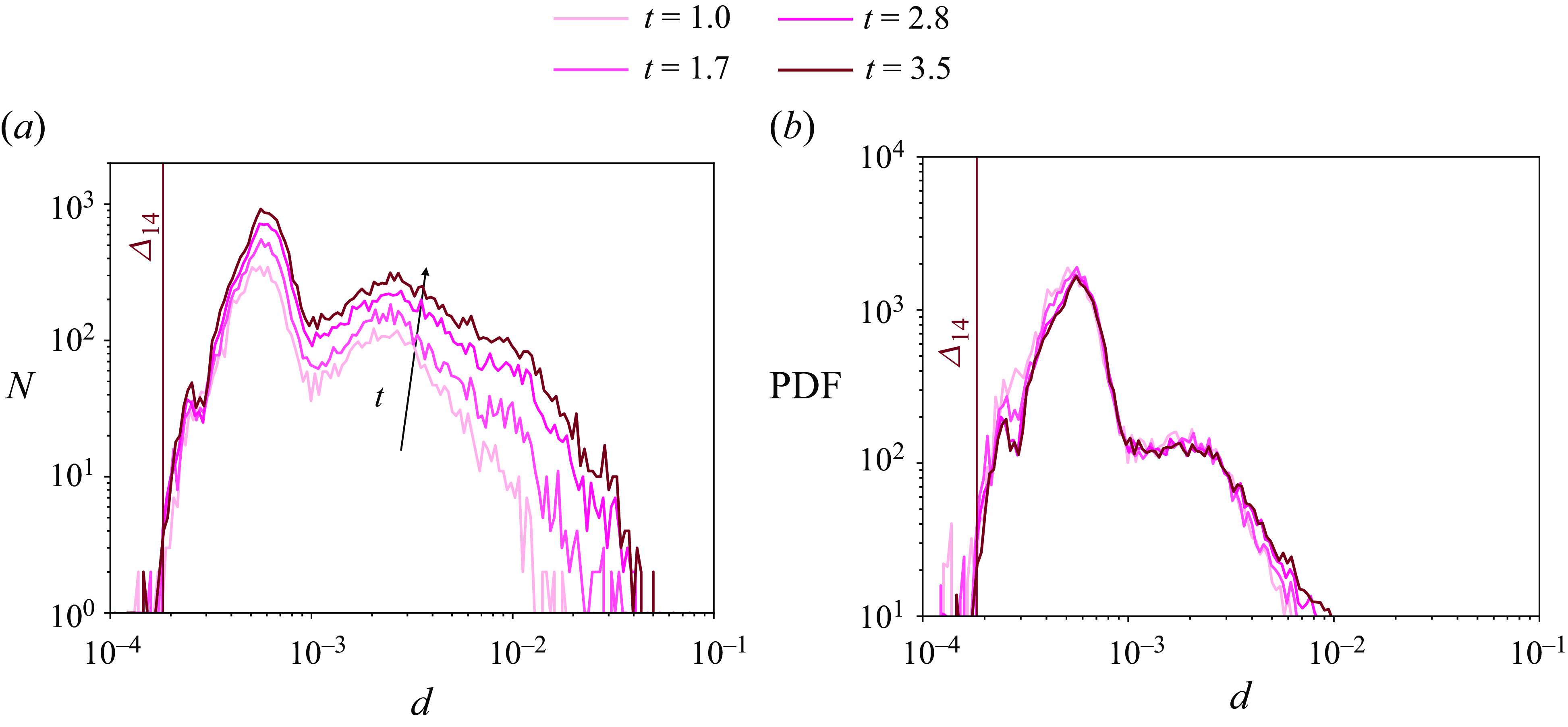
(a) The droplet-size distribution and (b) the probability density function of the droplet diameter $d$
at the final time
$d$
at the final time $t=3.5$
for various grid resolutions. The grid sizes are shown with vertical dashed lines and
$t=3.5$
for various grid resolutions. The grid sizes are shown with vertical dashed lines and $\varDelta _{\ell }$
is defined as in (2.7). The inset in (a) shows the converged tail region. All the plots are done with 200 bins. A Pareto distribution
$\varDelta _{\ell }$
is defined as in (2.7). The inset in (a) shows the converged tail region. All the plots are done with 200 bins. A Pareto distribution $N(d) \sim d^{-2}$
is added to compare with the converged region of the distributions.
$N(d) \sim d^{-2}$
is added to compare with the converged region of the distributions.
We investigate the statistical convergence of the droplet-size distribution by plotting in figure 7 the histogram at $t=3.5$
when the jet is fully developed. We plot various grid resolutions or levels on that same figure. The highest resolution in the no-MD case corresponds to the
$t=3.5$
when the jet is fully developed. We plot various grid resolutions or levels on that same figure. The highest resolution in the no-MD case corresponds to the $\varDelta _{14}$
line. This implies
$\varDelta _{14}$
line. This implies $D/\varDelta = 920$
grid points per initial diameter. Figure 7 has two important characteristics: (i) the histograms at various resolutions are qualitatively similar, that is, bimodal with a major peak 1 at small scales and a minor peak 2 at large scales; and (ii) despite such high resolution, it is clear that there is no convergence for the droplet-size distribution. However, the tail region of the distribution, to the right of peak 2, shows some degree of convergence. In that tail region a Pareto distribution
$D/\varDelta = 920$
grid points per initial diameter. Figure 7 has two important characteristics: (i) the histograms at various resolutions are qualitatively similar, that is, bimodal with a major peak 1 at small scales and a minor peak 2 at large scales; and (ii) despite such high resolution, it is clear that there is no convergence for the droplet-size distribution. However, the tail region of the distribution, to the right of peak 2, shows some degree of convergence. In that tail region a Pareto distribution $n(d) \sim d^{-2}$
is seen reminiscent of such distributions found in other contexts (Balachandar et al. Reference Balachandar, Zaleski, Soldati, Ahmadi and Bourouiba2020; Pairetti et al. Reference Pairetti, Villiers and Zaleski2021). The dependence of the two peaks with the grid size is shown explicitly in figure 8(b) where we plot the ratios
$n(d) \sim d^{-2}$
is seen reminiscent of such distributions found in other contexts (Balachandar et al. Reference Balachandar, Zaleski, Soldati, Ahmadi and Bourouiba2020; Pairetti et al. Reference Pairetti, Villiers and Zaleski2021). The dependence of the two peaks with the grid size is shown explicitly in figure 8(b) where we plot the ratios $d_i/\varDelta _\ell$
corresponding to the peaks as a function of the maximum level
$d_i/\varDelta _\ell$
corresponding to the peaks as a function of the maximum level $\ell$
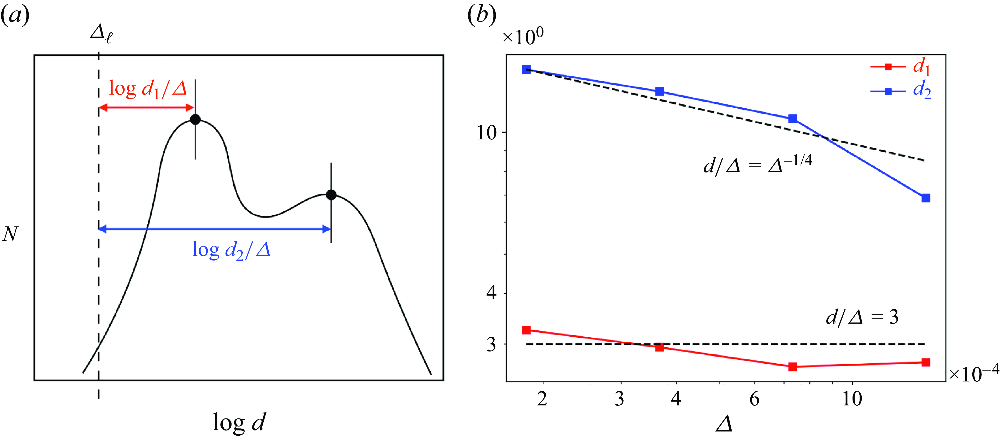
. We observe that the ratio for peak 1,
$\ell$
. We observe that the ratio for peak 1, $d_1/\varDelta _\ell$
, remains constant around a value of 3, while for peak 2,
$d_1/\varDelta _\ell$
, remains constant around a value of 3, while for peak 2, $d_2/\varDelta _\ell$
weakly increases with
$d_2/\varDelta _\ell$
weakly increases with $\ell$
. The grid dependence of these two peaks is synonymous with the absence of statistical convergence. We discuss possible explanations for the behaviour of these two peaks below and, in particular, the relation between peak 1 and the curvature ripples appearing just before sheet rupture. We also discuss a mechanism and a possible scaling for peak 2 in Appendix A. Since the grid dependence behaviour is maintained at all resolutions, the constant scaling of the diameter
$\ell$
. The grid dependence of these two peaks is synonymous with the absence of statistical convergence. We discuss possible explanations for the behaviour of these two peaks below and, in particular, the relation between peak 1 and the curvature ripples appearing just before sheet rupture. We also discuss a mechanism and a possible scaling for peak 2 in Appendix A. Since the grid dependence behaviour is maintained at all resolutions, the constant scaling of the diameter $d_1$
of peak 1 with the grid size implies that no matter how much we refine the grid, the distribution of droplet sizes is grid dependent.
$d_1$
of peak 1 with the grid size implies that no matter how much we refine the grid, the distribution of droplet sizes is grid dependent.
(a) Schematic of the bimodal droplet-size distribution. The arrows indicate the logarithmic distance from the grid size $\log d_i/\varDelta = \log d_i - \log \varDelta$
. (b) The values of
$\log d_i/\varDelta = \log d_i - \log \varDelta$
. (b) The values of $d_i/\varDelta$
as a function of the maximum grid refinement level
$d_i/\varDelta$
as a function of the maximum grid refinement level $\ell$
for the distribution of figure 7. The dashed line is at
$\ell$
for the distribution of figure 7. The dashed line is at $3\varDelta$
, implying the droplets at peak 1 have a grid-dependent diameter of
$3\varDelta$
, implying the droplets at peak 1 have a grid-dependent diameter of $d_1 \sim 3\varDelta$
.
$d_1 \sim 3\varDelta$
.
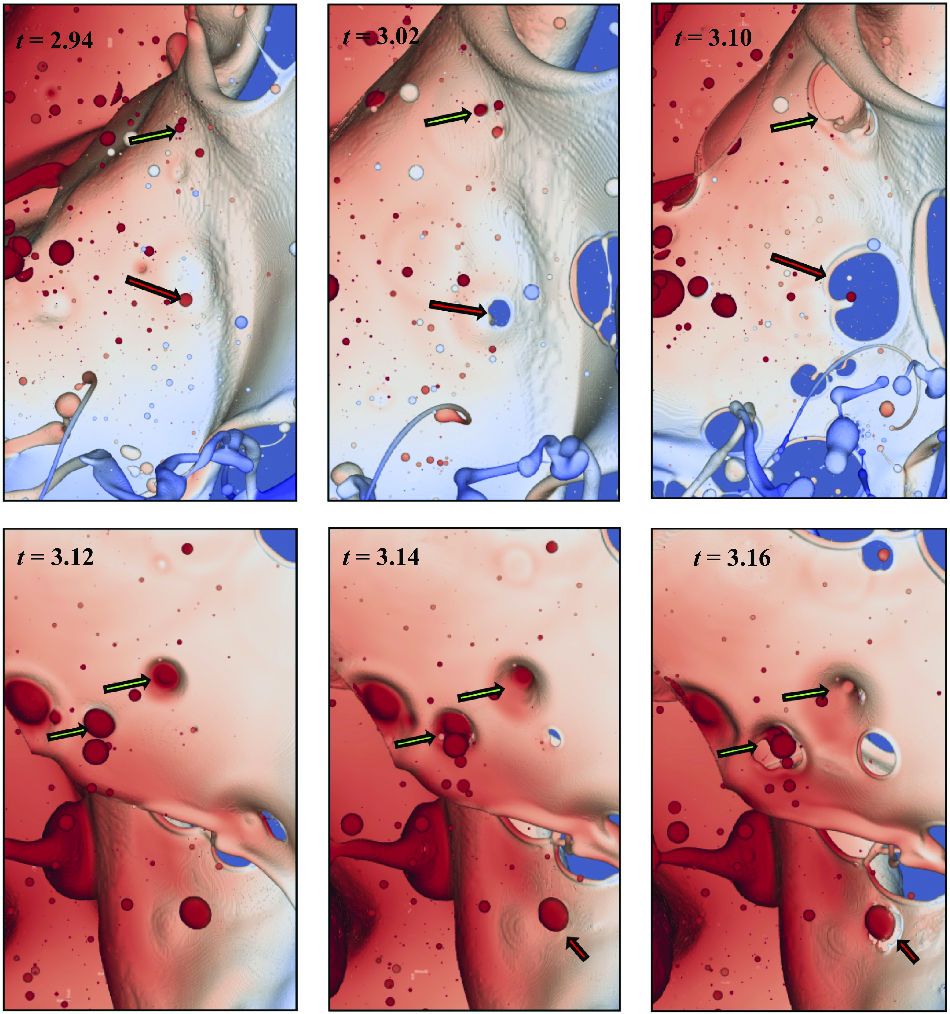
Droplet impacts on the frontal liquid sheet. The points of interest are indicated by the arrows. Droplet impacts can result in holes with characteristic ligaments as seen at $t=3.10$
. In some cases droplets coalesce into the sheet seen at
$t=3.10$
. In some cases droplets coalesce into the sheet seen at $t=3.12$
and
$t=3.12$
and $t=3.14$
. At
$t=3.14$
. At $t=3.16$
, the sheet is ruptured but the droplet is still identifiable. All simulations are for the maximum level
$t=3.16$
, the sheet is ruptured but the droplet is still identifiable. All simulations are for the maximum level $\ell = 13$
. The MD method is not applied. The interface is coloured by axial velocity. The artefacts or corrugated surfaces particularly visible at t = 3.02 and t = 3.10 at the top right are not aliasing artefacts (due to an approximate isosurface interpolation) but are representative of the curvature oscillations seen in the next figures.
$\ell = 13$
. The MD method is not applied. The interface is coloured by axial velocity. The artefacts or corrugated surfaces particularly visible at t = 3.02 and t = 3.10 at the top right are not aliasing artefacts (due to an approximate isosurface interpolation) but are representative of the curvature oscillations seen in the next figures.
Appearance and evolution of the curvature ripples on the interface. The interface is coloured by the interface curvature. These ligaments are coloured a darker red and the interfaces on the thin sheets are closer to white. Ligament rupture is encircled in blue. The rupture or ligament pinch off appears in a darker red colour. Sheet rupture, encircled in green, displays curvature ripples in the form of red–blue oscillations. At time $t=2.82$
, the green-circled rupture region displays a grid-dependent ligament network that has evolved from these ripples. These images correspond to a level
$t=2.82$
, the green-circled rupture region displays a grid-dependent ligament network that has evolved from these ripples. These images correspond to a level $\ell = 14$
simulation. (See also supplementary movie 5.)
$\ell = 14$
simulation. (See also supplementary movie 5.)

The mechanism leading to peak 1 is related to the perforation of thin sheets. This perforation is observed to occur in two contrasted ways. A simple mechanism is the impact of small droplets on the liquid sheet. The droplets are formed by breakup previously occurring elsewhere in the simulation. The impacts yield in some cases the formation of an expanding hole, as shown on figure 9. We note that such impacts have already been observed in previous studies such as those of Ménard et al. (Reference Ménard, Tanguy and Berlemont2007) and Shinjo & Umemura (Reference Shinjo and Umemura2010). Not all droplet impacts create perforations. In figure 9, at time $t=2.94$
, we track the droplets indicated by arrows. We see that droplet impacts often create holes with a characteristic finger-like ligament inside the hole. Impacts are shown by arrows at time
$t=2.94$
, we track the droplets indicated by arrows. We see that droplet impacts often create holes with a characteristic finger-like ligament inside the hole. Impacts are shown by arrows at time $t=3.10$
in figure 9. In the lower panel at
$t=3.10$
in figure 9. In the lower panel at $t=3.12$
and
$t=3.12$
and $t=3.14$
some droplet impacts do not result in holes but instead droplets merge with the sheet. This hypothesis was confirmed by repeated observations of the sheets at various angles and by visioning supplementary movie 5. The red arrow from
$t=3.14$
some droplet impacts do not result in holes but instead droplets merge with the sheet. This hypothesis was confirmed by repeated observations of the sheets at various angles and by visioning supplementary movie 5. The red arrow from $t=3.14$
and
$t=3.14$
and $t=3.16$
captures an interesting moment, where the droplet impact and sheet rupture happen simultaneously and it is unclear if the hole was created by the numerical rupture process discussed below or by droplet impact.
$t=3.16$
captures an interesting moment, where the droplet impact and sheet rupture happen simultaneously and it is unclear if the hole was created by the numerical rupture process discussed below or by droplet impact.
Another mode of thin sheet perforation, much more complex and purely numerical, is illustrated on figure 10 as well as supplementary movie 5. The curvature colouring of the interface helps us identify the perforation spots. We see high-frequency oscillations of the curvature field in the form of alternating red and blue colours. These indicate that the ripples originate at the fluid interface before the sheet rupture happens. Finally, at $t=2.82$
, we see a dense network of small diameter ligaments, scaling with grid size. Another mechanism that may contribute to peaks 1 and 2 is the rupture of ligaments, also shown on figure 10. Small diameter ligaments have large curvature and are thus easily identified by their colour. They break physically and not numerically by the Rayleigh–Plateau instability. The origin of these ligaments themselves is often an expanding hole whose rim collides into other rims.
$t=2.82$
, we see a dense network of small diameter ligaments, scaling with grid size. Another mechanism that may contribute to peaks 1 and 2 is the rupture of ligaments, also shown on figure 10. Small diameter ligaments have large curvature and are thus easily identified by their colour. They break physically and not numerically by the Rayleigh–Plateau instability. The origin of these ligaments themselves is often an expanding hole whose rim collides into other rims.
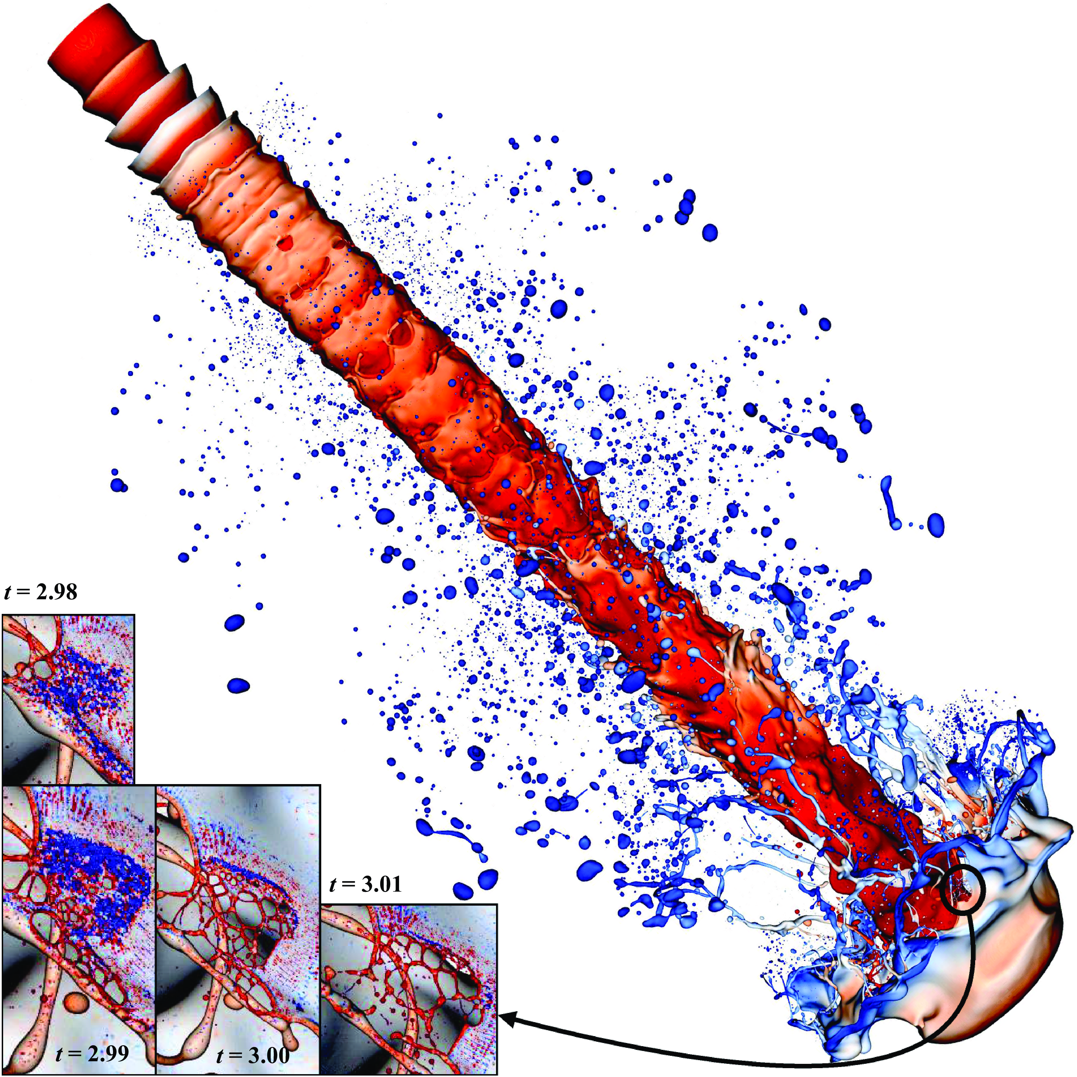
The fully developed jet at $t= 2.8$
. The inset shows a zoom in at the sheet rupture spot showing the curvature ripples in the weak spot about to be punctured and the resulting ligament network. This ligament network eventually produces grid-dependent droplets. The simulation shown here is at level
$t= 2.8$
. The inset shows a zoom in at the sheet rupture spot showing the curvature ripples in the weak spot about to be punctured and the resulting ligament network. This ligament network eventually produces grid-dependent droplets. The simulation shown here is at level $\ell =14$
.
$\ell =14$
.

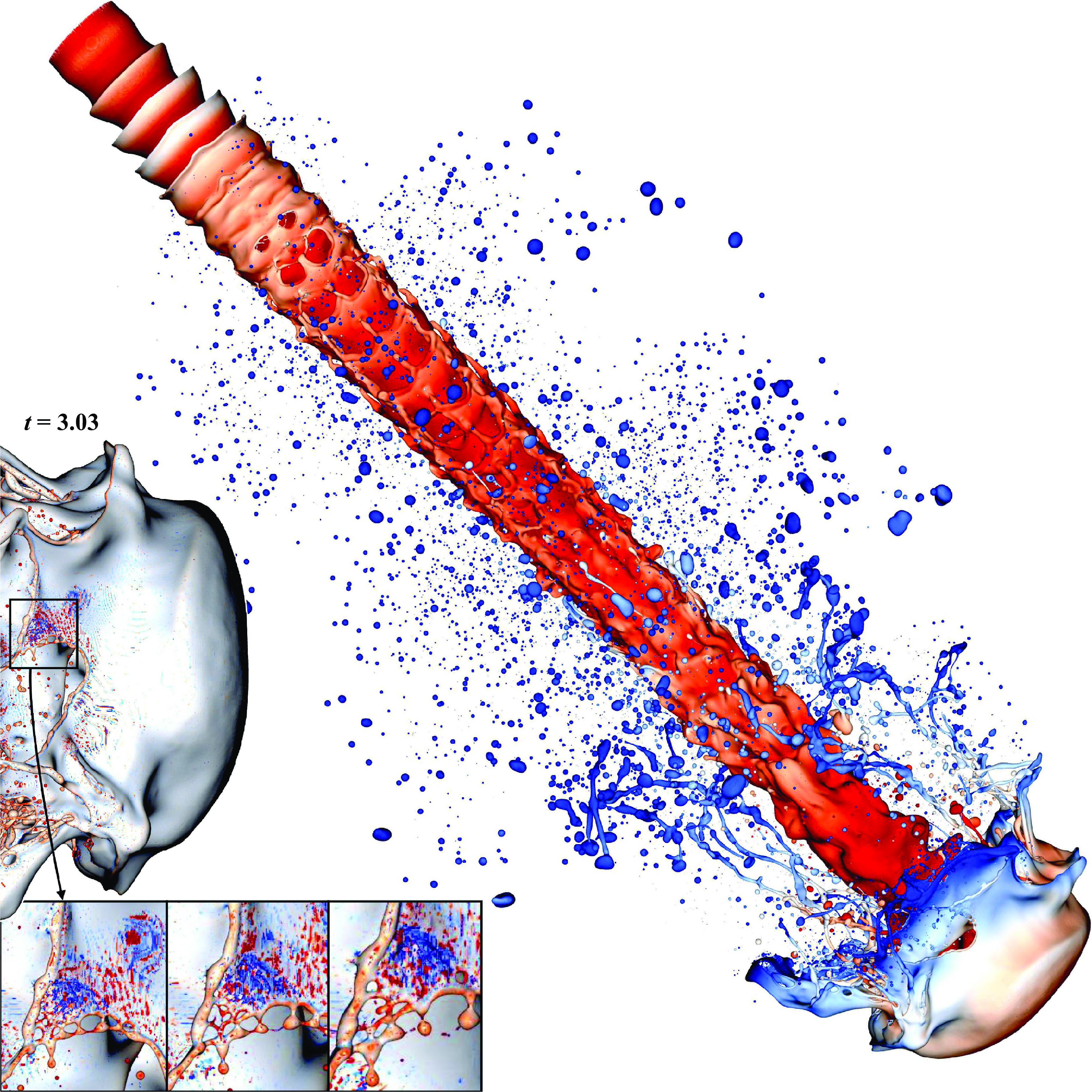
The fully developed jet at $t= 3.03$
. The inset shows a zoom in at the sheet rupture spot showing the curvature ripples in the weak spot about to be punctured. The simulation shown here is at level
$t= 3.03$
. The inset shows a zoom in at the sheet rupture spot showing the curvature ripples in the weak spot about to be punctured. The simulation shown here is at level $\ell =13$
.
$\ell =13$
.
The fully developed jet at $t= 3.01$
. The inset shows a zoom in at the sheet rupture spot showing the curvature ripples in the weak spot about to be punctured. The simulation shown here is at level
$t= 3.01$
. The inset shows a zoom in at the sheet rupture spot showing the curvature ripples in the weak spot about to be punctured. The simulation shown here is at level $\ell =14$
.
$\ell =14$
.
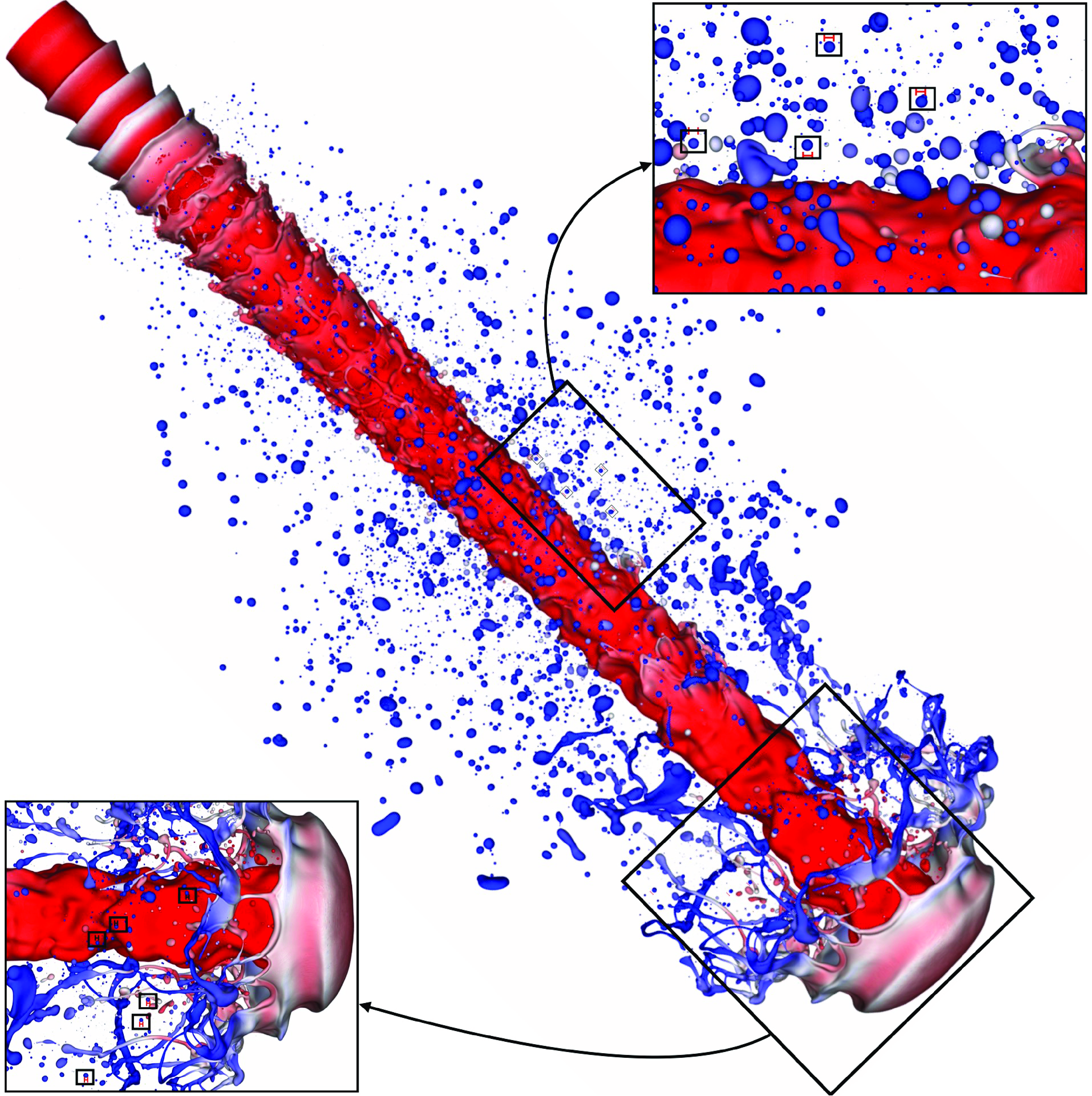
The $(14,13)$
jet at
$(14,13)$
jet at $t= 3.1$
with MD applied. The basilisk level
$t= 3.1$
with MD applied. The basilisk level $\ell =14$
and MD level is
$\ell =14$
and MD level is $13$
. The insets and the boxes indicate droplets that are near the maximum size of the distribution in the converged region.
$13$
. The insets and the boxes indicate droplets that are near the maximum size of the distribution in the converged region.
We note that the high-frequency pressure oscillations are due in part to the use of the height-function method to compute curvature. The height-function method ceases to work when the sheet is too thin. However, other methods will also fail as represented in figure 1. To investigate the small-scale ligament networks, we zoom around such a breakup event in figure 11. We see that a weak spot develops and curvature ripples appear at $t=2.78$
as soon as the sheet reaches a thickness of a few times the cell size, as shown in the inset. These curvature ripples then give rise to ligament networks inside the expanded hole eventually leading to the grid-dependent droplets. To summarise, as the sheet reaches a thickness of order
$t=2.78$
as soon as the sheet reaches a thickness of a few times the cell size, as shown in the inset. These curvature ripples then give rise to ligament networks inside the expanded hole eventually leading to the grid-dependent droplets. To summarise, as the sheet reaches a thickness of order $ 3 \varDelta$
, the rupture mechanism is as follows: thin sheet regions
$ 3 \varDelta$
, the rupture mechanism is as follows: thin sheet regions $\gt$
curvature ripples
$\gt$
curvature ripples $\gt$
ligament networks and tiny droplets
$\gt$
ligament networks and tiny droplets $(d \sim 3\varDelta )$
. Since this sequence of events is inherent to the numerical breakup of thin sheets, it is impossible to escape its occurrence by increasing the grid refinement, although refinement can delay it. The numerical sheet breakup identified here is the direct cause of the lack of convergence of peak 1. Indirectly, the formation of droplets and ligaments of a given size in a non-converged manner leads to all the droplet size counts being unconverged as these other size droplets are formed through coalescence and breakup events from the peak 1 droplets and similarly scaled ligaments.
$(d \sim 3\varDelta )$
. Since this sequence of events is inherent to the numerical breakup of thin sheets, it is impossible to escape its occurrence by increasing the grid refinement, although refinement can delay it. The numerical sheet breakup identified here is the direct cause of the lack of convergence of peak 1. Indirectly, the formation of droplets and ligaments of a given size in a non-converged manner leads to all the droplet size counts being unconverged as these other size droplets are formed through coalescence and breakup events from the peak 1 droplets and similarly scaled ligaments.
We also note that the point of view and region of figure 9 were selected to show a large number of drop impact situations, which are however scarcer than the numerical breakup of sheets.
To give an overall idea of the evolution of the jet, we show the fully evolved jet at $\ell = 13$
in figure 12 and the same fully evolved jet but at
$\ell = 13$
in figure 12 and the same fully evolved jet but at $\ell = 14$
in figure 13. The mist of tiny droplets near the mushroom head and near the inlet flaps is more pronounced in the
$\ell = 14$
in figure 13. The mist of tiny droplets near the mushroom head and near the inlet flaps is more pronounced in the $\ell = 14$
case than in the
$\ell = 14$
case than in the $\ell = 13$
case. The
$\ell = 13$
case. The $\ell =14$
case retains more large drops and deformed ligaments at mid-length compared with the
$\ell =14$
case retains more large drops and deformed ligaments at mid-length compared with the $\ell =13$
case. The inset zoom shows the numerical sheet rupture. The ligament network structure is more clearly seen at
$\ell =13$
case. The inset zoom shows the numerical sheet rupture. The ligament network structure is more clearly seen at $\ell = 14$
than at
$\ell = 14$
than at $\ell =13$
.
$\ell =13$
.
3.2. Controlled perforation by the MD method
We now present the results of atomisation when we apply the MD method. Here we adopt the following conventions.
-
(i) The octree maximum refinement level $\ell$
defines the finest grid size as given in (2.7).
$\ell$
defines the finest grid size as given in (2.7). -
(ii) The MD level
$m$
implies that the critical thickness for punching holes is given by
$h_c = 3 \varDelta _{m}$
.


As an example, the notation $(\ell ,m)=(13,12)$
would mean that the finest cell size in the simulation is
$(\ell ,m)=(13,12)$
would mean that the finest cell size in the simulation is $\varDelta _{13}$
and the critical thickness at which holes are being punched is
$\varDelta _{13}$
and the critical thickness at which holes are being punched is $h_c = 3\varDelta _{12} = 3\times (2\varDelta _{13}) = 6 \varDelta _{13}$
. This convention for the definition of the ‘MD level
$h_c = 3\varDelta _{12} = 3\times (2\varDelta _{13}) = 6 \varDelta _{13}$
. This convention for the definition of the ‘MD level $m$
’ maintains consistency with the comments in the code available at http://basilisk.fr/sandbox/lchirco/signature.h.
$m$
’ maintains consistency with the comments in the code available at http://basilisk.fr/sandbox/lchirco/signature.h.
The probability density function at various times $t$
for the droplet-size distribution when MD is applied. The PDF has converged in time at
$t$
for the droplet-size distribution when MD is applied. The PDF has converged in time at $t=2.5$
. (a) The PDF at maximum level
$t=2.5$
. (a) The PDF at maximum level $\ell =13$
and MD level
$\ell =13$
and MD level $m=12$
and (b) the PDF at maximum level
$m=12$
and (b) the PDF at maximum level $\ell =14$
and MD level
$\ell =14$
and MD level $m=12$
. The critical hole punching thickness
$m=12$
. The critical hole punching thickness $h_c = 3 \varDelta _{m=12}$
is shown as the black dashed line and is the same for both plots.
$h_c = 3 \varDelta _{m=12}$
is shown as the black dashed line and is the same for both plots.
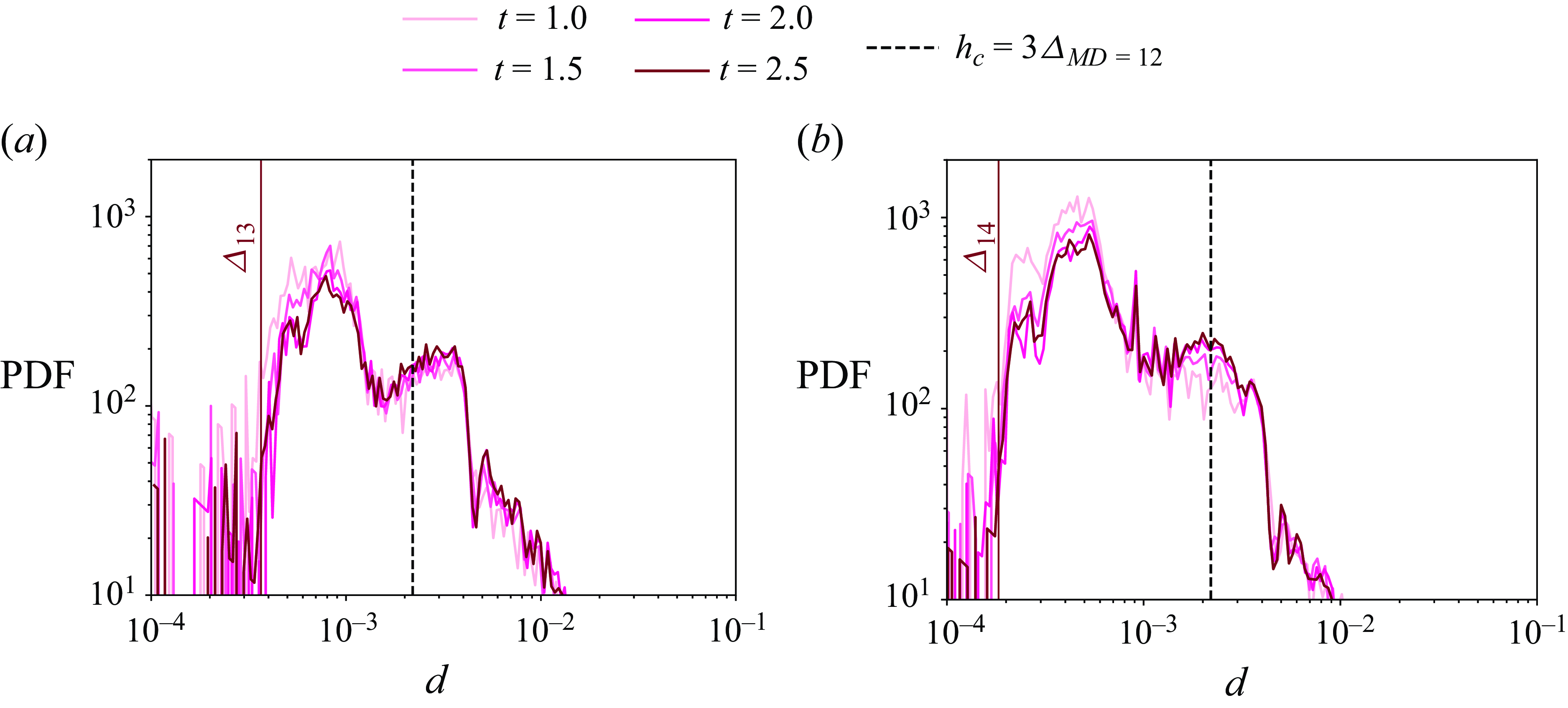
The extent of the integrated region in the quadratic form computation leads to the correspondence $h_c = 3 \varDelta _m$
. The overall evolution of the jet shows important variations with the no-MD case. Comparing figure 14 MD
$h_c = 3 \varDelta _m$
. The overall evolution of the jet shows important variations with the no-MD case. Comparing figure 14 MD $(14,13)$
to figures 12 (
$(14,13)$
to figures 12 ( $\ell =13$
) and 13 (
$\ell =13$
) and 13 ( $\ell =14$
), we note that (i) the mist of tiny droplets near the mushroom head has disappeared in figure 14, (ii) the mushroom-head corona-flap sheet is more affected by holes and breakups and is closer to figure 13
$\ell =14$
), we note that (i) the mist of tiny droplets near the mushroom head has disappeared in figure 14, (ii) the mushroom-head corona-flap sheet is more affected by holes and breakups and is closer to figure 13 $\ell =14$
than to figure 12
$\ell =14$
than to figure 12 $\ell =13$
, (iii) the cloud of droplets at mid-length is similar to both no-MD cases but is more uniform and closer to the figure 12
$\ell =13$
, (iii) the cloud of droplets at mid-length is similar to both no-MD cases but is more uniform and closer to the figure 12 $\ell =13$
case.
$\ell =13$
case.
Figure 15 shows the evolution of the PDF of the droplet-size distribution with time. Similar to the no-MD plots, we see that here also the statistics are converged in time as soon as $t=2.5$
. When compared with figure 7, we see that the peak corresponding to the smaller droplet size has a smaller amplitude.
$t=2.5$
. When compared with figure 7, we see that the peak corresponding to the smaller droplet size has a smaller amplitude.
The droplet-size distribution from simulations using the MD method. Each curve is labelled $\varDelta _{\ell }-\varDelta _{MD=m}$
, where
$\varDelta _{\ell }-\varDelta _{MD=m}$
, where $\ell$
is the grid level and
$\ell$
is the grid level and $m$
is the MD level. The dashed black vertical line represents
$m$
is the MD level. The dashed black vertical line represents $h_c = 3 \varDelta _{m}$
, that is, the critical thickness of punching holes. The solid vertical lines indicate the values of the converged diameter
$h_c = 3 \varDelta _{m}$
, that is, the critical thickness of punching holes. The solid vertical lines indicate the values of the converged diameter $d_c$
, corresponding to the smallest diameter above which the difference between subsequent distributions is not significant. All curves in (a) have fixed
$d_c$
, corresponding to the smallest diameter above which the difference between subsequent distributions is not significant. All curves in (a) have fixed $h_c = 3\varDelta _{12}$
and all curves in (b) have fixed
$h_c = 3\varDelta _{12}$
and all curves in (b) have fixed $h_c = 3 \varDelta _{13}$
. Note that the
$h_c = 3 \varDelta _{13}$
. Note that the $\varDelta _{11}$
curve in (a) and the
$\varDelta _{11}$
curve in (a) and the $\varDelta _{12}$
curve in (b) indicate the no-MD method and roughly correspond to respectively
$\varDelta _{12}$
curve in (b) indicate the no-MD method and roughly correspond to respectively $h_c = 3\varDelta _{MD=12}$
and
$h_c = 3\varDelta _{MD=12}$
and $h_c = 3 \varDelta _{MD=13}$
, given the breakup due to a lack of sheet resolution in VOF simulations. The shading highlights the departure from the converged region. We see that
$h_c = 3 \varDelta _{MD=13}$
, given the breakup due to a lack of sheet resolution in VOF simulations. The shading highlights the departure from the converged region. We see that $d_c$
approaches
$d_c$
approaches $h_c$
as the grid size is reduced. The inset shows the important change in the typical sizes of droplets in the first peak above
$h_c$
as the grid size is reduced. The inset shows the important change in the typical sizes of droplets in the first peak above $h_c$
as MD is applied. Peak A corresponds to peak 2 in the no-MD distributions of figure 7 while peak B, with much smaller droplets, corresponds to droplets seen in the MD figure 14.
$h_c$
as MD is applied. Peak A corresponds to peak 2 in the no-MD distributions of figure 7 while peak B, with much smaller droplets, corresponds to droplets seen in the MD figure 14.
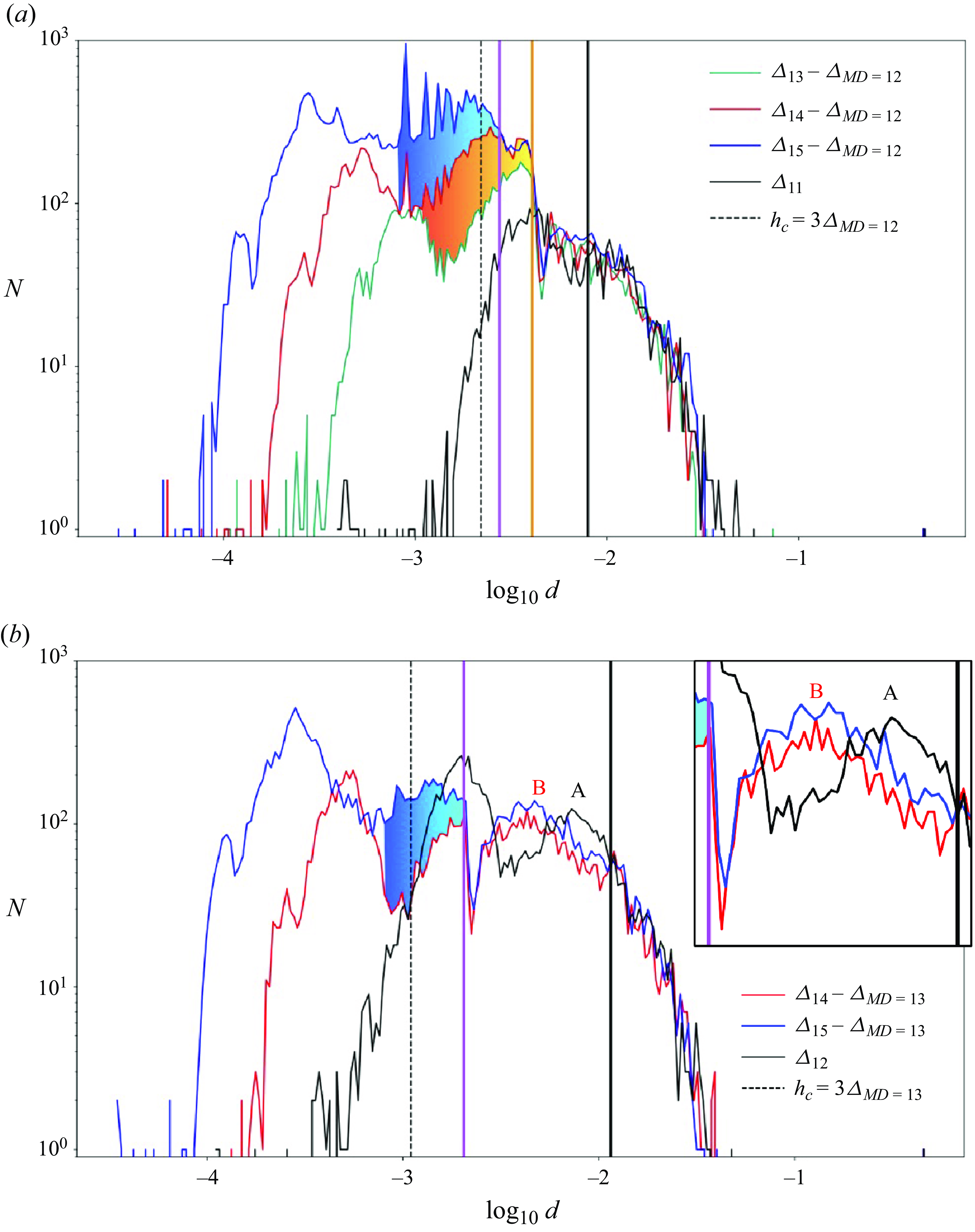
We show the number density $n(d)$
in figure 16. Figure 16(a) shows the histograms at various grid resolutions for a fixed MD threshold
$n(d)$
in figure 16. Figure 16(a) shows the histograms at various grid resolutions for a fixed MD threshold $h_c = 3 \varDelta _{12}$
. The distribution is again bimodal, but the peak corresponding to the smaller droplets is weaker. We also observe a clear converged region in the interval
$h_c = 3 \varDelta _{12}$
. The distribution is again bimodal, but the peak corresponding to the smaller droplets is weaker. We also observe a clear converged region in the interval $[d_c, d_{i_m+1})$
, where
$[d_c, d_{i_m+1})$
, where $d_c$
is the minimum converged equivalent droplet diameter or ‘converged diameter’ for simplicity. The extent of the converged region increases, that is,
$d_c$
is the minimum converged equivalent droplet diameter or ‘converged diameter’ for simplicity. The extent of the converged region increases, that is, $d_c$
decreases as the grid size
$d_c$
decreases as the grid size $\varDelta _l$
decreases. In figure 16(a) the vertical line marks
$\varDelta _l$
decreases. In figure 16(a) the vertical line marks $d_c$
for two consecutive grid sizes. We have shaded the onset of the non-converged region between two consecutive grid refinements for clarity.
$d_c$
for two consecutive grid sizes. We have shaded the onset of the non-converged region between two consecutive grid refinements for clarity.
In practice, the ‘converged diameter’ $d_c$
is determined from the comparison of a pair of distributions from simulations of two different grid sizes
$d_c$
is determined from the comparison of a pair of distributions from simulations of two different grid sizes $\varDelta _l$
. We note this pair
$\varDelta _l$
. We note this pair $\varDelta _{l_1} - \varDelta _{l_2}$
. In figure 16(a) the orange vertical line marks
$\varDelta _{l_1} - \varDelta _{l_2}$
. In figure 16(a) the orange vertical line marks $d_c$
for the pair {
$d_c$
for the pair { $\varDelta _{14} - \varDelta _{13}$
}. Similarly, the purple vertical line marks
$\varDelta _{14} - \varDelta _{13}$
}. Similarly, the purple vertical line marks $d_c$
for the pair {
$d_c$
for the pair { $\varDelta _{15} - \varDelta _{14}$
}. Some additional information may be obtained by investigating a no-MD case. In such a case, there is a typical sheet thickness at breakup
$\varDelta _{15} - \varDelta _{14}$
}. Some additional information may be obtained by investigating a no-MD case. In such a case, there is a typical sheet thickness at breakup $h_e$
that is comparable to the controlled breakup for
$h_e$
that is comparable to the controlled breakup for $h_c \simeq h_e$
. Indeed, the critical breakup film thickness
$h_c \simeq h_e$
. Indeed, the critical breakup film thickness $h_e$
for no-MD is
$h_e$
for no-MD is $h_e \simeq 1.5 \varDelta$
, Then the above case
$h_e \simeq 1.5 \varDelta$
, Then the above case $h_c = 3\varDelta _{12}$
with MD has a critical sheet thickness equal to, per expression (2.7),
$h_c = 3\varDelta _{12}$
with MD has a critical sheet thickness equal to, per expression (2.7), $h_e = 1.5 \varDelta _{11}$
in the no-MD case at level 11. Thus, the no-MD simulation at
$h_e = 1.5 \varDelta _{11}$
in the no-MD case at level 11. Thus, the no-MD simulation at $\ell =11$
is a rough equivalent to the three simulations with MD level
$\ell =11$
is a rough equivalent to the three simulations with MD level $m=12$
. The vertical black line is the converged thickness
$m=12$
. The vertical black line is the converged thickness $d_c$
for the pair {
$d_c$
for the pair { $\varDelta _{13}, \varDelta _{11}$
} where the first simulation is MD and the second is no-MD. One sees on figure 16(a) that the converged diameters, indicated by the solid vertical lines, decrease and tend to approach the critical sheet thickness
$\varDelta _{13}, \varDelta _{11}$
} where the first simulation is MD and the second is no-MD. One sees on figure 16(a) that the converged diameters, indicated by the solid vertical lines, decrease and tend to approach the critical sheet thickness $h_c$
for MD breakup, represented by the dashed vertical line. We now show the droplet-size distribution and converged region for a smaller critical sheet thickness
$h_c$
for MD breakup, represented by the dashed vertical line. We now show the droplet-size distribution and converged region for a smaller critical sheet thickness $h_c = 3 \varDelta _{13}$
. In figure 16(b) we see similar results but with only two instead of three levels,
$h_c = 3 \varDelta _{13}$
. In figure 16(b) we see similar results but with only two instead of three levels, $l=14$
and 15. Since a simulation at
$l=14$
and 15. Since a simulation at $\varDelta _{15}$
is already quite expensive (it implies an equivalent of
$\varDelta _{15}$
is already quite expensive (it implies an equivalent of $35$
trillion cells for a uniform grid with
$35$
trillion cells for a uniform grid with $\varDelta _{15}$
), we did not perform a third simulation at
$\varDelta _{15}$
), we did not perform a third simulation at $l=16$
in that case. A zoomed-in view for the converged region
$l=16$
in that case. A zoomed-in view for the converged region $d_c$
for each consecutive pair is shown in Appendix E.
$d_c$
for each consecutive pair is shown in Appendix E.
The closely packed peaks around $\log(d)=-3$
in figure 16(a), mostly visible for
$\log(d)=-3$
in figure 16(a), mostly visible for $(\ell ,m)=(15,12)$
, are related to a process that produces a narrow spectrum of small droplets of size
$(\ell ,m)=(15,12)$
, are related to a process that produces a narrow spectrum of small droplets of size $\bar d$
with
$\bar d$
with $\varDelta _{15} \lt \bar d \lt h_c$
. These small droplets coalesce at least two or three times to produce additional small droplets of size
$\varDelta _{15} \lt \bar d \lt h_c$
. These small droplets coalesce at least two or three times to produce additional small droplets of size $2\bar d, 3\bar d$
, etc. We are unsure of the mechanism producing these initial droplets of well-defined diameter
$2\bar d, 3\bar d$
, etc. We are unsure of the mechanism producing these initial droplets of well-defined diameter $\bar d$
and why it appears most clearly for the pair (
$\bar d$
and why it appears most clearly for the pair ( $15,12$
).
$15,12$
).
(a) Schematic of the comparison of two simulations and how it allows us to define the `converged diameter’ $d_c$
. It is seen that
$d_c$
. It is seen that $d_c$
approaches
$d_c$
approaches $h_c$
as the simulations are refined. (b) Plot of
$h_c$
as the simulations are refined. (b) Plot of $d_c/h_c$
versus
$d_c/h_c$
versus $h_{c}$
corresponding to the
$h_{c}$
corresponding to the $d_c$
values of figure 16. Along a fixed
$d_c$
values of figure 16. Along a fixed $h_c$
, the
$h_c$
, the $d_c/h_c$
points move closer to unity as the maximum level is increased. The black squares corresponds to the no-MD case, while all circles are for the cases with MD.
$d_c/h_c$
points move closer to unity as the maximum level is increased. The black squares corresponds to the no-MD case, while all circles are for the cases with MD.
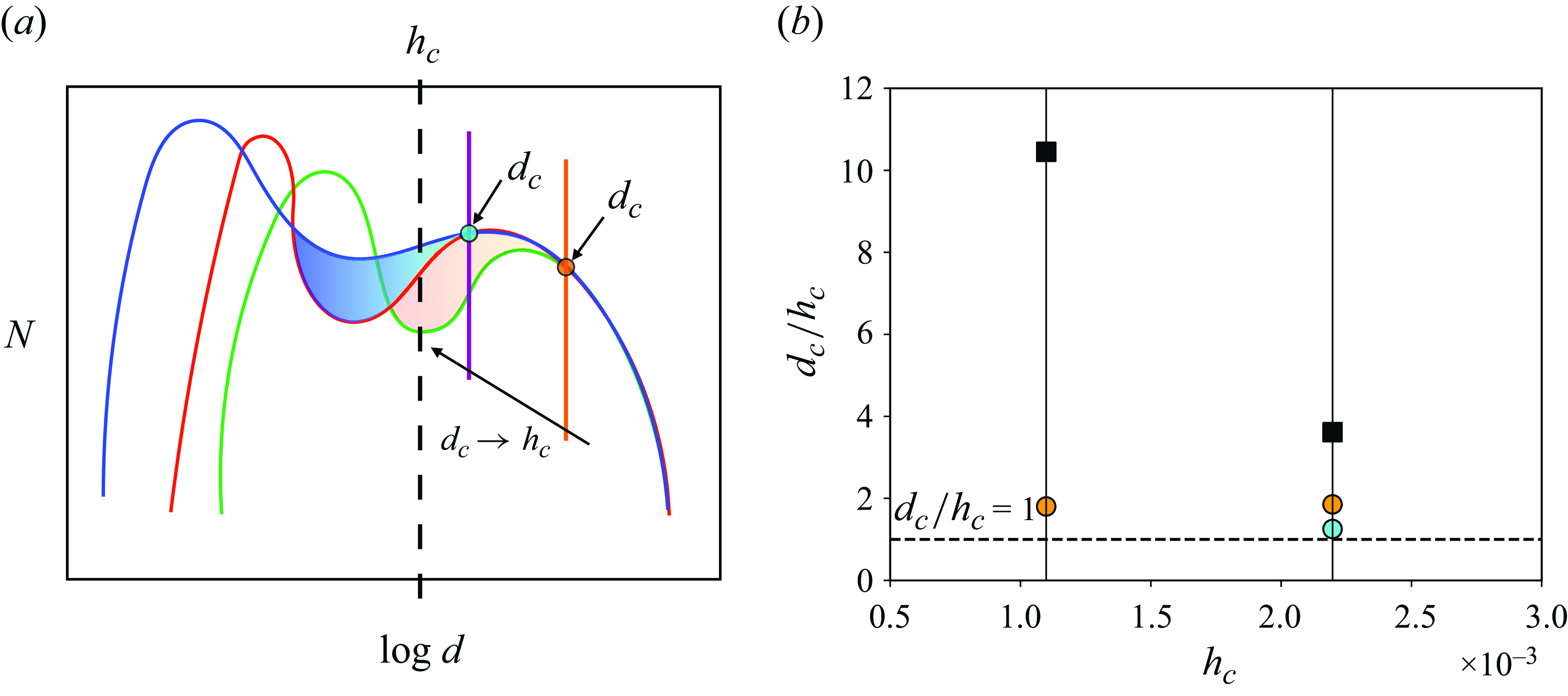
The variation of the converged diameter $d_c$
as a function of
$d_c$
as a function of $h_c$
and
$h_c$
and $\varDelta _\ell$
is shown explicitly in figure 17. Figure 17(a) illustrates schematically how the converged diameter approaches
$\varDelta _\ell$
is shown explicitly in figure 17. Figure 17(a) illustrates schematically how the converged diameter approaches $h_c$
as
$h_c$
as $\varDelta _\ell$
is reduced. Figure 17(b) shows the data in the
$\varDelta _\ell$
is reduced. Figure 17(b) shows the data in the $d_c/h_c, h_c$
plane. Each data point in that plane corresponds to a simulation pair discussed above such as {
$d_c/h_c, h_c$
plane. Each data point in that plane corresponds to a simulation pair discussed above such as { $\varDelta _{14} - \varDelta _{13}$
}, and to a vertical line in figure 16. Following a vertical line in figure 17(b), one can see
$\varDelta _{14} - \varDelta _{13}$
}, and to a vertical line in figure 16. Following a vertical line in figure 17(b), one can see $d_c$
tending to
$d_c$
tending to $h_c$
as the grid is refined for a fixed
$h_c$
as the grid is refined for a fixed $h_c$
.
$h_c$
.
Sheet perforation when the MD method is applied. Unlike figure 11, the holes are not preceded by large regions containing curvature ripples. Holes are punched at $t=3.01$
and expand with time as shown. The interface in the left part is coloured by curvature and on the right is coloured by the axial velocity. The simulation shown here corresponds to
$t=3.01$
and expand with time as shown. The interface in the left part is coloured by curvature and on the right is coloured by the axial velocity. The simulation shown here corresponds to $(\ell ,m)=(14,13)$
.
$(\ell ,m)=(14,13)$
.
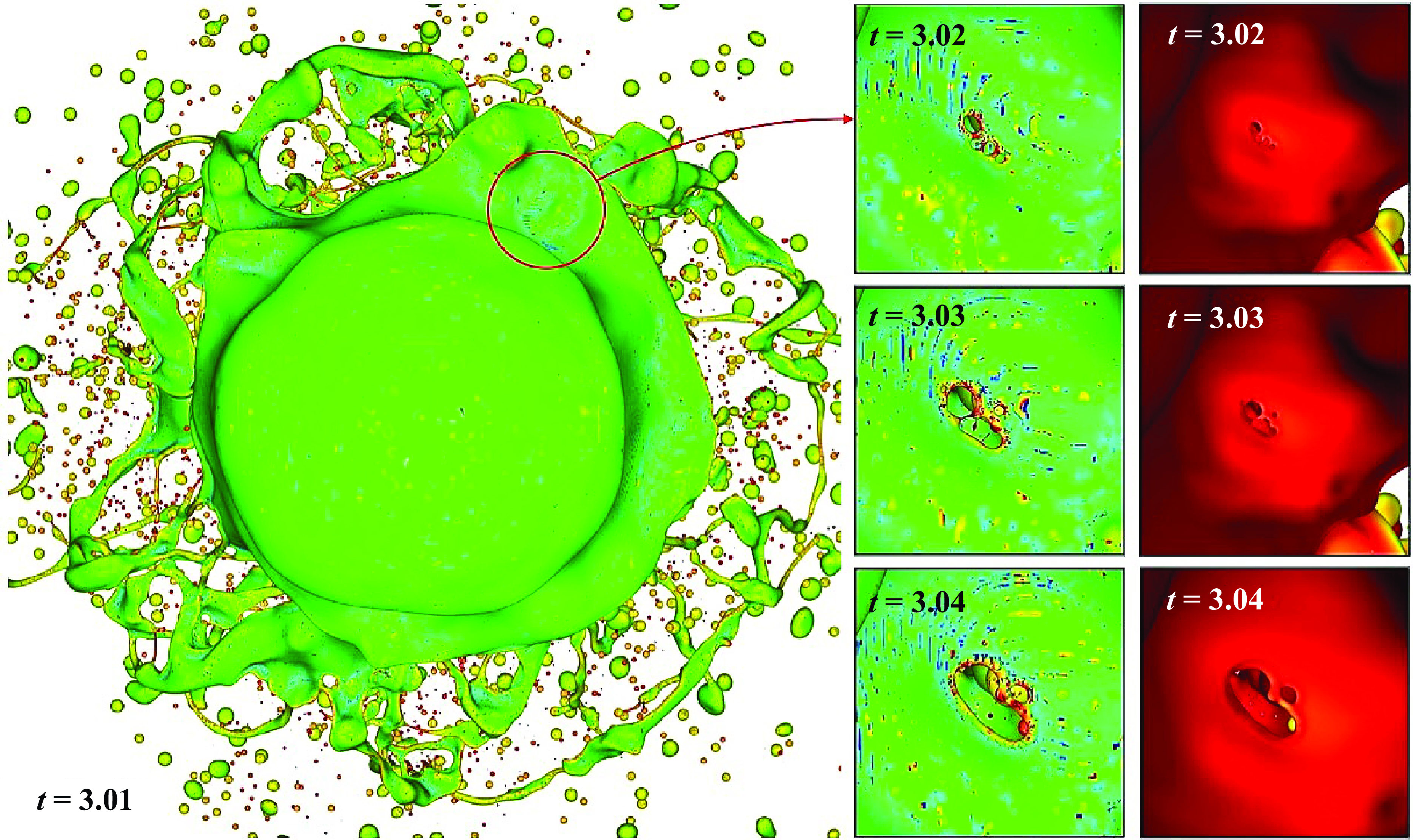
Figure 18 shows a zoom in at a hole expansion that was initiated by the MD method. The phase modification region is a cube but in less than 5–10 time steps the hole takes a rounded shape due to surface tension and starts expanding. When these holes expand, we do not see the noisy curvature ripples that resulted in grid-dependent droplets in the no-MD simulation of figure 11. This qualitative improvement in sheet collapse helps to obtain grid convergence.
Further evolution of the holes of figure 18. The image is coloured by axial velocity. We see that near the rims of the main expanding holes, additional holes are punched, encircled in black. (Manifold death is applied.)
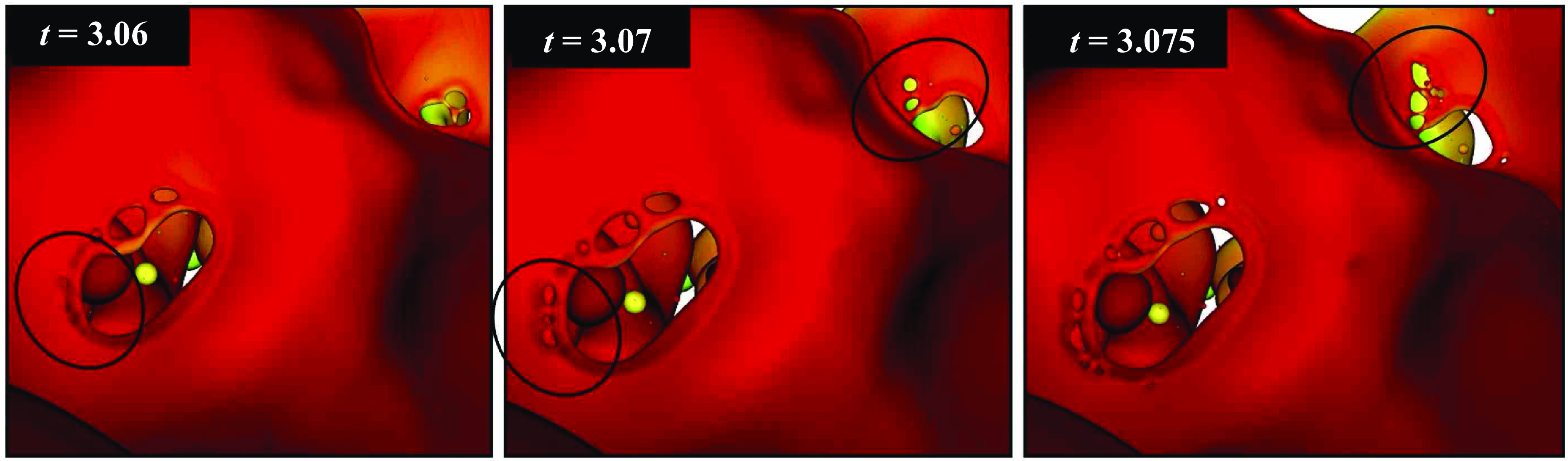
The MD procedure we use is tuned to a relatively large frequency of hole formation. This results in features such as those shown in figure 19. We see that once we detect a thin sheet and the MD process generates holes, these expand. However, it often happens that before the holes have expanded over the entire sheet more holes are punched just outside the rim. These kind of holes are identified as black circles in figure 19. This effect is also seen in supplementary movie 4 that shows the evolution of thin sheets with MD. Experimental photographs and the reasoning in Appendix A point to a smaller number of holes. This smaller number could be achieved by an improved MD algorithm that would involve a more realistic model of the physical process of hole formation.
Two distributions of droplet sizes at two MD levels, $m=12$
and
$m=12$
and $m=13$
, with the same ratio of the grid size to the MD threshold
$m=13$
, with the same ratio of the grid size to the MD threshold $h_c/\varDelta _\ell$
. We only plot the converged region, that is,
$h_c/\varDelta _\ell$
. We only plot the converged region, that is, $d\gt d_c(h_c)$
. The most refined simulation
$d\gt d_c(h_c)$
. The most refined simulation $(l,m)=(15,13)$
yields a distribution somewhat but not exactly similar to the less refined. Both distributions show a sudden increase in droplet number (a `ridge’) as the droplet size is decreased at the edge of the converged region. The vertical line shows the limit of convergence
$(l,m)=(15,13)$
yields a distribution somewhat but not exactly similar to the less refined. Both distributions show a sudden increase in droplet number (a `ridge’) as the droplet size is decreased at the edge of the converged region. The vertical line shows the limit of convergence $d_c$
. Plot (a) shows the un-rescaled number distribution, while plot (b) shows the PDFs. Plot (a) is clipped to show the PDFs
$d_c$
. Plot (a) shows the un-rescaled number distribution, while plot (b) shows the PDFs. Plot (a) is clipped to show the PDFs $p(d)$
for
$p(d)$
for $d\gt d_c(m=12)$
, where
$d\gt d_c(m=12)$
, where $d_c$
is the edge of the converged region for
$d_c$
is the edge of the converged region for $m=12$
. The Pareto distribution
$m=12$
. The Pareto distribution $n(d) \sim d^{-2}$
is also plotted.
$n(d) \sim d^{-2}$
is also plotted.
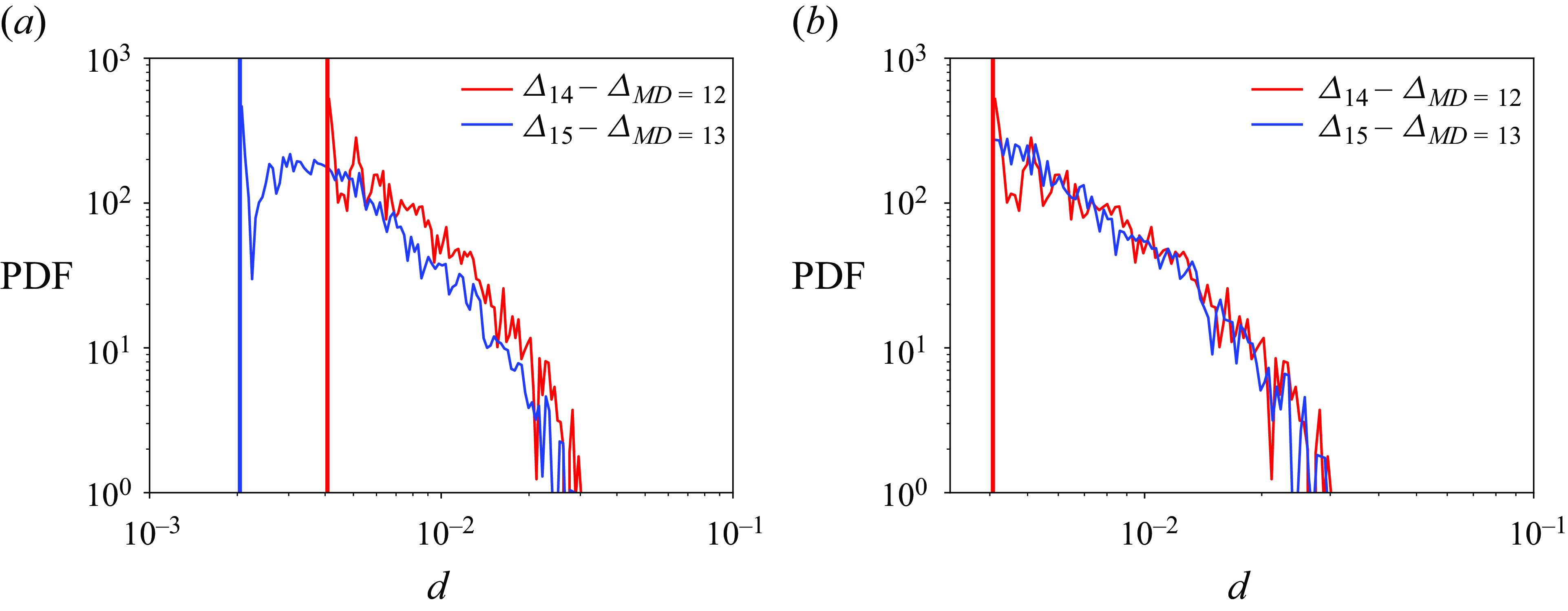
Same as figure 20 but with a linear abcissa and a fit to gamma and log-normal distributions.
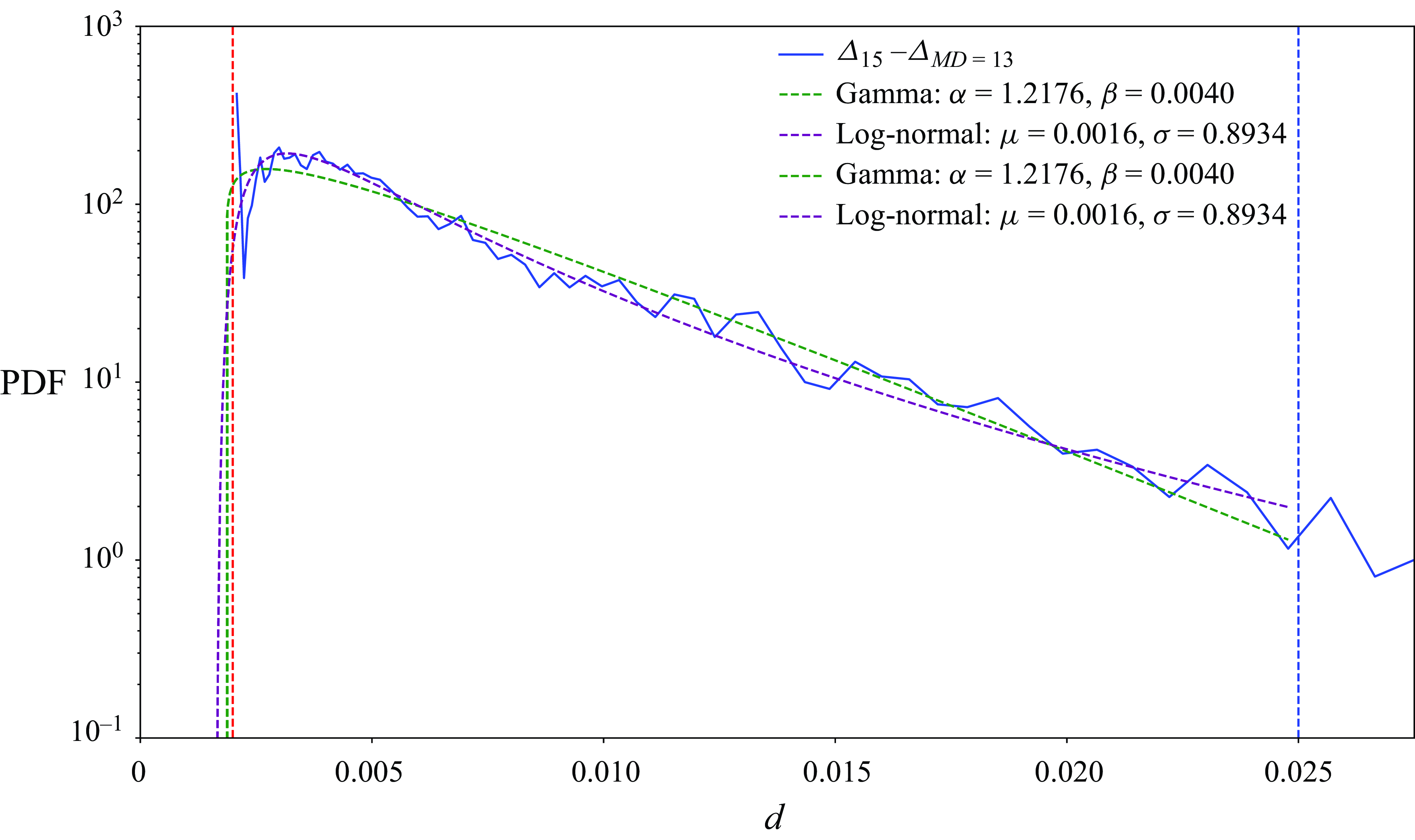
The final result of our manifold-death-enhanced study of droplet sizes is summarised on figure 20. In this figure we select two distributions of droplet sizes at two MD levels, $m=12$
and
$m=12$
and $m=13$
, and we keep the ratio of the grid size to the MD threshold
$m=13$
, and we keep the ratio of the grid size to the MD threshold $h_c/\varDelta _\ell$
constant so the level difference is always
$h_c/\varDelta _\ell$
constant so the level difference is always $\ell - m= 2$
. The two obtained distributions are similar to each other, with a sudden increase in droplet number at the edge of the converged region. Moreover, these plots show that a sufficiently thin grid produces a bump-shaped distribution with a clear maximum (this is the case at
$\ell - m= 2$
. The two obtained distributions are similar to each other, with a sudden increase in droplet number at the edge of the converged region. Moreover, these plots show that a sufficiently thin grid produces a bump-shaped distribution with a clear maximum (this is the case at $m=13$
but not at
$m=13$
but not at $m=12$
). This maximum is located at
$m=12$
). This maximum is located at $d_{\textrm {max}}/D = 4.3 \, 10^{-2}$
in our case. It is interesting to try to understand the origin of this bump. By dimensional analysis the maximum should be expressed as
$d_{\textrm {max}}/D = 4.3 \, 10^{-2}$
in our case. It is interesting to try to understand the origin of this bump. By dimensional analysis the maximum should be expressed as
 \begin{equation} d_{max} = D f(h_c/D,N_1,\ldots, N_n), \end{equation}
where the $N_i$
are the dimensionless numbers of the problem other than
$N_i$
are the dimensionless numbers of the problem other than $h_c/D$
. It is quite tempting to assume that in some range of
$h_c/D$
. It is quite tempting to assume that in some range of $h_c/D$
and of the dimensionless numbers a proportionality relation holds. From the existing data it would be
$h_c/D$
and of the dimensionless numbers a proportionality relation holds. From the existing data it would be
 \begin{equation} d_{max} = 4.3 \, h_c. \end{equation}
We note that this is to our knowledge the only example of a converged bump-shaped (unimodal) distribution in simulations of jet atomisation at a large Weber number. We attempt to fit this bump shape to standard distributions in the literature, namely the gamma and the log-normal. Both distributions are acceptable in the large $d$
range, above 0.005, as seen in figure 21. The fitting distributions are defined as follows:
$d$
range, above 0.005, as seen in figure 21. The fitting distributions are defined as follows:
 \begin{align} \text {Log-normal: } \, P\left ( x ; \mu , \sigma \right ) &= \frac {1}{x \sigma \sqrt {2\pi }} \,\textrm {exp}\left [-\frac {1}{2}\left (\frac {\text {ln}( x) - \mu }{\sigma }\right )^2\right ] \,,\\ \nonumber \text {Gamma: } \, P\left ( x ; \alpha , \beta \right ) &= \frac {\beta ^{\alpha }}{\Gamma (\alpha )} x^{\alpha - 1} \textrm {exp}\left (-\beta x\right ) \,. \end{align}
4. Conclusions
We have studied an atomising, pulsed round jet at a succession of grid sizes with unprecedented resolution. Visual inspection of the resulting interface topology reveals a new numerical phenomenon preceding hole formation in the VOF method: high-frequency curvature oscillations followed by the appearance of a small-scale network of ligaments. While the experimental observation and theoretical analysis of droplet formation by expansion of holes is not new, this is the first time that these high-frequency oscillations of curvature are observed in VOF simulations. The inspection of droplet-size frequency distributions reveals the presence of two large peaks tied to the grid size. It is clear that the small- $d$
peak and probably the second one are related to the unphysical breakup.
$d$
peak and probably the second one are related to the unphysical breakup.
To mitigate this effect, we apply the MD procedure of Chirco et al. (Reference Chirco, Maarek, Popinet and Zaleski2022). The procedure forces hole formation when sheets reach a set thickness $h_c$
. Number frequency plots show convergence in a range of droplet sizes starting at a critical diameter
$h_c$
. Number frequency plots show convergence in a range of droplet sizes starting at a critical diameter $d_c$
. The extent of this converged range increases when either the grid size
$d_c$
. The extent of this converged range increases when either the grid size $\varDelta _\ell$
or the critical thickness
$\varDelta _\ell$
or the critical thickness $h_c$
are decreased. For a fixed
$h_c$
are decreased. For a fixed $h_c$
, when we reduce
$h_c$
, when we reduce $\varDelta _\ell$
, the converged diameter
$\varDelta _\ell$
, the converged diameter $d_c$
approaches the critical thickness
$d_c$
approaches the critical thickness $h_c$
. We thus recover the convergence properties observed by Chirco et al. (Reference Chirco, Maarek, Popinet and Zaleski2022) and by Tang et al. (Reference Tang, Adcock and Mostert2023). We characterise them in the
$h_c$
. We thus recover the convergence properties observed by Chirco et al. (Reference Chirco, Maarek, Popinet and Zaleski2022) and by Tang et al. (Reference Tang, Adcock and Mostert2023). We characterise them in the $h_c$
–
$h_c$
– $d_c$
plot of figure 17(b). We note that the statistical accuracy is much stronger in the present case since our pulsed jet produces three orders of magnitude more droplets than the phase inversion case of Chirco et al. (Reference Chirco, Maarek, Popinet and Zaleski2022). We do not have a definite explanation for the lack of convergence below the diameter
$d_c$
plot of figure 17(b). We note that the statistical accuracy is much stronger in the present case since our pulsed jet produces three orders of magnitude more droplets than the phase inversion case of Chirco et al. (Reference Chirco, Maarek, Popinet and Zaleski2022). We do not have a definite explanation for the lack of convergence below the diameter $h_c$
, that is, we are not sure why
$h_c$
, that is, we are not sure why $d_c$
does not decrease below
$d_c$
does not decrease below $h_c$
as
$h_c$
as $\varDelta _\ell$
is decreased. We can however offer several avenues for improvement of this feature and for future exploration. One is the smoothness of the MD procedure itself and the choice of its parameters such as the number of holes punched or the punching frequency
$\varDelta _\ell$
is decreased. We can however offer several avenues for improvement of this feature and for future exploration. One is the smoothness of the MD procedure itself and the choice of its parameters such as the number of holes punched or the punching frequency $1/\tau _m$
. For the first time in VOF simulations of atomisation, a bump-shaped, converged droplet-size distribution is obtained. Even without convergence, bump-shaped distributions are harder to obtain in VOF simulations than in level-set or diffuse-interface simulations where they are common (Herrmann Reference Herrmann2010; Khanwale et al. Reference Khanwale, Saurabh, Ishii, Sundar and Ganapathysubramanian2022; Saurabh et al. Reference Saurabh, Ishii, Khanwale, Sundar and Ganapathysubramanian2023), because these two other methods tend to ‘evaporate’ small droplets, as shown on figure 1. A scaling relation for the position of the bump is suggested. The bump only appears at the highest level. Whether the proposed scaling (3.6) for the bump would persist if yet more refined simulations are performed is an interesting open question.
$1/\tau _m$
. For the first time in VOF simulations of atomisation, a bump-shaped, converged droplet-size distribution is obtained. Even without convergence, bump-shaped distributions are harder to obtain in VOF simulations than in level-set or diffuse-interface simulations where they are common (Herrmann Reference Herrmann2010; Khanwale et al. Reference Khanwale, Saurabh, Ishii, Sundar and Ganapathysubramanian2022; Saurabh et al. Reference Saurabh, Ishii, Khanwale, Sundar and Ganapathysubramanian2023), because these two other methods tend to ‘evaporate’ small droplets, as shown on figure 1. A scaling relation for the position of the bump is suggested. The bump only appears at the highest level. Whether the proposed scaling (3.6) for the bump would persist if yet more refined simulations are performed is an interesting open question.
Beyond the physics of hole formation and expansion, the simulations reveal a rich spectrum of elementary phenomena that are the building blocks of atomisation. These include networks of well-resolved ligaments in and around holes, ligaments detached from the main liquid core and either aligned or at an angle with it, bubbles trapped in liquid regions, droplets impacting on sheets, etc. This rich physics is seen in increasing detail as grid resolution is increased. For example, the sharpness and apparent realism of the various expanding holes, with attached ligaments or networks of ligaments inside, was not seen in previous simulations, for example, in Ling et al. (Reference Ling, Fuster, Zaleski and Tryggvason2017). Moreover, a large number of each type of object or ‘building block’ are visible at each instant of time, leading to more significant and converged statistics.
A tantalising question is that of the physical, as opposed to numerical, origin of the perforations. We attempt some discussion of this issue in Appendix A. Two types of rate processes for heterogeneous nucleation are postulated, one based on in-sheet germs or nuclei, such as small bubbles, the other on external perturbations such as floating droplets or particles. Our simulations do not allow us to decide at present between these two processes for hole formation. However, they may in the future helpus to understand how to discriminate between them.
Unlike most of the other round-jet simulations in the literature, ours is bimodal and even trimodal after the application of MD. It seems however that a single mode emerges in the converged range of the best resolved MD simulations, indicating that the appearance of a maximum of droplet size well in the converged region is possible only if the physics is correctly captured down to scales much smaller than the integral scales such as the jet diameter $D$
.
$D$
.
Another important characteristic of simulations and experiments are the state of the fluids at the inlet. The primary mixing-layer instability in our simulations is initiated not by upstream turbulence, as in most round-jet simulations in the literature, but by a pulsating flow. In future investigations it would be interesting to compare the visual aspects of the fragmenting interface as well as number distributions and PDFs, between simulations with or without noisy/turbulent inflow conditions.
The other perspectives opened by this work are numerous. Clearly, simulations of comparable quality at a higher Weber number may allow investigation of the ‘fibre-type’ regime observed in many experiments. Currently, our simulations sit on the boundary between membrane type and fibre type. Simulations of comparable resolution should also be performed in the planar mixing-layer case investigated experimentally by the Grenoble group (Ben Rayana et al. Reference Ben Rayana, Cartellier and Hopfinger2006; Fuster et al. Reference Fuster, Matas, Marty, Popinet, Hoepffner, Cartellier and Zaleski2013) and numerically by Jiang & Ling (Reference Jiang and Ling2021). The latter authors performed very high resolution simulations with hole formation and interestingly obtained a bimodal distribution, but they did not apply a controlled perforation scheme as in this paper. Simulations of secondary atomisation, that is, the atomisation of a droplet suddenly plunged in a high-speed flow, has already been performed together with controlled perforation by Tang et al. (Reference Tang, Adcock and Mostert2023) achieving convergence of the PDF. The secondary atomisation case is probably the most promising for an eventual comparison of the distribution of droplet sizes obtained by simulation with the rich experimental data reviewed and modelled, for example, by Jackiw & Ashgriz (Reference Jackiw and Ashgriz2022).
More distant perspectives or more difficult problems remaining to solve are in our opinion twofold. One is clearly the improvement of the MD procedure, to have a better control of the number of holes punched in each thin sheet region, and a smoother manner to ‘cut out’ the initial hole. The breakup frequency and number of attempted breakups were chosen in a rather arbitrary way. These values are too high as shown above. An adequate breakup frequency would correspond to smaller values of $f_b$
and
$f_b$
and $N_b$
. A caveat is however that if the breakup frequency (
$N_b$
. A caveat is however that if the breakup frequency ( $f_b$
,
$f_b$
, $N_b$
) is too low, some bags may escape MD and breakup numerically. An expensive trial-and-error procedure could be attempted to tune the breakup frequency. Another avenue of improvement would be to modify the MD method to perform an analysis of the bag region to identify the connected thin sheet regions. Then a controlled number of perforations could be performed in any of these regions. This controlled number of perforations per thin region could be inspired by experimental observations or by a theory such as the one in Appendix A. A final, intriguing possibility is that if a level-set or diffuse-interface method is used in conjunction with MD, and the frequency is on the low side, numerical breakup will be avoided in the regions that would not be sufficiently perforated because of the low frequency. There would still be mass loss because of the evaporation of thin sheets, but no curvature oscillations nor an excessive number of small droplets scaling with grid size.
$N_b$
) is too low, some bags may escape MD and breakup numerically. An expensive trial-and-error procedure could be attempted to tune the breakup frequency. Another avenue of improvement would be to modify the MD method to perform an analysis of the bag region to identify the connected thin sheet regions. Then a controlled number of perforations could be performed in any of these regions. This controlled number of perforations per thin region could be inspired by experimental observations or by a theory such as the one in Appendix A. A final, intriguing possibility is that if a level-set or diffuse-interface method is used in conjunction with MD, and the frequency is on the low side, numerical breakup will be avoided in the regions that would not be sufficiently perforated because of the low frequency. There would still be mass loss because of the evaporation of thin sheets, but no curvature oscillations nor an excessive number of small droplets scaling with grid size.
Another challenging future task is to use this type of simulation to infer, by careful matching of simulation results and experiments, the physical mechanisms for weak spots and sheet perforations. Given the wide variety of such mechanisms that have been advanced, this is a formidable enterprise for which we hope this paper could provide partial guidance.
Supplementary movies
Supplementary movies are available at https://doi.org/10.1017/jfm.2025.218.
Acknowledgements
We thank Marco Crialesi and Daniel Fuster for fruitful discussions. S.Z. would like to thank Ousmane Kodio for mentionning the Kibble–Zurek theory in discussions on pattern formation.
Funding
This project has received funding from the European Research Council (ERC) under the European Union’s Horizon 2020 research and innovation programme (grant agreement nr 883849). We thank the European PRACE group, the Swiss supercomputing agency CSCS, the French national GENCI supercomputing agency and the relevant supercomputer centers for their grants of CPU time on massively parallel machines, and their teams for assistance and the use of Irene-Rome at TGCC and ADASTRA at CINES. This project was provided in particular with HPC computing and storage resources by GENCI at TGCC thanks to the grants 2023-A0152B14629 and 2022 SS012B15405 on the supercomputer Joliot Curie’s SKL partition.
Declaration of interests
The authors report no conflict of interest.
Appendix A. A phenomenological theory for hole nucleation and expansion
In what follows we describe hole nucleation and expansion as a random process. Its consequences on ligament size are given based on the hole nucleation rate in a manner independent on the exact physical mechanism of nucleation. An analogy between this description and the Kibble–Zurek theory is made.
In atomisation processes, sheet rupture may have several causes. Without deciding between these causes, we distinguish two mathematical forms of the hole forming process (Villermaux Reference Villermaux2020). In one it is in-sheet germs or nuclei, such as small bubbles or small droplets of an immiscible liquid (Vernay et al. Reference Vernay, Ramos, Würger and Ligoure2017) that create the holes. In the other one, external nuclei such as floating droplets, particles or hot puffs are the cause of perforation. The probability of punching a hole per unit area of thin sheet can be written to model both processes as
 \begin{equation} {\mathrm d}\mathcal {P} = \mathcal {A}(h) {\mathrm d}t + \mathcal {B}(h) {\mathrm d}h. \end{equation}
Here $\mathcal {A}(h) {\mathrm d}t$
is the probability that an external object that would be able to punch a hole in a sheet of thickness
$\mathcal {A}(h) {\mathrm d}t$
is the probability that an external object that would be able to punch a hole in a sheet of thickness $h$
actually hits the sheet during the time interval
$h$
actually hits the sheet during the time interval ${\mathrm d}t$
, while
${\mathrm d}t$
, while $\mathcal {B}(h) {\mathrm d}h$
is the probability that an in-sheet heterogeneity is present that will nucleate a hole while the sheet thins from
$\mathcal {B}(h) {\mathrm d}h$
is the probability that an in-sheet heterogeneity is present that will nucleate a hole while the sheet thins from $h$
to
$h$
to $h - {\mathrm d}h$
. In our present study we do not have external objects such as solid particles, but we still have holes appearing due to the drop impact. Thus, in our simulations, the atomisation driven by drop impact is mostly contained in
$h - {\mathrm d}h$
. In our present study we do not have external objects such as solid particles, but we still have holes appearing due to the drop impact. Thus, in our simulations, the atomisation driven by drop impact is mostly contained in $\mathcal {A}(h)$
, while those appearing due to numerical perforation of sheets are contained in
$\mathcal {A}(h)$
, while those appearing due to numerical perforation of sheets are contained in $\mathcal {B}(h)$
. Our simulation captures an overall picture and it is difficult to isolate the effect of any one of the two. In the MD method, we focus on tuning the hole appearance due to the in-sheet heterogeneity part having a simplistic model for
$\mathcal {B}(h)$
. Our simulation captures an overall picture and it is difficult to isolate the effect of any one of the two. In the MD method, we focus on tuning the hole appearance due to the in-sheet heterogeneity part having a simplistic model for $\mathcal {B}(h)$
as a step function with critical size being
$\mathcal {B}(h)$
as a step function with critical size being $h_c$
. However, in fluids, heterogeneities such as bubbles do not have a single size but a distribution of sizes, and correlations obtained experimentally may be obtained that yield
$h_c$
. However, in fluids, heterogeneities such as bubbles do not have a single size but a distribution of sizes, and correlations obtained experimentally may be obtained that yield $n_b(r)$
(Brujan Reference Brujan2010) such that
$n_b(r)$
(Brujan Reference Brujan2010) such that $n_b(r)$
d
$n_b(r)$
d $r$
is the number of bubbles with size between
$r$
is the number of bubbles with size between $r$
and
$r$
and $r+$
d
$r+$
d $r$
per unit volume. The number of bubbles between
$r$
per unit volume. The number of bubbles between $r$
and
$r$
and $2r$
then scales like
$2r$
then scales like $n_b(r) r$
and the average distance between such bubbles is
$n_b(r) r$
and the average distance between such bubbles is $l_1 = [r n_b(r)]^{-1/3}$
. A natural requirement is that this distance between bubbles is much larger than their radius. Then one must have
$l_1 = [r n_b(r)]^{-1/3}$
. A natural requirement is that this distance between bubbles is much larger than their radius. Then one must have $[r n_b(r)]^{-1/3}\gg r$
. Since we probe the distribution at length scales
$[r n_b(r)]^{-1/3}\gg r$
. Since we probe the distribution at length scales $r \sim h$
that are relatively small, it makes sense to require that
$r \sim h$
that are relatively small, it makes sense to require that $n_b(r) \ll r^{-4}$
in the limit of small
$n_b(r) \ll r^{-4}$
in the limit of small $r$
. A simple model for the distribution of nuclei or number of nuclei per unit volume is
$r$
. A simple model for the distribution of nuclei or number of nuclei per unit volume is
 \begin{equation} n_b(r) \sim c_n r^{-\gamma }, \end{equation}
where $\gamma$
is an exponent to be determined by measurement and
$\gamma$
is an exponent to be determined by measurement and $c_n$
is a constant. By the requirement above the exponent
$c_n$
is a constant. By the requirement above the exponent $\gamma \lt 4$
and indeed Gavrilov (Reference Gavrilov1969) found
$\gamma \lt 4$
and indeed Gavrilov (Reference Gavrilov1969) found $\gamma \simeq 3.5$
while measurements by Shima & Sakai (Reference Shima and Sakai1987) give
$\gamma \simeq 3.5$
while measurements by Shima & Sakai (Reference Shima and Sakai1987) give $\gamma$
between
$\gamma$
between $2$
and
$2$
and $4$
. As a result, the volume fraction
$4$
. As a result, the volume fraction $r^4 n_b(r)$
of bubbles between
$r^4 n_b(r)$
of bubbles between $r$
and
$r$
and $2r$
vanishes at small
$2r$
vanishes at small $r$
. Now suppose that bubbles of radius
$r$
. Now suppose that bubbles of radius $r$
are the cause of weak spots in a sheet of thickness
$r$
are the cause of weak spots in a sheet of thickness $r$
. Then from (A.1) the probability of `in-sheet’ nucleation in a region of extent
$r$
. Then from (A.1) the probability of `in-sheet’ nucleation in a region of extent $\lambda ^2$
while the sheet thickness decreases from
$\lambda ^2$
while the sheet thickness decreases from $h$
to
$h$
to $h/2$
scales like
$h/2$
scales like $\mathcal {B}(h) h \lambda ^2$
. This nucleation is caused by small bubbles in the volume
$\mathcal {B}(h) h \lambda ^2$
. This nucleation is caused by small bubbles in the volume $\lambda ^2 h$
then
$\lambda ^2 h$
then $\mathcal {B}(h) h \lambda ^2= n_b(h) \lambda ^2 h^2$
, and the `in-sheet’ nucleation probability per unit area is just
$\mathcal {B}(h) h \lambda ^2= n_b(h) \lambda ^2 h^2$
, and the `in-sheet’ nucleation probability per unit area is just
 \begin{equation} \mathcal {B}(h)= n_b(h) h. \end{equation}
The typical distance $\lambda$
between weak spots in a sheet of size
$\lambda$
between weak spots in a sheet of size $h$
thinning to
$h$
thinning to $h/2$
is given by the condition that the expected number of weak spots in area
$h/2$
is given by the condition that the expected number of weak spots in area $\lambda ^2$
is one, which reads
$\lambda ^2$
is one, which reads
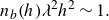 \begin{equation} n_b(h) \lambda ^2 h^2 \sim 1. \end{equation}
Then
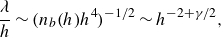 \begin{equation} \frac \lambda h \sim ( n_b(h) h^4 )^{-1/2} \sim h^{-2 + \gamma /2} ,\end{equation}
so for $2 \lt \gamma \lt 4$
, one has
$2 \lt \gamma \lt 4$
, one has $\lambda \gg h$
, while
$\lambda \gg h$
, while $\lambda$
still tends to vanish at small
$\lambda$
still tends to vanish at small $h$
. The distance between holes
$h$
. The distance between holes $\lambda$
is much larger than the thickness of the sheet but is still small compared with the total size of the sheet. We shall call
$\lambda$
is much larger than the thickness of the sheet but is still small compared with the total size of the sheet. We shall call $L$
the total size of the sheet so the above reads
$L$
the total size of the sheet so the above reads $L \gg \lambda$
. In other words, the holes are rather numerous in each sheet.
$L \gg \lambda$
. In other words, the holes are rather numerous in each sheet.
This is not what is observed in experiments, for example, by Kant et al. (Reference Kant, Pairetti, Saade, Popinet, Zaleski and Lohse2023), and one instead seems to see one or two holes per sheet. To resolve this contradiction, one must take into account the speed of expansion of the holes that form during sheet thinning. Indeed, expansion of the holes brings the process of hole formation to a halt after a short time $\tau _1$
that we determine below. We can now give a physical meaning to the critical thickness
$\tau _1$
that we determine below. We can now give a physical meaning to the critical thickness $h_c$
in the MD algorithm. The expected value of the number of nucleations in a thin sheet of area
$h_c$
in the MD algorithm. The expected value of the number of nucleations in a thin sheet of area $L^2$
while the sheet retracts from
$L^2$
while the sheet retracts from $h_c$
to
$h_c$
to $h_c/2$
is
$h_c/2$
is
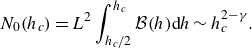 \begin{equation} N_0(h_c) = L^2 \int _{h_c/2}^{h_c} \mathcal {B}(h) {\mathrm d}h \sim h_c^{2 - \gamma }. \end{equation}
The critical thickness $h_c$
is then that for which
$h_c$
is then that for which
 \begin{equation} N_0(h_c) \sim 1 \end{equation}
is of order unity. Independently of the above prediction for $\mathcal {B}(h)$
, and only on the basis of a model where the nucleation probability increases as
$\mathcal {B}(h)$
, and only on the basis of a model where the nucleation probability increases as $h(t)$
decreases, it is possible to predict the effective number of holes that will be observed. First consider the typical size
$h(t)$
decreases, it is possible to predict the effective number of holes that will be observed. First consider the typical size $L(t)$
of an expanding bag. Experimental observations (Opfer et al. Reference Opfer, Roisman, Venzmer, Klostermann and Tropea2014; Kant et al. Reference Kant, Pairetti, Saade, Popinet, Zaleski and Lohse2023) show that bags inflate exponentially. We consider only large-scale bags governed by the large-scale properties of the flow that thus inflate at a rate
$L(t)$
of an expanding bag. Experimental observations (Opfer et al. Reference Opfer, Roisman, Venzmer, Klostermann and Tropea2014; Kant et al. Reference Kant, Pairetti, Saade, Popinet, Zaleski and Lohse2023) show that bags inflate exponentially. We consider only large-scale bags governed by the large-scale properties of the flow that thus inflate at a rate $\omega = 1/(2\tau _c)$
. Then
$\omega = 1/(2\tau _c)$
. Then $L(t) \sim L_0 \exp ( \omega t)$
and the bag thickness decreases as
$L(t) \sim L_0 \exp ( \omega t)$
and the bag thickness decreases as
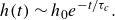 \begin{equation} h(t) \sim h_0 e^{ - t/\tau _c}. \end{equation}
Theory and experimental observations (Villermaux & Bossa Reference Villermaux and Bossa2009; Opfer et al. Reference Opfer, Roisman, Venzmer, Klostermann and Tropea2014; Marcotte & Zaleski Reference Marcotte and Zaleski2019; Kant et al. Reference Kant, Pairetti, Saade, Popinet, Zaleski and Lohse2023) indicate the scaling
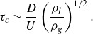 \begin{equation} \tau _c \sim \frac D U \left ( \frac {\rho _l }{\rho _g} \right )^{1/2}. \end{equation}
Once weak spots are activated in such a bag they expand at the Taylor–Culick velocity (Taylor Reference Taylor1959; Culick Reference Culick1960)
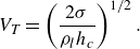 \begin{equation} V_{T} = \left ( \frac {2 \sigma }{\rho _l h_c} \right )^{1/2}. \end{equation}
If $N$
holes are activated in a typical bag of size
$N$
holes are activated in a typical bag of size $L$
, the average distance between hole nuclei positions scales like
$L$
, the average distance between hole nuclei positions scales like $\lambda = L N^{-1/2}$
. This distance is covered by the expanding hole edges in a time
$\lambda = L N^{-1/2}$
. This distance is covered by the expanding hole edges in a time $\tau _1 = \lambda /V_T$
and
$\tau _1 = \lambda /V_T$
and
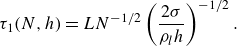 \begin{equation} \tau _1(N,h) = L N^{-1/2} \left ( \frac {2 \sigma }{\rho _l h} \right )^{-1/2}. \end{equation}
We now distinguish between two extreme cases. In the first case $\tau _1(1,h_c) \ll \tau _c$
. This means that after the first hole has formed, it will expand to the whole bag size before the sheet has significantly thinned. During the expansion of that first hole,
$\tau _1(1,h_c) \ll \tau _c$
. This means that after the first hole has formed, it will expand to the whole bag size before the sheet has significantly thinned. During the expansion of that first hole, $h$
will vary from the initial thickness noted
$h$
will vary from the initial thickness noted $h_0$
to
$h_0$
to $h_0 e^{-\tau _1/\tau _c} \simeq h_0 - h_0\tau _1/\tau _c$
and the expected number of other holes that could form during that time is
$h_0 e^{-\tau _1/\tau _c} \simeq h_0 - h_0\tau _1/\tau _c$
and the expected number of other holes that could form during that time is
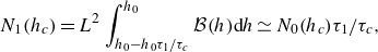 \begin{equation} N_1(h_c) = L^2 \int _{h_0 - h_0\tau _1/\tau _c}^{h_0} \mathcal {B}(h) {\mathrm d}h \simeq N_0(h_c) \tau _1/\tau _c ,\end{equation}
and from (A.7) we obtain $N_1(h_c) \ll 1$
, that is, the expected number of additional holes is much less than one, which means that in practice typically a single hole will be observed. Another way of deriving this result is to say that the hole expansion time is much shorter than the hole nucleation time. In the opposite extreme, the hole expansion time for a single hole is much longer than the hole nucleation time. One then needs to consider the expansion time
$N_1(h_c) \ll 1$
, that is, the expected number of additional holes is much less than one, which means that in practice typically a single hole will be observed. Another way of deriving this result is to say that the hole expansion time is much shorter than the hole nucleation time. In the opposite extreme, the hole expansion time for a single hole is much longer than the hole nucleation time. One then needs to consider the expansion time $ \tau _1(N)$
for a large number of holes
$ \tau _1(N)$
for a large number of holes $N$
. At this point it is useful to borrow an argument from the theory of bifurcations or instabilities in time-varying environments. The Kibble–Zurek theory (Kibble Reference Kibble1976; Zurek Reference Zurek1985) argues that the time scale of the environment variation is equal to the time scale of the growth of the instability. We thus argue that the multi-hole expansion time
$N$
. At this point it is useful to borrow an argument from the theory of bifurcations or instabilities in time-varying environments. The Kibble–Zurek theory (Kibble Reference Kibble1976; Zurek Reference Zurek1985) argues that the time scale of the environment variation is equal to the time scale of the growth of the instability. We thus argue that the multi-hole expansion time $\tau _1(N)$
scales like the characteristic bag expansion time
$\tau _1(N)$
scales like the characteristic bag expansion time $\tau _c$
, that is,
$\tau _c$
, that is,
 \begin{equation} \tau _1(N) = \tau _c. \end{equation}
To obtain this rule, consider how nucleation occurs as time progresses from the first perforation at time $t_0$
to a time where most of the surface is covered by expanded holes. At first the nucleation rate is near the threshold given by (A.7). As time progresses, previously nucleated holes expand and the thickness decreases. The decrease in thickness implies a higher nucleation rate since
$t_0$
to a time where most of the surface is covered by expanded holes. At first the nucleation rate is near the threshold given by (A.7). As time progresses, previously nucleated holes expand and the thickness decreases. The decrease in thickness implies a higher nucleation rate since ${\mathcal B}(h)$
increases as
${\mathcal B}(h)$
increases as $h$
decreases. Hole density increases and the typical distance
$h$
decreases. Hole density increases and the typical distance $\lambda (t)$
between holes decreases. When
$\lambda (t)$
between holes decreases. When $\lambda (t)$
becomes of the same magnitude as the distance covered by the expanding rims, one has
$\lambda (t)$
becomes of the same magnitude as the distance covered by the expanding rims, one has $\lambda (t) \sim V_T (t - t_0)$
and the process stops with
$\lambda (t) \sim V_T (t - t_0)$
and the process stops with $t - t_0 \sim \tau _1(N)$
. Since we are in the second extreme case
$t - t_0 \sim \tau _1(N)$
. Since we are in the second extreme case $N \gg 1$
, the hole density and nucleation rate have increased considerably from that at
$N \gg 1$
, the hole density and nucleation rate have increased considerably from that at $t_0$
, which means that the sheet thickness has decreased significantly. A significant decrease of the sheet thickness requires a time of order
$t_0$
, which means that the sheet thickness has decreased significantly. A significant decrease of the sheet thickness requires a time of order $t-t_0 \sim \tau _c$
, hence, (A.13). Then from the balance of time scales (A.13) the number of holes in a bag of size
$t-t_0 \sim \tau _c$
, hence, (A.13). Then from the balance of time scales (A.13) the number of holes in a bag of size $L$
can be obtained as
$L$
can be obtained as
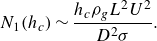 \begin{equation} N_1(h_c) \sim \frac { h_c \rho _g L^2 U^2 }{D^2 \sigma } . \end{equation}
There is a degree of uncertainty for the ratio $L/D$
, however,
$L/D$
, however, $L$
and
$L$
and $D$
are both integral scales of the turbulent flow and can be considered of the same order of magnitude. (We disregard the possible case where eddies of smaller scale than the integral scale of turbulence are sufficiently energetic to generate smaller-scale bags.) The number of holes per bag in this mechanism is then the ratio of two typically large numbers,
$D$
are both integral scales of the turbulent flow and can be considered of the same order of magnitude. (We disregard the possible case where eddies of smaller scale than the integral scale of turbulence are sufficiently energetic to generate smaller-scale bags.) The number of holes per bag in this mechanism is then the ratio of two typically large numbers, $D/h_c$
and
$D/h_c$
and $\textit{We}_g$
. Equation (A.14) is valid in the second extreme case when the right-hand side is much larger than unity. A very rough extrapolation between the two extreme cases is then
$\textit{We}_g$
. Equation (A.14) is valid in the second extreme case when the right-hand side is much larger than unity. A very rough extrapolation between the two extreme cases is then
 \begin{equation} N(h_c) \sim \mathrm {Max} \left [1, N_1(h_c) \right ]. \end{equation}
In most cases one expects $L$
to be of the same order of magnitude as
$L$
to be of the same order of magnitude as $D$
, which leads to the simplified prediction
$D$
, which leads to the simplified prediction
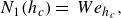 \begin{equation} N_1(h_c) = \ {We}_{h_c}, \end{equation}
where ${We}_l = \rho _g l U^2/\sigma$
. Table 2 gives some typical values for
${We}_l = \rho _g l U^2/\sigma$
. Table 2 gives some typical values for ${We}_{h_c}$
and
${We}_{h_c}$
and ${We}_\varDelta$
, allowing a prediction of the expected number of holes in the corresponding simulations. We note that the estimate above is only based on the assumption that
${We}_\varDelta$
, allowing a prediction of the expected number of holes in the corresponding simulations. We note that the estimate above is only based on the assumption that ${\mathcal B}(h)$
increases as
${\mathcal B}(h)$
increases as $h$
decreases and does not depend on a specific model such as the distribution of bubbles (A.2).
$h$
decreases and does not depend on a specific model such as the distribution of bubbles (A.2).
A more sophisticated model of the number of holes can be obtained as follows. Considering the time $\tau _2(N)$
taken by the rate of nucleation
$\tau _2(N)$
taken by the rate of nucleation ${\mathcal B}(h)$
to increase from the initial rate, producing a single hole
${\mathcal B}(h)$
to increase from the initial rate, producing a single hole $N_0 \sim 1$
, to the final nucleation rate, producing a large density of holes, the final number of holes
$N_0 \sim 1$
, to the final nucleation rate, producing a large density of holes, the final number of holes $N(h_f)$
is given by
$N(h_f)$
is given by
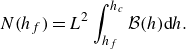 \begin{equation} N(h_f)= L^2 \int _{h_f}^{h_c} \mathcal {B}(h) {\mathrm d}h . \end{equation}
Then
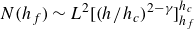 \begin{equation} N(h_f) \sim L^2 [ (h/h_c)^{2-\gamma }]_{h_f}^{h_c} \end{equation}
and
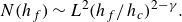 \begin{equation} N(h_f) \sim L^2 (h_f/h_c)^{2-\gamma } . \end{equation}
On the other hand, using (A.8),
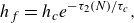 \begin{equation} h_f = h_c e^{-\tau _2(N)/\tau _c} ,\end{equation}
where, for simplicity, we write $N$
for
$N$
for $N(h_f)$
. Hence,
$N(h_f)$
. Hence,
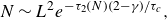 \begin{equation} N \sim L^2 e^{-\tau _2(N) (2-\gamma )/\tau _c} , \end{equation}
and thus,
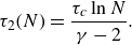 \begin{equation} \tau _2(N) = \frac {\tau _c \ln N}{\gamma -2}. \end{equation}
Here we use again an equality of time scales assumption so that $\tau _1 \sim \tau _2$
and (A.13) becomes
$\tau _1 \sim \tau _2$
and (A.13) becomes
 \begin{equation} \tau _1(N) = \frac {\tau _c \ln N}{\gamma -2}. \end{equation}
This brings a $\gamma$
-dependent and logarithmic correction to the prediction (A.13) and, hence, to (A.14).
$\gamma$
-dependent and logarithmic correction to the prediction (A.13) and, hence, to (A.14).
A schematic view of how expanding holes in a thin sheet merge into ligaments.
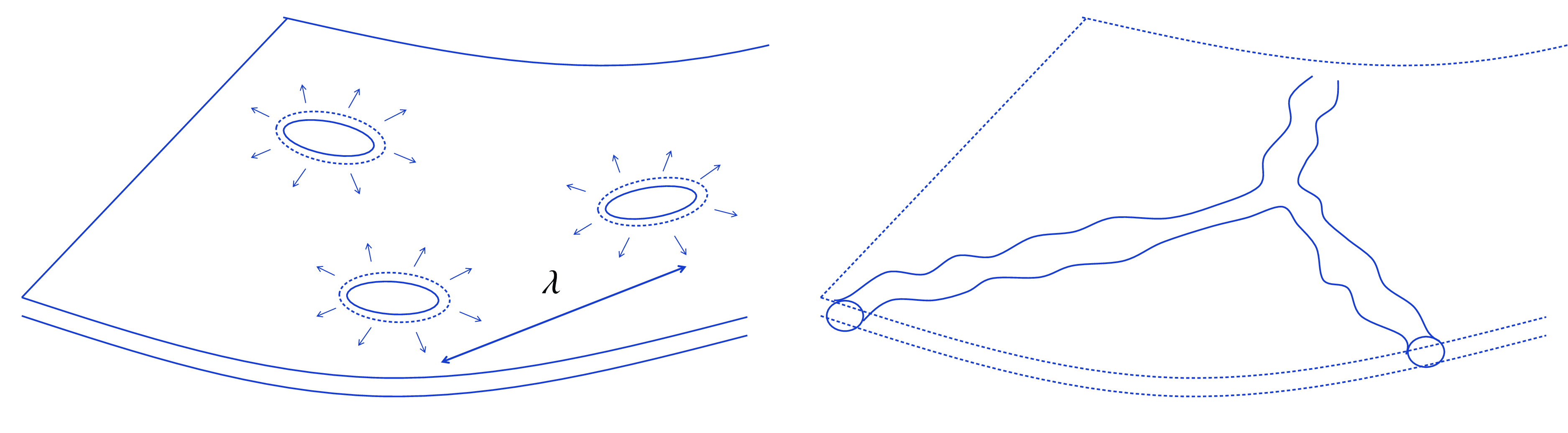
Beyond the number of holes, another interesting prediction is that of the final size of ligaments obtained from hole expansion. There are at least two possible regimes for hole expansion, either unsteady fragmentation or smooth expansion. In the unsteady fragmentation regime the advancing rims bordering the expanding hole continuously shed small droplets (Wang & Bourouiba Reference Wang and Bourouiba2018). In the smooth expansion regime, the rim advances without shedding droplets and volume is conserved. At the end of expansion a network of ligaments of diameter $\delta$
is formed, as schematised in figure 22 and shown numerically by Agbaglah (Reference Agbaglah2021). The number of ligaments is of the same order as the number of holes
$\delta$
is formed, as schematised in figure 22 and shown numerically by Agbaglah (Reference Agbaglah2021). The number of ligaments is of the same order as the number of holes $N$
and their length is of order of the diameter of the hole at the end of expansion
$N$
and their length is of order of the diameter of the hole at the end of expansion $\lambda$
. The volume of ligaments is equal to the initial sheet volume so that equating the initial and final volumes
$\lambda$
. The volume of ligaments is equal to the initial sheet volume so that equating the initial and final volumes
 \begin{equation} N \pi \lambda ^2 h_c / 4 \sim N \pi ^2 \lambda \delta ^2/4, \end{equation}
from which we can deduce the ligament diameter
 \begin{equation} \delta \sim \sqrt {h_c \lambda }. \end{equation}
On the other hand, the number of holes is related to $\lambda$
by
$\lambda$
by
 \begin{equation} N_1 = \frac {L^2}{\lambda ^2}. \end{equation}
Then using (A.14) and (A.26) we obtain
 \begin{equation} \delta \sim h_c^{3/4} L^{1/4} . \end{equation}
It is possible, although this is a purely heuristic guess, that the second peak observed in the simulations with uncontrolled sheet perforation is caused by the breakup of this type of ligament into droplets. To obtain a simple scaling, we consider $L \simeq D$
and
$L \simeq D$
and $h_c \simeq \varDelta$
when sheet perforation is uncontrolled. The Rayleigh–Plateau instability of the ligament will yield
$h_c \simeq \varDelta$
when sheet perforation is uncontrolled. The Rayleigh–Plateau instability of the ligament will yield $d_2 \sim \delta$
for the second peak. One then obtains
$d_2 \sim \delta$
for the second peak. One then obtains
 \begin{equation} \frac {d_2} \varDelta \sim \varDelta ^{-1/4} . \end{equation}
When plotted alongside our numerical data (figure 8 b), a fair agreement is obtained.
Thin structure detection and MD perforation in an example 2-D case. The cells tagged as a thin structure at the MD level are filled with a red colour. The upper image corresponds to the fluid structure right before perforation when a thin sheet is detected and the lower part shows the fluid structure after perforation. Note that the images are atthe same time stamp to explicitly show the perforation process. The image is done for case $(\ell ,m) = (9,8)$
. Adaptive mesh refinement can be seen inthe background.
$(\ell ,m) = (9,8)$
. Adaptive mesh refinement can be seen inthe background.
Appendix B. Grid adaptation
As discussed in the main text, the mesh is adapted dynamically, by splitting the parent cells whenever the local discretisation error estimated by a wavelet approximation exceeds a threshold. This threshold is set at $\epsilon _c = 0.01$
for the error on the volume fraction variable
$\epsilon _c = 0.01$
for the error on the volume fraction variable $c$
and to
$c$
and to $\epsilon _u=0.1$
for the error on the velocity field. To investigate the influence of the relatively large error level on the velocity, we plot the histograms of droplet sizes at various error thresholds in figure 24. In that figure it is seen that although the total number of droplets changes significantly when
$\epsilon _u=0.1$
for the error on the velocity field. To investigate the influence of the relatively large error level on the velocity, we plot the histograms of droplet sizes at various error thresholds in figure 24. In that figure it is seen that although the total number of droplets changes significantly when $\epsilon _u$
decreases from 0.1 to 0.01, the position of the relative maxima and, hence, the typical droplet sizes vary relatively little. It is interesting to illustrate how grid adaptation interacts with ligament detection and perforation in the signature and MD methods. The signature method (Chirco et al. Reference Chirco, Maarek, Popinet and Zaleski2022) typifies the phase distribution with an index
$\epsilon _u$
decreases from 0.1 to 0.01, the position of the relative maxima and, hence, the typical droplet sizes vary relatively little. It is interesting to illustrate how grid adaptation interacts with ligament detection and perforation in the signature and MD methods. The signature method (Chirco et al. Reference Chirco, Maarek, Popinet and Zaleski2022) typifies the phase distribution with an index $i_s$
. This index
$i_s$
. This index $i_s$
is determined by the signature of the quadratic form of Chirco et al. (Reference Chirco, Maarek, Popinet and Zaleski2022). In summary,
$i_s$
is determined by the signature of the quadratic form of Chirco et al. (Reference Chirco, Maarek, Popinet and Zaleski2022). In summary, $i_s$
can take four values. The index
$i_s$
can take four values. The index $i_s=-1$
designates a gas phase, the index
$i_s=-1$
designates a gas phase, the index $i_s = 2$
designates a liquid phase while the index
$i_s = 2$
designates a liquid phase while the index $i_s=0$
designates an interface. The fourth value that the index takes is
$i_s=0$
designates an interface. The fourth value that the index takes is $i_s = 1$
, which designates a thin film region. Note that this detection is performed at the MD level and is later prolonged to the maximum level. Moreover, the thin structure detection procedure acts without affecting the existing mesh refinement. Hence, the mesh refinement is controlled only by the thresholds on the volume fraction and velocity field and in no way depends on the thinsheet detection procedure. We illustrate the process of controlled sheet perforation using the MD method in figure 23. We see that we have detected a thin region (red) in the upper image and a part of this region is eventually punctured in the lower image.
$i_s = 1$
, which designates a thin film region. Note that this detection is performed at the MD level and is later prolonged to the maximum level. Moreover, the thin structure detection procedure acts without affecting the existing mesh refinement. Hence, the mesh refinement is controlled only by the thresholds on the volume fraction and velocity field and in no way depends on the thinsheet detection procedure. We illustrate the process of controlled sheet perforation using the MD method in figure 23. We see that we have detected a thin region (red) in the upper image and a part of this region is eventually punctured in the lower image.
The droplet-size frequency for maximum level $\ell =13$
and no MD at various error thresholds for the velocity.
$\ell =13$
and no MD at various error thresholds for the velocity.
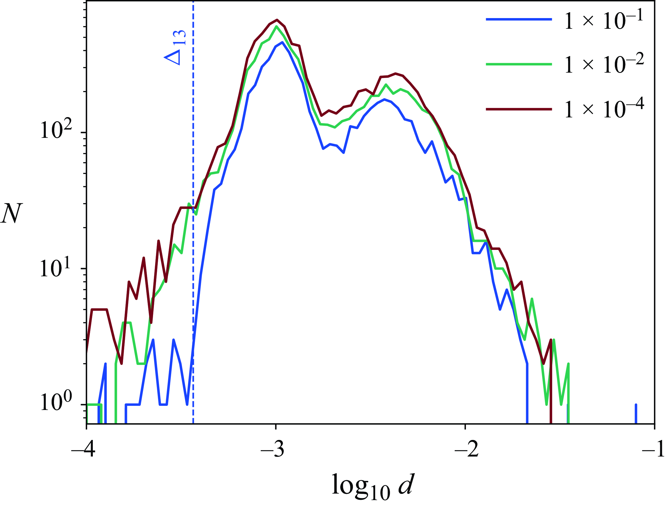
Appendix C. Estimates of the mass loss due to the MD
In the MD method we artificially punch holes in thin structures. This results in some fluid disappearance and, hence, mass loss. Here we give an estimate of the mass loss for the case $(l,m)=(14,13)$
, that is, the simulation corresponding to the red line in figure 16(b). Figure 25(a) shows how the total mass behaves as a function of time. It is a linear rise in time with a tiny sinusoidal pulsation caused by the injection condition. Since we punch holes in these structures every
$(l,m)=(14,13)$
, that is, the simulation corresponding to the red line in figure 16(b). Figure 25(a) shows how the total mass behaves as a function of time. It is a linear rise in time with a tiny sinusoidal pulsation caused by the injection condition. Since we punch holes in these structures every $t {\mathrel {+}=} 0.01$
, a tiny decrease from this linear rise is expected every
$t {\mathrel {+}=} 0.01$
, a tiny decrease from this linear rise is expected every $ {\mathrel {+}=} 0.01$
interval. The inset zoomed at
$ {\mathrel {+}=} 0.01$
interval. The inset zoomed at $t=1.35$
shows this decrease in mass. The decrease is so small that it is not visible on the scale of the outer plot. To quantify this decrease, we calculate two quantities illustrated in the schematic of figure 25(b). The
$t=1.35$
shows this decrease in mass. The decrease is so small that it is not visible on the scale of the outer plot. To quantify this decrease, we calculate two quantities illustrated in the schematic of figure 25(b). The $\Delta M$
is the difference in the total mass at the time stamp just before punching a hole and the time stamp just after punching the hole. The plot as a function of time is shown in figure 25(c), where the
$\Delta M$
is the difference in the total mass at the time stamp just before punching a hole and the time stamp just after punching the hole. The plot as a function of time is shown in figure 25(c), where the $\Delta M$
values are indicated every
$\Delta M$
values are indicated every $t {\mathrel {+}=} 0.01$
. Note that as mass is constantly being injected, this implies that the number of thin structures will increase with time and, hence, the
$t {\mathrel {+}=} 0.01$
. Note that as mass is constantly being injected, this implies that the number of thin structures will increase with time and, hence, the $\Delta M$
is seen increasing with an oscillating behaviour. To get a non-dimensional estimate, we calculate the DIFF defined as
$\Delta M$
is seen increasing with an oscillating behaviour. To get a non-dimensional estimate, we calculate the DIFF defined as
 \begin{equation} DIFF = 2 M(i) - M(i-1) - M(i+1) \end{equation}
(see also the sketch in figure 25 b) and calculate the percentage mass loss as
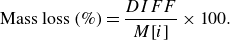 \begin{equation} \text {Mass loss } (\%) = \frac {DIFF}{M[i]} \times 100 . \end{equation}
Estimates of the mass loss with MD performed at levels $(\ell ,m) = (14,13)$
. (a) Total mass as a function of time. Inset shows the tiny droplet at time
$(\ell ,m) = (14,13)$
. (a) Total mass as a function of time. Inset shows the tiny droplet at time $t=1.35$
due to artificial punching of thin structures every
$t=1.35$
due to artificial punching of thin structures every $t {\mathrel {+}=} 0.01$
. (b) Schematic of the data points and the procedure to estimate the mass loss. The value at
$t {\mathrel {+}=} 0.01$
. (b) Schematic of the data points and the procedure to estimate the mass loss. The value at $i$
represents the mass just before punching the holes and the value at
$i$
represents the mass just before punching the holes and the value at $i+1$
represents the value just after punching the holes. Here
$i+1$
represents the value just after punching the holes. Here $\Delta M$
and DIFF are used to do mass loss estimates. Panel (c) shows
$\Delta M$
and DIFF are used to do mass loss estimates. Panel (c) shows $\Delta M$
at every
$\Delta M$
at every $t {\mathrel {+}=} 0.01$
. (d) Mass loss in percentage calculated as
$t {\mathrel {+}=} 0.01$
. (d) Mass loss in percentage calculated as $ ({\text {DIFF}}/{M[i]}) \times 100$
and the red line is the best fit line done for
$ ({\text {DIFF}}/{M[i]}) \times 100$
and the red line is the best fit line done for $t \in (0.8,1.4)$
.
$t \in (0.8,1.4)$
.
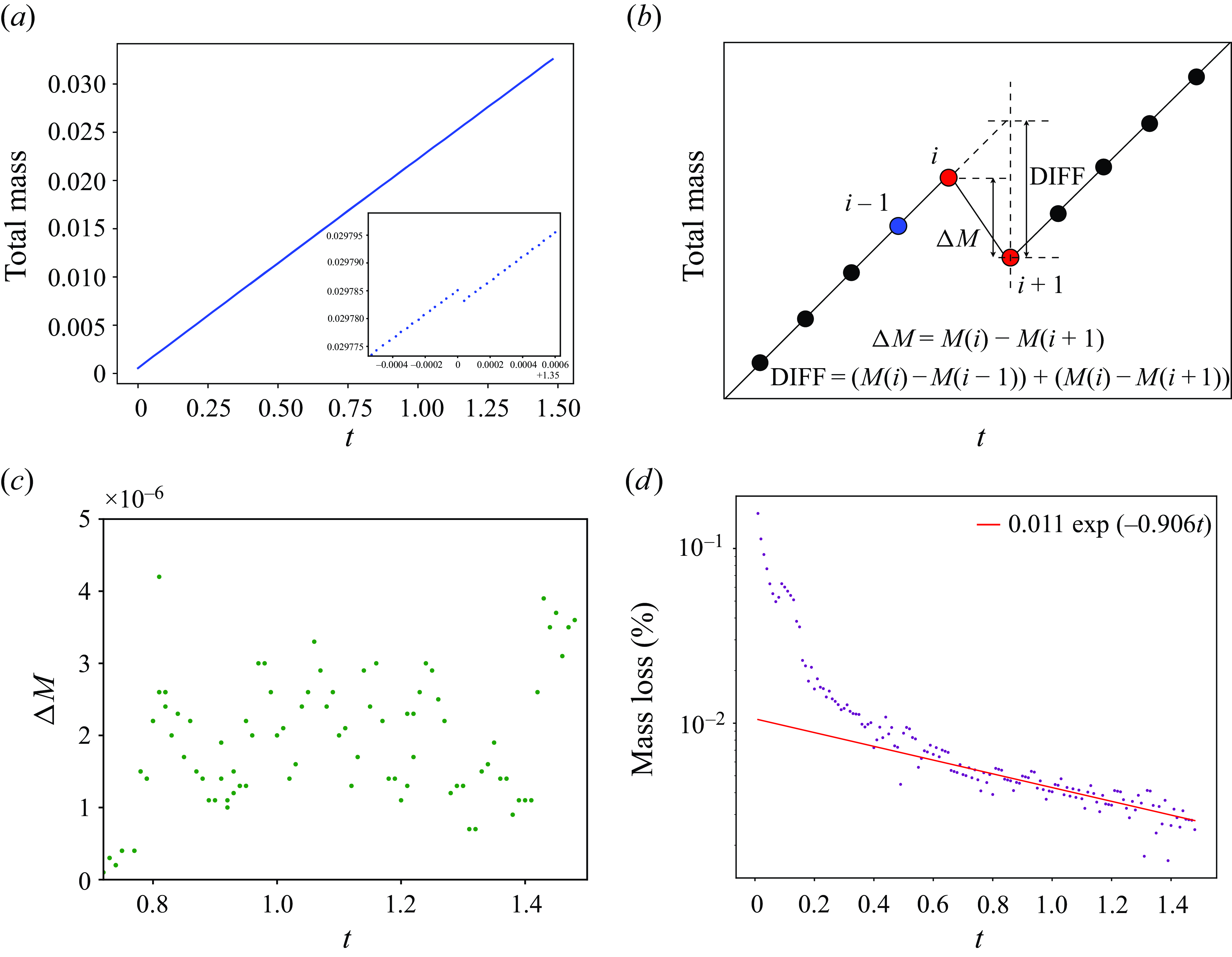
The rationale of using DIFF over $\Delta M$
is that since we are injecting some liquid constantly, we want to estimate how the mass differs not only from the value just before punching holes but from the expected value that it was supposed to have. The percentage loss is shown in figure 22(d), where we can see a decrease in time. We fit an exponential power law of mass loss percentage as
$\Delta M$
is that since we are injecting some liquid constantly, we want to estimate how the mass differs not only from the value just before punching holes but from the expected value that it was supposed to have. The percentage loss is shown in figure 22(d), where we can see a decrease in time. We fit an exponential power law of mass loss percentage as $a\exp {(-bt)}$
and in the steady-state time interval, we see that
$a\exp {(-bt)}$
and in the steady-state time interval, we see that $b \sim \mathcal {O}(1)$
. The mass loss relative to the total mass is going to zero as the jet advances. The question of the effect of the mass loss on the PDF also arises. Since the mass loss occurs in very thin sheets, it affects the very small-scale droplets produced in these sheets and has a negligible effect on the part of the PDF above the converged radius
$b \sim \mathcal {O}(1)$
. The mass loss relative to the total mass is going to zero as the jet advances. The question of the effect of the mass loss on the PDF also arises. Since the mass loss occurs in very thin sheets, it affects the very small-scale droplets produced in these sheets and has a negligible effect on the part of the PDF above the converged radius $d_c$
.
$d_c$
.
Appendix D. Evolving initial mushroom: MD in action
Figure 26 shows the evolution of the initial mushroom jet and the first sheet rupture. Figure 26(a) shows the no-MD case at $\ell = 14$
. We can see in the inset at
$\ell = 14$
. We can see in the inset at $t=0.15$
, numerical sheet rupture happens in the flap connecting the rolled-up mushroom rim with the mushroom head. The inset shows how a spectrum of tiny droplets forms along with a circular ligament rim at
$t=0.15$
, numerical sheet rupture happens in the flap connecting the rolled-up mushroom rim with the mushroom head. The inset shows how a spectrum of tiny droplets forms along with a circular ligament rim at $t=0.17$
. Figure 26(b) shows the first sheet rupture for the case with MD method applied, corresponding to
$t=0.17$
. Figure 26(b) shows the first sheet rupture for the case with MD method applied, corresponding to $(\ell ,m)$
=
$(\ell ,m)$
= $({15,13})$
, and the one corresponding to the blue line in figure 16(b). One can see the sheet rupture at
$({15,13})$
, and the one corresponding to the blue line in figure 16(b). One can see the sheet rupture at $t=0.11$
is much more clear now and the curvature oscillations are not present. In this case too we see detachment of the rolled-up tip in forming a circular ligament at
$t=0.11$
is much more clear now and the curvature oscillations are not present. In this case too we see detachment of the rolled-up tip in forming a circular ligament at $t=0.17$
. Simple analysis suggests that sheet thickness near the tip at the moment of rim formation should scale as
$t=0.17$
. Simple analysis suggests that sheet thickness near the tip at the moment of rim formation should scale as $D/\ {We}_g$
(see, for example, Marcotte & Zaleski Reference Marcotte and Zaleski2019). The condition
$D/\ {We}_g$
(see, for example, Marcotte & Zaleski Reference Marcotte and Zaleski2019). The condition $D/\ {We}_g \gg \varDelta$
is then necessary for proper resolution of the sheet. This condition is equivalent to
$D/\ {We}_g \gg \varDelta$
is then necessary for proper resolution of the sheet. This condition is equivalent to ${We}_\varDelta \gg 1$
, which is verified only for
${We}_\varDelta \gg 1$
, which is verified only for $\ell =15$
and perhaps 14 according to table 2. At lower levels, it is clear that numerical breakup may appear soon behind the rim in no-MD simulations.
$\ell =15$
and perhaps 14 according to table 2. At lower levels, it is clear that numerical breakup may appear soon behind the rim in no-MD simulations.
Evolution of the initial mushroom and the first breakup in (a) no MD and (b) with MD. The interface is coloured by the curvature field in both cases. Image (a) shows a detailed view of the first numerical sheet rupture for an $\ell = 14$
simulation. Image (b) corresponds to the simulation withthe MD method applied corresponding to
$\ell = 14$
simulation. Image (b) corresponds to the simulation withthe MD method applied corresponding to $(\ell ,m) = ({15,13})$
. The images shown in (b) are at time
$(\ell ,m) = ({15,13})$
. The images shown in (b) are at time $t={0.1, \, 0.11, \, 0.12, \, \ldots \, , 0.17.}$
The detachment of a circular ligament rim is seen in both cases at
$t={0.1, \, 0.11, \, 0.12, \, \ldots \, , 0.17.}$
The detachment of a circular ligament rim is seen in both cases at $t=0.17$
.
$t=0.17$
.
Appendix E. Determination of
$d_c$
for MD statistics


The determination of $d_c$
, that is, the diameter marking the lower bound of the converged region is done by visual inspection of the histogram showing the droplet-size distribution. Figure 27 shows a zoom in explaining how we determine
$d_c$
, that is, the diameter marking the lower bound of the converged region is done by visual inspection of the histogram showing the droplet-size distribution. Figure 27 shows a zoom in explaining how we determine $d_c$
for each consecutive level. Note that the black curve in the no-MD case is not overlapping in the converged region of the various MD simulations. This is an important fact since it means that an MD simulation is not ‘equivalent’ to a no-MD simulation with a similar ‘effective’ critical thickness
$d_c$
for each consecutive level. Note that the black curve in the no-MD case is not overlapping in the converged region of the various MD simulations. This is an important fact since it means that an MD simulation is not ‘equivalent’ to a no-MD simulation with a similar ‘effective’ critical thickness $h_c$
. Hence, it makes more sense to compare the MD plots to each other and treat the black no-MD curves only for the purpose of analysing the properties of classical non-converging simulations.
$h_c$
. Hence, it makes more sense to compare the MD plots to each other and treat the black no-MD curves only for the purpose of analysing the properties of classical non-converging simulations.
Appendix F. Forensics of the Chirco et al. (Reference Chirco, Maarek, Popinet and Zaleski2022) study
The MD method appeared first in the work of Chirco et al. (Reference Chirco, Maarek, Popinet and Zaleski2022). Here we revisit this previous study with the droplet-size distribution comparison method described above. In Chirco et al. (Reference Chirco, Maarek, Popinet and Zaleski2022) a region of convergence was identified at $8 \varDelta _9$
, where
$8 \varDelta _9$
, where $\varDelta _9$
was the grid size of the coarsest simulation, also used as the MD level. In our study, we have shown that the region of statistical convergence can be reached up to the critical sheet thickness of the MD threshold
$\varDelta _9$
was the grid size of the coarsest simulation, also used as the MD level. In our study, we have shown that the region of statistical convergence can be reached up to the critical sheet thickness of the MD threshold $h_c$
, given that the mesh is refined sufficiently. In figure 12 of Chirco et al. (Reference Chirco, Maarek, Popinet and Zaleski2022), the authors argue that above
$h_c$
, given that the mesh is refined sufficiently. In figure 12 of Chirco et al. (Reference Chirco, Maarek, Popinet and Zaleski2022), the authors argue that above $d_c = 8\varDelta _{9}$
, the simulations seem to converge, where the coarsest mesh had the equivalent of
$d_c = 8\varDelta _{9}$
, the simulations seem to converge, where the coarsest mesh had the equivalent of $512^3$
cells (
$512^3$
cells ( $\ell =9$
) and the finest mesh was the equivalent of
$\ell =9$
) and the finest mesh was the equivalent of $2048^3$
cells (
$2048^3$
cells ( $\ell =11$
). The case that the authors simulated was a phase inversion case that produces a much smaller number of droplets than our pulsed jet case does. This implies that the number frequencies are affected by a large statistical error. Hence, the conclusions presented in Chirco et al. (Reference Chirco, Maarek, Popinet and Zaleski2022) are qualitative: they demonstrate the rupture of the sheet by MD in a clear manner. To attempt a more quantitative analysis in line with our analysis of the pulsed jet, we replot figure 12 of Chirco et al. (Reference Chirco, Maarek, Popinet and Zaleski2022) in our figure 28. There we mark the MD threshold
$\ell =11$
). The case that the authors simulated was a phase inversion case that produces a much smaller number of droplets than our pulsed jet case does. This implies that the number frequencies are affected by a large statistical error. Hence, the conclusions presented in Chirco et al. (Reference Chirco, Maarek, Popinet and Zaleski2022) are qualitative: they demonstrate the rupture of the sheet by MD in a clear manner. To attempt a more quantitative analysis in line with our analysis of the pulsed jet, we replot figure 12 of Chirco et al. (Reference Chirco, Maarek, Popinet and Zaleski2022) in our figure 28. There we mark the MD threshold $h_c = 3\varDelta _{9}$
and two values of
$h_c = 3\varDelta _{9}$
and two values of $d_c$
. We see that
$d_c$
. We see that $d_c$
again moves towards
$d_c$
again moves towards $h_c$
. This movement is in line with our results. Due to computational cost, Chirco et al. (Reference Chirco, Maarek, Popinet and Zaleski2022) stopped at the
$h_c$
. This movement is in line with our results. Due to computational cost, Chirco et al. (Reference Chirco, Maarek, Popinet and Zaleski2022) stopped at the $2048^3$
mesh and concluded that the boundary of the converged region lies at
$2048^3$
mesh and concluded that the boundary of the converged region lies at $d_c \sim 8 \varDelta _{9}$
. It is likely that the converged region could be pushed more towards
$d_c \sim 8 \varDelta _{9}$
. It is likely that the converged region could be pushed more towards $h_c$
with increased resolution.
$h_c$
with increased resolution.
Replotting figure 12 of Chirco et al. (Reference Chirco, Maarek, Popinet and Zaleski2022) with additional vertical lines showing the critical thickness for MD sheet perforation threshold $h_c$
, along with two vertical lines for
$h_c$
, along with two vertical lines for $d_c$
. The shaded regions illustrate the departure of the measured distribution from each other below
$d_c$
. The shaded regions illustrate the departure of the measured distribution from each other below $d_c$
.
$d_c$
.
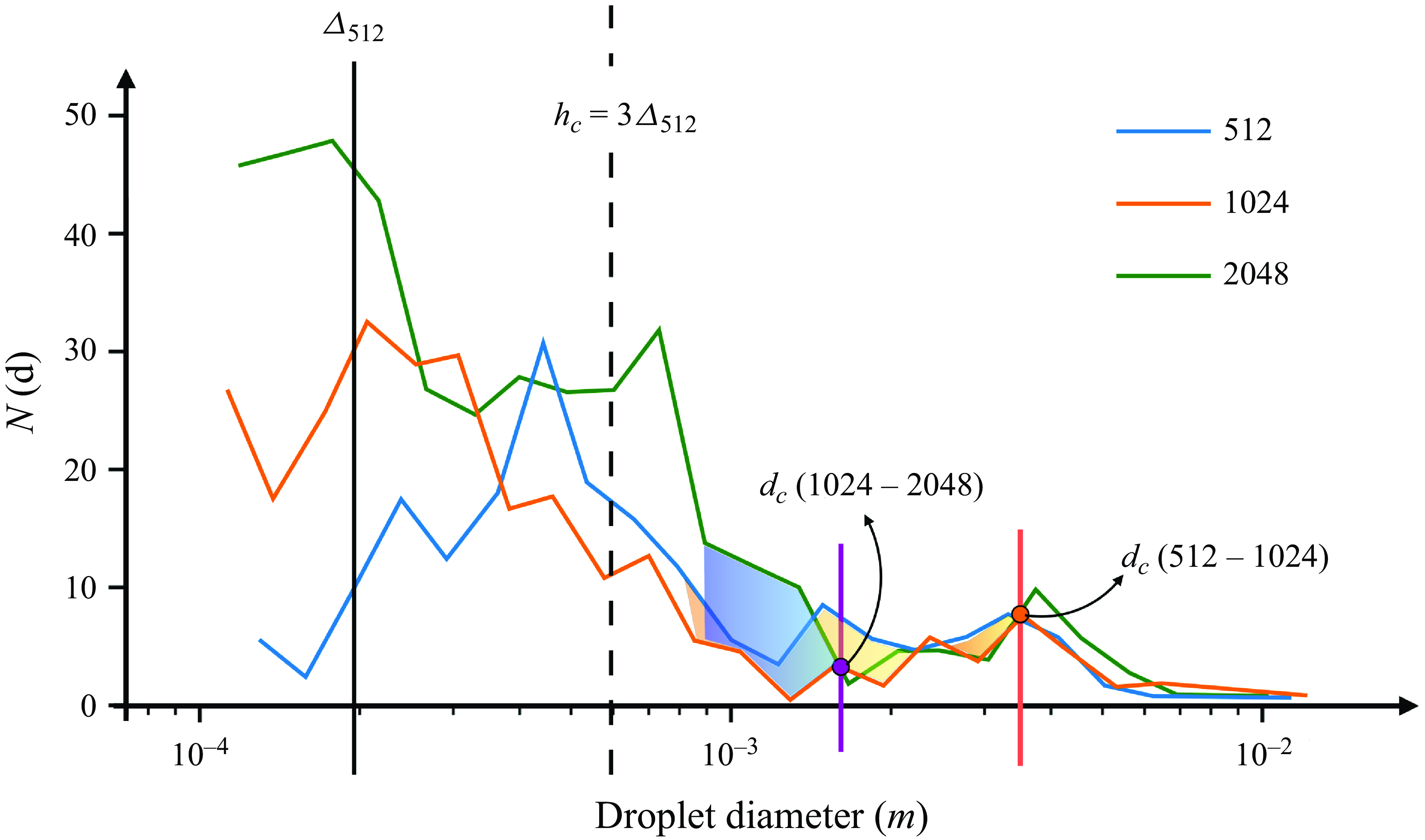


 Open access