1. Introduction
State estimation and localization in unknown environments have emerged as critical research areas in mobile robotics, with Simultaneous Localization and Mapping (SLAM) being one of the most prominent topics. Based on the types of sensors used, contemporary SLAM systems are mainly categorized into laser SLAM, visual SLAM [Reference Zhang, Dong, Guo, Ye, Gao, Xiang, Chen and Wu1], and multi-sensor fusion SLAM [Reference Hu, Zhou, Miao, Yuan and Liu2] technologies, which integrate laser or vision sensors with additional sensory modalities. Visual SLAM, which relies on cameras as the primary sensors, is particularly popular among researchers due to its ability to capture rich information, a lightweight design, and cost-effectiveness. However, visual SLAM systems require processing large amounts of image data, and its performance is limited by the camera’s sensitivity to lighting conditions and its inability to directly measure distances. Consequently, these systems may fail in low-light environments, exhibit reduced accuracy, and face challenges in maintaining real-time performance [Reference Mur-Artal, Montiel and Tardos3–Reference Zhu, Zheng, Yuan, Huang and Hong6]. Laser SLAM [Reference Liang, Zhao, Wang and Chen7], which primarily employs LiDAR sensors, effectively addresses these limitations. LiDAR sensors enable direct distance measurements, facilitating more accurate environmental perception and capturing spatial information about object geometries to construct high-fidelity maps for precise localization [Reference Fasiolo, Scalera and Maset8]. This inherent capability confers enhanced reliability and stability to SLAM operations, making laser SLAM widely adopted in applications such as indoor navigation [Reference Deshmukh, Hasamnis, Kulkarni and Bhaiyya9], 3D reconstruction, and autonomous driving.
Solid-state LiDARs have garnered growing attention owing to their high performance, reliability, and cost-effectiveness, with the potential to substantially advance and reshape the robotics industry. However, in indoor environments characterized by narrow spaces and thin walls, or in scenarios involving sharp turns, the constrained horizontal FoV of solid-state LiDARs exacerbates LiDAR degeneracy (see [Reference Zhou, Koppel and Kaess10–Reference Ye, Chen and Liu13]). In this work, we define a “small FoV” as a horizontal or effective field of view constrained to
 $90^\circ$
or less, in contrast to the
$90^\circ$
or less, in contrast to the
 $360^\circ$
panoramic coverage of standard mechanical LiDARs. As an example, the Livox Mid-70 employed here offers an effective FoV of
$360^\circ$
panoramic coverage of standard mechanical LiDARs. As an example, the Livox Mid-70 employed here offers an effective FoV of
 $70.4^\circ$
. This restricted angular range is highly susceptible to degeneracy, particularly in feature-sparse environments. Lin et al. [Reference Lin and Zhang14] developed a comprehensive LOAM algorithm for solid-state LiDARs, enhancing the accuracy and robustness of small-FoV LiDARs, yet their work neglecting research into degeneracy issues specific to such a system. Zhong et al. [Reference Zhong, Huang, Zhang, Wen and Hsu15] mitigated map-matching failures for small-FoV LiDARs by fusing an inertial measurement unit (IMU) with solid-state LiDARs (SSLs), leveraging IMU data to provide a coarse yet high-frequency initial guess for map matching; nonetheless, their tests were conducted outdoors, which exhibits richer feature distributions compared to indoor environments. Zheng et al. [Reference Zheng and Zhu16] proposed an efficient continuous-time LiDAR odometry method, adopting a filter-based point-to-plane Gaussian mixture model for robust registration and achieving successful mapping; however, this method solely utilized extracted LiDAR data and failed to address the issue of LiDAR degeneracy.
$70.4^\circ$
. This restricted angular range is highly susceptible to degeneracy, particularly in feature-sparse environments. Lin et al. [Reference Lin and Zhang14] developed a comprehensive LOAM algorithm for solid-state LiDARs, enhancing the accuracy and robustness of small-FoV LiDARs, yet their work neglecting research into degeneracy issues specific to such a system. Zhong et al. [Reference Zhong, Huang, Zhang, Wen and Hsu15] mitigated map-matching failures for small-FoV LiDARs by fusing an inertial measurement unit (IMU) with solid-state LiDARs (SSLs), leveraging IMU data to provide a coarse yet high-frequency initial guess for map matching; nonetheless, their tests were conducted outdoors, which exhibits richer feature distributions compared to indoor environments. Zheng et al. [Reference Zheng and Zhu16] proposed an efficient continuous-time LiDAR odometry method, adopting a filter-based point-to-plane Gaussian mixture model for robust registration and achieving successful mapping; however, this method solely utilized extracted LiDAR data and failed to address the issue of LiDAR degeneracy.
The present paper proposes the use of artificial landmarks to address the issue of mapping failures caused by degradation in indoor environments when deploying small field-of-view LiDARs. The contributions of this paper are listed as follows:
-
1. We propose integrating the extracted reflector feature residuals into the LOAM framework and fusing wheel odometry predictions, reflector observations, and LOAM-derived measurements via an EKF to construct submaps. This approach effectively mitigates the adverse effects of LiDAR degradation on mapping performance, which often arises from insufficient feature information in narrow corridors.
-
2. We introduce a LiDAR scan-based keyframe selection method for fine-grained matching, leveraging CostMap-based multilateration to provide an initial pose estimate and a target submap. This strategy accelerates the scan-to-map matching process and robustly establishes constraint relationships.
-
3. We develop a 3D SLAM system that incorporates multilateration-based loop closure detection. By leveraging a mobile robot platform equipped with LiDAR sensors and spatially distributed artificial landmarks, the system accurately estimates the robot’s trajectory and effectively identifies loop closures, thereby yielding a globally consistent map. Our source code is available at https://github.com/shadowing207/ALLOAM.
2. Relate work
2.1. 3D LiDAR odometry
In 3D LiDAR SLAM, point cloud registration is performed to estimate pose changes, thereby achieving accurate localization. In the early days, the primary methods for point cloud registration were based on the Iterative Closest Point algorithm [Reference Besl and McKay17], Normal Iterative Closest Point algorithm [Reference Serafin and Grisetti18], and Normal Distributions Transform algorithm [Reference Takeuchi and Takashi Tsubouchi19]. In recent years, research has increasingly shifted to feature-based matching algorithms. Feature-based LiDAR odometry has been widely adopted in mainstream SLAM frameworks, significantly reducing matching time and thereby ensuring real-time system performance.
In 2014, Zhang et al. [Reference Zhang and Singh20] proposed the LOAM algorithm, which significantly advanced the development of 3D LiDAR SLAM. The algorithm innovatively identifies edge and planar points based on curvature-magnitude thresholds, rather than matching the entire LiDAR point cloud. Jiao et al. [Reference Jiao, Ye, Zhu and Liu21] proposed the M-LOAM algorithm for a multi-LiDAR sensor system to improve the robot’s environmental perception. In this approach, each LiDAR sensor processes the data independently before combining the features for further mapping. In addition, the experiments were conducted using multi-line LiDAR, which provides richer information compared to solid-state LiDAR.
Degeneracy remains a critical challenge in LiDAR SLAM, stemming from insufficient constraints on the robot’s state. This issue is particularly pronounced for solid-state LiDARs with a small horizontal FoV, such as when a robot navigates long, narrow indoor corridors.
Li et al. [Reference Li, Tian, Shen and Lu22] proposed a novel feature extraction method that leverages both geometry and intensity to address the degradation problem. To fully utilize the extracted features, dual-weighting functions are developed for planar and edge points, respectively, during the attitude optimization process. However, the method still exhibits susceptibility to failure when dealing with areas where features cannot be extracted based on intensity alone. Ma et al. [Reference Ma, Xu, Yuan, Zhi, Yu, Zhou and Xie23] proposed a map-building algorithm, MM-LINS, for addressing LiDAR degradation problems, but if there is minimal overlap in point clouds, the accuracy of map fusion will be significantly reduced. As concluded in [Reference Jiao, Zhu, Ye, Huang, Yun, Jiang, Wang and Liu24], actively selecting a subset of features greatly enhances the accuracy and efficiency of a LiDAR SLAM system and proves effective in addressing degeneracy. Burnett et al. [Reference Burnett, Schoellig and Barfoot25] demonstrated that incorporating an IMU into LiDAR odometry improves localization in geometrically degenerate environments. This also contributes to the advancement of semantic SLAM [Reference Chen, Milioto, Palazzolo, Giguere, Behley and Stachniss26–Reference Chen, Wang, Wang, Deng, Wang and Zhang28], where semantic information is extracted to enhance the understanding of the environment, helping to address challenges in degraded conditions. Liu et al. [Reference Liu and Zhang29] proposed a novel adaptive voxelization method to support LiDAR bundle adjustment (BA). These BA and optimization methods were further incorporated into a LOAM framework, termed BALM (Bundle Adjustment for LiDAR Mapping), to serve as a back-end for map refinement. However, the algorithm requires a good initial pose, and its performance is sensitive to any degeneracy during mapping.
2.2. Loop closure detection
The loop closure detection module is critical for reducing accumulated errors and improving mapping accuracy, especially in long-term or large-scale SLAM systems with multiple loops. By matching geometric similarities between LiDAR frames, it identifies loop closures via point cloud scan matching. Given the high dimensionality and structural sparsity of raw point clouds, feature extraction techniques compress dense data into sparse discriminative representations, enhancing detection efficiency and robustness.
Belongie et al. [Reference Belongie, Malik and Puzicha30] proposed the Shape Context algorithm, which encodes the shape of the point cloud around local feature points into an image, specifically targeting the characteristics of LiDAR data. However, this algorithm requires a large amount of point cloud data. Therefore, the point cloud to be matched must be larger than the reference point cloud; otherwise, mismatches may occur. A vehicle-mounted LiDAR system, which typically operates at a fixed frequency, frequently demonstrates an inability to supply sufficient data volume to satisfy the requirements of this algorithm. Behley et al. [Reference Behley and Stachniss31] proposed the SuMa method, which was the first to employ Surfel maps to efficiently generate projection data associations and achieve loop closure detection using only LiDAR data. He et al. [Reference He, Wang and Zhang32] have proposed M2DP, which projects raw point clouds onto several 2D planes and forms signatures based on descriptors from distinct planes. Kim et al. [Reference Kim and Kim33] introduced the scan context method, which is a non-histogram-based global descriptor that divides each point cloud frame into several regions, selects representative points, and stores them in a two-dimensional array. The advantage of the scan context algorithm lies in its low computational complexity and high robustness, making it suitable for handling real-world challenges such as varying viewpoints, noise, and partial occlusions, thereby enabling efficient loop closure detection in large-scale environments. However, during the encoding process, it records only the highest point in the height direction of the point cloud, leaving room for further improvement. Scan Context++ [Reference Kim, Choi and Kim34] is an improved version of scan context that introduces translation invariance in addition to the existing rotational invariance, thereby enhancing its speed. In 2020, Wang et al. [Reference Wang, Sun, Xu, Sarma, Yang and Kong35] proposed LiDAR Iris, which uses a globally invariant descriptor with rotational invariance. By extracting binary features using the LoG-Gabor filter, a binary-encoded Iris image is generated, making full use of most of the point cloud information. This global descriptor also possesses rotational invariance, avoiding brute-force search and thereby conserving computational resources. This method enables the establishment of globally consistent maps in large-scale environments based solely on LiDAR point clouds. Zhang et al. [Reference Zhang, Wang and Wu36] proposed a novel neural network architecture called VPD-Map, which utilizes visual point clouds to generate global 3D visual descriptors for fast loop closure detection and also provides prior information for feature maps in front-end pose estimation.
Using LiDAR odometry, we register scans to build submaps and extract artificial landmark ROIs. A CostMap-multilateration system enhances loop closure detection accuracy while providing coarse inter-submap matches. Keyframes are selected from submaps based on their contribution to artificial landmark ROIs, establishing submap constraints via scan-to-map registration for fine matching. Back-end optimization then minimizes submap errors, generating a globally consistent map.

3. System design
The primary objective of this paper is to address the SLAM problem for a small-FoV 3D solid-state LiDAR. Our framework comprises three main components: front-end submap construction, inter-submap constraints (i.e., loop detection), and back-end optimization through a multi-submap constraint graph. In the back-end stage, the robot’s pose is iteratively adjusted based on these constraints to ensure the global consistency of the map. The proposed framework’s overall process is illustrated in Figure 1.
In the front-end submap construction phase, our framework first performs extrinsic LiDAR calibration to align the coordinate systems of the LiDAR and the robot body, ensuring data fusion consistency. It then constructs submaps by integrating the EKF algorithm. For loop closure detection, artificial landmarks are first extracted within the submaps. Loop closure is then detected using the CostMap-Multilateration algorithm, which provides an initial coarse registration. Finally, back-end optimization is achieved by obtaining inter-submap constraints through fine matching and integrating them into a pose graph for optimization, thus ensuring the global consistency of the map.
3.1. Extrinsic LiDAR calibration
Inspired by [Reference Censi, Franchi, Marchionni and Oriolo37], we extend the research to 3D LiDAR calibration in feature-rich areas. By obtaining the wheel diameter and track width from CAD drawings, we simplify the process, reducing the calibration to only the LiDAR’s external parameters
 $\ell = (x, y, z, rx, ry, rz)^T$
. Since the LiDAR is horizontally mounted, we focus on calibrating
$\ell = (x, y, z, rx, ry, rz)^T$
. Since the LiDAR is horizontally mounted, we focus on calibrating
 $x, y, rz$
. Let
$x, y, rz$
. Let
 $SE(3)$
be the special Euclidean group, and
$SE(3)$
be the special Euclidean group, and
 $q = (q_x, q_y, q_z, q_{rx}, q_{ry}, q_{rz}) \in SE(3)$
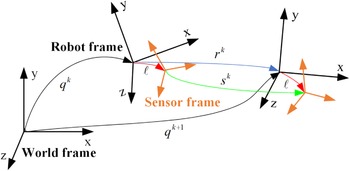
represent the robot pose. As shown in Figure 2, the transformation between the wheel odometry and the LiDAR in the global coordinate system is:
$q = (q_x, q_y, q_z, q_{rx}, q_{ry}, q_{rz}) \in SE(3)$
represent the robot pose. As shown in Figure 2, the transformation between the wheel odometry and the LiDAR in the global coordinate system is:
 \begin{equation} s^k = \ell ^{-1} \cdot r^k \cdot \ell \end{equation}
where
 $s^k$
and
$s^k$
and
 $r^k$
are the pose changes of the laser frame and odometry from
$r^k$
are the pose changes of the laser frame and odometry from
 $t$
to
$t$
to
 $t+1$
, respectively.
$t+1$
, respectively.
The robot pose is
 $q_k \in \text{SE}(3)$
with respect to the world frame; the sensor pose is
$q_k \in \text{SE}(3)$
with respect to the world frame; the sensor pose is
 $\ell \in \text{SE}(3)$
with respect to the robot frame;
$\ell \in \text{SE}(3)$
with respect to the robot frame;
 $r_k \in \text{SE}(3)$
is the robot displacement between poses; and
$r_k \in \text{SE}(3)$
is the robot displacement between poses; and
 $s_k \in \text{SE}(3)$
is the displacement seen by the sensor in its own reference frame.
$s_k \in \text{SE}(3)$
is the displacement seen by the sensor in its own reference frame.

As the equation is unsolvable during straight-line motion, we calibrate by rotating along an arc. We design the loss function in Eq. (2) and use gradient descent to solve for
 $\ell$
:
$\ell$
:
 \begin{equation} \ell ^{*} = \arg \min _{\ell } \sum _{i \in C} \hat {s}^i - (\ell ^{-1} \cdot \hat {r}^i \cdot \ell ) \end{equation}
Artificial landmark point cloud obtained by light intensity thresholding.

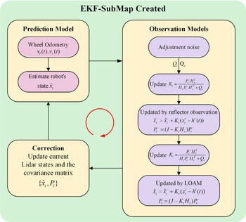
3.2. EKF-submap construction
The detection of artificial landmarks
 $z_t^r$
at time
$z_t^r$
at time
 $t$
is implemented through the following components: first, the artificial landmarks are created by applying high-reflection film on the objects (in this paper, the reflector film is applied on the cylinders), which can be easily distinguished from external objects by the level of light intensity, as shown in Figure 3.
$t$
is implemented through the following components: first, the artificial landmarks are created by applying high-reflection film on the objects (in this paper, the reflector film is applied on the cylinders), which can be easily distinguished from external objects by the level of light intensity, as shown in Figure 3.
We denote the laser points that hit a reflector as
 $S = \{ S_i (x_i, y_i, z_i, f_i) \mid i \in \{ 1, 2, \ldots , n \} \}$
, where the artificial landmark is a cylindrical object with a known radius
$S = \{ S_i (x_i, y_i, z_i, f_i) \mid i \in \{ 1, 2, \ldots , n \} \}$
, where the artificial landmark is a cylindrical object with a known radius
 $R$
. Given that the mobile platform operates in real time on the same horizontal plane, the position of the artificial landmark along the Z-axis is disregarded, and only its planar coordinates are calculated within the search window
$R$
. Given that the mobile platform operates in real time on the same horizontal plane, the position of the artificial landmark along the Z-axis is disregarded, and only its planar coordinates are calculated within the search window
 $W = \{ (x_{\text{min}}, y_{\text{min}}), (x_{\text{max}}, y_{\text{max}}) \}$
. The search is conducted in step increments of
$W = \{ (x_{\text{min}}, y_{\text{min}}), (x_{\text{max}}, y_{\text{max}}) \}$
. The search is conducted in step increments of
 $\delta _{\text{step}}$
, ultimately determining the optimal center position of the landmark
$\delta _{\text{step}}$
, ultimately determining the optimal center position of the landmark
 $z_t^r(z_x, z_y)$
. The calculation is provided in Eq. (3).
$z_t^r(z_x, z_y)$
. The calculation is provided in Eq. (3).
 \begin{equation} \begin{cases} (z_x, z_y) = \arg \min \sum _{w \in W} Dis_w \\ Dis_w = \left(n*R^2 -\sum _{i=0}^{n}(w_x-x_i)^2+(w_y-y_i)^2\right) \end{cases} \end{equation}
The submap construction framework is derived from LiDAR odometry. We propose leveraging artificial landmarks to construct precise submaps. In LOAM, high-reflectivity objects are typically filtered out because LiDAR measurements exhibit reduced accuracy when encountering high-reflection surfaces [Reference Lin and Zhang14]. However, this study posits that even in degenerate environments, these high-intensity objects with marginally degraded precision can still provide coarse pose estimation, thereby potentially alleviating degradation scenarios. To address this, we propose integrating artificial landmark feature points into the pose optimization process. Specifically, we establish data associations between odometry predictions and retro-reflector pillars in the map. Let
 $S_k$
denote the point cloud cluster of an artificial landmark observed in the current frame, and let
$S_k$
denote the point cloud cluster of an artificial landmark observed in the current frame, and let
 $L_m$
represent the corresponding retro-reflector pillar center in the map. For each point in
$L_m$
represent the corresponding retro-reflector pillar center in the map. For each point in
 $S_k$
, its distance to the associated pillar center
$S_k$
, its distance to the associated pillar center
 $L_m$
should theoretically equal the pillar radius
$L_m$
should theoretically equal the pillar radius
 $R$
.
$R$
.
 \begin{equation} p_w = R_kp_l+t_k \end{equation}
where
 $(R_k, t_k)$
is the LiDAR pose when the last point in the current frame is sampled and needs to be determined by the pose optimization. The corresponding point-to-point residual is then computed according to Eq. (5) and incorporated into the pose optimization problem.
$(R_k, t_k)$
is the LiDAR pose when the last point in the current frame is sampled and needs to be determined by the pose optimization. The corresponding point-to-point residual is then computed according to Eq. (5) and incorporated into the pose optimization problem.
 \begin{equation} r_{p2p}(p_w) = ||p_w - L_m|| - R \end{equation}
After obtaining the pose estimation from LOAM, we construct a traditional EKF framework. The detailed algorithmic procedure is outlined in Figure 4, which consists of three main steps: prediction, observation, and correction. First, state prediction is performed using the left and right wheel speeds
 $v_l(t)$
and
$v_l(t)$
and
 $v_r(t)$
at time
$v_r(t)$
at time
 $t$
. Subsequently, process noise
$t$
. Subsequently, process noise
 $Q_r$
and
$Q_r$
and
 $Q_l$
are introduced, and the Kalman gain
$Q_l$
are introduced, and the Kalman gain
 $K_t$
is updated to process sensor observations collected from artificial landmarks and the LOAM system to optimize the state estimation.
$K_t$
is updated to process sensor observations collected from artificial landmarks and the LOAM system to optimize the state estimation.
Workflow for EKF-based submap creation.

First, the robot’s initial pose for the new submap in the global coordinate system is given by
 $M_i^G = M_{i-1}^G \oplus T^i_{i-1}$
, where
$M_i^G = M_{i-1}^G \oplus T^i_{i-1}$
, where
 $M_{i-1}^G$
is the previous submap’s pose in the global coordinate system, and
$M_{i-1}^G$
is the previous submap’s pose in the global coordinate system, and
 $T^i_{i-1}$
is the alignment transformation between the new submap
$T^i_{i-1}$
is the alignment transformation between the new submap
 $M_i$
and the previous submap
$M_i$
and the previous submap
 $M_{i-1}$
.
$M_{i-1}$
.
The new submap is then initialized with
 $M_0^G = (0, 0, 0, 0, 0, 0)^T$
. To balance the time required for submap updates and the accuracy of submaps, a new submap is initialized when either the number of observations processed in the submap reaches a certain threshold or a large error occurs between the observations and predictions.
$M_0^G = (0, 0, 0, 0, 0, 0)^T$
. To balance the time required for submap updates and the accuracy of submaps, a new submap is initialized when either the number of observations processed in the submap reaches a certain threshold or a large error occurs between the observations and predictions.
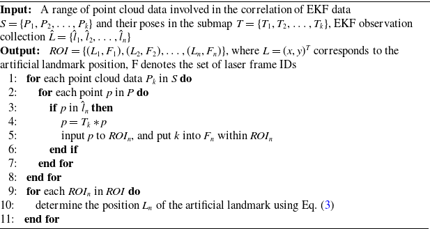
3.3. Artificial landmark extraction in submap
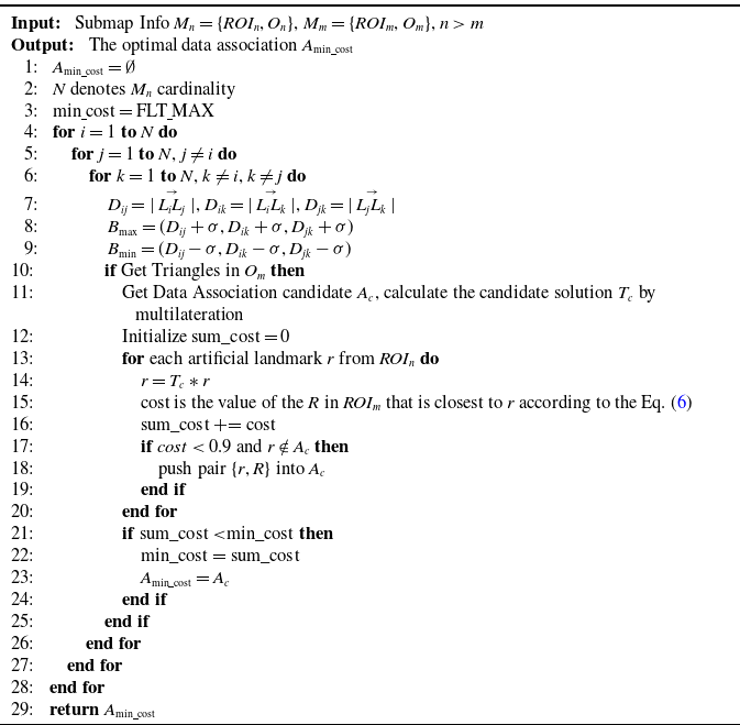
This subsection details the principles for extracting artificial landmarks and selecting keyframes from high-reflection ROIs in submaps. Specific steps are outlined in Algorithm 1. Lines 1–8 collect LiDAR frame identifiers and point cloud data for the ROI regions, incorporating them into the corresponding ROI set using prior information from the EKF to generate data-associated observations. Lines 9-11 determine the artificial landmark location based on the point cloud data within the ROIs, in conjunction with Eq. (3).
Artificial Landmark Extraction in Submap

(a) CostMap builds on reflectors. (b) Optimal data association in similar environments.

3.4. CostMap-multilateration for loop closure detection
Loop closure detection identifies similar regions within submaps. To accelerate the search process, we directly project artificial landmarks onto the horizontal plane. This detection is implemented via CostMap-Multilateration, as detailed in Algorithm 2.
On completion of the new submap
 $M_{i+1}$
, an octree map
$M_{i+1}$
, an octree map
 $O_{i+1}$
is built using reflector-configured triangles, serving as loop closure detection input. Algorithm 2 lines 7–10 identify similar triangles via octree traversal.
$O_{i+1}$
is built using reflector-configured triangles, serving as loop closure detection input. Algorithm 2 lines 7–10 identify similar triangles via octree traversal.
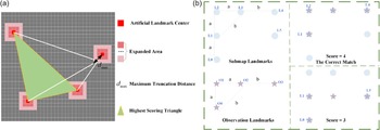
To find corresponding reflectors (data association) while avoiding false loop closures caused by overly similar triangles, a cost map is introduced, as shown in Figure 5. The maximum expansion distance
 $d_{\text{max}}$
is defined based on LiDAR ranging measurements and artificial landmark recognition errors. A high-resolution grid map with resolution
$d_{\text{max}}$
is defined based on LiDAR ranging measurements and artificial landmark recognition errors. A high-resolution grid map with resolution
 $res$
is then constructed, where grids surrounding artificial landmarks are proportionally expanded according to their distance from the landmark center. The cost function is defined in Eq. (6). Figure 5(b) depicts six reflectors in a highly similar arrangement, a common occurrence in structured industrial environments. When the reflector set {O0, O1, O3} is observed, five similar triangles can be matched within the submap. Relying solely on an octree-based method would fail to achieve correct data association under such ambiguity. However, by employing the CostMap’s scoring mechanism, the triangle {L1, L2, L4} is identified as the correct match due to its highest score. This process effectively excludes other geometrically similar candidate triangles, such as {L0, L1, L5}, thereby resolving the data association problem in environments with repetitive geometries and ensuring robust performance. Concurrently, this approach suppresses false positives in loop closure detection, thereby preventing incorrect loop closures, which could lead to eventual mapping failure.
$res$
is then constructed, where grids surrounding artificial landmarks are proportionally expanded according to their distance from the landmark center. The cost function is defined in Eq. (6). Figure 5(b) depicts six reflectors in a highly similar arrangement, a common occurrence in structured industrial environments. When the reflector set {O0, O1, O3} is observed, five similar triangles can be matched within the submap. Relying solely on an octree-based method would fail to achieve correct data association under such ambiguity. However, by employing the CostMap’s scoring mechanism, the triangle {L1, L2, L4} is identified as the correct match due to its highest score. This process effectively excludes other geometrically similar candidate triangles, such as {L0, L1, L5}, thereby resolving the data association problem in environments with repetitive geometries and ensuring robust performance. Concurrently, this approach suppresses false positives in loop closure detection, thereby preventing incorrect loop closures, which could lead to eventual mapping failure.
 \begin{equation} \text{cost} = 0.1 + 0.8 \cdot \frac {d}{d_{\text{max}}} \end{equation}
where
 $d$
represents the Euclidean distance from the center of a grid to the center of the artificial landmark. Grids that lie beyond the maximum truncation distance are assigned a value of
$d$
represents the Euclidean distance from the center of a grid to the center of the artificial landmark. Grids that lie beyond the maximum truncation distance are assigned a value of
 $C_{\text{max}}$
.
$C_{\text{max}}$
.
By integrating the cost map in lines 10–25 of Algorithm 2, the data association set
 $A_{\text{min}{\underline{\ }}{\text{cost}}} = \left \{ \{r_i\}, \{R_i\} \mid 1 \leq i \leq n \right \}$
is obtained, yielding the optimal pose transformation
$A_{\text{min}{\underline{\ }}{\text{cost}}} = \left \{ \{r_i\}, \{R_i\} \mid 1 \leq i \leq n \right \}$
is obtained, yielding the optimal pose transformation
 $T_n^m$
from submap
$T_n^m$
from submap
 $M_n$
to
$M_n$
to
 $M_m$
– the result of coarse matching between the two submaps. Herein,
$M_m$
– the result of coarse matching between the two submaps. Herein,
 $T_n^m$
can be obtained through multilateration based on the data association results.
$T_n^m$
can be obtained through multilateration based on the data association results.
Finding the Optimal Data Association

3.5. Building constraints and optimization
Upon completing loop closure detection, coarse inter-submap matches are obtained. To establish higher-precision constraints, keyframes derived from submaps undergo fine matching via scan-to-map registration, ultimately constructing submap constraints. This workflow essentially highlights two core components:
1. Selection of Keyframes: The selection of keyframes is based on their contribution to the matched reflector pillar ROI. To avoid selecting an excessive number of adjacent keyframes, only the keyframe with the highest contribution weight among adjacent ones is extracted. If multiple keyframes exhibit equal contribution weights, the centrally located keyframe is selected. Following this criterion, a predefined number of keyframes are chosen to participate in submap matching and constraint relationship construction.
2. Scan-to-Map Matching: From the previous section, it has been established that the optimal transformation from submap
 $M_i$
to submap
$M_i$
to submap
 $M_j$
is denoted as
$M_j$
is denoted as
 $T_i^j$
. The set of keyframes selected from submap
$T_i^j$
. The set of keyframes selected from submap
 $M_i$
is represented as
$M_i$
is represented as
 $K = \{ k_1, k_2, \ldots , k_n \}$
, with the pose of each keyframe in submap
$K = \{ k_1, k_2, \ldots , k_n \}$
, with the pose of each keyframe in submap
 $M_i$
given by
$M_i$
given by
 $T_{i_n}$
. Accordingly, the initial predicted pose of the keyframes within submap
$T_{i_n}$
. Accordingly, the initial predicted pose of the keyframes within submap
 $M_j$
can be expressed as
$M_j$
can be expressed as
 $T_{j_n} = T_i^j \times T_{i_n}$
. During the construction of the submap, the LOAM front-end module records information pertaining to key corner features and planar features within the map. By introducing the keyframes and their respective initial poses, the final matched pose information is obtained according to the method described in [Reference Lin and Zhang14], and is denoted by
$T_{j_n} = T_i^j \times T_{i_n}$
. During the construction of the submap, the LOAM front-end module records information pertaining to key corner features and planar features within the map. By introducing the keyframes and their respective initial poses, the final matched pose information is obtained according to the method described in [Reference Lin and Zhang14], and is denoted by
 $\hat {T}_{j_n}$
. This approach ensures accurate alignment of keyframes, facilitating an optimal estimation of the relative transformation between submaps.
$\hat {T}_{j_n}$
. This approach ensures accurate alignment of keyframes, facilitating an optimal estimation of the relative transformation between submaps.
As the robot moves, optimization is performed by incorporating both odometry constraints and loop closure constraints. Specifically, an optimization problem is formulated by adding adjacent submaps and establishing constraints for loop closure detection. In this paper, the set
 $ M^G = \{M^G_0, M^G_1, \ldots , M^G_t\},{} M^G \in SE(3)$
represents the positional information of a sequence of submaps in the global context, while the loop closure constraints between submaps are denoted by pairs
$ M^G = \{M^G_0, M^G_1, \ldots , M^G_t\},{} M^G \in SE(3)$
represents the positional information of a sequence of submaps in the global context, while the loop closure constraints between submaps are denoted by pairs
 $(i, j) \in C$
. To quantify the discrepancy between the observed and predicted transformations, we define the error
$(i, j) \in C$
. To quantify the discrepancy between the observed and predicted transformations, we define the error
 $ e_{ij}$
as shown in Eq. (7):
$ e_{ij}$
as shown in Eq. (7):
 \begin{equation} e_{ij}(p_i, p_j, O_{ij}) = O_{ij} \boxminus \hat {O}_{ij}(M^G_i, M^G_j) \end{equation}
The error term
 $e_{ij}$
represents the difference between the observed transformation
$e_{ij}$
represents the difference between the observed transformation
 $O_{ij} \in SE(3)$
, which corresponds to the loop closure constraint between nodes
$O_{ij} \in SE(3)$
, which corresponds to the loop closure constraint between nodes
 $i$
and
$i$
and
 $j$
, and the predicted transformation
$j$
, and the predicted transformation
 $\hat {O}_{ij} \in SE(3)$
, derived from odometry and the estimated positions of the submaps. The operator
$\hat {O}_{ij} \in SE(3)$
, derived from odometry and the estimated positions of the submaps. The operator
 $\boxminus$
denotes a mapping from the local neighborhood of
$\boxminus$
denotes a mapping from the local neighborhood of
 $SE(3)$
to its tangent space, enabling effective comparison between transformations. The predicted transformation is given by
$SE(3)$
to its tangent space, enabling effective comparison between transformations. The predicted transformation is given by
 $\hat {O}_{ij} (M^{G}_i, M^{G}_j) = {M^{G}_i}^{-1} M^{G}_j = T_{jn} \hat {T}_{in}^{-1}$
, which represents the relative transformation between submaps
$\hat {O}_{ij} (M^{G}_i, M^{G}_j) = {M^{G}_i}^{-1} M^{G}_j = T_{jn} \hat {T}_{in}^{-1}$
, which represents the relative transformation between submaps
 $M^{G}_i$
and
$M^{G}_i$
and
 $M^{G}_j$
in the global reference frame.
$M^{G}_j$
in the global reference frame.
This optimization problem can be formulated as a nonlinear least squares problem, as shown in Eq. (8). The system aims to optimize the robot’s pose by minimizing the error.
 \begin{equation} \left \{ \begin{aligned} P^* &= \arg \min _M \sum _{(i,\,j) \,\in\, C} R_{ij} \\ R_{ij} &= e_{ij}^T e_{ij} \end{aligned} \right . \end{equation}
where
 $R_{ij}$
signifies the negative log-likelihood function of a constraint between
$R_{ij}$
signifies the negative log-likelihood function of a constraint between
 $M^G_i$
and
$M^G_i$
and
 $M^G_j$
.
$M^G_j$
.
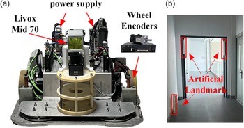
Logistics robot and sensor platform with LIVOX Lidar.

4. Experiments and evaluations
4.1. Implementation and evaluation setup
To verify the feasibility of the algorithm, we collected real-world environmental data using the AGV, as shown in Figure 6(a). The AGV is equipped with a differential drive chassis and utilizes a LIVOX Mid-70 3D LiDAR. The Mid-70 LiDAR has a circular FoV of 70.4 degrees both horizontally and vertically, with a significantly reduced near blind zone of 5 centimeters. During the experiments, the LiDAR operated at 10 Hz, capturing 10,000 points per frame. To provide an initial pose estimate for the algorithm, a KINCO servo motor drives the robot, with an encoder resolution of 65,536 pulses per revolution and a data acquisition frequency of 20 Hz. The data processing system is equipped with an 11th Gen Intel(R) Core(TM) i7-11370H processor, featuring an x86_64 architecture with 4 cores and 8 threads.
Submap construction qualitative experiment.
 $\times$
represents mapping failure and
$\times$
represents mapping failure and
 $\checkmark$
represents mapping success.
$\checkmark$
represents mapping success.

The experiments were conducted in an indoor setting simulating dynamic scenarios within a generic factory environment. Artificial landmarks were non-uniformly positioned at varying heights across multiple indoor regions. At selected positions, the landmarks were wall-mounted, as shown in Figure 6(b). Experimental data were collected from the onboard robotic platform. This dataset was subsequently used to systematically evaluate our proposed algorithm and perform comparisons against other methods.
The proposed method is deployed to compare with competing state-of-the-art methods. These include works on LOAM-livox, BALM, EKF, Scan Context, and M2DP (in loop closure detection experiments) and the proposed method. Since accurate ground truth cannot be obtained indoors, the end-to-end error is used for comparison in quantitative evaluation.
4.2. Qualitative evaluation
4.2.1. Submap creation experiments
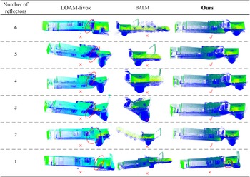
The accuracy of submap construction is critical for global map consistency, as LiDAR frames within a finalized submap are no longer modified. As shown in Figure 7, we evaluated three common turning scenarios in indoor environments.
Comparative results from three algorithms demonstrate that in geometrically constrained areas prone to degeneracy, BALM successfully reconstructs one scenario but exhibits significant degradation in the other two. In contrast, the LOAM-livox method exhibits Z-axis drift during wall reconstruction and ground/ceiling distortion, which may compromise subsequent global mapping. Our proposed method effectively mitigates LiDAR drift and achieves complete map reconstruction.
4.2.2. Focused study on the number and placement of artificial landmarks
To validate the impact of the number and arrangement of reflectors on our algorithm, we collected six sets of data in the environment shown in Figure 8.
Real environment. (a) Start environment (b) End environment (c) Path and reflectors distribution map.

For each data collection, we removed one reflector according to the serial numbers of the green icons in the figure, allowing us to observe the algorithm’s performance under different numbers and arrangements of reflectors. We compared our algorithm with two other methods, and the results are presented in Figure 9.
Experiment on the number and placement of artificial landmarks.

The results indicate that when LiDAR degeneracy occurs, both the BALM and LOAM-Livox algorithms exhibit significant performance degradation. Removing the first four reflectors (corresponding to the serial numbers) has little impact on the results, as reflectors No. 5 and No. 6 play a crucial role in compensating for information loss during vehicle rotation. However, when only one reflector was present, our algorithm inevitably produced mapping errors – specifically, two reflectors were visibly reconstructed in the map instead of one. This is because the LiDAR failed to continuously scan the column during degeneracy. The experiment clearly demonstrates that reflectors should be deployed as supplementary information in areas prone to LiDAR degeneracy.
Combining the experimental results and algorithmic principles, we propose several key considerations for deploying reflectors: in scenarios prone to LiDAR degeneracy, at least two reflectors should be deployed to provide necessary geometric constraints; to avoid point cloud overlap or feature confusion, the horizontal spacing between adjacent reflectors should be no less than 1 m; to support reliable loop closure detection, multiple reflectors should be arranged in an asymmetric configuration with randomized orientations to eliminate ambiguity caused by symmetry; and in spatially constrained narrow areas, reflectors should be placed outside the sensor’s minimum blind zone (typically at a distance greater than 0.5 m) – a requirement that can be effectively met by mounting them on vertical surfaces such as walls, thereby increasing their spatial separation and enhancing observability and system robustness.
4.2.3. Circular indoor scene mapping experiments
To qualitatively analyze the loop closure effects, we selected a circular area indoors and manually placed artificial landmarks within it. The mapping results of the three algorithms are depicted in Figure 10.
Mapping performance comparison diagram: LOAM-LIVOX shows increased mapping errors in circular environments, resulting in mapping failure.

Evidently, LOAM-livox exhibits drift at the third turn due to insufficient environmental features in degenerate scenarios, ultimately causing mapping failure. Similarly, BALM demonstrates significant mapping errors at the second turn and fails to complete the mapping process. In contrast, our proposed algorithm correctly identifies loop closure upon returning to the mapping origin and successfully constructs a globally consistent map.
4.3. Quantitative evaluation
4.3.1. Evaluation on loop closure detection
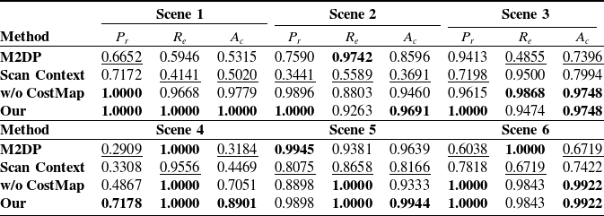
To evaluate the performance of our algorithm in 3D SLAM, we compared it with two state-of-the-art methods: Scan Context and M2DP. An ablation study was conducted by removing the CostMap component from the CostMap-Multilateration framework (denoted as “w/o CostMap” in the table) to validate its effectiveness. To assess the stability of our algorithm’s performance, we collected data in six different environments. During the experiments, data acquired from the same environment were used to form positive loop-closure pairs, whereas data from different environments formed negative pairs (i.e., non-loop-closure pairs).
The performance of loop closure detection is quantitatively evaluated using three standard metrics: accuracy
 $A_c$
, precision
$A_c$
, precision
 $P_r$
, and recall
$P_r$
, and recall
 $R_e$
, defined as follows:
$R_e$
, defined as follows:
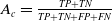 $A_c = \frac {TP + TN}{TP + TN + FP + FN}$
,
$A_c = \frac {TP + TN}{TP + TN + FP + FN}$
,
 $P_r = \frac {TP}{TP + FP}$
, and
$P_r = \frac {TP}{TP + FP}$
, and
 $R_e = \frac {TP}{TP + FN}$
. Here,
$R_e = \frac {TP}{TP + FN}$
. Here,
 $TP$
,
$TP$
,
 $FP$
,
$FP$
,
 $FN$
, and
$FN$
, and
 $TN$
denote true positive, false positive, false negative, and true negative, respectively. The evaluation results of the loop closure detection algorithms on these data are presented in Table I.
$TN$
denote true positive, false positive, false negative, and true negative, respectively. The evaluation results of the loop closure detection algorithms on these data are presented in Table I.
Loop closure detection results comparison in multiple indoor scenarios.

Best results are boldened, and the same group of tests’ worst results are underlined.
As shown by the experimental results, both Scan Context and M2DP generally perform moderately across most scenarios. This is because they generate feature descriptors from the raw sensor data. However, the limited field of view and sparse point cloud from a single-frame solid-state LiDAR (Livox Mid-70) often provide insufficient information. Consequently, these methods struggle to correctly identify loop closures due to information scarcity. Although they achieve relatively high recall in a few specific scenarios, their precision and accuracy in indoor environments with similar layouts are generally lower than those of our method. The algorithm with CostMap removed can only achieve loop closure detection by identifying a unique similar triangle. Nevertheless, this approach has two inherent limitations. First, when multiple similar triangles are observed in a single scan relative to the environment, the inability to determine a unique correspondence results in detection failure; second, the accidental presence of a similar triangle in two entirely unrelated environments is more likely to trigger a false loop closure. These findings demonstrate that our method establishes an evaluation framework that integrates information from all reflective markers, enabling more accurate loop closure identification.
To mitigate timing fluctuations induced by OS scheduling and CPU dynamic frequency scaling, we conducted 20 identical trials measuring loop closure detection and fine matching durations (Figure 11). Experimental results demonstrate a mean total constraint construction time of 38.3584 ms, with loop closure detection consuming 7.20 ms and fine matching accounting for 31.1512 ms of the total processing time.
Overall elapsed time for loopback constraint construction.

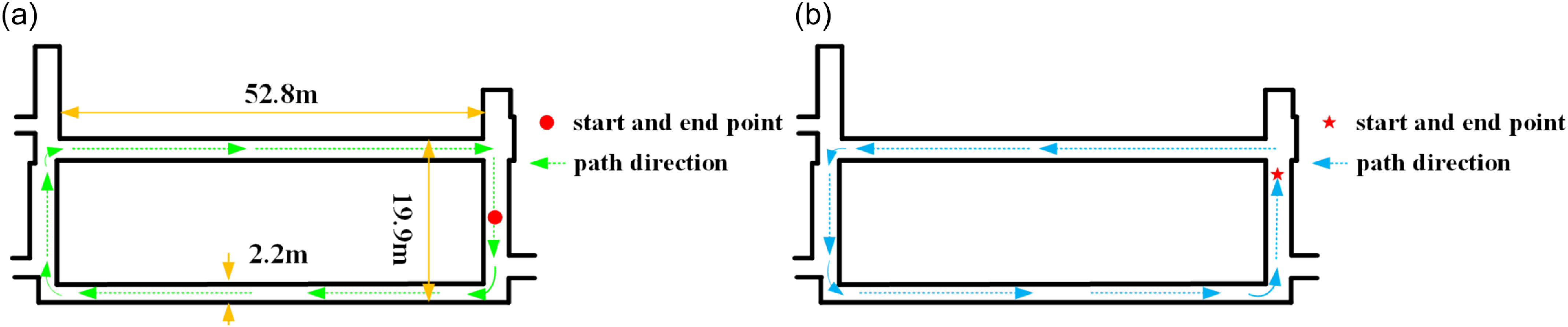
Long circular corridor environmental. (a) Clockwise path (b) Counterclockwise path.

Circular corridor indoor experiments(Clockwise). (a) Results of LOAM-livox map building. (b) Results of BALM map building. (c) Results of EKF map building. (d) Results of proposed map building. Only the proposed methodology completes the building of the map.

4.3.2. Evaluation on end-to-end distance
To quantify algorithmic accuracy improvements, we conducted dual experiments in a 59-meter-long circular indoor corridor (width: 19.9 m), with its primary segment spanning 52.8 m × 2.2 m (Figure 12). Given the susceptibility of corridor corners to degeneracy, reflective columns were strategically deployed at all four corners of the ring-shaped region for algorithm validation. After designating an origin point, the AGV traversed clockwise and counterclockwise paths returning to the origin. End-to-end positioning error was quantified by comparing LiDAR poses between initial and final frames.
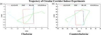
To compare the mapping performance, we conducted experiments on the same dataset. The results of the two experiments are shown in Figures 13 and 14, respectively, and their trajectory plots are shown in Figure 15. Since our AGV operates on a plane, we focused on the planar trajectory.
Circular corridor indoor experiments(Counterclockwise). (a) Results of LOAM-livox map building. (b) Results of BALM map building. (c) Results of EKF map building. (d) Results of proposed map building. Only the proposed methodology completes the building of the map.

Trajectory of circular corridor indoor experiments. (a) Clockwise mapping trajectory. (b) Counterclockwise mapping trajectory.

From the above experiments, it can be seen that the LOAM-Livox algorithm shows significant deviations in both the rotational and translational directions at the corners of narrow corridors due to geometric degeneracy. In the end-to-end distance tests, the differences between the start and end points were 34.2834 m and 17.2454 m, respectively. By contrast, the BALM algorithm produces obvious mapping errors during the initial mapping stage of the long corridor when mapping clockwise, ultimately failing to construct a valid map. When mapping counterclockwise, significant degeneration occurs at corridor corners, resulting in an inability to build a map. The EKF algorithm can achieve mapping in areas with artificial landmarks; however, once it moves away from such areas, significant mapping errors occur, making it unable to complete the mapping process. While our proposed algorithm does have certain LiDAR frame data errors at corners, it generally achieves normal mapping in both experiments. After identifying loop-closure submaps, the relationship between them was corrected, with the final end-to-end errors measured as 0.0345m and 0.1898m, respectively.
5. Conclusion
In this paper, we presented a 3D SLAM system tailored for small-FoV LiDARs, designed to mitigate degeneracy in feature-sparse environments through strategic reflector deployment. By incorporating artificial landmarks into degenerate regions and implementing CostMap-Multilateration for loop closure detection, the system provides coarse alignment priors for back-end optimization while ensuring global map consistency. Experimental validation in loop closure scenarios demonstrates superior performance over state-of-the-art methods, confirming the system’s capability to construct globally consistent maps in degenerate environments using reflector-assisted localization.
Moreover, in environments such as crowded shopping malls or dynamic logistics warehouses where stable features are scarce, strategically deploying reflectors (e.g., placing reflectors on walls – within the LiDAR’s vertical FoV – instead of only on the ground) can provide supplemental reference points. This enhances feature availability and mitigates environmental feature degradation. Although artificial landmarks offer high flexibility across various application scenarios, evaluating their practical feasibility requires careful consideration of deployment costs. Currently, material expenses for small-scale applications remain relatively manageable (for instance, the standalone reflective columns used in this experiment cost approximately $8 each). However, when scaled to large facilities, the cumulative cost of materials and the labor required for strategic installation will increase significantly. Furthermore, their practical implementation presents other notable limitations: deployment relies heavily on prior planning, making it difficult to adapt to temporary or emergency scenarios. In the future, integrating multi-source data processing technologies such as IMUs and visual sensors is expected to reduce reliance on maintenance while enhancing adaptability to dynamic scenarios, thus providing feasible solutions for broader applications in dynamic/large-scale environments.
Author contributions
The research work of this paper is the result of the joint efforts of the whole team. Jiying Ren led the research and wrote the manuscript, while ChenXu Wang provided important insights on the key research focuses of the paper. YongXin Ma offered guidance on experimental design. Jun Zhou and PanLing Huang provided comprehensive guidance on the review of the manuscript.
Financial support
This work is supported in part by the Shandong Key R&D Program of China under Grant 2024CXGC010213.
Competing interests
The authors declare no conflicts of interest exist.
Ethical standards
Not applicable.
Use of AI
The authors used generative AI tools – specifically Doubao (by ByteDance) and Yuanbao (by Tencent) (versions available in March 2025) – exclusively for language assistance. This included the correction of grammar, spelling, and punctuation, as well as minor phrasing adjustments to improve clarity, fluency, and adherence to academic English conventions. These tools were accessed via their public web interfaces; no proprietary data, unpublished results, or sensitive information were shared with the AI systems. The AI was not involved in research design, data analysis, or the interpretation of findings. All final decisions regarding the manuscript’s wording, structure, and meaning were made independently by the authors. To the best of our knowledge, this use does not introduce competing interests or algorithmic bias relevant to the scientific integrity of the work.