


1 Introduction
Finding a stellarator configuration with favourable properties for magnetic confinement fusion poses a high-dimensional multi-objective optimization problem. One of these objectives is to minimize the losses of energetic fusion alpha particles over their slowing-down time in order to be able to heat the bulk plasma of a reactor. Direct computation of such losses with usual numerical methods is relatively time consuming compared to other calculations within the optimization loop, in particular computation of three-dimensional (3-D) magnetohydrodynamic equilibria. This is why fusion alpha loss estimation is often performed via faster proxy models (Nemov et al. Reference Nemov, Kasilov, Kernbichler and Leitold2005, Reference Nemov, Kasilov, Kernbichler and Leitold2008; Bader et al. Reference Bader, Drevlak, Anderson, Faber, Hegna, Likin, Schmitt and Talmadge2019) that, however, cannot capture the full physics of drift orbits and, therefore, are suited only for the initial stage of optimization. The reason for this is the high alpha energy of 3.5 MeV, leading to the following consequences. On the one hand, alpha particles show a rather fast cross-field drift and rather wide guiding-centre orbits on the bounce time scale. On the other hand, the collisional decorrelation time of orbits from the magnetic field is very large because of very low collision frequencies for alphas. These two factors combined can lead to diverse and unpredictable behaviour of drift orbits in 3-D magnetic geometry. Therefore, direct tracing of an ensemble of orbits and statistical estimation of losses is still a preferable option for accurate results (Lotz et al. Reference Lotz, Merkel, Nührenberg and Strumberger1992; Nemov, Kasilov & Kernbichler Reference Nemov, Kasilov and Kernbichler2014).
To address this problem, a class of symplectic integrators for guiding-centre motion (Zhang et al. Reference Zhang, Liu, Tang, Qin, Xiao and Zhu2014) has recently been extended and applied (Albert, Kasilov & Kernbichler Reference Albert, Kasilov and Kernbichler2020a) to alpha loss computation in stellarator configurations. Despite reaching a significant speed up of factor 3–6 compared to adaptive Runge–Kutta orbit integration, further improvements are required to reduce the wall-clock run time below the time needed to compute magnetohydrodynamic equilibria.
To reach this goal, fast symplectic guiding-centre integration is complemented by classification of orbits as regular or chaotic based on Poincaré maps. In this context, ‘regular’ orbits are those that stay bound to some surfaces, called ‘drift surfaces’ and, therefore, can never leave the confinement volume. In particular, most of passing particle orbits are regular, as their drift surfaces are close to magnetic surfaces and only somewhat corrugated by cross-field drifts. This fact has been used in the past to reduce the number of orbits that have to be traced (e.g. Nührenberg, Lotz & Gori Reference Nührenberg, Lotz, Gori, Sindoni, Troyon and Vaclavic1994), and has inspired the idea of using a more rigorous classification, as presented here. The method treats trapped and passing particles in the same way and, therefore, takes into account possible losses of particles which would be classified from their starting conditions as passing (‘marginally passing particles’). It should be noted that in modern advanced stellarator concepts (Nührenberg & Zille Reference Nührenberg and Zille1988; Mikhailov et al. Reference Mikhailov, Shafranov, Subbotin, Isaev, Nührenberg, Zille and Cooper2002) not only most passing but also most trapped particles have regular orbits. Therefore, the gain in efficiency via classification is significant.
The combination of the two techniques allows us to reduce the wall-clock time for collisionless alpha loss estimation by another factor 2–5 compared to using symplectic schemes alone, and thus reaches the required target to be used directly in optimization. This claim is supported by the presented results for three stellarator reactor configurations of quasi-isodynamic (Drevlak et al. Reference Drevlak, Beidler, Geiger, Helander and Turkin2014), quasi-helical (Drevlak et al. Reference Drevlak, Beidler, Geiger, Helander, Henneberg, Nührenberg and Turkin2018) and quasi-axisymmetric type (Henneberg et al. Reference Henneberg, Drevlak, Nührenberg, Beidler, Turkin, Loizu and Helander2019), respectively. The implementation of the method is available in the code SIMPLE (Albert, Kasilov & Kernbichler Reference Albert, Kasilov and Kernbichler2020b) as open source under the MIT License. To produce the present results, version 1.1.1 of SIMPLE has been used.
2 Methods
2.1 Canonicalized flux coordinates
The guiding-centre Lagrangian (Littlejohn Reference Littlejohn1983; Cary & Brizard Reference Cary and Brizard2009) in magnetic flux coordinates, omitting the ignorable term with gyrophase velocity  $\dot{\unicode[STIX]{x1D719}}$, is given by
 $$\begin{eqnarray}L_{\text{gc}}=h_{r}{\dot{r}}+\left(mv_{\Vert }h_{\unicode[STIX]{x1D717}}+\frac{e}{c}A_{\unicode[STIX]{x1D717}}\right)\dot{\unicode[STIX]{x1D717}}+\left(mv_{\Vert }h_{\unicode[STIX]{x1D711}}+\frac{e}{c}A_{\unicode[STIX]{x1D711}}\right)\dot{\unicode[STIX]{x1D711}}-H,\end{eqnarray}$$
 where  $h_{i}=B_{i}/B$ are covariant components of unit vectors in direction of the magnetic field $\boldsymbol{B}$, the triple $(r,\unicode[STIX]{x1D717},\unicode[STIX]{x1D711})$ are some spatial straight field line magnetic flux coordinates, $m$ and $e$ are particle mass and charge, respectively, $c$ is the speed of light, $A_{k}=A_{k}(r)$ are covariant vector potential components and
 $$\begin{eqnarray}H=\frac{mv_{\Vert }^{2}}{2}+\unicode[STIX]{x1D707}B+e\unicode[STIX]{x1D6F7}\end{eqnarray}$$
 is the Hamiltonian containing magnetic moment  $\unicode[STIX]{x1D707}$ and electrostatic potential $\unicode[STIX]{x1D6F7}$.
In spatial coordinates with  $h_{r}=0$ it is immediately possible to identify canonical momenta $p_{\unicode[STIX]{x1D717}},p_{\unicode[STIX]{x1D711}}$ of the reduced 4-D phase space in front of $\dot{\unicode[STIX]{x1D717}}$ and $\dot{\unicode[STIX]{x1D711}}$ in (2.1). An efficient means of transformation from arbitrary 3-D magnetic flux coordinates to such coordinates has been presented recently (Albert et al. Reference Albert, Kasilov and Kernbichler2020a), being a three-dimensional generalization and synthesis of Meiss & Hazeltine (Reference Meiss and Hazeltine1990) and Li, Breizman & Zheng (Reference Li, Breizman and Zheng2016). Based on such a transformation, phase-space coordinates $\boldsymbol{z}=(r,\unicode[STIX]{x1D717},\unicode[STIX]{x1D711},p_{\unicode[STIX]{x1D711}})$ are used, with only $r$ remaining as a non-canonical variable, resulting in dependencies
 $$\begin{eqnarray}\displaystyle & \displaystyle L_{\text{gc}}(\boldsymbol{z},\dot{\unicode[STIX]{x1D717}},\dot{\unicode[STIX]{x1D711}})=p_{\unicode[STIX]{x1D717}}(\boldsymbol{z})\dot{\unicode[STIX]{x1D717}}+p_{\unicode[STIX]{x1D711}}\dot{\unicode[STIX]{x1D711}}-H(\boldsymbol{z}), & \displaystyle\end{eqnarray}$$
 $$\begin{eqnarray}\displaystyle & \displaystyle p_{\unicode[STIX]{x1D717}}(\boldsymbol{z})=mv_{\Vert }(\boldsymbol{z})h_{\unicode[STIX]{x1D717}}(r,\unicode[STIX]{x1D717},\unicode[STIX]{x1D711})+\frac{e}{c}A_{\unicode[STIX]{x1D717}}(r), & \displaystyle\end{eqnarray}$$
 $$\begin{eqnarray}\displaystyle & \displaystyle v_{\Vert }(\boldsymbol{z})=\frac{1}{mh_{\unicode[STIX]{x1D711}}(r,\unicode[STIX]{x1D717},\unicode[STIX]{x1D711})}\left(p_{\unicode[STIX]{x1D711}}-\frac{e}{c}A_{\unicode[STIX]{x1D711}}(r)\right). & \displaystyle\end{eqnarray}$$
 Computations of the exact transformation in the treated stellarator equilibria show that  $(r,\unicode[STIX]{x1D717},\unicode[STIX]{x1D711})$ remain close to Boozer magnetic coordinates, becoming identical to them in the zero beta limit. It has been argued by Boozer (Reference Boozer2005) that, in such coordinates, $h_{r}$ can be neglected for the purpose of orbit integration, thereby immediately providing approximate canonicalized flux coordinates. Using such coordinates would further increase performance, as they depend on fewer free 3-D parameters for which interpolants have to be computed during evaluation of the magnetic field. Even though for the current work the exact canonicalization of flux coordinates has been chosen, a comparison to computation in Boozer coordinates with neglected $h_{r}$ could be an interesting task for future investigations.
2.2 Symplectic integration in non-canonical coordinates
With canonical momenta given in terms of (partially) non-canonical coordinates, we can proceed to apply a generalized form of symplectic integration (Zhang et al. Reference Zhang, Liu, Tang, Qin, Xiao and Zhu2014; Albert et al. Reference Albert, Kasilov and Kernbichler2020a). Here, dependencies and derivatives of Hamiltonian  $H$ are written in terms of non-canonical phase-space coordinates $\boldsymbol{z}$, but the quadrature scheme relies on classical symplectic integrators in canonical coordinates (Hairer, Lubich & Wanner Reference Hairer, Lubich and Wanner2006). For the present investigation, a semi-implicit symplectic Euler method has been employed. In step number $(n)$ with time difference $\unicode[STIX]{x0394}t$, two implicit equations
 $$\begin{eqnarray}\displaystyle & \displaystyle 0=\frac{\unicode[STIX]{x2202}p_{\unicode[STIX]{x1D717}}}{\unicode[STIX]{x2202}r}(p_{\unicode[STIX]{x1D717},(n+1)}-p_{\unicode[STIX]{x1D717},(n)})+\unicode[STIX]{x0394}t\left(\frac{\unicode[STIX]{x2202}p_{\unicode[STIX]{x1D717}}}{\unicode[STIX]{x2202}r}\frac{\unicode[STIX]{x2202}H}{\unicode[STIX]{x2202}\unicode[STIX]{x1D717}}-\frac{\unicode[STIX]{x2202}p_{\unicode[STIX]{x1D717}}}{\unicode[STIX]{x2202}\unicode[STIX]{x1D717}}\frac{\unicode[STIX]{x2202}H}{\unicode[STIX]{x2202}r}\right), & \displaystyle\end{eqnarray}$$
 $$\begin{eqnarray}\displaystyle & \displaystyle 0=\frac{\unicode[STIX]{x2202}p_{\unicode[STIX]{x1D717}}}{\unicode[STIX]{x2202}r}(p_{\unicode[STIX]{x1D711},(n+1)}-p_{\unicode[STIX]{x1D711},(n)})+\unicode[STIX]{x0394}t\left(\frac{\unicode[STIX]{x2202}p_{\unicode[STIX]{x1D717}}}{\unicode[STIX]{x2202}r}\frac{\unicode[STIX]{x2202}H}{\unicode[STIX]{x2202}\unicode[STIX]{x1D711}}-\frac{\unicode[STIX]{x2202}p_{\unicode[STIX]{x1D717}}}{\unicode[STIX]{x2202}\unicode[STIX]{x1D711}}\frac{\unicode[STIX]{x2202}H}{\unicode[STIX]{x2202}r}\right) & \displaystyle\end{eqnarray}$$
 are first solved in  $r=r_{(n,\text{ei})}$ and $p_{\unicode[STIX]{x1D711}}=p_{\unicode[STIX]{x1D711},(n+1)}$. Partial derivatives of poloidal momentum $p_{\unicode[STIX]{x1D717}}$ and Hamiltonian $H$ are evaluated at $(r_{(n,\text{ei})},\unicode[STIX]{x1D717}_{(n)},\unicode[STIX]{x1D711}_{(n)},p_{\unicode[STIX]{x1D711},(n+1)})$, according to (2.2) and (2.4), expressing $v_{\Vert }$ via (2.5). Subscripts $(n)$ denote values at current time $t$, and $(n+1)$ the ones at $t+\unicode[STIX]{x0394}t$. The internal stage $r_{(n,\text{ei})}$ (with subscript ‘ $\text{ei}$’ for ‘explicit–implicit’ Euler) does not correspond to a full time step but remains sufficiently close to the actual radial position $r$ of the guiding centre. In particular, this evaluation point in phase space is also used to express the poloidal momentum at step $(n+1)$ via
 $$\begin{eqnarray}p_{\unicode[STIX]{x1D717},(n+1)}=p_{\unicode[STIX]{x1D717}}(r_{(n,\text{ei})},\unicode[STIX]{x1D717}_{(n)},\unicode[STIX]{x1D711}_{(n)},p_{\unicode[STIX]{x1D711},(n+1)}).\end{eqnarray}$$
 In the remaining stages, new positions  $\unicode[STIX]{x1D717},\unicode[STIX]{x1D711}$ follow explicitly in two equations
 $$\begin{eqnarray}\displaystyle & \displaystyle \unicode[STIX]{x1D717}_{(n+1)}=\unicode[STIX]{x1D717}_{(n)}+\unicode[STIX]{x0394}t\frac{\unicode[STIX]{x2202}H}{\unicode[STIX]{x2202}r}\left(\frac{\unicode[STIX]{x2202}p_{\unicode[STIX]{x1D717}}}{\unicode[STIX]{x2202}r}\right)^{-1}, & \displaystyle\end{eqnarray}$$
 $$\begin{eqnarray}\displaystyle & \displaystyle \unicode[STIX]{x1D711}_{(n+1)}=\unicode[STIX]{x1D711}_{(n)}+\unicode[STIX]{x0394}t\frac{1}{h_{\unicode[STIX]{x1D711}}}\left(v_{\Vert }-\frac{\unicode[STIX]{x2202}H}{\unicode[STIX]{x2202}r}\left(\frac{\unicode[STIX]{x2202}p_{\unicode[STIX]{x1D717}}}{\unicode[STIX]{x2202}r}\right)^{-1}h_{\unicode[STIX]{x1D717}}\right), & \displaystyle\end{eqnarray}$$
 where derivatives of  $p_{\unicode[STIX]{x1D717}}$ and $H$, as well as $h_{\unicode[STIX]{x1D717}}$ and $v_{\Vert }$, are evaluated at the same phase point as in (2.6) and (2.7).
2.3 Classification of Poincaré sections
As discussed above, regular orbits are bound to ‘drift surfaces’ which reduce to a line (or set of closed lines) on some given cross-sections (Poincaré sections). For the present analysis and classification, we use two types of Poincaré section of the whole phase space defined by
 $$\begin{eqnarray}v_{\Vert }=0^{\pm },\end{eqnarray}$$
 with  $v_{\Vert }$ switching either from negative to positive ( $0^{-}$) or vice versa ( $0^{+}$), and
 $$\begin{eqnarray}\unicode[STIX]{x1D711}=\frac{2\unicode[STIX]{x03C0}l}{N_{\text{per}}},\end{eqnarray}$$
 where  $N_{\text{per}}$ is the number of field periods of the configuration and $l$ is an integer between 0 and $N_{\text{per}}-1$. Each of these sections is illustrated based on orbits in figures 1–2.
(a) Trapped orbit with a Poincaré section (red) at turning points  $v_{\Vert }=0^{-}$, and outer plasma boundary (blue). Panel (b) shows the projection of the section to the poloidal plane.

(a) Passing orbit with Poincaré sections (red) at toroidal field periods  $\unicode[STIX]{x1D711}=\unicode[STIX]{x1D711}_{k}$, and outer plasma boundary (blue). (b) Projection of the section to the poloidal plane.
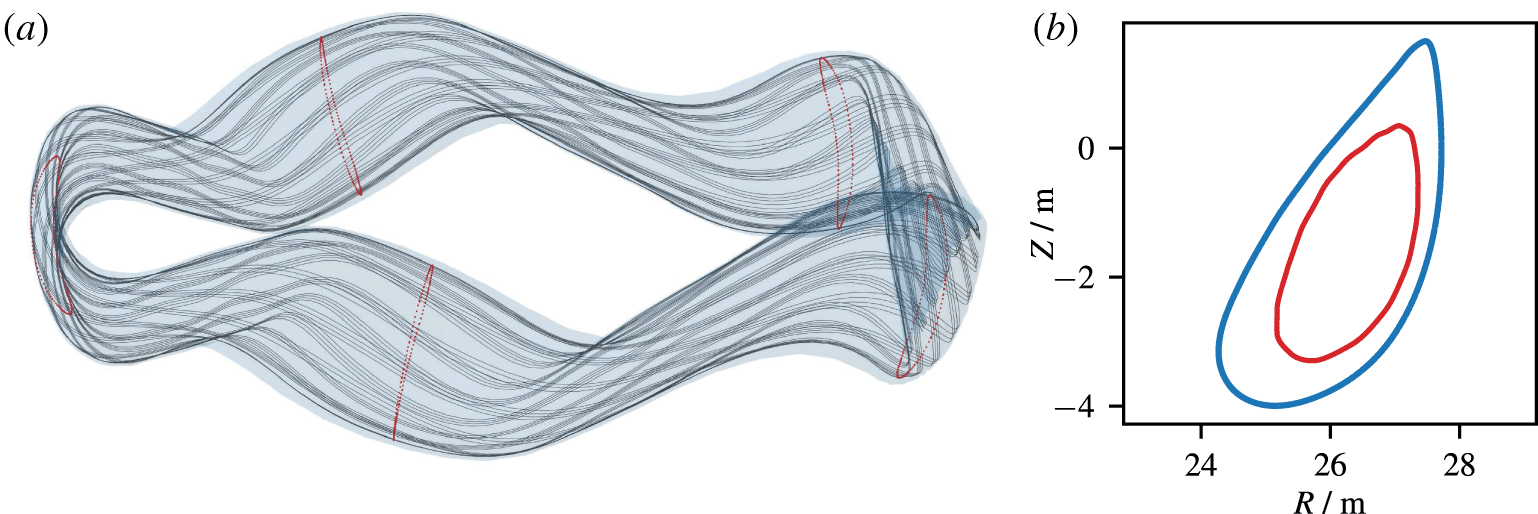
The considered Poincaré sections are actually 3-D hypersurfaces in a 4-D phase space (ignoring the gyrophase and treating the conserved magnetic moment  $\unicode[STIX]{x1D707}$ as an auxiliary parameter). Imposing the additional constraint of conservation of total energy $H$ together with one of (2.11)–(2.12), hypersurfaces are reduced to 1-D lines in the case of regular orbits, or structures of fractal dimension between one and two in the case of chaotic orbits. Classification of the kind of orbit at hand is performed with the help of the box-counting fractal dimension described below.
The box-counting fractal dimension of a set of points (see, e.g., Falconer Reference Falconer2014, chap. 3), also known as the Minkowski–Bouligand dimension, is defined as follows. One considers the number of boxes  $N(\unicode[STIX]{x1D700})$ of width $\unicode[STIX]{x1D700}$ required to cover all points in the set. In the limiting case of small boxes, the fractal dimension is obtained as a ratio of exponents via
 $$\begin{eqnarray}d_{f}=\lim _{\unicode[STIX]{x1D700}\rightarrow 0}\frac{\log N(\unicode[STIX]{x1D700})}{\log (\unicode[STIX]{x1D700}^{-1})}.\end{eqnarray}$$
 For a finite set of points and for numerical implementation, a sufficiently small finite minimum value of  $\unicode[STIX]{x1D700}$ is used instead of this limit. Figure 3 illustrates the behaviour in terms of a regular orbit and a chaotic orbit. In the regular case, the number $N(\unicode[STIX]{x1D700})$ grows linearly with $\unicode[STIX]{x1D700}^{-1}$ and $d_{f}$ is computed close to one. In comparison, for the chaotic case, more boxes are required with smaller $\unicode[STIX]{x1D700}$, leading to an estimated fractal dimension $d_{f}$ well between one and two. In the limit of points covering the whole section equally, $d_{f}$ approaches two.
Classification of poloidal projections of Poincaré sections via box counting. The regular orbit in the upper plots has a one-dimensional projection, while the projection of the chaotic orbit on the bottom has a fractal dimension between one and two apparent on refinement.

In practice, to classify orbits, a threshold value for  $d_{f}$ has to be set, below which orbits are classified as regular. In the present implementation this threshold has been determined empirically as $d_{f}\approx 1.6$ with adaptation to more conservative criteria with decreasing number of available points. If all section types (2.11)–(2.12) have a dimension below the threshold, the orbit is classified as regular. In the actual code realization it is more convenient to use, instead of the fractal dimension, a ratio $\unicode[STIX]{x1D708}$ of full boxes $N_{\text{full}}$ to the total number of boxes $N_{\text{box}}$, linked to $d_{f}$ by
 $$\begin{eqnarray}d_{f}=2\frac{\log (\unicode[STIX]{x1D708})}{\log (N_{\text{box}})}+2.\end{eqnarray}$$
 Here, the threshold is set directly as  $\unicode[STIX]{x1D708}=0.2$.
Figure 4 shows an example of the estimated fractal dimension as a function of  $N_{\text{box}}$ for a number of regular and chaotic orbits in a quasi-isodynamic stellarator configuration. Actual classification happens when the number of boxes becomes equal to the number of orbit footprints in the Poincaré section. At higher $N_{\text{box}}$ this estimate can no longer be used, which is clearly seen from the behaviour of chaotic orbits.
Estimated fractal dimension  $d_{f}$ by box counting versus number of boxes $N_{\text{box}}$ for several regular (a) and chaotic (b) orbits in a quasi-isodynamic configuration. Orbits are classified when $N_{\text{box}}$ equals the number of footprints using the threshold value $d_{f}=1.6$ (dashed lines).

3 Results
In this section numerical results on fusion alpha particle confinement are presented for three optimized stellarator configurations of similar (reactor) size with an on-axis magnetic field of  $B_{0}=5~\text{T}$: a quasi-isodynamic (QI) configuration (major radius $R=25~\text{m}$, aspect ratio $A=12$, plasma $\unicode[STIX]{x1D6FD}=4.9\,\%$) of Drevlak et al. (Reference Drevlak, Beidler, Geiger, Helander and Turkin2014), a quasi-helical (QH) configuration ( $R=19~\text{m}$, $A=8.7$, $\unicode[STIX]{x1D6FD}=3.9\,\%$) of Drevlak et al. (Reference Drevlak, Beidler, Geiger, Helander, Henneberg, Nührenberg and Turkin2018) and a quasi-axisymmetric (QA) configuration ( $R=10.3~\text{m}$, $A=3.4$, $\unicode[STIX]{x1D6FD}=3.5\,\%$) of Henneberg et al. (Reference Henneberg, Drevlak, Nührenberg, Beidler, Turkin, Loizu and Helander2019). Resulting loss fractions over time match the ones in the references. It should be stressed once more that the high degree of optimization in these configurations makes the present classification method especially efficient, as most orbits are regular and losses are small. Still, the algorithm is expected to give a significant speed up in optimizing any magnetic configuration where the initial equilibrium already has an alpha loss fraction below 0.5 at the alpha particle slowing-down time $t_{\text{s}}$. If this is not the case, alpha loss computations are anyway fast as long as losses happen well before $t_{\text{s}}$ and tracing can be terminated frequently.
Figures 5–7 show losses of alpha particles over time and a trapping parameter defined as
 $$\begin{eqnarray}\unicode[STIX]{x1D703}_{\text{trap}}=\left(\frac{\unicode[STIX]{x1D707}}{\unicode[STIX]{x1D707}_{\text{tp}}}-1\right)\left(\frac{B_{\text{max}}}{B_{\text{min}}}-1\right)^{-1},\end{eqnarray}$$
 where  $\unicode[STIX]{x1D707}_{\text{tp}}$ is the magnetic moment corresponding to the trapped passing boundary, and $B_{\text{min}}$ and $B_{\text{max}}$ are maximum and minimum values of the magnetic field modulus on the starting flux surface, respectively. For deeply trapped particles $\unicode[STIX]{x1D703}_{\text{trap}}=1$, while it vanishes at the trapped passing boundary. Negative values of $\unicode[STIX]{x1D703}_{\text{trap}}$ correspond to passing particles. In addition to black dots marking the actual loss of a test particle, shaded plots from a kernel density estimator based on the statistical samples have been added to mark regions of losses in time and phase space. Finally, the confined fraction $f_{c}$ over time is plotted as a curve.
Two cases are considered for each configuration where particles are started at a flux surface with radius  $r=s\equiv \unicode[STIX]{x1D713}_{\text{tor}}/\unicode[STIX]{x1D713}_{\text{tor}}^{a}=0.6$ and $s=0.3$, respectively, where $\unicode[STIX]{x1D713}_{\text{tor}}$ is the toroidal magnetic flux and $\unicode[STIX]{x1D713}_{\text{tor}}^{a}$ its value at the outer plasma boundary. A total of $N_{\text{tot}}=1000$ randomly chosen orbits are traced up to physical time $t=1~\text{s}$ such that the slowing-down time is well covered. The estimated standard deviation $\unicode[STIX]{x1D70E}$ (random error) in the computed fraction $f_{c}$ of particles which remain confined scales inversely with this number as $\unicode[STIX]{x1D70E}=\sqrt{f_{c}(1-f_{c})/N_{\text{tot}}}$. Classification of regular/chaotic orbit types is performed at $t=10^{-1}~\text{s}$. After this point, regular orbits are considered to be confined and only chaotic orbits are traced further. Initial conditions are set to isotropic in velocity space with spatial positions distributed along the field line densely covering the flux surface so that particle density is constant in the flux tube. This method has worked without problems in the present cases and is also suitable in the general case where the coordinate system is not necessarily flux-surface aligned (Nemov et al. Reference Nemov, Kasilov and Kernbichler2014). It has, however, some disadvantage if the starting surface is close to a low-order rational surface such that one needs a very long field line to cover it. In that case, the method of Bader et al. (Reference Bader, Drevlak, Anderson, Faber, Hegna, Likin, Schmitt and Talmadge2019) for flux coordinate systems would be preferable.
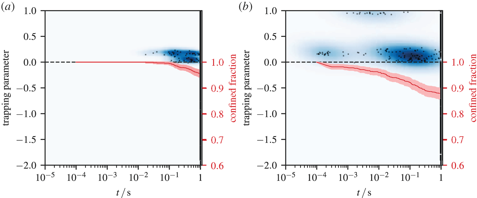
Alpha particle losses from  $s=0.3$ (a) and $s=0.6$ (b) over time and trapping parameter (left axis) for a quasi-isodynamic stellarator configuration. Density plot over lost particles (black dots); confined fraction $f_{c}$ over time (lower curve, right axis). Error bands at $\pm 1.96\unicode[STIX]{x1D70E}$ around this curve describe the 95 % confidence interval due to the Monte Carlo error.
Alpha particle losses from  $s=0.3$ (a) and $s=0.6$ (b) over time and trapping parameter (left axis) for a quasi-helical stellarator configuration in the style of figure 5. Final losses at $s=0.3$ are below 2 %, including error bars.

Alpha particle losses from  $s=0.3$ (a) and $s=0.6$ (b) over time and trapping parameter (left axis) for a quasi-axisymmetric stellarator configuration in the style of figure 5.

At the outer flux surface  $s=0.6$ the QI configuration in figure 5 first shows some prompt losses ( $t=10^{-4}~\text{s}$) near the trapped–passing boundary. Those are orbits such that they immediately cross the boundary at $s=1.0$ before even completing a significant number of poloidal or toroidal turns in the device. At intermediate times between $t=10^{-3}~\text{s}$ and $10^{-2}~\text{s}$ originally deeply trapped particles are lost as drift motion and stochasticity remove them from their magnetic well. Finally, late losses at the trapped–passing boundary set in due to chaotic trajectories. In the QH configuration in figure 6 most losses from $s=0.6$ happen already early, between $t=10^{-4}~\text{s}$ and $10^{-3}~\text{s}$ for trapped particles that are neither deeply nor marginally trapped. Late losses are again located around the trapped–passing boundary, where chaotic effects are especially pronounced. The QA configuration in figure 7 spreads losses from $s=0.6$ more evenly over both time and trapping parameter. Most losses happen at $t$ between $10^{-3}~\text{s}$ and $10^{-2}~\text{s}$, depleting the population in the region near the trapped–passing boundary.
At the inner flux surface  $s=0.3$ alpha confinement in the QI configuration in figure 5 is governed by late losses close to the trapped–passing boundary. In contrast, the QH configuration in figure 6 shows a few prompt losses and retains alphas up to the tracing time of 1 s. In the quasi-axisymmetric configuration in figure 7 losses appear over the whole trapped region with deeply and marginally trapped orbits lost earlier. Here, the region of losses also extends into the marginally passing range.
If the threshold for the fractal dimension to identify chaotic orbits is set too high, the classification might produce ‘false negatives’. In that case, an orbit is classified as regular despite being chaotic and lost if traced up to the end. In that case, final losses are underestimated if classification is used. In the computations for figures 5–7 no false negatives occurred, meaning that classification did not deteriorate results on late losses. In contrast, ‘false positive’ classification of chaotic orbits just increases computation time by tracing them up to the end, but does not influence the result. This trade-off between accuracy and computation time is adjusted via the choice of the threshold fractal dimension (2.13) to decide whether an orbit is chaotic. As mentioned above, this option has been left at default settings independent of the treated cases and could potentially be optimized.
Orbit types over initial condition in  $v_{\Vert }/v$ and $\unicode[STIX]{x1D717}$ from $s=0.6$ for QI (a), QH (b) and QA configuration (c). The background (▪) is filled by regular orbits, early losses before $t=0.1~\text{s}$ are marked as ‘○’, and chaotic orbits potentially causing late losses after $t=0.1~\text{s}$ as ‘ $\times$’ with some ‘false positives’ visible that remain confined. The trapped–passing boundary is marked by a white line.
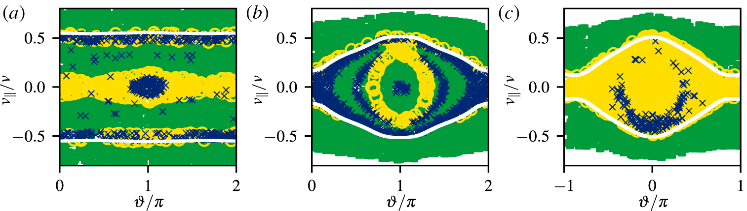
Figure 8 shows the classification results depending on initial conditions in pitch parameter  $v_{\Vert }/v$ and poloidal angle $\unicode[STIX]{x1D717}$ for $10^{4}$ orbits started at $s=0.6$ and $\unicode[STIX]{x1D711}=\unicode[STIX]{x1D711}_{n}/2$, i.e. in the middle of the first field period. All three configurations show regular orbits in the passing region at some distance from the trapped–passing boundary. For the QI and QH configurations there is a clear separation of early losses of orbits that cross the plasma boundary soon and chaotic orbits that slowly diffuse away. Losses are localized at the trapped–passing boundary and in certain phase-space regions for more deeply trapped orbits. In the QA configuration most trapped orbits are chaotic, but some are lost relatively late due to slow stochastic diffusion. The described behaviour is also seen in figures 5–7. Therefore, the classification is of less use in the QA case, as most regular orbits are passing and could be identified in simpler ways. In contrast, for QI and QH types the method allows us to exclude also a large portion of the trapped region from further computation. A relatively small number of ‘false positives’ that are incorrectly classified as chaotic are seen, in particular in the QI configuration, and traced to the end despite being actually regular.
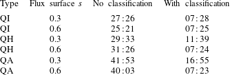
Table 1 shows numerical values of respective regular fractions for trapped and passing orbits in the considered configurations. A significant portion of chaotic trapped orbits in the QH and QA configurations stays confined within  $t=1~\text{s}$, which makes confinement properties of alphas acceptable even in cases where only a small fraction of trapped orbits are regular.
Fractions of regular orbits in the trapped and passing regions for different configurations.

Computations were performed on the COBRA cluster of MPCDF on a single node with 40 cores/80 threads of Intel(R) Xeon(R) Gold 6126 CPUs. Table 2 shows a summary of computation wall-clock time using a symplectic integrator alone compared to added classification after  $1/10\text{th}$ of the integration time. The obtained speed up of another factor 2–5 compared to an integration method that is already a factor 3–6 faster than conventional Runge–Kutta integration for alpha loss results of the same accuracy (Albert et al. Reference Albert, Kasilov and Kernbichler2020a) leads to a total speed up of factor 6–30 compared to conventional methods.
Wall-clock run times in minutes on 40 CPU cores with hyperthreading for the considered configurations. Computation for the QA equilibrium at inner flux surfaces is least efficient, as most orbits are chaotic, even when confined over their slowing-down time.
4 Summary and outlook
A combined method of symplectic integration and early classification has been presented to accelerate the computation of loss fractions of fusion alpha particles over their slowing-down time in stellarator reactor configurations. Reliable results could be obtained for three different stellarator configuration types within wall-clock times of approximately 10 min. This corresponds to a speed up of approximately an order of magnitude compared to conventional methods and makes the technique useful for integrated in stellarator optimization, where computation times for magnetic equilibria are of the same order.
Currently, the approach is limited to collisionless orbits. Adding collisions could limit the effectiveness of early classification by additional diffusion and requires further investigations. Even though mis-classifications influencing final results were rare with default settings, the classification algorithm could benefit from additional tuning in order to become even more robust. Finally, the influence of using Boozer coordinates instead of exact canonicalized flux coordinates should be studied further, as it provides room for further efficiency improvements.
Acknowledgements
The authors would like to thank M. Heyn for pointing out the Minkowski dimension, M. Drevlak, S. Henneberg and F. Hindenlang for equilibrium configurations and validation, A. Boozer and A. Punjabi for useful comments and J. Ganglbauer for supporting investigations. This work has been carried out within the framework of the EUROfusion Consortium and has received funding from the Euratom research and training programmes 2014–2018 and 2019–2020 under grant agreement no. 633053. The views and opinions expressed herein do not necessarily reflect those of the European Commission. The study is a contribution to the Reduced Complexity Models grant number ZT-I-0010 funded by the Helmholtz Association of German Research Centers. Support from NAWI Graz, and from the OeAD under the WTZ grant agreement with Ukraine No. UA 04/2017 is gratefully acknowledged.


 Open access