





1. Introduction
1.1. The graph alignment problem
There are various statistical problems where we observe a network of linked objects which can be represented by a large graph; for instance, a network of protein–protein interactions or a social network. The graph alignment problem, in a broad sense, is the following: we observe the same underlying data multiple times, obtaining $p \geq 2$
unlabelled graphs which should be very similar, and attempt to retrieve the underlying isomorphism which pairs up any two nodes representing the same element.
$p \geq 2$
unlabelled graphs which should be very similar, and attempt to retrieve the underlying isomorphism which pairs up any two nodes representing the same element.
Formally, the problem can be described as follows. Assume that we have an underlying p-tuple of labelled random graphs $(G^{(1)}, \ldots, G^{(p)})$
with vertex set
$(G^{(1)}, \ldots, G^{(p)})$
with vertex set $\left[ \! \left[ 1,n \right] \! \right]$
. We select
$\left[ \! \left[ 1,n \right] \! \right]$
. We select $\pi^* = (\pi_1^* = \textrm{Id}, \pi_2^*, \ldots, \pi_p^*)$
with
$\pi^* = (\pi_1^* = \textrm{Id}, \pi_2^*, \ldots, \pi_p^*)$
with $\pi_2^* , \ldots, \pi_p^* $
chosen independent and identically distributed (i.i.d.), uniformly at random, over
$\pi_2^* , \ldots, \pi_p^* $
chosen independent and identically distributed (i.i.d.), uniformly at random, over $\mathcal{S}_n$
; we observe
$\mathcal{S}_n$
; we observe
 \begin{equation} (\boldsymbol{\pi}^*)^{-1}(G) \underset{{\rm def}}{=} (G_{(\pi_1^*)^{-1}(e)}^{(1)})_{e \in E}, \ldots, (G_{(\pi_p^*)^{-1}(e)}^{(p)})_{e \in E},\end{equation}
where E is the set of edges in the complete graph on $\left[ \! \left[ 1, n \right] \! \right]$
, and
$\left[ \! \left[ 1, n \right] \! \right]$
, and $\mathcal{S}_n$
acts on E via
$\mathcal{S}_n$
acts on E via $\sigma(\{ u, v \}) \underset{{\rm def}}{=} \{ \sigma(u), \sigma(v) \}$
. Our aim is to recover
$\sigma(\{ u, v \}) \underset{{\rm def}}{=} \{ \sigma(u), \sigma(v) \}$
. Our aim is to recover $\pi_2^*, \ldots, \pi_p^*$
.
$\pi_2^*, \ldots, \pi_p^*$
.
Typically, in order to analyse the problem for ‘typical’ values of G, we assume that G is also a random variable, such that the $(G_e^{(i)})_{1 \leq i \leq p}$
are correlated for any fixed
$(G_e^{(i)})_{1 \leq i \leq p}$
are correlated for any fixed $e \in E$
. Two important examples are the following models.
$e \in E$
. Two important examples are the following models.
-
• The Gaussian model $\mathcal{N}(n, \rho)$
, where
$G^{(1)}, \ldots, G^{(p)}$
are weighted graphs: the weights
$(G_e^{(i)})_{1 \leq i \leq p, e \in E}$
are drawn as a centred normal vector over
$\mathbb{R}^E \otimes \mathbb{R}^p$
, with the following covariance matrix: (2)
\begin{equation} \textrm{Cov}(G_{e}^{(i)}, G_{e'}^{(j)}) = \begin{cases} 1 & \text{ if } e=e',\, i=j ,\\[2pt] \rho \in [0, 1] & \text{ if } e=e',\, i \neq j ,\\[2pt] 0 & \text{ otherwise.} \end{cases}\end{equation}
$\mathcal{N}(n, \rho)$
, where
$G^{(1)}, \ldots, G^{(p)}$
are weighted graphs: the weights
$(G_e^{(i)})_{1 \leq i \leq p, e \in E}$
are drawn as a centred normal vector over
$\mathbb{R}^E \otimes \mathbb{R}^p$
, with the following covariance matrix: (2)
\begin{equation} \textrm{Cov}(G_{e}^{(i)}, G_{e'}^{(j)}) = \begin{cases} 1 & \text{ if } e=e',\, i=j ,\\[2pt] \rho \in [0, 1] & \text{ if } e=e',\, i \neq j ,\\[2pt] 0 & \text{ otherwise.} \end{cases}\end{equation}
-
• The (correlated) Erdös–Rényi model
$\mathcal{G}(n, \lambda, s)$
, in which
$G^{(1)}, \ldots, G^{(p)}$
are unweighted graphs: we sample a ‘master graph’
$G^{(0)}$
from the standard Erdös–Rényi model
$\mathcal{G}(n, \frac{\lambda}{n})$
(for some
$\lambda > 0$
); then, the
$(G^{(i)})$
are subgraphs of
$G^{(0)}$
, which are mutually independent conditional on
$G^{(0)}$
, and which contain any given edge of
$G^{(0)}$
with a (fixed) probability
$0 < s < 1$
.


1.2. Previous works
The graph alignment problem has been studied extensively in the 2-graph case, particularly for the two toy models described previously. Much attention has been given to finding algorithms which, with high probability, recover the underlying permutation in reasonable time [Reference Feizi, Quon, Recamonde-Mendoza, Medard, Kellis and Jadbabaie15, Reference Fan, Mao, Wu and Xu16, Reference Fan, Mao, Wu and Xu17, Reference Ganassali, Lelarge and Massoulié18, Reference Ding, Ma, Wu and Xu19, Reference Dym, Maron and Lipman20, Reference Mao, Wu, Xu and Yu21, Reference Even, Ganassali, Maier and Massoulié22, Reference Ganassali, Massoulié and Semerjian26]. These algorithms, in turn, can be used in various applications: for instance, de-anonymisation problems [Reference Narayanan and Shmatikov23], natural language processing [Reference Bayati, Gleich, Saberi and Wang24], or the analysis of protein interaction networks [Reference Kazemi, Hassani, Grossglauser and Pezeshgi Modarres25].
Another line of research consists in the information-theoretical analysis of the alignment problem, i.e. understanding when alignment is feasible (without regards to time complexity). Again, much progress has been made on the subject [Reference Cullina and Kiyavash1, Reference Ganassali, Massoulié and Lelarge2, Reference Ganassali5, Reference Cullina, Kiyavash, Mittal and Poor9, Reference Ding and Du10, Reference Wu, Xu and Yu27] and we have a good understanding of the cutoffs for alignment feasibility. Note that, often enough, there is a real difference between feasibility and polynomial-time feasibility: there can be a ‘hard phase’ where alignment is feasible, but likely not in polynomial time [Reference Ding, Du and Li28].
When there are more than two graphs, the problem has been less extensively studied. Several studies have focused on developing algorithms [Reference Zhu, Zhu and Geng29, Reference Vijayan and Milenković30, Reference Liao, Lu, Baym, Singh and Berger31]; a few studies [Reference Ameen and Hajek4, Reference Ameen and Hajek32] have also looked at the information-theoretical side of this problem. Here, we pursue this information-theoretical line of inquiry; [Reference Ameen and Hajek33] is the most closely related to our present work, and we contrast its contributions with ours right after the statement of Theorem 1.
1.3. Contributions
Let us state the main results of this paper. If $\boldsymbol{\pi}, \boldsymbol{\pi}' \in \{ \textrm{Id} \} \times \mathcal{S}_n^{p-1}$
, we define
$\boldsymbol{\pi}, \boldsymbol{\pi}' \in \{ \textrm{Id} \} \times \mathcal{S}_n^{p-1}$
, we define
 \begin{equation} ov(\boldsymbol{\pi}, \boldsymbol{\pi}') = \frac{1}{n} \sum_{i=1}^n \mathbf{1}_{\pi_2(i) = \pi'_2(i), \ldots, \pi_p(i) = \pi'_p(i)}.\end{equation}
We begin by examining whether alignment is possible for the Gaussian model.
Theorem 1. Let $c_p = {8}/{p}$
; there is a cutoff for graph alignment at
$c_p = {8}/{p}$
; there is a cutoff for graph alignment at $\rho_0 = \sqrt{{c_p \log n}/{n}}$
.
$\rho_0 = \sqrt{{c_p \log n}/{n}}$
.
Specifically, for any $\varepsilon > 0$
:
$\varepsilon > 0$
:
-
• if
$\rho \geq (1 + \varepsilon) \rho_0$
, there exists an estimator
$\hat{\boldsymbol{\pi}}$
which is equal to the underlying permutation
$\boldsymbol{\pi}^*$
with high probability; -
• if
$\rho \leq (1 - \varepsilon) \rho_0$
, partial alignment is intractable; for any estimator
$\hat{\boldsymbol{\pi}}$
of
$\boldsymbol{\pi}^*$
,
$ov(\hat{\boldsymbol{\pi}}, \boldsymbol{\pi}^*) = o_{\mathbb{P}}(1)$
.



As in the 2-graph case (see [Reference Wu, Xu and Yu27]), we observe an ‘all-or-nothing’ phenomenon: either exact alignment is possible, or partial alignment is intractable. This is a broad phenomenon, which has been observed for many classes of dense models; we thus see that it still holds for $p \geq 3$
graphs.
$p \geq 3$
graphs.
Following submission of this article, the authors were made aware of the concurrent study [Reference Ameen and Hajek33] studying the closely related detection problem for the Gaussian case (i.e. determining whether the graphs are correlated); it shows that detection is possible above the threshold $\rho_0$
, and is impossible underneath the threshold
$\rho_0$
, and is impossible underneath the threshold ${\rho_0}/{2}$
. The second part of our theorem suggests that the true threshold for this problem may also be
${\rho_0}/{2}$
. The second part of our theorem suggests that the true threshold for this problem may also be $\rho_0$
, but this is not immediately clear.
$\rho_0$
, but this is not immediately clear.
We also formulate a similar statement for the Erdös–Rényi model.
Theorem 2. Assume that $\lambda s(1 - (1 - s)^{p-1}) < 1$
. Then, partial alignment is intractable.
$\lambda s(1 - (1 - s)^{p-1}) < 1$
. Then, partial alignment is intractable.
Just like in the 2-graph case, this hypothetical cutoff represents a topological phenomenon: $\lambda s(1 - (1 - s)^{p-1})$
is the parameter of the Erdös–Rényi graph
$\lambda s(1 - (1 - s)^{p-1})$
is the parameter of the Erdös–Rényi graph $H^{(1)} = G^{(1)} \cap (G^{(2)} \cup \cdots \cup G^{(p)})$
, and so our theorem–conjecture pair states that the feasibility of partial alignment should depend only on whether the graph
$H^{(1)} = G^{(1)} \cap (G^{(2)} \cup \cdots \cup G^{(p)})$
, and so our theorem–conjecture pair states that the feasibility of partial alignment should depend only on whether the graph $H^{(1)}$
has a giant component. This idea is supported by the results from the recent preprint [Reference Ameen and Hajek4], where it is proven that the cutoff for exact alignment is the same as the cutoff for
$H^{(1)}$
has a giant component. This idea is supported by the results from the recent preprint [Reference Ameen and Hajek4], where it is proven that the cutoff for exact alignment is the same as the cutoff for $H^{(1)}$
to be connected.
$H^{(1)}$
to be connected.
The proofs of these theorems are based upon a common framework, which we develop in Section 2: we establish some necessary and sufficient conditions for the feasibility of a certain class of Bayesian estimation problems (including partial graph alignment). This framework is applicable to a large number of high-dimensional statistical problems, beyond simply graph alignment problems.
How about the feasibility threshold for the Erdös–Rényi model? Well, the authors believe that Theorem 2 is, in fact, sharp.
Conjecture 1. Assume that $\lambda s(1 - (1 - s)^{p-1}) > 1$
. Then, partial alignment is feasible: there exists an estimator
$\lambda s(1 - (1 - s)^{p-1}) > 1$
. Then, partial alignment is feasible: there exists an estimator $\hat{\boldsymbol{\pi}}$
and some
$\hat{\boldsymbol{\pi}}$
and some $\varepsilon > 0$
such that, with high probability,
$\varepsilon > 0$
such that, with high probability, $ov(\hat{\boldsymbol{\pi}}, \boldsymbol{\pi}^*) > \varepsilon$
.
$ov(\hat{\boldsymbol{\pi}}, \boldsymbol{\pi}^*) > \varepsilon$
.
This seems harder to prove than our intractability statement even if it is the same threshold. For our theorem, we simply need to exhibit an obstruction to alignment: finding any symmetries of the problem which make alignment intractable is sufficient, and this is exactly what we do in Proposition 9. However, if we wished to tackle the conjecture, this would amount to showing that no such symmetries exist. The method used to show Conjecture 1 in the case $p=2$
, in the paper [Reference Wu, Xu and Yu8], uses cycle decompositions to obtain uniform controls over
$p=2$
, in the paper [Reference Wu, Xu and Yu8], uses cycle decompositions to obtain uniform controls over $\sigma \in \mathcal{S}_n$
and prove that a certain estimator succeeds; in our case, due to the overlapping structures of multiple permutations, cycle decompositions are not possible and the method fails.
$\sigma \in \mathcal{S}_n$
and prove that a certain estimator succeeds; in our case, due to the overlapping structures of multiple permutations, cycle decompositions are not possible and the method fails.
Finally, we note that during the proof of Theorem 1, we also prove a lower bound on the weight of the maximal spanning tree of certain weighted graphs, which appears to be novel (to the best of the authors’ knowledge) and may be of independent interest. The specific result is detailed in Theorem 6 and Remark 6.
1.4. Structure of the paper and notation
In Section 2, we lay out the aforementioned framework for analysing a certain class of Bayesian estimation problems. In Section 3, we prove Theorem 1 regarding the Gaussian model; in Section 4, we prove Theorem 2 regarding the Erdös–Rényi model.
Throughout this paper, n represents the size of the considered graphs; all limits are taken as $n \to +\infty$
. For random variables
$n \to +\infty$
. For random variables $X_n, Y_n$
, we write
$X_n, Y_n$
, we write $X = O_{\mathbb{P}}(Y)$
(respectively,
$X = O_{\mathbb{P}}(Y)$
(respectively, $X = o_{\mathbb{P}}(Y)$
) to mean that
$X = o_{\mathbb{P}}(Y)$
) to mean that ${X_n}/{Y_n}$
is tight (respectively,
${X_n}/{Y_n}$
is tight (respectively, ${X_n}/{Y_n} \underset{\mathbb{P}}{\longrightarrow} 0$
). We write
${X_n}/{Y_n} \underset{\mathbb{P}}{\longrightarrow} 0$
). We write $x_n \ll y_n$
to mean
$x_n \ll y_n$
to mean $x_n = o(y_n)$
, and we define
$x_n = o(y_n)$
, and we define $\ll_{\mathbb{P}}$
similarly. We say that a sequence
$\ll_{\mathbb{P}}$
similarly. We say that a sequence $(A_n)$
of events occurs with high probability if
$(A_n)$
of events occurs with high probability if $\mathbb{P}(A_n) \to 1$
. E is the set of edges (i.e. unordered pairs of integers) in
$\mathbb{P}(A_n) \to 1$
. E is the set of edges (i.e. unordered pairs of integers) in $\left[ \! \left[ 1, n \right] \! \right]$
.
$\left[ \! \left[ 1, n \right] \! \right]$
.
An alignment $\boldsymbol{\pi}$
of p graphs
$\boldsymbol{\pi}$
of p graphs $(G^{(1)}, \ldots, G^{(p)})$
is a p-tuple
$(G^{(1)}, \ldots, G^{(p)})$
is a p-tuple $(\pi_1 = \textrm{Id}, \ldots, \pi_p)$
, where
$(\pi_1 = \textrm{Id}, \ldots, \pi_p)$
, where $\pi_i$
is a bijection between the vertices of
$\pi_i$
is a bijection between the vertices of $G^{(i)}$
and those of
$G^{(i)}$
and those of $G^{(1)}$
. Since the vertex set of
$G^{(1)}$
. Since the vertex set of $G^{(i)}$
is assumed to be
$G^{(i)}$
is assumed to be $\left[ \! \left[ 1, n \right] \! \right]$
, the set of alignments can be identified with
$\left[ \! \left[ 1, n \right] \! \right]$
, the set of alignments can be identified with $\{ \textrm{Id} \} \times \mathcal{S}_n^{p-1} \simeq \mathcal{S}_n^{p-1}$
, which we do for the rest of this paper.
$\{ \textrm{Id} \} \times \mathcal{S}_n^{p-1} \simeq \mathcal{S}_n^{p-1}$
, which we do for the rest of this paper.
For any matrix M, $\|M\|_F$
is its Frobenius norm and
$\|M\|_F$
is its Frobenius norm and $\|M\|_{\rm op}$
is the associated operator norm.
$\|M\|_{\rm op}$
is the associated operator norm. $I_k$
is the identity matrix of size
$I_k$
is the identity matrix of size $k \times k$
;
$k \times k$
; $J_k$
is the all-ones matrix of size
$J_k$
is the all-ones matrix of size $k \times k$
. If A is a set, we denote by
$k \times k$
. If A is a set, we denote by $\mathcal{P}(A)$
the set of subsets of A.
$\mathcal{P}(A)$
the set of subsets of A.
Proofs of the various statements made in the following can be found in the appendix if they are not in the main body of text.
2. Bayesian estimation over metric spaces
2.1. The graph alignment problem as a Bayesian inference problem
The graph alignment problem is a Bayesian inference problem. As defined previously, it involves sampling p random graphs $(G^{(1)}, G^{(2)}, \ldots, G^{(p)})$
from some fixed joint distribution; an alignment
$(G^{(1)}, G^{(2)}, \ldots, G^{(p)})$
from some fixed joint distribution; an alignment $\boldsymbol{\pi}^* \in \mathcal{S}_n^{p-1}$
is then picked uniformly at random, and we try to recover
$\boldsymbol{\pi}^* \in \mathcal{S}_n^{p-1}$
is then picked uniformly at random, and we try to recover $\boldsymbol{\pi}^*$
from the observation of the graphs
$\boldsymbol{\pi}^*$
from the observation of the graphs $(\boldsymbol{\pi}^*)^{-1}(G) = ((\boldsymbol{\pi}^*_1)^{-1}(G^{(1)}), (\boldsymbol{\pi}^*_2)^{-1}(G^{(2)}), \ldots, (\boldsymbol{\pi}^*_p)^{-1}(G^{(p)}))$
. Another way to formulate this is that we have observed a p-tuple of random graphs
$(\boldsymbol{\pi}^*)^{-1}(G) = ((\boldsymbol{\pi}^*_1)^{-1}(G^{(1)}), (\boldsymbol{\pi}^*_2)^{-1}(G^{(2)}), \ldots, (\boldsymbol{\pi}^*_p)^{-1}(G^{(p)}))$
. Another way to formulate this is that we have observed a p-tuple of random graphs $\tilde{G} =(\tilde{G}^{(1)}, \ldots, \tilde{G}^{(p)})$
(where
$\tilde{G} =(\tilde{G}^{(1)}, \ldots, \tilde{G}^{(p)})$
(where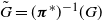 $\tilde{G} = (\boldsymbol{\pi}^*)^{-1}(G)$
), sampled from a distribution
$\tilde{G} = (\boldsymbol{\pi}^*)^{-1}(G)$
), sampled from a distribution $\mathbb{P}_{\boldsymbol{\pi}^*}$
for some unknown
$\mathbb{P}_{\boldsymbol{\pi}^*}$
for some unknown $\boldsymbol{\pi}^* \in \mathcal{S}_n^{p-1}$
whose prior distribution is assumed to be the uniform distribution
$\boldsymbol{\pi}^* \in \mathcal{S}_n^{p-1}$
whose prior distribution is assumed to be the uniform distribution $\mathcal{U}(\mathcal{S}_n^{p-1})$
; again, we wish to estimate
$\mathcal{U}(\mathcal{S}_n^{p-1})$
; again, we wish to estimate $\boldsymbol{\pi}^*$
. This reformulation of the problem places it squarely within the zoo of Bayesian inference problems. Specifically, we are trying to construct an estimator
$\boldsymbol{\pi}^*$
. This reformulation of the problem places it squarely within the zoo of Bayesian inference problems. Specifically, we are trying to construct an estimator $\hat{\boldsymbol{\pi}}$
, which is a
$\hat{\boldsymbol{\pi}}$
, which is a $\tilde{G}$
-measurable random variable, such that the expected loss
$\tilde{G}$
-measurable random variable, such that the expected loss
 \begin{equation} L = \mathbb{E}_{\boldsymbol{\pi}^* \sim \mathcal{U}(\mathcal{S}_n^{p-1})}[\mathbb{E}_{(\tilde{G}^{(1)}, \ldots, \tilde{G}^{(p)}) \sim \mathbb{P}_{\boldsymbol{\pi}^*}}[l(\boldsymbol{\pi}^*, \hat{\boldsymbol{\pi}})]]\end{equation}
is as small as possible, where $l: (\mathcal{S}_n^{p-1})^2 \to \mathbb{R}_+$
is a predetermined loss function.
$l: (\mathcal{S}_n^{p-1})^2 \to \mathbb{R}_+$
is a predetermined loss function.
What would be an adequate choice for l? A natural default choice could be the all-or-nothing loss function $l(\boldsymbol{\pi}, \boldsymbol{\pi}') = \mathbf{1}_{\boldsymbol{\pi} \neq \boldsymbol{\pi}'}$
; with this loss function, this inference problem is known as exact alignment. However, we have a notion of closeness for permutations, and we would like to acknowledge estimators which are ‘close enough’ to the true alignment.
$l(\boldsymbol{\pi}, \boldsymbol{\pi}') = \mathbf{1}_{\boldsymbol{\pi} \neq \boldsymbol{\pi}'}$
; with this loss function, this inference problem is known as exact alignment. However, we have a notion of closeness for permutations, and we would like to acknowledge estimators which are ‘close enough’ to the true alignment.
In the case where $p=2$
, we may define
$p=2$
, we may define
 \begin{equation} ov(\pi, \pi') = \frac{1}{n} \sum_{i=1}^n \mathbf{1}_{\pi(i) = \pi'(i)} \in [0, 1]\end{equation}
and $d = (1 - ov)$
is a distance over
$d = (1 - ov)$
is a distance over $\mathcal{S}_n$
. This means that we now have other natural loss functions: for instance, the functions
$\mathcal{S}_n$
. This means that we now have other natural loss functions: for instance, the functions $l_r(\pi, \pi') = \mathbf{1}_{d(\pi, \pi') \geq r}$
, for
$l_r(\pi, \pi') = \mathbf{1}_{d(\pi, \pi') \geq r}$
, for $0 \leq r < 1$
. This allows us to ask slightly different questions: namely, the so-called almost exact and partial alignment problems, which we describe in the next section. We may similarly extend the notion of overlap to
$0 \leq r < 1$
. This allows us to ask slightly different questions: namely, the so-called almost exact and partial alignment problems, which we describe in the next section. We may similarly extend the notion of overlap to $\mathcal{S}_n^{p-1}$
when
$\mathcal{S}_n^{p-1}$
when $p \geq 3$
; there are multiple ways to do this, including the definition (3) which we adopted to state our main results. We discuss this further in Section 2.3.
$p \geq 3$
; there are multiple ways to do this, including the definition (3) which we adopted to state our main results. We discuss this further in Section 2.3.
Before proceeding, let us describe what the metric space $\mathcal{S}_n$
actually looks like. One way to conceptualise it is as a hyperbolic space: for any
$\mathcal{S}_n$
actually looks like. One way to conceptualise it is as a hyperbolic space: for any $\pi \in \mathcal{S}_n$
, the size of the ball
$\pi \in \mathcal{S}_n$
, the size of the ball $B(\pi, r)$
grows roughly like
$B(\pi, r)$
grows roughly like $(n^n)^r$
, for
$(n^n)^r$
, for $0 \leq r \leq 1$
.
$0 \leq r \leq 1$
.
Another, more explicit, description of this space is the following. Within the space $\mathcal{M}_n(\mathbb{R})$
of
$\mathcal{M}_n(\mathbb{R})$
of $n \times n$
matrices, the set
$n \times n$
matrices, the set $B_n$
of doubly stochastic matrices is a polytope (known as the Birkhoff polytope), whose vertices are the permutation matrices (which we may identify with
$B_n$
of doubly stochastic matrices is a polytope (known as the Birkhoff polytope), whose vertices are the permutation matrices (which we may identify with $\mathcal{S}_n$
). The canonical Euclidean structure on this space gives us the metric
$\mathcal{S}_n$
). The canonical Euclidean structure on this space gives us the metric
 \begin{equation} \langle \pi, \pi' \rangle = ov(\pi, \pi') \text{ i.e. } d_B(\pi, \pi') = \sqrt{2(1 - ov(\pi, \pi'))}, \end{equation}
which largely serves the same purpose as our previous distance d in this context. This description also shows quite nicely why we often relax the alignment problem to solve a more general quadratic assignment problem over $B_n$
, as in [Reference Varma, Waldspurger and Massoulié13, Reference Fan, Mao, Wu and Xu34].
$B_n$
, as in [Reference Varma, Waldspurger and Massoulié13, Reference Fan, Mao, Wu and Xu34].
2.2. Metric estimation problems
What follows is fairly general; as motivation for our definitions, it may be helpful to think of the specific case of the graph alignment problem, as defined above.
Fix a sequence $(A_n, d = d_n, \mu = \mu_n)$
, which are metric spaces equipped with an a priori probability distribution. Fix a sequence
$(A_n, d = d_n, \mu = \mu_n)$
, which are metric spaces equipped with an a priori probability distribution. Fix a sequence $(B_n)$
of (measurable) observation spaces, equipped with probability distributions
$(B_n)$
of (measurable) observation spaces, equipped with probability distributions $(\nu_x)_{x \in A_n}$
such that
$(\nu_x)_{x \in A_n}$
such that $x \mapsto \nu_x$
is measurable. To fix ideas, we assume that
$x \mapsto \nu_x$
is measurable. To fix ideas, we assume that $\textrm{diam} A_n = 1$
, so that
$\textrm{diam} A_n = 1$
, so that $d(x, y) \simeq 1$
means that x, y are far apart.
$d(x, y) \simeq 1$
means that x, y are far apart.
We set $X_n \in A_n$
a random variable with law
$X_n \in A_n$
a random variable with law $\mu$
, and
$\mu$
, and $Y_n \in B_n$
a random variable with law
$Y_n \in B_n$
a random variable with law $\nu_{X_n}$
; from the observation of
$\nu_{X_n}$
; from the observation of $Y_n$
, we are trying to estimate the value of
$Y_n$
, we are trying to estimate the value of $X_n$
. We define
$X_n$
. We define $\mathbb{P} = \mathbb{P}_n$
to be the distribution of
$\mathbb{P} = \mathbb{P}_n$
to be the distribution of $(X_n, Y_n)$
, and, for any measurable
$(X_n, Y_n)$
, and, for any measurable $S_n \subseteq A_n$
,
$S_n \subseteq A_n$
,
 \begin{equation} \mathbb{P}_{\rm post}(S_n) = \mathbb{P}(S_n | Y_n)\end{equation}
the a posteriori probability of $S_n$
.
$S_n$
.
Definition 1.
A partial estimator $\hat{X}_n$
of
$\hat{X}_n$
of $X_n$
is a
$X_n$
is a $Y_n$
-measurable random variable such that, for some
$Y_n$
-measurable random variable such that, for some $0 \leq r < 1$
,
$0 \leq r < 1$
,
 \begin{equation} \mathbb{E}[l_r(\hat{X}_n, X_n)] \underset{n \to +\infty}{\longrightarrow} 0, \quad \text{i.e.} \ \ \mathbb{P}(d(\hat{X}_n, X_n) > r) \underset{n \to +\infty}{\longrightarrow} 0. \end{equation}
We say that partial estimation is feasible if a partial estimator exists.
On the other hand, we say that partial estimation of $X_n$
is intractable if, for any
$X_n$
is intractable if, for any $0 \leq r < 1$
, and for any sequence
$0 \leq r < 1$
, and for any sequence $(\hat{X}_n)$
of estimators,
$(\hat{X}_n)$
of estimators,
 \begin{equation} \mathbb{E}[l_r(\hat{X}_n, X_n)] \underset{n \to +\infty}{\longrightarrow} 1. \end{equation}
An almost exact estimator $\hat{X}_n$
of
$\hat{X}_n$
of $X_n$
is a
$X_n$
is a $Y_n$
-measurable random variable such that, for any
$Y_n$
-measurable random variable such that, for any $\varepsilon > 0$
,
$\varepsilon > 0$
,
 \begin{equation} \mathbb{E}[l_\varepsilon(\hat{X}_n, X_n)] \underset{n \to +\infty}{\longrightarrow} 0 \quad \text{i.e.} \ \ \mathbb{P}(d(\hat{X}_n, X_n) > \varepsilon) \underset{n \to +\infty}{\longrightarrow} 0. \end{equation}
We say that almost exact estimation is feasible if an almost exact estimator exists.
On the other hand, we say that almost exact estimation of $X_n$
is intractable if, for some
$X_n$
is intractable if, for some $\varepsilon > 0$
, and for any sequence
$\varepsilon > 0$
, and for any sequence $(\hat{X}_n)$
of estimators,
$(\hat{X}_n)$
of estimators,
 \begin{equation} \mathbb{E}[l_\varepsilon(\hat{X}_n, X_n)] \underset{n \to +\infty}{\longrightarrow} 1. \end{equation}
Remark 1. Note that partial (respectively, almost exact) estimation being intractable is a stronger statement than the nonexistence of a partial (respectively, almost exact) estimator. Indeed, there exists an intermediate regime where one could build estimators which, say, succeed half the time and fail half the time.
A classical result from Bayesian decision theory (see [Reference Berger11, Section 4] for instance) is the following.
Proposition 1. Fix $r \geq 0$
: we define
$r \geq 0$
: we define
 \begin{equation} \hat{X}_n^{\rm opt} = \underset{x \in A_n}{\arg \min}\mathbb{E}[l_r(x,X_n) | Y_n] = \underset{x \in A_n}{\arg \max} \mathbb{P}_{\rm post}(B(x, r)), \end{equation}
where B(x, r) is the (closed) ball of radius r centred at x, for the distance d. Then, $\hat{X}_n^{\rm opt}$
minimises the expected loss
$\hat{X}_n^{\rm opt}$
minimises the expected loss $\mathbb{E}[l_r]$
.
$\mathbb{E}[l_r]$
.
To use this, we define a random variable
 \begin{equation} C_n(r) \underset{{\rm def}}{=} \max_{x \in A_n} \mathbb{P}_{\rm post}(B(x, r)) = 1 - \mathbb{E}[l_r(\hat{X}_n^{\rm opt}, X_n) | Y_n],\end{equation}
which measures to what extent the random measure $\mathbb{P}_{\rm post}$
concentrates around a single point. Then, owing to the choices made in defining feasibility and intractability, the following result is an immediate consequence of the proposition.
$\mathbb{P}_{\rm post}$
concentrates around a single point. Then, owing to the choices made in defining feasibility and intractability, the following result is an immediate consequence of the proposition.
Corollary 1. With $C_n$
defined as above:
$C_n$
defined as above:
-
(i). partial estimation is feasible if and only if, for some
$0 \leq r < 1$
,
$C_n(r) \underset{\mathbb{P}}{\longrightarrow} 1$
; -
(ii). almost exact estimation is feasible if and only if, for any
$\varepsilon > 0$
,
$C_n(\varepsilon) \underset{\mathbb{P}}{\longrightarrow} 1$
.


On the other hand:
-
(i). partial estimation is intractable if and only if, for any
$0 \leq r < 1$
,
$C_n(r) \underset{\mathbb{P}}{\longrightarrow} 0$
; -
(ii). almost exact estimation is intractable if and only if, for some
$\varepsilon > 0$
,
$C_n(\varepsilon) \underset{\mathbb{P}}{\longrightarrow} 0$
.


Remark 2. Assume that almost exact estimation is feasible, and let $\varepsilon > 0$
. Then,
$\varepsilon > 0$
. Then,
 \begin{equation} \mathbb{P}_{\rm post}(B(X_n, 2 \varepsilon)) \geq \mathbb{P}_{\rm post}(B(\hat{X}_n^{\rm opt}, \varepsilon) )\mathbf{1}_{d(X_n, \hat{X}_n^{\rm opt}) < \varepsilon} = 1 - o_{\mathbb{P}}(1).\end{equation}
Otherwise put, with high probability, the mass of $\mathbb{P}_{\rm post}$
will tend to concentrate around
$\mathbb{P}_{\rm post}$
will tend to concentrate around $X_n$
.
$X_n$
.
2.3. A brief aside on multi-graph alignment
As we previously suggested, there are a few natural extensions of ov to $\mathcal{S}_n^{p-1}$
. Two particularly relevant ones here are
$\mathcal{S}_n^{p-1}$
. Two particularly relevant ones here are
 \begin{equation} ov(\boldsymbol{\pi}, \boldsymbol{\pi}') = \frac{1}{n} \sum_{i=1}^n \mathbf{1}_{\pi_2(i) = \pi'_2(i), \ldots, \pi_p(i) = \pi'_p(i)} \text{ (as defined earlier)},\end{equation}
 \begin{align} ov_w(\boldsymbol{\pi}, \boldsymbol{\pi}') = \frac{1}{p-1} \sum_{i=2}^p ov(\pi_i, \pi'_i).\\[6pt] \nonumber \end{align}
Essentially, ov measures how often the $(\pi_i, \pi_i')$
all agree at the same time; while
$(\pi_i, \pi_i')$
all agree at the same time; while $ov_w$
measures how often they will agree pairwise. Thus, informally, graph alignment for
$ov_w$
measures how often they will agree pairwise. Thus, informally, graph alignment for $d = 1 - ov$
involves determining
$d = 1 - ov$
involves determining $(\pi_2^*, \ldots, \pi_p^*)$
on some given set X, while graph alignment for
$(\pi_2^*, \ldots, \pi_p^*)$
on some given set X, while graph alignment for $d_w = 1 - ov_w$
involves determining
$d_w = 1 - ov_w$
involves determining $\pi_2^*$
on some (large) set
$\pi_2^*$
on some (large) set $X_2, \ldots$
, and
$X_2, \ldots$
, and $\pi_p^*$
on some (large) set
$\pi_p^*$
on some (large) set $X_p$
. With this in mind, it seems that the distance d should be more natural as a choice, motivating the following definition.
$X_p$
. With this in mind, it seems that the distance d should be more natural as a choice, motivating the following definition.
Definition 2. We say that partial graph alignment is possible (respectively, intractable) if partial estimation of the true alignment $\boldsymbol{\pi}^*$
, for the distance function d, is possible (respectively, intractable), as defined in Definition 1. For the distance
$\boldsymbol{\pi}^*$
, for the distance function d, is possible (respectively, intractable), as defined in Definition 1. For the distance $d_w$
, we instead speak of weak partial alignment.
$d_w$
, we instead speak of weak partial alignment.
The same definition applies to almost exact alignment. However, in this case, we do not need to make the distinction between normal and weak alignment.
Proposition 2. If partial alignment is possible (respectively, not intractable), then weak partial alignment is possible (respectively, not intractable).
Almost exact alignment is possible (respectively, intractable) if and only if weak almost exact alignment is possible (respectively, intractable).
Proof. This follows from the fact that $d_w \leq d \leq (p - 1) d_w$
.
$d_w \leq d \leq (p - 1) d_w$
.
2.4. Applying metric estimation
If we want to understand partial, or almost exact, alignment, our job is thus to control the random variable $C_n(r)$
defined earlier. In the Gaussian case, in order to show intractability of partial alignment, we can directly perform calculations to estimate
$C_n(r)$
defined earlier. In the Gaussian case, in order to show intractability of partial alignment, we can directly perform calculations to estimate $C_n(r)$
.
$C_n(r)$
.
In the Erdös–Rényi case, however, our arguments are much more combinatorial in nature. The general idea is quite simple: if $B = B(\boldsymbol{\pi}^*, r)$
is a ball, we would like to take the alignments within B (which are close to the true alignment
$B = B(\boldsymbol{\pi}^*, r)$
is a ball, we would like to take the alignments within B (which are close to the true alignment $\boldsymbol{\pi}^*$
) and modify them to obtain a large number of other alignments, which are nowhere near
$\boldsymbol{\pi}^*$
) and modify them to obtain a large number of other alignments, which are nowhere near $\boldsymbol{\pi}^*$
but which seem just as plausible to an outside observer. In the case where
$\boldsymbol{\pi}^*$
but which seem just as plausible to an outside observer. In the case where $p=2$
, this is done in [Reference Ganassali, Massoulié and Lelarge2]: they construct a large number of
$p=2$
, this is done in [Reference Ganassali, Massoulié and Lelarge2]: they construct a large number of $(\sigma_i) \in S_n$
which are far apart and which exactly preserve
$(\sigma_i) \in S_n$
which are far apart and which exactly preserve $\mathbb{P}_{\rm post}$
, so that
$\mathbb{P}_{\rm post}$
, so that $\mathbb{P}_{\rm post}(\sigma_i(B)) = \mathbb{P}_{\rm post}(B)$
and the
$\mathbb{P}_{\rm post}(\sigma_i(B)) = \mathbb{P}_{\rm post}(B)$
and the $\sigma_i(B)$
are all disjoint. This is fairly technical, and not quite necessary: at the cost of some abstraction, we can provide a significantly more robust argument, which holds for any metric estimation problem, and does not require that we preserve
$\sigma_i(B)$
are all disjoint. This is fairly technical, and not quite necessary: at the cost of some abstraction, we can provide a significantly more robust argument, which holds for any metric estimation problem, and does not require that we preserve $\mathbb{P}_{\rm post}$
exactly.
$\mathbb{P}_{\rm post}$
exactly.
Lemma 1. Assume that the state space $A_n$
is finite. Let
$A_n$
is finite. Let $\textrm{Neg}_n \subseteq A_n$
, such that
$\textrm{Neg}_n \subseteq A_n$
, such that $\mathbb{P}_{\rm post}(\textrm{Neg}_n) = o_\mathbb{P}(1)$
. (This contains states which are implausibly ill-behaved and which we may ignore.)
$\mathbb{P}_{\rm post}(\textrm{Neg}_n) = o_\mathbb{P}(1)$
. (This contains states which are implausibly ill-behaved and which we may ignore.)
For any ball $B = B(x_0, r)$
with radius
$B = B(x_0, r)$
with radius $r < 1$
, assume that there exists a random function
$r < 1$
, assume that there exists a random function $F: B \setminus \textrm{Neg}_n \to \mathcal{P}(A_n)$
(which depends upon n, B), satisfying certain conditions:
$F: B \setminus \textrm{Neg}_n \to \mathcal{P}(A_n)$
(which depends upon n, B), satisfying certain conditions:
-
(i) F outputs an overwhelmingly plausible set of states, in the following sense: there exists
$\varepsilon_n(r) > 0$
such that, for
$x \in B \setminus \textrm{Neg}_n$
, (17)
\begin{equation} \mathbb{P}_{\rm post}(x) \leq \varepsilon_n(r) \mathbb{P}_{\rm post}(F(x)); \end{equation}
-
(ii) F is quasi-injective, in the following sense; for any
$r < 1$
, there exists
$K_n(r) > 0$
such that
$K_n(r) \varepsilon_n(r) \overset{\mathbb{P}}{\underset{n \to +\infty}{\longrightarrow}} 0$
and, if
$y \in A_n$
, there are at most
$K_n(r)$
values of
$x \in B$
such that
$y \in F(x)$
.


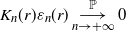


Then, partial estimation is intractable.
Remark 3. Notably, we do not require that the quantities $\varepsilon_n, K_n$
be deterministic: this would be somewhat restrictive given that the measure
$\varepsilon_n, K_n$
be deterministic: this would be somewhat restrictive given that the measure $\mathbb{P}_{\rm post}$
is itself random.
$\mathbb{P}_{\rm post}$
is itself random.
Here, F takes on the same role as the map $\pi \mapsto (\sigma_i \circ \pi)_{i}$
, in the 2-graph argument from [Reference Ganassali, Massoulié and Lelarge2].
$\pi \mapsto (\sigma_i \circ \pi)_{i}$
, in the 2-graph argument from [Reference Ganassali, Massoulié and Lelarge2].
Proof. Let $B = B(x, r)$
be a ball with radius
$B = B(x, r)$
be a ball with radius $r < 1$
. Then:
$r < 1$
. Then:
 \begin{align} \mathbb{P}_{\rm post}(B) & \leq \mathbb{P}_{\rm post}(\textrm{Neg}_n) + \sum_{y \in B \setminus \textrm{Neg}_n} \mathbb{P}_{\rm post}(y) \nonumber\\[3pt] & \leq o_{\mathbb{P}}(1) + \varepsilon_n(r)\sum_{y \in B \setminus \textrm{Neg}_n} \mathbb{P}_{\rm post}(F(y)) \nonumber\\[3pt] & \leq o_{\mathbb{P}}(1) + \varepsilon_n(r) \sum_{y' \in A_n} \sum_{y \text{ s.t. }y' \in F(y)} \mathbb{P}_{\rm post}(y') \nonumber\\[3pt] & \leq o_{\mathbb{P}}(1) + \varepsilon_n(r) \sum_{y' \in A_n} K_n(r) \mathbb{P}_{\rm post}(y') \nonumber\\[3pt] & = o_{\mathbb{P}}(1) + \varepsilon_n(r) K_n(r) \mathbb{P}_{\rm post}(A_n) = o_{\mathbb{P}}(1).\end{align}
Applying Corollary 1, the lemma is shown.
3. Solving the Gaussian model
In this section, we prove Theorem 1. As discussed in Section 2.3, it is sufficient for us to prove it for the distance function d; from now on, all balls $B(\boldsymbol{\pi}, r)$
are defined with regards to this metric.
$B(\boldsymbol{\pi}, r)$
are defined with regards to this metric.
In all of the following theorems, we assume that
 \begin{equation} \rho = \displaystyle\sqrt{\frac{8(1 + \eta) \log n}{p n}}\end{equation}
for some $\eta = O(1)$
. We will prove the feasibility of exact alignment for any fixed
$\eta = O(1)$
. We will prove the feasibility of exact alignment for any fixed $\eta > 0$
, and show that partial alignment is intractable when
$\eta > 0$
, and show that partial alignment is intractable when $\eta = -(\!\log n)^{- {1}/{5}}$
.
$\eta = -(\!\log n)^{- {1}/{5}}$
.
Note that this is, in fact, sufficient to prove the theorem for general $\rho$
. Indeed, if we observe
$\rho$
. Indeed, if we observe $(\boldsymbol{\pi}^*)^{-1}(G)$
for some
$(\boldsymbol{\pi}^*)^{-1}(G)$
for some $G \sim \mathcal{N}(n, \rho)$
, we may form a set of graphs
$G \sim \mathcal{N}(n, \rho)$
, we may form a set of graphs $(\boldsymbol{\pi}^*)^{-1}(G')$
where
$(\boldsymbol{\pi}^*)^{-1}(G')$
where $G' \sim \mathcal{N}(n, \rho')$
for any
$G' \sim \mathcal{N}(n, \rho')$
for any $\rho' \leq \rho$
, simply by adding independent and identically distributed (i.i.d.) Gaussian weights to the edges of
$\rho' \leq \rho$
, simply by adding independent and identically distributed (i.i.d.) Gaussian weights to the edges of $(\boldsymbol{\pi}^*)^{-1}(G)$
and renormalising; then, solving the alignment problem for G’ allows us to solve it for G.
$(\boldsymbol{\pi}^*)^{-1}(G)$
and renormalising; then, solving the alignment problem for G’ allows us to solve it for G.
In what follows, for $\boldsymbol{\sigma} \in \mathcal{S}_n^{p-1}$
and
$\boldsymbol{\sigma} \in \mathcal{S}_n^{p-1}$
and $1 \leq i \neq j \leq p$
, we set
$1 \leq i \neq j \leq p$
, we set $\sigma_{ij} = \sigma_j (\pi_j^*)^{-1} \pi_i^* \sigma_i^{-1} $
. It may be helpful to assume that
$\sigma_{ij} = \sigma_j (\pi_j^*)^{-1} \pi_i^* \sigma_i^{-1} $
. It may be helpful to assume that $\boldsymbol{\pi}^* = \textrm{Id}$
, since we can (up to some notational bookkeeping) reduce the problem down to this case; then,
$\boldsymbol{\pi}^* = \textrm{Id}$
, since we can (up to some notational bookkeeping) reduce the problem down to this case; then, $\sigma_{ij}$
measures how different
$\sigma_{ij}$
measures how different $\sigma_i$
and
$\sigma_i$
and $\sigma_j$
are.
$\sigma_j$
are.
3.1. The Gibbs measure
The main appeal of the Gaussian model is that the a posteriori distribution has a nice expression. Specifically, it is as follows.
Proposition 3. For any $\boldsymbol{\sigma} \in \mathcal{S}_n^{p-1}$
, we may write
$\boldsymbol{\sigma} \in \mathcal{S}_n^{p-1}$
, we may write
 \begin{equation} \mathbb{P}_{\rm post}(\boldsymbol{\sigma}) = \frac{1}{\mathcal{Z}} \mathrm{e}^{- \beta \mathcal{H}(\sigma)} \end{equation}
where the partition function $\mathcal{Z}$
is independent from
$\mathcal{Z}$
is independent from $\boldsymbol{\sigma}$
. Here,
$\boldsymbol{\sigma}$
. Here,
 \begin{equation} \mathcal{H}(\boldsymbol{\sigma}) = - \sum_{e \in E} \sum_{1 \leq i \neq j \leq p} G_e^{(i)} G_{\sigma_{ij}(e)}^{(j)}; \quad \beta = \dfrac{\rho}{2(1 - \rho)(1 + (p-1)\rho)} = \dfrac{\rho}{2}(1 + o(1)). \end{equation}
Proof. By definition, the probability density function for $(\boldsymbol{\sigma}, G^{(1)}, \ldots, G^{(p)})$
is proportional to
$(\boldsymbol{\sigma}, G^{(1)}, \ldots, G^{(p)})$
is proportional to
 \begin{equation} p(\boldsymbol{\sigma}, G^{(1)}, \ldots, G^{(p)}) = \frac{1}{(n!)^{p-1}} \prod_{e \in E} \exp\bigg( \!-\!\frac{1}{2}\sum_{1 \leq i,j \leq p} (M^{-1})_{ij} G^{(i)}_{e} G^{(j)}_{e}\bigg), \end{equation}
where $M = (1 - \rho)I_p + \rho J_p$
is our covariance matrix. Consequently, if we observe the graphs
$M = (1 - \rho)I_p + \rho J_p$
is our covariance matrix. Consequently, if we observe the graphs $H^{(i)} = (\pi_i^*)^{-1}(G^{(i)})$
, the distribution
$H^{(i)} = (\pi_i^*)^{-1}(G^{(i)})$
, the distribution $\mathbb{P}_{\rm post}$
is given by
$\mathbb{P}_{\rm post}$
is given by
 \begin{align} \mathbb{P}_{\rm post}(\boldsymbol{\sigma}) & = \mathbb{P}(\boldsymbol{\pi}^* = \boldsymbol{\sigma} | H^{(1)}, \ldots, H^{(p)}) \nonumber\\[3pt] & = \frac{1}{\mathcal{Z}'} p(\boldsymbol{\sigma}, \sigma_1(H^{(1)}), \ldots, \sigma_p(H^{(p)})) \nonumber\\[3pt] & = \frac{1}{\mathcal{Z}'} \prod_{e \in E} \exp\bigg( \!-\!\frac{1}{2}\sum_{1 \leq i,j \leq p} (M^{-1})_{ij} G^{(i)}_{(\pi_i^*)^{-1} \sigma_i(e)} G^{(j)}_{(\pi_j^*)^{-1} \sigma_j(e)}\bigg) \nonumber\\[3pt] & = \frac{1}{\mathcal{Z}} \exp \bigg( \!- \!\frac{1}{2}\sum_{e \in E} \sum_{1 \leq i \neq j \leq p} (M^{-1})_{ij} G^{(i)}_{(\pi_i^*)^{-1} \sigma_i(e)} G^{(j)}_{(\pi_j^*)^{-1} \sigma_j(e)}\bigg), \end{align}
since the product over the diagonal terms ( $i=j$
) is independent from
$i=j$
) is independent from $\boldsymbol{\sigma}$
. (Here,
$\boldsymbol{\sigma}$
. (Here, $\mathcal{Z}, \mathcal{Z'}$
are quantities which may depend upon the
$\mathcal{Z}, \mathcal{Z'}$
are quantities which may depend upon the $(H^{(i)})$
but not upon
$(H^{(i)})$
but not upon $\boldsymbol{\sigma}$
.) However, for
$\boldsymbol{\sigma}$
.) However, for $i \neq j$
,
$i \neq j$
, $(M^{-1})_{ij} = - 2 \beta$
; we thus obtain our desired expression, with
$(M^{-1})_{ij} = - 2 \beta$
; we thus obtain our desired expression, with
 \begin{align} \mathcal{H}(\sigma) & = -\sum_{e \in E} \sum_{1 \leq i \neq j \leq p} G^{(i)}_{(\pi_i^*)^{-1} \sigma_i(e)} G^{(j)}_{(\pi_j^*)^{-1} \sigma_j(e)} \nonumber\\[3pt] & = -\sum_{e \in E} \sum_{1 \leq i \neq j \leq p} G^{(i)}_{e} G^{(j)}_{\sigma_{ij}(e)}. \end{align}
This Hamiltonian is quite descriptive, and invites a natural visual interpretation of the graph alignment problem: we have p weighted graphs which we ‘stick’ together with our alignment $\boldsymbol{\sigma}$
, and each edge has a fixed ‘spin’ such that edges with similar spins try to stick to each other.
$\boldsymbol{\sigma}$
, and each edge has a fixed ‘spin’ such that edges with similar spins try to stick to each other.
From a technical perspective however, this Hamiltonian is not quite what we want. Recall that our ultimate goal is to understand to what extent the measure $\mathbb{P}_{\rm post}$
concentrates around any given point; and, if it is to be concentrated around a point, we should expect that point to be the ground truth
$\mathbb{P}_{\rm post}$
concentrates around any given point; and, if it is to be concentrated around a point, we should expect that point to be the ground truth $\pi^*$
. As a result, it makes sense to renormalise our system, writing
$\pi^*$
. As a result, it makes sense to renormalise our system, writing
 \begin{equation} \mathbb{P}_{\rm post}(\boldsymbol{\sigma}) = \frac{1}{Z} \mathrm{e}^{- \beta V(\boldsymbol{\sigma})},\end{equation}
where the potential $V(\boldsymbol{\sigma})$
is equal to
$V(\boldsymbol{\sigma})$
is equal to
 \begin{align} V(\boldsymbol{\sigma}) & = \mathcal{H}(\boldsymbol{\sigma}) - \mathcal{H}(\pi^*) \nonumber\\[3pt] & = \sum_{e \in E, 1 \leq i \neq j \leq p} G_e^{(i)} (G_e^{(j)} - G_{\sigma_{ij}(e)}^{(j)}) \nonumber\\[3pt] & = \sum_{\underset{\sigma_{ij}(e) \neq e}{e \in E, 1 \leq i \neq j \leq p}}G_e^{(i)} G_e^{(j)} - \sum_{\underset{\sigma_{ij}(e) \neq e}{e \in E, 1 \leq i \neq j \leq p}}G_e^{(i)} G_{\sigma_{ij}(e)}^{(j)} \nonumber\\[3pt] & \underset{{\rm def}}{=} - V_{\mathrm{diag}}(\boldsymbol{\sigma}) + V_{\mathrm{off}}(\boldsymbol{\sigma}).\end{align}
We have split up the potential V into two terms for a couple of reasons. The first is that, viewing V as a quadratic form of $G \in \mathbb{R}^{E} \otimes \mathbb{R}^p$
,
$G \in \mathbb{R}^{E} \otimes \mathbb{R}^p$
, $V_{\mathrm{diag}}$
contains the block-diagonal terms while
$V_{\mathrm{diag}}$
contains the block-diagonal terms while $V_{\mathrm{off}}$
contains the off-diagonal blocks. (The expression of V as a quadratic form is made explicit in Appendices C and B.) It is typical, when studying quadratic forms of Gaussian vectors, to separate the two; they tend to require different tools. The second reason is that
$V_{\mathrm{off}}$
contains the off-diagonal blocks. (The expression of V as a quadratic form is made explicit in Appendices C and B.) It is typical, when studying quadratic forms of Gaussian vectors, to separate the two; they tend to require different tools. The second reason is that $V_{\mathrm{diag}}(\boldsymbol{\sigma})$
concentrates around its mean quite uniformly in
$V_{\mathrm{diag}}(\boldsymbol{\sigma})$
concentrates around its mean quite uniformly in $\boldsymbol{\sigma}$
, in a sense which we make explicit in a moment.
$\boldsymbol{\sigma}$
, in a sense which we make explicit in a moment.
Before moving on, let us briefly explain the structure of the rest of this section. Our ultimate goal is to prove that $\mathbb{P}_{\rm post}$
concentrates around the true alignment
$\mathbb{P}_{\rm post}$
concentrates around the true alignment $\boldsymbol{\pi}^*$
(respectively, is spread out over the entire state space) if
$\boldsymbol{\pi}^*$
(respectively, is spread out over the entire state space) if $\eta > 0$
(respectively,
$\eta > 0$
(respectively, $\eta < 0$
). Doing this will require a few steps:
$\eta < 0$
). Doing this will require a few steps:
-
• first, we do a bit of combinatorics in order to understand the structure of
$(\mathcal{S}_n^{p-1}, d)$
a bit better; -
• next, we compute the ‘annealed free energy’
$\log \mathbb{E}[Z]$
; -
• finally, we use this to compute the quenched free energy
$\mathbb{E}[\log Z]$
.


This last step is the hardest; as is fairly standard in systems derived from Gibbs measures, once we have $\mathbb{E}[\log Z]$
it is not too hard to obtain most relevant properties of the distribution
$\mathbb{E}[\log Z]$
it is not too hard to obtain most relevant properties of the distribution $\mathbb{P}_{\rm post}$
.
$\mathbb{P}_{\rm post}$
.
3.2. Some combinatorics
For the rest of this section, we define $d_{ij}(\boldsymbol{\sigma}) =\# \{ u \in \left[ \! \left[ 1, n \right] \! \right]\!, \sigma_{ij}(u) = u \}$
: this combinatorial quantity appears a fair amount in our analysis, as it is closely linked to the number of terms in the sums defining
$d_{ij}(\boldsymbol{\sigma}) =\# \{ u \in \left[ \! \left[ 1, n \right] \! \right]\!, \sigma_{ij}(u) = u \}$
: this combinatorial quantity appears a fair amount in our analysis, as it is closely linked to the number of terms in the sums defining $V_{\mathrm{diag}}$
and
$V_{\mathrm{diag}}$
and $V_{\mathrm{off}}$
. In this section, we control the behaviour of
$V_{\mathrm{off}}$
. In this section, we control the behaviour of $(d_{ij}(\boldsymbol{\sigma}))$
as a function of
$(d_{ij}(\boldsymbol{\sigma}))$
as a function of $\boldsymbol{\sigma} \in \mathcal{S}_n^{p-1}$
.
$\boldsymbol{\sigma} \in \mathcal{S}_n^{p-1}$
.
Theorem 3. Let $(d_{ij})_{1 \leq i \neq j \leq p}$
be positive integers, with
$(d_{ij})_{1 \leq i \neq j \leq p}$
be positive integers, with $d_{ij} = d_{\rm ji}$
for any i, j. We set
$d_{ij} = d_{\rm ji}$
for any i, j. We set
 \begin{equation} F((d_{ij})) = \# \{\boldsymbol{\sigma} \in \mathcal{S}_n^{p-1}, \ {for\, all }\, 1 \leq i \neq j \leq p,\ d_{ij}(\boldsymbol{\sigma}) \geq d_{ij} \}. \end{equation}
Then, for any permutation $\tau \in \mathcal{S}_p$
,
$\tau \in \mathcal{S}_p$
,
 \begin{equation} F((d_{ij})) \leq \frac{(n!)^{p-1}}{(\!\displaystyle\max_{j < 2} d_{\tau(j)\tau(2)})!(\!\displaystyle\max_{j < 3} d_{\tau(j) \tau(3)})! \ldots (\!\displaystyle\max_{j < p} d_{\tau(j) \tau(p)})!}. \end{equation}
Proof. It is sufficient to handle the case where $\boldsymbol{\pi}^* = \textrm{Id}$
; the general case follows by replacing
$\boldsymbol{\pi}^* = \textrm{Id}$
; the general case follows by replacing $\boldsymbol{\sigma}$
by
$\boldsymbol{\sigma}$
by $\boldsymbol{\pi}^* \circ \boldsymbol{\sigma}$
in the following proof.
$\boldsymbol{\pi}^* \circ \boldsymbol{\sigma}$
in the following proof.
We begin by noting that F is a symmetric function of $(d_{ij})$
, in the sense that if
$(d_{ij})$
, in the sense that if $\tau \in \mathcal{S}_p$
,
$\tau \in \mathcal{S}_p$
, $F((d_{\tau(i)\tau(j)})) = F((d_{ij}))$
. As a result, we just need to show the theorem when
$F((d_{\tau(i)\tau(j)})) = F((d_{ij}))$
. As a result, we just need to show the theorem when $\tau = \textrm{Id}$
; the general statement then follows.
$\tau = \textrm{Id}$
; the general statement then follows.
We now note that, for any $(d_{ij})$
, setting
$(d_{ij})$
, setting $Y_{ij}(\boldsymbol{\sigma}) \underset{{\rm def}}{=} \{ u \in \left[ \! \left[ 1, n \right] \! \right]\!, \sigma_{ij}(u) = u \}$
,
$Y_{ij}(\boldsymbol{\sigma}) \underset{{\rm def}}{=} \{ u \in \left[ \! \left[ 1, n \right] \! \right]\!, \sigma_{ij}(u) = u \}$
,
 \begin{equation} F((d_{ij})) = \frac{1}{n!}\# \{\boldsymbol{\sigma} \in \mathcal{S}_n^{p}, \mbox{ for all }1 \leq i \neq j \leq p,\ |Y_{ij}(\boldsymbol{\sigma})| \geq d_{ij} \} \end{equation}
(i.e. counting the p-tuples of permutations where we do not enforce that $\sigma_1 = \textrm{Id}$
). To see this, note that the map
$\sigma_1 = \textrm{Id}$
). To see this, note that the map
 \begin{align*} \mathcal{S}_n^{p} & \longrightarrow \mathcal{S}_n^{p-1} \simeq \{ \textrm{Id} \} \times \mathcal{S}_n^{p-1} \\[2pt] (\sigma_1, \sigma_2, \ldots, \sigma_p) & \longmapsto (\textrm{Id}, \sigma_1^{-1} \sigma_2, \ldots, \sigma_1^{-1} \sigma_p) \end{align*}
preserves the values of $(d_{ij})_{1 \leq i \neq j \leq p}$
, and any given element of
$(d_{ij})_{1 \leq i \neq j \leq p}$
, and any given element of $\mathcal{S}_n^{p-1}$
has exactly
$\mathcal{S}_n^{p-1}$
has exactly $n!$
preimages. We therefore count the number of elements of the subset defined in (29).
$n!$
preimages. We therefore count the number of elements of the subset defined in (29).
Fix $(d_{ij})_{i\neq j}$
. We are going to bound the number of possible choices for
$(d_{ij})_{i\neq j}$
. We are going to bound the number of possible choices for $\sigma_1$
, then bound the number of possible choices for
$\sigma_1$
, then bound the number of possible choices for $\sigma_{2}$
given a choice of
$\sigma_{2}$
given a choice of $\sigma_{1}$
and so on; finally, bounding the number of choices for
$\sigma_{1}$
and so on; finally, bounding the number of choices for $\sigma_{p}$
given a choice of
$\sigma_{p}$
given a choice of $\sigma_{1}, \ldots, \sigma_{p-1}$
.
$\sigma_{1}, \ldots, \sigma_{p-1}$
.
There are $n!$
choices for
$n!$
choices for $\sigma_{1}$
. In order to fix
$\sigma_{1}$
. In order to fix $\sigma_{2}$
given
$\sigma_{2}$
given $\sigma_{1}$
, it is sufficient to determine the set
$\sigma_{1}$
, it is sufficient to determine the set $X_2 = \left[ \! \left[ 1, n \right] \! \right] \setminus Y_{1 2}(\sigma)$
of points where
$X_2 = \left[ \! \left[ 1, n \right] \! \right] \setminus Y_{1 2}(\sigma)$
of points where $\sigma_{2} \neq \sigma_1$
, as well as
$\sigma_{2} \neq \sigma_1$
, as well as $\sigma_{2}|_{X_2}^{\sigma_1(X_2)}$
, giving at most
$\sigma_{2}|_{X_2}^{\sigma_1(X_2)}$
, giving at most
 \begin{equation} \binom{n}{n - d_{12}}(n - d_{12})! = \frac{n!}{d_{12}!} \end{equation}
possible choices.
Recursively, given $\sigma_{1}, \sigma_{2}, \ldots, \sigma_{l-1}$
, in order to fix
$\sigma_{1}, \sigma_{2}, \ldots, \sigma_{l-1}$
, in order to fix $\sigma_{l}$
, it is sufficient to choose
$\sigma_{l}$
, it is sufficient to choose $j < l$
, and determine the set
$j < l$
, and determine the set $X_{l} = \left[ \! \left[ 1, n \right] \! \right] \setminus Y_{jl}(\sigma)$
of points where
$X_{l} = \left[ \! \left[ 1, n \right] \! \right] \setminus Y_{jl}(\sigma)$
of points where $\sigma_{l} \neq \sigma_{j}$
as well as the restriction
$\sigma_{l} \neq \sigma_{j}$
as well as the restriction $\sigma_{l}|_{X_{l}}^{\sigma_{j}(X_{l})}$
, giving at most
$\sigma_{l}|_{X_{l}}^{\sigma_{j}(X_{l})}$
, giving at most ${n!}/{d_{jl}!}$
possibilities. Since j can be chosen arbitrarily, we can pick j such that
${n!}/{d_{jl}!}$
possibilities. Since j can be chosen arbitrarily, we can pick j such that $d_{jl}$
is maximal. The total number of possible choices is thus at most
$d_{jl}$
is maximal. The total number of possible choices is thus at most
 \begin{equation} \frac{1}{n!} \cdot n! \cdot \frac{n!}{(\!\displaystyle\max_{j < 2} d_{j2})!} \cdot \cdots \cdot \frac{n!}{(\!\displaystyle\max_{j < p} d_{jp})!} \end{equation}
giving us the desired inequality and concluding the proof of Theorem 3.
Theorem 3 can be used by itself, but the introduction of the quantities $\max_{j < k} d_{\tau(j)\tau(k)}$
for
$\max_{j < k} d_{\tau(j)\tau(k)}$
for $1 < k \leq p$
makes it somewhat unwieldy to use. Instead, we will mostly use the following corollary.
$1 < k \leq p$
makes it somewhat unwieldy to use. Instead, we will mostly use the following corollary.
Corollary 2. Let $(d_{ij})_{1 \leq i \neq j \leq p}$
be positive integers, with
$(d_{ij})_{1 \leq i \neq j \leq p}$
be positive integers, with $d_{ij} = d_{\rm ji}$
for any i,j. Then,
$d_{ij} = d_{\rm ji}$
for any i,j. Then,
 \begin{equation} F((d_{ij})) \leq \frac{(n!)^{p-1}}{\bigg( \displaystyle\prod_{1 \leq i \neq j \leq p} (d_{ij}!) \bigg)^{{1}/{p}}} \end{equation}
Proof. For $\tau \in \mathcal{S}_p$
, set
$\tau \in \mathcal{S}_p$
, set $D_{i}(\tau) = \max_{j < i} d_{\tau(j)\tau(i)}$
. In order to deduce Corollary 2 from Theorem 3, we need to show that, for some choice of
$D_{i}(\tau) = \max_{j < i} d_{\tau(j)\tau(i)}$
. In order to deduce Corollary 2 from Theorem 3, we need to show that, for some choice of $\tau$
,
$\tau$
,
 \begin{equation} \prod_{i=2}^p D_i(\tau)! \geq \bigg( \prod_{1 \leq i \neq j \leq p} (d_{ij}!) \bigg)^{{1}/{p}}.\end{equation}
In order to show this, we use the probabilistic method, showing that if $\tau \in \mathcal{S}_p$
is chosen uniformly at random, then
$\tau \in \mathcal{S}_p$
is chosen uniformly at random, then
 \begin{equation} \frac{1}{p} \sum_{1 \leq i \neq j \leq p} \log (d_{ij}!) \leq \mathbb{E}_\tau\bigg[ \sum_{i=2}^p \log (D_i(\tau)!) \bigg].\end{equation}
Indeed, more generally, if $\varphi$
is any increasing function,
$\varphi$
is any increasing function,
 \begin{align} \mathbb{E}_\tau\bigg[ \sum_{i=2}^p \varphi(D_i(\tau)) \bigg] & = \mathbb{E}_\tau\bigg[ \sum_{i=2}^p \max_{1 \leq j \leq i-1} \varphi(d_{\tau(i) \tau(j)}) \bigg]\nonumber\\[3pt] & \geq \mathbb{E}_\tau\bigg[ \sum_{i=2}^p \frac{1}{i-1} \sum_{j=1}^{i-1} \varphi(d_{\tau(i) \tau(j)}) \bigg] \nonumber\\[3pt] & = \sum_{i=2}^p \frac{1}{i-1} \sum_{j=1}^{i-1} \mathbb{E}_\tau[ \varphi(d_{\tau(i) \tau(j)})].\end{align}
However, for any $i,j \in \left[ \! \left[ 1, p \right] \! \right]$
,
$i,j \in \left[ \! \left[ 1, p \right] \! \right]$
,
 \begin{align*}\mathbb{E}_\tau[\varphi(d_{\tau(i) \tau(j)})] = \dfrac{1}{p(p-1)}\displaystyle \sum_{1 \leq i \neq j \leq p} \varphi(d_{ij}).\end{align*}
Plugging this into (35), we obtain
 \begin{equation} \frac{1}{p} \sum_{1 \leq i \neq j \leq p} \varphi(d_{ij}) \leq \mathbb{E}_\tau\bigg[ \sum_{i=2}^p \varphi(D_i(\tau)) \bigg]\end{equation}
and this holds in particular for the function $\varphi(d) = \log(d!)$
, proving the corollary.
$\varphi(d) = \log(d!)$
, proving the corollary.
3.3. The annealed free energy
The propositions in this subsection are consequences of some sharp controls on the behaviour of their Gaussian components; their proofs are all deferred to the appendix.
In order to compute $\log \mathbb{E}[Z]$
, we begin by computing
$\log \mathbb{E}[Z]$
, we begin by computing $V_{\mathrm{diag}}$
and
$V_{\mathrm{diag}}$
and $V_{\mathrm{off}}$
. The behaviour of
$V_{\mathrm{off}}$
. The behaviour of $V_{\mathrm{diag}}$
is the simplest to bound: it is essentially deterministic.
$V_{\mathrm{diag}}$
is the simplest to bound: it is essentially deterministic.
Proposition 4. For some $c > 0$
, the following property
$c > 0$
, the following property $(\mathcal{C})$
holds with probability at least
$(\mathcal{C})$
holds with probability at least $1 - \exp(-c n \sqrt{\log n})$
:
$1 - \exp(-c n \sqrt{\log n})$
:
 \begin{equation} {for\, all\, }\boldsymbol{\sigma} \in \mathcal{S}_n^{p-1}, \left|V_{\mathrm{diag}}(\boldsymbol{\sigma}) - \mathbb{E}[V_{\mathrm{diag}}(\boldsymbol{\sigma})]\right| \leq (\!\log n)^{{1}/{4}} n^{{3}/{2}} \end{equation}
Consequently, for any $\boldsymbol{\sigma} \in \mathcal{S}_n^{p-1}$
,
$\boldsymbol{\sigma} \in \mathcal{S}_n^{p-1}$
,
 \begin{equation} V(\boldsymbol{\sigma})\mathbf{1}_\mathcal{C} = \rho \sum_{1 \leq i \neq j \leq p} \bigg( \binom{n}{2} - \binom{d_{ij}(\boldsymbol{\sigma})}{2} \bigg)\mathbf{1}_\mathcal{C} + V_{\mathrm{off}}(\boldsymbol{\sigma}) \mathbf{1}_{\mathcal{C}} + O(n^{{3}/{2}} (\!\log n)^{{1}/{4}}), \end{equation}
where the error term is bounded uniformly in $\boldsymbol{\sigma}$
.
$\boldsymbol{\sigma}$
.
The fluctuations of $V_{\mathrm{off}}$
are somewhat less nice but can still be controlled.
$V_{\mathrm{off}}$
are somewhat less nice but can still be controlled.
Proposition 5. Let $\boldsymbol{\sigma} \in \mathcal{S}_n^{p-1}$
. Then,
$\boldsymbol{\sigma} \in \mathcal{S}_n^{p-1}$
. Then,
 \begin{equation} \log \mathbb{E}[e^{-\beta V_{\mathrm{off}}(\boldsymbol{\sigma})}] = \beta^2\displaystyle\sum_{1 \leq i \neq j \leq p} \bigg(\displaystyle\binom{n}{2} - \displaystyle \binom{d_{ij}(\boldsymbol{\sigma})}{2} \bigg) + O(n), \end{equation}
where, again, the error term is bounded uniformly in $\boldsymbol{\sigma}$
.
$\boldsymbol{\sigma}$
.
Putting these together allows us to obtain the behaviour of the annealed free energy. To this end, for any $\boldsymbol{\pi} \in \mathcal{S}_n^{p-1}$
and
$\boldsymbol{\pi} \in \mathcal{S}_n^{p-1}$
and $0 < r \leq 1$
, we define
$0 < r \leq 1$
, we define
 \begin{equation} Z_r(\boldsymbol{\pi}) = \sum_{\boldsymbol{\sigma} \in B(\boldsymbol{\pi}, r)} e^{-\beta V(\boldsymbol{\sigma})}. \end{equation}
Proposition 6. For any $0 < r \leq 1$
,
$0 < r \leq 1$
,
 \begin{equation} \log \mathbb{E}[Z_r(\boldsymbol{\pi}^*) \mathbf{1}_\mathcal{C}] \leq (p-1) n \log n \max_{0 \leq \rho \leq r} \varphi(\rho) + O(n(\!\log n)^{{3}/{4}}) \end{equation}
and
 \begin{align} \log \mathbb{E}[(Z - Z_r(\boldsymbol{\pi}^*))\mathbf{1}_{\mathcal{C}} ] &\leq (p-1) n \log n \bigg( \frac{p-1}{p} \max_{r' \in [0,1]} \varphi(r') + \frac{1}{p} \max_{r' \in [{r}/({p-1}), 1] } \varphi(r') \bigg) \end{align}
 \begin{align} &\quad + O(n (\!\log n)^{3/4}), \end{align}
where $\varphi(r') = (1 + \eta)(r')^2 - (1 + 2 \eta)r'$
for
$\varphi(r') = (1 + \eta)(r')^2 - (1 + 2 \eta)r'$
for $r' \in [0,1]$
.
$r' \in [0,1]$
.
3.4. The quenched free energy
Recall that we have written the parameter $\rho$
of our system as
$\rho$
of our system as
 \begin{align*}\rho = \sqrt{\frac{8(1 + \eta) \log n}{p n}};\end{align*}
we wish to estimate the quenched free energy $\mathbb{E}[\log Z]$
as a function of
$\mathbb{E}[\log Z]$
as a function of $\eta$
. This quantity captures the typical behaviour of Z better than the annealed free energy; controlling it is the difficult part in bounding
$\eta$
. This quantity captures the typical behaviour of Z better than the annealed free energy; controlling it is the difficult part in bounding $\mathbb{P}_{\rm post}$
. In these systems, we cannot usually expect to have
$\mathbb{P}_{\rm post}$
. In these systems, we cannot usually expect to have $\mathbb{E}[\log Z] \sim \log \mathbb{E}[Z]$
in general; however, when
$\mathbb{E}[\log Z] \sim \log \mathbb{E}[Z]$
in general; however, when $\eta > 0$
the system fluctuates sufficiently little for this to hold.
$\eta > 0$
the system fluctuates sufficiently little for this to hold.
Lemma 2. In general, we have
 \begin{equation} 0 \leq \mathbb{E}[(\!\log Z)\mathbf{1}_{\mathcal{C}}] \leq \log \mathbb{E}[Z\mathbf{1}_{\mathcal{C}}](1 + o(1)). \end{equation}
In particular, if $\eta > 0$
,
$\eta > 0$
,
 \begin{equation} \mathbb{E}[(\!\log Z)\mathbf{1}_{\mathcal{C}}]= o(n \log n). \end{equation}
Proof. The first inequality simply follows from the fact that
 \begin{equation} Z \geq \mathrm{e}^{-\beta V(\boldsymbol{\pi}^*)} = 1 \end{equation}
since $V(\boldsymbol{\pi}^*) = \mathcal{H}(\boldsymbol{\pi}^*) - \mathcal{H}(\boldsymbol{\pi}^*) = 0$
.
$V(\boldsymbol{\pi}^*) = \mathcal{H}(\boldsymbol{\pi}^*) - \mathcal{H}(\boldsymbol{\pi}^*) = 0$
.
The second inequality follows from Jensen’s inequality:
 \begin{equation} \mathbb{E}[(\!\log Z)\mathbf{1}_\mathcal{C}] \leq \mathbb{P}(\mathcal{C}) \log \mathbb{E}[Z | \mathcal{C}] = \log \mathbb{E}[Z \mathbf{1}_{\mathcal{C}}](1 + o(1)). \end{equation}
The final inequality follows from the previous proposition.
The difficult part comes when $\eta < 0$
: typically, we believe that
$\eta < 0$
: typically, we believe that $\mathbb{E}[\log Z]$
will be significantly smaller than
$\mathbb{E}[\log Z]$
will be significantly smaller than $\log \mathbb{E}[Z]$
. To get around this, we take a small value
$\log \mathbb{E}[Z]$
. To get around this, we take a small value $\eta = (\!\log n)^{-{1}/{5}}$
in the hope that the annealed free energy still provides some information in this regime. Indeed, we have the following.
$\eta = (\!\log n)^{-{1}/{5}}$
in the hope that the annealed free energy still provides some information in this regime. Indeed, we have the following.
Proposition 7. If $\eta = -(\!\log n)^{-{1}/{5}}$
,
$\eta = -(\!\log n)^{-{1}/{5}}$
,
 \begin{equation} \mathbb{E}[\log Z] \sim \log \mathbb{E}[Z \mathbf{1}_{\mathcal{C}}] \sim (p-1)|\eta| n \log n. \end{equation}
Proof. The idea is as follows. We show that:
-
•
$\log Z$
is strongly concentrated around its mean, via standard Gaussian concentration theorems; -
•
$\log Z$
has a somewhat reasonable probability of being larger than
$\log \mathbb{E}[Z\mathbf{1}_{\mathcal{C}}] (1 - o(1))$
;



implying that $\mathbb{E}[\log Z]$
and
$\mathbb{E}[\log Z]$
and $\log \mathbb{E}[Z]$
are not too far from each other. Explicitly, we have the following.
$\log \mathbb{E}[Z]$
are not too far from each other. Explicitly, we have the following.
Lemma 3. For some constant $c_0 > 0$
, if
$c_0 > 0$
, if $0 \leq K \leq n^{{3}/{2}}$
,
$0 \leq K \leq n^{{3}/{2}}$
,
 \begin{equation} \mathbb{P}(|\log Z - \mathbb{E}[\log Z]| > K) \leq 2\exp\bigg(\!-\! c_0 \frac{K^2}{n \log n}\bigg). \end{equation}
Lemma 4. With probability at least $\exp(\!-\!O(n))$
,
$\exp(\!-\!O(n))$
,
 \begin{equation} (\!\log Z) \mathbf{1}_{\mathcal{C}} \geq (p-1)|\eta| n \log n - (p-1) n (\!\log n)^{{3}/{5}}. \end{equation}
The proof of these lemmas is deferred to the appendix.
With these results in hand, we may note that
 \begin{align} & \mathbb{P}((\!\log Z)\mathbf{1}_{\mathcal{C}} > \mathbb{E}[\log Z] + n (\!\log n)^{{3}/{5}} ) \nonumber\\ &\quad \leq 2\exp(\! -\! C' n (\!\log n)^{{1}/{5}}) + \mathbb{P}(\mathcal{\overline{C}}) \end{align}
 \begin{align} & \quad < \exp(\!-\! O(n)) \end{align}
 \begin{align} & \quad \leq \mathbb{P}((\!\log Z)\mathbf{1}_{\mathcal{C}} \geq (p-1)|\eta| n \log n - (p-1) n (\!\log n)^{{3}/{5}}), \end{align}
so that
 \begin{align} \mathbb{E}[\log Z] + n (\!\log n)^{3/5}& \geq (p-1)|\eta| n \log n - (p-1) n (\!\log n)^{{3}/{5}} \\[-30pt] \nonumber \end{align}
 \begin{align} &\qquad \qquad \qquad \geq \log \mathbb{E}[Z\mathbf{1}_\mathcal{C}] + O(n (\!\log n)^{{3}/{4}}).\end{align}
This proves the difficult part of Proposition 7. The full proposition follows if we prove that $\mathbb{E}[\log Z] \sim \mathbb{E}[(\!\log Z)\mathbf{1}_{\mathcal{C}}]$
since, in this case, we may apply Lemma 2 and
$\mathbb{E}[\log Z] \sim \mathbb{E}[(\!\log Z)\mathbf{1}_{\mathcal{C}}]$
since, in this case, we may apply Lemma 2 and
 \begin{equation} \mathbb{E}[\log Z] \sim \mathbb{E}[(\!\log Z)\mathbf{1}_\mathcal{C}] \leq \log \mathbb{E}[Z \mathbf{1}_\mathcal{C}](1 + o(1)).\end{equation}
However, if we define $t_0 > 0$
by the condition
$t_0 > 0$
by the condition
 \begin{align*}\displaystyle\int_{t_0}^{+\infty} \exp \bigg(\!-\! c_0 \frac{u^2}{n \log n} \bigg) \,du = \mathbb{P}(\overline{\mathcal{C}}),\end{align*}
then by Lemma 3:
 \begin{align} \mathbb{E}[\log Z] - \mathbb{E}[(\!\log Z)\mathbf{1}_\mathcal{C}] & = \mathbb{E}[(\!\log Z)\mathbf{1}_{\overline{\mathcal{C}}}]\nonumber\\[3pt] & \leq 2\int_{t_0}^{+\infty} (u + \mathbb{E}[\log Z]) \exp \bigg(\!-\! c_0 \frac{u^2}{n \log n} \bigg) \,du \nonumber\\[3pt] & \ll \mathbb{E}[\log Z].\end{align}
This concludes the proof.
With this result, we have most of the required elements to prove Theorem 1.
Proof of Theorem
1. Assume that $\eta > 0$
: we begin by showing the existence of an almost exact estimator. In order to apply Corollary 1, we simply need to prove that
$\eta > 0$
: we begin by showing the existence of an almost exact estimator. In order to apply Corollary 1, we simply need to prove that
 \begin{equation} \mathbb{P}_{\rm post}(B(\boldsymbol{\pi}^*, \varepsilon)) \underset{\mathbb{P}}{\longrightarrow} 1,\quad \text{i.e.}\ Z_\varepsilon(\boldsymbol{\pi}^*) \underset{\mathbb{P}}{\sim} Z. \end{equation}
This is true since, by Proposition 6,
 \begin{equation} \log \mathbb{E}[(Z - Z_{\varepsilon}(\boldsymbol{\pi}^*)) \mathbf{1}_{\mathcal{C}}] \leq -\frac{\varepsilon}{p} n \log n(1 + o(1)) \end{equation}
and so $Z - Z_{\varepsilon}(\boldsymbol{\pi}^*) \ll_{\mathbb{P}} 1 \leq Z$
.
$Z - Z_{\varepsilon}(\boldsymbol{\pi}^*) \ll_{\mathbb{P}} 1 \leq Z$
.
Conversely, when $\eta = -(\!\log n)^{-{1}/{5}}$
, our job is to prove that for any
$\eta = -(\!\log n)^{-{1}/{5}}$
, our job is to prove that for any $r < 1$
,
$r < 1$
, $\sup_{\boldsymbol{\pi} \in \mathcal{S}_n^{p-1}} Z_r(\boldsymbol{\pi}) \ll_{\mathbb{P}} Z$
: by Corollary 1, this will imply that partial alignment is intractable. Here:
$\sup_{\boldsymbol{\pi} \in \mathcal{S}_n^{p-1}} Z_r(\boldsymbol{\pi}) \ll_{\mathbb{P}} Z$
: by Corollary 1, this will imply that partial alignment is intractable. Here:
 \begin{equation} \log \mathbb{E}[Z_r(\boldsymbol{\pi}^*)\mathbf{1}_{\mathcal{C}}] \leq c_r (p-1)n (\!\log n)^{{4}/{5}}(1 + o(1))\end{equation}
for some $0 \leq c_r < 1$
, by Proposition 6. However, by Proposition 7 and Lemma 3,
$0 \leq c_r < 1$
, by Proposition 6. However, by Proposition 7 and Lemma 3,
 \begin{equation} \log Z \geq (p-1)|\eta|n\log n(1 - o_{\mathbb{P}}(1)) = (p-1)n (\!\log n)^{{4}/{5}}(1 -o_{\mathbb{P}}(1)) \end{equation}
so that $Z_r(\boldsymbol{\pi}^*) \ll_{\mathbb{P}} Z$
.
$Z_r(\boldsymbol{\pi}^*) \ll_{\mathbb{P}} Z$
.
This is close to what we wanted, but not quite there: we still need to go from $Z_r(\boldsymbol{\pi}^*) \ll_{\mathbb{P}} Z$
to the uniform bound
$Z_r(\boldsymbol{\pi}^*) \ll_{\mathbb{P}} Z$
to the uniform bound $\sup_{\boldsymbol{\pi} \in \mathcal{S}_n^{p-1}} Z_r(\boldsymbol{\pi}) \ll_{\mathbb{P}} Z$
. This requires another technical argument which we defer to Section H. With this extra argument, the case
$\sup_{\boldsymbol{\pi} \in \mathcal{S}_n^{p-1}} Z_r(\boldsymbol{\pi}) \ll_{\mathbb{P}} Z$
. This requires another technical argument which we defer to Section H. With this extra argument, the case $\eta < 0$
is complete.
$\eta < 0$
is complete.
Finally, as for when $\eta > 0$
, we still wish to show that there exists an exact estimator. For this, we require the following extra lemma, whose proof is given in the appendix.
$\eta > 0$
, we still wish to show that there exists an exact estimator. For this, we require the following extra lemma, whose proof is given in the appendix.
Lemma 5. Assume that $\eta > 0$
. Then, there exists
$\eta > 0$
. Then, there exists $\varepsilon > 0$
such that, with high probability, for any
$\varepsilon > 0$
such that, with high probability, for any $\boldsymbol{\sigma} \in B(\boldsymbol{\pi}^*, \varepsilon)$
which is different from
$\boldsymbol{\sigma} \in B(\boldsymbol{\pi}^*, \varepsilon)$
which is different from $\boldsymbol{\pi}^*$
,
$\boldsymbol{\pi}^*$
, $V(\boldsymbol{\sigma}) > 0$
.
$V(\boldsymbol{\sigma}) > 0$
.
Since, for any $\boldsymbol{\sigma} \notin B(\boldsymbol{\pi}^*, \varepsilon)$
,
$\boldsymbol{\sigma} \notin B(\boldsymbol{\pi}^*, \varepsilon)$
, $\mathrm{e}^{-\beta V(\boldsymbol{\sigma})} \leq Z - Z_{\varepsilon} \ll_{\mathbb{P}} 1$
, this means that with high probability,
$\mathrm{e}^{-\beta V(\boldsymbol{\sigma})} \leq Z - Z_{\varepsilon} \ll_{\mathbb{P}} 1$
, this means that with high probability,
 \begin{equation} \boldsymbol{\pi}^* = \underset{\boldsymbol{\pi} \in \mathcal{S}_n^{p-1}}{\arg \max} \mathbb{P}_{\rm post}(\boldsymbol{\pi}),\end{equation}
concluding the proof of our main theorem.
4. The Erdös–Rényi model: proof of Theorem 2
In this section, we provide a proof of Theorem 2. We define $\Gamma = (\Gamma^{(1)}, \ldots, \Gamma^{(p)}) = (\boldsymbol{\pi}^*)^{-1}(G)$
(the observed graph), such that
$\Gamma = (\Gamma^{(1)}, \ldots, \Gamma^{(p)}) = (\boldsymbol{\pi}^*)^{-1}(G)$
(the observed graph), such that $\mathbb{P}_{\rm post} = \mathbb{P}(\cdot | \Gamma)$
.
$\mathbb{P}_{\rm post} = \mathbb{P}(\cdot | \Gamma)$
.
4.1. A description of the system
As in the Gaussian case, we begin by evaluating the Hamiltonian of our system, and formulate a proof strategy based upon the behaviour of said Hamiltonian.
Proposition 8. Let $\boldsymbol{\pi} = (\pi_1 = \textrm{Id} , \pi_2, \ldots, \pi_p) \in \mathcal{S}_n^{p-1}$
. For any subset
$\boldsymbol{\pi} = (\pi_1 = \textrm{Id} , \pi_2, \ldots, \pi_p) \in \mathcal{S}_n^{p-1}$
. For any subset $X \subseteq \left[ \! \left[ 1, p \right] \! \right]$
, we define
$X \subseteq \left[ \! \left[ 1, p \right] \! \right]$
, we define $e_X = e_X(\boldsymbol{\pi})$
to be the number of edges
$e_X = e_X(\boldsymbol{\pi})$
to be the number of edges $e \in E$
‘of type X’; i.e. such that for any
$e \in E$
‘of type X’; i.e. such that for any $1 \leq i \leq p$
,
$1 \leq i \leq p$
, $e \in \pi_i(\Gamma^{(i)})$
if and only if
$e \in \pi_i(\Gamma^{(i)})$
if and only if $i \in X$
. (In this sense,
$i \in X$
. (In this sense, $\sum_X e_X = \binom{n}{2}$
.)
$\sum_X e_X = \binom{n}{2}$
.)
With this setup, we may write
 \begin{equation} \mathbb{P}_{\rm post}(\boldsymbol{\pi}^* = \boldsymbol{\pi}) = \frac{1}{Z} \mathrm{e}^{- \beta' \mathcal{H}(\boldsymbol{\pi})(1 + o(1))}\quad \textit{with}\ \beta' = \log n; { \mathcal{H}(\boldsymbol{\pi}) = -\sum_{X \neq \emptyset} e_X(\boldsymbol{\pi})}.\end{equation}
Here, Z is a random variable which does not depend on $\boldsymbol{\pi}$
, and the error term o(1) is bounded uniformly in
$\boldsymbol{\pi}$
, and the error term o(1) is bounded uniformly in $\boldsymbol{\pi}$
.
$\boldsymbol{\pi}$
.
In other words, if we ‘glue’ together all of our graphs using the correspondence $\boldsymbol{\pi}$
, the associated energy for this configuration is equal to the total number of edges in the combined graph (plus a smaller, negligible term).
$\boldsymbol{\pi}$
, the associated energy for this configuration is equal to the total number of edges in the combined graph (plus a smaller, negligible term).
Also note that, in contrast to the Gaussian case, we are now in a low-temperature configuration: we care very much about correctly matching our edges since we have so much fewer of them.
Proof. Let $\boldsymbol{\pi} \in \mathcal{S}_n^{p-1}$
, and let
$\boldsymbol{\pi} \in \mathcal{S}_n^{p-1}$
, and let $(A^{(1)}, \ldots, A^{(p)})$
be graphs over
$(A^{(1)}, \ldots, A^{(p)})$
be graphs over $\left[ \! \left[ 1, n \right] \! \right]$
. Then:
$\left[ \! \left[ 1, n \right] \! \right]$
. Then:
 \begin{align} \mathbb{P}(\boldsymbol{\pi}^* = \boldsymbol{\pi}, G^{(1)} = A^{(1)}, \ldots, G^{(p)} = A^{(p)}) & = \frac{1}{(n!)^{p-1}} \mathbb{P}( G^{(1)} = A^{(1)}, \ldots, G^{(p)} = A^{(p)} | \boldsymbol{\pi}^* = \boldsymbol{\pi}) \nonumber\\[3pt] & = \frac{1}{(n!)^{p-1}} \prod_{e \in E} \mathbb{P}(\mbox{for all }i \in \left[ \! \left[ 1, p \right] \! \right]\!, e \in G^{(i)} \Leftrightarrow e \in A^{(i)})\end{align}
since the variables $((\mathbf{1}_{e \in G^{(1)}}, \ldots, \mathbf{1}_{e \in G^{(p)}}))_{e \in E}$
are all independent, and independent from
$((\mathbf{1}_{e \in G^{(1)}}, \ldots, \mathbf{1}_{e \in G^{(p)}}))_{e \in E}$
are all independent, and independent from $\boldsymbol{\pi}^*$
. In fact, we know the laws of these variables explicitly, and so we may write
$\boldsymbol{\pi}^*$
. In fact, we know the laws of these variables explicitly, and so we may write
 \begin{equation} \mathbb{P}(\mbox{for all }i \in \left[ \! \left[ 1, p \right] \! \right]\!, e \in G^{(i)} \Leftrightarrow e \in A^{(i)}) = \begin{cases} 1 - \frac{\lambda (1 - (1 - s)^{p})}{n} & \text{ if for all }1 \leq i \leq p,\ e \notin A^{(i)}, \\[3pt] \frac{\lambda}{n}s^k (1-s)^{p-k} & \text{ if } \# \{ 1 \leq i \leq p,\ e \in A^{(i)} \} = k > 0. \end{cases}\end{equation}
Consequently, if $B^{(1)}, \ldots, B^{(p)}$
are graphs over
$B^{(1)}, \ldots, B^{(p)}$
are graphs over $\left[ \! \left[ 1, n \right] \! \right]$
:
$\left[ \! \left[ 1, n \right] \! \right]$
:
 \begin{align} \mathbb{P} & (\boldsymbol{\pi}^* = \boldsymbol{\pi} | \Gamma^{(1)} = B^{(1)}, \ldots, \Gamma^{(p)} = B^{(p)}) \nonumber\\[3pt] & = \frac{1}{Z'} \mathbb{P}(\boldsymbol{\pi}^* = \boldsymbol{\pi}, G^{(1)} = \pi_1(B^{(1)}), \ldots, G^{(p)} = \pi_p(B^{(p)}))\end{align}
meaning that
 \begin{align} \mathbb{P}_{\rm post}(\boldsymbol{\pi}^* = \boldsymbol{\pi})& = \mathbb{P}(\boldsymbol{\pi}^* = \boldsymbol{\pi} | \Gamma) \nonumber\\[3pt] & = \frac{1}{Z'} \bigg( 1 - \frac{\lambda (1 - (1 - s)^{p})}{n} \bigg)^{e_{\emptyset}(\boldsymbol{\pi})} \prod_{X \subseteq \left[ \! \left[ 1, p \right] \! \right] \setminus \emptyset} \bigg(\frac{\lambda s^{|X|} (1- s)^{p - |X|}}{n} \bigg)^{e_X(\boldsymbol{\pi})}.\end{align}
Since $\sum_{X \subseteq \left[ \! \left[ 1, p \right] \! \right] }e_X(\boldsymbol{\pi}) = \binom{n}{2}$
is independent from
$\sum_{X \subseteq \left[ \! \left[ 1, p \right] \! \right] }e_X(\boldsymbol{\pi}) = \binom{n}{2}$
is independent from $\boldsymbol{\pi}$
, we may therefore rewrite
$\boldsymbol{\pi}$
, we may therefore rewrite
 \begin{align} \mathbb{P}_{\rm post} (\boldsymbol{\pi}^* = \boldsymbol{\pi}) & = \frac{1}{Z'} \prod_{X \subseteq \left[ \! \left[ 1, p \right] \! \right] \setminus \emptyset} \bigg(\frac{\lambda s^{|X|} (1- s)^{p - |X|}}{n} \bigg)^{e_X(\boldsymbol{\pi})} \bigg( 1 - \frac{\lambda (1 - (1 - s)^{p})}{n} \bigg)^{-e_{X}(\boldsymbol{\pi})} \nonumber\\[3pt] & = \frac{1}{Z} \exp \bigg( \!-\! \log n\sum_{X \neq \emptyset} e_X(\boldsymbol{\pi}) \bigg(1 - \frac{1}{\log n} \log \bigg( \frac{1 - \frac{\lambda (1 - (1 - s)^{p})}{n} }{\lambda s^{|X|} (1- s)^{p - |X|}}\bigg)\bigg) \bigg)\nonumber\\[3pt] & = \frac{1}{Z} \exp ( \!-\! \mathcal{H}(\boldsymbol{\pi}) \log n (1 + o(1)) ),\end{align}
which is what we wanted to show.
4.2. Symmetries of
$\mathcal{H}$

Recall that our aim is to apply Lemma 1 in order to show Theorem 2. To this end, we fix a ball $B = B(\boldsymbol{\pi}_0, r) \subseteq \mathcal{S}_n^{p-1}$
: we wish to construct a subset
$B = B(\boldsymbol{\pi}_0, r) \subseteq \mathcal{S}_n^{p-1}$
: we wish to construct a subset $\text{Neg} \subseteq \mathcal{S}_n^{p-1}$
and a function
$\text{Neg} \subseteq \mathcal{S}_n^{p-1}$
and a function $F: B \setminus \text{Neg} \to \mathcal{P}(\mathcal{S}_{n}^{p-1})$
such that:
$F: B \setminus \text{Neg} \to \mathcal{P}(\mathcal{S}_{n}^{p-1})$
such that:
-
(i) for some
$c > 0$
, for any
$\boldsymbol{\pi} \in B \setminus \text{Neg}$
,
\begin{align*} \mathbb{P}_{\rm post}(\boldsymbol{\pi}) \leq \frac{1}{(cn)!}\mathbb{P}_{\rm post}(F(\boldsymbol{\pi})); \end{align*}
-
(ii) if
$\boldsymbol{\pi}' \in \mathcal{S}_n^{p-1}$
, the set
$F^{-1}(\boldsymbol{\pi}') \underset{{\rm def}}{=} \{ \boldsymbol{\pi} \in B \setminus \text{Neg}\,:\, \boldsymbol{\pi}' \in F(\boldsymbol{\pi}) \}$
has size at most
$\exp O_\mathbb{P}(n)$
; -
(iii)
$\mathbb{P}_{\rm post}(\text{Neg}) = o_\mathbb{P}(1)$
.





This guarantees that the prerequisites of Lemma 1 are verified, and thus prove Theorem 2.
In this subsection, we describe the symmetries which we intend to make use of, in order to construct our function F. In the following subsection, we define our set Neg verifying (iii), in such a way that, if $\boldsymbol{\pi} \notin \text{Neg}$
, there are many of these symmetries which we may exploit in order to build F. Then, in our final subsection, we explicitly construct F, and prove that conditions (i) and (ii) are verified, thus showing the theorem.
$\boldsymbol{\pi} \notin \text{Neg}$
, there are many of these symmetries which we may exploit in order to build F. Then, in our final subsection, we explicitly construct F, and prove that conditions (i) and (ii) are verified, thus showing the theorem.
Thus, let us begin by describing the symmetries which we are interested in.
Proposition 9. Let $\boldsymbol{\pi} \in \mathcal{S}_n^{p-1}$
; set
$\boldsymbol{\pi} \in \mathcal{S}_n^{p-1}$
; set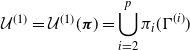 $\mathcal{U}^{(1)} = \mathcal{U}^{(1)}(\boldsymbol{\pi}) = \displaystyle \bigcup_{i=2}^p \pi_i(\Gamma^{(i)})$
.
$\mathcal{U}^{(1)} = \mathcal{U}^{(1)}(\boldsymbol{\pi}) = \displaystyle \bigcup_{i=2}^p \pi_i(\Gamma^{(i)})$
.
Then, if $\sigma \in \mathcal{S}_n$
is an automorphism of
$\sigma \in \mathcal{S}_n$
is an automorphism of $\Gamma^{(1)} \cap \mathcal{U}^{(1)}$
, setting
$\Gamma^{(1)} \cap \mathcal{U}^{(1)}$
, setting $\boldsymbol{\sigma} = (\textrm{Id}, \sigma, \ldots, \sigma) \in \{ \textrm{Id} \} \times \mathcal{S}_n^{p-1}$
,
$\boldsymbol{\sigma} = (\textrm{Id}, \sigma, \ldots, \sigma) \in \{ \textrm{Id} \} \times \mathcal{S}_n^{p-1}$
,
 \begin{equation} \mathcal{H}(\boldsymbol{\sigma} \boldsymbol{\pi}) \underset{{\rm def}}{=} \mathcal{H}(( \pi_1, \sigma \circ \pi_2, \ldots, \sigma \circ \pi_p)) \leq \mathcal{H}(\boldsymbol{\pi}). \end{equation}
The reason why such symmetries interest us is that $\mathcal{H}(\boldsymbol{\sigma} \boldsymbol{\pi}) \leq \mathcal{H}( \boldsymbol{\pi})$
corresponds (roughly) to having
$\mathcal{H}(\boldsymbol{\sigma} \boldsymbol{\pi}) \leq \mathcal{H}( \boldsymbol{\pi})$
corresponds (roughly) to having $\mathbb{P}_{\rm post}(\boldsymbol{\sigma} \boldsymbol{\pi}) \geq \mathbb{P}_{\rm post}(\boldsymbol{\pi})$
; thus, if our function F is of the form
$\mathbb{P}_{\rm post}(\boldsymbol{\sigma} \boldsymbol{\pi}) \geq \mathbb{P}_{\rm post}(\boldsymbol{\pi})$
; thus, if our function F is of the form
 \begin{equation} \boldsymbol{\pi} \mapsto \{ \boldsymbol{\sigma}_1 \boldsymbol{\pi}, \ldots, \boldsymbol{\sigma}_N \boldsymbol{\pi} \}\end{equation}
for some large N, then condition (i) from above will automatically be verified.
Remark 4. There is of course nothing special about $\Gamma^{(1)}$
: we could have defined
$\Gamma^{(1)}$
: we could have defined $\mathcal{U}^{(i)}(\pi)$
similarly for any
$\mathcal{U}^{(i)}(\pi)$
similarly for any $2 \leq i \leq p$
, and the same proposition would hold for any automorphisms of
$2 \leq i \leq p$
, and the same proposition would hold for any automorphisms of $\Gamma^{(i)} \cap \mathcal{U}^{(i)}$
.
$\Gamma^{(i)} \cap \mathcal{U}^{(i)}$
.
Proof. Let $\sigma$
be an automorphism of
$\sigma$
be an automorphism of $\Gamma^{(1)} \cap \mathcal{U}^{(1)}(\boldsymbol{\pi})$
, and denote
$\Gamma^{(1)} \cap \mathcal{U}^{(1)}(\boldsymbol{\pi})$
, and denote $\boldsymbol{\sigma} = (\textrm{Id}, \sigma, \ldots, \sigma) \in \{ \textrm{Id}\} \times \mathcal{S}_n^{p-1}$
. We note a few identities relating
$\boldsymbol{\sigma} = (\textrm{Id}, \sigma, \ldots, \sigma) \in \{ \textrm{Id}\} \times \mathcal{S}_n^{p-1}$
. We note a few identities relating $e_X(\boldsymbol{\sigma} \boldsymbol{\pi})$
to
$e_X(\boldsymbol{\sigma} \boldsymbol{\pi})$
to $e_X(\boldsymbol{\pi})$
.
$e_X(\boldsymbol{\pi})$
.
First of all,
 \begin{equation} \sum_{X \neq \emptyset, \{ 1 \} } e_X(\boldsymbol{\sigma} \boldsymbol{\pi}) = e(\sigma(\mathcal{U}^{(1)})) = e(\mathcal{U}^{(1)}) = \sum_{X \neq \emptyset, \{ 1 \} } e_X(\boldsymbol{\pi})\end{equation}
and
 \begin{equation} \sum_{1 \in X \subseteq \left[ \! \left[ 1, p \right] \! \right]} e_X(\boldsymbol{\sigma} \boldsymbol{\pi}) = e(\Gamma^{(1)}) = \sum_{1 \in X \subseteq \left[ \! \left[ 1, p \right] \! \right]} e_X(\boldsymbol{\pi}).\end{equation}
(These identities are true for any $\sigma \in \mathcal{S}_n$
.) Furthermore, since
$\sigma \in \mathcal{S}_n$
.) Furthermore, since $\sigma$
is an automorphism of
$\sigma$
is an automorphism of $\Gamma^{(1)} \cap \mathcal{U}^{(1)}$
,
$\Gamma^{(1)} \cap \mathcal{U}^{(1)}$
,
 \begin{align} \sum_{\underset{X \neq \{ 1 \}}{1 \in X \subseteq \left[ \! \left[ 1, p \right] \! \right]}}e_X(\boldsymbol{\sigma} \boldsymbol{\pi}) & = e(\Gamma^{(1)} \cap \sigma(\mathcal{U}^{(1)})) \nonumber\\[3pt] & \geq e((\Gamma^{(1)} \cap \mathcal{U}^{(1)}) \cap \sigma(\Gamma^{(1)} \cap \mathcal{U}^{(1)})) \nonumber\\[3pt] & = e(\Gamma^{(1)} \cap \mathcal{U}^{(1)}) \nonumber\\[3pt] & = \sum_{\underset{X \neq \{ 1 \}}{1 \in X \subseteq \left[ \! \left[ 1, p \right] \! \right]}}e_X(\boldsymbol{\pi}). \end{align}
Putting these three identities together, we obtain:
 \begin{align*} \sum_{X \neq \emptyset} e_X(\boldsymbol{\sigma} \boldsymbol{\pi}) & = \bigg( \sum_{X \neq \emptyset, \{ 1\}} e_X(\boldsymbol{\sigma} \boldsymbol{\pi}) \bigg) + e_{\{ 1 \}}(\boldsymbol{\sigma} \boldsymbol{\pi})\nonumber\\[3pt] & = \sum_{X \neq \emptyset, \{ 1\}} e_X(\boldsymbol{\sigma} \boldsymbol{\pi}) + \sum_{1 \in X \subseteq \left[ \! \left[ 1, p \right] \! \right]} e_X(\boldsymbol{\sigma} \boldsymbol{\pi}) - \sum_{\underset{X \neq \{ 1 \}}{1 \in X \subseteq \left[ \! \left[ 1, p \right] \! \right]}} e_X(\boldsymbol{\sigma} \boldsymbol{\pi}) \\[-30pt] & \leq \sum_{X \neq \emptyset, \{ 1\}} e_X(\boldsymbol{\pi}) + \sum_{1 \in X \subseteq \left[ \! \left[ 1, p \right] \! \right]} e_X(\boldsymbol{\pi}) - \sum_{\underset{X \neq \{ 1 \}}{1 \in X \subseteq \left[ \! \left[ 1, p \right] \! \right]}} e_X(\boldsymbol{\pi}) \nonumber\\ & = \sum_{X \neq \emptyset} e_X(\boldsymbol{\pi}) \end{align*}
concluding the proof.
4.3. Building many automorphisms
We are now tasked with finding such automorphisms $(\boldsymbol{\sigma}_k)_k$
of
$(\boldsymbol{\sigma}_k)_k$
of $A(\boldsymbol{\pi}) \underset{{\rm def}}{=} \Gamma^{(1)} \cap \mathcal{U}^{(1)}(\boldsymbol{\pi})$
. For the true alignment
$A(\boldsymbol{\pi}) \underset{{\rm def}}{=} \Gamma^{(1)} \cap \mathcal{U}^{(1)}(\boldsymbol{\pi})$
. For the true alignment $\boldsymbol{\pi}^*$
, given that the intersection graph
$\boldsymbol{\pi}^*$
, given that the intersection graph $\Gamma^{(1)} \cap \mathcal{U}^{(1)}(\boldsymbol{\pi}^*)$
is an Erdös–Rényi graph, this is possible when that graph is subcritical. Specifically, we have the following.
$\Gamma^{(1)} \cap \mathcal{U}^{(1)}(\boldsymbol{\pi}^*)$
is an Erdös–Rényi graph, this is possible when that graph is subcritical. Specifically, we have the following.
Proposition 10. Let G be a graph over $\left[ \! \left[ 1, n \right] \! \right]$
, and let
$\left[ \! \left[ 1, n \right] \! \right]$
, and let $c > 0, \delta > 0$
. We say that G verifies the property
$c > 0, \delta > 0$
. We say that G verifies the property $(P_{c, \delta})$
if, for any
$(P_{c, \delta})$
if, for any $X \subseteq [n]$
of size at least
$X \subseteq [n]$
of size at least $\delta n$
with no outgoing edges, there are at least
$\delta n$
with no outgoing edges, there are at least $(c n)!$
automorphisms of G which leave
$(c n)!$
automorphisms of G which leave $X^c = (\left[ \! \left[ 1,n \right] \! \right] \setminus X)$
fixed, and which have at most
$X^c = (\left[ \! \left[ 1,n \right] \! \right] \setminus X)$
fixed, and which have at most $\delta^2 n$
fixed points within X.
$\delta^2 n$
fixed points within X.
Now, assume that A is an Erdös–Rényi graph with size n and parameter $\rho < 1$
, and let
$\rho < 1$
, and let $\delta > 0$
. Then, there exists
$\delta > 0$
. Then, there exists $c = c(\rho, \delta)$
such that, with high probability, A verifies the property
$c = c(\rho, \delta)$
such that, with high probability, A verifies the property $(P_{c, \delta})$
.
$(P_{c, \delta})$
.
Essentially, a graph verifying the property $(P_{c, \delta})$
is one such that any reasonably large subgraph has a lot of symmetries: this is naturally the case for a subcritical Erdös–Rényi graph, which is locally a forest whose trees can be swapped around.
$(P_{c, \delta})$
is one such that any reasonably large subgraph has a lot of symmetries: this is naturally the case for a subcritical Erdös–Rényi graph, which is locally a forest whose trees can be swapped around.
Proof. Let A be as in the proposition. Fix an ordering $(\mathcal{T}_1, \mathcal{T}_2, \ldots)$
of all isomorphism classes of trees. For any
$(\mathcal{T}_1, \mathcal{T}_2, \ldots)$
of all isomorphism classes of trees. For any $i \geq 1$
, we set
$i \geq 1$
, we set $n_{i}$
to be the number of connected components of A which are isomorphic to
$n_{i}$
to be the number of connected components of A which are isomorphic to $\mathcal{T}_i$
. Then, for any i, there exists a constant
$\mathcal{T}_i$
. Then, for any i, there exists a constant $c_i$
with
$c_i$
with
 \begin{equation} \frac{n_i}{n} \underset{\mathbb{P}}{\longrightarrow} c_{i}\end{equation}
and $\sum_{i \geq 1} |\mathcal{T}_i|c_i = 1 $
. (This is shown in [Reference Bollobás12].)
$\sum_{i \geq 1} |\mathcal{T}_i|c_i = 1 $
. (This is shown in [Reference Bollobás12].)
Thus, let $\delta > 0$
. If
$\delta > 0$
. If $K > 0$
is large enough, with high probability,
$K > 0$
is large enough, with high probability,
 \begin{equation} \sum_{\underset{|\mathcal{T}_i| \leq K}{i \geq 1}} |\mathcal{T}_i| \frac{n_i}{n} \geq 1 - \frac{\delta^2}{2}.\end{equation}
As a result, any $X \subseteq \left[ \! \left[ 1, n \right] \! \right]$
with size at least
$X \subseteq \left[ \! \left[ 1, n \right] \! \right]$
with size at least $\delta n$
and with no outgoing edges, contains a subset
$\delta n$
and with no outgoing edges, contains a subset $X' \subseteq X$
of size at least
$X' \subseteq X$
of size at least $(\delta - {\delta^2}/{2}) n$
which is a disjoint union of connected components of size at most K.
$(\delta - {\delta^2}/{2}) n$
which is a disjoint union of connected components of size at most K.
Call $m_i$
the number of connected components of X’ isomorphic to
$m_i$
the number of connected components of X’ isomorphic to $\mathcal{T}_i$
, for any i: then, we may assume that
$\mathcal{T}_i$
, for any i: then, we may assume that $m_i \neq 1$
for any
$m_i \neq 1$
for any $i \geq 1$
, even if that means decreasing the size of X’ to be at least
$i \geq 1$
, even if that means decreasing the size of X’ to be at least $(\delta - \delta^2) n$
. Consequently, we may build automorphisms of X’ by permuting its connected components which are isomorphic. The number of automorphisms with no fixed point which we can build in this way is at least equal to
$(\delta - \delta^2) n$
. Consequently, we may build automorphisms of X’ by permuting its connected components which are isomorphic. The number of automorphisms with no fixed point which we can build in this way is at least equal to
 \begin{equation} \prod_{\underset{|\mathcal{T}_i| \leq K}{i \geq 1}} \frac{m_i!}{3}\end{equation}
since, for any $k \neq 1$
, there are at least
$k \neq 1$
, there are at least ${k!}/{3}$
elements of
${k!}/{3}$
elements of $\mathcal{S}_k$
with no fixed points. Since K is independent from n and
$\mathcal{S}_k$
with no fixed points. Since K is independent from n and
 \begin{align*}\sum_i m_i \geq \frac{(\delta-\delta^2) n}{K},\end{align*}
this provides us with at least
 \begin{equation} \exp\bigg({\frac{(\delta-\delta^2)}{K} n \log n + O(n)} \bigg) \geq (cn)!\end{equation}
automorphisms of X’, for large enough n (and some $c > 0$
independent from n).
$c > 0$
independent from n).
Finally, we may extend these automorphisms to be $\textrm{Id}$
on the complement of X’, proving the proposition.
$\textrm{Id}$
on the complement of X’, proving the proposition.
The previous proposition concerns the structure of $A(\boldsymbol{\pi}^*)$
. However, the measure
$A(\boldsymbol{\pi}^*)$
. However, the measure $\mathbb{P}_{\rm post}$
puts a large weight on permutations which are ‘hard to distinguish’ from
$\mathbb{P}_{\rm post}$
puts a large weight on permutations which are ‘hard to distinguish’ from $\boldsymbol{\pi}^*$
; such permutations
$\boldsymbol{\pi}^*$
; such permutations $\boldsymbol{\pi}$
give us a graph
$\boldsymbol{\pi}$
give us a graph $A(\boldsymbol{\pi})$
with a similar structure. This is captured in the following corollary.
$A(\boldsymbol{\pi})$
with a similar structure. This is captured in the following corollary.
Corollary 3. Let $\delta > 0$
. If
$\delta > 0$
. If $\lambda s (1 - (1 - s)^{p-1}) < 1$
, the graph
$\lambda s (1 - (1 - s)^{p-1}) < 1$
, the graph $A(\boldsymbol{\pi}^*) = \Gamma^{(1)} \cap \mathcal{U}^{(1)}(\boldsymbol{\pi}^*)$
is subcritical: there exists
$A(\boldsymbol{\pi}^*) = \Gamma^{(1)} \cap \mathcal{U}^{(1)}(\boldsymbol{\pi}^*)$
is subcritical: there exists $c > 0$
such that A verifies the property
$c > 0$
such that A verifies the property $(P_{c, \delta})$
defined above with high probability. Otherwise put, the set
$(P_{c, \delta})$
defined above with high probability. Otherwise put, the set
 \begin{equation} \textrm{Neg} = \{ \boldsymbol{\pi} \in \mathcal{S}_n^{p-1} | \Gamma^{(1)} \cap \mathcal{U}^{(1)}(\boldsymbol{\pi}) \textit{ does not verify }(P_{c, \delta}) \} \end{equation}
verifies $\mathbb{P}(\pi^* \in \textrm{Neg}) = o(1)$
. Consequently,
$\mathbb{P}(\pi^* \in \textrm{Neg}) = o(1)$
. Consequently, $\mathbb{P}_{\rm post}(\pi^* \in \textrm{Neg}) = o_{\mathbb{P}}(1)$
.
$\mathbb{P}_{\rm post}(\pi^* \in \textrm{Neg}) = o_{\mathbb{P}}(1)$
.
4.4. Applying the lemma
We now have most of the ingredients necessary to apply Lemma 1 and thus prove Theorem 2.
Proof of Theorem
2. Let $\boldsymbol{\pi}_0 \in \mathcal{S}_n^{p-1}$
and
$\boldsymbol{\pi}_0 \in \mathcal{S}_n^{p-1}$
and $\varepsilon > 0$
; we build
$\varepsilon > 0$
; we build $F\,:\, B(\boldsymbol{\pi}_0, 1- \varepsilon) \setminus \textrm{Neg} \to \mathcal{P}(\mathcal{S}_n^{p-1})$
verifying the conditions of Lemma 1.
$F\,:\, B(\boldsymbol{\pi}_0, 1- \varepsilon) \setminus \textrm{Neg} \to \mathcal{P}(\mathcal{S}_n^{p-1})$
verifying the conditions of Lemma 1.
Thus, let $\boldsymbol{\pi} \in B(\boldsymbol{\pi}_0, 1-\varepsilon) \setminus \textrm{Neg}$
. We consider the set
$\boldsymbol{\pi} \in B(\boldsymbol{\pi}_0, 1-\varepsilon) \setminus \textrm{Neg}$
. We consider the set $X(\boldsymbol{\pi}) = \{ u \in \left[ \! \left[ 1, n \right] \! \right]\!, \mbox{ for all }i \in \left[ \! \left[ 1, n \right] \! \right]\!, \pi_i(u) = (\boldsymbol{\pi}_0)_i(u) \}$
; by construction,
$X(\boldsymbol{\pi}) = \{ u \in \left[ \! \left[ 1, n \right] \! \right]\!, \mbox{ for all }i \in \left[ \! \left[ 1, n \right] \! \right]\!, \pi_i(u) = (\boldsymbol{\pi}_0)_i(u) \}$
; by construction, $|X| \geq \varepsilon n$
. We then consider the set
$|X| \geq \varepsilon n$
. We then consider the set $\overline{X}(\boldsymbol{\pi})$
, which is the minimal subset of
$\overline{X}(\boldsymbol{\pi})$
, which is the minimal subset of $\left[ \! \left[ 1, n \right] \! \right]$
containing X such that no edges of
$\left[ \! \left[ 1, n \right] \! \right]$
containing X such that no edges of $A(\boldsymbol{\pi})$
link
$A(\boldsymbol{\pi})$
link $\overline{X}$
and
$\overline{X}$
and $\overline{X}^c$
. Since
$\overline{X}^c$
. Since $\boldsymbol{\pi} \notin \textrm{Neg}$
, by Proposition 10, we may construct
$\boldsymbol{\pi} \notin \textrm{Neg}$
, by Proposition 10, we may construct $(c n)!$
automorphisms
$(c n)!$
automorphisms $(\sigma_1, \ldots, \sigma_N)$
of the graph A which leave
$(\sigma_1, \ldots, \sigma_N)$
of the graph A which leave $\overline{X}^c$
fixed, and which have at most
$\overline{X}^c$
fixed, and which have at most $\varepsilon^2 n$
fixed points within
$\varepsilon^2 n$
fixed points within $\overline{X}$
, for some
$\overline{X}$
, for some $c > 0$
independent of n. The function F is defined as mapping
$c > 0$
independent of n. The function F is defined as mapping $\boldsymbol{\pi}$
to the set
$\boldsymbol{\pi}$
to the set $\{ \boldsymbol{\sigma}_i \boldsymbol{\pi}, 1 \leq i \leq N \}$
(where, as defined earlier,
$\{ \boldsymbol{\sigma}_i \boldsymbol{\pi}, 1 \leq i \leq N \}$
(where, as defined earlier, $\boldsymbol{\sigma}_i = (\textrm{Id}, \sigma_i, \ldots, \sigma_i)$
).
$\boldsymbol{\sigma}_i = (\textrm{Id}, \sigma_i, \ldots, \sigma_i)$
).
Does F satisfy the conditions of Lemma 1? Condition (i) is verified by construction: for any $\boldsymbol{\pi} \in B(\boldsymbol{\pi}_0, 1-\varepsilon)$
,
$\boldsymbol{\pi} \in B(\boldsymbol{\pi}_0, 1-\varepsilon)$
,
 \begin{equation} \mathbb{P}_{\rm post}(\boldsymbol{\pi}) \leq \frac{e^{o(n \log n)}}{(cn)!} \mathbb{P}_{\rm post}(F(\boldsymbol{\pi})) \end{equation}
since $\mathcal{H}(\boldsymbol{\sigma}_i \boldsymbol{\pi}) \leq \mathcal{H}(\boldsymbol{\pi})$
for any
$\mathcal{H}(\boldsymbol{\sigma}_i \boldsymbol{\pi}) \leq \mathcal{H}(\boldsymbol{\pi})$
for any $1 \leq i \leq N$
. Condition (ii), however, is less obvious. We prove that it holds with
$1 \leq i \leq N$
. Condition (ii), however, is less obvious. We prove that it holds with $K_n(r) = \exp O_{\mathbb{P}}(n)$
.
$K_n(r) = \exp O_{\mathbb{P}}(n)$
.
Let $\boldsymbol{\pi}' \in \mathcal{S}_n^{p-1}$
. We may partition
$\boldsymbol{\pi}' \in \mathcal{S}_n^{p-1}$
. We may partition $F^{-1}(\boldsymbol{\pi}') = \{ \boldsymbol{\pi}: \boldsymbol{\pi}' \in F(\boldsymbol{\pi}) \}$
as
$F^{-1}(\boldsymbol{\pi}') = \{ \boldsymbol{\pi}: \boldsymbol{\pi}' \in F(\boldsymbol{\pi}) \}$
as
 \begin{align} F^{-1}(\boldsymbol{\pi}') & = \bigsqcup_{\underset{S \text{ subgraph of } (\Gamma^{(1)})|_Z}{Y \subseteq Z \subseteq \left[ \! \left[ 1, n \right] \! \right]}} \{ \boldsymbol{\pi} \in F^{-1}(\boldsymbol{\pi}')\,:\, X(\boldsymbol{\pi}) = Y, \overline{X}(\boldsymbol{\pi}) = Z, (\Gamma^{(1)}\cap \mathcal{U}^{(1)}(\boldsymbol{\pi}))|_Z = S \} \end{align}
 \begin{align} & \underset{{\rm def}}{=} \bigsqcup_{\underset{S \text{ subgraph of } (\Gamma^{(1)})|_Z}{Y \subseteq Z \subseteq \left[ \! \left[ 1, n \right] \! \right]}} W(Y, Z, S).\end{align}
Then, there are only $\exp O_\mathbb{P}(n)$
possible values for (Y, Z, S), as
$\exp O_\mathbb{P}(n)$
possible values for (Y, Z, S), as $|\Gamma^{(1)}| = O_{\mathbb{P}}(n)$
. We therefore just need to show that
$|\Gamma^{(1)}| = O_{\mathbb{P}}(n)$
. We therefore just need to show that $|W(Y, Z, S)| \leq \exp O_\mathbb{P}(n)$
for any triplet (Y, Z, S). To this end, let
$|W(Y, Z, S)| \leq \exp O_\mathbb{P}(n)$
for any triplet (Y, Z, S). To this end, let $\boldsymbol{\pi}_1, \boldsymbol{\pi}_2 \in W(Y, Z, S)$
: by construction,
$\boldsymbol{\pi}_1, \boldsymbol{\pi}_2 \in W(Y, Z, S)$
: by construction, $\boldsymbol{\pi}_2 \boldsymbol{\pi}_1^{-1}$
is of the form
$\boldsymbol{\pi}_2 \boldsymbol{\pi}_1^{-1}$
is of the form $(\textrm{Id}, \sigma, \ldots, \sigma)$
for some
$(\textrm{Id}, \sigma, \ldots, \sigma)$
for some $\sigma \in \mathcal{S}_n$
. Furthermore, given such a
$\sigma \in \mathcal{S}_n$
. Furthermore, given such a $\sigma$
, we know that
$\sigma$
, we know that $\sigma|_Y = \textrm{Id}$
, and
$\sigma|_Y = \textrm{Id}$
, and $\sigma|_Z$
must be an automorphism of S. This allows us to use the following lemma, whose proof is deferred to the appendix.
$\sigma|_Z$
must be an automorphism of S. This allows us to use the following lemma, whose proof is deferred to the appendix.
Lemma 6. Let H be a graph over some set V, with degree distribution $(d_v)_{v \in V}$
. Then, H has at most
$(d_v)_{v \in V}$
. Then, H has at most $e^{{|V|}/{e}} \prod_{v \in V} (d_v!)$
automorphisms which send each connected component of H to itself.
$e^{{|V|}/{e}} \prod_{v \in V} (d_v!)$
automorphisms which send each connected component of H to itself.
Indeed, by construction of $\overline{X}(\boldsymbol{\pi}_1) = Z$
, any connected component of S intersects Y, and so
$\overline{X}(\boldsymbol{\pi}_1) = Z$
, any connected component of S intersects Y, and so $\sigma$
must send it to itself. This gives us at most
$\sigma$
must send it to itself. This gives us at most $e^{{n}/{e}}\prod_{i=1}^n (d_i!) $
possible values for
$e^{{n}/{e}}\prod_{i=1}^n (d_i!) $
possible values for $\sigma$
, showing that (ii) is verified as
$\sigma$
, showing that (ii) is verified as
 \begin{equation} \log \prod_{i=1}^n (d_i!) \leq \sum_{i=1}^n d_i \log d_i = O_{\mathbb{P}}(n \mathbb{E}[d_i \log d_i ]) = O_{\mathbb{P}}(n), \end{equation}
given that $\mathbb{E}[d_i \log d_i ] = O(1)$
. Applying Lemma 1 thus proves Theorem 2.
$\mathbb{E}[d_i \log d_i ] = O(1)$
. Applying Lemma 1 thus proves Theorem 2.
Appendix A. Some results on quadratic forms of normal vectors
In this appendix, we list a few results on the behaviour of quadratic forms of normal vectors, for use in the following sections.
We begin with a general lemma on cumulants of quadratic forms of normal vectors.
Lemma 7. Let M be a symmetric matrix: then, if $A \sim \mathcal{N}(0, \Sigma)$
, and
$A \sim \mathcal{N}(0, \Sigma)$
, and $Q = A^T M A$
is a quadratic form of A, the log-moment generating function of Q exists for small enough t, and can be written as
$Q = A^T M A$
is a quadratic form of A, the log-moment generating function of Q exists for small enough t, and can be written as
 \begin{equation} \log \mathbb{E}[e^{t Q}] = - \frac{1}{2} \log \det(\textrm{Id} - 2 t \Sigma M) = \sum_{k \geq 1} 2^{k-1}\textrm{Tr}((\Sigma M)^k) \frac{t^k}{k}.\end{equation}
The following proof is a standard calculation, often used to prove the Hanson–Wright inequality (see [Reference Rudelson and Vershynin6] for instance).
Proof. Replacing A by $\Sigma^{-{1}/{2}} A$
, it is sufficient for us to handle the case where
$\Sigma^{-{1}/{2}} A$
, it is sufficient for us to handle the case where $\Sigma = \textrm{Id}$
.
$\Sigma = \textrm{Id}$
.
We may diagonalise M to obtain the expression $M = P^T D P$
, where P is an orthogonal matrix. Then, we may write
$M = P^T D P$
, where P is an orthogonal matrix. Then, we may write
 \begin{equation} Q = (PA)^T D (PA) \underset{{\rm def}}{=} Y^T D Y. \end{equation}
However, since the standard Gaussian distribution is invariant by the action of the orthogonal group O(n), Y is also a (standard, centred) normal vector. As such, setting $Y = (Y_1, \ldots, Y_n)$
and denoting by
$Y = (Y_1, \ldots, Y_n)$
and denoting by $(\lambda_1, \ldots, \lambda_n)$
the eigenvalues of M,
$(\lambda_1, \ldots, \lambda_n)$
the eigenvalues of M,
 \begin{align} \mathbb{E}[e^{t Q}] & = \prod_{i=1}^n \mathbb{E}[\mathrm{e}^{t\lambda_i Y_i^2}] \nonumber\\ & = \prod_{i=1}^n \frac{1}{\sqrt{1 - 2 t \lambda_i}} \nonumber\\ & = (\!\det(\textrm{Id} - 2 t M))^{-{1}/{2}}\end{align}
for small enough t, showing the first identity.
For the second, note that if t is small enough, we may write $\textrm{Id} - 2 t M = e^L$
for some matrix
$\textrm{Id} - 2 t M = e^L$
for some matrix $L = - \sum_{k \geq 1} 2^k M^k ({t^k}/{k})$
. Thus,
$L = - \sum_{k \geq 1} 2^k M^k ({t^k}/{k})$
. Thus,
 \begin{equation} \log \det (\textrm{Id} - 2 t M) = \textrm{Tr} L = - \displaystyle\sum_{k \geq 1} 2^k \textrm{Tr}(M^k) \frac{t^k}{k},\end{equation}
concluding the proof.
In the same vein, we may obtain tail bounds on such random variables. Again, the following result is fairly standard: a proof can be found in [Reference Boucheron, Lugosi and Massart7] for instance.
Lemma 8. Let X be a centred normal vector with covariance matrix $\Sigma$
,
$\Sigma$
, $S_N$
a symmetric matrix with size
$S_N$
a symmetric matrix with size $N \to + \infty$
. Then,
$N \to + \infty$
. Then,
 \begin{align} \log \mathbb{P}(X^T S_N X - \mathbb{E}[X^T S_N X] > C_N) & \leq -\frac{C_N^2}{4(\textrm{Tr}((\Sigma S_N)^2) + C_N \|\Sigma^{{1}/{2}} S_N \Sigma^{{1}/{2}}\|_{\rm op})} \nonumber\\ & = -\frac{C_N^2}{2 \textrm{Var}(X^T S_N X) + C_N \|\Sigma^{{1}/{2}} S_N \Sigma^{{1}/{2}}\|_{\rm op})}. \end{align}
Finally, we state a significantly sharper tail bound which we may apply if the quantity $C_N$
is not too large.
$C_N$
is not too large.
Proposition 11. Let X be a centred normal vector with covariance matrix $\Sigma$
,
$\Sigma$
, $S_N$
a symmetric matrix with size
$S_N$
a symmetric matrix with size $N \to + \infty$
, verifying
$N \to + \infty$
, verifying $\|\Sigma^{{1}/{2}}S_N \Sigma^{{1}/{2}} \|_{\rm op} \leq K$
independent of N. Then, if
$\|\Sigma^{{1}/{2}}S_N \Sigma^{{1}/{2}} \|_{\rm op} \leq K$
independent of N. Then, if $C_N > 0$
with
$C_N > 0$
with $1\ll C_N \ll \textrm{Tr}((\Sigma S_N)^2)$
,
$1\ll C_N \ll \textrm{Tr}((\Sigma S_N)^2)$
,
 \begin{align} & \mathbb{P}(X^T S_N X - \mathbb{E}[X^T S_N X] > C_N)\nonumber\\ &\quad \underset{N \to + \infty}{\sim} \frac{\sqrt{\text{Tr}((\Sigma S_N)^2)}}{\sqrt{\pi} C_N}\exp \bigg(- \frac{C_N^2}{4 \text{Tr}((\Sigma S_N)^2)} + O\bigg(\frac{C_N^3}{\text{Tr}((\Sigma S_N)^2)^2}\bigg) \bigg) \end{align}
and a symmetric result holds for $\mathbb{P}(X^T S_N X - \mathbb{E}[X^T S_N X] < - C_N)$
.
$\mathbb{P}(X^T S_N X - \mathbb{E}[X^T S_N X] < - C_N)$
.
Proof. Again, we may write
 \begin{equation} Q_N = X^T S_N X - \mathbb{E}[X^T S_N X] = \sum_{i=1}^N \lambda_i (Y_i^2-1) \end{equation}
as in the previous proof.
This time, we apply the following theorem from [Reference Fan, Grama and Liu14, Eq. (2.11)].
Theorem 4. Let $\xi_1, \ldots, \xi_N$
be independent centred random variables such that, for some
$\xi_1, \ldots, \xi_N$
be independent centred random variables such that, for some $A > 0$
, for any
$A > 0$
, for any $i, k \geq 0$
,
$i, k \geq 0$
,
 \begin{equation} \mathbb{E}[|\xi_i|^k] \leq A^k k!. \end{equation}
Then, setting
 \begin{align*} \Phi(x) = \frac{1}{\sqrt{2\pi}} \int_{-\infty}^x \mathrm{e}^{-{u^2}/{2}} \,du, \end{align*}
and $s^2 = \sum_{i} \mathbb{E}[\xi_i^2]$
, if
$s^2 = \sum_{i} \mathbb{E}[\xi_i^2]$
, if $1 \ll x \ll s$
,
$1 \ll x \ll s$
,
 \begin{equation} \mathbb{P}\left( \dfrac{1}{s} \sum_{i=1}^N \xi_i > x \right) \underset{N \to + \infty}{\sim} [1 - \Phi(x)]e^{O({x^3}/{s})} \underset{N \to + \infty}{\sim} \frac{1}{\sqrt{2\pi}x} e^{-({x^2}/{2}) + O({x^3}/{s})} \end{equation}
In this case, $s^2 = 2\sum_{i=1}^n \lambda_i^2 = 2\textrm{Tr}((\Sigma S_N)^2)$
and so
$s^2 = 2\sum_{i=1}^n \lambda_i^2 = 2\textrm{Tr}((\Sigma S_N)^2)$
and so $x^2 = {C_N^2}/{2 \textrm{Tr}((\Sigma S_N)^2)}$
; Proposition 11 follows immediately.
$x^2 = {C_N^2}/{2 \textrm{Tr}((\Sigma S_N)^2)}$
; Proposition 11 follows immediately.
Appendix B. Proof of Proposition 5
We now turn to proving Proposition 5. Here, for any $\boldsymbol{\sigma} \in \mathcal{S}_n^{p-1}$
, we may write
$\boldsymbol{\sigma} \in \mathcal{S}_n^{p-1}$
, we may write $V_{\mathrm{off}}(\boldsymbol{\sigma}) = -G^T M_{\boldsymbol{\sigma}} G$
, as a quadratic form over
$V_{\mathrm{off}}(\boldsymbol{\sigma}) = -G^T M_{\boldsymbol{\sigma}} G$
, as a quadratic form over $\mathbb{R}^E \otimes \mathbb{R}^{p}$
, where
$\mathbb{R}^E \otimes \mathbb{R}^{p}$
, where
 \begin{equation} (M_{\boldsymbol{\sigma}})_{(e, i), (e', j)} = \mathbf{1}_{e'=\sigma_{ij}(e)} \mathbf{1}_{e \neq e'} \mathbf{1}_{i \neq j}\end{equation}
for any $e, e' \in E,\ 1 \leq i ,\ j \leq p$
; and, as described in (2), the covariance matrix of G is
$e, e' \in E,\ 1 \leq i ,\ j \leq p$
; and, as described in (2), the covariance matrix of G is
 \begin{equation} \Sigma = (1 - \rho) I_N + \rho ( I_{\binom{n}{2}} \otimes J_p) \underset{{\rm def}}{=} (1 - \rho) I_N + \rho \tilde{J},\end{equation}
where $J_p$
is the
$J_p$
is the $p \times p$
all-ones matrix. For the sake of convenience, we set
$p \times p$
all-ones matrix. For the sake of convenience, we set $\mathcal{M}_{\boldsymbol{\sigma}} = \Sigma^{{1}/{2}} M_{\boldsymbol{\sigma}}\Sigma^{{1}/{2}}$
for the rest of this proof.
$\mathcal{M}_{\boldsymbol{\sigma}} = \Sigma^{{1}/{2}} M_{\boldsymbol{\sigma}}\Sigma^{{1}/{2}}$
for the rest of this proof.
We also note that, for symmetric positive U and symmetric V,
 \begin{equation} \textrm{Tr} UV \leq \|V\|_{\rm op} \textrm{Tr} U.\end{equation}
This allows us to bound the traces of our matrices in order to properly control our error terms. Explicitly, since $\|M_{\boldsymbol{\sigma}}\|_{\rm op} \leq p-1$
and
$\|M_{\boldsymbol{\sigma}}\|_{\rm op} \leq p-1$
and $\|\Sigma\|_{\rm op} = 1 + o(1)$
, we may use the fact that
$\|\Sigma\|_{\rm op} = 1 + o(1)$
, we may use the fact that $ \mathcal{M}_{\boldsymbol{\sigma}}^2$
is positive, so that for
$ \mathcal{M}_{\boldsymbol{\sigma}}^2$
is positive, so that for $k \geq 2$
and large enough n
$k \geq 2$
and large enough n
 \begin{align} \textrm{Tr}(\mathcal{M}_{\boldsymbol{\sigma}}^k) &\leq \textrm{Tr}(\mathcal{M}_{\boldsymbol{\sigma}}^2) \|\mathcal{M}_{\boldsymbol{\sigma}}^{k-2}\|_{\rm op} \nonumber\\[3pt] & \leq p^{k-2}\textrm{Tr}(\mathcal{M}_{\boldsymbol{\sigma}}^2)\end{align}
This allows us, by applying Lemma 7, to obtain that
 \begin{align} \log \mathbb{E}[\mathrm{e}^{-\beta V_{\mathrm{off}}(\boldsymbol{\sigma})}] & = \sum_{k \geq 1} 2^{k-1} \textrm{Tr}((\Sigma M_{\boldsymbol{\sigma}})^k) \frac{\beta^k}{k} \nonumber\\[3pt] & = \beta \textrm{Tr}(\mathcal{M}_{\boldsymbol{\sigma}}) + \beta^2 \textrm{Tr} (\mathcal{M}_{\boldsymbol{\sigma}}^2)(1 + o(1)).\end{align}
We now simply need to evaluate some traces.
To begin with, by definition, $\Sigma$
and
$\Sigma$
and $M_{\boldsymbol{\sigma}}$
can be written as block matrices with (
$M_{\boldsymbol{\sigma}}$
can be written as block matrices with ( $|E|$
blocks
$|E|$
blocks $ \times $ $ |E|$
blocks), where each block is of size
$ |E|$
blocks), where each block is of size $p \times p$
. The matrix
$p \times p$
. The matrix $\Sigma$
is block diagonal, while the diagonal blocks of
$\Sigma$
is block diagonal, while the diagonal blocks of $M_{\boldsymbol{\sigma}}$
are all zero matrices. Consequently,
$M_{\boldsymbol{\sigma}}$
are all zero matrices. Consequently, $\textrm{Tr}(\Sigma M_{\boldsymbol{\sigma}}) = 0$
.
$\textrm{Tr}(\Sigma M_{\boldsymbol{\sigma}}) = 0$
.
We now move on to $\textrm{Tr}(\mathcal{M}_{\boldsymbol{\sigma}}^2)$
. Given that
$\textrm{Tr}(\mathcal{M}_{\boldsymbol{\sigma}}^2)$
. Given that $\|\Sigma - \textrm{Id}\|_{\rm op} = O(\rho)$
,
$\|\Sigma - \textrm{Id}\|_{\rm op} = O(\rho)$
,
 \begin{align} \textrm{Tr}(\mathcal{M}_{\boldsymbol{\sigma}}^2) & = \textrm{Tr}(\Sigma M_{\boldsymbol{\sigma}}\Sigma M_{\boldsymbol{\sigma}}) \nonumber\\[3pt] & = \textrm{Tr}(M_{\boldsymbol{\sigma}}^2) + 2\textrm{Tr}((\Sigma - \textrm{Id}) M_{\boldsymbol{\sigma}}^2) + \textrm{Tr}((\Sigma - \textrm{Id}) M_{\boldsymbol{\sigma}}(\Sigma - \textrm{Id}) M_{\boldsymbol{\sigma}})\end{align}
so that
 \begin{align} \textrm{Tr}(\mathcal{M}_{\boldsymbol{\sigma}}^2) - \textrm{Tr}(M_{\boldsymbol{\sigma}}^2) & \leq 2 \|\Sigma - \textrm{Id}\|_{\rm op} \textrm{Tr}(M_{\boldsymbol{\sigma}}^2) +\|\Sigma - \textrm{Id}\|_{\rm op} \textrm{Tr}((\Sigma - \textrm{Id})M_{\boldsymbol{\sigma}}^2) \nonumber\\[3pt] & = \textrm{Tr}(M_{\boldsymbol{\sigma}}^2)(1 + O(\rho))\end{align}
by (B3).
We may now compute:
 \begin{align} \textrm{Tr}(M_{\boldsymbol{\sigma}}^2) & = \sum_{e, e' \in E} \sum_{1 \leq i, j \leq p} (M_{\boldsymbol{\sigma}})_{(e, i), (e', j)}^2 \nonumber\\[3pt] & = \# \{ e \neq e' \in E, 1 \leq i \neq j \leq p, e' = \sigma_{ij}(e) \} \nonumber\\[3pt] & = \sum_{ 1 \leq i \neq j \leq p} \bigg(\binom{n}{2} - \# \{ e \in E, \sigma_{ij}(e) = e \}\bigg)\\[3pt] & \underset{{\rm def}}{=} \sum_{1 \leq i \neq j \leq p} \bigg(\binom{n}{2} - D_{ij}(\boldsymbol{\sigma}) \bigg).\nonumber\end{align}
Thus,
 \begin{equation} \log \mathbb{E}[e^{-\beta V_{\mathrm{off}}(\boldsymbol{\sigma})}] = \beta^2 \sum_{1 \leq i \neq j \leq p} \bigg(\binom{n}{2} - D_{ij}(\boldsymbol{\sigma}) \bigg) + O(\beta^3 n^2).\end{equation}
Note that $\beta^3 n^2 = o(n)$
; thus, to conclude the proof, we just need to show the following lemma.
$\beta^3 n^2 = o(n)$
; thus, to conclude the proof, we just need to show the following lemma.
Lemma 9. For $\boldsymbol{\sigma} \in \mathcal{S}_n^{p-1}$
,
$\boldsymbol{\sigma} \in \mathcal{S}_n^{p-1}$
,
 \begin{equation} D_{ij}(\boldsymbol{\sigma}) = \binom{d_{ij}(\boldsymbol{\sigma})}{2} + R_{\boldsymbol{\sigma}},\end{equation}
where
 \begin{align*}0 \leq R_{\boldsymbol{\sigma}} \leq \frac{n - d_{ij}(\boldsymbol{\sigma})}{2}.\end{align*}
Proof. If $e \in E$
, writing
$e \in E$
, writing $e = \{u, v \}$
, we may see that
$e = \{u, v \}$
, we may see that $\sigma_{ij}(e) = e$
if and only if
$\sigma_{ij}(e) = e$
if and only if
 \begin{equation} \begin{cases} \sigma_{ij}(u) = u ,\\[3pt] \sigma_{ij}(v) = v, \end{cases} \quad\text{or}\quad \begin{cases} \sigma_{ij}(u) = v ,\\[3pt] \sigma_{ij}(v) = u. \end{cases}.\end{equation}
There are $\binom{d_{ij}(\boldsymbol{\sigma})}{2}$
pairs verifying the first condition. The pairs verifying the second condition are the orbits of length 2 for the action of
$\binom{d_{ij}(\boldsymbol{\sigma})}{2}$
pairs verifying the first condition. The pairs verifying the second condition are the orbits of length 2 for the action of $\sigma_{ij}$
over
$\sigma_{ij}$
over $\left[ \! \left[ 1, n \right] \! \right]$
: there are at most
$\left[ \! \left[ 1, n \right] \! \right]$
: there are at most $({n - d_{ij}})/{2}$
of these.
$({n - d_{ij}})/{2}$
of these.
We have thus proven Proposition 5.
Before moving on, we perform a final computation which we need later on. Namely, if $\boldsymbol{\sigma}, \boldsymbol{\sigma}' \in \mathcal{S}_n^{p-1}$
:
$\boldsymbol{\sigma}, \boldsymbol{\sigma}' \in \mathcal{S}_n^{p-1}$
:
 \begin{align} \textrm{Tr}(M_{\boldsymbol{\sigma}} M_{\boldsymbol{\sigma}'}) & = \sum_{e, e' \in E} \sum_{1 \leq i, j \leq p} (M_{\boldsymbol{\sigma}})_{(e, i), (e', j)} (M_{\boldsymbol{\sigma}'})_{(e, i), (e', j)} \nonumber\\[3pt] & = \# \{ e \neq e' \in E, 1 \leq i \neq j \leq p, e' = \sigma_{ij}(e) = \sigma'_{ij}(e) \} \nonumber\\[3pt] & = \sum_{ 1 \leq i \neq j \leq p}\# \{ e \in E, \sigma_{ij}(e) = \sigma'_{ij}(e) \neq e \} \nonumber\\[3pt] & \leq \sum_{ 1 \leq i \neq j \leq p}\# \{ e \in E, \sigma_{ij}(e) = \sigma'_{ij}(e) \}\nonumber\\[3pt] & \underset{{\rm def}}{=} \sum_{1 \leq i \neq j \leq p} C_{ij}(\boldsymbol{\sigma}, \boldsymbol{\sigma}'). \\[-30pt] \nonumber \end{align}
As for $(D_{ij}(\boldsymbol{\sigma}))$
, we may show that, setting
$(D_{ij}(\boldsymbol{\sigma}))$
, we may show that, setting $c_{ij}(\boldsymbol{\sigma}, \boldsymbol{\sigma}') = \{u \in \left[ \! \left[ 1, n \right] \! \right]\!, \sigma_{ij}(u) = \sigma'_{ij}(u) \}$
,
$c_{ij}(\boldsymbol{\sigma}, \boldsymbol{\sigma}') = \{u \in \left[ \! \left[ 1, n \right] \! \right]\!, \sigma_{ij}(u) = \sigma'_{ij}(u) \}$
,
 \begin{equation} C_{ij}(\boldsymbol{\sigma}, \boldsymbol{\sigma}') = \binom{c_{ij}(\boldsymbol{\sigma}, \boldsymbol{\sigma}')}{2} + O(n)\end{equation}
and so
 \begin{align} \textrm{Tr}((\mathcal{M}_{\boldsymbol{\sigma}} + \mathcal{M}_{\boldsymbol{\sigma}'})^2) & = \textrm{Tr}((M_{\boldsymbol{\sigma}} + M_{\boldsymbol{\sigma}'})^2) + O(\rho n^2) \nonumber\\[3pt] & = \textrm{Tr}(M_{\boldsymbol{\sigma}}^2) + \textrm{Tr}(M_{\boldsymbol{\sigma}'}^2) + 2 \textrm{Tr}(M_{\boldsymbol{\sigma}} M_{\boldsymbol{\sigma}'}) \nonumber\\[3pt] & = \sum_{1 \leq i \neq j \leq p}\bigg( \binom{n}{2} - \binom{d_{ij}(\boldsymbol{\sigma})}{2} - \binom{d_{ij}(\boldsymbol{\sigma}')}{2} + 2 \binom{c_{ij}(\boldsymbol{\sigma}, \boldsymbol{\sigma}')}{2} \bigg) + O(\rho n^2).\end{align}
Appendix C. Proof of Proposition 4
Recall that the value of $V_{\mathrm{diag}}(\boldsymbol{\sigma})$
is equal to
$V_{\mathrm{diag}}(\boldsymbol{\sigma})$
is equal to
 \begin{align} V_{\mathrm{diag}}(\boldsymbol{\sigma}) & = -\sum_{\underset{\sigma_{ij}(e) \neq e}{e \in E, 1 \leq i \neq j \leq p}}G_e^{(i)} G_e^{(j)} \nonumber\\[3pt] & = \sum_{1 \leq i \neq j \leq p} \bigg[-\sum_{e \in E} G_e^{(i)} G_e^{(j)} + \sum_{\underset{u, v \in \textrm{Fix} \sigma_{ij}}{e = \{u, v \} \in E}}G_e^{(i)} G_e^{(j)} + \sum_{\underset{\sigma_{ij}(u) = v, \sigma_{ij}(v) = u}{e = \{u, v \} \in E}}G_e^{(i)} G_e^{(j)}\bigg] \nonumber\\[3pt] & \underset{{\rm def}}{=} \sum_{1 \leq i \neq j \leq p} [ V_{ij}^{(1)} - V_{ij}^{(2)}(\textrm{Fix} \sigma_{ij}) - V_{ij}^{(3)}(\boldsymbol{\sigma}) ].\end{align}
Since this is a quadratic form of the vector $(G_{e}^{(i)})$
, we may apply Lemma 8 to bound the probability that any of these three terms ever becomes too large. First,
$(G_{e}^{(i)})$
, we may apply Lemma 8 to bound the probability that any of these three terms ever becomes too large. First,
 \begin{align} \mathbb{P} & (\exists 1 \leq i \neq j \leq p, \exists Y \subseteq \left[ \! \left[ 1, n \right] \! \right]\!, | V_{ij}^{(2)}(Y) - \mathbb{E}[ V_{ij}^{(2)}(Y)]| > (\!\log n)^{{1}/{4}}n^{{3}/{2}}) \nonumber\\[3pt] & \leq \sum_{1 \leq i \neq j \leq p} \sum_{ Y \subseteq \left[ \! \left[ 1, n \right] \! \right]} \mathbb{P}(| V_{ij}^{(2)}(Y) - \mathbb{E}[ V_{ij}^{(2)}(Y)]| > (\!\log n)^{{1}/{4}}n^{{3}/{2}}) \nonumber\\[3pt] & \leq \sum_{1 \leq i \neq j \leq p} \sum_{ Y \subseteq \left[ \! \left[ 1, n \right] \! \right]} \exp\bigg(\!- \!\frac{n^3 (\!\log n)^{{1}/{2}}}{O(n^2) + O((\!\log n)^{{1}/{4}}n^{{3}/{2}})}\bigg) \nonumber\\[3pt] & = \exp(\!-\! c n \sqrt{\log n} + o(n \sqrt{\log n})) = o(1) \\[-10pt] \nonumber \end{align}
for some $c > 0$
, since
$c > 0$
, since $\textrm{Var} V_{ij}^{(2)}(Y) = O(n^2) $
(uniformly in Y) and the operator-norm term is O(1) (again uniformly in Y).
$\textrm{Var} V_{ij}^{(2)}(Y) = O(n^2) $
(uniformly in Y) and the operator-norm term is O(1) (again uniformly in Y).
Noting that $V_{ij}^{(1)} = V_{ij}^{(2)}(\left[ \! \left[ 1, n \right] \! \right])$
, this also shows that
$V_{ij}^{(1)} = V_{ij}^{(2)}(\left[ \! \left[ 1, n \right] \! \right])$
, this also shows that
 \begin{align} &\mathbb{P} (\exists 1 \leq i \neq j \leq p, | V_{ij}^{(1)} - \mathbb{E}[ V_{ij}^{(1)}]| > (\!\log n)^{{1}/{4}}n^{{3}/{2}}) \\[-8pt] \nonumber \end{align}
 \begin{align} &\quad \leq \exp(\!-\! c n \sqrt{\log n} + o(n \sqrt{\log n})) = o(1).\end{align}
Finally,
 \begin{align} \mathbb{P} & (\exists 1 \leq i \neq j \leq p, \exists \boldsymbol{\sigma} \in \mathcal{S}_n^{p-1}, | V_{ij}^{(3)}(\boldsymbol{\sigma}) - \mathbb{E}[ V_{ij}^{(3)}(\boldsymbol{\sigma})]| > (\!\log n)^{{1}/{4}}n^{{3}/{2}}) \nonumber\\[3pt] & \leq \sum_{1 \leq i \neq j \leq p} \sum_{ \boldsymbol{\sigma} \in \mathcal{S}_n^{p-1}} \mathbb{P}(| V_{ij}^{(3)}(\boldsymbol{\sigma}) - \mathbb{E}[ V_{ij}^{(3)}(\boldsymbol{\sigma})]| > (\!\log n)^{{1}/{4}}n^{{3}/{2}}) \nonumber\\[3pt] & \leq \sum_{1 \leq i \neq j \leq p} \sum_{ \boldsymbol{\sigma} \in \mathcal{S}_n^{p-1}}\exp\bigg(\!- \!\frac{n^3 (\!\log n)^{{1}/{2}}}{O(n) + O((\!\log n)^{{1}/{4}}n^{{3}{2}})}\bigg) \nonumber\\[3pt] & = \exp(\!-\! c n^{{3}/{2}}(\!\log n)^{{1}/{4}} + o(n^{{3}/{2}}(\!\log n)^{{1}/{4}})) = o(1)\end{align}
as, this time,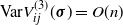 $\textrm{Var} V_{ij}^{(3)}(\boldsymbol{\sigma}) = O(n)$
(uniformly in
$\textrm{Var} V_{ij}^{(3)}(\boldsymbol{\sigma}) = O(n)$
(uniformly in $\boldsymbol{\sigma}$
). This proves the first part of the proposition.
$\boldsymbol{\sigma}$
). This proves the first part of the proposition.
The second part follows, simply by noting that, if $D_{ij}(\boldsymbol{\sigma}) = \# \{ e \in E, \sigma_{ij}(e) = e \}$
for
$D_{ij}(\boldsymbol{\sigma}) = \# \{ e \in E, \sigma_{ij}(e) = e \}$
for $1 \leq i \neq j \leq p$
,
$1 \leq i \neq j \leq p$
,
 \begin{align} \mathbb{E}[V_{\mathrm{diag}}(\boldsymbol{\sigma})] & = - \sum_{1 \leq i \neq j \leq p} \sum_{\underset{\sigma_{ij}(e) \neq e}{e \in E}} \mathbb{E}[G_e^{(i)} G_e^{(j)}] \nonumber\\[3pt] & = - \rho \sum_{1 \leq i \neq j \leq p} \bigg(\binom{n}{2} - D_{ij}(\boldsymbol{\sigma})\bigg) \\[3pt] & = - \rho \sum_{1 \leq i \neq j \leq p} \bigg( \binom{n}{2} -\binom{d_{ij}(\boldsymbol{\sigma})}{2}\bigg) + O(\rho n)\nonumber \end{align}
by Lemma 9.
Appendix D. Proof of Proposition 6
If $r\geq 0$
,
$r\geq 0$
,
 \begin{align} \mathbb{E}[Z_r(\boldsymbol{\pi}^*) \mathbf{1}_{\mathcal{C}}] & = \sum_{\boldsymbol{\sigma} \in B(\boldsymbol{\pi}^*,r) } \mathbb{E}[\mathrm{e}^{-\beta V(\boldsymbol{\sigma})}\mathbf{1}_{\mathcal{C}}] \nonumber\\[3pt] & \leq \sum_{\boldsymbol{\sigma} \in B(\boldsymbol{\pi}^*,r)} \mathbb{E}[\mathrm{e}^{- \beta(V_{\mathrm{off}}(\boldsymbol{\sigma}) + \mathbb{E}[V_{\mathrm{diag}}(\boldsymbol{\sigma})] + O((\!\log n)^{{1}/{4}} n^{{3}/{2}}))}] \nonumber\\[3pt] & = \sum_{\boldsymbol{\sigma} \in B(\boldsymbol{\pi}^*,r) } \exp \bigg( \!- \!\frac{\rho^2}{4} \sum_{1 \leq i \neq j \leq p} \bigg( \binom{n}{2} - \binom{d_{ij}(\boldsymbol{\sigma})}{2} \bigg) + O(n (\!\log n)^{3/4}) \bigg) \nonumber\\[3pt] & = e^{O(n (\!\log n)^{3/4})}\sum_{\boldsymbol{\sigma} \in B(\boldsymbol{\pi}^*,r) } \exp \bigg( \!- \!\frac{\rho^2}{4} \sum_{1 \leq i \neq j \leq p} \bigg( \frac{n^2 - d_{ij}(\boldsymbol{\sigma})^2}{2} \bigg) \bigg).\end{align}
By definition of $B(\boldsymbol{\pi}^*, r)$
, we have
$B(\boldsymbol{\pi}^*, r)$
, we have $d_{ij}(\boldsymbol{\sigma}) \geq (1-r)n$
for any
$d_{ij}(\boldsymbol{\sigma}) \geq (1-r)n$
for any $\boldsymbol{\sigma} \in B(\boldsymbol{\pi}^*, r)$
and
$\boldsymbol{\sigma} \in B(\boldsymbol{\pi}^*, r)$
and $1 \leq i \neq j \leq p$
. Thus,
$1 \leq i \neq j \leq p$
. Thus,
 \begin{align} &\mathbb{E}[Z_r(\boldsymbol{\pi}^*) \mathbf{1}_{\mathcal{C}}] \nonumber\\[3pt] &\quad\leq \sum_{(1-r)n \leq (d_{ij}) \leq n} F(d_{ij})\exp \bigg( \!- \!\frac{\rho^2}{4} \sum_{1 \leq i \neq j \leq p} \bigg( \frac{n^2 - d_{ij}(\boldsymbol{\sigma})^2}{2} \bigg) + O(n (\!\log n)^{3/4}) \bigg) \nonumber\\[3pt] &\quad \leq \max_{(\alpha_{ij}) \in [(1-r), 1]^{\binom{p}{2}}} F(n \alpha_{ij})\exp \bigg(\!-\! \frac{1}{p}n \log n\sum_{1 \leq i \neq j \leq p} (1 + \eta) (1 - \alpha_{ij}^2) + O(n (\!\log n)^{3/4}) \bigg), \end{align}
where F was defined in Theorem 3, and we have substituted $\alpha_{ij} = {d_{ij}}/{n}$
. Therefore, applying Corollary 2,
$\alpha_{ij} = {d_{ij}}/{n}$
. Therefore, applying Corollary 2,
 \begin{align} &\log \mathbb{E} [Z_r(\boldsymbol{\pi}^*) \mathbf{1}_{\mathcal{C}}] \nonumber\\[3pt] &\quad\leq n \log n \max_{(\alpha_{ij}) \in [(1-r), 1]^{\binom{p}{2}}} \bigg( \frac{1}{p}\sum_{1 \leq i \neq j \leq p} (1 - \alpha_{ij} - (1 + \eta) (1 - \alpha_{ij}^2)) \bigg)+ O(n (\!\log n)^{3/4}) \nonumber\\[3pt] &\quad \leq (p-1) n \log n \max_{(\alpha_{ij}) \in [(1-r), 1]^{\binom{p}{2}}} \frac{1}{p(p-1)} \sum_{1 \leq i \neq j \leq p} \varphi(1 - \alpha_{ij}) + O(n (\!\log n)^{3/4}) \nonumber\\[3pt] &\quad = (p-1) n \log n \max_{r' \in [0, r]} \varphi(r') + O(n (\!\log n)^{3/4}),\end{align}
proving the first half of the proposition.
In the same way,
 \begin{equation} \mathbb{E}[(Z - Z_r(\boldsymbol{\pi}^*))\mathbf{1}_{\mathcal{C}}] = \mathrm{e}^{O(n (\!\log n)^{3/4})}\sum_{\boldsymbol{\sigma} \notin B(\boldsymbol{\pi}^*,r) } \exp \bigg( \!- \!\frac{\rho^2}{4} \sum_{1 \leq i \neq j \leq p} \bigg( \frac{n^2 - d_{ij}(\boldsymbol{\sigma})^2}{2} \bigg) \bigg).\end{equation}
This time, we use the fact that if $\boldsymbol{\sigma} \notin B(\boldsymbol{\pi}^*, r)$
, then for some
$\boldsymbol{\sigma} \notin B(\boldsymbol{\pi}^*, r)$
, then for some $j > 1$
,
$j > 1$
,
 \begin{align*}\frac{d_{1j}(\boldsymbol{\sigma})}{n} \leq 1 - \frac{r}{p-1}.\end{align*}
As a result, setting $\mathcal{A} = \{(\alpha_{ij})_{1 \leq i < j \leq p} \in [0, 1]^{\binom{p}{2}} | \exists 2 \leq j \leq p, \alpha_{1j} \leq 1- r/(p-1) \}$
,
$\mathcal{A} = \{(\alpha_{ij})_{1 \leq i < j \leq p} \in [0, 1]^{\binom{p}{2}} | \exists 2 \leq j \leq p, \alpha_{1j} \leq 1- r/(p-1) \}$
,
 \begin{equation} \mathbb{E}[(Z - Z_r(\boldsymbol{\pi}^*))\mathbf{1}_{\mathcal{C}}] \leq \max_{(\alpha_{ij}) \in \mathcal{A}} F(n \alpha_{ij})\exp \bigg(\!-\! \frac{1}{p}n \log n\sum_{1 \leq i \neq j \leq p} (1 + \eta) (1 - \alpha_{ij}^2) + O(n (\!\log n)^{3/4}) \bigg)\end{equation}
as in (D2). Again upper bounding F via Corollary 2, we thus obtain
 \begin{align} \log \mathbb{E}[(Z - Z_r(\boldsymbol{\pi}^*))\mathbf{1}_{\mathcal{C}}] & \leq (p-1) n \log n \max_{(\alpha_{ij}) \in \mathcal{A}} \frac{1}{p(p-1)} \sum_{1 \leq i \neq j \leq p} \varphi(1 - \alpha_{ij}) + O(n (\!\log n)^{3/4}) \end{align}
 \begin{align} & = (p-1) n \log n \bigg( \frac{p-1}{p} \max_{r' \in [0,1]} \varphi(r') + \frac{1}{p} \max_{r' \in [{r}/({p-1}), 1] } \varphi(r') \bigg) + O(n (\!\log n)^{3/4})\end{align}
concluding the proof.
Appendix E. Proof of Lemma 3
We rely upon the following concentration theorem.
Theorem 5. Let $(X_1, \ldots, X_N)$
be a standard centred normal vector, and let
$(X_1, \ldots, X_N)$
be a standard centred normal vector, and let $f\,:\, \mathbb{R}^N \to \mathbb{R}$
be an L-Lipschitz function. Then, if
$f\,:\, \mathbb{R}^N \to \mathbb{R}$
be an L-Lipschitz function. Then, if $t > 0$
,
$t > 0$
,
 \begin{equation} \mathbb{P}(|f(X) - \mathbb{E}[\,f(X)]| \geq t) \leq 2 \exp \bigg({-\frac{t^2}{2 L^2}}\bigg). \end{equation}
A proof of this theorem can be found in [Reference Boucheron, Lugosi and Massart7].
Note that this remains almost true if $(X_1, \ldots, X_N)$
is a centred normal vector with covariance matrix
$(X_1, \ldots, X_N)$
is a centred normal vector with covariance matrix $\Sigma$
, such that
$\Sigma$
, such that $\|\Sigma \|_{\rm op} = 1 + o(1)$
. Specifically, in this case, applying the theorem to the standard normal vector
$\|\Sigma \|_{\rm op} = 1 + o(1)$
. Specifically, in this case, applying the theorem to the standard normal vector $\tilde{X} = \Sigma^{-\frac{1}{2}} X$
and to
$\tilde{X} = \Sigma^{-\frac{1}{2}} X$
and to $g = f(\Sigma^{1/2} \cdot)$
,
$g = f(\Sigma^{1/2} \cdot)$
,
 \begin{equation} \mathbb{P}(f(X) - \mathbb{E}[f(X)] \geq t) = \mathbb{P}(g(\tilde{X}) - \mathbb{E}[g(\tilde{X})] \geq t) \leq 2\exp\bigg({-\frac{t^2}{2 L^2}(1 + o(1))}\bigg)\end{equation}
as g is a $L(1 + o(1))$
-Lipschitz function.
$L(1 + o(1))$
-Lipschitz function.
Here, $\log Z$
is a function F of the normal random variables
$\log Z$
is a function F of the normal random variables $(G^{(e)}_i)_{e \in E, 1 \leq i \leq p}$
; in order to apply this, we therefore want to evaluate
$(G^{(e)}_i)_{e \in E, 1 \leq i \leq p}$
; in order to apply this, we therefore want to evaluate $\nabla F$
. Thus, if
$\nabla F$
. Thus, if $e \in E$
and
$e \in E$
and $1 \leq i \leq p$
:
$1 \leq i \leq p$
:
 \begin{align} \partial_{(e, i)}F((G_e^{(i)})) & = \frac{1}{Z} \partial_{e, i} Z((G_e^{(i)})) \nonumber\\[3pt] & = \frac{1}{Z} \sum_{\boldsymbol{\sigma} \in \mathcal{S}_n^{p-1}} 2 \beta \bigg( \sum_{{j \neq i}} (G_{\sigma_{ij}(e)}^{(j)} - G_e^{(j)}) \bigg) \mathrm{e}^{-\beta V(\boldsymbol{\sigma})} \nonumber\\[3pt] & = 2 \beta \sum_{e' \in E, j \neq i}G_{e'}^{(j)}\bigg( \mathbf{1}_{e = e'} + \mathbf{1}_{e \neq e'} \sum_{\underset{\sigma_{ij}(e) = e'}{\boldsymbol{\sigma} \in \mathcal{S}_n^{p-1}}} \frac{\mathrm{e}^{-\beta V(\boldsymbol{\sigma})}}{Z} \bigg) \nonumber\\[3pt] & \underset{{\rm def}}{=} 2 \beta \sum_{e' \in E, j \neq i}G_{e'}^{(j)} \alpha_{(e, i), (e', j)}.\end{align}
(We set $\alpha_{(e, i), (e', j)} = 0$
when
$\alpha_{(e, i), (e', j)} = 0$
when $i=j$
.) Defined as such, we may note that
$i=j$
.) Defined as such, we may note that $0 \leq \alpha_{(e, i), (e, j)} \leq 1 $
, and that for any fixed e’, j (respectively, any fixed e, i),
$0 \leq \alpha_{(e, i), (e, j)} \leq 1 $
, and that for any fixed e’, j (respectively, any fixed e, i),
 \begin{equation} \sum_{e \in E, 1 \leq i \leq p} \alpha_{(e, i), (e', j)} = 2,\quad \text{respectively, }\sum_{e' \in E} \alpha_{(e, i), (e', j)} = 2.\end{equation}
This means that, defining the matrix A by $A_{(e, i), (e', j)} = \alpha_{(e, i), (e', j)}$
, the matrix
$A_{(e, i), (e', j)} = \alpha_{(e, i), (e', j)}$
, the matrix ${A}/{2 p}$
is doubly stochastic. We may use this in order to bound
${A}/{2 p}$
is doubly stochastic. We may use this in order to bound $\nabla F$
:
$\nabla F$
:
 \begin{align} \|\nabla F(G) \|^2 & = 4 \beta^2 \sum_{e \in E} \sum_{i=1}^p (\partial_{(e, i)}F(G))^2\nonumber\\[3pt] & = 4 \beta^2 \sum_{e \in E} \sum_{i=1}^p \bigg( \sum_{e' \in E, j \neq i}G_{e'}^{(j)} \alpha_{(e, i), (e, j)} \bigg)^2 \nonumber\\[3pt] & = 4 \beta^2 \| A G\|_F^2 \leq 16 p^2 \beta^2 \|G\|_F^2\end{align}
since $\|A\|_{\rm op} \leq 2p$
.
$\|A\|_{\rm op} \leq 2p$
.
As a result, for $M > 0$
, we define
$M > 0$
, we define $p_M$
to be the orthogonal projection onto the
$p_M$
to be the orthogonal projection onto the $\| \cdot \|_F$
ball of radius M: if we truncate our function to obtain
$\| \cdot \|_F$
ball of radius M: if we truncate our function to obtain $F_M(G) = F(p_M(G))$
for
$F_M(G) = F(p_M(G))$
for $M > 0$
, then
$M > 0$
, then $F_M$
is
$F_M$
is $(4 p \beta M)$
-Lipschitz. In this instance, we take
$(4 p \beta M)$
-Lipschitz. In this instance, we take $M = pn^2$
.
$M = pn^2$
.
Consequently, if $K \leq n^{3/2}$
, for large enough n,
$K \leq n^{3/2}$
, for large enough n,
 \begin{align} \mathbb{P}(\!\log Z - \mathbb{E}[\log Z] > K) & \leq \mathbb{P}(\|G \|_{F} \geq M) + \mathbb{P}(F_M(G) - \mathbb{E}[F_M(G)] > K) \nonumber\\ & \leq \exp(\!-\!C n^2) + 2\exp\bigg({\!-\! \frac{K^2}{16 p^2 \beta^2 M^2}(1 + o(1)) }\bigg) \nonumber\\[3pt] & \leq 2\exp\bigg(\!-\! C' \frac{K^2}{n \log n}\bigg),\end{align}
where C, C’ are independent from n.
Remark 5. We may prove the same theorem for $\log Z_r(\boldsymbol{\pi}^*)$
instead of
$\log Z_r(\boldsymbol{\pi}^*)$
instead of $\log Z$
in the same way; the changes required are minimal.
$\log Z$
in the same way; the changes required are minimal.
Appendix F. Proof of Lemma 4
Set
 \begin{equation} U = \{ \boldsymbol{\sigma} \in \mathcal{S}_n^{p-1}, \forall 1 \leq i \neq j \leq p, d_{ij}(\boldsymbol{\sigma}) \leq 2 \}\end{equation}
Then, by Corollary 2, $|U| \geq \tfrac{1}{2}(n!)^{p-1}$
. We estimate
$|U| \geq \tfrac{1}{2}(n!)^{p-1}$
. We estimate
 \begin{equation} N = \# \{ \boldsymbol{\sigma} \in U, \beta V_{\mathrm{off}}(\boldsymbol{\sigma}) \leq -c (p-1) n \log n \},\end{equation}
where $c = 2\sqrt{1 + \eta} > 0$
.
$c = 2\sqrt{1 + \eta} > 0$
.
Here, $V_{\mathrm{off}}(\boldsymbol{\sigma}) = G^T M_{\boldsymbol{\sigma}} G$
for some matrix
$V_{\mathrm{off}}(\boldsymbol{\sigma}) = G^T M_{\boldsymbol{\sigma}} G$
for some matrix $M_{\boldsymbol{\sigma}}$
defined in (B1) such that, for any
$M_{\boldsymbol{\sigma}}$
defined in (B1) such that, for any $\boldsymbol{\sigma} \in U$
,
$\boldsymbol{\sigma} \in U$
,
 \begin{equation} \text{Tr}((\Sigma M_{\boldsymbol{\sigma}})^2) = p(p-1)\binom{n}{2}(1 + O(\rho)).\end{equation}
Thus, we may apply Proposition 11:
 \begin{align} \mathbb{E}[N] & = |U| \mathbb{P}\left(V_{\mathrm{off}}(\boldsymbol{\sigma})\leq -\frac{c}{\beta} (p-1) n \log n \right) \nonumber\\[3pt] & \sim |U| \cdot \sqrt{\frac{8p}{c^2 \pi}} \sqrt{\frac{n}{\log n}} \exp \left( - \frac{c^2 (p-1) n \log n}{4 (1 + \eta)} + O\Big(\sqrt{n \log^3 n}\Big) \right). \nonumber\\[3pt] & = \exp \left((p-1) n \log \frac{n}{e} - (p-1) n \log n + O\Big(\sqrt{n \log^3 n}\Big) \right) \nonumber\\[3pt] & = \exp \left( O(n) \right). \end{align}
We would like to show that $\mathbb{E}[N^2] = \exp O(n)$
. Assuming this, by the Paley–Zygmund inequality,
$\mathbb{E}[N^2] = \exp O(n)$
. Assuming this, by the Paley–Zygmund inequality,
 \begin{equation} \mathbb{P}(N > 0) \geq \frac{\mathbb{E}[N]^2}{\mathbb{E}[N^2]} = \exp({-} O(n))\end{equation}
However, if $N> 0$
, there exists
$N> 0$
, there exists $\boldsymbol{\sigma} \in U$
such that
$\boldsymbol{\sigma} \in U$
such that
 \begin{align} \log Z & \geq - \beta V(\boldsymbol{\sigma}) \nonumber \\[3pt] & \geq - \rho \beta p(p-1) \binom{n}{2} - \beta V_{\mathrm{off}}(\boldsymbol{\sigma}) + \beta(V_{\mathrm{diag}}(\boldsymbol{\sigma}) - \mathbb{E}[V_{\mathrm{diag}}(\boldsymbol{\sigma})]) \nonumber\\[3pt] & \geq - 2 (1 + \eta) (p-1) n \log n + 2 \sqrt{1 + \eta} (p-1) n \log n + \beta(V_{\mathrm{diag}}(\boldsymbol{\sigma}) - \mathbb{E}[V_{\mathrm{diag}}(\boldsymbol{\sigma})]) \nonumber\\[3pt] & \geq - (p-1)\eta n \log n - (p-1) \eta^2 n \log n + \beta(V_{\mathrm{diag}}(\boldsymbol{\sigma}) - \mathbb{E}[V_{\mathrm{diag}}(\boldsymbol{\sigma})]) \nonumber\\[3pt] & = (p-1)|\eta| n \log n - (p-1) n (\!\log n)^{\frac{3}{5}} + \beta(V_{\mathrm{diag}}(\boldsymbol{\sigma}) - \mathbb{E}[V_{\mathrm{diag}}(\boldsymbol{\sigma})]) \end{align}
Furthermore, by Proposition 4,
 \begin{align} \mathbb{P}(\exists \boldsymbol{\sigma} \in \mathcal{S}_n^{p-1}, |V_{\mathrm{diag}}(\boldsymbol{\sigma}) - \mathbb{E}[V_{\mathrm{diag}}(\boldsymbol{\sigma})]| \geq (\!\log n)^{\frac{1}{4}}n^{\frac{3}{2}}) = \mathbb{P}(\overline{\mathcal{C}}) \leq \exp({-} c n \sqrt{\log n}(1 + o(1))). \\[-25pt] \nonumber \end{align}
where $\overline{\mathcal{C}}$
is the complement of the event
$\overline{\mathcal{C}}$
is the complement of the event $\mathcal{C}$
. This will mean that
$\mathcal{C}$
. This will mean that $\mathbb{P}((\!\log Z) \mathbf{1}_{\mathcal{C}} \geq - (p-1)\eta n \log n - (p-1) n (\!\log n)^{3/5} \geq \exp(\!-\! O(n)) - \mathbb{P}(\overline{\mathcal{C}}) = \exp(\!-\! O(n)) $
, concluding the proof of Lemma 4.
$\mathbb{P}((\!\log Z) \mathbf{1}_{\mathcal{C}} \geq - (p-1)\eta n \log n - (p-1) n (\!\log n)^{3/5} \geq \exp(\!-\! O(n)) - \mathbb{P}(\overline{\mathcal{C}}) = \exp(\!-\! O(n)) $
, concluding the proof of Lemma 4.
We now just need to show that $\mathbb{E}[N^2] = \exp (O(n))$
. Indeed, by Proposition 11,
$\mathbb{E}[N^2] = \exp (O(n))$
. Indeed, by Proposition 11,
 \begin{align} \mathbb{E}[N^2] & = \sum_{\boldsymbol{\sigma}, \boldsymbol{\sigma}' \in U} \mathbb{P}\bigg(V_{\mathrm{off}}(\boldsymbol{\sigma})\leq -\frac{c}{\beta} (p-1) n \log n ,V_{\mathrm{off}}(\boldsymbol{\sigma}') \leq - \frac{c}{\beta} (p-1) n \log n\bigg) \nonumber\\[3pt] & \leq \sum_{\boldsymbol{\sigma}, \boldsymbol{\sigma}' \in U}\mathbb{P}\bigg(V_{\mathrm{off}}(\boldsymbol{\sigma}) +V_{\mathrm{off}}(\boldsymbol{\sigma}') \leq -2\frac{c}{\beta} (p-1) n \log n \bigg) \nonumber\\[3pt] & \leq \frac{\beta\sqrt{\text{Tr}((\Sigma(M_{\boldsymbol{\sigma}}\! + M_{\boldsymbol{\sigma}'}))^2)}}{2\sqrt{\pi} c (p-1) n \log n}\exp\! \bigg(\!- \frac{c^2 n^2 \log^2 n}{\beta^2 \text{Tr}((\Sigma(M_{\boldsymbol{\sigma}} + M_{\boldsymbol{\sigma}'}))^2)} +\! O\Big(\sqrt{n \log^3 n}\Big) \bigg)(1 + o(1)) \nonumber\\[3pt] & = \exp \bigg(- \frac{c^2 (p-1)^2 n^2 \log^2 n}{\beta^2 \text{Tr}((\Sigma(M_{\boldsymbol{\sigma}} + M_{\boldsymbol{\sigma}'}))^2)} + O(n) \bigg) \end{align}
To continue, we note that, as we showed in (B14), we may write
 \begin{align} \text{Tr}((\Sigma(M_{\boldsymbol{\sigma}} + M_{\boldsymbol{\sigma}'}))^2) &\leq 2p(p-1)\binom{n}{2} + 2\sum_{1 \leq i \neq j \leq p} \binom{c_{ij}(\boldsymbol{\sigma}, \boldsymbol{\sigma}')}{2} + O(\rho n^2) \nonumber\\[3pt] & \leq \bigg( p(p-1) n^2 + \sum_{1 \leq i \neq j \leq p} c_{ij}(\boldsymbol{\sigma}, \boldsymbol{\sigma}')^2 \bigg) (1 + O(\rho)) \end{align}
where $c_{ij}(\boldsymbol{\sigma}, \boldsymbol{\sigma}') = \# \{u \in \left[ \! \left[ 1, n \right] \! \right]\!, \sigma_{ij}(u)=\sigma'_{ij}(u) \} = n \cdot ov(\pi_i^*\sigma_i^{-1} \sigma_i'(\pi_i^*)^{-1},\pi_j^*\sigma_j^{-1}\sigma'_j (\pi_j^*)^{-1})$
. Note that this definition parallels that of
$c_{ij}(\boldsymbol{\sigma}, \boldsymbol{\sigma}') = \# \{u \in \left[ \! \left[ 1, n \right] \! \right]\!, \sigma_{ij}(u)=\sigma'_{ij}(u) \} = n \cdot ov(\pi_i^*\sigma_i^{-1} \sigma_i'(\pi_i^*)^{-1},\pi_j^*\sigma_j^{-1}\sigma'_j (\pi_j^*)^{-1})$
. Note that this definition parallels that of $d_{ij}(\boldsymbol{\sigma}) = n \cdot ov(\pi_i^* \sigma_i^{-1}, \pi_j^* \sigma_j^{-1})$
; in particular, we point out that, for fixed
$d_{ij}(\boldsymbol{\sigma}) = n \cdot ov(\pi_i^* \sigma_i^{-1}, \pi_j^* \sigma_j^{-1})$
; in particular, we point out that, for fixed $\boldsymbol{\sigma} \in \mathcal{S}_n^{p-1}$
, if
$\boldsymbol{\sigma} \in \mathcal{S}_n^{p-1}$
, if $0 \leq (c_{ij})_{i \neq j} \leq n$
,
$0 \leq (c_{ij})_{i \neq j} \leq n$
,
 \begin{equation} \# \{ \boldsymbol{\sigma}' \in \mathcal{S}_n^{p-1}, \forall 1 \leq i \neq j \leq p, c_{ij}(\boldsymbol{\sigma}, \boldsymbol{\sigma}') = c_{ij}\} = F(c_{ij})\end{equation}
where F was defined in Theorem 3. Thus,
 \begin{align} \mathbb{E}[N^2] & \leq \sum_{\boldsymbol{\sigma} \in U} \sum_{\boldsymbol{\sigma}' \in U} \exp \bigg(- \frac{2 (p-1) n \log n}{1 + \frac{1}{p(p-1) n^2}\sum_{1 \leq i \neq j \leq p} c_{ij}(\boldsymbol{\sigma}, \boldsymbol{\sigma}')^2} + O(n)\bigg) \nonumber \\[3pt] & \leq \sum_{\boldsymbol{\sigma} \in \mathcal{S}_n^{p-1}} \sum_{\boldsymbol{\sigma}' \in \mathcal{S}_n^{p-1}} \exp \bigg(- \frac{2 (p-1) n \log n}{1 + \frac{1}{p(p-1) n^2}\sum_{1 \leq i \neq j \leq p} c_{ij}(\boldsymbol{\sigma}, \boldsymbol{\sigma}')^2} + O(n)\bigg) \nonumber \\[3pt] & \leq (n!)^{p-1}\sum_{\boldsymbol{\sigma}' \in \mathcal{S}_n^{p-1}}\exp \bigg(- \frac{2(p-1) n \log n}{1 + \frac{1}{p(p-1) n^2}\sum_{1 \leq i \neq j \leq p} d_{ij}(\boldsymbol{\sigma}')^2} + O(n)\bigg) \end{align}
and so
 \begin{equation} \mathbb{E}[N^2] \leq (n!)^{p-1} \sum_{0 \leq (d_{ij})_{1 \leq i \neq j \leq p} \leq n} F(d_{ij}) \exp \bigg(- \frac{2 (p-1) n \log n}{1 + \frac{1}{p(p-1) n^2}\sum_{1 \leq i \neq j \leq p} d_{ij}^2} + O(n) \bigg) \end{equation}
However, instead of using Corollary 2 to bound $F(d_{ij})$
, we need to use the full Theorem 3. For any
$F(d_{ij})$
, we need to use the full Theorem 3. For any $\tau \in \mathcal{S}_p$
,
$\tau \in \mathcal{S}_p$
,
 \begin{align} & \mathbb{E}[N^2 ] \leq \sum_{0 \leq (d_{ij})_{1 \leq i \neq j \leq p} \leq n} \frac{(n!)^{p-1}}{(\!\displaystyle\max_{j < 2} d_{\tau(j)\tau(2)})!\ldots (\!\displaystyle\max_{j < p} d_{\tau(j) \tau(p)})!}\nonumber\\&\quad\quad\quad\ \ \exp \bigg(- \frac{2 (p-1) n \log n}{1 + \frac{1}{p(p-1)n^2}\sum_{1 \leq i \neq j \leq p} d_{ij}^2} + O(n) \bigg) \nonumber\\[3pt] & \leq (n!)^{2(p-1)}\!\sum_{0 \leq (d_{ij})_{1 \leq i \neq j \leq p} \leq n} \! \exp\! \bigg(\! - \sum_{i=2}^p D_i(\tau) \log_+(D_i(\tau)) - \frac{2 (p-1) n \log n}{1 + \frac{1}{p(p-1)n^2}\sum_{1 \leq i \neq j \leq p} d_{ij}^2} + O(n) \bigg) \end{align}
where we have set $D_i(\tau) = \max_{j < i} d_{\tau(j) \tau(i)}$
for
$D_i(\tau) = \max_{j < i} d_{\tau(j) \tau(i)}$
for $2 \leq i \leq p$
.
$2 \leq i \leq p$
.
Note that, in fact, $D_i(\tau) \log_+(D_i(\tau)) = D_i(\tau) \log n + O(n)$
. Thus, in order to show that
$D_i(\tau) \log_+(D_i(\tau)) = D_i(\tau) \log n + O(n)$
. Thus, in order to show that $\mathbb{E}[N^2] \leq e^{O(n)}$
, we prove that, for any values of
$\mathbb{E}[N^2] \leq e^{O(n)}$
, we prove that, for any values of $(d_{ij})$
, there exists
$(d_{ij})$
, there exists $\tau$
such that
$\tau$
such that
 \begin{equation} \sum_{i=2}^p D_i(\tau) \log n + \frac{2 (p-1) n \log n}{1 + \frac{1}{p(p-1)n^2}\sum_{1 \leq i \neq j \leq p} d_{ij}^2} \geq 2(p-1) n \log n.\end{equation}
Setting $\alpha_{ij} = {d_{ij}}/{n}$
and
$\alpha_{ij} = {d_{ij}}/{n}$
and $A_i(\tau) = ({1}/{n})D_i(\tau)$
, this is equivalent to showing that there exists
$A_i(\tau) = ({1}/{n})D_i(\tau)$
, this is equivalent to showing that there exists $\tau$
such that
$\tau$
such that
 \begin{equation} \frac{1}{p-1} \sum_{i=2}^p A_i(\tau) \geq \frac{\frac{2}{p(p-1)}\sum_{1 \leq i \neq j \leq p} \alpha_{ij}^2}{1 + \frac{1}{p(p-1)}\sum_{1 \leq i \neq j \leq p} \alpha_{ij}^2}.\end{equation}
This fact is true, but its proof is quite technical: we defer it to Appendix J. Assuming this, we indeed have $\mathbb{E}[N^2] \leq e^{O(n)}$
and so Lemma 4 is proven.
$\mathbb{E}[N^2] \leq e^{O(n)}$
and so Lemma 4 is proven.
Appendix G. Proof of Lemma 5
The main difference between this argument and the proof of Proposition 6 is that, in this instance, we cannot ignore the fluctuations of $V_{\mathrm{diag}}$
: we will be directly evaluating
$V_{\mathrm{diag}}$
: we will be directly evaluating $\sum_{\boldsymbol{\sigma} \in B(\boldsymbol{\pi}^*, \varepsilon)}\mathbb{E}[\mathrm{e}^{- \beta V(\boldsymbol{\sigma})}]$
. To this end, note that, for any
$\sum_{\boldsymbol{\sigma} \in B(\boldsymbol{\pi}^*, \varepsilon)}\mathbb{E}[\mathrm{e}^{- \beta V(\boldsymbol{\sigma})}]$
. To this end, note that, for any $\boldsymbol{\sigma} \in \mathcal{S}_n^{p-1}$
, we may write
$\boldsymbol{\sigma} \in \mathcal{S}_n^{p-1}$
, we may write $V(\boldsymbol{\sigma}) = -G^T M'_{\boldsymbol{\sigma}} G$
, as a quadratic form over
$V(\boldsymbol{\sigma}) = -G^T M'_{\boldsymbol{\sigma}} G$
, as a quadratic form over $\mathbb{R}^E \otimes \mathbb{R}^{p}$
, where
$\mathbb{R}^E \otimes \mathbb{R}^{p}$
, where
 \begin{equation} (M'_{\boldsymbol{\sigma}})_{(e, i), (e', j)} = \mathbf{1}_{i \neq j}(\mathbf{1}_{e'=\sigma_{ij}(e)} - \mathbf{1}_{e'=e})\end{equation}
for any $e, e' \in E,\ 1 \leq i ,\ j \leq p$
. As we saw in Appendix B, the covariance matrix
$e, e' \in E,\ 1 \leq i ,\ j \leq p$
. As we saw in Appendix B, the covariance matrix $\Sigma$
of G is equal to
$\Sigma$
of G is equal to $(1 - \rho)\textrm{Id} + \rho \tilde{J}$
, where
$(1 - \rho)\textrm{Id} + \rho \tilde{J}$
, where $\|\tilde{J}\|_{\rm op} \leq p-1$
. Therefore, for any
$\|\tilde{J}\|_{\rm op} \leq p-1$
. Therefore, for any $\boldsymbol{\sigma} \in \mathcal{S}_n^{p-1}$
, as in (B4),
$\boldsymbol{\sigma} \in \mathcal{S}_n^{p-1}$
, as in (B4),
 \begin{align} \textrm{Tr}((\Sigma M_{\boldsymbol{\sigma}}')^k) & = \textrm{Tr}((\Sigma^{1/2} M_{\boldsymbol{\sigma}}' \Sigma^{1/2})^k)\nonumber\\[3pt] &\leq \textrm{Tr}(( \Sigma M_{\boldsymbol{\sigma}}')^2)(2p)^{k-2}.\end{align}
Furthermore, again by (B3):
 \begin{equation} \textrm{Tr}(( \Sigma M_{\boldsymbol{\sigma}}')^2) = \textrm{Tr}((M_{\boldsymbol{\sigma}}')^2)(1 + o(1)) + 2 \rho (1-\rho) \textrm{Tr}(\tilde{J} M_{\boldsymbol{\sigma}}^2) + \rho^2\textrm{Tr}((\tilde{J} M_{\boldsymbol{\sigma}}')^2).\end{equation}
Here, by Lemma 9:
 \begin{align} \textrm{Tr}((M_{\boldsymbol{\sigma}}')^2) &= \sum_{(e, i), (e', j)} \mathbf{1}_{i \neq j}(\mathbf{1}_{e'=\sigma_{ij}(e)} - \mathbf{1}_{e'=e})^2 \nonumber\\[3pt] & = 2 \sum_{1 \leq i \neq j \leq p} \bigg( \binom{n}{2} - D_{ij}(\boldsymbol{\sigma})\bigg) \nonumber\\[3pt] & = 2 \sum_{1 \leq i \neq j \leq p} \bigg( \binom{n}{2} - \binom{d_{ij}(\boldsymbol{\sigma})}{2} \bigg)(1 + o(1)).\end{align}
Similarly,
 \begin{align} \textrm{Tr}((\tilde{J}M_{\boldsymbol{\sigma}}')^2) & = \sum_{(e, i), (e', j), (e'', k)} \bigg(\sum_{l=1}^{p} \mathbf{1}_{l \neq k}(1_{e'' = \sigma_{lk}(e)} - 1_{e'' = e})\bigg)\bigg(\sum_{l=1}^{p} \mathbf{1}_{l \neq j}(1_{e' = \sigma_{lj}(e'')} - 1_{e' = e''})\bigg) \nonumber\\[3pt] & \leq 2 \sum_{(e, i), (e', j)} \sum_{1 \leq k, l, l' \leq p } \mathbf{1}_{\sigma_{lk}(e) \neq e} \mathbf{1}_{\sigma_{jl'}(e') \neq e'} \mathbf{1}_{e' \in \{ \sigma_{l'j}\sigma_{lk}(e), \sigma_{l'k}(e), \sigma_{lj}(e), e \}} \nonumber\\[3pt] & \leq 2 \sum_{(e, i)} \sum_{1 \leq k, l, l' \leq p } \mathbf{1}_{\sigma_{lk}(e) \neq e} \bigg( \sum_{ (e', j)} \mathbf{1}_{e' \in \{ \sigma_{l'j}\sigma_{lk}(e), \sigma_{l'k}(e), \sigma_{lj}(e), e \}} \bigg) \nonumber\\[3pt] & \leq 8 p^2 \sum_{e \in E}\sum_{1 \leq k, l \leq p } \mathbf{1}_{\sigma_{lk}(e) \neq e} \nonumber\\[3pt] & = 4 p^2 (1 + o(1)) \textrm{Tr}((M_{\boldsymbol{\sigma}}')^2)\end{align}
and so
 \begin{equation} \textrm{Tr}(( \Sigma M_{\boldsymbol{\sigma}}')^2) = 2 \sum_{1 \leq i \neq j \leq p} \bigg( \binom{n}{2} - \binom{d_{ij}(\boldsymbol{\sigma})}{2} \bigg)(1 + o(1)).\end{equation}
Finally, by Cauchy–Schwarz,
 \begin{equation} |\textrm{Tr}(\tilde{J} (M_{\boldsymbol{\sigma}}')^2)| \leq \sqrt{\textrm{Tr}((M_{\boldsymbol{\sigma}}')^2)\textrm{Tr}((\tilde{J} M_{\boldsymbol{\sigma}}')^2)} = O(1) \textrm{Tr}((M_{\boldsymbol{\sigma}}')^2).\end{equation}
As a result, if $\varepsilon > 0$
, by Lemma 8,
$\varepsilon > 0$
, by Lemma 8,
 \begin{align} \mathbb{P}& (\exists \boldsymbol{\sigma} \in B(\boldsymbol{\pi}^*, \varepsilon) \setminus \{ \boldsymbol{\pi}^* \}, V(\boldsymbol{\sigma}) \leq 0) \nonumber\\[3pt] &\leq \sum_{\boldsymbol{\sigma} \in B(\boldsymbol{\pi}^*, \varepsilon)}\mathbb{P}(V(\boldsymbol{\sigma}) \leq 0) \nonumber\\[3pt] & \leq \sum_{\boldsymbol{\sigma} \in B(\boldsymbol{\pi}^*, \varepsilon)\setminus \{ \boldsymbol{\pi}^* \}} \exp \bigg( \!- \!\frac{\mathbb{E}[V(\boldsymbol{\sigma})]^2}{4 \textrm{Tr}((\Sigma M_{\boldsymbol{\sigma}}')^2)} \bigg) \nonumber\\[3pt] & = \sum_{\boldsymbol{\sigma} \in B(\boldsymbol{\pi}^*, \varepsilon)\setminus \{ \boldsymbol{\pi}^* \}}\exp \bigg( \!- \!\frac{\rho^2}{8} \sum_{1 \leq i \neq j \leq p} \bigg( \binom{n}{2} - \binom{d_{ij}(\boldsymbol{\sigma})}{2} \bigg) (1 + o(1)) \bigg) \nonumber\\[3pt] & = \sum_{ \underset{(d_{ij}) \neq (n)}{(1 - p(p-1) \varepsilon)n < (d_{ij})_{1 \leq i \neq j \leq p} \leq n}} F((d_{ij}))\exp \bigg( \!- \!\frac{\rho^2}{8} \sum_{1 \leq i \neq j \leq p} \bigg( \binom{n}{2} - \binom{d_{ij}}{2} \bigg)(1 + o(1)) \bigg),\end{align}
since $B(\boldsymbol{\pi}^*, \varepsilon) \subseteq \{ \boldsymbol{\sigma} \in \mathcal{S}_n^{p-1}, \mbox{ for all }1 \leq i \neq j \leq p, d_{ij}(\boldsymbol{\sigma}) > 1 - p(p-1) \varepsilon \}$
. By Corollary 2, thus,
$B(\boldsymbol{\pi}^*, \varepsilon) \subseteq \{ \boldsymbol{\sigma} \in \mathcal{S}_n^{p-1}, \mbox{ for all }1 \leq i \neq j \leq p, d_{ij}(\boldsymbol{\sigma}) > 1 - p(p-1) \varepsilon \}$
. By Corollary 2, thus,
 \begin{align} &\mathbb{P} (\exists \boldsymbol{\sigma} \in B(\boldsymbol{\pi}^*, \varepsilon) \setminus \{ \boldsymbol{\pi}^* \}, V(\boldsymbol{\sigma}) \leq 0)\nonumber\\[3pt] &\quad \leq \!\! \sum_{ \underset{(d_{ij}) \neq (n)}{(1 - p(p-1) \varepsilon )n < (d_{ij}) \leq n}} \!\!\! \exp \bigg( \frac{1}{p} \sum_{1 \leq i \neq j \leq p}\! (n - d_{ij}) \log n - \frac{\rho^2}{8} \sum_{1 \leq i \neq j \leq p} \bigg( \binom{n}{2} - \binom{d_{ij}}{2} \bigg)(1 + o(1)) \bigg).\end{align}
since ${n!}/{(d_{ij})!} \leq n^{n-d_{ij}} = \mathrm{e}^{(n - d_{ij}) \log n}$
. Setting
${n!}/{(d_{ij})!} \leq n^{n-d_{ij}} = \mathrm{e}^{(n - d_{ij}) \log n}$
. Setting $\alpha_{ij} = {d_{ij}}/{n}$
, we may simplify this:
$\alpha_{ij} = {d_{ij}}/{n}$
, we may simplify this:
 \begin{align} &\mathbb{P} (\exists \boldsymbol{\sigma} \in B(\boldsymbol{\pi}^*, \varepsilon) \setminus \{ \boldsymbol{\pi}^* \}, V(\boldsymbol{\sigma}) \leq 0)\nonumber\\[3pt] &\quad \sum_{ \underset{(d_{ij}) \neq (n)}{(1 - p(p-1) \varepsilon )n < (d_{ij}) \leq n}}\leq \exp \bigg(\frac{1}{p} n \log n \sum_{1 \leq i \neq j \leq p} \bigg((1 - \alpha_{ij}) - (1 + \eta)(1 + o(1))\frac{1 - \alpha_{ij}^2}{2} \bigg)\bigg) \nonumber\\[3pt] &\quad \leq \!\!\sum_{ \underset{(d_{ij}) \neq (n)}{(1 - p(p-1) \varepsilon )n < (d_{ij}) \leq n}}\!\!\! \exp \bigg(\frac{1}{p} n \log n \sum_{1 \leq i \neq j \leq p} (1 - \alpha_{ij})\bigg(1 - (1 + \eta)(1 + o(1))\frac{2 - p(p-1)\varepsilon}{2}\bigg) \bigg) \nonumber\\[3pt] &\quad = \sum_{ \underset{(d_{ij}) \neq (n)}{(1 - p(p-1) \varepsilon )n < (d_{ij}) \leq n}} \exp \bigg(\!- \!\frac{1}{p} n \log n c_{\varepsilon} \sum_{1 \leq i \neq j \leq p} (1 - \alpha_{ij}) \bigg) = o(1),\end{align}
where $c_{\varepsilon} > 0$
as soon as
$c_{\varepsilon} > 0$
as soon as $\varepsilon < {\eta}/{p(p-1)}$
.
$\varepsilon < {\eta}/{p(p-1)}$
.
Appendix H. Proof of Theorem 1 continued: extra technical step
Recall that we need to prove that
 \begin{equation} \max_{\boldsymbol{\pi} \in \mathcal{S}_n^{p-1}} Z_r(\boldsymbol{\pi}) \ll_{\mathbb{P}} Z\end{equation}
where $r < 1$
has been fixed.
$r < 1$
has been fixed.
Define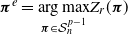 $\boldsymbol{\pi}^e = \underset{\boldsymbol{\pi} \in \mathcal{S}_n^{p-1}}{\arg \max} Z_r(\boldsymbol{\pi})$
. We also set
$\boldsymbol{\pi}^e = \underset{\boldsymbol{\pi} \in \mathcal{S}_n^{p-1}}{\arg \max} Z_r(\boldsymbol{\pi})$
. We also set $\mathcal{Y} = \sigma((\boldsymbol{\pi}^*)^{-1}(G))$
the
$\mathcal{Y} = \sigma((\boldsymbol{\pi}^*)^{-1}(G))$
the $\sigma$
-algebra of all observable random variables.
$\sigma$
-algebra of all observable random variables.
Let $\varepsilon > 0$
, and
$\varepsilon > 0$
, and $\mathcal{X}_\varepsilon$
be the event
$\mathcal{X}_\varepsilon$
be the event $\{Z_r(\boldsymbol{\pi}^e) \geq \varepsilon Z\}$
. In this sense, showing (H1) is equivalent to showing that
$\{Z_r(\boldsymbol{\pi}^e) \geq \varepsilon Z\}$
. In this sense, showing (H1) is equivalent to showing that $\mathbb{P}(\mathcal{X}_\varepsilon) = o(1)$
for any such
$\mathbb{P}(\mathcal{X}_\varepsilon) = o(1)$
for any such $\varepsilon$
.
$\varepsilon$
.
We begin with the following lemma.
Lemma 10. We have
 \begin{equation} \mathbb{P}(\boldsymbol{\pi}^e \in B(\boldsymbol{\pi}^*, r)|\mathcal{X}_\varepsilon) \geq \varepsilon.\end{equation}
Proof. We compute
 \begin{align} \mathbb{P}(\boldsymbol{\pi}^e \in B(\boldsymbol{\pi}^*, r) \wedge \mathcal{X}_\varepsilon) & = \mathbb{E}[\mathbf{1}_{\boldsymbol{\pi}^e \in B(\boldsymbol{\pi}^*, r)} \mathbf{1}_{Z_r(\boldsymbol{\pi}^e) \geq \varepsilon Z}] \nonumber\\[3pt] & = \mathbb{E}[\mathbf{1}_{\boldsymbol{\pi}^* \in B(\boldsymbol{\pi}^e, r)} \mathbf{1}_{\mathbb{P}_{\rm post}(B(\boldsymbol{\pi}^e, r)) \geq \varepsilon}] \nonumber\\[3pt] & = \mathbb{E}[\mathbb{E} [\mathbf{1}_{\boldsymbol{\pi}^* \in B(\boldsymbol{\pi}^e, r)} | \mathcal{Y} ] \mathbf{1}_{\mathbb{P}_{\rm post}(B(\boldsymbol{\pi}^e, r)) \geq \varepsilon} ] \nonumber\\[3pt] & = \mathbb{E} [\mathbb{P}_{\rm post}(B(\boldsymbol{\pi}^e, r)) \mathbf{1}_{\mathbb{P}_{\rm post}(B(\boldsymbol{\pi}^e, r)) \geq \varepsilon} ] \nonumber\\[3pt] & \geq \varepsilon \mathbb{P}(\mathcal{X}_\varepsilon). \end{align}
This means that, defining the new event $\mathcal{X}_\varepsilon^{\rm int} = \{Z_r(\boldsymbol{\pi}^e) \geq \varepsilon Z\} \wedge \{ \boldsymbol{\pi}^e \in B(\boldsymbol{\pi}^*, r)\})$
, it is sufficient for us to show that
$\mathcal{X}_\varepsilon^{\rm int} = \{Z_r(\boldsymbol{\pi}^e) \geq \varepsilon Z\} \wedge \{ \boldsymbol{\pi}^e \in B(\boldsymbol{\pi}^*, r)\})$
, it is sufficient for us to show that $\mathbb{P}(\mathcal{X}_\varepsilon^{\rm int}) = o(1)$
. To achieve this, we show the following lemma.
$\mathbb{P}(\mathcal{X}_\varepsilon^{\rm int}) = o(1)$
. To achieve this, we show the following lemma.
Lemma 11. There exists an estimator $\hat{Y} \in \mathcal{P}(\mathcal{S}_n^{p-1})$
such that
$\hat{Y} \in \mathcal{P}(\mathcal{S}_n^{p-1})$
such that
 \begin{equation} \mathbb{P}(\boldsymbol{\pi}^* \in \hat{Y} \subseteq B(\boldsymbol{\pi}^*, r) | \mathcal{X}_\varepsilon^{\rm int}) \geq \exp(\!-\!O(n)).\end{equation}
Assume this lemma. Then,
 \begin{equation} \mathbb{P}(\boldsymbol{\pi}^* \in \hat{Y} \subseteq B(\boldsymbol{\pi}^*, r)) \geq \mathbb{P}(\mathcal{X}_\varepsilon^{\rm int}) \exp(\!-\!O(n)).\end{equation}
However, we know that
 \begin{align} \mathbb{P}(\boldsymbol{\pi}^* \in \hat{Y} \subseteq B(\boldsymbol{\pi}^*, r)) & = \mathbb{E}[\mathbf{1}_{\boldsymbol{\pi}^* \in \hat{Y}}\mathbf{1}_{\hat{Y} \subseteq B(\boldsymbol{\pi}^*, r)}] \nonumber\\[3pt] & \leq \mathbb{E}[\mathbf{1}_{\boldsymbol{\pi}^* \in \hat{Y}} \mathbf{1}_{\mathbb{P}_{\rm post}(\hat{Y}) \leq \frac{Z_r(\boldsymbol{\pi}^*)}{Z}}]\nonumber\\[3pt] & \leq \mathbb{P}\bigg(\frac{Z_r(\boldsymbol{\pi}^*)}{Z} \geq \delta_n\bigg) + \mathbb{E}[\mathbf{1}_{\boldsymbol{\pi}^* \in \hat{Y}} \mathbf{1}_{\mathbb{P}_{\rm post}(\hat{Y}) \leq \delta_n}],\end{align}
where $\delta_n = \exp(\!-\!n (\!\log n)^{3/5})$
.
$\delta_n = \exp(\!-\!n (\!\log n)^{3/5})$
.
By applying Lemma 3 (as well as Remark 5), we may see that for some $c > 0$
,
$c > 0$
,
 \begin{equation} \mathbb{P}\Big(\frac{Z_r(\boldsymbol{\pi}^*)}{Z} \geq \delta_n\Big) \leq 2\exp(\!-\!c n (\!\log n)^{1/5})\end{equation}
since $\mathbb{E}[\log Z] \sim (p-1) n (\!\log n)^{4/5}$
and, by the same argument as in (57),
$\mathbb{E}[\log Z] \sim (p-1) n (\!\log n)^{4/5}$
and, by the same argument as in (57),
 \begin{equation} \mathbb{E}[\log Z_r(\boldsymbol{\pi}^*)] \sim \mathbb{E}[\log Z_r(\boldsymbol{\pi}^*)\mathbf{1}_{\mathcal{C}}] \leq c_r (p-1) n (\!\log n)^{4/5}(1 + o(1))\end{equation}
for some $0 \leq c_r < 1$
.
$0 \leq c_r < 1$
.
Furthermore,
 \begin{align} \mathbb{E}[\mathbf{1}_{\boldsymbol{\pi}^* \in \hat{Y}} \mathbf{1}_{\mathbb{P}_{\rm post}(\hat{Y}) \leq \delta_n}] & = \mathbb{E} [\mathbb{E} [\mathbf{1}_{\boldsymbol{\pi}^* \in \hat{Y}} |\mathcal{Y}] \mathbf{1}_{\mathbb{P}_{\rm post}(\hat{Y}) \leq \delta_n}] \nonumber\\[3pt] & = \mathbb{E}[\mathbb{P}_{\rm post}(\hat{Y})\mathbf{1}_{\mathbb{P}_{\rm post}(\hat{Y}) \leq \delta_n}] \nonumber\\[3pt] & \leq \delta_n.\end{align}
This all implies that
 \begin{equation} \mathbb{P}(\mathcal{X}_\varepsilon^{\rm int}) \leq \exp O(n) (\exp(\!-\!c n (\!\log n)^{1/5}) + \delta_n) = o(1),\end{equation}
which is what we wanted.
We now just need to prove Lemma 11.
Proof of Lemma
11. Pick $I_1, \ldots, I_p \subseteq \left[ \! \left[ 1, n \right] \! \right]$
to be uniformly random subsets of
$I_1, \ldots, I_p \subseteq \left[ \! \left[ 1, n \right] \! \right]$
to be uniformly random subsets of $\left[ \! \left[ 1, n \right] \! \right]$
, independently from each other and everything else; we then define
$\left[ \! \left[ 1, n \right] \! \right]$
, independently from each other and everything else; we then define
 \begin{equation} \hat{Y} = \{ \boldsymbol{\pi} \in \mathcal{S}_{n}^{p-1}, \mbox{ for all }1 \leq l \leq p, \mbox{ for all }i \in I_l, \boldsymbol{\pi}_l(i) = \boldsymbol{\pi}_l^e(i) \}. \end{equation}
Assume that $\mathcal{X}_\varepsilon^{\rm int}$
holds. Then, if
$\mathcal{X}_\varepsilon^{\rm int}$
holds. Then, if $I_l = \{ i \in \left[ \! \left[ 1, n \right] \! \right]\!, \boldsymbol{\pi}^e_l(i) = \boldsymbol{\pi}_l^*(i) \}$
for any
$I_l = \{ i \in \left[ \! \left[ 1, n \right] \! \right]\!, \boldsymbol{\pi}^e_l(i) = \boldsymbol{\pi}_l^*(i) \}$
for any $1 \leq l \leq p$
(which occurs with probability at least
$1 \leq l \leq p$
(which occurs with probability at least $\exp (\!-\! O(n))$
), we in fact have
$\exp (\!-\! O(n))$
), we in fact have
 \begin{equation} \boldsymbol{\pi}^* \in \hat{Y} \subseteq B(\boldsymbol{\pi}^*, r). \end{equation}
Indeed, given that $\mathcal{X}_\varepsilon^{\rm int}$
is verified, we may set
$\mathcal{X}_\varepsilon^{\rm int}$
is verified, we may set $J = \bigcap_{1 \leq l \leq p} I_l$
, and
$J = \bigcap_{1 \leq l \leq p} I_l$
, and $|J| \geq (1-r)n$
; thus, if
$|J| \geq (1-r)n$
; thus, if $\boldsymbol{\pi} \in \hat{Y}$
,
$\boldsymbol{\pi} \in \hat{Y}$
,
 \begin{equation} ov(\boldsymbol{\pi}, \boldsymbol{\pi}^*) \geq \frac{|J|}{n} = 1-r \end{equation}
and $\hat{Y} \subseteq B(\boldsymbol{\pi}^*, r)$
.
$\hat{Y} \subseteq B(\boldsymbol{\pi}^*, r)$
.
Appendix I. Proof of Lemma 6
We begin by assuming that H is connected. We prove by recursion that, for any $1 \leq i \leq |V|$
, there exists
$1 \leq i \leq |V|$
, there exists $X \subseteq V$
with
$X \subseteq V$
with $|X| \geq i$
such that the cardinal of
$|X| \geq i$
such that the cardinal of $\{ \sigma|_{X}, \sigma \in \textrm{Aut} H \}$
is at most equal to
$\{ \sigma|_{X}, \sigma \in \textrm{Aut} H \}$
is at most equal to
 \begin{equation} |V|\prod_{\underset{N_u \subseteq X}{u \in X}} (d_u)!,\end{equation}
where, for any vertex u, $N_u$
is the set of neighbours of u.
$N_u$
is the set of neighbours of u.
This is clear for $i=1$
. Furthermore, if we have such a set
$i=1$
. Furthermore, if we have such a set $X \neq V$
, then there exist
$X \neq V$
, then there exist $u \in X$
such that
$u \in X$
such that $N_u$
is not contained within X. However, if
$N_u$
is not contained within X. However, if $\sigma \in \textrm{Aut} H$
,
$\sigma \in \textrm{Aut} H$
, $\sigma(N_{u}) = N_{\sigma(u)}$
and so, given the value of
$\sigma(N_{u}) = N_{\sigma(u)}$
and so, given the value of $\sigma(u)$
, there are at most
$\sigma(u)$
, there are at most $d_u!$
possible values for
$d_u!$
possible values for $\sigma|_{N_u}$
. Thus, the property remains true for
$\sigma|_{N_u}$
. Thus, the property remains true for $X' = X \cup N_u$
. By recursion, this concludes the case where H is connected.
$X' = X \cup N_u$
. By recursion, this concludes the case where H is connected.
Now, we move on to the general case: assume that H splits into connected components $(H_i)_{1 \leq i \leq l}$
with vertex sets
$(H_i)_{1 \leq i \leq l}$
with vertex sets $(V_i)_{1 \leq i \leq l}$
. From the connected case, we deduce that the number of automorphisms of H which send each
$(V_i)_{1 \leq i \leq l}$
. From the connected case, we deduce that the number of automorphisms of H which send each $H_i$
to itself, is at most equal to
$H_i$
to itself, is at most equal to
 \begin{equation} \bigg(\prod_{i=1}^l |V_i| \bigg)\prod_{v \in V}(d_v!).\end{equation}
However, since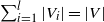 $\sum_{i=1}^l |V_i| = |V|$
, by the arithmetic mean/geometric mean inequality,
$\sum_{i=1}^l |V_i| = |V|$
, by the arithmetic mean/geometric mean inequality,
 \begin{equation} \prod_{i=1}^l |V_i| \leq \bigg(\frac{1}{l} \sum_{i=1}^l |V_i|\bigg)^l = \bigg(\bigg(\frac{|V|}{l} \bigg)^{{l}/{|V|}} \bigg)^{|V|} \leq (\mathrm{e}^{{1}/{e}} )^{|V|},\end{equation}
concluding the proof.
Appendix J. An extra theorem
At the end of Appendix F, we made use of an inequality which we now prove.
Theorem 6. Let $0 \leq (x_{ij})_{1 \leq i \neq j \leq p} \leq 1$
be real numbers with
$0 \leq (x_{ij})_{1 \leq i \neq j \leq p} \leq 1$
be real numbers with $x_{ij} = x_{\rm ji}$
for all
$x_{ij} = x_{\rm ji}$
for all $i \neq j$
. If
$i \neq j$
. If $\tau \in \mathcal{S}_p$
, and
$\tau \in \mathcal{S}_p$
, and $2 \leq i \leq p$
, define
$2 \leq i \leq p$
, define $X_{i}(\tau) = \max_{j<i} x_{\tau(j) \tau(i)}$
. We also set
$X_{i}(\tau) = \max_{j<i} x_{\tau(j) \tau(i)}$
. We also set
 \begin{equation} S_*(\tau) = S_*(\tau, (x_{ij})) \underset{{\rm def}}{=} \frac{1}{p-1}\sum_{i=2}^p X_{i}(\tau). \end{equation}
Then, there exists $\tau \in \mathcal{S}_p$
such that
$\tau \in \mathcal{S}_p$
such that
 \begin{equation} S_*(\tau) \geq \frac{\dfrac{2}{p(p-1)}\displaystyle\sum_{1 \leq i \neq j \leq p} x_{ij}^2}{1 + \dfrac{1}{p(p-1)}\displaystyle\sum_{1 \leq i \neq j \leq p} x_{ij}^2}. \end{equation}
Remark 6. Consider the complete graph $K_p$
over
$K_p$
over $\left[ \! \left[ 1, p \right] \! \right]$
; we put the weight
$\left[ \! \left[ 1, p \right] \! \right]$
; we put the weight $x_{ij}$
on the edge linking i to j, obtaining a graph
$x_{ij}$
on the edge linking i to j, obtaining a graph $\mathcal{G}$
. We construct a spanning tree of
$\mathcal{G}$
. We construct a spanning tree of $\mathcal{G}$
, by:
$\mathcal{G}$
, by:
-
• picking
$\tau(1)$
; -
• picking
$\tau(2)$
and connecting it to
$\tau(1)$
; -
• picking
$\tau(3)$
and connecting it to
$\tau(1)$
or
$\tau(2)$
(depending on whether
$x_{\tau(1) \tau(3)}$
or
$x_{\tau(2) \tau(3)}$
) is larger; -
• and continuing the process in this fashion.


Here $X_i(\tau)$
is the
$X_i(\tau)$
is the $(i-1)$
th edge constructed by this process, and so
$(i-1)$
th edge constructed by this process, and so $(p-1)S_*(\tau)$
is the total weight of the tree. Furthermore, if
$(p-1)S_*(\tau)$
is the total weight of the tree. Furthermore, if $\tau$
is chosen correctly, this is simply the application of Prim’s algorithm; thus,
$\tau$
is chosen correctly, this is simply the application of Prim’s algorithm; thus, $\max_{\tau \in \mathcal{S}_p} (p-1)S_*(\tau)$
is the total weight of the maximal spanning tree of
$\max_{\tau \in \mathcal{S}_p} (p-1)S_*(\tau)$
is the total weight of the maximal spanning tree of $\mathcal{G}$
. We are therefore claiming that there exists a spanning tree of
$\mathcal{G}$
. We are therefore claiming that there exists a spanning tree of $\mathcal{G}$
, with weight at least
$\mathcal{G}$
, with weight at least
 \begin{equation} (p-1) \cdot \frac{ \dfrac{2}{p(p-1)}\displaystyle\sum_{1 \leq i \neq j \leq p}x_{ij}^2}{1 + \dfrac{1}{p(p-1)}\displaystyle\sum_{1 \leq i \neq j \leq p}x_{ij}^2}. \end{equation}
Proof. We proceed by recursion over $p \geq 1$
. If
$p \geq 1$
. If $p=1$
, there is nothing to prove. From now on, we assume that
$p=1$
, there is nothing to prove. From now on, we assume that $p \geq 2$
.
$p \geq 2$
.
Let x be the minimum weight of an edge contained in the maximal spanning tree. Then, the graph over $\left[ \! \left[ 1, p \right] \! \right]$
with edges
$\left[ \! \left[ 1, p \right] \! \right]$
with edges $\{ \{i\neq j \}, x_{ij} > x \}$
cannot be connected; otherwise, Prim’s algorithm would give us a maximal spanning tree with edges whose weights are strictly larger than x. Thus, we may partition
$\{ \{i\neq j \}, x_{ij} > x \}$
cannot be connected; otherwise, Prim’s algorithm would give us a maximal spanning tree with edges whose weights are strictly larger than x. Thus, we may partition $\left[ \! \left[ 1, p \right] \! \right]$
into two (nonempty) subsets
$\left[ \! \left[ 1, p \right] \! \right]$
into two (nonempty) subsets $B_1, B_2 \subseteq \left[ \! \left[ 1, p \right] \! \right]$
such that
$B_1, B_2 \subseteq \left[ \! \left[ 1, p \right] \! \right]$
such that $x_{ij} \leq x$
for
$x_{ij} \leq x$
for $i \in B_1, j \in B_2$
, and there exists a maximal spanning tree which is the union of:
$i \in B_1, j \in B_2$
, and there exists a maximal spanning tree which is the union of:
-
• a maximal spanning tree of the induced subgraph of
$\mathcal{G}$
over
$B_1$
; -
• a maximal spanning tree of the induced subgraph of
$\mathcal{G}$
over
$B_2$
; -
• an edge with weight x.


Also note that we may assume, without loss of generality, that $x_{ij} \geq x$
for any
$x_{ij} \geq x$
for any $i \neq j \in B_1$
or
$i \neq j \in B_1$
or $i \neq j \in B_2$
. Indeed, even after increasing the
$i \neq j \in B_2$
. Indeed, even after increasing the $x_{ij}$
to satisfy this condition, applying Prim’s algorithm (with suitable tiebreakers) will still give us the same spanning tree (since all of the edges of the spanning tree are
$x_{ij}$
to satisfy this condition, applying Prim’s algorithm (with suitable tiebreakers) will still give us the same spanning tree (since all of the edges of the spanning tree are $\geq x$
) but the quantity
$\geq x$
) but the quantity ${2 \sum_{1 \leq i \neq j \leq p}x_{ij}^2}/({1 + \sum_{1 \leq i \neq j \leq p}x_{ij}^2})$
will have increased.
${2 \sum_{1 \leq i \neq j \leq p}x_{ij}^2}/({1 + \sum_{1 \leq i \neq j \leq p}x_{ij}^2})$
will have increased.
Noting $|B_1| = k_1$
and
$|B_1| = k_1$
and $|B_2| = k_2 = p-k_1$
, this means that
$|B_2| = k_2 = p-k_1$
, this means that
 \begin{equation} (p-1)S_* = (k_1-1)S_*((x_{ij})_{i,j \in B_1}) + (k_2 - 1)S_*((x_{ij})_{i,j \in B_2}) + x. \end{equation}
However, by induction, we have
 \begin{equation} (k_1-1)S_*((x_{ij})_{i,j \in B_1}) + (k_2 - 1)S_*((x_{ij})_{i,j \in B_2})\geq (k_1 - 1) \frac{2 S_1}{1 + S_1} + (k_2 - 1) \frac{2 S_2}{1 +S_2}, \end{equation}
where $S_l = ({1}/{k_l(k_l - 1)} ) \sum_{i \neq j \in B_l} x_{ij}^2$
for
$S_l = ({1}/{k_l(k_l - 1)} ) \sum_{i \neq j \in B_l} x_{ij}^2$
for $l = 1$
or 2. (Note that, in our case,
$l = 1$
or 2. (Note that, in our case, $S_l \geq x^2$
.) In order to conclude, we thus simply need to show that
$S_l \geq x^2$
.) In order to conclude, we thus simply need to show that
 \begin{equation} (k_1 - 1) \frac{2 S_1}{1 + S_1} + (k_2 - 1) \frac{2 S_2}{1 +S_2} + x \geq (p-1)\frac{2 \frac{1}{p(p-1)} \sum_{1 \leq i \neq j \leq p} x_{ij}^2}{1 + \frac{1}{p(p-1)} \sum_{1 \leq i \neq j \leq p} x_{ij}^2}. \end{equation}
To simplify notation, we define
 \begin{align} \alpha_1 = \frac{k_1 - 1}{p-1},\quad \alpha_2 = \frac{k_2 - 1}{p-1},\quad \alpha_3 = \frac{1}{p-1}, \\[-10pt] \nonumber \end{align}
 \begin{align} \beta_1 = \frac{k_1(k_1 - 1)}{p(p-1)}, \quad \beta_2 = \frac{k_2(k_2 - 1)}{p(p-1)}, \quad \beta_3 = \frac{2k_1k_2}{p(p-1)}, \\[8pt] \nonumber \end{align}
such that $\alpha_1 + \alpha_2 + \alpha_3 = \beta_1 + \beta_2 + \beta_3 = 1$
. By definition of our blocks, we have
$\alpha_1 + \alpha_2 + \alpha_3 = \beta_1 + \beta_2 + \beta_3 = 1$
. By definition of our blocks, we have
 \begin{equation} \frac{1}{p(p-1)} \sum_{1 \leq i \neq j \leq p} x_{ij}^2 \leq \beta_1 S_1 + \beta_2 S_2 + \beta_3 x^2 \end{equation}
and so, in order to show (J6), we just need to show that
 \begin{equation} \alpha_1 \frac{2 S_1}{1 + S_1} + \alpha_2 \frac{2 S_2}{1 + S_2} + \alpha_3 x \geq \frac{2(\beta_1 S_1 + \beta_2 S_2 + \beta_3 x^2)}{1 + \beta_1 S_1 + \beta_2 S_2 + \beta_3 x^2}. \end{equation}
Expanding out, the above inequality reduces to
 \begin{align} f(S_1, S_2) &\underset{{\rm def}}{=} (2\alpha_1 S_1(1 + S_2) + 2\alpha_2 S_2(1 + S_1) + \alpha_3 x (1 + S_1)(1 + S_2))(1 + \beta_1 S_1 + \beta_2 S_2 + \beta_3 x^2) \nonumber\\[3pt] & - (2\beta_1 S_1 + 2\beta_2 S_2 + 2 \beta_3 x^2)(1 + S_1)(1 + S_2) \nonumber\\[3pt] & \geq 0. \end{align}
We show that:
-
• for
$x \leq S_1, S_2 \leq 1$
,
$({\partial^2 f}/{\partial S_i^2})(S_1, S_2) \leq 0$
, i.e. f is concave in both arguments; -
•
$f(x^2, 1) \geq 0$
,
$f(1, x^2) \geq 0$
,
$f(1, 1) \geq 0$
, and
$f(x^2, x^2) \geq 0$
;




proving that indeed $f(S_1, S_2) \geq 0$
for
$f(S_1, S_2) \geq 0$
for $x^2 \leq S_1, S_2 \leq 1$
.
$x^2 \leq S_1, S_2 \leq 1$
.
First of all,
 \begin{equation} \dfrac{\partial^2 f}{\partial S_1^2}(S_1, S_2) = 2 \alpha_1 \beta_1 (1 + S_2) - 2 \beta_1 (1 + S_2) \leq 0 \end{equation}
and, by symmetry, $ {\partial^2 f}/{\partial S_2^2} \leq 0$
. Second, expanding out f,
$ {\partial^2 f}/{\partial S_2^2} \leq 0$
. Second, expanding out f,
 \begin{align} f(x^2, 1) & = 2 \alpha_{3} x(1 - x)^2 + 2 \alpha_3 (1 - \beta_2) x^3 (1 - x)^2 \nonumber\\[3pt] &\quad + 2 \alpha_2(1 + \beta_2) - 4 \beta_2 + 2 \alpha_3 \beta_2 x + 4 \alpha_1 \beta_2 x^2 + 2 \alpha_3 \beta_2 x^3 - 2 \alpha_2(1 - \beta_2)x^4 \nonumber\\[3pt] & \geq 2 \alpha_2(1 + \beta_2) - 4 \beta_2 + 2 \alpha_3 \beta_2 + 4 \alpha_1 \beta_2 + 2 \alpha_3 \beta_2 - 2 \alpha_2(1 - \beta_2) = 0 \end{align}
since $2 \alpha_2(1 + \beta_2) - 4 \beta_2 = {2k_1(k_2 - 1)}/{p(p-1)} \geq 0$
.
$2 \alpha_2(1 + \beta_2) - 4 \beta_2 = {2k_1(k_2 - 1)}/{p(p-1)} \geq 0$
.
Third, by symmetry, $f(1, x^2) \geq 0$
.
$f(1, x^2) \geq 0$
.
Fourth,
 \begin{align} f(1, 1) & = 4(1 - \alpha_3(1 - x))(2 - \beta_3(1-x^2)) - 8(1 - \beta_3(1 - x^2)) \nonumber\\[3pt] & = 8 \frac{k_1 k_2}{p(p-1)}(1 - x^2) - \frac{8}{p-1}(1-x) + \frac{8 k_1 k_2}{p(p-1)^2}(1-x)(1-x^2) \nonumber\\[3pt] & = \frac{8}{p(p-1)^2}(k_1(p-k_1)(p-1)(1-x^2) - p(p-1)(1-x) + k_1(p - k_1)(1-x)(1-x^2)). \end{align}
If $k_1 \geq 2$
and
$k_1 \geq 2$
and $k_2 = p-k_1 \geq 2$
, then
$k_2 = p-k_1 \geq 2$
, then $k_1(p-k_1) \geq p$
and
$k_1(p-k_1) \geq p$
and $f(1, 1) \geq 0$
. Otherwise
$f(1, 1) \geq 0$
. Otherwise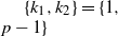 $\{k_1, k_2 \} = \{1, p-1 \}$
, and
$\{k_1, k_2 \} = \{1, p-1 \}$
, and
 \begin{align} f(1, 1) & = \frac{8}{p(p-1)^2}((p-1)^2(1-x^2) - p(p-1)(1-x)+(p-1)(1-x)(1-x^2)) \nonumber\\[3pt] & = \frac{8}{p(p-1)^2}(p-1)(p-2)x^2(1-x) \geq 0. \end{align}
Finally,
 \begin{align} f(x^2, x^2) & = (1 + x^2)^2(2(\alpha_1 + \alpha_2)x^2 + \alpha_3 x(1 + x^2) - 2 x^2) \nonumber\\[3pt] & = (1 + x^2)^2 \alpha_3 x (1-x)^2 \geq 0. \end{align}
Acknowledgements
The authors would like to thank Mohammad Hassan Ahmad Yarandi and Luca Ganassali for their helpful comments on earlier versions of the article.
Funding information
There are no funding bodies to thank relating to this creation of this article.
Competing interests
There were no competing interests to declare which arose during the preparation or publication process of this article.

 Open access

