





1 Introduction
Translation surfaces are geometric objects in which it is possible to define a notion of geodesics for every direction $\theta \in [0,2\pi )$
. The collection of geodesics for a direction
$\theta \in [0,2\pi )$
. The collection of geodesics for a direction $\theta $
yields a foliation. (It is not a foliation in the strict sense since there are geodesics whose domain of definition cannot be extended to
$\theta $
yields a foliation. (It is not a foliation in the strict sense since there are geodesics whose domain of definition cannot be extended to $(-\infty ,\infty )$
. Nevertheless, in most of the cases, in particular, in those that we are going to consider, the set of these problematic geodesics has measure zero.) In the last few decades, interest has grown in the distribution of the leaves of this foliation or in the dynamical properties of the flow (usually called translation flow or billiard flow) that define this foliation, from an ergodic theory point of view.
$(-\infty ,\infty )$
. Nevertheless, in most of the cases, in particular, in those that we are going to consider, the set of these problematic geodesics has measure zero.) In the last few decades, interest has grown in the distribution of the leaves of this foliation or in the dynamical properties of the flow (usually called translation flow or billiard flow) that define this foliation, from an ergodic theory point of view.
The study of translation flows on surfaces of finite type, that is, surfaces homeomorphic to compact Riemann surfaces, has yielded significant results. In particular, in [Reference Kerckhoff, Masur and SmillieKMS86], the authors establish the unique ergodicity of the translation flows, showing that for almost every direction, the leaves of the associated foliation are equidistributed. Furthermore, in [Reference Avila and ForniAF07], it is proven that for almost every translation surface in every stratum, the translation flow is weakly mixing for almost every direction.
In recent years, there has been growing interest in understanding the geometry and dynamics of translation surfaces beyond the compact setting. As expected, many properties established for compact translation surfaces no longer hold, while new phenomena emerge. A comprehensive overview of recent developments can be found in [Reference Delecroix, Hubert and ValdezDHV24].
In this work, we study vertical translation flows on infinite-type translation surfaces of finite area. In contrast to surfaces of finite type, where translation flows cannot be mixing [Reference KatokKat80], we construct examples of finite-area and infinite-genus translation surfaces whose vertical flows are mixing. Our examples are obtained by suspending a carefully constructed mixing infinite interval exchange transformation, called staircase transformation, over a simple two-valued roof function. The main result can be informally described as follows.
Theorem 1.1. Consider an L-shaped polygon whose two vertical sides have rationally independent heights. If the horizontal sides are glued according to a mixing staircase transformation, then the resulting finite-area, infinite-genus translation surface has a mixing vertical flow.
See Theorem 3.11 for a precise formulation.
This result highlights a striking contrast between finite- and infinite-type translation surfaces. While surfaces of finite-type are constrained by classical rigidity results and cannot support mixing vertical translation flows, infinite-genus surfaces can exhibit genuinely chaotic vertical dynamics. Previous related work includes Ulcigrai’s study of mixing suspension flows over finite interval exchange transformations [Reference UlcigraiUlc07]. We emphasize, however, that her constructions do not produce translation flows. In contrast, our work deals with infinite-genus surfaces while preserving the translation structure.
Infinite translation surfaces can have infinite area, with interesting examples such as the wind tree model [Reference Avila and HubertAH20] or $\mathbb {Z}$
-coverings [Reference Hubert and WeissHW13], as well as finite-area surfaces, as shown in [Reference TrevinoTre14]. In [Reference Lindsey and TreviñoLTn16], Lindsey and Treviño use techniques from cutting and stacking constructions to study the dynamics of translation flows on finite-area translation surfaces, encoding their information in bi-infinite Vershik–Brattelli diagrams. One particularly interesting result they present is an extension of Rudolph’s classical representation theorem for aperiodic flows [Reference RudolphRud76]. Specifically, they prove [Reference Lindsey and TreviñoLTn16, Proposition 7.6, Lemma 7.7] that any aperiodic flow on a finite Lebesgue measure space with finite entropy is measure-theoretically isomorphic to the vertical flow of a translation surface of finite area arising from a Vershik–Brattelli diagram.
$\mathbb {Z}$
-coverings [Reference Hubert and WeissHW13], as well as finite-area surfaces, as shown in [Reference TrevinoTre14]. In [Reference Lindsey and TreviñoLTn16], Lindsey and Treviño use techniques from cutting and stacking constructions to study the dynamics of translation flows on finite-area translation surfaces, encoding their information in bi-infinite Vershik–Brattelli diagrams. One particularly interesting result they present is an extension of Rudolph’s classical representation theorem for aperiodic flows [Reference RudolphRud76]. Specifically, they prove [Reference Lindsey and TreviñoLTn16, Proposition 7.6, Lemma 7.7] that any aperiodic flow on a finite Lebesgue measure space with finite entropy is measure-theoretically isomorphic to the vertical flow of a translation surface of finite area arising from a Vershik–Brattelli diagram.
This theorem yields, in particular, the existence of mixing translation flows. Anosov flows give natural examples: they are mixing and, in fact, Bernoulli. Therefore, for an Anosov flow $\gamma _t$
, there exists a finite-area translation surface S whose vertical flow
$\gamma _t$
, there exists a finite-area translation surface S whose vertical flow $\phi _t$
is measure-theoretically isomorphic to
$\phi _t$
is measure-theoretically isomorphic to $\gamma _t$
. In particular,
$\gamma _t$
. In particular, $\phi _t$
is mixing.
$\phi _t$
is mixing.
In their work, Lindsey and Treviño do not construct explicit examples of such flows. To produce concrete mixing translation flows, we use the classical representation of translation flows as suspension flows over interval transformations under piecewise constant roof functions. In contrast to the finite-area case, the base transformations are typically infinite interval exchange transformations.
A natural class of examples is given by staircase transformations: rank-one transformations obtained via cutting-and-stacking constructions in which the associated Rokhlin towers acquire a staircase profile. Certain staircase transformations are known to be mixing [Reference AdamsAda98, Reference Creutz and SilvaCS04]. Lindsey and Treviño conjectured [Reference Lindsey and TreviñoLTn16, Conjecture 7.8] that suspensions over mixing staircase transformations may produce mixing translation flows.
In Theorems 2.1 and 2.2, we show that a suspension flow over a mixing staircase transformation, under a roof function taking two rationally independent values on complementary subintervals, is mixing. These suspension flows correspond to vertical flows on infinite translation surfaces, thereby establishing Theorem 1.1 and providing a positive answer to the question posed by Lindsey and Treviño.
The complexity of a suspension flow arises from both the base transformation and the roof function. When the roof function is constant, the flow is never mixing. Our construction produces mixing behavior in what can be considered the simplest non-trivial class of roof functions, namely those taking just two distinct values.
2 Organization
Our goal is to construct a family of examples of infinite translation surfaces with finite area such that their translation flow is mixing.
In §3, we provide basic definitions of translation surfaces, rank-one transformations and staircase transformations, suspension flows, and a way to construct a translation surface from a cutting and stacking process. In §4, we prove the result on a suspension flow over the classical staircase.
Theorem 2.1. Let T be the classical staircase transformation and $p,q$
two rationally independent positive numbers. Let f be a 2-wise constant function such that f attains the values
$p,q$
two rationally independent positive numbers. Let f be a 2-wise constant function such that f attains the values $p,q$
on complementary intervals. Then, the suspension flow
$p,q$
on complementary intervals. Then, the suspension flow $([0,1],T,f,\mu )$
is mixing.
$([0,1],T,f,\mu )$
is mixing.
The motivation to start with this case is due to the fact that the classical staircase T was the first staircase transformation that was proved to be mixing [Reference AdamsAda98].
The strategy to establish the mixing property for suspension flows over any mixing staircase transformation follows essentially the same approach as in the classical staircase case. Accordingly, in §4, we present the full details of the argument. In §5, we focus only on the modifications required for the generalized case and explain why these adjustments are valid. This allows us to conclude the following theorem.
Theorem 2.2. Let T be any mixing staircase transformation and $p,q$
two rationally independent positive numbers. Let f be a 2-wise constant function such that f attains the values
$p,q$
two rationally independent positive numbers. Let f be a 2-wise constant function such that f attains the values $p,q$
on complementary intervals. Then, the suspension flow
$p,q$
on complementary intervals. Then, the suspension flow $([0,1],T,f,\mu )$
is mixing.
$([0,1],T,f,\mu )$
is mixing.
Note that the graph of the function f from Theorems 2.1 and 2.2, together with the x-axis and y-axis, forms an L-shaped polygon. By identifying the bottom edges with the top edges using the staircase transformation T and the vertical edges with their opposite edges, we obtain a translation surface with finite area and infinite genus. Moreover, the vertical translation flow on this surface corresponds to the suspension flows described in both theorems. Therefore, Theorems 2.1 and 2.2 together yield Theorem 1.1.
We believe that it should be possible to impose some mild conditions on the growth of spacers and cutting sequences such that these results could be extended to more general rank-one transformations satisfying these conditions. For example, the restricted growth conditions on the cutting sequences and additional conditions on the spacer sequences, as explained in [Reference Creutz and SilvaCS04, Reference Creutz and SilvaCS06].
It is almost immediate from the construction of the suspension flows considered in Theorems 2.1 and 2.2 that they can be regarded as rank-one flows. In the 1990s, Ryzhikov proved that if rank-one flows are mixing, then they are also n-fold mixing for any n [Reference RyzhikovRyz92]. Therefore, we immediately obtain this result in §6.
Theorem 2.3. Let T be any mixing staircase transformation and $p,q$
two rationally independent positive numbers. Let f be a 2-wise constant function such that f attains the values
$p,q$
two rationally independent positive numbers. Let f be a 2-wise constant function such that f attains the values $p,q$
on complementary intervals. Then, the suspension flow
$p,q$
on complementary intervals. Then, the suspension flow $([0,1],T,f,\mu )$
is mixing of any order.
$([0,1],T,f,\mu )$
is mixing of any order.
3 Preliminaries
3.1 Translation surfaces
There are various approaches to defining a translation surface, each tailored to different interests.
One common depiction of a translation surface involves considering a connected topological surface S alongside a discrete subset $ \Sigma \subseteq S$
. Within
$ \Sigma \subseteq S$
. Within $ S \setminus \Sigma $
, a maximal atlas called the translation atlas
$ S \setminus \Sigma $
, a maximal atlas called the translation atlas $ \{ \phi _\alpha , U_\alpha \}_{\alpha \in \Lambda }$
is defined, where the transition maps are Euclidean translations.
$ \{ \phi _\alpha , U_\alpha \}_{\alpha \in \Lambda }$
is defined, where the transition maps are Euclidean translations.
For the purposes of studying billiard dynamics within polygons and generalized polygons, a more practical definition of a translation surface involves an at-most-countable collection of convex polygons $\{ P_n \} \subset \mathbb {R}^2 $
, where each pair of edges is identified by translations. Denoting the collection of vertices of these polygons as
$\{ P_n \} \subset \mathbb {R}^2 $
, where each pair of edges is identified by translations. Denoting the collection of vertices of these polygons as $ V $
, we define the surface as
$ V $
, we define the surface as
 $$ \begin{align*} S^\circ = \bigg( \bigg(\!\bigcup_{n \in \mathbb{N}} P_n \bigg) \setminus V \bigg) / \sim. \end{align*} $$
If $S^\circ $
is a connected space, we call S, the metric completion of
$S^\circ $
is a connected space, we call S, the metric completion of $S^\circ $
, a translation surface.
$S^\circ $
, a translation surface.
These two definitions are equivalent (see [Reference Delecroix, Hubert and ValdezDHV24]). A translation surface S is categorized as finite type if the collection of polygons is finite or if the topological surface S on which the translation atlas is defined is homeomorphic to a compact surface X; otherwise, it is termed infinite type.
Now, for any direction $[0,2\pi )$
, we have a well-defined translation flow in
$[0,2\pi )$
, we have a well-defined translation flow in $\mathbb {C} = \mathbb {R}^2$
given by
$\mathbb {C} = \mathbb {R}^2$
given by
 $$ \begin{align*} F_{\theta}^t(z) = z + t e^{i\theta}, \end{align*} $$
which yields a constant vector field
 $$ \begin{align*} X_{\theta} = \frac{\partial F_{\theta}^t}{\partial t} \bigg|_{t=0}(z). \end{align*} $$
The definition of a translation surface allows us to pull back this vector field to $S \setminus \Sigma $
. For any
$S \setminus \Sigma $
. For any $z \in S \setminus \Sigma $
, we can consider a maximal integral curve
$z \in S \setminus \Sigma $
, we can consider a maximal integral curve $\gamma _z: I \to S \setminus \Sigma $
such that
$\gamma _z: I \to S \setminus \Sigma $
such that $\gamma _z(0) = z$
and we can define a flow on
$\gamma _z(0) = z$
and we can define a flow on $S \setminus \Sigma $
as
$S \setminus \Sigma $
as
 $$ \begin{align*} \phi_{\theta}^t(z) = \gamma_z(t). \end{align*} $$
This is the translation flow in direction $\theta $
. When the direction is not stated, meaning only writing
$\theta $
. When the direction is not stated, meaning only writing $\phi _t$
, we will mean the translation flow in the vertical direction.
$\phi _t$
, we will mean the translation flow in the vertical direction.
3.2 Ergodic theory
Definition 3.1. If $(X,T,\mathcal {B},\mu )$
is a measurable dynamical system, we say T is an ergodic transformation if for every measurable invariant set A such that
$(X,T,\mathcal {B},\mu )$
is a measurable dynamical system, we say T is an ergodic transformation if for every measurable invariant set A such that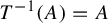 $T^{-1}(A)=A$
implies
$T^{-1}(A)=A$
implies $\mu (A)\in \{0,1\}$
.
$\mu (A)\in \{0,1\}$
.
In terms of the Birkhoff theorem, it can be stated as for every measurable function f,
 $$ \begin{align*} \lim \frac{1}{n}\sum_{i=0}^n f\circ T^n(x)\to \int_X f\,d\mu \end{align*} $$
for $\mu -$
almost every x.
$\mu -$
almost every x.
In the ergodic theory category, we have the following chain of implications:
 $$ \begin{align*} \textit{Mixing} \to \textit{Weakly}\ \textit{mixing} \to \textit{Ergodic.} \end{align*} $$
Definition 3.2. Let $(X,\mathcal B,\mu )$
be a probability space and let
$(X,\mathcal B,\mu )$
be a probability space and let $T : X \to X$
be a measure-preserving transformation.
$T : X \to X$
be a measure-preserving transformation.
-
(1) We say that T is mixing if for all $A,B \in \mathcal B$
,
$$ \begin{align*} \lim_{n\to\infty} \mu(T^{-n}A \cap B) = \mu(A)\mu(B). \end{align*} $$
$A,B \in \mathcal B$
,
$$ \begin{align*} \lim_{n\to\infty} \mu(T^{-n}A \cap B) = \mu(A)\mu(B). \end{align*} $$
-
(2) We say that T is weakly mixing if for all
$A,B \in \mathcal B$
,
$$ \begin{align*} \lim_{n\to\infty} \frac{1}{n} \sum_{i=0}^{n-1} |\mu(T^{-i}A \cap B) - \mu(A)\mu(B) | = 0. \end{align*} $$


Our aim is to study the continuous version of these properties.
Definition 3.3. A flow $\phi _t$
is a family of measurable transformations
$\phi _t$
is a family of measurable transformations $\{\phi _t\}_{t\in \mathbb {R}}$
on a measurable space
$\{\phi _t\}_{t\in \mathbb {R}}$
on a measurable space $(X,\mathcal {B},\mu )$
parameterized with
$(X,\mathcal {B},\mu )$
parameterized with $\mathbb {R}$
such that
$\mathbb {R}$
such that $\phi _{t+s}=\phi _t(\phi _s).$
Definition 3.4. We say that the flow $\phi _t$
on a measurable space
$\phi _t$
on a measurable space $(X,\mathcal {B},\mu )$
is mixing if for every
$(X,\mathcal {B},\mu )$
is mixing if for every $A,B\in \mathcal {B}$
,
$A,B\in \mathcal {B}$
,
 $$ \begin{align*}\lim_{t\to\infty} \mu(\phi_{-t}(A)\cap B)= \mu(A)\mu(B).\end{align*} $$
As we shall see in following sections, the notion of equidistribution plays an important role.
Definition 3.5. Let $\{x_n\}_{n\ge 1}$
be a sequence of points in
$\{x_n\}_{n\ge 1}$
be a sequence of points in $[a,b]$
. We say that
$[a,b]$
. We say that $\{x_n\}$
is equidistributed in
$\{x_n\}$
is equidistributed in $[a,b]$
if for every subinterval
$[a,b]$
if for every subinterval $[c,d] \subset [a,b] $
, one has
$[c,d] \subset [a,b] $
, one has
 $$ \begin{align*} \lim_{n\to\infty} \dfrac{1}{n} \#\{1 \le k \le n : x_k \in [c,d]\} = \frac{d-c}{b-a}. \end{align*} $$
Remark 3.6. By the equidistribution theorem, if q is an irrational number, then the sequence $\{nq\!\! \mod {1}\:\: n\in \mathbb {N}\} $
is equidistributed in the unitary interval.
$\{nq\!\! \mod {1}\:\: n\in \mathbb {N}\} $
is equidistributed in the unitary interval.
Definition 3.7. A transformation $T:X\to X$
is said to be uniquely ergodic if there exists only one invariant measure for T.
$T:X\to X$
is said to be uniquely ergodic if there exists only one invariant measure for T.
When a transformation is uniquely ergodic, the unique invariant measure is ergodic and the conclusion of the Birkhoff ergodic theorem applies for every $x\in X$
.
$x\in X$
.
Observe that if T is a continuous uniquely ergodic transformation in an interval $[a,b)$
, then for any x, the sequence
$[a,b)$
, then for any x, the sequence $x_n=T^n(x)$
fulfills that for every continuous function f,
$x_n=T^n(x)$
fulfills that for every continuous function f,
 $$ \begin{align*} \lim_{n\to \infty} \frac{1}{n}\sum_{i=0}^n f(x_n)\to\frac{1}{b-a} \int_a^b f(x)\,dx, \end{align*} $$
in particular, the sequence $x_n$
equidistributes in the interval
$x_n$
equidistributes in the interval $[a,b)$
.
$[a,b)$
.
3.3 Cutting and stacking constructions
Cutting and stacking constructions represent a powerful tool extensively used in ergodic theory to construct measurable invertible transformations on the interval. Intuitively, they can be conceptualized as a limit process involving compositions of periodic maps on subintervals. This process entails considering a sequence of transformations $T_1, T_2, \ldots , T_n, \ldots $
satisfying the following properties:
$T_1, T_2, \ldots , T_n, \ldots $
satisfying the following properties:
-
(1) Domain
$(T_i)\subseteq \textbf {Domain}(T_{i+1})$
; -
(2)
$T_{n+1|_{\textbf {Domain}(T_n)}}=T_n.$


We can define a map T such that
 $$ \begin{align*} \textbf{Domain}(T)=\bigcup_{n\in \mathbb{N}}\textbf{Domain}(T_n) \end{align*} $$
and such that T is the pointwise limit of the sequence $T_n$
.
$T_n$
.
We are going to pay attention to a class of transformations derived from cutting and stacking constructions, referred to as rank-one transformations. These transformations originate from a geometric framework inspired by Rokhlin’s column theorem [Reference Cornfeld, Fomin and Grigor’evǐc SinaiCFS12]. Their significance was highlighted by Ornstein [Reference OrnsteinOrn72], who employed them to construct examples of interval transformations demonstrating mixing properties without the presence of a square root. Ornstein’s stochastic argument established the almost sure mixing property of these transformations. Subsequent contributions by Adams [Reference AdamsAda98], or Creutz and Silva [Reference Creutz and SilvaCS04, Reference Creutz and SilvaCS06] and others have provided concrete examples and conditions under which these transformations exhibit mixing behavior.
3.3.1 Rank-one transformations
We provide an algorithmic definition of such transformations. Consider an interval $I=[0,b)$
with b possibly infinite, and a subinterval
$I=[0,b)$
with b possibly infinite, and a subinterval $J=[0,a)$
with a necessarily finite. We denote the length of the interval J as A. The interval J serves as the initial step of the transformation, with the initial transformation
$J=[0,a)$
with a necessarily finite. We denote the length of the interval J as A. The interval J serves as the initial step of the transformation, with the initial transformation $T_0$
being the identity. The interval I acts as the domain of the transformation T.
$T_0$
being the identity. The interval I acts as the domain of the transformation T.
Now, let $\{r_n\}$
be a sequence of positive integers. First, we divide interval J into
$\{r_n\}$
be a sequence of positive integers. First, we divide interval J into $r_1$
subintervals
$r_1$
subintervals $J_i$
with equal lengths
$J_i$
with equal lengths ${A}/{r_1}$
. Then, we introduce another sequence of non-negative integers
${A}/{r_1}$
. Then, we introduce another sequence of non-negative integers $\{s_n\}$
. Each interval
$\{s_n\}$
. Each interval $[a,a+ ({s_1A}/{r_1}))$
is divided into
$[a,a+ ({s_1A}/{r_1}))$
is divided into $s_1$
equal parts and each of these subintervals, referred to as spacers, is placed above one of the parts into which we divided the interval J.
$s_1$
equal parts and each of these subintervals, referred to as spacers, is placed above one of the parts into which we divided the interval J.
After adding all these spacers above the corresponding subintervals, the set of all intervals stacked above each subinterval $J_i$
of the partition of J is called a column
$J_i$
of the partition of J is called a column $C_{1,i}$
. We stack all these columns one above the other such that column
$C_{1,i}$
. We stack all these columns one above the other such that column $C_{1,i}$
lies beneath
$C_{1,i}$
lies beneath $C_{1,i+1}$
for each
$C_{1,i+1}$
for each $i\leq r_1-1$
. The height
$i\leq r_1-1$
. The height $h_1$
of this first step of the transformation T is given by
$h_1$
of this first step of the transformation T is given by
 $$ \begin{align*} h_1=r_1+ \sum_{i=1}^{r_1}s_{1,i}, \end{align*} $$
where $s_{1,i}$
is the number of spacers added above interval
$s_{1,i}$
is the number of spacers added above interval $J_i$
.
$J_i$
.
We define a transformation $T_1$
on the first
$T_1$
on the first $h_1-1$
intervals of this column
$h_1-1$
intervals of this column $\bigcup _i C_{1,i}$
such that
$\bigcup _i C_{1,i}$
such that
 $$ \begin{align*}T_1(x,j)=(x,j+1),\end{align*} $$
where the second entry indicates the interval in the column. Throughout this text, this column will be referred to as the first step of the configuration of the transformation T.
To define the transformation $T_2$
, we partition the first step of the transformation’s configuration into
$T_2$
, we partition the first step of the transformation’s configuration into $r_2$
equal parts, resulting in
$r_2$
equal parts, resulting in $r_2$
new subcolumns. We further divide the interval
$r_2$
new subcolumns. We further divide the interval $[a+({As_1}/{r_1}),a+({As_1}/{r_1})+ ({As_2}/{r_1r_2}))$
into
$[a+({As_1}/{r_1}),a+({As_1}/{r_1})+ ({As_2}/{r_1r_2}))$
into $s_2$
equal parts, each denoted as spacers. These new spacers are positioned above the
$s_2$
equal parts, each denoted as spacers. These new spacers are positioned above the $r_2$
new subcolumns. The number of spacers above each subcolumn is denoted as
$r_2$
new subcolumns. The number of spacers above each subcolumn is denoted as $s_{2,i}$
. Similar to the previous step, we stack the new subcolumns
$s_{2,i}$
. Similar to the previous step, we stack the new subcolumns $C_{2,i}$
one above the other.
$C_{2,i}$
one above the other.
The height $h_2$
is given by
$h_2$
is given by
 $$ \begin{align*}h_2=r_2h_1+ \sum_{i=1}^{r_2}s_{2,i}.\end{align*} $$
The transformation $T_2$
is defined on the first
$T_2$
is defined on the first $h_2-1$
intervals as
$h_2-1$
intervals as $T_2(x,j)=(x,j+1)$
. It is important to note that
$T_2(x,j)=(x,j+1)$
. It is important to note that $T_2$
coincides with
$T_2$
coincides with $T_1$
in the intervals corresponding to the first step of the configuration. This new stack is referred to as the second step of the configuration of the transformation T.
$T_1$
in the intervals corresponding to the first step of the configuration. This new stack is referred to as the second step of the configuration of the transformation T.
Continuing this process, suppose we have defined the nth step of the configuration of the transformation T, with height $h_n$
and a well-defined transformation
$h_n$
and a well-defined transformation $T_n$
. To define the next step, we partition the column with
$T_n$
. To define the next step, we partition the column with $h_n$
intervals into
$h_n$
intervals into $r_{n+1}$
equal parts, resulting in
$r_{n+1}$
equal parts, resulting in $r_{n+1}$
new subcolumns. We further divide the interval
$r_{n+1}$
new subcolumns. We further divide the interval
 $$ \begin{align*} \bigg[a+\sum_{i=1}^{n}\frac{s_nA}{\prod_{j=1}^{i}r_j},a+\sum_{i=1}^{n+1}\frac{s_{n+1}A}{\prod_{j=1}^{i}r_j}\bigg) \end{align*} $$
into $s_{n+1}$
equal parts and they are positioned above each of the
$s_{n+1}$
equal parts and they are positioned above each of the $r_{n+1}$
new subcolumns according to the provided extra information. The number of intervals attached to the top of each subcolumn is denoted as
$r_{n+1}$
new subcolumns according to the provided extra information. The number of intervals attached to the top of each subcolumn is denoted as $s_{n+1,i}$
.
$s_{n+1,i}$
.
We stack each of these new stacks one above the other, similar to previous cases. The height is given by
 $$ \begin{align*} h_{n+1}=r_{n+1}h_n+\sum_{i=1}^{r_{n+1}}s_{n+1,i}. \end{align*} $$
The transformation $T_{n+1}$
is defined such that
$T_{n+1}$
is defined such that $T_{n+1}(x,j)=(x,j+1)$
for each
$T_{n+1}(x,j)=(x,j+1)$
for each $j\leq h_{n+1}-1$
.
$j\leq h_{n+1}-1$
.
Continuing this process to infinity, we obtain a transformation T defined on the interval
 $$ \begin{align*} [0,b)=\bigg[0, \lim_{n\to\infty}\frac{h_n A}{r_1\cdots r_n}\bigg). \end{align*} $$
Definition 3.8. The sequences $\{r_n\}$
and
$\{r_n\}$
and $\{s_n\}$
are referred as cutting sequence and spacer sequence, respectively, for the transformation T that comes from the described cutting and stacking construction.
$\{s_n\}$
are referred as cutting sequence and spacer sequence, respectively, for the transformation T that comes from the described cutting and stacking construction.
Definition 3.9. We call the interval $J=[0,a)$
the non-spacer interval and the interval
$J=[0,a)$
the non-spacer interval and the interval $I\setminus {J}$
as the spacer interval.
$I\setminus {J}$
as the spacer interval.
Under suitable growth assumptions, for example, when
 $$ \begin{align*} \frac{r_n^2}{h_n} \longrightarrow 0, \end{align*} $$
the interval $[0,b)$
has finite length; this is the regime of interest here. Such assumptions are referred to as restricted growth conditions. Moreover, by a result of Ryzhikov [Reference RyzhikovRyz92], mixing staircase transformations satisfying restricted growth are n-fold mixing for every
$[0,b)$
has finite length; this is the regime of interest here. Such assumptions are referred to as restricted growth conditions. Moreover, by a result of Ryzhikov [Reference RyzhikovRyz92], mixing staircase transformations satisfying restricted growth are n-fold mixing for every $n\in \mathbb {N}$
. We refer to §6 for further discussion.
$n\in \mathbb {N}$
. We refer to §6 for further discussion.
3.3.2 Staircase transformations
We are going to define a particular class of rank-one transformations that are relevant for this paper.
Definition 3.10. Let T be a rank-one transformation and $\{r_n\}$
its cutting sequence. We say T is a staircase transformation if for any step n of the configuration, the number of spacers
$\{r_n\}$
its cutting sequence. We say T is a staircase transformation if for any step n of the configuration, the number of spacers $s_{n,i}$
added to the subcolumn
$s_{n,i}$
added to the subcolumn $C_{n,i}$
is
$C_{n,i}$
is $i-1$
for
$i-1$
for $1\leq i\leq r_n$
and after adding the spacers, the subcolumn
$1\leq i\leq r_n$
and after adding the spacers, the subcolumn $C_{n,i+1}$
is stacked over the subcolumn
$C_{n,i+1}$
is stacked over the subcolumn $C_{n,i}$
for every
$C_{n,i}$
for every $1\leq i \leq r_n-1$
.
$1\leq i \leq r_n-1$
.
The most typical example of a staircase transformation is the one regarded as the classical staircase transformation, in which the cutting sequence is given by $r_n=n$
. This was the first example of a staircase transformation to be proved to be mixing [Reference AdamsAda98].
$r_n=n$
. This was the first example of a staircase transformation to be proved to be mixing [Reference AdamsAda98].
3.4 Translation surfaces from rank-one transformations
The description we present here is a specific instance of a broader framework outlined in [Reference Lindsey and TreviñoLTn16].
Let us recall the definition of a flow constructed under a function, often referred to as a suspension flow.
Let $ T:I\to I$
be a measurable transformation on the unit interval and let
$ T:I\to I$
be a measurable transformation on the unit interval and let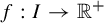 $f:I\to \mathbb {R}^+ $
be a bounded, square-integrable function that is strictly positive. Consider the space
$f:I\to \mathbb {R}^+ $
be a bounded, square-integrable function that is strictly positive. Consider the space
 $$ \begin{align*} X=\{(x,y)\mid x\in I, \ y<f(x)\}. \end{align*} $$
We define a suspension flow $\phi _t\hspace{-0.5pt}=\hspace{-0.5pt}(I,T,f,\mu )$
as follows: fix
$\phi _t\hspace{-0.5pt}=\hspace{-0.5pt}(I,T,f,\mu )$
as follows: fix $p,q\hspace{-0.5pt}\in\hspace{-0.5pt} \mathbb {R}^+$
; for
$p,q\hspace{-0.5pt}\in\hspace{-0.5pt} \mathbb {R}^+$
; for $(x,y)\hspace{-0.5pt}\in\hspace{-0.5pt} X$
, the flow
$(x,y)\hspace{-0.5pt}\in\hspace{-0.5pt} X$
, the flow $\phi _t(x,y)=(x,y+t)$
if
$\phi _t(x,y)=(x,y+t)$
if $y+t<f(x)$
, and
$y+t<f(x)$
, and $\phi _t(x,y)=(T(x),0)$
if
$\phi _t(x,y)=(T(x),0)$
if $y+t=f(x)$
. This flow preserves the Lebesgue measure
$y+t=f(x)$
. This flow preserves the Lebesgue measure $\mu $
and provides an identification of the interval I with the graph of f.
$\mu $
and provides an identification of the interval I with the graph of f.
Now, consider a transformation T derived from a cutting and stacking process, and let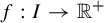 $f:I\to \mathbb {R}^+$
be such that for some
$f:I\to \mathbb {R}^+$
be such that for some $c\in I$
point of discontinuity for T,
$c\in I$
point of discontinuity for T, $f(x)=p$
for every
$f(x)=p$
for every $x\in [0,c)$
, and
$x\in [0,c)$
, and $f(x)=q$
for every
$f(x)=q$
for every $x\in [c,1]$
. Moreover, we require that f is constant on each subinterval of continuity of the transformation T.
$x\in [c,1]$
. Moreover, we require that f is constant on each subinterval of continuity of the transformation T.
Observe that from this construction, we obtain S together with the segments $\{0\} {\kern-1.5pt}\times{\kern-1.5pt} [0,p]$
,
$\{0\} {\kern-1.5pt}\times{\kern-1.5pt} [0,p]$
, $\{c\}\times [ \min (\{p,q\}),\max (\{p,q\})]$
, and
$\{c\}\times [ \min (\{p,q\}),\max (\{p,q\})]$
, and $\{1\}\times [0,q]$
as a rectangle or an
$\{1\}\times [0,q]$
as a rectangle or an $L-$
shaped polygon.
$L-$
shaped polygon.
Without loss of generality, we may assume that $p>q$
. We do the following identification.
$p>q$
. We do the following identification.
-
(1) Identify
$\{0\}\times [0,q]$
with
$\{1\}\times [0,q]$
. -
(2) Identify
$\{c\}\times [q,p]$
with
$\{0\}\times [q,p]$
. -
(3) If
$f(x)=\epsilon (x)\in \{p,q\}$
, identify
$(x,0)$
with
$(T(x),\epsilon (x))$
.





See Figure 1. Observe that after these identifications, we obtain a translation surface S, and the suspension flow $\phi _t$
built under f is isomorphic in the measure-theoretical sense to the vertical translation flow in the surface S.
$\phi _t$
built under f is isomorphic in the measure-theoretical sense to the vertical translation flow in the surface S.
Identify horizontal sides according to as shown in the picture and vertical sides with respect the transformation T (colour online).

Our main result is stated as follows.
Theorem 3.11. Let S be a finite-area, infinite-genus translation surface constructed from an L-shaped polygon satisfying the following conditions.
-
(1) The heights p and q of the L-shaped polygon are rationally independent, with
$p> q$
. Let
$x_0 \in (0,1)$
denote the point separating the base interval into two parts:
$[0,x_0)$
, corresponding to the non-spacer subinterval; and
$[x_0,1)$
, corresponding to the spacer subinterval of a mixing staircase transformation T. The roof function over
$[0,x_0)$
has height p, while over
$[x_0,1)$
, it has height q. -
(2) The vertical edges are glued by identifying opposite sides.
-
(3) The horizontal edges are glued according to a mixing staircase transformation T defined on the base interval
$[0,1)$
.


Then, the vertical translation flow $\phi _t$
on S is mixing.
$\phi _t$
on S is mixing.
4 Mixing in the case of the classical staircase
To illustrate the techniques we employ, we focus on the classical staircase transformation, defined by the cutting sequence $r_n = n$
. This example represents a staircase with restricted growth and was the first instance of a staircase transformation proven to be mixing [Reference AdamsAda98]. We begin by introducing a class of functions f, which will serve as the foundation for constructing our flows.
$r_n = n$
. This example represents a staircase with restricted growth and was the first instance of a staircase transformation proven to be mixing [Reference AdamsAda98]. We begin by introducing a class of functions f, which will serve as the foundation for constructing our flows.
Definition 4.1. Let f be a measurable strictly positive function defined on the unit interval $[0,1]$
characterized by constant values in two intervals with rationally independent heights
$[0,1]$
characterized by constant values in two intervals with rationally independent heights $p,q$
with
$p,q$
with $p>q$
. Moreover, let T be a classical staircase, assume that
$p>q$
. Moreover, let T be a classical staircase, assume that $f_{|\textit {non-spacer}}=p$
and
$f_{|\textit {non-spacer}}=p$
and $f_{|\textit {spacer}}=q$
. We refer to this function as
$f_{|\textit {spacer}}=q$
. We refer to this function as $2$
-wise constant.
$2$
-wise constant.
In this section, our aim is to establish the mixing property of the flow $\phi _t$
constructed under a classical staircase transformation T and a roof
$\phi _t$
constructed under a classical staircase transformation T and a roof $2$
-wise constant function f. To accomplish this, we rely on a result by Ulcigrai [Reference UlcigraiUlc07], which outlines conditions for a flow constructed under a given function and a measurable interval transformation to be mixing. Formally, our result states the following theorem.
$2$
-wise constant function f. To accomplish this, we rely on a result by Ulcigrai [Reference UlcigraiUlc07], which outlines conditions for a flow constructed under a given function and a measurable interval transformation to be mixing. Formally, our result states the following theorem.
Theorem 4.2. Let T be the classical staircase transformation, and let p and q two positive rationally independent numbers. Let f be a 2-wise constant function such that f attains the values $p,q$
on complementary intervals. Then, the suspension flow
$p,q$
on complementary intervals. Then, the suspension flow $([0,1],T,f,\mu )$
is mixing.
$([0,1],T,f,\mu )$
is mixing.
Notation. Throughout the text, we denote the Lebesgue measure on $\mathbb {R}$
as
$\mathbb {R}$
as $\unicode{x3bb} $
and the Lebesgue measure on
$\unicode{x3bb} $
and the Lebesgue measure on $\mathbb {R}^2$
as
$\mathbb {R}^2$
as $\mu $
.
$\mu $
.
The fourth step of the classical staircase transformation, where the first $14$
levels have length equal to
$14$
levels have length equal to ${A}/{6}$
, then we add
${A}/{6}$
, then we add $6$
spacers of length
$6$
spacers of length ${A}/{24}$
presented as dotted segments.
${A}/{24}$
presented as dotted segments.

Following the notation in [Reference UlcigraiUlc07], we consider partial partitions $\eta (t)$
of the interval
$\eta (t)$
of the interval $[0,1]$
, parameterized by
$[0,1]$
, parameterized by $t \in \mathbb {R}_+$
. (A partial partition refers to a finite collection of disjoint subintervals of
$t \in \mathbb {R}_+$
. (A partial partition refers to a finite collection of disjoint subintervals of $[0,1]$
whose union is a subset
$[0,1]$
whose union is a subset $A \subset [0,1]$
.) Each
$A \subset [0,1]$
.) Each $\eta (t)$
consists of finitely many subintervals. We denote by
$\eta (t)$
consists of finitely many subintervals. We denote by $\mathrm{Mesh}(\eta (t))$
the maximal length of these subintervals and by
$\mathrm{Mesh}(\eta (t))$
the maximal length of these subintervals and by $\unicode{x3bb} (\eta (t))$
the total measure, that is, the sum of the lengths of all subintervals in the partition.
$\unicode{x3bb} (\eta (t))$
the total measure, that is, the sum of the lengths of all subintervals in the partition.
Lemma 4.3. [Reference UlcigraiUlc07]
Let $\phi _t$
be a suspension flow built under a measurable transformation T on the interval
$\phi _t$
be a suspension flow built under a measurable transformation T on the interval $[0,1]$
and a roof function f. Assume for every rectangle (a rectangle
$[0,1]$
and a roof function f. Assume for every rectangle (a rectangle $R \subset X$
with base
$R \subset X$
with base $B(R) \subset [0,1)$
and height
$B(R) \subset [0,1)$
and height $H(R) \subset \mathbb {R}$
is a set of the form
$H(R) \subset \mathbb {R}$
is a set of the form $R = \{(x,y) \in X : x \in B(R),\ y \in H(R)\}$
)
$R = \{(x,y) \in X : x \in B(R),\ y \in H(R)\}$
) $R\subseteq X$
and every
$R\subseteq X$
and every $\epsilon ,\delta>0$
, there is a
$\epsilon ,\delta>0$
, there is a $t_0>0$
such that for every
$t_0>0$
such that for every $t\geq t_0$
, there exists a partial partition
$t\geq t_0$
, there exists a partial partition $\eta (t)$
of
$\eta (t)$
of $[0,1)$
such that:
$[0,1)$
such that:
-
(1)
$\unicode{x3bb} (\eta (t))>1-\delta $
and
$\mathrm{Mesh}(\eta (t))\leq \delta $
; -
(2) for every
$I\in \eta (t)$
, we have that
$\unicode{x3bb} (I\cap \phi _{-t}(R))\geq (1-\epsilon )\mu (R)\unicode{x3bb} (I).$




Then, the flow $\phi _t$
is mixing.
$\phi _t$
is mixing.
4.1 Outline of the proof of Theorem 4.2
Staircase transformations arise from the Rokhlin tower theorem. This theorem implies that for each step in the construction of the transformation, we obtain a finite number of subintervals whose lengths strictly decrease at each step. As the process continues indefinitely, the union of these subintervals will cover the interval $[0,1]$
. These unions at each step provide natural candidates for partial coverings of
$[0,1]$
. These unions at each step provide natural candidates for partial coverings of $[0,1]$
.
$[0,1]$
.
For any $\delta> 0$
, there exists an m such that for any subinterval
$\delta> 0$
, there exists an m such that for any subinterval $I_j^{(m)}$
from the m-step of the staircase transformation configuration, the following conditions are met.
$I_j^{(m)}$
from the m-step of the staircase transformation configuration, the following conditions are met.
-
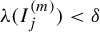
(1) The measure of
$I_j^{(m)}$
satisfies that
$\unicode{x3bb} (I_j^{(m)})<\delta $
. -
(2) The measure of the union of these subintervals satisfies that
$$ \begin{align*}\unicode{x3bb}\bigg(\!\bigcup_{i=1}^{h_m}I_i^{(m)}\bigg)>1-\delta.\end{align*} $$


Therefore, for that $\delta $
, the partial partition
$\delta $
, the partial partition $\eta $
is the union of those intervals. Note that the partial partition depends only on
$\eta $
is the union of those intervals. Note that the partial partition depends only on $\delta $
and not
$\delta $
and not $t\in \mathbb {R}_+$
.
$t\in \mathbb {R}_+$
.
It is noteworthy that for any interval $I^{(m)}$
, the application of the flow
$I^{(m)}$
, the application of the flow $\phi _t$
will produce a partition of
$\phi _t$
will produce a partition of $ I^{(m)} $
into several horizontal segments. Our goal is to approximate the distribution of these horizontal segments.
$ I^{(m)} $
into several horizontal segments. Our goal is to approximate the distribution of these horizontal segments.
To prove that the partitions arising from the staircase construction satisfy the second requirement of Lemma 4.3, we first consider the cases where $ R \subseteq [0, x_0] \times [0, p] $
and
$ R \subseteq [0, x_0] \times [0, p] $
and $ R \subseteq [x_0, 1] \times [0, q] $
, with
$ R \subseteq [x_0, 1] \times [0, q] $
, with $ x_0 $
being the point that divides the spacer and non-spacer intervals. These two rectangles yield a natural partition of the L-shaped polygon, the first is the non-spacer part of the polygon and the second is the spacer part of the polygon. Then, we have to approximate the product of measures
$ x_0 $
being the point that divides the spacer and non-spacer intervals. These two rectangles yield a natural partition of the L-shaped polygon, the first is the non-spacer part of the polygon and the second is the spacer part of the polygon. Then, we have to approximate the product of measures $\mu (R) \unicode{x3bb} (I)$
by
$\mu (R) \unicode{x3bb} (I)$
by $\unicode{x3bb} (\phi _t(I) \cap R)$
. For the remainder of the paper, we assume that
$\unicode{x3bb} (\phi _t(I) \cap R)$
. For the remainder of the paper, we assume that $(p,q)=(1,q)$
.
$(p,q)=(1,q)$
.
First, we prove a lemma inspired by the fact that a staircase transformation $ T $
exhibits mixing properties [Reference AdamsAda98]. Lemma 4.4 states that there exists an
$ T $
exhibits mixing properties [Reference AdamsAda98]. Lemma 4.4 states that there exists an $m_0$
such that for every
$m_0$
such that for every $n\geq m_0$
, any level
$n\geq m_0$
, any level $ I^{(n)} $
at the nth step of the staircase transformation, and any rectangle
$ I^{(n)} $
at the nth step of the staircase transformation, and any rectangle $ R $
, the measure
$ R $
, the measure
 $$ \begin{align*} \unicode{x3bb}(\pi_x(\phi_t(I^{(n)}))\cap \pi_x(R)) \end{align*} $$
converges to $ \unicode{x3bb} (I^{(n)})\unicode{x3bb} (\pi _x(R)) $
.
$ \unicode{x3bb} (I^{(n)})\unicode{x3bb} (\pi _x(R)) $
.
Next, we establish that for any level at any step of the staircase construction, the action of the flow $ \phi _t $
on this interval produces an equidistributed set of heights. More precisely, given any level
$ \phi _t $
on this interval produces an equidistributed set of heights. More precisely, given any level $ I^{(n)} $
, we define the
$ I^{(n)} $
, we define the $ I^{(n)} $
-cylinder as either
$ I^{(n)} $
-cylinder as either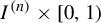 $ I^{(n)} \times [0,1) $
or
$ I^{(n)} \times [0,1) $
or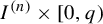 $ I^{(n)} \times [0,q) $
, depending on whether
$ I^{(n)} \times [0,q) $
, depending on whether $ I^{(n)} $
is a non-spacer or a spacer interval. We then show that for any
$ I^{(n)} $
is a non-spacer or a spacer interval. We then show that for any $ I^{(m)} $
, the application of
$ I^{(m)} $
, the application of $ \phi _t $
generates different heights. In the non-spacer case, we prove that for any vertical subinterval
$ \phi _t $
generates different heights. In the non-spacer case, we prove that for any vertical subinterval $ [a,b] \subseteq [0,1] $
and any horizontal interval
$ [a,b] \subseteq [0,1] $
and any horizontal interval $ I^{(n)} $
, the ratio of the number of heights attained by
$ I^{(n)} $
, the ratio of the number of heights attained by $ \phi _t(I^{(m)}) $
within
$ \phi _t(I^{(m)}) $
within $ [a,b] $
(such that
$ [a,b] $
(such that $ \phi _t(I^{(m)}) $
remains in the
$ \phi _t(I^{(m)}) $
remains in the $ I^{(n)} $
-cylinder) to the total number of heights within the
$ I^{(n)} $
-cylinder) to the total number of heights within the $ I^{(n)} $
-cylinder converges to the measure of
$ I^{(n)} $
-cylinder converges to the measure of $ [a,b] $
. Similarly, for any
$ [a,b] $
. Similarly, for any $ [a,b) \subseteq [0,q) $
, the ratio of the number of heights attained by
$ [a,b) \subseteq [0,q) $
, the ratio of the number of heights attained by $ \phi _t(I^{(m)}) $
within
$ \phi _t(I^{(m)}) $
within $ [a,b] $
in the
$ [a,b] $
in the $ I^{(n)} $
-cylinder to the total number of heights in
$ I^{(n)} $
-cylinder to the total number of heights in $ I^{(n)} $
converges to
$ I^{(n)} $
converges to $ \unicode{x3bb} ([a,b]) / q $
.
$ \unicode{x3bb} ([a,b]) / q $
.
From there, if $R=b(R)\times h(R)$
and
$R=b(R)\times h(R)$
and
 $$ \begin{align*}b(R)=\bigcup_{i\in J}I^{(n_i)},\end{align*} $$
where J is some index and $I^{(n_i)}$
is an interval in the
$I^{(n_i)}$
is an interval in the $n_i$
th step of the staircase configuration, then
$n_i$
th step of the staircase configuration, then
 $$ \begin{align*} \lim_{t\to\infty}\unicode{x3bb}(I^{(m)}\cap \phi_{-t}(R))=\lim_{t\to\infty}\sum_{i\in J}\unicode{x3bb}(\phi_t(I)\cap I^{(n_i)}\times h(R))\geq \mu(R)\unicode{x3bb}(I^{(m)}). \end{align*} $$
For the classical staircase case, we can calculate explicitly the intervals where the roof function is $1$
and q. If the first interval of definition has length A, then the first spacer
$1$
and q. If the first interval of definition has length A, then the first spacer $s_2$
(remember that
$s_2$
(remember that $s_1=0$
) will have length
$s_1=0$
) will have length $({A}/{2})$
, and for the third step, we have to add
$({A}/{2})$
, and for the third step, we have to add $3$
spacers each of length
$3$
spacers each of length $({A}/{6})$
. In general, we have that the total length of all the spacers added after k steps is
$({A}/{6})$
. In general, we have that the total length of all the spacers added after k steps is
 $$ \begin{align*} \sum_{n=1}^k \frac{A}{n!}\sum_{i=1}^n(i-1)=\sum_{n=1}^{k} \frac{A(n-1)}{2(n-1)!}=\frac{A}{2} + \sum_{n=2}^{k}\frac{A}{2(n-2)!}, \end{align*} $$
which converges to $({A}/{2}) + ({Ae}/{2})$
. Therefore, if we want the interval I to have length
$({A}/{2}) + ({Ae}/{2})$
. Therefore, if we want the interval I to have length $1$
, then we should have that
$1$
, then we should have that $A={2}/({3+e})$
.
$A={2}/({3+e})$
.
Lemma 4.4. There exists an $m_0$
depending solely on q such that for every
$m_0$
depending solely on q such that for every $m\geq m_0$
, when
$m\geq m_0$
, when $I^{(m)}$
is an m-level of the configuration of the classical staircase T and R is a rectangle under the graph of f, if
$I^{(m)}$
is an m-level of the configuration of the classical staircase T and R is a rectangle under the graph of f, if $\pi _x$
is the horizontal projection and
$\pi _x$
is the horizontal projection and $b(R)=\pi _x(R)$
is the base of the rectangle R, then
$b(R)=\pi _x(R)$
is the base of the rectangle R, then
 $$ \begin{align*} \lim_{t\to \infty} \unicode{x3bb}(\phi_t(I^{(m)}))\cap \pi_x^{-1}(\pi_x(R))=\unicode{x3bb}(I^{(m)})\unicode{x3bb}(b(R)). \end{align*} $$
Proof. For this proof, we use the fact that the classical staircase transformation T is mixing.
First, we need to check that if m is large, then for arbitrary t,
 $$ \begin{align*} \unicode{x3bb}(\pi_x(\phi_t(I^{(m)})))=\unicode{x3bb}(I^{(m)}).\end{align*} $$
Suppose that for a level $I^{(m)}$
,
$I^{(m)}$
,
 $$ \begin{align*}\unicode{x3bb}(\pi_x(\phi_t(I^{(m)})))<\unicode{x3bb}(I^{(m)}).\end{align*} $$
This implies that there exist two different sublevels $I^{(n+m)}_{i}$
and
$I^{(n+m)}_{i}$
and $I^{(n+m)}_{j}$
and non-negative real numbers
$I^{(n+m)}_{j}$
and non-negative real numbers $t,s$
such that
$t,s$
such that
 $$ \begin{align*} \phi_{t-s}(I^{(n+m)}_{i})=\phi_t(I^{(n+m)}_{j}). \end{align*} $$
Moreover, $s\geq 0$
must be smaller than
$s\geq 0$
must be smaller than $1$
or q.
$1$
or q.
Part of the orbit of the special flow built under f and the classical staircase T (colour online).

Observe that if we order upwards the sublevels in which $I^{(m)}$
is partitioned in the
$I^{(m)}$
is partitioned in the $(m+n)$
th step of the configuration of the staircase, then
$(m+n)$
th step of the configuration of the staircase, then $j<i$
. This complication arises because under the intervals positioned beneath
$j<i$
. This complication arises because under the intervals positioned beneath $1$
, there may be accumulations of other intervals at varying heights. To illustrate this concept, if an interval lies below q, a single iteration of
$1$
, there may be accumulations of other intervals at varying heights. To illustrate this concept, if an interval lies below q, a single iteration of $\phi _q$
elevates this interval to the subsequent level in the staircase configuration. Conversely, if the interval lies beneath
$\phi _q$
elevates this interval to the subsequent level in the staircase configuration. Conversely, if the interval lies beneath $1$
, there exists a value
$1$
, there exists a value $N_0>1$
such that
$N_0>1$
such that $(N_0-1)q<1\leq N_0q$
. This indicates that it takes several iterations (specifically, at most
$(N_0-1)q<1\leq N_0q$
. This indicates that it takes several iterations (specifically, at most $N_0$
iterations) before the interval advances to the next level in the staircase configuration; therefore, if two sublevels
$N_0$
iterations) before the interval advances to the next level in the staircase configuration; therefore, if two sublevels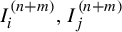 $I^{(n+m)}_i,I^{(n+m)}_j$
are in a distance smaller than
$I^{(n+m)}_i,I^{(n+m)}_j$
are in a distance smaller than $2N_0$
, it follows that under the action of the flow
$2N_0$
, it follows that under the action of the flow $\phi _t$
, we might encounter several instances
$\phi _t$
, we might encounter several instances $t_l$
in which
$t_l$
in which
 $$ \begin{align*}\pi_x(\phi_{t_l}(I_i^{(n+m)}))\cap \pi_x(\phi_{t_l}(I_j^{(n+m)}))\neq\emptyset.\end{align*} $$
We demonstrate that if the initial interval is sufficiently small, we will not find this problem.
Observe that if $I^{(m)}$
is in the mth step of the configuration of the staircase, when we consider the
$I^{(m)}$
is in the mth step of the configuration of the staircase, when we consider the $m+1$
subintervals in which it is divided in the
$m+1$
subintervals in which it is divided in the $(m+1)$
th step of the configuration of the staircase, then the distance between any two of those levels will be bounded from below by
$(m+1)$
th step of the configuration of the staircase, then the distance between any two of those levels will be bounded from below by $h_m$
, the height of the mth step of the configuration. Since
$h_m$
, the height of the mth step of the configuration. Since $h_m$
is an increasing sequence, then there exists an
$h_m$
is an increasing sequence, then there exists an $m_0$
such that
$m_0$
such that $h_{m_0}\geq M_0= 4N_0$
; therefore, for any
$h_{m_0}\geq M_0= 4N_0$
; therefore, for any $m\geq m_0$
and for any interval
$m\geq m_0$
and for any interval $I^{(m)}$
in the mth step of the configuration of the staircase, it follows that the number of levels between any two subintervals
$I^{(m)}$
in the mth step of the configuration of the staircase, it follows that the number of levels between any two subintervals $I^{(m+n)}_i$
and
$I^{(m+n)}_i$
and $I^{(m+n)}_j$
for any
$I^{(m+n)}_j$
for any $n\geq 0$
will be bounded from below by
$n\geq 0$
will be bounded from below by $4N_0$
and, therefore,
$4N_0$
and, therefore,
 $$ \begin{align*}\pi_x(\phi_{t}(I_i^{(n+m)}))\cap \pi_x(\phi_{t}(I_j^{(n+m)}))=\emptyset.\end{align*} $$
Continuing with the proof, notice that for each t, there exists an $n\geq 0$
such that
$n\geq 0$
such that $\phi _t(I^{(m)})$
is scattered in
$\phi _t(I^{(m)})$
is scattered in ${n!}/{m!}$
subintervals. For each subinterval
${n!}/{m!}$
subintervals. For each subinterval $I_j^{(m)}$
with
$I_j^{(m)}$
with $j=1,\ldots ,{n!}/{m!}$
, there exists
$j=1,\ldots ,{n!}/{m!}$
, there exists $l_j$
such that
$l_j$
such that $\pi _x(\phi _t(I_j^{(m)}))=T^{l_j}(I_j^{(m)})$
. From previous observation,
$\pi _x(\phi _t(I_j^{(m)}))=T^{l_j}(I_j^{(m)})$
. From previous observation,
 $$ \begin{align*} \pi_x(\phi_t(I^{(m)}))=\bigcup_{j=1}^{n!/m!}T^{l_j}(I_j^{(m)}). \end{align*} $$
Define $m(t)$
as the minimum of such
$m(t)$
as the minimum of such $l_j$
and
$l_j$
and $M(t)$
as the maximum. We can assume that for large t, it holds true that
$M(t)$
as the maximum. We can assume that for large t, it holds true that
 $$ \begin{align*} |\unicode{x3bb}(b(R)\cap T^{M(t)}(I^{(m)}))-\unicode{x3bb}(b(R))\unicode{x3bb}(I^{(m)})| & \leq |\unicode{x3bb}(b(R)\cap \pi_x(\phi_t(I^{(m)})))-\unicode{x3bb}(b(R))\unicode{x3bb}(I^{(m)})| \\ & \leq |\unicode{x3bb}(b(R)\cap T^{m(t)}(I^{(m)}))-\unicode{x3bb}(b(R))\unicode{x3bb}(I^{(m)})|. \end{align*} $$
Since T is mixing, this implies that
 $$ \begin{align*} \begin{aligned} \unicode{x3bb}(b(R)\cap \pi_x(\phi_t(I^{(m)})))\to\unicode{x3bb}(b(R))\unicode{x3bb}(I^{(m)}). \end{aligned}\\[-36pt] \end{align*} $$
Remark 4.5. Let $m_0$
be the integer such that for every
$m_0$
be the integer such that for every $m\geq m_0$
and every
$m\geq m_0$
and every $I^{(m)}$
, Lemma 4.4 holds. If
$I^{(m)}$
, Lemma 4.4 holds. If $I^{(n)}$
is an interval in the nth step of the configuration of the staircase with
$I^{(n)}$
is an interval in the nth step of the configuration of the staircase with $n<m_0$
, observe that
$n<m_0$
, observe that $I^{(n)}$
is made up by
$I^{(n)}$
is made up by
 $$ \begin{align*}I^{(n)}=\bigsqcup_{i=1}^{m!/n!}I^{(m)}_i.\end{align*} $$
Therefore, for any rectangle R, it follows that
 $$ \begin{align*} \lim_{t\to\infty}\unicode{x3bb}(\phi_t(I^{(n)})\cap \pi_x^{-1}(b(R)))=\sum_{i=1}^{m!/n!}\unicode{x3bb}(I^{(m)}_i)(\unicode{x3bb}(b(R)))=\unicode{x3bb}(I^{(n)})\unicode{x3bb}(b(R)).\end{align*} $$
It is worth noting that when we consider an interval $I^{(n)}$
and observe how it evolves under the flow
$I^{(n)}$
and observe how it evolves under the flow $\phi _t$
, over time, this interval will break up into several horizontal segments scattered throughout the polygon. For the second part of the proof, our goal is to approximate the distribution of the heights achieved by these horizontal segments.
$\phi _t$
, over time, this interval will break up into several horizontal segments scattered throughout the polygon. For the second part of the proof, our goal is to approximate the distribution of the heights achieved by these horizontal segments.
Our strategy will be to assume, without loss of generality, that the heights of the polygon are 1 and q. We then consider a discretization of the flow given by the iterates of $\phi _q$
. By doing so, we aim to emulate the behavior of an irrational rotation and demonstrate that the heights of the horizontal segments follow a distribution similar to the set
$\phi _q$
. By doing so, we aim to emulate the behavior of an irrational rotation and demonstrate that the heights of the horizontal segments follow a distribution similar to the set $ \{nq\!\! \mod {1} : n \in \mathbb {N}\} $
.
$ \{nq\!\! \mod {1} : n \in \mathbb {N}\} $
.
4.2 Behavior of the first subcolumn
The discussion that follows is crucial for delving into the second part of the proof, with the aim of convincing us that by discretizing the flow $ \phi _t $
through iterations of
$ \phi _t $
through iterations of $ \phi _q $
, applying
$ \phi _q $
, applying $ \phi _{mq} $
to any level
$ \phi _{mq} $
to any level $ I^{(n)} $
yields an increasing sequence of heights contained in
$ I^{(n)} $
yields an increasing sequence of heights contained in $ \{nq, n \in \mathbb {N}\!\! \mod {1}\} $
.
$ \{nq, n \in \mathbb {N}\!\! \mod {1}\} $
.
Notation. We say that $ x \in I $
lies beneath
$ x \in I $
lies beneath $ q $
if
$ q $
if $ f(x) = q $
; similarly, we say that
$ f(x) = q $
; similarly, we say that $x\in I$
lies beneath
$x\in I$
lies beneath $1\, f(x) = 1 $
.
$1\, f(x) = 1 $
.
Note that if a subinterval $ I^{(m)}$
lies beneath
$ I^{(m)}$
lies beneath $ q $
at height zero, applying
$ q $
at height zero, applying $ \phi _q $
resets its height to zero. Subsequent applications of
$ \phi _q $
resets its height to zero. Subsequent applications of $ \phi _q $
maintain this zero height as long as the subinterval remains beneath
$ \phi _q $
maintain this zero height as long as the subinterval remains beneath $ q $
, until it eventually reaches a height of zero beneath
$ q $
, until it eventually reaches a height of zero beneath $ 1 $
. At this point, the application of
$ 1 $
. At this point, the application of $ \phi _q $
results in alternating heights: first
$ \phi _q $
results in alternating heights: first $ q $
, then
$ q $
, then $ 2q\!\! \mod {1} $
, and so forth. Due to the construction of the classical staircase, the subinterval passes through the roof whose value is
$ 2q\!\! \mod {1} $
, and so forth. Due to the construction of the classical staircase, the subinterval passes through the roof whose value is $ 1 $
twice consecutively before going to the spacer side.
$ 1 $
twice consecutively before going to the spacer side.
Now, consider $ I^{(m)} $
as the last level of the
$ I^{(m)} $
as the last level of the $ m $
th step configuration of the staircase before it breaks into
$ m $
th step configuration of the staircase before it breaks into $ m+1 $
new subintervals
$ m+1 $
new subintervals $ I_j^{(m)} $
with
$ I_j^{(m)} $
with $ j \leq m+1 $
. We explain that the heights attained by
$ j \leq m+1 $
. We explain that the heights attained by $ \phi _{nq}(I^{(m)}) $
with
$ \phi _{nq}(I^{(m)}) $
with $m+1\leq n\leq h_m$
coincide with the heights attained by
$m+1\leq n\leq h_m$
coincide with the heights attained by $ \phi _{nq}(I^{(m)}_1),\phi _{(n-1)q}(I^{(m)}_1),\ldots ,\phi _{(n-1-m)q}(I^{(m)}_1) $
.
$ \phi _{nq}(I^{(m)}_1),\phi _{(n-1)q}(I^{(m)}_1),\ldots ,\phi _{(n-1-m)q}(I^{(m)}_1) $
.
Let $ I^{(m)} $
be as defined in the previous paragraph. Observe that each subinterval
$ I^{(m)} $
be as defined in the previous paragraph. Observe that each subinterval $ I^{(m)}_j $
has
$ I^{(m)}_j $
has $ j-1 $
spacers above it, all of which lie beneath
$ j-1 $
spacers above it, all of which lie beneath $ q $
by construction. Consequently, applying
$ q $
by construction. Consequently, applying $ \phi _q $
to
$ \phi _q $
to $ I^{(m)}_j $
up to
$ I^{(m)}_j $
up to $ j-1 $
times ensures that
$ j-1 $
times ensures that $ \phi _{nq}(I^{(m)}_j) $
remains beneath
$ \phi _{nq}(I^{(m)}_j) $
remains beneath $ q $
and has height zero for any
$ q $
and has height zero for any $ n \leq j-1 $
. Moreover, applying
$ n \leq j-1 $
. Moreover, applying $ \phi _q $
exactly
$ \phi _q $
exactly $ j $
times to
$ j $
times to $ I^{(m)}_j $
results in an image that lies beneath
$ I^{(m)}_j $
results in an image that lies beneath $ 1 $
and also has height zero.
$ 1 $
and also has height zero.
Thus, for any $ j \leq m $
, the height of
$ j \leq m $
, the height of $ \phi _q(I^{(m)}_{j+1}) $
matches that of
$ \phi _q(I^{(m)}_{j+1}) $
matches that of $ I^{(m)}_{j} $
. This observation implies that the heights attained by successive iterations of
$ I^{(m)}_{j} $
. This observation implies that the heights attained by successive iterations of $ \phi _{nq} $
on
$ \phi _{nq} $
on $ I^{(m)}_{j+1} $
are directly related to those attained by iterating
$ I^{(m)}_{j+1} $
are directly related to those attained by iterating $ \phi _{(n-1)q} $
on
$ \phi _{(n-1)q} $
on $ I^{(m)}_{j} $
. Therefore, in the
$ I^{(m)}_{j} $
. Therefore, in the $ (m+1) $
th step configuration of the staircase, the heights of the intervals
$ (m+1) $
th step configuration of the staircase, the heights of the intervals $ I^{(m)}_j $
are fully determined by the heights attained by
$ I^{(m)}_j $
are fully determined by the heights attained by $ I^{(m)}_1 $
. We show that this reasoning extends to arbitrarily large iterations. For now, it is clear this holds when
$ I^{(m)}_1 $
. We show that this reasoning extends to arbitrarily large iterations. For now, it is clear this holds when $ n \leq h_m $
. See Figures 4, 5, and 6 for a visualization of this concept.
$ n \leq h_m $
. See Figures 4, 5, and 6 for a visualization of this concept.
Left: Third step of the staircase configuration, the first two levels are non-spacers, the last three are spacers, the level $I^{(3)}$
is partitioned in the sublevels before it breaks into three levels. Right: Representation of
$I^{(3)}$
is partitioned in the sublevels before it breaks into three levels. Right: Representation of $I^{(3)}$
in the L-shaped polygon (colour online).
$I^{(3)}$
in the L-shaped polygon (colour online).

After one application of $\phi _q$
, the heights are reset to zero, but the intervals spread in the staircase configuration (colour online).
$\phi _q$
, the heights are reset to zero, but the intervals spread in the staircase configuration (colour online).

After two iterations of $\phi _q$
, we obtain a first height different than zero (colour online).
$\phi _q$
, we obtain a first height different than zero (colour online).

This behavior continues until the level $I^{(m)}_{m+1}$
reaches the final level in the
$I^{(m)}_{m+1}$
reaches the final level in the $(m+1)$
th step of the staircase configuration, just before it splits into
$(m+1)$
th step of the staircase configuration, just before it splits into $m+2$
new sublevels
$m+2$
new sublevels $I^{(m)}_{m+1,l}$
, where
$I^{(m)}_{m+1,l}$
, where $l \leq m+2$
. Using a similar argument, we find that the dynamics at this step of the configuration for the sublevels
$l \leq m+2$
. Using a similar argument, we find that the dynamics at this step of the configuration for the sublevels $I^{(m)}_{m+1,l}$
are governed by those attained by
$I^{(m)}_{m+1,l}$
are governed by those attained by $I^{(m)}_{m+1,1}$
. Furthermore, the heights reached by
$I^{(m)}_{m+1,1}$
. Furthermore, the heights reached by $I^{(m)}_{m+1,1}$
remain connected to the heights attained by the sublevels
$I^{(m)}_{m+1,1}$
remain connected to the heights attained by the sublevels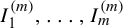 $I^{(m)}_1,\ldots ,I_{m}^{(m)}$
, as explained in the previous paragraph. Therefore, to analyze the dynamics in the
$I^{(m)}_1,\ldots ,I_{m}^{(m)}$
, as explained in the previous paragraph. Therefore, to analyze the dynamics in the $(m+2)$
th step of the staircase configuration, it is sufficient to focus on
$(m+2)$
th step of the staircase configuration, it is sufficient to focus on $I^{(m)}_{1,1}$
. Following this reasoning, we conclude that for any interval
$I^{(m)}_{1,1}$
. Following this reasoning, we conclude that for any interval $I^{(m)}$
, when considering its representation in the
$I^{(m)}$
, when considering its representation in the $(m+n)$
th step of the staircase configuration, the heights attained after several iterations, say n, coincide with the heights obtained by the set
$(m+n)$
th step of the staircase configuration, the heights attained after several iterations, say n, coincide with the heights obtained by the set
 $$ \begin{align*}{\phi_q(I^{(m)}_{1,\ldots,1}), \ldots, \phi_{nq}(I^{(m)}_{1,\ldots,1})}.\end{align*} $$
From the previous paragraphs, we can draw the following conclusion. Let $I^{(m)}$
represent the final interval in the mth step of the staircase configuration. Consider how this interval is represented in the
$I^{(m)}$
represent the final interval in the mth step of the staircase configuration. Consider how this interval is represented in the $(m+n)$
th step of the staircase configuration. The heights reached by applying
$(m+n)$
th step of the staircase configuration. The heights reached by applying $\phi _q$
to
$\phi _q$
to $I^{(m)}\, n$
times correspond to the heights achieved by the intervals
$I^{(m)}\, n$
times correspond to the heights achieved by the intervals $I^{(m+n)}_1, \phi _q(I^{(m+n)}_1),\ldots , \phi _{nq}(I^{(m+n)}_1)$
, where
$I^{(m+n)}_1, \phi _q(I^{(m+n)}_1),\ldots , \phi _{nq}(I^{(m+n)}_1)$
, where $I^{(m+n)}_1$
is the lowest level in the representation of
$I^{(m+n)}_1$
is the lowest level in the representation of $I^{(m)}$
within the
$I^{(m)}$
within the $(m+n)$
th step of the staircase configuration, corresponding to
$(m+n)$
th step of the staircase configuration, corresponding to $I^{(m)}_{1,\ldots ,1}$
.
$I^{(m)}_{1,\ldots ,1}$
.
More precisely, if k iterations of $\phi _q$
produce that
$\phi _q$
produce that $I^{(m)}$
lies in the
$I^{(m)}$
lies in the $(m+n)$
th step of the staircase configuration,
$(m+n)$
th step of the staircase configuration, $I^{(m)}$
will be broken into several subintervals
$I^{(m)}$
will be broken into several subintervals $I^{(m)}_J$
, where J is an index of length bounded by
$I^{(m)}_J$
, where J is an index of length bounded by $(m+n-1)!/m!$
; for one of such subintervals
$(m+n-1)!/m!$
; for one of such subintervals $I^{(m)}_{a_1,\ldots ,a_j}$
, it will hold true that the height attained by
$I^{(m)}_{a_1,\ldots ,a_j}$
, it will hold true that the height attained by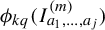 $\phi _{kq}(I^{(m)}_{a_1,\ldots ,a_j})$
will coincide with the height attained by
$\phi _{kq}(I^{(m)}_{a_1,\ldots ,a_j})$
will coincide with the height attained by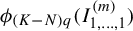 $\phi _{(K-N)q}(I^{(m)}_{1,\ldots ,1})$
, where
$\phi _{(K-N)q}(I^{(m)}_{1,\ldots ,1})$
, where
 $$ \begin{align*} N=\sum_{i=1}^j|1-a_i|. \end{align*} $$
As $k\to \infty $
, the staircase where
$k\to \infty $
, the staircase where $I^{(m)}$
will lie is the
$I^{(m)}$
will lie is the $(m+n)$
th step of the staircase configuration with
$(m+n)$
th step of the staircase configuration with $n\to \infty $
, then the number of different heights also diverges. This result hints that, in the limiting process of iterations, and due to the equidistribution of
$n\to \infty $
, then the number of different heights also diverges. This result hints that, in the limiting process of iterations, and due to the equidistribution of $\{nq\!\! \mod 1 : n \in \mathbb {N}\}$
, the heights obtained will also equidistribute.
$\{nq\!\! \mod 1 : n \in \mathbb {N}\}$
, the heights obtained will also equidistribute.
Remark 4.6. Observe that, although the heights obtained are described by the sets given in the previous paragraphs, there are many repetitions of heights, meaning that multiple subintervals can share the same height.
Remark 4.7. In this procedure, we described the heights that can be obtained by iterating $\phi _q$
in the classical staircase configuration. However, if
$\phi _q$
in the classical staircase configuration. However, if $\phi _t$
is a flow constructed under any mixing staircase T, the result remains nearly the same. Specifically, we obtain an increasing sequence of attainable heights for an interval
$\phi _t$
is a flow constructed under any mixing staircase T, the result remains nearly the same. Specifically, we obtain an increasing sequence of attainable heights for an interval $I^{(m)}$
as the flow
$I^{(m)}$
as the flow $\phi _t$
approaches infinity.
$\phi _t$
approaches infinity.
We would like to prove that
 $$ \begin{align*} \lim_{t\to\infty} \unicode{x3bb}(\phi_t(I^{(m)})\cap R)\geq\unicode{x3bb}(I^{(m)})\unicode{x3bb}(b(R))\unicode{x3bb}(h(R)). \end{align*} $$
We already have the first part; for the second part, we would like that the concentration of heights contained in the vertical interval spanned by R does not depend on $I^{(m)}$
but only on
$I^{(m)}$
but only on $h(R)$
. For this purpose, we need a notion of equidistribution.
$h(R)$
. For this purpose, we need a notion of equidistribution.
As noted in §4.2, when examining the images of a subinterval from any m-step configuration of the staircase under the flow $\phi _t$
, the subinterval breaks into further segments. Due to the presence of spacers arranged in a staircase-like pattern, this process results in a sequence of different heights. Our objective is to study the distribution of these heights.
$\phi _t$
, the subinterval breaks into further segments. Due to the presence of spacers arranged in a staircase-like pattern, this process results in a sequence of different heights. Our objective is to study the distribution of these heights.
The distribution of heights behaves differently depending on whether the intervals lie beneath $1$
or beneath q. Specifically, if an interval lies under
$1$
or beneath q. Specifically, if an interval lies under $1$
, every iteration of
$1$
, every iteration of $\phi _q$
changes its height. In contrast, if the interval lies under q, it is mapped to another level of the staircase while preserving its height. Moreover, blocks of spacer intervals all share the same height. Thus, to analyze the distribution of heights generated by iterations of
$\phi _q$
changes its height. In contrast, if the interval lies under q, it is mapped to another level of the staircase while preserving its height. Moreover, blocks of spacer intervals all share the same height. Thus, to analyze the distribution of heights generated by iterations of $\phi _q$
, it is essential to distinguish between intervals lying beneath
$\phi _q$
, it is essential to distinguish between intervals lying beneath $1$
and those lying beneath q. For the next lemma, we introduce a convenient notation.
$1$
and those lying beneath q. For the next lemma, we introduce a convenient notation.
Definition 4.8. Define $I_{ns}$
as the set of
$I_{ns}$
as the set of $x\in [0,1]$
such that x is beneath 1 and define
$x\in [0,1]$
such that x is beneath 1 and define $I_s$
as the set of
$I_s$
as the set of $x\in [0,1]$
such that x is beneath q.
$x\in [0,1]$
such that x is beneath q.
Definition 4.9. Let $t \in \mathbb {R}$
and let
$t \in \mathbb {R}$
and let $I,J$
be horizontal intervals, while
$I,J$
be horizontal intervals, while $[a,b] \subseteq [0,1)$
(or
$[a,b] \subseteq [0,1)$
(or $[0,q)$
, depending on whether we are in the non-spacer or spacer part) is a vertical interval. We define the set of heights as follows:
$[0,q)$
, depending on whether we are in the non-spacer or spacer part) is a vertical interval. We define the set of heights as follows:
 $$ \begin{align*} H_t^{ns}(I,J,[a,b]) &= \{ z \in [a,b] \;:\;\text{there exists } y \in I \\& \qquad \text{ such that } \pi_y(\phi_t(y)) = z \text{ and } \pi_x(\phi_t(y)) \in J \}, \end{align*} $$
when J is contained in the non-spacer part. Similarly, we set
 $$ \begin{align*} H_t^{s}(I,J,[a,b]) &= \{ z \in [a,b] \;:\; \text{there exists } y \in I \\& \qquad \text{ such that } \pi_y(\phi_t(y)) = z \text{ and } \pi_x(\phi_t(y)) \in J \}, \end{align*} $$
when J is contained in the spacer part.
Definition 4.10. Let $I^{(m)}$
be a level in the m-step of the staircase configuration. We say that
$I^{(m)}$
be a level in the m-step of the staircase configuration. We say that $I^{(m)}$
is H-equidistributed if, for any interval
$I^{(m)}$
is H-equidistributed if, for any interval $[a,b] \subseteq [0,1]$
in the vertical direction,
$[a,b] \subseteq [0,1]$
in the vertical direction,
 $$ \begin{align*} \lim_{t\to\infty} \frac{\textbf{card}(H_t^{ns}(I^{(m)},I_{ns},[a,b]))}{\textbf{card}((H_t^{ns}(I^{(m)},I_{ns},[0,1]))}=b-a, \end{align*} $$
and if, for any $[a,b] \subseteq [0,q)$
,
$[a,b] \subseteq [0,q)$
,
 $$ \begin{align*} \lim_{t\to\infty} \frac{\textbf{card}(H_t^{s}(I^{(m)},I_s,[a,b]))}{\textbf{card}((H_t^{ns}(I^{(m)},I_s,[0,q]))}=\frac{b-a}{q}. \end{align*} $$
Achieving $ H $
-equidistribution in the spacer part is not straightforward. Although iterating
$ H $
-equidistribution in the spacer part is not straightforward. Although iterating $ \phi _q $
yields an increasing sequence of heights, understanding the precise distribution of these heights in the spacer part is crucial. While this might initially appear to obstruct
$ \phi _q $
yields an increasing sequence of heights, understanding the precise distribution of these heights in the spacer part is crucial. While this might initially appear to obstruct $ H $
-equidistribution, the following result shows that the structured nature of these repetitions ensures that
$ H $
-equidistribution, the following result shows that the structured nature of these repetitions ensures that $ H $
-equidistribution is still achieved.
$ H $
-equidistribution is still achieved.
Remark 4.11. As noted in §4.2, the heights attained by $\phi _{kq}(I^{(m)})$
are determined by the heights of the iterates
$\phi _{kq}(I^{(m)})$
are determined by the heights of the iterates
 $$ \begin{align*} \phi_{kq}(I^{(m)}_{1,\ldots ,1}), \quad \phi_{(k-1)q}(I^{(m)}_{1,\ldots ,1}), \quad \ldots, \quad \phi_{q}(I^{(m)}_{1,\ldots ,1}), \end{align*} $$
where the length of the sequence $1,\ldots ,1$
reflects the number of times
$1,\ldots ,1$
reflects the number of times $I^{(m)}$
has passed through the endpoint of different steps in the staircase configuration.
$I^{(m)}$
has passed through the endpoint of different steps in the staircase configuration.
Among these iterations, there exist specific times $n^s_1,\ldots , n^s_i$
at which
$n^s_1,\ldots , n^s_i$
at which $\phi _{n^s_l q}(I^{(m)}_{1,\ldots ,1})$
falls into a spacer interval, and times
$\phi _{n^s_l q}(I^{(m)}_{1,\ldots ,1})$
falls into a spacer interval, and times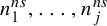 $n_1^{ns},\ldots , n_j^{ns}$
at which
$n_1^{ns},\ldots , n_j^{ns}$
at which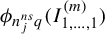 $\phi _{n_j^{ns} q}(I^{(m)}_{1,\ldots ,1})$
falls into a non-spacer interval.
$\phi _{n_j^{ns} q}(I^{(m)}_{1,\ldots ,1})$
falls into a non-spacer interval.
From the observations in §4.2, we note that the heights attained by subintervals of $I^{(m)}$
after multiple iterations of
$I^{(m)}$
after multiple iterations of $\phi _q$
are determined by those achieved by
$\phi _q$
are determined by those achieved by $I^{(m)}_{1,\ldots ,1}$
. Moreover, applying
$I^{(m)}_{1,\ldots ,1}$
. Moreover, applying $\phi _q$
to a spacer interval preserves its height, whereas applying it to a non-spacer interval changes its height. This leads to the following conclusions.
$\phi _q$
to a spacer interval preserves its height, whereas applying it to a non-spacer interval changes its height. This leads to the following conclusions.
-
• For each time
$n_l^s$
, there is an associated height
$h_l^s$
such that these heights correspond to subintervals of
$I^{(m)}$
that, after k iterations of
$\phi _q$
, lie in cylinders whose base is a spacer interval. -
• Similarly, for each time
$n_l^{ns}$
, there is an associated height
$h_l^{ns}$
such that these heights correspond to subintervals of
$I^{(m)}$
that, after k iterations of
$\phi _q$
, lie in cylinders whose base is a non-spacer interval.


The heights $h_l^s$
and
$h_l^s$
and $h_l^{ns}$
correspond to the values attained by
$h_l^{ns}$
correspond to the values attained by $\phi _{n_l^sq}(I^{(m)}_{1,\ldots ,1})$
and
$\phi _{n_l^sq}(I^{(m)}_{1,\ldots ,1})$
and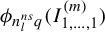 $\phi _{n_l^{ns}q}(I^{(m)}_{1,\ldots ,1})$
. Since the heights of the iterates of
$\phi _{n_l^{ns}q}(I^{(m)}_{1,\ldots ,1})$
. Since the heights of the iterates of $\phi _q$
for
$\phi _q$
for $I^{(m)}_{1,\ldots ,1}$
remain unchanged while passing through spacer blocks, multiple times
$I^{(m)}_{1,\ldots ,1}$
remain unchanged while passing through spacer blocks, multiple times $n_l^s$
can correspond to a single height. In contrast, for the times
$n_l^s$
can correspond to a single height. In contrast, for the times $n_l^{ns}$
, the mapping to heights is injective.
$n_l^{ns}$
, the mapping to heights is injective.
Proposition 4.12. For any subinterval, $I^{(m)}$
is H-equidistributed.
$I^{(m)}$
is H-equidistributed.
Proof. First, consider the non-spacer case. To establish the claim, we assume that $ I^{(m)} $
is initially at the uppermost level in the
$ I^{(m)} $
is initially at the uppermost level in the $ m $
-step configuration of the staircase transformation before breaking into
$ m $
-step configuration of the staircase transformation before breaking into $ m+1 $
new subintervals. If this is not the case, we can shift the interval using the flow until it reaches this uppermost level. This adjustment preserves the connectedness of the interval, ensuring that during the shifting process, it attains only one height.
$ m+1 $
new subintervals. If this is not the case, we can shift the interval using the flow until it reaches this uppermost level. This adjustment preserves the connectedness of the interval, ensuring that during the shifting process, it attains only one height.
Using the ideas developed in §4.2, we observe that the heights attained by $ \phi _{kq}(I^{(m)}) $
coincide with those attained by
$ \phi _{kq}(I^{(m)}) $
coincide with those attained by $ I^{(m)}_{1,\ldots ,1} $
. Since the heights of
$ I^{(m)}_{1,\ldots ,1} $
. Since the heights of $ I^{(m)}_{1,\ldots ,1} $
remain unchanged while passing through spacer blocks, it follows that all the heights achieved by
$ I^{(m)}_{1,\ldots ,1} $
remain unchanged while passing through spacer blocks, it follows that all the heights achieved by $ I^{(m)}_{1,\ldots ,1} $
after multiple iterations of
$ I^{(m)}_{1,\ldots ,1} $
after multiple iterations of $ \phi _q $
are found in the non-spacer side, while in the spacer, we find only a subsequence of such heights. From the observations in Remark 4.11, we conclude that these heights are attained by subintervals that, after multiple iterations, lie in cylinders whose base is non-spacer. The equidistribution of
$ \phi _q $
are found in the non-spacer side, while in the spacer, we find only a subsequence of such heights. From the observations in Remark 4.11, we conclude that these heights are attained by subintervals that, after multiple iterations, lie in cylinders whose base is non-spacer. The equidistribution of $ nq\!\! \mod 1 $
then establishes the first part of the proof.
$ nq\!\! \mod 1 $
then establishes the first part of the proof.
For the second part of the proof, we analyze the heights attained by the spacer subintervals, which correspond to the blocks of spacer levels in the staircase configuration. First, observe that, by Remark 4.11, the heights of the intervals of $ I^{(m)} $
that, after iterations of
$ I^{(m)} $
that, after iterations of $ \phi _q $
, lie in cylinders whose base is a spacer interval correspond to the heights
$ \phi _q $
, lie in cylinders whose base is a spacer interval correspond to the heights $ h^{ns}_l $
. Thus, it suffices to study the distribution of heights achieved by
$ h^{ns}_l $
. Thus, it suffices to study the distribution of heights achieved by $ I^{(m)}_{1,\ldots ,1} $
after multiple iterations. To achieve this, we construct two sequences as follows.
$ I^{(m)}_{1,\ldots ,1} $
after multiple iterations. To achieve this, we construct two sequences as follows.
Let $m_1$
be the smallest integer such that
$m_1$
be the smallest integer such that $(m_1 - 1)q < 1 < m_1 q$
. Note that
$(m_1 - 1)q < 1 < m_1 q$
. Note that $m_1 q \mod {1} < q$
. Let
$m_1 q \mod {1} < q$
. Let $k_1'$
be the smallest integer such that
$k_1'$
be the smallest integer such that
 $$ \begin{align*} (k_1' - 1)(m_1 q\!\!\! \mod\kern-1.6pt {1}) < 1 < k_1'(m_1 q\!\!\! \mod\kern-1.6pt {1}) \end{align*} $$
and define $k_1 = k_1' m_1$
. In addition,
$k_1 = k_1' m_1$
. In addition, $k_1 q\!\! \mod 1 < q$
.
$k_1 q\!\! \mod 1 < q$
.
Next, let $m_2'$
be the smallest integer such that
$m_2'$
be the smallest integer such that
 $$ \begin{align*}(m_2' - 1)(k_1 q\!\!\! \mod\kern-1.6pt 1) < 1 < m_2' (k_1 q\!\!\! \mod\kern-1.6pt 1)\end{align*} $$
and define $m_2 = m_2' k_1$
.
$m_2 = m_2' k_1$
.
Then, let $k_2'$
be the smallest integer such that
$k_2'$
be the smallest integer such that
 $$ \begin{align*}(k_2' - 1)(m_2 q\!\!\! \mod\kern-1.6pt 1) < 1 < k_2'(m_2 q\!\!\! \mod\kern-1.6pt 1)\end{align*} $$
and define $k_2 = k_2' m_2$
.
$k_2 = k_2' m_2$
.
In general, suppose $k_n$
is defined. Let
$k_n$
is defined. Let $m_{n+1}'$
be the smallest integer such that
$m_{n+1}'$
be the smallest integer such that
 $$ \begin{align*}(m_{n+1}' - 1)(k_n q\!\!\! \mod\kern-1.6pt 1) < 1 < m_{n+1}' (k_n q\!\!\! \mod\kern-1.6pt 1)\end{align*} $$
and define $m_{n+1} = m_{n+1}' k_n$
.
$m_{n+1} = m_{n+1}' k_n$
.
Let $k_{n+1}'$
be the smallest integer such that
$k_{n+1}'$
be the smallest integer such that
 $$ \begin{align*}(k_{n+1}' - 1)(m_{n+1} q\!\!\! \mod\kern-1.6pt 1) < 1 < k_{n+1}'(m_{n+1} q\!\!\! \mod\kern-1.6pt 1)\end{align*} $$
and define $k_{n+1} = k_{n+1}' m_{n+1}$
.
$k_{n+1} = k_{n+1}' m_{n+1}$
.
It is clear that both sequences satisfy $k_n q\!\! \mod 1 < q$
and
$k_n q\!\! \mod 1 < q$
and $m_n q\!\! \mod 1 < q$
. Moreover, the sequence
$m_n q\!\! \mod 1 < q$
. Moreover, the sequence $k_n q\!\! \mod 1$
describes the heights attained by the spacer intervals under the iterations of
$k_n q\!\! \mod 1$
describes the heights attained by the spacer intervals under the iterations of $\phi _q$
.
$\phi _q$
.
From this, we can convince ourselves that if $a_n$
is the sequence such that
$a_n$
is the sequence such that $a_n q\!\! \mod 1 < q$
, then since
$a_n q\!\! \mod 1 < q$
, then since $\{nq\!\! \mod 1\}$
equidistributes in
$\{nq\!\! \mod 1\}$
equidistributes in $[0,1)$
, it follows that since
$[0,1)$
, it follows that since $\{a_n q\!\! \mod 1\}$
describes the orbit of
$\{a_n q\!\! \mod 1\}$
describes the orbit of $0$
of the first return map of the irrational rotation by q to
$0$
of the first return map of the irrational rotation by q to $[0,q)$
, this first return map g is again an irrational rotation, in particular, all its iterates
$[0,q)$
, this first return map g is again an irrational rotation, in particular, all its iterates $g^k$
are uniquely ergodic; therefore, its orbits equidistribute in
$g^k$
are uniquely ergodic; therefore, its orbits equidistribute in $[0,q)$
.
$[0,q)$
.
From the construction of the sequence $k_i$
, we can observe that
$k_i$
, we can observe that $k_i = a_{2i}$
since the odd-indexed terms correspond to
$k_i = a_{2i}$
since the odd-indexed terms correspond to $m_i$
. In other words, the sequence
$m_i$
. In other words, the sequence $k_nq\!\! \mod 1$
describes the orbit of the second return map to
$k_nq\!\! \mod 1$
describes the orbit of the second return map to $[0,q)$
, which is
$[0,q)$
, which is $g^2$
in the last paragraph. In particular, it is uniquely ergodic and the orbit of zero will equidistribute. Consequently,
$g^2$
in the last paragraph. In particular, it is uniquely ergodic and the orbit of zero will equidistribute. Consequently,
 $$ \begin{align*} \lim_{n \to \infty} \frac{\textbf{card} (\{ m \leq n \mid k_m q \mod\kern-1.6pt 1 \in [a,b] \} )}{n} =\frac{b-a}{q} \end{align*} $$
for every $ [a,b] \subseteq [0,q)$
.
$ [a,b] \subseteq [0,q)$
.
As mentioned, the analysis in the spacer case is complicated since multiple intervals can share the same height. According to the last paragraph, the sequence $k_n q\!\! \mod 1$
describes the heights attained by the spacer intervals. In the mth step of the staircase configuration, spacers appear in blocks. Following §4.2, if we apply sufficiently many times
$k_n q\!\! \mod 1$
describes the heights attained by the spacer intervals. In the mth step of the staircase configuration, spacers appear in blocks. Following §4.2, if we apply sufficiently many times $\phi _q$
in such a way that
$\phi _q$
in such a way that $I^{(m)}_1$
goes its way through one
$I^{(m)}_1$
goes its way through one $m(q)$
th step of the staircase configuration, all intervals within a block of spacers share the same height. Rather than considering individual intervals, we focus on these blocks as a whole.
$m(q)$
th step of the staircase configuration, all intervals within a block of spacers share the same height. Rather than considering individual intervals, we focus on these blocks as a whole.
Arrange the blocks of spacers by order of appearance upwards in a staircase configuration. Consider an enumeration $\{d(l)\}_{l\in \mathbb {N}}$
of that appearance such that
$\{d(l)\}_{l\in \mathbb {N}}$
of that appearance such that $d(l)$
describes the number of intervals that the lth spacer block has in order of appearance. For any n, we examine the sequence of blocks containing n intervals. It can be observed that the appearance of these blocks follows a linear pattern. Specifically, for each n, there exists values
$d(l)$
describes the number of intervals that the lth spacer block has in order of appearance. For any n, we examine the sequence of blocks containing n intervals. It can be observed that the appearance of these blocks follows a linear pattern. Specifically, for each n, there exists values $a_n$
and
$a_n$
and $b_n$
such that for any l, the block of spacers
$b_n$
such that for any l, the block of spacers $d(b_n+a_n l)$
contains exactly n intervals. Consequently, for each n, the sequence
$d(b_n+a_n l)$
contains exactly n intervals. Consequently, for each n, the sequence $n_l = k_{b_n+a_n l}$
is such that the set
$n_l = k_{b_n+a_n l}$
is such that the set $\{n_l q \ mod 1 : l \in \mathbb {N}\}$
accurately describes the heights of spacer intervals that appear in blocks of n elements.
$\{n_l q \ mod 1 : l \in \mathbb {N}\}$
accurately describes the heights of spacer intervals that appear in blocks of n elements.
We can give a description of the sequences $n_j$
. For the case
$n_j$
. For the case $n=1,2$
, the sequences are given by
$n=1,2$
, the sequences are given by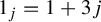 $1_j=1+3j$
and
$1_j=1+3j$
and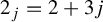 $2_j=2+3j$
, respectively.
$2_j=2+3j$
, respectively.
Let n be any other number. Consider $m(n)$
the first step in the staircase configuration such that there exists a block of spacers with n intervals. For
$m(n)$
the first step in the staircase configuration such that there exists a block of spacers with n intervals. For $m(n)$
, there will be
$m(n)$
, there will be $m(n)-1$
new numbers
$m(n)-1$
new numbers $c_i$
such that there exists a block with
$c_i$
such that there exists a block with $c_i$
spacer intervals such that these numbers did not appear in the
$c_i$
spacer intervals such that these numbers did not appear in the $(m(n)-1)$
th step of the staircase configuration. Order them from bottom to top. Let
$(m(n)-1)$
th step of the staircase configuration. Order them from bottom to top. Let $F(n)$
be the first time n appears in the list of blocks. If n is not
$F(n)$
be the first time n appears in the list of blocks. If n is not $c_{m(n)-1}$
, then
$c_{m(n)-1}$
, then
 $$ \begin{align*} n_j=F(n)+ j\frac{m(n)!}{2} \end{align*} $$
and if n is $c_{m(n)-1}$
, then
$c_{m(n)-1}$
, then
 $$ \begin{align*} n_j=F(n)+j\frac{(m(n)+1)!}{2}. \end{align*} $$
Continuing with the proof; just as before, using the fact that the first return map of a rotation by $q $
to the subinterval
$q $
to the subinterval $[0,q)$
is totally ergodic, and observing that for any n, the sequence
$[0,q)$
is totally ergodic, and observing that for any n, the sequence $n_jq\!\! \mod 1$
is the orbit of
$n_jq\!\! \mod 1$
is the orbit of $g^{2b_n}(0)$
under the transformation
$g^{2b_n}(0)$
under the transformation $g^{2a_n}$
, we see that the sequence of heights attained by blocks with n intervals equidistribute in
$g^{2a_n}$
, we see that the sequence of heights attained by blocks with n intervals equidistribute in $[0,q)$
.
$[0,q)$
.
Define $P_n$
as the probability of finding a block with n elements. Then,
$P_n$
as the probability of finding a block with n elements. Then,
 $$ \begin{align*} \lim_{n\to\infty} \frac{\textbf{card}(H_{nq}^{s}(I^{(m)}, I_{s,} [a,b]))}{\textbf{card}(H_{nq}^{s}(I^{(m)}, I_{s},[0,q)])}=\sum_{n\in\mathbb{N}}\bigg(\frac{b-a}{q}\bigg)P_n=\frac{b-a}{q}. \end{align*} $$
Observe that H-equidistribution for $t\to \infty $
follows directly from the H-equidistribution when
$t\to \infty $
follows directly from the H-equidistribution when $nq\to \infty $
, since for large t, the variation when considered, the discrete and continuous version converges to zero. The proposition follows.
$nq\to \infty $
, since for large t, the variation when considered, the discrete and continuous version converges to zero. The proposition follows.
Remark 4.13. Observe that H-equidistribution alone is not sufficient to approximate $\unicode{x3bb} (\phi _t(I^{(m)}) \cap R)$
with
$\unicode{x3bb} (\phi _t(I^{(m)}) \cap R)$
with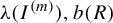 $\unicode{x3bb} (I^{(m)}),b(R)$
and
$\unicode{x3bb} (I^{(m)}),b(R)$
and $h(R)$
. A diagonal concentration phenomenon (see Figure 7) may occur: although the heights of
$h(R)$
. A diagonal concentration phenomenon (see Figure 7) may occur: although the heights of $\phi _t(I^{(m)})$
equidistribute in
$\phi _t(I^{(m)})$
equidistribute in $[0,1]$
over the non-spacer part and in
$[0,1]$
over the non-spacer part and in $[0,q]$
over the spacer part, this only yields equidistribution in the vertical projection
$[0,q]$
over the spacer part, this only yields equidistribution in the vertical projection $\pi _y(R)$
. It does not imply equidistribution inside the rectangle R itself, in other words, it does not ensure that the vertical coordinates of
$\pi _y(R)$
. It does not imply equidistribution inside the rectangle R itself, in other words, it does not ensure that the vertical coordinates of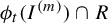 $\phi _t(I^{(m)}) \cap R$
equidistribute in
$\phi _t(I^{(m)}) \cap R$
equidistribute in $[0,1]$
or in
$[0,1]$
or in $[0,q]$
, respectively.
$[0,q]$
, respectively.
A diagonal behavior causes the intervals to miss several rectangles (colour online).

To overcome this difficulty, we prove a stronger statement. Given an arbitrary interval $I^{(n)}$
in the staircase configuration, we take
$I^{(n)}$
in the staircase configuration, we take $J = I^{(n)}$
in Definition 4.10 and establish equidistribution of the heights within the corresponding cylinders over
$J = I^{(n)}$
in Definition 4.10 and establish equidistribution of the heights within the corresponding cylinders over $I^{(n)}$
. This refined form of equidistribution yields the desired approximation.
$I^{(n)}$
. This refined form of equidistribution yields the desired approximation.
Definition 4.14. Let $I^{(m)}$
be a level in the m-step of the staircase configuration. We say that
$I^{(m)}$
be a level in the m-step of the staircase configuration. We say that $I^{(m)}$
is
$I^{(m)}$
is $\overline {H}$
-equidistributed if, for any interval
$\overline {H}$
-equidistributed if, for any interval $[a,b] \subseteq [0,1]$
in the vertical direction and any interval of the staircase configuration
$[a,b] \subseteq [0,1]$
in the vertical direction and any interval of the staircase configuration $I^{(n)}$
,
$I^{(n)}$
,
 $$ \begin{align*} \lim_{t\to\infty} \frac{\textbf{card}(H_t^{ns}(I^{(m)},I^{(n)},[a,b]))}{\textbf{card}((H_t^{ns}(I^{(m)},I^{(n)},[0,1]))}=b-a, \end{align*} $$
and if, for any $[a,b] \subseteq [0,q)$
,
$[a,b] \subseteq [0,q)$
,
 $$ \begin{align*} \lim_{t\to\infty} \frac{\textbf{card}(H_t^{s}(I^{(m)},I^{(n)},[a,b]))}{\textbf{card}((H_t^{ns}(I^{(m)},I^{(n)},[0,q]))}=\frac{b-a}{q}. \end{align*} $$
Lemma 4.15. For any $I^{(m)}$
, it is
$I^{(m)}$
, it is $\overline {H}$
-equidistributed.
$\overline {H}$
-equidistributed.
Proof. Using the $ H $
-equidistribution stated in Proposition 4.12 and Lemma 4.4, we establish that for any intervals
$ H $
-equidistribution stated in Proposition 4.12 and Lemma 4.4, we establish that for any intervals $ I^{(m)} $
and
$ I^{(m)} $
and $ I^{(n)} $
, the heights attained by
$ I^{(n)} $
, the heights attained by $ \phi _t(I^{(m)}) $
become equidistributed within the
$ \phi _t(I^{(m)}) $
become equidistributed within the $ I^{(n)} $
-cylinder.
$ I^{(n)} $
-cylinder.
We begin by analyzing the case where $ I^{(n)} $
lies in the non-spacer region. Without loss of generality, we assume
$ I^{(n)} $
lies in the non-spacer region. Without loss of generality, we assume $ m \geq n $
. Considering a discretization of the flow given by iterates of
$ m \geq n $
. Considering a discretization of the flow given by iterates of $ q $
, the evolution of
$ q $
, the evolution of $ \phi _{kq}(I^{(m)}) $
through the staircase causes it to break into subintervals. Over multiple iterations, some of these subintervals return to the
$ \phi _{kq}(I^{(m)}) $
through the staircase causes it to break into subintervals. Over multiple iterations, some of these subintervals return to the $ I^{(n)} $
-cylinder due to the staircase-like structure. This implies the existence of subintervals
$ I^{(n)} $
-cylinder due to the staircase-like structure. This implies the existence of subintervals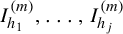 $ I^{(m)}_{h_1},\ldots , I^{(m)}_{h_j} $
such that every
$ I^{(m)}_{h_1},\ldots , I^{(m)}_{h_j} $
such that every $ \phi _{kq}(I^{(m)}_{h_i}) $
lies within the
$ \phi _{kq}(I^{(m)}_{h_i}) $
lies within the $ I^{(n)} $
-cylinder.
$ I^{(n)} $
-cylinder.
These subintervals, in turn, belong to specific subcylinders of $ I^{(n)} $
, denoted by
$ I^{(n)} $
, denoted by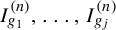 $ I^{(n)}_{g_1},\ldots , I^{(n)}_{g_j} $
. Among the different heights achieved by these subintervals, there exists a leading interval, meaning that if the heights are given by
$ I^{(n)}_{g_1},\ldots , I^{(n)}_{g_j} $
. Among the different heights achieved by these subintervals, there exists a leading interval, meaning that if the heights are given by $ n_iq\!\! \mod 1 $
, one interval attains the maximum height
$ n_iq\!\! \mod 1 $
, one interval attains the maximum height $n_{i_0}q\!\! \mod 1$
. More precisely, we can label the subintervals as
$n_{i_0}q\!\! \mod 1$
. More precisely, we can label the subintervals as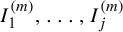 $ I^{(m)}_1,\ldots , I^{(m)}_j $
such that
$ I^{(m)}_1,\ldots , I^{(m)}_j $
such that $ I_1^{(m)} = I^{(m)}_{i_0} $
, and the height of each
$ I_1^{(m)} = I^{(m)}_{i_0} $
, and the height of each $ I_l^{(m)} $
coincides with that of
$ I_l^{(m)} $
coincides with that of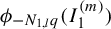 $ \phi _{-N_{1,l}q}(I^{(m)}_1) $
, where
$ \phi _{-N_{1,l}q}(I^{(m)}_1) $
, where $ N_{1,l} $
represents the distance between
$ N_{1,l} $
represents the distance between $ l $
and
$ l $
and $ 1 $
in this enumeration.
$ 1 $
in this enumeration.
By iterating this process, we observe that if $\phi _{Kq}$
causes
$\phi _{Kq}$
causes $I^{(m)}$
to reach the
$I^{(m)}$
to reach the $(m+d)$
th step of the staircase configuration, an even smaller portion of
$(m+d)$
th step of the staircase configuration, an even smaller portion of $ I^{(m)} $
will lie within the
$ I^{(m)} $
will lie within the $ I^{(n)} $
-cylinder. More precisely, there exist subintervals
$ I^{(n)} $
-cylinder. More precisely, there exist subintervals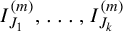 $ I^{(m)}_{J_1},\ldots , I^{(m)}_{J_k} $
, where each index
$ I^{(m)}_{J_1},\ldots , I^{(m)}_{J_k} $
, where each index $ J_i $
has length bounded by
$ J_i $
has length bounded by $ {(m+d-1)!}/{m!} $
.
$ {(m+d-1)!}/{m!} $
.
Similarly, there are subcylinders over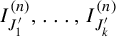 $ I^{(n)}_{J^{\prime }_1},\ldots , I^{(n)}_{J^{\prime }_k} $
, where each
$ I^{(n)}_{J^{\prime }_1},\ldots , I^{(n)}_{J^{\prime }_k} $
, where each $ J^{\prime }_i $
has length bounded by
$ J^{\prime }_i $
has length bounded by $ {(n+d-1)!}/{n!} $
. For each
$ {(n+d-1)!}/{n!} $
. For each $ J_i $
, there exist subsubintervals
$ J_i $
, there exist subsubintervals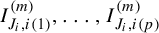 $ I^{(m)}_{J_i,i(1)},\ldots , I^{(m)}_{J_i,i(p)} $
that lie within some subcylinder
$ I^{(m)}_{J_i,i(1)},\ldots , I^{(m)}_{J_i,i(p)} $
that lie within some subcylinder $ I^{(n)}_{J^{\prime }_i} $
. Among these subsubintervals, one achieves the greatest height within the subcylinder, which we denote as the leading subsubinterval
$ I^{(n)}_{J^{\prime }_i} $
. Among these subsubintervals, one achieves the greatest height within the subcylinder, which we denote as the leading subsubinterval $ I^{(m)}_{J_i,i(j_0)} $
.
$ I^{(m)}_{J_i,i(j_0)} $
.
Following the reasoning from the previous paragraph, we can enumerate these subsubintervals as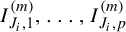 $ I^{(m)}_{J_i,1},\ldots , I^{(m)}_{J_i,p} $
so that
$ I^{(m)}_{J_i,1},\ldots , I^{(m)}_{J_i,p} $
so that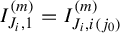 $ I^{(m)}_{J_i,1} = I^{(m)}_{J_i,i(j_0)} $
. The heights achieved by these subsubintervals satisfy
$ I^{(m)}_{J_i,1} = I^{(m)}_{J_i,i(j_0)} $
. The heights achieved by these subsubintervals satisfy
 $$ \begin{align*} \pi_y(\phi_{Kq(} I^{(m)}_{J_i,l})) = \pi_y(\phi_{(K-N_{1,l})q}(I^{(m)}_{J_i,1})), \end{align*} $$
where $ N_{1,l} $
denotes the distance between
$ N_{1,l} $
denotes the distance between $ l $
and
$ l $
and $ 1 $
in this enumeration.
$ 1 $
in this enumeration.
Next, considering the heights of the leading subsubintervals across different subcylinders $ I^{(m)}_{J_i,1} $
, we apply the previous argument. If multiple subsubintervals attain the maximum height, we order them from left to right according to their appearance in the subcylinders of
$ I^{(m)}_{J_i,1} $
, we apply the previous argument. If multiple subsubintervals attain the maximum height, we order them from left to right according to their appearance in the subcylinders of $ I^{(n)} $
. We then relabel the leftmost interval with the leading height as
$ I^{(n)} $
. We then relabel the leftmost interval with the leading height as $ I^{(m)}_{1,1} $
and establish an enumeration such that the height of
$ I^{(m)}_{1,1} $
and establish an enumeration such that the height of $ I^{(m)}_{j,1} $
satisfies
$ I^{(m)}_{j,1} $
satisfies
 $$ \begin{align*} \pi_y(\phi_{Kq}(I^{(m)}_{j,1})) = \pi_y(\phi_{(K-N_{1,j})q}(I^{(m)}_{1,1})), \end{align*} $$
where $ N_{1,j} $
represents the distance between
$ N_{1,j} $
represents the distance between $ j $
and
$ j $
and $ 1 $
. Extending this enumeration within each subcylinder, we ensure that for each subsubinterval
$ 1 $
. Extending this enumeration within each subcylinder, we ensure that for each subsubinterval $ I^{(m)}_{i,j} $
,
$ I^{(m)}_{i,j} $
,
 $$ \begin{align*} \pi_y(\phi_{Kq}(I^{(m)}_{i,j})) = \pi_y(\phi_{(K-N_{1,j}+ N_{1,i})q}(I^{(m)}_{1,1})). \end{align*} $$
See Figure 8 for a toy model illustrating this behavior.
Toy model of the behavior of $\phi _{nq}(I^{(m)})$
in the
$\phi _{nq}(I^{(m)})$
in the $I^{(n)}$
-cylinder (colour online).
$I^{(n)}$
-cylinder (colour online).

With further iterations of $ \phi _q $
, the measure of the portion of
$ \phi _q $
, the measure of the portion of $ I^{(m)} $
that lies within the
$ I^{(m)} $
that lies within the $ I^{(n)} $
-cylinder converges to
$ I^{(n)} $
-cylinder converges to $ \unicode{x3bb} (I^{(m)}) \unicode{x3bb} (I^{(n)}) $
, as established in Lemma 4.4. Moreover, these portions become equidistributed among the subcylinders
$ \unicode{x3bb} (I^{(m)}) \unicode{x3bb} (I^{(n)}) $
, as established in Lemma 4.4. Moreover, these portions become equidistributed among the subcylinders $ I^{(n)}_J $
, where
$ I^{(n)}_J $
, where $ J $
is an index of a specified length that depends on the number of iterations of
$ J $
is an index of a specified length that depends on the number of iterations of $ \phi _q $
. The heights attained within these subintervals follow the same pattern as before, forming an increasing sequence of the form
$ \phi _q $
. The heights attained within these subintervals follow the same pattern as before, forming an increasing sequence of the form
 $$ \begin{align*} kq, (k+1)q,\ldots , (k+r)q \mod\kern-1.6pt 1. \end{align*} $$
As $ q \to \infty $
, the length of these sequences increases, leading to the equidistribution of heights within the cylinder generated by
$ q \to \infty $
, the length of these sequences increases, leading to the equidistribution of heights within the cylinder generated by $ I^{(n)} $
.
$ I^{(n)} $
.
If $ I^{(n)} $
is a spacer interval, we observe that, due to the staircase-like pattern, the behavior is analogous to the non-spacer case. After multiple iterations of
$ I^{(n)} $
is a spacer interval, we observe that, due to the staircase-like pattern, the behavior is analogous to the non-spacer case. After multiple iterations of $ \phi _q $
, the subintervals forming
$ \phi _q $
, the subintervals forming $ I^{(m)} $
distribute across subcylinders of
$ I^{(m)} $
distribute across subcylinders of $ I^{(n)} $
, attaining different heights. The only distinction from the non-spacer case is that these heights do not differ by one iteration of
$ I^{(n)} $
, attaining different heights. The only distinction from the non-spacer case is that these heights do not differ by one iteration of $q\!\! \mod 1$
as in the non-spacer case, rather they follow the subsequence described in Proposition 4.12, which, as proved there, ensures their equidistribution within the
$q\!\! \mod 1$
as in the non-spacer case, rather they follow the subsequence described in Proposition 4.12, which, as proved there, ensures their equidistribution within the $ I^{(n)} $
-cylinder.
$ I^{(n)} $
-cylinder.
Now, we can observe that Lemma 4.4 and Lemma 4.15 imply the following theorem.
Theorem 4.16. Let T represent the classical staircase transformation, and let f be a $2$
-wise constant function characterized by roof values p and q that are rationally independent. If all the spacers of the transformation T are positioned beneath the roof with value q, then the flow constructed under f respecting T is mixing.
$2$
-wise constant function characterized by roof values p and q that are rationally independent. If all the spacers of the transformation T are positioned beneath the roof with value q, then the flow constructed under f respecting T is mixing.
Proof. According to Lemma 4.3, we need to prove that for any $\epsilon ,\delta>0$
and for every rectangle R, there is a
$\epsilon ,\delta>0$
and for every rectangle R, there is a $t_0>0$
such that for every
$t_0>0$
such that for every $t\geq t_0$
, there exists a partition
$t\geq t_0$
, there exists a partition $\eta (t)$
such that:
$\eta (t)$
such that:
-
(1)
$\unicode{x3bb} (\eta (t))>1-\delta $
and
$\mathrm{Mesh}(\eta (t))\leq \delta $
; -
(2) for every
$I\in \eta (t)$
, it follows that
$\mu (I\cap \phi _{-t}(R))\geq (1-\epsilon )\mu (R)\unicode{x3bb} (I).$




The partitions we construct depend on $\delta $
, while
$\delta $
, while $t_0$
is determined by
$t_0$
is determined by $\epsilon $
.
$\epsilon $
.
The natural partitions under consideration stem from the m-steps within the staircase configuration. Referring to §4.1, if A denotes the length of $I^{(1)}$
, then for any subinterval
$I^{(1)}$
, then for any subinterval $I^{(m)}$
in the m-step, we have
$I^{(m)}$
in the m-step, we have
 $$ \begin{align} \unicode{x3bb}(I^{(m)})=\frac{A}{(m)!}\to0. \end{align} $$
Moreover, since all the intervals in this choice of partition have the same measure, then $\mathrm{Mesh}$
of any of this partition will converge to zero according to (4.1).
$\mathrm{Mesh}$
of any of this partition will converge to zero according to (4.1).
However, we observe that the measure of the covers converges to 1 by construction. Therefore, there exists an m such that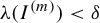 $\unicode{x3bb} (I^{(m)})<\delta $
and simultaneously
$\unicode{x3bb} (I^{(m)})<\delta $
and simultaneously $h_m\unicode{x3bb} (I^{(m)})<1-\delta $
and also
$h_m\unicode{x3bb} (I^{(m)})<1-\delta $
and also $m\geq m_0(q)$
, where
$m\geq m_0(q)$
, where $h_m$
represents the number of intervals in the m-step of the transformation and
$h_m$
represents the number of intervals in the m-step of the transformation and $m_0(q)$
is the constant given in Lemma 4.4. This satisfies the initial requirement.
$m_0(q)$
is the constant given in Lemma 4.4. This satisfies the initial requirement.
Without loss of generality, we may assume that $b(R)$
is one interval
$b(R)$
is one interval $I^{(n)}$
of the nth step of the staircase configuration for some n. For the second requirement, we need to consider three cases.
$I^{(n)}$
of the nth step of the staircase configuration for some n. For the second requirement, we need to consider three cases.
(1) The rectangle R is inside the non-spacer part. Then,
 $$ \begin{align*} \unicode{x3bb}(\phi_t(I^{(m)})\cap R)\to \unicode{x3bb}(\phi_t(I^{(m)})\cap \pi_x^{-1}(b(R)))\frac{\textbf{card}(H_t^{ns}(I^{(m)},I^{(n)},h(R)))}{\textbf{card}((H_t^{ns}(I^{(m)},I^{(n)},[0,1]))}.\end{align*} $$
By Lemma 4.4,
 $$ \begin{align*}\unicode{x3bb}(\phi_t(I^{(m)})\cap \pi_x^{-1}(b(R)))\to \unicode{x3bb}(I^{(m)})\unicode{x3bb}(b(R)).\end{align*} $$
In addition, by Lemma 4.15, we have that
 $$ \begin{align*} \frac{\textbf{card}(H_t^{ns}(I^{(m)},I^{(n)},h(R)))}{\textbf{card}((H_t^{ns}(I^{(m)},I^{(n)},[0,1]))}\to\unicode{x3bb}(h(R)).\end{align*} $$
This implies, in particular, that
 $$ \begin{align*}\unicode{x3bb}(I^{(m)}\cap \phi_{-t}(R))\to \unicode{x3bb}(I^{(m)})\unicode{x3bb}(b(R))\unicode{x3bb}(h(R))=\unicode{x3bb}(I^{(m)})\mu(R).\end{align*} $$
(2) The rectangle R is inside the spacer part of the polygon. Then, by Lemma 4.15,
 $$ \begin{align*} \frac{\textbf{card}(H_t^{ns}(I^{(m)},I^{(n)},h(R)))}{\textbf{card}((H_t^{ns}(I^{(m)},I^{(n)},[0,1]))}\to\frac{\unicode{x3bb}(h(R))}{q}.\end{align*} $$
Then,
 $$ \begin{align*}\unicode{x3bb}(I^{(m)}\cap \phi_{-t}(R))\to \frac{\unicode{x3bb}(I^{(m)})\mu(R)}{q}>\unicode{x3bb}(I^{(m)})\mu(R).\end{align*} $$
(3) The rectangle R has a part inside the spacer and non-spacer part. Let $R_1$
be the part inside the non-spacer part and
$R_1$
be the part inside the non-spacer part and $R_2$
be the part inside the spacer part. Observe that
$R_2$
be the part inside the spacer part. Observe that $h(R_1)=h(R_2)=h(R)$
and
$h(R_1)=h(R_2)=h(R)$
and $b(R_1)+b(R_2)=b(R)$
. Suppose that
$b(R_1)+b(R_2)=b(R)$
. Suppose that $b(R_1)=I^{n_1}$
and
$b(R_1)=I^{n_1}$
and $b(R_2)=I^{(n_2)}$
. By Lemmas 4.4 and 4.15, we have that
$b(R_2)=I^{(n_2)}$
. By Lemmas 4.4 and 4.15, we have that
 $$ \begin{align*} \unicode{x3bb}(I^{(m)}\cap \phi_{-t}(R))&=\unicode{x3bb}(\phi_t(I^{(m)})\cap \pi_x^{-1}(b(R_1)))\frac{\textbf{card}(H_t^{ns}(I^{(m)},I^{(n_1)},h(R)))}{\textbf{card}((H_t^{ns}(I^{(m)},I^{(n_1)},[0,1]))} \\ &\quad+ \unicode{x3bb}(\phi_t(I^{(m)})\cap \pi_x^{-1}(b(R_2)))\frac{\textbf{card}(H_t^{ns}(I^{(m)},I^{(n_2)},h(R)))}{\textbf{card}((H_t^{ns}(I^{(m)},I^{(n_2)},[0,1]))}\\ &\quad \to \unicode{x3bb}(I^{(m)})\unicode{x3bb}(b(R_1))\unicode{x3bb}(h(R_1))\\ &\quad +\unicode{x3bb}(I^{(m)})\unicode{x3bb}(b(R_2))\frac{\unicode{x3bb}(h(R_2))}{q}>\unicode{x3bb}(I^{(m)})\mu(R). \end{align*} $$
Observe that in all three cases,
 $$ \begin{align*}\lim_{t\to\infty}\unicode{x3bb}(I^{(m)}\cap \phi_{-t}(R))\geq\unicode{x3bb}(I^{(m)})\mu(R).\end{align*} $$
In particular, for $\epsilon>0$
, there exists a
$\epsilon>0$
, there exists a $t_0$
such that for any
$t_0$
such that for any $t\geq t_0$
, we have that
$t\geq t_0$
, we have that
 $$ \begin{align*}\unicode{x3bb}(I^{(m)}\cap \phi_{-t}(R))\geq (1-\epsilon)\unicode{x3bb}(I^{(m)})\mu(R).\end{align*} $$
To conclude the proof, we state that the $t_0$
constructed above will be useful, and the covers that serve for this purpose will consist of the intervals for the m-step configuration of the staircase, where the m is the one that is useful for the
$t_0$
constructed above will be useful, and the covers that serve for this purpose will consist of the intervals for the m-step configuration of the staircase, where the m is the one that is useful for the $\delta $
. With this, and by virtue of Lemma 4.3, we conclude the proof.
$\delta $
. With this, and by virtue of Lemma 4.3, we conclude the proof.
In particular, this implies the following scenario.
5 General mixing staircase
The strategy for demonstrating that the flow constructed under a $2$
-wise constant function, where its two heights are rationally independent values, over any mixing staircase transformation is analogous to the approach used for the classical staircase. In this section, we outline the minor adjustments required from the previous procedure and refer to the proofs there.
$2$
-wise constant function, where its two heights are rationally independent values, over any mixing staircase transformation is analogous to the approach used for the classical staircase. In this section, we outline the minor adjustments required from the previous procedure and refer to the proofs there.
We once more rely on Lemma 4.3. The choice of partitions will be based on the natural partitions within the interval defined by the staircase transformation, with the specific partition determined by $\delta $
as per Lemma 4.3, while the time
$\delta $
as per Lemma 4.3, while the time $t_0$
will be contingent on
$t_0$
will be contingent on $\epsilon $
and the rectangle.
$\epsilon $
and the rectangle.
In [Reference Creutz and SilvaCS04, Reference Creutz and SilvaCS06], a sufficient condition is provided to characterize mixing staircase transformations and rank-one transformations.
Continuing with the previous procedure, our initial step is to demonstrate the following.
Lemma 5.1. There exists an $m_0$
such that for any
$m_0$
such that for any $m \geq m_0$
, for any level
$m \geq m_0$
, for any level $I^{(m)}$
in the mth step of the staircase configuration of any mixing staircase transformation T, and for any rectangle R under the graph of f, the following holds. Let
$I^{(m)}$
in the mth step of the staircase configuration of any mixing staircase transformation T, and for any rectangle R under the graph of f, the following holds. Let $\pi _x$
denote the horizontal projection, then
$\pi _x$
denote the horizontal projection, then
 $$ \begin{align*}\lim_{t\to \infty} \unicode{x3bb}(\phi_t(I^{(n)})\cap \pi_x^{-1}(b(R)))=\unicode{x3bb}(I^{(n)})\unicode{x3bb}((b(R))),\end{align*} $$
where $b(R)$
is the basis of the rectangle R.
$b(R)$
is the basis of the rectangle R.
Proof. The proof is essentially the same as in the case of the classical staircase.
Consider an interval $I^{(n)}$
such that for some subintervals
$I^{(n)}$
such that for some subintervals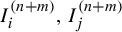 $I^{(n+m)}_i, I^{(n+m)}_j$
such that for some non-negative real numbers
$I^{(n+m)}_i, I^{(n+m)}_j$
such that for some non-negative real numbers $t,s $
,
$t,s $
,
 $$ \begin{align*}\phi_{t-s}(I^{(n+m)}_i)= \phi_t(I^{(n+m)}_j).\end{align*} $$
Consider $N_0$
such that
$N_0$
such that $(N_0-1)q<1\leq N_0q$
. Just as in Lemma 4.4, the only problem that can arise is when there are two subintervals in the
$(N_0-1)q<1\leq N_0q$
. Just as in Lemma 4.4, the only problem that can arise is when there are two subintervals in the $(m+n)$
th step of the staircase configuration such that their distance is smaller than
$(m+n)$
th step of the staircase configuration such that their distance is smaller than $2r_1N_0$
(remember that
$2r_1N_0$
(remember that $\{r_n\}$
is the cutting sequence for T). This is due to the fact that there can be accumulations in the
$\{r_n\}$
is the cutting sequence for T). This is due to the fact that there can be accumulations in the $r_1$
intervals that are in the non-spacer blocks. Since
$r_1$
intervals that are in the non-spacer blocks. Since $h_m$
is an increasing sequence, there exists an
$h_m$
is an increasing sequence, there exists an $m_0$
such that
$m_0$
such that $h_m\geq 4r_1 N_0$
for any
$h_m\geq 4r_1 N_0$
for any $m\geq m_0$
. Therefore, for any n, the distance between any two sublevels
$m\geq m_0$
. Therefore, for any n, the distance between any two sublevels $I^{(n+m)}_i$
and
$I^{(n+m)}_i$
and $I^{(n+m)}_j$
of
$I^{(n+m)}_j$
of $I^{(m)}$
in the
$I^{(m)}$
in the $(m+n)$
th step of the staircase configuration is greater than
$(m+n)$
th step of the staircase configuration is greater than $4r_1N_0$
. The argument to conclude the proof is the same as in Lemma 4.4.
$4r_1N_0$
. The argument to conclude the proof is the same as in Lemma 4.4.
Remark 5.2. Notably, for this proof, we only necessitate the divergence of the sequence $h_n$
associated with the rank-one transformation. Therefore, assuming the transformation is mixing, the second requirement implies that as the flow approaches infinity, considering the transformation T suffices instead. Since T is mixing, we can attain the convergence outlined in Lemma 5.1.
$h_n$
associated with the rank-one transformation. Therefore, assuming the transformation is mixing, the second requirement implies that as the flow approaches infinity, considering the transformation T suffices instead. Since T is mixing, we can attain the convergence outlined in Lemma 5.1.
Just as in the classical staircase case, any mixing staircase exhibits a staircase-like pattern, even if the cutting sequence is not given by $ r_n = n $
. Consequently, multiple iterations of
$ r_n = n $
. Consequently, multiple iterations of $ \phi _q $
applied to an interval
$ \phi _q $
applied to an interval $ I^{(m)} $
cause it to break into several subintervals. Due to the staircase-like structure of the spacer intervals, the resulting heights exhibit the same behavior as in the classical case.
$ I^{(m)} $
cause it to break into several subintervals. Due to the staircase-like structure of the spacer intervals, the resulting heights exhibit the same behavior as in the classical case.
Another way to interpret this phenomenon is by considering the $(m+n)$
th step of the staircase configuration. At this stage, multiple copies of the
$(m+n)$
th step of the staircase configuration. At this stage, multiple copies of the $ m $
th step appear, separated by spacer intervals. These spacer intervals introduce delays in the heights of the newly formed subintervals, meaning that the new heights differ by one, as discussed in the previous section. Our goal is to prove that these heights equidistribute.
$ m $
th step appear, separated by spacer intervals. These spacer intervals introduce delays in the heights of the newly formed subintervals, meaning that the new heights differ by one, as discussed in the previous section. Our goal is to prove that these heights equidistribute.
Following the notation in Definitions 4.9 and 4.10, we want to prove the following.
Proposition 5.3. Any subinterval $I^{(m)}$
is H-equidistributed.
$I^{(m)}$
is H-equidistributed.
Proof. Following the same reasoning as in the proof of Proposition 4.12, we note that since $ T $
is a staircase transformation, the introduction of new spacers at each step of the staircase configuration results in the behavior described in §4.2. Specifically, after several iterations of
$ T $
is a staircase transformation, the introduction of new spacers at each step of the staircase configuration results in the behavior described in §4.2. Specifically, after several iterations of $ \phi _q $
, the heights attained by an interval
$ \phi _q $
, the heights attained by an interval $ I^{(m)} $
correspond to those attained by the lowest interval in its representation at the
$ I^{(m)} $
correspond to those attained by the lowest interval in its representation at the $ (m+n) $
th step of the staircase configuration. Consequently, when the k iterations of
$ (m+n) $
th step of the staircase configuration. Consequently, when the k iterations of $\phi _q$
go to infinity, the sequence of heights eventually approaches the set
$\phi _q$
go to infinity, the sequence of heights eventually approaches the set $ \{nq\!\! \mod 1\}, a_k\leq n\leq b_k $
, where
$ \{nq\!\! \mod 1\}, a_k\leq n\leq b_k $
, where $b_k-a_k\to \infty $
. Moreover, in the non-spacer part of the polygon, each height is attained by exactly one interval, which establishes
$b_k-a_k\to \infty $
. Moreover, in the non-spacer part of the polygon, each height is attained by exactly one interval, which establishes $ H $
-equidistribution in the non-spacer case.
$ H $
-equidistribution in the non-spacer case.
For the second part, following Proposition 4.12, we construct a sequence $ a_n $
that describes the heights such that
$ a_n $
that describes the heights such that $ a_nq\!\! \mod 1 < q $
. Since the non-spacer blocks contain
$ a_nq\!\! \mod 1 < q $
. Since the non-spacer blocks contain $ r_1 $
intervals, moving from one spacer block to the next requires passing through the roof at
$ r_1 $
intervals, moving from one spacer block to the next requires passing through the roof at $ 1 $
exactly
$ 1 $
exactly $ r_1 $
consecutive times. Therefore, we can construct
$ r_1 $
consecutive times. Therefore, we can construct $ r_1 $
different sequences
$ r_1 $
different sequences $ a_{in} $
, each describing the height achieved after passing through the roof at
$ a_{in} $
, each describing the height achieved after passing through the roof at $ 1 $
exactly
$ 1 $
exactly $ n \leq r_1 $
times. In other words, for any of these
$ n \leq r_1 $
times. In other words, for any of these $ r_1 $
sequences,
$ r_1 $
sequences, $ a_{in}q\!\! \mod 1 $
describes the orbit of the
$ a_{in}q\!\! \mod 1 $
describes the orbit of the $ n $
th return map of an irrational rotation by
$ n $
th return map of an irrational rotation by $ q $
on the interval
$ q $
on the interval $ [0,q) $
, which is known to be uniquely ergodic. This implies that the heights attained by the spacer blocks are described by the sequence
$ [0,q) $
, which is known to be uniquely ergodic. This implies that the heights attained by the spacer blocks are described by the sequence $ a_{ir_1}q\!\! \mod 1 $
, which equidistributes in
$ a_{ir_1}q\!\! \mod 1 $
, which equidistributes in $ [0,q) $
.
$ [0,q) $
.
Just as in the classical staircase case, if we enumerate the spacer blocks by counting the number of intervals they contain, we aim to describe, for each $ n $
, a sequence
$ n $
, a sequence $ n_i $
such that the
$ n_i $
such that the $ n_k $
th spacer block contains exactly
$ n_k $
th spacer block contains exactly $ n $
intervals.
$ n $
intervals.
For each $ n $
, define the function
$ n $
, define the function
 $$ \begin{align*} g(n) = \prod_{i=2}^{n} r_i. \end{align*} $$
Let $ n $
be any number and consider
$ n $
be any number and consider $ m(n) $
the first step in the staircase configuration where a spacer block with
$ m(n) $
the first step in the staircase configuration where a spacer block with $ n $
intervals appears. At step
$ n $
intervals appears. At step $ m(n) $
, there will be
$ m(n) $
, there will be $ m(n)-1 $
new values
$ m(n)-1 $
new values $ c_i $
corresponding to block sizes that were not present in the
$ c_i $
corresponding to block sizes that were not present in the $ (m(n)-1) $
th step. Ordering these from bottom to top, let
$ (m(n)-1) $
th step. Ordering these from bottom to top, let $ F(n) $
denote the first occurrence of
$ F(n) $
denote the first occurrence of $ n $
in this list of blocks. If
$ n $
in this list of blocks. If $ n \neq c_{m(n)-1} $
, then
$ n \neq c_{m(n)-1} $
, then
 $$ \begin{align*} n_j = F(n) + j g(m(n)), \end{align*} $$
and if $ n = c_{m(n)-1} $
, then
$ n = c_{m(n)-1} $
, then
 $$ \begin{align*} n_j = F(n) + j g(m(n) + 1). \end{align*} $$
In this setting, for every $ n $
, the sequence
$ n $
, the sequence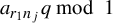 $ a_{r_1n_j}q \!\! \mod 1 $
represents the orbit of
$ a_{r_1n_j}q \!\! \mod 1 $
represents the orbit of $ g^{F(n)r_1}(0) $
under the transformation
$ g^{F(n)r_1}(0) $
under the transformation $ g^{r_1g(m(n)+1)} $
or
$ g^{r_1g(m(n)+1)} $
or $ g^{r_1g(m(n))} $
, where
$ g^{r_1g(m(n))} $
, where $ g $
is the first return map of an irrational rotation by
$ g $
is the first return map of an irrational rotation by $ q $
on the subinterval
$ q $
on the subinterval $ [0,q)$
. Consequently, the sequences
$ [0,q)$
. Consequently, the sequences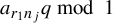 $ a_{r_1n_j}q \!\! \mod 1 $
equidistribute in
$ a_{r_1n_j}q \!\! \mod 1 $
equidistribute in $ [0,q)$
.
$ [0,q)$
.
For the spacer part of the polygon, as observed in the previous paragraph, the sequences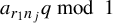 $ a_{r_1n_j}q \!\! \mod 1 $
describe the heights attained by spacer blocks containing
$ a_{r_1n_j}q \!\! \mod 1 $
describe the heights attained by spacer blocks containing $ n $
intervals. These sequences equidistribute in
$ n $
intervals. These sequences equidistribute in $ [0,q)$
. It follows that if
$ [0,q)$
. It follows that if $ P_n $
denotes the probability of finding a spacer block with
$ P_n $
denotes the probability of finding a spacer block with $ n $
intervals, then
$ n $
intervals, then
 $$ \begin{align*} \begin{aligned} \lim_{t\to\infty} \frac{\mathbf{card}(A_t^{s}(I^{(m)})\cap [a,b])}{\mathbf{card}(A_t^{s}(I^{(m)}))}=\sum_{n\in\mathbb{N}}\bigg(\frac{b-a}{q}\bigg)P_n=\frac{b-a}{q}. \end{aligned}\\[-34pt] \end{align*} $$
As discussed in the previous section, it is not enough to consider H-equidistribution.
Lemma 5.4. Each $I^{(m)}$
is
$I^{(m)}$
is $\overline {H}$
-equidistributed.
$\overline {H}$
-equidistributed.
Proof. Observe that the staircase-like behavior described in §4.2 and Lemma 4.15 also holds for a flow built under any staircase transformation. Using the ideas from Lemma 4.15, the proof follows directly from Lemmas 5.1 and 4.15 and Proposition 5.3.
Theorem 5.5. Let T represent any mixing staircase transformation, and let f be a $2$
-wise constant function characterized by roof values p and q that are rationally independent. If all the spacers of the transformation T are positioned beneath the roof with value q, then the flow constructed under f respecting T is mixing.
$2$
-wise constant function characterized by roof values p and q that are rationally independent. If all the spacers of the transformation T are positioned beneath the roof with value q, then the flow constructed under f respecting T is mixing.
Proof. Just like in the proof of Theorem 4.16, we make use of Lemmas 5.1 and 5.4 to prove that there exists $m_0$
such that for any
$m_0$
such that for any $m\geq m_0$
, for any interval
$m\geq m_0$
, for any interval $I^{(m)}$
in the m-step configuration of the staircase, and for any rectangle R,
$I^{(m)}$
in the m-step configuration of the staircase, and for any rectangle R,
 $$ \begin{align*}\lim_{t\to\infty}\unicode{x3bb}(I^{(m)}\cap \phi_{-t}(R))\geq \unicode{x3bb}(I^{(m)})\unicode{x3bb}(b(R))\unicode{x3bb}(h(R))=\unicode{x3bb}(I^{(m)})\mu(R).\end{align*} $$
Following the same idea as in Theorem 4.16, we check that the conditions for Lemma 4.3 are fulfilled, then $\phi _t$
is mixing.
$\phi _t$
is mixing.
6 n-fold mixing property
In the first half of the last century, Rokhlin defined the notion of being n-fold mixing [Reference RokhlinRok49].
Definition 6.1. We say that a measurable dynamical system $(X,T,\mu )$
is n-fold mixing if for every
$(X,T,\mu )$
is n-fold mixing if for every $A_1,\ldots ,A_n$
measurable sets, it is true that
$A_1,\ldots ,A_n$
measurable sets, it is true that
 $$ \begin{align*}\lim_{m_1,\ldots,m_{n-1}\to\infty}\mu(A_1\cap T^{m_1}(A_2)\cdots\cap T^{m_1+m_2+\cdots+m_{n-1}}(A_n))=\prod_{i=1}^n\mu(A_i).\end{align*} $$
Note that $1$
-fold mixing is just the notion of being strongly mixing. Rokhlin [Reference RokhlinRok49] asked if every mixing transformation is also n-fold mixing for any n. This question remains open.
$1$
-fold mixing is just the notion of being strongly mixing. Rokhlin [Reference RokhlinRok49] asked if every mixing transformation is also n-fold mixing for any n. This question remains open.
Ryzhikov [Reference RyzhikovRyz92] provided a result which partially answers affirmatively this question for mixing rank-one transformations and rank-one flows.
In the preliminaries, we provided a definition of rank-one transformations. There is an alternative definition that follows from the Rokhlin column theorem for aperiodic (where the set of periodic points has zero measure) transformation T.
Definition 6.2. Let $(X, T,\mu )$
be a measurable dynamical system. We say T is of rank-one if there exists a sequence of partitions of X given by
$(X, T,\mu )$
be a measurable dynamical system. We say T is of rank-one if there exists a sequence of partitions of X given by
 $$ \begin{align*} \eta_i= \bigg\{A_i, T(A_i),\ldots ,T^{h_i-1}(A_i),X\setminus \bigcup_{j=0}^{h_i}T^j(A_i) \bigg\} \end{align*} $$
such that the measure of the elements of those partitions goes to zero uniformly as $i\to \infty $
.
$i\to \infty $
.
By Rokhlin column theorem, every aperiodic transformation T has a representation like that, which is called a Rokhlin column, and $h_i$
is the height of such column.
$h_i$
is the height of such column.
We can observe that because of the construction of staircase transformation, they are rank-one transformations.
There are some generalizations of such transformations to flows. We are going to use the definition used by Ryzhikov [Reference RyzhikovRyz92].
Definition 6.3. A rank-one flow $ (X, \mathcal {B}, \mu , \phi _t) $
is a measure-preserving flow on a probability space such that there exists a sequence of measurable sets
$ (X, \mathcal {B}, \mu , \phi _t) $
is a measure-preserving flow on a probability space such that there exists a sequence of measurable sets $ A_n $
(the tower bases), a decreasing sequence of times
$ A_n $
(the tower bases), a decreasing sequence of times $ t_n $
, and an increasing sequence of heights
$ t_n $
, and an increasing sequence of heights $ h_n $
such that:
$ h_n $
such that:
-
(1)
$ t_n \to 0 $
as
$ n \to \infty $
; -
(2) the total height satisfies
$ h_n t_n \to \infty $
, meaning that the towers approximate arbitrarily large segments of the flow; -
(3) the sets
$ \{ \phi _{k t_n}(A_n) \}_{k=0}^{h_n-1} $
are essentially disjoint, meaning for every
$k_1\neq k_2$
$$ \begin{align*} \mu (\phi_{k_1t_n}A_n \cap \phi_{k_2 t_n}(A_n)) = 0 \quad \text{for all } k_1,k_2 = 0,\ldots , h_n-1; \end{align*} $$
-
(4) the space
$ X $
is well approximated in measure by the union of these towers, that is,
$$ \begin{align*} \mu \bigg( X \setminus \bigcup_{k=0}^{h_n -1} \phi_{kt_n}(A_n) \bigg) \to 0 \quad \text{as } n \to \infty. \end{align*} $$


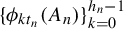


If $(X,\phi _t,\mu )$
is the flow considered in the previous two sections, since it is a suspension over a rank-one transformation and the roof function is piecewise constant, the following is immediate.
$(X,\phi _t,\mu )$
is the flow considered in the previous two sections, since it is a suspension over a rank-one transformation and the roof function is piecewise constant, the following is immediate.
Lemma 6.4. Let T denote any staircase transformation and let f be a roof function that is $2$
-wise constant, characterized by two height values that are rationally independent. Consider
$2$
-wise constant, characterized by two height values that are rationally independent. Consider $\phi _t$
as the flow constructed under f for T. Then,
$\phi _t$
as the flow constructed under f for T. Then, $\phi _t$
is a rank-one flow.
$\phi _t$
is a rank-one flow.
In [Reference RyzhikovRyz92, §4], Ryzhikov proved the following theorem.
Theorem 6.5. (Ryzhikov [Reference RyzhikovRyz92])
If $\phi _t$
is a mixing rank-one flow, then
$\phi _t$
is a mixing rank-one flow, then $\phi _t$
is n-fold mixing for any n.
$\phi _t$
is n-fold mixing for any n.
In sight of Theorems 5.5 and 6.5, the following is obtained.
Corollary 6.6. Let T denote any mixing staircase transformation and let f be a roof function that is $2$
-wise constant, characterized by two height values that are rationally independent. Consider
$2$
-wise constant, characterized by two height values that are rationally independent. Consider $\phi _t$
as the flow constructed under f for T. Then, the flow
$\phi _t$
as the flow constructed under f for T. Then, the flow $\phi _t$
is n-fold mixing for any n.
$\phi _t$
is n-fold mixing for any n.
7 Conclusion
Exploring the case of general rank-one mixing transformations would be a natural next step. Our results for mixing staircases suggest that, under additional suitable conditions on the rank-one construction, mixing in the associated suspension flows could potentially be established. Notably, the first part of our proof relies only on the mixing properties of T, which are well understood for rank-one transformations. However, the second part crucially depends on the staircase-like structure to obtain sequences of heights with controlled properties. Extending this approach to general mixing rank-one transformations would likely require further refinement and deeper investigation.
Acknowledgement
I sincerely thank my advisor, Anja Randecker, for her encouragement and meticulous reading of this work. I am also grateful to Rodrigo Treviño for bringing this problem to my attention. This work was funded by the Deutsche Forschungsgemeinschaft (DFG, German Research Foundation)—Project number RTG 2229: Asymptotic Invariants and Limits of Groups and Spaces.
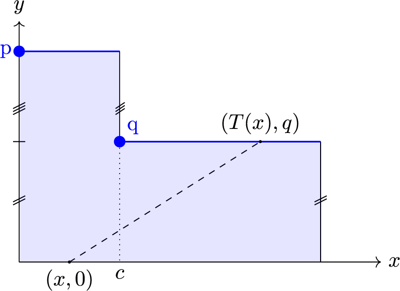
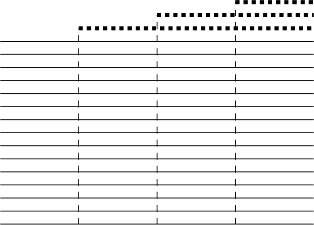


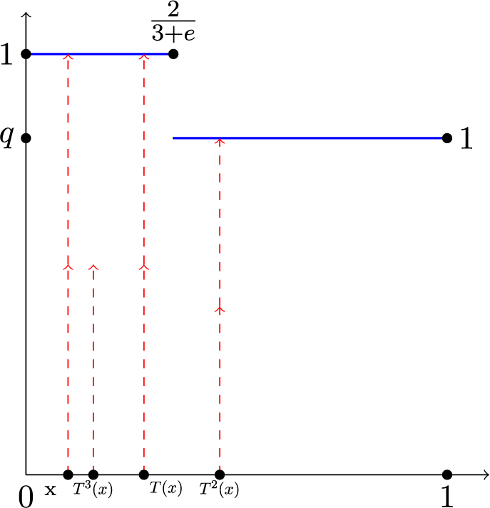







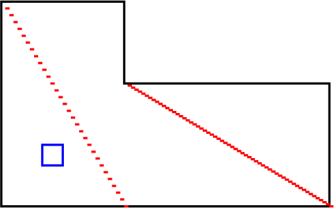
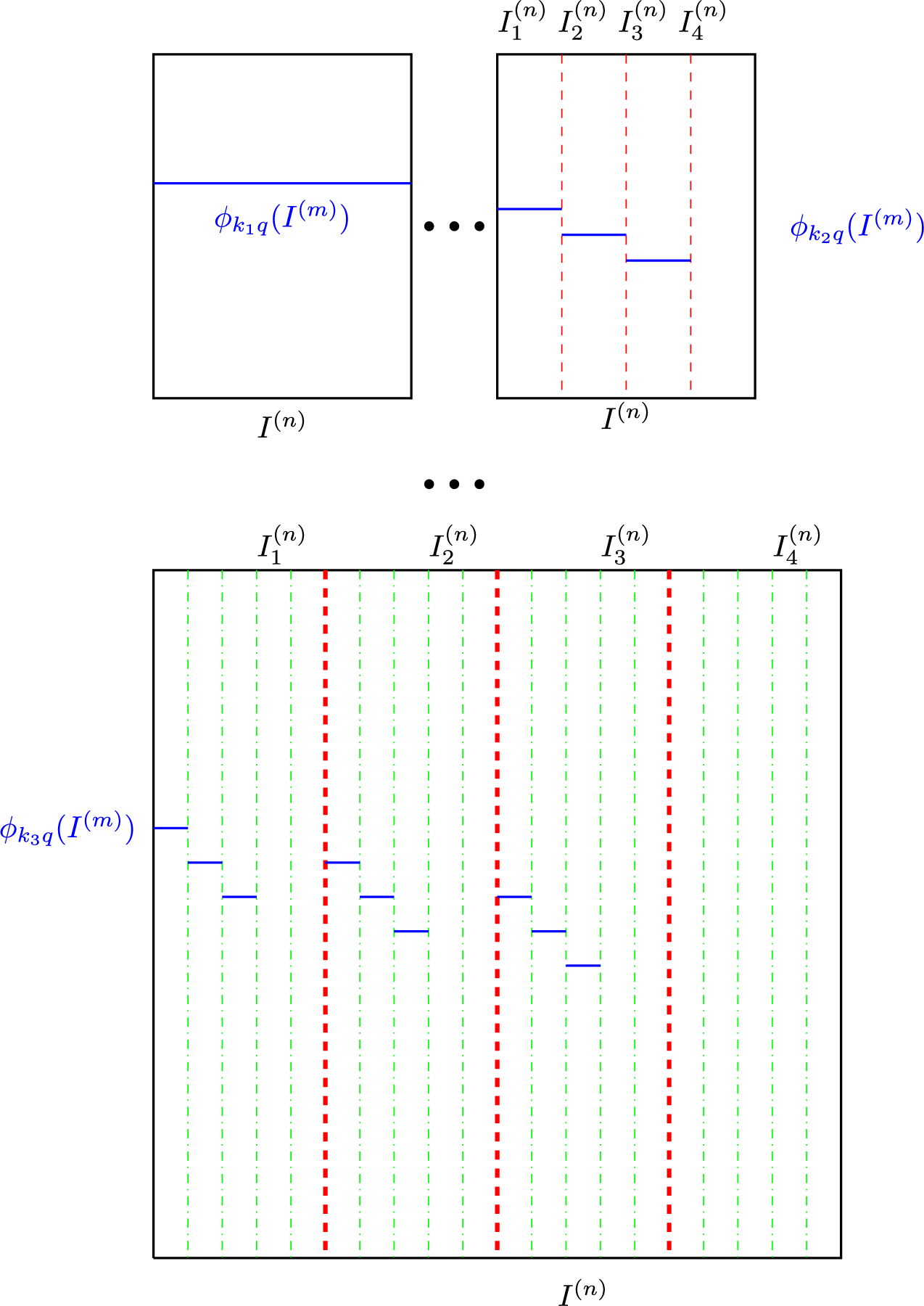


 Open access

