


1. Introduction
High-Reynolds-number flows are characterised by complex spatio-temporal dynamics resulting from the superposition and interactions of flow features spanning a wide range of spatial and temporal scales. We often seek low-dimensional descriptions in the form of an optimal set of basis functions which capture the dominant flow dynamics, physically controlling features and coherent patterns embedded in noise. The distinct vortex shedding pattern due to the Bénard–von Kármán instability (Perry, Chong & Lim Reference Perry, Chong and Lim1982) and shear layer vortices due to the Kelvin–Helmholtz instability (Prasad & Williamson Reference Prasad and Williamson1997) are examples of dynamically important coherent structures in turbulent shear flows. Low-dimensional structures such as these can be identified and extracted from high-dimensional data using a range of different methods. These include both physics-based methods, such as hydrodynamic stability analysis, and data-driven techniques, such as proper orthogonal decomposition (POD), dynamic mode decomposition (DMD) or traditional Fourier mode decomposition. This work is based on POD (Lumley Reference Lumley1967, Reference Lumley1970), which has been extensively used for dimensionality reduction, feature extraction, reduced-order modelling and data reconstruction/visualisation (Holmes et al. Reference Holmes, Lumley, Berkooz and Rowley2012; Rowley & Dawson Reference Rowley and Dawson2017; Taira et al. Reference Taira, Brunton, Dawson, Rowley, Colonius, McKeon, Schmidt, Gordeyev, Theofilis and Ukeiley2017).
Fluid flows are commonly described by space–time data, here denoted  $\boldsymbol {q}(\boldsymbol {x},t)$, where
  $\boldsymbol {q}$ represents a measured or calculated quantity,
  $\boldsymbol {x}$ represents a general spatial coordinate system and
  $t$ denotes time. The most commonly used form of POD, which provides a space–time separated representation of these data, is referred to as space-only POD in this work, following the naming convention used by Towne, Schmidt & Colonius (Reference Towne, Schmidt and Colonius2018). This form of POD decomposes the mean subtracted flow,
  $\boldsymbol {q}'(\boldsymbol {x},t)=\boldsymbol {q}(\boldsymbol {x},t)-\bar {\boldsymbol {q}}(\boldsymbol {x})$, according to
 \begin{equation} \boldsymbol{q}'\left(\boldsymbol{x},t\right)=\sum_ja_j\left(t\right)\boldsymbol{\phi}_j\left(\boldsymbol{x}\right), \end{equation}
where  $a_j(t)$ are the scalar time-dependent coefficients and
  $\boldsymbol {\phi }_j(\boldsymbol {x})$ are the spatially orthogonal modes. These modes are defined as the uncorrelated directions which maximise the projected variance (or equivalently, minimise the mean squared error) of the input data (Jolliffe Reference Jolliffe2002; Bishop Reference Bishop2006; Holmes et al. Reference Holmes, Lumley, Berkooz and Rowley2012). Proper orthogonal decomposition provides an optimal decomposition of a given flow, as the ordering of the modes ensures that the POD basis captures as much of the variance in the given data with as few modes as possible. Hence, the POD basis can be used to reconstruct a truncated approximation,
  $\boldsymbol {q}_r(\boldsymbol {x},t)$, defined as
 \begin{equation} \boldsymbol{q}_r\left(\boldsymbol{x},t\right)=\bar{\boldsymbol{q}}\left(\boldsymbol{x}\right)+\sum_{j=1}^r a_j\left(t\right)\boldsymbol{\phi}_j\left(\boldsymbol{x}\right), \end{equation}
which provides an optimal linear representation of the flow for any order  $r$. Equation (1.2) provides the smallest mean squared error approximation of the given flow: no other basis can reconstruct the flow with a smaller error. When the input data are in the form of constant-density turbulent velocity fields, the projected variance is proportional to the average turbulent kinetic energy in each mode (Holmes et al. Reference Holmes, Lumley, Berkooz and Rowley2012; Rowley & Dawson Reference Rowley and Dawson2017; Taira et al. Reference Taira, Brunton, Dawson, Rowley, Colonius, McKeon, Schmidt, Gordeyev, Theofilis and Ukeiley2017). Therefore, space-only POD is commonly used to extract high-energy spatial structures from a given flow. Note, however, that there is no restriction on the properties of the time coefficients, and hence a single mode can contain a superposition of flow structures with very different time scales. Further properties of space-only POD relevant to this work are discussed in § 2.1.
Spectral POD (SPOD) is an alternative decomposition approach for statistically stationary flows, which formulates POD in frequency space (Lumley Reference Lumley1970; Towne et al. Reference Towne, Schmidt and Colonius2018). The input data are transformed into Fourier space along the temporal dimension and POD is performed at each discrete frequency. This results in a set of time-harmonic, spatially orthogonal modes ranked according to their energy at each of these frequencies. Thus, SPOD targets flow structures which evolve coherently in space and time. As shown by Towne et al. (Reference Towne, Schmidt and Colonius2018), there is no localised relationship between space-only POD and SPOD modes. For example, a single space-only POD mode can potentially contain information from every single SPOD mode across all frequencies, and vice versa.
This work is motivated by the desire to analyse spatio-temporal data from advection-dominated turbulent flows. Advection is a prominent feature of fluid mechanics problems, as evidenced by the substantial derivatives appearing in the governing equations. However, different decomposition techniques capture advection differently. As discussed by Holmes et al. (Reference Holmes, Lumley, Berkooz and Rowley2012) and Brunton & Kutz (Reference Brunton and Kutz2019), space-only POD represents advecting features (i.e. features with coupled space–time dependencies via their translational character) by a superposition of modes. For example, the simplest case of a single-frequency travelling wave, when cast in the form of (1.1), can be written as
 \begin{equation} A\sin\left[\omega\left(t-\frac{x}{u_c}\right)\right]=A\sin\left(\omega t\right)\cos\left(\frac{\omega x}{u_c}\right)-A\cos\left(\omega t\right)\sin\left(\frac{\omega x}{u_c}\right), \end{equation}
where  $x$ refers to a one-dimensional spatial coordinate,
  $A$ is the amplitude,
  $\omega$ is the angular frequency and
  $u_c$ is the convection velocity of the travelling wave. Thus, a combination of at least two standing waves is required to represent a travelling wave. In practice, travelling structures in real, high-Reynolds-number flows are spread across many space-only POD modes. Often, manual inspection is used to interpret which modes collectively represent a travelling disturbance (e.g. see figure 7), although techniques have been developed which automate this process, such as identifying ‘linked modes’ via a DMD on the time coefficients from POD (Sieber, Paschereit & Oberleithner Reference Sieber, Paschereit and Oberleithner2016). In contrast, the ‘translation’ property of the Fourier transform enables SPOD to capture space–time correlated information, such as travelling waves (Towne et al. Reference Towne, Schmidt and Colonius2018). For example, SPOD decomposes equation (1.3) as a single complex mode, whose mode shape is given by
  $\exp ({\mathrm {i}\omega x/u_c})$, while decomposing a more general, non-dispersive travelling wave,
  $f(t-x/u_c)$, as a single mode with a spectrum given by
  $F(\omega )\exp ({\mathrm {i}\omega x/u_c})$. However, in the event that a single physical flow feature contains multi-frequency content, SPOD splits this information across different SPOD modes. For highly turbulent flows, where coherent structures can occur intermittently and often display variable-frequency characteristics due to phase jitter or frequency modulations, a single physical feature is therefore likely to be represented by multiple SPOD modes.
Many alternative POD methods have been suggested to provide additional insights and complementary perspectives to the ones offered by space-only POD and SPOD. Often, the goal of these methods is to capture space–time correlated flow features with an easy-to-interpret, more compact set of basis functions, as the performance of space-only POD depends on the coordinate system in which the data are represented. As discussed by Brunton & Kutz (Reference Brunton and Kutz2019), the increased rank of the space-only POD basis due to translation is not intrinsic to the method itself but, rather, reflects the ‘geometric dependence’ of the singular value decomposition (SVD). Using a spatial transformation, translational symmetries can be removed from the data before extracting the modes, as expressed by
 \begin{equation} \boldsymbol{q}'_{sh}\left(\boldsymbol{x},t\right)=\sum_{j}a_j\left(t\right)\boldsymbol{\phi}_j(\boldsymbol{x}+c_j(\boldsymbol{x},t)), \end{equation}
where  $c_j(\boldsymbol {x},t)$ denotes a specified shift velocity such that the decomposition is performed in the reference frame of a travelling structure. Commonly, a single shift velocity is assumed, which is determined using centring or template fitting. Centring refers to the procedure of identifying the centre point of a wave and then shifting the data such that the centre in each snapshot is at the same point (Glavaski, Marsden & Murray Reference Glavaski, Marsden and Murray1998). Template fitting shifts the data at each time such that they align with (i.e. are maximally correlated to) a preselected template (Sirovich, Kirby & Winter Reference Sirovich, Kirby and Winter1990; Kirby & Armbruster Reference Kirby and Armbruster1992; Rowley & Marsden Reference Rowley and Marsden2000; Rowley et al. Reference Rowley, Kevrekidis, Marsden and Lust2003). Furthermore, Fedele, Abessi & Roberts (Reference Fedele, Abessi and Roberts2015) reduced translational symmetry in turbulent pipe flow measurements using a Fourier-based method, while Reiss et al. (Reference Reiss, Schulze, Sesterhenn and Mehrmann2018) developed an iterative procedure which handles structures advecting at different velocities. This iterative procedure separates the modes into different reference frames using a spatial shift determined by the different advection velocities. Common to all these studies is that determining the shift velocity and calculating the (shifted) POD modes are independent, potentially iterative steps.
Extending the idea of a spatial transformation, Sesterhenn & Shahirpour (Reference Sesterhenn and Shahirpour2019) introduced a spatio-temporal transformation whereby the modal decomposition (space-only POD or DMD) is carried out along a direction characteristic to the travelling structure. This direction is identified as the rotation of the data in space and time which produces the largest reduction in the singular values when performing an SVD. Physically, this direction coincides with the group velocity of the travelling structure. A new time coordinate is aligned with the direction of the characteristic and the decomposition (demonstrated using DMD) is performed on planes (snapshots) normal to it. Hence, each new, transformed snapshot contains spatial information about the travelling structure across a range of physical time steps, enhancing the method's ability to capture coherent space–time structures with fewer modes.
In a different vein, Sieber et al. (Reference Sieber, Paschereit and Oberleithner2016) introduced a method which applies a filtering operation on the POD covariance matrix, resulting in a decomposition which mitigates the superposition of features with different time scales within a given spatial POD mode. Since coherent structures are generally associated with a relatively narrow range of time scales (but not necessarily a distinct frequency), this filtering operation allows for a single mode to provide a more comprehensive representation of a given flow structure. Furthermore, Schmidt & Schmid (Reference Schmidt and Schmid2019) proposed a conditional space–time POD formulation targeting the statistics of rare or intermittent events via their space–time coherence during finite time intervals. By construction, this method provides spatio-temporal POD modes which are orthogonal in a space–time inner product over a finite time interval.
A key motivator for this work is the reorientation of the space–time coordinates noted by Schmid (Reference Schmid2010), who demonstrated that DMD can be applied either spatially or temporally. The temporal DMD analysis decomposes the data into spatial modes that temporally evolve as  $\exp ({\mathrm {i}\omega _r t}) \exp ({\omega _i t})$. In this way, the modes are analogous to the linear modes from global hydrodynamic stability analysis. However, Schmid also noted that the method could be applied equally well for a spatial analysis of the data by reorienting the space–time axes. In this case, the DMD modes are transverse space–time modes that spatially evolve as
  $\exp ({\mathrm {i}k_r x}) \exp ({k_i x})$ in a similar manner to spatial stability modes from local hydrodynamic stability analysis
This work utilises Schmid's (Reference Schmid2010) approach of reorienting the space–time coordinates in the context of POD, while noting that the multi-dimensional POD theory is independent of an a priori distinction between the space and time variables (Holmes et al. Reference Holmes, Lumley, Berkooz and Rowley2012). The reorientation can be accomplished by simply permuting the input data to obtain a snapshot sequence in space rather than time. This permutation applied to POD, an approach referred to as permuted POD (PPOD), is the focus of this paper (Ek et al. Reference Ek, Proscia, Lieuwen and Emerson2019). In PPOD, the space–time variables are permuted such that the PPOD modes are orthogonal in time and the spatial coordinate  $s$, defined along the bulk advection direction, while the coefficients provide the profiles along the mutually orthogonal directions
  $\boldsymbol {n}=(n_1,n_2)$ which are taken to be normal to the advection direction. Permuted POD is noted to have several interesting properties. First, PPOD targets correlations in
  $s,t$ space and naturally captures advecting structures. As such, it is not necessary to do an a priori determination of disturbance advection speeds. Rather, such speeds are a natural output of the analysis and can vary in an arbitrary and dispersive manner along the
  $s$ coordinate. Second, the modes can have an arbitrary time dependence, and need not be composed of a single fundamental frequency, so a broadband or multi-frequency disturbance can be described by a single mode. This can be an attractive property, as high-Reynolds-number flows generally have coherent advecting structures with a combination of narrowband fundamental and harmonic spectral features, as well as more spectrally distributed features. This arbitrary time dependence also allows PPOD to be applied to transient flow phenomena, since the method does not require the flow to be statistically stationary. Finally, the two-dimensional Fourier transform of the PPOD modes presents amplitudes in the
  $k$–
$k$– $\omega$ plane, which provides a useful alternative way to summarise modal characteristics. For example, in cases where the PPOD mode is dominated by a structure with a narrowband spectral signature, the wavenumber–frequency spectrum can be compared with the dispersion relation from local linear hydrodynamic stability analysis and the transverse coefficients,
  $a_j(\boldsymbol {n})$, can be compared to the stability mode shapes. Thus, while space-only POD modes can be compared to the modes from a global linear stability analysis (Tammisola & Juniper Reference Tammisola and Juniper2016), a local linear stability analysis naturally lends itself to comparison with PPOD modes.
The objective of this paper is to further evaluate the PPOD technique and compare its results with space-only POD, emphasising the complementary and distinctive perspectives that the two approaches provide. In addition to basic characterisation of PPOD, key questions we wish to address include:
(i) What are the dominant energetic structures in PPOD and how do they compare with space-only POD?
(ii) In cases where these dominant structures appear the same, how do the energy convergence rates compare?
(iii) Due to nonlinearity, coherent structures generally consist of many disturbance frequencies with spatially evolving spectral content and higher harmonics. How does PPOD decompose such multi-frequency content?
(iv) A given flow may consist of distinct structures which advect dispersively and at different phase speeds (e.g. the inner and outer shear layers of a coaxial or annular jet). How does PPOD decompose such different disturbances across modes?
This work consists of two major sections. First, § 2 presents the basic mathematical features of PPOD and highlights key differences compared with space-only POD. Then, § 3 presents three case studies, using data from high-Reynolds-number, advection-dominated flows including a reacting wake, a reacting swirling annular jet and a non-reacting jet in cross-flow (JICF).
2. Overview of space-only POD and permuted POD properties
2.1. Space-only POD properties
The implementation of space-only POD has been detailed by many authors (e.g. Berkooz, Holmes & Lumley Reference Berkooz, Holmes and Lumley1993; Holmes et al. Reference Holmes, Lumley, Berkooz and Rowley2012; Rowley & Dawson Reference Rowley and Dawson2017; Taira et al. Reference Taira, Brunton, Dawson, Rowley, Colonius, McKeon, Schmidt, Gordeyev, Theofilis and Ukeiley2017), and this section briefly summarises key details in order to compare with PPOD. The flow data,  $\boldsymbol {q}(\boldsymbol {x},t)$, are acquired at a number of discrete time instants over a set of discrete points in one, two or three spatial dimensions. Here, we will assume for convenience that the data are obtained on a uniformly spaced grid in a Cartesian coordinate system; more general situations are addressed in § 2.3. The mean-subtracted data at each time instant
  $t_j$ are arranged as a column vector denoted
  $\boldsymbol {q}_j\in \mathbb {R}^{N_{\boldsymbol {x}}}$ which is then stacked alongside column vectors from other time instants to form the data matrix
  $\boldsymbol{\mathsf{Q}}\in \mathbb {R}^{N_{\boldsymbol {x}}\times N_t}$. Here,
  $N_{\boldsymbol {x}}$ refers to the dimensionality of each observation which equals the number of spatial grid points multiplied by the number of variables considered at each grid point, and
  $N_t$ is the number of temporal observations. The space-only POD modes are the eigenvectors of the spatial covariance matrix
  $\boldsymbol{\mathsf{C}}_{\boldsymbol {x}}=\boldsymbol{\mathsf{Q}}\boldsymbol{\mathsf{Q}}^{\mathrm {T}}\in \mathbb {R}^{N_{\boldsymbol {x}}\times N_{\boldsymbol {x}}}$ (excluding the factor
  $1/N_t$ in the covariance definition). When the spatial dimensionality of an observation is much larger than the number of temporal observations (i.e.
  $N_{\boldsymbol {x}}\gg N_t$), it is computationally less expensive to obtain the space-only POD modes from a method commonly referred to as snapshot POD. Snapshot POD was introduced by Sirovich (Reference Sirovich1987) and utilises the temporal covariance matrix
  $\boldsymbol{\mathsf{C}}_t=\boldsymbol{\mathsf{Q}}^{\mathrm {T}}\boldsymbol{\mathsf{Q}}\in \mathbb {R}^{N_t\times N_t}$. Assuming a linearly independent set of observations, the rank of the space-only POD problem is governed by
  $\min (N_{\boldsymbol {x}},N_t)$. The reader is referred to Taira et al. (Reference Taira, Brunton, Dawson, Rowley, Colonius, McKeon, Schmidt, Gordeyev, Theofilis and Ukeiley2017) and Holmes et al. (Reference Holmes, Lumley, Berkooz and Rowley2012) for more information on the spatial versus temporal eigenvalue problems and their connection to the SVD.
This work utilises an economy sized SVD of the data matrix  $\boldsymbol{\mathsf{Q}}$, computed using a direct algorithm, which provides
  $M$ spatially orthogonal modes, where
  $M$ is equal to the number of temporal snapshots (
 $N_t$) used for the decomposition (equivalent to snapshot POD). Associated with each space-only POD mode
  $\boldsymbol {\phi }_j(\boldsymbol {x})$ is an eigenvalue
  $\lambda _j$ (related to the singular values
  $\sigma _j$ from the SVD via
  $\lambda _j=\sigma _j^2$) and a time coefficient
  $a_j(t)=\boldsymbol{\mathsf{Q}}^\mathrm {T}\boldsymbol {\phi }_j(\boldsymbol {x})$. The modes are ordered according to their eigenvalues via
  $\lambda _1\geq \lambda _2\geq \cdots \geq \lambda _M\geq 0$, where each eigenvalue
  $\lambda _j$ is equal to the projected variance of the input data onto mode
  $\boldsymbol {\phi }_j(\boldsymbol {x})$. The projection operation is defined according to the standard inner product, which constitutes a sum over the spatial domain. This provides the energy-based ranking referred to in § 1, where it was remarked that the projected variance
  $\lambda _j$ is proportional to the average turbulent kinetic energy in mode
  $\boldsymbol {\phi }_j(\boldsymbol {x})$ when the input data consist of mean-subtracted, constant-density velocity fields. This work utilises cumulative percent energy,
  $E_c(m)$, which is the sum of the energy of modes 1 through
  $m$ as a fraction of the energy summed over all modes
  $M$, as a measure of convergence for the POD basis:
 \begin{equation} E_c\left(m\right)=100\times\left(\frac{\sum_{j=1}^m\lambda_j}{\sum_{j=1}^M\lambda_j}\right). \end{equation}
2.2. Permuted POD properties
With this background, we next consider PPOD in more detail. Permuted POD is formulated by describing space in terms of  $\boldsymbol {x}=(s,\boldsymbol {n})$ coordinates, where the
  $s$ coordinate is taken along the bulk advection direction in curvilinear space, and
  $\boldsymbol {n}=(n_1,n_2)$ are defined along mutually orthogonal directions normal to it. This provides a decomposition of
  $\boldsymbol {q}'(\boldsymbol {x},t)$ according to
 \begin{equation} \boldsymbol{q}'\left(\boldsymbol{x},t\right)=\sum_{j}a_j\left(\boldsymbol{n}\right)\boldsymbol{\phi}_j\left(s,t\right), \end{equation}
where  $a_j(\boldsymbol {n})$ are the transverse coefficients and
  $\boldsymbol {\phi }_j(s,t)$ are the orthogonal modes. Utilising the discrete space–time form of the data
  $\boldsymbol {q}(\boldsymbol {x},t)$ centred by the temporal mean, the
  $s,t$ data at each normal location
  $n_j$ are formed into a column vector
  $\boldsymbol {p}_j\in \mathbb {R}^{(N_s\times N_t)\times 1}$ and stacked side by side to form the data matrix
  $\boldsymbol{\mathsf{P}}\in \mathbb {R}^{(N_s\times N_t)\times N_{\boldsymbol {n}}}$, where
  $N_s$ is the dimensionality in the
  $s$ coordinate (the number of grid points times the number of variables considered at each grid point) and
  $N_{\boldsymbol {n}}$ refers to the number of total grid points in
  $\boldsymbol {n}$. Hence, the data matrix
  $\boldsymbol{\mathsf{P}}$ is constructed from a ‘snapshot’ sequence in the spatial directions
  $\boldsymbol {n}$. In the case where the data are derived from a uniform Cartesian grid and where
  $s$ is aligned with one of the coordinate directions,
  $\boldsymbol{\mathsf{P}}$ can easily be obtained from a simple permutation of
  $\boldsymbol{\mathsf{Q}}$. The PPOD eigenvalue problem is derived using a variational argument (similar to the derivations detailed by Bishop (Reference Bishop2006) and Holmes et al. (Reference Holmes, Lumley, Berkooz and Rowley2012)), where the variance of the input data is maximised as it is projected onto subsequent orthogonal directions, in this case in the
  $s,t$ space. This provides a set of orthogonal modes,
  $\boldsymbol {\phi }_j(s,t)$, which are the eigenvectors of the
  $s,t$ covariance matrix,
  $\boldsymbol{\mathsf{C}}_{s,t}=\boldsymbol{\mathsf{P}}\boldsymbol{\mathsf{P}}^\mathrm {T}\in \mathbb {R}^{(N_s\times N_t)\times (N_s\times N_t)}$. When
  $N_s\times N_t\gg N_{\boldsymbol {n}}$, which is often the case for experimental data, it is computationally less expensive to obtain the PPOD modes from the
  $\boldsymbol {n}$ covariance matrix
  $\boldsymbol{\mathsf{C}}_{\boldsymbol {n}}=\boldsymbol{\mathsf{P}}^\mathrm {T}\boldsymbol{\mathsf{P}}\in \mathbb {R}^{N_{\boldsymbol {n}}\times N_{\boldsymbol {n}}}$, i.e. the PPOD equivalent of snapshot POD. Assuming the ‘snapshots’ in
  $\boldsymbol {n}$ are linearly independent, the rank of the PPOD problem is governed by
 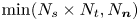 $\min (N_s\times N_t,N_{\boldsymbol {n}})$.
The PPOD modes in this work are calculated using an economy sized SVD of the data matrix  $\boldsymbol{\mathsf{P}}$, the same direct method as for space-only POD, which provides
  $M'$ orthogonal modes, where
  $M'$ is equal to the number of normal locations (
 $N_{\boldsymbol {n}}$) used for the decomposition. Associated with each PPOD mode
  $\boldsymbol {\phi }_j(s,t)$ is a corresponding eigenvalue
  $\lambda _j$ and normal coefficient
  $a_j(\boldsymbol {n})=\boldsymbol{\mathsf{P}}^\mathrm {T}\boldsymbol {\phi }_j(s,t)$. The PPOD approach provides an optimal description of the input data, where the PPOD modes are ordered according to their eigenvalues,
  $\lambda _1\geq \lambda _2\geq \cdots \geq \lambda _{M'}\geq 0$, and the eigenvalue
  $\lambda _j$ is equal to the projected variance of the input data onto mode
  $\boldsymbol {\phi }_j(s,t)$. The standard inner product for the PPOD projection operation constitutes a sum over the
  $s,t$ domain, rather than a sum over the spatial domain as for space-only POD. In the case of mean-subtracted velocity data, the PPOD eigenvalues are proportional to the turbulent kinetic energy density (an intrinsic property) summed over
  $s$ and
  $t$. The implications due to the different inner products, and hence the different energy-based rankings associated with PPOD and space-only POD are discussed further in the context of a simple model problem in § 2.4 as well as in the high-Reynolds-number datasets in § 3. The convergence behaviour of PPOD is evaluated in a similar manner to (2.1), where the sum of the first
  $m$ eigenvalues is divided by the sum of all the eigenvalues, 1 through
  $M'$. We refer to the convergence behaviour and the ordering of both PPOD and space-only POD modes as being based on the flow ‘energy’, keeping in mind that the ‘energy’ metrics for PPOD and space-only POD are different and that a physical energy ranking based on the turbulent kinetic energy only applies to space-only POD performed on mean-subtracted, constant-density velocity data.
2.3. Coordinate transformations
Since PPOD is formulated in a curvilinear orthogonal coordinate system where  $s$ is defined along the bulk advection direction, a coordinate transformation is often required before performing the decomposition. For example, when the bulk advection direction does not coincide with one of the coordinates in which the data are acquired, a transformation to curvilinear coordinates is necessary for optimal PPOD convergence characteristics, as demonstrated in § 2.4. To enable back-to-back comparison of PPOD and space-only POD results in the curvilinear orthogonal coordinate system (as utilised for case 3, § 3.3), the space-only POD calculation must be appropriately weighted. Since we choose to formulate space-only POD in a uniformly spaced Cartesian coordinate system (motivated by the physical energy interpretation of its spatial inner product), but perform the calculation in the
  $s,\boldsymbol {n}$ coordinate system, the spatial inner product must be weighted by the Jacobian determinant of the coordinate transformation to preserve the physical turbulent kinetic energy ranking of the space-only POD basis. In contrast, PPOD is defined based on the
  $s,t$ inner product, which does not require any weighting for interpretation in uniformly sampled
  $s,\boldsymbol {n},t$ spaces. In the rest of this paper, we consider data from planar measurements such that only two-dimensional (i.e.
  $\boldsymbol {x}=(s,n)$) coordinates are necessary. Furthermore, planar three-component velocity data in curvilinear orthogonal form are denoted
  $u_s,u_n,u_z$, where
  $u_z$ is the out-of-plane component.
A second set of coordinate transformation considerations arise when considering planar data through systems with other symmetries. For example, consider the transverse velocity component associated with planar data acquired through the centre of a round jet (as in e.g. Alomar et al. Reference Alomar, Nicole, Sipp, Rialland and Vuillot2020). In a cylindrical coordinate system, radial velocity components directed away from the centreline are positive. These radial velocity components will have the same (opposite) sign as the corresponding transverse velocity in a Cartesian coordinate system above (below) the centreline, respectively. The same is true for the out-of-plane velocity component, which corresponds to an azimuthal velocity in cylindrical coordinates. This is important, as PPOD will decompose a velocity disturbance with azimuthal symmetry given by  $\exp (\mathrm {i}m_{\theta }\theta )$ differently in these two coordinate systems. In the cylindrical coordinate system, the three velocity components (
 $u_x,u_r,u_{\theta }$) have consistent symmetries across the centreline (i.e. at
  $\theta =0$ or
  $\theta ={\rm \pi}$). More specifically, the cylindrical velocity components all have even symmetry for even
  $m_\theta$, and odd symmetry for odd
  $m_\theta$. In contrast, in Cartesian form, the different velocity components have different symmetries. Thus, if a helical disturbance were considered in Cartesian coordinates, its disparate symmetries would necessarily be split between different PPOD modes despite representing a single disturbance.
Appropriate symmetries are achieved by simply reversing the sign of the transverse and out-of-plane velocity components below the jet centreline. The sign convention is consistent with that of a cylindrical coordinate system, but the velocity components are not scaled by a change in volume since the measurement plane, and hence the cell size associated with the measurement resolution, is constant. This coordinate system is therefore referred to as ‘locally cylindrical’ in the rest of the paper.
It should also be noted that the locally cylindrical coordinate transformation can provide appropriate symmetries for non-axisymmetric flows. As in the JICF case study in § 3.3, where velocity data acquired in a plane through the jet and aligned in the direction of the cross-flow are analysed, a sign convention corresponding to a cylindrical coordinate system provides consistent symmetries for capturing windward and leeward shear layer structures. If these structures appear in a symmetric (asymmetric) configuration across the jet centreline, the three velocity components associated with the shear layer rollup will all be symmetric (respectively, asymmetric) in locally cylindrical form, while the velocity components in a Cartesian coordinate system will have mixed symmetries (the axial component will have the opposite symmetry across the jet centreline compared to the transverse and out-of-plane components). Hence, all vector data are subject to the locally cylindrical transformation, and the velocity components do not carry the above noted subscripts ( $x,r,\theta$) when also transformed into curvilinear orthogonal form (applicable to the JICF velocity data in § 3.3).
2.4. Model problem with advecting structures
This section compares the convergence characteristics of PPOD and space-only POD for a synthetic dataset with advecting structures. To clearly illustrate key features of PPOD, consider a time series of linearly independent scalar data sampled uniformly in the two-dimensional plane  $s,n$, which corresponds to a Cartesian plane where
  $N_{\boldsymbol {x}}=N_s\times N_n=25\times 25$. The number of temporal snapshots is chosen such that it equals the number of spatial points in
  $n$, i.e.
  $N_t=N_n=25$, which governs the rank of the space-only POD and PPOD eigenvalue problems via
  $N_t< N_{\boldsymbol {x}}$ and
  $N_n< N_s\times N_t$, respectively. Hence, both methods provide the same number of modes
  $(M=M'=25)$, making comparisons of the convergence characteristics straightforward. The mean-subtracted scalar fields consist of a train of high-intensity
  $5\times 5$ pixel squares with a wavelength of
  $\lambda _s=10$ pixels advecting across the domain at an angle
  $\alpha$ with respect to the
  $s$ axis. To emulate turbulent flow data and prevent rank deficiencies, these advecting structures are superimposed onto a background of low-intensity noise sampled from a uniform distribution with
  ${\pm }20\,\%$ relative amplitude. Additionally, the centre locations of the high-intensity squares are randomly perturbed in order to simulate ‘phase jitter’ effects (Shanbhogue, Seelhorst & Lieuwen Reference Shanbhogue, Seelhorst and Lieuwen2009). These perturbations correspond to spatial shifts of
  ${\pm }1.75$ pixels in both
  $s$ and
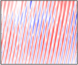
  $n$. To illustrate, three consecutive temporal snapshots of the disturbance scalar fields are displayed in figure 1, where the advecting structures travel along the nominal trajectory indicated by the red dotted line oriented at an angle
  $\alpha$ with respect to the
  $s$ coordinate axis. The black dotted outlines surrounding the advecting structures indicate their maximum allowable spatial variation due to phase noise.
(a–c) Three consecutive temporal snapshots of mean-subtracted scalar fields containing advecting, high-intensity squares, superimposed onto a noisy background. The advecting structures travel along the nominal trajectory indicated by the red dotted line, oriented at an angle  $\alpha$ with respect to the red dashed line parallel to
  $s$. The black dotted outlines surrounding the advecting structures indicate their maximum allowable spatial variation due to phase noise.

It should be emphasised that this model problem is constructed such that two temporal snapshots exactly capture one period of advection, i.e. the sampling frequency is two times the frequency of these structures, and the  $s$ domain fits 2.5 structures (
 $s/\lambda _s=2.5$). In the case of no phase noise, this means that the data are sampled/generated such that the advecting structures are captured in only two distinct spatial configurations as they travel through the domain, and the time series consists of repetitions of these two configurations. Intuitively, space-only POD captures the train of advecting structures with two high-energy modes, while the random background noise is relegated to the remaining 23 low-energy modes. This rank-2 representation of the advecting structures demonstrates that space-only POD can capture certain translations very efficiently (similar to the example of a harmonic travelling wave discussed in the introduction (e.g. (1.3)), which is also described by two space-only modes).
However, translating structures generally are not captured by such a small set of modes, as noted previously. For example, if the data are sampled/generated such that the square structures are captured at many different streamwise locations as they travel through the domain (e.g. if the sampling frequency is increased), the rank of the space-only POD representation of these structures will increase. This can be considered an artificial rank inflation which is strictly due to the translation since critical features no longer appear in the same spatial location from time to time. This decreases the correlation and the variance is redistributed from a few leading, high-energy modes to many lower-energy modes. Whether space-only POD provides a low- or high-rank representation of advecting structures depends on the underlying functional form of the data (i.e. sinusoidal, square, Gaussian, etc.), and the sampling frequency relative to the frequency of the advecting structures. On the other hand, PPOD captures the advecting structures in these cases with a single high-energy mode (assuming that the structure(s) travel along  $s$). The objective of the data permutation associated with PPOD is to align critical features, whether periodic or non-periodic, such that they occur at constant
  $n$. As long as the critical features appear in the same
  $s,t$ locations across ‘normal’ snapshots, PPOD provides a rank-1 representation of the advecting structures. This is similar to the ability of space-only POD to provide a rank-1 representation of a spatially stationary structure (Brunton & Kutz Reference Brunton and Kutz2019).
The following paragraphs demonstrate the effects of phase noise and alignment of the nominal advection trajectory with the  $s$ axis, which can be explained using intuition from the previous discussion. Calculations are performed on datasets with ten different values of
  $\alpha$, from
  $0^{\circ }$ to
  $45^{\circ }$. To ensure a statistical representation of the convergence behaviour at each angle, 100 datasets with 25 temporal snapshots each are generated with randomly assigned phase and background noise, as specified above. Space-only POD and PPOD are performed on each of these 100 model datasets, and the results (i.e. the eigenvalues) at each
  $\alpha$ are averaged. The averaged cumulative percent energy as a function of mode number is shown in figure 2(a). Consider first the case where the nominal advection trajectory is perfectly aligned with
  $s$ (i.e.
  $\alpha =0^{\circ }$). As expected from our previous discussion, PPOD displays a significantly higher convergence rate than space-only POD, since the advecting structures are mostly (apart from the random displacement caused by the normal phase noise) aligned in
  $n$. The first PPOD mode captures
  ${\sim }70\,\%$ of the energy, while four space-only POD modes are required to capture the same amount. For a complete representation of the advecting structures,
  $E_c\sim 90\,\%$ is required, which is captured by the first four PPOD modes and the first 12 space-only POD modes. This can be compared to the one PPOD mode and two space-only POD modes required to capture these structures in the case of no phase noise and
  $\alpha =0^{\circ }$. Hence, the phase noise causes a four times versus six times increase in the number of modes required to capture the advecting information for PPOD and space-only POD, respectively. This demonstrates that the convergence behaviour of PPOD is less sensitive to phase noise than space-only POD, since the convergence of PPOD is only affected by the phase noise in the normal direction, while space-only POD is sensitive to the phase noise in both the normal and streamwise directions, consistent with the discussion in the previous paragraph.
Dependence of (a) cumulative percent energy,  $E_c$, as a function of the number of modes,
  $m$, and (b) condition number,
  $\kappa$, as a function of the angle,
  $\alpha$, between the nominal advection trajectory and
  $s$. The error bars in (b) represent the variability in
  $\kappa$ due to the random background noise and phase jitter displaying one standard deviation.

Next, consider the effect of  $\alpha$. The convergence characteristics of PPOD are a strong function of the alignment of the advecting structures with respect to
  $s$. This is demonstrated in figure 2(a), where the energy of the leading mode decreases as
  $\alpha$ increases, and a larger number of modes is required to capture the advecting structures (i.e. reach
  $90\,\%$
  $E_{c}$). This increase in rank for increasing
  $\alpha$ occurs since the advecting structures are no longer perfectly aligned between ‘normal’ snapshots, consistent with previous discussions. The convergence characteristics of space-only POD, on the other hand, are independent of
  $\alpha$ since the advecting structures appear in two distinct spatial configurations through time for each
  $\alpha$.
To clearly visualise each method's convergence rate as a function of  $\alpha$, we use the condition number
  $\kappa$, defined as the ratio of the largest to the smallest eigenvalue. As mentioned previously, economy sized SVDs of the data matrices
  $\boldsymbol{\mathsf{Q}}$ and
  $\boldsymbol{\mathsf{P}}$ (which correspond to the eigenvalue problems of the temporal covariance matrix
  $\boldsymbol{\mathsf{C}}_t$ and the normal covariance matrix
  $\boldsymbol{\mathsf{C}}_n$) are used to compute all eigenvalues for space-only POD and PPOD, respectively. Since
  $N_t=N_s=N_n=25$ for this model problem,
  $N_t< N_{\boldsymbol {x}}$ and
  $N_n< N_s\times N_t$, and the economy sized SVDs provide non-zero eigenvalues for both methods. Under such conditions,
  $\kappa$ can be used as a measure of each decomposition's convergence rate, where a large
  $\kappa$ indicates fast convergence. The averaged
  $\kappa$ as a function of
  $\alpha$ is shown in figure 2(b), where the error bars indicate one standard deviation over the 100 datasets used for the calculation at each
  $\alpha$. Figure 2(b) quantifies the slower convergence of PPOD as
  $\alpha$ increases and shows that the convergence rate of PPOD is higher than that of space-only POD below a certain
  $\alpha$. For the specified phase noise, PPOD has a faster convergence rate when
  $\alpha \lesssim 30^{\circ }$.
To summarise, this model problem demonstrates that PPOD achieves the highest possible convergence rates when it is performed in a coordinate system aligned with the bulk direction of advecting disturbances, i.e.  $\alpha =0^{\circ }$. It also shows that PPOD achieves favourable convergence rates compared to space-only POD as long as
  $\alpha$ is sufficiently small. Realistic examples with small
  $\alpha$, where the data are acquired in coordinate systems which are closely aligned with the direction of the advecting structures, are considered in §§ 3.1 and 3.2. On the other hand, if
  $\alpha$ is large due to a misalignment between the measurement plane and the
  $s,n$ coordinates, a spatial transformation can be performed to improve the PPOD convergence rate. Such a transformation is implemented in § 3.3.
3. Case studies
This section contains three case studies, using scalar and velocity data from three different turbulent, shear flow experiments. Case 1 uses chemiluminescence data from a forced reacting wake flow with advecting shear layer structures with symmetric and asymmetric features. These datasets were used as they contain different transverse flow symmetries, as well as sharp spatial variation in the flame luminosity, and so require multiple wavenumbers in spectral space to decompose these spatial patterns. In addition, periodic disturbances manifest themselves as a number of spectrally concentrated temporal harmonics in flame luminosity at a given point. As such, this case illustrates how PPOD decomposes a single structure with many constituent frequencies. Case 2 uses planar, three-component velocity data from a reacting, swirl-stabilised flow. High-Reynolds-number swirl flows have significant amounts of strong helical disturbances and phase jitter (i.e. phase noise) in the space–time characteristics of their coherent structures. A common feature of cases 1 and 2 is that the leading snapshot POD and PPOD modes capture similar information. In these cases, our analysis primarily considers the differences in their convergence rates, as well as fidelity in reconstructing spatial and temporal features. Case 3 involves a JICF and the high-energy snapshot POD and PPOD modes capture qualitatively different information, providing additional insights into the differences between the two approaches.
3.1. Case 1: scalar imaging of a forced, reacting wake flow
This case study utilises CH $^*$ chemiluminescence data from a
  $Re_d\sim 10\,000$, rectangular test section housing a flame stabilised by a nominally two-dimensional bluff body of width
  $d_b$, previously detailed by Emerson, Murphy & Lieuwen (Reference Emerson, Murphy and Lieuwen2013) and Emerson & Lieuwen (Reference Emerson and Lieuwen2015). The datasets were acquired at a sampling frequency of 5 kHz, while subjected to axial acoustic forcing at a forcing frequency of
  $f_f=515$ Hz. The bluff body lip velocity,
  $U_{{lip}}$, and the ratio of unburned to burned gas density,
  $\rho _{u}/\rho _{b}$, for each case are summarised in table 1.
Test conditions for the bluff body cases.

Combustion-induced density stratification strongly affects the global stability characteristics, and associated mode shapes, of reacting wake flows. At high density ratios, represented by case 1A ( $\rho _{u}/\rho _{b}=7$), the flow is globally stable, but the axial forcing excites symmetric rollup of the convectively unstable shear layers, resulting in the symmetric flame wrinkling in figure 3(a). As the density ratio is decreased, the global wake mode is destabilised. Case 1B (
 $\rho _{u}/\rho _{b}=2.5$) is an intermittent case; while the flow is still globally stable but convectively unstable, the flame wrinkling is intermittently symmetric and asymmetric due to the superposition of varicose forcing upon a sinuous global mode as seen in figure 3(b). At the density ratio of
  $\rho _{u}/\rho _{b}=1.7$, case 1C, the flow is globally unstable and the flame shape displays the strong sinuous character of the underlying flow disturbances (see figure 3c).
Instantaneous flame images of normalised CH $^{*}$ chemiluminescence for three different density ratios: case 1A,
  $\rho _{u}/\rho _{b}=7$ (a); case 1B,
  $\rho _{u}/\rho _{b}=2.5$ (b); case 1C,
  $\rho _{u}/\rho _{b}=1.7$ (c).

This case study is used to demonstrate PPOD on datasets dominated by coherent advecting structures with different symmetries. The primary focus of this section is the analysis of the high-density-ratio case (1A), while the lower-density-ratio cases (1B and 1C) are used to highlight the different transverse symmetries of the flow.
Decompositions are performed on 1500 chemiluminescence snapshots from each of the three cases in table 1. For these wake flows, the bulk advection direction above and below the bluff body centreline is defined along the trajectory of the maximum time-averaged intensity. The angle between each trajectory and the  $x$ axis is small (approximately
  $5^{\circ }$), and PPOD is therefore performed on the data in Cartesian form (i.e.
  $(x,y)=(s,n)$), where the number of spatial grid points in
  $x$ and
  $y$ are 696 and 194, respectively. Since only one variable is considered at each grid point,
  $N_x=N_s=696$,
  $N_y=N_n=194$ and
  $N_{\boldsymbol {x}}=N_x\times N_y=696\times 194$. Snapshot POD produces
  $M=1500$ modes (equal to the number of temporal snapshots,
  $N_t$) while PPOD produces
  $M'=194$ modes (equal to the number of transverse locations,
  $N_y=N_n$).
First, the basic features of the PPOD modes,  $\boldsymbol {\phi }_j(x,t)$, are considered. The first three most energetic modes for case 1A, corresponding to 65 % of the energy, are presented in figure 4. The dominant features of these modes in
  $x$–
$x$– $t$ space form a roughly diagonal pattern, indicative of advecting flow structures propagating in the streamwise direction. Advection properties such as phase speed, wavenumber and temporal frequency can be readily obtained from these modes. For example, it is apparent that the phase speed, which corresponds to the slope of the diagonal structures, increases as a function of streamwise distance, especially noticeable in the small
  $x/d_b$ regions close to the bluff body. This is a gas expansion effect, reflecting the acceleration of the flow in the confined channel.
Space–time dependence of the first three PPOD modes,  $\boldsymbol {\phi }_j(x,t)$, for case 1A.

The PPOD coefficients,  $a_j(y)$, describe the transverse structure of each mode. The profiles associated with the first three modes for case 1A are displayed in figure 5(a), from which it is apparent that the three dominant modes are all symmetric about the centreline. This is consistent with the strong varicose flame shape observed in figure 3, as symmetric vortex structures dominate the unsteady flow field. The transverse profiles associated with modes 1–3 for the lower-density-ratio cases, 1B and 1C, are shown in figures 5(b) and 5(c), respectively. For case 1C, where the flame exhibits a strong sinuous character, the transverse profiles corresponding to the first three modes are all asymmetric. For case 1B, the intermittent case, which exhibits a superposition of varicose and sinuous disturbance features, the profiles corresponding to the first two modes are symmetric, while the profile of the third mode is asymmetric. Although not plotted, the first two symmetric modes of case 1B contain 45 % and 15 % of the total energy, respectively, and the third asymmetric mode contains 10 %.
Transverse profiles,  $a_j(y)$, corresponding to the first three PPOD modes for case 1A (a), case 1B (b) and case 1C (c). Circles indicate symmetric profiles and crosses indicate asymmetric profiles.

Alternative visualisations of the PPOD modes can be obtained by considering the spatial evolution of the temporal Fourier transform or the spatio-temporal Fourier transform, denoted as  $\hat {\boldsymbol {\phi }}_j(x,f)$ and
  $\hat {\boldsymbol {\phi }}_j(k,f)$, respectively. Here, we use
  $f$ instead of
  $\omega =2{\rm \pi} f$ such that the frequency represents a Strouhal number. First, consider the temporal Fourier transform of the spatio-temporal mode,
  $\hat {\boldsymbol {\phi }}_j(x,f)$, shown in figure 6(a) for case 1A. This plot shows that the first mode is dominated by spectral content at the forcing frequency, but also clear spectral content at the first three harmonics. In other words, these lower-amplitude, higher-frequency harmonics are all superimposed into this first mode, rather than being divided out into other modes. As shown later, the snapshot POD analysis separates these higher-order temporal harmonics into lower-energy modes.
Fourier reductions of PPOD modes 1, 2 and 4 for case 1A. (a) The amplitude of  $\hat {\boldsymbol {\phi }}_j(x,f)$ as a function of frequency and streamwise position, where the red profiles represent the streamwise dependence of the amplitude at the forcing frequency and the harmonics. (b) The amplitude of
  $\hat {\boldsymbol {\phi }}_j(k,f)$ as a function of frequency and streamwise wavenumber. The black lines indicate constant phase speed, while the black crosses (mode 1) indicate the maximum amplitude at the forcing frequency and its harmonics.

Performing an additional Fourier transform in the streamwise direction renders the modal structure as a function of frequency and axial wavenumber,  $k$, which is shown in figure 6(b). The black lines of constant slope correspond to lines of constant phase velocity,
  $c_{ph}$. It is apparent that the energy of the first mode is concentrated in a structure that is oscillating at the forcing frequency and advecting at a speed just above the lip velocity. It is noteworthy that the external excitation forces oscillations at the forcing frequency and its harmonics, which exhibit weakly dispersive behaviour. This is particularly apparent for mode 1 (and 5), where the peak amplitude at the fundamental frequency and its harmonics are indicated by black crosses for clarity. For lower-energy modes, which contain more information on higher-degree-of-freedom turbulent motions than coherent advecting disturbances, spectral information is spread more broadly across the constant-speed line rather than clustered at the forcing frequency and harmonics, as demonstrated by mode 4.
We next provide a comparative analysis of the snapshot POD results for case 1A. Figure 7 presents the spatial modes,  $\boldsymbol {\phi }_j(x,y)$, and the Fourier transforms of the associated time coefficients,
  $\hat {a}_j(f)$, are shown in figure 8(a). Mode 1 seems to describe the inherent spatial phase variation in the disturbance characteristics at
  $f_s/f_f=1$; i.e. spatial variability in the flame wrinkling at the same phase in subsequent cycles. Modes 2 and 3, which together contain approximately 33 % of the energy, display the same spatial pattern shifted axially by a quarter-wave relative to one another, and their temporal frequency spectra both display a distinct peak at the forcing frequency,
  $f_s/f_f=1$, indicating the same temporal evolution of these two modes. Modes 2 and 3 constitute the first advecting mode pair. Similarly, modes 7 and 8, which together contain approximately 2.7 % of the energy, form a second advecting mode pair associated with a first-harmonic frequency as indicated by the distinct peak at
  $f_s/f_f=2$. Consistent with (1.3), the mode pairs (
 $2,3$) and (
 $7,8$) independently represent standing wave structures but superimpose in space and time to represent an advecting structure. The clear correlation between these modes is illustrated by the phase portrait in figure 8(b), which plots the relationship between the time coefficients of modes 2, 3 and 7. The (
 $2,3$) superposition captures the symmetric flame wrinkling throughout the domain, from the rollup immediately after the bluff body followed by the growth of these spatial features as they advect downstream. The (
 $7,8$) mode pair captures shorter-length-scale advecting information, which provides the finer details of the flame rollup close to the bluff body (primarily in the region
  $x/d_b<4$). Furthermore, second and third harmonics can also be identified; mode 44 (containing 0.2 % of the energy) and mode 142 (with 0.048 % of the energy) correspond to the peak amplitude at
  $f_s/f_f=3$ and
  $f_s/f_f=4$, respectively. As the order of the harmonic increases, the length scale associated with the coherent flame structures decreases, while the region in which they are coherent shifts closer to the bluff body. In comparison, note that spectral information at the forcing frequency and the harmonics were contained in the first PPOD mode (see figure 6). However, the information captured by this PPOD mode is not identical to the information captured by the combination of space-only POD modes in figure 7. Rather, they capture similar physical flow features, and should be considered approximate qualitative comparisons.
Snapshot POD modes,  $\boldsymbol {\phi }_j(x,y)$, for case 1A, where the colours represent regions of high (red) and low (blue) chemiluminescence.

(a) Fourier transform representation of the time coefficients,  $\hat {a}_j(f)$, from snapshot POD for case 1A, where the spectrum for mode 8 is very similar to the one corresponding to mode 7. (b) The phase portrait of the time coefficients corresponding to modes 2, 3 and 7.

The snapshot POD results for the lower-density-ratio cases (1B and 1C) are similar to the ones just discussed. Both cases have a high-energy advecting mode pair associated with the fundamental frequency, followed by a second advecting mode pair associated with the first harmonic. The primary difference between the three datasets is the spatial patterns associated with the advecting mode pairs, which reflect the different symmetries (as discussed previously in the context of figure 3) due to the difference in density ratio, and hence stability characteristics.
We next compare the convergence characteristics, as well as the nature of the space–time reconstructions for snapshot POD and PPOD. Recall that the convergence according to (2.1) is a measure of the cumulative percent energy, or variance, in the data, and the low-order reconstructions according to (1.2) provide maximum variance/minimum mean squared error approximations of the given flow. Of course, it should be emphasised that these are not true comparisons, as the energy metrics of space-only POD and PPOD are different. However, as long as this caveat is kept in mind, it is still interesting to consider the convergence rates of each method and to plot them together to compare the number of modes required to capture a certain fraction of each one's energy metric. When evaluating the convergence rates, note that experimental flow data commonly consist of many temporal snapshots,  $N_t$, while the spatial resolution is coarser (i.e. small
  $N_y$). Under such conditions, when
  $N_y\ll N_t$ the number of PPOD modes,
  $M'$, is much smaller than the number of snapshot POD modes,
  $M$, i.e.
  $M'\ll M$. With this in mind, consider figure 9, which shows cumulative percent energy,
  $E_c$, as a function of the number of modes,
  $m$, for snapshot POD and PPOD. Using all the temporal snapshots for the comparison (i.e.
  $N_t=1500$), it is clear that fewer PPOD modes are required to capture a specific percentage of the energy as compared to snapshot POD. This is especially apparent among the high-energy modes. However, the total number of PPOD modes is much smaller as compared to the total number of snapshot POD modes due to
  $N_y\ll N_t$.
Cumulative percent energy,  $E_c$, as a function of the number of modes,
  $m$, for snapshot POD and PPOD for case 1A. The light-blue filled circles for snapshot POD (
 $M=1500$) correspond to modes 1–3, 7, 8, 44 and 142 associated with the train of advecting flame wrinkles.

To gain more insight, consider the difference in rank between the two methods. For the reacting wake datasets,  $N_t< N_x\times N_y$ and
  $N_y< N_x\times N_t$. Hence,
  $N_t$ and
  $N_y$ govern the rank of the snapshot POD and PPOD problems, respectively, and additionally
  $N_y< N_x$. Therefore, if the number of temporal snapshots used for the decompositions is reduced, the rank of the snapshot POD problem (
 $N_t$) will decrease, while the rank of the PPOD problem (
 $N_y$) is unaffected. To demonstrate, we have recomputed the results shown in figure 9 as the number of temporal snapshots is reduced from 1500 to 194, such that
  $N_y=N_t$ and
  $M'=M$. Here, the large reduction in temporal snapshots noticeably alters the snapshot POD convergence behaviour due to the change in rank (notice the deviation near
  $m\sim 10$), and since
  $N_t=194$ is no longer a sufficient number of temporal snapshots for a statistical representation of this particular flow. The convergence behaviour of PPOD, on the other hand, is not affected by the reduction in the number of temporal snapshots, since the rank of the PPOD eigenvalue problem is unaffected and its convergence behaviour is tied to the resolution and number of snapshots in the normal direction, rather then in time. Additionally, it should be noted that a change in rank does not necessarily impact convergence. For example, the effect of adding or removing snapshots is negligible if such changes only affect the near-zero eigenvalues, as would be the case for a converged statistically stationary flow.
A more direct way to compare the leading snapshot POD and PPOD modes is to evaluate their truncated space–time reconstructions calculated according to (1.2). Figure 10 shows three instantaneous chemiluminescence fields from the original time series (case 1A) (figure 10a), and the corresponding reconstructed ones based on modes 1–3 for snapshot POD (figure 10b) and PPOD (figure 10c), which account for  ${\sim }52\,\%$ and 62 % of the energy, respectively. The three instantaneous snapshots in figure 10 provide a typical representation of the instantaneous flow, and a visual comparison between these snapshots and the reconstructions can be used to qualitatively evaluate the types of flow structures that space-only POD and PPOD capture in their respective high-energy modes. Additionally, the frequency spectrum for each time series is included, calculated in the shear layer at
  $(x/d_b,y/d_b)=(2,0.5)$. While the reconstructions from both snapshot POD and PPOD provide reasonable overall representations of the flame rollup, including both accurate symmetry and dominant length-scale information, the primary differences between these results are observed in the fine-scale spatial patterns and frequency spectra. While the spectrum of the reconstructed snapshot POD data displays a single, distinct peak at the forcing frequency, the PPOD spectrum contains information at the first four harmonics. In contrast, the fine-scale spatial features, particularly near the first flame rollup region, are much better resolved in snapshot POD. These different results arise from the two different inner products used for maximising the variance as discussed in § 2 and provide insights into the differences in the two approaches for reduced-basis descriptions of the data.
Three instantaneous chemiluminescence images (a) and the corresponding reconstructed fields based on modes 1–3 for snapshot POD (b) and PPOD (c), together with the frequency spectrum for each time series.

3.2. Case 2: velocity fields from a reacting swirling annular jet
This section considers three-component velocity data acquired in the centre plane of a high-Reynolds-number swirling flow. Notable features in the flow include vortex breakdown, shear layer structures, much more rapid spatial decorrelation of these structures and significant levels of phase noise. Full details of the facility, optical set-up and particle image velocimetry (PIV) data processing approaches are presented in Rock et al. (Reference Rock, Chterev, Emerson, Won, Seitzman and Lieuwen2019) and Chterev et al. (Reference Chterev, Rock, Ek, Emerson, Seitzman, Jiang, Roy, Lee, Gord and Lieuwen2017). The dataset in this section was acquired at a combustor pressure of 3.6 bar, a preheat temperature of 445 K, an equivalence ratio of 0.36 and an air inlet velocity of  $65\,\textrm {m}\,\textrm {s}^{-1}$ using a liquid fuel (C5; Edwards Reference Edwards2017; Rock et al. Reference Rock, Chterev, Emerson, Won, Seitzman and Lieuwen2019) injected using a generic pressure atomiser. The nozzle exit diameter is denoted as
  $d_s$. Stereo-PIV measurements were acquired at 5 kHz in the region immediately downstream of the swirler exit.
A total of 3750 mean-subtracted velocity fields were used as input for the POD calculations, including all three velocity components. In this case, the bulk advection direction in each half-plane is defined along the trajectory of the maximum time-averaged velocity magnitude. Near the nozzle exit, each trajectory forms an angle of approximately  $13^{\circ }$ to the
  $x$ axis, a relatively small angle considering the effects of
  $\alpha$ on the PPOD convergence rate explored in § 2.4. Additionally, previous work on similar data has shown that a coordinate transformation which aligns the apparently travelling shear layer structures in the axial direction only marginally effects the results (Ek et al. Reference Ek, Proscia, Lieuwen and Emerson2019). Hence, the coordinate transformation is not a critical step for the PPOD analysis of the annular swirling jet data. In this work, PPOD is therefore performed on data in their original spatial coordinates (i.e.
  $(x,y)=(s,n)$), where the numbers of spatial grid points in
  $x$ and
  $y$ are 35 and 45, respectively. Since three variables are considered at each grid point,
  $N_x=N_s=3\times 35$,
  $N_y=N_n=45$ and
  $N_{\boldsymbol {x}}=N_x\times N_y=3\times 35\times 45$. Additionally, the velocity data are converted to locally cylindrical form (for reasons discussed in § 2.3).
Figure 11(a) shows the first three PPOD modes, together with their associated transverse coefficient indicating the symmetry of each mode in figure 11(b). Based on the clear diagonal pattern in the axial and radial velocity components together with the asymmetric transverse profile, mode 1 describes an asymmetric inner shear layer structure appearing as a staggered pattern of vortices advecting downstream in the combustor centre plane. These vortices are the footprint of a three-dimensional spiral structure with an odd azimuthal periodicity rotating about the flow centreline. Modes 2 and 3 also display diagonal patterns, indicating advecting disturbances in the measurement plane, but are accompanied by different transverse profiles compared with mode 1.
Space–time dependence of the first three PPOD modes,  $\boldsymbol {\phi }_j(x,t)$, for case 2 (a), together with the corresponding transverse coefficient,
  $a_j(y)$, for each mode (b).

Figure 12(a) displays the Fourier transforms, plotting the amplitude of  $\hat {\boldsymbol {\phi }}_1(x,f)$ as a function of frequency and axial position in the form of a waterfall plot for the three velocity components of mode 1, where the red profiles indicate the growth and decay along the peak frequency. Moving from the nozzle exit in the downstream direction, the amplitude initially grows, representing the spatial amplification of the advecting structure. The amplitude then reaches a peak, followed by decay, which likely reflects the breakup of the helical structure into a more complex and less coherent pattern (Grinstein & Fureby Reference Grinstein and Fureby2005; Huang, Wang & Yang Reference Huang, Wang and Yang2006). Figure 12(b) plots the amplitude of
  $\hat {\boldsymbol {\phi }}_1(k,f)$ as a function of frequency and axial wavenumber. This latter representation displays how the information contained in the high-energy modes can be reduced to a relatively concentrated
  $k$–
$k$– $f$ region.
Fourier reductions of the three velocity components for the first PPOD mode. (a) The amplitude of  $\hat {\boldsymbol {\phi }}_1(x,f)$ as a function of frequency and streamwise position, where the red profiles represent the streamwise dependence at the peak frequency. (b) The amplitude of
  $\hat {\boldsymbol {\phi }}_1(k,f)$ as a function of frequency and streamwise wavenumber. The black lines indicate constant phase speed.

We next present the snapshot POD results. The three most energetic snapshot POD modes are shown in figure 13, together with their respective frequency spectra. It is apparent that modes 1 and 2 display similar spatial structures, phase-shifted  $90^{\circ }$ in the streamwise direction, with the same temporal frequency. Although not plotted, these modes are a phase-correlated pair with a phase portrait similar to modes 2 and 3 in figure 8. In the measurement plane, these disturbances correspond to a train of advecting inner shear layer vortices, which physically correspond to a rotating three-dimensional structure, as mentioned in the discussion of the leading PPOD modes.
(a) The first three snapshot POD modes,  $\boldsymbol {\phi }_j(x,y)$, for case 2, where the flow is going from left to right,
  $(x/d_s,y/d_s)=(0,0)$ is the nozzle exit centreline, the in-plane velocity components are visualised as streamlines and the background colour is the out-of-plane vorticity. (b) Below each mode is the corresponding frequency spectrum,
  $\hat {a}_j(f)$.

We next compare the convergence characteristic of snapshot POD and PPOD, keeping in mind the caveat noted earlier of their different energy metrics, and the difference between their eigenvalue problems and rank. As for case 1,  $E_c$ is evaluated for two different numbers of temporal snapshots:
  $N_t=3750$, consistent with previous results, and
  $N_t=45$, which is equal to the number of transverse locations (
 $N_y=N_n$) and, hence, the number of PPOD modes (
 $M'$). The results are displayed in figure 14, and observations similar to those for the wake flow can be seen here. Again
  $N_t< N_{\boldsymbol {x}}$ and
  $N_y< N_x\times N_t$, and hence
  $N_t$ and
  $N_y$ govern the rank of the snapshot POD and PPOD problems, respectively. A reduction in the number of temporal snapshots will therefore have an effect similar to what is observed in § 3.2, where the rank of the snapshot POD problem is reduced, noting that
  $N_t=45$ is not sufficient for a statistical representation of the flow. For PPOD, on the other hand, the rank is unaffected.
Cumulative percent energy,  $E_c$, as a function of the number of modes,
  $m$, for snapshot POD and PPOD for case 2.

Next, the leading, high-energy modes are reconstructed and compared for the two methods. Figure 15 shows three consecutive instantaneous velocity fields ordered from top to bottom (figure 15a), together with the corresponding reconstructions for snapshot POD modes 1 and 2 (figure 15b) and PPOD mode 1 (figure 15c). Both these snapshot POD and PPOD reconstructions capture a majority of the large-scale inner shear layer structures, providing strikingly similar results.
Three consecutive instantaneous flow fields (a), together with the corresponding reconstructed flow fields including mode 1 and 2 from snapshot POD (b) and mode 1 from PPOD (c). Note that the reconstructions include the time-averaged flow.

Although not displayed here, PPOD modes 2 and 3 also contribute to the advecting structures, and we can conclude that the dominant high-energy PPOD modes contain primarily advecting information. In the case of snapshot POD, the inclusion of additional modes (for example modes 3–6) does not significantly alter the vortex shedding pattern as compared to the reconstruction of modes 1 and 2. Rather, modes even further down in the snapshot POD energy ranking must be identified and included in the reconstruction if a more accurate description of the vortex dynamics is desirable. We will come back to this for the JICF case study, where it becomes even more apparent that PPOD and snapshot POD target different types of flow structures, with PPOD focusing on advecting structures and shifting them up in the energy ranking.
3.3. Case 3: velocity fields from a non-reacting jet in vitiated cross-flow
This section presents three-component velocity data acquired in the centre plane of a non-reacting JICF, detailed in Nair et al. (Reference Nair, Sirignano, Schmidheiser, Dillon, Fugger, Yi, Jiang, Hsu, Slipchenko and Roy2020), using the same jet nozzle profile as in Megerian et al. (Reference Megerian, Davitian, De B Alves and Karagozian2007). The main flow entering the test section has a velocity of  $u_\infty =14.5\,\textrm {m}\,\textrm {s}^{-1}$ and a temperature of
  $T_\infty =1250$ K corresponding to a bulk Reynolds number of
  $Re_\infty =11\,000$ based on the cross-channel height. The jet temperature was fixed (
 $T_j=300$ K) and the composition adjusted based on the required density ratio,
  $S=\rho _j/\rho _\infty$, for the two different cases in table 2. The bulk-averaged velocity,
  $u_j$, was set based on the momentum flux ratio
  $J=\rho _ju_j^2/\rho _{\infty } u_{\infty }^2$ and
  $S$. The two test conditions correspond to convectively (case 3A) and globally (case 3B) unstable conditions (Megerian et al. Reference Megerian, Davitian, De B Alves and Karagozian2007; Getsinger et al. Reference Getsinger, Gevorkyan, Smith and Karagozian2014).
Test conditions and data properties for the two JICF cases;  $J=12$ for both cases.

Stereo-PIV was used to obtain the velocity information in the near field of the jet. Raw Mie-scattering image pairs were acquired at a rate of 40 kHz. A representative instantaneous velocity field is presented in figure 16(a), where the in-plane velocity components are displayed as streamlines and the background colour corresponds to the out-of-plane vorticity. The cross-flow enters the measurement region from the left, while the jet is entering from the bottom. The point  $(x/d_j,y/d_j)=(0,0)$ corresponds to the jet exit centreline and the black solid trajectory represents the time-averaged jet centreline defined as the midpoint between the maximum and minimum vorticity. The dotted outline represents the subset of data displayed in figure 16(b), which have been mapped onto the
  $s,n$ coordinate system, where
  $s$ is the coordinate along the time-averaged jet centreline and
  $n$ is the coordinate normal to it. Shear layer vortex (SLV) structures are evident in both the representations shown in figure 16. The measurement region slices these three-dimensional ring structures through the centre plane, resulting in a distinct windward and leeward shear layer, which appears as a staggered, asymmetric pattern, caused due to tilting of the vortex rings (Fric & Roshko Reference Fric and Roshko1994; Kelso, Lim & Perry Reference Kelso, Lim and Perry1996) across the jet centreline. While not evident from a single instantaneous image, there is also a clear, lower-frequency bulk jet flapping motion.
Representative instantaneous velocity field from case 3A in the original Cartesian coordinate system (a), where the streamlines provide the in-plane velocity information, the colour indicates the out-of-plane vorticity, the black solid line is the time-averaged jet centreline and the black dotted outline represents the section of data used for the POD analysis in the curvilinear orthogonal coordinate system shown in (b).

Similar to the previous case studies, the mean-subtracted velocity fields were analysed using PPOD and snapshot POD. A total of  $N_t=3750$ snapshots were used for the analysis including all three velocity components. Both the PPOD and snapshot POD analyses are conducted in the curvilinear orthogonal coordinate system, as motivated by the angle between the jet centreline and
  $y$ axis, which is negligible close to the jet exit, but increases up to
  $24^{\circ }$ and
  $39^{\circ }$ in the downstream region for cases 3A and 3B, respectively. Additionally, the velocity components were converted to locally cylindrical form to enforce consistent symmetries across the jet centreline for the three velocity components associated with the SLV structures, as discussed in § 2.3. Even though the flow is not axisymmetric, the sign convention of the velocity components in locally cylindrical form prevents splitting of the physical structure across PPOD modes due to disparate symmetries. The following results are normalised by the frequency scale
  $u_j/d_j$, when applicable.
The normal velocity component,  $u_n$, of the most energetic PPOD mode,
  $\boldsymbol {\phi }_1(s,t)$, and the associated transverse coefficient,
  $a_1(n)$, are presented in figures 17(a,c) and 17(b,d) for cases 3A and 3B, respectively. Mode 1 is the primary contributor to the high-frequency SLV dynamics in both cases. The Fourier transformed representations of these PPOD modes are shown in figure 17(e,f). Case 3A displays a high-amplitude band extending diagonally in
  $k$–
$k$– $f$ space, approximately along a constant phase speed line. Case 3B, on the other hand, has most of its high-amplitude information clustered in much narrower frequency and wavenumber bands. These observations are consistent with the convective and global stability characteristics for the two cases (Megerian et al. Reference Megerian, Davitian, De B Alves and Karagozian2007).
(a,b) Space–time dependence of the first PPOD mode,  $\boldsymbol {\phi }_1(s,t)$, (c,d) the corresponding transverse coefficient,
  $a_1(n)$, and (e,f) the amplitude of the two-dimensional Fourier reduction,
  $\hat {\boldsymbol {\phi }}_1(k,f)$, together with lines of constant phase speed,
  $c_{ph}/u_j$, for the normal velocity component,
  $u_n$, for case 3A (a,c,e) and case 3B (b,d,f).

Next, a comparative analysis is performed based on the snapshot POD results for case 3A. As observed in previous work on reacting (Nair et al. Reference Nair, Douglas, Wilde, Emerson and Lieuwen2018) and non-reacting (Meyer, Pedersen & Ozcan Reference Meyer, Pedersen and Ozcan2007) jets, the leading, high-energy modes represent jet flapping normal to the jet centreline. Modes 1 and 2, which together capture 28 % of the energy, both represent flapping. Mode 1 is displayed in figure 18(a) as an example of such a mode, while modes 3, 4, 6 and 7 all contribute to the SLV dynamics, representing advecting motion aligned with the jet centreline. Modes 3 and 4, which together account for 9.5 % of the energy, form the first advecting mode pair, primarily capturing large-scale vortex structures starting at  ${\sim }s/d_j=2.5$ and extending downstream. Modes 6 and 7, which together account for 5.5 % of the energy, form a second vortex shedding pair, capturing closely spaced vortex structures closer to the jet exit, and their development downstream. Frequency spectra of modes 1, 3 and 6 are displayed in figure 18(b), where the relatively broadband nature of the peaks for spectra 3 and 6 are characteristic of a convectively unstable JICF. The frequency and length scales of the two mode pairs indicate that these modes correspond to the fundamental and subharmonic shear layer instability mode (Megerian et al. Reference Megerian, Davitian, De B Alves and Karagozian2007).
(a) High-energy snapshot POD modes,  $\boldsymbol {\phi }_j(s,n)$, for case 3A, where the in-plane velocity components are displayed as streamlines and the out-of-plane vorticity is displayed as the background colour. (b) Frequency spectra from the time coefficients,
  $\hat {a}_j(f)$, corresponding to modes 1, 3 and 6, where the spectra for modes 4 and 7 are similar to those for modes 3 and 6, respectively.

These results clearly demonstrate that the leading-order PPOD and snapshot POD modes capture different features of the jet dynamics – the advecting SLV structures in the case of PPOD and the flapping jet motion for snapshot POD. These points can also be seen by reconstructing the high-energy modes from the two methods. Figure 19(a) shows three consecutive instantaneous flow fields (top to bottom) for case 3A. The corresponding reconstructed flow fields based on snapshot POD modes 1–4 ( ${\sim }37\,\%$ of the energy) and 1–7 (
 ${\sim }47\,\%$ of the energy) are displayed in figures 19(b) and 19(c), respectively. The reconstruction of modes 1–4 is dominated by the contribution from the jet flapping modes 1 and 2 (as confirmed by reconstructing these modes separately), while the contribution from the vortex shedding modes 3 and 4 adds only a subtle wave-like pattern in the downstream region. A minimum of the first seven snapshot POD modes must be included in the reconstruction for it to capture the SLV structures along the entire shear layer region, including the smaller but yet distinct features closer to the jet exit. For PPOD, on the other hand, the reconstruction of only mode 1 (
 ${\sim }39\,\%$ of the energy), as displayed in figure 19(d), captures the staggered SLV pattern, including the location of both windward and leeward structures throughout the entire domain. In this manner, extraction of the SLV dynamics in a JICF lends itself to analysis in a PPOD frame of reference, since the
  $s,t$ inner product of PPOD allows us to directly target coherent structures advecting along a fixed direction.
Three consecutive instantaneous flow fields (a), together with the corresponding reconstructed flow fields for snapshot POD modes 1–4 (b), 1–7 (c) and PPOD mode 1 (d) for case 3A. The reconstructions include the time-averaged flow.

4. Concluding remarks
The PPOD formulation inherently targets  $s,t$ correlations by decomposing a given flow field as
  $\boldsymbol {q}'(\boldsymbol {x},t)=\sum _ja_j(\boldsymbol {n})\boldsymbol {\phi }_j(s,t)$, where
  $s$ is along the bulk advection direction. This decomposition is optimal in the
  $s,t$ inner product and therefore targets high-energy advecting structures, while the commonly used space-only POD method is based on a spatial inner product and therefore targets high-energy spatial structures. The PPOD approach exhibits several useful properties for analysis of advection-dominated flows as showcased in this work. First, PPOD modes are not restricted to have any particular time dependence. Hence, a single mode can capture a physical disturbance characterised by multiple frequencies, while the coefficient provides insight about its normal profile. Furthermore, the two-dimensional Fourier transform of a given PPOD mode provides an amplitude map in the
  $k$–
$k$– $\omega$ space, which provides a compact visualisation of disturbance advection velocity or dispersion, and in certain cases can be compared with results from local linear hydrodynamic stability analysis. Note also that the phase speed information in the wavenumber–frequency representation, which can display frequency and space dependencies when applicable, is an output of the decomposition rather than a quantity to be determined a priori.
These properties were considered through the analysis of three case studies using experimental data from high-Reynolds-number canonical flows. Scalar image data from a reacting wake, which is characterised by a broad range of spectral and wavenumber content, showed that the most energetic PPOD and snapshot POD modes appear to be focusing on similar features (also true for the swirling annular jet). However, considering the low-rank approximations of the wake flow, there are in this case clear differences in the methods’ fidelity in capturing spatial and temporal information: space-only POD clearly provides higher-fidelity spatial reconstructions with a smaller number of modes, while PPOD provides more higher-order temporal-spectra content (e.g. the inclusion of the first four harmonics seen in figure 10c). In contrast, the high-energy PPOD and snapshot POD modes for the JICF cases capture completely different types of flow structures. The most energetic snapshot POD modes capture side-to-side flapping of the jet column (standing wave), while the leading PPOD mode(s) captures advecting shear layer structures. This example, in particular, shows that the different energy metrics of PPOD and space-only POD, tied to their different inner products (the  $s,t$ inner product and the spatial inner product, respectively), clearly target different features in flows consisting of both advecting and stationary disturbances.
Taken together, these results demonstrate that there is no ‘best’ method for decomposing these complex, high-degree-of-freedom turbulent flows. Rather, these different approaches provide fascinating insights and ‘lenses’ into different features of the flow that, taken together, provide a deeper understanding of the system dynamics.
Acknowledgements
Any opinions, findings, conclusions or recommendations expressed in this material are those of the authors and do not necessarily reflect the views of the FAA.
Funding
This work was partially supported by the Air Force Office of Scientific Research under award no. FA9550-20-1-0215 (contract monitor Dr C. Li), the National Science Foundation under contract no. 1705649 (contract monitor Dr H. Chelliah) and the FAA Center of Excellence for Alternative Jet Fuels and the Environment (award no. 13-C-AJFE-GIT-008) under the supervision of Cecilia Shaw.
Declaration of interests
The authors report no conflict of interest.


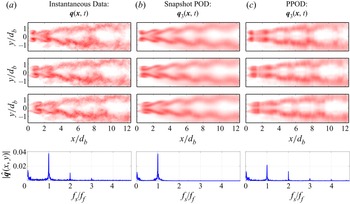


 Open access