




1. Introduction
1.1 Overview
A general problem in commutative algebra and algebraic geometry is to calculate the local cohomology sheaves $\mathscr{H}^q_Z(\mathcal{O}_X)$
associated to a smooth complex variety X and a closed subvariety
$\mathscr{H}^q_Z(\mathcal{O}_X)$
associated to a smooth complex variety X and a closed subvariety $Z\subseteq X$
. In the recent past, a great deal of progress has been made by taking advantage of deeper structure on these sheaves, namely that of holonomic
$Z\subseteq X$
. In the recent past, a great deal of progress has been made by taking advantage of deeper structure on these sheaves, namely that of holonomic $\mathcal{D}_X$
-modules, where
$\mathcal{D}_X$
-modules, where $\mathcal{D}_X$
is the sheaf of algebraic differential operators on X. This strong finiteness property has facilitated numerous new calculations, especially in the presence of a group action. In particular, when X has finitely many orbits under the action of a linear algebraic group and Z is an orbit closure, the theory of equivariant
$\mathcal{D}_X$
is the sheaf of algebraic differential operators on X. This strong finiteness property has facilitated numerous new calculations, especially in the presence of a group action. In particular, when X has finitely many orbits under the action of a linear algebraic group and Z is an orbit closure, the theory of equivariant $\mathcal{D}_X$
-modules has provided a fruitful framework to investigate the modules
$\mathcal{D}_X$
-modules has provided a fruitful framework to investigate the modules $\mathscr{H}^q_Z(\mathcal{O}_X)$
(see [Reference Lõrincz and WaltherLW19]). A well-understood example is the case when X is a space of matrices and Z is a determinantal variety (see [Reference Raicu and WeymanRW16, Reference Lõrincz and RaicuLR20, Reference PerlmanPer24]). More recently, the extra layer of Saito’s theory of mixed Hodge modules [Reference SaitoSai90] has provided new insights as to how local cohomology detects and measures singularities of Z (see [Reference Mustaţă and PopaMP19, Reference Mustaţă and PopaMP22]).
$\mathscr{H}^q_Z(\mathcal{O}_X)$
(see [Reference Lõrincz and WaltherLW19]). A well-understood example is the case when X is a space of matrices and Z is a determinantal variety (see [Reference Raicu and WeymanRW16, Reference Lõrincz and RaicuLR20, Reference PerlmanPer24]). More recently, the extra layer of Saito’s theory of mixed Hodge modules [Reference SaitoSai90] has provided new insights as to how local cohomology detects and measures singularities of Z (see [Reference Mustaţă and PopaMP19, Reference Mustaţă and PopaMP22]).
Another context in which equivariant $\mathcal{D}_X$
-modules appear is in geometric representation theory, e.g., in the study of composition-factor multiplicities of Verma modules over simple Lie algebras (see [Reference Hotta, Takeuchi and TanisakiHTT08]), which is the subject of the Kazhdan–Lusztig theorem. In particular, the Beilinson–Bernstein theorem [Reference Beilinson and BernsteinBB81] identifies, via the global sections functor, Borel-equivariant
$\mathcal{D}_X$
-modules appear is in geometric representation theory, e.g., in the study of composition-factor multiplicities of Verma modules over simple Lie algebras (see [Reference Hotta, Takeuchi and TanisakiHTT08]), which is the subject of the Kazhdan–Lusztig theorem. In particular, the Beilinson–Bernstein theorem [Reference Beilinson and BernsteinBB81] identifies, via the global sections functor, Borel-equivariant $\mathcal{D}_X$
-modules on flag varieties with highest-weight modules over the corresponding Lie algebra. Here, intersection cohomology modules associated to Schubert cells correspond to irreducible representations with trivial central character, and (Verdier duals of) pushforwards of structure sheaves on Schubert cells correspond to Verma modules. In commutative algebra and algebraic geometry, we would refer to these geometric Verma modules as the local cohomology modules
$\mathcal{D}_X$
-modules on flag varieties with highest-weight modules over the corresponding Lie algebra. Here, intersection cohomology modules associated to Schubert cells correspond to irreducible representations with trivial central character, and (Verdier duals of) pushforwards of structure sheaves on Schubert cells correspond to Verma modules. In commutative algebra and algebraic geometry, we would refer to these geometric Verma modules as the local cohomology modules $\mathscr{H}^q_{O_w}(\mathcal{O}_X)$
with support in the (locally closed) Schubert cells
$\mathscr{H}^q_{O_w}(\mathcal{O}_X)$
with support in the (locally closed) Schubert cells $O_w$
. Via the theory of mixed Hodge modules, the weight filtration on
$O_w$
. Via the theory of mixed Hodge modules, the weight filtration on $\mathscr{H}^q_{O_w}(\mathcal{O}_X)$
induces the Jantzen filtration on the corresponding Verma module [Reference Beilinson and BernsteinBB93].
$\mathscr{H}^q_{O_w}(\mathcal{O}_X)$
induces the Jantzen filtration on the corresponding Verma module [Reference Beilinson and BernsteinBB93].
The purpose of this paper is to reconcile the above two theories by calculating the local cohomology modules $\mathscr{H}^q_{Z_w}(\mathcal{O}_X)$
with support in closed Schubert varieties
$\mathscr{H}^q_{Z_w}(\mathcal{O}_X)$
with support in closed Schubert varieties $Z_w=\overline{O}_w$
in flag varieties
$Z_w=\overline{O}_w$
in flag varieties $X=G/P$
, where G is a complex simple linear algebraic group and P is a parabolic subgroup. Such modules are B-equivariant holonomic
$X=G/P$
, where G is a complex simple linear algebraic group and P is a parabolic subgroup. Such modules are B-equivariant holonomic $\mathcal{D}_X$
-modules, where B is a Borel subgroup with
$\mathcal{D}_X$
-modules, where B is a Borel subgroup with $B\subseteq P\subseteq G$
. Each local cohomology module
$B\subseteq P\subseteq G$
. Each local cohomology module $\mathscr{H}^q_{Z_w}(\mathcal{O}_X)$
is finite length over
$\mathscr{H}^q_{Z_w}(\mathcal{O}_X)$
is finite length over $\mathcal{D}_X$
and, since Schubert cells are simply connected, has composition factors among
$\mathcal{D}_X$
and, since Schubert cells are simply connected, has composition factors among $\mathcal{L}(Z_v,X)$
, where
$\mathcal{L}(Z_v,X)$
, where $Z_v\subseteq Z_w$
and
$Z_v\subseteq Z_w$
and $\mathcal{L}(Z_v,X)$
is the intersection cohomology
$\mathcal{L}(Z_v,X)$
is the intersection cohomology $\mathcal{D}_X$
-module associated to the trivial local system on the Schubert cell
$\mathcal{D}_X$
-module associated to the trivial local system on the Schubert cell $O_v$
. These local cohomology modules are functorially endowed with structures as mixed Hodge modules, and in particular are endowed with two increasing filtrations of geometric origin: (1) the Hodge filtration
$O_v$
. These local cohomology modules are functorially endowed with structures as mixed Hodge modules, and in particular are endowed with two increasing filtrations of geometric origin: (1) the Hodge filtration $F_{\bullet}(\mathscr{H}^q_{Z_w}(\mathcal{O}_X))$
, an infinite filtration by coherent
$F_{\bullet}(\mathscr{H}^q_{Z_w}(\mathcal{O}_X))$
, an infinite filtration by coherent $\mathcal{O}_X$
-modules; and (2) the weight filtration
$\mathcal{O}_X$
-modules; and (2) the weight filtration $W_{\bullet}(\mathscr{H}^q_{Z_w}(\mathcal{O}_X))$
, a finite filtration by holonomic
$W_{\bullet}(\mathscr{H}^q_{Z_w}(\mathcal{O}_X))$
, a finite filtration by holonomic $\mathcal{D}_X$
-modules. In this work, we provide a framework to determine the Hodge and weight filtrations on
$\mathcal{D}_X$
-modules. In this work, we provide a framework to determine the Hodge and weight filtrations on $\mathscr{H}^q_{Z_w}(\mathcal{O}_X)$
from those on the geometric (dual) Verma modules
$\mathscr{H}^q_{Z_w}(\mathcal{O}_X)$
from those on the geometric (dual) Verma modules $\mathscr{H}^q_{O_v}(\mathcal{O}_X)$
. Our main result in this direction is Theorem 3.3, which we now summarize.
$\mathscr{H}^q_{O_v}(\mathcal{O}_X)$
. Our main result in this direction is Theorem 3.3, which we now summarize.
Let $W^P$
be the relative Weyl group associated to P, and let
$W^P$
be the relative Weyl group associated to P, and let $\ell$
denote the length function on
$\ell$
denote the length function on $W^P$
. As the Schubert cells
$W^P$
. As the Schubert cells $\{O_w\}_{w\in W^P}$
give an affine paving of X, the Grothendieck–Cousin complex
$\{O_w\}_{w\in W^P}$
give an affine paving of X, the Grothendieck–Cousin complex $\mathcal{GC}^{\bullet}$
provides a right resolution of
$\mathcal{GC}^{\bullet}$
provides a right resolution of $\mathcal{O}_X$
in the category of
$\mathcal{O}_X$
in the category of $\mathcal{D}_X$
-modules:
$\mathcal{D}_X$
-modules:
 $$0 \longrightarrow \mathscr{H}^0_{O_{w_{\circ}(P)}}(\mathcal{O}_X)\longrightarrow \bigoplus_{\ell(v)=d-1}\mathscr{H}^1_{O_v}(\mathcal{O}_X) \longrightarrow \cdots \longrightarrow \bigoplus_{\ell(v)=1}\mathscr{H}^{d-1}_{O_v}(\mathcal{O}_X)\longrightarrow \mathscr{H}^{d}_{O_{e}}(\mathcal{O}_X)\longrightarrow 0,$$
where e is the identity and $w_{\circ}(P)$
is the longest element in
$w_{\circ}(P)$
is the longest element in $W^P$
, of length
$W^P$
, of length $d=d_X$
. Therefore, for a Schubert variety
$d=d_X$
. Therefore, for a Schubert variety $Z_w$
, we have
$Z_w$
, we have $\mathscr{H}^q_{Z_w}(\mathcal{O}_X)=\mathscr{H}^q_{Z_w}(\mathcal{GC}^{\bullet})$
for
$\mathscr{H}^q_{Z_w}(\mathcal{O}_X)=\mathscr{H}^q_{Z_w}(\mathcal{GC}^{\bullet})$
for $q\geqslant 0$
. Furthermore, using affineness of the inclusions of the Schubert cells, it can be shown that, for
$q\geqslant 0$
. Furthermore, using affineness of the inclusions of the Schubert cells, it can be shown that, for $0\leqslant q\leqslant d$
, we have (see Theorem 3.1)
$0\leqslant q\leqslant d$
, we have (see Theorem 3.1)
 \begin{equation}\mathscr{H}^0_{Z_w}(\mathcal{GC}^{q})=\bigoplus_{v\leqslant w,\;\ell(v)=d-q}\mathscr{H}^q_{O_v}(\mathcal{O}_X) \quad{\rm and}\quad \mathscr{H}^q_{Z_w}(\mathcal{O}_X)=\mathcal{H}^q(\mathscr{H}^0_{Z_w}(\mathcal{GC}^{\bullet})).\end{equation}
The complex $\mathcal{GC}^{\bullet}$
was introduced by Kempf [Reference KempfKem78] in his study of Bernstein–Gel’fand–Gel’fand (BGG) resolutions of highest-weight modules over simple Lie algebras. In particular, via the Beilinson–Bernstein theorem [Reference Beilinson and BernsteinBB81], the terms
$\mathcal{GC}^{\bullet}$
was introduced by Kempf [Reference KempfKem78] in his study of Bernstein–Gel’fand–Gel’fand (BGG) resolutions of highest-weight modules over simple Lie algebras. In particular, via the Beilinson–Bernstein theorem [Reference Beilinson and BernsteinBB81], the terms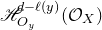 $\mathscr{H}^{d-\ell(y)}_{O_y}(\mathcal{O}_X)$
correspond to duals of parabolic Verma modules. Since
$\mathscr{H}^{d-\ell(y)}_{O_y}(\mathcal{O}_X)$
correspond to duals of parabolic Verma modules. Since $\Gamma(X,\mathcal{O}_X)=\mathbb{C}$
, it follows that
$\Gamma(X,\mathcal{O}_X)=\mathbb{C}$
, it follows that $\mathcal{GC}^{\bullet}$
is a geometric realization of the dual of the BGG resolution of the trivial representation.
$\mathcal{GC}^{\bullet}$
is a geometric realization of the dual of the BGG resolution of the trivial representation.
For $w\in W^P$
, we write
$w\in W^P$
, we write $\mathcal{GC}_w^{\bullet}=\mathscr{H}^0_{Z_w}(\mathcal{GC}^{\bullet})$
, which by the above discussion satisfies
$\mathcal{GC}_w^{\bullet}=\mathscr{H}^0_{Z_w}(\mathcal{GC}^{\bullet})$
, which by the above discussion satisfies $\mathcal{H}^q(\mathcal{GC}^{\bullet}_w)=\mathscr{H}^q_{Z_w}(\mathcal{O}_X)$
for
$\mathcal{H}^q(\mathcal{GC}^{\bullet}_w)=\mathscr{H}^q_{Z_w}(\mathcal{O}_X)$
for $q\geqslant 0$
. The idea to use
$q\geqslant 0$
. The idea to use $\mathcal{GC}_w^{\bullet}$
to study local cohomology is not new. For instance, Raben and Pedersen [Reference Raben-PedersenRP05] use
$\mathcal{GC}_w^{\bullet}$
to study local cohomology is not new. For instance, Raben and Pedersen [Reference Raben-PedersenRP05] use $\mathcal{GC}_w^{\bullet}$
to investigate qualitative properties of
$\mathcal{GC}_w^{\bullet}$
to investigate qualitative properties of $\mathscr{H}^q_{Z_w}(\mathcal{O}_X)$
and local cohomological dimension in the case when
$\mathscr{H}^q_{Z_w}(\mathcal{O}_X)$
and local cohomological dimension in the case when $X=G/B$
or
$X=G/B$
or $X=\operatorname{{\rm Gr}}(k,n)$
, though a clear picture is not obtained. The complex
$X=\operatorname{{\rm Gr}}(k,n)$
, though a clear picture is not obtained. The complex $\mathcal{GC}_w^{\bullet}$
has also been examined in positive characteristic (see [Reference Kashiwara and LauritzenKL02, Reference Raben-PedersenRP05, Reference Lauritzen, Raben-Pedersen and ThomsenLRPT06]). Our approach to get at the cohomology of
$\mathcal{GC}_w^{\bullet}$
has also been examined in positive characteristic (see [Reference Kashiwara and LauritzenKL02, Reference Raben-PedersenRP05, Reference Lauritzen, Raben-Pedersen and ThomsenLRPT06]). Our approach to get at the cohomology of $\mathcal{GC}_w^{\bullet}$
is to enhance it to a complex in the category of mixed Hodge modules, and use strictness to obtain degeneration of the spectral sequences associated to the Hodge and weight filtrations. The following is a consequence of Theorem 3.3.
$\mathcal{GC}_w^{\bullet}$
is to enhance it to a complex in the category of mixed Hodge modules, and use strictness to obtain degeneration of the spectral sequences associated to the Hodge and weight filtrations. The following is a consequence of Theorem 3.3.
Theorem A. For $w\in W^P$
, the complex
$w\in W^P$
, the complex $\mathcal{GC}^{\bullet}_w$
underlies a complex of mixed Hodge modules, and hence is endowed with a Hodge filtration
$\mathcal{GC}^{\bullet}_w$
underlies a complex of mixed Hodge modules, and hence is endowed with a Hodge filtration $F_{\bullet}(\mathcal{GC}^{\bullet}_w)$
by coherent
$F_{\bullet}(\mathcal{GC}^{\bullet}_w)$
by coherent $\mathcal{O}_X$
-modules and a weight filtration
$\mathcal{O}_X$
-modules and a weight filtration $W_{\bullet}(\mathcal{GC}^{\bullet}_w)$
by holonomic
$W_{\bullet}(\mathcal{GC}^{\bullet}_w)$
by holonomic $\mathcal{D}_X$
-modules. Furthermore, taking cohomology commutes with taking associated graded with respect to these filtrations, i.e. for all
$\mathcal{D}_X$
-modules. Furthermore, taking cohomology commutes with taking associated graded with respect to these filtrations, i.e. for all $p\in \mathbb{Z}$
and
$p\in \mathbb{Z}$
and $q\geqslant 0$
we have isomorphisms
$q\geqslant 0$
we have isomorphisms
 $${\rm gr}^F_p(\mathscr{H}_{Z_w}^{q}(\mathcal{O}_X^H))\cong \mathcal{H}^q({\rm gr}^F_p(\mathcal{GC}_w^{\bullet})) \quad{and}\quad{\rm gr}^W_p(\mathscr{H}_{Z_w}^{q}(\mathcal{O}_X^H))\cong \mathcal{H}^q({\rm gr}^W_p(\mathcal{GC}_w^{\bullet})).$$
In particular, in order to calculate the composition factors and weight filtration on $\mathscr{H}^q_{Z_w}(\mathcal{O}_X)$
, instead of working with the complicated complex
$\mathscr{H}^q_{Z_w}(\mathcal{O}_X)$
, instead of working with the complicated complex $\mathcal{GC}_w^{\bullet}$
, one can study the cohomology of the complexes
$\mathcal{GC}_w^{\bullet}$
, one can study the cohomology of the complexes ${\rm gr}^W_p(\mathcal{GC}_w^{\bullet})$
, which are complexes of semi-simple
${\rm gr}^W_p(\mathcal{GC}_w^{\bullet})$
, which are complexes of semi-simple $\mathcal{D}_X$
-modules. Furthermore, via the Beilinson–Bernstein theorem, one can first take global sections and instead work with parabolic Verma modules and irreducible representations of the corresponding Lie algebra (see Corollary 3.7). The composition factors and weight filtrations on the parabolic Verma modules are known, and are dictated by inverse parabolic Kazhdan–Lusztig polynomials (see [Reference Casian and CollingwoodCC87, Reference Kashiwara and TanisakiKT02]). Recent work of Davis and Vilonen [Reference Davis and VilonenDV23, Theorem 1.1] implies that the global sections functor is also exact with respect to the Hodge filtration.
$\mathcal{D}_X$
-modules. Furthermore, via the Beilinson–Bernstein theorem, one can first take global sections and instead work with parabolic Verma modules and irreducible representations of the corresponding Lie algebra (see Corollary 3.7). The composition factors and weight filtrations on the parabolic Verma modules are known, and are dictated by inverse parabolic Kazhdan–Lusztig polynomials (see [Reference Casian and CollingwoodCC87, Reference Kashiwara and TanisakiKT02]). Recent work of Davis and Vilonen [Reference Davis and VilonenDV23, Theorem 1.1] implies that the global sections functor is also exact with respect to the Hodge filtration.
After establishing the above framework in §2 and 3, we carry out the following.
-
– In §4, we investigate the weight filtration on $\mathcal{GC}_w^{\bullet}$
in the case when X is the classical Grassmannian
$\operatorname{{\rm Gr}}(k,n)$
. We employ Kazhdan–Lusztig theory and the known submodule lattice of the relevant parabolic Verma modules to obtain the composition factors and weight filtration on
$\mathscr{H}_{Z_w}^{q}(\mathcal{O}_X^H)$
. Our results in this direction are stated in §1.2. Remarkably, the weight filtration is controlled by the admissible augmented Dyck patterns of Raicu and Weyman [Reference Raicu and WeymanRW19], which also control the syzygies of determinantal thickenings [Reference HuangHua20]. In §4.4, we explain the connection between local cohomology and syzygies via the BGG correspondence and super duality, showing that part of our Theorem 1.1 is equivalent to [Reference HuangHua20, Theorem 3.7].
$\mathcal{GC}_w^{\bullet}$
in the case when X is the classical Grassmannian
$\operatorname{{\rm Gr}}(k,n)$
. We employ Kazhdan–Lusztig theory and the known submodule lattice of the relevant parabolic Verma modules to obtain the composition factors and weight filtration on
$\mathscr{H}_{Z_w}^{q}(\mathcal{O}_X^H)$
. Our results in this direction are stated in §1.2. Remarkably, the weight filtration is controlled by the admissible augmented Dyck patterns of Raicu and Weyman [Reference Raicu and WeymanRW19], which also control the syzygies of determinantal thickenings [Reference HuangHua20]. In §4.4, we explain the connection between local cohomology and syzygies via the BGG correspondence and super duality, showing that part of our Theorem 1.1 is equivalent to [Reference HuangHua20, Theorem 3.7]. -
– In §4.5, we restrict these calculations to the opposite big cell of the Grassmannian to recover the composition factors and weight filtration on local cohomology with support in determinantal varieties of generic matrices. This gives a new combinatorial interpretation of the composition-factor formula [Reference Raicu and WeymanRW16] and the weight-filtration formula [Reference PerlmanPer24].


At the end of §4.3, we discuss how one might approach a similar analysis for Schubert varieties in the remaining Hermitian symmetric spaces.
1.2 Statement of results for the Grassmannian
For positive integers $k<n$
, we consider the Grassmannian
$k<n$
, we consider the Grassmannian $X=\operatorname{{\rm Gr}}(k,V)$
of k-dimensional subspaces of an n-dimensional complex vector space V. We fix a complete flag
$X=\operatorname{{\rm Gr}}(k,V)$
of k-dimensional subspaces of an n-dimensional complex vector space V. We fix a complete flag $\mathcal{V}_{\bullet}$
of vector subspaces in V,
$\mathcal{V}_{\bullet}$
of vector subspaces in V,
 $$0\subset V_1\subset \cdots \subset V_{n-1}\subset V_n=V,$$
with $\dim V_i=i$
. Given a partition
$\dim V_i=i$
. Given a partition $\underline{a}=(a_1,\ldots,a_k)$
satisfying
$\underline{a}=(a_1,\ldots,a_k)$
satisfying
 \begin{equation}n-k\geqslant a_1\geqslant a_2\geqslant \cdots \geqslant a_k\geqslant 0,\end{equation}
we define the Schubert variety $Z_{\underline{a}}\subseteq X$
as the closed subset
$Z_{\underline{a}}\subseteq X$
as the closed subset

It is the closure of the Schubert cell $O_{\underline{a}}$
. This variety has dimension
$O_{\underline{a}}$
. This variety has dimension
 $$\dim Z_{\underline{a}}=|\underline{a}|=a_1+\cdots +a_k,$$
and given two partitions $\underline{a}$
and
$\underline{a}$
and $\underline{b}$
satisfying (1.2), we have
$\underline{b}$
satisfying (1.2), we have
 $$Z_{\underline{b}}\subseteq Z_{\underline{a}} \quad \iff \quad \underline{b} \subseteq \underline{a},$$
where the latter notation means that $b_i\leqslant a_i$
for all
$b_i\leqslant a_i$
for all $1\leqslant i \leqslant k$
.
$1\leqslant i \leqslant k$
.
We identify a partition $\underline{a}=(a_1,a_2,\ldots ,a_k)$
with its Young diagram,
$\underline{a}=(a_1,a_2,\ldots ,a_k)$
with its Young diagram,
 $$\underline{a}=(a_1,a_2,\ldots ,a_k) \quad \leftrightarrow \quad \{(i,j)\in \mathbb{Z}^2_+\mid 1\leqslant i \leqslant k,\ 1\leqslant j\leqslant a_i\},$$
which we picture as a left-justified collection of boxes, with $a_i$
boxes in row i. For example, the partition
$a_i$
boxes in row i. For example, the partition $\underline{a}=(5,4,2,2)$
corresponds to the following Young diagram.
$\underline{a}=(5,4,2,2)$
corresponds to the following Young diagram.

A path P in $\mathbb{Z}^2_+$
is a collection of boxes
$\mathbb{Z}^2_+$
is a collection of boxes
 $$P=\{ (i_1,j_1),(i_2,j_2),\ldots ,(i_t, j_t)\},$$
satisfying the following for all $1\leqslant s \leqslant t-1$
:
$1\leqslant s \leqslant t-1$
:
 $$(i_{s+1},j_{s+1})=(i_s-1, j_s)\quad {\rm or} \quad (i_{s+1},j_{s+1})=(i_s, j_s+1).$$
In other words, a path is a connected collection of boxes obtained by starting at some box $(i_1,j_1)$
, and walking in any combination of north and east. We write
$(i_1,j_1)$
, and walking in any combination of north and east. We write $|P|=t$
for the length of P, which is the number of boxes in P. The path P is called a Dyck path if, for some
$|P|=t$
for the length of P, which is the number of boxes in P. The path P is called a Dyck path if, for some $d\geqslant 0$
, we have:
$d\geqslant 0$
, we have:
-
–
$i_1+j_1=i_t+j_t=d$
; and -
–
$i_s+j_s\leqslant d$
for all
$1\leqslant s\leqslant t$
.



In words, $(i_1,j_1)$
and
$(i_1,j_1)$
and $(i_t,j_t)$
lie on the same antidiagonal of
$(i_t,j_t)$
lie on the same antidiagonal of $\mathbb{Z}^2_+$
, and no intermediate box
$\mathbb{Z}^2_+$
, and no intermediate box $(i_s,j_s)$
lies below this antidiagonal. In this case, we say that P is a Dyck path of level d, and that
$(i_s,j_s)$
lies below this antidiagonal. In this case, we say that P is a Dyck path of level d, and that $(i_1,j_1)$
and
$(i_1,j_1)$
and $(i_t,j_t)$
lie on the dth antidiagonal. The following three paths are examples of Dyck paths.
$(i_t,j_t)$
lie on the dth antidiagonal. The following three paths are examples of Dyck paths.

The next two paths fail to be Dyck paths.

The left path fails the second condition of a Dyck path, and the right path fails the first condition.
Observe that the properties of a Dyck path P imply that $|P|$
is odd,
$|P|$
is odd, $(i_2,j_2)=(i_1-1,j_1)$
, and
$(i_2,j_2)=(i_1-1,j_1)$
, and $(i_t,j_t)=(i_{t-1},j_{t-1}+1)$
, i.e. a Dyck path starts by moving north and ends by moving east.
$(i_t,j_t)=(i_{t-1},j_{t-1}+1)$
, i.e. a Dyck path starts by moving north and ends by moving east.
Following Raicu and Weyman [Reference Raicu and WeymanRW19], we define an augmented Dyck path as a pair $\tilde{P}=(P,B)$
, where P is a Dyck path and B is a set of boxes, called the bullets in
$\tilde{P}=(P,B)$
, where P is a Dyck path and B is a set of boxes, called the bullets in $\tilde{P}$
. The set B is a disjoint union of two sets of boxes
$\tilde{P}$
. The set B is a disjoint union of two sets of boxes $B = B_{\rm head} \sqcup B_{\rm tail}$
, where
$B = B_{\rm head} \sqcup B_{\rm tail}$
, where
 \begin{equation}\begin{aligned}B_{\rm head} & = \{(i_t,j_t+1), (i_t,j_t+2),\ldots,(i_t,j_t+u)\} \quad \mbox{for some }u\geqslant 0, \\B_{\rm tail} & = \{(i_1+1,j_1), (i_1+2,j_1), \ldots,(i_1+v,j_1)\} \quad \mbox{for some }v\geqslant 0. \\\end{aligned}\end{equation}
In words, $B_{\rm head}$
is a connected collection of boxes obtained from starting in the box directly east of
$B_{\rm head}$
is a connected collection of boxes obtained from starting in the box directly east of $(i_t,j_t)$
and taking some number of steps east. Similarly,
$(i_t,j_t)$
and taking some number of steps east. Similarly, $B_{\rm tail}$
is a connected collection of boxes obtained from starting in the box directly south of
$B_{\rm tail}$
is a connected collection of boxes obtained from starting in the box directly south of $(i_1,j_1)$
and taking some number of steps south.
$(i_1,j_1)$
and taking some number of steps south.

Given a partition $\underline{a}$
, an augmented Dyck pattern in
$\underline{a}$
, an augmented Dyck pattern in $\underline{a}$
is a collection
$\underline{a}$
is a collection
 $$\mathbb{D} = (D_1,D_2,\ldots,D_r;\mathbb{B}),$$
where:
-
– each
$D_i\subseteq \underline{a}$
is a Dyck path and
$\mathbb{B} \subseteq \underline{a}$
is a finite set of boxes; -
– the sets
$D_1,D_2,\ldots,D_r$
and
$\mathbb{B}$
are pairwise disjoint; and -
–
$\mathbb{B}$
can be expressed as a union (1.4)in such a way that
\begin{equation} \mathbb{B} = B_1 \cup B_2 \cup \cdots \cup B_r \end{equation}
$(D_i,B_i)$
is an augmented Dyck path for every
$i=1,\ldots,r$
.





We emphasize that the expression given in (1.4) need not be unique, and the sets $B_i$
are not necessarily disjoint. We write
$B_i$
are not necessarily disjoint. We write $|\mathbb{D}|=r$
for the number of Dyck paths in
$|\mathbb{D}|=r$
for the number of Dyck paths in $\mathbb{D}$
(so we are not counting elements of
$\mathbb{D}$
(so we are not counting elements of $\mathbb{B}$
). We often refer to augmented Dyck patterns simply as ‘Dyck patterns’.
$\mathbb{B}$
). We often refer to augmented Dyck patterns simply as ‘Dyck patterns’.
We define the support of $\mathbb{D}$
by
$\mathbb{D}$
by
 \begin{equation} \operatorname{{\rm supp}}(\mathbb{D}) = D_1 \cup D_2 \cup \cdots \cup D_r \cup \mathbb{B}.\end{equation}
If $\underline{a}$
is a partition and
$\underline{a}$
is a partition and $\mathbb{D}$
is an augmented Dyck pattern in
$\mathbb{D}$
is an augmented Dyck pattern in $\underline{a}$
, we write
$\underline{a}$
, we write
 \begin{equation}\underline{a}^{\mathbb{D}}=\underline{a} \setminus \operatorname{{\rm supp}}(\mathbb{D}).\end{equation}
Raicu and Weyman [Reference Raicu and WeymanRW19] define a Dyck pattern $\mathbb{D}=(D_1,D_2,\ldots,D_r;\mathbb{B})$
in
$\mathbb{D}=(D_1,D_2,\ldots,D_r;\mathbb{B})$
in $\underline{a}$
to be admissible if the following conditions are satisfied:
$\underline{a}$
to be admissible if the following conditions are satisfied:
-
(i)
$a^{\mathbb{D}}$
is a set of boxes corresponding to a partition; -
(ii) (covering condition) for every
$p\neq q$
, if there exists a box
$(i',j')\in D_q$
that is located directly north, northwest, or west from a box
$(i,j)\in D_p$
, then every box located directly north, northwest, or west from a box in
$D_p$
must also belong to
$D_p$
or
$D_q$
; and -
(iii) there is no box in
$\mathbb{B}$
that is located directly north, northwest, or west from a box in any Dyck path
$D_p$
.


The following are four examples of admissible Dyck patterns in $\underline{a}=(5,4,3,2,2)$
.
$\underline{a}=(5,4,3,2,2)$
.

The following three patterns are not admissible.

The covering condition is Rule II in [Reference Shigechi and Zinn-JustinSZJ12, § 3.1]. This condition may also be described in terms of boundary strip removals from skew diagrams [Reference BrentiBre02, § 2].
We distinguish between Dyck patterns with bullets and those without bullets as follows:
 \begin{align} {\rm Dyck}^{\bullet}(\underline{a})&=\{\mbox{admissible augmented Dyck patterns in $\underline{a}$}\}, \end{align}
 \begin{align} {\rm Dyck}(\underline{a})&=\{\mathbb{D}=(D_1,D_2,\ldots,D_r;\mathbb{B})\in {\rm Dyck}^{\bullet}(\underline{a})\mid \mathbb{B}=\emptyset\}.\end{align}
We write $\mathbb{D}=(D_1,\ldots,D_r)$
when
$\mathbb{D}=(D_1,\ldots,D_r)$
when $\mathbb{B}=\emptyset$
. The empty pattern
$\mathbb{B}=\emptyset$
. The empty pattern $\mathbb{D}=\emptyset$
satisfies
$\mathbb{D}=\emptyset$
satisfies $\underline{a}^{\mathbb{D}}=\underline{a}$
and belongs to both
$\underline{a}^{\mathbb{D}}=\underline{a}$
and belongs to both ${\rm Dyck}^{\bullet}(\underline{a})$
and
${\rm Dyck}^{\bullet}(\underline{a})$
and ${\rm Dyck}(\underline{a})$
.
${\rm Dyck}(\underline{a})$
.
With these combinatorial definitions, we now prepare to state the main result. Let $d_X=\dim X=k(n-k)$
. Given a partition
$d_X=\dim X=k(n-k)$
. Given a partition $\underline{a}$
and
$\underline{a}$
and $q\in \mathbb{Z}_{\geqslant 0}$
, we consider the following sets of augmented Dyck patterns:
$q\in \mathbb{Z}_{\geqslant 0}$
, we consider the following sets of augmented Dyck patterns:
 \begin{equation}\mathcal{A}(\underline{a}; q)=\{ (D_1,D_2,\ldots,D_r;\mathbb{B})\in {\rm Dyck}^{\bullet}(\underline{a}) \mid |D_i|\geqslant 3\ \mbox{\rm for $1\leqslant i\leqslant r$},\ |\mathbb{B}|=q+|\underline{a}|-d_{X}\}.\end{equation}
For $p\in \mathbb{Z}_{\geqslant 0}$
, we consider the subset of
$p\in \mathbb{Z}_{\geqslant 0}$
, we consider the subset of $\mathcal{A}(\underline{a}; q)$
consisting of patterns with
$\mathcal{A}(\underline{a}; q)$
consisting of patterns with $p-q-d_X$
paths:
$p-q-d_X$
paths:
 \begin{equation}\mathcal{A}_p(\underline{a};q)=\{\mathbb{D}\in \mathcal{A}(\underline{a}; q)\mid |\mathbb{D}|=p-q-d_X\}.\end{equation}
For the following statement, we write $\mathcal{L}(\underline{b})=\mathcal{L}(Z_{\underline{b}},X)$
for the intersection cohomology
$\mathcal{L}(\underline{b})=\mathcal{L}(Z_{\underline{b}},X)$
for the intersection cohomology $\mathcal{D}_X$
-module associated to the trivial local system on the Schubert cell
$\mathcal{D}_X$
-module associated to the trivial local system on the Schubert cell $O_{\underline{b}}$
. For
$O_{\underline{b}}$
. For $k\in \mathbb{Z}$
, the Hodge modules
$k\in \mathbb{Z}$
, the Hodge modules $IC^H_{Z_{\underline{b}}}(k)$
provide a complete list of polarizable pure Hodge modules that may overlie
$IC^H_{Z_{\underline{b}}}(k)$
provide a complete list of polarizable pure Hodge modules that may overlie $\mathcal{L}(\underline{b})$
(see §2.1). By the Beilinson–Bernstein theorem (see §3.4), the global sections functor is exact, and
$\mathcal{L}(\underline{b})$
(see §2.1). By the Beilinson–Bernstein theorem (see §3.4), the global sections functor is exact, and $\Gamma(X,\mathcal{L}(\underline{b}))$
is the irreducible
$\Gamma(X,\mathcal{L}(\underline{b}))$
is the irreducible $\mathfrak{sl}_n(\mathbb{C})$
-representation
$\mathfrak{sl}_n(\mathbb{C})$
-representation $L(\underline{b})$
, whose highest weight is described in §4.1.
$L(\underline{b})$
, whose highest weight is described in §4.1.
Theorem 1.1. With the above notation, we have the following expression in the Grothendieck group of $\mathcal{D}_{X}$
-modules (respectively, representations of
$\mathcal{D}_{X}$
-modules (respectively, representations of $\mathfrak{sl}_{n}(\mathbb{C}))$
for
$\mathfrak{sl}_{n}(\mathbb{C}))$
for $q\geqslant 0$
:
$q\geqslant 0$
:
 $$\big[ \mathscr{H}_{Z_{\underline{a}}}^{q}(\mathcal{O}_{X})\big]=\sum_{\mathbb{D}\in \mathcal{A}(\underline{a};q)} [\mathcal{L}(\underline{a}^{\mathbb{D}})] \quad{and}\quad \big[H^q_{Z_{\underline{a}}}(X,\mathcal{O}_{X})\big]=\sum_{\mathbb{D}\in \mathcal{A}(\underline{a};q)} [L(\underline{a}^{\mathbb{D}})].$$
Furthermore, the following is true about the weight filtration $W_{\bullet}$
for
$W_{\bullet}$
for $p\in \mathbb{Z}$
:
$p\in \mathbb{Z}$
:
 $${\rm gr}^W_p\mathscr{H}_{Z_{\underline{a}}}^q(\mathcal{O}^H_{X})=\bigoplus_{\mathbb{D}\in \mathcal{A}_p(\underline{a};q)} IC^H_{Z_{\underline{a}^{\mathbb{D}}}}\bigg(\frac{(|\underline{a}^{\mathbb{D}}|-p)}{2}\bigg).$$
In §4.4, we explain a remarkable connection to syzygies of some equivariant ideals. Specifically, via super duality, an equivalence of categories between representations of Lie (super)algebras, our description of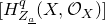 $[H^q_{Z_{\underline{a}}}(X,\mathcal{O}_{X})]$
is equivalent to Huang’s theorem on linear strands of syzygies of determinantal thickenings [Reference HuangHua20].
$[H^q_{Z_{\underline{a}}}(X,\mathcal{O}_{X})]$
is equivalent to Huang’s theorem on linear strands of syzygies of determinantal thickenings [Reference HuangHua20].
We carry out a first example.
Example 1.2. Let $X=\operatorname{{\rm Gr}}(4,9)$
and
$X=\operatorname{{\rm Gr}}(4,9)$
and $\underline{a}=(5,4,2,2)$
. There are eight elements of Dyck
$\underline{a}=(5,4,2,2)$
. There are eight elements of Dyck $^{\bullet}(\underline{a})$
for which all paths have length at least 3.
$^{\bullet}(\underline{a})$
for which all paths have length at least 3.

The number of bullets determines the cohomological degree, after an initial shift by codimension, which is $c=7$
in this example. The first four patterns belong to
$c=7$
in this example. The first four patterns belong to $\mathcal{A}(\underline{a};7)$
, the fifth belongs to
$\mathcal{A}(\underline{a};7)$
, the fifth belongs to $\mathcal{A}(\underline{a};8)$
, the sixth belongs to
$\mathcal{A}(\underline{a};8)$
, the sixth belongs to $\mathcal{A}(\underline{a};9)$
, the seventh belongs to
$\mathcal{A}(\underline{a};9)$
, the seventh belongs to $\mathcal{A}(\underline{a},10)$
, and the eighth belongs to
$\mathcal{A}(\underline{a},10)$
, and the eighth belongs to $\mathcal{A}(\underline{a};12)$
. By Theorem 1.1, we have the following in the Grothendieck group of
$\mathcal{A}(\underline{a};12)$
. By Theorem 1.1, we have the following in the Grothendieck group of $\mathcal{D}_X$
-modules:
$\mathcal{D}_X$
-modules:
 \begin{align*}\big[\mathscr{H}^{7}_{Z_{\underline{a}}}(\mathcal{O}_{X})\big]&=\big[\mathcal{L}(5,4,2,2)\big]+\big[\mathcal{L}(3,3,2,2)\big]+\big[\mathcal{L}(3,1,1,1)\big]+\big[\mathcal{L}(5,1,1,1)\big],\\\big[\mathscr{H}^{8}_{Z_{\underline{a}}}(\mathcal{O}_{X})\big]&=\big[\mathcal{L}(0)\big],\quad\big[\mathscr{H}^{9}_{Z_{\underline{a}}}(\mathcal{O}_{X})\big]=\big[\mathcal{L}(5,1,1,1)\big],\quad \big[\mathscr{H}^{10}_{Z_{\underline{a}}}(\mathcal{O}_{X})\big]=\big[\mathscr{H}^{12}_{Z_{\underline{a}}}(\mathcal{O}_{X})\big]=\big[\mathcal{L}(0)\big].\end{align*}
The graded pieces of the weight filtration are given by the number of paths plus the number of bullets, after an initial shift of $c+d_X$
, which is 27 in this example. Thus, the weights of the simple modules above are (from left to right) 27, 28, 28, 28, 30, 30, and 32, 34.
$c+d_X$
, which is 27 in this example. Thus, the weights of the simple modules above are (from left to right) 27, 28, 28, 28, 30, 30, and 32, 34.
Every Grassmannian has a unique Schubert divisor $Z_{\underline{a}}$
, where
$Z_{\underline{a}}$
, where $\underline{a}$
is obtained by removing the bottom-right box from the
$\underline{a}$
is obtained by removing the bottom-right box from the $k\times (n-k)$
rectangle. The following example illustrates the general behavior for Schubert divisors. We see that there is only one way to remove Dyck paths of lengths
$k\times (n-k)$
rectangle. The following example illustrates the general behavior for Schubert divisors. We see that there is only one way to remove Dyck paths of lengths $\geqslant 3$
such that the covering condition is satisfied, yielding only one nonzero local cohomology module.
$\geqslant 3$
such that the covering condition is satisfied, yielding only one nonzero local cohomology module.
Example 1.3. Set $X=\operatorname{{\rm Gr}}(4,9)$
and let
$X=\operatorname{{\rm Gr}}(4,9)$
and let $\underline{a}=(5,5,5,4)$
. There are four elements of Dyck
$\underline{a}=(5,5,5,4)$
. There are four elements of Dyck $^{\bullet}(\underline{a})$
for which all paths have length at least 3.
$^{\bullet}(\underline{a})$
for which all paths have length at least 3.

There is one local cohomology module, given as follows in the Grothendieck group of $\mathcal{D}_X$
-modules:
$\mathcal{D}_X$
-modules:
 $$\big[\mathscr{H}^{1}_{Z_{\underline{a}}}(\mathcal{O}_{X})\big]=\big[\mathcal{L}(5,5,5,4)\big]+\big[\mathcal{L}(5,5,3,3)\big]+\big[\mathcal{L}(5,2,2,2)\big]+\big[\mathcal{L}(1,1,1,1)\big].$$
The weight filtration is given by the number of paths in the pattern, after an initial shift by $c+d_X=21$
. From left to right, the weights of the composition factors are 21, 22, 23, and 24.
$c+d_X=21$
. From left to right, the weights of the composition factors are 21, 22, 23, and 24.
In the next example, we discuss the singular locus of $Z_{\underline{a}}$
in relation to local cohomology.
$Z_{\underline{a}}$
in relation to local cohomology.
Example 1.4. Let $\underline{a}$
be a partition, and write
$\underline{a}$
be a partition, and write $\underline{a}=(\tilde{a}_1^{d_1}, \tilde{a}_2^{d_2},\ldots, \tilde{a}_t^{d_t})$
, with
$\underline{a}=(\tilde{a}_1^{d_1}, \tilde{a}_2^{d_2},\ldots, \tilde{a}_t^{d_t})$
, with $\tilde{a}_1 \gt \tilde{a}_2 \gt \cdots \gt \tilde{a}_t$
and
$\tilde{a}_1 \gt \tilde{a}_2 \gt \cdots \gt \tilde{a}_t$
and $d_i \gt 0$
for
$d_i \gt 0$
for $1\leqslant i\leqslant t$
. Pictorially, this expression for
$1\leqslant i\leqslant t$
. Pictorially, this expression for $\underline{a}$
decomposes the Young diagram for
$\underline{a}$
decomposes the Young diagram for $\underline{a}$
into blocks of distinct widths. For instance,
$\underline{a}$
into blocks of distinct widths. For instance, $\underline{a}=(5^1,4^1,2^2)$
in Example 1.2, and
$\underline{a}=(5^1,4^1,2^2)$
in Example 1.2, and $\underline{a}=(5^3,4^1)$
in Example 1.3. For
$\underline{a}=(5^3,4^1)$
in Example 1.3. For $1\leqslant i\leqslant t-1$
, we define the partitions
$1\leqslant i\leqslant t-1$
, we define the partitions
 $$\underline{a}^i:=(\tilde{a}_1^{d_1}, \ldots, \tilde{a}_{i-1}^{d_{i-1}},\tilde{a}_i^{d_i-1}, (\tilde{a}_{i+1}-1)^{d_{i+1}+1},\tilde{a}_{i+2}^{d_{i+2}},\ldots, \tilde{a}_t^{d_t}).$$
In words, $\underline{a}^i$
is obtained from
$\underline{a}^i$
is obtained from $\underline{a}$
by removing
$\underline{a}$
by removing $\tilde{a}_i-\tilde{a}_{i+1}+1$
many boxes from the last row of the
$\tilde{a}_i-\tilde{a}_{i+1}+1$
many boxes from the last row of the $\tilde{a}_i$
block, and removing one box from every row of the
$\tilde{a}_i$
block, and removing one box from every row of the $\tilde{a}_{i+1}$
block. Together, the boxes being removed to make
$\tilde{a}_{i+1}$
block. Together, the boxes being removed to make $\underline{a}^i$
form a path
$\underline{a}^i$
form a path $P_i$
in the shape of a hook around the corner formed by the blocks in question. Lakshmibai and Weyman [Reference Lakshmibai and WeymanLW90, Theorem 5.3] give the following expression for the singular locus of
$P_i$
in the shape of a hook around the corner formed by the blocks in question. Lakshmibai and Weyman [Reference Lakshmibai and WeymanLW90, Theorem 5.3] give the following expression for the singular locus of $Z_{\underline{a}}$
:
$Z_{\underline{a}}$
:
 $$\operatorname{{\rm Sing}}(Z_{\underline{a}})=\bigcup_{i=1}^{t-1} Z_{\underline{a}^i}.$$
We now discuss the appearances of $\mathcal{L}(\underline{a}^i)$
as composition factors of
$\mathcal{L}(\underline{a}^i)$
as composition factors of $\mathscr{H}^{\bullet}_{Z_{\underline{a}}}(\mathcal{O}_X)$
. By Theorem 1.1, the multiplicity of
$\mathscr{H}^{\bullet}_{Z_{\underline{a}}}(\mathcal{O}_X)$
. By Theorem 1.1, the multiplicity of $\mathcal{L}(\underline{a}^i)$
in
$\mathcal{L}(\underline{a}^i)$
in $\mathscr{H}^{\bullet}_{Z_{\underline{a}}}(\mathcal{O}_X)$
is determined by the fillings of the path
$\mathscr{H}^{\bullet}_{Z_{\underline{a}}}(\mathcal{O}_X)$
is determined by the fillings of the path $P_i$
with augmented Dyck paths. More precisely, if we write
$P_i$
with augmented Dyck paths. More precisely, if we write $c=\operatorname{{\rm codim}}(Z_{\underline{a}},X)$
, then the multiplicity of
$c=\operatorname{{\rm codim}}(Z_{\underline{a}},X)$
, then the multiplicity of $\mathcal{L}(\underline{a}^i)$
in
$\mathcal{L}(\underline{a}^i)$
in $\mathscr{H}^{c+j}_{Z_{\underline{a}}}(\mathcal{O}_X)$
is one if
$\mathscr{H}^{c+j}_{Z_{\underline{a}}}(\mathcal{O}_X)$
is one if $P_i$
can be filled with an augmented Dyck path with j bullets, and zero otherwise. A straightforward calculation gives the following generating function for the desired multiplicities:
$P_i$
can be filled with an augmented Dyck path with j bullets, and zero otherwise. A straightforward calculation gives the following generating function for the desired multiplicities:
 \begin{equation}\sum_{j\geqslant 0} \big[\mathscr{H}^{j}_{Z_{\underline{a}}}(\mathcal{O}_X):\mathcal{L}(\underline{a}^i)\big]\cdot q^j=q^c\cdot (q^{|\tilde{a}_i-\tilde{a}_{i+1}-d_{i+1}|}+q^{|\tilde{a}_i-\tilde{a}_{i+1}-d_{i+1}|+2}+\cdots+q^{\tilde{a}_i-\tilde{a}_{i+1}+d_{i+1}-2}),\end{equation}
where $|\tilde{a}_i-\tilde{a}_{i+1}-d_{i+1}|$
denotes the absolute value of the integer
$|\tilde{a}_i-\tilde{a}_{i+1}-d_{i+1}|$
denotes the absolute value of the integer $\tilde{a}_i-\tilde{a}_{i+1}-d_{i+1}$
. In particular, all cohomological degrees in which
$\tilde{a}_i-\tilde{a}_{i+1}-d_{i+1}$
. In particular, all cohomological degrees in which $\mathcal{L}(\underline{a}^i)$
appears have the same parity.
$\mathcal{L}(\underline{a}^i)$
appears have the same parity.
For instance, in Example 1.2, we have $\underline{a}=(5^1,4^1,2^2)$
,
$\underline{a}=(5^1,4^1,2^2)$
, $\underline{a}^1=(3^2,2^2)$
,
$\underline{a}^1=(3^2,2^2)$
, $\underline{a}^2=(5^1,1^3)$
, and
$\underline{a}^2=(5^1,1^3)$
, and $c=7$
. The multiplicity of
$c=7$
. The multiplicity of $\mathcal{L}(\underline{a}^1)$
in local cohomology is described by the generating function
$\mathcal{L}(\underline{a}^1)$
in local cohomology is described by the generating function $q^7(q^0)$
and the multiplicity of
$q^7(q^0)$
and the multiplicity of $\mathcal{L}(\underline{a}^2)$
in local cohomology is described by the generating function
$\mathcal{L}(\underline{a}^2)$
in local cohomology is described by the generating function $q^7(q^0+q^2)$
.
$q^7(q^0+q^2)$
.
In the next example, we discuss the (rationally) smooth case.
Example 1.5. A Schubert variety $Z_{\underline{a}}$
is smooth if and only if
$Z_{\underline{a}}$
is smooth if and only if $\underline{a}$
is a rectangle [Reference Lakshmibai and WeymanLW90, Theorem 5.3], in which case
$\underline{a}$
is a rectangle [Reference Lakshmibai and WeymanLW90, Theorem 5.3], in which case $Z_{\underline{a}}$
is isomorphic to a smaller Grassmannian. Observe that if
$Z_{\underline{a}}$
is isomorphic to a smaller Grassmannian. Observe that if $\underline{a}$
is a rectangle with
$\underline{a}$
is a rectangle with $c=\operatorname{{\rm codim}}(Z_{\underline{a}},X)$
, then
$c=\operatorname{{\rm codim}}(Z_{\underline{a}},X)$
, then $\mathcal{A}(\underline{a};c)=\{(\emptyset)\}$
and
$\mathcal{A}(\underline{a};c)=\{(\emptyset)\}$
and $\mathcal{A}(\underline{a},c+j)=\emptyset$
for all
$\mathcal{A}(\underline{a},c+j)=\emptyset$
for all $j\geqslant 1$
. In particular, we recover the following well-known fact in the smooth case:
$j\geqslant 1$
. In particular, we recover the following well-known fact in the smooth case:
 \begin{equation}\mathscr{H}^c_{Z_{\underline{a}}}(\mathcal{O}_X)=\mathcal{L}(\underline{a})\quad{\rm and}\quad \mathscr{H}^{c+j}_{Z_{\underline{a}}}(\mathcal{O}_X)=0\quad \mbox{for $j\geqslant 1$}.\end{equation}
The cohomological condition given in (1.12) is referred to as rational smoothness. If $Z_{\underline{a}}$
is rationally smooth, then by Theorem 1.1, it follows that
$Z_{\underline{a}}$
is rationally smooth, then by Theorem 1.1, it follows that $\underline{a}$
does not have any inside corners, i.e.
$\underline{a}$
does not have any inside corners, i.e. $\underline{a}$
is a rectangle. In particular, we recover the well-known fact that a Schubert variety in the Grassmannian is rationally smooth if and only if it is smooth (for a survey of rational smoothness properties of Schubert varieties in Hermitian symmetric spaces, see [Reference Enright, Hunziker and Andrew PruettEHAP14, §§ 4.3 and 5.3]). Using notation from §1.1, we have that
$\underline{a}$
is a rectangle. In particular, we recover the well-known fact that a Schubert variety in the Grassmannian is rationally smooth if and only if it is smooth (for a survey of rational smoothness properties of Schubert varieties in Hermitian symmetric spaces, see [Reference Enright, Hunziker and Andrew PruettEHAP14, §§ 4.3 and 5.3]). Using notation from §1.1, we have that $Z_w\subseteq G/P$
is rationally smooth if and only if
$Z_w\subseteq G/P$
is rationally smooth if and only if $\mathcal{GC}_w^{\bullet}$
is a resolution of
$\mathcal{GC}_w^{\bullet}$
is a resolution of $\mathcal{L}(Z_w,G/P)$
.
$\mathcal{L}(Z_w,G/P)$
.
We prove Theorem 1.1 in §4 and we use it to calculate composition factors and weight filtration on local cohomology with support in generic determinantal varieties in §4.5.
2. The Hodge-theoretic Grothendieck–Cousin complex
In this section, we review background on $\mathcal{D}$
-modules, mixed Hodge modules, and local cohomology (§2.1), and we construct the Hodge-theoretic Grothendieck–Cousin complex (§2.2).
$\mathcal{D}$
-modules, mixed Hodge modules, and local cohomology (§2.1), and we construct the Hodge-theoretic Grothendieck–Cousin complex (§2.2).
In our arguments below, our convention is that complex varieties are possibly reducible.
2.1
$\mathcal{D}$
-modules, mixed Hodge modules, and local cohomology

Let X be a smooth complex variety of dimension $d_{X}$
, with sheaf of algebraic differential operators
$d_{X}$
, with sheaf of algebraic differential operators $\mathcal{D}_{X}$
. A
$\mathcal{D}_{X}$
. A $\mathcal{D}_X$
-module is a sheaf of left modules over
$\mathcal{D}_X$
-module is a sheaf of left modules over $\mathcal{D}_X$
. We write
$\mathcal{D}_X$
. We write ${\rm MHM}(X)$
for the category of algebraic mixed Hodge modules on X (see [Reference Hotta, Takeuchi and TanisakiHTT08, § 8.3.3] or [Reference SaitoSai88, Reference SaitoSai90]), with bounded derived category
${\rm MHM}(X)$
for the category of algebraic mixed Hodge modules on X (see [Reference Hotta, Takeuchi and TanisakiHTT08, § 8.3.3] or [Reference SaitoSai88, Reference SaitoSai90]), with bounded derived category ${\rm D}^b{\rm MHM}(X)$
. These categories are also defined on singular varieties.
${\rm D}^b{\rm MHM}(X)$
. These categories are also defined on singular varieties.
Given an irreducible closed subvariety $Z\subseteq X$
, we write
$Z\subseteq X$
, we write $\mathcal{L}(Z,X)$
for the intersection cohomology
$\mathcal{L}(Z,X)$
for the intersection cohomology $\mathcal{D}_X$
-module associated to the trivial local system on the regular locus
$\mathcal{D}_X$
-module associated to the trivial local system on the regular locus $Z_{{\rm reg}}\subseteq Z$
(see [Reference Hotta, Takeuchi and TanisakiHTT08, Definition 3.4.1]), and we write
$Z_{{\rm reg}}\subseteq Z$
(see [Reference Hotta, Takeuchi and TanisakiHTT08, Definition 3.4.1]), and we write $IC^H_Z$
for the pure Hodge module associated to the trivial variation of Hodge structure on
$IC^H_Z$
for the pure Hodge module associated to the trivial variation of Hodge structure on $Z_{{\rm reg}}$
(see [Reference Hotta, Takeuchi and TanisakiHTT08, § 8.3.3(m13)]), which has weight
$Z_{{\rm reg}}$
(see [Reference Hotta, Takeuchi and TanisakiHTT08, § 8.3.3(m13)]), which has weight $d_Z$
. For instance, we have
$d_Z$
. For instance, we have $\mathcal{L}(X,X)=\mathcal{O}_X$
and
$\mathcal{L}(X,X)=\mathcal{O}_X$
and $IC^H_X=\mathcal{O}_X^H$
. For
$IC^H_X=\mathcal{O}_X^H$
. For $k\in \mathbb{Z}$
, we write
$k\in \mathbb{Z}$
, we write $IC^H_Z(k)$
for the kth Tate twist of
$IC^H_Z(k)$
for the kth Tate twist of $IC^H_Z$
(see [Reference Hotta, Takeuchi and TanisakiHTT08, § 8.3.3(m5)]), which is pure of weight
$IC^H_Z$
(see [Reference Hotta, Takeuchi and TanisakiHTT08, § 8.3.3(m5)]), which is pure of weight $d_Z-2k$
. The modules
$d_Z-2k$
. The modules $IC^H_Z(k)$
provide a complete list of polarizable pure Hodge modules that may overlie the
$IC^H_Z(k)$
provide a complete list of polarizable pure Hodge modules that may overlie the $\mathcal{D}_X$
-module
$\mathcal{D}_X$
-module $\mathcal{L}(Z,X)$
(see [Reference Hotta, Takeuchi and TanisakiHTT08, § 8.3.3(m13)]).
$\mathcal{L}(Z,X)$
(see [Reference Hotta, Takeuchi and TanisakiHTT08, § 8.3.3(m13)]).
Let $f:X\to Y$
be a morphism between complex varieties. We write the following for the corresponding direct and inverse image functors for mixed Hodge modules [Reference SaitoSai90, § 4]:
$f:X\to Y$
be a morphism between complex varieties. We write the following for the corresponding direct and inverse image functors for mixed Hodge modules [Reference SaitoSai90, § 4]:
 $$f_{\ast}:{\rm D}^b{\rm MHM}(X)\to {\rm D}^b{\rm MHM}(Y) \quad{\rm and} \quad f^{!}:{\rm D}^b{\rm MHM}(Y)\to {\rm D}^b{\rm MHM}(X).$$
If X and Y are smooth, then these functors lift the $\mathcal{D}$
-module functors
$\mathcal{D}$
-module functors $\int_f$
and
$\int_f$
and $f^{\dagger}$
from [Reference Hotta, Takeuchi and TanisakiHTT08, Chapter 1.5], and if f is a closed immersion of codimension c, then
$f^{\dagger}$
from [Reference Hotta, Takeuchi and TanisakiHTT08, Chapter 1.5], and if f is a closed immersion of codimension c, then $f^{!}\mathcal{O}_Y^H=\mathcal{O}_X^H(-c)[-c]$
.
$f^{!}\mathcal{O}_Y^H=\mathcal{O}_X^H(-c)[-c]$
.
Let X be smooth and let $i:Z\hookrightarrow X$
be a locally closed subvariety of X. Given
$i:Z\hookrightarrow X$
be a locally closed subvariety of X. Given $\mathcal{M}\in {\rm D}^b{\rm MHM}(X)$
, we define the local cohomology modules of
$\mathcal{M}\in {\rm D}^b{\rm MHM}(X)$
, we define the local cohomology modules of $\mathcal{M}$
with support in Z via
$\mathcal{M}$
with support in Z via
 $$\mathscr{H}_{Z}^q(\mathcal{M}):=\mathcal{H}^q(i_{\ast}i^{!}\mathcal{M}),\quad q\in \mathbb{Z}.$$
In particular, for $\mathcal{M}=\mathcal{O}^H_X$
, this endows each local cohomology module
$\mathcal{M}=\mathcal{O}^H_X$
, this endows each local cohomology module $\mathscr{H}_{Z}^q(\mathcal{O}_X)$
with a mixed Hodge module structure, which we denote by
$\mathscr{H}_{Z}^q(\mathcal{O}_X)$
with a mixed Hodge module structure, which we denote by $\mathscr{H}_{Z}^q(\mathcal{O}^H_X)$
. For more information, see [Reference Mustaţă and PopaMP22, § B].
$\mathscr{H}_{Z}^q(\mathcal{O}^H_X)$
. For more information, see [Reference Mustaţă and PopaMP22, § B].
Now assume that $Z\subseteq X$
is a closed subvariety of X, with complement
$Z\subseteq X$
is a closed subvariety of X, with complement $U=X\setminus Z$
, and open immersion
$U=X\setminus Z$
, and open immersion $j:U\to X$
. Given
$j:U\to X$
. Given $\mathcal{M}\in {\rm D}^b{\rm MHM}(X)$
, there is an exact triangle [Reference SaitoSai90, (4.4.1)]
$\mathcal{M}\in {\rm D}^b{\rm MHM}(X)$
, there is an exact triangle [Reference SaitoSai90, (4.4.1)]
 \begin{equation}i_{\ast}i^{!}(\mathcal{M})\longrightarrow \mathcal{M}\longrightarrow j_{\ast}j^{!}(\mathcal{M})\overset{+1}\longrightarrow.\end{equation}
In particular, if $\mathcal{M}$
is a mixed Hodge module, we obtain an exact sequence
$\mathcal{M}$
is a mixed Hodge module, we obtain an exact sequence
 $$0\longrightarrow \mathscr{H}_{Z}^0(\mathcal{M})\longrightarrow \mathcal{M}\longrightarrow \mathcal{H}^0(j_{\ast}(\mathcal{M}|_U))\longrightarrow \mathscr{H}_{Z}^1(\mathcal{M})\longrightarrow 0,$$
and isomorphisms
 $$\mathscr{H}_{Z}^q(\mathcal{M})\cong \mathcal{H}^{q-1}(j_{\ast}(\mathcal{M}|_U))\quad \mbox{for $q\geqslant 2$.}$$
We write $F_{\bullet}$
and
$F_{\bullet}$
and $W_{\bullet}$
for the Hodge and weight filtrations of
$W_{\bullet}$
for the Hodge and weight filtrations of $\mathscr{H}_{Z}^q(\mathcal{M})$
.
$\mathscr{H}_{Z}^q(\mathcal{M})$
.
2.2 Construction of the Grothendieck–Cousin complex
Lemma 2.1. Let $\mathcal{M}$
be a mixed Hodge module on a smooth complex variety X, and let
$\mathcal{M}$
be a mixed Hodge module on a smooth complex variety X, and let $Z'\subsetneq Z$
be closed subvarieties of X. We have the following exact sequence of mixed Hodge modules:
$Z'\subsetneq Z$
be closed subvarieties of X. We have the following exact sequence of mixed Hodge modules:
 $$0 \to \mathscr{H}^0_{Z'}(\mathcal{M})\to \mathscr{H}^0_Z(\mathcal{M}) \to \mathscr{H}^0_{Z\setminus Z'}(\mathcal{M})\to \mathscr{H}^{1}_{Z'}(\mathcal{M})\to \mathscr{H}^{1}_Z(\mathcal{M}) \to \mathscr{H}^{1}_{Z\setminus Z'}(\mathcal{M})\to \cdots$$
Proof. We set $U=X\setminus Z'$
with open immersion j, and we write
$U=X\setminus Z'$
with open immersion j, and we write $i':Z'\to X$
,
$i':Z'\to X$
, $i:Z\to X$
for the natural inclusions. By (2.1) applied to
$i:Z\to X$
for the natural inclusions. By (2.1) applied to $i'=i$
and
$i'=i$
and $i_{\ast}i^!\mathcal{M}$
, we obtain an exact triangle
$i_{\ast}i^!\mathcal{M}$
, we obtain an exact triangle
 $$i'_{\ast}i'^!i_{\ast}i^!\mathcal{M}\longrightarrow i_{\ast}i^!\mathcal{M}\longrightarrow j_{\ast}j^!i_{\ast}i^!\mathcal{M}\overset{+1}\longrightarrow.$$
Let f be the inclusion of Z’ into Z. Since $i'=i\circ f$
, we have
$i'=i\circ f$
, we have $i'_{\ast}i'^!i_{\ast}i^!= i'_{\ast}f^!i^!i_{\ast}i^!$
, which by adjunction of
$i'_{\ast}i'^!i_{\ast}i^!= i'_{\ast}f^!i^!i_{\ast}i^!$
, which by adjunction of $i^!$
and
$i^!$
and $i_{\ast}$
is equal to
$i_{\ast}$
is equal to $i_{\ast}'i'^!$
. Let
$i_{\ast}'i'^!$
. Let $\tilde{j}$
be the inclusion of
$\tilde{j}$
be the inclusion of $Z\setminus Z'$
into Z, and let
$Z\setminus Z'$
into Z, and let $\tilde{i}$
be the inclusion of
$\tilde{i}$
be the inclusion of $Z\setminus Z'$
into U. By base change [Reference SaitoSai90, (4.4.3)], we have that
$Z\setminus Z'$
into U. By base change [Reference SaitoSai90, (4.4.3)], we have that $j_{\ast}j^!i_{\ast}i^!=k_{\ast}k^!$
. Therefore, the above triangle becomes
$j_{\ast}j^!i_{\ast}i^!=k_{\ast}k^!$
. Therefore, the above triangle becomes
 \begin{equation}i'_{\ast}i'^!\mathcal{M}\longrightarrow i_{\ast}i^!\mathcal{M}\longrightarrow k_{\ast}k^!\mathcal{M}\overset{+1}\longrightarrow.\end{equation}
The desired exact sequence is obtained as the long exact sequence of cohomology of (2.2).
Proposition 2.2. Let X be a smooth complex variety and let
 $$X=Z_0\supsetneq Z_1 \supsetneq \cdots \supsetneq Z_{\ell} \supsetneq Z_{\ell+1}=\emptyset$$
be a decreasing sequence of closed subsets. If $\mathcal{M}$
is a mixed Hodge module on X satisfying
$\mathcal{M}$
is a mixed Hodge module on X satisfying $\mathscr{H}^{j-1}_{Z_j}(\mathcal{M})=\mathscr{H}^{j+1}_{Z_j}(\mathcal{M})=0$
for all
$\mathscr{H}^{j-1}_{Z_j}(\mathcal{M})=\mathscr{H}^{j+1}_{Z_j}(\mathcal{M})=0$
for all $0\leqslant j\leqslant \ell$
, then there exists a complex
$0\leqslant j\leqslant \ell$
, then there exists a complex
 $$\mathcal{GC}^{\bullet}_{\{Z\}}(\mathcal{M}):\quad 0 \to \mathscr{H}^0_{Z_0\setminus Z_1}(\mathcal{M})\to \mathscr{H}^1_{Z_1\setminus Z_2}(\mathcal{M}) \to \cdots \to \mathscr{H}^{\ell}_{Z_{\ell}\setminus Z_{\ell+1}}(\mathcal{M})\to 0,$$
which is a right resolution of $\mathcal{M}$
in the category of mixed Hodge modules. This complex is known as the Grothendieck–Cousin of
$\mathcal{M}$
in the category of mixed Hodge modules. This complex is known as the Grothendieck–Cousin of $\mathcal{M}$
complex associated to the filtration
$\mathcal{M}$
complex associated to the filtration $\{Z\}$
.
$\{Z\}$
.
Proof. By Lemma 2.1 and the hypothesis on $\mathcal{M}$
, we obtain exact sequences
$\mathcal{M}$
, we obtain exact sequences
 $$0 \to \mathscr{H}^j_{Z_j}(\mathcal{M}) \overset{\alpha^j}\longrightarrow \mathscr{H}^j_{Z_j\setminus Z_{j+1}}(\mathcal{M})\overset{\beta^j}\longrightarrow \mathscr{H}^{j+1}_{Z_{j+1}}(\mathcal{M})\to 0.$$
For $0\leqslant j\leqslant \ell$
, we set
$0\leqslant j\leqslant \ell$
, we set $\mathcal{GC}^{j}_{\{Z\}}(\mathcal{M})=\mathscr{H}^j_{Z_j\setminus Z_{j+1}}(\mathcal{M})$
, and we define
$\mathcal{GC}^{j}_{\{Z\}}(\mathcal{M})=\mathscr{H}^j_{Z_j\setminus Z_{j+1}}(\mathcal{M})$
, and we define $d^j:\mathcal{GC}^{j}_{\{Z\}}(\mathcal{M})\to \mathcal{GC}^{j+1}_{\{Z\}}(\mathcal{M})$
to be the composition of maps
$d^j:\mathcal{GC}^{j}_{\{Z\}}(\mathcal{M})\to \mathcal{GC}^{j+1}_{\{Z\}}(\mathcal{M})$
to be the composition of maps
 $$d^j=\alpha^{j+1}\circ \beta^j.$$
By construction, the image of $d^j$
is
$d^j$
is $\mathscr{H}^{j+1}_{Z_{j+1}}(\mathcal{M})$
, which is the kernel of
$\mathscr{H}^{j+1}_{Z_{j+1}}(\mathcal{M})$
, which is the kernel of $d^{j+1}$
. Thus,
$d^{j+1}$
. Thus, $\mathcal{GC}^{\bullet}_{\{Z\}}(\mathcal{M})$
is exact in cohomological degrees
$\mathcal{GC}^{\bullet}_{\{Z\}}(\mathcal{M})$
is exact in cohomological degrees $j\geqslant 1$
. Since the kernel of
$j\geqslant 1$
. Since the kernel of $\beta^0$
is
$\beta^0$
is $\mathscr{H}^0_{X}(\mathcal{M})=\mathcal{M}$
, we conclude that
$\mathscr{H}^0_{X}(\mathcal{M})=\mathcal{M}$
, we conclude that $\mathcal{GC}^{\bullet}_{\{Z\}}(\mathcal{M})$
is a resolution of
$\mathcal{GC}^{\bullet}_{\{Z\}}(\mathcal{M})$
is a resolution of $\mathcal{M}$
.
$\mathcal{M}$
.
The Grothendieck–Cousin complex was introduced and studied in greater generality in [Reference KempfKem78]. In particular, Kempf considers more general input sheaves. We are interested in the following case.
Corollary 2.3. Let X be an irreducible smooth complex variety of dimension d, and let
 $$X=Z_0\supsetneq Z_1 \supsetneq \cdots \supsetneq Z_{d} \supsetneq Z_{d+1}=\emptyset$$
be a decreasing sequence of equidimensional closed subsets with $\operatorname{{\rm codim}}(Z_j,X)=j$
. If
$\operatorname{{\rm codim}}(Z_j,X)=j$
. If $Z_j\setminus Z_{j+1}$
is smooth and the inclusion
$Z_j\setminus Z_{j+1}$
is smooth and the inclusion $Z_j\setminus Z_{j+1}\subseteq X$
is affine for all
$Z_j\setminus Z_{j+1}\subseteq X$
is affine for all $0\leqslant j \leqslant d$
, then
$0\leqslant j \leqslant d$
, then $\mathcal{GC}^{\bullet}_{\{Z\}}:=\mathcal{GC}^{\bullet}_{\{Z\}}(\mathcal{O}_X^H)$
is a right resolution of
$\mathcal{GC}^{\bullet}_{\{Z\}}:=\mathcal{GC}^{\bullet}_{\{Z\}}(\mathcal{O}_X^H)$
is a right resolution of $\mathcal{O}_X^H$
in the category of mixed Hodge modules.
$\mathcal{O}_X^H$
in the category of mixed Hodge modules.
Proof. By Proposition 2.2, it suffices to show that $\mathscr{H}^{j-1}_{Z_j}(\mathcal{O}_X^H)=\mathscr{H}^{j+1}_{Z_j}(\mathcal{O}_X^H)=0$
for all j. Since
$\mathscr{H}^{j-1}_{Z_j}(\mathcal{O}_X^H)=\mathscr{H}^{j+1}_{Z_j}(\mathcal{O}_X^H)=0$
for all j. Since $Z_j$
is equidimensional with
$Z_j$
is equidimensional with $\operatorname{{\rm codim}}(Z_j,X)=j$
, we have that
$\operatorname{{\rm codim}}(Z_j,X)=j$
, we have that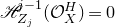 $\mathscr{H}^{j-1}_{Z_j}(\mathcal{O}_X^H)=0$
.
$\mathscr{H}^{j-1}_{Z_j}(\mathcal{O}_X^H)=0$
.
Let k be the inclusion of $Z_j\setminus Z_{j+1}$
into X. Since
$Z_j\setminus Z_{j+1}$
into X. Since $Z_j\setminus Z_{j+1}$
is smooth, we have
$Z_j\setminus Z_{j+1}$
is smooth, we have $k^{!}\mathcal{O}_X^H=\mathcal{O}_{Z_j\setminus Z_{j+1}}^H(-j)[-j]$
, and since k is affine, we have that
$k^{!}\mathcal{O}_X^H=\mathcal{O}_{Z_j\setminus Z_{j+1}}^H(-j)[-j]$
, and since k is affine, we have that $k_{\ast}k^{!}\mathcal{O}_X^H$
only has cohomology in degree j, which is
$k_{\ast}k^{!}\mathcal{O}_X^H$
only has cohomology in degree j, which is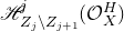 $\mathscr{H}^j_{Z_j\setminus Z_{j+1}}(\mathcal{O}_X^H)$
. By Lemma 2.1, we obtain that
$\mathscr{H}^j_{Z_j\setminus Z_{j+1}}(\mathcal{O}_X^H)$
. By Lemma 2.1, we obtain that $\mathscr{H}^i_{Z_j}(\mathcal{O}_X^H)\cong \mathscr{H}^i_{Z_{j+1}}(\mathcal{O}_X^H)$
for all
$\mathscr{H}^i_{Z_j}(\mathcal{O}_X^H)\cong \mathscr{H}^i_{Z_{j+1}}(\mathcal{O}_X^H)$
for all $i \gt j+1$
. Since
$i \gt j+1$
. Since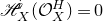 $\mathscr{H}^i_X(\mathcal{O}_X^H)=0$
for all
$\mathscr{H}^i_X(\mathcal{O}_X^H)=0$
for all $i \gt 0$
, we conclude that, for all
$i \gt 0$
, we conclude that, for all $0\leqslant j\leqslant d$
, we have
$0\leqslant j\leqslant d$
, we have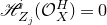 $\mathscr{H}^i_{Z_j}(\mathcal{O}_X^H)=0$
for
$\mathscr{H}^i_{Z_j}(\mathcal{O}_X^H)=0$
for $i \gt j$
. In particular,
$i \gt j$
. In particular,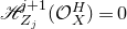 $\mathscr{H}^{j+1}_{Z_j}(\mathcal{O}_X^H)=0$
.
$\mathscr{H}^{j+1}_{Z_j}(\mathcal{O}_X^H)=0$
.
3. The Grothendieck–Cousin complex of a Schubert variety
3.1 Lie algebras and Weyl groups
We let $\mathfrak{g}$
be a complex simple Lie algebra of rank n. We fix a Cartan subalgebra
$\mathfrak{g}$
be a complex simple Lie algebra of rank n. We fix a Cartan subalgebra $\mathfrak{h}\subset \mathfrak{g}$
, and we write
$\mathfrak{h}\subset \mathfrak{g}$
, and we write $\Phi\subset \mathfrak{h}^{\ast}$
for the root system of
$\Phi\subset \mathfrak{h}^{\ast}$
for the root system of $\mathfrak{g}$
with respect to
$\mathfrak{g}$
with respect to $\mathfrak{h}$
. We have the root space decomposition of
$\mathfrak{h}$
. We have the root space decomposition of $\mathfrak{g}$
:
$\mathfrak{g}$
:
 $$\mathfrak{g}=\mathfrak{h}\oplus \bigoplus_{\alpha \in \Phi} \mathfrak{g}_{\alpha}.$$
We denote by $\Delta=\{\alpha_1,\ldots, \alpha_n\}\subset \Phi$
a choice of simple roots, and we write
$\Delta=\{\alpha_1,\ldots, \alpha_n\}\subset \Phi$
a choice of simple roots, and we write $\Phi^{+}\subset \Phi$
for the set of positive roots with respect to
$\Phi^{+}\subset \Phi$
for the set of positive roots with respect to $\Delta$
. The standard Borel subalgebra of
$\Delta$
. The standard Borel subalgebra of $\mathfrak{g}$
associated to this data is
$\mathfrak{g}$
associated to this data is
 $$\mathfrak{b}=\mathfrak{h}\oplus \bigoplus_{\alpha \in \Phi^+} \mathfrak{g}_{\alpha}.$$
A subset $I\subset \Delta$
determines a root system
$I\subset \Delta$
determines a root system $\Phi_I$
via
$\Phi_I$
via
 $$\Phi_I:=\Phi\cap \sum_{\alpha\in I}\mathbb{Z}\alpha,$$
and thus determines the following three subalgebras of $\mathfrak{g}$
:
$\mathfrak{g}$
:
 \begin{equation}\mathfrak{l}_I=\mathfrak{h}\oplus \bigoplus_{\alpha \in \Phi_I} \mathfrak{g}_{\alpha},\quad \mathfrak{u}_I= \bigoplus_{\alpha \in \Phi^+\setminus \Phi_I}\mathfrak{g}_{\alpha},\quad \mathfrak{p}_I=\mathfrak{l}_I\oplus \mathfrak{u}_I.\end{equation}
We say that $\mathfrak{p}_I$
is a parabolic subalgebra of
$\mathfrak{p}_I$
is a parabolic subalgebra of $\mathfrak{g}$
, with Levi factor
$\mathfrak{g}$
, with Levi factor $\mathfrak{l}_I$
and nilradical
$\mathfrak{l}_I$
and nilradical $\mathfrak{u}_I$
. When the set I is understood, we will sometimes omit the subscript I and simply write
$\mathfrak{u}_I$
. When the set I is understood, we will sometimes omit the subscript I and simply write $\mathfrak{p}=\mathfrak{l}\oplus \mathfrak{u}$
.
$\mathfrak{p}=\mathfrak{l}\oplus \mathfrak{u}$
.
Let W denote the Weyl group of $\mathfrak{g}$
, generated by the simple reflections
$\mathfrak{g}$
, generated by the simple reflections $s_{\alpha}$
, where
$s_{\alpha}$
, where $\alpha\in \Delta$
. Given
$\alpha\in \Delta$
. Given $w\in W$
, we write
$w\in W$
, we write $\ell(w)$
for the length of w, which is the length of the shortest word for w in the simple reflections. The group W has a unique longest element, which we will denote by
$\ell(w)$
for the length of w, which is the length of the shortest word for w in the simple reflections. The group W has a unique longest element, which we will denote by $w_{\circ}$
, with length
$w_{\circ}$
, with length $\ell(w_{\circ})=|\Phi^+|$
. Given a parabolic subalgebra
$\ell(w_{\circ})=|\Phi^+|$
. Given a parabolic subalgebra $\mathfrak{p}_I=\mathfrak{l}\oplus \mathfrak{u}$
, we write
$\mathfrak{p}_I=\mathfrak{l}\oplus \mathfrak{u}$
, we write $W_I=\langle s_{\alpha}\mid \alpha \in I\rangle$
for the Weyl group of the Levi factor
$W_I=\langle s_{\alpha}\mid \alpha \in I\rangle$
for the Weyl group of the Levi factor $\mathfrak{l}$
, with longest element
$\mathfrak{l}$
, with longest element $w_I$
. In each left coset
$w_I$
. In each left coset $wW_I\in W/W_I$
, there exists a unique element of minimal length. We consider the set of minimal-length coset representatives:
$wW_I\in W/W_I$
, there exists a unique element of minimal length. We consider the set of minimal-length coset representatives:
 \begin{equation}W^I=\{ w\in W\mid \ell(ww)=\ell(w)+\ell(w')\ \mbox{for all $w'\in W_I$}\}.\end{equation}
Each $x\in W$
may be expressed uniquely as
$x\in W$
may be expressed uniquely as $x=ww'$
, where
$x=ww'$
, where $w\in W^I$
and
$w\in W^I$
and $w'\in W_I$
. We write
$w'\in W_I$
. We write $w_{\circ}(I)$
for the longest element in
$w_{\circ}(I)$
for the longest element in $W^I$
, which satisfies
$W^I$
, which satisfies $w_{\circ}(I)w_I=w_{\circ}$
and
$w_{\circ}(I)w_I=w_{\circ}$
and $\ell(w_{\circ}(I))=|\Phi^+\setminus \Phi_I|$
.
$\ell(w_{\circ}(I))=|\Phi^+\setminus \Phi_I|$
.
3.2 Generalized flag varieties and Schubert varieties
Let G be the simply connected complex simple linear algebraic group with Lie algebra $\mathfrak{g}$
, and with Borel subgroup B corresponding to
$\mathfrak{g}$
, and with Borel subgroup B corresponding to $\mathfrak{b}\subset \mathfrak{g}$
. For
$\mathfrak{b}\subset \mathfrak{g}$
. For $I\subset \Phi$
, we write
$I\subset \Phi$
, we write $P=P_I$
for the parabolic subgroup of G corresponding to
$P=P_I$
for the parabolic subgroup of G corresponding to $\mathfrak{p}=\mathfrak{p}_I$
. We refer to
$\mathfrak{p}=\mathfrak{p}_I$
. We refer to $G/B$
as the complete flag variety of G, and we call
$G/B$
as the complete flag variety of G, and we call $G/P$
the generalized flag variety associated to P. The dimension of
$G/P$
the generalized flag variety associated to P. The dimension of $G/P$
is
$G/P$
is $\dim(G/P)=\ell(w_{\circ}(I))$
.
$\dim(G/P)=\ell(w_{\circ}(I))$
.
Let T be the maximal torus of G associated to the fixed Cartan subalgebra $\mathfrak{h}$
of
$\mathfrak{h}$
of $\mathfrak{g}$
. With this notation, the Weyl group of G is
$\mathfrak{g}$
. With this notation, the Weyl group of G is $W=N_G(T)/T$
. The group G has the Bruhat decomposition
$W=N_G(T)/T$
. The group G has the Bruhat decomposition
 $$G=\bigcup_{w\in W} BwB,$$
where the w in BwB is any representative in G of the class of w. Furthermore, $G/P$
has Bruhat decomposition
$G/P$
has Bruhat decomposition
 $$G/P=\bigcup_{w\in W^I}BwP/P.$$
The sets $BwP/P$
are the B-orbits on
$BwP/P$
are the B-orbits on $G/P$
, known as the Schubert cells. For
$G/P$
, known as the Schubert cells. For $w\in W^I$
, we set
$w\in W^I$
, we set
 \begin{equation}O_{w}=BwP/P\subseteq G/P.\end{equation}
The Zariski closure $Z_{w}$
of
$Z_{w}$
of $O_{w}$
is the Schubert variety associated to
$O_{w}$
is the Schubert variety associated to $w\in W^I$
in
$w\in W^I$
in $G/P$
. It has dimension
$G/P$
. It has dimension $\ell(w)$
and codimension
$\ell(w)$
and codimension $c(w):=\operatorname{{\rm codim}}(Z_{w},X)$
. We say that
$c(w):=\operatorname{{\rm codim}}(Z_{w},X)$
. We say that $v\leqslant w$
if
$v\leqslant w$
if $O_v\subseteq Z_w$
.
$O_v\subseteq Z_w$
.
3.3 Structure of the Grothendieck–Cousin complex
We let $X=G/P_I$
and
$X=G/P_I$
and $d=\dim X$
. For
$d=\dim X$
. For $0\leqslant j\leqslant d$
, we consider the closed sets
$0\leqslant j\leqslant d$
, we consider the closed sets
 $$Z_j=\bigcup_{\substack{v \in W^I\\ c(v)=j}} Z_{v}.$$
The sets $Z_j$
fit into a descending chain
$Z_j$
fit into a descending chain
 $$X=Z_0\supset Z_1 \supset \cdots \supset Z_d \supset Z_{d+1}=\emptyset,$$
where the inclusion $Z_j\setminus Z_{j+1}\subseteq X$
is affine. Each
$Z_j\setminus Z_{j+1}\subseteq X$
is affine. Each $Z_j\setminus Z_{j+1}$
is the disjoint union of closed smooth subvarieties
$Z_j\setminus Z_{j+1}$
is the disjoint union of closed smooth subvarieties $O_v$
over
$O_v$
over $v\in W^I$
with
$v\in W^I$
with $c(v)=j$
, so
$c(v)=j$
, so $Z_j\setminus Z_{j+1}$
is smooth and
$Z_j\setminus Z_{j+1}$
is smooth and $Z_j$
satisfies
$Z_j$
satisfies $\operatorname{{\rm codim}}(Z_j,X)=j$
.
$\operatorname{{\rm codim}}(Z_j,X)=j$
.
By Corollary 2.3, the mixed Hodge module $\mathcal{O}^H_X$
admits a right resolution
$\mathcal{O}^H_X$
admits a right resolution
 $$\mathcal{GC}^{\bullet}_{\{Z\}}:\quad 0 \longrightarrow \mathscr{H}^0_{Z_0\setminus Z_1}(\mathcal{O}_X^H)\longrightarrow \mathscr{H}^1_{Z_1\setminus Z_2}(\mathcal{O}_X^H) \longrightarrow \cdots \longrightarrow \mathscr{H}^d_{Z_d\setminus Z_{d+1}}(\mathcal{O}_X^H)\longrightarrow 0,$$
where we view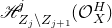 $\mathscr{H}^j_{Z_j\setminus Z_{j+1}}(\mathcal{O}_X^H)$
as being in cohomological degree j. For
$\mathscr{H}^j_{Z_j\setminus Z_{j+1}}(\mathcal{O}_X^H)$
as being in cohomological degree j. For $w\in W^I$
, we define
$w\in W^I$
, we define
 \begin{equation}\mathcal{GC}^{\bullet}_{w}=\mathscr{H}^0_{Z_{w}}(\mathcal{GC}^{\bullet}_{\{Z\}}).\end{equation}
The main result of this subsection is the following.
Theorem 3.1. The following is true about $\mathcal{GC}^{\bullet}_{w}$
.
$\mathcal{GC}^{\bullet}_{w}$
.
-
(i) For all
$0\leqslant j\leqslant d$
, we have
$$\mathcal{H}^j(\mathcal{GC}^{\bullet}_{w})=\mathscr{H}^j_{Z_{w}}(\mathcal{O}_X^H).$$
-
(ii)
$\mathcal{GC}^j_{w}=0$
for
$j<c(w)$
, and for
$j\geqslant c(w)$
we have an isomorphism
$$\mathcal{GC}^j_{w}=\bigoplus_{\substack{v \leqslant w \\ c(v)=j}} \mathscr{H}^j_{O_{v}}(\mathcal{O}_X^H).$$
-
(iii) For
$u<v \leqslant w$
with
$j=c(v)=c(u)-1$
, the differential in
$\mathcal{GC}^{\bullet}_{w}$
induces a nonzero morphism: with
$$\mathscr{H}^j_{O_{v}}(\mathcal{O}_X^H)\longrightarrow \mathscr{H}^{j+1}_{O_{u}}(\mathcal{O}_X^H),$$
$\mathcal{L}(Z_u,X)$
in its image.





We note that part (iii) is not formal: its proof uses the fact that Schubert varieties are normal. In order to prove Theorem 3.1, we first need the following lemma.
Lemma 3.2. For $0\leqslant j\leqslant d$
, we have
$0\leqslant j\leqslant d$
, we have
 $$\mathscr{H}^j_{Z_j\setminus Z_{j+1}}(\mathcal{O}_X^H)=\bigoplus_{\substack{v \in W^I\\ c(v)=j}} \mathscr{H}^j_{O_{v}}(\mathcal{O}_X^H).$$
Proof. Let $k^j:Z_j\setminus Z_{j+1}\hookrightarrow X$
,
$k^j:Z_j\setminus Z_{j+1}\hookrightarrow X$
, $i_v:O_v\hookrightarrow X$
, and
$i_v:O_v\hookrightarrow X$
, and $i^j_v: O_v\hookrightarrow Z_j\setminus Z_{j+1}$
. The variety
$i^j_v: O_v\hookrightarrow Z_j\setminus Z_{j+1}$
. The variety $Z_j\setminus Z_{j+1}$
is the disjoint union of closed smooth subvarieties
$Z_j\setminus Z_{j+1}$
is the disjoint union of closed smooth subvarieties $O_v$
over
$O_v$
over $v\in W^I$
with
$v\in W^I$
with $c(v)=j$
. Thus,
$c(v)=j$
. Thus,
 $$\mathcal{O}^H_{Z_j\setminus Z_{j+1}}=\bigoplus_{\substack{v \in W^I\\ c(v)=j}} i^j_{v\ast}\mathcal{O}^H_{O_v}.$$
Since $\mathscr{H}^j_{Z_j\setminus Z_{j+1}}(\mathcal{O}_X^H)=k^j_{\ast} \mathcal{O}^H_{Z_j\setminus Z_{j+1}}(-j)[-j]$
and
$\mathscr{H}^j_{Z_j\setminus Z_{j+1}}(\mathcal{O}_X^H)=k^j_{\ast} \mathcal{O}^H_{Z_j\setminus Z_{j+1}}(-j)[-j]$
and $\mathscr{H}^j_{O_{v}}(\mathcal{O}_X^H)=i_{v\ast}\mathcal{O}^H_{O_v}(-j)[-j]$
, we obtain the desired result using
$\mathscr{H}^j_{O_{v}}(\mathcal{O}_X^H)=i_{v\ast}\mathcal{O}^H_{O_v}(-j)[-j]$
, we obtain the desired result using $k^j_{\ast}\circ i^j_{v\ast}=i_{v\ast}$
.
$k^j_{\ast}\circ i^j_{v\ast}=i_{v\ast}$
.
Proof
of Theorem 3.1. Since $\mathcal{GC}^{\bullet}_{\{Z\}}$
is a resolution of
$\mathcal{GC}^{\bullet}_{\{Z\}}$
is a resolution of $\mathcal{O}_X^H$
, to prove parts (i) and (ii) it suffices to show that
$\mathcal{O}_X^H$
, to prove parts (i) and (ii) it suffices to show that
 $$\mathscr{H}^0_{Z_{w}}( \mathscr{H}^j_{Z_j\setminus Z_{j+1}}(\mathcal{O}_X^H))=\bigoplus_{\substack{v \leqslant w \\ c(v)=j}}\mathscr{H}^j_{O_{v}}(\mathcal{O}_X^H),$$
and $\mathscr{H}^i_{Z_{w}}(\mathscr{H}^{j}_{Z_j\setminus Z_{j+1}}(\mathcal{O}_X^H))=0$
for
$\mathscr{H}^i_{Z_{w}}(\mathscr{H}^{j}_{Z_j\setminus Z_{j+1}}(\mathcal{O}_X^H))=0$
for $i \gt 0$
. By Lemma 3.2, we have that
$i \gt 0$
. By Lemma 3.2, we have that
 $$\mathscr{H}^j_{Z_j\setminus Z_{j+1}}(\mathcal{O}_X^H)=\bigoplus_{\substack{v \in W^I\\ c(v)=j}} \mathscr{H}^j_{O_{v}}(\mathcal{O}_X^H).$$
Let $v\in W^I$
with
$v\in W^I$
with $c(v)=j$
. If
$c(v)=j$
. If $v\leqslant w$
, then
$v\leqslant w$
, then $O_{v}\cap Z_{w}=O_{v}$
. Let
$O_{v}\cap Z_{w}=O_{v}$
. Let $\beta:O_{v}\hookrightarrow Z_{w}$
,
$\beta:O_{v}\hookrightarrow Z_{w}$
, $\alpha:O_{v}\hookrightarrow X$
,
$\alpha:O_{v}\hookrightarrow X$
, $\gamma:Z_{w}\hookrightarrow X$
, so that
$\gamma:Z_{w}\hookrightarrow X$
, so that $\alpha=\gamma\circ \beta$
. By base change [Reference SaitoSai90, (4.4.3)], we have
$\alpha=\gamma\circ \beta$
. By base change [Reference SaitoSai90, (4.4.3)], we have $\gamma_{\ast}\gamma^!\alpha_{\ast}\alpha^!=\gamma_{\ast}\beta_{\ast}\alpha^!=\alpha_{\ast}\alpha^!$
. Thus, there is a Grothendieck spectral sequence
$\gamma_{\ast}\gamma^!\alpha_{\ast}\alpha^!=\gamma_{\ast}\beta_{\ast}\alpha^!=\alpha_{\ast}\alpha^!$
. Thus, there is a Grothendieck spectral sequence
 $$E^{p,q}_2=\mathscr{H}^p_{Z_{w}}(\mathscr{H}^q_{O_{v}}(\mathcal{O}_X^H)) \implies \mathscr{H}^{p+q}_{O_{v}\cap Z_{w}}(\mathcal{O}_X^H)=\mathscr{H}^{p+q}_{O_{v}}(\mathcal{O}_X^H).$$
Since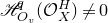 $\mathscr{H}^q_{O_{v}}(\mathcal{O}_X^H)\neq 0$
only if
$\mathscr{H}^q_{O_{v}}(\mathcal{O}_X^H)\neq 0$
only if $q=j$
, this spectral sequence has only one nonzero column on the
$q=j$
, this spectral sequence has only one nonzero column on the $E_2$
-page, and has only one nonzero row on the
$E_2$
-page, and has only one nonzero row on the $E_{\infty}$
-page. Thus, the spectral sequence degenerates at
$E_{\infty}$
-page. Thus, the spectral sequence degenerates at $E_2$
, so we have
$E_2$
, so we have $\mathscr{H}^0_{Z_{w}}(\mathscr{H}^j_{O_{v}}(\mathcal{O}_X^H))=\mathscr{H}^{j}_{O_{v}}(\mathcal{O}_X^H)$
, and
$\mathscr{H}^0_{Z_{w}}(\mathscr{H}^j_{O_{v}}(\mathcal{O}_X^H))=\mathscr{H}^{j}_{O_{v}}(\mathcal{O}_X^H)$
, and $\mathscr{H}^i_{Z_{w}}(\mathscr{H}^{j}_{O_{v}}(\mathcal{O}_X^H))=0$
for
$\mathscr{H}^i_{Z_{w}}(\mathscr{H}^{j}_{O_{v}}(\mathcal{O}_X^H))=0$
for $i \gt 0$
. On the other hand, if
$i \gt 0$
. On the other hand, if $v\nleq w$
, then
$v\nleq w$
, then $O_v\cap Z_w=\emptyset$
, so by base change we obtain a spectral sequence
$O_v\cap Z_w=\emptyset$
, so by base change we obtain a spectral sequence
 $$E^{p,q}_2=\mathscr{H}^p_{Z_{w}}(\mathscr{H}^q_{O_{v}}(\mathcal{O}_X^H)) \implies 0.$$
Since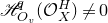 $\mathscr{H}^q_{O_{v}}(\mathcal{O}_X^H)\neq 0$
only if
$\mathscr{H}^q_{O_{v}}(\mathcal{O}_X^H)\neq 0$
only if $q=j$
, this spectral sequence is degenerate, yielding
$q=j$
, this spectral sequence is degenerate, yielding $\mathscr{H}^i_{Z_{w}}(\mathscr{H}^{j}_{O_{v}}(\mathcal{O}_X^H))=0$
for all i and j, which completes the proof of parts (i) and (ii).
$\mathscr{H}^i_{Z_{w}}(\mathscr{H}^{j}_{O_{v}}(\mathcal{O}_X^H))=0$
for all i and j, which completes the proof of parts (i) and (ii).
It suffices to prove part (iii) in the case $w=w_{\circ}(I)$
is the longest element of
$w=w_{\circ}(I)$
is the longest element of $W^I$
so that
$W^I$
so that $\mathcal{GC}^{\bullet}_{w}=\mathcal{GC}^{\bullet}_{\{Z\}}$
, and after restricting to the following open set:
$\mathcal{GC}^{\bullet}_{w}=\mathcal{GC}^{\bullet}_{\{Z\}}$
, and after restricting to the following open set:
 $$U=X \setminus \bigcup_{x \not\geqslant u} Z_{x}.$$
We note that $O_u$
is closed in U. By construction of
$O_u$
is closed in U. By construction of $\mathcal{GC}^{\bullet}_{\{Z\}}$
, the map from
$\mathcal{GC}^{\bullet}_{\{Z\}}$
, the map from $\mathscr{H}^j_{O_{v}}(\mathcal{O}_U^H)$
to
$\mathscr{H}^j_{O_{v}}(\mathcal{O}_U^H)$
to $\mathscr{H}^{j+1}_{O_{u}}(\mathcal{O}_U^H)$
in
$\mathscr{H}^{j+1}_{O_{u}}(\mathcal{O}_U^H)$
in $\mathcal{GC}^{\bullet}_{\{Z\}}|_U$
fits into the following exact sequence (see Lemma 2.1):
$\mathcal{GC}^{\bullet}_{\{Z\}}|_U$
fits into the following exact sequence (see Lemma 2.1):
 $$ 0\longrightarrow \mathscr{H}^j_{\overline{O}_v}(\mathcal{O}_U^H)\longrightarrow \mathscr{H}^j_{O_{v}}(\mathcal{O}_U^H)\longrightarrow \mathscr{H}^{j+1}_{O_{u}}(\mathcal{O}_U^H)\longrightarrow \mathscr{H}^{j+1}_{\overline{O}_v}(\mathcal{O}_U^H)\longrightarrow 0. $$
Since $Z_{v}$
is normal [Reference Ramanan and RamanathanRR85, Theorem 3], its singular locus must have dimension
$Z_{v}$
is normal [Reference Ramanan and RamanathanRR85, Theorem 3], its singular locus must have dimension $\leqslant \ell(v)-2$
, and by equivariance it must be a union of Schubert varieties. Since
$\leqslant \ell(v)-2$
, and by equivariance it must be a union of Schubert varieties. Since $\ell(v)=\ell(u)+1$
, it follows that
$\ell(v)=\ell(u)+1$
, it follows that $\overline{O}_v$
is smooth in U, so we have
$\overline{O}_v$
is smooth in U, so we have $\mathscr{H}^{j+1}_{\overline{O}_v}(\mathcal{O}_U^H)=0$
. As
$\mathscr{H}^{j+1}_{\overline{O}_v}(\mathcal{O}_U^H)=0$
. As $\mathscr{H}^{j+1}_{O_{u}}(\mathcal{O}_U^H)\cong \mathcal{L}(Z_u,X)|_U\neq 0$
, we conclude that the map
$\mathscr{H}^{j+1}_{O_{u}}(\mathcal{O}_U^H)\cong \mathcal{L}(Z_u,X)|_U\neq 0$
, we conclude that the map $\mathscr{H}^j_{O_{v}}(\mathcal{O}_U^H)\to \mathscr{H}^{j+1}_{O_{u}}(\mathcal{O}_U^H)$
is surjective, and therefore the desired map is nonzero, with
$\mathscr{H}^j_{O_{v}}(\mathcal{O}_U^H)\to \mathscr{H}^{j+1}_{O_{u}}(\mathcal{O}_U^H)$
is surjective, and therefore the desired map is nonzero, with $\mathcal{L}(Z_u,X)$
in its image.
$\mathcal{L}(Z_u,X)$
in its image.
Since $\mathcal{GC}_w^{\bullet}$
is a complex of mixed Hodge modules, it is endowed with a Hodge filtration
$\mathcal{GC}_w^{\bullet}$
is a complex of mixed Hodge modules, it is endowed with a Hodge filtration $F_{\bullet}$
and a weight filtration
$F_{\bullet}$
and a weight filtration $W_{\bullet}$
. The next result gives our main tool to get information about the mixed Hodge module structure on local cohomology. The following result implies Theorem A.
$W_{\bullet}$
. The next result gives our main tool to get information about the mixed Hodge module structure on local cohomology. The following result implies Theorem A.
Theorem 3.3. Let $w\in W^I$
, let
$w\in W^I$
, let $p\in \mathbb{Z}$
, and let
$p\in \mathbb{Z}$
, and let $q\geqslant 0$
. The following is true about the Hodge and weight filtrations on local cohomology with support in
$q\geqslant 0$
. The following is true about the Hodge and weight filtrations on local cohomology with support in $Z_{w}$
:
$Z_{w}$
:
 $$F_p(\mathscr{H}_{Z_w}^{q}(\mathcal{O}_X^H))\cong \mathcal{H}^q(F_p(\mathcal{GC}_w^{\bullet})) \quad{and}\quad W_p(\mathscr{H}_{Z_w}^{q}(\mathcal{O}_X^H))\cong \mathcal{H}^q(W_p(\mathcal{GC}_w^{\bullet})).$$
Furthermore, the following is true for $i\in \mathbb{Z}$
:
$i\in \mathbb{Z}$
:
 $$F_pW_i(\mathscr{H}_{Z_w}^{q}(\mathcal{O}_X^H))\cong \mathcal{H}^q(F_pW_i(\mathcal{GC}_w^{\bullet})),$$
where the left-hand side is the intersection of the two filtrations.
Proof. This is an immediate consequence of the fact that morphisms in the category of mixed Hodge modules are bi-strict with respect to the Hodge and weight filtrations [Reference Hotta, Takeuchi and TanisakiHTT08, § 8.3.3(m4)].
3.4 Parabolic Verma modules, P-orbits, and localization
Let $U(\mathfrak{g})$
be the universal enveloping algebra of
$U(\mathfrak{g})$
be the universal enveloping algebra of $\mathfrak{g}$
, and let
$\mathfrak{g}$
, and let $\mathfrak{p}=\mathfrak{p}_I$
be a parabolic subalgebra of
$\mathfrak{p}=\mathfrak{p}_I$
be a parabolic subalgebra of $\mathfrak{g}$
with Levi decomposition
$\mathfrak{g}$
with Levi decomposition $\mathfrak{p}=\mathfrak{l}\oplus \mathfrak{u}$
and adjoint group
$\mathfrak{p}=\mathfrak{l}\oplus \mathfrak{u}$
and adjoint group $P=P_I$
. Let
$P=P_I$
. Let ${\rm mod}_P(\mathfrak{g},\chi_{0})$
denote the category of P-equivariant finitely generated
${\rm mod}_P(\mathfrak{g},\chi_{0})$
denote the category of P-equivariant finitely generated $U(\mathfrak{g})$
-modules with trivial central character (see [Reference Hotta, Takeuchi and TanisakiHTT08, § 11.5]). We write
$U(\mathfrak{g})$
-modules with trivial central character (see [Reference Hotta, Takeuchi and TanisakiHTT08, § 11.5]). We write $\rho=({1}/{2})\sum_{\alpha\in \Phi^+}\alpha$
.
$\rho=({1}/{2})\sum_{\alpha\in \Phi^+}\alpha$
.
For $w\in W^I$
, we let
$w\in W^I$
, we let $F_{w}$
denote the finite-dimensional irreducible
$F_{w}$
denote the finite-dimensional irreducible $\mathfrak{l}$
-representation with highest weight
$\mathfrak{l}$
-representation with highest weight $ww_I\rho-\rho$
, where
$ww_I\rho-\rho$
, where $w_I$
is the longest element in
$w_I$
is the longest element in $W_I$
. We view
$W_I$
. We view $F_{w}$
as a representation of
$F_{w}$
as a representation of $\mathfrak{p}$
, with
$\mathfrak{p}$
, with $\mathfrak{u}$
acting trivially. The parabolic Verma module (sometimes called the generalized Verma module) with highest weight
$\mathfrak{u}$
acting trivially. The parabolic Verma module (sometimes called the generalized Verma module) with highest weight $ww_I\rho-\rho$
is the left
$ww_I\rho-\rho$
is the left $U(\mathfrak{g})$
-module
$U(\mathfrak{g})$
-module
 \begin{equation}M_I(w)=U(\mathfrak{g})\otimes _{U(\mathfrak{p})}F_{w}.\end{equation}
The module $M_I(w)$
is a quotient of the Verma module
$M_I(w)$
is a quotient of the Verma module $M_{\emptyset}(w)$
, and thus has unique simple quotient L(w), the irreducible representation of
$M_{\emptyset}(w)$
, and thus has unique simple quotient L(w), the irreducible representation of $\mathfrak{g}$
with highest weight
$\mathfrak{g}$
with highest weight $ww_I\rho-\rho$
. We define the BGG dual of
$ww_I\rho-\rho$
. We define the BGG dual of $M_I(w)$
as
$M_I(w)$
as $N_I(w)=M_I(w)^{\vee}$
(see [Reference HumphreysHum08, § 3.2]). The module
$N_I(w)=M_I(w)^{\vee}$
(see [Reference HumphreysHum08, § 3.2]). The module $N_I(w)$
is dual to
$N_I(w)$
is dual to $M_I(w)$
in the sense that they have the same composition factors and multiplicities of factors, and the submodule lattice of
$M_I(w)$
in the sense that they have the same composition factors and multiplicities of factors, and the submodule lattice of $N_I(w)$
is dual to that of
$N_I(w)$
is dual to that of $M_I(w)$
(see [Reference HumphreysHum08, § 3.2 Theorem]).
$M_I(w)$
(see [Reference HumphreysHum08, § 3.2 Theorem]).
We now state the Beilinson–Bernstein theorem [Reference Beilinson and BernsteinBB81] for trivial central characters. Consider the natural left action of P on the complete flag variety $G/B$
, with orbits
$G/B$
, with orbits
 \begin{equation}G/B=\bigcup_{w\in W^I}\mathbb{O}_w\quad{\rm where}\ \mathbb{O}_w=\bigcup_{z\in W_I} O_{wz},\end{equation}
in which $O_{y}$
denotes the B-orbit of yB in
$O_{y}$
denotes the B-orbit of yB in $G/B$
. Here,
$G/B$
. Here, $O_{ww_I}$
is dense in
$O_{ww_I}$
is dense in $\mathbb{O}_w$
, so that
$\mathbb{O}_w$
, so that $\overline{O}_{ww_I}=\overline{\mathbb{O}}_w=Z_{w}$
in
$\overline{O}_{ww_I}=\overline{\mathbb{O}}_w=Z_{w}$
in $G/B$
. For
$G/B$
. For $w\in W^I$
, we define the
$w\in W^I$
, we define the $\mathcal{D}_{G/B}$
-modules:
$\mathcal{D}_{G/B}$
-modules:
 \begin{equation}\mathcal{N}_w=\mathscr{H}_{\mathbb{O}_w}^{c(w)}(\mathcal{O}_{G/B}),\quad \mathcal{M}_w=\mathbb{D}\mathcal{N}_w,\quad \mathcal{L}_w=\mathcal{L}(\mathbb{O}_w,G/B).\end{equation}
For the following statements, we write ${\rm mod}_P(\mathcal{D}_{G/B})$
for the category of P-equivariant coherent
${\rm mod}_P(\mathcal{D}_{G/B})$
for the category of P-equivariant coherent $\mathcal{D}_{G/B}$
-modules (see [Reference Lõrincz and WaltherLW19, § 2.1] or [Reference Hotta, Takeuchi and TanisakiHTT08, § 11.5]), and we write
$\mathcal{D}_{G/B}$
-modules (see [Reference Lõrincz and WaltherLW19, § 2.1] or [Reference Hotta, Takeuchi and TanisakiHTT08, § 11.5]), and we write ${\rm mod}_B(\mathcal{D}_{G/P})$
for the category of B-equivariant coherent
${\rm mod}_B(\mathcal{D}_{G/P})$
for the category of B-equivariant coherent $\mathcal{D}_{G/P}$
-modules.
$\mathcal{D}_{G/P}$
-modules.
Theorem 3.4. The following is true about ${\rm mod}_P(\mathcal{D}_{G/B})$
.
${\rm mod}_P(\mathcal{D}_{G/B})$
.
-
(i) The global sections functor
$\Gamma(G/B,-)$
induces an equivalence of categories
$${\rm mod}_P(\mathcal{D}_{G/B})\cong {\rm mod}_P(\mathfrak{g},\chi_0).$$
-
(ii) Furthermore, given
$w\in W^I$
, we have
$$\Gamma(G/B,\mathcal{N}_w)\cong N_I(w),\quad \Gamma(G/B,\mathcal{M}_w)\cong M_I(w),\quad \Gamma(G/B,\mathcal{L}_w)\cong L(w).$$


Proof. The equivalence of categories in part (i) is a special case of the Beilinson–Bernstein theorem [Reference Beilinson and BernsteinBB81] (for a textbook account, see [Reference Hotta, Takeuchi and TanisakiHTT08, Theorem 11.5.3]). For the first two isomorphisms in part (ii), see [Reference Casian and CollingwoodCC87, (3.27) Lemma] and subsequent discussion. The final isomorphism follows from [Reference Beilinson and BernsteinBB81, Proposition] (alternatively, [Reference Hotta, Takeuchi and TanisakiHTT08, Proposition 12.3.2], noting that $\mathcal{L}(\mathbb{O}_w,G/B)=\mathcal{L}(O_{ww_I},G/B)$
).
$\mathcal{L}(\mathbb{O}_w,G/B)=\mathcal{L}(O_{ww_I},G/B)$
).
For the remainder of the subsection, we write $\pi^{\ast}$
for the (unshifted) pullback functor of
$\pi^{\ast}$
for the (unshifted) pullback functor of $\mathcal{D}$
-modules [Reference Hotta, Takeuchi and TanisakiHTT08, § 1.3] and we write
$\mathcal{D}$
-modules [Reference Hotta, Takeuchi and TanisakiHTT08, § 1.3] and we write $\pi_{\ast}$
for the direct image functor of quasi-coherent
$\pi_{\ast}$
for the direct image functor of quasi-coherent $\mathcal{O}$
-modules.
$\mathcal{O}$
-modules.
Theorem 3.5. Consider the natural projection $\pi: G/B \to G/P$
. Then,
$\pi: G/B \to G/P$
. Then, $\pi^{\ast}$
is exact and induces an equivalence of categories
$\pi^{\ast}$
is exact and induces an equivalence of categories
 $${\rm mod}_B(\mathcal{D}_{G/P})\cong {\rm mod}_P(\mathcal{D}_{G/B}).$$
Furthermore, given $w\in W^I$
, we have
$w\in W^I$
, we have
 $$\pi^{\ast}\mathscr{H}_{O_{w}}^{c(w)}(\mathcal{O}_{G/P})\cong \mathcal{N}_w,\quad \pi^{\ast}(\mathbb{D}(\mathscr{H}_{O_{w}}^{c(w)}(\mathcal{O}_{G/P})))\cong \mathcal{M}_w,\quad \pi^{\ast}\mathcal{L}(O_{w},G/P)\cong \mathcal{L}_w.$$
Proof. Since $\pi$
is smooth, the functor
$\pi$
is smooth, the functor $\pi^{\ast}$
is exact [Reference Hotta, Takeuchi and TanisakiHTT08, Proposition 1.5.13]. By [Reference Lõrincz and WaltherLW19, Proposition 4.5(b)], the functor
$\pi^{\ast}$
is exact [Reference Hotta, Takeuchi and TanisakiHTT08, Proposition 1.5.13]. By [Reference Lõrincz and WaltherLW19, Proposition 4.5(b)], the functor $\pi^{\ast}$
induces the desired equivalence of categories.
$\pi^{\ast}$
induces the desired equivalence of categories.
It follows from (3.6) that $\pi^{-1}(O_w)=\mathbb{O}_w$
, so base change [Reference Hotta, Takeuchi and TanisakiHTT08, Theorem 1.7.3] yields the first two isomorphisms. The third isomorphism follows from the first and the equivalence of categories.
$\pi^{-1}(O_w)=\mathbb{O}_w$
, so base change [Reference Hotta, Takeuchi and TanisakiHTT08, Theorem 1.7.3] yields the first two isomorphisms. The third isomorphism follows from the first and the equivalence of categories.
Combining Theorems 3.4 and 3.5, we obtain the following.
Corollary 3.6. The following is true about ${\rm mod}_B(\mathcal{D}_{G/P})$
.
${\rm mod}_B(\mathcal{D}_{G/P})$
.
-
(i) The global sections functor
$\Gamma(G/P,-)$
induces an equivalence of categories
$${\rm mod}_B(\mathcal{D}_{G/P})\cong {\rm mod}_P(\mathfrak{g},\chi_0).$$
-
(ii) Furthermore, given
$w\in W^I$
, we have
\begin{align*}&\Gamma(G/P,\mathscr{H}_{O_{w}}^{c(w)}(\mathcal{O}_{G/P}))\cong N_I(w),\quad \Gamma(G/P,\mathbb{D}(\mathscr{H}_{O_{w}}^{c(w)}(\mathcal{O}_{G/P})))\cong M_I(w),\\& \Gamma(G/P,\mathcal{L}_w)\cong L(w).\end{align*}


Proof. We follow the strategy described in [Reference Borho and BrylinskiBB85, footnote p. 14] (see also [Reference Holland and PoloHP96, Proposition 2.14]). Let $\pi:G/B\to G/P$
be the projection. For
$\pi:G/B\to G/P$
be the projection. For $\mathcal{M}\in {\rm mod}_B(\mathcal{D}_{G/P})$
, we have that
$\mathcal{M}\in {\rm mod}_B(\mathcal{D}_{G/P})$
, we have that $\mathbb{R}^j\pi_{\ast}(\pi^{\ast}\mathcal{M})=0$
for
$\mathbb{R}^j\pi_{\ast}(\pi^{\ast}\mathcal{M})=0$
for $j \gt 0$
(see [Reference Holland and PoloHP96, Proposition 2.14(a)]). By Theorem 3.4(1), we have that the Leray–Serre spectral sequence
$j \gt 0$
(see [Reference Holland and PoloHP96, Proposition 2.14(a)]). By Theorem 3.4(1), we have that the Leray–Serre spectral sequence
 $$H^i(G/P,\mathbb{R}^j\pi_{\ast}(\pi^{\ast}\mathcal{M}))\quad \implies \quad H^{i+j}(G/B,\pi^{\ast}\mathcal{M})$$
degenerates to yield an isomorphism $\Gamma(G/P,\mathcal{M})\cong \Gamma(G/B, \pi^{\ast}\mathcal{M})$
as
$\Gamma(G/P,\mathcal{M})\cong \Gamma(G/B, \pi^{\ast}\mathcal{M})$
as $U(\mathfrak{g})$
-modules. By Theorems 3.4 and 3.5, this proves both part (i) and part (ii).
$U(\mathfrak{g})$
-modules. By Theorems 3.4 and 3.5, this proves both part (i) and part (ii).
For $w\in W^I$
, we consider the global Grothendieck–Cousin complex
$w\in W^I$
, we consider the global Grothendieck–Cousin complex $GC_w^{\bullet}=\Gamma(X,\mathcal{GC}^{\bullet}_w)$
:
$GC_w^{\bullet}=\Gamma(X,\mathcal{GC}^{\bullet}_w)$
:
 \begin{equation}GC^{\bullet}_w:\quad 0 \longrightarrow N_I(w) \longrightarrow \bigoplus_{\substack{v\leqslant w\\ c(v)=c(w)+1}} N_I(v)\longrightarrow \cdots \longrightarrow \bigoplus_{\substack{v\leqslant w\\ c(w)=\ell(w_I)-1}} N_I(v) \longrightarrow N_I(e)\longrightarrow 0.\end{equation}
We define the Hodge filtration $F_{\bullet}$
and weight filtration
$F_{\bullet}$
and weight filtration $W_{\bullet}$
on
$W_{\bullet}$
on $N_I(w)$
via (see [Reference Davis and VilonenDV23, Theorem 1.1])
$N_I(w)$
via (see [Reference Davis and VilonenDV23, Theorem 1.1])
 \begin{equation}F_p(N_I(w))=\Gamma(F_p(\mathscr{H}_{O_{w}}^{c(w)}(\mathcal{O}_{X}))) \quad {\rm and}\quad W_p(N_I(w))=\Gamma(W_p(\mathscr{H}_{O_{w}}^{c(w)}(\mathcal{O}_{X}))).\end{equation}
We endow $M_I(w)$
with filtrations in similar manner. The weight filtration on
$M_I(w)$
with filtrations in similar manner. The weight filtration on $M_I(w)$
is called the Jantzen filtration (see [Reference Beilinson and BernsteinBB93, Reference HumphreysHum08]). Similarly, we define Hodge and weight filtrations on the global local cohomology modules for
$M_I(w)$
is called the Jantzen filtration (see [Reference Beilinson and BernsteinBB93, Reference HumphreysHum08]). Similarly, we define Hodge and weight filtrations on the global local cohomology modules for $q\geqslant 0$
:
$q\geqslant 0$
:
 \begin{equation}F_p(H_{Z_w}^{q}(X,\mathcal{O}_X))=\Gamma(F_p(\mathscr{H}^q_{Z_w}(\mathcal{O}_X))) \quad{\rm and}\quad W_p(H_{Z_w}^{q}(X,\mathcal{O}_X))=\Gamma(W_p(\mathscr{H}^q_{Z_w}(\mathcal{O}_X))).\end{equation}
By Theorem 3.1, Corollary 3.6, and [Reference Davis and VilonenDV23, Theorem 1.1], we obtain the following.
Corollary 3.7.
-
(i) For
$w\in W^I$
, we have that the morphisms in
$GC^{\bullet}_w$
are strict with respect to the Hodge and weight filtrations. In particular,
$${\rm gr}^F_p(H_{Z_w}^{q}(X,\mathcal{O}_X))\cong \mathcal{H}^q({\rm gr}^F_p(GC_w^{\bullet})) \quad{and}\quad{\rm gr}^W_p(H_{Z_w}^{q}(X,\mathcal{O}_X))\cong \mathcal{H}^q({\rm gr}^W_p(GC_w^{\bullet})).$$
-
(ii) For
$u<v \leqslant w$
with
$j=c(v)=c(u)-1$
, the differential in
$GC^{\bullet}_{w}$
induces a nonzero morphism
$$N_I(v)\to N_I(u).$$
-
(iii) For
$v\leqslant w$
, the multiplicity of L(v) as a composition factor of
${\rm gr}^W_p(H_{Z_w}^{q}(X,\mathcal{O}_X))$
is equal to the multiplicity of
$\mathcal{L}(O_v,X)$
as a composition factor of
${\rm gr}^W_p(\mathscr{H}^q_{Z_w}(\mathcal{O}_X^H))$
.








We do not pursue the Hodge filtration further in this work.
4. Calculations for the Grassmannian
Let $X={\rm Gr}(k,n)$
be the Grassmannian of k-dimensional subspaces of an n-dimensional complex vector space, so that
$X={\rm Gr}(k,n)$
be the Grassmannian of k-dimensional subspaces of an n-dimensional complex vector space, so that $d_X=k(n-k)$
. We prove Theorem 1.1 and apply it in §4.5 to calculate local cohomology with support in determinantal varieties. We freely use notation from §1.2.
$d_X=k(n-k)$
. We prove Theorem 1.1 and apply it in §4.5 to calculate local cohomology with support in determinantal varieties. We freely use notation from §1.2.
4.1 The Grassmannian and minimal-length coset representatives
Let $\mathfrak{g}=\mathfrak{sl}_n(\mathbb{C})$
, with simple roots
$\mathfrak{g}=\mathfrak{sl}_n(\mathbb{C})$
, with simple roots $\Delta=\{\alpha_1,\ldots, \alpha_{n-1}\}$
, where
$\Delta=\{\alpha_1,\ldots, \alpha_{n-1}\}$
, where $\alpha_i=\epsilon_i-\epsilon_{i+1}$
. Let
$\alpha_i=\epsilon_i-\epsilon_{i+1}$
. Let $I=\Delta\setminus \{\alpha_k\}$
and let
$I=\Delta\setminus \{\alpha_k\}$
and let $\mathfrak{p}=\mathfrak{p}_I$
. We write
$\mathfrak{p}=\mathfrak{p}_I$
. We write $G=\operatorname{{\rm SL}}_n(\mathbb{C})$
and P for the groups corresponding to
$G=\operatorname{{\rm SL}}_n(\mathbb{C})$
and P for the groups corresponding to $\mathfrak{g}$
and
$\mathfrak{g}$
and $\mathfrak{p}$
, so that
$\mathfrak{p}$
, so that $X\cong G/P$
.
$X\cong G/P$
.
The set of minimal-length coset representatives of $W/W_I$
is
$W/W_I$
is
 \begin{equation}W^I=\{(i_1,\ldots, i_n)\in \mathfrak{S}_n\mid i_1<\cdots <i_k, i_{k+1}<\cdots<i_n\},\end{equation}
where $\mathfrak{S}_n$
is the symmetric group on n elements. In our notation, the identity e is represented by
$\mathfrak{S}_n$
is the symmetric group on n elements. In our notation, the identity e is represented by $(1,2,\ldots, n)$
, and the longest element
$(1,2,\ldots, n)$
, and the longest element $w_{\circ}(I)$
is represented by
$w_{\circ}(I)$
is represented by $(n-k+1,\ldots, n,1,\ldots, n-k)$
. To each
$(n-k+1,\ldots, n,1,\ldots, n-k)$
. To each $w=(i_1,\ldots, i_n)\in W^I$
, we associate a Young diagram
$w=(i_1,\ldots, i_n)\in W^I$
, we associate a Young diagram $\underline{a}=\underline{a}(w)$
:
$\underline{a}=\underline{a}(w)$
:
 $$a_1=i_k-k,\quad a_2=i_{k-1}-(k-1),\quad \ldots, \quad a_k=i_1-1,$$
i.e. $a_j=i_{k+1-j}-(k+1-j)$
for
$a_j=i_{k+1-j}-(k+1-j)$
for $1\leqslant j\leqslant k$
and
$1\leqslant j\leqslant k$
and $a_j=0$
for
$a_j=0$
for $j \gt k$
. For instance, we have
$j \gt k$
. For instance, we have
 $$e \;\longleftrightarrow \;(0,\ldots, 0) \quad {\rm and}\quad w_{\circ}(I)\; \longleftrightarrow \; (n-k,\ldots, n-k).$$
We obtain a bijection between $W^I$
and the set
$W^I$
and the set
 \begin{equation}\mathcal{R}_{k,n}=\{\underline{a} \mid n-k\geqslant a_1\geqslant a_2\geqslant \cdots \geqslant a_k\geqslant 0\}.\end{equation}
We think of $\mathcal{R}_{k,n}$
as the set of Young diagrams that fit into a
$\mathcal{R}_{k,n}$
as the set of Young diagrams that fit into a $k\times (n-k)$
rectangle.
$k\times (n-k)$
rectangle.
Given $w\in W^I$
with
$w\in W^I$
with $\underline{a}=\underline{a}(w)$
, we write
$\underline{a}=\underline{a}(w)$
, we write $O_{\underline{a}}=O_{w}$
and
$O_{\underline{a}}=O_{w}$
and $Z_{\underline{a}}=Z_{w}$
for the corresponding Schubert cell and Schubert variety. We have
$Z_{\underline{a}}=Z_{w}$
for the corresponding Schubert cell and Schubert variety. We have $\dim Z_{\underline{a}}=|\underline{a}|=\ell(w)$
. We write
$\dim Z_{\underline{a}}=|\underline{a}|=\ell(w)$
. We write $M(\underline{a})=M_I(w)$
,
$M(\underline{a})=M_I(w)$
, $N(\underline{a})=N_I(w)$
,
$N(\underline{a})=N_I(w)$
, $L(\underline{a})=L_I(w)$
, so that
$L(\underline{a})=L_I(w)$
, so that $M(\underline{a})$
and
$M(\underline{a})$
and $L(\underline{a})$
have highest weight
$L(\underline{a})$
have highest weight
 \begin{equation}\lambda_{\underline{a},n}:=ww_I\rho-\rho=(-a_k^c,-a_{k-1}^c,\ldots, -a_1^c\mid (a^c)_1',(a^c)_2',\ldots, (a^c)_{n-k}'),\end{equation}
where $\underline{a}^c=(n-k-a_k,\ldots, n-k-a_1)$
is the complementary partition of
$\underline{a}^c=(n-k-a_k,\ldots, n-k-a_1)$
is the complementary partition of $\underline{a}$
in
$\underline{a}$
in $\mathcal{R}_{k,n}$
and
$\mathcal{R}_{k,n}$
and $(\underline{a}^c)'$
is the conjugate partition to
$(\underline{a}^c)'$
is the conjugate partition to $\underline{a}^c$
. We use the notation
$\underline{a}^c$
. We use the notation $\lambda_{\underline{a},n}$
to emphasize the dependence on n.
$\lambda_{\underline{a},n}$
to emphasize the dependence on n.
4.2 Properties of the parabolic Verma modules
Let $\underline{a}\in \mathcal{R}_{k,n}$
. We freely identify the modules
$\underline{a}\in \mathcal{R}_{k,n}$
. We freely identify the modules $N(\underline{a})$
,
$N(\underline{a})$
, $M(\underline{a})$
, and
$M(\underline{a})$
, and $L(\underline{a})$
with their
$L(\underline{a})$
with their $\mathcal{D}_X$
-module-theoretic counterparts via Corollary 3.6, i.e.
$\mathcal{D}_X$
-module-theoretic counterparts via Corollary 3.6, i.e.
 $$ N(\underline{a})\;\longleftrightarrow \;\mathscr{H}^{c(\underline{a})}_{O_{\underline{a}}}(\mathcal{O}_X),\quad M(\underline{a})\;\longleftrightarrow \; \mathbb{D}(\mathscr{H}^{c(\underline{a})}_{O_{\underline{a}}}(\mathcal{O}_X)),\quad L(\underline{a})\;\longleftrightarrow \; \mathcal{L}(O_{\underline{a}},X),$$
and we recall that $M(\underline{a})$
and
$M(\underline{a})$
and $N(\underline{a})$
are endowed with weight filtrations
$N(\underline{a})$
are endowed with weight filtrations $W_{\bullet}$
via this equivalence.
$W_{\bullet}$
via this equivalence.
A Loewy filtration on a finite length $U(\mathfrak{g})$
-module M is a filtration of minimal length such that the subquotients are semi-simple. Two examples of Loewy filtrations are the socle and radical filtrations (see [Reference HumphreysHum08, § 8.14]). We say that M is rigid if the socle and radical filtrations coincide, in which case there is a unique Loewy filtration on M. For
$U(\mathfrak{g})$
-module M is a filtration of minimal length such that the subquotients are semi-simple. Two examples of Loewy filtrations are the socle and radical filtrations (see [Reference HumphreysHum08, § 8.14]). We say that M is rigid if the socle and radical filtrations coincide, in which case there is a unique Loewy filtration on M. For $p\in \mathbb{Z}$
, we write
$p\in \mathbb{Z}$
, we write
 \begin{equation}\mathcal{Z}_p(\underline{a})=\{\mathbb{D}\in {\rm Dyck}(\underline{a}) \mid |\mathbb{D}|=p+|\underline{a}|-2d_{X} \}.\end{equation}
We emphasize that elements of $\mathcal{Z}_p(\underline{a})$
may have Dyck paths of length 1, and they have no bullets. Recall that
$\mathcal{Z}_p(\underline{a})$
may have Dyck paths of length 1, and they have no bullets. Recall that $\underline{a}^{\mathbb{D}}$
is the partition obtained from
$\underline{a}^{\mathbb{D}}$
is the partition obtained from $\underline{a}$
by removing the boxes in the support of
$\underline{a}$
by removing the boxes in the support of $\mathbb{D}$
(see (1.6)).
$\mathbb{D}$
(see (1.6)).
The following result is a collection of facts from the literature.
Theorem 4.1. The modules $M(\underline{a})$
and
$M(\underline{a})$
and $N(\underline{a})$
are rigid, and the weight filtration
$N(\underline{a})$
are rigid, and the weight filtration $W_{\bullet}$
is the unique Loewy filtration. For
$W_{\bullet}$
is the unique Loewy filtration. For $p\in \mathbb{Z}$
, the graded pieces of the weight filtration are given by
$p\in \mathbb{Z}$
, the graded pieces of the weight filtration are given by
 $$ {\rm gr}_p^W(M(\underline{a}))=\bigoplus_{\mathbb{D}\in \mathcal{Z}_{-p}(\underline{a})} L(\underline{a}^{\mathbb{D}}) \quad{and}\quad {\rm gr}_p^W(N(\underline{a}))=\bigoplus_{\mathbb{D}\in \mathcal{Z}_p(\underline{a})} L(\underline{a}^{\mathbb{D}}).$$
In particular, each composition factor of $M(\underline{a})$
and
$M(\underline{a})$
and $N(\underline{a})$
appears with multiplicity one.
$N(\underline{a})$
appears with multiplicity one.
Proof. The composition factors of $M(\underline{a})$
(and, hence,
$M(\underline{a})$
(and, hence, $N(\underline{a})$
) are described in [Reference Collingwood, Irving and SheltonCIS88, Theorem 1.3]. The authors also show that the socle, radical, and
$N(\underline{a})$
) are described in [Reference Collingwood, Irving and SheltonCIS88, Theorem 1.3]. The authors also show that the socle, radical, and $\ell$
-adic weight filtrations coincide and are the unique Loewy filtration [Reference Collingwood, Irving and SheltonCIS88, Corollary 1.7]. The graded pieces of the Loewy filtration are interpreted in terms of inverse parabolic Kazhdan–Lusztig polynomials in [Reference IrvingIrv90, Corollary 7.1.3]. For the Dyck-pattern interpretation of these inverse Kazhdan–Lusztig polynomials, see [Reference Shigechi and Zinn-JustinSZJ12, Corollary 1] (see also [Reference Shigechi and Zinn-JustinSZJ12, § 3.1]). In [Reference Kashiwara and TanisakiKT02, Theorem 1.4], it is shown that these inverse Kazhdan–Lusztig polynomials also describe the weight filtration on
$\ell$
-adic weight filtrations coincide and are the unique Loewy filtration [Reference Collingwood, Irving and SheltonCIS88, Corollary 1.7]. The graded pieces of the Loewy filtration are interpreted in terms of inverse parabolic Kazhdan–Lusztig polynomials in [Reference IrvingIrv90, Corollary 7.1.3]. For the Dyck-pattern interpretation of these inverse Kazhdan–Lusztig polynomials, see [Reference Shigechi and Zinn-JustinSZJ12, Corollary 1] (see also [Reference Shigechi and Zinn-JustinSZJ12, § 3.1]). In [Reference Kashiwara and TanisakiKT02, Theorem 1.4], it is shown that these inverse Kazhdan–Lusztig polynomials also describe the weight filtration on $N(\underline{a})$
(and, hence,
$N(\underline{a})$
(and, hence, $M(\underline{a})$
). Thus, the weight filtration is the unique Loewy filtration. We have normalized the shift on
$M(\underline{a})$
). Thus, the weight filtration is the unique Loewy filtration. We have normalized the shift on $W_{\bullet}$
so that
$W_{\bullet}$
so that $L(\underline{a})$
lives in weight
$L(\underline{a})$
lives in weight $p=2d_{X}-|\underline{a}|$
of
$p=2d_{X}-|\underline{a}|$
of $N(\underline{a})$
.
$N(\underline{a})$
.
We remark that the original combinatorial description of the relevant Kazhdan–Lusztig polynomials may be found in [Reference Lascoux and SchützenbergerLS81].
Example 4.2. Let $\underline{a}=(3,2,2)$
. The following example works equally well for any k,n for which
$\underline{a}=(3,2,2)$
. The following example works equally well for any k,n for which $\underline{a}\in \mathcal{R}_{k,n}$
. For concreteness, let
$\underline{a}\in \mathcal{R}_{k,n}$
. For concreteness, let $k=3$
and
$k=3$
and $n=6$
, so that
$n=6$
, so that $d_X=9$
. The elements of Dyck
$d_X=9$
. The elements of Dyck $(\underline{a})$
are as follows.
$(\underline{a})$
are as follows.

It follows from Theorem 4.1 that the weight filtration on $N(\underline{a})$
is given by
$N(\underline{a})$
is given by
 \begin{align*}\operatorname{{\rm gr}}^W_{11}(N(\underline{a})) & =L(3,2,2),\quad \operatorname{{\rm gr}}^W_{12}(N(\underline{a}))=L(2,2,2)\oplus L(3,2,1),\\\operatorname{{\rm gr}}^W_{13}(N(\underline{a})) & =L(3,0,0)\oplus L(2,2,1)\oplus L(1,0,0),\quad \operatorname{{\rm gr}}^W_{14}(N(\underline{a}))=L(2,0,0).\end{align*}
The composition factors of $M(\underline{a})$
are the same and
$M(\underline{a})$
are the same and $\operatorname{{\rm gr}}_p^W(M(\underline{a}))=\operatorname{{\rm gr}}^W_{-p}(N(\underline{a}))$
for all
$\operatorname{{\rm gr}}_p^W(M(\underline{a}))=\operatorname{{\rm gr}}^W_{-p}(N(\underline{a}))$
for all $p\in \mathbb{Z}$
.
$p\in \mathbb{Z}$
.
For a larger example, see [Reference HuangHua20, Example 2.19] for composition factors of N(5,4,2,1) when $k=4$
,
$k=4$
, $n= 9$
, noting that the author uses the complementary convention for partitions. In particular, the simple L(2,2) (shown in the bottom right) has weight
$n= 9$
, noting that the author uses the complementary convention for partitions. In particular, the simple L(2,2) (shown in the bottom right) has weight $p=32$
, which is maximal in N(5,4,2,1).
$p=32$
, which is maximal in N(5,4,2,1).
Given $\mathbb{D}\in {\rm Dyck}(\underline{a})$
, we write
$\mathbb{D}\in {\rm Dyck}(\underline{a})$
, we write $v_{\underline{a}}^{\mathbb{D}}$
for any vector v in
$v_{\underline{a}}^{\mathbb{D}}$
for any vector v in $M(\underline{a})$
such that the class of v in a quotient of
$M(\underline{a})$
such that the class of v in a quotient of $M(\underline{a})$
is a highest-weight vector for
$M(\underline{a})$
is a highest-weight vector for $L(\underline{a}^{\mathbb{D}})$
. Such vectors are called primitive vectors. For two Dyck patterns with no bullets
$L(\underline{a}^{\mathbb{D}})$
. Such vectors are called primitive vectors. For two Dyck patterns with no bullets $\mathbb{D},\mathbb{D}'\in {\rm Dyck}(\underline{a})$
, we write
$\mathbb{D},\mathbb{D}'\in {\rm Dyck}(\underline{a})$
, we write $\mathbb{D}\subseteq \mathbb{D}'$
if all paths in
$\mathbb{D}\subseteq \mathbb{D}'$
if all paths in $\mathbb{D}$
are also paths in
$\mathbb{D}$
are also paths in $\mathbb{D}'$
.
$\mathbb{D}'$
.
Theorem 4.3. Let $\mathbb{D}$
,
$\mathbb{D}$
, $\mathbb{D}'\in {\rm Dyck}(\underline{a})$
. The following is true about
$\mathbb{D}'\in {\rm Dyck}(\underline{a})$
. The following is true about $M(\underline{a})$
.
$M(\underline{a})$
.
-
(i) If
$\mathbb{D}\subseteq \mathbb{D}'$
, then
$v^{\mathbb{D}'}_{\underline{a}}\in U(\mathfrak{g}) v_{\underline{a}}^{\mathbb{D}}$
. -
(ii) If
$\mathbb{D}=\{(x,y)\}$
and
$v^{\mathbb{D}'}_{\underline{a}}\in U(\mathfrak{g}) v_{\underline{a}}^{\mathbb{D}}$
, then
$\mathbb{D}\subseteq \mathbb{D}'$
.

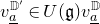

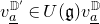

We emphasize that the converse to part (i) is false in general (see [Reference Su and ZhangSZ12, Theorem 5.18] or [Reference Boe and EnrightBE86]). For instance, in Example 4.2, a primitive vector for L(2,0,0) generates a primitive vector for L(1,0,0). In the terminology of [Reference Su and ZhangSZ12], the Dyck pattern corresponding to L(1,0,0) is a ‘path with bridges’.
Proof. The best reference for this information is obtained via super duality (see, e.g., [Reference Su and ZhangSZ12, § 3.3]), which relates parabolic Verma modules over an infinite-dimensional general linear Lie algebra to Kac modules over an infinite-dimensional general linear Lie superalgebra. Once we have set up notation, Theorem 4.3 will follow readily from [Reference Su and ZhangSZ12, Theorem 5.18].
For each $r\geqslant n-k$
, we consider the general linear Lie algebra
$r\geqslant n-k$
, we consider the general linear Lie algebra $\mathfrak{gl}_{k+r}$
with the parabolic subalgebra
$\mathfrak{gl}_{k+r}$
with the parabolic subalgebra $\mathfrak{p}_{k+r}$
with Levi subalgebra
$\mathfrak{p}_{k+r}$
with Levi subalgebra $\mathfrak{gl}_{k}\times \mathfrak{gl}_{r}$
. Let
$\mathfrak{gl}_{k}\times \mathfrak{gl}_{r}$
. Let $\underline{a}$
be as above, and consider the parabolic Verma module
$\underline{a}$
be as above, and consider the parabolic Verma module $M^{k+r}(\lambda_{\underline{a}})$
over
$M^{k+r}(\lambda_{\underline{a}})$
over $\mathfrak{gl}_{k+r}$
with highest weight (see §4.1)
$\mathfrak{gl}_{k+r}$
with highest weight (see §4.1)
 $$\lambda_{\underline{a},n}=(-a_k^c,-a_{k-1}^c,\ldots, -a_1^c\mid (a^c)_1',(a^c)_2',\ldots, (a^c)_r'),$$
so that $M^{n}(\lambda_{\underline{a},n})=M(\underline{a})$
. We consider the irreducible
$M^{n}(\lambda_{\underline{a},n})=M(\underline{a})$
. We consider the irreducible $\mathfrak{gl}_{k+r}$
-module
$\mathfrak{gl}_{k+r}$
-module $L^{k+r}(\lambda_{\underline{a},n})$
of highest weight
$L^{k+r}(\lambda_{\underline{a},n})$
of highest weight $\lambda_{\underline{a},n}$
, so that
$\lambda_{\underline{a},n}$
, so that $L^{n}(\lambda_{\underline{a},n})=L(\underline{a})$
. Taking the limit as
$L^{n}(\lambda_{\underline{a},n})=L(\underline{a})$
. Taking the limit as $r\to \infty$
, we obtain
$r\to \infty$
, we obtain $\mathfrak{gl}_{k+\infty}$
and the modules
$\mathfrak{gl}_{k+\infty}$
and the modules $M^{k+\infty}(\lambda_{\underline{a},n})$
,
$M^{k+\infty}(\lambda_{\underline{a},n})$
, $L^{k+\infty}(\lambda_{\underline{a},n })$
. We write
$L^{k+\infty}(\lambda_{\underline{a},n })$
. We write $\mathcal{O}^{\mathfrak{p}_{k+r}}_{{\rm int}}$
and
$\mathcal{O}^{\mathfrak{p}_{k+r}}_{{\rm int}}$
and $\mathcal{O}^{\mathfrak{p}_{k+\infty}}_{{\rm int}}$
for the corresponding parabolic categories
$\mathcal{O}^{\mathfrak{p}_{k+\infty}}_{{\rm int}}$
for the corresponding parabolic categories $\mathcal{O}$
with integral weights. Similar to Theorem 4.1,
$\mathcal{O}$
with integral weights. Similar to Theorem 4.1, $M^{k+\infty}(\lambda_{\underline{a},n})$
has composition factors
$M^{k+\infty}(\lambda_{\underline{a},n})$
has composition factors $L^{k+\infty}(-b_k,-b_{k-1},\ldots, -b_1\,|\,b_1',b_2',\ldots)$
, where
$L^{k+\infty}(-b_k,-b_{k-1},\ldots, -b_1\,|\,b_1',b_2',\ldots)$
, where $\underline{b}=(b_1,\ldots, b_k)$
is obtained from
$\underline{b}=(b_1,\ldots, b_k)$
is obtained from $\underline{a}^c$
by adding an admissible Dyck pattern with no bullets (over an infinite-dimensional space, it is more convenient to work with
$\underline{a}^c$
by adding an admissible Dyck pattern with no bullets (over an infinite-dimensional space, it is more convenient to work with $\underline{a}^c$
rather than
$\underline{a}^c$
rather than $\underline{a}$
). We have an exact truncation functor
$\underline{a}$
). We have an exact truncation functor $\operatorname{{\rm tr}}_{n-k}:\mathcal{O}^{\mathfrak{p}_{k+\infty}}_{{\rm int}}\to \mathcal{O}^{\mathfrak{p}_{n}}_{{\rm int}}$
sending
$\operatorname{{\rm tr}}_{n-k}:\mathcal{O}^{\mathfrak{p}_{k+\infty}}_{{\rm int}}\to \mathcal{O}^{\mathfrak{p}_{n}}_{{\rm int}}$
sending $M^{k+\infty}(\lambda_{\underline{a},n})$
to
$M^{k+\infty}(\lambda_{\underline{a},n})$
to $M(\underline{a})$
and
$M(\underline{a})$
and $L^{k+\infty}(\lambda_{\underline{a},n})$
to
$L^{k+\infty}(\lambda_{\underline{a},n})$
to $L(\underline{a})$
. Thus,
$L(\underline{a})$
. Thus, $\operatorname{{\rm tr}}_{n-k}L^{k+\infty}(-b_k,\ldots, -b_1\,|\,b_1',b_2',\ldots)$
is nonzero if and only if
$\operatorname{{\rm tr}}_{n-k}L^{k+\infty}(-b_k,\ldots, -b_1\,|\,b_1',b_2',\ldots)$
is nonzero if and only if $\underline{b}\in \mathcal{R}_{k,n}$
, in which case
$\underline{b}\in \mathcal{R}_{k,n}$
, in which case $\operatorname{{\rm tr}}_{n-k}L^{k+\infty}(-b_k,-b_{k-1},\ldots, -b_1\,|\,b_1',b_2',\ldots)=L(n-k-b_k,\ldots, n-k-b_1)=L(\underline{b}^c).$
For $s\geqslant r$
, we consider the general linear Lie superalgebra
$s\geqslant r$
, we consider the general linear Lie superalgebra $\mathfrak{gl}_{k|s}$
with parabolic subalgebra
$\mathfrak{gl}_{k|s}$
with parabolic subalgebra $\mathfrak{p}_{k|s}$
and with Kac module
$\mathfrak{p}_{k|s}$
and with Kac module $K^{k|s}(\lambda_{\underline{a},n}^{\sharp})$
and irreducible module
$K^{k|s}(\lambda_{\underline{a},n}^{\sharp})$
and irreducible module $L^{k|r}(\lambda_{\underline{a},n}^{\sharp})$
, where
$L^{k|r}(\lambda_{\underline{a},n}^{\sharp})$
, where
 $$\lambda^{\sharp}_{\underline{a},n}=(-a_k^c,-a_{k-1}^c,\ldots, -a_1^c\mid a_1^c, a_2^c,\ldots, a_k^c,0^{s-k}).$$
We write $\mathfrak{gl}_{k|\infty}$
,
$\mathfrak{gl}_{k|\infty}$
, $\mathfrak{p}_{k|\infty}$
,
$\mathfrak{p}_{k|\infty}$
, $K^{k|\infty}(\lambda_{\underline{a},n}^{\sharp})$
, and
$K^{k|\infty}(\lambda_{\underline{a},n}^{\sharp})$
, and $L^{k|\infty}(\lambda_{\underline{a},n}^{\sharp})$
for their limits, and we write
$L^{k|\infty}(\lambda_{\underline{a},n}^{\sharp})$
for their limits, and we write $\mathcal{O}^{\mathfrak{p}_{k|s}}_{{\rm int}}$
and
$\mathcal{O}^{\mathfrak{p}_{k|s}}_{{\rm int}}$
and $\mathcal{O}^{\mathfrak{p}_{k|\infty}}_{{\rm int}}$
for the corresponding parabolic categories
$\mathcal{O}^{\mathfrak{p}_{k|\infty}}_{{\rm int}}$
for the corresponding parabolic categories $\mathcal{O}$
. There is an exact truncation functor
$\mathcal{O}$
. There is an exact truncation functor $\operatorname{{\rm tr}}_s:\mathcal{O}^{\mathfrak{p}_{k|\infty}}_{{\rm int}}\to \mathcal{O}^{\mathfrak{p}_{k|s}}_{{\rm int}}$
sending
$\operatorname{{\rm tr}}_s:\mathcal{O}^{\mathfrak{p}_{k|\infty}}_{{\rm int}}\to \mathcal{O}^{\mathfrak{p}_{k|s}}_{{\rm int}}$
sending $M^{k|\infty}(\lambda_{\underline{a},n}^{\sharp})$
to
$M^{k|\infty}(\lambda_{\underline{a},n}^{\sharp})$
to $M^{k|s}(\lambda_{\underline{a},n}^{\sharp})$
and
$M^{k|s}(\lambda_{\underline{a},n}^{\sharp})$
and $L^{k|\infty}(\lambda_{\underline{a},n}^{\sharp})$
to
$L^{k|\infty}(\lambda_{\underline{a},n}^{\sharp})$
to $L^{k|s}(\lambda_{\underline{a},n}^{\sharp})$
.
$L^{k|s}(\lambda_{\underline{a},n}^{\sharp})$
.
As a consequence of super duality (see [Reference Su and ZhangSZ12, Theorem 3.13]), there is an equivalence of categories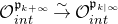 $\mathcal{O}^{\mathfrak{p}_{k+\infty}}_{{\rm int}}\overset{\sim}\to \mathcal{O}^{\mathfrak{p}_{k|\infty}}_{{\rm int}}$
identifying the pairs
$\mathcal{O}^{\mathfrak{p}_{k+\infty}}_{{\rm int}}\overset{\sim}\to \mathcal{O}^{\mathfrak{p}_{k|\infty}}_{{\rm int}}$
identifying the pairs
 $$M^{k+\infty}(\lambda_{\underline{a},n})\;\longleftrightarrow \;K^{k|\infty}(\lambda_{\underline{a},n}^{\sharp}),\quad L^{k+\infty}(\lambda_{\underline{a},n})\;\longleftrightarrow \;L^{k|\infty}(\lambda_{\underline{a},n}^{\sharp}).$$
In particular, the composition factors of $K^{k|\infty}(\lambda_{\underline{a},n}^{\sharp})$
are given by
$K^{k|\infty}(\lambda_{\underline{a},n}^{\sharp})$
are given by $L^{k|\infty}(-b_k,\ldots, -b_1\,|\,b_1,\ldots, b_k)$
, where
$L^{k|\infty}(-b_k,\ldots, -b_1\,|\,b_1,\ldots, b_k)$
, where $\underline{b}=(b_1,\ldots, b_k)$
is obtained from
$\underline{b}=(b_1,\ldots, b_k)$
is obtained from $\underline{a}^c$
by adding an admissible Dyck pattern with no bullets. Given
$\underline{a}^c$
by adding an admissible Dyck pattern with no bullets. Given $\mathbb{D}\in {\rm Dyck}(\underline{a})$
, we write
$\mathbb{D}\in {\rm Dyck}(\underline{a})$
, we write $v_{\underline{a}}^{\mathbb{D}}$
for any vector in
$v_{\underline{a}}^{\mathbb{D}}$
for any vector in $M(\underline{a})$
that becomes a highest-weight vector for
$M(\underline{a})$
that becomes a highest-weight vector for $L(\underline{a}^{\mathbb{D}})$
in a quotient of
$L(\underline{a}^{\mathbb{D}})$
in a quotient of $M(\underline{a})$
, and we write
$M(\underline{a})$
, and we write $v_{\underline{a}}^{\mathbb{D},\infty}$
for any vector in
$v_{\underline{a}}^{\mathbb{D},\infty}$
for any vector in $M^{k+\infty}(\lambda_{\underline{a},n})$
that becomes a highest-weight vector for
$M^{k+\infty}(\lambda_{\underline{a},n})$
that becomes a highest-weight vector for $L^{k+\infty}(\lambda_{\underline{a}^{\mathbb{D}},n})$
in a quotient of
$L^{k+\infty}(\lambda_{\underline{a}^{\mathbb{D}},n})$
in a quotient of $M^{k+\infty}(\lambda_{\underline{a},n})$
. Similarly, we write
$M^{k+\infty}(\lambda_{\underline{a},n})$
. Similarly, we write ${\sharp}{}{v_{\underline{a}}^{\mathbb{D},\infty}}$
for any vector in
${\sharp}{}{v_{\underline{a}}^{\mathbb{D},\infty}}$
for any vector in $K^{k|\infty}(\lambda_{\underline{a},n}^{\sharp})$
that becomes a highest-weight vector for
$K^{k|\infty}(\lambda_{\underline{a},n}^{\sharp})$
that becomes a highest-weight vector for $L^{k|\infty}(\lambda^{\sharp}_{\underline{a}^{\mathbb{D}},n})$
in a quotient of
$L^{k|\infty}(\lambda^{\sharp}_{\underline{a}^{\mathbb{D}},n})$
in a quotient of $K^{k|\infty}(\lambda_{\underline{a},n}^{\sharp})$
.
$K^{k|\infty}(\lambda_{\underline{a},n}^{\sharp})$
.
With this setup, we now proceed with the proof of Theorem 4.3.
-
(i) It suffices to show that
$v^{\mathbb{D}'}_{\underline{a}}\in U(\mathfrak{gl}_n) v_{\underline{a}}^{\mathbb{D}}$
in
$M(\underline{a})$
when
$\mathbb{D}\subseteq \mathbb{D}'$
and
$|\mathbb{D}'|=|\mathbb{D}|+1$
. Since the socle filtration on
$M^{k+\infty}(\lambda_{\underline{a},n})$
is determined by the number of paths in the Dyck pattern, it suffices to prove that
$v^{\mathbb{D}',\infty}_{\underline{a}}\in U(\mathfrak{gl}_{k+\infty}) v_{\underline{a}}^{\mathbb{D},\infty}$
in
$M^{k+\infty}(\lambda_{\underline{a},n})$
. By super duality, this is equivalent to
${\sharp}{}{v^{\mathbb{D}',\infty}_{\underline{a}}}\in U(\mathfrak{gl}_{k|\infty}) {\sharp}{}{v_{\underline{a}}^{\mathbb{D},\infty}}$
in
$K^{k|\infty}(\lambda_{\underline{a},n}^{\sharp})$
, which follows from [Reference Su and ZhangSZ12, Theorem 5.18]. -
(ii) Suppose that
$\mathbb{D}=\{(x,y)\}$
and that
$v^{\mathbb{D}'}_{\underline{a}}\in U(\mathfrak{gl}_n) v_{\underline{a}}^{\mathbb{D}}$
in
$M(\underline{a})$
. By super duality, we have that
${\sharp}{}{v^{\mathbb{D}',\infty}_{\underline{a}}}\in U(\mathfrak{gl}_{k|\infty}) {\sharp}{}{v_{\underline{a}}^{\mathbb{D},\infty}}$
in
$K^{k|\infty}(\lambda_{\underline{a},n}^{\sharp})$
. We induct on
$|\mathbb{D}'|$
. If
$|\mathbb{D}'|=2$
, then since
$\mathbb{D}=\{(x,y)\}$
is a ‘path without bridges’, it follows from [Reference Su and ZhangSZ12, Theorem 5.18] that
$\mathbb{D}\subseteq \mathbb{D}'$
. If
$|\mathbb{D}'| \gt 2$
, then by inductive hypothesis there exists
$\mathbb{D}''$
with
$\mathbb{D}\subseteq \mathbb{D}''$
,
${\sharp}{}{v^{\mathbb{D}'',\infty}_{\underline{a}}}\in U(\mathfrak{gl}_{k|\infty}) {\sharp}{}{v_{\underline{a}}^{\mathbb{D},\infty}}$
,
${\sharp}{}{v^{\mathbb{D}',\infty}_{\underline{a}}}\in U(\mathfrak{gl}_{k|\infty}) {\sharp}{}{v_{\underline{a}}^{\mathbb{D}'',\infty}}$
, and
$|\mathbb{D}''|=|\mathbb{D}'|-1$
. Then, by [Reference Su and ZhangSZ12, Theorem 5.18], we have that either
$\mathbb{D}''\subseteq \mathbb{D}'$
or
$\mathbb{D}'$
is obtained from
$\mathbb{D}''$
by replacing a path
$P\neq \{(x,y)\}$
in
$\mathbb{D}''$
with two paths. In either case, we have that
$\{(x,y)\} \in \mathbb{D}'$
.















Let $\underline{a},\underline{b}\in \mathcal{R}_{k,n}$
with
$\underline{a},\underline{b}\in \mathcal{R}_{k,n}$
with $\underline{b}=\underline{a}^{(\{(x,y)\})}$
, where (x,y) is a corner of
$\underline{b}=\underline{a}^{(\{(x,y)\})}$
, where (x,y) is a corner of $\underline{a}$
. By [Reference Boe and EnrightBE86], there is a unique (up to nonzero scalar) nonzero map
$\underline{a}$
. By [Reference Boe and EnrightBE86], there is a unique (up to nonzero scalar) nonzero map $\phi^{\underline{a}}_{\underline{b}}:N(\underline{a})\to N(\underline{b})$
. In particular,
$\phi^{\underline{a}}_{\underline{b}}:N(\underline{a})\to N(\underline{b})$
. In particular, $\phi^{\underline{a}}_{\underline{b}}$
appears in the global Grothendieck–Cousin complex (Corollary 3.7), and thus is strict with respect to the weight filtration
$\phi^{\underline{a}}_{\underline{b}}$
appears in the global Grothendieck–Cousin complex (Corollary 3.7), and thus is strict with respect to the weight filtration $W_{\bullet}$
.
$W_{\bullet}$
.
Corollary 4.4. Let $\underline{a}$
and
$\underline{a}$
and $\underline{b}$
with
$\underline{b}$
with $\underline{b}=\underline{a}^{(\{(x,y)\})}$
, where (x,y) is a corner of
$\underline{b}=\underline{a}^{(\{(x,y)\})}$
, where (x,y) is a corner of $\underline{a}$
. Let
$\underline{a}$
. Let $\phi^{\underline{a}}_{\underline{b}}$
be the natural map from
$\phi^{\underline{a}}_{\underline{b}}$
be the natural map from $N(\underline{a})$
to
$N(\underline{a})$
to $N(\underline{b})$
. Let
$N(\underline{b})$
. Let $p\in \mathbb{Z}$
and
$p\in \mathbb{Z}$
and $\underline{c}$
be such that
$\underline{c}$
be such that $L(\underline{c})$
is a composition factor of both
$L(\underline{c})$
is a composition factor of both $\operatorname{{\rm gr}}^W_pN(\underline{a})$
and
$\operatorname{{\rm gr}}^W_pN(\underline{a})$
and $\operatorname{{\rm gr}}^W_pN(\underline{b})$
, so that
$\operatorname{{\rm gr}}^W_pN(\underline{b})$
, so that $\underline{c}=\underline{a}^{\mathbb{D}'}=\underline{b}^{\mathbb{D}}$
, where
$\underline{c}=\underline{a}^{\mathbb{D}'}=\underline{b}^{\mathbb{D}}$
, where $\mathbb{D}'$
is an
$\mathbb{D}'$
is an $\underline{a}$
-admissible Dyck pattern with
$\underline{a}$
-admissible Dyck pattern with $|\mathbb{D}'|=p+|\underline{a}|-2d_X$
, and
$|\mathbb{D}'|=p+|\underline{a}|-2d_X$
, and $\mathbb{D}$
is a
$\mathbb{D}$
is a $\underline{b}$
-admissible Dyck pattern
$\underline{b}$
-admissible Dyck pattern $|\mathbb{D}|=p+|\underline{b}|-2d_X$
.
$|\mathbb{D}|=p+|\underline{b}|-2d_X$
.
-
(i) If
$\mathbb{D}'=\mathbb{D}\cup (\{(x,y)\})$
, then
$(\operatorname{{\rm gr}}^W_p\phi^{\underline{a}}_{\underline{b}})(L(\underline{a}^{\mathbb{D}'}))\cong L(\underline{b}^{\mathbb{D}})$
. -
(ii) If
$\mathbb{D}'\neq \mathbb{D}\cup (\{(x,y)\})$
, then
$(\operatorname{{\rm gr}}^W_p\phi^{\underline{a}}_{\underline{b}})(L(\underline{a}^{\mathbb{D}'}))=0$
.




Proof. We prove the dual statement for the natural map $\psi_{\underline{a}}^{\underline{b}}:M(\underline{b})\to M(\underline{a})$
.
$\psi_{\underline{a}}^{\underline{b}}:M(\underline{b})\to M(\underline{a})$
.
-
(i) The image of
$\psi^{\underline{a}}_{\underline{b}}$
is the submodule of
$M(\underline{a})$
generated by
$v_{\underline{a}}^{\{(x,y)\}}$
. If
$\mathbb{D}'$
is
$\underline{a}$
-admissible, then by Theorem 4.3(i), we have that
$\psi^{\underline{a}}_{\underline{b}}(v_{\underline{b}}^{\mathbb{E}})=v_{\underline{a}}^{\mathbb{D}'}$
for some
$\mathbb{E}$
with
$\underline{b}^{\mathbb{E}}=\underline{c}$
. Since
$L(\underline{c})$
is a composition factor of
$M(\underline{b})$
with multiplicity one, we conclude that
$\mathbb{E}=\mathbb{D}$
, as required. -
(ii) If
$\mathbb{D}'\neq \mathbb{D}\cup (\{(x,y)\})$
and
$\psi^{\underline{a}}_{\underline{b}}(v_{\underline{b}}^{\mathbb{D}})\neq 0$
, then
$\psi^{\underline{a}}_{\underline{b}}(v_{\underline{b}}^{\mathbb{D}})=v_{\underline{a}}^{\mathbb{E}'}$
, where
$\{(x,y)\}\in \mathbb{E}'$
by Theorem 4.3(ii). Since
$\mathbb{D}'\neq \mathbb{E}'$
and
$L(\underline{c})$
has multiplicity one as a composition factor of
$M(\underline{a})$
, we obtain a contradiction.





4.3 Cohomology of the Grothendieck–Cousin complex
The argument in this section is based on [Reference HuangHua20, § 3], though functoriality and strictness of the weight filtration simplifies things in our setting (see §4.4). We fix $\underline{a}\in \mathcal{R}_{k,n}$
.
$\underline{a}\in \mathcal{R}_{k,n}$
.
Lemma 4.5. Let $\underline{b}\subseteq \underline{a}$
, and let
$\underline{b}\subseteq \underline{a}$
, and let $\mathbb{D}\in {Dyck}(\underline{b})$
. We define the following set of boxes:
$\mathbb{D}\in {Dyck}(\underline{b})$
. We define the following set of boxes:
 $$\mathcal{I}(\underline{a},\underline{b},\mathbb{D})=\big\{(i,j)\in \underline{a} / \underline{b} \mid \mbox{$\underline{b}\cup (i,j)$ {is a partition}, $\mathbb{D}\cup \{(i,j)\}\in {Dyck}(\underline{b} \cup (i,j))$}\big\}.$$
For all $J\subseteq \mathcal{I}(\underline{a},\underline{b},\mathbb{D})$
we have that
$J\subseteq \mathcal{I}(\underline{a},\underline{b},\mathbb{D})$
we have that $\underline{b} \cup J$
is a partition and
$\underline{b} \cup J$
is a partition and $\mathbb{D}\cup J\in {\rm Dyck}(\underline{b}\cup J)$
.
$\mathbb{D}\cup J\in {\rm Dyck}(\underline{b}\cup J)$
.
Proof. Let $J\subseteq \mathcal{I}(\underline{a},\underline{b},\mathbb{D})$
. If
$J\subseteq \mathcal{I}(\underline{a},\underline{b},\mathbb{D})$
. If $\underline{b} \cup (i,j)$
is a partition for all
$\underline{b} \cup (i,j)$
is a partition for all $(i,j)\in J$
, then no box in J lies directly north, south, east, or west of another. Thus,
$(i,j)\in J$
, then no box in J lies directly north, south, east, or west of another. Thus, $b\cup J$
is a partition as well. Since no box in J lies directly north, south, east, or west of another, and
$b\cup J$
is a partition as well. Since no box in J lies directly north, south, east, or west of another, and $\mathbb{D}\cup\{(i,j)\}$
is an admissible Dyck pattern for all
$\mathbb{D}\cup\{(i,j)\}$
is an admissible Dyck pattern for all $(i,j)\in J$
, it follows that
$(i,j)\in J$
, it follows that $\mathbb{D}\cup J$
is an admissible Dyck pattern.
$\mathbb{D}\cup J$
is an admissible Dyck pattern.
Let $GC^{\bullet}_{\underline{a}}$
denote the global Grothendieck–Cousin complex for
$GC^{\bullet}_{\underline{a}}$
denote the global Grothendieck–Cousin complex for $\underline{a}$
, so that for
$\underline{a}$
, so that for $j,p\in \mathbb{Z}$
we have
$j,p\in \mathbb{Z}$
we have
 \begin{equation}GC_{\underline{a}}^j=\bigoplus_{\underline{b}\subseteq \underline{a},\;|\underline{b}|=d_X-j}N(\underline{b}),\quad \operatorname{{\rm gr}}^W_p(GC^j_{\underline{a}})=\bigoplus_{\underline{b}\subseteq \underline{a},\;|\underline{b}|=d_X-j} \bigoplus_{\mathbb{D}\in \mathcal{Z}_p(\underline{b})} L(\underline{b}^{\mathbb{D}}).\end{equation}
Using Corollary 4.4, we break $\operatorname{{\rm gr}}^W_p GC^{\bullet}_{\underline{a}}$
into a direct sum of Koszul subcomplexes.
$\operatorname{{\rm gr}}^W_p GC^{\bullet}_{\underline{a}}$
into a direct sum of Koszul subcomplexes.
Theorem 4.6. Given $p,q\in \mathbb{Z}$
, we define
$p,q\in \mathbb{Z}$
, we define
 $$\mathcal{Y}_p(\underline{a};q)=\left\{(\underline{b},\mathbb{D})\middle\vert \begin{array}{l} \mbox{$b\subseteq \underline{a}$ and $q=d_{X}-|\underline{b}|$, }\\ \mbox{$\mathbb{D}\in {\rm Dyck}(\underline{b})$,} \\ \mbox{$|D|\geqslant 3$ for all $D\in \mathbb{D}$ and $|\mathbb{D}|=p-q-d_{X}$ } \end{array} \right\}.$$
The following is true about the complex $\operatorname{{\rm gr}}^W_pGC^{\bullet}_{\underline{a}}$
.
$\operatorname{{\rm gr}}^W_pGC^{\bullet}_{\underline{a}}$
.
-
(i) We have that
$\operatorname{{\rm gr}}^W_pGC^{\bullet}_{\underline{a}}$
is a direct sum of subcomplexes where
$$\operatorname{{\rm gr}}^W_p(GC^{\bullet}_{\underline{a}})=\bigoplus_{0\leqslant q\leqslant |\underline{a}|}\bigoplus_{(\underline{b},\mathbb{D})\in \mathcal{Y}_p(\underline{a};q)} \mathcal{K}(\underline{a},\underline{b},\mathbb{D}),$$
$\mathcal{K}(\underline{a},\underline{b},\mathbb{D})$
is a complex concentrated in degrees
$q-|\mathcal{I}(\underline{a},\underline{b},\mathbb{D})|,\ldots, q$
, with
$$\mathcal{K}(\underline{a},\underline{b},\mathbb{D})_j=\bigoplus_{J\subseteq \mathcal{I}(\underline{a},\underline{b},\mathbb{D}),\; |J|=q-j} L((\underline{b}\cup J)^{\mathbb{D}\cup J}),\quad q-|\mathcal{I}(\underline{a},\underline{b},\mathbb{D})|\leqslant j \leqslant q.$$
-
(ii) For
$0\leqslant q\leqslant d_{X}$
, we have
$$\mathcal{H}^q(\operatorname{{\rm gr}}^W_p(GC^{\bullet}_{\underline{a}})) =\bigoplus_{\substack{(\underline{b},\mathbb{D})\in \mathcal{Y}_p(\underline{a};q)\\ \mathcal{I}(\underline{a},\underline{b},\mathbb{D})=\emptyset}} L(\underline{b}^{\mathbb{D}}).$$





We note that all summands of $\mathcal{K}(\underline{a},\underline{b},\mathbb{D})$
are isomorphic to
$\mathcal{K}(\underline{a},\underline{b},\mathbb{D})$
are isomorphic to $L(\underline{b}^{\mathbb{D}})$
.
$L(\underline{b}^{\mathbb{D}})$
.
Proof. Let $0\leqslant j\leqslant d_{X}$
and let
$0\leqslant j\leqslant d_{X}$
and let $N(\underline{x})$
be a summand of
$N(\underline{x})$
be a summand of $GC^j_{\underline{a}}$
. Let
$GC^j_{\underline{a}}$
. Let $\mathbb{X}\in {\rm Dyck}(\underline{x})$
with
$\mathbb{X}\in {\rm Dyck}(\underline{x})$
with $|\mathbb{X}|=p-j-d_{X}$
, so that
$|\mathbb{X}|=p-j-d_{X}$
, so that $L(\underline{x}^{\mathbb{X}})$
is a composition factor of
$L(\underline{x}^{\mathbb{X}})$
is a composition factor of $\operatorname{{\rm gr}}^W_pN(\underline{x})$
. Let
$\operatorname{{\rm gr}}^W_pN(\underline{x})$
. Let $J\subseteq \underline{x}$
be the set of boxes in
$J\subseteq \underline{x}$
be the set of boxes in $\underline{x}$
corresponding to paths of length 1 in
$\underline{x}$
corresponding to paths of length 1 in $\mathbb{X}$
. Set
$\mathbb{X}$
. Set $\underline{b}=\underline{x}\setminus J$
and
$\underline{b}=\underline{x}\setminus J$
and $\mathbb{D}=\mathbb{X}\setminus J$
. Then,
$\mathbb{D}=\mathbb{X}\setminus J$
. Then, $(\underline{b},\mathbb{D})\in \mathcal{Y}_p(\underline{a};j+|J|)$
. Thus,
$(\underline{b},\mathbb{D})\in \mathcal{Y}_p(\underline{a};j+|J|)$
. Thus, $L(\underline{x}^{\mathbb{X}})$
is a summand of
$L(\underline{x}^{\mathbb{X}})$
is a summand of $\mathcal{K}(\underline{a},\underline{b},\mathbb{D})_j$
, and there is no other pair
$\mathcal{K}(\underline{a},\underline{b},\mathbb{D})_j$
, and there is no other pair $(\underline{b}',\mathbb{D}')\in\mathcal{Y}_p(\underline{a};j+|J|)$
for which
$(\underline{b}',\mathbb{D}')\in\mathcal{Y}_p(\underline{a};j+|J|)$
for which $L(\underline{x}^{\mathbb{X}})$
is a summand of
$L(\underline{x}^{\mathbb{X}})$
is a summand of $\mathcal{K}(\underline{a},\underline{b}',\mathbb{D}')_j$
.
$\mathcal{K}(\underline{a},\underline{b}',\mathbb{D}')_j$
.
By Corollary 3.7, the morphism $\partial^j:GC^j_{\underline{a}}\to GC^{j+1}_{\underline{a}}$
induces a nonzero morphism from
$\partial^j:GC^j_{\underline{a}}\to GC^{j+1}_{\underline{a}}$
induces a nonzero morphism from $N(\underline{x})$
to
$N(\underline{x})$
to $N(\underline{x}\setminus k)$
for all
$N(\underline{x}\setminus k)$
for all $k\in J$
(and such a morphism is unique up to a nonzero scalar [Reference Boe and EnrightBE86]). By Corollary 4.4, it follows that
$k\in J$
(and such a morphism is unique up to a nonzero scalar [Reference Boe and EnrightBE86]). By Corollary 4.4, it follows that $\partial^j$
maps
$\partial^j$
maps $L(\underline{x}^{\mathbb{X}})$
diagonally to
$L(\underline{x}^{\mathbb{X}})$
diagonally to
 $$\bigoplus_{k\in J} L((\underline{x}\setminus k)^{\mathbb{X}\setminus k}).$$
This proves part (i). To see part (ii), note that $\mathcal{K}(\underline{a},\underline{b},\mathbb{D})$
is a Koszul complex (see [Reference HuangHua20, Lemma 3.6]) and hence is exact unless it has only one term, which is equivalent to
$\mathcal{K}(\underline{a},\underline{b},\mathbb{D})$
is a Koszul complex (see [Reference HuangHua20, Lemma 3.6]) and hence is exact unless it has only one term, which is equivalent to $\mathcal{I}(\underline{a},\underline{b},\mathbb{D})=\emptyset$
.
$\mathcal{I}(\underline{a},\underline{b},\mathbb{D})=\emptyset$
.
Example 4.7. Let $X=\operatorname{{\rm Gr}}(2,4)$
and
$X=\operatorname{{\rm Gr}}(2,4)$
and $\underline{a}=(2,1)$
. Then,
$\underline{a}=(2,1)$
. Then, $GC^{\bullet}_{\underline{a}}$
is the complex
$GC^{\bullet}_{\underline{a}}$
is the complex

In the following table, the column indices are the cohomological degree and the row indices indicate the graded pieces of the weight filtration.

To create the sets $\mathcal{Y}_p(\underline{a};q)$
, we select all composition factors of
$\mathcal{Y}_p(\underline{a};q)$
, we select all composition factors of $N(\underline{b})$
in cohomological degree q that were obtained by removing Dyck patterns for which all paths have length
$N(\underline{b})$
in cohomological degree q that were obtained by removing Dyck patterns for which all paths have length $\geqslant 3$
(including the empty pattern):
$\geqslant 3$
(including the empty pattern):

Therefore, we obtain direct-sum decompositions:

For each pair $(\underline{b},\mathbb{D})$
as above, we have
$(\underline{b},\mathbb{D})$
as above, we have $\mathcal{I}(\underline{a},\underline{b},\mathbb{D})=\emptyset$
if and only if
$\mathcal{I}(\underline{a},\underline{b},\mathbb{D})=\emptyset$
if and only if $(\underline{b},\mathbb{D})$
is one of the following:
$(\underline{b},\mathbb{D})$
is one of the following:

These correspond to the Koszul complexes with one term. In particular, we obtain a non-split exact sequence

and $H^q_{Z_{\underline{a}}}(X,\mathcal{O}_X)=0$
for
$H^q_{Z_{\underline{a}}}(X,\mathcal{O}_X)=0$
for $q\neq 1$
. We note that
$q\neq 1$
. We note that $Z_{(0)}$
is the singular locus of
$Z_{(0)}$
is the singular locus of $Z_{\underline{a}}$
.
$Z_{\underline{a}}$
.
We provide a combinatorial bijection relating Theorems 4.6 and 1.1.
Lemma 4.8. There is a bijection between the sets
 $$\{(\underline{b},\mathbb{D})\in \mathcal{Y}_p(\underline{a};q)\mid \mathcal{I}(\underline{a},\underline{b},\mathbb{D})=\emptyset\}\quad \leftrightarrow \quad \mathcal{A}_p(\underline{a};q),$$
given by sending $(\underline{b},\mathbb{D}=(D_1,\ldots, D_{p-q-d_{X}}))$
to
$(\underline{b},\mathbb{D}=(D_1,\ldots, D_{p-q-d_{X}}))$
to
 $$\mathbb{D}'=(D_1,\ldots, D_{p-q-d_{X}};\mathbb{B}),$$
where $\mathbb{B}$
is the set of boxes in
$\mathbb{B}$
is the set of boxes in $\underline{a} /\underline{b}$
.
$\underline{a} /\underline{b}$
.
Proof. We note that the number of paths and bullets in $\mathbb{D}'$
is correct. To show that the map is well defined, we need to verify that
$\mathbb{D}'$
is correct. To show that the map is well defined, we need to verify that $\mathbb{D}'\in {\rm Dyck}^{\bullet}(\underline{a})$
. First,
$\mathbb{D}'\in {\rm Dyck}^{\bullet}(\underline{a})$
. First, $\underline{a}^{\mathbb{D}'}=\underline{b}^{\mathbb{D}}$
is a partition, as
$\underline{a}^{\mathbb{D}'}=\underline{b}^{\mathbb{D}}$
is a partition, as $\mathbb{D}$
is
$\mathbb{D}$
is $\underline{b}$
-admissible. Since
$\underline{b}$
-admissible. Since $\mathbb{D}$
is a Dyck pattern, we have that
$\mathbb{D}$
is a Dyck pattern, we have that $(D_1,\ldots, D_{p-q-d_{X}})$
satisfies the covering condition. Since the support of
$(D_1,\ldots, D_{p-q-d_{X}})$
satisfies the covering condition. Since the support of $\mathbb{D}$
is contained in
$\mathbb{D}$
is contained in $\underline{b}$
, and the support of
$\underline{b}$
, and the support of $\mathbb{B}$
is
$\mathbb{B}$
is $\underline{a}/\underline{b}$
, it follows that no box of
$\underline{a}/\underline{b}$
, it follows that no box of $\mathbb{B}$
is located directly north, northwest, or west from a box in
$\mathbb{B}$
is located directly north, northwest, or west from a box in $\mathbb{D}$
. Therefore, the map is well defined.
$\mathbb{D}$
. Therefore, the map is well defined.
The map is clearly injective, as $\mathbb{B}$
completely determines
$\mathbb{B}$
completely determines $\underline{b}$
, and
$\underline{b}$
, and $(D_1,\ldots, D_{p-q-d_{X}})$
completely determines
$(D_1,\ldots, D_{p-q-d_{X}})$
completely determines $\mathbb{D}$
. To show surjectivity, let
$\mathbb{D}$
. To show surjectivity, let $\mathbb{D}'=(D_1,\ldots, D_{p-q-d_{X}};\mathbb{B})\in \mathcal{A}_p(\underline{a};q)$
,
$\mathbb{D}'=(D_1,\ldots, D_{p-q-d_{X}};\mathbb{B})\in \mathcal{A}_p(\underline{a};q)$
, $\underline{b}=\underline{a}\setminus \mathbb{B}$
, and
$\underline{b}=\underline{a}\setminus \mathbb{B}$
, and $\mathbb{D}=(D_1,\ldots, D_{p-q-d_{X}})$
. We need to show that
$\mathbb{D}=(D_1,\ldots, D_{p-q-d_{X}})$
. We need to show that $\mathcal{I}(\underline{a},\underline{b},\mathbb{D})=\emptyset$
. All boxes of
$\mathcal{I}(\underline{a},\underline{b},\mathbb{D})=\emptyset$
. All boxes of $\underline{a}/\underline{b}$
belong to the heads or tails of paths in
$\underline{a}/\underline{b}$
belong to the heads or tails of paths in $\mathbb{D}$
. Thus, for every box (i,j) in
$\mathbb{D}$
. Thus, for every box (i,j) in $\mathbb{B}$
such that
$\mathbb{B}$
such that $\underline{b}\cup (i,j)$
is a partition, there exists a path
$\underline{b}\cup (i,j)$
is a partition, there exists a path $D\in \mathbb{D}$
such that (i,j) belongs directly to the head or tail of D. In particular, the covering condition fails for D and (i,j). Thus, (i,j) does not belong to
$D\in \mathbb{D}$
such that (i,j) belongs directly to the head or tail of D. In particular, the covering condition fails for D and (i,j). Thus, (i,j) does not belong to $\mathcal{I}(\underline{a},\underline{b},\mathbb{D})$
, and thus
$\mathcal{I}(\underline{a},\underline{b},\mathbb{D})$
, and thus $\mathcal{I}(\underline{a},\underline{b},\mathbb{D})=\emptyset$
.
$\mathcal{I}(\underline{a},\underline{b},\mathbb{D})=\emptyset$
.
Combining Corollary 3.7, Theorem 4.6(ii), and Lemma 4.8, we obtain the description of $[\mathscr{H}^q_{Z_{\underline{a}}}(\mathcal{O}_X)]$
and
$[\mathscr{H}^q_{Z_{\underline{a}}}(\mathcal{O}_X)]$
and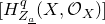 $[H^q_{Z_{\underline{a}}}(X,\mathcal{O}_X)]$
in Theorem 1.1. Via Theorem 3.1, the following result implies the assertion in Theorem 1.1 about the graded pieces of the weight filtration.
$[H^q_{Z_{\underline{a}}}(X,\mathcal{O}_X)]$
in Theorem 1.1. Via Theorem 3.1, the following result implies the assertion in Theorem 1.1 about the graded pieces of the weight filtration.
Corollary 4.9. For all $\underline{a}\in \mathcal{R}_{k,n}$
,
$\underline{a}\in \mathcal{R}_{k,n}$
, $0\leqslant q\leqslant d_X$
, and
$0\leqslant q\leqslant d_X$
, and $p\in \mathbb{Z}$
, we have that
$p\in \mathbb{Z}$
, we have that
 $$\mathcal{H}^q(\operatorname{{\rm gr}}^W_p\mathcal{GC}^{\bullet}_{\underline{a}})\cong \bigoplus_{\mathbb{D}\in \mathcal{A}_p(\underline{a};q)} IC^H_{Z_{\underline{a}^{\mathbb{D}}}}\left(\frac{(|\underline{a}^{\mathbb{D}}|-p)}{2}\right).$$
Proof. By multiplicity-freeness of the modules $N(\underline{b})$
(Theorem 4.1), we have that, for all
$N(\underline{b})$
(Theorem 4.1), we have that, for all $\underline{b}\in \mathcal{R}_{k,n}$
and all
$\underline{b}\in \mathcal{R}_{k,n}$
and all $p\in \mathbb{Z}$
, the Hodge modules
$p\in \mathbb{Z}$
, the Hodge modules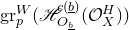 $\operatorname{{\rm gr}}^W_p( \mathscr{H}^{c(\underline{b})}_{O_{\underline{b}}}(\mathcal{O}_X^H))$
are direct sums of intersection cohomology Hodge modules of the form
$\operatorname{{\rm gr}}^W_p( \mathscr{H}^{c(\underline{b})}_{O_{\underline{b}}}(\mathcal{O}_X^H))$
are direct sums of intersection cohomology Hodge modules of the form $IC^H_{Z_{\underline{b}^{\mathbb{D}}}}(k)$
, where
$IC^H_{Z_{\underline{b}^{\mathbb{D}}}}(k)$
, where $k=(|\underline{b}^{\mathbb{D}}|-p)/2$
, so that the summands have weight p. It follows that the direct-sum decompositions in (4.5) and the conclusions of Theorem 4.6 may be lifted to the category of mixed Hodge modules. In particular, the complex
$k=(|\underline{b}^{\mathbb{D}}|-p)/2$
, so that the summands have weight p. It follows that the direct-sum decompositions in (4.5) and the conclusions of Theorem 4.6 may be lifted to the category of mixed Hodge modules. In particular, the complex $\operatorname{{\rm gr}}^W_p\mathcal{GC}^{\bullet}_{\underline{a}}$
of Hodge modules is a direct sum of Koszul subcomplexes of intersection cohomology Hodge modules of the form
$\operatorname{{\rm gr}}^W_p\mathcal{GC}^{\bullet}_{\underline{a}}$
of Hodge modules is a direct sum of Koszul subcomplexes of intersection cohomology Hodge modules of the form $IC^H_{Z_{\underline{b}^{\mathbb{D}}}}(k)$
, and
$IC^H_{Z_{\underline{b}^{\mathbb{D}}}}(k)$
, and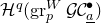 $\mathcal{H}^q(\operatorname{{\rm gr}}^W_p\mathcal{GC}^{\bullet}_{\underline{a}})$
is a direct sum over
$\mathcal{H}^q(\operatorname{{\rm gr}}^W_p\mathcal{GC}^{\bullet}_{\underline{a}})$
is a direct sum over $\mathbb{D}\in \mathcal{A}_p(\underline{a};q)$
of modules
$\mathbb{D}\in \mathcal{A}_p(\underline{a};q)$
of modules $IC^H_{Z_{\underline{a}^{\mathbb{D}}}}(k)$
, where
$IC^H_{Z_{\underline{a}^{\mathbb{D}}}}(k)$
, where $k=(|\underline{a}^{\mathbb{D}}|-p)/2$
, so that the summands have weight p.
$k=(|\underline{a}^{\mathbb{D}}|-p)/2$
, so that the summands have weight p.
Remark 4.10. One could attempt to carry out a similar argument for the remaining Hermitian pairs:
 $$(\mathsf{B}_n,\mathsf{B}_{n-1}),\quad (\mathsf{C}_n,\mathsf{A}_{n-1}),\quad (\mathsf{D}_n,\mathsf{A}_{n-1}),\quad (\mathsf{D}_n,\mathsf{D}_{n-1}),\quad (\mathsf{E}_6,\mathsf{D}_5),\quad (\mathsf{E}_7,\mathsf{E}_6).$$
The corresponding parabolic Verma modules are again rigid and multiplicity free [Reference Collingwood, Irving and SheltonCIS88], and the composition factors are described by parabolic Kazhdan–Lusztig polynomials [Reference Casian and CollingwoodCC87] (see also [Reference BoeBoe88, Reference BrentiBre09]). Unfortunately, the submodule lattices are not known in full generality, so that we do not currently have analogues of Theorem 4.3 for all Hermitian pairs. One may use our techniques in any setting where the relevant parabolic Verma modules have Loewy length at most 3 (because then the submodule lattice is determined by the Loewy filtration), which covers the cases $(\mathsf{B}_n,\mathsf{B}_{n-1})$
and
$(\mathsf{B}_n,\mathsf{B}_{n-1})$
and $(\mathsf{D}_n,\mathsf{D}_{n-1})$
. In the cases
$(\mathsf{D}_n,\mathsf{D}_{n-1})$
. In the cases $(\mathsf{E}_6,\mathsf{D}_5)$
and
$(\mathsf{E}_6,\mathsf{D}_5)$
and $(\mathsf{E}_7,\mathsf{E}_6)$
, many of the parabolic Verma modules have Loewy length at most 3 (see [Reference Collingwood, Irving and SheltonCIS88, Tables 7.1 and 7.2]), so our techniques are applicable to some of the Schubert varieties. In the major cases
$(\mathsf{E}_7,\mathsf{E}_6)$
, many of the parabolic Verma modules have Loewy length at most 3 (see [Reference Collingwood, Irving and SheltonCIS88, Tables 7.1 and 7.2]), so our techniques are applicable to some of the Schubert varieties. In the major cases $(\mathsf{C}_n,\mathsf{A}_{n-1})$
and
$(\mathsf{C}_n,\mathsf{A}_{n-1})$
and $(\mathsf{D}_n,\mathsf{A}_{n-1})$
, the weight filtrations are dictated by shifted Dyck patterns [Reference BrentiBre09]. We expect a combinatorial formula for local cohomology in these cases similar to ours, via ‘augmented shifted Dyck patterns’. Formulating and proving such a result would allow one to calculate the weight filtration on local cohomology with support in determinantal varieties of symmetric matrices and Pfaffian varieties of skew-symmetric matrices as in §4.5, upon restricting to the opposite big cell. The composition factors are known [Reference Raicu and WeymanRW16], but the Hodge and weight filtrations are not.
$(\mathsf{D}_n,\mathsf{A}_{n-1})$
, the weight filtrations are dictated by shifted Dyck patterns [Reference BrentiBre09]. We expect a combinatorial formula for local cohomology in these cases similar to ours, via ‘augmented shifted Dyck patterns’. Formulating and proving such a result would allow one to calculate the weight filtration on local cohomology with support in determinantal varieties of symmetric matrices and Pfaffian varieties of skew-symmetric matrices as in §4.5, upon restricting to the opposite big cell. The composition factors are known [Reference Raicu and WeymanRW16], but the Hodge and weight filtrations are not.
4.4 Equivalence to syzygies of determinantal thickenings
A determinantal thickening is a $\operatorname{{\rm GL}}_m(\mathbb{C})\times \operatorname{{\rm GL}}_n(\mathbb{C})$
invariant ideal in the polynomial ring
$\operatorname{{\rm GL}}_m(\mathbb{C})\times \operatorname{{\rm GL}}_n(\mathbb{C})$
invariant ideal in the polynomial ring $S=\operatorname{{\rm Sym}}(\mathbb{C}^m\otimes \mathbb{C}^n)\cong \mathbb{C}[x_{i,j}]_{1\leqslant i\leqslant m,1\leqslant j\leqslant n}$
on the space of
$S=\operatorname{{\rm Sym}}(\mathbb{C}^m\otimes \mathbb{C}^n)\cong \mathbb{C}[x_{i,j}]_{1\leqslant i\leqslant m,1\leqslant j\leqslant n}$
on the space of $m\times n$
matrices, with
$m\times n$
matrices, with $m\geqslant n$
(see [Reference de Concini, Eisenbud and ProcesidCEP80]). Given a partition
$m\geqslant n$
(see [Reference de Concini, Eisenbud and ProcesidCEP80]). Given a partition $\lambda=(\lambda_1\geqslant \cdots \geqslant \lambda_n\geqslant 0)$
, there is a basic thickening
$\lambda=(\lambda_1\geqslant \cdots \geqslant \lambda_n\geqslant 0)$
, there is a basic thickening $I_{\lambda}\subseteq S$
generated by the subrepresentation
$I_{\lambda}\subseteq S$
generated by the subrepresentation $\mathbb{S}_{\lambda}\mathbb{C}^m\otimes \mathbb{S}_{\lambda}\mathbb{C}^n\subseteq S$
. Via the BGG correspondence, the linear strands of the free resolutions of all determinantal thickenings admit actions of the general linear Lie superalgebra
$\mathbb{S}_{\lambda}\mathbb{C}^m\otimes \mathbb{S}_{\lambda}\mathbb{C}^n\subseteq S$
. Via the BGG correspondence, the linear strands of the free resolutions of all determinantal thickenings admit actions of the general linear Lie superalgebra $\mathfrak{gl}(m|n)$
(see [Reference Raicu and WeymanRW19] and references therein). In [Reference Raicu and WeymanRW19], Raicu and Weyman make a conjecture on the structure of the linear strands of the basic thickenings
$\mathfrak{gl}(m|n)$
(see [Reference Raicu and WeymanRW19] and references therein). In [Reference Raicu and WeymanRW19], Raicu and Weyman make a conjecture on the structure of the linear strands of the basic thickenings $I_{\lambda}$
, in terms of admissible augmented Dyck patterns [Reference Raicu and WeymanRW19, Conjecture 4.1], and prove it for the first strand [Reference Raicu and WeymanRW19, Theorem 5.1]. Huang proves their full conjecture in [Reference HuangHua20, Theorem 3.7].
$I_{\lambda}$
, in terms of admissible augmented Dyck patterns [Reference Raicu and WeymanRW19, Conjecture 4.1], and prove it for the first strand [Reference Raicu and WeymanRW19, Theorem 5.1]. Huang proves their full conjecture in [Reference HuangHua20, Theorem 3.7].
Via super duality (see [Reference Su and ZhangSZ12, §3.3] or the proof of Theorem 4.3 above), our Theorem 1.1 is equivalent to [Reference HuangHua20, Theorem 3.7]. Indeed, over infinite-dimensional Lie (super)algebras, our complex $GC^{\bullet}_{\underline{a}}$
is identified with dual of the complex
$GC^{\bullet}_{\underline{a}}$
is identified with dual of the complex $\tilde{\mathbf{R}}(I_{\underline{a}^c})$
in [Reference HuangHua20]. The cohomology of
$\tilde{\mathbf{R}}(I_{\underline{a}^c})$
in [Reference HuangHua20]. The cohomology of $GC^{\bullet}_{\underline{a}}$
calculates local cohomology for us, while the cohomology of
$GC^{\bullet}_{\underline{a}}$
calculates local cohomology for us, while the cohomology of $\tilde{\mathbf{R}}(I_{\underline{a}^c})$
calculates the linear strands of the free resolution of
$\tilde{\mathbf{R}}(I_{\underline{a}^c})$
calculates the linear strands of the free resolution of $I_{\underline{a}^c}$
. This explains the appearance of admissible augmented Dyck patterns in both works. Our argument above is closely modeled after that of Huang. There are two advantages to our treatment, however. First, from our point of view, it is clear that the weight filtration is functorial and that
$I_{\underline{a}^c}$
. This explains the appearance of admissible augmented Dyck patterns in both works. Our argument above is closely modeled after that of Huang. There are two advantages to our treatment, however. First, from our point of view, it is clear that the weight filtration is functorial and that $GC^{\bullet}_{\underline{a}}$
is a filtered complex, whereas it is not immediate that the Loewy filtration in [Reference HuangHua20] is compatible with the morphisms in
$GC^{\bullet}_{\underline{a}}$
is a filtered complex, whereas it is not immediate that the Loewy filtration in [Reference HuangHua20] is compatible with the morphisms in $\tilde{\mathbf{R}}(I_{\underline{a}^c})$
. Second, strictness of the weight filtration immediately implies that the spectral sequence for
$\tilde{\mathbf{R}}(I_{\underline{a}^c})$
. Second, strictness of the weight filtration immediately implies that the spectral sequence for $(GC^{\bullet}_{\underline{a}}, W_{\bullet})$
degenerates, whereas it requires justification for
$(GC^{\bullet}_{\underline{a}}, W_{\bullet})$
degenerates, whereas it requires justification for $\tilde{\mathbf{R}}(I_{\underline{a}^c})$
.
$\tilde{\mathbf{R}}(I_{\underline{a}^c})$
.
It would be interesting to use duality results for other Lie (super)algebras (see [Reference Cheng and WangCW12]) to relate local cohomology on other flag varieties to linear strands of free resolutions of interesting classes of ideals. A natural case to investigate next would be the Hermitian pairs $(\mathsf{C}_n,\mathsf{A}_{n-1})$
,
$(\mathsf{C}_n,\mathsf{A}_{n-1})$
, $(\mathsf{D}_n,\mathsf{A}_{n-1})$
.
$(\mathsf{D}_n,\mathsf{A}_{n-1})$
.
4.5 Application to local cohomology supported in determinantal varieties
Let $\mathscr{X}=\mathbb{C}^{m\times n}$
be the space of
$\mathscr{X}=\mathbb{C}^{m\times n}$
be the space of $m\times n$
matrices over the complex numbers with
$m\times n$
matrices over the complex numbers with $m\geqslant n$
, and for
$m\geqslant n$
, and for $0\leqslant p \leqslant n$
let
$0\leqslant p \leqslant n$
let $\mathscr{Z}_p\subseteq \mathscr{X}$
denote the determinantal variety of matrices of rank
$\mathscr{Z}_p\subseteq \mathscr{X}$
denote the determinantal variety of matrices of rank $\leqslant p$
. In recent past, a great deal of information has been learned about the local cohomology modules
$\leqslant p$
. In recent past, a great deal of information has been learned about the local cohomology modules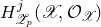 $H^j_{\mathscr{Z}_p}(\mathscr{X},\mathcal{O}_{\mathscr{X}})$
(see [Reference Raicu, Weyman and WittRWW14, Reference Raicu and WeymanRW14, Reference RaicuRai16, Reference Raicu and WeymanRW16, Reference Lõrincz and WaltherLW19, Reference Lõrincz and RaicuLR20, Reference Perlman and RaicuPR21, Reference PerlmanPer24]).
$H^j_{\mathscr{Z}_p}(\mathscr{X},\mathcal{O}_{\mathscr{X}})$
(see [Reference Raicu, Weyman and WittRWW14, Reference Raicu and WeymanRW14, Reference RaicuRai16, Reference Raicu and WeymanRW16, Reference Lõrincz and WaltherLW19, Reference Lõrincz and RaicuLR20, Reference Perlman and RaicuPR21, Reference PerlmanPer24]).
In this section, we use Theorem 1.1 to recover the composition factors and weight filtration on $H^j_{\mathscr{Z}_p}(\mathscr{X},\mathcal{O}_{\mathscr{X}})$
, obtained in full generality in [Reference Raicu and WeymanRW16] and [Reference PerlmanPer24]. We set
$H^j_{\mathscr{Z}_p}(\mathscr{X},\mathcal{O}_{\mathscr{X}})$
, obtained in full generality in [Reference Raicu and WeymanRW16] and [Reference PerlmanPer24]. We set $D_p=\mathcal{L}(\mathscr{Z}_p,\mathscr{X})$
for the intersection cohomology
$D_p=\mathcal{L}(\mathscr{Z}_p,\mathscr{X})$
for the intersection cohomology $\mathcal{D}$
-module associated to the trivial local system on
$\mathcal{D}$
-module associated to the trivial local system on $\mathscr{Z}_p\setminus \mathscr{Z}_{p-1}$
.
$\mathscr{Z}_p\setminus \mathscr{Z}_{p-1}$
.
Theorem 4.11. The following is true about the local cohomology modules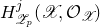 $H^j_{\mathscr{Z}_p}(\mathscr{X},\mathcal{O}_{\mathscr{X}})$
.
$H^j_{\mathscr{Z}_p}(\mathscr{X},\mathcal{O}_{\mathscr{X}})$
.
-
(i) [Reference Raicu and WeymanRW16, Main Theorem]. We have the following in the Grothendieck group of
$\mathcal{D}$
-modules on
$\mathscr{X}$
:
$$\sum_{j\geqslant 0} \big[H^j_{\mathscr{Z}_p}(\mathscr{X},\mathcal{O}_{\mathscr{X}})\big]\cdot q^j=\sum_{s=0}^p [D_s]\cdot q^{(n-p)^2+(n-s)\cdot (m-n)}\cdot \binom{n-s-1}{p-s}_{q^2}.$$
-
(ii) [Reference PerlmanPer24, Theorem 1.1]. Each copy of
$D_s$
in
$H^j_{\mathscr{Z}_p}(\mathscr{X},\mathcal{O}_{\mathscr{X}})$
underlies a pure Hodge module of weight
$mn+p-s+j$
.


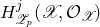

Let $X=\operatorname{{\rm Gr}}(n,m+n)$
and let
$X=\operatorname{{\rm Gr}}(n,m+n)$
and let $U\subseteq X$
be the opposite big cell with respect to the fixed flag
$U\subseteq X$
be the opposite big cell with respect to the fixed flag $\mathcal{V}_{\bullet}$
. Then,
$\mathcal{V}_{\bullet}$
. Then, $U\cong \mathscr{X}$
and we have that
$U\cong \mathscr{X}$
and we have that $Z_{\underline{p}}|_U=\mathscr{Z}_p$
, where
$Z_{\underline{p}}|_U=\mathscr{Z}_p$
, where $\underline{p}=(m^p,p^{n-p})$
is the partition obtained from the
$\underline{p}=(m^p,p^{n-p})$
is the partition obtained from the $n\times m$
rectangle by removing the bottom-right
$n\times m$
rectangle by removing the bottom-right $(n-p)\times (m-p)$
rectangle (see [Reference Lakshmibai and RaghavanLR08, Chapter 5]). For instance, when
$(n-p)\times (m-p)$
rectangle (see [Reference Lakshmibai and RaghavanLR08, Chapter 5]). For instance, when $m=5$
and
$m=5$
and $n=4$
, the following Young diagrams correspond to Schubert varieties in
$n=4$
, the following Young diagrams correspond to Schubert varieties in $\operatorname{{\rm Gr}}(4,9)$
that restrict to the determinantal varieties in
$\operatorname{{\rm Gr}}(4,9)$
that restrict to the determinantal varieties in $\mathbb{C}^{5\times 4}$
.
$\mathbb{C}^{5\times 4}$
.

Furthermore, via this identification, we have that
 \begin{equation}\mathcal{L}(O_{\underline{p}},X)|_U=D_p,\quad IC^H_{Z_{\underline{p}}}|_U\cong IC^H_{\mathscr{Z}_p},\quad \mathscr{H}^j_{Z_{\underline{p}}}(\mathcal{O}_X^H)|_U\cong H^j_{\mathscr{Z}_p}(\mathscr{X},\mathcal{O}_{\mathscr{X}}^H).\end{equation}
We observe that the only elements of Dyck $^{\bullet}(\underline{p})$
consisting of paths of length
$^{\bullet}(\underline{p})$
consisting of paths of length $\geqslant 3$
are obtained by removing hooks supported on the inside corner of
$\geqslant 3$
are obtained by removing hooks supported on the inside corner of $\underline{p}$
. For instance, continuing the above example, we obtain the following elements of Dyck
$\underline{p}$
. For instance, continuing the above example, we obtain the following elements of Dyck $^{\bullet}(\underline{2})$
when
$^{\bullet}(\underline{2})$
when $m=5$
and
$m=5$
and $n=4$
.
$n=4$
.

In particular, by Theorem 1.1, the multiplicity of $D_s$
in
$D_s$
in $H^{(m-p)(n-p)+j}_{\mathscr{Z}_p}(\mathscr{X},\mathcal{O}_{\mathscr{X}})$
is the number of ways to remove
$H^{(m-p)(n-p)+j}_{\mathscr{Z}_p}(\mathscr{X},\mathcal{O}_{\mathscr{X}})$
is the number of ways to remove $p-s$
hooks from
$p-s$
hooks from $\underline{p}$
with j bullets. Since the said hooks must start and end on the same antidiagonal, and
$\underline{p}$
with j bullets. Since the said hooks must start and end on the same antidiagonal, and $m\geqslant n$
, there will always be a
$m\geqslant n$
, there will always be a $(p-s)\times (m-n)$
rectangle of bullets in rows
$(p-s)\times (m-n)$
rectangle of bullets in rows $s+1,\ldots, p$
of
$s+1,\ldots, p$
of $\underline{p}$
and columns
$\underline{p}$
and columns $n+1,\ldots, m$
(these are the bullets depicted in the fifth columns of the above patterns). Thus, we may reduce to the case
$n+1,\ldots, m$
(these are the bullets depicted in the fifth columns of the above patterns). Thus, we may reduce to the case $m=n$
, and assume that
$m=n$
, and assume that $\underline{p}$
and its Dyck patterns are symmetric with respect to the operation of transposing the diagram.
$\underline{p}$
and its Dyck patterns are symmetric with respect to the operation of transposing the diagram.
Let $m=n$
and let
$m=n$
and let $0\leqslant p\leqslant n$
. Let
$0\leqslant p\leqslant n$
. Let $\mathbb{D}\in {\rm Dyck}^{\bullet}(\underline{p})$
consist of paths of length
$\mathbb{D}\in {\rm Dyck}^{\bullet}(\underline{p})$
consist of paths of length $\geqslant 3$
and set
$\geqslant 3$
and set $\underline{s}=\underline{p}^{\mathbb{D}}$
for
$\underline{s}=\underline{p}^{\mathbb{D}}$
for $0\leqslant s\leqslant p$
. The union of the support of the paths in
$0\leqslant s\leqslant p$
. The union of the support of the paths in $\mathbb{D}$
will contain all boxes (x,y) such that
$\mathbb{D}$
will contain all boxes (x,y) such that $s+1\leqslant x,y\leqslant p+1$
(except the box
$s+1\leqslant x,y\leqslant p+1$
(except the box $(p+1,p+1)$
, which lies just outside the inside corner of
$(p+1,p+1)$
, which lies just outside the inside corner of $\underline{p}$
). Due to the covering condition for Dyck patterns, the number of bullets in row
$\underline{p}$
). Due to the covering condition for Dyck patterns, the number of bullets in row $s+i$
must be less than or equal to the number of bullets in row
$s+i$
must be less than or equal to the number of bullets in row $s+i+1$
for
$s+i+1$
for $1\leqslant i\leqslant p-1$
. Thus, there is a partition shape of bullets in rows
$1\leqslant i\leqslant p-1$
. Thus, there is a partition shape of bullets in rows $s+1,\ldots, p$
, and the transpose partition of bullets in columns
$s+1,\ldots, p$
, and the transpose partition of bullets in columns $s+1,\ldots, p$
.
$s+1,\ldots, p$
.
Here is a picture when $m=n=9$
,
$m=n=9$
, $p=4$
, and
$p=4$
, and $s=1$
.
$s=1$
.

The partition formed by the bullets is (4,3,1). We conclude that, for $m=n$
, the multiplicity of
$m=n$
, the multiplicity of $D_s$
in
$D_s$
in $H^{(n-p)^2+2j}_{\mathscr{Z}_p}(\mathscr{X},\mathcal{O}_{\mathscr{X}})$
is the number of partitions of size j that fit inside a
$H^{(n-p)^2+2j}_{\mathscr{Z}_p}(\mathscr{X},\mathcal{O}_{\mathscr{X}})$
is the number of partitions of size j that fit inside a $(p-s)\times (n-p-1)$
rectangle, which is the coefficient of
$(p-s)\times (n-p-1)$
rectangle, which is the coefficient of $q^j$
in the Gaussian binomial coefficient
$q^j$
in the Gaussian binomial coefficient $({n-s-1\atop p-s})_q$
.
$({n-s-1\atop p-s})_q$
.
Putting it all together, we obtain, for $m\geqslant n$
, the following multiplicity formula:
$m\geqslant n$
, the following multiplicity formula:
 $$\sum_{j \geqslant 0}\big[H^j_{\mathscr{Z}_p}(\mathscr{X},\mathcal{O}_{\mathscr{X}}): D_s \big]\cdot q^j=q^{(m-p)(n-p)+(p-s)(m-n)}\cdot \Big({n-s-1\atop p-s}\Big)_{q^2}.$$
Since $(m-p)(n-p)+(p-s)(m-n)=(n-p)^2+(n-s)(m-n)$
, we recover Theorem 4.11(i).
$(m-p)(n-p)+(p-s)(m-n)=(n-p)^2+(n-s)(m-n)$
, we recover Theorem 4.11(i).
By Theorem 1.1, the weight of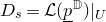 $D_s=\mathcal{L}(\underline{p}^{\mathbb{D}})|_U$
in
$D_s=\mathcal{L}(\underline{p}^{\mathbb{D}})|_U$
in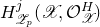 $H^j_{\mathscr{Z}_p}(\mathscr{X},\mathcal{O}_{\mathscr{X}}^H)$
is
$H^j_{\mathscr{Z}_p}(\mathscr{X},\mathcal{O}_{\mathscr{X}}^H)$
is $mn+|\mathbb{D}|+j=mn+p-s+j$
, recovering Theorem 4.11(ii).
$mn+|\mathbb{D}|+j=mn+p-s+j$
, recovering Theorem 4.11(ii).
Acknowledgements
We are grateful to Sam Evens, András Lörincz, Claudiu Raicu, and Vic Reiner for advice and useful conversations regarding this project. We thank anonymous referees for numerous helpful comments.
Conflicts of interest
None.
Journal information
Compositio Mathematica is owned by the Foundation Compositio Mathematica and published by the London Mathematical Society in partnership with Cambridge University Press. All surplus income from the publication of Compositio Mathematica is returned to mathematics and higher education through the charitable activities of the Foundation, the London Mathematical Society and Cambridge University Press.


 Open access

