







1. Introduction
Vortices are a common phenomenon in fluid motion, occurring at scales ranging from the tiny vortices in a cup of coffee to the massive Great Red Spot on Jupiter. The study of vortex dynamics has been a central area of research since the 19th century, pioneered by Helmholtz and Lord Kelvin, and later advanced through the contributions of Saffman and other researchers in fluid dynamics and applied mathematics. The fundamental concepts in this field are comprehensively outlined in Saffman’s renowned book Vortex Dynamics (Saffman Reference Saffman1995). A particularly significant aspect of vortices is their susceptibility to instabilities, which can arise from interactions with their surroundings or within the vortices themselves. In recent decades, extensive research has been conducted on vortex stability, with particular focus on vortex pairs, which are crucial in the context of aircraft trailing wakes and their amplification. An extensive summary of the general stability study of vortices can be found in Ash, Khorrami & Green (Reference Ash, Khorrami and Green1995), and the advancements in the study of vortex pair dynamics and instabilities have been thoroughly reviewed by Leweke, Le Dizès & Williamson (Reference Leweke, Le Dizès and Williamson2016). Such studies have also been essential for understanding how turbulence arises from instabilities caused by eddy interactions and the dynamics of coherent structures within turbulent flows (Pullin & Saffman Reference Pullin and Saffman1998).
Vortex pairs are known to experience two main types of instabilities: long-wave and short-wave instabilities. These are often referred to as cooperative instabilities, as they primarily result from the interaction between the vortices within the pair. They are also three-dimensional (3-D) in nature. Long-wave instability, also known as Crow instability, occurs at scales much larger than the size of the vortex core. It was discovered by Crow (Reference Crow1970) for a vortex pair. More studies about long-wave instabilities can be found in Brion, Sipp & Jacquin (Reference Brion, Sipp and Jacquin2007), Leweke & Williamson (Reference Leweke and Williamson2011), and similar works. They are often observed in the sky, affecting the contrails of aircraft flying at high altitudes.
In contrast, short-wave instability occurs at scales comparable to or smaller than the vortex core. Moore & Saffman (Reference Moore and Saffman1975) and Tsai & Widnall (Reference Tsai and Widnall1976) were the first to discover and explain the mechanism of this instability. It is understood to occur because the streamlines of the vortex undergo elliptic deformation due to the strain induced by the adjacent vortex, causing two Kelvin waves (small perturbations) with specific azimuthal wavenumber combinations to resonate with the strain and become unstable. Due to the elliptic nature of the streamline deformation, this is also referred to as elliptic instability and is sometimes known as the Moore–Saffman–Tsai–Widnall instability. An extensive summary on the elliptic instability can be found in Kerswell (Reference Kerswell2002), and some important original contributions include Bayly (Reference Bayly1986), Pierrehumbert (Reference Pierrehumbert1986), Leweke & Williamson (Reference Leweke and Williamson1998), Le Dizès & Laporte (Reference Le Dizès and Laporte2002), Meunier & Leweke (Reference Meunier and Leweke2005) and Schaeffer & Le Dizès (Reference Schaeffer and Le Dizès2010). The modes with $m=1$
and
$m=1$
and $m=- 1$
, also known as stationary helical modes, were found to be the most unstable.
$m=- 1$
, also known as stationary helical modes, were found to be the most unstable.
Tsai & Widnall (Reference Tsai and Widnall1976) analysed the Rankine vortex, while Moore & Saffman (Reference Moore and Saffman1975) focused on the Lamb–Oseen vortex. For the Rankine vortex, the eigenvalue problem for linearised disturbances on the unstrained vortex can be solved analytically, yielding the eigenmodes and eigenfunctions of the Kelvin waves. These eigenfunctions are expressed in terms of Bessel functions (Tsai & Widnall Reference Tsai and Widnall1976; Saffman Reference Saffman1995; Fukumoto Reference Fukumoto2003). However, for the Lamb–Oseen and Batchelor vortices, obtaining explicit analytical expressions for the eigenfunctions is not possible. Nevertheless, their asymptotic forms can be derived in the limit of large $k$
, as shown by Le Dizès & Lacaze (Reference Le Dizès and Lacaze2005). Using the Wentzel–Kramers–Brillouin (WKB) approach, they provided approximate analytical expressions for the dispersion relation and eigenmodes, and discussed the conditions for the existence of regular neutral core and ring modes. Sipp & Jacquin (Reference Sipp and Jacquin2003) and Fabre, Sipp & Jacquin (Reference Fabre, Sipp and Jacquin2006) solved the problem numerically using a Chebyshev spectral collocation method. Their findings revealed that many eigenmodes are suppressed due to critical layer damping, which arises due to the smooth distribution of vorticity. Additionally, Eloy & Le Dizès (Reference Eloy and Le Dizès2001) performed a detailed stability analysis of the Rankine vortex, identifying resonant combinations beyond the helical modes. Their analysis was also extended to consider a multipolar straining field.
$k$
, as shown by Le Dizès & Lacaze (Reference Le Dizès and Lacaze2005). Using the Wentzel–Kramers–Brillouin (WKB) approach, they provided approximate analytical expressions for the dispersion relation and eigenmodes, and discussed the conditions for the existence of regular neutral core and ring modes. Sipp & Jacquin (Reference Sipp and Jacquin2003) and Fabre, Sipp & Jacquin (Reference Fabre, Sipp and Jacquin2006) solved the problem numerically using a Chebyshev spectral collocation method. Their findings revealed that many eigenmodes are suppressed due to critical layer damping, which arises due to the smooth distribution of vorticity. Additionally, Eloy & Le Dizès (Reference Eloy and Le Dizès2001) performed a detailed stability analysis of the Rankine vortex, identifying resonant combinations beyond the helical modes. Their analysis was also extended to consider a multipolar straining field.
Another type of short-wave instability was found to occur theoretically in vortex rings by Hattori & Fukumoto (Reference Hattori and Fukumoto2003) and Fukumoto & Hattori (Reference Fukumoto and Hattori2005). It was caused by the inherent curvature of the vortex rings, and occurred for combinations of azimuthal wavenumbers differing by one. The authors conducted stability analyses on the Rankine vortex to deduce the characteristics of curvature instability. Blanco-Rodríguez & Le Dizès (Reference Blanco-Rodríguez and Le Dizès2017) theoretically computed the growth rates for a Batchelor vortex, and, along with Blanco-Rodríguez & Le Dizès (Reference Blanco-Rodríguez and Le Dizès2016), demonstrated that curvature also contributes to elliptic instability. Hattori, Blanco-Rodríguez & Le Dizès (Reference Hattori, Blanco-Rodríguez and Le Dizès2019) further confirmed curvature instability in a vortex ring with swirl through numerical stability analysis using direct numerical simulations (DNS). Recently, Xu et al. (Reference Xu, Delbende, Hattori and Rossi2025) proposed a numerical procedure to study instabilities in helical vortex systems, and showed that curvature instability is also present in such systems.
Although elliptic and curvature instabilities have been studied extensively over the past few decades, much less attention has been given to multipolar instabilities, particularly triangular instabilities. The only studies on triangular instability have been conducted for the Rankine vortex (Eloy, Le Gal & Le Dizès Reference Eloy, Le Gal and Le Dizès2000, Reference Eloy, Le Gal and Le Dizès2003; Eloy & Le Dizès Reference Eloy and Le Dizès2001), and there are no theoretical or numerical studies confirming the existence of triangular instability for Lamb–Oseen or Batchelor vortices. The existence of triangular instability in more realistic vortices such as the Lamb–Oseen and Batchelor vortices could have significant implications and provide valuable insights for engineering applications such as turbomachines with three blades, e.g. ship or aircraft propellers, wind turbines, and more. In such cases, the helical vortices that form around the central hub vortex may induce triangular straining on the hub vortex, potentially triggering instabilities. Additionally, long-lived non-axisymmetric vortices, such as dipoles, tripoles and higher-order multipolar structures, have been observed in rotating turbulent flows through experiments and DNS (Hopfinger & Van Heijst Reference Hopfinger and Van Heijst1993; Carnevale & Kloosterziel Reference Carnevale and Kloosterziel1994; Rossi, Lingevitch & Bernoff Reference Rossi, Lingevitch and Bernoff1997; Dritschel Reference Dritschel1998). Kelvin waves have also been identified on vortex filaments in transitional flows (Arendt, Fritts & Andreassen Reference Arendt, Fritts and Andreassen1998), with elliptic and multipolar instabilities potentially explaining the emergence and growth of these waves.
In this study, we aim to investigate the stability of a Lamb–Oseen vortex under triangular straining to short-wave instabilities through the parametric resonance of Kelvin waves. This is achieved by conducting a linear stability analysis using both DNS and theoretical analysis. Our objectives include computing and comparing the growth rates and structures of the unstable modes (if present) obtained through linearised DNS and theoretical analysis. Nonlinear effects are not considered in this work. Although the simulations that we conduct are linearised DNS, we will refer to them simply as DNS for brevity. In the DNS approach, we first determine the base flow and then integrate the linearised Navier–Stokes equations to identify the most unstable mode. In the theoretical analysis, we derive an approximation for the base flow under the assumption of a weak triangular straining field, and use this approximation to derive linear perturbation equations for the strained Lamb–Oseen vortex. These equations are then used to compute the growth rates of the resonant modes. To identify the resonant modes, we solve the eigenvalue problem corresponding to the unperturbed vortex. Further details of the methods and analysis are provided in the subsequent sections.
The paper is structured as follows. In § 2, we formulate the problem and describe the numerical procedure in detail, for both obtaining the base flow, and performing the linearised DNS to identify the most unstable mode. In § 3, we derive the base flow using theoretical analysis, and outline the procedure for obtaining its analytical expressions. We then compare these theoretical results with those from DNS. In § 4, we provide a comprehensive explanation of the linear stability analysis, including the linearised perturbation equations and the expressions for the growth rates of the resonant modes. We then compare the results from DNS and theory. Finally, in § 5, we summarise the key findings of this work and discuss potential future research directions.
2. Numerical procedure
Before delving into the theoretical analysis, we present an outline and detailed description of the numerical procedure used to perform the DNS.
2.1. Outline
Geometry of the hub vortex and the three satellite vortices.

As an initial state, we consider a central hub Lamb–Oseen vortex surrounded symmetrically by three satellite Lamb–Oseen vortices in an incompressible, viscous fluid, where the satellite vortices provide triangular straining to the hub vortex, similar to the illustration in figure 1. The satellite vortices are positioned at the vertices of an equilateral triangle, with the hub vortex at its centre. If $\Gamma$
denotes the circulation of the hub vortex, then the circulation of each satellite vortex is chosen to be
$\Gamma$
denotes the circulation of the hub vortex, then the circulation of each satellite vortex is chosen to be $-\Gamma$
. This choice ensures that the velocity induced by the other vortices at the centre of any vortex vanishes. As a result, the vortices are not expected to move. In this manner, the system composed of hub and satellite vortices can form a quasi-steady state, the stability of which can be analysed.
$-\Gamma$
. This choice ensures that the velocity induced by the other vortices at the centre of any vortex vanishes. As a result, the vortices are not expected to move. In this manner, the system composed of hub and satellite vortices can form a quasi-steady state, the stability of which can be analysed.
2.2. Numerical methods
The numerical analysis will involve two main steps. First, we obtain the quasi-steady base flow by solving the two-dimensional (2-D) Navier–Stokes equations; then we integrate the linearised Navier–Stokes equations around this base flow over a sufficiently long duration to determine the most unstable mode, if it exists, for a linear disturbance with a specified axial wavenumber, as detailed in the following paragraphs.
The analysis is performed in cylindrical coordinates. The base flow is computed in two dimensions $(r, \theta )$
, while the linear stability analysis extends to three dimensions
$(r, \theta )$
, while the linear stability analysis extends to three dimensions $(r, \theta , z)$
. The linearised Navier–Stokes equations for the disturbances
$(r, \theta , z)$
. The linearised Navier–Stokes equations for the disturbances $u, v, w$
and
$u, v, w$
and $p$
around a given 2-D base flow
$p$
around a given 2-D base flow $(U, V)$
can be expressed as
$(U, V)$
can be expressed as
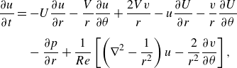 \begin{align} {\frac {\partial {u}}{\partial {t}}} &= -U{\frac {\partial {u}}{\partial {r}}} -\frac {V}{r}{\frac {\partial {u}}{\partial {\theta }}} + \frac {2Vv}{r} -u{\frac {\partial {U}}{\partial {r}}} -\frac {v}{r}{\frac {\partial {U}}{\partial {\theta }}} \nonumber \\[6pt] & \quad-{\frac {\partial {p}}{\partial {r}}} + \frac {1}{{Re}} \left [\left (\nabla ^2 -\frac {1}{r^2}\right ) u - \frac {2}{r^2} {\frac {\partial {v}}{\partial {\theta }}}\right ], \end{align}
 \begin{align} {\frac {\partial {v}}{\partial {t}}} &= -U{\frac {\partial {v}}{\partial {r}}} -\frac {V}{r}{\frac {\partial {v}}{\partial {\theta }}} -u{\frac {\partial {V}}{\partial {r}}} -\frac {v}{r}{\frac {\partial {V}}{\partial {\theta }}} - \frac {Uv +uV}{r} \nonumber \\[6pt] & \quad-\frac {1}{r}{\frac {\partial {p}}{\partial {\theta }}} + \frac {1}{{Re}} \left [\left (\nabla ^2 -\frac {1}{r^2}\right ) v + \frac {2}{r^2} {\frac {\partial {u}}{\partial {\theta }}}\right ], \end{align}
 \begin{align} {\frac {\partial {w}}{\partial {t}}} &= -U{\frac {\partial {w}}{\partial {r}}} -\frac {V}{r}{\frac {\partial {w}}{\partial {\theta }}} -{\frac {\partial {p}}{\partial {z}}} + \frac {1}{{Re}}\, \nabla ^2 w, \end{align}
where $\nabla ^2 = \partial _r^2 + (1/r)\,\partial _r + (1/r^2)\, \partial ^2_{\theta } + \partial ^2_{z}$
. These equations are discretised and solved numerically on the same 2-D grid as the base flow. By assuming periodic boundary conditions in the
$\nabla ^2 = \partial _r^2 + (1/r)\,\partial _r + (1/r^2)\, \partial ^2_{\theta } + \partial ^2_{z}$
. These equations are discretised and solved numerically on the same 2-D grid as the base flow. By assuming periodic boundary conditions in the $z$
-direction, the above equations are separable in the
$z$
-direction, the above equations are separable in the $z$
-direction, which allows us to consider a single wave of the form
$z$
-direction, which allows us to consider a single wave of the form
 \begin{eqnarray} F(t, r, \theta , z) = {\textrm e}^{{\textrm {i}} k z} \sum _{m} \hat {F}_{m} (t,r)\,{\textrm e}^{{\textrm {i}} m\theta } \end{eqnarray}
for $u, v, w$
and
$u, v, w$
and $p$
. The 2-D numerical domain spans
$p$
. The 2-D numerical domain spans $0 \leqslant r \leqslant L_r$
and
$0 \leqslant r \leqslant L_r$
and $0 \leqslant \theta \leqslant 2\pi$
, with
$0 \leqslant \theta \leqslant 2\pi$
, with $L_r = 1000$
. For spatial discretisation, we use a sixth-order-accurate compact scheme (Lele Reference Lele1992) in
$L_r = 1000$
. For spatial discretisation, we use a sixth-order-accurate compact scheme (Lele Reference Lele1992) in $r$
, and a Fourier spectral method in
$r$
, and a Fourier spectral method in $\theta$
, with periodic boundary conditions. To avoid the singularity at
$\theta$
, with periodic boundary conditions. To avoid the singularity at $r = 0$
, we expand the
$r = 0$
, we expand the $r$
axis to
$r$
axis to $-L_r \leqslant r \leqslant L_r$
, and omit a grid point at
$-L_r \leqslant r \leqslant L_r$
, and omit a grid point at $r = 0$
. The Poisson equation for the pressure is decomposed into a set of ordinary differential equations for individual Fourier modes, which are also solved with the sixth-order compact scheme. For temporal discretisation, we apply the Crank–Nicolson scheme to the viscous terms, and the second-order Adams–Bashforth method to the other terms. Further details are provided in Appendix A of Hattori et al. (Reference Hattori, Blanco-Rodríguez and Le Dizès2019).
$r = 0$
. The Poisson equation for the pressure is decomposed into a set of ordinary differential equations for individual Fourier modes, which are also solved with the sixth-order compact scheme. For temporal discretisation, we apply the Crank–Nicolson scheme to the viscous terms, and the second-order Adams–Bashforth method to the other terms. Further details are provided in Appendix A of Hattori et al. (Reference Hattori, Blanco-Rodríguez and Le Dizès2019).
The base flow is obtained once the vortices have equilibrated in the field of the other vortices. This rapid relaxation process has been described in the literature for two vortices (Sipp, Jacquin & Cosssu Reference Sipp, Jacquin and Cossu2000; Le Dizès & Verga Reference Le Dizès and Verga2002). After equilibrium is reached, the 2-D solution evolves on a slow viscous time scale. This evolution will not be considered further, as we assume a frozen base flow and linearise the Navier–Stokes equations around it. The same numerical methods and discretisation used for obtaining the base flow are applied to integrate the frozen linearised Navier–Stokes equations.
2.3. Initial conditions and simulation parameters
The vortices are initially positioned as shown in figure 1. The hub vortex is located at the centre of the frame, and the three satellite vortices are placed at distance of $R$
from the hub vortex centre, with angular separation
$R$
from the hub vortex centre, with angular separation $2\pi /3$
. Initially, all vortices are assumed to have a Gaussian vorticity profile with core radius
$2\pi /3$
. Initially, all vortices are assumed to have a Gaussian vorticity profile with core radius $a_i$
. After the relaxation process, the core size of the vortices has slightly increased to a larger value
$a_i$
. After the relaxation process, the core size of the vortices has slightly increased to a larger value $a$
. This new core size will be used to non-dimensionalise all spatial variables in the theory. The vortex circulation, however, is conserved. Thus the Reynolds number
$a$
. This new core size will be used to non-dimensionalise all spatial variables in the theory. The vortex circulation, however, is conserved. Thus the Reynolds number ${Re}$
defined by
${Re}$
defined by
 \begin{equation} {Re} =\frac {\Gamma }{2 \pi \nu }, \end{equation}
where $\nu$
is the kinematic viscosity, does not change. We start the simulation with core size
$\nu$
is the kinematic viscosity, does not change. We start the simulation with core size $a_i = 0.8$
for both hub and satellite vortices, and stop it when the core size of the hub vortex reaches
$a_i = 0.8$
for both hub and satellite vortices, and stop it when the core size of the hub vortex reaches $a = 1$
, which occurs well after the establishment of a quasi-steady state. The distance between the hub and the satellite vortices, denoted by
$a = 1$
, which occurs well after the establishment of a quasi-steady state. The distance between the hub and the satellite vortices, denoted by $R$
, is set to
$R$
, is set to $R = 5$
. Unlike the growing core size, this distance remains nearly constant as the base flow reaches a quasi-steady state. Thus at the quasi-steady state, we have
$R = 5$
. Unlike the growing core size, this distance remains nearly constant as the base flow reaches a quasi-steady state. Thus at the quasi-steady state, we have $a = 1$
and
$a = 1$
and $R = 5$
. The initial circulation
$R = 5$
. The initial circulation $\Gamma$
of the hub vortex is set to
$\Gamma$
of the hub vortex is set to $2\pi$
(
$2\pi$
( $-\Gamma$
for the satellite vortices). We tracked the circulation, first-order and second-order moments of the vorticity field of the hub vortex throughout the simulation, which allowed us to compute its core radius and keep track of how it changes with time. The details of these calculations are provided in Appendix A.
$-\Gamma$
for the satellite vortices). We tracked the circulation, first-order and second-order moments of the vorticity field of the hub vortex throughout the simulation, which allowed us to compute its core radius and keep track of how it changes with time. The details of these calculations are provided in Appendix A.
In the simulations, we select ${Re} = 10^3$
to obtain the base flow, but choose a larger value
${Re} = 10^3$
to obtain the base flow, but choose a larger value ${Re} = 10^4$
for the perturbation analysis. This large value of the Reynolds number for the perturbation analysis will guarantee the existence of unstable modes. The choice of a smaller value of the Reynolds number for the base flow is just to reach the quasi-steady state of core size
${Re} = 10^4$
for the perturbation analysis. This large value of the Reynolds number for the perturbation analysis will guarantee the existence of unstable modes. The choice of a smaller value of the Reynolds number for the base flow is just to reach the quasi-steady state of core size $a=1$
from
$a=1$
from $a_i=0.8$
more rapidly. This is justified because the quasi-steady state is not expected to depend on the Reynolds number (Le Dizès & Verga Reference Le Dizès and Verga2002). The most unstable mode for a given axial wavenumber
$a_i=0.8$
more rapidly. This is justified because the quasi-steady state is not expected to depend on the Reynolds number (Le Dizès & Verga Reference Le Dizès and Verga2002). The most unstable mode for a given axial wavenumber $k$
, if it exists, is obtained by DNS from a random vorticity initial condition. The irrelevant modes decay, and the unstable modes grow exponentially, from which the growth rate can be obtained. A non-uniform grid is used where the number of grid points in
$k$
, if it exists, is obtained by DNS from a random vorticity initial condition. The irrelevant modes decay, and the unstable modes grow exponentially, from which the growth rate can be obtained. A non-uniform grid is used where the number of grid points in $r$
is taken to be
$r$
is taken to be $695$
, and the number of Fourier modes in
$695$
, and the number of Fourier modes in $\theta$
to be
$\theta$
to be $512$
. Radial grid spacing
$512$
. Radial grid spacing $0.0475$
is used in the region of the hub vortex and satellite vortices.
$0.0475$
is used in the region of the hub vortex and satellite vortices.
3. Base flow: theory and results
In this section, we present the theoretical analysis used to derive the analytical expressions for the base flow, which are then applied in the linear stability analysis. While the numerical simulations consider the full system composed of the hub vortex and the three satellite vortices, the theory focuses on the hub vortex. The objective is to obtain an approximation for the velocity field of the hub vortex in the presence of satellite vortices. Such an analysis has already been performed for a vortex pair (Le Dizès & Verga Reference Le Dizès and Verga2002).
The idea is to obtain an asymptotic solution in the limit of small $a/R$
. For this purpose, we introduce a small parameter
$a/R$
. For this purpose, we introduce a small parameter $\epsilon = (a/R)^3$
, giving us
$\epsilon = (a/R)^3$
, giving us $\epsilon = 0.008$
, for the values of
$\epsilon = 0.008$
, for the values of $a$
and
$a$
and $R$
at the quasi-steady state. The field induced by the satellite vortices on the hub vortex can then be modelled using a point vortex approximation for the satellite vortices. In the centre of the hub vortex, this gives an expression for the induced velocity field that reads, in Cartesian coordinates at leading order, as
$R$
at the quasi-steady state. The field induced by the satellite vortices on the hub vortex can then be modelled using a point vortex approximation for the satellite vortices. In the centre of the hub vortex, this gives an expression for the induced velocity field that reads, in Cartesian coordinates at leading order, as
 \begin{equation} U_{x} = - 3 \epsilon (x^2-y^2), \; \; \; U_{y}= 6 \epsilon xy, \end{equation}
and upon transformation into 2-D polar coordinates, we get the components in $r$
and
$r$
and $\theta$
as
$\theta$
as
 \begin{equation} U_{r} = - 3 \epsilon r^2 \cos 3\theta , \; \; \; U_{\theta }= 3\epsilon r^2 \sin 3\theta . \end{equation}
Thus $(U_r, U_{\theta })$
does correspond to a triangular straining field.
$(U_r, U_{\theta })$
does correspond to a triangular straining field.
In Moore & Saffman (Reference Moore and Saffman1975), Moffatt, Kida & Ohkitani (Reference Moffatt, Kida and Ohkitani1994), Jiménez et al. (Reference Jiménez, Moffatt and Vasco1996) and Le Dizès (Reference Le Dizès2000), it was theoretically derived and shown how a Lamb–Oseen vortex interacts with a quadripolar straining field. The interaction with a triangular straining field is similar. We begin by taking a perturbation expansion of the streamfunction $\psi (r,\theta )$
up to
$\psi (r,\theta )$
up to $O(\epsilon )$
. For the
$O(\epsilon )$
. For the $O(\epsilon )$
term, we assume a normal modes form corresponding to a triangular azimuthal wavenumber (see § 2 in Le Dizès (Reference Le Dizès2000) for a detailed and more general derivation). The resulting expression for
$O(\epsilon )$
term, we assume a normal modes form corresponding to a triangular azimuthal wavenumber (see § 2 in Le Dizès (Reference Le Dizès2000) for a detailed and more general derivation). The resulting expression for $\psi$
is substituted in the 2-D inviscid steady-state vorticity equation given by
$\psi$
is substituted in the 2-D inviscid steady-state vorticity equation given by
 \begin{equation} \frac {\partial \zeta }{\partial r}\frac {\partial \psi }{\partial \theta } - \frac {\partial \psi }{\partial r}\frac {\partial \zeta }{\partial \theta } = 0, \end{equation}
where the vorticity field $\zeta (r,\theta )$
is given by
$\zeta (r,\theta )$
is given by
 \begin{equation} \zeta = -\nabla ^2\psi . \end{equation}
The approximation of the 2-D velocity field $(\overline {U}, \overline {V})$
for the triangular-strained Lamb–Oseen vortex, where
$(\overline {U}, \overline {V})$
for the triangular-strained Lamb–Oseen vortex, where $\overline {U}$
and
$\overline {U}$
and $\overline {V}$
denote the radial and azimuthal velocity components, respectively, can then be obtained from the streamfunction as
$\overline {V}$
denote the radial and azimuthal velocity components, respectively, can then be obtained from the streamfunction as
 \begin{align} \overline {U} &= \epsilon \frac {3f(r)}{r}\cos {3\theta } + O(\epsilon ^2), \end{align}
 \begin{align} \overline {V} &= r\Omega _0(r) - \epsilon f'(r)\sin {3\theta } + O(\epsilon ^2), \end{align}
where
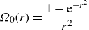 \begin{equation} \Omega _0(r) = \frac {1-{\textrm e}^{-r^2}}{r^2} \end{equation}
is the angular velocity of the Lamb–Oseen vortex, and $f(r)$
is a function governed by the second-order linear ordinary differential equation
$f(r)$
is a function governed by the second-order linear ordinary differential equation
 \begin{equation} {f}'' + r^{-1}{f}' - \left (9r^{-2} + \frac {4r^2}{1 - {\textrm e}^{r^2} }\right )f = 0, \end{equation}
with the boundary conditions
 \begin{align}& f(r) \sim s_0r^3\quad {\textrm at} \ r \rightarrow 0, \end{align}
 \begin{align}& f(r) \sim r^3\quad {\textrm at} \ r \rightarrow \infty . \end{align}
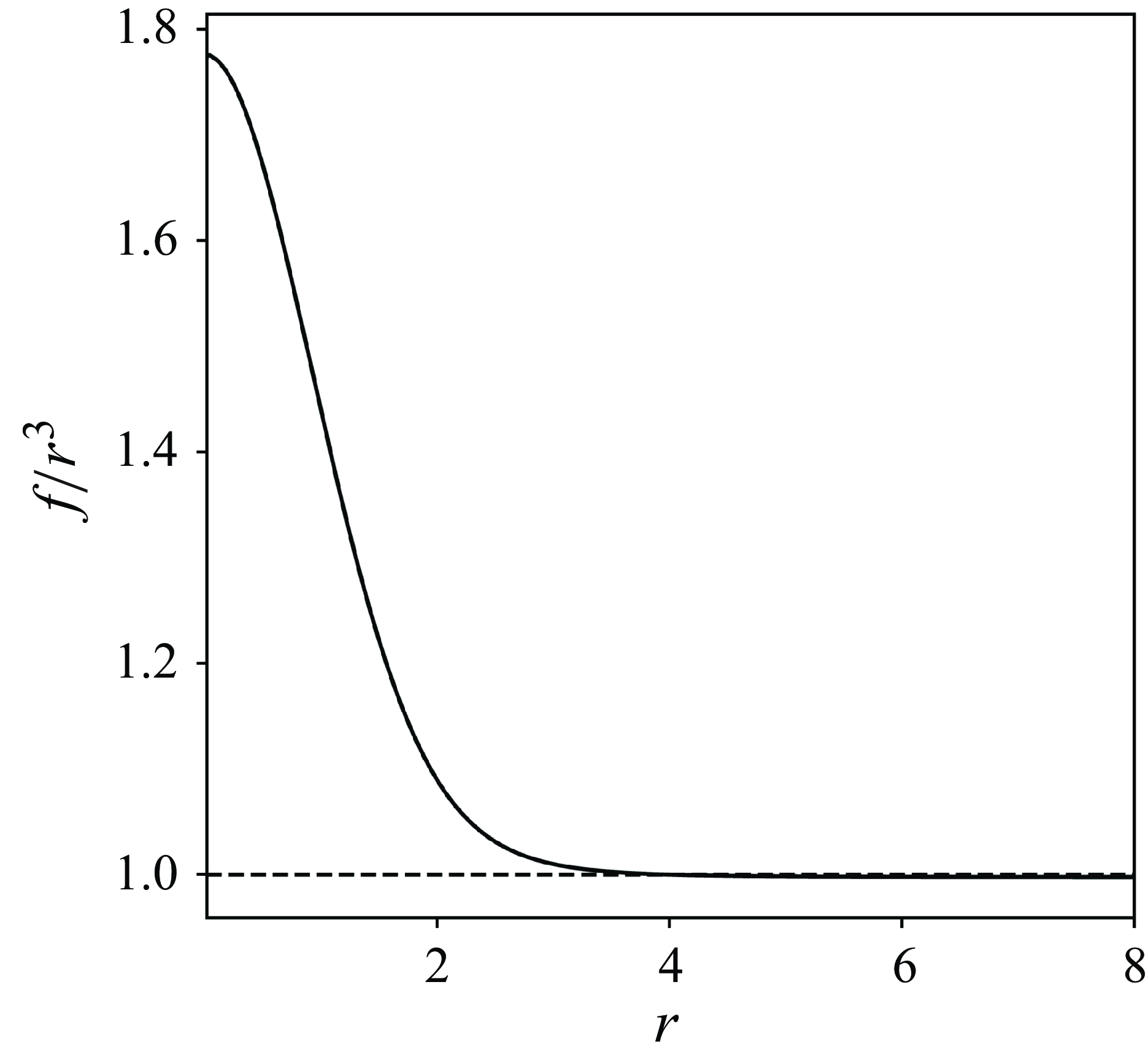
The constant $s_0\approx 1.7724$
appearing in these equations is a numerical constant derived from the integration of (3.8). It corresponds to the amplitude of the straining field in the vortex centre, normalised by the amplitude of the straining field at the same point in the absence of the vortex. This ratio corresponds to the value at the origin of the function plotted in figure 2.
$s_0\approx 1.7724$
appearing in these equations is a numerical constant derived from the integration of (3.8). It corresponds to the amplitude of the straining field in the vortex centre, normalised by the amplitude of the straining field at the same point in the absence of the vortex. This ratio corresponds to the value at the origin of the function plotted in figure 2.
Plot of $f(r)/r^3$
as a function of the radial coordinate
$f(r)/r^3$
as a function of the radial coordinate $r$
. The value at zero is
$r$
. The value at zero is $s_0 \approx 1.7724$
.
$s_0 \approx 1.7724$
.
The vorticity field of the hub vortex can be written as $\zeta = \zeta _0 + \epsilon \zeta _1 + O(\epsilon ^2)$
, with
$\zeta = \zeta _0 + \epsilon \zeta _1 + O(\epsilon ^2)$
, with
 \begin{equation} \zeta _0 = 2 {\textrm e}^{- r^2} ,\quad \zeta _1 = g(r)\sin {3\theta }, \end{equation}
and
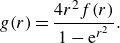 \begin{equation} g(r) = \frac {4r^2 f(r)}{1 - {\textrm e}^{r^2}}. \end{equation}
We compare the DNS-obtained base flow with that derived theoretically to ensure consistency before conducting a linear stability analysis of small disturbances on the base flow. This process involves two steps. First, we verify that a quasi-steady state is reached in DNS by plotting the vorticity field $\zeta (r,\theta )$
and streamfunction
$\zeta (r,\theta )$
and streamfunction $\psi (r,\theta )$
scatter points, where the vorticity and the streamfunction are related via the Poisson equation
$\psi (r,\theta )$
scatter points, where the vorticity and the streamfunction are related via the Poisson equation $\zeta = -\nabla ^2\psi$
. The absence of dispersed regions confirms a quasi-steady state. Such a verification is shown in figure 3. We also calculate the Euler-residue
$\zeta = -\nabla ^2\psi$
. The absence of dispersed regions confirms a quasi-steady state. Such a verification is shown in figure 3. We also calculate the Euler-residue $N$
given by
$N$
given by $N = [ \langle (\boldsymbol{u}\boldsymbol{\cdot} \boldsymbol{\nabla} \omega )^2 \rangle /\langle \omega ^2 \rangle ]^{1/2}\times 2\pi R^2/\Gamma$
, which compares the inviscid evolution time scale of the vorticity distribution with the advection time (Sipp et al. Reference Sipp, Jacquin and Cossu2000). Figure 4 shows the Euler-residue, indicating that the quasi-steady state is reached well before
$N = [ \langle (\boldsymbol{u}\boldsymbol{\cdot} \boldsymbol{\nabla} \omega )^2 \rangle /\langle \omega ^2 \rangle ]^{1/2}\times 2\pi R^2/\Gamma$
, which compares the inviscid evolution time scale of the vorticity distribution with the advection time (Sipp et al. Reference Sipp, Jacquin and Cossu2000). Figure 4 shows the Euler-residue, indicating that the quasi-steady state is reached well before $a=1$
(marked by the red diamond).
$a=1$
(marked by the red diamond).
Scatter plot of $\zeta (r,\theta )$
and
$\zeta (r,\theta )$
and $\Psi (r,\theta )$
for
$\Psi (r,\theta )$
for ${Re}=1000$
and
${Re}=1000$
and $\epsilon =0.008$
: (a) during the relaxation process at
$\epsilon =0.008$
: (a) during the relaxation process at $t = 2.5$
; and (b) when the core size reaches
$t = 2.5$
; and (b) when the core size reaches $a = 1$
at
$a = 1$
at $t=87.35$
, which is well after the establishment of a quasi-steady state. The absence of dispersed regions in (b) indicates that a quasi-steady state has been reached. Zoomed-in regions are included to highlight the differences clearly.
$t=87.35$
, which is well after the establishment of a quasi-steady state. The absence of dispersed regions in (b) indicates that a quasi-steady state has been reached. Zoomed-in regions are included to highlight the differences clearly.

Log-scale plot of Euler-residue $N$
versus
$N$
versus $t$
, scaled by viscous time. The red diamond indicates the time when
$t$
, scaled by viscous time. The red diamond indicates the time when $a = 1$
.
$a = 1$
.

Comparison of the base flow vorticity field obtained with DNS (solid black line) and theory (red dashed line) for ${Re}=1000$
and
${Re}=1000$
and $\epsilon =0.008$
: (a) leading-order term; (b) correction term due to triangular straining. The correction term is obtained at the angular location of a satellite vortex.
$\epsilon =0.008$
: (a) leading-order term; (b) correction term due to triangular straining. The correction term is obtained at the angular location of a satellite vortex.
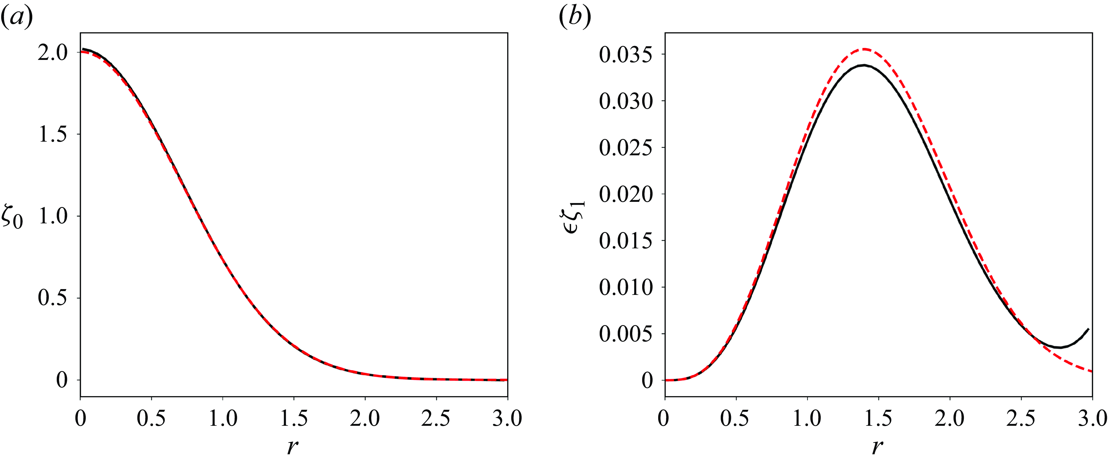
A2-D visualisation of the base flow. (a) Streamlines depicted by solid black lines where the streamfunction $\psi$
is a constant, plotted from
$\psi$
is a constant, plotted from $r_0 = 1$
(innermost contour) to
$r_0 = 1$
(innermost contour) to $r_0 = 2.75$
in intervals of
$r_0 = 2.75$
in intervals of $0.25$
. The values of
$0.25$
. The values of $\psi$
starting from
$\psi$
starting from $r=1$
are
$r=1$
are $2.05, 1.90, 1.74, 1.59, 1.47, 1.35, 1.24, 1.15$
. The corresponding unstrained streamlines are depicted by dashed lines. (b) Contours of
$2.05, 1.90, 1.74, 1.59, 1.47, 1.35, 1.24, 1.15$
. The corresponding unstrained streamlines are depicted by dashed lines. (b) Contours of $\epsilon \zeta _1$
.
$\epsilon \zeta _1$
.
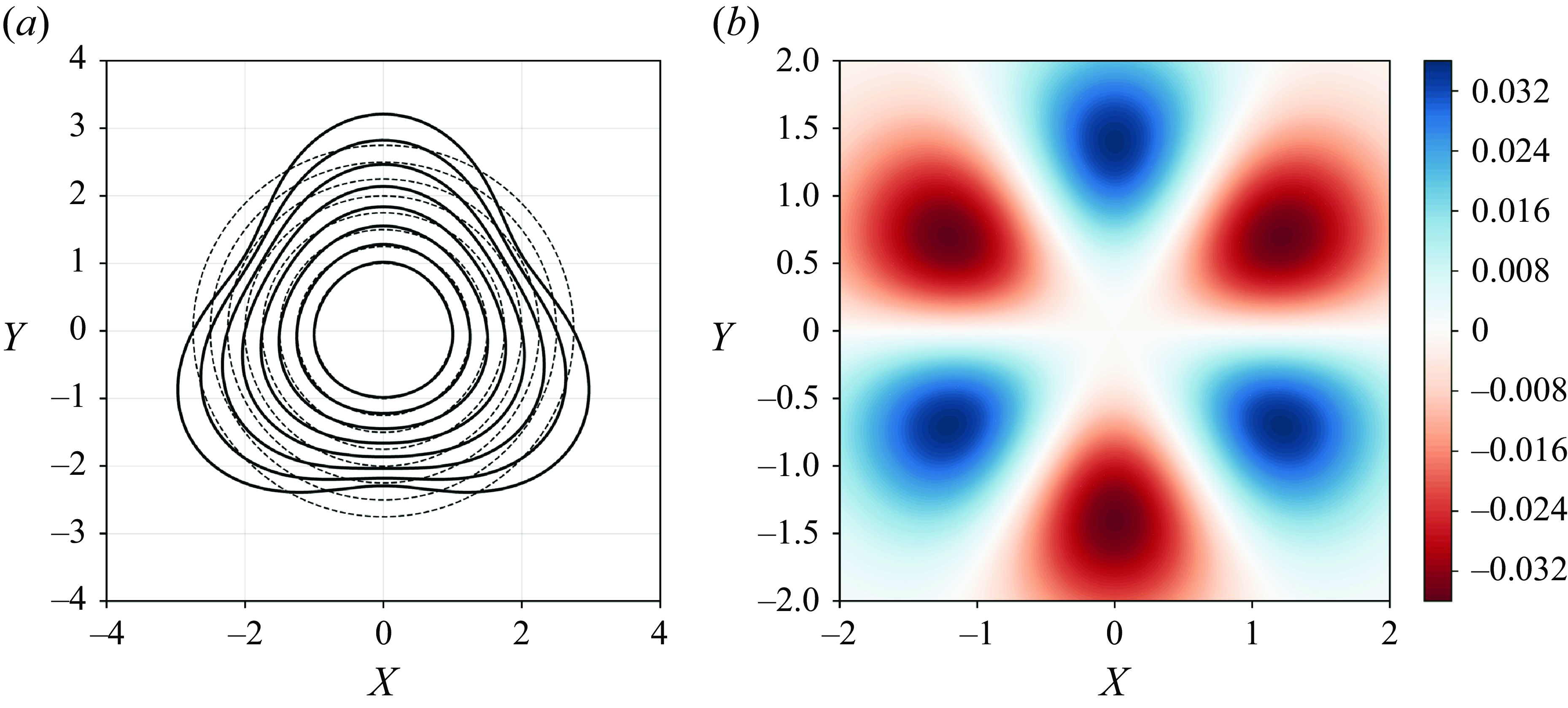
Second, we compare the leading-order and correction terms of the vorticity field accounting for triangular straining. The correction term is obtained from DNS at the angular location of a satellite vortex and compared to $\zeta _1(r,\theta )$
by taking
$\zeta _1(r,\theta )$
by taking $\theta = \pi /2$
or
$\theta = \pi /2$
or $7\pi /6$
or
$7\pi /6$
or $11\pi /6$
. This comparison is shown in figure 5 for
$11\pi /6$
. This comparison is shown in figure 5 for $\epsilon = 0.008$
and
$\epsilon = 0.008$
and ${Re}=1000$
. Good agreement is observed that validates the description of the base flow close to the hub vortex by (3.5) and (3.6). It is important to note that in figure 5(b), the rise in the curve for the correction term obtained numerically, near
${Re}=1000$
. Good agreement is observed that validates the description of the base flow close to the hub vortex by (3.5) and (3.6). It is important to note that in figure 5(b), the rise in the curve for the correction term obtained numerically, near $r \approx 3$
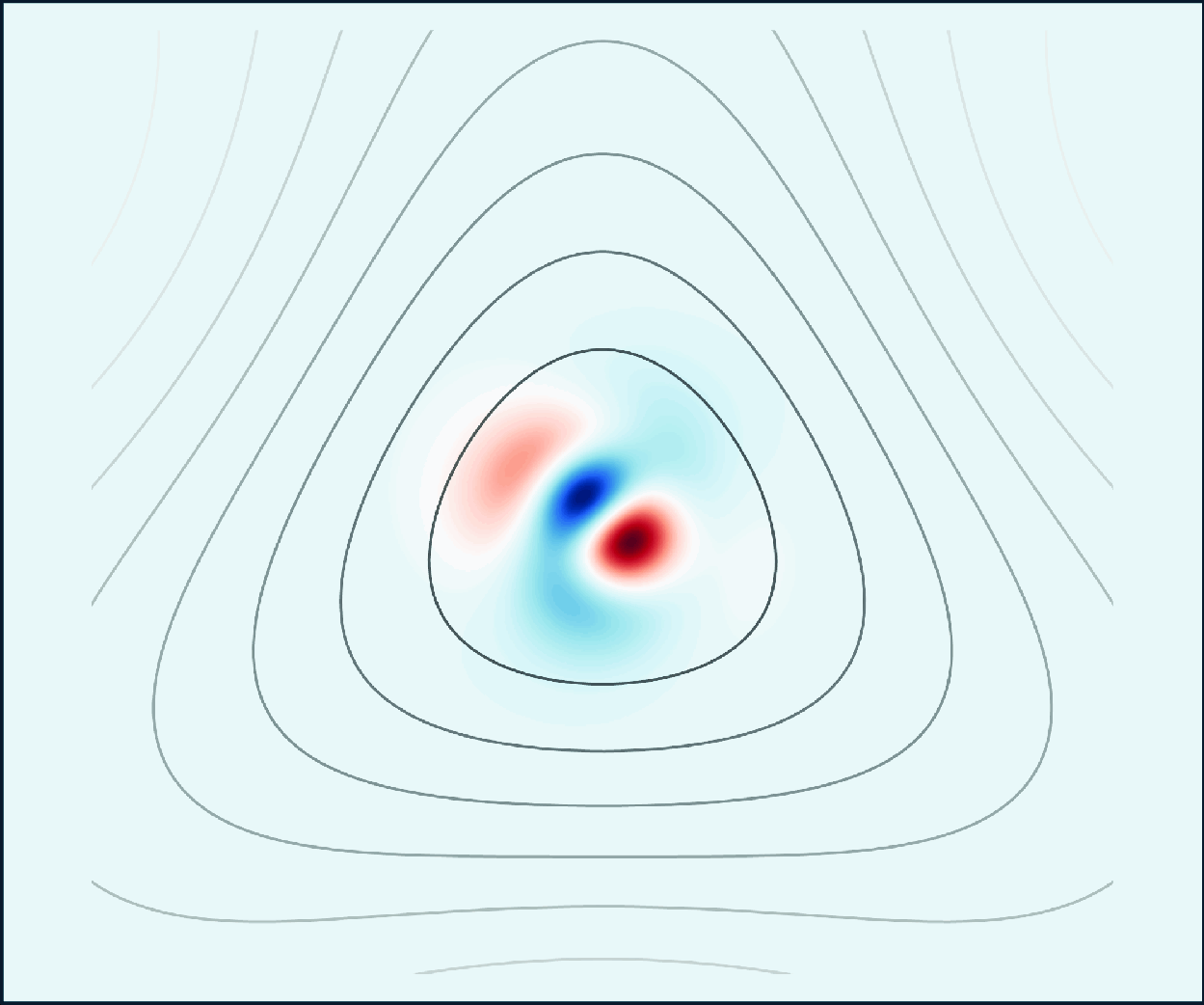
, is due to the presence of the satellite vortices. Figure 6(a) displays the streamlines of the base flow, illustrating the triangular straining effect caused by the three satellite vortices. However, the distortion near the vortex core remains subtle due to the weak strain (
$r \approx 3$
, is due to the presence of the satellite vortices. Figure 6(a) displays the streamlines of the base flow, illustrating the triangular straining effect caused by the three satellite vortices. However, the distortion near the vortex core remains subtle due to the weak strain ( $\epsilon = 0.008$
). The streamfunction, expanded up to first order in
$\epsilon = 0.008$
). The streamfunction, expanded up to first order in $\epsilon$
, is given by
$\epsilon$
, is given by
 \begin{equation} \psi = \psi _0 + \epsilon f(r)\sin 3\theta + O(\epsilon ^2). \end{equation}
The streamlines, to order $\epsilon$
, are expressed as
$\epsilon$
, are expressed as
 \begin{equation} r = r_0 + \epsilon r_{\psi }(\theta ), \end{equation}
and substituting this into the perturbation expansion for the streamfunction yields
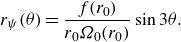 \begin{equation} r_{\psi }(\theta ) = \frac {f(r_0)}{r_0\Omega _0(r_0)}\sin 3\theta . \end{equation}
Here, $r_0$
represents the streamlines of the unstrained vortex, while
$r_0$
represents the streamlines of the unstrained vortex, while $\epsilon\, r_{\psi }(\theta )$
quantifies the distortion induced by triangular straining. Figure 6(b) shows the 2-D representation of the vorticity field of the base flow, considering only the contribution from the correction term.
$\epsilon\, r_{\psi }(\theta )$
quantifies the distortion induced by triangular straining. Figure 6(b) shows the 2-D representation of the vorticity field of the base flow, considering only the contribution from the correction term.
4. Linear stability analysis – theory and results
4.1. Perturbation equations of linear disturbances
If one uses expressions (3.5) and (3.6) for the base flow, then the linearised Navier–Stokes equations for the velocity–pressure field $\boldsymbol{u} = (u,v,w,p)$
of the perturbations can be written in the form
$\boldsymbol{u} = (u,v,w,p)$
of the perturbations can be written in the form
 \begin{equation} \left ( \mathcal{L}\frac {\partial }{\partial t} + \mathcal{P}\frac {\partial }{\partial z} + \mathcal{M} - \frac {\mathcal{V}}{{Re}} \right )\boldsymbol{u} = \epsilon \left ( {\textrm{e}}^{3{\textrm{i}}\theta }\,\mathcal{N} + {\textrm{e}}^{-3{\textrm{i}}\theta }\,\overline {\mathcal{N}} \right )\boldsymbol{u}, \end{equation}
where the matrices $\mathcal{L}$
,
$\mathcal{L}$
, $\mathcal{P}$
,
$\mathcal{P}$
, $\mathcal{M}$
,
$\mathcal{M}$
, $\mathcal{V}$
,
$\mathcal{V}$
, $\mathcal{N}$
are given in Appendix B.
$\mathcal{N}$
are given in Appendix B.
4.2. Triangular instability resonance mechanism
The mechanism for the growth of perturbations in a triangular-strained vortex is the same as that for the elliptic instability in the quadripolar-strained vortex (Moore & Saffman Reference Moore and Saffman1975; Tsai & Widnall Reference Tsai and Widnall1976). The only difference is that the triangular strain field corresponds to an azimuthal wavenumber $m=3$
perturbation of the vortex, while the elliptic strain field corresponds to an
$m=3$
perturbation of the vortex, while the elliptic strain field corresponds to an $m=2$
perturbation.
$m=2$
perturbation.
As for the elliptic instability, it is associated with a phenomenon of resonance of two quasi-neutral waves of the underlying vortex with the strain field. These waves, also called Kelvin modes, have an expression of the form
 \begin{equation} \boldsymbol{u} = \tilde {\boldsymbol{u}}(r)\,{\textrm{e}}^{{\textrm{i}}(m\theta + kz - \omega t)}, \end{equation}
where $m$
is the azimuthal wavenumber,
$m$
is the azimuthal wavenumber, $k$
is the axial wavenumber,
$k$
is the axial wavenumber, $\omega$
is the frequency, and
$\omega$
is the frequency, and $\tilde {\boldsymbol{u}}(r)$
is the eigenfunction field of the Kelvin mode. They satisfy the perturbation equations for the unstrained vortex
$\tilde {\boldsymbol{u}}(r)$
is the eigenfunction field of the Kelvin mode. They satisfy the perturbation equations for the unstrained vortex
 \begin{equation} \left ( \omega \mathcal{L} - k\mathcal{P} + {\textrm{i}}\,\mathcal{M}(m)-\frac {{\textrm{i}}}{{Re}}\,\mathcal{V}(m,k)\right )\tilde {\boldsymbol{u}} = 0, \end{equation}
where $\mathcal{M}(m)$
and
$\mathcal{M}(m)$
and $\mathcal{V}(m,k)$
are obtained by replacing
$\mathcal{V}(m,k)$
are obtained by replacing $\partial /\partial \theta$
with
$\partial /\partial \theta$
with ${i}m$
and
${i}m$
and $\partial /\partial z$
with
$\partial /\partial z$
with ${i}k$
, in the matrix operators
${i}k$
, in the matrix operators $\mathcal{M}$
and
$\mathcal{M}$
and $\mathcal{V}$
, given in Appendix B.
$\mathcal{V}$
, given in Appendix B.
To get the possible coupling of two Kelvin modes with the strain field, one should find two neutral Kelvin modes $(\omega _A, k_A, m_A)$
and
$(\omega _A, k_A, m_A)$
and $(\omega _B, k_B, m_B)$
satisfying
$(\omega _B, k_B, m_B)$
satisfying
 \begin{equation} \omega _A = \omega _B,\;\;\; k_A = k_B,\;\;\;|m_A-m_B|=3. \end{equation}
Kelvin modes of the Lamb–Oseen vortex have been analysed by Fabre et al. (Reference Fabre, Sipp and Jacquin2006). In a viscous fluid, Kelvin modes are always damped ( $\textrm {Im}(\omega ) \lt 0$
). Some of the Kelvin modes become neutral as the Reynolds number goes to infinity. But others continue to exhibit a large damping, which is associated with the presence of a critical layer (Sipp & Jacquin Reference Sipp and Jacquin2003). This feature makes the Lamb–Oseen vortex very different from the Rankine vortex, for which there is no critical layer damping.
$\textrm {Im}(\omega ) \lt 0$
). Some of the Kelvin modes become neutral as the Reynolds number goes to infinity. But others continue to exhibit a large damping, which is associated with the presence of a critical layer (Sipp & Jacquin Reference Sipp and Jacquin2003). This feature makes the Lamb–Oseen vortex very different from the Rankine vortex, for which there is no critical layer damping.
4.2.1. Large- $k$
asymptotic prediction of the Kelvin modes
$k$
asymptotic prediction of the Kelvin modes

Le Dizès & Lacaze (Reference Le Dizès and Verga2005) have developed an asymptotic theory using WKB analysis to describe the various types of Kelvin modes that can be obtained in the infinite Reynolds number and large axial wavenumber limit. For the Lamb–Oseen vortex, they found two types of neutral modes: regular neutral core modes where no critical point is present, and singular neutral core modes for which a critical point is present on the real axis but the critical layer damping is asymptotically small. They showed that the frequency range of each mode can be obtained by analysing the three functions $\omega _\pm (r)$
and
$\omega _\pm (r)$
and $\omega _c(r)$
defined by
$\omega _c(r)$
defined by
 \begin{align}& \omega _{\pm }(r) = m\Omega _0(r) \pm \sqrt {2\Omega _0(r)\zeta _0(r)}, \end{align}
 \begin{align}&\qquad\qquad \omega _c(r) = m\Omega _0(r). \end{align}
The functions $\omega _\pm (r)$
are known as the epicyclic frequencies. They define the upper and lower bounds of the frequency range within which regular neutral core modes (blue regions in figure 7) can exist at a given radial location
$\omega _\pm (r)$
are known as the epicyclic frequencies. They define the upper and lower bounds of the frequency range within which regular neutral core modes (blue regions in figure 7) can exist at a given radial location $r$
. Within this frequency range, the modes exhibit oscillatory behaviour for radial positions less than
$r$
. Within this frequency range, the modes exhibit oscillatory behaviour for radial positions less than $r$
, and decay exponentially beyond that point. The function
$r$
, and decay exponentially beyond that point. The function $\omega _c(r)$
, referred to as the critical frequency curve, gives the frequency at which a critical point occurs at
$\omega _c(r)$
, referred to as the critical frequency curve, gives the frequency at which a critical point occurs at $r$
. Regular modes cannot exist at these critical frequencies. However, the damping caused by the critical layer can become asymptotically small if the critical point for a given mode lies at a very large value of
$r$
. Regular modes cannot exist at these critical frequencies. However, the damping caused by the critical layer can become asymptotically small if the critical point for a given mode lies at a very large value of $r$
, far from the region where the mode behaves neutrally. Such modes are called singular neutral core modes (red regions in figure 7). For each azimuthal wavenumber
$r$
, far from the region where the mode behaves neutrally. Such modes are called singular neutral core modes (red regions in figure 7). For each azimuthal wavenumber $m$
, one can determine the corresponding frequency intervals in which these behaviours occur. For a more detailed explanation, readers are referred to Le Dizès & Lacaze (Reference Le Dizès and Lacaze2005). The condition of resonance can therefore be analysed by looking at the possible overlap of these frequency intervals for a couple of azimuthal wavenumbers
$m$
, one can determine the corresponding frequency intervals in which these behaviours occur. For a more detailed explanation, readers are referred to Le Dizès & Lacaze (Reference Le Dizès and Lacaze2005). The condition of resonance can therefore be analysed by looking at the possible overlap of these frequency intervals for a couple of azimuthal wavenumbers $m$
and
$m$
and $m+3$
. This analysis leads to a unique possibility: only the couple
$m+3$
. This analysis leads to a unique possibility: only the couple $(m_A,m_B)=(1,- 2)$
(and
$(m_A,m_B)=(1,- 2)$
(and $(m_A,m_B)=(- 1,2)$
, by symmetry) exhibits a frequency overlap. It corresponds to the frequency interval
$(m_A,m_B)=(- 1,2)$
, by symmetry) exhibits a frequency overlap. It corresponds to the frequency interval $ - 0.387 \lt \omega \lt 0$
, where
$ - 0.387 \lt \omega \lt 0$
, where $m_A=- 2$
singular core modes and
$m_A=- 2$
singular core modes and $m_B=1$
regular core modes both exist, as shown in figure 7.
$m_B=1$
regular core modes both exist, as shown in figure 7.
Plots of the epicyclic frequencies $\omega _+$
,
$\omega _+$
, $\omega _-$
(solid lines) and the critical frequency
$\omega _-$
(solid lines) and the critical frequency $\omega _c$
(dashed line) as functions of the radial coordinate
$\omega _c$
(dashed line) as functions of the radial coordinate $r$
, for (a)
$r$
, for (a) $m=1$
, (b)
$m=1$
, (b) $m=- 2$
. In each plot, the blue regions (resp. red regions) indicate the frequency intervals of regular neutral core modes (resp. singular neutral core modes); the hatched region indicates the frequency interval where resonance between
$m=- 2$
. In each plot, the blue regions (resp. red regions) indicate the frequency intervals of regular neutral core modes (resp. singular neutral core modes); the hatched region indicates the frequency interval where resonance between $m=1$
and
$m=1$
and $m=- 2$
modes is possible.
$m=- 2$
modes is possible.

4.2.2. Numerical determination of the Kelvin modes
The Kelvin modes can also be obtained by numerically solving the eigenvalue problem (4.3), and we use these numerically computed modes for the remainder of the analysis. Our numerical solver employs a Chebyshev spectral collocation method, following the approach of Fabre & Jacquin (Reference Fabre and Jacquin2004). The eigenvalue problem defined in the domain $0 \lt r \lt \infty$
is extended to
$0 \lt r \lt \infty$
is extended to $- \infty \lt r \lt \infty$
and mapped onto a contour in the complex-
$- \infty \lt r \lt \infty$
and mapped onto a contour in the complex- $r$
plane. It is then solved in the Chebyshev domain
$r$
plane. It is then solved in the Chebyshev domain $(- 1, 1)$
using
$(- 1, 1)$
using $2(N+1)$
collocation points. A resolution
$2(N+1)$
collocation points. A resolution $N = 200$
is found to be sufficient. For the inviscid limit, we adopt a complex mapping function, similar to the one used by Fabre & Jacquin (Reference Fabre and Jacquin2004), defined as
$N = 200$
is found to be sufficient. For the inviscid limit, we adopt a complex mapping function, similar to the one used by Fabre & Jacquin (Reference Fabre and Jacquin2004), defined as
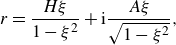 \begin{equation} r = \frac {H\xi }{1-\xi ^2} + {\textrm{i}}\frac {A\xi }{\sqrt {1-\xi ^2}}, \end{equation}
where the parameter $H$
controls the radial spreading of the collocation points, and the parameter
$H$
controls the radial spreading of the collocation points, and the parameter $A$
determines the inclination of the contour in the complex plane. We also take advantage of the parity properties of the eigenfunctions. For odd values of
$A$
determines the inclination of the contour in the complex plane. We also take advantage of the parity properties of the eigenfunctions. For odd values of $m$
, we express
$m$
, we express $\tilde {w}$
and
$\tilde {w}$
and $\tilde {p}$
using odd polynomials, and
$\tilde {p}$
using odd polynomials, and $\tilde {u}$
and
$\tilde {u}$
and $\tilde {v}$
using even polynomials. Conversely, even values of
$\tilde {v}$
using even polynomials. Conversely, even values of $m$
,
$m$
, $\tilde {w}$
and
$\tilde {w}$
and $\tilde {p}$
are represented using even polynomials, while
$\tilde {p}$
are represented using even polynomials, while $\tilde {u}$
and
$\tilde {u}$
and $\tilde {v}$
are expressed using odd polynomials.
$\tilde {v}$
are expressed using odd polynomials.
The above procedure has been done for the two azimuthal wavenumbers $m_A=1$
and
$m_A=1$
and $m_B=- 2$
, and a wavenumber
$m_B=- 2$
, and a wavenumber $k$
varying between
$k$
varying between $0$
and
$0$
and $10$
at
$10$
at ${Re} = 10^4$
. The result gives the complex frequency curves that have been plotted in figure 8(a,b). One clearly sees in these plots the frequency interval where regular and singular core modes were expected from figure 7.
${Re} = 10^4$
. The result gives the complex frequency curves that have been plotted in figure 8(a,b). One clearly sees in these plots the frequency interval where regular and singular core modes were expected from figure 7.
Dispersion curves of the Kelvin modes, obtained by solving the eigenvalue problem in (4.3) on the real axis for (a) $m_A = 1$
and (b)
$m_A = 1$
and (b) $m_B = -2$
at
$m_B = -2$
at ${Re} = 10^4$
. The real part of the frequency,
${Re} = 10^4$
. The real part of the frequency, $\omega _r$
, is plotted against
$\omega _r$
, is plotted against $k$
, while the damping is represented by the greyscale intensity of
$k$
, while the damping is represented by the greyscale intensity of $-\omega _i$
, the imaginary part of the frequency. (c) Resonant Kelvin modes of the unstrained Lamb–Oseen vortex at
$-\omega _i$
, the imaginary part of the frequency. (c) Resonant Kelvin modes of the unstrained Lamb–Oseen vortex at ${Re} = 10^4$
, identified at the crossing points of the dispersion curves. Modes with positive growth rates at
${Re} = 10^4$
, identified at the crossing points of the dispersion curves. Modes with positive growth rates at ${Re} = 10^4$
are circled in red, with their corresponding branch indices indicated in parentheses.
${Re} = 10^4$
are circled in red, with their corresponding branch indices indicated in parentheses.

Figure 8(c) displays the crossing points of $m_A=1$
and
$m_A=1$
and $m_B=- 2$
branches. As the damping rate of the modes shown in this figure is small, each crossing point corresponds to a (quasi-)resonant configuration. The resonant configurations marked with red circles exhibited positive growth rates, while the other resonant modes showed no growth or negligible growth rates due to critical layer damping and volumic viscous damping. A detailed analysis is provided in the subsequent subsections. We label the branches of the dispersion curves as
$m_B=- 2$
branches. As the damping rate of the modes shown in this figure is small, each crossing point corresponds to a (quasi-)resonant configuration. The resonant configurations marked with red circles exhibited positive growth rates, while the other resonant modes showed no growth or negligible growth rates due to critical layer damping and volumic viscous damping. A detailed analysis is provided in the subsequent subsections. We label the branches of the dispersion curves as $(l_A,l_B)$
where
$(l_A,l_B)$
where $l_A$
and
$l_A$
and $l_B$
are the branch labels of
$l_B$
are the branch labels of $m_A=1$
and
$m_A=1$
and $m_B=- 2$
modes, respectively.
$m_B=- 2$
modes, respectively.
An interesting observation is that the branches of the dispersion curves for $m = - 2$
involved in the resonance correspond to the ‘L branches’ described in Fabre et al. (Reference Fabre, Sipp and Jacquin2006) (see their figures 19 and 20). In particular, the first branch in figure 8(c) for
$m = - 2$
involved in the resonance correspond to the ‘L branches’ described in Fabre et al. (Reference Fabre, Sipp and Jacquin2006) (see their figures 19 and 20). In particular, the first branch in figure 8(c) for $m = - 2$
matches the ‘F branch’, also known as the flattening wave. Modes on this branch with axial wavenumber
$m = - 2$
matches the ‘F branch’, also known as the flattening wave. Modes on this branch with axial wavenumber $k \lt 3.45$
are reported to experience significant critical layer damping, while modes with larger
$k \lt 3.45$
are reported to experience significant critical layer damping, while modes with larger $k$
behave as regular, weakly damped waves. This trend is also evident here: the first mode, labelled
$k$
behave as regular, weakly damped waves. This trend is also evident here: the first mode, labelled $(1,1)$
, shows stronger critical layer damping compared to the modes labelled
$(1,1)$
, shows stronger critical layer damping compared to the modes labelled $(2,1)$
and
$(2,1)$
and $(3,1)$
, which are only weakly damped. The F branch also has an analogue in the Rankine vortex, where it is referred to as the ‘isolated branch’ by Eloy & Le Dizès (Reference Eloy and Le Dizès2001) and Fukumoto (Reference Fukumoto2003). The branches below the first one are referred to as ‘L2 branches’. In our results, the modes labelled
$(3,1)$
, which are only weakly damped. The F branch also has an analogue in the Rankine vortex, where it is referred to as the ‘isolated branch’ by Eloy & Le Dizès (Reference Eloy and Le Dizès2001) and Fukumoto (Reference Fukumoto2003). The branches below the first one are referred to as ‘L2 branches’. In our results, the modes labelled $(3,2)$
and
$(3,2)$
and $(4,2)$
lie in the weakly damped regions of these L2 branches. Hence among the resonant modes considered, only
$(4,2)$
lie in the weakly damped regions of these L2 branches. Hence among the resonant modes considered, only $(1,1)$
exhibits strong critical layer damping (also see table 1).
$(1,1)$
exhibits strong critical layer damping (also see table 1).
Values of the parameters of the growth rate equation (4.18) for the resonance of two Kelvin modes of azimuthal wavenumbers $m_A=1$
and
$m_A=1$
and $m_B=- 2$
at the different resonant points. Integration is done in the complex plane as explained in the text.
$m_B=- 2$
at the different resonant points. Integration is done in the complex plane as explained in the text.

4.3. Theoretical expression for the triangular instability growth rate
The method for computing the growth rate associated with the resonant coupling of two Kelvin modes with the triangular straining field is the same as that used for the elliptic instability. It is based on an asymptotic analysis in the limit of small $\epsilon$
. For more details, we refer the reader to Moore & Saffman (Reference Moore and Saffman1975).
$\epsilon$
. For more details, we refer the reader to Moore & Saffman (Reference Moore and Saffman1975).
The idea is to consider the perturbation as a combination of two normal modes of azimuthal wavenumbers $m_A$
and
$m_A$
and $m_B$
(related by (4.4)) that corresponds at leading order in
$m_B$
(related by (4.4)) that corresponds at leading order in $\epsilon$
to a resonant configuration of Kelvin modes. We then write
$\epsilon$
to a resonant configuration of Kelvin modes. We then write
 \begin{equation} \boldsymbol{u} \sim \left (A\tilde{\boldsymbol {u}}_A(r)\textrm{e}^{{\textrm{i}}(m_A\theta )} + B\tilde{\boldsymbol {u}}_B(r)\textrm{e}^{{\textrm{i}}(m_B\theta )}\right )\textrm{e}^{{\textrm{i}}(kz - \omega t)}, \end{equation}
where the (real) axial wavenumber $k$
and the (complex) frequency
$k$
and the (complex) frequency $\omega$
of the two modes are assumed to be close to a resonant point defined by an axial wavenumber
$\omega$
of the two modes are assumed to be close to a resonant point defined by an axial wavenumber $k_c$
and a real frequency
$k_c$
and a real frequency $\omega _c$
(corresponding to one of the crossing points shown in figure 8
c).
$\omega _c$
(corresponding to one of the crossing points shown in figure 8
c).
Substituting (4.8) in (4.1), we get two equations for the components proportional to $e^{{i}m_A\theta }$
and
$e^{{i}m_A\theta }$
and $e^{{i}m_B\theta }$
, respectively:
$e^{{i}m_B\theta }$
, respectively:
 \begin{align} & A\left ( \omega \mathcal{L} - k\mathcal{P} + {\textrm{i}}\,\mathcal{M}(m_A)-\frac {{\textrm{i}}}{{Re}}\,\mathcal{V}(m_A,k)\right )\tilde{\boldsymbol {u}}_A = {\textrm{i}}B\epsilon\, \mathcal{N}(m_B)\,\tilde{\boldsymbol {u}}_B, \end{align}
 \begin{align}& B\left ( \omega \mathcal{L} - k\mathcal{P} + {\textrm{i}}\,\mathcal{M}(m_B)-\frac {{\textrm{i}}}{{Re}}\,\mathcal{V}(m_B,k)\right )\tilde{\boldsymbol {u}}_B = {i}A\epsilon\, \overline {\mathcal{N}}(m_A)\,\tilde{\boldsymbol {u}}_A, \end{align}
where $\mathcal{N}(m_B)$
and
$\mathcal{N}(m_B)$
and $\overline {\mathcal{N}}(m_A)$
are obtained by replacing
$\overline {\mathcal{N}}(m_A)$
are obtained by replacing $\partial /\partial \theta$
with
$\partial /\partial \theta$
with ${i}m_B$
and
${i}m_B$
and ${i}m_A$
, respectively, in the
${i}m_A$
, respectively, in the $\mathcal{N}$
and
$\mathcal{N}$
and $\overline {\mathcal{N}}$
operators given in Appendix B. These equations show how the two modes are coupled by the straining field that is responsible for the terms on the right-hand sides of these equations.
$\overline {\mathcal{N}}$
operators given in Appendix B. These equations show how the two modes are coupled by the straining field that is responsible for the terms on the right-hand sides of these equations.
The equation giving the complex frequency $\omega$
is obtained from an orthogonality condition with the adjoint resonant Kelvin modes. The eigenfunctions
$\omega$
is obtained from an orthogonality condition with the adjoint resonant Kelvin modes. The eigenfunctions $\tilde{\boldsymbol {u}}_A^{\dagger }$
and
$\tilde{\boldsymbol {u}}_A^{\dagger }$
and $\tilde{\boldsymbol {u}}_B^{\dagger }$
of these two adjoint modes are the solutions of the adjoint equation of (4.3) for
$\tilde{\boldsymbol {u}}_B^{\dagger }$
of these two adjoint modes are the solutions of the adjoint equation of (4.3) for $(m,k) =(m_A,k_c)$
and
$(m,k) =(m_A,k_c)$
and $(m,k)= (m_B,k_c)$
, respectively. These adjoint equations are obtained using the scalar product
$(m,k)= (m_B,k_c)$
, respectively. These adjoint equations are obtained using the scalar product
 \begin{equation} \left \langle \boldsymbol{u_1},\boldsymbol{u_2} \right \rangle = \int _{0}^{\infty }\boldsymbol{u}^*_1(r)\,\boldsymbol{u}_2(r) r\,{\textrm d}r, \end{equation}
where $*$
denotes the complex conjugate. We have two options for applying the orthogonality condition: either we consider the inviscid expressions
$*$
denotes the complex conjugate. We have two options for applying the orthogonality condition: either we consider the inviscid expressions $(\tilde{\boldsymbol {u}}_A^{(\infty )},\tilde{\boldsymbol {u}}_B^{(\infty )})$
and
$(\tilde{\boldsymbol {u}}_A^{(\infty )},\tilde{\boldsymbol {u}}_B^{(\infty )})$
and $(\tilde{\boldsymbol {u}}_A^{\dagger (\infty )},\tilde{\boldsymbol {u}}_B^{\dagger (\infty )})$
of the Kelvin and adjoint modes, or we choose their expression for a given (large) Reynolds number.
$(\tilde{\boldsymbol {u}}_A^{\dagger (\infty )},\tilde{\boldsymbol {u}}_B^{\dagger (\infty )})$
of the Kelvin and adjoint modes, or we choose their expression for a given (large) Reynolds number.
In the first case, upon performing the scalar product of (4.9) with $\tilde{\boldsymbol {u}}_A^{\dagger (\infty )}$
and of (4.10) with
$\tilde{\boldsymbol {u}}_A^{\dagger (\infty )}$
and of (4.10) with $\tilde{\boldsymbol {u}}_B^{\dagger (\infty )}$
, we obtain
$\tilde{\boldsymbol {u}}_B^{\dagger (\infty )}$
, we obtain
 \begin{align}& \left ( \omega -\omega _A^{(\infty )} -Q_A^{(\infty )}\left(k-k_c^{(\infty )}\right)-{\textrm{i}}\frac {V_A^{(\infty )}}{{Re}} \right )A = {\textrm{i}}\epsilon C_{AB}^{(\infty )}B, \end{align}
 \begin{align}& \left ( \omega -\omega _B^{(\infty )}-Q_B^{(\infty )}\left(k-k_c^{(\infty )}\right)-{\textrm{i}}\frac {V_B^{(\infty )}}{{Re}} \right )B = {\textrm{i}}\epsilon C_{BA}^{(\infty )}A, \end{align}
where the coefficients $Q_A^{(\infty )}$
,
$Q_A^{(\infty )}$
, $Q_B^{(\infty )}$
,
$Q_B^{(\infty )}$
, $V_A^{(\infty )}$
,
$V_A^{(\infty )}$
, $V_B^{(\infty )}$
,
$V_B^{(\infty )}$
, $C_{AB}^{(\infty )}$
,
$C_{AB}^{(\infty )}$
, $C_{BA}^{(\infty )}$
are given by
$C_{BA}^{(\infty )}$
are given by
 \begin{align}&\qquad Q_A^{(\infty )} = \frac {\left \langle \tilde{\boldsymbol {u}}_A^{\dagger (\infty )},\mathcal{P}\tilde{\boldsymbol {u}}_A^{(\infty )} \right \rangle }{\left \langle \tilde{\boldsymbol {u}}_A^{\dagger (\infty )},\mathcal{L}\tilde{\boldsymbol {u}}_A^{(\infty )} \right \rangle }, \qquad Q_B^{(\infty )} = \frac {\left \langle \tilde{\boldsymbol {u}}_B^{\dagger (\infty )},\mathcal{P}\tilde{\boldsymbol {u}}_B^{(\infty )} \right \rangle }{\left \langle \tilde{\boldsymbol {u}}_B^{\dagger (\infty )},\mathcal{L}\tilde{\boldsymbol {u}}_B^{(\infty )} \right \rangle }, \end{align}
 \begin{align}&\qquad V_A^{(\infty )}= \frac {\left \langle \tilde{\boldsymbol {u}}_A^{\dagger (\infty )},\mathcal{V}\tilde{\boldsymbol {u}}_A^{(\infty )} \right \rangle }{\left \langle \tilde{\boldsymbol {u}}_A^{\dagger (\infty )},\mathcal{L}\tilde{\boldsymbol {u}}_A^{(\infty )}\right \rangle }, \qquad V_B^{(\infty )} = \frac {\left \langle \tilde{\boldsymbol {u}}_B^{\dagger (\infty )},\mathcal{V}\tilde{\boldsymbol {u}}_B^{(\infty )} \right \rangle }{\left \langle \tilde{\boldsymbol {u}}_B^{\dagger (\infty )},\mathcal{L}\tilde{\boldsymbol {u}}_B^{(\infty )} \right \rangle }, \end{align}
 \begin{align}& C_{AB}^{(\infty )} = \frac {\left \langle \tilde{\boldsymbol {u}}_A^{\dagger },\mathcal{N}(m_B)\,\tilde{\boldsymbol {u}}_B^{(\infty )} \right \rangle }{\left \langle \tilde{\boldsymbol {u}}_A^{\dagger (\infty )},\mathcal{L}\tilde{\boldsymbol {u}}_A^{(\infty )} \right \rangle }, \qquad C_{BA}^{(\infty )} = \frac {\left \langle \tilde{\boldsymbol {u}}_B^{\dagger (\infty )},\overline {\mathcal{N}}(m_A)\,\tilde{\boldsymbol {u}}_A^{(\infty )} \right \rangle }{\left \langle \tilde{\boldsymbol {u}}_B^{\dagger (\infty )},\mathcal{L}\tilde{\boldsymbol {u}}_B^{(\infty )}\right \rangle } . \end{align}
The frequencies $\omega _A^{(\infty )}$
and
$\omega _A^{(\infty )}$
and $\omega _B^{(\infty )}$
are the inviscid estimates of the frequencies of the resonant Kelvin modes at
$\omega _B^{(\infty )}$
are the inviscid estimates of the frequencies of the resonant Kelvin modes at $k=k_c^{(\infty )}$
. They can be expressed as
$k=k_c^{(\infty )}$
. They can be expressed as
 \begin{equation} \omega _A^{(\infty )} = \omega _c^{(\infty )} + {i}\, \textrm {Im}\left(\omega _A^{(\infty )}\right) ,\quad\omega _B^{(\infty )} = \omega _c^{(\infty )} + {i}\, \textrm {Im}\left(\omega _B^{(\infty )}\right), \end{equation}
where $\textrm {Im}(\omega _A^{(\infty )} )$
and
$\textrm {Im}(\omega _A^{(\infty )} )$
and $\textrm {Im}(\omega _B^{(\infty )})$
are the critical layer damping rates of the modes.
$\textrm {Im}(\omega _B^{(\infty )})$
are the critical layer damping rates of the modes.
For the azimuthal wavenumber couple $(m_A,m_B) = (1,-2)$
, only the Kelvin mode with azimuthal wavenumber
$(m_A,m_B) = (1,-2)$
, only the Kelvin mode with azimuthal wavenumber $m_B=- 2$
is expected to experience critical layer damping at resonance. In particular, we have
$m_B=- 2$
is expected to experience critical layer damping at resonance. In particular, we have $\textrm {Im}(\omega _A^{(\infty )}) =0$
for
$\textrm {Im}(\omega _A^{(\infty )}) =0$
for $m_A=1$
at resonance.
$m_A=1$
at resonance.
Equations (4.12) and ( 4.13) with ( 4.17) give an equation for the complex frequency $\omega$
:
$\omega$
:
 \begin{align} & \left ( \omega - \omega _c^{(\infty )} - Q_A^{(\infty )}\left(k - k_c^{(\infty )}\right) - {\textrm{i}}\frac {V_A^{(\infty )}}{{Re}} \right ) \nonumber \\[2pt] &\left ( \omega - \omega _c^{(\infty )} - {\textrm{i}}\,\textrm {Im}\left(\omega _B^{(\infty )}\right) - Q_B^{(\infty )}\left(k - k_c^{(\infty )}\right) - {i}\frac {V_B^{(\infty )}}{{Re}} \right ) = -\epsilon ^2 \left(N^{(\infty )}\right)^2, \end{align}
where
 \begin{equation} N^{(\infty )} = \sqrt {C_{AB}^{(\infty )}C_{BA}^{(\infty )}}. \end{equation}
The growth rate $\sigma$
is defined as
$\sigma$
is defined as $\textrm {Im}(\omega )$
and is computed using the equation above. Both modes oscillate with a common resonant frequency given by
$\textrm {Im}(\omega )$
and is computed using the equation above. Both modes oscillate with a common resonant frequency given by ${{Re}}(\omega )$
. On the left-hand side of (4.18), we recognise the dispersion relation for the two resonant modes,
${{Re}}(\omega )$
. On the left-hand side of (4.18), we recognise the dispersion relation for the two resonant modes, $A$
and
$A$
and $B$
, close to the resonant point. More precisely, the left-hand side can be written as
$B$
, close to the resonant point. More precisely, the left-hand side can be written as $(\omega - \omega _{A}(k,{Re}))(\omega -\omega _B(k,{Re}))$
, where
$(\omega - \omega _{A}(k,{Re}))(\omega -\omega _B(k,{Re}))$
, where $\omega _A(k,{Re})$
and
$\omega _A(k,{Re})$
and $\omega _B(k,{Re})$
are the complex frequencies of the two Kelvin modes for a wavenumber
$\omega _B(k,{Re})$
are the complex frequencies of the two Kelvin modes for a wavenumber $k$
close to
$k$
close to $k_c$
, and a large Reynolds number. The right-hand side corresponds to the coupling term that is responsible for the instability.
$k_c$
, and a large Reynolds number. The right-hand side corresponds to the coupling term that is responsible for the instability.
The integrals in the inner products that appear in the coefficients of (4.14), (4.15) and (4.16) are evaluated along a complex path that avoids the critical point associated with the mode $m = - 2$
from below, since it moves in the lower part of the complex plane, as explained in Le Dizès (Reference Le Dizès2004). To achieve this, we use the complex mapping given in (4.7) with parameters
$m = - 2$
from below, since it moves in the lower part of the complex plane, as explained in Le Dizès (Reference Le Dizès2004). To achieve this, we use the complex mapping given in (4.7) with parameters $H = 4$
and
$H = 4$
and $A = - 0.5$
. These values of
$A = - 0.5$
. These values of $H$
and
$H$
and $A$
result in the contour passing slightly below the critical points for all the resonant points corresponding to
$A$
result in the contour passing slightly below the critical points for all the resonant points corresponding to $m=- 2$
. The integrals corresponding to
$m=- 2$
. The integrals corresponding to $m = 1$
are also computed along this same contour. Since the
$m = 1$
are also computed along this same contour. Since the $m = 1$
modes do not have a critical point, the values of the integrals remain unchanged. In table 1, we provide the values of the parameters appearing in (4.18) for all the resonant points that have been identified in figure 8 for the two azimuthal wavenumbers
$m = 1$
modes do not have a critical point, the values of the integrals remain unchanged. In table 1, we provide the values of the parameters appearing in (4.18) for all the resonant points that have been identified in figure 8 for the two azimuthal wavenumbers $m_A=1$
and
$m_A=1$
and $m_B=- 2$
.
$m_B=- 2$
.
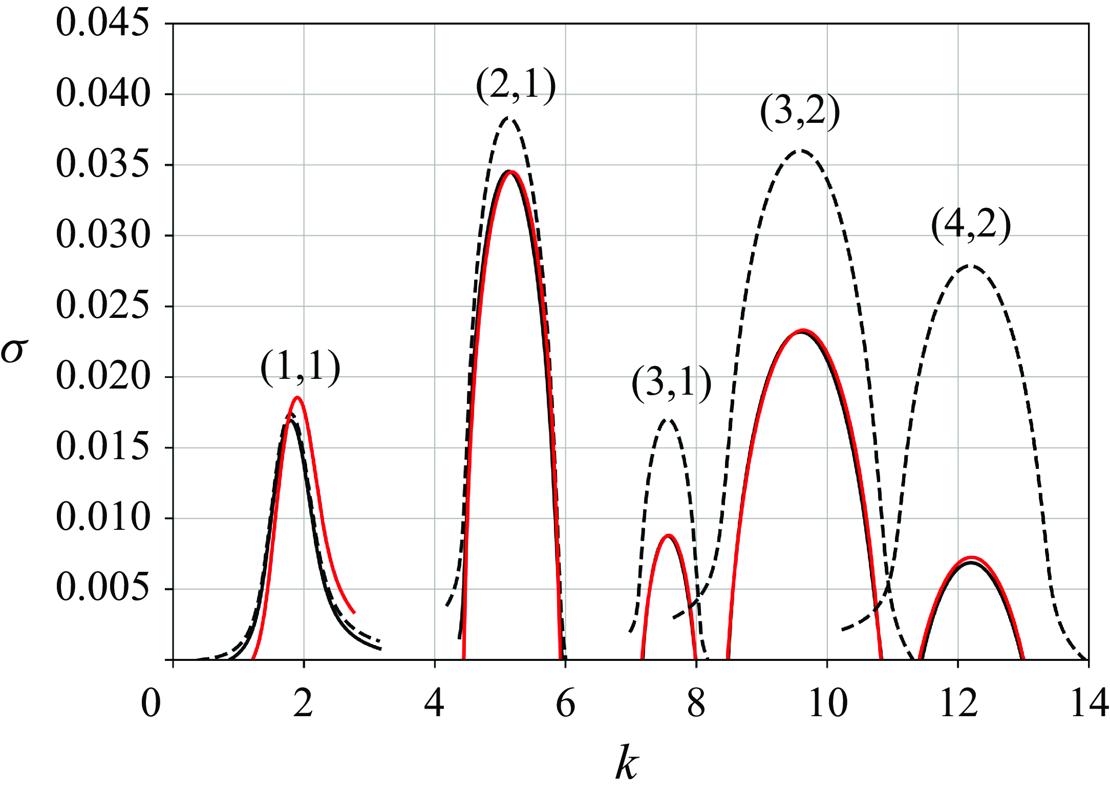
Growth rates $\sigma$
are plotted against the axial wavenumber
$\sigma$
are plotted against the axial wavenumber $k$
for the resonant modes, based on theoretical predictions. Solid black lines represent results from (4.18), while solid red lines correspond to (4.20), both computed for
$k$
for the resonant modes, based on theoretical predictions. Solid black lines represent results from (4.18), while solid red lines correspond to (4.20), both computed for ${Re} = 10^4$
. Dashed black lines show results from (4.18) in the inviscid limit (
${Re} = 10^4$
. Dashed black lines show results from (4.18) in the inviscid limit ( ${Re} = \infty$
). The corresponding branch indices are also indicated.
${Re} = \infty$
). The corresponding branch indices are also indicated.
Comparison of growth rates $\sigma$
against the axial wavenumber
$\sigma$
against the axial wavenumber $k$
for the first four resonant modes computed using (4.20) (solid black lines) and DNS (circles). Values of the corresponding branch indices are reported.
$k$
for the first four resonant modes computed using (4.20) (solid black lines) and DNS (circles). Values of the corresponding branch indices are reported.

An equation for the growth rate can also be obtained using the viscous expression of the resonant Kelvin modes. In that case, instead of (4.18), we get
 \begin{align}& \left ( \omega - \omega _c({Re}) - {\textrm{i}}\,\textrm {Im}(\omega _A({Re})) - Q_A({Re})(k - k_c({Re})) \right ) \nonumber\\[4pt] &\quad \times \left ( \omega - \omega _c({Re}) - {\textrm{i}}\,\textrm {Im}(\omega _B({Re})) - Q_B({Re})(k - k_c({Re})) \right ) = -\epsilon ^2 (N({Re}))^2, \end{align}
where the coefficients now depend on the Reynolds number. Note that the volumic viscous damping terms ${\textrm i}V_A^{(\infty )}/{Re}$
and
${\textrm i}V_A^{(\infty )}/{Re}$
and ${\textrm i}V_B^{(\infty )}/{Re}$
in (4.18) are now included in the terms
${\textrm i}V_B^{(\infty )}/{Re}$
in (4.18) are now included in the terms ${\textrm i}\,\textrm {Im}(\omega _A({Re}))$
and
${\textrm i}\,\textrm {Im}(\omega _A({Re}))$
and ${\textrm i}\,\textrm {Im}(\omega _B({Re}))$
. This second approach has also been used. For the Reynolds number
${\textrm i}\,\textrm {Im}(\omega _B({Re}))$
. This second approach has also been used. For the Reynolds number ${Re}=10^4$
that we have considered, the results are similar, as can be seen in figure 9. This figure shows the five resonant modes for which a positive viscous growth rate was obtained. In this figure, we have also plotted the growth rate curves obtained from (4.18) for
${Re}=10^4$
that we have considered, the results are similar, as can be seen in figure 9. This figure shows the five resonant modes for which a positive viscous growth rate was obtained. In this figure, we have also plotted the growth rate curves obtained from (4.18) for ${Re}=\infty$
. We clearly see that the viscous damping of the modes significantly affects the resonant configurations with the largest wavenumbers.
${Re}=\infty$
. We clearly see that the viscous damping of the modes significantly affects the resonant configurations with the largest wavenumbers.
4.4. Numerical results
In this subsection, we first describe how growth rates and frequencies are obtained numerically, and then compare the results predicted by (4.18) or (4.20) with those obtained from DNS. The numerical results are obtained for ${Re}=10^4$
. Starting from a random initial energy distribution, modes associated with different azimuthal wavenumbers grow exponentially in time if they are unstable. The growth rate is determined as the slope (divided by 2) of the logarithm of the energy of the unstable modes. The frequency of the modes is computed by tracking their phase and measuring their rotation rate about the
${Re}=10^4$
. Starting from a random initial energy distribution, modes associated with different azimuthal wavenumbers grow exponentially in time if they are unstable. The growth rate is determined as the slope (divided by 2) of the logarithm of the energy of the unstable modes. The frequency of the modes is computed by tracking their phase and measuring their rotation rate about the $z$
axis. The comparison of growth rates is shown in figure 10 for
$z$
axis. The comparison of growth rates is shown in figure 10 for $\epsilon =0.008$
and
$\epsilon =0.008$
and $k$
ranging from 0.7 to 10. We observe that the first four unstable modes predicted by the theory within this wavenumber range are also captured in the DNS. The agreement in the growth rates is almost perfect. The values for the frequency and growth rate, obtained by both theory and DNS, for the four unstable modes at their resonant wavenumbers are given in table 2.
$k$
ranging from 0.7 to 10. We observe that the first four unstable modes predicted by the theory within this wavenumber range are also captured in the DNS. The agreement in the growth rates is almost perfect. The values for the frequency and growth rate, obtained by both theory and DNS, for the four unstable modes at their resonant wavenumbers are given in table 2.
Growth rate $\sigma$
and real part of the frequency
$\sigma$
and real part of the frequency $\omega$
of the most unstable mode for different axial wavenumbers
$\omega$
of the most unstable mode for different axial wavenumbers $k$
, obtained by DNS and theory (4.20), for
$k$
, obtained by DNS and theory (4.20), for ${Re}=10^4$
and
${Re}=10^4$
and $\epsilon =0.008$
. The maximum growth rates predicted by (4.18) in the inviscid limit, denoted by
$\epsilon =0.008$
. The maximum growth rates predicted by (4.18) in the inviscid limit, denoted by $\sigma _{th}^{(\infty )}$
, are given in the last column. The chosen axial wavenumbers correspond to the resonant values for the Kelvin modes of azimuthal wavenumbers
$\sigma _{th}^{(\infty )}$
, are given in the last column. The chosen axial wavenumbers correspond to the resonant values for the Kelvin modes of azimuthal wavenumbers $(m_A=1,m_B=- 2)$
and branch labels
$(m_A=1,m_B=- 2)$
and branch labels $(l_A,l_B)$
.
$(l_A,l_B)$
.

In figure 11, we analyse the effect of $\epsilon$
on the growth rate curve of the most unstable mode corresponding to
$\epsilon$
on the growth rate curve of the most unstable mode corresponding to $(l_A,l_B)=(2,1)$
. As expected, the growth rate decreases when
$(l_A,l_B)=(2,1)$
. As expected, the growth rate decreases when $\epsilon$
is halved, and the agreement between the growth rate curves is excellent, as illustrated in the figure.
$\epsilon$
is halved, and the agreement between the growth rate curves is excellent, as illustrated in the figure.
Growth rate $\sigma$
versus
$\sigma$
versus $k$
for the resonant mode with
$k$
for the resonant mode with $(l_A,l_B)=(2,1)$
at
$(l_A,l_B)=(2,1)$
at ${Re}= 10^4$
. Circles indicate DNS; solid black lines indicate theory; with black for
${Re}= 10^4$
. Circles indicate DNS; solid black lines indicate theory; with black for $\epsilon = 0.008$
, and blue for
$\epsilon = 0.008$
, and blue for $\epsilon = 0.004$
.
$\epsilon = 0.004$
.

The structures and the energy ratio of the contributions from various azimuthal wavenumbers of the unstable modes are displayed in figures 12, 13, 14 and 15. In each figure, the leftmost panel shows the 2-D contours of the perturbation axial vorticity field in the hub vortex, obtained by DNS. The values are divided by $e^{\sigma t_s}$
, where
$e^{\sigma t_s}$
, where $\sigma$
is the corresponding growth rate, and
$\sigma$
is the corresponding growth rate, and $t_s$
is the simulation time of the snapshot used. In the centre panels, we analyse the azimuthal composition of the unstable mode, by computing the energy percentage of each azimuthal component. This decomposition is compared to the theoretical prediction obtained for each resonant configuration. The theoretical energy ratio for mode
$t_s$
is the simulation time of the snapshot used. In the centre panels, we analyse the azimuthal composition of the unstable mode, by computing the energy percentage of each azimuthal component. This decomposition is compared to the theoretical prediction obtained for each resonant configuration. The theoretical energy ratio for mode $A$
, for instance, can be calculated by
$A$
, for instance, can be calculated by
 \begin{equation} \frac {E_A}{E_A + E_B} = \frac {\int |\tilde{\boldsymbol {u}}_A|^2\, r\,{\textrm d}r}{\int |\tilde{\boldsymbol {u}}_A|^2\, r\,{\textrm d}r + (B^2/A^2)\int |\tilde{\boldsymbol {u}}_B|^2\, r\,{\textrm d}r}, \end{equation}
Structure of the resonant combination with $k = 1.76$
for
$k = 1.76$
for ${Re}= 10^4$
and
${Re}= 10^4$
and $\epsilon =0.008$
, for mode
$\epsilon =0.008$
, for mode $(1,1)$
. (a) Contours of the axial vorticity using DNS. (b) Energy ratio: red circles indicate DNS; blue crosses indicate theory. (c) Radial structure of the amplitude
$(1,1)$
. (a) Contours of the axial vorticity using DNS. (b) Energy ratio: red circles indicate DNS; blue crosses indicate theory. (c) Radial structure of the amplitude $|u(r)|$
of radial velocity: coloured lines indicate DNS; black lines indicate theory.
$|u(r)|$
of radial velocity: coloured lines indicate DNS; black lines indicate theory.
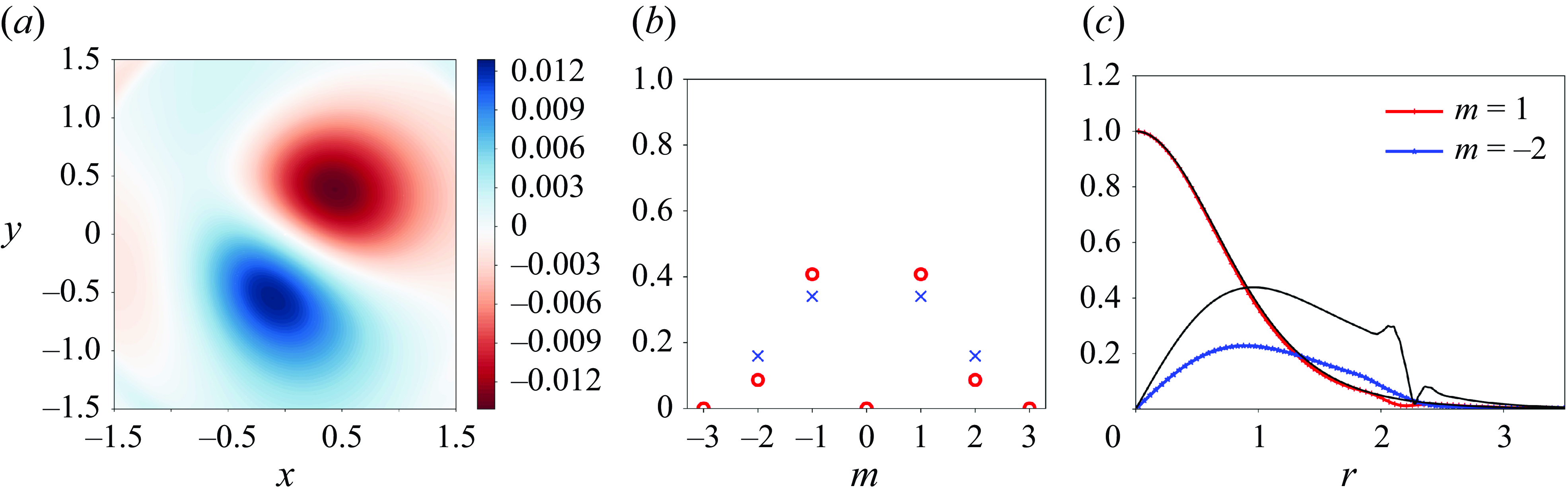
Structure of the resonant combination with $k = 5.18$
for
$k = 5.18$
for ${Re}= 10^4$
and
${Re}= 10^4$
and $\epsilon =0.008$
, for mode
$\epsilon =0.008$
, for mode $(2,1)$
. (a) Contours of the axial vorticity using DNS. (b) Energy ratio: red circles indicate DNS; blue crosses indicate theory. (c) Radial structure of the amplitude
$(2,1)$
. (a) Contours of the axial vorticity using DNS. (b) Energy ratio: red circles indicate DNS; blue crosses indicate theory. (c) Radial structure of the amplitude $|u(r)|$
of radial velocity: coloured lines indicate DNS; black lines indicate theory.
$|u(r)|$
of radial velocity: coloured lines indicate DNS; black lines indicate theory.

Structure of the resonant combination with $k = 7.58$
for
$k = 7.58$
for ${Re}= 10^4$
and
${Re}= 10^4$
and $\epsilon =0.008$
, for mode
$\epsilon =0.008$
, for mode $(3 ,1)$
. (a) Contours of the axial vorticity using DNS. (b) Energy ratio: red circles indicate DNS; blue crosses indicate theory. (c) Radial structure of the amplitude
$(3 ,1)$
. (a) Contours of the axial vorticity using DNS. (b) Energy ratio: red circles indicate DNS; blue crosses indicate theory. (c) Radial structure of the amplitude $|u(r)|$
of radial velocity: coloured lines indicate DNS; black lines indicate theory.
$|u(r)|$
of radial velocity: coloured lines indicate DNS; black lines indicate theory.
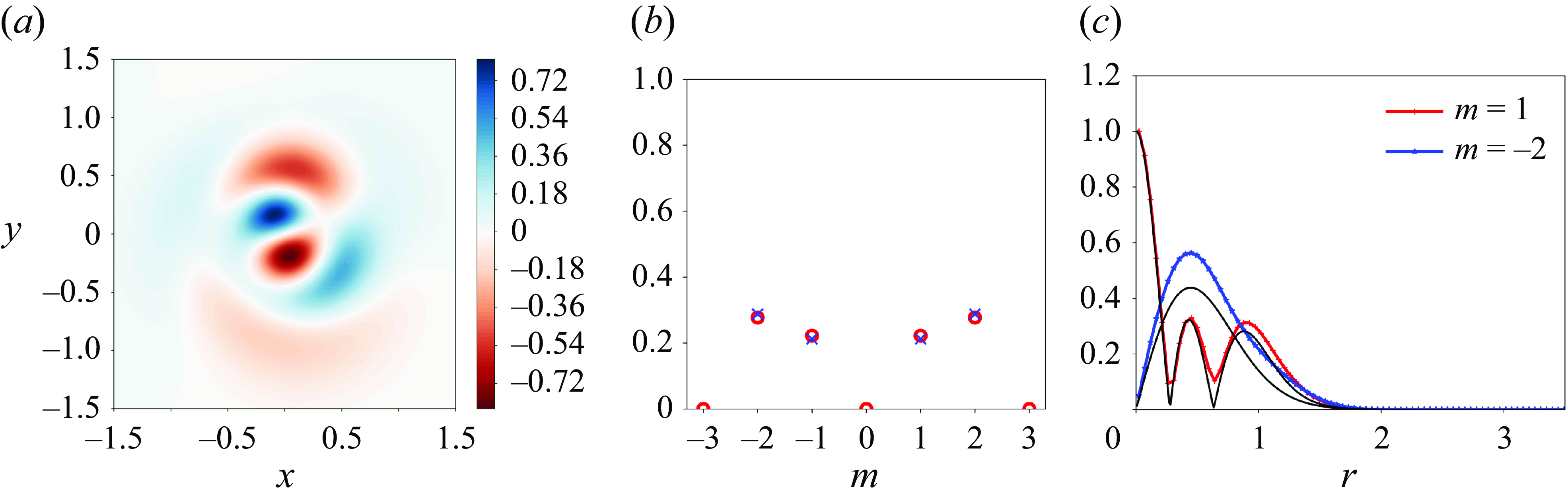
Structure of the resonant combination with $k = 9.64$
for
$k = 9.64$
for ${Re}= 10^4$
and
${Re}= 10^4$
and $\epsilon =0.008$
, for mode
$\epsilon =0.008$
, for mode $(3,2)$
. (a) Contours of the axial vorticity using DNS. (b) Energy ratio: red circles indicate DNS; blue crosses indicate theory. (c) Radial structure of the amplitude
$(3,2)$
. (a) Contours of the axial vorticity using DNS. (b) Energy ratio: red circles indicate DNS; blue crosses indicate theory. (c) Radial structure of the amplitude $|u(r)|$
of radial velocity: coloured lines indicate DNS; black lines indicate theory.
$|u(r)|$
of radial velocity: coloured lines indicate DNS; black lines indicate theory.
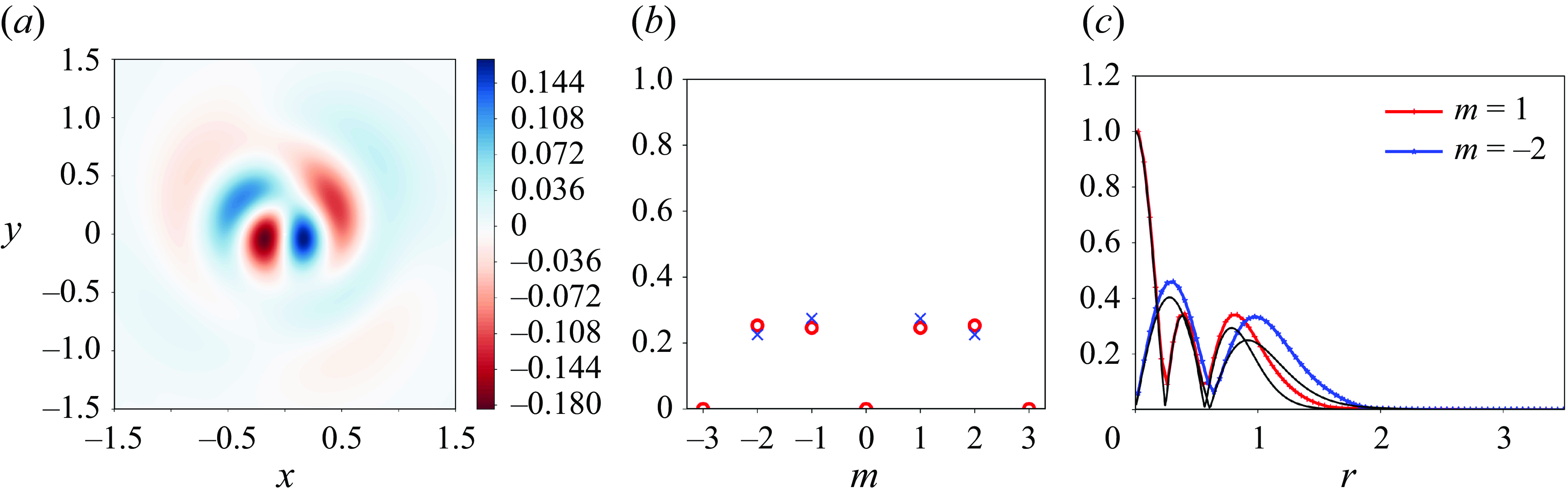
where $|\tilde{\boldsymbol {u}}_A|^2 = \tilde {u}_A(r)^2 + \tilde {v}_A(r)^2 + \tilde {w}_A(r)^2$
, and
$|\tilde{\boldsymbol {u}}_A|^2 = \tilde {u}_A(r)^2 + \tilde {v}_A(r)^2 + \tilde {w}_A(r)^2$
, and $(B^2/A^2)$
can be calculated from (4.12) or (4.13). We can see that the unstable modes obtained from DNS are primarily composed of the azimuthal wavenumber pairs
$(B^2/A^2)$
can be calculated from (4.12) or (4.13). We can see that the unstable modes obtained from DNS are primarily composed of the azimuthal wavenumber pairs $m_A = 1$
,
$m_A = 1$
, $m_B = - 2$
and
$m_B = - 2$
and $m_A = - 1$
,
$m_A = - 1$
, $m_B = 2$
, with negligible contributions from other azimuthal wavenumbers, as resonance is expected only between these wavenumbers. The energy ratio of the resonant azimuthal wavenumbers aligns well with theoretical predictions, except for the mode corresponding to the branch labels
$m_B = 2$
, with negligible contributions from other azimuthal wavenumbers, as resonance is expected only between these wavenumbers. The energy ratio of the resonant azimuthal wavenumbers aligns well with theoretical predictions, except for the mode corresponding to the branch labels $(1,1)$
, which shows a slight discrepancy. It might be useful to note that the numerically obtained energy percentages of
$(1,1)$
, which shows a slight discrepancy. It might be useful to note that the numerically obtained energy percentages of $m_A = 1$
and
$m_A = 1$
and $m_B = - 2$
are respectively the same as those of
$m_B = - 2$
are respectively the same as those of $m_A = - 1$
and
$m_A = - 1$
and $m_B = 2$
. This is due to a certain symmetry that we enforce in the initial random vorticity distribution. Without this symmetry condition, these percentages might differ; however, the mutual energy ratio between the resonant pairs would still be the same. To further validate that the unstable resonant modes obtained from DNS share the same structure as those predicted by theory, the radial distributions of the absolute value of the radial disturbance velocity for both azimuthal wavenumbers are plotted in the right most panels of figures 12, 13, 14 and 15, comparing DNS results with theoretical predictions. The radial structures from DNS are extracted by performing a Fourier decomposition of the disturbance fields into components corresponding to different azimuthal wavenumbers. This comparison is conducted by normalising the amplitude of the
$m_B = 2$
. This is due to a certain symmetry that we enforce in the initial random vorticity distribution. Without this symmetry condition, these percentages might differ; however, the mutual energy ratio between the resonant pairs would still be the same. To further validate that the unstable resonant modes obtained from DNS share the same structure as those predicted by theory, the radial distributions of the absolute value of the radial disturbance velocity for both azimuthal wavenumbers are plotted in the right most panels of figures 12, 13, 14 and 15, comparing DNS results with theoretical predictions. The radial structures from DNS are extracted by performing a Fourier decomposition of the disturbance fields into components corresponding to different azimuthal wavenumbers. This comparison is conducted by normalising the amplitude of the $m_A=1$
azimuthal component to one at the origin in both DNS and theory. Good agreement is also observed here, except for a significant discrepancy in the amplitude of the mode
$m_A=1$
azimuthal component to one at the origin in both DNS and theory. Good agreement is also observed here, except for a significant discrepancy in the amplitude of the mode $(1,1)$
corresponding to
$(1,1)$
corresponding to $m=- 2$
. We do not have a definitive explanation for these discrepancies in both the energy ratios and the eigenfunction radial structures for
$m=- 2$
. We do not have a definitive explanation for these discrepancies in both the energy ratios and the eigenfunction radial structures for $m=- 2$
. However, we suspect that they arise from an imperfect representation of the critical layer, particularly strong for
$m=- 2$
. However, we suspect that they arise from an imperfect representation of the critical layer, particularly strong for $(1,1)$
. Figure 12(c) shows additional oscillations in the theoretical predictions just beyond
$(1,1)$
. Figure 12(c) shows additional oscillations in the theoretical predictions just beyond $r = 2$
. These oscillations result from the regularisation of the critical layer by viscous effects, which are absent in the numerical results. Therefore, we believe that the observed discrepancy is due to the inaccurate representation of the critical layer. From the leftmost and rightmost panels, it is also evident that modes associated with higher branches exhibit more zeros in the radial distributions of the disturbance fields.
$r = 2$
. These oscillations result from the regularisation of the critical layer by viscous effects, which are absent in the numerical results. Therefore, we believe that the observed discrepancy is due to the inaccurate representation of the critical layer. From the leftmost and rightmost panels, it is also evident that modes associated with higher branches exhibit more zeros in the radial distributions of the disturbance fields.
4.5. Variation of maximum growth rate with
${Re}$
and
$\epsilon$


Contours of the maximum growth rate in the $(\epsilon , {Re})$
parameter space, computed from theory using (4.18). Grey regions indicate where the mode
$(\epsilon , {Re})$
parameter space, computed from theory using (4.18). Grey regions indicate where the mode $(1,1)$
is the most unstable, while blue regions indicate where the mode
$(1,1)$
is the most unstable, while blue regions indicate where the mode $(2,1)$
is the most unstable. Black contour lines represent growth rate levels from
$(2,1)$
is the most unstable. Black contour lines represent growth rate levels from $0$
to
$0$
to $0.045$
, in steps of
$0.045$
, in steps of $0.005$
. The overall marginal stability curve, obtained from (4.22), is shown as a thick dashed black line and corresponds to the zero-growth-rate contour. The individual marginal stability curves for modes
$0.005$
. The overall marginal stability curve, obtained from (4.22), is shown as a thick dashed black line and corresponds to the zero-growth-rate contour. The individual marginal stability curves for modes $(1,1)$
and
$(1,1)$
and $(2,1)$
are shown as black and blue dotted lines, respectively. Red stars mark the growth rates used in the main test cases:
$(2,1)$
are shown as black and blue dotted lines, respectively. Red stars mark the growth rates used in the main test cases: $\sigma = 0.0153$
for
$\sigma = 0.0153$
for $\epsilon = 0.004$
, and
$\epsilon = 0.004$
, and $\sigma = 0.0345$
for
$\sigma = 0.0345$
for $\epsilon = 0.008$
, at
$\epsilon = 0.008$
, at ${Re} = 10^4$
.
${Re} = 10^4$
.

The theory allows us to easily analyse the effect of $\epsilon$
and
$\epsilon$
and ${Re}$
on the instability. Using (4.18), one can compute, for each resonant configuration, the maximum growth rate for any values of
${Re}$
on the instability. Using (4.18), one can compute, for each resonant configuration, the maximum growth rate for any values of $\epsilon$
and
$\epsilon$
and ${Re}$
. Figure 16 shows the contours of the maximum growth rate in the
${Re}$
. Figure 16 shows the contours of the maximum growth rate in the $(\epsilon ,{Re})$
parameter space. For large ranges of
$(\epsilon ,{Re})$
parameter space. For large ranges of $\epsilon$
(
$\epsilon$
( $0\lt \epsilon \lt 0.01$
) and
$0\lt \epsilon \lt 0.01$
) and ${Re}$
(
${Re}$
( $100\lt {Re} \lt 10^5$
), we find that the most unstable modes correspond to the branch label combinations
$100\lt {Re} \lt 10^5$
), we find that the most unstable modes correspond to the branch label combinations $(l_A, l_B) = (1,1)$
and
$(l_A, l_B) = (1,1)$
and $(2,1)$
. Among these, the
$(2,1)$
. Among these, the $(2,1)$
mode (shown in blue contours) is dominant over most of the parameter space, while the
$(2,1)$
mode (shown in blue contours) is dominant over most of the parameter space, while the $(1,1)$
mode (shown in grey contours) becomes more unstable only at lower Reynolds numbers because of its small volumic viscous damping coefficients, as seen in the figure. The contour
$(1,1)$
mode (shown in grey contours) becomes more unstable only at lower Reynolds numbers because of its small volumic viscous damping coefficients, as seen in the figure. The contour $\sigma = 0$
represents the marginal stability curve
$\sigma = 0$
represents the marginal stability curve $\epsilon _s({Re})$
, which separates stable and unstable regions for these resonant modes and thus marks the onset of triangular instability. Using (4.18), this curve can be approximated as
$\epsilon _s({Re})$
, which separates stable and unstable regions for these resonant modes and thus marks the onset of triangular instability. Using (4.18), this curve can be approximated as
 \begin{equation} \epsilon _s({Re}) \approx \left | \frac {\sqrt {V_A^{(\infty )} V_B^{(\infty )} + V_A^{(\infty )}\,\textrm {Im}(\omega _B^{(\infty )})\,{Re}}}{N^{(\infty )}\,{Re}} \right |, \end{equation}
with the relevant coefficients listed in table 1 for each resonant configuration. The figure also shows that for realistic values of $\epsilon$
(towards the right-hand side of the plot), triangular instability can arise at Reynolds numbers as low as
$\epsilon$
(towards the right-hand side of the plot), triangular instability can arise at Reynolds numbers as low as ${Re} \sim 200$
. Likewise, even under weak straining conditions (
${Re} \sim 200$
. Likewise, even under weak straining conditions ( $\epsilon \lt 0.001$
), instability may still occur at moderate Reynolds numbers
$\epsilon \lt 0.001$
), instability may still occur at moderate Reynolds numbers ${Re} \sim 10{\,}000$
, albeit with small growth rates.
${Re} \sim 10{\,}000$
, albeit with small growth rates.
4.6. Comparison with triangular instability in the Rankine vortex
In this subsection, we briefly compare the characteristics of the triangular instability observed in the Lamb–Oseen vortex with those reported for the Rankine vortex. The latter has been studied theoretically by Eloy & Le Dizès (Reference Eloy and Le Dizès2001), and their results are used here for comparison.
The most notable difference lies in the absence of a critical layer in the Rankine vortex. This allows resonances for any pair of azimuthal wavenumbers $m$
and
$m$
and $m+3$
, even for asymptotically large
$m+3$
, even for asymptotically large $m$
. In contrast, for the Lamb–Oseen vortex, resonance is limited only between
$m$
. In contrast, for the Lamb–Oseen vortex, resonance is limited only between $m = 1$
and
$m = 1$
and $m = - 2$
(or
$m = - 2$
(or $m = - 1$
and
$m = - 1$
and $m = 2$
), as critical layer damping suppresses other combinations.
$m = 2$
), as critical layer damping suppresses other combinations.
For the Rankine vortex, the maximum growth rate is achieved in the large- $m$
, large-
$m$
, large- $k$
limit, with
$k$
limit, with $\sigma _{max }^{(R)}= 49/32 \tilde {\epsilon } = 1.53 \tilde {\epsilon }$
, where
$\sigma _{max }^{(R)}= 49/32 \tilde {\epsilon } = 1.53 \tilde {\epsilon }$
, where $\tilde {\epsilon }$
is related to our external strain rate parameter
$\tilde {\epsilon }$
is related to our external strain rate parameter $\epsilon$
by
$\epsilon$
by $\tilde {\epsilon } = 9/2 \epsilon$
. This gives
$\tilde {\epsilon } = 9/2 \epsilon$
. This gives $\sigma _{max }^{(R)} = 6.89 \epsilon$
. For the Lamb–Oseen vortex, the highest inviscid growth rate is
$\sigma _{max }^{(R)} = 6.89 \epsilon$
. For the Lamb–Oseen vortex, the highest inviscid growth rate is $\sigma _{max }^{(L)} = 4.78 \epsilon$
for mode
$\sigma _{max }^{(L)} = 4.78 \epsilon$
for mode $(2,1)$
(see table 1). Alternatively, if one uses the strain rate parameter at the vortex centre, which is
$(2,1)$
(see table 1). Alternatively, if one uses the strain rate parameter at the vortex centre, which is $\epsilon _0 = (3/2) \epsilon$
for the Rankine vortex, but
$\epsilon _0 = (3/2) \epsilon$
for the Rankine vortex, but $\epsilon _0 = s_0 \epsilon$
for the Lamb–Oseen vortex, we get
$\epsilon _0 = s_0 \epsilon$
for the Lamb–Oseen vortex, we get $\sigma _{max }^{(R)} = 4.59 \epsilon _0$
and
$\sigma _{max }^{(R)} = 4.59 \epsilon _0$
and $\sigma _{max }^{(L)} = 2.70 \epsilon _0$
. In both cases, the values remain below the maximum growth rate reported for the Rankine vortex. However, focusing only on modes from the
$\sigma _{max }^{(L)} = 2.70 \epsilon _0$
. In both cases, the values remain below the maximum growth rate reported for the Rankine vortex. However, focusing only on modes from the $m = 1$
and
$m = 1$
and $m = - 2$
resonance, Eloy & Le Dizès (Reference Eloy and Le Dizès2001) reported
$m = - 2$
resonance, Eloy & Le Dizès (Reference Eloy and Le Dizès2001) reported $\sigma ^{(R)}= 0.95 \tilde {\epsilon } = 4.27 \epsilon = 2.85 \epsilon _0$
for the first principal mode (see their Figure 4
b). This value is comparable to the maximum inviscid growth rate found for the Lamb–Oseen vortex, which occurred for the non-principal mode
$\sigma ^{(R)}= 0.95 \tilde {\epsilon } = 4.27 \epsilon = 2.85 \epsilon _0$
for the first principal mode (see their Figure 4
b). This value is comparable to the maximum inviscid growth rate found for the Lamb–Oseen vortex, which occurred for the non-principal mode $(2,1)$
. As shown in this study, the first principal mode is subject to significant critical layer damping and does not become the most unstable mode in the inviscid limit.
$(2,1)$
. As shown in this study, the first principal mode is subject to significant critical layer damping and does not become the most unstable mode in the inviscid limit.
5. Concluding remarks
We have studied the linear instability of a Lamb–Oseen vortex subjected to triangular straining, and, for the first time, demonstrated the occurrence of triangular instability in such a vortex, both numerically and theoretically. In our numerical analysis, we modelled the triangular strain field acting on the Lamb–Oseen vortex as being generated by three surrounding satellite vortices with opposite circulation. A 2-D quasi-steady solution was first obtained numerically and then used as the base flow for a 3-D linear stability analysis. The theoretical analysis involved deriving an asymptotic solution for the base flow in the limit of small strain rates, which was shown to accurately describe the numerical solution in the core of the strained vortex. In this framework, the strain rate parameter $\epsilon$
was defined as the ratio
$\epsilon$
was defined as the ratio $(a/R)^3$
, where
$(a/R)^3$
, where $a$
is the vortex core size, and
$a$
is the vortex core size, and $R$
is the distance of satellite vortices from the vortex centre. By interpreting the triangular instability as a resonance phenomenon similar to that occurring in elliptic instability, we showed that only Kelvin modes with azimuthal wavenumbers
$R$
is the distance of satellite vortices from the vortex centre. By interpreting the triangular instability as a resonance phenomenon similar to that occurring in elliptic instability, we showed that only Kelvin modes with azimuthal wavenumbers $m=1$
and
$m=1$
and $m=- 2$
(or
$m=- 2$
(or $m=- 1$
and
$m=- 1$
and $m=2$
) can resonate with the triangular strain field and drive the instability. This mode selection has been attributed to critical layer damping affecting many of the Kelvin modes in the Lamb–Oseen vortex. In particular, the resonant modes belonging to
$m=2$
) can resonate with the triangular strain field and drive the instability. This mode selection has been attributed to critical layer damping affecting many of the Kelvin modes in the Lamb–Oseen vortex. In particular, the resonant modes belonging to $m = - 2$
exhibit critical layer damping, whereas the
$m = - 2$
exhibit critical layer damping, whereas the $m = 1$
modes are regular and do not undergo any critical layer damping. We derived an explicit expression for the growth rate of the first few resonant modes – corresponding to the intersections of the branches of the two modes with the smallest labels – and compared it with the growth rates obtained numerically. For
$m = 1$
modes are regular and do not undergo any critical layer damping. We derived an explicit expression for the growth rate of the first few resonant modes – corresponding to the intersections of the branches of the two modes with the smallest labels – and compared it with the growth rates obtained numerically. For ${Re}=10^4$
and
${Re}=10^4$
and $\epsilon =0.008$
, very good agreement was observed. The structures of the unstable modes obtained from DNS and those predicted by the theory were compared and found to be in excellent agreement in all cases, except for the mode with the smallest axial wavenumber, where the agreement for structures corresponding to
$\epsilon =0.008$
, very good agreement was observed. The structures of the unstable modes obtained from DNS and those predicted by the theory were compared and found to be in excellent agreement in all cases, except for the mode with the smallest axial wavenumber, where the agreement for structures corresponding to $m = - 2$
was not perfect due to the imperfect representation of the strong critical layer effect in the theoretical analysis. Using the theory, a complete stability diagram in the
$m = - 2$
was not perfect due to the imperfect representation of the strong critical layer effect in the theoretical analysis. Using the theory, a complete stability diagram in the $(\epsilon ,{Re})$
parameter space was also constructed. We showed that the most unstable mode always corresponds to one of two resonant configurations: either the mode with branch labels
$(\epsilon ,{Re})$
parameter space was also constructed. We showed that the most unstable mode always corresponds to one of two resonant configurations: either the mode with branch labels $l_A = 1$
and
$l_A = 1$
and $l_B = 1$
, or the mode with
$l_B = 1$
, or the mode with $l_A = 2$
and
$l_A = 2$
and $l_B = 1$
. The latter becomes the most unstable at higher Reynolds numbers, while the former dominates at lower Reynolds numbers. The first mode has axial wavenumber
$l_B = 1$
. The latter becomes the most unstable at higher Reynolds numbers, while the former dominates at lower Reynolds numbers. The first mode has axial wavenumber $k \approx 1.76/a$
and frequency
$k \approx 1.76/a$
and frequency $\omega \approx - 0.407 \Omega$
, and the second mode has
$\omega \approx - 0.407 \Omega$
, and the second mode has $k \approx 5.18/a$
and
$k \approx 5.18/a$
and $\omega \approx - 0.312 \Omega$
, where
$\omega \approx - 0.312 \Omega$
, where $\Omega$
is the angular velocity at the vortex centre.
$\Omega$
is the angular velocity at the vortex centre.
In this work, we focused on the strained Lamb–Oseen vortex. In applications where the vortices are created by lifting surfaces, vortices also possess an axial flow component. In such cases, a more adequate model would be the Batchelor vortex. As explained in Le Dizès & Lacaze (Reference Le Dizès and Lacaze2005), the characteristics of the Kelvin modes are strongly impacted by the addition of axial flow. Therefore, in a Batchelor vortex, the conditions of resonance are expected to be modified, and other modes with different azimuthal wavenumbers may be excited, as observed in the case of the elliptic instability (Lacaze, Ryan & Le Dizès Reference Lacaze, Ryan and Le Dizès2007).
By choosing satellite vortices of opposite circulation, we exactly cancelled the rotation of the satellite vortices around the central vortex. If the circulation of the satellite vortices were different, then the satellite vortices would rotate, causing the induced triangular strain field to rotate as well. This effect is known to impact the base flow. Specifically, if the rotation is in the same direction as the vortex’s angular rotation, then a critical layer is expected to appear, significantly modifying the strain field structure (Le Dizès Reference Le Dizès2000). The conditions of resonance would also be modified, potentially suppressing some resonances and creating new ones.
It is also worth emphasising that our base flow model is 2-D. In wind turbine applications, if the rotor has three blades, then the tip vortices generate a strain field on the hub vortex with $m=3$
azimuthal symmetry. However, tip vortices are helical, meaning that induced strain also has helical symmetry and exhibits an axial dependence related to the pitch of the helical structure. It would be interesting to study the impact of this effect on the triangular instability.
$m=3$
azimuthal symmetry. However, tip vortices are helical, meaning that induced strain also has helical symmetry and exhibits an axial dependence related to the pitch of the helical structure. It would be interesting to study the impact of this effect on the triangular instability.
Furthermore, it is important to note that the hub vortex is not always a straight vortex on the rotor axis. It may also exhibit a helical structure, depending on the rotor blade design (Durán Venegas & Le Dizès Reference Durán Venegas and Le Dizès2019), which makes it sensitive to other short-wavelength instabilities such as elliptic and curvature instabilities (Blanco-Rodríguez & Le Dizès Reference Blanco-Rodríguez and Le Dizès2016, Reference Blanco-Rodríguez and Le Dizès2017). The instability of the hub vortex is also expected to compete with the short-wavelength instabilities that develop in the core of the helical satellite vortices, as well as with the long-wavelength instabilities affecting the entire system composed of hub and satellite vortices (Quaranta, Bolnot & Leweke Reference Quaranta, Bolnot and Leweke2015; Durán Venegas & Le Dizès Reference Durán Venegas and Le Dizès2019).
Finally, our analysis considered only the linear dynamics associated with the triangular instability. Whether this instability can lead to the destruction of the vortex structure remains an open question, requiring further investigation in the nonlinear regime.
Declaration of interests
The authors report no conflict of interest.
Appendix A. Computation of the base flow parameters from numerical simulations
The circulation ( $\Gamma$
), first-order moments (
$\Gamma$
), first-order moments ( $M_{x}$
,
$M_{x}$
, $M_{y}$
) and second-order moments (
$M_{y}$
) and second-order moments ( $M_{xx}$
,
$M_{xx}$
, $M_{yy}$
) of vorticity for the hub vortex are tracked over time as the simulation progresses, and are computed from the vorticity field
$M_{yy}$
) of vorticity for the hub vortex are tracked over time as the simulation progresses, and are computed from the vorticity field $\zeta$
as
$\zeta$
as
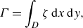 \begin{align}&\qquad\qquad\qquad \Gamma = \int _D\zeta \,{\textrm d}x\,{\textrm d}y, \end{align}
 \begin{align}&\,\,\,\, M_{x} = \int _D x\zeta \,{\textrm d}x\,{\textrm d}y, \quad M_{y} = \int _D y\zeta \,{\textrm d}x\,{\textrm d}y, \end{align}
 \begin{align}& M_{xx} = \int _D x^2\zeta \,{\textrm d}x\,{\textrm d}y, \quad M_{yy} = \int _D y^2\zeta \,{\textrm d}x\,{\textrm d}y, \end{align}
where these integrals are evaluated over the disk $D$
of radius
$D$
of radius $0.5 R$
around the point where the vorticity reaches its maximum. The core radius of the hub vortex is then computed as
$0.5 R$
around the point where the vorticity reaches its maximum. The core radius of the hub vortex is then computed as
 \begin{equation} a^2 = \frac {M_{xx} + M_{yy}}{\Gamma }. \end{equation}
Alternatively, the core radius can be determined by fitting a Gaussian profile to the axisymmetric component of the vorticity distribution. We have verified that the difference between the core radius values obtained through these two methods is negligible.
Appendix B. Linear stability analysis – operators and coefficients
The operators appearing in (4.1) are
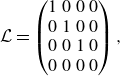 \begin{equation} \mathcal{L} = \begin{pmatrix} 1 & 0 & 0 & 0\\ 0 & 1 & 0 & 0\\ 0 & 0 & 1 & 0\\ 0 & 0 & 0 & 0 \end{pmatrix}, \end{equation}
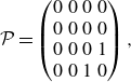 \begin{equation} \mathcal{P} = \begin{pmatrix} 0 & 0 & 0 & 0\\ 0 & 0 & 0 & 0\\ 0 & 0 & 0 & 1\\ 0 & 0 & 1 & 0 \end{pmatrix}, \end{equation}
 \begin{equation} \mathcal{M} = \begin{pmatrix} \Omega \frac {\partial }{\partial \theta } & -2\Omega & 0 & \frac {\partial }{\partial r} \\[6pt] 2\Omega + r\frac {{\textrm d}\Omega }{{\textrm d}r}& \Omega \frac {\partial }{\partial \theta } & 0 & \frac {1}{r}\frac {\partial }{\partial \theta } \\[6pt] 0 & 0 & \Omega \frac {\partial }{\partial \theta } & 0 \\[6pt] \frac {\partial }{\partial r} + \frac {1}{r} & \frac {1}{r}\frac {\partial }{\partial \theta } & 0 & 0 \end{pmatrix}, \end{equation}
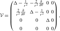 \begin{equation} \mathcal{V} = \begin{pmatrix} \Delta - \frac {1}{r^2} & -\frac {2}{r^2}\frac {\partial }{\partial \theta } & 0 & 0 \\[6pt] \frac {2}{r^2}\frac {\partial }{\partial \theta } & \Delta - \frac {1}{r^2} & 0 & 0 \\[6pt] 0 & 0 & \Delta & 0 \\[6pt] 0 & 0 & 0 & 0 \end{pmatrix}, \end{equation}
where
 \begin{equation} \Delta = \frac {1}{r}\frac {\partial }{\partial r} + \frac {\partial ^2 }{\partial r^2} + \frac {1}{r^2}\frac {\partial ^2 }{\partial \theta ^2} + \frac {\partial ^2 }{\partial z^2}, \end{equation}
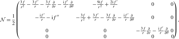 \begin{equation} \mathcal{N} = \dfrac {1}{2}\!\begin{pmatrix} \frac {3f}{r^2} - \frac {3f'}{r} - \frac {3f}{r}\frac {\partial }{\partial r} - \frac {{\textrm{i}}f'}{r}\frac {\partial }{\partial \theta } & -\frac {9{\textrm{i}}f}{r^2} + \frac {2{\textrm{i}}f'}{r} & 0 & 0 \\[12pt] -\frac {{\textrm{i}}f'}{r} - {\textrm{i}}f''& -\frac {3f}{r^2} + \frac {3f'}{r} - \frac {3f}{r}\frac {\partial }{\partial r} - \frac {{\textrm{i}}f'}{r}\frac {\partial }{\partial \theta } & 0 & 0 \\[12pt] 0 & 0 & - \frac {3f}{r}\frac {\partial }{\partial r} - \frac {{\textrm{i}}f'}{r}\frac {\partial }{\partial \theta } & 0\\ 0 & 0 & 0 & 0 \!\end{pmatrix}\!, \end{equation}
with $\overline {\mathcal{N}}$
being the complex conjugate of
$\overline {\mathcal{N}}$
being the complex conjugate of $\mathcal{N}$
.
$\mathcal{N}$
.


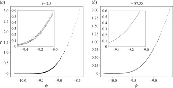


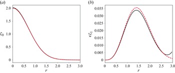


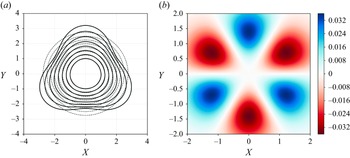


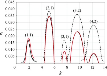


 Open access

