





Non-technical Summary
Studies of biodiversity patterns in the geologic past have traditionally focused on changes in the number of species (or genera or families), but this approach ignores how species were related through their evolutionary history, as reflected by their taxonomic classification. The concept of taxonomic distinctness (TD) addresses this aspect by examining the structure of the taxonomic tree, which allows for the incorporation of the differential relatedness among species in the analysis of biodiversity change. In this study, we apply TD metrics to the fossil record of marine bivalves to investigate how their taxonomic tree evolved after the Permian–Triassic mass extinction, which provides insights into macroevolutionary processes after a major biodiversity crash. Our analysis reveals two main phases: a relatively short lag phase during which diversification occurred mainly within surviving groups, followed by a prolonged phase characterized by an increased appearance of supraspecific taxa (i.e., genera, families, orders, etc., in the taxonomic classification). From this “deeper” perspective, the recovery from the greatest mass extinction took nearly 50 million years, much longer than inferred from species counts. We also observe that the balance among taxa in the evolutionary tree improved over time and that recovery patterns differed between tropical and subtropical regions.
Introduction
Analyses of biodiversity through the geologic past have traditionally applied a “taxic” approach, which is based on counting the number of taxa (richness) at a given level in the Linnaean classification. The rigorous application of this approach started with the “Paleobiology revolution” of the 1970s (Benton Reference Benton2013; Sepkoski Reference Sepkoski2013), in particular Sepkoski’s (Reference Sepkoski1978, Reference Sepkoski1979, Reference Sepkoski1984; Sepkoski et al. Reference Sepkoski, Bambach, Raup and Valentine1981) papers on Phanerozoic marine biodiversity, and it still thrives today using statistically advanced analyses of large databases (e.g., Alroy et al. Reference Alroy, Aberhan, Bottjer, Foote, Fürsich, Harries and Hendy2008; Close et al. Reference Close, Evers, Alroy and Butler2018; Fan et al. Reference Fan, Shen, Erwin, Sadler, MacLeod, Cheng and Hou2020; Bush and Payne Reference Bush and Payne2021). This research has provided us with a valuable overview of biodiversity change through deep time that allowed for the formulation of explanatory models such as Sepkoski’s (Reference Sepkoski1984) three-phased coupled logistic model or Benton’s (Reference Benton1997) expansion model. However, richness does not consider the phylogenetic aspect of biodiversity contained in phylogenetic and taxonomic trees (Benton Reference Benton2013). Conservation biologists, for instance, have long emphasized the importance of taxonomic disparity, the evolutionary distance between species, which carries critical information about biodiversity and evolutionary history (Faith Reference Faith1992, Reference Faith1994; Dubois Reference Dubois2003; Vogel Ely et al. Reference Vogel Ely, de L. Bordignon, Trevisan and Boldrini2017; González‐Orozco and Parra‐Quijano Reference González‐Orozco and Parra‐Quijano2023). Accordingly, a set of species representing distinct higher taxa includes more phylogenetic history and morphological disparity than an equivalent set within the same genus (Warwick and Clarke Reference Warwick and Clarke1995; Von Euler and Svensson Reference Von Euler and Svensson2001). Analyzing this neglected aspect of biodiversity in a deep-time context provides a new approach to classic questions in evolutionary research, such as how biodiversity builds up and how the tempo of evolution changes after a global biodiversity crash.
Useful metrics for this kind of analysis have been proposed by Warwick and Clarke (Reference Warwick and Clarke1995) and Clarke and Warwick (Reference Clarke and Warwick1998, Reference Clarke and Warwick2001), who defined:
-
1. Taxonomic diversity (Δ): the average taxonomic “distance” (path length) between any two organisms, chosen at random from the sample.
-
2. Taxonomic distinctness (TD, Δ*): the average path length between any two randomly chosen organisms, conditional on them being from different species.
-
3. Average taxonomic distinctness (AvTD, Δ+): the average taxonomic path length between any two randomly chosen species.
-
4. Variation of taxonomic distinctness (VarTD, Λ+): the variance of these pairwise path lengths.
These TD metrics highlight differences in the evenness and structure of the taxonomic tree that are not captured by species richness. The first two of these indices require quantitative data and converge into the third (AvTD, Δ+) in the special case when the dataset consists only of presence/absence data. AvTD (∆+) is calculated by summing the path lengths through a taxonomic tree connecting every pair of species (= number of steps to their first common node) and dividing this value by the total number of paths (Clarke and Warwick Reference Clarke and Warwick1998, Reference Clarke and Warwick2001).
Figure 1 illustrates three different taxonomic trees, each with the same species richness (S = 7), but differing in AvTD and VarTD. These differences reflect different aspects of the tree structure and evenness. In the first tree (Fig. 1A), the maximum possible AvTD value indicates the longest possible taxonomic path lengths between all species, suggesting greater taxonomic distance, while a zero VarTD reflects the uniform structure. In contrast, the second tree (Fig. 1B) shows a lower convergence point in the taxonomic hierarchy, resulting in shorter path lengths between species and indicating a more closely related community of species, which reduces AvTD. Finally, the third tree (Fig. 1C) presents a more complex structure with a mixture of closely and distantly related species. Despite having the same AvTD as tree B, the higher VarTD of tree C indicates greater variability in its taxonomic structure, suggesting less uniformity in the community.
Taxonomic distinctness (TD) metrics illustrated through different trees, A, B, and C, each with identical species richness but differing in average taxonomic distinctness (AvTD) and variation in taxonomic distinctness (VarTD). AvTD is given as percentage of the maximum path length in a range between 0 and 100. Adapted from Clarke and Warwick (Reference Clarke and Warwick1998: fig. 2, 2001: fig. 2).

Figure 1. Long description
There are three panels arranged left to right. Panel A shows a symmetrical tree with one top node branching evenly to seven terminal nodes, labeled Av T D equals 100 and Var T D equals 0. Panel B shows a star-shaped tree with one top node directly connected to seven terminal nodes, labeled Av T D equals 66.67 and Var T D equals 0. Panel C shows an asymmetrical tree with uneven branching, labeled Av T D equals 66.67 and Var T D equals 634.9. All panels indicate s equals 7 below the trees. The y-axis on the left is labeled Taxonomical level.
Generally, the metrics discussed earlier can be applied to both phylogenetic and taxonomic trees. In practice, however, studies based on taxonomic trees largely prevail, not least because the Linnaean taxonomy is often readily available and contains fewer levels than phylogenetic trees. Although this practice may omit phylogenetic details, taxonomic trees still reflect the principal phylogenetic structure and “impose an ordering of branch length which is interpretable and should be used” (Clarke and Warwick Reference Clarke and Warwick1998: p. 524). Moreover, the Linnaean taxonomy typically contains aspects of disparity and ecology that are often not adequately reflected by the pattern of phylogenetic branching. For example, the traditional Linnaean taxonomy that recognizes Aves and the paraphyletic taxon Reptilia accounts better for the huge differences in disparity, ecology, and functional diversity between these taxa than the monophyletic taxon Sauropsida of the strict phylogenetic approach.
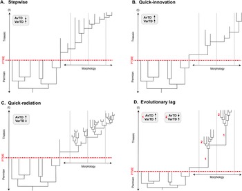
The study of TD parameters in paleontological data has great potential for a variety of research questions, from the ecological characterization of paleocommunities from different geological times and environmental settings to the study of large-scale evolutionary patterns. In this study, we explore the question of how the structure of taxonomic trees evolves when a taxon diversifies, exemplified by the rediversification of marine bivalves after the end-Permian mass extinction. Triassic bivalves, with their well-established taxonomic framework, broad ecological range, and extensive fossil record, provide an ideal model group for macroevolutionary and macroecological studies (Jablonski et al. Reference Jablonski, Roy, Valentine, Price and Anderson2003; Valentine et al. Reference Valentine, Jablonski, Kidwell and Roy2006). We test four models that represent different macroevolutionary modes (Figs. 2, 3):
-
1. Stepwise model: Higher taxa appear in a stepwise manner through successive speciation events, each of which involves only moderate morphological change. This model implies constant, diversity-independent evolutionary rates that were little affected by niche space availability. As shown in Figure 3B,D, this evolutionary mode will lead to an initial postextinction decrease in AvTD accompanied by an increment of VarTD.
-
2. Quick innovation model: Increased ecological opportunity after the end-Permian mass extinction allowed for increased rates of morphological change and a corresponding increase in the appearance of higher taxa relative to the number of new species. This scenario, which has previously been suggested by Patzkowsky (Reference Patzkowsky1995), leads to an initial postextinction increase in both AvTD and VarTD (Fig. 3C).
-
3. Quick radiation model: Similar to the second model, open ecological niches promote significant morphological changes, leading to the establishment of higher taxonomic levels. However, this process is followed by rapid diversification within these new levels. This pattern is reflected by an increase in AvTD but a decrease in VarTD and illustrated in Figure 3E.
-
4. Evolutionary lag model: Higher taxa emerge early during the rediversification as in the quick innovation model, but macroevolutionary lags (Jablonski et al. Reference Jablonski, Bottjer, Nitecki and Nitecki1990; Jablonski Reference Jablonski2017) delayed their taxonomic diversification. This scenario would be reflected by an initial increase in AvTD (Fig. 3C) followed by a long-term decrease (Fig. 3 B–D).
Conceptual evolutionary models for species diversification and postextinction recovery. The diagrams illustrate taxonomic branching patterns and their impact on biodiversity metrics through time: stepwise (A), quick innovation (B), quick radiation (C), and evolutionary lag (D) models. The red dashed line marks the Permian–Triassic mass extinction (PTME). Horizontal arrows represent the expansion of morphological disparity relative to taxonomic branching.

Figure 2. Long description
Top left panel A, labeled Stepwise, shows a phylogenetic tree with branching events distributed both before and after the red dashed P T M E line. The vertical axis is labeled t, with Permian below and Triassic above. The horizontal axis is labeled Morphology. A gray box indicates Av T D down arrow and Var T D up arrow. Top right panel B, Quick-innovation, shows most branching events occurring immediately after the P T M E line, with Av T D up arrow and Var T D up arrow. Bottom left panel C, Quick-radiation, shows dense branching after P T M E, with Av T D up arrow and Var T D up arrow. Bottom right panel D, Evolutionary lag, shows little branching immediately after P T M E, with two gray boxes: one labeled 1 with Av T D down arrow and Var T D up arrow, and one labeled 2 with Av T D up arrow and Var T D up arrow. Red numbers 1 and 2 mark corresponding regions on the tree. All panels have horizontal arrows indicating expansion of morphology after P T M E.
Possible pathways of species diversification are illustrated by taxonomic trees, reflecting the changes in average taxonomic distinctness (AvTD) and variation in taxonomic distinctness (VarTD). The base tree (A) represents the initial stage, followed by two alternative speciation scenarios (+2 new species). The B scenario shows the addition of the new species from an existent genus, reflecting a more regular structure in the taxonomic tree (low VarTD) and a decline in AvTD. In contrast, C introduces two more distantly related species, leading to a greater unevenness of the tree structure and the longer path between species having an increment in AvTD and VarTD. The D scenario illustrates the addition of two species to the same genus, resulting in a less regular structure, increment in VarTD, with the l lowest AvTD value between our possible scenarios. Finally, the E scenario introduces both a new genus and two rapidly spreading new species from that genus, leading to an equilibrated structure with a very low VarTD and a slight increase in AvTD.

Figure 3. Long description
Panel A at top left shows a base tree with four species, Av T D equals 41.66, Var T D equals 138.88. Panel B at top right adds two species to an existing genus, resulting in a more regular tree, Av T D equals 40.0, Var T D equals 150.0. Panel C at bottom left adds two distantly related species, creating a more uneven tree, Av T D equals 70.00, Var T D equals 683.33. Panel D at bottom right adds two species to the same genus, making the tree less regular, Av T D equals 38.33, Var T D equals 155.5. Panel E at bottom far right introduces a new genus and two new species, resulting in a balanced tree, Av T D equals 45.0, Var T D equals 100.0. Arrows in each panel indicate increases or decreases in Av T D and Var T D relative to the base tree. All trees are rooted, with red lines marking new branches and black lines showing original structure. Grey shapes highlight genus clusters. S equals number of species is labeled in each panel.
Testing these models through the analysis of TD allows us to identify new aspects of macroevolutionary pathways in rediversifying ecosystems in space and time. By analyzing these patterns in Triassic bivalves, we aim to reveal how taxonomic structures evolved during this critical period of rediversification, offering new insights into broader evolutionary processes that shape biodiversity and its paleogeographic relationships.
Material and Methods
Dataset Construction
A total of 86 fossil faunas of Triassic bivalves were compiled from published literature. We collected data at the finest resolution that was available from the source references (documented in the Supplementary Material), but for the purpose of the analyses, we combined these data to the level of lithological units of comparable size. Residual differences in sample sizes have no impact on the results, because the TD metrics are unbiased by sample size (Clarke and Warwick Reference Clarke and Warwick1998). The rationale of using collections rather than global compilations of stratigraphic intervals is that the latter approach would require a full taxonomic revision at the species level, because unrecognized synonyms in the species lists would bias TD toward lower values. In contrast, the collection approach requires only the elimination of synonyms within each collection, which is much easier to fulfill. The underlying assumption of this approach is, of course, that the fossil faunas that are employed are statistically representative of the time and habitat in which they were found. Accordingly, fossil faunas with species counts n < 10 were excluded from the analysis, because they were not considered as sufficiently representative of the former faunas. Moreover, only records meeting specific criteria, such as reliable stratigraphic information and sufficient documentation of the species’ morphology (generally through illustrations), were included. Following this quality control process, including taxonomic revision and refinement of stratigraphic resolution, we retained a total of 59 assemblages for the analysis. Approximately 1450 species records were revised and retained in the main database for the Triassic Period.
As noted earlier, the collection approach requires only the correct identification of the number of species present in each collection and their supraspecific classification. This also means that species descriptions in open nomenclature are acceptable as long as it can be demonstrated that these species are different from congeneric species. The second basic requirement is the application of a coherent taxonomic classification. We developed a synthesis of the major synoptical classifications (Cox et al. Reference Cox, Turner, Nuttall, Trueman, Boyd, Perkins and Puri1969; Carter et al. Reference Carter, Altaba, Anderson, Araujo, Biakov, Bogan and Campbell2011; Bieler et al. Reference Bieler, Mikkelsen, Collins, Glover, González, Graf and Harper2014), added to by the evaluation of numerous specialized publications on chiefly lower-rank taxonomy. Next, we defined the taxonomic levels that were considered for the analysis. This is crucial, because the number of taxonomic levels impacts the results not only quantitatively but also qualitatively. In the same way, if a particular taxonomic level (such as “subgenus”) is only well defined for a subset of the dataset, while being absent, ambiguous, or inconsistently applied across other groups, it can artificially inflate the taxonomic distances in those better-resolved lineages. This can result in misleadingly high distinctness values for some faunas, even if their actual distinctness is comparable. This concern has also been highlighted in earlier studies (Clarke and Warwick Reference Clarke and Warwick2001), emphasizing the importance of using coherent and balanced taxonomic hierarchies in comparative analyses.
Moreover, higher taxonomic ranks are not necessarily comparable among the major groups of bivalves. We found that the levels genus, subfamily, family, superfamily, order, superorder, infraclass, and subclass best reflect the hierarchy applied to the major groups of bivalves (Palaeotaxodonta, Pteriomorphia, Heteroconchia); we thereby raised all subgenera to the rank of genera. We further changed the levels of some taxa in order to make these comparable among the major groups. For example, we ranked Palaeoheterodonta, Archiheterodonta, Imparidentia, and Anomalodesmata as superorders among Heteroconchia and omitted Euheterodonta (= Imparidentia + Anomalodesmata), because this level has no equivalent in Pteriomorphia and Palaeotaxodonta. In some cases where appropriate formal taxonomic names were missing, we added artificial taxa for an appropriate reflection of taxonomic differences (e.g., we introduced “Schafhaeutliidae” to accommodate the genus Schafhaeutlia , which is generally classified inappropriately within Lucinidae but still awaits formal taxonomic revision; occasionally, we also used informal placeholders such as “Gen A-REF”). We acknowledge that taxonomic decisions are always subjective to some degree, but the coherent application of the scheme that we developed in the course of this study ensures consistency and comparability of the results.
Fossil occurrence coordinates were collected based on published locality data; when exact coordinates were unavailable, they were inferred using regional descriptions and geographic or geological maps. The methods used for coordinate processing and paleogeographic projection are described in detail in the “Data Analysis” subsection later in the paper.
Analytical Methods
Two TD metrics according to Clarke and Warwick (Reference Clarke and Warwick1998, Reference Clarke and Warwick2001) have been applied to explore changes in the taxonomic structure of Triassic bivalves; average taxonomic distinctness (AvTD) and variation in taxonomic distinctness (VarTD), which are briefly explained below in the following sections.
AvTD (Δ+)
AvTD is defined as the mean path length between two randomly selected species within a given dataset, which is calculated as:

where
$ {\omega}_{ij} $
 represents the taxonomic path length between species i and j, s is the number of species present. The indices i and j denote individual species from the set of s species for the summation (Warwick and Clarke Reference Warwick and Clarke1998). AvTD is expressed as a percentage of the maximum possible path length.
VarTD (Λ+)
VarTD is measured as the variance in pairwise path lengths, capturing the spread of taxonomic relationships within a dataset. Unlike AvTD, VarTD has no consistent upper limit, as variance increases with greater taxonomic unevenness, and maximum VarTD differs among samples. Using the notation from equation (1), Clarke and Warwick (Reference Clarke and Warwick2001) define VarTD algebraically as:

AvTD and VarTD are independent of sample size, as they are defined based on the pairwise comparisons between species instead of summing species (see eqs. 1 and 2; Clarke and Warwick Reference Clarke and Warwick1998, Reference Clarke and Warwick2001). Therefore, if more species are added, the average and variance of pairwise distances stabilize near the “real” value, but they do not systematically increase or decrease, in contrast to richness metrics. This characteristic allows the integration of data from various scales without introducing biases related to sample size. Consequently, assemblages from different stratigraphic levels (from bed to formation) can be analyzed jointly, enabling a comprehensive assessment of taxonomic structure and variability across diverse paleontological contexts.
As a tool for the statistical assessment of these metrics, Clarke and Warwick (Reference Clarke and Warwick1998) developed an algorithm for the calculation of confidence funnels that allow the evaluation of whether the observed values of AvTD and VarTD fall within the expected range of variation. These funnels provide a graphical representation of the 95% confidence limits around the expected mean value of each metric, based on random drawing of subsamples from the full list of all species occurring in the analysis. The funnel shape reflects the expected increase in variation at lower sample sizes and a stabilization around the value that represents a fully sampled collection at higher sample sizes. Observed values falling outside the funnel indicate significantly higher or lower TD than expected, indicating unusual taxonomic compositions in the analyzed data. Conceptually, the application of the confidence funnel method to fossil faunas is restricted to time intervals that are short enough to include only species that coexisted in time. We have therefore restricted the use of this method to faunas from the same stage (Fig. 5).
Data Analysis
Analyses were conducted using the R programming language. Our calculations for the TD metrics, specifically AvTD and VarTD, along with the generation of their expected mean values and standard deviations (SD) for the subsampling analysis, were implemented using a custom script. The methods implemented in our script, including the notation used, are based on Clarke and Warwick (Reference Clarke and Warwick1998). Although constructed from the original vegan package (Oksanen Reference Oksanen2010), our script was modified to meet the specific requirements of our analysis. First, we simulate smaller datasets by randomly drawing subsamples from the full list of all species occurring in the analysis (the species pool). For each possible subsample size m (ranging from 2 up to the total number of species in the species pool), we randomly select m species and calculate the taxonomic metrics. This process is repeated 1000 times for each m value. Following these simulations, the expected value and SD for AvTD and VarTD are calculated per m. Finally, these data are used to construct confidence funnels, where the expected value for each metric forms the center of the funnel, and the confidence intervals are defined by the mean ± SD.
For the reconstruction of stratigraphic trends and mean values for time bins (Figs. 4, 5), we removed all samples that fell outside the confidence funnels, because such samples may reflect taphonomic bias, sampling issues, or unusual ecological conditions (Clarke and Warwick Reference Clarke and Warwick1998) that are not representative of their respective stratigraphic intervals (see Appendix 2 for more details). However, we retained a full dataset for the reconstruction of uncorrected trends (Supplementary Fig. S1). We note that the datasets show the same main trends, with the only exception being the “expected mean” of AvTD in the Induan–Olenekian interval, which is discussed later.
Patterns of taxonomic distinctness (TD) metrics of bivalves during the Triassic: (A) average taxonomic distinctness (AvTD, Δ+) and (B) variation in taxonomic distinctness (VarTD, Λ+). The observed values are represented by a solid dark gray line, with the standard deviations shown in light gray shading. The expected values for the TD metrics are indicated by a black dashed line, while the mean of species richness is represented by a gray dashed line. The five distinct phases of the trend are demarcated by vertical light gray dashed lines, labeled 1 through 5.

Figure 4. Long description
The top panel displays average taxonomic distinctness, labeled as A V T D delta plus, on the y-axis from 70 to 86, and Triassic stages on the x-axis from Induan to Rhaetian. The right y-axis shows number of species from 15 to 50. Three lines are plotted: a solid dark gray line for observed mean, a black dashed line for expected values, and a dotted gray line for mean species richness. Light gray shading indicates standard deviation around the observed mean. Colored dots represent data points for each stage: blue for Induan and Olenekian, orange for Anisian and Ladinian, green for Carnian, Norian, and Rhaetian. Five vertical light gray dashed lines divide the graph into phases labeled 1 through 5. The observed mean dips at Olenekian, rises steadily through Anisian to Carnian, then plateaus from Norian to Rhaetian. The expected line follows a similar trend but is slightly lower. Species richness peaks at Carnian and Norian, then declines. The bottom panel shows variation in taxonomic distinctness, labeled as V a r T D lambda plus, on the y-axis from 200 to 600, with the same x-axis and right y-axis as the top panel. The same three lines and color scheme are used. The observed mean starts high in Induan, drops sharply at Olenekian, rises at Ladinian, then remains low and stable from Carnian to Rhaetian. The expected line is lower and flatter, while species richness mirrors the top panel. Vertical dashed lines and phase numbers match the top panel.
Paleogeographic reconstructions were performed using rgplates package in R, applying the MERDITH2021 global plate motion model (Müller et al. Reference Müller, Cannon, Qin, Watson, Gurnis, Williams, Pfaffelmoser, Seton, Russell and Zahirovic2018). Paleolatitudinal bins were defined as tropical (−30° to 30°) and subtropical to boreal (−30° to −90° and 30° to 90°), ensuring complete latitudinal coverage while maintaining adequate sample sizes. Additionally, a secondary binning scheme based on 30° intervals was implemented to provide a finer-resolution assessment of paleolatitudinal patterns. Although some paleolatitudinal bins contained relatively small sample sizes, the binning scheme was selected to optimize data coverage. These analyses followed the same methodological framework used for the reconstruction of temporal trends.
Results
From an initial set of 59 fossil assemblages, 43 were retained after detailed data revision, ensuring consistency and completeness in the final dataset. These include 12 from the Lower Triassic, 10 from the Middle Triassic, and 21 from the Upper Triassic.
TD
The analysis of TD throughout the Triassic reveals five distinct phases, illustrated in Figure 4, which are marked by contrasting trends in AvTD and VarTD. The first stage, immediately after the end-Permian Extinction (Induan to Olenekian), shows a slight decline in AvTD accompanied by a significant increase in VarTD. This pattern reflects reduced taxonomic disparity alongside growing unevenness in taxonomic structure, likely driven by diversification at lower taxonomic levels (see Fig. 3B,D). During this stage, five new orders appear in our dataset—Arcida, Veneroida, Lucinida, Limida, and Pholadoida—accompanied by rapid diversification, with a total of 14 new families and approximately 22 new genera. The taxonomic structure during this interval is influenced by highly diverse genera such as Eumorphotis, Leptochondria, and Unionites, which likely had a strong impact on the metrics due to their species-level diversification.
The second phase, spanning from the Olenekian to the Ladinian, is characterized by a rapid increase in AvTD and a simultaneous decrease in VarTD. Although this interval saw fewer new orders (3) compared with the first stage (5), these new orders were taxonomically more distant and thus had a higher impact on AvTD than those of the previous stage. This reflects accelerated diversification at higher taxonomic levels and greater taxonomic uniformity within paleocommunities. Notable new orders in our database during this time include Ostreida and Solemyida, along with rapidly diversifying families like Daonellidae. The increase in AvTD is likely driven by the rise of new orders, while the decline in VarTD reflects more evenly distributed diversification across lower taxonomic levels (see Fig. 3E).
The third phase, the Ladinian to Carnian transition, shows a near stasis of both AvTD and VarTD. This is also the first stage in which the richness that is represented by our samples declined (Fig. 4). However, 32 new genera are recorded during this phase in our database, with particularly high species diversification observed in genera such as Cassianella, Mysidioptera, and Schafhaeutlia , which counterbalanced the appearance of supraspecific taxa.
In the fourth segment, from the Carnian to the Norian, AvTD increases while VarTD declines. New orders such as Thraciida and Myida are incorporated smoothly into the existing taxonomic framework, contributing to the rise in AvTD without significantly affecting VarTD. Additionally, 45 new genera are added to the dataset during this stage, and the number of species per genus appears more balanced, reinforcing the observed trend.
Finally, the fifth stage, from the Norian to the Rhaetian, both AvTD and VarTD show stasis again. The emergence of one new order and three new families, alongside their limited initial spread and restricted diversification at lower taxonomic ranks, maintains a taxonomic configuration characterized by structural unevenness that closely resembles the pattern illustrated in Figure 3C.
In addition, Figure 4 illustrates the expected values calculated for AvTD and VarTD in each of the Triassic stages (dashed lines in Fig. 4). These expected values closely align with the observed data (mean values), which reinforces the robustness of our findings. Specifically, AvTD shows a minor decline from the Induan to Olenekian, then a consistent increase through the rest of the period. The observed VarTD also parallels the expected VarTD, with exception of the Induan–Olenekian interval (discussed later in this section).
Mean richness increases from Induan to Ladinian, reaching its highest point during the Triassic, followed by a progressive decline until the Norian, and closing the period with a slight increase in the Rhaetian (see Fig. 4).
Alternative scenarios for TD trends are presented in Supplementary Figure S1. Both scenarios display a similar pattern, including a distinct phase immediately after the extinction and convergence in the final two phases. In the reference dataset (Fig. 4), expected AvTD and VarTD show a slight decline during the first phase (Induan–Olenekian), whereas both metrics rise in the unfiltered dataset (Supplementary Fig. S1).
Figure 5 and Supplementary Figure S2 provide a more detailed breakdown of TD metrics in relation to the number of species in the different Triassic stages—Lower, Middle and Upper. Figure 5 displays the main dataset after data cleaning and preparation, showing that all AvTD data points fall within the 95% confidence limits. For VarTD, only a few data points in the Upper Triassic (Carnian), from Hausmann and Nützel (Reference Hausmann and Nützel2015) and Chen and Sha (Reference Chen and Sha2022), hardly fall outside the expected range. In contrast, Supplementary Figure S2 presents the complete dataset, where visible anomalies are found in both AvTD and VarTD.
Scatter plots showing (A) average taxonomic distinctness (AvTD, Δ+) and (B) variation in taxonomic distinctness (VarTD, Λ+) against the number of species for all studied stages, grouped into the three Triassic series: Lower, Middle, and Upper. Dotted lines represent confidence funnels for each stage.

Figure 5. Long description
The top row, labeled A, displays three scatter plots of average taxonomic distinctness, Av T D, delta plus, against number of species. The left plot shows Induan and Olenekian stages in blue, with data points clustered between 15 and 75 species and Av T D values from 65 to 85. The center plot shows Anisian and Ladinian stages in orange, with species counts from about 50 to 200 and Av T D values from 65 to 85. The right plot shows Carnian, Norian, and Rhaetian stages in green, with species counts from 0 to 300 and Av T D values from 65 to 85. Each plot includes dotted lines forming confidence funnels around the data. The bottom row, labeled B, follows the same structure but plots variation in taxonomic distinctness, Var T D, lambda plus, on the y-axis, ranging from 100 to 700. The same color scheme and species count ranges apply. Legends in each plot identify the corresponding Triassic stages by color.
The global distribution of samples (fossil assemblages) for the different series of the Triassic is illustrated in the first panel of Figure 6. Paleolatitudinal trends are shown in the second panel of Figure 6, illustrating the relationship between paleolatitudinal intervals and taxonomical distinctness metrics. Paleolatitudinal bins were defined as tropical (−30° to 30°) and subtropical to boreal (−30° to −90°, 30° to 90°), ensuring complete coverage and significant sample representation in most cases. Additionally, gray lines marking a second bin of 30° intervals are included to further refine the paleolatitudinal breakdown. Throughout the Triassic, AvTD values generally increase toward higher paleolatitudes, a trend particularly pronounced in the Upper Triassic (Fig. 6, Supplementary Fig. A2). Conversely, VarTD displays the opposite pattern, with higher values in tropical regions and lower values in subtropical zones. In summary, subtropical latitudes are characterized by high AvTD and low VarTD, while tropical regions exhibit low AvTD and high VarTD. While these trends are robust for the Upper Triassic due to broader sampling, we consider the patterns for the Lower and Middle Triassic as tentative, as the data for these series do not yet provide sufficient coverage of the entire latitudinal range to confirm a global gradient.
Paleogeographic reconstruction showing the location with the distribution of the fossil assemblages for Lower (C1), Middle (B1) and Upper (A1) Triassic. Distribution patterns of average taxonomic distinctness (AvTD) and variation in taxonomic distinctness (VarTD) through the different Triassic series, Lower (C2), Middle (B2), and Upper (A2), are also illustrated. For AvTD and VarTD, colored line plots indicate standard latitudinal bins (tropical and subtropical), while gray lines represent finer latitudinal divisions at 30° intervals.

Figure 6. Long description
Top row: A1 at top-left is a paleogeographic map for the Upper Triassic with green fossil site markers, mainly in the Northern Hemisphere. A2 at top-right has two vertical line graphs, both with y-axis labeled Paleolatitude (degrees) from 60 North to 60 South. The left graph plots AvTD (Delta star) and the right graph plots VarTD (Delta star), both with green lines for standard latitudinal bins and gray lines for finer divisions. Middle row: B1 at left is a Middle Triassic map with orange fossil sites, concentrated in the Northern Hemisphere. B2 at right shows paired orange line graphs for AvTD and VarTD, with similar axis structure and color coding. Bottom row: C1 at left is a Lower Triassic map with blue fossil sites, more evenly distributed across hemispheres. C2 at right shows blue line graphs for AvTD and VarTD, with the same axis and color conventions. Across all graphs, colored lines represent tropical and subtropical bins, gray lines show 30-degree intervals, and data points are connected to illustrate trends in taxonomic distinctness by latitude.
Discussion
Triassic Trends in TD
The five described phases represent two megatrends: the first megatrend is identical to phase 1 (Early Triassic) and is characterized by a decrease in mean AvTD and an increase in mean VarTD (Fig. 4, Supplementary Fig. S1). However, it should be noted that expected VarTD shows a slight Induan–Olenekian decline in our reference dataset (Fig. 4B, stippled line), whereas expected AvTD increases in the unfiltered dataset (Supplementary Fig. S1, dashed line). The second megatrend (phases 2–5; Middle to Late Triassic) shows a long-term tendency toward increasing AvTD and decreasing VarTD, which is largely stable among datasets and metrics (Fig. 4, Supplementary Fig. S1). We herein refer to the first megatrend as retrograde, because it is characterized by an overall depletion of TD, indicated by a decline in TD in combination with an increasing unevenness in the tree, and conversely, we refer to the second megatrend as prograde, as it leads to higher distinctness and evenness of the taxonomic structure.
The first thing to note is that these two megatrends are unrelated to published trends in richness. Bivalve richness already increased from the Induan to the Olenekian (corresponding to megatrend 1; see data in Posenato Reference Posenato2008; Hautmann et al. Reference Hautmann, Bucher, Brühwiler, Goudemand, Kaim and Nützel2011, Reference Hautmann, Smith, McGowan and Bucher2013, Reference Hautmann, Bagherpour, Brosse, Frisk, Hofmann, Baud, Nützel, Goudemand and Bucher2015; Hofmann et al. Reference Hofmann, Hautmann and Bucher2013a,Reference Hofmann, Hautmann, Wasmer and Bucherb, Reference Hofmann, Hautmann, Brayard, Nützel, Bylund, Jenks, Vennin, Olivier and Bucher2014, Reference Hofmann, Hautmann and Bucher2015; Tu et al. Reference Tu, Chen and Harper2016; Foster et al. Reference Foster, Lehrmann, Yu, Ji and Martindale2018). This increase accelerated in the Anisian (Middle Triassic; Friesenbichler et al. Reference Friesenbichler, Hautmann, Nützel, Urlichs and Bucher2019, Reference Friesenbichler, Hautmann, Grădinaru and Bucher2021; Hautmann Reference Hautmann2007; Posenato Reference Posenato2008; Ros et al. Reference Ros, De Renzi, Damborenea and Márquez-Aliaga2011; Tu et al. Reference Tu, Chen and Harper2016), and genus richness continued to increase until the Norian or Rhaetian (Late Triassic), respectively (Hautmann Reference Hautmann2007; Ros et al. Reference Ros, De Renzi, Damborenea and Márquez-Aliaga2011). The richness that is represented by our samples is not (and cannot be) a representation of global richness, but it does show a continuous increase until the Ladinian (Fig. 4); the transition between megatrends 1 and 2 is therefore obviously unrelated to richness.
A second unexpected result is that two opposing megatrends occurred that correspond to two different macroevolutionary modes, as discussed in the “Introduction.” Megatrend 1 corresponds to scenario 1 (Fig. 3 B,D), wherein morphological changes during speciation events remained small in spite of ecological opportunity, leading to a deficit of new supraspecific taxa relative to new species. In contrast, megatrend 2 corresponds to scenario 3 (Fig. 3E), wherein ecological opportunity promoted the evolution of supraspecific taxa that diversified quickly after their appearance. How can the transition between these two apparently opposing models be explained?
A clue to resolve this question might come from the differences between mean and expected values for AvTD and VarTD in the different Early Triassic datasets (discussed earlier). Whereas the mean values are affected by the frequency at which a certain value is observed, the expected value is calculated from the full list of species present in the analyzed time bin and thus gives a higher weight to the less commonly encountered taxa, which might also be more frequent in samples that fell outside the confidence funnels. A tentative interpretation is that evolutionary rates were geographically heterogeneous in the Early Triassic, possibly due to still volatile environmental conditions (Tong et al. Reference Tong, Zhang, Zuo and Xiong2007; Fraiser and Bottjer Reference Fraiser and Bottjer2009; Hofmann et al. Reference Hofmann, Goudemand, Wasmer, Bucher and Hautmann2011; Foster et al. Reference Foster, Lehrmann, Yu, Ji and Martindale2018) and that the retrograde Early Triassic trend was dominant but geographically not universal at that time.
A second possible explanation is that there is a positive correlation between evolutionary rates and richness, ultimately because biotic interactions are a main agent of selection (e.g., Emerson and Kolm Reference Emerson and Kolm2005; Meyer and Kassen Reference Meyer and Kassen2007), and their intensity increases with the number of species present. The case that a low intensity of biotic interactions (specifically interspecific competition) in the wake of the end-Permian mass extinction was the principal cause of the delayed recovery has explicitly been made for the Triassic rediversification of marine benthos (Hautmann et al. Reference Hautmann, Bagherpour, Brosse, Frisk, Hofmann, Baud, Nützel, Goudemand and Bucher2015; Friesenbichler et al. Reference Friesenbichler, Hautmann, Grădinaru and Bucher2021) and aligns well with the herein observed retrograde pattern of TD during the Early Triassic.
Regardless of the explanation for the retrograde Early Triassic trend, the Middle to Late Triassic prograde megatrend 2 confirms the prediction that the opportunity for new adaptive zones to be filled at higher taxonomic levels is proportionately higher after mass extinctions (Patzkowsky Reference Patzkowsky1995). The possibly most remarkable aspect of our data is that this situation continues far beyond “complete” recovery as defined by many conventional indicators, such as reappearance of reefs (Erwin Reference Erwin1998), tiering (Twitchett Reference Twitchett1999), body size (Payne Reference Payne2005), and diversity partitioning (Hofmann et al. Reference Hofmann, Hautmann and Bucher2013a,Reference Hofmann, Hautmann, Wasmer and Bucherb, Reference Hofmann, Hautmann, Brayard, Nützel, Bylund, Jenks, Vennin, Olivier and Bucher2014; Hautmann et al. Reference Hautmann, Bagherpour, Brosse, Frisk, Hofmann, Baud, Nützel, Goudemand and Bucher2015). The extended time that saw a surplus of supraspecific taxa is in sharp contrast to the quick evolution of higher taxa in localized radiations, such as that of the cockles of the Pontian sea (e.g., Stanley Reference Stanley1975) or the cichlids of Lake Malawi (e.g., Kocher Reference Kocher2004), which were completed within few million years (but note that data on TD are not yet available for these cases). Whether the reason for this difference is rooted in the difference of the geographic scale (local vs. global) or of the macroecological setting (newly colonized habitats vs. depleted but not barren ecosystems) remains unanswered.
In contrast to the increase in AvTD, VarTD decreases during the second megatrend. As noted earlier, this corresponds to scenario 3 (Fig. 3E), wherein newly emerged higher taxa evolved similar numbers of species. The increasing balance within the taxonomic tree, which is indicated by decreasing VarTD, likely reflects macroecological saturation through refined niche partitioning.
Apart from TD, richness also continued to increase until the end of the Triassic, at least at the global scale, but as noted earlier, it is largely uncorrelated with TD in the Early and the Middle Triassic. Yet the two megatrends in TD are at least broadly similar to trends in functional richness, as recently described by Wang et al. (Reference Wang, Huang, Song, Tian, Chu and Tong2024: fig. 3C–D). This is not unexpected, because differences in lifestyles of bivalves correspond to basic differences in the shell morphology that in turn are reflected by the taxonomic classification at higher taxonomic levels.
Summarized, our analysis of TD suggests that speciation among bivalves after the end-Permian mass extinction produced a surplus of supraspecific taxa at least until the Norian. The macroevolutionary bearings of this find are (1) that ecological opportunity fostered evolutionary rates, as expressed by an increased number of speciation events that found new supraspecific taxa and (2) that this process was not concentrated in a short evolutionary burst, as suggested generally (e.g., Jablonski Reference Jablonski2001) or for certain taxa (e.g., Brayard et al. Reference Brayard, Escarguel, Bucher, Monnet, Brühwiler, Goudemand, Galfetti and Guex2009; Friedman Reference Friedman2010), but extended over nearly 50 Myr. Our analysis thus highlights what might be called the paradox of evolutionary rates: ecological opportunity may likewise promote geologically instantaneous evolutionary bursts, as in the cases of the localized radiations cited earlier, or provide an apparently low but long-lasting evolutionary stimulus, as evident in our data. The long duration of the macroevolutionary response resembles Jablonski’s “macroevolutionary lag” (Jablonski and Bottjer Reference Jablonski, Bottjer, Taylor and Larwood1990; Jablonski Reference Jablonski2017, Reference Jablonski2022), but Jablonski’s model refers to the failure of taxa to diversify after the acquisition of key adaptations and thus should be reflected by an increase in both AvTD and VarTD (Fig. 3C), contrary to the decrease in VarTD observed in our data. Recently, Hull (Reference Hull2015: p. 941) suggested that “a speed limit might exist for the pace of global biotic change after massive disturbance,” which is set by “geosphere–biosphere interactions”; Hull’s (Reference Hull2015) model ultimately explains the macroevolutionary delay after mass extinctions by the time intensity of global ecosystem rebuilding after such massive disruptions. Notably, Hull (Reference Hull2015: fig. 4) points out the prevalence of biotic forcing during this rebuilding, a mechanism that has also been suggested as an explanation for the delayed recovery of benthos (Hautmann et al. Reference Hautmann, Bagherpour, Brosse, Frisk, Hofmann, Baud, Nützel, Goudemand and Bucher2015). However, Hull’s model predicts that an extended lag phase is followed by an explosive increase in richness, contrary to the slow but steady increase in AvTD observed in the present study. This is not necessarily contradictory, because richness and AvTD reflect different aspects of biodiversity, which may respond differently to a given stimulus. Another aspect of biotic forcing of evolutionary change is predator–prey interactions, which gradually increased throughout the Triassic, although their effects are controversial (McRoberts Reference McRoberts2001). Ultimately, resolving the paradox of evolutionary rates requires the incorporation of the TD approach in future empirical and theoretical studies.
Paleolatitudinal Patterns
The paleolatitudinal variation in AvTD and VarTD during the Triassic for bivalves provides insight into the relationship between taxonomic structure and paleolatitude in the postextinction recovery and diversification. AvTD values show a tendency to increase toward higher paleolatitudes, while VarTD tends to decrease, which is evident during the Late Triassic (Fig. 6C2). This implies that subtropical–temperate and boreal regions hosted bivalve communities with taxonomically more distinct lineages compared with the tropical areas, but with a more even taxonomic structure. The temporal trend parallels the reestablishment of latitudinal diversity structure after the end-Permian mass extinction (Song et al. Reference Song, Huang, Jia, Dai, Wignall and Dunhill2020) and with the progressive biogeographic differentiation of bivalve faunas through the Middle and Late Triassic (Echevarría and Ros-Franch Reference Echevarría and Ros-Franch2024; Miao et al. Reference Miao, Tong, Huang, Zhang, Li, Cao, Chu and Kiessling2025).
These latitudinal patterns may reflect large-scale paleoenvironmental variations across the different paleolatitudes, consistent with several hypotheses proposed to explain the modern latitudinal diversity gradient (LDG). These include variation in ambient energy and productivity (Pianka Reference Pianka1966; Willig et al. Reference Willig, Kaufman and Stevens2003; Turner Reference Turner2004; Coelho et al. Reference Coelho, Barreto, Rangel, Diniz-Filho, Wüest, Bach, Skeels, McFadden, Roberts and Pellissier2023), as well as the effects of long-term climatic stability and the accumulation of evolutionary time in warm, stable regions (Willig et al. Reference Willig, Kaufman and Stevens2003; Mittelbach et al. Reference Mittelbach, Schemske, Cornell, Allen, Brown, Bush and Harrison2007). Although our analyses provide a valuable first insight about the paleolatitudinal patterns using TD, they should not be interpreted as definitive evidence for the mechanisms driving these trends. Further work is necessary to properly evaluate the processes shaping paleolatitudinal and latitudinal gradients in taxonomic structure.
Nevertheless, the contrasting AvTD and VarTD values along the gradient align well with major frameworks proposed for the LDG. These frameworks characterize higher latitudes as having lower ambient energy, shorter growing seasons, and high seasonal variability conditions that constrain diversification. Such environments tend to support species-poor but taxonomically broad assemblages dominated by evolutionarily distant and broad-tolerance lineages (Stevens Reference Stevens1989). The higher AvTD and lower VarTD observed at boreal paleolatitudes are consistent with this scenario, a smaller species pool composed of distantly related taxa that diversify primarily at higher taxonomic levels. An analogous pattern is shown in Figure 3E, where the introduction of a new genus and limited subsequent diversification produces a taxonomic tree with relatively high AvTD and low VarTD; this illustrates how high-latitude assemblages can maintain wide taxonomic breadth despite low species numbers.
In contrast, tropical regions were marked by the traditional LDG framework, characterized by high energy availability, long-term climatic stability, and greater resource heterogeneity, conditions that favored continuous evolutionary diversification and fine-scale niche partitioning. The lower AvTD and higher VarTD observed at low paleolatitudes match predictions for communities shaped by these conditions, which lead to diversification of tropical taxa at lower taxonomic levels. This taxonomic clustering resembles the patterns shown in Figure 3B,D, where diversification concentrated within existing genera yields lower AvTD and elevated VarTD. These scenarios provide a conceptual illustration of how tropical conditions can promote taxonomically dense assemblages dominated by closely related species.
In summary, tropical bivalve assemblages were more taxonomically variable but less distinct, while subtropical–temperate and boreal communities were composed of more evenly distributed, taxonomically distinct taxa. Similar dynamics have been described in modern marine systems (Menegotto and Rangel Reference Menegotto and Rangel2018) and postextinction recoveries (Song et al. Reference Song, Huang, Jia, Dai, Wignall and Dunhill2020; Benson et al. Reference Benson, Close, Antell, Whittaker, Valdes, Farnsworth, Lunt, Shen, Fan and Saupe2025), suggesting that ecological filtering (e.g., season variability versus long-term stability) and latitudinally structured niche occupation (e.g., fine niche partitioning in the tropics) are drivers of marine biodiversity patterns through both space and time. Furthermore, similar patterns of TD have been documented in modern marine systems. Ellingsen et al. (Reference Ellingsen, Clarke, Somerfield and Warwick2005) found that AvTD for annelids and crustaceans was positively related to latitude (i.e., increased toward higher latitudes), while mollusks showed no such relationship. They attributed these differences primarily to depth and habitat variation, which may override latitudinal patterns.
Conclusions
This study investigated how taxonomic structure is rebuilt after mass extinctions by applying taxonomic distinctness (TD) metrics to Triassic bivalves following the end-Permian event. Two different metrics were applied, average taxonomic distinctness (AvTD) and variation in taxonomic distinctness (VarTD). By moving beyond species richness, this approach provides a deeper view into how taxonomic structures evolved and recovered during the postextinction phase. Our analysis reveals two megatrends: (1) a retrograde phase (decreasing AvTD, increasing VarTD), reflecting a deficit of new supraspecific taxa relative to new species; and (2) a prograde phase (increasing AvTD, decreasing VarTD), in which speciation among Middle and Late Triassic bivalves promoted the diversification of supraspecific taxa soon after their appearance.
The delayed increase in AvTD during the retrograde phase suggests that ecological opportunities did not immediately lead to higher taxonomic disparity. Instead, diversification began with abundant speciation within surviving genera and the successive accumulation of morphological change that led to a later appearance of higher taxa.
By contrast, the long-lasting prograde phase indicates a steady surplus of supraspecific taxa relative to newly evolved species until the Norian, suggesting that ecological opportunities were not exhausted for nearly 50 Ma after the end-Permian mass extinction.
The observed patterns are inconsistent with a purely stepwise mode of diversification (Model 1) or with short-lived evolutionary bursts (Models 2 and 3). Instead, they align most closely with a lagged evolutionary response (Model 4), though in a form distinct from Jablonski’s (Jablonski et al. Reference Jablonski, Bottjer, Nitecki and Nitecki1990; Jablonski Reference Jablonski2017) classic macroevolutionary lag. Whereas Jablonski’s model predicts simultaneous increases in AvTD and VarTD, our results show a steady rise in AvTD accompanied by a decline in VarTD. This suggests that diversification was prolonged, rather than delayed and then explosive. This prolonged recovery in the Triassic resembles Hull’s (Reference Hull2015) proposed “speed limit” for global biotic change after massive disturbances, driven by geosphere–biosphere interactions, yet it lacks the explosive richness increase predicted by some biotic-forcing models. While these results clarify the temporal dynamics of postextinction diversification, recovery patterns may also have been shaped by spatial environmental gradients reflected in paleolatitude.
The paleolatitudinal variation in AvTD and VarTD provides additional insight into how bivalve communities reassembled across environmental gradients following the end-Permian extinction. AvTD increases toward higher paleolatitudes, whereas VarTD shows the opposite trend, particularly during the Late Triassic. This pattern indicates that mid- to high-latitude assemblages comprised more taxonomically distinct and evenly distributed lineages, while tropical assemblages were dominated by diversification within fewer clades.
The application of TD metrics provides a novel approach in paleobiology studies, considering deep taxonomy to explore evolutionary dynamics and biodiversity patterns in evolutionary timescales. This case study shows that rebuilding of biodiversity after a mass extinction is neither uniform nor instantaneous. Rather, the prolonged “deep” rediversification of bivalves during the Triassic indicates that ecological opportunities for the evolution of higher taxa persisted long beyond the extinction event. The inclusion of taxonomic distinctness in future studies could provide additional insights into evolutionary trends across both spatial and temporal scales.
Acknowledgments
This research was funded by the Swiss National Science Foundation, grant 20021/212132/1 (to M.H.). We are grateful to two anonymous reviewers and editors E. Saupe and A. Dunhill for constructive comments.
Competing Interests
The authors declare no competing interests.
Data Availability Statement
Supplementary Material is available from Zenodo: https://doi.org/10.5281/zenodo.16785306.
Appendix 1. Resolution Effects on Taxonomic Distinctness
To illustrate how taxonomic resolution influences taxonomic distinctness (TD) metrics, we constructed a synthetic example dataset (“E1”) consisting of three communities (E1-A, E1-B, and E1-C), each containing between four and six species. All taxa share a common higher-level classification at the superorder and subclass level. This dataset was evaluated under three taxonomic configurations. In the first case (N1), the full hierarchy of seven ranks (subgenus, genus, subfamily, family, order, superorder, and subclass) was used. The second case (N2) omitted the subgenus rank, while the third case (N3) considered only four ranks (genus, family, order, and subclass).
The resulting values exhibit shifts in both the magnitude and relative ordering of average taxonomic distinctness (AvTD) and its variance (VarTD) across taxonomic resolutions (see Table A1.1 and Fig. A1.1). For instance, under the full hierarchy (N1), community E1-A shows an AvTD of 59.5 compared with 80.0 in E1-C. However, when the subgenus level is removed (N2), AvTD in E1-A decreases to 55.6, whereas E1-C remain higher (77.8). When taxonomy N3 is used, this pattern becomes even more pronounced, with AvTD for E1-A dropping to 53.3, while E1-C retains comparatively high values (76.0). These shifts are even more evident in the VarTD, where the changes were not proportional. For example, VarTD for E1-A decreases sharply from 300.45 at N1 to 88.89 at N3, whereas E1-C increases from 429.93 to 437.33 across the same transition.
Changes in average taxonomic distinctness (AvTD) and variation in taxonomic distinctness (VarTD) across three taxonomic resolutions (N1, N2, and N3) for three different example localities.

Figure A1.1. Long description
The grid contains six panels. The top row (labeled A) shows average taxonomic distinctness (A v T D) on the y-axis, with three panels labeled N1, N2, and N3. The x-axis in each panel lists E1-A, E1-B, and E1-C. In each panel, three colored points (blue for E1-A, orange for E1-B, green for E1-C) are plotted. For all N panels, A v T D increases from E1-A to E1-C. The bottom row (labeled B) shows variation in taxonomic distinctness (V a r T D) on the y-axis, with the same N1, N2, N3 columns and E1-A, E1-B, E1-C x-axis labels. In each panel, three colored points are plotted, with V a r T D increasing from E1-A to E1-C. The trend is consistent across all taxonomic resolutions: both A v T D and V a r T D are lowest for E1-A, intermediate for E1-B, and highest for E1-C. No lines connect the points.
Average taxonomic distinctness (AvTD), standard deviation for AvTD (SD AvTD), and variation in taxonomic distinctness (VarTD) for our example localities under three taxonomic resolutions. N1 = seven taxonomic levels (subgenus, genus, subfamily, family, order, superorder, and subclass); N2 = six levels (no subgenus); N3 = four levels (genus, family, order, and subclass)

Table A1.1. Long description
The table is divided into three main row groups by taxonomic resolution. The first group, N1, includes E1-A with 4 species, AvTD 59.52380952, SD AvTD 8.000069415, VarTD 300.4535147; E1-B with 6 species, AvTD 74.28571429, SD AvTD 3.553078873, VarTD 277.5510204; E1-C with 6 species, AvTD 80, SD AvTD 3.553078873, VarTD 429.9319728. The second group, N2, lists E1-A with 4 species, AvTD 55.55555556, SD AvTD 8.664980358, VarTD 246.9135802; E1-B with 6 species, AvTD 71.11111111, SD AvTD 3.888078957, VarTD 276.5432099; E1-C with 6 species, AvTD 77.77777778, SD AvTD 3.888078957, VarTD 469.1358025. The third group, N3, shows E1-A with 4 species, AvTD 53.33333333, SD AvTD 9.020007994, VarTD 88.88888889; E1-B with 6 species, AvTD 68, SD AvTD 4.120630029, VarTD 202.6666667; E1-C with 6 species, AvTD 76, SD AvTD 4.120630029, VarTD 437.3333333. AvTD and VarTD generally increase from E1-A to E1-C within each group, while SD AvTD decreases as the number of species increases.
Appendix 2. Confidence Funnel Discussion
Confidence funnel analyses reveal anomalies in individual assemblages, pointing to potential paleoenvironmental, biogeographic, or data-quality issues. The examples given here illustrate the range of factors that may account for these anomalous values. The confidence funnels in Supplementary Figure S3 highlight different assemblages with average taxonomic distinctness (AvTD) and variation in taxonomic distinctness (VarTD) values falling outside the 95% confidence range. This figure represents the complete dataset before the cleaning and refinement process.
Although deviations from the expected range are not necessarily outliers, they may reflect variations in paleoenvironmental conditions, biogeographic factors, or taphonomic biases, rather than artifacts introduced by inconsistent taxonomy or incomplete data. In some cases, unusual AvTD or VarTD values could be linked to specialized paleoenvironmental settings, such as isolated marine basins, that produce distinctive community structures.
Each case was examined individually to clarify the underlying causes. During the Olenekian, problematic assemblages such as Nakazawa (Reference Nakazawa1961) a Japanese locality and Dagys and Kurushin (Reference Dagys and Kurushin1985) in south Russia, were excluded due to anomalous VarTD values. The Nakazawa assemblage displayed a highly unusual community structure, likely caused by mixing faunas from different facies and horizons, and the high proportion of deformed specimens described by the author. In the Ladinian, the Farsan (Reference Farsan1972) assemblage, locality from Afghanistan, was notable for producing a “double hit” in the confidence funnel analysis. This may be explained by differences in facies and stratigraphy, as reported by the author (see Farsan Reference Farsan1972: p. 141, table 1): the lower-series fauna is shallow marine, whereas the upper-series fauna is deep marine. The Kiparisova (Reference Kiparisova1937) assemblage from Russia, also present across multiple age sets, proved difficult to verify due to mismatches in reported ages and missing contextual information. Finally, Kollárová-Andrusovová and Kochanová (Reference Kollárová-Andrusovová and Kochanová1973) from the Slovak Norian represent a very particular depositional setting, reflecting the unique taphonomic conditions of the site as an “outlier,” rather than issues with taxonomic interpretation.
Furthermore, the Dagys and Kurushin assemblage, which is divided into multiple sub-age sets, comes from a broad regional monograph and lacks sufficiently detailed stratigraphic and taxonomic descriptions or plates for some age intervals (Anisian and Ladinian), making taxonomic verification difficult.
Appendix 3. Summary Table of the Global Triassic Taxonomic Dataset
This table lists the fossil faunas incorporated into our dataset, including the stratigraphic age, reconstructed paleo-coordinates (PaleoLon/PaleoLat), and original bibliographic references (Reference).

Appendix 3. Long description
The table contains seven columns. The first row lists column headers: Fossil faunas, Period, Age, Series, Reference, PaleoLon, PaleoLat. Each subsequent row provides data for a fossil fauna dataset. For example, the first data row lists Foster-et-al–2019, Triassic, Lower, Induan, a full reference to Foster et al. 2019, paleolongitude 98.7473, and paleolatitude 6.1148. The table continues with datasets such as Hautmann-et-al–2015, Hofmann–2013-DinwoodyFm, Hofmann–2015, Shigeta-et-al–2009, and others, each with corresponding period, age, series, reference, paleolongitude, and paleolatitude values. Some references include multiple authors and publication details, with a mix of modern and historical sources. Paleolongitude and paleolatitude values range widely, including both positive and negative values, indicating global geographic coverage. The table includes data from the Lower, Middle, and Upper Triassic, with series such as Induan, Olenekian, Anisian, Ladinian, Carnian, Norian, and Rhaetian. The references are detailed, often including journal names, volumes, pages, and in some cases, web links or notes about missing reference details.



 Open access

