


1 Introduction
Fluid models are an extremely important tool in many areas of space physics, astrophysics and laboratory plasmas. Even though many physical systems studied in these fields are almost collisionless, where a proper kinetic description should be used, traditional fluid models with isotropic scalar pressures (temperatures), such as the usual magnetohydrodynamic description (MHD) and multi-fluid models based on this description, were extremely successful in modelling, interpreting or at least offering the first insight into many space physics phenomena. For example, it was indeed the simplified fluid approach that allowed Parker (Reference Parker1958b ) to predict the existence of the solar wind, which was surprisingly several decades after the breakthrough discoveries in quantum mechanics and relativity. In recent years, observational studies re-sparked interest in the temperature anisotropy effects, that cannot be studied with the usual MHD fluid descriptions, and we anticipate that the interest will grow even further, once data from the Parker Solar Probe and the future Solar Orbiter missions are analysed.
The correct modelling and understanding of collisionless plasmas in a fluid framework concerns not only systems with plasma temperatures far from an isotropic state. It is sometimes forgotten that while the application of fluid theory to strongly collisional systems is intuitively obvious, the approach to collisionless (or weakly collisional) systems is not. From a linear perspective, the usual MHD description does not converge to the collisionless kinetic description even in the low-frequency long-wavelength limit (even when the kinetic distribution function is considered to be an isotropic Maxwellian), since in the absence of collisions the isotropic equation of state is never correct. Additionally, Landau damping never completely vanishes (even when electrons are hot). The situation is much more complicated from a nonlinear perspective where, on average, the effect of Landau damping might be balanced by processes called stochastic plasma echoes (Meyrand et al. Reference Meyrand, Kanekar, Dorland and Schekochihin2019).
As a linear example, the ordering of the phase speeds in MHD is always slow, Alfvén, fast, i.e.
 $v_{s}\leqslant v_{A}\leqslant v_{f}$
. In contrast, in collisionless systems with a sufficiently high plasma beta, the real phase speed of the slow mode can become faster than the Alfvén mode, so that the ordering can become Alfvén, slow, fast, i.e.
$v_{s}\leqslant v_{A}\leqslant v_{f}$
. In contrast, in collisionless systems with a sufficiently high plasma beta, the real phase speed of the slow mode can become faster than the Alfvén mode, so that the ordering can become Alfvén, slow, fast, i.e.
 $v_{A}\leqslant v_{s}\leqslant v_{f}$
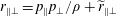
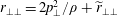
. Or in another words, the phase speeds of linear eigenmodes that are present in MHD do not hold in the collisionless (or weakly collisional) regime, and this effect exists even if the temperatures are isotropic. From a fluid perspective, the main reason for this discrepancy is that, in magnetized collisionless systems, the pressure fluctuations in the directions parallel and perpendicular to the magnetic field lines are not equivalent, and cannot be described with a single scalar pressure equation. The pressure fluctuations have to be described with two different evolution equations for
$v_{A}\leqslant v_{s}\leqslant v_{f}$
. Or in another words, the phase speeds of linear eigenmodes that are present in MHD do not hold in the collisionless (or weakly collisional) regime, and this effect exists even if the temperatures are isotropic. From a fluid perspective, the main reason for this discrepancy is that, in magnetized collisionless systems, the pressure fluctuations in the directions parallel and perpendicular to the magnetic field lines are not equivalent, and cannot be described with a single scalar pressure equation. The pressure fluctuations have to be described with two different evolution equations for
 $p_{\Vert }$
and
$p_{\Vert }$
and
 $p_{\bot }$
, even if the mean pressure values are equal
$p_{\bot }$
, even if the mean pressure values are equal
 $(p_{\Vert }^{(0)}=p_{\bot }^{(0)})$
and no mean temperature anisotropy exists.
$(p_{\Vert }^{(0)}=p_{\bot }^{(0)})$
and no mean temperature anisotropy exists.
The simplest collisionless fluid description is the CGL fluid model – named after Chew, Goldberger & Low (Reference Chew, Goldberger and Low1956) – and sometimes also referred to as collisionless MHD. The CGL dispersion relation is not equivalent to the MHD dispersion relation (even in the case
 $p_{\Vert }^{(0)}=p_{\bot }^{(0)}$
), since the pressure fluctuations still remain anisotropic and the evolution equations for
$p_{\Vert }^{(0)}=p_{\bot }^{(0)}$
), since the pressure fluctuations still remain anisotropic and the evolution equations for
 $p_{\Vert }$
and
$p_{\Vert }$
and
 $p_{\bot }$
remain different. In another words, in collisionless systems the distribution function is free to evolve from its initial state and to become anisotropic. By ‘forcibly’ prescribing only one scalar pressure, one effectively prescribes a high-collisionality regime, even if collisions are not prescribed explicitly. Formally, the MHD equations can indeed be derived from the collisionless Vlasov equation, i.e. with no explicit collisional operator. It is therefore often stated, that the MHD description is highly collisional implicitly. Moreover, as discussed for example by Kulsrud (Reference Kulsrud, Galeev and Sudan1983), while in the presence of a magnetic field, transverse motions can in some circumstances be described by fluid-type equations, the determination of pressures as well as longitudinal motions a priori requires a kinetic description.
$p_{\bot }$
remain different. In another words, in collisionless systems the distribution function is free to evolve from its initial state and to become anisotropic. By ‘forcibly’ prescribing only one scalar pressure, one effectively prescribes a high-collisionality regime, even if collisions are not prescribed explicitly. Formally, the MHD equations can indeed be derived from the collisionless Vlasov equation, i.e. with no explicit collisional operator. It is therefore often stated, that the MHD description is highly collisional implicitly. Moreover, as discussed for example by Kulsrud (Reference Kulsrud, Galeev and Sudan1983), while in the presence of a magnetic field, transverse motions can in some circumstances be described by fluid-type equations, the determination of pressures as well as longitudinal motions a priori requires a kinetic description.
Here we focus on collisionless fluid models. Nevertheless, weak collisions can be incorporated easily, and calculations just yield additional terms on the right-hand sides of the parallel and perpendicular pressure and heat flux equations. For the simple Bhatnagar–Gross–Krook (BGK) collisional operator (Bhatnagar, Gross & Krook Reference Bhatnagar, Gross and Krook1954), see for example Snyder, Hammett & Dorland (Reference Snyder, Hammett and Dorland1997). A thorough review of anisotropic fluid models, including the collisional dynamics, was presented by Barakat & Schunk (Reference Barakat and Schunk1982). A very good discussion about collisionality of various astrophysical plasmas, such as the solar wind, interstellar medium, accretion disks and galaxy clusters, can be found for example in Schekochihin et al. (Reference Schekochihin, Cowley, Dorland, Hammett, Howes, Quataert and Tatsung2009). Weakly collisional fluid models also seem to be applicable for modelling the upper solar photosphere and chromosphere, where a curious situation exists and the proton–proton collisional frequency is roughly equal to the proton cyclotron frequency – see for example figure 1 in Khomenko et al. (Reference Khomenko, Collados, Díaz and Vitas2014). We note that in this guide we use the definition of a ‘collisionless fluid model’ as being a fluid model that (i) is derived from the collisionless Vlasov equation with zero right-hand side; and (ii) that has two different pressure equations. Our definition therefore differs from an alternative view of for example Zank et al. (Reference Zank, Hunana, Mostafavi and Goldstein2014) and Zank (Reference Zank2014), where models with a scattering operator that reflects charged particle scattering by electromagnetic fluctuations on the right-hand side of the Vlasov equation are also viewed as collisionless.
Fluid modelling of collisionless plasmas is an extremely attractive subject, and an enormous amount of theoretical and numerical work was done in this field in the past. The manuscript presented here has no intention of being a proper review paper in this field. In our opinion, no satisfactory easy-to-read introductory paper exists about collisionless fluid models, and this manuscript attempts to fill such a spot. Instead of just stating the major results and discussing what was done in the past and by whom, we make a significant effort to present a (hopefully consistent) derivation of basic collisionless fluid models. On one hand, the presented calculations might be considered as too detailed in many places. On the other hand, it is exactly the relatively complicated algebra of collisionless fluid models, that makes the field difficult to enter for new researchers. The primary goal of this paper is to allow researchers new to the subject to follow the algebra easily. Instead of spending years, an interested reader should be able to become comfortable with the basics of the subject in a matter of days, or perhaps a couple of weeks. The text is separated to two parts. Part 1 is dedicated to fluid models that are obtained by closing the fluid hierarchy with simple (non-Landau fluid) closures. Part 2 is dedicated to Landau fluid closures.
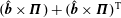
Here, in Part 1, § 2, we start with the detailed derivation of the pressure tensor equation. The pressure tensor
 $\boldsymbol{p}$
is then decomposed to its gyrotropic part
$\boldsymbol{p}$
is then decomposed to its gyrotropic part
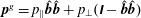 $\boldsymbol{p}^{g}=p_{\Vert }\hat{\boldsymbol{b}}\hat{\boldsymbol{b}}+p_{\bot }(\unicode[STIX]{x1D644}-\hat{\boldsymbol{b}}\hat{\boldsymbol{b}})$
(also referred to as
$\boldsymbol{p}^{g}=p_{\Vert }\hat{\boldsymbol{b}}\hat{\boldsymbol{b}}+p_{\bot }(\unicode[STIX]{x1D644}-\hat{\boldsymbol{b}}\hat{\boldsymbol{b}})$
(also referred to as
 $\boldsymbol{p}^{\text{CGL}}$
), and non-gyrotropic part
$\boldsymbol{p}^{\text{CGL}}$
), and non-gyrotropic part
 $\unicode[STIX]{x1D72B}$
, the latter usually called the finite Larmor radius (FLR) corrections to the pressure tensor, or the gyroviscous stress tensor. In the highly collisional decomposition
$\unicode[STIX]{x1D72B}$
, the latter usually called the finite Larmor radius (FLR) corrections to the pressure tensor, or the gyroviscous stress tensor. In the highly collisional decomposition
 $\boldsymbol{p}=p\unicode[STIX]{x1D644}+\unicode[STIX]{x1D72B}$
, see e.g. Braginskii (Reference Braginskii1958, Reference Braginskii1965), the quantity
$\boldsymbol{p}=p\unicode[STIX]{x1D644}+\unicode[STIX]{x1D72B}$
, see e.g. Braginskii (Reference Braginskii1958, Reference Braginskii1965), the quantity
 $\unicode[STIX]{x1D72B}$
is called the stress tensor. The decomposition procedure yields rigorously exact (even though still not closed) evolution equations for
$\unicode[STIX]{x1D72B}$
is called the stress tensor. The decomposition procedure yields rigorously exact (even though still not closed) evolution equations for
 $p_{\Vert }$
and
$p_{\Vert }$
and
 $p_{\bot }$
, see e.g. Oraevskii, Chodura & Feneberg (Reference Oraevskii, Chodura and Feneberg1968), Passot & Sulem (Reference Passot and Sulem2004) and Goswami, Passot & Sulem (Reference Goswami, Passot and Sulem2005). Importantly, at the leading order (by neglecting the
$p_{\bot }$
, see e.g. Oraevskii, Chodura & Feneberg (Reference Oraevskii, Chodura and Feneberg1968), Passot & Sulem (Reference Passot and Sulem2004) and Goswami, Passot & Sulem (Reference Goswami, Passot and Sulem2005). Importantly, at the leading order (by neglecting the
 $\unicode[STIX]{x1D72B}$
and also the non-gyrotropic heat flux contributions
$\unicode[STIX]{x1D72B}$
and also the non-gyrotropic heat flux contributions
 $\boldsymbol{q}^{\text{ng}}$
), the equations of Chew et al. (Reference Chew, Goldberger and Low1956), hereafter referred to as CGL, are recovered. We discuss the paper by Chew et al. (Reference Chew, Goldberger and Low1956) and point out that the paper derived the correct form of the pressure equations with the gyrotropic heat flux contributions included, however, the quantities
$\boldsymbol{q}^{\text{ng}}$
), the equations of Chew et al. (Reference Chew, Goldberger and Low1956), hereafter referred to as CGL, are recovered. We discuss the paper by Chew et al. (Reference Chew, Goldberger and Low1956) and point out that the paper derived the correct form of the pressure equations with the gyrotropic heat flux contributions included, however, the quantities
 $q_{n},q_{s}$
used in that paper are related to the usual
$q_{n},q_{s}$
used in that paper are related to the usual
 $q_{\Vert },q_{\bot }$
by relations
$q_{\Vert },q_{\bot }$
by relations
 $q_{n}=q_{\Vert }-3q_{\bot }$
and
$q_{n}=q_{\Vert }-3q_{\bot }$
and
 $q_{s}=q_{\bot }$
. By further neglecting the heat flux contributions, the pressure equations can be written in conservative form. The resulting pressure equations became known as the CGL equations, and they can be interpreted as the conservation laws for the first and second adiabatic invariants (Kulsrud Reference Kulsrud, Galeev and Sudan1983; Gurnett & Bhattacharjee Reference Gurnett and Bhattacharjee2005).
$q_{s}=q_{\bot }$
. By further neglecting the heat flux contributions, the pressure equations can be written in conservative form. The resulting pressure equations became known as the CGL equations, and they can be interpreted as the conservation laws for the first and second adiabatic invariants (Kulsrud Reference Kulsrud, Galeev and Sudan1983; Gurnett & Bhattacharjee Reference Gurnett and Bhattacharjee2005).
Furthermore, we discuss the general equations of collisionless multi-fluid models. The pressure equations are rigorously exact, even though the system is not closed, since the FLR pressure tensor and the entire heat flux tensor are not specified; for a quick look see (2.89)–(2.92). Rewriting the system to a form where the usual CGL conservation laws are on the left-hand side, and all other contributions on the right-hand side, nicely represents the complicated plasma heating processes that can be encountered, and that are responsible for the breaking of the adiabatic invariants; see (2.100), (2.101). We also discuss the conservation of energy. For the case of periodic boundary conditions, the total conservation of energy has a very illuminating form, that can be found for example in Yang et al. (Reference Yang, Matthaeus, Parashar, Haggerty, Roytershteyn, Daughton, Wan, Shi and Chen2017a
,Reference Yang, Matthaeus, Parashar, Wu, Wan, Shi, Chen, Roytershteyn and Daughton
b
). That formulation is obtained by considering the total ‘internal’ energy for each particle species
 $E_{r}^{\text{int}}=\frac{1}{2}\langle \text{Tr}\,\boldsymbol{p}_{r}\rangle$
(where the brackets represent integration over the entire spatial domain), which only reveals the total plasma heating. Here, we split the internal energy into its parallel and perpendicular components
$E_{r}^{\text{int}}=\frac{1}{2}\langle \text{Tr}\,\boldsymbol{p}_{r}\rangle$
(where the brackets represent integration over the entire spatial domain), which only reveals the total plasma heating. Here, we split the internal energy into its parallel and perpendicular components
 $E_{\Vert r}^{\text{int}}=\frac{1}{2}\langle p_{\Vert r}\rangle$
,
$E_{\Vert r}^{\text{int}}=\frac{1}{2}\langle p_{\Vert r}\rangle$
,
 $E_{\bot r}^{\text{int}}=\langle p_{\bot r}\rangle$
, and formulate the total conservation of energy with the possibility of anisotropic plasma heating, see (2.113)–(2.116).
$E_{\bot r}^{\text{int}}=\langle p_{\bot r}\rangle$
, and formulate the total conservation of energy with the possibility of anisotropic plasma heating, see (2.113)–(2.116).
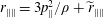
The CGL description is analysed in great detail in § 3. We derive the CGL dispersion relation, and discuss properties of the slow, Alfvén and fast modes that are present. We verify many of the classical results of Abraham-Shrauner (Reference Abraham-Shrauner1967), here written in a slightly more convenient notation by using the parallel plasma beta
 $\unicode[STIX]{x1D6FD}_{\Vert }$
, and the temperature anisotropy ratio
$\unicode[STIX]{x1D6FD}_{\Vert }$
, and the temperature anisotropy ratio
 $a_{p}=T_{\bot }/T_{\Vert }$
. Collisionless plasmas cannot reach arbitrarily large values of temperature anisotropy, and the linear CGL eigenmodes can indeed become unstable, with the associated instabilities referred to as the (parallel and oblique) firehose instability and the mirror instability. Similarly to MHD, the simple CGL description does not contain any dispersive effects and is technically scale invariant, even though valid only on the largest scales. The instability thresholds present in the CGL model therefore can be referred to as ‘hard’ thresholds, i.e. thresholds that are obtained in the long-wavelength low-frequency limit. The firehose and mirror instabilities are believed to play a crucial role in solar wind dynamics (see e.g. Hellinger et al.
Reference Hellinger, Trávníček, Kasper and Lazarus2006; Bale et al.
Reference Bale, Kasper, Howes, Quataert, Salem and Sundkvist2009), and in figure 1, they are plotted in the usual
$a_{p}=T_{\bot }/T_{\Vert }$
. Collisionless plasmas cannot reach arbitrarily large values of temperature anisotropy, and the linear CGL eigenmodes can indeed become unstable, with the associated instabilities referred to as the (parallel and oblique) firehose instability and the mirror instability. Similarly to MHD, the simple CGL description does not contain any dispersive effects and is technically scale invariant, even though valid only on the largest scales. The instability thresholds present in the CGL model therefore can be referred to as ‘hard’ thresholds, i.e. thresholds that are obtained in the long-wavelength low-frequency limit. The firehose and mirror instabilities are believed to play a crucial role in solar wind dynamics (see e.g. Hellinger et al.
Reference Hellinger, Trávníček, Kasper and Lazarus2006; Bale et al.
Reference Bale, Kasper, Howes, Quataert, Salem and Sundkvist2009), and in figure 1, they are plotted in the usual
 $\unicode[STIX]{x1D6FD}_{\Vert }-T_{\bot }/T_{\Vert }$
plane with logarithmic scales. While the firehose threshold matches the one obtained from kinetic theory, the CGL mirror threshold contains the well-known factor of 6 error for large
$\unicode[STIX]{x1D6FD}_{\Vert }-T_{\bot }/T_{\Vert }$
plane with logarithmic scales. While the firehose threshold matches the one obtained from kinetic theory, the CGL mirror threshold contains the well-known factor of 6 error for large
 $\unicode[STIX]{x1D6FD}_{\Vert }$
values. The factor of 6 error can be interpreted as inadequacy of the adiabatic CGL closure in the very slow-dynamics context, such as the mirror instability. This is further addressed in § 9.4, where we discuss that the ‘static’ closure, which can be viewed as a generalization of isothermal closure in the presence of temperature anisotropy and variations of magnetic field strength, reproduces the correct mirror threshold (Constantinescu Reference Constantinescu2002; Chust & Belmont Reference Chust and Belmont2006; Passot, Ruban & Sulem Reference Passot, Ruban and Sulem2006).
$\unicode[STIX]{x1D6FD}_{\Vert }$
values. The factor of 6 error can be interpreted as inadequacy of the adiabatic CGL closure in the very slow-dynamics context, such as the mirror instability. This is further addressed in § 9.4, where we discuss that the ‘static’ closure, which can be viewed as a generalization of isothermal closure in the presence of temperature anisotropy and variations of magnetic field strength, reproduces the correct mirror threshold (Constantinescu Reference Constantinescu2002; Chust & Belmont Reference Chust and Belmont2006; Passot, Ruban & Sulem Reference Passot, Ruban and Sulem2006).
We discuss the core differences between MHD and CGL, which can be nicely summarized with the concept of adiabatic indices
 $\unicode[STIX]{x1D6FE}$
, related to the number of degrees of freedom
$\unicode[STIX]{x1D6FE}$
, related to the number of degrees of freedom
 $i$
by
$i$
by
 $\unicode[STIX]{x1D6FE}=(i+2)/i$
. While MHD is fully three-dimensional with
$\unicode[STIX]{x1D6FE}=(i+2)/i$
. While MHD is fully three-dimensional with
 $\unicode[STIX]{x1D6FE}=5/3$
, the CGL can be viewed as composed of one- and two-dimensional dynamics with
$\unicode[STIX]{x1D6FE}=5/3$
, the CGL can be viewed as composed of one- and two-dimensional dynamics with
 $\unicode[STIX]{x1D6FE}_{\Vert }=3$
and
$\unicode[STIX]{x1D6FE}_{\Vert }=3$
and
 $\unicode[STIX]{x1D6FE}_{\bot }=2$
. We also address the velocity and magnetic field eigenvectors. Similarly to the velocity field eigenvector in MHD (see figure 2), which shows a ‘singular’ behaviour for strictly parallel propagation with
$\unicode[STIX]{x1D6FE}_{\bot }=2$
. We also address the velocity and magnetic field eigenvectors. Similarly to the velocity field eigenvector in MHD (see figure 2), which shows a ‘singular’ behaviour for strictly parallel propagation with
 $V_{A}=C_{s}$
, the CGL eigenvector (figure 3) shows similar singularity for
$V_{A}=C_{s}$
, the CGL eigenvector (figure 3) shows similar singularity for
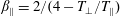 $\unicode[STIX]{x1D6FD}_{\Vert }=2/(4-T_{\bot }/T_{\Vert })$
. We also briefly discuss fluid models with empirical ‘free’ polytropic indices
$\unicode[STIX]{x1D6FD}_{\Vert }=2/(4-T_{\bot }/T_{\Vert })$
. We also briefly discuss fluid models with empirical ‘free’ polytropic indices
 $\unicode[STIX]{x1D6FE}_{\Vert },\unicode[STIX]{x1D6FE}_{\bot }$
, studied for example by Hau & Sonnerup (Reference Hau and Sonnerup1993), Hau et al. (Reference Hau, Phan, Sonnerup and Paschmann1993) and Abraham-Shrauner (Reference Abraham-Shrauner1973).
$\unicode[STIX]{x1D6FE}_{\Vert },\unicode[STIX]{x1D6FE}_{\bot }$
, studied for example by Hau & Sonnerup (Reference Hau and Sonnerup1993), Hau et al. (Reference Hau, Phan, Sonnerup and Paschmann1993) and Abraham-Shrauner (Reference Abraham-Shrauner1973).
In § 4, we introduce the simplest dispersive effects by including the Hall term into the induction equation, and study dispersion relations of the Hall-CGL model. We focus on the parallel firehose instability, and show that the instability is indeed associated with the whistler mode, see figures 4 and 5. We show that negative real frequencies
 $\unicode[STIX]{x1D714}_{r}<0$
have to be handled carefully, and that non-causal analytic solutions (4.32)–(4.35) have to be modified to the causal form (4.43)–(4.46). We briefly discuss the simplest ion-cyclotron resonances, and compare solutions of the Hall-CGL model with solutions of linear kinetic theory, see figure 6.
$\unicode[STIX]{x1D714}_{r}<0$
have to be handled carefully, and that non-causal analytic solutions (4.32)–(4.35) have to be modified to the causal form (4.43)–(4.46). We briefly discuss the simplest ion-cyclotron resonances, and compare solutions of the Hall-CGL model with solutions of linear kinetic theory, see figure 6.
In § 5, we evaluate the FLR tensor
 $\unicode[STIX]{x1D72B}$
at several levels of approximation. The evaluation of the FLR tensor is cumbersome, because the tensor is described by the pressure tensor equation implicitly. We first reproduce the fully nonlinear ‘inversion’ procedure on how to obtain
$\unicode[STIX]{x1D72B}$
at several levels of approximation. The evaluation of the FLR tensor is cumbersome, because the tensor is described by the pressure tensor equation implicitly. We first reproduce the fully nonlinear ‘inversion’ procedure on how to obtain
 $\unicode[STIX]{x1D72B}$
from expression
$\unicode[STIX]{x1D72B}$
from expression
 $(\hat{\boldsymbol{b}}\times \unicode[STIX]{x1D72B})+(\hat{\boldsymbol{b}}\times \unicode[STIX]{x1D72B})^{\text{T}}$
that can be found for example in Hsu, Hazeltine & Morrison (Reference Hsu, Hazeltine and Morrison1986), Passot & Sulem (Reference Passot and Sulem2004) and Ramos (Reference Ramos2005) as a brief note. Applying this inversion procedure to the pressure tensor equation evaluates the FLR corrections correctly along the magnetic field lines, but leads to an equation for
$(\hat{\boldsymbol{b}}\times \unicode[STIX]{x1D72B})+(\hat{\boldsymbol{b}}\times \unicode[STIX]{x1D72B})^{\text{T}}$
that can be found for example in Hsu, Hazeltine & Morrison (Reference Hsu, Hazeltine and Morrison1986), Passot & Sulem (Reference Passot and Sulem2004) and Ramos (Reference Ramos2005) as a brief note. Applying this inversion procedure to the pressure tensor equation evaluates the FLR corrections correctly along the magnetic field lines, but leads to an equation for
 $\unicode[STIX]{x1D72B}$
that is still implicit. Nevertheless, evaluating the resulting equation at the leading order (technically first order in frequency and wavenumber), leads to an explicit expression for
$\unicode[STIX]{x1D72B}$
that is still implicit. Nevertheless, evaluating the resulting equation at the leading order (technically first order in frequency and wavenumber), leads to an explicit expression for
 $\unicode[STIX]{x1D72B}$
. We first recover the nonlinear result of Schekochihin et al. (Reference Schekochihin, Cowley, Rincon and Rosin2010), derived in that paper slightly differently, without using the inversion procedure. We point out that the result can be slightly simplified, and rearranging the expression yields two different useful forms for writing the nonlinear
$\unicode[STIX]{x1D72B}$
. We first recover the nonlinear result of Schekochihin et al. (Reference Schekochihin, Cowley, Rincon and Rosin2010), derived in that paper slightly differently, without using the inversion procedure. We point out that the result can be slightly simplified, and rearranging the expression yields two different useful forms for writing the nonlinear
 $\unicode[STIX]{x1D72B}$
. Finally, by using the non-dispersive (MHD) induction equation, we obtain the nonlinear result of Ramos (Reference Ramos2005) (see also Macmahon (Reference Macmahon1965)). For further evaluation of nonlinear FLR corrections to higher orders, an advanced reader is referred to Ramos (Reference Ramos2005). We continue with the evaluation of the FLR tensor in the linear approximation, i.e. when the magnetic field lines are not too distorted. For the first-order tensor (here called FLR1), we recover the classical result of Yajima (Reference Yajima1966), which is notably different from the one provided by Oraevskii et al. (Reference Oraevskii, Chodura and Feneberg1968). In the isotropic case, the FLR1 tensor is consistent with the one extracted from the stress tensor of Braginskii (Reference Braginskii1965), if the collisional terms are ‘ignored’. It is noteworthy that a proper collisionless limit cannot be achieved from the stress tensor of Braginskii (Reference Braginskii1965), because expressions are proportional to
$\unicode[STIX]{x1D72B}$
. Finally, by using the non-dispersive (MHD) induction equation, we obtain the nonlinear result of Ramos (Reference Ramos2005) (see also Macmahon (Reference Macmahon1965)). For further evaluation of nonlinear FLR corrections to higher orders, an advanced reader is referred to Ramos (Reference Ramos2005). We continue with the evaluation of the FLR tensor in the linear approximation, i.e. when the magnetic field lines are not too distorted. For the first-order tensor (here called FLR1), we recover the classical result of Yajima (Reference Yajima1966), which is notably different from the one provided by Oraevskii et al. (Reference Oraevskii, Chodura and Feneberg1968). In the isotropic case, the FLR1 tensor is consistent with the one extracted from the stress tensor of Braginskii (Reference Braginskii1965), if the collisional terms are ‘ignored’. It is noteworthy that a proper collisionless limit cannot be achieved from the stress tensor of Braginskii (Reference Braginskii1965), because expressions are proportional to
 $\unicode[STIX]{x1D70F}$
(and also
$\unicode[STIX]{x1D70F}$
(and also
 $1/\unicode[STIX]{x1D70F}$
), where
$1/\unicode[STIX]{x1D70F}$
), where
 $\unicode[STIX]{x1D70F}$
is time between two collisions (
$\unicode[STIX]{x1D70F}$
is time between two collisions (
 $\unicode[STIX]{x1D70F}\sim 1/\unicode[STIX]{x1D708}$
where
$\unicode[STIX]{x1D70F}\sim 1/\unicode[STIX]{x1D708}$
where
 $\unicode[STIX]{x1D708}$
is the usual collisional frequency), so the collisionless limit
$\unicode[STIX]{x1D708}$
is the usual collisional frequency), so the collisionless limit
 $\unicode[STIX]{x1D70F}\rightarrow \infty$
does not work.
$\unicode[STIX]{x1D70F}\rightarrow \infty$
does not work.
We consider the Hall-CGL-FLR1 fluid model, and we provide dispersion relation for generally oblique propagation, which can be also found in Hunana & Zank (Reference Hunana and Zank2017). For higher-order FLR corrections, we only provide analytic dispersion relations for the parallel propagating whistler and ion-cyclotron modes, as well as the perpendicular fast mode. Nevertheless, we provide linearized, normalized and Fourier transformed equations written in the
 $x$
–
$x$
–
 $z$
plane for all the fluid models. To obtain the dispersion relation for an oblique propagation, the reader is encouraged to use analytic software such as Maple or Mathematica, or to solve the system numerically. The second-order FLR corrections (FLR2) are here defined as containing the Hall term and the time derivative
$z$
plane for all the fluid models. To obtain the dispersion relation for an oblique propagation, the reader is encouraged to use analytic software such as Maple or Mathematica, or to solve the system numerically. The second-order FLR corrections (FLR2) are here defined as containing the Hall term and the time derivative
 $\unicode[STIX]{x2202}\unicode[STIX]{x1D72B}/\unicode[STIX]{x2202}t$
. We also consider FLR corrections with the non-gyrotropic heat flux vectors
$\unicode[STIX]{x2202}\unicode[STIX]{x1D72B}/\unicode[STIX]{x2202}t$
. We also consider FLR corrections with the non-gyrotropic heat flux vectors
 $\boldsymbol{S}_{\bot }^{\Vert }$
,
$\boldsymbol{S}_{\bot }^{\Vert }$
,
 $\boldsymbol{S}_{\bot }^{\bot }$
, that are here defined as FLR3. The precision of various FLR corrections can be compared nicely by considering the perpendicular fast mode in the long-wavelength limit. The comparison is especially meaningful, when written in the notation of Del Sarto, Pegoraro & Tenerani (Reference Del Sarto, Pegoraro and Tenerani2017), see (5.119)–(5.121). We proceed by showing that the FLR3 corrections (with the second-order non-gyrotropic heat flux vectors) indeed recover the fully kinetic dispersion relation for the fast mode in the long-wavelength (low-frequency) limit, a result reported by Mikhailovskii & Smolyakov (Reference Mikhailovskii and Smolyakov1985). Instead of expanding the pressure tensor equation, one can derive very precise linear FLR corrections from linear kinetic theory, which is not addressed here, and the reader is referred to papers by Passot & Sulem (Reference Passot and Sulem2007) and Sulem & Passot (Reference Sulem and Passot2015) and references therein.
$\boldsymbol{S}_{\bot }^{\bot }$
, that are here defined as FLR3. The precision of various FLR corrections can be compared nicely by considering the perpendicular fast mode in the long-wavelength limit. The comparison is especially meaningful, when written in the notation of Del Sarto, Pegoraro & Tenerani (Reference Del Sarto, Pegoraro and Tenerani2017), see (5.119)–(5.121). We proceed by showing that the FLR3 corrections (with the second-order non-gyrotropic heat flux vectors) indeed recover the fully kinetic dispersion relation for the fast mode in the long-wavelength (low-frequency) limit, a result reported by Mikhailovskii & Smolyakov (Reference Mikhailovskii and Smolyakov1985). Instead of expanding the pressure tensor equation, one can derive very precise linear FLR corrections from linear kinetic theory, which is not addressed here, and the reader is referred to papers by Passot & Sulem (Reference Passot and Sulem2007) and Sulem & Passot (Reference Sulem and Passot2015) and references therein.
In § 6, we investigate the parallel and oblique firehose instability. The FLR and Hall dispersive effects are crucial for the stabilization of the firehose instability at small scales, and a comprehensive discussion can be found in Hunana & Zank (Reference Hunana and Zank2017). That paper was essentially extracted from this guide (with many figures that we do not republish here), and an interested reader who wants to focus on the firehose instability can find further information there. Nevertheless, here we briefly investigate improvements that can be made by considering the FLR2 and FLR3 corrections, see figures 7–11. Importantly, we show that the non-gyrotropic heat flux vectors in the FLR3 model, partially reproduce the large ‘bump’ in the imaginary phase speed (growth rate normalized to the wavenumber), when the plasma is close to the long-wavelength limit ‘hard’ firehose threshold, see figure 7. The firehose instability in a fluid formalism was also investigated by Wang & Hau (Reference Wang and Hau2003, Reference Wang and Hau2010), Schekochihin et al. (Reference Schekochihin, Cowley, Rincon and Rosin2010) and Rosin et al. (Reference Rosin, Schekochihin, Rincon and Cowley2011) and references therein.
In § 7, we derive the heat flux tensor equation. The heat flux tensor is then decomposed into its gyrotropic and non-gyrotropic parts,
 $\boldsymbol{q}=\boldsymbol{q}^{\text{g}}+\boldsymbol{q}^{\text{ng}}$
. The procedure yields evolution equations for the gyrotropic parallel and perpendicular heat fluxes,
$\boldsymbol{q}=\boldsymbol{q}^{\text{g}}+\boldsymbol{q}^{\text{ng}}$
. The procedure yields evolution equations for the gyrotropic parallel and perpendicular heat fluxes,
 $q_{\Vert }$
and
$q_{\Vert }$
and
 $q_{\bot }$
, that contain the tensor of the fourth-order moment
$q_{\bot }$
, that contain the tensor of the fourth-order moment
 $\boldsymbol{r}$
. It is emphasized that, if one wants to keep the non-gyrotropic
$\boldsymbol{r}$
. It is emphasized that, if one wants to keep the non-gyrotropic
 $\unicode[STIX]{x1D72B}$
contributions in the scalar heat flux equations, one needs to keep the non-gyrotropic contributions of the fourth-order moment
$\unicode[STIX]{x1D72B}$
contributions in the scalar heat flux equations, one needs to keep the non-gyrotropic contributions of the fourth-order moment
 $\boldsymbol{r}^{\text{ng}}$
as well, since there are several possible cancellations even at the linear level. The non-gyrotropic heat flux
$\boldsymbol{r}^{\text{ng}}$
as well, since there are several possible cancellations even at the linear level. The non-gyrotropic heat flux
 $\boldsymbol{q}^{\text{ng}}$
can be further decomposed to the non-gyrotropic heat flux vectors
$\boldsymbol{q}^{\text{ng}}$
can be further decomposed to the non-gyrotropic heat flux vectors
 $\boldsymbol{S}_{\bot }^{\Vert }$
,
$\boldsymbol{S}_{\bot }^{\Vert }$
,
 $\boldsymbol{S}_{\bot }^{\bot }$
and tensor
$\boldsymbol{S}_{\bot }^{\bot }$
and tensor
 $\unicode[STIX]{x1D748}$
. The detailed algebra of the non-gyrotropic heat flux vectors
$\unicode[STIX]{x1D748}$
. The detailed algebra of the non-gyrotropic heat flux vectors
 $\boldsymbol{S}_{\bot }^{\Vert }$
,
$\boldsymbol{S}_{\bot }^{\Vert }$
,
 $\boldsymbol{S}_{\bot }^{\bot }$
, i.e. how to express them through lower-order moments, is presented in appendix D. The first-order expressions are obtained at the nonlinear level and the second-order expressions at the linear level. We do not address how to decompose the tensor
$\boldsymbol{S}_{\bot }^{\bot }$
, i.e. how to express them through lower-order moments, is presented in appendix D. The first-order expressions are obtained at the nonlinear level and the second-order expressions at the linear level. We do not address how to decompose the tensor
 $\unicode[STIX]{x1D748}$
through lower-order moments. Such calculations require a complicated ‘inversion’ procedure for a third-rank tensor
$\unicode[STIX]{x1D748}$
through lower-order moments. Such calculations require a complicated ‘inversion’ procedure for a third-rank tensor
 $(\hat{\boldsymbol{b}}\times \unicode[STIX]{x1D748})^{S}$
, and an advanced reader is referred to Ramos (Reference Ramos2005).
$(\hat{\boldsymbol{b}}\times \unicode[STIX]{x1D748})^{S}$
, and an advanced reader is referred to Ramos (Reference Ramos2005).
In § 8, we consider the fourth-order moment
 $\boldsymbol{r}$
which is a tensor of fourth rank,
$\boldsymbol{r}$
which is a tensor of fourth rank,
 $r_{ijkl}$
. The moment is again decomposed to its gyrotropic and non-gyrotropic parts,
$r_{ijkl}$
. The moment is again decomposed to its gyrotropic and non-gyrotropic parts,
 $\boldsymbol{r}=\boldsymbol{r}^{\text{g}}+\boldsymbol{r}^{\text{ng}}$
and the gyrotropic part has three scalar components,
$\boldsymbol{r}=\boldsymbol{r}^{\text{g}}+\boldsymbol{r}^{\text{ng}}$
and the gyrotropic part has three scalar components,
 $r_{\Vert \Vert }$
,
$r_{\Vert \Vert }$
,
 $r_{\Vert \bot }$
and
$r_{\Vert \bot }$
and
 $r_{\bot \bot }$
. We show that for a bi-Maxwellian distribution function, the gyrotropic components can indeed be evaluated as
$r_{\bot \bot }$
. We show that for a bi-Maxwellian distribution function, the gyrotropic components can indeed be evaluated as
 $r_{\Vert \Vert }=3p_{\Vert }^{2}/\unicode[STIX]{x1D70C}$
,
$r_{\Vert \Vert }=3p_{\Vert }^{2}/\unicode[STIX]{x1D70C}$
,
 $r_{\Vert \bot }=p_{\Vert }p_{\bot }/\unicode[STIX]{x1D70C}$
and
$r_{\Vert \bot }=p_{\Vert }p_{\bot }/\unicode[STIX]{x1D70C}$
and
 $r_{\bot \bot }=2p_{\bot }^{2}/\unicode[STIX]{x1D70C}$
. This constitutes a ‘normal’ closure, a name suggested by Chust & Belmont (Reference Chust and Belmont2006). By using a similar procedure to the one provided by Grad (Reference Grad1949) for dilute gases, it is possible to express the non-gyrotropic bi-Maxwellian
$r_{\bot \bot }=2p_{\bot }^{2}/\unicode[STIX]{x1D70C}$
. This constitutes a ‘normal’ closure, a name suggested by Chust & Belmont (Reference Chust and Belmont2006). By using a similar procedure to the one provided by Grad (Reference Grad1949) for dilute gases, it is possible to express the non-gyrotropic bi-Maxwellian
 $\boldsymbol{r}^{\text{ng}}$
through a combination of
$\boldsymbol{r}^{\text{ng}}$
through a combination of
 $\boldsymbol{p}^{g}$
and
$\boldsymbol{p}^{g}$
and
 $\unicode[STIX]{x1D72B}$
, see e.g. Oraevskii et al. (Reference Oraevskii, Chodura and Feneberg1968).
$\unicode[STIX]{x1D72B}$
, see e.g. Oraevskii et al. (Reference Oraevskii, Chodura and Feneberg1968).
In § 9, a dispersion relation of a fluid model closed with the bi-Maxwellian ‘normal’ closure is provided for generally oblique propagation, and we call this model second-order CGL (CGL2). We specifically focus on the mirror instability, since this simple fluid model (without any Landau damping) corrects the erroneous
 $1/6$
factor in the ‘hard’ mirror threshold found in the basic CGL description, a result also reported by Dzhalilov, Kuznetsov & Staude (Reference Dzhalilov, Kuznetsov and Staude2011). The mirror instability is not addressed to a higher level of sophistication in this guide. However, we note that capturing the mirror growth rate (when the threshold is crossed) sufficiently well requires Landau fluid models (Snyder et al.
Reference Snyder, Hammett and Dorland1997) and the stabilization at small scales requires FLR corrections (Passot & Sulem Reference Passot and Sulem2007; Sulem & Passot Reference Sulem and Passot2015). We also provide the dispersion relation of the Hall-CGL2 fluid model. Finally, the CGL2 model can be simplified by considering slow-dynamics regime and constructing generalized isothermal closure that is called the ‘static’ closure, yielding the simplest fluid model that captures the correct mirror threshold (Constantinescu Reference Constantinescu2002; Chust & Belmont Reference Chust and Belmont2006; Passot et al.
Reference Passot, Ruban and Sulem2006).
$1/6$
factor in the ‘hard’ mirror threshold found in the basic CGL description, a result also reported by Dzhalilov, Kuznetsov & Staude (Reference Dzhalilov, Kuznetsov and Staude2011). The mirror instability is not addressed to a higher level of sophistication in this guide. However, we note that capturing the mirror growth rate (when the threshold is crossed) sufficiently well requires Landau fluid models (Snyder et al.
Reference Snyder, Hammett and Dorland1997) and the stabilization at small scales requires FLR corrections (Passot & Sulem Reference Passot and Sulem2007; Sulem & Passot Reference Sulem and Passot2015). We also provide the dispersion relation of the Hall-CGL2 fluid model. Finally, the CGL2 model can be simplified by considering slow-dynamics regime and constructing generalized isothermal closure that is called the ‘static’ closure, yielding the simplest fluid model that captures the correct mirror threshold (Constantinescu Reference Constantinescu2002; Chust & Belmont Reference Chust and Belmont2006; Passot et al.
Reference Passot, Ruban and Sulem2006).
In § 10, we consider the bi-kappa distribution function. We show that the closure at the fourth-order moment is constructed by
 $r_{\Vert \Vert }=\unicode[STIX]{x1D6FC}_{\unicode[STIX]{x1D705}}3p_{\Vert }^{2}/\unicode[STIX]{x1D70C}$
,
$r_{\Vert \Vert }=\unicode[STIX]{x1D6FC}_{\unicode[STIX]{x1D705}}3p_{\Vert }^{2}/\unicode[STIX]{x1D70C}$
,
 $r_{\Vert \bot }=\unicode[STIX]{x1D6FC}_{\unicode[STIX]{x1D705}}p_{\Vert }p_{\bot }/\unicode[STIX]{x1D70C}$
and
$r_{\Vert \bot }=\unicode[STIX]{x1D6FC}_{\unicode[STIX]{x1D705}}p_{\Vert }p_{\bot }/\unicode[STIX]{x1D70C}$
and
 $r_{\bot \bot }=\unicode[STIX]{x1D6FC}_{\unicode[STIX]{x1D705}}2p_{\bot }^{2}/\unicode[STIX]{x1D70C}$
, where the coefficient
$r_{\bot \bot }=\unicode[STIX]{x1D6FC}_{\unicode[STIX]{x1D705}}2p_{\bot }^{2}/\unicode[STIX]{x1D70C}$
, where the coefficient
 $\unicode[STIX]{x1D6FC}_{\unicode[STIX]{x1D705}}=(\unicode[STIX]{x1D705}-3/2)/(\unicode[STIX]{x1D705}-5/2)$
, and the closure is valid for
$\unicode[STIX]{x1D6FC}_{\unicode[STIX]{x1D705}}=(\unicode[STIX]{x1D705}-3/2)/(\unicode[STIX]{x1D705}-5/2)$
, and the closure is valid for
 $\unicode[STIX]{x1D705}>5/2$
. We call this closure and the associated fluid model ‘BiKappa’, and we discuss its dispersion relations. Even though the linear modes are generally different in this fluid model than in the CGL2 fluid model, we show that the ‘hard’ thresholds for the parallel and oblique firehose instability, and for the highly oblique mirror instability, are not affected by and are independent of the
$\unicode[STIX]{x1D705}>5/2$
. We call this closure and the associated fluid model ‘BiKappa’, and we discuss its dispersion relations. Even though the linear modes are generally different in this fluid model than in the CGL2 fluid model, we show that the ‘hard’ thresholds for the parallel and oblique firehose instability, and for the highly oblique mirror instability, are not affected by and are independent of the
 $\unicode[STIX]{x1D705}$
value. The Hall-BiKappa fluid dispersion relation is also provided. We also provide the first-order non-gyrotropic heat flux vectors
$\unicode[STIX]{x1D705}$
value. The Hall-BiKappa fluid dispersion relation is also provided. We also provide the first-order non-gyrotropic heat flux vectors
 $\boldsymbol{S}_{\bot }^{\Vert }$
,
$\boldsymbol{S}_{\bot }^{\Vert }$
,
 $\boldsymbol{S}_{\bot }^{\bot }$
. We do not calculate the
$\boldsymbol{S}_{\bot }^{\bot }$
. We do not calculate the
 $\boldsymbol{r}^{\text{ng}}$
for the bi-kappa distribution, and therefore we do not provide the second-order non-gyrotropic heat flux vectors.
$\boldsymbol{r}^{\text{ng}}$
for the bi-kappa distribution, and therefore we do not provide the second-order non-gyrotropic heat flux vectors.
In § 11, we discuss the core differences between the usual fluid models and kinetic theory. Namely, we discuss why the usual fluid models do not contain collisionless damping mechanisms, such as Landau damping, regardless of the order to which the fluid hierarchy is developed. The effect of Landau damping is present in the collisionless Vlasov equation, and the crucial difference between the usual fluid hierarchy and kinetic calculations just lies in the technique of how the Vlasov equation is integrated over the velocity space. We introduce preliminary ideas as to how the Landau fluid closures will be constructed. For example, for closures performed at the fourth-order moment instead of the ‘normal’ closure, one needs to consider perturbations around this state, and prescribe
 $r_{\Vert \Vert }=3p_{\Vert }^{2}/\unicode[STIX]{x1D70C}+\widetilde{r}_{\Vert \Vert }$
,
$r_{\Vert \Vert }=3p_{\Vert }^{2}/\unicode[STIX]{x1D70C}+\widetilde{r}_{\Vert \Vert }$
,
 $r_{\Vert \bot }=p_{\Vert }p_{\bot }/\unicode[STIX]{x1D70C}+\widetilde{r}_{\Vert \bot }$
and
$r_{\Vert \bot }=p_{\Vert }p_{\bot }/\unicode[STIX]{x1D70C}+\widetilde{r}_{\Vert \bot }$
and
 $r_{\bot \bot }=2p_{\bot }^{2}/\unicode[STIX]{x1D70C}+\widetilde{r}_{\bot \bot }$
. The deviations
$r_{\bot \bot }=2p_{\bot }^{2}/\unicode[STIX]{x1D70C}+\widetilde{r}_{\bot \bot }$
. The deviations
 $\widetilde{r}_{\Vert \Vert }$
,
$\widetilde{r}_{\Vert \Vert }$
,
 $\widetilde{r}_{\Vert \bot }$
,
$\widetilde{r}_{\Vert \bot }$
,
 $\widetilde{r}_{\bot \bot }$
will be calculated from linear kinetic theory in Part 2, by performing Landau fluid closures.
$\widetilde{r}_{\bot \bot }$
will be calculated from linear kinetic theory in Part 2, by performing Landau fluid closures.
In § 12, we derive the evolution equation for a general
 $n$
th-order fluid moment (a tensor with
$n$
th-order fluid moment (a tensor with
 $3^{n}$
components). We then consider fluid models in the simplified one-dimensional (1-D) geometry that can be viewed as an electrostatic case (or as a propagation along the mean magnetic field), and that are closed at a general
$3^{n}$
components). We then consider fluid models in the simplified one-dimensional (1-D) geometry that can be viewed as an electrostatic case (or as a propagation along the mean magnetic field), and that are closed at a general
 $n$
th-order level by a Maxwellian fluid closure. A dispersion relation is obtained, which for
$n$
th-order level by a Maxwellian fluid closure. A dispersion relation is obtained, which for
 $n>4$
always yields some solutions that are unstable. It is therefore concluded that the last non-Landau fluid closure is the ‘normal’ closure and that for
$n>4$
always yields some solutions that are unstable. It is therefore concluded that the last non-Landau fluid closure is the ‘normal’ closure and that for
 $n>4$
, Landau fluid closures are required. This surprising result, first reported in Hunana et al. (Reference Hunana, Zank, Laurenza, Tenerani, Webb, Goldstein, Velli and Adhikari2018), serves as motivation for Part 2, which is a detailed guide to Landau fluid closures.
$n>4$
, Landau fluid closures are required. This surprising result, first reported in Hunana et al. (Reference Hunana, Zank, Laurenza, Tenerani, Webb, Goldstein, Velli and Adhikari2018), serves as motivation for Part 2, which is a detailed guide to Landau fluid closures.
2 Pressure tensor equation
Collisionless plasmas are described by the Vlasov equation, which in CGS units reads
 $$\begin{eqnarray}\frac{\unicode[STIX]{x2202}f_{r}}{\unicode[STIX]{x2202}t}+\boldsymbol{v}\boldsymbol{\cdot }\unicode[STIX]{x1D735}f_{r}+\frac{q_{r}}{m_{r}}\left(\boldsymbol{E}+\frac{1}{c}\boldsymbol{v}\times \boldsymbol{B}\right)\boldsymbol{\cdot }\unicode[STIX]{x1D735}_{v}f_{r}=0,\end{eqnarray}$$
and which describes how a distribution function
 $f_{r}(\boldsymbol{x},\boldsymbol{v},t)$
evolves in time. The
$f_{r}(\boldsymbol{x},\boldsymbol{v},t)$
evolves in time. The
 $r$
is the index of species and
$r$
is the index of species and
 $r=p$
for protons,
$r=p$
for protons,
 $r=e$
for electrons, etc. The
$r=e$
for electrons, etc. The
 $q_{r}$
is the particle charge,
$q_{r}$
is the particle charge,
 $m_{r}$
the particle mass,
$m_{r}$
the particle mass,
 $c$
the speed of light,
$c$
the speed of light,
 $\boldsymbol{E}$
the electric field vector and
$\boldsymbol{E}$
the electric field vector and
 $\boldsymbol{B}$
the magnetic field vector. The species index
$\boldsymbol{B}$
the magnetic field vector. The species index
 $r$
can sometimes be confusing in lengthy tensor calculations with multiple indices and for clarity we will often drop it and reintroduce it when required. To derive the fluid equations, we need to integrate (perform an averaging) at each spatial point over the ‘kinetic’ velocity
$r$
can sometimes be confusing in lengthy tensor calculations with multiple indices and for clarity we will often drop it and reintroduce it when required. To derive the fluid equations, we need to integrate (perform an averaging) at each spatial point over the ‘kinetic’ velocity
 $\boldsymbol{v}$
. It is important to realize that the distribution function just describes the probability of finding a particle with velocity
$\boldsymbol{v}$
. It is important to realize that the distribution function just describes the probability of finding a particle with velocity
 $\boldsymbol{v}$
at the position
$\boldsymbol{v}$
at the position
 $\boldsymbol{x},t$
and that the ‘kinetic’ velocity
$\boldsymbol{x},t$
and that the ‘kinetic’ velocity
 $\boldsymbol{v}$
entering the distribution function
$\boldsymbol{v}$
entering the distribution function
 $f(\boldsymbol{x},\boldsymbol{v},t)$
is a completely independent variable from
$f(\boldsymbol{x},\boldsymbol{v},t)$
is a completely independent variable from
 $\boldsymbol{x},t$
, i.e.
$\boldsymbol{x},t$
, i.e.
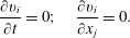 $$\begin{eqnarray}\frac{\unicode[STIX]{x2202}v_{i}}{\unicode[STIX]{x2202}t}=0;\quad \frac{\unicode[STIX]{x2202}v_{i}}{\unicode[STIX]{x2202}x_{j}}=0.\end{eqnarray}$$
Also, the magnetic and electric fields
 $\boldsymbol{B}(\boldsymbol{x},t),\boldsymbol{E}(\boldsymbol{x},t)$
are macroscopic quantities that do not depend on
$\boldsymbol{B}(\boldsymbol{x},t),\boldsymbol{E}(\boldsymbol{x},t)$
are macroscopic quantities that do not depend on
 $\boldsymbol{v}$
and can be moved outside of velocity integrals over
$\boldsymbol{v}$
and can be moved outside of velocity integrals over
 $d^{3}v$
, or in another words
$d^{3}v$
, or in another words
 $\unicode[STIX]{x2202}B_{i}/\unicode[STIX]{x2202}v_{j}=0$
and
$\unicode[STIX]{x2202}B_{i}/\unicode[STIX]{x2202}v_{j}=0$
and
 $\unicode[STIX]{x2202}E_{i}/\unicode[STIX]{x2202}v_{j}=0$
. The definitions of the fluid moments are
$\unicode[STIX]{x2202}E_{i}/\unicode[STIX]{x2202}v_{j}=0$
. The definitions of the fluid moments are
 $$\begin{eqnarray}\displaystyle & \displaystyle n=\int f\,\text{d}^{3}v; & \displaystyle\end{eqnarray}$$
 $$\begin{eqnarray}\displaystyle & \displaystyle n\boldsymbol{u}=\int \boldsymbol{v}f\,\text{d}^{3}v; & \displaystyle\end{eqnarray}$$
 $$\begin{eqnarray}\displaystyle & \displaystyle \boldsymbol{p}=m\int (\boldsymbol{v}-\boldsymbol{u})(\boldsymbol{v}-\boldsymbol{u})f\,\text{d}^{3}v; & \displaystyle\end{eqnarray}$$
 $$\begin{eqnarray}\displaystyle & \displaystyle \boldsymbol{q}=m\int (\boldsymbol{v}-\boldsymbol{u})(\boldsymbol{v}-\boldsymbol{u})(\boldsymbol{v}-\boldsymbol{u})f\,\text{d}^{3}v; & \displaystyle\end{eqnarray}$$
 $$\begin{eqnarray}\displaystyle & \displaystyle \boldsymbol{r}=m\int (\boldsymbol{v}-\boldsymbol{u})(\boldsymbol{v}-\boldsymbol{u})(\boldsymbol{v}-\boldsymbol{u})(\boldsymbol{v}-\boldsymbol{u})f\,\text{d}^{3}v, & \displaystyle\end{eqnarray}$$
where we have omitted the tensor product notation that is sometimes written down explicitly as
 $\boldsymbol{u}\boldsymbol{u}=\boldsymbol{u}\otimes \boldsymbol{u}$
and in the index notation
$\boldsymbol{u}\boldsymbol{u}=\boldsymbol{u}\otimes \boldsymbol{u}$
and in the index notation
 $(\boldsymbol{u}\boldsymbol{u})_{ij}=u_{i}u_{j}$
. If two vectors or tensors are next to each other without an operator between them, a tensor product is always assumed. The number density
$(\boldsymbol{u}\boldsymbol{u})_{ij}=u_{i}u_{j}$
. If two vectors or tensors are next to each other without an operator between them, a tensor product is always assumed. The number density
 $n$
is a scalar, the fluid velocity
$n$
is a scalar, the fluid velocity
 $\boldsymbol{u}$
is a vector, the pressure tensor
$\boldsymbol{u}$
is a vector, the pressure tensor
 $\boldsymbol{p}$
is a tensor of second rank (
$\boldsymbol{p}$
is a tensor of second rank (
 $3\times 3$
matrix), the heat flux tensor
$3\times 3$
matrix), the heat flux tensor
 $\boldsymbol{q}$
is a tensor of third rank (with
$\boldsymbol{q}$
is a tensor of third rank (with
 $3\times 3\times 3$
components), the tensor
$3\times 3\times 3$
components), the tensor
 $\boldsymbol{r}$
is of fourth rank (with
$\boldsymbol{r}$
is of fourth rank (with
 $3\times 3\times 3\times 3$
components), etc. Directly from the definitions, it is obvious that all fluid tensors must be symmetric in all of their indices, i.e.
$3\times 3\times 3\times 3$
components), etc. Directly from the definitions, it is obvious that all fluid tensors must be symmetric in all of their indices, i.e.
 $p_{ij}=p_{ji}$
,
$p_{ij}=p_{ji}$
,
 $q_{ijk}=q_{ikj}=\cdots \,$
. The fluctuating velocity is defined as
$q_{ijk}=q_{ikj}=\cdots \,$
. The fluctuating velocity is defined as
 $$\begin{eqnarray}\boldsymbol{c}=\boldsymbol{v}-\boldsymbol{u},\end{eqnarray}$$
and should not be confused with the speed of light
 $c$
.
$c$
.
The second important concept that is used in deriving the fluid hierarchy, is the use of the usual Gauss–Ostrogradsky (divergence) theorem. The divergence theorem is used in velocity space and, written in a form that is typically encountered when calculating the fluid hierarchy, it reads
 $$\begin{eqnarray}\int _{V}\unicode[STIX]{x1D735}_{v}\boldsymbol{\cdot }(f\unicode[STIX]{x1D63C})\,\text{d}^{3}v=\int _{S}f\unicode[STIX]{x1D63C}\boldsymbol{\cdot }\text{d}\boldsymbol{S}.\end{eqnarray}$$
The
 $\unicode[STIX]{x1D63C}$
is a general
$\unicode[STIX]{x1D63C}$
is a general
 $n$
th-order tensor,
$n$
th-order tensor,
 $f$
is a distribution function, the left-hand side is a 3-D integral calculated over the entire velocity volume
$f$
is a distribution function, the left-hand side is a 3-D integral calculated over the entire velocity volume
 $V$
and the right-hand side is a surface integral calculated over a boundary of that volume
$V$
and the right-hand side is a surface integral calculated over a boundary of that volume
 $\text{d}\boldsymbol{S}=\hat{\boldsymbol{n}}\,\text{d}S$
, where
$\text{d}\boldsymbol{S}=\hat{\boldsymbol{n}}\,\text{d}S$
, where
 $\hat{\boldsymbol{n}}$
is a unit normal vector to the local surface area pointing outwards. When such an integral is encountered in the fluid hierarchy, the result is always assumed to be zero. The volume integrals are from
$\hat{\boldsymbol{n}}$
is a unit normal vector to the local surface area pointing outwards. When such an integral is encountered in the fluid hierarchy, the result is always assumed to be zero. The volume integrals are from
 $v=-\infty$
to
$v=-\infty$
to
 $v=\infty$
in each velocity component and the integration on the right-hand side of (2.9) is therefore performed over the velocity surface area at infinity. The necessary (but technically not sufficient) condition for the integral to be negligible is
$v=\infty$
in each velocity component and the integration on the right-hand side of (2.9) is therefore performed over the velocity surface area at infinity. The necessary (but technically not sufficient) condition for the integral to be negligible is
 $$\begin{eqnarray}\lim _{v\rightarrow \infty }f(v)=0.\end{eqnarray}$$
Since the area
 $\text{d}S\sim v^{2}\,\text{d}v$
, the sufficient condition for the integral to vanish, can be estimated more precisely as
$\text{d}S\sim v^{2}\,\text{d}v$
, the sufficient condition for the integral to vanish, can be estimated more precisely as
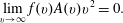 $$\begin{eqnarray}\lim _{v\rightarrow \infty }f(v)A(v)v^{2}=0.\end{eqnarray}$$
When calculating the fluid hierarchy, the encountered expressions are always
 $A(v)\sim v^{n}$
, where
$A(v)\sim v^{n}$
, where
 $n$
is a positive integer. Then, for example, for a Maxwellian distribution
$n$
is a positive integer. Then, for example, for a Maxwellian distribution
 $f(v)\sim \text{e}^{-v^{2}}$
the limit (2.11) is always zero for all
$f(v)\sim \text{e}^{-v^{2}}$
the limit (2.11) is always zero for all
 $n$
. Even for a slower converging distribution
$n$
. Even for a slower converging distribution
 $f(v)\sim \text{e}^{-|v|}$
, the limit is always zero. For distribution functions proportional to a power law, for example
$f(v)\sim \text{e}^{-|v|}$
, the limit is always zero. For distribution functions proportional to a power law, for example
 $f(v)\sim (v^{2})^{-(\unicode[STIX]{x1D705}+1)}$
as for a kappa distribution, the situation is more restrictive, with some minimum required values of
$f(v)\sim (v^{2})^{-(\unicode[STIX]{x1D705}+1)}$
as for a kappa distribution, the situation is more restrictive, with some minimum required values of
 $\unicode[STIX]{x1D705}$
. When we will calculate the
$\unicode[STIX]{x1D705}$
. When we will calculate the
 $n$
th-order fluid moment (§ 12), we will see that two surface integrals are encountered, one with
$n$
th-order fluid moment (§ 12), we will see that two surface integrals are encountered, one with
 $A(v)\sim v^{n}$
and one with
$A(v)\sim v^{n}$
and one with
 $A(v)\sim v^{n+1}$
. Therefore, for a kappa distribution, the strict condition for
$A(v)\sim v^{n+1}$
. Therefore, for a kappa distribution, the strict condition for
 $\lim _{v\rightarrow \infty }(v^{2})^{-(\unicode[STIX]{x1D705}+1)}v^{n+1}v^{2}=0$
yields the requirement
$\lim _{v\rightarrow \infty }(v^{2})^{-(\unicode[STIX]{x1D705}+1)}v^{n+1}v^{2}=0$
yields the requirement
 $\unicode[STIX]{x1D705}>(n+1)/2$
. For example, many fluid models discussed in this guide are closed at the fourth-order moment
$\unicode[STIX]{x1D705}>(n+1)/2$
. For example, many fluid models discussed in this guide are closed at the fourth-order moment
 $\boldsymbol{r}$
, so
$\boldsymbol{r}$
, so
 $n=4$
, which implies the requirement
$n=4$
, which implies the requirement
 $\unicode[STIX]{x1D705}>5/2$
. At first sight, the required limit (2.11) can be considered only a technical mathematical detail since, physically, one can argue that particles with enormously large energies will not be measured/observed, and some physical mechanism that is responsible for a cutoff of the distribution function at finite energies can be usually assumed. Or in another words, even observational studies that fit the data with a kappa distribution do not assume that the fit is valid all the way up to
$\unicode[STIX]{x1D705}>5/2$
. At first sight, the required limit (2.11) can be considered only a technical mathematical detail since, physically, one can argue that particles with enormously large energies will not be measured/observed, and some physical mechanism that is responsible for a cutoff of the distribution function at finite energies can be usually assumed. Or in another words, even observational studies that fit the data with a kappa distribution do not assume that the fit is valid all the way up to
 $v\rightarrow \infty$
, and usually a cutoff is implicitly assumed. However, once we calculate the fourth-order moments for a kappa distribution, we will see that, for example
$v\rightarrow \infty$
, and usually a cutoff is implicitly assumed. However, once we calculate the fourth-order moments for a kappa distribution, we will see that, for example
 $r_{\Vert \Vert }=\unicode[STIX]{x1D6FC}_{\unicode[STIX]{x1D705}}3p_{\Vert }^{2}/\unicode[STIX]{x1D70C}$
, where
$r_{\Vert \Vert }=\unicode[STIX]{x1D6FC}_{\unicode[STIX]{x1D705}}3p_{\Vert }^{2}/\unicode[STIX]{x1D70C}$
, where
 $\unicode[STIX]{x1D6FC}_{\unicode[STIX]{x1D705}}=(\unicode[STIX]{x1D705}-3/2)/(\unicode[STIX]{x1D705}-5/2)$
, so the restriction
$\unicode[STIX]{x1D6FC}_{\unicode[STIX]{x1D705}}=(\unicode[STIX]{x1D705}-3/2)/(\unicode[STIX]{x1D705}-5/2)$
, so the restriction
 $\unicode[STIX]{x1D705}>5/2$
returns, and has to be applied regardless. When the limit (2.11) is satisfied, the neglect of the surface integrals (2.9) is therefore based on solid theoretical principles, and it is not an approximate or an ad hoc choice, the surface integrals are really zero. Nevertheless, for complete clarity in the upcoming fluid hierarchy calculations, we will differentiate between expressions that are zero exactly, and between the surface integrals (2.9) that are zero asymptotically, by using
$\unicode[STIX]{x1D705}>5/2$
returns, and has to be applied regardless. When the limit (2.11) is satisfied, the neglect of the surface integrals (2.9) is therefore based on solid theoretical principles, and it is not an approximate or an ad hoc choice, the surface integrals are really zero. Nevertheless, for complete clarity in the upcoming fluid hierarchy calculations, we will differentiate between expressions that are zero exactly, and between the surface integrals (2.9) that are zero asymptotically, by using
 $=0$
and
$=0$
and
 $\rightarrow 0$
.
$\rightarrow 0$
.
We start directly with the derivation of the pressure tensor equation, since a detailed derivation of the density and momentum equations can be found in many books. To derive the pressure tensor equation, it is possible to multiply the Vlasov equation by
 $mc_{i}c_{j}$
or
$mc_{i}c_{j}$
or
 $mv_{i}v_{j}$
(another possibility is
$mv_{i}v_{j}$
(another possibility is
 $mc_{i}v_{j}$
). Here, we will use the first choice, which is slightly easier to present in detail, because the second choice requires the use of density and momentum equations to cancel several terms. It is useful to derive the following identities
$mc_{i}v_{j}$
). Here, we will use the first choice, which is slightly easier to present in detail, because the second choice requires the use of density and momentum equations to cancel several terms. It is useful to derive the following identities
 $$\begin{eqnarray}\displaystyle \int \boldsymbol{c}f\,\text{d}^{3}v=\int (\boldsymbol{v}-\boldsymbol{u})f\,\text{d}^{3}v=\int \boldsymbol{v}f\,\text{d}^{3}v-\boldsymbol{u}\int f\,\text{d}^{3}v=n\boldsymbol{u}-\boldsymbol{u}n=0; & & \displaystyle\end{eqnarray}$$
 $$\begin{eqnarray}\displaystyle m\int \boldsymbol{c}\boldsymbol{v}f\,\text{d}^{3}v & = & \displaystyle m\int (\boldsymbol{v}-\boldsymbol{u})(\boldsymbol{v}-\boldsymbol{u}+\boldsymbol{u})f\,\text{d}^{3}v\nonumber\\ \displaystyle & = & \displaystyle m\int (\boldsymbol{v}-\boldsymbol{u})(\boldsymbol{v}-\boldsymbol{u})f\,\text{d}^{3}v+m\boldsymbol{u}\underbrace{\int (\boldsymbol{v}-\boldsymbol{u})f\,\text{d}^{3}v}_{=0}=\boldsymbol{p};\end{eqnarray}$$
 $$\begin{eqnarray}\displaystyle m\int \boldsymbol{c}\boldsymbol{c}\boldsymbol{v}f\,\text{d}^{3}v=m\int \boldsymbol{c}\boldsymbol{c}(\boldsymbol{v}-\boldsymbol{u}+\boldsymbol{u})f\,\text{d}^{3}v=\boldsymbol{q}+\boldsymbol{p}\boldsymbol{u}. & & \displaystyle\end{eqnarray}$$
We write down the derivatives with respect to time
 $\unicode[STIX]{x2202}/\unicode[STIX]{x2202}t$
and velocity
$\unicode[STIX]{x2202}/\unicode[STIX]{x2202}t$
and velocity
 $\unicode[STIX]{x2202}/\unicode[STIX]{x2202}v_{i}$
explicitly, but we abbreviate the derivative with respect to spatial coordinates as
$\unicode[STIX]{x2202}/\unicode[STIX]{x2202}v_{i}$
explicitly, but we abbreviate the derivative with respect to spatial coordinates as
 $\unicode[STIX]{x2202}/\unicode[STIX]{x2202}x_{i}\equiv \unicode[STIX]{x2202}_{i}$
. We will need
$\unicode[STIX]{x2202}/\unicode[STIX]{x2202}x_{i}\equiv \unicode[STIX]{x2202}_{i}$
. We will need
 $$\begin{eqnarray}\displaystyle & \displaystyle \frac{\unicode[STIX]{x2202}}{\unicode[STIX]{x2202}t}c_{i}=\frac{\unicode[STIX]{x2202}}{\unicode[STIX]{x2202}t}(v_{i}-u_{i})=-\frac{\unicode[STIX]{x2202}}{\unicode[STIX]{x2202}t}u_{i}; & \displaystyle\end{eqnarray}$$
 $$\begin{eqnarray}\displaystyle & \displaystyle \frac{\unicode[STIX]{x2202}}{\unicode[STIX]{x2202}t}(c_{i}c_{j})=-c_{i}\frac{\unicode[STIX]{x2202}u_{j}}{\unicode[STIX]{x2202}t}-c_{j}\frac{\unicode[STIX]{x2202}u_{i}}{\unicode[STIX]{x2202}t}; & \displaystyle\end{eqnarray}$$
 $$\begin{eqnarray}\displaystyle & \displaystyle \unicode[STIX]{x2202}_{k}(c_{i}c_{j})=-c_{i}\unicode[STIX]{x2202}_{k}u_{j}-c_{j}\unicode[STIX]{x2202}_{k}u_{i}; & \displaystyle\end{eqnarray}$$
 $$\begin{eqnarray}\displaystyle & \displaystyle \frac{\unicode[STIX]{x2202}}{\unicode[STIX]{x2202}v_{k}}c_{i}=\frac{\unicode[STIX]{x2202}}{\unicode[STIX]{x2202}v_{k}}(v_{i}-u_{i})=\frac{\unicode[STIX]{x2202}v_{i}}{\unicode[STIX]{x2202}v_{k}}=\unicode[STIX]{x1D6FF}_{ik}; & \displaystyle\end{eqnarray}$$
 $$\begin{eqnarray}\displaystyle & \displaystyle \frac{\unicode[STIX]{x2202}}{\unicode[STIX]{x2202}v_{k}}(c_{i}c_{j})=c_{i}\unicode[STIX]{x1D6FF}_{jk}+c_{j}\unicode[STIX]{x1D6FF}_{ik}; & \displaystyle\end{eqnarray}$$
 $$\begin{eqnarray}\displaystyle \frac{\unicode[STIX]{x2202}}{\unicode[STIX]{x2202}v_{k}}[c_{i}c_{j}(\boldsymbol{v}\times \boldsymbol{B})_{k}] & = & \displaystyle \frac{\unicode[STIX]{x2202}}{\unicode[STIX]{x2202}v_{k}}(c_{i}c_{j})(\boldsymbol{v}\times \boldsymbol{B})_{k}+c_{i}c_{j}\frac{\unicode[STIX]{x2202}}{\unicode[STIX]{x2202}v_{k}}(\unicode[STIX]{x1D716}_{klm}v_{l}B_{m})\nonumber\\ \displaystyle & = & \displaystyle (\unicode[STIX]{x1D6FF}_{ik}c_{j}+\unicode[STIX]{x1D6FF}_{jk}c_{i})(\boldsymbol{v}\times \boldsymbol{B})_{k}+c_{i}c_{j}\underbrace{\unicode[STIX]{x1D716}_{klm}\unicode[STIX]{x1D6FF}_{lk}}_{=0}B_{m}\nonumber\\ \displaystyle & = & \displaystyle c_{j}(\boldsymbol{v}\times \boldsymbol{B})_{i}+c_{i}(\boldsymbol{v}\times \boldsymbol{B})_{j},\end{eqnarray}$$
where in the last identity we used the result
 $\unicode[STIX]{x1D716}_{klm}\unicode[STIX]{x1D6FF}_{lk}=0$
since the Levi-Civita tensor
$\unicode[STIX]{x1D716}_{klm}\unicode[STIX]{x1D6FF}_{lk}=0$
since the Levi-Civita tensor
 $\unicode[STIX]{x1D716}_{ijk}$
is antisymmetric and the Kronecker
$\unicode[STIX]{x1D716}_{ijk}$
is antisymmetric and the Kronecker
 $\unicode[STIX]{x1D6FF}_{ij}$
is a symmetric tensor. Integrating the first term of the Vlasov equation yields
$\unicode[STIX]{x1D6FF}_{ij}$
is a symmetric tensor. Integrating the first term of the Vlasov equation yields
 $$\begin{eqnarray}\displaystyle \unicode[STIX]{x2460} & = & \displaystyle m\int c_{i}c_{j}\frac{\unicode[STIX]{x2202}f}{\unicode[STIX]{x2202}t}\,\text{d}^{3}v=\frac{\unicode[STIX]{x2202}}{\unicode[STIX]{x2202}t}\underbrace{\left(m\int c_{i}c_{j}f\,\text{d}^{3}v\right)}_{=p_{ij}}-m\int f\frac{\unicode[STIX]{x2202}}{\unicode[STIX]{x2202}t}(c_{i}c_{j})\,\text{d}^{3}v\nonumber\\ \displaystyle & = & \displaystyle \frac{\unicode[STIX]{x2202}}{\unicode[STIX]{x2202}t}p_{ij}+m\frac{\unicode[STIX]{x2202}u_{j}}{\unicode[STIX]{x2202}t}\underbrace{\int fc_{i}\,\text{d}^{3}v}_{=0}+m\frac{\unicode[STIX]{x2202}u_{i}}{\unicode[STIX]{x2202}t}\underbrace{\int fc_{j}\,\text{d}^{3}v}_{=0}\nonumber\\ \displaystyle & = & \displaystyle \frac{\unicode[STIX]{x2202}}{\unicode[STIX]{x2202}t}p_{ij}.\end{eqnarray}$$
The second term of the Vlasov equation yields
 $$\begin{eqnarray}\displaystyle \unicode[STIX]{x2461} & = & \displaystyle m\int c_{i}c_{j}\underbrace{\boldsymbol{v}\boldsymbol{\cdot }\unicode[STIX]{x1D735}}_{=v_{k}\unicode[STIX]{x2202}_{k}}f\,\text{d}^{3}v=\unicode[STIX]{x2202}_{k}\underbrace{\left(m\int c_{i}c_{j}v_{k}f\,\text{d}^{3}v\right)}_{=q_{ijk}+p_{ij}u_{k}}-m\int v_{k}f\unicode[STIX]{x2202}_{k}(c_{i}c_{j})\,\text{d}^{3}v\nonumber\\ \displaystyle & = & \displaystyle \unicode[STIX]{x2202}_{k}(q_{ijk}+p_{ij}u_{k})+(\unicode[STIX]{x2202}_{k}u_{j})\underbrace{m\int c_{i}v_{k}f\,\text{d}^{3}v}_{=p_{ik}}\nonumber\\ \displaystyle & & \displaystyle +\,(\unicode[STIX]{x2202}_{k}u_{i})\underbrace{m\int c_{j}v_{k}f\,\text{d}^{3}v}_{=p_{jk}}=\unicode[STIX]{x2202}_{k}(\!\underbrace{q_{ijk}}_{=q_{kij}}+p_{ij}u_{k})+p_{ik}\unicode[STIX]{x2202}_{k}u_{j}+p_{jk}\unicode[STIX]{x2202}_{k}u_{i}\nonumber\\ \displaystyle & = & \displaystyle \unicode[STIX]{x2202}_{k}(q_{kij}+u_{k}p_{ij})+p_{ik}\unicode[STIX]{x2202}_{k}u_{j}+p_{jk}\unicode[STIX]{x2202}_{k}u_{i}\nonumber\\ \displaystyle & = & \displaystyle [\unicode[STIX]{x1D735}\boldsymbol{\cdot }(\boldsymbol{q}+\boldsymbol{u}\boldsymbol{p})+\boldsymbol{p}\boldsymbol{\cdot }\unicode[STIX]{x1D735}\boldsymbol{u}+(\boldsymbol{p}\boldsymbol{\cdot }\unicode[STIX]{x1D735}\boldsymbol{u})^{\text{T}}]_{ij}.\end{eqnarray}$$
To go back and forth between the index notation and the vector notation in a fully consistent matter, it is important to establish some conventions that were not required in simple fluid models. One important convention that is typically used is that the divergence of a tensor is meant to be through its first component, i.e. for a general tensor
 $\unicode[STIX]{x1D61F}_{ijk\ldots n}$
, the divergence
$\unicode[STIX]{x1D61F}_{ijk\ldots n}$
, the divergence
 $\unicode[STIX]{x1D735}\boldsymbol{\cdot }\unicode[STIX]{x1D653}$
means
$\unicode[STIX]{x1D735}\boldsymbol{\cdot }\unicode[STIX]{x1D653}$
means
 $\unicode[STIX]{x2202}_{i}\unicode[STIX]{x1D61F}_{ijk\ldots n}$
. This convention is the reason why in the above expression we used that
$\unicode[STIX]{x2202}_{i}\unicode[STIX]{x1D61F}_{ijk\ldots n}$
. This convention is the reason why in the above expression we used that
 $q_{ijk}=q_{kij}$
and also the ordering of
$q_{ijk}=q_{kij}$
and also the ordering of
 $\boldsymbol{u}$
and
$\boldsymbol{u}$
and
 $\boldsymbol{p}$
inside
$\boldsymbol{p}$
inside
 $\unicode[STIX]{x1D735}\boldsymbol{\cdot }(\boldsymbol{u}\boldsymbol{p})$
reflects that in the index notation we have
$\unicode[STIX]{x1D735}\boldsymbol{\cdot }(\boldsymbol{u}\boldsymbol{p})$
reflects that in the index notation we have
 $\unicode[STIX]{x2202}_{k}(u_{k}p_{ij})$
.
$\unicode[STIX]{x2202}_{k}(u_{k}p_{ij})$
.
The third term of the Vlasov equation calculates
 $$\begin{eqnarray}\displaystyle \unicode[STIX]{x2462} & = & \displaystyle q\int c_{i}c_{j}\boldsymbol{E}\boldsymbol{\cdot }\unicode[STIX]{x1D735}_{v}f\,\text{d}^{3}v=q\int c_{i}c_{j}E_{k}\frac{\unicode[STIX]{x2202}}{\unicode[STIX]{x2202}v_{k}}f\,\text{d}^{3}v\nonumber\\ \displaystyle & = & \displaystyle qE_{k}\underbrace{\int \frac{\unicode[STIX]{x2202}}{\unicode[STIX]{x2202}v_{k}}(c_{i}c_{j}f)\,\text{d}^{3}v}_{\rightarrow 0}-qE_{k}\int \frac{\unicode[STIX]{x2202}}{\unicode[STIX]{x2202}v_{k}}(c_{i}c_{j})f\,\text{d}^{3}v\nonumber\\ \displaystyle & = & \displaystyle -qE_{k}\int \frac{\unicode[STIX]{x2202}}{\unicode[STIX]{x2202}v_{k}}(c_{i}c_{j})f\,\text{d}^{3}v=-qE_{k}\int (\unicode[STIX]{x1D6FF}_{ik}c_{j}+\unicode[STIX]{x1D6FF}_{jk}c_{i})f\,\text{d}^{3}v\nonumber\\ \displaystyle & = & \displaystyle -qE_{i}\underbrace{\int c_{j}f\,\text{d}^{3}v}_{=0}-qE_{j}\underbrace{\int c_{i}f\,\text{d}^{3}v}_{=0}=0.\end{eqnarray}$$
Finally, the fourth term of the Vlasov equation calculates
 $$\begin{eqnarray}\displaystyle \unicode[STIX]{x2463} & = & \displaystyle \frac{q}{c}\int c_{i}c_{j}(\boldsymbol{v}\times \boldsymbol{B})\boldsymbol{\cdot }\unicode[STIX]{x1D735}_{v}f\,\text{d}^{3}v=\frac{q}{c}\int c_{i}c_{j}(\boldsymbol{v}\times \boldsymbol{B})_{k}\frac{\unicode[STIX]{x2202}f}{\unicode[STIX]{x2202}v_{k}}\,\text{d}^{3}v\nonumber\\ \displaystyle & = & \displaystyle \frac{q}{c}\underbrace{\int \frac{\unicode[STIX]{x2202}}{\unicode[STIX]{x2202}v_{k}}[c_{i}c_{j}(\boldsymbol{v}\times \boldsymbol{B})_{k}f]\,\text{d}^{3}v}_{\rightarrow 0}-\frac{q}{c}\int \frac{\unicode[STIX]{x2202}}{\unicode[STIX]{x2202}v_{k}}[c_{i}c_{j}(\boldsymbol{v}\times \boldsymbol{B})_{k}]f\,\text{d}^{3}v\nonumber\\ \displaystyle & = & \displaystyle -\frac{q}{c}\int [c_{j}(\boldsymbol{v}\times \boldsymbol{B})_{i}+c_{i}(\boldsymbol{v}\times \boldsymbol{B})_{j}]f\,\text{d}^{3}v=-\frac{q}{c}\int c_{j}\unicode[STIX]{x1D716}_{ikl}v_{k}B_{l}f\,\text{d}^{3}v-\frac{q}{c}\int c_{i}\unicode[STIX]{x1D716}_{jkl}v_{k}B_{l}f\,\text{d}^{3}v\nonumber\\ \displaystyle & = & \displaystyle -\frac{q}{c}\unicode[STIX]{x1D716}_{ikl}B_{l}\underbrace{\int c_{j}v_{k}f\,\text{d}^{3}v}_{=(1/m)p_{jk}}-\frac{q}{c}\unicode[STIX]{x1D716}_{jkl}B_{l}\underbrace{\int c_{i}v_{k}f\,\text{d}^{3}v}_{=(1/m)p_{ik}}=-\frac{q}{mc}[\unicode[STIX]{x1D716}_{ikl}B_{l}p_{jk}+\unicode[STIX]{x1D716}_{jkl}B_{l}p_{ik}]\nonumber\\ \displaystyle & = & \displaystyle \frac{q}{mc}[\unicode[STIX]{x1D716}_{ilk}B_{l}p_{kj}+\unicode[STIX]{x1D716}_{jlk}B_{l}p_{ki}]=\frac{q}{mc}[(\boldsymbol{B}\times \boldsymbol{p})_{ij}+(\boldsymbol{B}\times \boldsymbol{p})_{ji}]=\frac{q}{mc}[\boldsymbol{B}\times \boldsymbol{p}+(\boldsymbol{B}\times \boldsymbol{p})^{\text{T}}]_{ij}.\nonumber\\ \displaystyle & & \displaystyle\end{eqnarray}$$
In the expression above, one encounters a vector product of a vector with a matrix,
 $\boldsymbol{B}\times \boldsymbol{p}$
. This operator might appear unusual at first, but it is just a generalization of a vector product of two vectors, it is defined as
$\boldsymbol{B}\times \boldsymbol{p}$
. This operator might appear unusual at first, but it is just a generalization of a vector product of two vectors, it is defined as
 $(\boldsymbol{B}\times \boldsymbol{p})_{ij}=\unicode[STIX]{x1D716}_{ikl}B_{k}p_{lj}$
and the result is a matrix. Similarly, a vector product between a vector and a tensor of third rank is defined as
$(\boldsymbol{B}\times \boldsymbol{p})_{ij}=\unicode[STIX]{x1D716}_{ikl}B_{k}p_{lj}$
and the result is a matrix. Similarly, a vector product between a vector and a tensor of third rank is defined as
 $(\boldsymbol{B}\times \boldsymbol{q})_{ijk}=\unicode[STIX]{x1D716}_{ilm}B_{l}q_{mjk}$
and for a tensor of
$(\boldsymbol{B}\times \boldsymbol{q})_{ijk}=\unicode[STIX]{x1D716}_{ilm}B_{l}q_{mjk}$
and for a tensor of
 $n$
th rank
$n$
th rank
 $(\boldsymbol{B}\times \unicode[STIX]{x1D653})_{i\ldots jk}=\unicode[STIX]{x1D716}_{ilm}B_{l}\unicode[STIX]{x1D61F}_{m\ldots jk}$
(i.e. the second index in
$(\boldsymbol{B}\times \unicode[STIX]{x1D653})_{i\ldots jk}=\unicode[STIX]{x1D716}_{ilm}B_{l}\unicode[STIX]{x1D61F}_{m\ldots jk}$
(i.e. the second index in
 $\unicode[STIX]{x1D716}$
is the vector
$\unicode[STIX]{x1D716}$
is the vector
 $\boldsymbol{B}$
index and the third index in
$\boldsymbol{B}$
index and the third index in
 $\unicode[STIX]{x1D716}$
is the first index of tensor
$\unicode[STIX]{x1D716}$
is the first index of tensor
 $\unicode[STIX]{x1D653}$
). However, a definition of a vector product where a matrix is applied on a vector reads
$\unicode[STIX]{x1D653}$
). However, a definition of a vector product where a matrix is applied on a vector reads
 $(\boldsymbol{p}\times \boldsymbol{B})_{ij}=\unicode[STIX]{x1D716}_{jkl}p_{ik}\boldsymbol{B}_{l}$
, and in general
$(\boldsymbol{p}\times \boldsymbol{B})_{ij}=\unicode[STIX]{x1D716}_{jkl}p_{ik}\boldsymbol{B}_{l}$
, and in general
 $\boldsymbol{p}\times \boldsymbol{B}=-(\boldsymbol{B}\times \boldsymbol{p}^{\text{T}})^{\text{T}}$
, but since the
$\boldsymbol{p}\times \boldsymbol{B}=-(\boldsymbol{B}\times \boldsymbol{p}^{\text{T}})^{\text{T}}$
, but since the
 $\boldsymbol{p}$
is here symmetric,
$\boldsymbol{p}$
is here symmetric,
 $\boldsymbol{p}\times \boldsymbol{B}=-(\boldsymbol{B}\times \boldsymbol{p})^{\text{T}}$
. The vector product (cross-product) is addressed further in appendix B. The term (2.24) is sometimes rewritten as
$\boldsymbol{p}\times \boldsymbol{B}=-(\boldsymbol{B}\times \boldsymbol{p})^{\text{T}}$
. The vector product (cross-product) is addressed further in appendix B. The term (2.24) is sometimes rewritten as
 $$\begin{eqnarray}\boldsymbol{B}\times \boldsymbol{p}+(\boldsymbol{B}\times \boldsymbol{p})^{\text{T}}=\boldsymbol{B}\times \boldsymbol{p}-\boldsymbol{p}\times \boldsymbol{B}.\end{eqnarray}$$
Combining all the results together
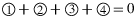 $\unicode[STIX]{x2460}+\unicode[STIX]{x2461}+\unicode[STIX]{x2462}+\unicode[STIX]{x2463}=0$
, yields the entire pressure tensor equation as
$\unicode[STIX]{x2460}+\unicode[STIX]{x2461}+\unicode[STIX]{x2462}+\unicode[STIX]{x2463}=0$
, yields the entire pressure tensor equation as
 $$\begin{eqnarray}\frac{\unicode[STIX]{x2202}\boldsymbol{p}}{\unicode[STIX]{x2202}t}+\unicode[STIX]{x1D735}\boldsymbol{\cdot }(\boldsymbol{u}\boldsymbol{p}+\boldsymbol{q})+\boldsymbol{p}\boldsymbol{\cdot }\unicode[STIX]{x1D735}\boldsymbol{u}+(\boldsymbol{p}\boldsymbol{\cdot }\unicode[STIX]{x1D735}\boldsymbol{u})^{\text{T}}+\frac{q}{mc}[\boldsymbol{B}\times \boldsymbol{p}+(\boldsymbol{B}\times \boldsymbol{p})^{\text{T}}]=0.\end{eqnarray}$$
One notices that, for example, the pressure tensor equation of Kulsrud (Reference Kulsrud, Galeev and Sudan1983), equation (57), contains a minus sign typo in the last term, which should be written as (2.25). That it is indeed a typo and not a definition of
 $\boldsymbol{p}\times \boldsymbol{B}$
is evident from his subsequent equation (59). It is useful to introduce a symmetric operator that acts on a matrix
$\boldsymbol{p}\times \boldsymbol{B}$
is evident from his subsequent equation (59). It is useful to introduce a symmetric operator that acts on a matrix
 $\unicode[STIX]{x1D63C}$
according to
$\unicode[STIX]{x1D63C}$
according to
 $$\begin{eqnarray}\unicode[STIX]{x1D63C}^{S}\equiv \unicode[STIX]{x1D63C}+\unicode[STIX]{x1D63C}^{\text{T}};\quad \unicode[STIX]{x1D608}_{ij}^{S}\equiv \unicode[STIX]{x1D608}_{ij}+\unicode[STIX]{x1D608}_{ji},\end{eqnarray}$$
which yields a more compact form of the pressure tensor equation
 $$\begin{eqnarray}\frac{\unicode[STIX]{x2202}\boldsymbol{p}}{\unicode[STIX]{x2202}t}+\unicode[STIX]{x1D735}\boldsymbol{\cdot }(\boldsymbol{u}\boldsymbol{p}+\boldsymbol{q})+\left[\boldsymbol{p}\boldsymbol{\cdot }\unicode[STIX]{x1D735}\boldsymbol{u}+\frac{q}{mc}\boldsymbol{B}\times \boldsymbol{p}\right]^{S}=0.\end{eqnarray}$$
2.1 Pressure tensor decomposition
By introducing a unit vector in the direction of the local magnetic field
 $\hat{\boldsymbol{b}}=\boldsymbol{B}/|\boldsymbol{B}|$
and the gyrofrequency
$\hat{\boldsymbol{b}}=\boldsymbol{B}/|\boldsymbol{B}|$
and the gyrofrequency
 $\unicode[STIX]{x1D6FA}=qB_{0}/(mc)$
, the last term in the pressure tensor equation (2.26) can be rewritten as
$\unicode[STIX]{x1D6FA}=qB_{0}/(mc)$
, the last term in the pressure tensor equation (2.26) can be rewritten as
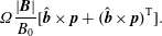 $$\begin{eqnarray}\unicode[STIX]{x1D6FA}\frac{|\boldsymbol{B}|}{B_{0}}[\hat{\boldsymbol{b}}\times \boldsymbol{p}+(\hat{\boldsymbol{b}}\times \boldsymbol{p})^{\text{T}}].\end{eqnarray}$$
At very low frequencies
 $\unicode[STIX]{x1D714}\ll \unicode[STIX]{x1D6FA}$
(and at very long spatial scales) this term will dominate and must be equal to zero. The simplest possibility that makes this term to be equal to zero is
$\unicode[STIX]{x1D714}\ll \unicode[STIX]{x1D6FA}$
(and at very long spatial scales) this term will dominate and must be equal to zero. The simplest possibility that makes this term to be equal to zero is
 $\boldsymbol{p}^{\text{iso}}=p\unicode[STIX]{x1D644}$
, where
$\boldsymbol{p}^{\text{iso}}=p\unicode[STIX]{x1D644}$
, where
 $p$
is the scalar pressure and
$p$
is the scalar pressure and
 $\unicode[STIX]{x1D644}$
is the unit matrix. In index notation
$\unicode[STIX]{x1D644}$
is the unit matrix. In index notation
 $p_{ij}^{\text{iso}}=p\unicode[STIX]{x1D6FF}_{ij}$
, and we can verify that
$p_{ij}^{\text{iso}}=p\unicode[STIX]{x1D6FF}_{ij}$
, and we can verify that
 $$\begin{eqnarray}\displaystyle & \displaystyle (\hat{\boldsymbol{b}}\times \boldsymbol{p}^{\text{iso}})_{ij}=\unicode[STIX]{x1D716}_{ikl}\hat{b}_{k}p_{lj}^{\text{iso}}=\unicode[STIX]{x1D716}_{ikl}\hat{b}_{k}p\unicode[STIX]{x1D6FF}_{lj}=p\unicode[STIX]{x1D716}_{ikj}\hat{b}_{k}=-p\unicode[STIX]{x1D716}_{ijk}\hat{b}_{k}; & \displaystyle\end{eqnarray}$$
 $$\begin{eqnarray}\displaystyle & \displaystyle [\hat{\boldsymbol{b}}\times \boldsymbol{p}^{\text{iso}}+(\hat{\boldsymbol{b}}\times \boldsymbol{p}^{\text{iso}})^{\text{T}}]_{ij}=-p\unicode[STIX]{x1D716}_{ijk}\hat{b}_{k}-p\unicode[STIX]{x1D716}_{jik}\hat{b}_{k}=-p\hat{b}_{k}(\unicode[STIX]{x1D716}_{ijk}-\unicode[STIX]{x1D716}_{ijk})=0. & \displaystyle\end{eqnarray}$$
There is however a much more general solution that makes the term (2.29) equal to zero, which is
 $$\begin{eqnarray}\boldsymbol{p}^{\text{g}}=p_{\Vert }\hat{\boldsymbol{b}}\hat{\boldsymbol{b}}+p_{\bot }(\unicode[STIX]{x1D644}-\hat{\boldsymbol{b}}\hat{\boldsymbol{b}}),\end{eqnarray}$$
where the ‘g’ stands for gyrotropic. For quick analytic calculations it is sometimes easier to use
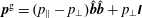 $\boldsymbol{p}^{\text{g}}=(p_{\Vert }-p_{\bot })\hat{\boldsymbol{b}}\hat{\boldsymbol{b}}+p_{\bot }\unicode[STIX]{x1D644}$
since we have to deal with
$\boldsymbol{p}^{\text{g}}=(p_{\Vert }-p_{\bot })\hat{\boldsymbol{b}}\hat{\boldsymbol{b}}+p_{\bot }\unicode[STIX]{x1D644}$
since we have to deal with
 $\hat{\boldsymbol{b}}\hat{\boldsymbol{b}}$
only once instead of twice. We need to verify that the term (2.29) indeed disappears,
$\hat{\boldsymbol{b}}\hat{\boldsymbol{b}}$
only once instead of twice. We need to verify that the term (2.29) indeed disappears,
 $$\begin{eqnarray}\displaystyle & & \displaystyle (\hat{\boldsymbol{b}}\times \boldsymbol{p}^{\text{g}})_{ij}=\unicode[STIX]{x1D716}_{ikl}\hat{b}_{k}p_{lj}^{\text{g}}=\unicode[STIX]{x1D716}_{ikl}\hat{b}_{k}((p_{\Vert }-p_{\bot })\hat{b}_{l}\hat{b}_{j}+p_{\bot }\unicode[STIX]{x1D6FF}_{lj})\nonumber\\ \displaystyle & & \displaystyle =(p_{\Vert }-p_{\bot })\hat{b}_{j}\underbrace{\unicode[STIX]{x1D716}_{ikl}\hat{b}_{k}\hat{b}_{l}}_{=0}+p_{\bot }\unicode[STIX]{x1D716}_{ikj}\hat{b}_{k}=-p_{\bot }\unicode[STIX]{x1D716}_{ijk}\hat{b}_{k};\end{eqnarray}$$
 $$\begin{eqnarray}\displaystyle \Rightarrow \quad & & \displaystyle [\hat{\boldsymbol{b}}\times \boldsymbol{p}^{\text{g}}+(\hat{\boldsymbol{b}}\times \boldsymbol{p}^{\text{g}})^{\text{T}}]_{ij}=-p_{\bot }\hat{b}_{k}(\unicode[STIX]{x1D716}_{ijk}+\unicode[STIX]{x1D716}_{jik})=0.\end{eqnarray}$$
It is easy to see that the parallel and perpendicular pressures can be extracted from the gyrotropic pressure tensor matrix by performing double contractions according to
 $$\begin{eqnarray}p_{\Vert }=\boldsymbol{p}^{\text{g}}\boldsymbol{ : }\hat{\boldsymbol{b}}\hat{\boldsymbol{b}},\quad \text{and}\quad p_{\bot }=\boldsymbol{p}^{\text{g}}\boldsymbol{ : }(\unicode[STIX]{x1D644}-\hat{\boldsymbol{b}}\hat{\boldsymbol{b}})/2.\end{eqnarray}$$
The double contraction (the double dot product, represented by the colon) is a very useful operator that is frequently encountered in higher-order fluid models. For two matrices it is defined as
 $\unicode[STIX]{x1D63C}\boldsymbol{ : }\unicode[STIX]{x1D63D}=\unicode[STIX]{x1D608}_{ij}\unicode[STIX]{x1D609}_{ij}$
and yields a scalar. Sometimes, the double contraction is defined as
$\unicode[STIX]{x1D63C}\boldsymbol{ : }\unicode[STIX]{x1D63D}=\unicode[STIX]{x1D608}_{ij}\unicode[STIX]{x1D609}_{ij}$
and yields a scalar. Sometimes, the double contraction is defined as
 $\unicode[STIX]{x1D63C}\boldsymbol{ : }\unicode[STIX]{x1D63D}=\unicode[STIX]{x1D608}_{ij}\unicode[STIX]{x1D609}_{ji}$
, which for symmetric matrices is equivalent to the previous definition. As a reminder, the usual matrix product of two matrices is
$\unicode[STIX]{x1D63C}\boldsymbol{ : }\unicode[STIX]{x1D63D}=\unicode[STIX]{x1D608}_{ij}\unicode[STIX]{x1D609}_{ji}$
, which for symmetric matrices is equivalent to the previous definition. As a reminder, the usual matrix product of two matrices is
 $(\unicode[STIX]{x1D63C}\boldsymbol{\cdot }\unicode[STIX]{x1D63D})_{ij}=\unicode[STIX]{x1D608}_{ik}\unicode[STIX]{x1D609}_{kj}$
and yields a matrix. It is useful to write down the following identities that involve the double contraction,
$(\unicode[STIX]{x1D63C}\boldsymbol{\cdot }\unicode[STIX]{x1D63D})_{ij}=\unicode[STIX]{x1D608}_{ik}\unicode[STIX]{x1D609}_{kj}$
and yields a matrix. It is useful to write down the following identities that involve the double contraction,
 $$\begin{eqnarray}\displaystyle & \displaystyle \hat{\boldsymbol{b}}\hat{\boldsymbol{b}}:\hat{\boldsymbol{b}}\hat{\boldsymbol{b}}=1; & \displaystyle\end{eqnarray}$$
 $$\begin{eqnarray}\displaystyle & \displaystyle \unicode[STIX]{x1D644}:\hat{\boldsymbol{b}}\hat{\boldsymbol{b}}=1; & \displaystyle\end{eqnarray}$$
 $$\begin{eqnarray}\displaystyle & \displaystyle (\unicode[STIX]{x1D644}-\hat{\boldsymbol{b}}\hat{\boldsymbol{b}}):\hat{\boldsymbol{b}}\hat{\boldsymbol{b}}=0; & \displaystyle\end{eqnarray}$$
 $$\begin{eqnarray}\displaystyle & \displaystyle \unicode[STIX]{x1D644}:\unicode[STIX]{x1D644}=3; & \displaystyle\end{eqnarray}$$
 $$\begin{eqnarray}\displaystyle & \displaystyle (\unicode[STIX]{x1D644}-\hat{\boldsymbol{b}}\hat{\boldsymbol{b}}):(\unicode[STIX]{x1D644}-\hat{\boldsymbol{b}}\hat{\boldsymbol{b}})/2=1. & \displaystyle\end{eqnarray}$$
Also interestingly, the trace of a matrix
 $\unicode[STIX]{x1D63C}$
can be expressed through the double contraction with
$\unicode[STIX]{x1D63C}$
can be expressed through the double contraction with
 $\unicode[STIX]{x1D644}$
, i.e.
$\unicode[STIX]{x1D644}$
, i.e.
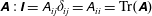 $\unicode[STIX]{x1D63C}:\unicode[STIX]{x1D644}=\unicode[STIX]{x1D608}_{ij}\unicode[STIX]{x1D6FF}_{ij}=\unicode[STIX]{x1D608}_{ii}=\text{Tr}(\unicode[STIX]{x1D63C})$
. The pressure decomposition (2.35) can now be verified easily. Even more revealing is to apply the decomposition (2.35) directly to the definition of the entire pressure tensor (2.5), which yields
$\unicode[STIX]{x1D63C}:\unicode[STIX]{x1D644}=\unicode[STIX]{x1D608}_{ij}\unicode[STIX]{x1D6FF}_{ij}=\unicode[STIX]{x1D608}_{ii}=\text{Tr}(\unicode[STIX]{x1D63C})$
. The pressure decomposition (2.35) can now be verified easily. Even more revealing is to apply the decomposition (2.35) directly to the definition of the entire pressure tensor (2.5), which yields
 $$\begin{eqnarray}\displaystyle & \displaystyle \boldsymbol{p}:\hat{\boldsymbol{b}}\hat{\boldsymbol{b}}=m\int \boldsymbol{c}\boldsymbol{c}f\,\text{d}^{3}v:\hat{\boldsymbol{b}}\hat{\boldsymbol{b}}=m\int (\boldsymbol{v}\boldsymbol{\cdot }\hat{\boldsymbol{b}}-\boldsymbol{u}\boldsymbol{\cdot }\hat{\boldsymbol{b}})^{2}f\,\text{d}^{3}v=m\int (v_{\Vert }-u_{\Vert })^{2}f\,\text{d}^{3}v\equiv p_{\Vert }; & \displaystyle\end{eqnarray}$$
 $$\begin{eqnarray}\displaystyle & \displaystyle \boldsymbol{p}:(\unicode[STIX]{x1D644}-\hat{\boldsymbol{b}}\hat{\boldsymbol{b}})/2=\frac{m}{2}\int |\boldsymbol{v}_{\bot }-\boldsymbol{u}_{\bot }|^{2}f\,\text{d}^{3}v\equiv p_{\bot }, & \displaystyle\end{eqnarray}$$
where we have used the fact that the magnitude of the 3-D velocity vector can be decomposed as
 $|\boldsymbol{v}-\boldsymbol{u}|^{2}=|\boldsymbol{v}_{\bot }-\boldsymbol{u}_{\bot }|^{2}+(v_{\Vert }-u_{\Vert })^{2}$
, or equivalently
$|\boldsymbol{v}-\boldsymbol{u}|^{2}=|\boldsymbol{v}_{\bot }-\boldsymbol{u}_{\bot }|^{2}+(v_{\Vert }-u_{\Vert })^{2}$
, or equivalently
 $|\boldsymbol{c}|^{2}=|\boldsymbol{c}_{\bot }|^{2}+c_{\Vert }^{2}$
.
$|\boldsymbol{c}|^{2}=|\boldsymbol{c}_{\bot }|^{2}+c_{\Vert }^{2}$
.
A distribution function is called isotropic when the direction of the velocity vector
 $\boldsymbol{v}$
does not matter, and the distribution function depends only on magnitude
$\boldsymbol{v}$
does not matter, and the distribution function depends only on magnitude
 $|\boldsymbol{v}|$
, as for example the Maxwellian distribution
$|\boldsymbol{v}|$
, as for example the Maxwellian distribution
 $\text{e}^{-|\boldsymbol{v}|^{2}}$
. A distribution function is called gyrotropic when the direction of the perpendicular velocity vector
$\text{e}^{-|\boldsymbol{v}|^{2}}$
. A distribution function is called gyrotropic when the direction of the perpendicular velocity vector
 $\boldsymbol{v}_{\bot }$
does not matter, and the function depends only on
$\boldsymbol{v}_{\bot }$
does not matter, and the function depends only on
 $|\boldsymbol{v}_{\bot }|$
, as for example the bi-Maxwellian distribution
$|\boldsymbol{v}_{\bot }|$
, as for example the bi-Maxwellian distribution
 $\text{e}^{-\unicode[STIX]{x1D6FC}_{\Vert }v_{\Vert }^{2}}\text{e}^{-\unicode[STIX]{x1D6FC}_{\bot }|\boldsymbol{v}_{\bot }|^{2}}$
. In another words, the gyrotropic distribution function is isotropic only in its transverse velocity components. The same vocabulary is used for the fluid moments, and a fluid moment is called gyrotropic when it involves integrals over
$\text{e}^{-\unicode[STIX]{x1D6FC}_{\Vert }v_{\Vert }^{2}}\text{e}^{-\unicode[STIX]{x1D6FC}_{\bot }|\boldsymbol{v}_{\bot }|^{2}}$
. In another words, the gyrotropic distribution function is isotropic only in its transverse velocity components. The same vocabulary is used for the fluid moments, and a fluid moment is called gyrotropic when it involves integrals over
 $|\boldsymbol{c}_{\bot }|^{2i}$
,
$|\boldsymbol{c}_{\bot }|^{2i}$
,
 $i=0,1,2,3\ldots \,$
. For the pressure tensor, there are only two possibilities, represented by the parallel and perpendicular pressures (2.41), (2.42).
$i=0,1,2,3\ldots \,$
. For the pressure tensor, there are only two possibilities, represented by the parallel and perpendicular pressures (2.41), (2.42).
The part of the pressure tensor extracted by the decomposition (2.35) is therefore called the gyrotropic pressure
 $\boldsymbol{p}^{\text{g}}$
, sometimes also called the CGL pressure
$\boldsymbol{p}^{\text{g}}$
, sometimes also called the CGL pressure
 $\boldsymbol{p}^{\text{CGL}}$
. The gyrotropic approximation is sufficient at very long spatial scales, where the Larmor radius (
$\boldsymbol{p}^{\text{CGL}}$
. The gyrotropic approximation is sufficient at very long spatial scales, where the Larmor radius (
 $=$
the gyroradius) of particles gyrating around the magnetic field is small, and the non-gyrotropic contributions become negligible. However, at sufficiently small spatial scales comparable to the gyroradius, the non-gyrotropic pressure contributions become significant and we represent these through a tensor
$=$
the gyroradius) of particles gyrating around the magnetic field is small, and the non-gyrotropic contributions become negligible. However, at sufficiently small spatial scales comparable to the gyroradius, the non-gyrotropic pressure contributions become significant and we represent these through a tensor
 $\unicode[STIX]{x1D72B}$
, that is called the finite Larmor radius corrections to the (gyrotropic) pressure tensor, or sometimes non-gyrotropic or gyroviscous stress tensor. The entire pressure tensor is thus decomposed according to
$\unicode[STIX]{x1D72B}$
, that is called the finite Larmor radius corrections to the (gyrotropic) pressure tensor, or sometimes non-gyrotropic or gyroviscous stress tensor. The entire pressure tensor is thus decomposed according to
 $$\begin{eqnarray}\displaystyle \boldsymbol{p}=p_{\Vert }\hat{\boldsymbol{b}}\hat{\boldsymbol{b}}+p_{\bot }(\unicode[STIX]{x1D644}-\hat{\boldsymbol{b}}\hat{\boldsymbol{b}})+\unicode[STIX]{x1D72B}, & & \displaystyle\end{eqnarray}$$
and for clarity we write down the decomposition explicitly in matrix notation
 $$\begin{eqnarray}\displaystyle \boldsymbol{p} & = & \displaystyle p_{\Vert }\left(\begin{array}{@{}ccc@{}}\hat{b}_{x}\hat{b}_{x}, & \hat{b}_{x}\hat{b}_{y}, & \hat{b}_{x}\hat{b}_{z}\\ \hat{b}_{y}\hat{b}_{x}, & \hat{b}_{y}\hat{b}_{y}, & \hat{b}_{y}\hat{b}_{z}\\ \hat{b}_{z}\hat{b}_{x}, & \hat{b}_{z}\hat{b}_{y}, & \hat{b}_{z}\hat{b}_{z}\end{array}\right)+p_{\bot }\left(\begin{array}{@{}ccc@{}}1-\hat{b}_{x}\hat{b}_{x}, & -\hat{b}_{x}\hat{b}_{y}, & -\hat{b}_{x}\hat{b}_{z}\\ -\hat{b}_{y}\hat{b}_{x}, & 1-\hat{b}_{y}\hat{b}_{y}, & -\hat{b}_{y}\hat{b}_{z}\\ -\hat{b}_{z}\hat{b}_{x}, & -\hat{b}_{z}\hat{b}_{y}, & 1-\hat{b}_{z}\hat{b}_{z}\end{array}\right)\nonumber\\ \displaystyle & & \displaystyle +\,\left(\begin{array}{@{}ccc@{}}\unicode[STIX]{x1D6F1}_{xx}, & \unicode[STIX]{x1D6F1}_{xy}, & \unicode[STIX]{x1D6F1}_{xz}\\ \unicode[STIX]{x1D6F1}_{yx}, & \unicode[STIX]{x1D6F1}_{yy}, & \unicode[STIX]{x1D6F1}_{yz}\\ \unicode[STIX]{x1D6F1}_{zx}, & \unicode[STIX]{x1D6F1}_{zy}, & \unicode[STIX]{x1D6F1}_{zz}\end{array}\right).\end{eqnarray}$$
In the momentum equation, the pressure tensor enters through its divergence, which is useful to break down into its components. Since
 $\unicode[STIX]{x1D735}\boldsymbol{\cdot }(\hat{\boldsymbol{b}}\hat{\boldsymbol{b}})=\hat{\boldsymbol{b}}(\unicode[STIX]{x1D735}\boldsymbol{\cdot }\hat{\boldsymbol{b}})+(\hat{\boldsymbol{b}}\boldsymbol{\cdot }\unicode[STIX]{x1D735})\hat{\boldsymbol{b}}$
, and
$\unicode[STIX]{x1D735}\boldsymbol{\cdot }(\hat{\boldsymbol{b}}\hat{\boldsymbol{b}})=\hat{\boldsymbol{b}}(\unicode[STIX]{x1D735}\boldsymbol{\cdot }\hat{\boldsymbol{b}})+(\hat{\boldsymbol{b}}\boldsymbol{\cdot }\unicode[STIX]{x1D735})\hat{\boldsymbol{b}}$
, and
 $\unicode[STIX]{x1D735}\boldsymbol{\cdot }(p_{\bot }\unicode[STIX]{x1D644})=\unicode[STIX]{x1D735}p_{\bot }$
, the divergence of the pressure tensor calculates as
$\unicode[STIX]{x1D735}\boldsymbol{\cdot }(p_{\bot }\unicode[STIX]{x1D644})=\unicode[STIX]{x1D735}p_{\bot }$
, the divergence of the pressure tensor calculates as
 $$\begin{eqnarray}\displaystyle \unicode[STIX]{x1D735}\boldsymbol{\cdot }\boldsymbol{p} & = & \displaystyle \unicode[STIX]{x1D735}\boldsymbol{\cdot }(p_{\bot }\unicode[STIX]{x1D644})+\unicode[STIX]{x1D735}\boldsymbol{\cdot }[(p_{\Vert }-p_{\bot })\hat{\boldsymbol{b}}\hat{\boldsymbol{b}}]+\unicode[STIX]{x1D735}\boldsymbol{\cdot }\unicode[STIX]{x1D72B}\nonumber\\ \displaystyle & = & \displaystyle \unicode[STIX]{x1D735}p_{\bot }+(p_{\Vert }-p_{\bot })[\hat{\boldsymbol{b}}(\unicode[STIX]{x1D735}\boldsymbol{\cdot }\hat{\boldsymbol{b}})+(\hat{\boldsymbol{b}}\boldsymbol{\cdot }\unicode[STIX]{x1D735})\hat{\boldsymbol{b}}]+\hat{\boldsymbol{b}}(\hat{\boldsymbol{b}}\boldsymbol{\cdot }\unicode[STIX]{x1D735})(p_{\Vert }-p_{\bot })+\unicode[STIX]{x1D735}\boldsymbol{\cdot }\unicode[STIX]{x1D72B}.\end{eqnarray}$$
Importantly, we have seen in (2.41), (2.42) that the scalar parallel and perpendicular pressures are extracted by applying the double contractions to the entire pressure tensor (and not necessarily only at the gyrotropic part). The decomposition (2.43) can be rewritten as
 $$\begin{eqnarray}\displaystyle \boldsymbol{p}=(\boldsymbol{p}:\hat{\boldsymbol{b}}\hat{\boldsymbol{b}})\hat{\boldsymbol{b}}\hat{\boldsymbol{b}}+(\boldsymbol{p}:(\unicode[STIX]{x1D644}-\hat{\boldsymbol{b}}\hat{\boldsymbol{b}})/2)(\unicode[STIX]{x1D644}-\hat{\boldsymbol{b}}\hat{\boldsymbol{b}})+\unicode[STIX]{x1D72B}. & & \displaystyle\end{eqnarray}$$
Applying the double contraction
 $:\hat{\boldsymbol{b}}\hat{\boldsymbol{b}}$
to (2.46) yields the first requirement for the FLR tensor
$:\hat{\boldsymbol{b}}\hat{\boldsymbol{b}}$
to (2.46) yields the first requirement for the FLR tensor
 $$\begin{eqnarray}\unicode[STIX]{x1D72B}:\hat{\boldsymbol{b}}\hat{\boldsymbol{b}}=0.\end{eqnarray}$$
Similarly, applying
 $:(\unicode[STIX]{x1D644}-\hat{\boldsymbol{b}}\hat{\boldsymbol{b}})/2$
to (2.46) yields the second requirement for the FLR tensor,
$:(\unicode[STIX]{x1D644}-\hat{\boldsymbol{b}}\hat{\boldsymbol{b}})/2$
to (2.46) yields the second requirement for the FLR tensor,
 $$\begin{eqnarray}\unicode[STIX]{x1D72B}:(\unicode[STIX]{x1D644}-\hat{\boldsymbol{b}}\hat{\boldsymbol{b}})=0.\end{eqnarray}$$
By further using the first requirement, the second requirement can be rewritten as
 $$\begin{eqnarray}\unicode[STIX]{x1D72B}:\unicode[STIX]{x1D644}=\text{Tr}(\unicode[STIX]{x1D72B})=0.\end{eqnarray}$$
By using the pressure decomposition (2.43) in the pressure tensor equation (2.26), and using the fact that the gyrotropic part of pressure satisfies
 $\hat{\boldsymbol{b}}\times \boldsymbol{p}^{g}+(\hat{\boldsymbol{b}}\times \boldsymbol{p}^{g})^{\text{T}}=0$
, the pressure tensor equation can be rewritten as
$\hat{\boldsymbol{b}}\times \boldsymbol{p}^{g}+(\hat{\boldsymbol{b}}\times \boldsymbol{p}^{g})^{\text{T}}=0$
, the pressure tensor equation can be rewritten as
 $$\begin{eqnarray}\frac{\unicode[STIX]{x2202}\boldsymbol{p}}{\unicode[STIX]{x2202}t}+\unicode[STIX]{x1D735}\boldsymbol{\cdot }(\boldsymbol{u}\boldsymbol{p}+\boldsymbol{q})+\boldsymbol{p}\boldsymbol{\cdot }\unicode[STIX]{x1D735}\boldsymbol{u}+(\boldsymbol{p}\boldsymbol{\cdot }\unicode[STIX]{x1D735}\boldsymbol{u})^{\text{T}}+\unicode[STIX]{x1D6FA}\frac{|\boldsymbol{B}|}{B_{0}}[\hat{\boldsymbol{b}}\times \unicode[STIX]{x1D72B}+(\hat{\boldsymbol{b}}\times \unicode[STIX]{x1D72B})^{\text{T}}]=0.\end{eqnarray}$$
We can now derive the time dependent equations for parallel and perpendicular pressures by applying the usual double contractions to this pressure tensor equation.
2.2 Parallel pressure equation
We calculate the double contraction with
 $\hat{\boldsymbol{b}}\hat{\boldsymbol{b}}$
term by term. We will need the following identities
$\hat{\boldsymbol{b}}\hat{\boldsymbol{b}}$
term by term. We will need the following identities
 $$\begin{eqnarray}\displaystyle \frac{\unicode[STIX]{x2202}}{\unicode[STIX]{x2202}t}(\hat{\boldsymbol{b}}\hat{\boldsymbol{b}}):\hat{\boldsymbol{b}}\hat{\boldsymbol{b}}=0;\quad \unicode[STIX]{x2202}_{k}(\hat{\boldsymbol{b}}\hat{\boldsymbol{b}}):\hat{\boldsymbol{b}}\hat{\boldsymbol{b}}=0. & & \displaystyle\end{eqnarray}$$
The first term calculates as
 $$\begin{eqnarray}\displaystyle \frac{\unicode[STIX]{x2202}\boldsymbol{p}}{\unicode[STIX]{x2202}t}:\hat{\boldsymbol{b}}\hat{\boldsymbol{b}} & = & \displaystyle \frac{\unicode[STIX]{x2202}}{\unicode[STIX]{x2202}t}(p_{\Vert }\hat{b}_{i}\hat{b}_{j}+p_{\bot }(\unicode[STIX]{x1D6FF}_{ij}-\hat{b}_{i}\hat{b}_{j})+\unicode[STIX]{x1D6F1}_{ij})\hat{b}_{i}\hat{b}_{j}=\frac{\unicode[STIX]{x2202}p_{\Vert }}{\unicode[STIX]{x2202}t}\underbrace{|\hat{\boldsymbol{b}}|^{2}|\hat{\boldsymbol{b}}|^{2}}_{=1}\nonumber\\ \displaystyle & & \displaystyle +\,p_{\Vert }\underbrace{\frac{\unicode[STIX]{x2202}}{\unicode[STIX]{x2202}t}(\hat{b}_{i}\hat{b}_{j})\hat{b}_{i}\hat{b}_{j}}_{=0}+\frac{\unicode[STIX]{x2202}p_{\bot }}{\unicode[STIX]{x2202}t}\underbrace{(\unicode[STIX]{x1D6FF}_{ij}-\hat{b}_{i}\hat{b}_{j})\hat{b}_{i}\hat{b}_{j}}_{=0}\nonumber\\ \displaystyle & & \displaystyle +\,p_{\bot }\underbrace{\hat{b}_{i}\hat{b}_{j}\frac{\unicode[STIX]{x2202}}{\unicode[STIX]{x2202}t}(\unicode[STIX]{x1D6FF}_{ij}-\hat{b}_{i}\hat{b}_{j})}_{=0}+\frac{\unicode[STIX]{x2202}}{\unicode[STIX]{x2202}t}(\underbrace{\unicode[STIX]{x1D6F1}_{ij}\hat{b}_{i}\hat{b}_{j}}_{=0})-\unicode[STIX]{x1D6F1}_{ij}\frac{\unicode[STIX]{x2202}}{\unicode[STIX]{x2202}t}(\hat{b}_{i}\hat{b}_{j})=\frac{\unicode[STIX]{x2202}p_{\Vert }}{\unicode[STIX]{x2202}t}-\unicode[STIX]{x1D72B}:\frac{\unicode[STIX]{x2202}}{\unicode[STIX]{x2202}t}(\hat{\boldsymbol{b}}\hat{\boldsymbol{b}}).\nonumber\\ \displaystyle & & \displaystyle\end{eqnarray}$$
The second term calculates as
 $$\begin{eqnarray}\displaystyle \unicode[STIX]{x1D735}\boldsymbol{\cdot }(\boldsymbol{u}\boldsymbol{p}):\hat{\boldsymbol{b}}\hat{\boldsymbol{b}} & = & \displaystyle \unicode[STIX]{x2202}_{k}(u_{k}p_{ij})\hat{b}_{i}\hat{b}_{j}=\unicode[STIX]{x2202}_{k}(u_{k}\underbrace{p_{ij}\hat{b}_{i}\hat{b}_{j}}_{=p_{\Vert }})-u_{k}p_{ij}\unicode[STIX]{x2202}_{k}(\hat{b}_{i}\hat{b}_{j})=\unicode[STIX]{x2202}_{k}(u_{k}p_{\Vert })-u_{k}p_{\Vert }\underbrace{\hat{b}_{i}\hat{b}_{j}\unicode[STIX]{x2202}_{k}(\hat{b}_{i}\hat{b}_{j})}_{=0}\nonumber\\ \displaystyle & & \displaystyle -p_{\bot }u_{k}\underbrace{(\unicode[STIX]{x1D6FF}_{ij}-\hat{b}_{i}\hat{b}_{j})\unicode[STIX]{x2202}_{k}(\hat{b}_{i}\hat{b}_{j})}_{=0}-\unicode[STIX]{x1D6F1}_{ij}u_{k}\unicode[STIX]{x2202}_{k}(\hat{b}_{i}\hat{b}_{j})=\unicode[STIX]{x1D735}\boldsymbol{\cdot }(p_{\Vert }\boldsymbol{u})-\unicode[STIX]{x1D72B}:(\boldsymbol{u}\boldsymbol{\cdot }\unicode[STIX]{x1D735}(\hat{\boldsymbol{b}}\hat{\boldsymbol{b}}));\nonumber\\ \displaystyle & & \displaystyle\end{eqnarray}$$
 $$\begin{eqnarray}\displaystyle (\unicode[STIX]{x1D735}\boldsymbol{\cdot }\boldsymbol{q}):\hat{\boldsymbol{b}}\hat{\boldsymbol{b}}=(\unicode[STIX]{x1D735}\boldsymbol{\cdot }\boldsymbol{q})_{ij}\hat{b}_{i}\hat{b}_{j}=\hat{\boldsymbol{b}}\boldsymbol{\cdot }(\unicode[STIX]{x1D735}\boldsymbol{\cdot }\boldsymbol{q})\boldsymbol{\cdot }\hat{\boldsymbol{b}}. & & \displaystyle\end{eqnarray}$$
The third term calculates as
 $$\begin{eqnarray}\displaystyle (\boldsymbol{p}\boldsymbol{\cdot }\unicode[STIX]{x1D735}\boldsymbol{u}):\hat{\boldsymbol{b}}\hat{\boldsymbol{b}} & = & \displaystyle (\boldsymbol{p}\boldsymbol{\cdot }\unicode[STIX]{x1D735}\boldsymbol{u})_{ij}\hat{b}_{i}\hat{b}_{j}=(p_{ik}\unicode[STIX]{x2202}_{k}u_{j})\hat{b}_{i}\hat{b}_{j}=(\unicode[STIX]{x2202}_{k}u_{j})p_{ik}\hat{b}_{i}\hat{b}_{j}\nonumber\\ \displaystyle & = & \displaystyle (\unicode[STIX]{x2202}_{k}u_{j})[p_{\Vert }\hat{b}_{i}\hat{b}_{k}+p_{\bot }(\unicode[STIX]{x1D6FF}_{ik}-\hat{b}_{i}\hat{b}_{k})+\unicode[STIX]{x1D6F1}_{ik}]\hat{b}_{i}\hat{b}_{j}\nonumber\\ \displaystyle & = & \displaystyle (\unicode[STIX]{x2202}_{k}u_{j})[p_{\Vert }\hat{b}_{k}\hat{b}_{j}+p_{\bot }\underbrace{(\hat{b}_{k}\hat{b}_{j}-\hat{b}_{k}\hat{b}_{j})}_{=0}+\unicode[STIX]{x1D6F1}_{ik}\hat{b}_{i}\hat{b}_{j}]=p_{\Vert }\hat{b}_{k}(\unicode[STIX]{x2202}_{k}u_{j})\hat{b}_{j}+\unicode[STIX]{x1D6F1}_{ik}(\unicode[STIX]{x2202}_{k}u_{j})\hat{b}_{i}\hat{b}_{j}\nonumber\\ \displaystyle & = & \displaystyle p_{\Vert }\hat{\boldsymbol{b}}\boldsymbol{\cdot }\unicode[STIX]{x1D735}\boldsymbol{u}\boldsymbol{\cdot }\hat{\boldsymbol{b}}+(\unicode[STIX]{x1D72B}\boldsymbol{\cdot }\unicode[STIX]{x1D735}\boldsymbol{u}):\hat{\boldsymbol{b}}\hat{\boldsymbol{b}}.\end{eqnarray}$$
The fourth term calculates similarly as
 $$\begin{eqnarray}\displaystyle (\boldsymbol{p}\boldsymbol{\cdot }\unicode[STIX]{x1D735}\boldsymbol{u})^{\text{T}}:\hat{\boldsymbol{b}}\hat{\boldsymbol{b}} & = & \displaystyle (\boldsymbol{p}\boldsymbol{\cdot }\unicode[STIX]{x1D735}\boldsymbol{u})_{ji}\hat{b}_{i}\hat{b}_{j}=(p_{jk}\unicode[STIX]{x2202}_{k}u_{i})\hat{b}_{i}\hat{b}_{j}=(\unicode[STIX]{x2202}_{k}u_{i})p_{jk}\hat{b}_{i}\hat{b}_{j}\nonumber\\ \displaystyle & = & \displaystyle (\unicode[STIX]{x2202}_{k}u_{i})[p_{\Vert }\hat{b}_{j}\hat{b}_{k}+p_{\bot }(\unicode[STIX]{x1D6FF}_{jk}-\hat{b}_{j}\hat{b}_{k})+\unicode[STIX]{x1D6F1}_{jk}]\hat{b}_{i}\hat{b}_{j}\nonumber\\ \displaystyle & = & \displaystyle (\unicode[STIX]{x2202}_{k}u_{i})[p_{\Vert }\hat{b}_{k}\hat{b}_{i}+p_{\bot }\underbrace{(\hat{b}_{i}\hat{b}_{k}-\hat{b}_{k}\hat{b}_{i})}_{=0}+\unicode[STIX]{x1D6F1}_{jk}\hat{b}_{i}\hat{b}_{j}]=p_{\Vert }\hat{b}_{k}(\unicode[STIX]{x2202}_{k}u_{i})\hat{b}_{i}+\unicode[STIX]{x1D6F1}_{jk}(\unicode[STIX]{x2202}_{k}u_{i})\hat{b}_{i}\hat{b}_{j}\nonumber\\ \displaystyle & = & \displaystyle p_{\Vert }\hat{\boldsymbol{b}}\boldsymbol{\cdot }\unicode[STIX]{x1D735}\boldsymbol{u}\boldsymbol{\cdot }\hat{\boldsymbol{b}}+(\unicode[STIX]{x1D72B}\boldsymbol{\cdot }\unicode[STIX]{x1D735}\boldsymbol{u})_{ji}\hat{b}_{i}\hat{b}_{j}=p_{\Vert }\hat{\boldsymbol{b}}\boldsymbol{\cdot }\unicode[STIX]{x1D735}\boldsymbol{u}\boldsymbol{\cdot }\hat{\boldsymbol{b}}+(\unicode[STIX]{x1D72B}\boldsymbol{\cdot }\unicode[STIX]{x1D735}\boldsymbol{u})^{\text{T}}:\hat{\boldsymbol{b}}\hat{\boldsymbol{b}},\end{eqnarray}$$
and the final fifth term becomes
 $$\begin{eqnarray}\displaystyle [\hat{\boldsymbol{b}}\times \unicode[STIX]{x1D72B}+(\hat{\boldsymbol{b}}\times \unicode[STIX]{x1D72B})^{\text{T}}]:\hat{\boldsymbol{b}}\hat{\boldsymbol{b}} & = & \displaystyle [(\hat{\boldsymbol{b}}\times \unicode[STIX]{x1D72B})_{ij}+(\hat{\boldsymbol{b}}\times \unicode[STIX]{x1D72B})_{ji}]\hat{b}_{i}\hat{b}_{j}=[\unicode[STIX]{x1D716}_{ikl}\hat{b}_{k}\unicode[STIX]{x1D6F1}_{lj}+\unicode[STIX]{x1D716}_{jkl}\hat{b}_{k}\unicode[STIX]{x1D6F1}_{li}]\hat{b}_{i}\hat{b}_{j}\nonumber\\ \displaystyle & = & \displaystyle \hat{b}_{j}\unicode[STIX]{x1D6F1}_{lj}\underbrace{\unicode[STIX]{x1D716}_{ikl}\hat{b}_{i}\hat{b}_{k}}_{=0}+\hat{b}_{i}\unicode[STIX]{x1D6F1}_{li}\underbrace{\unicode[STIX]{x1D716}_{jkl}\hat{b}_{j}\hat{b}_{k}}_{=0}=0.\end{eqnarray}$$
The entire equation for the parallel pressure therefore reads
 $$\begin{eqnarray}\displaystyle & & \displaystyle \frac{\unicode[STIX]{x2202}p_{\Vert }}{\unicode[STIX]{x2202}t}+\unicode[STIX]{x1D735}\boldsymbol{\cdot }(p_{\Vert }\boldsymbol{u})+2p_{\Vert }\hat{\boldsymbol{b}}\boldsymbol{\cdot }\unicode[STIX]{x1D735}\boldsymbol{u}\boldsymbol{\cdot }\hat{\boldsymbol{b}}+\hat{\boldsymbol{b}}\boldsymbol{\cdot }(\unicode[STIX]{x1D735}\boldsymbol{\cdot }\boldsymbol{q})\boldsymbol{\cdot }\hat{\boldsymbol{b}}-\unicode[STIX]{x1D72B}:\left[\left(\frac{\unicode[STIX]{x2202}}{\unicode[STIX]{x2202}t}+\boldsymbol{u}\boldsymbol{\cdot }\unicode[STIX]{x1D735}\right)(\hat{\boldsymbol{b}}\hat{\boldsymbol{b}})\right]\nonumber\\ \displaystyle & & \displaystyle \qquad +\,[\unicode[STIX]{x1D72B}\boldsymbol{\cdot }\unicode[STIX]{x1D735}\boldsymbol{u}+(\unicode[STIX]{x1D72B}\boldsymbol{\cdot }\unicode[STIX]{x1D735}\boldsymbol{u})^{\text{T}}]:\hat{\boldsymbol{b}}\hat{\boldsymbol{b}}=0.\end{eqnarray}$$
Using the symmetric operator (2.27) and the definition for the convective derivative
 $\text{d}/\text{d}t\equiv \unicode[STIX]{x2202}/\unicode[STIX]{x2202}t+\boldsymbol{u}\boldsymbol{\cdot }\unicode[STIX]{x1D735}$
, the equation is written in a simple form as
$\text{d}/\text{d}t\equiv \unicode[STIX]{x2202}/\unicode[STIX]{x2202}t+\boldsymbol{u}\boldsymbol{\cdot }\unicode[STIX]{x1D735}$
, the equation is written in a simple form as
 $$\begin{eqnarray}\displaystyle \frac{\unicode[STIX]{x2202}p_{\Vert }}{\unicode[STIX]{x2202}t}+\unicode[STIX]{x1D735}\boldsymbol{\cdot }(p_{\Vert }\boldsymbol{u})+2p_{\Vert }\hat{\boldsymbol{b}}\boldsymbol{\cdot }\unicode[STIX]{x1D735}\boldsymbol{u}\boldsymbol{\cdot }\hat{\boldsymbol{b}}+\hat{\boldsymbol{b}}\boldsymbol{\cdot }(\unicode[STIX]{x1D735}\boldsymbol{\cdot }\boldsymbol{q})\boldsymbol{\cdot }\hat{\boldsymbol{b}}-\unicode[STIX]{x1D72B}:\frac{\text{d}}{\text{d}t}(\hat{\boldsymbol{b}}\hat{\boldsymbol{b}})+(\unicode[STIX]{x1D72B}\boldsymbol{\cdot }\unicode[STIX]{x1D735}\boldsymbol{u})^{S}:\hat{\boldsymbol{b}}\hat{\boldsymbol{b}}=0, & & \displaystyle \nonumber\\ \displaystyle & & \displaystyle\end{eqnarray}$$
which corresponds to (26) of Passot & Sulem (Reference Passot and Sulem2004), equation (9) of Goswami et al. (Reference Goswami, Passot and Sulem2005) (see also Oraevskii et al. (Reference Oraevskii, Chodura and Feneberg1968), Passot & Sulem (Reference Passot and Sulem2007) and Passot, Sulem & Hunana (Reference Passot, Sulem and Hunana2012)).
2.3 Perpendicular pressure equation
It is possible to either apply the double contraction
 $:(\unicode[STIX]{x1D644}-\hat{\boldsymbol{b}}\hat{\boldsymbol{b}})/2$
to the pressure tensor equation to directly obtain the equation for
$:(\unicode[STIX]{x1D644}-\hat{\boldsymbol{b}}\hat{\boldsymbol{b}})/2$
to the pressure tensor equation to directly obtain the equation for
 $\unicode[STIX]{x2202}p_{\bot }/\unicode[STIX]{x2202}t$
, or to apply the trace (the double contraction
$\unicode[STIX]{x2202}p_{\bot }/\unicode[STIX]{x2202}t$
, or to apply the trace (the double contraction
 $:\unicode[STIX]{x1D644}$
) to obtain the equation for
$:\unicode[STIX]{x1D644}$
) to obtain the equation for
 $\unicode[STIX]{x2202}p_{\Vert }/\unicode[STIX]{x2202}t+2\unicode[STIX]{x2202}p_{\bot }/\unicode[STIX]{x2202}t$
, and then subtract the previously obtained equation for
$\unicode[STIX]{x2202}p_{\Vert }/\unicode[STIX]{x2202}t+2\unicode[STIX]{x2202}p_{\bot }/\unicode[STIX]{x2202}t$
, and then subtract the previously obtained equation for
 $\unicode[STIX]{x2202}p_{\Vert }/\unicode[STIX]{x2202}t$
. Both approaches are equivalent, since
$\unicode[STIX]{x2202}p_{\Vert }/\unicode[STIX]{x2202}t$
. Both approaches are equivalent, since
 $p_{\bot }=(\text{Tr}(\boldsymbol{p})-p_{\Vert })/2$
. In another words, directly calculating the trace of the pressure tensor yields
$p_{\bot }=(\text{Tr}(\boldsymbol{p})-p_{\Vert })/2$
. In another words, directly calculating the trace of the pressure tensor yields
 $$\begin{eqnarray}\text{Tr}\,\boldsymbol{p}=\unicode[STIX]{x1D6FF}_{ij}p_{ij}=p_{ii}=p_{\Vert }\underbrace{\hat{b}_{i}\hat{b}_{i}}_{=1}+p_{\bot }\underbrace{(\unicode[STIX]{x1D6FF}_{ii}-\hat{b}_{i}\hat{b}_{i})}_{=2}+\underbrace{\unicode[STIX]{x1D6F1}_{ii}}_{=0}=p_{\Vert }+2p_{\bot },\end{eqnarray}$$
where we have used that
 $\text{Tr}\,\unicode[STIX]{x1D72B}=\unicode[STIX]{x1D6F1}_{ii}=0$
. Applying the trace operator to the pressure tensor equation (2.50) term by term yields for the first term
$\text{Tr}\,\unicode[STIX]{x1D72B}=\unicode[STIX]{x1D6F1}_{ii}=0$
. Applying the trace operator to the pressure tensor equation (2.50) term by term yields for the first term
 $$\begin{eqnarray}\displaystyle \text{Tr}\,\frac{\unicode[STIX]{x2202}}{\unicode[STIX]{x2202}t}\boldsymbol{p}=\unicode[STIX]{x1D6FF}_{ij}\frac{\unicode[STIX]{x2202}}{\unicode[STIX]{x2202}t}p_{ij}=\frac{\unicode[STIX]{x2202}}{\unicode[STIX]{x2202}t}p_{ii}=\frac{\unicode[STIX]{x2202}}{\unicode[STIX]{x2202}t}(p_{\Vert }+2p_{\bot }); & & \displaystyle\end{eqnarray}$$
for the second term
 $$\begin{eqnarray}\displaystyle \text{Tr}(\unicode[STIX]{x1D735}\boldsymbol{\cdot }(\boldsymbol{u}\boldsymbol{p})) & = & \displaystyle \unicode[STIX]{x1D6FF}_{ij}\unicode[STIX]{x2202}_{k}(u_{k}p_{ij})=\unicode[STIX]{x2202}_{k}(u_{k}p_{ii})=u_{k}\unicode[STIX]{x2202}_{k}p_{ii}+p_{ii}\unicode[STIX]{x2202}_{k}u_{k}\nonumber\\ \displaystyle & = & \displaystyle \boldsymbol{u}\boldsymbol{\cdot }\unicode[STIX]{x1D735}(p_{\Vert }+2p_{\bot })+(p_{\Vert }+2p_{\bot })\unicode[STIX]{x1D735}\boldsymbol{\cdot }\boldsymbol{u};\end{eqnarray}$$
 $$\begin{eqnarray}\displaystyle \text{Tr}(\unicode[STIX]{x1D735}\boldsymbol{\cdot }\boldsymbol{q})=\text{unchanged}; & & \displaystyle\end{eqnarray}$$
the third term
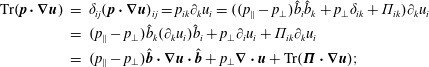 $$\begin{eqnarray}\displaystyle \text{Tr}(\boldsymbol{p}\boldsymbol{\cdot }\unicode[STIX]{x1D735}\boldsymbol{u}) & = & \displaystyle \unicode[STIX]{x1D6FF}_{ij}(\boldsymbol{p}\boldsymbol{\cdot }\unicode[STIX]{x1D735}\boldsymbol{u})_{ij}=p_{ik}\unicode[STIX]{x2202}_{k}u_{i}=((p_{\Vert }-p_{\bot })\hat{b}_{i}\hat{b}_{k}+p_{\bot }\unicode[STIX]{x1D6FF}_{ik}+\unicode[STIX]{x1D6F1}_{ik})\unicode[STIX]{x2202}_{k}u_{i}\nonumber\\ \displaystyle & = & \displaystyle (p_{\Vert }-p_{\bot })\hat{b}_{k}(\unicode[STIX]{x2202}_{k}u_{i})\hat{b}_{i}+p_{\bot }\unicode[STIX]{x2202}_{i}u_{i}+\unicode[STIX]{x1D6F1}_{ik}\unicode[STIX]{x2202}_{k}u_{i}\nonumber\\ \displaystyle & = & \displaystyle (p_{\Vert }-p_{\bot })\hat{\boldsymbol{b}}\boldsymbol{\cdot }\unicode[STIX]{x1D735}\boldsymbol{u}\boldsymbol{\cdot }\hat{\boldsymbol{b}}+p_{\bot }\unicode[STIX]{x1D735}\boldsymbol{\cdot }\boldsymbol{u}+\text{Tr}(\unicode[STIX]{x1D72B}\boldsymbol{\cdot }\unicode[STIX]{x1D735}\boldsymbol{u});\end{eqnarray}$$
the fourth term is equivalent to the third term
 $$\begin{eqnarray}\displaystyle \text{Tr}(\boldsymbol{p}\boldsymbol{\cdot }\unicode[STIX]{x1D735}\boldsymbol{u})^{\text{T}}=(\boldsymbol{p}\boldsymbol{\cdot }\unicode[STIX]{x1D735}\boldsymbol{u})_{ii}=(p_{\Vert }-p_{\bot })\hat{\boldsymbol{b}}\boldsymbol{\cdot }\unicode[STIX]{x1D735}\boldsymbol{u}\boldsymbol{\cdot }\hat{\boldsymbol{b}}+p_{\bot }\unicode[STIX]{x1D735}\boldsymbol{\cdot }\boldsymbol{u}+\text{Tr}(\unicode[STIX]{x1D72B}\boldsymbol{\cdot }\unicode[STIX]{x1D735}\boldsymbol{u})^{\text{T}}; & & \displaystyle\end{eqnarray}$$
even though we kept the last expression in transpose form so that we can use the symmetric operator after we combine all the terms. Finally the fifth term
 $$\begin{eqnarray}\displaystyle & \displaystyle \text{Tr}(\hat{\boldsymbol{b}}\times \unicode[STIX]{x1D72B})=\unicode[STIX]{x1D6FF}_{ij}\unicode[STIX]{x1D716}_{ikl}\hat{b}_{k}\unicode[STIX]{x1D6F1}_{lj}=\hat{b}_{k}\underbrace{\unicode[STIX]{x1D716}_{ikl}\unicode[STIX]{x1D6F1}_{li}}_{=0}=0; & \displaystyle\end{eqnarray}$$
 $$\begin{eqnarray}\displaystyle & \displaystyle \text{Tr}(\hat{\boldsymbol{b}}\times \unicode[STIX]{x1D72B})^{\text{T}}=\text{Tr}(\hat{\boldsymbol{b}}\times \unicode[STIX]{x1D72B})=0. & \displaystyle\end{eqnarray}$$
Combining all the terms, using the parallel pressure equation (2.59) and dividing by 2 yields the time-dependent equation for the perpendicular pressure that reads
 $$\begin{eqnarray}\displaystyle & & \displaystyle \frac{\unicode[STIX]{x2202}p_{\bot }}{\unicode[STIX]{x2202}t}+\unicode[STIX]{x1D735}\boldsymbol{\cdot }(p_{\bot }\boldsymbol{u})+p_{\bot }\unicode[STIX]{x1D735}\boldsymbol{\cdot }\boldsymbol{u}-p_{\bot }\hat{\boldsymbol{b}}\boldsymbol{\cdot }\unicode[STIX]{x1D735}\boldsymbol{u}\boldsymbol{\cdot }\hat{\boldsymbol{b}}+\frac{1}{2}[\text{Tr}\,\unicode[STIX]{x1D735}\boldsymbol{\cdot }\boldsymbol{q}-\hat{\boldsymbol{b}}\boldsymbol{\cdot }(\unicode[STIX]{x1D735}\boldsymbol{\cdot }\boldsymbol{q})\boldsymbol{\cdot }\hat{\boldsymbol{b}}]\nonumber\\ \displaystyle & & \displaystyle \qquad +\,\frac{1}{2}\left[\text{Tr}(\unicode[STIX]{x1D72B}\boldsymbol{\cdot }\unicode[STIX]{x1D735}\boldsymbol{u})^{S}+\unicode[STIX]{x1D72B}:\frac{\text{d}}{\text{d}t}(\hat{\boldsymbol{b}}\hat{\boldsymbol{b}})-(\unicode[STIX]{x1D72B}\boldsymbol{\cdot }\unicode[STIX]{x1D735}\boldsymbol{u})^{S}:\hat{\boldsymbol{b}}\hat{\boldsymbol{b}}\right]=0.\end{eqnarray}$$
The result corresponds to, for example, equation (25) of Passot & Sulem (Reference Passot and Sulem2004), equation (8) of Goswami et al. (Reference Goswami, Passot and Sulem2005). It is important to note that the parallel and perpendicular pressure equations are exact equations. These equations are valid regardless of what kind of higher-order closure will be adopted later. It is useful to rewrite the term
 $\unicode[STIX]{x1D72B}:(\text{d}/\text{d}t)(\hat{\boldsymbol{b}}\hat{\boldsymbol{b}})$
slightly so that we can directly use the induction equation and eliminate the time derivative. The term can be rewritten as
$\unicode[STIX]{x1D72B}:(\text{d}/\text{d}t)(\hat{\boldsymbol{b}}\hat{\boldsymbol{b}})$
slightly so that we can directly use the induction equation and eliminate the time derivative. The term can be rewritten as
 $$\begin{eqnarray}\displaystyle \unicode[STIX]{x1D72B}:\frac{\text{d}}{\text{d}t}(\hat{\boldsymbol{b}}\hat{\boldsymbol{b}}) & = & \displaystyle \unicode[STIX]{x1D6F1}_{ij}\frac{\text{d}}{\text{d}t}(\hat{b}_{i}\hat{b}_{j})=\unicode[STIX]{x1D6F1}_{ij}\left(\hat{b}_{i}\frac{\text{d}}{\text{d}t}\hat{b}_{j}+\hat{b}_{j}\frac{\text{d}}{\text{d}t}\hat{b}_{i}\right)\nonumber\\ \displaystyle & = & \displaystyle \hat{b}_{i}\unicode[STIX]{x1D6F1}_{ij}\frac{\text{d}}{\text{d}t}\hat{b}_{j}+\hat{b}_{j}\underbrace{\unicode[STIX]{x1D6F1}_{ij}}_{\unicode[STIX]{x1D6F1}_{ji}}\frac{\text{d}}{\text{d}t}\hat{b}_{i}=2\hat{\boldsymbol{b}}\boldsymbol{\cdot }\unicode[STIX]{x1D72B}\boldsymbol{\cdot }\frac{\text{d}\hat{\boldsymbol{b}}}{\text{d}t}.\end{eqnarray}$$
We will need the following identity for the time derivative of the unit vector (see later in the text),
 $$\begin{eqnarray}\displaystyle \frac{\text{d}}{\text{d}t}\hat{\boldsymbol{b}}=\frac{1}{|\boldsymbol{B}|}\left[\frac{\text{d}\boldsymbol{B}}{\text{d}t}-\hat{\boldsymbol{b}}\left(\hat{\boldsymbol{b}}\boldsymbol{\cdot }\frac{\text{d}\boldsymbol{B}}{\text{d}t}\right)\right], & & \displaystyle\end{eqnarray}$$
which, when used in the above expression together with
 $\hat{\boldsymbol{b}}\boldsymbol{\cdot }\unicode[STIX]{x1D72B}\boldsymbol{\cdot }\hat{\boldsymbol{b}}=0$
, allows us to write
$\hat{\boldsymbol{b}}\boldsymbol{\cdot }\unicode[STIX]{x1D72B}\boldsymbol{\cdot }\hat{\boldsymbol{b}}=0$
, allows us to write
 $$\begin{eqnarray}\displaystyle \unicode[STIX]{x1D72B}:\frac{\text{d}}{\text{d}t}(\hat{\boldsymbol{b}}\hat{\boldsymbol{b}})=\frac{2}{|\boldsymbol{B}|}\hat{\boldsymbol{b}}\boldsymbol{\cdot }\unicode[STIX]{x1D72B}\boldsymbol{\cdot }\frac{\text{d}\boldsymbol{B}}{\text{d}t}, & & \displaystyle\end{eqnarray}$$
which is an expression of general validity since no specific form of the induction equation was assumed yet. In the next section we will calculate the decomposition of the heat flux tensor
 $\boldsymbol{q}$
and we will show that, if only the gyrotropic heat flux components
$\boldsymbol{q}$
and we will show that, if only the gyrotropic heat flux components
 $q_{\Vert },q_{\bot }$
are considered, the heat flux terms entering the pressure equations read
$q_{\Vert },q_{\bot }$
are considered, the heat flux terms entering the pressure equations read
 $$\begin{eqnarray}\displaystyle & \displaystyle \hat{\boldsymbol{b}}\boldsymbol{\cdot }(\unicode[STIX]{x1D735}\boldsymbol{\cdot }\boldsymbol{q}^{\text{g}})\boldsymbol{\cdot }\hat{\boldsymbol{b}}=\unicode[STIX]{x1D735}\boldsymbol{\cdot }(q_{\Vert }\hat{\boldsymbol{b}})-2q_{\bot }\unicode[STIX]{x1D735}\boldsymbol{\cdot }\hat{\boldsymbol{b}}; & \displaystyle\end{eqnarray}$$
 $$\begin{eqnarray}\displaystyle & \displaystyle {\textstyle \frac{1}{2}}[\text{Tr}\,\unicode[STIX]{x1D735}\boldsymbol{\cdot }\boldsymbol{q}^{\text{g}}-\hat{\boldsymbol{b}}\boldsymbol{\cdot }(\unicode[STIX]{x1D735}\boldsymbol{\cdot }\boldsymbol{q}^{\text{g}})\boldsymbol{\cdot }\hat{\boldsymbol{b}}]=\unicode[STIX]{x1D735}\boldsymbol{\cdot }(q_{\bot }\hat{\boldsymbol{b}})+q_{\bot }\unicode[STIX]{x1D735}\boldsymbol{\cdot }\hat{\boldsymbol{b}}. & \displaystyle\end{eqnarray}$$
Therefore, by splitting the heat flux into gyrotropic and non-gyrotropic parts,
 $\boldsymbol{q}=\boldsymbol{q}^{\text{g}}+\boldsymbol{q}^{\text{ng}}$
, the pressure equations read
$\boldsymbol{q}=\boldsymbol{q}^{\text{g}}+\boldsymbol{q}^{\text{ng}}$
, the pressure equations read
 $$\begin{eqnarray}\displaystyle & & \displaystyle \frac{\unicode[STIX]{x2202}p_{\Vert }}{\unicode[STIX]{x2202}t}+\unicode[STIX]{x1D735}\boldsymbol{\cdot }(p_{\Vert }\boldsymbol{u})+2p_{\Vert }\hat{\boldsymbol{b}}\boldsymbol{\cdot }\unicode[STIX]{x1D735}\boldsymbol{u}\boldsymbol{\cdot }\hat{\boldsymbol{b}}+\unicode[STIX]{x1D735}\boldsymbol{\cdot }(q_{\Vert }\hat{\boldsymbol{b}})-2q_{\bot }\unicode[STIX]{x1D735}\boldsymbol{\cdot }\hat{\boldsymbol{b}}+\hat{\boldsymbol{b}}\boldsymbol{\cdot }(\unicode[STIX]{x1D735}\boldsymbol{\cdot }\boldsymbol{q}^{\text{ng}})\boldsymbol{\cdot }\hat{\boldsymbol{b}}\nonumber\\ \displaystyle & & \displaystyle \qquad -\,\frac{2}{|\boldsymbol{B}|}\hat{\boldsymbol{b}}\boldsymbol{\cdot }\unicode[STIX]{x1D72B}\boldsymbol{\cdot }\frac{\text{d}\boldsymbol{B}}{\text{d}t}+(\unicode[STIX]{x1D72B}\boldsymbol{\cdot }\unicode[STIX]{x1D735}\boldsymbol{u})^{S}:\hat{\boldsymbol{b}}\hat{\boldsymbol{b}}=0;\end{eqnarray}$$
 $$\begin{eqnarray}\displaystyle & & \displaystyle \frac{\unicode[STIX]{x2202}p_{\bot }}{\unicode[STIX]{x2202}t}+\unicode[STIX]{x1D735}\boldsymbol{\cdot }(p_{\bot }\boldsymbol{u})+p_{\bot }\unicode[STIX]{x1D735}\boldsymbol{\cdot }\boldsymbol{u}-p_{\bot }\hat{\boldsymbol{b}}\boldsymbol{\cdot }\unicode[STIX]{x1D735}\boldsymbol{u}\boldsymbol{\cdot }\hat{\boldsymbol{b}}+\unicode[STIX]{x1D735}\boldsymbol{\cdot }(q_{\bot }\hat{\boldsymbol{b}})\nonumber\\ \displaystyle & & \displaystyle \qquad +\,q_{\bot }\unicode[STIX]{x1D735}\boldsymbol{\cdot }\hat{\boldsymbol{b}}+\frac{1}{2}[\text{Tr}\,\unicode[STIX]{x1D735}\boldsymbol{\cdot }\boldsymbol{q}^{\text{ng}}-\hat{\boldsymbol{b}}\boldsymbol{\cdot }(\unicode[STIX]{x1D735}\boldsymbol{\cdot }\boldsymbol{q}^{\text{ng}})\boldsymbol{\cdot }\hat{\boldsymbol{b}}]\nonumber\\ \displaystyle & & \displaystyle \qquad +\,\frac{1}{2}\left[\text{Tr}(\unicode[STIX]{x1D72B}\boldsymbol{\cdot }\unicode[STIX]{x1D735}\boldsymbol{u})^{S}+\frac{2}{|\boldsymbol{B}|}\hat{\boldsymbol{b}}\boldsymbol{\cdot }\unicode[STIX]{x1D72B}\boldsymbol{\cdot }\frac{\text{d}\boldsymbol{B}}{\text{d}t}-(\unicode[STIX]{x1D72B}\boldsymbol{\cdot }\unicode[STIX]{x1D735}\boldsymbol{u})^{S}:\hat{\boldsymbol{b}}\hat{\boldsymbol{b}}\right]=0.\end{eqnarray}$$
Terms with the non-gyrotropic heat flux
 $\boldsymbol{q}^{\text{ng}}$
can be further split into non-gyrotropic heat flux vectors
$\boldsymbol{q}^{\text{ng}}$
can be further split into non-gyrotropic heat flux vectors
 $\boldsymbol{S}_{\bot }^{\Vert }$
,
$\boldsymbol{S}_{\bot }^{\Vert }$
,
 $\boldsymbol{S}_{\bot }^{\bot }$
and the heat flux tensor
$\boldsymbol{S}_{\bot }^{\bot }$
and the heat flux tensor
 $\unicode[STIX]{x1D748}$
, which is addressed in appendix D, see (D 124), (D 126). Terms containing the FLR pressure tensor
$\unicode[STIX]{x1D748}$
, which is addressed in appendix D, see (D 124), (D 126). Terms containing the FLR pressure tensor
 $\unicode[STIX]{x1D72B}$
are usually called the FLR stress forces, and these forces can generate complicated plasma heating processes. The FLR stress forces can generate both parallel and perpendicular plasma heating that can be determined only from fully nonlinear numerical simulations, since all the terms disappear at the linear level. This process is also sometimes called ‘stochastic heating’. The importance of stochastic heating was shown by Laveder, Passot & Sulem (Reference Laveder, Passot and Sulem2013), who performed 1.5-dimensional numerical simulations with the sophisticated FLR Landau fluid model of Passot & Sulem (Reference Passot and Sulem2007), Passot et al. (Reference Passot, Sulem and Hunana2012).
$\unicode[STIX]{x1D72B}$
are usually called the FLR stress forces, and these forces can generate complicated plasma heating processes. The FLR stress forces can generate both parallel and perpendicular plasma heating that can be determined only from fully nonlinear numerical simulations, since all the terms disappear at the linear level. This process is also sometimes called ‘stochastic heating’. The importance of stochastic heating was shown by Laveder, Passot & Sulem (Reference Laveder, Passot and Sulem2013), who performed 1.5-dimensional numerical simulations with the sophisticated FLR Landau fluid model of Passot & Sulem (Reference Passot and Sulem2007), Passot et al. (Reference Passot, Sulem and Hunana2012).
2.4 On the paper by Chew et al. (Reference Chew, Goldberger and Low1956)
The very influential paper by Chew et al. (Reference Chew, Goldberger and Low1956) that is typically cited for the CGL equations (with zero heat fluxes) actually also derived the pressure equations when the gyrotropic heat fluxes are considered. It is important to emphasize that, even though the scalar pressures
 $p_{n}$
,
$p_{n}$
,
 $p_{s}$
in the notation of that paper are equal to the usual pressures
$p_{s}$
in the notation of that paper are equal to the usual pressures
 $p_{\Vert }$
,
$p_{\Vert }$
,
 $p_{\bot }$
, this is not the case for the heat fluxes. The gyrotropic heat flux tensor in that paper is decomposed into components
$p_{\bot }$
, this is not the case for the heat fluxes. The gyrotropic heat flux tensor in that paper is decomposed into components
 $q_{n}$
,
$q_{n}$
,
 $q_{s}$
according to (Chew et al.
Reference Chew, Goldberger and Low1956, equation (34))
$q_{s}$
according to (Chew et al.
Reference Chew, Goldberger and Low1956, equation (34))
 $$\begin{eqnarray}q_{ijk}^{\text{g}}=q_{n}\hat{b}_{i}\hat{b}_{j}\hat{b}_{k}+q_{s}(\unicode[STIX]{x1D6FF}_{ij}\hat{b}_{k}+\unicode[STIX]{x1D6FF}_{jk}\hat{b}_{i}+\unicode[STIX]{x1D6FF}_{ik}\hat{b}_{j}).\end{eqnarray}$$
In contrast, the usual gyrotropic heat flux decomposition to
 $q_{\Vert }$
,
$q_{\Vert }$
,
 $q_{\bot }$
reads (see later in the text)
$q_{\bot }$
reads (see later in the text)
 $$\begin{eqnarray}q_{ijk}^{\text{g}}=q_{\Vert }\hat{b}_{i}\hat{b}_{j}\hat{b}_{k}+q_{\bot }(\unicode[STIX]{x1D6FF}_{ij}\hat{b}_{k}+\unicode[STIX]{x1D6FF}_{jk}\hat{b}_{i}+\unicode[STIX]{x1D6FF}_{ik}\hat{b}_{j}-3\hat{b}_{i}\hat{b}_{j}\hat{b}_{k}),\end{eqnarray}$$
i.e. the last term is not present in their decomposition. However, this does not mean that their pressure equations (Chew et al. Reference Chew, Goldberger and Low1956, equations (31), (32)) are incorrect. It only implies that their equations are written in terms of
 $$\begin{eqnarray}q_{n}=q_{\Vert }-3q_{\bot };\quad q_{s}=q_{\bot }.\end{eqnarray}$$
By neglecting the FLR corrections
 $\unicode[STIX]{x1D72B}$
and
$\unicode[STIX]{x1D72B}$
and
 $\boldsymbol{q}^{\text{ng}}$
, the parallel and perpendicular pressure equations (2.74), (2.75) simplify to
$\boldsymbol{q}^{\text{ng}}$
, the parallel and perpendicular pressure equations (2.74), (2.75) simplify to
 $$\begin{eqnarray}\displaystyle & \displaystyle \frac{\text{d}p_{\Vert }}{\text{d}t}+p_{\Vert }\unicode[STIX]{x1D735}\boldsymbol{\cdot }\boldsymbol{u}+2p_{\Vert }\hat{\boldsymbol{b}}\boldsymbol{\cdot }\unicode[STIX]{x1D735}\boldsymbol{u}\boldsymbol{\cdot }\hat{\boldsymbol{b}}+\unicode[STIX]{x1D735}\boldsymbol{\cdot }(q_{\Vert }\hat{\boldsymbol{b}})-2q_{\bot }\unicode[STIX]{x1D735}\boldsymbol{\cdot }\hat{\boldsymbol{b}}=0; & \displaystyle\end{eqnarray}$$
 $$\begin{eqnarray}\displaystyle & \displaystyle \frac{\text{d}p_{\bot }}{\text{d}t}+2p_{\bot }\unicode[STIX]{x1D735}\boldsymbol{\cdot }\boldsymbol{u}-p_{\bot }\hat{\boldsymbol{b}}\boldsymbol{\cdot }\unicode[STIX]{x1D735}\boldsymbol{u}\boldsymbol{\cdot }\hat{\boldsymbol{b}}+\unicode[STIX]{x1D735}\boldsymbol{\cdot }(q_{\bot }\hat{\boldsymbol{b}})+q_{\bot }\unicode[STIX]{x1D735}\boldsymbol{\cdot }\hat{\boldsymbol{b}}=0. & \displaystyle\end{eqnarray}$$
By using (2.78), the heat flux contributions in the parallel pressure equation above can be rewritten as
 $$\begin{eqnarray}\displaystyle \unicode[STIX]{x1D735}\boldsymbol{\cdot }(q_{\Vert }\hat{\boldsymbol{b}})-2q_{\bot }\unicode[STIX]{x1D735}\boldsymbol{\cdot }\hat{\boldsymbol{b}}=\unicode[STIX]{x1D735}\boldsymbol{\cdot }[(q_{n}+q_{s})\hat{\boldsymbol{b}}]+2\hat{\boldsymbol{b}}\boldsymbol{\cdot }\unicode[STIX]{x1D735}q_{s}, & & \displaystyle\end{eqnarray}$$
which agrees with the parallel pressure equation obtained by Chew et al. (Reference Chew, Goldberger and Low1956), equation (31). The pressure equations of Chew et al. (Reference Chew, Goldberger and Low1956) are therefore correct, but it has to be remembered that
 $q_{n}$
is not the usual parallel heat flux
$q_{n}$
is not the usual parallel heat flux
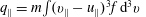 $q_{\Vert }=m\!\int (v_{\Vert }-u_{\Vert })^{3}f\,\text{d}^{3}v$
.Footnote
1
Actually, the authors do not even call the quantities
$q_{\Vert }=m\!\int (v_{\Vert }-u_{\Vert })^{3}f\,\text{d}^{3}v$
.Footnote
1
Actually, the authors do not even call the quantities
 $q_{n},q_{s}$
heat flux components, but components of a ‘pressure-transport’ tensor.
$q_{n},q_{s}$
heat flux components, but components of a ‘pressure-transport’ tensor.
To conclude this subsection, we will go slightly ahead and use (3.51), (3.52) (without the zero right-hand sides) that are the usual CGL pressure equations and valid only at long spatial scales when the Hall term in the induction equation is neglected. Under this assumption, the pressure equations (2.79), (2.80) are rewritten as
 $$\begin{eqnarray}\displaystyle & \displaystyle \frac{\text{d}}{\text{d}t}\left(\frac{p_{\Vert }|\boldsymbol{B}|^{2}}{\unicode[STIX]{x1D70C}^{3}}\right)=-\frac{|\boldsymbol{B}|^{2}}{\unicode[STIX]{x1D70C}^{3}}[\unicode[STIX]{x1D735}\boldsymbol{\cdot }(q_{\Vert }\hat{\boldsymbol{b}})-2q_{\bot }\unicode[STIX]{x1D735}\boldsymbol{\cdot }\hat{\boldsymbol{b}}]; & \displaystyle\end{eqnarray}$$
 $$\begin{eqnarray}\displaystyle & \displaystyle \frac{\text{d}}{\text{d}t}\left(\frac{p_{\bot }}{\unicode[STIX]{x1D70C}|\boldsymbol{B}|}\right)=-\frac{1}{\unicode[STIX]{x1D70C}|\boldsymbol{B}|}[\unicode[STIX]{x1D735}\boldsymbol{\cdot }(q_{\bot }\hat{\boldsymbol{b}})+q_{\bot }\unicode[STIX]{x1D735}\boldsymbol{\cdot }\hat{\boldsymbol{b}}]. & \displaystyle\end{eqnarray}$$
It is often forgotten that the paper by Chew et al. (Reference Chew, Goldberger and Low1956) derived the correct pressure equations with gyrotropic heat flux contributions. The authors, however, did not write the equations in the form (2.82), (2.83), and left them in the form (2.79), (2.80), using the ‘conservative’ form only after prescribing the closure
 $q_{\Vert }=q_{\bot }=0$
(their equations (35), (36)),
$q_{\Vert }=q_{\bot }=0$
(their equations (35), (36)),
 $$\begin{eqnarray}\displaystyle & \displaystyle \frac{\text{d}}{\text{d}t}\left(\frac{p_{\Vert }|\boldsymbol{B}|^{2}}{\unicode[STIX]{x1D70C}^{3}}\right)=0; & \displaystyle\end{eqnarray}$$
 $$\begin{eqnarray}\displaystyle & \displaystyle \frac{\text{d}}{\text{d}t}\left(\frac{p_{\bot }}{\unicode[STIX]{x1D70C}|\boldsymbol{B}|}\right)=0. & \displaystyle\end{eqnarray}$$
Over time, equations (2.84), (2.85) became known as the CGL description. Equations (2.84), (2.85) are often replaced by the equations of state
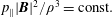 $p_{\Vert }|\boldsymbol{B}|^{2}/\unicode[STIX]{x1D70C}^{3}=\text{const.}$
and
$p_{\Vert }|\boldsymbol{B}|^{2}/\unicode[STIX]{x1D70C}^{3}=\text{const.}$
and
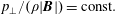 $p_{\bot }/(\unicode[STIX]{x1D70C}|\boldsymbol{B}|)=\text{const.}$
, see e.g. Mjølhus (Reference Mjølhus2009). Additionally, similarly to the definition of (appropriately normalized) entropy in MHD,
$p_{\bot }/(\unicode[STIX]{x1D70C}|\boldsymbol{B}|)=\text{const.}$
, see e.g. Mjølhus (Reference Mjølhus2009). Additionally, similarly to the definition of (appropriately normalized) entropy in MHD,
 $s=\ln (p/\unicode[STIX]{x1D70C}^{\unicode[STIX]{x1D6FE}})$
, it is useful to define parallel and perpendicular entropy in the CGL model, according to
$s=\ln (p/\unicode[STIX]{x1D70C}^{\unicode[STIX]{x1D6FE}})$
, it is useful to define parallel and perpendicular entropy in the CGL model, according to
 $$\begin{eqnarray}s_{\Vert }=\frac{1}{3}\ln \left(\frac{p_{\Vert }|\boldsymbol{B}|^{2}}{\unicode[STIX]{x1D70C}^{3}}\right);\quad s_{\bot }=\frac{2}{3}\ln \left(\frac{p_{\bot }}{\unicode[STIX]{x1D70C}|\boldsymbol{B}|}\right).\end{eqnarray}$$
The total entropy,
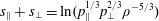 $s_{\Vert }+s_{\bot }=\ln (p_{\Vert }^{1/3}p_{\bot }^{2/3}\unicode[STIX]{x1D70C}^{-5/3})$
, is equivalent to the MHD entropy when
$s_{\Vert }+s_{\bot }=\ln (p_{\Vert }^{1/3}p_{\bot }^{2/3}\unicode[STIX]{x1D70C}^{-5/3})$
, is equivalent to the MHD entropy when
 $p_{\Vert }=p_{\bot }$
, see for example (9)–(11) in Abraham-Shrauner (Reference Abraham-Shrauner1967).
$p_{\Vert }=p_{\bot }$
, see for example (9)–(11) in Abraham-Shrauner (Reference Abraham-Shrauner1967).
2.5 Physical meaning of CGL equations
The exact derivation of the CGL equation (2.84), (2.85) will be completed in the next section. Here, we briefly discuss the physical meaning of these equations. The CGL equations (2.85), (2.84) can be interpreted as the conservation of the first and second adiabatic invariants, as is nicely discussed for example by Kulsrud (Reference Kulsrud, Galeev and Sudan1983) and by Gurnett & Bhattacharjee (Reference Gurnett and Bhattacharjee2005). Considering many particles with velocity components
 $v_{\Vert }$
and
$v_{\Vert }$
and
 $v_{\bot }$
with respect to the mean magnetic field, the parallel and perpendicular pressures can be estimated as
$v_{\bot }$
with respect to the mean magnetic field, the parallel and perpendicular pressures can be estimated as
 $$\begin{eqnarray}p_{\Vert }\sim \langle v_{\Vert }^{2}\rangle \unicode[STIX]{x1D70C};\quad p_{\bot }\sim \langle v_{\bot }^{2}\rangle \unicode[STIX]{x1D70C},\end{eqnarray}$$
where the brackets represent an average over all particles. To complete the estimate, we need expressions for
 $\langle v_{\Vert }^{2}\rangle$
and
$\langle v_{\Vert }^{2}\rangle$
and
 $\langle v_{\bot }^{2}\rangle$
, which come from the conservation of the adiabatic invariants. The first adiabatic invariant is the conservation of magnetic moment
$\langle v_{\bot }^{2}\rangle$
, which come from the conservation of the adiabatic invariants. The first adiabatic invariant is the conservation of magnetic moment
 $\unicode[STIX]{x1D707}$
of a particle that is gyrating periodically around a mean magnetic field. The second adiabatic invariant, sometimes also called the longitudinal invariant, is associated with a particle bouncing periodically between two magnetic mirror points. The conserved quantity is the integral over the parallel momentum of a particle
$\unicode[STIX]{x1D707}$
of a particle that is gyrating periodically around a mean magnetic field. The second adiabatic invariant, sometimes also called the longitudinal invariant, is associated with a particle bouncing periodically between two magnetic mirror points. The conserved quantity is the integral over the parallel momentum of a particle
 $J\equiv \oint _{a}^{b}mv_{\Vert }\,\text{d}l$
, where the magnetic mirrors are located at ‘
$J\equiv \oint _{a}^{b}mv_{\Vert }\,\text{d}l$
, where the magnetic mirrors are located at ‘
 $a$
’ and ‘
$a$
’ and ‘
 $b$
’ and the integral is performed along the magnetic field line. The distance between the two magnetic mirrors at ‘
$b$
’ and the integral is performed along the magnetic field line. The distance between the two magnetic mirrors at ‘
 $a$
’ and ‘
$a$
’ and ‘
 $b$
’ can be labelled as
$b$
’ can be labelled as
 $L$
. The conservation of the first and second adiabatic invariants is therefore
$L$
. The conservation of the first and second adiabatic invariants is therefore
 $$\begin{eqnarray}\unicode[STIX]{x1D707}\equiv \frac{mv_{\bot }^{2}}{2B}=\text{const.};\quad J\equiv mv_{\Vert }L=\text{const.}\end{eqnarray}$$
Since we are considering only non-relativistic particles, the particle mass ‘
 $m$
’ is also a constant. The conservation of magnetic moment
$m$
’ is also a constant. The conservation of magnetic moment
 $\unicode[STIX]{x1D707}$
therefore implies
$\unicode[STIX]{x1D707}$
therefore implies
 $v_{\bot }^{2}\sim B$
, and using this in (2.87) yields
$v_{\bot }^{2}\sim B$
, and using this in (2.87) yields
 $p_{\bot }\sim B\unicode[STIX]{x1D70C}$
, recovering (2.85). The CGL equation (2.85) therefore corresponds to conservation of magnetic moment, i.e. the first adiabatic invariant. The conservation of the second adiabatic invariant
$p_{\bot }\sim B\unicode[STIX]{x1D70C}$
, recovering (2.85). The CGL equation (2.85) therefore corresponds to conservation of magnetic moment, i.e. the first adiabatic invariant. The conservation of the second adiabatic invariant
 $J$
is more tricky, since we need to somehow estimate the non-intuitive length
$J$
is more tricky, since we need to somehow estimate the non-intuitive length
 $L$
between the two magnetic mirrors, and no magnetic mirrors are explicitly assumed, since we are just dealing with somewhat random magnetic field lines. The length
$L$
between the two magnetic mirrors, and no magnetic mirrors are explicitly assumed, since we are just dealing with somewhat random magnetic field lines. The length
 $L$
can be nevertheless estimated from two fundamental physical principles. Consider a magnetic flux tube (a deformed cylinder) with cross-sectional area
$L$
can be nevertheless estimated from two fundamental physical principles. Consider a magnetic flux tube (a deformed cylinder) with cross-sectional area
 $A$
and length
$A$
and length
 $L$
. The conservation of the total magnetic flux through the area
$L$
. The conservation of the total magnetic flux through the area
 $A$
implies
$A$
implies
 $AB=\text{const.}$
, which yields an estimate for the area
$AB=\text{const.}$
, which yields an estimate for the area
 $A\sim 1/B$
. The second principle is the conservation of the total mass of particles that are completely trapped in that flux tube and that cannot escape,
$A\sim 1/B$
. The second principle is the conservation of the total mass of particles that are completely trapped in that flux tube and that cannot escape,
 $mnAL=\text{const.}$
, yielding
$mnAL=\text{const.}$
, yielding
 $L\sim 1/(\unicode[STIX]{x1D70C}A)$
. The use of
$L\sim 1/(\unicode[STIX]{x1D70C}A)$
. The use of
 $A\sim 1/B$
yields the final estimate for the non-intuitive length
$A\sim 1/B$
yields the final estimate for the non-intuitive length
 $L\sim B/\unicode[STIX]{x1D70C}$
. The conservation of the second adiabatic invariant
$L\sim B/\unicode[STIX]{x1D70C}$
. The conservation of the second adiabatic invariant
 $J$
therefore implies
$J$
therefore implies
 $v_{\Vert }\sim 1/L\sim \unicode[STIX]{x1D70C}/B$
. Using this result in (2.87) implies
$v_{\Vert }\sim 1/L\sim \unicode[STIX]{x1D70C}/B$
. Using this result in (2.87) implies
 $p_{\Vert }\sim \unicode[STIX]{x1D70C}^{3}/B^{2}$
, recovering (2.84). The CGL equation (2.84) corresponds to conservation of the second adiabatic invariant
$p_{\Vert }\sim \unicode[STIX]{x1D70C}^{3}/B^{2}$
, recovering (2.84). The CGL equation (2.84) corresponds to conservation of the second adiabatic invariant
 $J$
, and the equation is valid for particles that are completely trapped and therefore cannot carry a heat flux. As we discuss later, the consideration of the Hall term, the heat flux and the FLR stress forces (the stochastic heating), leads to the breaking of these two adiabatic invariants. Nevertheless, exact conservation laws can still be derived, and the very simple CGL equations (2.84), (2.85) have to be modified with non-zero right-hand sides.
$J$
, and the equation is valid for particles that are completely trapped and therefore cannot carry a heat flux. As we discuss later, the consideration of the Hall term, the heat flux and the FLR stress forces (the stochastic heating), leads to the breaking of these two adiabatic invariants. Nevertheless, exact conservation laws can still be derived, and the very simple CGL equations (2.84), (2.85) have to be modified with non-zero right-hand sides.
In Part 2 of our guide (see § 4.1), we show that the conservation of magnetic moment is very useful for understanding the form of the perturbed distribution function
 $f^{(1)}$
in the gyrotropic limit. By performing calculations in the laboratory reference frame, we show that to obtain the correct
$f^{(1)}$
in the gyrotropic limit. By performing calculations in the laboratory reference frame, we show that to obtain the correct
 $f^{(1)}$
in the gyrotropic limit actually requires the usual complicated kinetic integration around the unperturbed orbit (see the Appendix of Part 2) and only then the gyrotropic limit can be imposed. In contrast, performing calculations in the guiding-centre reference frame allows one to prescribe the conservation of magnetic moment from the beginning, and obtain the correct
$f^{(1)}$
in the gyrotropic limit actually requires the usual complicated kinetic integration around the unperturbed orbit (see the Appendix of Part 2) and only then the gyrotropic limit can be imposed. In contrast, performing calculations in the guiding-centre reference frame allows one to prescribe the conservation of magnetic moment from the beginning, and obtain the correct
 $f^{(1)}$
in the gyrotropic limit perhaps more intuitively. Conservation of adiabatic invariants is important in many areas of space physics and astrophysics. For example, conservation of adiabatic invariants is used to construct models that describe particles trapped inside of magnetic islands and that are being accelerated during magnetic island contraction and merging (Drake, Swisdak & Fermo Reference Drake, Swisdak and Fermo2013; Zank et al.
Reference Zank, le Roux, Webb, Dosch and Khabarova2014).
$f^{(1)}$
in the gyrotropic limit perhaps more intuitively. Conservation of adiabatic invariants is important in many areas of space physics and astrophysics. For example, conservation of adiabatic invariants is used to construct models that describe particles trapped inside of magnetic islands and that are being accelerated during magnetic island contraction and merging (Drake, Swisdak & Fermo Reference Drake, Swisdak and Fermo2013; Zank et al.
Reference Zank, le Roux, Webb, Dosch and Khabarova2014).
2.6 Exact equations of anisotropic multi-fluid models
Before we discuss solutions of specific fluid models, it is beneficial to summarize the most general equations of multi-fluid models that were derived with no simplifications at all. By reintroducing the species index
 $r$
, the equations that were directly obtained by integrating the collisionless Vlasov equation read
$r$
, the equations that were directly obtained by integrating the collisionless Vlasov equation read
 $$\begin{eqnarray}\displaystyle & \displaystyle \frac{\unicode[STIX]{x2202}\unicode[STIX]{x1D70C}_{r}}{\unicode[STIX]{x2202}t}+\unicode[STIX]{x1D735}\boldsymbol{\cdot }(\unicode[STIX]{x1D70C}_{r}\boldsymbol{u}_{r})=0; & \displaystyle\end{eqnarray}$$
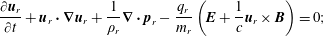 $$\begin{eqnarray}\displaystyle & \displaystyle \frac{\unicode[STIX]{x2202}\boldsymbol{u}_{r}}{\unicode[STIX]{x2202}t}+\boldsymbol{u}_{r}\boldsymbol{\cdot }\unicode[STIX]{x1D735}\boldsymbol{u}_{r}+\frac{1}{\unicode[STIX]{x1D70C}_{r}}\unicode[STIX]{x1D735}\boldsymbol{\cdot }\boldsymbol{p}_{r}-\frac{q_{r}}{m_{r}}\left(\boldsymbol{E}+\frac{1}{c}\boldsymbol{u}_{r}\times \boldsymbol{B}\right)=0; & \displaystyle\end{eqnarray}$$
 $$\begin{eqnarray}\displaystyle & & \displaystyle \frac{\unicode[STIX]{x2202}p_{\Vert r}}{\unicode[STIX]{x2202}t}+\unicode[STIX]{x1D735}\boldsymbol{\cdot }(p_{\Vert r}\boldsymbol{u}_{r})+2p_{\Vert r}\hat{\boldsymbol{b}}\boldsymbol{\cdot }\unicode[STIX]{x1D735}\boldsymbol{u}_{r}\boldsymbol{\cdot }\hat{\boldsymbol{b}}+\hat{\boldsymbol{b}}\boldsymbol{\cdot }(\unicode[STIX]{x1D735}\boldsymbol{\cdot }\boldsymbol{q}_{r})\boldsymbol{\cdot }\hat{\boldsymbol{b}}\nonumber\\ \displaystyle & & \displaystyle \qquad -\,\frac{2}{|\boldsymbol{B}|}\hat{\boldsymbol{b}}\boldsymbol{\cdot }\unicode[STIX]{x1D72B}_{r}\boldsymbol{\cdot }\frac{\text{d}_{r}\boldsymbol{B}}{\text{d}t}+(\unicode[STIX]{x1D72B}_{r}\boldsymbol{\cdot }\unicode[STIX]{x1D735}\boldsymbol{u}_{r})^{S}:\hat{\boldsymbol{b}}\hat{\boldsymbol{b}}=0;\end{eqnarray}$$
 $$\begin{eqnarray}\displaystyle & & \displaystyle \frac{\unicode[STIX]{x2202}p_{\bot r}}{\unicode[STIX]{x2202}t}+\unicode[STIX]{x1D735}\boldsymbol{\cdot }(p_{\bot r}\boldsymbol{u}_{r})+p_{\bot r}\unicode[STIX]{x1D735}\boldsymbol{\cdot }\boldsymbol{u}_{r}-p_{\bot r}\hat{\boldsymbol{b}}\boldsymbol{\cdot }\unicode[STIX]{x1D735}\boldsymbol{u}_{r}\boldsymbol{\cdot }\hat{\boldsymbol{b}}+\frac{1}{2}[\text{Tr}\,\unicode[STIX]{x1D735}\boldsymbol{\cdot }\boldsymbol{q}_{r}-\hat{\boldsymbol{b}}\boldsymbol{\cdot }(\unicode[STIX]{x1D735}\boldsymbol{\cdot }\boldsymbol{q}_{r})\boldsymbol{\cdot }\hat{\boldsymbol{b}}]\nonumber\\ \displaystyle & & \displaystyle \qquad +\,\frac{1}{2}\left[\text{Tr}(\unicode[STIX]{x1D72B}_{r}\boldsymbol{\cdot }\unicode[STIX]{x1D735}\boldsymbol{u}_{r})^{S}+\frac{2}{|\boldsymbol{B}|}\hat{\boldsymbol{b}}\boldsymbol{\cdot }\unicode[STIX]{x1D72B}_{r}\boldsymbol{\cdot }\frac{\text{d}_{r}\boldsymbol{B}}{\text{d}t}-(\unicode[STIX]{x1D72B}_{r}\boldsymbol{\cdot }\unicode[STIX]{x1D735}\boldsymbol{u}_{r})^{S}:\hat{\boldsymbol{b}}\hat{\boldsymbol{b}}\right]=0,\end{eqnarray}$$
where the convective derivative
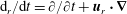 $\text{d}_{r}/\text{d}t=\unicode[STIX]{x2202}/\unicode[STIX]{x2202}t+\boldsymbol{u}_{r}\boldsymbol{\cdot }\unicode[STIX]{x1D735}$
. In the above equations, the pressure tensor for each species was just decomposed into gyrotropic contributions
$\text{d}_{r}/\text{d}t=\unicode[STIX]{x2202}/\unicode[STIX]{x2202}t+\boldsymbol{u}_{r}\boldsymbol{\cdot }\unicode[STIX]{x1D735}$
. In the above equations, the pressure tensor for each species was just decomposed into gyrotropic contributions
 $p_{\Vert r}$
,
$p_{\Vert r}$
,
 $p_{\bot r}$
and the rest of the pressure tensor (the FLR pressure tensor
$p_{\bot r}$
and the rest of the pressure tensor (the FLR pressure tensor
 $\unicode[STIX]{x1D72B}_{r}$
), according to
$\unicode[STIX]{x1D72B}_{r}$
), according to
 $$\begin{eqnarray}\boldsymbol{p}_{r}=p_{\Vert r}\hat{\boldsymbol{b}}\hat{\boldsymbol{b}}+p_{\bot r}(\unicode[STIX]{x1D644}-\hat{\boldsymbol{b}}\hat{\boldsymbol{b}})+\unicode[STIX]{x1D72B}_{r},\end{eqnarray}$$
which is a rigorous decomposition not introducing any simplifications. The heat flux
 $\boldsymbol{q}_{r}$
contributions are here left at the most general level without any simplifications either. The equations are accompanied by Maxwell’s equations, that for now we write down here with no simplifications to emphasize that no Maxwell equations were used in deriving the above system,
$\boldsymbol{q}_{r}$
contributions are here left at the most general level without any simplifications either. The equations are accompanied by Maxwell’s equations, that for now we write down here with no simplifications to emphasize that no Maxwell equations were used in deriving the above system,
 $$\begin{eqnarray}\displaystyle & \displaystyle \unicode[STIX]{x1D735}\boldsymbol{\cdot }\boldsymbol{E}=4\unicode[STIX]{x03C0}\unicode[STIX]{x1D70C}_{c}=4\unicode[STIX]{x03C0}\mathop{\sum }_{r}q_{r}n_{r};\quad \unicode[STIX]{x1D735}\boldsymbol{\cdot }\boldsymbol{B}=0; & \displaystyle\end{eqnarray}$$
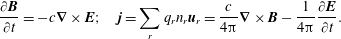 $$\begin{eqnarray}\displaystyle & \displaystyle \frac{\unicode[STIX]{x2202}\boldsymbol{B}}{\unicode[STIX]{x2202}t}=-c\unicode[STIX]{x1D735}\times \boldsymbol{E};\quad \boldsymbol{j}=\mathop{\sum }_{r}q_{r}n_{r}\boldsymbol{u}_{r}=\frac{c}{4\unicode[STIX]{x03C0}}\unicode[STIX]{x1D735}\times \boldsymbol{B}-\frac{1}{4\unicode[STIX]{x03C0}}\frac{\unicode[STIX]{x2202}\boldsymbol{E}}{\unicode[STIX]{x2202}t}. & \displaystyle\end{eqnarray}$$
Equations (2.89)–(2.95) represent an exact (even though not closed) kinetic Vlasov–Maxwell system formulated in fluid variables, and the description is valid for any general distribution function and for all considered spatial and temporal scales. All advanced collisionless multi-fluid models have to be based in one way or another on these equations. One can concentrate on the proton dynamics or one can concentrate on the electron dynamics and simplify these equations accordingly for these spatial scales. Naturally, one can consider complicated multi-fluid descriptions composed of many particle species.
For a new reader who just jumped straight to this section, the symmetric operator ‘
 $S$
’ acts on a matrix
$S$
’ acts on a matrix
 $\unicode[STIX]{x1D608}_{ij}$
according to
$\unicode[STIX]{x1D608}_{ij}$
according to
 $\unicode[STIX]{x1D608}_{ij}^{S}=\unicode[STIX]{x1D608}_{ij}+\unicode[STIX]{x1D608}_{ji}$
. If one does not like the symmetric operator in the expressions above, the symmetric operator is actually not necessary, since
$\unicode[STIX]{x1D608}_{ij}^{S}=\unicode[STIX]{x1D608}_{ij}+\unicode[STIX]{x1D608}_{ji}$
. If one does not like the symmetric operator in the expressions above, the symmetric operator is actually not necessary, since
 $$\begin{eqnarray}\displaystyle & \displaystyle (\unicode[STIX]{x1D72B}\boldsymbol{\cdot }\unicode[STIX]{x1D735}\boldsymbol{u})_{ij}=\unicode[STIX]{x1D6F1}_{ik}\unicode[STIX]{x2202}_{k}u_{j}; & \displaystyle\end{eqnarray}$$
 $$\begin{eqnarray}\displaystyle & \displaystyle (\unicode[STIX]{x1D72B}\boldsymbol{\cdot }\unicode[STIX]{x1D735}\boldsymbol{u})_{ij}^{S}=\unicode[STIX]{x1D6F1}_{ik}\unicode[STIX]{x2202}_{k}u_{j}+\unicode[STIX]{x1D6F1}_{jk}\unicode[STIX]{x2202}_{k}u_{i}; & \displaystyle\end{eqnarray}$$
 $$\begin{eqnarray}\displaystyle & \displaystyle (\unicode[STIX]{x1D72B}\boldsymbol{\cdot }\unicode[STIX]{x1D735}\boldsymbol{u})^{S}:\hat{\boldsymbol{b}}\hat{\boldsymbol{b}}=2\hat{b}_{i}\unicode[STIX]{x1D6F1}_{ik}(\unicode[STIX]{x2202}_{k}u_{j})\hat{b}_{j}=2(\unicode[STIX]{x1D72B}\boldsymbol{\cdot }\unicode[STIX]{x1D735}\boldsymbol{u}):\hat{\boldsymbol{b}}\hat{\boldsymbol{b}}=2\hat{\boldsymbol{b}}\boldsymbol{\cdot }(\unicode[STIX]{x1D72B}\boldsymbol{\cdot }\unicode[STIX]{x1D735}\boldsymbol{u})\boldsymbol{\cdot }\hat{\boldsymbol{b}}; & \displaystyle\end{eqnarray}$$
 $$\begin{eqnarray}\displaystyle & \displaystyle \text{Tr}(\unicode[STIX]{x1D72B}\boldsymbol{\cdot }\unicode[STIX]{x1D735}\boldsymbol{u})^{S}=2\unicode[STIX]{x1D6F1}_{ik}\unicode[STIX]{x2202}_{k}u_{i}=2\unicode[STIX]{x1D72B}:\unicode[STIX]{x1D735}\boldsymbol{u}=2(\unicode[STIX]{x1D72B}\boldsymbol{\cdot }\unicode[STIX]{x1D735})\boldsymbol{\cdot }\boldsymbol{u}, & \displaystyle\end{eqnarray}$$
where we also got rid of the double contractions. Note that
 $\unicode[STIX]{x1D6F1}_{ik}=\unicode[STIX]{x1D6F1}_{ki}$
and also
$\unicode[STIX]{x1D6F1}_{ik}=\unicode[STIX]{x1D6F1}_{ki}$
and also
 $p_{ik}=p_{ki}$
.
$p_{ik}=p_{ki}$
.
Equations (2.89)–(2.92) contain two very important catches – the entire heat flux tensor
 $\boldsymbol{q}_{r}$
and the non-gyrotropic pressure tensor
$\boldsymbol{q}_{r}$
and the non-gyrotropic pressure tensor
 $\unicode[STIX]{x1D72B}_{r}$
are not specified yet. In this moment, the entire class of collisionless fluid models separates to many possible classes and sub-classes, depending on how precisely one wants to evaluate the heat flux tensor
$\unicode[STIX]{x1D72B}_{r}$
are not specified yet. In this moment, the entire class of collisionless fluid models separates to many possible classes and sub-classes, depending on how precisely one wants to evaluate the heat flux tensor
 $\boldsymbol{q}_{r}$
and the FLR pressure tensor
$\boldsymbol{q}_{r}$
and the FLR pressure tensor
 $\unicode[STIX]{x1D72B}_{r}$
. There are several complications how to correctly model these two quantities, but before we discuss this, we want to point out that by using the simple general identities (3.46), (3.47) (that are nothing more than calculating derivatives and using the density equation for each species separately), the above pressure equations can be rewritten to the following form
$\unicode[STIX]{x1D72B}_{r}$
. There are several complications how to correctly model these two quantities, but before we discuss this, we want to point out that by using the simple general identities (3.46), (3.47) (that are nothing more than calculating derivatives and using the density equation for each species separately), the above pressure equations can be rewritten to the following form
 $$\begin{eqnarray}\displaystyle \frac{\text{d}_{r}}{\text{d}t}\left(\frac{p_{\Vert r}|\boldsymbol{B}|^{2}}{\unicode[STIX]{x1D70C}_{r}^{3}}\right) & = & \displaystyle \frac{|\boldsymbol{B}|^{2}}{\unicode[STIX]{x1D70C}_{r}^{3}}\left\{2p_{\Vert r}\unicode[STIX]{x1D735}\boldsymbol{\cdot }\boldsymbol{u}_{r}-2p_{\Vert r}\hat{\boldsymbol{b}}\boldsymbol{\cdot }\unicode[STIX]{x1D735}\boldsymbol{u}_{r}\boldsymbol{\cdot }\hat{\boldsymbol{b}}+2\frac{p_{\Vert r}}{|\boldsymbol{B}|}\hat{\boldsymbol{b}}\boldsymbol{\cdot }\frac{\text{d}_{r}\boldsymbol{B}}{\text{d}t}-\hat{\boldsymbol{b}}\boldsymbol{\cdot }(\unicode[STIX]{x1D735}\boldsymbol{\cdot }\boldsymbol{q}_{r})\boldsymbol{\cdot }\hat{\boldsymbol{b}}\right.\nonumber\\ \displaystyle & & \displaystyle +\left.\frac{2}{|\boldsymbol{B}|}\hat{\boldsymbol{b}}\boldsymbol{\cdot }\unicode[STIX]{x1D72B}_{r}\boldsymbol{\cdot }\frac{\text{d}_{r}\boldsymbol{B}}{\text{d}t}-(\unicode[STIX]{x1D72B}_{r}\boldsymbol{\cdot }\unicode[STIX]{x1D735}\boldsymbol{u}_{r})^{S}:\hat{\boldsymbol{b}}\hat{\boldsymbol{b}}\right\};\end{eqnarray}$$
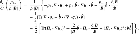 $$\begin{eqnarray}\displaystyle \frac{\text{d}_{r}}{\text{d}t}\left(\frac{p_{\bot r}}{\unicode[STIX]{x1D70C}_{r}|\boldsymbol{B}|}\right) & = & \displaystyle \frac{1}{\unicode[STIX]{x1D70C}_{r}|\boldsymbol{B}|}\left\{-p_{\bot r}\unicode[STIX]{x1D735}\boldsymbol{\cdot }\boldsymbol{u}_{r}+p_{\bot r}\hat{\boldsymbol{b}}\boldsymbol{\cdot }\unicode[STIX]{x1D735}\boldsymbol{u}_{r}\boldsymbol{\cdot }\hat{\boldsymbol{b}}-\frac{p_{\bot r}}{|\boldsymbol{B}|}\hat{\boldsymbol{b}}\boldsymbol{\cdot }\frac{\text{d}_{r}\boldsymbol{B}}{\text{d}t}\right.\nonumber\\ \displaystyle & & \displaystyle -\,\frac{1}{2}[\text{Tr}\,\unicode[STIX]{x1D735}\boldsymbol{\cdot }\boldsymbol{q}_{r}-\hat{\boldsymbol{b}}\boldsymbol{\cdot }(\unicode[STIX]{x1D735}\boldsymbol{\cdot }\boldsymbol{q}_{r})\boldsymbol{\cdot }\hat{\boldsymbol{b}}]\nonumber\\ \displaystyle & & \displaystyle -\left.\frac{1}{2}\left[\text{Tr}(\unicode[STIX]{x1D72B}_{r}\boldsymbol{\cdot }\unicode[STIX]{x1D735}\boldsymbol{u}_{r})^{S}+\frac{2}{|\boldsymbol{B}|}\hat{\boldsymbol{b}}\boldsymbol{\cdot }\unicode[STIX]{x1D72B}_{r}\boldsymbol{\cdot }\frac{\text{d}_{r}\boldsymbol{B}}{\text{d}t}-(\unicode[STIX]{x1D72B}_{r}\boldsymbol{\cdot }\unicode[STIX]{x1D735}\boldsymbol{u}_{r})^{S}:\hat{\boldsymbol{b}}\hat{\boldsymbol{b}}\right]\right\}.\end{eqnarray}$$
Again, no simplifications were introduced and no Maxwell equations were used yet. The equations are exact. The equations represent the complicated plasma heating processes that are responsible for anisotropic plasma heating, and that are in general very difficult to classify. The left-hand sides of (2.100)–(2.101) are the familiar CGL equations that represent conservations of the first and second adiabatic invariants, and all the expressions on the right-hand sides break these adiabatic invariants. On the right-hand side, we have the
 $\unicode[STIX]{x2202}\boldsymbol{B}/\unicode[STIX]{x2202}t$
that couples various species together through Maxwell’s equations, and that also introduces the Hall term responsible for the simplest dispersive effects. The heat flux tensor
$\unicode[STIX]{x2202}\boldsymbol{B}/\unicode[STIX]{x2202}t$
that couples various species together through Maxwell’s equations, and that also introduces the Hall term responsible for the simplest dispersive effects. The heat flux tensor
 $\boldsymbol{q}_{r}$
(a tensor of third rank), is decomposed into its gyrotropic and non-gyrotropic (FLR) parts
$\boldsymbol{q}_{r}$
(a tensor of third rank), is decomposed into its gyrotropic and non-gyrotropic (FLR) parts
 $\boldsymbol{q}_{r}=\boldsymbol{q}_{r}^{\text{g}}+\boldsymbol{q}_{r}^{\text{ng}}$
. At large scales, the gyrotropic heat flux can be viewed as a gateway for the simplest form of collisionless damping mechanism, known as Landau damping, that can be further separated to a ‘pure’ electrostatic Landau damping, and its magnetic analogue, the transit-time damping – see Part 2 of the text, subsection ‘Coulomb force and mirror force (Landau damping and transit time damping)’. Nevertheless, fluid models that contain the gyrotropic heat flux fluctuations, but that do not contain any Landau damping, can be constructed as well (see CGL2 model later in the text). The FLR pressure tensor
$\boldsymbol{q}_{r}=\boldsymbol{q}_{r}^{\text{g}}+\boldsymbol{q}_{r}^{\text{ng}}$
. At large scales, the gyrotropic heat flux can be viewed as a gateway for the simplest form of collisionless damping mechanism, known as Landau damping, that can be further separated to a ‘pure’ electrostatic Landau damping, and its magnetic analogue, the transit-time damping – see Part 2 of the text, subsection ‘Coulomb force and mirror force (Landau damping and transit time damping)’. Nevertheless, fluid models that contain the gyrotropic heat flux fluctuations, but that do not contain any Landau damping, can be constructed as well (see CGL2 model later in the text). The FLR pressure tensor
 $\unicode[STIX]{x1D72B}_{r}$
introduces further dispersive effects and therefore also modifies the collisionless damping rates, as well as the heat flux
$\unicode[STIX]{x1D72B}_{r}$
introduces further dispersive effects and therefore also modifies the collisionless damping rates, as well as the heat flux
 $\boldsymbol{q}_{r}$
modifies the FLR pressure corrections
$\boldsymbol{q}_{r}$
modifies the FLR pressure corrections
 $\unicode[STIX]{x1D72B}_{r}$
. The quantities
$\unicode[STIX]{x1D72B}_{r}$
. The quantities
 $\boldsymbol{q}_{r}$
and
$\boldsymbol{q}_{r}$
and
 $\unicode[STIX]{x1D72B}_{r}$
are therefore generally coupled. Importantly, the FLR pressure tensor
$\unicode[STIX]{x1D72B}_{r}$
are therefore generally coupled. Importantly, the FLR pressure tensor
 $\unicode[STIX]{x1D72B}_{r}$
introduces complicated turbulent plasma heating processes, referred to as stochastic heating. Since these FLR stress forces completely disappear at the linear level in the above pressure equations, they can be explored only with fully nonlinear numerical simulations (
$\unicode[STIX]{x1D72B}_{r}$
introduces complicated turbulent plasma heating processes, referred to as stochastic heating. Since these FLR stress forces completely disappear at the linear level in the above pressure equations, they can be explored only with fully nonlinear numerical simulations (
 $\unicode[STIX]{x1D72B}_{r}$
still enters at the linear level in the momentum equation and modifies the dispersion relations).
$\unicode[STIX]{x1D72B}_{r}$
still enters at the linear level in the momentum equation and modifies the dispersion relations).
From a fluid perspective, there are several major difficulties how to correctly model the quantities
 $\unicode[STIX]{x1D72B}_{r}$
and
$\unicode[STIX]{x1D72B}_{r}$
and
 $\boldsymbol{q}_{r}$
. The heat flux tensor
$\boldsymbol{q}_{r}$
. The heat flux tensor
 $\boldsymbol{q}_{r}$
is described by an infinite hierarchy of higher-order fluid moments, and one needs to find an appropriate way, how to close the system. The FLR pressure tensor
$\boldsymbol{q}_{r}$
is described by an infinite hierarchy of higher-order fluid moments, and one needs to find an appropriate way, how to close the system. The FLR pressure tensor
 $\unicode[STIX]{x1D72B}_{r}$
is described by equations that are implicit, and the FLR corrections have to be typically expanded on temporal and spatial scales in order to obtain tractable expressions that can be used for numerical simulations. This expansion will naturally restrict the area of validity of such fluid models to those scales considered. For example, for the proton–electron plasma where the spatial and temporal scales are largely separated because of the mass ratio
$\unicode[STIX]{x1D72B}_{r}$
is described by equations that are implicit, and the FLR corrections have to be typically expanded on temporal and spatial scales in order to obtain tractable expressions that can be used for numerical simulations. This expansion will naturally restrict the area of validity of such fluid models to those scales considered. For example, for the proton–electron plasma where the spatial and temporal scales are largely separated because of the mass ratio
 $m_{p}/m_{e}=1836$
, simple first-order FLR corrections expanded around the proton scales
$m_{p}/m_{e}=1836$
, simple first-order FLR corrections expanded around the proton scales
 $k\unicode[STIX]{x1D70C}_{i},\unicode[STIX]{x1D714}/\unicode[STIX]{x1D6FA}_{p}$
will long lose their validity at the electron scales. The most complicated Landau fluid models that use linear kinetic theory to evaluate
$k\unicode[STIX]{x1D70C}_{i},\unicode[STIX]{x1D714}/\unicode[STIX]{x1D6FA}_{p}$
will long lose their validity at the electron scales. The most complicated Landau fluid models that use linear kinetic theory to evaluate
 $\unicode[STIX]{x1D72B}$
and that contain the Bessel functions (Passot & Sulem Reference Passot and Sulem2007; Passot et al.
Reference Passot, Sulem and Hunana2012; Sulem & Passot Reference Sulem and Passot2015), have technically no restriction for wavenumbers
$\unicode[STIX]{x1D72B}$
and that contain the Bessel functions (Passot & Sulem Reference Passot and Sulem2007; Passot et al.
Reference Passot, Sulem and Hunana2012; Sulem & Passot Reference Sulem and Passot2015), have technically no restriction for wavenumbers
 $k_{\bot }\unicode[STIX]{x1D70C}_{i}$
, but the first-order frequency restriction is there nevertheless.
$k_{\bot }\unicode[STIX]{x1D70C}_{i}$
, but the first-order frequency restriction is there nevertheless.
2.7 Conservation of energy
The equations (2.100)–(2.101), that correctly split the entire plasma heating into parallel and perpendicular heating, are indeed quite complicated. To gain further insight, let us briefly consider a case in which we are not interested in parallel and perpendicular heating (whose net effect can possibly be zero), and we are only interested in the heating of the entire system. Such formulations are sometimes used to interpret plasma heating in fully kinetic simulations (Yang et al.
Reference Yang, Matthaeus, Parashar, Haggerty, Roytershteyn, Daughton, Wan, Shi and Chen2017a
,Reference Yang, Matthaeus, Parashar, Wu, Wan, Shi, Chen, Roytershteyn and Daughton
b
). By summing together the pressure equations (2.91), (2.92), we are interested in the evolution equation
 $\unicode[STIX]{x2202}(p_{\Vert }+2p_{\bot })/\unicode[STIX]{x2202}t$
, or in another words, we are interested in
$\unicode[STIX]{x2202}(p_{\Vert }+2p_{\bot })/\unicode[STIX]{x2202}t$
, or in another words, we are interested in
 $\unicode[STIX]{x2202}\text{Tr}\,\boldsymbol{p}/\unicode[STIX]{x2202}t$
. Summing the equations together (actually the trace of the entire pressure tensor equation was calculated a few pages back, that is how the
$\unicode[STIX]{x2202}\text{Tr}\,\boldsymbol{p}/\unicode[STIX]{x2202}t$
. Summing the equations together (actually the trace of the entire pressure tensor equation was calculated a few pages back, that is how the
 $p_{\bot }$
equation was derived) yields
$p_{\bot }$
equation was derived) yields
 $$\begin{eqnarray}\displaystyle \frac{\unicode[STIX]{x2202}}{\unicode[STIX]{x2202}t}(p_{\Vert r}+2p_{\bot r})+\unicode[STIX]{x1D735}\boldsymbol{\cdot }((p_{\Vert r}+2p_{\bot r})\boldsymbol{u}_{r})+\unicode[STIX]{x1D735}\boldsymbol{\cdot }(\text{Tr}\,\boldsymbol{q}_{r})+2((\underbrace{\boldsymbol{p}_{r}^{g}+\unicode[STIX]{x1D72B}_{r}}_{=\boldsymbol{p}_{r}})\boldsymbol{\cdot }\unicode[STIX]{x1D735})\boldsymbol{\cdot }\boldsymbol{u}_{r}=0. & & \displaystyle\end{eqnarray}$$
Note that
 $\text{Tr}\,\unicode[STIX]{x1D735}\boldsymbol{\cdot }\boldsymbol{q}_{r}=\unicode[STIX]{x1D735}\boldsymbol{\cdot }(\text{Tr}\,\boldsymbol{q}_{r})$
, and also
$\text{Tr}\,\unicode[STIX]{x1D735}\boldsymbol{\cdot }\boldsymbol{q}_{r}=\unicode[STIX]{x1D735}\boldsymbol{\cdot }(\text{Tr}\,\boldsymbol{q}_{r})$
, and also
 $\text{Tr}\,\unicode[STIX]{x1D72B}_{r}=0$
. By integrating over the entire spatial volume of the plasma, one can define the internal energy (or thermal energy) for each particle species as
$\text{Tr}\,\unicode[STIX]{x1D72B}_{r}=0$
. By integrating over the entire spatial volume of the plasma, one can define the internal energy (or thermal energy) for each particle species as
 $$\begin{eqnarray}E_{r}^{\text{int}}=\frac{1}{2}\int \text{Tr}\,\boldsymbol{p}_{r}\,\text{d}^{3}x=\frac{1}{2}\int (p_{\Vert r}+2p_{\bot r})\,\text{d}^{3}x\equiv \frac{1}{2}\langle p_{\Vert r}+2p_{\bot r}\rangle .\end{eqnarray}$$
By considering a special case of periodic boundary conditions, i.e. typical numerical simulations of turbulence in a periodic box, one can use the Gauss–Ostrogradsky theorem (2.9), now in a spatial domain, and for periodic boundary conditions all divergence operators in (2.102) vanish, yielding
 $$\begin{eqnarray}\frac{\unicode[STIX]{x2202}}{\unicode[STIX]{x2202}t}E_{r}^{\text{int}}=-\langle ((\boldsymbol{p}_{r}^{g}+\unicode[STIX]{x1D72B}_{r})\boldsymbol{\cdot }\unicode[STIX]{x1D735})\boldsymbol{\cdot }\boldsymbol{u}_{r}\rangle .\end{eqnarray}$$
Equations (2.102), (2.104) are equivalent to (4) and (7) of Yang et al. (Reference Yang, Matthaeus, Parashar, Wu, Wan, Shi, Chen, Roytershteyn and Daughton2017b
). Here the equations are just written in such a way that one can explicitly see the pressure components
 $p_{\Vert },p_{\bot },\unicode[STIX]{x1D72B}$
, but the equations are equivalent. Following Yang et al. (Reference Yang, Matthaeus, Parashar, Wu, Wan, Shi, Chen, Roytershteyn and Daughton2017b
), one can also easily derive the evolution equations for the ‘kinetic’ energy and the electromagnetic energy
$p_{\Vert },p_{\bot },\unicode[STIX]{x1D72B}$
, but the equations are equivalent. Following Yang et al. (Reference Yang, Matthaeus, Parashar, Wu, Wan, Shi, Chen, Roytershteyn and Daughton2017b
), one can also easily derive the evolution equations for the ‘kinetic’ energy and the electromagnetic energy
 $$\begin{eqnarray}E_{r}^{\text{kin}}=\frac{1}{2}\langle \unicode[STIX]{x1D70C}_{r}|\boldsymbol{u}_{r}|^{2}\rangle ;\quad E^{\text{mag}}=\frac{1}{8\unicode[STIX]{x03C0}}\langle (|\boldsymbol{B}|^{2}+|\boldsymbol{E}|^{2})\rangle .\end{eqnarray}$$
For the kinetic energy, by first applying
 $\boldsymbol{u}_{r}\boldsymbol{\cdot }$
to the momentum equation (2.90)
$\boldsymbol{u}_{r}\boldsymbol{\cdot }$
to the momentum equation (2.90)
 $$\begin{eqnarray}\boldsymbol{u}_{r}\boldsymbol{\cdot }\left(\unicode[STIX]{x1D70C}_{r}\frac{\unicode[STIX]{x2202}\boldsymbol{u}_{r}}{\unicode[STIX]{x2202}t}+\unicode[STIX]{x1D70C}_{r}\boldsymbol{u}_{r}\boldsymbol{\cdot }\unicode[STIX]{x1D735}\boldsymbol{u}_{r}\right)=-\boldsymbol{u}_{r}\boldsymbol{\cdot }(\unicode[STIX]{x1D735}\boldsymbol{\cdot }\boldsymbol{p}_{r})+\underbrace{q_{r}n_{r}\boldsymbol{u}_{r}}_{=\boldsymbol{j}_{r}}\boldsymbol{\cdot }\,\boldsymbol{E},\end{eqnarray}$$
which further implies
 $$\begin{eqnarray}\displaystyle \frac{1}{2}\frac{\unicode[STIX]{x2202}}{\unicode[STIX]{x2202}t}(\unicode[STIX]{x1D70C}|\boldsymbol{u}|^{2}) & = & \displaystyle \frac{1}{2}\left(\frac{\unicode[STIX]{x2202}\unicode[STIX]{x1D70C}}{\unicode[STIX]{x2202}t}|\boldsymbol{u}|^{2}+\unicode[STIX]{x1D70C}\frac{\unicode[STIX]{x2202}|\boldsymbol{u}|^{2}}{\unicode[STIX]{x2202}t}\right)=-\frac{1}{2}\unicode[STIX]{x1D735}\boldsymbol{\cdot }(\unicode[STIX]{x1D70C}\boldsymbol{u})|\boldsymbol{u}|^{2}+\unicode[STIX]{x1D70C}\boldsymbol{u}\boldsymbol{\cdot }\frac{\unicode[STIX]{x2202}\boldsymbol{u}}{\unicode[STIX]{x2202}t}\nonumber\\ \displaystyle & = & \displaystyle -\frac{1}{2}\unicode[STIX]{x1D735}\boldsymbol{\cdot }(\unicode[STIX]{x1D70C}\boldsymbol{u}|\boldsymbol{u}|^{2})+\boldsymbol{u}\boldsymbol{\cdot }\left(\unicode[STIX]{x1D70C}\frac{\unicode[STIX]{x2202}\boldsymbol{u}}{\unicode[STIX]{x2202}t}+\unicode[STIX]{x1D70C}\boldsymbol{u}\boldsymbol{\cdot }\unicode[STIX]{x1D735}\boldsymbol{u}\right)\nonumber\\ \displaystyle & = & \displaystyle -\frac{1}{2}\unicode[STIX]{x1D735}\boldsymbol{\cdot }(\unicode[STIX]{x1D70C}_{r}\boldsymbol{u}_{r}|\boldsymbol{u}_{r}|^{2})-\unicode[STIX]{x1D735}\boldsymbol{\cdot }(\boldsymbol{p}_{r}\boldsymbol{u}_{r})+(\boldsymbol{p}_{r}\boldsymbol{\cdot }\unicode[STIX]{x1D735})\boldsymbol{\cdot }\boldsymbol{u}_{r}+\boldsymbol{j}_{r}\boldsymbol{\cdot }\boldsymbol{E},\end{eqnarray}$$
and for the electromagnetic energy
 $$\begin{eqnarray}\displaystyle \frac{1}{8\unicode[STIX]{x03C0}}\frac{\unicode[STIX]{x2202}}{\unicode[STIX]{x2202}t}(|\boldsymbol{B}|^{2}+|\boldsymbol{E}|^{2}) & = & \displaystyle \frac{1}{4\unicode[STIX]{x03C0}}\frac{\unicode[STIX]{x2202}}{\unicode[STIX]{x2202}t}\left(\boldsymbol{B}\boldsymbol{\cdot }\frac{\unicode[STIX]{x2202}\boldsymbol{B}}{\unicode[STIX]{x2202}t}+\boldsymbol{E}\boldsymbol{\cdot }\frac{\unicode[STIX]{x2202}\boldsymbol{E}}{\unicode[STIX]{x2202}t}\right)\nonumber\\ \displaystyle & = & \displaystyle -\frac{c}{4\unicode[STIX]{x03C0}}(\boldsymbol{B}\boldsymbol{\cdot }(\unicode[STIX]{x1D735}\times \boldsymbol{E})-\boldsymbol{E}\boldsymbol{\cdot }(\unicode[STIX]{x1D735}\times \boldsymbol{B}))-\boldsymbol{j}\boldsymbol{\cdot }\boldsymbol{E}\nonumber\\ \displaystyle & = & \displaystyle -\frac{c}{4\unicode[STIX]{x03C0}}\unicode[STIX]{x1D735}\boldsymbol{\cdot }(\boldsymbol{E}\times \boldsymbol{B})-\boldsymbol{j}\boldsymbol{\cdot }\boldsymbol{E}.\end{eqnarray}$$
Therefore, by integrating over the entire volume and assuming periodic boundary conditions, the total conservation of energy can be expressed as (Yang et al. Reference Yang, Matthaeus, Parashar, Wu, Wan, Shi, Chen, Roytershteyn and Daughton2017b )
 $$\begin{eqnarray}\displaystyle \frac{\unicode[STIX]{x2202}}{\unicode[STIX]{x2202}t}E_{r}^{\text{int}} & = & \displaystyle -\langle (\boldsymbol{p}_{r}\boldsymbol{\cdot }\unicode[STIX]{x1D735})\boldsymbol{\cdot }\boldsymbol{u}_{r}\rangle ;\end{eqnarray}$$
 $$\begin{eqnarray}\displaystyle \frac{\unicode[STIX]{x2202}}{\unicode[STIX]{x2202}t}E_{r}^{\text{kin}} & = & \displaystyle +\langle (\boldsymbol{p}_{r}\boldsymbol{\cdot }\unicode[STIX]{x1D735})\boldsymbol{\cdot }\boldsymbol{u}_{r}\rangle +\langle \boldsymbol{j}_{r}\boldsymbol{\cdot }\boldsymbol{E}\rangle ;\end{eqnarray}$$
 $$\begin{eqnarray}\displaystyle \frac{\unicode[STIX]{x2202}}{\unicode[STIX]{x2202}t}E^{\text{mag}} & = & \displaystyle -\langle \boldsymbol{j}\boldsymbol{\cdot }\boldsymbol{E}\rangle ,\end{eqnarray}$$
which beautifully clarifies how the energy can be transferred. Nevertheless, we point out that it is exactly the splitting into the parallel and perpendicular heating that is so complicated, since even with periodic boundary conditions, only a few terms in the pressure equations (2.91), (2.92) vanish. Considering anisotropic heating, and splitting the internal (thermal) energy into parallel and perpendicular parts
 $$\begin{eqnarray}E_{r}^{\text{int}}=E_{\Vert r}^{\text{int}}+E_{\bot r}^{\text{int}};\quad E_{\Vert r}^{\text{int}}={\textstyle \frac{1}{2}}\langle p_{\Vert r}\rangle ;\quad E_{\bot r}^{\text{int}}=\langle p_{\bot r}\rangle ,\end{eqnarray}$$
the conservation of total energy can be expressed as
 $$\begin{eqnarray}\displaystyle \frac{\unicode[STIX]{x2202}}{\unicode[STIX]{x2202}t}E_{\Vert r}^{\text{int}} & = & \displaystyle -\langle p_{\Vert r}\hat{\boldsymbol{b}}\boldsymbol{\cdot }\unicode[STIX]{x1D735}\boldsymbol{u}_{r}\boldsymbol{\cdot }\hat{\boldsymbol{b}}\rangle -\frac{1}{2}\langle \hat{\boldsymbol{b}}\boldsymbol{\cdot }(\unicode[STIX]{x1D735}\boldsymbol{\cdot }\boldsymbol{q}_{r})\boldsymbol{\cdot }\hat{\boldsymbol{b}}\rangle \nonumber\\ \displaystyle & & \displaystyle +\,\langle \frac{\hat{\boldsymbol{b}}}{|\boldsymbol{B}|}\boldsymbol{\cdot }\unicode[STIX]{x1D72B}_{r}\boldsymbol{\cdot }\frac{\text{d}_{r}\boldsymbol{B}}{\text{d}t}\rangle -\langle \hat{\boldsymbol{b}}\boldsymbol{\cdot }(\unicode[STIX]{x1D72B}_{r}\boldsymbol{\cdot }\unicode[STIX]{x1D735}\boldsymbol{u}_{r})\boldsymbol{\cdot }\hat{\boldsymbol{b}}\rangle ;\end{eqnarray}$$
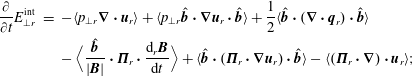 $$\begin{eqnarray}\displaystyle \frac{\unicode[STIX]{x2202}}{\unicode[STIX]{x2202}t}E_{\bot r}^{\text{int}} & = & \displaystyle -\langle p_{\bot r}\unicode[STIX]{x1D735}\boldsymbol{\cdot }\boldsymbol{u}_{r}\rangle +\langle p_{\bot r}\hat{\boldsymbol{b}}\boldsymbol{\cdot }\unicode[STIX]{x1D735}\boldsymbol{u}_{r}\boldsymbol{\cdot }\hat{\boldsymbol{b}}\rangle +\frac{1}{2}\langle \hat{\boldsymbol{b}}\boldsymbol{\cdot }(\unicode[STIX]{x1D735}\boldsymbol{\cdot }\boldsymbol{q}_{r})\boldsymbol{\cdot }\hat{\boldsymbol{b}}\rangle \nonumber\\ \displaystyle & & \displaystyle -\,\langle \frac{\hat{\boldsymbol{b}}}{|\boldsymbol{B}|}\boldsymbol{\cdot }\unicode[STIX]{x1D72B}_{r}\boldsymbol{\cdot }\frac{\text{d}_{r}\boldsymbol{B}}{\text{d}t}\rangle +\langle \hat{\boldsymbol{b}}\boldsymbol{\cdot }(\unicode[STIX]{x1D72B}_{r}\boldsymbol{\cdot }\unicode[STIX]{x1D735}\boldsymbol{u}_{r})\boldsymbol{\cdot }\hat{\boldsymbol{b}}\rangle -\langle (\unicode[STIX]{x1D72B}_{r}\boldsymbol{\cdot }\unicode[STIX]{x1D735})\boldsymbol{\cdot }\boldsymbol{u}_{r}\rangle ;\end{eqnarray}$$
 $$\begin{eqnarray}\displaystyle \frac{\unicode[STIX]{x2202}}{\unicode[STIX]{x2202}t}E_{r}^{\text{kin}} & = & \displaystyle +\langle (\boldsymbol{p}_{r}\boldsymbol{\cdot }\unicode[STIX]{x1D735})\boldsymbol{\cdot }\boldsymbol{u}_{r}\rangle +\langle \boldsymbol{j}_{r}\boldsymbol{\cdot }\boldsymbol{E}\rangle ;\end{eqnarray}$$
 $$\begin{eqnarray}\displaystyle \frac{\unicode[STIX]{x2202}}{\unicode[STIX]{x2202}t}E^{\text{mag}} & = & \displaystyle -\langle \boldsymbol{j}\boldsymbol{\cdot }\boldsymbol{E}\rangle ,\end{eqnarray}$$
where
 $$\begin{eqnarray}\langle (\boldsymbol{p}_{r}\boldsymbol{\cdot }\unicode[STIX]{x1D735})\boldsymbol{\cdot }\boldsymbol{u}_{r}\rangle =\langle p_{\Vert r}\hat{\boldsymbol{b}}\boldsymbol{\cdot }\unicode[STIX]{x1D735}\boldsymbol{u}_{r}\boldsymbol{\cdot }\hat{\boldsymbol{b}}\rangle -\langle p_{\bot r}\hat{\boldsymbol{b}}\boldsymbol{\cdot }\unicode[STIX]{x1D735}\boldsymbol{u}_{r}\boldsymbol{\cdot }\hat{\boldsymbol{b}}\rangle +\langle p_{\bot r}\unicode[STIX]{x1D735}\boldsymbol{\cdot }\boldsymbol{u}_{r}\rangle +\langle (\unicode[STIX]{x1D72B}_{r}\boldsymbol{\cdot }\unicode[STIX]{x1D735})\boldsymbol{\cdot }\boldsymbol{u}_{r}\rangle .\end{eqnarray}$$
The anisotropic plasma heating is obviously a very complicated process.
3 CGL description
The CGL model is the simplest possible fluid model that incorporates anisotropic temperatures. In contrast to MHD, CGL contains two pressure equations. For very good MHD reviews, from the perspective of turbulence in the solar wind, and the use of MHD in modelling heliospheric and astrophysical plasmas, we recommend the reviews by Goldstein, Roberts & Matthaeus (Reference Goldstein, Roberts and Matthaeus1995), Tu & Marsch (Reference Tu and Marsch1995), Zank (Reference Zank1999), Zhou, Matthaeus & Dmitruk (Reference Zhou, Matthaeus and Dmitruk2004) and Bruno & Carbone (Reference Bruno and Carbone2013). The CGL model is obtained by using the parallel and perpendicular pressure equations (2.74), (2.75) and prescribing zero heat flux
 $q_{\Vert }=q_{\bot }=0$
,
$q_{\Vert }=q_{\bot }=0$
,
 $\boldsymbol{q}^{\text{ng}}=0$
, and by neglecting the FLR pressure tensor
$\boldsymbol{q}^{\text{ng}}=0$
, and by neglecting the FLR pressure tensor
 $\unicode[STIX]{x1D72B}=0$
. The pressure equations greatly simplify to the form
$\unicode[STIX]{x1D72B}=0$
. The pressure equations greatly simplify to the form
 $$\begin{eqnarray}\displaystyle & \displaystyle \frac{\unicode[STIX]{x2202}p_{\Vert }}{\unicode[STIX]{x2202}t}+\unicode[STIX]{x1D735}\boldsymbol{\cdot }(p_{\Vert }\boldsymbol{u})+2p_{\Vert }\hat{\boldsymbol{b}}\boldsymbol{\cdot }\unicode[STIX]{x1D735}\boldsymbol{u}\boldsymbol{\cdot }\hat{\boldsymbol{b}}=0; & \displaystyle\end{eqnarray}$$
 $$\begin{eqnarray}\displaystyle & \displaystyle \frac{\unicode[STIX]{x2202}p_{\bot }}{\unicode[STIX]{x2202}t}+\unicode[STIX]{x1D735}\boldsymbol{\cdot }(p_{\bot }\boldsymbol{u})+p_{\bot }\unicode[STIX]{x1D735}\boldsymbol{\cdot }\boldsymbol{u}-p_{\bot }\hat{\boldsymbol{b}}\boldsymbol{\cdot }\unicode[STIX]{x1D735}\boldsymbol{u}\boldsymbol{\cdot }\hat{\boldsymbol{b}}=0. & \displaystyle\end{eqnarray}$$
By using the notation for the convective derivative
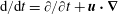 $\text{d}/\text{d}t=\unicode[STIX]{x2202}/\unicode[STIX]{x2202}t+\boldsymbol{u}\boldsymbol{\cdot }\unicode[STIX]{x1D735}$
, the pressure equations can be rewritten as
$\text{d}/\text{d}t=\unicode[STIX]{x2202}/\unicode[STIX]{x2202}t+\boldsymbol{u}\boldsymbol{\cdot }\unicode[STIX]{x1D735}$
, the pressure equations can be rewritten as
 $$\begin{eqnarray}\displaystyle & \displaystyle \frac{\text{d}p_{\Vert }}{\text{d}t}+p_{\Vert }\unicode[STIX]{x1D735}\boldsymbol{\cdot }\boldsymbol{u}+2p_{\Vert }\hat{\boldsymbol{b}}\boldsymbol{\cdot }\unicode[STIX]{x1D735}\boldsymbol{u}\boldsymbol{\cdot }\hat{\boldsymbol{b}}=0; & \displaystyle\end{eqnarray}$$
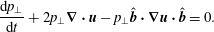 $$\begin{eqnarray}\displaystyle & \displaystyle \frac{\text{d}p_{\bot }}{\text{d}t}+2p_{\bot }\unicode[STIX]{x1D735}\boldsymbol{\cdot }\boldsymbol{u}-p_{\bot }\hat{\boldsymbol{b}}\boldsymbol{\cdot }\unicode[STIX]{x1D735}\boldsymbol{u}\boldsymbol{\cdot }\hat{\boldsymbol{b}}=0. & \displaystyle\end{eqnarray}$$
Note that the CGL pressure equations are fully nonlinear and that the nonlinearities are actually of fourth order, i.e. CGL pressure equations are more nonlinear than the usual MHD pressure equation
 $\text{d}p/\text{d}t+\unicode[STIX]{x1D6FE}p\unicode[STIX]{x1D735}\boldsymbol{\cdot }\boldsymbol{u}=0$
, where the nonlinearity is only of second order. At first sight, expressions
$\text{d}p/\text{d}t+\unicode[STIX]{x1D6FE}p\unicode[STIX]{x1D735}\boldsymbol{\cdot }\boldsymbol{u}=0$
, where the nonlinearity is only of second order. At first sight, expressions
 $\hat{\boldsymbol{b}}\boldsymbol{\cdot }\unicode[STIX]{x1D735}\boldsymbol{u}\boldsymbol{\cdot }\hat{\boldsymbol{b}}$
might appear to be a little unusual when written without any brackets. From MHD, one is familiar with nonlinear expressions of the type
$\hat{\boldsymbol{b}}\boldsymbol{\cdot }\unicode[STIX]{x1D735}\boldsymbol{u}\boldsymbol{\cdot }\hat{\boldsymbol{b}}$
might appear to be a little unusual when written without any brackets. From MHD, one is familiar with nonlinear expressions of the type
 $\boldsymbol{u}\boldsymbol{\cdot }\unicode[STIX]{x1D735}\boldsymbol{u}$
, which are also usually written without any brackets and can be interpreted in two equivalent forms, either as
$\boldsymbol{u}\boldsymbol{\cdot }\unicode[STIX]{x1D735}\boldsymbol{u}$
, which are also usually written without any brackets and can be interpreted in two equivalent forms, either as
 $(\boldsymbol{u}\boldsymbol{\cdot }\unicode[STIX]{x1D735})\boldsymbol{u}$
(a scalar
$(\boldsymbol{u}\boldsymbol{\cdot }\unicode[STIX]{x1D735})\boldsymbol{u}$
(a scalar
 $\boldsymbol{u}\boldsymbol{\cdot }\unicode[STIX]{x1D735}$
applied on a vector
$\boldsymbol{u}\boldsymbol{\cdot }\unicode[STIX]{x1D735}$
applied on a vector
 $\boldsymbol{u}$
; or
$\boldsymbol{u}$
; or
 $\boldsymbol{u}\boldsymbol{\cdot }(\unicode[STIX]{x1D735}\boldsymbol{u})$
(a vector
$\boldsymbol{u}\boldsymbol{\cdot }(\unicode[STIX]{x1D735}\boldsymbol{u})$
(a vector
 $\boldsymbol{u}$
multiplied by a matrix
$\boldsymbol{u}$
multiplied by a matrix
 $\unicode[STIX]{x1D735}\boldsymbol{u}$
). In a similar fashion, the expression
$\unicode[STIX]{x1D735}\boldsymbol{u}$
). In a similar fashion, the expression
 $\hat{\boldsymbol{b}}\boldsymbol{\cdot }\unicode[STIX]{x1D735}\boldsymbol{u}\boldsymbol{\cdot }\hat{\boldsymbol{b}}$
is meant to be interpreted as
$\hat{\boldsymbol{b}}\boldsymbol{\cdot }\unicode[STIX]{x1D735}\boldsymbol{u}\boldsymbol{\cdot }\hat{\boldsymbol{b}}$
is meant to be interpreted as
 $(\hat{\boldsymbol{b}}\boldsymbol{\cdot }\unicode[STIX]{x1D735}\boldsymbol{u})\boldsymbol{\cdot }\hat{\boldsymbol{b}}$
or
$(\hat{\boldsymbol{b}}\boldsymbol{\cdot }\unicode[STIX]{x1D735}\boldsymbol{u})\boldsymbol{\cdot }\hat{\boldsymbol{b}}$
or
 $\hat{\boldsymbol{b}}\boldsymbol{\cdot }(\unicode[STIX]{x1D735}\boldsymbol{u})\boldsymbol{\cdot }\hat{\boldsymbol{b}}$
; but importantly, it is not meant to be interpreted as
$\hat{\boldsymbol{b}}\boldsymbol{\cdot }(\unicode[STIX]{x1D735}\boldsymbol{u})\boldsymbol{\cdot }\hat{\boldsymbol{b}}$
; but importantly, it is not meant to be interpreted as
 $\hat{\boldsymbol{b}}\boldsymbol{\cdot }\unicode[STIX]{x1D735}(\boldsymbol{u}\boldsymbol{\cdot }\hat{\boldsymbol{b}})$
, because the derivative is meant to act only on
$\hat{\boldsymbol{b}}\boldsymbol{\cdot }\unicode[STIX]{x1D735}(\boldsymbol{u}\boldsymbol{\cdot }\hat{\boldsymbol{b}})$
, because the derivative is meant to act only on
 $\boldsymbol{u}$
in this case. For direct numerical simulations, the fourth-order nonlinearity explicitly reads
$\boldsymbol{u}$
in this case. For direct numerical simulations, the fourth-order nonlinearity explicitly reads
 $$\begin{eqnarray}\displaystyle \hat{\boldsymbol{b}}\boldsymbol{\cdot }\unicode[STIX]{x1D735}\boldsymbol{u}\boldsymbol{\cdot }\hat{\boldsymbol{b}} & = & \displaystyle \hat{b}_{i}(\unicode[STIX]{x1D735}\boldsymbol{u})_{ij}\hat{b}_{j}=\hat{b}_{i}\hat{b}_{j}\unicode[STIX]{x2202}_{i}u_{j}=\hat{b}_{x}(\hat{b}_{x}\unicode[STIX]{x2202}_{x}u_{x}+\hat{b}_{y}\unicode[STIX]{x2202}_{x}u_{y}+\hat{b}_{z}\unicode[STIX]{x2202}_{x}u_{z})\nonumber\\ \displaystyle & & \displaystyle +\,\hat{b}_{y}(\hat{b}_{x}\unicode[STIX]{x2202}_{y}u_{x}+\hat{b}_{y}\unicode[STIX]{x2202}_{y}u_{y}+\hat{b}_{z}\unicode[STIX]{x2202}_{y}u_{z})+\hat{b}_{z}(\hat{b}_{x}\unicode[STIX]{x2202}_{z}u_{x}+\hat{b}_{y}\unicode[STIX]{x2202}_{z}u_{y}+\hat{b}_{z}\unicode[STIX]{x2202}_{z}u_{z}),\end{eqnarray}$$
and is of course a scalar. So far, we have not made any assumptions about particle species, and have only integrated the Vlasov equation and derived the density, momentum and scalar pressure equations, which can be done for each species separately. By re-introducing the species index
 $r$
, where
$r$
, where
 $r=p$
for protons,
$r=p$
for protons,
 $r=e$
for electrons etc., the n-fluid CGL-type equations become
$r=e$
for electrons etc., the n-fluid CGL-type equations become
 $$\begin{eqnarray}\displaystyle & \displaystyle \frac{\unicode[STIX]{x2202}\unicode[STIX]{x1D70C}_{r}}{\unicode[STIX]{x2202}t}+\unicode[STIX]{x1D735}\boldsymbol{\cdot }(\unicode[STIX]{x1D70C}_{r}\boldsymbol{u}_{r})=0; & \displaystyle\end{eqnarray}$$
 $$\begin{eqnarray}\displaystyle & \displaystyle \frac{\unicode[STIX]{x2202}\boldsymbol{u}_{r}}{\unicode[STIX]{x2202}t}+\boldsymbol{u}_{r}\boldsymbol{\cdot }\unicode[STIX]{x1D735}\boldsymbol{u}_{r}+\frac{1}{\unicode[STIX]{x1D70C}_{r}}\unicode[STIX]{x1D735}\boldsymbol{\cdot }\boldsymbol{p}_{r}-\frac{q_{r}}{m_{r}}\left(\boldsymbol{E}+\frac{1}{c}\boldsymbol{u}_{r}\times \boldsymbol{B}\right)=0; & \displaystyle\end{eqnarray}$$
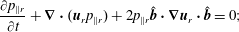 $$\begin{eqnarray}\displaystyle & \displaystyle \frac{\unicode[STIX]{x2202}p_{\Vert r}}{\unicode[STIX]{x2202}t}+\unicode[STIX]{x1D735}\boldsymbol{\cdot }(\boldsymbol{u}_{r}p_{\Vert r})+2p_{\Vert r}\hat{\boldsymbol{b}}\boldsymbol{\cdot }\unicode[STIX]{x1D735}\boldsymbol{u}_{r}\boldsymbol{\cdot }\hat{\boldsymbol{b}}=0; & \displaystyle\end{eqnarray}$$
 $$\begin{eqnarray}\displaystyle & \displaystyle \frac{\unicode[STIX]{x2202}p_{\bot r}}{\unicode[STIX]{x2202}t}+\unicode[STIX]{x1D735}\boldsymbol{\cdot }(\boldsymbol{u}_{r}p_{\bot r})+p_{\bot r}\unicode[STIX]{x1D735}\boldsymbol{\cdot }\boldsymbol{u}_{r}-p_{\bot r}\hat{\boldsymbol{b}}\boldsymbol{\cdot }\unicode[STIX]{x1D735}\boldsymbol{u}_{r}\boldsymbol{\cdot }\hat{\boldsymbol{b}}=0. & \displaystyle\end{eqnarray}$$
The above CGL pressure equations are valid regardless of the form of the induction equation
 $\unicode[STIX]{x2202}\boldsymbol{B}/\unicode[STIX]{x2202}t$
and are therefore very general and valid for a wide range of CGL-type n-fluid models. It is advisable to keep them in this form when considering direct numerical simulations or solving linear dispersion relations. The above equations are accompanied by Maxwell’s equations. Specifically, (i) Gauss’s law
$\unicode[STIX]{x2202}\boldsymbol{B}/\unicode[STIX]{x2202}t$
and are therefore very general and valid for a wide range of CGL-type n-fluid models. It is advisable to keep them in this form when considering direct numerical simulations or solving linear dispersion relations. The above equations are accompanied by Maxwell’s equations. Specifically, (i) Gauss’s law
 $\unicode[STIX]{x1D735}\boldsymbol{\cdot }\boldsymbol{E}=4\unicode[STIX]{x03C0}\unicode[STIX]{x1D70C}_{c}$
where the total charge density
$\unicode[STIX]{x1D735}\boldsymbol{\cdot }\boldsymbol{E}=4\unicode[STIX]{x03C0}\unicode[STIX]{x1D70C}_{c}$
where the total charge density
 $\unicode[STIX]{x1D70C}_{c}=\sum _{r}q_{r}n_{r}$
, (ii)
$\unicode[STIX]{x1D70C}_{c}=\sum _{r}q_{r}n_{r}$
, (ii)
 $\unicode[STIX]{x1D735}\boldsymbol{\cdot }\boldsymbol{B}=0$
, (iii) Faraday’s induction equation
$\unicode[STIX]{x1D735}\boldsymbol{\cdot }\boldsymbol{B}=0$
, (iii) Faraday’s induction equation
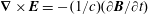 $\unicode[STIX]{x1D735}\times \boldsymbol{E}=-(1/c)(\unicode[STIX]{x2202}\boldsymbol{B}/\unicode[STIX]{x2202}t)$
and (iv) Ampère’s law
$\unicode[STIX]{x1D735}\times \boldsymbol{E}=-(1/c)(\unicode[STIX]{x2202}\boldsymbol{B}/\unicode[STIX]{x2202}t)$
and (iv) Ampère’s law
 $\unicode[STIX]{x1D735}\times \boldsymbol{B}=(4\unicode[STIX]{x03C0}/c)\boldsymbol{j}+(1/c)(\unicode[STIX]{x2202}\boldsymbol{E}/\unicode[STIX]{x2202}t)$
, where the total current
$\unicode[STIX]{x1D735}\times \boldsymbol{B}=(4\unicode[STIX]{x03C0}/c)\boldsymbol{j}+(1/c)(\unicode[STIX]{x2202}\boldsymbol{E}/\unicode[STIX]{x2202}t)$
, where the total current
 $\boldsymbol{j}=\sum _{r}q_{r}n_{r}\boldsymbol{u}_{r}$
. In many areas of space physics and astrophysics it is often very useful to eliminate very high frequency effects occurring at frequencies higher than the plasma frequency. This is achieved by prescribing local charge neutrality (so called quasi-neutrality since the plasma is still ionized) by
$\boldsymbol{j}=\sum _{r}q_{r}n_{r}\boldsymbol{u}_{r}$
. In many areas of space physics and astrophysics it is often very useful to eliminate very high frequency effects occurring at frequencies higher than the plasma frequency. This is achieved by prescribing local charge neutrality (so called quasi-neutrality since the plasma is still ionized) by
 $\unicode[STIX]{x1D70C}_{c}=0$
and by neglecting the second term in Ampère’s law
$\unicode[STIX]{x1D70C}_{c}=0$
and by neglecting the second term in Ampère’s law
 $(1/c)(\unicode[STIX]{x2202}\boldsymbol{E}/\unicode[STIX]{x2202}t)$
known as Maxwell’s displacement current (or Maxwell’s correction to Ampère’s law). This eliminates high-frequency effects such as for example plasma oscillations, known as Langmuir waves. This assumption is also equivalent to assuming that the Alfvén speed is much less than the speed of light
$(1/c)(\unicode[STIX]{x2202}\boldsymbol{E}/\unicode[STIX]{x2202}t)$
known as Maxwell’s displacement current (or Maxwell’s correction to Ampère’s law). This eliminates high-frequency effects such as for example plasma oscillations, known as Langmuir waves. This assumption is also equivalent to assuming that the Alfvén speed is much less than the speed of light
 $V_{A}/c\ll 1$
. It is important to emphasize that Gauss’s law
$V_{A}/c\ll 1$
. It is important to emphasize that Gauss’s law
 $\unicode[STIX]{x1D735}\boldsymbol{\cdot }\boldsymbol{E}=4\unicode[STIX]{x03C0}\unicode[STIX]{x1D70C}_{c}$
is replaced by the quasi-neutrality condition
$\unicode[STIX]{x1D735}\boldsymbol{\cdot }\boldsymbol{E}=4\unicode[STIX]{x03C0}\unicode[STIX]{x1D70C}_{c}$
is replaced by the quasi-neutrality condition
 $\unicode[STIX]{x1D70C}_{c}=0$
and no requirement is imposed on
$\unicode[STIX]{x1D70C}_{c}=0$
and no requirement is imposed on
 $\unicode[STIX]{x1D735}\boldsymbol{\cdot }\boldsymbol{E}$
(other than that it is small). For further discussion concerning the charge neutrality and
$\unicode[STIX]{x1D735}\boldsymbol{\cdot }\boldsymbol{E}$
(other than that it is small). For further discussion concerning the charge neutrality and
 $\unicode[STIX]{x1D735}\boldsymbol{\cdot }\boldsymbol{E}$
, see for example Braginskii (Reference Braginskii1965) page 264, Webb et al. (Reference Webb, McKenzie, Mace, Ko and Zank2007) equation (7) and Passot & Sulem (Reference Passot and Sulem2007) equation (A 1). Maxwell’s equations in this approximation simplify to
$\unicode[STIX]{x1D735}\boldsymbol{\cdot }\boldsymbol{E}$
, see for example Braginskii (Reference Braginskii1965) page 264, Webb et al. (Reference Webb, McKenzie, Mace, Ko and Zank2007) equation (7) and Passot & Sulem (Reference Passot and Sulem2007) equation (A 1). Maxwell’s equations in this approximation simplify to
 $$\begin{eqnarray}\displaystyle & \displaystyle \unicode[STIX]{x1D735}\boldsymbol{\cdot }\boldsymbol{B}=0; & \displaystyle\end{eqnarray}$$
 $$\begin{eqnarray}\displaystyle & \displaystyle \frac{\unicode[STIX]{x2202}\boldsymbol{B}}{\unicode[STIX]{x2202}t}=-c\unicode[STIX]{x1D735}\times \boldsymbol{E}; & \displaystyle\end{eqnarray}$$
 $$\begin{eqnarray}\displaystyle & \displaystyle \boldsymbol{j}=\mathop{\sum }_{r}q_{r}n_{r}\boldsymbol{u}_{r}=\frac{c}{4\unicode[STIX]{x03C0}}\unicode[STIX]{x1D735}\times \boldsymbol{B}, & \displaystyle\end{eqnarray}$$
and this form of Maxwell’s equations is considered in most of the fluid models that we discuss, regardless of future complexities arising from FLR corrections, heat flux, Landau damping and so on. The exception is the section in Part 2 ‘Electron Landau damping of the Langmuir mode’, where the displacement current has to be retained. Here, we further focus only on a plasma consisting of protons and electrons, with charges
 $q_{p}=e$
and
$q_{p}=e$
and
 $q_{e}=-e$
, but models with more species can of course be considered. Charge neutrality implies that the proton and electron number densities are equal, i.e.
$q_{e}=-e$
, but models with more species can of course be considered. Charge neutrality implies that the proton and electron number densities are equal, i.e.
 $n_{p}=n_{e}=n$
. By using the definition of current
$n_{p}=n_{e}=n$
. By using the definition of current
 $\boldsymbol{j}=en\boldsymbol{u}_{p}-en\boldsymbol{u}_{e}$
, the electron velocities are related to the proton velocities by
$\boldsymbol{j}=en\boldsymbol{u}_{p}-en\boldsymbol{u}_{e}$
, the electron velocities are related to the proton velocities by
 $$\begin{eqnarray}\boldsymbol{u}_{e}=\boldsymbol{u}_{p}-\frac{1}{en}\boldsymbol{j},\end{eqnarray}$$
which after using (3.12) yields
 $$\begin{eqnarray}\boldsymbol{u}_{e}=\boldsymbol{u}_{p}-\frac{1}{en}\frac{c}{4\unicode[STIX]{x03C0}}\unicode[STIX]{x1D735}\times \boldsymbol{B}.\end{eqnarray}$$
By using the momentum equation (3.7) for electrons, the electric field can be expressed as
 $$\begin{eqnarray}\boldsymbol{E}=-\frac{1}{c}\boldsymbol{u}_{e}\times \boldsymbol{B}-\frac{1}{en}\unicode[STIX]{x1D735}\boldsymbol{\cdot }\boldsymbol{p}_{e}-\frac{m_{e}}{e}\left(\frac{\unicode[STIX]{x2202}\boldsymbol{u}_{e}}{\unicode[STIX]{x2202}t}+\boldsymbol{u}_{e}\boldsymbol{\cdot }\unicode[STIX]{x1D735}\boldsymbol{u}_{e}\right).\end{eqnarray}$$
The last term represents the effects of electron inertia and is for example responsible for the effect that at small spatial scales the frequency
 $\unicode[STIX]{x1D714}$
of the parallel whistler mode converges to the electron cyclotron frequency
$\unicode[STIX]{x1D714}$
of the parallel whistler mode converges to the electron cyclotron frequency
 $\unicode[STIX]{x1D6FA}_{e}$
instead of increasing to infinity. When considering only relatively low frequencies, it is very useful to neglect the electron inertia term.Footnote
2
This yields somewhat simpler analytic expressions, but most importantly, it provides a great benefit for direct numerical simulations since the time step is not restricted by the requirement to fully resolve the electron motion. This of course restricts the validity of a model to frequencies that are sufficiently smaller than the electron cyclotron frequency. By neglecting the electron inertia and using (3.14), the electric field can be expressed as
$\unicode[STIX]{x1D6FA}_{e}$
instead of increasing to infinity. When considering only relatively low frequencies, it is very useful to neglect the electron inertia term.Footnote
2
This yields somewhat simpler analytic expressions, but most importantly, it provides a great benefit for direct numerical simulations since the time step is not restricted by the requirement to fully resolve the electron motion. This of course restricts the validity of a model to frequencies that are sufficiently smaller than the electron cyclotron frequency. By neglecting the electron inertia and using (3.14), the electric field can be expressed as
 $$\begin{eqnarray}\boldsymbol{E}=-\frac{1}{c}\boldsymbol{u}_{p}\times \boldsymbol{B}+\frac{1}{4\unicode[STIX]{x03C0}en}(\unicode[STIX]{x1D735}\times \boldsymbol{B})\times \boldsymbol{B}-\frac{1}{en}\unicode[STIX]{x1D735}\boldsymbol{\cdot }\boldsymbol{p}_{e}.\end{eqnarray}$$
Using this expression in the proton momentum equation and in the induction equation eliminates the electric field from the entire system. The system of equations therefore reads
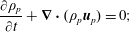 $$\begin{eqnarray}\displaystyle & \displaystyle \frac{\unicode[STIX]{x2202}\unicode[STIX]{x1D70C}_{p}}{\unicode[STIX]{x2202}t}+\unicode[STIX]{x1D735}\boldsymbol{\cdot }(\unicode[STIX]{x1D70C}_{p}\boldsymbol{u}_{p})=0; & \displaystyle\end{eqnarray}$$
 $$\begin{eqnarray}\displaystyle & \displaystyle \frac{\unicode[STIX]{x2202}\boldsymbol{u}_{p}}{\unicode[STIX]{x2202}t}+\boldsymbol{u}_{p}\boldsymbol{\cdot }\unicode[STIX]{x1D735}\boldsymbol{u}_{p}+\frac{1}{\unicode[STIX]{x1D70C}_{p}}\unicode[STIX]{x1D735}\boldsymbol{\cdot }(\boldsymbol{p}_{p}+\boldsymbol{p}_{e})-\frac{1}{4\unicode[STIX]{x03C0}\unicode[STIX]{x1D70C}_{p}}(\unicode[STIX]{x1D735}\times \boldsymbol{B})\times \boldsymbol{B}=0; & \displaystyle\end{eqnarray}$$
 $$\begin{eqnarray}\displaystyle & \displaystyle \frac{\unicode[STIX]{x2202}\boldsymbol{B}}{\unicode[STIX]{x2202}t}=\unicode[STIX]{x1D735}\times (\boldsymbol{u}_{p}\times \boldsymbol{B})-\frac{c}{4\unicode[STIX]{x03C0}e}\unicode[STIX]{x1D735}\times \left[\frac{1}{n}(\unicode[STIX]{x1D735}\times \boldsymbol{B})\times \boldsymbol{B}\right]+\frac{c}{e}\unicode[STIX]{x1D735}\times \left[\frac{1}{n}\unicode[STIX]{x1D735}\boldsymbol{\cdot }\boldsymbol{p}_{e}\right], & \displaystyle\end{eqnarray}$$
and is accompanied by the parallel and perpendicular pressure equations (3.8), (3.9) for the proton and electron species. In the induction equation (3.20), the first term is the familiar term from the MHD induction equation and considering only this first term yields the classical CGL model (where in addition the electrons are prescribed to be cold to eliminate
 $\boldsymbol{p}_{e}$
from the momentum equation). The second term in the induction equation represents the Hall term, and fluid models containing this term are generally referred to as Hall-CGL fluid models. The third term represents the electron pressure contributions and in CGL plasmas the term is in general non-zero, since
$\boldsymbol{p}_{e}$
from the momentum equation). The second term in the induction equation represents the Hall term, and fluid models containing this term are generally referred to as Hall-CGL fluid models. The third term represents the electron pressure contributions and in CGL plasmas the term is in general non-zero, since
 $$\begin{eqnarray}\unicode[STIX]{x1D735}\boldsymbol{\cdot }\boldsymbol{p}_{e}=(p_{\Vert e}-p_{\bot e})(\hat{\boldsymbol{b}}\boldsymbol{\cdot }\unicode[STIX]{x1D735}\hat{\boldsymbol{b}}+\hat{\boldsymbol{b}}\unicode[STIX]{x1D735}\boldsymbol{\cdot }\hat{\boldsymbol{b}})+\hat{\boldsymbol{b}}\hat{\boldsymbol{b}}\boldsymbol{\cdot }\unicode[STIX]{x1D735}(p_{\Vert e}-p_{\bot e})+\unicode[STIX]{x1D735}p_{\bot e}.\end{eqnarray}$$
In contrast, by prescribing the electrons to be isotropic and isothermal (a typical assumption used in hybrid simulations) with pressure
 $\boldsymbol{p}_{e}=p_{e}\unicode[STIX]{x1D644}$
,
$\boldsymbol{p}_{e}=p_{e}\unicode[STIX]{x1D644}$
,
 $p_{e}=nT_{e}^{(0)}$
, so that
$p_{e}=nT_{e}^{(0)}$
, so that
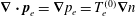 $\unicode[STIX]{x1D735}\boldsymbol{\cdot }\boldsymbol{p}_{e}=\unicode[STIX]{x1D735}p_{e}=T_{e}^{(0)}\unicode[STIX]{x1D735}n$
, eliminates the pressure term since
$\unicode[STIX]{x1D735}\boldsymbol{\cdot }\boldsymbol{p}_{e}=\unicode[STIX]{x1D735}p_{e}=T_{e}^{(0)}\unicode[STIX]{x1D735}n$
, eliminates the pressure term since
 $\unicode[STIX]{x1D735}\times [(1/n)\unicode[STIX]{x1D735}n]=\unicode[STIX]{x1D735}\times [\unicode[STIX]{x1D735}\ln (n)]=0$
. By prescribing the electrons to be isotropic but not isothermal, with pressure
$\unicode[STIX]{x1D735}\times [(1/n)\unicode[STIX]{x1D735}n]=\unicode[STIX]{x1D735}\times [\unicode[STIX]{x1D735}\ln (n)]=0$
. By prescribing the electrons to be isotropic but not isothermal, with pressure
 $\boldsymbol{p}_{e}=p_{e}\unicode[STIX]{x1D644}$
, the term initially does not disappear and it is equal to
$\boldsymbol{p}_{e}=p_{e}\unicode[STIX]{x1D644}$
, the term initially does not disappear and it is equal to
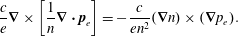 $$\begin{eqnarray}\frac{c}{e}\unicode[STIX]{x1D735}\times \left[\frac{1}{n}\unicode[STIX]{x1D735}\boldsymbol{\cdot }\boldsymbol{p}_{e}\right]=-\frac{c}{en^{2}}(\unicode[STIX]{x1D735}n)\times (\unicode[STIX]{x1D735}p_{e}).\end{eqnarray}$$
The term only disappears after the equation of state is prescribed, for example for
 $p_{e}\sim n^{\unicode[STIX]{x1D6FE}}$
. The term (3.22) is sometimes called the ‘battery’ term (Biermann Reference Biermann1950; Kulsrud et al.
Reference Kulsrud, Cen, Ostriker and Ryu1997; Khomenko et al.
Reference Khomenko, Vitas, Collados and de Vicente2017), since it is argued that for any deviations from an ideal equation of state (caused for example by shocks), the term can produce magnetic field fluctuations even if there is no magnetic field initially.
$p_{e}\sim n^{\unicode[STIX]{x1D6FE}}$
. The term (3.22) is sometimes called the ‘battery’ term (Biermann Reference Biermann1950; Kulsrud et al.
Reference Kulsrud, Cen, Ostriker and Ryu1997; Khomenko et al.
Reference Khomenko, Vitas, Collados and de Vicente2017), since it is argued that for any deviations from an ideal equation of state (caused for example by shocks), the term can produce magnetic field fluctuations even if there is no magnetic field initially.
3.1 Normalized equations and definitions
As with MHD and Hall-MHD, it is often useful to work with normalized equations. The density, velocity, magnetic field and pressure are normalized with respect to
 $\unicode[STIX]{x1D70C}_{0},u_{0},B_{0},p_{\Vert }^{(0)}$
. The length is normalized with respect to (for now) arbitrary
$\unicode[STIX]{x1D70C}_{0},u_{0},B_{0},p_{\Vert }^{(0)}$
. The length is normalized with respect to (for now) arbitrary
 $x_{0}$
and the time with respect to
$x_{0}$
and the time with respect to
 $t_{0}=x_{0}/u_{0}$
. The normalized quantities are then
$t_{0}=x_{0}/u_{0}$
. The normalized quantities are then
 $$\begin{eqnarray}\displaystyle \widetilde{\unicode[STIX]{x1D70C}}=\frac{\unicode[STIX]{x1D70C}}{\unicode[STIX]{x1D70C}_{0}};\quad \widetilde{\boldsymbol{u}}=\frac{\boldsymbol{u}}{u_{0}};\quad \widetilde{\boldsymbol{B}}=\frac{\boldsymbol{B}}{B_{0}};\quad \widetilde{p}_{\Vert }=\frac{p_{\Vert }}{p_{\Vert }^{(0)}};\quad \widetilde{p}_{\bot }=\frac{p_{\bot }}{p_{\Vert }^{(0)}}; & & \displaystyle\end{eqnarray}$$
 $$\begin{eqnarray}\displaystyle \widetilde{\boldsymbol{x}}=\frac{\boldsymbol{x}}{x_{0}};\quad \widetilde{\unicode[STIX]{x1D735}}=\unicode[STIX]{x1D735}x_{0};\quad \widetilde{t}=t\frac{u_{0}}{x_{0}};\quad \frac{\unicode[STIX]{x2202}}{\unicode[STIX]{x2202}\widetilde{t}}=\frac{\unicode[STIX]{x2202}}{\unicode[STIX]{x2202}t}\frac{x_{0}}{u_{0}}. & & \displaystyle\end{eqnarray}$$
Obviously
 $\widetilde{n}=\widetilde{\unicode[STIX]{x1D70C}}$
. After dropping the tilde, the normalization yields the same density and pressure equations, whereas the normalized momentum and induction equation become
$\widetilde{n}=\widetilde{\unicode[STIX]{x1D70C}}$
. After dropping the tilde, the normalization yields the same density and pressure equations, whereas the normalized momentum and induction equation become
 $$\begin{eqnarray}\displaystyle & \displaystyle \frac{\unicode[STIX]{x2202}\boldsymbol{u}_{p}}{\unicode[STIX]{x2202}t}+\boldsymbol{u}_{p}\boldsymbol{\cdot }\unicode[STIX]{x1D735}\boldsymbol{u}_{p}+\frac{p_{\Vert }^{(0)}}{\unicode[STIX]{x1D70C}_{0}u_{0}^{2}}\frac{1}{\unicode[STIX]{x1D70C}_{p}}\unicode[STIX]{x1D735}\boldsymbol{\cdot }(\boldsymbol{p}_{p}+\boldsymbol{p}_{e})-\frac{V_{A}^{2}}{u_{0}^{2}}\frac{1}{\unicode[STIX]{x1D70C}_{p}}(\unicode[STIX]{x1D735}\times \boldsymbol{B})\times \boldsymbol{B}=0; & \displaystyle\end{eqnarray}$$
 $$\begin{eqnarray}\displaystyle & \displaystyle \frac{\unicode[STIX]{x2202}\boldsymbol{B}}{\unicode[STIX]{x2202}t}=\unicode[STIX]{x1D735}\times (\boldsymbol{u}\times \boldsymbol{B})-\frac{V_{A}^{2}}{\unicode[STIX]{x1D6FA}_{p}u_{0}x_{0}}\unicode[STIX]{x1D735}\times \left[\frac{1}{n}(\unicode[STIX]{x1D735}\times \boldsymbol{B})\times \boldsymbol{B}\right]+\frac{p_{\Vert }^{(0)}}{\unicode[STIX]{x1D6FA}_{p}\unicode[STIX]{x1D70C}_{0}u_{0}x_{0}}\unicode[STIX]{x1D735}\times \left[\frac{1}{n}\unicode[STIX]{x1D735}\boldsymbol{\cdot }\boldsymbol{p}_{e}\right], & \displaystyle\end{eqnarray}$$
where the Alfvén speed
 $V_{A}=B_{0}/\sqrt{4\unicode[STIX]{x03C0}\unicode[STIX]{x1D70C}_{0}}$
. The momentum equation implies that it is beneficial to choose the (so far unspecified) normalizing velocity
$V_{A}=B_{0}/\sqrt{4\unicode[STIX]{x03C0}\unicode[STIX]{x1D70C}_{0}}$
. The momentum equation implies that it is beneficial to choose the (so far unspecified) normalizing velocity
 $u_{0}$
to be the Alfvén speed
$u_{0}$
to be the Alfvén speed
 $u_{0}=V_{A}$
. If the second and third terms are neglected in the induction equation (i.e. when the usual MHD induction equation is used), the CGL system is independent of length scale
$u_{0}=V_{A}$
. If the second and third terms are neglected in the induction equation (i.e. when the usual MHD induction equation is used), the CGL system is independent of length scale
 $x_{0}$
, similarly to the MHD system. If the Hall term is considered, it is beneficial to choose the (so far unspecified) normalizing length scale
$x_{0}$
, similarly to the MHD system. If the Hall term is considered, it is beneficial to choose the (so far unspecified) normalizing length scale
 $x_{0}$
to be the ion inertial length
$x_{0}$
to be the ion inertial length
 $$\begin{eqnarray}d_{i}=\frac{V_{A}}{\unicode[STIX]{x1D6FA}_{p}}.\end{eqnarray}$$
Therefore by choosing
 $x_{0}=d_{i}$
, the normalizations that we use in all fluid models in this paper read
$x_{0}=d_{i}$
, the normalizations that we use in all fluid models in this paper read
 $$\begin{eqnarray}\displaystyle \widetilde{\boldsymbol{u}}=\frac{\boldsymbol{u}}{V_{A}};\quad \widetilde{\boldsymbol{x}}=\frac{\boldsymbol{x}}{d_{i}};\quad \widetilde{t}=t\frac{V_{A}}{d_{i}}=t\unicode[STIX]{x1D6FA}_{p}. & & \displaystyle\end{eqnarray}$$
The normalization also has the advantage that, when transferred to Fourier space, one obtains the dispersion relations for normalized wavenumber
 $\widetilde{k}$
and frequency
$\widetilde{k}$
and frequency
 $\widetilde{\unicode[STIX]{x1D714}}$
as
$\widetilde{\unicode[STIX]{x1D714}}$
as
 $$\begin{eqnarray}\widetilde{k}=\frac{kV_{A}}{\unicode[STIX]{x1D6FA}_{p}},\quad \widetilde{\unicode[STIX]{x1D714}}=\frac{\unicode[STIX]{x1D714}}{\unicode[STIX]{x1D6FA}_{p}}.\end{eqnarray}$$
It is useful to define the parallel and perpendicular thermal speeds
 $$\begin{eqnarray}v_{\text{th}\Vert }=\sqrt{\frac{2T_{\Vert }^{(0)}}{m_{p}}};\quad v_{\text{th}\bot }=\sqrt{\frac{2T_{\bot }^{(0)}}{m_{p}}},\end{eqnarray}$$
and the definition of parallel and perpendicular temperatures are
 $T_{\Vert }=p_{\Vert }/n$
and
$T_{\Vert }=p_{\Vert }/n$
and
 $T_{\bot }=p_{\bot }/n$
. We use the usual convention with the Boltzmann constant
$T_{\bot }=p_{\bot }/n$
. We use the usual convention with the Boltzmann constant
 $k_{B}=1$
.Footnote
3
The parallel and perpendicular plasma beta are defined according to
$k_{B}=1$
.Footnote
3
The parallel and perpendicular plasma beta are defined according to
 $$\begin{eqnarray}\unicode[STIX]{x1D6FD}_{\Vert }=\frac{v_{\text{th}\Vert }^{2}}{V_{A}^{2}}=\frac{2p_{\Vert }^{(0)}}{\unicode[STIX]{x1D70C}_{0}V_{A}^{2}}=\frac{p_{\Vert }^{(0)}}{B_{0}^{2}/(8\unicode[STIX]{x03C0})};\quad \unicode[STIX]{x1D6FD}_{\bot }=\frac{v_{\text{th}\bot }^{2}}{V_{A}^{2}}=\frac{2p_{\bot }^{(0)}}{\unicode[STIX]{x1D70C}_{0}V_{A}^{2}}=\frac{p_{\bot }^{(0)}}{B_{0}^{2}/(8\unicode[STIX]{x03C0})}=\unicode[STIX]{x1D6FD}_{\Vert }\frac{T_{\bot }^{(0)}}{T_{\Vert }^{(0)}},\end{eqnarray}$$
and later we will often use the abbreviation
 $a_{p}$
for the proton temperature anisotropy ratio
$a_{p}$
for the proton temperature anisotropy ratio
 $$\begin{eqnarray}a_{p}=\frac{T_{\bot }^{(0)}}{T_{\Vert }^{(0)}}=\frac{p_{\bot }^{(0)}}{p_{\Vert }^{(0)}}.\end{eqnarray}$$
The normalized momentum and induction equations therefore read (tilde are dropped)
 $$\begin{eqnarray}\displaystyle & \displaystyle \frac{\unicode[STIX]{x2202}\boldsymbol{u}_{p}}{\unicode[STIX]{x2202}t}+\boldsymbol{u}_{p}\boldsymbol{\cdot }\unicode[STIX]{x1D735}\boldsymbol{u}_{p}+\frac{\unicode[STIX]{x1D6FD}_{\Vert }}{2}\frac{1}{\unicode[STIX]{x1D70C}_{p}}\unicode[STIX]{x1D735}\boldsymbol{\cdot }(\boldsymbol{p}_{p}+\boldsymbol{p}_{e})-\frac{1}{\unicode[STIX]{x1D70C}_{p}}(\unicode[STIX]{x1D735}\times \boldsymbol{B})\times \boldsymbol{B}=0; & \displaystyle\end{eqnarray}$$
 $$\begin{eqnarray}\displaystyle & \displaystyle \frac{\unicode[STIX]{x2202}\boldsymbol{B}}{\unicode[STIX]{x2202}t}=\unicode[STIX]{x1D735}\times (\boldsymbol{u}\times \boldsymbol{B})-\unicode[STIX]{x1D735}\times \left[\frac{1}{n}(\unicode[STIX]{x1D735}\times \boldsymbol{B})\times \boldsymbol{B}\right]+\frac{\unicode[STIX]{x1D6FD}_{\Vert }}{2}\unicode[STIX]{x1D735}\times \left[\frac{1}{n}\unicode[STIX]{x1D735}\boldsymbol{\cdot }\boldsymbol{p}_{e}\right]. & \displaystyle\end{eqnarray}$$
Another useful quantity that we will use later in the text is the proton Larmor radius (the gyroradius)
 $\unicode[STIX]{x1D70C}_{i}$
, defined according to
$\unicode[STIX]{x1D70C}_{i}$
, defined according to
 $$\begin{eqnarray}\unicode[STIX]{x1D70C}_{i}=\frac{v_{\text{th}\bot }}{\unicode[STIX]{x1D6FA}_{p}}.\end{eqnarray}$$
We note that normalizations do not have to be done with respect to mean values, and normalizations with respect to fluctuating (turbulent) quantities are used for example in the nearly incompressible models of Zank et al. (Reference Zank, Adhikari, Hunana, Shiota, Bruno and Telloni2017) and Zank & Matthaeus (Reference Zank and Matthaeus1993).
3.2 Classical CGL model with cold electrons
Here we want to consider the simplest possible CGL model for the proton species. We assume the electrons to be massless and cold (
 $\boldsymbol{p}_{e}=0$
), and we also neglect the Hall term in the induction equation. Since only proton species are present, for simplicity we can drop the proton index ‘
$\boldsymbol{p}_{e}=0$
), and we also neglect the Hall term in the induction equation. Since only proton species are present, for simplicity we can drop the proton index ‘
 $p$
’. Let us work in physical units for a moment. The classical CGL model with cold electrons therefore reads (written in physical units)
$p$
’. Let us work in physical units for a moment. The classical CGL model with cold electrons therefore reads (written in physical units)
 $$\begin{eqnarray}\displaystyle & \displaystyle \frac{\unicode[STIX]{x2202}\unicode[STIX]{x1D70C}}{\unicode[STIX]{x2202}t}+\unicode[STIX]{x1D735}\boldsymbol{\cdot }(\unicode[STIX]{x1D70C}\boldsymbol{u})=0; & \displaystyle\end{eqnarray}$$
 $$\begin{eqnarray}\displaystyle & \displaystyle \frac{\unicode[STIX]{x2202}\boldsymbol{u}}{\unicode[STIX]{x2202}t}+\boldsymbol{u}\boldsymbol{\cdot }\unicode[STIX]{x1D735}\boldsymbol{u}+\frac{1}{\unicode[STIX]{x1D70C}}\unicode[STIX]{x1D735}\boldsymbol{\cdot }\boldsymbol{p}-\frac{1}{4\unicode[STIX]{x03C0}\unicode[STIX]{x1D70C}}(\unicode[STIX]{x1D735}\times \boldsymbol{B})\times \boldsymbol{B}=0; & \displaystyle\end{eqnarray}$$
 $$\begin{eqnarray}\displaystyle & \displaystyle \frac{\unicode[STIX]{x2202}p_{\Vert }}{\unicode[STIX]{x2202}t}+\unicode[STIX]{x1D735}\boldsymbol{\cdot }(p_{\Vert }\boldsymbol{u})+2p_{\Vert }\hat{\boldsymbol{b}}\boldsymbol{\cdot }\unicode[STIX]{x1D735}\boldsymbol{u}\boldsymbol{\cdot }\hat{\boldsymbol{b}}=0; & \displaystyle\end{eqnarray}$$
 $$\begin{eqnarray}\displaystyle & \displaystyle \frac{\unicode[STIX]{x2202}p_{\bot }}{\unicode[STIX]{x2202}t}+\unicode[STIX]{x1D735}\boldsymbol{\cdot }(p_{\bot }\boldsymbol{u})+p_{\bot }\unicode[STIX]{x1D735}\boldsymbol{\cdot }\boldsymbol{u}-p_{\bot }\hat{\boldsymbol{b}}\boldsymbol{\cdot }\unicode[STIX]{x1D735}\boldsymbol{u}\boldsymbol{\cdot }\hat{\boldsymbol{b}}=0; & \displaystyle\end{eqnarray}$$
 $$\begin{eqnarray}\displaystyle & \displaystyle \frac{\unicode[STIX]{x2202}\boldsymbol{B}}{\unicode[STIX]{x2202}t}=\unicode[STIX]{x1D735}\times (\boldsymbol{u}\times \boldsymbol{B}). & \displaystyle\end{eqnarray}$$
Similarly to the usual MHD model, the CGL equations are scale invariant and do not contain any information about the physical length scale. A length scale is introduced by considering the Hall term in the induction equation, and we discuss the Hall-CGL model in the next section. Also, the absence of the Hall term allows the CGL pressure equations to be rewritten into ‘conservative’ form as
 $$\begin{eqnarray}\frac{\text{d}}{\text{d}t}\left(\frac{p_{\Vert }|\boldsymbol{B}|^{2}}{\unicode[STIX]{x1D70C}^{3}}\right)=0;\quad \frac{\text{d}}{\text{d}t}\left(\frac{p_{\bot }}{\unicode[STIX]{x1D70C}|\boldsymbol{B}|}\right)=0,\end{eqnarray}$$
where
 $\text{d}/\text{d}t$
is the convective derivative. This formulation is the most often cited form of the CGL pressure equations (often the
$\text{d}/\text{d}t$
is the convective derivative. This formulation is the most often cited form of the CGL pressure equations (often the
 $|\boldsymbol{B}|$
is abbreviated only as
$|\boldsymbol{B}|$
is abbreviated only as
 $B$
, which can lead to confusion on how to correctly calculate the derivatives). We want to show the equivalence of (3.41) and (3.38), (3.39). We need the following identity,
$B$
, which can lead to confusion on how to correctly calculate the derivatives). We want to show the equivalence of (3.41) and (3.38), (3.39). We need the following identity,
 $$\begin{eqnarray}\displaystyle \frac{\unicode[STIX]{x2202}}{\unicode[STIX]{x2202}t}|\boldsymbol{B}|=\frac{\unicode[STIX]{x2202}}{\unicode[STIX]{x2202}t}(B_{x}^{2}+B_{y}^{2}+B_{z}^{2})^{1/2}=\frac{1}{|\boldsymbol{B}|}\boldsymbol{B}\boldsymbol{\cdot }\frac{\unicode[STIX]{x2202}\boldsymbol{B}}{\unicode[STIX]{x2202}t}=\hat{\boldsymbol{b}}\boldsymbol{\cdot }\frac{\unicode[STIX]{x2202}\boldsymbol{B}}{\unicode[STIX]{x2202}t}, & & \displaystyle\end{eqnarray}$$
and the result is of course a scalar. Similarly for the spatial and convective derivative
 $$\begin{eqnarray}\unicode[STIX]{x2202}_{i}|\boldsymbol{B}|=\hat{\boldsymbol{b}}\boldsymbol{\cdot }(\unicode[STIX]{x2202}_{i}\boldsymbol{B});\quad \frac{\text{d}}{\text{d}t}|\boldsymbol{B}|=\left(\frac{\unicode[STIX]{x2202}}{\unicode[STIX]{x2202}t}+u_{i}\unicode[STIX]{x2202}_{i}\right)|\boldsymbol{B}|=\hat{\boldsymbol{b}}\boldsymbol{\cdot }\frac{\text{d}\boldsymbol{B}}{\text{d}t}.\end{eqnarray}$$
Later we will need
 $$\begin{eqnarray}\frac{\text{d}}{\text{d}t}|\boldsymbol{B}|^{2}=\frac{\text{d}}{\text{d}t}(B_{x}^{2}+B_{y}^{2}+B_{z}^{2})=2\boldsymbol{B}\boldsymbol{\cdot }\frac{\text{d}\boldsymbol{B}}{\text{d}t}.\end{eqnarray}$$
Now we can directly calculate
 $$\begin{eqnarray}\displaystyle \frac{\text{d}}{\text{d}t}\left(\frac{p_{\bot }}{\unicode[STIX]{x1D70C}|\boldsymbol{B}|}\right) & = & \displaystyle \frac{1}{\unicode[STIX]{x1D70C}|\boldsymbol{B}|}\frac{\text{d}p_{\bot }}{\text{d}t}-\frac{p_{\bot }}{|\boldsymbol{B}|\unicode[STIX]{x1D70C}^{2}}\frac{\text{d}\unicode[STIX]{x1D70C}}{\text{d}t}-\frac{p_{\bot }}{\unicode[STIX]{x1D70C}|\boldsymbol{B}|^{2}}\frac{\text{d}|\boldsymbol{B}|}{\text{d}t}\nonumber\\ \displaystyle & = & \displaystyle \frac{1}{\unicode[STIX]{x1D70C}|\boldsymbol{B}|}\left(\frac{\text{d}p_{\bot }}{\text{d}t}-\frac{p_{\bot }}{\unicode[STIX]{x1D70C}}\frac{\text{d}\unicode[STIX]{x1D70C}}{\text{d}t}-\frac{p_{\bot }}{|\boldsymbol{B}|}\frac{\text{d}|\boldsymbol{B}|}{\text{d}t}\right),\end{eqnarray}$$
and, by using the density equation
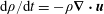 $\text{d}\unicode[STIX]{x1D70C}/\text{d}t=-\unicode[STIX]{x1D70C}\unicode[STIX]{x1D735}\boldsymbol{\cdot }\boldsymbol{u}$
and the identity (3.43), we obtain
$\text{d}\unicode[STIX]{x1D70C}/\text{d}t=-\unicode[STIX]{x1D70C}\unicode[STIX]{x1D735}\boldsymbol{\cdot }\boldsymbol{u}$
and the identity (3.43), we obtain
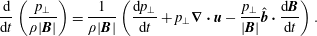 $$\begin{eqnarray}\displaystyle \frac{\text{d}}{\text{d}t}\left(\frac{p_{\bot }}{\unicode[STIX]{x1D70C}|\boldsymbol{B}|}\right)=\frac{1}{\unicode[STIX]{x1D70C}|\boldsymbol{B}|}\left(\frac{\text{d}p_{\bot }}{\text{d}t}+p_{\bot }\unicode[STIX]{x1D735}\boldsymbol{\cdot }\boldsymbol{u}-\frac{p_{\bot }}{|\boldsymbol{B}|}\hat{\boldsymbol{b}}\boldsymbol{\cdot }\frac{\text{d}\boldsymbol{B}}{\text{d}t}\right). & & \displaystyle\end{eqnarray}$$
The above equation is completely general since we did not use the induction equation so far and we will use this equation in the next section when we consider the Hall-CGL model. In a similar way one derives a completely general identity
 $$\begin{eqnarray}\displaystyle \frac{\text{d}}{\text{d}t}\left(\frac{p_{\Vert }|\boldsymbol{B}|^{2}}{\unicode[STIX]{x1D70C}^{3}}\right) & = & \displaystyle \frac{|\boldsymbol{B}|^{2}}{\unicode[STIX]{x1D70C}^{3}}\left(\frac{\text{d}p_{\Vert }}{\text{d}t}+\frac{p_{\Vert }}{|\boldsymbol{B}|^{2}}\frac{\text{d}|\boldsymbol{B}|^{2}}{\text{d}t}-3\frac{p_{\Vert }}{\unicode[STIX]{x1D70C}}\frac{\text{d}\unicode[STIX]{x1D70C}}{\text{d}t}\right)\nonumber\\ \displaystyle & = & \displaystyle \frac{|\boldsymbol{B}|^{2}}{\unicode[STIX]{x1D70C}^{3}}\left(\frac{\text{d}p_{\Vert }}{\text{d}t}+3p_{\Vert }\unicode[STIX]{x1D735}\boldsymbol{\cdot }\boldsymbol{u}+\frac{2p_{\Vert }}{|\boldsymbol{B}|}\hat{\boldsymbol{b}}\boldsymbol{\cdot }\frac{\text{d}\boldsymbol{B}}{\text{d}t}\right).\end{eqnarray}$$
Now, we use the induction equation
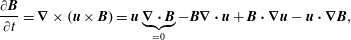 $$\begin{eqnarray}\frac{\unicode[STIX]{x2202}\boldsymbol{B}}{\unicode[STIX]{x2202}t}=\unicode[STIX]{x1D735}\times (\boldsymbol{u}\times \boldsymbol{B})=\boldsymbol{u}\underbrace{\unicode[STIX]{x1D735}\boldsymbol{\cdot }\boldsymbol{B}}_{=0}-\boldsymbol{B}\unicode[STIX]{x1D735}\boldsymbol{\cdot }\boldsymbol{u}+\boldsymbol{B}\boldsymbol{\cdot }\unicode[STIX]{x1D735}\boldsymbol{u}-\boldsymbol{u}\boldsymbol{\cdot }\unicode[STIX]{x1D735}\boldsymbol{B},\end{eqnarray}$$
that allows us to calculate
 $$\begin{eqnarray}\displaystyle & \displaystyle \frac{\text{d}\boldsymbol{B}}{\text{d}t}=\frac{\unicode[STIX]{x2202}\boldsymbol{B}}{\unicode[STIX]{x2202}t}+\boldsymbol{u}\boldsymbol{\cdot }\unicode[STIX]{x1D735}\boldsymbol{B}=-\boldsymbol{B}\unicode[STIX]{x1D735}\boldsymbol{\cdot }\boldsymbol{u}+\boldsymbol{B}\boldsymbol{\cdot }\unicode[STIX]{x1D735}\boldsymbol{u}; & \displaystyle\end{eqnarray}$$
 $$\begin{eqnarray}\displaystyle & \displaystyle \frac{\hat{\boldsymbol{b}}}{|\boldsymbol{B}|}\boldsymbol{\cdot }\frac{\text{d}\boldsymbol{B}}{\text{d}t}=-\unicode[STIX]{x1D735}\boldsymbol{\cdot }\boldsymbol{u}+\hat{\boldsymbol{b}}\boldsymbol{\cdot }\unicode[STIX]{x1D735}\boldsymbol{u}\boldsymbol{\cdot }\hat{\boldsymbol{b}}, & \displaystyle\end{eqnarray}$$
and which, when used in (3.47)–(3.46) yields the final result
 $$\begin{eqnarray}\displaystyle & \displaystyle \frac{\text{d}}{\text{d}t}\left(\frac{p_{\Vert }|\boldsymbol{B}|^{2}}{\unicode[STIX]{x1D70C}^{3}}\right)=\frac{|\boldsymbol{B}|^{2}}{\unicode[STIX]{x1D70C}^{3}}\left(\frac{\text{d}p_{\Vert }}{\text{d}t}+p_{\Vert }\unicode[STIX]{x1D735}\boldsymbol{\cdot }\boldsymbol{u}+2p_{\Vert }\hat{\boldsymbol{b}}\boldsymbol{\cdot }\unicode[STIX]{x1D735}\boldsymbol{u}\boldsymbol{\cdot }\hat{\boldsymbol{b}}\right)=0; & \displaystyle\end{eqnarray}$$
 $$\begin{eqnarray}\displaystyle & \displaystyle \frac{\text{d}}{\text{d}t}\left(\frac{p_{\bot }}{\unicode[STIX]{x1D70C}|\boldsymbol{B}|}\right)=\frac{1}{\unicode[STIX]{x1D70C}|\boldsymbol{B}|}\left(\frac{\text{d}p_{\bot }}{\text{d}t}+2p_{\bot }\unicode[STIX]{x1D735}\boldsymbol{\cdot }\boldsymbol{u}-p_{\bot }\hat{\boldsymbol{b}}\boldsymbol{\cdot }\unicode[STIX]{x1D735}\boldsymbol{u}\boldsymbol{\cdot }\hat{\boldsymbol{b}}\right)=0. & \displaystyle\end{eqnarray}$$
Equations (3.51)–(3.52) verify that the CGL pressure equations (3.41) written in the ‘conservative’ form and the directly derived CGL equations (3.38)–(3.39) are equivalent. We will see that the right-hand side of the usual CGL equations (3.41) is non-zero if the Hall term is considered, and that it is further modified by the heat flux contributions and by the FLR stress forces.
3.3 Linearized CGL equations
To obtain the dispersion relations, the equations need to be linearized and transformed to Fourier space. Equations (3.36)–(3.40) are linearized with respect to mean values
 $\unicode[STIX]{x1D70C}_{0};\boldsymbol{u}^{(0)}\equiv \langle \boldsymbol{u}\rangle =0;p_{\Vert \bot }^{(0)};\boldsymbol{B}_{0}=(0,0,B_{0});\hat{\boldsymbol{b}}_{0}=(0,0,1)$
where the magnetic field
$\unicode[STIX]{x1D70C}_{0};\boldsymbol{u}^{(0)}\equiv \langle \boldsymbol{u}\rangle =0;p_{\Vert \bot }^{(0)};\boldsymbol{B}_{0}=(0,0,B_{0});\hat{\boldsymbol{b}}_{0}=(0,0,1)$
where the magnetic field
 $B_{0}$
is assumed to be in the
$B_{0}$
is assumed to be in the
 $z$
-direction. We assume that the mean value of the velocity is zero (the zero mean velocity value
$z$
-direction. We assume that the mean value of the velocity is zero (the zero mean velocity value
 $\boldsymbol{u}^{(0)}=0$
should not be confused with the normalizing velocity as in (3.23), which is later chosen to be
$\boldsymbol{u}^{(0)}=0$
should not be confused with the normalizing velocity as in (3.23), which is later chosen to be
 $V_{A}$
). The terms
$V_{A}$
). The terms
 $\hat{\boldsymbol{b}}\boldsymbol{\cdot }\unicode[STIX]{x1D735}\boldsymbol{u}\boldsymbol{\cdot }\hat{\boldsymbol{b}}$
are linearized as
$\hat{\boldsymbol{b}}\boldsymbol{\cdot }\unicode[STIX]{x1D735}\boldsymbol{u}\boldsymbol{\cdot }\hat{\boldsymbol{b}}$
are linearized as
 $\hat{\boldsymbol{b}}\boldsymbol{\cdot }\unicode[STIX]{x1D735}\boldsymbol{u}\boldsymbol{\cdot }\hat{\boldsymbol{b}}\overset{\text{lin}}{=}\unicode[STIX]{x2202}_{z}u_{z}$
and the linearized system reads
$\hat{\boldsymbol{b}}\boldsymbol{\cdot }\unicode[STIX]{x1D735}\boldsymbol{u}\boldsymbol{\cdot }\hat{\boldsymbol{b}}\overset{\text{lin}}{=}\unicode[STIX]{x2202}_{z}u_{z}$
and the linearized system reads
 $$\begin{eqnarray}\displaystyle & \displaystyle \frac{\unicode[STIX]{x2202}\unicode[STIX]{x1D70C}}{\unicode[STIX]{x2202}t}+\unicode[STIX]{x1D70C}_{0}\unicode[STIX]{x1D735}\boldsymbol{\cdot }\boldsymbol{u}=0; & \displaystyle\end{eqnarray}$$
 $$\begin{eqnarray}\displaystyle & \displaystyle \frac{\unicode[STIX]{x2202}\boldsymbol{u}}{\unicode[STIX]{x2202}t}+\frac{1}{\unicode[STIX]{x1D70C}_{0}}\unicode[STIX]{x1D735}\boldsymbol{\cdot }\boldsymbol{p}-\frac{1}{4\unicode[STIX]{x03C0}\unicode[STIX]{x1D70C}_{0}}(\unicode[STIX]{x1D735}\times \boldsymbol{B})\times \boldsymbol{B}_{0}=0; & \displaystyle\end{eqnarray}$$
 $$\begin{eqnarray}\displaystyle & \displaystyle \frac{\unicode[STIX]{x2202}p_{\Vert }}{\unicode[STIX]{x2202}t}+p_{\Vert }^{(0)}\unicode[STIX]{x1D735}\boldsymbol{\cdot }\boldsymbol{u}+2p_{\Vert }^{(0)}\unicode[STIX]{x2202}_{z}u_{z}=0; & \displaystyle\end{eqnarray}$$
 $$\begin{eqnarray}\displaystyle & \displaystyle \frac{\unicode[STIX]{x2202}p_{\bot }}{\unicode[STIX]{x2202}t}+2p_{\bot }^{(0)}\unicode[STIX]{x1D735}\boldsymbol{\cdot }\boldsymbol{u}-p_{\bot }^{(0)}\unicode[STIX]{x2202}_{z}u_{z}=0; & \displaystyle\end{eqnarray}$$
 $$\begin{eqnarray}\displaystyle & \displaystyle \frac{\unicode[STIX]{x2202}\boldsymbol{B}}{\unicode[STIX]{x2202}t}=\unicode[STIX]{x1D735}\times (\boldsymbol{u}\times \boldsymbol{B}_{0}). & \displaystyle\end{eqnarray}$$
The divergence of the pressure tensor is
 $$\begin{eqnarray}\displaystyle (\unicode[STIX]{x1D735}\boldsymbol{\cdot }\boldsymbol{p})_{i}=\unicode[STIX]{x2202}_{j}p_{ji}=\hat{b}_{i}\hat{b}_{j}\unicode[STIX]{x2202}_{j}p_{\Vert }+(\unicode[STIX]{x1D6FF}_{ij}-\hat{b}_{i}\hat{b}_{j})\unicode[STIX]{x2202}_{j}p_{\bot }+(p_{\Vert }-p_{\bot })(\hat{b}_{i}\unicode[STIX]{x2202}_{j}\hat{b}_{j}+\hat{b}_{j}\unicode[STIX]{x2202}_{j}\hat{b}_{i}), & & \displaystyle\end{eqnarray}$$
and the first step of linearization yields, by components,
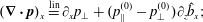 $$\begin{eqnarray}\displaystyle & \displaystyle (\unicode[STIX]{x1D735}\boldsymbol{\cdot }\boldsymbol{p})_{x}\overset{\text{lin}}{=}\unicode[STIX]{x2202}_{x}p_{\bot }+(p_{\Vert }^{(0)}-p_{\bot }^{(0)})\unicode[STIX]{x2202}_{z}\hat{b}_{x}; & \displaystyle\end{eqnarray}$$
 $$\begin{eqnarray}\displaystyle & \displaystyle (\unicode[STIX]{x1D735}\boldsymbol{\cdot }\boldsymbol{p})_{y}\overset{\text{lin}}{=}\unicode[STIX]{x2202}_{y}p_{\bot }+(p_{\Vert }^{(0)}-p_{\bot }^{(0)})\unicode[STIX]{x2202}_{z}\hat{b}_{y}; & \displaystyle\end{eqnarray}$$
 $$\begin{eqnarray}\displaystyle & \displaystyle (\unicode[STIX]{x1D735}\boldsymbol{\cdot }\boldsymbol{p})_{z}\overset{\text{lin}}{=}\unicode[STIX]{x2202}_{z}p_{\Vert }+(p_{\Vert }^{(0)}-p_{\bot }^{(0)})(\unicode[STIX]{x1D735}\boldsymbol{\cdot }\hat{\boldsymbol{b}}+\unicode[STIX]{x2202}_{z}\hat{b}_{z}), & \displaystyle\end{eqnarray}$$
which can be conveniently written in matrix notation as
 $$\begin{eqnarray}\displaystyle \unicode[STIX]{x1D735}\boldsymbol{\cdot }\boldsymbol{p}\overset{\text{lin}}{=}\unicode[STIX]{x1D735}\boldsymbol{\cdot }\left(\begin{array}{@{}ccc@{}}p_{\bot } & 0 & 0\\ 0 & p_{\bot } & 0\\ 0 & 0 & p_{\Vert }\end{array}\right)+(p_{\Vert }^{(0)}-p_{\bot }^{(0)})\unicode[STIX]{x1D735}\boldsymbol{\cdot }\left.\left(\begin{array}{@{}ccc@{}}0 & 0 & \hat{b}_{x}\\ 0 & 0 & \hat{b}_{y}\\ \hat{b}_{x} & \hat{b}_{y} & 2\hat{b}_{z}\end{array}\right)\right|_{\text{lin}}. & & \displaystyle\end{eqnarray}$$
Notice that, since
 $\unicode[STIX]{x2202}_{i}|\boldsymbol{B}|=\hat{\boldsymbol{b}}\boldsymbol{\cdot }(\unicode[STIX]{x2202}_{i}\boldsymbol{B})$
, the derivatives of unit vectors are calculated according to
$\unicode[STIX]{x2202}_{i}|\boldsymbol{B}|=\hat{\boldsymbol{b}}\boldsymbol{\cdot }(\unicode[STIX]{x2202}_{i}\boldsymbol{B})$
, the derivatives of unit vectors are calculated according to
 $$\begin{eqnarray}\displaystyle \unicode[STIX]{x2202}_{i}\hat{\boldsymbol{b}}=\unicode[STIX]{x2202}_{i}\frac{\boldsymbol{B}}{|\boldsymbol{B}|}=\frac{1}{|\boldsymbol{B}|}\left[\unicode[STIX]{x2202}_{i}\boldsymbol{B}-\frac{\boldsymbol{B}}{|\boldsymbol{B}|}\unicode[STIX]{x2202}_{i}|\boldsymbol{B}|\right]=\frac{1}{|\boldsymbol{B}|}[\unicode[STIX]{x2202}_{i}\boldsymbol{B}-\hat{\boldsymbol{b}}(\hat{\boldsymbol{b}}\boldsymbol{\cdot }(\unicode[STIX]{x2202}_{i}\boldsymbol{B}))], & & \displaystyle\end{eqnarray}$$
and in the linear approximation one has
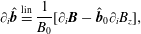 $$\begin{eqnarray}\displaystyle \unicode[STIX]{x2202}_{i}\hat{\boldsymbol{b}}\overset{\text{lin}}{=}\frac{1}{B_{0}}[\unicode[STIX]{x2202}_{i}\boldsymbol{B}-\hat{\boldsymbol{b}}_{0}\unicode[STIX]{x2202}_{i}B_{z}], & & \displaystyle\end{eqnarray}$$
which by components reads
 $$\begin{eqnarray}\displaystyle \unicode[STIX]{x2202}_{i}\hat{b}_{x}\overset{\text{lin}}{=}\frac{1}{B_{0}}\unicode[STIX]{x2202}_{i}B_{x};\quad \unicode[STIX]{x2202}_{i}\hat{b}_{y}\overset{\text{lin}}{=}\frac{1}{B_{0}}\unicode[STIX]{x2202}_{i}B_{y};\quad \unicode[STIX]{x2202}_{i}\hat{b}_{z}\overset{\text{lin}}{=}\frac{1}{B_{0}}(\unicode[STIX]{x2202}_{i}B_{z}-\unicode[STIX]{x2202}_{z}B_{z}), & & \displaystyle\end{eqnarray}$$
where, importantly,
 $\unicode[STIX]{x2202}_{z}\hat{b}_{z}\overset{\text{lin}}{=}0$
. The divergence of the pressure tensor in the liner approximation is therefore expressed as
$\unicode[STIX]{x2202}_{z}\hat{b}_{z}\overset{\text{lin}}{=}0$
. The divergence of the pressure tensor in the liner approximation is therefore expressed as
 $$\begin{eqnarray}\displaystyle \unicode[STIX]{x1D735}\boldsymbol{\cdot }\boldsymbol{p}\overset{\text{lin}}{=}\unicode[STIX]{x1D735}\boldsymbol{\cdot }\left(\begin{array}{@{}ccc@{}}p_{\bot } & 0 & 0\\ 0 & p_{\bot } & 0\\ 0 & 0 & p_{\Vert }\end{array}\right)+\frac{1}{B_{0}}(p_{\Vert }^{(0)}-p_{\bot }^{(0)})\unicode[STIX]{x1D735}\boldsymbol{\cdot }\left(\begin{array}{@{}ccc@{}}0 & 0 & B_{x}\\ 0 & 0 & B_{y}\\ B_{x} & B_{y} & 0\end{array}\right), & & \displaystyle\end{eqnarray}$$
where the second term contributes if the temperature anisotropy is present, i.e. when
 $p_{\Vert }^{(0)}\neq p_{\bot }^{(0)}$
. The vectors
$p_{\Vert }^{(0)}\neq p_{\bot }^{(0)}$
. The vectors
 $(\unicode[STIX]{x1D735}\times \boldsymbol{B})\times \boldsymbol{B}_{0}$
and
$(\unicode[STIX]{x1D735}\times \boldsymbol{B})\times \boldsymbol{B}_{0}$
and
 $\unicode[STIX]{x1D735}\times (\boldsymbol{u}\times \boldsymbol{B}_{0})$
are straightforward to calculate and are
$\unicode[STIX]{x1D735}\times (\boldsymbol{u}\times \boldsymbol{B}_{0})$
are straightforward to calculate and are
 $$\begin{eqnarray}\displaystyle (\unicode[STIX]{x1D735}\times \boldsymbol{B})\times \boldsymbol{B}_{0}=B_{0}\left(\begin{array}{@{}c@{}}-\unicode[STIX]{x2202}_{x}B_{z}+\unicode[STIX]{x2202}_{z}B_{x}\\ -\unicode[STIX]{x2202}_{y}B_{z}+\unicode[STIX]{x2202}_{z}B_{y}\\ 0\end{array}\right);\quad \unicode[STIX]{x1D735}\times (\boldsymbol{u}\times \boldsymbol{B}_{0})=B_{0}\left(\begin{array}{@{}c@{}}\unicode[STIX]{x2202}_{z}u_{x}\\ \unicode[STIX]{x2202}_{z}u_{y}\\ -\unicode[STIX]{x2202}_{x}u_{x}-\unicode[STIX]{x2202}_{y}u_{y}\end{array}\right). & & \displaystyle\end{eqnarray}$$
The entire set of linearized CGL equations reads
 $$\begin{eqnarray}\displaystyle & \displaystyle \frac{\unicode[STIX]{x2202}\unicode[STIX]{x1D70C}}{\unicode[STIX]{x2202}t}+\unicode[STIX]{x1D70C}_{0}\unicode[STIX]{x1D735}\boldsymbol{\cdot }\boldsymbol{u}=0; & \displaystyle\end{eqnarray}$$
 $$\begin{eqnarray}\displaystyle & \displaystyle \frac{\unicode[STIX]{x2202}u_{x}}{\unicode[STIX]{x2202}t}+\frac{1}{\unicode[STIX]{x1D70C}_{0}}\unicode[STIX]{x2202}_{x}p_{\bot }+\frac{1}{B_{0}\unicode[STIX]{x1D70C}_{0}}(p_{\Vert }^{(0)}-p_{\bot }^{(0)})\unicode[STIX]{x2202}_{z}B_{x}-\frac{B_{0}}{4\unicode[STIX]{x03C0}\unicode[STIX]{x1D70C}_{0}}(-\unicode[STIX]{x2202}_{x}B_{z}+\unicode[STIX]{x2202}_{z}B_{x})=0; & \displaystyle\end{eqnarray}$$
 $$\begin{eqnarray}\displaystyle & \displaystyle \frac{\unicode[STIX]{x2202}u_{y}}{\unicode[STIX]{x2202}t}+\frac{1}{\unicode[STIX]{x1D70C}_{0}}\unicode[STIX]{x2202}_{y}p_{\bot }+\frac{1}{B_{0}\unicode[STIX]{x1D70C}_{0}}(p_{\Vert }^{(0)}-p_{\bot }^{(0)})\unicode[STIX]{x2202}_{z}B_{y}-\frac{B_{0}}{4\unicode[STIX]{x03C0}\unicode[STIX]{x1D70C}_{0}}(-\unicode[STIX]{x2202}_{y}B_{z}+\unicode[STIX]{x2202}_{z}B_{y})=0; & \displaystyle\end{eqnarray}$$
 $$\begin{eqnarray}\displaystyle & \displaystyle \frac{\unicode[STIX]{x2202}u_{z}}{\unicode[STIX]{x2202}t}+\frac{1}{\unicode[STIX]{x1D70C}_{0}}\unicode[STIX]{x2202}_{z}p_{\Vert }+\frac{1}{B_{0}\unicode[STIX]{x1D70C}_{0}}(p_{\Vert }^{(0)}-p_{\bot }^{(0)})(\unicode[STIX]{x2202}_{x}B_{x}+\unicode[STIX]{x2202}_{y}B_{y})=0; & \displaystyle\end{eqnarray}$$
 $$\begin{eqnarray}\displaystyle & \displaystyle \frac{\unicode[STIX]{x2202}B_{x}}{\unicode[STIX]{x2202}t}=B_{0}\unicode[STIX]{x2202}_{z}u_{x};\quad \frac{\unicode[STIX]{x2202}B_{y}}{\unicode[STIX]{x2202}t}=B_{0}\unicode[STIX]{x2202}_{z}u_{y};\quad \frac{\unicode[STIX]{x2202}B_{z}}{\unicode[STIX]{x2202}t}=-B_{0}\unicode[STIX]{x2202}_{x}u_{x}-B_{0}\unicode[STIX]{x2202}_{y}u_{y}; & \displaystyle\end{eqnarray}$$
 $$\begin{eqnarray}\displaystyle & \displaystyle \frac{\unicode[STIX]{x2202}p_{\Vert }}{\unicode[STIX]{x2202}t}+p_{\Vert }^{(0)}(\unicode[STIX]{x2202}_{x}u_{x}+\unicode[STIX]{x2202}_{y}u_{y})+3p_{\Vert }^{(0)}\unicode[STIX]{x2202}_{z}u_{z}=0; & \displaystyle\end{eqnarray}$$
 $$\begin{eqnarray}\displaystyle & \displaystyle \frac{\unicode[STIX]{x2202}p_{\bot }}{\unicode[STIX]{x2202}t}+2p_{\bot }^{(0)}(\unicode[STIX]{x2202}_{x}u_{x}+\unicode[STIX]{x2202}_{y}u_{y})+p_{\bot }^{(0)}\unicode[STIX]{x2202}_{z}u_{z}=0. & \displaystyle\end{eqnarray}$$
Additionally, the 3 components of the induction equation are not independent, but satisfy the
 $\unicode[STIX]{x1D735}\boldsymbol{\cdot }\boldsymbol{B}=0$
constraint. In order to find the linear dispersion relations, without any loss of generality, we consider wave propagation in the
$\unicode[STIX]{x1D735}\boldsymbol{\cdot }\boldsymbol{B}=0$
constraint. In order to find the linear dispersion relations, without any loss of generality, we consider wave propagation in the
 $x$
–
$x$
–
 $z$
plane and assume that there is no variation with respect to the
$z$
plane and assume that there is no variation with respect to the
 $y$
-coordinate (i.e. one assumes that all expressions containing
$y$
-coordinate (i.e. one assumes that all expressions containing
 $\unicode[STIX]{x2202}_{y}$
are zero; alternatively, one can consider propagation in the
$\unicode[STIX]{x2202}_{y}$
are zero; alternatively, one can consider propagation in the
 $y$
–
$y$
–
 $z$
plane, where all expressions containing
$z$
plane, where all expressions containing
 $\unicode[STIX]{x2202}_{x}$
would be zero). By exploring the above system, it is noteworthy that the density equation does not play any role in determining the dispersion relation, since no other equation contains the variable
$\unicode[STIX]{x2202}_{x}$
would be zero). By exploring the above system, it is noteworthy that the density equation does not play any role in determining the dispersion relation, since no other equation contains the variable
 $\unicode[STIX]{x1D70C}$
.
$\unicode[STIX]{x1D70C}$
.
3.4 Alfvén mode
On considering (3.68)–(3.74) written in the
 $x$
–
$x$
–
 $z$
plane with
$z$
plane with
 $\unicode[STIX]{x2202}_{y}=0$
, it is apparent that the equations for
$\unicode[STIX]{x2202}_{y}=0$
, it is apparent that the equations for
 $u_{y}$
and
$u_{y}$
and
 $B_{y}$
decouple from the entire system and applying
$B_{y}$
decouple from the entire system and applying
 $\unicode[STIX]{x2202}/\unicode[STIX]{x2202}t$
to the equation for
$\unicode[STIX]{x2202}/\unicode[STIX]{x2202}t$
to the equation for
 $u_{y}$
yields
$u_{y}$
yields
 $$\begin{eqnarray}\displaystyle \frac{\unicode[STIX]{x2202}^{2}u_{y}}{\unicode[STIX]{x2202}t^{2}}-\frac{1}{\unicode[STIX]{x1D70C}_{0}}\left(\frac{B_{0}^{2}}{4\unicode[STIX]{x03C0}}-p_{\Vert }^{(0)}+p_{\bot }^{(0)}\right)\unicode[STIX]{x2202}_{z}^{2}u_{y}=0, & & \displaystyle\end{eqnarray}$$
which is a wave equation describing the propagation of (generally oblique) Alfvén waves in the CGL description. The same wave equation can be obtained for the component
 $B_{y}$
. For isotropic mean pressures
$B_{y}$
. For isotropic mean pressures
 $p_{\Vert }^{(0)}=p_{\bot }^{(0)}$
the equation is equivalent to the MHD description with the usual Alfvén speed
$p_{\Vert }^{(0)}=p_{\bot }^{(0)}$
the equation is equivalent to the MHD description with the usual Alfvén speed
 $V_{A}=B_{0}/(4\unicode[STIX]{x03C0}\unicode[STIX]{x1D70C}_{0})^{1/2}$
. Since
$V_{A}=B_{0}/(4\unicode[STIX]{x03C0}\unicode[STIX]{x1D70C}_{0})^{1/2}$
. Since
 $$\begin{eqnarray}\displaystyle \frac{\unicode[STIX]{x1D6FD}_{\Vert }}{2}=\frac{p_{\Vert }^{(0)}}{\unicode[STIX]{x1D70C}_{0}V_{A}^{2}};\quad a_{p}\frac{\unicode[STIX]{x1D6FD}_{\Vert }}{2}=\frac{p_{\bot }^{(0)}}{\unicode[STIX]{x1D70C}_{0}V_{A}^{2}}, & & \displaystyle\end{eqnarray}$$
where
 $a_{p}$
is the temperature ratio (3.32), the Alfvén wave equation can be rewritten as
$a_{p}$
is the temperature ratio (3.32), the Alfvén wave equation can be rewritten as
 $$\begin{eqnarray}\displaystyle \frac{\unicode[STIX]{x2202}^{2}u_{y}}{\unicode[STIX]{x2202}t^{2}}-V_{A}^{2}\left[1+\frac{\unicode[STIX]{x1D6FD}_{\Vert }}{2}(a_{p}-1)\right]\unicode[STIX]{x2202}_{z}^{2}u_{y}=0. & & \displaystyle\end{eqnarray}$$
Considering a wave propagating obliquely in the
 $x$
–
$x$
–
 $z$
plane with the wavevector
$z$
plane with the wavevector
 $\boldsymbol{k}=(k_{\bot },0,k_{\Vert })$
at an angle
$\boldsymbol{k}=(k_{\bot },0,k_{\Vert })$
at an angle
 $\unicode[STIX]{x1D703}$
with respect to the
$\unicode[STIX]{x1D703}$
with respect to the
 $z$
-direction (the
$z$
-direction (the
 $B_{0}$
direction), the parallel and perpendicular wavenumbers are defined as
$B_{0}$
direction), the parallel and perpendicular wavenumbers are defined as
 $$\begin{eqnarray}k_{\Vert }=k\cos \unicode[STIX]{x1D703};\quad k_{\bot }=k\sin \unicode[STIX]{x1D703},\end{eqnarray}$$
and the transformation to Fourier space is performed according to (see appendix A)
 $$\begin{eqnarray}\frac{\unicode[STIX]{x2202}}{\unicode[STIX]{x2202}t}\rightarrow -\text{i}\unicode[STIX]{x1D714};\quad \unicode[STIX]{x2202}_{z}\rightarrow \text{i}k_{\Vert };\quad \unicode[STIX]{x2202}_{x}\rightarrow \text{i}k_{\bot }.\end{eqnarray}$$
The wave equation (3.77) is then
 $$\begin{eqnarray}\unicode[STIX]{x1D714}^{2}u_{y}-V_{A}^{2}\left[1+\frac{\unicode[STIX]{x1D6FD}_{\Vert }}{2}(a_{p}-1)\right]k^{2}\cos ^{2}\unicode[STIX]{x1D703}u_{y}=0,\end{eqnarray}$$
which yields the dispersion relation for the Alfvén waves
 $$\begin{eqnarray}\displaystyle \unicode[STIX]{x1D714}=\pm k\cos \unicode[STIX]{x1D703}V_{A}\sqrt{1+{\textstyle \frac{1}{2}}\unicode[STIX]{x1D6FD}_{\Vert }(a_{p}-1)}=\pm k_{\Vert }V_{A}\sqrt{1+{\textstyle \frac{1}{2}}\unicode[STIX]{x1D6FD}_{\Vert }(a_{p}-1)}. & & \displaystyle\end{eqnarray}$$
It is important to emphasize that, similarly to MHD, the Alfvén mode propagates in all the oblique directions, with a frequency
 $\unicode[STIX]{x1D714}$
that is proportional to the projection of the wavenumber
$\unicode[STIX]{x1D714}$
that is proportional to the projection of the wavenumber
 $\boldsymbol{k}$
in the direction of
$\boldsymbol{k}$
in the direction of
 $B_{0}$
, i.e.
$B_{0}$
, i.e.
 $k_{\Vert }=k\cos \unicode[STIX]{x1D703}$
. If the expression under the square root in (3.81) becomes negative, i.e. if
$k_{\Vert }=k\cos \unicode[STIX]{x1D703}$
. If the expression under the square root in (3.81) becomes negative, i.e. if
 $1+\unicode[STIX]{x1D6FD}_{\Vert }(a_{p}-1)/2<0$
, the frequency
$1+\unicode[STIX]{x1D6FD}_{\Vert }(a_{p}-1)/2<0$
, the frequency
 $\unicode[STIX]{x1D714}$
is imaginary and the Alfvén mode becomes unstable. This instability, that affects the obliquely propagating Alfvén mode, is known as the oblique firehose instability. The necessary (but not sufficient) condition for the instability to develop is
$\unicode[STIX]{x1D714}$
is imaginary and the Alfvén mode becomes unstable. This instability, that affects the obliquely propagating Alfvén mode, is known as the oblique firehose instability. The necessary (but not sufficient) condition for the instability to develop is
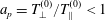 $a_{p}=T_{\bot }^{(0)}/T_{\Vert }^{(0)}<1$
. The firehose instability criterion can be rewritten in many forms, the most common being
$a_{p}=T_{\bot }^{(0)}/T_{\Vert }^{(0)}<1$
. The firehose instability criterion can be rewritten in many forms, the most common being
 $$\begin{eqnarray}1-\frac{\unicode[STIX]{x1D6FD}_{\Vert }}{2}+\frac{1}{2}\unicode[STIX]{x1D6FD}_{\Vert }a_{p}<0;\quad \frac{T_{\bot }^{(0)}}{T_{\Vert }^{(0)}}+\frac{2}{\unicode[STIX]{x1D6FD}_{\Vert }}-1<0;\quad \unicode[STIX]{x1D6FD}_{\Vert }-\unicode[STIX]{x1D6FD}_{\bot }>2;\quad p_{\Vert }^{(0)}-p_{\bot }^{(0)}>\frac{B_{0}^{2}}{4\unicode[STIX]{x03C0}}.\end{eqnarray}$$
The first expression directly implies that, if
 $\unicode[STIX]{x1D6FD}_{\Vert }\leqslant 2$
, no firehose instability can exist. The firehose instability therefore exists only for a relatively high plasma beta
$\unicode[STIX]{x1D6FD}_{\Vert }\leqslant 2$
, no firehose instability can exist. The firehose instability therefore exists only for a relatively high plasma beta
 $\unicode[STIX]{x1D6FD}_{\Vert }>2$
and only if the parallel temperature is higher than the perpendicular temperature. Importantly, the firehose instability criterion in the CGL model is equivalent to the one found from linear kinetic theory in the long-wavelength limit (for example, Rosenbluth (Reference Rosenbluth1956), Chandrasekhar, Kaufman & Watson (Reference Chandrasekhar, Kaufman and Watson1958), Parker (Reference Parker1958a
) and Vedenov & Sagdeev (Reference Vedenov and Sagdeev1958)). Alfvén wave propagation only affects components
$\unicode[STIX]{x1D6FD}_{\Vert }>2$
and only if the parallel temperature is higher than the perpendicular temperature. Importantly, the firehose instability criterion in the CGL model is equivalent to the one found from linear kinetic theory in the long-wavelength limit (for example, Rosenbluth (Reference Rosenbluth1956), Chandrasekhar, Kaufman & Watson (Reference Chandrasekhar, Kaufman and Watson1958), Parker (Reference Parker1958a
) and Vedenov & Sagdeev (Reference Vedenov and Sagdeev1958)). Alfvén wave propagation only affects components
 $u_{y}$
and
$u_{y}$
and
 $B_{y}$
which are decoupled from the rest of the system, and yields the other (eigenvector) components
$B_{y}$
which are decoupled from the rest of the system, and yields the other (eigenvector) components
 $u_{x},u_{z},B_{x},B_{z}$
as zero. The
$u_{x},u_{z},B_{x},B_{z}$
as zero. The
 $u_{y}$
component does not enter the density equation and Alfvén mode fluctuations therefore do not produce any density fluctuations or pressure fluctuations. The Alfvén mode is therefore incompressible. It is also useful to define the magnetic compressibility
$u_{y}$
component does not enter the density equation and Alfvén mode fluctuations therefore do not produce any density fluctuations or pressure fluctuations. The Alfvén mode is therefore incompressible. It is also useful to define the magnetic compressibility
 $\unicode[STIX]{x1D712}_{b}(k_{\Vert },k_{\bot })$
in Fourier space, that measures the relative ratio of magnetic energy in the parallel component versus the total magnetic energy
$\unicode[STIX]{x1D712}_{b}(k_{\Vert },k_{\bot })$
in Fourier space, that measures the relative ratio of magnetic energy in the parallel component versus the total magnetic energy
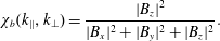 $$\begin{eqnarray}\unicode[STIX]{x1D712}_{b}(k_{\Vert },k_{\bot })=\frac{|B_{z}|^{2}}{|B_{x}|^{2}+|B_{y}|^{2}+|B_{z}|^{2}}.\end{eqnarray}$$
Since the Alfvén mode produces only
 $B_{y}$
fluctuations, with
$B_{y}$
fluctuations, with
 $B_{x}=B_{z}=0$
, the magnetic compressibility for this mode is
$B_{x}=B_{z}=0$
, the magnetic compressibility for this mode is
 $$\begin{eqnarray}\unicode[STIX]{x1D712}_{b}(k_{\Vert },k_{\bot })=0,\end{eqnarray}$$
for all the propagation directions. Sometimes the magnetic compressibility is defined as a ratio of parallel and perpendicular energies
 $|B_{z}|^{2}/(|B_{x}|^{2}+|B_{y}|^{2})$
, this quantity however has a slight disadvantage in that the values can become very large (and actually equal to infinity), which makes plotting of this quantity problematic. In contrast, the magnetic compressibility as defined in (3.83), has a nicely bounded range of values between 0 and 1. A similar quantity is defined for the ratio of the energy in velocity fluctuations
$|B_{z}|^{2}/(|B_{x}|^{2}+|B_{y}|^{2})$
, this quantity however has a slight disadvantage in that the values can become very large (and actually equal to infinity), which makes plotting of this quantity problematic. In contrast, the magnetic compressibility as defined in (3.83), has a nicely bounded range of values between 0 and 1. A similar quantity is defined for the ratio of the energy in velocity fluctuations
 $$\begin{eqnarray}\unicode[STIX]{x1D712}_{u}(k_{\Vert },k_{\bot })=\frac{|u_{z}|^{2}}{|u_{x}|^{2}+|u_{y}|^{2}+|u_{z}|^{2}},\end{eqnarray}$$
and the Alfvén mode has
 $\unicode[STIX]{x1D712}_{u}=0$
for all propagation directions, since only the perpendicular velocity component
$\unicode[STIX]{x1D712}_{u}=0$
for all propagation directions, since only the perpendicular velocity component
 $u_{y}$
is non-zero.
$u_{y}$
is non-zero.
3.5 Slow and fast modes
By applying
 $\unicode[STIX]{x2202}/\unicode[STIX]{x2202}t$
to the equations for
$\unicode[STIX]{x2202}/\unicode[STIX]{x2202}t$
to the equations for
 $\unicode[STIX]{x2202}u_{x}/\unicode[STIX]{x2202}t$
and
$\unicode[STIX]{x2202}u_{x}/\unicode[STIX]{x2202}t$
and
 $\unicode[STIX]{x2202}u_{z}/\unicode[STIX]{x2202}t$
and using the evolution equations for
$\unicode[STIX]{x2202}u_{z}/\unicode[STIX]{x2202}t$
and using the evolution equations for
 $B_{x},B_{z},p_{\Vert },p_{\bot }$
one obtains
$B_{x},B_{z},p_{\Vert },p_{\bot }$
one obtains
 $$\begin{eqnarray}\displaystyle & \displaystyle \frac{\unicode[STIX]{x2202}^{2}u_{x}}{\unicode[STIX]{x2202}t^{2}}-\frac{p_{\bot }^{(0)}}{\unicode[STIX]{x1D70C}_{0}}(2\unicode[STIX]{x2202}_{x}^{2}u_{x}+\unicode[STIX]{x2202}_{x}\unicode[STIX]{x2202}_{z}u_{z})+\left(\frac{p_{\Vert }^{(0)}}{\unicode[STIX]{x1D70C}_{0}}-\frac{p_{\bot }^{(0)}}{\unicode[STIX]{x1D70C}_{0}}-V_{A}^{2}\right)\unicode[STIX]{x2202}_{z}^{2}u_{x}-V_{A}^{2}\unicode[STIX]{x2202}_{x}^{2}u_{x}=0; & \displaystyle\end{eqnarray}$$
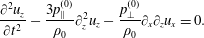 $$\begin{eqnarray}\displaystyle & \displaystyle \frac{\unicode[STIX]{x2202}^{2}u_{z}}{\unicode[STIX]{x2202}t^{2}}-\frac{3p_{\Vert }^{(0)}}{\unicode[STIX]{x1D70C}_{0}}\unicode[STIX]{x2202}_{z}^{2}u_{z}-\frac{p_{\bot }^{(0)}}{\unicode[STIX]{x1D70C}_{0}}\unicode[STIX]{x2202}_{x}\unicode[STIX]{x2202}_{z}u_{x}=0. & \displaystyle\end{eqnarray}$$
The easiest way to solve this coupled system is to transform to Fourier space, which yields
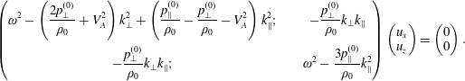 $$\begin{eqnarray}\displaystyle \left(\begin{array}{@{}cc@{}}\displaystyle \unicode[STIX]{x1D714}^{2}-\left(\frac{2p_{\bot }^{(0)}}{\unicode[STIX]{x1D70C}_{0}}+V_{A}^{2}\right)k_{\bot }^{2}+\left(\frac{p_{\Vert }^{(0)}}{\unicode[STIX]{x1D70C}_{0}}-\frac{p_{\bot }^{(0)}}{\unicode[STIX]{x1D70C}_{0}}-V_{A}^{2}\right)k_{\Vert }^{2}; & \quad \displaystyle -\frac{p_{\bot }^{(0)}}{\unicode[STIX]{x1D70C}_{0}}k_{\bot }k_{\Vert }\\ \displaystyle -\frac{p_{\bot }^{(0)}}{\unicode[STIX]{x1D70C}_{0}}k_{\bot }k_{\Vert }; & \quad \displaystyle \unicode[STIX]{x1D714}^{2}-\frac{3p_{\Vert }^{(0)}}{\unicode[STIX]{x1D70C}_{0}}k_{\Vert }^{2}\end{array}\right)\left(\begin{array}{@{}c@{}}u_{x}\\ u_{z}\end{array}\right)=\left(\begin{array}{@{}c@{}}0\\ 0\end{array}\right). & & \displaystyle \nonumber\\ \displaystyle & & \displaystyle\end{eqnarray}$$
The system has non-trivial solutions only if the determinant of the matrix is zero, yielding the CGL dispersion relation at fourth order in frequency
 $\unicode[STIX]{x1D714}$
that contains the slow and fast modes
$\unicode[STIX]{x1D714}$
that contains the slow and fast modes
 $$\begin{eqnarray}\displaystyle & & \displaystyle \unicode[STIX]{x1D714}^{4}-\unicode[STIX]{x1D714}^{2}\left[\left(\frac{2p_{\bot }^{(0)}}{\unicode[STIX]{x1D70C}_{0}}+V_{A}^{2}\right)k_{\bot }^{2}+\left(\frac{2p_{\Vert }^{(0)}}{\unicode[STIX]{x1D70C}_{0}}+\frac{p_{\bot }^{(0)}}{\unicode[STIX]{x1D70C}_{0}}+V_{A}^{2}\right)k_{\Vert }^{2}\right]\nonumber\\ \displaystyle & & \displaystyle \qquad +\,3k_{\Vert }^{2}\frac{p_{\Vert }^{(0)}}{\unicode[STIX]{x1D70C}_{0}}\left[\left(\frac{2p_{\bot }^{(0)}}{\unicode[STIX]{x1D70C}_{0}}-\frac{{p_{\bot }^{(0)}}^{2}}{3p_{\Vert }^{(0)}\unicode[STIX]{x1D70C}_{0}}+V_{A}^{2}\right)k_{\bot }^{2}-\left(\frac{p_{\Vert }^{(0)}}{\unicode[STIX]{x1D70C}_{0}}-\frac{p_{\bot }^{(0)}}{\unicode[STIX]{x1D70C}_{0}}-V_{A}^{2}\right)k_{\Vert }^{2}\right]=0.\end{eqnarray}$$
One can proceed in several ways with the above dispersion relation.
In the specific cases of strictly parallel (
 $k_{\bot }=0$
) and strictly perpendicular (
$k_{\bot }=0$
) and strictly perpendicular (
 $k_{\Vert }=0$
) propagation directions it is actually easier to work directly with the system (3.88), because the off-diagonal components in the matrix are zero and the dynamics in the
$k_{\Vert }=0$
) propagation directions it is actually easier to work directly with the system (3.88), because the off-diagonal components in the matrix are zero and the dynamics in the
 $u_{x}$
and
$u_{x}$
and
 $u_{z}$
components decouples. For strictly parallel propagation, one solution is in the
$u_{z}$
components decouples. For strictly parallel propagation, one solution is in the
 $u_{x}$
component, with the dispersion relation identical to the Alfvén wave (3.81). Since the magnetic and velocity fluctuations are only in the
$u_{x}$
component, with the dispersion relation identical to the Alfvén wave (3.81). Since the magnetic and velocity fluctuations are only in the
 $u_{x}$
,
$u_{x}$
,
 $b_{x}$
components, the compressibility
$b_{x}$
components, the compressibility
 $\unicode[STIX]{x1D712}_{b}=0$
and
$\unicode[STIX]{x1D712}_{b}=0$
and
 $\unicode[STIX]{x1D712}_{u}=0$
for this mode. The second solution for parallel propagation is in the
$\unicode[STIX]{x1D712}_{u}=0$
for this mode. The second solution for parallel propagation is in the
 $u_{z}$
component, and it is called the sound mode, or the ion-acoustic mode, with dispersion relation
$u_{z}$
component, and it is called the sound mode, or the ion-acoustic mode, with dispersion relation
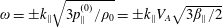 $\unicode[STIX]{x1D714}=\pm k_{\Vert }\sqrt{3p_{\Vert }^{(0)}/\unicode[STIX]{x1D70C}_{0}}=\pm k_{\Vert }V_{A}\sqrt{3\unicode[STIX]{x1D6FD}_{\Vert }/2}$
. The parallel ion-acoustic mode has
$\unicode[STIX]{x1D714}=\pm k_{\Vert }\sqrt{3p_{\Vert }^{(0)}/\unicode[STIX]{x1D70C}_{0}}=\pm k_{\Vert }V_{A}\sqrt{3\unicode[STIX]{x1D6FD}_{\Vert }/2}$
. The parallel ion-acoustic mode has
 $\unicode[STIX]{x1D712}_{u}=1$
and
$\unicode[STIX]{x1D712}_{u}=1$
and
 $\unicode[STIX]{x1D712}_{b}=0$
. Considering strictly perpendicular propagation, the waves in the
$\unicode[STIX]{x1D712}_{b}=0$
. Considering strictly perpendicular propagation, the waves in the
 $u_{z}$
component vanish with the solution
$u_{z}$
component vanish with the solution
 $\unicode[STIX]{x1D714}=0$
. The waves in the
$\unicode[STIX]{x1D714}=0$
. The waves in the
 $u_{x}$
component are fast magnetosonic waves with dispersion relation
$u_{x}$
component are fast magnetosonic waves with dispersion relation
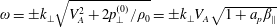 $\unicode[STIX]{x1D714}=\pm k_{\bot }\sqrt{V_{A}^{2}+2p_{\bot }^{(0)}/\unicode[STIX]{x1D70C}_{0}}=\pm k_{\bot }V_{A}\sqrt{1+a_{p}\unicode[STIX]{x1D6FD}_{\Vert }}$
, and
$\unicode[STIX]{x1D714}=\pm k_{\bot }\sqrt{V_{A}^{2}+2p_{\bot }^{(0)}/\unicode[STIX]{x1D70C}_{0}}=\pm k_{\bot }V_{A}\sqrt{1+a_{p}\unicode[STIX]{x1D6FD}_{\Vert }}$
, and
 $\unicode[STIX]{x1D712}_{u}=0$
and
$\unicode[STIX]{x1D712}_{u}=0$
and
 $\unicode[STIX]{x1D712}_{b}=1$
. It is also possible to define the parallel and perpendicular sound speeds
$\unicode[STIX]{x1D712}_{b}=1$
. It is also possible to define the parallel and perpendicular sound speeds
 $C_{\Vert }=\sqrt{3p_{\Vert }^{(0)}/\unicode[STIX]{x1D70C}_{0}}$
;
$C_{\Vert }=\sqrt{3p_{\Vert }^{(0)}/\unicode[STIX]{x1D70C}_{0}}$
;
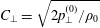 $C_{\bot }=\sqrt{2p_{\bot }^{(0)}/\unicode[STIX]{x1D70C}_{0}}$
, which yields the parallel acoustic mode dispersion
$C_{\bot }=\sqrt{2p_{\bot }^{(0)}/\unicode[STIX]{x1D70C}_{0}}$
, which yields the parallel acoustic mode dispersion
 $\unicode[STIX]{x1D714}=\pm k_{\Vert }C_{\Vert }$
and the perpendicular fast mode dispersion
$\unicode[STIX]{x1D714}=\pm k_{\Vert }C_{\Vert }$
and the perpendicular fast mode dispersion
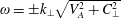 $\unicode[STIX]{x1D714}=\pm k_{\bot }\sqrt{V_{A}^{2}+C_{\bot }^{2}}$
.Footnote
4
$\unicode[STIX]{x1D714}=\pm k_{\bot }\sqrt{V_{A}^{2}+C_{\bot }^{2}}$
.Footnote
4
In the general case of oblique propagation, we choose to use the normalized frequencies and wavenumbers (3.29), and rewrite the dispersion relation as
 $$\begin{eqnarray}\displaystyle \left.\begin{array}{@{}c@{}}\displaystyle \widetilde{\unicode[STIX]{x1D714}}^{4}-A_{2}\widetilde{\unicode[STIX]{x1D714}}^{2}+A_{0}=0;\\ \displaystyle A_{2}=\widetilde{k}_{\bot }^{2}(1+a_{p}\unicode[STIX]{x1D6FD}_{\Vert })+\widetilde{k}_{\Vert }^{2}\left(1+\unicode[STIX]{x1D6FD}_{\Vert }+{\textstyle \frac{1}{2}}a_{p}\unicode[STIX]{x1D6FD}_{\Vert }\right);\\ \displaystyle A_{0}={\textstyle \frac{3}{2}}\widetilde{k}_{\Vert }^{2}\unicode[STIX]{x1D6FD}_{\Vert }\left[\widetilde{k}_{\Vert }^{2}\left(1-{\textstyle \frac{1}{2}}\unicode[STIX]{x1D6FD}_{\Vert }+{\textstyle \frac{1}{2}}a_{p}\unicode[STIX]{x1D6FD}_{\Vert }\right)+\widetilde{k}_{\bot }^{2}\left(1+a_{p}\unicode[STIX]{x1D6FD}_{\Vert }-{\textstyle \frac{1}{6}}a_{p}^{2}\unicode[STIX]{x1D6FD}_{\Vert }\right)\right].\end{array}\right\} & & \displaystyle\end{eqnarray}$$
It is sometimes useful to introduce the parallel Alfvén phase speed
 $v_{A\Vert }$
, and its normalization
$v_{A\Vert }$
, and its normalization
 $\widetilde{v}_{A\Vert }\equiv v_{A\Vert }/V_{A}$
, so that
$\widetilde{v}_{A\Vert }\equiv v_{A\Vert }/V_{A}$
, so that
 $$\begin{eqnarray}v_{A\Vert }=V_{A}\sqrt{1+\frac{\unicode[STIX]{x1D6FD}_{\Vert }}{2}(a_{p}-1)};\quad \widetilde{v}_{A\Vert }^{2}=1+\frac{\unicode[STIX]{x1D6FD}_{\Vert }}{2}(a_{p}-1),\end{eqnarray}$$
since
 $\widetilde{v}_{A\Vert }^{2}$
can be used to write the CGL dispersion relation in a shorter form, as done later in (3.193). The solution of the polynomial (3.90) is simply
$\widetilde{v}_{A\Vert }^{2}$
can be used to write the CGL dispersion relation in a shorter form, as done later in (3.193). The solution of the polynomial (3.90) is simply
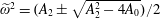 $\widetilde{\unicode[STIX]{x1D714}}^{2}=(A_{2}\pm \sqrt{A_{2}^{2}-4A_{0}})/2$
, and it is obvious that the coefficient
$\widetilde{\unicode[STIX]{x1D714}}^{2}=(A_{2}\pm \sqrt{A_{2}^{2}-4A_{0}})/2$
, and it is obvious that the coefficient
 $A_{2}$
is always positive, since both the plasma beta and the temperature anisotropy ratio must always be positive. It is also possible to show that the discriminant under the square root
$A_{2}$
is always positive, since both the plasma beta and the temperature anisotropy ratio must always be positive. It is also possible to show that the discriminant under the square root
 $A_{2}^{2}-4A_{0}\geqslant 0$
(proof shown a few lines below). The solution with the minus sign is called the slow mode and the solution with the plus sign is called the fast mode. For the slow mode,
$A_{2}^{2}-4A_{0}\geqslant 0$
(proof shown a few lines below). The solution with the minus sign is called the slow mode and the solution with the plus sign is called the fast mode. For the slow mode,
 $\widetilde{\unicode[STIX]{x1D714}}^{2}$
becomes negative (and
$\widetilde{\unicode[STIX]{x1D714}}^{2}$
becomes negative (and
 $\widetilde{\unicode[STIX]{x1D714}}$
complex) when
$\widetilde{\unicode[STIX]{x1D714}}$
complex) when
 $A_{0}<0$
, implying that the slow mode becomes unstable when
$A_{0}<0$
, implying that the slow mode becomes unstable when
 $$\begin{eqnarray}\left[k_{\Vert }^{2}\left(1-{\textstyle \frac{1}{2}}\unicode[STIX]{x1D6FD}_{\Vert }+{\textstyle \frac{1}{2}}a_{p}\unicode[STIX]{x1D6FD}_{\Vert }\right)+k_{\bot }^{2}\left(1+a_{p}\unicode[STIX]{x1D6FD}_{\Vert }-{\textstyle \frac{1}{6}}a_{p}^{2}\unicode[STIX]{x1D6FD}_{\Vert }\right)\right]<0,\end{eqnarray}$$
where we suppress the tildes on the wavenumbers since the above condition is valid for both
 $\widetilde{k}$
and
$\widetilde{k}$
and
 $k$
forms of wavenumbers. The above condition implies that there are two competing instabilities. The highly parallel propagation with
$k$
forms of wavenumbers. The above condition implies that there are two competing instabilities. The highly parallel propagation with
 $k_{\Vert }\gg k_{\bot }$
yields an instability threshold equivalent to (3.82) and the associated instability is called the parallel firehose instability. The highly oblique propagation with
$k_{\Vert }\gg k_{\bot }$
yields an instability threshold equivalent to (3.82) and the associated instability is called the parallel firehose instability. The highly oblique propagation with
 $k_{\bot }\gg k_{\Vert }$
yields the mirror instability and the threshold in the CGL description readsFootnote
5
$k_{\bot }\gg k_{\Vert }$
yields the mirror instability and the threshold in the CGL description readsFootnote
5
 $$\begin{eqnarray}1+a_{p}\unicode[STIX]{x1D6FD}_{\Vert }-\frac{1}{6}a_{p}^{2}\unicode[STIX]{x1D6FD}_{\Vert }<0;\quad \frac{1}{6}\frac{T_{\bot }^{(0)}}{T_{\Vert }^{(0)}}-1-\frac{1}{\unicode[STIX]{x1D6FD}_{\bot }}>0;\quad \frac{1}{6}\frac{\unicode[STIX]{x1D6FD}_{\bot }^{2}}{\unicode[STIX]{x1D6FD}_{\Vert }}>1+\unicode[STIX]{x1D6FD}_{\bot }.\end{eqnarray}$$
It is well documented that the mirror instability threshold in the CGL description is not equivalent to the one found in linear kinetic theory. In particular, the CGL mirror threshold contains a factor of 6 error (Abraham-Shrauner Reference Abraham-Shrauner1967; Tajiri Reference Tajiri1967; Kulsrud Reference Kulsrud, Galeev and Sudan1983; Ferrière & André Reference Ferrière and André2002), since the correct threshold obtained from kinetic theory reads
 $$\begin{eqnarray}1+a_{p}\unicode[STIX]{x1D6FD}_{\Vert }-a_{p}^{2}\unicode[STIX]{x1D6FD}_{\Vert }<0;\quad \frac{T_{\bot }^{(0)}}{T_{\Vert }^{(0)}}-1-\frac{1}{\unicode[STIX]{x1D6FD}_{\bot }}>0;\quad \frac{\unicode[STIX]{x1D6FD}_{\bot }^{2}}{\unicode[STIX]{x1D6FD}_{\Vert }}>1+\unicode[STIX]{x1D6FD}_{\bot }.\end{eqnarray}$$
The threshold (3.93) implies that the necessary condition for the mirror instability to exist in the CGL description is
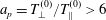 $a_{p}=T_{\bot }^{(0)}/T_{\Vert }^{(0)}>6$
, whereas in kinetic theory the necessary condition is
$a_{p}=T_{\bot }^{(0)}/T_{\Vert }^{(0)}>6$
, whereas in kinetic theory the necessary condition is
 $a_{p}>1$
. A very good discussion about the physical mechanism of the mirror instability and the role of resonant particles can be found in Southwood & Kivelson (Reference Southwood and Kivelson1993) and Kivelson & Southwood (Reference Kivelson and Southwood1996). The correct mirror instability threshold is obtained when using the normal closure discussed later on in the text or, more simply, its quasi-static limit (Constantinescu Reference Constantinescu2002; Chust & Belmont Reference Chust and Belmont2006; Passot et al.
Reference Passot, Ruban and Sulem2006). In the opposite case where ions are cold, a similar electron temperature anisotropy instability is obtained which is called the field-swelling instability, see e.g. Basu & Coppi (Reference Basu and Coppi1984).
$a_{p}>1$
. A very good discussion about the physical mechanism of the mirror instability and the role of resonant particles can be found in Southwood & Kivelson (Reference Southwood and Kivelson1993) and Kivelson & Southwood (Reference Kivelson and Southwood1996). The correct mirror instability threshold is obtained when using the normal closure discussed later on in the text or, more simply, its quasi-static limit (Constantinescu Reference Constantinescu2002; Chust & Belmont Reference Chust and Belmont2006; Passot et al.
Reference Passot, Ruban and Sulem2006). In the opposite case where ions are cold, a similar electron temperature anisotropy instability is obtained which is called the field-swelling instability, see e.g. Basu & Coppi (Reference Basu and Coppi1984).
Returning to the oblique dispersion relation, we show that indeed
 $A_{2}^{2}-4A_{0}\geqslant 0$
. By using (3.78) the wavenumber
$A_{2}^{2}-4A_{0}\geqslant 0$
. By using (3.78) the wavenumber
 $k$
can be pulled out of the
$k$
can be pulled out of the
 $A_{0},A_{2}$
coefficients and the dispersion relation can be rewritten in terms of a phase speed as
$A_{0},A_{2}$
coefficients and the dispersion relation can be rewritten in terms of a phase speed as
 $$\begin{eqnarray}\displaystyle & \displaystyle (\widetilde{\unicode[STIX]{x1D714}}/\widetilde{k})^{4}-A_{2}(\widetilde{\unicode[STIX]{x1D714}}/\widetilde{k})^{2}+A_{0}=0; & \displaystyle\end{eqnarray}$$
 $$\begin{eqnarray}\displaystyle & \displaystyle A_{2}=1+a_{p}\unicode[STIX]{x1D6FD}_{\Vert }\left(1-{\textstyle \frac{1}{2}}\cos ^{2}\unicode[STIX]{x1D703}\right)+\unicode[STIX]{x1D6FD}_{\Vert }\cos ^{2}\unicode[STIX]{x1D703}; & \displaystyle\end{eqnarray}$$
 $$\begin{eqnarray}\displaystyle & \displaystyle A_{0}={\textstyle \frac{3}{2}}\unicode[STIX]{x1D6FD}_{\Vert }\cos ^{2}\unicode[STIX]{x1D703}\left[1+a_{p}\unicode[STIX]{x1D6FD}_{\Vert }\left(1-{\textstyle \frac{1}{2}}\cos ^{2}\unicode[STIX]{x1D703}\right)-{\textstyle \frac{1}{2}}\unicode[STIX]{x1D6FD}_{\Vert }\cos ^{2}\unicode[STIX]{x1D703}-{\textstyle \frac{1}{6}}a_{p}^{2}\unicode[STIX]{x1D6FD}_{\Vert }\sin ^{2}\unicode[STIX]{x1D703}\right], & \displaystyle\end{eqnarray}$$
and (after staring for a sufficiently long time) it can be shown that
 $$\begin{eqnarray}A_{2}^{2}-4A_{0}=\left[1+a_{p}\unicode[STIX]{x1D6FD}_{\Vert }\left(1-{\textstyle \frac{1}{2}}\cos ^{2}\unicode[STIX]{x1D703}\right)-2\unicode[STIX]{x1D6FD}_{\Vert }\cos ^{2}\unicode[STIX]{x1D703}\right]^{2}+a_{p}^{2}\unicode[STIX]{x1D6FD}_{\Vert }^{2}\sin ^{2}\unicode[STIX]{x1D703}\cos ^{2}\unicode[STIX]{x1D703},\end{eqnarray}$$
which is obviously always non-negative. The dispersion relation for the slow and fast waves in the CGL description can be written in the compact form
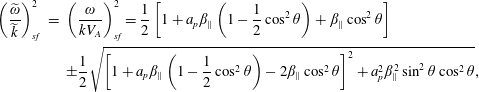 $$\begin{eqnarray}\displaystyle \left(\frac{\widetilde{\unicode[STIX]{x1D714}}}{\widetilde{k}}\right)_{sf}^{2} & = & \displaystyle \left(\frac{\unicode[STIX]{x1D714}}{kV_{A}}\right)_{sf}^{2}=\frac{1}{2}\left[1+a_{p}\unicode[STIX]{x1D6FD}_{\Vert }\left(1-\frac{1}{2}\cos ^{2}\unicode[STIX]{x1D703}\right)+\unicode[STIX]{x1D6FD}_{\Vert }\cos ^{2}\unicode[STIX]{x1D703}\right]\nonumber\\ \displaystyle & & \displaystyle \pm \frac{1}{2}\sqrt{\left[1+a_{p}\unicode[STIX]{x1D6FD}_{\Vert }\left(1-\frac{1}{2}\cos ^{2}\unicode[STIX]{x1D703}\right)-2\unicode[STIX]{x1D6FD}_{\Vert }\cos ^{2}\unicode[STIX]{x1D703}\right]^{2}+a_{p}^{2}\unicode[STIX]{x1D6FD}_{\Vert }^{2}\sin ^{2}\unicode[STIX]{x1D703}\cos ^{2}\unicode[STIX]{x1D703}},\nonumber\\ \displaystyle & & \displaystyle\end{eqnarray}$$
which is equivalent to the dispersion relation of Abraham-Shrauner (Reference Abraham-Shrauner1967), equation (30), here written in the convenient units of
 $\unicode[STIX]{x1D6FD}_{\Vert }$
and
$\unicode[STIX]{x1D6FD}_{\Vert }$
and
 $a_{p}=T_{\bot }^{(0)}/T_{\Vert }^{(0)}$
(for a direct comparison with the units used in that paper, the relations are
$a_{p}=T_{\bot }^{(0)}/T_{\Vert }^{(0)}$
(for a direct comparison with the units used in that paper, the relations are
 $\unicode[STIX]{x1D6FD}_{\Vert }=2S_{\Vert }$
and
$\unicode[STIX]{x1D6FD}_{\Vert }=2S_{\Vert }$
and
 $a_{p}\unicode[STIX]{x1D6FD}_{\Vert }=2S_{\bot }$
). The magnetic compressibility of the slow and fast modes can be calculated easily directly from the induction equations (3.72). The slow and fast modes generate only components
$a_{p}\unicode[STIX]{x1D6FD}_{\Vert }=2S_{\bot }$
). The magnetic compressibility of the slow and fast modes can be calculated easily directly from the induction equations (3.72). The slow and fast modes generate only components
 $B_{x}$
and
$B_{x}$
and
 $B_{z}$
with the component
$B_{z}$
with the component
 $B_{y}=0$
. The transformation of (3.72) to Fourier space yields
$B_{y}=0$
. The transformation of (3.72) to Fourier space yields
 $-\unicode[STIX]{x1D714}B_{x}=B_{0}k_{\Vert }u_{x}$
, and
$-\unicode[STIX]{x1D714}B_{x}=B_{0}k_{\Vert }u_{x}$
, and
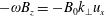 $-\unicode[STIX]{x1D714}B_{z}=-B_{0}k_{\bot }u_{x}$
, and by applying the magnitude operator yields the magnetic compressibility
$-\unicode[STIX]{x1D714}B_{z}=-B_{0}k_{\bot }u_{x}$
, and by applying the magnitude operator yields the magnetic compressibility
 $$\begin{eqnarray}\unicode[STIX]{x1D712}_{b}(k_{\Vert },k_{\bot })=\frac{k_{\bot }^{2}}{k_{\Vert }^{2}+k_{\bot }^{2}}=\sin ^{2}\unicode[STIX]{x1D703}.\end{eqnarray}$$
For quasi-parallel propagation angles the magnetic compressibility
 $\unicode[STIX]{x1D712}_{b}$
is therefore not a good indicator for mode recognition, since all three modes have
$\unicode[STIX]{x1D712}_{b}$
is therefore not a good indicator for mode recognition, since all three modes have
 $\unicode[STIX]{x1D712}_{b}$
close to zero. The magnetic compressibility is, however, an excellent tool for oblique propagation angles, because the Alfvén mode has
$\unicode[STIX]{x1D712}_{b}$
close to zero. The magnetic compressibility is, however, an excellent tool for oblique propagation angles, because the Alfvén mode has
 $\unicode[STIX]{x1D712}_{b}=0$
regardless of the propagation direction, whereas for the slow and fast modes
$\unicode[STIX]{x1D712}_{b}=0$
regardless of the propagation direction, whereas for the slow and fast modes
 $\unicode[STIX]{x1D712}_{b}$
increases with
$\unicode[STIX]{x1D712}_{b}$
increases with
 $\unicode[STIX]{x1D703}$
towards
$\unicode[STIX]{x1D703}$
towards
 $\unicode[STIX]{x1D712}_{b}=1$
. We will leave discussion about the CGL velocity eigenvector (the ratio
$\unicode[STIX]{x1D712}_{b}=1$
. We will leave discussion about the CGL velocity eigenvector (the ratio
 $\unicode[STIX]{x1D712}_{u}$
) to a later subsection since the discussion is a bit technical, and we instead focus now on an interesting effect that can be directly obtained by considering the CGL dispersion relations.
$\unicode[STIX]{x1D712}_{u}$
) to a later subsection since the discussion is a bit technical, and we instead focus now on an interesting effect that can be directly obtained by considering the CGL dispersion relations.
Analytic ‘hard’ thresholds of the mirror instability (blue) and the firehose instability (red) at long wavelengths. Solid lines are solutions of the linear kinetic theory (bi-Maxwellian) and crosses are solutions of the linear CGL model. The firehose instability is described correctly (both the oblique firehose and the parallel firehose), whereas the mirror instability contains an asymptotic factor of 6 error for large
 $\unicode[STIX]{x1D6FD}_{\Vert }$
values. The black dashed line is the CGL threshold (3.103), where for all oblique directions the slow mode speed
$\unicode[STIX]{x1D6FD}_{\Vert }$
values. The black dashed line is the CGL threshold (3.103), where for all oblique directions the slow mode speed
 $v_{s}$
matches the Alfvén mode speed
$v_{s}$
matches the Alfvén mode speed
 $v_{A}$
, and which separates two regions where
$v_{A}$
, and which separates two regions where
 $v_{s}<v_{A}$
and
$v_{s}<v_{A}$
and
 $v_{s}>v_{A}$
. The green dotted curve is a special case for parallel propagation (3.108) where
$v_{s}>v_{A}$
. The green dotted curve is a special case for parallel propagation (3.108) where
 $v_{s\Vert }=v_{A\Vert }$
. For parallel propagation, the slow mode speed cannot exceed the Alfvén mode speed, but can only match it, and the green dotted curve separates two regions where
$v_{s\Vert }=v_{A\Vert }$
. For parallel propagation, the slow mode speed cannot exceed the Alfvén mode speed, but can only match it, and the green dotted curve separates two regions where
 $v_{s\Vert }<v_{A\Vert }$
and
$v_{s\Vert }<v_{A\Vert }$
and
 $v_{s\Vert }=v_{A\Vert }$
. For a similar plot in linear scale, see figure 1 of Abraham-Shrauner (Reference Abraham-Shrauner1967).
$v_{s\Vert }=v_{A\Vert }$
. For a similar plot in linear scale, see figure 1 of Abraham-Shrauner (Reference Abraham-Shrauner1967).
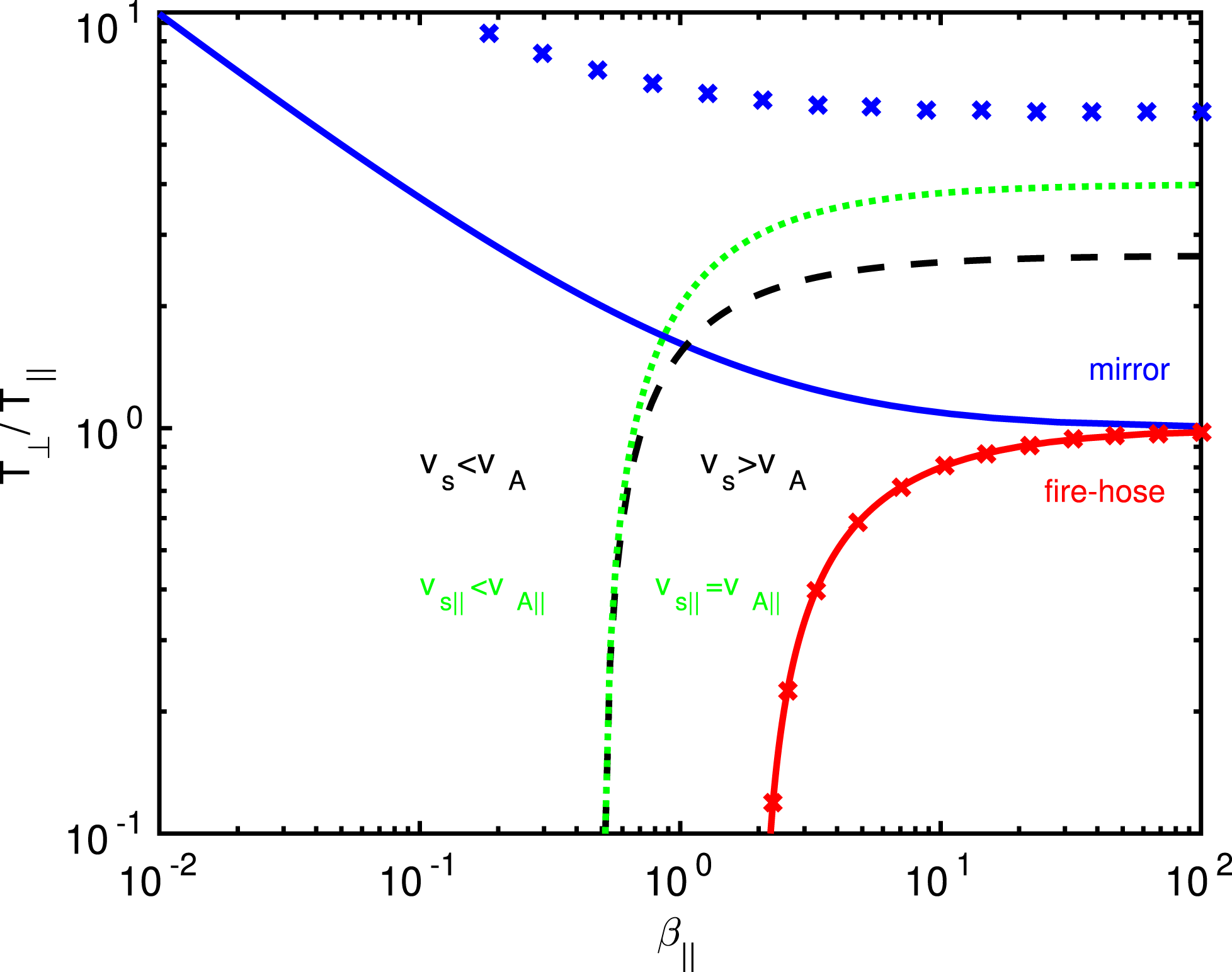
3.6 Slow mode can become faster than Alfvén mode
There is a very interesting phenomenon present in the CGL description that is also observed in the kinetic description but that is absent in the MHD description. For a sufficiently high plasma beta, the slow mode phase speed can be larger than the Alfvén mode phase speed. To obtain the critical plasma beta when this happens, one can write the dispersion relation for the Alfvén wave as
 $(\widetilde{\unicode[STIX]{x1D714}}/\widetilde{k})_{A}^{2}=(1-\unicode[STIX]{x1D6FD}_{\Vert }/2+a_{p}\unicode[STIX]{x1D6FD}_{\Vert }/2)\cos ^{2}\unicode[STIX]{x1D703}\equiv A_{A}$
and using this expression with the dispersion relation (3.95), the critical condition when the slow mode speed matches the Alfvén speed is
$(\widetilde{\unicode[STIX]{x1D714}}/\widetilde{k})_{A}^{2}=(1-\unicode[STIX]{x1D6FD}_{\Vert }/2+a_{p}\unicode[STIX]{x1D6FD}_{\Vert }/2)\cos ^{2}\unicode[STIX]{x1D703}\equiv A_{A}$
and using this expression with the dispersion relation (3.95), the critical condition when the slow mode speed matches the Alfvén speed is
 $(A_{2}-\sqrt{A_{2}^{2}-4A_{0}})/2=A_{A}$
, and since
$(A_{2}-\sqrt{A_{2}^{2}-4A_{0}})/2=A_{A}$
, and since
 $A_{2}^{2}-4A_{0}\geqslant 0$
, this further yields
$A_{2}^{2}-4A_{0}\geqslant 0$
, this further yields
 $A_{A}^{2}-A_{2}A_{A}+A_{0}=0$
. It takes quite a few algebraic operations to simplify the result, the easiest way is to collect terms with different powers of
$A_{A}^{2}-A_{2}A_{A}+A_{0}=0$
. It takes quite a few algebraic operations to simplify the result, the easiest way is to collect terms with different powers of
 $\unicode[STIX]{x1D6FD}_{\Vert }$
and then simplify. A very valuable approach available now is to use mathematical software such as Maple or Mathematica for guidance, and for example the Maple command simplify(expr,trig) immediately simplifies the result, which can then be of course verified with pencil and paper. The result is
$\unicode[STIX]{x1D6FD}_{\Vert }$
and then simplify. A very valuable approach available now is to use mathematical software such as Maple or Mathematica for guidance, and for example the Maple command simplify(expr,trig) immediately simplifies the result, which can then be of course verified with pencil and paper. The result is
 $$\begin{eqnarray}\displaystyle A_{A}^{2}-A_{2}A_{A}+A_{0}=-\sin ^{2}\,\unicode[STIX]{x1D703}\cos ^{2}\unicode[STIX]{x1D703}\left[1+\unicode[STIX]{x1D6FD}_{\Vert }\left({\textstyle \frac{3}{2}}a_{p}-2\right)+\unicode[STIX]{x1D6FD}_{\Vert }^{2}a_{p}\left({\textstyle \frac{3}{4}}a_{p}-2\right)\right]=0. & & \displaystyle\end{eqnarray}$$
The expression is naturally satisfied for cases of strictly parallel and strictly perpendicular propagation. For
 $\unicode[STIX]{x1D703}=\unicode[STIX]{x03C0}/2$
, both the slow mode and the Alfvén mode have zero frequency. For
$\unicode[STIX]{x1D703}=\unicode[STIX]{x03C0}/2$
, both the slow mode and the Alfvén mode have zero frequency. For
 $\unicode[STIX]{x1D703}=0$
, the slow mode speed can be only smaller or equal to the speed of the Alfvén mode (never higher), depending on another condition that will be easier to clarify later when specifically considering the parallel propagation limit. Now, on which side of the threshold (3.101) does the speed of the slow mode become faster than the speed of the Alfvén mode? Working with inequalities is a bit trickier. By assuming that both modes have real frequencies (and are not firehose or mirror unstable), the condition is derived to be
$\unicode[STIX]{x1D703}=0$
, the slow mode speed can be only smaller or equal to the speed of the Alfvén mode (never higher), depending on another condition that will be easier to clarify later when specifically considering the parallel propagation limit. Now, on which side of the threshold (3.101) does the speed of the slow mode become faster than the speed of the Alfvén mode? Working with inequalities is a bit trickier. By assuming that both modes have real frequencies (and are not firehose or mirror unstable), the condition is derived to be
 $$\begin{eqnarray}\displaystyle -\sin ^{2}\unicode[STIX]{x1D703}\cos ^{2}\unicode[STIX]{x1D703}\left[1+\unicode[STIX]{x1D6FD}_{\Vert }\left({\textstyle \frac{3}{2}}a_{p}-2\right)+\unicode[STIX]{x1D6FD}_{\Vert }^{2}a_{p}\left({\textstyle \frac{3}{4}}a_{p}-2\right)\right]\geqslant 0, & & \displaystyle\end{eqnarray}$$
which agrees with the result obtained by Abraham-Shrauner (Reference Abraham-Shrauner1967), equation (42). The expression (3.102) reveals that there is a condition that can be satisfied for all directions of propagation and that reads
 $$\begin{eqnarray}\displaystyle 1+\unicode[STIX]{x1D6FD}_{\Vert }\left({\textstyle \frac{3}{2}}a_{p}-2\right)+\unicode[STIX]{x1D6FD}_{\Vert }^{2}a_{p}\left({\textstyle \frac{3}{4}}a_{p}-2\right)\leqslant 0. & & \displaystyle\end{eqnarray}$$
This is a quadratic equation in
 $\unicode[STIX]{x1D6FD}_{\Vert }$
which can be solved easily for a given
$\unicode[STIX]{x1D6FD}_{\Vert }$
which can be solved easily for a given
 $a_{p}$
(or solved for
$a_{p}$
(or solved for
 $a_{p}$
for a given
$a_{p}$
for a given
 $\unicode[STIX]{x1D6FD}_{\Vert }$
). To visualize this equation, the threshold is plotted in figure 1 as a black dashed line. A particularly useful result is obtained for isotropic temperatures (
$\unicode[STIX]{x1D6FD}_{\Vert }$
). To visualize this equation, the threshold is plotted in figure 1 as a black dashed line. A particularly useful result is obtained for isotropic temperatures (
 $a_{p}=1$
). In this case the inequality (3.103) becomes
$a_{p}=1$
). In this case the inequality (3.103) becomes
 $1-\unicode[STIX]{x1D6FD}_{\Vert }/2-\unicode[STIX]{x1D6FD}_{\Vert }^{2}5/4\leqslant 0$
and the critical plasma beta at which the slow mode speed becomes larger than the Alfvén mode speed is
$1-\unicode[STIX]{x1D6FD}_{\Vert }/2-\unicode[STIX]{x1D6FD}_{\Vert }^{2}5/4\leqslant 0$
and the critical plasma beta at which the slow mode speed becomes larger than the Alfvén mode speed is
 $$\begin{eqnarray}\unicode[STIX]{x1D6FD}_{\Vert }^{\text{crit}}\geqslant \frac{\sqrt{21}-1}{5}\approx 0.72.\end{eqnarray}$$
Thus, this effect exists in the CGL description even when the temperatures are isotropic.
3.7 CGL parallel propagation
When numerically solving the CGL dispersion relations for finite (non-zero) propagation angles, the slow and fast mode expressions always get the correct ordering with
 $\unicode[STIX]{x1D714}_{s}\leqslant \unicode[STIX]{x1D714}_{f}$
. It is sometimes confusing about how the dispersion relations hold in the limit of parallel propagation
$\unicode[STIX]{x1D714}_{s}\leqslant \unicode[STIX]{x1D714}_{f}$
. It is sometimes confusing about how the dispersion relations hold in the limit of parallel propagation
 $\unicode[STIX]{x1D703}\rightarrow 0$
which we will address here. In this limit, the dispersion relations (3.99) for the slow and fast modes can be directly evaluated as
$\unicode[STIX]{x1D703}\rightarrow 0$
which we will address here. In this limit, the dispersion relations (3.99) for the slow and fast modes can be directly evaluated as
 $$\begin{eqnarray}\displaystyle \left(\frac{\widetilde{\unicode[STIX]{x1D714}}}{\widetilde{k}}\right)_{sf}^{2}=\frac{1}{2}\left[1+\frac{1}{2}a_{p}\unicode[STIX]{x1D6FD}_{\Vert }+\unicode[STIX]{x1D6FD}_{\Vert }\right]\pm \frac{1}{2}\sqrt{\left[1+\frac{1}{2}a_{p}\unicode[STIX]{x1D6FD}_{\Vert }-2\unicode[STIX]{x1D6FD}_{\Vert }\right]^{2}}. & & \displaystyle\end{eqnarray}$$
Now, because
 $\sqrt{a^{2}}=|a|$
, for further calculation one needs to determine the sign of the expression under the square root. For
$\sqrt{a^{2}}=|a|$
, for further calculation one needs to determine the sign of the expression under the square root. For
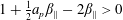 $1+\frac{1}{2}a_{p}\unicode[STIX]{x1D6FD}_{\Vert }-2\unicode[STIX]{x1D6FD}_{\Vert }>0$
, i.e. when
$1+\frac{1}{2}a_{p}\unicode[STIX]{x1D6FD}_{\Vert }-2\unicode[STIX]{x1D6FD}_{\Vert }>0$
, i.e. when
 $\unicode[STIX]{x1D6FD}_{\Vert }<2/(4-a_{p})$
, the above equations yield
$\unicode[STIX]{x1D6FD}_{\Vert }<2/(4-a_{p})$
, the above equations yield
 $$\begin{eqnarray}\displaystyle (\widetilde{\unicode[STIX]{x1D714}}/\widetilde{k})_{s}^{2}=\frac{3}{2}\unicode[STIX]{x1D6FD}_{\Vert };\quad (\widetilde{\unicode[STIX]{x1D714}}/\widetilde{k})_{f}^{2}=1+\frac{\unicode[STIX]{x1D6FD}_{\Vert }}{2}(a_{p}-1)=(\widetilde{\unicode[STIX]{x1D714}}/\widetilde{k})_{A}^{2}, & & \displaystyle\end{eqnarray}$$
so the slow mode is the sound/acoustic mode and the fast mode coincides with the Alfvén mode. However, for
 $1+\frac{1}{2}a_{p}\unicode[STIX]{x1D6FD}_{\Vert }-2\unicode[STIX]{x1D6FD}_{\Vert }<0$
, i.e. when
$1+\frac{1}{2}a_{p}\unicode[STIX]{x1D6FD}_{\Vert }-2\unicode[STIX]{x1D6FD}_{\Vert }<0$
, i.e. when
 $\unicode[STIX]{x1D6FD}_{\Vert }>2/(4-a_{p})$
, the dispersion relations yield
$\unicode[STIX]{x1D6FD}_{\Vert }>2/(4-a_{p})$
, the dispersion relations yield
 $$\begin{eqnarray}\displaystyle (\widetilde{\unicode[STIX]{x1D714}}/\widetilde{k})_{s}^{2}=1+\frac{\unicode[STIX]{x1D6FD}_{\Vert }}{2}(a_{p}-1)=(\widetilde{\unicode[STIX]{x1D714}}/\widetilde{k})_{A}^{2};\quad (\widetilde{\unicode[STIX]{x1D714}}/\widetilde{k})_{f}^{2}=\frac{3}{2}\unicode[STIX]{x1D6FD}_{\Vert }, & & \displaystyle\end{eqnarray}$$
so the slow mode coincides with the Alfvén mode and the fast mode is the sound/acoustic mode. In this region, the slow mode phase speed will always stay equal to the Alfvén mode phase speed, regardless of further increases of
 $\unicode[STIX]{x1D6FD}_{\Vert }$
. In the special case when
$\unicode[STIX]{x1D6FD}_{\Vert }$
. In the special case when
 $1+\frac{1}{2}a_{p}\unicode[STIX]{x1D6FD}_{\Vert }-2\unicode[STIX]{x1D6FD}_{\Vert }=0$
, which is equivalent to
$1+\frac{1}{2}a_{p}\unicode[STIX]{x1D6FD}_{\Vert }-2\unicode[STIX]{x1D6FD}_{\Vert }=0$
, which is equivalent to
 $$\begin{eqnarray}\unicode[STIX]{x1D6FD}_{\Vert }=\frac{2}{4-a_{p}};\quad a_{p}=4-\frac{2}{\unicode[STIX]{x1D6FD}_{\Vert }},\end{eqnarray}$$
all three modes propagate with the same phase speed
 $(\widetilde{\unicode[STIX]{x1D714}}/\widetilde{k})_{Asf}^{2}=\frac{3}{2}\unicode[STIX]{x1D6FD}_{\Vert }$
. The criterion (3.108) can be satisfied only for
$(\widetilde{\unicode[STIX]{x1D714}}/\widetilde{k})_{Asf}^{2}=\frac{3}{2}\unicode[STIX]{x1D6FD}_{\Vert }$
. The criterion (3.108) can be satisfied only for
 $\unicode[STIX]{x1D6FD}_{\Vert }\geqslant 1/2$
and in the limit
$\unicode[STIX]{x1D6FD}_{\Vert }\geqslant 1/2$
and in the limit
 $\unicode[STIX]{x1D6FD}_{\Vert }\rightarrow \infty$
the asymptote is
$\unicode[STIX]{x1D6FD}_{\Vert }\rightarrow \infty$
the asymptote is
 $a_{p}=4$
, so the possible range of
$a_{p}=4$
, so the possible range of
 $a_{p}$
is
$a_{p}$
is
 $[0,4]$
. This curve is plotted in figure 1 as a green dotted line. The curve separates two regions. In the first region
$[0,4]$
. This curve is plotted in figure 1 as a green dotted line. The curve separates two regions. In the first region
 $\unicode[STIX]{x1D6FD}_{\Vert }<2/(4-a_{p})$
and
$\unicode[STIX]{x1D6FD}_{\Vert }<2/(4-a_{p})$
and
 $v_{s\Vert }<v_{A\Vert }$
. In the second region
$v_{s\Vert }<v_{A\Vert }$
. In the second region
 $\unicode[STIX]{x1D6FD}_{\Vert }>2/(4-a_{p})$
and
$\unicode[STIX]{x1D6FD}_{\Vert }>2/(4-a_{p})$
and
 $v_{s\Vert }=v_{A\Vert }$
. The interesting result to remember is that, for isotropic temperatures (
$v_{s\Vert }=v_{A\Vert }$
. The interesting result to remember is that, for isotropic temperatures (
 $a_{p}=1$
) and parallel propagation, the critical plasma beta at which the slow mode speed matches the Alfvén mode speed is
$a_{p}=1$
) and parallel propagation, the critical plasma beta at which the slow mode speed matches the Alfvén mode speed is
 $$\begin{eqnarray}\unicode[STIX]{x1D6FD}_{\Vert }^{\text{crit}}(0)\geqslant {\textstyle \frac{2}{3}}.\end{eqnarray}$$
3.8 CGL with
 $T_{\bot }=T_{\Vert }$
is not equivalent to MHD
$T_{\bot }=T_{\Vert }$
is not equivalent to MHD

It is important to emphasize that, even for isotropic temperatures
 $a_{p}=1$
, the CGL dispersion (3.99) is not equivalent to the MHD dispersion for the slow and fast waves. The MHD dispersion is usually written in the form (see (C 20) in appendix C)
$a_{p}=1$
, the CGL dispersion (3.99) is not equivalent to the MHD dispersion for the slow and fast waves. The MHD dispersion is usually written in the form (see (C 20) in appendix C)
 $$\begin{eqnarray}\displaystyle \left(\frac{\unicode[STIX]{x1D714}}{k}\right)^{2}=\frac{1}{2}(V_{A}^{2}+C_{s}^{2})\pm \frac{1}{2}\sqrt{(V_{A}^{2}+C_{s}^{2})^{2}-4V_{A}^{2}C_{s}^{2}\cos ^{2}\unicode[STIX]{x1D703}}, & & \displaystyle\end{eqnarray}$$
or alternatively
 $$\begin{eqnarray}\displaystyle \left(\frac{\unicode[STIX]{x1D714}}{k}\right)^{2}=\frac{1}{2}(V_{A}^{2}+C_{s}^{2})\pm \frac{1}{2}\sqrt{(V_{A}^{2}-C_{s}^{2})^{2}+4V_{A}^{2}C_{s}^{2}\sin ^{2}\unicode[STIX]{x1D703}}, & & \displaystyle\end{eqnarray}$$
which nicely shows that the expression under the square root is always greater or equal to zero. The MHD sound speed is defined as
 $C_{s}^{2}=\unicode[STIX]{x1D6FE}p^{(0)}/\unicode[STIX]{x1D70C}_{0}$
, where
$C_{s}^{2}=\unicode[STIX]{x1D6FE}p^{(0)}/\unicode[STIX]{x1D70C}_{0}$
, where
 $\unicode[STIX]{x1D6FE}=5/3$
. Rewritten with the parameters we use here
$\unicode[STIX]{x1D6FE}=5/3$
. Rewritten with the parameters we use here
 $C_{s}^{2}/V_{A}^{2}=\unicode[STIX]{x1D6FE}\unicode[STIX]{x1D6FD}_{\Vert }/2=5\unicode[STIX]{x1D6FD}_{\Vert }/6$
, the MHD dispersion for the slow and fast waves reads
$C_{s}^{2}/V_{A}^{2}=\unicode[STIX]{x1D6FE}\unicode[STIX]{x1D6FD}_{\Vert }/2=5\unicode[STIX]{x1D6FD}_{\Vert }/6$
, the MHD dispersion for the slow and fast waves reads
 $$\begin{eqnarray}\displaystyle \left(\frac{\unicode[STIX]{x1D714}}{kV_{A}}\right)_{\text{MHD}}^{2}=\frac{1}{2}\left(1+\frac{\unicode[STIX]{x1D6FE}}{2}\unicode[STIX]{x1D6FD}_{\Vert }\right)\pm \frac{1}{2}\sqrt{\left(1+\frac{\unicode[STIX]{x1D6FE}}{2}\unicode[STIX]{x1D6FD}_{\Vert }\right)^{2}-2\unicode[STIX]{x1D6FE}\unicode[STIX]{x1D6FD}_{\Vert }\cos ^{2}\unicode[STIX]{x1D703}}, & & \displaystyle\end{eqnarray}$$
or alternatively
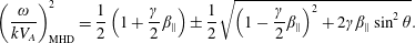 $$\begin{eqnarray}\displaystyle \left(\frac{\unicode[STIX]{x1D714}}{kV_{A}}\right)_{\text{MHD}}^{2}=\frac{1}{2}\left(1+\frac{\unicode[STIX]{x1D6FE}}{2}\unicode[STIX]{x1D6FD}_{\Vert }\right)\pm \frac{1}{2}\sqrt{\left(1-\frac{\unicode[STIX]{x1D6FE}}{2}\unicode[STIX]{x1D6FD}_{\Vert }\right)^{2}+2\unicode[STIX]{x1D6FE}\unicode[STIX]{x1D6FD}_{\Vert }\sin ^{2}\unicode[STIX]{x1D703}}. & & \displaystyle\end{eqnarray}$$
In the CGL description with isotropic temperatures
 $(a_{p}=1)$
the dispersion relation (3.99) for slow and fast waves reads
$(a_{p}=1)$
the dispersion relation (3.99) for slow and fast waves reads
 $$\begin{eqnarray}\displaystyle \left(\frac{\unicode[STIX]{x1D714}}{kV_{A}}\right)_{\text{CGL}}^{2} & = & \displaystyle \frac{1}{2}\left[1+\unicode[STIX]{x1D6FD}_{\Vert }\left(1+\frac{1}{2}\cos ^{2}\unicode[STIX]{x1D703}\right)\right]\nonumber\\ \displaystyle & & \displaystyle \pm \,\frac{1}{2}\sqrt{\left[1+\unicode[STIX]{x1D6FD}_{\Vert }\left(1-\frac{5}{2}\cos ^{2}\unicode[STIX]{x1D703}\right)\right]^{2}+\unicode[STIX]{x1D6FD}_{\Vert }^{2}\sin ^{2}\unicode[STIX]{x1D703}\cos ^{2}\unicode[STIX]{x1D703}},\end{eqnarray}$$
or alternatively
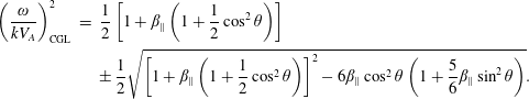 $$\begin{eqnarray}\displaystyle \left(\frac{\unicode[STIX]{x1D714}}{kV_{A}}\right)_{\text{CGL}}^{2} & = & \displaystyle \frac{1}{2}\left[1+\unicode[STIX]{x1D6FD}_{\Vert }\left(1+\frac{1}{2}\cos ^{2}\unicode[STIX]{x1D703}\right)\right]\nonumber\\ \displaystyle & & \displaystyle \pm \,\frac{1}{2}\sqrt{\left[1+\unicode[STIX]{x1D6FD}_{\Vert }\left(1+\frac{1}{2}\cos ^{2}\unicode[STIX]{x1D703}\right)\right]^{2}-6\unicode[STIX]{x1D6FD}_{\Vert }\cos ^{2}\unicode[STIX]{x1D703}\left(1+\frac{5}{6}\unicode[STIX]{x1D6FD}_{\Vert }\sin ^{2}\unicode[STIX]{x1D703}\right)}.\nonumber\\ \displaystyle & & \displaystyle\end{eqnarray}$$
We wrote down all major possibilities on purpose, since we wanted to clearly show that, regardless of the choice of
 $\unicode[STIX]{x1D6FD}_{\Vert }$
and
$\unicode[STIX]{x1D6FD}_{\Vert }$
and
 $\unicode[STIX]{x1D6FE}$
, the MHD dispersion relation cannot match the CGL dispersion relation simultaneously for all propagation directions
$\unicode[STIX]{x1D6FE}$
, the MHD dispersion relation cannot match the CGL dispersion relation simultaneously for all propagation directions
 $\unicode[STIX]{x1D703}$
. One could even play with an abstract idea to make the MHD
$\unicode[STIX]{x1D703}$
. One could even play with an abstract idea to make the MHD
 $\unicode[STIX]{x1D6FE}$
dependent on the angle
$\unicode[STIX]{x1D6FE}$
dependent on the angle
 $\unicode[STIX]{x1D703}$
, and possibly
$\unicode[STIX]{x1D703}$
, and possibly
 $\unicode[STIX]{x1D6FD}_{\Vert }$
. Even then, there is no obvious way to modify the MHD dispersion relation so that it behaves like the CGL model. Additionally, the CGL description leads to the development of pressure anisotropy even when the initial pressure is isotropic.
$\unicode[STIX]{x1D6FD}_{\Vert }$
. Even then, there is no obvious way to modify the MHD dispersion relation so that it behaves like the CGL model. Additionally, the CGL description leads to the development of pressure anisotropy even when the initial pressure is isotropic.
3.9 MHD velocity eigenvector
Before we proceed with the discussion of the CGL velocity eigenvector (which can appear to be a bit tricky), for the sake of clarity it is useful to consider the simpler MHD case first. By following the steps outlined above, it is easy to show that again the Alfvén mode dynamics in the
 $u_{y}$
decouples from the dynamics in the other directions and the velocity eigenvector matrix for the slow and fast waves in MHD is
$u_{y}$
decouples from the dynamics in the other directions and the velocity eigenvector matrix for the slow and fast waves in MHD is
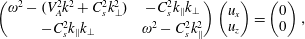 $$\begin{eqnarray}\displaystyle \left(\begin{array}{@{}cc@{}}\unicode[STIX]{x1D714}^{2}-(V_{A}^{2}k^{2}+C_{s}^{2}k_{\bot }^{2}) & -C_{s}^{2}k_{\Vert }k_{\bot }\\ -C_{s}^{2}k_{\Vert }k_{\bot } & \unicode[STIX]{x1D714}^{2}-C_{s}^{2}k_{\Vert }^{2}\end{array}\right)\left(\begin{array}{@{}c@{}}u_{x}\\ u_{z}\end{array}\right)=\left(\begin{array}{@{}c@{}}0\\ 0\end{array}\right), & & \displaystyle\end{eqnarray}$$
or alternatively
 $$\begin{eqnarray}\displaystyle \left(\begin{array}{@{}cc@{}}(\unicode[STIX]{x1D714}/k)^{2}-(V_{A}^{2}+C_{s}^{2}\sin ^{2}\unicode[STIX]{x1D703}) & -C_{s}^{2}\sin \unicode[STIX]{x1D703}\cos \unicode[STIX]{x1D703}\\ -C_{s}^{2}\sin \unicode[STIX]{x1D703}\cos \unicode[STIX]{x1D703} & (\unicode[STIX]{x1D714}/k)^{2}-C_{s}^{2}\cos ^{2}\unicode[STIX]{x1D703}\end{array}\right)\left(\begin{array}{@{}c@{}}u_{x}\\ u_{z}\end{array}\right)=\left(\begin{array}{@{}c@{}}0\\ 0\end{array}\right). & & \displaystyle\end{eqnarray}$$
This yields the MHD dispersion relations for the slow and fast modes in the form of (3.110) or alternatively (3.111). It possible to either express the ratio
 $u_{x}/u_{z}$
or
$u_{x}/u_{z}$
or
 $u_{z}/u_{x}$
. We want to calculate the velocity ratio
$u_{z}/u_{x}$
. We want to calculate the velocity ratio
 $\unicode[STIX]{x1D712}_{u}$
and we choose the first possibility that allows us to express that for the slow and fast modes (since
$\unicode[STIX]{x1D712}_{u}$
and we choose the first possibility that allows us to express that for the slow and fast modes (since
 $u_{y}=0$
)
$u_{y}=0$
)
 $$\begin{eqnarray}\displaystyle \unicode[STIX]{x1D712}_{u}(k_{\Vert },k_{\bot })=\frac{|u_{z}|^{2}}{|u_{x}|^{2}+|u_{z}|^{2}}=\frac{1}{\displaystyle \left|\frac{u_{x}}{u_{z}}\right|^{2}+1}. & & \displaystyle\end{eqnarray}$$
The ratio
 $u_{x}/u_{z}$
can be found for example from the second row of the matrix as
$u_{x}/u_{z}$
can be found for example from the second row of the matrix as
 $$\begin{eqnarray}\frac{u_{x}}{u_{z}}=\frac{(\unicode[STIX]{x1D714}/k)^{2}-C_{s}^{2}\cos ^{2}\unicode[STIX]{x1D703}}{C_{s}^{2}\sin \unicode[STIX]{x1D703}\cos \unicode[STIX]{x1D703}},\end{eqnarray}$$
or equivalently from the first row of the matrix as
 $$\begin{eqnarray}\frac{u_{x}}{u_{z}}=\frac{C_{s}^{2}\sin \unicode[STIX]{x1D703}\cos \unicode[STIX]{x1D703}}{(\unicode[STIX]{x1D714}/k)^{2}-(V_{A}^{2}+C_{s}^{2}\sin ^{2}\unicode[STIX]{x1D703})}.\end{eqnarray}$$
The possible range of the ratio
 $u_{x}/u_{z}$
is from
$u_{x}/u_{z}$
is from
 $-\infty$
to
$-\infty$
to
 $+\infty$
and the possible range for
$+\infty$
and the possible range for
 $\unicode[STIX]{x1D712}_{u}$
is from
$\unicode[STIX]{x1D712}_{u}$
is from
 $0$
to
$0$
to
 $1$
. Solutions can be easily divided into two categories – depending on the behaviour for parallel propagation – and are plotted in figure 2. For the sake of clarity, we only consider propagation with positive wavenumbers
$1$
. Solutions can be easily divided into two categories – depending on the behaviour for parallel propagation – and are plotted in figure 2. For the sake of clarity, we only consider propagation with positive wavenumbers
 $k_{\Vert }$
and
$k_{\Vert }$
and
 $k_{\bot }$
, so the possible range of angle
$k_{\bot }$
, so the possible range of angle
 $\unicode[STIX]{x1D703}$
is from
$\unicode[STIX]{x1D703}$
is from
 $0$
to
$0$
to
 $\unicode[STIX]{x03C0}/2$
and
$\unicode[STIX]{x03C0}/2$
and
 $\sin \unicode[STIX]{x1D703}\geqslant 0$
,
$\sin \unicode[STIX]{x1D703}\geqslant 0$
,
 $\cos \unicode[STIX]{x1D703}\geqslant 0$
. Consider first the case
$\cos \unicode[STIX]{x1D703}\geqslant 0$
. Consider first the case
 $C_{s}<V_{A}$
. For parallel propagation, the dispersion relation (3.111) directly yields that for the fast mode
$C_{s}<V_{A}$
. For parallel propagation, the dispersion relation (3.111) directly yields that for the fast mode
 $(\unicode[STIX]{x1D714}/k)_{f}^{2}|_{\unicode[STIX]{x1D703}=0}=V_{A}^{2}$
and for the slow mode
$(\unicode[STIX]{x1D714}/k)_{f}^{2}|_{\unicode[STIX]{x1D703}=0}=V_{A}^{2}$
and for the slow mode
 $(\unicode[STIX]{x1D714}/k)_{s}^{2}|_{\unicode[STIX]{x1D703}=0}=C_{s}^{2}$
. Using the expression (3.119) then yields that for the fast mode
$(\unicode[STIX]{x1D714}/k)_{s}^{2}|_{\unicode[STIX]{x1D703}=0}=C_{s}^{2}$
. Using the expression (3.119) then yields that for the fast mode
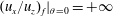 $(u_{x}/u_{z})_{f}|_{\unicode[STIX]{x1D703}=0}=+\infty$
and for the slow mode
$(u_{x}/u_{z})_{f}|_{\unicode[STIX]{x1D703}=0}=+\infty$
and for the slow mode
 $(u_{x}/u_{z})_{s}|_{\unicode[STIX]{x1D703}=0}=0$
. This implies that for
$(u_{x}/u_{z})_{s}|_{\unicode[STIX]{x1D703}=0}=0$
. This implies that for
 $C_{s}<V_{A}$
, all the
$C_{s}<V_{A}$
, all the
 $\unicode[STIX]{x1D712}_{u}(\unicode[STIX]{x1D703})$
curves start at
$\unicode[STIX]{x1D712}_{u}(\unicode[STIX]{x1D703})$
curves start at
 $$\begin{eqnarray}C_{s}<V_{A}:\quad \unicode[STIX]{x1D712}_{u}^{f}(\unicode[STIX]{x1D703}=0)=0;\quad \unicode[STIX]{x1D712}_{u}^{s}(\unicode[STIX]{x1D703}=0)=1,\end{eqnarray}$$
regardless of the actual value of
 $C_{s}/V_{A}<1$
. The second case
$C_{s}/V_{A}<1$
. The second case
 $C_{s}>V_{A}$
is straightforward, since for parallel propagation everything is just turned around; the fast mode dispersion relation is
$C_{s}>V_{A}$
is straightforward, since for parallel propagation everything is just turned around; the fast mode dispersion relation is
 $(\unicode[STIX]{x1D714}/k)_{f}^{2}|_{\unicode[STIX]{x1D703}=0}=C_{s}^{2}$
and the slow mode dispersion relation is
$(\unicode[STIX]{x1D714}/k)_{f}^{2}|_{\unicode[STIX]{x1D703}=0}=C_{s}^{2}$
and the slow mode dispersion relation is
 $(\unicode[STIX]{x1D714}/k)_{s}^{2}|_{\unicode[STIX]{x1D703}=0}=V_{A}^{2}$
. Implying that for
$(\unicode[STIX]{x1D714}/k)_{s}^{2}|_{\unicode[STIX]{x1D703}=0}=V_{A}^{2}$
. Implying that for
 $C_{s}>V_{A}$
, all the
$C_{s}>V_{A}$
, all the
 $\unicode[STIX]{x1D712}_{u}(\unicode[STIX]{x1D703})$
curves start at
$\unicode[STIX]{x1D712}_{u}(\unicode[STIX]{x1D703})$
curves start at
 $$\begin{eqnarray}C_{s}>V_{A}:\quad \unicode[STIX]{x1D712}_{u}^{f}(\unicode[STIX]{x1D703}=0)=1;\quad \unicode[STIX]{x1D712}_{u}^{s}(\unicode[STIX]{x1D703}=0)=0,\end{eqnarray}$$
regardless of the actual value of
 $C_{s}/V_{A}>1$
. The perpendicular propagation limit is even easier since the split into two categories is not required and for both cases the dispersion (3.110) yields
$C_{s}/V_{A}>1$
. The perpendicular propagation limit is even easier since the split into two categories is not required and for both cases the dispersion (3.110) yields
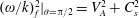 $(\unicode[STIX]{x1D714}/k)_{f}^{2}|_{\unicode[STIX]{x1D703}=\unicode[STIX]{x03C0}/2}=V_{A}^{2}+C_{s}^{2}$
and
$(\unicode[STIX]{x1D714}/k)_{f}^{2}|_{\unicode[STIX]{x1D703}=\unicode[STIX]{x03C0}/2}=V_{A}^{2}+C_{s}^{2}$
and
 $(\unicode[STIX]{x1D714}/k)_{s}^{2}|_{\unicode[STIX]{x1D703}=\unicode[STIX]{x03C0}/2}=0$
, implying that for the fast mode
$(\unicode[STIX]{x1D714}/k)_{s}^{2}|_{\unicode[STIX]{x1D703}=\unicode[STIX]{x03C0}/2}=0$
, implying that for the fast mode
 $(u_{x}/u_{z})_{f}|_{\unicode[STIX]{x1D703}=\unicode[STIX]{x03C0}/2}=+\infty$
and that for the slow mode
$(u_{x}/u_{z})_{f}|_{\unicode[STIX]{x1D703}=\unicode[STIX]{x03C0}/2}=+\infty$
and that for the slow mode
 $(u_{x}/u_{z})_{s}|_{\unicode[STIX]{x1D703}=\unicode[STIX]{x03C0}/2}=0$
. All the
$(u_{x}/u_{z})_{s}|_{\unicode[STIX]{x1D703}=\unicode[STIX]{x03C0}/2}=0$
. All the
 $\unicode[STIX]{x1D712}_{u}(\unicode[STIX]{x1D703})$
curves therefore ‘end’ at
$\unicode[STIX]{x1D712}_{u}(\unicode[STIX]{x1D703})$
curves therefore ‘end’ at
 $$\begin{eqnarray}\unicode[STIX]{x1D712}_{u}^{f}(\unicode[STIX]{x1D703}=\unicode[STIX]{x03C0}/2)=0;\quad \unicode[STIX]{x1D712}_{u}^{s}(\unicode[STIX]{x1D703}=\unicode[STIX]{x03C0}/2)=1,\end{eqnarray}$$
whether the ratio
 $C_{s}/V_{A}<1$
or
$C_{s}/V_{A}<1$
or
 $C_{s}/V_{A}>1$
. The behaviour of the
$C_{s}/V_{A}>1$
. The behaviour of the
 $\unicode[STIX]{x1D712}_{u}(\unicode[STIX]{x1D703})$
curves is plotted in figure 2.
$\unicode[STIX]{x1D712}_{u}(\unicode[STIX]{x1D703})$
curves is plotted in figure 2.
In MHD, the ratio
 $C_{s}^{2}/V_{A}^{2}$
is sometimes used as the definition of plasma beta, which we will call here
$C_{s}^{2}/V_{A}^{2}$
is sometimes used as the definition of plasma beta, which we will call here
 $\unicode[STIX]{x1D6FD}_{\text{MHD}}\equiv C_{s}^{2}/V_{A}^{2}$
. As can be seen in figure 2, for
$\unicode[STIX]{x1D6FD}_{\text{MHD}}\equiv C_{s}^{2}/V_{A}^{2}$
. As can be seen in figure 2, for
 $\unicode[STIX]{x1D6FD}_{\text{MHD}}$
approaching 1, the curves display a ‘singular’ behaviour, and it is difficult to guess what will happen when
$\unicode[STIX]{x1D6FD}_{\text{MHD}}$
approaching 1, the curves display a ‘singular’ behaviour, and it is difficult to guess what will happen when
 $\unicode[STIX]{x1D6FD}_{\text{MHD}}$
reaches the value of 1 exactly. This special case is addressed in the next subsection. There are also two special cases, one for
$\unicode[STIX]{x1D6FD}_{\text{MHD}}$
reaches the value of 1 exactly. This special case is addressed in the next subsection. There are also two special cases, one for
 $C_{s}\ll V_{A}$
or
$C_{s}\ll V_{A}$
or
 $\unicode[STIX]{x1D6FD}_{\text{MHD}}\ll 1$
and one for
$\unicode[STIX]{x1D6FD}_{\text{MHD}}\ll 1$
and one for
 $C_{s}\gg V_{A}$
or
$C_{s}\gg V_{A}$
or
 $\unicode[STIX]{x1D6FD}_{\text{MHD}}\gg 1$
. Both limits
$\unicode[STIX]{x1D6FD}_{\text{MHD}}\gg 1$
. Both limits
 $C_{s}\ll V_{A}$
and
$C_{s}\ll V_{A}$
and
 $C_{s}\gg V_{A}$
are easily obtained by rewriting the dispersion relation (3.110) to a form
$C_{s}\gg V_{A}$
are easily obtained by rewriting the dispersion relation (3.110) to a form
 $$\begin{eqnarray}\left(\frac{\unicode[STIX]{x1D714}}{k}\right)^{2}=\frac{1}{2}(V_{A}^{2}+C_{s}^{2})\pm \frac{1}{2}(V_{A}^{2}+C_{s}^{2})\sqrt{1-\frac{4V_{A}^{2}C_{s}^{2}}{(V_{A}^{2}+C_{s}^{2})^{2}}\cos ^{2}\unicode[STIX]{x1D703}}.\end{eqnarray}$$
In both limits the second term under the square root is small and the expression can be expanded as
 $\sqrt{1-\unicode[STIX]{x1D716}}=1-\unicode[STIX]{x1D716}/2$
, yielding the slow and fast mode dispersion relations
$\sqrt{1-\unicode[STIX]{x1D716}}=1-\unicode[STIX]{x1D716}/2$
, yielding the slow and fast mode dispersion relations
 $$\begin{eqnarray}C_{s}\ll V_{A}~\text{or}~C_{s}\gg V_{A}:\quad \left(\frac{\unicode[STIX]{x1D714}}{k}\right)_{f}^{2}=V_{A}^{2}+C_{s}^{2}-\frac{V_{A}^{2}C_{s}^{2}}{V_{A}^{2}+C_{s}^{2}}\cos ^{2}\unicode[STIX]{x1D703};\quad \left(\frac{\unicode[STIX]{x1D714}}{k}\right)_{s}^{2}=\frac{V_{A}^{2}C_{s}^{2}}{V_{A}^{2}+C_{s}^{2}}\cos ^{2}\unicode[STIX]{x1D703},\end{eqnarray}$$
which further yield dispersion relations (3.126), (3.128). Note that the limit
 $C_{s}\ll V_{A}$
can be easily obtained directly from the velocity matrix (3.117) by neglecting the off-diagonal terms that decouple the two modes. In contrast, the limit
$C_{s}\ll V_{A}$
can be easily obtained directly from the velocity matrix (3.117) by neglecting the off-diagonal terms that decouple the two modes. In contrast, the limit
 $C_{s}\gg V_{A}$
is not that obvious and one needs to calculate the determinant.
$C_{s}\gg V_{A}$
is not that obvious and one needs to calculate the determinant.
In the limit
 $\unicode[STIX]{x1D6FD}_{\text{MHD}}\ll 1$
, the MHD dispersion relation simplifies to
$\unicode[STIX]{x1D6FD}_{\text{MHD}}\ll 1$
, the MHD dispersion relation simplifies to
 $$\begin{eqnarray}\unicode[STIX]{x1D6FD}_{\text{MHD}}\ll 1:\quad (\unicode[STIX]{x1D714}/k)_{f}^{2}=V_{A}^{2}+C_{s}^{2}\sin ^{2}\unicode[STIX]{x1D703};\quad (\unicode[STIX]{x1D714}/k)_{s}^{2}=C_{s}^{2}\cos ^{2}\unicode[STIX]{x1D703}.\end{eqnarray}$$
The expression (3.119) yields for the fast mode
 $(u_{x}/u_{z})_{f}(\unicode[STIX]{x1D703})=\infty$
and the expression (3.120) yields for the slow mode
$(u_{x}/u_{z})_{f}(\unicode[STIX]{x1D703})=\infty$
and the expression (3.120) yields for the slow mode
 $(u_{x}/u_{z})_{s}(\unicode[STIX]{x1D703})=0$
, implying
$(u_{x}/u_{z})_{s}(\unicode[STIX]{x1D703})=0$
, implying
 $$\begin{eqnarray}\unicode[STIX]{x1D6FD}_{\text{MHD}}\ll 1:\quad \unicode[STIX]{x1D712}_{u}^{f}(\unicode[STIX]{x1D703})=0;\quad \unicode[STIX]{x1D712}_{u}^{s}(\unicode[STIX]{x1D703})=1.\end{eqnarray}$$
In the opposite limit
 $\unicode[STIX]{x1D6FD}_{\text{MHD}}\gg 1$
, the MHD dispersions simplify to
$\unicode[STIX]{x1D6FD}_{\text{MHD}}\gg 1$
, the MHD dispersions simplify to
 $$\begin{eqnarray}\unicode[STIX]{x1D6FD}_{\text{MHD}}\gg 1:\quad (\unicode[STIX]{x1D714}/k)_{f}^{2}=C_{s}^{2}+V_{A}^{2}\sin ^{2}\unicode[STIX]{x1D703};\quad (\unicode[STIX]{x1D714}/k)_{s}^{2}=V_{A}^{2}\cos ^{2}\unicode[STIX]{x1D703}.\end{eqnarray}$$
In this limit, the expression (3.119) yields
 $(u_{x}/u_{z})_{f}(\unicode[STIX]{x1D703})=(1+V_{A}^{2}/C_{s}^{2})\tan \unicode[STIX]{x1D703}$
, that describes the behaviour of the fast mode for large beta values and the complete limit is
$(u_{x}/u_{z})_{f}(\unicode[STIX]{x1D703})=(1+V_{A}^{2}/C_{s}^{2})\tan \unicode[STIX]{x1D703}$
, that describes the behaviour of the fast mode for large beta values and the complete limit is
 $(u_{x}/u_{z})_{f}(\unicode[STIX]{x1D703})=\tan \unicode[STIX]{x1D703}$
. For the slow mode the expression (3.119) yields
$(u_{x}/u_{z})_{f}(\unicode[STIX]{x1D703})=\tan \unicode[STIX]{x1D703}$
. For the slow mode the expression (3.119) yields
 $(u_{x}/u_{z})_{s}(\unicode[STIX]{x1D703})=-(1-V_{A}^{2}/C_{s}^{2})\cot \unicode[STIX]{x1D703}$
and the complete limit is
$(u_{x}/u_{z})_{s}(\unicode[STIX]{x1D703})=-(1-V_{A}^{2}/C_{s}^{2})\cot \unicode[STIX]{x1D703}$
and the complete limit is
 $(u_{x}/u_{z})_{s}(\unicode[STIX]{x1D703})=-\cot \unicode[STIX]{x1D703}$
. The
$(u_{x}/u_{z})_{s}(\unicode[STIX]{x1D703})=-\cot \unicode[STIX]{x1D703}$
. The
 $\unicode[STIX]{x1D712}_{u}(\unicode[STIX]{x1D703})$
solutions for large beta values therefore converge to
$\unicode[STIX]{x1D712}_{u}(\unicode[STIX]{x1D703})$
solutions for large beta values therefore converge to
 $$\begin{eqnarray}\unicode[STIX]{x1D6FD}_{\text{MHD}}\gg 1:\quad \unicode[STIX]{x1D712}_{u}^{f}(\unicode[STIX]{x1D703})=\cos ^{2}\unicode[STIX]{x1D703};\quad \unicode[STIX]{x1D712}_{u}^{s}(\unicode[STIX]{x1D703})=\sin ^{2}\unicode[STIX]{x1D703},\end{eqnarray}$$
and these two curves are plotted in figure 2 as dashed lines.
MHD velocity ratio
 $\unicode[STIX]{x1D712}_{u}(\unicode[STIX]{x1D703})=|u_{\Vert }|^{2}/|u|^{2}$
for the slow mode (red lines) and the fast mode (blue lines) for different ratios of
$\unicode[STIX]{x1D712}_{u}(\unicode[STIX]{x1D703})=|u_{\Vert }|^{2}/|u|^{2}$
for the slow mode (red lines) and the fast mode (blue lines) for different ratios of
 $C_{s}^{2}/V_{A}^{2}=\unicode[STIX]{x1D6FD}_{\text{MHD}}$
. Panel (a) is for
$C_{s}^{2}/V_{A}^{2}=\unicode[STIX]{x1D6FD}_{\text{MHD}}$
. Panel (a) is for
 $\unicode[STIX]{x1D6FD}_{\text{MHD}}<1$
, and the thickness of the lines increases with
$\unicode[STIX]{x1D6FD}_{\text{MHD}}<1$
, and the thickness of the lines increases with
 $\unicode[STIX]{x1D6FD}_{\text{MHD}}$
when approaching the critical value of
$\unicode[STIX]{x1D6FD}_{\text{MHD}}$
when approaching the critical value of
 $\unicode[STIX]{x1D6FD}_{\text{MHD}}=1$
. The plotted lines have
$\unicode[STIX]{x1D6FD}_{\text{MHD}}=1$
. The plotted lines have
 $\unicode[STIX]{x1D6FD}_{\text{MHD}}=0.3;0.6;0.8;0.9;0.99$
. Panel (b) is for
$\unicode[STIX]{x1D6FD}_{\text{MHD}}=0.3;0.6;0.8;0.9;0.99$
. Panel (b) is for
 $\unicode[STIX]{x1D6FD}_{\text{MHD}}>1$
and the thickness of the lines decreases with
$\unicode[STIX]{x1D6FD}_{\text{MHD}}>1$
and the thickness of the lines decreases with
 $\unicode[STIX]{x1D6FD}_{\text{MHD}}$
when going away from the critical value of
$\unicode[STIX]{x1D6FD}_{\text{MHD}}$
when going away from the critical value of
 $\unicode[STIX]{x1D6FD}_{\text{MHD}}=1$
. The plotted lines have
$\unicode[STIX]{x1D6FD}_{\text{MHD}}=1$
. The plotted lines have
 $\unicode[STIX]{x1D6FD}_{\text{MHD}}=1.01;1.1;1.2;2.0;10;10^{3}$
. In both figures, the dotted lines are the critical case
$\unicode[STIX]{x1D6FD}_{\text{MHD}}=1.01;1.1;1.2;2.0;10;10^{3}$
. In both figures, the dotted lines are the critical case
 $\unicode[STIX]{x1D6FD}_{\text{MHD}}=1$
with solutions (3.134). In (b) the dashed lines represent the limit
$\unicode[STIX]{x1D6FD}_{\text{MHD}}=1$
with solutions (3.134). In (b) the dashed lines represent the limit
 $\unicode[STIX]{x1D6FD}_{\text{MHD}}\gg 1$
with solutions (3.129) and the dashed lines nicely overlap with a thin solid line solutions obtained for
$\unicode[STIX]{x1D6FD}_{\text{MHD}}\gg 1$
with solutions (3.129) and the dashed lines nicely overlap with a thin solid line solutions obtained for
 $\unicode[STIX]{x1D6FD}_{\text{MHD}}=10^{3}$
. The Alfvén mode has
$\unicode[STIX]{x1D6FD}_{\text{MHD}}=10^{3}$
. The Alfvén mode has
 $\unicode[STIX]{x1D712}_{u}(\unicode[STIX]{x1D703})=0$
regardless of the plasma beta and is not plotted.
$\unicode[STIX]{x1D712}_{u}(\unicode[STIX]{x1D703})=0$
regardless of the plasma beta and is not plotted.
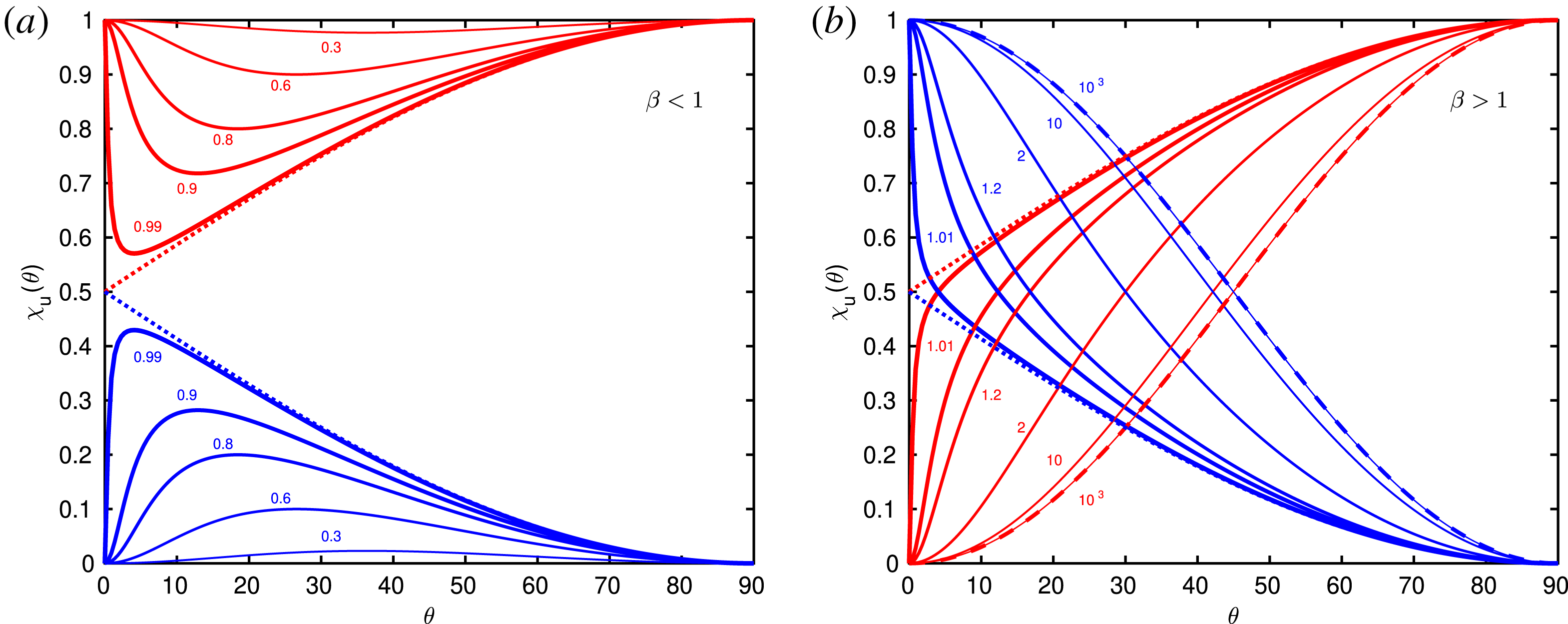
3.9.1 MHD special case
$V_{A}=C_{s}$

Consider the very peculiar case of parallel propagation
 $\unicode[STIX]{x1D703}=0$
with
$\unicode[STIX]{x1D703}=0$
with
 $V_{A}=C_{s}$
. The velocity eigenvector matrix (3.117), when evaluated exactly at these values reads
$V_{A}=C_{s}$
. The velocity eigenvector matrix (3.117), when evaluated exactly at these values reads
 $$\begin{eqnarray}\displaystyle \left(\begin{array}{@{}cc@{}}0 & 0\\ 0 & 0\end{array}\right)\left(\begin{array}{@{}c@{}}u_{x}\\ u_{z}\end{array}\right)=\left(\begin{array}{@{}c@{}}0\\ 0\end{array}\right). & & \displaystyle\end{eqnarray}$$
It is not possible to determine the ratio
 $u_{x}/u_{z}$
and the eigenvector must be found by taking the limit
$u_{x}/u_{z}$
and the eigenvector must be found by taking the limit
 $\unicode[STIX]{x1D703}\rightarrow 0$
. For
$\unicode[STIX]{x1D703}\rightarrow 0$
. For
 $V_{A}=C_{s}$
the dispersion relation for the slow and fast modes (3.111) simplifies to
$V_{A}=C_{s}$
the dispersion relation for the slow and fast modes (3.111) simplifies to
 $(\unicode[STIX]{x1D714}/k)^{2}=V_{A}^{2}\pm V_{A}^{2}|\sin \unicode[STIX]{x1D703}|$
. As before, for the sake of simplicity we consider only positive wavenumbers, so the propagation angle
$(\unicode[STIX]{x1D714}/k)^{2}=V_{A}^{2}\pm V_{A}^{2}|\sin \unicode[STIX]{x1D703}|$
. As before, for the sake of simplicity we consider only positive wavenumbers, so the propagation angle
 $\unicode[STIX]{x1D703}$
is in the range
$\unicode[STIX]{x1D703}$
is in the range
 $[0,\unicode[STIX]{x03C0}/2]$
and
$[0,\unicode[STIX]{x03C0}/2]$
and
 $\sin \unicode[STIX]{x1D703}\geqslant 0$
,
$\sin \unicode[STIX]{x1D703}\geqslant 0$
,
 $\cos \unicode[STIX]{x1D703}\geqslant 0$
. Evaluating the velocity matrix (3.117) at
$\cos \unicode[STIX]{x1D703}\geqslant 0$
. Evaluating the velocity matrix (3.117) at
 $V_{A}=C_{s}$
only, it is possible to pull the
$V_{A}=C_{s}$
only, it is possible to pull the
 $\sin \unicode[STIX]{x1D703}$
out of the system so that
$\sin \unicode[STIX]{x1D703}$
out of the system so that
 $$\begin{eqnarray}\displaystyle \left(\begin{array}{@{}cc@{}}\pm 1-\sin \unicode[STIX]{x1D703} & -\cos \unicode[STIX]{x1D703}\\ -\cos \unicode[STIX]{x1D703} & \pm 1+\sin \unicode[STIX]{x1D703}\end{array}\right)V_{A}^{2}\sin \unicode[STIX]{x1D703}\left(\begin{array}{@{}c@{}}u_{x}\\ u_{z}\end{array}\right)=\left(\begin{array}{@{}c@{}}0\\ 0\end{array}\right), & & \displaystyle\end{eqnarray}$$
which nicely demonstrates that for
 $\unicode[STIX]{x1D703}\rightarrow 0$
the system approaches (3.130). Nevertheless, we can now calculate the velocity ratio (for example from the second row) as
$\unicode[STIX]{x1D703}\rightarrow 0$
the system approaches (3.130). Nevertheless, we can now calculate the velocity ratio (for example from the second row) as
 $$\begin{eqnarray}\frac{u_{x}}{u_{z}}=\frac{\pm 1+\sin \unicode[STIX]{x1D703}}{\cos \unicode[STIX]{x1D703}},\end{eqnarray}$$
which can be evaluated at
 $\unicode[STIX]{x1D703}=0$
. For the fast mode
$\unicode[STIX]{x1D703}=0$
. For the fast mode
 $(u_{x}/u_{z})^{f}(0)=1$
and for the slow mode
$(u_{x}/u_{z})^{f}(0)=1$
and for the slow mode
 $(u_{x}/u_{z})^{s}(0)=-1$
. This implies that for the peculiar case of
$(u_{x}/u_{z})^{s}(0)=-1$
. This implies that for the peculiar case of
 $V_{A}=C_{s}$
, the velocity ratio
$V_{A}=C_{s}$
, the velocity ratio
 $\unicode[STIX]{x1D712}_{u}^{sf}(0)=1/2$
for both the fast and slow modes. The expression (3.132) can of course be directly obtained by using the result
$\unicode[STIX]{x1D712}_{u}^{sf}(0)=1/2$
for both the fast and slow modes. The expression (3.132) can of course be directly obtained by using the result
 $(\unicode[STIX]{x1D714}/k)^{2}=V_{A}^{2}\pm V_{A}^{2}\sin \unicode[STIX]{x1D703}$
in the expression (3.119) and by cancelling the
$(\unicode[STIX]{x1D714}/k)^{2}=V_{A}^{2}\pm V_{A}^{2}\sin \unicode[STIX]{x1D703}$
in the expression (3.119) and by cancelling the
 $\sin \unicode[STIX]{x1D703}$
in the nominator and denominator. The expression (3.132) is valid for any angle
$\sin \unicode[STIX]{x1D703}$
in the nominator and denominator. The expression (3.132) is valid for any angle
 $\unicode[STIX]{x1D703}$
. However, for the slow mode it becomes singular at
$\unicode[STIX]{x1D703}$
. However, for the slow mode it becomes singular at
 $\unicode[STIX]{x1D703}=\unicode[STIX]{x03C0}/2$
, and has to be rearranged by multiplying and dividing with
$\unicode[STIX]{x1D703}=\unicode[STIX]{x03C0}/2$
, and has to be rearranged by multiplying and dividing with
 $1+\sin \unicode[STIX]{x1D703}$
(or equivalently, use the first row of the matrix). To have useful expression for the entire range of
$1+\sin \unicode[STIX]{x1D703}$
(or equivalently, use the first row of the matrix). To have useful expression for the entire range of
 $\unicode[STIX]{x1D703}$
, we therefore split the expressions for the slow and fast modes as
$\unicode[STIX]{x1D703}$
, we therefore split the expressions for the slow and fast modes as
 $$\begin{eqnarray}(u_{x}/u_{z})^{s}=-\frac{\cos \unicode[STIX]{x1D703}}{1+\sin \unicode[STIX]{x1D703}};\quad (u_{x}/u_{z})^{f}=\frac{1+\sin \unicode[STIX]{x1D703}}{\cos \unicode[STIX]{x1D703}},\end{eqnarray}$$
which yields, in this peculiar case of
 $V_{A}=C_{s}$
, that the ratio
$V_{A}=C_{s}$
, that the ratio
 $\unicode[STIX]{x1D712}_{u}$
for the slow and fast modes can be expressed as
$\unicode[STIX]{x1D712}_{u}$
for the slow and fast modes can be expressed as
 $$\begin{eqnarray}V_{A}=C_{s}:\quad \unicode[STIX]{x1D712}_{u}^{s}(\unicode[STIX]{x1D703})={\textstyle \frac{1}{2}}(1+\sin \unicode[STIX]{x1D703});\quad \unicode[STIX]{x1D712}_{u}^{f}(\unicode[STIX]{x1D703})={\textstyle \frac{1}{2}}(1-\sin \unicode[STIX]{x1D703}).\end{eqnarray}$$
These solutions are plotted in figure 2 as dotted lines.
3.10 CGL velocity eigenvector
To find the ratio for velocity components
 $\unicode[STIX]{x1D712}_{u}$
in the CGL description, it is useful for a moment to work with abbreviated symbols, and we write the matrix (3.88) for the
$\unicode[STIX]{x1D712}_{u}$
in the CGL description, it is useful for a moment to work with abbreviated symbols, and we write the matrix (3.88) for the
 $u_{x}$
and
$u_{x}$
and
 $u_{z}$
components as
$u_{z}$
components as
 $$\begin{eqnarray}\displaystyle \left(\begin{array}{@{}cc@{}}(\widetilde{\unicode[STIX]{x1D714}}/\widetilde{k})^{2}-a; & -b\\ -b & (\widetilde{\unicode[STIX]{x1D714}}/\widetilde{k})^{2}-c\end{array}\right)\left(\begin{array}{@{}c@{}}u_{x}\\ u_{z}\end{array}\right)=\left(\begin{array}{@{}c@{}}0\\ 0\end{array}\right), & & \displaystyle\end{eqnarray}$$
where the coefficients are
 $$\begin{eqnarray}\displaystyle a=1+a_{p}\unicode[STIX]{x1D6FD}_{\Vert }\left(1-\frac{1}{2}\cos ^{2}\unicode[STIX]{x1D703}\right)-\frac{\unicode[STIX]{x1D6FD}_{\Vert }}{2}\cos ^{2}\unicode[STIX]{x1D703};\quad b=\frac{\unicode[STIX]{x1D6FD}_{\Vert }}{2}a_{p}\sin \unicode[STIX]{x1D703}\cos \unicode[STIX]{x1D703};\quad c=\frac{3}{2}\unicode[STIX]{x1D6FD}_{\Vert }\cos ^{2}\unicode[STIX]{x1D703}. & & \displaystyle \nonumber\\ \displaystyle & & \displaystyle\end{eqnarray}$$
The determinant must be zero, which implies
 $(\widetilde{\unicode[STIX]{x1D714}}/\widetilde{k})^{4}-(\widetilde{\unicode[STIX]{x1D714}}/\widetilde{k})^{2}(a+c)+ac-b^{2}=0$
, and has a solution
$(\widetilde{\unicode[STIX]{x1D714}}/\widetilde{k})^{4}-(\widetilde{\unicode[STIX]{x1D714}}/\widetilde{k})^{2}(a+c)+ac-b^{2}=0$
, and has a solution
 $$\begin{eqnarray}(\widetilde{\unicode[STIX]{x1D714}}/\widetilde{k})^{2}={\textstyle \frac{1}{2}}(a+c)\pm {\textstyle \frac{1}{2}}\sqrt{(a+c)^{2}-4ac+4b^{2}}={\textstyle \frac{1}{2}}(a+c)\pm {\textstyle \frac{1}{2}}\sqrt{(a-c)^{2}+4b^{2}}.\end{eqnarray}$$
The last step was actually used in obtaining (3.98) which is otherwise quite difficult to see. Using this result in the above matrix, the eigenvector matrix becomes
 $$\begin{eqnarray}\displaystyle \left(\begin{array}{@{}cc@{}}-\frac{1}{2}(a-c)\pm \frac{1}{2}\sqrt{(a-c)^{2}+4b^{2}}; & -b\\ -b & \frac{1}{2}(a-c)\pm \frac{1}{2}\sqrt{(a-c)^{2}+4b^{2}}\end{array}\right)\left(\begin{array}{@{}c@{}}u_{x}\\ u_{z}\end{array}\right)=\left(\begin{array}{@{}c@{}}0\\ 0\end{array}\right), & & \displaystyle \nonumber\\ \displaystyle & & \displaystyle\end{eqnarray}$$
where
 $$\begin{eqnarray}\displaystyle a-c=1+a_{p}\unicode[STIX]{x1D6FD}_{\Vert }\left(1-{\textstyle \frac{1}{2}}\cos ^{2}\unicode[STIX]{x1D703}\right)-2\unicode[STIX]{x1D6FD}_{\Vert }\cos ^{2}\unicode[STIX]{x1D703}. & & \displaystyle\end{eqnarray}$$
The ratio of
 $u_{x}/u_{z}$
can be expressed (for example from the second row) as
$u_{x}/u_{z}$
can be expressed (for example from the second row) as
 $$\begin{eqnarray}\displaystyle \frac{u_{x}}{u_{z}} & = & \displaystyle \frac{1}{b}[(\widetilde{\unicode[STIX]{x1D714}}/\widetilde{k})^{2}-c]=\frac{1}{2b}[a-c\pm \sqrt{(a-c)^{2}+4b^{2}}]\nonumber\\ \displaystyle & = & \displaystyle \frac{1}{\unicode[STIX]{x1D6FD}_{\Vert }a_{p}\sin \unicode[STIX]{x1D703}\cos \unicode[STIX]{x1D703}}\left[1+a_{p}\unicode[STIX]{x1D6FD}_{\Vert }\left(1-\frac{1}{2}\cos ^{2}\unicode[STIX]{x1D703}\right)-2\unicode[STIX]{x1D6FD}_{\Vert }\cos ^{2}\unicode[STIX]{x1D703}\right.\nonumber\\ \displaystyle & & \displaystyle \pm \left.\sqrt{\left(1+a_{p}\unicode[STIX]{x1D6FD}_{\Vert }\left(1-\frac{1}{2}\cos ^{2}\unicode[STIX]{x1D703}\right)-2\unicode[STIX]{x1D6FD}_{\Vert }\cos ^{2}\unicode[STIX]{x1D703}\right)^{2}+a_{p}^{2}\unicode[STIX]{x1D6FD}_{\Vert }^{2}\sin ^{2}\unicode[STIX]{x1D703}\cos ^{2}\unicode[STIX]{x1D703}}\right],\end{eqnarray}$$
or alternatively (from the first row) as
 $$\begin{eqnarray}\displaystyle \frac{u_{x}}{u_{z}} & = & \displaystyle \frac{b}{(\widetilde{\unicode[STIX]{x1D714}}/\widetilde{k})^{2}-a}=\frac{2b}{-(a-c)\pm \sqrt{(a-c)^{2}+4b^{2}}}\nonumber\\ \displaystyle & = & \displaystyle \unicode[STIX]{x1D6FD}_{\Vert }a_{p}\sin \unicode[STIX]{x1D703}\cos \unicode[STIX]{x1D703}\left[-1-a_{p}\unicode[STIX]{x1D6FD}_{\Vert }\left(1-\frac{1}{2}\cos ^{2}\unicode[STIX]{x1D703}\right)+2\unicode[STIX]{x1D6FD}_{\Vert }\cos ^{2}\unicode[STIX]{x1D703}\right.\nonumber\\ \displaystyle & & \displaystyle \pm \left.\sqrt{\left(1+a_{p}\unicode[STIX]{x1D6FD}_{\Vert }\left(1-\frac{1}{2}\cos ^{2}\unicode[STIX]{x1D703}\right)-2\unicode[STIX]{x1D6FD}_{\Vert }\cos ^{2}\unicode[STIX]{x1D703}\right)^{2}+a_{p}^{2}\unicode[STIX]{x1D6FD}_{\Vert }^{2}\sin ^{2}\unicode[STIX]{x1D703}\cos ^{2}\unicode[STIX]{x1D703}}\right]^{-1}.\nonumber\\ \displaystyle & & \displaystyle\end{eqnarray}$$
The behaviour of these solutions is plotted in figure 3, where we plot solutions for isotropic temperatures
 $a_{p}=1$
. Similarly to MHD, two classes of solutions can be characterized based upon the behaviour for parallel propagation
$a_{p}=1$
. Similarly to MHD, two classes of solutions can be characterized based upon the behaviour for parallel propagation
 $\unicode[STIX]{x1D703}=0$
, depending if the quantity
$\unicode[STIX]{x1D703}=0$
, depending if the quantity
 $a-c$
(3.139) evaluated at
$a-c$
(3.139) evaluated at
 $\unicode[STIX]{x1D703}=0$
is positive or negative. The quantity
$\unicode[STIX]{x1D703}=0$
is positive or negative. The quantity
 $(a-c)|_{\unicode[STIX]{x1D703}=0}=1+\frac{1}{2}a_{p}\unicode[STIX]{x1D6FD}_{\Vert }-2\unicode[STIX]{x1D6FD}_{\Vert }$
was discussed in the section for parallel propagation and this quantity represents the green dotted curve in figure 1 that separates the system into two regions. For
$(a-c)|_{\unicode[STIX]{x1D703}=0}=1+\frac{1}{2}a_{p}\unicode[STIX]{x1D6FD}_{\Vert }-2\unicode[STIX]{x1D6FD}_{\Vert }$
was discussed in the section for parallel propagation and this quantity represents the green dotted curve in figure 1 that separates the system into two regions. For
 $(a-c)|_{\unicode[STIX]{x1D703}=0}>0$
, i.e. in the region
$(a-c)|_{\unicode[STIX]{x1D703}=0}>0$
, i.e. in the region
 $\unicode[STIX]{x1D6FD}_{\Vert }<2/(4-a_{p})$
, for the slow mode (use (3.141)) the ratio
$\unicode[STIX]{x1D6FD}_{\Vert }<2/(4-a_{p})$
, for the slow mode (use (3.141)) the ratio
 $(u_{x}/u_{z})^{s}(0)=0$
and for the fast mode (use (3.140)) the ratio
$(u_{x}/u_{z})^{s}(0)=0$
and for the fast mode (use (3.140)) the ratio
 $(u_{x}/u_{z})^{f}(0)=+\infty$
. In this region, all the
$(u_{x}/u_{z})^{f}(0)=+\infty$
. In this region, all the
 $\unicode[STIX]{x1D712}_{u}(\unicode[STIX]{x1D703})$
curves start at
$\unicode[STIX]{x1D712}_{u}(\unicode[STIX]{x1D703})$
curves start at
 $$\begin{eqnarray}\unicode[STIX]{x1D6FD}_{\Vert }<2/(4-a_{p}):\quad \unicode[STIX]{x1D712}_{u}^{s}(0)=1;\quad \unicode[STIX]{x1D712}_{u}^{f}(0)=0.\end{eqnarray}$$
For
 $(a-c)|_{\unicode[STIX]{x1D703}=0}<0$
, i.e. in the region
$(a-c)|_{\unicode[STIX]{x1D703}=0}<0$
, i.e. in the region
 $\unicode[STIX]{x1D6FD}_{\Vert }>2/(4-a_{p})$
, for the slow mode (use (3.140)) the ratio
$\unicode[STIX]{x1D6FD}_{\Vert }>2/(4-a_{p})$
, for the slow mode (use (3.140)) the ratio
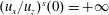 $(u_{x}/u_{z})^{s}(0)=+\infty$
and for the fast mode (use (3.141)) the ratio
$(u_{x}/u_{z})^{s}(0)=+\infty$
and for the fast mode (use (3.141)) the ratio
 $(u_{x}/u_{z})^{f}(0)=0$
. In this region, all the
$(u_{x}/u_{z})^{f}(0)=0$
. In this region, all the
 $\unicode[STIX]{x1D712}_{u}(\unicode[STIX]{x1D703})$
curves start at
$\unicode[STIX]{x1D712}_{u}(\unicode[STIX]{x1D703})$
curves start at
 $$\begin{eqnarray}\unicode[STIX]{x1D6FD}_{\Vert }>2/(4-a_{p}):\quad \unicode[STIX]{x1D712}_{u}^{s}(0)=0;\quad \unicode[STIX]{x1D712}_{u}^{f}(0)=1.\end{eqnarray}$$
For perpendicular propagation
 $\unicode[STIX]{x1D703}=\unicode[STIX]{x03C0}/2$
the quantity
$\unicode[STIX]{x1D703}=\unicode[STIX]{x03C0}/2$
the quantity
 $(a-c)|_{\unicode[STIX]{x1D703}=\unicode[STIX]{x03C0}/2}=1+a_{p}\unicode[STIX]{x1D6FD}_{\Vert }$
is always positive and the separation into two regions is not necessary. For the slow mode
$(a-c)|_{\unicode[STIX]{x1D703}=\unicode[STIX]{x03C0}/2}=1+a_{p}\unicode[STIX]{x1D6FD}_{\Vert }$
is always positive and the separation into two regions is not necessary. For the slow mode
 $(u_{x}/u_{z})^{s}(\unicode[STIX]{x03C0}/2)=0$
and for the fast mode
$(u_{x}/u_{z})^{s}(\unicode[STIX]{x03C0}/2)=0$
and for the fast mode
 $(u_{x}/u_{z})^{f}(\unicode[STIX]{x03C0}/2)=+\infty$
. All the
$(u_{x}/u_{z})^{f}(\unicode[STIX]{x03C0}/2)=+\infty$
. All the
 $\unicode[STIX]{x1D712}_{u}(\unicode[STIX]{x1D703})$
curves, regardless of the value of
$\unicode[STIX]{x1D712}_{u}(\unicode[STIX]{x1D703})$
curves, regardless of the value of
 $\unicode[STIX]{x1D6FD}_{\Vert }$
therefore end at
$\unicode[STIX]{x1D6FD}_{\Vert }$
therefore end at
 $$\begin{eqnarray}\quad \unicode[STIX]{x1D712}_{u}^{s}(\unicode[STIX]{x03C0}/2)=1;\quad \unicode[STIX]{x1D712}_{u}^{f}(\unicode[STIX]{x03C0}/2)=0.\end{eqnarray}$$
This summarizes the general behaviour of the solutions. However, as can be seen from figure 3, there is a special case when the parameters approach
 $\unicode[STIX]{x1D6FD}_{\Vert }=2/(4-a_{p})$
, i.e. when
$\unicode[STIX]{x1D6FD}_{\Vert }=2/(4-a_{p})$
, i.e. when
 $(a-c)|_{\unicode[STIX]{x1D703}=0}=0$
, that will be discussed in the next subsection. One can again consider the two limiting cases when
$(a-c)|_{\unicode[STIX]{x1D703}=0}=0$
, that will be discussed in the next subsection. One can again consider the two limiting cases when
 $\unicode[STIX]{x1D6FD}_{\Vert }$
is small or large. The
$\unicode[STIX]{x1D6FD}_{\Vert }$
is small or large. The
 $\unicode[STIX]{x1D6FD}_{\Vert }\ll 1$
case yields dispersion relationsFootnote
6
$\unicode[STIX]{x1D6FD}_{\Vert }\ll 1$
case yields dispersion relationsFootnote
6
 $$\begin{eqnarray}\displaystyle \unicode[STIX]{x1D6FD}_{\Vert }\ll 1:\quad (\widetilde{\unicode[STIX]{x1D714}}/\widetilde{k})_{f}^{2} & = & \displaystyle 1+a_{p}\unicode[STIX]{x1D6FD}_{\Vert }\left(1-\frac{1}{2}\cos ^{2}\unicode[STIX]{x1D703}\right)-\frac{\unicode[STIX]{x1D6FD}_{\Vert }}{2}\cos ^{2}\unicode[STIX]{x1D703};\end{eqnarray}$$
 $$\begin{eqnarray}\displaystyle (\widetilde{\unicode[STIX]{x1D714}}/\widetilde{k})_{s}^{2} & = & \displaystyle {\textstyle \frac{3}{2}}\unicode[STIX]{x1D6FD}_{\Vert }\cos ^{2}\unicode[STIX]{x1D703}.\end{eqnarray}$$
Using expression (3.141) for the slow mode yields
 $(u_{x}/u_{z})^{s}(\unicode[STIX]{x1D703})=0$
and expression (3.140) for the fast mode yields
$(u_{x}/u_{z})^{s}(\unicode[STIX]{x1D703})=0$
and expression (3.140) for the fast mode yields
 $(u_{x}/u_{z})^{f}(\unicode[STIX]{x1D703})=\infty$
, implying that, in low beta limit, the
$(u_{x}/u_{z})^{f}(\unicode[STIX]{x1D703})=\infty$
, implying that, in low beta limit, the
 $\unicode[STIX]{x1D712}_{u}(\unicode[STIX]{x1D703})$
solutions are
$\unicode[STIX]{x1D712}_{u}(\unicode[STIX]{x1D703})$
solutions are
 $$\begin{eqnarray}\unicode[STIX]{x1D6FD}_{\Vert }\ll 1:\quad \unicode[STIX]{x1D712}_{u}^{s}(\unicode[STIX]{x1D703})=1;\quad \unicode[STIX]{x1D712}_{u}^{f}(\unicode[STIX]{x1D703})=0,\end{eqnarray}$$
and the constant solutions approaching this limit are visible in the plot of figure 3. The opposite
 $\unicode[STIX]{x1D6FD}_{\Vert }\gg 1$
limit in the CGL description is not particularly revealing since there is no obvious way to simplify the expansion, even for isotropic temperatures. For
$\unicode[STIX]{x1D6FD}_{\Vert }\gg 1$
limit in the CGL description is not particularly revealing since there is no obvious way to simplify the expansion, even for isotropic temperatures. For
 $a_{p}=1$
, the
$a_{p}=1$
, the
 $\unicode[STIX]{x1D6FD}_{\Vert }\gg 1$
expansion yields
$\unicode[STIX]{x1D6FD}_{\Vert }\gg 1$
expansion yields
 $$\begin{eqnarray}\displaystyle \unicode[STIX]{x1D6FD}_{\Vert }\gg 1: & & \displaystyle (\widetilde{\unicode[STIX]{x1D714}}/\widetilde{k})_{sf}^{2}=\frac{1}{2}\left(1+\unicode[STIX]{x1D6FD}_{\Vert }\left(1+\frac{1}{2}\cos ^{2}\unicode[STIX]{x1D703}\right)\right)\pm \frac{1}{2}\left[\unicode[STIX]{x1D6FD}_{\Vert }\sqrt{A}+\frac{1-\frac{5}{2}\cos ^{2}\unicode[STIX]{x1D703}}{\sqrt{A}}\right],\end{eqnarray}$$
 $$\begin{eqnarray}\displaystyle & & \displaystyle A=\left(1-{\textstyle \frac{5}{2}}\cos ^{2}\unicode[STIX]{x1D703}\right)^{2}+\sin ^{2}\unicode[STIX]{x1D703}\cos ^{2}\unicode[STIX]{x1D703},\end{eqnarray}$$
where we neglected a term proportional to
 $1/\unicode[STIX]{x1D6FD}_{\Vert }$
. The expression results in the correct parallel limit
$1/\unicode[STIX]{x1D6FD}_{\Vert }$
. The expression results in the correct parallel limit
 $(\widetilde{\unicode[STIX]{x1D714}}/\widetilde{k})_{f}^{2}(0)=\frac{3}{2}\unicode[STIX]{x1D6FD}_{\Vert }$
,
$(\widetilde{\unicode[STIX]{x1D714}}/\widetilde{k})_{f}^{2}(0)=\frac{3}{2}\unicode[STIX]{x1D6FD}_{\Vert }$
,
 $(\widetilde{\unicode[STIX]{x1D714}}/\widetilde{k})_{s}^{2}(0)=1$
and the correct perpendicular limit
$(\widetilde{\unicode[STIX]{x1D714}}/\widetilde{k})_{s}^{2}(0)=1$
and the correct perpendicular limit
 $(\widetilde{\unicode[STIX]{x1D714}}/\widetilde{k})_{f}^{2}(\unicode[STIX]{x03C0}/2)=1+\unicode[STIX]{x1D6FD}_{\Vert }$
,
$(\widetilde{\unicode[STIX]{x1D714}}/\widetilde{k})_{f}^{2}(\unicode[STIX]{x03C0}/2)=1+\unicode[STIX]{x1D6FD}_{\Vert }$
,
 $(\widetilde{\unicode[STIX]{x1D714}}/\widetilde{k})_{s}^{2}(\unicode[STIX]{x03C0}/2)=0$
. If the perpendicular fast mode limit is sufficient to be
$(\widetilde{\unicode[STIX]{x1D714}}/\widetilde{k})_{s}^{2}(\unicode[STIX]{x03C0}/2)=0$
. If the perpendicular fast mode limit is sufficient to be
 $(\widetilde{\unicode[STIX]{x1D714}}/\widetilde{k})_{f}^{2}(\unicode[STIX]{x03C0}/2)=\unicode[STIX]{x1D6FD}_{\Vert }$
(which is acceptable since
$(\widetilde{\unicode[STIX]{x1D714}}/\widetilde{k})_{f}^{2}(\unicode[STIX]{x03C0}/2)=\unicode[STIX]{x1D6FD}_{\Vert }$
(which is acceptable since
 $\unicode[STIX]{x1D6FD}_{\Vert }\gg 1$
), only the terms proportional to
$\unicode[STIX]{x1D6FD}_{\Vert }\gg 1$
), only the terms proportional to
 $\unicode[STIX]{x1D6FD}_{\Vert }$
can be retained and the fast mode dispersion relation can be simplified to
$\unicode[STIX]{x1D6FD}_{\Vert }$
can be retained and the fast mode dispersion relation can be simplified to
 $$\begin{eqnarray}\unicode[STIX]{x1D6FD}_{\Vert }\gg 1:\quad (\widetilde{\unicode[STIX]{x1D714}}/\widetilde{k})_{f}^{2}={\textstyle \frac{1}{2}}\unicode[STIX]{x1D6FD}_{\Vert }\left[1+{\textstyle \frac{1}{2}}\cos ^{2}\unicode[STIX]{x1D703}+\sqrt{\left(1-{\textstyle \frac{5}{2}}\cos ^{2}\unicode[STIX]{x1D703}\right)^{2}+\sin ^{2}\unicode[STIX]{x1D703}\cos ^{2}\unicode[STIX]{x1D703}}\right].\end{eqnarray}$$
The expression (3.140) yields the velocity ratio of the fast mode as
 $$\begin{eqnarray}\unicode[STIX]{x1D6FD}_{\Vert }\gg 1:\quad \left(\frac{u_{x}}{u_{z}}\right)^{f}=\frac{1-\frac{5}{2}\cos ^{2}\unicode[STIX]{x1D703}+\sqrt{\left(1-\frac{5}{2}\cos ^{2}\unicode[STIX]{x1D703}\right)^{2}+\sin ^{2}\unicode[STIX]{x1D703}\cos ^{2}\unicode[STIX]{x1D703}}}{\sin \unicode[STIX]{x1D703}\cos \unicode[STIX]{x1D703}},\end{eqnarray}$$
that is independent of
 $\unicode[STIX]{x1D6FD}_{\Vert }$
. For the slow mode wave the dispersion relation cannot be further simplified because if we collect only terms proportional to
$\unicode[STIX]{x1D6FD}_{\Vert }$
. For the slow mode wave the dispersion relation cannot be further simplified because if we collect only terms proportional to
 $\unicode[STIX]{x1D6FD}_{\Vert }$
, the resulting expression will be non-zero everywhere except exactly at
$\unicode[STIX]{x1D6FD}_{\Vert }$
, the resulting expression will be non-zero everywhere except exactly at
 $\unicode[STIX]{x1D703}=0$
(and also
$\unicode[STIX]{x1D703}=0$
(and also
 $\unicode[STIX]{x1D703}=\unicode[STIX]{x03C0}/2$
). For
$\unicode[STIX]{x1D703}=\unicode[STIX]{x03C0}/2$
). For
 $\unicode[STIX]{x1D703}=0$
, the entire contribution of
$\unicode[STIX]{x1D703}=0$
, the entire contribution of
 $(\widetilde{\unicode[STIX]{x1D714}}/\widetilde{k})_{s}^{2}(0)=1$
comes from terms in (3.149) that are not proportional to
$(\widetilde{\unicode[STIX]{x1D714}}/\widetilde{k})_{s}^{2}(0)=1$
comes from terms in (3.149) that are not proportional to
 $\unicode[STIX]{x1D6FD}_{\Vert }$
. Nevertheless, the analytic velocity ratio (3.152) for the fast mode is sufficiently simple and to obtain analytic
$\unicode[STIX]{x1D6FD}_{\Vert }$
. Nevertheless, the analytic velocity ratio (3.152) for the fast mode is sufficiently simple and to obtain analytic
 $\unicode[STIX]{x1D712}_{u}^{s}(\unicode[STIX]{x1D703})$
for the slow mode, it is actually possible to cheat a little by realizing that the slow and fast mode curves are always symmetric and that
$\unicode[STIX]{x1D712}_{u}^{s}(\unicode[STIX]{x1D703})$
for the slow mode, it is actually possible to cheat a little by realizing that the slow and fast mode curves are always symmetric and that
 $\unicode[STIX]{x1D712}_{u}^{s}(\unicode[STIX]{x1D703})+\unicode[STIX]{x1D712}_{u}^{f}(\unicode[STIX]{x1D703})=1$
. Our final large beta results therefore are
$\unicode[STIX]{x1D712}_{u}^{s}(\unicode[STIX]{x1D703})+\unicode[STIX]{x1D712}_{u}^{f}(\unicode[STIX]{x1D703})=1$
. Our final large beta results therefore are
 $$\begin{eqnarray}\displaystyle & \displaystyle \unicode[STIX]{x1D712}_{u}^{f}(\unicode[STIX]{x1D703})=\left[1+\left(\frac{1-\frac{5}{2}\cos ^{2}\unicode[STIX]{x1D703}+\sqrt{\left(1-\frac{5}{2}\cos ^{2}\unicode[STIX]{x1D703}\right)^{2}+\sin ^{2}\unicode[STIX]{x1D703}\cos ^{2}\unicode[STIX]{x1D703}}}{\sin \unicode[STIX]{x1D703}\cos \unicode[STIX]{x1D703}}\right)^{2}\right]^{-1}; & \displaystyle\end{eqnarray}$$
 $$\begin{eqnarray}\displaystyle & \displaystyle \unicode[STIX]{x1D712}_{u}^{s}(\unicode[STIX]{x1D703})=1-\unicode[STIX]{x1D712}_{u}^{f}(\unicode[STIX]{x1D703}). & \displaystyle\end{eqnarray}$$
Solutions are plotted in figure 3 as dashed lines and fit the solutions of the full dispersion relations with
 $\unicode[STIX]{x1D6FD}_{\Vert }=10^{3}$
very nicely.
$\unicode[STIX]{x1D6FD}_{\Vert }=10^{3}$
very nicely.
CGL velocity ratio
 $\unicode[STIX]{x1D712}_{u}(\unicode[STIX]{x1D703})=|u_{\Vert }|^{2}/|u|^{2}$
for the slow mode (red lines) and the fast mode (blue lines) for different values of
$\unicode[STIX]{x1D712}_{u}(\unicode[STIX]{x1D703})=|u_{\Vert }|^{2}/|u|^{2}$
for the slow mode (red lines) and the fast mode (blue lines) for different values of
 $\unicode[STIX]{x1D6FD}_{\Vert }$
, with isotropic temperature
$\unicode[STIX]{x1D6FD}_{\Vert }$
, with isotropic temperature
 $T_{\bot }=T_{\Vert }$
(or the temperature anisotropy ratio
$T_{\bot }=T_{\Vert }$
(or the temperature anisotropy ratio
 $a_{p}=1$
). Panel (a) is for
$a_{p}=1$
). Panel (a) is for
 $\unicode[STIX]{x1D6FD}_{\Vert }<2/3$
, and the thickness of the lines increases with
$\unicode[STIX]{x1D6FD}_{\Vert }<2/3$
, and the thickness of the lines increases with
 $\unicode[STIX]{x1D6FD}_{\Vert }$
when approaching the critical value of
$\unicode[STIX]{x1D6FD}_{\Vert }$
when approaching the critical value of
 $\unicode[STIX]{x1D6FD}_{\Vert }=2/3$
. The plotted lines have
$\unicode[STIX]{x1D6FD}_{\Vert }=2/3$
. The plotted lines have
 $\unicode[STIX]{x1D6FD}_{\Vert }=0.5;0.6;0.64;0.66;0.666$
. Panel (b) is for
$\unicode[STIX]{x1D6FD}_{\Vert }=0.5;0.6;0.64;0.66;0.666$
. Panel (b) is for
 $\unicode[STIX]{x1D6FD}_{\Vert }>2/3$
and the thickness of the lines decreases with
$\unicode[STIX]{x1D6FD}_{\Vert }>2/3$
and the thickness of the lines decreases with
 $\unicode[STIX]{x1D6FD}_{\Vert }$
when going away from the critical value of
$\unicode[STIX]{x1D6FD}_{\Vert }$
when going away from the critical value of
 $\unicode[STIX]{x1D6FD}_{\Vert }=2/3$
. The plotted lines have
$\unicode[STIX]{x1D6FD}_{\Vert }=2/3$
. The plotted lines have
 $\unicode[STIX]{x1D6FD}_{\Vert }=0.67;0.7;0.8;1.0;10,10^{3}$
. In both figures, the dotted lines are the critical case
$\unicode[STIX]{x1D6FD}_{\Vert }=0.67;0.7;0.8;1.0;10,10^{3}$
. In both figures, the dotted lines are the critical case
 $\unicode[STIX]{x1D6FD}_{\Vert }=2/3$
with solutions (3.155). In (b) the dashed lines represent the limit
$\unicode[STIX]{x1D6FD}_{\Vert }=2/3$
with solutions (3.155). In (b) the dashed lines represent the limit
 $\unicode[STIX]{x1D6FD}_{\Vert }\gg 1$
with solutions (3.153), (3.154) and the dashed lines nicely overlap with a thin solid line solutions obtained for
$\unicode[STIX]{x1D6FD}_{\Vert }\gg 1$
with solutions (3.153), (3.154) and the dashed lines nicely overlap with a thin solid line solutions obtained for
 $\unicode[STIX]{x1D6FD}_{\Vert }=10^{3}$
. The Alfvén mode has
$\unicode[STIX]{x1D6FD}_{\Vert }=10^{3}$
. The Alfvén mode has
 $\unicode[STIX]{x1D712}_{u}(\unicode[STIX]{x1D703})=0$
regardless of the plasma beta and is not plotted.
$\unicode[STIX]{x1D712}_{u}(\unicode[STIX]{x1D703})=0$
regardless of the plasma beta and is not plotted.

3.10.1 CGL special case
$\unicode[STIX]{x1D6FD}_{\Vert }=2/(4-T_{\bot }/T_{\Vert })$

In this peculiar case when all 3 modes propagate in the parallel direction with the same phase speed, one again faces complications when calculating the velocity eigenvector, as with the MHD peculiar case when
 $V_{A}=C_{s}$
. This CGL special case can be encountered only for
$V_{A}=C_{s}$
. This CGL special case can be encountered only for
 $\unicode[STIX]{x1D6FD}_{\Vert }\geqslant 1/2$
because the temperature anisotropy must be
$\unicode[STIX]{x1D6FD}_{\Vert }\geqslant 1/2$
because the temperature anisotropy must be
 $a_{p}\geqslant 0$
. We start with the velocity eigenvector matrix (3.138) and for the special case considered
$a_{p}\geqslant 0$
. We start with the velocity eigenvector matrix (3.138) and for the special case considered
 $1+\frac{1}{2}a_{p}\unicode[STIX]{x1D6FD}_{\Vert }-2\unicode[STIX]{x1D6FD}_{\Vert }=0$
, the expression (3.139) simplifies to
$1+\frac{1}{2}a_{p}\unicode[STIX]{x1D6FD}_{\Vert }-2\unicode[STIX]{x1D6FD}_{\Vert }=0$
, the expression (3.139) simplifies to
 $a-c=(4\unicode[STIX]{x1D6FD}_{\Vert }-1)\sin ^{2}\unicode[STIX]{x1D703}$
. One can already see that for strictly parallel propagation the entire matrix will be zero and it will not be possible to evaluate the eigenvector. Similarly to the MHD case, the
$a-c=(4\unicode[STIX]{x1D6FD}_{\Vert }-1)\sin ^{2}\unicode[STIX]{x1D703}$
. One can already see that for strictly parallel propagation the entire matrix will be zero and it will not be possible to evaluate the eigenvector. Similarly to the MHD case, the
 $\sin \unicode[STIX]{x1D703}$
can be pulled out of the matrix or alternatively one can use (3.140), (3.141) and calculate the limit. For the special case considered here, the parameter
$\sin \unicode[STIX]{x1D703}$
can be pulled out of the matrix or alternatively one can use (3.140), (3.141) and calculate the limit. For the special case considered here, the parameter
 $b=\frac{1}{2}(4\unicode[STIX]{x1D6FD}_{\Vert }-2)\sin \unicode[STIX]{x1D703}\cos \unicode[STIX]{x1D703}$
. Considering again for simplicity only positive wavenumbers, the expression (3.140) yields in this particular case
$b=\frac{1}{2}(4\unicode[STIX]{x1D6FD}_{\Vert }-2)\sin \unicode[STIX]{x1D703}\cos \unicode[STIX]{x1D703}$
. Considering again for simplicity only positive wavenumbers, the expression (3.140) yields in this particular case
 $$\begin{eqnarray}\frac{u_{x}}{u_{z}}=\frac{4\unicode[STIX]{x1D6FD}_{\Vert }-1}{4\unicode[STIX]{x1D6FD}_{\Vert }-2}\tan \unicode[STIX]{x1D703}\pm \sqrt{\left(\frac{4\unicode[STIX]{x1D6FD}_{\Vert }-1}{4\unicode[STIX]{x1D6FD}_{\Vert }-2}\right)^{2}\tan ^{2}\unicode[STIX]{x1D703}+1}.\end{eqnarray}$$
The expression can be evaluated at
 $\unicode[STIX]{x1D703}=0$
, which yields for the slow mode
$\unicode[STIX]{x1D703}=0$
, which yields for the slow mode
 $(u_{x}/u_{z})^{s}(0)=-1$
and for the fast mode
$(u_{x}/u_{z})^{s}(0)=-1$
and for the fast mode
 $(u_{x}/u_{z})^{f}(0)=+1$
, implying that both modes start at
$(u_{x}/u_{z})^{f}(0)=+1$
, implying that both modes start at
 $$\begin{eqnarray}\unicode[STIX]{x1D6FD}_{\Vert }=2/(4-a_{p}):\quad \unicode[STIX]{x1D712}_{u}^{s}(0)={\textstyle \frac{1}{2}};\quad \unicode[STIX]{x1D712}_{u}^{f}(0)={\textstyle \frac{1}{2}}.\end{eqnarray}$$
For the perpendicular propagation the discussion is unchanged from the previous general case and yields
 $\unicode[STIX]{x1D712}_{u}^{s}(\unicode[STIX]{x03C0}/2)=1$
and
$\unicode[STIX]{x1D712}_{u}^{s}(\unicode[STIX]{x03C0}/2)=1$
and
 $\unicode[STIX]{x1D712}_{u}^{f}(\unicode[STIX]{x03C0}/2)=0$
.
$\unicode[STIX]{x1D712}_{u}^{f}(\unicode[STIX]{x03C0}/2)=0$
.
3.11 Empirical models with polytropic indices
$\unicode[STIX]{x1D6FE}_{\Vert }$
,
$\unicode[STIX]{x1D6FE}_{\bot }$


The differences between MHD and CGL can be further clarified with polytropic indices. The linearized MHD pressure equation reads
 $$\begin{eqnarray}\frac{\unicode[STIX]{x2202}p}{\unicode[STIX]{x2202}t}+\unicode[STIX]{x1D6FE}p^{(0)}(\unicode[STIX]{x2202}_{x}u_{x}+\unicode[STIX]{x2202}_{y}u_{y}+\unicode[STIX]{x2202}_{z}u_{z})=0.\end{eqnarray}$$
One can introduce the concept of polytropic indices
 $\unicode[STIX]{x1D6FE}_{\Vert }$
and
$\unicode[STIX]{x1D6FE}_{\Vert }$
and
 $\unicode[STIX]{x1D6FE}_{\bot }$
to the CGL pressure equations (3.73), (3.74) and write
$\unicode[STIX]{x1D6FE}_{\bot }$
to the CGL pressure equations (3.73), (3.74) and write
 $$\begin{eqnarray}\displaystyle & \displaystyle \frac{\unicode[STIX]{x2202}p_{\Vert }}{\unicode[STIX]{x2202}t}+p_{\Vert }^{(0)}(\unicode[STIX]{x2202}_{x}u_{x}+\unicode[STIX]{x2202}_{y}u_{y})+\unicode[STIX]{x1D6FE}_{\Vert }p_{\Vert }^{(0)}\unicode[STIX]{x2202}_{z}u_{z}=0; & \displaystyle\end{eqnarray}$$
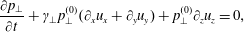 $$\begin{eqnarray}\displaystyle & \displaystyle \frac{\unicode[STIX]{x2202}p_{\bot }}{\unicode[STIX]{x2202}t}+\unicode[STIX]{x1D6FE}_{\bot }p_{\bot }^{(0)}(\unicode[STIX]{x2202}_{x}u_{x}+\unicode[STIX]{x2202}_{y}u_{y})+p_{\bot }^{(0)}\unicode[STIX]{x2202}_{z}u_{z}=0, & \displaystyle\end{eqnarray}$$
where for the CGL model
 $\unicode[STIX]{x1D6FE}_{\Vert }=3$
and
$\unicode[STIX]{x1D6FE}_{\Vert }=3$
and
 $\unicode[STIX]{x1D6FE}_{\bot }=2$
.Footnote
7
The reasoning for such a construction is to enable a smooth transition between two extreme cases – the CGL model on one side, and the isothermal model
$\unicode[STIX]{x1D6FE}_{\bot }=2$
.Footnote
7
The reasoning for such a construction is to enable a smooth transition between two extreme cases – the CGL model on one side, and the isothermal model
 $\unicode[STIX]{x1D6FE}_{\Vert }=1$
and
$\unicode[STIX]{x1D6FE}_{\Vert }=1$
and
 $\unicode[STIX]{x1D6FE}_{\bot }=1$
on the other side. The important observation is that in the parallel pressure equation the
$\unicode[STIX]{x1D6FE}_{\bot }=1$
on the other side. The important observation is that in the parallel pressure equation the
 $\unicode[STIX]{x1D6FE}_{\Vert }$
acts only on the parallel velocity component
$\unicode[STIX]{x1D6FE}_{\Vert }$
acts only on the parallel velocity component
 $u_{z}$
, and in the perpendicular pressure equation the
$u_{z}$
, and in the perpendicular pressure equation the
 $\unicode[STIX]{x1D6FE}_{\bot }$
acts only on the perpendicular velocity components
$\unicode[STIX]{x1D6FE}_{\bot }$
acts only on the perpendicular velocity components
 $u_{x},u_{y}$
. In MHD, the
$u_{x},u_{y}$
. In MHD, the
 $\unicode[STIX]{x1D6FE}$
acts on all three components
$\unicode[STIX]{x1D6FE}$
acts on all three components
 $u_{x},u_{y},u_{z}$
. The values of polytropic indices are directly related to the number of degrees of freedom
$u_{x},u_{y},u_{z}$
. The values of polytropic indices are directly related to the number of degrees of freedom
 $i$
, through the well-known relation
$i$
, through the well-known relation
 $\unicode[STIX]{x1D6FE}=(i+2)/i$
. In the MHD description the number of degrees of freedom is
$\unicode[STIX]{x1D6FE}=(i+2)/i$
. In the MHD description the number of degrees of freedom is
 $i=3$
and so
$i=3$
and so
 $\unicode[STIX]{x1D6FE}=5/3$
. In contrast, the CGL description can be interpreted as being composed of a (strongly coupled) mixture of one-dimensional and two-dimensional dynamics, where for the parallel direction
$\unicode[STIX]{x1D6FE}=5/3$
. In contrast, the CGL description can be interpreted as being composed of a (strongly coupled) mixture of one-dimensional and two-dimensional dynamics, where for the parallel direction
 $i=1$
and
$i=1$
and
 $\unicode[STIX]{x1D6FE}_{\Vert }=3$
and for the perpendicular direction
$\unicode[STIX]{x1D6FE}_{\Vert }=3$
and for the perpendicular direction
 $i=2$
and
$i=2$
and
 $\unicode[STIX]{x1D6FE}_{\bot }=2$
. The apparently subtle, but nevertheless fundamental difference between (3.157) and (3.158), (3.159) is the core of many differences between the MHD and CGL descriptions, such as for example the effect of the slow mode becoming faster than the Alfvén mode. The two systems remain different even if the mean CGL pressures (or temperatures) are prescribed to be isotropic
$\unicode[STIX]{x1D6FE}_{\bot }=2$
. The apparently subtle, but nevertheless fundamental difference between (3.157) and (3.158), (3.159) is the core of many differences between the MHD and CGL descriptions, such as for example the effect of the slow mode becoming faster than the Alfvén mode. The two systems remain different even if the mean CGL pressures (or temperatures) are prescribed to be isotropic
 $p_{\Vert }^{(0)}=p_{\bot }^{(0)}$
and equal to the mean MHD pressure
$p_{\Vert }^{(0)}=p_{\bot }^{(0)}$
and equal to the mean MHD pressure
 $p^{(0)}$
. This means that the MHD does not match the CGL description even if the distribution function is isotropic, as for example Maxwellian.
$p^{(0)}$
. This means that the MHD does not match the CGL description even if the distribution function is isotropic, as for example Maxwellian.
We briefly consider models with polytropic indices
 $\unicode[STIX]{x1D6FE}_{\Vert },\unicode[STIX]{x1D6FE}_{\bot }$
that are based on the linearized pressure equations (3.158), (3.159). If these pressure equations are ‘un-linearized’, i.e. if one performs a ‘reverse engineering’ procedure to obtain nonlinear equations (a procedure that is possible to do because of the known guidance by the CGL model), the nonlinear equations read
$\unicode[STIX]{x1D6FE}_{\Vert },\unicode[STIX]{x1D6FE}_{\bot }$
that are based on the linearized pressure equations (3.158), (3.159). If these pressure equations are ‘un-linearized’, i.e. if one performs a ‘reverse engineering’ procedure to obtain nonlinear equations (a procedure that is possible to do because of the known guidance by the CGL model), the nonlinear equations read
 $$\begin{eqnarray}\displaystyle & \displaystyle \frac{\text{d}p_{\Vert }}{\text{d}t}+p_{\Vert }\unicode[STIX]{x1D735}\boldsymbol{\cdot }\boldsymbol{u}+(\unicode[STIX]{x1D6FE}_{\Vert }-1)p_{\Vert }\hat{\boldsymbol{b}}\boldsymbol{\cdot }\unicode[STIX]{x1D735}\boldsymbol{u}\boldsymbol{\cdot }\hat{\boldsymbol{b}}=0; & \displaystyle\end{eqnarray}$$
 $$\begin{eqnarray}\displaystyle & \displaystyle \frac{\text{d}p_{\bot }}{\text{d}t}+\unicode[STIX]{x1D6FE}_{\bot }p_{\bot }\unicode[STIX]{x1D735}\boldsymbol{\cdot }\boldsymbol{u}-(\unicode[STIX]{x1D6FE}_{\bot }-1)p_{\bot }\hat{\boldsymbol{b}}\boldsymbol{\cdot }\unicode[STIX]{x1D735}\boldsymbol{u}\boldsymbol{\cdot }\hat{\boldsymbol{b}}=0, & \displaystyle\end{eqnarray}$$
which can be rewritten as
 $$\begin{eqnarray}\displaystyle \frac{\text{d}}{\text{d}t}\left(\frac{p_{\Vert }|\boldsymbol{B}|^{\unicode[STIX]{x1D6FE}_{\Vert }-1}}{\unicode[STIX]{x1D70C}^{\unicode[STIX]{x1D6FE}_{\Vert }}}\right)=0;\quad \frac{\text{d}}{\text{d}t}\left(\frac{p_{\bot }}{\unicode[STIX]{x1D70C}|\boldsymbol{B}|^{\unicode[STIX]{x1D6FE}_{\bot }-1}}\right)=0. & & \displaystyle\end{eqnarray}$$
Empirical fluid models of this type were studied for example by Hau & Sonnerup (Reference Hau and Sonnerup1993) and Hau et al. (Reference Hau, Phan, Sonnerup and Paschmann1993) with the motivation that spacecraft observations in the Earth’s magnetosheath often show behaviour that cannot be explained by the CGL values of
 $\unicode[STIX]{x1D6FE}_{\Vert }=3,\unicode[STIX]{x1D6FE}_{\bot }=2$
or by the isothermal values of
$\unicode[STIX]{x1D6FE}_{\Vert }=3,\unicode[STIX]{x1D6FE}_{\bot }=2$
or by the isothermal values of
 $\unicode[STIX]{x1D6FE}_{\Vert }=1,\unicode[STIX]{x1D6FE}_{\bot }=1$
, but can be fitted by the values that lie somewhere in between (and actually quite close to the isothermal case). For a direct comparison with the CGL model, the equations (3.162) can be rewritten to a form
$\unicode[STIX]{x1D6FE}_{\Vert }=1,\unicode[STIX]{x1D6FE}_{\bot }=1$
, but can be fitted by the values that lie somewhere in between (and actually quite close to the isothermal case). For a direct comparison with the CGL model, the equations (3.162) can be rewritten to a form
 $$\begin{eqnarray}\displaystyle & \displaystyle \frac{\text{d}}{\text{d}t}\left(\frac{p_{\Vert }|\boldsymbol{B}|^{2}}{\unicode[STIX]{x1D70C}^{3}}\right)=-(\unicode[STIX]{x1D6FE}_{\Vert }-3)\left(\frac{p_{\Vert }|\boldsymbol{B}|^{2}}{\unicode[STIX]{x1D70C}^{3}}\right)\frac{\unicode[STIX]{x1D70C}}{|\boldsymbol{B}|}\frac{\text{d}}{\text{d}t}\left(\frac{|\boldsymbol{B}|}{\unicode[STIX]{x1D70C}}\right); & \displaystyle\end{eqnarray}$$
 $$\begin{eqnarray}\displaystyle & \displaystyle \frac{\text{d}}{\text{d}t}\left(\frac{p_{\bot }}{\unicode[STIX]{x1D70C}|\boldsymbol{B}|}\right)=(\unicode[STIX]{x1D6FE}_{\bot }-2)\left(\frac{p_{\bot }}{\unicode[STIX]{x1D70C}|\boldsymbol{B}|}\right)\frac{1}{|\boldsymbol{B}|}\frac{\text{d}}{\text{d}t}|\boldsymbol{B}|, & \displaystyle\end{eqnarray}$$
or to an interesting alternative form
 $$\begin{eqnarray}\displaystyle & \displaystyle \frac{\text{d}}{\text{d}t}\ln \left(\frac{p_{\Vert }|\boldsymbol{B}|^{2}}{\unicode[STIX]{x1D70C}^{3}}\right)=-(\unicode[STIX]{x1D6FE}_{\Vert }-3)\frac{\text{d}}{\text{d}t}\ln \left(\frac{|\boldsymbol{B}|}{\unicode[STIX]{x1D70C}}\right); & \displaystyle\end{eqnarray}$$
 $$\begin{eqnarray}\displaystyle & \displaystyle \frac{\text{d}}{\text{d}t}\ln \left(\frac{p_{\bot }}{\unicode[STIX]{x1D70C}|\boldsymbol{B}|}\right)=(\unicode[STIX]{x1D6FE}_{\bot }-2)\frac{\text{d}}{\text{d}t}\ln |\boldsymbol{B}|. & \displaystyle\end{eqnarray}$$
Obviously, for CGL values of
 $\unicode[STIX]{x1D6FE}_{\Vert }=3,\unicode[STIX]{x1D6FE}_{\bot }=2$
the right-hand sides disappear and one obtains the classical CGL expressions. The right-hand sides of the above expressions can be compared with equations of Chew et al. (Reference Chew, Goldberger and Low1956) equations (2.82), (2.83) which contain the gyrotropic heat flux contributions. Therefore, the deviations from the CGL values of
$\unicode[STIX]{x1D6FE}_{\Vert }=3,\unicode[STIX]{x1D6FE}_{\bot }=2$
the right-hand sides disappear and one obtains the classical CGL expressions. The right-hand sides of the above expressions can be compared with equations of Chew et al. (Reference Chew, Goldberger and Low1956) equations (2.82), (2.83) which contain the gyrotropic heat flux contributions. Therefore, the deviations from the CGL values of
 $\unicode[STIX]{x1D6FE}_{\Vert }=3,\unicode[STIX]{x1D6FE}_{\bot }=2$
can be considered to offer a very simple empirical model (perhaps too simple) that shows how the heat flux contributions modify the CGL dynamics. The dispersion relations for this fluid model can be found in Hau et al. (Reference Hau, Phan, Sonnerup and Paschmann1993) and also in Abraham-Shrauner (Reference Abraham-Shrauner1973), who studied an even more general empirical model with four polytropic indices (essentially, the
$\unicode[STIX]{x1D6FE}_{\Vert }=3,\unicode[STIX]{x1D6FE}_{\bot }=2$
can be considered to offer a very simple empirical model (perhaps too simple) that shows how the heat flux contributions modify the CGL dynamics. The dispersion relations for this fluid model can be found in Hau et al. (Reference Hau, Phan, Sonnerup and Paschmann1993) and also in Abraham-Shrauner (Reference Abraham-Shrauner1973), who studied an even more general empirical model with four polytropic indices (essentially, the
 $\unicode[STIX]{x1D6FE}_{\Vert }$
,
$\unicode[STIX]{x1D6FE}_{\Vert }$
,
 $\unicode[STIX]{x1D6FE}_{\bot }$
acting on
$\unicode[STIX]{x1D6FE}_{\bot }$
acting on
 $|\boldsymbol{B}|$
and
$|\boldsymbol{B}|$
and
 $\unicode[STIX]{x1D70C}$
in (3.162) can be further split to two independent parameters). Interestingly, complex polytropic indices have been suggested to model Landau damping (Belmont & Mazelle Reference Belmont and Mazelle1992). Considering the linearized CGL equations (3.68)–(3.72) and linearized polytropic pressure equations (3.158)–(3.159) written in the
$\unicode[STIX]{x1D70C}$
in (3.162) can be further split to two independent parameters). Interestingly, complex polytropic indices have been suggested to model Landau damping (Belmont & Mazelle Reference Belmont and Mazelle1992). Considering the linearized CGL equations (3.68)–(3.72) and linearized polytropic pressure equations (3.158)–(3.159) written in the
 $x$
–
$x$
–
 $z$
plane yields the dispersion relations for this model. The Alfvén wave is still decoupled from the rest of the system and the Alfvén wave dispersion relation is unaffected by the different pressure equations, therefore also yielding the same oblique firehose instability threshold. What is modified is the dispersion relation of the slow and fast waves. The velocity equations read
$z$
plane yields the dispersion relations for this model. The Alfvén wave is still decoupled from the rest of the system and the Alfvén wave dispersion relation is unaffected by the different pressure equations, therefore also yielding the same oblique firehose instability threshold. What is modified is the dispersion relation of the slow and fast waves. The velocity equations read
 $$\begin{eqnarray}\displaystyle & \displaystyle \frac{\unicode[STIX]{x2202}^{2}u_{x}}{\unicode[STIX]{x2202}t^{2}}-\frac{p_{\bot }^{(0)}}{\unicode[STIX]{x1D70C}_{0}}(\unicode[STIX]{x1D6FE}_{\bot }\unicode[STIX]{x2202}_{x}^{2}u_{x}+\unicode[STIX]{x2202}_{x}\unicode[STIX]{x2202}_{z}u_{z})+\left(\frac{p_{\Vert }^{(0)}}{\unicode[STIX]{x1D70C}_{0}}-\frac{p_{\bot }^{(0)}}{\unicode[STIX]{x1D70C}_{0}}-V_{A}^{2}\right)\unicode[STIX]{x2202}_{z}^{2}u_{x}-V_{A}^{2}\unicode[STIX]{x2202}_{x}^{2}u_{x}=0; & \displaystyle\end{eqnarray}$$
 $$\begin{eqnarray}\displaystyle & \displaystyle \frac{\unicode[STIX]{x2202}^{2}u_{z}}{\unicode[STIX]{x2202}t^{2}}-\unicode[STIX]{x1D6FE}_{\Vert }\frac{p_{\Vert }^{(0)}}{\unicode[STIX]{x1D70C}_{0}}\unicode[STIX]{x2202}_{z}^{2}u_{z}-\frac{p_{\bot }^{(0)}}{\unicode[STIX]{x1D70C}_{0}}\unicode[STIX]{x2202}_{x}\unicode[STIX]{x2202}_{z}u_{x}=0, & \displaystyle\end{eqnarray}$$
and the transformation to Fourier space yields the velocity matrix
 $$\begin{eqnarray}\displaystyle \left(\begin{array}{@{}cc@{}}\displaystyle \unicode[STIX]{x1D714}^{2}-\left(\unicode[STIX]{x1D6FE}_{\bot }\frac{p_{\bot }^{(0)}}{\unicode[STIX]{x1D70C}_{0}}+V_{A}^{2}\right)k_{\bot }^{2}+\left(\frac{p_{\Vert }^{(0)}}{\unicode[STIX]{x1D70C}_{0}}-\frac{p_{\bot }^{(0)}}{\unicode[STIX]{x1D70C}_{0}}-V_{A}^{2}\right)k_{\Vert }^{2}; & \displaystyle -\frac{p_{\bot }^{(0)}}{\unicode[STIX]{x1D70C}_{0}}k_{\bot }k_{\Vert }\\ \displaystyle -\frac{p_{\bot }^{(0)}}{\unicode[STIX]{x1D70C}_{0}}k_{\bot }k_{\Vert }; & \displaystyle \unicode[STIX]{x1D714}^{2}-\unicode[STIX]{x1D6FE}_{\Vert }\frac{p_{\Vert }^{(0)}}{\unicode[STIX]{x1D70C}_{0}}k_{\Vert }^{2}\end{array}\right)\left(\begin{array}{@{}c@{}}u_{x}\\ u_{z}\end{array}\right)=\left(\begin{array}{@{}c@{}}0\\ 0\end{array}\right), & & \displaystyle \nonumber\\ \displaystyle & & \displaystyle\end{eqnarray}$$
or alternatively
 $$\begin{eqnarray}\displaystyle \left(\begin{array}{@{}cc@{}}\displaystyle \widetilde{\unicode[STIX]{x1D714}}^{2}-\left(\unicode[STIX]{x1D6FE}_{\bot }a_{p}\frac{\unicode[STIX]{x1D6FD}_{\Vert }}{2}+1\right)\widetilde{k}_{\bot }^{2}-\left(1+\frac{\unicode[STIX]{x1D6FD}_{\Vert }}{2}(a_{p}-1)\right)\widetilde{k}_{\Vert }^{2}; & \displaystyle -\frac{1}{2}a_{p}\unicode[STIX]{x1D6FD}_{\Vert }\widetilde{k}_{\bot }\widetilde{k}_{\Vert }\\ \displaystyle -\frac{1}{2}a_{p}\unicode[STIX]{x1D6FD}_{\Vert }\widetilde{k}_{\bot }\widetilde{k}_{\Vert }; & \displaystyle \widetilde{\unicode[STIX]{x1D714}}^{2}-\unicode[STIX]{x1D6FE}_{\Vert }\frac{\unicode[STIX]{x1D6FD}_{\Vert }}{2}\widetilde{k}_{\Vert }^{2}\end{array}\right)\left(\begin{array}{@{}c@{}}u_{x}\\ u_{z}\end{array}\right)=\left(\begin{array}{@{}c@{}}0\\ 0\end{array}\right). & & \displaystyle \nonumber\\ \displaystyle & & \displaystyle\end{eqnarray}$$
Calculating the determinant yields a dispersion relation for the slow and fast modes in the form
 $$\begin{eqnarray}\displaystyle & \displaystyle \widetilde{\unicode[STIX]{x1D714}}^{4}-A_{2}\widetilde{\unicode[STIX]{x1D714}}^{2}+A_{0}=0; & \displaystyle\end{eqnarray}$$
 $$\begin{eqnarray}\displaystyle & \displaystyle A_{2}=\widetilde{k}_{\bot }^{2}\left(1+\frac{\unicode[STIX]{x1D6FE}_{\bot }}{2}a_{p}\unicode[STIX]{x1D6FD}_{\Vert }\right)+\widetilde{k}_{\Vert }^{2}\left(1+\frac{1}{2}\unicode[STIX]{x1D6FD}_{\Vert }(\unicode[STIX]{x1D6FE}_{\Vert }-1)+\frac{1}{2}a_{p}\unicode[STIX]{x1D6FD}_{\Vert }\right); & \displaystyle\end{eqnarray}$$
 $$\begin{eqnarray}\displaystyle & \displaystyle A_{0}=\frac{\unicode[STIX]{x1D6FE}_{\Vert }}{2}\widetilde{k}_{\Vert }^{2}\unicode[STIX]{x1D6FD}_{\Vert }\left[\widetilde{k}_{\Vert }^{2}\left(1-\frac{1}{2}\unicode[STIX]{x1D6FD}_{\Vert }+\frac{1}{2}a_{p}\unicode[STIX]{x1D6FD}_{\Vert }\right)+\widetilde{k}_{\bot }^{2}\left(1+\frac{\unicode[STIX]{x1D6FE}_{\bot }}{2}a_{p}\unicode[STIX]{x1D6FD}_{\Vert }-\frac{1}{2\unicode[STIX]{x1D6FE}_{\Vert }}a_{p}^{2}\unicode[STIX]{x1D6FD}_{\Vert }\right)\right]. & \displaystyle\end{eqnarray}$$
Solutions for parallel propagation
 $(k_{\bot }=0)$
are the usual CGL Alfvén mode and the ion-acoustic mode
$(k_{\bot }=0)$
are the usual CGL Alfvén mode and the ion-acoustic mode
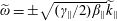 $\widetilde{\unicode[STIX]{x1D714}}=\pm \sqrt{(\unicode[STIX]{x1D6FE}_{\Vert }/2)\unicode[STIX]{x1D6FD}_{\Vert }}\widetilde{k}_{\Vert }$
, and for perpendicular propagation
$\widetilde{\unicode[STIX]{x1D714}}=\pm \sqrt{(\unicode[STIX]{x1D6FE}_{\Vert }/2)\unicode[STIX]{x1D6FD}_{\Vert }}\widetilde{k}_{\Vert }$
, and for perpendicular propagation
 $(k_{\Vert }=0)$
the fast mode
$(k_{\Vert }=0)$
the fast mode
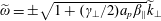 $\widetilde{\unicode[STIX]{x1D714}}=\pm \sqrt{1+(\unicode[STIX]{x1D6FE}_{\bot }/2)a_{p}\unicode[STIX]{x1D6FD}_{\Vert }}\widetilde{k}_{\bot }$
. Similarly to the CGL description it can be shown that
$\widetilde{\unicode[STIX]{x1D714}}=\pm \sqrt{1+(\unicode[STIX]{x1D6FE}_{\bot }/2)a_{p}\unicode[STIX]{x1D6FD}_{\Vert }}\widetilde{k}_{\bot }$
. Similarly to the CGL description it can be shown that
 $A_{2}^{2}-4A_{0}\geqslant 0$
because of the trick (3.137), implying that the slow mode becomes unstable when
$A_{2}^{2}-4A_{0}\geqslant 0$
because of the trick (3.137), implying that the slow mode becomes unstable when
 $A_{0}<0$
, i.e. when
$A_{0}<0$
, i.e. when
 $$\begin{eqnarray}\left[k_{\Vert }^{2}\left(1-\frac{1}{2}\unicode[STIX]{x1D6FD}_{\Vert }+\frac{1}{2}a_{p}\unicode[STIX]{x1D6FD}_{\Vert }\right)+k_{\bot }^{2}\left(1+\frac{\unicode[STIX]{x1D6FE}_{\bot }}{2}a_{p}\unicode[STIX]{x1D6FD}_{\Vert }-\frac{1}{2\unicode[STIX]{x1D6FE}_{\Vert }}a_{p}^{2}\unicode[STIX]{x1D6FD}_{\Vert }\right)\right]<0.\end{eqnarray}$$
The two competing instabilities are again the parallel firehose instability and the highly oblique mirror instability. The parallel firehose instability has the same threshold as obtained previously. However, the mirror instability threshold reads
 $$\begin{eqnarray}1+\frac{\unicode[STIX]{x1D6FE}_{\bot }}{2}a_{p}\unicode[STIX]{x1D6FD}_{\Vert }-\frac{1}{2\unicode[STIX]{x1D6FE}_{\Vert }}a_{p}^{2}\unicode[STIX]{x1D6FD}_{\Vert }<0,\end{eqnarray}$$
which is consistent with the result of Hau & Sonnerup (Reference Hau and Sonnerup1993), their equation (14), written in the formFootnote 8
 $$\begin{eqnarray}\unicode[STIX]{x1D6FE}_{\Vert }\unicode[STIX]{x1D6FD}_{\Vert }<\frac{\unicode[STIX]{x1D6FD}_{\bot }^{2}}{2+\unicode[STIX]{x1D6FE}_{\bot }\unicode[STIX]{x1D6FD}_{\bot }}.\end{eqnarray}$$
For
 $\unicode[STIX]{x1D6FE}_{\Vert }=3,\unicode[STIX]{x1D6FE}_{\bot }=2$
, the condition (3.175) is naturally equivalent to the CGL mirror threshold. However, the condition offers a temptingly simple result to keep the perpendicular polytropic index unchanged
$\unicode[STIX]{x1D6FE}_{\Vert }=3,\unicode[STIX]{x1D6FE}_{\bot }=2$
, the condition (3.175) is naturally equivalent to the CGL mirror threshold. However, the condition offers a temptingly simple result to keep the perpendicular polytropic index unchanged
 $\unicode[STIX]{x1D6FE}_{\bot }=2$
and modifies the parallel polytropic index to
$\unicode[STIX]{x1D6FE}_{\bot }=2$
and modifies the parallel polytropic index to
 $\unicode[STIX]{x1D6FE}_{\Vert }=1/2$
. In this way, the mirror threshold matches the correct kinetic threshold (3.94). Nevertheless, this is just an interesting empirical concept, it fixes the highly oblique mirror threshold but at the same time moves the slow and fast mode dispersion relations in other directions, for example the parallel sound speed in such a model is
$\unicode[STIX]{x1D6FE}_{\Vert }=1/2$
. In this way, the mirror threshold matches the correct kinetic threshold (3.94). Nevertheless, this is just an interesting empirical concept, it fixes the highly oblique mirror threshold but at the same time moves the slow and fast mode dispersion relations in other directions, for example the parallel sound speed in such a model is
 $C_{\Vert }^{2}=\frac{1}{2}p_{\Vert }^{(0)}/\unicode[STIX]{x1D70C}_{0}$
, which appears to be unrealistically low. Such a ‘tuning’ of models with free parameters – only in one particular direction and only at the level of the dispersion relations – can be sometimes useful for interpretation of observational data, however, such models will usually lead to unphysical situations. We will not consider models with polytropic indices further in this text. Instead, to obtain a better match with kinetic description, it is advisable to use the correct CGL values of
$C_{\Vert }^{2}=\frac{1}{2}p_{\Vert }^{(0)}/\unicode[STIX]{x1D70C}_{0}$
, which appears to be unrealistically low. Such a ‘tuning’ of models with free parameters – only in one particular direction and only at the level of the dispersion relations – can be sometimes useful for interpretation of observational data, however, such models will usually lead to unphysical situations. We will not consider models with polytropic indices further in this text. Instead, to obtain a better match with kinetic description, it is advisable to use the correct CGL values of
 $\unicode[STIX]{x1D6FE}_{\Vert }=3,\unicode[STIX]{x1D6FE}_{\bot }=2$
and focus on fluid models that derive the correct heat flux contributions
$\unicode[STIX]{x1D6FE}_{\Vert }=3,\unicode[STIX]{x1D6FE}_{\bot }=2$
and focus on fluid models that derive the correct heat flux contributions
 $q_{\Vert }$
and
$q_{\Vert }$
and
 $q_{\bot }$
.
$q_{\bot }$
.
3.12 CGL and radially expanding solar wind
Similarly to MHD, the CGL fluid model can be very useful for understanding the evolution of temperature in the radially expanding solar wind. A good discussion can be found for example in Matteini et al. (Reference Matteini, Landi, Hellinger, Pantellini, Maksimovic, Velli, Goldstein and Marsch2007), Matteini et al. (Reference Matteini, Hellinger, Goldstein, Landi, Velli and Neugebauer2013) and references therein. Let us first consider the MHD case. Combining the pressure equation
 $\text{d}p/\text{d}t+\unicode[STIX]{x1D6FE}\unicode[STIX]{x1D735}\boldsymbol{\cdot }\boldsymbol{u}=0$
with the density equation
$\text{d}p/\text{d}t+\unicode[STIX]{x1D6FE}\unicode[STIX]{x1D735}\boldsymbol{\cdot }\boldsymbol{u}=0$
with the density equation
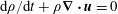 $\text{d}\unicode[STIX]{x1D70C}/\text{d}t+\unicode[STIX]{x1D70C}\unicode[STIX]{x1D735}\boldsymbol{\cdot }\boldsymbol{u}=0$
yields
$\text{d}\unicode[STIX]{x1D70C}/\text{d}t+\unicode[STIX]{x1D70C}\unicode[STIX]{x1D735}\boldsymbol{\cdot }\boldsymbol{u}=0$
yields
 $$\begin{eqnarray}\text{MHD:}\quad \frac{\text{d}}{\text{d}t}\left(\frac{p}{\unicode[STIX]{x1D70C}^{\unicode[STIX]{x1D6FE}}}\right)=0;\quad \Rightarrow \quad \frac{\text{d}}{\text{d}t}\left(\frac{T}{\unicode[STIX]{x1D70C}^{\unicode[STIX]{x1D6FE}-1}}\right)=0,\end{eqnarray}$$
which in a steady state (or co-moving with the convective derivative) implies
 $T\sim \unicode[STIX]{x1D70C}^{\unicode[STIX]{x1D6FE}-1}$
. By considering simple radially expanding solar wind, one prescribes that the density
$T\sim \unicode[STIX]{x1D70C}^{\unicode[STIX]{x1D6FE}-1}$
. By considering simple radially expanding solar wind, one prescribes that the density
 $\unicode[STIX]{x1D70C}$
evolves with the heliocentric distance
$\unicode[STIX]{x1D70C}$
evolves with the heliocentric distance
 $r$
as
$r$
as
 $\unicode[STIX]{x1D70C}\sim 1/r^{2}$
, and by using
$\unicode[STIX]{x1D70C}\sim 1/r^{2}$
, and by using
 $\unicode[STIX]{x1D6FE}=5/3$
, the ideal MHD model yields (in the absence of any dissipation and associated turbulent heating)
$\unicode[STIX]{x1D6FE}=5/3$
, the ideal MHD model yields (in the absence of any dissipation and associated turbulent heating)
 $$\begin{eqnarray}T\sim r^{-4/3}.\end{eqnarray}$$
In contrast, the CGL equations (3.41) are rewritten as
 $$\begin{eqnarray}\text{CGL:}\quad \frac{\text{d}}{\text{d}t}\left(\frac{T_{\Vert }|\boldsymbol{B}|^{2}}{\unicode[STIX]{x1D70C}^{2}}\right)=0;\quad \frac{\text{d}}{\text{d}t}\left(\frac{T_{\bot }}{|\boldsymbol{B}|}\right)=0,\end{eqnarray}$$
which in a steady state implies
 $$\begin{eqnarray}T_{\Vert }\sim \frac{\unicode[STIX]{x1D70C}^{2}}{|\boldsymbol{B}|^{2}};\quad T_{\bot }\sim |\boldsymbol{B}|;\quad \frac{T_{\bot }}{T_{\Vert }}=\frac{|\boldsymbol{B}|^{3}}{\unicode[STIX]{x1D70C}^{2}}.\end{eqnarray}$$
For the magnetic field it is possible to consider profiles of roughly
 $|\boldsymbol{B}|\sim 1/r^{2}$
, or
$|\boldsymbol{B}|\sim 1/r^{2}$
, or
 $|\boldsymbol{B}|\sim 1/r$
(one can be more precise and consider the Parker spiral profile). The first magnetic field profile yields
$|\boldsymbol{B}|\sim 1/r$
(one can be more precise and consider the Parker spiral profile). The first magnetic field profile yields
 $$\begin{eqnarray}|\boldsymbol{B}|\sim 1/r^{2};\quad \Rightarrow \quad T_{\Vert }\sim \text{const.};\quad T_{\bot }\sim 1/r^{2};\quad \frac{T_{\bot }}{T_{\Vert }}\sim 1/r^{2}.\end{eqnarray}$$
The second magnetic field profile yields
 $$\begin{eqnarray}|\boldsymbol{B}|\sim 1/r;\quad \Rightarrow \quad T_{\Vert }\sim 1/r^{2};\quad T_{\bot }\sim 1/r;\quad \frac{T_{\bot }}{T_{\Vert }}\sim r.\end{eqnarray}$$
There is also a curious case when the magnetic field profile is prescribed to be
 $|\boldsymbol{B}|\sim r^{-4/3}$
, i.e. a profile between two cases of
$|\boldsymbol{B}|\sim r^{-4/3}$
, i.e. a profile between two cases of
 $1/r$
and
$1/r$
and
 $1/r^{2}$
, that yields
$1/r^{2}$
, that yields
 $$\begin{eqnarray}|\boldsymbol{B}|\sim r^{-4/3};\quad \Rightarrow \quad T_{\Vert }\sim r^{-4/3};\quad T_{\bot }\sim r^{-4/3};\quad \frac{T_{\bot }}{T_{\Vert }}\sim \text{const.},\end{eqnarray}$$
and the temperature anisotropy stays constant. The estimations are of course valid only until a firehose threshold or a mirror threshold is reached. For example, evolution according to (3.181) will lead the system to a firehose threshold, and evolution according to (3.182) will lead the system to a mirror threshold. In general, if we fix the density profile to
 $\unicode[STIX]{x1D70C}\sim 1/r^{2}$
, any magnetic field profile steeper than
$\unicode[STIX]{x1D70C}\sim 1/r^{2}$
, any magnetic field profile steeper than
 $r^{-4/3}$
will evolve the system towards a firehose threshold, and a magnetic field profile shallower than
$r^{-4/3}$
will evolve the system towards a firehose threshold, and a magnetic field profile shallower than
 $r^{-4/3}$
will evolve the system towards a mirror threshold. The estimations do not reveal the presence of the firehose instability or the mirror instability in the CGL model, since the solutions are written in a steady state, and concern only evolution of mean temperatures (i.e. the solutions should be written with
$r^{-4/3}$
will evolve the system towards a mirror threshold. The estimations do not reveal the presence of the firehose instability or the mirror instability in the CGL model, since the solutions are written in a steady state, and concern only evolution of mean temperatures (i.e. the solutions should be written with
 $T_{\Vert }^{(0)},T_{\bot }^{(0)}$
). To find an instability, one of course needs to consider evolution equations for fluctuating variables and to analyse the associated dispersion relations, since it is the fluctuations that become unstable. Further discussion can be found in Hunana & Zank (Reference Hunana and Zank2017).
$T_{\Vert }^{(0)},T_{\bot }^{(0)}$
). To find an instability, one of course needs to consider evolution equations for fluctuating variables and to analyse the associated dispersion relations, since it is the fluctuations that become unstable. Further discussion can be found in Hunana & Zank (Reference Hunana and Zank2017).
From a linear perspective, the CGL model has to be accompanied by the Hall term and FLR corrections, so that the instabilities are stabilized at small spatial scales. However, considering nonlinear evolution with finite amplitudes of fluctuations, even the non-dispersive CGL model is stabilized. For example, considering parallel propagation, Tenerani, Velli & Hellinger (Reference Tenerani, Velli and Hellinger2017) has shown that the firehose instability criterion reads (see (9) in that paper)
 $$\begin{eqnarray}V_{A}^{2}+\frac{1}{\unicode[STIX]{x1D70C}_{0}}\frac{p_{\bot }^{(0)}-p_{\Vert }^{(0)}}{1+\left|\displaystyle \frac{\boldsymbol{B}_{\bot }}{B_{0}}\right|^{2}}<0;\quad \Rightarrow \quad 1+\frac{\unicode[STIX]{x1D6FD}_{\Vert }}{2}\frac{a_{p}-1}{1+\left|\displaystyle \frac{\boldsymbol{B}_{\bot }}{B_{0}}\right|^{2}}<0,\end{eqnarray}$$
i.e. for infinitely small amplitudes of the magnetic field, the usual firehose criterion is obtained. However, when the CGL system reaches firehose-unstable regime and the amplitude of the fluctuations starts to grow, the firehose criterion is modified according to (3.184). Therefore, the amplitude of the fluctuations cannot grow without bounds, and beyond some critical amplitude, the system becomes again stabilized. The condition (3.184) nicely demonstrates how the CGL system is stabilized during nonlinear evolution, once the firehose instability is reached. For further discussion, see Tenerani et al. (Reference Tenerani, Velli and Hellinger2017), Tenerani & Velli (Reference Tenerani and Velli2018).
To finish this subsection, the heuristically generalized CGL model with polytropic indices
 $\unicode[STIX]{x1D6FE}_{\Vert }$
,
$\unicode[STIX]{x1D6FE}_{\Vert }$
,
 $\unicode[STIX]{x1D6FE}_{\bot }$
yields that, in the steady state, the mean temperatures evolve according to
$\unicode[STIX]{x1D6FE}_{\bot }$
yields that, in the steady state, the mean temperatures evolve according to
 $$\begin{eqnarray}T_{\Vert }=\left(\frac{\unicode[STIX]{x1D70C}}{|\boldsymbol{B}|}\right)^{\unicode[STIX]{x1D6FE}_{\Vert }-1};\quad T_{\bot }=|\boldsymbol{B}|^{\unicode[STIX]{x1D6FE}_{\bot }-1};\quad \frac{T_{\bot }}{T_{\Vert }}=\frac{|\boldsymbol{B}|^{\unicode[STIX]{x1D6FE}_{\Vert }+\unicode[STIX]{x1D6FE}_{\bot }-2}}{\unicode[STIX]{x1D70C}^{\unicode[STIX]{x1D6FE}_{\Vert }-1}},\end{eqnarray}$$
and such heuristic models can yield a wide array of possible temperature profiles.
3.13 CGL model – summary
The usual ‘combining’ of evolution equations (by performing
 $\unicode[STIX]{x2202}/\unicode[STIX]{x2202}t$
and substituting one equation into another) is very useful to gain insight into the linear eigenmodes of a considered system. However, for more advanced fluid models, such a procedure can become very analytically involved, and it is much easier to calculate the determinant of the entire system with analytic software, such as Maple or Mathematica. Therefore, for more advanced fluid models we often do not write down the final dispersion relation for arbitrary propagation angle (which might be uneconomically large to write down), and we only provide normalized, linearized in the
$\unicode[STIX]{x2202}/\unicode[STIX]{x2202}t$
and substituting one equation into another) is very useful to gain insight into the linear eigenmodes of a considered system. However, for more advanced fluid models, such a procedure can become very analytically involved, and it is much easier to calculate the determinant of the entire system with analytic software, such as Maple or Mathematica. Therefore, for more advanced fluid models we often do not write down the final dispersion relation for arbitrary propagation angle (which might be uneconomically large to write down), and we only provide normalized, linearized in the
 $x$
–
$x$
–
 $z$
plane and Fourier transformed equations. For easy comparison with more advanced fluid models, it is beneficial to write the final CGL equations in the same form. It is useful to work in normalized units, and we drop writing the tilde. The normalized, linearized in the
$z$
plane and Fourier transformed equations. For easy comparison with more advanced fluid models, it is beneficial to write the final CGL equations in the same form. It is useful to work in normalized units, and we drop writing the tilde. The normalized, linearized in the
 $x$
–
$x$
–
 $z$
plane, and Fourier transformed CGL equations read
$z$
plane, and Fourier transformed CGL equations read
 $$\begin{eqnarray}\displaystyle & \displaystyle -\unicode[STIX]{x1D714}\unicode[STIX]{x1D70C}+k_{\bot }u_{x}+k_{\Vert }u_{z}=0; & \displaystyle\end{eqnarray}$$
 $$\begin{eqnarray}\displaystyle & \displaystyle -\unicode[STIX]{x1D714}u_{x}+\frac{\unicode[STIX]{x1D6FD}_{\Vert }}{2}k_{\bot }p_{\bot }-v_{A\Vert }^{2}k_{\Vert }B_{x}+k_{\bot }B_{z}=0; & \displaystyle\end{eqnarray}$$
 $$\begin{eqnarray}\displaystyle & \displaystyle -\unicode[STIX]{x1D714}u_{y}-v_{A\Vert }^{2}k_{\Vert }B_{y}=0; & \displaystyle\end{eqnarray}$$
 $$\begin{eqnarray}\displaystyle & \displaystyle -\unicode[STIX]{x1D714}u_{z}+\frac{\unicode[STIX]{x1D6FD}_{\Vert }}{2}k_{\Vert }p_{\Vert }+\frac{\unicode[STIX]{x1D6FD}_{\Vert }}{2}(1-a_{p})k_{\bot }B_{x}=0; & \displaystyle\end{eqnarray}$$
 $$\begin{eqnarray}\displaystyle & \displaystyle -\unicode[STIX]{x1D714}B_{x}-k_{\Vert }u_{x}=0;\quad -\unicode[STIX]{x1D714}B_{y}-k_{\Vert }u_{y}=0;\quad -\unicode[STIX]{x1D714}B_{z}+k_{\bot }u_{x}=0; & \displaystyle\end{eqnarray}$$
 $$\begin{eqnarray}\displaystyle & \displaystyle -\unicode[STIX]{x1D714}p_{\Vert }+k_{\bot }u_{x}+3k_{\Vert }u_{z}=0; & \displaystyle\end{eqnarray}$$
 $$\begin{eqnarray}\displaystyle & \displaystyle -\unicode[STIX]{x1D714}p_{\bot }+2a_{p}k_{\bot }u_{x}+a_{p}k_{\Vert }u_{z}=0, & \displaystyle\end{eqnarray}$$
where we have introduced the normalized parallel Alfvén speed
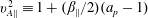 $v_{A\Vert }^{2}\equiv 1+(\unicode[STIX]{x1D6FD}_{\Vert }/2)(a_{p}-1)$
(the tilde on
$v_{A\Vert }^{2}\equiv 1+(\unicode[STIX]{x1D6FD}_{\Vert }/2)(a_{p}-1)$
(the tilde on
 $v_{A\Vert }$
is dropped too). The determinant can be easily calculated and factorized in Maple, yielding the CGL dispersion relation in normalized units (tilde are dropped)
$v_{A\Vert }$
is dropped too). The determinant can be easily calculated and factorized in Maple, yielding the CGL dispersion relation in normalized units (tilde are dropped)
 $$\begin{eqnarray}\displaystyle & \displaystyle (\unicode[STIX]{x1D714}^{2}-k_{\Vert }^{2}v_{A\Vert }^{2})(\unicode[STIX]{x1D714}^{4}-A_{2}\unicode[STIX]{x1D714}^{2}+A_{0})=0; & \displaystyle\end{eqnarray}$$
 $$\begin{eqnarray}\displaystyle & \displaystyle A_{2}=k_{\bot }^{2}(1+a_{p}\unicode[STIX]{x1D6FD}_{\Vert })+k_{\Vert }^{2}\left(v_{A\Vert }^{2}+{\textstyle \frac{3}{2}}\unicode[STIX]{x1D6FD}_{\Vert }\right); & \displaystyle\end{eqnarray}$$
 $$\begin{eqnarray}\displaystyle & \displaystyle A_{0}={\textstyle \frac{3}{2}}k_{\Vert }^{2}\unicode[STIX]{x1D6FD}_{\Vert }\left[k_{\Vert }^{2}v_{A\Vert }^{2}+k_{\bot }^{2}\left(1+a_{p}\unicode[STIX]{x1D6FD}_{\Vert }-{\textstyle \frac{1}{6}}a_{p}^{2}\unicode[STIX]{x1D6FD}_{\Vert }\right)\right], & \displaystyle\end{eqnarray}$$
which of course agrees with the previously obtained CGL solutions for the Alfvén mode (3.81), and the slow and fast modes (3.90).
4 Hall-CGL model
Here we consider a slightly generalized CGL model when the Hall term is included in the induction equation. Concerning the isotropic Hall-MHD model, a good comparison with solutions of kinetic theory can be found for example in Howes (Reference Howes2009). Before we proceed with the discussion of dispersion relations, we want to point out how the Hall term and the electron pressure contributions and the electron inertia contributions modify the usual ‘CGL conservation equations’ for protons. The general electric field was already written down in (3.15). For a moment it is beneficial to consider this most general form including the electron inertia and the electron pressure contributions and separate the electric field into two parts
 $$\begin{eqnarray}\displaystyle & \displaystyle \boldsymbol{E}=-\frac{1}{c}\boldsymbol{u}_{p}\times \boldsymbol{B}+\boldsymbol{E}_{H} & \displaystyle\end{eqnarray}$$
 $$\begin{eqnarray}\displaystyle & \displaystyle \boldsymbol{E}_{H}=\frac{1}{4\unicode[STIX]{x03C0}en}(\unicode[STIX]{x1D735}\times \boldsymbol{B})\times \boldsymbol{B}-\frac{1}{en}\unicode[STIX]{x1D735}\boldsymbol{\cdot }\boldsymbol{p}_{e}-\frac{m_{e}}{e}\left(\frac{\unicode[STIX]{x2202}\boldsymbol{u}_{e}}{\unicode[STIX]{x2202}t}+\boldsymbol{u}_{e}\boldsymbol{\cdot }\unicode[STIX]{x1D735}\boldsymbol{u}_{e}\right). & \displaystyle\end{eqnarray}$$
The notation
 $\boldsymbol{E}_{H}$
is perhaps slightly misleading since only the first term in (4.2) is usually called the Hall electric field. Note that the first term in
$\boldsymbol{E}_{H}$
is perhaps slightly misleading since only the first term in (4.2) is usually called the Hall electric field. Note that the first term in
 $\boldsymbol{E}_{H}$
still has to be used in the proton momentum equation even for the simplest CGL (or MHD) models. The induction equation then reads
$\boldsymbol{E}_{H}$
still has to be used in the proton momentum equation even for the simplest CGL (or MHD) models. The induction equation then reads
 $$\begin{eqnarray}\frac{\unicode[STIX]{x2202}\boldsymbol{B}}{\unicode[STIX]{x2202}t}=\unicode[STIX]{x1D735}\times (\boldsymbol{u}_{p}\times \boldsymbol{B})-c\unicode[STIX]{x1D735}\times \boldsymbol{E}_{H},\end{eqnarray}$$
which is then rewritten with the use of the convective derivative as
 $$\begin{eqnarray}\displaystyle & \displaystyle \frac{\text{d}\boldsymbol{B}}{\text{d}t}=-\boldsymbol{B}\unicode[STIX]{x1D735}\boldsymbol{\cdot }\boldsymbol{u}_{p}+\boldsymbol{B}\boldsymbol{\cdot }\unicode[STIX]{x1D735}\boldsymbol{u}_{p}-c\unicode[STIX]{x1D735}\times \boldsymbol{E}_{H}; & \displaystyle\end{eqnarray}$$
 $$\begin{eqnarray}\displaystyle & \displaystyle \frac{\hat{\boldsymbol{b}}}{|\boldsymbol{B}|}\boldsymbol{\cdot }\frac{\text{d}\boldsymbol{B}}{\text{d}t}=-\unicode[STIX]{x1D735}\boldsymbol{\cdot }\boldsymbol{u}_{p}+\hat{\boldsymbol{b}}\boldsymbol{\cdot }\unicode[STIX]{x1D735}\boldsymbol{u}_{p}\boldsymbol{\cdot }\hat{\boldsymbol{b}}-\frac{c\hat{\boldsymbol{b}}}{|\boldsymbol{B}|}\boldsymbol{\cdot }(\unicode[STIX]{x1D735}\times \boldsymbol{E}_{H}). & \displaystyle\end{eqnarray}$$
The last expression is then used in the completely general equations (3.46), (3.47), which yields
 $$\begin{eqnarray}\displaystyle & \displaystyle \frac{\text{d}}{\text{d}t}\left(\frac{p_{\Vert p}|\boldsymbol{B}|^{2}}{\unicode[STIX]{x1D70C}_{p}^{3}}\right)=\frac{|\boldsymbol{B}|^{2}}{\unicode[STIX]{x1D70C}_{p}^{3}}\left(\frac{\text{d}p_{\Vert p}}{\text{d}t}+p_{\Vert p}\unicode[STIX]{x1D735}\boldsymbol{\cdot }\boldsymbol{u}_{p}+2p_{\Vert p}\hat{\boldsymbol{b}}\boldsymbol{\cdot }\unicode[STIX]{x1D735}\boldsymbol{u}_{p}\boldsymbol{\cdot }\hat{\boldsymbol{b}}-2p_{\Vert p}\frac{c\hat{\boldsymbol{b}}}{|\boldsymbol{B}|}\boldsymbol{\cdot }(\unicode[STIX]{x1D735}\times \boldsymbol{E}_{H})\right); & \displaystyle \nonumber\\ \displaystyle & & \displaystyle\end{eqnarray}$$
 $$\begin{eqnarray}\displaystyle & \displaystyle \frac{\text{d}}{\text{d}t}\left(\frac{p_{\bot p}}{\unicode[STIX]{x1D70C}_{p}|\boldsymbol{B}|}\right)=\frac{1}{\unicode[STIX]{x1D70C}_{p}|\boldsymbol{B}|}\left(\frac{\text{d}p_{\bot p}}{\text{d}t}+2p_{\bot p}\unicode[STIX]{x1D735}\boldsymbol{\cdot }\boldsymbol{u}_{p}-p_{\bot p}\hat{\boldsymbol{b}}\boldsymbol{\cdot }\unicode[STIX]{x1D735}\boldsymbol{u}_{p}\boldsymbol{\cdot }\hat{\boldsymbol{b}}+p_{\bot p}\frac{c\hat{\boldsymbol{b}}}{|\boldsymbol{B}|}\boldsymbol{\cdot }(\unicode[STIX]{x1D735}\times \boldsymbol{E}_{H})\right). & \displaystyle \nonumber\\ \displaystyle & & \displaystyle\end{eqnarray}$$
By cancelling pressure equations (3.3), (3.4), that are also the pressure equations of the Hall-CGL model, one obtains that for a general Hall-CGL model the electric field
 $\boldsymbol{E}_{H}$
modifies the conservation laws according to
$\boldsymbol{E}_{H}$
modifies the conservation laws according to
 $$\begin{eqnarray}\displaystyle & \displaystyle \frac{\text{d}}{\text{d}t}\left(\frac{p_{\Vert p}|\boldsymbol{B}|^{2}}{\unicode[STIX]{x1D70C}_{p}^{3}}\right)=\frac{p_{\Vert p}|\boldsymbol{B}|^{2}}{\unicode[STIX]{x1D70C}_{p}^{3}}\left[-2\frac{c\hat{\boldsymbol{b}}}{|\boldsymbol{B}|}\boldsymbol{\cdot }(\unicode[STIX]{x1D735}\times \boldsymbol{E}_{H})\right]; & \displaystyle\end{eqnarray}$$
 $$\begin{eqnarray}\displaystyle & \displaystyle \frac{\text{d}}{\text{d}t}\left(\frac{p_{\bot p}}{\unicode[STIX]{x1D70C}_{p}|\boldsymbol{B}|}\right)=\frac{p_{\bot p}}{\unicode[STIX]{x1D70C}_{p}|\boldsymbol{B}|}\left[\frac{c\hat{\boldsymbol{b}}}{|\boldsymbol{B}|}\boldsymbol{\cdot }(\unicode[STIX]{x1D735}\times \boldsymbol{E}_{H})\right], & \displaystyle\end{eqnarray}$$
implying the Hall term breaks the first and second adiabatic invariants.
4.1 Hall-CGL model with cold electrons
Here, we want to study the simplest Hall-CGL model for the proton species. We neglect the electron inertia and we make the electrons cold with
 $\boldsymbol{p}_{e}=0$
. The full model is described by the usual CGL equations (3.36)–(3.39), but the induction equation now reads
$\boldsymbol{p}_{e}=0$
. The full model is described by the usual CGL equations (3.36)–(3.39), but the induction equation now reads
 $$\begin{eqnarray}\frac{\unicode[STIX]{x2202}\boldsymbol{B}}{\unicode[STIX]{x2202}t}=\unicode[STIX]{x1D735}\times (\boldsymbol{u}_{p}\times \boldsymbol{B})-\frac{c}{4\unicode[STIX]{x03C0}e}\unicode[STIX]{x1D735}\times \left(\frac{1}{n}(\unicode[STIX]{x1D735}\times \boldsymbol{B})\times \boldsymbol{B}\right).\end{eqnarray}$$
The induction equation is linearized as
 $$\begin{eqnarray}\frac{\unicode[STIX]{x2202}\boldsymbol{B}}{\unicode[STIX]{x2202}t}\overset{\text{lin}}{=}\unicode[STIX]{x1D735}\times (\boldsymbol{u}_{p}\times \boldsymbol{B}_{0})-\frac{c}{4\unicode[STIX]{x03C0}en_{0}}\unicode[STIX]{x1D735}\times ((\unicode[STIX]{x1D735}\times \boldsymbol{B})\times \boldsymbol{B}_{0}).\end{eqnarray}$$
By using (3.67), direct calculation of the second term yields
 $$\begin{eqnarray}\displaystyle \unicode[STIX]{x1D735}\times ((\unicode[STIX]{x1D735}\times \boldsymbol{B})\times \boldsymbol{B}_{0})=B_{0}\left(\begin{array}{@{}c@{}}\unicode[STIX]{x2202}_{y}\unicode[STIX]{x2202}_{z}B_{z}-\unicode[STIX]{x2202}_{z}^{2}B_{y}\\ -\unicode[STIX]{x2202}_{x}\unicode[STIX]{x2202}_{z}B_{z}+\unicode[STIX]{x2202}_{z}^{2}B_{x}\\ \unicode[STIX]{x2202}_{x}\unicode[STIX]{x2202}_{z}B_{y}-\unicode[STIX]{x2202}_{y}\unicode[STIX]{x2202}_{z}B_{x}\end{array}\right), & & \displaystyle\end{eqnarray}$$
and by using
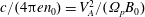 $c/(4\unicode[STIX]{x03C0}en_{0})=V_{A}^{2}/(\unicode[STIX]{x1D6FA}_{p}B_{0})$
, the Hall-term contributions are
$c/(4\unicode[STIX]{x03C0}en_{0})=V_{A}^{2}/(\unicode[STIX]{x1D6FA}_{p}B_{0})$
, the Hall-term contributions are
 $$\begin{eqnarray}\displaystyle c\unicode[STIX]{x1D735}\times \boldsymbol{E}_{H}\overset{\text{lin}}{=}\frac{V_{A}^{2}}{\unicode[STIX]{x1D6FA}_{p}}\left(\begin{array}{@{}c@{}}\unicode[STIX]{x2202}_{y}\unicode[STIX]{x2202}_{z}B_{z}-\unicode[STIX]{x2202}_{z}^{2}B_{y}\\ -\unicode[STIX]{x2202}_{x}\unicode[STIX]{x2202}_{z}B_{z}+\unicode[STIX]{x2202}_{z}^{2}B_{x}\\ \unicode[STIX]{x2202}_{x}\unicode[STIX]{x2202}_{z}B_{y}-\unicode[STIX]{x2202}_{y}\unicode[STIX]{x2202}_{z}B_{x}\end{array}\right). & & \displaystyle\end{eqnarray}$$
The entire linearized induction equation reads
 $$\begin{eqnarray}\displaystyle \frac{\unicode[STIX]{x2202}\boldsymbol{B}}{\unicode[STIX]{x2202}t}\overset{\text{lin}}{=}B_{0}\left(\begin{array}{@{}c@{}}\unicode[STIX]{x2202}_{z}u_{x}\\ \unicode[STIX]{x2202}_{z}u_{y}\\ -\unicode[STIX]{x2202}_{x}u_{x}-\unicode[STIX]{x2202}_{y}u_{y}\end{array}\right)-\frac{V_{A}^{2}}{\unicode[STIX]{x1D6FA}_{p}}\left(\begin{array}{@{}c@{}}\unicode[STIX]{x2202}_{y}\unicode[STIX]{x2202}_{z}B_{z}-\unicode[STIX]{x2202}_{z}^{2}B_{y}\\ -\unicode[STIX]{x2202}_{x}\unicode[STIX]{x2202}_{z}B_{z}+\unicode[STIX]{x2202}_{z}^{2}B_{x}\\ \unicode[STIX]{x2202}_{x}\unicode[STIX]{x2202}_{z}B_{y}-\unicode[STIX]{x2202}_{y}\unicode[STIX]{x2202}_{z}B_{x}\end{array}\right), & & \displaystyle\end{eqnarray}$$
which when written in the
 $x$
–
$x$
–
 $z$
plane (all
$z$
plane (all
 $\unicode[STIX]{x2202}_{y}=0$
) yields
$\unicode[STIX]{x2202}_{y}=0$
) yields
 $$\begin{eqnarray}\displaystyle & \displaystyle \frac{\unicode[STIX]{x2202}B_{x}}{\unicode[STIX]{x2202}t}=B_{0}\unicode[STIX]{x2202}_{z}u_{x}+\frac{V_{A}^{2}}{\unicode[STIX]{x1D6FA}_{p}}\unicode[STIX]{x2202}_{z}^{2}B_{y}; & \displaystyle\end{eqnarray}$$
 $$\begin{eqnarray}\displaystyle & \displaystyle \frac{\unicode[STIX]{x2202}B_{y}}{\unicode[STIX]{x2202}t}=B_{0}\unicode[STIX]{x2202}_{z}u_{y}+\frac{V_{A}^{2}}{\unicode[STIX]{x1D6FA}_{p}}(\unicode[STIX]{x2202}_{x}\unicode[STIX]{x2202}_{z}B_{z}-\unicode[STIX]{x2202}_{z}^{2}B_{x}); & \displaystyle\end{eqnarray}$$
 $$\begin{eqnarray}\displaystyle & \displaystyle \frac{\unicode[STIX]{x2202}B_{z}}{\unicode[STIX]{x2202}t}=-B_{0}\unicode[STIX]{x2202}_{x}u_{x}-\frac{V_{A}^{2}}{\unicode[STIX]{x1D6FA}_{p}}\unicode[STIX]{x2202}_{x}\unicode[STIX]{x2202}_{z}B_{y}. & \displaystyle\end{eqnarray}$$
These equations replace the
 $\unicode[STIX]{x2202}B/\unicode[STIX]{x2202}t$
equations in the linearized CGL system written in the
$\unicode[STIX]{x2202}B/\unicode[STIX]{x2202}t$
equations in the linearized CGL system written in the
 $x$
–
$x$
–
 $z$
plane. And the trouble is immediately apparent. In contrast to the CGL system, we are no longer able to separate the Alfvén mode which was before exclusively in the
$z$
plane. And the trouble is immediately apparent. In contrast to the CGL system, we are no longer able to separate the Alfvén mode which was before exclusively in the
 $B_{y}$
,
$B_{y}$
,
 $u_{y}$
components. Now, all the components are coupled and all three modes, the Alfvén mode, the slow mode and the fast mode are coupled. This is not surprising, since the same situation is in the Hall-MHD. In this case, we have no other choice and we have to calculate the dispersion relation for all three modes. The dispersion relation can be solved analytically only for special cases and, in general, the dispersion relation has to be solved numerically. Let us quickly consider the two special cases of parallel and perpendicular propagation that can be solved analytically.
$u_{y}$
components. Now, all the components are coupled and all three modes, the Alfvén mode, the slow mode and the fast mode are coupled. This is not surprising, since the same situation is in the Hall-MHD. In this case, we have no other choice and we have to calculate the dispersion relation for all three modes. The dispersion relation can be solved analytically only for special cases and, in general, the dispersion relation has to be solved numerically. Let us quickly consider the two special cases of parallel and perpendicular propagation that can be solved analytically.
4.2 Parallel propagation
For propagation parallel to the mean magnetic field, all
 $\unicode[STIX]{x2202}_{x}=0$
and the familiar sound mode/ion-acoustic mode decouples in the
$\unicode[STIX]{x2202}_{x}=0$
and the familiar sound mode/ion-acoustic mode decouples in the
 $u_{z}$
,
$u_{z}$
,
 $p_{\Vert }$
components as
$p_{\Vert }$
components as
 $$\begin{eqnarray}\frac{\unicode[STIX]{x2202}^{2}u_{z}}{\unicode[STIX]{x2202}t^{2}}-\frac{3p_{\Vert }^{(0)}}{\unicode[STIX]{x1D70C}_{0}}\unicode[STIX]{x2202}_{z}^{2}u_{z}=0,\end{eqnarray}$$
with the familiar dispersion relation
 $\unicode[STIX]{x1D714}^{2}=C_{\Vert }^{2}k_{\Vert }^{2}$
. The dispersion relation of this mode does not depend on the Hall term. However, the other two modes are now coupled through
$\unicode[STIX]{x1D714}^{2}=C_{\Vert }^{2}k_{\Vert }^{2}$
. The dispersion relation of this mode does not depend on the Hall term. However, the other two modes are now coupled through
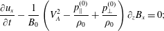 $$\begin{eqnarray}\displaystyle & \displaystyle \frac{\unicode[STIX]{x2202}u_{x}}{\unicode[STIX]{x2202}t}-\frac{1}{B_{0}}\left(V_{A}^{2}-\frac{p_{\Vert }^{(0)}}{\unicode[STIX]{x1D70C}_{0}}+\frac{p_{\bot }^{(0)}}{\unicode[STIX]{x1D70C}_{0}}\right)\unicode[STIX]{x2202}_{z}B_{x}=0; & \displaystyle\end{eqnarray}$$
 $$\begin{eqnarray}\displaystyle & \displaystyle \frac{\unicode[STIX]{x2202}u_{y}}{\unicode[STIX]{x2202}t}-\frac{1}{B_{0}}\left(V_{A}^{2}-\frac{p_{\Vert }^{(0)}}{\unicode[STIX]{x1D70C}_{0}}+\frac{p_{\bot }^{(0)}}{\unicode[STIX]{x1D70C}_{0}}\right)\unicode[STIX]{x2202}_{z}B_{y}=0; & \displaystyle\end{eqnarray}$$
 $$\begin{eqnarray}\displaystyle & \displaystyle \frac{\unicode[STIX]{x2202}B_{x}}{\unicode[STIX]{x2202}t}=B_{0}\unicode[STIX]{x2202}_{z}u_{x}+\frac{V_{A}^{2}}{\unicode[STIX]{x1D6FA}_{p}}\unicode[STIX]{x2202}_{z}^{2}B_{y}; & \displaystyle\end{eqnarray}$$
 $$\begin{eqnarray}\displaystyle & \displaystyle \frac{\unicode[STIX]{x2202}B_{y}}{\unicode[STIX]{x2202}t}=B_{0}\unicode[STIX]{x2202}_{z}u_{y}-\frac{V_{A}^{2}}{\unicode[STIX]{x1D6FA}_{p}}\unicode[STIX]{x2202}_{z}^{2}B_{x}. & \displaystyle\end{eqnarray}$$
If the last terms in the
 $B$
-field equations are neglected, i.e. if the Hall term is neglected, the two modes decouple and one naturally recovers the CGL parallel propagating Alfvén modes, both propagating with the phase speed
$B$
-field equations are neglected, i.e. if the Hall term is neglected, the two modes decouple and one naturally recovers the CGL parallel propagating Alfvén modes, both propagating with the phase speed
 $$\begin{eqnarray}v_{A\Vert }^{2}=V_{A}^{2}-\frac{p_{\Vert }^{(0)}}{\unicode[STIX]{x1D70C}_{0}}+\frac{p_{\bot }^{(0)}}{\unicode[STIX]{x1D70C}_{0}}=V_{A}^{2}\left(1+\frac{\unicode[STIX]{x1D6FD}_{\Vert }}{2}(a_{p}-1)\right).\end{eqnarray}$$
Applying
 $\unicode[STIX]{x2202}_{t}$
to the
$\unicode[STIX]{x2202}_{t}$
to the
 $B$
-field equations yields
$B$
-field equations yields
 $$\begin{eqnarray}\displaystyle & \displaystyle \frac{\unicode[STIX]{x2202}^{2}B_{x}}{\unicode[STIX]{x2202}t^{2}}=v_{A\Vert }^{2}\unicode[STIX]{x2202}_{z}^{2}B_{x}+\frac{V_{A}^{2}}{\unicode[STIX]{x1D6FA}_{p}}\unicode[STIX]{x2202}_{z}^{2}\frac{\unicode[STIX]{x2202}B_{y}}{\unicode[STIX]{x2202}t}; & \displaystyle\end{eqnarray}$$
 $$\begin{eqnarray}\displaystyle & \displaystyle \frac{\unicode[STIX]{x2202}^{2}B_{y}}{\unicode[STIX]{x2202}t^{2}}=v_{A\Vert }^{2}\unicode[STIX]{x2202}_{z}^{2}B_{y}-\frac{V_{A}^{2}}{\unicode[STIX]{x1D6FA}_{p}}\unicode[STIX]{x2202}_{z}^{2}\frac{\unicode[STIX]{x2202}B_{x}}{\unicode[STIX]{x2202}t}, & \displaystyle\end{eqnarray}$$
which when transformed to Fourier space read
 $$\begin{eqnarray}\displaystyle \left(\begin{array}{@{}cc@{}}\unicode[STIX]{x1D714}^{2}-v_{A\Vert }^{2}k_{\Vert }^{2}; & \displaystyle +\text{i}\frac{V_{A}^{2}}{\unicode[STIX]{x1D6FA}_{p}}k_{\Vert }^{2}\unicode[STIX]{x1D714}\\ \displaystyle -\text{i}\frac{V_{A}^{2}}{\unicode[STIX]{x1D6FA}_{p}}k_{\Vert }^{2}\unicode[STIX]{x1D714}; & \unicode[STIX]{x1D714}^{2}-v_{A\Vert }^{2}k_{\Vert }^{2}\end{array}\right)\left(\begin{array}{@{}c@{}}B_{x}\\ B_{y}\end{array}\right)=\left(\begin{array}{@{}c@{}}0\\ 0\end{array}\right), & & \displaystyle\end{eqnarray}$$
and the zero determinant requirement implies
 $$\begin{eqnarray}\unicode[STIX]{x1D714}^{4}-\unicode[STIX]{x1D714}^{2}k_{\Vert }^{2}\left(2v_{A\Vert }^{2}+k_{\Vert }^{2}\frac{V_{A}^{4}}{\unicode[STIX]{x1D6FA}_{p}^{2}}\right)+k_{\Vert }^{4}v_{A\Vert }^{4}=0.\end{eqnarray}$$
The solutions of the dispersion relation (quadratic polynomial in
 $\unicode[STIX]{x1D714}^{2}$
) is simply
$\unicode[STIX]{x1D714}^{2}$
) is simply
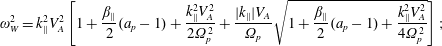 $$\begin{eqnarray}\displaystyle \unicode[STIX]{x1D714}_{W}^{2}=k_{\Vert }^{2}V_{A}^{2}\left[1+\frac{\unicode[STIX]{x1D6FD}_{\Vert }}{2}(a_{p}-1)+\frac{k_{\Vert }^{2}V_{A}^{2}}{2\unicode[STIX]{x1D6FA}_{p}^{2}}+\frac{|k_{\Vert }|V_{A}}{\unicode[STIX]{x1D6FA}_{p}}\sqrt{1+\frac{\unicode[STIX]{x1D6FD}_{\Vert }}{2}(a_{p}-1)+\frac{k_{\Vert }^{2}V_{A}^{2}}{4\unicode[STIX]{x1D6FA}_{p}^{2}}}\right]; & & \displaystyle\end{eqnarray}$$
 $$\begin{eqnarray}\displaystyle \unicode[STIX]{x1D714}_{IC}^{2}=k_{\Vert }^{2}V_{A}^{2}\left[1+\frac{\unicode[STIX]{x1D6FD}_{\Vert }}{2}(a_{p}-1)+\frac{k_{\Vert }^{2}V_{A}^{2}}{2\unicode[STIX]{x1D6FA}_{p}^{2}}-\frac{|k_{\Vert }|V_{A}}{\unicode[STIX]{x1D6FA}_{p}}\sqrt{1+\frac{\unicode[STIX]{x1D6FD}_{\Vert }}{2}(a_{p}-1)+\frac{k_{\Vert }^{2}V_{A}^{2}}{4\unicode[STIX]{x1D6FA}_{p}^{2}}}\right], & & \displaystyle\end{eqnarray}$$
where, importantly,
 $\sqrt{k_{\Vert }^{2}}=|k_{\Vert }|$
was used. The solution (4.28) is the whistler mode, and the solution (4.29) is the ion-cyclotron mode. For isotropic temperatures (
$\sqrt{k_{\Vert }^{2}}=|k_{\Vert }|$
was used. The solution (4.28) is the whistler mode, and the solution (4.29) is the ion-cyclotron mode. For isotropic temperatures (
 $a_{p}=1$
), the result is equal to the Hall-MHD dispersion relation. At long wavelengths (
$a_{p}=1$
), the result is equal to the Hall-MHD dispersion relation. At long wavelengths (
 $k_{\Vert }\rightarrow 0$
) the solutions become non-dispersive and connect to the usual CGL Alfvén modes. For parallel propagation, the Hall term is therefore responsible for splitting the two modes that otherwise would propagate at the same speed, while it does not influence the ion-acoustic mode. Or in another words, using the vocabulary of slow, Alfvén, fast, depending on plasma
$k_{\Vert }\rightarrow 0$
) the solutions become non-dispersive and connect to the usual CGL Alfvén modes. For parallel propagation, the Hall term is therefore responsible for splitting the two modes that otherwise would propagate at the same speed, while it does not influence the ion-acoustic mode. Or in another words, using the vocabulary of slow, Alfvén, fast, depending on plasma
 $\unicode[STIX]{x1D6FD}_{\Vert }$
and temperature anisotropy
$\unicode[STIX]{x1D6FD}_{\Vert }$
and temperature anisotropy
 $a_{p}$
, the Hall term either splits the parallel propagating Alfvén and fast mode, or the slow and Alfvén mode. At very short spatial scales
$a_{p}$
, the Hall term either splits the parallel propagating Alfvén and fast mode, or the slow and Alfvén mode. At very short spatial scales
 $(k_{\Vert }\gg 1)$
, the limits areFootnote
9
$(k_{\Vert }\gg 1)$
, the limits areFootnote
9
 $$\begin{eqnarray}k_{\Vert }\rightarrow \pm \infty :\quad \unicode[STIX]{x1D714}_{IC}^{2}=\unicode[STIX]{x1D6FA}_{p}^{2}\left(1+\frac{\unicode[STIX]{x1D6FD}_{\Vert }}{2}(a_{p}-1)\right)^{2};\quad \unicode[STIX]{x1D714}_{W}^{2}=k_{\Vert }^{4}\frac{V_{A}^{4}}{\unicode[STIX]{x1D6FA}_{p}^{2}}.\end{eqnarray}$$
For isotropic temperatures
 $a_{p}=1$
the frequency of the ion-cyclotron mode (that should be actually called the proton-cyclotron mode) converges towards the proton-cyclotron frequency
$a_{p}=1$
the frequency of the ion-cyclotron mode (that should be actually called the proton-cyclotron mode) converges towards the proton-cyclotron frequency
 $\pm \unicode[STIX]{x1D6FA}_{p}$
. For anisotropic temperatures, the frequency of the mode starts to be
$\pm \unicode[STIX]{x1D6FA}_{p}$
. For anisotropic temperatures, the frequency of the mode starts to be
 $\unicode[STIX]{x1D6FD}_{\Vert }$
dependent and will converge to frequencies that can be higher or lower than
$\unicode[STIX]{x1D6FD}_{\Vert }$
dependent and will converge to frequencies that can be higher or lower than
 $\unicode[STIX]{x1D6FA}_{p}$
. The frequency of the whistler mode is not bounded and technically goes to infinity, which is a consequence of neglecting the electron inertia. Importantly, both modes are stable for high wavenumbers. The solutions (4.28), (4.29) are analytically correct, but similarly to the Hall-MHD, the solutions can be rewritten to a more useful form, by realizing that the dispersion equation (4.27) can be decomposed asFootnote
10
$\unicode[STIX]{x1D6FA}_{p}$
. The frequency of the whistler mode is not bounded and technically goes to infinity, which is a consequence of neglecting the electron inertia. Importantly, both modes are stable for high wavenumbers. The solutions (4.28), (4.29) are analytically correct, but similarly to the Hall-MHD, the solutions can be rewritten to a more useful form, by realizing that the dispersion equation (4.27) can be decomposed asFootnote
10
 $$\begin{eqnarray}\left(\unicode[STIX]{x1D714}^{2}+\frac{k_{\Vert }^{2}V_{A}^{2}}{\unicode[STIX]{x1D6FA}_{p}}\unicode[STIX]{x1D714}-k_{\Vert }^{2}v_{A\Vert }^{2}\right)\left(\unicode[STIX]{x1D714}^{2}-\frac{k_{\Vert }^{2}V_{A}^{2}}{\unicode[STIX]{x1D6FA}_{p}}\unicode[STIX]{x1D714}-k_{\Vert }^{2}v_{A\Vert }^{2}\right)=0.\end{eqnarray}$$
The first bracket yields two solutions
 $$\begin{eqnarray}\displaystyle \unicode[STIX]{x1D714}_{IC,1} & = & \displaystyle -\frac{k_{\Vert }^{2}V_{A}^{2}}{2\unicode[STIX]{x1D6FA}_{p}}+|k_{\Vert }|V_{A}\sqrt{1+\frac{\unicode[STIX]{x1D6FD}_{\Vert }}{2}(a_{p}-1)+\frac{k_{\Vert }^{2}V_{A}^{2}}{4\unicode[STIX]{x1D6FA}_{p}^{2}}};\quad -\text{Green line};\end{eqnarray}$$
 $$\begin{eqnarray}\displaystyle \unicode[STIX]{x1D714}_{W,1} & = & \displaystyle -\frac{k_{\Vert }^{2}V_{A}^{2}}{2\unicode[STIX]{x1D6FA}_{p}}-|k_{\Vert }|V_{A}\sqrt{1+\frac{\unicode[STIX]{x1D6FD}_{\Vert }}{2}(a_{p}-1)+\frac{k_{\Vert }^{2}V_{A}^{2}}{4\unicode[STIX]{x1D6FA}_{p}^{2}}};\quad -\text{dashed Magenta line},\end{eqnarray}$$
and the second bracket yields two solutions
 $$\begin{eqnarray}\displaystyle \unicode[STIX]{x1D714}_{W,2} & = & \displaystyle +\frac{k_{\Vert }^{2}V_{A}^{2}}{2\unicode[STIX]{x1D6FA}_{p}}+|k_{\Vert }|V_{A}\sqrt{1+\frac{\unicode[STIX]{x1D6FD}_{\Vert }}{2}(a_{p}-1)+\frac{k_{\Vert }^{2}V_{A}^{2}}{4\unicode[STIX]{x1D6FA}_{p}^{2}}};\quad -\text{Blue line};\end{eqnarray}$$
 $$\begin{eqnarray}\displaystyle \unicode[STIX]{x1D714}_{IC,2} & = & \displaystyle +\frac{k_{\Vert }^{2}V_{A}^{2}}{2\unicode[STIX]{x1D6FA}_{p}}-|k_{\Vert }|V_{A}\sqrt{1+\frac{\unicode[STIX]{x1D6FD}_{\Vert }}{2}(a_{p}-1)+\frac{k_{\Vert }^{2}V_{A}^{2}}{4\unicode[STIX]{x1D6FA}_{p}^{2}}};\quad -\text{dashed Cyan line}.\end{eqnarray}$$
It is straightforward to check that
 $(\unicode[STIX]{x1D714}-\unicode[STIX]{x1D714}_{W,1})(\unicode[STIX]{x1D714}-\unicode[STIX]{x1D714}_{W,2})=0$
yields the whistler mode solution (4.28), and
$(\unicode[STIX]{x1D714}-\unicode[STIX]{x1D714}_{W,1})(\unicode[STIX]{x1D714}-\unicode[STIX]{x1D714}_{W,2})=0$
yields the whistler mode solution (4.28), and
 $(\unicode[STIX]{x1D714}-\unicode[STIX]{x1D714}_{IC,1})(\unicode[STIX]{x1D714}-\unicode[STIX]{x1D714}_{IC,2})=0$
yields the ion-cyclotron mode solution (4.29). Often, solutions (4.32)–(4.35) are written in an alternative form where the absolute value on
$(\unicode[STIX]{x1D714}-\unicode[STIX]{x1D714}_{IC,1})(\unicode[STIX]{x1D714}-\unicode[STIX]{x1D714}_{IC,2})=0$
yields the ion-cyclotron mode solution (4.29). Often, solutions (4.32)–(4.35) are written in an alternative form where the absolute value on
 $k_{\Vert }$
is removed (which obviously can be done), and the solutions are just slightly re-arranged. Additionally, for more complicated fluid models, we want to write solution in one line instead of four lines. In this example, we just write a shortcut that two solutions are
$k_{\Vert }$
is removed (which obviously can be done), and the solutions are just slightly re-arranged. Additionally, for more complicated fluid models, we want to write solution in one line instead of four lines. In this example, we just write a shortcut that two solutions are
 $$\begin{eqnarray}\unicode[STIX]{x1D714}=\pm \frac{k_{\Vert }^{2}V_{A}^{2}}{2\unicode[STIX]{x1D6FA}_{p}}+k_{\Vert }V_{A}\sqrt{1+\frac{\unicode[STIX]{x1D6FD}_{\Vert }}{2}(a_{p}-1)+\frac{k_{\Vert }^{2}V_{A}^{2}}{4\unicode[STIX]{x1D6FA}_{p}^{2}}},\end{eqnarray}$$
with another two solutions obtained by substituting
 $\unicode[STIX]{x1D714}$
with
$\unicode[STIX]{x1D714}$
with
 $-\unicode[STIX]{x1D714}$
.
$-\unicode[STIX]{x1D714}$
.
4.2.1 Firehose instability
Now we can discuss the firehose instability. If the quantity
 $1+(\unicode[STIX]{x1D6FD}_{\Vert }/2)(a_{p}-1)>0$
, then all the solutions (4.32)–(4.35) have frequencies that are purely real for the entire range of wavenumbers. For isotropic temperatures
$1+(\unicode[STIX]{x1D6FD}_{\Vert }/2)(a_{p}-1)>0$
, then all the solutions (4.32)–(4.35) have frequencies that are purely real for the entire range of wavenumbers. For isotropic temperatures
 $a_{p}=1$
, the dispersion relations do not depend on the value of
$a_{p}=1$
, the dispersion relations do not depend on the value of
 $\unicode[STIX]{x1D6FD}_{\Vert }$
, which is a consequence of neglecting the FLR pressure corrections, as will be discussed later, and all solutions are equivalent to the Hall-MHD dispersion relations. Solutions (4.32)–(4.35) with
$\unicode[STIX]{x1D6FD}_{\Vert }$
, which is a consequence of neglecting the FLR pressure corrections, as will be discussed later, and all solutions are equivalent to the Hall-MHD dispersion relations. Solutions (4.32)–(4.35) with
 $a_{p}=1$
are plotted in figure 4(a), where we plotted both positive and negative wavenumbers and positive and negative frequencies to clearly understand how the modes are connected to each other. The magenta and cyan lines are plotted as dashed lines, so that the growth rates in the firehose-unstable regime (plotted in figure 5) are clearly visible. For anisotropic temperatures
$a_{p}=1$
are plotted in figure 4(a), where we plotted both positive and negative wavenumbers and positive and negative frequencies to clearly understand how the modes are connected to each other. The magenta and cyan lines are plotted as dashed lines, so that the growth rates in the firehose-unstable regime (plotted in figure 5) are clearly visible. For anisotropic temperatures
 $a_{p}\neq 1$
, the solutions are naturally
$a_{p}\neq 1$
, the solutions are naturally
 $\unicode[STIX]{x1D6FD}_{\Vert }$
dependent. To show solutions in a firehose unstable regime, one has to choose
$\unicode[STIX]{x1D6FD}_{\Vert }$
dependent. To show solutions in a firehose unstable regime, one has to choose
 $\unicode[STIX]{x1D6FD}_{\Vert }>2$
since the instability does not exist for lower values of
$\unicode[STIX]{x1D6FD}_{\Vert }>2$
since the instability does not exist for lower values of
 $\unicode[STIX]{x1D6FD}_{\Vert }$
. In figure 4(b), we have chosen a value of
$\unicode[STIX]{x1D6FD}_{\Vert }$
. In figure 4(b), we have chosen a value of
 $\unicode[STIX]{x1D6FD}_{\Vert }=4$
and varied the temperature anisotropy from
$\unicode[STIX]{x1D6FD}_{\Vert }=4$
and varied the temperature anisotropy from
 $a_{p}=2$
down to a critical value of
$a_{p}=2$
down to a critical value of
 $a_{p}=0.5$
. In this regime, all the modes have purely real frequencies.
$a_{p}=0.5$
. In this regime, all the modes have purely real frequencies.
Dispersion relations for the Hall-CGL model (with cold electrons), for parallel propagation
 $\unicode[STIX]{x1D703}=0$
. The colour coding of lines is according to (4.32)–(4.35). (a) Isotropic temperatures
$\unicode[STIX]{x1D703}=0$
. The colour coding of lines is according to (4.32)–(4.35). (a) Isotropic temperatures
 $a_{p}=T_{\bot }/T_{\Vert }=1.0$
. The dispersion relations do not depend on the value of
$a_{p}=T_{\bot }/T_{\Vert }=1.0$
. The dispersion relations do not depend on the value of
 $\unicode[STIX]{x1D6FD}_{\Vert }$
, which is a consequence of neglecting the FLR pressure corrections, etc. The figure is actually equivalent to the Hall-MHD model. (b) the value of
$\unicode[STIX]{x1D6FD}_{\Vert }$
, which is a consequence of neglecting the FLR pressure corrections, etc. The figure is actually equivalent to the Hall-MHD model. (b) the value of
 $\unicode[STIX]{x1D6FD}_{\Vert }$
is fixed with the value
$\unicode[STIX]{x1D6FD}_{\Vert }$
is fixed with the value
 $\unicode[STIX]{x1D6FD}_{\Vert }=4.0$
and the temperature anisotropy is varied as
$\unicode[STIX]{x1D6FD}_{\Vert }=4.0$
and the temperature anisotropy is varied as
 $a_{p}=2.0;1.0;0.5$
. The thickness of the curves increases with decreasing
$a_{p}=2.0;1.0;0.5$
. The thickness of the curves increases with decreasing
 $a_{p}$
as we approach the firehose threshold at
$a_{p}$
as we approach the firehose threshold at
 $a_{p}=0.5$
. All the curves have purely real frequency
$a_{p}=0.5$
. All the curves have purely real frequency
 $\unicode[STIX]{x1D714}$
.
$\unicode[STIX]{x1D714}$
.
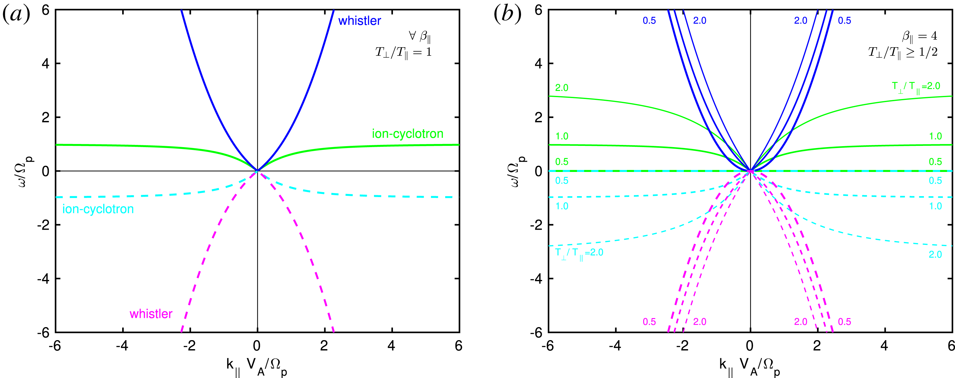
Importantly, if the temperature anisotropy parameter
 $a_{p}$
is further decreased, the frequencies of all the modes will become complex numbers (with a real and imaginary part) in the region where
$a_{p}$
is further decreased, the frequencies of all the modes will become complex numbers (with a real and imaginary part) in the region where
 $$\begin{eqnarray}1+\frac{\unicode[STIX]{x1D6FD}_{\Vert }}{2}(a_{p}-1)+\frac{k_{\Vert }^{2}V_{A}^{2}}{4\unicode[STIX]{x1D6FA}_{p}^{2}}<0,\end{eqnarray}$$
which can be viewed as a modified Hall-CGL firehose instability threshold that is now length-scale dependent. At long spatial scales (
 $k_{\Vert }\rightarrow 0$
), the above criterion is naturally equivalent to the CGL firehose criterion. The term proportional to
$k_{\Vert }\rightarrow 0$
), the above criterion is naturally equivalent to the CGL firehose criterion. The term proportional to
 $k_{\Vert }^{2}$
in (4.37) is always positive and as
$k_{\Vert }^{2}$
in (4.37) is always positive and as
 $k_{\Vert }$
increases, after some critical wavenumber the frequency of modes will become purely real. The Hall term is therefore responsible for the stabilization of the firehose instability at sufficiently high wavenumbers (small spatial scales). The solutions in this firehose-unstable regime are plotted in figure 5, where again
$k_{\Vert }$
increases, after some critical wavenumber the frequency of modes will become purely real. The Hall term is therefore responsible for the stabilization of the firehose instability at sufficiently high wavenumbers (small spatial scales). The solutions in this firehose-unstable regime are plotted in figure 5, where again
 $\unicode[STIX]{x1D6FD}_{\Vert }=4$
and the temperature anisotropy is varied from
$\unicode[STIX]{x1D6FD}_{\Vert }=4$
and the temperature anisotropy is varied from
 $a_{p}=0.49$
to the lowest possible value of
$a_{p}=0.49$
to the lowest possible value of
 $a_{p}=0.0$
. Figure 5(a) shows real frequencies and the (b) shows imaginary frequencies.
$a_{p}=0.0$
. Figure 5(a) shows real frequencies and the (b) shows imaginary frequencies.
Dispersion relations for the Hall-CGL model (with cold electrons), for parallel propagation
 $\unicode[STIX]{x1D703}=0$
, with fixed
$\unicode[STIX]{x1D703}=0$
, with fixed
 $\unicode[STIX]{x1D6FD}_{\Vert }=4$
, after crossing the firehose threshold
$\unicode[STIX]{x1D6FD}_{\Vert }=4$
, after crossing the firehose threshold
 $a_{p}=T_{\bot }/T_{\Vert }<0.5$
. The colour coding of lines is according to (4.32)–(4.35). The thickness of the lines decreases as going away from the threshold
$a_{p}=T_{\bot }/T_{\Vert }<0.5$
. The colour coding of lines is according to (4.32)–(4.35). The thickness of the lines decreases as going away from the threshold
 $a_{p}=0.5$
. (a) Real frequency and the curves have
$a_{p}=0.5$
. (a) Real frequency and the curves have
 $a_{p}=0.49;0.2;0.0$
. (b) Imaginary frequency and the curves have
$a_{p}=0.49;0.2;0.0$
. (b) Imaginary frequency and the curves have
 $a_{p}=0.4;0.2;0.0$
. The mode with
$a_{p}=0.4;0.2;0.0$
. The mode with
 $a_{p}=0.49$
, shown in (a), has an imaginary part of the frequency which is very close to zero for the entire range of
$a_{p}=0.49$
, shown in (a), has an imaginary part of the frequency which is very close to zero for the entire range of
 $k_{\Vert }$
. For this reason this mode is not plotted in (b), where instead a mode with
$k_{\Vert }$
. For this reason this mode is not plotted in (b), where instead a mode with
 $a_{p}=0.4$
is plotted. A mode that has
$a_{p}=0.4$
is plotted. A mode that has
 $\text{Im}\,\unicode[STIX]{x1D714}>0$
is unstable and growing in time. A mode that has
$\text{Im}\,\unicode[STIX]{x1D714}>0$
is unstable and growing in time. A mode that has
 $\text{Im}\,\unicode[STIX]{x1D714}<0$
is stable and damped. According to the figure, whistler modes with
$\text{Im}\,\unicode[STIX]{x1D714}<0$
is stable and damped. According to the figure, whistler modes with
 $\unicode[STIX]{x1D714}_{r}>0$
are unstable, and ion-cyclotron modes with
$\unicode[STIX]{x1D714}_{r}>0$
are unstable, and ion-cyclotron modes with
 $\unicode[STIX]{x1D714}_{r}<0$
are unstable. It is assumed that
$\unicode[STIX]{x1D714}_{r}<0$
are unstable. It is assumed that
 $\sqrt{-1}=+\text{i}$
. The solutions for
$\sqrt{-1}=+\text{i}$
. The solutions for
 $\unicode[STIX]{x1D714}_{r}<0$
are here non-causal, and (b) should be re-plotted with causal solutions (4.43)–(4.46), so that whistler modes are always unstable, and ion-cyclotron modes stable.
$\unicode[STIX]{x1D714}_{r}<0$
are here non-causal, and (b) should be re-plotted with causal solutions (4.43)–(4.46), so that whistler modes are always unstable, and ion-cyclotron modes stable.
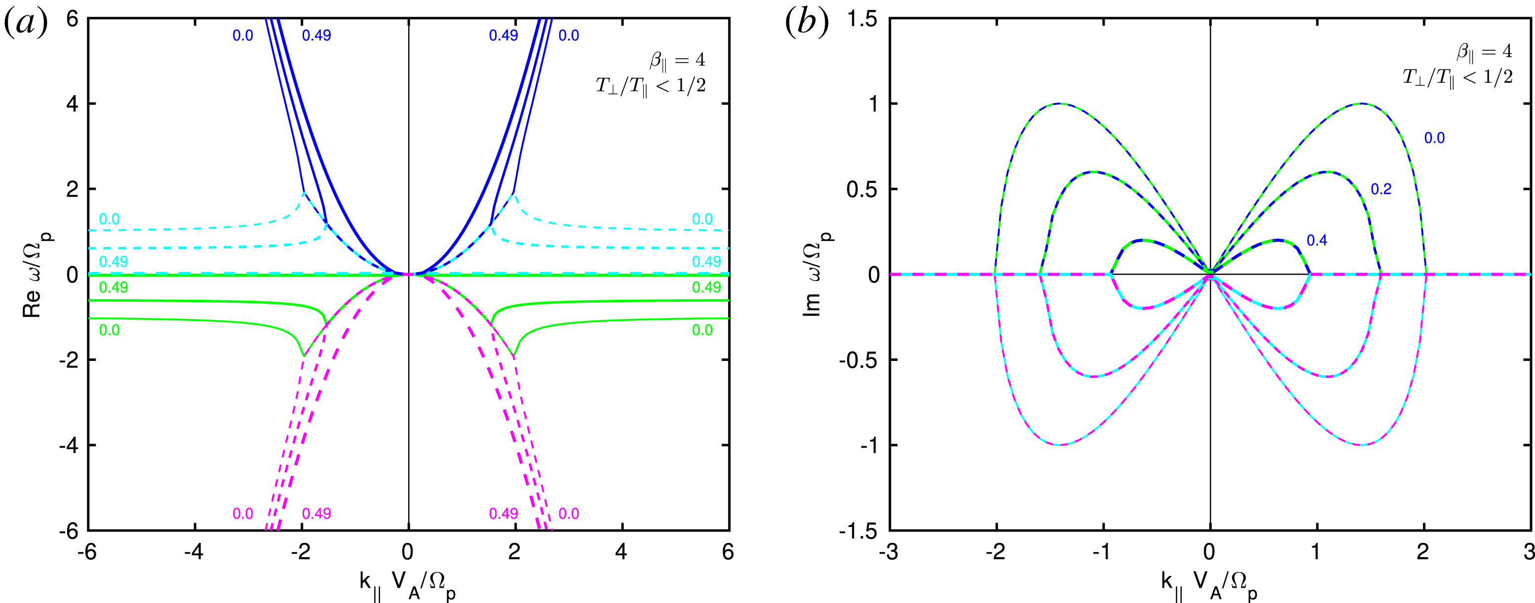
It is of interest to determine which mode becomes unstable. According to our Fourier transform (see appendix A), a mode with positive imaginary frequency is unstable and growing, and a mode with negative imaginary frequency is stable and damped. If the firehose threshold (4.37) is satisfied, for some range of
 $k_{\Vert }$
the second terms in solutions (4.32)–(4.35) become purely imaginary and the first terms stay purely real. Consider one of the four possible quadrants in figure 5(a), for example the quadrant with
$k_{\Vert }$
the second terms in solutions (4.32)–(4.35) become purely imaginary and the first terms stay purely real. Consider one of the four possible quadrants in figure 5(a), for example the quadrant with
 $k_{\Vert }>0;\unicode[STIX]{x1D714}_{r}>0$
. Up to some critical
$k_{\Vert }>0;\unicode[STIX]{x1D714}_{r}>0$
. Up to some critical
 $k_{\Vert }$
where the Hall-CGL firehose criterion is satisfied, both the blue mode and the cyan mode propagate with the same real frequency
$k_{\Vert }$
where the Hall-CGL firehose criterion is satisfied, both the blue mode and the cyan mode propagate with the same real frequency
 $\unicode[STIX]{x1D714}_{r}=+k_{\Vert }^{2}V_{A}^{2}/(2\unicode[STIX]{x1D6FA}_{p})$
. The differences are in the imaginary frequency, see figure 5(b), where in this quadrant the blue mode is unstable and the cyan mode is stable (and damped). After a critical
$\unicode[STIX]{x1D714}_{r}=+k_{\Vert }^{2}V_{A}^{2}/(2\unicode[STIX]{x1D6FA}_{p})$
. The differences are in the imaginary frequency, see figure 5(b), where in this quadrant the blue mode is unstable and the cyan mode is stable (and damped). After a critical
 $k_{\Vert }$
(for example for
$k_{\Vert }$
(for example for
 $a_{p}=0$
it is
$a_{p}=0$
it is
 $k_{\Vert }V_{A}/\unicode[STIX]{x1D6FA}_{p}=2$
), both modes become purely real and evolve with different real frequencies, here the blue mode is obviously the whistler mode and the cyan mode is the ion-cyclotron mode. The same situation is in the quadrant
$k_{\Vert }V_{A}/\unicode[STIX]{x1D6FA}_{p}=2$
), both modes become purely real and evolve with different real frequencies, here the blue mode is obviously the whistler mode and the cyan mode is the ion-cyclotron mode. The same situation is in the quadrant
 $k_{\Vert }<0;\unicode[STIX]{x1D714}_{r}>0$
. We can therefore conclude that for positive real frequencies,
$k_{\Vert }<0;\unicode[STIX]{x1D714}_{r}>0$
. We can therefore conclude that for positive real frequencies,
 $\unicode[STIX]{x1D714}_{r}>0$
, the whistler mode is unstable and the ion-cyclotron mode is stable and damped.
$\unicode[STIX]{x1D714}_{r}>0$
, the whistler mode is unstable and the ion-cyclotron mode is stable and damped.
Now we could say that considering both positive and negative wavenumbers and frequencies is redundant, and that we are finished. However, from a perspective of this guide, we consider useful to show that one might easily come into contradictions, if negative frequencies are not handled with sufficient care. Importantly, according to figure 5, for negative real frequencies
 $\unicode[STIX]{x1D714}_{r}<0$
, the whistler mode is stable and the ion-cyclotron mode is unstable. This is indeed contradictory. Keeping the
$\unicode[STIX]{x1D714}_{r}<0$
, the whistler mode is stable and the ion-cyclotron mode is unstable. This is indeed contradictory. Keeping the
 $k_{\Vert }>0$
, a change from positive to negative
$k_{\Vert }>0$
, a change from positive to negative
 $\unicode[STIX]{x1D714}_{r}$
represents a change of direction of propagation along
$\unicode[STIX]{x1D714}_{r}$
represents a change of direction of propagation along
 $B_{0}$
. One can argue, that in a homogeneous system (e.g. excluding propagation in a stratified fluid), a change of direction of propagation should not yield a change of stability. Additionally, kinetic theory and simulations show, that it is the whistler mode that is firehose unstable for both
$B_{0}$
. One can argue, that in a homogeneous system (e.g. excluding propagation in a stratified fluid), a change of direction of propagation should not yield a change of stability. Additionally, kinetic theory and simulations show, that it is the whistler mode that is firehose unstable for both
 $\unicode[STIX]{x1D714}_{r}>0$
and
$\unicode[STIX]{x1D714}_{r}>0$
and
 $\unicode[STIX]{x1D714}_{r}<0$
, and the ion-cyclotron mode is stable. It is important to emphasize that, from a perspective of solutions (4.32)–(4.35), at the range of wavenumbers where the firehose instability is present, the whistler and ion-cyclotron modes propagate (in a given quadrant) with the same real frequency. Moreover, both modes have the same polarization of electric and magnetic field (see § 4.2.3). Both modes are completely degenerate, and not distinguishable. Thus, how the modes are continued for higher wavenumbers once the firehose instability disappears, is not obvious (since
$\unicode[STIX]{x1D714}_{r}<0$
, and the ion-cyclotron mode is stable. It is important to emphasize that, from a perspective of solutions (4.32)–(4.35), at the range of wavenumbers where the firehose instability is present, the whistler and ion-cyclotron modes propagate (in a given quadrant) with the same real frequency. Moreover, both modes have the same polarization of electric and magnetic field (see § 4.2.3). Both modes are completely degenerate, and not distinguishable. Thus, how the modes are continued for higher wavenumbers once the firehose instability disappears, is not obvious (since
 $\sqrt{-1}$
can be possibly both
$\sqrt{-1}$
can be possibly both
 $+\text{i}$
or
$+\text{i}$
or
 $-\text{i}$
). One should consider all the possible solutions and verify, which solutions are physically plausible. Therefore, after the firehose threshold is crossed, the analytic solutions (4.32)–(4.35) are not correctly separated. Obviously, more ‘physical information’ is needed to distinguish between the ion-cyclotron and whistler modes in the firehose-unstable regime, and to determine which solutions are causal and which are non-causal.
$-\text{i}$
). One should consider all the possible solutions and verify, which solutions are physically plausible. Therefore, after the firehose threshold is crossed, the analytic solutions (4.32)–(4.35) are not correctly separated. Obviously, more ‘physical information’ is needed to distinguish between the ion-cyclotron and whistler modes in the firehose-unstable regime, and to determine which solutions are causal and which are non-causal.
4.2.2 Generalization to causal (correct) solutions
The mind boggling puzzle as why the Hall-CGL solutions (4.32)–(4.35) are in contradiction to kinetic theory and to common sense (a discrepancy found by one of the referees of this text), was beautifully solved by Paul Cally. The easiest way to obtain correct solutions is to introduce a very small ‘causal’ dissipation into the system, and remove it later. Alternatively, it should be possible to obtain the same result by using Laplace–Fourier transforms on temporal-spatial scales and considering an initial value problem.
We introduce causality, by adding a tiny amount of dissipation on the right-hand sides of momentum equations (4.19)–(4.20), in the following form
 $$\begin{eqnarray}\displaystyle & \displaystyle \frac{\unicode[STIX]{x2202}u_{x}}{\unicode[STIX]{x2202}t}-v_{A\Vert }^{2}\unicode[STIX]{x2202}_{z}\frac{B_{x}}{B_{0}}=+\unicode[STIX]{x1D716}\frac{2V_{A}^{2}}{\unicode[STIX]{x1D6FA}_{p}}\unicode[STIX]{x2202}_{z}^{2}u_{x}; & \displaystyle\end{eqnarray}$$
 $$\begin{eqnarray}\displaystyle & \displaystyle \frac{\unicode[STIX]{x2202}u_{y}}{\unicode[STIX]{x2202}t}-v_{A\Vert }^{2}\unicode[STIX]{x2202}_{z}\frac{B_{y}}{B_{0}}=+\unicode[STIX]{x1D716}\frac{2V_{A}^{2}}{\unicode[STIX]{x1D6FA}_{p}}\unicode[STIX]{x2202}_{z}^{2}u_{y}, & \displaystyle\end{eqnarray}$$
where
 $\unicode[STIX]{x1D716}$
is a dimensionless real small positive number, for example
$\unicode[STIX]{x1D716}$
is a dimensionless real small positive number, for example
 $\unicode[STIX]{x1D716}=10^{-8}$
. The dissipation will be later completely removed by the limit
$\unicode[STIX]{x1D716}=10^{-8}$
. The dissipation will be later completely removed by the limit
 $\lim _{\unicode[STIX]{x1D716}\rightarrow 0^{+}}$
. The
$\lim _{\unicode[STIX]{x1D716}\rightarrow 0^{+}}$
. The
 $V_{A}^{2}/\unicode[STIX]{x1D6FA}_{p}$
is there so that the parameter
$V_{A}^{2}/\unicode[STIX]{x1D6FA}_{p}$
is there so that the parameter
 $\unicode[STIX]{x1D716}$
is indeed dimensionless (since here we usually normalize with respect to
$\unicode[STIX]{x1D716}$
is indeed dimensionless (since here we usually normalize with respect to
 $V_{A}$
and
$V_{A}$
and
 $\unicode[STIX]{x1D6FA}_{p}$
, but other normalizations can be of course considered). The factor of 2 is there for pure convenience, so that the final dispersion relations (4.43)–(4.46) are of the utmost beauty, and that we do not have to later redefine
$\unicode[STIX]{x1D6FA}_{p}$
, but other normalizations can be of course considered). The factor of 2 is there for pure convenience, so that the final dispersion relations (4.43)–(4.46) are of the utmost beauty, and that we do not have to later redefine
 $\unicode[STIX]{x1D716}$
. The momentum equations are accompanied by the induction equations (4.21)–(4.22). The reader is encouraged to verify the calculations by switching to normalized variables
$\unicode[STIX]{x1D716}$
. The momentum equations are accompanied by the induction equations (4.21)–(4.22). The reader is encouraged to verify the calculations by switching to normalized variables
 $\widetilde{k_{\Vert }}=k_{\Vert }V_{A}/\unicode[STIX]{x1D6FA}_{p}$
,
$\widetilde{k_{\Vert }}=k_{\Vert }V_{A}/\unicode[STIX]{x1D6FA}_{p}$
,
 $\widetilde{\unicode[STIX]{x1D714}}=\unicode[STIX]{x1D714}/\unicode[STIX]{x1D6FA}_{p}$
,
$\widetilde{\unicode[STIX]{x1D714}}=\unicode[STIX]{x1D714}/\unicode[STIX]{x1D6FA}_{p}$
,
 $\widetilde{v}_{A\Vert }^{2}=1+(\unicode[STIX]{x1D6FD}_{\Vert }/2)(a_{p}-1)$
, we continue in physical units.
$\widetilde{v}_{A\Vert }^{2}=1+(\unicode[STIX]{x1D6FD}_{\Vert }/2)(a_{p}-1)$
, we continue in physical units.
By adding the dissipation, the dispersion relation (4.31) is modified to the following form
 $$\begin{eqnarray}\displaystyle & \displaystyle \left[\unicode[STIX]{x1D714}^{2}+\frac{k_{\Vert }^{2}V_{A}^{2}}{\unicode[STIX]{x1D6FA}_{p}}\unicode[STIX]{x1D714}(1+2\text{i}\unicode[STIX]{x1D716})-k_{\Vert }^{2}v_{A\Vert }^{2}+2\text{i}\unicode[STIX]{x1D716}\frac{k_{\Vert }^{4}V_{A}^{4}}{\unicode[STIX]{x1D6FA}_{p}^{2}}\right](\text{i}B_{x}-B_{y})=0; & \displaystyle\end{eqnarray}$$
 $$\begin{eqnarray}\displaystyle & \displaystyle \left[\unicode[STIX]{x1D714}^{2}-\frac{k_{\Vert }^{2}V_{A}^{2}}{\unicode[STIX]{x1D6FA}_{p}}\unicode[STIX]{x1D714}(1-2\text{i}\unicode[STIX]{x1D716})-k_{\Vert }^{2}v_{A\Vert }^{2}-2\text{i}\unicode[STIX]{x1D716}\frac{k_{\Vert }^{4}V_{A}^{4}}{\unicode[STIX]{x1D6FA}_{p}^{2}}\right](\text{i}B_{x}+B_{y})=0. & \displaystyle\end{eqnarray}$$
It is useful to define the Hall-CGL firehose threshold
 $$\begin{eqnarray}\unicode[STIX]{x1D6E5}\equiv 1+\frac{\unicode[STIX]{x1D6FD}_{\Vert }}{2}(a_{p}-1)+\frac{k_{\Vert }^{2}V_{A}^{2}}{4\unicode[STIX]{x1D6FA}_{p}^{2}},\end{eqnarray}$$
and similar generalizations can be done for models with FLR corrections. Then, since
 $\unicode[STIX]{x1D716}$
is small, it is easy to show that the non-causal solutions (4.32)–(4.35) are ‘corrected’ by the tiny dissipation to the following causal form
$\unicode[STIX]{x1D716}$
is small, it is easy to show that the non-causal solutions (4.32)–(4.35) are ‘corrected’ by the tiny dissipation to the following causal form
 $$\begin{eqnarray}\displaystyle \unicode[STIX]{x1D714}_{IC,1} & = & \displaystyle -\frac{k_{\Vert }^{2}V_{A}^{2}}{2\unicode[STIX]{x1D6FA}_{p}}+|k_{\Vert }|V_{A}\lim _{\unicode[STIX]{x1D716}\rightarrow 0^{+}}\sqrt{\unicode[STIX]{x1D6E5}-\text{i}\unicode[STIX]{x1D716}};\quad -\text{Green line};\end{eqnarray}$$
 $$\begin{eqnarray}\displaystyle \unicode[STIX]{x1D714}_{W,1} & = & \displaystyle -\frac{k_{\Vert }^{2}V_{A}^{2}}{2\unicode[STIX]{x1D6FA}_{p}}-|k_{\Vert }|V_{A}\lim _{\unicode[STIX]{x1D716}\rightarrow 0^{+}}\sqrt{\unicode[STIX]{x1D6E5}-\text{i}\unicode[STIX]{x1D716}};\quad -\text{dashed Magenta line};\end{eqnarray}$$
 $$\begin{eqnarray}\displaystyle \unicode[STIX]{x1D714}_{W,2} & = & \displaystyle +\frac{k_{\Vert }^{2}V_{A}^{2}}{2\unicode[STIX]{x1D6FA}_{p}}+|k_{\Vert }|V_{A}\lim _{\unicode[STIX]{x1D716}\rightarrow 0^{+}}\sqrt{\unicode[STIX]{x1D6E5}+\text{i}\unicode[STIX]{x1D716}};\quad -\text{Blue line};\end{eqnarray}$$
 $$\begin{eqnarray}\displaystyle \unicode[STIX]{x1D714}_{IC,2} & = & \displaystyle +\frac{k_{\Vert }^{2}V_{A}^{2}}{2\unicode[STIX]{x1D6FA}_{p}}-|k_{\Vert }|V_{A}\lim _{\unicode[STIX]{x1D716}\rightarrow 0^{+}}\sqrt{\unicode[STIX]{x1D6E5}+\text{i}\unicode[STIX]{x1D716}};\quad -\text{dashed Cyan line}.\end{eqnarray}$$
The reader is encouraged to plot these solutions, for example with
 $\unicode[STIX]{x1D716}=10^{-8}$
, and verify that figure 5(b), is indeed corrected, i.e. that the whistler is unstable for both
$\unicode[STIX]{x1D716}=10^{-8}$
, and verify that figure 5(b), is indeed corrected, i.e. that the whistler is unstable for both
 $\unicode[STIX]{x1D714}_{r}>0$
and
$\unicode[STIX]{x1D714}_{r}>0$
and
 $\unicode[STIX]{x1D714}_{r}<0$
. We want to further address the limits. For clarity, let us first consider the following simplest case
$\unicode[STIX]{x1D714}_{r}<0$
. We want to further address the limits. For clarity, let us first consider the following simplest case
 $$\begin{eqnarray}\lim _{\unicode[STIX]{x1D716}\rightarrow 0^{+}}\sqrt{-1\pm \text{i}\unicode[STIX]{x1D716}}=\frac{\unicode[STIX]{x1D716}}{2}\pm \text{i},\end{eqnarray}$$
where one can further suppress the small real
 $\unicode[STIX]{x1D716}/2$
on the right-hand side. The limit (4.47) provides an answer, when
$\unicode[STIX]{x1D716}/2$
on the right-hand side. The limit (4.47) provides an answer, when
 $\sqrt{-1}$
is equal to
$\sqrt{-1}$
is equal to
 $+\text{i}$
or
$+\text{i}$
or
 $-\text{i}$
. The result (4.47) can be easily generalized, and limits in expressions (4.43)–(4.46) are calculated according to
$-\text{i}$
. The result (4.47) can be easily generalized, and limits in expressions (4.43)–(4.46) are calculated according to
 $$\begin{eqnarray}\lim _{\unicode[STIX]{x1D716}\rightarrow 0^{+}}\sqrt{\unicode[STIX]{x1D6E5}\pm \text{i}\unicode[STIX]{x1D716}}=\left\{\begin{array}{@{}ll@{}}\sqrt{\unicode[STIX]{x1D6E5}},\quad & \quad \unicode[STIX]{x1D6E5}>0;\\ 0,\quad & \quad \unicode[STIX]{x1D6E5}=0;\\ \pm \text{i}\sqrt{-\unicode[STIX]{x1D6E5}},\quad & \quad \unicode[STIX]{x1D6E5}<0.\end{array}\right.\end{eqnarray}$$
Obviously, the whistler solutions (4.44), (4.45) are unstable, and the ion-cyclotron solutions (4.43), (4.46) are damped. Only now we can conclude with confidence, that the parallel firehose instability as an instability of the whistler mode.
We note that if instead of the momentum equations, we added the dissipation (diffusivity) to the induction equations, the solutions (4.43)–(4.46) are recovered with
 $\unicode[STIX]{x1D716}\rightarrow -\unicode[STIX]{x1D716}$
. In other words, by adding dissipation to the induction equations, the whistler mode would be always damped and the ion-cyclotron mode unstable. The result makes sense with respect to kinetic theory, since the ion-cyclotron resonances enter through the velocity moment (by integration over the perturbation of the distribution function
$\unicode[STIX]{x1D716}\rightarrow -\unicode[STIX]{x1D716}$
. In other words, by adding dissipation to the induction equations, the whistler mode would be always damped and the ion-cyclotron mode unstable. The result makes sense with respect to kinetic theory, since the ion-cyclotron resonances enter through the velocity moment (by integration over the perturbation of the distribution function
 $f^{(1)}$
), or more precisely through the current
$f^{(1)}$
), or more precisely through the current
 $\boldsymbol{j}=\sum _{r}q_{r}n_{r}\boldsymbol{u}_{r}$
, see Part 2.
$\boldsymbol{j}=\sum _{r}q_{r}n_{r}\boldsymbol{u}_{r}$
, see Part 2.
4.2.3 Polarization
The polarization of the magnetic field can be easily checked, actually without plugging any dispersion relations into the matrix (4.26), since the matrix can be represented simply as
 $$\begin{eqnarray}\displaystyle \left(\begin{array}{@{}cc@{}}a & +\text{i}b\\ -\text{i}b & a\end{array}\right)\left(\begin{array}{@{}c@{}}B_{x}\\ B_{y}\end{array}\right)=\left(\begin{array}{@{}c@{}}0\\ 0\end{array}\right), & & \displaystyle\end{eqnarray}$$
where
 $a=\unicode[STIX]{x1D714}^{2}-v_{A\Vert }^{2}k_{\Vert }^{2}$
and
$a=\unicode[STIX]{x1D714}^{2}-v_{A\Vert }^{2}k_{\Vert }^{2}$
and
 $b=V_{A}^{2}k_{\Vert }^{2}\unicode[STIX]{x1D714}/\unicode[STIX]{x1D6FA}_{p}$
. It is useful to define the polarization as the angle between the complex
$b=V_{A}^{2}k_{\Vert }^{2}\unicode[STIX]{x1D714}/\unicode[STIX]{x1D6FA}_{p}$
. It is useful to define the polarization as the angle between the complex
 $B_{x}$
and
$B_{x}$
and
 $B_{y}$
components, which is calculated as
$B_{y}$
components, which is calculated as
 $\text{Arg}(B_{y}/B_{x})$
. If the result is smaller than zero, the wave is left polarized. If the result is larger than zero, the wave is right polarized. The determinant of the matrix (4.49) is
$\text{Arg}(B_{y}/B_{x})$
. If the result is smaller than zero, the wave is left polarized. If the result is larger than zero, the wave is right polarized. The determinant of the matrix (4.49) is
 $a^{2}-b^{2}=0$
, so
$a^{2}-b^{2}=0$
, so
 $a=\pm b$
. The case
$a=\pm b$
. The case
 $a=-b$
(which is directly equal to the first bracket in (4.31) with solutions (4.32), (4.33)) yields that
$a=-b$
(which is directly equal to the first bracket in (4.31) with solutions (4.32), (4.33)) yields that
 $B_{y}=-\text{i}B_{x}$
, so that
$B_{y}=-\text{i}B_{x}$
, so that
 $$\begin{eqnarray}\frac{B_{y}}{B_{x}}=-\text{i}=\text{e}^{-\text{i}(\unicode[STIX]{x03C0}/2)};\quad \Rightarrow \quad \text{Arg}\,\frac{B_{y}}{B_{x}}=-\frac{\unicode[STIX]{x03C0}}{2}<0\quad (\text{left polarized}).\end{eqnarray}$$
The second case
 $a=+b$
(which is equal to the second bracket in (4.31) with solutions (4.34), (4.35)) yields that
$a=+b$
(which is equal to the second bracket in (4.31) with solutions (4.34), (4.35)) yields that
 $B_{y}=+\text{i}B_{x}$
, so that
$B_{y}=+\text{i}B_{x}$
, so that
 $$\begin{eqnarray}\frac{B_{y}}{B_{x}}=+\text{i}=\text{e}^{+\text{i}(\unicode[STIX]{x03C0}/2)};\quad \Rightarrow \quad \text{Arg}\,\frac{B_{y}}{B_{x}}=+\frac{\unicode[STIX]{x03C0}}{2}>0\quad (\text{right polarized}).\end{eqnarray}$$
Similarly, one can calculate the polarization of electric field
 $\boldsymbol{E}$
, and (when not specified that the
$\boldsymbol{E}$
, and (when not specified that the
 $\boldsymbol{B}$
field is considered), the words left/right polarized are usually meant for the
$\boldsymbol{B}$
field is considered), the words left/right polarized are usually meant for the
 $\boldsymbol{E}$
field. The ratio
$\boldsymbol{E}$
field. The ratio
 $E_{y}/E_{x}$
can be easily calculated, for example from equations (4.74), (4.75) (written there in the normalized form), which when multiplied by
$E_{y}/E_{x}$
can be easily calculated, for example from equations (4.74), (4.75) (written there in the normalized form), which when multiplied by
 $\unicode[STIX]{x1D714}$
and use of momentum equations, yields for the special case of parallel propagation considered here
$\unicode[STIX]{x1D714}$
and use of momentum equations, yields for the special case of parallel propagation considered here
 $$\begin{eqnarray}\frac{E_{y}}{E_{x}}=\frac{\displaystyle -\widetilde{v}_{A\Vert }^{2}+\text{i}\widetilde{\unicode[STIX]{x1D714}}\frac{B_{y}}{B_{x}}}{\displaystyle \widetilde{v}_{A\Vert }^{2}\frac{B_{y}}{B_{x}}+\text{i}\widetilde{\unicode[STIX]{x1D714}}}.\end{eqnarray}$$
When plotting many solutions, it is useful to additionally divide the angle by
 $\unicode[STIX]{x03C0}$
, and define the
$\unicode[STIX]{x03C0}$
, and define the
 $\boldsymbol{B}$
and
$\boldsymbol{B}$
and
 $\boldsymbol{E}$
field polarizations as
$\boldsymbol{E}$
field polarizations as
 $$\begin{eqnarray}{\mathcal{P}}_{B}=\frac{1}{\unicode[STIX]{x03C0}}\,\text{Arg}\,\frac{B_{y}}{B_{x}};\quad {\mathcal{P}}_{E}=\frac{1}{\unicode[STIX]{x03C0}}\,\text{Arg}\,\frac{E_{y}}{E_{x}}.\end{eqnarray}$$
Electric field polarization defined this way was used for example by Hunana et al. (Reference Hunana, Goldstein, Passot, Sulem, Laveder and Zank2013) to investigate properties of (highly oblique) kinetic Alfvén waves in various fluid models and the kinetic description; and also by Camporeale & Burgess (Reference Camporeale and Burgess2017), who compared various linear modes in hybrid, gyrokinetic and fully kinetic descriptions.Footnote
11
When
 ${\mathcal{P}}_{E}<0$
the wave is called left polarized and when
${\mathcal{P}}_{E}<0$
the wave is called left polarized and when
 ${\mathcal{P}}_{E}>0$
, the wave is called right polarized. For the first group (4.50) this yields
${\mathcal{P}}_{E}>0$
, the wave is called right polarized. For the first group (4.50) this yields
 $E_{y}/E_{x}=-\text{i}$
and
$E_{y}/E_{x}=-\text{i}$
and
 ${\mathcal{P}}_{E}=-1/2<0$
(left polarized wave), and for the second group (4.51)
${\mathcal{P}}_{E}=-1/2<0$
(left polarized wave), and for the second group (4.51)
 $E_{y}/E_{x}=+\text{i}$
and
$E_{y}/E_{x}=+\text{i}$
and
 ${\mathcal{P}}_{E}=+1/2>0$
(right polarized wave).
${\mathcal{P}}_{E}=+1/2>0$
(right polarized wave).
Finally, it is of interest to note another possible definition of polarization, that is defined with respect to positive real frequency, i.e. the electric field polarization (4.53) is redefined to
 $$\begin{eqnarray}{\mathcal{P}}_{E}=\frac{\text{sign}(\unicode[STIX]{x1D714}_{r})}{\unicode[STIX]{x03C0}}\,\text{Arg}\,\frac{E_{y}}{E_{x}}.\end{eqnarray}$$
A similar definition of polarization with
 $\text{sign}(\unicode[STIX]{x1D714}_{r})$
is used for example in the book by Gary (Reference Gary1993), page 91. With such a definition, the whistler mode is always right polarized, both in the firehose-stable and firehose-unstable regimes, since for the whistler mode ((4.34), blue line) the real frequency remains
$\text{sign}(\unicode[STIX]{x1D714}_{r})$
is used for example in the book by Gary (Reference Gary1993), page 91. With such a definition, the whistler mode is always right polarized, both in the firehose-stable and firehose-unstable regimes, since for the whistler mode ((4.34), blue line) the real frequency remains
 $\unicode[STIX]{x1D714}_{r}>0$
, and for the whistler mode ((4.33), magenta line)
$\unicode[STIX]{x1D714}_{r}>0$
, and for the whistler mode ((4.33), magenta line)
 $\unicode[STIX]{x1D714}_{r}<0$
. The situation is more confusing for the ion-cyclotron mode, where the firehose-stable and firehose-unstable regimes have to be considered separately. (i) In the firehose-stable regime, both ion-cyclotron modes are left polarized, since for the mode ((4.32), green line)
$\unicode[STIX]{x1D714}_{r}<0$
. The situation is more confusing for the ion-cyclotron mode, where the firehose-stable and firehose-unstable regimes have to be considered separately. (i) In the firehose-stable regime, both ion-cyclotron modes are left polarized, since for the mode ((4.32), green line)
 $\unicode[STIX]{x1D714}_{r}>0$
, and for the mode ((4.35), cyan line)
$\unicode[STIX]{x1D714}_{r}>0$
, and for the mode ((4.35), cyan line)
 $\unicode[STIX]{x1D714}_{r}<0$
. (ii) In contrast, in the firehose-unstable regime, both ion-cyclotron modes are right polarized, since for the mode ((4.32), green line)
$\unicode[STIX]{x1D714}_{r}<0$
. (ii) In contrast, in the firehose-unstable regime, both ion-cyclotron modes are right polarized, since for the mode ((4.32), green line)
 $\unicode[STIX]{x1D714}_{r}<0$
, and for the mode ((4.35), cyan line)
$\unicode[STIX]{x1D714}_{r}<0$
, and for the mode ((4.35), cyan line)
 $\unicode[STIX]{x1D714}_{r}>0$
.
$\unicode[STIX]{x1D714}_{r}>0$
.
4.2.4 Simplest ion-cyclotron resonances
When talking about ‘resonances’, one often expects to see expressions with a denominator that becomes zero. Generally speaking, the simplest ‘singular’ expressions representing resonances just arise from a technique used in deriving the dispersion relations. If one eliminates the electric field
 $\boldsymbol{E}$
from the beginning and expresses the fluid model through a matrix multiplied by a vector (
$\boldsymbol{E}$
from the beginning and expresses the fluid model through a matrix multiplied by a vector (
 $\unicode[STIX]{x1D70C}$
,
$\unicode[STIX]{x1D70C}$
,
 $u_{x}$
,
$u_{x}$
,
 $u_{y}$
,
$u_{y}$
,
 $u_{z}$
,
$u_{z}$
,
 $b_{x}$
,
$b_{x}$
,
 $b_{y}$
,
$b_{y}$
,
 $b_{z}$
,
$b_{z}$
,
 $p_{\Vert }$
,
$p_{\Vert }$
,
 $p_{\bot }$
), leads to dispersion relations that are not singular explicitly. In contrast, expressing the model through a matrix multiplied by a vector
$p_{\bot }$
), leads to dispersion relations that are not singular explicitly. In contrast, expressing the model through a matrix multiplied by a vector
 $(E_{x},E_{y},E_{z})$
, yields equivalent dispersion relations where the resonances are shown explicitly. The dispersion equation (4.31) can be easily rewritten as
$(E_{x},E_{y},E_{z})$
, yields equivalent dispersion relations where the resonances are shown explicitly. The dispersion equation (4.31) can be easily rewritten as
 $$\begin{eqnarray}\frac{k_{\Vert }^{2}}{\unicode[STIX]{x1D714}^{2}}=-\frac{\unicode[STIX]{x1D6FA}_{p}/V_{A}^{2}}{\displaystyle \unicode[STIX]{x1D714}-\unicode[STIX]{x1D6FA}_{p}\left(1+\frac{\unicode[STIX]{x1D6FD}_{\Vert }}{2}(a_{p}-1)\right)};\quad \frac{k_{\Vert }^{2}}{\unicode[STIX]{x1D714}^{2}}=+\frac{\unicode[STIX]{x1D6FA}_{p}/V_{A}^{2}}{\displaystyle \unicode[STIX]{x1D714}+\unicode[STIX]{x1D6FA}_{p}\left(1+\frac{\unicode[STIX]{x1D6FD}_{\Vert }}{2}(a_{p}-1)\right)},\end{eqnarray}$$
which, in the cold plasma limit (
 $\unicode[STIX]{x1D6FD}_{\Vert }=0$
) or in this case also for isotropic temperatures
$\unicode[STIX]{x1D6FD}_{\Vert }=0$
) or in this case also for isotropic temperatures
 $(a_{p}=1)$
, simplifies to
$(a_{p}=1)$
, simplifies to
 $$\begin{eqnarray}\frac{k_{\Vert }^{2}}{\unicode[STIX]{x1D714}^{2}}=-\frac{\unicode[STIX]{x1D6FA}_{p}/V_{A}^{2}}{\unicode[STIX]{x1D714}-\unicode[STIX]{x1D6FA}_{p}};\quad \frac{k_{\Vert }^{2}}{\unicode[STIX]{x1D714}^{2}}=+\frac{\unicode[STIX]{x1D6FA}_{p}/V_{A}^{2}}{\unicode[STIX]{x1D714}+\unicode[STIX]{x1D6FA}_{p}},\end{eqnarray}$$
making it more evident that we have the simplest ion-cyclotron resonances here too. Indeed, for
 $k\rightarrow \infty$
the frequency
$k\rightarrow \infty$
the frequency
 $\unicode[STIX]{x1D714}\rightarrow \unicode[STIX]{x1D6FA}_{p}$
(first case) and
$\unicode[STIX]{x1D714}\rightarrow \unicode[STIX]{x1D6FA}_{p}$
(first case) and
 $\unicode[STIX]{x1D714}\rightarrow -\unicode[STIX]{x1D6FA}_{p}$
(second case). For a plasma with finite
$\unicode[STIX]{x1D714}\rightarrow -\unicode[STIX]{x1D6FA}_{p}$
(second case). For a plasma with finite
 $\unicode[STIX]{x1D6FD}_{\Vert }$
and non-isotropic temperatures, the
$\unicode[STIX]{x1D6FD}_{\Vert }$
and non-isotropic temperatures, the
 $k\rightarrow \infty$
limit yields more general ion-cyclotron resonances (4.30).
$k\rightarrow \infty$
limit yields more general ion-cyclotron resonances (4.30).
To better understand what effects are present and what effects are absent in the Hall-CGL model, we plot fully kinetic solutions obtained with the WHAMP code in figure 6. The proton temperature is prescribed to be isotropic
 $T_{\bot }/T_{\Vert }=1$
and the electrons are prescribed to be cold with
$T_{\bot }/T_{\Vert }=1$
and the electrons are prescribed to be cold with
 $T_{e}/T_{p}=0$
(in the WHAMP code, the value is chosen to be
$T_{e}/T_{p}=0$
(in the WHAMP code, the value is chosen to be
 $10^{-8}$
). In the WHAMP code it is necessary to prescribe the ratio of the parallel proton thermal speed to the speed of light, and we choose
$10^{-8}$
). In the WHAMP code it is necessary to prescribe the ratio of the parallel proton thermal speed to the speed of light, and we choose
 $v_{\text{th}\Vert }/c=10^{-4}$
. The solid lines are kinetic solutions with different
$v_{\text{th}\Vert }/c=10^{-4}$
. The solid lines are kinetic solutions with different
 $\unicode[STIX]{x1D6FD}_{\Vert }=10^{-4};0.1;1;2;4$
. The blue curve is the whistler mode and the green curve is the ion-cyclotron mode. Solutions of the Hall-CGL model are shown in figure 6(a) and, for isotropic temperatures, the solutions are completely
$\unicode[STIX]{x1D6FD}_{\Vert }=10^{-4};0.1;1;2;4$
. The blue curve is the whistler mode and the green curve is the ion-cyclotron mode. Solutions of the Hall-CGL model are shown in figure 6(a) and, for isotropic temperatures, the solutions are completely
 $\unicode[STIX]{x1D6FD}_{\Vert }$
independent and are represented with two dashed curves. It is shown that the kinetic solutions for the whistler mode are almost
$\unicode[STIX]{x1D6FD}_{\Vert }$
independent and are represented with two dashed curves. It is shown that the kinetic solutions for the whistler mode are almost
 $\unicode[STIX]{x1D6FD}_{\Vert }$
independent and only the mode with
$\unicode[STIX]{x1D6FD}_{\Vert }$
independent and only the mode with
 $\unicode[STIX]{x1D6FD}_{\Vert }=4$
deviates from the other whistler solutions, and only between
$\unicode[STIX]{x1D6FD}_{\Vert }=4$
deviates from the other whistler solutions, and only between
 $kd_{i}=0.1-2.0$
. For comparison, in figure 6(b) we plot solutions of the Hall-CGL-FLR2 model (the model is discussed later in the text).
$kd_{i}=0.1-2.0$
. For comparison, in figure 6(b) we plot solutions of the Hall-CGL-FLR2 model (the model is discussed later in the text).
(a) Comparison of solutions of full kinetic theory obtained with the WHAMP code (solid lines) and the simple dispersion of the Hall-CGL model (dashed lines) for the whistler mode (blue) and the ion-cyclotron mode (green). The proton temperatures are isotropic
 $T_{\bot }/T_{\Vert }=1$
, electrons are cold and the angle of propagation
$T_{\bot }/T_{\Vert }=1$
, electrons are cold and the angle of propagation
 $\unicode[STIX]{x1D703}=0$
. Real frequency is plotted. The
$\unicode[STIX]{x1D703}=0$
. Real frequency is plotted. The
 $\unicode[STIX]{x1D6FD}_{\Vert }$
is varied as
$\unicode[STIX]{x1D6FD}_{\Vert }$
is varied as
 $\unicode[STIX]{x1D6FD}_{\Vert }=10^{-4};0.1;1;2;4$
. The kinetic solutions show that while the frequency of whistler mode is not very
$\unicode[STIX]{x1D6FD}_{\Vert }=10^{-4};0.1;1;2;4$
. The kinetic solutions show that while the frequency of whistler mode is not very
 $\unicode[STIX]{x1D6FD}_{\Vert }$
dependent (only the case
$\unicode[STIX]{x1D6FD}_{\Vert }$
dependent (only the case
 $\unicode[STIX]{x1D6FD}_{\Vert }=4$
is slightly different), the frequency of the ion-cyclotron mode is strongly
$\unicode[STIX]{x1D6FD}_{\Vert }=4$
is slightly different), the frequency of the ion-cyclotron mode is strongly
 $\unicode[STIX]{x1D6FD}_{\Vert }$
dependent since the mode experiences strong damping. The Hall-CGL model has only the simplest ion-cyclotron resonance, and the Hall-CGL ion-cyclotron mode matches the kinetic ion-cyclotron mode only for the lowest
$\unicode[STIX]{x1D6FD}_{\Vert }$
dependent since the mode experiences strong damping. The Hall-CGL model has only the simplest ion-cyclotron resonance, and the Hall-CGL ion-cyclotron mode matches the kinetic ion-cyclotron mode only for the lowest
 $\unicode[STIX]{x1D6FD}_{\Vert }=10^{-4}$
. (b) Solutions of the Hall-CGL-FLR2 model are plotted. Note that the real frequency of the ion-cyclotron mode is crudely reproduced.
$\unicode[STIX]{x1D6FD}_{\Vert }=10^{-4}$
. (b) Solutions of the Hall-CGL-FLR2 model are plotted. Note that the real frequency of the ion-cyclotron mode is crudely reproduced.
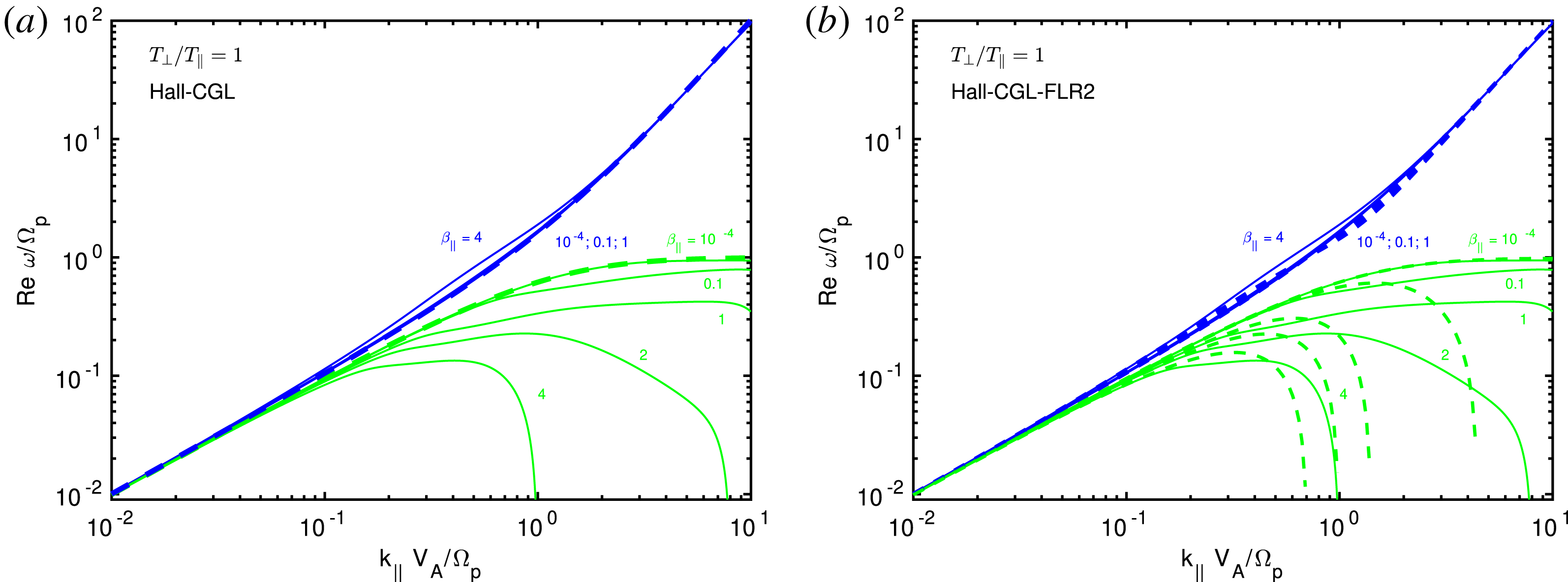
4.3 Hall-CGL dispersion relation for arbitrary propagation angle
To make everything as clear as possible, let us write down one more time the normalized equations we are solving, including the linearized and Fourier transformed equations in the
 $x$
–
$x$
–
 $z$
plane. The nonlinear Hall-CGL equations with cold electrons are (dropping the tilde)
$z$
plane. The nonlinear Hall-CGL equations with cold electrons are (dropping the tilde)
 $$\begin{eqnarray}\displaystyle & \displaystyle \frac{\unicode[STIX]{x2202}\unicode[STIX]{x1D70C}_{p}}{\unicode[STIX]{x2202}t}+\unicode[STIX]{x1D735}\boldsymbol{\cdot }(\unicode[STIX]{x1D70C}\boldsymbol{u}_{p})=0; & \displaystyle\end{eqnarray}$$
 $$\begin{eqnarray}\displaystyle & \displaystyle \frac{\unicode[STIX]{x2202}\boldsymbol{u}_{p}}{\unicode[STIX]{x2202}t}+\boldsymbol{u}_{p}\boldsymbol{\cdot }\unicode[STIX]{x1D735}\boldsymbol{u}_{p}+\frac{\unicode[STIX]{x1D6FD}_{\Vert }}{2}\frac{1}{\unicode[STIX]{x1D70C}_{p}}\unicode[STIX]{x1D735}\boldsymbol{\cdot }\boldsymbol{p}_{p}-\frac{1}{\unicode[STIX]{x1D70C}_{p}}(\unicode[STIX]{x1D735}\times \boldsymbol{B})\times \boldsymbol{B}=0; & \displaystyle\end{eqnarray}$$
 $$\begin{eqnarray}\displaystyle & \displaystyle \frac{\unicode[STIX]{x2202}\boldsymbol{B}}{\unicode[STIX]{x2202}t}-\unicode[STIX]{x1D735}\times (\boldsymbol{u}_{p}\times \boldsymbol{B})+\unicode[STIX]{x1D735}\times \left[\frac{1}{\unicode[STIX]{x1D70C}_{p}}(\unicode[STIX]{x1D735}\times \boldsymbol{B})\times \boldsymbol{B}\right]=0; & \displaystyle\end{eqnarray}$$
 $$\begin{eqnarray}\displaystyle & \displaystyle \frac{\unicode[STIX]{x2202}p_{\Vert p}}{\unicode[STIX]{x2202}t}+\unicode[STIX]{x1D735}\boldsymbol{\cdot }(p_{\Vert p}\boldsymbol{u}_{p})+2p_{\Vert p}\hat{\boldsymbol{b}}\boldsymbol{\cdot }\unicode[STIX]{x1D735}\boldsymbol{u}_{p}\boldsymbol{\cdot }\hat{\boldsymbol{b}}=0; & \displaystyle\end{eqnarray}$$
 $$\begin{eqnarray}\displaystyle & \displaystyle \frac{\unicode[STIX]{x2202}p_{\bot p}}{\unicode[STIX]{x2202}t}+\unicode[STIX]{x1D735}\boldsymbol{\cdot }(p_{\bot p}\boldsymbol{u}_{p})+p_{\bot p}\unicode[STIX]{x1D735}\boldsymbol{\cdot }\boldsymbol{u}_{p}-p_{\bot p}\hat{\boldsymbol{b}}\boldsymbol{\cdot }\unicode[STIX]{x1D735}\boldsymbol{u}_{p}\boldsymbol{\cdot }\hat{\boldsymbol{b}}=0. & \displaystyle\end{eqnarray}$$
Linearizing in normalized units is even easier, because (temporarily introducing back the tilde for clarity)
 $\widetilde{p}_{\Vert p}^{(0)}=1$
;
$\widetilde{p}_{\Vert p}^{(0)}=1$
;
 $\widetilde{p}_{\bot p}^{(0)}=a_{p}$
;
$\widetilde{p}_{\bot p}^{(0)}=a_{p}$
;
 $\widetilde{\unicode[STIX]{x1D70C}}_{0}=1$
;
$\widetilde{\unicode[STIX]{x1D70C}}_{0}=1$
;
 $\widetilde{B}_{0}=1$
. Linearizing these equations, writing them in the
$\widetilde{B}_{0}=1$
. Linearizing these equations, writing them in the
 $x$
–
$x$
–
 $z$
plane and Fourier transforming yields (dropping also the proton index ‘
$z$
plane and Fourier transforming yields (dropping also the proton index ‘
 $p$
’)
$p$
’)
 $$\begin{eqnarray}\displaystyle & \displaystyle -\unicode[STIX]{x1D714}\unicode[STIX]{x1D70C}+k_{\bot }u_{x}+k_{\Vert }u_{z}=0; & \displaystyle\end{eqnarray}$$
 $$\begin{eqnarray}\displaystyle & \displaystyle -\unicode[STIX]{x1D714}u_{x}+\frac{\unicode[STIX]{x1D6FD}_{\Vert }}{2}k_{\bot }p_{\bot }-v_{A\Vert }^{2}k_{\Vert }B_{x}+k_{\bot }B_{z}=0; & \displaystyle\end{eqnarray}$$
 $$\begin{eqnarray}\displaystyle & \displaystyle -\unicode[STIX]{x1D714}u_{y}-v_{A\Vert }^{2}k_{\Vert }B_{y}=0; & \displaystyle\end{eqnarray}$$
 $$\begin{eqnarray}\displaystyle & \displaystyle -\unicode[STIX]{x1D714}u_{z}+\frac{\unicode[STIX]{x1D6FD}_{\Vert }}{2}k_{\Vert }p_{\Vert }+\frac{\unicode[STIX]{x1D6FD}_{\Vert }}{2}(1-a_{p})k_{\bot }B_{x}=0; & \displaystyle\end{eqnarray}$$
 $$\begin{eqnarray}\displaystyle & \displaystyle -\unicode[STIX]{x1D714}B_{x}-k_{\Vert }u_{x}-\text{i}k_{\Vert }^{2}B_{y}=0; & \displaystyle\end{eqnarray}$$
 $$\begin{eqnarray}\displaystyle & \displaystyle -\unicode[STIX]{x1D714}B_{y}-k_{\Vert }u_{y}-\text{i}k_{\Vert }k_{\bot }B_{z}+\text{i}k_{\Vert }^{2}B_{x}=0; & \displaystyle\end{eqnarray}$$
 $$\begin{eqnarray}\displaystyle & \displaystyle -\unicode[STIX]{x1D714}B_{z}+k_{\bot }u_{x}+\text{i}k_{\Vert }k_{\bot }B_{y}=0; & \displaystyle\end{eqnarray}$$
 $$\begin{eqnarray}\displaystyle & \displaystyle -\unicode[STIX]{x1D714}p_{\Vert }+k_{\bot }u_{x}+3k_{\Vert }u_{z}=0; & \displaystyle\end{eqnarray}$$
 $$\begin{eqnarray}\displaystyle & \displaystyle -\unicode[STIX]{x1D714}p_{\bot }+2a_{p}k_{\bot }u_{x}+a_{p}k_{\Vert }u_{z}=0, & \displaystyle\end{eqnarray}$$
where the normalized
 $v_{A\Vert }^{2}=1+(\unicode[STIX]{x1D6FD}_{\Vert }/2)(a_{p}-1)$
. Alternatively, it is sometimes illuminating to work with the general induction equation where the electric field is used
$v_{A\Vert }^{2}=1+(\unicode[STIX]{x1D6FD}_{\Vert }/2)(a_{p}-1)$
. Alternatively, it is sometimes illuminating to work with the general induction equation where the electric field is used
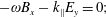 $$\begin{eqnarray}\displaystyle & \displaystyle -\unicode[STIX]{x1D714}B_{x}-k_{\Vert }E_{y}=0; & \displaystyle\end{eqnarray}$$
 $$\begin{eqnarray}\displaystyle & \displaystyle -\unicode[STIX]{x1D714}B_{y}-k_{\bot }E_{z}+k_{\Vert }E_{x}=0; & \displaystyle\end{eqnarray}$$
 $$\begin{eqnarray}\displaystyle & \displaystyle -\unicode[STIX]{x1D714}B_{z}+k_{\bot }E_{y}=0, & \displaystyle\end{eqnarray}$$
and in this case with cold electrons the electric field components are
 $$\begin{eqnarray}\displaystyle & \displaystyle E_{x}=-u_{y}-\text{i}k_{\bot }B_{z}+\text{i}k_{\Vert }B_{x}; & \displaystyle\end{eqnarray}$$
 $$\begin{eqnarray}\displaystyle & \displaystyle E_{y}=u_{x}+\text{i}k_{\Vert }B_{y}; & \displaystyle\end{eqnarray}$$
 $$\begin{eqnarray}\displaystyle & \displaystyle E_{z}=0. & \displaystyle\end{eqnarray}$$
The induction equation (4.71)–(4.73) with the above electric field components is of course equivalent to the induction equation (4.66)–(4.68). All equations are normalized, the tilde are dropped, and the electric field
 $\widetilde{E}=E/E_{0}$
, where
$\widetilde{E}=E/E_{0}$
, where
 $E_{0}=V_{A}B_{0}/c$
. The Hall-CGL dispersion relation reads
$E_{0}=V_{A}B_{0}/c$
. The Hall-CGL dispersion relation reads
 $$\begin{eqnarray}\displaystyle & \displaystyle \unicode[STIX]{x1D714}^{6}-A_{4}\unicode[STIX]{x1D714}^{4}+A_{2}\unicode[STIX]{x1D714}^{2}-A_{0}=0; & \displaystyle\end{eqnarray}$$
 $$\begin{eqnarray}\displaystyle & \displaystyle A_{4}=k_{\Vert }^{2}\left({\textstyle \frac{3}{2}}\unicode[STIX]{x1D6FD}_{\Vert }+2v_{A\Vert }^{2}\right)+k_{\bot }^{2}(1+a_{p}\unicode[STIX]{x1D6FD}_{\Vert })+k^{2}k_{\Vert }^{2}; & \displaystyle\end{eqnarray}$$
 $$\begin{eqnarray}\displaystyle A_{2} & = & \displaystyle k_{\Vert }^{2}\left[k_{\Vert }^{2}v_{A\Vert }^{2}(v_{A\Vert }^{2}+3\unicode[STIX]{x1D6FD}_{\Vert })+k_{\bot }^{2}\left(v_{A\Vert }^{2}(1+a_{p}\unicode[STIX]{x1D6FD}_{\Vert })+{\textstyle \frac{3}{2}}\unicode[STIX]{x1D6FD}_{\Vert }\left(1+a_{p}\unicode[STIX]{x1D6FD}_{\Vert }-{\textstyle \frac{1}{6}}a_{p}^{2}\unicode[STIX]{x1D6FD}_{\Vert }\right)\right)\right]\nonumber\\ \displaystyle & & \displaystyle +\,k^{2}k_{\Vert }^{2}\unicode[STIX]{x1D6FD}_{\Vert }\left({\textstyle \frac{3}{2}}k_{\Vert }^{2}+a_{p}k_{\bot }^{2}\right);\end{eqnarray}$$
 $$\begin{eqnarray}\displaystyle & \displaystyle A_{0}={\textstyle \frac{3}{2}}\unicode[STIX]{x1D6FD}_{\Vert }k_{\Vert }^{4}v_{A\Vert }^{2}\left[k_{\Vert }^{2}v_{A\Vert }^{2}+k_{\bot }^{2}\left(1+a_{p}\unicode[STIX]{x1D6FD}_{\Vert }-{\textstyle \frac{1}{6}}a_{p}^{2}\unicode[STIX]{x1D6FD}_{\Vert }\right)\right]+k^{2}k_{\Vert }^{4}k_{\bot }^{2}{\textstyle \frac{5}{4}}a_{p}\unicode[STIX]{x1D6FD}_{\Vert }^{2}, & \displaystyle\end{eqnarray}$$
where the wavenumber
 $k^{2}=k_{\Vert }^{2}+k_{\bot }^{2}$
. Perhaps the nicest form is to keep the CGL contributions on the left-hand side (so the terms can be factorized to form the CGL dispersion relation) and put the Hall term contributions on the right-hand side, which yields the Hall-CGL dispersion relation
$k^{2}=k_{\Vert }^{2}+k_{\bot }^{2}$
. Perhaps the nicest form is to keep the CGL contributions on the left-hand side (so the terms can be factorized to form the CGL dispersion relation) and put the Hall term contributions on the right-hand side, which yields the Hall-CGL dispersion relation
 $$\begin{eqnarray}\displaystyle & \displaystyle (\unicode[STIX]{x1D714}^{2}-k_{\Vert }^{2}v_{A\Vert }^{2})(\unicode[STIX]{x1D714}^{4}-A_{2}\unicode[STIX]{x1D714}^{2}+A_{0})=k^{2}k_{\Vert }^{2}\left[\unicode[STIX]{x1D714}^{4}-\unicode[STIX]{x1D6FD}_{\Vert }\left({\textstyle \frac{3}{2}}k_{\Vert }^{2}+a_{p}k_{\bot }^{2}\right)\unicode[STIX]{x1D714}^{2}+k_{\Vert }^{2}k_{\bot }^{2}{\textstyle \frac{5}{4}}a_{p}\unicode[STIX]{x1D6FD}_{\Vert }^{2}\right]; & \displaystyle\end{eqnarray}$$
 $$\begin{eqnarray}\displaystyle & \displaystyle A_{2}=k_{\bot }^{2}(1+a_{p}\unicode[STIX]{x1D6FD}_{\Vert })+k_{\Vert }^{2}\left(v_{A\Vert }^{2}+{\textstyle \frac{3}{2}}\unicode[STIX]{x1D6FD}_{\Vert }\right); & \displaystyle\end{eqnarray}$$
 $$\begin{eqnarray}\displaystyle & \displaystyle A_{0}={\textstyle \frac{3}{2}}k_{\Vert }^{2}\unicode[STIX]{x1D6FD}_{\Vert }\left[k_{\Vert }^{2}v_{A\Vert }^{2}+k_{\bot }^{2}\left(1+a_{p}\unicode[STIX]{x1D6FD}_{\Vert }-{\textstyle \frac{1}{6}}a_{p}^{2}\unicode[STIX]{x1D6FD}_{\Vert }\right)\right]. & \displaystyle\end{eqnarray}$$
Solutions for the parallel propagation (
 $k_{\bot }=0$
) are of course the whistler and the ion-cyclotron mode
$k_{\bot }=0$
) are of course the whistler and the ion-cyclotron mode
 $$\begin{eqnarray}\unicode[STIX]{x1D714}=\pm \frac{k_{\Vert }^{2}}{2}+k_{\Vert }\sqrt{v_{A\Vert }^{2}+\frac{k_{\Vert }^{2}}{4}},\end{eqnarray}$$
with other two solutions obtained by exchanging
 $\unicode[STIX]{x1D714}$
with
$\unicode[STIX]{x1D714}$
with
 $-\unicode[STIX]{x1D714}$
. By bringing back the tilde to the normalized solution (4.84), the result (4.36) in physical units is easily recovered. The other parallel solution is the ion-acoustic mode
$-\unicode[STIX]{x1D714}$
. By bringing back the tilde to the normalized solution (4.84), the result (4.36) in physical units is easily recovered. The other parallel solution is the ion-acoustic mode
 $\unicode[STIX]{x1D714}=\pm \sqrt{3\unicode[STIX]{x1D6FD}_{\Vert }/2}k_{\Vert }$
. For perpendicular propagation (
$\unicode[STIX]{x1D714}=\pm \sqrt{3\unicode[STIX]{x1D6FD}_{\Vert }/2}k_{\Vert }$
. For perpendicular propagation (
 $k_{\Vert }=0$
), the fast mode solution is
$k_{\Vert }=0$
), the fast mode solution is
 $\unicode[STIX]{x1D714}=\pm k_{\bot }\sqrt{1+a_{p}\unicode[STIX]{x1D6FD}_{\Vert }}$
, which is equivalent to CGL since the Hall term disappears.
$\unicode[STIX]{x1D714}=\pm k_{\bot }\sqrt{1+a_{p}\unicode[STIX]{x1D6FD}_{\Vert }}$
, which is equivalent to CGL since the Hall term disappears.
We investigated solutions of the Hall-CGL model in much greater detail in our paper ‘On the Parallel and Oblique Firehose Instability in Fluid Models’ (Hunana & Zank Reference Hunana and Zank2017), a paper which was essentially pulled out of this guide. We do not want to repeat the discussion with many associated figures here, and a reader who is further interested in the Hall-CGL firehose instability can find much more information in that paper.
5 FLR corrections to the pressure tensor
The finite Larmor radius corrections to the pressure tensor can be derived at several levels of approximation. The pressure tensor equation (2.50) can be rewritten as
 $$\begin{eqnarray}\hat{\boldsymbol{b}}\times \unicode[STIX]{x1D72B}+(\hat{\boldsymbol{b}}\times \unicode[STIX]{x1D72B})^{\text{T}}=-\frac{1}{\unicode[STIX]{x1D6FA}}\frac{B_{0}}{|\boldsymbol{B}|}\left[\frac{\unicode[STIX]{x2202}\boldsymbol{p}}{\unicode[STIX]{x2202}t}+\unicode[STIX]{x1D735}\boldsymbol{\cdot }(\boldsymbol{u}\boldsymbol{p}+\boldsymbol{q})+\boldsymbol{p}\boldsymbol{\cdot }\unicode[STIX]{x1D735}\boldsymbol{u}+(\boldsymbol{p}\boldsymbol{\cdot }\unicode[STIX]{x1D735}\boldsymbol{u})^{\text{T}}\right].\end{eqnarray}$$
This equation is exact and since
 $\boldsymbol{p}=\boldsymbol{p}^{\text{g}}+\unicode[STIX]{x1D72B}$
, the FLR tensor
$\boldsymbol{p}=\boldsymbol{p}^{\text{g}}+\unicode[STIX]{x1D72B}$
, the FLR tensor
 $\unicode[STIX]{x1D72B}$
is described implicitly.
$\unicode[STIX]{x1D72B}$
is described implicitly.
5.1 Fully nonlinear FLR corrections
If preservation of all nonlinearities is desired, this implicit equation can be further rewritten by the following procedure that can be found for example in Hsu et al. (Reference Hsu, Hazeltine and Morrison1986), Passot & Sulem (Reference Passot and Sulem2004) and Ramos (Reference Ramos2005) as a brief note. By applying
 $\hat{\boldsymbol{b}}\times$
to the left-hand side, the first term calculates as
$\hat{\boldsymbol{b}}\times$
to the left-hand side, the first term calculates as
 $$\begin{eqnarray}\displaystyle [\hat{\boldsymbol{b}}\times (\hat{\boldsymbol{b}}\times \unicode[STIX]{x1D72B})]_{ij} & = & \displaystyle \unicode[STIX]{x1D716}_{ikl}\hat{b}_{k}(\hat{\boldsymbol{b}}\times \unicode[STIX]{x1D72B})_{lj}=\unicode[STIX]{x1D716}_{ikl}\hat{b}_{k}\unicode[STIX]{x1D716}_{lrs}\hat{b}_{r}\unicode[STIX]{x1D6F1}_{sj}=(\unicode[STIX]{x1D6FF}_{ir}\unicode[STIX]{x1D6FF}_{ks}-\unicode[STIX]{x1D6FF}_{is}\unicode[STIX]{x1D6FF}_{kr})\hat{b}_{k}\hat{b}_{r}\unicode[STIX]{x1D6F1}_{sj}\nonumber\\ \displaystyle & = & \displaystyle \hat{b}_{k}\hat{b}_{i}\unicode[STIX]{x1D6F1}_{kj}-\underbrace{\hat{b}_{k}\hat{b}_{k}}_{=1}\unicode[STIX]{x1D6F1}_{ij}=\hat{b}_{i}\hat{b}_{k}\unicode[STIX]{x1D6F1}_{kj}-\unicode[STIX]{x1D6F1}_{ij},\end{eqnarray}$$
where we have used that
 $\unicode[STIX]{x1D716}_{ikl}\unicode[STIX]{x1D716}_{lrs}=\unicode[STIX]{x1D6FF}_{ir}\unicode[STIX]{x1D6FF}_{ks}-\unicode[STIX]{x1D6FF}_{is}\unicode[STIX]{x1D6FF}_{kr}$
. The second term on the left-hand side of (5.1) calculates quite differently and we will need an identity
$\unicode[STIX]{x1D716}_{ikl}\unicode[STIX]{x1D716}_{lrs}=\unicode[STIX]{x1D6FF}_{ir}\unicode[STIX]{x1D6FF}_{ks}-\unicode[STIX]{x1D6FF}_{is}\unicode[STIX]{x1D6FF}_{kr}$
. The second term on the left-hand side of (5.1) calculates quite differently and we will need an identity
 $$\begin{eqnarray}\displaystyle \unicode[STIX]{x1D716}_{ikl}\unicode[STIX]{x1D716}_{jrs}=\unicode[STIX]{x1D6FF}_{ij}(\unicode[STIX]{x1D6FF}_{kr}\unicode[STIX]{x1D6FF}_{ls}-\unicode[STIX]{x1D6FF}_{ks}\unicode[STIX]{x1D6FF}_{lr})-\unicode[STIX]{x1D6FF}_{ir}(\unicode[STIX]{x1D6FF}_{kj}\unicode[STIX]{x1D6FF}_{ls}-\unicode[STIX]{x1D6FF}_{ks}\unicode[STIX]{x1D6FF}_{lj})+\unicode[STIX]{x1D6FF}_{is}(\unicode[STIX]{x1D6FF}_{kj}\unicode[STIX]{x1D6FF}_{lr}-\unicode[STIX]{x1D6FF}_{kr}\unicode[STIX]{x1D6FF}_{lj}). & & \displaystyle\end{eqnarray}$$
Let us also remind ourselves that in the index notation
 $\unicode[STIX]{x1D6F1}_{ss}=\text{Tr}\,\unicode[STIX]{x1D72B}=0$
and
$\unicode[STIX]{x1D6F1}_{ss}=\text{Tr}\,\unicode[STIX]{x1D72B}=0$
and
 $\hat{b}_{k}\hat{b}_{l}\unicode[STIX]{x1D6F1}_{kl}=\unicode[STIX]{x1D72B}:\hat{\boldsymbol{b}}\hat{\boldsymbol{b}}=0$
. The second term calculates as
$\hat{b}_{k}\hat{b}_{l}\unicode[STIX]{x1D6F1}_{kl}=\unicode[STIX]{x1D72B}:\hat{\boldsymbol{b}}\hat{\boldsymbol{b}}=0$
. The second term calculates as
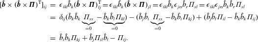 $$\begin{eqnarray}\displaystyle [\hat{\boldsymbol{b}}\times (\hat{\boldsymbol{b}}\times \unicode[STIX]{x1D72B})^{\text{T}}]_{ij} & = & \displaystyle \unicode[STIX]{x1D716}_{ikl}\hat{b}_{k}(\hat{\boldsymbol{b}}\times \unicode[STIX]{x1D72B})_{lj}^{\text{T}}=\unicode[STIX]{x1D716}_{ikl}\hat{b}_{k}(\hat{\boldsymbol{b}}\times \unicode[STIX]{x1D72B})_{jl}=\unicode[STIX]{x1D716}_{ikl}\hat{b}_{k}\unicode[STIX]{x1D716}_{jrs}\hat{b}_{r}\unicode[STIX]{x1D6F1}_{sl}=\unicode[STIX]{x1D716}_{ikl}\unicode[STIX]{x1D716}_{jrs}\hat{b}_{k}\hat{b}_{r}\unicode[STIX]{x1D6F1}_{sl}\nonumber\\ \displaystyle & = & \displaystyle \unicode[STIX]{x1D6FF}_{ij}(\hat{b}_{k}\hat{b}_{k}\underbrace{\unicode[STIX]{x1D6F1}_{ss}}_{=0}-\underbrace{\hat{b}_{k}\hat{b}_{l}\unicode[STIX]{x1D6F1}_{kl}}_{=0})-(\hat{b}_{j}\hat{b}_{i}\underbrace{\unicode[STIX]{x1D6F1}_{ss}}_{=0}-\hat{b}_{k}\hat{b}_{i}\unicode[STIX]{x1D6F1}_{kj})+(\hat{b}_{j}\hat{b}_{l}\unicode[STIX]{x1D6F1}_{il}-\hat{b}_{k}\hat{b}_{k}\unicode[STIX]{x1D6F1}_{ij})\nonumber\\ \displaystyle & = & \displaystyle \hat{b}_{i}\hat{b}_{k}\unicode[STIX]{x1D6F1}_{kj}+\hat{b}_{j}\unicode[STIX]{x1D6F1}_{il}\hat{b}_{l}-\unicode[STIX]{x1D6F1}_{ij}.\end{eqnarray}$$
The entire left-hand side therefore reads
 $$\begin{eqnarray}\displaystyle [\hat{\boldsymbol{b}}\times (\hat{\boldsymbol{b}}\times \unicode[STIX]{x1D72B})+\hat{\boldsymbol{b}}\times (\hat{\boldsymbol{b}}\times \unicode[STIX]{x1D72B})^{\text{T}}]_{ij}=-2\unicode[STIX]{x1D6F1}_{ij}+2\hat{b}_{i}\hat{b}_{l}\unicode[STIX]{x1D6F1}_{lj}+\hat{b}_{j}\unicode[STIX]{x1D6F1}_{il}\hat{b}_{l}. & & \displaystyle\end{eqnarray}$$
Performing a usual matrix (single) dot product of this result with matrix
 $\hat{\boldsymbol{b}}\hat{\boldsymbol{b}}$
yields
$\hat{\boldsymbol{b}}\hat{\boldsymbol{b}}$
yields
 $$\begin{eqnarray}\displaystyle & & \displaystyle [[\hat{\boldsymbol{b}}\times (\hat{\boldsymbol{b}}\times \unicode[STIX]{x1D72B})+\hat{\boldsymbol{b}}\times (\hat{\boldsymbol{b}}\times \unicode[STIX]{x1D72B})^{\text{T}}]\boldsymbol{\cdot }(\hat{\boldsymbol{b}}\hat{\boldsymbol{b}})]_{ij}=[\hat{\boldsymbol{b}}\times (\hat{\boldsymbol{b}}\times \unicode[STIX]{x1D72B})+\hat{\boldsymbol{b}}\times (\hat{\boldsymbol{b}}\times \unicode[STIX]{x1D72B})^{\text{T}}]_{ik}(\hat{\boldsymbol{b}}\hat{\boldsymbol{b}})_{kj}\nonumber\\ \displaystyle & & \displaystyle \quad =[-2\unicode[STIX]{x1D6F1}_{ik}+2\hat{b}_{i}\hat{b}_{l}\unicode[STIX]{x1D6F1}_{lk}+\hat{b}_{k}\unicode[STIX]{x1D6F1}_{il}\hat{b}_{l}]\hat{b}_{k}\hat{b}_{j}=-2\unicode[STIX]{x1D6F1}_{ik}\hat{b}_{k}\hat{b}_{j}+2\hat{b}_{i}\hat{b}_{j}\underbrace{\unicode[STIX]{x1D6F1}_{lk}\hat{b}_{l}\hat{b}_{k}}_{=0}+\unicode[STIX]{x1D6F1}_{il}\hat{b}_{l}\hat{b}_{j}\underbrace{\hat{b}_{k}\hat{b}_{k}}_{=1}\nonumber\\ \displaystyle & & \displaystyle \quad =-2\unicode[STIX]{x1D6F1}_{ik}\hat{b}_{k}\hat{b}_{j}+\unicode[STIX]{x1D6F1}_{il}\hat{b}_{l}\hat{b}_{j}=-2\unicode[STIX]{x1D6F1}_{ik}\hat{b}_{k}\hat{b}_{j}+\unicode[STIX]{x1D6F1}_{ik}\hat{b}_{k}\hat{b}_{j}=-\unicode[STIX]{x1D6F1}_{ik}\hat{b}_{k}\hat{b}_{j}.\end{eqnarray}$$
This further yields that
 $$\begin{eqnarray}\displaystyle [[\hat{\boldsymbol{b}}\times (\hat{\boldsymbol{b}}\times \unicode[STIX]{x1D72B})+\hat{\boldsymbol{b}}\times (\hat{\boldsymbol{b}}\times \unicode[STIX]{x1D72B})^{\text{T}}]\boldsymbol{\cdot }(\unicode[STIX]{x1D644}+3\hat{\boldsymbol{b}}\hat{\boldsymbol{b}})]_{ij} & = & \displaystyle -2\unicode[STIX]{x1D6F1}_{ij}+2\hat{b}_{i}\hat{b}_{k}\unicode[STIX]{x1D6F1}_{kj}+\hat{b}_{j}\unicode[STIX]{x1D6F1}_{ik}\hat{b}_{k}-3\unicode[STIX]{x1D6F1}_{ik}\hat{b}_{k}\hat{b}_{j}\nonumber\\ \displaystyle & = & \displaystyle -2\unicode[STIX]{x1D6F1}_{ij}+2\hat{b}_{i}\hat{b}_{k}\unicode[STIX]{x1D6F1}_{kj}-2\unicode[STIX]{x1D6F1}_{ik}\hat{b}_{k}\hat{b}_{j},\end{eqnarray}$$
and adding this result together with its transpose implies
 $$\begin{eqnarray}\displaystyle & & \displaystyle [[\hat{\boldsymbol{b}}\times (\hat{\boldsymbol{b}}\times \unicode[STIX]{x1D72B})+\hat{\boldsymbol{b}}\times (\hat{\boldsymbol{b}}\times \unicode[STIX]{x1D72B})^{\text{T}}]\boldsymbol{\cdot }(\unicode[STIX]{x1D644}+3\hat{\boldsymbol{b}}\hat{\boldsymbol{b}})]_{ij}^{S}\nonumber\\ \displaystyle & & \displaystyle \quad =-2\unicode[STIX]{x1D6F1}_{ij}+2\hat{b}_{i}\hat{b}_{k}\unicode[STIX]{x1D6F1}_{kj}-2\unicode[STIX]{x1D6F1}_{ik}\hat{b}_{k}\hat{b}_{j}-2\unicode[STIX]{x1D6F1}_{ji}+2\hat{b}_{j}\hat{b}_{k}\unicode[STIX]{x1D6F1}_{ki}-2\unicode[STIX]{x1D6F1}_{jk}\hat{b}_{k}\hat{b}_{i}=-4\unicode[STIX]{x1D6F1}_{ij},\end{eqnarray}$$
where we have used that the
 $\unicode[STIX]{x1D6F1}_{ij}=\unicode[STIX]{x1D6F1}_{ji}$
. One therefore derives that the FLR tensor can be extracted from the left-hand side of (5.1) by performing an ‘inversion’ procedure
$\unicode[STIX]{x1D6F1}_{ij}=\unicode[STIX]{x1D6F1}_{ji}$
. One therefore derives that the FLR tensor can be extracted from the left-hand side of (5.1) by performing an ‘inversion’ procedure
 $$\begin{eqnarray}\displaystyle \unicode[STIX]{x1D72B}=-{\textstyle \frac{1}{4}}[[\hat{\boldsymbol{b}}\times (\hat{\boldsymbol{b}}\times \unicode[STIX]{x1D72B})+\hat{\boldsymbol{b}}\times (\hat{\boldsymbol{b}}\times \unicode[STIX]{x1D72B})^{\text{T}}]\boldsymbol{\cdot }(\unicode[STIX]{x1D644}+3\hat{\boldsymbol{b}}\hat{\boldsymbol{b}})]^{S}. & & \displaystyle\end{eqnarray}$$
We can introduce matrix
 $\unicode[STIX]{x1D73F}$
that will represent the right-hand side of (5.1) as
$\unicode[STIX]{x1D73F}$
that will represent the right-hand side of (5.1) as
 $$\begin{eqnarray}\displaystyle & \displaystyle \hat{\boldsymbol{b}}\times \unicode[STIX]{x1D72B}+(\hat{\boldsymbol{b}}\times \unicode[STIX]{x1D72B})^{\text{T}}=-\unicode[STIX]{x1D73F}; & \displaystyle\end{eqnarray}$$
 $$\begin{eqnarray}\displaystyle & \displaystyle \unicode[STIX]{x1D73F}=\frac{1}{\unicode[STIX]{x1D6FA}}\frac{B_{0}}{|\boldsymbol{B}|}\left[\frac{\unicode[STIX]{x2202}\boldsymbol{p}}{\unicode[STIX]{x2202}t}+\unicode[STIX]{x1D735}\boldsymbol{\cdot }(\boldsymbol{u}\boldsymbol{p}+\boldsymbol{q})+\boldsymbol{p}\boldsymbol{\cdot }\unicode[STIX]{x1D735}\boldsymbol{u}+(\boldsymbol{p}\boldsymbol{\cdot }\unicode[STIX]{x1D735}\boldsymbol{u})^{\text{T}}\right]. & \displaystyle\end{eqnarray}$$
By performing operations (5.9) in this equation yields the FLR tensor in the following form
The expression (5.12) is completely general since no simplifications were introduced, the expression is exact. However, the equation is still implicit, since on the right-hand side the tensor
 $\unicode[STIX]{x1D73F}$
contains the full pressure tensor
$\unicode[STIX]{x1D73F}$
contains the full pressure tensor
 $\boldsymbol{p}=\boldsymbol{p}^{\text{g}}+\unicode[STIX]{x1D72B}$
. Nevertheless, the equation is extremely useful, once the expansion of the right-hand side is performed, as we will do below. Note that the brackets are not unique, since
$\boldsymbol{p}=\boldsymbol{p}^{\text{g}}+\unicode[STIX]{x1D72B}$
. Nevertheless, the equation is extremely useful, once the expansion of the right-hand side is performed, as we will do below. Note that the brackets are not unique, since
 $$\begin{eqnarray}(\hat{\boldsymbol{b}}\times \unicode[STIX]{x1D73F})\boldsymbol{\cdot }(\unicode[STIX]{x1D644}+3\hat{\boldsymbol{b}}\hat{\boldsymbol{b}})=\hat{\boldsymbol{b}}\times [\unicode[STIX]{x1D73F}\boldsymbol{\cdot }(\unicode[STIX]{x1D644}+3\hat{\boldsymbol{b}}\hat{\boldsymbol{b}})]=\hat{\boldsymbol{b}}\times \unicode[STIX]{x1D73F}\boldsymbol{\cdot }(\unicode[STIX]{x1D644}+3\hat{\boldsymbol{b}}\hat{\boldsymbol{b}}),\end{eqnarray}$$
where the last choice leaves the brackets unspecified (since both options are allowed), similarly to
 $\hat{\boldsymbol{b}}\boldsymbol{\cdot }\unicode[STIX]{x1D735}\boldsymbol{u}$
. Alternatively, one can get rid of the operator
$\hat{\boldsymbol{b}}\boldsymbol{\cdot }\unicode[STIX]{x1D735}\boldsymbol{u}$
. Alternatively, one can get rid of the operator
 $\boldsymbol{\cdot }\unicode[STIX]{x1D644}$
(which acting on a matrix yields the same matrix), and split the result into two parts
$\boldsymbol{\cdot }\unicode[STIX]{x1D644}$
(which acting on a matrix yields the same matrix), and split the result into two parts
 $$\begin{eqnarray}\displaystyle \unicode[STIX]{x1D72B}={\textstyle \frac{1}{4}}(\hat{\boldsymbol{b}}\times \unicode[STIX]{x1D73F})^{S}+{\textstyle \frac{3}{4}}(\hat{\boldsymbol{b}}\times \unicode[STIX]{x1D73F}\boldsymbol{\cdot }\hat{\boldsymbol{b}}\hat{\boldsymbol{b}})^{S}. & & \displaystyle\end{eqnarray}$$
Another possible form can be obtained by subtracting the evolution equations for the gyrotropic pressure components
 $\unicode[STIX]{x2202}p_{\Vert }/\unicode[STIX]{x2202}t$
and
$\unicode[STIX]{x2202}p_{\Vert }/\unicode[STIX]{x2202}t$
and
 $\unicode[STIX]{x2202}p_{\bot }/\unicode[STIX]{x2202}t$
. The scalar pressure equations were derived by applying
$\unicode[STIX]{x2202}p_{\bot }/\unicode[STIX]{x2202}t$
. The scalar pressure equations were derived by applying
 $:\hat{\boldsymbol{b}}\hat{\boldsymbol{b}}$
and
$:\hat{\boldsymbol{b}}\hat{\boldsymbol{b}}$
and
 $:(\unicode[STIX]{x1D644}-\hat{\boldsymbol{b}}\hat{\boldsymbol{b}})/2$
to the pressure tensor equation. The subtraction can be formally represented by introducing ‘overbar’ projection operator
$:(\unicode[STIX]{x1D644}-\hat{\boldsymbol{b}}\hat{\boldsymbol{b}})/2$
to the pressure tensor equation. The subtraction can be formally represented by introducing ‘overbar’ projection operator
 $\bar{\boldsymbol{a}}$
that projects any
$\bar{\boldsymbol{a}}$
that projects any
 $(3\times 3)$
matrix
$(3\times 3)$
matrix
 $\boldsymbol{a}$
to
$\boldsymbol{a}$
to
 $$\begin{eqnarray}\displaystyle \bar{\boldsymbol{a}}=\boldsymbol{a}-[\boldsymbol{a}:\hat{\boldsymbol{b}}\hat{\boldsymbol{b}}]\hat{\boldsymbol{b}}\hat{\boldsymbol{b}}-[\boldsymbol{a}:(\unicode[STIX]{x1D644}-\hat{\boldsymbol{b}}\hat{\boldsymbol{b}})/2](\unicode[STIX]{x1D644}-\hat{\boldsymbol{b}}\hat{\boldsymbol{b}}). & & \displaystyle\end{eqnarray}$$
The definition is of course motivated by the pressure decomposition (2.46). By applying this operator to (5.10), the left-hand side remains the same, yielding
 $(\hat{\boldsymbol{b}}\times \unicode[STIX]{x1D72B})^{S}=-\bar{\unicode[STIX]{x1D73F}}$
. The solution (5.12) for the FLR tensor therefore rewrites
$(\hat{\boldsymbol{b}}\times \unicode[STIX]{x1D72B})^{S}=-\bar{\unicode[STIX]{x1D73F}}$
. The solution (5.12) for the FLR tensor therefore rewrites
 $$\begin{eqnarray}\displaystyle \unicode[STIX]{x1D72B}={\textstyle \frac{1}{4}}[(\hat{\boldsymbol{b}}\times \bar{\unicode[STIX]{x1D73F}})\boldsymbol{\cdot }(\unicode[STIX]{x1D644}+3\hat{\boldsymbol{b}}\hat{\boldsymbol{b}})]^{S}. & & \displaystyle\end{eqnarray}$$
The subtraction of scalar pressure equations is motivated by the observation that when working in the linear approximation directly with (5.10), i.e. without performing the inversion procedure, the scalar pressure equations have to be subtracted at the end. However, by performing the inversion procedure, the scalar pressure equations are subtracted ‘automatically’ during calculations, and it is actually easier to work directly with (5.12) instead of (5.16).
Therefore, let us work with (5.12). The leading-order nonlinear FLR corrections are obtained by neglecting the non-gyrotropic contributions
 $\unicode[STIX]{x1D72B}$
and
$\unicode[STIX]{x1D72B}$
and
 $\boldsymbol{q}^{\text{ng}}$
on the right-hand side of (5.12), i.e. by prescribing
$\boldsymbol{q}^{\text{ng}}$
on the right-hand side of (5.12), i.e. by prescribing
 $$\begin{eqnarray}\displaystyle & \displaystyle \unicode[STIX]{x1D72B}={\textstyle \frac{1}{4}}[(\hat{\boldsymbol{b}}\times \unicode[STIX]{x1D73F}^{(1)})\boldsymbol{\cdot }(\unicode[STIX]{x1D644}+3\hat{\boldsymbol{b}}\hat{\boldsymbol{b}})]^{S}; & \displaystyle\end{eqnarray}$$
 $$\begin{eqnarray}\displaystyle & \displaystyle \unicode[STIX]{x1D73F}^{(1)}=\frac{1}{\unicode[STIX]{x1D6FA}}\frac{B_{0}}{|\boldsymbol{B}|}\left[\frac{\unicode[STIX]{x2202}\boldsymbol{p}^{\text{g}}}{\unicode[STIX]{x2202}t}+\unicode[STIX]{x1D735}\boldsymbol{\cdot }(\boldsymbol{u}\boldsymbol{p}^{\text{g}}+\boldsymbol{q}^{\text{g}})+\boldsymbol{p}^{\text{g}}\boldsymbol{\cdot }\unicode[STIX]{x1D735}\boldsymbol{u}+(\boldsymbol{p}^{\text{g}}\boldsymbol{\cdot }\unicode[STIX]{x1D735}\boldsymbol{u})^{\text{T}}\right]. & \displaystyle\end{eqnarray}$$
Therefore, the only non-gyrotropic quantities that were retained on the right-hand side of (5.12), are the perpendicular components of the velocity
 $\boldsymbol{u}$
. The slightly unappealing factors
$\boldsymbol{u}$
. The slightly unappealing factors
 $B_{0}/|\boldsymbol{B}|$
in all the expressions can be removed, by redefining the cyclotron frequency with
$B_{0}/|\boldsymbol{B}|$
in all the expressions can be removed, by redefining the cyclotron frequency with
 $|\boldsymbol{B}|$
instead of
$|\boldsymbol{B}|$
instead of
 $B_{0}$
, so that
$B_{0}$
, so that
 $\unicode[STIX]{x1D6FA}_{|\boldsymbol{B}|}=e|\boldsymbol{B}|/(mc)$
. Let us calculate (5.17) step by step. For the brevity of the calculations, it is useful to introduce convective derivative
$\unicode[STIX]{x1D6FA}_{|\boldsymbol{B}|}=e|\boldsymbol{B}|/(mc)$
. Let us calculate (5.17) step by step. For the brevity of the calculations, it is useful to introduce convective derivative
 $\text{d}/\text{d}t=\unicode[STIX]{x2202}/\unicode[STIX]{x2202}t+\boldsymbol{u}\boldsymbol{\cdot }\unicode[STIX]{x1D735}$
and work with
$\text{d}/\text{d}t=\unicode[STIX]{x2202}/\unicode[STIX]{x2202}t+\boldsymbol{u}\boldsymbol{\cdot }\unicode[STIX]{x1D735}$
and work with
 $$\begin{eqnarray}\unicode[STIX]{x1D73F}^{(1)}=\frac{1}{\unicode[STIX]{x1D6FA}_{|\boldsymbol{B}|}}\left[\frac{\text{d}\boldsymbol{p}^{\text{g}}}{\text{d}t}+\boldsymbol{p}^{\text{g}}\unicode[STIX]{x1D735}\boldsymbol{\cdot }\boldsymbol{u}+\unicode[STIX]{x1D735}\boldsymbol{\cdot }\boldsymbol{q}^{\text{g}}+\boldsymbol{p}^{\text{g}}\boldsymbol{\cdot }\unicode[STIX]{x1D735}\boldsymbol{u}+(\boldsymbol{p}^{\text{g}}\boldsymbol{\cdot }\unicode[STIX]{x1D735}\boldsymbol{u})^{\text{T}}\right].\end{eqnarray}$$
We want to present complete derivation with the least amount of algebra involved, and we first want to obtain the form of Schekochihin et al. (Reference Schekochihin, Cowley, Rincon and Rosin2010). Let us first write each term in
 $\unicode[STIX]{x1D73F}^{(1)}$
in the index notation. By using
$\unicode[STIX]{x1D73F}^{(1)}$
in the index notation. By using
 $$\begin{eqnarray}\displaystyle & \displaystyle p_{ij}^{g}=(p_{\Vert }-p_{\bot })\hat{b}_{i}\hat{b}_{j}+p_{\bot }\unicode[STIX]{x1D6FF}_{ij}; & \displaystyle\end{eqnarray}$$
 $$\begin{eqnarray}\displaystyle & \displaystyle q_{ijk}^{\text{g}}=(q_{\Vert }-3q_{\bot })\hat{b}_{i}\hat{b}_{j}\hat{b}_{k}+q_{\bot }(\unicode[STIX]{x1D6FF}_{ij}\hat{b}_{k}+\unicode[STIX]{x1D6FF}_{jk}\hat{b}_{i}+\unicode[STIX]{x1D6FF}_{ik}\hat{b}_{j}), & \displaystyle\end{eqnarray}$$
in the following form
 $$\begin{eqnarray}\displaystyle & \displaystyle \left(\frac{\text{d}\boldsymbol{p}^{\text{g}}}{\text{d}t}\right)_{ij}=\hat{b}_{i}\hat{b}_{j}\frac{\text{d}}{\text{d}t}(p_{\Vert }-p_{\bot })+(p_{\Vert }-p_{\bot })\frac{\text{d}}{\text{d}t}(\hat{b}_{i}\hat{b}_{j})+\unicode[STIX]{x1D6FF}_{ij}\frac{\text{d}p_{\bot }}{\text{d}t}; & \displaystyle\end{eqnarray}$$
 $$\begin{eqnarray}\displaystyle & \displaystyle (\boldsymbol{p}^{\text{g}}\unicode[STIX]{x1D735}\boldsymbol{\cdot }\boldsymbol{u})_{ij}=((p_{\Vert }-p_{\bot })\hat{b}_{i}\hat{b}_{j}+\unicode[STIX]{x1D6FF}_{ij}p_{\bot })\unicode[STIX]{x1D735}\boldsymbol{\cdot }\boldsymbol{u}; & \displaystyle\end{eqnarray}$$
 $$\begin{eqnarray}\displaystyle & \displaystyle (\boldsymbol{p}^{\text{g}}\boldsymbol{\cdot }\unicode[STIX]{x1D735}\boldsymbol{u})_{ij}=(p_{\Vert }-p_{\bot })\hat{b}_{i}\hat{\boldsymbol{b}}\boldsymbol{\cdot }\unicode[STIX]{x1D735}u_{j}+p_{\bot }\unicode[STIX]{x2202}_{i}u_{j}; & \displaystyle\end{eqnarray}$$
 $$\begin{eqnarray}\displaystyle & \displaystyle (\boldsymbol{p}^{\text{g}}\boldsymbol{\cdot }\unicode[STIX]{x1D735}\boldsymbol{u})_{ij}^{\text{T}}=(p_{\Vert }-p_{\bot })\hat{b}_{j}\hat{\boldsymbol{b}}\boldsymbol{\cdot }\unicode[STIX]{x1D735}u_{i}+p_{\bot }\unicode[STIX]{x2202}_{j}u_{i}; & \displaystyle\end{eqnarray}$$
 $$\begin{eqnarray}\displaystyle (\unicode[STIX]{x1D735}\boldsymbol{\cdot }\boldsymbol{q}^{\text{g}})_{ij} & = & \displaystyle \hat{b}_{i}\hat{b}_{j}\unicode[STIX]{x1D735}\boldsymbol{\cdot }((q_{\Vert }-3q_{\bot })\hat{\boldsymbol{b}})+(q_{\Vert }-3q_{\bot })\hat{\boldsymbol{b}}\boldsymbol{\cdot }\unicode[STIX]{x1D735}(\hat{b}_{i}\hat{b}_{j})\nonumber\\ \displaystyle & & \displaystyle +\,\unicode[STIX]{x1D6FF}_{ij}\unicode[STIX]{x1D735}\boldsymbol{\cdot }(q_{\bot }\hat{\boldsymbol{b}})+\unicode[STIX]{x2202}_{i}(q_{\bot }\hat{b}_{j})+\unicode[STIX]{x2202}_{j}(q_{\bot }\hat{b}_{i})\end{eqnarray}$$
and grouping similar terms in
 $\unicode[STIX]{x1D73F}^{(1)}$
together yields
$\unicode[STIX]{x1D73F}^{(1)}$
together yields
 $$\begin{eqnarray}\displaystyle \unicode[STIX]{x1D705}_{ij}^{(1)} & = & \displaystyle \frac{1}{\unicode[STIX]{x1D6FA}_{|\boldsymbol{B}|}}\left\{p_{\bot }(\unicode[STIX]{x2202}_{i}u_{j}+\unicode[STIX]{x2202}_{j}u_{i})+\unicode[STIX]{x2202}_{i}(q_{\bot }\hat{b}_{j})+\unicode[STIX]{x2202}_{j}(q_{\bot }\hat{b}_{i})\right.\nonumber\\ \displaystyle & & \displaystyle +\,(p_{\Vert }-p_{\bot })\left[\frac{\text{d}}{\text{d}t}(\hat{b}_{i}\hat{b}_{j})+\hat{b}_{i}\hat{\boldsymbol{b}}\boldsymbol{\cdot }\unicode[STIX]{x1D735}u_{j}+\hat{b}_{j}\hat{\boldsymbol{b}}\boldsymbol{\cdot }\unicode[STIX]{x1D735}u_{i}\right]+(q_{\Vert }-3q_{\bot })\hat{\boldsymbol{b}}\boldsymbol{\cdot }\unicode[STIX]{x1D735}(\hat{b}_{i}\hat{b}_{j})\nonumber\\ \displaystyle & & \displaystyle +\hat{b}_{i}\hat{b}_{j}\left[\frac{\text{d}}{\text{d}t}(p_{\Vert }-p_{\bot })+(p_{\Vert }-p_{\bot })\unicode[STIX]{x1D735}\boldsymbol{\cdot }\boldsymbol{u}+\unicode[STIX]{x1D735}\boldsymbol{\cdot }((q_{\Vert }-3q_{\bot })\hat{\boldsymbol{b}})\right]\nonumber\\ \displaystyle & & \displaystyle +\left.\unicode[STIX]{x1D6FF}_{ij}\left[\frac{\text{d}p_{\bot }}{\text{d}t}+p_{\bot }\unicode[STIX]{x1D735}\boldsymbol{\cdot }\boldsymbol{u}+\unicode[STIX]{x1D735}\boldsymbol{\cdot }(q_{\bot }\hat{\boldsymbol{b}})\right]\right\}.\end{eqnarray}$$
The first line in the above expression is left unchanged, since it is the final result, defined below as a matrix
 $\unicode[STIX]{x1D61E}_{ij}=p_{\bot }(\unicode[STIX]{x2202}_{i}u_{j}+\unicode[STIX]{x2202}_{j}u_{i})+\unicode[STIX]{x2202}_{j}(q_{\bot }\hat{b}_{i})+\unicode[STIX]{x2202}_{i}(q_{\bot }\hat{b}_{j})$
, that can be written as
$\unicode[STIX]{x1D61E}_{ij}=p_{\bot }(\unicode[STIX]{x2202}_{i}u_{j}+\unicode[STIX]{x2202}_{j}u_{i})+\unicode[STIX]{x2202}_{j}(q_{\bot }\hat{b}_{i})+\unicode[STIX]{x2202}_{i}(q_{\bot }\hat{b}_{j})$
, that can be written as
 $\unicode[STIX]{x1D652}=p_{\bot }\unicode[STIX]{x1D735}\boldsymbol{u}+\unicode[STIX]{x1D735}(q_{\bot }\hat{\boldsymbol{b}})+(p_{\bot }\unicode[STIX]{x1D735}\boldsymbol{u}+\unicode[STIX]{x1D735}(q_{\bot }\hat{\boldsymbol{b}}))^{\text{T}}=(p_{\bot }\unicode[STIX]{x1D735}\boldsymbol{u}+\unicode[STIX]{x1D735}(q_{\bot }\hat{\boldsymbol{b}}))^{S}$
. However, calculating the rest of the expression according to (5.17) simplifies several terms, and for example all terms in the third line of (5.27) vanish. The terms in the third line containing
$\unicode[STIX]{x1D652}=p_{\bot }\unicode[STIX]{x1D735}\boldsymbol{u}+\unicode[STIX]{x1D735}(q_{\bot }\hat{\boldsymbol{b}})+(p_{\bot }\unicode[STIX]{x1D735}\boldsymbol{u}+\unicode[STIX]{x1D735}(q_{\bot }\hat{\boldsymbol{b}}))^{\text{T}}=(p_{\bot }\unicode[STIX]{x1D735}\boldsymbol{u}+\unicode[STIX]{x1D735}(q_{\bot }\hat{\boldsymbol{b}}))^{S}$
. However, calculating the rest of the expression according to (5.17) simplifies several terms, and for example all terms in the third line of (5.27) vanish. The terms in the third line containing
 $\hat{b}_{i}\hat{b}_{j}$
vanish after applying
$\hat{b}_{i}\hat{b}_{j}$
vanish after applying
 $\hat{\boldsymbol{b}}\times$
, since
$\hat{\boldsymbol{b}}\times$
, since
 $(\hat{\boldsymbol{b}}\times (\hat{\boldsymbol{b}}\hat{\boldsymbol{b}}))_{ij}=\unicode[STIX]{x1D716}_{ikl}\hat{b}_{k}\hat{b}_{l}\hat{b}_{j}=0$
. The terms in the third line containing
$(\hat{\boldsymbol{b}}\times (\hat{\boldsymbol{b}}\hat{\boldsymbol{b}}))_{ij}=\unicode[STIX]{x1D716}_{ikl}\hat{b}_{k}\hat{b}_{l}\hat{b}_{j}=0$
. The terms in the third line containing
 $\unicode[STIX]{x1D6FF}_{ij}$
vanish after applying the symmetric operator since
$\unicode[STIX]{x1D6FF}_{ij}$
vanish after applying the symmetric operator since
 $$\begin{eqnarray}\displaystyle [(\hat{\boldsymbol{b}}\times \unicode[STIX]{x1D644})\boldsymbol{\cdot }(\unicode[STIX]{x1D644}+3\hat{\boldsymbol{b}}\hat{\boldsymbol{b}})]_{ij}^{S} & = & \displaystyle [(\hat{\boldsymbol{b}}\times \unicode[STIX]{x1D644})_{im}(\unicode[STIX]{x1D644}+3\hat{\boldsymbol{b}}\hat{\boldsymbol{b}})_{mj}]^{S}=[\unicode[STIX]{x1D716}_{ikl}\hat{b}_{k}\unicode[STIX]{x1D6FF}_{lm}(\unicode[STIX]{x1D6FF}_{mj}+3\hat{b}_{m}\hat{b}_{j})]^{S}\nonumber\\ \displaystyle & = & \displaystyle [\unicode[STIX]{x1D716}_{ikj}\hat{b}_{k}+3\underbrace{\unicode[STIX]{x1D716}_{ikl}\hat{b}_{k}\hat{b}_{l}}_{=0}\hat{b}_{j}]^{S}=\unicode[STIX]{x1D716}_{ikj}\hat{b}_{k}+\unicode[STIX]{x1D716}_{jki}\hat{b}_{k}=\unicode[STIX]{x1D716}_{ikj}\hat{b}_{k}-\unicode[STIX]{x1D716}_{ikj}\hat{b}_{k}=0.\nonumber\\ \displaystyle & & \displaystyle\end{eqnarray}$$
We therefore need to concentrate only on the second line of (5.27), and slightly rewrite that one. For example, the first term in the second line of (5.27), the term
 $\text{d}/\text{d}t(\hat{b}_{i}\hat{b}_{j})$
, calculates as
$\text{d}/\text{d}t(\hat{b}_{i}\hat{b}_{j})$
, calculates as

The second term in the second line of (5.27), the term
 $\hat{b}_{i}\hat{\boldsymbol{b}}\boldsymbol{\cdot }\unicode[STIX]{x1D735}u_{j}$
, vanishes after applying
$\hat{b}_{i}\hat{\boldsymbol{b}}\boldsymbol{\cdot }\unicode[STIX]{x1D735}u_{j}$
, vanishes after applying
 $\hat{\boldsymbol{b}}\times$
, since
$\hat{\boldsymbol{b}}\times$
, since
 $$\begin{eqnarray}\displaystyle [\hat{\boldsymbol{b}}\times (\hat{\boldsymbol{b}}(\hat{\boldsymbol{b}}\boldsymbol{\cdot }\unicode[STIX]{x1D735}\boldsymbol{u}))]_{ij}=\unicode[STIX]{x1D716}_{ikl}\hat{b}_{k}(\hat{\boldsymbol{b}}(\hat{\boldsymbol{b}}\boldsymbol{\cdot }\unicode[STIX]{x1D735}\boldsymbol{u}))_{lj}=\underbrace{\unicode[STIX]{x1D716}_{ikl}\hat{b}_{k}\hat{b}_{l}}_{=0}(\hat{\boldsymbol{b}}\boldsymbol{\cdot }\unicode[STIX]{x1D735}\boldsymbol{u})_{j}=0. & & \displaystyle\end{eqnarray}$$
The third term in the second line of (5.27), the term
 $\hat{b}_{j}\hat{\boldsymbol{b}}\boldsymbol{\cdot }\unicode[STIX]{x1D735}u_{i}$
however does not vanish. Note that
$\hat{b}_{j}\hat{\boldsymbol{b}}\boldsymbol{\cdot }\unicode[STIX]{x1D735}u_{i}$
however does not vanish. Note that
 $b_{j}\hat{\boldsymbol{b}}\boldsymbol{\cdot }\unicode[STIX]{x1D735}u_{i}=((\hat{\boldsymbol{b}}\boldsymbol{\cdot }\unicode[STIX]{x1D735}\boldsymbol{u})\hat{\boldsymbol{b}})_{ij}$
and the third term calculates as
$b_{j}\hat{\boldsymbol{b}}\boldsymbol{\cdot }\unicode[STIX]{x1D735}u_{i}=((\hat{\boldsymbol{b}}\boldsymbol{\cdot }\unicode[STIX]{x1D735}\boldsymbol{u})\hat{\boldsymbol{b}})_{ij}$
and the third term calculates as
 $$\begin{eqnarray}\displaystyle & & \displaystyle [(\hat{\boldsymbol{b}}\times ((\hat{\boldsymbol{b}}\boldsymbol{\cdot }\unicode[STIX]{x1D735}\boldsymbol{u})\hat{\boldsymbol{b}}))\boldsymbol{\cdot }(\unicode[STIX]{x1D644}+3\hat{\boldsymbol{b}}\hat{\boldsymbol{b}})]_{ij}^{S}=[(\hat{\boldsymbol{b}}\times ((\hat{\boldsymbol{b}}\boldsymbol{\cdot }\unicode[STIX]{x1D735}\boldsymbol{u})\hat{\boldsymbol{b}}))_{im}(\unicode[STIX]{x1D644}+3\hat{\boldsymbol{b}}\hat{\boldsymbol{b}})_{mj}]^{S}\nonumber\\ \displaystyle & & \displaystyle \quad =[\unicode[STIX]{x1D716}_{ikl}\hat{b}_{k}((\hat{\boldsymbol{b}}\boldsymbol{\cdot }\unicode[STIX]{x1D735}\boldsymbol{u})\hat{\boldsymbol{b}})_{lm}(\unicode[STIX]{x1D6FF}_{mj}+3\hat{b}_{m}\hat{b}_{j})]^{S}=[\unicode[STIX]{x1D716}_{ikl}\hat{b}_{k}(\hat{\boldsymbol{b}}\boldsymbol{\cdot }\unicode[STIX]{x1D735}u_{l})\hat{b}_{m}(\unicode[STIX]{x1D6FF}_{mj}+3\hat{b}_{m}\hat{b}_{j})]^{S}\nonumber\\ \displaystyle & & \displaystyle \quad =4[\unicode[STIX]{x1D716}_{ikl}\hat{b}_{k}(\hat{\boldsymbol{b}}\boldsymbol{\cdot }\unicode[STIX]{x1D735}u_{l})\hat{b}_{j}]^{S}=4[(\hat{\boldsymbol{b}}\times (\hat{\boldsymbol{b}}\boldsymbol{\cdot }\unicode[STIX]{x1D735}\boldsymbol{u}))_{i}\hat{b}_{j}]^{S}=4[(\hat{\boldsymbol{b}}\times (\hat{\boldsymbol{b}}\boldsymbol{\cdot }\unicode[STIX]{x1D735}\boldsymbol{u}))\hat{\boldsymbol{b}}]_{ij}^{S}.\end{eqnarray}$$
The fourth term in the second line of (5.27), calculates in the same fashion than the second and third terms since
 $\hat{\boldsymbol{b}}\boldsymbol{\cdot }\unicode[STIX]{x1D735}(\hat{b}_{i}\hat{b}_{j})=\hat{b}_{i}(\hat{\boldsymbol{b}}\boldsymbol{\cdot }\unicode[STIX]{x1D735}\hat{b}_{j})+(\hat{\boldsymbol{b}}\boldsymbol{\cdot }\unicode[STIX]{x1D735}\hat{b}_{i})\hat{b}_{j}$
, yielding
$\hat{\boldsymbol{b}}\boldsymbol{\cdot }\unicode[STIX]{x1D735}(\hat{b}_{i}\hat{b}_{j})=\hat{b}_{i}(\hat{\boldsymbol{b}}\boldsymbol{\cdot }\unicode[STIX]{x1D735}\hat{b}_{j})+(\hat{\boldsymbol{b}}\boldsymbol{\cdot }\unicode[STIX]{x1D735}\hat{b}_{i})\hat{b}_{j}$
, yielding
 $$\begin{eqnarray}\displaystyle [(\hat{\boldsymbol{b}}\times (\hat{\boldsymbol{b}}\boldsymbol{\cdot }\unicode[STIX]{x1D735}(\hat{\boldsymbol{b}}\hat{\boldsymbol{b}})))\boldsymbol{\cdot }(\unicode[STIX]{x1D644}+3\hat{\boldsymbol{b}}\hat{\boldsymbol{b}})]_{ij}^{S}=4[(\hat{\boldsymbol{b}}\times (\hat{\boldsymbol{b}}\boldsymbol{\cdot }\unicode[STIX]{x1D735}\hat{\boldsymbol{b}}))\hat{\boldsymbol{b}}]_{ij}^{S}. & & \displaystyle\end{eqnarray}$$
Collecting all the results together yields the FLR tensor
 $$\begin{eqnarray}\displaystyle & \displaystyle \unicode[STIX]{x1D72B}=\frac{1}{4\unicode[STIX]{x1D6FA}_{|\boldsymbol{B}|}}[(\hat{\boldsymbol{b}}\times \unicode[STIX]{x1D652})\boldsymbol{\cdot }(\unicode[STIX]{x1D644}+3\hat{\boldsymbol{b}}\hat{\boldsymbol{b}})]^{S}+\frac{1}{\unicode[STIX]{x1D6FA}_{|\boldsymbol{B}|}}[(\hat{\boldsymbol{b}}\times \boldsymbol{w})\hat{\boldsymbol{b}}]^{S}; & \displaystyle\end{eqnarray}$$
 $$\begin{eqnarray}\displaystyle & \displaystyle \unicode[STIX]{x1D652}=[p_{\bot }\unicode[STIX]{x1D735}\boldsymbol{u}+\unicode[STIX]{x1D735}(q_{\bot }\hat{\boldsymbol{b}})]^{S}; & \displaystyle\end{eqnarray}$$
 $$\begin{eqnarray}\displaystyle & \displaystyle \boldsymbol{w}=(p_{\Vert }-p_{\bot })\left(\frac{\text{d}\hat{\boldsymbol{b}}}{\text{d}t}+\hat{\boldsymbol{b}}\boldsymbol{\cdot }\unicode[STIX]{x1D735}\boldsymbol{u}\right)+(q_{\Vert }-3q_{\bot })\hat{\boldsymbol{b}}\boldsymbol{\cdot }\unicode[STIX]{x1D735}\hat{\boldsymbol{b}}, & \displaystyle\end{eqnarray}$$
where
 $\unicode[STIX]{x1D652}$
is a matrix and
$\unicode[STIX]{x1D652}$
is a matrix and
 $\boldsymbol{w}$
is a vector. The result is equivalent to (5)–(8) of Schekochihin et al. (Reference Schekochihin, Cowley, Rincon and Rosin2010), derived in the Appendix of that paper in a somewhat simpler way. In Schekochihin et al. (Reference Schekochihin, Cowley, Rincon and Rosin2010), instead of our notation for matrix
$\boldsymbol{w}$
is a vector. The result is equivalent to (5)–(8) of Schekochihin et al. (Reference Schekochihin, Cowley, Rincon and Rosin2010), derived in the Appendix of that paper in a somewhat simpler way. In Schekochihin et al. (Reference Schekochihin, Cowley, Rincon and Rosin2010), instead of our notation for matrix
 $\unicode[STIX]{x1D652}$
and vector
$\unicode[STIX]{x1D652}$
and vector
 $\boldsymbol{w}$
, the symbols
$\boldsymbol{w}$
, the symbols
 $\boldsymbol{S}$
and
$\boldsymbol{S}$
and
 $\unicode[STIX]{x1D748}$
are used, where
$\unicode[STIX]{x1D748}$
are used, where
 $\boldsymbol{S}=\unicode[STIX]{x1D652}$
and
$\boldsymbol{S}=\unicode[STIX]{x1D652}$
and
 $\unicode[STIX]{x1D748}=-\boldsymbol{w}$
. We wanted to avoid the use of
$\unicode[STIX]{x1D748}=-\boldsymbol{w}$
. We wanted to avoid the use of
 $\boldsymbol{S}$
and
$\boldsymbol{S}$
and
 $\unicode[STIX]{x1D748}$
, since these symbols are typically used when decomposing the heat flux tensor. For a reader who just jumped to this result, the symmetric operator is defined as
$\unicode[STIX]{x1D748}$
, since these symbols are typically used when decomposing the heat flux tensor. For a reader who just jumped to this result, the symmetric operator is defined as
 $\unicode[STIX]{x1D608}_{ij}^{S}=\unicode[STIX]{x1D608}_{ij}+\unicode[STIX]{x1D608}_{ji}$
. For clarity, for any vector
$\unicode[STIX]{x1D608}_{ij}^{S}=\unicode[STIX]{x1D608}_{ij}+\unicode[STIX]{x1D608}_{ji}$
. For clarity, for any vector
 $\boldsymbol{w}$
and any matrix
$\boldsymbol{w}$
and any matrix
 $\unicode[STIX]{x1D652}$
, the following identities hold
$\unicode[STIX]{x1D652}$
, the following identities hold
 $$\begin{eqnarray}\displaystyle & \displaystyle [(\hat{\boldsymbol{b}}\times \boldsymbol{w})\hat{\boldsymbol{b}}]^{S}=(\hat{\boldsymbol{b}}\times \boldsymbol{w})\hat{\boldsymbol{b}}+\hat{\boldsymbol{b}}(\hat{\boldsymbol{b}}\times \boldsymbol{w}); & \displaystyle\end{eqnarray}$$
 $$\begin{eqnarray}\displaystyle & \displaystyle [\hat{\boldsymbol{b}}\times \unicode[STIX]{x1D652}\boldsymbol{\cdot }(\unicode[STIX]{x1D644}+3\hat{\boldsymbol{b}}\hat{\boldsymbol{b}})]^{S}=\hat{\boldsymbol{b}}\times \unicode[STIX]{x1D652}\boldsymbol{\cdot }(\unicode[STIX]{x1D644}+3\hat{\boldsymbol{b}}\hat{\boldsymbol{b}})-(\unicode[STIX]{x1D644}+3\hat{\boldsymbol{b}}\hat{\boldsymbol{b}})\boldsymbol{\cdot }\unicode[STIX]{x1D652}^{\text{T}}\times \hat{\boldsymbol{b}}. & \displaystyle\end{eqnarray}$$
The last identity follows from an identity for general matrix
 $\unicode[STIX]{x1D63C}$
, that reads
$\unicode[STIX]{x1D63C}$
, that reads
 $(\hat{\boldsymbol{b}}\times \unicode[STIX]{x1D63C})^{\text{T}}=-\unicode[STIX]{x1D63C}^{\text{T}}\times \hat{\boldsymbol{b}}$
, and for a matrix
$(\hat{\boldsymbol{b}}\times \unicode[STIX]{x1D63C})^{\text{T}}=-\unicode[STIX]{x1D63C}^{\text{T}}\times \hat{\boldsymbol{b}}$
, and for a matrix
 $\unicode[STIX]{x1D63C}=\unicode[STIX]{x1D63D}\boldsymbol{\cdot }\boldsymbol{C}$
the
$\unicode[STIX]{x1D63C}=\unicode[STIX]{x1D63D}\boldsymbol{\cdot }\boldsymbol{C}$
the
 $\unicode[STIX]{x1D63C}^{\text{T}}=\boldsymbol{C}^{\text{T}}\boldsymbol{\cdot }\unicode[STIX]{x1D63D}^{\text{T}}$
, implying
$\unicode[STIX]{x1D63C}^{\text{T}}=\boldsymbol{C}^{\text{T}}\boldsymbol{\cdot }\unicode[STIX]{x1D63D}^{\text{T}}$
, implying
 $(\hat{\boldsymbol{b}}\times \unicode[STIX]{x1D63D}\boldsymbol{\cdot }\boldsymbol{C})^{\text{T}}=-\boldsymbol{C}^{\text{T}}\boldsymbol{\cdot }\unicode[STIX]{x1D63D}^{\text{T}}\times \hat{\boldsymbol{b}}$
.
$(\hat{\boldsymbol{b}}\times \unicode[STIX]{x1D63D}\boldsymbol{\cdot }\boldsymbol{C})^{\text{T}}=-\boldsymbol{C}^{\text{T}}\boldsymbol{\cdot }\unicode[STIX]{x1D63D}^{\text{T}}\times \hat{\boldsymbol{b}}$
.
The result (5.33)–(5.35) can be slightly simplified. The matrix
 $\unicode[STIX]{x1D652}$
in the index notation reads
$\unicode[STIX]{x1D652}$
in the index notation reads
 $$\begin{eqnarray}\unicode[STIX]{x1D61E}_{ij}=p_{\bot }(\unicode[STIX]{x2202}_{i}u_{j}+\unicode[STIX]{x2202}_{j}u_{i})+q_{\bot }(\unicode[STIX]{x2202}_{i}\hat{b}_{j}+\unicode[STIX]{x2202}_{j}\hat{b}_{i})+(\unicode[STIX]{x2202}_{i}q_{\bot })\hat{b}_{j}+(\unicode[STIX]{x2202}_{j}q_{\bot })\hat{b}_{i},\end{eqnarray}$$
and by applying
 $\hat{\boldsymbol{b}}\times$
eliminates only the last term
$\hat{\boldsymbol{b}}\times$
eliminates only the last term
implying that the matrix
 $\unicode[STIX]{x1D652}$
could possibly be redefined to
$\unicode[STIX]{x1D652}$
could possibly be redefined to
 $$\begin{eqnarray}\unicode[STIX]{x1D652}=[p_{\bot }\unicode[STIX]{x1D735}\boldsymbol{u}+q_{\bot }\unicode[STIX]{x1D735}\hat{\boldsymbol{b}}]^{S}+(\unicode[STIX]{x1D735}q_{\bot })\hat{\boldsymbol{b}}.\end{eqnarray}$$
However, now the matrix is not symmetric. Note that the brackets in the expression (5.33) are not unique, and one can for example pull the
 $\hat{\boldsymbol{b}}\times$
out, so that the expression reads
$\hat{\boldsymbol{b}}\times$
out, so that the expression reads
 $$\begin{eqnarray}\displaystyle \unicode[STIX]{x1D72B}=\frac{1}{\unicode[STIX]{x1D6FA}_{|\boldsymbol{B}|}}\left\{\hat{\boldsymbol{b}}\times \left[\frac{1}{4}\unicode[STIX]{x1D652}\boldsymbol{\cdot }(\unicode[STIX]{x1D644}+3\hat{\boldsymbol{b}}\hat{\boldsymbol{b}})+\boldsymbol{w}\hat{\boldsymbol{b}}\right]\right\}^{S}. & & \displaystyle\end{eqnarray}$$
Let us multiply the last term in (5.40) by
 $\boldsymbol{\cdot }(\unicode[STIX]{x1D644}+3\hat{\boldsymbol{b}}\hat{\boldsymbol{b}})$
, it calculates as
$\boldsymbol{\cdot }(\unicode[STIX]{x1D644}+3\hat{\boldsymbol{b}}\hat{\boldsymbol{b}})$
, it calculates as
 $$\begin{eqnarray}((\unicode[STIX]{x1D735}q_{\bot })\hat{\boldsymbol{b}})\boldsymbol{\cdot }(\unicode[STIX]{x1D644}+3\hat{\boldsymbol{b}}\hat{\boldsymbol{b}})=4(\unicode[STIX]{x1D735}q_{\bot })\hat{\boldsymbol{b}}.\end{eqnarray}$$
Obviously, it is beneficial to move this term to the vector
 $\boldsymbol{w}$
. Therefore, redefining
$\boldsymbol{w}$
. Therefore, redefining
 $\unicode[STIX]{x1D652}$
and
$\unicode[STIX]{x1D652}$
and
 $\boldsymbol{w}$
, the solution reads
$\boldsymbol{w}$
, the solution reads
 $$\begin{eqnarray}\displaystyle & \displaystyle \unicode[STIX]{x1D72B}=\frac{1}{4\unicode[STIX]{x1D6FA}_{|\boldsymbol{B}|}}[(\hat{\boldsymbol{b}}\times \unicode[STIX]{x1D652})\boldsymbol{\cdot }(\unicode[STIX]{x1D644}+3\hat{\boldsymbol{b}}\hat{\boldsymbol{b}})]^{S}+\frac{1}{\unicode[STIX]{x1D6FA}_{|\boldsymbol{B}|}}[(\hat{\boldsymbol{b}}\times \boldsymbol{w})\hat{\boldsymbol{b}}]^{S}; & \displaystyle\end{eqnarray}$$
 $$\begin{eqnarray}\displaystyle & \displaystyle \unicode[STIX]{x1D652}=[p_{\bot }\unicode[STIX]{x1D735}\boldsymbol{u}+q_{\bot }\unicode[STIX]{x1D735}\hat{\boldsymbol{b}}]^{S}; & \displaystyle\end{eqnarray}$$
 $$\begin{eqnarray}\displaystyle & \displaystyle \boldsymbol{w}=(p_{\Vert }-p_{\bot })\left(\frac{\text{d}\hat{\boldsymbol{b}}}{\text{d}t}+\hat{\boldsymbol{b}}\boldsymbol{\cdot }\unicode[STIX]{x1D735}\boldsymbol{u}\right)+\unicode[STIX]{x1D735}q_{\bot }+(q_{\Vert }-3q_{\bot })\hat{\boldsymbol{b}}\boldsymbol{\cdot }\unicode[STIX]{x1D735}\hat{\boldsymbol{b}}. & \displaystyle\end{eqnarray}$$
Now the matrix
 $\unicode[STIX]{x1D652}$
is again symmetric, and
$\unicode[STIX]{x1D652}$
is again symmetric, and
 $\boldsymbol{w}$
is just a vector. This solution with matrix (5.44) is slightly nicer than the solution with matrix (5.34). Alternatively, one can write the solution in its full form
$\boldsymbol{w}$
is just a vector. This solution with matrix (5.44) is slightly nicer than the solution with matrix (5.34). Alternatively, one can write the solution in its full form
 $$\begin{eqnarray}\displaystyle \unicode[STIX]{x1D72B} & = & \displaystyle \frac{1}{\unicode[STIX]{x1D6FA}_{|\boldsymbol{B}|}}\left\{\hat{\boldsymbol{b}}\times \left[\frac{1}{4}[p_{\bot }\unicode[STIX]{x1D735}\boldsymbol{u}+q_{\bot }\unicode[STIX]{x1D735}\hat{\boldsymbol{b}}]^{S}\boldsymbol{\cdot }(\unicode[STIX]{x1D644}+3\hat{\boldsymbol{b}}\hat{\boldsymbol{b}})+(p_{\Vert }-p_{\bot })\left(\frac{\text{d}\hat{\boldsymbol{b}}}{\text{d}t}+\hat{\boldsymbol{b}}\boldsymbol{\cdot }\unicode[STIX]{x1D735}\boldsymbol{u}\right)\hat{\boldsymbol{b}}\right.\right.\nonumber\\ \displaystyle & & \displaystyle +\left.\left.(\unicode[STIX]{x1D735}q_{\bot })\hat{\boldsymbol{b}}+(q_{\Vert }-3q_{\bot })(\hat{\boldsymbol{b}}\boldsymbol{\cdot }\unicode[STIX]{x1D735}\hat{\boldsymbol{b}})\hat{\boldsymbol{b}}\right]\right\}^{S}.\end{eqnarray}$$
The nonlinear solution for the FLR tensor
 $\unicode[STIX]{x1D72B}$
can be further re-arranged. For example, to obtain the form reported by Ramos (Reference Ramos2005), one needs to separate a part that is obtained by performing
$\unicode[STIX]{x1D72B}$
can be further re-arranged. For example, to obtain the form reported by Ramos (Reference Ramos2005), one needs to separate a part that is obtained by performing
 $\unicode[STIX]{x1D72B}\boldsymbol{\cdot }\hat{\boldsymbol{b}}$
. The solution (5.43) in the index notation reads
$\unicode[STIX]{x1D72B}\boldsymbol{\cdot }\hat{\boldsymbol{b}}$
. The solution (5.43) in the index notation reads
 $$\begin{eqnarray}\displaystyle \unicode[STIX]{x1D6F1}_{ij} & = & \displaystyle \frac{1}{\unicode[STIX]{x1D6FA}_{|\boldsymbol{B}|}}\left\{\unicode[STIX]{x1D716}_{ikl}\hat{b}_{k}\left[\frac{1}{4}\unicode[STIX]{x1D61E}_{lm}(\unicode[STIX]{x1D6FF}_{mj}+3\hat{b}_{m}\hat{b}_{j})+w_{l}\hat{b}_{j}\right]\right.\nonumber\\ \displaystyle & & \displaystyle +\left.\unicode[STIX]{x1D716}_{jkl}\hat{b}_{k}\left[\frac{1}{4}\unicode[STIX]{x1D61E}_{lm}(\unicode[STIX]{x1D6FF}_{mi}+3\hat{b}_{m}\hat{b}_{i})+w_{l}\hat{b}_{i}\right]\right\},\end{eqnarray}$$
and direct calculation yields
 $$\begin{eqnarray}\displaystyle & \displaystyle \unicode[STIX]{x1D6F1}_{ij}\hat{b}_{j}=\frac{1}{\unicode[STIX]{x1D6FA}_{|\boldsymbol{B}|}}\left\{\unicode[STIX]{x1D716}_{ikl}\hat{b}_{k}\left[\frac{1}{4}\unicode[STIX]{x1D61E}_{lm}(\unicode[STIX]{x1D6FF}_{mj}+3\hat{b}_{m}\hat{b}_{j})+w_{l}\hat{b}_{j}\right]\hat{b}_{j}\right\}=\frac{1}{\unicode[STIX]{x1D6FA}_{|\boldsymbol{B}|}}\unicode[STIX]{x1D716}_{ikl}\hat{b}_{k}(\unicode[STIX]{x1D61E}_{lm}\hat{b}_{m}+w_{l}); & \displaystyle \nonumber\\ \displaystyle & & \displaystyle\end{eqnarray}$$
 $$\begin{eqnarray}\displaystyle & \displaystyle \unicode[STIX]{x1D72B}\boldsymbol{\cdot }\hat{\boldsymbol{b}}=\frac{1}{\unicode[STIX]{x1D6FA}_{|\boldsymbol{B}|}}\hat{\boldsymbol{b}}\times (\unicode[STIX]{x1D652}\boldsymbol{\cdot }\hat{\boldsymbol{b}}+\boldsymbol{w})\equiv \frac{1}{\unicode[STIX]{x1D6FA}_{|\boldsymbol{B}|}}\hat{\boldsymbol{b}}\times \boldsymbol{h}, & \displaystyle\end{eqnarray}$$
where it was useful to define the new vector
 $\boldsymbol{h}\equiv \unicode[STIX]{x1D652}\boldsymbol{\cdot }\hat{\boldsymbol{b}}+\boldsymbol{w}$
, by adding the quantity
$\boldsymbol{h}\equiv \unicode[STIX]{x1D652}\boldsymbol{\cdot }\hat{\boldsymbol{b}}+\boldsymbol{w}$
, by adding the quantity
 $$\begin{eqnarray}\unicode[STIX]{x1D652}\boldsymbol{\cdot }\hat{\boldsymbol{b}}=p_{\bot }((\unicode[STIX]{x1D735}\boldsymbol{u})\boldsymbol{\cdot }\hat{\boldsymbol{b}}+\hat{\boldsymbol{b}}\boldsymbol{\cdot }\unicode[STIX]{x1D735}\boldsymbol{u})+q_{\bot }\hat{\boldsymbol{b}}\boldsymbol{\cdot }\unicode[STIX]{x1D735}\hat{\boldsymbol{b}}\end{eqnarray}$$
to the vector
 $\boldsymbol{w}$
. By separating the
$\boldsymbol{w}$
. By separating the
 $\unicode[STIX]{x1D72B}\boldsymbol{\cdot }\hat{\boldsymbol{b}}$
part, the solution (5.43) for
$\unicode[STIX]{x1D72B}\boldsymbol{\cdot }\hat{\boldsymbol{b}}$
part, the solution (5.43) for
 $\unicode[STIX]{x1D72B}$
is therefore re-arranged to the following form
$\unicode[STIX]{x1D72B}$
is therefore re-arranged to the following form
 $$\begin{eqnarray}\displaystyle & \displaystyle \unicode[STIX]{x1D72B}=\frac{1}{4\unicode[STIX]{x1D6FA}_{|\boldsymbol{B}|}}[(\hat{\boldsymbol{b}}\times \unicode[STIX]{x1D652})\boldsymbol{\cdot }(\unicode[STIX]{x1D644}-\hat{\boldsymbol{b}}\hat{\boldsymbol{b}})]^{S}+\frac{1}{\unicode[STIX]{x1D6FA}_{|\boldsymbol{B}|}}[(\hat{\boldsymbol{b}}\times \boldsymbol{h})\hat{\boldsymbol{b}}]^{S}; & \displaystyle\end{eqnarray}$$
 $$\begin{eqnarray}\displaystyle & \displaystyle \unicode[STIX]{x1D652}=[p_{\bot }\unicode[STIX]{x1D735}\boldsymbol{u}+q_{\bot }\unicode[STIX]{x1D735}\hat{\boldsymbol{b}}]^{S}; & \displaystyle\end{eqnarray}$$
 $$\begin{eqnarray}\displaystyle & \displaystyle \boldsymbol{h}=p_{\Vert }\left(\frac{\text{d}\hat{\boldsymbol{b}}}{\text{d}t}+\hat{\boldsymbol{b}}\boldsymbol{\cdot }\unicode[STIX]{x1D735}\boldsymbol{u}\right)-p_{\bot }\left(\frac{\text{d}\hat{\boldsymbol{b}}}{\text{d}t}-(\unicode[STIX]{x1D735}\boldsymbol{u})\boldsymbol{\cdot }\hat{\boldsymbol{b}}\right)+\unicode[STIX]{x1D735}q_{\bot }+(q_{\Vert }-2q_{\bot })\hat{\boldsymbol{b}}\boldsymbol{\cdot }\unicode[STIX]{x1D735}\hat{\boldsymbol{b}}. & \displaystyle\end{eqnarray}$$
The solution (5.51) has a nice advantage in that it is decomposed with respect to the magnetic field lines. In other words, projecting
 $\unicode[STIX]{x1D72B}$
along the field lines by performing
$\unicode[STIX]{x1D72B}$
along the field lines by performing
 $\unicode[STIX]{x1D72B}\boldsymbol{\cdot }\hat{\boldsymbol{b}}$
cancels the first term, and directly yields vector
$\unicode[STIX]{x1D72B}\boldsymbol{\cdot }\hat{\boldsymbol{b}}$
cancels the first term, and directly yields vector
 $\hat{\boldsymbol{b}}\times \boldsymbol{h}/\unicode[STIX]{x1D6FA}_{|\boldsymbol{B}|}$
, that could be defined as vector
$\hat{\boldsymbol{b}}\times \boldsymbol{h}/\unicode[STIX]{x1D6FA}_{|\boldsymbol{B}|}$
, that could be defined as vector
 $\vec{\unicode[STIX]{x1D72B}}_{z}$
.
$\vec{\unicode[STIX]{x1D72B}}_{z}$
.
5.1.1 Employing a non-dispersive induction equation
Considering the long-wavelength low-frequency limit, the solution (5.45) for vector
 $\boldsymbol{w}$
and the solution (5.53) for vector
$\boldsymbol{w}$
and the solution (5.53) for vector
 $\boldsymbol{h}$
can be further simplified, by using the usual non-dispersive CGL/MHD induction equation, that can be written in the following form (see later in the text)
$\boldsymbol{h}$
can be further simplified, by using the usual non-dispersive CGL/MHD induction equation, that can be written in the following form (see later in the text)
 $$\begin{eqnarray}\frac{\text{d}\hat{\boldsymbol{b}}}{\text{d}t}=\hat{\boldsymbol{b}}\boldsymbol{\cdot }\unicode[STIX]{x1D735}\boldsymbol{u}-\hat{\boldsymbol{b}}[\hat{\boldsymbol{b}}\boldsymbol{\cdot }(\unicode[STIX]{x1D735}\boldsymbol{u})\boldsymbol{\cdot }\hat{\boldsymbol{b}}].\end{eqnarray}$$
By further applying
 $\hat{\boldsymbol{b}}\times$
to the induction equation, the last term on the right-hand side disappears
$\hat{\boldsymbol{b}}\times$
to the induction equation, the last term on the right-hand side disappears
 $$\begin{eqnarray}\hat{\boldsymbol{b}}\times \frac{\text{d}\hat{\boldsymbol{b}}}{\text{d}t}=\hat{\boldsymbol{b}}\times (\hat{\boldsymbol{b}}\boldsymbol{\cdot }\unicode[STIX]{x1D735}\boldsymbol{u}),\end{eqnarray}$$
and vectors (5.45), (5.53) simplify to
 $$\begin{eqnarray}\displaystyle & \displaystyle \boldsymbol{w}=2(p_{\Vert }-p_{\bot })\hat{\boldsymbol{b}}\boldsymbol{\cdot }\unicode[STIX]{x1D735}\boldsymbol{u}+\unicode[STIX]{x1D735}q_{\bot }+(q_{\Vert }-3q_{\bot })\hat{\boldsymbol{b}}\boldsymbol{\cdot }\unicode[STIX]{x1D735}\hat{\boldsymbol{b}}; & \displaystyle\end{eqnarray}$$
 $$\begin{eqnarray}\displaystyle & \displaystyle \boldsymbol{h}=2p_{\Vert }\hat{\boldsymbol{b}}\boldsymbol{\cdot }\unicode[STIX]{x1D735}\boldsymbol{u}-p_{\bot }(\hat{\boldsymbol{b}}\boldsymbol{\cdot }\unicode[STIX]{x1D735}\boldsymbol{u}-(\unicode[STIX]{x1D735}\boldsymbol{u})\boldsymbol{\cdot }\hat{\boldsymbol{b}})+\unicode[STIX]{x1D735}q_{\bot }+(q_{\Vert }-2q_{\bot })\hat{\boldsymbol{b}}\boldsymbol{\cdot }\unicode[STIX]{x1D735}\hat{\boldsymbol{b}}. & \displaystyle\end{eqnarray}$$
The result (5.57) can be further rewritten with vorticity
 $\unicode[STIX]{x1D74E}=\unicode[STIX]{x1D735}\times \boldsymbol{u}$
, by using identity
$\unicode[STIX]{x1D74E}=\unicode[STIX]{x1D735}\times \boldsymbol{u}$
, by using identity
 $(\unicode[STIX]{x1D735}\boldsymbol{u})\boldsymbol{\cdot }\hat{\boldsymbol{b}}-\hat{\boldsymbol{b}}\boldsymbol{\cdot }\unicode[STIX]{x1D735}\boldsymbol{u}=\hat{\boldsymbol{b}}\times (\unicode[STIX]{x1D735}\times \boldsymbol{u})=\hat{\boldsymbol{b}}\times \unicode[STIX]{x1D74E}$
, finally yielding
$(\unicode[STIX]{x1D735}\boldsymbol{u})\boldsymbol{\cdot }\hat{\boldsymbol{b}}-\hat{\boldsymbol{b}}\boldsymbol{\cdot }\unicode[STIX]{x1D735}\boldsymbol{u}=\hat{\boldsymbol{b}}\times (\unicode[STIX]{x1D735}\times \boldsymbol{u})=\hat{\boldsymbol{b}}\times \unicode[STIX]{x1D74E}$
, finally yielding
 $$\begin{eqnarray}\boldsymbol{h}=2p_{\Vert }\hat{\boldsymbol{b}}\boldsymbol{\cdot }\unicode[STIX]{x1D735}\boldsymbol{u}+p_{\bot }\hat{\boldsymbol{b}}\times \unicode[STIX]{x1D74E}+\unicode[STIX]{x1D735}q_{\bot }+(q_{\Vert }-2q_{\bot })\hat{\boldsymbol{b}}\boldsymbol{\cdot }\unicode[STIX]{x1D735}\hat{\boldsymbol{b}}.\end{eqnarray}$$
Results (5.51), (5.52), (5.58) are equivalent to equations (49)–(51) of Ramos (Reference Ramos2005) (see also (11)–(13) of Macmahon (Reference Macmahon1965)). Further evaluation of nonlinear FLR corrections to higher precision is out of the scope of this simple guide, and the interested reader is referred to Ramos (Reference Ramos2005). We will continue in a much simpler linear approximation.
5.2 Simplest FLR corrections (FLR1)
We could continue by evaluating the obtained nonlinear results in the linear approximation. However, the nonlinear FLR calculations were quite complicated and it is very useful to clarify how we derive the simplest FLR corrections directly in the linear approximation. Let us start again, and work with the general equation (5.1). To derive the simplest finite Larmor radius corrections to the pressure tensor, one has to cancel the
 $\unicode[STIX]{x1D72B}$
contributions on the right-hand side of equation (5.1) and also neglect the heat flux contributions, which yields
$\unicode[STIX]{x1D72B}$
contributions on the right-hand side of equation (5.1) and also neglect the heat flux contributions, which yields
 $$\begin{eqnarray}\displaystyle \hat{\boldsymbol{b}}\times \unicode[STIX]{x1D72B}+(\hat{\boldsymbol{b}}\times \unicode[STIX]{x1D72B})^{\text{T}}=-\frac{1}{\unicode[STIX]{x1D6FA}}\frac{B_{0}}{|\boldsymbol{B}|}\left[\frac{\unicode[STIX]{x2202}\boldsymbol{p}^{\text{g}}}{\unicode[STIX]{x2202}t}+\boldsymbol{u}\boldsymbol{\cdot }\unicode[STIX]{x1D735}\boldsymbol{p}^{\text{g}}+\boldsymbol{p}^{\text{g}}\unicode[STIX]{x1D735}\boldsymbol{\cdot }\boldsymbol{u}+\boldsymbol{p}^{\text{g}}\boldsymbol{\cdot }\unicode[STIX]{x1D735}\boldsymbol{u}+(\boldsymbol{p}^{\text{g}}\boldsymbol{\cdot }\unicode[STIX]{x1D735}\boldsymbol{u})^{\text{T}}\right]. & & \displaystyle \nonumber\\ \displaystyle & & \displaystyle\end{eqnarray}$$
Considering complete linearization (so that we can easily go to Fourier space), this is equivalent to performing expansion to the first order in frequency
 $\unicode[STIX]{x1D714}/\unicode[STIX]{x1D6FA}$
and to the first order in wavenumber
$\unicode[STIX]{x1D714}/\unicode[STIX]{x1D6FA}$
and to the first order in wavenumber
 $r_{L}k$
. We do not want to perform complete linearization just yet. However, to move further, we introduce simplification by not evaluating the FLR corrections along the magnetic field lines, but along the ambient magnetic field
$r_{L}k$
. We do not want to perform complete linearization just yet. However, to move further, we introduce simplification by not evaluating the FLR corrections along the magnetic field lines, but along the ambient magnetic field
 $B_{0}$
that is prescribed to be in the
$B_{0}$
that is prescribed to be in the
 $z$
-direction, and therefore
$z$
-direction, and therefore
 $\hat{\boldsymbol{b}}=(0,0,1)\equiv \hat{\boldsymbol{b}}_{0}$
. This simplification, typically used in numerical simulations, is appropriate if the magnetic field lines are not too distorted with respect to the mean magnetic field. Here, we will distinguish between complete linearization and evaluation along
$\hat{\boldsymbol{b}}=(0,0,1)\equiv \hat{\boldsymbol{b}}_{0}$
. This simplification, typically used in numerical simulations, is appropriate if the magnetic field lines are not too distorted with respect to the mean magnetic field. Here, we will distinguish between complete linearization and evaluation along
 $\hat{\boldsymbol{b}}_{0}$
. However, it is important to note that the procedure of evaluating some terms with
$\hat{\boldsymbol{b}}_{0}$
. However, it is important to note that the procedure of evaluating some terms with
 $\hat{\boldsymbol{b}}_{0}$
, while other nonlinearities are kept, is of course not a fully consistent procedure. With the approach presented here, the only fully consistent procedure that simplifies the general equation (5.1), is complete linearization. Additionally, as discussed by Passot et al. (Reference Passot, Henri, Laveder and Sulem2014), neglecting magnetic field line distortion may in some instances lead to spurious instabilities.
$\hat{\boldsymbol{b}}_{0}$
, while other nonlinearities are kept, is of course not a fully consistent procedure. With the approach presented here, the only fully consistent procedure that simplifies the general equation (5.1), is complete linearization. Additionally, as discussed by Passot et al. (Reference Passot, Henri, Laveder and Sulem2014), neglecting magnetic field line distortion may in some instances lead to spurious instabilities.
Let us evaluate (5.59) along
 $\hat{\boldsymbol{b}}_{0}$
. On the left-hand side we calculate each component in the matrix separately. Since
$\hat{\boldsymbol{b}}_{0}$
. On the left-hand side we calculate each component in the matrix separately. Since
 $(\hat{\boldsymbol{b}}\times \unicode[STIX]{x1D72B})_{ij}=\unicode[STIX]{x1D716}_{ikl}\hat{b}_{k}\unicode[STIX]{x1D6F1}_{lj}$
, it is obvious that non-zero contributions are obtained only if
$(\hat{\boldsymbol{b}}\times \unicode[STIX]{x1D72B})_{ij}=\unicode[STIX]{x1D716}_{ikl}\hat{b}_{k}\unicode[STIX]{x1D6F1}_{lj}$
, it is obvious that non-zero contributions are obtained only if
 $\hat{b}_{k}=\hat{b}_{z}=1$
, so the index
$\hat{b}_{k}=\hat{b}_{z}=1$
, so the index
 $k=z$
, and
$k=z$
, and
 $(\hat{\boldsymbol{b}}\times \unicode[STIX]{x1D72B})_{ij}=\unicode[STIX]{x1D716}_{izl}\unicode[STIX]{x1D6F1}_{lj}$
. Now, for example, the
$(\hat{\boldsymbol{b}}\times \unicode[STIX]{x1D72B})_{ij}=\unicode[STIX]{x1D716}_{izl}\unicode[STIX]{x1D6F1}_{lj}$
. Now, for example, the
 $^{\prime }xx^{\prime }$
component calculates as
$^{\prime }xx^{\prime }$
component calculates as
 $(\hat{\boldsymbol{b}}\times \unicode[STIX]{x1D72B})_{xx}=\unicode[STIX]{x1D716}_{xzl}\unicode[STIX]{x1D6F1}_{lx}$
and the only non-zero contribution is obtained for index
$(\hat{\boldsymbol{b}}\times \unicode[STIX]{x1D72B})_{xx}=\unicode[STIX]{x1D716}_{xzl}\unicode[STIX]{x1D6F1}_{lx}$
and the only non-zero contribution is obtained for index
 $l=y$
, which yields
$l=y$
, which yields
 $(\hat{\boldsymbol{b}}\times \unicode[STIX]{x1D72B})_{xx}=\unicode[STIX]{x1D716}_{xzy}\unicode[STIX]{x1D6F1}_{yx}=-\unicode[STIX]{x1D716}_{xyz}\unicode[STIX]{x1D6F1}_{yx}=-\unicode[STIX]{x1D6F1}_{yx}=-\unicode[STIX]{x1D6F1}_{xy}$
, where in the last step we used that the FLR tensor is symmetric. The entire left-hand side
$(\hat{\boldsymbol{b}}\times \unicode[STIX]{x1D72B})_{xx}=\unicode[STIX]{x1D716}_{xzy}\unicode[STIX]{x1D6F1}_{yx}=-\unicode[STIX]{x1D716}_{xyz}\unicode[STIX]{x1D6F1}_{yx}=-\unicode[STIX]{x1D6F1}_{yx}=-\unicode[STIX]{x1D6F1}_{xy}$
, where in the last step we used that the FLR tensor is symmetric. The entire left-hand side
 $[\hat{\boldsymbol{b}}\times \unicode[STIX]{x1D72B}+(\hat{\boldsymbol{b}}\times \unicode[STIX]{x1D72B})^{\text{T}}]_{ij}=\unicode[STIX]{x1D716}_{izl}\unicode[STIX]{x1D6F1}_{lj}+\unicode[STIX]{x1D716}_{jzl}\unicode[STIX]{x1D6F1}_{li}$
and it is straightforward to calculate each component, which yields
$[\hat{\boldsymbol{b}}\times \unicode[STIX]{x1D72B}+(\hat{\boldsymbol{b}}\times \unicode[STIX]{x1D72B})^{\text{T}}]_{ij}=\unicode[STIX]{x1D716}_{izl}\unicode[STIX]{x1D6F1}_{lj}+\unicode[STIX]{x1D716}_{jzl}\unicode[STIX]{x1D6F1}_{li}$
and it is straightforward to calculate each component, which yields
 $$\begin{eqnarray}\displaystyle \hat{\boldsymbol{b}}\times \unicode[STIX]{x1D72B}+(\hat{\boldsymbol{b}}\times \unicode[STIX]{x1D72B})^{\text{T}}|_{\hat{\boldsymbol{b}}=\hat{\boldsymbol{b}}_{0}}=\left(\begin{array}{@{}ccc@{}}-2\unicode[STIX]{x1D6F1}_{xy}, & \unicode[STIX]{x1D6F1}_{xx}-\unicode[STIX]{x1D6F1}_{yy}, & -\unicode[STIX]{x1D6F1}_{yz}\\ \unicode[STIX]{x1D6F1}_{xx}-\unicode[STIX]{x1D6F1}_{yy}, & +2\unicode[STIX]{x1D6F1}_{xy}, & \unicode[STIX]{x1D6F1}_{xz}\\ -\unicode[STIX]{x1D6F1}_{yz}, & \unicode[STIX]{x1D6F1}_{xz}, & 0\end{array}\right). & & \displaystyle\end{eqnarray}$$
The gyrotropic pressure tensor is of course
 $$\begin{eqnarray}\displaystyle \boldsymbol{p}^{\text{g}}|_{\hat{\boldsymbol{b}}=\hat{\boldsymbol{b}}_{0}}=\left(\begin{array}{@{}ccc@{}}p_{\bot } & 0 & 0\\ 0 & p_{\bot } & 0\\ 0 & 0 & p_{\Vert }\end{array}\right). & & \displaystyle\end{eqnarray}$$
The first term on the right-hand side of (5.59) calculates as
 $$\begin{eqnarray}\displaystyle \frac{\unicode[STIX]{x2202}}{\unicode[STIX]{x2202}t}p_{ij}^{\text{g}}=\hat{b}_{i}\hat{b}_{j}\frac{\unicode[STIX]{x2202}}{\unicode[STIX]{x2202}t}p_{\Vert }+(\unicode[STIX]{x1D6FF}_{ij}-\hat{b}_{i}\hat{b}_{j})\frac{\unicode[STIX]{x2202}}{\unicode[STIX]{x2202}t}p_{\bot }+(p_{\Vert }-p_{\bot })\left(\hat{b}_{i}\frac{\unicode[STIX]{x2202}}{\unicode[STIX]{x2202}t}\hat{b}_{j}+\hat{b}_{j}\frac{\unicode[STIX]{x2202}}{\unicode[STIX]{x2202}t}\hat{b}_{i}\right), & & \displaystyle\end{eqnarray}$$
and using the matrix notation
 $$\begin{eqnarray}\displaystyle \left.\left(\frac{\unicode[STIX]{x2202}}{\unicode[STIX]{x2202}t}\boldsymbol{p}^{\text{g}}\right)\right|_{\hat{\boldsymbol{ b}}=\hat{\boldsymbol{b}}_{0}}=\frac{\unicode[STIX]{x2202}}{\unicode[STIX]{x2202}t}\left(\begin{array}{@{}ccc@{}}p_{\bot } & 0 & 0\\ 0 & p_{\bot } & 0\\ 0 & 0 & p_{\Vert }\end{array}\right)+(p_{\Vert }-p_{\bot })\left.\left(\begin{array}{@{}ccc@{}}0 & 0 & \frac{\unicode[STIX]{x2202}\hat{b}_{x}}{\unicode[STIX]{x2202}t}\\ 0 & 0 & \frac{\unicode[STIX]{x2202}\hat{b}_{y}}{\unicode[STIX]{x2202}t}\\ \frac{\unicode[STIX]{x2202}\hat{b}_{x}}{\unicode[STIX]{x2202}t} & \frac{\unicode[STIX]{x2202}\hat{b}_{y}}{\unicode[STIX]{x2202}t} & 2\frac{\unicode[STIX]{x2202}\hat{b}_{z}}{\unicode[STIX]{x2202}t}\end{array}\right)\right|_{\hat{\boldsymbol{b}}=\hat{\boldsymbol{b}}_{0}}. & & \displaystyle\end{eqnarray}$$
The second term in (5.63) contributes because of the induction equation
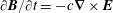 $\unicode[STIX]{x2202}\boldsymbol{B}/\unicode[STIX]{x2202}t=-c\unicode[STIX]{x1D735}\times \boldsymbol{E}$
. For now, we will not use the induction equation and keep our FLR calculations in the above form. Let us continue with the second term on the right-hand side of (5.59). When completely linearized this term does not contribute, but for now we will keep it and combine it with the first term into a convective derivative
$\unicode[STIX]{x2202}\boldsymbol{B}/\unicode[STIX]{x2202}t=-c\unicode[STIX]{x1D735}\times \boldsymbol{E}$
. For now, we will not use the induction equation and keep our FLR calculations in the above form. Let us continue with the second term on the right-hand side of (5.59). When completely linearized this term does not contribute, but for now we will keep it and combine it with the first term into a convective derivative
 $\unicode[STIX]{x2202}\boldsymbol{p}^{\text{g}}/\unicode[STIX]{x2202}t+\boldsymbol{u}\boldsymbol{\cdot }\unicode[STIX]{x1D735}\boldsymbol{p}^{\text{g}}=\text{d}\boldsymbol{p}^{\text{g}}/\text{d}t$
, so that
$\unicode[STIX]{x2202}\boldsymbol{p}^{\text{g}}/\unicode[STIX]{x2202}t+\boldsymbol{u}\boldsymbol{\cdot }\unicode[STIX]{x1D735}\boldsymbol{p}^{\text{g}}=\text{d}\boldsymbol{p}^{\text{g}}/\text{d}t$
, so that
 $\unicode[STIX]{x2202}/\unicode[STIX]{x2202}t$
in (5.63) is replaced by
$\unicode[STIX]{x2202}/\unicode[STIX]{x2202}t$
in (5.63) is replaced by
 $\text{d}/\text{d}t$
. The remaining terms on the right-hand side of (5.59) are straightforward to evaluate since no derivatives of
$\text{d}/\text{d}t$
. The remaining terms on the right-hand side of (5.59) are straightforward to evaluate since no derivatives of
 $\hat{\boldsymbol{b}}$
are encountered, and the third term
$\hat{\boldsymbol{b}}$
are encountered, and the third term
 $\boldsymbol{p}^{\text{g}}\unicode[STIX]{x1D735}\boldsymbol{\cdot }\boldsymbol{u}|_{\hat{\boldsymbol{b}}=\hat{\boldsymbol{b}}_{0}}$
is equal to matrix (5.61) multiplied by
$\boldsymbol{p}^{\text{g}}\unicode[STIX]{x1D735}\boldsymbol{\cdot }\boldsymbol{u}|_{\hat{\boldsymbol{b}}=\hat{\boldsymbol{b}}_{0}}$
is equal to matrix (5.61) multiplied by
 $\unicode[STIX]{x1D735}\boldsymbol{\cdot }\boldsymbol{u}$
. The last two terms of (5.59) are together evaluated as
$\unicode[STIX]{x1D735}\boldsymbol{\cdot }\boldsymbol{u}$
. The last two terms of (5.59) are together evaluated as
 $$\begin{eqnarray}\displaystyle \boldsymbol{p}^{\text{g}}\boldsymbol{\cdot }\unicode[STIX]{x1D735}\boldsymbol{u}+(\boldsymbol{p}^{\text{g}}\boldsymbol{\cdot }\unicode[STIX]{x1D735}\boldsymbol{u})^{\text{T}}|_{\hat{\boldsymbol{b}}=\hat{\boldsymbol{b}}_{0}}=\left(\begin{array}{@{}ccc@{}}2p_{\bot }\unicode[STIX]{x2202}_{x}u_{x}; & p_{\bot }(\unicode[STIX]{x2202}_{x}u_{y}+\unicode[STIX]{x2202}_{y}u_{x}); & p_{\bot }\unicode[STIX]{x2202}_{x}u_{z}+p_{\Vert }\unicode[STIX]{x2202}_{z}u_{x}\\ p_{\bot }(\unicode[STIX]{x2202}_{y}u_{x}+\unicode[STIX]{x2202}_{x}u_{y}); & 2p_{\bot }\unicode[STIX]{x2202}_{y}u_{y}; & p_{\bot }\unicode[STIX]{x2202}_{y}u_{z}+p_{\Vert }\unicode[STIX]{x2202}_{z}u_{y}\\ p_{\Vert }\unicode[STIX]{x2202}_{z}u_{x}+p_{\bot }\unicode[STIX]{x2202}_{x}u_{z}; & p_{\Vert }\unicode[STIX]{x2202}_{z}u_{y}+p_{\bot }\unicode[STIX]{x2202}_{y}u_{z}; & 2p_{\Vert }\unicode[STIX]{x2202}_{z}u_{z}\end{array}\right). & & \displaystyle \nonumber\\ \displaystyle & & \displaystyle\end{eqnarray}$$
Now we need to subtract the scalar CGL pressure equations obtained previously. Since
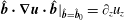 $\hat{\boldsymbol{b}}\boldsymbol{\cdot }\unicode[STIX]{x1D735}\boldsymbol{u}\boldsymbol{\cdot }\hat{\boldsymbol{b}}|_{\hat{\boldsymbol{b}}=\hat{\boldsymbol{b}}_{0}}=\unicode[STIX]{x2202}_{z}u_{z}$
, the scalar pressure equations read
$\hat{\boldsymbol{b}}\boldsymbol{\cdot }\unicode[STIX]{x1D735}\boldsymbol{u}\boldsymbol{\cdot }\hat{\boldsymbol{b}}|_{\hat{\boldsymbol{b}}=\hat{\boldsymbol{b}}_{0}}=\unicode[STIX]{x2202}_{z}u_{z}$
, the scalar pressure equations read
 $$\begin{eqnarray}\displaystyle \frac{\text{d}p_{\Vert }}{\text{d}t}+p_{\Vert }\unicode[STIX]{x1D735}\boldsymbol{\cdot }\boldsymbol{u}+2p_{\Vert }\unicode[STIX]{x2202}_{z}u_{z}=0;\quad \frac{\text{d}p_{\bot }}{\text{d}t}+2p_{\bot }\unicode[STIX]{x1D735}\boldsymbol{\cdot }\boldsymbol{u}-p_{\bot }\unicode[STIX]{x2202}_{z}u_{z}=0. & & \displaystyle\end{eqnarray}$$
By cancelling terms coming from these two equations (affecting only the diagonal components), the entire equation (5.59) rewrites
 $$\begin{eqnarray}\displaystyle & & \displaystyle \left(\begin{array}{@{}ccc@{}}-2\unicode[STIX]{x1D6F1}_{xy}, & \unicode[STIX]{x1D6F1}_{xx}-\unicode[STIX]{x1D6F1}_{yy}, & -\unicode[STIX]{x1D6F1}_{yz}\\ \unicode[STIX]{x1D6F1}_{xx}-\unicode[STIX]{x1D6F1}_{yy}, & +2\unicode[STIX]{x1D6F1}_{xy}, & \unicode[STIX]{x1D6F1}_{xz}\\ -\unicode[STIX]{x1D6F1}_{yz}, & \unicode[STIX]{x1D6F1}_{xz}, & 0\end{array}\right)=-\frac{1}{\unicode[STIX]{x1D6FA}}(p_{\Vert }-p_{\bot })\left.\left(\begin{array}{@{}ccc@{}}0 & 0 & \frac{\text{d}\hat{b}_{x}}{\text{d}t}\\ 0 & 0 & \frac{\text{d}\hat{b}_{y}}{\text{d}t}\\ \frac{\text{d}\hat{b}_{x}}{\text{d}t} & \frac{\text{d}\hat{b}_{y}}{\text{d}t} & \frac{\text{d}\hat{b}_{z}}{\text{d}t}\end{array}\right)\right|_{\hat{\boldsymbol{b}}=\hat{\boldsymbol{b}}_{0}}\nonumber\\ \displaystyle & & \displaystyle -\,\frac{1}{\unicode[STIX]{x1D6FA}}\left(\begin{array}{@{}ccc@{}}p_{\bot }(\unicode[STIX]{x2202}_{x}u_{x}-\unicode[STIX]{x2202}_{y}u_{y}); & p_{\bot }(\unicode[STIX]{x2202}_{x}u_{y}+\unicode[STIX]{x2202}_{y}u_{x}); & p_{\bot }\unicode[STIX]{x2202}_{x}u_{z}+p_{\Vert }\unicode[STIX]{x2202}_{z}u_{x}\\ p_{\bot }(\unicode[STIX]{x2202}_{y}u_{x}+\unicode[STIX]{x2202}_{x}u_{y}); & p_{\bot }(\unicode[STIX]{x2202}_{y}u_{y}-\unicode[STIX]{x2202}_{x}u_{x}); & p_{\bot }\unicode[STIX]{x2202}_{y}u_{z}+p_{\Vert }\unicode[STIX]{x2202}_{z}u_{y}\\ p_{\Vert }\unicode[STIX]{x2202}_{z}u_{x}+p_{\bot }\unicode[STIX]{x2202}_{x}u_{z}; & p_{\Vert }\unicode[STIX]{x2202}_{z}u_{y}+p_{\bot }\unicode[STIX]{x2202}_{y}u_{z}; & 0\end{array}\right).\end{eqnarray}$$
The identity
 $\unicode[STIX]{x1D72B}:\hat{\boldsymbol{b}}\hat{\boldsymbol{b}}=0$
evaluated for
$\unicode[STIX]{x1D72B}:\hat{\boldsymbol{b}}\hat{\boldsymbol{b}}=0$
evaluated for
 $\hat{\boldsymbol{b}}=\hat{\boldsymbol{b}}_{0}$
implies that
$\hat{\boldsymbol{b}}=\hat{\boldsymbol{b}}_{0}$
implies that
 $\unicode[STIX]{x1D6F1}_{zz}=0$
and the identity
$\unicode[STIX]{x1D6F1}_{zz}=0$
and the identity
 $\text{Tr}\,\unicode[STIX]{x1D72B}=0$
further implies that
$\text{Tr}\,\unicode[STIX]{x1D72B}=0$
further implies that
 $\unicode[STIX]{x1D6F1}_{xx}=-\unicode[STIX]{x1D6F1}_{yy}$
. The components of the pressure tensor therefore read
$\unicode[STIX]{x1D6F1}_{xx}=-\unicode[STIX]{x1D6F1}_{yy}$
. The components of the pressure tensor therefore read
 $$\begin{eqnarray}\displaystyle \left.\begin{array}{@{}c@{}}\displaystyle \unicode[STIX]{x1D6F1}_{xx}=-\unicode[STIX]{x1D6F1}_{yy}=-\frac{p_{\bot }}{2\unicode[STIX]{x1D6FA}}(\unicode[STIX]{x2202}_{x}u_{y}+\unicode[STIX]{x2202}_{y}u_{x});\quad \unicode[STIX]{x1D6F1}_{xy}=\frac{p_{\bot }}{2\unicode[STIX]{x1D6FA}}(\unicode[STIX]{x2202}_{x}u_{x}-\unicode[STIX]{x2202}_{y}u_{y});\quad \unicode[STIX]{x1D6F1}_{zz}=0;\\ \displaystyle \unicode[STIX]{x1D6F1}_{xz}=-\frac{1}{\unicode[STIX]{x1D6FA}}\left((p_{\Vert }-p_{\bot })\frac{\text{d}\hat{b}_{y}}{\text{d}t}+p_{\Vert }\unicode[STIX]{x2202}_{z}u_{y}+p_{\bot }\unicode[STIX]{x2202}_{y}u_{z}\right);\\ \displaystyle \unicode[STIX]{x1D6F1}_{yz}=\frac{1}{\unicode[STIX]{x1D6FA}}\left((p_{\Vert }-p_{\bot })\frac{\text{d}\hat{b}_{x}}{\text{d}t}+p_{\Vert }\unicode[STIX]{x2202}_{z}u_{x}+p_{\bot }\unicode[STIX]{x2202}_{x}u_{z}\right).\end{array}\right\} & & \displaystyle\end{eqnarray}$$
Finally, the time derivative of the unit vector
 $$\begin{eqnarray}\displaystyle \frac{\text{d}}{\text{d}t}\hat{\boldsymbol{b}}=\frac{\text{d}}{\text{d}t}\frac{\boldsymbol{B}}{|\boldsymbol{B}|}=\frac{1}{|\boldsymbol{B}|}\frac{\text{d}\boldsymbol{B}}{\text{d}t}-\frac{\boldsymbol{B}}{|\boldsymbol{B}|^{2}}\frac{\text{d}|\boldsymbol{B}|}{\text{d}t}=\frac{1}{|\boldsymbol{B}|}\left[\frac{\text{d}\boldsymbol{B}}{\text{d}t}-\hat{\boldsymbol{b}}\frac{\text{d}|\boldsymbol{B}|}{\text{d}t}\right]=\frac{1}{|\boldsymbol{B}|}\left[\frac{\text{d}\boldsymbol{B}}{\text{d}t}-\hat{\boldsymbol{b}}\left(\hat{\boldsymbol{b}}\boldsymbol{\cdot }\frac{\text{d}\boldsymbol{B}}{\text{d}t}\right)\right], & & \displaystyle \nonumber\\ \displaystyle & & \displaystyle\end{eqnarray}$$
which evaluated for
 $\hat{\boldsymbol{b}}=\hat{\boldsymbol{b}}_{0}=(0,0,1)$
,
$\hat{\boldsymbol{b}}=\hat{\boldsymbol{b}}_{0}=(0,0,1)$
,
 $|\boldsymbol{B}|=B_{0}$
yields
$|\boldsymbol{B}|=B_{0}$
yields
 $$\begin{eqnarray}\displaystyle \left.\begin{array}{@{}c@{}}\displaystyle \left.\frac{\text{d}\hat{b}_{x}}{\text{d}t}\right|_{\hat{\boldsymbol{b}}=\hat{\boldsymbol{b}}_{0}}=\frac{1}{B_{0}}\left.\frac{\text{d}B_{x}}{\text{d}t}\right|_{\hat{\boldsymbol{b}}=\hat{\boldsymbol{b}}_{0}};\quad \left.\frac{\text{d}\hat{b}_{y}}{\text{d}t}\right|_{\hat{\boldsymbol{b}}=\hat{\boldsymbol{b}}_{0}}=\frac{1}{B_{0}}\left.\frac{\text{d}B_{y}}{\text{d}t}\right|_{\hat{\boldsymbol{b}}=\hat{\boldsymbol{b}}_{0}};\\ \displaystyle \left.\frac{\text{d}\hat{b}_{z}}{\text{d}t}\right|_{\hat{\boldsymbol{b}}=\hat{\boldsymbol{b}}_{0}}=\frac{1}{B_{0}}\left(\frac{\text{d}B_{z}}{\text{d}t}-\frac{\text{d}B_{z}}{\text{d}t}\right)=0.\end{array}\right\} & & \displaystyle\end{eqnarray}$$
The general induction equation reads
 $$\begin{eqnarray}\displaystyle \frac{\text{d}\boldsymbol{B}}{\text{d}t}=-\boldsymbol{B}\unicode[STIX]{x1D735}\boldsymbol{\cdot }\boldsymbol{u}+\boldsymbol{B}\boldsymbol{\cdot }\unicode[STIX]{x1D735}\boldsymbol{u}-c\unicode[STIX]{x1D735}\times \boldsymbol{E}_{H}, & & \displaystyle\end{eqnarray}$$
which evaluates in the
 $\hat{\boldsymbol{b}}=\hat{\boldsymbol{b}}_{0}$
approximation as
$\hat{\boldsymbol{b}}=\hat{\boldsymbol{b}}_{0}$
approximation as
 $$\begin{eqnarray}\displaystyle \left.\begin{array}{@{}c@{}}\displaystyle \left.\frac{\text{d}B_{x}}{\text{d}t}\right|_{\hat{\boldsymbol{b}}=\hat{\boldsymbol{b}}_{0}}=B_{0}\unicode[STIX]{x2202}_{z}u_{x}-c(\unicode[STIX]{x1D735}\times \boldsymbol{E}_{H})_{x};\quad \left.\frac{\text{d}B_{y}}{\text{d}t}\right|_{\hat{\boldsymbol{b}}=\hat{\boldsymbol{b}}_{0}}=B_{0}\unicode[STIX]{x2202}_{z}u_{y}-c(\unicode[STIX]{x1D735}\times \boldsymbol{E}_{H})_{y};\\ \displaystyle \left.\frac{\text{d}B_{z}}{\text{d}t}\right|_{\hat{\boldsymbol{b}}=\hat{\boldsymbol{b}}_{0}}=-B_{0}\unicode[STIX]{x1D735}\boldsymbol{\cdot }\boldsymbol{u}+B_{0}\unicode[STIX]{x2202}_{z}u_{z}-c(\unicode[STIX]{x1D735}\times \boldsymbol{E}_{H})_{z}.\end{array}\right\} & & \displaystyle\end{eqnarray}$$
These expressions are used in the FLR tensor components
 $\unicode[STIX]{x1D6F1}_{xz}$
and
$\unicode[STIX]{x1D6F1}_{xz}$
and
 $\unicode[STIX]{x1D6F1}_{yz}$
, and the FLR tensor reads
$\unicode[STIX]{x1D6F1}_{yz}$
, and the FLR tensor reads
 $$\begin{eqnarray}\displaystyle \left.\begin{array}{@{}c@{}}\displaystyle \unicode[STIX]{x1D6F1}_{xx}=-\unicode[STIX]{x1D6F1}_{yy}=-\frac{p_{\bot }}{2\unicode[STIX]{x1D6FA}}(\unicode[STIX]{x2202}_{x}u_{y}+\unicode[STIX]{x2202}_{y}u_{x});\quad \unicode[STIX]{x1D6F1}_{xy}=\frac{p_{\bot }}{2\unicode[STIX]{x1D6FA}}(\unicode[STIX]{x2202}_{x}u_{x}-\unicode[STIX]{x2202}_{y}u_{y});\quad \unicode[STIX]{x1D6F1}_{zz}=0;\\ \displaystyle \unicode[STIX]{x1D6F1}_{xz}=-\frac{1}{\unicode[STIX]{x1D6FA}}\left[(p_{\Vert }-p_{\bot })\left(\unicode[STIX]{x2202}_{z}u_{y}-\frac{c}{B_{0}}(\unicode[STIX]{x1D735}\times \boldsymbol{E}_{H})_{y}\right)+p_{\Vert }\unicode[STIX]{x2202}_{z}u_{y}+p_{\bot }\unicode[STIX]{x2202}_{y}u_{z}\right];\\ \displaystyle \unicode[STIX]{x1D6F1}_{yz}=\frac{1}{\unicode[STIX]{x1D6FA}}\left[(p_{\Vert }-p_{\bot })\left(\unicode[STIX]{x2202}_{z}u_{x}-\frac{c}{B_{0}}(\unicode[STIX]{x1D735}\times \boldsymbol{E}_{H})_{x}\right)+p_{\Vert }\unicode[STIX]{x2202}_{z}u_{x}+p_{\bot }\unicode[STIX]{x2202}_{x}u_{z}\right].\end{array}\right\} & & \displaystyle\end{eqnarray}$$
However, since the FLR tensor was derived with a precision to only first order in wavenumber
 $k$
, to make everything consistent, the Hall contributions in the induction equation are usually (but not always) neglected. We therefore have
$k$
, to make everything consistent, the Hall contributions in the induction equation are usually (but not always) neglected. We therefore have
 $\text{d}\hat{b}_{x}/\text{d}t=\unicode[STIX]{x2202}_{z}u_{x}$
and
$\text{d}\hat{b}_{x}/\text{d}t=\unicode[STIX]{x2202}_{z}u_{x}$
and
 $\text{d}\hat{b}_{y}/\text{d}t=\unicode[STIX]{x2202}_{z}u_{y}$
which yields the leading-order FLR pressure tensor evaluated along the magnetic field
$\text{d}\hat{b}_{y}/\text{d}t=\unicode[STIX]{x2202}_{z}u_{y}$
which yields the leading-order FLR pressure tensor evaluated along the magnetic field
 $\hat{\boldsymbol{b}}=(0,0,1)$
in the form
$\hat{\boldsymbol{b}}=(0,0,1)$
in the form
 $$\begin{eqnarray}\displaystyle \left.\begin{array}{@{}c@{}}\displaystyle \unicode[STIX]{x1D6F1}_{xx}=-\unicode[STIX]{x1D6F1}_{yy}=-\frac{p_{\bot }}{2\unicode[STIX]{x1D6FA}}(\unicode[STIX]{x2202}_{x}u_{y}+\unicode[STIX]{x2202}_{y}u_{x});\quad \unicode[STIX]{x1D6F1}_{xy}=\frac{p_{\bot }}{2\unicode[STIX]{x1D6FA}}(\unicode[STIX]{x2202}_{x}u_{x}-\unicode[STIX]{x2202}_{y}u_{y});\quad \unicode[STIX]{x1D6F1}_{zz}=0;\\ \displaystyle \unicode[STIX]{x1D6F1}_{xz}=-\frac{1}{\unicode[STIX]{x1D6FA}}((2p_{\Vert }-p_{\bot })\unicode[STIX]{x2202}_{z}u_{y}+p_{\bot }\unicode[STIX]{x2202}_{y}u_{z});\quad \unicode[STIX]{x1D6F1}_{yz}=\frac{1}{\unicode[STIX]{x1D6FA}}((2p_{\Vert }-p_{\bot })\unicode[STIX]{x2202}_{z}u_{x}+p_{\bot }\unicode[STIX]{x2202}_{x}u_{z}),\end{array}\right\} & & \displaystyle\end{eqnarray}$$
which is equivalent to equation (5) of Yajima (Reference Yajima1966). Perhaps surprisingly, the result is also equivalent to the highly collisional equations (2.20)–(2.24) of Braginskii (Reference Braginskii1965), after one prescribes
 $p_{\Vert }=p_{\bot }$
and after terms containing the collisional time
$p_{\Vert }=p_{\bot }$
and after terms containing the collisional time
 $\unicode[STIX]{x1D70F}$
are ‘ignored’ (
$\unicode[STIX]{x1D70F}$
are ‘ignored’ (
 $\unicode[STIX]{x1D70F}\sim 1/\unicode[STIX]{x1D708}$
where
$\unicode[STIX]{x1D70F}\sim 1/\unicode[STIX]{x1D708}$
where
 $\unicode[STIX]{x1D708}$
is the usual collisional frequency). A proper collisionless limit
$\unicode[STIX]{x1D708}$
is the usual collisional frequency). A proper collisionless limit
 $\unicode[STIX]{x1D70F}\rightarrow \infty$
cannot be obtained from the expressions of Braginskii (Reference Braginskii1965), since the results are proportional to
$\unicode[STIX]{x1D70F}\rightarrow \infty$
cannot be obtained from the expressions of Braginskii (Reference Braginskii1965), since the results are proportional to
 $\unicode[STIX]{x1D70F}$
(and also
$\unicode[STIX]{x1D70F}$
(and also
 $1/\unicode[STIX]{x1D70F}$
).
$1/\unicode[STIX]{x1D70F}$
).
Furthermore, evaluation along
 $\hat{\boldsymbol{b}}=(0,0,1)$
basically means that the magnetic field terms of the system were linearized and other parts of the system were not. The expansion procedure preserved some nonlinearities, but other nonlinearities that are of the same order were implicitly neglected. Therefore, the only fully consistent procedure is to evaluate the FLR tensor in the linear approximation, yielding
$\hat{\boldsymbol{b}}=(0,0,1)$
basically means that the magnetic field terms of the system were linearized and other parts of the system were not. The expansion procedure preserved some nonlinearities, but other nonlinearities that are of the same order were implicitly neglected. Therefore, the only fully consistent procedure is to evaluate the FLR tensor in the linear approximation, yielding
 $$\begin{eqnarray}\displaystyle \left.\begin{array}{@{}c@{}}\displaystyle \unicode[STIX]{x1D6F1}_{xx}^{(1)}=-\unicode[STIX]{x1D6F1}_{yy}^{(1)}=-\frac{p_{\bot }^{(0)}}{2\unicode[STIX]{x1D6FA}}(\unicode[STIX]{x2202}_{x}u_{y}+\unicode[STIX]{x2202}_{y}u_{x});\quad \unicode[STIX]{x1D6F1}_{xy}^{(1)}=\frac{p_{\bot }^{(0)}}{2\unicode[STIX]{x1D6FA}}(\unicode[STIX]{x2202}_{x}u_{x}-\unicode[STIX]{x2202}_{y}u_{y});\quad \unicode[STIX]{x1D6F1}_{zz}^{(1)}=0;\\ \displaystyle \unicode[STIX]{x1D6F1}_{xz}^{(1)}=-\frac{1}{\unicode[STIX]{x1D6FA}}((2p_{\Vert }^{(0)}-p_{\bot }^{(0)})\unicode[STIX]{x2202}_{z}u_{y}+p_{\bot }^{(0)}\unicode[STIX]{x2202}_{y}u_{z});\quad \unicode[STIX]{x1D6F1}_{yz}^{(1)}=\frac{1}{\unicode[STIX]{x1D6FA}}((2p_{\Vert }^{(0)}-p_{\bot }^{(0)})\unicode[STIX]{x2202}_{z}u_{x}+p_{\bot }^{(0)}\unicode[STIX]{x2202}_{x}u_{z}).\end{array}\right\} & & \displaystyle \nonumber\\ \displaystyle & & \displaystyle\end{eqnarray}$$
Notably, the tensor is very different from (3.10)–(3.13) of Oraevskii et al. (Reference Oraevskii, Chodura and Feneberg1968). The FLR corrections to the pressure tensor (these ones or more complicated ones) were used in a number of direct numerical simulations, see for example Borgogno et al. (Reference Borgogno, Hellinger, Passot, Sulem and Trávníček2009), Hunana et al. (Reference Hunana, Laveder, Passot, Sulem and Borgogno2011), Kobayashi et al. (Reference Kobayashi, Sahraoui, Passot, Laveder, Sulem, Huang, Henri and Smets2017) and Perrone et al. (Reference Perrone, Passot, Laveder, Valentini, Sulem, Zouganelis, Veltri and Servidio2018), or for the isotropic case see for example Ghosh & Parashar (Reference Ghosh and Parashar2015), and references therein.
5.3 Hall-CGL-FLR1 fluid model
The normalized, linearized, Fourier transformed system of equations written in the
 $x$
–
$x$
–
 $z$
plane reads (dropping the tilde everywhere)
$z$
plane reads (dropping the tilde everywhere)
 $$\begin{eqnarray}\displaystyle & \displaystyle -\unicode[STIX]{x1D714}\unicode[STIX]{x1D70C}+k_{\bot }u_{x}+k_{\Vert }u_{z}=0; & \displaystyle\end{eqnarray}$$
 $$\begin{eqnarray}\displaystyle & \displaystyle -\unicode[STIX]{x1D714}u_{x}+\frac{\unicode[STIX]{x1D6FD}_{\Vert }}{2}k_{\bot }p_{\bot }-v_{A\Vert }^{2}k_{\Vert }B_{x}+k_{\bot }B_{z}+\frac{\unicode[STIX]{x1D6FD}_{\Vert }}{2}(k_{\bot }\unicode[STIX]{x1D6F1}_{xx}+k_{\Vert }\unicode[STIX]{x1D6F1}_{xz})=0; & \displaystyle\end{eqnarray}$$
 $$\begin{eqnarray}\displaystyle & \displaystyle -\unicode[STIX]{x1D714}u_{y}-v_{A\Vert }^{2}k_{\Vert }B_{y}+\frac{\unicode[STIX]{x1D6FD}_{\Vert }}{2}(k_{\bot }\unicode[STIX]{x1D6F1}_{xy}+k_{\Vert }\unicode[STIX]{x1D6F1}_{yz})=0; & \displaystyle\end{eqnarray}$$
 $$\begin{eqnarray}\displaystyle & \displaystyle -\unicode[STIX]{x1D714}u_{z}+\frac{\unicode[STIX]{x1D6FD}_{\Vert }}{2}k_{\Vert }p_{\Vert }+\frac{\unicode[STIX]{x1D6FD}_{\Vert }}{2}(1-a_{p})k_{\bot }B_{x}+\frac{\unicode[STIX]{x1D6FD}_{\Vert }}{2}k_{\bot }\unicode[STIX]{x1D6F1}_{xz}=0; & \displaystyle\end{eqnarray}$$
 $$\begin{eqnarray}\displaystyle & \displaystyle -\unicode[STIX]{x1D714}B_{x}-k_{\Vert }u_{x}-\text{i}k_{\Vert }^{2}B_{y}=0; & \displaystyle\end{eqnarray}$$
 $$\begin{eqnarray}\displaystyle & \displaystyle -\unicode[STIX]{x1D714}B_{y}-k_{\Vert }u_{y}-\text{i}k_{\Vert }k_{\bot }B_{z}+\text{i}k_{\Vert }^{2}B_{x}=0; & \displaystyle\end{eqnarray}$$
 $$\begin{eqnarray}\displaystyle & \displaystyle -\unicode[STIX]{x1D714}B_{z}+k_{\bot }u_{x}+\text{i}k_{\Vert }k_{\bot }B_{y}=0; & \displaystyle\end{eqnarray}$$
 $$\begin{eqnarray}\displaystyle & \displaystyle -\unicode[STIX]{x1D714}p_{\Vert }+k_{\bot }u_{x}+3k_{\Vert }u_{z}=0; & \displaystyle\end{eqnarray}$$
 $$\begin{eqnarray}\displaystyle & \displaystyle -\unicode[STIX]{x1D714}p_{\bot }+2a_{p}k_{\bot }u_{x}+a_{p}k_{\Vert }u_{z}=0, & \displaystyle\end{eqnarray}$$
where
 $v_{A\Vert }^{2}=1+(\unicode[STIX]{x1D6FD}_{\Vert }/2)(a_{p}-1)$
, and the first-order FLR tensor
$v_{A\Vert }^{2}=1+(\unicode[STIX]{x1D6FD}_{\Vert }/2)(a_{p}-1)$
, and the first-order FLR tensor
 $\unicode[STIX]{x1D72B}=\unicode[STIX]{x1D72B}^{(1)}$
is
$\unicode[STIX]{x1D72B}=\unicode[STIX]{x1D72B}^{(1)}$
is
 $$\begin{eqnarray}\displaystyle \left.\begin{array}{@{}c@{}}\displaystyle \unicode[STIX]{x1D6F1}_{xx}^{(1)}=-\frac{a_{p}}{2}\text{i}k_{\bot }u_{y};\quad \unicode[STIX]{x1D6F1}_{xy}^{(1)}=\frac{a_{p}}{2}\text{i}k_{\bot }u_{x};\quad \unicode[STIX]{x1D6F1}_{zz}^{(1)}=0;\\ \displaystyle \unicode[STIX]{x1D6F1}_{xz}^{(1)}=-(2-a_{p})\text{i}k_{\Vert }u_{y};\quad \unicode[STIX]{x1D6F1}_{yz}^{(1)}=(2-a_{p})\text{i}k_{\Vert }u_{x}+a_{p}\text{i}k_{\bot }u_{z}.\end{array}\right\} & & \displaystyle\end{eqnarray}$$
The dispersion relation for the Hall-CGL-FLR1 fluid model can be written as
 $$\begin{eqnarray}\displaystyle (\unicode[STIX]{x1D714}^{2}-k_{\Vert }^{2}v_{A\Vert }^{2})(\unicode[STIX]{x1D714}^{4}-A_{2}\unicode[STIX]{x1D714}^{2}+A_{0}) & = & \displaystyle k^{2}k_{\Vert }^{2}\left[\unicode[STIX]{x1D714}^{4}-\unicode[STIX]{x1D6FD}_{\Vert }\left({\textstyle \frac{3}{2}}k_{\Vert }^{2}+a_{p}k_{\bot }^{2}\right)\unicode[STIX]{x1D714}^{2}+k_{\Vert }^{2}k_{\bot }^{2}{\textstyle \frac{5}{4}}a_{p}\unicode[STIX]{x1D6FD}_{\Vert }^{2}\right]\nonumber\\ \displaystyle & & \displaystyle +\,{\mathcal{P}}^{\text{FLR}};\end{eqnarray}$$
 $$\begin{eqnarray}\displaystyle & \displaystyle A_{2}=k_{\bot }^{2}(1+a_{p}\unicode[STIX]{x1D6FD}_{\Vert })+k_{\Vert }^{2}\left(v_{A\Vert }^{2}+{\textstyle \frac{3}{2}}\unicode[STIX]{x1D6FD}_{\Vert }\right); & \displaystyle\end{eqnarray}$$
 $$\begin{eqnarray}\displaystyle & \displaystyle A_{0}={\textstyle \frac{3}{2}}k_{\Vert }^{2}\unicode[STIX]{x1D6FD}_{\Vert }\left[k_{\Vert }^{2}v_{A\Vert }^{2}+k_{\bot }^{2}\left(1+a_{p}\unicode[STIX]{x1D6FD}_{\Vert }-{\textstyle \frac{1}{6}}a_{p}^{2}\unicode[STIX]{x1D6FD}_{\Vert }\right)\right], & \displaystyle\end{eqnarray}$$
where the polynomial on the right-hand side
 $$\begin{eqnarray}\displaystyle & \displaystyle {\mathcal{P}}^{\text{FLR}}=A_{4}^{\prime }\unicode[STIX]{x1D714}^{4}-A_{2}^{\prime }\unicode[STIX]{x1D714}^{2}+A_{0}^{\prime }; & \displaystyle\end{eqnarray}$$
 $$\begin{eqnarray}\displaystyle & \displaystyle A_{4}^{\prime }=\unicode[STIX]{x1D6FD}_{\Vert }^{2}\left[k_{\Vert }^{4}\left(1-\frac{a_{p}}{2}\right)^{2}+k_{\bot }^{4}\frac{a_{p}^{2}}{16}+k_{\Vert }^{2}k_{\bot }^{2}a_{p}\left(1-\frac{a_{p}}{2}\right)\right]; & \displaystyle\end{eqnarray}$$
 $$\begin{eqnarray}\displaystyle A_{2}^{\prime } & = & \displaystyle \unicode[STIX]{x1D6FD}_{\Vert }k_{\Vert }^{2}\left\{k_{\Vert }^{6}\unicode[STIX]{x1D6FD}_{\Vert }\left(1-\frac{a_{p}}{2}\right)^{2}+k_{\Vert }^{4}\left[\frac{3}{2}\unicode[STIX]{x1D6FD}_{\Vert }^{2}\left(1-\frac{a_{p}}{2}\right)^{2}+k_{\bot }^{2}\unicode[STIX]{x1D6FD}_{\Vert }\left(1-\frac{a_{p}^{2}}{4}\right)+v_{A\Vert }^{2}(a_{p}-2)\right]\right.\nonumber\\ \displaystyle & & \displaystyle +\,k_{\Vert }^{2}k_{\bot }^{2}\left[-1+\frac{a_{p}}{2}+\unicode[STIX]{x1D6FD}_{\Vert }\frac{a_{p}}{4}\left(1-a_{p}+\unicode[STIX]{x1D6FD}_{\Vert }\left(1-\frac{a_{p}}{2}\right)\right)\right.\nonumber\\ \displaystyle & & \displaystyle -\left.v_{A\Vert }^{2}\left(1-\unicode[STIX]{x1D6FD}_{\Vert }\frac{a_{p}}{2}\left(1-\frac{a_{p}}{2}\right)\right)+k_{\bot }^{2}a_{p}\unicode[STIX]{x1D6FD}_{\Vert }\left(1-\frac{7}{16}a_{p}\right)\right]\nonumber\\ \displaystyle & & \displaystyle +\left.k_{\bot }^{4}\frac{a_{p}}{4}\left[-1+2\unicode[STIX]{x1D6FD}_{\Vert }-v_{A\Vert }^{2}-a_{p}\unicode[STIX]{x1D6FD}_{\Vert }\left(1+\unicode[STIX]{x1D6FD}_{\Vert }\left(a_{p}-\frac{15}{8}\right)-\frac{1}{4}k_{\bot }^{2}\right)\right]\right\};\end{eqnarray}$$
 $$\begin{eqnarray}\displaystyle A_{0}^{\prime } & = & \displaystyle \unicode[STIX]{x1D6FD}_{\Vert }^{2}k_{\Vert }^{4}\left\{k_{\Vert }^{6}\frac{3}{2}\unicode[STIX]{x1D6FD}_{\Vert }\left(1-\frac{a_{p}}{2}\right)^{2}+k_{\Vert }^{4}\left(1-\frac{a_{p}}{2}\right)\left[-3v_{A\Vert }^{2}+k_{\bot }^{2}\unicode[STIX]{x1D6FD}_{\Vert }\frac{3}{2}\left(1-\frac{a_{p}}{2}+\frac{a_{p}^{2}}{6}\right)\right]\right.\nonumber\\ \displaystyle & & \displaystyle +\,k_{\Vert }^{2}k_{\bot }^{2}\left[k_{\bot }^{2}\unicode[STIX]{x1D6FD}_{\Vert }a_{p}^{2}\left(\frac{21}{32}-\frac{5}{16}a_{p}\right)-v_{A\Vert }^{2}\frac{3}{2}\left(1-\frac{a_{p}}{2}+\frac{1}{6}a_{p}^{2}\right)\right.\nonumber\\ \displaystyle & & \displaystyle -\left.\left(1-\frac{a_{p}}{2}\right)\frac{3}{2}\left(1+\frac{1}{6}a_{p}\unicode[STIX]{x1D6FD}_{\Vert }-\frac{1}{6}a_{p}^{2}\unicode[STIX]{x1D6FD}_{\Vert }\right)\right]\nonumber\\ \displaystyle & & \displaystyle +\left.k_{\bot }^{4}a_{p}\left[k_{\bot }^{2}a_{p}\unicode[STIX]{x1D6FD}_{\Vert }\left(\frac{13}{32}-\frac{3}{16}a_{p}\right)+\frac{v_{A\Vert }^{2}}{8}(1-2a_{p})-\frac{1}{8}+\frac{3}{16}a_{p}\unicode[STIX]{x1D6FD}_{\Vert }(1-a_{p})\right]\right\}.\nonumber\\ \displaystyle & & \displaystyle\end{eqnarray}$$
The solution for strictly parallel propagation is
 $$\begin{eqnarray}\unicode[STIX]{x1D714}=\pm \frac{k_{\Vert }^{2}}{2}\left(1+\unicode[STIX]{x1D6FD}_{\Vert }\left(1-\frac{a_{p}}{2}\right)\right)+k_{\Vert }\sqrt{1+\frac{\unicode[STIX]{x1D6FD}_{\Vert }}{2}(a_{p}-1)+\frac{k_{\Vert }^{2}}{4}\left(1-\unicode[STIX]{x1D6FD}_{\Vert }\left(1-\frac{a_{p}}{2}\right)\right)^{2}}.\end{eqnarray}$$
For strictly perpendicular propagation the solution is
 $$\begin{eqnarray}\unicode[STIX]{x1D714}=\pm k_{\bot }\sqrt{1+a_{p}\unicode[STIX]{x1D6FD}_{\Vert }+\frac{k_{\bot }^{2}\unicode[STIX]{x1D6FD}_{\Vert }^{2}a_{p}^{2}}{16}},\end{eqnarray}$$
and the result is consistent with equation (17) of Yajima (Reference Yajima1966), after neglecting the electron inertia in that paper (by
 $\unicode[STIX]{x1D714}_{0}\rightarrow \infty$
). The strictly perpendicular propagation is an excellent example to point out the deficiencies of the Hall-CGL-FLR1 fluid model, or actually the CGL-FLR1 model, since the Hall contributions are zero for
$\unicode[STIX]{x1D714}_{0}\rightarrow \infty$
). The strictly perpendicular propagation is an excellent example to point out the deficiencies of the Hall-CGL-FLR1 fluid model, or actually the CGL-FLR1 model, since the Hall contributions are zero for
 $k_{\Vert }=0$
. The result (5.93) is also equal to equation (34) of Del Sarto et al. (Reference Del Sarto, Pegoraro and Tenerani2017), who discuss in detail that, compared to solutions of a truncated kinetic Vlasov system, and also of a fluid model with more precise FLR corrections, the solution (5.93) actually has the opposite sign in front of the FLR term
$k_{\Vert }=0$
. The result (5.93) is also equal to equation (34) of Del Sarto et al. (Reference Del Sarto, Pegoraro and Tenerani2017), who discuss in detail that, compared to solutions of a truncated kinetic Vlasov system, and also of a fluid model with more precise FLR corrections, the solution (5.93) actually has the opposite sign in front of the FLR term
 ${\sim}k_{\bot }^{2}$
. For further refinement with FLR2, see (5.117) and the subsequent discussion.
${\sim}k_{\bot }^{2}$
. For further refinement with FLR2, see (5.117) and the subsequent discussion.
5.4 CGL-FLR1 fluid model (no Hall term)
If the Hall term is neglected, the general dispersion relation of the CGL-FLR1 fluid model reads
 $$\begin{eqnarray}(\unicode[STIX]{x1D714}^{2}-k_{\Vert }^{2}v_{A\Vert }^{2})(\unicode[STIX]{x1D714}^{4}-A_{2}\unicode[STIX]{x1D714}^{2}+A_{0})={\mathcal{P}}^{\text{FLR-only}},\end{eqnarray}$$
where the CGL parameters
 $A_{2},A_{0}$
are (5.87) and the FLR1 polynomial on the right-hand side has the form
$A_{2},A_{0}$
are (5.87) and the FLR1 polynomial on the right-hand side has the form
 $$\begin{eqnarray}\displaystyle & \displaystyle {\mathcal{P}}^{\text{FLR-only}}=\unicode[STIX]{x1D714}^{2}\unicode[STIX]{x1D6FD}_{\Vert }^{2}(A_{2}^{\prime \prime }\unicode[STIX]{x1D714}^{2}-A_{0}^{\prime \prime }); & \displaystyle\end{eqnarray}$$
 $$\begin{eqnarray}\displaystyle & \displaystyle A_{2}^{\prime \prime }=k_{\Vert }^{4}\left(1-\frac{a_{p}}{2}\right)^{2}+k_{\bot }^{4}\frac{a_{p}^{2}}{16}+k_{\Vert }^{2}k_{\bot }^{2}a_{p}\left(1-\frac{a_{p}}{2}\right); & \displaystyle\end{eqnarray}$$
 $$\begin{eqnarray}\displaystyle A_{0}^{\prime \prime } & = & \displaystyle k_{\Vert }^{2}\left\{k_{\Vert }^{4}\frac{3}{2}\unicode[STIX]{x1D6FD}_{\Vert }\left(1-\frac{a_{p}}{2}\right)^{2}+k_{\Vert }^{2}k_{\bot }^{2}\frac{a_{p}}{2}\left(v_{A\Vert }^{2}+\frac{\unicode[STIX]{x1D6FD}_{\Vert }}{2}\right)\left(1-\frac{a_{p}}{2}\right)\right.\nonumber\\ \displaystyle & & \displaystyle +\left.k_{\bot }^{4}\frac{a_{p}}{2}\left[1-\frac{a_{p}}{2}+a_{p}\unicode[STIX]{x1D6FD}_{\Vert }\left(\frac{15}{16}-\frac{a_{p}}{2}\right)\right]\right\},\end{eqnarray}$$
where
 $v_{A\Vert }^{2}=1+(\unicode[STIX]{x1D6FD}_{\Vert }/2)(a_{p}-1)$
. For strictly parallel propagation, the solution for the whistler and ion-cyclotron waves reads
$v_{A\Vert }^{2}=1+(\unicode[STIX]{x1D6FD}_{\Vert }/2)(a_{p}-1)$
. For strictly parallel propagation, the solution for the whistler and ion-cyclotron waves reads
 $$\begin{eqnarray}\unicode[STIX]{x1D714}=\pm k_{\Vert }^{2}\frac{\unicode[STIX]{x1D6FD}_{\Vert }}{2}\left(1-\frac{a_{p}}{2}\right)+k_{\Vert }\sqrt{v_{A\Vert }^{2}+\frac{k_{\Vert }^{2}\unicode[STIX]{x1D6FD}_{\Vert }^{2}}{4}\left(1-\frac{a_{p}}{2}\right)^{2}}.\end{eqnarray}$$
For strictly perpendicular propagation the solution is equivalent to (5.93) since the Hall contributions vanish.
5.5 Second-order FLR corrections (FLR2)
If more precise FLR corrections are desired, it is relatively easy to increase the precision to the second order in frequency
 $\unicode[STIX]{x1D714}/\unicode[STIX]{x1D6FA}$
while keeping the precision in wavenumber
$\unicode[STIX]{x1D714}/\unicode[STIX]{x1D6FA}$
while keeping the precision in wavenumber
 $kr_{L}$
at first order. The pressure tensor equation (5.1) is simplified to
$kr_{L}$
at first order. The pressure tensor equation (5.1) is simplified to
 $$\begin{eqnarray}\displaystyle \hat{\boldsymbol{b}}\times \unicode[STIX]{x1D72B}+(\hat{\boldsymbol{b}}\times \unicode[STIX]{x1D72B})^{\text{T}}=-\frac{1}{\unicode[STIX]{x1D6FA}}\frac{B_{0}}{|\boldsymbol{B}|}\left[\frac{\unicode[STIX]{x2202}}{\unicode[STIX]{x2202}t}(\boldsymbol{p}^{\text{g}}+\unicode[STIX]{x1D72B})+\unicode[STIX]{x1D735}\boldsymbol{\cdot }(\boldsymbol{u}\boldsymbol{p}^{\text{g}}+\boldsymbol{q}^{\text{g}})+\boldsymbol{p}^{\text{g}}\boldsymbol{\cdot }\unicode[STIX]{x1D735}\boldsymbol{u}+(\boldsymbol{p}^{\text{g}}\boldsymbol{\cdot }\unicode[STIX]{x1D735}\boldsymbol{u})^{\text{T}}\right]. & & \displaystyle \nonumber\\ \displaystyle & & \displaystyle\end{eqnarray}$$
For clarity, let us first consider the case with the heat flux
 $\boldsymbol{q}=0$
. Compared to the first-order FLR corrections in the previous section, we just have one more matrix present,
$\boldsymbol{q}=0$
. Compared to the first-order FLR corrections in the previous section, we just have one more matrix present,
 $(\unicode[STIX]{x2202}/\unicode[STIX]{x2202}t)\unicode[STIX]{x1D72B}$
. As before, the FLR tensor must be symmetric and also satisfy conditions
$(\unicode[STIX]{x2202}/\unicode[STIX]{x2202}t)\unicode[STIX]{x1D72B}$
. As before, the FLR tensor must be symmetric and also satisfy conditions
 $\unicode[STIX]{x1D6F1}_{zz}=0$
and
$\unicode[STIX]{x1D6F1}_{zz}=0$
and
 $\unicode[STIX]{x1D6F1}_{yy}=-\unicode[STIX]{x1D6F1}_{xx}$
. Following the previous derivation, the system (5.66) now includes also the time derivative of the FLR tensor on the right-hand side. Let us write down the system directly in the linear approximation. The system reads
$\unicode[STIX]{x1D6F1}_{yy}=-\unicode[STIX]{x1D6F1}_{xx}$
. Following the previous derivation, the system (5.66) now includes also the time derivative of the FLR tensor on the right-hand side. Let us write down the system directly in the linear approximation. The system reads
 $$\begin{eqnarray}\displaystyle & & \displaystyle \left(\begin{array}{@{}ccc@{}}-2\unicode[STIX]{x1D6F1}_{xy}, & 2\unicode[STIX]{x1D6F1}_{xx}, & -\unicode[STIX]{x1D6F1}_{yz}\\ 2\unicode[STIX]{x1D6F1}_{xx}, & 2\unicode[STIX]{x1D6F1}_{xy}, & \unicode[STIX]{x1D6F1}_{xz}\\ -\unicode[STIX]{x1D6F1}_{yz}, & \unicode[STIX]{x1D6F1}_{xz}, & 0\end{array}\right)=-\frac{1}{\unicode[STIX]{x1D6FA}}\frac{\unicode[STIX]{x2202}}{\unicode[STIX]{x2202}t}\left(\begin{array}{@{}ccc@{}}\unicode[STIX]{x1D6F1}_{xx} & \unicode[STIX]{x1D6F1}_{xy} & \unicode[STIX]{x1D6F1}_{xz}\\ \unicode[STIX]{x1D6F1}_{xy} & -\unicode[STIX]{x1D6F1}_{xx} & \unicode[STIX]{x1D6F1}_{yz}\\ \unicode[STIX]{x1D6F1}_{xz} & \unicode[STIX]{x1D6F1}_{yz} & 0\end{array}\right)\nonumber\\ \displaystyle & & \displaystyle \qquad -\,\frac{1}{\unicode[STIX]{x1D6FA}}(p_{\Vert }^{(0)}-p_{\bot }^{(0)})\left(\begin{array}{@{}ccc@{}}0 & 0 & \frac{\unicode[STIX]{x2202}\hat{b}_{x}}{\unicode[STIX]{x2202}t}\\ 0 & 0 & \frac{\unicode[STIX]{x2202}\hat{b}_{y}}{\unicode[STIX]{x2202}t}\\ \frac{\unicode[STIX]{x2202}\hat{b}_{x}}{\unicode[STIX]{x2202}t} & \frac{\unicode[STIX]{x2202}\hat{b}_{y}}{\unicode[STIX]{x2202}t} & 0\end{array}\right)\nonumber\\ \displaystyle & & \displaystyle \qquad -\,\frac{1}{\unicode[STIX]{x1D6FA}}\left(\begin{array}{@{}ccc@{}}p_{\bot }^{(0)}(\unicode[STIX]{x2202}_{x}u_{x}-\unicode[STIX]{x2202}_{y}u_{y}); & p_{\bot }^{(0)}(\unicode[STIX]{x2202}_{x}u_{y}+\unicode[STIX]{x2202}_{y}u_{x}); & p_{\bot }^{(0)}\unicode[STIX]{x2202}_{x}u_{z}+p_{\Vert }^{(0)}\unicode[STIX]{x2202}_{z}u_{x}\\ p_{\bot }^{(0)}(\unicode[STIX]{x2202}_{y}u_{x}+\unicode[STIX]{x2202}_{x}u_{y}); & p_{\bot }^{(0)}(\unicode[STIX]{x2202}_{y}u_{y}-\unicode[STIX]{x2202}_{x}u_{x}); & p_{\bot }^{(0)}\unicode[STIX]{x2202}_{y}u_{z}+p_{\Vert }^{(0)}\unicode[STIX]{x2202}_{z}u_{y}\\ p_{\Vert }^{(0)}\unicode[STIX]{x2202}_{z}u_{x}+p_{\bot }^{(0)}\unicode[STIX]{x2202}_{x}u_{z}; & p_{\Vert }^{(0)}\unicode[STIX]{x2202}_{z}u_{y}+p_{\bot }^{(0)}\unicode[STIX]{x2202}_{y}u_{z}; & 0\end{array}\right).\end{eqnarray}$$
There are only four FLR components that have to be considered and which can be rewritten separately as
 $$\begin{eqnarray}\displaystyle & \displaystyle \frac{\unicode[STIX]{x2202}}{\unicode[STIX]{x2202}t}\unicode[STIX]{x1D6F1}_{xx}-2\unicode[STIX]{x1D6FA}\unicode[STIX]{x1D6F1}_{xy}+p_{\bot }^{(0)}(\unicode[STIX]{x2202}_{x}u_{x}-\unicode[STIX]{x2202}_{y}u_{y})=0; & \displaystyle\end{eqnarray}$$
 $$\begin{eqnarray}\displaystyle & \displaystyle \frac{\unicode[STIX]{x2202}}{\unicode[STIX]{x2202}t}\unicode[STIX]{x1D6F1}_{xy}+2\unicode[STIX]{x1D6FA}\unicode[STIX]{x1D6F1}_{xx}+p_{\bot }^{(0)}(\unicode[STIX]{x2202}_{x}u_{y}+\unicode[STIX]{x2202}_{y}u_{x})=0; & \displaystyle\end{eqnarray}$$
 $$\begin{eqnarray}\displaystyle & \displaystyle \frac{\unicode[STIX]{x2202}}{\unicode[STIX]{x2202}t}\unicode[STIX]{x1D6F1}_{xz}-\unicode[STIX]{x1D6FA}\unicode[STIX]{x1D6F1}_{yz}+p_{\bot }^{(0)}\unicode[STIX]{x2202}_{x}u_{z}+p_{\Vert }^{(0)}\unicode[STIX]{x2202}_{z}u_{x}+(p_{\Vert }^{(0)}-p_{\bot }^{(0)})\frac{\unicode[STIX]{x2202}\hat{b}_{x}}{\unicode[STIX]{x2202}t}=0; & \displaystyle\end{eqnarray}$$
 $$\begin{eqnarray}\displaystyle & \displaystyle \frac{\unicode[STIX]{x2202}}{\unicode[STIX]{x2202}t}\unicode[STIX]{x1D6F1}_{yz}+\unicode[STIX]{x1D6FA}\unicode[STIX]{x1D6F1}_{xz}+p_{\bot }^{(0)}\unicode[STIX]{x2202}_{y}u_{z}+p_{\Vert }^{(0)}\unicode[STIX]{x2202}_{z}u_{y}+(p_{\Vert }^{(0)}-p_{\bot }^{(0)})\frac{\unicode[STIX]{x2202}\hat{b}_{y}}{\unicode[STIX]{x2202}t}=0. & \displaystyle\end{eqnarray}$$
The FLR components could be considered as independent fluid quantities described by the time-dependent equations as written above. However, from a linear perspective this introduces additional linear modes, and from a direct numerical simulation perspective it is preferred not to introduce an additional four time-dependent equations (nevertheless, numerical simulations with the full pressure tensor equation are sometimes performed, see e.g. Wang et al. (Reference Wang, Hakim, Bhattacharjee and Germaschewski2015), Del Sarto, Pegoraro & Califano (Reference Del Sarto, Pegoraro and Califano2016) and Ng et al. (Reference Ng, Hakim, Bhattacharjee, Stanier and Daughton2017)). The above equations are therefore typically simplified by expanding the FLR tensor to the first and second orders as
 $\unicode[STIX]{x1D72B}=\unicode[STIX]{x1D72B}^{(1)}+\unicode[STIX]{x1D72B}^{(2)}$
and the time derivative of the second-order tensor is neglected, i.e.
$\unicode[STIX]{x1D72B}=\unicode[STIX]{x1D72B}^{(1)}+\unicode[STIX]{x1D72B}^{(2)}$
and the time derivative of the second-order tensor is neglected, i.e.
 $(\unicode[STIX]{x2202}/\unicode[STIX]{x2202}t)\unicode[STIX]{x1D72B}^{(2)}=0$
and the system reads
$(\unicode[STIX]{x2202}/\unicode[STIX]{x2202}t)\unicode[STIX]{x1D72B}^{(2)}=0$
and the system reads
 $$\begin{eqnarray}\displaystyle & \displaystyle \frac{\unicode[STIX]{x2202}}{\unicode[STIX]{x2202}t}\unicode[STIX]{x1D6F1}_{xx}^{(1)}-2\unicode[STIX]{x1D6FA}(\unicode[STIX]{x1D6F1}_{xy}^{(1)}+\unicode[STIX]{x1D6F1}_{xy}^{(2)})+p_{\bot }^{(0)}(\unicode[STIX]{x2202}_{x}u_{x}-\unicode[STIX]{x2202}_{y}u_{y})=0; & \displaystyle\end{eqnarray}$$
 $$\begin{eqnarray}\displaystyle & \displaystyle \frac{\unicode[STIX]{x2202}}{\unicode[STIX]{x2202}t}\unicode[STIX]{x1D6F1}_{xy}^{(1)}+2\unicode[STIX]{x1D6FA}(\unicode[STIX]{x1D6F1}_{xx}^{(1)}+\unicode[STIX]{x1D6F1}_{xx}^{(2)})+p_{\bot }^{(0)}(\unicode[STIX]{x2202}_{x}u_{y}+\unicode[STIX]{x2202}_{y}u_{x})=0; & \displaystyle\end{eqnarray}$$
 $$\begin{eqnarray}\displaystyle & & \displaystyle \frac{\unicode[STIX]{x2202}}{\unicode[STIX]{x2202}t}\unicode[STIX]{x1D6F1}_{xz}^{(1)}-\unicode[STIX]{x1D6FA}(\unicode[STIX]{x1D6F1}_{yz}^{(1)}+\unicode[STIX]{x1D6F1}_{yz}^{(2)})+p_{\bot }^{(0)}\unicode[STIX]{x2202}_{x}u_{z}+p_{\Vert }^{(0)}\unicode[STIX]{x2202}_{z}u_{x}\nonumber\\ \displaystyle & & \displaystyle \qquad +\,(p_{\Vert }^{(0)}-p_{\bot }^{(0)})\left(\unicode[STIX]{x2202}_{z}u_{x}-\frac{c}{B_{0}}(\unicode[STIX]{x1D735}\times \boldsymbol{E}_{H})_{x}\right)=0;\end{eqnarray}$$
 $$\begin{eqnarray}\displaystyle & & \displaystyle \frac{\unicode[STIX]{x2202}}{\unicode[STIX]{x2202}t}\unicode[STIX]{x1D6F1}_{yz}^{(1)}+\unicode[STIX]{x1D6FA}(\unicode[STIX]{x1D6F1}_{xz}^{(1)}+\unicode[STIX]{x1D6F1}_{xz}^{(2)})+p_{\bot }^{(0)}\unicode[STIX]{x2202}_{y}u_{z}+p_{\Vert }^{(0)}\unicode[STIX]{x2202}_{z}u_{y}\nonumber\\ \displaystyle & & \displaystyle \qquad +\,(p_{\Vert }^{(0)}-p_{\bot }^{(0)})\left(\unicode[STIX]{x2202}_{z}u_{y}-\frac{c}{B_{0}}(\unicode[STIX]{x1D735}\times \boldsymbol{E}_{H})_{y}\right)=0,\end{eqnarray}$$
where we also used the linearized induction equation in the last two equations. Now, there are two possibilities to handle the Hall-term contributions coming from the induction equation. It is possible to either define
 $\unicode[STIX]{x1D72B}^{(1)}$
to be equal to set (5.74) and move the Hall term to
$\unicode[STIX]{x1D72B}^{(1)}$
to be equal to set (5.74) and move the Hall term to
 $\unicode[STIX]{x1D72B}^{(2)}$
, or it is possible to keep the Hall term in
$\unicode[STIX]{x1D72B}^{(2)}$
, or it is possible to keep the Hall term in
 $\unicode[STIX]{x1D72B}^{(1)}$
that is equal to linearized set (5.72). The first choice, i.e. if
$\unicode[STIX]{x1D72B}^{(1)}$
that is equal to linearized set (5.72). The first choice, i.e. if
 $\unicode[STIX]{x1D72B}^{(1)}$
is set, (5.74) yields the second-order components
$\unicode[STIX]{x1D72B}^{(1)}$
is set, (5.74) yields the second-order components
 $$\begin{eqnarray}\displaystyle \left.\begin{array}{@{}c@{}}\displaystyle \unicode[STIX]{x1D6F1}_{xx}^{(2)}=-\frac{1}{2\unicode[STIX]{x1D6FA}}\frac{\unicode[STIX]{x2202}}{\unicode[STIX]{x2202}t}\unicode[STIX]{x1D6F1}_{xy}^{(1)};\quad \unicode[STIX]{x1D6F1}_{xy}^{(2)}=\frac{1}{2\unicode[STIX]{x1D6FA}}\frac{\unicode[STIX]{x2202}}{\unicode[STIX]{x2202}t}\unicode[STIX]{x1D6F1}_{xx}^{(1)};\\ \displaystyle \unicode[STIX]{x1D6F1}_{xz}^{(2)}=-\frac{1}{\unicode[STIX]{x1D6FA}}\frac{\unicode[STIX]{x2202}}{\unicode[STIX]{x2202}t}\unicode[STIX]{x1D6F1}_{yz}^{(1)}+\frac{1}{\unicode[STIX]{x1D6FA}}(p_{\Vert }^{(0)}-p_{\bot }^{(0)})\frac{c}{B_{0}}(\unicode[STIX]{x1D735}\times \boldsymbol{E}_{H})_{y};\\ \displaystyle \unicode[STIX]{x1D6F1}_{yz}^{(2)}=\frac{1}{\unicode[STIX]{x1D6FA}}\frac{\unicode[STIX]{x2202}}{\unicode[STIX]{x2202}t}\unicode[STIX]{x1D6F1}_{xz}^{(1)}-\frac{1}{\unicode[STIX]{x1D6FA}}(p_{\Vert }^{(0)}-p_{\bot }^{(0)})\frac{c}{B_{0}}(\unicode[STIX]{x1D735}\times \boldsymbol{E}_{H})_{x}.\end{array}\right\} & & \displaystyle\end{eqnarray}$$
The second choice, i.e. when
 $\unicode[STIX]{x1D72B}^{(1)}$
is equal to linearized set (5.72), yields
$\unicode[STIX]{x1D72B}^{(1)}$
is equal to linearized set (5.72), yields
 $$\begin{eqnarray}\displaystyle \unicode[STIX]{x1D6F1}_{xx}^{(2)}=-\frac{1}{2\unicode[STIX]{x1D6FA}}\frac{\unicode[STIX]{x2202}}{\unicode[STIX]{x2202}t}\unicode[STIX]{x1D6F1}_{xy}^{(1)};\quad \unicode[STIX]{x1D6F1}_{xy}^{(2)}=\frac{1}{2\unicode[STIX]{x1D6FA}}\frac{\unicode[STIX]{x2202}}{\unicode[STIX]{x2202}t}\unicode[STIX]{x1D6F1}_{xx}^{(1)};\quad \unicode[STIX]{x1D6F1}_{xz}^{(2)}=-\frac{1}{\unicode[STIX]{x1D6FA}}\frac{\unicode[STIX]{x2202}}{\unicode[STIX]{x2202}t}\unicode[STIX]{x1D6F1}_{yz}^{(1)};\quad \unicode[STIX]{x1D6F1}_{yz}^{(2)}=\frac{1}{\unicode[STIX]{x1D6FA}}\frac{\unicode[STIX]{x2202}}{\unicode[STIX]{x2202}t}\unicode[STIX]{x1D6F1}_{xz}^{(1)}. & & \displaystyle \nonumber\\ \displaystyle & & \displaystyle\end{eqnarray}$$
The difference between the two approaches therefore is that the first approach neglects the time derivative of the Hall term. It is noted that the second approach is not necessarily better or more accurate than the first approach. For example, for parallel propagation, the frequency of the whistler mode seems to be better described by the first approach and the solutions are closer to kinetic theory.
5.6 Hall-CGL-FLR2 fluid model
The second-order FLR tensor (5.109) is normalized and written in Fourier space according to
 $$\begin{eqnarray}\displaystyle \left.\begin{array}{@{}c@{}}\displaystyle \unicode[STIX]{x1D6F1}_{xx}^{(2)}=+\frac{\text{i}}{2}\unicode[STIX]{x1D714}\unicode[STIX]{x1D6F1}_{xy}^{(1)};\quad \unicode[STIX]{x1D6F1}_{xy}^{(2)}=-\frac{\text{i}}{2}\unicode[STIX]{x1D714}\unicode[STIX]{x1D6F1}_{xx}^{(1)};\quad \unicode[STIX]{x1D6F1}_{zz}^{(2)}=0;\\ \displaystyle \unicode[STIX]{x1D6F1}_{xz}^{(2)}=+\text{i}\unicode[STIX]{x1D714}\unicode[STIX]{x1D6F1}_{yz}^{(1)}+(1-a_{p})(\unicode[STIX]{x1D735}\times \boldsymbol{E}_{H})_{y};\quad \unicode[STIX]{x1D6F1}_{yz}^{(2)}=-\text{i}\unicode[STIX]{x1D714}\unicode[STIX]{x1D6F1}_{xz}^{(1)}-(1-a_{p})(\unicode[STIX]{x1D735}\times \boldsymbol{E}_{H})_{x},\end{array}\right\} & & \displaystyle \nonumber\\ \displaystyle & & \displaystyle\end{eqnarray}$$
where for cold (and massless) electrons in the
 $x$
–
$x$
–
 $z$
plane
$z$
plane
 $$\begin{eqnarray}\displaystyle (\unicode[STIX]{x1D735}\times \boldsymbol{E}_{H})_{x}=+k_{\Vert }^{2}B_{y};\quad (\unicode[STIX]{x1D735}\times \boldsymbol{E}_{H})_{y}=k_{\Vert }k_{\bot }B_{z}-k_{\Vert }^{2}B_{x};\quad (\unicode[STIX]{x1D735}\times \boldsymbol{E}_{H})_{z}=-k_{\Vert }k_{\bot }B_{y}. & & \displaystyle\end{eqnarray}$$
We purposely wrote the equations with
 $E_{H}$
so that the generalization to a more elaborate electric field will be straightforward. Note that the Hall contributions (5.112) in the FLR tensor completely vanish for isotropic temperatures
$E_{H}$
so that the generalization to a more elaborate electric field will be straightforward. Note that the Hall contributions (5.112) in the FLR tensor completely vanish for isotropic temperatures
 $a_{p}=1$
, regardless of the form of
$a_{p}=1$
, regardless of the form of
 $E_{H}$
, i.e. regardless if the electrons are cold or not.
$E_{H}$
, i.e. regardless if the electrons are cold or not.
To write down the solution for parallel propagation
 $(k_{\bot }=0)$
it is useful for brevity to introduce the following quantity
$(k_{\bot }=0)$
it is useful for brevity to introduce the following quantity
 $$\begin{eqnarray}v_{b}\equiv \unicode[STIX]{x1D6FD}_{\Vert }\left(1-\frac{a_{p}}{2}\right),\end{eqnarray}$$
and the parallel propagating whistler and ion-cyclotron modes factorize as
 $$\begin{eqnarray}\displaystyle \unicode[STIX]{x1D714}^{2}(1+v_{b}k_{\Vert }^{2})\mp \unicode[STIX]{x1D714}k_{\Vert }^{2}(1+v_{b}(1+k_{\Vert }^{2}))-k_{\Vert }^{2}\left(v_{A\Vert }^{2}-\frac{\unicode[STIX]{x1D6FD}_{\Vert }}{2}k_{\Vert }^{2}\right)=0, & & \displaystyle\end{eqnarray}$$
and the two solutions are
 $$\begin{eqnarray}\displaystyle \unicode[STIX]{x1D714} & = & \displaystyle \frac{1}{1+v_{b}k_{\Vert }^{2}}\left[\pm \frac{k_{\Vert }^{2}}{2}(1+v_{b}(1+k_{\Vert }^{2}))\right.\nonumber\\ \displaystyle & & \displaystyle +\left.k_{\Vert }\sqrt{\left(1+\frac{\unicode[STIX]{x1D6FD}_{\Vert }}{2}(a_{p}-1)-\frac{\unicode[STIX]{x1D6FD}_{\Vert }}{2}k_{\Vert }^{2}\right)(1+v_{b}k_{\Vert }^{2})+\frac{k_{\Vert }^{2}}{4}(1+v_{b}(1+k_{\Vert }^{2}))^{2}}\right],\end{eqnarray}$$
with two further solutions corresponding to
 $-\unicode[STIX]{x1D714}$
on the left-hand side. It is perhaps useful to rewrite expression (5.114) to the ‘ion-cyclotron’ resonance form
$-\unicode[STIX]{x1D714}$
on the left-hand side. It is perhaps useful to rewrite expression (5.114) to the ‘ion-cyclotron’ resonance form
 $$\begin{eqnarray}\frac{k_{\Vert }^{2}}{\unicode[STIX]{x1D714}^{2}}=\frac{1+v_{b}k_{\Vert }^{2}}{\pm \unicode[STIX]{x1D714}(1+v_{b}(1+k_{\Vert }^{2}))+\left(v_{A\Vert }^{2}-\displaystyle \frac{\unicode[STIX]{x1D6FD}_{\Vert }}{2}k_{\Vert }^{2}\right)},\end{eqnarray}$$
that clearly shows that the ion-cyclotron resonances (in the parallel direction) become more and more complicated. For strictly perpendicular propagation
 $(k_{\Vert }=0)$
, where notably the Hall contributions (5.112) vanish, the solution of the model is
$(k_{\Vert }=0)$
, where notably the Hall contributions (5.112) vanish, the solution of the model is
 $$\begin{eqnarray}\displaystyle \unicode[STIX]{x1D714}=\pm \frac{k_{\bot }}{\displaystyle 1+k_{\bot }^{2}\frac{a_{p}}{8}\unicode[STIX]{x1D6FD}_{\Vert }}\sqrt{1+a_{p}\unicode[STIX]{x1D6FD}_{\Vert }+k_{\bot }^{2}\frac{a_{p}}{8}\unicode[STIX]{x1D6FD}_{\Vert }\left(1+\frac{3}{2}a_{p}\unicode[STIX]{x1D6FD}_{\Vert }\right)}. & & \displaystyle\end{eqnarray}$$
It is useful to compare this result with the solution obtained for FLR1 corrections, equation (5.93). For direct comparison, expanding the solution (5.117) for small
 $|k_{\bot }|\ll 1$
yields
$|k_{\bot }|\ll 1$
yields
 $$\begin{eqnarray}\unicode[STIX]{x1D714}=\pm k_{\bot }\sqrt{1+a_{p}\unicode[STIX]{x1D6FD}_{\Vert }-k_{\bot }^{2}\frac{a_{p}}{8}\unicode[STIX]{x1D6FD}_{\Vert }\left(1+\frac{a_{p}}{2}\unicode[STIX]{x1D6FD}_{\Vert }\right)}.\end{eqnarray}$$
Importantly, in comparison to the FLR1 solution (5.93), the FLR2 solution (5.118) has the opposite sign in front of the FLR term
 ${\sim}k_{\bot }^{2}$
. The equation (5.118) is equivalent to (32) of Del Sarto et al. (Reference Del Sarto, Pegoraro and Tenerani2017), obtained by solving the pressure tensor equation without the expansion to
${\sim}k_{\bot }^{2}$
. The equation (5.118) is equivalent to (32) of Del Sarto et al. (Reference Del Sarto, Pegoraro and Tenerani2017), obtained by solving the pressure tensor equation without the expansion to
 $\unicode[STIX]{x1D72B}^{(1)}$
and
$\unicode[STIX]{x1D72B}^{(1)}$
and
 $\unicode[STIX]{x1D72B}^{(2)}$
, and by expanding for small wavenumber afterwards. The difference between the FLR1 solution (5.93) and the FLR2 solution (5.118) is perhaps even more clear, when written in physical units for
$\unicode[STIX]{x1D72B}^{(2)}$
, and by expanding for small wavenumber afterwards. The difference between the FLR1 solution (5.93) and the FLR2 solution (5.118) is perhaps even more clear, when written in physical units for
 $\unicode[STIX]{x1D714}$
and
$\unicode[STIX]{x1D714}$
and
 $k$
, and by using the gyroradius
$k$
, and by using the gyroradius
 $\unicode[STIX]{x1D70C}_{i}=v_{\text{th}\bot }/\unicode[STIX]{x1D6FA}_{p}$
, in the following form
$\unicode[STIX]{x1D70C}_{i}=v_{\text{th}\bot }/\unicode[STIX]{x1D6FA}_{p}$
, in the following form
 $$\begin{eqnarray}\displaystyle \text{FLR1}: & & \displaystyle \quad \unicode[STIX]{x1D714}^{2}=k_{\bot }^{2}\left[V_{A}^{2}+v_{\text{th}\bot }^{2}\left(1+\frac{k_{\bot }^{2}\unicode[STIX]{x1D70C}_{i}^{2}}{16}\right)\right];\end{eqnarray}$$
 $$\begin{eqnarray}\displaystyle \text{FLR2}: & & \displaystyle \quad \unicode[STIX]{x1D714}^{2}=k_{\bot }^{2}\left[V_{A}^{2}\left(1-\frac{k_{\bot }^{2}\unicode[STIX]{x1D70C}_{i}^{2}}{8}\right)+v_{\text{th}\bot }^{2}\left(1-\frac{k_{\bot }^{2}\unicode[STIX]{x1D70C}_{i}^{2}}{16}\right)\right];\end{eqnarray}$$
 $$\begin{eqnarray}\displaystyle \text{Kinetic}: & & \displaystyle \quad \unicode[STIX]{x1D714}^{2}=k_{\bot }^{2}\left[V_{A}^{2}\left(1-\frac{k_{\bot }^{2}\unicode[STIX]{x1D70C}_{i}^{2}}{8}\right)+v_{\text{th}\bot }^{2}\left(1-\frac{5}{16}k_{\bot }^{2}\unicode[STIX]{x1D70C}_{i}^{2}\right)\right].\end{eqnarray}$$
Equations (5.119), (5.120), (5.121) are equations (34), (32), (56) of Del Sarto et al. (Reference Del Sarto, Pegoraro and Tenerani2017). As discussed in that paper, the FLR1 model not only fails to capture the correction to the Alfvén velocity, it also introduces a correction to the thermal velocity with the incorrect sign. The kinetic result can be obtained for example from (2.10) of Mikhailovskii & Smolyakov (Reference Mikhailovskii and Smolyakov1985), when written for cold electrons
 $(\unicode[STIX]{x1D6FD}_{e}=0)$
, and rewritten to our notation (thermal speed in that paper does not have a factor of 2, so
$(\unicode[STIX]{x1D6FD}_{e}=0)$
, and rewritten to our notation (thermal speed in that paper does not have a factor of 2, so
 $(\unicode[STIX]{x1D70C}_{i}^{2})^{(MS)}=\unicode[STIX]{x1D70C}_{i}^{2}/2$
).
$(\unicode[STIX]{x1D70C}_{i}^{2})^{(MS)}=\unicode[STIX]{x1D70C}_{i}^{2}/2$
).
Coming back to the generally oblique propagation, the second approach to writing the FLR2 tensor, i.e. when the time derivative of the Hall term is not neglected and kept in the first-order tensor
 $\unicode[STIX]{x1D72B}^{(1)}$
with components
$\unicode[STIX]{x1D72B}^{(1)}$
with components
 $$\begin{eqnarray}\displaystyle \left.\begin{array}{@{}c@{}}\displaystyle \unicode[STIX]{x1D6F1}_{xx}^{(1)}=-\frac{a_{p}}{2}\text{i}k_{\bot }u_{y};\quad \displaystyle \unicode[STIX]{x1D6F1}_{xy}^{(1)}=\frac{a_{p}}{2}\text{i}k_{\bot }u_{x};\quad \unicode[STIX]{x1D6F1}_{zz}^{(1)}=0;\\ \displaystyle \unicode[STIX]{x1D6F1}_{xz}^{(1)}=-(2-a_{p})\text{i}k_{\Vert }u_{y}+(1-a_{p})(\unicode[STIX]{x1D735}\times E_{H})_{y};\\ \displaystyle \unicode[STIX]{x1D6F1}_{yz}^{(1)}=(2-a_{p})\text{i}k_{\Vert }u_{x}+a_{p}\text{i}k_{\bot }u_{z}-(1-a_{p})(\unicode[STIX]{x1D735}\times E_{H})_{x},\end{array}\right\} & & \displaystyle\end{eqnarray}$$
yields the second-order tensor
 $$\begin{eqnarray}\displaystyle \left.\begin{array}{@{}c@{}}\displaystyle \unicode[STIX]{x1D6F1}_{xx}^{(2)}=+\frac{\text{i}}{2}\unicode[STIX]{x1D714}\unicode[STIX]{x1D6F1}_{xy}^{(1)};\quad \unicode[STIX]{x1D6F1}_{xy}^{(2)}=-\frac{\text{i}}{2}\unicode[STIX]{x1D714}\unicode[STIX]{x1D6F1}_{xx}^{(1)};\\ \displaystyle \unicode[STIX]{x1D6F1}_{xz}^{(2)}=+\text{i}\unicode[STIX]{x1D714}\unicode[STIX]{x1D6F1}_{yz}^{(1)};\quad \unicode[STIX]{x1D6F1}_{yz}^{(2)}=-\text{i}\unicode[STIX]{x1D714}\unicode[STIX]{x1D6F1}_{xz}^{(1)};\quad \unicode[STIX]{x1D6F1}_{zz}^{(2)}=0.\end{array}\right\} & & \displaystyle\end{eqnarray}$$
The resulting dispersion relation for strictly parallel propagation is slightly different
 $$\begin{eqnarray}\displaystyle \unicode[STIX]{x1D714}^{2}(1+v_{b}k_{\Vert }^{2})\mp \unicode[STIX]{x1D714}k_{\Vert }^{2}\left(1+v_{b}+\frac{\unicode[STIX]{x1D6FD}_{\Vert }}{2}k_{\Vert }^{2}\right)-k_{\Vert }^{2}\left(v_{A\Vert }^{2}-\frac{\unicode[STIX]{x1D6FD}_{\Vert }}{2}k_{\Vert }^{2}\right)=0, & & \displaystyle\end{eqnarray}$$
with explicit solutions
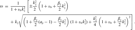 $$\begin{eqnarray}\displaystyle \unicode[STIX]{x1D714} & = & \displaystyle \frac{1}{1+v_{b}k_{\Vert }^{2}}\left[\pm \frac{k_{\Vert }^{2}}{2}\left(1+v_{b}+\frac{\unicode[STIX]{x1D6FD}_{\Vert }}{2}k_{\Vert }^{2}\right)\right.\nonumber\\ \displaystyle & & \displaystyle +\left.k_{\Vert }\sqrt{\left(1+\frac{\unicode[STIX]{x1D6FD}_{\Vert }}{2}(a_{p}-1)-\frac{\unicode[STIX]{x1D6FD}_{\Vert }}{2}k_{\Vert }^{2}\right)(1+v_{b}k_{\Vert }^{2})+\frac{k_{\Vert }^{2}}{4}\left(1+v_{b}+\frac{\unicode[STIX]{x1D6FD}_{\Vert }}{2}k_{\Vert }^{2}\right)^{2}}\right].\end{eqnarray}$$
For isotropic temperatures
 $(a_{p}=1)$
the result is equivalent to (5.115) since the Hall-term contributions for the FLR tensor disappear for all propagation directions. Also, for perpendicular propagation, the dispersion relation is naturally equal to (5.117).
$(a_{p}=1)$
the result is equivalent to (5.115) since the Hall-term contributions for the FLR tensor disappear for all propagation directions. Also, for perpendicular propagation, the dispersion relation is naturally equal to (5.117).
5.7 FLR corrections with gyrotropic heat flux
The equation (5.99) contains the divergence of the gyrotropic heat flux,
 $\unicode[STIX]{x1D735}\boldsymbol{\cdot }\boldsymbol{q}^{\text{g}}$
, which in the index notation calculates as
$\unicode[STIX]{x1D735}\boldsymbol{\cdot }\boldsymbol{q}^{\text{g}}$
, which in the index notation calculates as
 $$\begin{eqnarray}\displaystyle (\unicode[STIX]{x1D735}\boldsymbol{\cdot }\boldsymbol{q}^{\text{g}})_{ij} & = & \displaystyle \unicode[STIX]{x2202}_{k}q_{kij}^{\text{g}}=\unicode[STIX]{x2202}_{k}q_{ijk}^{\text{g}}=\unicode[STIX]{x2202}_{k}[q_{\Vert }\hat{b}_{i}\hat{b}_{j}\hat{b}_{k}+q_{\bot }(\unicode[STIX]{x1D6FF}_{ij}\hat{b}_{k}+\unicode[STIX]{x1D6FF}_{jk}\hat{b}_{i}+\unicode[STIX]{x1D6FF}_{ki}\hat{b}_{j}-3\hat{b}_{i}\hat{b}_{j}\hat{b}_{k})]\nonumber\\ \displaystyle & = & \displaystyle \unicode[STIX]{x2202}_{k}[(q_{\Vert }-3q_{\bot })\hat{b}_{i}\hat{b}_{j}\hat{b}_{k}+q_{\bot }(\unicode[STIX]{x1D6FF}_{ij}\hat{b}_{k}+\unicode[STIX]{x1D6FF}_{jk}\hat{b}_{i}+\unicode[STIX]{x1D6FF}_{ki}\hat{b}_{j})]\nonumber\\ \displaystyle & = & \displaystyle \hat{b}_{i}\hat{b}_{j}\hat{b}_{k}\unicode[STIX]{x2202}_{k}(q_{\Vert }-3q_{\bot })+(q_{\Vert }-3q_{\bot })(\hat{b}_{j}\hat{b}_{k}\unicode[STIX]{x2202}_{k}\hat{b}_{i}+\hat{b}_{i}\hat{b}_{k}\unicode[STIX]{x2202}_{k}\hat{b}_{j}+\hat{b}_{i}\hat{b}_{j}\unicode[STIX]{x2202}_{k}\hat{b}_{k})\nonumber\\ \displaystyle & & \displaystyle +\,(\unicode[STIX]{x1D6FF}_{ij}\hat{b}_{k}\unicode[STIX]{x2202}_{k}+\hat{b}_{i}\unicode[STIX]{x2202}_{j}+\hat{b}_{j}\unicode[STIX]{x2202}_{i})q_{\bot }+q_{\bot }(\unicode[STIX]{x1D6FF}_{ij}\unicode[STIX]{x2202}_{k}\hat{b}_{k}+\unicode[STIX]{x2202}_{j}\hat{b}_{i}+\unicode[STIX]{x2202}_{i}\hat{b}_{j}).\end{eqnarray}$$
Evaluation along magnetic field
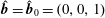 $\hat{\boldsymbol{b}}=\hat{\boldsymbol{b}}_{0}=(0,0,1)$
yields
$\hat{\boldsymbol{b}}=\hat{\boldsymbol{b}}_{0}=(0,0,1)$
yields
 $\hat{b}_{k}\unicode[STIX]{x2202}_{k}\rightarrow \unicode[STIX]{x2202}_{z}$
and the matrix is evaluated as
$\hat{b}_{k}\unicode[STIX]{x2202}_{k}\rightarrow \unicode[STIX]{x2202}_{z}$
and the matrix is evaluated as
 $$\begin{eqnarray}\displaystyle & \displaystyle (\unicode[STIX]{x1D735}\boldsymbol{\cdot }\boldsymbol{q}^{\text{g}})_{xx}=\unicode[STIX]{x2202}_{z}q_{\bot }+q_{\bot }(\unicode[STIX]{x1D735}\boldsymbol{\cdot }\hat{\boldsymbol{b}}+2\unicode[STIX]{x2202}_{x}\hat{b}_{x}); & \displaystyle\end{eqnarray}$$
 $$\begin{eqnarray}\displaystyle & \displaystyle (\unicode[STIX]{x1D735}\boldsymbol{\cdot }\boldsymbol{q}^{\text{g}})_{xy}=q_{\bot }(\unicode[STIX]{x2202}_{y}\hat{b}_{x}+\unicode[STIX]{x2202}_{x}\hat{b}_{y})=(\unicode[STIX]{x1D735}\boldsymbol{\cdot }\boldsymbol{q}^{\text{g}})_{yx}; & \displaystyle\end{eqnarray}$$
 $$\begin{eqnarray}\displaystyle & \displaystyle (\unicode[STIX]{x1D735}\boldsymbol{\cdot }\boldsymbol{q}^{\text{g}})_{xz}=(q_{\Vert }-2q_{\bot })\unicode[STIX]{x2202}_{z}\hat{b}_{x}+\unicode[STIX]{x2202}_{x}q_{\bot }+q_{\bot }\unicode[STIX]{x2202}_{x}\hat{b}_{z}=(\unicode[STIX]{x1D735}\boldsymbol{\cdot }\boldsymbol{q}^{\text{g}})_{zx}; & \displaystyle\end{eqnarray}$$
 $$\begin{eqnarray}\displaystyle & \displaystyle (\unicode[STIX]{x1D735}\boldsymbol{\cdot }\boldsymbol{q}^{\text{g}})_{yz}=(q_{\Vert }-2q_{\bot })\unicode[STIX]{x2202}_{z}\hat{b}_{y}+\unicode[STIX]{x2202}_{y}q_{\bot }+q_{\bot }\unicode[STIX]{x2202}_{y}\hat{b}_{z}=(\unicode[STIX]{x1D735}\boldsymbol{\cdot }\boldsymbol{q}^{\text{g}})_{zy}; & \displaystyle\end{eqnarray}$$
 $$\begin{eqnarray}\displaystyle & \displaystyle (\unicode[STIX]{x1D735}\boldsymbol{\cdot }\boldsymbol{q}^{\text{g}})_{yy}=\unicode[STIX]{x2202}_{z}q_{\bot }+q_{\bot }(\unicode[STIX]{x1D735}\boldsymbol{\cdot }\hat{\boldsymbol{b}}+2\unicode[STIX]{x2202}_{y}\hat{b}_{y}); & \displaystyle\end{eqnarray}$$
 $$\begin{eqnarray}\displaystyle & \displaystyle (\unicode[STIX]{x1D735}\boldsymbol{\cdot }\boldsymbol{q}^{\text{g}})_{zz}=\unicode[STIX]{x2202}_{z}q_{\Vert }+(q_{\Vert }-2q_{\bot })\unicode[STIX]{x1D735}\boldsymbol{\cdot }\hat{\boldsymbol{b}}, & \displaystyle\end{eqnarray}$$
where in the last ‘
 $zz$
’ component we also used
$zz$
’ component we also used
 $\unicode[STIX]{x2202}_{z}\hat{b}_{z}=0$
, but for brevity we left the divergence
$\unicode[STIX]{x2202}_{z}\hat{b}_{z}=0$
, but for brevity we left the divergence
 $\unicode[STIX]{x1D735}\boldsymbol{\cdot }\hat{\boldsymbol{b}}=\unicode[STIX]{x2202}_{x}\hat{b}_{x}+\unicode[STIX]{x2202}_{y}\hat{b}_{y}$
intact in all expressions. Note that
$\unicode[STIX]{x1D735}\boldsymbol{\cdot }\hat{\boldsymbol{b}}=\unicode[STIX]{x2202}_{x}\hat{b}_{x}+\unicode[STIX]{x2202}_{y}\hat{b}_{y}$
intact in all expressions. Note that
 $(\unicode[STIX]{x1D735}\boldsymbol{\cdot }\boldsymbol{q}^{\text{g}})_{yy}\neq -(\unicode[STIX]{x1D735}\boldsymbol{\cdot }\boldsymbol{q}^{\text{g}})_{xx}$
, which is not a problem as will be described below. The pressure tensor equation is here approximated as
$(\unicode[STIX]{x1D735}\boldsymbol{\cdot }\boldsymbol{q}^{\text{g}})_{yy}\neq -(\unicode[STIX]{x1D735}\boldsymbol{\cdot }\boldsymbol{q}^{\text{g}})_{xx}$
, which is not a problem as will be described below. The pressure tensor equation is here approximated as
 $$\begin{eqnarray}\frac{\unicode[STIX]{x2202}(\boldsymbol{p}^{\text{g}}+\unicode[STIX]{x1D72B})}{\unicode[STIX]{x2202}t}+\unicode[STIX]{x1D735}\boldsymbol{\cdot }(\boldsymbol{u}\boldsymbol{p}^{\text{g}}+\boldsymbol{q}^{\text{g}})+\boldsymbol{p}^{\text{g}}\boldsymbol{\cdot }\unicode[STIX]{x1D735}\boldsymbol{u}+(\boldsymbol{p}^{\text{g}}\boldsymbol{\cdot }\unicode[STIX]{x1D735}\boldsymbol{u})^{\text{T}}+\unicode[STIX]{x1D6FA}[\hat{\boldsymbol{b}}\times \unicode[STIX]{x1D72B}+(\hat{\boldsymbol{b}}\times \unicode[STIX]{x1D72B})^{\text{T}}]=0,\end{eqnarray}$$
and evaluated with respect to
 $\hat{\boldsymbol{b}}=\hat{\boldsymbol{b}}_{0}=(0,0,1)$
. All components were already evaluated and the calculation is straightforward, however, we need to subtract from diagonal components the scalar pressure equations that contain the gyrotropic heat flux contributions and that evaluated along
$\hat{\boldsymbol{b}}=\hat{\boldsymbol{b}}_{0}=(0,0,1)$
. All components were already evaluated and the calculation is straightforward, however, we need to subtract from diagonal components the scalar pressure equations that contain the gyrotropic heat flux contributions and that evaluated along
 $\hat{\boldsymbol{b}}_{0}$
read
$\hat{\boldsymbol{b}}_{0}$
read
 $$\begin{eqnarray}\displaystyle & \displaystyle \frac{\text{d}p_{\Vert }}{\text{d}t}+p_{\Vert }\unicode[STIX]{x1D735}\boldsymbol{\cdot }\boldsymbol{u}+2p_{\Vert }\unicode[STIX]{x2202}_{z}u_{z}+\unicode[STIX]{x2202}_{z}q_{\Vert }+(q_{\Vert }-2q_{\bot })\unicode[STIX]{x1D735}\boldsymbol{\cdot }\hat{\boldsymbol{b}}=0; & \displaystyle\end{eqnarray}$$
 $$\begin{eqnarray}\displaystyle & \displaystyle \frac{\text{d}p_{\bot }}{\text{d}t}+2p_{\bot }\unicode[STIX]{x1D735}\boldsymbol{\cdot }\boldsymbol{u}-p_{\bot }\unicode[STIX]{x2202}_{z}u_{z}+\unicode[STIX]{x2202}_{z}q_{\bot }+2q_{\bot }\unicode[STIX]{x1D735}\boldsymbol{\cdot }\hat{\boldsymbol{b}}=0. & \displaystyle\end{eqnarray}$$
The requirement again is that
 $\unicode[STIX]{x1D6F1}_{zz}=0$
and
$\unicode[STIX]{x1D6F1}_{zz}=0$
and
 $\unicode[STIX]{x1D6F1}_{yy}=-\unicode[STIX]{x1D6F1}_{xx}$
. Direct calculation yields
$\unicode[STIX]{x1D6F1}_{yy}=-\unicode[STIX]{x1D6F1}_{xx}$
. Direct calculation yields
 $$\begin{eqnarray}\displaystyle & \displaystyle \frac{\unicode[STIX]{x2202}}{\unicode[STIX]{x2202}t}\unicode[STIX]{x1D6F1}_{xx}-2\unicode[STIX]{x1D6FA}\unicode[STIX]{x1D6F1}_{xy}+p_{\bot }(\unicode[STIX]{x2202}_{x}u_{x}-\unicode[STIX]{x2202}_{y}u_{y})+q_{\bot }(\unicode[STIX]{x2202}_{x}\hat{b}_{x}-\unicode[STIX]{x2202}_{y}\hat{b}_{y})=0; & \displaystyle\end{eqnarray}$$
 $$\begin{eqnarray}\displaystyle & \displaystyle \frac{\unicode[STIX]{x2202}}{\unicode[STIX]{x2202}t}\unicode[STIX]{x1D6F1}_{xy}+2\unicode[STIX]{x1D6FA}\unicode[STIX]{x1D6F1}_{xx}+p_{\bot }(\unicode[STIX]{x2202}_{x}u_{y}+\unicode[STIX]{x2202}_{y}u_{x})+q_{\bot }(\unicode[STIX]{x2202}_{x}\hat{b}_{y}+\unicode[STIX]{x2202}_{y}\hat{b}_{x})=0; & \displaystyle\end{eqnarray}$$
 $$\begin{eqnarray}\displaystyle & & \displaystyle \frac{\unicode[STIX]{x2202}}{\unicode[STIX]{x2202}t}\unicode[STIX]{x1D6F1}_{xz}-\unicode[STIX]{x1D6FA}\unicode[STIX]{x1D6F1}_{yz}+p_{\bot }\unicode[STIX]{x2202}_{x}u_{z}+p_{\Vert }\unicode[STIX]{x2202}_{z}u_{x}+(p_{\Vert }-p_{\bot })\frac{\text{d}\hat{b}_{x}}{\text{d}t}\nonumber\\ \displaystyle & & \displaystyle \qquad +\,(q_{\Vert }-2q_{\bot })\unicode[STIX]{x2202}_{z}\hat{b}_{x}+q_{\bot }\unicode[STIX]{x2202}_{x}\hat{b}_{z}+\unicode[STIX]{x2202}_{x}q_{\bot }=0;\end{eqnarray}$$
 $$\begin{eqnarray}\displaystyle & & \displaystyle \frac{\unicode[STIX]{x2202}}{\unicode[STIX]{x2202}t}\unicode[STIX]{x1D6F1}_{yz}+\unicode[STIX]{x1D6FA}\unicode[STIX]{x1D6F1}_{xz}+p_{\bot }\unicode[STIX]{x2202}_{y}u_{z}+p_{\Vert }\unicode[STIX]{x2202}_{z}u_{y}+(p_{\Vert }-p_{\bot })\frac{\text{d}\hat{b}_{y}}{\text{d}t}\nonumber\\ \displaystyle & & \displaystyle \qquad +\,(q_{\Vert }-2q_{\bot })\unicode[STIX]{x2202}_{z}\hat{b}_{y}+q_{\bot }\unicode[STIX]{x2202}_{y}\hat{b}_{z}+\unicode[STIX]{x2202}_{y}q_{\bot }=0.\end{eqnarray}$$
Note that after subtraction of the perpendicular pressure equation, the
 $^{\prime }xx^{\prime }$
and
$^{\prime }xx^{\prime }$
and
 $^{\prime }yy^{\prime }$
components are again anti-symmetric, i.e.
$^{\prime }yy^{\prime }$
components are again anti-symmetric, i.e.
 $(\unicode[STIX]{x1D735}\boldsymbol{\cdot }\boldsymbol{q}^{\text{g}})_{yy}-\unicode[STIX]{x2202}_{z}q_{\bot }-2q_{\bot }\unicode[STIX]{x1D735}\boldsymbol{\cdot }\hat{\boldsymbol{b}}=-q_{\bot }(\unicode[STIX]{x2202}_{x}\hat{b}_{x}-\unicode[STIX]{x2202}_{y}\hat{b}_{y})$
, and the system indeed satisfies that
$(\unicode[STIX]{x1D735}\boldsymbol{\cdot }\boldsymbol{q}^{\text{g}})_{yy}-\unicode[STIX]{x2202}_{z}q_{\bot }-2q_{\bot }\unicode[STIX]{x1D735}\boldsymbol{\cdot }\hat{\boldsymbol{b}}=-q_{\bot }(\unicode[STIX]{x2202}_{x}\hat{b}_{x}-\unicode[STIX]{x2202}_{y}\hat{b}_{y})$
, and the system indeed satisfies that
 $\unicode[STIX]{x1D6F1}_{yy}=-\unicode[STIX]{x1D6F1}_{xx}$
. Also, considering the
$\unicode[STIX]{x1D6F1}_{yy}=-\unicode[STIX]{x1D6F1}_{xx}$
. Also, considering the
 $^{\prime }zz^{\prime }$
component, after subtraction of the parallel pressure equation all the terms cancel, i.e.
$^{\prime }zz^{\prime }$
component, after subtraction of the parallel pressure equation all the terms cancel, i.e.
 $(\unicode[STIX]{x1D735}\boldsymbol{\cdot }\boldsymbol{q}^{\text{g}})_{zz}-\unicode[STIX]{x2202}_{z}q_{\Vert }-(q_{\Vert }-2q_{\bot })\unicode[STIX]{x1D735}\boldsymbol{\cdot }\hat{\boldsymbol{b}}=0$
and the system indeed satisfies
$(\unicode[STIX]{x1D735}\boldsymbol{\cdot }\boldsymbol{q}^{\text{g}})_{zz}-\unicode[STIX]{x2202}_{z}q_{\Vert }-(q_{\Vert }-2q_{\bot })\unicode[STIX]{x1D735}\boldsymbol{\cdot }\hat{\boldsymbol{b}}=0$
and the system indeed satisfies
 $\unicode[STIX]{x1D6F1}_{zz}=0$
.
$\unicode[STIX]{x1D6F1}_{zz}=0$
.
Finally, expressing the above system in the linear approximation, with the assumption that mean heat flux values are zero, i.e.
 $q_{\Vert }^{(0)}=0$
,
$q_{\Vert }^{(0)}=0$
,
 $q_{\bot }^{(0)}=0$
, the only gyrotropic heat flux contributions that remain are
$q_{\bot }^{(0)}=0$
, the only gyrotropic heat flux contributions that remain are
 $\unicode[STIX]{x2202}_{x}q_{\bot }$
and
$\unicode[STIX]{x2202}_{x}q_{\bot }$
and
 $\unicode[STIX]{x2202}_{y}q_{\bot }$
, in equations (5.138), (5.139). The FLR tensor is again separated to
$\unicode[STIX]{x2202}_{y}q_{\bot }$
, in equations (5.138), (5.139). The FLR tensor is again separated to
 $\unicode[STIX]{x1D72B}^{(1)}+\unicode[STIX]{x1D72B}^{(2)}$
and similarly to the Hall-term contributions, it is again a matter of choice if the heat flux contributions are pushed to
$\unicode[STIX]{x1D72B}^{(1)}+\unicode[STIX]{x1D72B}^{(2)}$
and similarly to the Hall-term contributions, it is again a matter of choice if the heat flux contributions are pushed to
 $\unicode[STIX]{x1D72B}^{(2)}$
or kept in
$\unicode[STIX]{x1D72B}^{(2)}$
or kept in
 $\unicode[STIX]{x1D72B}^{(1)}$
. We prefer the first choice, i.e. when
$\unicode[STIX]{x1D72B}^{(1)}$
. We prefer the first choice, i.e. when
 $\unicode[STIX]{x1D72B}^{(1)}$
is equivalent to (5.74), which yields the second-order tensor
$\unicode[STIX]{x1D72B}^{(1)}$
is equivalent to (5.74), which yields the second-order tensor
 $$\begin{eqnarray}\displaystyle \left.\begin{array}{@{}c@{}}\displaystyle \unicode[STIX]{x1D6F1}_{xx}^{(2)}=-\frac{1}{2\unicode[STIX]{x1D6FA}}\frac{\unicode[STIX]{x2202}}{\unicode[STIX]{x2202}t}\unicode[STIX]{x1D6F1}_{xy}^{(1)};\quad \unicode[STIX]{x1D6F1}_{xy}^{(2)}=\frac{1}{2\unicode[STIX]{x1D6FA}}\frac{\unicode[STIX]{x2202}}{\unicode[STIX]{x2202}t}\unicode[STIX]{x1D6F1}_{xx}^{(1)};\\ \displaystyle \unicode[STIX]{x1D6F1}_{xz}^{(2)}=-\frac{1}{\unicode[STIX]{x1D6FA}}\frac{\unicode[STIX]{x2202}}{\unicode[STIX]{x2202}t}\unicode[STIX]{x1D6F1}_{yz}^{(1)}+\frac{1}{\unicode[STIX]{x1D6FA}}(p_{\Vert }^{(0)}-p_{\bot }^{(0)})\frac{c}{B_{0}}(\unicode[STIX]{x1D735}\times \boldsymbol{E}_{H})_{y}-\frac{1}{\unicode[STIX]{x1D6FA}}\unicode[STIX]{x2202}_{y}q_{\bot };\\ \displaystyle \unicode[STIX]{x1D6F1}_{yz}^{(2)}=\frac{1}{\unicode[STIX]{x1D6FA}}\frac{\unicode[STIX]{x2202}}{\unicode[STIX]{x2202}t}\unicode[STIX]{x1D6F1}_{xz}^{(1)}-\frac{1}{\unicode[STIX]{x1D6FA}}(p_{\Vert }^{(0)}-p_{\bot }^{(0)})\frac{c}{B_{0}}(\unicode[STIX]{x1D735}\times \boldsymbol{E}_{H})_{x}+\frac{1}{\unicode[STIX]{x1D6FA}}\unicode[STIX]{x2202}_{x}q_{\bot }.\end{array}\right\} & & \displaystyle\end{eqnarray}$$
Note that we could have derived the contributions
 $\unicode[STIX]{x2202}_{x}q_{\bot }$
and
$\unicode[STIX]{x2202}_{x}q_{\bot }$
and
 $\unicode[STIX]{x2202}_{y}q_{\bot }$
in a much quicker way, if the expression (5.126) was linearized from the beginning. However, we wanted to demonstrate that if nonlinear FLR corrections are considered, the heat flux nonlinearities can significantly complicate the dynamics, even if simplified evaluation along
$\unicode[STIX]{x2202}_{y}q_{\bot }$
in a much quicker way, if the expression (5.126) was linearized from the beginning. However, we wanted to demonstrate that if nonlinear FLR corrections are considered, the heat flux nonlinearities can significantly complicate the dynamics, even if simplified evaluation along
 $\hat{\boldsymbol{b}}_{0}$
is performed. Right now, we cannot use these FLR corrections to obtain a dispersion relation, since we have no means to determine a closure for the gyrotropic heat flux
$\hat{\boldsymbol{b}}_{0}$
is performed. Right now, we cannot use these FLR corrections to obtain a dispersion relation, since we have no means to determine a closure for the gyrotropic heat flux
 $q_{\bot }$
. We would have to consider CGL2 fluid model or more complicated Landau fluid models, that contains evolution equations for
$q_{\bot }$
. We would have to consider CGL2 fluid model or more complicated Landau fluid models, that contains evolution equations for
 $q_{\Vert }$
and
$q_{\Vert }$
and
 $q_{\bot }$
. Additionally, the perpendicular propagating fast mode, as well as the parallel propagating ion-cyclotron and whistler modes, are not influenced by the gyrotropic heat flux. Instead, as the last step, we will consider contributions of the non-gyrotropic heat flux.
$q_{\bot }$
. Additionally, the perpendicular propagating fast mode, as well as the parallel propagating ion-cyclotron and whistler modes, are not influenced by the gyrotropic heat flux. Instead, as the last step, we will consider contributions of the non-gyrotropic heat flux.
5.8 FLR corrections with non-gyrotropic heat flux vectors (FLR3)
It is possible to further increase precision of the FLR corrections by considering non-gyrotropic heat flux contributions. Detailed calculations with the non-gyrotropic heat flux vectors
 $\boldsymbol{S}_{\bot }^{\Vert }$
and
$\boldsymbol{S}_{\bot }^{\Vert }$
and
 $\boldsymbol{S}_{\bot }^{\bot }$
are presented in appendix D. At the linear level, these non-gyrotropic heat flux vectors contribute to the linearized pressure equations
$\boldsymbol{S}_{\bot }^{\bot }$
are presented in appendix D. At the linear level, these non-gyrotropic heat flux vectors contribute to the linearized pressure equations
 $$\begin{eqnarray}\displaystyle & \displaystyle \frac{\unicode[STIX]{x2202}p_{\Vert }}{\unicode[STIX]{x2202}t}+p_{\Vert }^{(0)}\unicode[STIX]{x1D735}\boldsymbol{\cdot }\boldsymbol{u}+2p_{\Vert }^{(0)}\unicode[STIX]{x2202}_{z}u_{z}+\unicode[STIX]{x2202}_{z}q_{\Vert }+\unicode[STIX]{x2202}_{x}(S_{\bot }^{\Vert })_{x}+\unicode[STIX]{x2202}_{y}(S_{\bot }^{\Vert })_{y}=0; & \displaystyle\end{eqnarray}$$
 $$\begin{eqnarray}\displaystyle & \displaystyle \frac{\unicode[STIX]{x2202}p_{\bot }}{\unicode[STIX]{x2202}t}+2p_{\bot }^{(0)}\unicode[STIX]{x1D735}\boldsymbol{\cdot }\boldsymbol{u}-p_{\bot }^{(0)}\unicode[STIX]{x2202}_{z}u_{z}+\unicode[STIX]{x2202}_{z}q_{\bot }+\unicode[STIX]{x2202}_{x}(S_{\bot }^{\bot })_{x}+\unicode[STIX]{x2202}_{y}(S_{\bot }^{\bot })_{y}=0, & \displaystyle\end{eqnarray}$$
and also to the linearized equations for the FLR tensor
 $$\begin{eqnarray}\displaystyle & \displaystyle \frac{\unicode[STIX]{x2202}}{\unicode[STIX]{x2202}t}\unicode[STIX]{x1D6F1}_{xx}-2\unicode[STIX]{x1D6FA}\unicode[STIX]{x1D6F1}_{xy}+p_{\bot }^{(0)}(\unicode[STIX]{x2202}_{x}u_{x}-\unicode[STIX]{x2202}_{y}u_{y})+\frac{1}{2}[\unicode[STIX]{x2202}_{x}(S_{\bot }^{\bot })_{x}-\unicode[STIX]{x2202}_{y}(S_{\bot }^{\bot })_{y}]=0; & \displaystyle\end{eqnarray}$$
 $$\begin{eqnarray}\displaystyle & \displaystyle \frac{\unicode[STIX]{x2202}}{\unicode[STIX]{x2202}t}\unicode[STIX]{x1D6F1}_{xy}+2\unicode[STIX]{x1D6FA}\unicode[STIX]{x1D6F1}_{xx}+p_{\bot }^{(0)}(\unicode[STIX]{x2202}_{x}u_{y}+\unicode[STIX]{x2202}_{y}u_{x})+\frac{1}{2}[\unicode[STIX]{x2202}_{y}(S_{\bot }^{\bot })_{x}+\unicode[STIX]{x2202}_{x}(S_{\bot }^{\bot })_{y}]=0; & \displaystyle\end{eqnarray}$$
 $$\begin{eqnarray}\displaystyle & \displaystyle \frac{\unicode[STIX]{x2202}}{\unicode[STIX]{x2202}t}\unicode[STIX]{x1D6F1}_{xz}-\unicode[STIX]{x1D6FA}\unicode[STIX]{x1D6F1}_{yz}+p_{\bot }^{(0)}\unicode[STIX]{x2202}_{x}u_{z}+p_{\Vert }^{(0)}\unicode[STIX]{x2202}_{z}u_{x}+(p_{\Vert }^{(0)}-p_{\bot }^{(0)})\frac{\unicode[STIX]{x2202}\hat{b}_{x}}{\unicode[STIX]{x2202}t}+\unicode[STIX]{x2202}_{x}q_{\bot }+\unicode[STIX]{x2202}_{z}(S_{\bot }^{\Vert })_{x}=0; & \displaystyle\end{eqnarray}$$
 $$\begin{eqnarray}\displaystyle & \displaystyle \frac{\unicode[STIX]{x2202}}{\unicode[STIX]{x2202}t}\unicode[STIX]{x1D6F1}_{yz}+\unicode[STIX]{x1D6FA}\unicode[STIX]{x1D6F1}_{xz}+p_{\bot }^{(0)}\unicode[STIX]{x2202}_{y}u_{z}+p_{\Vert }^{(0)}\unicode[STIX]{x2202}_{z}u_{y}+(p_{\Vert }^{(0)}-p_{\bot }^{(0)})\frac{\unicode[STIX]{x2202}\hat{b}_{y}}{\unicode[STIX]{x2202}t}+\unicode[STIX]{x2202}_{y}q_{\bot }+\unicode[STIX]{x2202}_{z}(S_{\bot }^{\Vert })_{y}=0. & \displaystyle\end{eqnarray}$$
These equations are equivalent to (18)–(21) of Goswami et al. (Reference Goswami, Passot and Sulem2005) (by noting that the vector
 $\boldsymbol{S}^{\bot }=q_{\bot }\hat{\boldsymbol{b}}+\boldsymbol{S}_{\bot }^{\bot }$
, so at the linear level
$\boldsymbol{S}^{\bot }=q_{\bot }\hat{\boldsymbol{b}}+\boldsymbol{S}_{\bot }^{\bot }$
, so at the linear level
 $S_{z}^{\bot }=q_{\bot }$
). The non-gyrotropic heat flux vectors are separated to the first and second order
$S_{z}^{\bot }=q_{\bot }$
). The non-gyrotropic heat flux vectors are separated to the first and second order
 $$\begin{eqnarray}\displaystyle \boldsymbol{S}_{\bot }^{\Vert }=\boldsymbol{S}_{\bot }^{\Vert (1)}+\boldsymbol{S}_{\bot }^{\Vert (2)};\quad \boldsymbol{S}_{\bot }^{\bot }=\boldsymbol{S}_{\bot }^{\bot (1)}+\boldsymbol{S}_{\bot }^{\bot (2)}. & & \displaystyle\end{eqnarray}$$
By using the nonlinear results for the first-order vectors derived in appendix D, (D 37), (D 60), yields that, at the linear level,
 $$\begin{eqnarray}\displaystyle & \displaystyle \boldsymbol{S}_{\bot }^{\Vert (1)}=\frac{1}{\unicode[STIX]{x1D6FA}}\hat{\boldsymbol{b}}_{0}\times \left[p_{\bot }^{(0)}\unicode[STIX]{x1D735}\left(\frac{p_{\Vert }}{\unicode[STIX]{x1D70C}}\right)+2\frac{p_{\Vert }^{(0)}}{\unicode[STIX]{x1D70C}_{0}}(p_{\Vert }^{(0)}-p_{\bot }^{(0)})\unicode[STIX]{x2202}_{z}\hat{\boldsymbol{b}}\right]; & \displaystyle\end{eqnarray}$$
 $$\begin{eqnarray}\displaystyle & \displaystyle \boldsymbol{S}_{\bot }^{\bot (1)}=\frac{1}{\unicode[STIX]{x1D6FA}}\hat{\boldsymbol{b}}_{0}\times \left[2p_{\bot }^{(0)}\unicode[STIX]{x1D735}\left(\frac{p_{\bot }}{\unicode[STIX]{x1D70C}}\right)\right], & \displaystyle\end{eqnarray}$$
where the gradients are meant to be further linearized. Nevertheless, the above form is useful to point out that the non-gyrotropic heat fluxes are proportional to the gradients of the temperature. For clarity, partially linearized expressions are also written down by components in appendix D, see (D 24), (D 25) and (D 61), (D 62). It is important to emphasize that the expressions (5.148), (5.149) were derived for a bi-Maxwellian distribution function. As discussed later in the text, this is achieved by prescribing closures for the gyrotropic fourth-order moment in the form
 $r_{\Vert \Vert }=3p_{\Vert }^{2}/\unicode[STIX]{x1D70C}+\widetilde{r}_{\Vert \Vert }$
,
$r_{\Vert \Vert }=3p_{\Vert }^{2}/\unicode[STIX]{x1D70C}+\widetilde{r}_{\Vert \Vert }$
,
 $r_{\Vert \bot }=p_{\Vert }p_{\bot }/\unicode[STIX]{x1D70C}+\widetilde{r}_{\Vert \bot }$
, and
$r_{\Vert \bot }=p_{\Vert }p_{\bot }/\unicode[STIX]{x1D70C}+\widetilde{r}_{\Vert \bot }$
, and
 $r_{\bot \bot }=2p_{\bot }^{2}/\unicode[STIX]{x1D70C}+\widetilde{r}_{\bot \bot }$
. In (5.148), (5.149), we additionally neglected the perturbations
$r_{\bot \bot }=2p_{\bot }^{2}/\unicode[STIX]{x1D70C}+\widetilde{r}_{\bot \bot }$
. In (5.148), (5.149), we additionally neglected the perturbations
 $\widetilde{r}$
(since right now we do not want to consider models where these perturbations are evaluated from linear kinetic theory). Therefore, the FLR corrections with the non-gyrotropic heat flux, that we call here FLR3, are distribution function specific. Nevertheless, as discussed later in the text, very similar closures can be also obtained for the bi-kappa distribution function, just with additional coefficients
$\widetilde{r}$
(since right now we do not want to consider models where these perturbations are evaluated from linear kinetic theory). Therefore, the FLR corrections with the non-gyrotropic heat flux, that we call here FLR3, are distribution function specific. Nevertheless, as discussed later in the text, very similar closures can be also obtained for the bi-kappa distribution function, just with additional coefficients
 $\unicode[STIX]{x1D6FC}_{\unicode[STIX]{x1D705}}=(\unicode[STIX]{x1D705}-3/2)/(\unicode[STIX]{x1D705}-5/2)$
, and expressions similar to (5.148), (5.149) can be derived.
$\unicode[STIX]{x1D6FC}_{\unicode[STIX]{x1D705}}=(\unicode[STIX]{x1D705}-3/2)/(\unicode[STIX]{x1D705}-5/2)$
, and expressions similar to (5.148), (5.149) can be derived.
The second-order vectors are also derived in appendix D, this time directly in the linear approximation, equations (D 88), (D 89) and the vectors read
 $$\begin{eqnarray}\displaystyle & \displaystyle (\boldsymbol{S}_{\bot }^{\Vert })_{k}^{(2)}=\frac{1}{\unicode[STIX]{x1D6FA}}\hat{\boldsymbol{b}}_{0}\times \left[\frac{\unicode[STIX]{x2202}}{\unicode[STIX]{x2202}t}(\boldsymbol{S}_{\bot }^{\Vert })_{k}^{(1)}+2\frac{p_{\Vert }^{(0)}}{\unicode[STIX]{x1D70C}_{0}}\unicode[STIX]{x2202}_{z}\unicode[STIX]{x1D6F1}_{kz}^{(1)}\right]; & \displaystyle\end{eqnarray}$$
 $$\begin{eqnarray}\displaystyle & \displaystyle (\boldsymbol{S}_{\bot }^{\bot })_{k}^{(2)}=\frac{1}{\unicode[STIX]{x1D6FA}}\hat{\boldsymbol{b}}_{0}\times \left[\frac{\unicode[STIX]{x2202}}{\unicode[STIX]{x2202}t}(\boldsymbol{S}_{\bot }^{\bot })_{k}^{(1)}+\frac{p_{\bot }^{(0)}}{\unicode[STIX]{x1D70C}_{0}}\left(\unicode[STIX]{x2202}_{x}\unicode[STIX]{x1D6F1}_{xk}^{(1)}+\unicode[STIX]{x2202}_{y}\unicode[STIX]{x1D6F1}_{yk}^{(1)}\right)\right]. & \displaystyle\end{eqnarray}$$
As a reminder,
 $\unicode[STIX]{x1D6F1}_{ij}=\unicode[STIX]{x1D6F1}_{ji}$
. For clarity, we wrote the expressions above explicitly in the index notation. The non-gyrotropic heat flux vectors are perpendicular to
$\unicode[STIX]{x1D6F1}_{ij}=\unicode[STIX]{x1D6F1}_{ji}$
. For clarity, we wrote the expressions above explicitly in the index notation. The non-gyrotropic heat flux vectors are perpendicular to
 $\hat{\boldsymbol{b}}_{0}=(0,0,1)$
, and the non-zero components are for index
$\hat{\boldsymbol{b}}_{0}=(0,0,1)$
, and the non-zero components are for index
 $k=x,y$
. The expressions can be written in a more elegant vector form, by defining vector
$k=x,y$
. The expressions can be written in a more elegant vector form, by defining vector
 $\vec{\unicode[STIX]{x1D72B}}_{z}\equiv (\unicode[STIX]{x1D6F1}_{xz},\unicode[STIX]{x1D6F1}_{yz},\unicode[STIX]{x1D6F1}_{zz}=0)$
, vector
$\vec{\unicode[STIX]{x1D72B}}_{z}\equiv (\unicode[STIX]{x1D6F1}_{xz},\unicode[STIX]{x1D6F1}_{yz},\unicode[STIX]{x1D6F1}_{zz}=0)$
, vector
 $\unicode[STIX]{x1D735}_{\bot }=(\unicode[STIX]{x2202}_{x},\unicode[STIX]{x2202}_{y},0)$
and matrix
$\unicode[STIX]{x1D735}_{\bot }=(\unicode[STIX]{x2202}_{x},\unicode[STIX]{x2202}_{y},0)$
and matrix
 $$\begin{eqnarray}\displaystyle \unicode[STIX]{x1D72B}_{\bot }\equiv \left(\begin{array}{@{}ccc@{}}\unicode[STIX]{x1D6F1}_{xx}, & \unicode[STIX]{x1D6F1}_{xy}, & 0\\ \unicode[STIX]{x1D6F1}_{yx}, & \unicode[STIX]{x1D6F1}_{yy}, & 0\\ 0, & 0, & 0\end{array}\right), & & \displaystyle\end{eqnarray}$$
so that
 $\unicode[STIX]{x1D735}_{\bot }\boldsymbol{\cdot }\unicode[STIX]{x1D72B}_{\bot }=(\unicode[STIX]{x2202}_{x}\unicode[STIX]{x1D6F1}_{xx}+\unicode[STIX]{x2202}_{y}\unicode[STIX]{x1D6F1}_{yx},\unicode[STIX]{x2202}_{x}\unicode[STIX]{x1D6F1}_{xy}+\unicode[STIX]{x2202}_{y}\unicode[STIX]{x1D6F1}_{yy})$
, yielding
$\unicode[STIX]{x1D735}_{\bot }\boldsymbol{\cdot }\unicode[STIX]{x1D72B}_{\bot }=(\unicode[STIX]{x2202}_{x}\unicode[STIX]{x1D6F1}_{xx}+\unicode[STIX]{x2202}_{y}\unicode[STIX]{x1D6F1}_{yx},\unicode[STIX]{x2202}_{x}\unicode[STIX]{x1D6F1}_{xy}+\unicode[STIX]{x2202}_{y}\unicode[STIX]{x1D6F1}_{yy})$
, yielding
 $$\begin{eqnarray}\displaystyle & \displaystyle \boldsymbol{S}_{\bot }^{\Vert (2)}=\frac{1}{\unicode[STIX]{x1D6FA}}\hat{\boldsymbol{b}}_{0}\times \left[\frac{\unicode[STIX]{x2202}}{\unicode[STIX]{x2202}t}\boldsymbol{S}_{\bot }^{\Vert (1)}+2\frac{p_{\Vert }^{(0)}}{\unicode[STIX]{x1D70C}_{0}}\unicode[STIX]{x2202}_{z}\vec{\unicode[STIX]{x1D72B}}_{z}^{(1)}\right]; & \displaystyle\end{eqnarray}$$
 $$\begin{eqnarray}\displaystyle & \displaystyle \boldsymbol{S}_{\bot }^{\bot (2)}=\frac{1}{\unicode[STIX]{x1D6FA}}\hat{\boldsymbol{b}}_{0}\times \left[\frac{\unicode[STIX]{x2202}}{\unicode[STIX]{x2202}t}\boldsymbol{S}_{\bot }^{\bot (1)}+\frac{p_{\bot }^{(0)}}{\unicode[STIX]{x1D70C}_{0}}\unicode[STIX]{x1D735}_{\bot }\boldsymbol{\cdot }\unicode[STIX]{x1D72B}_{\bot }^{(1)}\right], & \displaystyle\end{eqnarray}$$
which are equations (53) and (54) of Passot et al. (Reference Passot, Sulem and Hunana2012).
Normalizing the equations (dropping the tilde), Fourier transforming, and writing them in the
 $x$
–
$x$
–
 $z$
plane (with
$z$
plane (with
 $\unicode[STIX]{x2202}_{y}=0$
) yields
$\unicode[STIX]{x2202}_{y}=0$
) yields
 $$\begin{eqnarray}\displaystyle & \displaystyle -\text{i}\unicode[STIX]{x1D714}\unicode[STIX]{x1D6F1}_{xx}-2\unicode[STIX]{x1D6F1}_{xy}+a_{p}\text{i}k_{\bot }u_{x}+{\textstyle \frac{1}{2}}\text{i}k_{\bot }(S_{\bot }^{\bot })_{x}=0; & \displaystyle\end{eqnarray}$$
 $$\begin{eqnarray}\displaystyle & \displaystyle -\text{i}\unicode[STIX]{x1D714}\unicode[STIX]{x1D6F1}_{xy}+2\unicode[STIX]{x1D6F1}_{xx}+a_{p}\text{i}k_{\bot }u_{y}+{\textstyle \frac{1}{2}}\text{i}k_{\bot }(S_{\bot }^{\bot })_{y}=0; & \displaystyle\end{eqnarray}$$
 $$\begin{eqnarray}\displaystyle & & \displaystyle -\text{i}\unicode[STIX]{x1D714}\unicode[STIX]{x1D6F1}_{xz}-\unicode[STIX]{x1D6F1}_{yz}+a_{p}\text{i}k_{\bot }u_{z}+\text{i}k_{\Vert }u_{x}+(1-a_{p})(\text{i}k_{\Vert }u_{x}-(\unicode[STIX]{x1D735}\times \boldsymbol{E}_{H})_{x})\nonumber\\ \displaystyle & & \displaystyle \qquad +\,\text{i}k_{\bot }q_{\bot }+\text{i}k_{\Vert }(S_{\bot }^{\Vert })_{x}=0;\end{eqnarray}$$
 $$\begin{eqnarray}\displaystyle & \displaystyle -\text{i}\unicode[STIX]{x1D714}\unicode[STIX]{x1D6F1}_{yz}+\unicode[STIX]{x1D6F1}_{xz}+\text{i}k_{\Vert }u_{y}+(1-a_{p})(\text{i}k_{\Vert }u_{y}-(\unicode[STIX]{x1D735}\times \boldsymbol{E}_{H})_{y})+\text{i}k_{\Vert }(S_{\bot }^{\Vert })_{y}=0, & \displaystyle\end{eqnarray}$$
where the terms with Hall electric field components are specified in (5.112). At this moment we do not consider higher-order fluid models with gyrotropic heat fluxes such as CGL2 or Landau fluids (see later in the text) and to have a closed model, here we prescribe
 $q_{\bot }=0$
,
$q_{\bot }=0$
,
 $q_{\Vert }=0$
. It is useful to briefly explore what fluid models are obtained, if we decide to keep only the first-order vectors
$q_{\Vert }=0$
. It is useful to briefly explore what fluid models are obtained, if we decide to keep only the first-order vectors
 $\boldsymbol{S}_{\bot }^{\Vert (1)}$
,
$\boldsymbol{S}_{\bot }^{\Vert (1)}$
,
 $\boldsymbol{S}_{\bot }^{\bot (1)}$
, and ignore the second-order corrections
$\boldsymbol{S}_{\bot }^{\bot (1)}$
, and ignore the second-order corrections
 $\boldsymbol{S}_{\bot }^{\Vert (2)}$
,
$\boldsymbol{S}_{\bot }^{\Vert (2)}$
,
 $\boldsymbol{S}_{\bot }^{\bot (2)}$
. By considering only the
$\boldsymbol{S}_{\bot }^{\bot (2)}$
. By considering only the
 $\boldsymbol{S}_{\bot }^{\Vert (1)}$
,
$\boldsymbol{S}_{\bot }^{\Vert (1)}$
,
 $\boldsymbol{S}_{\bot }^{\bot (1)}$
contributions, we can either put them into to
$\boldsymbol{S}_{\bot }^{\bot (1)}$
contributions, we can either put them into to
 $\unicode[STIX]{x1D72B}^{(1)}$
or
$\unicode[STIX]{x1D72B}^{(1)}$
or
 $\unicode[STIX]{x1D72B}^{(2)}$
. However, it can be shown that both options yield dispersion relation for the perpendicular fast mode (long-wavelength, in physical units)
$\unicode[STIX]{x1D72B}^{(2)}$
. However, it can be shown that both options yield dispersion relation for the perpendicular fast mode (long-wavelength, in physical units)
 $$\begin{eqnarray}\unicode[STIX]{x1D714}^{2}=k_{\bot }^{2}\left[V_{A}^{2}\left(1-\frac{k_{\bot }^{2}\unicode[STIX]{x1D70C}_{i}^{2}}{8}\right)+v_{\text{th}\bot }^{2}\left(1+\frac{k_{\bot }^{2}\unicode[STIX]{x1D70C}_{i}^{2}}{16}\right)\right].\end{eqnarray}$$
Rather amusingly, in comparison to the FLR2 result (5.120), the wrong sign in the correction of the thermal speed is back!
5.9 Hall-CGL-FLR3 fluid model
Obviously, if matching with kinetic theory for the fast perpendicular mode is of upmost importance (for small wavenumbers), we have no other choice and we have to keep the second-order non-gyrotropic heat flux contributions
 $\boldsymbol{S}_{\bot }^{\Vert (2)}$
,
$\boldsymbol{S}_{\bot }^{\Vert (2)}$
,
 $\boldsymbol{S}_{\bot }^{\bot (2)}$
. We call this FLR pressure tensor as FLR3, and as stated previously, the FLR3 pressure tensor is distribution function specific. This model is very important to us and especially for the following discussion of the firehose instability. In order to be completely clear on which equations we are solving and also so that our results can be easily reproduced, let us state the entire model in all of its beauty. The linearized, normalized, Fourier transformed equations written in the
$\boldsymbol{S}_{\bot }^{\bot (2)}$
. We call this FLR pressure tensor as FLR3, and as stated previously, the FLR3 pressure tensor is distribution function specific. This model is very important to us and especially for the following discussion of the firehose instability. In order to be completely clear on which equations we are solving and also so that our results can be easily reproduced, let us state the entire model in all of its beauty. The linearized, normalized, Fourier transformed equations written in the
 $x$
–
$x$
–
 $z$
plane read
$z$
plane read

where each component of the (FLR) pressure tensor
 $\unicode[STIX]{x1D72B}$
, and each component of the (FLR) heat flux vectors
$\unicode[STIX]{x1D72B}$
, and each component of the (FLR) heat flux vectors
 $\boldsymbol{S}_{\bot }^{\Vert }$
,
$\boldsymbol{S}_{\bot }^{\Vert }$
,
 $\boldsymbol{S}_{\bot }^{\bot }$
, is separated to
$\boldsymbol{S}_{\bot }^{\bot }$
, is separated to
 $$\begin{eqnarray}\unicode[STIX]{x1D72B}=\unicode[STIX]{x1D72B}^{(1)}+\unicode[STIX]{x1D72B}^{(2)};\quad \boldsymbol{S}_{\bot }^{\Vert }=\boldsymbol{S}_{\bot }^{\Vert (1)}+\boldsymbol{S}_{\bot }^{\Vert (2)};\quad \boldsymbol{S}_{\bot }^{\bot }=\boldsymbol{S}_{\bot }^{\bot (1)}+\boldsymbol{S}_{\bot }^{\bot (2)}.\end{eqnarray}$$
The components of the
 $\unicode[STIX]{x1D72B}$
tensor are given by
$\unicode[STIX]{x1D72B}$
tensor are given by

where the Hall electric field contributions for cold massless electrons read
 $$\begin{eqnarray}\displaystyle (\unicode[STIX]{x1D735}\times \boldsymbol{E}_{H})_{x}=+k_{\Vert }^{2}B_{y};\quad (\unicode[STIX]{x1D735}\times \boldsymbol{E}_{H})_{y}=k_{\Vert }k_{\bot }B_{z}-k_{\Vert }^{2}B_{x}, & & \displaystyle\end{eqnarray}$$
and the components of the non-gyrotropic (FLR) heat fluxes are given by

Importantly, the
 $\unicode[STIX]{x1D72B}^{(2)}$
expressions contain both the first- and second-order contributions from the heat flux vectors
$\unicode[STIX]{x1D72B}^{(2)}$
expressions contain both the first- and second-order contributions from the heat flux vectors
 $\boldsymbol{S}_{\bot }^{\Vert }$
,
$\boldsymbol{S}_{\bot }^{\Vert }$
,
 $\boldsymbol{S}_{\bot }^{\bot }$
. To explicitly see where the closure for the gyrotropic heat fluxes
$\boldsymbol{S}_{\bot }^{\bot }$
. To explicitly see where the closure for the gyrotropic heat fluxes
 $q_{\Vert }=0,q_{\bot }=0$
was performed, we scratched the terms involving these quantities. Additionally, we also scratched contributions from
$q_{\Vert }=0,q_{\bot }=0$
was performed, we scratched the terms involving these quantities. Additionally, we also scratched contributions from
 $(S_{\bot }^{\bot })_{x}^{(1)}$
, which are here zero at the linear level.
$(S_{\bot }^{\bot })_{x}^{(1)}$
, which are here zero at the linear level.
Let us check the solution of the Hall-CGL-FLR3 fluid model for the perpendicular propagation (
 $k_{\Vert }=0$
), which in this case reads
$k_{\Vert }=0$
), which in this case reads
 $$\begin{eqnarray}\unicode[STIX]{x1D714}^{2}=\frac{k_{\bot }^{2}}{\displaystyle \left(1+k_{\bot }^{2}\frac{a_{p}}{8}\unicode[STIX]{x1D6FD}_{\Vert }\right)(1+a_{p}\unicode[STIX]{x1D6FD}_{\Vert }k_{\bot }^{2})}\left[1+a_{p}\unicode[STIX]{x1D6FD}_{\Vert }+k_{\bot }^{2}a_{p}\unicode[STIX]{x1D6FD}_{\Vert }\left(1+\frac{13}{16}a_{p}\unicode[STIX]{x1D6FD}_{\Vert }+\frac{9}{128}a_{p}^{2}\unicode[STIX]{x1D6FD}_{\Vert }^{2}k_{\bot }^{2}\right)\right].\end{eqnarray}$$
As a ‘sanity check’, since the solution stays always positive for all the wavenumbers and we do not have any instability, the model appears to be good. For small wavenumbers, the expansion yields
 $$\begin{eqnarray}\unicode[STIX]{x1D714}^{2}=k_{\bot }^{2}\left[1+a_{p}\unicode[STIX]{x1D6FD}_{\Vert }-k_{\bot }^{2}a_{p}\unicode[STIX]{x1D6FD}_{\Vert }\left({\textstyle \frac{1}{8}}+{\textstyle \frac{5}{16}}a_{p}\unicode[STIX]{x1D6FD}_{\Vert }\right)+\cdots \right],\end{eqnarray}$$
and in physical units
 $$\begin{eqnarray}\text{FLR3:}\quad \unicode[STIX]{x1D714}^{2}=k_{\bot }^{2}\left[V_{A}^{2}\left(1-\frac{k_{\bot }^{2}\unicode[STIX]{x1D70C}_{i}^{2}}{8}\right)+v_{\text{th}\bot }^{2}\left(1-\frac{5}{16}k_{\bot }^{2}\unicode[STIX]{x1D70C}_{i}^{2}\right)\right].\end{eqnarray}$$
Therefore, the Hall-CGL-FLR3 fluid model finally matches the analytic result from kinetic theory! We note that if the
 $\unicode[STIX]{x1D72B}$
contributions are neglected in the second-order heat flux expressions (5.164), instead of the correct
$\unicode[STIX]{x1D72B}$
contributions are neglected in the second-order heat flux expressions (5.164), instead of the correct
 $-5/16$
FLR correction to the thermal speed, one obtains
$-5/16$
FLR correction to the thermal speed, one obtains
 $-7/16$
. The necessity to keep the second-order heat flux contributions to recover the kinetic result for the perpendicular fast mode was discovered by Mikhailovskii & Smolyakov (Reference Mikhailovskii and Smolyakov1985).
$-7/16$
. The necessity to keep the second-order heat flux contributions to recover the kinetic result for the perpendicular fast mode was discovered by Mikhailovskii & Smolyakov (Reference Mikhailovskii and Smolyakov1985).
Checking the solution for the parallel propagating (
 $k_{\bot }=0$
) ion-cyclotron and whistler modes yields the following dispersion relation
$k_{\bot }=0$
) ion-cyclotron and whistler modes yields the following dispersion relation
 $$\begin{eqnarray}\displaystyle & & \displaystyle \unicode[STIX]{x1D714}^{2}(1+v_{b}k_{\Vert }^{2})\mp \unicode[STIX]{x1D714}k_{\Vert }^{2}\left[1+v_{b}(1+k_{\Vert }^{2})+k_{\Vert }^{2}\unicode[STIX]{x1D6FD}_{\Vert }^{2}\left(\frac{3}{2}-a_{p}\right)\right]\nonumber\\ \displaystyle & & \displaystyle \qquad -\,k_{\Vert }^{2}\left[v_{A\Vert }^{2}-\frac{\unicode[STIX]{x1D6FD}_{\Vert }}{2}k_{\Vert }^{2}(1+\unicode[STIX]{x1D6FD}_{\Vert }(1-a_{p}))+\frac{\unicode[STIX]{x1D6FD}_{\Vert }^{2}}{2}(a_{p}-2)k_{\Vert }^{4}\right]=0,\end{eqnarray}$$
where the quantities
 $v_{b}=\unicode[STIX]{x1D6FD}_{\Vert }(1-a_{p}/2)$
and
$v_{b}=\unicode[STIX]{x1D6FD}_{\Vert }(1-a_{p}/2)$
and
 $v_{A\Vert }^{2}=1+(\unicode[STIX]{x1D6FD}_{\Vert }/2)(a_{p}-1)$
. We will use this dispersion relation to study the firehose instability. For a general oblique propagation direction, the dispersion relation is obviously way too large to write down, and we recommend using analytic software such as Maple or Mathematica.
$v_{A\Vert }^{2}=1+(\unicode[STIX]{x1D6FD}_{\Vert }/2)(a_{p}-1)$
. We will use this dispersion relation to study the firehose instability. For a general oblique propagation direction, the dispersion relation is obviously way too large to write down, and we recommend using analytic software such as Maple or Mathematica.
Moving the Hall term to
$\unicode[STIX]{x1D72B}^{(1)}$

For completeness, just in case we want to investigate later the influence of the Hall term, moving it to
 $\unicode[STIX]{x1D72B}^{(1)}$
yields the following dispersion relation for the parallel propagation
$\unicode[STIX]{x1D72B}^{(1)}$
yields the following dispersion relation for the parallel propagation
 $$\begin{eqnarray}\displaystyle & & \displaystyle \unicode[STIX]{x1D714}^{2}(1+v_{b}k_{\Vert }^{2})\mp \unicode[STIX]{x1D714}k_{\Vert }^{2}\left[1+v_{b}+k_{\Vert }^{2}\frac{\unicode[STIX]{x1D6FD}_{\Vert }}{2}+k_{\Vert }^{2}\unicode[STIX]{x1D6FD}_{\Vert }^{2}\left(\frac{3}{2}-a_{p}\right)\right]\nonumber\\ \displaystyle & & \displaystyle \qquad -k_{\Vert }^{2}\left[v_{A\Vert }^{2}-\frac{\unicode[STIX]{x1D6FD}_{\Vert }}{2}k_{\Vert }^{2}(1+\unicode[STIX]{x1D6FD}_{\Vert }(1-a_{p}))-\frac{\unicode[STIX]{x1D6FD}_{\Vert }^{2}}{2}k_{\Vert }^{4}\right]=0.\end{eqnarray}$$
6 Parallel and oblique firehose instability
6.1 Parallel propagation
For clarity, it is useful to summarize all 3 major models that describe the parallel propagating ion-cyclotron and whistler modes. By prescribing
 $k_{\bot }=0$
in the equations of the Hall-CGL-FLR3 fluid model, the model greatly simplifies. The parallel magnetic field
$k_{\bot }=0$
in the equations of the Hall-CGL-FLR3 fluid model, the model greatly simplifies. The parallel magnetic field
 $B_{z}=0$
, the ion-acoustic mode decouples, and both the first- and second-order contributions to
$B_{z}=0$
, the ion-acoustic mode decouples, and both the first- and second-order contributions to
 $\unicode[STIX]{x1D6F1}_{xx}=0$
,
$\unicode[STIX]{x1D6F1}_{xx}=0$
,
 $\unicode[STIX]{x1D6F1}_{xy}=0$
,
$\unicode[STIX]{x1D6F1}_{xy}=0$
,
 $\boldsymbol{S}_{\bot }^{\bot }=0$
. The normalized, Fourier transformed equations written in the
$\boldsymbol{S}_{\bot }^{\bot }=0$
. The normalized, Fourier transformed equations written in the
 $x$
–
$x$
–
 $z$
plane read
$z$
plane read
 $$\begin{eqnarray}\displaystyle \left.\begin{array}{@{}c@{}}\displaystyle -\unicode[STIX]{x1D714}u_{x}-v_{A\Vert }^{2}k_{\Vert }B_{x}+\frac{\unicode[STIX]{x1D6FD}_{\Vert }}{2}k_{\Vert }\unicode[STIX]{x1D6F1}_{xz}=0;\\ \displaystyle -\unicode[STIX]{x1D714}u_{y}-v_{A\Vert }^{2}k_{\Vert }B_{y}+\frac{\unicode[STIX]{x1D6FD}_{\Vert }}{2}k_{\Vert }\unicode[STIX]{x1D6F1}_{yz}=0;\\ \displaystyle -\unicode[STIX]{x1D714}B_{x}-k_{\Vert }u_{x}-\text{i}k_{\Vert }^{2}B_{y}=0;\\ \displaystyle -\unicode[STIX]{x1D714}B_{y}-k_{\Vert }u_{y}+\text{i}k_{\Vert }^{2}B_{x}=0,\end{array}\right\} & & \displaystyle\end{eqnarray}$$
where the components of the non-gyrotropic (FLR) pressure tensor
 $\unicode[STIX]{x1D72B}$
are given by
$\unicode[STIX]{x1D72B}$
are given by
 $$\begin{eqnarray}\displaystyle \left.\begin{array}{@{}ll@{}}\displaystyle \unicode[STIX]{x1D6F1}_{xz}^{(1)}=-(2-a_{p})\text{i}k_{\Vert }u_{y}; & \displaystyle \unicode[STIX]{x1D6F1}_{xz}^{(2)}=+\text{i}\unicode[STIX]{x1D714}\unicode[STIX]{x1D6F1}_{yz}^{(1)}-(1-a_{p})k_{\Vert }^{2}B_{x}-\text{i}k_{\Vert }(S_{\bot }^{\Vert })_{y}^{(1)+(2)};\\ \displaystyle \unicode[STIX]{x1D6F1}_{yz}^{(1)}=+(2-a_{p})\text{i}k_{\Vert }u_{x}; & \displaystyle \unicode[STIX]{x1D6F1}_{yz}^{(2)}=-\text{i}\unicode[STIX]{x1D714}\unicode[STIX]{x1D6F1}_{xz}^{(1)}-(1-a_{p})k_{\Vert }^{2}B_{y}+\text{i}k_{\Vert }(S_{\bot }^{\Vert })_{x}^{(1)+(2)},\end{array}\right\} & & \displaystyle\end{eqnarray}$$
and the components of the non-gyrotropic (FLR) heat flux
 $\boldsymbol{S}_{\bot }^{\Vert }$
read
$\boldsymbol{S}_{\bot }^{\Vert }$
read
 $$\begin{eqnarray}\displaystyle \left.\begin{array}{@{}ll@{}}(S_{\bot }^{\Vert })_{x}^{(1)}=-\unicode[STIX]{x1D6FD}_{\Vert }(1-a_{p})\text{i}k_{\Vert }B_{y}; & (S_{\bot }^{\Vert })_{x}^{(2)}=+\text{i}\unicode[STIX]{x1D714}(S_{\bot }^{\Vert })_{y}^{(1)}-\unicode[STIX]{x1D6FD}_{\Vert }\text{i}k_{\Vert }\unicode[STIX]{x1D6F1}_{yz}^{(1)};\\ (S_{\bot }^{\Vert })_{y}^{(1)}=+\unicode[STIX]{x1D6FD}_{\Vert }(1-a_{p})\text{i}k_{\Vert }B_{x}; & (S_{\bot }^{\Vert })_{y}^{(2)}=-\text{i}\unicode[STIX]{x1D714}(S_{\bot }^{\Vert })_{x}^{(1)}+\unicode[STIX]{x1D6FD}_{\Vert }\text{i}k_{\Vert }\unicode[STIX]{x1D6F1}_{xz}^{(1)}.\end{array}\right\} & & \displaystyle\end{eqnarray}$$
When the entire
 $\unicode[STIX]{x1D72B}$
is neglected, yields the Hall-CGL solution
$\unicode[STIX]{x1D72B}$
is neglected, yields the Hall-CGL solution
 $$\begin{eqnarray}\unicode[STIX]{x1D714}=\pm \frac{k_{\Vert }^{2}}{2}+k_{\Vert }\sqrt{v_{A\Vert }^{2}+\frac{k_{\Vert }^{2}}{4}}.\end{eqnarray}$$
Neglecting the
 $\unicode[STIX]{x1D72B}^{(2)}$
contributions yields the Hall-CGL-FLR1 solution
$\unicode[STIX]{x1D72B}^{(2)}$
contributions yields the Hall-CGL-FLR1 solution
 $$\begin{eqnarray}\unicode[STIX]{x1D714}=\pm \frac{k_{\Vert }^{2}}{2}(1+v_{b})+k_{\Vert }\sqrt{v_{A\Vert }^{2}+\frac{k_{\Vert }^{2}}{4}(1-v_{b})^{2}},\end{eqnarray}$$
and neglecting the heat flux
 $\boldsymbol{S}_{\bot }^{\Vert }$
yields the Hall-CGL-FLR2 solution
$\boldsymbol{S}_{\bot }^{\Vert }$
yields the Hall-CGL-FLR2 solution
 $$\begin{eqnarray}\displaystyle \unicode[STIX]{x1D714} & = & \displaystyle \frac{1}{1+v_{b}k_{\Vert }^{2}}\left[\pm \frac{k_{\Vert }^{2}}{2}(1+v_{b}(1+k_{\Vert }^{2}))\right.\nonumber\\ \displaystyle & & \displaystyle +\left.k_{\Vert }\sqrt{\left(v_{A\Vert }^{2}-\frac{\unicode[STIX]{x1D6FD}_{\Vert }}{2}k_{\Vert }^{2}\right)(1+v_{b}k_{\Vert }^{2})+\frac{k_{\Vert }^{2}}{4}(1+v_{b}(1+k_{\Vert }^{2}))^{2}}\right].\end{eqnarray}$$
Finally, the full model yields Hall-CGL-FLR3 solution
 $$\begin{eqnarray}\displaystyle \unicode[STIX]{x1D714} & = & \displaystyle \frac{1}{1+v_{b}k_{\Vert }^{2}}\left\{\pm \frac{k_{\Vert }^{2}}{2}\left[1+v_{b}(1+k_{\Vert }^{2})+k_{\Vert }^{2}\unicode[STIX]{x1D6FD}_{\Vert }^{2}\left(\frac{3}{2}-a_{p}\right)\right]\right.\nonumber\\ \displaystyle & & \displaystyle +\left.k_{\Vert }\sqrt{\left[v_{A\Vert }^{2}-\frac{\unicode[STIX]{x1D6FD}_{\Vert }}{2}k_{\Vert }^{2}(1+\unicode[STIX]{x1D6FD}_{\Vert }(1-a_{p}))+\frac{\unicode[STIX]{x1D6FD}_{\Vert }^{2}}{2}(a_{p}-2)k_{\Vert }^{4}\right](1+v_{b}k_{\Vert }^{2})+\frac{k_{\Vert }^{2}}{4}\left[1+v_{b}(1+k_{\Vert }^{2})+k_{\Vert }^{2}\unicode[STIX]{x1D6FD}_{\Vert }^{2}\left(\frac{3}{2}-a_{p}\right)\right]^{2}}\right\}.\nonumber\\ \displaystyle & & \displaystyle\end{eqnarray}$$
The quantities
 $v_{b}$
and
$v_{b}$
and
 $v_{A\Vert }^{2}$
used in the solutions are defined as
$v_{A\Vert }^{2}$
used in the solutions are defined as
 $$\begin{eqnarray}v_{b}=\unicode[STIX]{x1D6FD}_{\Vert }\left(1-\frac{a_{p}}{2}\right);\quad v_{A\Vert }^{2}=1+\frac{\unicode[STIX]{x1D6FD}_{\Vert }}{2}(a_{p}-1).\end{eqnarray}$$
Importantly, the solutions are written here for
 $\unicode[STIX]{x1D714}$
(and not
$\unicode[STIX]{x1D714}$
(and not
 $\unicode[STIX]{x1D714}^{2}$
), and all the models of course yield 4 solutions, the other two solutions are obtained by substituting
$\unicode[STIX]{x1D714}^{2}$
), and all the models of course yield 4 solutions, the other two solutions are obtained by substituting
 $\unicode[STIX]{x1D714}$
with
$\unicode[STIX]{x1D714}$
with
 $-\unicode[STIX]{x1D714}$
. For a reader who just jumped to this section, and is confused on how the solutions were split, see § 4.2 where the Hall-CGL model is discussed with final equation (4.36). The solutions can be written in various forms, and one possibility is to keep
$-\unicode[STIX]{x1D714}$
. For a reader who just jumped to this section, and is confused on how the solutions were split, see § 4.2 where the Hall-CGL model is discussed with final equation (4.36). The solutions can be written in various forms, and one possibility is to keep
 $|k_{\Vert }|$
in front of the square roots.
$|k_{\Vert }|$
in front of the square roots.
The (parallel and oblique) firehose instability was studied in detail by Hunana & Zank (Reference Hunana and Zank2017), who focused on the Hall-CGL and Hall-CGL-FLR1 models. One of the conclusions reached in that paper was that the main reason for the relatively large discrepancy between the usual fluid models and the kinetic description is the appearance of a huge ‘bump’ in the imaginary phase speed, when close to the firehose threshold. The situation is demonstrated in figure 7, where kinetic solutions obtained by the WHAMP code (blue solid lines) are compared to solutions of the Hall-CGL-FLR2 model (a, blue dashed lines) and the Hall-CGL-FLR3 fluid model (b, black dashed lines). The plasma
 $\unicode[STIX]{x1D6FD}_{\Vert }=4$
, so the long-wavelength firehose threshold, that we call the ‘hard threshold’, is at
$\unicode[STIX]{x1D6FD}_{\Vert }=4$
, so the long-wavelength firehose threshold, that we call the ‘hard threshold’, is at
 $a_{p}=0.5$
. The temperature anisotropy is varied from
$a_{p}=0.5$
. The temperature anisotropy is varied from
 $a_{p}=0$
to
$a_{p}=0$
to
 $a_{p}=0.501$
. For solutions with the Hall-CGL and Hall-CGL-FLR1 models see figures 3 and 4 of Hunana & Zank (Reference Hunana and Zank2017). In the WHAMP code the value of
$a_{p}=0.501$
. For solutions with the Hall-CGL and Hall-CGL-FLR1 models see figures 3 and 4 of Hunana & Zank (Reference Hunana and Zank2017). In the WHAMP code the value of
 $a_{p}=0$
cannot be used, and
$a_{p}=0$
cannot be used, and
 $a_{p}=10^{-4}$
was chosen instead. Also, since here we concentrate on proton dynamics, the influence of electrons in the WHAMP code was eliminated by making the electrons cold (with
$a_{p}=10^{-4}$
was chosen instead. Also, since here we concentrate on proton dynamics, the influence of electrons in the WHAMP code was eliminated by making the electrons cold (with
 $T_{e}/T_{p}=10^{-8}$
).
$T_{e}/T_{p}=10^{-8}$
).
Imaginary phase speed (growth rate normalized to the wavenumber) of the parallel firehose instability. The value of
 $\unicode[STIX]{x1D6FD}_{\Vert }=4$
, and the temperature anisotropy is varied so that the whistler mode is in the firehose-unstable regime. Solid lines (blue) are kinetic solutions, obtained with the WHAMP code. Dashed lines are fluid solutions. (a) FLR2 solutions (blue), (b) FLR3 solutions (black). It is shown that in contrast to the FLR2 model, the FLR3 model reproduces the large ‘bump’ when close to the long-wavelength ‘hard’ firehose threshold
$\unicode[STIX]{x1D6FD}_{\Vert }=4$
, and the temperature anisotropy is varied so that the whistler mode is in the firehose-unstable regime. Solid lines (blue) are kinetic solutions, obtained with the WHAMP code. Dashed lines are fluid solutions. (a) FLR2 solutions (blue), (b) FLR3 solutions (black). It is shown that in contrast to the FLR2 model, the FLR3 model reproduces the large ‘bump’ when close to the long-wavelength ‘hard’ firehose threshold
 $T_{\bot }/T_{\Vert }=0.5$
.
$T_{\bot }/T_{\Vert }=0.5$
.
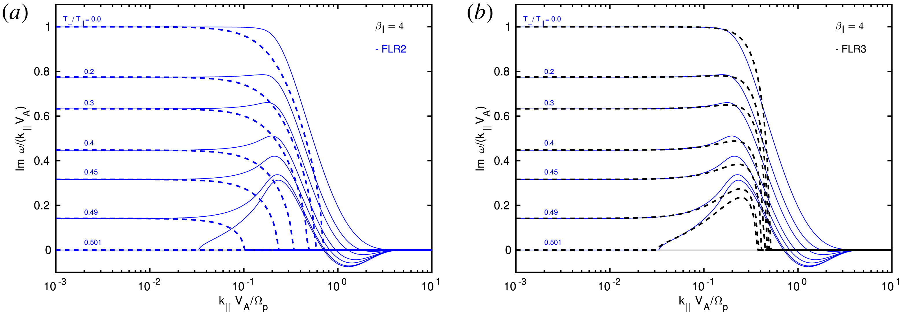
Same parameters as in figure 7, but the growth rate is plotted, and a linear scale is used for the
 $x$
-axis. Notice the excellent precision of the FLR3 model for small wavenumbers up to
$x$
-axis. Notice the excellent precision of the FLR3 model for small wavenumbers up to
 $kd_{i}=0.1{-}0.2$
. In comparison to kinetic theory, the fluid solutions are stabilized much more ‘rapidly’. Nevertheless, the value of the maximum growth rate, and the wavenumber where the maximum growth rate is achieved, is surprisingly close to kinetic theory. This is an excellent result for a fluid model, which does not contain collisionless ion-cyclotron damping.
$kd_{i}=0.1{-}0.2$
. In comparison to kinetic theory, the fluid solutions are stabilized much more ‘rapidly’. Nevertheless, the value of the maximum growth rate, and the wavenumber where the maximum growth rate is achieved, is surprisingly close to kinetic theory. This is an excellent result for a fluid model, which does not contain collisionless ion-cyclotron damping.
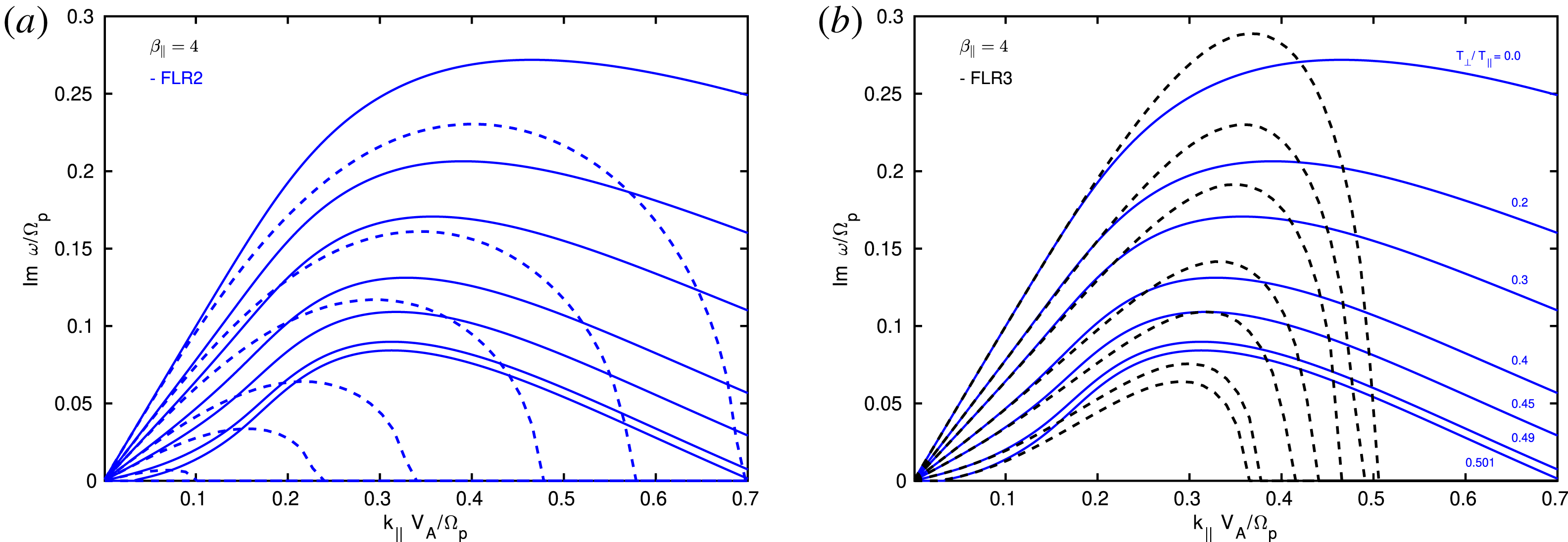
Very surprisingly, figure 7 shows that the large ‘bump’ is reproduced by the FLR3 model, and the precision is quite good! The situation is further analysed in figure 8, where instead of the imaginary phase speed, the growth rate is plotted. The same conclusion is obtained. For the temperature anisotropy
 $a_{p}=0.501$
, all simpler fluid models (Hall-CGL, FLR1, FLR2) are fully stable for all ranges of wavenumbers. In contrast, the FLR3 model still develops a strong firehose instability. Therefore, it is the non-gyrotropic heat flux
$a_{p}=0.501$
, all simpler fluid models (Hall-CGL, FLR1, FLR2) are fully stable for all ranges of wavenumbers. In contrast, the FLR3 model still develops a strong firehose instability. Therefore, it is the non-gyrotropic heat flux
 $\boldsymbol{S}_{\bot }^{\Vert }$
of the FLR3 model that is responsible for the ‘bump’ (for the case of strictly parallel propagation). The appearance of the ‘bump’ can be understood analytically, by evaluating the fluid dispersion relations exactly at the ‘hard’ firehose threshold
$\boldsymbol{S}_{\bot }^{\Vert }$
of the FLR3 model that is responsible for the ‘bump’ (for the case of strictly parallel propagation). The appearance of the ‘bump’ can be understood analytically, by evaluating the fluid dispersion relations exactly at the ‘hard’ firehose threshold
 $a_{p}=1-2/\unicode[STIX]{x1D6FD}_{\Vert }$
, where the quantities
$a_{p}=1-2/\unicode[STIX]{x1D6FD}_{\Vert }$
, where the quantities
 $v_{A\Vert }^{2}=0$
and
$v_{A\Vert }^{2}=0$
and
 $v_{b}=1+\unicode[STIX]{x1D6FD}_{\Vert }/2$
. At the hard firehose threshold, the expression under the square root of the FLR2 solution (6.6) can be factorized as
$v_{b}=1+\unicode[STIX]{x1D6FD}_{\Vert }/2$
. At the hard firehose threshold, the expression under the square root of the FLR2 solution (6.6) can be factorized as
 $$\begin{eqnarray}k_{\Vert }^{2}\left[1-\frac{\unicode[STIX]{x1D6FD}_{\Vert }}{4}+\frac{k_{\Vert }^{2}}{2}\left(1+\frac{\unicode[STIX]{x1D6FD}_{\Vert }}{2}\right)\right]^{2}+k_{\Vert }^{2}\frac{\unicode[STIX]{x1D6FD}_{\Vert }}{2},\end{eqnarray}$$
implying that the FLR2 model is always stable for all values of
 $k_{\Vert }$
and
$k_{\Vert }$
and
 $\unicode[STIX]{x1D6FD}_{\Vert }$
. Such a factorization cannot be achieved for the FLR3 model, and the solution (6.7) still becomes unstable at some range of wavenumbers, where
$\unicode[STIX]{x1D6FD}_{\Vert }$
. Such a factorization cannot be achieved for the FLR3 model, and the solution (6.7) still becomes unstable at some range of wavenumbers, where
 $$\begin{eqnarray}\displaystyle & & \displaystyle \left[v_{A\Vert }^{2}-\frac{\unicode[STIX]{x1D6FD}_{\Vert }}{2}k_{\Vert }^{2}(1+\unicode[STIX]{x1D6FD}_{\Vert }(1-a_{p}))+\frac{\unicode[STIX]{x1D6FD}_{\Vert }^{2}}{2}(a_{p}-2)k_{\Vert }^{4}\right](1+v_{b}k_{\Vert }^{2})\nonumber\\ \displaystyle & & \displaystyle \qquad +\,\frac{k_{\Vert }^{2}}{4}\left[1+v_{b}(1+k_{\Vert }^{2})+k_{\Vert }^{2}\unicode[STIX]{x1D6FD}_{\Vert }^{2}\left(\frac{3}{2}-a_{p}\right)\right]^{2}<0,\end{eqnarray}$$
which is the (strictly parallel) firehose instability criterion of the FLR3 model. We note that the model can become unstable also for the temperature anisotropy
 $a_{p}>1$
. This can be perhaps considered as some remnant of the ion-cyclotron anisotropy instability, but we did not study the situation further since the instability should not be reproduced correctly. The parallel firehose instability for high plasma beta value
$a_{p}>1$
. This can be perhaps considered as some remnant of the ion-cyclotron anisotropy instability, but we did not study the situation further since the instability should not be reproduced correctly. The parallel firehose instability for high plasma beta value
 $\unicode[STIX]{x1D6FD}_{\Vert }=100$
is shown in figure 9. The left figure is from Hunana & Zank (Reference Hunana and Zank2017), and it shows solutions of the Hall-CGL model (blue dashed lines) and of the Hall-CGL-FLR1 model (green dashed lines). The kinetic solutions are blue solid lines. It is shown that the FLR corrections are crucial for the correct stabilization of the firehose instability. Figure 9(b) shows refinement with FLR2 (blue dashed lines) and FLR3 tensors (black dashed lines). Obviously, for high plasma beta values, the maximum growth rate of the (strictly) parallel firehose instability is captured very precisely by the Hall-CGL-FLR3 model. The maximum growth rate (for parallel propagation) can be easily found analytically only for the Hall-CGL and Hall-CGL-FLR1 models. For models with the FLR2 and FLR3 tensors it is easier to find the maximum growth rate numerically. For example, let us consider the Hall-CGL model. Assuming the firehose-unstable regime, the frequency of the Hall-CGL solution (6.4) can be split into
$\unicode[STIX]{x1D6FD}_{\Vert }=100$
is shown in figure 9. The left figure is from Hunana & Zank (Reference Hunana and Zank2017), and it shows solutions of the Hall-CGL model (blue dashed lines) and of the Hall-CGL-FLR1 model (green dashed lines). The kinetic solutions are blue solid lines. It is shown that the FLR corrections are crucial for the correct stabilization of the firehose instability. Figure 9(b) shows refinement with FLR2 (blue dashed lines) and FLR3 tensors (black dashed lines). Obviously, for high plasma beta values, the maximum growth rate of the (strictly) parallel firehose instability is captured very precisely by the Hall-CGL-FLR3 model. The maximum growth rate (for parallel propagation) can be easily found analytically only for the Hall-CGL and Hall-CGL-FLR1 models. For models with the FLR2 and FLR3 tensors it is easier to find the maximum growth rate numerically. For example, let us consider the Hall-CGL model. Assuming the firehose-unstable regime, the frequency of the Hall-CGL solution (6.4) can be split into
 $\unicode[STIX]{x1D714}=\unicode[STIX]{x1D714}_{r}+\text{i}\unicode[STIX]{x1D714}_{i}$
, where the imaginary part
$\unicode[STIX]{x1D714}=\unicode[STIX]{x1D714}_{r}+\text{i}\unicode[STIX]{x1D714}_{i}$
, where the imaginary part
 $\unicode[STIX]{x1D714}_{i}=k_{\Vert }\sqrt{-v_{A\Vert }^{2}-k_{\Vert }^{2}/4}$
. Then, calculating
$\unicode[STIX]{x1D714}_{i}=k_{\Vert }\sqrt{-v_{A\Vert }^{2}-k_{\Vert }^{2}/4}$
. Then, calculating
 $\unicode[STIX]{x2202}\unicode[STIX]{x1D714}_{i}/\unicode[STIX]{x2202}k_{\Vert }=0$
, yields the wavenumber
$\unicode[STIX]{x2202}\unicode[STIX]{x1D714}_{i}/\unicode[STIX]{x2202}k_{\Vert }=0$
, yields the wavenumber
 $k_{\Vert \text{max}}$
and the maximum growth rate
$k_{\Vert \text{max}}$
and the maximum growth rate
 $\unicode[STIX]{x1D6FE}_{\text{max}}$
in the following form
$\unicode[STIX]{x1D6FE}_{\text{max}}$
in the following form
 $$\begin{eqnarray}k_{\Vert \text{max}}^{2}=-2v_{A\Vert }^{2};\quad \unicode[STIX]{x1D6FE}_{\text{max}}=-v_{A\Vert }^{2}=-\left(1+\frac{\unicode[STIX]{x1D6FD}_{\Vert }}{2}(a_{p}-1)\right).\end{eqnarray}$$
Similarly, the Hall-CGL-FLR1 model yields
 $$\begin{eqnarray}k_{\Vert \text{max}}^{2}=-\frac{2v_{A\Vert }^{2}}{(1-v_{b})^{2}};\quad \unicode[STIX]{x1D6FE}_{\text{max}}=\frac{v_{A\Vert }^{2}}{\displaystyle v_{A\Vert }^{2}-\frac{\unicode[STIX]{x1D6FD}_{\Vert }}{2}}=\frac{\displaystyle 1+\frac{\unicode[STIX]{x1D6FD}_{\Vert }}{2}(a_{p}-1)}{\displaystyle 1+\frac{\unicode[STIX]{x1D6FD}_{\Vert }}{2}(a_{p}-2)}.\end{eqnarray}$$
Growth rate of the parallel firehose instability for
 $\unicode[STIX]{x1D6FD}_{\Vert }=100$
. Kinetic solutions are solid blue lines. The temperature anisotropy is varied as
$\unicode[STIX]{x1D6FD}_{\Vert }=100$
. Kinetic solutions are solid blue lines. The temperature anisotropy is varied as
 $a_{p}=0.95;0.96;0.97;0.979$
(the hard firehose threshold is at
$a_{p}=0.95;0.96;0.97;0.979$
(the hard firehose threshold is at
 $a_{p}=0.98$
). Four different fluid models are plotted, and all fluid solutions have dashed lines. (a) Hall-CGL (blue), Hall-CGL-FLR1 (green). (b) Hall-CGL-FLR2 (blue), Hall-CGL-FLR3 (black).
$a_{p}=0.98$
). Four different fluid models are plotted, and all fluid solutions have dashed lines. (a) Hall-CGL (blue), Hall-CGL-FLR1 (green). (b) Hall-CGL-FLR2 (blue), Hall-CGL-FLR3 (black).
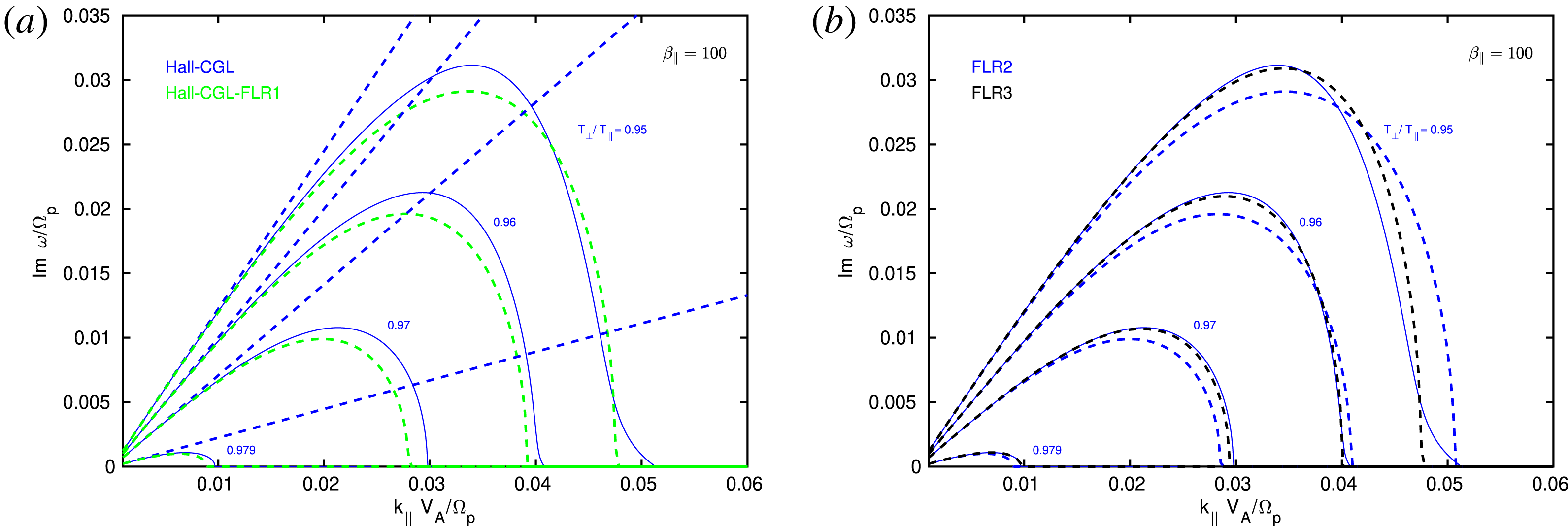
6.2 Oblique propagation
Here, we briefly investigate the parallel and oblique firehose instability for oblique propagation directions. Contour plots of the growth rate in the
 $k-\unicode[STIX]{x1D703}$
plane are shown in figure 10. The plasma
$k-\unicode[STIX]{x1D703}$
plane are shown in figure 10. The plasma
 $\unicode[STIX]{x1D6FD}_{\Vert }=4$
and the temperature anisotropy
$\unicode[STIX]{x1D6FD}_{\Vert }=4$
and the temperature anisotropy
 $a_{p}=0.49$
, so all the fluid models are in the firehose-unstable regime. We compare four different fluid models, Hall-CGL (a), and enhancement with FLR1 (b), FLR2 (c) and FLR3 (d). The FLR2 solution shows an additional instability at higher wavenumbers that we did not study further. Note the large differences between the four solutions. Importantly, the FLR3 solution shows large enhancement of the growth rate. We use the WHAMP code for kinetic calculations, and we do not provide a contour plot for the kinetic theory. Instead, we plot the growth rate for several propagation angles, so that the comparison with the contour plots can be made easily. The figure (e) is the FLR3 model, and (f) is the kinetic result. It is noted that, similarly to other fluid models with higher-order FLR corrections, the FLR3 model can develop secondary instabilities at scales below the proton gyroscale.
$a_{p}=0.49$
, so all the fluid models are in the firehose-unstable regime. We compare four different fluid models, Hall-CGL (a), and enhancement with FLR1 (b), FLR2 (c) and FLR3 (d). The FLR2 solution shows an additional instability at higher wavenumbers that we did not study further. Note the large differences between the four solutions. Importantly, the FLR3 solution shows large enhancement of the growth rate. We use the WHAMP code for kinetic calculations, and we do not provide a contour plot for the kinetic theory. Instead, we plot the growth rate for several propagation angles, so that the comparison with the contour plots can be made easily. The figure (e) is the FLR3 model, and (f) is the kinetic result. It is noted that, similarly to other fluid models with higher-order FLR corrections, the FLR3 model can develop secondary instabilities at scales below the proton gyroscale.
The growth rate plotted in the
 $k-\unicode[STIX]{x1D703}$
plane, with fixed
$k-\unicode[STIX]{x1D703}$
plane, with fixed
 $\unicode[STIX]{x1D6FD}_{\Vert }=4$
and
$\unicode[STIX]{x1D6FD}_{\Vert }=4$
and
 $a_{p}=0.49$
(the hard firehose threshold is at
$a_{p}=0.49$
(the hard firehose threshold is at
 $a_{p}=0.5$
), showing the parallel and oblique firehose instability. Four different fluid models are plotted. (a) Hall-CGL; (b) Hall-CGL-FLR1; (c) Hall-CGL-FLR2, (d) Hall-CGL-FLR3. We do not provide a contour plot for kinetic theory. Nevertheless, the bottom figures show solutions for several propagation angles. (e) Hall-CGL-FLR3 model, (f) kinetic.
$a_{p}=0.5$
), showing the parallel and oblique firehose instability. Four different fluid models are plotted. (a) Hall-CGL; (b) Hall-CGL-FLR1; (c) Hall-CGL-FLR2, (d) Hall-CGL-FLR3. We do not provide a contour plot for kinetic theory. Nevertheless, the bottom figures show solutions for several propagation angles. (e) Hall-CGL-FLR3 model, (f) kinetic.
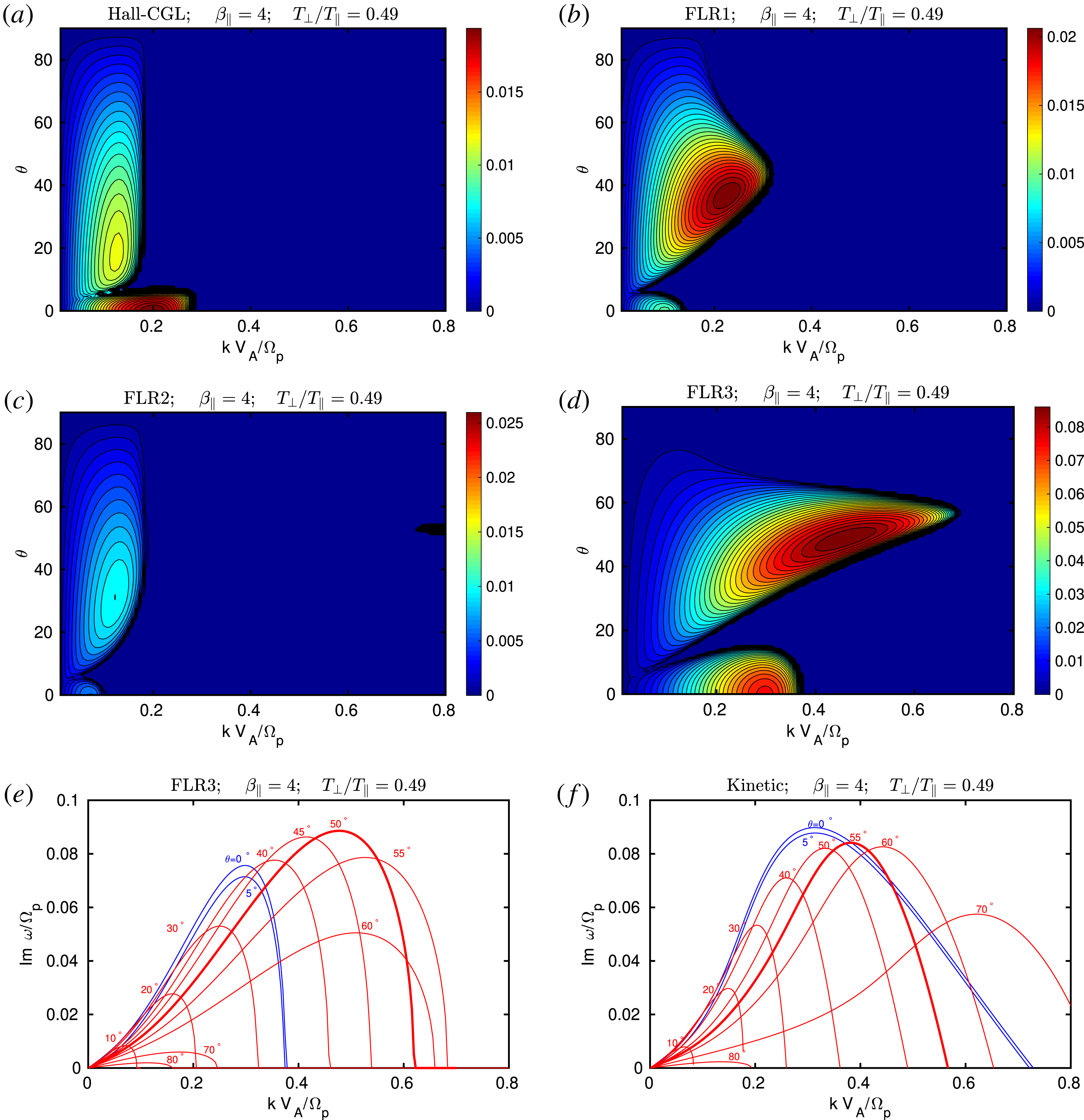
6.3 Hellinger’s contours for the Hall-CGL-FLR3 model
Here, we prescribe a fixed value for the maximum growth rate,
 $\unicode[STIX]{x1D6FE}_{\text{max}}=10^{-3};10^{-2};10^{-1}$
, and plot solutions in the
$\unicode[STIX]{x1D6FE}_{\text{max}}=10^{-3};10^{-2};10^{-1}$
, and plot solutions in the
 $\unicode[STIX]{x1D6FD}_{\Vert }-a_{p}$
plane, which is shown in figure 11. (a,c) Show the parallel firehose instability, and (b,d) show the oblique firehose instability. Panels (a,b) are plotted with the usual logarithmic scales, and (c,d) with linear scales. Additionally, only solutions with
$\unicode[STIX]{x1D6FD}_{\Vert }-a_{p}$
plane, which is shown in figure 11. (a,c) Show the parallel firehose instability, and (b,d) show the oblique firehose instability. Panels (a,b) are plotted with the usual logarithmic scales, and (c,d) with linear scales. Additionally, only solutions with
 $\unicode[STIX]{x1D6FD}_{\Vert }<6$
are shown at the bottom panels. Solutions for the Hall-CGL-FLR3 fluid model are black dashed lines, and kinetic solutions are solid blue lines (a,c) and solid red lines (b,d). The kinetic solutions were provided to us by P. Hellinger (private communication) and are identical to solutions shown in figure 1 of Hellinger et al. (Reference Hellinger, Trávníček, Kasper and Lazarus2006). It is shown that the
$\unicode[STIX]{x1D6FD}_{\Vert }<6$
are shown at the bottom panels. Solutions for the Hall-CGL-FLR3 fluid model are black dashed lines, and kinetic solutions are solid blue lines (a,c) and solid red lines (b,d). The kinetic solutions were provided to us by P. Hellinger (private communication) and are identical to solutions shown in figure 1 of Hellinger et al. (Reference Hellinger, Trávníček, Kasper and Lazarus2006). It is shown that the
 $\unicode[STIX]{x1D6FE}_{\text{max}}=10^{-3};10^{-2}$
contours clearly lie below the hard firehose threshold, i.e. the firehose instability in the FLR3 fluid model develops at some range of wavenumbers, even if the model is stable in the long-wavelength limit. Importantly, the kinetic contours of Hellinger et al. (Reference Hellinger, Trávníček, Kasper and Lazarus2006) were not calculated for cold electrons, but for isotropic electrons with
$\unicode[STIX]{x1D6FE}_{\text{max}}=10^{-3};10^{-2}$
contours clearly lie below the hard firehose threshold, i.e. the firehose instability in the FLR3 fluid model develops at some range of wavenumbers, even if the model is stable in the long-wavelength limit. Importantly, the kinetic contours of Hellinger et al. (Reference Hellinger, Trávníček, Kasper and Lazarus2006) were not calculated for cold electrons, but for isotropic electrons with
 $\unicode[STIX]{x1D6FD}_{e}=1$
. This does not matter for the parallel propagation, since the isotropic electron pressure does not influence the dispersion relations for the parallel propagating whistler and ion-cyclotron modes. Only the effect of electron inertia will enter, however, the effect should be negligible at the scales considered here. Unfortunately, the solution for the parallel firehose instability cannot be further improved by currently developed fluid models. The oblique case is different, since even isotropic electron pressure will influence the dynamics. The contours for the oblique firehose instability should be therefore recalculated by using a proper proton–electron two fluid model. The oblique case could be further improved, by considering FLR contributions from the non-gyrotropic heat flux tensor
$\unicode[STIX]{x1D6FD}_{e}=1$
. This does not matter for the parallel propagation, since the isotropic electron pressure does not influence the dispersion relations for the parallel propagating whistler and ion-cyclotron modes. Only the effect of electron inertia will enter, however, the effect should be negligible at the scales considered here. Unfortunately, the solution for the parallel firehose instability cannot be further improved by currently developed fluid models. The oblique case is different, since even isotropic electron pressure will influence the dynamics. The contours for the oblique firehose instability should be therefore recalculated by using a proper proton–electron two fluid model. The oblique case could be further improved, by considering FLR contributions from the non-gyrotropic heat flux tensor
 $\unicode[STIX]{x1D748}$
that were neglected here (contributions for parallel propagation are zero). For the oblique case, one can also use higher-order fluid models with the gyrotropic heat flux fluctuations
$\unicode[STIX]{x1D748}$
that were neglected here (contributions for parallel propagation are zero). For the oblique case, one can also use higher-order fluid models with the gyrotropic heat flux fluctuations
 $q_{\Vert },q_{\bot }$
(such as the CGL2 model discussed later), or even Landau fluid models. The main reason for the relatively large discrepancies found in the contours for the parallel firehose instability is demonstrated in figure 12.
$q_{\Vert },q_{\bot }$
(such as the CGL2 model discussed later), or even Landau fluid models. The main reason for the relatively large discrepancies found in the contours for the parallel firehose instability is demonstrated in figure 12.
(a,b) Solutions for the parallel (a,c) and oblique (b,d) firehose instability in the
 $\unicode[STIX]{x1D6FD}_{\Vert }-a_{p}$
plane for a prescribed maximum growth rate
$\unicode[STIX]{x1D6FD}_{\Vert }-a_{p}$
plane for a prescribed maximum growth rate
 $\unicode[STIX]{x1D6FE}_{\text{max}}=10^{-3};10^{-2};10^{-1}$
. Solid blue and red lines are kinetic solutions from Hellinger et al. (Reference Hellinger, Trávníček, Kasper and Lazarus2006). Black dashed lines are solutions of the Hall-CGL-FLR3 model. The magenta line is the ‘hard’ (long-wavelength limit) firehose threshold. (c,d) Same as top panels, but with linear scales for both axes, and only showing results for
$\unicode[STIX]{x1D6FE}_{\text{max}}=10^{-3};10^{-2};10^{-1}$
. Solid blue and red lines are kinetic solutions from Hellinger et al. (Reference Hellinger, Trávníček, Kasper and Lazarus2006). Black dashed lines are solutions of the Hall-CGL-FLR3 model. The magenta line is the ‘hard’ (long-wavelength limit) firehose threshold. (c,d) Same as top panels, but with linear scales for both axes, and only showing results for
 $\unicode[STIX]{x1D6FD}_{\Vert }<6$
.
$\unicode[STIX]{x1D6FD}_{\Vert }<6$
.
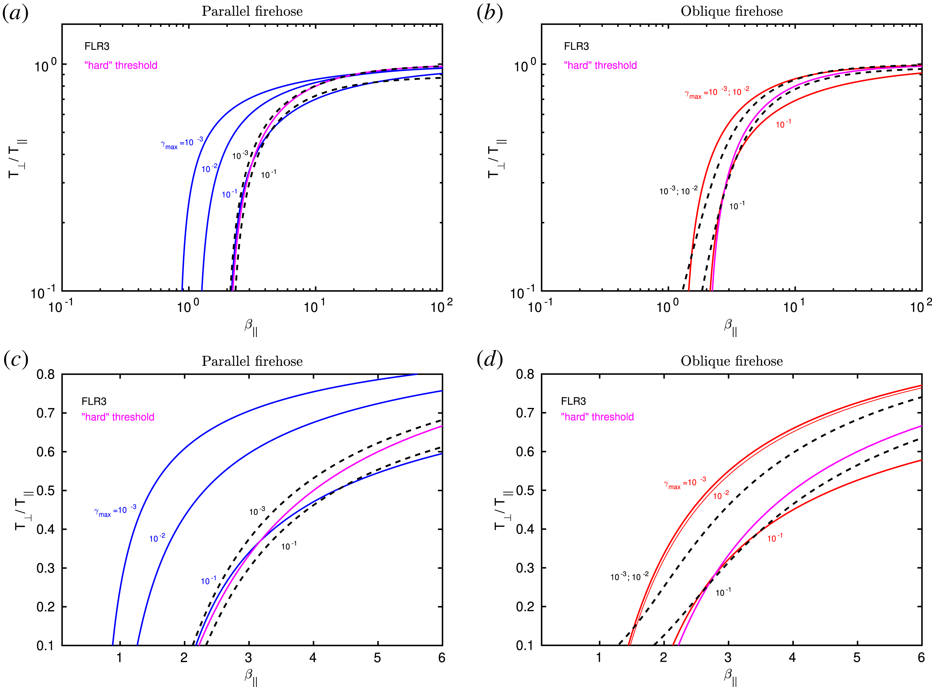
Parallel firehose instability,
 $\unicode[STIX]{x1D6FD}_{\Vert }=4$
. It is shown that the Hall-CGL-FLR3 model (black dashed lines) indeed develops the firehose instability even for values of
$\unicode[STIX]{x1D6FD}_{\Vert }=4$
. It is shown that the Hall-CGL-FLR3 model (black dashed lines) indeed develops the firehose instability even for values of
 $a_{p}>0.5$
, i.e. when there is no instability in the long-wavelength limit. Nevertheless, by increasing the value of
$a_{p}>0.5$
, i.e. when there is no instability in the long-wavelength limit. Nevertheless, by increasing the value of
 $a_{p}$
beyond
$a_{p}$
beyond
 $0.5$
, the growth rate in the FLR3 model quickly falls off, and the instability disappears for
$0.5$
, the growth rate in the FLR3 model quickly falls off, and the instability disappears for
 $a_{p}>0.5317$
. In contrast, kinetic theory (blue solid lines) develops a strong firehose instability even at
$a_{p}>0.5317$
. In contrast, kinetic theory (blue solid lines) develops a strong firehose instability even at
 $a_{p}=0.6$
.
$a_{p}=0.6$
.
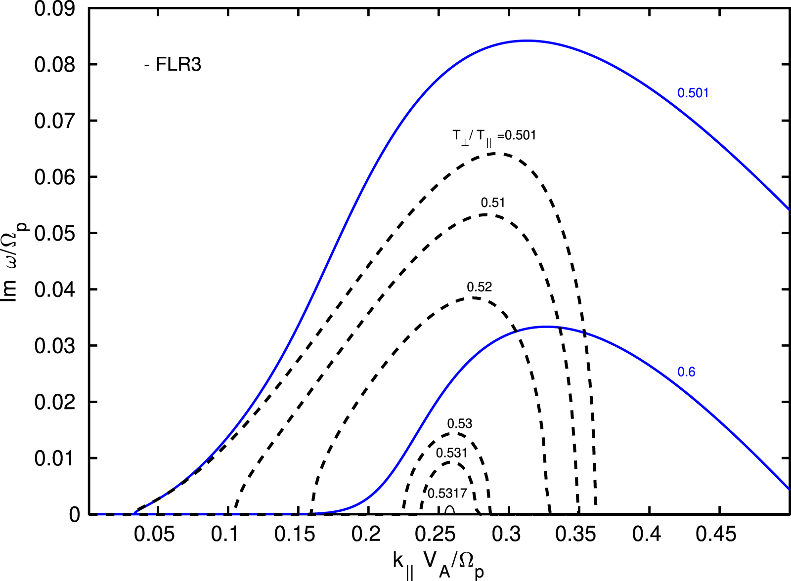
7 Heat flux tensor equation
Multiply the Vlasov equation by
 $mc_{i}c_{j}c_{k}$
and integrate over the velocity space. Naturally, the other possibilities are to multiply by
$mc_{i}c_{j}c_{k}$
and integrate over the velocity space. Naturally, the other possibilities are to multiply by
 $mc_{i}c_{j}v_{k}$
,
$mc_{i}c_{j}v_{k}$
,
 $mc_{i}v_{j}v_{k}$
or
$mc_{i}v_{j}v_{k}$
or
 $mv_{i}v_{j}v_{k}$
, although none of them is more revealing and we will use the first choice. It is convenient to define the symmetric operator
$mv_{i}v_{j}v_{k}$
, although none of them is more revealing and we will use the first choice. It is convenient to define the symmetric operator
 $^{S}$
that acts on a tensor of third rank according to
$^{S}$
that acts on a tensor of third rank according to
 $$\begin{eqnarray}\unicode[STIX]{x1D608}_{ijk}^{S}=\unicode[STIX]{x1D608}_{ijk}+\unicode[STIX]{x1D608}_{jki}+\unicode[STIX]{x1D608}_{kij},\end{eqnarray}$$
i.e. the operator represents all possible cyclic permutations. For the first term we will need the following identities
 $$\begin{eqnarray}\displaystyle \frac{\unicode[STIX]{x2202}}{\unicode[STIX]{x2202}t}(c_{i}c_{j}c_{k})=-\frac{\unicode[STIX]{x2202}u_{i}}{\unicode[STIX]{x2202}t}c_{j}c_{k}-c_{i}\frac{\unicode[STIX]{x2202}u_{j}}{\unicode[STIX]{x2202}t}c_{k}-c_{i}c_{j}\frac{\unicode[STIX]{x2202}u_{k}}{\unicode[STIX]{x2202}t}; & & \displaystyle\end{eqnarray}$$
 $$\begin{eqnarray}\displaystyle m\int f\frac{\unicode[STIX]{x2202}}{\unicode[STIX]{x2202}t}(c_{i}c_{j}c_{k})\,\text{d}^{3}v & = & \displaystyle -\frac{\unicode[STIX]{x2202}u_{i}}{\unicode[STIX]{x2202}t}\underbrace{m\int c_{j}c_{k}f\,\text{d}^{3}v}_{p_{jk}}-\frac{\unicode[STIX]{x2202}u_{j}}{\unicode[STIX]{x2202}t}\underbrace{m\int c_{i}c_{k}f\,\text{d}^{3}v}_{p_{ik}}-\frac{\unicode[STIX]{x2202}u_{k}}{\unicode[STIX]{x2202}t}\underbrace{m\int c_{i}c_{j}f\,\text{d}^{3}v}_{p_{ij}}\nonumber\\ \displaystyle & = & \displaystyle -\frac{\unicode[STIX]{x2202}u_{i}}{\unicode[STIX]{x2202}t}p_{jk}-\frac{\unicode[STIX]{x2202}u_{j}}{\unicode[STIX]{x2202}t}p_{ik}-\frac{\unicode[STIX]{x2202}u_{k}}{\unicode[STIX]{x2202}t}p_{ij},\end{eqnarray}$$
and the entire first term of the integrated Vlasov equation calculates as
 $$\begin{eqnarray}\displaystyle \unicode[STIX]{x2460} & = & \displaystyle m\int c_{i}c_{j}c_{k}\frac{\unicode[STIX]{x2202}f}{\unicode[STIX]{x2202}t}\,\text{d}^{3}v=\frac{\unicode[STIX]{x2202}}{\unicode[STIX]{x2202}t}\underbrace{\left(m\int c_{i}c_{j}c_{k}f\,\text{d}^{3}v\right)}_{q_{ijk}}-m\int f\frac{\unicode[STIX]{x2202}}{\unicode[STIX]{x2202}t}(c_{i}c_{j}c_{k})\,\text{d}^{3}v\nonumber\\ \displaystyle & = & \displaystyle \frac{\unicode[STIX]{x2202}}{\unicode[STIX]{x2202}t}q_{ijk}+\frac{\unicode[STIX]{x2202}u_{i}}{\unicode[STIX]{x2202}t}p_{jk}+\frac{\unicode[STIX]{x2202}u_{j}}{\unicode[STIX]{x2202}t}p_{ik}+\frac{\unicode[STIX]{x2202}u_{k}}{\unicode[STIX]{x2202}t}p_{ij}=\frac{\unicode[STIX]{x2202}}{\unicode[STIX]{x2202}t}q_{ijk}+\left[\frac{\unicode[STIX]{x2202}\boldsymbol{u}}{\unicode[STIX]{x2202}t}\boldsymbol{p}\right]_{ijk}^{S}.\end{eqnarray}$$
For the second term we will need identities
 $$\begin{eqnarray}\displaystyle m\int \boldsymbol{c}\boldsymbol{c}\boldsymbol{c}\boldsymbol{v}f\,\text{d}^{3}v=\boldsymbol{r}+\boldsymbol{q}\boldsymbol{u}; & & \displaystyle\end{eqnarray}$$
 $$\begin{eqnarray}\displaystyle m\int c_{i}c_{j}c_{k}v_{l}f\,\text{d}^{3}v & = & \displaystyle m\int c_{i}c_{j}c_{k}(v_{l}-u_{l}+u_{l})f\,\text{d}^{3}v\nonumber\\ \displaystyle & = & \displaystyle \underbrace{m\int c_{i}c_{j}c_{k}c_{l}f\,\text{d}^{3}v}_{r_{ijkl}}+u_{l}\underbrace{m\int c_{i}c_{j}c_{k}f\,\text{d}^{3}v}_{q_{ijk}}=r_{ijkl}+q_{ijk}u_{l};\end{eqnarray}$$
 $$\begin{eqnarray}\displaystyle \unicode[STIX]{x2202}_{l}(c_{i}c_{j}c_{k})=-c_{j}c_{k}\unicode[STIX]{x2202}_{l}u_{i}-c_{i}c_{k}\unicode[STIX]{x2202}_{l}u_{j}-c_{i}c_{j}\unicode[STIX]{x2202}_{l}u_{k}; & & \displaystyle\end{eqnarray}$$
 $$\begin{eqnarray}\displaystyle m\int fv_{l}\unicode[STIX]{x2202}_{l}(c_{i}c_{j}c_{k})\,\text{d}^{3}v & = & \displaystyle -(\unicode[STIX]{x2202}_{l}u_{i})\underbrace{m\int c_{j}c_{k}v_{l}f\,\text{d}^{3}v}_{q_{jkl}+p_{jk}u_{l}}\nonumber\\ \displaystyle & & \displaystyle -\,(\unicode[STIX]{x2202}_{l}u_{j})\underbrace{m\int c_{i}c_{k}v_{l}f\,\text{d}^{3}v}_{q_{ikl}+p_{ik}u_{l}}-(\unicode[STIX]{x2202}_{l}u_{k})\underbrace{m\int c_{i}c_{j}v_{l}f\,\text{d}^{3}v}_{q_{ijl}+p_{ij}u_{l}}\nonumber\\ \displaystyle & = & \displaystyle -(q_{jkl}+p_{jk}u_{l})\unicode[STIX]{x2202}_{l}u_{i}-(q_{ikl}+p_{ik}u_{l})\unicode[STIX]{x2202}_{l}u_{j}-(q_{ijl}+p_{ij}u_{l})\unicode[STIX]{x2202}_{l}u_{k},\nonumber\\ \displaystyle & & \displaystyle\end{eqnarray}$$
and the second term calculates as
 $$\begin{eqnarray}\displaystyle \unicode[STIX]{x2461} & = & \displaystyle m\int c_{i}c_{j}c_{k}v_{l}\unicode[STIX]{x2202}_{l}f\,\text{d}^{3}v=\unicode[STIX]{x2202}_{l}\left(m\int c_{i}c_{j}c_{k}v_{l}f\,\text{d}^{3}v\right)-m\int fv_{l}\unicode[STIX]{x2202}_{l}(c_{i}c_{j}c_{k})\,\text{d}^{3}v\nonumber\\ \displaystyle & = & \displaystyle \unicode[STIX]{x2202}_{l}(r_{lijk}+u_{l}q_{ijk})+(q_{jkl}+p_{jk}u_{l})\unicode[STIX]{x2202}_{l}u_{i}+(q_{ikl}+p_{ik}u_{l})\unicode[STIX]{x2202}_{l}u_{j}+(q_{ijl}+p_{ij}u_{l})\unicode[STIX]{x2202}_{l}u_{k}\nonumber\\ \displaystyle & = & \displaystyle [\unicode[STIX]{x1D735}\boldsymbol{\cdot }(\boldsymbol{r}+\boldsymbol{u}\boldsymbol{q})]_{ijk}+[(\boldsymbol{q}+\boldsymbol{p}\boldsymbol{u})\boldsymbol{\cdot }\unicode[STIX]{x1D735}\boldsymbol{u}]_{jki}+[(\boldsymbol{q}+\boldsymbol{p}\boldsymbol{u})\boldsymbol{\cdot }\unicode[STIX]{x1D735}\boldsymbol{u}]_{ikj}+[(\boldsymbol{q}+\boldsymbol{p}\boldsymbol{u})\boldsymbol{\cdot }\unicode[STIX]{x1D735}\boldsymbol{u}]_{ijk}\nonumber\\ \displaystyle & = & \displaystyle [\unicode[STIX]{x1D735}\boldsymbol{\cdot }(\boldsymbol{r}+\boldsymbol{u}\boldsymbol{q})]_{ijk}+[(\boldsymbol{q}+\boldsymbol{p}\boldsymbol{u})\boldsymbol{\cdot }\unicode[STIX]{x1D735}\boldsymbol{u}]_{ijk}^{S}.\end{eqnarray}$$
Note again that the divergence of a tensor operates through its first component
 $\unicode[STIX]{x2202}_{l}(r_{lijk}+u_{l}q_{ijk})=[\unicode[STIX]{x1D735}\boldsymbol{\cdot }(\boldsymbol{r}+\boldsymbol{u}\boldsymbol{q})]_{ijk}$
. Similarly, if the operator acts on a tensor from the right-hand side, the most natural way is to define that it operates through the last component, i.e.
$\unicode[STIX]{x2202}_{l}(r_{lijk}+u_{l}q_{ijk})=[\unicode[STIX]{x1D735}\boldsymbol{\cdot }(\boldsymbol{r}+\boldsymbol{u}\boldsymbol{q})]_{ijk}$
. Similarly, if the operator acts on a tensor from the right-hand side, the most natural way is to define that it operates through the last component, i.e.
 $[\boldsymbol{q}\boldsymbol{\cdot }\unicode[STIX]{x1D735}]_{ij}=q_{ijl}\unicode[STIX]{x2202}_{l}$
. In the expressions above
$[\boldsymbol{q}\boldsymbol{\cdot }\unicode[STIX]{x1D735}]_{ij}=q_{ijl}\unicode[STIX]{x2202}_{l}$
. In the expressions above
 $[\boldsymbol{q}\boldsymbol{\cdot }\unicode[STIX]{x1D735}\boldsymbol{u}]_{ijk}=q_{ijl}\unicode[STIX]{x2202}_{l}u_{k}$
and
$[\boldsymbol{q}\boldsymbol{\cdot }\unicode[STIX]{x1D735}\boldsymbol{u}]_{ijk}=q_{ijl}\unicode[STIX]{x2202}_{l}u_{k}$
and
 $[\boldsymbol{p}\boldsymbol{u}\boldsymbol{\cdot }\unicode[STIX]{x1D735}\boldsymbol{u}]_{ijk}=(\boldsymbol{p}\boldsymbol{u})_{ijl}\unicode[STIX]{x2202}_{l}u_{k}=p_{ij}u_{l}\unicode[STIX]{x2202}_{l}u_{k}$
. The last term can also be rewritten as
$[\boldsymbol{p}\boldsymbol{u}\boldsymbol{\cdot }\unicode[STIX]{x1D735}\boldsymbol{u}]_{ijk}=(\boldsymbol{p}\boldsymbol{u})_{ijl}\unicode[STIX]{x2202}_{l}u_{k}=p_{ij}u_{l}\unicode[STIX]{x2202}_{l}u_{k}$
. The last term can also be rewritten as
 $p_{ij}(\boldsymbol{u}\boldsymbol{\cdot }\unicode[STIX]{x1D735}\boldsymbol{u})_{k}$
, where the expression
$p_{ij}(\boldsymbol{u}\boldsymbol{\cdot }\unicode[STIX]{x1D735}\boldsymbol{u})_{k}$
, where the expression
 $(\boldsymbol{u}\boldsymbol{\cdot }\unicode[STIX]{x1D735}\boldsymbol{u})_{k}=u_{l}\unicode[STIX]{x2202}_{l}u_{k}$
is familiar from MHD. For the third term we will need identities
$(\boldsymbol{u}\boldsymbol{\cdot }\unicode[STIX]{x1D735}\boldsymbol{u})_{k}=u_{l}\unicode[STIX]{x2202}_{l}u_{k}$
is familiar from MHD. For the third term we will need identities
 $$\begin{eqnarray}\displaystyle & \displaystyle \frac{\unicode[STIX]{x2202}c_{i}}{\unicode[STIX]{x2202}v_{l}}=\unicode[STIX]{x1D6FF}_{il}; & \displaystyle\end{eqnarray}$$
 $$\begin{eqnarray}\displaystyle & \displaystyle \frac{\unicode[STIX]{x2202}}{\unicode[STIX]{x2202}v_{l}}(c_{i}c_{j}c_{k})=\unicode[STIX]{x1D6FF}_{il}c_{j}c_{k}+c_{i}\unicode[STIX]{x1D6FF}_{jl}c_{k}+c_{i}c_{j}\unicode[STIX]{x1D6FF}_{kl}, & \displaystyle\end{eqnarray}$$
and the entire third term calculates as
 $$\begin{eqnarray}\displaystyle \unicode[STIX]{x2462} & = & \displaystyle q\int c_{i}c_{j}c_{k}E_{l}\frac{\unicode[STIX]{x2202}f}{\unicode[STIX]{x2202}v_{l}}\,\text{d}^{3}v=qE_{l}\underbrace{\int \frac{\unicode[STIX]{x2202}}{\unicode[STIX]{x2202}v_{l}}(c_{i}c_{j}c_{k}f)\,\text{d}^{3}v}_{\rightarrow 0}-qE_{l}\int \frac{\unicode[STIX]{x2202}}{\unicode[STIX]{x2202}v_{l}}(c_{i}c_{j}c_{k})f\,\text{d}^{3}v\nonumber\\ \displaystyle & = & \displaystyle -qE_{l}\int (\unicode[STIX]{x1D6FF}_{il}c_{j}c_{k}+\unicode[STIX]{x1D6FF}_{jl}c_{i}c_{k}+\unicode[STIX]{x1D6FF}_{kl}c_{i}c_{j})f\,\text{d}^{3}v=-\frac{q}{m}(E_{i}p_{jk}+E_{j}p_{ik}+E_{k}p_{ij})\nonumber\\ \displaystyle & = & \displaystyle -\frac{q}{m}[\boldsymbol{E}\boldsymbol{p}]_{ijk}^{S}.\end{eqnarray}$$
For the fourth term we will need identities
 $$\begin{eqnarray}\displaystyle & \displaystyle \frac{\unicode[STIX]{x2202}}{\unicode[STIX]{x2202}v_{l}}(\boldsymbol{v}\times \boldsymbol{B})_{l}=0; & \displaystyle\end{eqnarray}$$
 $$\begin{eqnarray}\displaystyle & \displaystyle \frac{\unicode[STIX]{x2202}}{\unicode[STIX]{x2202}v_{l}}[c_{i}c_{j}c_{k}(\boldsymbol{v}\times \boldsymbol{B})_{l}]=c_{j}c_{k}(\boldsymbol{v}\times \boldsymbol{B})_{i}+c_{i}c_{k}(\boldsymbol{v}\times \boldsymbol{B})_{j}+c_{i}c_{j}(\boldsymbol{v}\times \boldsymbol{B})_{k}; & \displaystyle\end{eqnarray}$$
 $$\begin{eqnarray}\displaystyle & \displaystyle \int c_{j}(\boldsymbol{v}\times \boldsymbol{B})_{i}f\,\text{d}^{3}v=-\frac{1}{m}(\boldsymbol{B}\times \boldsymbol{p})_{ij}; & \displaystyle\end{eqnarray}$$
 $$\begin{eqnarray}\displaystyle & \displaystyle \int c_{j}c_{k}(\boldsymbol{v}\times \boldsymbol{B})_{i}f\,\text{d}^{3}v=-\frac{1}{m}[\boldsymbol{B}\times (\boldsymbol{q}+\boldsymbol{u}\boldsymbol{p})]_{ijk}, & \displaystyle\end{eqnarray}$$
and the entire fourth term calculates as
 $$\begin{eqnarray}\displaystyle \unicode[STIX]{x2463} & = & \displaystyle \frac{q}{c}\int c_{i}c_{j}c_{k}(\boldsymbol{v}\times \boldsymbol{B})_{l}\frac{\unicode[STIX]{x2202}f}{\unicode[STIX]{x2202}v_{l}}\,\text{d}^{3}v\nonumber\\ \displaystyle & = & \displaystyle \frac{q}{c}\underbrace{\int \frac{\unicode[STIX]{x2202}}{\unicode[STIX]{x2202}v_{l}}[c_{i}c_{j}c_{k}(\boldsymbol{v}\times \boldsymbol{B})_{l}f]\,\text{d}^{3}v}_{\rightarrow 0}-\frac{q}{c}\int f\frac{\unicode[STIX]{x2202}}{\unicode[STIX]{x2202}v_{l}}[c_{i}c_{j}c_{k}(\boldsymbol{v}\times \boldsymbol{B})_{l}]\,\text{d}^{3}v\nonumber\\ \displaystyle & = & \displaystyle -\frac{q}{c}\left\{\int fc_{j}c_{k}(\boldsymbol{v}\times \boldsymbol{B})_{i}\,\text{d}^{3}v+\int fc_{k}c_{i}(\boldsymbol{v}\times \boldsymbol{B})_{j}\,\text{d}^{3}v+\int fc_{i}c_{j}(\boldsymbol{v}\times \boldsymbol{B})_{k}\,\text{d}^{3}v\right\}\nonumber\\ \displaystyle & = & \displaystyle \frac{q}{mc}\{[\boldsymbol{B}\times (\boldsymbol{q}+\boldsymbol{u}\boldsymbol{p})]_{ijk}+[\boldsymbol{B}\times (\boldsymbol{q}+\boldsymbol{u}\boldsymbol{p})]_{jki}+[\boldsymbol{B}\times (\boldsymbol{q}+\boldsymbol{u}\boldsymbol{p})]_{kij}\}\nonumber\\ \displaystyle & \equiv & \displaystyle \frac{q}{mc}[\boldsymbol{B}\times (\boldsymbol{q}+\boldsymbol{u}\boldsymbol{p})]_{ijk}^{S}.\end{eqnarray}$$
Combining all the results together
 $\unicode[STIX]{x2460}+\unicode[STIX]{x2461}+\unicode[STIX]{x2462}+\unicode[STIX]{x2463}=0$
, the entire heat flux tensor equation obtained by direct integration of the Vlasov equation reads
$\unicode[STIX]{x2460}+\unicode[STIX]{x2461}+\unicode[STIX]{x2462}+\unicode[STIX]{x2463}=0$
, the entire heat flux tensor equation obtained by direct integration of the Vlasov equation reads
 $$\begin{eqnarray}\displaystyle \frac{\unicode[STIX]{x2202}\boldsymbol{q}}{\unicode[STIX]{x2202}t}+\unicode[STIX]{x1D735}\boldsymbol{\cdot }(\boldsymbol{r}+\boldsymbol{u}\boldsymbol{q})+\left[\frac{\unicode[STIX]{x2202}\boldsymbol{u}}{\unicode[STIX]{x2202}t}\boldsymbol{p}+(\boldsymbol{q}+\boldsymbol{p}\boldsymbol{u})\boldsymbol{\cdot }\unicode[STIX]{x1D735}\boldsymbol{u}-\frac{q}{m}\boldsymbol{E}\boldsymbol{p}+\frac{q}{mc}\boldsymbol{B}\times (\boldsymbol{q}+\boldsymbol{u}\boldsymbol{p})\right]^{S}=0. & & \displaystyle\end{eqnarray}$$
Now we will need to use 3 different momentum equations that will cancel various terms. We will also need identity
 $$\begin{eqnarray}[(\boldsymbol{u}\times \boldsymbol{B})\boldsymbol{p}]_{ijk}=-[\boldsymbol{B}\times (\boldsymbol{u}\boldsymbol{p})]_{ijk}.\end{eqnarray}$$
We need to multiply the momentum equation for
 $\unicode[STIX]{x2202}u_{i}/\unicode[STIX]{x2202}t$
by
$\unicode[STIX]{x2202}u_{i}/\unicode[STIX]{x2202}t$
by
 $p_{jk}$
, the equation for
$p_{jk}$
, the equation for
 $\unicode[STIX]{x2202}u_{j}/\unicode[STIX]{x2202}t$
by
$\unicode[STIX]{x2202}u_{j}/\unicode[STIX]{x2202}t$
by
 $p_{ki}$
and the equation for
$p_{ki}$
and the equation for
 $\unicode[STIX]{x2202}u_{k}/\unicode[STIX]{x2202}t$
by
$\unicode[STIX]{x2202}u_{k}/\unicode[STIX]{x2202}t$
by
 $p_{ij}$
. All the three momentum equations that we want to subtract from the heat flux equation can be written together as
$p_{ij}$
. All the three momentum equations that we want to subtract from the heat flux equation can be written together as
 $$\begin{eqnarray}\displaystyle \left[\left(\frac{\unicode[STIX]{x2202}\boldsymbol{u}}{\unicode[STIX]{x2202}t}+\boldsymbol{u}\boldsymbol{\cdot }\unicode[STIX]{x1D735}\boldsymbol{u}+\frac{1}{mn}\unicode[STIX]{x1D735}\boldsymbol{\cdot }\boldsymbol{p}-\frac{q}{m}\boldsymbol{E}-\frac{q}{mc}\boldsymbol{u}\times \boldsymbol{B}\right)\boldsymbol{p}\right]_{ijk}^{S}=0, & & \displaystyle\end{eqnarray}$$
and because of identity (7.19), this is equivalent to
 $$\begin{eqnarray}\displaystyle \left[\left(\frac{\unicode[STIX]{x2202}\boldsymbol{u}}{\unicode[STIX]{x2202}t}+\boldsymbol{u}\boldsymbol{\cdot }\unicode[STIX]{x1D735}\boldsymbol{u}+\frac{1}{mn}\unicode[STIX]{x1D735}\boldsymbol{\cdot }\boldsymbol{p}-\frac{q}{m}\boldsymbol{E}\right)\boldsymbol{p}+\frac{q}{mc}[\boldsymbol{B}\times (\boldsymbol{u}\boldsymbol{p})]\right]_{ijk}^{S}=0. & & \displaystyle\end{eqnarray}$$
Note that, because of the symmetric operator, it does not matter if the tensor
 $\boldsymbol{p}$
is applied to the momentum equation from the left or right, since all the expressions are symmetric in this regard, i.e. for example
$\boldsymbol{p}$
is applied to the momentum equation from the left or right, since all the expressions are symmetric in this regard, i.e. for example
 $[(\unicode[STIX]{x1D735}\boldsymbol{\cdot }\boldsymbol{p})\boldsymbol{p}]^{S}=[\boldsymbol{p}(\unicode[STIX]{x1D735}\boldsymbol{\cdot }\boldsymbol{p})]^{S}$
. By subtracting (7.21) from (7.18), the final heat flux tensor equation reads
$[(\unicode[STIX]{x1D735}\boldsymbol{\cdot }\boldsymbol{p})\boldsymbol{p}]^{S}=[\boldsymbol{p}(\unicode[STIX]{x1D735}\boldsymbol{\cdot }\boldsymbol{p})]^{S}$
. By subtracting (7.21) from (7.18), the final heat flux tensor equation reads
 $$\begin{eqnarray}\displaystyle \frac{\unicode[STIX]{x2202}}{\unicode[STIX]{x2202}t}\boldsymbol{q}+\unicode[STIX]{x1D735}\boldsymbol{\cdot }(\boldsymbol{r}+\boldsymbol{u}\boldsymbol{q})+\left[\boldsymbol{q}\boldsymbol{\cdot }\unicode[STIX]{x1D735}\boldsymbol{u}+\frac{q}{mc}\boldsymbol{B}\times \boldsymbol{q}-\frac{1}{\unicode[STIX]{x1D70C}}\boldsymbol{p}(\unicode[STIX]{x1D735}\boldsymbol{\cdot }\boldsymbol{p})\right]^{S}=0. & & \displaystyle\end{eqnarray}$$
By defining the cyclotron frequency vector
 $\unicode[STIX]{x1D734}=q\boldsymbol{B}/mc$
, this equation identifies with equation (A 5) in Chust & Belmont (Reference Chust and Belmont2006). By using the scalar cyclotron frequency defined with respect to
$\unicode[STIX]{x1D734}=q\boldsymbol{B}/mc$
, this equation identifies with equation (A 5) in Chust & Belmont (Reference Chust and Belmont2006). By using the scalar cyclotron frequency defined with respect to
 $|\boldsymbol{B}|$
as
$|\boldsymbol{B}|$
as
 $\unicode[STIX]{x1D6FA}=q|\boldsymbol{B}|/mc$
, the heat flux tensor equation is written explicitly in the index notation
$\unicode[STIX]{x1D6FA}=q|\boldsymbol{B}|/mc$
, the heat flux tensor equation is written explicitly in the index notation
 $$\begin{eqnarray}\displaystyle & & \displaystyle \frac{\unicode[STIX]{x2202}}{\unicode[STIX]{x2202}t}q_{ijk}+\unicode[STIX]{x2202}_{l}(r_{lijk}+u_{l}q_{ijk})+q_{ijl}\unicode[STIX]{x2202}_{l}u_{k}+q_{jkl}\unicode[STIX]{x2202}_{l}u_{i}+q_{kil}\unicode[STIX]{x2202}_{l}u_{j}+\unicode[STIX]{x1D6FA}\hat{b}_{l}(\unicode[STIX]{x1D716}_{ilm}q_{mjk}+\unicode[STIX]{x1D716}_{jlm}q_{mki}+\unicode[STIX]{x1D716}_{klm}q_{mij})\nonumber\\ \displaystyle & & \displaystyle \qquad -\,\frac{1}{mn}(p_{ij}\unicode[STIX]{x2202}_{l}p_{lk}+p_{jk}\unicode[STIX]{x2202}_{l}p_{li}+p_{ki}\unicode[STIX]{x2202}_{l}p_{lj})=0,\end{eqnarray}$$
which is equivalent to (4) in Goswami et al. (Reference Goswami, Passot and Sulem2005) with the term
 $$\begin{eqnarray}\displaystyle (\hat{\boldsymbol{b}}\times \boldsymbol{q})_{ijk}^{S} & = & \displaystyle \unicode[STIX]{x1D716}_{ilm}\hat{b}_{l}q_{mjk}+\unicode[STIX]{x1D716}_{jlm}\hat{b}_{l}q_{mki}+\unicode[STIX]{x1D716}_{klm}\hat{b}_{l}q_{mij}\nonumber\\ \displaystyle & = & \displaystyle -\hat{b}_{l}(\unicode[STIX]{x1D716}_{iml}q_{jkm}+\unicode[STIX]{x1D716}_{jml}q_{ikm}+\unicode[STIX]{x1D716}_{kml}q_{ijm}).\end{eqnarray}$$
7.1 Heat flux tensor decomposition
Considering only the gyrotropic part of the heat flux tensor
 $(3\times 3\times 3)$
cube, the heat flux is decomposed into the scalar parallel and perpendicular heat flux components
$(3\times 3\times 3)$
cube, the heat flux is decomposed into the scalar parallel and perpendicular heat flux components
 $q_{\Vert },q_{\bot }$
according to
$q_{\Vert },q_{\bot }$
according to
 $$\begin{eqnarray}\boldsymbol{q}^{\text{g}}=q_{\Vert }\hat{\boldsymbol{b}}\hat{\boldsymbol{b}}\hat{\boldsymbol{b}}+q_{\bot }[(\unicode[STIX]{x1D644}-\hat{\boldsymbol{b}}\hat{\boldsymbol{b}})\hat{\boldsymbol{b}}]^{S},\end{eqnarray}$$
and which in the index notation reads
 $$\begin{eqnarray}q_{ijk}^{\text{g}}=q_{\Vert }\hat{b}_{i}\hat{b}_{j}\hat{b}_{k}+q_{\bot }(\unicode[STIX]{x1D6FF}_{ij}\hat{b}_{k}+\unicode[STIX]{x1D6FF}_{jk}\hat{b}_{i}+\unicode[STIX]{x1D6FF}_{ki}\hat{b}_{j}-3\hat{b}_{i}\hat{b}_{j}\hat{b}_{k}).\end{eqnarray}$$
This part of the pressure tensor represents only the gyrotropic part, and the full heat flux decomposition can be written as
 $\boldsymbol{q}=\boldsymbol{q}^{\text{g}}+\boldsymbol{q}^{\text{ng}}$
. In the heat flux tensor equation, the term
$\boldsymbol{q}=\boldsymbol{q}^{\text{g}}+\boldsymbol{q}^{\text{ng}}$
. In the heat flux tensor equation, the term
 $\boldsymbol{B}\times \boldsymbol{q}$
is proportional to the cyclotron frequency
$\boldsymbol{B}\times \boldsymbol{q}$
is proportional to the cyclotron frequency
 $\unicode[STIX]{x1D6FA}=qB_{0}/mc$
and the equation rewrites as
$\unicode[STIX]{x1D6FA}=qB_{0}/mc$
and the equation rewrites as
 $$\begin{eqnarray}\displaystyle \frac{\unicode[STIX]{x2202}}{\unicode[STIX]{x2202}t}\boldsymbol{q}+\unicode[STIX]{x1D735}\boldsymbol{\cdot }(\boldsymbol{r}+\boldsymbol{u}\boldsymbol{q})+\left[\boldsymbol{q}\boldsymbol{\cdot }\unicode[STIX]{x1D735}\boldsymbol{u}+\unicode[STIX]{x1D6FA}\frac{|\boldsymbol{B}|}{B_{0}}\hat{\boldsymbol{b}}\times \boldsymbol{q}-\frac{1}{\unicode[STIX]{x1D70C}}\boldsymbol{p}(\unicode[STIX]{x1D735}\boldsymbol{\cdot }\boldsymbol{p})\right]^{S}=0. & & \displaystyle\end{eqnarray}$$
The situation is now similar to the previously studied pressure tensor. At long spatial scales (low frequencies
 $\unicode[STIX]{x1D714}$
), this term will dominate and the gyrotropic contribution must be equal to zero
$\unicode[STIX]{x1D714}$
), this term will dominate and the gyrotropic contribution must be equal to zero
 $$\begin{eqnarray}[\hat{\boldsymbol{b}}\times \boldsymbol{q}^{\text{g}}]^{S}=0.\end{eqnarray}$$
At first look, it is not that obvious that the decomposition (7.25) satisfies this equation. It is however possible to verify that indeed
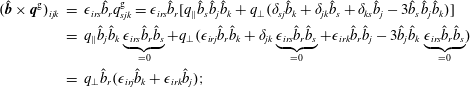 $$\begin{eqnarray}\displaystyle (\hat{\boldsymbol{b}}\times \boldsymbol{q}^{\text{g}})_{ijk} & = & \displaystyle \unicode[STIX]{x1D716}_{irs}\hat{b}_{r}q_{sjk}^{\text{g}}=\unicode[STIX]{x1D716}_{irs}\hat{b}_{r}[q_{\Vert }\hat{b}_{s}\hat{b}_{j}\hat{b}_{k}+q_{\bot }(\unicode[STIX]{x1D6FF}_{sj}\hat{b}_{k}+\unicode[STIX]{x1D6FF}_{jk}\hat{b}_{s}+\unicode[STIX]{x1D6FF}_{ks}\hat{b}_{j}-3\hat{b}_{s}\hat{b}_{j}\hat{b}_{k})]\nonumber\\ \displaystyle & = & \displaystyle q_{\Vert }\hat{b}_{j}\hat{b}_{k}\underbrace{\unicode[STIX]{x1D716}_{irs}\hat{b}_{r}\hat{b}_{s}}_{=0}+q_{\bot }(\unicode[STIX]{x1D716}_{irj}\hat{b}_{r}\hat{b}_{k}+\unicode[STIX]{x1D6FF}_{jk}\underbrace{\unicode[STIX]{x1D716}_{irs}\hat{b}_{r}\hat{b}_{s}}_{=0}+\unicode[STIX]{x1D716}_{irk}\hat{b}_{r}\hat{b}_{j}-3\hat{b}_{j}\hat{b}_{k}\underbrace{\unicode[STIX]{x1D716}_{irs}\hat{b}_{r}\hat{b}_{s}}_{=0})\nonumber\\ \displaystyle & = & \displaystyle q_{\bot }\hat{b}_{r}(\unicode[STIX]{x1D716}_{irj}\hat{b}_{k}+\unicode[STIX]{x1D716}_{irk}\hat{b}_{j});\end{eqnarray}$$
 $$\begin{eqnarray}\displaystyle & \displaystyle (\hat{\boldsymbol{b}}\times \boldsymbol{q}^{\text{g}})_{jki}=q_{\bot }\hat{b}_{r}(\unicode[STIX]{x1D716}_{jrk}\hat{b}_{i}+\unicode[STIX]{x1D716}_{jri}\hat{b}_{k}); & \displaystyle\end{eqnarray}$$
 $$\begin{eqnarray}\displaystyle & \displaystyle (\hat{\boldsymbol{b}}\times \boldsymbol{q}^{\text{g}})_{kij}=q_{\bot }\hat{b}_{r}(\unicode[STIX]{x1D716}_{kri}\hat{b}_{j}+\unicode[STIX]{x1D716}_{krj}\hat{b}_{i}). & \displaystyle\end{eqnarray}$$
Putting all terms together
 $$\begin{eqnarray}\displaystyle [\hat{\boldsymbol{b}}\times \boldsymbol{q}^{\text{g}}]_{ijk}^{S} & = & \displaystyle [\hat{\boldsymbol{b}}\times \boldsymbol{q}^{\text{g}}]_{ijk}+[\hat{\boldsymbol{b}}\times \boldsymbol{q}^{\text{g}}]_{jki}+[\hat{\boldsymbol{b}}\times \boldsymbol{q}^{\text{g}}]_{kij}\nonumber\\ \displaystyle & = & \displaystyle q_{\bot }\hat{b}_{r}[\hat{b}_{i}\underbrace{(\unicode[STIX]{x1D716}_{jrk}+\unicode[STIX]{x1D716}_{krj})}_{=0}+\,\hat{b}_{j}\underbrace{(\unicode[STIX]{x1D716}_{irk}+\unicode[STIX]{x1D716}_{kri})}_{=0}+\,\hat{b}_{k}\underbrace{(\unicode[STIX]{x1D716}_{irj}+\unicode[STIX]{x1D716}_{jri})}_{=0}]=0,\end{eqnarray}$$
and we see that all three parts of the symmetric operator are required to make this term equal to zero. Therefore, the exact heat flux tensor equation reads
 $$\begin{eqnarray}\displaystyle \frac{\unicode[STIX]{x2202}}{\unicode[STIX]{x2202}t}\boldsymbol{q}+\unicode[STIX]{x1D735}\boldsymbol{\cdot }(\boldsymbol{r}+\boldsymbol{u}\boldsymbol{q})+\left[\boldsymbol{q}\boldsymbol{\cdot }\unicode[STIX]{x1D735}\boldsymbol{u}+\unicode[STIX]{x1D6FA}\frac{|\boldsymbol{B}|}{B_{0}}\hat{\boldsymbol{b}}\times \boldsymbol{q}^{\text{ng}}-\frac{1}{\unicode[STIX]{x1D70C}}\boldsymbol{p}(\unicode[STIX]{x1D735}\boldsymbol{\cdot }\boldsymbol{p})\right]^{S}=0. & & \displaystyle\end{eqnarray}$$
Since this should be an introductory text, we do not want to be bothered right now with the complicated algebra of the non-gyrotropic heat flux
 $\boldsymbol{q}^{\text{ng}}$
. For the clarity of the presented material, here we separate the non-gyrotropic heat flux into a separate term
$\boldsymbol{q}^{\text{ng}}$
. For the clarity of the presented material, here we separate the non-gyrotropic heat flux into a separate term
 $\boldsymbol{Q}^{\text{ng}}$
, and write the heat flux tensor equation in the following form
$\boldsymbol{Q}^{\text{ng}}$
, and write the heat flux tensor equation in the following form
 $$\begin{eqnarray}\displaystyle \frac{\unicode[STIX]{x2202}}{\unicode[STIX]{x2202}t}\boldsymbol{q}^{\text{g}}+\unicode[STIX]{x1D735}\boldsymbol{\cdot }(\boldsymbol{r}+\boldsymbol{u}\boldsymbol{q}^{\text{g}})+\left[\boldsymbol{q}^{\text{g}}\boldsymbol{\cdot }\unicode[STIX]{x1D735}\boldsymbol{u}-\frac{1}{\unicode[STIX]{x1D70C}}\boldsymbol{p}(\unicode[STIX]{x1D735}\boldsymbol{\cdot }\boldsymbol{p})\right]^{S}+\boldsymbol{Q}^{\text{ng}}=0, & & \displaystyle\end{eqnarray}$$
where
 $$\begin{eqnarray}\boldsymbol{Q}^{\text{ng}}=\frac{\unicode[STIX]{x2202}}{\unicode[STIX]{x2202}t}\boldsymbol{q}^{\text{ng}}+\unicode[STIX]{x1D735}\boldsymbol{\cdot }(\boldsymbol{u}\boldsymbol{q}^{\text{ng}})+\left[\boldsymbol{q}^{\text{ng}}\boldsymbol{\cdot }\unicode[STIX]{x1D735}\boldsymbol{u}+\unicode[STIX]{x1D6FA}\frac{|\boldsymbol{B}|}{B_{0}}\hat{\boldsymbol{b}}\times \boldsymbol{q}^{\text{ng}}\right]^{S}.\end{eqnarray}$$
We will address the non-gyrotropic heat flux contributions in appendix D.
In a similar fashion to the pressure decomposition (2.35), we are going to frequently apply double contractions with
 $\hat{\boldsymbol{b}}\hat{\boldsymbol{b}}$
and
$\hat{\boldsymbol{b}}\hat{\boldsymbol{b}}$
and
 $(\unicode[STIX]{x1D644}-\hat{\boldsymbol{b}}\hat{\boldsymbol{b}})/2$
. Applying these operators to the heat flux tensor
$(\unicode[STIX]{x1D644}-\hat{\boldsymbol{b}}\hat{\boldsymbol{b}})/2$
. Applying these operators to the heat flux tensor
 $q_{ijk}$
, must yield quantities that are vectors. It is therefore logical to define parallel and perpendicular heat flux vectors
$q_{ijk}$
, must yield quantities that are vectors. It is therefore logical to define parallel and perpendicular heat flux vectors
 $$\begin{eqnarray}\boldsymbol{S}^{\Vert }\equiv \boldsymbol{q}:\hat{\boldsymbol{b}}\hat{\boldsymbol{b}};\quad \boldsymbol{S}^{\bot }\equiv \boldsymbol{q}:(\unicode[STIX]{x1D644}-\hat{\boldsymbol{b}}\hat{\boldsymbol{b}})/2.\end{eqnarray}$$
The scalar parallel and perpendicular heat flux components
 $q_{\Vert },q_{\bot }$
(which are the only parts that are gyrotropic) are obtained by further projecting these heat flux vectors along the magnetic field lines, i.e. by performing
$q_{\Vert },q_{\bot }$
(which are the only parts that are gyrotropic) are obtained by further projecting these heat flux vectors along the magnetic field lines, i.e. by performing
 $\boldsymbol{\cdot }\hat{\boldsymbol{b}}$
, so that
$\boldsymbol{\cdot }\hat{\boldsymbol{b}}$
, so that
 $$\begin{eqnarray}\displaystyle q_{\Vert }=(\boldsymbol{q}:\hat{\boldsymbol{b}}\hat{\boldsymbol{b}})\boldsymbol{\cdot }\hat{\boldsymbol{b}};\quad q_{\bot }=(\boldsymbol{q}:(\unicode[STIX]{x1D644}-\hat{\boldsymbol{b}}\hat{\boldsymbol{b}})/2)\boldsymbol{\cdot }\hat{\boldsymbol{b}}. & & \displaystyle\end{eqnarray}$$
Briefly considering only the gyrotropic heat flux (7.26) on the right-hand side, it is easy to verify that the parallel decomposition indeed works
 $$\begin{eqnarray}\displaystyle (\boldsymbol{q}^{\text{g}}:\hat{\boldsymbol{b}}\hat{\boldsymbol{b}})_{k} & = & \displaystyle q_{kij}^{\text{g}}\hat{b}_{i}\hat{b}_{j}=q_{ijk}^{\text{g}}\hat{b}_{i}\hat{b}_{j}=[q_{\Vert }\hat{b}_{i}\hat{b}_{j}\hat{b}_{k}+q_{\bot }(\unicode[STIX]{x1D6FF}_{ij}\hat{b}_{k}+\unicode[STIX]{x1D6FF}_{jk}\hat{b}_{i}+\unicode[STIX]{x1D6FF}_{ki}\hat{b}_{j}-3\hat{b}_{i}\hat{b}_{j}\hat{b}_{k})]\hat{b}_{i}\hat{b}_{j}\nonumber\\ \displaystyle & = & \displaystyle q_{\Vert }\hat{b}_{k}+q_{\bot }(\hat{b}_{k}+\hat{b}_{k}+\hat{b}_{k}-3\hat{b}_{k})=q_{\Vert }\hat{b}_{k};\end{eqnarray}$$
 $$\begin{eqnarray}\displaystyle & \displaystyle \boldsymbol{q}^{\text{g}}:\hat{\boldsymbol{b}}\hat{\boldsymbol{b}}=q_{\Vert }\hat{\boldsymbol{b}}; & \displaystyle\end{eqnarray}$$
 $$\begin{eqnarray}\displaystyle & \displaystyle (\boldsymbol{q}^{\text{g}}:\hat{\boldsymbol{b}}\hat{\boldsymbol{b}})\boldsymbol{\cdot }\hat{\boldsymbol{b}}=q_{\Vert }. & \displaystyle\end{eqnarray}$$
For the perpendicular decomposition, it is useful to specifically calculate components
 $$\begin{eqnarray}q_{iik}^{\text{g}}=q_{\Vert }\hat{b}_{k}+q_{\bot }(\underbrace{\unicode[STIX]{x1D6FF}_{ii}}_{=3}\hat{b}_{k}+\hat{b}_{k}+\hat{b}_{k}-3\hat{b}_{k})=q_{\Vert }\hat{b}_{k}+2q_{\bot }\hat{b}_{k},\end{eqnarray}$$
so that
 $$\begin{eqnarray}\displaystyle & \displaystyle \text{Tr}\,\boldsymbol{q}^{\text{g}}=\boldsymbol{q}^{\text{g}}:\unicode[STIX]{x1D644}=q_{\Vert }\hat{\boldsymbol{b}}+2q_{\bot }\hat{\boldsymbol{b}}; & \displaystyle\end{eqnarray}$$
 $$\begin{eqnarray}\displaystyle & \displaystyle \boldsymbol{q}^{\text{g}}:(\unicode[STIX]{x1D644}-\hat{\boldsymbol{b}}\hat{\boldsymbol{b}})/2=(\boldsymbol{q}^{\text{g}}:\unicode[STIX]{x1D644}-\boldsymbol{q}^{\text{g}}:\hat{\boldsymbol{b}}\hat{\boldsymbol{b}})/2=(q_{\Vert }\hat{\boldsymbol{b}}+2q_{\bot }\hat{\boldsymbol{b}}-q_{\Vert }\hat{\boldsymbol{b}})/2=q_{\bot }\hat{\boldsymbol{b}}; & \displaystyle\end{eqnarray}$$
 $$\begin{eqnarray}\displaystyle & \displaystyle (\boldsymbol{q}^{\text{g}}:(\unicode[STIX]{x1D644}-\hat{\boldsymbol{b}}\hat{\boldsymbol{b}})/2)\boldsymbol{\cdot }\hat{\boldsymbol{b}}=q_{\bot }, & \displaystyle\end{eqnarray}$$
which verifies that the perpendicular decomposition (7.37) is satisfied for
 $\boldsymbol{q}^{\text{g}}$
. Now we apply the decomposition (7.37) directly to the definition of the entire heat flux tensor (2.6), which yields
$\boldsymbol{q}^{\text{g}}$
. Now we apply the decomposition (7.37) directly to the definition of the entire heat flux tensor (2.6), which yields
 $$\begin{eqnarray}\displaystyle (\boldsymbol{q}:\hat{\boldsymbol{b}}\hat{\boldsymbol{b}})_{k} & = & \displaystyle \left(m\int \boldsymbol{c}\boldsymbol{c}\boldsymbol{c}f\,\text{d}^{3}v:\hat{\boldsymbol{b}}\hat{\boldsymbol{b}}\right)_{k}=m\int c_{i}c_{j}c_{k}f\,\text{d}^{3}v\hat{b}_{i}\hat{b}_{j}\nonumber\\ \displaystyle & = & \displaystyle m\int (v_{i}-u_{u})\hat{b}_{i}(v_{j}-u_{j})\hat{b}_{j}(v_{k}-u_{k})f\,\text{d}^{3}v\nonumber\\ \displaystyle & = & \displaystyle m\int (v_{\Vert }-u_{\Vert })^{2}(v_{k}-u_{k})f\,\text{d}^{3}v\equiv (\boldsymbol{S}^{\Vert })_{k};\end{eqnarray}$$
 $$\begin{eqnarray}\displaystyle (\boldsymbol{q}:\hat{\boldsymbol{b}}\hat{\boldsymbol{b}})\boldsymbol{\cdot }\hat{\boldsymbol{b}}=m\int (v_{\Vert }-u_{\Vert })^{3}f\,\text{d}^{3}v\equiv q_{\Vert }; & & \displaystyle\end{eqnarray}$$
and the perpendicular decomposition
 $$\begin{eqnarray}\displaystyle (\boldsymbol{q}:\unicode[STIX]{x1D644}/2)_{k}=\frac{m}{2}\int c_{i}c_{j}c_{k}f\,\text{d}^{3}v\unicode[STIX]{x1D6FF}_{ij}=\frac{m}{2}\int |\boldsymbol{c}|^{2}c_{k}f\,\text{d}^{3}v=\frac{m}{2}\int |\boldsymbol{v}-\boldsymbol{u}|^{2}(v_{k}-u_{k})f\,\text{d}^{3}v; & & \displaystyle\end{eqnarray}$$
 $$\begin{eqnarray}\displaystyle (\boldsymbol{q}:(\unicode[STIX]{x1D644}-\hat{\boldsymbol{b}}\hat{\boldsymbol{b}})/2)_{k} & = & \displaystyle \frac{m}{2}\int (|\boldsymbol{v}-\boldsymbol{u}|^{2}-(v_{\Vert }-u_{\Vert })^{2})(v_{k}-u_{k})f\,\text{d}^{3}v\nonumber\\ \displaystyle & = & \displaystyle \frac{m}{2}\int |\boldsymbol{v}_{\bot }-\boldsymbol{u}_{\bot }|^{2}(v_{k}-u_{k})f\,\text{d}^{3}v\equiv (\boldsymbol{S}^{\bot })_{k};\end{eqnarray}$$
 $$\begin{eqnarray}\displaystyle (\boldsymbol{q}:(\unicode[STIX]{x1D644}-\hat{\boldsymbol{b}}\hat{\boldsymbol{b}})/2)\boldsymbol{\cdot }\hat{\boldsymbol{b}}=\frac{m}{2}\int |\boldsymbol{v}_{\bot }-\boldsymbol{u}_{\bot }|^{2}(v_{\Vert }-u_{\Vert })f\,\text{d}^{3}v\equiv q_{\bot }. & & \displaystyle\end{eqnarray}$$
The decomposition (7.37) obviously works for the entire heat flux
 $\boldsymbol{q}$
, as well as for the gyrotropic part
$\boldsymbol{q}$
, as well as for the gyrotropic part
 $\boldsymbol{q}^{\text{g}}$
. Similarly to the pressure decomposition, this further yields the required properties that the non-gyrotropic heat flux
$\boldsymbol{q}^{\text{g}}$
. Similarly to the pressure decomposition, this further yields the required properties that the non-gyrotropic heat flux
 $\boldsymbol{q}^{\text{ng}}$
must satisfy. By using (7.37), the entire heat flux decomposition reads
$\boldsymbol{q}^{\text{ng}}$
must satisfy. By using (7.37), the entire heat flux decomposition reads
 $$\begin{eqnarray}\displaystyle & \displaystyle \boldsymbol{q}=q_{\Vert }\hat{\boldsymbol{b}}\hat{\boldsymbol{b}}\hat{\boldsymbol{b}}+q_{\bot }[(\unicode[STIX]{x1D644}-\hat{\boldsymbol{b}}\hat{\boldsymbol{b}})\hat{\boldsymbol{b}}]^{S}+\boldsymbol{q}^{\text{ng}}; & \displaystyle\end{eqnarray}$$
 $$\begin{eqnarray}\displaystyle & \displaystyle \boldsymbol{q}=[(\boldsymbol{q}:\hat{\boldsymbol{b}}\hat{\boldsymbol{b}})\boldsymbol{\cdot }\hat{\boldsymbol{b}}]\hat{\boldsymbol{b}}\hat{\boldsymbol{b}}\hat{\boldsymbol{b}}+[(\boldsymbol{q}:(\unicode[STIX]{x1D644}-\hat{\boldsymbol{b}}\hat{\boldsymbol{b}})/2)\boldsymbol{\cdot }\hat{\boldsymbol{b}}][(\unicode[STIX]{x1D644}-\hat{\boldsymbol{b}}\hat{\boldsymbol{b}})\hat{\boldsymbol{b}}]^{S}+\boldsymbol{q}^{\text{ng}}. & \displaystyle\end{eqnarray}$$
Obviously, it would be useful to introduce a triple-contraction operator and instead of
 $(\boldsymbol{q}:\hat{\boldsymbol{b}}\hat{\boldsymbol{b}})\boldsymbol{\cdot }\hat{\boldsymbol{b}}$
to write something like
$(\boldsymbol{q}:\hat{\boldsymbol{b}}\hat{\boldsymbol{b}})\boldsymbol{\cdot }\hat{\boldsymbol{b}}$
to write something like
 $\boldsymbol{q}\,\vdots \,\hat{\boldsymbol{b}}\hat{\boldsymbol{b}}\hat{\boldsymbol{b}}$
, but we do not want to introduce new notations. Also, an alternative and perhaps prettier expression is to move the
$\boldsymbol{q}\,\vdots \,\hat{\boldsymbol{b}}\hat{\boldsymbol{b}}\hat{\boldsymbol{b}}$
, but we do not want to introduce new notations. Also, an alternative and perhaps prettier expression is to move the
 $\boldsymbol{\cdot }\hat{\boldsymbol{b}}$
to the left-hand side, as
$\boldsymbol{\cdot }\hat{\boldsymbol{b}}$
to the left-hand side, as
 $(\boldsymbol{q}:\hat{\boldsymbol{b}}\hat{\boldsymbol{b}})\boldsymbol{\cdot }\hat{\boldsymbol{b}}=\hat{\boldsymbol{b}}\boldsymbol{\cdot }\boldsymbol{q}:\hat{\boldsymbol{b}}\hat{\boldsymbol{b}}$
, but we will keep the first choice. Applying
$(\boldsymbol{q}:\hat{\boldsymbol{b}}\hat{\boldsymbol{b}})\boldsymbol{\cdot }\hat{\boldsymbol{b}}=\hat{\boldsymbol{b}}\boldsymbol{\cdot }\boldsymbol{q}:\hat{\boldsymbol{b}}\hat{\boldsymbol{b}}$
, but we will keep the first choice. Applying
 $:\hat{\boldsymbol{b}}\hat{\boldsymbol{b}}$
and
$:\hat{\boldsymbol{b}}\hat{\boldsymbol{b}}$
and
 $\boldsymbol{\cdot }\hat{\boldsymbol{b}}$
to the above equation yields
$\boldsymbol{\cdot }\hat{\boldsymbol{b}}$
to the above equation yields
 $$\begin{eqnarray}(\boldsymbol{q}:\hat{\boldsymbol{b}}\hat{\boldsymbol{b}})\boldsymbol{\cdot }\hat{\boldsymbol{b}}=(\boldsymbol{q}:\hat{\boldsymbol{b}}\hat{\boldsymbol{b}})\boldsymbol{\cdot }\hat{\boldsymbol{b}}+(\boldsymbol{q}^{\text{ng}}:\hat{\boldsymbol{b}}\hat{\boldsymbol{b}})\boldsymbol{\cdot }\hat{\boldsymbol{b}},\end{eqnarray}$$
implying the first requirement for the non-gyrotropic heat flux
 $$\begin{eqnarray}(\boldsymbol{q}^{\text{ng}}:\hat{\boldsymbol{b}}\hat{\boldsymbol{b}})\boldsymbol{\cdot }\hat{\boldsymbol{b}}=0.\end{eqnarray}$$
Similarly, the second requirement is obtained by applying
 $:(\unicode[STIX]{x1D644}-\hat{\boldsymbol{b}}\hat{\boldsymbol{b}})$
and
$:(\unicode[STIX]{x1D644}-\hat{\boldsymbol{b}}\hat{\boldsymbol{b}})$
and
 $\boldsymbol{\cdot }\hat{\boldsymbol{b}}$
, yielding
$\boldsymbol{\cdot }\hat{\boldsymbol{b}}$
, yielding
 $$\begin{eqnarray}(\boldsymbol{q}^{\text{ng}}:(\unicode[STIX]{x1D644}-\hat{\boldsymbol{b}}\hat{\boldsymbol{b}}))\boldsymbol{\cdot }\hat{\boldsymbol{b}}=0.\end{eqnarray}$$
By using the first requirement, the second requirement simplifies to
 $$\begin{eqnarray}(\boldsymbol{q}^{\text{ng}}:\unicode[STIX]{x1D644})\boldsymbol{\cdot }\hat{\boldsymbol{b}}=\text{Tr}\,\boldsymbol{q}^{\text{ng}}\boldsymbol{\cdot }\hat{\boldsymbol{b}}=0,\end{eqnarray}$$
where obviously the trace and
 $\boldsymbol{\cdot }\hat{\boldsymbol{b}}$
operators commute. The two requirements in the index notation read
$\boldsymbol{\cdot }\hat{\boldsymbol{b}}$
operators commute. The two requirements in the index notation read
 $$\begin{eqnarray}q_{ijk}^{\text{ng}}\hat{b}_{i}\hat{b}_{j}\hat{b}_{k}=0;\quad q_{iik}^{\text{ng}}\hat{b}_{k}=0.\end{eqnarray}$$
Instead of decomposing
 $\boldsymbol{q}=\boldsymbol{q}^{\text{g}}+\boldsymbol{q}^{\text{ng}}$
, an alternative and very useful decomposition of the entire heat flux tensor reads
$\boldsymbol{q}=\boldsymbol{q}^{\text{g}}+\boldsymbol{q}^{\text{ng}}$
, an alternative and very useful decomposition of the entire heat flux tensor reads
 $$\begin{eqnarray}\boldsymbol{q}=\boldsymbol{S}+\unicode[STIX]{x1D748},\end{eqnarray}$$
with the requirement
 $\unicode[STIX]{x1D748}:\hat{\boldsymbol{b}}\hat{\boldsymbol{b}}=0$
and
$\unicode[STIX]{x1D748}:\hat{\boldsymbol{b}}\hat{\boldsymbol{b}}=0$
and
 $\unicode[STIX]{x1D748}:(\unicode[STIX]{x1D644}-\hat{\boldsymbol{b}}\hat{\boldsymbol{b}})=0$
(or equivalently
$\unicode[STIX]{x1D748}:(\unicode[STIX]{x1D644}-\hat{\boldsymbol{b}}\hat{\boldsymbol{b}})=0$
(or equivalently
 $\unicode[STIX]{x1D748}:\unicode[STIX]{x1D644}=0$
). The heat flux vectors (7.36) therefore satisfy
$\unicode[STIX]{x1D748}:\unicode[STIX]{x1D644}=0$
). The heat flux vectors (7.36) therefore satisfy
 $\boldsymbol{S}^{\Vert }=\boldsymbol{S}:\hat{\boldsymbol{b}}\hat{\boldsymbol{b}}$
and
$\boldsymbol{S}^{\Vert }=\boldsymbol{S}:\hat{\boldsymbol{b}}\hat{\boldsymbol{b}}$
and
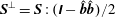 $\boldsymbol{S}^{\bot }=\boldsymbol{S}:(\unicode[STIX]{x1D644}-\hat{\boldsymbol{b}}\hat{\boldsymbol{b}})/2$
. The heat flux vectors contain both gyrotropic and non-gyrotropic contributions. Since the gyrotropic contributions are obtained by projecting these vectors along the magnetic field lines
$\boldsymbol{S}^{\bot }=\boldsymbol{S}:(\unicode[STIX]{x1D644}-\hat{\boldsymbol{b}}\hat{\boldsymbol{b}})/2$
. The heat flux vectors contain both gyrotropic and non-gyrotropic contributions. Since the gyrotropic contributions are obtained by projecting these vectors along the magnetic field lines
 $q_{\Vert }=\boldsymbol{S}^{\Vert }\boldsymbol{\cdot }\hat{\boldsymbol{b}}$
,
$q_{\Vert }=\boldsymbol{S}^{\Vert }\boldsymbol{\cdot }\hat{\boldsymbol{b}}$
,
 $q_{\bot }=\boldsymbol{S}^{\bot }\boldsymbol{\cdot }\hat{\boldsymbol{b}}$
, it is useful to introduce the following decomposition
$q_{\bot }=\boldsymbol{S}^{\bot }\boldsymbol{\cdot }\hat{\boldsymbol{b}}$
, it is useful to introduce the following decomposition
 $$\begin{eqnarray}\boldsymbol{S}^{\Vert }\equiv q_{\Vert }\hat{\boldsymbol{b}}+\boldsymbol{S}_{\bot }^{\Vert };\quad \boldsymbol{S}^{\bot }\equiv q_{\bot }\hat{\boldsymbol{b}}+\boldsymbol{S}_{\bot }^{\bot }.\end{eqnarray}$$
The vectors
 $\boldsymbol{S}_{\bot }^{\Vert }$
,
$\boldsymbol{S}_{\bot }^{\Vert }$
,
 $\boldsymbol{S}_{\bot }^{\bot }$
are referred to as the non-gyrotropic heat flux vectors, and their algebra is addressed in appendix D. Here, we only state that the
$\boldsymbol{S}_{\bot }^{\bot }$
are referred to as the non-gyrotropic heat flux vectors, and their algebra is addressed in appendix D. Here, we only state that the
 $\boldsymbol{q}^{\text{ng}}$
can be decomposed into vectors
$\boldsymbol{q}^{\text{ng}}$
can be decomposed into vectors
 $\boldsymbol{S}_{\bot }^{\Vert }$
,
$\boldsymbol{S}_{\bot }^{\Vert }$
,
 $\boldsymbol{S}_{\bot }^{\bot }$
and tensor
$\boldsymbol{S}_{\bot }^{\bot }$
and tensor
 $\unicode[STIX]{x1D748}$
according to
$\unicode[STIX]{x1D748}$
according to
 $$\begin{eqnarray}\boldsymbol{q}^{\text{ng}}=[\boldsymbol{S}_{\bot }^{\Vert }\hat{\boldsymbol{b}}\hat{\boldsymbol{b}}]^{S}+{\textstyle \frac{1}{2}}[\boldsymbol{S}_{\bot }^{\bot }(\unicode[STIX]{x1D644}-\hat{\boldsymbol{b}}\hat{\boldsymbol{b}})]^{S}+\unicode[STIX]{x1D748}.\end{eqnarray}$$
The entire heat flux tensor
 $\unicode[STIX]{x1D748}$
is of course non-gyrotropic.
$\unicode[STIX]{x1D748}$
is of course non-gyrotropic.
Now we need to verify the heat flux contributions (2.72), (2.73) that we used in the pressure equations (2.74), (2.75). To calculate the heat flux contributions to the pressure equations, we will need
 $$\begin{eqnarray}\displaystyle \text{Tr}(\unicode[STIX]{x1D735}\boldsymbol{\cdot }\boldsymbol{q}^{\text{g}}) & = & \displaystyle \unicode[STIX]{x1D6FF}_{ij}(\unicode[STIX]{x1D735}\boldsymbol{\cdot }\boldsymbol{q}^{\text{g}})_{ij}=\unicode[STIX]{x1D6FF}_{ij}\unicode[STIX]{x2202}_{k}q_{kij}^{\text{g}}=\unicode[STIX]{x2202}_{k}q_{iik}^{\text{g}}=\unicode[STIX]{x2202}_{k}(q_{\Vert }\hat{b}_{k}+2q_{\bot }\hat{b}_{k})\nonumber\\ \displaystyle & = & \displaystyle \unicode[STIX]{x1D735}\boldsymbol{\cdot }(q_{\Vert }\hat{\boldsymbol{b}})+2\unicode[STIX]{x1D735}\boldsymbol{\cdot }(q_{\bot }\hat{\boldsymbol{b}});\end{eqnarray}$$
 $$\begin{eqnarray}\displaystyle q_{ijk}^{\text{g}}\hat{b}_{i}\hat{b}_{j}=q_{\Vert }\hat{b}_{k}; & & \displaystyle\end{eqnarray}$$
 $$\begin{eqnarray}\displaystyle q_{ijk}^{\text{g}}\unicode[STIX]{x2202}_{k}(\hat{b}_{i}\hat{b}_{j}) & = & \displaystyle [q_{\Vert }\hat{b}_{i}\hat{b}_{j}\hat{b}_{k}+q_{\bot }(\unicode[STIX]{x1D6FF}_{ij}\hat{b}_{k}+\unicode[STIX]{x1D6FF}_{jk}\hat{b}_{i}+\unicode[STIX]{x1D6FF}_{ki}\hat{b}_{j}-3\hat{b}_{i}\hat{b}_{j}\hat{b}_{k})]\unicode[STIX]{x2202}_{k}(\hat{b}_{i}\hat{b}_{j})\nonumber\\ \displaystyle & = & \displaystyle q_{\Vert }\hat{b}_{k}\underbrace{\hat{b}_{i}\hat{b}_{j}\unicode[STIX]{x2202}_{k}(\hat{b}_{i}\hat{b}_{j})}_{=0}+q_{\bot }\hat{b}_{k}\underbrace{\unicode[STIX]{x2202}_{k}(\hat{b}_{i}\hat{b}_{i})}_{=0}\nonumber\\ \displaystyle & & \displaystyle +\,q_{\bot }\hat{b}_{i}\unicode[STIX]{x2202}_{j}(\hat{b}_{i}\hat{b}_{j})+q_{\bot }\hat{b}_{j}\unicode[STIX]{x2202}_{i}(\hat{b}_{i}\hat{b}_{j})-3q_{\bot }\hat{b}_{k}\underbrace{\hat{b}_{i}\hat{b}_{j}\unicode[STIX]{x2202}_{k}(\hat{b}_{i}\hat{b}_{j})}_{=0}\nonumber\\ \displaystyle & = & \displaystyle q_{\bot }\unicode[STIX]{x2202}_{j}\hat{b}_{j}+q_{\bot }\hat{b}_{j}\underbrace{\hat{b}_{i}\unicode[STIX]{x2202}_{j}\hat{b}_{i}}_{=0}+q_{\bot }\unicode[STIX]{x2202}_{i}\hat{b}_{i}+q_{\bot }\hat{b}_{i}\underbrace{\hat{b}_{j}\unicode[STIX]{x2202}_{i}\hat{b}_{j}}_{=0}\nonumber\\ \displaystyle & = & \displaystyle 2q_{\bot }\unicode[STIX]{x1D735}\boldsymbol{\cdot }\hat{\boldsymbol{b}},\end{eqnarray}$$
and the contributions are
 $$\begin{eqnarray}\displaystyle \hat{\boldsymbol{b}}\boldsymbol{\cdot }(\unicode[STIX]{x1D735}\boldsymbol{\cdot }\boldsymbol{q}^{\text{g}})\boldsymbol{\cdot }\hat{\boldsymbol{b}} & = & \displaystyle \hat{b}_{i}(\unicode[STIX]{x2202}_{k}q_{kij}^{\text{g}})\hat{b}_{j}=\unicode[STIX]{x2202}_{k}(q_{ijk}^{\text{g}}\hat{b}_{i}\hat{b}_{j})-q_{ijk}^{\text{g}}\unicode[STIX]{x2202}_{k}(\hat{b}_{i}\hat{b}_{j})=\unicode[STIX]{x2202}_{k}(q_{\Vert }\hat{b}_{k})-2q_{\bot }\unicode[STIX]{x1D735}\boldsymbol{\cdot }\hat{\boldsymbol{b}}\nonumber\\ \displaystyle & = & \displaystyle \unicode[STIX]{x1D735}\boldsymbol{\cdot }(q_{\Vert }\hat{\boldsymbol{b}})-2q_{\bot }\unicode[STIX]{x1D735}\boldsymbol{\cdot }\hat{\boldsymbol{b}};\end{eqnarray}$$
 $$\begin{eqnarray}\displaystyle {\textstyle \frac{1}{2}}[\text{Tr}\,\unicode[STIX]{x1D735}\boldsymbol{\cdot }\boldsymbol{q}^{\text{g}}-\hat{\boldsymbol{b}}\boldsymbol{\cdot }(\unicode[STIX]{x1D735}\boldsymbol{\cdot }\boldsymbol{q}^{\text{g}})\boldsymbol{\cdot }\hat{\boldsymbol{b}}]=\unicode[STIX]{x1D735}\boldsymbol{\cdot }(q_{\bot }\hat{\boldsymbol{b}})+q_{\bot }\unicode[STIX]{x1D735}\boldsymbol{\cdot }\hat{\boldsymbol{b}}. & & \displaystyle\end{eqnarray}$$
The left-hand side of the above equation can be also written naturally as
 $(\unicode[STIX]{x1D735}\boldsymbol{\cdot }\boldsymbol{q}^{\text{g}}):(\unicode[STIX]{x1D644}-\hat{\boldsymbol{b}}\hat{\boldsymbol{b}})/2$
, which is consistent with an alternative derivation of the perpendicular pressure equation, where instead of doing trace and subtracting the parallel pressure equation, one can directly perform
$(\unicode[STIX]{x1D735}\boldsymbol{\cdot }\boldsymbol{q}^{\text{g}}):(\unicode[STIX]{x1D644}-\hat{\boldsymbol{b}}\hat{\boldsymbol{b}})/2$
, which is consistent with an alternative derivation of the perpendicular pressure equation, where instead of doing trace and subtracting the parallel pressure equation, one can directly perform
 $:(\unicode[STIX]{x1D644}-\hat{\boldsymbol{b}}\hat{\boldsymbol{b}})/2$
.
$:(\unicode[STIX]{x1D644}-\hat{\boldsymbol{b}}\hat{\boldsymbol{b}})/2$
.
7.2 Parallel heat flux equation
Now we apply the decomposition (7.37) to the heat flux tensor equation (7.34) step by step. We consider only gyrotropic heat flux components. Starting with the equation for the parallel heat flux, the first term calculates as
 $$\begin{eqnarray}\displaystyle \left(\frac{\unicode[STIX]{x2202}\boldsymbol{q}^{\text{g}}}{\unicode[STIX]{x2202}t}:\hat{\boldsymbol{b}}\hat{\boldsymbol{b}}\right)\boldsymbol{\cdot }\hat{\boldsymbol{b}} & = & \displaystyle \frac{\unicode[STIX]{x2202}}{\unicode[STIX]{x2202}t}[q_{\Vert }\hat{b}_{i}\hat{b}_{j}\hat{b}_{k}+q_{\bot }(\unicode[STIX]{x1D6FF}_{ij}\hat{b}_{k}+\unicode[STIX]{x1D6FF}_{jk}\hat{b}_{i}+\unicode[STIX]{x1D6FF}_{ki}\hat{b}_{j}-3\hat{b}_{i}\hat{b}_{j}\hat{b}_{k})]\hat{b}_{i}\hat{b}_{j}\hat{b}_{k}\nonumber\\ \displaystyle & = & \displaystyle \frac{\unicode[STIX]{x2202}q_{\Vert }}{\unicode[STIX]{x2202}t}\underbrace{\hat{b}_{i}\hat{b}_{j}\hat{b}_{k}\hat{b}_{i}\hat{b}_{j}\hat{b}_{k}}_{=1}+q_{\Vert }\underbrace{\hat{b}_{i}\hat{b}_{j}\hat{b}_{k}\frac{\unicode[STIX]{x2202}}{\unicode[STIX]{x2202}t}(\hat{b}_{i}\hat{b}_{j}\hat{b}_{k})}_{=0}+\frac{\unicode[STIX]{x2202}q_{\bot }}{\unicode[STIX]{x2202}t}(\underbrace{1+1+1-3}_{=0})\nonumber\\ \displaystyle & & \displaystyle +\,q_{\bot }\left[\underbrace{\hat{b}_{k}\frac{\unicode[STIX]{x2202}}{\unicode[STIX]{x2202}t}\hat{b}_{k}}_{=0}+\underbrace{\hat{b}_{i}\frac{\unicode[STIX]{x2202}}{\unicode[STIX]{x2202}t}\hat{b}_{i}}_{=0}+\underbrace{\hat{b}_{j}\frac{\unicode[STIX]{x2202}}{\unicode[STIX]{x2202}t}\hat{b}_{j}}_{=0}-3\underbrace{\hat{b}_{i}\hat{b}_{j}\hat{b}_{k}\frac{\unicode[STIX]{x2202}}{\unicode[STIX]{x2202}t}(\hat{b}_{i}\hat{b}_{j}\hat{b}_{k})}_{=0}\right]\nonumber\\ \displaystyle & = & \displaystyle \frac{\unicode[STIX]{x2202}q_{\Vert }}{\unicode[STIX]{x2202}t};\end{eqnarray}$$
the second term calculates as
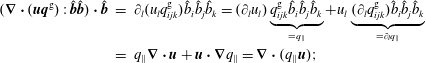 $$\begin{eqnarray}\displaystyle (\unicode[STIX]{x1D735}\boldsymbol{\cdot }(\boldsymbol{u}\boldsymbol{q}^{\text{g}}):\hat{\boldsymbol{b}}\hat{\boldsymbol{b}})\boldsymbol{\cdot }\hat{\boldsymbol{b}} & = & \displaystyle \unicode[STIX]{x2202}_{l}(u_{l}q_{ijk}^{\text{g}})\hat{b}_{i}\hat{b}_{j}\hat{b}_{k}=(\unicode[STIX]{x2202}_{l}u_{l})\underbrace{q_{ijk}^{\text{g}}\hat{b}_{i}\hat{b}_{j}\hat{b}_{k}}_{=q_{\Vert }}+u_{l}\underbrace{(\unicode[STIX]{x2202}_{l}q_{ijk}^{\text{g}})\hat{b}_{i}\hat{b}_{j}\hat{b}_{k}}_{=\unicode[STIX]{x2202}_{l}q_{\Vert }}\nonumber\\ \displaystyle & = & \displaystyle q_{\Vert }\unicode[STIX]{x1D735}\boldsymbol{\cdot }\boldsymbol{u}+\boldsymbol{u}\boldsymbol{\cdot }\unicode[STIX]{x1D735}q_{\Vert }=\unicode[STIX]{x1D735}\boldsymbol{\cdot }(q_{\Vert }\boldsymbol{u});\end{eqnarray}$$
 $$\begin{eqnarray}\displaystyle ((\unicode[STIX]{x1D735}\boldsymbol{\cdot }\boldsymbol{r}):\hat{\boldsymbol{b}}\hat{\boldsymbol{b}})\boldsymbol{\cdot }\hat{\boldsymbol{b}}=(\unicode[STIX]{x2202}_{l}r_{lijk})\hat{b}_{i}\hat{b}_{j}\hat{b}_{k}=\text{unchanged}. & & \displaystyle\end{eqnarray}$$
Note that in all of the expressions here, the operator
 $\boldsymbol{\cdot }\hat{\boldsymbol{b}}$
can be naturally moved to the left as
$\boldsymbol{\cdot }\hat{\boldsymbol{b}}$
can be naturally moved to the left as
 $\hat{\boldsymbol{b}}\boldsymbol{\cdot }$
. The third term calculates as
$\hat{\boldsymbol{b}}\boldsymbol{\cdot }$
. The third term calculates as
 $$\begin{eqnarray}\displaystyle ((\boldsymbol{q}^{\text{g}}\boldsymbol{\cdot }\unicode[STIX]{x1D735}\boldsymbol{u}):\hat{\boldsymbol{b}}\hat{\boldsymbol{b}})\boldsymbol{\cdot }\hat{\boldsymbol{b}} & = & \displaystyle (\boldsymbol{q}^{\text{g}}\boldsymbol{\cdot }\unicode[STIX]{x1D735}\boldsymbol{u})_{ijk}\hat{b}_{i}\hat{b}_{j}\hat{b}_{k}=q_{ijl}^{\text{g}}(\unicode[STIX]{x2202}_{l}u_{k})\hat{b}_{i}\hat{b}_{j}\hat{b}_{k}\nonumber\\ \displaystyle & = & \displaystyle (\unicode[STIX]{x2202}_{l}u_{k})[q_{\Vert }\hat{b}_{i}\hat{b}_{j}\hat{b}_{l}+q_{\bot }(\unicode[STIX]{x1D6FF}_{ij}\hat{b}_{l}+\unicode[STIX]{x1D6FF}_{jl}\hat{b}_{i}+\unicode[STIX]{x1D6FF}_{li}\hat{b}_{j}-3\hat{b}_{i}\hat{b}_{j}\hat{b}_{l})]\hat{b}_{i}\hat{b}_{j}\hat{b}_{k};\nonumber\\ \displaystyle & = & \displaystyle (\unicode[STIX]{x2202}_{l}u_{k})[q_{\Vert }\hat{b}_{l}\hat{b}_{k}+q_{\bot }\underbrace{(\hat{b}_{l}\hat{b}_{k}+\hat{b}_{l}\hat{b}_{k}+\hat{b}_{l}\hat{b}_{k}-3\hat{b}_{l}\hat{b}_{k})}_{=0}]\nonumber\\ \displaystyle & = & \displaystyle q_{\Vert }\hat{b}_{l}(\unicode[STIX]{x2202}_{l}u_{k})\hat{b}_{k}=q_{\Vert }\hat{\boldsymbol{b}}\boldsymbol{\cdot }\unicode[STIX]{x1D735}\boldsymbol{u}\boldsymbol{\cdot }\hat{\boldsymbol{b}};\end{eqnarray}$$
 $$\begin{eqnarray}\displaystyle [\boldsymbol{q}^{\text{g}}\boldsymbol{\cdot }\unicode[STIX]{x1D735}\boldsymbol{u}]_{ijk}^{S}\hat{b}_{i}\hat{b}_{j}\hat{b}_{k} & = & \displaystyle [q_{ijl}^{\text{g}}\unicode[STIX]{x2202}_{l}u_{k}+q_{jkl}^{\text{g}}\unicode[STIX]{x2202}_{l}u_{i}+q_{kil}^{\text{g}}\unicode[STIX]{x2202}_{l}u_{j}]\hat{b}_{i}\hat{b}_{j}\hat{b}_{k}\nonumber\\ \displaystyle & = & \displaystyle \underbrace{q_{ijl}^{\text{g}}\hat{b}_{i}\hat{b}_{j}}_{=q_{\Vert }\hat{b}_{l}}(\unicode[STIX]{x2202}_{l}u_{k})\hat{b}_{k}+\underbrace{q_{jkl}^{\text{g}}\hat{b}_{j}\hat{b}_{k}}_{=q_{\Vert }\hat{b}_{l}}(\unicode[STIX]{x2202}_{l}u_{i})\hat{b}_{i}+\underbrace{q_{kil}^{\text{g}}\hat{b}_{k}\hat{b}_{i}}_{=q_{\Vert }\hat{b}_{l}}(\unicode[STIX]{x2202}_{l}u_{j})\hat{b}_{j}\nonumber\\ \displaystyle & = & \displaystyle 3q_{\Vert }\hat{\boldsymbol{b}}\boldsymbol{\cdot }\unicode[STIX]{x1D735}\boldsymbol{u}\boldsymbol{\cdot }\hat{\boldsymbol{b}}.\end{eqnarray}$$
For the final fourth term we will need
 $$\begin{eqnarray}\displaystyle (\unicode[STIX]{x1D735}\boldsymbol{\cdot }\boldsymbol{p})\boldsymbol{\cdot }\hat{\boldsymbol{b}} & = & \displaystyle \hat{b}_{k}\unicode[STIX]{x2202}_{l}p_{lk}=\hat{b}_{k}\unicode[STIX]{x2202}_{l}[(p_{\Vert }-p_{\bot })\hat{b}_{l}\hat{b}_{k}+p_{\bot }\unicode[STIX]{x1D6FF}_{lk}+\unicode[STIX]{x1D6F1}_{lk}]\nonumber\\ \displaystyle & = & \displaystyle \hat{b}_{k}[\hat{b}_{l}\hat{b}_{k}\unicode[STIX]{x2202}_{l}(p_{\Vert }-p_{\bot })+(p_{\Vert }-p_{\bot })\unicode[STIX]{x2202}_{l}(\hat{b}_{l}\hat{b}_{k})+\unicode[STIX]{x2202}_{k}p_{\bot }+\unicode[STIX]{x2202}_{l}\unicode[STIX]{x1D6F1}_{lk}]\nonumber\\ \displaystyle & = & \displaystyle [\hat{b}_{l}\unicode[STIX]{x2202}_{l}(p_{\Vert }-p_{\bot })+(p_{\Vert }-p_{\bot })\underbrace{\hat{b}_{k}\unicode[STIX]{x2202}_{l}(\hat{b}_{l}\hat{b}_{k})}_{=\unicode[STIX]{x1D735}\boldsymbol{\cdot }\hat{\boldsymbol{b}}}+\hat{b}_{k}\unicode[STIX]{x2202}_{k}p_{\bot }+(\unicode[STIX]{x2202}_{l}\unicode[STIX]{x1D6F1}_{lk})\hat{b}_{k}]\nonumber\\ \displaystyle & = & \displaystyle \hat{\boldsymbol{b}}\boldsymbol{\cdot }\unicode[STIX]{x1D735}p_{\Vert }+(p_{\Vert }-p_{\bot })\unicode[STIX]{x1D735}\boldsymbol{\cdot }\hat{\boldsymbol{b}}+(\unicode[STIX]{x1D735}\boldsymbol{\cdot }\unicode[STIX]{x1D72B})\boldsymbol{\cdot }\hat{\boldsymbol{b}},\end{eqnarray}$$
and the fourth term calculates as
 $$\begin{eqnarray}\displaystyle [\boldsymbol{p}(\unicode[STIX]{x1D735}\boldsymbol{\cdot }\boldsymbol{p})]_{ijk}\hat{b}_{i}\hat{b}_{j}\hat{b}_{k} & = & \displaystyle p_{ij}(\unicode[STIX]{x2202}_{l}p_{lk})\hat{b}_{i}\hat{b}_{j}\hat{b}_{k}=\underbrace{p_{ij}\hat{b}_{i}\hat{b}_{j}}_{=p_{\Vert }}\hat{b}_{k}\unicode[STIX]{x2202}_{l}p_{lk}=p_{\Vert }\hat{b}_{k}\unicode[STIX]{x2202}_{l}p_{lk}\nonumber\\ \displaystyle & = & \displaystyle p_{\Vert }\hat{\boldsymbol{b}}\boldsymbol{\cdot }\unicode[STIX]{x1D735}p_{\Vert }+p_{\Vert }(p_{\Vert }-p_{\bot })\unicode[STIX]{x1D735}\boldsymbol{\cdot }\hat{\boldsymbol{b}}+p_{\Vert }(\unicode[STIX]{x1D735}\boldsymbol{\cdot }\unicode[STIX]{x1D72B})\boldsymbol{\cdot }\hat{\boldsymbol{b}};\end{eqnarray}$$
 $$\begin{eqnarray}\displaystyle [\boldsymbol{p}(\unicode[STIX]{x1D735}\boldsymbol{\cdot }\boldsymbol{p})]_{ijk}^{S}\hat{b}_{i}\hat{b}_{j}\hat{b}_{k} & = & \displaystyle [p_{ij}\unicode[STIX]{x2202}_{l}p_{lk}+p_{jk}\unicode[STIX]{x2202}_{l}p_{li}+p_{ki}\unicode[STIX]{x2202}_{l}p_{lj}]\hat{b}_{i}\hat{b}_{j}\hat{b}_{k}\nonumber\\ \displaystyle & = & \displaystyle \underbrace{p_{ij}\hat{b}_{i}\hat{b}_{j}}_{=p_{\Vert }}\hat{b}_{k}\unicode[STIX]{x2202}_{l}p_{lk}+\underbrace{p_{jk}\hat{b}_{j}\hat{b}_{k}}_{=p_{\Vert }}\hat{b}_{i}\unicode[STIX]{x2202}_{l}p_{li}+\underbrace{p_{ki}\hat{b}_{k}\hat{b}_{i}}_{=p_{\Vert }}\hat{b}_{j}\unicode[STIX]{x2202}_{l}p_{lj}=3p_{\Vert }\hat{b}_{k}\unicode[STIX]{x2202}_{l}p_{lk};\nonumber\\ \displaystyle & & \displaystyle\end{eqnarray}$$
 $$\begin{eqnarray}\displaystyle -\frac{1}{\unicode[STIX]{x1D70C}}[\boldsymbol{p}(\unicode[STIX]{x1D735}\boldsymbol{\cdot }\boldsymbol{p})]_{ijk}^{S}\hat{b}_{i}\hat{b}_{j}\hat{b}_{k} & = & \displaystyle -3\frac{p_{\Vert }}{\unicode[STIX]{x1D70C}}\hat{\boldsymbol{b}}\boldsymbol{\cdot }\unicode[STIX]{x1D735}p_{\Vert }-3\frac{p_{\Vert }}{\unicode[STIX]{x1D70C}}(p_{\Vert }-p_{\bot })\unicode[STIX]{x1D735}\boldsymbol{\cdot }\hat{\boldsymbol{b}}-3\frac{p_{\Vert }}{\unicode[STIX]{x1D70C}}(\unicode[STIX]{x1D735}\boldsymbol{\cdot }\unicode[STIX]{x1D72B})\boldsymbol{\cdot }\hat{\boldsymbol{b}}.\nonumber\\ \displaystyle & & \displaystyle\end{eqnarray}$$
Combining all the terms yields the equation for the scalar parallel heat flux
 $$\begin{eqnarray}\displaystyle & & \displaystyle \frac{\unicode[STIX]{x2202}q_{\Vert }}{\unicode[STIX]{x2202}t}+\unicode[STIX]{x1D735}\boldsymbol{\cdot }(q_{\Vert }\boldsymbol{u})+\hat{\boldsymbol{b}}\boldsymbol{\cdot }(\unicode[STIX]{x1D735}\boldsymbol{\cdot }\boldsymbol{r}):\hat{\boldsymbol{b}}\hat{\boldsymbol{b}}+3q_{\Vert }\hat{\boldsymbol{b}}\boldsymbol{\cdot }\unicode[STIX]{x1D735}\boldsymbol{u}\boldsymbol{\cdot }\hat{\boldsymbol{b}}-3\frac{p_{\Vert }}{\unicode[STIX]{x1D70C}}\hat{\boldsymbol{b}}\boldsymbol{\cdot }\unicode[STIX]{x1D735}p_{\Vert }-3\frac{p_{\Vert }}{\unicode[STIX]{x1D70C}}(p_{\Vert }-p_{\bot })\unicode[STIX]{x1D735}\boldsymbol{\cdot }\hat{\boldsymbol{b}}\nonumber\\ \displaystyle & & \displaystyle \qquad -\,3\frac{p_{\Vert }}{\unicode[STIX]{x1D70C}}(\unicode[STIX]{x1D735}\boldsymbol{\cdot }\unicode[STIX]{x1D72B})\boldsymbol{\cdot }\hat{\boldsymbol{b}}+Q_{\Vert }^{\text{ng}}=0,\end{eqnarray}$$
where
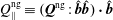 $Q_{\Vert }^{\text{ng}}\equiv (\boldsymbol{Q}^{\text{ng}}:\hat{\boldsymbol{b}}\hat{\boldsymbol{b}})\boldsymbol{\cdot }\hat{\boldsymbol{b}}$
. The heat flux equations contain the fourth-order moment
$Q_{\Vert }^{\text{ng}}\equiv (\boldsymbol{Q}^{\text{ng}}:\hat{\boldsymbol{b}}\hat{\boldsymbol{b}})\boldsymbol{\cdot }\hat{\boldsymbol{b}}$
. The heat flux equations contain the fourth-order moment
 $r_{ijkl}$
, which we will consider in the next section and at this stage it is unspecified.
$r_{ijkl}$
, which we will consider in the next section and at this stage it is unspecified.
7.3 Perpendicular heat flux equation
We will apply the trace operator to (7.34) and also perform
 $\boldsymbol{\cdot }\hat{\boldsymbol{b}}$
step by step. In the index notation, we are basically multiplying the entire equation by
$\boldsymbol{\cdot }\hat{\boldsymbol{b}}$
step by step. In the index notation, we are basically multiplying the entire equation by
 $\unicode[STIX]{x1D6FF}_{ij}\hat{b}_{k}$
. The first term calculates
$\unicode[STIX]{x1D6FF}_{ij}\hat{b}_{k}$
. The first term calculates
 $$\begin{eqnarray}\displaystyle & \displaystyle \text{Tr}\,\frac{\unicode[STIX]{x2202}}{\unicode[STIX]{x2202}t}\boldsymbol{q}^{\text{g}}=\frac{\unicode[STIX]{x2202}}{\unicode[STIX]{x2202}t}\text{Tr}\,\boldsymbol{q}^{\text{g}}=\frac{\unicode[STIX]{x2202}}{\unicode[STIX]{x2202}t}(q_{\Vert }\hat{\boldsymbol{b}}+2q_{\bot }\hat{\boldsymbol{b}})=\hat{\boldsymbol{b}}\frac{\unicode[STIX]{x2202}}{\unicode[STIX]{x2202}t}(q_{\Vert }+2q_{\bot })+(q_{\Vert }+2q_{\bot })\frac{\unicode[STIX]{x2202}}{\unicode[STIX]{x2202}t}\hat{\boldsymbol{b}}; & \displaystyle\end{eqnarray}$$
 $$\begin{eqnarray}\displaystyle & \displaystyle \left(\text{Tr}\,\frac{\unicode[STIX]{x2202}}{\unicode[STIX]{x2202}t}\boldsymbol{q}^{\text{g}}\right)\boldsymbol{\cdot }\hat{\boldsymbol{b}}=\underbrace{\hat{\boldsymbol{b}}\boldsymbol{\cdot }\hat{\boldsymbol{b}}}_{=1}\frac{\unicode[STIX]{x2202}}{\unicode[STIX]{x2202}t}(q_{\Vert }+2q_{\bot })+(q_{\Vert }+2q_{\bot })\underbrace{\frac{\unicode[STIX]{x2202}\hat{\boldsymbol{b}}}{\unicode[STIX]{x2202}t}\boldsymbol{\cdot }\hat{\boldsymbol{b}}}_{=0}=\frac{\unicode[STIX]{x2202}}{\unicode[STIX]{x2202}t}(q_{\Vert }+2q_{\bot }). & \displaystyle\end{eqnarray}$$
The second term
 $\unicode[STIX]{x1D735}\boldsymbol{\cdot }(\boldsymbol{r}+\boldsymbol{u}\boldsymbol{q}^{\text{g}})$
calculates as
$\unicode[STIX]{x1D735}\boldsymbol{\cdot }(\boldsymbol{r}+\boldsymbol{u}\boldsymbol{q}^{\text{g}})$
calculates as
 $$\begin{eqnarray}\displaystyle [\text{Tr}\,\unicode[STIX]{x1D735}\boldsymbol{\cdot }(\boldsymbol{u}\boldsymbol{q}^{\text{g}})]_{k}=\unicode[STIX]{x1D6FF}_{ij}\unicode[STIX]{x2202}_{l}(u_{l}q_{ijk}^{\text{g}})=\unicode[STIX]{x2202}_{l}(u_{l}q_{iik}^{\text{g}}); & & \displaystyle\end{eqnarray}$$
 $$\begin{eqnarray}\displaystyle [\text{Tr}\,\unicode[STIX]{x1D735}\boldsymbol{\cdot }(\boldsymbol{u}\boldsymbol{q}^{\text{g}})]\boldsymbol{\cdot }\hat{\boldsymbol{b}} & = & \displaystyle \unicode[STIX]{x2202}_{l}(u_{l}q_{iik}^{\text{g}})\hat{b}_{k}=\unicode[STIX]{x2202}_{l}(u_{l}q_{iik}^{\text{g}}\hat{b}_{k})-u_{l}\underbrace{q_{iik}^{\text{g}}\unicode[STIX]{x2202}_{l}\hat{b}_{k}}_{=0}=\unicode[STIX]{x2202}_{l}[u_{l}(q_{\Vert }+2q_{\bot })]\nonumber\\ \displaystyle & = & \displaystyle (q_{\Vert }+2q_{\bot })\unicode[STIX]{x1D735}\boldsymbol{\cdot }\boldsymbol{u}+\boldsymbol{u}\boldsymbol{\cdot }\unicode[STIX]{x1D735}(q_{\Vert }+2q_{\bot });\end{eqnarray}$$
 $$\begin{eqnarray}\displaystyle & \displaystyle [\text{Tr}\,\unicode[STIX]{x1D735}\boldsymbol{\cdot }\boldsymbol{r}]_{k}=\unicode[STIX]{x1D6FF}_{ij}\unicode[STIX]{x2202}_{l}r_{lijk}=\unicode[STIX]{x2202}_{l}r_{liik}; & \displaystyle\end{eqnarray}$$
 $$\begin{eqnarray}\displaystyle & \displaystyle [\text{Tr}\,\unicode[STIX]{x1D735}\boldsymbol{\cdot }\boldsymbol{r}]\boldsymbol{\cdot }\hat{\boldsymbol{b}}=(\unicode[STIX]{x2202}_{l}r_{liik})\hat{b}_{k}=\text{unchanged}. & \displaystyle\end{eqnarray}$$
The components
 $r_{liik}=r_{iikl}$
are nothing else but the trace of the moment
$r_{liik}=r_{iikl}$
are nothing else but the trace of the moment
 $\boldsymbol{r}$
 $$\begin{eqnarray}\displaystyle [\text{Tr}\,\boldsymbol{r}]_{kl}=\unicode[STIX]{x1D6FF}_{ij}r_{ijkl}=r_{iikl}. & & \displaystyle\end{eqnarray}$$
The third term in (7.34) calculates as
 $$\begin{eqnarray}\displaystyle & \displaystyle [\boldsymbol{q}^{\text{g}}\boldsymbol{\cdot }\unicode[STIX]{x1D735}\boldsymbol{u}]_{ijk}^{S}=q_{ijl}^{\text{g}}\unicode[STIX]{x2202}_{l}u_{k}+q_{jkl}^{\text{g}}\unicode[STIX]{x2202}_{l}u_{i}+q_{kil}^{\text{g}}\unicode[STIX]{x2202}_{l}u_{j}; & \displaystyle\end{eqnarray}$$
 $$\begin{eqnarray}\displaystyle & \displaystyle \text{Tr}[\boldsymbol{q}^{\text{g}}\boldsymbol{\cdot }\unicode[STIX]{x1D735}\boldsymbol{u}]_{ijk}^{S}=q_{iil}^{\text{g}}\unicode[STIX]{x2202}_{l}u_{k}+q_{ikl}^{\text{g}}\unicode[STIX]{x2202}_{l}u_{i}+\underbrace{q_{kil}^{\text{g}}}_{=q_{ikl}^{\text{g}}}\unicode[STIX]{x2202}_{l}u_{i}=q_{iil}^{\text{g}}\unicode[STIX]{x2202}_{l}u_{k}+2q_{ikl}^{\text{g}}\unicode[STIX]{x2202}_{l}u_{i} & \displaystyle\end{eqnarray}$$
 $$\begin{eqnarray}\displaystyle \text{Tr}[\boldsymbol{q}^{\text{g}}\boldsymbol{\cdot }\unicode[STIX]{x1D735}\boldsymbol{u}]_{ijk}^{S}\hat{b}_{k} & = & \displaystyle q_{iil}^{\text{g}}(\unicode[STIX]{x2202}_{l}u_{k})\hat{b}_{k}+2q_{ikl}^{\text{g}}\hat{b}_{k}\unicode[STIX]{x2202}_{l}u_{i}\nonumber\\ \displaystyle & = & \displaystyle (q_{\Vert }+2q_{\bot })\hat{b}_{l}(\unicode[STIX]{x2202}_{l}u_{k})\hat{b}_{k}+2[q_{\Vert }\hat{b}_{i}\hat{b}_{l}+q_{\bot }(\unicode[STIX]{x1D6FF}_{il}-\hat{b}_{i}\hat{b}_{l})]\unicode[STIX]{x2202}_{l}u_{i}\nonumber\\ \displaystyle & = & \displaystyle (q_{\Vert }+2q_{\bot })\hat{b}_{l}(\unicode[STIX]{x2202}_{l}u_{k})\hat{b}_{k}+2(q_{\Vert }-q_{\bot })\hat{b}_{l}(\unicode[STIX]{x2202}_{l}u_{i})\hat{b}_{i}+2q_{\bot }\unicode[STIX]{x2202}_{i}u_{i}\nonumber\\ \displaystyle & = & \displaystyle 3q_{\Vert }\hat{\boldsymbol{b}}\boldsymbol{\cdot }\unicode[STIX]{x1D735}\boldsymbol{u}\boldsymbol{\cdot }\hat{\boldsymbol{b}}+2q_{\bot }\unicode[STIX]{x1D735}\boldsymbol{\cdot }\boldsymbol{u},\end{eqnarray}$$
where we have used that
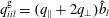 $q_{iil}^{\text{g}}=(q_{\Vert }+2q_{\bot })\hat{b}_{l}$
and
$q_{iil}^{\text{g}}=(q_{\Vert }+2q_{\bot })\hat{b}_{l}$
and
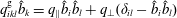 $q_{ikl}^{\text{g}}\hat{b}_{k}=q_{\Vert }\hat{b}_{i}\hat{b}_{l}+q_{\bot }(\unicode[STIX]{x1D6FF}_{il}-\hat{b}_{i}\hat{b}_{l})$
. The fourth term in (7.34) calculates as
$q_{ikl}^{\text{g}}\hat{b}_{k}=q_{\Vert }\hat{b}_{i}\hat{b}_{l}+q_{\bot }(\unicode[STIX]{x1D6FF}_{il}-\hat{b}_{i}\hat{b}_{l})$
. The fourth term in (7.34) calculates as
 $$\begin{eqnarray}\displaystyle & \displaystyle [\boldsymbol{p}(\unicode[STIX]{x1D735}\boldsymbol{\cdot }\boldsymbol{p})]_{ijk}^{S}=p_{ij}\unicode[STIX]{x2202}_{l}p_{lk}+p_{jk}\unicode[STIX]{x2202}_{l}p_{li}+p_{ki}\unicode[STIX]{x2202}_{l}p_{lj}; & \displaystyle\end{eqnarray}$$
 $$\begin{eqnarray}\displaystyle & \displaystyle \text{Tr}[\boldsymbol{p}(\unicode[STIX]{x1D735}\boldsymbol{\cdot }\boldsymbol{p})]_{ijk}^{S}=p_{ii}\unicode[STIX]{x2202}_{l}p_{lk}+p_{ik}\unicode[STIX]{x2202}_{l}p_{li}+\underbrace{p_{ki}}_{=p_{ik}}\unicode[STIX]{x2202}_{l}p_{li}=p_{ii}\unicode[STIX]{x2202}_{l}p_{lk}+2p_{ik}\unicode[STIX]{x2202}_{l}p_{li}; & \displaystyle\end{eqnarray}$$
 $$\begin{eqnarray}\displaystyle & \displaystyle \text{Tr}[\boldsymbol{p}(\unicode[STIX]{x1D735}\boldsymbol{\cdot }\boldsymbol{p})]_{ijk}^{S}\hat{b}_{k}=p_{ii}\hat{b}_{k}\unicode[STIX]{x2202}_{l}p_{lk}+2p_{ik}\hat{b}_{k}\unicode[STIX]{x2202}_{l}p_{li}, & \displaystyle\end{eqnarray}$$
and we have to calculate each term separately. Since
 $p_{ii}=p_{\Vert }+2p_{\bot }$
and by using the already calculated equation (7.70) for
$p_{ii}=p_{\Vert }+2p_{\bot }$
and by using the already calculated equation (7.70) for
 $\hat{b}_{k}\unicode[STIX]{x2202}_{l}p_{lk}$
and identities
$\hat{b}_{k}\unicode[STIX]{x2202}_{l}p_{lk}$
and identities
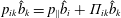 $p_{ik}\hat{b}_{k}=p_{\Vert }\hat{b}_{i}+\unicode[STIX]{x1D6F1}_{ik}\hat{b}_{k}$
and
$p_{ik}\hat{b}_{k}=p_{\Vert }\hat{b}_{i}+\unicode[STIX]{x1D6F1}_{ik}\hat{b}_{k}$
and
 $\unicode[STIX]{x1D6F1}_{ik}\hat{b}_{i}\hat{b}_{k}=0$
one obtains
$\unicode[STIX]{x1D6F1}_{ik}\hat{b}_{i}\hat{b}_{k}=0$
one obtains
 $$\begin{eqnarray}\displaystyle p_{ii}\hat{b}_{k}\unicode[STIX]{x2202}_{l}p_{lk}=(p_{\Vert }+2p_{\bot })[\hat{\boldsymbol{b}}\boldsymbol{\cdot }\unicode[STIX]{x1D735}p_{\Vert }+(p_{\Vert }-p_{\bot })\unicode[STIX]{x1D735}\boldsymbol{\cdot }\hat{\boldsymbol{b}}+(\unicode[STIX]{x1D735}\boldsymbol{\cdot }\unicode[STIX]{x1D72B})\boldsymbol{\cdot }\hat{\boldsymbol{b}}]; & & \displaystyle\end{eqnarray}$$
 $$\begin{eqnarray}\displaystyle p_{ik}\hat{b}_{k}\unicode[STIX]{x2202}_{l}p_{li} & = & \displaystyle (p_{\Vert }\hat{b}_{i}+\unicode[STIX]{x1D6F1}_{ik}\hat{b}_{k})[\unicode[STIX]{x2202}_{i}p_{\bot }+(p_{\Vert }-p_{\bot })(\hat{b}_{i}\unicode[STIX]{x2202}_{l}\hat{b}_{l}+\hat{b}_{l}\unicode[STIX]{x2202}_{l}\hat{b}_{i})+\hat{b}_{i}\hat{b}_{l}\unicode[STIX]{x2202}_{l}(p_{\Vert }-p_{\bot })+\unicode[STIX]{x2202}_{l}\unicode[STIX]{x1D6F1}_{li}]\nonumber\\ \displaystyle & = & \displaystyle p_{\Vert }[\hat{\boldsymbol{b}}\boldsymbol{\cdot }\unicode[STIX]{x1D735}p_{\Vert }+(p_{\Vert }-p_{\bot })\unicode[STIX]{x1D735}\boldsymbol{\cdot }\hat{\boldsymbol{b}}+(\unicode[STIX]{x1D735}\boldsymbol{\cdot }\unicode[STIX]{x1D72B})\boldsymbol{\cdot }\hat{\boldsymbol{b}}]\nonumber\\ \displaystyle & & \displaystyle +\,\unicode[STIX]{x1D6F1}_{ik}\hat{b}_{k}[\unicode[STIX]{x2202}_{i}p_{\bot }+(p_{\Vert }-p_{\bot })\hat{b}_{l}\unicode[STIX]{x2202}_{l}\hat{b}_{i}+\unicode[STIX]{x2202}_{l}\unicode[STIX]{x1D6F1}_{li}]\nonumber\\ \displaystyle & = & \displaystyle p_{\Vert }[\hat{\boldsymbol{b}}\boldsymbol{\cdot }\unicode[STIX]{x1D735}p_{\Vert }+(p_{\Vert }-p_{\bot })\unicode[STIX]{x1D735}\boldsymbol{\cdot }\hat{\boldsymbol{b}}+(\unicode[STIX]{x1D735}\boldsymbol{\cdot }\unicode[STIX]{x1D72B})\boldsymbol{\cdot }\hat{\boldsymbol{b}}]\nonumber\\ \displaystyle & & \displaystyle +\,[\unicode[STIX]{x1D735}p_{\bot }+(p_{\Vert }-p_{\bot })\hat{\boldsymbol{b}}\boldsymbol{\cdot }\unicode[STIX]{x1D735}\hat{\boldsymbol{b}}+\unicode[STIX]{x1D735}\boldsymbol{\cdot }\unicode[STIX]{x1D72B}]\boldsymbol{\cdot }\unicode[STIX]{x1D72B}\boldsymbol{\cdot }\hat{\boldsymbol{b}};\end{eqnarray}$$
and the final result of (7.87) is
 $$\begin{eqnarray}\displaystyle \text{Tr}[\boldsymbol{p}(\unicode[STIX]{x1D735}\boldsymbol{\cdot }\boldsymbol{p})]_{ijk}^{S}\hat{b}_{k} & = & \displaystyle (3p_{\Vert }+2p_{\bot })[\hat{\boldsymbol{b}}\boldsymbol{\cdot }\unicode[STIX]{x1D735}p_{\Vert }+(p_{\Vert }-p_{\bot })\unicode[STIX]{x1D735}\boldsymbol{\cdot }\hat{\boldsymbol{b}}+(\unicode[STIX]{x1D735}\boldsymbol{\cdot }\unicode[STIX]{x1D72B})\boldsymbol{\cdot }\hat{\boldsymbol{b}}]\nonumber\\ \displaystyle & & \displaystyle +\,2[\unicode[STIX]{x1D735}p_{\bot }+(p_{\Vert }-p_{\bot })\hat{\boldsymbol{b}}\boldsymbol{\cdot }\unicode[STIX]{x1D735}\hat{\boldsymbol{b}}+\unicode[STIX]{x1D735}\boldsymbol{\cdot }\unicode[STIX]{x1D72B}]\boldsymbol{\cdot }\unicode[STIX]{x1D72B}\boldsymbol{\cdot }\hat{\boldsymbol{b}}.\end{eqnarray}$$
Collecting all the terms, one obtains
 $$\begin{eqnarray}\displaystyle & & \displaystyle \frac{\unicode[STIX]{x2202}}{\unicode[STIX]{x2202}t}(q_{\Vert }+2q_{\bot })+(q_{\Vert }+2q_{\bot })\unicode[STIX]{x1D735}\boldsymbol{\cdot }\boldsymbol{u}+\boldsymbol{u}\boldsymbol{\cdot }\unicode[STIX]{x1D735}(q_{\Vert }+2q_{\bot })+(\text{Tr}\,\unicode[STIX]{x1D735}\boldsymbol{\cdot }\boldsymbol{r})\boldsymbol{\cdot }\hat{\boldsymbol{b}}+3q_{\Vert }\hat{\boldsymbol{b}}\boldsymbol{\cdot }\unicode[STIX]{x1D735}\boldsymbol{u}\boldsymbol{\cdot }\hat{\boldsymbol{b}}\nonumber\\ \displaystyle & & \displaystyle \qquad +\,2q_{\bot }\unicode[STIX]{x1D735}\boldsymbol{\cdot }\boldsymbol{u}-\frac{1}{\unicode[STIX]{x1D70C}}(3p_{\Vert }+2p_{\bot })[\hat{\boldsymbol{b}}\boldsymbol{\cdot }\unicode[STIX]{x1D735}p_{\Vert }+(p_{\Vert }-p_{\bot })\unicode[STIX]{x1D735}\boldsymbol{\cdot }\hat{\boldsymbol{b}}+(\unicode[STIX]{x1D735}\boldsymbol{\cdot }\unicode[STIX]{x1D72B})\boldsymbol{\cdot }\hat{\boldsymbol{b}}]\nonumber\\ \displaystyle & & \displaystyle \qquad -\,\frac{2}{\unicode[STIX]{x1D70C}}[\unicode[STIX]{x1D735}p_{\bot }+(p_{\Vert }-p_{\bot })\hat{\boldsymbol{b}}\boldsymbol{\cdot }\unicode[STIX]{x1D735}\hat{\boldsymbol{b}}+\unicode[STIX]{x1D735}\boldsymbol{\cdot }\unicode[STIX]{x1D72B}]\boldsymbol{\cdot }\unicode[STIX]{x1D72B}\boldsymbol{\cdot }\hat{\boldsymbol{b}}+(Q_{\Vert }^{\text{ng}}+2Q_{\bot }^{\text{ng}})=0,\end{eqnarray}$$
and subtracting the parallel heat flux equation (7.74) and dividing by two yields the perpendicular heat flux equation
 $$\begin{eqnarray}\displaystyle & & \displaystyle \frac{\unicode[STIX]{x2202}}{\unicode[STIX]{x2202}t}q_{\bot }+\boldsymbol{u}\boldsymbol{\cdot }\unicode[STIX]{x1D735}q_{\bot }+2q_{\bot }\unicode[STIX]{x1D735}\boldsymbol{\cdot }\boldsymbol{u}+\frac{1}{2}[(\text{Tr}\,\unicode[STIX]{x1D735}\boldsymbol{\cdot }\boldsymbol{r})\boldsymbol{\cdot }\hat{\boldsymbol{b}}-\hat{\boldsymbol{b}}\boldsymbol{\cdot }(\unicode[STIX]{x1D735}\boldsymbol{\cdot }\boldsymbol{r}):\hat{\boldsymbol{b}}\hat{\boldsymbol{b}}]\nonumber\\ \displaystyle & & \displaystyle \qquad -\,\frac{p_{\bot }}{\unicode[STIX]{x1D70C}}[\hat{\boldsymbol{b}}\boldsymbol{\cdot }\unicode[STIX]{x1D735}p_{\Vert }+(p_{\Vert }-p_{\bot })\unicode[STIX]{x1D735}\boldsymbol{\cdot }\hat{\boldsymbol{b}}+(\unicode[STIX]{x1D735}\boldsymbol{\cdot }\unicode[STIX]{x1D72B})\boldsymbol{\cdot }\hat{\boldsymbol{b}}]\nonumber\\ \displaystyle & & \displaystyle \qquad -\,\frac{1}{\unicode[STIX]{x1D70C}}[\unicode[STIX]{x1D735}p_{\bot }+(p_{\Vert }-p_{\bot })\hat{\boldsymbol{b}}\boldsymbol{\cdot }\unicode[STIX]{x1D735}\hat{\boldsymbol{b}}+\unicode[STIX]{x1D735}\boldsymbol{\cdot }\unicode[STIX]{x1D72B}]\boldsymbol{\cdot }\unicode[STIX]{x1D72B}\boldsymbol{\cdot }\hat{\boldsymbol{b}}+Q_{\bot }^{\text{ng}}=0,\end{eqnarray}$$
where
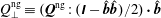 $Q_{\bot }^{\text{ng}}\equiv (\boldsymbol{Q}^{\text{ng}}:(\unicode[STIX]{x1D644}-\hat{\boldsymbol{b}}\hat{\boldsymbol{b}})/2)\boldsymbol{\cdot }\hat{\boldsymbol{b}}$
. The term containing
$Q_{\bot }^{\text{ng}}\equiv (\boldsymbol{Q}^{\text{ng}}:(\unicode[STIX]{x1D644}-\hat{\boldsymbol{b}}\hat{\boldsymbol{b}})/2)\boldsymbol{\cdot }\hat{\boldsymbol{b}}$
. The term containing
 $\boldsymbol{r}$
in the above equation can be rewritten to many possible forms, for example
$\boldsymbol{r}$
in the above equation can be rewritten to many possible forms, for example
 $$\begin{eqnarray}\displaystyle {\textstyle \frac{1}{2}}[(\text{Tr}\,\unicode[STIX]{x1D735}\boldsymbol{\cdot }\boldsymbol{r})\boldsymbol{\cdot }\hat{\boldsymbol{b}}-\hat{\boldsymbol{b}}\boldsymbol{\cdot }(\unicode[STIX]{x1D735}\boldsymbol{\cdot }\boldsymbol{r}):\hat{\boldsymbol{b}}\hat{\boldsymbol{b}}] & = & \displaystyle {\textstyle \frac{1}{2}}[(\unicode[STIX]{x2202}_{l}r_{liik})\hat{b}_{k}-(\unicode[STIX]{x2202}_{l}r_{lijk})\hat{b}_{i}\hat{b}_{j}\hat{b}_{k}]\nonumber\\ \displaystyle & = & \displaystyle {\textstyle \frac{1}{2}}[(\text{Tr}\,\unicode[STIX]{x1D735}\boldsymbol{\cdot }\boldsymbol{r})-(\unicode[STIX]{x1D735}\boldsymbol{\cdot }\boldsymbol{r}):\hat{\boldsymbol{b}}\hat{\boldsymbol{b}}]\boldsymbol{\cdot }\hat{\boldsymbol{b}}\nonumber\\ \displaystyle & = & \displaystyle \hat{\boldsymbol{b}}\boldsymbol{\cdot }(\unicode[STIX]{x1D735}\boldsymbol{\cdot }\boldsymbol{r}):(\unicode[STIX]{x1D644}-\hat{\boldsymbol{b}}\hat{\boldsymbol{b}})/2.\end{eqnarray}$$
The last expression is of course consistent with an alternative way to derive the perpendicular heat flux equation, where instead of doing trace of the heat flux tensor equation and subtracting the scalar parallel heat flux equation, one can directly apply operators
 $:(\unicode[STIX]{x1D644}-\hat{\boldsymbol{b}}\hat{\boldsymbol{b}})/2$
and
$:(\unicode[STIX]{x1D644}-\hat{\boldsymbol{b}}\hat{\boldsymbol{b}})/2$
and
 $\boldsymbol{\cdot }\hat{\boldsymbol{b}}$
.
$\boldsymbol{\cdot }\hat{\boldsymbol{b}}$
.
7.4 Scalar heat flux equations continued
The parallel and perpendicular heat flux equations (7.74), (7.92) contain expressions for the fourth-order moment
 $\boldsymbol{r}$
, and even though we will consider this moment in detail in the next section, here we want to finish the derivation of the scalar heat flux equations, and we write down the required expressions. Similarly to the pressure tensor and the heat flux tensor, the fourth-order moment can be decomposed into its gyrotropic and non-gyrotropic parts,
$\boldsymbol{r}$
, and even though we will consider this moment in detail in the next section, here we want to finish the derivation of the scalar heat flux equations, and we write down the required expressions. Similarly to the pressure tensor and the heat flux tensor, the fourth-order moment can be decomposed into its gyrotropic and non-gyrotropic parts,
 $\boldsymbol{r}=\boldsymbol{r}^{\text{g}}+\boldsymbol{r}^{\text{ng}}$
. The gyrotropic part
$\boldsymbol{r}=\boldsymbol{r}^{\text{g}}+\boldsymbol{r}^{\text{ng}}$
. The gyrotropic part
 $\boldsymbol{r}^{\text{g}}$
is decomposed according to (8.10), and it can be shown (see later in the text), that direct calculation yields
$\boldsymbol{r}^{\text{g}}$
is decomposed according to (8.10), and it can be shown (see later in the text), that direct calculation yields
 $$\begin{eqnarray}\displaystyle & \displaystyle \hat{\boldsymbol{b}}\boldsymbol{\cdot }(\unicode[STIX]{x1D735}\boldsymbol{\cdot }\boldsymbol{r}^{\text{g}}):\hat{\boldsymbol{b}}\hat{\boldsymbol{b}}=\unicode[STIX]{x1D735}\boldsymbol{\cdot }(r_{\Vert \Vert }\hat{\boldsymbol{b}})-3r_{\Vert \bot }\unicode[STIX]{x1D735}\boldsymbol{\cdot }\hat{\boldsymbol{b}}; & \displaystyle\end{eqnarray}$$
 $$\begin{eqnarray}\displaystyle & \displaystyle {\textstyle \frac{1}{2}}[(\text{Tr}\,\unicode[STIX]{x1D735}\boldsymbol{\cdot }\boldsymbol{r}^{\text{g}})\boldsymbol{\cdot }\hat{\boldsymbol{b}}-\hat{\boldsymbol{b}}\boldsymbol{\cdot }(\unicode[STIX]{x1D735}\boldsymbol{\cdot }\boldsymbol{r}^{\text{g}}):\hat{\boldsymbol{b}}\hat{\boldsymbol{b}}]=\unicode[STIX]{x1D735}\boldsymbol{\cdot }(r_{\Vert \bot }\hat{\boldsymbol{b}})+(r_{\Vert \bot }-r_{\bot \bot })\unicode[STIX]{x1D735}\boldsymbol{\cdot }\hat{\boldsymbol{b}}, & \displaystyle\end{eqnarray}$$
which yields the parallel heat flux equation
 $$\begin{eqnarray}\displaystyle & & \displaystyle \frac{\unicode[STIX]{x2202}q_{\Vert }}{\unicode[STIX]{x2202}t}+\unicode[STIX]{x1D735}\boldsymbol{\cdot }(q_{\Vert }\boldsymbol{u})+\unicode[STIX]{x1D735}\boldsymbol{\cdot }(r_{\Vert \Vert }\hat{\boldsymbol{b}})-3r_{\Vert \bot }\unicode[STIX]{x1D735}\boldsymbol{\cdot }\hat{\boldsymbol{b}}+3q_{\Vert }\hat{\boldsymbol{b}}\boldsymbol{\cdot }\unicode[STIX]{x1D735}\boldsymbol{u}\boldsymbol{\cdot }\hat{\boldsymbol{b}}-3\frac{p_{\Vert }}{\unicode[STIX]{x1D70C}}\hat{\boldsymbol{b}}\boldsymbol{\cdot }\unicode[STIX]{x1D735}p_{\Vert }\nonumber\\ \displaystyle & & \displaystyle \qquad -\,3\frac{p_{\Vert }}{\unicode[STIX]{x1D70C}}(p_{\Vert }-p_{\bot })\unicode[STIX]{x1D735}\boldsymbol{\cdot }\hat{\boldsymbol{b}}+\hat{\boldsymbol{b}}\boldsymbol{\cdot }(\unicode[STIX]{x1D735}\boldsymbol{\cdot }\boldsymbol{r}^{\text{ng}}):\hat{\boldsymbol{b}}\hat{\boldsymbol{b}}-3\frac{p_{\Vert }}{\unicode[STIX]{x1D70C}}(\unicode[STIX]{x1D735}\boldsymbol{\cdot }\unicode[STIX]{x1D72B})\boldsymbol{\cdot }\hat{\boldsymbol{b}}+Q_{\Vert }^{\text{ng}}=0,\end{eqnarray}$$
and the perpendicular heat flux equation
 $$\begin{eqnarray}\displaystyle & & \displaystyle \frac{\unicode[STIX]{x2202}q_{\bot }}{\unicode[STIX]{x2202}t}+\boldsymbol{u}\boldsymbol{\cdot }\unicode[STIX]{x1D735}q_{\bot }+2q_{\bot }\unicode[STIX]{x1D735}\boldsymbol{\cdot }\boldsymbol{u}+\unicode[STIX]{x1D735}\boldsymbol{\cdot }(r_{\Vert \bot }\hat{\boldsymbol{b}})+(r_{\Vert \bot }-r_{\bot \bot })\unicode[STIX]{x1D735}\boldsymbol{\cdot }\hat{\boldsymbol{b}}\nonumber\\ \displaystyle & & \displaystyle \qquad -\frac{p_{\bot }}{\unicode[STIX]{x1D70C}}[\hat{\boldsymbol{b}}\boldsymbol{\cdot }\unicode[STIX]{x1D735}p_{\Vert }+(p_{\Vert }-p_{\bot })\unicode[STIX]{x1D735}\boldsymbol{\cdot }\hat{\boldsymbol{b}}]+\frac{1}{2}[(\text{Tr}\,\unicode[STIX]{x1D735}\boldsymbol{\cdot }\boldsymbol{r}^{\text{ng}})\boldsymbol{\cdot }\hat{\boldsymbol{b}}-\hat{\boldsymbol{b}}\boldsymbol{\cdot }(\unicode[STIX]{x1D735}\boldsymbol{\cdot }\boldsymbol{r}^{\text{ng}}):\hat{\boldsymbol{b}}\hat{\boldsymbol{b}}]\nonumber\\ \displaystyle & & \displaystyle \qquad -\,\frac{p_{\bot }}{\unicode[STIX]{x1D70C}}(\unicode[STIX]{x1D735}\boldsymbol{\cdot }\unicode[STIX]{x1D72B})\boldsymbol{\cdot }\hat{\boldsymbol{b}}-\frac{1}{\unicode[STIX]{x1D70C}}[\unicode[STIX]{x1D735}p_{\bot }+(p_{\Vert }-p_{\bot })\hat{\boldsymbol{b}}\boldsymbol{\cdot }\unicode[STIX]{x1D735}\hat{\boldsymbol{b}}+\unicode[STIX]{x1D735}\boldsymbol{\cdot }\unicode[STIX]{x1D72B}]\boldsymbol{\cdot }\unicode[STIX]{x1D72B}\boldsymbol{\cdot }\hat{\boldsymbol{b}}+Q_{\bot }^{\text{ng}}=0.\end{eqnarray}$$
Exact nonlinear expressions for
 $Q_{\Vert }^{\text{ng}}$
and
$Q_{\Vert }^{\text{ng}}$
and
 $Q_{\bot }^{\text{ng}}$
that represent contributions from the non-gyrotropic heat flux
$Q_{\bot }^{\text{ng}}$
that represent contributions from the non-gyrotropic heat flux
 $\boldsymbol{q}^{\text{ng}}$
are calculated in appendix D, see (D 110), (D 120). The scalar heat flux equations (7.96) and (7.97) are completely general at this stage, since no distribution function has been prescribed yet, and no simplification has been introduced. These equations are exact.
$\boldsymbol{q}^{\text{ng}}$
are calculated in appendix D, see (D 110), (D 120). The scalar heat flux equations (7.96) and (7.97) are completely general at this stage, since no distribution function has been prescribed yet, and no simplification has been introduced. These equations are exact.
Nevertheless, equations (7.96), (7.97) are very complicated, and at this stage, it is beneficial to simplify them. One possibility is to cancel all the non-gyrotropic contributions
 $\unicode[STIX]{x1D72B}$
,
$\unicode[STIX]{x1D72B}$
,
 $\boldsymbol{q}^{\text{ng}}$
and
$\boldsymbol{q}^{\text{ng}}$
and
 $\boldsymbol{r}^{\text{ng}}$
, and we will study such fluid models later. Another possibility is to keep only those non-gyrotropic terms that have some non-zero contribution at the linear level. This eliminates the last term in the second line of (7.97) that is proportional to
$\boldsymbol{r}^{\text{ng}}$
, and we will study such fluid models later. Another possibility is to keep only those non-gyrotropic terms that have some non-zero contribution at the linear level. This eliminates the last term in the second line of (7.97) that is proportional to
 $[\ldots ]\boldsymbol{\cdot }\unicode[STIX]{x1D72B}\boldsymbol{\cdot }\hat{\boldsymbol{b}}$
. Also, by following the derivations in appendix D, it is easy to show that the terms
$[\ldots ]\boldsymbol{\cdot }\unicode[STIX]{x1D72B}\boldsymbol{\cdot }\hat{\boldsymbol{b}}$
. Also, by following the derivations in appendix D, it is easy to show that the terms
 $Q_{\Vert }^{\text{ng}}$
,
$Q_{\Vert }^{\text{ng}}$
,
 $Q_{\bot }^{\text{ng}}$
(that represent the non-gyrotropic heat flux
$Q_{\bot }^{\text{ng}}$
(that represent the non-gyrotropic heat flux
 $\boldsymbol{q}^{\text{ng}}$
), do not contribute at the linear level. Therefore, the heat flux equations simplify
$\boldsymbol{q}^{\text{ng}}$
), do not contribute at the linear level. Therefore, the heat flux equations simplify
 $$\begin{eqnarray}\displaystyle & & \displaystyle \frac{\unicode[STIX]{x2202}q_{\Vert }}{\unicode[STIX]{x2202}t}+\unicode[STIX]{x1D735}\boldsymbol{\cdot }(q_{\Vert }\boldsymbol{u})+\unicode[STIX]{x1D735}\boldsymbol{\cdot }(r_{\Vert \Vert }\hat{\boldsymbol{b}})-3r_{\Vert \bot }\unicode[STIX]{x1D735}\boldsymbol{\cdot }\hat{\boldsymbol{b}}+3q_{\Vert }\hat{\boldsymbol{b}}\boldsymbol{\cdot }\unicode[STIX]{x1D735}\boldsymbol{u}\boldsymbol{\cdot }\hat{\boldsymbol{b}}-3\frac{p_{\Vert }}{\unicode[STIX]{x1D70C}}\hat{\boldsymbol{b}}\boldsymbol{\cdot }\unicode[STIX]{x1D735}p_{\Vert }\nonumber\\ \displaystyle & & \displaystyle \qquad -\,3\frac{p_{\Vert }}{\unicode[STIX]{x1D70C}}(p_{\Vert }-p_{\bot })\unicode[STIX]{x1D735}\boldsymbol{\cdot }\hat{\boldsymbol{b}}+\hat{\boldsymbol{b}}\boldsymbol{\cdot }(\unicode[STIX]{x1D735}\boldsymbol{\cdot }\boldsymbol{r}^{\text{ng}}):\hat{\boldsymbol{b}}\hat{\boldsymbol{b}}-3\frac{p_{\Vert }}{\unicode[STIX]{x1D70C}}(\unicode[STIX]{x1D735}\boldsymbol{\cdot }\unicode[STIX]{x1D72B})\boldsymbol{\cdot }\hat{\boldsymbol{b}}=0;\end{eqnarray}$$
 $$\begin{eqnarray}\displaystyle & & \displaystyle \frac{\unicode[STIX]{x2202}q_{\bot }}{\unicode[STIX]{x2202}t}+\boldsymbol{u}\boldsymbol{\cdot }\unicode[STIX]{x1D735}q_{\bot }+2q_{\bot }\unicode[STIX]{x1D735}\boldsymbol{\cdot }\boldsymbol{u}+\unicode[STIX]{x1D735}\boldsymbol{\cdot }(r_{\Vert \bot }\hat{\boldsymbol{b}})+(r_{\Vert \bot }-r_{\bot \bot })\unicode[STIX]{x1D735}\boldsymbol{\cdot }\hat{\boldsymbol{b}}\nonumber\\ \displaystyle & & \displaystyle \qquad -\,\frac{p_{\bot }}{\unicode[STIX]{x1D70C}}[\hat{\boldsymbol{b}}\boldsymbol{\cdot }\unicode[STIX]{x1D735}p_{\Vert }+(p_{\Vert }-p_{\bot })\unicode[STIX]{x1D735}\boldsymbol{\cdot }\hat{\boldsymbol{b}}]+\frac{1}{2}[(\text{Tr}\,\unicode[STIX]{x1D735}\boldsymbol{\cdot }\boldsymbol{r}^{\text{ng}})\boldsymbol{\cdot }\hat{\boldsymbol{b}}-\hat{\boldsymbol{b}}\boldsymbol{\cdot }(\unicode[STIX]{x1D735}\boldsymbol{\cdot }\boldsymbol{r}^{\text{ng}}):\hat{\boldsymbol{b}}\hat{\boldsymbol{b}}]\nonumber\\ \displaystyle & & \displaystyle \qquad -\,\frac{p_{\bot }}{\unicode[STIX]{x1D70C}}(\unicode[STIX]{x1D735}\boldsymbol{\cdot }\unicode[STIX]{x1D72B})\boldsymbol{\cdot }\hat{\boldsymbol{b}}=0.\end{eqnarray}$$
Still, no specific distribution function was assumed. However, to evaluate the non-gyrotropic
 $\boldsymbol{r}^{\text{ng}}$
, and correctly evaluate possible cancellations with terms containing
$\boldsymbol{r}^{\text{ng}}$
, and correctly evaluate possible cancellations with terms containing
 $\unicode[STIX]{x1D72B}$
, we need to use
$\unicode[STIX]{x1D72B}$
, we need to use
 $\boldsymbol{r}^{\text{ng}}$
decomposition (8.58). Importantly, the decomposition (8.58) is valid only for perturbations around a bi-Maxwellian distribution function. By keeping only terms that have non-zero contribution at the linear level, see equations (8.63), (8.65) later in the text, the
$\boldsymbol{r}^{\text{ng}}$
decomposition (8.58). Importantly, the decomposition (8.58) is valid only for perturbations around a bi-Maxwellian distribution function. By keeping only terms that have non-zero contribution at the linear level, see equations (8.63), (8.65) later in the text, the
 $\boldsymbol{r}^{\text{ng}}$
terms are evaluated as
$\boldsymbol{r}^{\text{ng}}$
terms are evaluated as
 $$\begin{eqnarray}\displaystyle & \displaystyle \hat{\boldsymbol{b}}\boldsymbol{\cdot }(\unicode[STIX]{x1D735}\boldsymbol{\cdot }\boldsymbol{r}^{\text{ng}}):\hat{\boldsymbol{b}}\hat{\boldsymbol{b}}=\frac{3p_{\Vert }}{\unicode[STIX]{x1D70C}}(\unicode[STIX]{x1D735}\boldsymbol{\cdot }\unicode[STIX]{x1D72B})\boldsymbol{\cdot }\hat{\boldsymbol{b}}; & \displaystyle\end{eqnarray}$$
 $$\begin{eqnarray}\displaystyle & \displaystyle \frac{1}{2}[(\text{Tr}\,\unicode[STIX]{x1D735}\boldsymbol{\cdot }\boldsymbol{r}^{\text{ng}})\boldsymbol{\cdot }\hat{\boldsymbol{b}}-\hat{\boldsymbol{b}}\boldsymbol{\cdot }(\unicode[STIX]{x1D735}\boldsymbol{\cdot }\boldsymbol{r}^{\text{ng}}):\hat{\boldsymbol{b}}\hat{\boldsymbol{b}}]=\frac{2p_{\bot }}{\unicode[STIX]{x1D70C}}(\unicode[STIX]{x1D735}\boldsymbol{\cdot }\unicode[STIX]{x1D72B})\boldsymbol{\cdot }\hat{\boldsymbol{b}}. & \displaystyle\end{eqnarray}$$
Importantly, both non-gyrotropic contributions in the parallel heat flux equation (7.98) completely cancel out! The cancellation demonstrates the importance of keeping the non-gyrotropic
 $\boldsymbol{r}^{\text{ng}}$
, if one wants to keep the non-gyrotropic
$\boldsymbol{r}^{\text{ng}}$
, if one wants to keep the non-gyrotropic
 $\unicode[STIX]{x1D72B}$
. Also, there is a partial cancellation in the perpendicular heat flux equation (7.99). The heat flux equations therefore read
$\unicode[STIX]{x1D72B}$
. Also, there is a partial cancellation in the perpendicular heat flux equation (7.99). The heat flux equations therefore read
 $$\begin{eqnarray}\displaystyle & & \displaystyle \frac{\unicode[STIX]{x2202}q_{\Vert }}{\unicode[STIX]{x2202}t}+\unicode[STIX]{x1D735}\boldsymbol{\cdot }(q_{\Vert }\boldsymbol{u})+\unicode[STIX]{x1D735}\boldsymbol{\cdot }(r_{\Vert \Vert }\hat{\boldsymbol{b}})-3r_{\Vert \bot }\unicode[STIX]{x1D735}\boldsymbol{\cdot }\hat{\boldsymbol{b}}+3q_{\Vert }\hat{\boldsymbol{b}}\boldsymbol{\cdot }\unicode[STIX]{x1D735}\boldsymbol{u}\boldsymbol{\cdot }\hat{\boldsymbol{b}}-3\frac{p_{\Vert }}{\unicode[STIX]{x1D70C}}\hat{\boldsymbol{b}}\boldsymbol{\cdot }\unicode[STIX]{x1D735}p_{\Vert }\nonumber\\ \displaystyle & & \displaystyle \qquad -\,3\frac{p_{\Vert }}{\unicode[STIX]{x1D70C}}(p_{\Vert }-p_{\bot })\unicode[STIX]{x1D735}\boldsymbol{\cdot }\hat{\boldsymbol{b}}=0;\end{eqnarray}$$
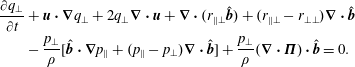 $$\begin{eqnarray}\displaystyle & & \displaystyle \frac{\unicode[STIX]{x2202}q_{\bot }}{\unicode[STIX]{x2202}t}+\boldsymbol{u}\boldsymbol{\cdot }\unicode[STIX]{x1D735}q_{\bot }+2q_{\bot }\unicode[STIX]{x1D735}\boldsymbol{\cdot }\boldsymbol{u}+\unicode[STIX]{x1D735}\boldsymbol{\cdot }(r_{\Vert \bot }\hat{\boldsymbol{b}})+(r_{\Vert \bot }-r_{\bot \bot })\unicode[STIX]{x1D735}\boldsymbol{\cdot }\hat{\boldsymbol{b}}\nonumber\\ \displaystyle & & \displaystyle \qquad -\,\frac{p_{\bot }}{\unicode[STIX]{x1D70C}}[\hat{\boldsymbol{b}}\boldsymbol{\cdot }\unicode[STIX]{x1D735}p_{\Vert }+(p_{\Vert }-p_{\bot })\unicode[STIX]{x1D735}\boldsymbol{\cdot }\hat{\boldsymbol{b}}]+\frac{p_{\bot }}{\unicode[STIX]{x1D70C}}(\unicode[STIX]{x1D735}\boldsymbol{\cdot }\unicode[STIX]{x1D72B})\boldsymbol{\cdot }\hat{\boldsymbol{b}}=0.\end{eqnarray}$$
The last term can be evaluated with respect to the mean magnetic field, and assuming that
 $\hat{\boldsymbol{b}}_{0}$
is in the
$\hat{\boldsymbol{b}}_{0}$
is in the
 $z$
-direction, the term is equal to
$z$
-direction, the term is equal to
 $(p_{\bot }/\unicode[STIX]{x1D70C})(\unicode[STIX]{x2202}_{x}\unicode[STIX]{x1D6F1}_{xz}+\unicode[STIX]{x2202}_{y}\unicode[STIX]{x1D6F1}_{yz})$
, since
$(p_{\bot }/\unicode[STIX]{x1D70C})(\unicode[STIX]{x2202}_{x}\unicode[STIX]{x1D6F1}_{xz}+\unicode[STIX]{x2202}_{y}\unicode[STIX]{x1D6F1}_{yz})$
, since
 $\unicode[STIX]{x1D6F1}_{zz}=0$
. Essentially, the term should be written in a fully linearized form
$\unicode[STIX]{x1D6F1}_{zz}=0$
. Essentially, the term should be written in a fully linearized form
 $(p_{\bot }^{(0)}/\unicode[STIX]{x1D70C}_{0})(\unicode[STIX]{x1D735}\boldsymbol{\cdot }\unicode[STIX]{x1D72B})\boldsymbol{\cdot }\hat{\boldsymbol{b}}_{0}$
, since other non-gyrotropic nonlinear terms were neglected. It is important to emphasize that it is because of this one term, that the equations (7.102), (7.103) are valid only for perturbations around a bi-Maxwellian distribution function. If the term is neglected, i.e. if one neglects from the beginning the non-gyrotropic contributions in (7.98), (7.99), the heat flux equations are valid for perturbations around any distribution function. We will consider a bi-kappa distribution function later.
$(p_{\bot }^{(0)}/\unicode[STIX]{x1D70C}_{0})(\unicode[STIX]{x1D735}\boldsymbol{\cdot }\unicode[STIX]{x1D72B})\boldsymbol{\cdot }\hat{\boldsymbol{b}}_{0}$
, since other non-gyrotropic nonlinear terms were neglected. It is important to emphasize that it is because of this one term, that the equations (7.102), (7.103) are valid only for perturbations around a bi-Maxwellian distribution function. If the term is neglected, i.e. if one neglects from the beginning the non-gyrotropic contributions in (7.98), (7.99), the heat flux equations are valid for perturbations around any distribution function. We will consider a bi-kappa distribution function later.
7.5 Heat flux equations with ‘normal’ closure
Detailed calculations with the fourth-order moment will be presented in the next section. Here we want to finish the derivation, and by using the bi-Maxwellian ‘normal’ fluid closure
 $$\begin{eqnarray}r_{\Vert \Vert }=\frac{3p_{\Vert }^{2}}{\unicode[STIX]{x1D70C}};\quad r_{\Vert \bot }=\frac{p_{\Vert }p_{\bot }}{\unicode[STIX]{x1D70C}};\quad r_{\bot \bot }=\frac{2p_{\bot }^{2}}{\unicode[STIX]{x1D70C}},\end{eqnarray}$$
terms entering the heat flux equations directly calculate as
 $$\begin{eqnarray}\displaystyle & \displaystyle \unicode[STIX]{x1D735}\boldsymbol{\cdot }(r_{\Vert \Vert }\hat{\boldsymbol{b}})-3r_{\Vert \bot }\unicode[STIX]{x1D735}\boldsymbol{\cdot }\hat{\boldsymbol{b}}=3\frac{p_{\Vert }^{2}}{\unicode[STIX]{x1D70C}}\unicode[STIX]{x1D735}\boldsymbol{\cdot }\hat{\boldsymbol{b}}+3p_{\Vert }\hat{\boldsymbol{b}}\boldsymbol{\cdot }\unicode[STIX]{x1D735}\left(\frac{p_{\Vert }}{\unicode[STIX]{x1D70C}}\right)+3\frac{p_{\Vert }}{\unicode[STIX]{x1D70C}}\hat{\boldsymbol{b}}\boldsymbol{\cdot }\unicode[STIX]{x1D735}p_{\Vert }-3\frac{p_{\Vert }p_{\bot }}{\unicode[STIX]{x1D70C}}\unicode[STIX]{x1D735}\boldsymbol{\cdot }\hat{\boldsymbol{b}}; & \displaystyle \nonumber\\ \displaystyle & & \displaystyle\end{eqnarray}$$
 $$\begin{eqnarray}\displaystyle & \displaystyle \unicode[STIX]{x1D735}\boldsymbol{\cdot }(r_{\Vert \bot }\hat{\boldsymbol{b}})+(r_{\Vert \bot }-r_{\bot \bot })\unicode[STIX]{x1D735}\boldsymbol{\cdot }\hat{\boldsymbol{b}}=\frac{p_{\bot }}{\unicode[STIX]{x1D70C}}\hat{\boldsymbol{b}}\boldsymbol{\cdot }\unicode[STIX]{x1D735}p_{\Vert }+p_{\Vert }\hat{\boldsymbol{b}}\boldsymbol{\cdot }\unicode[STIX]{x1D735}\left(\frac{p_{\bot }}{\unicode[STIX]{x1D70C}}\right)+2\frac{p_{\bot }}{\unicode[STIX]{x1D70C}}(p_{\Vert }-p_{\bot })\unicode[STIX]{x1D735}\boldsymbol{\cdot }\hat{\boldsymbol{b}}. & \displaystyle \nonumber\\ \displaystyle & & \displaystyle\end{eqnarray}$$
The use of these expressions in (7.102), (7.103) cancels various terms, and the scalar heat flux equations read
 $$\begin{eqnarray}\displaystyle & \displaystyle \frac{\unicode[STIX]{x2202}q_{\Vert }}{\unicode[STIX]{x2202}t}+\unicode[STIX]{x1D735}\boldsymbol{\cdot }(q_{\Vert }\boldsymbol{u})+3p_{\Vert }\hat{\boldsymbol{b}}\boldsymbol{\cdot }\unicode[STIX]{x1D735}\left(\frac{p_{\Vert }}{\unicode[STIX]{x1D70C}}\right)+3q_{\Vert }\hat{\boldsymbol{b}}\boldsymbol{\cdot }\unicode[STIX]{x1D735}\boldsymbol{u}\boldsymbol{\cdot }\hat{\boldsymbol{b}}=0; & \displaystyle\end{eqnarray}$$
 $$\begin{eqnarray}\displaystyle & \displaystyle \frac{\unicode[STIX]{x2202}q_{\bot }}{\unicode[STIX]{x2202}t}+\boldsymbol{u}\boldsymbol{\cdot }\unicode[STIX]{x1D735}q_{\bot }+2q_{\bot }\unicode[STIX]{x1D735}\boldsymbol{\cdot }\boldsymbol{u}+p_{\Vert }\hat{\boldsymbol{b}}\boldsymbol{\cdot }\unicode[STIX]{x1D735}\left(\!\frac{p_{\bot }}{\unicode[STIX]{x1D70C}}\!\right)+\frac{p_{\bot }}{\unicode[STIX]{x1D70C}}(p_{\Vert }-p_{\bot })\unicode[STIX]{x1D735}\boldsymbol{\cdot }\hat{\boldsymbol{b}}+\frac{p_{\bot }}{\unicode[STIX]{x1D70C}}(\unicode[STIX]{x1D735}\boldsymbol{\cdot }\unicode[STIX]{x1D72B})\boldsymbol{\cdot }\hat{\boldsymbol{b}}_{0}=0. & \displaystyle \nonumber\\ \displaystyle & & \displaystyle\end{eqnarray}$$
8 Fourth-order fluid moment
The algebra of the fourth-order fluid moment
 $\boldsymbol{r}=m\int \boldsymbol{c}\boldsymbol{c}\boldsymbol{c}\boldsymbol{c}f\,\text{d}^{3}v$
can be quite intimidating at first, since the moment is a 4-D cube (
$\boldsymbol{r}=m\int \boldsymbol{c}\boldsymbol{c}\boldsymbol{c}\boldsymbol{c}f\,\text{d}^{3}v$
can be quite intimidating at first, since the moment is a 4-D cube (
 $3x3x3x3$
). We are not going to derive the time evolution equation for this moment step by step, nevertheless, later in the text we derive the evolution equation of the
$3x3x3x3$
). We are not going to derive the time evolution equation for this moment step by step, nevertheless, later in the text we derive the evolution equation of the
 $n$
th-order fluid moment
$n$
th-order fluid moment
 $\unicode[STIX]{x1D653}^{(n)}$
, see (12.16), and therefore, for
$\unicode[STIX]{x1D653}^{(n)}$
, see (12.16), and therefore, for
 $n=4$
, the equation reads
$n=4$
, the equation reads
 $$\begin{eqnarray}\displaystyle \frac{\unicode[STIX]{x2202}}{\unicode[STIX]{x2202}t}\boldsymbol{r}+\unicode[STIX]{x1D735}\boldsymbol{\cdot }(\unicode[STIX]{x1D653}^{(5)}+\boldsymbol{u}\boldsymbol{r})+\left[\boldsymbol{r}\boldsymbol{\cdot }\unicode[STIX]{x1D735}\boldsymbol{u}+\frac{q}{mc}\boldsymbol{B}\times \boldsymbol{r}-\frac{1}{\unicode[STIX]{x1D70C}}(\unicode[STIX]{x1D735}\boldsymbol{\cdot }\boldsymbol{p})\boldsymbol{q}\right]^{S}=0. & & \displaystyle\end{eqnarray}$$
The symmetric operator ‘
 $S$
’ is here defined as
$S$
’ is here defined as
 $$\begin{eqnarray}\unicode[STIX]{x1D608}_{ijkl}^{S}=\unicode[STIX]{x1D608}_{ijkl}+\unicode[STIX]{x1D608}_{jkli}+\unicode[STIX]{x1D608}_{klij}+\unicode[STIX]{x1D608}_{lijk}.\end{eqnarray}$$
Here, we are not that interested in the evolution equation for
 $\boldsymbol{r}$
, we just want to clarify its decomposition, that we need in the heat flux equations. The definition of gyrotropy means that the integral has to be evaluated only over combinations of
$\boldsymbol{r}$
, we just want to clarify its decomposition, that we need in the heat flux equations. The definition of gyrotropy means that the integral has to be evaluated only over combinations of
 $(v_{\Vert }-u_{\bot })\equiv c_{\Vert }$
and
$(v_{\Vert }-u_{\bot })\equiv c_{\Vert }$
and
 $|\boldsymbol{v}_{\bot }-\boldsymbol{u}_{\bot }|^{2}\equiv c_{\bot }^{2}$
. For the fourth moment
$|\boldsymbol{v}_{\bot }-\boldsymbol{u}_{\bot }|^{2}\equiv c_{\bot }^{2}$
. For the fourth moment
 $\boldsymbol{r}$
, there are obviously only 3 possibilities:
$\boldsymbol{r}$
, there are obviously only 3 possibilities:
 $c_{\Vert }^{4}$
,
$c_{\Vert }^{4}$
,
 $c_{\Vert }^{2}c_{\bot }^{2}$
and
$c_{\Vert }^{2}c_{\bot }^{2}$
and
 $(c_{\bot }^{2})^{2}$
, and these gyrotropic components will be called
$(c_{\bot }^{2})^{2}$
, and these gyrotropic components will be called
 $r_{\Vert \Vert },r_{\Vert \bot }$
and
$r_{\Vert \Vert },r_{\Vert \bot }$
and
 $r_{\bot \bot }$
. We have already seen that the double contractions with
$r_{\bot \bot }$
. We have already seen that the double contractions with
 $\hat{\boldsymbol{b}}\hat{\boldsymbol{b}}$
and
$\hat{\boldsymbol{b}}\hat{\boldsymbol{b}}$
and
 $(\unicode[STIX]{x1D644}-\hat{\boldsymbol{b}}\hat{\boldsymbol{b}})/2$
, were very useful operators to extract the gyrotropic components for the lower-order moments,
$(\unicode[STIX]{x1D644}-\hat{\boldsymbol{b}}\hat{\boldsymbol{b}})/2$
, were very useful operators to extract the gyrotropic components for the lower-order moments,
 $\boldsymbol{p}$
and
$\boldsymbol{p}$
and
 $\boldsymbol{q}$
. To obtain any scalar quantity from the fourth moment, we obviously need to apply two double contractions. There are 3 possibilities: we can apply
$\boldsymbol{q}$
. To obtain any scalar quantity from the fourth moment, we obviously need to apply two double contractions. There are 3 possibilities: we can apply
 $\hat{\boldsymbol{b}}\hat{\boldsymbol{b}}$
twice, we can apply
$\hat{\boldsymbol{b}}\hat{\boldsymbol{b}}$
twice, we can apply
 $\hat{\boldsymbol{b}}\hat{\boldsymbol{b}}$
and
$\hat{\boldsymbol{b}}\hat{\boldsymbol{b}}$
and
 $(\unicode[STIX]{x1D644}-\hat{\boldsymbol{b}}\hat{\boldsymbol{b}})/2$
or we can apply
$(\unicode[STIX]{x1D644}-\hat{\boldsymbol{b}}\hat{\boldsymbol{b}})/2$
or we can apply
 $(\unicode[STIX]{x1D644}-\hat{\boldsymbol{b}}\hat{\boldsymbol{b}})/2$
twice. Not surprisingly, these double contractions with
$(\unicode[STIX]{x1D644}-\hat{\boldsymbol{b}}\hat{\boldsymbol{b}})/2$
twice. Not surprisingly, these double contractions with
 $\boldsymbol{r}$
indeed extract the 3 possible gyrotropic parts, as it is easy to verify that
$\boldsymbol{r}$
indeed extract the 3 possible gyrotropic parts, as it is easy to verify that
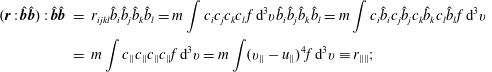 $$\begin{eqnarray}\displaystyle (\boldsymbol{r}:\hat{\boldsymbol{b}}\hat{\boldsymbol{b}}):\hat{\boldsymbol{b}}\hat{\boldsymbol{b}} & = & \displaystyle r_{ijkl}\hat{b}_{i}\hat{b}_{j}\hat{b}_{k}\hat{b}_{l}=m\int c_{i}c_{j}c_{k}c_{l}f\,\text{d}^{3}v\hat{b}_{i}\hat{b}_{j}\hat{b}_{k}\hat{b}_{l}=m\int c_{i}\hat{b}_{i}c_{j}\hat{b}_{j}c_{k}\hat{b}_{k}c_{l}\hat{b}_{l}f\,\text{d}^{3}v\nonumber\\ \displaystyle & = & \displaystyle m\int c_{\Vert }c_{\Vert }c_{\Vert }c_{\Vert }f\,\text{d}^{3}v=m\int (v_{\Vert }-u_{\Vert })^{4}f\,\text{d}^{3}v\equiv r_{\Vert \Vert };\end{eqnarray}$$
 $$\begin{eqnarray}\displaystyle (\boldsymbol{r}:\hat{\boldsymbol{b}}\hat{\boldsymbol{b}}):(\unicode[STIX]{x1D644}-\hat{\boldsymbol{b}}\hat{\boldsymbol{b}})/2 & = & \displaystyle \frac{m}{2}\int c_{i}c_{j}c_{k}c_{l}\hat{b}_{i}\hat{b}_{j}(\unicode[STIX]{x1D6FF}_{kl}-\hat{b}_{k}\hat{b}_{l})f\,\text{d}^{3}v=\frac{m}{2}\int c_{\Vert }^{2}c_{k}c_{l}(\unicode[STIX]{x1D6FF}_{kl}-\hat{b}_{k}\hat{b}_{l})f\,\text{d}^{3}v\nonumber\\ \displaystyle & = & \displaystyle \frac{m}{2}\int c_{\Vert }^{2}(|\boldsymbol{c}|^{2}-c_{\Vert }^{2})f\,\text{d}^{3}v=\frac{m}{2}\int c_{\Vert }^{2}c_{\bot }^{2}f\,\text{d}^{3}v\nonumber\\ \displaystyle & = & \displaystyle \frac{m}{2}\int (v_{\Vert }-u_{\Vert })^{2}|\boldsymbol{v}_{\bot }-\boldsymbol{u}_{\bot }|^{2}f\,\text{d}^{3}v\equiv r_{\Vert \bot };\end{eqnarray}$$
 $$\begin{eqnarray}\displaystyle (\boldsymbol{r}:(\unicode[STIX]{x1D644}-\hat{\boldsymbol{b}}\hat{\boldsymbol{b}})/2):(\unicode[STIX]{x1D644}-\hat{\boldsymbol{b}}\hat{\boldsymbol{b}})/2 & = & \displaystyle \frac{m}{4}\!\int \!c_{i}c_{j}c_{k}c_{l}(\unicode[STIX]{x1D6FF}_{ij}-\hat{b}_{i}\hat{b}_{j})(\unicode[STIX]{x1D6FF}_{kl}-\hat{b}_{k}\hat{b}_{l})f\,\text{d}^{3}v=\frac{m}{4}\!\int \!c_{\bot }^{2}c_{\bot }^{2}f\,\text{d}^{3}v\nonumber\\ \displaystyle & = & \displaystyle \frac{m}{4}\int |\boldsymbol{v}_{\bot }-\boldsymbol{u}_{\bot }|^{4}f\,\text{d}^{3}v\equiv r_{\bot \bot }.\end{eqnarray}$$
We are now ready to guess how to write the decomposition of the gyrotropic fourth-order moment. Motivated by the previous decompositions, it obviously has to be something in the form of
 $$\begin{eqnarray}\boldsymbol{r}^{\text{g}}=r_{\Vert \Vert }\hat{\boldsymbol{b}}\hat{\boldsymbol{b}}\hat{\boldsymbol{b}}\hat{\boldsymbol{b}}+r_{\Vert \bot }[\hat{\boldsymbol{b}}\hat{\boldsymbol{b}}(\unicode[STIX]{x1D644}-\hat{\boldsymbol{b}}\hat{\boldsymbol{b}})]^{\text{Sym}}+r_{\bot \bot }[(\unicode[STIX]{x1D644}-\hat{\boldsymbol{b}}\hat{\boldsymbol{b}})(\unicode[STIX]{x1D644}-\hat{\boldsymbol{b}}\hat{\boldsymbol{b}})]^{\text{Sym}},\end{eqnarray}$$
where we still did not determine how the symmetric operator acts here. Importantly, the symmetric operator ‘Sym’ is not equivalent to the symmetric operator ‘
 $S$
’ that cycles all the indices around, equation (8.2). The fluid hierarchy obviously needs two symmetric operators, one unique ‘
$S$
’ that cycles all the indices around, equation (8.2). The fluid hierarchy obviously needs two symmetric operators, one unique ‘
 $S$
’ that is used to derive the evolution equation of a given fluid moment
$S$
’ that is used to derive the evolution equation of a given fluid moment
 $\unicode[STIX]{x1D653}^{(n)}$
, and one non-unique ‘Sym’ that is used for the decomposition of that fluid moment. The determination of how ‘Sym’ acts here is not that obvious. Nevertheless, one can consider in how many ways one can extract the gyrotropic components from
$\unicode[STIX]{x1D653}^{(n)}$
, and one non-unique ‘Sym’ that is used for the decomposition of that fluid moment. The determination of how ‘Sym’ acts here is not that obvious. Nevertheless, one can consider in how many ways one can extract the gyrotropic components from
 $r_{ijkl}$
. For
$r_{ijkl}$
. For
 $r_{\Vert \Vert }$
, one does two double contractions with
$r_{\Vert \Vert }$
, one does two double contractions with
 $(\hat{\boldsymbol{b}}\hat{\boldsymbol{b}})$
. The possible choices are
$(\hat{\boldsymbol{b}}\hat{\boldsymbol{b}})$
. The possible choices are
 $(\hat{\boldsymbol{b}}\hat{\boldsymbol{b}})_{ij}(\hat{\boldsymbol{b}}\hat{\boldsymbol{b}})_{kl}$
;
$(\hat{\boldsymbol{b}}\hat{\boldsymbol{b}})_{ij}(\hat{\boldsymbol{b}}\hat{\boldsymbol{b}})_{kl}$
;
 $(\hat{\boldsymbol{b}}\hat{\boldsymbol{b}})_{ik}(\hat{\boldsymbol{b}}\hat{\boldsymbol{b}})_{jl}$
and
$(\hat{\boldsymbol{b}}\hat{\boldsymbol{b}})_{ik}(\hat{\boldsymbol{b}}\hat{\boldsymbol{b}})_{jl}$
and
 $(\hat{\boldsymbol{b}}\hat{\boldsymbol{b}})_{il}(\hat{\boldsymbol{b}}\hat{\boldsymbol{b}})_{jk}$
, however, all of these choices are equivalent. To obtain the
$(\hat{\boldsymbol{b}}\hat{\boldsymbol{b}})_{il}(\hat{\boldsymbol{b}}\hat{\boldsymbol{b}})_{jk}$
, however, all of these choices are equivalent. To obtain the
 $r_{\Vert \bot }$
, we perform double contractions with
$r_{\Vert \bot }$
, we perform double contractions with
 $(\hat{\boldsymbol{b}}\hat{\boldsymbol{b}})$
and
$(\hat{\boldsymbol{b}}\hat{\boldsymbol{b}})$
and
 $(\unicode[STIX]{x1D644}-\hat{\boldsymbol{b}}\hat{\boldsymbol{b}})/2$
, where the last operator contains a function
$(\unicode[STIX]{x1D644}-\hat{\boldsymbol{b}}\hat{\boldsymbol{b}})/2$
, where the last operator contains a function
 $\unicode[STIX]{x1D6FF}_{ij}$
. How many different delta functions we can obtain from 4 indices
$\unicode[STIX]{x1D6FF}_{ij}$
. How many different delta functions we can obtain from 4 indices
 $i,j,k,l$
? There are
$i,j,k,l$
? There are
 $\binom{4}{2}=4!/2!(4-2)!=6$
different possibilities:
$\binom{4}{2}=4!/2!(4-2)!=6$
different possibilities:
 $$\begin{eqnarray}\unicode[STIX]{x1D6FF}_{ij};\quad \unicode[STIX]{x1D6FF}_{ik};\quad \unicode[STIX]{x1D6FF}_{il};\quad \unicode[STIX]{x1D6FF}_{jk};\quad \unicode[STIX]{x1D6FF}_{jl};\quad \unicode[STIX]{x1D6FF}_{kl},\end{eqnarray}$$
and all of them are non-equivalent. The symmetric operator acting in the second term therefore has 6 components
 $$\begin{eqnarray}\displaystyle [\hat{\boldsymbol{b}}\hat{\boldsymbol{b}}(\unicode[STIX]{x1D644}-\hat{\boldsymbol{b}}\hat{\boldsymbol{b}})]_{ijkl}^{\text{Sym}} & = & \displaystyle (\unicode[STIX]{x1D644}-\hat{\boldsymbol{b}}\hat{\boldsymbol{b}})_{ij}\hat{b}_{k}\hat{b}_{l}+(\unicode[STIX]{x1D644}-\hat{\boldsymbol{b}}\hat{\boldsymbol{b}})_{ik}\hat{b}_{j}\hat{b}_{l}+(\unicode[STIX]{x1D644}-\hat{\boldsymbol{b}}\hat{\boldsymbol{b}})_{il}\hat{b}_{j}\hat{b}_{k}+(\unicode[STIX]{x1D644}-\hat{\boldsymbol{b}}\hat{\boldsymbol{b}})_{jk}\hat{b}_{i}\hat{b}_{l}\nonumber\\ \displaystyle & & \displaystyle +\,(\unicode[STIX]{x1D644}-\hat{\boldsymbol{b}}\hat{\boldsymbol{b}})_{jl}\hat{b}_{i}\hat{b}_{k}+(\unicode[STIX]{x1D644}-\hat{\boldsymbol{b}}\hat{\boldsymbol{b}})_{kl}\hat{b}_{i}\hat{b}_{j}\nonumber\\ \displaystyle & = & \displaystyle \unicode[STIX]{x1D6FF}_{ij}\hat{b}_{k}\hat{b}_{l}+\unicode[STIX]{x1D6FF}_{ik}\hat{b}_{j}\hat{b}_{l}+\unicode[STIX]{x1D6FF}_{il}\hat{b}_{j}\hat{b}_{k}+\unicode[STIX]{x1D6FF}_{jk}\hat{b}_{i}\hat{b}_{l}+\unicode[STIX]{x1D6FF}_{jl}\hat{b}_{i}\hat{b}_{k}+\unicode[STIX]{x1D6FF}_{kl}\hat{b}_{i}\hat{b}_{j}-6\hat{b}_{i}\hat{b}_{j}\hat{b}_{k}\hat{b}_{l}.\nonumber\\ \displaystyle & & \displaystyle\end{eqnarray}$$
Lastly, to obtain the
 $r_{\bot \bot }$
component, one applies two double contractions with
$r_{\bot \bot }$
component, one applies two double contractions with
 $(\unicode[STIX]{x1D644}-\hat{\boldsymbol{b}}\hat{\boldsymbol{b}})/2$
that results in combinations of
$(\unicode[STIX]{x1D644}-\hat{\boldsymbol{b}}\hat{\boldsymbol{b}})/2$
that results in combinations of
 $\unicode[STIX]{x1D6FF}_{ij}\unicode[STIX]{x1D6FF}_{kl}$
. How many possibilities do we have? Obviously, there are 6 possibilities for the first delta function, which, by pairing with the other delta function in a way that indices are not repeated, yields together 6 possibilities
$\unicode[STIX]{x1D6FF}_{ij}\unicode[STIX]{x1D6FF}_{kl}$
. How many possibilities do we have? Obviously, there are 6 possibilities for the first delta function, which, by pairing with the other delta function in a way that indices are not repeated, yields together 6 possibilities
 $\unicode[STIX]{x1D6FF}_{ij}\unicode[STIX]{x1D6FF}_{kl};\unicode[STIX]{x1D6FF}_{ik}\unicode[STIX]{x1D6FF}_{jl};\unicode[STIX]{x1D6FF}_{il}\unicode[STIX]{x1D6FF}_{jk};\unicode[STIX]{x1D6FF}_{jk}\unicode[STIX]{x1D6FF}_{il};\unicode[STIX]{x1D6FF}_{jl}\unicode[STIX]{x1D6FF}_{ik};\unicode[STIX]{x1D6FF}_{kl}\unicode[STIX]{x1D6FF}_{ij}$
. However, 3 possibilities have an equivalent pair,
$\unicode[STIX]{x1D6FF}_{ij}\unicode[STIX]{x1D6FF}_{kl};\unicode[STIX]{x1D6FF}_{ik}\unicode[STIX]{x1D6FF}_{jl};\unicode[STIX]{x1D6FF}_{il}\unicode[STIX]{x1D6FF}_{jk};\unicode[STIX]{x1D6FF}_{jk}\unicode[STIX]{x1D6FF}_{il};\unicode[STIX]{x1D6FF}_{jl}\unicode[STIX]{x1D6FF}_{ik};\unicode[STIX]{x1D6FF}_{kl}\unicode[STIX]{x1D6FF}_{ij}$
. However, 3 possibilities have an equivalent pair,
 $\unicode[STIX]{x1D6FF}_{ij}\unicode[STIX]{x1D6FF}_{kl}=\unicode[STIX]{x1D6FF}_{kl}\unicode[STIX]{x1D6FF}_{ij}$
;
$\unicode[STIX]{x1D6FF}_{ij}\unicode[STIX]{x1D6FF}_{kl}=\unicode[STIX]{x1D6FF}_{kl}\unicode[STIX]{x1D6FF}_{ij}$
;
 $\unicode[STIX]{x1D6FF}_{ik}\unicode[STIX]{x1D6FF}_{jl}=\unicode[STIX]{x1D6FF}_{jl}\unicode[STIX]{x1D6FF}_{ik}$
and
$\unicode[STIX]{x1D6FF}_{ik}\unicode[STIX]{x1D6FF}_{jl}=\unicode[STIX]{x1D6FF}_{jl}\unicode[STIX]{x1D6FF}_{ik}$
and
 $\unicode[STIX]{x1D6FF}_{il}\unicode[STIX]{x1D6FF}_{jk}=\unicode[STIX]{x1D6FF}_{jk}\unicode[STIX]{x1D6FF}_{il}$
and there are only 3 non-equivalent combinations. The symmetric operator acting on the last term in (8.6) can be determined to be
$\unicode[STIX]{x1D6FF}_{il}\unicode[STIX]{x1D6FF}_{jk}=\unicode[STIX]{x1D6FF}_{jk}\unicode[STIX]{x1D6FF}_{il}$
and there are only 3 non-equivalent combinations. The symmetric operator acting on the last term in (8.6) can be determined to be
 $$\begin{eqnarray}\displaystyle & & \displaystyle [(\unicode[STIX]{x1D644}-\hat{\boldsymbol{b}}\hat{\boldsymbol{b}})(\unicode[STIX]{x1D644}-\hat{\boldsymbol{b}}\hat{\boldsymbol{b}})]_{ijkl}^{\text{Sym}}\nonumber\\ \displaystyle & & \displaystyle \quad ={\textstyle \frac{1}{2}}[(\unicode[STIX]{x1D644}-\hat{\boldsymbol{b}}\hat{\boldsymbol{b}})_{ij}(\unicode[STIX]{x1D644}-\hat{\boldsymbol{b}}\hat{\boldsymbol{b}})_{kl}+(\unicode[STIX]{x1D644}-\hat{\boldsymbol{b}}\hat{\boldsymbol{b}})_{ik}(\unicode[STIX]{x1D644}-\hat{\boldsymbol{b}}\hat{\boldsymbol{b}})_{jl}+(\unicode[STIX]{x1D644}-\hat{\boldsymbol{b}}\hat{\boldsymbol{b}})_{il}(\unicode[STIX]{x1D644}-\hat{\boldsymbol{b}}\hat{\boldsymbol{b}})_{jk}]\nonumber\\ \displaystyle & & \displaystyle \quad ={\textstyle \frac{1}{2}}\left[\unicode[STIX]{x1D6FF}_{ij}\unicode[STIX]{x1D6FF}_{kl}-\unicode[STIX]{x1D6FF}_{kl}\hat{b}_{i}\hat{b}_{j}-\unicode[STIX]{x1D6FF}_{ij}\hat{b}_{k}\hat{b}_{l}+\unicode[STIX]{x1D6FF}_{ik}\unicode[STIX]{x1D6FF}_{jl}-\unicode[STIX]{x1D6FF}_{jl}\hat{b}_{i}\hat{b}_{k}-\unicode[STIX]{x1D6FF}_{ik}\hat{b}_{j}\hat{b}_{l}\right.\nonumber\\ \displaystyle & & \displaystyle \qquad +\left.\unicode[STIX]{x1D6FF}_{il}\unicode[STIX]{x1D6FF}_{jk}-\unicode[STIX]{x1D6FF}_{jk}\hat{b}_{i}\hat{b}_{l}-\unicode[STIX]{x1D6FF}_{il}\hat{b}_{j}\hat{b}_{k}+3\hat{b}_{i}\hat{b}_{j}\hat{b}_{k}\hat{b}_{l}\right].\end{eqnarray}$$
The factor
 $1/2$
is actually not that obvious, and one needs to verify that the decomposition indeed satisfies (8.5). The entire fourth-order gyrotropic moment
$1/2$
is actually not that obvious, and one needs to verify that the decomposition indeed satisfies (8.5). The entire fourth-order gyrotropic moment
 $\boldsymbol{r}^{\text{g}}$
is decomposed in the index notation according to
$\boldsymbol{r}^{\text{g}}$
is decomposed in the index notation according to
 $$\begin{eqnarray}\displaystyle r_{ijkl}^{\text{g}} & = & \displaystyle r_{\Vert \Vert }\hat{b}_{i}\hat{b}_{j}\hat{b}_{k}\hat{b}_{l}+r_{\Vert \bot }[\unicode[STIX]{x1D6FF}_{ij}\hat{b}_{k}\hat{b}_{l}+\unicode[STIX]{x1D6FF}_{ik}\hat{b}_{j}\hat{b}_{l}+\unicode[STIX]{x1D6FF}_{il}\hat{b}_{j}\hat{b}_{k}+\unicode[STIX]{x1D6FF}_{jk}\hat{b}_{i}\hat{b}_{l}+\unicode[STIX]{x1D6FF}_{jl}\hat{b}_{i}\hat{b}_{k}+\unicode[STIX]{x1D6FF}_{kl}\hat{b}_{i}\hat{b}_{j}-6\hat{b}_{i}\hat{b}_{j}\hat{b}_{k}\hat{b}_{l}]\nonumber\\ \displaystyle & & \displaystyle +\,\frac{r_{\bot \bot }}{2}\left[\unicode[STIX]{x1D6FF}_{ij}\unicode[STIX]{x1D6FF}_{kl}+\unicode[STIX]{x1D6FF}_{ik}\unicode[STIX]{x1D6FF}_{jl}+\unicode[STIX]{x1D6FF}_{il}\unicode[STIX]{x1D6FF}_{jk}-\unicode[STIX]{x1D6FF}_{ij}\hat{b}_{k}\hat{b}_{l}-\unicode[STIX]{x1D6FF}_{ik}\hat{b}_{j}\hat{b}_{l}-\unicode[STIX]{x1D6FF}_{il}\hat{b}_{j}\hat{b}_{k}-\unicode[STIX]{x1D6FF}_{jk}\hat{b}_{i}\hat{b}_{l}\right.\nonumber\\ \displaystyle & & \displaystyle -\left.\unicode[STIX]{x1D6FF}_{jl}\hat{b}_{i}\hat{b}_{k}-\unicode[STIX]{x1D6FF}_{kl}\hat{b}_{i}\hat{b}_{j}+3\hat{b}_{i}\hat{b}_{j}\hat{b}_{k}\hat{b}_{l}\right].\end{eqnarray}$$
It might be tempting to rearrange this decomposition to a more compact form
 $$\begin{eqnarray}\displaystyle r_{ijkl}^{\text{g}} & = & \displaystyle \left(r_{\Vert \Vert }-6r_{\Vert \bot }+\frac{3}{2}r_{\bot \bot }\right)\hat{b}_{i}\hat{b}_{j}\hat{b}_{k}\hat{b}_{l}\nonumber\\ \displaystyle & & \displaystyle +\,\left(r_{\Vert \bot }-\frac{r_{\bot \bot }}{2}\right)[\unicode[STIX]{x1D6FF}_{ij}\hat{b}_{k}\hat{b}_{l}+\unicode[STIX]{x1D6FF}_{ik}\hat{b}_{j}\hat{b}_{l}+\unicode[STIX]{x1D6FF}_{il}\hat{b}_{j}\hat{b}_{k}+\unicode[STIX]{x1D6FF}_{jk}\hat{b}_{i}\hat{b}_{l}+\unicode[STIX]{x1D6FF}_{jl}\hat{b}_{i}\hat{b}_{k}+\unicode[STIX]{x1D6FF}_{kl}\hat{b}_{i}\hat{b}_{j}]\nonumber\\ \displaystyle & & \displaystyle +\,\frac{r_{\bot \bot }}{2}[\unicode[STIX]{x1D6FF}_{ij}\unicode[STIX]{x1D6FF}_{kl}+\unicode[STIX]{x1D6FF}_{ik}\unicode[STIX]{x1D6FF}_{jl}+\unicode[STIX]{x1D6FF}_{il}\unicode[STIX]{x1D6FF}_{jk}],\end{eqnarray}$$
nevertheless, in actual calculations we find the form (8.10) to be more useful. It is important to verity that the decomposition (8.10) really works. A straightforward calculation yields
 $$\begin{eqnarray}\displaystyle & \displaystyle r_{ijkl}^{\text{g}}\hat{b}_{i}=r_{\Vert \Vert }\hat{b}_{j}\hat{b}_{k}\hat{b}_{l}+r_{\Vert \bot }[\unicode[STIX]{x1D6FF}_{jk}\hat{b}_{l}+\unicode[STIX]{x1D6FF}_{jl}\hat{b}_{k}+\unicode[STIX]{x1D6FF}_{kl}\hat{b}_{j}-3\hat{b}_{j}\hat{b}_{k}\hat{b}_{l}]; & \displaystyle\end{eqnarray}$$
 $$\begin{eqnarray}\displaystyle & \displaystyle r_{ijkl}^{\text{g}}\hat{b}_{i}\hat{b}_{j}=r_{\Vert \Vert }\hat{b}_{k}\hat{b}_{l}+r_{\Vert \bot }[\unicode[STIX]{x1D6FF}_{kl}-\hat{b}_{k}\hat{b}_{l}]; & \displaystyle\end{eqnarray}$$
 $$\begin{eqnarray}\displaystyle & \displaystyle r_{ijkl}^{\text{g}}\hat{b}_{i}\hat{b}_{j}\hat{b}_{k}=r_{\Vert \Vert }\hat{b}_{l}; & \displaystyle\end{eqnarray}$$
 $$\begin{eqnarray}\displaystyle & \displaystyle r_{ijkl}^{\text{g}}\hat{b}_{i}\hat{b}_{j}\hat{b}_{k}\hat{b}_{l}=r_{\Vert \Vert }, & \displaystyle\end{eqnarray}$$
which is consistent with (8.3). The
 $r_{\Vert \bot }$
component calculates as
$r_{\Vert \bot }$
component calculates as
 $$\begin{eqnarray}\displaystyle & \displaystyle r_{ijkl}^{\text{g}}\hat{b}_{i}\hat{b}_{j}\unicode[STIX]{x1D6FF}_{kl}=r_{\Vert \Vert }+2r_{\Vert \bot }; & \displaystyle\end{eqnarray}$$
 $$\begin{eqnarray}\displaystyle & \displaystyle r_{ijkl}^{\text{g}}\hat{b}_{i}\hat{b}_{j}(\unicode[STIX]{x1D6FF}_{kl}-\hat{b}_{k}\hat{b}_{l})/2=r_{ijkl}^{\text{g}}\hat{b}_{i}\hat{b}_{j}\unicode[STIX]{x1D6FF}_{kl}/2-r_{ijkl}^{\text{g}}\hat{b}_{i}\hat{b}_{j}\hat{b}_{k}\hat{b}_{l}/2=r_{\Vert \Vert }/2+r_{\Vert \bot }-r_{\Vert \Vert }/2=r_{\Vert \bot }, & \displaystyle\end{eqnarray}$$
which is consistent with (8.4). The
 $r_{\bot \bot }$
component calculates as
$r_{\bot \bot }$
component calculates as
 $$\begin{eqnarray}\displaystyle & \displaystyle r_{ijkl}^{\text{g}}\unicode[STIX]{x1D6FF}_{ij}=r_{iikl}^{\text{g}}=r_{\Vert \Vert }\hat{b}_{k}\hat{b}_{l}+r_{\Vert \bot }(\unicode[STIX]{x1D6FF}_{kl}+\hat{b}_{k}\hat{b}_{l})+2r_{\bot \bot }(\unicode[STIX]{x1D6FF}_{kl}-\hat{b}_{k}\hat{b}_{l}); & \displaystyle\end{eqnarray}$$
 $$\begin{eqnarray}\displaystyle & \displaystyle r_{ijkl}^{\text{g}}\unicode[STIX]{x1D6FF}_{ij}\unicode[STIX]{x1D6FF}_{kl}=r_{iikk}^{\text{g}}=r_{\Vert \Vert }+4r_{\Vert \bot }+4r_{\bot \bot }; & \displaystyle\end{eqnarray}$$
 $$\begin{eqnarray}\displaystyle & \displaystyle r_{ijkl}^{\text{g}}\unicode[STIX]{x1D6FF}_{ij}\hat{b}_{k}\hat{b}_{l}=r_{\Vert \Vert }+2r_{\Vert \bot }; & \displaystyle\end{eqnarray}$$
 $$\begin{eqnarray}\displaystyle & \displaystyle r_{ijkl}^{\text{g}}\unicode[STIX]{x1D6FF}_{ij}(\unicode[STIX]{x1D6FF}_{kl}-\hat{b}_{k}\hat{b}_{l})=2r_{\Vert \bot }+4r_{\bot \bot }; & \displaystyle\end{eqnarray}$$
 $$\begin{eqnarray}\displaystyle r_{ijkl}^{\text{g}}(\unicode[STIX]{x1D6FF}_{ij}-\hat{b}_{i}\hat{b}_{j})(\unicode[STIX]{x1D6FF}_{kl}-\hat{b}_{k}\hat{b}_{l})/4 & = & \displaystyle r_{ijkl}^{\text{g}}\unicode[STIX]{x1D6FF}_{ij}(\unicode[STIX]{x1D6FF}_{kl}-\hat{b}_{k}\hat{b}_{l})/4-r_{ijkl}^{\text{g}}\hat{b}_{i}\hat{b}_{j}(\unicode[STIX]{x1D6FF}_{kl}-\hat{b}_{k}\hat{b}_{l})/4\nonumber\\ \displaystyle & = & \displaystyle r_{\Vert \bot }/2+r_{\bot \bot }-r_{\Vert \bot }/2=r_{\bot \bot },\end{eqnarray}$$
which is consistent with (8.5). The decomposition (8.10) indeed works.
Now we need to verify expressions (7.94), (7.95) that were used in the scalar heat flux equations. The first expression calculates as
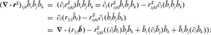 $$\begin{eqnarray}\displaystyle (\unicode[STIX]{x1D735}\boldsymbol{\cdot }\boldsymbol{r}^{\text{g}})_{ijk}\hat{b}_{i}\hat{b}_{j}\hat{b}_{k} & = & \displaystyle (\unicode[STIX]{x2202}_{l}r_{ijkl}^{\text{g}})\hat{b}_{i}\hat{b}_{j}\hat{b}_{k}=\unicode[STIX]{x2202}_{l}(r_{ijkl}^{\text{g}}\hat{b}_{i}\hat{b}_{j}\hat{b}_{k})-r_{ijkl}^{\text{g}}\unicode[STIX]{x2202}_{l}(\hat{b}_{i}\hat{b}_{j}\hat{b}_{k})\nonumber\\ \displaystyle & = & \displaystyle \unicode[STIX]{x2202}_{l}(r_{\Vert \Vert }\hat{b}_{l})-r_{ijkl}^{\text{g}}\unicode[STIX]{x2202}_{l}(\hat{b}_{i}\hat{b}_{j}\hat{b}_{k})\nonumber\\ \displaystyle & = & \displaystyle \unicode[STIX]{x1D735}\boldsymbol{\cdot }(r_{\Vert \Vert }\hat{\boldsymbol{b}})-r_{ijkl}^{\text{g}}((\unicode[STIX]{x2202}_{l}\hat{b}_{i})\hat{b}_{j}\hat{b}_{k}+\hat{b}_{i}(\unicode[STIX]{x2202}_{l}\hat{b}_{j})\hat{b}_{k}+\hat{b}_{i}\hat{b}_{j}(\unicode[STIX]{x2202}_{l}\hat{b}_{k}));\end{eqnarray}$$
 $$\begin{eqnarray}\displaystyle & \displaystyle r_{ijkl}^{\text{g}}\hat{b}_{j}\hat{b}_{k}=r_{\Vert \Vert }\hat{b}_{i}\hat{b}_{l}+r_{\Vert \bot }[\unicode[STIX]{x1D6FF}_{il}-\hat{b}_{i}\hat{b}_{l}]; & \displaystyle\end{eqnarray}$$
 $$\begin{eqnarray}\displaystyle & \displaystyle r_{ijkl}^{\text{g}}\hat{b}_{j}\hat{b}_{k}\unicode[STIX]{x2202}_{l}\hat{b}_{i}=r_{\Vert \bot }\unicode[STIX]{x1D735}\boldsymbol{\cdot }\hat{\boldsymbol{b}}; & \displaystyle\end{eqnarray}$$
 $$\begin{eqnarray}\displaystyle & \displaystyle (\unicode[STIX]{x1D735}\boldsymbol{\cdot }\boldsymbol{r}^{\text{g}})_{ijk}\hat{b}_{i}\hat{b}_{j}\hat{b}_{k}=\unicode[STIX]{x1D735}\boldsymbol{\cdot }(r_{\Vert \Vert }\hat{\boldsymbol{b}})-3r_{\Vert \bot }\unicode[STIX]{x1D735}\boldsymbol{\cdot }\hat{\boldsymbol{b}}, & \displaystyle\end{eqnarray}$$
and the second expression calculates similarly as
 $$\begin{eqnarray}\displaystyle & \displaystyle (\unicode[STIX]{x1D735}\boldsymbol{\cdot }\boldsymbol{r}^{\text{g}})_{ijk}\unicode[STIX]{x1D6FF}_{ij}\hat{b}_{k}=(\unicode[STIX]{x2202}_{l}r_{iikl}^{\text{g}})\hat{b}_{k}=\unicode[STIX]{x2202}_{l}(r_{iikl}^{\text{g}}\hat{b}_{k})-r_{iikl}^{\text{g}}\unicode[STIX]{x2202}_{l}\hat{b}_{k}; & \displaystyle\end{eqnarray}$$
 $$\begin{eqnarray}\displaystyle & \displaystyle r_{iikl}^{\text{g}}\hat{b}_{k}=r_{\Vert \Vert }\hat{b}_{l}+2r_{\Vert \bot }\hat{b}_{l}; & \displaystyle\end{eqnarray}$$
 $$\begin{eqnarray}\displaystyle & \displaystyle r_{iikl}^{\text{g}}\unicode[STIX]{x2202}_{l}\hat{b}_{k}=(r_{\Vert \bot }+2r_{\bot \bot })\unicode[STIX]{x1D735}\boldsymbol{\cdot }\hat{\boldsymbol{b}}; & \displaystyle\end{eqnarray}$$
 $$\begin{eqnarray}\displaystyle & \displaystyle (\unicode[STIX]{x1D735}\boldsymbol{\cdot }\boldsymbol{r}^{\text{g}})_{ijk}\unicode[STIX]{x1D6FF}_{ij}\hat{b}_{k}=\unicode[STIX]{x1D735}\boldsymbol{\cdot }(r_{\Vert \Vert }\hat{\boldsymbol{b}})+2\unicode[STIX]{x1D735}\boldsymbol{\cdot }(r_{\Vert \bot }\hat{\boldsymbol{b}})-(r_{\Vert \bot }+2r_{\bot \bot })\unicode[STIX]{x1D735}\boldsymbol{\cdot }\hat{\boldsymbol{b}}; & \displaystyle\end{eqnarray}$$
 $$\begin{eqnarray}\displaystyle & \displaystyle (\unicode[STIX]{x1D735}\boldsymbol{\cdot }\boldsymbol{r}^{\text{g}})_{ijk}(\unicode[STIX]{x1D6FF}_{ij}-\hat{b}_{i}\hat{b}_{j})\hat{b}_{k}/2=\unicode[STIX]{x1D735}\boldsymbol{\cdot }(r_{\Vert \bot }\hat{\boldsymbol{b}})+(r_{\Vert \bot }-r_{\bot \bot })\unicode[STIX]{x1D735}\boldsymbol{\cdot }\hat{\boldsymbol{b}}, & \displaystyle\end{eqnarray}$$
which verifies (7.94), (7.95).
Furthermore, by exploring the
 $\unicode[STIX]{x2202}\boldsymbol{r}/\unicode[STIX]{x2202}t$
equation (8.1), at frequencies that are much smaller than the gyrofrequency, the gyrotropic part of
$\unicode[STIX]{x2202}\boldsymbol{r}/\unicode[STIX]{x2202}t$
equation (8.1), at frequencies that are much smaller than the gyrofrequency, the gyrotropic part of
 $\boldsymbol{r}$
should satisfy
$\boldsymbol{r}$
should satisfy
 $$\begin{eqnarray}(\hat{\boldsymbol{b}}\times \boldsymbol{r}^{\text{g}})^{S}=0,\end{eqnarray}$$
in the same way that the gyrotropic parts of
 $\boldsymbol{p}$
and
$\boldsymbol{p}$
and
 $\boldsymbol{q}$
satisfied this requirement. By using the gyrotropic (8.10), it is easy to calculate for example that
$\boldsymbol{q}$
satisfied this requirement. By using the gyrotropic (8.10), it is easy to calculate for example that
 $$\begin{eqnarray}\displaystyle (\hat{\boldsymbol{b}}\times \boldsymbol{r}^{\text{g}})_{ijkl} & = & \displaystyle \unicode[STIX]{x1D716}_{irs}\hat{b}_{r}r_{sjkl}^{\text{g}}=r_{\Vert \bot }(\unicode[STIX]{x1D716}_{irj}\hat{b}_{r}\hat{b}_{k}\hat{b}_{l}+\unicode[STIX]{x1D716}_{irk}\hat{b}_{r}\hat{b}_{j}\hat{b}_{l}+\unicode[STIX]{x1D716}_{irl}\hat{b}_{r}\hat{b}_{j}\hat{b}_{k})\nonumber\\ \displaystyle & & \displaystyle +\,\frac{r_{\bot \bot }}{2}(\unicode[STIX]{x1D716}_{irj}\hat{b}_{r}\unicode[STIX]{x1D6FF}_{kl}+\unicode[STIX]{x1D716}_{irk}\hat{b}_{r}\unicode[STIX]{x1D6FF}_{jl}+\unicode[STIX]{x1D716}_{irl}\hat{b}_{r}\unicode[STIX]{x1D6FF}_{jk}-\unicode[STIX]{x1D716}_{irj}\hat{b}_{r}\hat{b}_{k}\hat{b}_{l}-\unicode[STIX]{x1D716}_{irk}\hat{b}_{r}\hat{b}_{j}\hat{b}_{l}-\unicode[STIX]{x1D716}_{irl}\hat{b}_{r}\hat{b}_{j}\hat{b}_{k}),\nonumber\\ \displaystyle & & \displaystyle\end{eqnarray}$$
and by adding together all the 4 representations of the ‘
 $S$
’ operator, one can indeed verify that all the terms cancel, yielding (8.32). By decomposing the entire fourth-order moment into its gyrotropic and non-gyrotropic parts
$S$
’ operator, one can indeed verify that all the terms cancel, yielding (8.32). By decomposing the entire fourth-order moment into its gyrotropic and non-gyrotropic parts
 $$\begin{eqnarray}\boldsymbol{r}=\boldsymbol{r}^{\text{g}}+\boldsymbol{r}^{\text{ng}},\end{eqnarray}$$
the evolution equation (8.1) can therefore be rewritten as
 $$\begin{eqnarray}\displaystyle \frac{\unicode[STIX]{x2202}}{\unicode[STIX]{x2202}t}\boldsymbol{r}+\unicode[STIX]{x1D735}\boldsymbol{\cdot }(\unicode[STIX]{x1D653}^{(5)}+\boldsymbol{u}\boldsymbol{r})+\left[\boldsymbol{r}\boldsymbol{\cdot }\unicode[STIX]{x1D735}\boldsymbol{u}+\unicode[STIX]{x1D6FA}\frac{|\boldsymbol{B}|}{B_{0}}\hat{\boldsymbol{b}}\times \boldsymbol{r}^{\text{ng}}-\frac{1}{\unicode[STIX]{x1D70C}}(\unicode[STIX]{x1D735}\boldsymbol{\cdot }\boldsymbol{p})\boldsymbol{q}\right]^{S}=0. & & \displaystyle\end{eqnarray}$$
8.1 Non-gyrotropic
$\boldsymbol{r}^{\text{ng}}$

Basic properties of the non-gyrotropic tensor
 $\boldsymbol{r}^{\text{ng}}$
can be easily determined with a similar procedure as those we used for the non-gyrotropic pressure
$\boldsymbol{r}^{\text{ng}}$
can be easily determined with a similar procedure as those we used for the non-gyrotropic pressure
 $\unicode[STIX]{x1D72B}$
and the non-gyrotropic heat flux
$\unicode[STIX]{x1D72B}$
and the non-gyrotropic heat flux
 $\boldsymbol{q}^{\text{ng}}$
. The decomposition of the entire fourth-order moment is
$\boldsymbol{q}^{\text{ng}}$
. The decomposition of the entire fourth-order moment is
 $$\begin{eqnarray}\boldsymbol{r}=r_{\Vert \Vert }\hat{\boldsymbol{b}}\hat{\boldsymbol{b}}\hat{\boldsymbol{b}}\hat{\boldsymbol{b}}+r_{\Vert \bot }[\hat{\boldsymbol{b}}\hat{\boldsymbol{b}}(\unicode[STIX]{x1D644}-\hat{\boldsymbol{b}}\hat{\boldsymbol{b}})]^{\text{Sym}}+r_{\bot \bot }[(\unicode[STIX]{x1D644}-\hat{\boldsymbol{b}}\hat{\boldsymbol{b}})(\unicode[STIX]{x1D644}-\hat{\boldsymbol{b}}\hat{\boldsymbol{b}})]^{\text{Sym}}+\boldsymbol{r}^{\text{ng}},\end{eqnarray}$$
and the meaning of the ‘Sym’ operators was specified by (8.8), (8.9). By using definitions (8.3), (8.4), (8.5) for
 $r_{\Vert \Vert }$
,
$r_{\Vert \Vert }$
,
 $r_{\Vert \bot }$
,
$r_{\Vert \bot }$
,
 $r_{\bot \bot }$
in the expression above, the full decomposition reads
$r_{\bot \bot }$
in the expression above, the full decomposition reads
 $$\begin{eqnarray}\displaystyle \boldsymbol{r} & = & \displaystyle [(\boldsymbol{r}:\hat{\boldsymbol{b}}\hat{\boldsymbol{b}}):(\hat{\boldsymbol{b}}\hat{\boldsymbol{b}})]\hat{\boldsymbol{b}}\hat{\boldsymbol{b}}\hat{\boldsymbol{b}}\hat{\boldsymbol{b}}+[(\boldsymbol{r}:\hat{\boldsymbol{b}}\hat{\boldsymbol{b}}):(\unicode[STIX]{x1D644}-\hat{\boldsymbol{b}}\hat{\boldsymbol{b}})/2][\hat{\boldsymbol{b}}\hat{\boldsymbol{b}}(\unicode[STIX]{x1D644}-\hat{\boldsymbol{b}}\hat{\boldsymbol{b}})]^{\text{Sym}}\nonumber\\ \displaystyle & & \displaystyle +\,[(\boldsymbol{r}:(\unicode[STIX]{x1D644}-\hat{\boldsymbol{b}}\hat{\boldsymbol{b}})/2):(\unicode[STIX]{x1D644}-\hat{\boldsymbol{b}}\hat{\boldsymbol{b}})/2][(\unicode[STIX]{x1D644}-\hat{\boldsymbol{b}}\hat{\boldsymbol{b}})(\unicode[STIX]{x1D644}-\hat{\boldsymbol{b}}\hat{\boldsymbol{b}})]^{\text{Sym}}+\boldsymbol{r}^{\text{ng}}.\end{eqnarray}$$
Now, applying
 $:\hat{\boldsymbol{b}}\hat{\boldsymbol{b}}$
twice to both sides of the equation yields
$:\hat{\boldsymbol{b}}\hat{\boldsymbol{b}}$
twice to both sides of the equation yields
 $(\boldsymbol{r}:\hat{\boldsymbol{b}}\hat{\boldsymbol{b}}):(\hat{\boldsymbol{b}}\hat{\boldsymbol{b}})=(\boldsymbol{r}:\hat{\boldsymbol{b}}\hat{\boldsymbol{b}}):(\hat{\boldsymbol{b}}\hat{\boldsymbol{b}})+(\boldsymbol{r}^{\text{ng}}:\hat{\boldsymbol{b}}\hat{\boldsymbol{b}}):(\hat{\boldsymbol{b}}\hat{\boldsymbol{b}})$
, implying
$(\boldsymbol{r}:\hat{\boldsymbol{b}}\hat{\boldsymbol{b}}):(\hat{\boldsymbol{b}}\hat{\boldsymbol{b}})=(\boldsymbol{r}:\hat{\boldsymbol{b}}\hat{\boldsymbol{b}}):(\hat{\boldsymbol{b}}\hat{\boldsymbol{b}})+(\boldsymbol{r}^{\text{ng}}:\hat{\boldsymbol{b}}\hat{\boldsymbol{b}}):(\hat{\boldsymbol{b}}\hat{\boldsymbol{b}})$
, implying
 $(\boldsymbol{r}^{\text{ng}}:\hat{\boldsymbol{b}}\hat{\boldsymbol{b}}):(\hat{\boldsymbol{b}}\hat{\boldsymbol{b}})=0$
, which can be also rewritten as
$(\boldsymbol{r}^{\text{ng}}:\hat{\boldsymbol{b}}\hat{\boldsymbol{b}}):(\hat{\boldsymbol{b}}\hat{\boldsymbol{b}})=0$
, which can be also rewritten as
 $$\begin{eqnarray}\hat{\boldsymbol{b}}\hat{\boldsymbol{b}}:\boldsymbol{r}^{\text{ng}}:\hat{\boldsymbol{b}}\hat{\boldsymbol{b}}=0.\end{eqnarray}$$
Similarly, the other two properties are derived by either applying
 $:\hat{\boldsymbol{b}}$
and
$:\hat{\boldsymbol{b}}$
and
 $:(\unicode[STIX]{x1D644}-\hat{\boldsymbol{b}}\hat{\boldsymbol{b}})$
, or twice
$:(\unicode[STIX]{x1D644}-\hat{\boldsymbol{b}}\hat{\boldsymbol{b}})$
, or twice
 $:(\unicode[STIX]{x1D644}-\hat{\boldsymbol{b}}\hat{\boldsymbol{b}})$
, yielding
$:(\unicode[STIX]{x1D644}-\hat{\boldsymbol{b}}\hat{\boldsymbol{b}})$
, yielding
 $$\begin{eqnarray}(\unicode[STIX]{x1D644}-\hat{\boldsymbol{b}}\hat{\boldsymbol{b}}):\boldsymbol{r}^{\text{ng}}:\hat{\boldsymbol{b}}\hat{\boldsymbol{b}}=0;\quad (\unicode[STIX]{x1D644}-\hat{\boldsymbol{b}}\hat{\boldsymbol{b}}):\boldsymbol{r}^{\text{ng}}:(\unicode[STIX]{x1D644}-\hat{\boldsymbol{b}}\hat{\boldsymbol{b}})=0,\end{eqnarray}$$
which, by using the property (8.38), are further reduced to
 $$\begin{eqnarray}\unicode[STIX]{x1D644}:\boldsymbol{r}^{\text{ng}}:\hat{\boldsymbol{b}}\hat{\boldsymbol{b}}=0;\quad \unicode[STIX]{x1D644}:\boldsymbol{r}^{\text{ng}}:\unicode[STIX]{x1D644}=0.\end{eqnarray}$$
The last two properties can be also written as
 $\text{Tr}\,\boldsymbol{r}^{\text{ng}}:\hat{\boldsymbol{b}}\hat{\boldsymbol{b}}=0$
,
$\text{Tr}\,\boldsymbol{r}^{\text{ng}}:\hat{\boldsymbol{b}}\hat{\boldsymbol{b}}=0$
,
 $\text{Tr}\,\text{Tr}\,\boldsymbol{r}^{\text{ng}}=0$
. Finally, writing all 3 properties in the index notation
$\text{Tr}\,\text{Tr}\,\boldsymbol{r}^{\text{ng}}=0$
. Finally, writing all 3 properties in the index notation
 $$\begin{eqnarray}r_{ijkl}^{\text{ng}}\hat{b}_{i}\hat{b}_{j}\hat{b}_{k}\hat{b}_{l}=0;\quad r_{iikl}^{\text{ng}}\hat{b}_{k}\hat{b}_{l}=0;\quad r_{iikk}^{\text{ng}}=0.\end{eqnarray}$$
One would assume that the non-gyrotropic
 $\boldsymbol{r}^{\text{ng}}$
can be evaluated by rewriting (8.35) as
$\boldsymbol{r}^{\text{ng}}$
can be evaluated by rewriting (8.35) as
 $$\begin{eqnarray}\displaystyle (\hat{\boldsymbol{b}}\times \boldsymbol{r}^{\text{ng}})^{S}=-\frac{B_{0}}{\unicode[STIX]{x1D6FA}|\boldsymbol{B}|}\left[\frac{\unicode[STIX]{x2202}}{\unicode[STIX]{x2202}t}\boldsymbol{r}+\unicode[STIX]{x1D735}\boldsymbol{\cdot }(\unicode[STIX]{x1D653}^{(5)}+\boldsymbol{u}\boldsymbol{r})+\left(\boldsymbol{r}\boldsymbol{\cdot }\unicode[STIX]{x1D735}\boldsymbol{u}-\frac{1}{\unicode[STIX]{x1D70C}}(\unicode[STIX]{x1D735}\boldsymbol{\cdot }\boldsymbol{p})\boldsymbol{q}\right)^{S}\right], & & \displaystyle\end{eqnarray}$$
and then expanding the right-hand side similarly to what we did for the non-gyrotropic
 $\unicode[STIX]{x1D72B}$
(and also the non-gyrotropic heat flux vectors in appendix D). However, the equation does not seem to yield anything useful. Instead, one needs to consider a specific example of a bi-Maxwellian distribution function.
$\unicode[STIX]{x1D72B}$
(and also the non-gyrotropic heat flux vectors in appendix D). However, the equation does not seem to yield anything useful. Instead, one needs to consider a specific example of a bi-Maxwellian distribution function.
8.2 Bi-Maxwellian distribution
Here we consider a special case of a bi-Maxwellian distribution function
 $$\begin{eqnarray}f_{0}=n\left(\frac{m}{2\unicode[STIX]{x03C0}}\right)^{3/2}\frac{1}{T_{\Vert }^{1/2}T_{\bot }}\exp \left[-m\frac{(v_{\Vert }-u_{\Vert })^{2}}{2T_{\Vert }}-m\frac{|\boldsymbol{v}_{\bot }-\boldsymbol{u}_{\bot }|^{2}}{2T_{\bot }}\right].\end{eqnarray}$$
It is useful to use the fluctuating velocity
 $\boldsymbol{c}=\boldsymbol{v}-\boldsymbol{u}$
, where
$\boldsymbol{c}=\boldsymbol{v}-\boldsymbol{u}$
, where
 $c^{2}=c_{\Vert }^{2}+c_{\bot }^{2}$
and
$c^{2}=c_{\Vert }^{2}+c_{\bot }^{2}$
and
 $c_{\bot }^{2}=c_{x}^{2}+c_{y}^{2}$
. For brevity of the calculations we introduce
$c_{\bot }^{2}=c_{x}^{2}+c_{y}^{2}$
. For brevity of the calculations we introduce
 $$\begin{eqnarray}\unicode[STIX]{x1D6FC}_{\Vert }\equiv \frac{m}{2T_{\Vert }}=\frac{1}{v_{\text{th}\Vert }^{2}};\quad \unicode[STIX]{x1D6FC}_{\bot }\equiv \frac{m}{2T_{\bot }}=\frac{1}{v_{\text{th}\bot }^{2}},\end{eqnarray}$$
where here the thermal speeds are meant to be spatially dependent, i.e. they are written with
 $T$
and not with
$T$
and not with
 $T^{(0)}$
. The bi-Maxwellian distribution therefore reads
$T^{(0)}$
. The bi-Maxwellian distribution therefore reads
 $$\begin{eqnarray}f_{0}=n\sqrt{\frac{\unicode[STIX]{x1D6FC}_{\Vert }}{\unicode[STIX]{x03C0}}}\frac{\unicode[STIX]{x1D6FC}_{\bot }}{\unicode[STIX]{x03C0}}\text{e}^{-\unicode[STIX]{x1D6FC}_{\Vert }c_{\Vert }^{2}}\text{e}^{-\unicode[STIX]{x1D6FC}_{\bot }c_{\bot }^{2}}.\end{eqnarray}$$
It is useful to remind ourselves of the following one-dimensional integrals
 $$\begin{eqnarray}\int _{-\infty }^{\infty }\text{e}^{-\unicode[STIX]{x1D6FC}x^{2}}\,\text{d}x=\sqrt{\frac{\unicode[STIX]{x03C0}}{\unicode[STIX]{x1D6FC}}};\quad \int _{-\infty }^{\infty }x^{2}\text{e}^{-\unicode[STIX]{x1D6FC}x^{2}}\,\text{d}x=\frac{1}{2}\sqrt{\frac{\unicode[STIX]{x03C0}}{\unicode[STIX]{x1D6FC}^{3}}};\quad \int _{-\infty }^{\infty }x^{4}\text{e}^{-\unicode[STIX]{x1D6FC}x^{2}}\,\text{d}x=\frac{3}{4}\sqrt{\frac{\unicode[STIX]{x03C0}}{\unicode[STIX]{x1D6FC}^{5}}},\end{eqnarray}$$
and that the general integral with
 $x^{n}$
, where
$x^{n}$
, where
 $n$
is an integer, reads
$n$
is an integer, reads
 $$\begin{eqnarray}\displaystyle \int _{-\infty }^{\infty }x^{n}\text{e}^{-\unicode[STIX]{x1D6FC}x^{2}}\,\text{d}x & = & \displaystyle \frac{(n-1)!!}{2^{n/2}}\sqrt{\frac{\unicode[STIX]{x03C0}}{\unicode[STIX]{x1D6FC}^{n+1}}};\quad n=0,2,4\ldots \quad (n=\text{even});\end{eqnarray}$$
 $$\begin{eqnarray}\displaystyle & = & \displaystyle 0;\qquad \qquad \qquad \quad \;\;n=1,3,5\ldots \quad (n=\text{odd}).\end{eqnarray}$$
The double factorial
 $(n-1)!!=1\cdot 3\cdot 5\cdots (n-1)$
, with
$(n-1)!!=1\cdot 3\cdot 5\cdots (n-1)$
, with
 $(-1)!!=1$
. The identity (8.47) is easily obtained by performing differentiation
$(-1)!!=1$
. The identity (8.47) is easily obtained by performing differentiation
 $\unicode[STIX]{x2202}/\unicode[STIX]{x2202}\unicode[STIX]{x1D6FC}$
of the first result in (8.46), and this technique is useful in the calculation of the fluid moments.
$\unicode[STIX]{x2202}/\unicode[STIX]{x2202}\unicode[STIX]{x1D6FC}$
of the first result in (8.46), and this technique is useful in the calculation of the fluid moments.
To become more familiar with the bi-Maxwellian distribution, it is useful to verify whether integrals over
 $f_{0}$
indeed yield the expected fluid moments. Since the macroscopic velocity
$f_{0}$
indeed yield the expected fluid moments. Since the macroscopic velocity
 $\boldsymbol{u}$
is independent of
$\boldsymbol{u}$
is independent of
 $\boldsymbol{v}$
, changing from variable
$\boldsymbol{v}$
, changing from variable
 $\boldsymbol{v}$
to
$\boldsymbol{v}$
to
 $\boldsymbol{c}$
just yields
$\boldsymbol{c}$
just yields
 $\text{d}^{3}v=\text{d}^{3}c$
(similarly to the substitution
$\text{d}^{3}v=\text{d}^{3}c$
(similarly to the substitution
 $y=x+\text{const.}$
that yields
$y=x+\text{const.}$
that yields
 $\text{d}y=\,\text{d}x$
). We use the notations
$\text{d}y=\,\text{d}x$
). We use the notations
 $\text{d}^{3}c=\text{d}c_{\Vert }\,\text{d}^{2}c_{\bot }$
and
$\text{d}^{3}c=\text{d}c_{\Vert }\,\text{d}^{2}c_{\bot }$
and
 $\text{d}^{2}c_{\bot }=\text{d}c_{x}\,\text{d}c_{y}$
. Also, because the integrals are evaluated from
$\text{d}^{2}c_{\bot }=\text{d}c_{x}\,\text{d}c_{y}$
. Also, because the integrals are evaluated from
 $-\infty$
to
$-\infty$
to
 $\infty$
, substitution from
$\infty$
, substitution from
 $\boldsymbol{v}$
to
$\boldsymbol{v}$
to
 $\boldsymbol{c}$
does not change these bounds. Integration in velocity space therefore yields
$\boldsymbol{c}$
does not change these bounds. Integration in velocity space therefore yields
 $$\begin{eqnarray}\displaystyle \int _{-\infty }^{\infty }\text{e}^{-\unicode[STIX]{x1D6FC}_{\Vert }c_{\Vert }^{2}}\,\text{d}c_{\Vert }=\sqrt{\frac{\unicode[STIX]{x03C0}}{\unicode[STIX]{x1D6FC}_{\Vert }}};\quad \int _{-\infty }^{\infty }\text{e}^{-\unicode[STIX]{x1D6FC}_{\bot }c_{\bot }^{2}}\,\text{d}^{2}c_{\bot }=\int \text{e}^{-\unicode[STIX]{x1D6FC}_{\bot }(c_{x}^{2}+c_{y}^{2})}\,\text{d}c_{x}\,\text{d}c_{y}=\frac{\unicode[STIX]{x03C0}}{\unicode[STIX]{x1D6FC}_{\bot }}. & & \displaystyle\end{eqnarray}$$
For simplicity we have integrated in Cartesian coordinates (instead of perhaps the more elegant cylindrical coordinates), which has an additional benefit in that we can stop writing the integral bounds, since the integrals are always from
 $-\infty$
to
$-\infty$
to
 $\infty$
. By using the bi-Maxwellian
$\infty$
. By using the bi-Maxwellian
 $f_{0}$
it is very easy to verify that
$f_{0}$
it is very easy to verify that
 $$\begin{eqnarray}n=\int f_{0}\,\text{d}^{3}v;\quad n\boldsymbol{u}=\int \boldsymbol{v}f_{0}\,\text{d}^{3}v;\quad p_{\Vert }=m\int c_{\Vert }^{2}f_{0}\,\text{d}^{3}v;\quad p_{\bot }=\frac{m}{2}\int c_{\bot }^{2}f_{0}\,\text{d}^{3}v.\end{eqnarray}$$
Continuing with the heat flux components yields
 $$\begin{eqnarray}\displaystyle & \displaystyle q_{\Vert }=m\int c_{\Vert }^{3}f_{0}\,\text{d}^{3}v=mn\sqrt{\frac{\unicode[STIX]{x1D6FC}_{\Vert }}{\unicode[STIX]{x03C0}}}\underbrace{\int c_{\Vert }^{3}\text{e}^{-\unicode[STIX]{x1D6FC}_{\Vert }c_{\Vert }^{2}}\,\text{d}c_{\Vert }}_{=0}\frac{\unicode[STIX]{x1D6FC}_{\bot }}{\unicode[STIX]{x03C0}}\int \text{e}^{-\unicode[STIX]{x1D6FC}_{\bot }c_{\bot }^{2}}\,\text{d}^{2}c_{\bot }=0; & \displaystyle\end{eqnarray}$$
 $$\begin{eqnarray}\displaystyle & \displaystyle q_{\bot }=\frac{m}{2}\int c_{\Vert }c_{\bot }^{2}f_{0}\,\text{d}^{3}v=\frac{m}{2}n\sqrt{\frac{\unicode[STIX]{x1D6FC}_{\Vert }}{\unicode[STIX]{x03C0}}}\underbrace{\int c_{\Vert }\text{e}^{-\unicode[STIX]{x1D6FC}_{\Vert }c_{\Vert }^{2}}\,\text{d}c_{\Vert }}_{=0}\frac{\unicode[STIX]{x1D6FC}_{\bot }}{\unicode[STIX]{x03C0}}\int c_{\bot }^{2}\text{e}^{-\unicode[STIX]{x1D6FC}_{\bot }c_{\bot }^{2}}\,\text{d}^{2}c_{\bot }=0. & \displaystyle\end{eqnarray}$$
It is important to emphasize that the zero heat flux values were obtained by assuming some prescribed equilibrium
 $f_{0}$
, here bi-Maxwellian. A crucial principle used in constructing fluid models with higher-order moments is that the specific
$f_{0}$
, here bi-Maxwellian. A crucial principle used in constructing fluid models with higher-order moments is that the specific
 $f_{0}$
is assumed only for the last retained moment. Indeed, if one closes the hierarchy by prescribing
$f_{0}$
is assumed only for the last retained moment. Indeed, if one closes the hierarchy by prescribing
 $q_{\Vert }=0,q_{\bot }=0$
, the CGL fluid model is obtained. However, to go higher in the fluid hierarchy, evolution equations for
$q_{\Vert }=0,q_{\bot }=0$
, the CGL fluid model is obtained. However, to go higher in the fluid hierarchy, evolution equations for
 $q_{\Vert }$
and
$q_{\Vert }$
and
 $q_{\bot }$
cannot be eliminated, even if the hierarchy will be eventually closed, for example at the fourth-order moment level, by assuming a bi-Maxwellian
$q_{\bot }$
cannot be eliminated, even if the hierarchy will be eventually closed, for example at the fourth-order moment level, by assuming a bi-Maxwellian
 $f_{0}$
. Or in another words, the zero heat flux values were obtained for a distribution function that is strictly
$f_{0}$
. Or in another words, the zero heat flux values were obtained for a distribution function that is strictly
 $f_{0}$
, however, fluctuations/perturbations around
$f_{0}$
, however, fluctuations/perturbations around
 $f_{0}$
are still allowed. Therefore, to obtain the next available model after the CGL, the heat flux equations must be retained, and a closure is performed on the fourth-order moment. Only this last moment is calculated by assuming a specific distribution function, that is strictly
$f_{0}$
are still allowed. Therefore, to obtain the next available model after the CGL, the heat flux equations must be retained, and a closure is performed on the fourth-order moment. Only this last moment is calculated by assuming a specific distribution function, that is strictly
 $f_{0}$
. For a bi-Maxwellian, the gyrotropic fourth-order moments are calculated according to
$f_{0}$
. For a bi-Maxwellian, the gyrotropic fourth-order moments are calculated according to
 $$\begin{eqnarray}\displaystyle r_{\Vert \Vert }\equiv m\int c_{\Vert }^{4}f_{0}\,\text{d}^{3}v & = & \displaystyle mn\underbrace{\sqrt{\frac{\unicode[STIX]{x1D6FC}_{\Vert }}{\unicode[STIX]{x03C0}}}\int c_{\Vert }^{4}\text{e}^{-\unicode[STIX]{x1D6FC}_{\Vert }c_{\Vert }^{2}}\,\text{d}c_{\Vert }}_{=3/(4\unicode[STIX]{x1D6FC}_{\Vert }^{2})}\underbrace{\frac{\unicode[STIX]{x1D6FC}_{\bot }}{\unicode[STIX]{x03C0}}\int \text{e}^{-\unicode[STIX]{x1D6FC}_{\bot }c_{\bot }^{2}}\,\text{d}^{2}c_{\bot }}_{=1}\nonumber\\ \displaystyle & = & \displaystyle \frac{3}{4}\frac{mn}{\unicode[STIX]{x1D6FC}_{\Vert }^{2}}=3\frac{n^{2}T_{\Vert }^{2}}{nm}=3\frac{p_{\Vert }^{2}}{\unicode[STIX]{x1D70C}};\end{eqnarray}$$
 $$\begin{eqnarray}\displaystyle r_{\Vert \bot }\equiv \frac{m}{2}\int c_{\Vert }^{2}c_{\bot }^{2}f_{0}\,\text{d}^{3}v & = & \displaystyle \frac{m}{2}n\underbrace{\sqrt{\frac{\unicode[STIX]{x1D6FC}_{\Vert }}{\unicode[STIX]{x03C0}}}\int c_{\Vert }^{2}\text{e}^{-\unicode[STIX]{x1D6FC}_{\Vert }c_{\Vert }^{2}}\,\text{d}c_{\Vert }}_{=1/(2\unicode[STIX]{x1D6FC}_{\Vert })}\underbrace{\frac{\unicode[STIX]{x1D6FC}_{\bot }}{\unicode[STIX]{x03C0}}\int c_{\bot }^{2}\text{e}^{-\unicode[STIX]{x1D6FC}_{\bot }c_{\bot }^{2}}\,\text{d}^{2}c_{\bot }}_{=1/\unicode[STIX]{x1D6FC}_{\bot }}\nonumber\\ \displaystyle & = & \displaystyle \frac{mn}{4\unicode[STIX]{x1D6FC}_{\Vert }\unicode[STIX]{x1D6FC}_{\bot }}=\frac{n^{2}T_{\Vert }T_{\bot }}{mn}=\frac{p_{\Vert }p_{\bot }}{\unicode[STIX]{x1D70C}};\end{eqnarray}$$
 $$\begin{eqnarray}\displaystyle r_{\bot \bot }\equiv \frac{m}{4}\int c_{\bot }^{4}f_{0}\,\text{d}^{3}v & = & \displaystyle \frac{m}{4}n\underbrace{\sqrt{\frac{\unicode[STIX]{x1D6FC}_{\Vert }}{\unicode[STIX]{x03C0}}}\int \text{e}^{-\unicode[STIX]{x1D6FC}_{\Vert }c_{\Vert }^{2}}\,\text{d}c_{\Vert }}_{=1}\underbrace{\frac{\unicode[STIX]{x1D6FC}_{\bot }}{\unicode[STIX]{x03C0}}\int c_{\bot }^{4}\text{e}^{-\unicode[STIX]{x1D6FC}_{\bot }c_{\bot }^{2}}\,\text{d}^{2}c_{\bot }}_{=2/\unicode[STIX]{x1D6FC}_{\bot }^{2}}\nonumber\\ \displaystyle & = & \displaystyle \frac{mn}{2\unicode[STIX]{x1D6FC}_{\bot }^{2}}=2\frac{n^{2}T_{\bot }^{2}}{mn}=2\frac{p_{\bot }^{2}}{\unicode[STIX]{x1D70C}}.\end{eqnarray}$$
Therefore, for a bi-Maxwellian, the following closure can be constructed
 $$\begin{eqnarray}r_{\Vert \Vert }=\frac{3p_{\Vert }^{2}}{\unicode[STIX]{x1D70C}};\quad r_{\Vert \bot }=\frac{p_{\Vert }p_{\bot }}{\unicode[STIX]{x1D70C}};\quad r_{\bot \bot }=\frac{2p_{\bot }^{2}}{\unicode[STIX]{x1D70C}},\end{eqnarray}$$
and this closure is known as the ‘normal’ closure, a name suggested by Chust & Belmont (Reference Chust and Belmont2006).
8.3 Bi-Maxwellian non-gyrotropic
$\boldsymbol{r}^{\text{ng}}$
contributions

Let us consider a specific case of a bi-Maxwellian distribution function. Then, an expansion procedure analogous to the one developed by Grad (Reference Grad1949) for rarefied gases can be used, where the distribution function is expanded in a series of Hermite polynomials. By keeping only the first few terms, one can express the fourth-order moment through the second-order (pressure) moments. The procedure is written down in Oraevskii et al. (Reference Oraevskii, Chodura and Feneberg1968), and the entire fourth-order moment can be decomposed in the following way: see (2.31) in Oraevskii et al. (Reference Oraevskii, Chodura and Feneberg1968) (where a small typo on the left-hand side is present, where instead of
 $q_{\unicode[STIX]{x1D6FC}\unicode[STIX]{x1D6FD}\unicode[STIX]{x1D6FE}\unicode[STIX]{x1D716}}$
, there should be
$q_{\unicode[STIX]{x1D6FC}\unicode[STIX]{x1D6FD}\unicode[STIX]{x1D6FE}\unicode[STIX]{x1D716}}$
, there should be
 $q_{\unicode[STIX]{x1D6FC}\unicode[STIX]{x1D6FD}\unicode[STIX]{x1D6FE}\unicode[STIX]{x1D6FF}}$
), equation (24) in Goswami et al. (Reference Goswami, Passot and Sulem2005), equation (9) in Passot & Sulem (Reference Passot and Sulem2007)
$q_{\unicode[STIX]{x1D6FC}\unicode[STIX]{x1D6FD}\unicode[STIX]{x1D6FE}\unicode[STIX]{x1D6FF}}$
), equation (24) in Goswami et al. (Reference Goswami, Passot and Sulem2005), equation (9) in Passot & Sulem (Reference Passot and Sulem2007)
 $$\begin{eqnarray}\unicode[STIX]{x1D70C}r_{ijkl}=p_{ij}^{\text{g}}p_{kl}^{\text{g}}+p_{ik}^{\text{g}}p_{jl}^{\text{g}}+p_{il}^{\text{g}}p_{jk}^{\text{g}}+\unicode[STIX]{x1D70C}r_{ijkl}^{\text{ng}},\end{eqnarray}$$
where the non-gyrotropic contributions read
 $$\begin{eqnarray}\unicode[STIX]{x1D70C}r_{ijkl}^{\text{ng}}=p_{ij}^{\text{g}}\unicode[STIX]{x1D6F1}_{kl}+p_{ik}^{\text{g}}\unicode[STIX]{x1D6F1}_{jl}+p_{il}^{\text{g}}\unicode[STIX]{x1D6F1}_{jk}+\unicode[STIX]{x1D6F1}_{ij}p_{kl}^{\text{g}}+\unicode[STIX]{x1D6F1}_{ik}p_{jl}^{\text{g}}+\unicode[STIX]{x1D6F1}_{il}p_{jk}^{\text{g}},\end{eqnarray}$$
and where terms
 $\unicode[STIX]{x1D6F1}_{ij}\unicode[STIX]{x1D6F1}_{lk}+\unicode[STIX]{x1D6F1}_{ik}\unicode[STIX]{x1D6F1}_{jl}+\unicode[STIX]{x1D6F1}_{il}\unicode[STIX]{x1D6F1}_{jk}$
were neglected. By using
$\unicode[STIX]{x1D6F1}_{ij}\unicode[STIX]{x1D6F1}_{lk}+\unicode[STIX]{x1D6F1}_{ik}\unicode[STIX]{x1D6F1}_{jl}+\unicode[STIX]{x1D6F1}_{il}\unicode[STIX]{x1D6F1}_{jk}$
were neglected. By using
 $p_{ij}^{\text{g}}=p_{\Vert }\hat{b}_{i}\hat{b}_{j}+p_{\bot }(\unicode[STIX]{x1D6FF}_{ij}-\hat{b}_{i}\hat{b}_{j})$
, it can be indeed shown by direct straightforward calculation that the gyrotropic part
$p_{ij}^{\text{g}}=p_{\Vert }\hat{b}_{i}\hat{b}_{j}+p_{\bot }(\unicode[STIX]{x1D6FF}_{ij}-\hat{b}_{i}\hat{b}_{j})$
, it can be indeed shown by direct straightforward calculation that the gyrotropic part
 $$\begin{eqnarray}\displaystyle \unicode[STIX]{x1D70C}r_{ijkl}^{\text{g}} & = & \displaystyle p_{ij}^{\text{g}}p_{kl}^{\text{g}}+p_{ik}^{\text{g}}p_{jl}^{\text{g}}+p_{il}^{\text{g}}p_{jk}^{\text{g}}=3p_{\Vert }^{2}\hat{b}_{i}\hat{b}_{j}\hat{b}_{k}\hat{b}_{l}\nonumber\\ \displaystyle & & \displaystyle +\,p_{\Vert }p_{\bot }[\unicode[STIX]{x1D6FF}_{ij}\hat{b}_{k}\hat{b}_{l}+\unicode[STIX]{x1D6FF}_{ik}\hat{b}_{j}\hat{b}_{l}+\unicode[STIX]{x1D6FF}_{il}\hat{b}_{j}\hat{b}_{k}+\unicode[STIX]{x1D6FF}_{jk}\hat{b}_{i}\hat{b}_{l}+\unicode[STIX]{x1D6FF}_{jl}\hat{b}_{i}\hat{b}_{k}+\unicode[STIX]{x1D6FF}_{kl}\hat{b}_{i}\hat{b}_{j}-6\hat{b}_{i}\hat{b}_{j}\hat{b}_{k}\hat{b}_{l}]\nonumber\\ \displaystyle & & \displaystyle +\,p_{\bot }^{2}\left[\unicode[STIX]{x1D6FF}_{ij}\unicode[STIX]{x1D6FF}_{kl}+\unicode[STIX]{x1D6FF}_{ik}\unicode[STIX]{x1D6FF}_{jl}+\unicode[STIX]{x1D6FF}_{il}\unicode[STIX]{x1D6FF}_{jk}-\unicode[STIX]{x1D6FF}_{ij}\hat{b}_{k}\hat{b}_{l}-\unicode[STIX]{x1D6FF}_{ik}\hat{b}_{j}\hat{b}_{l}-\unicode[STIX]{x1D6FF}_{il}\hat{b}_{j}\hat{b}_{k}-\unicode[STIX]{x1D6FF}_{jk}\hat{b}_{i}\hat{b}_{l}\right.\nonumber\\ \displaystyle & & \displaystyle -\left.\unicode[STIX]{x1D6FF}_{jl}\hat{b}_{i}\hat{b}_{k}-\unicode[STIX]{x1D6FF}_{kl}\hat{b}_{i}\hat{b}_{j}+3\hat{b}_{i}\hat{b}_{j}\hat{b}_{k}\hat{b}_{l}\right].\end{eqnarray}$$
This agrees with the decomposition (8.10) valid for a general distribution function, after one specifies that for a bi-Maxwellian distribution
 $r_{\Vert \Vert }=3p_{\Vert }^{2}/\unicode[STIX]{x1D70C}$
,
$r_{\Vert \Vert }=3p_{\Vert }^{2}/\unicode[STIX]{x1D70C}$
,
 $r_{\Vert \bot }=p_{\Vert }p_{\bot }/\unicode[STIX]{x1D70C}$
and
$r_{\Vert \bot }=p_{\Vert }p_{\bot }/\unicode[STIX]{x1D70C}$
and
 $r_{\bot \bot }=2p_{\bot }^{2}/\unicode[STIX]{x1D70C}$
(last term in (8.10) contains
$r_{\bot \bot }=2p_{\bot }^{2}/\unicode[STIX]{x1D70C}$
(last term in (8.10) contains
 $r_{\bot \bot }/2$
).
$r_{\bot \bot }/2$
).
Now it is possible to calculate the non-gyrotropic contributions
 $\boldsymbol{r}^{\text{ng}}$
, by using (8.58). It is useful to pre-calculate the trace of (8.58) that reads
$\boldsymbol{r}^{\text{ng}}$
, by using (8.58). It is useful to pre-calculate the trace of (8.58) that reads
 $$\begin{eqnarray}\unicode[STIX]{x1D70C}r_{iikl}=(p_{\Vert }+6p_{\bot })\unicode[STIX]{x1D6F1}_{kl}+2(p_{\Vert }-p_{\bot })\hat{b}_{i}(\hat{b}_{k}\unicode[STIX]{x1D6F1}_{il}+\hat{b}_{l}\unicode[STIX]{x1D6F1}_{ik}).\end{eqnarray}$$
The two terms that enter the parallel and perpendicular heat flux equations (7.96), (7.97) calculate as
 $$\begin{eqnarray}\displaystyle \hat{\boldsymbol{b}}\boldsymbol{\cdot }(\unicode[STIX]{x1D735}\boldsymbol{\cdot }\boldsymbol{r}^{\text{ng}}):\hat{\boldsymbol{b}}\hat{\boldsymbol{b}}=\frac{3p_{\Vert }}{\unicode[STIX]{x1D70C}}(\unicode[STIX]{x1D735}\boldsymbol{\cdot }\unicode[STIX]{x1D72B})\boldsymbol{\cdot }\hat{\boldsymbol{b}}+\frac{3p_{\Vert }}{\unicode[STIX]{x1D70C}}(\hat{\boldsymbol{b}}\boldsymbol{\cdot }\unicode[STIX]{x1D735}\unicode[STIX]{x1D72B}):\hat{\boldsymbol{b}}\hat{\boldsymbol{b}}+3\left(\unicode[STIX]{x1D735}\frac{p_{\Vert }}{\unicode[STIX]{x1D70C}}\right)\boldsymbol{\cdot }\unicode[STIX]{x1D72B}\boldsymbol{\cdot }\hat{\boldsymbol{b}}; & & \displaystyle\end{eqnarray}$$
 $$\begin{eqnarray}\displaystyle \unicode[STIX]{x1D644}:(\unicode[STIX]{x1D735}\boldsymbol{\cdot }\boldsymbol{r}^{\text{ng}})\boldsymbol{\cdot }\hat{\boldsymbol{b}} & = & \displaystyle \left(\unicode[STIX]{x1D735}\frac{3p_{\Vert }+4p_{\bot }}{\unicode[STIX]{x1D70C}}\right)\boldsymbol{\cdot }\unicode[STIX]{x1D72B}\boldsymbol{\cdot }\hat{\boldsymbol{b}}+\frac{(3p_{\Vert }+4p_{\bot })}{\unicode[STIX]{x1D70C}}(\unicode[STIX]{x1D735}\boldsymbol{\cdot }\unicode[STIX]{x1D72B})\boldsymbol{\cdot }\hat{\boldsymbol{b}}\nonumber\\ \displaystyle & & \displaystyle +\,\frac{2}{\unicode[STIX]{x1D70C}}(p_{\Vert }-p_{\bot })[\unicode[STIX]{x1D72B}:(\unicode[STIX]{x1D735}\hat{\boldsymbol{b}})+(\hat{\boldsymbol{b}}\boldsymbol{\cdot }\unicode[STIX]{x1D735}\hat{\boldsymbol{b}})\boldsymbol{\cdot }\unicode[STIX]{x1D72B}\boldsymbol{\cdot }\hat{\boldsymbol{b}}+\hat{\boldsymbol{b}}\boldsymbol{\cdot }(\unicode[STIX]{x1D735}\unicode[STIX]{x1D72B}):\hat{\boldsymbol{b}}\hat{\boldsymbol{b}}].\end{eqnarray}$$
At this stage, we need to further simplify, and we keep only those terms that contribute at the linear level, yielding
 $$\begin{eqnarray}\displaystyle & \displaystyle \hat{\boldsymbol{b}}\boldsymbol{\cdot }(\unicode[STIX]{x1D735}\boldsymbol{\cdot }\boldsymbol{r}^{\text{ng}}):\hat{\boldsymbol{b}}\hat{\boldsymbol{b}}=\frac{3p_{\Vert }}{\unicode[STIX]{x1D70C}}(\unicode[STIX]{x1D735}\boldsymbol{\cdot }\unicode[STIX]{x1D72B})\boldsymbol{\cdot }\hat{\boldsymbol{b}}; & \displaystyle\end{eqnarray}$$
 $$\begin{eqnarray}\displaystyle & \displaystyle \unicode[STIX]{x1D644}:(\unicode[STIX]{x1D735}\boldsymbol{\cdot }\boldsymbol{r}^{\text{ng}})\boldsymbol{\cdot }\hat{\boldsymbol{b}}=\frac{(3p_{\Vert }+4p_{\bot })}{\unicode[STIX]{x1D70C}}(\unicode[STIX]{x1D735}\boldsymbol{\cdot }\unicode[STIX]{x1D72B})\boldsymbol{\cdot }\hat{\boldsymbol{b}}, & \displaystyle\end{eqnarray}$$
so the term entering the
 $q_{\bot }$
equation (7.97) reads
$q_{\bot }$
equation (7.97) reads
 $$\begin{eqnarray}\frac{1}{2}(\unicode[STIX]{x1D644}-\hat{\boldsymbol{b}}\hat{\boldsymbol{b}}):(\unicode[STIX]{x1D735}\boldsymbol{\cdot }\boldsymbol{r}^{\text{ng}})\boldsymbol{\cdot }\hat{\boldsymbol{b}}=\frac{2p_{\bot }}{\unicode[STIX]{x1D70C}}(\unicode[STIX]{x1D735}\boldsymbol{\cdot }\unicode[STIX]{x1D72B})\boldsymbol{\cdot }\hat{\boldsymbol{b}}.\end{eqnarray}$$
Note that
 $(\hat{\boldsymbol{b}}\boldsymbol{\cdot }\unicode[STIX]{x1D735}\unicode[STIX]{x1D72B}):\hat{\boldsymbol{b}}\hat{\boldsymbol{b}}=-\unicode[STIX]{x1D72B}:(\hat{\boldsymbol{b}}(\hat{\boldsymbol{b}}\boldsymbol{\cdot }\unicode[STIX]{x1D735})\hat{\boldsymbol{b}})^{S}$
, and the term does not contribute at the linear level. Of course, many nonlinear terms were neglected, and technically, the only fully consistent procedure is to explicitly write those terms at the linear level, in the form
$(\hat{\boldsymbol{b}}\boldsymbol{\cdot }\unicode[STIX]{x1D735}\unicode[STIX]{x1D72B}):\hat{\boldsymbol{b}}\hat{\boldsymbol{b}}=-\unicode[STIX]{x1D72B}:(\hat{\boldsymbol{b}}(\hat{\boldsymbol{b}}\boldsymbol{\cdot }\unicode[STIX]{x1D735})\hat{\boldsymbol{b}})^{S}$
, and the term does not contribute at the linear level. Of course, many nonlinear terms were neglected, and technically, the only fully consistent procedure is to explicitly write those terms at the linear level, in the form
 $$\begin{eqnarray}\displaystyle & \displaystyle \hat{\boldsymbol{b}}\boldsymbol{\cdot }(\unicode[STIX]{x1D735}\boldsymbol{\cdot }\boldsymbol{r}^{\text{ng}}):\hat{\boldsymbol{b}}\hat{\boldsymbol{b}}=\frac{3p_{\Vert }^{(0)}}{\unicode[STIX]{x1D70C}_{0}}(\unicode[STIX]{x1D735}\boldsymbol{\cdot }\unicode[STIX]{x1D72B})\boldsymbol{\cdot }\hat{\boldsymbol{b}}_{0}=\frac{3p_{\Vert }^{(0)}}{\unicode[STIX]{x1D70C}_{0}}(\unicode[STIX]{x2202}_{x}\unicode[STIX]{x1D6F1}_{xz}+\unicode[STIX]{x2202}_{y}\unicode[STIX]{x1D6F1}_{yz}); & \displaystyle\end{eqnarray}$$
 $$\begin{eqnarray}\displaystyle & \displaystyle \frac{1}{2}(\unicode[STIX]{x1D644}-\hat{\boldsymbol{b}}\hat{\boldsymbol{b}}):(\unicode[STIX]{x1D735}\boldsymbol{\cdot }\boldsymbol{r}^{\text{ng}})\boldsymbol{\cdot }\hat{\boldsymbol{b}}=\frac{2p_{\bot }^{(0)}}{\unicode[STIX]{x1D70C}_{0}}(\unicode[STIX]{x1D735}\boldsymbol{\cdot }\unicode[STIX]{x1D72B})\boldsymbol{\cdot }\hat{\boldsymbol{b}}_{0}=\frac{2p_{\bot }^{(0)}}{\unicode[STIX]{x1D70C}_{0}}(\unicode[STIX]{x2202}_{x}\unicode[STIX]{x1D6F1}_{xz}+\unicode[STIX]{x2202}_{y}\unicode[STIX]{x1D6F1}_{yz}). & \displaystyle\end{eqnarray}$$
The results show that, if the
 $\unicode[STIX]{x1D72B}$
contributions are kept in the heat flux equations, the
$\unicode[STIX]{x1D72B}$
contributions are kept in the heat flux equations, the
 $\boldsymbol{r}^{\text{ng}}$
contributions cannot just be straightforwardly neglected, since the
$\boldsymbol{r}^{\text{ng}}$
contributions cannot just be straightforwardly neglected, since the
 $\unicode[STIX]{x1D72B}$
and
$\unicode[STIX]{x1D72B}$
and
 $\boldsymbol{r}^{\text{ng}}$
contributions partially cancel out.
$\boldsymbol{r}^{\text{ng}}$
contributions partially cancel out.
9 Bi-Maxwellian fluid model, second-order CGL (CGL2)
In the previous section we have seen that for a bi-Maxwellian distribution function, one can close the fluid hierarchy by prescribing the ‘normal’ closure
 $$\begin{eqnarray}r_{\Vert \Vert }=\frac{3p_{\Vert }^{2}}{\unicode[STIX]{x1D70C}};\quad r_{\Vert \bot }=\frac{p_{\Vert }p_{\bot }}{\unicode[STIX]{x1D70C}};\quad r_{\bot \bot }=\frac{2p_{\bot }^{2}}{\unicode[STIX]{x1D70C}}.\end{eqnarray}$$
It is useful to summarize the fully nonlinear model that we want to consider here. We consider only proton species, and we make the electrons massless and cold. We simplify the pressure equations, by neglecting the FLR stress forces (which enter only nonlinearly), and we keep only those non-gyrotropic contributions in the pressure and heat flux equations that have a non-zero linear contributions. The nonlinear model reads
 $$\begin{eqnarray}\displaystyle & \displaystyle \frac{\unicode[STIX]{x2202}\unicode[STIX]{x1D70C}}{\unicode[STIX]{x2202}t}+\unicode[STIX]{x1D735}\boldsymbol{\cdot }(\unicode[STIX]{x1D70C}\boldsymbol{u})=0; & \displaystyle\end{eqnarray}$$
 $$\begin{eqnarray}\displaystyle & \displaystyle \frac{\unicode[STIX]{x2202}\boldsymbol{u}}{\unicode[STIX]{x2202}t}+\boldsymbol{u}\boldsymbol{\cdot }\unicode[STIX]{x1D735}\boldsymbol{u}+\frac{1}{\unicode[STIX]{x1D70C}}\unicode[STIX]{x1D735}\boldsymbol{\cdot }[p_{\Vert }\hat{\boldsymbol{b}}\hat{\boldsymbol{b}}+p_{\bot }(\unicode[STIX]{x1D644}-\hat{\boldsymbol{b}}\hat{\boldsymbol{b}})+\unicode[STIX]{x1D72B}]-\frac{1}{4\unicode[STIX]{x03C0}\unicode[STIX]{x1D70C}}(\unicode[STIX]{x1D735}\times \boldsymbol{B})\times \boldsymbol{B}=0; & \displaystyle\end{eqnarray}$$
 $$\begin{eqnarray}\displaystyle & \displaystyle \frac{\unicode[STIX]{x2202}\boldsymbol{B}}{\unicode[STIX]{x2202}t}=\unicode[STIX]{x1D735}\times (\boldsymbol{u}\times \boldsymbol{B})-\frac{1}{\unicode[STIX]{x1D6FA}_{p}}\frac{B_{0}}{4\unicode[STIX]{x03C0}}\unicode[STIX]{x1D735}\times \left[\frac{1}{\unicode[STIX]{x1D70C}}(\unicode[STIX]{x1D735}\times \boldsymbol{B})\times \boldsymbol{B}\right]; & \displaystyle\end{eqnarray}$$
 $$\begin{eqnarray}\displaystyle & \displaystyle \frac{\unicode[STIX]{x2202}p_{\Vert }}{\unicode[STIX]{x2202}t}+\boldsymbol{u}\boldsymbol{\cdot }\unicode[STIX]{x1D735}p_{\Vert }+p_{\Vert }\unicode[STIX]{x1D735}\boldsymbol{\cdot }\boldsymbol{u}+2p_{\Vert }\hat{\boldsymbol{b}}\boldsymbol{\cdot }\unicode[STIX]{x1D735}\boldsymbol{u}\boldsymbol{\cdot }\hat{\boldsymbol{b}}+\unicode[STIX]{x1D735}\boldsymbol{\cdot }(q_{\Vert }\hat{\boldsymbol{b}})-2q_{\bot }\unicode[STIX]{x1D735}\boldsymbol{\cdot }\hat{\boldsymbol{b}}+\unicode[STIX]{x1D735}\boldsymbol{\cdot }\boldsymbol{S}_{\bot }^{\Vert }=0; & \displaystyle\end{eqnarray}$$
 $$\begin{eqnarray}\displaystyle & \displaystyle \frac{\unicode[STIX]{x2202}p_{\bot }}{\unicode[STIX]{x2202}t}+\boldsymbol{u}\boldsymbol{\cdot }\unicode[STIX]{x1D735}p_{\bot }+2p_{\bot }\unicode[STIX]{x1D735}\boldsymbol{\cdot }\boldsymbol{u}-p_{\bot }\hat{\boldsymbol{b}}\boldsymbol{\cdot }\unicode[STIX]{x1D735}\boldsymbol{u}\boldsymbol{\cdot }\hat{\boldsymbol{b}}+\unicode[STIX]{x1D735}\boldsymbol{\cdot }(q_{\bot }\hat{\boldsymbol{b}})+q_{\bot }\unicode[STIX]{x1D735}\boldsymbol{\cdot }\hat{\boldsymbol{b}}+\unicode[STIX]{x1D735}\boldsymbol{\cdot }\boldsymbol{S}_{\bot }^{\bot }=0; & \displaystyle\end{eqnarray}$$
 $$\begin{eqnarray}\displaystyle & \displaystyle \frac{\unicode[STIX]{x2202}q_{\Vert }}{\unicode[STIX]{x2202}t}+\boldsymbol{u}\boldsymbol{\cdot }\unicode[STIX]{x1D735}q_{\Vert }+q_{\Vert }\unicode[STIX]{x1D735}\boldsymbol{\cdot }\boldsymbol{u}+3p_{\Vert }\hat{\boldsymbol{b}}\boldsymbol{\cdot }\unicode[STIX]{x1D735}\left(\frac{p_{\Vert }}{\unicode[STIX]{x1D70C}}\right)+3q_{\Vert }\hat{\boldsymbol{b}}\boldsymbol{\cdot }\unicode[STIX]{x1D735}\boldsymbol{u}\boldsymbol{\cdot }\hat{\boldsymbol{b}}=0; & \displaystyle\end{eqnarray}$$
 $$\begin{eqnarray}\displaystyle & \displaystyle \frac{\unicode[STIX]{x2202}q_{\bot }}{\unicode[STIX]{x2202}t}+\boldsymbol{u}\boldsymbol{\cdot }\unicode[STIX]{x1D735}q_{\bot }+2q_{\bot }\unicode[STIX]{x1D735}\boldsymbol{\cdot }\boldsymbol{u}+p_{\Vert }\hat{\boldsymbol{b}}\boldsymbol{\cdot }\unicode[STIX]{x1D735}\left(\frac{p_{\bot }}{\unicode[STIX]{x1D70C}}\right)+\frac{p_{\bot }}{\unicode[STIX]{x1D70C}}(p_{\Vert }-p_{\bot })\unicode[STIX]{x1D735}\boldsymbol{\cdot }\hat{\boldsymbol{b}}+\frac{p_{\bot }}{\unicode[STIX]{x1D70C}}(\unicode[STIX]{x1D735}\boldsymbol{\cdot }\unicode[STIX]{x1D72B})\boldsymbol{\cdot }\hat{\boldsymbol{b}}_{0}=0. & \displaystyle \nonumber\\ \displaystyle & & \displaystyle\end{eqnarray}$$
To develop a vocabulary, let us first consider the above fluid model with all the non-gyrotropic fluctuations neglected, i.e. when all the terms with
 $\unicode[STIX]{x1D72B}$
,
$\unicode[STIX]{x1D72B}$
,
 $\boldsymbol{S}_{\bot }^{\Vert }$
,
$\boldsymbol{S}_{\bot }^{\Vert }$
,
 $\boldsymbol{S}_{\bot }^{\bot }$
are neglected. Additionally, let us neglect the Hall term in the induction equation. Such a fluid model is non-dispersive, and represents a generalization of the non-dispersive CGL model. Even though such a fluid model was not explicitly considered by Chew, Goldberger and Low, the pressure equations that include the gyrotropic heat flux contributions
$\boldsymbol{S}_{\bot }^{\bot }$
are neglected. Additionally, let us neglect the Hall term in the induction equation. Such a fluid model is non-dispersive, and represents a generalization of the non-dispersive CGL model. Even though such a fluid model was not explicitly considered by Chew, Goldberger and Low, the pressure equations that include the gyrotropic heat flux contributions
 $q_{\Vert },q_{\bot }$
, were indeed given by Chew et al. (Reference Chew, Goldberger and Low1956). As discussed previously, the authors just used a different notation with
$q_{\Vert },q_{\bot }$
, were indeed given by Chew et al. (Reference Chew, Goldberger and Low1956). As discussed previously, the authors just used a different notation with
 $q_{n}=q_{\Vert }-3q_{\bot }$
and
$q_{n}=q_{\Vert }-3q_{\bot }$
and
 $q_{s}=q_{\bot }$
, but their pressure equations contain the gyrotropic heat flux. The authors did not consider evolution equations for the gyrotropic heat fluxes, equations (9.7), (9.8). Nevertheless, the name CGL is so well recognized by the community, i.e. the name CGL is essentially recognized as the collisionless MHD, that we suggest calling the non-dispersive fluid model that used the above gyrotropic heat flux equations, ‘the second-order CGL’, abbreviated as ‘CGL2’. The name CGL2 has a nice advantage in that the abbreviations for many models considered previously can be easily and naturally generalized.
$q_{s}=q_{\bot }$
, but their pressure equations contain the gyrotropic heat flux. The authors did not consider evolution equations for the gyrotropic heat fluxes, equations (9.7), (9.8). Nevertheless, the name CGL is so well recognized by the community, i.e. the name CGL is essentially recognized as the collisionless MHD, that we suggest calling the non-dispersive fluid model that used the above gyrotropic heat flux equations, ‘the second-order CGL’, abbreviated as ‘CGL2’. The name CGL2 has a nice advantage in that the abbreviations for many models considered previously can be easily and naturally generalized.
The CGL2 fluid model does not contain any dispersive effects and it is length-scale invariant, similarly to the CGL and MHD models. If the Hall term in the induction equation is considered, this yields the ‘Hall-CGL2’ model. Considering also the first-order FLR corrections to the pressure tensor (FLR1) or the second-order corrections (FLR2), yields the ‘Hall-CGL2-FLR1’ and the ‘Hall-CGL2-FLR2’ fluid models. Finally, considering the non-gyrotropic heat flux fluctuations
 $\boldsymbol{S}_{\bot }^{\Vert }$
,
$\boldsymbol{S}_{\bot }^{\Vert }$
,
 $\boldsymbol{S}_{\bot }^{\bot }$
, yields the Hall-CGL2-FLR3 model. Fluid models with the Hall term neglected can be easily abbreviated as ‘CGL2-FLR1’, ‘CGL2-FLR2’ etc. Even though, if the dispersive effects of the FLR corrections are considered, there is really no reason to neglect the simple Hall term, and the use of such fluid models is discouraged. Obviously, the name ‘CGL2’ is extremely beneficial and the very natural for the classification of fluid models, and we will use this name henceforth.
$\boldsymbol{S}_{\bot }^{\bot }$
, yields the Hall-CGL2-FLR3 model. Fluid models with the Hall term neglected can be easily abbreviated as ‘CGL2-FLR1’, ‘CGL2-FLR2’ etc. Even though, if the dispersive effects of the FLR corrections are considered, there is really no reason to neglect the simple Hall term, and the use of such fluid models is discouraged. Obviously, the name ‘CGL2’ is extremely beneficial and the very natural for the classification of fluid models, and we will use this name henceforth.
It is important to correctly normalize the heat flux, and the normalization is according to
 $\widetilde{q}_{\Vert ,\bot }=q_{\Vert ,\bot }/(p_{\Vert }^{(0)}V_{A})$
, so both the parallel and perpendicular heat fluxes are normalized in the same way (similarly, both
$\widetilde{q}_{\Vert ,\bot }=q_{\Vert ,\bot }/(p_{\Vert }^{(0)}V_{A})$
, so both the parallel and perpendicular heat fluxes are normalized in the same way (similarly, both
 $p_{\Vert }$
and
$p_{\Vert }$
and
 $p_{\bot }$
are normalized with respect to
$p_{\bot }$
are normalized with respect to
 $p_{\Vert }^{(0)}$
). By dropping the tilde, the scalar pressure equations (9.5), (9.6) remain unchanged, and the normalized nonlinear heat flux equations read
$p_{\Vert }^{(0)}$
). By dropping the tilde, the scalar pressure equations (9.5), (9.6) remain unchanged, and the normalized nonlinear heat flux equations read
 $$\begin{eqnarray}\displaystyle & \displaystyle \frac{\unicode[STIX]{x2202}q_{\Vert }}{\unicode[STIX]{x2202}t}+\boldsymbol{u}\boldsymbol{\cdot }\unicode[STIX]{x1D735}q_{\Vert }+q_{\Vert }\unicode[STIX]{x1D735}\boldsymbol{\cdot }\boldsymbol{u}+3\frac{\unicode[STIX]{x1D6FD}_{\Vert }}{2}p_{\Vert }\hat{\boldsymbol{b}}\boldsymbol{\cdot }\unicode[STIX]{x1D735}\left(\frac{p_{\Vert }}{\unicode[STIX]{x1D70C}}\right)+3q_{\Vert }\hat{\boldsymbol{b}}\boldsymbol{\cdot }\unicode[STIX]{x1D735}\boldsymbol{u}\boldsymbol{\cdot }\hat{\boldsymbol{b}}=0; & \displaystyle\end{eqnarray}$$
 $$\begin{eqnarray}\displaystyle & & \displaystyle \frac{\unicode[STIX]{x2202}q_{\bot }}{\unicode[STIX]{x2202}t}+\boldsymbol{u}\boldsymbol{\cdot }\unicode[STIX]{x1D735}q_{\bot }+2q_{\bot }\unicode[STIX]{x1D735}\boldsymbol{\cdot }\boldsymbol{u}+\frac{\unicode[STIX]{x1D6FD}_{\Vert }}{2}p_{\Vert }\hat{\boldsymbol{b}}\boldsymbol{\cdot }\unicode[STIX]{x1D735}\left(\frac{p_{\bot }}{\unicode[STIX]{x1D70C}}\right)\nonumber\\ \displaystyle & & \displaystyle \qquad +\,\frac{\unicode[STIX]{x1D6FD}_{\Vert }}{2}\frac{p_{\bot }}{\unicode[STIX]{x1D70C}}(p_{\Vert }-p_{\bot })\unicode[STIX]{x1D735}\boldsymbol{\cdot }\hat{\boldsymbol{b}}+\frac{\unicode[STIX]{x1D6FD}_{\Vert }}{2}\frac{p_{\bot }}{\unicode[STIX]{x1D70C}}(\unicode[STIX]{x1D735}\boldsymbol{\cdot }\unicode[STIX]{x1D72B})\boldsymbol{\cdot }\hat{\boldsymbol{b}}_{0}=0.\end{eqnarray}$$
Now we need to linearize the system, where one prescribes
 $q_{\Vert }^{(0)}=0$
and
$q_{\Vert }^{(0)}=0$
and
 $q_{\bot }^{(0)}=0$
. Once normalized, linearized, transformed to Fourier space and written in the
$q_{\bot }^{(0)}=0$
. Once normalized, linearized, transformed to Fourier space and written in the
 $x$
–
$x$
–
 $z$
plane, the model reads (dropping the tilde everywhere)
$z$
plane, the model reads (dropping the tilde everywhere)
 $$\begin{eqnarray}\displaystyle & \displaystyle -\unicode[STIX]{x1D714}\unicode[STIX]{x1D70C}+k_{\bot }u_{x}+k_{\Vert }u_{z}=0; & \displaystyle\end{eqnarray}$$
 $$\begin{eqnarray}\displaystyle & \displaystyle -\unicode[STIX]{x1D714}u_{x}+\frac{\unicode[STIX]{x1D6FD}_{\Vert }}{2}k_{\bot }p_{\bot }-v_{A\Vert }^{2}k_{\Vert }B_{x}+k_{\bot }B_{z}+\frac{\unicode[STIX]{x1D6FD}_{\Vert }}{2}(k_{\bot }\unicode[STIX]{x1D6F1}_{xx}+k_{\Vert }\unicode[STIX]{x1D6F1}_{xz})=0; & \displaystyle\end{eqnarray}$$
 $$\begin{eqnarray}\displaystyle & \displaystyle -\unicode[STIX]{x1D714}u_{y}-v_{A\Vert }^{2}k_{\Vert }B_{y}+\frac{\unicode[STIX]{x1D6FD}_{\Vert }}{2}(k_{\bot }\unicode[STIX]{x1D6F1}_{xy}+k_{\Vert }\unicode[STIX]{x1D6F1}_{yz})=0; & \displaystyle\end{eqnarray}$$
 $$\begin{eqnarray}\displaystyle & \displaystyle -\unicode[STIX]{x1D714}u_{z}+\frac{\unicode[STIX]{x1D6FD}_{\Vert }}{2}k_{\Vert }p_{\Vert }+\frac{\unicode[STIX]{x1D6FD}_{\Vert }}{2}(1-a_{p})k_{\bot }B_{x}+\frac{\unicode[STIX]{x1D6FD}_{\Vert }}{2}k_{\bot }\unicode[STIX]{x1D6F1}_{xz}=0; & \displaystyle\end{eqnarray}$$
 $$\begin{eqnarray}\displaystyle & \displaystyle -\unicode[STIX]{x1D714}B_{x}-k_{\Vert }u_{x}-\text{i}k_{\Vert }^{2}B_{y}=0; & \displaystyle\end{eqnarray}$$
 $$\begin{eqnarray}\displaystyle & \displaystyle -\unicode[STIX]{x1D714}B_{y}-k_{\Vert }u_{y}-\text{i}k_{\Vert }k_{\bot }B_{z}+\text{i}k_{\Vert }^{2}B_{x}=0; & \displaystyle\end{eqnarray}$$
 $$\begin{eqnarray}\displaystyle & \displaystyle -\unicode[STIX]{x1D714}B_{z}+k_{\bot }u_{x}+\text{i}k_{\Vert }k_{\bot }B_{y}=0; & \displaystyle\end{eqnarray}$$
 $$\begin{eqnarray}\displaystyle & \displaystyle -\unicode[STIX]{x1D714}p_{\Vert }+k_{\bot }u_{x}+3k_{\Vert }u_{z}+k_{\Vert }q_{\Vert }+k_{\bot }S_{\bot }^{\Vert }=0; & \displaystyle\end{eqnarray}$$
 $$\begin{eqnarray}\displaystyle & \displaystyle -\unicode[STIX]{x1D714}p_{\bot }+2a_{p}k_{\bot }u_{x}+a_{p}k_{\Vert }u_{z}+k_{\Vert }q_{\bot }+k_{\bot }S_{\bot }^{\bot }=0; & \displaystyle\end{eqnarray}$$
 $$\begin{eqnarray}\displaystyle & \displaystyle -\unicode[STIX]{x1D714}q_{\Vert }+{\textstyle \frac{3}{2}}\unicode[STIX]{x1D6FD}_{\Vert }k_{\Vert }(p_{\Vert }-\unicode[STIX]{x1D70C})=0; & \displaystyle\end{eqnarray}$$
 $$\begin{eqnarray}\displaystyle & \displaystyle -\unicode[STIX]{x1D714}q_{\bot }+\frac{\unicode[STIX]{x1D6FD}_{\Vert }}{2}k_{\Vert }(p_{\bot }-a_{p}\unicode[STIX]{x1D70C})+\frac{\unicode[STIX]{x1D6FD}_{\Vert }}{2}a_{p}(1-a_{p})k_{\bot }B_{x}+\frac{\unicode[STIX]{x1D6FD}_{\Vert }}{2}a_{p}k_{\bot }\unicode[STIX]{x1D6F1}_{xz}=0. & \displaystyle\end{eqnarray}$$
As previously,
 $v_{A\Vert }^{2}=1+(\unicode[STIX]{x1D6FD}_{\Vert }/2)(a_{p}-1)$
.
$v_{A\Vert }^{2}=1+(\unicode[STIX]{x1D6FD}_{\Vert }/2)(a_{p}-1)$
.
9.1 CGL2 dispersion relation
Neglecting all the dispersive effects, prescribing
 $\unicode[STIX]{x1D72B}=0$
,
$\unicode[STIX]{x1D72B}=0$
,
 $\boldsymbol{S}_{\bot }^{\Vert }=0$
,
$\boldsymbol{S}_{\bot }^{\Vert }=0$
,
 $\boldsymbol{S}_{\bot }^{\bot }=0$
, and eliminating the Hall term in the induction equation (i.e. terms proportional to
$\boldsymbol{S}_{\bot }^{\bot }=0$
, and eliminating the Hall term in the induction equation (i.e. terms proportional to
 $\text{i}k^{2}$
in the above induction equation), yields the CGL2 model. By exploring the system, it is obvious that the Alfvén mode separates from the system in the
$\text{i}k^{2}$
in the above induction equation), yields the CGL2 model. By exploring the system, it is obvious that the Alfvén mode separates from the system in the
 $u_{y},B_{y}$
components. The dispersion relation of the Alfvén mode in the (non-dispersive) CGL2 model is therefore the same as in the CGL model, and reads (the normalization tildes are dropped)
$u_{y},B_{y}$
components. The dispersion relation of the Alfvén mode in the (non-dispersive) CGL2 model is therefore the same as in the CGL model, and reads (the normalization tildes are dropped)
 $$\begin{eqnarray}\unicode[STIX]{x1D714}=\pm k_{\Vert }v_{A\Vert }=\pm k\cos (\unicode[STIX]{x1D703})\sqrt{1+\frac{\unicode[STIX]{x1D6FD}_{\Vert }}{2}(a_{p}-1)}.\end{eqnarray}$$
The ‘hard’ threshold of the oblique firehose instability is therefore the same as in the CGL model, and correctly reproduced. The entire dispersion relation for the CGL2 fluid model can be written in the following form
 $$\begin{eqnarray}\displaystyle & \displaystyle (\unicode[STIX]{x1D714}^{2}-v_{A\Vert }^{2}k_{\Vert }^{2})(\unicode[STIX]{x1D714}^{8}-A_{6}\unicode[STIX]{x1D714}^{6}+A_{4}\unicode[STIX]{x1D714}^{4}-A_{2}\unicode[STIX]{x1D714}^{2}+A_{0})=0; & \displaystyle\end{eqnarray}$$
 $$\begin{eqnarray}\displaystyle & \displaystyle A_{6}=k_{\Vert }^{2}\left(v_{A\Vert }^{2}+{\textstyle \frac{7}{2}}\unicode[STIX]{x1D6FD}_{\Vert }\right)+k_{\bot }^{2}(1+a_{p}\unicode[STIX]{x1D6FD}); & \displaystyle\end{eqnarray}$$
 $$\begin{eqnarray}\displaystyle & \displaystyle A_{4}=k_{\Vert }^{2}\unicode[STIX]{x1D6FD}_{\Vert }\left\{k_{\Vert }^{2}\left({\textstyle \frac{7}{2}}v_{A\Vert }^{2}+{\textstyle \frac{9}{4}}\unicode[STIX]{x1D6FD}_{\Vert }\right)+k_{\bot }^{2}{\textstyle \frac{7}{2}}\left(1+a_{p}\unicode[STIX]{x1D6FD}_{\Vert }-{\textstyle \frac{1}{7}}a_{p}^{2}\unicode[STIX]{x1D6FD}_{\Vert }\right)\right\}; & \displaystyle\end{eqnarray}$$
 $$\begin{eqnarray}\displaystyle & \displaystyle A_{2}=k_{\Vert }^{4}\unicode[STIX]{x1D6FD}_{\Vert }^{2}\left\{k_{\Vert }^{2}\left({\textstyle \frac{9}{4}}v_{A\Vert }^{2}+{\textstyle \frac{3}{8}}\unicode[STIX]{x1D6FD}_{\Vert }\right)+k_{\bot }^{2}{\textstyle \frac{9}{4}}\left(1+a_{p}\unicode[STIX]{x1D6FD}_{\Vert }-{\textstyle \frac{5}{9}}a_{p}^{2}\unicode[STIX]{x1D6FD}_{\Vert }\right)\right\}; & \displaystyle\end{eqnarray}$$
 $$\begin{eqnarray}\displaystyle & \displaystyle A_{0}={\textstyle \frac{3}{8}}k_{\Vert }^{6}\unicode[STIX]{x1D6FD}_{\Vert }^{3}\{k_{\Vert }^{2}v_{A\Vert }^{2}+k_{\bot }^{2}(1+a_{p}\unicode[STIX]{x1D6FD}_{\Vert }-a_{p}^{2}\unicode[STIX]{x1D6FD}_{\Vert })\}. & \displaystyle\end{eqnarray}$$
The CGL2 fluid model therefore contains 5 forward and 5 backward propagating modes. The oblique Alfvén mode is separated as stated above, and is incompressible. The remaining 4 forward and 4 backward waves are generally compressible and coupled together through the eighth-order polynomial in
 $\unicode[STIX]{x1D714}$
(fourth-order polynomial in
$\unicode[STIX]{x1D714}$
(fourth-order polynomial in
 $\unicode[STIX]{x1D714}^{2}$
). Let us ignore for a moment the distinction between the forward and backward modes, since these will always be symmetric in
$\unicode[STIX]{x1D714}^{2}$
). Let us ignore for a moment the distinction between the forward and backward modes, since these will always be symmetric in
 $\unicode[STIX]{x1D714}$
. The CGL2 model contains 5 waves/modes. The oblique Alfvén mode is separated, and the remaining 4 compressible modes are in general strongly coupled. In contrast to the simpler CGL (and MHD) model, that contains only 2 compressible modes (slow and fast), we therefore have 2 ‘new’ modes, that do not have an analogy in the usual CGL and MHD descriptions. There is no standardized vocabulary on how the modes should be named, perhaps the expression ‘higher-order modes’ is the most appropriate. For the highly oblique propagation, considering the mirror instability, sometimes the expression ‘mirror modes’ is used. Nevertheless, since none of the 4 compressible modes match the slow and fast CGL dispersion relations, the distinction between modes becomes blurry. The reader has to get used to the fact that, by considering higher-order fluid moments, we perhaps came closer to the kinetic theory, which admits an infinite number of modes that are difficult to classify, unless a specific situation is considered. The difference between the CGL2 model and the kinetic description is that, unless a firehose or mirror instability threshold is reached, the fluid modes are un-damped.
$\unicode[STIX]{x1D714}$
. The CGL2 model contains 5 waves/modes. The oblique Alfvén mode is separated, and the remaining 4 compressible modes are in general strongly coupled. In contrast to the simpler CGL (and MHD) model, that contains only 2 compressible modes (slow and fast), we therefore have 2 ‘new’ modes, that do not have an analogy in the usual CGL and MHD descriptions. There is no standardized vocabulary on how the modes should be named, perhaps the expression ‘higher-order modes’ is the most appropriate. For the highly oblique propagation, considering the mirror instability, sometimes the expression ‘mirror modes’ is used. Nevertheless, since none of the 4 compressible modes match the slow and fast CGL dispersion relations, the distinction between modes becomes blurry. The reader has to get used to the fact that, by considering higher-order fluid moments, we perhaps came closer to the kinetic theory, which admits an infinite number of modes that are difficult to classify, unless a specific situation is considered. The difference between the CGL2 model and the kinetic description is that, unless a firehose or mirror instability threshold is reached, the fluid modes are un-damped.
For strictly parallel propagation
 $(k_{\bot }=0)$
, in addition to the parallel Alfvén mode (9.22)
$(k_{\bot }=0)$
, in addition to the parallel Alfvén mode (9.22)
 $\unicode[STIX]{x1D714}=\pm k_{\Vert }v_{A\Vert }$
that was already separated, the solution of the eighth-order polynomial contains another Alfvén mode
$\unicode[STIX]{x1D714}=\pm k_{\Vert }v_{A\Vert }$
that was already separated, the solution of the eighth-order polynomial contains another Alfvén mode
 $\unicode[STIX]{x1D714}=\pm k_{\Vert }v_{A\Vert }$
, which was of course expected and is equivalent to the CGL model, since the components
$\unicode[STIX]{x1D714}=\pm k_{\Vert }v_{A\Vert }$
, which was of course expected and is equivalent to the CGL model, since the components
 $u_{x},u_{y},B_{x},B_{y}$
de-couple for parallel propagation. The remaining solutions are
$u_{x},u_{y},B_{x},B_{y}$
de-couple for parallel propagation. The remaining solutions are
 $$\begin{eqnarray}\displaystyle & \displaystyle \unicode[STIX]{x1D714}=\pm k_{\Vert }\sqrt{\unicode[STIX]{x1D6FD}_{\Vert }\left({\textstyle \frac{3}{2}}+\sqrt{{\textstyle \frac{3}{2}}}\right)}=\pm 1.65k_{\Vert }\sqrt{\unicode[STIX]{x1D6FD}_{\Vert }}; & \displaystyle\end{eqnarray}$$
 $$\begin{eqnarray}\displaystyle & \displaystyle \unicode[STIX]{x1D714}=\pm k_{\Vert }\sqrt{\unicode[STIX]{x1D6FD}_{\Vert }\left({\textstyle \frac{3}{2}}-\sqrt{{\textstyle \frac{3}{2}}}\right)}=\pm 0.52k_{\Vert }\sqrt{\unicode[STIX]{x1D6FD}_{\Vert }}; & \displaystyle\end{eqnarray}$$
 $$\begin{eqnarray}\displaystyle & \displaystyle \unicode[STIX]{x1D714}=\pm k_{\Vert }\sqrt{\frac{\unicode[STIX]{x1D6FD}_{\Vert }}{2}}=\pm 0.71k_{\Vert }\sqrt{\unicode[STIX]{x1D6FD}_{\Vert }}. & \displaystyle\end{eqnarray}$$
Solutions (9.28) and (9.29) can be obtained by considering a pure 1-D geometry (where
 $p_{\bot }$
and
$p_{\bot }$
and
 $q_{\bot }$
disappear since the kinetic velocity
$q_{\bot }$
disappear since the kinetic velocity
 $v_{\bot }$
disappears) and considering only fluctuations in the quantities
$v_{\bot }$
disappears) and considering only fluctuations in the quantities
 $\unicode[STIX]{x1D70C},u_{z},p_{\Vert },q_{\Vert }$
. The
$\unicode[STIX]{x1D70C},u_{z},p_{\Vert },q_{\Vert }$
. The
 $q_{\Vert }$
heat flux fluctuations in the CGL2 fluid model are therefore responsible for ‘splitting’ of the CGL ion-acoustic mode
$q_{\Vert }$
heat flux fluctuations in the CGL2 fluid model are therefore responsible for ‘splitting’ of the CGL ion-acoustic mode
 $\unicode[STIX]{x1D714}=\pm k_{\Vert }\sqrt{3\unicode[STIX]{x1D6FD}_{\Vert }/2}$
into two modes (9.28) and (9.29).
$\unicode[STIX]{x1D714}=\pm k_{\Vert }\sqrt{3\unicode[STIX]{x1D6FD}_{\Vert }/2}$
into two modes (9.28) and (9.29).
Considering solutions for strictly perpendicular propagation
 $(k_{\Vert }=0)$
, the only non-zero mode is the fast mode
$(k_{\Vert }=0)$
, the only non-zero mode is the fast mode
 $$\begin{eqnarray}\unicode[STIX]{x1D714}=\pm k_{\bot }\sqrt{1+a_{p}\unicode[STIX]{x1D6FD}_{\Vert }},\end{eqnarray}$$
and the dispersion relation is unchanged from the CGL model (for perpendicular propagation the
 $q_{\Vert },q_{\bot }$
contributions to the equations for
$q_{\Vert },q_{\bot }$
contributions to the equations for
 $p_{\Vert },p_{\bot }$
naturally vanish and the CGL2 model is equivalent to the CGL model).
$p_{\Vert },p_{\bot }$
naturally vanish and the CGL2 model is equivalent to the CGL model).
9.2 Mirror instability
A very interesting direction of propagation for this fluid model is the highly oblique limit,
 $k_{\bot }\gg k_{\Vert }$
, since the CGL2 fluid model contains the correct mirror instability threshold. The correct mirror threshold can be already seen in the quantity
$k_{\bot }\gg k_{\Vert }$
, since the CGL2 fluid model contains the correct mirror instability threshold. The correct mirror threshold can be already seen in the quantity
 $A_{0}$
, where, in contrast to the usual CGL model, the factor
$A_{0}$
, where, in contrast to the usual CGL model, the factor
 $1/6$
disappears in the last term
$1/6$
disappears in the last term
 ${\sim}a_{p}^{2}\unicode[STIX]{x1D6FD}_{\Vert }$
.
${\sim}a_{p}^{2}\unicode[STIX]{x1D6FD}_{\Vert }$
.
In the highly oblique limit, the fast mode (9.31) can be separated from the coupled eighth degree polynomial (actually fourth degree polynomial in
 $\unicode[STIX]{x1D714}^{2}$
) in the following way. Importantly, one cannot prescribe a completely perpendicular propagation
$\unicode[STIX]{x1D714}^{2}$
) in the following way. Importantly, one cannot prescribe a completely perpendicular propagation
 $k_{\Vert }=0$
, and a highly oblique limit
$k_{\Vert }=0$
, and a highly oblique limit
 $k_{\bot }\gg k_{\Vert }$
, or
$k_{\bot }\gg k_{\Vert }$
, or
 $k_{\Vert }\rightarrow 0$
, has to be considered. The polynomial coefficients can be approximated as
$k_{\Vert }\rightarrow 0$
, has to be considered. The polynomial coefficients can be approximated as
 $$\begin{eqnarray}\displaystyle & \displaystyle A_{6}=k_{\bot }^{2}(1+a_{p}\unicode[STIX]{x1D6FD}); & \displaystyle\end{eqnarray}$$
 $$\begin{eqnarray}\displaystyle & \displaystyle A_{4}=k_{\Vert }^{2}\unicode[STIX]{x1D6FD}_{\Vert }k_{\bot }^{2}{\textstyle \frac{7}{2}}\left(1+a_{p}\unicode[STIX]{x1D6FD}_{\Vert }-{\textstyle \frac{1}{7}}a_{p}^{2}\unicode[STIX]{x1D6FD}_{\Vert }\right); & \displaystyle\end{eqnarray}$$
 $$\begin{eqnarray}\displaystyle & \displaystyle A_{2}=k_{\Vert }^{4}\unicode[STIX]{x1D6FD}_{\Vert }^{2}k_{\bot }^{2}{\textstyle \frac{9}{4}}\left(1+a_{p}\unicode[STIX]{x1D6FD}_{\Vert }-{\textstyle \frac{5}{9}}a_{p}^{2}\unicode[STIX]{x1D6FD}_{\Vert }\right); & \displaystyle\end{eqnarray}$$
 $$\begin{eqnarray}\displaystyle & \displaystyle A_{0}=\frac{3}{8}k_{\Vert }^{6}\unicode[STIX]{x1D6FD}_{\Vert }^{3}k_{\bot }^{2}(1+a_{p}\unicode[STIX]{x1D6FD}_{\Vert }-a_{p}^{2}\unicode[STIX]{x1D6FD}_{\Vert }). & \displaystyle\end{eqnarray}$$
An alternative approximation is to use
 $k_{\bot }\rightarrow k$
in the above expressions. The coefficient
$k_{\bot }\rightarrow k$
in the above expressions. The coefficient
 $A_{6}$
does not contain any
$A_{6}$
does not contain any
 $k_{\Vert }$
and is very large compared to
$k_{\Vert }$
and is very large compared to
 $A_{4},A_{2},A_{0}$
that all contain
$A_{4},A_{2},A_{0}$
that all contain
 $k_{\Vert }$
. The solutions will inevitably be one fast mode, and 3 very slow modes. In this specific case, the fast mode can be quickly separated from the eighth-order polynomial in (9.23) with a neat trick
$k_{\Vert }$
. The solutions will inevitably be one fast mode, and 3 very slow modes. In this specific case, the fast mode can be quickly separated from the eighth-order polynomial in (9.23) with a neat trick
 $$\begin{eqnarray}\displaystyle \left.\begin{array}{@{}c@{}}\displaystyle (\unicode[STIX]{x1D714}^{8}-A_{6}\unicode[STIX]{x1D714}^{6}+A_{4}\unicode[STIX]{x1D714}^{4}-A_{2}\unicode[STIX]{x1D714}^{2}+A_{0})=0;\\ \displaystyle (\unicode[STIX]{x1D714}^{2}-A_{6})(-A_{6}\unicode[STIX]{x1D714}^{6}+A_{4}\unicode[STIX]{x1D714}^{4}-A_{2}\unicode[STIX]{x1D714}^{2}+A_{0})=0.\end{array}\right\} & & \displaystyle\end{eqnarray}$$
The trick can be verified by multiplying both brackets term by term, dividing by
 $-A_{6}$
and observing that
$-A_{6}$
and observing that
 $(A_{4},A_{2},A_{0})/A_{6}$
is negligible. The fast mode is always obtained correctly in this way (when the
$(A_{4},A_{2},A_{0})/A_{6}$
is negligible. The fast mode is always obtained correctly in this way (when the
 $A_{6}$
is much larger than all the other coefficients), however, the dispersion relation for the 3 slow modes is correct only in this specific case when the system is non-dispersive, and all 3 slow modes have constant phase speeds. A proper limit and expansion should be always checked.
$A_{6}$
is much larger than all the other coefficients), however, the dispersion relation for the 3 slow modes is correct only in this specific case when the system is non-dispersive, and all 3 slow modes have constant phase speeds. A proper limit and expansion should be always checked.
Nevertheless, in the highly oblique limit, the fast mode
 $\unicode[STIX]{x1D714}=\pm k_{\bot }\sqrt{1+a_{p}\unicode[STIX]{x1D6FD}_{\Vert }}$
is separated, and the rest of the dispersion is of sixth order in
$\unicode[STIX]{x1D714}=\pm k_{\bot }\sqrt{1+a_{p}\unicode[STIX]{x1D6FD}_{\Vert }}$
is separated, and the rest of the dispersion is of sixth order in
 $\unicode[STIX]{x1D714}$
and contains 3 ‘slow’ modes. By cancelling out the
$\unicode[STIX]{x1D714}$
and contains 3 ‘slow’ modes. By cancelling out the
 $k_{\bot }^{2}$
that is common in all of the remaining coefficients (or
$k_{\bot }^{2}$
that is common in all of the remaining coefficients (or
 $k^{2}$
), an obvious substitution is offered that reads
$k^{2}$
), an obvious substitution is offered that reads
 $\bar{\unicode[STIX]{x1D714}}=\unicode[STIX]{x1D714}/(k_{\Vert }\sqrt{\unicode[STIX]{x1D6FD}_{\Vert }})$
, and that yields a dispersion equation of third order in
$\bar{\unicode[STIX]{x1D714}}=\unicode[STIX]{x1D714}/(k_{\Vert }\sqrt{\unicode[STIX]{x1D6FD}_{\Vert }})$
, and that yields a dispersion equation of third order in
 $\bar{\unicode[STIX]{x1D714}}^{2}$
in the form
$\bar{\unicode[STIX]{x1D714}}^{2}$
in the form
 $$\begin{eqnarray}\displaystyle & & \displaystyle -(1+a_{p}\unicode[STIX]{x1D6FD}_{\Vert })(\bar{\unicode[STIX]{x1D714}}^{2})^{3}+{\textstyle \frac{7}{2}}\left(1+a_{p}\unicode[STIX]{x1D6FD}_{\Vert }-{\textstyle \frac{1}{7}}a_{p}^{2}\unicode[STIX]{x1D6FD}_{\Vert }\right)(\bar{\unicode[STIX]{x1D714}}^{2})^{2}-{\textstyle \frac{9}{4}}\left(1+a_{p}\unicode[STIX]{x1D6FD}_{\Vert }-{\textstyle \frac{5}{9}}a_{p}^{2}\unicode[STIX]{x1D6FD}_{\Vert }\right)(\bar{\unicode[STIX]{x1D714}}^{2})\nonumber\\ \displaystyle & & \displaystyle \qquad +\,{\textstyle \frac{3}{8}}(1+a_{p}\unicode[STIX]{x1D6FD}_{\Vert }-a_{p}^{2}\unicode[STIX]{x1D6FD}_{\Vert })=0.\end{eqnarray}$$
Now, at exactly the mirror threshold
 $a_{p}^{2}\unicode[STIX]{x1D6FD}_{\Vert }=1+a_{p}\unicode[STIX]{x1D6FD}_{\Vert }$
, the last term disappears and we have one solution
$a_{p}^{2}\unicode[STIX]{x1D6FD}_{\Vert }=1+a_{p}\unicode[STIX]{x1D6FD}_{\Vert }$
, the last term disappears and we have one solution
 $\bar{\unicode[STIX]{x1D714}}^{2}=0$
, and two solutions
$\bar{\unicode[STIX]{x1D714}}^{2}=0$
, and two solutions
 $$\begin{eqnarray}\bar{\unicode[STIX]{x1D714}}^{2}=(3\pm \sqrt{5})/2,\end{eqnarray}$$
that are both positive. Slightly below or beyond the mirror threshold, we can prescribe
 $a_{p}^{2}\unicode[STIX]{x1D6FD}_{\Vert }=(1+a_{p}\unicode[STIX]{x1D6FD}_{\Vert })(1+\unicode[STIX]{x1D716})$
, where
$a_{p}^{2}\unicode[STIX]{x1D6FD}_{\Vert }=(1+a_{p}\unicode[STIX]{x1D6FD}_{\Vert })(1+\unicode[STIX]{x1D716})$
, where
 $\unicode[STIX]{x1D716}$
is a small parameter, meaning that for
$\unicode[STIX]{x1D716}$
is a small parameter, meaning that for
 $\unicode[STIX]{x1D716}<0$
, the system is slightly below the expected mirror threshold, i.e. stable. For
$\unicode[STIX]{x1D716}<0$
, the system is slightly below the expected mirror threshold, i.e. stable. For
 $\unicode[STIX]{x1D716}>0$
, the system is slightly beyond the expected mirror threshold, i.e. unstable. The polynomial transforms to
$\unicode[STIX]{x1D716}>0$
, the system is slightly beyond the expected mirror threshold, i.e. unstable. The polynomial transforms to
 $$\begin{eqnarray}(\bar{\unicode[STIX]{x1D714}}^{2})^{3}-\left(3-\frac{\unicode[STIX]{x1D716}}{2}\right)(\bar{\unicode[STIX]{x1D714}}^{2})^{2}+\left(1-\frac{5}{4}\unicode[STIX]{x1D716}\right)(\bar{\unicode[STIX]{x1D714}}^{2})+\frac{3}{8}\unicode[STIX]{x1D716}=0.\end{eqnarray}$$
It is possible to show that this polynomial has a discriminantFootnote
12
 $\triangle >0$
, implying the existence of 3 distinct real roots. Now, when
$\triangle >0$
, implying the existence of 3 distinct real roots. Now, when
 $\unicode[STIX]{x1D716}$
is small, the two solutions (9.38) will remain almost the same and change only slightly, importantly, the solutions will remain positive. Solutions of a cubic polynomial
$\unicode[STIX]{x1D716}$
is small, the two solutions (9.38) will remain almost the same and change only slightly, importantly, the solutions will remain positive. Solutions of a cubic polynomial
 $(x-x_{1})(x-x_{2})(x-x_{3})=0$
form the last coefficient in that polynomial,
$(x-x_{1})(x-x_{2})(x-x_{3})=0$
form the last coefficient in that polynomial,
 $-x_{1}x_{2}x_{3}$
, here equal to
$-x_{1}x_{2}x_{3}$
, here equal to
 $\frac{3}{8}\unicode[STIX]{x1D716}$
, and here
$\frac{3}{8}\unicode[STIX]{x1D716}$
, and here
 $x_{1}$
and
$x_{1}$
and
 $x_{2}$
are positive. Therefore,
$x_{2}$
are positive. Therefore,
 $\unicode[STIX]{x1D716}<0$
(slightly below the threshold) implies
$\unicode[STIX]{x1D716}<0$
(slightly below the threshold) implies
 $x_{3}>0$
; and
$x_{3}>0$
; and
 $\unicode[STIX]{x1D716}>0$
(slightly beyond the threshold) implies
$\unicode[STIX]{x1D716}>0$
(slightly beyond the threshold) implies
 $x_{3}<0$
. The negative solution (in
$x_{3}<0$
. The negative solution (in
 $(\bar{\unicode[STIX]{x1D714}}^{2})$
) represents the mirror instability, which finishes the analytic proof that the (highly oblique) mirror threshold in CGL2 model is indeed
$(\bar{\unicode[STIX]{x1D714}}^{2})$
) represents the mirror instability, which finishes the analytic proof that the (highly oblique) mirror threshold in CGL2 model is indeed
 $a_{p}^{2}\unicode[STIX]{x1D6FD}_{\Vert }=1+a_{p}\unicode[STIX]{x1D6FD}_{\Vert }$
. The CGL2 fluid model therefore contains the same mirror instability threshold, as is found in kinetic theory.
$a_{p}^{2}\unicode[STIX]{x1D6FD}_{\Vert }=1+a_{p}\unicode[STIX]{x1D6FD}_{\Vert }$
. The CGL2 fluid model therefore contains the same mirror instability threshold, as is found in kinetic theory.
The conclusion can be double checked by numerically exploring solutions of (9.39) for several values of
 $\unicode[STIX]{x1D716}$
, and it is indeed possible to conclude that, for
$\unicode[STIX]{x1D716}$
, and it is indeed possible to conclude that, for
 $\unicode[STIX]{x1D716}<0$
(slightly below the threshold), the signs of the solutions are
$\unicode[STIX]{x1D716}<0$
(slightly below the threshold), the signs of the solutions are
 $\bar{\unicode[STIX]{x1D714}}^{2}=+,+,+$
; and that, for
$\bar{\unicode[STIX]{x1D714}}^{2}=+,+,+$
; and that, for
 $\unicode[STIX]{x1D716}>0$
(slightly beyond the mirror threshold), the signs of the solutions are
$\unicode[STIX]{x1D716}>0$
(slightly beyond the mirror threshold), the signs of the solutions are
 $\bar{\unicode[STIX]{x1D714}}^{2}=+,+,-$
. The solution with the minus sign represents the mirror instability. It is noted that the Landau fluid description allows for the construction of a fluid model with quasi-static heat fluxes, that also correctly reproduces the ‘hard’ mirror instability threshold (Sulem & Passot Reference Sulem and Passot2012). Considering Landau fluid models, the mirror instability was numerically investigated in detail for example by Passot & Sulem (Reference Passot and Sulem2007), Passot et al. (Reference Passot, Sulem and Hunana2012) and Sulem & Passot (Reference Sulem and Passot2015). As a suggestion for possible future work, it would be beneficial to numerically calculate ‘Hellinger’s’ contours (see § 6.3) with the prescribed maximum growth rate for the mirror instability. If one uses Landau fluid models with sufficiently precise FLR corrections, the results should match the kinetic contours very precisely.
$\bar{\unicode[STIX]{x1D714}}^{2}=+,+,-$
. The solution with the minus sign represents the mirror instability. It is noted that the Landau fluid description allows for the construction of a fluid model with quasi-static heat fluxes, that also correctly reproduces the ‘hard’ mirror instability threshold (Sulem & Passot Reference Sulem and Passot2012). Considering Landau fluid models, the mirror instability was numerically investigated in detail for example by Passot & Sulem (Reference Passot and Sulem2007), Passot et al. (Reference Passot, Sulem and Hunana2012) and Sulem & Passot (Reference Sulem and Passot2015). As a suggestion for possible future work, it would be beneficial to numerically calculate ‘Hellinger’s’ contours (see § 6.3) with the prescribed maximum growth rate for the mirror instability. If one uses Landau fluid models with sufficiently precise FLR corrections, the results should match the kinetic contours very precisely.
9.3 Hall-CGL2 dispersion relation
Considering the Hall term, the dispersion relation of the Hall-CGL2 fluid model reads
 $$\begin{eqnarray}\displaystyle & & \displaystyle (\unicode[STIX]{x1D714}^{2}-v_{A\Vert }^{2}k_{\Vert }^{2})(\unicode[STIX]{x1D714}^{8}-A_{6}\unicode[STIX]{x1D714}^{6}+A_{4}\unicode[STIX]{x1D714}^{4}-A_{2}\unicode[STIX]{x1D714}^{2}+A_{0})\nonumber\\ \displaystyle & & \displaystyle \quad =k^{2}k_{\Vert }^{2}\unicode[STIX]{x1D714}^{2}\left[\unicode[STIX]{x1D714}^{6}-\unicode[STIX]{x1D714}^{4}\unicode[STIX]{x1D6FD}_{\Vert }\left({\textstyle \frac{7}{2}}k_{\Vert }^{2}+a_{p}k_{\bot }^{2}\right)+\unicode[STIX]{x1D714}^{2}\unicode[STIX]{x1D6FD}_{\Vert }^{2}k_{\Vert }^{2}\left({\textstyle \frac{9}{4}}k_{\Vert }^{2}+3a_{p}k_{\bot }^{2}\right)-k_{\Vert }^{4}\unicode[STIX]{x1D6FD}_{\Vert }^{3}\left({\textstyle \frac{3}{8}}k_{\Vert }^{2}+a_{p}k_{\bot }^{2}\right)\right],\nonumber\\ \displaystyle & & \displaystyle\end{eqnarray}$$
where the left-hand side represents the CGL2 dispersion relation (9.23) and the right-hand side is the Hall-term contribution. For strictly parallel propagation, the solutions are the usual Hall-CGL whistler and ion-cyclotron waves
 $\unicode[STIX]{x1D714}=\pm k_{\Vert }^{2}/2+k_{\Vert }\sqrt{v_{A\Vert }^{2}+k_{\Vert }^{2}/4}$
,
$\unicode[STIX]{x1D714}=\pm k_{\Vert }^{2}/2+k_{\Vert }\sqrt{v_{A\Vert }^{2}+k_{\Vert }^{2}/4}$
,
 $\unicode[STIX]{x1D714}=\pm k_{\Vert }^{2}/2-k_{\Vert }\sqrt{v_{A\Vert }^{2}+k_{\Vert }^{2}/4}$
, that are accompanied by the CGL2 solutions (9.28), (9.30) and (9.29). For strictly perpendicular propagation, the solution is (9.31) since the Hall term vanishes. The dispersion relation of the Hall-CGL-FLR1 model was already quite large to write down, and we do not provide the final dispersion relation for the Hall-CGL2-FLR1 model, instead we recommend working with the full system of linearized equations and solving it numerically or using analytic software such as Maple.
$\unicode[STIX]{x1D714}=\pm k_{\Vert }^{2}/2-k_{\Vert }\sqrt{v_{A\Vert }^{2}+k_{\Vert }^{2}/4}$
, that are accompanied by the CGL2 solutions (9.28), (9.30) and (9.29). For strictly perpendicular propagation, the solution is (9.31) since the Hall term vanishes. The dispersion relation of the Hall-CGL-FLR1 model was already quite large to write down, and we do not provide the final dispersion relation for the Hall-CGL2-FLR1 model, instead we recommend working with the full system of linearized equations and solving it numerically or using analytic software such as Maple.
9.4 ‘Static’ closure – generalized isothermal closure
There exists even simpler fluid closure that recovers the correct mirror threshold, called the ‘static’ or ‘quasi-static’ closure (Constantinescu Reference Constantinescu2002; Chust & Belmont Reference Chust and Belmont2006; Passot et al.
Reference Passot, Ruban and Sulem2006). By using heat flux equations (9.7), (9.8) and considering the quasi-static regime with
 $\unicode[STIX]{x2202}q_{\Vert }/\unicode[STIX]{x2202}t=0$
,
$\unicode[STIX]{x2202}q_{\Vert }/\unicode[STIX]{x2202}t=0$
,
 $\unicode[STIX]{x2202}q_{\bot }/\unicode[STIX]{x2202}t=0$
,
$\unicode[STIX]{x2202}q_{\bot }/\unicode[STIX]{x2202}t=0$
,
 $\boldsymbol{u}=0$
yields
$\boldsymbol{u}=0$
yields
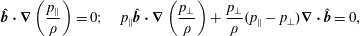 $$\begin{eqnarray}\hat{\boldsymbol{b}}\boldsymbol{\cdot }\unicode[STIX]{x1D735}\left(\frac{p_{\Vert }}{\unicode[STIX]{x1D70C}}\right)=0;\quad p_{\Vert }\hat{\boldsymbol{b}}\boldsymbol{\cdot }\unicode[STIX]{x1D735}\left(\frac{p_{\bot }}{\unicode[STIX]{x1D70C}}\right)+\frac{p_{\bot }}{\unicode[STIX]{x1D70C}}(p_{\Vert }-p_{\bot })\unicode[STIX]{x1D735}\boldsymbol{\cdot }\hat{\boldsymbol{b}}=0,\end{eqnarray}$$
where the FLR pressure tensor
 $\unicode[STIX]{x1D72B}$
was neglected in the second equation. It is useful to define
$\unicode[STIX]{x1D72B}$
was neglected in the second equation. It is useful to define
 $\unicode[STIX]{x2202}_{\Vert }\equiv \hat{\boldsymbol{b}}\boldsymbol{\cdot }\unicode[STIX]{x1D735}$
, which represents the gradient along the magnetic field lines, and to use the identity
$\unicode[STIX]{x2202}_{\Vert }\equiv \hat{\boldsymbol{b}}\boldsymbol{\cdot }\unicode[STIX]{x1D735}$
, which represents the gradient along the magnetic field lines, and to use the identity
 $$\begin{eqnarray}\unicode[STIX]{x1D735}\boldsymbol{\cdot }\hat{\boldsymbol{b}}=-\frac{1}{|\boldsymbol{B}|}\hat{\boldsymbol{b}}\boldsymbol{\cdot }\unicode[STIX]{x1D735}|\boldsymbol{B}|,\end{eqnarray}$$
further yielding
 $$\begin{eqnarray}\unicode[STIX]{x2202}_{\Vert }T_{\Vert }=0;\quad \frac{\unicode[STIX]{x2202}_{\Vert }T_{\bot }}{T_{\bot }}=\left(1-\frac{T_{\bot }}{T_{\Vert }}\right)\frac{\unicode[STIX]{x2202}_{\Vert }|\boldsymbol{B}|}{|\boldsymbol{B}|}.\end{eqnarray}$$
Equation (9.43) describes the evolution of the parallel and perpendicular temperature fluctuations along the magnetic field lines, and it can be verified that the solution is
 $$\begin{eqnarray}T_{\Vert }=T_{\Vert }^{(0)};\quad T_{\bot }=T_{\bot }^{(0)}\frac{\displaystyle \frac{|\boldsymbol{B}|}{B_{0}}}{\displaystyle 1-a_{p}+a_{p}\frac{|\boldsymbol{B}|}{B_{0}}},\end{eqnarray}$$
where
 $a_{p}=T_{\bot }^{(0)}/T_{\Vert }^{(0)}$
. Solution (9.44) is referred to as the ‘static’ closure and it is, for example, equivalent to (19), (20) of Passot et al. (Reference Passot, Ruban and Sulem2006), and (2) of Constantinescu (Reference Constantinescu2002). For isotropic mean temperatures
$a_{p}=T_{\bot }^{(0)}/T_{\Vert }^{(0)}$
. Solution (9.44) is referred to as the ‘static’ closure and it is, for example, equivalent to (19), (20) of Passot et al. (Reference Passot, Ruban and Sulem2006), and (2) of Constantinescu (Reference Constantinescu2002). For isotropic mean temperatures
 $a_{p}=1$
, equation (9.44) yields
$a_{p}=1$
, equation (9.44) yields
 $T_{\bot }=T_{\bot }^{(0)}=T_{\Vert }^{(0)}$
and both parallel and perpendicular temperatures are isothermal. A similar result is obtained for general
$T_{\bot }=T_{\bot }^{(0)}=T_{\Vert }^{(0)}$
and both parallel and perpendicular temperatures are isothermal. A similar result is obtained for general
 $a_{p}$
with
$a_{p}$
with
 $|\boldsymbol{B}|=B_{0}$
, which yields
$|\boldsymbol{B}|=B_{0}$
, which yields
 $T_{\bot }=T_{\bot }^{(0)}$
. The closure (9.44) can be therefore viewed as a generalization of the isothermal closure in the presence of temperature anisotropy and variations of magnetic field strength. The closure is used directly in the momentum equation (9.3), and the time-dependent pressure equations (9.5), (9.6) are disregarded. Therefore, even though the closure was derived by considering fourth-order moments, the resulting fluid model is actually simpler than the CGL2 and CGL models. As discussed for example by Passot et al. (Reference Passot, Ruban and Sulem2006), the closure prescribes a limitation for the minimal value of
$T_{\bot }=T_{\bot }^{(0)}$
. The closure (9.44) can be therefore viewed as a generalization of the isothermal closure in the presence of temperature anisotropy and variations of magnetic field strength. The closure is used directly in the momentum equation (9.3), and the time-dependent pressure equations (9.5), (9.6) are disregarded. Therefore, even though the closure was derived by considering fourth-order moments, the resulting fluid model is actually simpler than the CGL2 and CGL models. As discussed for example by Passot et al. (Reference Passot, Ruban and Sulem2006), the closure prescribes a limitation for the minimal value of
 $|\boldsymbol{B}|/B_{0}>1-1/a_{p}$
that is required to prevent temperature singularity. Or in other words, by separating
$|\boldsymbol{B}|/B_{0}>1-1/a_{p}$
that is required to prevent temperature singularity. Or in other words, by separating
 $|\boldsymbol{B}|=B_{0}+B^{(1)}$
the requirement reads
$|\boldsymbol{B}|=B_{0}+B^{(1)}$
the requirement reads
 $B^{(1)}>-1/a_{p}$
, meaning that the fluctuating
$B^{(1)}>-1/a_{p}$
, meaning that the fluctuating
 $B^{(1)}$
cannot be too negative. Mirror instability is often associated with nonlinear structures in the form of magnetic holes and humps, and the requirement implies that the magnetic holes cannot be too deep. To easily analyse the dispersion relations, it is useful to write the closure at the linear level, in the following form
$B^{(1)}$
cannot be too negative. Mirror instability is often associated with nonlinear structures in the form of magnetic holes and humps, and the requirement implies that the magnetic holes cannot be too deep. To easily analyse the dispersion relations, it is useful to write the closure at the linear level, in the following form
 $$\begin{eqnarray}p_{\Vert }=nT_{\Vert }^{(0)};\quad p_{\bot }\overset{\text{lin}}{=}nT_{\bot }^{(0)}+p_{\bot }^{(0)}(1-a_{p})\frac{B_{z}^{(1)}}{B_{0}}.\end{eqnarray}$$
The result can be obtained by linearizing (9.44) or (9.43), and at the linear level
 $\unicode[STIX]{x2202}_{i}|\boldsymbol{B}|\overset{\text{lin}}{=}\unicode[STIX]{x2202}_{i}B_{z}$
. The normalized closure reads (tildes are dropped)
$\unicode[STIX]{x2202}_{i}|\boldsymbol{B}|\overset{\text{lin}}{=}\unicode[STIX]{x2202}_{i}B_{z}$
. The normalized closure reads (tildes are dropped)
 $p_{\Vert }=n$
and
$p_{\Vert }=n$
and
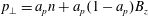 $p_{\bot }=a_{p}n+a_{p}(1-a_{p})B_{z}$
. Considering the simplest non-dispersive model (by neglecting the Hall term and
$p_{\bot }=a_{p}n+a_{p}(1-a_{p})B_{z}$
. Considering the simplest non-dispersive model (by neglecting the Hall term and
 $\unicode[STIX]{x1D72B}$
), the dispersion relation of this fluid model reads
$\unicode[STIX]{x1D72B}$
), the dispersion relation of this fluid model reads
 $$\begin{eqnarray}\displaystyle \left.\begin{array}{@{}c@{}}\displaystyle (\unicode[STIX]{x1D714}^{2}-k_{\Vert }^{2}v_{A\Vert }^{2})(\unicode[STIX]{x1D714}^{4}-A_{2}\unicode[STIX]{x1D714}^{2}+A_{0})=0;\\ \displaystyle A_{2}=k_{\Vert }^{2}\left(v_{A\Vert }^{2}+\frac{\unicode[STIX]{x1D6FD}_{\Vert }}{2}\right)+k_{\bot }^{2}\left(1+a_{p}\unicode[STIX]{x1D6FD}_{\Vert }-a_{p}^{2}\frac{\unicode[STIX]{x1D6FD}_{\Vert }}{2}\right);\\ \displaystyle A_{0}=k_{\Vert }^{2}\frac{\unicode[STIX]{x1D6FD}_{\Vert }}{2}[k_{\Vert }^{2}v_{A\Vert }^{2}+k_{\bot }^{2}(1+a_{p}\unicode[STIX]{x1D6FD}_{\Vert }-a_{p}^{2}\unicode[STIX]{x1D6FD}_{\Vert })].\end{array}\right\} & & \displaystyle\end{eqnarray}$$
In comparison with the dispersion relation (3.193) of the adiabatic CGL model, the ‘static’ closure eliminates the erroneous
 $1/6$
factor in the
$1/6$
factor in the
 $A_{0}$
coefficient and yields the correct mirror threshold. The erroneous
$A_{0}$
coefficient and yields the correct mirror threshold. The erroneous
 $1/6$
factor in the CGL model can be therefore interpreted as a result of inadequacy of adiabatic closures in the very slow-dynamics context, such as the mirror instability. For completeness, solutions for parallel propagation (
$1/6$
factor in the CGL model can be therefore interpreted as a result of inadequacy of adiabatic closures in the very slow-dynamics context, such as the mirror instability. For completeness, solutions for parallel propagation (
 $k_{\bot }=0$
) are
$k_{\bot }=0$
) are
 $\unicode[STIX]{x1D714}=\pm v_{A\Vert }k_{\Vert }$
and
$\unicode[STIX]{x1D714}=\pm v_{A\Vert }k_{\Vert }$
and
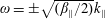 $\unicode[STIX]{x1D714}=\pm \sqrt{(\unicode[STIX]{x1D6FD}_{\Vert }/2)}k_{\Vert }$
. For perpendicular propagation (
$\unicode[STIX]{x1D714}=\pm \sqrt{(\unicode[STIX]{x1D6FD}_{\Vert }/2)}k_{\Vert }$
. For perpendicular propagation (
 $k_{\Vert }=0$
) the solution is
$k_{\Vert }=0$
) the solution is
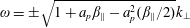 $\unicode[STIX]{x1D714}=\pm \sqrt{1+a_{p}\unicode[STIX]{x1D6FD}_{\Vert }-a_{p}^{2}(\unicode[STIX]{x1D6FD}_{\Vert }/2)}k_{\bot }$
. Obviously, somewhere beyond the mirror threshold, the perpendicular fast mode experiences unphysical instability, which can be interpreted as a result of inadequacy of ‘static’ (isothermal) closures in the fast-dynamics context.
$\unicode[STIX]{x1D714}=\pm \sqrt{1+a_{p}\unicode[STIX]{x1D6FD}_{\Vert }-a_{p}^{2}(\unicode[STIX]{x1D6FD}_{\Vert }/2)}k_{\bot }$
. Obviously, somewhere beyond the mirror threshold, the perpendicular fast mode experiences unphysical instability, which can be interpreted as a result of inadequacy of ‘static’ (isothermal) closures in the fast-dynamics context.
To clearly demonstrate that variations of magnetic field in the ‘static’ closures (9.45) are indeed crucial in recovering the mirror instability, let us neglect them and quickly consider strictly isothermal closure
 $p_{\Vert }=nT_{\Vert }^{(0)}$
;
$p_{\Vert }=nT_{\Vert }^{(0)}$
;
 $p_{\bot }=nT_{\bot }^{(0)}$
, which yields the following dispersion relation
$p_{\bot }=nT_{\bot }^{(0)}$
, which yields the following dispersion relation
 $$\begin{eqnarray}\displaystyle \left.\begin{array}{@{}c@{}}\displaystyle (\unicode[STIX]{x1D714}^{2}-k_{\Vert }^{2}v_{A\Vert }^{2})(\unicode[STIX]{x1D714}^{4}-A_{2}\unicode[STIX]{x1D714}^{2}+A_{0})=0;\\ \displaystyle A_{2}=k_{\Vert }^{2}\left(v_{A\Vert }^{2}+\frac{\unicode[STIX]{x1D6FD}_{\Vert }}{2}\right)+k_{\bot }^{2}\left(1+a_{p}\frac{\unicode[STIX]{x1D6FD}_{\Vert }}{2}\right);\\ \displaystyle A_{0}=k_{\Vert }^{2}\frac{\unicode[STIX]{x1D6FD}_{\Vert }}{2}\left[k_{\Vert }^{2}v_{A\Vert }^{2}+k_{\bot }^{2}\left(1+a_{p}\frac{\unicode[STIX]{x1D6FD}_{\Vert }}{2}-a_{p}^{2}\frac{\unicode[STIX]{x1D6FD}_{\Vert }}{2}\right)\right].\end{array}\right\} & & \displaystyle\end{eqnarray}$$
As can be seen from the
 $A_{0}$
coefficient, this model does not recover the mirror instability. For parallel propagation the solutions are the same as for the ‘static’ closure, nevertheless, the perpendicular fast mode is now always stable with
$A_{0}$
coefficient, this model does not recover the mirror instability. For parallel propagation the solutions are the same as for the ‘static’ closure, nevertheless, the perpendicular fast mode is now always stable with
 $\unicode[STIX]{x1D714}=\pm \sqrt{1+a_{p}(\unicode[STIX]{x1D6FD}_{\Vert }/2)}k_{\bot }$
. As a double check, after prescribing
$\unicode[STIX]{x1D714}=\pm \sqrt{1+a_{p}(\unicode[STIX]{x1D6FD}_{\Vert }/2)}k_{\bot }$
. As a double check, after prescribing
 $a_{p}=1$
, the dispersion relation (9.47) is equal to (9.46), since the
$a_{p}=1$
, the dispersion relation (9.47) is equal to (9.46), since the
 $B_{z}$
contributions in the ‘static’ closure disappear. Also, we considered models with polytropic indices
$B_{z}$
contributions in the ‘static’ closure disappear. Also, we considered models with polytropic indices
 $\unicode[STIX]{x1D6FE}_{\Vert },\unicode[STIX]{x1D6FE}_{\bot }$
in § 3.11, and the dispersion relation (9.47) is consistent with (3.171), after prescribing
$\unicode[STIX]{x1D6FE}_{\Vert },\unicode[STIX]{x1D6FE}_{\bot }$
in § 3.11, and the dispersion relation (9.47) is consistent with (3.171), after prescribing
 $\unicode[STIX]{x1D6FE}_{\Vert }=1$
,
$\unicode[STIX]{x1D6FE}_{\Vert }=1$
,
 $\unicode[STIX]{x1D6FE}_{\bot }=1$
.
$\unicode[STIX]{x1D6FE}_{\bot }=1$
.
10 Bi-kappa fluid model (BiKappa)
10.1 Bi-kappa distribution function
Often in the solar wind and in space plasma physics, distribution functions with elongated high-energy ‘suprathermal’ tails are observed, that cannot be modelled with the bi-Maxwellian distribution. A slightly more general distribution function is the bi-kappa distribution, that contains one free parameter
 $\unicode[STIX]{x1D705}$
, see for example Summers & Thorne (Reference Summers and Thorne1992), Pierrard & Lazar (Reference Pierrard and Lazar2010), Livadiotis & McComas (Reference Livadiotis and McComas2013) and references therein. The
$\unicode[STIX]{x1D705}$
, see for example Summers & Thorne (Reference Summers and Thorne1992), Pierrard & Lazar (Reference Pierrard and Lazar2010), Livadiotis & McComas (Reference Livadiotis and McComas2013) and references therein. The
 $\unicode[STIX]{x1D705}$
parameter can be different in the parallel and transverse directions (see e.g. Basu (Reference Basu2009), dos Santos, Ziebell & Gaelzer (Reference dos Santos, Ziebell and Gaelzer2015)). Here, we consider only one free
$\unicode[STIX]{x1D705}$
parameter can be different in the parallel and transverse directions (see e.g. Basu (Reference Basu2009), dos Santos, Ziebell & Gaelzer (Reference dos Santos, Ziebell and Gaelzer2015)). Here, we consider only one free
 $\unicode[STIX]{x1D705}$
parameter. The distribution has the following form
$\unicode[STIX]{x1D705}$
parameter. The distribution has the following form
 $$\begin{eqnarray}f_{0}=n\frac{\unicode[STIX]{x1D6E4}(\unicode[STIX]{x1D705}+1)}{\unicode[STIX]{x03C0}^{3/2}\unicode[STIX]{x1D705}^{3/2}\unicode[STIX]{x1D6E4}(\unicode[STIX]{x1D705}-\frac{1}{2})}\frac{1}{\unicode[STIX]{x1D703}_{\Vert }\unicode[STIX]{x1D703}_{\bot }^{2}}\left[1+\frac{(v_{\Vert }-u_{\Vert })^{2}}{\unicode[STIX]{x1D705}\unicode[STIX]{x1D703}_{\Vert }^{2}}+\frac{|\boldsymbol{v}_{\bot }-\boldsymbol{u}_{\bot }|^{2}}{\unicode[STIX]{x1D705}\unicode[STIX]{x1D703}_{\bot }^{2}}\right]^{-\unicode[STIX]{x1D705}-1},\end{eqnarray}$$
where the generalized thermal speeds
 $$\begin{eqnarray}\unicode[STIX]{x1D703}_{\Vert }=\sqrt{1-\frac{3}{2\unicode[STIX]{x1D705}}}\sqrt{\frac{2T_{\Vert }}{m}};\quad \unicode[STIX]{x1D703}_{\bot }=\sqrt{1-\frac{3}{2\unicode[STIX]{x1D705}}}\sqrt{\frac{2T_{\bot }}{m}},\end{eqnarray}$$
and
 $\unicode[STIX]{x1D6E4}$
is the usual gamma function. In the limit
$\unicode[STIX]{x1D6E4}$
is the usual gamma function. In the limit
 $\unicode[STIX]{x1D705}\rightarrow \infty$
, the generalized thermal speeds are the usual thermal speeds and the distribution function is bi-Maxwellian, since
$\unicode[STIX]{x1D705}\rightarrow \infty$
, the generalized thermal speeds are the usual thermal speeds and the distribution function is bi-Maxwellian, since
 $$\begin{eqnarray}\lim _{x\rightarrow \infty }\left(1+\frac{a}{x}\right)^{-x}=\text{e}^{-a};\quad \lim _{x\rightarrow \infty }\left(1+\frac{a}{x}\right)^{-x-1}=\text{e}^{-a}.\end{eqnarray}$$
Why the generalized thermal speeds are defined this way will become clear from later calculations of the moments, and the choice of the power law index
 $-(\unicode[STIX]{x1D705}+1)$
, instead of perhaps the more logical
$-(\unicode[STIX]{x1D705}+1)$
, instead of perhaps the more logical
 $-\unicode[STIX]{x1D705}$
, is attributed to purely historical reasons. Calculating second-order (pressure) integrals with this distribution requires for convergence
$-\unicode[STIX]{x1D705}$
, is attributed to purely historical reasons. Calculating second-order (pressure) integrals with this distribution requires for convergence
 $\unicode[STIX]{x1D705}>3/2$
, and this value is also the minimum value for the generalized thermal speeds (10.2) to have real values. Sometimes, in the definition of the isotropic kappa distribution, a value of
$\unicode[STIX]{x1D705}>3/2$
, and this value is also the minimum value for the generalized thermal speeds (10.2) to have real values. Sometimes, in the definition of the isotropic kappa distribution, a value of
 $\unicode[STIX]{x1D6E4}(3/2)=\sqrt{\unicode[STIX]{x03C0}}/2$
is used and
$\unicode[STIX]{x1D6E4}(3/2)=\sqrt{\unicode[STIX]{x03C0}}/2$
is used and
 $\unicode[STIX]{x03C0}^{3/2}=2\unicode[STIX]{x03C0}\sqrt{\unicode[STIX]{x03C0}}/2=2\unicode[STIX]{x03C0}\unicode[STIX]{x1D6E4}(3/2)$
. Again, for brevity of the calculations, it is useful to introduce
$\unicode[STIX]{x03C0}^{3/2}=2\unicode[STIX]{x03C0}\sqrt{\unicode[STIX]{x03C0}}/2=2\unicode[STIX]{x03C0}\unicode[STIX]{x1D6E4}(3/2)$
. Again, for brevity of the calculations, it is useful to introduce
 $\unicode[STIX]{x1D6FC}_{\Vert }=1/(\unicode[STIX]{x1D705}\unicode[STIX]{x1D703}_{\Vert }^{2})$
,
$\unicode[STIX]{x1D6FC}_{\Vert }=1/(\unicode[STIX]{x1D705}\unicode[STIX]{x1D703}_{\Vert }^{2})$
,
 $\unicode[STIX]{x1D6FC}_{\bot }=1/(\unicode[STIX]{x1D705}\unicode[STIX]{x1D703}_{\bot }^{2})$
, and rewrite the bi-kappa distribution (10.1) in the following form
$\unicode[STIX]{x1D6FC}_{\bot }=1/(\unicode[STIX]{x1D705}\unicode[STIX]{x1D703}_{\bot }^{2})$
, and rewrite the bi-kappa distribution (10.1) in the following form
 $$\begin{eqnarray}f_{0}=n\frac{\unicode[STIX]{x1D6E4}(\unicode[STIX]{x1D705}+1)}{\unicode[STIX]{x1D6E4}(\unicode[STIX]{x1D705}-\frac{1}{2})}\sqrt{\frac{\unicode[STIX]{x1D6FC}_{\Vert }}{\unicode[STIX]{x03C0}}}\frac{\unicode[STIX]{x1D6FC}_{\bot }}{\unicode[STIX]{x03C0}}[1+\unicode[STIX]{x1D6FC}_{\Vert }c_{\Vert }^{2}+\unicode[STIX]{x1D6FC}_{\bot }c_{\bot }^{2}]^{-\unicode[STIX]{x1D705}-1}.\end{eqnarray}$$
The important integral is
 $$\begin{eqnarray}\int _{-\infty }^{\infty }(1+x^{2})^{-a}\,\text{d}x=\sqrt{\unicode[STIX]{x03C0}}\frac{\unicode[STIX]{x1D6E4}(a-\frac{1}{2})}{\unicode[STIX]{x1D6E4}(a)},\quad a>\frac{1}{2}.\end{eqnarray}$$
For the critical value of
 $a=1/2$
, the integral
$a=1/2$
, the integral
 $\int 1/\sqrt{1+x^{2}}\,\text{d}x=\text{arcsinh}(x)$
, and since
$\int 1/\sqrt{1+x^{2}}\,\text{d}x=\text{arcsinh}(x)$
, and since
 $\lim _{x\rightarrow \pm \infty }\text{arcsinh}(x)=\pm \infty$
, the integral diverges. For an isotropic kappa distribution
$\lim _{x\rightarrow \pm \infty }\text{arcsinh}(x)=\pm \infty$
, the integral diverges. For an isotropic kappa distribution
 $f(c^{2})$
, the three-dimensional integrals can be conveniently evaluated by transformation to spherical coordinates
$f(c^{2})$
, the three-dimensional integrals can be conveniently evaluated by transformation to spherical coordinates
 $$\begin{eqnarray}\int _{-\infty }^{\infty }f(c^{2})\,\text{d}^{3}c=4\unicode[STIX]{x03C0}\int _{0}^{\infty }c^{2}f(c^{2})\,\text{d}c.\end{eqnarray}$$
In this case, the important integral is
 $$\begin{eqnarray}\int _{0}^{\infty }x^{2}(1+x^{2})^{-a}\,\text{d}x=\frac{\sqrt{\unicode[STIX]{x03C0}}}{4}\frac{\unicode[STIX]{x1D6E4}(a-\frac{3}{2})}{\unicode[STIX]{x1D6E4}(a)};\quad a>\frac{3}{2},\end{eqnarray}$$
and by a direct substitution
 $$\begin{eqnarray}\displaystyle \int _{0}^{\infty }x^{2}(1+\unicode[STIX]{x1D6FC}x^{2})^{-(\unicode[STIX]{x1D705}+1)}\,\text{d}x=\frac{\sqrt{\unicode[STIX]{x03C0}}}{4\unicode[STIX]{x1D6FC}^{3/2}}\frac{\unicode[STIX]{x1D6E4}(\unicode[STIX]{x1D705}-\frac{1}{2})}{\unicode[STIX]{x1D6E4}(\unicode[STIX]{x1D705}+1)};\quad \unicode[STIX]{x1D705}>\frac{1}{2}. & & \displaystyle\end{eqnarray}$$
For an isotropic kappa distribution therefore
 $$\begin{eqnarray}\int _{-\infty }^{\infty }(1+\unicode[STIX]{x1D6FC}c^{2})^{-(\unicode[STIX]{x1D705}+1)}\,\text{d}^{3}c=4\unicode[STIX]{x03C0}\int _{0}^{\infty }c^{2}(1+\unicode[STIX]{x1D6FC}c^{2})^{-(\unicode[STIX]{x1D705}+1)}\,\text{d}c=\left(\frac{\unicode[STIX]{x03C0}}{\unicode[STIX]{x1D6FC}}\right)^{3/2}\frac{\unicode[STIX]{x1D6E4}(\unicode[STIX]{x1D705}-\frac{1}{2})}{\unicode[STIX]{x1D6E4}(\unicode[STIX]{x1D705}+1)},\end{eqnarray}$$
which explains the normalization factors. For an anisotropic bi-kappa distributions
 $f(c_{\Vert }^{2},c_{\bot }^{2})$
, the integration is slightly more complicated because, in contrast to a bi-Maxwellian distribution, the integration cannot be fully separated into two independent integrations over parallel and perpendicular velocity components, and has to be performed successively. It is possible to use a cylindrical coordinate system and integrate
$f(c_{\Vert }^{2},c_{\bot }^{2})$
, the integration is slightly more complicated because, in contrast to a bi-Maxwellian distribution, the integration cannot be fully separated into two independent integrations over parallel and perpendicular velocity components, and has to be performed successively. It is possible to use a cylindrical coordinate system and integrate
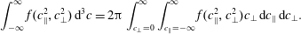 $$\begin{eqnarray}\int _{-\infty }^{\infty }f(c_{\Vert }^{2},c_{\bot }^{2})\,\text{d}^{3}c=2\unicode[STIX]{x03C0}\int _{c_{\bot }=0}^{\infty }\int _{c_{\Vert }=-\infty }^{\infty }f(c_{\Vert }^{2},c_{\bot }^{2})c_{\bot }\,\text{d}c_{\Vert }\,\text{d}c_{\bot }.\end{eqnarray}$$
However, here we keep the old fashioned Cartesian coordinates, and at the expense of a slightly bit more algebra (i.e. one more integration), we will integrate over
 $\,\text{d}^{3}c=\,\text{d}c_{\Vert }\,\text{d}^{2}c_{\bot }=\,\text{d}c_{\Vert }\,\text{d}c_{x}\,\text{d}c_{y}$
. A small added benefit is that we do not have to follow whether the integrals are
$\,\text{d}^{3}c=\,\text{d}c_{\Vert }\,\text{d}^{2}c_{\bot }=\,\text{d}c_{\Vert }\,\text{d}c_{x}\,\text{d}c_{y}$
. A small added benefit is that we do not have to follow whether the integrals are
 $\int _{-\infty }^{\infty }$
or
$\int _{-\infty }^{\infty }$
or
 $\int _{0}^{\infty }$
, and we can stop writing the boundaries.
$\int _{0}^{\infty }$
, and we can stop writing the boundaries.
The most important integral is a slight generalization of (10.5) in the form
 $$\begin{eqnarray}\int _{-\infty }^{\infty }(1+b+\unicode[STIX]{x1D6FC}x^{2})^{-a}\,\text{d}x=\sqrt{\frac{\unicode[STIX]{x03C0}}{\unicode[STIX]{x1D6FC}}}\frac{\unicode[STIX]{x1D6E4}(a-\frac{1}{2})}{\unicode[STIX]{x1D6E4}(a)}(1+b)^{-(a-\frac{1}{2})};\quad a>\frac{1}{2},\end{eqnarray}$$
where for simplicity
 $b,\unicode[STIX]{x1D6FC}$
are assumed to be positive constants. So one can calculate
$b,\unicode[STIX]{x1D6FC}$
are assumed to be positive constants. So one can calculate
 $$\begin{eqnarray}\int _{-\infty }^{\infty }(1+\unicode[STIX]{x1D6FC}_{x}x^{2}+\unicode[STIX]{x1D6FC}_{y}y^{2}+\unicode[STIX]{x1D6FC}_{z}z^{2})^{-a}\,\text{d}x=\sqrt{\frac{\unicode[STIX]{x03C0}}{\unicode[STIX]{x1D6FC}_{x}}}\frac{\unicode[STIX]{x1D6E4}(a-\frac{1}{2})}{\unicode[STIX]{x1D6E4}(a)}(1+\unicode[STIX]{x1D6FC}_{y}y^{2}+\unicode[STIX]{x1D6FC}_{z}z^{2})^{-(a-1/2)},\end{eqnarray}$$
where, importantly, the ‘power law’ changed from
 $-a$
to
$-a$
to
 $-(a-1/2)$
. Performing a successive three-dimensional integral therefore yields
$-(a-1/2)$
. Performing a successive three-dimensional integral therefore yields
 $$\begin{eqnarray}\displaystyle & & \displaystyle \int _{-\infty }^{\infty }(1+\unicode[STIX]{x1D6FC}_{x}x^{2}+\unicode[STIX]{x1D6FC}_{y}y^{2}+\unicode[STIX]{x1D6FC}_{z}z^{2})^{-a}\,\text{d}x\,\text{d}y\,\text{d}z\nonumber\\ \displaystyle & & \displaystyle \quad =\sqrt{\frac{\unicode[STIX]{x03C0}}{\unicode[STIX]{x1D6FC}_{x}}}\frac{\unicode[STIX]{x1D6E4}(a-\frac{1}{2})}{\unicode[STIX]{x1D6E4}(a)}\int (1+\unicode[STIX]{x1D6FC}_{y}y^{2}+\unicode[STIX]{x1D6FC}_{z}z^{2})^{-(a-1/2)}\,\text{d}y\,\text{d}z\nonumber\\ \displaystyle & & \displaystyle \quad =\sqrt{\frac{\unicode[STIX]{x03C0}}{\unicode[STIX]{x1D6FC}_{x}}}\sqrt{\frac{\unicode[STIX]{x03C0}}{\unicode[STIX]{x1D6FC}_{y}}}\frac{\unicode[STIX]{x1D6E4}(a-\frac{1}{2})}{\unicode[STIX]{x1D6E4}(a)}\frac{\unicode[STIX]{x1D6E4}(a-1)}{\unicode[STIX]{x1D6E4}(a-\frac{1}{2})}\int (1+\unicode[STIX]{x1D6FC}_{z}z^{2})^{-(a-1)}\,\text{d}z\nonumber\\ \displaystyle & & \displaystyle \quad =\sqrt{\frac{\unicode[STIX]{x03C0}}{\unicode[STIX]{x1D6FC}_{x}}}\sqrt{\frac{\unicode[STIX]{x03C0}}{\unicode[STIX]{x1D6FC}_{y}}}\sqrt{\frac{\unicode[STIX]{x03C0}}{\unicode[STIX]{x1D6FC}_{z}}}\frac{\unicode[STIX]{x1D6E4}(a-\frac{1}{2})}{\unicode[STIX]{x1D6E4}(a)}\frac{\unicode[STIX]{x1D6E4}(a-1)}{\unicode[STIX]{x1D6E4}(a-\frac{1}{2})}\frac{\unicode[STIX]{x1D6E4}(a-\frac{3}{2})}{\unicode[STIX]{x1D6E4}(a-1)}\nonumber\\ \displaystyle & & \displaystyle \quad =\sqrt{\frac{\unicode[STIX]{x03C0}}{\unicode[STIX]{x1D6FC}_{x}}}\sqrt{\frac{\unicode[STIX]{x03C0}}{\unicode[STIX]{x1D6FC}_{y}}}\sqrt{\frac{\unicode[STIX]{x03C0}}{\unicode[STIX]{x1D6FC}_{z}}}\frac{\unicode[STIX]{x1D6E4}(a-\frac{3}{2})}{\unicode[STIX]{x1D6E4}(a)};\quad a>\frac{3}{2},\end{eqnarray}$$
and integrating the bi-kappa distribution over the velocity space
 $$\begin{eqnarray}\displaystyle \int _{-\infty }^{\infty }(1+\unicode[STIX]{x1D6FC}_{\Vert }c_{\Vert }^{2}+\unicode[STIX]{x1D6FC}_{\bot }c_{\bot }^{2})^{-(\unicode[STIX]{x1D705}+1)}\,\text{d}c_{\Vert }\,\text{d}^{2}c_{\bot }=\sqrt{\frac{\unicode[STIX]{x03C0}}{\unicode[STIX]{x1D6FC}_{\Vert }}}\frac{\unicode[STIX]{x03C0}}{\unicode[STIX]{x1D6FC}_{\bot }}\frac{\unicode[STIX]{x1D6E4}(\unicode[STIX]{x1D705}-\frac{1}{2})}{\unicode[STIX]{x1D6E4}(\unicode[STIX]{x1D705}+1)};\quad \unicode[STIX]{x1D705}>\frac{1}{2}, & & \displaystyle\end{eqnarray}$$
which verifies that the normalization constants in the bi-kappa definition (10.4) are indeed correct, and that
 $\int f_{0}d^{3}c=n$
. For later calculations, it is useful to write down two partial integrals when the integration is done over
$\int f_{0}d^{3}c=n$
. For later calculations, it is useful to write down two partial integrals when the integration is done over
 $\,\text{d}c_{\Vert }$
and
$\,\text{d}c_{\Vert }$
and
 $\,\text{d}^{2}c_{\bot }$
that read
$\,\text{d}^{2}c_{\bot }$
that read
 $$\begin{eqnarray}\displaystyle & \displaystyle \int _{-\infty }^{\infty }(1+\unicode[STIX]{x1D6FC}_{\Vert }c_{\Vert }^{2})^{-a}\,\text{d}c_{\Vert }=\sqrt{\frac{\unicode[STIX]{x03C0}}{\unicode[STIX]{x1D6FC}_{\Vert }}}\frac{\unicode[STIX]{x1D6E4}(a-\frac{1}{2})}{\unicode[STIX]{x1D6E4}(a)}; & \displaystyle\end{eqnarray}$$
 $$\begin{eqnarray}\displaystyle & \displaystyle \int _{-\infty }^{\infty }(1+\unicode[STIX]{x1D6FC}_{\Vert }c_{\Vert }^{2}+\unicode[STIX]{x1D6FC}_{\bot }c_{\bot }^{2})^{-(\unicode[STIX]{x1D705}+1)}\,\text{d}c_{\Vert }=\sqrt{\frac{\unicode[STIX]{x03C0}}{\unicode[STIX]{x1D6FC}_{\Vert }}}\frac{\unicode[STIX]{x1D6E4}(\unicode[STIX]{x1D705}+\frac{1}{2})}{\unicode[STIX]{x1D6E4}(\unicode[STIX]{x1D705}+1)}(1+\unicode[STIX]{x1D6FC}_{\bot }c_{\bot }^{2})^{-(\unicode[STIX]{x1D705}+1/2)}; & \displaystyle\end{eqnarray}$$
 $$\begin{eqnarray}\displaystyle & \displaystyle \int f_{0}\,\text{d}c_{\Vert }=n\frac{\unicode[STIX]{x1D6E4}(\unicode[STIX]{x1D705}+\frac{1}{2})}{\unicode[STIX]{x1D6E4}(\unicode[STIX]{x1D705}-\frac{1}{2})}\frac{\unicode[STIX]{x1D6FC}_{\bot }}{\unicode[STIX]{x03C0}}(1+\unicode[STIX]{x1D6FC}_{\bot }c_{\bot }^{2})^{-(\unicode[STIX]{x1D705}+1/2)}, & \displaystyle\end{eqnarray}$$
and
 $$\begin{eqnarray}\displaystyle & \displaystyle \int _{-\infty }^{\infty }(1+\unicode[STIX]{x1D6FC}_{\bot }c_{\bot }^{2})^{-a}\,\text{d}^{2}c_{\bot }=\frac{\unicode[STIX]{x03C0}}{\unicode[STIX]{x1D6FC}_{\bot }}\frac{\unicode[STIX]{x1D6E4}(a-1)}{\unicode[STIX]{x1D6E4}(a)}; & \displaystyle\end{eqnarray}$$
 $$\begin{eqnarray}\displaystyle & \displaystyle \int (1+\unicode[STIX]{x1D6FC}_{\Vert }c_{\Vert }^{2}+\unicode[STIX]{x1D6FC}_{\bot }c_{\bot }^{2})^{-(\unicode[STIX]{x1D705}+1)}\,\text{d}^{2}c_{\bot }=\frac{\unicode[STIX]{x03C0}}{\unicode[STIX]{x1D6FC}_{\bot }}\frac{\unicode[STIX]{x1D6E4}(\unicode[STIX]{x1D705})}{\unicode[STIX]{x1D6E4}(\unicode[STIX]{x1D705}+1)}(1+\unicode[STIX]{x1D6FC}_{\Vert }c_{\Vert }^{2})^{-\unicode[STIX]{x1D705}}; & \displaystyle\end{eqnarray}$$
 $$\begin{eqnarray}\displaystyle & \displaystyle \int f_{0}\,\text{d}^{2}c_{\bot }=n\frac{\unicode[STIX]{x1D6E4}(\unicode[STIX]{x1D705})}{\unicode[STIX]{x1D6E4}(\unicode[STIX]{x1D705}-\frac{1}{2})}\sqrt{\frac{\unicode[STIX]{x1D6FC}_{\Vert }}{\unicode[STIX]{x03C0}}}(1+\unicode[STIX]{x1D6FC}_{\Vert }c_{\Vert }^{2})^{-\unicode[STIX]{x1D705}}. & \displaystyle\end{eqnarray}$$
Continuing with the calculation of velocity moments, it is easy to show that
 $\int \boldsymbol{c}f_{0}\,\text{d}^{3}c=0$
, which verifies
$\int \boldsymbol{c}f_{0}\,\text{d}^{3}c=0$
, which verifies
 $n\boldsymbol{u}=\int \boldsymbol{v}f_{0}\,\text{d}^{3}v$
. Continuing with the higher-order moments, it is possible to calculate those from table integrals (a great help for double checking is an analytic software like Maple or Mathematica) or similarly for a bi-Maxwellian distribution to use a trick with the differentiation with respect to
$n\boldsymbol{u}=\int \boldsymbol{v}f_{0}\,\text{d}^{3}v$
. Continuing with the higher-order moments, it is possible to calculate those from table integrals (a great help for double checking is an analytic software like Maple or Mathematica) or similarly for a bi-Maxwellian distribution to use a trick with the differentiation with respect to
 $\unicode[STIX]{x1D6FC}$
as
$\unicode[STIX]{x1D6FC}$
as
 $$\begin{eqnarray}\displaystyle \int _{-\infty }^{\infty }x^{2}(1+\unicode[STIX]{x1D6FC}x^{2})^{-(\unicode[STIX]{x1D705}+1)}\,\text{d}x & = & \displaystyle -\frac{1}{\unicode[STIX]{x1D705}}\frac{\unicode[STIX]{x2202}}{\unicode[STIX]{x2202}\unicode[STIX]{x1D6FC}}\int _{-\infty }^{\infty }(1+\unicode[STIX]{x1D6FC}x^{2})^{-\unicode[STIX]{x1D705}}\,\text{d}x=-\frac{1}{\unicode[STIX]{x1D705}}\sqrt{\unicode[STIX]{x03C0}}\frac{\unicode[STIX]{x1D6E4}(\unicode[STIX]{x1D705}-\frac{1}{2})}{\unicode[STIX]{x1D6E4}(\unicode[STIX]{x1D705})}\frac{\unicode[STIX]{x2202}}{\unicode[STIX]{x2202}\unicode[STIX]{x1D6FC}}\unicode[STIX]{x1D6FC}^{-1/2}\nonumber\\ \displaystyle & = & \displaystyle \frac{\sqrt{\unicode[STIX]{x03C0}}}{2\unicode[STIX]{x1D6FC}^{3/2}}\frac{\unicode[STIX]{x1D6E4}(\unicode[STIX]{x1D705}-\frac{1}{2})}{\unicode[STIX]{x1D6E4}(\unicode[STIX]{x1D705}+1)},\end{eqnarray}$$
where we have also used a property of the gamma function
 $x\unicode[STIX]{x1D6E4}(x)=\unicode[STIX]{x1D6E4}(x+1)$
, and the last integral requires
$x\unicode[STIX]{x1D6E4}(x)=\unicode[STIX]{x1D6E4}(x+1)$
, and the last integral requires
 $\unicode[STIX]{x1D705}>\frac{1}{2}$
. A slightly more general integral is
$\unicode[STIX]{x1D705}>\frac{1}{2}$
. A slightly more general integral is
 $$\begin{eqnarray}\int _{-\infty }^{\infty }x^{2}(1+b+\unicode[STIX]{x1D6FC}x^{2})^{-a}\,\text{d}x=\frac{\sqrt{\unicode[STIX]{x03C0}}}{2\unicode[STIX]{x1D6FC}^{3/2}}\frac{\unicode[STIX]{x1D6E4}(a-\frac{3}{2})}{\unicode[STIX]{x1D6E4}(a)}(1+b)^{-(a-3/2)},\end{eqnarray}$$
which can be used to evaluate the following integrals
 $$\begin{eqnarray}\displaystyle \int _{-\infty }^{\infty }c_{\Vert }^{2}(1+\unicode[STIX]{x1D6FC}_{\Vert }c_{\Vert }^{2})^{-a}\,\text{d}c_{\Vert }=\frac{\sqrt{\unicode[STIX]{x03C0}}}{2\unicode[STIX]{x1D6FC}_{\Vert }^{3/2}}\frac{\unicode[STIX]{x1D6E4}(a-\frac{3}{2})}{\unicode[STIX]{x1D6E4}(a)}; & & \displaystyle\end{eqnarray}$$
 $$\begin{eqnarray}\displaystyle \int _{-\infty }^{\infty }c_{x}^{2}(1+\unicode[STIX]{x1D6FC}_{\bot }c_{\bot }^{2})^{-a}\,\text{d}^{2}c_{\bot } & = & \displaystyle \int _{-\infty }^{\infty }c_{x}^{2}(1+\unicode[STIX]{x1D6FC}_{\bot }c_{x}^{2}+\unicode[STIX]{x1D6FC}_{\bot }c_{y}^{2})^{-a}\,\text{d}c_{x}\,\text{d}c_{y}\nonumber\\ \displaystyle & = & \displaystyle \frac{\sqrt{\unicode[STIX]{x03C0}}}{2\unicode[STIX]{x1D6FC}_{\bot }^{3/2}}\frac{\unicode[STIX]{x1D6E4}(a-\frac{3}{2})}{\unicode[STIX]{x1D6E4}(a)}\int _{-\infty }^{\infty }(1+\unicode[STIX]{x1D6FC}_{\bot }c_{y}^{2})^{-(a-3/2)}\,\text{d}c_{y}\nonumber\\ \displaystyle & = & \displaystyle \frac{\sqrt{\unicode[STIX]{x03C0}}}{2\unicode[STIX]{x1D6FC}_{\bot }^{3/2}}\frac{\unicode[STIX]{x1D6E4}(a-\frac{3}{2})}{\unicode[STIX]{x1D6E4}(a)}\sqrt{\frac{\unicode[STIX]{x03C0}}{\unicode[STIX]{x1D6FC}_{\bot }}}\frac{\unicode[STIX]{x1D6E4}(a-2)}{\unicode[STIX]{x1D6E4}(a-\frac{3}{2})}=\frac{\unicode[STIX]{x03C0}}{2\unicode[STIX]{x1D6FC}_{\bot }^{2}}\frac{\unicode[STIX]{x1D6E4}(a-2)}{\unicode[STIX]{x1D6E4}(a)};\nonumber\\ \displaystyle & & \displaystyle\end{eqnarray}$$
 $$\begin{eqnarray}\displaystyle \int _{-\infty }^{\infty }c_{\bot }^{2}(1+\unicode[STIX]{x1D6FC}_{\bot }c_{\bot }^{2})^{-a}\,\text{d}^{2}c_{\bot }=\frac{\unicode[STIX]{x03C0}}{\unicode[STIX]{x1D6FC}_{\bot }^{2}}\frac{\unicode[STIX]{x1D6E4}(a-2)}{\unicode[STIX]{x1D6E4}(a)}. & & \displaystyle\end{eqnarray}$$
Since we like to double check everything, the above integral can be also calculated as
 $$\begin{eqnarray}\displaystyle \int _{-\infty }^{\infty }c_{\bot }^{2}(1+\unicode[STIX]{x1D6FC}_{\bot }c_{\bot }^{2})^{-a}\,\text{d}^{2}c_{\bot } & = & \displaystyle -\frac{1}{a-1}\frac{\unicode[STIX]{x2202}}{\unicode[STIX]{x2202}\unicode[STIX]{x1D6FC}_{\bot }}\int _{-\infty }^{\infty }(1+\unicode[STIX]{x1D6FC}_{\bot }c_{\bot }^{2})^{-(a-1)}\,\text{d}^{2}c_{\bot }\nonumber\\ \displaystyle & = & \displaystyle -\frac{1}{a-1}\frac{\unicode[STIX]{x1D6E4}(a-2)}{\unicode[STIX]{x1D6E4}(a-1)}\frac{\unicode[STIX]{x2202}}{\unicode[STIX]{x2202}\unicode[STIX]{x1D6FC}_{\bot }}\frac{\unicode[STIX]{x03C0}}{\unicode[STIX]{x1D6FC}_{\bot }}\nonumber\\ \displaystyle & = & \displaystyle \frac{\unicode[STIX]{x03C0}}{\unicode[STIX]{x1D6FC}_{\bot }^{2}}\frac{\unicode[STIX]{x1D6E4}(a-2)}{\unicode[STIX]{x1D6E4}(a)}.\end{eqnarray}$$
For the calculation of the parallel pressure, we first integrate over
 $\text{d}^{2}c_{\bot }$
so we can use result (10.20) and then over
$\text{d}^{2}c_{\bot }$
so we can use result (10.20) and then over
 $\text{d}c_{\Vert }$
 $$\begin{eqnarray}\displaystyle p_{\Vert }\equiv m\int c_{\Vert }^{2}f_{0}\,\text{d}^{2}c_{\bot }\,\text{d}c_{\Vert } & = & \displaystyle mn\frac{\unicode[STIX]{x1D6E4}(\unicode[STIX]{x1D705})}{\unicode[STIX]{x1D6E4}(\unicode[STIX]{x1D705}-\frac{1}{2})}\sqrt{\frac{\unicode[STIX]{x1D6FC}_{\Vert }}{\unicode[STIX]{x03C0}}}\int c_{\Vert }^{2}(1+\unicode[STIX]{x1D6FC}_{\Vert }c_{\Vert }^{2})^{-\unicode[STIX]{x1D705}}\,\text{d}c_{\Vert }\nonumber\\ \displaystyle & = & \displaystyle mn\frac{\unicode[STIX]{x1D6E4}(\unicode[STIX]{x1D705})}{\unicode[STIX]{x1D6E4}(\unicode[STIX]{x1D705}-\frac{1}{2})}\sqrt{\frac{\unicode[STIX]{x1D6FC}_{\Vert }}{\unicode[STIX]{x03C0}}}\frac{\sqrt{\unicode[STIX]{x03C0}}}{2\unicode[STIX]{x1D6FC}_{\Vert }^{3/2}}\frac{\unicode[STIX]{x1D6E4}(\unicode[STIX]{x1D705}-\frac{3}{2})}{\unicode[STIX]{x1D6E4}(\unicode[STIX]{x1D705})}\nonumber\\ \displaystyle & = & \displaystyle mn\frac{\unicode[STIX]{x1D6E4}(\unicode[STIX]{x1D705}-\frac{3}{2})}{\unicode[STIX]{x1D6E4}(\unicode[STIX]{x1D705}-\frac{1}{2})}\frac{1}{2\unicode[STIX]{x1D6FC}_{\Vert }}=mn\frac{\unicode[STIX]{x1D6E4}(\unicode[STIX]{x1D705}-\frac{3}{2})}{\unicode[STIX]{x1D6E4}(\unicode[STIX]{x1D705}-\frac{1}{2})}\frac{1}{2}\left(\unicode[STIX]{x1D705}-\frac{3}{2}\right)\frac{2T_{\Vert }}{m}=nT_{\Vert },\nonumber\\ \displaystyle & & \displaystyle\end{eqnarray}$$
where we have used
 $(\unicode[STIX]{x1D705}-\frac{3}{2})\unicode[STIX]{x1D6E4}(\unicode[STIX]{x1D705}-\frac{3}{2})=\unicode[STIX]{x1D6E4}(\unicode[STIX]{x1D705}-\frac{1}{2})$
. Calculating the perpendicular pressure, we here first integrate over
$(\unicode[STIX]{x1D705}-\frac{3}{2})\unicode[STIX]{x1D6E4}(\unicode[STIX]{x1D705}-\frac{3}{2})=\unicode[STIX]{x1D6E4}(\unicode[STIX]{x1D705}-\frac{1}{2})$
. Calculating the perpendicular pressure, we here first integrate over
 $\text{d}c_{\Vert }$
so we can use result (10.17) and then over
$\text{d}c_{\Vert }$
so we can use result (10.17) and then over
 $\text{d}^{2}c_{\bot }$
 $$\begin{eqnarray}\displaystyle p_{\bot }\equiv \frac{m}{2}\int c_{\bot }^{2}f_{0}\,\text{d}c_{\Vert }\,\text{d}^{2}c_{\bot } & = & \displaystyle \frac{m}{2}n\frac{\unicode[STIX]{x1D6E4}(\unicode[STIX]{x1D705}+\frac{1}{2})}{\unicode[STIX]{x1D6E4}(\unicode[STIX]{x1D705}-\frac{1}{2})}\frac{\unicode[STIX]{x1D6FC}_{\bot }}{\unicode[STIX]{x03C0}}\int c_{\bot }^{2}(1+\unicode[STIX]{x1D6FC}_{\bot }c_{\bot }^{2})^{-(\unicode[STIX]{x1D705}+1/2)}\,\text{d}^{2}c_{\bot }\nonumber\\ \displaystyle & = & \displaystyle \frac{m}{2}n\frac{\unicode[STIX]{x1D6E4}(\unicode[STIX]{x1D705}+\frac{1}{2})}{\unicode[STIX]{x1D6E4}(\unicode[STIX]{x1D705}-\frac{1}{2})}\frac{\unicode[STIX]{x1D6FC}_{\bot }}{\unicode[STIX]{x03C0}}\frac{\unicode[STIX]{x03C0}}{\unicode[STIX]{x1D6FC}_{\bot }^{2}}\frac{\unicode[STIX]{x1D6E4}(\unicode[STIX]{x1D705}-\frac{3}{2})}{\unicode[STIX]{x1D6E4}(\unicode[STIX]{x1D705}+\frac{1}{2})}\nonumber\\ \displaystyle & = & \displaystyle mn\frac{\unicode[STIX]{x1D6E4}(\unicode[STIX]{x1D705}-\frac{3}{2})}{\unicode[STIX]{x1D6E4}(\unicode[STIX]{x1D705}-\frac{1}{2})}\frac{1}{2\unicode[STIX]{x1D6FC}_{\bot }}=mn\frac{\unicode[STIX]{x1D6E4}(\unicode[STIX]{x1D705}-\frac{3}{2})}{\unicode[STIX]{x1D6E4}(\unicode[STIX]{x1D705}-\frac{1}{2})}\frac{1}{2}\left(\unicode[STIX]{x1D705}-\frac{3}{2}\right)\frac{2T_{\bot }}{m}=nT_{\bot }.\nonumber\\ \displaystyle & & \displaystyle\end{eqnarray}$$
The last two calculations clarify the reasoning behind the definition of the bi-kappa generalized thermal speeds
 $\unicode[STIX]{x1D703}_{\Vert }$
,
$\unicode[STIX]{x1D703}_{\Vert }$
,
 $\unicode[STIX]{x1D703}_{\bot }$
(here rewritten with the notation
$\unicode[STIX]{x1D703}_{\bot }$
(here rewritten with the notation
 $\unicode[STIX]{x1D6FC}_{\Vert }$
and
$\unicode[STIX]{x1D6FC}_{\Vert }$
and
 $\unicode[STIX]{x1D6FC}_{\bot }$
), where one starts with a bi-kappa distribution with unspecified
$\unicode[STIX]{x1D6FC}_{\bot }$
), where one starts with a bi-kappa distribution with unspecified
 $\unicode[STIX]{x1D6FC}_{\Vert }$
and
$\unicode[STIX]{x1D6FC}_{\Vert }$
and
 $\unicode[STIX]{x1D6FC}_{\bot }$
, and calculating the parallel and perpendicular pressure integrals, yields the required forms
$\unicode[STIX]{x1D6FC}_{\bot }$
, and calculating the parallel and perpendicular pressure integrals, yields the required forms
 $\unicode[STIX]{x1D6FC}_{\Vert }^{-1}=(\unicode[STIX]{x1D705}-\frac{3}{2})(2T_{\Vert }/m)$
;
$\unicode[STIX]{x1D6FC}_{\Vert }^{-1}=(\unicode[STIX]{x1D705}-\frac{3}{2})(2T_{\Vert }/m)$
;
 $\unicode[STIX]{x1D6FC}_{\bot }^{-1}=(\unicode[STIX]{x1D705}-\frac{3}{2})(2T_{\bot }/m)$
. Then, the split to
$\unicode[STIX]{x1D6FC}_{\bot }^{-1}=(\unicode[STIX]{x1D705}-\frac{3}{2})(2T_{\bot }/m)$
. Then, the split to
 $\unicode[STIX]{x1D6FC}_{\Vert }^{-1}=\unicode[STIX]{x1D705}\unicode[STIX]{x1D703}_{\Vert }^{2}$
;
$\unicode[STIX]{x1D6FC}_{\Vert }^{-1}=\unicode[STIX]{x1D705}\unicode[STIX]{x1D703}_{\Vert }^{2}$
;
 $\unicode[STIX]{x1D6FC}_{\bot }^{-1}=\unicode[STIX]{x1D705}\unicode[STIX]{x1D703}_{\bot }^{2}$
is dictated by the requirement that for
$\unicode[STIX]{x1D6FC}_{\bot }^{-1}=\unicode[STIX]{x1D705}\unicode[STIX]{x1D703}_{\bot }^{2}$
is dictated by the requirement that for
 $\unicode[STIX]{x1D705}\rightarrow \infty$
, the generalized thermal speeds converge to the usual thermal speeds, and which also yields that in this limit the distribution is bi-Maxwellian.
$\unicode[STIX]{x1D705}\rightarrow \infty$
, the generalized thermal speeds converge to the usual thermal speeds, and which also yields that in this limit the distribution is bi-Maxwellian.
The bi-kappa distribution was specified with perhaps a somewhat obscure power law
 $-(\unicode[STIX]{x1D705}+1)$
instead of the more logical
$-(\unicode[STIX]{x1D705}+1)$
instead of the more logical
 $-\unicode[STIX]{x1D705}$
, which is attributed to purely historical reasons. If one wants to define an anisotropic power-law distribution, a first guess would be
$-\unicode[STIX]{x1D705}$
, which is attributed to purely historical reasons. If one wants to define an anisotropic power-law distribution, a first guess would be
 $$\begin{eqnarray}\widetilde{f}_{0}\sim n[1+\unicode[STIX]{x1D6FC}_{\Vert }c_{\Vert }^{2}+\unicode[STIX]{x1D6FC}_{\bot }c_{\bot }^{2}]^{-\unicode[STIX]{x1D705}},\end{eqnarray}$$
which then yields normalization constants
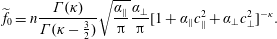 $$\begin{eqnarray}\widetilde{f}_{0}=n\frac{\unicode[STIX]{x1D6E4}(\unicode[STIX]{x1D705})}{\unicode[STIX]{x1D6E4}(\unicode[STIX]{x1D705}-\frac{3}{2})}\sqrt{\frac{\unicode[STIX]{x1D6FC}_{\Vert }}{\unicode[STIX]{x03C0}}}\frac{\unicode[STIX]{x1D6FC}_{\bot }}{\unicode[STIX]{x03C0}}[1+\unicode[STIX]{x1D6FC}_{\Vert }c_{\Vert }^{2}+\unicode[STIX]{x1D6FC}_{\bot }c_{\bot }^{2}]^{-\unicode[STIX]{x1D705}}.\end{eqnarray}$$
Then, calculating the parallel and perpendicular pressures yields the requirement
 $\unicode[STIX]{x1D6FC}_{\Vert ,\bot }^{-1}=(\unicode[STIX]{x1D705}-\frac{5}{2})(2T_{\Vert ,\bot }/m)$
. Further writing
$\unicode[STIX]{x1D6FC}_{\Vert ,\bot }^{-1}=(\unicode[STIX]{x1D705}-\frac{5}{2})(2T_{\Vert ,\bot }/m)$
. Further writing
 $\unicode[STIX]{x1D6FC}_{\Vert ,\bot }^{-1}=\unicode[STIX]{x1D705}\unicode[STIX]{x1D703}_{\Vert ,\bot }^{2}$
yields a distribution function
$\unicode[STIX]{x1D6FC}_{\Vert ,\bot }^{-1}=\unicode[STIX]{x1D705}\unicode[STIX]{x1D703}_{\Vert ,\bot }^{2}$
yields a distribution function
 $$\begin{eqnarray}\widetilde{f}_{0}=n\frac{\unicode[STIX]{x1D6E4}(\unicode[STIX]{x1D705})}{\unicode[STIX]{x03C0}^{3/2}\unicode[STIX]{x1D705}^{3/2}\unicode[STIX]{x1D6E4}(\unicode[STIX]{x1D705}-\frac{3}{2})}\frac{1}{\unicode[STIX]{x1D703}_{\Vert }\unicode[STIX]{x1D703}_{\bot }^{2}}\left[1+\frac{c_{\Vert }^{2}}{\unicode[STIX]{x1D705}\unicode[STIX]{x1D703}_{\Vert }^{2}}+\frac{c_{\bot }^{2}}{\unicode[STIX]{x1D705}\unicode[STIX]{x1D703}_{\bot }^{2}}\right]^{-\unicode[STIX]{x1D705}},\end{eqnarray}$$
with generalized thermal speeds
 $$\begin{eqnarray}\unicode[STIX]{x1D703}_{\Vert }=\sqrt{1-\frac{5}{2\unicode[STIX]{x1D705}}}\sqrt{\frac{2T_{\Vert }}{m}};\quad \unicode[STIX]{x1D703}_{\bot }=\sqrt{1-\frac{5}{2\unicode[STIX]{x1D705}}}\sqrt{\frac{2T_{\bot }}{m}}.\end{eqnarray}$$
The convergence of the pressure integrals requires
 $\unicode[STIX]{x1D705}>\frac{5}{2}$
, which is also the limiting case for the thermal speeds to be real. In the limit
$\unicode[STIX]{x1D705}>\frac{5}{2}$
, which is also the limiting case for the thermal speeds to be real. In the limit
 $\unicode[STIX]{x1D705}\rightarrow \infty$
the generalized thermal speeds converge to the usual thermal speeds and the distribution converges to the bi-Maxwellian. To double check that the distribution (10.31) is really correct, one can of course substitute
$\unicode[STIX]{x1D705}\rightarrow \infty$
the generalized thermal speeds converge to the usual thermal speeds and the distribution converges to the bi-Maxwellian. To double check that the distribution (10.31) is really correct, one can of course substitute
 $\unicode[STIX]{x1D705}\rightarrow \unicode[STIX]{x1D705}+1$
, which fully recovers the original bi-kappa distribution (10.1), since
$\unicode[STIX]{x1D705}\rightarrow \unicode[STIX]{x1D705}+1$
, which fully recovers the original bi-kappa distribution (10.1), since
 $\unicode[STIX]{x1D705}\unicode[STIX]{x1D703}^{2}\rightarrow (\unicode[STIX]{x1D705}+1)(1-5/2(\unicode[STIX]{x1D705}+1))(2T/m)=\unicode[STIX]{x1D705}(1-3/2\unicode[STIX]{x1D705})(2T/m)$
. From now on, let us continue calculations with the original bi-kappa distribution (10.1), that uses the
$\unicode[STIX]{x1D705}\unicode[STIX]{x1D703}^{2}\rightarrow (\unicode[STIX]{x1D705}+1)(1-5/2(\unicode[STIX]{x1D705}+1))(2T/m)=\unicode[STIX]{x1D705}(1-3/2\unicode[STIX]{x1D705})(2T/m)$
. From now on, let us continue calculations with the original bi-kappa distribution (10.1), that uses the
 $-(\unicode[STIX]{x1D705}+1)$
power-law index.
$-(\unicode[STIX]{x1D705}+1)$
power-law index.
10.2 Bi-kappa fluid closure
Now that we are familiar with the bi-kappa distribution, we are ready to calculate higher-order moments. The heat fluxes are zero and easy to calculate, since both
 $q_{\Vert },q_{\bot }$
are anti-symmetric in
$q_{\Vert },q_{\bot }$
are anti-symmetric in
 $c_{\Vert }$
, and by a direct calculation
$c_{\Vert }$
, and by a direct calculation
 $$\begin{eqnarray}\displaystyle & & \displaystyle \int _{-\infty }^{\infty }c_{\Vert }^{3}(1+\unicode[STIX]{x1D6FC}_{\Vert }c_{\Vert }^{2}+\unicode[STIX]{x1D6FC}_{\bot }c_{\bot }^{2})^{-a}\,\text{d}c_{\Vert }\text{d}^{2}c_{\bot }\nonumber\\ \displaystyle & & \displaystyle \quad =-\frac{1}{a-1}\frac{\unicode[STIX]{x2202}}{\unicode[STIX]{x2202}\unicode[STIX]{x1D6FC}_{\Vert }}\underbrace{\int _{-\infty }^{\infty }c_{\Vert }(1+\unicode[STIX]{x1D6FC}_{\Vert }c_{\Vert }^{2}+\unicode[STIX]{x1D6FC}_{\bot }c_{\bot }^{2})^{-(a-1)}\,\text{d}c_{\Vert }}_{=0}\,\text{d}^{2}c_{\bot }=0,\end{eqnarray}$$
implying
 $$\begin{eqnarray}q_{\Vert }\equiv m\int c_{\Vert }^{3}f_{0}\,\text{d}^{3}c=0;\quad q_{\bot }\equiv \frac{m}{2}\int c_{\Vert }c_{\bot }^{2}f_{0}\,\text{d}^{3}c=0.\end{eqnarray}$$
As discussed previously for the bi-Maxwellian distribution, the heat fluxes must be kept in the general form, since we want to consider closure performed at the fourth-order moment level. To calculate the fourth-order fluid moments, we will need the following integrals
 $$\begin{eqnarray}\displaystyle & \displaystyle \int _{-\infty }^{\infty }c_{\Vert }^{4}(1+\unicode[STIX]{x1D6FC}_{\Vert }c_{\Vert }^{2})^{-a}\,\text{d}c_{\Vert }=\frac{3}{4}\frac{\sqrt{\unicode[STIX]{x03C0}}}{\unicode[STIX]{x1D6FC}_{\Vert }^{5/2}}\frac{\unicode[STIX]{x1D6E4}(a-\frac{5}{2})}{\unicode[STIX]{x1D6E4}(a)};\quad a>\frac{5}{2}; & \displaystyle\end{eqnarray}$$
 $$\begin{eqnarray}\displaystyle & \displaystyle \int _{-\infty }^{\infty }c_{\Vert }^{2}(1+\unicode[STIX]{x1D6FC}_{\Vert }c_{\Vert }^{2}+\unicode[STIX]{x1D6FC}_{\bot }c_{\bot }^{2})^{-a}\,\text{d}c_{\Vert }=\frac{\sqrt{\unicode[STIX]{x03C0}}}{2\unicode[STIX]{x1D6FC}_{\Vert }^{3/2}}\frac{\unicode[STIX]{x1D6E4}(a-\frac{3}{2})}{\unicode[STIX]{x1D6E4}(a)}(1+\unicode[STIX]{x1D6FC}_{\bot }c_{\bot }^{2})^{-(a-3/2)};\quad a>\frac{3}{2}; & \displaystyle \nonumber\\ \displaystyle & & \displaystyle\end{eqnarray}$$
 $$\begin{eqnarray}\displaystyle & \displaystyle \int _{-\infty }^{\infty }c_{\Vert }^{2}c_{\bot }^{2}(1+\unicode[STIX]{x1D6FC}_{\Vert }c_{\Vert }^{2}+\unicode[STIX]{x1D6FC}_{\bot }c_{\bot }^{2})^{-a}\,\text{d}c_{\Vert }\,\text{d}^{2}c_{\bot }=\frac{\sqrt{\unicode[STIX]{x03C0}}}{2\unicode[STIX]{x1D6FC}_{\Vert }^{3/2}}\frac{\unicode[STIX]{x03C0}}{\unicode[STIX]{x1D6FC}_{\bot }^{2}}\frac{\unicode[STIX]{x1D6E4}(a-\frac{7}{2})}{\unicode[STIX]{x1D6E4}(a)};\quad a>\frac{7}{2}; & \displaystyle\end{eqnarray}$$
 $$\begin{eqnarray}\displaystyle & \displaystyle \int _{-\infty }^{\infty }c_{\bot }^{4}(1+\unicode[STIX]{x1D6FC}_{\bot }c_{\bot }^{2})^{-a}\,\text{d}^{2}c_{\bot }=\frac{2\unicode[STIX]{x03C0}}{\unicode[STIX]{x1D6FC}_{\bot }^{3}}\frac{\unicode[STIX]{x1D6E4}(a-3)}{\unicode[STIX]{x1D6E4}(a)};\quad a>3. & \displaystyle\end{eqnarray}$$
The
 $r_{\Vert \Vert }$
moment then calculates as
$r_{\Vert \Vert }$
moment then calculates as
 $$\begin{eqnarray}\displaystyle r_{\Vert \Vert } & \equiv & \displaystyle m\int c_{\Vert }^{4}f_{0}\,\text{d}^{2}c_{\bot }\,\text{d}c_{\Vert }=mn\frac{\unicode[STIX]{x1D6E4}(\unicode[STIX]{x1D705})}{\unicode[STIX]{x1D6E4}(\unicode[STIX]{x1D705}-\frac{1}{2})}\sqrt{\frac{\unicode[STIX]{x1D6FC}_{\Vert }}{\unicode[STIX]{x03C0}}}\int c_{\Vert }^{4}(1+\unicode[STIX]{x1D6FC}_{\Vert }c_{\Vert }^{2})^{-\unicode[STIX]{x1D705}}\,\text{d}c_{\Vert }\nonumber\\ \displaystyle & = & \displaystyle mn\frac{\unicode[STIX]{x1D6E4}(\unicode[STIX]{x1D705})}{\unicode[STIX]{x1D6E4}(\unicode[STIX]{x1D705}-\frac{1}{2})}\sqrt{\frac{\unicode[STIX]{x1D6FC}_{\Vert }}{\unicode[STIX]{x03C0}}}\frac{3}{4}\frac{\sqrt{\unicode[STIX]{x03C0}}}{\unicode[STIX]{x1D6FC}_{\Vert }^{5/2}}\frac{\unicode[STIX]{x1D6E4}(\unicode[STIX]{x1D705}-\frac{5}{2})}{\unicode[STIX]{x1D6E4}(\unicode[STIX]{x1D705})}\nonumber\\ \displaystyle & = & \displaystyle mn\frac{3}{4}\frac{\unicode[STIX]{x1D6E4}(\unicode[STIX]{x1D705}-\frac{5}{2})}{\unicode[STIX]{x1D6E4}(\unicode[STIX]{x1D705}-\frac{1}{2})}\frac{1}{\unicode[STIX]{x1D6FC}_{\Vert }^{2}}=mn\frac{3}{4}\frac{\unicode[STIX]{x1D6E4}(\unicode[STIX]{x1D705}-\frac{5}{2})}{\unicode[STIX]{x1D6E4}(\unicode[STIX]{x1D705}-\frac{1}{2})}(\unicode[STIX]{x1D705}-\frac{3}{2})^{2}\frac{4T_{\Vert }^{2}}{m^{2}}=3\frac{p_{\Vert }^{2}}{\unicode[STIX]{x1D70C}}\frac{(\unicode[STIX]{x1D705}-3/2)}{(\unicode[STIX]{x1D705}-5/2)};\quad \unicode[STIX]{x1D705}>\frac{5}{2},\nonumber\\ \displaystyle & & \displaystyle\end{eqnarray}$$
where in the last step we used that
 $\unicode[STIX]{x1D6E4}(x)(x+1)^{2}/\unicode[STIX]{x1D6E4}(x+2)=(x+1)/x$
with
$\unicode[STIX]{x1D6E4}(x)(x+1)^{2}/\unicode[STIX]{x1D6E4}(x+2)=(x+1)/x$
with
 $x=\unicode[STIX]{x1D705}-5/2$
. The
$x=\unicode[STIX]{x1D705}-5/2$
. The
 $r_{\Vert \bot }$
moment calculates as
$r_{\Vert \bot }$
moment calculates as
 $$\begin{eqnarray}\displaystyle r_{\Vert \bot } & \equiv & \displaystyle \frac{m}{2}\int c_{\Vert }^{2}c_{\bot }^{2}f_{0}\,\text{d}c_{\Vert }\,\text{d}^{2}c_{\bot }=\frac{m}{2}n\frac{\unicode[STIX]{x1D6E4}(\unicode[STIX]{x1D705}+1)}{\unicode[STIX]{x1D6E4}(\unicode[STIX]{x1D705}-\frac{1}{2})}\sqrt{\frac{\unicode[STIX]{x1D6FC}_{\Vert }}{\unicode[STIX]{x03C0}}}\frac{\unicode[STIX]{x1D6FC}_{\bot }}{\unicode[STIX]{x03C0}}\frac{\sqrt{\unicode[STIX]{x03C0}}}{2\unicode[STIX]{x1D6FC}_{\Vert }^{3/2}}\frac{\unicode[STIX]{x03C0}}{\unicode[STIX]{x1D6FC}_{\bot }^{2}}\frac{\unicode[STIX]{x1D6E4}(\unicode[STIX]{x1D705}-\frac{5}{2})}{\unicode[STIX]{x1D6E4}(\unicode[STIX]{x1D705}+1)}\nonumber\\ \displaystyle & = & \displaystyle \frac{1}{4}mn\frac{\unicode[STIX]{x1D6E4}(\unicode[STIX]{x1D705}-\frac{5}{2})}{\unicode[STIX]{x1D6E4}(\unicode[STIX]{x1D705}-\frac{1}{2})}\frac{1}{\unicode[STIX]{x1D6FC}_{\Vert }\unicode[STIX]{x1D6FC}_{\bot }}\nonumber\\ \displaystyle & = & \displaystyle \frac{1}{4}mn\frac{\unicode[STIX]{x1D6E4}(\unicode[STIX]{x1D705}-\frac{5}{2})}{\unicode[STIX]{x1D6E4}(\unicode[STIX]{x1D705}-\frac{1}{2})}\left(\unicode[STIX]{x1D705}-\frac{3}{2}\right)^{2}\frac{4T_{\Vert }T_{\bot }}{m^{2}}=\frac{p_{\Vert }p_{\bot }}{\unicode[STIX]{x1D70C}}\frac{(\unicode[STIX]{x1D705}-3/2)}{(\unicode[STIX]{x1D705}-5/2)};\quad \unicode[STIX]{x1D705}>\frac{5}{2},\end{eqnarray}$$
and finally the
 $r_{\bot \bot }$
moment calculates as
$r_{\bot \bot }$
moment calculates as
 $$\begin{eqnarray}\displaystyle r_{\bot \bot } & \equiv & \displaystyle \frac{m}{4}\int c_{\bot }^{4}f_{0}\,\text{d}c_{\Vert }\,\text{d}^{2}c_{\bot }=\frac{m}{4}n\frac{\unicode[STIX]{x1D6E4}(\unicode[STIX]{x1D705}+\frac{1}{2})}{\unicode[STIX]{x1D6E4}(\unicode[STIX]{x1D705}-\frac{1}{2})}\frac{\unicode[STIX]{x1D6FC}_{\bot }}{\unicode[STIX]{x03C0}}\int c_{\bot }^{4}(1+\unicode[STIX]{x1D6FC}_{\bot }c_{\bot }^{2})^{-(\unicode[STIX]{x1D705}+1/2)}\,\text{d}^{2}c_{\bot }\nonumber\\ \displaystyle & = & \displaystyle \frac{m}{4}n\frac{\unicode[STIX]{x1D6E4}(\unicode[STIX]{x1D705}+\frac{1}{2})}{\unicode[STIX]{x1D6E4}(\unicode[STIX]{x1D705}-\frac{1}{2})}\frac{\unicode[STIX]{x1D6FC}_{\bot }}{\unicode[STIX]{x03C0}}\frac{2\unicode[STIX]{x03C0}}{\unicode[STIX]{x1D6FC}_{\bot }^{3}}\frac{\unicode[STIX]{x1D6E4}(\unicode[STIX]{x1D705}-\frac{5}{2})}{\unicode[STIX]{x1D6E4}(\unicode[STIX]{x1D705}+\frac{1}{2})}=\frac{1}{2}mn\frac{\unicode[STIX]{x1D6E4}(\unicode[STIX]{x1D705}-\frac{5}{2})}{\unicode[STIX]{x1D6E4}(\unicode[STIX]{x1D705}-\frac{1}{2})}\frac{1}{\unicode[STIX]{x1D6FC}_{\bot }^{2}}=2\frac{p_{\bot }^{2}}{\unicode[STIX]{x1D70C}}\frac{(\unicode[STIX]{x1D705}-3/2)}{(\unicode[STIX]{x1D705}-5/2)};\quad \unicode[STIX]{x1D705}>\frac{5}{2}.\nonumber\\ \displaystyle & & \displaystyle\end{eqnarray}$$
To summarize, the following closure can be constructed
 $$\begin{eqnarray}r_{\Vert \Vert }=\unicode[STIX]{x1D6FC}_{\unicode[STIX]{x1D705}}\frac{3p_{\Vert }^{2}}{\unicode[STIX]{x1D70C}};\quad r_{\Vert \bot }=\unicode[STIX]{x1D6FC}_{\unicode[STIX]{x1D705}}\frac{p_{\Vert }p_{\bot }}{\unicode[STIX]{x1D70C}};\quad r_{\bot \bot }=\unicode[STIX]{x1D6FC}_{\unicode[STIX]{x1D705}}\frac{2p_{\bot }^{2}}{\unicode[STIX]{x1D70C}},\end{eqnarray}$$
where for the bi-kappa distribution (10.1), the
 $\unicode[STIX]{x1D6FC}_{\unicode[STIX]{x1D705}}$
coefficient reads
$\unicode[STIX]{x1D6FC}_{\unicode[STIX]{x1D705}}$
coefficient reads
 $$\begin{eqnarray}\unicode[STIX]{x1D6FC}_{\unicode[STIX]{x1D705}}=\frac{\unicode[STIX]{x1D705}-\frac{3}{2}}{\unicode[STIX]{x1D705}-\frac{5}{2}};\quad \unicode[STIX]{x1D705}>\frac{5}{2}.\end{eqnarray}$$
It is noteworthy that all three fourth-order moments are just multiplied by the same constant
 $\unicode[STIX]{x1D6FC}_{\unicode[STIX]{x1D705}}$
. Obviously, in the limit
$\unicode[STIX]{x1D6FC}_{\unicode[STIX]{x1D705}}$
. Obviously, in the limit
 $\unicode[STIX]{x1D705}\rightarrow \infty$
,
$\unicode[STIX]{x1D705}\rightarrow \infty$
,
 $\unicode[STIX]{x1D6FC}_{\unicode[STIX]{x1D705}}\rightarrow 1$
, and the ‘normal’ bi-Maxwellian closure is obtained.
$\unicode[STIX]{x1D6FC}_{\unicode[STIX]{x1D705}}\rightarrow 1$
, and the ‘normal’ bi-Maxwellian closure is obtained.
As suggested for example by Chust & Belmont (Reference Chust and Belmont2006), a very large class of distribution functions can be accounted for by considering closures
 $$\begin{eqnarray}r_{\Vert \Vert }=\unicode[STIX]{x1D6FC}_{\Vert \Vert }\frac{3p_{\Vert }^{2}}{\unicode[STIX]{x1D70C}};\quad r_{\Vert \bot }=\unicode[STIX]{x1D6FC}_{\Vert \bot }\frac{p_{\Vert }p_{\bot }}{\unicode[STIX]{x1D70C}};\quad r_{\bot \bot }=\unicode[STIX]{x1D6FC}_{\bot \bot }\frac{2p_{\bot }^{2}}{\unicode[STIX]{x1D70C}},\end{eqnarray}$$
where the 3 proportionality constants
 $\unicode[STIX]{x1D6FC}_{\Vert \Vert },\unicode[STIX]{x1D6FC}_{\Vert \bot },\unicode[STIX]{x1D6FC}_{\bot \bot }$
have to be determined, once a specific distribution function is prescribed. Such an unspecified closure can account for a very wide class of distribution functions. Also, a much more complicated distribution functions can be modelled by considering multi-fluid models. For example, one could consider a plasma consisting of 3 different electron species, that would describe the core, halo and the tail/strahl parts of the electron distribution function. Further information about the core, halo and strahl components of the electron distribution function can be found for example in Vocks et al. (Reference Vocks, Salem, Lin and Mann2005), Vocks, Mann & Rausche (Reference Vocks, Mann and Rausche2008), Pierrard, Lazar & Schlickeiser (Reference Pierrard, Lazar and Schlickeiser2011) and references therein.
$\unicode[STIX]{x1D6FC}_{\Vert \Vert },\unicode[STIX]{x1D6FC}_{\Vert \bot },\unicode[STIX]{x1D6FC}_{\bot \bot }$
have to be determined, once a specific distribution function is prescribed. Such an unspecified closure can account for a very wide class of distribution functions. Also, a much more complicated distribution functions can be modelled by considering multi-fluid models. For example, one could consider a plasma consisting of 3 different electron species, that would describe the core, halo and the tail/strahl parts of the electron distribution function. Further information about the core, halo and strahl components of the electron distribution function can be found for example in Vocks et al. (Reference Vocks, Salem, Lin and Mann2005), Vocks, Mann & Rausche (Reference Vocks, Mann and Rausche2008), Pierrard, Lazar & Schlickeiser (Reference Pierrard, Lazar and Schlickeiser2011) and references therein.
Here, we consider closure (10.42), (10.43). Nevertheless, in the following calculations one can we keep the value of
 $\unicode[STIX]{x1D6FC}_{\unicode[STIX]{x1D705}}$
unspecified. Therefore, the results are actually valid for a much larger class of fluid models, and not just for a bi-kappa distribution. Let us completely neglect the non-gyrotropic
$\unicode[STIX]{x1D6FC}_{\unicode[STIX]{x1D705}}$
unspecified. Therefore, the results are actually valid for a much larger class of fluid models, and not just for a bi-kappa distribution. Let us completely neglect the non-gyrotropic
 $\unicode[STIX]{x1D72B}$
and
$\unicode[STIX]{x1D72B}$
and
 $\boldsymbol{r}^{\text{ng}}$
in the heat flux equations (7.98) and (7.99). We need to calculate
$\boldsymbol{r}^{\text{ng}}$
in the heat flux equations (7.98) and (7.99). We need to calculate
 $$\begin{eqnarray}\displaystyle & \displaystyle \unicode[STIX]{x1D735}\boldsymbol{\cdot }(r_{\Vert \Vert }\hat{\boldsymbol{b}})-3r_{\Vert \bot }\unicode[STIX]{x1D735}\boldsymbol{\cdot }\hat{\boldsymbol{b}}=\unicode[STIX]{x1D6FC}_{\unicode[STIX]{x1D705}}\left[3\frac{p_{\Vert }^{2}}{\unicode[STIX]{x1D70C}}\unicode[STIX]{x1D735}\boldsymbol{\cdot }\hat{\boldsymbol{b}}+3p_{\Vert }\hat{\boldsymbol{b}}\boldsymbol{\cdot }\unicode[STIX]{x1D735}\left(\frac{p_{\Vert }}{\unicode[STIX]{x1D70C}}\right)+3\frac{p_{\Vert }}{\unicode[STIX]{x1D70C}}\hat{\boldsymbol{b}}\boldsymbol{\cdot }\unicode[STIX]{x1D735}p_{\Vert }-3\frac{p_{\Vert }p_{\bot }}{\unicode[STIX]{x1D70C}}\unicode[STIX]{x1D735}\boldsymbol{\cdot }\hat{\boldsymbol{b}}\right]; & \displaystyle \nonumber\\ \displaystyle & & \displaystyle\end{eqnarray}$$
 $$\begin{eqnarray}\displaystyle & \displaystyle \unicode[STIX]{x1D735}\boldsymbol{\cdot }(r_{\Vert \bot }\hat{\boldsymbol{b}})+(r_{\Vert \bot }-r_{\bot \bot })\unicode[STIX]{x1D735}\boldsymbol{\cdot }\hat{\boldsymbol{b}}=\unicode[STIX]{x1D6FC}_{\unicode[STIX]{x1D705}}\left[\frac{p_{\bot }}{\unicode[STIX]{x1D70C}}\hat{\boldsymbol{b}}\boldsymbol{\cdot }\unicode[STIX]{x1D735}p_{\Vert }+p_{\Vert }\hat{\boldsymbol{b}}\boldsymbol{\cdot }\unicode[STIX]{x1D735}\left(\frac{p_{\bot }}{\unicode[STIX]{x1D70C}}\right)+2\frac{p_{\bot }}{\unicode[STIX]{x1D70C}}(p_{\Vert }-p_{\bot })\unicode[STIX]{x1D735}\boldsymbol{\cdot }\hat{\boldsymbol{b}}\right], & \displaystyle \nonumber\\ \displaystyle & & \displaystyle\end{eqnarray}$$
and the nonlinear heat flux equations for the bi-kappa fluid model read
 $$\begin{eqnarray}\displaystyle & & \displaystyle \frac{\unicode[STIX]{x2202}q_{\Vert }}{\unicode[STIX]{x2202}t}+\boldsymbol{u}\boldsymbol{\cdot }\unicode[STIX]{x1D735}q_{\Vert }+q_{\Vert }\unicode[STIX]{x1D735}\boldsymbol{\cdot }\boldsymbol{u}+\unicode[STIX]{x1D6FC}_{\unicode[STIX]{x1D705}}3p_{\Vert }\hat{\boldsymbol{b}}\boldsymbol{\cdot }\unicode[STIX]{x1D735}\left(\frac{p_{\Vert }}{\unicode[STIX]{x1D70C}}\right)+3q_{\Vert }\hat{\boldsymbol{b}}\boldsymbol{\cdot }\unicode[STIX]{x1D735}\boldsymbol{u}\boldsymbol{\cdot }\hat{\boldsymbol{b}}\nonumber\\ \displaystyle & & \displaystyle \qquad +\,(\unicode[STIX]{x1D6FC}_{\unicode[STIX]{x1D705}}-1)\frac{3p_{\Vert }}{\unicode[STIX]{x1D70C}}[(p_{\Vert }-p_{\bot })\unicode[STIX]{x1D735}\boldsymbol{\cdot }\hat{\boldsymbol{b}}+\hat{\boldsymbol{b}}\boldsymbol{\cdot }\unicode[STIX]{x1D735}p_{\Vert }]=0;\end{eqnarray}$$
 $$\begin{eqnarray}\displaystyle & & \displaystyle \frac{\unicode[STIX]{x2202}q_{\bot }}{\unicode[STIX]{x2202}t}+\boldsymbol{u}\boldsymbol{\cdot }\unicode[STIX]{x1D735}q_{\bot }+2q_{\bot }\unicode[STIX]{x1D735}\boldsymbol{\cdot }\boldsymbol{u}+\unicode[STIX]{x1D6FC}_{\unicode[STIX]{x1D705}}p_{\Vert }\hat{\boldsymbol{b}}\boldsymbol{\cdot }\unicode[STIX]{x1D735}\left(\frac{p_{\bot }}{\unicode[STIX]{x1D70C}}\right)+(2\unicode[STIX]{x1D6FC}_{\unicode[STIX]{x1D705}}-1)\frac{p_{\bot }}{\unicode[STIX]{x1D70C}}(p_{\Vert }-p_{\bot })\unicode[STIX]{x1D735}\boldsymbol{\cdot }\hat{\boldsymbol{b}}\nonumber\\ \displaystyle & & \displaystyle \qquad +\,(\unicode[STIX]{x1D6FC}_{\unicode[STIX]{x1D705}}-1)\frac{p_{\bot }}{\unicode[STIX]{x1D70C}}\hat{\boldsymbol{b}}\boldsymbol{\cdot }\unicode[STIX]{x1D735}p_{\Vert }=0.\end{eqnarray}$$
Obviously, for
 $\unicode[STIX]{x1D6FC}_{\unicode[STIX]{x1D705}}=1$
(i.e. for
$\unicode[STIX]{x1D6FC}_{\unicode[STIX]{x1D705}}=1$
(i.e. for
 $\unicode[STIX]{x1D705}\rightarrow \infty$
), the bi-Maxwellian heat flux equations are obtained. The model is now closed, and it is accompanied by (9.2)–(9.6). The model is nonlinear and numerical simulations for a chosen (and fixed) value of
$\unicode[STIX]{x1D705}\rightarrow \infty$
), the bi-Maxwellian heat flux equations are obtained. The model is now closed, and it is accompanied by (9.2)–(9.6). The model is nonlinear and numerical simulations for a chosen (and fixed) value of
 $\unicode[STIX]{x1D705}$
can be considered. Even though the
$\unicode[STIX]{x1D705}$
can be considered. Even though the
 $\unicode[STIX]{x1D705}$
coefficient is fixed, similarly to bi-Maxwellian nonlinear simulations, the temperature anisotropy is free to develop, and complicated plasma heating processes can be studied (we recommend adding the FLR pressure stress forces to the scalar pressure equations). We abbreviate the non-dispersive fluid model that uses the above heat flux equations as ‘BiKappa’. If the Hall term is considered in the induction equation, the ‘Hall-BiKappa’ fluid model is obtained. Similarly, considering FLR1 and FLR2 corrections to the pressure tensor, yields the ‘Hall-BiKappa-FLR1’ and ‘Hall-BiKappa-FLR2’ fluid models. The heat flux equations are normalized, linearized, written in the
$\unicode[STIX]{x1D705}$
coefficient is fixed, similarly to bi-Maxwellian nonlinear simulations, the temperature anisotropy is free to develop, and complicated plasma heating processes can be studied (we recommend adding the FLR pressure stress forces to the scalar pressure equations). We abbreviate the non-dispersive fluid model that uses the above heat flux equations as ‘BiKappa’. If the Hall term is considered in the induction equation, the ‘Hall-BiKappa’ fluid model is obtained. Similarly, considering FLR1 and FLR2 corrections to the pressure tensor, yields the ‘Hall-BiKappa-FLR1’ and ‘Hall-BiKappa-FLR2’ fluid models. The heat flux equations are normalized, linearized, written in the
 $x$
–
$x$
–
 $z$
plane and Fourier transformed according to
$z$
plane and Fourier transformed according to
 $$\begin{eqnarray}\displaystyle & \displaystyle -\unicode[STIX]{x1D714}q_{\Vert }+\unicode[STIX]{x1D6FC}_{\unicode[STIX]{x1D705}}{\textstyle \frac{3}{2}}\unicode[STIX]{x1D6FD}_{\Vert }k_{\Vert }(p_{\Vert }-\unicode[STIX]{x1D70C})+(\unicode[STIX]{x1D6FC}_{\unicode[STIX]{x1D705}}-1){\textstyle \frac{3}{2}}\unicode[STIX]{x1D6FD}_{\Vert }\left[(1-a_{p})k_{\bot }B_{x}+k_{\Vert }p_{\Vert }\right]=0; & \displaystyle\end{eqnarray}$$
 $$\begin{eqnarray}\displaystyle & \displaystyle -\unicode[STIX]{x1D714}q_{\bot }+\unicode[STIX]{x1D6FC}_{\unicode[STIX]{x1D705}}\frac{\unicode[STIX]{x1D6FD}_{\Vert }}{2}k_{\Vert }(p_{\bot }-a_{p}\unicode[STIX]{x1D70C})+(2\unicode[STIX]{x1D6FC}_{\unicode[STIX]{x1D705}}-1)\frac{\unicode[STIX]{x1D6FD}_{\Vert }}{2}a_{p}(1-a_{p})k_{\bot }B_{x}+(\unicode[STIX]{x1D6FC}_{\unicode[STIX]{x1D705}}-1)\frac{\unicode[STIX]{x1D6FD}_{\Vert }}{2}a_{p}k_{\Vert }p_{\Vert }=0, & \displaystyle \nonumber\\ \displaystyle & & \displaystyle\end{eqnarray}$$
where we have used the same plasma beta definition as always
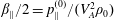 $\unicode[STIX]{x1D6FD}_{\Vert }/2=p_{\Vert }^{(0)}/(V_{A}^{2}\unicode[STIX]{x1D70C}_{0})$
. The heat flux equations are accompanied by the linearized system (9.11)–(9.19).
$\unicode[STIX]{x1D6FD}_{\Vert }/2=p_{\Vert }^{(0)}/(V_{A}^{2}\unicode[STIX]{x1D70C}_{0})$
. The heat flux equations are accompanied by the linearized system (9.11)–(9.19).
To consider FLR3 corrections, one needs to derive non-gyrotropic heat flux vectors
 $\boldsymbol{S}_{\bot }^{\Vert }$
,
$\boldsymbol{S}_{\bot }^{\Vert }$
,
 $\boldsymbol{S}_{\bot }^{\bot }$
for the bi-kappa distribution. For the first-order vectors the derivation is straightforward, and by following the calculations in appendix D, it is easy to show that the nonlinear
$\boldsymbol{S}_{\bot }^{\bot }$
for the bi-kappa distribution. For the first-order vectors the derivation is straightforward, and by following the calculations in appendix D, it is easy to show that the nonlinear
 $$\begin{eqnarray}\displaystyle \boldsymbol{S}_{\bot }^{\Vert (1)} & = & \displaystyle \frac{B_{0}}{\unicode[STIX]{x1D6FA}|\boldsymbol{B}|}\hat{\boldsymbol{b}}\times \left[\unicode[STIX]{x1D6FC}_{\unicode[STIX]{x1D705}}p_{\bot }\unicode[STIX]{x1D735}\left(\frac{p_{\Vert }}{\unicode[STIX]{x1D70C}}\right)+(\unicode[STIX]{x1D6FC}_{\unicode[STIX]{x1D705}}-1)\frac{p_{\Vert }}{\unicode[STIX]{x1D70C}}\unicode[STIX]{x1D735}p_{\bot }\right.\nonumber\\ \displaystyle & & \displaystyle +\left.(3\unicode[STIX]{x1D6FC}_{\unicode[STIX]{x1D705}}-1)\frac{p_{\Vert }}{\unicode[STIX]{x1D70C}}(p_{\Vert }-p_{\bot })\hat{\boldsymbol{b}}\boldsymbol{\cdot }\unicode[STIX]{x1D735}\hat{\boldsymbol{b}}+2q_{\Vert }\hat{\boldsymbol{b}}\boldsymbol{\cdot }\unicode[STIX]{x1D735}\boldsymbol{u}+2q_{\bot }\hat{\boldsymbol{b}}\times \unicode[STIX]{x1D74E}\right];\end{eqnarray}$$
 $$\begin{eqnarray}\displaystyle \boldsymbol{S}_{\bot }^{\bot (1)} & = & \displaystyle \frac{B_{0}}{\unicode[STIX]{x1D6FA}|\boldsymbol{B}|}\hat{\boldsymbol{b}}\times \left[2\unicode[STIX]{x1D6FC}_{\unicode[STIX]{x1D705}}p_{\bot }\unicode[STIX]{x1D735}\left(\frac{p_{\bot }}{\unicode[STIX]{x1D70C}}\right)\right.\nonumber\\ \displaystyle & & \displaystyle +\left.2(\unicode[STIX]{x1D6FC}_{\unicode[STIX]{x1D705}}-1)\frac{p_{\bot }}{\unicode[STIX]{x1D70C}}\unicode[STIX]{x1D735}p_{\bot }+2(\unicode[STIX]{x1D6FC}_{\unicode[STIX]{x1D705}}-1)\frac{p_{\bot }}{\unicode[STIX]{x1D70C}}(p_{\Vert }-p_{\bot })\hat{\boldsymbol{b}}\boldsymbol{\cdot }\unicode[STIX]{x1D735}\hat{\boldsymbol{b}}+4q_{\bot }\hat{\boldsymbol{b}}\boldsymbol{\cdot }\unicode[STIX]{x1D735}\boldsymbol{u}\right].\end{eqnarray}$$
Here, we neglected perturbations
 $\widetilde{r}$
, since we will not consider Landau fluid models for bi-kappa distribution. For
$\widetilde{r}$
, since we will not consider Landau fluid models for bi-kappa distribution. For
 $\unicode[STIX]{x1D6FC}_{\unicode[STIX]{x1D705}}=1$
, the results are of course equivalent to the bi-Maxwellian expressions (D 37), (D 60). The second-order heat flux vectors are not addressed here, since we would have to derive
$\unicode[STIX]{x1D6FC}_{\unicode[STIX]{x1D705}}=1$
, the results are of course equivalent to the bi-Maxwellian expressions (D 37), (D 60). The second-order heat flux vectors are not addressed here, since we would have to derive
 $\boldsymbol{r}^{\text{ng}}$
for the bi-kappa distribution.
$\boldsymbol{r}^{\text{ng}}$
for the bi-kappa distribution.
10.3 BiKappa dispersion relation
The BiKappa dispersion relation can be written in the following form
 $$\begin{eqnarray}\displaystyle & \displaystyle (\unicode[STIX]{x1D714}^{2}-v_{A\Vert }^{2}k_{\Vert }^{2})(\unicode[STIX]{x1D714}^{8}-A_{6}\unicode[STIX]{x1D714}^{6}+A_{4}\unicode[STIX]{x1D714}^{4}-A_{2}\unicode[STIX]{x1D714}^{2}+A_{0})=0; & \displaystyle\end{eqnarray}$$
 $$\begin{eqnarray}\displaystyle & \displaystyle A_{6}=k_{\Vert }^{2}\left(v_{A\Vert }^{2}+\unicode[STIX]{x1D6FC}_{\unicode[STIX]{x1D705}}{\textstyle \frac{7}{2}}\unicode[STIX]{x1D6FD}_{\Vert }\right)+k_{\bot }^{2}(1+a_{p}\unicode[STIX]{x1D6FD}); & \displaystyle\end{eqnarray}$$
 $$\begin{eqnarray}\displaystyle & \displaystyle A_{4}=\unicode[STIX]{x1D6FC}_{\unicode[STIX]{x1D705}}k_{\Vert }^{2}\unicode[STIX]{x1D6FD}_{\Vert }\left\{k_{\Vert }^{2}\left(\frac{7}{2}v_{A\Vert }^{2}+\frac{(3+6\unicode[STIX]{x1D6FC}_{\unicode[STIX]{x1D705}})}{4}\unicode[STIX]{x1D6FD}_{\Vert }\right)+k_{\bot }^{2}\frac{7}{2}\left(1+a_{p}\unicode[STIX]{x1D6FD}_{\Vert }-\frac{1}{7}a_{p}^{2}\unicode[STIX]{x1D6FD}_{\Vert }\right)\right\}; & \displaystyle\end{eqnarray}$$
 $$\begin{eqnarray}\displaystyle A_{2} & = & \displaystyle \unicode[STIX]{x1D6FC}_{\unicode[STIX]{x1D705}}k_{\Vert }^{4}\unicode[STIX]{x1D6FD}_{\Vert }^{2}\left\{k_{\Vert }^{2}\left(\frac{(3+6\unicode[STIX]{x1D6FC}_{\unicode[STIX]{x1D705}})}{4}v_{A\Vert }^{2}+\unicode[STIX]{x1D6FC}_{\unicode[STIX]{x1D705}}\frac{3}{8}\unicode[STIX]{x1D6FD}_{\Vert }\right)\right.\nonumber\\ \displaystyle & & \displaystyle +\left.k_{\bot }^{2}\frac{9}{4}\left(\frac{(1+2\unicode[STIX]{x1D6FC}_{\unicode[STIX]{x1D705}})}{3}(1+a_{p}\unicode[STIX]{x1D6FD}_{\Vert })-\frac{(1+9\unicode[STIX]{x1D6FC}_{\unicode[STIX]{x1D705}})}{18}a_{p}^{2}\unicode[STIX]{x1D6FD}_{\Vert }\right)\right\};\end{eqnarray}$$
 $$\begin{eqnarray}\displaystyle & \displaystyle A_{0}=\unicode[STIX]{x1D6FC}_{\unicode[STIX]{x1D705}}^{2}\frac{3}{8}k_{\Vert }^{6}\unicode[STIX]{x1D6FD}_{\Vert }^{3}\{k_{\Vert }^{2}v_{A\Vert }^{2}+k_{\bot }^{2}(1+a_{p}\unicode[STIX]{x1D6FD}_{\Vert }-a_{p}^{2}\unicode[STIX]{x1D6FD}_{\Vert })\}, & \displaystyle\end{eqnarray}$$
and for
 $\unicode[STIX]{x1D6FC}_{\unicode[STIX]{x1D705}}=1$
it is of course equivalent to the CGL2 dispersion relation (9.23). The oblique Alfvén mode is not affected, and is identical to (9.22), implying that the long-wavelength threshold of the oblique firehose instability is identical as well.
$\unicode[STIX]{x1D6FC}_{\unicode[STIX]{x1D705}}=1$
it is of course equivalent to the CGL2 dispersion relation (9.23). The oblique Alfvén mode is not affected, and is identical to (9.22), implying that the long-wavelength threshold of the oblique firehose instability is identical as well.
For strictly parallel propagation
 $(k_{\bot }=0)$
, the solutions of the remaining eighth-order polynomial are
$(k_{\bot }=0)$
, the solutions of the remaining eighth-order polynomial are
 $$\begin{eqnarray}\displaystyle & \displaystyle \unicode[STIX]{x1D714}=\pm k_{\Vert }v_{A\Vert }; & \displaystyle\end{eqnarray}$$
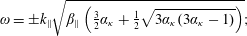 $$\begin{eqnarray}\displaystyle & \displaystyle \unicode[STIX]{x1D714}=\pm k_{\Vert }\sqrt{\unicode[STIX]{x1D6FD}_{\Vert }\left({\textstyle \frac{3}{2}}\unicode[STIX]{x1D6FC}_{\unicode[STIX]{x1D705}}+{\textstyle \frac{1}{2}}\sqrt{3\unicode[STIX]{x1D6FC}_{\unicode[STIX]{x1D705}}(3\unicode[STIX]{x1D6FC}_{\unicode[STIX]{x1D705}}-1)}\right)}; & \displaystyle\end{eqnarray}$$
 $$\begin{eqnarray}\displaystyle & \displaystyle \unicode[STIX]{x1D714}=\pm k_{\Vert }\sqrt{\unicode[STIX]{x1D6FC}_{\unicode[STIX]{x1D705}}\frac{\unicode[STIX]{x1D6FD}_{\Vert }}{2}}; & \displaystyle\end{eqnarray}$$
 $$\begin{eqnarray}\displaystyle & \displaystyle \unicode[STIX]{x1D714}=\pm k_{\Vert }\sqrt{\unicode[STIX]{x1D6FD}_{\Vert }\left({\textstyle \frac{3}{2}}\unicode[STIX]{x1D6FC}_{\unicode[STIX]{x1D705}}-{\textstyle \frac{1}{2}}\sqrt{3\unicode[STIX]{x1D6FC}_{\unicode[STIX]{x1D705}}(3\unicode[STIX]{x1D6FC}_{\unicode[STIX]{x1D705}}-1)}\right)}. & \displaystyle\end{eqnarray}$$
Note that in the last solution (10.61), the expression under the square root remains always positive, regardless of how large
 $\unicode[STIX]{x1D6FC}_{\unicode[STIX]{x1D705}}$
is (i.e. when the
$\unicode[STIX]{x1D6FC}_{\unicode[STIX]{x1D705}}$
is (i.e. when the
 $\unicode[STIX]{x1D705}$
-index approaches
$\unicode[STIX]{x1D705}$
-index approaches
 $5/2$
). For strictly perpendicular propagation
$5/2$
). For strictly perpendicular propagation
 $(k_{\Vert }=0)$
, the fast mode is not affected, and is equivalent to (9.31).
$(k_{\Vert }=0)$
, the fast mode is not affected, and is equivalent to (9.31).
10.4 Mirror instability
By considering the highly oblique limit
 $k_{\bot }\gg k_{\Vert }$
, and by assuming that
$k_{\bot }\gg k_{\Vert }$
, and by assuming that
 $\unicode[STIX]{x1D6FC}_{\unicode[STIX]{x1D705}}$
is not enormously large (i.e. that
$\unicode[STIX]{x1D6FC}_{\unicode[STIX]{x1D705}}$
is not enormously large (i.e. that
 $\unicode[STIX]{x1D705}$
is not very close to
$\unicode[STIX]{x1D705}$
is not very close to
 $5/2$
) so that
$5/2$
) so that
 $\unicode[STIX]{x1D6FC}_{\unicode[STIX]{x1D705}}k_{\Vert }$
can be neglected with respect to
$\unicode[STIX]{x1D6FC}_{\unicode[STIX]{x1D705}}k_{\Vert }$
can be neglected with respect to
 $k_{\bot }$
, the polynomial coefficients can be approximated as
$k_{\bot }$
, the polynomial coefficients can be approximated as
 $$\begin{eqnarray}\displaystyle & \displaystyle A_{6}=k_{\bot }^{2}(1+a_{p}\unicode[STIX]{x1D6FD}_{\Vert }); & \displaystyle\end{eqnarray}$$
 $$\begin{eqnarray}\displaystyle & \displaystyle A_{4}=\unicode[STIX]{x1D6FC}_{\unicode[STIX]{x1D705}}k_{\Vert }^{2}\unicode[STIX]{x1D6FD}_{\Vert }k_{\bot }^{2}{\textstyle \frac{7}{2}}\left(1+a_{p}\unicode[STIX]{x1D6FD}_{\Vert }-{\textstyle \frac{1}{7}}a_{p}^{2}\unicode[STIX]{x1D6FD}_{\Vert }\right); & \displaystyle\end{eqnarray}$$
 $$\begin{eqnarray}\displaystyle & \displaystyle A_{2}=\unicode[STIX]{x1D6FC}_{\unicode[STIX]{x1D705}}k_{\Vert }^{4}\unicode[STIX]{x1D6FD}_{\Vert }^{2}k_{\bot }^{2}\frac{9}{4}\left(\frac{(1+2\unicode[STIX]{x1D6FC}_{\unicode[STIX]{x1D705}})}{3}(1+a_{p}\unicode[STIX]{x1D6FD}_{\Vert })-\frac{(1+9\unicode[STIX]{x1D6FC}_{\unicode[STIX]{x1D705}})}{18}a_{p}^{2}\unicode[STIX]{x1D6FD}_{\Vert }\right); & \displaystyle\end{eqnarray}$$
 $$\begin{eqnarray}\displaystyle & \displaystyle A_{0}=\unicode[STIX]{x1D6FC}_{\unicode[STIX]{x1D705}}^{2}\frac{3}{8}k_{\Vert }^{6}\unicode[STIX]{x1D6FD}_{\Vert }^{3}k_{\bot }^{2}(1+a_{p}\unicode[STIX]{x1D6FD}_{\Vert }-a_{p}^{2}\unicode[STIX]{x1D6FD}_{\Vert }). & \displaystyle\end{eqnarray}$$
The fast mode can be quickly separated with the trick (9.36), and by using the substitution
 $\bar{\unicode[STIX]{x1D714}}=\unicode[STIX]{x1D714}/(k_{\Vert }\sqrt{\unicode[STIX]{x1D6FD}_{\Vert }})$
, the resulting polynomial reads
$\bar{\unicode[STIX]{x1D714}}=\unicode[STIX]{x1D714}/(k_{\Vert }\sqrt{\unicode[STIX]{x1D6FD}_{\Vert }})$
, the resulting polynomial reads
 $$\begin{eqnarray}\displaystyle & & \displaystyle -(1+a_{p}\unicode[STIX]{x1D6FD}_{\Vert })\bar{\unicode[STIX]{x1D714}}^{6}+\unicode[STIX]{x1D6FC}_{\unicode[STIX]{x1D705}}\frac{7}{2}\left(1+a_{p}\unicode[STIX]{x1D6FD}_{\Vert }-\frac{1}{7}a_{p}^{2}\unicode[STIX]{x1D6FD}_{\Vert }\right)\bar{\unicode[STIX]{x1D714}}^{4}\nonumber\\ \displaystyle & & \displaystyle \qquad -\,\unicode[STIX]{x1D6FC}_{\unicode[STIX]{x1D705}}\frac{9}{4}\left(\frac{(1+2\unicode[STIX]{x1D6FC}_{\unicode[STIX]{x1D705}})}{3}(1+a_{p}\unicode[STIX]{x1D6FD}_{\Vert })-\frac{(1+9\unicode[STIX]{x1D6FC}_{\unicode[STIX]{x1D705}})}{18}a_{p}^{2}\unicode[STIX]{x1D6FD}_{\Vert }\right)\bar{\unicode[STIX]{x1D714}}^{2}\nonumber\\ \displaystyle & & \displaystyle \qquad +\,\unicode[STIX]{x1D6FC}_{\unicode[STIX]{x1D705}}^{2}\frac{3}{8}(1+a_{p}\unicode[STIX]{x1D6FD}_{\Vert }-a_{p}^{2}\unicode[STIX]{x1D6FD}_{\Vert })=0.\end{eqnarray}$$
At exactly the (assumed) mirror threshold
 $a_{p}^{2}\unicode[STIX]{x1D6FD}_{\Vert }=1+a_{p}\unicode[STIX]{x1D6FD}_{\Vert }$
, the coefficient
$a_{p}^{2}\unicode[STIX]{x1D6FD}_{\Vert }=1+a_{p}\unicode[STIX]{x1D6FD}_{\Vert }$
, the coefficient
 $A_{0}$
disappears, so we have one solution
$A_{0}$
disappears, so we have one solution
 $\bar{\unicode[STIX]{x1D714}}^{2}=0$
; from the remaining polynomial the
$\bar{\unicode[STIX]{x1D714}}^{2}=0$
; from the remaining polynomial the
 $1+a_{p}\unicode[STIX]{x1D6FD}_{\Vert }$
can be factored out and the solutions are
$1+a_{p}\unicode[STIX]{x1D6FD}_{\Vert }$
can be factored out and the solutions are
 $$\begin{eqnarray}\bar{\unicode[STIX]{x1D714}}^{2}={\textstyle \frac{3}{2}}\unicode[STIX]{x1D6FC}_{\unicode[STIX]{x1D705}}\pm {\textstyle \frac{1}{4}}\sqrt{10\unicode[STIX]{x1D6FC}_{\unicode[STIX]{x1D705}}(3\unicode[STIX]{x1D6FC}_{\unicode[STIX]{x1D705}}-1)},\end{eqnarray}$$
both always positive. Slightly below
 $(\unicode[STIX]{x1D716}<0)$
or beyond
$(\unicode[STIX]{x1D716}<0)$
or beyond
 $(\unicode[STIX]{x1D716}>0)$
the mirror threshold, one can prescribe
$(\unicode[STIX]{x1D716}>0)$
the mirror threshold, one can prescribe
 $a_{p}^{2}\unicode[STIX]{x1D6FD}_{\Vert }=(1+a_{p}\unicode[STIX]{x1D6FD}_{\Vert })(1+\unicode[STIX]{x1D716})$
, where
$a_{p}^{2}\unicode[STIX]{x1D6FD}_{\Vert }=(1+a_{p}\unicode[STIX]{x1D6FD}_{\Vert })(1+\unicode[STIX]{x1D716})$
, where
 $\unicode[STIX]{x1D716}$
is a small parameter and the polynomial transforms to
$\unicode[STIX]{x1D716}$
is a small parameter and the polynomial transforms to
 $$\begin{eqnarray}(\bar{\unicode[STIX]{x1D714}}^{2})^{3}-\unicode[STIX]{x1D6FC}_{\unicode[STIX]{x1D705}}\left(3-\frac{\unicode[STIX]{x1D716}}{2}\right)(\bar{\unicode[STIX]{x1D714}}^{2})^{2}+\frac{\unicode[STIX]{x1D6FC}_{\unicode[STIX]{x1D705}}}{8}(5+3\unicode[STIX]{x1D6FC}_{\unicode[STIX]{x1D705}}-\unicode[STIX]{x1D716}(1+9\unicode[STIX]{x1D6FC}_{\unicode[STIX]{x1D705}}))(\bar{\unicode[STIX]{x1D714}}^{2})+\frac{3}{8}\unicode[STIX]{x1D6FC}_{\unicode[STIX]{x1D705}}^{2}\unicode[STIX]{x1D716}=0,\end{eqnarray}$$
and which for
 $\unicode[STIX]{x1D6FC}_{\unicode[STIX]{x1D705}}=1$
is equivalent to the bi-Maxwellian polynomial (9.39). As previously, for small
$\unicode[STIX]{x1D6FC}_{\unicode[STIX]{x1D705}}=1$
is equivalent to the bi-Maxwellian polynomial (9.39). As previously, for small
 $\unicode[STIX]{x1D716}$
the solutions (10.67) remain almost the same, and positive. Furthermore, since multiplying all 3 solutions together must yield
$\unicode[STIX]{x1D716}$
the solutions (10.67) remain almost the same, and positive. Furthermore, since multiplying all 3 solutions together must yield
 $-\frac{3}{8}\unicode[STIX]{x1D6FC}_{\unicode[STIX]{x1D705}}^{2}\unicode[STIX]{x1D716}$
, this implies that below
$-\frac{3}{8}\unicode[STIX]{x1D6FC}_{\unicode[STIX]{x1D705}}^{2}\unicode[STIX]{x1D716}$
, this implies that below
 $(\unicode[STIX]{x1D716}<0)$
the threshold the third solution is positive, and beyond
$(\unicode[STIX]{x1D716}<0)$
the threshold the third solution is positive, and beyond
 $(\unicode[STIX]{x1D716}>0)$
the threshold the third solution is negative, which analytically proves that the (highly oblique) mirror instability threshold is
$(\unicode[STIX]{x1D716}>0)$
the threshold the third solution is negative, which analytically proves that the (highly oblique) mirror instability threshold is
 $a_{p}^{2}\unicode[STIX]{x1D6FD}_{\Vert }=1+a_{p}\unicode[STIX]{x1D6FD}_{\Vert }$
, regardless of
$a_{p}^{2}\unicode[STIX]{x1D6FD}_{\Vert }=1+a_{p}\unicode[STIX]{x1D6FD}_{\Vert }$
, regardless of
 $\unicode[STIX]{x1D6FC}_{\unicode[STIX]{x1D705}}$
. The long-wavelength limit or ‘hard’ mirror threshold for the bi-kappa distribution is therefore the same as for the bi-Maxwellian distribution.
$\unicode[STIX]{x1D6FC}_{\unicode[STIX]{x1D705}}$
. The long-wavelength limit or ‘hard’ mirror threshold for the bi-kappa distribution is therefore the same as for the bi-Maxwellian distribution.
Conclusion
We investigated solutions of the (non-dispersive) BiKappa fluid model. The calculations were done with closure (10.42) for a general
 $\unicode[STIX]{x1D6FC}_{\unicode[STIX]{x1D705}}$
coefficient, i.e. without using the specific value (10.43) for the bi-kappa distribution. The calculations are therefore more general and valid for any distribution function that can be closed as (10.42). We conclude that all 3 long-wavelength ‘hard’ thresholds – for the parallel and oblique firehose instability and the highly oblique mirror instability – are not affected by the value of
$\unicode[STIX]{x1D6FC}_{\unicode[STIX]{x1D705}}$
coefficient, i.e. without using the specific value (10.43) for the bi-kappa distribution. The calculations are therefore more general and valid for any distribution function that can be closed as (10.42). We conclude that all 3 long-wavelength ‘hard’ thresholds – for the parallel and oblique firehose instability and the highly oblique mirror instability – are not affected by the value of
 $\unicode[STIX]{x1D6FC}_{\unicode[STIX]{x1D705}}$
.
$\unicode[STIX]{x1D6FC}_{\unicode[STIX]{x1D705}}$
.
10.5 Hall-BiKappa dispersion relation
The Hall-BiKappa dispersion relation can be written in the following form
 $$\begin{eqnarray}\displaystyle & & \displaystyle (\unicode[STIX]{x1D714}^{2}-v_{A\Vert }^{2}k_{\Vert }^{2})(\unicode[STIX]{x1D714}^{8}-A_{6}\unicode[STIX]{x1D714}^{6}+A_{4}\unicode[STIX]{x1D714}^{4}-A_{2}\unicode[STIX]{x1D714}^{2}+A_{0})\nonumber\\ \displaystyle & & \displaystyle \quad =k^{2}k_{\Vert }^{2}\unicode[STIX]{x1D714}^{2}\left[\unicode[STIX]{x1D714}^{6}-\unicode[STIX]{x1D714}^{4}\unicode[STIX]{x1D6FD}_{\Vert }\left({\textstyle \frac{7}{2}}\unicode[STIX]{x1D6FC}_{\unicode[STIX]{x1D705}}k_{\Vert }^{2}+a_{p}k_{\bot }^{2}\right)+\unicode[STIX]{x1D714}^{2}\unicode[STIX]{x1D6FC}_{\unicode[STIX]{x1D705}}\unicode[STIX]{x1D6FD}_{\Vert }^{2}k_{\Vert }^{2}\left({\textstyle \frac{3}{4}}(1+2\unicode[STIX]{x1D6FC}_{\unicode[STIX]{x1D705}})k_{\Vert }^{2}+3a_{p}k_{\bot }^{2}\right)\right.\nonumber\\ \displaystyle & & \displaystyle \qquad -\left.\unicode[STIX]{x1D6FC}_{\unicode[STIX]{x1D705}}k_{\Vert }^{4}\unicode[STIX]{x1D6FD}_{\Vert }^{3}\left({\textstyle \frac{3}{8}}\unicode[STIX]{x1D6FC}_{\unicode[STIX]{x1D705}}k_{\Vert }^{2}+{\textstyle \frac{1}{8}}(5+3\unicode[STIX]{x1D6FC}_{\unicode[STIX]{x1D705}})a_{p}k_{\bot }^{2}\right)\right],\end{eqnarray}$$
where we kept the BiKappa dispersion relation (10.53)–(10.57) on the left-hand side, and the Hall term contributions to the right-hand side. For the bi-Maxwellian value
 $\unicode[STIX]{x1D6FC}_{\unicode[STIX]{x1D705}}=1$
, the result is equivalent to the Hall-CGL2 dispersion relation (9.40). For strictly parallel propagation, the solutions are the usual dispersive ion-cyclotron and whistler waves (that are not affected by the
$\unicode[STIX]{x1D6FC}_{\unicode[STIX]{x1D705}}=1$
, the result is equivalent to the Hall-CGL2 dispersion relation (9.40). For strictly parallel propagation, the solutions are the usual dispersive ion-cyclotron and whistler waves (that are not affected by the
 $\unicode[STIX]{x1D6FC}_{\unicode[STIX]{x1D705}}$
coefficient) and the non-dispersive solutions (10.59)–(10.61) of the BiKappa model. For strictly perpendicular propagation, the Hall term naturally disappears and the fast mode solution is (9.31).
$\unicode[STIX]{x1D6FC}_{\unicode[STIX]{x1D705}}$
coefficient) and the non-dispersive solutions (10.59)–(10.61) of the BiKappa model. For strictly perpendicular propagation, the Hall term naturally disappears and the fast mode solution is (9.31).
11 Collisionless damping in fluid models – Landau fluid models
In the previous sections, we have calculated the fluid hierarchy up to the fourth-order fluid moment
 $\boldsymbol{r}$
. We have seen that, unless we crossed some instability threshold, the dispersion relations yielded frequencies
$\boldsymbol{r}$
. We have seen that, unless we crossed some instability threshold, the dispersion relations yielded frequencies
 $\unicode[STIX]{x1D714}$
that were purely real, and there was no collisionless damping present. Remarkably, collisionless damping, i.e. Landau damping, will be absent even if we continue to develop the fluid hierarchy to higher-order moments. In fact, we will see in the next section that, by considering parallel 1-D propagation (where all the fluctuations are along
$\unicode[STIX]{x1D714}$
that were purely real, and there was no collisionless damping present. Remarkably, collisionless damping, i.e. Landau damping, will be absent even if we continue to develop the fluid hierarchy to higher-order moments. In fact, we will see in the next section that, by considering parallel 1-D propagation (where all the fluctuations are along
 $\boldsymbol{B}_{0}$
), the fluid models closed by a bi-Maxwellian fluid closure at higher-order moments than
$\boldsymbol{B}_{0}$
), the fluid models closed by a bi-Maxwellian fluid closure at higher-order moments than
 $\boldsymbol{r}$
are always unstable. Such fluid models are physically ill posed. To go higher in the fluid hierarchy, one needs to incorporate the Landau damping phenomenon into the fluid framework, and consider Landau fluid closures.
$\boldsymbol{r}$
are always unstable. Such fluid models are physically ill posed. To go higher in the fluid hierarchy, one needs to incorporate the Landau damping phenomenon into the fluid framework, and consider Landau fluid closures.
Nevertheless, to capture the Landau damping, it is not necessary to go beyond the fourth-order moment and closures performed at the fourth moment level describe the Landau damping with very good accuracy. Even though the entire Part 2 of this text is dedicated to Landau fluid closures, it is beneficial to briefly show why the Landau damping was omitted in the previous calculations. Let us consider the simplest example of 1-D electrostatic propagation. The collisionless Vlasov equation reads
 $$\begin{eqnarray}\frac{\unicode[STIX]{x2202}f}{\unicode[STIX]{x2202}t}+v_{z}\unicode[STIX]{x2202}_{z}f+\frac{q}{m}E_{z}\frac{\unicode[STIX]{x2202}f}{\unicode[STIX]{x2202}v_{z}}=0.\end{eqnarray}$$
Direct integration of the Vlasov equation (over
 $v_{z}$
) for a general distribution function
$v_{z}$
) for a general distribution function
 $f$
, of course yields the usual density equation,
$f$
, of course yields the usual density equation,
 $\unicode[STIX]{x2202}n/\unicode[STIX]{x2202}t+\unicode[STIX]{x2202}_{z}(nu_{z})=0$
. The same result is obtained if one considers a specific
$\unicode[STIX]{x2202}n/\unicode[STIX]{x2202}t+\unicode[STIX]{x2202}_{z}(nu_{z})=0$
. The same result is obtained if one considers a specific
 $f_{0}$
, such as for example 1-D Maxwellian
$f_{0}$
, such as for example 1-D Maxwellian
 $f_{0}=n\sqrt{(\unicode[STIX]{x1D6FC}/\unicode[STIX]{x03C0})}\text{e}^{-\unicode[STIX]{x1D6FC}(v_{z}-u_{z})^{2}}$
, 1-D kappa distribution, etc. The last term of the Vlasov equation
$f_{0}=n\sqrt{(\unicode[STIX]{x1D6FC}/\unicode[STIX]{x03C0})}\text{e}^{-\unicode[STIX]{x1D6FC}(v_{z}-u_{z})^{2}}$
, 1-D kappa distribution, etc. The last term of the Vlasov equation
 ${\sim}E_{z}$
vanishes by the integration, since
${\sim}E_{z}$
vanishes by the integration, since
 $\int _{-\infty }^{\infty }(\unicode[STIX]{x2202}f/\unicode[STIX]{x2202}v_{z})\,\text{d}v_{z}=0$
. Now let us do the calculation differently, by expanding the distribution function
$\int _{-\infty }^{\infty }(\unicode[STIX]{x2202}f/\unicode[STIX]{x2202}v_{z})\,\text{d}v_{z}=0$
. Now let us do the calculation differently, by expanding the distribution function
 $f=f_{0}+f^{(1)}$
, where
$f=f_{0}+f^{(1)}$
, where
 $f_{0}$
does not have any time or spatial dependence, so
$f_{0}$
does not have any time or spatial dependence, so
 $\unicode[STIX]{x2202}f_{0}/\unicode[STIX]{x2202}t=0,\unicode[STIX]{x2202}_{z}f_{0}=0$
. We can consider the Maxwellian
$\unicode[STIX]{x2202}f_{0}/\unicode[STIX]{x2202}t=0,\unicode[STIX]{x2202}_{z}f_{0}=0$
. We can consider the Maxwellian
 $f_{0}=n_{0}\sqrt{(\unicode[STIX]{x1D6FC}/\unicode[STIX]{x03C0})}\text{e}^{-\unicode[STIX]{x1D6FC}v_{z}^{2}}$
where
$f_{0}=n_{0}\sqrt{(\unicode[STIX]{x1D6FC}/\unicode[STIX]{x03C0})}\text{e}^{-\unicode[STIX]{x1D6FC}v_{z}^{2}}$
where
 $\unicode[STIX]{x1D6FC}=m/(2T^{(0)})=1/v_{\text{th}}^{2}$
. The electric field is also expanded
$\unicode[STIX]{x1D6FC}=m/(2T^{(0)})=1/v_{\text{th}}^{2}$
. The electric field is also expanded
 $E_{z}=E_{z}^{(0)}+E_{z}^{(1)}$
, and one assumes that there is no large-scale electric field, so
$E_{z}=E_{z}^{(0)}+E_{z}^{(1)}$
, and one assumes that there is no large-scale electric field, so
 $E_{z}^{(0)}=0$
. By neglecting the term with two small quantities
$E_{z}^{(0)}=0$
. By neglecting the term with two small quantities
 $E_{z}^{(1)}\unicode[STIX]{x2202}f^{(1)}/\unicode[STIX]{x2202}v_{z}$
, the Vlasov equation reads
$E_{z}^{(1)}\unicode[STIX]{x2202}f^{(1)}/\unicode[STIX]{x2202}v_{z}$
, the Vlasov equation reads
 $$\begin{eqnarray}\frac{\unicode[STIX]{x2202}f^{(1)}}{\unicode[STIX]{x2202}t}+v_{z}\unicode[STIX]{x2202}_{z}f^{(1)}+\frac{q}{m}E_{z}^{(1)}\frac{\unicode[STIX]{x2202}f_{0}}{\unicode[STIX]{x2202}v_{z}}=0,\end{eqnarray}$$
and transformation to Fourier space yields
 $$\begin{eqnarray}-\text{i}(\unicode[STIX]{x1D714}-k_{z}v_{z})f^{(1)}+\frac{q}{m}E_{z}^{(1)}\frac{\unicode[STIX]{x2202}f_{0}}{\unicode[STIX]{x2202}v_{z}}=0.\end{eqnarray}$$
The equation (11.3) is actually not that much different from (11.1), the Vlasov equation is just fully linearized and written in Fourier space. However, in kinetic calculations, the (11.3) is not directly integrated in this form. The crucial technique that reveals the presence of Landau damping in the Vlasov equation is that the equation (11.3) is first divided by
 $(\unicode[STIX]{x1D714}-k_{z}v_{z})$
, and an expression for
$(\unicode[STIX]{x1D714}-k_{z}v_{z})$
, and an expression for
 $f^{(1)}$
is obtained. Only then is the equation integrated over the velocity space, yielding
$f^{(1)}$
is obtained. Only then is the equation integrated over the velocity space, yielding
 $$\begin{eqnarray}f^{(1)}=-\frac{q}{m}\text{i}E_{z}^{(1)}\frac{\displaystyle \frac{\unicode[STIX]{x2202}f_{0}}{\unicode[STIX]{x2202}v_{z}}}{\unicode[STIX]{x1D714}-k_{z}v_{z}};\quad \Rightarrow \quad n^{(1)}=\int _{-\infty }^{\infty }f^{(1)}\,\text{d}v_{z}=-\frac{q}{m}\text{i}E_{z}^{(1)}\int _{-\infty }^{\infty }\frac{\displaystyle \frac{\unicode[STIX]{x2202}f_{0}}{\unicode[STIX]{x2202}v_{z}}}{\unicode[STIX]{x1D714}-k_{z}v_{z}}\,\text{d}v_{z}.\end{eqnarray}$$
The integral contains a ‘singularity’ in the denominator, and it is not obvious how to calculate this integral. Such singularities are called wave–particle resonances, and can have a more general form
 $\unicode[STIX]{x1D714}-k_{z}v_{z}\pm l\unicode[STIX]{x1D6FA}$
, where
$\unicode[STIX]{x1D714}-k_{z}v_{z}\pm l\unicode[STIX]{x1D6FA}$
, where
 $\unicode[STIX]{x1D6FA}$
is the cyclotron frequency of the considered species, and
$\unicode[STIX]{x1D6FA}$
is the cyclotron frequency of the considered species, and
 $l$
is an integer. The resonance for
$l$
is an integer. The resonance for
 $l=0$
is called the Landau resonance, and the other resonances for
$l=0$
is called the Landau resonance, and the other resonances for
 $l\neq 0$
are called cyclotron resonances. It is the presence of these resonances in integrals such as (11.4), that yields collisionless damping mechanisms, the Landau damping and the cyclotron damping. In Part 2 of our guide, we will see that the integral actually cannot be ‘calculated’, i.e. the integral cannot be expressed through elementary functions, even if
$l\neq 0$
are called cyclotron resonances. It is the presence of these resonances in integrals such as (11.4), that yields collisionless damping mechanisms, the Landau damping and the cyclotron damping. In Part 2 of our guide, we will see that the integral actually cannot be ‘calculated’, i.e. the integral cannot be expressed through elementary functions, even if
 $f_{0}$
is a simple Maxwellian. The integral is just expressed through the famous plasma dispersion function
$f_{0}$
is a simple Maxwellian. The integral is just expressed through the famous plasma dispersion function
 $Z(\unicode[STIX]{x1D701})$
, where
$Z(\unicode[STIX]{x1D701})$
, where
 $\unicode[STIX]{x1D701}=\unicode[STIX]{x1D714}/(|k_{z}|v_{\text{th}})$
, since the plasma dispersion function was specifically developed to describe this integral. Skipping many technical (but very important) details, such as the definition of
$\unicode[STIX]{x1D701}=\unicode[STIX]{x1D714}/(|k_{z}|v_{\text{th}})$
, since the plasma dispersion function was specifically developed to describe this integral. Skipping many technical (but very important) details, such as the definition of
 $Z(\unicode[STIX]{x1D701})$
, for a Maxwellian
$Z(\unicode[STIX]{x1D701})$
, for a Maxwellian
 $f_{0}$
the density integral is simply expressed as
$f_{0}$
the density integral is simply expressed as
 $$\begin{eqnarray}n^{(1)}=-\frac{q}{m}\frac{\text{i}E_{z}^{(1)}}{k_{z}}(1+\unicode[STIX]{x1D701}Z(\unicode[STIX]{x1D701})).\end{eqnarray}$$
One can define function
 $R(\unicode[STIX]{x1D701})=1+\unicode[STIX]{x1D701}Z(\unicode[STIX]{x1D701})$
, that is called the plasma response function. Now, for example, considering a proton–electron plasma with
$R(\unicode[STIX]{x1D701})=1+\unicode[STIX]{x1D701}Z(\unicode[STIX]{x1D701})$
, that is called the plasma response function. Now, for example, considering a proton–electron plasma with
 $T_{e}^{(0)}=T_{p}^{(0)}$
at wavelengths that are much longer than the Debye length, yields the following dispersion relation and numerical solution
$T_{e}^{(0)}=T_{p}^{(0)}$
at wavelengths that are much longer than the Debye length, yields the following dispersion relation and numerical solution
 $$\begin{eqnarray}\displaystyle R(\unicode[STIX]{x1D701}_{p})+R(\unicode[STIX]{x1D701}_{e})=0;\quad \Rightarrow \quad \unicode[STIX]{x1D701}_{p}=\frac{\unicode[STIX]{x1D714}}{|k_{z}|v_{\text{th}p}}=\pm 1.457-0.627\text{i}. & & \displaystyle\end{eqnarray}$$
The negative imaginary part represents the Landau damping, and the effect comes from the Landau resonance in the integral (11.4). Obviously, integrating the Vlasov equation directly in the form (11.1) or (2.1) neglects the wave–particle resonances in velocity space, which clarifies why traditional fluid models do not contain collisionless damping mechanisms. It is
 $f^{(1)}$
– the fluctuations/perturbations around
$f^{(1)}$
– the fluctuations/perturbations around
 $f_{0}$
– where the wave–particle resonances are written down explicitly, that yields the collisionless damping mechanisms in kinetic theory. To introduce collisionless damping into fluid models, we have no other choice, and we have to calculate the hierarchy of moments again, this time by integrating over the ‘kinetic’
$f_{0}$
– where the wave–particle resonances are written down explicitly, that yields the collisionless damping mechanisms in kinetic theory. To introduce collisionless damping into fluid models, we have no other choice, and we have to calculate the hierarchy of moments again, this time by integrating over the ‘kinetic’
 $f^{(1)}$
. We find it useful to introduce the following vocabulary:
$f^{(1)}$
. We find it useful to introduce the following vocabulary:
(i) Fluid moments
$=$
integrals over a general (unspecified) distribution function
$f$
, or over a specific
$f_{0}$
. Evolution equations for fluid moments are obtained by direct integration of the Vlasov equation written in a form that does not explicitly contain wave–particle resonances. The resulting expressions can be nonlinear or linear and contain only fluid variables, i.e. expressions do not contain
$Z(\unicode[STIX]{x1D701})$
.(ii) Kinetic moments
$=$
integrals over
$f^{(1)}$
(perturbations
$f^{(1)}=f-f_{0}$
, where a specific equilibrium
$f_{0}$
is assumed), where the wave–particle resonances in velocity space are written down explicitly. The resulting expressions are linear and contain
$Z(\unicode[STIX]{x1D701})$
, which is not a fluid variable.


Importantly, we want to keep the entire nonlinear fluid hierarchy discussed so far, including the nonlinear heat flux equations. Therefore, considering bi-Maxwellian distribution
 $f_{0}$
, instead of the ‘normal’ closure, the fourth-order moment is decomposed in the following form
$f_{0}$
, instead of the ‘normal’ closure, the fourth-order moment is decomposed in the following form
 $$\begin{eqnarray}\displaystyle r_{\Vert \Vert }=\frac{3p_{\Vert }^{2}}{\unicode[STIX]{x1D70C}}+\widetilde{r}_{\Vert \Vert };\quad r_{\Vert \bot }=\frac{p_{\Vert }p_{\bot }}{\unicode[STIX]{x1D70C}}+\widetilde{r}_{\Vert \bot };\quad r_{\bot \bot }=\frac{2p_{\bot }^{2}}{\unicode[STIX]{x1D70C}}+\widetilde{r}_{\bot \bot }. & & \displaystyle\end{eqnarray}$$
The first terms represent the ‘normal’ closure, i.e. when an exact bi-Maxwellian
 $f_{0}$
is prescribed. The tilde components represent fluctuations/perturbations around
$f_{0}$
is prescribed. The tilde components represent fluctuations/perturbations around
 $f_{0}$
, and a good notation would also be
$f_{0}$
, and a good notation would also be
 $\unicode[STIX]{x1D6FF}r$
. The decomposition (11.7) yields the following form of the nonlinear heat flux equations
$\unicode[STIX]{x1D6FF}r$
. The decomposition (11.7) yields the following form of the nonlinear heat flux equations
 $$\begin{eqnarray}\displaystyle & & \displaystyle \frac{\unicode[STIX]{x2202}q_{\Vert }}{\unicode[STIX]{x2202}t}+\unicode[STIX]{x1D735}\boldsymbol{\cdot }(q_{\Vert }\boldsymbol{u})+\unicode[STIX]{x1D735}\boldsymbol{\cdot }(\widetilde{r}_{\Vert \Vert }\hat{\boldsymbol{b}})-3\widetilde{r}_{\Vert \bot }\unicode[STIX]{x1D735}\boldsymbol{\cdot }\hat{\boldsymbol{b}}+3p_{\Vert }\hat{\boldsymbol{b}}\boldsymbol{\cdot }\unicode[STIX]{x1D735}\left(\frac{p_{\Vert }}{\unicode[STIX]{x1D70C}}\right)+3q_{\Vert }\hat{\boldsymbol{b}}\boldsymbol{\cdot }\unicode[STIX]{x1D735}\boldsymbol{u}\boldsymbol{\cdot }\hat{\boldsymbol{b}}=0;\nonumber\\ \displaystyle & & \displaystyle\end{eqnarray}$$
 $$\begin{eqnarray}\displaystyle & & \displaystyle \frac{\unicode[STIX]{x2202}q_{\bot }}{\unicode[STIX]{x2202}t}+\unicode[STIX]{x1D735}\boldsymbol{\cdot }(q_{\bot }\boldsymbol{u})+q_{\bot }\unicode[STIX]{x1D735}\boldsymbol{\cdot }\boldsymbol{u}+\unicode[STIX]{x1D735}\boldsymbol{\cdot }(\widetilde{r}_{\Vert \bot }\hat{\boldsymbol{b}})+(\widetilde{r}_{\Vert \bot }-\widetilde{r}_{\bot \bot })\unicode[STIX]{x1D735}\boldsymbol{\cdot }\hat{\boldsymbol{b}}+p_{\Vert }\hat{\boldsymbol{b}}\boldsymbol{\cdot }\unicode[STIX]{x1D735}\left(\frac{p_{\bot }}{\unicode[STIX]{x1D70C}}\right)\nonumber\\ \displaystyle & & \displaystyle \qquad +\,\frac{p_{\bot }}{\unicode[STIX]{x1D70C}}(p_{\Vert }-p_{\bot })\unicode[STIX]{x1D735}\boldsymbol{\cdot }\hat{\boldsymbol{b}}+\frac{p_{\bot }}{\unicode[STIX]{x1D70C}}(\unicode[STIX]{x1D735}\boldsymbol{\cdot }\unicode[STIX]{x1D72B})\boldsymbol{\cdot }\hat{\boldsymbol{b}}_{0}=0.\end{eqnarray}$$
Similarly to decomposition (11.7), ‘kinetic’ corrections with wave–particle resonances can also be considered for the non-gyrotropic
 $\boldsymbol{r}^{\text{ng}}$
, which is not addressed in this guide. Neglecting those contributions, the heat flux equations are equivalent for example to equations (14), (15) of Passot & Sulem (Reference Passot and Sulem2007), and equations (9), (10) of Passot et al. (Reference Passot, Sulem and Hunana2012).
$\boldsymbol{r}^{\text{ng}}$
, which is not addressed in this guide. Neglecting those contributions, the heat flux equations are equivalent for example to equations (14), (15) of Passot & Sulem (Reference Passot and Sulem2007), and equations (9), (10) of Passot et al. (Reference Passot, Sulem and Hunana2012).
In Part 2 of this guide, we will calculate the ‘kinetic moments’ for
 $\widetilde{r}_{\Vert \Vert }$
,
$\widetilde{r}_{\Vert \Vert }$
,
 $\widetilde{r}_{\Vert \bot }$
,
$\widetilde{r}_{\Vert \bot }$
,
 $\widetilde{r}_{\bot \bot }$
, by integrating over
$\widetilde{r}_{\bot \bot }$
, by integrating over
 $f^{(1)}$
. In the 3-D electromagnetic geometry, we will use a more sophisticated
$f^{(1)}$
. In the 3-D electromagnetic geometry, we will use a more sophisticated
 $f^{(1)}$
in the gyrotropic limit, which describes both Landau damping and its magnetic analogue, the transit-time damping. The expressions for the entire ‘kinetic’ hierarchy will contain
$f^{(1)}$
in the gyrotropic limit, which describes both Landau damping and its magnetic analogue, the transit-time damping. The expressions for the entire ‘kinetic’ hierarchy will contain
 $Z(\unicode[STIX]{x1D701})$
, or actually
$Z(\unicode[STIX]{x1D701})$
, or actually
 $R(\unicode[STIX]{x1D701})$
, which is not a fluid variable. Nevertheless, we will see that by introducing the concept of the Padé approximation to
$R(\unicode[STIX]{x1D701})$
, which is not a fluid variable. Nevertheless, we will see that by introducing the concept of the Padé approximation to
 $R(\unicode[STIX]{x1D701})$
, that sometimes a rare possibility arises, when the ‘kinetic’ moment
$R(\unicode[STIX]{x1D701})$
, that sometimes a rare possibility arises, when the ‘kinetic’ moment
 $\widetilde{r}$
can be expressed through lower-order ‘kinetic’ moments. Such a closure, where the last retained kinetic moment (in this case
$\widetilde{r}$
can be expressed through lower-order ‘kinetic’ moments. Such a closure, where the last retained kinetic moment (in this case
 $\widetilde{r}$
) is expressed through lower-order moments, in a way such that the kinetic
$\widetilde{r}$
) is expressed through lower-order moments, in a way such that the kinetic
 $Z(\unicode[STIX]{x1D701})$
function is completely eliminated and that the closure is valid for all
$Z(\unicode[STIX]{x1D701})$
function is completely eliminated and that the closure is valid for all
 $\unicode[STIX]{x1D701}$
values, will be called a Landau fluid closure. For the impatient reader, we will reveal that one of the possibilities is going to be (written in Fourier space)
$\unicode[STIX]{x1D701}$
values, will be called a Landau fluid closure. For the impatient reader, we will reveal that one of the possibilities is going to be (written in Fourier space)
 $$\begin{eqnarray}\displaystyle & \displaystyle \widetilde{r}_{\Vert \Vert }=\frac{32-9\unicode[STIX]{x03C0}}{2(3\unicode[STIX]{x03C0}-8)}n_{0}v_{\text{th}\Vert }^{2}T_{\Vert }-\frac{2\sqrt{\unicode[STIX]{x03C0}}}{3\unicode[STIX]{x03C0}-8}v_{\text{th}\Vert }\frac{\text{i}k_{\Vert }}{|k_{\Vert }|}q_{\Vert }; & \displaystyle\end{eqnarray}$$
 $$\begin{eqnarray}\displaystyle & \displaystyle \widetilde{r}_{\Vert \bot }=-\frac{\sqrt{\unicode[STIX]{x03C0}}}{2}v_{\text{th}\Vert }\frac{\text{i}k_{\Vert }}{|k_{\Vert }|}q_{\bot }; & \displaystyle\end{eqnarray}$$
 $$\begin{eqnarray}\displaystyle & \displaystyle \widetilde{r}_{\bot \bot }=0. & \displaystyle\end{eqnarray}$$
The first closure was obtained in the slab geometry by Hammett & Perkins (Reference Hammett and Perkins1990) and the remaining closures were obtained in the 3-D geometry by Snyder et al. (Reference Snyder, Hammett and Dorland1997) (note that thermal speeds in those papers are defined without the factor of 2). In Part 2 of our guide, we are going to map all the Landau fluid closures that can be constructed at the fourth-moment level, and we will identify the most precise closures. A summary of these findings can be found in Hunana et al. (Reference Hunana, Zank, Laurenza, Tenerani, Webb, Goldstein, Velli and Adhikari2018).
12 Evolution equation for
$n$
th-order fluid moment

Now we are proficient with calculating the fluid moments for general
 $f$
, and before we start with kinetic calculations, it is useful to derive the time-dependent evolution equation for a general
$f$
, and before we start with kinetic calculations, it is useful to derive the time-dependent evolution equation for a general
 $n$
th-order fluid moment. Before going through this part, we highly recommend going through the parts of the paper where the pressure tensor and heat flux tensor equations are obtained. Then the algebra and the notation used here will look hopefully logical and natural. We define the
$n$
th-order fluid moment. Before going through this part, we highly recommend going through the parts of the paper where the pressure tensor and heat flux tensor equations are obtained. Then the algebra and the notation used here will look hopefully logical and natural. We define the
 $n$
th-order fluid moment
$n$
th-order fluid moment
 $\unicode[STIX]{x1D653}^{(n)}$
according to
$\unicode[STIX]{x1D653}^{(n)}$
according to
 $$\begin{eqnarray}\unicode[STIX]{x1D61F}_{ij\ldots n}^{(n)}=m\int c_{i}c_{j}\ldots c_{n}f\,\text{d}^{3}v.\end{eqnarray}$$
The symmetric operator is defined such that it cycles around through all possibilities according to
 $$\begin{eqnarray}[\unicode[STIX]{x1D61F}^{(n)}]_{ijk\ldots n}^{S}=\unicode[STIX]{x1D61F}_{ijk\ldots n}^{(n)}+\unicode[STIX]{x1D61F}_{jk\ldots ni}^{(n)}+\unicode[STIX]{x1D61F}_{k\ldots nij}^{(n)}+\cdots +\unicode[STIX]{x1D61F}_{nijk\ldots n-1}^{(n)},\end{eqnarray}$$
and it is compatible with the previously used symmetric operators for a second-order tensor
 $[\unicode[STIX]{x1D61F}^{(2)}]_{ij}^{S}=\unicode[STIX]{x1D61F}_{ij}^{(2)}+\unicode[STIX]{x1D61F}_{ji}^{(2)}$
and for a third-order tensor
$[\unicode[STIX]{x1D61F}^{(2)}]_{ij}^{S}=\unicode[STIX]{x1D61F}_{ij}^{(2)}+\unicode[STIX]{x1D61F}_{ji}^{(2)}$
and for a third-order tensor
 $[\unicode[STIX]{x1D61F}^{(3)}]_{ijk}^{S}=\unicode[STIX]{x1D61F}_{ijk}^{(3)}+\unicode[STIX]{x1D61F}_{jki}^{(3)}+\unicode[STIX]{x1D61F}_{kij}^{(3)}$
. We multiply the Vlasov equation by the mass
$[\unicode[STIX]{x1D61F}^{(3)}]_{ijk}^{S}=\unicode[STIX]{x1D61F}_{ijk}^{(3)}+\unicode[STIX]{x1D61F}_{jki}^{(3)}+\unicode[STIX]{x1D61F}_{kij}^{(3)}$
. We multiply the Vlasov equation by the mass
 $m$
and by the velocities
$m$
and by the velocities
 $c_{i}c_{j}\ldots c_{n}$
and integrate over
$c_{i}c_{j}\ldots c_{n}$
and integrate over
 $d^{3}v$
. To integrate the first term of the Vlasov equation we will need
$d^{3}v$
. To integrate the first term of the Vlasov equation we will need
 $$\begin{eqnarray}\displaystyle \frac{\unicode[STIX]{x2202}}{\unicode[STIX]{x2202}t}(c_{i}c_{j}\ldots c_{n})=-\left(\frac{\unicode[STIX]{x2202}u_{i}}{\unicode[STIX]{x2202}t}c_{j}\ldots c_{n}\right)-\left(c_{i}\frac{\unicode[STIX]{x2202}u_{j}}{\unicode[STIX]{x2202}t}\ldots c_{n}\right)-\cdots -\left(c_{i}c_{j}\ldots \frac{\unicode[STIX]{x2202}u_{n}}{\unicode[STIX]{x2202}t}\right); & & \displaystyle\end{eqnarray}$$
and the first term of the Vlasov equation calculates as
 $$\begin{eqnarray}\displaystyle \unicode[STIX]{x2460} & = & \displaystyle m\int c_{i}c_{j}\ldots c_{n}\frac{\unicode[STIX]{x2202}f}{\unicode[STIX]{x2202}t}\,\text{d}^{3}v\nonumber\\ \displaystyle & = & \displaystyle \frac{\unicode[STIX]{x2202}}{\unicode[STIX]{x2202}t}\underbrace{\left(m\int c_{i}c_{j}\ldots c_{n}f\,\text{d}^{3}v\right)}_{\unicode[STIX]{x1D61F}_{ij\ldots n}^{(n)}}-m\int f\frac{\unicode[STIX]{x2202}}{\unicode[STIX]{x2202}t}(c_{i}c_{j}\ldots c_{n})\,\text{d}^{3}v=\frac{\unicode[STIX]{x2202}}{\unicode[STIX]{x2202}t}\unicode[STIX]{x1D61F}_{ij\ldots n}^{(n)}\nonumber\\ \displaystyle & & \displaystyle +\,\frac{\unicode[STIX]{x2202}u_{i}}{\unicode[STIX]{x2202}t}\underbrace{m\int fc_{j}c_{k}\ldots c_{n}\,\text{d}^{3}v}_{=\unicode[STIX]{x1D61F}_{jk\ldots n}^{(n-1)}}+\frac{\unicode[STIX]{x2202}u_{j}}{\unicode[STIX]{x2202}t}\underbrace{m\int c_{i}c_{k}\ldots c_{n}\,\text{d}^{3}v}_{=\unicode[STIX]{x1D61F}_{ik\ldots n}^{(n-1)}}+\cdots \nonumber\\ \displaystyle & & \displaystyle +\,\frac{\unicode[STIX]{x2202}u_{n}}{\unicode[STIX]{x2202}t}\underbrace{m\int fc_{i}c_{j}c_{k}\ldots c_{n-1}}_{=\unicode[STIX]{x1D61F}_{ij\ldots n-1}^{(n-1)}}\,\text{d}^{3}v\nonumber\\ \displaystyle & = & \displaystyle \left\{\frac{\unicode[STIX]{x2202}}{\unicode[STIX]{x2202}t}\unicode[STIX]{x1D653}^{(n)}+\left[\frac{\unicode[STIX]{x2202}\boldsymbol{u}}{\unicode[STIX]{x2202}t}\unicode[STIX]{x1D653}^{(n-1)}\right]^{S}\right\}_{ij\ldots n}.\end{eqnarray}$$
For the second term we will need
 $$\begin{eqnarray}\displaystyle m\int c_{i}c_{j}c_{k}\ldots c_{n}v_{l}f\,\text{d}^{3}v & = & \displaystyle m\int c_{i}c_{j}c_{k}\ldots c_{n}(\underbrace{v_{l}-u_{l}}_{=c_{l}}+u_{l})f\,\text{d}^{3}v\nonumber\\ \displaystyle & = & \displaystyle \underbrace{m\int c_{i}c_{j}c_{k}\ldots c_{n}c_{l}f\,\text{d}^{3}v}_{=X_{ij\ldots nl}^{(n+1)}}+u_{l}\underbrace{m\int c_{i}c_{j}c_{k}\ldots c_{n}f\,\text{d}^{3}v}_{=\unicode[STIX]{x1D61F}_{ij\ldots n}^{(n)}}\nonumber\\ \displaystyle & = & \displaystyle X_{ij\ldots nl}^{(n+1)}+\unicode[STIX]{x1D61F}_{ij\ldots n}^{(n)}u_{l};\end{eqnarray}$$
 $$\begin{eqnarray}\displaystyle \unicode[STIX]{x2202}_{l}(c_{i}c_{j}\ldots c_{n})=-((\unicode[STIX]{x2202}_{l}u_{i})c_{j}\ldots c_{n})-(c_{i}(\unicode[STIX]{x2202}_{l}u_{j})\ldots c_{n})-\cdots -(c_{i}c_{j}\ldots (\unicode[STIX]{x2202}_{l}u_{n})); & & \displaystyle\end{eqnarray}$$
 $$\begin{eqnarray}\displaystyle & & \displaystyle m\int v_{l}f\unicode[STIX]{x2202}_{l}(c_{i}c_{j}c_{k}\ldots c_{n})\,\text{d}^{3}v\nonumber\\ \displaystyle & & \displaystyle \quad =m\int v_{l}f[-((\unicode[STIX]{x2202}_{l}u_{i})c_{j}\ldots c_{n})-(c_{i}(\unicode[STIX]{x2202}_{l}u_{j})\ldots c_{n})-\cdots -(c_{i}c_{j}\ldots (\unicode[STIX]{x2202}_{l}u_{n}))]\,\text{d}^{3}v\nonumber\\ \displaystyle & & \displaystyle \quad =-(\unicode[STIX]{x2202}_{l}u_{i})m\int fv_{l}c_{j}\ldots c_{n}\,\text{d}^{3}v-(\unicode[STIX]{x2202}_{l}u_{j})m\nonumber\\ \displaystyle & & \displaystyle \qquad \times \,\int fv_{l}c_{i}\ldots c_{n}\,\text{d}^{3}v(\unicode[STIX]{x2202}_{l}u_{n})-\cdots -(\unicode[STIX]{x2202}_{l}u_{n})m\int fv_{l}c_{i}c_{j}\ldots c_{n-1}\,\text{d}^{3}v\nonumber\\ \displaystyle & & \displaystyle \quad =-(\unicode[STIX]{x2202}_{l}u_{i})(X_{jk\ldots nl}^{(n)}+X_{jk\ldots n}^{(n-1)}u_{l})-(\unicode[STIX]{x2202}_{l}u_{j})(X_{ik\ldots nl}^{(n)}+X_{ik\ldots n}^{(n-1)}u_{l})-\cdots \nonumber\\ \displaystyle & & \displaystyle \qquad -\,(\unicode[STIX]{x2202}_{l}u_{n})(X_{ij\ldots (n-1)l}^{(n)}+X_{ij\ldots n-1}^{(n-1)}u_{l})\nonumber\\ \displaystyle & & \displaystyle \quad =-(X_{jk\ldots nl}^{(n)}+X_{jk\ldots n}^{(n-1)}u_{l})(\unicode[STIX]{x2202}_{l}u_{i})-(X_{ik\ldots nl}^{(n)}+X_{ik\ldots n}^{(n-1)}u_{l})(\unicode[STIX]{x2202}_{l}u_{j})-\cdots \nonumber\\ \displaystyle & & \displaystyle \qquad -\,(X_{ij\ldots (n-1)l}^{(n)}+X_{ij\ldots n-1}^{(n-1)}u_{l})(\unicode[STIX]{x2202}_{l}u_{n})\nonumber\\ \displaystyle & & \displaystyle \quad =-\{(\unicode[STIX]{x1D653}^{(n)}+\unicode[STIX]{x1D653}^{(n-1)}\boldsymbol{u})\boldsymbol{\cdot }\unicode[STIX]{x1D735}\boldsymbol{u}\}_{ij\ldots n}^{S}.\end{eqnarray}$$
The second term calculates as
 $$\begin{eqnarray}\displaystyle \unicode[STIX]{x2461} & = & \displaystyle m\int c_{i}c_{j}c_{k}\ldots c_{n}\underbrace{\boldsymbol{v}\boldsymbol{\cdot }\unicode[STIX]{x1D735}}_{=v_{l}\unicode[STIX]{x2202}_{l}}f\,\text{d}^{3}v\nonumber\\ \displaystyle & = & \displaystyle \unicode[STIX]{x2202}_{l}\left(m\int c_{i}c_{j}c_{k}\ldots c_{n}v_{l}f\,\text{d}^{3}v\right)-m\int v_{l}f\unicode[STIX]{x2202}_{l}(c_{i}c_{j}c_{k}\ldots c_{n})\,\text{d}^{3}v\nonumber\\ \displaystyle & = & \displaystyle \unicode[STIX]{x2202}_{l}(X_{ij\ldots nl}^{(n+1)}+u_{l}\unicode[STIX]{x1D61F}_{ij\ldots n}^{(n)})+\{(\unicode[STIX]{x1D653}^{(n)}+\unicode[STIX]{x1D653}^{(n-1)}\boldsymbol{u})\boldsymbol{\cdot }\unicode[STIX]{x1D735}\boldsymbol{u}\}_{ij\ldots n}^{S}\nonumber\\ \displaystyle & = & \displaystyle \{\unicode[STIX]{x1D735}\boldsymbol{\cdot }(\unicode[STIX]{x1D653}^{(n+1)}+\boldsymbol{u}\unicode[STIX]{x1D653}^{(n)})\}_{ij\ldots n}+\{(\unicode[STIX]{x1D653}^{(n)}+\unicode[STIX]{x1D653}^{(n-1)}\boldsymbol{u})\boldsymbol{\cdot }\unicode[STIX]{x1D735}\boldsymbol{u}\}_{ij\ldots n}^{S}.\end{eqnarray}$$
The third term calculates as
 $$\begin{eqnarray}\displaystyle \unicode[STIX]{x2462} & = & \displaystyle q\int c_{i}c_{j}\ldots c_{n}E_{l}\frac{\unicode[STIX]{x2202}f}{\unicode[STIX]{x2202}v_{l}}\,\text{d}^{3}v=qE_{l}\underbrace{\int \frac{\unicode[STIX]{x2202}}{\unicode[STIX]{x2202}v_{l}}(c_{i}c_{j}\ldots c_{n}f)\,\text{d}^{3}v}_{\rightarrow 0}-qE_{l}\int f\frac{\unicode[STIX]{x2202}}{\unicode[STIX]{x2202}v_{l}}(c_{i}c_{j}\ldots c_{n})\,\text{d}^{3}v\nonumber\\ \displaystyle & = & \displaystyle -qE_{l}\int f(\unicode[STIX]{x1D6FF}_{il}c_{j}\ldots c_{n}+c_{i}\unicode[STIX]{x1D6FF}_{jl}\ldots c_{n}+\cdots +c_{i}c_{j}\ldots c_{n-1}\unicode[STIX]{x1D6FF}_{nl})\,\text{d}^{3}v\nonumber\\ \displaystyle & = & \displaystyle -qE_{i}\int fc_{j}\ldots c_{n}d^{3}v-qE_{j}\int fc_{i}\ldots c_{n}\,\text{d}^{3}v-\cdots -qE_{n}\int fc_{i}c_{j}\ldots c_{n-1}\,\text{d}^{3}v\nonumber\\ \displaystyle & = & \displaystyle -\frac{q}{m}E_{i}X_{jk\ldots n}^{(n-1)}-\frac{q}{m}E_{j}\underbrace{X_{ik\ldots n}^{(n-1)}}_{=X_{k\ldots ni}^{(n-1)}}-\cdots -\frac{q}{m}E_{n}X_{ij\ldots n-1}^{(n-1)}\nonumber\\ \displaystyle & = & \displaystyle -\frac{q}{m}[\boldsymbol{E}\unicode[STIX]{x1D653}^{(n-1)}]_{ij\ldots n}^{S}.\end{eqnarray}$$
For the fourth term we will need
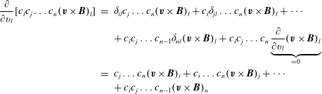 $$\begin{eqnarray}\displaystyle \frac{\unicode[STIX]{x2202}}{\unicode[STIX]{x2202}v_{l}}[c_{i}c_{j}\ldots c_{n}(\boldsymbol{v}\times \boldsymbol{B})_{l}] & = & \displaystyle \unicode[STIX]{x1D6FF}_{il}c_{j}\ldots c_{n}(\boldsymbol{v}\times \boldsymbol{B})_{l}+c_{i}\unicode[STIX]{x1D6FF}_{jl}\ldots c_{n}(\boldsymbol{v}\times \boldsymbol{B})_{l}+\cdots \nonumber\\ \displaystyle & & \displaystyle +\,c_{i}c_{j}\ldots c_{n-1}\unicode[STIX]{x1D6FF}_{nl}(\boldsymbol{v}\times \boldsymbol{B})_{l}+c_{i}c_{j}\ldots c_{n}\underbrace{\frac{\unicode[STIX]{x2202}}{\unicode[STIX]{x2202}v_{l}}(\boldsymbol{v}\times \boldsymbol{B})_{l}}_{=0}\nonumber\\ \displaystyle & = & \displaystyle c_{j}\ldots c_{n}(\boldsymbol{v}\times \boldsymbol{B})_{i}+c_{i}\ldots c_{n}(\boldsymbol{v}\times \boldsymbol{B})_{j}+\cdots \nonumber\\ \displaystyle & & \displaystyle +\,c_{i}c_{j}\ldots c_{n-1}(\boldsymbol{v}\times \boldsymbol{B})_{n}\nonumber\\ \displaystyle & & \displaystyle\end{eqnarray}$$
 $$\begin{eqnarray}\displaystyle \int c_{j}c_{k}\ldots c_{n}(\boldsymbol{v}\times \boldsymbol{B})_{i}f\,\text{d}^{3}v & = & \displaystyle \int c_{j}c_{k}\ldots c_{n}\unicode[STIX]{x1D716}_{irs}v_{r}B_{s}f\,\text{d}^{3}v=\unicode[STIX]{x1D716}_{irs}B_{s}\int c_{j}c_{k}\ldots c_{n}v_{r}f\,\text{d}^{3}v\nonumber\\ \displaystyle & = & \displaystyle \frac{1}{m}\!\underbrace{\unicode[STIX]{x1D716}_{irs}}_{=-\unicode[STIX]{x1D716}_{isr}}\!B_{s}(X_{jk\ldots nr}^{(n)}+\unicode[STIX]{x1D61F}_{jk\ldots n}^{(n-1)}u_{r})=-\frac{1}{m}\unicode[STIX]{x1D716}_{isr}B_{s}(X_{rjk\ldots n}^{(n)}+u_{r}\unicode[STIX]{x1D61F}_{jk\ldots n}^{(n-1)})\nonumber\\ \displaystyle & = & \displaystyle -\frac{1}{m}[\boldsymbol{B}\times (\unicode[STIX]{x1D653}^{(n)}+\boldsymbol{u}\unicode[STIX]{x1D653}^{(n-1)})]_{ijk\ldots n}.\end{eqnarray}$$
The fourth term calculates as
 $$\begin{eqnarray}\displaystyle \unicode[STIX]{x2463} & = & \displaystyle \frac{q}{c}\int c_{i}c_{j}\ldots c_{n}(\boldsymbol{v}\times \boldsymbol{B})_{l}\frac{\unicode[STIX]{x2202}f}{\unicode[STIX]{x2202}v_{l}}\,\text{d}^{3}v\nonumber\\ \displaystyle & = & \displaystyle \frac{q}{c}\underbrace{\int \frac{\unicode[STIX]{x2202}}{\unicode[STIX]{x2202}v_{l}}[c_{i}c_{j}\ldots c_{n}(\boldsymbol{v}\times \boldsymbol{B})_{l}f]\,\text{d}^{3}v}_{\rightarrow 0}-\frac{q}{c}\int f\frac{\unicode[STIX]{x2202}}{\unicode[STIX]{x2202}v_{l}}[c_{i}c_{j}\ldots c_{n}(\boldsymbol{v}\times \boldsymbol{B})_{l}]\,\text{d}^{3}v\nonumber\\ \displaystyle & = & \displaystyle -\frac{q}{c}\int f(c_{j}\ldots c_{n}(\boldsymbol{v}\times \boldsymbol{B})_{i}+c_{i}\ldots c_{n}(\boldsymbol{v}\times \boldsymbol{B})_{j}+\cdots +c_{i}c_{j}\ldots c_{n-1}(\boldsymbol{v}\times \boldsymbol{B})_{n})\,\text{d}^{3}v\nonumber\\ \displaystyle & = & \displaystyle +\frac{q}{mc}[\boldsymbol{B}\times (\unicode[STIX]{x1D653}^{(n)}+\boldsymbol{u}\unicode[STIX]{x1D653}^{(n-1)})]_{ijk\ldots n}^{S}\end{eqnarray}$$
Combining all the results together
 $\unicode[STIX]{x2460}+\unicode[STIX]{x2461}+\unicode[STIX]{x2462}+\unicode[STIX]{x2463}=0$
, the evolution equation for
$\unicode[STIX]{x2460}+\unicode[STIX]{x2461}+\unicode[STIX]{x2462}+\unicode[STIX]{x2463}=0$
, the evolution equation for
 $n$
th-order fluid moment
$n$
th-order fluid moment
 $\unicode[STIX]{x1D653}_{ij\ldots n}^{(n)}$
reads (written in the vector notation without indices)
$\unicode[STIX]{x1D653}_{ij\ldots n}^{(n)}$
reads (written in the vector notation without indices)
 $$\begin{eqnarray}\displaystyle & & \displaystyle \frac{\unicode[STIX]{x2202}}{\unicode[STIX]{x2202}t}\unicode[STIX]{x1D653}^{(n)}+\unicode[STIX]{x1D735}\boldsymbol{\cdot }(\unicode[STIX]{x1D653}^{(n+1)}+\boldsymbol{u}\unicode[STIX]{x1D653}^{(n)})+\left[\frac{\unicode[STIX]{x2202}\boldsymbol{u}}{\unicode[STIX]{x2202}t}\unicode[STIX]{x1D653}^{(n-1)}+(\unicode[STIX]{x1D653}^{(n)}+\unicode[STIX]{x1D653}^{(n-1)}\boldsymbol{u})\boldsymbol{\cdot }\unicode[STIX]{x1D735}\boldsymbol{u}-\frac{q}{m}\boldsymbol{E}\unicode[STIX]{x1D653}^{(n-1)}\right.\nonumber\\ \displaystyle & & \displaystyle \qquad +\left.\frac{q}{mc}\boldsymbol{B}\times (\unicode[STIX]{x1D653}^{(n)}+\boldsymbol{u}\unicode[STIX]{x1D653}^{(n-1)})\right]^{S}=0.\end{eqnarray}$$
The final result should have only the time derivative of
 $\unicode[STIX]{x1D653}^{(n)}$
and, similarly to the heat flux tensor, we need to use the momentum equation to eliminate
$\unicode[STIX]{x1D653}^{(n)}$
and, similarly to the heat flux tensor, we need to use the momentum equation to eliminate
 $\unicode[STIX]{x2202}_{t}\boldsymbol{u}$
. We subtract a total of
$\unicode[STIX]{x2202}_{t}\boldsymbol{u}$
. We subtract a total of
 $n$
momentum equations combined with
$n$
momentum equations combined with
 $\unicode[STIX]{x1D653}^{(n)}$
in the form
$\unicode[STIX]{x1D653}^{(n)}$
in the form
 $$\begin{eqnarray}\displaystyle \left[\left(\frac{\unicode[STIX]{x2202}\boldsymbol{u}}{\unicode[STIX]{x2202}t}+\boldsymbol{u}\boldsymbol{\cdot }\unicode[STIX]{x1D735}\boldsymbol{u}+\frac{1}{\unicode[STIX]{x1D70C}}\unicode[STIX]{x1D735}\boldsymbol{\cdot }\boldsymbol{p}-\frac{q}{m}\boldsymbol{E}-\frac{q}{mc}\boldsymbol{u}\times \boldsymbol{B}\right)\unicode[STIX]{x1D653}^{(n-1)}\right]^{S}=0. & & \displaystyle\end{eqnarray}$$
Again, because of the symmetric operator, it does not matter if
 $\unicode[STIX]{x1D653}^{(n)}$
is applied to the momentum equation from the left or right. The subtraction also conveniently eliminates the electric field, however it introduces
$\unicode[STIX]{x1D653}^{(n)}$
is applied to the momentum equation from the left or right. The subtraction also conveniently eliminates the electric field, however it introduces
 $\unicode[STIX]{x1D735}\boldsymbol{\cdot }\boldsymbol{p}$
. We also need an identity
$\unicode[STIX]{x1D735}\boldsymbol{\cdot }\boldsymbol{p}$
. We also need an identity
 $$\begin{eqnarray}\displaystyle [(\boldsymbol{u}\times \boldsymbol{B})\unicode[STIX]{x1D653}^{(n-1)}]_{ijk\ldots n} & = & \displaystyle (\boldsymbol{u}\times \boldsymbol{B})_{i}X_{jk\ldots n}^{(n-1)}=-(\boldsymbol{B}\times \boldsymbol{u})_{i}X_{jk\ldots n}^{(n-1)}=-[(\boldsymbol{B}\times \boldsymbol{u})\unicode[STIX]{x1D653}^{(n-1)}]_{ijk\ldots n}\nonumber\\ \displaystyle & = & \displaystyle -[\boldsymbol{B}\times (\boldsymbol{u}\unicode[STIX]{x1D653}^{(n-1)})]_{ijk\ldots n},\end{eqnarray}$$
where in the last step we emphasized that it does not matter if the
 $\boldsymbol{B}\times$
applies only to
$\boldsymbol{B}\times$
applies only to
 $\boldsymbol{u}$
or to the entire tensor
$\boldsymbol{u}$
or to the entire tensor
 $\boldsymbol{u}\unicode[STIX]{x1D653}^{(n-1)}$
, since the vector product operates only through the first component of the tensor anyway. The final evolution equation reads
$\boldsymbol{u}\unicode[STIX]{x1D653}^{(n-1)}$
, since the vector product operates only through the first component of the tensor anyway. The final evolution equation reads
and it is valid for
 $n\geqslant 2$
. Evaluation at
$n\geqslant 2$
. Evaluation at
 $m=3$
recovers the heat flux tensor equation (7.22) and evaluation at
$m=3$
recovers the heat flux tensor equation (7.22) and evaluation at
 $m=2$
recovers the pressure tensor equation (2.28). Note that
$m=2$
recovers the pressure tensor equation (2.28). Note that
 $\unicode[STIX]{x1D653}^{(4)}=\boldsymbol{r}$
,
$\unicode[STIX]{x1D653}^{(4)}=\boldsymbol{r}$
,
 $\unicode[STIX]{x1D653}^{(3)}=\boldsymbol{q}$
,
$\unicode[STIX]{x1D653}^{(3)}=\boldsymbol{q}$
,
 $\unicode[STIX]{x1D653}^{(2)}=\boldsymbol{p}$
, however, and very importantly, according to our definition (12.1),
$\unicode[STIX]{x1D653}^{(2)}=\boldsymbol{p}$
, however, and very importantly, according to our definition (12.1),
 $\unicode[STIX]{x1D653}^{(1)}=0$
and it is not equal to the velocity
$\unicode[STIX]{x1D653}^{(1)}=0$
and it is not equal to the velocity
 $\boldsymbol{u}$
, which is defined according to (2.4). Additionally,
$\boldsymbol{u}$
, which is defined according to (2.4). Additionally,
 $\unicode[STIX]{x1D653}^{(0)}=\unicode[STIX]{x1D70C}$
. The momentum equation can still be recovered by evaluating (12.13) at
$\unicode[STIX]{x1D653}^{(0)}=\unicode[STIX]{x1D70C}$
. The momentum equation can still be recovered by evaluating (12.13) at
 $n=1$
, and by dividing by
$n=1$
, and by dividing by
 $\unicode[STIX]{x1D70C}$
(where naturally the symmetric operator does not have any influence on a vector, and
$\unicode[STIX]{x1D70C}$
(where naturally the symmetric operator does not have any influence on a vector, and
 $u_{i}^{S}=u_{i}$
). Similar equation to our (12.13) was also obtained for example by Waelbroeck (Reference Waelbroeck2010), equation (22), even though we did not verify whether it is consistent with ours since
$u_{i}^{S}=u_{i}$
). Similar equation to our (12.13) was also obtained for example by Waelbroeck (Reference Waelbroeck2010), equation (22), even though we did not verify whether it is consistent with ours since
 $\unicode[STIX]{x1D653}^{(n)}$
in that work is defined with
$\unicode[STIX]{x1D653}^{(n)}$
in that work is defined with
 $v$
instead of our
$v$
instead of our
 $c$
.
$c$
.
We want to always decompose the tensor
 $\unicode[STIX]{x1D653}^{(n)}$
into its gyrotropic and non-gyrotropic parts, and to have space to write the ‘
$\unicode[STIX]{x1D653}^{(n)}$
into its gyrotropic and non-gyrotropic parts, and to have space to write the ‘
 $g$
’ and ‘
$g$
’ and ‘
 $ng$
’, let us move the index
$ng$
’, let us move the index
 $(n)$
down, so that
$(n)$
down, so that
 $$\begin{eqnarray}\unicode[STIX]{x1D653}_{(n)}=\unicode[STIX]{x1D653}_{(n)}^{\text{g}}+\unicode[STIX]{x1D653}_{(n)}^{\text{ng}}.\end{eqnarray}$$
By generalizing the results we have seen for the gyrotropic
 $\boldsymbol{p}^{\text{g}},\boldsymbol{q}^{\text{g}},\boldsymbol{r}^{\text{g}}$
, the same result is obtained for the
$\boldsymbol{p}^{\text{g}},\boldsymbol{q}^{\text{g}},\boldsymbol{r}^{\text{g}}$
, the same result is obtained for the
 $n$
th moment, and at low frequencies the gyrotropic part must satisfy
$n$
th moment, and at low frequencies the gyrotropic part must satisfy
 $$\begin{eqnarray}[\hat{\boldsymbol{b}}\times \unicode[STIX]{x1D653}_{(n)}^{\text{g}}]^{S}=0,\end{eqnarray}$$
which can be indeed viewed as a definition of gyrotropy. The general (12.16) therefore rewrites as
 $$\begin{eqnarray}\displaystyle \frac{\unicode[STIX]{x2202}}{\unicode[STIX]{x2202}t}\unicode[STIX]{x1D653}_{(n)}+\unicode[STIX]{x1D735}\boldsymbol{\cdot }(\unicode[STIX]{x1D653}_{(n+1)}+\boldsymbol{u}\unicode[STIX]{x1D653}_{(n)})+\left[\unicode[STIX]{x1D653}_{(n)}\boldsymbol{\cdot }\unicode[STIX]{x1D735}\boldsymbol{u}+\unicode[STIX]{x1D6FA}\frac{|\boldsymbol{B}|}{B_{0}}\hat{\boldsymbol{b}}\times \unicode[STIX]{x1D653}_{(n)}^{\text{ng}}-\frac{1}{\unicode[STIX]{x1D70C}}(\unicode[STIX]{x1D735}\boldsymbol{\cdot }\boldsymbol{p})\unicode[STIX]{x1D653}_{(n-1)}\right]^{S}=0, & & \displaystyle \nonumber\\ \displaystyle & & \displaystyle\end{eqnarray}$$
yielding an implicit equation for the non-gyrotropic part in the form
 $$\begin{eqnarray}\displaystyle [\hat{\boldsymbol{b}}\times \unicode[STIX]{x1D653}_{(n)}^{\text{ng}}]^{S}=-\frac{B_{0}}{\unicode[STIX]{x1D6FA}|\boldsymbol{B}|}\left\{\!\frac{\unicode[STIX]{x2202}}{\unicode[STIX]{x2202}t}\unicode[STIX]{x1D653}_{(n)}+\unicode[STIX]{x1D735}\boldsymbol{\cdot }(\unicode[STIX]{x1D653}_{(n+1)}+\boldsymbol{u}\unicode[STIX]{x1D653}_{(n)})+\left[\unicode[STIX]{x1D653}_{(n)}\boldsymbol{\cdot }\unicode[STIX]{x1D735}\boldsymbol{u}-\frac{1}{\unicode[STIX]{x1D70C}}(\unicode[STIX]{x1D735}\boldsymbol{\cdot }\boldsymbol{p})\unicode[STIX]{x1D653}_{(n-1)}\right]^{S}\right\}. & & \displaystyle \nonumber\\ \displaystyle & & \displaystyle\end{eqnarray}$$
Ideally, an ‘inversion procedure’ should be found for the left-hand side, so that an equation for
 $\unicode[STIX]{x1D653}_{(n)}^{\text{ng}}$
can be found, and then by expanding the right-hand side (for example at the leading order by considering only gyrotropic
$\unicode[STIX]{x1D653}_{(n)}^{\text{ng}}$
can be found, and then by expanding the right-hand side (for example at the leading order by considering only gyrotropic
 $\unicode[STIX]{x1D653}^{\text{g}}$
), a fully nonlinear expressions for
$\unicode[STIX]{x1D653}^{\text{g}}$
), a fully nonlinear expressions for
 $\unicode[STIX]{x1D653}_{(n)}^{\text{ng}}$
can be obtained. Nevertheless, we have seen that the inversion procedure was already quite complicated for the matrix
$\unicode[STIX]{x1D653}_{(n)}^{\text{ng}}$
can be obtained. Nevertheless, we have seen that the inversion procedure was already quite complicated for the matrix
 $(\hat{\boldsymbol{b}}\times \unicode[STIX]{x1D72B})^{S}$
, see (5.9). For a tensor of third rank, such as
$(\hat{\boldsymbol{b}}\times \unicode[STIX]{x1D72B})^{S}$
, see (5.9). For a tensor of third rank, such as
 $(\hat{\boldsymbol{b}}\times \boldsymbol{q}^{\text{ng}})^{S}$
, the full inversion procedure is actually not addressed in this guide and an advanced reader is referred to (43) of Ramos (Reference Ramos2005). The inversion procedure was obtained only for a part of the
$(\hat{\boldsymbol{b}}\times \boldsymbol{q}^{\text{ng}})^{S}$
, the full inversion procedure is actually not addressed in this guide and an advanced reader is referred to (43) of Ramos (Reference Ramos2005). The inversion procedure was obtained only for a part of the
 $\boldsymbol{q}^{\text{ng}}$
, that can be decomposed into the non-gyrotropic heat flux vectors
$\boldsymbol{q}^{\text{ng}}$
, that can be decomposed into the non-gyrotropic heat flux vectors
 $\boldsymbol{S}_{\bot }^{\Vert }$
,
$\boldsymbol{S}_{\bot }^{\Vert }$
,
 $\boldsymbol{S}_{\bot }^{\bot }$
, which is done in detail in appendix D. For the rest of
$\boldsymbol{S}_{\bot }^{\bot }$
, which is done in detail in appendix D. For the rest of
 $\boldsymbol{q}^{\text{ng}}$
that consists of heat flux tensor
$\boldsymbol{q}^{\text{ng}}$
that consists of heat flux tensor
 $\unicode[STIX]{x1D748}$
, the inversion procedure cannot be avoided. Additionally, we have seen that for fourth-order moment
$\unicode[STIX]{x1D748}$
, the inversion procedure cannot be avoided. Additionally, we have seen that for fourth-order moment
 $\boldsymbol{r}^{\text{ng}}$
, the equation (12.20) does not seem to yield anything useful even at the linear level, and a different procedure was used, where the specific bi-Maxwellian distribution was expanded in Hermite polynomials. Therefore, for higher-order moments, the equation (12.20) is immensely complicated.
$\boldsymbol{r}^{\text{ng}}$
, the equation (12.20) does not seem to yield anything useful even at the linear level, and a different procedure was used, where the specific bi-Maxwellian distribution was expanded in Hermite polynomials. Therefore, for higher-order moments, the equation (12.20) is immensely complicated.
It is useful to briefly consider how many scalar gyrotropic moments an
 $n$
th-order tensor
$n$
th-order tensor
 $\unicode[STIX]{x1D653}_{(n)}$
has. The scalar gyrotropic moments can be constructed only from combinations of
$\unicode[STIX]{x1D653}_{(n)}$
has. The scalar gyrotropic moments can be constructed only from combinations of
 $c_{\Vert }$
and
$c_{\Vert }$
and
 $c_{\bot }^{2}$
. It is beneficial to write down the following self-explanatory table
$c_{\bot }^{2}$
. It is beneficial to write down the following self-explanatory table

Obviously, the number of gyrotropic moments for tensor
 $\unicode[STIX]{x1D653}_{(n)}$
is equal to
$\unicode[STIX]{x1D653}_{(n)}$
is equal to
 $1+\text{int}[n/2]$
. The function ‘int’ means integer part. In mathematics, the integer function is often abbreviated with square brackets, as
$1+\text{int}[n/2]$
. The function ‘int’ means integer part. In mathematics, the integer function is often abbreviated with square brackets, as
 $1+[n/2]$
. However, this notation might be possibly confusing (we used square brackets in many other places), and we prefer to write explicitly ‘int’. Another possibility would be to use the ‘floor’ function.
$1+[n/2]$
. However, this notation might be possibly confusing (we used square brackets in many other places), and we prefer to write explicitly ‘int’. Another possibility would be to use the ‘floor’ function.
12.1 Hierarchy of moments in a 1-D geometry (electrostatic)
Let us see if we can use the
 $n$
th-order moment equation (12.16) for something useful, since the equation is immensely complicated. Let us consider the special case of strictly parallel propagation along
$n$
th-order moment equation (12.16) for something useful, since the equation is immensely complicated. Let us consider the special case of strictly parallel propagation along
 $B_{0}$
(in the
$B_{0}$
(in the
 $z$
-direction), where all the moments (including the velocity) are along
$z$
-direction), where all the moments (including the velocity) are along
 $B_{0}$
, i.e. let us consider the electrostatic case. Let us change the index of a moment from
$B_{0}$
, i.e. let us consider the electrostatic case. Let us change the index of a moment from
 $(n)$
to
$(n)$
to
 $(l)$
, so that the index is not confused with the number density. Let us stop writing the
$(l)$
, so that the index is not confused with the number density. Let us stop writing the
 $\Vert$
subscript on all the variables starting from the pressure, so
$\Vert$
subscript on all the variables starting from the pressure, so
 $p_{\Vert }$
,
$p_{\Vert }$
,
 $q_{\Vert }$
,
$q_{\Vert }$
,
 $r_{\Vert \Vert }$
are simply
$r_{\Vert \Vert }$
are simply
 $p,q,r$
and the
$p,q,r$
and the
 $l$
th-order parallel moment is just
$l$
th-order parallel moment is just
 $X^{(l)}\equiv m\int c_{\Vert }^{l}f\,\text{d}v$
. We keep the
$X^{(l)}\equiv m\int c_{\Vert }^{l}f\,\text{d}v$
. We keep the
 $z$
-subscript for
$z$
-subscript for
 $u_{z}$
to remind us we are writing 1-D equations. In a 1-D geometry, the nonlinear evolution equation (12.16) simplifies to
$u_{z}$
to remind us we are writing 1-D equations. In a 1-D geometry, the nonlinear evolution equation (12.16) simplifies to
 $$\begin{eqnarray}\frac{\unicode[STIX]{x2202}}{\unicode[STIX]{x2202}t}X^{(l)}+\unicode[STIX]{x2202}_{z}(X^{(l+1)}+u_{z}X^{(l)})+l(\unicode[STIX]{x2202}_{z}u_{z})X^{(l)}-\frac{l}{\unicode[STIX]{x1D70C}}(\unicode[STIX]{x2202}_{z}p)X^{(l-1)}=0;\quad l\geqslant 2.\end{eqnarray}$$
If one wants to be more general, instead of propagation along
 $B_{0}$
, it is possible to consider propagation along magnetic field line
$B_{0}$
, it is possible to consider propagation along magnetic field line
 $\hat{\boldsymbol{b}}$
, and write the same equation with
$\hat{\boldsymbol{b}}$
, and write the same equation with
 $u_{\Vert }$
and
$u_{\Vert }$
and
 $\unicode[STIX]{x2202}_{\Vert }$
. The equation is accompanied by the density and momentum equations
$\unicode[STIX]{x2202}_{\Vert }$
. The equation is accompanied by the density and momentum equations
 $$\begin{eqnarray}\displaystyle & \displaystyle \frac{\unicode[STIX]{x2202}}{\unicode[STIX]{x2202}t}\unicode[STIX]{x1D70C}+\unicode[STIX]{x2202}_{z}(u_{z}\unicode[STIX]{x1D70C})=0; & \displaystyle\end{eqnarray}$$
 $$\begin{eqnarray}\displaystyle & \displaystyle \frac{\unicode[STIX]{x2202}}{\unicode[STIX]{x2202}t}u_{z}+u_{z}\unicode[STIX]{x2202}_{z}u_{z}+\frac{1}{\unicode[STIX]{x1D70C}}\unicode[STIX]{x2202}_{z}p-\frac{q_{r}}{m}E_{z}=0, & \displaystyle\end{eqnarray}$$
where for the charge
 $q_{r}$
it is useful to keep the species index
$q_{r}$
it is useful to keep the species index
 $r$
, so that it is not confused with the heat flux
$r$
, so that it is not confused with the heat flux
 $q$
. The last term disappears anyway since in the case considered here
$q$
. The last term disappears anyway since in the case considered here
 $E_{z}=0$
. Evaluating equation (12.21) for
$E_{z}=0$
. Evaluating equation (12.21) for
 $l=2,3,4,5,6\ldots$
yields
$l=2,3,4,5,6\ldots$
yields
 $$\begin{eqnarray}\displaystyle & \displaystyle \frac{\unicode[STIX]{x2202}}{\unicode[STIX]{x2202}t}p+\unicode[STIX]{x2202}_{z}(q+u_{z}p)+2(\unicode[STIX]{x2202}_{z}u_{z})p=0; & \displaystyle\end{eqnarray}$$
 $$\begin{eqnarray}\displaystyle & \displaystyle \frac{\unicode[STIX]{x2202}}{\unicode[STIX]{x2202}t}q+\unicode[STIX]{x2202}_{z}(r+u_{z}q)+3(\unicode[STIX]{x2202}_{z}u_{z})q-\frac{3}{\unicode[STIX]{x1D70C}}(\unicode[STIX]{x2202}_{z}p)p=0; & \displaystyle\end{eqnarray}$$
 $$\begin{eqnarray}\displaystyle & \displaystyle \frac{\unicode[STIX]{x2202}}{\unicode[STIX]{x2202}t}r+\unicode[STIX]{x2202}_{z}(X^{(5)}+u_{z}r)+4(\unicode[STIX]{x2202}_{z}u_{z})r-\frac{4}{\unicode[STIX]{x1D70C}}(\unicode[STIX]{x2202}_{z}p)q=0; & \displaystyle\end{eqnarray}$$
 $$\begin{eqnarray}\displaystyle & \displaystyle \frac{\unicode[STIX]{x2202}}{\unicode[STIX]{x2202}t}X^{(5)}+\unicode[STIX]{x2202}_{z}(X^{(6)}+u_{z}X^{(5)})+5(\unicode[STIX]{x2202}_{z}u_{z})X^{(5)}-\frac{5}{\unicode[STIX]{x1D70C}}(\unicode[STIX]{x2202}_{z}p)r=0; & \displaystyle\end{eqnarray}$$
 $$\begin{eqnarray}\displaystyle & \displaystyle \frac{\unicode[STIX]{x2202}}{\unicode[STIX]{x2202}t}X^{(6)}+\unicode[STIX]{x2202}_{z}(X^{(7)}+u_{z}X^{(6)})+6(\unicode[STIX]{x2202}_{z}u_{z})X^{(6)}-\frac{6}{\unicode[STIX]{x1D70C}}(\unicode[STIX]{x2202}_{z}p)X^{(5)}=0, & \displaystyle\end{eqnarray}$$
and so on. The nonlinear equation (12.21) can be linearized, in the first step by assuming zero mean
 $u_{z0}$
value, yielding
$u_{z0}$
value, yielding
 $$\begin{eqnarray}\frac{\unicode[STIX]{x2202}}{\unicode[STIX]{x2202}t}X^{(l)}+\unicode[STIX]{x2202}_{z}X^{(l+1)}+(l+1)X_{0}^{(l)}(\unicode[STIX]{x2202}_{z}u_{z})-\frac{l}{\unicode[STIX]{x1D70C}_{0}}X_{0}^{(l-1)}(\unicode[STIX]{x2202}_{z}p)=0,\end{eqnarray}$$
and calculating it for
 $l=2-8$
and by prescribing
$l=2-8$
and by prescribing
 $q_{0}=0$
,
$q_{0}=0$
,
 $X_{0}^{(5)}=0$
and in general for
$X_{0}^{(5)}=0$
and in general for
 $l$
odd
$l$
odd
 $X_{0}^{(l)}=0$
, yields
$X_{0}^{(l)}=0$
, yields
 $$\begin{eqnarray}\displaystyle & \displaystyle \frac{\unicode[STIX]{x2202}}{\unicode[STIX]{x2202}t}p+\unicode[STIX]{x2202}_{z}q+3p_{0}(\unicode[STIX]{x2202}_{z}u_{z})=0; & \displaystyle\end{eqnarray}$$
 $$\begin{eqnarray}\displaystyle & \displaystyle \frac{\unicode[STIX]{x2202}}{\unicode[STIX]{x2202}t}q+\unicode[STIX]{x2202}_{z}r-3\frac{p_{0}}{\unicode[STIX]{x1D70C}_{0}}(\unicode[STIX]{x2202}_{z}p)=0; & \displaystyle\end{eqnarray}$$
 $$\begin{eqnarray}\displaystyle & \displaystyle \frac{\unicode[STIX]{x2202}}{\unicode[STIX]{x2202}t}r+\unicode[STIX]{x2202}_{z}X^{(5)}+5r_{0}(\unicode[STIX]{x2202}_{z}u_{z})=0; & \displaystyle\end{eqnarray}$$
 $$\begin{eqnarray}\displaystyle & \displaystyle \frac{\unicode[STIX]{x2202}}{\unicode[STIX]{x2202}t}X^{(5)}+\unicode[STIX]{x2202}_{z}X^{(6)}-5\frac{r_{0}}{\unicode[STIX]{x1D70C}_{0}}(\unicode[STIX]{x2202}_{z}p)=0; & \displaystyle\end{eqnarray}$$
 $$\begin{eqnarray}\displaystyle & \displaystyle \frac{\unicode[STIX]{x2202}}{\unicode[STIX]{x2202}t}X^{(6)}+\unicode[STIX]{x2202}_{z}X^{(7)}+7X_{0}^{(6)}(\unicode[STIX]{x2202}_{z}u_{z})=0; & \displaystyle\end{eqnarray}$$
 $$\begin{eqnarray}\displaystyle & \displaystyle \frac{\unicode[STIX]{x2202}}{\unicode[STIX]{x2202}t}X^{(7)}+\unicode[STIX]{x2202}_{z}X^{(8)}-7\frac{X_{0}^{(6)}}{\unicode[STIX]{x1D70C}_{0}}(\unicode[STIX]{x2202}_{z}p)=0; & \displaystyle\end{eqnarray}$$
 $$\begin{eqnarray}\displaystyle & \displaystyle \frac{\unicode[STIX]{x2202}}{\unicode[STIX]{x2202}t}X^{(8)}+\unicode[STIX]{x2202}_{z}X^{(9)}+9X_{0}^{(8)}(\unicode[STIX]{x2202}_{z}u_{z})=0. & \displaystyle\end{eqnarray}$$
Alternatively, we can split the linearized equations for even and odd
 $l$
according to
$l$
according to
 $$\begin{eqnarray}\displaystyle & \displaystyle l=\text{even}:\quad \frac{\unicode[STIX]{x2202}}{\unicode[STIX]{x2202}t}X^{(l)}+\unicode[STIX]{x2202}_{z}X^{(l+1)}+(l+1)X_{0}^{(l)}(\unicode[STIX]{x2202}_{z}u_{z})=0; & \displaystyle\end{eqnarray}$$
 $$\begin{eqnarray}\displaystyle & \displaystyle l=\text{odd}:\quad \frac{\unicode[STIX]{x2202}}{\unicode[STIX]{x2202}t}X^{(l)}+\unicode[STIX]{x2202}_{z}X^{(l+1)}-\frac{l}{\unicode[STIX]{x1D70C}_{0}}X_{0}^{(l-1)}(\unicode[STIX]{x2202}_{z}p)=0. & \displaystyle\end{eqnarray}$$
When closing the system, one has to be careful how to deal with
 $l=\text{even}$
quantities, since we want to separate the ‘deviations’, similarly as we did for
$l=\text{even}$
quantities, since we want to separate the ‘deviations’, similarly as we did for
 $r=3p^{2}/\unicode[STIX]{x1D70C}+\widetilde{r}$
. For a Maxwellian
$r=3p^{2}/\unicode[STIX]{x1D70C}+\widetilde{r}$
. For a Maxwellian
 $f_{0}$
and
$f_{0}$
and
 $l\geqslant 4$
and even, we therefore write
$l\geqslant 4$
and even, we therefore write
 $$\begin{eqnarray}l=\text{even}:\quad X^{(l)}=\frac{l-1}{\unicode[STIX]{x1D70C}}pX^{(l-2)}+\widetilde{X}^{(l)},\end{eqnarray}$$
or equivalently
 $$\begin{eqnarray}l=\text{even}:\quad X^{(l)}=(l-1)!!\frac{p^{l/2}}{\unicode[STIX]{x1D70C}^{l/2-1}}+\widetilde{X}^{(l)},\end{eqnarray}$$
so for example
 $r_{0}=3p_{0}^{2}/\unicode[STIX]{x1D70C}_{0}$
,
$r_{0}=3p_{0}^{2}/\unicode[STIX]{x1D70C}_{0}$
,
 $X_{0}^{(6)}=15p_{0}^{3}/\unicode[STIX]{x1D70C}_{0}^{2}$
,
$X_{0}^{(6)}=15p_{0}^{3}/\unicode[STIX]{x1D70C}_{0}^{2}$
,
 $X_{0}^{(8)}=105p_{0}^{4}/\unicode[STIX]{x1D70C}_{0}^{3}$
, and linearization of the
$X_{0}^{(8)}=105p_{0}^{4}/\unicode[STIX]{x1D70C}_{0}^{3}$
, and linearization of the
 $l$
th-order moment yields
$l$
th-order moment yields
 $$\begin{eqnarray}\displaystyle l=\text{even}:\quad X^{(l)} & \overset{\text{lin}}{=} & \displaystyle X_{0}^{(l)}\left[\frac{l}{2}\frac{p}{p_{0}}-\left(\frac{l}{2}-1\right)\frac{\unicode[STIX]{x1D70C}}{\unicode[STIX]{x1D70C}_{0}}\right]+\widetilde{X}^{(l)};\end{eqnarray}$$
 $$\begin{eqnarray}\displaystyle & \overset{\text{lin}}{=} & \displaystyle X_{0}^{(l)}\left[\frac{l}{2}\frac{T}{T_{0}}+\frac{\unicode[STIX]{x1D70C}}{\unicode[STIX]{x1D70C}_{0}}\right]+\widetilde{X}^{(l)}.\end{eqnarray}$$
Using (12.41) in the first term of
 $l=\text{even}$
equation (12.37), and using the pressure and density equations, yields linear evolution equation for deviations of even moments
$l=\text{even}$
equation (12.37), and using the pressure and density equations, yields linear evolution equation for deviations of even moments
 $$\begin{eqnarray}l=\text{even}:\quad \frac{\unicode[STIX]{x2202}}{\unicode[STIX]{x2202}t}\widetilde{X}^{(l)}+\unicode[STIX]{x2202}_{z}X^{(l+1)}-X_{0}^{(l)}\frac{l}{2p_{0}}\unicode[STIX]{x2202}_{z}q=0,\end{eqnarray}$$
and using (12.41) in the second term of
 $l=\text{odd}$
equation (12.38), and
$l=\text{odd}$
equation (12.38), and
 $T/T_{0}=p/p_{0}-\unicode[STIX]{x1D70C}/\unicode[STIX]{x1D70C}_{0}$
yields linear evolution equation for deviations of odd moments
$T/T_{0}=p/p_{0}-\unicode[STIX]{x1D70C}/\unicode[STIX]{x1D70C}_{0}$
yields linear evolution equation for deviations of odd moments
 $$\begin{eqnarray}l=\text{odd}:\quad \frac{\unicode[STIX]{x2202}}{\unicode[STIX]{x2202}t}X^{(l)}+\unicode[STIX]{x2202}_{z}\widetilde{X}^{(l+1)}+X_{0}^{(l-1)}\frac{l(l-1)}{2m}\unicode[STIX]{x2202}_{z}T=0.\end{eqnarray}$$
Finishing the calculation with evaluations of
 $X_{0}^{(l)}$
values, the evolution equations of deviations are
$X_{0}^{(l)}$
values, the evolution equations of deviations are
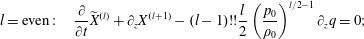 $$\begin{eqnarray}\displaystyle & \displaystyle l=\text{even}:\quad \frac{\unicode[STIX]{x2202}}{\unicode[STIX]{x2202}t}\widetilde{X}^{(l)}+\unicode[STIX]{x2202}_{z}X^{(l+1)}-(l-1)!!\frac{l}{2}\left(\frac{p_{0}}{\unicode[STIX]{x1D70C}_{0}}\right)^{l/2-1}\unicode[STIX]{x2202}_{z}q=0; & \displaystyle\end{eqnarray}$$
 $$\begin{eqnarray}\displaystyle & \displaystyle l=\text{odd}:\quad \frac{\unicode[STIX]{x2202}}{\unicode[STIX]{x2202}t}X^{(l)}+\unicode[STIX]{x2202}_{z}\widetilde{X}^{(l+1)}+l!!\frac{(l-1)}{2}n_{0}\left(\frac{p_{0}}{\unicode[STIX]{x1D70C}_{0}}\right)^{(l-1)/2}\unicode[STIX]{x2202}_{z}T=0, & \displaystyle\end{eqnarray}$$
or by using
 $p_{0}/\unicode[STIX]{x1D70C}_{0}=v_{\text{th}}^{2}/2$
, equivalently
$p_{0}/\unicode[STIX]{x1D70C}_{0}=v_{\text{th}}^{2}/2$
, equivalently
 $$\begin{eqnarray}\displaystyle & \displaystyle l=\text{even}:\quad \frac{\unicode[STIX]{x2202}}{\unicode[STIX]{x2202}t}\widetilde{X}^{(l)}+\unicode[STIX]{x2202}_{z}X^{(l+1)}-(l-1)!!\frac{l}{2^{l/2}}v_{\text{th}}^{l-2}\unicode[STIX]{x2202}_{z}q=0; & \displaystyle\end{eqnarray}$$
 $$\begin{eqnarray}\displaystyle & \displaystyle l=\text{odd}:\quad \frac{\unicode[STIX]{x2202}}{\unicode[STIX]{x2202}t}X^{(l)}+\unicode[STIX]{x2202}_{z}\widetilde{X}^{(l+1)}+l!!\frac{(l-1)}{2^{(l+1)/2}}n_{0}v_{\text{th}}^{l-1}\unicode[STIX]{x2202}_{z}T=0, & \displaystyle\end{eqnarray}$$
Continuing to higher orders, the hierarchy of deviations of Maxwellian moments therefore evaluates as
 $$\begin{eqnarray}\displaystyle & \displaystyle \frac{\unicode[STIX]{x2202}}{\unicode[STIX]{x2202}t}q+\unicode[STIX]{x2202}_{z}\widetilde{r}+\frac{3}{2}n_{0}v_{\text{th}}^{2}\unicode[STIX]{x2202}_{z}T=0; & \displaystyle\end{eqnarray}$$
 $$\begin{eqnarray}\displaystyle & \displaystyle \frac{\unicode[STIX]{x2202}}{\unicode[STIX]{x2202}t}\widetilde{r}+\unicode[STIX]{x2202}_{z}X^{(5)}-3v_{\text{th}}^{2}\unicode[STIX]{x2202}_{z}q=0; & \displaystyle\end{eqnarray}$$
 $$\begin{eqnarray}\displaystyle & \displaystyle \frac{\unicode[STIX]{x2202}}{\unicode[STIX]{x2202}t}X^{(5)}+\unicode[STIX]{x2202}_{z}\widetilde{X}^{(6)}+\frac{15}{2}n_{0}v_{\text{th}}^{4}\unicode[STIX]{x2202}_{z}T=0; & \displaystyle\end{eqnarray}$$
 $$\begin{eqnarray}\displaystyle & \displaystyle \frac{\unicode[STIX]{x2202}}{\unicode[STIX]{x2202}t}\widetilde{X}^{(6)}+\unicode[STIX]{x2202}_{z}X^{(7)}-\frac{45}{4}v_{\text{th}}^{4}\unicode[STIX]{x2202}_{z}q=0; & \displaystyle\end{eqnarray}$$
 $$\begin{eqnarray}\displaystyle & \displaystyle \frac{\unicode[STIX]{x2202}}{\unicode[STIX]{x2202}t}X^{(7)}+\unicode[STIX]{x2202}_{z}\widetilde{X}^{(8)}+\frac{315}{8}n_{0}v_{\text{th}}^{6}\unicode[STIX]{x2202}_{z}T=0; & \displaystyle\end{eqnarray}$$
 $$\begin{eqnarray}\displaystyle & \displaystyle \frac{\unicode[STIX]{x2202}}{\unicode[STIX]{x2202}t}\widetilde{X}^{(8)}+\unicode[STIX]{x2202}_{z}X^{(9)}-\frac{105}{2}v_{\text{th}}^{6}\unicode[STIX]{x2202}_{z}q=0. & \displaystyle\end{eqnarray}$$
The equations are written in physical units, and these results will be useful in Part 2, where we will calculate Landau fluid closures for deviations of various moments.
12.2 Impossibility of going beyond CGL2 without Landau fluid closures
One can analyse the dispersion relations easily in physical units, but since in this Part 1 we used normalized units with
 $\widetilde{k}=kV_{A}/\unicode[STIX]{x1D6FA}_{p}$
,
$\widetilde{k}=kV_{A}/\unicode[STIX]{x1D6FA}_{p}$
,
 $\widetilde{\unicode[STIX]{x1D714}}=\unicode[STIX]{x1D714}/\unicode[STIX]{x1D6FA}_{p}$
and
$\widetilde{\unicode[STIX]{x1D714}}=\unicode[STIX]{x1D714}/\unicode[STIX]{x1D6FA}_{p}$
and
 $\unicode[STIX]{x1D6FD}=v_{\text{th}}^{2}/V_{A}^{2}$
in almost all dispersion relations, let us rewrite the fluid hierarchy to normalized units, so that everything feels more familiar. The
$\unicode[STIX]{x1D6FD}=v_{\text{th}}^{2}/V_{A}^{2}$
in almost all dispersion relations, let us rewrite the fluid hierarchy to normalized units, so that everything feels more familiar. The
 $X^{(5)}$
is normalized with
$X^{(5)}$
is normalized with
 $p_{0}V_{A}^{3}$
, the
$p_{0}V_{A}^{3}$
, the
 $X^{(6)}$
with
$X^{(6)}$
with
 $p_{0}V_{A}^{4}$
and
$p_{0}V_{A}^{4}$
and
 $X^{(n)}$
with
$X^{(n)}$
with
 $p_{0}V_{A}^{n-2}$
. By dropping the normalization tilde as usual (but obviously not for even moments such as
$p_{0}V_{A}^{n-2}$
. By dropping the normalization tilde as usual (but obviously not for even moments such as
 $\widetilde{r}$
, that should be perhaps called
$\widetilde{r}$
, that should be perhaps called
 $\unicode[STIX]{x1D6FF}r$
), the equations in Fourier space read
$\unicode[STIX]{x1D6FF}r$
), the equations in Fourier space read
 $$\begin{eqnarray}\displaystyle & \displaystyle -\unicode[STIX]{x1D714}\unicode[STIX]{x1D70C}+ku_{z}=0; & \displaystyle\end{eqnarray}$$
 $$\begin{eqnarray}\displaystyle & \displaystyle -\unicode[STIX]{x1D714}u_{z}+\frac{\unicode[STIX]{x1D6FD}}{2}kp=0; & \displaystyle\end{eqnarray}$$
 $$\begin{eqnarray}\displaystyle & \displaystyle -\unicode[STIX]{x1D714}p+3ku_{z}+kq=0; & \displaystyle\end{eqnarray}$$
 $$\begin{eqnarray}\displaystyle & \displaystyle -\unicode[STIX]{x1D714}q+k\widetilde{r}+{\textstyle \frac{3}{2}}\unicode[STIX]{x1D6FD}k(p-\unicode[STIX]{x1D70C})=0; & \displaystyle\end{eqnarray}$$
 $$\begin{eqnarray}\displaystyle & \displaystyle -\unicode[STIX]{x1D714}\widetilde{r}+kX^{(5)}-3\unicode[STIX]{x1D6FD}kq=0; & \displaystyle\end{eqnarray}$$
 $$\begin{eqnarray}\displaystyle & \displaystyle -\unicode[STIX]{x1D714}X^{(5)}+k\widetilde{X}^{(6)}+{\textstyle \frac{15}{2}}\unicode[STIX]{x1D6FD}^{2}k(p-\unicode[STIX]{x1D70C})=0; & \displaystyle\end{eqnarray}$$
 $$\begin{eqnarray}\displaystyle & \displaystyle -\unicode[STIX]{x1D714}\widetilde{X}^{(6)}+kX^{(7)}-{\textstyle \frac{45}{4}}\unicode[STIX]{x1D6FD}^{2}kq=0. & \displaystyle\end{eqnarray}$$
Now, using just first 3 equations (12.55)–(12.57), and closing the system with a closure
 $q=0$
, yields the CGL model, with solution
$q=0$
, yields the CGL model, with solution
 $$\begin{eqnarray}\text{CGL:}\quad \unicode[STIX]{x1D714}=\pm k\sqrt{\unicode[STIX]{x1D6FD}{\textstyle \frac{3}{2}}},\end{eqnarray}$$
the familiar CGL ion-acoustic mode. Going higher in the fluid hierarchy and using the first 4 equations (12.55)–(12.58), and closing the system with
 $\widetilde{r}=0$
(which is equivalent to prescribing
$\widetilde{r}=0$
(which is equivalent to prescribing
 $r=3p^{2}/\unicode[STIX]{x1D70C}$
), yields the CGL2 model. The dispersion relation is
$r=3p^{2}/\unicode[STIX]{x1D70C}$
), yields the CGL2 model. The dispersion relation is
 $\unicode[STIX]{x1D714}^{4}-3\unicode[STIX]{x1D6FD}k^{2}\unicode[STIX]{x1D714}^{2}+\frac{3}{4}\unicode[STIX]{x1D6FD}^{2}k^{4}=0$
, with solutions
$\unicode[STIX]{x1D714}^{4}-3\unicode[STIX]{x1D6FD}k^{2}\unicode[STIX]{x1D714}^{2}+\frac{3}{4}\unicode[STIX]{x1D6FD}^{2}k^{4}=0$
, with solutions
 $$\begin{eqnarray}\displaystyle \text{CGL2:}\quad \unicode[STIX]{x1D714} & = & \displaystyle \pm k\sqrt{\unicode[STIX]{x1D6FD}\left({\textstyle \frac{3}{2}}+\sqrt{{\textstyle \frac{3}{2}}}\right)};\end{eqnarray}$$
 $$\begin{eqnarray}\displaystyle \unicode[STIX]{x1D714} & = & \displaystyle \pm k\sqrt{\unicode[STIX]{x1D6FD}\left({\textstyle \frac{3}{2}}-\sqrt{{\textstyle \frac{3}{2}}}\right)},\end{eqnarray}$$
the already obtained (9.28), (9.29). The heat flux fluctuations in the CGL2 model therefore did ‘split’ the CGL ion-acoustic mode to two modes. One might assume that this will always be the case when going higher and higher in the fluid hierarchy. With the next example we demonstrate that this does not happen. Let us consider fluctuations in
 $\widetilde{r}$
, and use the first 5 equations (12.55)–(12.59) with the closure
$\widetilde{r}$
, and use the first 5 equations (12.55)–(12.59) with the closure
 $X^{(5)}=0$
. We might call this model CGL3. The dispersion relation reads
$X^{(5)}=0$
. We might call this model CGL3. The dispersion relation reads
 $\unicode[STIX]{x1D714}^{4}=\frac{15}{4}\unicode[STIX]{x1D6FD}^{2}k^{4}$
, and the solutions are
$\unicode[STIX]{x1D714}^{4}=\frac{15}{4}\unicode[STIX]{x1D6FD}^{2}k^{4}$
, and the solutions are
 $$\begin{eqnarray}\displaystyle \text{CGL3:}\quad \unicode[STIX]{x1D714}=\pm k\sqrt{\unicode[STIX]{x1D6FD}}\left({\textstyle \frac{15}{4}}\right)^{1/4};\quad \unicode[STIX]{x1D714}=\pm \text{i}k\sqrt{\unicode[STIX]{x1D6FD}}\left({\textstyle \frac{15}{4}}\right)^{1/4}. & & \displaystyle\end{eqnarray}$$
Importantly, the last two modes are imaginary, and one is unstable. Therefore, such a fluid model does not make any physical sense. Why did this happen? For example, expressing everything through pressure fluctuations, and putting the
 $\widetilde{r}$
fluctuations on the right-hand side yields
$\widetilde{r}$
fluctuations on the right-hand side yields
 $$\begin{eqnarray}\displaystyle \left(\unicode[STIX]{x1D714}^{4}-3\unicode[STIX]{x1D6FD}k^{2}\unicode[STIX]{x1D714}^{2}+{\textstyle \frac{3}{4}}\unicode[STIX]{x1D6FD}^{2}k^{4}\right)p & = & \displaystyle k^{2}\unicode[STIX]{x1D714}^{2}\widetilde{r};\end{eqnarray}$$
 $$\begin{eqnarray}\displaystyle & = & \displaystyle k^{3}\unicode[STIX]{x1D714}X^{(5)}+\left(-3\unicode[STIX]{x1D6FD}k^{2}\unicode[STIX]{x1D714}^{2}+{\textstyle \frac{9}{2}}\unicode[STIX]{x1D6FD}^{2}k^{4}\right)p.\end{eqnarray}$$
Therefore, if
 $\widetilde{r}=0$
, so when (12.66) is used, the CGL2 model is obtained. However, when fluctuations in
$\widetilde{r}=0$
, so when (12.66) is used, the CGL2 model is obtained. However, when fluctuations in
 $\widetilde{r}$
are considered, so when (12.67) is used, the term
$\widetilde{r}$
are considered, so when (12.67) is used, the term
 $-3\unicode[STIX]{x1D6FD}k^{2}\unicode[STIX]{x1D714}^{2}$
cancels on both sides, with the resulting dispersion relation
$-3\unicode[STIX]{x1D6FD}k^{2}\unicode[STIX]{x1D714}^{2}$
cancels on both sides, with the resulting dispersion relation
 $$\begin{eqnarray}\left(\unicode[STIX]{x1D714}^{4}-{\textstyle \frac{15}{4}}\unicode[STIX]{x1D6FD}^{2}k^{4}\right)p=k^{3}\unicode[STIX]{x1D714}X^{(5)},\end{eqnarray}$$
and by prescribing closure
 $X^{(5)}=0$
, yields the dispersion relation of the CGL3 model.
$X^{(5)}=0$
, yields the dispersion relation of the CGL3 model.
Now it is easy to go higher in the fluid hierarchy. By considering the first 6 equations (12.55)–(12.60), the dispersion relation reads
 $$\begin{eqnarray}\left(\unicode[STIX]{x1D714}^{6}-{\textstyle \frac{45}{4}}\unicode[STIX]{x1D6FD}^{2}k^{4}\unicode[STIX]{x1D714}^{2}+{\textstyle \frac{15}{4}}\unicode[STIX]{x1D6FD}^{3}k^{6}\right)p=k^{4}\unicode[STIX]{x1D714}^{2}\widetilde{X}^{(6)},\end{eqnarray}$$
and prescribing closure
 $\widetilde{X}^{(6)}=0$
(which is equivalent to prescribing
$\widetilde{X}^{(6)}=0$
(which is equivalent to prescribing
 $X^{(6)}=15p^{3}/\unicode[STIX]{x1D70C}^{2}$
), yields a model that we can call CGL4, with numerical solutions
$X^{(6)}=15p^{3}/\unicode[STIX]{x1D70C}^{2}$
), yields a model that we can call CGL4, with numerical solutions
 $$\begin{eqnarray}\text{CGL4:}\quad \frac{\unicode[STIX]{x1D714}}{k\sqrt{\unicode[STIX]{x1D6FD}}}=\pm 0.58;\quad \frac{\unicode[STIX]{x1D714}}{k\sqrt{\unicode[STIX]{x1D6FD}}}=\pm 1.75;\quad \frac{\unicode[STIX]{x1D714}}{k\sqrt{\unicode[STIX]{x1D6FD}}}=\pm 1.87\text{i},\end{eqnarray}$$
again, two modes being imaginary, and one unstable.
The variable
 $\unicode[STIX]{x1D714}/(k\sqrt{\unicode[STIX]{x1D6FD}})$
, written here in normalized units, is easily rewritten to physical units (reintroducing tilde for clarity)
$\unicode[STIX]{x1D714}/(k\sqrt{\unicode[STIX]{x1D6FD}})$
, written here in normalized units, is easily rewritten to physical units (reintroducing tilde for clarity)
 $$\begin{eqnarray}\frac{\widetilde{\unicode[STIX]{x1D714}}}{\widetilde{k}\sqrt{\unicode[STIX]{x1D6FD}}}=\frac{\displaystyle \frac{\unicode[STIX]{x1D714}}{\unicode[STIX]{x1D6FA}_{p}}}{\displaystyle \frac{kV_{A}}{\unicode[STIX]{x1D6FA}_{p}}\sqrt{\frac{v_{\text{th}}^{2}}{V_{A}^{2}}}}=\frac{\unicode[STIX]{x1D714}}{kv_{\text{th}}},\end{eqnarray}$$
which is directly related to the ‘kinetic’ variable
 $\unicode[STIX]{x1D701}$
, that we will use in Part 2 of the text, defined as
$\unicode[STIX]{x1D701}$
, that we will use in Part 2 of the text, defined as
 $$\begin{eqnarray}\unicode[STIX]{x1D701}\equiv \frac{\unicode[STIX]{x1D714}}{|k|v_{\text{th}}},\end{eqnarray}$$
where the absolute value does not make any difference now (since all fluid models here contain
 $\unicode[STIX]{x1D701}^{2}$
), and will become important only when Landau fluid closures are considered. The hierarchy of CGL dispersion relations then can be written as
$\unicode[STIX]{x1D701}^{2}$
), and will become important only when Landau fluid closures are considered. The hierarchy of CGL dispersion relations then can be written as
 $$\begin{eqnarray}\displaystyle \text{CGL:} & & \displaystyle \quad \unicode[STIX]{x1D701}^{2}-{\textstyle \frac{3}{2}}=0;\quad\end{eqnarray}$$
 $$\begin{eqnarray}\displaystyle \text{CGL2:} & & \displaystyle \quad \unicode[STIX]{x1D701}^{4}-3\unicode[STIX]{x1D701}^{2}+{\textstyle \frac{3}{4}}=0;\end{eqnarray}$$
 $$\begin{eqnarray}\displaystyle \text{CGL3:} & & \displaystyle \quad \unicode[STIX]{x1D701}^{4}-{\textstyle \frac{15}{4}}=0;\end{eqnarray}$$
 $$\begin{eqnarray}\displaystyle \text{CGL4:} & & \displaystyle \quad \unicode[STIX]{x1D701}^{6}-{\textstyle \frac{45}{4}}\unicode[STIX]{x1D701}^{2}+{\textstyle \frac{15}{4}}=0;\end{eqnarray}$$
 $$\begin{eqnarray}\displaystyle \text{CGL5:} & & \displaystyle \quad \unicode[STIX]{x1D701}^{6}-{\textstyle \frac{105}{8}}=0;\end{eqnarray}$$
 $$\begin{eqnarray}\displaystyle \text{CGL6:} & & \displaystyle \quad \unicode[STIX]{x1D701}^{8}-{\textstyle \frac{105}{2}}\unicode[STIX]{x1D701}^{2}+{\textstyle \frac{315}{16}}=0;\end{eqnarray}$$
 $$\begin{eqnarray}\displaystyle \text{CGL7:} & & \displaystyle \quad \unicode[STIX]{x1D701}^{8}-{\textstyle \frac{945}{16}}=0.\end{eqnarray}$$
All the models beyond CGL2 contain modes that are unstable.
Double check
Let us double check our results, to verify that we calculated everything correctly. As stated previously, a closure should be performed only at the last retained fluid moment, and this is especially true when nonlinear numerical simulations are performed.Footnote 13 The CGL and CGL2 systems were already discussed at great length. Let us check the CGL3 dispersion relation, and let us work directly in physical units. The system of equations that we have in mind reads
 $$\begin{eqnarray}\displaystyle \left.\begin{array}{@{}c@{}}\displaystyle \frac{\unicode[STIX]{x2202}}{\unicode[STIX]{x2202}t}\unicode[STIX]{x1D70C}+\unicode[STIX]{x1D70C}_{0}\unicode[STIX]{x2202}_{z}u_{z}=0;\\ \displaystyle \frac{\unicode[STIX]{x2202}}{\unicode[STIX]{x2202}t}u_{z}+\frac{1}{\unicode[STIX]{x1D70C}_{0}}\unicode[STIX]{x2202}_{z}p=0;\\ \displaystyle \frac{\unicode[STIX]{x2202}}{\unicode[STIX]{x2202}t}p+\unicode[STIX]{x2202}_{z}q+3p_{0}(\unicode[STIX]{x2202}_{z}u_{z})=0;\\ \displaystyle \frac{\unicode[STIX]{x2202}}{\unicode[STIX]{x2202}t}q+\unicode[STIX]{x2202}_{z}r-3\frac{p_{0}}{\unicode[STIX]{x1D70C}_{0}}(\unicode[STIX]{x2202}_{z}p)=0;\\ \displaystyle \frac{\unicode[STIX]{x2202}}{\unicode[STIX]{x2202}t}r+\unicode[STIX]{x2202}_{z}X^{(5)}+5r_{0}(\unicode[STIX]{x2202}_{z}u_{z})=0,\end{array}\right\} & & \displaystyle\end{eqnarray}$$
and the closure is performed by setting
 $X^{(5)}=0$
. Importantly, the fourth-order moment
$X^{(5)}=0$
. Importantly, the fourth-order moment
 $r$
is kept undetermined, and it is not separated to its ‘core’ and
$r$
is kept undetermined, and it is not separated to its ‘core’ and
 $\widetilde{r}$
, nor any specific form of a distribution function is prescribed yet (other than the mean values of odd moments
$\widetilde{r}$
, nor any specific form of a distribution function is prescribed yet (other than the mean values of odd moments
 $X_{0}^{(l)}=0$
). Calculating dispersion relation of this system (a matrix multiplied by vector
$X_{0}^{(l)}=0$
). Calculating dispersion relation of this system (a matrix multiplied by vector
 $(\unicode[STIX]{x1D70C},u_{z},p,q,r)$
) yields result
$(\unicode[STIX]{x1D70C},u_{z},p,q,r)$
) yields result
 $\unicode[STIX]{x1D714}^{4}-5k^{4}r_{0}/\unicode[STIX]{x1D70C}_{0}=0$
, which for
$\unicode[STIX]{x1D714}^{4}-5k^{4}r_{0}/\unicode[STIX]{x1D70C}_{0}=0$
, which for
 $r_{0}=3p_{0}^{2}/\unicode[STIX]{x1D70C}_{0}$
recovers the CGL3 dispersion relation. Our calculations were therefore done right. Similarly, double checking the CGL4 dispersion, the system (12.80) is supplemented with (12.33), and a closure is performed with
$r_{0}=3p_{0}^{2}/\unicode[STIX]{x1D70C}_{0}$
recovers the CGL3 dispersion relation. Our calculations were therefore done right. Similarly, double checking the CGL4 dispersion, the system (12.80) is supplemented with (12.33), and a closure is performed with
 $X^{(6)}=15p^{3}/\unicode[STIX]{x1D70C}$
. Again, the
$X^{(6)}=15p^{3}/\unicode[STIX]{x1D70C}$
. Again, the
 $r$
is left untouched, and dispersion relation of this system recovers the CGL4 result. Checking the CGL5 dispersion relation, the system is supplemented with (12.34), and a closure
$r$
is left untouched, and dispersion relation of this system recovers the CGL4 result. Checking the CGL5 dispersion relation, the system is supplemented with (12.34), and a closure
 $X^{(7)}=0$
. Again, the
$X^{(7)}=0$
. Again, the
 $X^{(6)}$
is kept untouched and generally undetermined. Calculating the dispersion relation yields
$X^{(6)}$
is kept untouched and generally undetermined. Calculating the dispersion relation yields
 $\unicode[STIX]{x1D714}^{6}-7k^{6}X_{0}^{(6)}/\unicode[STIX]{x1D70C}_{0}=0$
, and prescribing Maxwellian
$\unicode[STIX]{x1D714}^{6}-7k^{6}X_{0}^{(6)}/\unicode[STIX]{x1D70C}_{0}=0$
, and prescribing Maxwellian
 $X_{0}^{(6)}=15p_{0}^{3}/\unicode[STIX]{x1D70C}_{0}^{2}$
recovers the CGL5 result. Going higher in the hierarchy, and using closure
$X_{0}^{(6)}=15p_{0}^{3}/\unicode[STIX]{x1D70C}_{0}^{2}$
recovers the CGL5 result. Going higher in the hierarchy, and using closure
 $X^{(8)}=105p^{4}/\unicode[STIX]{x1D70C}^{3}$
recovers the CGL6 results. And finally, keeping all the variables up to
$X^{(8)}=105p^{4}/\unicode[STIX]{x1D70C}^{3}$
recovers the CGL6 results. And finally, keeping all the variables up to
 $X^{(8)}$
undetermined and using closure
$X^{(8)}$
undetermined and using closure
 $X^{(9)}=0$
yields dispersion relation
$X^{(9)}=0$
yields dispersion relation
 $\unicode[STIX]{x1D714}^{8}-9k^{8}X_{0}^{(8)}/\unicode[STIX]{x1D70C}_{0}=0$
, which for Maxwellian
$\unicode[STIX]{x1D714}^{8}-9k^{8}X_{0}^{(8)}/\unicode[STIX]{x1D70C}_{0}=0$
, which for Maxwellian
 $X_{0}^{(8)}=105p_{0}^{4}/\unicode[STIX]{x1D70C}_{0}^{3}$
recovers the CGL7 result.
$X_{0}^{(8)}=105p_{0}^{4}/\unicode[STIX]{x1D70C}_{0}^{3}$
recovers the CGL7 result.
Or, in general, without yet performing a closure, and going higher and higher in the hierarchy step by step, a straightforward calculation yields
 $$\begin{eqnarray}\displaystyle \text{CGL:} & & \displaystyle \quad \left(-\unicode[STIX]{x1D714}^{2}+3\frac{p_{0}}{\unicode[STIX]{x1D70C}_{0}}k^{2}\right)p=-k\unicode[STIX]{x1D714}q;\end{eqnarray}$$
 $$\begin{eqnarray}\displaystyle \text{CGL2:} & & \displaystyle \quad -\unicode[STIX]{x1D714}^{2}p=-k^{2}r;\end{eqnarray}$$
 $$\begin{eqnarray}\displaystyle \text{CGL3:} & & \displaystyle \quad \left(-\unicode[STIX]{x1D714}^{4}+5\frac{r_{0}}{\unicode[STIX]{x1D70C}_{0}}k^{4}\right)p=-k^{3}\unicode[STIX]{x1D714}X^{(5)};\end{eqnarray}$$
 $$\begin{eqnarray}\displaystyle \text{CGL4:} & & \displaystyle \quad -\unicode[STIX]{x1D714}^{4}p=-k^{4}X^{(6)};\end{eqnarray}$$
 $$\begin{eqnarray}\displaystyle \text{CGL5:} & & \displaystyle \quad \left(-\unicode[STIX]{x1D714}^{6}+7\frac{X_{0}^{(6)}}{\unicode[STIX]{x1D70C}_{0}}k^{6}\right)p=-k^{5}\unicode[STIX]{x1D714}X^{(7)};\end{eqnarray}$$
 $$\begin{eqnarray}\displaystyle \text{CGL6:} & & \displaystyle \quad -\unicode[STIX]{x1D714}^{6}p=-k^{6}X^{(8)};\end{eqnarray}$$
 $$\begin{eqnarray}\displaystyle \text{CGL7:} & & \displaystyle \quad \left(-\unicode[STIX]{x1D714}^{8}+9\frac{X_{0}^{(8)}}{\unicode[STIX]{x1D70C}_{0}}k^{8}\right)p=-k^{7}\unicode[STIX]{x1D714}X^{(9)},\end{eqnarray}$$
and for higher orders therefore
 $$\begin{eqnarray}\displaystyle \text{CGLl:} & & \displaystyle \;l=\text{odd;}\quad \left(-\unicode[STIX]{x1D714}^{l+1}+(l+2)\frac{X_{0}^{(l+1)}}{\unicode[STIX]{x1D70C}_{0}}k^{l+1}\right)p=-k^{l}\unicode[STIX]{x1D714}X^{(l+2)};\end{eqnarray}$$
 $$\begin{eqnarray}\displaystyle \text{CGLl:} & & \displaystyle \;l=\text{even;}\quad -\unicode[STIX]{x1D714}^{l}p=-k^{l}X^{(l+2)},\end{eqnarray}$$
where the validity can be proven by induction and using (12.37), (12.38). CGLl model (or CGL of
 $l$
th order) is therefore defined as performing a closure on
$l$
th order) is therefore defined as performing a closure on
 $X^{(l+2)}$
moment. In the equations (12.81)–(12.89) we used the word CGL, even though no specific distribution function (nor any closure) was prescribed yet.
$X^{(l+2)}$
moment. In the equations (12.81)–(12.89) we used the word CGL, even though no specific distribution function (nor any closure) was prescribed yet.
The closure in each model is performed by specifying the right-hand side of (12.88), (12.89), which yields dispersion relations
 $$\begin{eqnarray}\displaystyle \text{CGLl:} & & \displaystyle \;l=\text{odd;}\quad \text{closure}\;X^{(l+2)}=0;\quad \Rightarrow \quad \left(\frac{\unicode[STIX]{x1D714}}{k}\right)^{l+1}-(l+2)\frac{X_{0}^{(l+1)}}{\unicode[STIX]{x1D70C}_{0}}=0;\end{eqnarray}$$
 $$\begin{eqnarray}\displaystyle \text{CGLl:} & & \displaystyle \;l=\text{even;}\quad \text{closure}\;X^{(l+2)}=(l+1)!!\frac{p^{(l+2)/2}}{\unicode[STIX]{x1D70C}^{l/2}};\quad \Rightarrow \quad \nonumber\\ \displaystyle & & \displaystyle \hspace{54.0pt}\left(\frac{\unicode[STIX]{x1D714}}{k}\right)^{l+2}-\left(\frac{l}{2}+1\right)\frac{X_{0}^{(l+2)}}{p_{0}}\left(\frac{\unicode[STIX]{x1D714}}{k}\right)^{2}+\frac{l}{2}\frac{X_{0}^{(l+2)}}{\unicode[STIX]{x1D70C}_{0}}=0.\end{eqnarray}$$
The results are written in physical units. Alternatively, by using the
 $\unicode[STIX]{x1D701}$
variable, the results are
$\unicode[STIX]{x1D701}$
variable, the results are
 $$\begin{eqnarray}\displaystyle \text{CGLl:} & & \displaystyle \;l=\text{odd;}\quad \Rightarrow \quad \unicode[STIX]{x1D701}^{l+1}-\frac{(l+2)!!}{2^{(l+1)/2}}=0;\end{eqnarray}$$
 $$\begin{eqnarray}\displaystyle \text{CGLl:} & & \displaystyle \;l=\text{even;}\quad \Rightarrow \quad \unicode[STIX]{x1D701}^{l+2}-(l+1)!!\frac{l+2}{2^{l/2+1}}\unicode[STIX]{x1D701}^{2}+(l+1)!!\frac{l}{2^{l/2+2}}=0,\end{eqnarray}$$
which for specific
 $l$
values recovers results (12.73)–(12.79).
$l$
values recovers results (12.73)–(12.79).
The results (12.90)–(12.91) are written for a closure performed on moment
 $X_{0}^{(l+2)}$
, which is dictated by the CGLl vocabulary, and which might be perhaps a bit confusing. Alternatively, one can reformulate the results for closures performed on moment
$X_{0}^{(l+2)}$
, which is dictated by the CGLl vocabulary, and which might be perhaps a bit confusing. Alternatively, one can reformulate the results for closures performed on moment
 $X_{0}^{(l)}$
(corresponding name for a Maxwellian is
$X_{0}^{(l)}$
(corresponding name for a Maxwellian is
 $\text{CGL}(l-2)$
) and that read
$\text{CGL}(l-2)$
) and that read
 $$\begin{eqnarray}\displaystyle l=\text{odd};l\geqslant 3 & & \displaystyle \quad \text{closure}\;X^{(l)}=0;\quad \Rightarrow \quad \left(\frac{\unicode[STIX]{x1D714}}{k}\right)^{l-1}-l\frac{X_{0}^{(l-1)}}{\unicode[STIX]{x1D70C}_{0}}=0;\end{eqnarray}$$
 $$\begin{eqnarray}\displaystyle l=\text{even};l\geqslant 4 & & \displaystyle \quad \text{closure}\;X^{(l)}=(l-1)!!\frac{p^{l/2}}{\unicode[STIX]{x1D70C}^{l/2-1}};\quad \Rightarrow \quad \nonumber\\ \displaystyle & & \displaystyle \hspace{12.0pt}\left(\frac{\unicode[STIX]{x1D714}}{k}\right)^{l}-\frac{l}{2}\left(\frac{\unicode[STIX]{x1D714}}{k}\right)^{2}\frac{X_{0}^{(l)}}{p_{0}}+\left(\frac{l}{2}-1\right)\frac{X_{0}^{(l)}}{\unicode[STIX]{x1D70C}_{0}}=0,\end{eqnarray}$$
or rewritten with the
 $\unicode[STIX]{x1D701}$
variable
$\unicode[STIX]{x1D701}$
variable
 $$\begin{eqnarray}\displaystyle l=\text{odd};l\geqslant 3 & \quad \text{closure}\;X^{(l)}=0;\quad \Rightarrow \quad \unicode[STIX]{x1D701}^{l-1}-\frac{l!!}{2^{(l-1)/2}}=0; & \displaystyle \nonumber\\ \displaystyle l=\text{even};l\geqslant 4 & \quad \text{closure}\;X^{(l)}=(l-1)!!\frac{p^{l/2}}{\unicode[STIX]{x1D70C}^{l/2-1}};\quad \Rightarrow \quad & \displaystyle \nonumber\\ \displaystyle & \unicode[STIX]{x1D701}^{l}-\frac{(l-1)!!}{2^{l/2}}\left(l\unicode[STIX]{x1D701}^{2}-\frac{l}{2}+1\right)=0, & \displaystyle\end{eqnarray}$$
a result reported in Hunana et al. (Reference Hunana, Zank, Laurenza, Tenerani, Webb, Goldstein, Velli and Adhikari2018), equation (10). Importantly, solutions of the above dispersion relations for
 $l>4$
, will always yield results with some complex numbers, and some solutions will be unstable.
$l>4$
, will always yield results with some complex numbers, and some solutions will be unstable.
Therefore, the last physically meaningful fluid model (without considering the Landau fluid closures) is the CGL2 model, and the last closure is the ‘normal’ closure,
 $r=3p^{2}/\unicode[STIX]{x1D70C}$
. To go higher in the fluid hierarchy, we necessarily need to make connection to kinetic theory, and consider Landau fluid closures. These closures are described in Part 2 of our guide, and for direct comparison with the simplest Landau fluid dispersion relations, see Part 2, § 3.12 ‘Parallel ion-acoustic (sound) mode, cold electrons’.
$r=3p^{2}/\unicode[STIX]{x1D70C}$
. To go higher in the fluid hierarchy, we necessarily need to make connection to kinetic theory, and consider Landau fluid closures. These closures are described in Part 2 of our guide, and for direct comparison with the simplest Landau fluid dispersion relations, see Part 2, § 3.12 ‘Parallel ion-acoustic (sound) mode, cold electrons’.
13 Conclusions
We offer a brief summary of the major results discussed throughout the text.
∙ A collisionless plasma is completely described by the kinetic Vlasov equation. Directly integrating the Vlasov equation over velocity space, yields evolution equations for an infinite hierarchy of fluid moments. In addition to the usual density and momentum equations, it is possible to derive an evolution equation for a general
$n$
th-order fluid moment (
$n\geqslant 2$
), see (12.16). Then, evolution equations for the pressure tensor and heat flux tensor can be obtained by simply evaluating (12.16) at
$n=2$
and
$n=3$
.∙ Even though the fluid hierarchy is infinite, the reformulation of the kinetic description to a fluid formalism is not necessarily complete, since the usual calculations neglect wave–particle resonances in velocity space. These wave–particle resonances, that are implicitly present in the Vlasov equation, are responsible for collisionless damping mechanisms, such as Landau damping, transit-time damping and cyclotron damping.
∙ The presence (or absence) of collisionless damping mechanisms in a fluid hierarchy is determined by the type of closure selected to truncate that fluid hierarchy. We differentiate between two classes of closures: a) ‘classical’ (non-Landau fluid) closures, that neglect wave–particle resonances, and b) Landau fluid closures, that account for Landau wave–particle resonances and associated Landau damping and transit-time damping, addressed in Part 2.
∙ There are currently no known closures that account for cyclotron wave–particle resonances and associated cyclotron damping. Nevertheless, there is a priori no reason why such fluid closures can not be found in the future, at least for the simplified case of electromagnetic propagation along the magnetic field (slab geometry).
∙ Considering ‘classical’ closures, the hierarchy of fluid moments therefore does not contain collisionless damping mechanisms, regardless of the order to which the hierarchy is developed. Or in another words, collisionless damping is beyond all orders in the classical hierarchy of fluid moments.
∙ In fact, it is impossible to go beyond the fourth-order moment with classical bi-Maxwellian fluid closures
$\unicode[STIX]{x1D653}^{(n)}=\unicode[STIX]{x1D653}_{0}^{(n)}+\widetilde{\unicode[STIX]{x1D653}}^{(n)}$
, where
$\unicode[STIX]{x1D653}_{0}^{(n)}$
represents bi-Maxwellian value of
$\unicode[STIX]{x1D653}^{(n)}$
and its perturbation
$\widetilde{\unicode[STIX]{x1D653}}^{(n)}=0$
, since all the fluid models contain higher-order modes that are unstable. This is perhaps the most surprising result discussed in Part 1. For a detailed proof, see § 12.2, where a 1-D geometry is considered and a bi-Maxwellian closure is used at the
$n$
th-order fluid moment, which yields dispersion relation (12.96). The same dispersion relation will be valid in a 3-D geometry for the propagation along the magnetic field, where additional de-coupled modes will be present as well. For
$n>4$
, all the fluid models contain unphysical instabilities. The same result is expected for other distribution functions.∙ The classical bi-Maxwellian closure at the fourth-order moment reads
$r_{\Vert \Vert }=3(p_{\Vert }^{2}/\unicode[STIX]{x1D70C});r_{\Vert \bot }=p_{\Vert }p_{\bot }/\unicode[STIX]{x1D70C};r_{\bot \bot }=2(p_{\bot }^{2}/\unicode[STIX]{x1D70C})$
(or equivalently
$\widetilde{\boldsymbol{r}}=0$
), and is called the ‘normal’ closure. Therefore, the ‘normal’ closure is the last classical fluid closure (
$\widetilde{\unicode[STIX]{x1D653}}^{(n)}=0$
) and beyond the fourth-order moment, Landau fluid closures (
$\widetilde{\unicode[STIX]{x1D653}}^{(n)}\neq 0$
) are required.∙ From a collisionless (or weakly collisional) perspective, the long-wavelength low-frequency limit of a distribution function is not necessarily an isotropic Maxwellian, but a general distribution function that is gyrotropic, i.e. isotropic only in its perpendicular velocity components. Fluid moments are therefore typically decomposed into their gyrotropic and non-gyrotropic parts. For example the pressure tensor
$\boldsymbol{p}=\boldsymbol{p}^{\text{g}}+\unicode[STIX]{x1D72B}$
, the heat flux tensor
$\boldsymbol{q}=\boldsymbol{q}^{\text{g}}+\boldsymbol{q}^{\text{ng}}$
, the fourth-order moment
$\boldsymbol{r}=\boldsymbol{r}^{\text{g}}+\boldsymbol{r}^{\text{ng}}$
. The non-gyrotropic parts are also referred to as the FLR corrections, since they represent deviations from gyrotropy at small spatial scales, when the Larmor radius (gyroradius) is not infinitely small.∙ A general
$n$
th-order fluid moment contains
$1+\text{int}[n/2]$
scalar gyrotropic moments, where the function ‘int’ means integer part.∙ The pressure tensor is second-order fluid moment and contains two gyrotropic moments,
$p_{\Vert }$
and
$p_{\bot }$
. Therefore, any fluid description of collisionless (or weakly collisional) plasmas, requires two separate evolution equations for
$p_{\Vert }$
and
$p_{\bot }$
. Importantly, from a linear perspective the evolution equations remain different even when the distribution function is isotropic, i.e. even when the mean pressure values are equal (
$p_{\Vert }^{(0)}=p_{\bot }^{(0)}$
), since pressure fluctuations in the directions parallel and perpendicular to the local magnetic field remain anisotropic. We often use proton pressure (temperature) anisotropy coefficient
$a_{p}=T_{\bot }^{(0)}/T_{\Vert }^{(0)}=p_{\bot }^{(0)}/p_{\Vert }^{(0)}$
.∙ The simplest fluid model that describes a collisionless plasma in an adiabatic regime is the CGL description (model) – named after Chew–Goldberger–Law (Chew et al. Reference Chew, Goldberger and Low1956). The model is non-dispersive and obtained by a closure with zero heat flux. The CGL description should be viewed as collisionless magnetohydrodynamics (collisionless MHD), since the usual MHD description with isotropic scalar pressure is highly collisional implicitly.
∙ The CGL pressure tensor is decomposed with respect to the direction of the local magnetic field lines according to
$\boldsymbol{p}^{\text{g}}=p_{\Vert }\hat{\boldsymbol{b}}\hat{\boldsymbol{b}}+p_{\bot }(\unicode[STIX]{x1D644}-\hat{\boldsymbol{b}}\hat{\boldsymbol{b}})$
. It is possible to switch to the reference frame of the magnetic field lines, where the pressure tensor is a diagonal matrix. However, it should not be forgotten that in a such a reference frame, imposing an external (mean) magnetic field is not straightforward. For nonlinear numerical simulations of turbulence and plasma heating, the laboratory reference frame is strongly recommended.∙ The two pressure equations of the CGL model can be interpreted as conservation laws for the first and second adiabatic invariants, see § 2.5. The first adiabatic invariant is a conservation of the magnetic moment of a particle that is periodically gyrating around a mean magnetic field. The second adiabatic invariant is a conservation of the average parallel momentum of a particle that is completely trapped and periodically bouncing inside of a magnetic bottle.
∙ Without performing (yet) any kind of closure and leaving the heat flux tensor
$\boldsymbol{q}$
and FLR pressure tensor
$\unicode[STIX]{x1D72B}$
unspecified, it is possible to derive rigorously exact evolution equations for
$p_{\Vert }$
and
$p_{\bot }$
, see (2.91)–(2.92).∙ Rewriting the pressure equations to an alternative form, equations (2.100)–(2.101), shows that the adiabatic invariants in the CGL model are broken by the inclusion of the Hall term in the induction equation, gyrotropic heat flux, non-gyrotropic FLR corrections to the pressure and heat flux, as well as by coupling of various species together. All of these contributions therefore yield very complicated anisotropic plasma heating processes, that can be studied only by nonlinear numerical simulations.
∙ The anisotropic plasma heating does not simplify much even in the case of periodic boundary conditions (i.e. when the system can be viewed as completely isolated) and when averaging over the entire spatial volume is performed and expressed as a conservation of total energy, see (2.113)–(2.116). Only when the anisotropic heating is neglected, i.e. when only total plasma heating studied, the conservation of energy significantly simplify, see (2.109)–(2.111).
∙ By using the concept of polytropic indices, the pressure equations in the ideal CGL model can be interpreted as having
$\unicode[STIX]{x1D6FE}_{\Vert }=3$
and
$\unicode[STIX]{x1D6FE}_{\bot }=2$
. Consequently, the CGL dispersion relation is in general not equal to the MHD dispersion relation, even when
$a_{p}=1$
. The exception is the Alfvén mode, which for
$a_{p}=1$
propagates with the same phase speed
$\unicode[STIX]{x1D714}/k=V_{A}\cos \unicode[STIX]{x1D703}$
in both CGL and MHD models, for all the propagation directions
$\unicode[STIX]{x1D703}$
.∙ Polytropic indices can be further related to the number of degrees of freedom
$i$
through
$\unicode[STIX]{x1D6FE}=(i+2)/i$
, which for the CGL model yields
$i_{\Vert }=1$
and
$i_{\bot }=2$
. The CGL pressure equations can be therefore viewed as being composed of strongly coupled 1-D and 2-D dynamics, whereas the dynamics in the MHD model with
$\unicode[STIX]{x1D6FE}=5/3$
and
$i=3$
can be viewed as isotropically three-dimensional.∙ In the CGL model, the Alfvén mode propagates with the phase speed
$\unicode[STIX]{x1D714}/k=V_{A}\cos \unicode[STIX]{x1D703}\sqrt{1+(\unicode[STIX]{x1D6FD}_{\Vert }/2)(a_{p}-1)}$
, which matches the (collisionless) kinetic theory in the long-wavelength limit. Consequently, for
$a_{p}=1$
, the Alfvén mode in the MHD model matches the kinetic theory as well. The CGL result is very useful when numerically solving kinetic dispersion relations (for example with the WHAMP solver), since the Alfvén mode can be easily identified at long wavelengths.∙ In contrast to MHD, where the ordering of phase speeds is always
$v_{s}\leqslant v_{A}\leqslant v_{f}$
(slow, Alfvén, fast), in collisionless plasmas the oblique slow mode can become faster than the oblique Alfvén mode. In general, oblique slow and fast modes in the CGL model do not necessarily match the kinetic theory in the long-wavelength limit. Nevertheless, the effect when
$v_{s}>v_{A}$
is present in the CGL model and exists even for
$a_{p}=1$
, see § 3.6. The effect is very important for the parallel firehose instability.∙ Considering strictly perpendicular propagation (
$\unicode[STIX]{x1D703}=90^{\circ }$
or
$k_{\Vert }=0$
), the fast mode in the CGL model propagates with the phase speed
$\unicode[STIX]{x1D714}/k=V_{A}\sqrt{1+a_{p}\unicode[STIX]{x1D6FD}_{\Vert }}$
, which matches the kinetic theory in the long-wavelength limit. The expression can be rewritten as
$(\unicode[STIX]{x1D714}/k)^{2}=V_{A}^{2}+v_{\text{th}\bot }^{2}=V_{A}^{2}+2(p_{\bot }^{(0)}/\unicode[STIX]{x1D70C}_{0})$
, and can be contrasted with the MHD result
$(\unicode[STIX]{x1D714}/k)^{2}=V_{A}^{2}+\frac{5}{3}(p^{(0)}/\unicode[STIX]{x1D70C}_{0})$
. The factor of 2 in the CGL result comes from
$\unicode[STIX]{x1D6FE}_{\bot }=2$
, which shows that the adiabatic assumption of the CGL model is appropriate for the perpendicular fast mode.∙ Contributions of the Hall term completely disappear for strictly perpendicular propagation.
∙ It is more difficult to analytically show where the adiabatic CGL value
$\unicode[STIX]{x1D6FE}_{\Vert }=3$
is appropriate, since for example the parallel propagating ion-acoustic (sound) mode is strongly Landau damped in kinetic theory (unless the electrons are hot), which also modifies its real frequency. The ion-acoustic mode in the CGL model therefore does not match kinetic theory. One needs to consider Landau fluid models with proton and electron species, which is addressed in Part 2.∙ Nevertheless, when electrons are hot (
$T_{e}\gg T_{i}$
) and the ion-acoustic mode is Landau damped only weakly, the real phase speed obtained from kinetic theory in the long-wavelength limit reads
$\unicode[STIX]{x1D714}/k=\sqrt{(T_{e}+3T_{i})/m_{i}}$
. Thus, in this example the kinetic theory is matched by a fluid model where protons are described adiabatically (with the CGL value
$\unicode[STIX]{x1D6FE}_{\Vert }=3$
), while electrons are isothermal (with
$\unicode[STIX]{x1D6FE}_{\Vert }=1$
). Also, a good example for
$\unicode[STIX]{x1D6FE}_{\Vert }=3$
is the real frequency of the Langmuir mode,
$\unicode[STIX]{x1D714}^{2}=\unicode[STIX]{x1D714}_{pe}^{2}+3(T_{\Vert e}^{(0)}/m_{e})k^{2}$
, which is addressed in Part 2.∙ For anisotropic temperatures (
$a_{p}\neq 1$
), some modes can become unstable. A threshold of an instability that is obtained in the long-wavelength (non-dispersive) limit is called a ‘hard’ threshold. The CGL model contains 3 instabilities, the oblique firehose instability, the parallel firehose instability and the mirror instability. The mirror instability is not described correctly.∙ The oblique firehose instability is an instability of the oblique Alfvén mode. Since the Alfvén mode is described correctly by the CGL model, its instability threshold
$1+(\unicode[STIX]{x1D6FD}_{\Vert }/2)(a_{p}-1)<0$
matches the kinetic theory. The instability requires
$a_{p}<1$
and (in the long-wavelength limit)
$\unicode[STIX]{x1D6FD}_{\Vert }>2$
. Since the CGL model is non-dispersive, here the instability growth rate only has a simple
$\cos \unicode[STIX]{x1D703}$
dependence. Once dispersive effects are considered, the instability reaches maximum growth rate at some wavenumber and angle
$\unicode[STIX]{x1D703}$
that is oblique, see figure 10.∙ The parallel firehose instability is an instability of the whistler mode, which can be shown by considering the Hall-CGL model. However, considering usual (non-causal) analytic solutions (4.32)–(4.35), one arrives at a contradiction that for
$\unicode[STIX]{x1D714}_{r}>0$
the whistler mode is unstable, and that for
$\unicode[STIX]{x1D714}_{r}<0$
the whistler mode is stable. The contradiction arises, because at the range of wavenumbers where the firehose instability exists, the ion-cyclotron and whistler modes are completely degenerate and distinguishing between them loses sense. The problem is resolved by introducing a small
$({\sim}\unicode[STIX]{x1D716})$
causal dissipation into the momentum equations, which is later removed by the limit
$\lim _{\unicode[STIX]{x1D716}\rightarrow 0^{+}}$
. The procedure yields causal dispersion relations (4.43)–(4.46), where the whistler mode is firehose unstable for both positive and negative
$\unicode[STIX]{x1D714}_{r}$
, and the ion-cyclotron mode is stable.∙ The parallel firehose instability occurs for quasi-parallel (small
$\unicode[STIX]{x1D703}$
) propagation directions, with the maximum growth rate at
$\unicode[STIX]{x1D703}=0^{\circ }$
, see figure 10. In the non-dispersive CGL model it corresponds to the instability of the slow mode. Its threshold obtained for
$\unicode[STIX]{x1D703}=0^{\circ }$
is equivalent to the oblique firehose instability (since
$v_{s}=v_{A}$
), and matches the kinetic theory. At first it might sound surprising that the slow mode connects to the whistler mode once dispersive effects are considered. However, considering
$\unicode[STIX]{x1D703}=0^{\circ }$
,
$\unicode[STIX]{x1D6FD}_{\Vert }>2$
,
$a_{p}<1$
yields that the fast mode is the ion-acoustic (sound) mode and
$v_{s}=v_{A}$
, see figure 1. After dispersive effects are introduced, which split the Alfvén and slow mode to the ion-cyclotron and whistler modes, it is clarified that the instability is associated with the whistler mode. For quasi-parallel propagation directions the situation is more obvious, since
$v_{s}>v_{A}$
(see figure 1), and the slow mode clearly becomes the whistler mode.∙ In the non-dispersive CGL model, all 3 instabilities are non-propagating, i.e. purely growing with zero real frequency. Once dispersive effects are introduced, the parallel firehose instability becomes propagating.
∙ The mirror instability requires
$a_{p}>1$
and usually develops for highly oblique propagation angles. In the CGL model it corresponds to the instability of the slow mode. Its threshold obtained in the highly oblique (but not completely perpendicular) limit reads
$1+a_{p}\unicode[STIX]{x1D6FD}_{\Vert }-\frac{1}{6}a_{p}^{2}\unicode[STIX]{x1D6FD}_{\Vert }<0$
, and with respect to kinetic theory the
$1/6$
factor is erroneous. The erroneous
$1/6$
factor shows that the adiabatic CGL closure is not appropriate for the very slow dynamics of the mirror instability.∙ The simplest fluid closure that recovers the correct threshold of the mirror instability is the ‘static’ closure, see § 9.4. This closure is derived from the ‘normal’ closure in a simplified quasi-static approximation, and represents a generalization of the isothermal closure (in the presence of temperature anisotropy and variations of magnetic field strength). The ‘static’ closure is very useful since it clarifies that the highly oblique very slow dynamics of the slow mode (and of the associated mirror instability) is better described by a generalized isothermal closure than the adiabatic CGL closure.
∙ However, the ‘static’ closure modifies the dynamics of the perpendicular fast mode, that now does not match the kinetic theory. Additionally, the fast mode now experiences an unphysical instability, even though the instability is beyond the mirror threshold, and should perhaps not play a role in numerical simulations. The erroneous result shows that the generalized isothermal closure is not appropriate for the relatively fast dynamics of the perpendicular fast mode, where the adiabatic CGL closure is appropriate.
∙ Heuristically, the correct mirror threshold can be also obtained by keeping the CGL value
$\unicode[STIX]{x1D6FE}_{\bot }=2$
and modifying the parallel polytropic index to
$\unicode[STIX]{x1D6FE}_{\Vert }=1/2$
. Such a closure does not alter the dynamics of the perpendicular fast mode, since the phase speed depends only on
$\unicode[STIX]{x1D6FE}_{\bot }$
(and not on
$\unicode[STIX]{x1D6FE}_{\Vert }$
). Thresholds of parallel and oblique firehose instability are not altered either. Nevertheless, the
$\unicode[STIX]{x1D6FE}_{\Vert }=1/2$
is even below the isothermal value
$\unicode[STIX]{x1D6FE}_{\Vert }=1$
, the closure is heuristic, and it is mentioned only as a curiosity.∙ Obviously, to correctly capture both the slow dynamics of the highly oblique mirror instability, as well as the fast dynamics of the perpendicular fast mode, neither adiabatic nor (generalized) isothermal closures are sufficient. Considering classical (rigorously derived) closures, one has no other choice but to keep the correct adiabatic CGL values
$\unicode[STIX]{x1D6FE}_{\Vert }=3$
,
$\unicode[STIX]{x1D6FE}_{\bot }=2$
unaltered, and instead, break the (long-wavelength) adiabaticity by going higher in the fluid hierarchy. One needs to consider fluid models with evolution equations for the heat flux tensor
$\boldsymbol{q}$
, that has two gyrotropic components,
$q_{\Vert }$
and
$q_{\bot }$
. The system is closed at the fourth-order moment
$\boldsymbol{r}$
, that has 3 gyrotropic components,
$r_{\Vert \Vert };r_{\Vert \bot };r_{\bot \bot }$
. To perform a closure, a specific distribution function (or a class of distribution functions) has to be assumed.∙ Considering a bi-Maxwellian distribution function, the closure
$\widetilde{\boldsymbol{r}}=0$
is known as the ‘normal’ closure (see above). We call this non-dispersive bi-Maxwellian fluid model the ‘second-order CGL’, abbreviated as CGL2. The abbreviation CGL2 seems beneficial, since the name CGL is associated with collisionless magnetohydrodynamics, now just taken to one higher order. Additionally, by showing that all classical bi-Maxwellian models beyond CGL2 do not make physical sense, fluid models can be easily classified as based on CGL or CGL2 descriptions. For direct comparison of the two systems, see dispersion relations of the CGL model (3.193) and the CGL2 model (9.23). The Hall term introduces the simplest dispersive effects; see the dispersion relations of the Hall-CGL model (4.81), and the Hall-CGL2 model (9.40).∙ By comparing the dispersion relations, it is obvious that the gyrotropic heat flux fluctuations in the CGL2 model modify the general dynamics (the mean heat flux values are zero
$q_{\Vert }^{(0)}=q_{\bot }^{(0)}=0$
). One of the exceptions is the perpendicular fast mode, which is not altered by the gyrotropic heat fluxes, and therefore described correctly. Other exceptions are the oblique Alfvén mode (the oblique firehose instability), and once dispersive effects are introduced also the parallel propagating ion-cyclotron and whistler modes (the parallel firehose instability).∙ Two additional evolution equations typically create two additional modes. For example, for the case of highly oblique CGL2 propagation, one obtains the Alfvén mode, the fast mode, and 3 ‘slow’ modes. One of these slow modes is responsible for the mirror instability, and is sometimes called the mirror mode. The CGL2 mirror threshold matches the kinetic theory. The CGL2 model is therefore the simplest classical model that correctly captures (in the long-wavelength limit) both the mirror instability threshold, as well as the perpendicular fast mode. Nevertheless, only the ‘hard’ mirror threshold is correctly recovered, and capturing the (long-wavelength) mirror instability growth rate requires Landau damping.
∙ One can construct closures for other distribution functions than bi-Maxwellians. For example, one can consider the bi-kappa distribution function (10.1) with a free parameter
$\unicode[STIX]{x1D705}>3/2$
. The closure then reads
$r_{\Vert \Vert }=3\unicode[STIX]{x1D6FC}_{\unicode[STIX]{x1D705}}(p_{\Vert }^{2}/\unicode[STIX]{x1D70C});r_{\Vert \bot }=\unicode[STIX]{x1D6FC}_{\unicode[STIX]{x1D705}}(p_{\Vert }p_{\bot }/\unicode[STIX]{x1D70C});r_{\bot \bot }=2\unicode[STIX]{x1D6FC}_{\unicode[STIX]{x1D705}}(p_{\bot }^{2}/\unicode[STIX]{x1D70C})$
, where the coefficient
$\unicode[STIX]{x1D6FC}_{\unicode[STIX]{x1D705}}=(\unicode[STIX]{x1D705}-\frac{3}{2})/(\unicode[STIX]{x1D705}-\frac{5}{2})$
. The closure is restricted to
$\unicode[STIX]{x1D705}>\frac{5}{2}$
, which can be seen from the
$\unicode[STIX]{x1D6FC}_{\unicode[STIX]{x1D705}}$
coefficient, and the same requirement is necessary for the convergence of the velocity integrals. We call this closure and resulting fluid model simply ‘BiKappa’.∙ If a closure for the bi-kappa distribution is performed at a higher
$n$
th-order moment (which is presumably not possible with classical closures since it is expected that for
$n>4$
all models contain unphysical instabilities), the closure will be restricted to
$\unicode[STIX]{x1D705}>(n+1)/2$
, which increases with
$n$
. The requirement for the minimum
$\unicode[STIX]{x1D705}$
value is there, since the power law in the bi-kappa distribution is assumed all the way till infinite velocities, and the requirement is necessary for the convergence of the velocity integrals. Therefore, by going higher and higher in the bi-kappa fluid hierarchy, the minimum value of
$\unicode[STIX]{x1D705}$
increases, and in the limit
$\unicode[STIX]{x1D705}\rightarrow \infty$
the required distribution function converges towards bi-Maxwellian.∙ The dispersion relation for the BiKappa model is given by (10.53). A general
$\unicode[STIX]{x1D6FC}_{\unicode[STIX]{x1D705}}$
coefficient is used, so the dispersion relation is valid for a much larger class of distribution functions that can be closed with an analogous closure with just one
$\unicode[STIX]{x1D6FC}_{\unicode[STIX]{x1D705}}$
coefficient. The dispersion relation shows that the general dynamics is of course altered by the value of the
$\unicode[STIX]{x1D6FC}_{\unicode[STIX]{x1D705}}$
coefficient. Nevertheless, few exceptions are: the oblique Alfvén mode (oblique firehose threshold), the perpendicular fast mode, the parallel firehose threshold and the mirror threshold. When dispersive effects are considered, and figures similar to figure 10 created, the growth rates for oblique propagation will of course be affected by the
$\unicode[STIX]{x1D6FC}_{\unicode[STIX]{x1D705}}$
value. The Hall-BiKappa dispersion relation is given by (10.69).∙ The non-gyrotropic (FLR) corrections
$\unicode[STIX]{x1D72B}$
to the pressure tensor were studied in § 5. The tensor
$\unicode[STIX]{x1D72B}$
is described by the pressure tensor equation implicitly. To prevent introducing several new independent fluid variables for components of the tensor
$\unicode[STIX]{x1D72B}$
, each with its own evolution equation, expansion on temporal and spatial scales is required. Correct evaluation of the FLR tensor with respect to magnetic field lines is quite cumbersome, and at the leading order (in temporal and spatial scales) one obtains (5.43)–(5.45), or equivalently (5.51)–(5.53). The FLR tensor
$\unicode[STIX]{x1D72B}$
is therefore often evaluated in the linear approximation, which is appropriate when the magnetic field lines are not too distorted.∙ Even though the FLR pressure tensor
$\unicode[STIX]{x1D72B}$
has a zero trace, its contributions should not be called ‘off diagonal’, since the diagonal components are non-zero. In the collisionless case considered here with the mean field in the
$z$
-direction, only
$\unicode[STIX]{x1D6F1}_{zz}=0$
, and
$\unicode[STIX]{x1D6F1}_{xx}=-\unicode[STIX]{x1D6F1}_{yy}\neq 0$
. In the collisional case (which was not considered) also
$\unicode[STIX]{x1D6F1}_{zz}\neq 0$
.∙ For the purpose of comparing various contributions, we differentiate between FLR1, FLR2 and FLR3 corrections, even though the classification can be a bit blurry and there are various possibilities. Perhaps the best definition that we used later is as follows. The classical FLR1 tensor
$\unicode[STIX]{x1D72B}$
contains only velocity gradients, see (5.74). The FLR2 tensor also contains
$\unicode[STIX]{x2202}\unicode[STIX]{x1D72B}/\unicode[STIX]{x2202}t$
and the Hall term from the induction equation, see (5.109). It can also contain gyrotropic heat flux contributions, see (5.140). The FLR3 contains non-gyrotropic heat flux vectors
$\boldsymbol{S}_{\bot }^{\Vert }$
,
$\boldsymbol{S}_{\bot }^{\bot }$
, described in § 5.8, with the detailed algebra presented in appendix D. It can also contain the non-gyrotropic heat flux tensor
$\unicode[STIX]{x1D748}$
, which we neglected. For complete clarity in analysing the dispersion relations, the entire Hall-CGL-FLR3 model (linearized in the
$x$
–
$z$
plane, normalized and Fourier transformed) is written down in § 5.9, see (5.160)–(5.164).∙ Considering the strictly perpendicular fast mode, kinetic theory yields the leading-order FLR corrections (in the long-wavelength limit) to the phase speed in the following form
$(\unicode[STIX]{x1D714}/k)^{2}=V_{A}^{2}(1-\frac{1}{8}k^{2}\unicode[STIX]{x1D70C}_{i}^{2})+v_{\text{th}\bot }^{2}(1-\frac{5}{16}k^{2}\unicode[STIX]{x1D70C}_{i}^{2})$
. The kinetic result is reproduced by the CGL-FLR3 model (the Hall contributions are zero). Importantly, both the first- and second-order non-gyrotropic heat flux vectors have to be retained.∙ If the second-order non-gyrotropic heat flux contributions are neglected in the FLR3 model, yields solution for the perpendicular fast mode (5.159). In such a model, the correction to the Alfvén speed is captured correctly, however, the correction to the thermal speed is
$+\frac{1}{16}k^{2}\unicode[STIX]{x1D70C}_{i}^{2}$
instead of
$-\frac{5}{16}k^{2}\unicode[STIX]{x1D70C}_{i}^{2}$
, i.e. the correction has the wrong sign. This is surprising, since the solution of the FLR2 model, equation (5.120), has a correction to the thermal speed
$-\frac{1}{16}k^{2}\unicode[STIX]{x1D70C}_{i}^{2}$
, i.e. at least the sign is correct. Finally, the FLR1 model yields solution (5.119), and does not capture any correction to the Alfvén speed, additionally, the correction to the thermal speed has the wrong sign as well.∙ We used the Hall-CGL-FLR3 model to investigate the parallel and oblique firehose instability, and compare it with results of the FLR2 and FLR1 models, see figures 7–11. It is shown that the growth rates of the parallel and oblique firehose instability are strongly enhanced by the non-gyrotropic heat flux vectors of the FLR3 model, see figure 10 (see the scales of the colour bars).
∙ In general, when the maximum growth rates are sufficiently large (let us say
$\unicode[STIX]{x1D714}_{i}/\unicode[STIX]{x1D6FA}\sim 0.1$
) and not tiny (such as
$0.001$
), the FLR3 model reproduces the kinetic results with unexpectedly good accuracy. See for example bottom panels of figure 10. Not only is the value of the maximum growth rate for the oblique firehose instability (red lines) approximately the same in the FLR3 model and kinetic theory, the maximum growth rate is also reached approximately for the same angle of propagation and the same wavenumber.∙ The oblique firehose instability can be (in general) reproduced with better accuracy than the parallel firehose instability. Nevertheless, for very high
$\unicode[STIX]{x1D6FD}_{\Vert }$
values, the parallel firehose instability is reproduced very accurately, see figure 9.∙ Importantly, we show that the non-gyrotropic heat flux vectors in the FLR3 model, partially reproduce the large ‘bump’ in the imaginary phase speed (growth rate normalized to the wavenumber), when the plasma is close to the long-wavelength limit ‘hard’ firehose threshold, see figure 7. The result clearly shows that, similarly to kinetic theory, fluid models can develop the firehose instability at small spatial scales, even when they are stable in the long-wavelength limit. Or in other words, fluid models can become unstable even before the ‘hard’ firehose threshold is reached. This unexpected result is perhaps the second most surprising result discussed in Part 1.


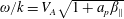

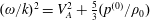


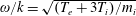


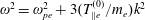


Acknowledgements
We acknowledge support of the NSF EPSCoR RII-Track-1 Cooperative Agreement no. OIA-1655280 ‘Connecting the Plasma Universe to Plasma Technology in Alabama’, led by G.P.Z. This work was supported by the European Research Council in the frame of the Consolidating grant ERC-2017-CoG771310-PI2FA ‘Partial Ionisation: Two-Fluid Approach’, led by Elena Khomenko. A.T. acknowledges support of the NASA Heliophysics Supporting Research grant no. 80NSSC18K1211. P.H. thanks T. Passot, M. Laurenza, N. Vitas, P. Hellinger and S. P. Gary for many useful discussions. We are also very thankful to two (out of three) anonymous referees whose comments and suggestions had a great impact on this text. Significant effort has been made to eliminate all the misprints from the equations. However, we will amend possible misprints, if found, in a corrigendum.
Appendix A. Fourier transformations
If we have an equation in real space, we decompose each quantity as a superposition of waves according to
 $$\begin{eqnarray}f(\boldsymbol{x},t)=\frac{1}{(2\unicode[STIX]{x03C0})^{4}}\int _{-\infty }^{\infty }\int _{-\infty }^{\infty }\hat{f}(\boldsymbol{k},\unicode[STIX]{x1D714})\text{e}^{\text{i}\boldsymbol{k}\boldsymbol{\cdot }\boldsymbol{x}-\text{i}\unicode[STIX]{x1D714}t}\,\text{d}^{3}k\,\text{d}\unicode[STIX]{x1D714}.\end{eqnarray}$$
Most of plasma physics books and kinetic papers use
 $\text{e}^{\text{i}\boldsymbol{k}\boldsymbol{\cdot }\boldsymbol{x}-\text{i}\unicode[STIX]{x1D714}t}$
in the definition (A 1). Decomposing the frequency to real and imaginary parts
$\text{e}^{\text{i}\boldsymbol{k}\boldsymbol{\cdot }\boldsymbol{x}-\text{i}\unicode[STIX]{x1D714}t}$
in the definition (A 1). Decomposing the frequency to real and imaginary parts
 $\unicode[STIX]{x1D714}=\unicode[STIX]{x1D714}_{r}+\text{i}\unicode[STIX]{x1D714}_{i}$
, so
$\unicode[STIX]{x1D714}=\unicode[STIX]{x1D714}_{r}+\text{i}\unicode[STIX]{x1D714}_{i}$
, so
 $\text{e}^{-\text{i}\unicode[STIX]{x1D714}t}=\text{e}^{-\text{i}\unicode[STIX]{x1D714}_{r}t}\text{e}^{+\unicode[STIX]{x1D714}_{i}t}$
, implies that a wave with
$\text{e}^{-\text{i}\unicode[STIX]{x1D714}t}=\text{e}^{-\text{i}\unicode[STIX]{x1D714}_{r}t}\text{e}^{+\unicode[STIX]{x1D714}_{i}t}$
, implies that a wave with
 $\unicode[STIX]{x1D714}_{i}>0$
grows (i.e. has a positive growth rate) and a wave with
$\unicode[STIX]{x1D714}_{i}>0$
grows (i.e. has a positive growth rate) and a wave with
 $\unicode[STIX]{x1D714}_{i}<0$
is damped. Of course, an alternative definition of (A 1) with
$\unicode[STIX]{x1D714}_{i}<0$
is damped. Of course, an alternative definition of (A 1) with
 $\text{e}^{-\text{i}\boldsymbol{k}\boldsymbol{\cdot }\boldsymbol{x}+\text{i}\unicode[STIX]{x1D714}t}$
is allowed, one just has to remember that a wave with
$\text{e}^{-\text{i}\boldsymbol{k}\boldsymbol{\cdot }\boldsymbol{x}+\text{i}\unicode[STIX]{x1D714}t}$
is allowed, one just has to remember that a wave with
 $\unicode[STIX]{x1D714}_{i}>0$
is damped and a wave with
$\unicode[STIX]{x1D714}_{i}>0$
is damped and a wave with
 $\unicode[STIX]{x1D714}_{i}<0$
grows. However, in Part 2 of the text, we will calculate the Landau damping and we will see that following all the correct minus signs in the Landau integral can be very confusing. We therefore recommend using the first decomposition, where waves with
$\unicode[STIX]{x1D714}_{i}<0$
grows. However, in Part 2 of the text, we will calculate the Landau damping and we will see that following all the correct minus signs in the Landau integral can be very confusing. We therefore recommend using the first decomposition, where waves with
 $\unicode[STIX]{x1D714}_{i}<0$
are damped. This choice yields that Fourier transformations in the
$\unicode[STIX]{x1D714}_{i}<0$
are damped. This choice yields that Fourier transformations in the
 $x$
–
$x$
–
 $z$
plane (with
$z$
plane (with
 $B_{0}$
in the
$B_{0}$
in the
 $z$
-direction) are performed according to a shortcut
$z$
-direction) are performed according to a shortcut
 $$\begin{eqnarray}\frac{\unicode[STIX]{x2202}}{\unicode[STIX]{x2202}t}\leftrightarrow -\text{i}\unicode[STIX]{x1D714};\quad \unicode[STIX]{x2202}_{z}\leftrightarrow \text{i}k_{\Vert };\quad \unicode[STIX]{x2202}_{x}\leftrightarrow \text{i}k_{\bot }.\end{eqnarray}$$
The transformation (A 1) is technically the inverse/backward Fourier transform
 ${\mathcal{F}}^{-1}\hat{f}(\boldsymbol{k},\unicode[STIX]{x1D714})$
. The forward Fourier transform reads
${\mathcal{F}}^{-1}\hat{f}(\boldsymbol{k},\unicode[STIX]{x1D714})$
. The forward Fourier transform reads
 $$\begin{eqnarray}f(\boldsymbol{k},\unicode[STIX]{x1D714})=\int _{-\infty }^{\infty }\int _{-\infty }^{\infty }\hat{f}(\boldsymbol{x},t)\text{e}^{-\text{i}\boldsymbol{k}\boldsymbol{\cdot }\boldsymbol{x}+\text{i}\unicode[STIX]{x1D714}t}\,\text{d}^{3}x\,\text{d}t.\end{eqnarray}$$
The location of the normalization constants
 $1/(2\unicode[STIX]{x03C0})$
is an ad hoc choice, one just needs to be consistent in using them, especially when calculating convolutions.
$1/(2\unicode[STIX]{x03C0})$
is an ad hoc choice, one just needs to be consistent in using them, especially when calculating convolutions.
Appendix B. Generalized vector (cross) product
In the collisionless fluid hierarchy one encounters a vector product between vectors and tensors, as for example in the pressure tensor equation (2.26). It is useful to clarify the definition of this generalized vector product. Consider matrix
 $\unicode[STIX]{x1D63C}$
, which is written as a tensor product between vectors
$\unicode[STIX]{x1D63C}$
, which is written as a tensor product between vectors
 $\boldsymbol{a},\boldsymbol{b}$
, so
$\boldsymbol{a},\boldsymbol{b}$
, so
 $\unicode[STIX]{x1D63C}=\boldsymbol{a}\otimes \boldsymbol{b}=\boldsymbol{a}\boldsymbol{b}$
, where, as everywhere in this text, we omit writing the tensor product
$\unicode[STIX]{x1D63C}=\boldsymbol{a}\otimes \boldsymbol{b}=\boldsymbol{a}\boldsymbol{b}$
, where, as everywhere in this text, we omit writing the tensor product
 $\otimes$
. Or in the index notation
$\otimes$
. Or in the index notation
 $\unicode[STIX]{x1D608}_{ij}=a_{i}b_{j}$
. Now consider vector
$\unicode[STIX]{x1D608}_{ij}=a_{i}b_{j}$
. Now consider vector
 $\boldsymbol{c}$
, and how can one define a generalized vector product
$\boldsymbol{c}$
, and how can one define a generalized vector product
 $\boldsymbol{c}\times \unicode[STIX]{x1D63C}$
, by using the usual vector product between two vectors. The natural definition is
$\boldsymbol{c}\times \unicode[STIX]{x1D63C}$
, by using the usual vector product between two vectors. The natural definition is
 $\boldsymbol{c}\times \unicode[STIX]{x1D63C}=\boldsymbol{c}\times (\boldsymbol{a}\boldsymbol{b})\equiv (\boldsymbol{c}\times \boldsymbol{a})\boldsymbol{b}$
, or in the index notation
$\boldsymbol{c}\times \unicode[STIX]{x1D63C}=\boldsymbol{c}\times (\boldsymbol{a}\boldsymbol{b})\equiv (\boldsymbol{c}\times \boldsymbol{a})\boldsymbol{b}$
, or in the index notation
 $(\boldsymbol{c}\times \unicode[STIX]{x1D63C})_{ij}=\unicode[STIX]{x1D716}_{ikl}c_{k}a_{l}b_{j}=\unicode[STIX]{x1D716}_{ikl}c_{k}\unicode[STIX]{x1D63C}_{lj}.$
Now let us consider how to define the much more confusing
$(\boldsymbol{c}\times \unicode[STIX]{x1D63C})_{ij}=\unicode[STIX]{x1D716}_{ikl}c_{k}a_{l}b_{j}=\unicode[STIX]{x1D716}_{ikl}c_{k}\unicode[STIX]{x1D63C}_{lj}.$
Now let us consider how to define the much more confusing
 $\unicode[STIX]{x1D63C}\times \boldsymbol{c}$
. The natural definition is
$\unicode[STIX]{x1D63C}\times \boldsymbol{c}$
. The natural definition is
 $\unicode[STIX]{x1D63C}\times \boldsymbol{c}=(\boldsymbol{a}\boldsymbol{b})\times \boldsymbol{c}\equiv \boldsymbol{a}(\boldsymbol{b}\times \boldsymbol{c})$
, and in the index notation
$\unicode[STIX]{x1D63C}\times \boldsymbol{c}=(\boldsymbol{a}\boldsymbol{b})\times \boldsymbol{c}\equiv \boldsymbol{a}(\boldsymbol{b}\times \boldsymbol{c})$
, and in the index notation
 $(\unicode[STIX]{x1D63C}\times \boldsymbol{c})_{ij}=a_{i}\unicode[STIX]{x1D716}_{jkl}b_{k}c_{l}=\unicode[STIX]{x1D716}_{jkl}\unicode[STIX]{x1D63C}_{ik}c_{l}$
. Now it is straightforward to show that
$(\unicode[STIX]{x1D63C}\times \boldsymbol{c})_{ij}=a_{i}\unicode[STIX]{x1D716}_{jkl}b_{k}c_{l}=\unicode[STIX]{x1D716}_{jkl}\unicode[STIX]{x1D63C}_{ik}c_{l}$
. Now it is straightforward to show that
 $$\begin{eqnarray}\unicode[STIX]{x1D63C}\times \boldsymbol{c}=-(\boldsymbol{c}\times \unicode[STIX]{x1D63C}^{\text{T}})^{\text{T}}.\end{eqnarray}$$
Generalizing the vector product to higher-order tensors is easy and in the fluid hierarchy we always encounter a vector
 $\hat{\boldsymbol{b}}$
, and tensors
$\hat{\boldsymbol{b}}$
, and tensors
 $\boldsymbol{p},\boldsymbol{q},\boldsymbol{r}$
, let us therefore write
$\boldsymbol{p},\boldsymbol{q},\boldsymbol{r}$
, let us therefore write
 $$\begin{eqnarray}\left.\begin{array}{@{}ll@{}}(\hat{\boldsymbol{b}}\times \boldsymbol{p})_{ij}=\unicode[STIX]{x1D716}_{irs}\hat{b}_{r}p_{sj}; & (\boldsymbol{p}\times \hat{\boldsymbol{b}})_{ij}=\unicode[STIX]{x1D716}_{jrs}p_{ir}\hat{b}_{s};\\ (\hat{\boldsymbol{b}}\times \boldsymbol{q})_{ijk}=\unicode[STIX]{x1D716}_{irs}\hat{b}_{r}q_{sjk}; & (\boldsymbol{q}\times \hat{\boldsymbol{b}})_{ijk}=\unicode[STIX]{x1D716}_{krs}q_{ijr}\hat{b}_{s};\\ (\hat{\boldsymbol{b}}\times \boldsymbol{r})_{ijkl}=\unicode[STIX]{x1D716}_{irs}\hat{b}_{r}r_{sjkl}; & (\boldsymbol{r}\times \hat{\boldsymbol{b}})_{ijkl}=\unicode[STIX]{x1D716}_{lrs}r_{ijkr}\hat{b}_{s}.\end{array}\right\}\end{eqnarray}$$
The vector product is very useful for decomposing quantities to the directions parallel and perpendicular with respect to
 $\hat{\boldsymbol{b}}$
. For example, the usual decomposition of the velocity
$\hat{\boldsymbol{b}}$
. For example, the usual decomposition of the velocity
 $\boldsymbol{u}$
reads
$\boldsymbol{u}$
reads
 $$\begin{eqnarray}\boldsymbol{u}=\underbrace{(\boldsymbol{u}\boldsymbol{\cdot }\hat{\boldsymbol{b}})\hat{\boldsymbol{b}}}_{\boldsymbol{u}_{\Vert }}+\underbrace{\boldsymbol{u}\boldsymbol{\cdot }(\unicode[STIX]{x1D644}-\hat{\boldsymbol{b}}\hat{\boldsymbol{b}})}_{\boldsymbol{u}_{\bot }}.\end{eqnarray}$$
Nevertheless, it is possible to directly obtain
 $\boldsymbol{u}_{\bot }$
, by applying
$\boldsymbol{u}_{\bot }$
, by applying
 $\hat{\boldsymbol{b}}\times$
twice on
$\hat{\boldsymbol{b}}\times$
twice on
 $\boldsymbol{u}$
, so that
$\boldsymbol{u}$
, so that
 $$\begin{eqnarray}\boldsymbol{u}=(\boldsymbol{u}\boldsymbol{\cdot }\hat{\boldsymbol{b}})\hat{\boldsymbol{b}}-\hat{\boldsymbol{b}}\times (\hat{\boldsymbol{b}}\times \boldsymbol{u}),\end{eqnarray}$$
or
 $\boldsymbol{u}_{\bot }=\hat{\boldsymbol{b}}\times \boldsymbol{u}\times \hat{\boldsymbol{b}}$
. Similar decompositions can be made for tensors. For example, a general matrix
$\boldsymbol{u}_{\bot }=\hat{\boldsymbol{b}}\times \boldsymbol{u}\times \hat{\boldsymbol{b}}$
. Similar decompositions can be made for tensors. For example, a general matrix
 $\unicode[STIX]{x1D72B}$
can be decomposed according to
$\unicode[STIX]{x1D72B}$
can be decomposed according to
 $$\begin{eqnarray}\unicode[STIX]{x1D72B}=(\unicode[STIX]{x1D72B}\boldsymbol{\cdot }\hat{\boldsymbol{b}})\hat{\boldsymbol{b}}+\unicode[STIX]{x1D72B}\boldsymbol{\cdot }(\unicode[STIX]{x1D644}-\hat{\boldsymbol{b}}\hat{\boldsymbol{b}}),\end{eqnarray}$$
where the perpendicular component can be written as
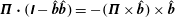 $\unicode[STIX]{x1D72B}\boldsymbol{\cdot }(\unicode[STIX]{x1D644}-\hat{\boldsymbol{b}}\hat{\boldsymbol{b}})=-(\unicode[STIX]{x1D72B}\times \hat{\boldsymbol{b}})\times \hat{\boldsymbol{b}}$
, i.e. where all the
$\unicode[STIX]{x1D72B}\boldsymbol{\cdot }(\unicode[STIX]{x1D644}-\hat{\boldsymbol{b}}\hat{\boldsymbol{b}})=-(\unicode[STIX]{x1D72B}\times \hat{\boldsymbol{b}})\times \hat{\boldsymbol{b}}$
, i.e. where all the
 $\hat{\boldsymbol{b}}$
act on
$\hat{\boldsymbol{b}}$
act on
 $\unicode[STIX]{x1D72B}$
from the right. Alternatively, one can write a decomposition when all the
$\unicode[STIX]{x1D72B}$
from the right. Alternatively, one can write a decomposition when all the
 $\hat{\boldsymbol{b}}$
act on the
$\hat{\boldsymbol{b}}$
act on the
 $\unicode[STIX]{x1D72B}$
from the left,
$\unicode[STIX]{x1D72B}$
from the left,
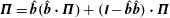 $\unicode[STIX]{x1D72B}=\hat{\boldsymbol{b}}(\hat{\boldsymbol{b}}\boldsymbol{\cdot }\unicode[STIX]{x1D72B})+(\unicode[STIX]{x1D644}-\hat{\boldsymbol{b}}\hat{\boldsymbol{b}})\boldsymbol{\cdot }\unicode[STIX]{x1D72B}$
, where the perpendicular part
$\unicode[STIX]{x1D72B}=\hat{\boldsymbol{b}}(\hat{\boldsymbol{b}}\boldsymbol{\cdot }\unicode[STIX]{x1D72B})+(\unicode[STIX]{x1D644}-\hat{\boldsymbol{b}}\hat{\boldsymbol{b}})\boldsymbol{\cdot }\unicode[STIX]{x1D72B}$
, where the perpendicular part
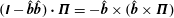 $(\unicode[STIX]{x1D644}-\hat{\boldsymbol{b}}\hat{\boldsymbol{b}})\boldsymbol{\cdot }\unicode[STIX]{x1D72B}=-\hat{\boldsymbol{b}}\times (\hat{\boldsymbol{b}}\times \unicode[STIX]{x1D72B})$
.
$(\unicode[STIX]{x1D644}-\hat{\boldsymbol{b}}\hat{\boldsymbol{b}})\boldsymbol{\cdot }\unicode[STIX]{x1D72B}=-\hat{\boldsymbol{b}}\times (\hat{\boldsymbol{b}}\times \unicode[STIX]{x1D72B})$
.
Appendix C. MHD dispersion relation
We assume that many people reading this text will have some previous experience with MHD. It is therefore beneficial to obtain the MHD dispersion relation, so that it will be clear how more advanced fluid models are treated in this text. The MHD fluid model reads
 $$\begin{eqnarray}\displaystyle & \displaystyle \frac{\unicode[STIX]{x2202}\unicode[STIX]{x1D70C}}{\unicode[STIX]{x2202}t}+\unicode[STIX]{x1D735}\boldsymbol{\cdot }(\unicode[STIX]{x1D70C}\boldsymbol{u})=0; & \displaystyle\end{eqnarray}$$
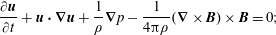 $$\begin{eqnarray}\displaystyle & \displaystyle \frac{\unicode[STIX]{x2202}\boldsymbol{u}}{\unicode[STIX]{x2202}t}+\boldsymbol{u}\boldsymbol{\cdot }\unicode[STIX]{x1D735}\boldsymbol{u}+\frac{1}{\unicode[STIX]{x1D70C}}\unicode[STIX]{x1D735}p-\frac{1}{4\unicode[STIX]{x03C0}\unicode[STIX]{x1D70C}}(\unicode[STIX]{x1D735}\times \boldsymbol{B})\times \boldsymbol{B}=0; & \displaystyle\end{eqnarray}$$
 $$\begin{eqnarray}\displaystyle & \displaystyle \frac{\unicode[STIX]{x2202}\boldsymbol{B}}{\unicode[STIX]{x2202}t}=\unicode[STIX]{x1D735}\times (\boldsymbol{u}\times \boldsymbol{B}); & \displaystyle\end{eqnarray}$$
 $$\begin{eqnarray}\displaystyle & \displaystyle \frac{\unicode[STIX]{x2202}p}{\unicode[STIX]{x2202}t}+\boldsymbol{u}\boldsymbol{\cdot }\unicode[STIX]{x1D735}p+\unicode[STIX]{x1D6FE}p\unicode[STIX]{x1D735}\boldsymbol{\cdot }\boldsymbol{u}=0, & \displaystyle\end{eqnarray}$$
where
 $\unicode[STIX]{x1D6FE}=5/3$
. As in advanced fluid models, it is beneficial to normalize the speed with respect to the Alfvén speed
$\unicode[STIX]{x1D6FE}=5/3$
. As in advanced fluid models, it is beneficial to normalize the speed with respect to the Alfvén speed
 $V_{A}$
, and normalize the length with respect to the ion inertial length
$V_{A}$
, and normalize the length with respect to the ion inertial length
 $d_{i}=V_{A}/\unicode[STIX]{x1D6FA}_{p}$
, i.e. by using normalizations (3.23)–(3.28), which in Fourier space yields
$d_{i}=V_{A}/\unicode[STIX]{x1D6FA}_{p}$
, i.e. by using normalizations (3.23)–(3.28), which in Fourier space yields
 $\widetilde{k}=kd_{i}$
,
$\widetilde{k}=kd_{i}$
,
 $\widetilde{\unicode[STIX]{x1D714}}=\unicode[STIX]{x1D714}/\unicode[STIX]{x1D6FA}_{p}$
. Normalizing the MHD equations and dropping the tilde yields unchanged density, induction and pressure equations, and the momentum equation reads
$\widetilde{\unicode[STIX]{x1D714}}=\unicode[STIX]{x1D714}/\unicode[STIX]{x1D6FA}_{p}$
. Normalizing the MHD equations and dropping the tilde yields unchanged density, induction and pressure equations, and the momentum equation reads
 $$\begin{eqnarray}\frac{\unicode[STIX]{x2202}\boldsymbol{u}}{\unicode[STIX]{x2202}t}+\boldsymbol{u}\boldsymbol{\cdot }\unicode[STIX]{x1D735}\boldsymbol{u}+\frac{p^{(0)}}{\unicode[STIX]{x1D70C}_{0}V_{A}^{2}}\frac{1}{\unicode[STIX]{x1D70C}}\unicode[STIX]{x1D735}p-\frac{1}{\unicode[STIX]{x1D70C}}(\unicode[STIX]{x1D735}\times \boldsymbol{B})\times \boldsymbol{B}=0.\end{eqnarray}$$
One can decide how to rewrite
 $p^{(0)}/(\unicode[STIX]{x1D70C}_{0}V_{A}^{2})$
, either by introducing the usual MHD sound speed
$p^{(0)}/(\unicode[STIX]{x1D70C}_{0}V_{A}^{2})$
, either by introducing the usual MHD sound speed
 $C_{s}^{2}=\unicode[STIX]{x1D6FE}p^{(0)}/\unicode[STIX]{x1D70C}_{0}$
, or by introducing the plasma beta
$C_{s}^{2}=\unicode[STIX]{x1D6FE}p^{(0)}/\unicode[STIX]{x1D70C}_{0}$
, or by introducing the plasma beta
 $$\begin{eqnarray}\unicode[STIX]{x1D6FD}=\frac{v_{\text{th}}^{2}}{V_{A}^{2}}=\frac{2T^{(0)}/m_{p}}{V_{A}^{2}}=\frac{2p^{(0)}/\unicode[STIX]{x1D70C}_{0}}{V_{A}^{2}}=\frac{p^{(0)}}{B_{0}^{2}/(8\unicode[STIX]{x03C0})};\quad \Rightarrow \quad \frac{p^{(0)}}{\unicode[STIX]{x1D70C}_{0}V_{A}^{2}}=\frac{1}{\unicode[STIX]{x1D6FE}}\frac{C_{s}^{2}}{V_{A}^{2}}=\frac{\unicode[STIX]{x1D6FD}}{2},\end{eqnarray}$$
where we use the Boltzmann constant
 $k_{B}=1$
, see the footnote 3 after the definition of thermal speeds (3.30). By specifying the mean magnetic field to be in the
$k_{B}=1$
, see the footnote 3 after the definition of thermal speeds (3.30). By specifying the mean magnetic field to be in the
 $z$
-direction, the normalized equations are linearized according to
$z$
-direction, the normalized equations are linearized according to
 $$\begin{eqnarray}\displaystyle & \displaystyle \frac{\unicode[STIX]{x2202}\unicode[STIX]{x1D70C}}{\unicode[STIX]{x2202}t}+\unicode[STIX]{x1D735}\boldsymbol{\cdot }\boldsymbol{u}=0; & \displaystyle\end{eqnarray}$$
 $$\begin{eqnarray}\displaystyle & \displaystyle \frac{\unicode[STIX]{x2202}u_{x}}{\unicode[STIX]{x2202}t}+\frac{\unicode[STIX]{x1D6FD}}{2}\unicode[STIX]{x2202}_{x}p+\unicode[STIX]{x2202}_{x}B_{z}-\unicode[STIX]{x2202}_{z}B_{x}=0; & \displaystyle\end{eqnarray}$$
 $$\begin{eqnarray}\displaystyle & \displaystyle \frac{\unicode[STIX]{x2202}u_{y}}{\unicode[STIX]{x2202}t}+\frac{\unicode[STIX]{x1D6FD}}{2}\unicode[STIX]{x2202}_{y}p+\unicode[STIX]{x2202}_{y}B_{z}-\unicode[STIX]{x2202}_{z}B_{y}=0; & \displaystyle\end{eqnarray}$$
 $$\begin{eqnarray}\displaystyle & \displaystyle \frac{\unicode[STIX]{x2202}u_{z}}{\unicode[STIX]{x2202}t}+\frac{\unicode[STIX]{x1D6FD}}{2}\unicode[STIX]{x2202}_{z}p=0; & \displaystyle\end{eqnarray}$$
 $$\begin{eqnarray}\displaystyle & \displaystyle \frac{\unicode[STIX]{x2202}B_{x}}{\unicode[STIX]{x2202}t}=\unicode[STIX]{x2202}_{z}u_{x};\quad \frac{\unicode[STIX]{x2202}B_{y}}{\unicode[STIX]{x2202}t}=\unicode[STIX]{x2202}_{z}u_{y};\quad \frac{\unicode[STIX]{x2202}B_{z}}{\unicode[STIX]{x2202}t}=-\unicode[STIX]{x2202}_{x}u_{x}-\unicode[STIX]{x2202}_{y}u_{y}; & \displaystyle\end{eqnarray}$$
 $$\begin{eqnarray}\displaystyle & \displaystyle \frac{\unicode[STIX]{x2202}p}{\unicode[STIX]{x2202}t}+\unicode[STIX]{x1D6FE}\unicode[STIX]{x1D735}\boldsymbol{\cdot }\boldsymbol{u}=0, & \displaystyle\end{eqnarray}$$
and without a loss of generality, we consider propagation in the
 $x$
–
$x$
–
 $z$
plane (with
$z$
plane (with
 $\unicode[STIX]{x2202}_{y}=0$
). By considering a wave propagating with wavenumber
$\unicode[STIX]{x2202}_{y}=0$
). By considering a wave propagating with wavenumber
 $\boldsymbol{k}=(k\sin \unicode[STIX]{x1D703},0,k\cos \unicode[STIX]{x1D703})=(k_{x},0,k_{z})=(k_{\bot },0,k_{\Vert })$
, i.e. a wave propagating in the direction that makes an angle
$\boldsymbol{k}=(k\sin \unicode[STIX]{x1D703},0,k\cos \unicode[STIX]{x1D703})=(k_{x},0,k_{z})=(k_{\bot },0,k_{\Vert })$
, i.e. a wave propagating in the direction that makes an angle
 $\unicode[STIX]{x1D703}$
with respect to
$\unicode[STIX]{x1D703}$
with respect to
 $\boldsymbol{B}_{0}$
, the MHD system written in Fourier space reads
$\boldsymbol{B}_{0}$
, the MHD system written in Fourier space reads
 $$\begin{eqnarray}\displaystyle & \displaystyle -\unicode[STIX]{x1D714}\unicode[STIX]{x1D70C}+(k\sin \unicode[STIX]{x1D703})u_{x}+(k\cos \unicode[STIX]{x1D703})u_{z}=0; & \displaystyle\end{eqnarray}$$
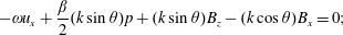 $$\begin{eqnarray}\displaystyle & \displaystyle -\unicode[STIX]{x1D714}u_{x}+\frac{\unicode[STIX]{x1D6FD}}{2}(k\sin \unicode[STIX]{x1D703})p+(k\sin \unicode[STIX]{x1D703})B_{z}-(k\cos \unicode[STIX]{x1D703})B_{x}=0; & \displaystyle\end{eqnarray}$$
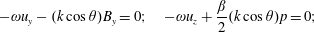 $$\begin{eqnarray}\displaystyle & \displaystyle -\unicode[STIX]{x1D714}u_{y}-(k\cos \unicode[STIX]{x1D703})B_{y}=0;\quad -\unicode[STIX]{x1D714}u_{z}+\frac{\unicode[STIX]{x1D6FD}}{2}(k\cos \unicode[STIX]{x1D703})p=0; & \displaystyle\end{eqnarray}$$
 $$\begin{eqnarray}\displaystyle & \displaystyle -\unicode[STIX]{x1D714}B_{x}-(k\cos \unicode[STIX]{x1D703})u_{x}=0;\quad -\unicode[STIX]{x1D714}B_{y}-(k\cos \unicode[STIX]{x1D703})u_{y}=0;\quad -\unicode[STIX]{x1D714}B_{z}+(k\sin \unicode[STIX]{x1D703})u_{x}=0; & \displaystyle\end{eqnarray}$$
 $$\begin{eqnarray}\displaystyle & \displaystyle -\unicode[STIX]{x1D714}p+\unicode[STIX]{x1D6FE}(k\sin \unicode[STIX]{x1D703})u_{x}+\unicode[STIX]{x1D6FE}(k\cos \unicode[STIX]{x1D703})u_{z}=0. & \displaystyle\end{eqnarray}$$
Calculating the determinant of this system yields the MHD dispersion relation in normalized units (bringing back tildes for clarity) that reads
 $$\begin{eqnarray}(\widetilde{\unicode[STIX]{x1D714}}^{2}-\widetilde{k}^{2}\cos ^{2}\unicode[STIX]{x1D703})\left(\widetilde{\unicode[STIX]{x1D714}}^{4}-\left(1+\unicode[STIX]{x1D6FE}\frac{\unicode[STIX]{x1D6FD}}{2}\right)\widetilde{k}^{2}\widetilde{\unicode[STIX]{x1D714}}^{2}+\unicode[STIX]{x1D6FE}\frac{\unicode[STIX]{x1D6FD}}{2}\widetilde{k}^{4}\cos ^{2}\unicode[STIX]{x1D703}\right)=0,\end{eqnarray}$$
or alternatively by using (C 6) with the sound speed
 $$\begin{eqnarray}(\widetilde{\unicode[STIX]{x1D714}}^{2}-\widetilde{k}^{2}\cos ^{2}\unicode[STIX]{x1D703})\left(\widetilde{\unicode[STIX]{x1D714}}^{4}-\left(1+\frac{C_{s}^{2}}{V_{A}^{2}}\right)\widetilde{k}^{2}\widetilde{\unicode[STIX]{x1D714}}^{2}+\frac{C_{s}^{2}}{V_{A}^{2}}\widetilde{k}^{4}\cos ^{2}\unicode[STIX]{x1D703}\right)=0,\end{eqnarray}$$
or in physical units
 $$\begin{eqnarray}(\unicode[STIX]{x1D714}^{2}-V_{A}^{2}k^{2}\cos ^{2}\unicode[STIX]{x1D703})(\unicode[STIX]{x1D714}^{4}-(V_{A}^{2}+C_{s}^{2})k^{2}\unicode[STIX]{x1D714}^{2}+V_{A}^{2}C_{s}^{2}k^{4}\cos ^{2}\unicode[STIX]{x1D703})=0,\end{eqnarray}$$
yielding the MHD dispersion relation for the Alfvén mode
 $\unicode[STIX]{x1D714}_{A}=\pm V_{A}k\cos \unicode[STIX]{x1D703}=\pm V_{A}k_{\Vert }$
(sometimes called the shear Alfvén mode), and the slow and fast modes (3.110).
$\unicode[STIX]{x1D714}_{A}=\pm V_{A}k\cos \unicode[STIX]{x1D703}=\pm V_{A}k_{\Vert }$
(sometimes called the shear Alfvén mode), and the slow and fast modes (3.110).
In the limit
 $\unicode[STIX]{x1D6FD}\rightarrow 0$
that corresponds to a cold plasma (
$\unicode[STIX]{x1D6FD}\rightarrow 0$
that corresponds to a cold plasma (
 $C_{s}\rightarrow 0$
) or a plasma with a very strong magnetic field (
$C_{s}\rightarrow 0$
) or a plasma with a very strong magnetic field (
 $V_{A}\rightarrow \infty$
), the slow mode
$V_{A}\rightarrow \infty$
), the slow mode
 $\unicode[STIX]{x1D714}_{s}=\pm C_{s}k_{\Vert }$
, and the fast mode
$\unicode[STIX]{x1D714}_{s}=\pm C_{s}k_{\Vert }$
, and the fast mode
 $\unicode[STIX]{x1D714}_{f}=\pm V_{A}k$
(sometimes called the compressional Alfvén mode). In the limit
$\unicode[STIX]{x1D714}_{f}=\pm V_{A}k$
(sometimes called the compressional Alfvén mode). In the limit
 $\unicode[STIX]{x1D6FD}\rightarrow \infty$
that corresponds to the incompressible MHD (
$\unicode[STIX]{x1D6FD}\rightarrow \infty$
that corresponds to the incompressible MHD (
 $C_{s}\rightarrow \infty$
) or a plasma with vanishing magnetic field (
$C_{s}\rightarrow \infty$
) or a plasma with vanishing magnetic field (
 $V_{A}\rightarrow 0$
), the slow mode
$V_{A}\rightarrow 0$
), the slow mode
 $\unicode[STIX]{x1D714}_{s}=\pm V_{A}k_{\Vert }$
, and the fast mode
$\unicode[STIX]{x1D714}_{s}=\pm V_{A}k_{\Vert }$
, and the fast mode
 $\unicode[STIX]{x1D714}_{f}=\pm C_{s}k$
. Note the difference in
$\unicode[STIX]{x1D714}_{f}=\pm C_{s}k$
. Note the difference in
 $k_{\Vert }$
and
$k_{\Vert }$
and
 $k$
in these two limits.
$k$
in these two limits.
Appendix D. Non-gyrotropic heat flux tensor
$\boldsymbol{q}^{\text{ng}}$

The heat flux tensor equation (7.33) is rewritten as
 $$\begin{eqnarray}(\hat{\boldsymbol{b}}\times \boldsymbol{q}^{\text{ng}})^{S}=-\frac{B_{0}}{\unicode[STIX]{x1D6FA}|\boldsymbol{B}|}\left[\frac{\text{d}}{\text{d}t}\boldsymbol{q}+\unicode[STIX]{x1D735}\boldsymbol{\cdot }\boldsymbol{r}+\boldsymbol{q}\unicode[STIX]{x1D735}\boldsymbol{\cdot }\boldsymbol{u}+(\boldsymbol{q}\boldsymbol{\cdot }\unicode[STIX]{x1D735}\boldsymbol{u})^{S}-\frac{1}{\unicode[STIX]{x1D70C}}(\boldsymbol{p}(\unicode[STIX]{x1D735}\boldsymbol{\cdot }\boldsymbol{p}))^{S}\right].\end{eqnarray}$$
The ‘inversion’ procedure for the left-hand side of this is equation is very complicated, and will not be addressed here. Nevertheless, the inversion procedure exists, and an interested reader can check equation (43) of Ramos (Reference Ramos2005). The leading-order
 $\boldsymbol{q}^{\text{ng}}$
(first order in frequency and wavenumber) can be obtained by making the quantities
$\boldsymbol{q}^{\text{ng}}$
(first order in frequency and wavenumber) can be obtained by making the quantities
 $\boldsymbol{q},\boldsymbol{r},\boldsymbol{p}$
on the right-hand side gyrotropic, and we want to solve
$\boldsymbol{q},\boldsymbol{r},\boldsymbol{p}$
on the right-hand side gyrotropic, and we want to solve
 $$\begin{eqnarray}(\hat{\boldsymbol{b}}\times \boldsymbol{q}^{\text{ng}})^{S}=-\frac{B_{0}}{\unicode[STIX]{x1D6FA}|\boldsymbol{B}|}\left[\frac{\text{d}}{\text{d}t}\boldsymbol{q}^{\text{g}}+\unicode[STIX]{x1D735}\boldsymbol{\cdot }\boldsymbol{r}^{\text{g}}+\boldsymbol{q}^{\text{g}}\unicode[STIX]{x1D735}\boldsymbol{\cdot }\boldsymbol{u}+(\boldsymbol{q}^{\text{g}}\boldsymbol{\cdot }\unicode[STIX]{x1D735}\boldsymbol{u})^{S}-\frac{1}{\unicode[STIX]{x1D70C}}(\boldsymbol{p}^{\text{g}}(\unicode[STIX]{x1D735}\boldsymbol{\cdot }\boldsymbol{p}^{\text{g}}))^{S}\right].\end{eqnarray}$$
The heat flux tensor decomposition is
 $\boldsymbol{q}=\boldsymbol{q}^{\text{g}}+\boldsymbol{q}^{\text{ng}}$
, or alternatively
$\boldsymbol{q}=\boldsymbol{q}^{\text{g}}+\boldsymbol{q}^{\text{ng}}$
, or alternatively
 $\boldsymbol{q}=\boldsymbol{S}+\unicode[STIX]{x1D748}$
, where
$\boldsymbol{q}=\boldsymbol{S}+\unicode[STIX]{x1D748}$
, where
 $\unicode[STIX]{x1D748}:\hat{\boldsymbol{b}}\hat{\boldsymbol{b}}=0$
,
$\unicode[STIX]{x1D748}:\hat{\boldsymbol{b}}\hat{\boldsymbol{b}}=0$
,
 $\unicode[STIX]{x1D748}:\unicode[STIX]{x1D644}=0$
. Since
$\unicode[STIX]{x1D748}:\unicode[STIX]{x1D644}=0$
. Since
 $$\begin{eqnarray}\displaystyle & \displaystyle \underbrace{\boldsymbol{q}:\hat{\boldsymbol{b}}\hat{\boldsymbol{b}}}_{\boldsymbol{S}^{\Vert }}=\underbrace{\boldsymbol{q}^{\text{g}}:\hat{\boldsymbol{b}}\hat{\boldsymbol{b}}}_{q_{\Vert }\hat{\boldsymbol{b}}}+\boldsymbol{q}^{\text{ng}}:\hat{\boldsymbol{b}}\hat{\boldsymbol{b}}; & \displaystyle\end{eqnarray}$$
 $$\begin{eqnarray}\displaystyle & \displaystyle \underbrace{\boldsymbol{q}:(\unicode[STIX]{x1D644}-\hat{\boldsymbol{b}}\hat{\boldsymbol{b}})/2}_{\boldsymbol{S}^{\bot }}=\underbrace{\boldsymbol{q}^{\text{g}}:(\unicode[STIX]{x1D644}-\hat{\boldsymbol{b}}\hat{\boldsymbol{b}})/2}_{q_{\bot }\hat{\boldsymbol{b}}}+\boldsymbol{q}^{\text{ng}}:(\unicode[STIX]{x1D644}-\hat{\boldsymbol{b}}\hat{\boldsymbol{b}})/2, & \displaystyle\end{eqnarray}$$
one can define perpendicular components of the heat flux vectors
 $$\begin{eqnarray}\displaystyle & \displaystyle \boldsymbol{S}_{\bot }^{\Vert }=\boldsymbol{q}^{\text{ng}}:\hat{\boldsymbol{b}}\hat{\boldsymbol{b}}; & \displaystyle\end{eqnarray}$$
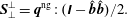 $$\begin{eqnarray}\displaystyle & \displaystyle \boldsymbol{S}_{\bot }^{\bot }=\boldsymbol{q}^{\text{ng}}:(\unicode[STIX]{x1D644}-\hat{\boldsymbol{b}}\hat{\boldsymbol{b}})/2. & \displaystyle\end{eqnarray}$$
Therefore, to obtain these vectors, we want to apply
 $:\hat{\boldsymbol{b}}\hat{\boldsymbol{b}}$
, and
$:\hat{\boldsymbol{b}}\hat{\boldsymbol{b}}$
, and
 $:(\unicode[STIX]{x1D644}-\hat{\boldsymbol{b}}\hat{\boldsymbol{b}})/2$
to the entire equation (D 2). A very useful expression also is
$:(\unicode[STIX]{x1D644}-\hat{\boldsymbol{b}}\hat{\boldsymbol{b}})/2$
to the entire equation (D 2). A very useful expression also is
 $$\begin{eqnarray}\text{Tr}\,\boldsymbol{q}^{\text{ng}}=\boldsymbol{q}^{\text{ng}}:\unicode[STIX]{x1D644}=\boldsymbol{S}_{\bot }^{\Vert }+2\boldsymbol{S}_{\bot }^{\bot },\end{eqnarray}$$
and the trace of the entire heat flux tensor reads
 $$\begin{eqnarray}\text{Tr}\,\boldsymbol{q}=q_{\Vert }\hat{\boldsymbol{b}}+2q_{\bot }\hat{\boldsymbol{b}}+\boldsymbol{S}_{\bot }^{\Vert }+2\boldsymbol{S}_{\bot }^{\bot }.\end{eqnarray}$$
D.1 Non-gyrotropic heat flux vector
$\boldsymbol{S}_{\bot }^{\Vert }$

Applying
 $:\hat{\boldsymbol{b}}\hat{\boldsymbol{b}}$
to the left-hand side of (D 2) yields
$:\hat{\boldsymbol{b}}\hat{\boldsymbol{b}}$
to the left-hand side of (D 2) yields

Terms on the right-hand side of (D 2) calculate as
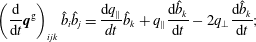 $$\begin{eqnarray}\displaystyle & \displaystyle \left(\frac{\text{d}}{\text{d}t}\boldsymbol{q}^{\text{g}}\right)_{ijk}\hat{b}_{i}\hat{b}_{j}=\frac{\text{d}q_{\Vert }}{dt}\hat{b}_{k}+q_{\Vert }\frac{\text{d}\hat{b}_{k}}{\text{d}t}-2q_{\bot }\frac{\text{d}\hat{b}_{k}}{\text{d}t}; & \displaystyle\end{eqnarray}$$
 $$\begin{eqnarray}\displaystyle & \displaystyle (\unicode[STIX]{x1D735}\boldsymbol{\cdot }\boldsymbol{r}^{\text{g}})_{ijk}\hat{b}_{i}\hat{b}_{j}=\hat{b}_{k}\hat{\boldsymbol{b}}\boldsymbol{\cdot }\unicode[STIX]{x1D735}r_{\Vert \Vert }+(r_{\Vert \Vert }-3r_{\Vert \bot })(\hat{\boldsymbol{b}}\boldsymbol{\cdot }\unicode[STIX]{x1D735}\hat{b}_{k}+\hat{b}_{k}\unicode[STIX]{x1D735}\boldsymbol{\cdot }\hat{\boldsymbol{b}})-\hat{b}_{k}\hat{\boldsymbol{b}}\boldsymbol{\cdot }\unicode[STIX]{x1D735}r_{\Vert \bot }+\unicode[STIX]{x2202}_{k}r_{\Vert \bot }; & \displaystyle \nonumber\\ \displaystyle & & \displaystyle\end{eqnarray}$$
 $$\begin{eqnarray}\displaystyle & \displaystyle q_{ijk}^{\text{g}}\hat{b}_{i}=q_{\Vert }\hat{b}_{j}\hat{b}_{k}+q_{\bot }(\unicode[STIX]{x1D6FF}_{jk}-\hat{b}_{j}\hat{b}_{k}); & \displaystyle\end{eqnarray}$$
 $$\begin{eqnarray}\displaystyle & \displaystyle q_{ijk}^{\text{g}}\hat{b}_{i}\hat{b}_{j}\unicode[STIX]{x1D735}\boldsymbol{\cdot }\boldsymbol{u}=q_{\Vert }\hat{b}_{k}\unicode[STIX]{x1D735}\boldsymbol{\cdot }\boldsymbol{u}; & \displaystyle\end{eqnarray}$$
 $$\begin{eqnarray}\displaystyle & \displaystyle (\boldsymbol{q}^{\text{g}}\boldsymbol{\cdot }\unicode[STIX]{x1D735}\boldsymbol{u})_{ijk}^{S}\hat{b}_{i}\hat{b}_{j}=q_{\Vert }\hat{\boldsymbol{b}}\boldsymbol{\cdot }\unicode[STIX]{x1D735}u_{k}+2(q_{\Vert }-q_{\bot })\hat{b}_{k}\hat{\boldsymbol{b}}\boldsymbol{\cdot }(\unicode[STIX]{x1D735}\boldsymbol{u})\boldsymbol{\cdot }\hat{\boldsymbol{b}}+2q_{\bot }(\unicode[STIX]{x2202}_{k}\boldsymbol{u})\boldsymbol{\cdot }\hat{\boldsymbol{b}}. & \displaystyle\end{eqnarray}$$
For the last term on the right-hand side of (D 2)
 $$\begin{eqnarray}\displaystyle & \displaystyle (\boldsymbol{p}(\unicode[STIX]{x1D735}\boldsymbol{\cdot }\boldsymbol{p}))_{ijk}^{S}\hat{b}_{i}\hat{b}_{j}=p_{\Vert }(\unicode[STIX]{x1D735}\boldsymbol{\cdot }\boldsymbol{p})_{k}+2(p_{\Vert }\hat{b}_{k}+\unicode[STIX]{x1D6F1}_{jk}\hat{b}_{j})(\unicode[STIX]{x1D735}\boldsymbol{\cdot }\boldsymbol{p})\boldsymbol{\cdot }\hat{\boldsymbol{b}}; & \displaystyle\end{eqnarray}$$
 $$\begin{eqnarray}\displaystyle & \displaystyle (\unicode[STIX]{x1D735}\boldsymbol{\cdot }\boldsymbol{p})_{k}=\hat{b}_{k}\hat{\boldsymbol{b}}\boldsymbol{\cdot }\unicode[STIX]{x1D735}(p_{\Vert }-p_{\bot })+(p_{\Vert }-p_{\bot })(\hat{\boldsymbol{b}}\boldsymbol{\cdot }\unicode[STIX]{x1D735}\hat{b}_{k}+\hat{b}_{k}\unicode[STIX]{x1D735}\boldsymbol{\cdot }\hat{\boldsymbol{b}})+\unicode[STIX]{x2202}_{k}p_{\bot }+(\unicode[STIX]{x1D735}\boldsymbol{\cdot }\unicode[STIX]{x1D72B})_{k}; & \displaystyle\end{eqnarray}$$
 $$\begin{eqnarray}\displaystyle & \displaystyle (\unicode[STIX]{x1D735}\boldsymbol{\cdot }\boldsymbol{p})\boldsymbol{\cdot }\hat{\boldsymbol{b}}=\hat{\boldsymbol{b}}\boldsymbol{\cdot }\unicode[STIX]{x1D735}p_{\Vert }+(p_{\Vert }-p_{\bot })\unicode[STIX]{x1D735}\boldsymbol{\cdot }\hat{\boldsymbol{b}}+(\unicode[STIX]{x1D735}\boldsymbol{\cdot }\unicode[STIX]{x1D72B})\boldsymbol{\cdot }\hat{\boldsymbol{b}}, & \displaystyle\end{eqnarray}$$
and so for the gyrotropic
 $$\begin{eqnarray}\displaystyle (\boldsymbol{p}^{\text{g}}(\unicode[STIX]{x1D735}\boldsymbol{\cdot }\boldsymbol{p}^{\text{g}}))_{ijk}^{S}\hat{b}_{i}\hat{b}_{j}=p_{\Vert }\hat{b}_{k}\hat{\boldsymbol{b}}\boldsymbol{\cdot }\unicode[STIX]{x1D735}(3p_{\Vert }-p_{\bot })+p_{\Vert }(p_{\Vert }-p_{\bot })(\hat{\boldsymbol{b}}\boldsymbol{\cdot }\unicode[STIX]{x1D735}\hat{b}_{k}+3\hat{b}_{k}\unicode[STIX]{x1D735}\boldsymbol{\cdot }\hat{\boldsymbol{b}})+p_{\Vert }\unicode[STIX]{x2202}_{k}p_{\bot }. & & \displaystyle \nonumber\\ \displaystyle & & \displaystyle\end{eqnarray}$$
Collecting all the results together yields
 $$\begin{eqnarray}\displaystyle (\hat{\boldsymbol{b}}\times \boldsymbol{S}_{\bot }^{\Vert })_{k} & = & \displaystyle -\frac{B_{0}}{\unicode[STIX]{x1D6FA}|\boldsymbol{B}|}\left[\frac{\text{d}q_{\Vert }}{\text{d}t}\hat{b}_{k}+q_{\Vert }\frac{\text{d}\hat{b}_{k}}{\text{d}t}-2q_{\bot }\frac{\text{d}\hat{b}_{k}}{\text{d}t}+\hat{b}_{k}\hat{\boldsymbol{b}}\boldsymbol{\cdot }\unicode[STIX]{x1D735}r_{\Vert \Vert }\right.\nonumber\\ \displaystyle & & \displaystyle +(r_{\Vert \Vert }-3r_{\Vert \bot })(\hat{\boldsymbol{b}}\boldsymbol{\cdot }\unicode[STIX]{x1D735}\hat{b}_{k}+\hat{b}_{k}\unicode[STIX]{x1D735}\boldsymbol{\cdot }\hat{\boldsymbol{b}})-\hat{b}_{k}\hat{\boldsymbol{b}}\boldsymbol{\cdot }\unicode[STIX]{x1D735}r_{\Vert \bot }+\unicode[STIX]{x2202}_{k}r_{\Vert \bot }\nonumber\\ \displaystyle & & \displaystyle +\,q_{\Vert }\hat{b}_{k}\unicode[STIX]{x1D735}\boldsymbol{\cdot }\boldsymbol{u}+q_{\Vert }\hat{\boldsymbol{b}}\boldsymbol{\cdot }\unicode[STIX]{x1D735}u_{k}+2(q_{\Vert }-q_{\bot })\hat{b}_{k}\hat{\boldsymbol{b}}\boldsymbol{\cdot }(\unicode[STIX]{x1D735}\boldsymbol{u})\boldsymbol{\cdot }\hat{\boldsymbol{b}}+2q_{\bot }(\unicode[STIX]{x2202}_{k}\boldsymbol{u})\boldsymbol{\cdot }\hat{\boldsymbol{b}}\nonumber\\ \displaystyle & & \displaystyle -\left.\frac{p_{\Vert }}{\unicode[STIX]{x1D70C}}\hat{b}_{k}\hat{\boldsymbol{b}}\boldsymbol{\cdot }\unicode[STIX]{x1D735}(3p_{\Vert }-p_{\bot })-\frac{p_{\Vert }}{\unicode[STIX]{x1D70C}}(p_{\Vert }-p_{\bot })(\hat{\boldsymbol{b}}\boldsymbol{\cdot }\unicode[STIX]{x1D735}\hat{b}_{k}+3\hat{b}_{k}\unicode[STIX]{x1D735}\boldsymbol{\cdot }\hat{\boldsymbol{b}})-\frac{p_{\Vert }}{\unicode[STIX]{x1D70C}}\unicode[STIX]{x2202}_{k}p_{\bot }\right].\nonumber\\ \displaystyle & & \displaystyle\end{eqnarray}$$
The equation appears very complicated, however, it is not overly so, since it is only a vector equation. The equation just describes perpendicular components of
 $\boldsymbol{S}_{\bot }^{\Vert }$
. By multiplying it with
$\boldsymbol{S}_{\bot }^{\Vert }$
. By multiplying it with
 $\hat{b}_{k}$
, the left-hand side is zero, and on the right-hand side one recovers the gyrotropic parallel heat flux equation (7.102). To understand the equation better, let us simplify for a moment and evaluate it with respect to
$\hat{b}_{k}$
, the left-hand side is zero, and on the right-hand side one recovers the gyrotropic parallel heat flux equation (7.102). To understand the equation better, let us simplify for a moment and evaluate it with respect to
 $\hat{\boldsymbol{b}}_{0}=(0,0,1)$
. The
$\hat{\boldsymbol{b}}_{0}=(0,0,1)$
. The
 $x$
-component
$x$
-component
 $(\hat{\boldsymbol{b}}_{0}\times \boldsymbol{S}_{\bot }^{\Vert })_{x}=-(\boldsymbol{S}_{\bot }^{\Vert })_{y}$
, so that
$(\hat{\boldsymbol{b}}_{0}\times \boldsymbol{S}_{\bot }^{\Vert })_{x}=-(\boldsymbol{S}_{\bot }^{\Vert })_{y}$
, so that
 $$\begin{eqnarray}\displaystyle (\boldsymbol{S}_{\bot }^{\Vert })_{y} & = & \displaystyle \frac{1}{\unicode[STIX]{x1D6FA}}\left[q_{\Vert }\frac{\text{d}\hat{b}_{x}}{\text{d}t}-2q_{\bot }\frac{\text{d}\hat{b}_{x}}{\text{d}t}+(r_{\Vert \Vert }-3r_{\Vert \bot })\unicode[STIX]{x2202}_{z}\hat{b}_{x}+\unicode[STIX]{x2202}_{x}r_{\Vert \bot }\right.\nonumber\\ \displaystyle & & \displaystyle +\left.q_{\Vert }\unicode[STIX]{x2202}_{z}u_{x}+2q_{\bot }\unicode[STIX]{x2202}_{x}u_{z}-\frac{p_{\Vert }}{\unicode[STIX]{x1D70C}}(p_{\Vert }-p_{\bot })\unicode[STIX]{x2202}_{z}\hat{b}_{x}-\frac{p_{\Vert }}{\unicode[STIX]{x1D70C}}\unicode[STIX]{x2202}_{x}p_{\bot }\right]\end{eqnarray}$$
and similarly for the
 $y$
-component
$y$
-component
 $(\hat{\boldsymbol{b}}_{0}\times \boldsymbol{S}_{\bot }^{\Vert })_{y}=+(\boldsymbol{S}_{\bot }^{\Vert })_{x}$
, yielding
$(\hat{\boldsymbol{b}}_{0}\times \boldsymbol{S}_{\bot }^{\Vert })_{y}=+(\boldsymbol{S}_{\bot }^{\Vert })_{x}$
, yielding
 $$\begin{eqnarray}\displaystyle (\boldsymbol{S}_{\bot }^{\Vert })_{x} & = & \displaystyle -\frac{1}{\unicode[STIX]{x1D6FA}}\left[q_{\Vert }\frac{\text{d}\hat{b}_{y}}{\text{d}t}-2q_{\bot }\frac{\text{d}\hat{b}_{y}}{\text{d}t}+(r_{\Vert \Vert }-3r_{\Vert \bot })\unicode[STIX]{x2202}_{z}\hat{b}_{y}+\unicode[STIX]{x2202}_{y}r_{\Vert \bot }\right.\nonumber\\ \displaystyle & & \displaystyle +\left.q_{\Vert }\unicode[STIX]{x2202}_{z}u_{y}+2q_{\bot }\unicode[STIX]{x2202}_{y}u_{z}-\frac{p_{\Vert }}{\unicode[STIX]{x1D70C}}(p_{\Vert }-p_{\bot })\unicode[STIX]{x2202}_{z}\hat{b}_{y}-\frac{p_{\Vert }}{\unicode[STIX]{x1D70C}}\unicode[STIX]{x2202}_{y}p_{\bot }\right].\end{eqnarray}$$
Now, by using the leading-order MHD induction equation
 $\text{d}\hat{b}_{x}/\text{d}t=\unicode[STIX]{x2202}_{z}u_{x}$
and
$\text{d}\hat{b}_{x}/\text{d}t=\unicode[STIX]{x2202}_{z}u_{x}$
and
 $\text{d}\hat{b}_{y}/\text{d}t=\unicode[STIX]{x2202}_{z}u_{y}$
(which was for example used to get the FLR1 pressure tensor), and further considering specific example of a bi-Maxwellian expressions for the fourth-order moments, i.e.
$\text{d}\hat{b}_{y}/\text{d}t=\unicode[STIX]{x2202}_{z}u_{y}$
(which was for example used to get the FLR1 pressure tensor), and further considering specific example of a bi-Maxwellian expressions for the fourth-order moments, i.e.
 $r_{\Vert \Vert }=3p_{\Vert }^{2}/\unicode[STIX]{x1D70C}+\widetilde{r}_{\Vert \Vert }$
etc., yields
$r_{\Vert \Vert }=3p_{\Vert }^{2}/\unicode[STIX]{x1D70C}+\widetilde{r}_{\Vert \Vert }$
etc., yields
 $$\begin{eqnarray}\displaystyle (\boldsymbol{S}_{\bot }^{\Vert })_{y} & = & \displaystyle \frac{1}{\unicode[STIX]{x1D6FA}}\left[p_{\bot }\unicode[STIX]{x2202}_{x}\left(\frac{p_{\Vert }}{\unicode[STIX]{x1D70C}}\right)+2\frac{p_{\Vert }}{\unicode[STIX]{x1D70C}}(p_{\Vert }-p_{\bot })\unicode[STIX]{x2202}_{z}\hat{b}_{x}+2q_{\Vert }\unicode[STIX]{x2202}_{z}u_{x}+2q_{\bot }(\unicode[STIX]{x2202}_{x}u_{z}-\unicode[STIX]{x2202}_{z}u_{x})\right.\nonumber\\ \displaystyle & & \displaystyle +\left.(\widetilde{r}_{\Vert \Vert }-3\widetilde{r}_{\Vert \bot })\unicode[STIX]{x2202}_{z}\hat{b}_{x}+\unicode[STIX]{x2202}_{x}\widetilde{r}_{\Vert \bot }\right];\end{eqnarray}$$
 $$\begin{eqnarray}\displaystyle (\boldsymbol{S}_{\bot }^{\Vert })_{x} & = & \displaystyle -\frac{1}{\unicode[STIX]{x1D6FA}}\left[p_{\bot }\unicode[STIX]{x2202}_{y}\left(\frac{p_{\Vert }}{\unicode[STIX]{x1D70C}}\right)+2\frac{p_{\Vert }}{\unicode[STIX]{x1D70C}}(p_{\Vert }-p_{\bot })\unicode[STIX]{x2202}_{z}\hat{b}_{y}+2q_{\Vert }\unicode[STIX]{x2202}_{z}u_{y}+2q_{\bot }(\unicode[STIX]{x2202}_{y}u_{z}-\unicode[STIX]{x2202}_{z}u_{y})\right.\nonumber\\ \displaystyle & & \displaystyle +\left.(\widetilde{r}_{\Vert \Vert }-3\widetilde{r}_{\Vert \bot })\unicode[STIX]{x2202}_{z}\hat{b}_{y}+\unicode[STIX]{x2202}_{y}\widetilde{r}_{\Vert \bot }\right].\end{eqnarray}$$
The above equations are very useful if we ever need linearized expressions for
 $\boldsymbol{S}_{\bot }^{\Vert }$
, which is beneficial to do right now, and the partially linearized expressions read
$\boldsymbol{S}_{\bot }^{\Vert }$
, which is beneficial to do right now, and the partially linearized expressions read
 $$\begin{eqnarray}\displaystyle & \displaystyle (\boldsymbol{S}_{\bot }^{\Vert })_{y}\overset{\text{lin}}{=}\frac{1}{\unicode[STIX]{x1D6FA}}\left[p_{\bot }\unicode[STIX]{x2202}_{x}\left(\frac{p_{\Vert }}{\unicode[STIX]{x1D70C}}\right)+2\frac{p_{\Vert }}{\unicode[STIX]{x1D70C}}(p_{\Vert }-p_{\bot })\unicode[STIX]{x2202}_{z}\hat{b}_{x}+\unicode[STIX]{x2202}_{x}\widetilde{r}_{\Vert \bot }\right]; & \displaystyle\end{eqnarray}$$
 $$\begin{eqnarray}\displaystyle & \displaystyle (\boldsymbol{S}_{\bot }^{\Vert })_{x}\overset{\text{lin}}{=}-\frac{1}{\unicode[STIX]{x1D6FA}}\left[p_{\bot }\unicode[STIX]{x2202}_{y}\left(\frac{p_{\Vert }}{\unicode[STIX]{x1D70C}}\right)+2\frac{p_{\Vert }}{\unicode[STIX]{x1D70C}}(p_{\Vert }-p_{\bot })\unicode[STIX]{x2202}_{z}\hat{b}_{y}+\unicode[STIX]{x2202}_{y}\widetilde{r}_{\Vert \bot }\right]. & \displaystyle\end{eqnarray}$$
Note that the mean values of perturbations
 $\widetilde{r}^{(0)}=0$
. It is also noteworthy to point out that the contributions from the induction equation
$\widetilde{r}^{(0)}=0$
. It is also noteworthy to point out that the contributions from the induction equation
 $\text{d}\hat{\boldsymbol{b}}/\text{d}t$
are completely eliminated by the linearization process, and more elaborate forms of induction equation will not bring additional precision at the linear level. Coming back to the expressions (D 22), (D 23), it is also possible to introduce vorticity
$\text{d}\hat{\boldsymbol{b}}/\text{d}t$
are completely eliminated by the linearization process, and more elaborate forms of induction equation will not bring additional precision at the linear level. Coming back to the expressions (D 22), (D 23), it is also possible to introduce vorticity
 $\unicode[STIX]{x1D74E}=\unicode[STIX]{x1D735}\times \boldsymbol{u}$
, with components
$\unicode[STIX]{x1D74E}=\unicode[STIX]{x1D735}\times \boldsymbol{u}$
, with components
 $\unicode[STIX]{x1D714}_{x}=(\unicode[STIX]{x2202}_{y}u_{z}-\unicode[STIX]{x2202}_{z}u_{y})$
and
$\unicode[STIX]{x1D714}_{x}=(\unicode[STIX]{x2202}_{y}u_{z}-\unicode[STIX]{x2202}_{z}u_{y})$
and
 $\unicode[STIX]{x1D714}_{y}=-(\unicode[STIX]{x2202}_{x}u_{z}-\unicode[STIX]{x2202}_{z}u_{x})$
. By noting that
$\unicode[STIX]{x1D714}_{y}=-(\unicode[STIX]{x2202}_{x}u_{z}-\unicode[STIX]{x2202}_{z}u_{x})$
. By noting that
 $(\hat{\boldsymbol{b}}_{0}\times \unicode[STIX]{x1D74E})_{x}=-\unicode[STIX]{x1D714}_{y}=(\unicode[STIX]{x2202}_{x}u_{z}-\unicode[STIX]{x2202}_{z}u_{x})$
and
$(\hat{\boldsymbol{b}}_{0}\times \unicode[STIX]{x1D74E})_{x}=-\unicode[STIX]{x1D714}_{y}=(\unicode[STIX]{x2202}_{x}u_{z}-\unicode[STIX]{x2202}_{z}u_{x})$
and
 $(\hat{\boldsymbol{b}}_{0}\times \unicode[STIX]{x1D74E})_{y}=\unicode[STIX]{x1D714}_{x}=(\unicode[STIX]{x2202}_{y}u_{z}-\unicode[STIX]{x2202}_{z}u_{y})$
, both equations can be written together as
$(\hat{\boldsymbol{b}}_{0}\times \unicode[STIX]{x1D74E})_{y}=\unicode[STIX]{x1D714}_{x}=(\unicode[STIX]{x2202}_{y}u_{z}-\unicode[STIX]{x2202}_{z}u_{y})$
, both equations can be written together as
 $$\begin{eqnarray}\displaystyle \boldsymbol{S}_{\bot }^{\Vert } & = & \displaystyle \frac{1}{\unicode[STIX]{x1D6FA}}\hat{\boldsymbol{b}}_{0}\times \left[p_{\bot }\unicode[STIX]{x1D735}\left(\frac{p_{\Vert }}{\unicode[STIX]{x1D70C}}\right)+2\frac{p_{\Vert }}{\unicode[STIX]{x1D70C}}(p_{\Vert }-p_{\bot })\unicode[STIX]{x2202}_{z}\hat{\boldsymbol{b}}+2q_{\Vert }\unicode[STIX]{x2202}_{z}\boldsymbol{u}+2q_{\bot }\hat{\boldsymbol{b}}_{0}\times \unicode[STIX]{x1D74E}\right.\nonumber\\ \displaystyle & & \displaystyle +\left.(\widetilde{r}_{\Vert \Vert }-3\widetilde{r}_{\Vert \bot })\unicode[STIX]{x2202}_{z}\hat{\boldsymbol{b}}+\unicode[STIX]{x1D735}\widetilde{r}_{\Vert \bot }\right].\end{eqnarray}$$
Now that we understand that equation (D 19) just describes the perpendicular components of
 $\boldsymbol{S}_{\bot }^{\Vert }$
with respect to
$\boldsymbol{S}_{\bot }^{\Vert }$
with respect to
 $\hat{\boldsymbol{b}}$
, since the parallel components are zero (directly from the decomposition of
$\hat{\boldsymbol{b}}$
, since the parallel components are zero (directly from the decomposition of
 $\boldsymbol{S}^{\Vert }$
)
$\boldsymbol{S}^{\Vert }$
)
 $$\begin{eqnarray}\boldsymbol{S}_{\bot }^{\Vert }\boldsymbol{\cdot }\hat{\boldsymbol{b}}=0;\quad \boldsymbol{S}_{\bot }^{\bot }\boldsymbol{\cdot }\hat{\boldsymbol{b}}=0,\end{eqnarray}$$
we actually do not have to evaluate equation (D 19) with respect to
 $\hat{\boldsymbol{b}}_{0}$
. For a general vector
$\hat{\boldsymbol{b}}_{0}$
. For a general vector
 $\boldsymbol{a}$
, the following identity holds
$\boldsymbol{a}$
, the following identity holds
 $\hat{\boldsymbol{b}}\times (\hat{\boldsymbol{b}}\times \boldsymbol{a})=\hat{\boldsymbol{b}}(\hat{\boldsymbol{b}}\boldsymbol{\cdot }\boldsymbol{a})-\boldsymbol{a}$
. So for a vector
$\hat{\boldsymbol{b}}\times (\hat{\boldsymbol{b}}\times \boldsymbol{a})=\hat{\boldsymbol{b}}(\hat{\boldsymbol{b}}\boldsymbol{\cdot }\boldsymbol{a})-\boldsymbol{a}$
. So for a vector
 $\boldsymbol{a}$
which does not have any parallel components to
$\boldsymbol{a}$
which does not have any parallel components to
 $\hat{\boldsymbol{b}}$
, so that
$\hat{\boldsymbol{b}}$
, so that
 $\hat{\boldsymbol{b}}\boldsymbol{\cdot }\boldsymbol{a}=0$
, the identity is
$\hat{\boldsymbol{b}}\boldsymbol{\cdot }\boldsymbol{a}=0$
, the identity is
 $\hat{\boldsymbol{b}}\times (\hat{\boldsymbol{b}}\times \boldsymbol{a})=-\boldsymbol{a}$
, and
$\hat{\boldsymbol{b}}\times (\hat{\boldsymbol{b}}\times \boldsymbol{a})=-\boldsymbol{a}$
, and
 $$\begin{eqnarray}\hat{\boldsymbol{b}}\times (\hat{\boldsymbol{b}}\times \boldsymbol{S}_{\bot }^{\Vert })=-\boldsymbol{S}_{\bot }^{\Vert };\quad \hat{\boldsymbol{b}}\times (\hat{\boldsymbol{b}}\times \boldsymbol{S}_{\bot }^{\bot })=-\boldsymbol{S}_{\bot }^{\bot }.\end{eqnarray}$$
We can apply
 $\hat{\boldsymbol{b}}\times$
to the entire equation (D 19), and get the fully nonlinear expression for
$\hat{\boldsymbol{b}}\times$
to the entire equation (D 19), and get the fully nonlinear expression for
 $\boldsymbol{S}_{\bot }^{\Vert }$
. Let us apply
$\boldsymbol{S}_{\bot }^{\Vert }$
. Let us apply
 $\hat{\boldsymbol{b}}\times$
to each term separately, since we will need these results later, the terms calculate as
$\hat{\boldsymbol{b}}\times$
to each term separately, since we will need these results later, the terms calculate as
 $$\begin{eqnarray}\displaystyle & \displaystyle \hat{\boldsymbol{b}}\times \left[\left(\frac{\text{d}}{\text{d}t}\boldsymbol{q}^{\text{g}}\right):\hat{\boldsymbol{b}}\hat{\boldsymbol{b}}\right]=\hat{\boldsymbol{b}}\times \left[q_{\Vert }\frac{\text{d}\hat{\boldsymbol{b}}}{\text{d}t}-2q_{\bot }\frac{\text{d}\hat{\boldsymbol{b}}}{\text{d}t}\right]; & \displaystyle\end{eqnarray}$$
 $$\begin{eqnarray}\displaystyle & \displaystyle \hat{\boldsymbol{b}}\times [(\unicode[STIX]{x1D735}\boldsymbol{\cdot }\boldsymbol{r}^{\text{g}}):\hat{\boldsymbol{b}}\hat{\boldsymbol{b}}]=\hat{\boldsymbol{b}}\times [(r_{\Vert \Vert }-3r_{\Vert \bot })\hat{\boldsymbol{b}}\boldsymbol{\cdot }\unicode[STIX]{x1D735}\hat{\boldsymbol{b}}+\unicode[STIX]{x1D735}r_{\Vert \bot }]; & \displaystyle\end{eqnarray}$$
 $$\begin{eqnarray}\displaystyle & \displaystyle \hat{\boldsymbol{b}}\times [\boldsymbol{q}^{\text{g}}(\unicode[STIX]{x1D735}\boldsymbol{\cdot }\boldsymbol{u}):\hat{\boldsymbol{b}}\hat{\boldsymbol{b}}]=0; & \displaystyle\end{eqnarray}$$
 $$\begin{eqnarray}\displaystyle & \displaystyle \hat{\boldsymbol{b}}\times [(\boldsymbol{q}^{\text{g}}\boldsymbol{\cdot }\unicode[STIX]{x1D735}\boldsymbol{u})^{S}:\hat{\boldsymbol{b}}\hat{\boldsymbol{b}}]=\hat{\boldsymbol{b}}\times [q_{\Vert }\hat{\boldsymbol{b}}\boldsymbol{\cdot }\unicode[STIX]{x1D735}\boldsymbol{u}+2q_{\bot }(\unicode[STIX]{x1D735}\boldsymbol{u})\boldsymbol{\cdot }\hat{\boldsymbol{b}}]; & \displaystyle\end{eqnarray}$$
 $$\begin{eqnarray}\displaystyle & \displaystyle \hat{\boldsymbol{b}}\times [(\boldsymbol{p}^{\text{g}}(\unicode[STIX]{x1D735}\boldsymbol{\cdot }\boldsymbol{p}^{\text{g}}))^{S}:\hat{\boldsymbol{b}}\hat{\boldsymbol{b}}]=\hat{\boldsymbol{b}}\times [p_{\Vert }(p_{\Vert }-p_{\bot })\hat{\boldsymbol{b}}\boldsymbol{\cdot }\unicode[STIX]{x1D735}\hat{\boldsymbol{b}}+p_{\Vert }\unicode[STIX]{x1D735}p_{\bot }]. & \displaystyle\end{eqnarray}$$
To summarize, applying
 $:\hat{\boldsymbol{b}}\hat{\boldsymbol{b}}$
and
$:\hat{\boldsymbol{b}}\hat{\boldsymbol{b}}$
and
 $\hat{\boldsymbol{b}}\times$
to equation (D 2), yields the following nonlinear expression
$\hat{\boldsymbol{b}}\times$
to equation (D 2), yields the following nonlinear expression
 $$\begin{eqnarray}\displaystyle \boldsymbol{S}_{\bot }^{\Vert } & = & \displaystyle \frac{B_{0}}{\unicode[STIX]{x1D6FA}|\boldsymbol{B}|}\hat{\boldsymbol{b}}\times \left[q_{\Vert }\left(\frac{\text{d}\hat{\boldsymbol{b}}}{\text{d}t}+\hat{\boldsymbol{b}}\boldsymbol{\cdot }\unicode[STIX]{x1D735}\boldsymbol{u}\right)+2q_{\bot }\left((\unicode[STIX]{x1D735}\boldsymbol{u})\boldsymbol{\cdot }\hat{\boldsymbol{b}}-\frac{\text{d}\hat{\boldsymbol{b}}}{\text{d}t}\right)+(r_{\Vert \Vert }-3r_{\Vert \bot })\hat{\boldsymbol{b}}\boldsymbol{\cdot }\unicode[STIX]{x1D735}\hat{\boldsymbol{b}}\right.\nonumber\\ \displaystyle & & \displaystyle -\left.\frac{p_{\Vert }}{\unicode[STIX]{x1D70C}}(p_{\Vert }-p_{\bot })\hat{\boldsymbol{b}}\boldsymbol{\cdot }\unicode[STIX]{x1D735}\hat{\boldsymbol{b}}+\unicode[STIX]{x1D735}r_{\Vert \bot }-\frac{p_{\Vert }}{\unicode[STIX]{x1D70C}}\unicode[STIX]{x1D735}p_{\bot }\right].\end{eqnarray}$$
Now the calculations proceed in a similar way as before. The usual (MHD) induction equation can be written as
 $$\begin{eqnarray}\frac{\text{d}\hat{\boldsymbol{b}}}{\text{d}t}=\hat{\boldsymbol{b}}\boldsymbol{\cdot }\unicode[STIX]{x1D735}\boldsymbol{u}-\hat{\boldsymbol{b}}\left[\hat{\boldsymbol{b}}\boldsymbol{\cdot }(\unicode[STIX]{x1D735}\boldsymbol{u})\boldsymbol{\cdot }\hat{\boldsymbol{b}}\right];\quad \Rightarrow \quad \hat{\boldsymbol{b}}\times \frac{\text{d}\hat{\boldsymbol{b}}}{\text{d}t}=\hat{\boldsymbol{b}}\times (\hat{\boldsymbol{b}}\boldsymbol{\cdot }\unicode[STIX]{x1D735}\boldsymbol{u}),\end{eqnarray}$$
and since
 $(\unicode[STIX]{x1D735}\boldsymbol{u})\boldsymbol{\cdot }\hat{\boldsymbol{b}}-\hat{\boldsymbol{b}}\boldsymbol{\cdot }\unicode[STIX]{x1D735}\boldsymbol{u}=\hat{\boldsymbol{b}}\times (\unicode[STIX]{x1D735}\times \boldsymbol{u})=\hat{\boldsymbol{b}}\times \unicode[STIX]{x1D74E}$
,
$(\unicode[STIX]{x1D735}\boldsymbol{u})\boldsymbol{\cdot }\hat{\boldsymbol{b}}-\hat{\boldsymbol{b}}\boldsymbol{\cdot }\unicode[STIX]{x1D735}\boldsymbol{u}=\hat{\boldsymbol{b}}\times (\unicode[STIX]{x1D735}\times \boldsymbol{u})=\hat{\boldsymbol{b}}\times \unicode[STIX]{x1D74E}$
,
 $$\begin{eqnarray}\displaystyle \boldsymbol{S}_{\bot }^{\Vert } & = & \displaystyle \frac{B_{0}}{\unicode[STIX]{x1D6FA}|\boldsymbol{B}|}\hat{\boldsymbol{b}}\times \left[2q_{\Vert }\hat{\boldsymbol{b}}\boldsymbol{\cdot }\unicode[STIX]{x1D735}\boldsymbol{u}+2q_{\bot }\hat{\boldsymbol{b}}\times \unicode[STIX]{x1D74E}+(r_{\Vert \Vert }-3r_{\Vert \bot })\hat{\boldsymbol{b}}\boldsymbol{\cdot }\unicode[STIX]{x1D735}\hat{\boldsymbol{b}}\right.\nonumber\\ \displaystyle & & \displaystyle -\left.\frac{p_{\Vert }}{\unicode[STIX]{x1D70C}}(p_{\Vert }-p_{\bot })\hat{\boldsymbol{b}}\boldsymbol{\cdot }\unicode[STIX]{x1D735}\hat{\boldsymbol{b}}+\unicode[STIX]{x1D735}r_{\Vert \bot }-\frac{p_{\Vert }}{\unicode[STIX]{x1D70C}}\unicode[STIX]{x1D735}p_{\bot }\right].\end{eqnarray}$$
Finally, by prescribing bi-Maxwellian perturbations for the fourth-order moment yields
 $$\begin{eqnarray}\displaystyle \boldsymbol{S}_{\bot }^{\Vert } & = & \displaystyle \frac{B_{0}}{\unicode[STIX]{x1D6FA}|\boldsymbol{B}|}\hat{\boldsymbol{b}}\times \left[p_{\bot }\unicode[STIX]{x1D735}\left(\frac{p_{\Vert }}{\unicode[STIX]{x1D70C}}\right)+2\frac{p_{\Vert }}{\unicode[STIX]{x1D70C}}(p_{\Vert }-p_{\bot })\hat{\boldsymbol{b}}\boldsymbol{\cdot }\unicode[STIX]{x1D735}\hat{\boldsymbol{b}}+2q_{\Vert }\hat{\boldsymbol{b}}\boldsymbol{\cdot }\unicode[STIX]{x1D735}\boldsymbol{u}+2q_{\bot }\hat{\boldsymbol{b}}\times \unicode[STIX]{x1D74E}\right.\nonumber\\ \displaystyle & & \displaystyle +\left.(\widetilde{r}_{\Vert \Vert }-3\widetilde{r}_{\Vert \bot })\hat{\boldsymbol{b}}\boldsymbol{\cdot }\unicode[STIX]{x1D735}\hat{\boldsymbol{b}}+\unicode[STIX]{x1D735}\widetilde{r}_{\Vert \bot }\right].\end{eqnarray}$$
We can report a sign typo in (3.7) of Sulem & Passot (Reference Sulem and Passot2015), whose term
 $3\widetilde{r}_{\Vert \bot }$
has the opposite sign.
$3\widetilde{r}_{\Vert \bot }$
has the opposite sign.
D.2 Conversion of other notations
In the paper of Ramos (Reference Ramos2005), the following notation is used
 $$\begin{eqnarray}\displaystyle \left.\begin{array}{@{}c@{}}\displaystyle q_{B\Vert }={\textstyle \frac{1}{2}}q_{\Vert };\quad q_{T\Vert }=q_{\bot };\quad \boldsymbol{q}_{B\bot }={\textstyle \frac{1}{2}}\boldsymbol{S}_{\bot }^{\Vert };\quad \boldsymbol{q}_{T\bot }=\boldsymbol{S}_{\bot }^{\bot };\\ \displaystyle \widetilde{r}_{\Vert }^{(0)}=m\left({\textstyle \frac{1}{2}}\widetilde{r}_{\Vert \Vert }+\widetilde{r}_{\Vert \bot }\right);\quad \widetilde{r}_{B\bot }^{(0)}=\frac{m}{2}\widetilde{r}_{\Vert \bot };\quad \widetilde{r}_{\bot }^{(0)}=m\left({\textstyle \frac{1}{2}}\widetilde{r}_{\Vert \bot }+\widetilde{r}_{\bot \bot }\right),\end{array}\right\} & & \displaystyle\end{eqnarray}$$
and his equations (54), (57) are indeed equivalent to (D 37).
In the paper by Macmahon (Reference Macmahon1965), the following notation is used
 $$\begin{eqnarray}\displaystyle \left.\begin{array}{@{}c@{}}\displaystyle \boldsymbol{q}^{\Vert }={\textstyle \frac{1}{2}}\boldsymbol{S}^{\Vert };\quad \boldsymbol{q}^{\bot }=\boldsymbol{S}^{\bot };\quad q_{\Vert }^{\Vert }={\textstyle \frac{1}{2}}q_{\Vert };\quad q_{\Vert }^{\bot }=q_{\bot };\quad \boldsymbol{q}_{\bot }^{\Vert }=\frac{1}{2}\boldsymbol{S}_{\bot }^{\Vert };\quad \boldsymbol{q}_{\bot }^{\bot }=\boldsymbol{S}_{\bot }^{\bot };\\ \displaystyle R_{1}=r_{\Vert \Vert };\quad R_{2}=r_{\Vert \bot };\quad R_{3}=2r_{\bot \bot }.\end{array}\right\} & & \displaystyle\end{eqnarray}$$
and his equation (14) is equivalent to (D 36), if in Macmahon (Reference Macmahon1965) we continue the calculation of
 $$\begin{eqnarray}\hat{\boldsymbol{b}}\times (\unicode[STIX]{x1D735}\boldsymbol{\cdot }\boldsymbol{p}^{\text{g}})=\hat{\boldsymbol{b}}\times [(p_{\Vert }-p_{\bot })\hat{\boldsymbol{b}}\boldsymbol{\cdot }\unicode[STIX]{x1D735}\hat{\boldsymbol{b}}+\unicode[STIX]{x1D735}p_{\bot }].\end{eqnarray}$$
D.3 Non-gyrotropic heat flux vector
$\boldsymbol{S}_{\bot }^{\bot }$

Now we want to apply
 $:(\unicode[STIX]{x1D644}-\hat{\boldsymbol{b}}\hat{\boldsymbol{b}})/2$
to equation (D 2). Additionally, we now know that
$:(\unicode[STIX]{x1D644}-\hat{\boldsymbol{b}}\hat{\boldsymbol{b}})/2$
to equation (D 2). Additionally, we now know that
 $\boldsymbol{S}_{\bot }^{\bot }$
has only perpendicular components, and that afterward we will be also applying
$\boldsymbol{S}_{\bot }^{\bot }$
has only perpendicular components, and that afterward we will be also applying
 $\hat{\boldsymbol{b}}\times$
. The left-hand side calculates trivially as
$\hat{\boldsymbol{b}}\times$
. The left-hand side calculates trivially as
 $$\begin{eqnarray}\displaystyle (\hat{\boldsymbol{b}}\times \boldsymbol{q}^{\text{ng}})^{S}:(\unicode[STIX]{x1D644}-\hat{\boldsymbol{b}}\hat{\boldsymbol{b}})/2=\hat{\boldsymbol{b}}\times \boldsymbol{S}_{\bot }^{\bot } & & \displaystyle\end{eqnarray}$$
and applying
 $\hat{\boldsymbol{b}}\times$
therefore yields
$\hat{\boldsymbol{b}}\times$
therefore yields
 $$\begin{eqnarray}\hat{\boldsymbol{b}}\times [(\hat{\boldsymbol{b}}\times \boldsymbol{q}^{\text{ng}})^{S}:(\unicode[STIX]{x1D644}-\hat{\boldsymbol{b}}\hat{\boldsymbol{b}})/2]=-\boldsymbol{S}_{\bot }^{\bot }.\end{eqnarray}$$
Let us continue with applying trace to equation (D 2) term by term
 $$\begin{eqnarray}\displaystyle & \displaystyle \unicode[STIX]{x1D6FF}_{ij}\left(\frac{\text{d}}{\text{d}t}\boldsymbol{q}^{\text{g}}\right)_{ijk}=\hat{b}_{k}\frac{\text{d}}{\text{d}t}(q_{\Vert }+2q_{\bot })+(q_{\Vert }+2q_{\bot })\frac{\text{d}}{\text{d}t}\hat{b}_{k}; & \displaystyle\end{eqnarray}$$
 $$\begin{eqnarray}\displaystyle \unicode[STIX]{x1D6FF}_{ij}(\unicode[STIX]{x1D735}\boldsymbol{\cdot }\boldsymbol{r}^{\text{g}})_{ijk} & = & \displaystyle \hat{b}_{k}\hat{\boldsymbol{b}}\boldsymbol{\cdot }\unicode[STIX]{x1D735}(r_{\Vert \Vert }+r_{\Vert \bot }-2r_{\bot \bot })\nonumber\\ \displaystyle & & \displaystyle +\,(r_{\Vert \Vert }+r_{\Vert \bot }-2r_{\bot \bot })(\hat{\boldsymbol{b}}\boldsymbol{\cdot }\unicode[STIX]{x1D735}\hat{b}_{k}+\hat{b}_{k}\unicode[STIX]{x1D735}\boldsymbol{\cdot }\hat{\boldsymbol{b}})+\unicode[STIX]{x2202}_{k}r_{\Vert \bot }+2\unicode[STIX]{x2202}_{k}r_{\bot \bot };\end{eqnarray}$$
 $$\begin{eqnarray}\displaystyle & \displaystyle \unicode[STIX]{x1D6FF}_{ij}q_{ijk}^{\text{g}}\unicode[STIX]{x1D735}\boldsymbol{\cdot }\boldsymbol{u}=(q_{\Vert }+2q_{\bot })\hat{b}_{k}\unicode[STIX]{x1D735}\boldsymbol{\cdot }\boldsymbol{u}; & \displaystyle\end{eqnarray}$$
 $$\begin{eqnarray}\displaystyle \unicode[STIX]{x1D6FF}_{ij}(\boldsymbol{q}^{\text{g}}\boldsymbol{\cdot }\unicode[STIX]{x1D735}\boldsymbol{u})_{ijk}^{S} & = & \displaystyle q_{\Vert }\hat{\boldsymbol{b}}\boldsymbol{\cdot }\unicode[STIX]{x1D735}u_{k}+2q_{\Vert }\hat{b}_{k}\hat{\boldsymbol{b}}\boldsymbol{\cdot }(\unicode[STIX]{x1D735}\boldsymbol{u})\boldsymbol{\cdot }\hat{\boldsymbol{b}}\nonumber\\ \displaystyle & & \displaystyle +\,2q_{\bot }[2\hat{\boldsymbol{b}}\boldsymbol{\cdot }\unicode[STIX]{x1D735}u_{k}+(\unicode[STIX]{x2202}_{k}\boldsymbol{u})\boldsymbol{\cdot }\hat{\boldsymbol{b}}+\hat{b}_{k}\unicode[STIX]{x1D735}\boldsymbol{\cdot }\boldsymbol{u}-3\hat{b}_{k}\hat{\boldsymbol{b}}\boldsymbol{\cdot }(\unicode[STIX]{x1D735}\boldsymbol{u})\boldsymbol{\cdot }\hat{\boldsymbol{b}}];\end{eqnarray}$$
 $$\begin{eqnarray}\displaystyle \unicode[STIX]{x1D6FF}_{ij}(\boldsymbol{p}^{\text{g}}(\unicode[STIX]{x1D735}\boldsymbol{\cdot }\boldsymbol{p}^{\text{g}}))_{ijk}^{S} & = & \displaystyle (3p_{\Vert }+2p_{\bot })(p_{\Vert }-p_{\bot })\hat{b}_{k}\unicode[STIX]{x1D735}\boldsymbol{\cdot }\hat{\boldsymbol{b}}+(p_{\Vert }+4p_{\bot })(p_{\Vert }-p_{\bot })\hat{\boldsymbol{b}}\boldsymbol{\cdot }\unicode[STIX]{x1D735}\hat{b}_{k}\nonumber\\ \displaystyle & & \displaystyle +\,(p_{\Vert }+4p_{\bot })\unicode[STIX]{x2202}_{k}p_{\bot }-(p_{\Vert }+4p_{\bot })\hat{b}_{k}\hat{\boldsymbol{b}}\boldsymbol{\cdot }\unicode[STIX]{x1D735}p_{\bot }+(3p_{\Vert }+2p_{\bot })\hat{b}_{k}\hat{\boldsymbol{b}}\boldsymbol{\cdot }\unicode[STIX]{x1D735}p_{\Vert },\nonumber\\ \displaystyle & & \displaystyle\end{eqnarray}$$
and by further applying
 $\hat{\boldsymbol{b}}\times$
to these terms yields
$\hat{\boldsymbol{b}}\times$
to these terms yields
 $$\begin{eqnarray}\displaystyle & \displaystyle \hat{\boldsymbol{b}}\times \text{Tr}\left(\frac{\text{d}}{\text{d}t}\boldsymbol{q}^{\text{g}}\right)=\hat{\boldsymbol{b}}\times \left[(q_{\Vert }+2q_{\bot })\frac{\text{d}}{\text{d}t}\hat{\boldsymbol{b}}\right]; & \displaystyle\end{eqnarray}$$
 $$\begin{eqnarray}\displaystyle & \displaystyle \hat{\boldsymbol{b}}\times \text{Tr}(\unicode[STIX]{x1D735}\boldsymbol{\cdot }\boldsymbol{r}^{\text{g}})=\hat{\boldsymbol{b}}\times [(r_{\Vert \Vert }+r_{\Vert \bot }-2r_{\bot \bot })\hat{\boldsymbol{b}}\boldsymbol{\cdot }\unicode[STIX]{x1D735}\hat{\boldsymbol{b}}+\unicode[STIX]{x1D735}r_{\Vert \bot }+2\unicode[STIX]{x1D735}r_{\bot \bot }]; & \displaystyle\end{eqnarray}$$
 $$\begin{eqnarray}\displaystyle & \displaystyle \hat{\boldsymbol{b}}\times \text{Tr}\,\boldsymbol{q}^{\text{g}}\unicode[STIX]{x1D735}\boldsymbol{\cdot }\boldsymbol{u}=0; & \displaystyle\end{eqnarray}$$
 $$\begin{eqnarray}\displaystyle & \displaystyle \hat{\boldsymbol{b}}\times \text{Tr}(\boldsymbol{q}^{\text{g}}\boldsymbol{\cdot }\unicode[STIX]{x1D735}\boldsymbol{u})^{S}=\hat{\boldsymbol{b}}\times [q_{\Vert }\hat{\boldsymbol{b}}\boldsymbol{\cdot }\unicode[STIX]{x1D735}\boldsymbol{u}+2q_{\bot }(2\hat{\boldsymbol{b}}\boldsymbol{\cdot }\unicode[STIX]{x1D735}\boldsymbol{u}+(\unicode[STIX]{x1D735}\boldsymbol{u})\boldsymbol{\cdot }\hat{\boldsymbol{b}})]; & \displaystyle\end{eqnarray}$$
 $$\begin{eqnarray}\displaystyle & \displaystyle \hat{\boldsymbol{b}}\times \text{Tr}(\boldsymbol{p}^{\text{g}}(\unicode[STIX]{x1D735}\boldsymbol{\cdot }\boldsymbol{p}^{\text{g}}))^{S}=\hat{\boldsymbol{b}}\times [(p_{\Vert }+4p_{\bot })(p_{\Vert }-p_{\bot })\hat{\boldsymbol{b}}\boldsymbol{\cdot }\unicode[STIX]{x1D735}\hat{\boldsymbol{b}}+(p_{\Vert }+4p_{\bot })\unicode[STIX]{x1D735}p_{\bot }], & \displaystyle\end{eqnarray}$$
and direct subtraction with results (D 29)–(D 33) gives
 $$\begin{eqnarray}\displaystyle & \displaystyle \hat{\boldsymbol{b}}\times \left[\left(\frac{\text{d}}{\text{d}t}\boldsymbol{q}^{\text{g}}\right):(\unicode[STIX]{x1D644}-\hat{\boldsymbol{b}}\hat{\boldsymbol{b}})/2\right]=\hat{\boldsymbol{b}}\times \left[2q_{\bot }\frac{\text{d}\hat{\boldsymbol{b}}}{\text{d}t}\right]; & \displaystyle\end{eqnarray}$$
 $$\begin{eqnarray}\displaystyle & \displaystyle \hat{\boldsymbol{b}}\times [(\unicode[STIX]{x1D735}\boldsymbol{\cdot }\boldsymbol{r}^{\text{g}}):(\unicode[STIX]{x1D644}-\hat{\boldsymbol{b}}\hat{\boldsymbol{b}})/2]=\hat{\boldsymbol{b}}\times [(2r_{\Vert \bot }-r_{\bot \bot })\hat{\boldsymbol{b}}\boldsymbol{\cdot }\unicode[STIX]{x1D735}\hat{\boldsymbol{b}}+\unicode[STIX]{x1D735}r_{\bot \bot }]; & \displaystyle\end{eqnarray}$$
 $$\begin{eqnarray}\displaystyle & \displaystyle \hat{\boldsymbol{b}}\times [(\boldsymbol{q}^{\text{g}}\boldsymbol{\cdot }\unicode[STIX]{x1D735}\boldsymbol{u})^{S}:(\unicode[STIX]{x1D644}-\hat{\boldsymbol{b}}\hat{\boldsymbol{b}})/2]=\hat{\boldsymbol{b}}\times [2q_{\bot }\hat{\boldsymbol{b}}\boldsymbol{\cdot }\unicode[STIX]{x1D735}\boldsymbol{u}]; & \displaystyle\end{eqnarray}$$
 $$\begin{eqnarray}\displaystyle & \displaystyle \hat{\boldsymbol{b}}\times [(\boldsymbol{p}^{\text{g}}(\unicode[STIX]{x1D735}\boldsymbol{\cdot }\boldsymbol{p}^{\text{g}}))^{S}:(\unicode[STIX]{x1D644}-\hat{\boldsymbol{b}}\hat{\boldsymbol{b}})/2]=\hat{\boldsymbol{b}}\times [2p_{\bot }(p_{\Vert }-p_{\bot })\hat{\boldsymbol{b}}\boldsymbol{\cdot }\unicode[STIX]{x1D735}\hat{\boldsymbol{b}}+2p_{\bot }\unicode[STIX]{x1D735}p_{\bot }]. & \displaystyle\end{eqnarray}$$
To summarize, applying
 $:(\unicode[STIX]{x1D644}-\hat{\boldsymbol{b}}\hat{\boldsymbol{b}})/2$
and
$:(\unicode[STIX]{x1D644}-\hat{\boldsymbol{b}}\hat{\boldsymbol{b}})/2$
and
 $\hat{\boldsymbol{b}}\times$
to equation (D 2) yields the following nonlinear expression
$\hat{\boldsymbol{b}}\times$
to equation (D 2) yields the following nonlinear expression
 $$\begin{eqnarray}\displaystyle \boldsymbol{S}_{\bot }^{\bot } & = & \displaystyle \frac{B_{0}}{\unicode[STIX]{x1D6FA}|\boldsymbol{B}|}\hat{\boldsymbol{b}}\times \left[2q_{\bot }\frac{\text{d}\hat{\boldsymbol{b}}}{\text{d}t}+(2r_{\Vert \bot }-r_{\bot \bot })\hat{\boldsymbol{b}}\boldsymbol{\cdot }\unicode[STIX]{x1D735}\hat{\boldsymbol{b}}+\unicode[STIX]{x1D735}r_{\bot \bot }+2q_{\bot }\hat{\boldsymbol{b}}\boldsymbol{\cdot }\unicode[STIX]{x1D735}\boldsymbol{u}\right.\nonumber\\ \displaystyle & & \displaystyle -\left.2\frac{p_{\bot }}{\unicode[STIX]{x1D70C}}(p_{\Vert }-p_{\bot })\hat{\boldsymbol{b}}\boldsymbol{\cdot }\unicode[STIX]{x1D735}\hat{\boldsymbol{b}}-2\frac{p_{\bot }}{\unicode[STIX]{x1D70C}}\unicode[STIX]{x1D735}p_{\bot }\right].\end{eqnarray}$$
Using the simple MHD induction equation gives
 $$\begin{eqnarray}\displaystyle \boldsymbol{S}_{\bot }^{\bot } & = & \displaystyle \frac{B_{0}}{\unicode[STIX]{x1D6FA}|\boldsymbol{B}|}\hat{\boldsymbol{b}}\times \left[(2r_{\Vert \bot }-r_{\bot \bot })\hat{\boldsymbol{b}}\boldsymbol{\cdot }\unicode[STIX]{x1D735}\hat{\boldsymbol{b}}+\unicode[STIX]{x1D735}r_{\bot \bot }+4q_{\bot }\hat{\boldsymbol{b}}\boldsymbol{\cdot }\unicode[STIX]{x1D735}\boldsymbol{u}\right.\nonumber\\ \displaystyle & & \displaystyle -\left.2\frac{p_{\bot }}{\unicode[STIX]{x1D70C}}(p_{\Vert }-p_{\bot })\hat{\boldsymbol{b}}\boldsymbol{\cdot }\unicode[STIX]{x1D735}\hat{\boldsymbol{b}}-2\frac{p_{\bot }}{\unicode[STIX]{x1D70C}}\unicode[STIX]{x1D735}p_{\bot }\right],\end{eqnarray}$$
and finally prescribing bi-Maxwellian values for the fourth-order moments yields
 $$\begin{eqnarray}\displaystyle \boldsymbol{S}_{\bot }^{\bot } & = & \displaystyle \frac{B_{0}}{\unicode[STIX]{x1D6FA}|\boldsymbol{B}|}\hat{\boldsymbol{b}}\times \left[2p_{\bot }\unicode[STIX]{x1D735}\left(\frac{p_{\bot }}{\unicode[STIX]{x1D70C}}\right)+4q_{\bot }\hat{\boldsymbol{b}}\boldsymbol{\cdot }\unicode[STIX]{x1D735}\boldsymbol{u}+(2\widetilde{r}_{\Vert \bot }-\widetilde{r}_{\bot \bot })\hat{\boldsymbol{b}}\boldsymbol{\cdot }\unicode[STIX]{x1D735}\hat{\boldsymbol{b}}+\unicode[STIX]{x1D735}\widetilde{r}_{\bot \bot }\right].\end{eqnarray}$$
Additionally, evaluation from linear kinetic theory in the gyrotropic limit (at long wavelengths) yields
 $\widetilde{r}_{\bot \bot }=0$
, as we will see in Part 2. With this requirement, equation (D 60) is equivalent to (3.6) of Sulem & Passot (Reference Sulem and Passot2015). The result (D 60) is also equivalent to expressions (55), (58) of Ramos (Reference Ramos2005). However, equation (15) of Macmahon (Reference Macmahon1965) appears to have a typo, where in comparison to our (D 59), his definition of
$\widetilde{r}_{\bot \bot }=0$
, as we will see in Part 2. With this requirement, equation (D 60) is equivalent to (3.6) of Sulem & Passot (Reference Sulem and Passot2015). The result (D 60) is also equivalent to expressions (55), (58) of Ramos (Reference Ramos2005). However, equation (15) of Macmahon (Reference Macmahon1965) appears to have a typo, where in comparison to our (D 59), his definition of
 $\boldsymbol{T}$
appears to be missing a factor of 2 in front of the
$\boldsymbol{T}$
appears to be missing a factor of 2 in front of the
 $\unicode[STIX]{x1D735}\boldsymbol{u}$
term. Ramos (Reference Ramos2005) however states that his results are equivalent to those of Macmahon (Reference Macmahon1965), so we might not correctly understand the notation in that paper.
$\unicode[STIX]{x1D735}\boldsymbol{u}$
term. Ramos (Reference Ramos2005) however states that his results are equivalent to those of Macmahon (Reference Macmahon1965), so we might not correctly understand the notation in that paper.
Partial linearization of result (D 60) yields that by components
 $$\begin{eqnarray}\displaystyle & \displaystyle (\boldsymbol{S}_{\bot }^{\bot })_{y}\overset{\text{lin}}{=}\frac{1}{\unicode[STIX]{x1D6FA}}\left[2p_{\bot }\unicode[STIX]{x2202}_{x}\left(\frac{p_{\bot }}{\unicode[STIX]{x1D70C}}\right)+\unicode[STIX]{x2202}_{x}\widetilde{r}_{\bot \bot }\right]; & \displaystyle\end{eqnarray}$$
 $$\begin{eqnarray}\displaystyle & \displaystyle (\boldsymbol{S}_{\bot }^{\bot })_{x}\overset{\text{lin}}{=}-\frac{1}{\unicode[STIX]{x1D6FA}}\left[2p_{\bot }\unicode[STIX]{x2202}_{y}\left(\frac{p_{\bot }}{\unicode[STIX]{x1D70C}}\right)+\unicode[STIX]{x2202}_{y}\widetilde{r}_{\bot \bot }\right], & \displaystyle\end{eqnarray}$$
where we have kept the
 $\widetilde{r}_{\bot \bot }$
contributions, just in case we need them in the future. Note that, similarly to the linearization of the vector
$\widetilde{r}_{\bot \bot }$
contributions, just in case we need them in the future. Note that, similarly to the linearization of the vector
 $\boldsymbol{S}_{\bot }^{\Vert }$
, the induction equation is completely eliminated at the linear level, and more elaborate forms of induction equation will not have additional contributions.
$\boldsymbol{S}_{\bot }^{\Vert }$
, the induction equation is completely eliminated at the linear level, and more elaborate forms of induction equation will not have additional contributions.
D.4 Second-order heat flux vectors
In a previous section we have seen that by applying
 $:\hat{\boldsymbol{b}}\hat{\boldsymbol{b}}$
,
$:\hat{\boldsymbol{b}}\hat{\boldsymbol{b}}$
,
 $:(\unicode[STIX]{x1D644}-\hat{\boldsymbol{b}}\hat{\boldsymbol{b}})/2$
and
$:(\unicode[STIX]{x1D644}-\hat{\boldsymbol{b}}\hat{\boldsymbol{b}})/2$
and
 $\hat{\boldsymbol{b}}\times$
to equation (D 1), the fully nonlinear (but implicit) expressions for the non-gyrotropic heat flux vectors read
$\hat{\boldsymbol{b}}\times$
to equation (D 1), the fully nonlinear (but implicit) expressions for the non-gyrotropic heat flux vectors read
 $$\begin{eqnarray}\displaystyle & \displaystyle \boldsymbol{S}_{\bot }^{\Vert }=\frac{B_{0}}{\unicode[STIX]{x1D6FA}|\boldsymbol{B}|}\hat{\boldsymbol{b}}\times \left\{\hat{\boldsymbol{b}}\hat{\boldsymbol{b}}:\left[\frac{\text{d}}{\text{d}t}\boldsymbol{q}+\unicode[STIX]{x1D735}\boldsymbol{\cdot }\boldsymbol{r}+\boldsymbol{q}\unicode[STIX]{x1D735}\boldsymbol{\cdot }\boldsymbol{u}+(\boldsymbol{q}\boldsymbol{\cdot }\unicode[STIX]{x1D735}\boldsymbol{u})^{S}-\frac{1}{\unicode[STIX]{x1D70C}}\left(\boldsymbol{p}(\unicode[STIX]{x1D735}\boldsymbol{\cdot }\boldsymbol{p})\right)^{S}\right]\right\}; & \displaystyle\end{eqnarray}$$
 $$\begin{eqnarray}\displaystyle & \displaystyle \boldsymbol{S}_{\bot }^{\bot }=\frac{B_{0}}{\unicode[STIX]{x1D6FA}|\boldsymbol{B}|}\hat{\boldsymbol{b}}\times \left\{(\unicode[STIX]{x1D644}-\hat{\boldsymbol{b}}\hat{\boldsymbol{b}})/2:\left[\frac{\text{d}}{\text{d}t}\boldsymbol{q}+\unicode[STIX]{x1D735}\boldsymbol{\cdot }\boldsymbol{r}+\boldsymbol{q}\unicode[STIX]{x1D735}\boldsymbol{\cdot }\boldsymbol{u}+(\boldsymbol{q}\boldsymbol{\cdot }\unicode[STIX]{x1D735}\boldsymbol{u})^{S}-\frac{1}{\unicode[STIX]{x1D70C}}\left(\boldsymbol{p}(\unicode[STIX]{x1D735}\boldsymbol{\cdot }\boldsymbol{p})\right)^{S}\right]\right\}. & \displaystyle \nonumber\\ \displaystyle & & \displaystyle\end{eqnarray}$$
Here, we are interested only in the linear level contributions, which we want to use in the FLR pressure tensor. Therefore, since we know that here we will linearize everything at the end, we can immediately get rid of the two heat flux terms
 $\boldsymbol{q}\unicode[STIX]{x1D735}\boldsymbol{\cdot }\boldsymbol{u}$
and
$\boldsymbol{q}\unicode[STIX]{x1D735}\boldsymbol{\cdot }\boldsymbol{u}$
and
 $(\boldsymbol{q}\boldsymbol{\cdot }\unicode[STIX]{x1D735}\boldsymbol{u})^{S}$
, and also replace the
$(\boldsymbol{q}\boldsymbol{\cdot }\unicode[STIX]{x1D735}\boldsymbol{u})^{S}$
, and also replace the
 $\text{d}/\text{d}t$
by
$\text{d}/\text{d}t$
by
 $\unicode[STIX]{x2202}/\unicode[STIX]{x2202}t$
, so partial linearization yields
$\unicode[STIX]{x2202}/\unicode[STIX]{x2202}t$
, so partial linearization yields
 $$\begin{eqnarray}\displaystyle & \displaystyle \boldsymbol{S}_{\bot }^{\Vert }\overset{\text{lin}}{=}\frac{1}{\unicode[STIX]{x1D6FA}}\hat{\boldsymbol{b}}\times \left\{\hat{\boldsymbol{b}}\hat{\boldsymbol{b}}:\left[\frac{\unicode[STIX]{x2202}}{\unicode[STIX]{x2202}t}\boldsymbol{q}+\unicode[STIX]{x1D735}\boldsymbol{\cdot }\boldsymbol{r}-\frac{1}{\unicode[STIX]{x1D70C}}\left(\boldsymbol{p}(\unicode[STIX]{x1D735}\boldsymbol{\cdot }\boldsymbol{p})\right)^{S}\right]\right\}; & \displaystyle\end{eqnarray}$$
 $$\begin{eqnarray}\displaystyle & \displaystyle \boldsymbol{S}_{\bot }^{\bot }\overset{\text{lin}}{=}\frac{1}{\unicode[STIX]{x1D6FA}}\hat{\boldsymbol{b}}\times \left\{(\unicode[STIX]{x1D644}-\hat{\boldsymbol{b}}\hat{\boldsymbol{b}})/2:\left[\frac{\unicode[STIX]{x2202}}{\unicode[STIX]{x2202}t}\boldsymbol{q}+\unicode[STIX]{x1D735}\boldsymbol{\cdot }\boldsymbol{r}-\frac{1}{\unicode[STIX]{x1D70C}}\left(\boldsymbol{p}(\unicode[STIX]{x1D735}\boldsymbol{\cdot }\boldsymbol{p})\right)^{S}\right]\right\}. & \displaystyle\end{eqnarray}$$
Additionally, the
 $\unicode[STIX]{x2202}\boldsymbol{q}/\unicode[STIX]{x2202}t$
term can be easily precalculated as
$\unicode[STIX]{x2202}\boldsymbol{q}/\unicode[STIX]{x2202}t$
term can be easily precalculated as
 $$\begin{eqnarray}\displaystyle & \displaystyle \left(\frac{\unicode[STIX]{x2202}}{\unicode[STIX]{x2202}t}\boldsymbol{q}\right):\hat{\boldsymbol{b}}\hat{\boldsymbol{b}}=\frac{\unicode[STIX]{x2202}}{\unicode[STIX]{x2202}t}(q_{\Vert }\hat{\boldsymbol{b}}+\boldsymbol{S}_{\bot }^{\Vert })-\boldsymbol{q}:\frac{\unicode[STIX]{x2202}}{\unicode[STIX]{x2202}t}(\hat{\boldsymbol{b}}\hat{\boldsymbol{b}})\overset{\text{lin}}{=}\frac{\unicode[STIX]{x2202}q_{\Vert }}{\unicode[STIX]{x2202}t}\hat{\boldsymbol{b}}+\frac{\unicode[STIX]{x2202}}{\unicode[STIX]{x2202}t}\boldsymbol{S}_{\bot }^{\Vert }; & \displaystyle\end{eqnarray}$$
 $$\begin{eqnarray}\displaystyle & \displaystyle \left(\frac{\unicode[STIX]{x2202}}{\unicode[STIX]{x2202}t}\boldsymbol{q}\right):(\unicode[STIX]{x1D644}-\hat{\boldsymbol{b}}\hat{\boldsymbol{b}})/2=\frac{\unicode[STIX]{x2202}}{\unicode[STIX]{x2202}t}(q_{\bot }\hat{\boldsymbol{b}}+\boldsymbol{S}_{\bot }^{\bot })+\boldsymbol{q}:\frac{\unicode[STIX]{x2202}}{\unicode[STIX]{x2202}t}(\hat{\boldsymbol{b}}\hat{\boldsymbol{b}}/2)\overset{\text{lin}}{=}\frac{\unicode[STIX]{x2202}q_{\bot }}{\unicode[STIX]{x2202}t}\hat{\boldsymbol{b}}+\frac{\unicode[STIX]{x2202}}{\unicode[STIX]{x2202}t}\boldsymbol{S}_{\bot }^{\bot }, & \displaystyle\end{eqnarray}$$
and by applying
 $\hat{\boldsymbol{b}}\times$
, terms proportional to
$\hat{\boldsymbol{b}}\times$
, terms proportional to
 $\hat{\boldsymbol{b}}$
disappear, yielding
$\hat{\boldsymbol{b}}$
disappear, yielding
 $$\begin{eqnarray}\displaystyle & \displaystyle \boldsymbol{S}_{\bot }^{\Vert }\overset{\text{lin}}{=}\frac{1}{\unicode[STIX]{x1D6FA}}\hat{\boldsymbol{b}}\times \left\{\frac{\unicode[STIX]{x2202}}{\unicode[STIX]{x2202}t}\boldsymbol{S}_{\bot }^{\Vert }+\hat{\boldsymbol{b}}\hat{\boldsymbol{b}}:\left[\unicode[STIX]{x1D735}\boldsymbol{\cdot }\boldsymbol{r}-\frac{1}{\unicode[STIX]{x1D70C}}(\boldsymbol{p}(\unicode[STIX]{x1D735}\boldsymbol{\cdot }\boldsymbol{p}))^{S}\right]\right\}; & \displaystyle\end{eqnarray}$$
 $$\begin{eqnarray}\displaystyle & \displaystyle \boldsymbol{S}_{\bot }^{\bot }\overset{\text{lin}}{=}\frac{1}{\unicode[STIX]{x1D6FA}}\hat{\boldsymbol{b}}\times \left\{\frac{\unicode[STIX]{x2202}}{\unicode[STIX]{x2202}t}\boldsymbol{S}_{\bot }^{\bot }+(\unicode[STIX]{x1D644}-\hat{\boldsymbol{b}}\hat{\boldsymbol{b}})/2:\left[\unicode[STIX]{x1D735}\boldsymbol{\cdot }\boldsymbol{r}-\frac{1}{\unicode[STIX]{x1D70C}}(\boldsymbol{p}(\unicode[STIX]{x1D735}\boldsymbol{\cdot }\boldsymbol{p}))^{S}\right]\right\}. & \displaystyle\end{eqnarray}$$
The first-order vectors were obtained by keeping only gyrotropic quantities on the right-hand side. Linearizing results (D 37), (D 60) indeed yields that at the linear level
 $$\begin{eqnarray}\displaystyle & \displaystyle \boldsymbol{S}_{\bot }^{\Vert (1)}\overset{\text{lin}}{=}\frac{1}{\unicode[STIX]{x1D6FA}}\hat{\boldsymbol{b}}_{0}\times \left[p_{\bot }^{(0)}\unicode[STIX]{x1D735}\left(\frac{p_{\Vert }}{\unicode[STIX]{x1D70C}}\right)+2\frac{p_{\Vert }^{(0)}}{\unicode[STIX]{x1D70C}_{0}}(p_{\Vert }^{(0)}-p_{\bot }^{(0)})\unicode[STIX]{x2202}_{z}\hat{\boldsymbol{b}}\right]; & \displaystyle\end{eqnarray}$$
 $$\begin{eqnarray}\displaystyle & \displaystyle \boldsymbol{S}_{\bot }^{\bot (1)}\overset{\text{lin}}{=}\frac{1}{\unicode[STIX]{x1D6FA}}\hat{\boldsymbol{b}}_{0}\times \left[2p_{\bot }^{(0)}\unicode[STIX]{x1D735}\left(\frac{p_{\bot }}{\unicode[STIX]{x1D70C}}\right)\right], & \displaystyle\end{eqnarray}$$
where the gradients are meant to be further linearized, and where we also neglected perturbations
 $\widetilde{r}$
, since right now we do not want to calculate these quantities from linear kinetic theory. To obtain the second-order heat flux vectors at the linear level, we need to calculate
$\widetilde{r}$
, since right now we do not want to calculate these quantities from linear kinetic theory. To obtain the second-order heat flux vectors at the linear level, we need to calculate
 $$\begin{eqnarray}\displaystyle & \displaystyle \boldsymbol{S}_{\bot }^{\Vert (2)}\overset{\text{lin}}{=}\frac{1}{\unicode[STIX]{x1D6FA}}\hat{\boldsymbol{b}}\times \left\{\frac{\unicode[STIX]{x2202}}{\unicode[STIX]{x2202}t}\boldsymbol{S}_{\bot }^{\Vert (1)}+\hat{\boldsymbol{b}}\hat{\boldsymbol{b}}:\left[\unicode[STIX]{x1D735}\boldsymbol{\cdot }\boldsymbol{r}^{\text{ng}}-\frac{1}{\unicode[STIX]{x1D70C}}(\boldsymbol{p}^{\text{g}}(\unicode[STIX]{x1D735}\boldsymbol{\cdot }\unicode[STIX]{x1D72B}))^{S}\right]\right\}; & \displaystyle\end{eqnarray}$$
 $$\begin{eqnarray}\displaystyle & \displaystyle \boldsymbol{S}_{\bot }^{\bot (2)}\overset{\text{lin}}{=}\frac{1}{\unicode[STIX]{x1D6FA}}\hat{\boldsymbol{b}}\times \left\{\frac{\unicode[STIX]{x2202}}{\unicode[STIX]{x2202}t}\boldsymbol{S}_{\bot }^{\bot (1)}+(\unicode[STIX]{x1D644}-\hat{\boldsymbol{b}}\hat{\boldsymbol{b}})/2:\left[\unicode[STIX]{x1D735}\boldsymbol{\cdot }\boldsymbol{r}^{\text{ng}}-\frac{1}{\unicode[STIX]{x1D70C}}(\boldsymbol{p}^{\text{g}}(\unicode[STIX]{x1D735}\boldsymbol{\cdot }\unicode[STIX]{x1D72B}))^{S}\right]\right\}. & \displaystyle\end{eqnarray}$$
To calculate the
 $\boldsymbol{r}^{\text{ng}}$
contributions it is enough to work with the partially linearized (valid only for bi-Maxwellian)
$\boldsymbol{r}^{\text{ng}}$
contributions it is enough to work with the partially linearized (valid only for bi-Maxwellian)
 $$\begin{eqnarray}\displaystyle \unicode[STIX]{x2202}_{l}r_{ijkl}^{\text{ng}}\overset{\text{lin}}{=}\frac{1}{\unicode[STIX]{x1D70C}_{0}}[p_{ij}^{\text{g}}\unicode[STIX]{x2202}_{l}\unicode[STIX]{x1D6F1}_{kl}+p_{ik}^{\text{g}}\unicode[STIX]{x2202}_{l}\unicode[STIX]{x1D6F1}_{jl}+p_{il}^{\text{g}}\unicode[STIX]{x2202}_{l}\unicode[STIX]{x1D6F1}_{jk}+p_{kl}^{\text{g}}\unicode[STIX]{x2202}_{l}\unicode[STIX]{x1D6F1}_{ij}+p_{jl}^{\text{g}}\unicode[STIX]{x2202}_{l}\unicode[STIX]{x1D6F1}_{ik}+p_{jk}^{\text{g}}\unicode[STIX]{x2202}_{l}\unicode[STIX]{x1D6F1}_{il}], & & \displaystyle\end{eqnarray}$$
which further yields
 $$\begin{eqnarray}\displaystyle (\unicode[STIX]{x2202}_{l}r_{ijkl}^{\text{ng}})\hat{b}_{i}\hat{b}_{j}\overset{\text{lin}}{=}\frac{1}{\unicode[STIX]{x1D70C}_{0}}[p_{\Vert }\unicode[STIX]{x2202}_{l}\unicode[STIX]{x1D6F1}_{kl}+2p_{\Vert }\hat{b}_{k}(\unicode[STIX]{x2202}_{l}\unicode[STIX]{x1D6F1}_{il})\hat{b}_{i}+2p_{\Vert }\hat{b}_{l}(\unicode[STIX]{x2202}_{l}\unicode[STIX]{x1D6F1}_{ik})\hat{b}_{i}+p_{kl}^{\text{g}}(\unicode[STIX]{x2202}_{l}\unicode[STIX]{x1D6F1}_{ij})\hat{b}_{i}\hat{b}_{j}]; & & \displaystyle\end{eqnarray}$$
 $$\begin{eqnarray}\displaystyle (\unicode[STIX]{x2202}_{l}r_{ijkl}^{\text{ng}})\unicode[STIX]{x1D6FF}_{ij}\overset{\text{lin}}{=}\frac{1}{\unicode[STIX]{x1D70C}_{0}}[(p_{\Vert }+6p_{\bot })\unicode[STIX]{x2202}_{l}\unicode[STIX]{x1D6F1}_{kl}+2(p_{\Vert }-p_{\bot })\hat{b}_{k}(\unicode[STIX]{x2202}_{l}\unicode[STIX]{x1D6F1}_{il})\hat{b}_{i}+2(p_{\Vert }-p_{\bot })\hat{b}_{l}(\unicode[STIX]{x2202}_{l}\unicode[STIX]{x1D6F1}_{ik})\hat{b}_{i}], & & \displaystyle \nonumber\\ \displaystyle & & \displaystyle\end{eqnarray}$$
and further evaluation with
 $\hat{\boldsymbol{b}}_{0}$
(e.g.
$\hat{\boldsymbol{b}}_{0}$
(e.g.
 $\hat{b}_{l}\unicode[STIX]{x2202}_{l}\rightarrow \unicode[STIX]{x2202}_{z}$
, or
$\hat{b}_{l}\unicode[STIX]{x2202}_{l}\rightarrow \unicode[STIX]{x2202}_{z}$
, or
 $\unicode[STIX]{x1D6F1}_{ik}\hat{b}_{i}\rightarrow \unicode[STIX]{x1D6F1}_{zk}$
, but keeping the
$\unicode[STIX]{x1D6F1}_{ik}\hat{b}_{i}\rightarrow \unicode[STIX]{x1D6F1}_{zk}$
, but keeping the
 $\hat{b}_{k}$
intact for now) yields
$\hat{b}_{k}$
intact for now) yields
 $$\begin{eqnarray}\displaystyle & \displaystyle [\hat{\boldsymbol{b}}\hat{\boldsymbol{b}}:(\unicode[STIX]{x1D735}\boldsymbol{\cdot }\boldsymbol{r}^{\text{ng}})]_{k}\overset{\text{lin}}{=}\frac{1}{\unicode[STIX]{x1D70C}_{0}}[p_{\Vert }\unicode[STIX]{x2202}_{l}\unicode[STIX]{x1D6F1}_{kl}+2p_{\Vert }\hat{b}_{k}\unicode[STIX]{x2202}_{l}\unicode[STIX]{x1D6F1}_{zl}+2p_{\Vert }\unicode[STIX]{x2202}_{z}\unicode[STIX]{x1D6F1}_{zk}]; & \displaystyle\end{eqnarray}$$
 $$\begin{eqnarray}\displaystyle & \displaystyle [\unicode[STIX]{x1D644}:(\unicode[STIX]{x1D735}\boldsymbol{\cdot }\boldsymbol{r}^{\text{ng}})]_{k}\overset{\text{lin}}{=}\frac{1}{\unicode[STIX]{x1D70C}_{0}}[(p_{\Vert }+6p_{\bot })\unicode[STIX]{x2202}_{l}\unicode[STIX]{x1D6F1}_{kl}+2(p_{\Vert }-p_{\bot })\hat{b}_{k}\unicode[STIX]{x2202}_{l}\unicode[STIX]{x1D6F1}_{zl}+2(p_{\Vert }-p_{\bot })\unicode[STIX]{x2202}_{z}\unicode[STIX]{x1D6F1}_{zk}]; & \displaystyle\end{eqnarray}$$
 $$\begin{eqnarray}\displaystyle & \displaystyle [(\unicode[STIX]{x1D644}-\hat{\boldsymbol{b}}\hat{\boldsymbol{b}})/2:(\unicode[STIX]{x1D735}\boldsymbol{\cdot }\boldsymbol{r}^{\text{ng}})]_{k}\overset{\text{lin}}{=}\frac{1}{\unicode[STIX]{x1D70C}_{0}}[3p_{\bot }\unicode[STIX]{x2202}_{l}\unicode[STIX]{x1D6F1}_{kl}-p_{\bot }\hat{b}_{k}\unicode[STIX]{x2202}_{l}\unicode[STIX]{x1D6F1}_{zl}-p_{\bot }\unicode[STIX]{x2202}_{z}\unicode[STIX]{x1D6F1}_{zk}]. & \displaystyle\end{eqnarray}$$
We purposely kept the
 $\hat{b}_{k}$
for now, since multiplying the results by
$\hat{b}_{k}$
for now, since multiplying the results by
 $\hat{b}_{k}$
and further linearizing yields
$\hat{b}_{k}$
and further linearizing yields
 $$\begin{eqnarray}\displaystyle & \displaystyle \hat{\boldsymbol{b}}\boldsymbol{\cdot }[\hat{\boldsymbol{b}}\hat{\boldsymbol{b}}:(\unicode[STIX]{x1D735}\boldsymbol{\cdot }\boldsymbol{r}^{\text{ng}})]\overset{\text{lin}}{=}3\frac{p_{\Vert }^{(0)}}{\unicode[STIX]{x1D70C}_{0}}\unicode[STIX]{x2202}_{l}\unicode[STIX]{x1D6F1}_{zl}; & \displaystyle\end{eqnarray}$$
 $$\begin{eqnarray}\displaystyle & \displaystyle \hat{\boldsymbol{b}}\boldsymbol{\cdot }[(\unicode[STIX]{x1D644}-\hat{\boldsymbol{b}}\hat{\boldsymbol{b}})/2:(\unicode[STIX]{x1D735}\boldsymbol{\cdot }\boldsymbol{r}^{\text{ng}})]\overset{\text{lin}}{=}2\frac{p_{\bot }^{(0)}}{\unicode[STIX]{x1D70C}_{0}}\unicode[STIX]{x2202}_{l}\unicode[STIX]{x1D6F1}_{zl}, & \displaystyle\end{eqnarray}$$
which verifies that the contributions (7.100), (7.101) to the gyrotropic heat flux equations were indeed calculated correctly. In contrast, applying
 $\hat{\boldsymbol{b}}\times$
eliminates terms proportional to
$\hat{\boldsymbol{b}}\times$
eliminates terms proportional to
 $\hat{b}_{k}$
, implying
$\hat{b}_{k}$
, implying
 $$\begin{eqnarray}\displaystyle & \displaystyle \hat{\boldsymbol{b}}\times [\hat{\boldsymbol{b}}\hat{\boldsymbol{b}}:(\unicode[STIX]{x1D735}\boldsymbol{\cdot }\boldsymbol{r}^{\text{ng}})]_{k}\overset{\text{lin}}{=}\hat{\boldsymbol{b}}_{0}\times \frac{p_{\Vert }^{(0)}}{\unicode[STIX]{x1D70C}_{0}}[\unicode[STIX]{x2202}_{l}\unicode[STIX]{x1D6F1}_{kl}+2\unicode[STIX]{x2202}_{z}\unicode[STIX]{x1D6F1}_{kz}]; & \displaystyle\end{eqnarray}$$
 $$\begin{eqnarray}\displaystyle & \displaystyle \hat{\boldsymbol{b}}\times [(\unicode[STIX]{x1D644}-\hat{\boldsymbol{b}}\hat{\boldsymbol{b}})/2:(\unicode[STIX]{x1D735}\boldsymbol{\cdot }\boldsymbol{r}^{\text{ng}})]_{k}\overset{\text{lin}}{=}\hat{\boldsymbol{b}}_{0}\times \frac{p_{\bot }^{(0)}}{\unicode[STIX]{x1D70C}_{0}}[3\unicode[STIX]{x2202}_{l}\unicode[STIX]{x1D6F1}_{kl}-\unicode[STIX]{x2202}_{z}\unicode[STIX]{x1D6F1}_{kz}], & \displaystyle\end{eqnarray}$$
where we have used perhaps a somewhat strange mixture of vector and index notations, but which should be otherwise clear. For any vector
 $\boldsymbol{a}$
, the notation just means
$\boldsymbol{a}$
, the notation just means
 $\hat{\boldsymbol{b}}_{0}\times \boldsymbol{a}=(-a_{y},a_{x},0)$
. Similarly straightforward calculation yields
$\hat{\boldsymbol{b}}_{0}\times \boldsymbol{a}=(-a_{y},a_{x},0)$
. Similarly straightforward calculation yields
 $$\begin{eqnarray}\displaystyle & \displaystyle \hat{\boldsymbol{b}}\times [\hat{\boldsymbol{b}}\hat{\boldsymbol{b}}:(\boldsymbol{p}^{\text{g}}\unicode[STIX]{x1D735}\boldsymbol{\cdot }\unicode[STIX]{x1D72B})^{S})]_{k}\overset{\text{lin}}{=}\hat{\boldsymbol{b}}_{0}\times p_{\Vert }^{(0)}\unicode[STIX]{x2202}_{l}\unicode[STIX]{x1D6F1}_{lk}; & \displaystyle\end{eqnarray}$$
 $$\begin{eqnarray}\displaystyle & \displaystyle \hat{\boldsymbol{b}}\times [\unicode[STIX]{x1D644}:(\boldsymbol{p}^{\text{g}}\unicode[STIX]{x1D735}\boldsymbol{\cdot }\unicode[STIX]{x1D72B})^{S})]_{k}\overset{\text{lin}}{=}\hat{\boldsymbol{b}}_{0}\times (p_{\Vert }^{(0)}+4p_{\bot }^{(0)})\unicode[STIX]{x2202}_{l}\unicode[STIX]{x1D6F1}_{lk}; & \displaystyle\end{eqnarray}$$
 $$\begin{eqnarray}\displaystyle & \displaystyle \hat{\boldsymbol{b}}\times [(\unicode[STIX]{x1D644}-\hat{\boldsymbol{b}}\hat{\boldsymbol{b}})/2:(\boldsymbol{p}^{\text{g}}\unicode[STIX]{x1D735}\boldsymbol{\cdot }\unicode[STIX]{x1D72B})^{S})]_{k}\overset{\text{lin}}{=}\hat{\boldsymbol{b}}_{0}\times 2p_{\bot }^{(0)}\unicode[STIX]{x2202}_{l}\unicode[STIX]{x1D6F1}_{lk}. & \displaystyle\end{eqnarray}$$
The final form of the second-order non-gyrotropic heat flux vectors reads
 $$\begin{eqnarray}\displaystyle & \displaystyle (\boldsymbol{S}_{\bot }^{\Vert })_{k}^{(2)}\overset{\text{lin}}{=}\frac{1}{\unicode[STIX]{x1D6FA}}\hat{\boldsymbol{b}}_{0}\times \left[\frac{\unicode[STIX]{x2202}}{\unicode[STIX]{x2202}t}(\boldsymbol{S}_{\bot }^{\Vert })_{k}^{(1)}+2\frac{p_{\Vert }^{(0)}}{\unicode[STIX]{x1D70C}_{0}}\unicode[STIX]{x2202}_{z}\unicode[STIX]{x1D6F1}_{kz}\right]; & \displaystyle\end{eqnarray}$$
 $$\begin{eqnarray}\displaystyle & \displaystyle (\boldsymbol{S}_{\bot }^{\bot })_{k}^{(2)}\overset{\text{lin}}{=}\frac{1}{\unicode[STIX]{x1D6FA}}\hat{\boldsymbol{b}}_{0}\times \left[\frac{\unicode[STIX]{x2202}}{\unicode[STIX]{x2202}t}(\boldsymbol{S}_{\bot }^{\bot })_{k}^{(1)}+\frac{p_{\bot }^{(0)}}{\unicode[STIX]{x1D70C}_{0}}(\unicode[STIX]{x2202}_{l}\unicode[STIX]{x1D6F1}_{lk}-\unicode[STIX]{x2202}_{z}\unicode[STIX]{x1D6F1}_{kz})\right]. & \displaystyle\end{eqnarray}$$
Alternatively, one can write
 $\unicode[STIX]{x2202}_{l}\unicode[STIX]{x1D6F1}_{lk}-\unicode[STIX]{x2202}_{z}\unicode[STIX]{x1D6F1}_{kz}=\unicode[STIX]{x2202}_{x}\unicode[STIX]{x1D6F1}_{xk}+\unicode[STIX]{x2202}_{y}\unicode[STIX]{x1D6F1}_{yk}$
. The second-order heat flux vectors contribute to the scalar (gyrotropic) pressure equations, and also to the FLR pressure tensor
$\unicode[STIX]{x2202}_{l}\unicode[STIX]{x1D6F1}_{lk}-\unicode[STIX]{x2202}_{z}\unicode[STIX]{x1D6F1}_{kz}=\unicode[STIX]{x2202}_{x}\unicode[STIX]{x1D6F1}_{xk}+\unicode[STIX]{x2202}_{y}\unicode[STIX]{x1D6F1}_{yk}$
. The second-order heat flux vectors contribute to the scalar (gyrotropic) pressure equations, and also to the FLR pressure tensor
 $\unicode[STIX]{x1D72B}$
. The non-gyrotropic pressure tensor
$\unicode[STIX]{x1D72B}$
. The non-gyrotropic pressure tensor
 $\unicode[STIX]{x1D72B}$
, and the non-gyrotropic heat flux vectors
$\unicode[STIX]{x1D72B}$
, and the non-gyrotropic heat flux vectors
 $\boldsymbol{S}_{\bot }^{\Vert }$
,
$\boldsymbol{S}_{\bot }^{\Vert }$
,
 $\boldsymbol{S}_{\bot }^{\bot }$
are therefore generally coupled. To make the system easily solvable, terms with
$\boldsymbol{S}_{\bot }^{\bot }$
are therefore generally coupled. To make the system easily solvable, terms with
 $\unicode[STIX]{x1D72B}$
on the right-hand side of (D 88), (D 89) are approximated by
$\unicode[STIX]{x1D72B}$
on the right-hand side of (D 88), (D 89) are approximated by
 $\unicode[STIX]{x1D72B}^{(1)}$
. The equations (D 88), (D 89) can be written in a more elegant vector form, see equations (5.153), (5.154), and the result is equivalent to equations (53), (54) of Passot et al. (Reference Passot, Sulem and Hunana2012).
$\unicode[STIX]{x1D72B}^{(1)}$
. The equations (D 88), (D 89) can be written in a more elegant vector form, see equations (5.153), (5.154), and the result is equivalent to equations (53), (54) of Passot et al. (Reference Passot, Sulem and Hunana2012).
Instead of splitting of
 $\unicode[STIX]{x1D72B}$
,
$\unicode[STIX]{x1D72B}$
,
 $\boldsymbol{S}_{\bot }^{\Vert }$
and
$\boldsymbol{S}_{\bot }^{\Vert }$
and
 $\boldsymbol{S}_{\bot }^{\bot }$
into the first- and second-order components, one might be interested in the future to check the behaviour of the coupled system, i.e. one might be interested in solving the pressure tensor equation, that is coupled to the heat flux vectors, by making the associated variables independent quantities. For example, one might be interested to double check the solutions for the parallel firehose instability. The procedure of how to obtain time-dependent equations for
$\boldsymbol{S}_{\bot }^{\bot }$
into the first- and second-order components, one might be interested in the future to check the behaviour of the coupled system, i.e. one might be interested in solving the pressure tensor equation, that is coupled to the heat flux vectors, by making the associated variables independent quantities. For example, one might be interested to double check the solutions for the parallel firehose instability. The procedure of how to obtain time-dependent equations for
 $\boldsymbol{S}_{\bot }^{\Vert }$
and
$\boldsymbol{S}_{\bot }^{\Vert }$
and
 $\boldsymbol{S}_{\bot }^{\bot }$
can be perhaps a bit blurry from the steps outlined above, so let us write it one more time, only for
$\boldsymbol{S}_{\bot }^{\bot }$
can be perhaps a bit blurry from the steps outlined above, so let us write it one more time, only for
 $\boldsymbol{S}_{\bot }^{\Vert }$
. One can work directly with the heat flux tensor equation (7.33), and keeping only terms that contribute at the linear level, the partially linearized heat flux tensor equation reads
$\boldsymbol{S}_{\bot }^{\Vert }$
. One can work directly with the heat flux tensor equation (7.33), and keeping only terms that contribute at the linear level, the partially linearized heat flux tensor equation reads
 $$\begin{eqnarray}\displaystyle \frac{\unicode[STIX]{x2202}}{\unicode[STIX]{x2202}t}\boldsymbol{q}+\unicode[STIX]{x1D6FA}(\hat{\boldsymbol{b}}\times \boldsymbol{q}^{\text{ng}})^{S}+\unicode[STIX]{x1D735}\boldsymbol{\cdot }\boldsymbol{r}-\frac{1}{\unicode[STIX]{x1D70C}_{0}}(\boldsymbol{p}(\unicode[STIX]{x1D735}\boldsymbol{\cdot }\boldsymbol{p}))^{S}=0. & & \displaystyle\end{eqnarray}$$
Applying
 $:\hat{\boldsymbol{b}}\hat{\boldsymbol{b}}$
and
$:\hat{\boldsymbol{b}}\hat{\boldsymbol{b}}$
and
 $\hat{\boldsymbol{b}}\times$
, yields that, at the linear level,
$\hat{\boldsymbol{b}}\times$
, yields that, at the linear level,
 $$\begin{eqnarray}\displaystyle \hat{\boldsymbol{b}}_{0}\times \frac{\unicode[STIX]{x2202}}{\unicode[STIX]{x2202}t}\boldsymbol{S}_{\bot }^{\Vert }-\unicode[STIX]{x1D6FA}\boldsymbol{S}_{\bot }^{\Vert }+\hat{\boldsymbol{b}}_{0}\times \left[p_{\bot }^{(0)}\unicode[STIX]{x1D735}\left(\frac{p_{\Vert }}{\unicode[STIX]{x1D70C}}\right)+2\frac{p_{\Vert }^{(0)}}{\unicode[STIX]{x1D70C}_{0}}(p_{\Vert }^{(0)}-p_{\bot }^{(0)})\unicode[STIX]{x2202}_{z}\hat{\boldsymbol{b}}\right]+\hat{\boldsymbol{b}}_{0}\times 2\frac{p_{\Vert }^{(0)}}{\unicode[STIX]{x1D70C}_{0}}\unicode[STIX]{x2202}_{z}\vec{\unicode[STIX]{x1D72B}}_{z}=0, & & \displaystyle \nonumber\\ \displaystyle & & \displaystyle\end{eqnarray}$$
or in the index notation
 $$\begin{eqnarray}\displaystyle & \displaystyle \frac{\unicode[STIX]{x2202}}{\unicode[STIX]{x2202}t}(S_{\bot }^{\Vert })_{x}-\unicode[STIX]{x1D6FA}(S_{\bot }^{\Vert })_{y}+p_{\bot }^{(0)}\unicode[STIX]{x2202}_{x}\left(\frac{p_{\Vert }}{\unicode[STIX]{x1D70C}}\right)+2\frac{p_{\Vert }^{(0)}}{\unicode[STIX]{x1D70C}_{0}}(p_{\Vert }^{(0)}-p_{\bot }^{(0)})\unicode[STIX]{x2202}_{z}\hat{b}_{x}+2\frac{p_{\Vert }^{(0)}}{\unicode[STIX]{x1D70C}_{0}}\unicode[STIX]{x2202}_{z}\unicode[STIX]{x1D6F1}_{xz}=0; & \displaystyle\end{eqnarray}$$
 $$\begin{eqnarray}\displaystyle & \displaystyle \frac{\unicode[STIX]{x2202}}{\unicode[STIX]{x2202}t}(S_{\bot }^{\Vert })_{y}+\unicode[STIX]{x1D6FA}(S_{\bot }^{\Vert })_{x}+p_{\bot }^{(0)}\unicode[STIX]{x2202}_{y}\left(\frac{p_{\Vert }}{\unicode[STIX]{x1D70C}}\right)+2\frac{p_{\Vert }^{(0)}}{\unicode[STIX]{x1D70C}_{0}}(p_{\Vert }^{(0)}-p_{\bot }^{(0)})\unicode[STIX]{x2202}_{z}\hat{b}_{y}+2\frac{p_{\Vert }^{(0)}}{\unicode[STIX]{x1D70C}_{0}}\unicode[STIX]{x2202}_{z}\unicode[STIX]{x1D6F1}_{yz}=0. & \displaystyle\end{eqnarray}$$
Importantly, bi-Maxwellian distribution function was assumed. Normalizing the equations, writing them in the
 $x$
–
$x$
–
 $z$
plane and Fourier transforming yields
$z$
plane and Fourier transforming yields
 $$\begin{eqnarray}\displaystyle & \displaystyle -\text{i}\unicode[STIX]{x1D714}(S_{\bot }^{\Vert })_{x}-(S_{\bot }^{\Vert })_{y}+\frac{\unicode[STIX]{x1D6FD}_{\Vert }}{2}a_{p}\text{i}k_{\bot }(p_{\Vert }-\unicode[STIX]{x1D70C})+\unicode[STIX]{x1D6FD}_{\Vert }(1-a_{p})\text{i}k_{\Vert }B_{x}+\unicode[STIX]{x1D6FD}_{\Vert }\text{i}k_{\Vert }\unicode[STIX]{x1D6F1}_{xz}=0; & \displaystyle\end{eqnarray}$$
 $$\begin{eqnarray}\displaystyle & \displaystyle -\text{i}\unicode[STIX]{x1D714}(S_{\bot }^{\Vert })_{y}+(S_{\bot }^{\Vert })_{x}+\unicode[STIX]{x1D6FD}_{\Vert }(1-a_{p})\text{i}k_{\Vert }B_{y}+\unicode[STIX]{x1D6FD}_{\Vert }\text{i}k_{\Vert }\unicode[STIX]{x1D6F1}_{yz}=0. & \displaystyle\end{eqnarray}$$
Considering parallel propagation (
 $k_{\bot }=0$
), these equations are coupled with equations for
$k_{\bot }=0$
), these equations are coupled with equations for
 $\unicode[STIX]{x1D6F1}_{xz},\unicode[STIX]{x1D6F1}_{yz}$
, equations (5.157), (5.158), and also with equations for
$\unicode[STIX]{x1D6F1}_{xz},\unicode[STIX]{x1D6F1}_{yz}$
, equations (5.157), (5.158), and also with equations for
 $u_{x},u_{y},B_{x},B_{y}$
, system (6.1). Now, it should be easy to derive the dispersion relation and, for example, check if the solutions for the parallel firehose instability are improved.
$u_{x},u_{y},B_{x},B_{y}$
, system (6.1). Now, it should be easy to derive the dispersion relation and, for example, check if the solutions for the parallel firehose instability are improved.
D.5 Contributions of
$\boldsymbol{q}^{\text{ng}}$
to various equations

Here we calculate contributions of
 $\boldsymbol{q}^{\text{ng}}$
to the FLR pressure tensor, scalar heat flux equation and scalar pressure equations. Contributions to the FLR pressure tensor are calculated at the linear level by neglecting
$\boldsymbol{q}^{\text{ng}}$
to the FLR pressure tensor, scalar heat flux equation and scalar pressure equations. Contributions to the FLR pressure tensor are calculated at the linear level by neglecting
 $\unicode[STIX]{x1D748}$
. Contributions to scalar heat flux equations and scalar pressure equations are calculated nonlinearly. In these calculations, no specific form of a distribution function is assumed.
$\unicode[STIX]{x1D748}$
. Contributions to scalar heat flux equations and scalar pressure equations are calculated nonlinearly. In these calculations, no specific form of a distribution function is assumed.
D.5.1 Contributions to FLR pressure tensor
For contributions to the FLR tensor
 $\unicode[STIX]{x1D72B}$
, we need to calculate
$\unicode[STIX]{x1D72B}$
, we need to calculate
 $\unicode[STIX]{x1D735}\boldsymbol{\cdot }\boldsymbol{q}^{\text{ng}}$
. To calculate it, we will neglect the heat flux tensor
$\unicode[STIX]{x1D735}\boldsymbol{\cdot }\boldsymbol{q}^{\text{ng}}$
. To calculate it, we will neglect the heat flux tensor
 $\unicode[STIX]{x1D748}$
, and use the decomposition of the heat flux tensor
$\unicode[STIX]{x1D748}$
, and use the decomposition of the heat flux tensor
 $\boldsymbol{S}$
, that can be figured out to be
$\boldsymbol{S}$
, that can be figured out to be
 $$\begin{eqnarray}\boldsymbol{S}=q_{\Vert }\hat{\boldsymbol{b}}\hat{\boldsymbol{b}}\hat{\boldsymbol{b}}+q_{\bot }[\hat{\boldsymbol{b}}(\unicode[STIX]{x1D644}-\hat{\boldsymbol{b}}\hat{\boldsymbol{b}})]^{S}+[\boldsymbol{S}_{\bot }^{\Vert }\hat{\boldsymbol{b}}\hat{\boldsymbol{b}}]^{S}+{\textstyle \frac{1}{2}}[\boldsymbol{S}_{\bot }^{\bot }(\unicode[STIX]{x1D644}-\hat{\boldsymbol{b}}\hat{\boldsymbol{b}})]^{S},\end{eqnarray}$$
or in the index notation
 $$\begin{eqnarray}\displaystyle S_{ijk} & = & \displaystyle q_{\Vert }\hat{b}_{i}\hat{b}_{j}\hat{b}_{k}+q_{\bot }[\hat{b}_{i}\unicode[STIX]{x1D6FF}_{jk}+\hat{b}_{j}\unicode[STIX]{x1D6FF}_{ik}+\hat{b}_{k}\unicode[STIX]{x1D6FF}_{ij}-3\hat{b}_{i}\hat{b}_{j}\hat{b}_{k}]\nonumber\\ \displaystyle & & \displaystyle +\,(S_{\bot }^{\Vert })_{i}\hat{b}_{j}\hat{b}_{k}+(S_{\bot }^{\Vert })_{j}\hat{b}_{i}\hat{b}_{k}+(S_{\bot }^{\Vert })_{k}\hat{b}_{i}\hat{b}_{j}\nonumber\\ \displaystyle & & \displaystyle +\,{\textstyle \frac{1}{2}}[(S_{\bot }^{\bot })_{i}(\unicode[STIX]{x1D6FF}_{jk}-\hat{b}_{j}\hat{b}_{k})+(S_{\bot }^{\bot })_{j}(\unicode[STIX]{x1D6FF}_{ik}-\hat{b}_{i}\hat{b}_{k})+(S_{\bot }^{\bot })_{k}(\unicode[STIX]{x1D6FF}_{ij}-\hat{b}_{i}\hat{b}_{j})].\end{eqnarray}$$
Here, we want to calculate only contributions at the linear level, and linearizing
 $\unicode[STIX]{x1D735}\boldsymbol{\cdot }\boldsymbol{S}$
yields
$\unicode[STIX]{x1D735}\boldsymbol{\cdot }\boldsymbol{S}$
yields
 $$\begin{eqnarray}\displaystyle \unicode[STIX]{x2202}_{k}S_{ijk} & \overset{\text{lin}}{=} & \displaystyle \hat{b}_{i}\hat{b}_{j}\unicode[STIX]{x2202}_{z}q_{\Vert }+\hat{b}_{i}\unicode[STIX]{x2202}_{j}q_{\bot }+\hat{b}_{j}\unicode[STIX]{x2202}_{i}q_{\bot }+\unicode[STIX]{x1D6FF}_{ij}\unicode[STIX]{x2202}_{z}q_{\bot }-3\hat{b}_{i}\hat{b}_{j}\unicode[STIX]{x2202}_{z}q_{\bot }\nonumber\\ \displaystyle & & \displaystyle +\,\hat{b}_{j}\unicode[STIX]{x2202}_{z}(S_{\bot }^{\Vert })_{i}+\hat{b}_{i}\unicode[STIX]{x2202}_{z}(S_{\bot }^{\Vert })_{j}+\hat{b}_{i}\hat{b}_{j}\unicode[STIX]{x2202}_{k}(S_{\bot }^{\Vert })_{k}\nonumber\\ \displaystyle & & \displaystyle +\,{\textstyle \frac{1}{2}}[\unicode[STIX]{x2202}_{j}(S_{\bot }^{\bot })_{i}-\hat{b}_{j}\unicode[STIX]{x2202}_{z}(S_{\bot }^{\bot })_{i}+\unicode[STIX]{x2202}_{i}(S_{\bot }^{\bot })_{j}-\hat{b}_{i}\unicode[STIX]{x2202}_{z}(S_{\bot }^{\bot })_{j}+\unicode[STIX]{x1D6FF}_{ij}\unicode[STIX]{x2202}_{k}(S_{\bot }^{\bot })_{k}-\hat{b}_{i}\hat{b}_{j}\unicode[STIX]{x2202}_{k}(S_{\bot }^{\bot })_{k}],\nonumber\\ \displaystyle & & \displaystyle\end{eqnarray}$$
and straightforward evaluation gives
 $$\begin{eqnarray}\displaystyle & \displaystyle (\unicode[STIX]{x1D735}\boldsymbol{\cdot }\boldsymbol{S})_{xx}=\unicode[STIX]{x2202}_{z}q_{\bot }+{\textstyle \frac{1}{2}}[3\unicode[STIX]{x2202}_{x}(S_{\bot }^{\bot })_{x}+\unicode[STIX]{x2202}_{y}(S_{\bot }^{\bot })_{y}]; & \displaystyle\end{eqnarray}$$
 $$\begin{eqnarray}\displaystyle & \displaystyle (\unicode[STIX]{x1D735}\boldsymbol{\cdot }\boldsymbol{S})_{xy}={\textstyle \frac{1}{2}}[\unicode[STIX]{x2202}_{y}(S_{\bot }^{\bot })_{x}+\unicode[STIX]{x2202}_{x}(S_{\bot }^{\bot })_{y}]; & \displaystyle\end{eqnarray}$$
 $$\begin{eqnarray}\displaystyle & \displaystyle (\unicode[STIX]{x1D735}\boldsymbol{\cdot }\boldsymbol{S})_{xz}=\unicode[STIX]{x2202}_{x}q_{\bot }+\unicode[STIX]{x2202}_{z}(S_{\bot }^{\Vert })_{x}; & \displaystyle\end{eqnarray}$$
 $$\begin{eqnarray}\displaystyle & \displaystyle (\unicode[STIX]{x1D735}\boldsymbol{\cdot }\boldsymbol{S})_{yy}=\unicode[STIX]{x2202}_{z}q_{\bot }+{\textstyle \frac{1}{2}}[\unicode[STIX]{x2202}_{x}(S_{\bot }^{\bot })_{x}+3\unicode[STIX]{x2202}_{y}(S_{\bot }^{\bot })_{y}]; & \displaystyle\end{eqnarray}$$
 $$\begin{eqnarray}\displaystyle & \displaystyle (\unicode[STIX]{x1D735}\boldsymbol{\cdot }\boldsymbol{S})_{yz}=\unicode[STIX]{x2202}_{y}q_{\bot }+\unicode[STIX]{x2202}_{z}(S_{\bot }^{\Vert })_{y}; & \displaystyle\end{eqnarray}$$
 $$\begin{eqnarray}\displaystyle & \displaystyle (\unicode[STIX]{x1D735}\boldsymbol{\cdot }\boldsymbol{S})_{zz}=\unicode[STIX]{x2202}_{z}q_{\Vert }+\unicode[STIX]{x2202}_{x}(S_{\bot }^{\Vert })_{x}+\unicode[STIX]{x2202}_{y}(S_{\bot }^{\Vert })_{y}. & \displaystyle\end{eqnarray}$$
D.5.2 Contributions to scalar heat flux equations
When we calculated the scalar heat flux equations, we separated the non-gyrotropic heat flux
 $\boldsymbol{q}^{\text{ng}}$
by defining a quantity
$\boldsymbol{q}^{\text{ng}}$
by defining a quantity
 $$\begin{eqnarray}\boldsymbol{Q}^{\text{ng}}=\frac{\text{d}}{\text{d}t}\boldsymbol{q}^{\text{ng}}+\boldsymbol{q}^{\text{ng}}\unicode[STIX]{x1D735}\boldsymbol{\cdot }\boldsymbol{u}+\left[\boldsymbol{q}^{\text{ng}}\boldsymbol{\cdot }\unicode[STIX]{x1D735}\boldsymbol{u}+\unicode[STIX]{x1D6FA}\frac{|\boldsymbol{B}|}{B_{0}}\hat{\boldsymbol{b}}\times \boldsymbol{q}^{\text{ng}}\right]^{S},\end{eqnarray}$$
and we need to calculate
 $$\begin{eqnarray}Q_{\Vert }^{\text{ng}}\equiv (\boldsymbol{Q}^{\text{ng}}:\hat{\boldsymbol{b}}\hat{\boldsymbol{b}})\boldsymbol{\cdot }\hat{\boldsymbol{b}};\quad Q_{\bot }^{\text{ng}}\equiv (\boldsymbol{Q}^{\text{ng}}:(\unicode[STIX]{x1D644}-\hat{\boldsymbol{b}}\hat{\boldsymbol{b}})/2)\boldsymbol{\cdot }\hat{\boldsymbol{b}}.\end{eqnarray}$$
Here, we want to obtain exact nonlinear expressions. Direct calculations yield
 $$\begin{eqnarray}\displaystyle & \displaystyle \left(\frac{\text{d}}{\text{d}t}q_{ijk}^{\text{ng}}\right)\hat{b}_{i}\hat{b}_{j}\hat{b}_{k}=\frac{\text{d}}{\text{d}t}(\underbrace{q_{ijk}^{\text{ng}}\hat{b}_{i}\hat{b}_{j}\hat{b}_{k}}_{=0})-q_{ijk}^{\text{ng}}\frac{\text{d}}{\text{d}t}(\hat{b}_{i}\hat{b}_{j}\hat{b}_{k})=-3\boldsymbol{S}_{\bot }^{\Vert }\boldsymbol{\cdot }\frac{\text{d}\hat{\boldsymbol{b}}}{\text{d}t}; & \displaystyle\end{eqnarray}$$
 $$\begin{eqnarray}\displaystyle & \displaystyle (\boldsymbol{q}^{\text{ng}}\boldsymbol{\cdot }\unicode[STIX]{x1D735}\boldsymbol{u})_{ijk}^{S}\hat{b}_{i}\hat{b}_{j}\hat{b}_{k}=3\boldsymbol{S}_{\bot }^{\Vert }\boldsymbol{\cdot }(\unicode[STIX]{x1D735}\boldsymbol{u})\boldsymbol{\cdot }\hat{\boldsymbol{b}}; & \displaystyle\end{eqnarray}$$
 $$\begin{eqnarray}\displaystyle & \displaystyle (\hat{\boldsymbol{b}}\times \boldsymbol{q}^{\text{ng}})_{ijk}^{S}\hat{b}_{i}\hat{b}_{j}\hat{b}_{k}=0, & \displaystyle\end{eqnarray}$$
and the final fully nonlinear result reads
 $$\begin{eqnarray}Q_{\Vert }^{\text{ng}}=-3\boldsymbol{S}_{\bot }^{\Vert }\boldsymbol{\cdot }\frac{\text{d}\hat{\boldsymbol{b}}}{\text{d}t}+3\boldsymbol{S}_{\bot }^{\Vert }\boldsymbol{\cdot }(\unicode[STIX]{x1D735}\boldsymbol{u})\boldsymbol{\cdot }\hat{\boldsymbol{b}}.\end{eqnarray}$$
Similar calculations yield a nonlinear expression for
 $Q_{\bot }^{\text{ng}}$
, which calculates as
$Q_{\bot }^{\text{ng}}$
, which calculates as
 $$\begin{eqnarray}\displaystyle & \displaystyle \left(\frac{\text{d}}{\text{d}t}q_{ijk}^{\text{ng}}\right)\unicode[STIX]{x1D6FF}_{ij}\hat{b}_{k}=\frac{\text{d}}{\text{d}t}(\underbrace{q_{ijk}^{\text{ng}}\unicode[STIX]{x1D6FF}_{ij}\hat{b}_{k}}_{=0})-q_{ijk}^{\text{ng}}\unicode[STIX]{x1D6FF}_{ij}\frac{\text{d}}{\text{d}t}\hat{b}_{k}=-(\boldsymbol{q}^{\text{ng}}:\unicode[STIX]{x1D644})\boldsymbol{\cdot }\frac{\text{d}\hat{\boldsymbol{b}}}{\text{d}t}=-(\boldsymbol{S}_{\bot }^{\Vert }+2\boldsymbol{S}_{\bot }^{\bot })\boldsymbol{\cdot }\frac{\text{d}\hat{\boldsymbol{b}}}{\text{d}t}; & \displaystyle \nonumber\\ \displaystyle & & \displaystyle\end{eqnarray}$$
 $$\begin{eqnarray}\displaystyle & \displaystyle \left(\frac{\text{d}}{\text{d}t}q_{ijk}^{\text{ng}}\right)(\unicode[STIX]{x1D6FF}_{ij}-\hat{b}_{i}\hat{b}_{j})\hat{b}_{k}/2=(\boldsymbol{S}_{\bot }^{\Vert }-\boldsymbol{S}_{\bot }^{\bot })\boldsymbol{\cdot }\frac{\text{d}\hat{\boldsymbol{b}}}{\text{d}t}; & \displaystyle\end{eqnarray}$$
 $$\begin{eqnarray}\displaystyle & \displaystyle (\hat{\boldsymbol{b}}\times \boldsymbol{q}^{\text{ng}})_{ijk}^{S}\unicode[STIX]{x1D6FF}_{ij}\hat{b}_{k}=0; & \displaystyle\end{eqnarray}$$
 $$\begin{eqnarray}\displaystyle (\boldsymbol{q}^{\text{ng}}\boldsymbol{\cdot }\unicode[STIX]{x1D735}\boldsymbol{u})_{ijk}^{S}\unicode[STIX]{x1D6FF}_{ij}\hat{b}_{k} & = & \displaystyle (q_{ijl}^{\text{ng}}\unicode[STIX]{x2202}_{l}u_{k}+q_{jkl}^{\text{ng}}\unicode[STIX]{x2202}_{l}u_{i}+q_{kil}^{\text{ng}}\unicode[STIX]{x2202}_{l}u_{j})\unicode[STIX]{x1D6FF}_{ij}\hat{b}_{k}=(\boldsymbol{q}^{\text{ng}}:\unicode[STIX]{x1D644})_{l}(\unicode[STIX]{x2202}_{l}u_{k})\hat{b}_{k}+2q_{ilk}^{\text{ng}}\hat{b}_{k}\unicode[STIX]{x2202}_{l}u_{i}\nonumber\\ \displaystyle & = & \displaystyle (\boldsymbol{S}_{\bot }^{\Vert }+2\boldsymbol{S}_{\bot }^{\bot })\boldsymbol{\cdot }(\unicode[STIX]{x1D735}\boldsymbol{u})\boldsymbol{\cdot }\hat{\boldsymbol{b}}+2(\boldsymbol{q}^{\text{ng}}\boldsymbol{\cdot }\hat{\boldsymbol{b}}):\unicode[STIX]{x1D735}\boldsymbol{u}.\end{eqnarray}$$
To continue the calculation, we need to use (an exact expression)
 $$\begin{eqnarray}\boldsymbol{q}^{\text{ng}}=[\boldsymbol{S}_{\bot }^{\Vert }\hat{\boldsymbol{b}}\hat{\boldsymbol{b}}]^{S}+{\textstyle \frac{1}{2}}[\boldsymbol{S}_{\bot }^{\bot }(\unicode[STIX]{x1D644}-\hat{\boldsymbol{b}}\hat{\boldsymbol{b}})]^{S}+\unicode[STIX]{x1D748},\end{eqnarray}$$
which allows us to calculate
 $$\begin{eqnarray}\displaystyle q_{ijk}^{\text{ng}}\hat{b}_{k}=(S_{\bot }^{\Vert })_{i}\hat{b}_{j}+(S_{\bot }^{\Vert })_{j}\hat{b}_{i}+\unicode[STIX]{x1D70E}_{ijk}\hat{b}_{k}; & & \displaystyle\end{eqnarray}$$
 $$\begin{eqnarray}\displaystyle q_{ilk}^{\text{ng}}\hat{b}_{k}\unicode[STIX]{x2202}_{l}u_{i} & = & \displaystyle (S_{\bot }^{\Vert })_{i}\hat{b}_{l}\unicode[STIX]{x2202}_{l}u_{i}+(S_{\bot }^{\Vert })_{l}(\unicode[STIX]{x2202}_{l}u_{i})\hat{b}_{i}+\unicode[STIX]{x1D70E}_{ilk}\hat{b}_{k}\unicode[STIX]{x2202}_{l}u_{i}\nonumber\\ \displaystyle & = & \displaystyle \boldsymbol{S}_{\bot }^{\Vert }\boldsymbol{\cdot }(\hat{\boldsymbol{b}}\boldsymbol{\cdot }\unicode[STIX]{x1D735}\boldsymbol{u})+\boldsymbol{S}_{\bot }^{\Vert }\boldsymbol{\cdot }(\unicode[STIX]{x1D735}\boldsymbol{u})\boldsymbol{\cdot }\hat{\boldsymbol{b}}+(\unicode[STIX]{x1D748}\boldsymbol{\cdot }\hat{\boldsymbol{b}}):\unicode[STIX]{x1D735}\boldsymbol{u},\end{eqnarray}$$
and therefore
 $$\begin{eqnarray}\displaystyle & \displaystyle (\boldsymbol{q}^{\text{ng}}\boldsymbol{\cdot }\unicode[STIX]{x1D735}\boldsymbol{u})_{ijk}^{S}\unicode[STIX]{x1D6FF}_{ij}\hat{b}_{k}=(3\boldsymbol{S}_{\bot }^{\Vert }+2\boldsymbol{S}_{\bot }^{\bot })\boldsymbol{\cdot }(\unicode[STIX]{x1D735}\boldsymbol{u})\boldsymbol{\cdot }\hat{\boldsymbol{b}}+2\boldsymbol{S}_{\bot }^{\Vert }\boldsymbol{\cdot }(\hat{\boldsymbol{b}}\boldsymbol{\cdot }\unicode[STIX]{x1D735}\boldsymbol{u})+2(\unicode[STIX]{x1D748}\boldsymbol{\cdot }\hat{\boldsymbol{b}}):\unicode[STIX]{x1D735}\boldsymbol{u}; & \displaystyle\end{eqnarray}$$
 $$\begin{eqnarray}\displaystyle & \displaystyle (\boldsymbol{q}^{\text{ng}}\boldsymbol{\cdot }\unicode[STIX]{x1D735}\boldsymbol{u})_{ijk}^{S}(\unicode[STIX]{x1D6FF}_{ij}-\hat{b}_{i}\hat{b}_{j})\hat{b}_{k}/2=\boldsymbol{S}_{\bot }^{\bot }\boldsymbol{\cdot }(\unicode[STIX]{x1D735}\boldsymbol{u})\boldsymbol{\cdot }\hat{\boldsymbol{b}}+\boldsymbol{S}_{\bot }^{\Vert }\boldsymbol{\cdot }(\hat{\boldsymbol{b}}\boldsymbol{\cdot }\unicode[STIX]{x1D735}\boldsymbol{u})+\hat{\boldsymbol{b}}\boldsymbol{\cdot }\unicode[STIX]{x1D748}:\unicode[STIX]{x1D735}\boldsymbol{u}. & \displaystyle\end{eqnarray}$$
The final fully nonlinear result reads
 $$\begin{eqnarray}Q_{\bot }^{\text{ng}}=(\boldsymbol{S}_{\bot }^{\Vert }-\boldsymbol{S}_{\bot }^{\bot })\boldsymbol{\cdot }\frac{\text{d}\hat{\boldsymbol{b}}}{\text{d}t}+\boldsymbol{S}_{\bot }^{\bot }\boldsymbol{\cdot }(\unicode[STIX]{x1D735}\boldsymbol{u})\boldsymbol{\cdot }\hat{\boldsymbol{b}}+(\hat{\boldsymbol{b}}\boldsymbol{\cdot }\unicode[STIX]{x1D735}\boldsymbol{u})\boldsymbol{\cdot }\boldsymbol{S}_{\bot }^{\Vert }+\hat{\boldsymbol{b}}\boldsymbol{\cdot }\unicode[STIX]{x1D748}:\unicode[STIX]{x1D735}\boldsymbol{u}.\end{eqnarray}$$
However, it is easy to see that, at the linear level, both
 $Q_{\Vert }^{\text{ng}}\overset{\text{lin}}{=}0$
and
$Q_{\Vert }^{\text{ng}}\overset{\text{lin}}{=}0$
and
 $Q_{\bot }^{\text{ng}}\overset{\text{lin}}{=}0$
.
$Q_{\bot }^{\text{ng}}\overset{\text{lin}}{=}0$
.
D.5.3 Contributions to scalar pressure equations
The non-gyrotropic heat flux term entering the parallel pressure equation calculates as
 $$\begin{eqnarray}\displaystyle (\unicode[STIX]{x1D735}\boldsymbol{\cdot }\boldsymbol{q}^{\text{ng}}):\hat{\boldsymbol{b}}\hat{\boldsymbol{b}} & = & \displaystyle (\unicode[STIX]{x2202}_{k}q_{kij}^{\text{ng}})\hat{b}_{i}\hat{b}_{j}=\unicode[STIX]{x2202}_{k}(q_{kij}^{\text{ng}}\hat{b}_{i}\hat{b}_{j})-q_{kij}^{\text{ng}}\unicode[STIX]{x2202}_{k}(\hat{b}_{i}\hat{b}_{j})\nonumber\\ \displaystyle & = & \displaystyle \unicode[STIX]{x2202}_{k}(S_{\bot }^{\Vert })_{k}-2q_{kij}^{\text{ng}}\hat{b}_{i}\unicode[STIX]{x2202}_{k}\hat{b}_{j},\end{eqnarray}$$
and since
 $$\begin{eqnarray}\displaystyle & \displaystyle q_{ijk}^{\text{ng}}\hat{b}_{i}=(S_{\bot }^{\Vert })_{j}\hat{b}_{k}+(S_{\bot }^{\Vert })_{k}\hat{b}_{j}+\unicode[STIX]{x1D70E}_{ijk}\hat{b}_{i}; & \displaystyle\end{eqnarray}$$
 $$\begin{eqnarray}\displaystyle & \displaystyle q_{ijk}^{\text{ng}}\hat{b}_{i}\unicode[STIX]{x2202}_{k}\hat{b}_{j}=(S_{\bot }^{\Vert })_{j}\hat{b}_{k}\unicode[STIX]{x2202}_{k}\hat{b}_{j}+(S_{\bot }^{\Vert })_{k}\underbrace{\hat{b}_{j}\unicode[STIX]{x2202}_{k}\hat{b}_{j}}_{=0}+\unicode[STIX]{x1D70E}_{ijk}\hat{b}_{i}\unicode[STIX]{x2202}_{k}\hat{b}_{j}=(\hat{\boldsymbol{b}}\boldsymbol{\cdot }\unicode[STIX]{x1D735}\hat{\boldsymbol{b}})\boldsymbol{\cdot }\boldsymbol{S}_{\bot }^{\Vert }+\hat{\boldsymbol{b}}\boldsymbol{\cdot }\unicode[STIX]{x1D748}:\unicode[STIX]{x1D735}\hat{\boldsymbol{b}}, & \displaystyle\end{eqnarray}$$
which yields the final nonlinear result
 $$\begin{eqnarray}\displaystyle (\unicode[STIX]{x1D735}\boldsymbol{\cdot }\boldsymbol{q}^{\text{ng}}):\hat{\boldsymbol{b}}\hat{\boldsymbol{b}}=\unicode[STIX]{x1D735}\boldsymbol{\cdot }\boldsymbol{S}_{\bot }^{\Vert }-2(\hat{\boldsymbol{b}}\boldsymbol{\cdot }\unicode[STIX]{x1D735}\hat{\boldsymbol{b}})\boldsymbol{\cdot }\boldsymbol{S}_{\bot }^{\Vert }-2\hat{\boldsymbol{b}}\boldsymbol{\cdot }\unicode[STIX]{x1D748}:\unicode[STIX]{x1D735}\hat{\boldsymbol{b}}. & & \displaystyle\end{eqnarray}$$
Similarly, the term entering the perpendicular pressure equation calculates as
 $$\begin{eqnarray}\displaystyle & \displaystyle (\unicode[STIX]{x1D735}\boldsymbol{\cdot }\boldsymbol{q}^{\text{ng}}):\unicode[STIX]{x1D644}=(\unicode[STIX]{x2202}_{k}q_{kij}^{\text{ng}})\unicode[STIX]{x1D6FF}_{ij}=\unicode[STIX]{x1D735}\boldsymbol{\cdot }(\boldsymbol{q}^{\text{ng}}:\unicode[STIX]{x1D644})=\unicode[STIX]{x1D735}\boldsymbol{\cdot }(\boldsymbol{S}_{\bot }^{\Vert }+2\boldsymbol{S}_{\bot }^{\bot }); & \displaystyle\end{eqnarray}$$
 $$\begin{eqnarray}\displaystyle & \displaystyle (\unicode[STIX]{x1D735}\boldsymbol{\cdot }\boldsymbol{q}^{\text{ng}}):(\unicode[STIX]{x1D644}-\hat{\boldsymbol{b}}\hat{\boldsymbol{b}})/2=\unicode[STIX]{x1D735}\boldsymbol{\cdot }\boldsymbol{S}_{\bot }^{\bot }+(\hat{\boldsymbol{b}}\boldsymbol{\cdot }\unicode[STIX]{x1D735}\hat{\boldsymbol{b}})\boldsymbol{\cdot }\boldsymbol{S}_{\bot }^{\Vert }+\hat{\boldsymbol{b}}\boldsymbol{\cdot }\unicode[STIX]{x1D748}:\unicode[STIX]{x1D735}\hat{\boldsymbol{b}}. & \displaystyle\end{eqnarray}$$
The nonlinear results (D 124), (D 126) are exact, and here we do not address how to further decompose the tensor
 $\unicode[STIX]{x1D748}$
. Finally, considering contributions at the linear level (assuming that the mean values of the entire heat flux
$\unicode[STIX]{x1D748}$
. Finally, considering contributions at the linear level (assuming that the mean values of the entire heat flux
 $\boldsymbol{q}^{(0)}=0$
), it is easy to see that
$\boldsymbol{q}^{(0)}=0$
), it is easy to see that
 $$\begin{eqnarray}\displaystyle & \displaystyle (\unicode[STIX]{x1D735}\boldsymbol{\cdot }\boldsymbol{q}^{\text{ng}}):\hat{\boldsymbol{b}}\hat{\boldsymbol{b}}\overset{\text{lin}}{=}\unicode[STIX]{x1D735}\boldsymbol{\cdot }\boldsymbol{S}_{\bot }^{\Vert }=\unicode[STIX]{x2202}_{x}(S_{\bot }^{\Vert })_{x}+\unicode[STIX]{x2202}_{y}(S_{\bot }^{\Vert })_{y}; & \displaystyle\end{eqnarray}$$
 $$\begin{eqnarray}\displaystyle & \displaystyle (\unicode[STIX]{x1D735}\boldsymbol{\cdot }\boldsymbol{q}^{\text{ng}}):(\unicode[STIX]{x1D644}-\hat{\boldsymbol{b}}\hat{\boldsymbol{b}})/2\overset{\text{lin}}{=}\unicode[STIX]{x1D735}\boldsymbol{\cdot }\boldsymbol{S}_{\bot }^{\bot }=\unicode[STIX]{x2202}_{x}(S_{\bot }^{\bot })_{x}+\unicode[STIX]{x2202}_{y}(S_{\bot }^{\bot })_{y}. & \displaystyle\end{eqnarray}$$
The heat flux tensor
 $\unicode[STIX]{x1D748}$
therefore does not contribute to the gyrotropic pressure equations at the linear level.
$\unicode[STIX]{x1D748}$
therefore does not contribute to the gyrotropic pressure equations at the linear level.


 Open access