


1. Introduction
The dynamical systems approach to turbulence, which considers the evolution of the flow as a chaotic trajectory in the infinite-dimensional state space of the governing equations, has provided remarkable insights into the complex nature of turbulent flows (Kawahara, Uhlmann & van Veen Reference Kawahara, Uhlmann and van Veen2012; Graham & Floryan Reference Graham and Floryan2021). This approach has proven to be a particularly powerful framework for characterising and understanding weakly chaotic flows and transitional turbulence (Eckhardt & Faisst Reference Eckhardt and Faisst2005; Kerswell Reference Kerswell2005; Eckhardt et al. Reference Eckhardt, Faisst, Armin and Schneider2007). Central to this approach are unstable invariant solutions such as unstable equilibria and unstable periodic orbits (UPOs) that are transiently visited by the chaotic trajectory, shaping the turbulent dynamics of the flow. While the idea of characterising chaotic flow in terms of its state-space structure has a long history (Hopf Reference Hopf1948), it is only in the past three decades that the numerical computation of unstable invariant solutions has made the practical application of this approach to chaotic fluid flows possible.
Following the numerical computation of the first unstable equilibrium solution by Nagata (Reference Nagata1990) in plane Couette flow, Kawahara & Kida (Reference Kawahara and Kida2001) discovered two UPOs related to spatial and temporal coherent structures in this flow. Further periodic solutions were found later (Viswanath Reference Viswanath2007; Cvitanović & Gibson Reference Cvitanović and Gibson2010; Kreilos & Eckhardt Reference Kreilos and Eckhardt2012), demonstrating their importance for understanding physical mechanisms behind the formation of coherent structures in plane Couette flow. Since then, growing interest in the dynamical systems approach to turbulence has spread to other flow configurations; invariant solutions have been found in the transitional and weakly turbulent regimes of pipe flow (Faisst & Eckhardt Reference Faisst and Eckhardt2003; Waleffe Reference Waleffe2003; Wedin & Kerswell Reference Wedin and Kerswell2004; Duguet, Pringle & Kerswell Reference Duguet, Pringle and Kerswell2008; Willis, Cvitanović & Avila Reference Willis, Cvitanović and Avila2013; Budanur et al. Reference Budanur, Short, Farazmand, Willis and Cvitanović2017), Taylor–Couette flow (Krygier, Pughe-Sanford & Grigoriev Reference Krygier, Pughe-Sanford and Grigoriev2021), Kolmogorov flow (Chandler & Kerswell Reference Chandler and Kerswell2013; Lucas & Kerswell Reference Lucas and Kerswell2015; Suri et al. Reference Suri, Tithof, Grigoriev and Schatz2017, Reference Suri, Tithof, Grigoriev and Schatz2018, Reference Suri, Kageorge, Grigoriev and Schatz2020; Yalnız et al. Reference Yalnız, Hof and Budanur2021), inclined layer convection (Reetz & Schneider Reference Reetz and Schneider2020) and magnetoconvection (McCormack et al. Reference McCormack, Teimurazov, Shishkina and Linkmann2023), and recently also in parallel shear flows of viscoelastic fluids (Page, Dubief & Kerswell Reference Page, Dubief and Kerswell2020; Morozov Reference Morozov2022). Somewhat surprisingly, much less work has been done in channel flow (Waleffe Reference Waleffe2001; Toh & Itano Reference Toh and Itano2003; Zammert & Eckhardt Reference Zammert and Eckhardt2014; Rawat, Cossu & Rincon Reference Rawat, Cossu and Rincon2014). In addition to steady and time-periodic solutions, efforts have been made towards more complete descriptions of chaotic flows in terms of state-space structures using heteroclinic and homoclinic orbits (van Veen & Kawahara Reference van Veen and Kawahara2011; Suri et al. Reference Suri, Pallantla, Schatz and Grigoriev2019), as well as more complex invariant solutions such as invariant tori (Parker, Ashtari & Schneider Reference Parker, Ashtari and Schneider2023). Evidence for the relevance of invariant solutions to flow dynamics has also been obtained in the laboratory for canonical shear flows (Hof et al. Reference Hof, van Doorne, Westerweel, Nieuwstadt, Faisst, Eckhardt, Wedin, Kerswell and Waleffe2004; de Lozar et al. Reference de Lozar, Mellibovsky, Avila and Hof2012) and quasi two-dimensional (2-D) Kolmogorov-like flow (Suri et al. Reference Suri, Tithof, Grigoriev and Schatz2017, Reference Suri, Tithof, Grigoriev and Schatz2018, Reference Suri, Kageorge, Grigoriev and Schatz2020). As the Reynolds number increases far beyond the transitional regime, the relevance of individual invariant solutions for describing the flow as a sequence of transitions between these elementary building blocks decreases. Nevertheless, invariant solutions of the fully nonlinear as well as filtered Navier–Stokes equations have been computed for high-Reynolds-number flows, and have offered new perspectives (see e.g. van Veen, Kida & Kawahara (Reference van Veen, Kida and Kawahara2006), Hwang, Willis & Cossu (Reference Hwang, Willis and Cossu2016), Cossu & Hwang (Reference Cossu and Hwang2017) and Azimi & Schneider (Reference Azimi and Schneider2020), among others).
While individual UPOs may capture essential features of coherent flow structures and thus provide a means to investigate their underlying mechanisms, the ensemble of UPOs holds promise for a quantitative framework relating the long-time statistics of the flow to those of the UPOs: the system’s chaotic attractor (or chaotic saddle) is expected to be covered densely by UPOs, implying that a chaotic trajectory shadows a UPO at any time. Consequently, ergodic averages over these invariant sets can be reproduced as properly weighted sums of one-cycle statistics of all UPOs, where the weights are independent of the statistical quantity of interest. Periodic orbit theory (POT) defines the weights in these ‘cycle expansions’ based on the stability properties and period of the UPOs (Cvitanović et al. Reference Cvitanović, Artuso, Mainieri, Tanner and Vattay2016). With UPOs ordered by these weights, cycle expansions become exponentially convergent series. However, in general, UPOs cannot be identified systematically in the order of their contribution to cycle expansions. In practice, therefore, the application of cycle expansions relies on collecting sufficiently large sets of UPOs, with the hope that no significantly relevant UPOs are missing for the desired accuracy. Developing sufficiently large databases of UPOs is challenging in high-dimensional dynamical systems, including fluid flow problems. Previous studies provide evidence that representing flow statistics via cycle expansions is viable for chaotic fluid flows (Kazantsev Reference Kazantsev1998; Chandler & Kerswell Reference Chandler and Kerswell2013; Cvitanović Reference Cvitanović2013; Lucas & Kerswell Reference Lucas and Kerswell2015; Suri et al. Reference Suri, Kageorge, Grigoriev and Schatz2020; Yalnız et al. Reference Yalnız, Hof and Budanur2021; Page et al. Reference Page, Norgaard, Brenner and Kerswell2024; Redfern, Lazer & Lucas Reference Redfern, Lazer and Lucas2024). However, this objective remains largely unexplored for three-dimensional (3-D) wall-bounded shear flows.
Further progress in explaining complex turbulent phenomena using invariant solutions, or in predicting chaotic statistics with large sets of UPOs, is hindered by challenges in the numerical computation of these solutions, even for weakly chaotic flows. A commonly used procedure to obtain UPOs from direct numerical simulations (DNS) begins with recurrent flow analysis. In this analysis, the $L_2$
-distance between future and past flow states is monitored to identify recurrence events, defined as instances when the distance between two flow states falls below a certain threshold. Such a recurrence event suggests that the chaotic trajectory has followed a UPO for at least one of its cycles (Kawahara & Kida Reference Kawahara and Kida2001; Chandler & Kerswell Reference Chandler and Kerswell2013). Subsequently, either of the two flow fields that exhibit a close distance, along with the time interval between them as an estimate for the period of the nearby UPO, are passed as initial conditions to a shooting-based Newton (–Raphson) search (Viswanath Reference Viswanath2007). The main drawback of this procedure lies in the need for recurrence events, which require the chaotic trajectory to follow a UPO for at least one complete cycle. This becomes less likely with increasing Reynolds number, rendering many UPOs inaccessible with this approach.
$L_2$
-distance between future and past flow states is monitored to identify recurrence events, defined as instances when the distance between two flow states falls below a certain threshold. Such a recurrence event suggests that the chaotic trajectory has followed a UPO for at least one of its cycles (Kawahara & Kida Reference Kawahara and Kida2001; Chandler & Kerswell Reference Chandler and Kerswell2013). Subsequently, either of the two flow fields that exhibit a close distance, along with the time interval between them as an estimate for the period of the nearby UPO, are passed as initial conditions to a shooting-based Newton (–Raphson) search (Viswanath Reference Viswanath2007). The main drawback of this procedure lies in the need for recurrence events, which require the chaotic trajectory to follow a UPO for at least one complete cycle. This becomes less likely with increasing Reynolds number, rendering many UPOs inaccessible with this approach.
To circumvent the need for following a UPO for a complete cycle, an alternative approach based on dynamic mode decomposition (DMD) was introduced by Page & Kerswell (Reference Page and Kerswell2020) to produce initial conditions for the Newton search. Using the DMD-based approach, Page & Kerswell (Reference Page and Kerswell2020) successfully detected and converged multiple UPOs in plane Couette flow at $\textit{Re}=400$
. The DMD (Schmid & Sesterhenn Reference Schmid and Sesterhenn2008; Schmid Reference Schmid2010) is a dimensionality reduction technique applicable to numerical or experimental flow data. It approximates a time series as a superposition of the so-called dynamic modes, which represent relevant spatial structures in the flow, each evolving exponentially in time. The DMD-based method of Page & Kerswell (Reference Page and Kerswell2020) identifies dynamic modes whose exponential time evolution shows nearly neutral growth or decay, but also oscillations as repeated harmonics of a fundamental frequency. The identification of such periodic dynamic modes suggests the presence of a nearby UPO, which can be readily approximated using the identified dynamic modes and their frequencies. Any snapshot of the approximated periodic trajectory, together with its approximated time period, can be used to initialise a shooting-based Newton search. This method is able to detect frequencies corresponding to oscillatory structures with periods longer than the DMD observation time window (Schmid et al. Reference Schmid, Li, Juniper and Pust2011). As such, the DMD-based method bypasses the need for recurrence events, providing a promising alternative and complementary approach to recurrent flow analysis when searching for UPOs. The DMD-based method enables us to access UPOs that, due to their high instability, are not likely to be followed for a complete cycle at a given Reynolds number. It also extends the range of Reynolds numbers over which we can practically study the flow in terms of its unstable periodic solutions, as recurrence events become less probable with higher Reynolds numbers.
$\textit{Re}=400$
. The DMD (Schmid & Sesterhenn Reference Schmid and Sesterhenn2008; Schmid Reference Schmid2010) is a dimensionality reduction technique applicable to numerical or experimental flow data. It approximates a time series as a superposition of the so-called dynamic modes, which represent relevant spatial structures in the flow, each evolving exponentially in time. The DMD-based method of Page & Kerswell (Reference Page and Kerswell2020) identifies dynamic modes whose exponential time evolution shows nearly neutral growth or decay, but also oscillations as repeated harmonics of a fundamental frequency. The identification of such periodic dynamic modes suggests the presence of a nearby UPO, which can be readily approximated using the identified dynamic modes and their frequencies. Any snapshot of the approximated periodic trajectory, together with its approximated time period, can be used to initialise a shooting-based Newton search. This method is able to detect frequencies corresponding to oscillatory structures with periods longer than the DMD observation time window (Schmid et al. Reference Schmid, Li, Juniper and Pust2011). As such, the DMD-based method bypasses the need for recurrence events, providing a promising alternative and complementary approach to recurrent flow analysis when searching for UPOs. The DMD-based method enables us to access UPOs that, due to their high instability, are not likely to be followed for a complete cycle at a given Reynolds number. It also extends the range of Reynolds numbers over which we can practically study the flow in terms of its unstable periodic solutions, as recurrence events become less probable with higher Reynolds numbers.
While the DMD-based approach has proven effective in detecting nearby periodic orbits from short segments of a chaotic trajectory, in the presence of continuous symmetries, DMD is known to perform poorly. This drawback arises because continuous symmetries lead to spurious dynamic modes representing features affected by the symmetries rather than the underlying physically relevant dynamics (Kutz et al. Reference Kutz, Brunton, Brunton and Proctor2016; Sesterhenn & Shahirpour Reference Sesterhenn and Shahirpour2019). A number of approaches to address continuous symmetries in the context of DMD have been developed, including physics-informed DMD considering the Fourier transformations of flow fields (Baddoo et al. Reference Baddoo, Herrmann, McKeon, Kutz and Brunton2023), and characteristic DMD, which operates on flow fields within an appropriately chosen reference frame (Sesterhenn & Shahirpour Reference Sesterhenn and Shahirpour2019). Recently, Marensi et al. (Reference Marensi, Yalnız, Hof and Budanur2023) introduced symmetry-reduced DMD (SRDMD) by combining DMD with the method of slices (Willis et al. Reference Willis, Cvitanović and Avila2013; Budanur et al. Reference Budanur, Cvitanović, Davidchack and Siminos2015), where the chaotic trajectory is first restricted to a symmetry-reduced lower-dimensional state space before utilising DMD. Marensi et al. (Reference Marensi, Yalnız, Hof and Budanur2023) applied this method to two translationally invariant flows. These applications include plane Couette flow at $\textit{Re}=400$
, where they search for unstable relative periodic orbits (URPOs), and plane Poiseuille flow at friction Reynolds numbers
$\textit{Re}=400$
, where they search for unstable relative periodic orbits (URPOs), and plane Poiseuille flow at friction Reynolds numbers $\textit{Re}_{\tau }\approx 98$
(
$\textit{Re}_{\tau }\approx 98$
( $\textit{Re}=2000$
) and
$\textit{Re}=2000$
) and $\textit{Re}_{\tau }\approx 205$
(
$\textit{Re}_{\tau }\approx 205$
( $\textit{Re}=5000$
), where they approximate turbulent episodes by low-dimensional linear expansions. Engel, Ashtari & Linkmann (Reference Engel, Ashtari and Linkmann2023) applied SRDMD to provide low-dimensional representations of the large-scale structures of the asymptotic suction boundary layer, identifying potentially self-sustaining ejections and sweeping events. For plane Couette flow, and most relevant in the context of the present work, Marensi et al. (Reference Marensi, Yalnız, Hof and Budanur2023) converged two out of 16 initial conditions produced by SRDMD to periodic orbits, where the first was an already known solution with zero translational drift, and the second one reported as yet unknown URPO with streamwise drift.
$\textit{Re}=5000$
), where they approximate turbulent episodes by low-dimensional linear expansions. Engel, Ashtari & Linkmann (Reference Engel, Ashtari and Linkmann2023) applied SRDMD to provide low-dimensional representations of the large-scale structures of the asymptotic suction boundary layer, identifying potentially self-sustaining ejections and sweeping events. For plane Couette flow, and most relevant in the context of the present work, Marensi et al. (Reference Marensi, Yalnız, Hof and Budanur2023) converged two out of 16 initial conditions produced by SRDMD to periodic orbits, where the first was an already known solution with zero translational drift, and the second one reported as yet unknown URPO with streamwise drift.
Here, we combine the SRDMD method for computing URPOs with the sparsity-promoting optimisation proposed by Jovanović et al. (Reference Jovanović, Schmid and Nichols2012). This technique allows us to isolate and select the most important dynamic modes necessary for reconstructing the trajectory. The effectiveness of sparsity promotion has been demonstrated for the robust identification of coherent flow features and understanding their underlying mechanisms using DMD in several settings, including near-wall turbulence (Schmid & Sayadi Reference Schmid and Sayadi2017), the 2-D cylinder wake and 3-D turbulent ship–air wake flows (Pan, Arnold-Medabalimi & Duraisamy Reference Pan, Arnold-Medabalimi and Duraisamy2021), wind turbine wakes (Dai et al. Reference Dai, Xu, Zhang and Stevens2022; De Cillis et al. Reference De Cillis, Cherubini, Semeraro, Leonardi and De Palma2022), and vortex ropes in hydraulic turbines (Salehi & Nilsson Reference Salehi and Nilsson2024). We discuss how the guesses generated by the SRDMD method in combination with sparsity promotion – comprising space–time fields with prescribed periodic behaviour in time, rather than single snapshots – can be used to initialise multi-shooting methods, which typically achieve higher success rates than the standard single-shot alternative. We also adapt the introduced DMD-based method to generate initial guesses for computing travelling wave (TW) solutions. We apply these methods to weakly turbulent channel flow at a low friction Reynolds number $\textit{Re}_{\tau }\approx 51$
(
$\textit{Re}_{\tau }\approx 51$
( $\textit{Re}=802$
), and present six new URPOs and two TW solutions with streamwise drifts. Additionally, we apply POT using these URPOs to analyse the mean velocity profile, Reynolds stresses, and the distributions of the energy input and dissipation rates, providing new insights into the role of these structures in the turbulent dynamics.
$\textit{Re}=802$
), and present six new URPOs and two TW solutions with streamwise drifts. Additionally, we apply POT using these URPOs to analyse the mean velocity profile, Reynolds stresses, and the distributions of the energy input and dissipation rates, providing new insights into the role of these structures in the turbulent dynamics.
The paper is organised as follows. In § 2, we review the DMD and slicing methods, and how they can be combined to generate initial conditions for Newton searches for periodic solutions. In § 3.1, we briefly discuss the method validation, followed by an extensive SRDMD and Newton search in § 3.2. In order to connect converged URPOs with the actual chaotic fluid flow, we describe the application of POT to predict statistical flow properties in § 4. We also highlight the complementary role of the SRDMD method in relation to traditional recurrent flow analysis – its ability to reconstruct a global estimate of a URPO over its entire period, as demonstrated in § 5, enabling multi-shooting methods to operate on a global object. The extension of the method to provide initial guesses for TWs is discussed in § 6. We summarise our results and provide suggestions for further work in § 7.
2. Methods
2.1. Dynamic mode decomposition
Here, we give a review of the well-established DMD method, where a time series is approximated by a linear combination of exponentially evolving modes, and its sparsity-promotion extension, which identifies a minimal subset of modes most relevant to the approximation. For key contributions to DMD and its extensions, the significance of this method in the broader context of model reduction and modal analysis, and an overview of its applications in fluid flows, see e.g. Schmid & Sesterhenn (Reference Schmid and Sesterhenn2008), Rowley et al. (Reference Rowley, Mezić, Bagheri, Schlatter and Henningson2009), Schmid (Reference Schmid2010, Reference Schmid2022), Jovanović et al. (Reference Jovanović, Schmid and Nichols2012), Tu et al. (Reference Tu, Rowley, Luchtenburg, Brunton and Kutz2014), Hemati, Williams & Rowley (Reference Hemati, Williams and Rowley2014), Kutz et al. (Reference Kutz, Brunton, Brunton and Proctor2016), Taira et al. (Reference Taira, Brunton, Dawson, Rowley, Colonius, McKeon, Schmidt, Gordeyev, Theofilis and Ukeiley2017), Rowley & Dawson (Reference Rowley and Dawson2017), Le Clainche & Vega (Reference Le Clainche and Vega2017), Brunton et al. (Reference Brunton, Budišić, Kaiser and Kutz2022) and Baddoo et al. (Reference Baddoo, Herrmann, McKeon, Kutz and Brunton2023).
Suppose that a discrete time series of spatially resolved velocity fields $\{\boldsymbol{u}(t)\}_{t\in \mathcal{T}}$
is given, where
$\{\boldsymbol{u}(t)\}_{t\in \mathcal{T}}$
is given, where $\mathcal{T}$
is a set of discrete indices, and the spatial dependence of the flow fields is suppressed in the notation for brevity. We sample a subset of
$\mathcal{T}$
is a set of discrete indices, and the spatial dependence of the flow fields is suppressed in the notation for brevity. We sample a subset of $M$
flow fields
$M$
flow fields $\{\boldsymbol{u}(t_1),\ldots ,\boldsymbol{u}(t_M)\}$
with a fixed spacing
$\{\boldsymbol{u}(t_1),\ldots ,\boldsymbol{u}(t_M)\}$
with a fixed spacing $\Delta t=t_j-t_{j-1}$
in time to construct the data matrix
$\Delta t=t_j-t_{j-1}$
in time to construct the data matrix
 \begin{equation} \boldsymbol{X}=[\boldsymbol{f}(\boldsymbol{u}(t_1)),\ldots ,\boldsymbol{f}(\boldsymbol{u}(t_M))]. \end{equation}
Here, we denote with $\boldsymbol{f}(\boldsymbol{u}(t_j))$
the state-space representation of the flow field
$\boldsymbol{f}(\boldsymbol{u}(t_j))$
the state-space representation of the flow field $\boldsymbol{u}(t_j)$
at time
$\boldsymbol{u}(t_j)$
at time $t_j$
, with respect to an observable
$t_j$
, with respect to an observable $\boldsymbol{f}$
. Shifting the time indices
$\boldsymbol{f}$
. Shifting the time indices $t_j$
forwards by a fixed time step
$t_j$
forwards by a fixed time step $\delta t$
leads to a second data matrix
$\delta t$
leads to a second data matrix
 \begin{equation} \boldsymbol{X}^{\prime}=[\boldsymbol{f}(\boldsymbol{u}(t_1+\delta t)),\ldots ,\boldsymbol{f}(\boldsymbol{u}(t_M+\delta t))], \end{equation}
whose columns are obtained by evolving the respective states in the matrix $\boldsymbol{X}$
over a time interval
$\boldsymbol{X}$
over a time interval $\delta t$
. The choice of
$\delta t$
. The choice of $\boldsymbol{f}$
and the fixed sample rate
$\boldsymbol{f}$
and the fixed sample rate $1/\Delta t$
are free and should depend on the characteristics of the system under consideration. In the present work,
$1/\Delta t$
are free and should depend on the characteristics of the system under consideration. In the present work, $\boldsymbol{f}$
is chosen as the identity operator, meaning that the columns of
$\boldsymbol{f}$
is chosen as the identity operator, meaning that the columns of $\boldsymbol{X}$
and
$\boldsymbol{X}$
and $\boldsymbol{X}^{\prime}$
correspond to the grid values of the velocity field for the spatial discretisation used. The two data matrices can be related by a linear relation
$\boldsymbol{X}^{\prime}$
correspond to the grid values of the velocity field for the spatial discretisation used. The two data matrices can be related by a linear relation $\boldsymbol{X}^{\prime}=\boldsymbol{AX}+\boldsymbol{E}$
, where
$\boldsymbol{X}^{\prime}=\boldsymbol{AX}+\boldsymbol{E}$
, where $\boldsymbol{E}$
represents the error in the linear approximation
$\boldsymbol{E}$
represents the error in the linear approximation
 \begin{equation} \boldsymbol{X}^{\prime}\approx \boldsymbol{AX}. \end{equation}
It can be shown that the best-fit linear operator $\boldsymbol{A}$
, which minimises the Frobenius norm of the error
$\boldsymbol{A}$
, which minimises the Frobenius norm of the error $\boldsymbol{E}$
, is given by
$\boldsymbol{E}$
, is given by
 \begin{equation} \boldsymbol{A}=\boldsymbol{X}^{\prime}\boldsymbol{X}^{+}, \end{equation}
where $+$
denotes the Moore–Penrose pseudo-inverse. The size of the system studied can be prohibitively large to construct the matrix
$+$
denotes the Moore–Penrose pseudo-inverse. The size of the system studied can be prohibitively large to construct the matrix $\boldsymbol{A}$
directly using (2.4). In practice, therefore, the projection of this matrix onto a feasibly low-dimensional basis is considered. To achieve such a reduction without explicitly constructing
$\boldsymbol{A}$
directly using (2.4). In practice, therefore, the projection of this matrix onto a feasibly low-dimensional basis is considered. To achieve such a reduction without explicitly constructing $\boldsymbol{A}$
, the singular-value decomposition (SVD) of the data matrix
$\boldsymbol{A}$
, the singular-value decomposition (SVD) of the data matrix $\boldsymbol{X}$
is first computed:
$\boldsymbol{X}$
is first computed:
 \begin{equation} \boldsymbol{X} = \boldsymbol{U}\boldsymbol{ \Sigma }\boldsymbol{V}^\ast , \end{equation}
where the matrix $\boldsymbol{ \Sigma }$
contains the singular values of
$\boldsymbol{ \Sigma }$
contains the singular values of $\boldsymbol{X}$
, the matrices
$\boldsymbol{X}$
, the matrices $\boldsymbol{U}$
and
$\boldsymbol{U}$
and $\boldsymbol{V}$
contain the left- and right-singular vectors of
$\boldsymbol{V}$
contain the left- and right-singular vectors of $\boldsymbol{X}$
, respectively, and
$\boldsymbol{X}$
, respectively, and $*$
indicates the Hermitian transposition. For a fully resolved fluid mechanics problem, the dimension of the
$*$
indicates the Hermitian transposition. For a fully resolved fluid mechanics problem, the dimension of the $\boldsymbol{u}$
vectors is significantly larger than the number of snapshots, implying that
$\boldsymbol{u}$
vectors is significantly larger than the number of snapshots, implying that $\boldsymbol{X}$
and
$\boldsymbol{X}$
and $\boldsymbol{X}^{\prime}$
are tall matrices. In this work, the SVD is truncated to the number of snapshots
$\boldsymbol{X}^{\prime}$
are tall matrices. In this work, the SVD is truncated to the number of snapshots $M$
, with no further rank reduction. This choice will become evident later in the context of sparsity-promoting DMD.
$M$
, with no further rank reduction. This choice will become evident later in the context of sparsity-promoting DMD.
The projection of $\boldsymbol{A}$
onto the low-dimensional orthonormal basis formed by the left-singular vectors is computed as
$\boldsymbol{A}$
onto the low-dimensional orthonormal basis formed by the left-singular vectors is computed as
 \begin{equation} \tilde{\boldsymbol {A}}=\boldsymbol{U}^{*}\boldsymbol{A}\boldsymbol{U}=\boldsymbol{U}^\ast \boldsymbol{X}^{\prime}\boldsymbol{V}\boldsymbol{ \Sigma }^{-1}, \end{equation}
where $\boldsymbol{X}^+$
is expressed based on the SVD in (2.5), and the result is substituted into the definition (2.4).
$\boldsymbol{X}^+$
is expressed based on the SVD in (2.5), and the result is substituted into the definition (2.4).
The matrix $\tilde{\boldsymbol {A}}$
defines the linear discrete-time evolution of
$\tilde{\boldsymbol {A}}$
defines the linear discrete-time evolution of $\boldsymbol{u}$
projected onto the column space of
$\boldsymbol{u}$
projected onto the column space of $\boldsymbol{U}$
. The corresponding linear continuous-time evolution, whose
$\boldsymbol{U}$
. The corresponding linear continuous-time evolution, whose $\delta t$
-sampling yields the linear discrete system defined by
$\delta t$
-sampling yields the linear discrete system defined by $\tilde{\boldsymbol {A}}$
, is reconstructed using the eigenvalue decomposition of this matrix:
$\tilde{\boldsymbol {A}}$
, is reconstructed using the eigenvalue decomposition of this matrix:
 \begin{equation} \boldsymbol{u}(t)\approx \sum _{k=-m+1}^{m-1}a_k\,{\rm e}^{(\sigma _k+\textrm{i}\omega _k)t}\,\boldsymbol{\psi }_k. \end{equation}
Here, $\boldsymbol{\psi }_k$
are the eigenvectors of
$\boldsymbol{\psi }_k$
are the eigenvectors of $\tilde{\boldsymbol {A}}$
, mapped from the column space of
$\tilde{\boldsymbol {A}}$
, mapped from the column space of $\boldsymbol{U}$
to the original full space. These vectors are referred to as the dynamic modes, and represent spatial structures. The complex-valued frequencies
$\boldsymbol{U}$
to the original full space. These vectors are referred to as the dynamic modes, and represent spatial structures. The complex-valued frequencies $\mu _k=\sigma _k+\textrm{i}\omega _k$
are related to the respective eigenvalues
$\mu _k=\sigma _k+\textrm{i}\omega _k$
are related to the respective eigenvalues $\lambda _k$
of
$\lambda _k$
of $\tilde{\boldsymbol {A}}$
through the relation
$\tilde{\boldsymbol {A}}$
through the relation
 \begin{equation} \mu _k = \dfrac {\ln \lambda _k}{\delta t}. \end{equation}
When DMD analysis is done on a purely periodic time series, the expression (2.7) represents a linear combination of $m\leqslant M$
distinct modes. These include the temporal mean and
$m\leqslant M$
distinct modes. These include the temporal mean and $(m-1)$
complex conjugate pairs of
$(m-1)$
complex conjugate pairs of $\boldsymbol{\psi }_k$
. In the case of a periodic time series, the
$\boldsymbol{\psi }_k$
. In the case of a periodic time series, the $\mu _k$
lie on the imaginary axis, and equivalently, the
$\mu _k$
lie on the imaginary axis, and equivalently, the $\lambda _k$
lie on the unit circle in the complex plane (see the validation test case in § 3.1).
$\lambda _k$
lie on the unit circle in the complex plane (see the validation test case in § 3.1).
The complex-valued amplitudes $a_k$
are not obtained directly from the DMD analysis; instead, they must be determined such that the resulting superposition of exponential evolutions approximates the given time series optimally with respect to an appropriately chosen objective function. The amplitudes can be computed by performing a least squares fit of the DMD reconstruction (2.7) to the original data, minimising the objective function
$a_k$
are not obtained directly from the DMD analysis; instead, they must be determined such that the resulting superposition of exponential evolutions approximates the given time series optimally with respect to an appropriately chosen objective function. The amplitudes can be computed by performing a least squares fit of the DMD reconstruction (2.7) to the original data, minimising the objective function
 \begin{equation} J(\boldsymbol{a}):=\frac {1}{M}\sum _{j=1}^{M}\left \| \boldsymbol{u}(\boldsymbol{x},t_j)-\sum _{k=-m+1}^{m-1}a_k\,\textrm{e}^{(\sigma _k+\textrm{i}\omega _k)t_j}\,\boldsymbol{\psi }_k(\boldsymbol{x})\right \|_{L_2}^2, \end{equation}
where $\boldsymbol{a}$
is the vector of amplitudes
$\boldsymbol{a}$
is the vector of amplitudes $a_k$
.
$a_k$
.
For a given SVD truncation, the absolute values of $a_k$
obtained by minimising
$a_k$
obtained by minimising $J(\boldsymbol{a})$
do not necessarily reflect the relevance of the respective modes to the approximation. To identify an optimal subset of the most relevant modes, we augment the objective function with the
$J(\boldsymbol{a})$
do not necessarily reflect the relevance of the respective modes to the approximation. To identify an optimal subset of the most relevant modes, we augment the objective function with the $L_1$
-norm of the vector of amplitudes. The amplitudes are determined by solving the following convex optimisation problem using the alternating direction method of multipliers (ADMM), as detailed in Jovanović et al. (Reference Jovanović, Schmid and Nichols2012):
$L_1$
-norm of the vector of amplitudes. The amplitudes are determined by solving the following convex optimisation problem using the alternating direction method of multipliers (ADMM), as detailed in Jovanović et al. (Reference Jovanović, Schmid and Nichols2012):
 \begin{equation} \min _{\boldsymbol{a}} J(\boldsymbol{a}) + \gamma \sum _{k=-m+1}^{m-1}|a_k|. \end{equation}
The sparsity-promoting optimisation consists of two steps. First, the ADMM algorithm iteratively determines the sparsity structure, with convergence determined by the primal residual $\epsilon _{\textit{prim}}$
and the dual residual
$\epsilon _{\textit{prim}}$
and the dual residual $\epsilon _{\textit{dual}}$
, which assess the solution’s accuracy. The iteration stops when both are less than or equal to
$\epsilon _{\textit{dual}}$
, which assess the solution’s accuracy. The iteration stops when both are less than or equal to $10^{-6}$
. Next, an optimisation step refines the remaining non-zero DMD amplitudes in a best fit to the data. As a result, when the sparsity structure remains unchanged, different
$10^{-6}$
. Next, an optimisation step refines the remaining non-zero DMD amplitudes in a best fit to the data. As a result, when the sparsity structure remains unchanged, different $\gamma$
values lead to identical DMD amplitudes. The augmented term does not explicitly enforce sparsity by penalising the number of non-zero entries in
$\gamma$
values lead to identical DMD amplitudes. The augmented term does not explicitly enforce sparsity by penalising the number of non-zero entries in $\boldsymbol{a}$
. Instead, it acts as a proxy to promote sparsity by suppressing the amplitudes of modes with minimal influence on the quality of the reconstruction. The penalty parameter
$\boldsymbol{a}$
. Instead, it acts as a proxy to promote sparsity by suppressing the amplitudes of modes with minimal influence on the quality of the reconstruction. The penalty parameter $\gamma$
controls the trade-off between the approximation quality and sparsity.
$\gamma$
controls the trade-off between the approximation quality and sparsity.
The sparsity-promoting approach eliminates the need to determine an optimal cut-off for truncated SVD, which is essential to exclude spurious dynamic modes caused by over-fitting, but cannot be predefined. Instead, the sparsity constraint automatically selects the most physically meaningful dynamic modes that best represent the system’s dynamics.
2.2. The DMD-based identification of periodic structures
Here, we are interested in finding initial guesses for the Newton search of UPOs. If the trajectory segment processed by DMD shadows a UPO, then the sparsity constraint selects the near-neutral dynamic mode with $\omega _0 = 0$
, dynamic modes related to the fundamental frequency
$\omega _0 = 0$
, dynamic modes related to the fundamental frequency $\omega _1$
, and those corresponding to its higher harmonics,
$\omega _1$
, and those corresponding to its higher harmonics, $\{\omega _2,\ldots,\omega _n\}$
. Following Page & Kerswell (Reference Page and Kerswell2020), we can then estimate the UPO’s period
$\{\omega _2,\ldots,\omega _n\}$
. Following Page & Kerswell (Reference Page and Kerswell2020), we can then estimate the UPO’s period $T_g=2\unicode{x03C0} /\omega _f$
by calculating the averaged fundamental frequency
$T_g=2\unicode{x03C0} /\omega _f$
by calculating the averaged fundamental frequency
 \begin{equation} \omega _f(n):=\frac {2}{n(n+1)}\sum _{k=1}^n\omega _k, \end{equation}
with its residual defined as
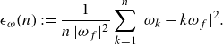 \begin{equation} \epsilon _\omega (n):=\frac {1}{n\,|\omega _f|^2}\sum _{k=1}^n|\omega _k-k\omega _f|^2. \end{equation}
If $\epsilon _\omega$
falls below a chosen threshold, then we reconstruct the best-fit periodic function for the given trajectory segment using the steady mode and the
$\epsilon _\omega$
falls below a chosen threshold, then we reconstruct the best-fit periodic function for the given trajectory segment using the steady mode and the $n$
periodic modes. This procedure is shown schematically in figure 1. The initial flow field for the Newton solver can be chosen as any instant from the time-periodic reconstruction. It is not a priori clear which of the reconstructed flow fields is best suited as an initial guess. In § 3.2, we consider the reconstructed flow field that is closest to the processed trajectory segment, using the
$n$
periodic modes. This procedure is shown schematically in figure 1. The initial flow field for the Newton solver can be chosen as any instant from the time-periodic reconstruction. It is not a priori clear which of the reconstructed flow fields is best suited as an initial guess. In § 3.2, we consider the reconstructed flow field that is closest to the processed trajectory segment, using the $L_2$
-distance as a global measure of the approximation quality. In § 5, we discuss how treating the reconstruction as a global object facilitates the use of multi-shooting methods.
$L_2$
-distance as a global measure of the approximation quality. In § 5, we discuss how treating the reconstruction as a global object facilitates the use of multi-shooting methods.
In this context, DMD offers a complementary approach by detecting nearby UPOs even in the absence of recurrence events in the data. This contrasts with the commonly used recurrent flow analysis (Cvitanović & Gibson Reference Cvitanović and Gibson2010), which identifies UPOs based on repeated flow patterns. Therein, the relative residual
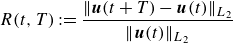 \begin{equation} R(t,T):=\frac {\|\boldsymbol{u}(t+T)-\boldsymbol{u}(t)\|_{L_2}}{\|\boldsymbol{u}(t)\|_{L_2}} \end{equation}
is used to flag the flow states that exhibit a near recurrence after a time interval $T$
. If
$T$
. If $R$
falls below a small threshold, then either
$R$
falls below a small threshold, then either $\boldsymbol{u}(t)$
or
$\boldsymbol{u}(t)$
or $\boldsymbol{u}(t+T)$
, together with
$\boldsymbol{u}(t+T)$
, together with $T$
as a guess for the period, is used to initialise a Newton search for a UPO.
$T$
as a guess for the period, is used to initialise a Newton search for a UPO.
In the presence of continuous translational symmetries, the solution can drift in space. Consequently, periodic structures may manifest as URPOs, where the periodicity condition is satisfied up to a spatial shift. In this case, DMD performs poorly, as a potentially low-dimensional evolution in a co-moving frame of reference would be obscured by spurious modes generated to capture spatial drifts. Therefore, continuous symmetries must be removed before attempting to identify time-periodic structures in the data using the DMD-based method described above. Details of the symmetry-reduction technique are provided in the next subsection. In the presence of continuous translational symmetries, recurrent flow analysis is also modified either by reducing the continuous symmetry in the time series prior to computing $R$
(Cvitanović & Gibson Reference Cvitanović and Gibson2010), or by modifying definition (2.13) to consider the smallest
$R$
(Cvitanović & Gibson Reference Cvitanović and Gibson2010), or by modifying definition (2.13) to consider the smallest $L_2$
-distance between
$L_2$
-distance between $\boldsymbol{u}(t)$
and
$\boldsymbol{u}(t)$
and $\boldsymbol{u}(t+T)$
among all possible relative phases (Chandler & Kerswell Reference Chandler and Kerswell2013).
$\boldsymbol{u}(t+T)$
among all possible relative phases (Chandler & Kerswell Reference Chandler and Kerswell2013).
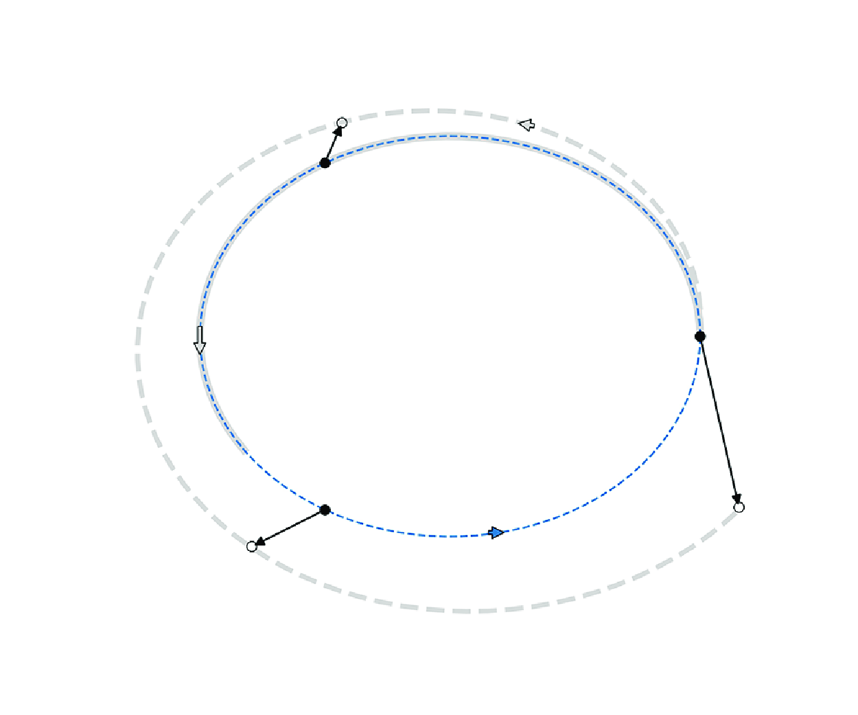
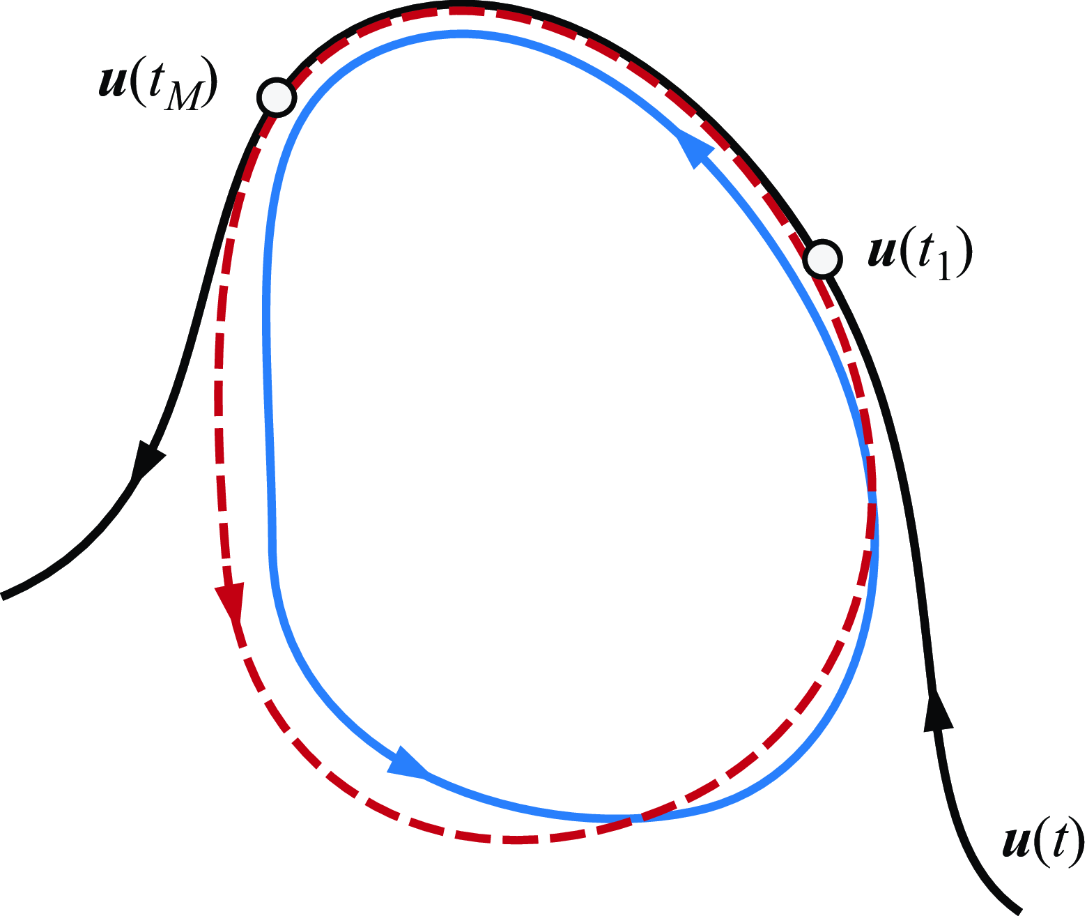
Schematic of the DMD-based method for constructing initial guesses for UPOs. The solid black curve represents a trajectory $\boldsymbol{u}(t)$
in the abstract state space of the system. This trajectory follows a UPO, shown in solid blue, for a time interval shorter than its period. A time window of fixed length is slid along this trajectory, and DMD is done on the covered trajectory segment. The nearby UPO results in dominant frequencies in the DMD spectrum of the trajectory between the time instants
$\boldsymbol{u}(t)$
in the abstract state space of the system. This trajectory follows a UPO, shown in solid blue, for a time interval shorter than its period. A time window of fixed length is slid along this trajectory, and DMD is done on the covered trajectory segment. The nearby UPO results in dominant frequencies in the DMD spectrum of the trajectory between the time instants $t_1$
and
$t_1$
and $t_M$
, where the UPO is followed closely, providing an estimate of its period. Using the extracted DMD modes and frequencies, the best-fit periodic function to the processed trajectory segment is constructed, shown in dashed red. Any section of this periodic function, together with the approximated period, can then be used to initialise a shooting-based Newton search to compute the exact UPO.
$t_M$
, where the UPO is followed closely, providing an estimate of its period. Using the extracted DMD modes and frequencies, the best-fit periodic function to the processed trajectory segment is constructed, shown in dashed red. Any section of this periodic function, together with the approximated period, can then be used to initialise a shooting-based Newton search to compute the exact UPO.
2.3. First Fourier mode slicing technique
In this study, we consider flow fields in a channel geometry that are periodically extended in the streamwise $x$
and spanwise
$x$
and spanwise $z$
directions, and bounded in the wall-normal direction
$z$
directions, and bounded in the wall-normal direction $y$
. Based on this construction, we can represent the flow fields numerically in a Fourier
$y$
. Based on this construction, we can represent the flow fields numerically in a Fourier $\times$
Chebyshev
$\times$
Chebyshev $\times$
Fourier basis, taking the form
$\times$
Fourier basis, taking the form
 \begin{equation} \boldsymbol{u}(\boldsymbol{x})=\sum _{\substack {k_x,k_z\in \mathbb{Z}\\n\in \mathbb{W}}}\tilde{\boldsymbol {u}}_{k_x,n,k_z}\,T_n(y)\,\textrm{e}^{2\unicode{x03C0} \textrm{i}(k_xx/L_{x}+k_zz/L_z)}. \end{equation}
In this expression, we denote by $\tilde{\boldsymbol {u}}_{k_x,n,k_z}$
the complex Fourier/Chebyshev/Fourier coefficients, and by
$\tilde{\boldsymbol {u}}_{k_x,n,k_z}$
the complex Fourier/Chebyshev/Fourier coefficients, and by $T_n$
the
$T_n$
the $n$
th Chebyshev polynomial that is a function of the wall-normal coordinate. In the non-dimensional form, the spatial extents of the computational domain in the streamwise and spanwise directions are denoted by
$n$
th Chebyshev polynomial that is a function of the wall-normal coordinate. In the non-dimensional form, the spatial extents of the computational domain in the streamwise and spanwise directions are denoted by $L_x$
and
$L_x$
and $L_z$
, respectively, while the wall-normal direction spans
$L_z$
, respectively, while the wall-normal direction spans $y\in [-h,h]$
.
$y\in [-h,h]$
.
Flows in this geometry can have continuous translation symmetries in the streamwise and/or spanwise direction, leading to additional degrees of freedom in the underlying flow dynamics. Budanur et al. (Reference Budanur, Cvitanović, Davidchack and Siminos2015) explored the problem of reducing the symmetry in systems with Fourier space discretisation and SO(2) symmetry. Their symmetry reduction technique has recently been extended to flows in channel geometries (Marensi et al. Reference Marensi, Yalnız, Hof and Budanur2023), which is particularly relevant to our numerical set-up. Using this method, we restrict the flow’s state-space trajectory to a linear approximation of a symmetry-reduced lower-dimensional sub-manifold, a so-called slice. Mathematically, a slice is the quotient space $\mathcal{M}/G$
, which represents the original manifold
$\mathcal{M}/G$
, which represents the original manifold $\mathcal{M}$
after accounting for the symmetry group
$\mathcal{M}$
after accounting for the symmetry group $G$
. This quotient space consists of equivalence classes where points in
$G$
. This quotient space consists of equivalence classes where points in $\mathcal{M}$
that can be transformed into each other by the actions of
$\mathcal{M}$
that can be transformed into each other by the actions of $G$
(in this case, translations in the streamwise and spanwise directions) are considered equivalent. In the factor space, these points are identified as the same, effectively removing the continuous symmetry of the system.
$G$
(in this case, translations in the streamwise and spanwise directions) are considered equivalent. In the factor space, these points are identified as the same, effectively removing the continuous symmetry of the system.
To construct the slice, we begin by introducing a coordinate system based on a template function for each direction having a continuous translation symmetry. Specifically, we define two flow field components: one for the $x$
direction, and one for the
$x$
direction, and one for the $z$
direction, which are given by
$z$
direction, which are given by
 \begin{equation} \hat{\boldsymbol{u}}^{\prime}_{\boldsymbol{x}}:=f(y)\cos (2\unicode{x03C0} x/L_x)\,\hat{\boldsymbol {x}} \quad \text{and} \quad \hat{\boldsymbol{u}}^{\prime}_{\boldsymbol{z}}:=f(y)\cos (2\unicode{x03C0} z/L_z)\,\hat{\boldsymbol{z}}, \end{equation}
where $f(y)$
is a function that defines the variation of the template flow field in the
$f(y)$
is a function that defines the variation of the template flow field in the $y$
direction. The form of
$y$
direction. The form of $f(y)$
is chosen based on the specific system being studied, particularly its discrete symmetries. Following similar considerations, the alignment direction of the template functions can also be chosen differently from (2.15) (see § 3.1). We next introduce a tangent vector at the corresponding group orbit, obtained by a quarter-domain shift of the template flow field. The symmetry reduction is then achieved by applying the shift operators
$f(y)$
is chosen based on the specific system being studied, particularly its discrete symmetries. Following similar considerations, the alignment direction of the template functions can also be chosen differently from (2.15) (see § 3.1). We next introduce a tangent vector at the corresponding group orbit, obtained by a quarter-domain shift of the template flow field. The symmetry reduction is then achieved by applying the shift operators $S_x$
and
$S_x$
and $S_z$
to the flow fields of the full state-space trajectory
$S_z$
to the flow fields of the full state-space trajectory $\boldsymbol{u}$
. These shift operators are defined using the function
$\boldsymbol{u}$
. These shift operators are defined using the function $g(\Delta x, \Delta z)$
, which shifts the flow field by
$g(\Delta x, \Delta z)$
, which shifts the flow field by $\Delta x$
and
$\Delta x$
and $\Delta z$
in the
$\Delta z$
in the $x$
and
$x$
and $z$
directions, respectively:
$z$
directions, respectively:
 \begin{equation} S_x(\boldsymbol{u}):=g(-(\phi _x/2\unicode{x03C0} )L_x,0)\,\boldsymbol{u} \quad\text{and} \quad S_z(\boldsymbol{u}):=g(0,-(\phi _z/2\unicode{x03C0} )L_z)\,\boldsymbol{u}. \end{equation}
The polar angles $\phi _x$
and
$\phi _x$
and $\phi _z$
, corresponding to the spatial shifts necessary for symmetry reduction, are defined as
$\phi _z$
, corresponding to the spatial shifts necessary for symmetry reduction, are defined as
 \begin{equation} \phi _x:=\arg \left(\left \langle \boldsymbol{u},\hat{\boldsymbol {u}}^{\prime}_x\right \rangle +\textrm{i}\left \langle \boldsymbol{u},g(L_x/4,0)\,\hat{\boldsymbol{u}}^{\prime}_{\boldsymbol{x}}\right \rangle \right) \end{equation}
and
 \begin{equation} \phi _z:=\arg \left(\left \langle \boldsymbol{u},\hat{\boldsymbol{u}}^{\prime}_z\right \rangle +\textrm{i}\left \langle \boldsymbol{u},g(0,L_z/4)\,\hat{\boldsymbol{u}}^{\prime}_{\boldsymbol{z}}\right \rangle \right). \end{equation}
The slicing phase velocities $\dot {\phi }_x$
and
$\dot {\phi }_x$
and $\dot {\phi }_z$
can be obtained either by finite differences using the time series of the slice phases
$\dot {\phi }_z$
can be obtained either by finite differences using the time series of the slice phases $\phi _x$
and
$\phi _x$
and $\phi _z$
, or alternatively by using the reconstruction equations derived by Rowley & Marsden (Reference Rowley and Marsden2000):
$\phi _z$
, or alternatively by using the reconstruction equations derived by Rowley & Marsden (Reference Rowley and Marsden2000):
 \begin{equation} \dot {\phi }_x(t)=\left (\frac {2\unicode{x03C0} }{L_x}\right )\frac {\left \langle \partial _x \hat{\boldsymbol{u}}^{\prime }_x, \partial _t\boldsymbol{u}|_{\boldsymbol{u}=\hat{\boldsymbol{u}}(t)}\right \rangle }{\left \langle \partial _x\hat{\boldsymbol{u}}^{\prime }_x, \partial _x\hat{\boldsymbol {u}}(t)\right \rangle } \end{equation}
and
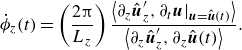 \begin{equation} \dot {\phi }_z(t)=\left (\frac {2\unicode{x03C0} }{L_z}\right )\frac {\left \langle \partial _z \hat{\boldsymbol {u}}^{\prime }_z, \partial _t\boldsymbol{u}|_{\boldsymbol{u}=\hat{\boldsymbol {u}}(t)}\right \rangle }{\left \langle \partial _z\hat{\boldsymbol {u}}^{\prime }_z, \partial _z\hat{\boldsymbol {u}}(t)\right \rangle }. \end{equation}
Here, $\hat{\boldsymbol {u}}(t)$
denotes the symmetry-reduced counterpart of
$\hat{\boldsymbol {u}}(t)$
denotes the symmetry-reduced counterpart of $\boldsymbol{u}(t)$
on the slice, namely
$\boldsymbol{u}(t)$
on the slice, namely $\hat{\boldsymbol {u}}(t)=S_x(S_z(\boldsymbol{u}(t)))$
. The slice velocities
$\hat{\boldsymbol {u}}(t)=S_x(S_z(\boldsymbol{u}(t)))$
. The slice velocities $\dot {\phi }_x$
and
$\dot {\phi }_x$
and $\dot {\phi }_z$
are crucial for tracking the evolution of the slice phases
$\dot {\phi }_z$
are crucial for tracking the evolution of the slice phases $\phi _x$
and
$\phi _x$
and $\phi _z$
, and they allow linking the full-state dynamics to the symmetry-reduced dynamics.
$\phi _z$
, and they allow linking the full-state dynamics to the symmetry-reduced dynamics.
3. Search for URPOs in 3-D plane Poiseuille flow
In this section, we present invariant solutions obtained by Newton searches initialised using SRDMD reconstructions for incompressible channel flow. The computational domain consists of two stationary parallel plates at wall-normal positions $y=\pm h$
, which are periodically extended in the streamwise and spanwise directions with periods
$y=\pm h$
, which are periodically extended in the streamwise and spanwise directions with periods $L_x$
and
$L_x$
and $L_z$
, respectively. The flow is driven by a constant mass flux and is characterised by the Reynolds number
$L_z$
, respectively. The flow is driven by a constant mass flux and is characterised by the Reynolds number $\textit{Re}=U_0h/\nu$
based on the laminar centreline velocity
$\textit{Re}=U_0h/\nu$
based on the laminar centreline velocity $U_0$
and the kinematic viscosity
$U_0$
and the kinematic viscosity $\nu$
. The flow is governed by the Navier–Stokes equations, which in their non-dimensional form read
$\nu$
. The flow is governed by the Navier–Stokes equations, which in their non-dimensional form read
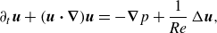 \begin{equation} \partial _t\boldsymbol{u}+(\boldsymbol{u}\boldsymbol{\cdot} \boldsymbol{\nabla} )\boldsymbol{u}=-\boldsymbol{\nabla} p+\dfrac {1}{\textit{Re}}\,\Delta \boldsymbol{u}, \end{equation}
together with the continuity equation
 \begin{equation} \boldsymbol{\nabla} \boldsymbol{\cdot} \boldsymbol{u}=0, \end{equation}
where $\boldsymbol{u}$
and
$\boldsymbol{u}$
and $p$
are the velocity and pressure, respectively. The Navier–Stokes equations are subject to no-slip and no-penetration boundary conditions at the walls,
$p$
are the velocity and pressure, respectively. The Navier–Stokes equations are subject to no-slip and no-penetration boundary conditions at the walls,
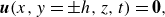 \begin{equation} \boldsymbol{u}(x,y=\pm h,z,t) = \boldsymbol{0}, \end{equation}
and periodic boundary conditions in $x$
and
$x$
and $z$
. This system admits the one-dimensional laminar velocity
$z$
. This system admits the one-dimensional laminar velocity $\boldsymbol{u}_l=U(y)\,\hat{\boldsymbol {x}}$
, with the parabolic profile
$\boldsymbol{u}_l=U(y)\,\hat{\boldsymbol {x}}$
, with the parabolic profile
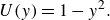 \begin{equation} U(y) = 1-y^2. \end{equation}
This profile corresponds to the choices $h=1$
and
$h=1$
and $U_0=1$
, which are used throughout this paper. We study the flow in a channel with a streamwise length
$U_0=1$
, which are used throughout this paper. We study the flow in a channel with a streamwise length $L_x=2\unicode{x03C0}$
and a spanwise width
$L_x=2\unicode{x03C0}$
and a spanwise width $L_z=0.77\unicode{x03C0}$
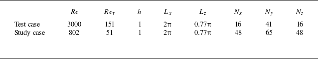
. For numerical integration of the Navier–Stokes equations and Newton searches for invariant solutions, we used the channelflow 2.0 library (Gibson Reference Gibson2014; Gibson et al. Reference Gibson2019). Numerical details for this study are summarised in table 1.
$L_z=0.77\unicode{x03C0}$
. For numerical integration of the Navier–Stokes equations and Newton searches for invariant solutions, we used the channelflow 2.0 library (Gibson Reference Gibson2014; Gibson et al. Reference Gibson2019). Numerical details for this study are summarised in table 1.
Numerical details. The Reynolds number is denoted by $\textit{Re}$
, and the friction Reynolds number by
$\textit{Re}$
, and the friction Reynolds number by $\textit{Re}_{\tau }$
. The streamwise, spanwise and wall-normal dimensions of the computational domain are denoted by
$\textit{Re}_{\tau }$
. The streamwise, spanwise and wall-normal dimensions of the computational domain are denoted by $L_x$
,
$L_x$
, $L_z$
and
$L_z$
and $2h$
, respectively. The number of grid points in the streamwise, spanwise and wall-normal directions are denoted by
$2h$
, respectively. The number of grid points in the streamwise, spanwise and wall-normal directions are denoted by $N_x$
,
$N_x$
, $N_z$
and
$N_z$
and $N_y$
, respectively. The test case is adopted from the work of Rawat et al. (Reference Rawat, Cossu and Rincon2014).
$N_y$
, respectively. The test case is adopted from the work of Rawat et al. (Reference Rawat, Cossu and Rincon2014).
The DNS trajectories were produced using an initial flow field based on the work of Rawat et al. (Reference Rawat, Cossu and Rincon2014). The initial flow field consists of the laminar profile (3.4), perturbed by streamwise counter-rotating vortices of amplitude $A_1$
and a sinusoidal perturbation of amplitude
$A_1$
and a sinusoidal perturbation of amplitude $A_2$
in the spanwise direction:
$A_2$
in the spanwise direction:
 \begin{equation} \boldsymbol{u}_0=\{U(y),0,0\}+A_1\left\{0,\frac {\partial \psi }{\partial z},-\frac {\partial \psi }{\partial y}\right\}+A_2\{0,0,W_{\textit{sin}}\}, \end{equation}
where
 \begin{equation} \psi (y,z)=(1-y^2)\sin {(\unicode{x03C0} y)}\sin {(2\unicode{x03C0} z/L_z)} \end{equation}
and
 \begin{equation} W_{\textit{sin}}(x,y)=(1-y^2)\sin {(2\unicode{x03C0} x/L_x)}. \end{equation}
The initial flow field (3.5) has the discrete symmetries
 \begin{align}&\quad\,\,\, [u,v,w](x,-y,z)=[u,-v,w](x,y,z), \end{align}
 \begin{align}& [u,v,w](x+L_x/2,y,-z)=[u,v,-w](x,y,z), \end{align}
 \begin{align}& [u,v,w](x+L_x/2,-y,z)=[u,-v,w](x,y,z), \end{align}
which were explicitly imposed during the simulations. Although the governing equations and boundary conditions are equivariant under continuous translations in either of the periodic wall-parallel directions, the imposed discrete symmetries prevent the solution from drifting in the spanwise direction $z$
. However, the flow is not constrained in the streamwise direction
$z$
. However, the flow is not constrained in the streamwise direction $x$
. The flow’s continuous symmetry in this direction allows for time-dependent drift, leading to poor performance of the DMD method, and necessitating the reduction of the continuous symmetry. In order to reduce the continuous symmetry, we applied the first Fourier mode slicing technique described in § 2.3. To ensure that all involved scalar products in (2.17) and (2.18) are well defined at all times when applying the slicing technique, we utilise the symmetries (3.8)–(3.10) for all velocity components and their relation to the symmetries of the template functions (Engel et al. Reference Engel, Ashtari and Linkmann2023).
$x$
. The flow’s continuous symmetry in this direction allows for time-dependent drift, leading to poor performance of the DMD method, and necessitating the reduction of the continuous symmetry. In order to reduce the continuous symmetry, we applied the first Fourier mode slicing technique described in § 2.3. To ensure that all involved scalar products in (2.17) and (2.18) are well defined at all times when applying the slicing technique, we utilise the symmetries (3.8)–(3.10) for all velocity components and their relation to the symmetries of the template functions (Engel et al. Reference Engel, Ashtari and Linkmann2023).
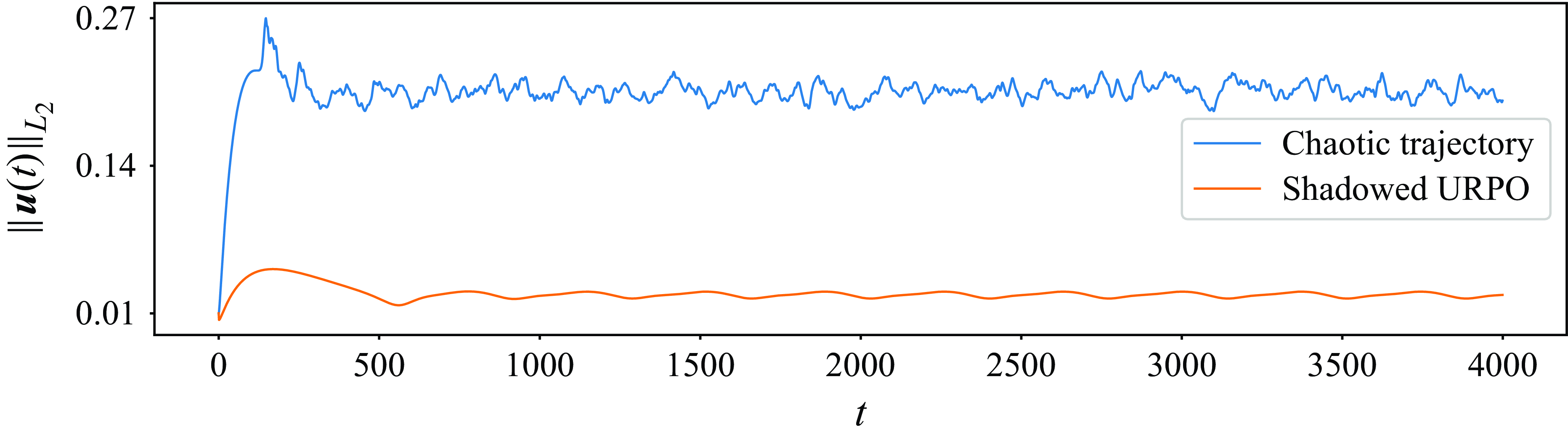
The $L_2$
-norm of the velocity as a function of time for the DNS of the chaotic trajectory (blue) and the trajectory that shadows the URPO for approximately four cycles between
$L_2$
-norm of the velocity as a function of time for the DNS of the chaotic trajectory (blue) and the trajectory that shadows the URPO for approximately four cycles between $t\approx 1000$
and
$t\approx 1000$
and $4000$
(orange). Both DNS correspond to Reynolds number
$4000$
(orange). Both DNS correspond to Reynolds number $\textit{Re}=3000$
.
$\textit{Re}=3000$
.
3.1. Method validation
To validate SRDMD, we applied both slicing and DMD to the URPO in the channel flow identified by Rawat et al. (Reference Rawat, Cossu and Rincon2014). This solution is obtained with the friction Reynolds number $\textit{Re}_{\tau }\approx 151$
(
$\textit{Re}_{\tau }\approx 151$
( $\textit{Re}=3000$
), and has period
$\textit{Re}=3000$
), and has period $T=739$
. We used the same computational domain size and resolution as Rawat et al. (Reference Rawat, Cossu and Rincon2014) (see table 1). With one unstable direction in the invariant subspace formed by the discrete symmetries (3.8)–(3.10), this solution serves as an ideal candidate for validating the methods, since it can be identified using a bisection method, as described in Rawat et al. (Reference Rawat, Cossu and Rincon2014). The bisection method iteratively adjusts the perturbation amplitudes
$T=739$
. We used the same computational domain size and resolution as Rawat et al. (Reference Rawat, Cossu and Rincon2014) (see table 1). With one unstable direction in the invariant subspace formed by the discrete symmetries (3.8)–(3.10), this solution serves as an ideal candidate for validating the methods, since it can be identified using a bisection method, as described in Rawat et al. (Reference Rawat, Cossu and Rincon2014). The bisection method iteratively adjusts the perturbation amplitudes $A_1$
and
$A_1$
and $A_2$
in the initial condition (3.5) to generate progressively longer trajectories that neither become turbulent nor decay to the laminar state. This is accomplished by performing a bisection on the amplitudes from two preceding bisection steps: one that leads to decay to the laminar state, and the other that leads to turbulent behaviour after a sufficiently long time. In this way, we tracked a trajectory shadowing the URPO of interest for approximately four cycles. Figure 2 illustrates the evolution of the velocity
$A_2$
in the initial condition (3.5) to generate progressively longer trajectories that neither become turbulent nor decay to the laminar state. This is accomplished by performing a bisection on the amplitudes from two preceding bisection steps: one that leads to decay to the laminar state, and the other that leads to turbulent behaviour after a sufficiently long time. In this way, we tracked a trajectory shadowing the URPO of interest for approximately four cycles. Figure 2 illustrates the evolution of the velocity $L_2$
-norm for both a chaotic trajectory and the trajectory shadowing the URPO. Inspection of the data reveals that the corresponding flow field shows a streamwise drift, since the plane Poiseuille flow has a continuous translation symmetry in the streamwise direction. However, the system is prevented from drifting in the spanwise direction through the imposed shift–reflect symmetry (3.9).
$L_2$
-norm for both a chaotic trajectory and the trajectory shadowing the URPO. Inspection of the data reveals that the corresponding flow field shows a streamwise drift, since the plane Poiseuille flow has a continuous translation symmetry in the streamwise direction. However, the system is prevented from drifting in the spanwise direction through the imposed shift–reflect symmetry (3.9).
To validate the methodology introduced in § 2, we first applied the slicing technique to reduce the drift from the flow. We used a slicing template function $\hat{\boldsymbol{u}}^{\prime}_x$
aligned in the spanwise direction
$\hat{\boldsymbol{u}}^{\prime}_x$
aligned in the spanwise direction $z$
, with a profile function
$z$
, with a profile function $f(y)=2.5\,T_2(y)-1.25\,T_3(y)-1.25\,T_5(y)$
(see § 2.3). Our choice of alignment direction and Chebyshev polynomials was based on the flow field’s discrete symmetries, ensuring that the slice velocity (2.19) is well defined at all times. Figure 3 shows the slicing phase velocity obtained via reconstruction equation (2.19) for the last 3000 advective time units. We observe that the slicing phase velocity is well defined over the whole time window. A failure of the slicing method at a specific moment in time would be indicated by discontinuities in
$f(y)=2.5\,T_2(y)-1.25\,T_3(y)-1.25\,T_5(y)$
(see § 2.3). Our choice of alignment direction and Chebyshev polynomials was based on the flow field’s discrete symmetries, ensuring that the slice velocity (2.19) is well defined at all times. Figure 3 shows the slicing phase velocity obtained via reconstruction equation (2.19) for the last 3000 advective time units. We observe that the slicing phase velocity is well defined over the whole time window. A failure of the slicing method at a specific moment in time would be indicated by discontinuities in $\dot {\phi }_x(t)$
, resulting in non-physical jumps of the flow field through the computational domain in the streamwise direction.
$\dot {\phi }_x(t)$
, resulting in non-physical jumps of the flow field through the computational domain in the streamwise direction.
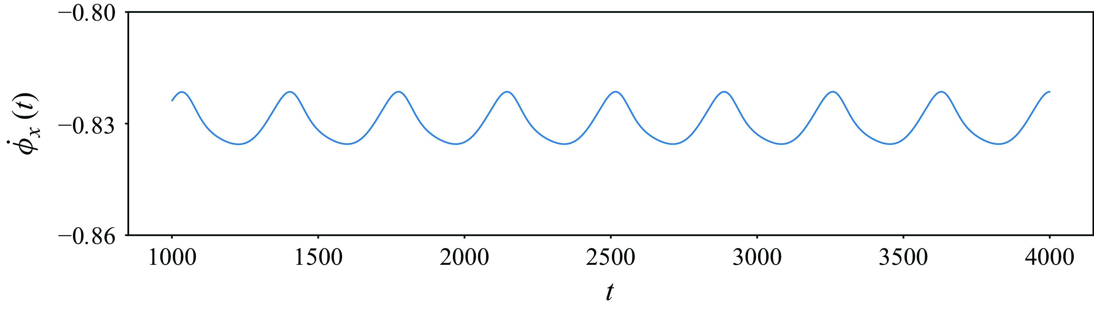
Phase velocity for the global drift in the streamwise direction as a function of time, obtained by applying the first Fourier mode slicing technique to the DNS dataset. Snapshots were sampled with time resolution $\Delta t=1$
. The flow does not have a global drift in the spanwise direction, as it is constrained by a discrete symmetry.
$\Delta t=1$
. The flow does not have a global drift in the spanwise direction, as it is constrained by a discrete symmetry.
State-space projections of the trajectory following a URPO over one period $T_p\approx742$
. The state space is projected onto the first three dominant POD modes, with
$T_p\approx742$
. The state space is projected onto the first three dominant POD modes, with $a_1, a_2, a_3$
representing the corresponding amplitudes. (a) Trajectory of the original dataset. (b) The symmetry-reduced trajectory after applying the first Fourier mode slicing technique. The black dots mark the start and end points of the trajectories.
$a_1, a_2, a_3$
representing the corresponding amplitudes. (a) Trajectory of the original dataset. (b) The symmetry-reduced trajectory after applying the first Fourier mode slicing technique. The black dots mark the start and end points of the trajectories.
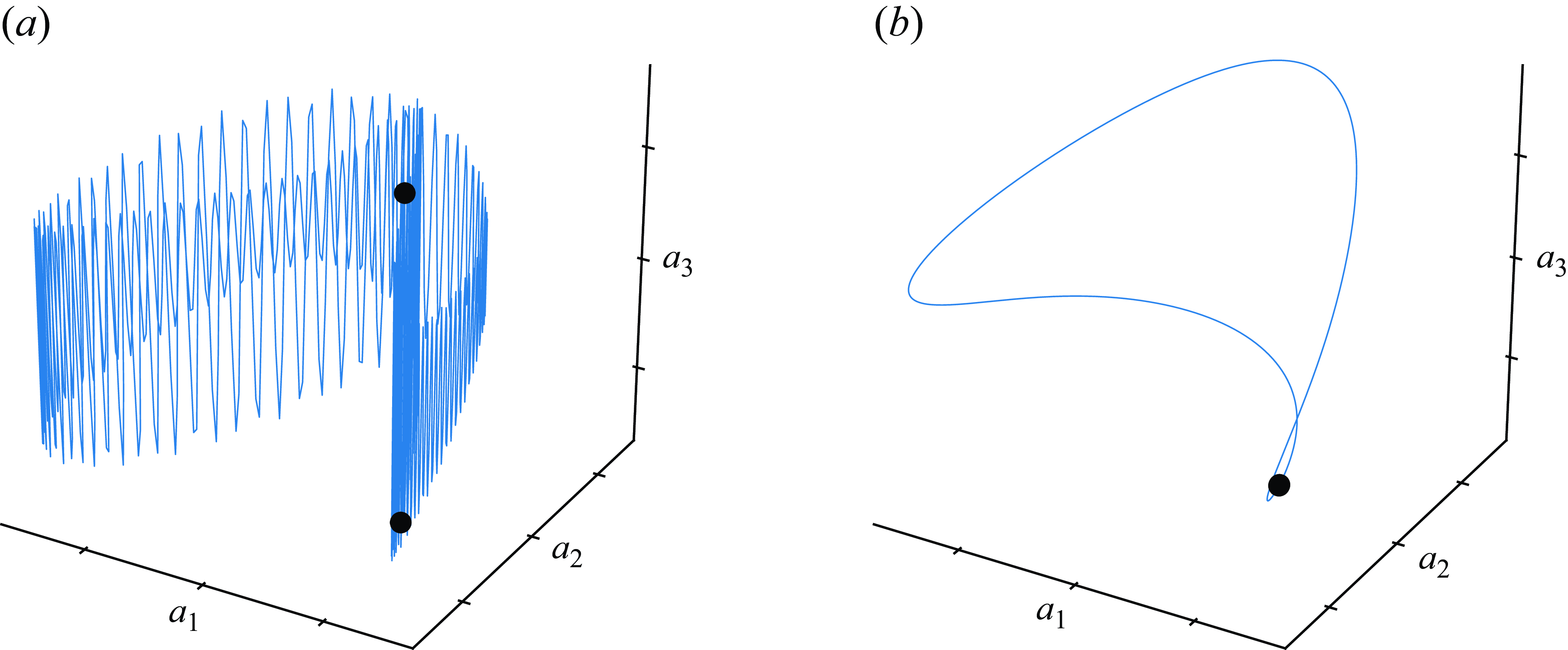
The result of the symmetry reduction is best illustrated by inspecting a 3-D state-space projection of the trajectory. Figure 4(a) presents the trajectory before symmetry reduction, and figure 4(b) after symmetry reduction, following the URPO for one of its cycles. The flow fields are projected onto the first three dominant modes of proper orthogonal decomposition (POD). The POD modes in the non-symmetry-reduced case were calculated for a data matrix corresponding to a segment of the original trajectory following the URPO for one full cycle. Columns of the data matrix contain the grid values of instantaneous velocity fields in the physical domain, separated by a $\Delta t = 1$
advection time unit. For the symmetry-reduced case, we applied the same procedure, but the POD modes were calculated from the symmetry-reduced segment of the flow fields. Clearly visible is the more complicated state-space trajectory for the DNS with no post-processing in comparison to the symmetry-reduced case, due to the additional degree of freedom. In contrast to the DNS without post-processing, the start and end points of the symmetry-reduced trajectory (indicated by black dots) coincide after a time period that matches the URPO period reported in Rawat et al. (Reference Rawat, Cossu and Rincon2014).
$\Delta t = 1$
advection time unit. For the symmetry-reduced case, we applied the same procedure, but the POD modes were calculated from the symmetry-reduced segment of the flow fields. Clearly visible is the more complicated state-space trajectory for the DNS with no post-processing in comparison to the symmetry-reduced case, due to the additional degree of freedom. In contrast to the DNS without post-processing, the start and end points of the symmetry-reduced trajectory (indicated by black dots) coincide after a time period that matches the URPO period reported in Rawat et al. (Reference Rawat, Cossu and Rincon2014).
After ensuring the success of the symmetry reduction, we proceeded with the DMD analysis of the DNS and symmetry-reduced data. All parameters used for producing the period guess and the low-dimensional flow field representation in this case were determined through experimentation. This includes the observation time window $T_w=680$
advective time units as well as the snapshot sampling separation
$T_w=680$
advective time units as well as the snapshot sampling separation $\Delta t$
and spacing
$\Delta t$
and spacing $\delta t$
of 17 advective time units. The sparsity-promoting SRDMD algorithm utilises a bisection method to determine the penalty parameter
$\delta t$
of 17 advective time units. The sparsity-promoting SRDMD algorithm utilises a bisection method to determine the penalty parameter $\gamma$
– calculated as 12.5 in this case – ensuring a low-dimensional reconstruction by selecting five optimal DMD modes. This choice is based on the study of Page & Kerswell (Reference Page and Kerswell2020), where five DMD modes were found to be sufficient to construct initial guesses for UPOs that converge successfully in a Newton search. Figure 5 compares the DMD spectra obtained by applying sparsity-promoting DMD to the DNS and symmetry-reduced data. The red line indicates the unit circle around which the eigenvalues are distributed. Eigenvalues selected by the sparsity-promoting DMD are highlighted in blue.
$\gamma$
– calculated as 12.5 in this case – ensuring a low-dimensional reconstruction by selecting five optimal DMD modes. This choice is based on the study of Page & Kerswell (Reference Page and Kerswell2020), where five DMD modes were found to be sufficient to construct initial guesses for UPOs that converge successfully in a Newton search. Figure 5 compares the DMD spectra obtained by applying sparsity-promoting DMD to the DNS and symmetry-reduced data. The red line indicates the unit circle around which the eigenvalues are distributed. Eigenvalues selected by the sparsity-promoting DMD are highlighted in blue.
Comparison of (a) the classical DMD spectra and (b) the SRDMD spectra for the trajectory shadowing the oscillating structure. The observation window when applying the SRDMD was set to be 680 advective time units, which represents approximately $92\,\%$
of the converged period. The snapshot separation was set to 17 advective time units. The red line represents the unit circle. The eigenvalues selected by the sparsity constraint for the reconstruction are highlighted with filled markers.
$92\,\%$
of the converged period. The snapshot separation was set to 17 advective time units. The red line represents the unit circle. The eigenvalues selected by the sparsity constraint for the reconstruction are highlighted with filled markers.

For both the original and the symmetry-reduced data, the neutral DMD mode corresponding to the temporal mean is selected, as well as the DMD mode corresponding to the fundamental frequency. In sparsity-promoting DMD without symmetry reduction, the third pair of eigenvalues lies off the unit circle and relates to fast and small-scale dynamics as its imaginary part is large in absolute value. In contrast, the sparsity-promoting SRDMD selects the third DMD mode corresponding to the first higher harmonic of the fundamental frequency. This is plausible because the processed trajectory, which closely shadows the URPO, already represents a low-dimensional flow. The symmetry reduction enabled the DMD-based analysis to capture this characteristic as expected. By selecting the fundamental frequency and its higher harmonics, both the fundamental frequency and its residual can be calculated, as given in (2.11) and (2.12), yielding $T_g=741.979$
and
$T_g=741.979$
and $\epsilon _{\omega }\approx 10^{-9}$
.
$\epsilon _{\omega }\approx 10^{-9}$
.
The low-dimensional reconstruction of the flow (2.7) provides a closed curve in state space, which is not a solution trajectory of the governing equations but approximates the DNS data over the processed time window. Any time section along this curve can serve as an initial condition for the Newton solver (see figure 1). However, we followed Page & Kerswell (Reference Page and Kerswell2020) and initialised the Newton searches using the reconstructed flow field closest to the original trajectory, considering the $L_2$
-norm as the metric. The drift in the streamwise direction, which needs to be taken into account when applying a Newton search, can be derived from the slice phase tracked during the symmetry reduction by
$L_2$
-norm as the metric. The drift in the streamwise direction, which needs to be taken into account when applying a Newton search, can be derived from the slice phase tracked during the symmetry reduction by
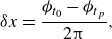 \begin{equation} \delta x = \frac {\phi _{t_0} - \phi _{t_p}}{2\unicode{x03C0} }, \end{equation}
where $t_0$
refers to the starting time of the SRDMD observation time window, and
$t_0$
refers to the starting time of the SRDMD observation time window, and $t_p = t_0 + T_g$
corresponds to the time instant after one estimated period. The Newton search converges after seven iterations, reaching a residual
$t_p = t_0 + T_g$
corresponds to the time instant after one estimated period. The Newton search converges after seven iterations, reaching a residual $\mathcal{O}(10^{-14})$
, and yielding the predicted URPO with period
$\mathcal{O}(10^{-14})$
, and yielding the predicted URPO with period $T_{\textit{URPO}}=742.017$
. The period of the converged URPO matches the period of the URPO reported in Rawat et al. (Reference Rawat, Cossu and Rincon2014) by a relative error
$T_{\textit{URPO}}=742.017$
. The period of the converged URPO matches the period of the URPO reported in Rawat et al. (Reference Rawat, Cossu and Rincon2014) by a relative error $0.4 \,\%$
.
$0.4 \,\%$
.
The $L_2$
-norm of the velocity along a trajectory at the friction Reynolds number
$L_2$
-norm of the velocity along a trajectory at the friction Reynolds number $\textit{Re}_{\tau }\approx 51$
as a function of time. The time series shows chaotic behaviour for approximately 2600 advective time units.
$\textit{Re}_{\tau }\approx 51$
as a function of time. The time series shows chaotic behaviour for approximately 2600 advective time units.
3.2. Search for previously unknown URPOs
In this subsection, we present previously unknown URPOs buried in the chaotic repeller of channel flow at friction Reynolds number $\textit{Re}_{\tau }\approx 51$
(Zammert & Eckhardt Reference Zammert and Eckhardt2015). The choice of the Reynolds number is motivated by producing a weakly turbulent but long enough trajectory with a state space feasible for a SRDMD study. The discrete symmetry (3.9) breaks the continuous translational symmetry in the spanwise direction, preventing the solution from drifting in that direction. As a result, the present study focuses on handling the drifts due to the mean advection in the streamwise direction only. The spatial resolution of the simulation was increased from the test case in § 3.1 to
$\textit{Re}_{\tau }\approx 51$
(Zammert & Eckhardt Reference Zammert and Eckhardt2015). The choice of the Reynolds number is motivated by producing a weakly turbulent but long enough trajectory with a state space feasible for a SRDMD study. The discrete symmetry (3.9) breaks the continuous translational symmetry in the spanwise direction, preventing the solution from drifting in that direction. As a result, the present study focuses on handling the drifts due to the mean advection in the streamwise direction only. The spatial resolution of the simulation was increased from the test case in § 3.1 to $(N_x,N_y,N_z)=(48,65,48)$
. We tested the existence of all obtained solutions with a higher resolution
$(N_x,N_y,N_z)=(48,65,48)$
. We tested the existence of all obtained solutions with a higher resolution $(N_x,N_y,N_z)=(60,81,60)$
, and found changes in their period to be below relative error
$(N_x,N_y,N_z)=(60,81,60)$
, and found changes in their period to be below relative error $0.01\,\%$
.
$0.01\,\%$
.
We obtained sufficiently long, weakly chaotic trajectories by applying the same bisection method used in § 3.1 to an initial condition according to (3.5). This procedure was necessary, since initial conditions of random perturbations can quickly laminarise. Figure 6 shows the $L_2$
-norm of the simulated velocity fields as a function of time, exhibiting a chaotic character for approximately 2600 advective time units. Figure 7 shows velocity contour plots of the snapshot taken from the DNS at time
$L_2$
-norm of the simulated velocity fields as a function of time, exhibiting a chaotic character for approximately 2600 advective time units. Figure 7 shows velocity contour plots of the snapshot taken from the DNS at time $t=1000$
. The colour code indicates the deviation of the streamwise velocity from the laminar profile (3.4). Figure 7(a) shows the 3-D flow field, and figure 7(b) shows the flow field averaged in the streamwise direction. The black lines indicate the streamwise-averaged
$t=1000$
. The colour code indicates the deviation of the streamwise velocity from the laminar profile (3.4). Figure 7(a) shows the 3-D flow field, and figure 7(b) shows the flow field averaged in the streamwise direction. The black lines indicate the streamwise-averaged $y$
–
$y$
– $z$
streamfunction. The flow is dominated by a low-momentum region around its centre, which extends in the streamwise direction and is accompanied by four near-wall high-momentum streamwise streaks. Similar to the test case, the flow drifts fast in the streamwise direction, while it is prohibited from drifting in the spanwise direction due to the imposed shift–reflect symmetry (3.9). To remove the streamwise drift from the flow, we followed our procedure from the test case, using the same template profile.
$z$
streamfunction. The flow is dominated by a low-momentum region around its centre, which extends in the streamwise direction and is accompanied by four near-wall high-momentum streamwise streaks. Similar to the test case, the flow drifts fast in the streamwise direction, while it is prohibited from drifting in the spanwise direction due to the imposed shift–reflect symmetry (3.9). To remove the streamwise drift from the flow, we followed our procedure from the test case, using the same template profile.
Velocity contour plots of the flow field taken from the DNS at $t=1000$
advective time units (see figure 6). The colour code indicates the deviation of the streamwise velocity from the laminar profile. (a) The velocity contour in a 3-D plot. (b) The velocity field averaged in the streamwise direction. The black lines indicate the streamwise-averaged
$t=1000$
advective time units (see figure 6). The colour code indicates the deviation of the streamwise velocity from the laminar profile. (a) The velocity contour in a 3-D plot. (b) The velocity field averaged in the streamwise direction. The black lines indicate the streamwise-averaged $y$
–
$y$
– $z$
streamfunction.
$z$
streamfunction.
Phase velocity for the global drift in the streamwise direction as a function of time for the chaotic trajectory over a duration of 2600 advective time units. The zoomed inset highlights a peak in the phase velocity, illustrating that the projection onto the symmetry-reduced slice remains well defined at this point. In contrast, the five dominant peaks correspond to singularities in the phase velocity, occurring when the denominator in the reconstruction equation (2.19) vanishes as the trajectory approaches the slice border.

Figure 8 shows the slice phase velocity in the streamwise direction as a function of time. The inset magnifies a peak in the slice phase velocity, demonstrating that the projection onto the symmetry-reduced slice remains well defined at this point. In contrast, the five dominant peaks correspond to singularities in the phase velocity, which occur when the denominator in the reconstruction equation (2.19) vanishes as the trajectory approaches the slice border. However, these peaks are rare cases. Therefore, the template choice is sufficient, as we can reject initial guesses from SRDMD whose observation windows include a change of sign in the denominator of (2.19), resulting in a singularity in the phase velocity.
The DMD analysis was performed by scanning the symmetry-reduced flow with observation time window sizes $T_w\in \{60,80,100,120\}$
advective time units. The scan started at
$T_w\in \{60,80,100,120\}$
advective time units. The scan started at $t=0$
, with each time window shifted in steps of one unit to
$t=0$
, with each time window shifted in steps of one unit to $t=2600$
, and snapshot spacing
$t=2600$
, and snapshot spacing $\Delta t=3$
was used. To ensure the convergence of the DMD algorithm, we focused on the distribution of the resulting eigenvalues, expecting them to lie on the unit circle in the complex plane when the observation windows shadow a URPO, as these are stationary on average. In practice, a range of parameter values typically satisfies this criterion. By setting the residual acceptance threshold for the estimated fundamental frequency to
$\Delta t=3$
was used. To ensure the convergence of the DMD algorithm, we focused on the distribution of the resulting eigenvalues, expecting them to lie on the unit circle in the complex plane when the observation windows shadow a URPO, as these are stationary on average. In practice, a range of parameter values typically satisfies this criterion. By setting the residual acceptance threshold for the estimated fundamental frequency to $\epsilon _\omega \lt 10^{-3}$
, we constructed 354 initial guesses, each comprising a flow field, an estimated period, and the shift information from the slicing analysis. In the subsequent Newton search, 35 out of the 354 initial conditions converged to a URPO, resulting in a success rate of approximately 10 %. Among these 35 cases, we identified six distinct URPOs, which were found at several positions in the time series, suggesting their importance for the flow dynamics. Table 2 summarises the properties of the distinct URPOs found within the chaotic flow.
$\epsilon _\omega \lt 10^{-3}$
, we constructed 354 initial guesses, each comprising a flow field, an estimated period, and the shift information from the slicing analysis. In the subsequent Newton search, 35 out of the 354 initial conditions converged to a URPO, resulting in a success rate of approximately 10 %. Among these 35 cases, we identified six distinct URPOs, which were found at several positions in the time series, suggesting their importance for the flow dynamics. Table 2 summarises the properties of the distinct URPOs found within the chaotic flow.
Distinct URPOs converged using SRDMD to estimate periods and construct initial flow fields for Newton searches. We denote by $t_{i}$
the time at which the
$t_{i}$
the time at which the $L_2$
-distance between the DNS and the SRDMD reconstruction is minimal. The reconstructed flow field at time
$L_2$
-distance between the DNS and the SRDMD reconstruction is minimal. The reconstructed flow field at time $t_{i}$
was used as the initial flow field for the Newton search. The length of the time window in the respective SRDMD analysis is denoted by
$t_{i}$
was used as the initial flow field for the Newton search. The length of the time window in the respective SRDMD analysis is denoted by $T_w$
. The estimated period is
$T_w$
. The estimated period is $T_g$
, and
$T_g$
, and $T_{\textit{URPO}}$
is the period of the converged URPO. We give the deviation of
$T_{\textit{URPO}}$
is the period of the converged URPO. We give the deviation of $T_g$
from
$T_g$
from $T_{\textit{URPO}}$
in per cent. The number of distinct initial data points resulting in the same converged URPO is denoted by
$T_{\textit{URPO}}$
in per cent. The number of distinct initial data points resulting in the same converged URPO is denoted by $N_{\textit{Hits}}$
. Also shown are
$N_{\textit{Hits}}$
. Also shown are $N$
, the number of unstable directions,
$N$
, the number of unstable directions, $\sum _{j=1}^N\text{Re} {(\lambda _j)}$
, the sum of the real parts of all the unstable eigenvalues (growth rates), and
$\sum _{j=1}^N\text{Re} {(\lambda _j)}$
, the sum of the real parts of all the unstable eigenvalues (growth rates), and $\max \,\text{Re} {(\lambda _j)}$
, the real part of the eigenvalue corresponding to the dominant unstable direction.
$\max \,\text{Re} {(\lambda _j)}$
, the real part of the eigenvalue corresponding to the dominant unstable direction.
Figure 9 shows a 2-D state-space projection of the URPOs listed in table 2. The projection shows the total energy input $I$
against the total dissipation
$I$
against the total dissipation $D$
, normalised by their respective laminar values
$D$
, normalised by their respective laminar values $I_0$
and
$I_0$
and $D_0$
. The grey shaded area represents the probability density function (p.d.f.) of the dynamics obtained from the DNS, where density decrease is represented by a grey scale from black to white. The majority of URPOs cover the dense part of the p.d.f. and therefore represent the typical dynamics. This is important since we aim to provide appropriate predictions of flow properties based on those of the identified URPOs. The URPO with the shortest period
$D_0$
. The grey shaded area represents the probability density function (p.d.f.) of the dynamics obtained from the DNS, where density decrease is represented by a grey scale from black to white. The majority of URPOs cover the dense part of the p.d.f. and therefore represent the typical dynamics. This is important since we aim to provide appropriate predictions of flow properties based on those of the identified URPOs. The URPO with the shortest period $T\approx 67$
is embedded in a low-probability region of low energy input and dissipation, and is only barely visited by the chaotic trajectory.
$T\approx 67$
is embedded in a low-probability region of low energy input and dissipation, and is only barely visited by the chaotic trajectory.
The 2-D state-space projection of the identified URPOs with respect to the total energy input $I$
and dissipation
$I$
and dissipation $D$
, normalised by their laminar values
$D$
, normalised by their laminar values $I_0$
and
$I_0$
and $D_0$
, respectively. The dashed line represents the diagonal in the
$D_0$
, respectively. The dashed line represents the diagonal in the $D$
–
$D$
– $I$
plane, indicating states where energy input
$I$
plane, indicating states where energy input $I$
and dissipation
$I$
and dissipation $D$
are exactly balanced. The grey shaded area corresponds to the p.d.f. of the dynamics, where the density decrease is represented by a grey scale from black to white.
$D$
are exactly balanced. The grey shaded area corresponds to the p.d.f. of the dynamics, where the density decrease is represented by a grey scale from black to white.
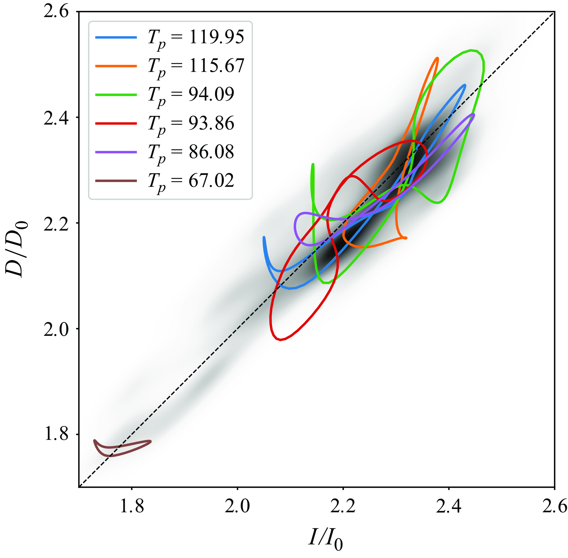
Recurrent flow analysis of the DNS. The greyscale colour code represents the $L_2$
-distance of DNS snapshot pairs separated by the time interval
$L_2$
-distance of DNS snapshot pairs separated by the time interval $T$
. Dark regions reflect close distances, suggesting possible recurrence events. Black circles show URPOs converged using the sparsity-promoting SRDMD method as a function of time
$T$
. Dark regions reflect close distances, suggesting possible recurrence events. Black circles show URPOs converged using the sparsity-promoting SRDMD method as a function of time $t$
, when initial flow fields were passed to the Newton solver, and their converged periods
$t$
, when initial flow fields were passed to the Newton solver, and their converged periods $T$
. Red-filled black circles indicate a selection of distinct URPOs from table 2. Multiple guesses have successfully converged to a URPO despite the absence of a recurrence signal, highlighting the complementary role of the DMD approach, which eliminates the need to track the entire URPO over a complete cycle.
$T$
. Red-filled black circles indicate a selection of distinct URPOs from table 2. Multiple guesses have successfully converged to a URPO despite the absence of a recurrence signal, highlighting the complementary role of the DMD approach, which eliminates the need to track the entire URPO over a complete cycle.
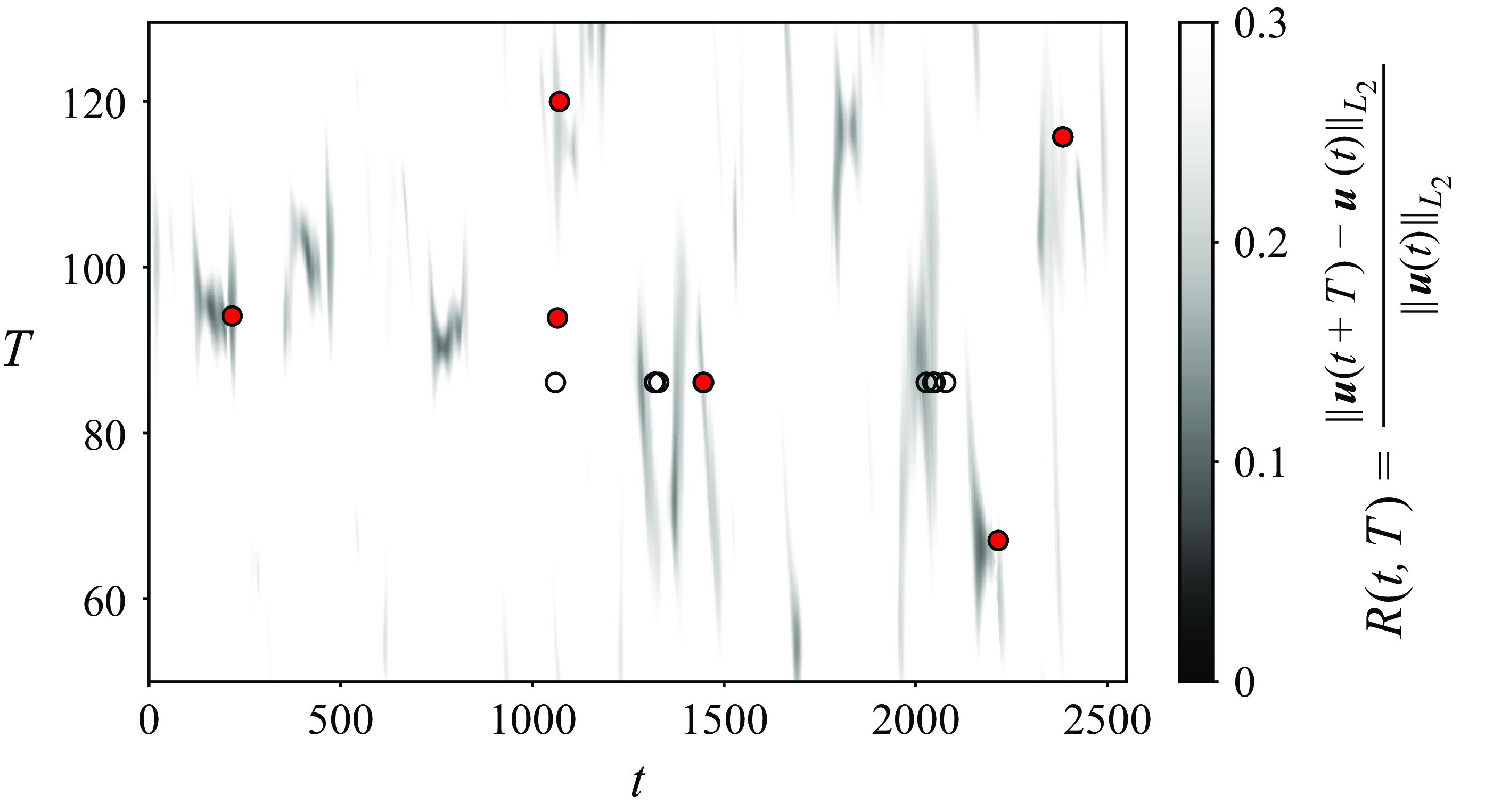
Figure 10 shows a classical recurrent flow analysis on the symmetry-reduced dataset (see § 2.2). The grey scale represents the $L_2$
-distance between future flow states and previous ones. Possible recurrences are indicated in dark regions as a function of simulation time on the horizontal axis and possible periods on the vertical axis. The scattered circles represent URPOs converged using the sparsity-promoting SRDMD method. Markers filled in red correspond to distinct URPOs listed in table 2. Each marker shows the period of the respective converged solution and the time location of the initial flow field used for the Newton search, taken from the SRDMD reconstruction of the DNS. At several points in time, URPOs with periods
$L_2$
-distance between future flow states and previous ones. Possible recurrences are indicated in dark regions as a function of simulation time on the horizontal axis and possible periods on the vertical axis. The scattered circles represent URPOs converged using the sparsity-promoting SRDMD method. Markers filled in red correspond to distinct URPOs listed in table 2. Each marker shows the period of the respective converged solution and the time location of the initial flow field used for the Newton search, taken from the SRDMD reconstruction of the DNS. At several points in time, URPOs with periods $T_{\textit{URPO}}\in \{86.08,93.86\}$
are identified in the absence of a recurrence event. This highlights the complementary role of symmetry-reduced DMD in the search for URPOs compared to recurrent flow analysis, as a URPO would likely have gone undetected in these cases. The complementary role of the DMD-based method is further supported by the results of Newton searches initialised using guesses from recurrent flow analysis. Our guesses from recurrent flow analysis consist of the velocity field at time
$T_{\textit{URPO}}\in \{86.08,93.86\}$
are identified in the absence of a recurrence event. This highlights the complementary role of symmetry-reduced DMD in the search for URPOs compared to recurrent flow analysis, as a URPO would likely have gone undetected in these cases. The complementary role of the DMD-based method is further supported by the results of Newton searches initialised using guesses from recurrent flow analysis. Our guesses from recurrent flow analysis consist of the velocity field at time $t$
, and the period
$t$
, and the period $T$
corresponding to the
$T$
corresponding to the $(t,T)$
coordinate where
$(t,T)$
coordinate where $R$
takes a local minimum value. The initial guess for the spatial shift is taken as the difference between the shifts applied to
$R$
takes a local minimum value. The initial guess for the spatial shift is taken as the difference between the shifts applied to $\boldsymbol{u}(t)$
and
$\boldsymbol{u}(t)$
and $\boldsymbol{u}(t+T)$
to bring them to the slice (see (2.16)). We selected the local minima where
$\boldsymbol{u}(t+T)$
to bring them to the slice (see (2.16)). We selected the local minima where $R_{\textit{min}}\lt 0.2$
, yielding twelve guesses, of which two successfully converged (not shown in figure 10). Both successful searches converged to the URPO with period
$R_{\textit{min}}\lt 0.2$
, yielding twelve guesses, of which two successfully converged (not shown in figure 10). Both successful searches converged to the URPO with period $T_{\textit{URPO}}=86.08$
, to which the DMD-based method converged 27 times. Therefore, guesses from recurrent flow analysis do not result in any additional URPOs compared to the DMD-based approach for the analysed time series.
$T_{\textit{URPO}}=86.08$
, to which the DMD-based method converged 27 times. Therefore, guesses from recurrent flow analysis do not result in any additional URPOs compared to the DMD-based approach for the analysed time series.
In what follows, we connect the set of successfully predicted and converged invariant solutions to the physical properties of the flow.
4. The URPOs and statistical properties of the flow
In order to use the set of URPOs to predict the statistical properties of the flow, we investigated two different periodic orbit averaging approaches. First, we utilised POT and followed Cvitanović et al. (Reference Cvitanović, Artuso, Mainieri, Tanner and Vattay2016) by applying a simplified averaging equation for bounded flows:
 \begin{equation} \Gamma _{\textit{Prediction}}:=\frac {\langle \Gamma \rangle }{\langle T\rangle }, \end{equation}
where
 \begin{equation} \langle T\rangle :=\sum _{\pi }(-1)^{k+1}\frac {\sum _{i=1}^kT_{p_i}}{\Lambda _{p_1}\Lambda _{p_2}\cdots \Lambda _{p_k}} \end{equation}
is the mean cycle period, and
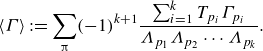 \begin{equation} \langle \Gamma \rangle :=\sum _{\unicode{x03C0} }(-1)^{k+1}\frac {\sum _{i=1}^{k}T_{p_i}\Gamma _{p_i}}{\Lambda _{p_1}\Lambda _{p_2}\cdots \Lambda _{p_k}}. \end{equation}
Here, we sum over so-called pseudo-cycles $\unicode{x03C0} =(p_1,p_2,\ldots ,p_k)$
, each consisting of combinations of prime cycles
$\unicode{x03C0} =(p_1,p_2,\ldots ,p_k)$
, each consisting of combinations of prime cycles $p_{i}$
. For each
$p_{i}$
. For each $i{\text{th}}$
URPO, the quantity
$i{\text{th}}$
URPO, the quantity $\Gamma _{i}$
represents the temporal average of the desired physical quantity, such as the mean flow, over one cycle. Additionally, (4.2) and (4.3) incorporate the URPOs’ periods
$\Gamma _{i}$
represents the temporal average of the desired physical quantity, such as the mean flow, over one cycle. Additionally, (4.2) and (4.3) incorporate the URPOs’ periods $T_{i}$
and their corresponding Floquet multipliers
$T_{i}$
and their corresponding Floquet multipliers
 \begin{equation} \Lambda _k^{(i)}=\exp {\left (\text{Re} {\left(\lambda _k^{(i)}\right)}\,T_{\textrm{i}}\right )}, \end{equation}
where we take into account unstable directions only. As a truncation criterion for the sums in (4.2) and (4.3), Cvitanović et al. (Reference Cvitanović, Artuso, Mainieri, Tanner and Vattay2016) suggest using the pseudo-cycle period and the stability ordering of the pseudo-cycle expansion. The latter is easily feasible using
 \begin{equation} \lvert \Lambda _{p_1}\cdots \Lambda _{p_k}\rvert \leqslant \Lambda _{\textit{max}} \end{equation}
as the truncation criterion, ignoring pseudo-cycles of greater instability than $\Lambda _{\textit{max}}$
. In the second approach, we followed Chandler & Kerswell (Reference Chandler and Kerswell2013) and applied the averaging formula
$\Lambda _{\textit{max}}$
. In the second approach, we followed Chandler & Kerswell (Reference Chandler and Kerswell2013) and applied the averaging formula
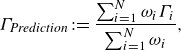 \begin{equation} \Gamma _{\textit{Prediction}}:=\frac {\sum _{i=1}^N\omega _{i}\Gamma _{i}}{\sum _{i=1}^N\omega _{i}}, \end{equation}
where the weights
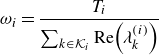 \begin{equation} \omega _i=\frac {T_i}{\sum _{k\in \mathcal{K}_{i}}\text{Re} {\left(\lambda _k^{(i)}\right)}} \end{equation}
incorporate the period $T_{i}$
and positive real parts of the
$T_{i}$
and positive real parts of the $i{\text{th}}$
URPO’s spectra. Though purely heuristic in nature, this approach, referred to as escape-time weighting, is intuitively understandable. First, it states that chaotic trajectories should spend less time in the vicinity of more unstable URPOs. Second, it assigns greater weight to URPOs with longer periods, as these occupy a larger proportion of the state space compared to those with shorter periods.
$i{\text{th}}$
URPO’s spectra. Though purely heuristic in nature, this approach, referred to as escape-time weighting, is intuitively understandable. First, it states that chaotic trajectories should spend less time in the vicinity of more unstable URPOs. Second, it assigns greater weight to URPOs with longer periods, as these occupy a larger proportion of the state space compared to those with shorter periods.
(a) Mean streamwise velocity profile $\langle u\rangle$
, and (b) Reynolds stress
$\langle u\rangle$
, and (b) Reynolds stress $\langle uu\rangle$
, both for the DNS (grey line) in comparison with the predictions using POT (blue) and the escape-time weighting (orange).
$\langle uu\rangle$
, both for the DNS (grey line) in comparison with the predictions using POT (blue) and the escape-time weighting (orange).
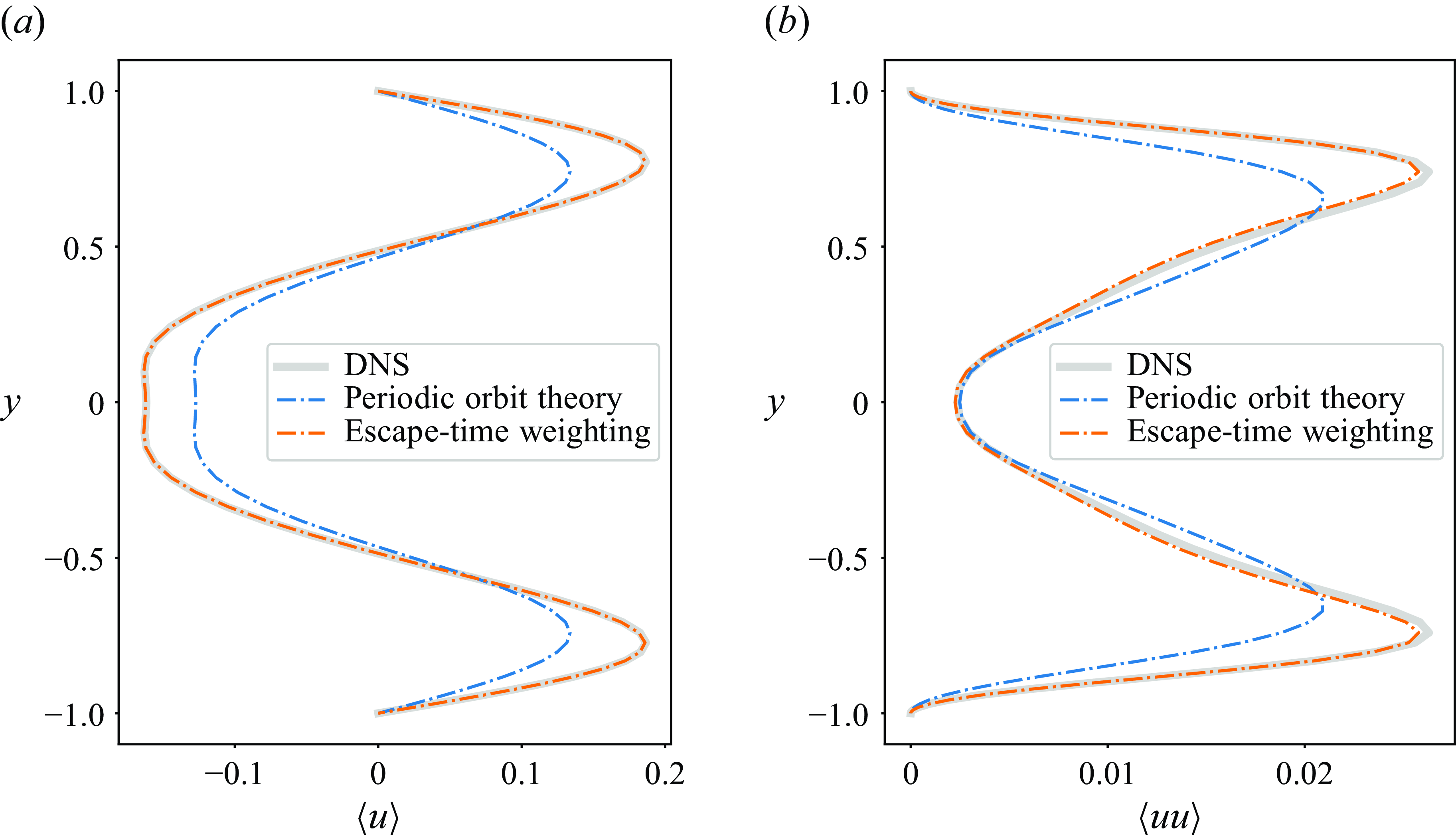
In the following, we present predictions of statistical flow properties provided by both approaches. We start with the mean streamwise velocity profile $\langle u\rangle$
and Reynolds stresses
$\langle u\rangle$
and Reynolds stresses $\langle u_{i} u_j\rangle$
, where the angle brackets indicate averaging in the
$\langle u_{i} u_j\rangle$
, where the angle brackets indicate averaging in the $x$
and
$x$
and $z$
directions as well as in time. These quantities, as evaluated from the DNS along with their predictions, are shown in figures 11 and 12. Both the POT and the escape-time weighting show promising predictions for each quantity. In a direct comparison, the escape-time weighting outperforms the POT approach. To explain why POT provides less accurate predictions than the escape-time weighting, we follow the argument of Chandler & Kerswell (Reference Chandler and Kerswell2013) and refer to a very strong variation of the amplitudes
$z$
directions as well as in time. These quantities, as evaluated from the DNS along with their predictions, are shown in figures 11 and 12. Both the POT and the escape-time weighting show promising predictions for each quantity. In a direct comparison, the escape-time weighting outperforms the POT approach. To explain why POT provides less accurate predictions than the escape-time weighting, we follow the argument of Chandler & Kerswell (Reference Chandler and Kerswell2013) and refer to a very strong variation of the amplitudes $\Lambda _{i}$
used in the pseudo-cycle expansion, which can differ by a factor of
$\Lambda _{i}$
used in the pseudo-cycle expansion, which can differ by a factor of $10^4$
; in contrast, the terms
$10^4$
; in contrast, the terms $\sum _{k\in \mathcal{K}_i}\text{Re} {(\lambda _k^{(i)})}$
used in the escape-time weighting lie much closer together. Furthermore, the accuracy of all predictions is restricted by the number of URPOs present in this study. More challenging is the p.d.f. prediction for energy input
$\sum _{k\in \mathcal{K}_i}\text{Re} {(\lambda _k^{(i)})}$
used in the escape-time weighting lie much closer together. Furthermore, the accuracy of all predictions is restricted by the number of URPOs present in this study. More challenging is the p.d.f. prediction for energy input $I$
and dissipation
$I$
and dissipation $D$
. Figure 13 shows the p.d.f.s of
$D$
. Figure 13 shows the p.d.f.s of $I$
and
$I$
and $D$
, normalised by their respective laminar values, for the DNS as well as their predictions using POT and escape-time weighting. We observe that the p.d.f. predictions for
$D$
, normalised by their respective laminar values, for the DNS as well as their predictions using POT and escape-time weighting. We observe that the p.d.f. predictions for $I/I_0$
and
$I/I_0$
and $D/D_0$
exhibit shapes similar to those obtained from the DNS. However, they over-predict high energy input (
$D/D_0$
exhibit shapes similar to those obtained from the DNS. However, they over-predict high energy input ( $I/I_0 \gt 2.4$
) and dissipation (
$I/I_0 \gt 2.4$
) and dissipation ( $D/D_0 \gt 2.4$
) regions, while under-predicting the mid-range energy input (
$D/D_0 \gt 2.4$
) regions, while under-predicting the mid-range energy input ( $1.8 \lt I/I_0 \lt 2.1$
) and dissipation (
$1.8 \lt I/I_0 \lt 2.1$
) and dissipation ( $1.8 \lt D/D_0 \lt 2.1$
) regions. This discrepancy arises from the absence of URPOs that correspond to these specific energy input and dissipation ranges, as illustrated in figure 9. Similarly, the predictions based on the single URPO with
$1.8 \lt D/D_0 \lt 2.1$
) regions. This discrepancy arises from the absence of URPOs that correspond to these specific energy input and dissipation ranges, as illustrated in figure 9. Similarly, the predictions based on the single URPO with $T_p = 67.02$
in the low energy input and dissipation regions fail to accurately capture the p.d.f. tails in those low-value ranges, as expected. Notably, the p.d.f. predictions based on POT and escape-time weighting show qualitatively similar results, reinforcing the consistency of these heuristic approaches.
$T_p = 67.02$
in the low energy input and dissipation regions fail to accurately capture the p.d.f. tails in those low-value ranges, as expected. Notably, the p.d.f. predictions based on POT and escape-time weighting show qualitatively similar results, reinforcing the consistency of these heuristic approaches.
(a) Reynolds stress $\langle uv\rangle$
and (b) Reynolds stress
$\langle uv\rangle$
and (b) Reynolds stress $\langle vv\rangle$
, both for the DNS (grey line) in comparison with the predictions using POT (blue) and the escape-time weighting (orange).
$\langle vv\rangle$
, both for the DNS (grey line) in comparison with the predictions using POT (blue) and the escape-time weighting (orange).

P.d.f.s for normalised (a) energy input $I/I_0$
and (b) dissipation
$I/I_0$
and (b) dissipation $D/D_0$
. The solid grey line represents the p.d.f. for the DNS. The dash-dotted lines represent the prediction using POT in blue and the escape-time weighting in orange. The p.d.f.s were calculated via kernel density estimation.
$D/D_0$
. The solid grey line represents the p.d.f. for the DNS. The dash-dotted lines represent the prediction using POT in blue and the escape-time weighting in orange. The p.d.f.s were calculated via kernel density estimation.
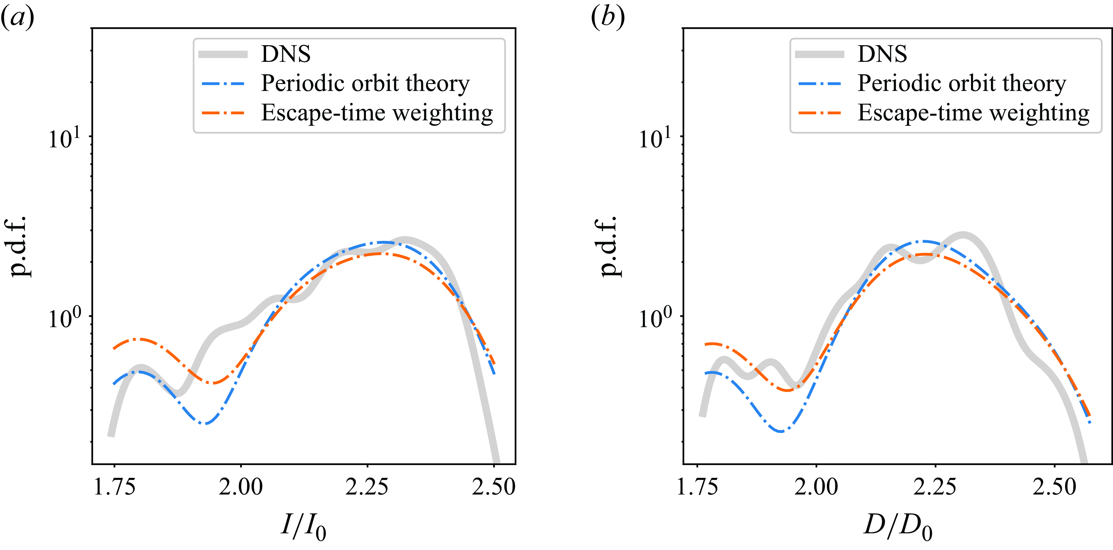
5. Enabling multi-shooting to find URPOs
The state-space complexity of turbulent flow makes finding URPOs with the Newton method challenging, as initial conditions $\{\boldsymbol{u}_0, T\}$
that are not close to the expected solution diverge further when integrated over time. A multi-shooting method can stabilise initial deviations by dividing the time interval
$\{\boldsymbol{u}_0, T\}$
that are not close to the expected solution diverge further when integrated over time. A multi-shooting method can stabilise initial deviations by dividing the time interval $[0,T]$
into smaller intervals, and therefore leads to improvements over the single-shot method (Sánchez & Net Reference Sánchez and Net2010). In this context, SRDMD provides a complementary approach by producing an entire object shadowing the suspected URPO, even in the absence of recurrences. Rather than choosing a single-shot method and taking as the initial guess the reconstructed flow field closest to the DNS trajectory with respect to a specific norm, we enable multi-shooting by incorporating reconstructed flow fields that are potentially not covered by the processed trajectory segment. Figure 14 shows a state-space sketch illustrating multi-shooting with three shots. The grey solid line represents a segment of the symmetry-reduced trajectory shadowing a symmetry-reduced URPO (not shown), whose period guess is
$[0,T]$
into smaller intervals, and therefore leads to improvements over the single-shot method (Sánchez & Net Reference Sánchez and Net2010). In this context, SRDMD provides a complementary approach by producing an entire object shadowing the suspected URPO, even in the absence of recurrences. Rather than choosing a single-shot method and taking as the initial guess the reconstructed flow field closest to the DNS trajectory with respect to a specific norm, we enable multi-shooting by incorporating reconstructed flow fields that are potentially not covered by the processed trajectory segment. Figure 14 shows a state-space sketch illustrating multi-shooting with three shots. The grey solid line represents a segment of the symmetry-reduced trajectory shadowing a symmetry-reduced URPO (not shown), whose period guess is $T$
. The blue dashed line represents the SRDMD reconstruction of the global object incorporating initial guesses that lie beyond the trajectory. The dashed grey line represents the trajectory resulting from time-forward integration
$T$
. The blue dashed line represents the SRDMD reconstruction of the global object incorporating initial guesses that lie beyond the trajectory. The dashed grey line represents the trajectory resulting from time-forward integration $f^T$
of the initial flow field
$f^T$
of the initial flow field $\boldsymbol{u}_0$
. Its deviation from the symmetry-reduced trajectory represents the effect of the system’s underlying continuous symmetry. The pull-back operator
$\boldsymbol{u}_0$
. Its deviation from the symmetry-reduced trajectory represents the effect of the system’s underlying continuous symmetry. The pull-back operator $\sigma (t)$
maps between the original and the symmetry-reduced trajectories. For an
$\sigma (t)$
maps between the original and the symmetry-reduced trajectories. For an $M$
-shot search, the pull-back operator
$M$
-shot search, the pull-back operator $\sigma _m$
, associated with the
$\sigma _m$
, associated with the $m$
th flow field, represents the spatial shift corresponding to the phase difference given by
$m$
th flow field, represents the spatial shift corresponding to the phase difference given by
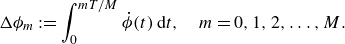 \begin{equation} \Delta \phi _m:=\int _0^{mT/M}\dot {\phi }(t)\,\mathrm{d}t,\quad m=0,1,2,\ldots ,M. \end{equation}
The relevant phase velocity $\dot {\phi }$
is given by (2.19) or (2.20), and results from symmetry reduction using the first Fourier slicing technique. Suppose that
$\dot {\phi }$
is given by (2.19) or (2.20), and results from symmetry reduction using the first Fourier slicing technique. Suppose that $\boldsymbol{u}_0,\boldsymbol{u}_1\ldots ,\boldsymbol{u}_{M-1}$
are
$\boldsymbol{u}_0,\boldsymbol{u}_1\ldots ,\boldsymbol{u}_{M-1}$
are $M$
snapshots from the reconstructed trajectory (2.7), equally spaced over the time interval
$M$
snapshots from the reconstructed trajectory (2.7), equally spaced over the time interval $t\in [0,T]$
. The multiple-shot Newton method solves the root-finding problem
$t\in [0,T]$
. The multiple-shot Newton method solves the root-finding problem
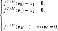 \begin{equation} \begin{cases} f^{T/M}(\boldsymbol{v}_0) - \boldsymbol{v}_1= \boldsymbol{0}, \\ f^{T/M}(\boldsymbol{v}_1) - \boldsymbol{v}_2= \boldsymbol{0}, \\ \quad \vdots \\ f^{T/M}(\boldsymbol{v}_{M-1}) - \sigma _M\boldsymbol{v}_0= \boldsymbol{0}, \end{cases} \end{equation}
Initialisation of a multiple-shot Newton search using the SRDMD technique. The schematic sketch illustrates the state space, where a symmetry-reduced DNS trajectory segment (solid grey line) serves as the observation window for the SRDMD method. This method reconstructs the trajectory as a periodic function of time, appearing as a closed loop on the slice (dashed blue line). Integration of the reconstruction equation along the loop (5.1) determines the relative phase of each snapshot with respect to a reference snapshot, denoted as $\boldsymbol{u}_0$
. This provides an approximation of the URPO in the full state space (dashed grey line), which does not close on itself. Filled markers represent three snapshots equally spaced in time along the reconstructed trajectory. These snapshots, when transformed to the unconstrained state space (empty markers), are used to initialise a multiple-shot Newton search. For an exact URPO, these snapshots lie on a single integral curve
$\boldsymbol{u}_0$
. This provides an approximation of the URPO in the full state space (dashed grey line), which does not close on itself. Filled markers represent three snapshots equally spaced in time along the reconstructed trajectory. These snapshots, when transformed to the unconstrained state space (empty markers), are used to initialise a multiple-shot Newton search. For an exact URPO, these snapshots lie on a single integral curve $f^t(\boldsymbol{u}_0)$
of the vector field induced by the Navier–Stokes equations.
$f^t(\boldsymbol{u}_0)$
of the vector field induced by the Navier–Stokes equations.
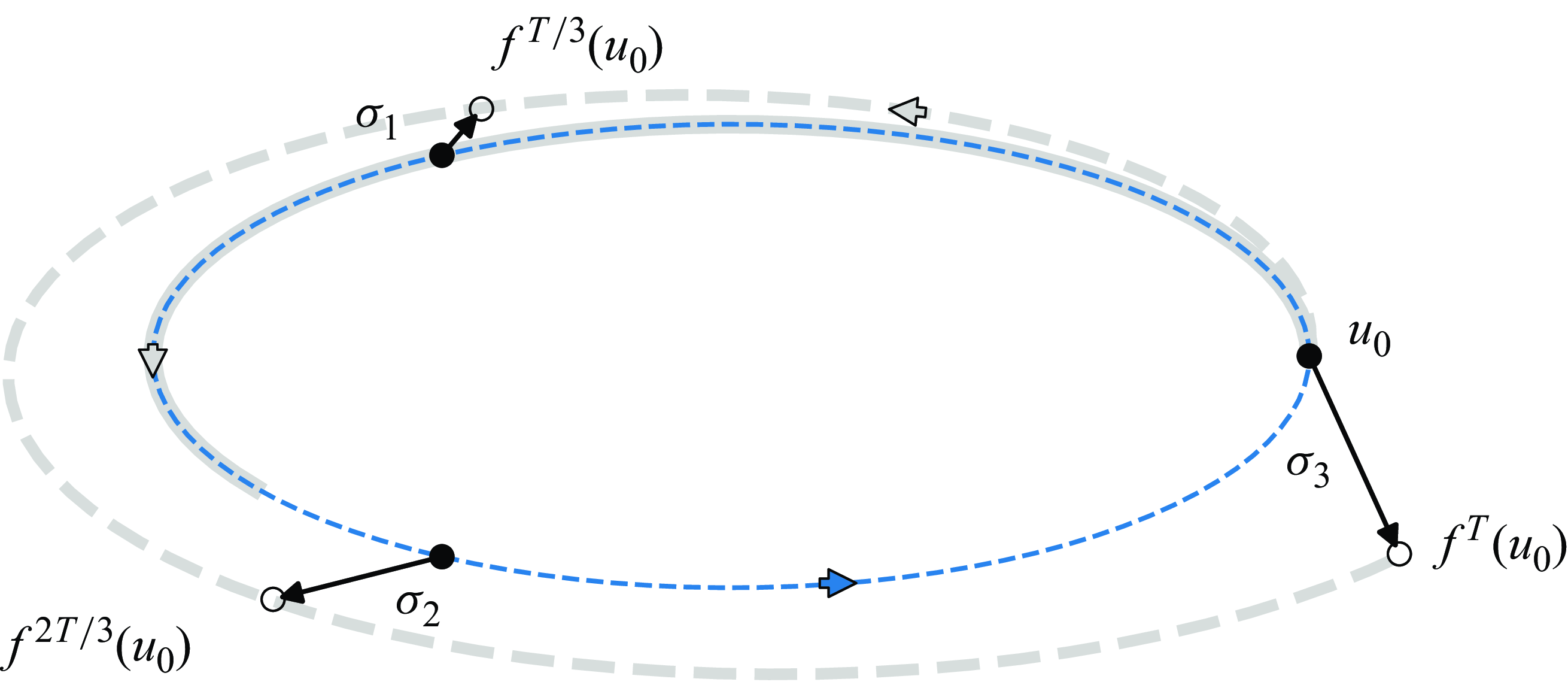
where $\boldsymbol{v}_m:=\sigma _m\boldsymbol{u}_m,\ m=0,1,\ldots ,M-1$
. The unknowns in this search include
$\boldsymbol{v}_m:=\sigma _m\boldsymbol{u}_m,\ m=0,1,\ldots ,M-1$
. The unknowns in this search include $\{\boldsymbol{v}_0,\ldots ,\boldsymbol{v}_{M-1},\sigma _M,T\}$
. For this vector of unknowns, a closed system of nonlinear equations is obtained by augmenting (5.2) with appropriate phase-locking constraints (Viswanath Reference Viswanath2009).
$\{\boldsymbol{v}_0,\ldots ,\boldsymbol{v}_{M-1},\sigma _M,T\}$
. For this vector of unknowns, a closed system of nonlinear equations is obtained by augmenting (5.2) with appropriate phase-locking constraints (Viswanath Reference Viswanath2009).
We demonstrate our approach with an example using a two-shot Newton search. We consider a guess identified by the SRDMD method described in § 2, with guessed period $T_g=62.1673$
. The standard single-shot Newton search failed to converge when initialised with snapshots corresponding to different phases along the reconstructed periodic function
$T_g=62.1673$
. The standard single-shot Newton search failed to converge when initialised with snapshots corresponding to different phases along the reconstructed periodic function $\boldsymbol{u}(t)$
, defined by (2.7). We did a two-shot search using snapshots at
$\boldsymbol{u}(t)$
, defined by (2.7). We did a two-shot search using snapshots at $t=0$
and
$t=0$
and $t=T_g/2$
from the reconstructed flow. The choice of the snapshots is not unique, and any pair of snapshots separated in time by
$t=T_g/2$
from the reconstructed flow. The choice of the snapshots is not unique, and any pair of snapshots separated in time by $T_g/2$
can be used for a two-shot search, as (2.7) provides an explicit continuous function of time. The two-shot Newton search converges within
$T_g/2$
can be used for a two-shot search, as (2.7) provides an explicit continuous function of time. The two-shot Newton search converges within $28$
iterations to an exact solution. Figure 15 shows the convergence result. In this plot,
$28$
iterations to an exact solution. Figure 15 shows the convergence result. In this plot, $G$
represents the to-be-zeroed vector in the respective root-finding problem, and
$G$
represents the to-be-zeroed vector in the respective root-finding problem, and $x$
represents the vector of unknowns in the discretised problem. We consider an exact solution to be achieved within machine accuracy if the
$x$
represents the vector of unknowns in the discretised problem. We consider an exact solution to be achieved within machine accuracy if the $L_2$
-norm of
$L_2$
-norm of $G(x)$
falls below
$G(x)$
falls below $10^{-13}$
. The single-shot search starting from the snapshot at
$10^{-13}$
. The single-shot search starting from the snapshot at $t=0$
could not converge within
$t=0$
could not converge within $200$
iterations, after which the search was terminated. The single-shot search starting from the snapshot at
$200$
iterations, after which the search was terminated. The single-shot search starting from the snapshot at $t=T_g/2$
stopped after
$t=T_g/2$
stopped after $117$
iterations because the hook-step trust-region method could no longer improve the residual. These two failed searches are shown too in figure 15, where the residual stagnates after approximately
$117$
iterations because the hook-step trust-region method could no longer improve the residual. These two failed searches are shown too in figure 15, where the residual stagnates after approximately $50$
Newton iterations. To save computational time, the multiple-shot Newton search was done at a lower resolution
$50$
Newton iterations. To save computational time, the multiple-shot Newton search was done at a lower resolution $(N_x,N_y,N_z)=(16,41,16)$
(convergence shown in figure 15). The converged URPO was then continued to the original resolution
$(N_x,N_y,N_z)=(16,41,16)$
(convergence shown in figure 15). The converged URPO was then continued to the original resolution $(N_x,N_y,N_z)=(48,65,48)$
to confirm that it is structurally stable and to determine its accurate period
$(N_x,N_y,N_z)=(48,65,48)$
to confirm that it is structurally stable and to determine its accurate period $T=67.0226$
.
$T=67.0226$
.
Results of two variants of Newton iterations for computing a URPO. The searches are initialised with a guess generated using the SRDMD method, that has guessed period $T_g=62.1673$
. The standard single-shot Newton iterations fail to converge when initialised with snapshots corresponding to
$T_g=62.1673$
. The standard single-shot Newton iterations fail to converge when initialised with snapshots corresponding to $t=0$
and
$t=0$
and $t=T_g/2$
along the reconstructed periodic trajectory (2.7) (red and grey circle markers). The two-shot Newton search, initialised with these two snapshots, converges successfully in
$t=T_g/2$
along the reconstructed periodic trajectory (2.7) (red and grey circle markers). The two-shot Newton search, initialised with these two snapshots, converges successfully in $28$
iterations (blue square markers). The vertical axis shows the
$28$
iterations (blue square markers). The vertical axis shows the $L_2$
-norm of the to-be-zeroed vector
$L_2$
-norm of the to-be-zeroed vector $G(x)$
in the respective root-finding problem, where
$G(x)$
in the respective root-finding problem, where $x$
denotes the vector of unknowns.
$x$
denotes the vector of unknowns.
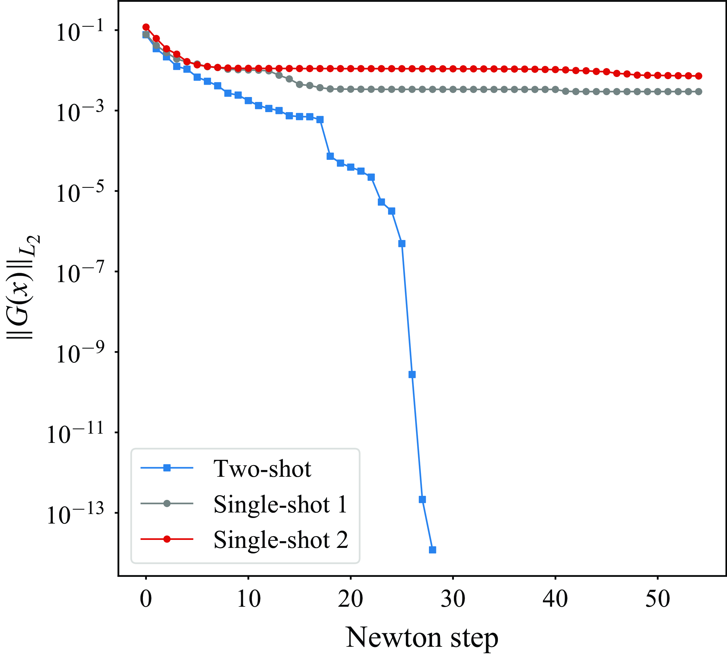
6. Search for unstable TWs in 3-D plane Poiseuille flow
The simplest category of invariant solutions to the Navier–Stokes equations (3.1) and (3.2) that can provide new insights into the flow are TWs. In this section, we demonstrate using two examples how the sparsity-promoting SRDMD can be used to construct initial conditions for the Newton search of TWs.
When a chaotic trajectory visits the neighbourhood of a steady state, the evolution is nearly linear; hence SRDMD is able to reconstruct trajectory segments accurately in the vicinity of a TW. In addition, when the trajectory is repelled from (or attracted to) the TW’s neighbourhood along its unstable (stable) manifold, the DMD spectrum is expected to be dominated by a few leading eigenvalues of the linearised dynamics. Therefore, we consider the trajectory segment processed by SRDMD to potentially be in the vicinity of a TW if the low-dimensional linear reconstruction is sufficiently accurate while the selected set of SRDMD eigenvalues includes one neutral eigenvalue with the remaining ones being repelling (attracting). In such cases, we can approximate the nearby TW solution by sending $t\to -\infty$
(or
$t\to -\infty$
(or $t\to +\infty$
) in the reconstruction.
$t\to +\infty$
) in the reconstruction.
Here, we specifically consider the case of purely real eigenvalues. If complex-valued eigenvalues were considered too, then SRDMD could detect a spiralling trajectory, suggesting oscillatory behaviour while the trajectory is being repelled from or attracted to a steady solution. However, since only the SRDMD spectra with real eigenvalues are considered, the trajectory instead resembles a star-type or a saddle-type solution, without oscillations. In this case, (2.7) for the SRDMD reconstruction simplifies to
 \begin{equation} \boldsymbol{u}(t_j)\approx \sum _{k=0}^{l-1}a_k\,{\rm e}^{\sigma _kt_j}\,\boldsymbol{\psi }_k, \end{equation}
where only the growth or decay rate $\sigma _k$
determines the temporal behaviour of the SRDMD reconstruction. The amplitudes
$\sigma _k$
determines the temporal behaviour of the SRDMD reconstruction. The amplitudes $a_k$
of the purely real dynamic modes
$a_k$
of the purely real dynamic modes $\boldsymbol{\psi }_k$
are again determined via sparsity-promoting optimisation as introduced in § 2. With
$\boldsymbol{\psi }_k$
are again determined via sparsity-promoting optimisation as introduced in § 2. With $l$
, we denote the number of dynamic modes being selected for the reconstruction. This approach is motivated by the idea that the sparsity-promoting optimisation selects dynamic modes hierarchically in accordance with their contribution to an optimal flow reconstruction, and therefore selects purely real dynamic modes prior to dynamic modes with fundamental frequencies, when the flow can be well captured by a non-oscillating SRDMD approximation.
$l$
, we denote the number of dynamic modes being selected for the reconstruction. This approach is motivated by the idea that the sparsity-promoting optimisation selects dynamic modes hierarchically in accordance with their contribution to an optimal flow reconstruction, and therefore selects purely real dynamic modes prior to dynamic modes with fundamental frequencies, when the flow can be well captured by a non-oscillating SRDMD approximation.
To provide a proof of concept, we chose two distant SRDMD observation time windows near state-space locations where energy input and dissipation balance out, and thus TW solutions can be expected. The SRDMD observation time windows were set to be short: each window spanned 7.5 advective time units, with snapshot sampling $\Delta t$
and spacing
$\Delta t$
and spacing $\delta t$
of 0.5 advective time units, to ensure that the flow could be well captured by the linear approximation. Furthermore, we found two real dynamic modes to be sufficient for reconstructing successful initial conditions. Figure 16(a) shows the resulting SRDMD spectra for both cases, where purely real eigenvalues selected through sparsity-promoting optimisation for the flow reconstruction are coloured in blue and orange. In both cases, the neutral eigenvalue
$\delta t$
of 0.5 advective time units, to ensure that the flow could be well captured by the linear approximation. Furthermore, we found two real dynamic modes to be sufficient for reconstructing successful initial conditions. Figure 16(a) shows the resulting SRDMD spectra for both cases, where purely real eigenvalues selected through sparsity-promoting optimisation for the flow reconstruction are coloured in blue and orange. In both cases, the neutral eigenvalue $\lambda _0=1$
(
$\lambda _0=1$
( $\sigma _0 = 0$
) corresponds to the time-independent part of the reconstruction (6.1), while the other eigenvalue
$\sigma _0 = 0$
) corresponds to the time-independent part of the reconstruction (6.1), while the other eigenvalue $\lambda _1\lt 1$
(
$\lambda _1\lt 1$
( $\sigma _1 \lt 0$
) corresponds to a decaying mode as
$\sigma _1 \lt 0$
) corresponds to a decaying mode as $t\to +\infty$
. Taking into account the phase shift
$t\to +\infty$
. Taking into account the phase shift $\Delta \phi$
from the symmetry reduction, the reconstructed initial conditions converged quickly to TW solutions by Newton iteration. Figure 16(b) shows the location of both TWs in a 2-D
$\Delta \phi$
from the symmetry reduction, the reconstructed initial conditions converged quickly to TW solutions by Newton iteration. Figure 16(b) shows the location of both TWs in a 2-D $I$
–
$I$
– $D$
state-space projection, with both quantities normalised by their respective laminar values
$D$
state-space projection, with both quantities normalised by their respective laminar values $I_0$
and
$I_0$
and $D_0$
. The colour coding of the markers relates the TWs to the dynamic modes in figure 16(a) that were used for constructing the initial conditions. In table 3, we summarise the numerical details and stability properties of both TWs.
$D_0$
. The colour coding of the markers relates the TWs to the dynamic modes in figure 16(a) that were used for constructing the initial conditions. In table 3, we summarise the numerical details and stability properties of both TWs.
(a) The SRDMD spectra obtained from the analysis of two segments of the chaotic trajectory in figure 6, each located at different times within the DNS. Marked in blue and orange are purely real eigenvalues corresponding to the two cases, automatically selected by the sparsity-promotion optimisation when reconstructing the flow. (b) The location of the converged unstable TWs in a state-space projection of energy input $I$
and dissipation
$I$
and dissipation $D$
, normalised by their respective laminar values
$D$
, normalised by their respective laminar values $I_0$
and
$I_0$
and $D_0$
. The grey-shaded area represents the p.d.f. of the dynamics, as described in figure 9. The marker colours relate the dynamic modes from the SRDMD in (a), selected to construct an initial condition for the Newton search, to the respective converged solutions indicated in (b).
$D_0$
. The grey-shaded area represents the p.d.f. of the dynamics, as described in figure 9. The marker colours relate the dynamic modes from the SRDMD in (a), selected to construct an initial condition for the Newton search, to the respective converged solutions indicated in (b).
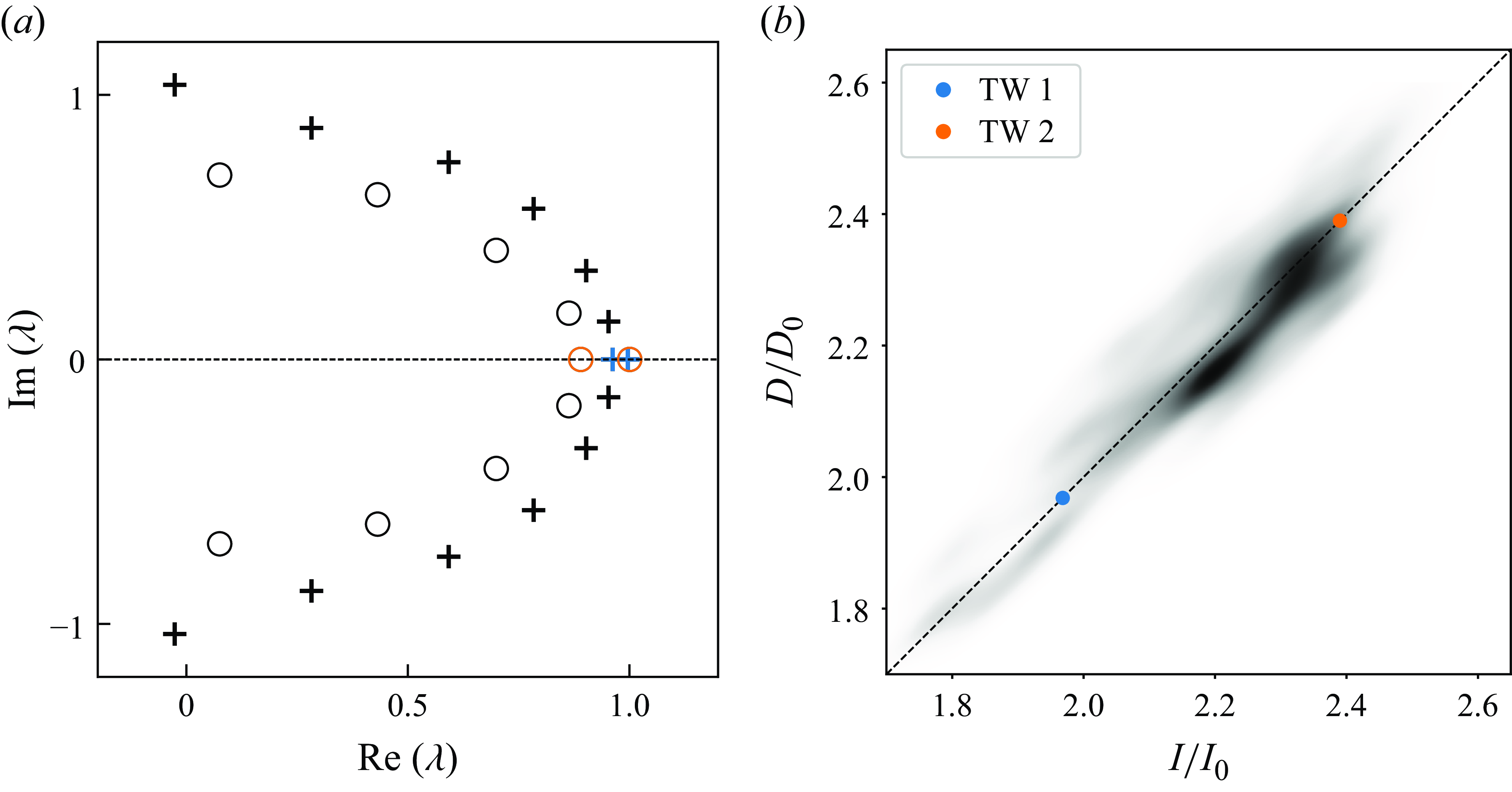
The unstable TWs converged from initial data constructed through SRDMD. The spatial resolutions of the computational domain in the streamwise, wall-normal and spanwise direction are $N_x$
,
$N_x$
, $N_y$
and
$N_y$
and $N_z$
, respectively, and
$N_z$
, respectively, and $c$
is the phase velocity of the TW. Stability properties of the TWs are summarised with the number of unstable directions
$c$
is the phase velocity of the TW. Stability properties of the TWs are summarised with the number of unstable directions $N$
, the sum
$N$
, the sum $\sum _{j=1}^N\text{Re} {(\lambda _j)}$
of real parts of the corresponding eigenvalues, and their maximal values
$\sum _{j=1}^N\text{Re} {(\lambda _j)}$
of real parts of the corresponding eigenvalues, and their maximal values $\max \,\text{Re} {(\lambda _j)}$
.
$\max \,\text{Re} {(\lambda _j)}$
.
7. Conclusion
In this paper, we applied and extended SRDMD – a method recently developed by Marensi et al. (Reference Marensi, Yalnız, Hof and Budanur2023) that combines classical DMD with the method of slices for symmetry reduction – to construct initial data for Newton searches to find unstable invariant solutions in systems with continuous symmetries. Since continuous symmetries lead to spurious DMD modes and complicate flow reconstruction, symmetry reduction is essential for constructing optimal flow approximations used to generate such initial data. As SRDMD provides global-in-time guesses for periodic solutions, namely closed loops in state space, we demonstrated how it can be used in conjunction with multi-shooting methods. We also extended the method to construct initial guesses for unstable travelling waves (TWs).
We applied SRDMD in conjunction with sparsity promotion to select an optimal set of DMD modes for a weakly turbulent channel flow at $\textit{Re}_{\tau }\approx 51$
, aiming to construct initial conditions for the Newton search for unstable relative periodic orbits (URPOs) and TWs. Using single-shot Newton searches, we converged
$\textit{Re}_{\tau }\approx 51$
, aiming to construct initial conditions for the Newton search for unstable relative periodic orbits (URPOs) and TWs. Using single-shot Newton searches, we converged $10\,\%$
of all initial conditions to exact URPOs. These include states that were identified even in the absence of a recurrence event. In total, we found 35 URPOs, six of which are distinct. That is, several URPOs were converged multiple times using initial data from different locations along the chaotic trajectory, indicating their dynamical importance. The importance of these orbits is also reflected in the fact that they cover regions of the state space visited most frequently by the dynamics, at least in an energy input–dissipation projection.
$10\,\%$
of all initial conditions to exact URPOs. These include states that were identified even in the absence of a recurrence event. In total, we found 35 URPOs, six of which are distinct. That is, several URPOs were converged multiple times using initial data from different locations along the chaotic trajectory, indicating their dynamical importance. The importance of these orbits is also reflected in the fact that they cover regions of the state space visited most frequently by the dynamics, at least in an energy input–dissipation projection.
To estimate the dynamical importance of our solutions in a more quantitative manner, we computed cycle averages of all distinct URPOs to predict statistical properties of the flow using periodic orbit theory (POT). As an alternative approach, we also applied heuristic escape-time weighting. We found that the mean velocity profile $\langle u\rangle$
and the Reynolds stresses
$\langle u\rangle$
and the Reynolds stresses $\langle uu\rangle$
,
$\langle uu\rangle$
, $\langle uv\rangle$
and
$\langle uv\rangle$
and $\langle vv\rangle$
of the chaotic trajectory can be predicted by escape-time weighting of the URPOs very well, both qualitatively and quantitatively. The POT results in a good qualitative approximation; however, it quantitatively deviates significantly from the DNS results. Unsurprisingly, the p.d.f.s of energy input and dissipation proved to be much more difficult to predict.
$\langle vv\rangle$
of the chaotic trajectory can be predicted by escape-time weighting of the URPOs very well, both qualitatively and quantitatively. The POT results in a good qualitative approximation; however, it quantitatively deviates significantly from the DNS results. Unsurprisingly, the p.d.f.s of energy input and dissipation proved to be much more difficult to predict.
To improve the quality of the predictions of statistical quantities substantially, we would need to find a larger number of URPOs. One way to achieve this is by utilising multi-shooting Newton searches initialised with guesses generated using the introduced SRDMD technique. An SRDMD reconstruction, possibly shadowing the suspected URPO, provides viable initial guesses for the Newton search at any desired location along the estimated trajectory. Thereby, this approach enables multi-shooting Newton methods to operate on the resulting global object. This potentially leads to a higher yield of converged URPOs. We demonstrated this approach using a guess identified by the SRDMD method, in a case where the standard single-shot Newton search fails to converge when initialised with snapshots corresponding to different temporal phases of the reconstructed data. However, a two-shot Newton search converges successfully by stabilising the error growth. Higher success rates are also anticipated by combining the SRDMD method, which generates global-in-time guesses for periodic solutions, with more robust convergence algorithms that leverage such global structures to eliminate the need for time-marching the chaotic dynamics. These include variational methods in which a cost function penalises the deviation of a loop from being a solution trajectory in the system’s state space, and minimising the cost function deforms the loop until it converges to an exact periodic solution trajectory (Lan & Cvitanović Reference Lan and Cvitanović2004; Azimi, Ashtari & Schneider Reference Azimi, Ashtari and Schneider2022; Parker & Schneider Reference Parker and Schneider2022).
Finally, we demonstrated how sparsity-promoting SRDMD can be used to detect TW solutions. In this case, the reconstructed flow comprises the neutral SRDMD mode, which represents the asymptotic state of the flow, as well as a second SRDMD mode with a purely real eigenvalue, that decays in either forward or backward time. The reconstruction, with both modes selected by the sparsity-promoting algorithm, provides an optimal low-dimensional representation of the flow and exhibits non-oscillatory behaviour. We showed this technique using two exemplary choices of SRDMD modes, whose resulting initial guesses converged successfully to unstable TWs.
In summary, we showed that SRDMD is an effective tool for the construction of initial data, complementary to recurrent flow analysis, for the numerical computation of unstable invariant solutions in weakly chaotic 3-D fluid flows. By relaxing the requirement that a chaotic trajectory must follow a UPO for an entire cycle, the DMD-based approach allows us to access more unstable UPOs, identify greater numbers of them, and extend the range of Reynolds numbers over which the dynamical systems approach can be successfully applied, compared to solely relying on recurrent flow analysis. In the context of flow control and stabilisation of invariant solutions (Willis et al. Reference Willis, Duguet, Omel’chenko and Wolfrum2017; Linkmann et al. Reference Linkmann, Knierim, Zammert and Eckhardt2020; Lucas & Yasuda Reference Lucas and Yasuda2022; Yasuda & Lucas Reference Yasuda and Lucas2025), an aspect worthy of further investigation is the application of DMD- or SRDMD-based flow reconstruction within feedback control approaches to stabilise invariant solutions.
Acknowledgements
We thank N.B. Budanur, E. Marensi and J. Page for helpful discussions.
Funding
This work received funding from Priority Programme SPP 1881 ‘Turbulent superstructures’ of the Deutsche Forschungsgemeinschaft (grant no. Li3694/1). M.E. was also supported by the School of Mathematics at the University of Edinburgh. O.A. was supported by the European Research Council (ERC) under the European Union’s Horizon 2020 research and innovation programme (grant agreement no. 865677, T.M.S.). Computational resources on Cirrus (www.cirrus.ac.uk) have been obtained through Scottish Academic Access.
Declaration of interests
The authors report no conflict of interest.


 Open access