


1 Introduction
Flows through porous media are ubiquitous. Many natural and human-made substances can be interpreted as porous media through which fluids flow. These materials exhibit a wide variability in the shape of their microstructures. They play a pivotal role in many natural phenomena, each one thanks to their distinguishing microstructural features. Examples are organic fluids flowing through biological tissues, where the pore shape regulates the biological activities (Khaled & Vafai Reference Khaled and Vafai2003), and water infiltrating through soils, where the spatial distribution of porous layers marks the rhythm of the water cycle, from the atmosphere to the oceans (Daly & Porporato Reference Daly and Porporato2005). Given their intrinsic capability of spreading active species and providing surface area for reactions, porous media are also widely used as electrodes. Good examples are electrodes in electrochemical batteries, such as lithium-ion batteries, supercapacitors, capacitive deionisators for water treatment technologies and redox flow batteries.
Redox flow batteries play a crucial role for energy storage applications. The future scenario of global electrification imposes the need of finding smart ways to store energy in the grid and to deliver it on demand. Redox flow batteries are electrochemical storage devices well suited for a wide range of operational powers and discharge times. Their scalability and flexibility make them ideal candidates for storing energy from renewable sources (Guarnieri et al. Reference Guarnieri, Mattavelli, Petrone and Spagnuolo2016). They are electrochemical rechargeable batteries; charging and discharging cycles are possible owing to the presence of two chemical species dissolved in each solution feeding the two electrodes of the battery cells, separated by a membrane, for producing chemical reduction and oxidation (‘redox’) reactions. The liquid solution, named the liquid electrolyte, flows through the porous electrodes to enable the storage of electrochemical energy. Because of the low molecular diffusivity  ${\mathcal{D}}_{m}$ of species in the liquid electrolyte compared to its viscosity $\unicode[STIX]{x1D708}$, i.e. because of a high Schmidt number $Sc=\unicode[STIX]{x1D708}/{\mathcal{D}}_{m}\sim O(10^{2}{-}10^{3})$, the porous microstructure is fundamental for sustaining effective dispersion of the species and for shortening the transport distances from the bulk to the reaction sites.
High Schmidt numbers are typical of liquid solutions. When a liquid solution flows through a reactive porous material, the dispersion of species can affect the reaction mechanism, and vice versa (Dentz et al. Reference Dentz, Le Borgne, Englert and Bijeljic2011). Indeed, it is the distribution and mixing mechanisms of the solute that regulate the mass transport of active species to the solid inner surfaces of the porous medium where the reactions occur. In this sense, pore-scale simulations have recently attracted attention as tools for the development of coupled transport formulations with reactive mechanisms, since they can take into account the effect of the microstructure (Alhashmi, Blunt & Bijeljic Reference Alhashmi, Blunt and Bijeljic2016; Romano et al. Reference Romano, Jiménez-Martínez, Parmigiani, Kong and Battiato2019). The prominent role of the microstructure in spreading active species carried by a liquid solution has been quantified in various studies (Berkowitz & Scher Reference Berkowitz and Scher1995; Icardi et al. Reference Icardi, Boccardo, Marchisio, Tosco and Sethi2014; Maggiolo, Picano & Guarnieri Reference Maggiolo, Picano and Guarnieri2016; Dentz, Icardi & Hidalgo Reference Dentz, Icardi and Hidalgo2018). The mechanism of species dispersion in liquids flowing through porous media has a distinctive characteristic in that, as opposed to dispersion of species carried by gases, it does not depend only on the value of the porosity, as predicted for instance by the commonly used Bruggeman equation (Chung et al. Reference Chung, Ebner, Ely, Wood and García2013; Maggiolo et al. Reference Maggiolo, Picano and Guarnieri2016). Knowing the value of the porosity of a medium is not sufficient to predict dispersion phenomena and evidence shows that more complex geometrical and fluid-dynamic factors contribute to the mechanisms of mass transport (e.g. tortuosity and pore connectivity, to name two) (Moldrup et al. Reference Moldrup, Olesen, Komatsu, Schjønning and Rolston2001; Yang et al. Reference Yang, Mehmani, Perkins, Pasquali, Schönherr, Kim, Perego, Parks, Trask and Balhoff2016).
Another key feature that makes porous media widely used as electrodes is their high value of specific surface area, that is, the total solid surface per unit volume. As a consequence, porous electrodes are characterised by a large area available for reactions of species and their global reaction efficiency is potentially very high. However, the actual efficiency of a porous electrode does not only depend on the overall reaction rate, but also on the amount of energy required to flow an electrolyte through the medium in order to deliver the species to the reaction sites (Tang, Bao & Skyllas-Kazacos Reference Tang, Bao and Skyllas-Kazacos2014). A large specific surface area does not only imply a potentially high amount of mass reacting in the electrode, but also a large fluid–solid interface, which contributes to increase the pressure drag and skin friction (Zhou et al. Reference Zhou, Zhao, Zeng, An and Wei2016). Consequently, the amount of energy required to flow an electrolyte through a porous medium can be very high, especially in the case of intricate geometries.
Moreover, the extent and mechanism of reaction at the fluid–solid boundaries also depend on the complex interaction between the liquid electrolyte and the porous microstructure. Local heterogeneities are distinguishing traits of porous microstructures and the local concentration of solute can be affected by such geometrical constraints (Yang, Crawshaw & Boek Reference Yang, Crawshaw and Boek2013). In flows through porous media at high Schmidt numbers, the heterogeneous nature of mass transport often emerges from a strongly intermittent velocity field (Kang et al. Reference Kang, de Anna, Nunes, Bijeljic, Blunt and Juanes2014). Heterogeneities affect not only the spatial distribution of the solute, but also a wide distribution of transport time scales can be observed. The latter leads to what is commonly referred to as non-Fickian transport, an anomalous behaviour that cannot be described by the classical Fickian description (Yang & Wang Reference Yang and Wang2019). In turn, the reaction can be heterogeneous, being affected by such uneven spatial and temporal distributions of the solute transport. Experimental observations confirm that the uniformity of solute transport plays a decisive role in determining the output power of, for instance, redox flow batteries (Kumar & Jayanti Reference Kumar and Jayanti2016).
Conversion is defined as the ratio between the mass reacted and the total mass delivered to a system: it is an indicator of the efficiency of operation of a porous electrode and its inverse is often named the ‘flow factor’ in redox flow battery applications (Guarnieri et al. Reference Guarnieri, Trovò, D’Anzi and Alotto2018). Practical experiences using liquid electrolytes through porous electrodes indicate that values of solute conversion are often low and that values close the maximum theoretical value are rarely achieved. Efficiency maximisation occurs close to conversion values of around  $1/8$ at high current densities, when the required energy output is high (Guarnieri et al. Reference Guarnieri, Trovò, D’Anzi and Alotto2018, Reference Guarnieri, Trovò, Marini, Sutto and Alotto2019). A high energy output is often challenging since it poses strong requirements on the minimum size of the system. This practical limitation can be overcome by maximising the efficiency of mass transport inside the porous microstructure, but the transport mechanisms that contribute to high conversion and power output of electrodes are still not well understood. The complex interaction between macroscopic output and microscopic fluid-dynamic phenomena has been traditionally described via empirical correlations and measured mass-transfer coefficients (Schmal, Van Erkel & Van Duin Reference Schmal, Van Erkel and Van Duin1986; Ström, Sasic & Andersson Reference Ström, Sasic and Andersson2012). The physical link with microstructural material characteristics and coupled reactive–transport phenomena is still a matter of debate; see e.g. Zhu & Zhao (Reference Zhu and Zhao2017) and Kok et al. (Reference Kok, Jervis, Tranter, Sadeghi, Brett, Shearing and Gostick2019). The picture that emerges from the latest experimental activities and preliminary theoretical analyses is that the optimum operative condition of a porous electrode, however defined, depends on the specific balance between the mechanisms of mass transport and reaction occurring at the pore scale. Such a balance is intuitively also dependent on the porous microstructure.
Hence, two important questions arise. (i) At high Schmidt numbers, what are the main transport phenomena contributing to reactions of the solute in porous electrodes? (ii) How should a porous electrode be designed in order to achieve the optimal performance, in terms of both conversion and power output? In this work we investigate, debate and clarify the fluid-dynamic aspects of such questions, by numerically simulating, modelling and comparing the flow, dispersion and reaction through real material microstructures, obtained via X-ray computed tomography. We restrict our analysis to solute transport in porous media at high Schmidt numbers in order to enrich the knowledge about dispersive phenomena in liquids flowing through reactive porous media. The study provides insights into the fluid-dynamic optimisation of systems based on such phenomena and it will eventually lead to a formulation of universal design guidelines for porous electrodes.
The article is structured as follows. In § 2 the theoretical framework and numerical methodology are described. The set-up of the numerical simulations and the engineering procedure for reconstructing the porous electrodes are also presented. In § 3 the mathematical framework used for the analysis of results, based on spatial smoothing and homogenisation technique, is described. In § 4 the results of the numerical simulations are presented. Different mechanisms of solute transport, dispersion and reaction are discussed. In light of these results, the modelling of the fluid-dynamic dispersion in porous media is discussed in § 5. In § 6 we identify the optimal design guidelines for porous electrodes and in § 7 we summarise the results of this study.
2 Pore-scale solute transport and reaction
The mechanism of solute transport through redox flow battery porous electrodes is traditionally modelled via the Nernst–Planck equation, which describes the motion of ions under the influence of ionic concentration gradients and electric fields (Probstein Reference Probstein2005; Arenas, de León & Walsh Reference Arenas, de León and Walsh2019). Such an approach is applied via numerical simulations to a scale larger than the characteristic pore size of the electrode and the microstructural effects are neglected. Further, pore-scale mechanisms can contribute to the transport and reactions of the solute, in the form of advective and reactive fluxes in the bulk and at the fluid–solid boundaries, respectively. When the gradients of the electric potential are much smaller than the gradients of the solute concentration, electric-field-induced ion migration can be considered negligible compared to other transport mechanisms. A suitable example concerns redox flow batteries where the typical length over which the electric potential varies, of the order of centimetres, is much greater than the characteristic pore size, which is in the range of tens of micrometres.
In the present analysis, we neglect ion migration due to electric field and we solve the physics of transport and reaction in porous electrodes at the smallest scale. The physical system that we investigate is then described at the pore scale by the advection–diffusion equation:
 $$\begin{eqnarray}\frac{\unicode[STIX]{x2202}c(\boldsymbol{x},t)}{\unicode[STIX]{x2202}t}+\frac{\unicode[STIX]{x2202}c(\boldsymbol{x},t)u_{j}(\boldsymbol{x})}{\unicode[STIX]{x2202}x_{j}}=\frac{\unicode[STIX]{x2202}}{\unicode[STIX]{x2202}x_{j}}\left({\mathcal{D}}_{m}\frac{\unicode[STIX]{x2202}c(\boldsymbol{x},t)}{\unicode[STIX]{x2202}x_{j}}\right),\end{eqnarray}$$
 with  ${\mathcal{D}}_{m}$ the molecular diffusion coefficient, $c(\boldsymbol{x},t)$ the solute concentration at position $\boldsymbol{x}$ and time $t$ and $u_{j}(\boldsymbol{x})$ the steady-state $j$th Eulerian component of the solenoidal fluid velocity along the direction $x_{j}$ that transports the solute (we assume that the solute has no influence on the properties of the fluid). In addition, we assume that the transported solute reacts at the fluid–solid boundaries inside the porous medium according to a first-order reaction equation. The surface flux depends on the chemical reaction velocity $k_{r}$ and on the molecular diffusion ${\mathcal{D}}_{m}$ as
 $$\begin{eqnarray}\left.-{\mathcal{D}}_{m}\frac{\unicode[STIX]{x2202}c(\boldsymbol{x},t)}{\unicode[STIX]{x2202}n}\right|_{S}=k_{r}(c(\boldsymbol{x},t)|_{S}-c_{0}),\end{eqnarray}$$
 where  $n$ is the versor normal to the boundary and the fluid–solid interface is here denoted as $S$. The term $c_{0}$ indicates an equilibrium value for the mass transfer at the boundary. In our case, $c_{0}=0$ since the kinetic rate of a realistic reaction is proportional to the concentration of reactant $c(\boldsymbol{x},t)|_{S}$. However, we keep the term $c_{0}$ in the mathematical formulations below since it can represent a non-null equilibrium value in other applications, such as for mixed boundary conditions in convective heat transfer.
2.1 The lattice Boltzmann method
The numerical methodology used in this work is based on the lattice Boltzmann method. This method represents an alternative way of solving the mass and momentum equations. It is well suited for solving flows through complex geometries with a pore-scale resolution (Succi Reference Succi2001). The lattice Boltzmann method solves the momentum transport equation through the discretisation of the Boltzmann equation, which reads as
 $$\begin{eqnarray}\displaystyle f_{r}(\boldsymbol{x}+c_{r}\unicode[STIX]{x0394}t,t+\unicode[STIX]{x0394}t)-f_{r}(\boldsymbol{x},t)=-\unicode[STIX]{x1D70F}_{\unicode[STIX]{x1D708}}^{-1}(f_{r}(\boldsymbol{x},t)-f_{r}^{eq}(\boldsymbol{x},t))+F_{r}, & & \displaystyle\end{eqnarray}$$
 where  $f_{r}(\boldsymbol{x},t)$ is the distribution function at position $\boldsymbol{x}=(x,y,z)$ and time $t$ along the $r$th direction, $c_{r}$ is the discrete velocity along the $r$th direction, $\unicode[STIX]{x1D70F}_{\unicode[STIX]{x1D708}}$ is the relaxation time that provides a direct link to fluid viscosity and $f_{r}^{eq}$ is the equilibrium distribution function along the $r$th direction:
 $$\begin{eqnarray}f_{r}^{eq}(\boldsymbol{x},t)=w_{r}\unicode[STIX]{x1D70C}\left(1+\frac{c_{rj}u_{j}(\boldsymbol{x},t)}{c_{s}^{2}}+\frac{(c_{rj}u_{j}(\boldsymbol{x},t))^{2}}{c_{s}^{4}}-\frac{u_{j}^{2}(\boldsymbol{x},t)}{2c_{s}^{2}}\right),\end{eqnarray}$$
 with  $c_{s}$ representing the speed of sound and $w_{r}$ the D3Q19 weight parameter of the three-dimensional lattice structure.
The first step of our numerical study consists of solving the fluid flow at the steady state,  $u_{j}(\boldsymbol{x})$, via equation (2.3). A pressure gradient $\unicode[STIX]{x0394}P/L$ that forces the fluid through the porous microstructure is modelled via an equivalent body force $F_{r}$ inserted in (2.3):
 $$\begin{eqnarray}F_{r}(\boldsymbol{x},t)=\left(1-\frac{1}{2\unicode[STIX]{x1D70F}_{\unicode[STIX]{x1D708}}}\right)w_{r}\left(\frac{c_{rj}-u_{j}(\boldsymbol{x},t)}{c_{s}^{2}}+\frac{c_{rj}u_{j}(\boldsymbol{x},t)}{c_{s}^{4}}c_{rj}\right)\left(\frac{\unicode[STIX]{x0394}P}{L}\right)_{r}.\end{eqnarray}$$
 We impose no-slip conditions at the fluid–solid interface and a periodic boundary condition along the streamwise direction  $x$. The physical domain is extended along the streamwise direction $x$ in order to straighten the flow after it exits the porous medium and avoid unphysical effects at the border of the samples. The length of the extension is $0.35~\text{mm}$ for all the three considered cases, a length that is larger than the characteristic fluid-dynamic scale in the porous medium, since the mean pore size of our samples is $d=0.08{-}0.18~\text{mm}$ (for further details of the geometrical parameters, see the next section). At the boundaries along the transverse directions $y$ and $z$, the symmetry is guaranteed by imposing free-slip boundary conditions.
The solution of the fluid field is deduced in each computational cell by integrating the hydrodynamic moments of the distribution functions, so that when the algorithm converges, we can extract the steady state velocity vector  $u_{j}(\boldsymbol{x})$ and density $\unicode[STIX]{x1D70C}(\boldsymbol{x})$ as
 $$\begin{eqnarray}\displaystyle & \displaystyle \unicode[STIX]{x1D70C}(\boldsymbol{x})=\mathop{\sum }_{r}f_{r}(\boldsymbol{x}), & \displaystyle\end{eqnarray}$$
 $$\begin{eqnarray}\displaystyle & \displaystyle \unicode[STIX]{x1D70C}(\boldsymbol{x})u_{j}(\boldsymbol{x})=\mathop{\sum }_{r}c_{rj}\,f_{r}(\boldsymbol{x})+\frac{1}{2}\left(\frac{\unicode[STIX]{x0394}P}{L}\right)_{j}. & \displaystyle\end{eqnarray}$$
In the case of low Mach numbers, the density can be considered constant and the solution of the momentum transport equation, provided by (2.3), exact with second-order accuracy (Succi Reference Succi2001; Guo, Zheng & Shi Reference Guo, Zheng and Shi2002).
The next step in the numerical analysis consists of solving the transport equation, equation (2.1), for a solute which is injected at the inlet face of the samples with a step input change of concentration  $c_{in}$. The advection–diffusion equation is thus solved via a further lattice Boltzmann equation. For simulating the solute transport, equation (2.3) is solved with the equivalent body force null, $F_{r}=0$, because the solute is advected by the previously resolved steady-state flow. From the first hydrodynamic moment of this second lattice population $g_{r}$, the local concentration $c(\boldsymbol{x},t)$ is then extracted:
 $$\begin{eqnarray}c(\boldsymbol{x},t)=\mathop{\sum }_{r}g_{r}(\boldsymbol{x},t).\end{eqnarray}$$
2.2 Porous electrode reconstruction
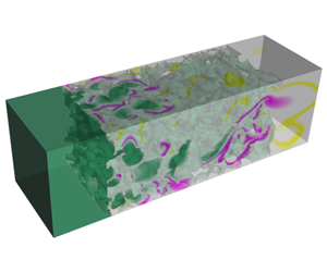
Left-hand panels: geometrical input for numerical simulations. Carbon felt (a) and carbon vitrified foam (b) reconstructed via X-ray computed tomography, and cluster of spheres (c). The cluster of spheres has been numerically generated to achieve a porosity intermediate between that of the two reconstructed materials by distributing the centres of the solid spheres in the domain according to a random uniform distribution. The parts of the spherical objects that lie out of the border of the domain are cut out along the transverse directions. Right-hand panels: simulations of solute transport at  $t^{\ast }=1$ with no reaction. The solute is transported from left to right with an applied pressure gradient $\unicode[STIX]{x0394}P/L$. The magenta and yellow colours indicate the beginning and the end of the solute front, respectively, at the same characteristic time, for a qualitative comparison.

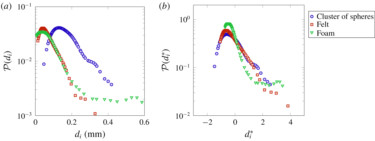
Probability distribution functions of pore diameters computed on several cross-sections on the  $(y,z)$ plane for the felt, foam and cluster of spheres. The PDFs refer to (a) the pore size $d_{i}$ and (b) the standardised pore size $d_{i}^{\ast }=(d_{i}-d)/\unicode[STIX]{x1D70E}(d_{i})$, with $d$ the mean value. To obtain a consistent statistical sample size for all three materials (around $650$), 4, 55 and 16 cross-sections have been selected for the felt, foam and cluster of spheres, respectively.
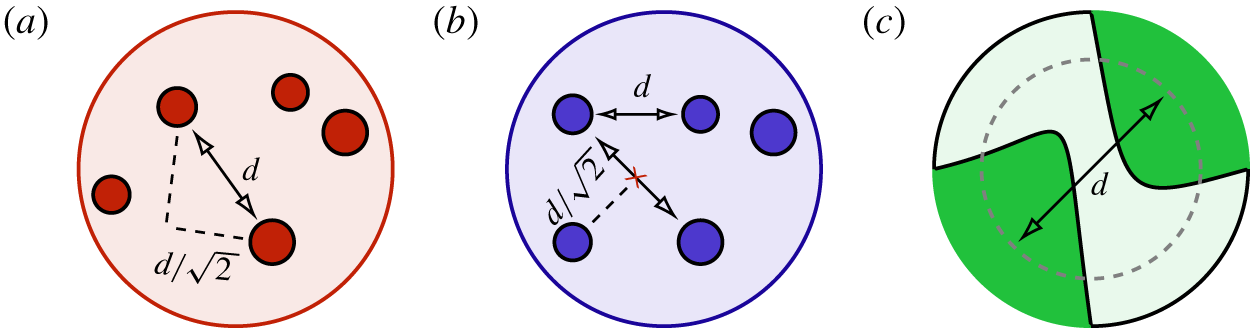
(a,b) Sketches describing the computation of pore diameters. The circles indicate the solid phase, i.e. the fibres composing the felt material or the spheres composing the bed of spheres. The dashed lines point out the criterion for selecting the distances between fibres as valid measurements of the pore diameters: the segments between the solid phase must pass at a minimum distance from the solid phase greater than  $d/\sqrt{2}$. (a) A computation of a pore diameter along a segment for which such a minimum distance is respected. (b) The situation where the fibres or spheres are positioned at the corners of a square of size $d^{2}$; for such a situation, the distance between solid objects computed along the diagonal of the square does not satisfy this geometric criterion. The minimum distance is computed along the major axis of the considered solid phase. (c) Sketch of the pore diameter computation in the foam material: the pore diameter is determined as the equivalent diameter of the pore.
The three-dimensional geometry of two real materials is acquired and reconstructed via X-ray computed tomography: a commonly used carbon felt composed of randomly intersected fibres and a carbon vitrified foam that exhibits a honeycomb-like microstructure. The materials are scanned by means of a metrological computed tomography system (Nikon Metrology MCT225), characterised by a micro-focus X-ray source (minimum focal spot size equal to  $3~\unicode[STIX]{x03BC}\text{m}$), a 16-bit detector with $2000\times 2000$ pixels and a cabinet ensuring a controlled temperature of $20\,^{\circ }\text{C}$. For further information about the real material reconstruction technique, the reader is referred to Maggiolo et al. (Reference Maggiolo, Zanini, Picano, Trovo, Carmignato and Guarnieri2019). A third material, a bed composed of spherical particles, is artificially generated by a uniform random distribution of spherical particles with diameter size $d_{s}=77~\unicode[STIX]{x03BC}\text{m}$. We have selected this specific third material in order to augment confidence in our fluid-dynamic data analysis and provide a rich variability in our samples, as depicted in figure 1; the number of spherical particles composing the cluster of spheres is set to attain the desired porosity value. The felt, the foam and the cluster of spheres are thus characterised by porosity values of $0.95$, $0.67$ and $0.81$, respectively. The length of the three samples is $L=1.3~\text{mm}$ and their cross-sectional area is a square with surface $A=0.615^{2}~\text{mm}^{2}$. The resolution of the computed tomography reconstructed models is maximised by minimising the voxel size and the focal spot size. In particular, the focal spot size is reduced by keeping the X-ray power at a minimum so that the metrological structural resolution is enhanced (Zanini & Carmignato Reference Zanini and Carmignato2017). On the other hand, the selected resolution of the artificial medium is sufficiently high to allow an accurate solution of the flow field, but without compromising the computational time. The resulting voxel size $\unicode[STIX]{x0394}x$ for the felt, foam (reconstructed via X-ray) and the cluster of spheres (artificially generated) is then 4.4, 5.9 and $7.7~\unicode[STIX]{x03BC}\text{m}$, respectively. The statistical difference between the materials in terms of pore diameter distribution is highlighted in figure 2 where the probability distribution function (PDF) of pore diameters is depicted. The computation of the PDF is not a trivial task. Typical strategies include methodologies based on effective pore area or volume computation. The latter strategies are effective if applied to porous structures formed mostly of disconnected pores, but they can become difficult to use in highly interconnected pore structures, such as a felt and a cluster of spheres. Therefore, given the great difference in the geometrical characteristics of the considered media, we adopt the following strategies. For the felt and the cluster of spheres we estimate the pore diameter distributions by computing all the distances between solid fibres and spheres, respectively, in different cross-sections. We only consider the interdistances between solid fibres or spheres for which the segment connecting the solid phases is not intersecting another solid phase or passing close to it, i.e. by setting a minimum distance from the solid phases. Such a distance is computed along the major axis of the solid phase (see figure 3a). In contrast to the felt and the cluster of spheres, the majority of the pore throats in the foam are not interconnected. Therefore, in the latter case, the PDF of the pore diameters is determined by evaluating the equivalent diameters of the pore areas, as depicted in figure 3(b). In both strategies, the pore diameters have been computed along planes perpendicular to the streamwise direction. It is important to notice that in the limit case represented by a squared pore defined, in the former strategy, by four fibres placed at the corners of the square and, in the latter strategy, by a squared cavity, both methodologies consistently compute the pore diameter as the side length of the square.
The values of the computed mean diameter  $d$ and the variance of the PDF $\unicode[STIX]{x1D70E}(d_{i})$ are reported in table 1. The significant difference of the sample microstructures is well visible from the PDFs in figure 2, with the cluster of spheres characterised by the largest mean pore diameter, i.e. $d/L=0.141$, and the foam material by the largest variance of pore diameter, i.e. $\unicode[STIX]{x1D70E}(d_{i})/L=0.108$. Also, we notice that the foam has the lowest value of porosity $\unicode[STIX]{x1D700}$. In § 4 we will observe how these microstructural differences influence the behaviour of the solute transport and reaction mechanisms.
2.3 Numerical accuracy and validation
We have carefully checked the accuracy of our numerical framework, which is mainly determined by the maximum resolution of the porous microstructure that we can achieve via X-ray computed tomography during material reconstruction. The error in the momentum equation for an incompressible flow  $\text{Err}=|1-\int _{in}u\,\text{d}A/\!\int _{out}u\,\text{d}A|$ is of $O(10^{-2})$ (see table 1 for the exact values).
We have also validated the numerical schemes adopted for simulating the reaction at the boundaries. To solve (2.2), we make use of the advective–diffusive Robin boundary condition applied to lattice Boltzmann formulations (Huang & Yong Reference Huang and Yong2015). We have compared the obtained numerical results with the analytical solution for the two-dimensional problem of diffusion and reaction in a rectangular domain with linear kinetics at a boundary (Zhang et al. Reference Zhang, Shi, Guo, Chai and Lu2012) and found an error within  $O(10^{-2})$. For further information about the numerical validation of the numerical framework the reader is referred to Maggiolo et al. (Reference Maggiolo, Picano and Guarnieri2016). We restrict our analysis to dimensionless times $t^{\ast }\sim 3$ (defined as the ratio between time and mean residence time; see equation (3.5)) since the simulations are long enough to provide a quantitative analysis of the dispersion and reaction mechanisms and to compare the behaviour of the porous electrodes in transporting and converting a solute.
Values of the parameters characterising the microstructures of the three considered materials. The computed compressible error  $\text{Err}$ is also reported.

2.4 Numerical set-up for porous electrode comparison
The pressure gradient is chosen such that the pump power is the same for all three cases:  $P_{w}=4~\text{kW}~\text{m}^{-3}$. Such a procedure allows us to correctly compare the efficiencies of the electrodes, in terms of a balance between the energy converted by the battery from/to an electric form and the energy spent to flow the electrolyte. The viscosity of the electrolyte is $\unicode[STIX]{x1D708}=4.4\times 10^{-6}~\text{m}^{2}~\text{s}^{-1}$ and its density $\unicode[STIX]{x1D70C}=1500~\text{kg}~\text{m}^{-3}$. The pump power is determined as
 $$\begin{eqnarray}P_{w}=\frac{\unicode[STIX]{x0394}P}{L}U,\end{eqnarray}$$
 where  $U$ is the spatially averaged velocity along the streamwise direction $x$ as defined by (3.3).
We are interested in the different behaviours of the electrodes in transporting and converting the solute. In our numerical approach, the physics of the reaction is defined by (2.2). By means of dimensional analysis, such an equation can be rewritten in terms of a dimensionless number that we address as the Thiele modulus; the Thiele modulus is defined as the ratio between the reaction rate and the characteristic diffusive mass transfer rate at the fluid–solid boundaries:
 $$\begin{eqnarray}\unicode[STIX]{x1D6F7}^{2}=\frac{k_{r}}{S_{s}{\mathcal{D}}_{m}}.\end{eqnarray}$$
 The length scale characterising the reactive flux at the fluid–solid boundary is the inverse of the specific surface area,  $1/S_{s}$. It is a measure of the mean pore size, and it is the smallest length scale characterising the physical system herein studied. We will further discuss the significance of this geometrical parameter in light of the numerical results later on.
In the present analysis, we vary the value of the Thiele modulus (i.e. the value of the reaction velocity  $k_{r}$) in order to identify the macroscopic behaviour of the considered materials when they are used as porous electrodes for a wide range of electrochemical reaction systems. A total of 17 simulations are performed: 5 for the felt, 5 for the the foam and 4 for the cluster of spheres, with varying reaction rate, together with 3 further simulations with null reaction, one for each material, as discussed in § 5. The pump power $P_{w}$ and the Schmidt number $Sc=10^{2}$ are constant in all the considered cases.
3 Spatial smoothing at larger length scales
The method of volume averaging is a mathematical technique that allows the derivation of continuum equations for multiphase systems (Whitaker Reference Whitaker2013). In particular, starting from the transport (2.1), valid in the fluid pores, and the boundary (2.2), it is possible to mathematically define an equation that is valid everywhere in the system, at a sufficiently larger scale. The resulting volume-averaged equation describes the transport in terms of the averaged quantities and effective parameters which convey information about spatial deviations of these physical quantities. In flows through porous media, the effective parameters are related to the underlying porous microstructure and their quantification is therefore useful for understanding the physical mechanisms contributing to the global efficiency of the system. In particular, for porous electrodes and chemical reactors, such analysis allows us to define the efficiency of the system by transferring the information about the rate of reaction from the microscopic characteristic scale to the ‘design length scale’  $L$.
$L$.
The spatial smoothing, or upscaling, is based on the identification of the characteristic lengths at the pore scale, mesoscale and macroscopic scale, to which the following averaging volumes correspond:
 $$\begin{eqnarray}d^{3}\ll V_{b}\ll V_{f}.\end{eqnarray}$$
 The averaging volume at the pore scale  $d^{3}$ is defined by the mean pore diameter $d$, whereas the total fluid volume of the sample is $V_{f}=\unicode[STIX]{x1D700}AL$. The mesoscale volume $V_{b}$ must lie between, larger than $d^{3}$ and smaller than the sample size. If these conditions are satisfied, the porous medium can be considered ‘disordered’ with respect to the mesoscale volume, in the sense defined by Quintard & Whitaker (Reference Quintard and Whitaker1994), and the spatial upscaling can rely on some simplifications that make the mathematical procedure more effective.
3.1 Mesoscopic description
We here make use of the spatial averaging procedure as suggested by Whitaker (Reference Whitaker2013). Firstly, the generic physical quantity  $\unicode[STIX]{x1D709}$ is decomposed into the averaged quantity $\langle \unicode[STIX]{x1D709}\rangle$ and its spatial fluctuation $\tilde{\unicode[STIX]{x1D709}}$:
 $$\begin{eqnarray}\unicode[STIX]{x1D709}=\langle \unicode[STIX]{x1D709}\rangle +\tilde{\unicode[STIX]{x1D709}}.\end{eqnarray}$$
 The spatially averaged quantities are computed at the mesoscale fluid volume  $V_{b}$ as
 $$\begin{eqnarray}\langle \unicode[STIX]{x1D709}\rangle =\frac{1}{V_{b}}\int _{V_{b}}\unicode[STIX]{x1D709}(\boldsymbol{x},t)\,\text{d}V,\end{eqnarray}$$
and the volume averaging theorem allows one to decompose the averaged derivatives as (Whitaker Reference Whitaker1967; Cushman Reference Cushman1982)
 $$\begin{eqnarray}\left\langle \frac{\unicode[STIX]{x2202}\unicode[STIX]{x1D709}}{\unicode[STIX]{x2202}x_{j}}\right\rangle =\frac{\unicode[STIX]{x2202}\langle \unicode[STIX]{x1D709}\rangle }{\unicode[STIX]{x2202}x_{j}}+\frac{1}{V_{b}}\int _{S_{b}}n_{j}\unicode[STIX]{x1D709}\,\text{d}S.\end{eqnarray}$$
 By considering the porous medium disordered with respect to the mesoscale volume, we can make use of the classic volume averaging theorem and of the following dimensionless parameters (with  $\unicode[STIX]{x1D70F}=L/U$ the mean residence time):
 $$\begin{eqnarray}x^{\ast }=\frac{x}{L};\quad t^{\ast }=\frac{t}{\unicode[STIX]{x1D70F}};\quad u_{j}^{\ast }(\boldsymbol{x})=\frac{u_{j}(\boldsymbol{x})}{U};\quad c^{\ast }(\boldsymbol{x},t)=\frac{c(\boldsymbol{x},t)}{c_{in}-c_{0}};\quad c_{0}^{\ast }=\frac{c_{0}}{c_{in}-c_{0}}\end{eqnarray}$$
in order to finally compute the following volume-averaged transport equation:
 $$\begin{eqnarray}\displaystyle & & \displaystyle \frac{\unicode[STIX]{x2202}\langle c^{\ast }(\boldsymbol{x},t)\rangle }{\unicode[STIX]{x2202}t^{\ast }}+\frac{\unicode[STIX]{x2202}\langle c^{\ast }(\boldsymbol{x},t)\rangle \langle u_{j}^{\ast }(\boldsymbol{x})\rangle }{\unicode[STIX]{x2202}x_{j}^{\ast }}=\frac{1}{Pe}\frac{\unicode[STIX]{x2202}}{\unicode[STIX]{x2202}x_{j}^{\ast }}\left(\frac{\unicode[STIX]{x2202}\langle c^{\ast }(\boldsymbol{x},t)\rangle }{\unicode[STIX]{x2202}x_{j}^{\ast }}+\frac{S_{s}L}{S_{b}}\int _{S_{b}}n_{j}\tilde{c}^{\ast }(\boldsymbol{x},t)\,\text{d}S\right)\nonumber\\ \displaystyle & & \displaystyle \quad -\,\frac{\unicode[STIX]{x2202}\langle \tilde{c}^{\ast }(\boldsymbol{x},t)\tilde{u} _{j}^{\ast }(\boldsymbol{x})\rangle }{\unicode[STIX]{x2202}x_{j}^{\ast }}-Da\,S_{s}L\left(\langle c^{\ast }(\boldsymbol{x},t)\rangle +\frac{1}{S_{b}}\int _{S_{b}}(\tilde{c}^{\ast }(\boldsymbol{x},t)-c_{0}^{\ast })\,\text{d}S\right).\end{eqnarray}$$
 It is interesting to notice that, besides the transport terms (accumulation, advection, diffusion and dispersion, from left to right), the reactive conditions at the fluid–solid boundaries are combined into the last term of equation (3.6). During the averaging procedure, we assume that the specific surface area  $S_{s}=S/V_{f}=S_{b}/V_{b}$ is constant at the averaging scale throughout the sample and we ensure the validity of this approximation by choosing an appropriate size of the mesoscopic averaging volume. In particular, by choosing the volume as
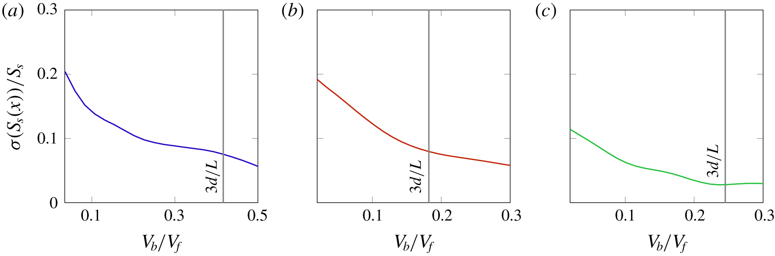
  $V_{b}=3d/L\,V_{f}$ we observe a sufficiently low value of the spatial fluctuations of the specific surface area, as depicted in figure 4. We therefore assume such a value as a reasonable one for performing the averaging procedure, also with respect to condition (3.1).
The standard deviation for the quantity  $S_{s}$ is plotted as a function of the mesoscopic volume averaging length for (a) the cluster of spheres, (b) the felt and (c) the foam material. By choosing a mesoscopic characteristic length as $3d$, the normalised fluctuation is reduced in all three material samples to ${\sim}O(10^{-1})$.
Equation (3.6) is defined via the dimensionless Péclet and Damköhler numbers, which quantify the balances between the fluid-dynamic mechanisms, advection, diffusion and reaction:
 $$\begin{eqnarray}\displaystyle & \displaystyle Pe=\frac{UL}{{\mathcal{D}}_{m}}, & \displaystyle\end{eqnarray}$$
 $$\begin{eqnarray}\displaystyle & \displaystyle Da=\frac{k_{r}}{U}. & \displaystyle\end{eqnarray}$$
Equation (3.6) represents a closure problem. To solve it, equation (3.6) should be formulated in terms of effective parameters that do not depend on the local concentration values. Various procedures have been proposed for achieving this mathematical expression, such as moment matching, moment-difference expansion and homogenisation (Mauri Reference Mauri1991). Identifying the exact mathematical solution for closing (3.6) is beyond the scope of the present study. Here, we impose a formulation of two mesoscopic parameters to obtain a one-dimensional volume-averaged equation; we then quantify via numerical simulations the leading and subleading microstructural terms of such a formulation and discuss their significance for possible mathematical closure strategies.
Since symmetric boundary conditions are imposed along  $y$ and $z$ directions, we thus rewrite (3.6) as
 $$\begin{eqnarray}\frac{\unicode[STIX]{x2202}\langle c^{\ast }(\boldsymbol{x},t)\rangle }{\unicode[STIX]{x2202}t^{\ast }}+\frac{\unicode[STIX]{x2202}\langle c^{\ast }(\boldsymbol{x},t)\rangle }{\unicode[STIX]{x2202}x^{\ast }}=\frac{1}{Pe_{b}}\frac{\unicode[STIX]{x2202}^{2}\langle c^{\ast }(\boldsymbol{x},t)\rangle }{\unicode[STIX]{x2202}{x^{\ast }}^{2}}-Da_{b}\,S_{s}L\,(\langle c^{\ast }(\boldsymbol{x},t)\rangle -c_{0}^{\ast }).\end{eqnarray}$$
The mesoscopic parameters convey information about the spatial fluctuations of the physical quantities induced by the porous microstructure. These parameters are defined as
 $$\begin{eqnarray}\displaystyle \frac{1}{Pe_{b}}\frac{\unicode[STIX]{x2202}^{2}\langle c^{\ast }(\boldsymbol{x},t)\rangle }{\unicode[STIX]{x2202}{x^{\ast }}^{2}} & = & \displaystyle \frac{1}{Pe}\left[\frac{\unicode[STIX]{x2202}^{2}\langle c^{\ast }(\boldsymbol{x},t)\rangle }{\unicode[STIX]{x2202}{x^{\ast }}^{2}}+\frac{\unicode[STIX]{x2202}}{\unicode[STIX]{x2202}x^{\ast }}\left(\frac{S_{s}L}{S_{b}}\int _{S_{b}}n_{x}\tilde{c}^{\ast }(\boldsymbol{x},t)\,\text{d}S\right)\right]\nonumber\\ \displaystyle & & \displaystyle -\,\frac{\unicode[STIX]{x2202}\langle \tilde{c}^{\ast }(\boldsymbol{x},t)\tilde{u} _{x}^{\ast }(\boldsymbol{x})\rangle }{\unicode[STIX]{x2202}x^{\ast }},\end{eqnarray}$$
 $$\begin{eqnarray}\displaystyle Da_{b}=Da\left(1+\frac{1}{\langle c^{\ast }(\boldsymbol{x},t)\rangle -c_{0}^{\ast }}\frac{1}{S_{b}}\int _{S_{b}}\tilde{c}^{\ast }(\boldsymbol{x},t)\,\text{d}S\right). & & \displaystyle\end{eqnarray}$$
 The mesoscopic Péclet number  $Pe_{b}$ is formulated so that it gathers all the diffusive and dispersive mechanisms, that is, the overall hydrodynamic dispersion, in the sense defined by Whitaker (Reference Whitaker2013). The overall dispersion in the porous medium is the sum of the molecular diffusion, the diffusive process induced by the microstructure and the dispersion mechanisms sustained by advective forces (i.e. the first, the second and the third terms on the right-hand side of (3.10)). The second parameter is the mesoscopic Damköhler number $Da_{b}$ that quantifies the spatial configuration of the concentration at the fluid–solid boundaries and it is therefore a measure of the actual reaction mechanism inside the porous electrodes. In the present analysis, we investigate the impact of these terms on the solute transport and reaction in the complex structure of the electrodes.
3.2 Macroscopic description
The three-dimensional mesoscopic domain  $V_{b}$ (in shaded blue colour) and the macroscopic domain of length $L^{\prime }$. The extremities of the macroscopic domain along the streamwise direction are identified by the positions $x^{\ast }=0^{+}$ and $x^{\ast }=1^{-}$ that correspond to the centroids of the mesoscopic averaging volume.
The final step of the spatial smoothing procedure consists of performing a further averaging step, at the design length scale, which is identified here by the sample macroscopic length  $L$. Again, we split the generic physical quantity $\unicode[STIX]{x1D709}$ into its averaged value $\bar{\unicode[STIX]{x1D709}}$ and spatial fluctuation $\unicode[STIX]{x1D709}^{\prime }$:
 $$\begin{eqnarray}\unicode[STIX]{x1D709}=\bar{\unicode[STIX]{x1D709}}+\unicode[STIX]{x1D709}^{\prime }.\end{eqnarray}$$
 The macroscopic averaging is identical to the one we have performed at the mesoscale, except for the size of the averaging volume that now is the sample fluid volume  $V_{f}^{\prime }=L^{\prime }A\unicode[STIX]{x1D700}$. The macroscopic volume is defined in order to perform the averaging as described and illustrated in figure 5: its length $L^{\prime }$ corresponds to the distance between the centroids of the mescoscopic averaging volumes $V_{b}$ at the extremities of the sample. Therefore, it is the case that $L^{\prime }=L-3d$. Since the mesoscopic quantity $\unicode[STIX]{x1D709}$ depends only on the position $x$ we can rewrite the macroscopic averaging as
 $$\begin{eqnarray}\bar{\unicode[STIX]{x1D709}}=\frac{1}{V_{f}^{\prime }}\int _{V_{f}^{\prime }}\langle \unicode[STIX]{x1D709}\rangle \,\text{d}V=\frac{L}{L^{\prime }}\int _{0^{+}}^{1^{-}}\langle \unicode[STIX]{x1D709}\rangle \,\text{d}x^{\ast },\end{eqnarray}$$
 where the first integration limit  $0^{+}$ and second limit $1^{-}$ here stand for the positions $x^{\ast }=(3/2)\,d/L$ and $x^{\ast }=(1-3/2)\,d/L$ corresponding to the extremes of the averaging volume $V_{f}^{\prime }$ (see figure 5). By applying macroscopic averaging to (3.9), we obtain the following averaged equation:
 $$\begin{eqnarray}\left.\frac{\text{d}\bar{c}^{\ast }}{\text{d}t^{\ast }}+\langle c^{\ast }\rangle \right|_{0^{+}}^{1^{-}}=\left.\frac{1}{Pe_{L}}\frac{\unicode[STIX]{x2202}\langle c^{\ast }\rangle }{\unicode[STIX]{x2202}x^{\ast }}\right|_{0^{+}}^{1^{-}}-Da_{L}S_{s}L^{\prime }\,(\bar{c}^{\ast }-c_{0}^{\ast }),\end{eqnarray}$$
 with the macroscopic Péclet and Damköhler numbers,  $Pe_{L}$ and $Da_{L}$, redefined with respect to the macroscopic averaged concentration and fluctuation values as
 $$\begin{eqnarray}\displaystyle & \displaystyle \left.\frac{1}{Pe_{L}}\frac{\unicode[STIX]{x2202}\langle c^{\ast }\rangle }{\unicode[STIX]{x2202}x^{\ast }}\right|_{0^{+}}^{1^{-}}=\left.\frac{1}{Pe}\frac{\unicode[STIX]{x2202}\langle c^{\ast }\rangle }{\unicode[STIX]{x2202}x^{\ast }}\right|_{0^{+}}^{1^{-}}+\frac{1}{Pe}\left[\frac{S_{s}L}{S_{b}}\int _{S_{b}}n_{x}\tilde{c}^{\ast }\,\text{d}S\right]_{0^{+}}^{1^{-}}-\langle \tilde{c}^{\ast }\tilde{u} _{x}^{\ast }\rangle |_{0^{+}}^{1^{-}}, & \displaystyle\end{eqnarray}$$
 $$\begin{eqnarray}\displaystyle & \displaystyle Da_{L}=Da\left(\frac{1}{\bar{c}^{\ast }-c_{0}^{\ast }}\frac{1}{S}\int _{S}(c^{\ast }-c_{0}^{\ast })\,\text{d}S\right). & \displaystyle\end{eqnarray}$$
 The macroscopic transport equation, equation (3.14), presents features similar to those of the pore-scale transport equation, equation (2.1), but the right-hand side of the equation presents two different terms, expressed as functions of the macroscopic observables (or flux ratios)  $Pe_{L}$ and $Da_{L}$. The first quantifies the overall dispersive behaviour of the flow embodying the effect of the microstructure as a function of the macroscopic concentration gradients; the second measures the actual reaction occurring inside the porous medium as a function of the averaged macroscopic concentration $\bar{c}^{\ast }$. We will later discuss the significance of these formulations in order to close the macroscopic advection–reaction–diffusion equation (3.14) and the conditions in which they can be considered as effective parameters, thus as physical quantities definable without referring to the small-scale concentrations.
The reactive term is defined with the additional geometrical knowledge provided by the dimensionless length  $S_{s}L^{\prime }$, which becomes $S_{s}L$ when one takes into account the total electrode length $L$. The values of $S_{s}L$ are listed in table 1. As already mentioned, the inverse of the specific surface area is the characteristic microscopic length. In the case of a pipe or of a duct, the inverse of the specific surface area varies linearly with the hydraulic diameter $d_{h}$. In other words, the inverse of the specific surface area can be considered as the generalised formulation of the hydraulic diameter. This evidence is confirmed by the fact that $4/(S_{s}L)\sim O(d/L)$ (see table 1). Consequently, the dimensionless length $S_{s}L$ represents a sort of aspect ratio of the porous medium, which, in the limit of a single circular pore of length $L_{c}$, becomes $S_{s}L\rightarrow 4L_{c}/d_{h}$. This parameter thus contains important information on the topology of the microstructure, which can play a prominent role in determining the working state of the porous electrode (in particular, see §§ 4.1 and 6).
4 Numerical simulations of solute transport and reaction
4.1 The mechanisms of conversion in a porous electrode
To measure the efficiency of a porous electrode, one has to quantify its intrinsic capability, provided by the microstructure, of spreading, transporting and promoting solute reactions. Such a quantification is often named electrode conversion, that is, the ratio between the rates of solute converted and solute injected into the electrode. The mathematical expression of electrode conversion can be deduced from the macroscopic equation of transport and reaction. It is intuitive to recognise that the reactive term in equation (3.14) represents, in a dimensionless form, the total amount of solute converted inside the electrode or, alternatively, the balance between the inlet and outlet fluxes. This term is therefore the measure of the electrode conversion, which at the steady state can be expressed as
 $$\begin{eqnarray}\displaystyle Da_{L}S_{s}L\,\bar{c}^{\ast }=\left(-\langle c^{\ast }\rangle |_{0^{+}}^{1^{-}}+\left.\frac{1}{Pe_{L}}\frac{\unicode[STIX]{x2202}\langle c^{\ast }\rangle }{\unicode[STIX]{x2202}x^{\ast }}\right|_{0^{+}}^{1^{-}}\right)\frac{L}{L^{\prime }}, & & \displaystyle\end{eqnarray}$$
 where the multiplier  $L/L^{\prime }$ has been introduced since we are measuring the conversion relative to the total electrode length $L$.
$L$.
Conversion values for the cluster of spheres (circles), felt (squares) and foam (triangles): (a) as a function of the Thiele modulus  $\unicode[STIX]{x1D6F7}^{2}$ and (b) as a function of the product between the Damköhler number and the geometrical factor $S_{s}L$.

The steady-state values of conversion computed from the numerical simulations are depicted in figure 6. In particular, the values of conversion as a function of the Thiele modulus  $\unicode[STIX]{x1D6F7}^{2}$ are indicated in figure 6(a). It can be noticed immediately that, at the same value of $\unicode[STIX]{x1D6F7}^{2}$, the foam performs better in terms of percentage of converted solute. It is now useful to recall that the Thiele modulus, as stated in (2.10), is defined as the ratio between the reaction rate at the fluid–solid boundaries $k_{r}S_{s}$ and the diffusive rate ${\mathcal{D}}_{m}S_{s}^{2}$. Therefore, at an equal Thiele modulus, the electrodes are characterised by the same mechanism of reaction at the boundaries, as stated in (2.2). Also, we remark that the Thiele modulus is proportional to the characteristic microscopic length of the system, that is, $\unicode[STIX]{x1D6F7}^{2}\propto S_{s}^{-1}$. Since the foam specific surface area is the largest and the molecular diffusion is the same (the Schmidt number is the same), at a fixed Thiele modulus the velocity of reaction $k_{r}$ in the foam is the highest. Intuitively, this will in turn translate into high values of global reaction rates and conversion, which are thus induced by the large area available to reaction in the foam material.
However, the high conversion value observed in the foam is not merely induced by a large specific surface area. The ratio between the conversion values of the foam and the felt is much greater than the ratio between their specific surface areas, at the same Thiele modulus (e.g. the specific surface areas are  $0.11$ and $0.33$, and the conversion values at $\unicode[STIX]{x1D6F7}^{2}\sim 0.4$ are $0.10$ and $0.55$ for the felt and the foam, respectively). Since the conversion is defined as the ratio between the global reaction rate and the averaged rate of solute transport $\unicode[STIX]{x1D70F}^{-1}=U/L$, it is not only a measure of the overall reactive flux at the boundaries, but it also depends on the behaviour of solute transport.
The global functioning of the electrodes in converting the solute is better quantified via the product  $Da\,S_{s}L$, which also encompasses the effects of the mean solute transport ( $U$) and of the microstructure ( $S_{s}L$). Figure 6(b) depicts the strong relationship between conversion and such a product, with all the data points denoting the different numerical solutions collapsing on a single master curve.
From figure 6, we can also observe two distinct regimes. At low Damköhler numbers, more precisely when  $Da\,S_{s}L<1$, the working mode of the electrode is reaction-limited. This regime corresponds to fast solute transport compared to the slow dynamics of the reaction at the boundaries or, equivalently, short solute residence time compared to long reaction times at the boundaries. Therefore, the physical system in this regime is governed by the fast dynamics with which the solute fills the pores so that the reactions occur uniformly at the steady state. In the limit defined by $Da\,S_{s}L<1$, the conversion is simply identified by ${\sim}Da\,S_{s}L$, that is, the global reaction rate is determined by the reaction velocity multiplied by the specific surface area, since at the boundaries $(c^{\ast }-c_{0}^{\ast })\sim 1$. The linear proportionality between conversion and $Da\,S_{s}L$ can also be easily seen in figure 6 where the data points are aligned along a line of slope 1. However, even though the reactions are almost homogeneous in the porous electrode in the reaction-limited regime, the solute transport can present some heterogeneous traits, as we will see and discuss in § 5.
The working mode of the porous electrode changes when  $Da\,S_{s}L\gtrsim 1$ and it becomes a mass-transfer-limited mode. This second regime is characterised by slow solute transport compared to the rate of reaction at the fluid–solid boundaries and the concentration of the solute inside the porous medium rapidly decreases along the electrode length, on average. The master curve slope is lower than unity, indicating that the conversion increases less than proportionally to the product $Da\,S_{s}L$, and then it eventually saturates at its theoretical maximum, i.e. the unit value.
4.2 The partitioning of the solute distribution in the porous medium
The ratio between the macroscopic Damköhler number and Damköhler number representing the partitioning of spatial solute concentration between fluid–solid boundaries and bulk. A value of one represents a perfect balance of such spatial partitioning with reactions occurring uniformly.

It is interesting to notice also that the macroscopic quantity formulated in the reactive term of equation (4.1) scales with the dimensionless product  $Da\,S_{s}L$, as highlighted in figure 7. By looking at the definition given in (3.16), we immediately recognise that the ratio $Da_{L}/Da$ quantifies the partitioning of the solute spatial distribution along the boundaries with respect to the averaged concentration. This observation suggests that such partitioning depends on both the reaction rate and the material geometrical characteristics; again the product $Da\,S_{s}L$ provides a reasonable measure of the solute partitioning mechanisms, evidencing the prominent role played by the aspect ratio $S_{s}L$. The values of $Da_{L}/Da$ tend to unity for low reaction rates and diminish for high reaction rates, as expected when the high velocity of the reaction significantly reduces the solute concentration at the fluid–solid boundaries. As a consequence, $c^{\ast }<\bar{c}^{\ast }$ at the boundaries and the value of the right-hand side of (3.16) diminishes.
The observed behaviour of the solute partitioning also suggests that the ratio  $Da_{L}/Da$ represents the closure variable for the reactive term of equation (3.14). Notably, such a variable conveys specific physical information and it can be interpreted as a sort of Nusselt number, as already suggested by Mauri (Reference Mauri1991), or, alternatively, as an effective fluid–solid mass-transfer coefficient (i.e. Sherwood number). Indeed, by combining equations (2.2) and (3.16), we can write
 $$\begin{eqnarray}\frac{Da_{L}}{Da}=\left(-\frac{{\mathcal{D}}_{m}}{S}\int _{S}\frac{\unicode[STIX]{x2202}c(\boldsymbol{x},t)}{\unicode[STIX]{x2202}n}\,\text{d}S\right)\frac{1}{k_{r}(\bar{c}^{\ast }-c_{0}^{\ast })}.\end{eqnarray}$$
 We notice that a value of unity of the ratio  $Da_{L}/Da$ indicates uniform reactions where the mass flux at the fluid–solid boundaries, determined by the numerator of (4.2), equals the product between the chemical reaction rate and the averaged concentration $k_{r}(\bar{c}^{\ast }-c_{0}^{\ast })$. Therefore $Da_{L}/Da=1$ identifies the maximum fluid–solid mass transfer achievable in the system with that value of solute concentration. In addition, we acknowledge that the mass-transfer coefficient decreases with increasing magnitude of the reaction rate with respect to flow velocity $k_{r}/U$. Such a trend indicates that the flow velocity is not high enough for delivering the solute into the pores and for sustaining the maximum chemical reaction theoretically attainable with the bulk concentration.
4.3 The contribution of the transport terms to the overall reaction
Since we are solving (2.1) at the pore scale, we can now focus on the individual contribution that each transport term has in determining the electrode operation, as stated in equations (3.14) and (3.15), in order to quantify the leading and subleading terms for the closure problem. The results of the numerical simulations indicate that the diffusive transport is negligible while the advective and dispersive forces play an important role, as depicted in figure 8. For the sake of clarity, it is important to stress that we refer to ‘dispersive’ forces following the traditional definition of the dispersion tensor (Whitaker Reference Whitaker2013); hence, we refer to the third term on the right-hand side of (3.15), while we name the other two terms ‘diffusive’. The global dispersion can thus be rewritten as
 $$\begin{eqnarray}\left.\frac{1}{Pe_{L}}\frac{\unicode[STIX]{x2202}\langle c^{\ast }\rangle }{\unicode[STIX]{x2202}x^{\ast }}\right|_{0^{+}}^{1^{-}}=-\langle \tilde{c}^{\ast }\tilde{u} _{x}^{\ast }\rangle |_{0^{+}}^{1^{-}}.\end{eqnarray}$$
 This result is not surprising, given the very low molecular diffusivity that species have in liquids or, in other words, the high Schmidt number that characterises our system. In fact, the mathematical expression of the two diffusive terms contains prefactors dependent on the Schmidt number. If we define the Reynolds number as  $Re=U/(S_{s}\unicode[STIX]{x1D708})$, the prefactors are $Pe^{-1}=(S_{s}L\,Re\,Sc)^{-1}$ in the case of the first diffusive term on the right-hand of (3.15) and $Pe^{-1}S_{s}L=(Re\,Sc)^{-1}$ in the case of the second term. Even in the case of low flow velocity and low Reynolds numbers, which are typical for liquids flowing through porous media, at high Schmidt numbers the Péclet number is high, unless the porous electrode is characterised by a very low value of the aspect ratio $S_{s}L$. A low value of this aspect ratio indicates a squat medium, with mean diameter larger than its length. Such a design is rarely encountered in electrodes because of its poor efficiency, induced by the small extent of reactive solid surface. Therefore, the first term on the right-hand side of (3.15) is expected to be negligible for most applications involving liquid flow solutions, as is the second term as long as the product of the Reynolds and Schmidt numbers is not less than unity. The values of the Reynolds and Péclet numbers are reported in table 2.
Individual contributions of transport terms to conversion. The sum of the contributions (solid line) is partitioned between advective (open symbols), dispersive (filled symbols) and two other diffusive terms, which here we address as pure diffusive term (dashed lines) and second diffusive term (dotted lines). The pure and second diffusive terms refer to the first and second terms on the right-hand side of (3.15), while the dispersive term refers to the third one. Note that the legend only indicates the symbols referring to the cluster of spheres material (circles, blue colour); the other symbols denote the felt material (squares, red colour) and the foam material (triangles, green colour). Inset: zoom of the dispersive terms plotted in logarithmic scale, pointing out a quasi-linear dependence on  $Da\,S_{s}L$ at high reaction rates.

The advective and dispersive terms significantly contribute to the transport. Figure 8 also highlights that such terms have a similar trend in the three materials: in the reaction-limited regime the conversion of the electrode is fully quantified by the balance between advective fluxes at the inlet and outlet, while the dispersion plays a negligible role. This situation corresponds to a moderate decrease of the averaged concentration in the medium along the streamwise direction at the steady state, and an almost uniform reaction, due to the low consumption of solute at the fluid–solid boundaries. When the reaction rate becomes limited by mass transport, that is, in the mass-transfer-limited regime, the mechanism of transport partitioning changes. In the latter case, the dispersive forces start to play a pivotal role, contributing to up to the 20 % of the global reaction. We can observe such a substantial contribution in figure 8 and also notice that, in the mass-transfer-limited regime, it increases proportionally to  $Da\,S_{s}L$.
4.4 The interaction between dispersion and reaction mechanisms
Example of solute transport along preferential paths in the felt material at  $Da\,S_{s}L=3.4$. (a) Contour lines of the dimensionless velocity fluctuations $\tilde{u} ^{\ast }$. (b) The dimensionless concentration $\tilde{c}^{\ast }$. The depicted section is taken at the position $y^{\ast }=0.24$, which corresponds to half of the lateral dimension.
Values of the mean residence time and of different flow dimensionless numbers for the three considered materials. The Schmidt number is  $Sc=100$ for all cases.
The dispersive term  $\langle \tilde{c}^{\ast }\tilde{u} _{x}^{\ast }\rangle$ represents the contribution provided by the microstructure in spreading the solute, at high Schmidt numbers. This contribution, which is analogous to the Reynolds stresses in turbulent flows, is a measure of the correlation between solute concentration and flow velocity spatial fluctuations. Alternatively, it can be conceptualised as the mean contribution to transport imposed on the solute concentration by such spatial fluctuations.
With low reaction rates, this mechanism of transport is switched off, while it is triggered when, with increasing product  $Da\,S_{s}L$, the reaction rate at the boundaries, $k_{r}S_{s}$, starts to be comparable to the mean advective transport rate, $U/L$. We can conceptualise this situation of the electrode as a demanding condition, where the high requirement of solute at the boundaries for sustaining reactions cannot be fulfilled everywhere, especially in the pores characterised by low flow velocities, and a further mechanism of transport is triggered for bolstering the reaction of solute in the electrode. This mechanism consists of the exploitation of the high-velocity flow paths for sustaining the global reaction. Indeed, we observe the creation of preferential flow paths for the solute transport in the pores characterised by high flow velocities, as clearly depicted in figure 9. In the low-velocity pores the reaction rate is high compared to mass transport and the solute is consumed rapidly, so that close to the inlet, for $\tilde{u} _{x}^{\ast }<0$, we have $\tilde{c}^{\ast }<0$. On the contrary, the mechanism in the high-velocity pores is different, since there the mass transport can sustain more reaction. In these pores, the solute is not consumed immediately, but rather transported for longer distances and decreases gradually along the flow direction, so that, at the inlet, for $\tilde{u} _{x}^{\ast }>0$, we have $\tilde{c}^{\ast }>0$. This correlation between solute concentration and flow velocity is mathematically translated into $-\langle \tilde{c}^{\ast }\tilde{u} _{x}^{\ast }\rangle |_{0^{+}}^{1^{-}}=\langle \tilde{c}^{\ast }\tilde{u} _{x}^{\ast }\rangle |_{0^{+}}-\langle \tilde{c}^{\ast }\tilde{u} _{x}^{\ast }\rangle |_{1^{-}}>0$.
Sketch of the solute transport in connected parallel pores with different sizes. (a) The functioning of pore filling is depicted; it is calculated accordingly to the balance between reactive and mass transfer rates. (b) The pore velocities are determined with the assumption of an equal pressure drop in the pores.

We can further confirm this correlation by computing the length  $\ell$ necessary for consuming the solute into a specific pore. This length can be estimated by imposing the balance between reaction rate and mass transport in the pore, that is, by reformulating the equation $Da\,S_{s}L=1$ at the single-pore level, from which we resolve
 $$\begin{eqnarray}\ell \sim \frac{ud}{k_{r}},\end{eqnarray}$$
 where we impose  $S_{s}=d^{-1}$. Let us then consider two pores, one small with $d_{1}<d$ and one large with $d_{2}>d$, as the sketch in figure 10 depicts. We make the hypothesis that the porous system is represented by these two pores connected in parallel; then, they experience the same pressure drop, so the relation between the velocities $u_{1}/d_{1}^{2}=u_{2}/d_{2}^{2}$ holds. We thus apply (4.4) to obtain the difference between pore filling lengths as $\unicode[STIX]{x0394}\ell /\ell _{1}\sim (d_{2}/d_{1})^{3}-1$. This result points out that the higher the pore variability, the greater the difference in the solute transport lengths and the greater the correlation between high-velocity pores and high concentration values. Indeed, the foam material that presents the higher pore variability (see table 1) exhibits a higher dispersive flux for high reaction rates. For low values of reaction $k_{r}$, the filling length is greater than the sample length, $\ell >L$; in this situation, in the reaction-limited regime, all pores are similarly filled along the electrode length and the correlation $\langle \tilde{c}^{\ast }\tilde{u} _{x}^{\ast }\rangle \sim 0$. As we increase the reaction rate, $\ell$ starts to be smaller than $L$, firstly in the low-velocity pores, then in the slightly faster pores and so on, so that the number of pores contributing to the global dispersive term increases as well as the magnitude of the correlation $\langle \tilde{c}^{\ast }\tilde{u} _{x}^{\ast }\rangle$. This trend explains why the dispersive term increases with increasing reaction rate in the mass-transfer-limited regime.
The dispersive terms are plotted against the averaged concentration gradients in order to extract the effective Péclet numbers, for each material sample, according to equation (4.3). The linear fit has been performed for the simulated cases for which  $Da\,S_{s}L>1$ (filled symbols), since for lower values (open symbols) the dispersive terms are considered negligible.
5 Modelling the effective dispersion in porous media
It has been long debated as to whether the dispersion mechanisms in porous media depend on the reaction (e.g. Valdés-Parada, Lasseux & Whitaker Reference Valdés-Parada, Lasseux and Whitaker2017). The possibility of computing each individual microstructural term that contributes to the transport and reaction of a solute allows us to further investigate this relationship in the case of high Schmidt numbers. It also allows us to test the observation formulated in (4.3), which suggests that the macroscopic (3.14) can be closed by means of an effective parameter represented by the macroscopic dispersive coefficient  $Pe_{L}$. We then assume the effective dispersion mechanisms, at such Schmidt numbers, to be independent of the reaction rate and we test this hypothesis. Therefore, an effective Péclet number $Pe_{L}$ is extracted for each material sample by fitting the microstructural values provided from (4.3) at a steady state. Figure 11 illustrates such a procedure; the linear fit has been performed by taking into account only the values corresponding to $Da\,S_{s}L>1$, since for lower values the dispersive term is considered negligible. According to this procedure, we evaluate the effective parameter that quantifies the global dispersion by assuming such dispersion proportional to the gradient of the averaged concentration. The computed effective Péclet numbers are listed in table 2.
To investigate the validity of the extracted  $Pe_{L}$ values, three further numerical simulations have been performed, one for each material, with the reaction switched off ( $k_{r}=0$). These three cases thus correspond to pure advective–dispersive problems and they should indicate whether the effective Péclet numbers are a good measure of the dispersive forces at low reaction rates, without loss of generality. For the three new cases, we compute the time-dependent breakthrough curves as a measure of the solute transport:
 $$\begin{eqnarray}\left.{\mathcal{B}}(t)=\frac{\displaystyle \int _{A}(c^{\ast }(\boldsymbol{x},t)-c_{0}^{\ast })u_{x}^{\ast }(\boldsymbol{x})\,\text{d}A}{\displaystyle \int _{A}u_{x}^{\ast }(\boldsymbol{x})\,\text{d}A}\right|_{1},\end{eqnarray}$$
 and compare them with the analytical solution provided by the effective parameter  $Pe_{L}$ (Kreft & Zuber Reference Kreft and Zuber1978):
 $$\begin{eqnarray}{\mathcal{B}}(t^{\ast })=\frac{1}{2}\left[\text{erfc}\left(\sqrt{\frac{Pe_{L}(1-t^{\ast })^{2}}{4t^{\ast }}}\right)+\exp (Pe_{L})\times \text{erfc}\left(\sqrt{\frac{Pe_{L}(1+t^{\ast })^{2}}{4t^{\ast }}}\right)\right].\end{eqnarray}$$
Complementary breakthrough curves for the three materials with null reaction ( $k_{r}=0$) versus dimensionless time $t^{\ast }$. The symbols indicate the numerical solution whereas the solid lines indicate the analytical solution in (5.2), with the parameter $Pe_{L}$ extracted from (4.3). Inset: PDFs ${\mathcal{P}}$ of spatial solute concentration for the three materials at $t^{\ast }\sim 2$; the dimensionless concentration value is reported on the abscissa.

The time-dependent complementary breakthrough curves  $1-{\mathcal{B}}(t)$ for the three materials with null reaction are shown in figure 12. The decay behaviour is qualitatively similar for the three materials, but we observe a very sharp decay for the felt and a smooth one for the foam. This observation suggests that the dispersion mechanism is more uniform in the felt, with the majority of the solute reaching the outlet at the same time, as it would be similarly observed in the case of transport of a homogeneous front. Instead, in the foam the distribution of concentration at the outlet is non-uniform, indicating that some pores are filled much faster than others. This different dispersive behaviour is also highlighted in the inset of figure 12 where the PDFs of the dimensionless concentration values are reported at the dimensionless time $t^{\ast }\sim 2$. Again, the variability in solute transport is visible in the foam material: some parts of the solute are characterised by longer residence times, so that the PDF presents a clear bimodal shape. It is intuitive to observe the relation between such a bimodal shape and the high tail of the residence time distribution of the foam: they both describe the anomalous dispersion behaviour triggered by the variability of the foam microstructure which, in turn, gives rise to substantially different residence times and concentration values.
Interestingly, the dispersive trend in these three unsteady simulations is well captured by the previously extracted steady-state effective Péclet numbers, with the foam characterised by the highest dispersion and the felt by the lowest. However, differences can again be observed; in particular, while a constant effective Péclet number describes well the dispersive behaviour in the case of the felt and the cluster of spheres, it fails to predict the long-tail behaviour observed for the foam, as well depicted in figure 12.
To understand the discrepancy between the solution extrapolated from the steady-state reactive simulations and numerical solutions of pure advective–dispersive transport, it is useful to look at the breakthrough curves in the presence of reactions. The complementary breakthrough curves with activated reactions for the three materials are plotted against dimensionless time in figure 13. In all cases the values decrease until  $t^{\ast }\sim 1$ when they reach a constant value, which shows that a global balance is found between the mass of solute introduced in the porous electrode and the mass that reacts inside it, after a time comparable to the mean residence time.
Complementary breakthrough curves for (a) the felt, (b) the foam and (c) the bed of spheres. Symbols: complementary breakthrough curves with  $k_{r}=0$. Solid lines: complementary breakthrough curves with reaction; the increasing darkness of the solid lines indicates the reduction of the reaction rate $k_{r}$.
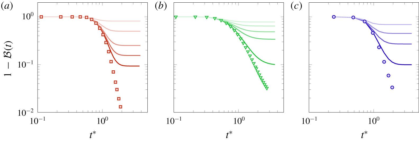
Since the solute is consumed in the porous electrode by the reaction occurring at the fluid–solid boundaries, the complementary breakthrough curves with reaction do not tend to zero as in the case of the pure advective–dispersive transport. The long tail observed in the case of null reaction in the foam material is thus filtered out by the reaction. In other words, the reaction can homogenise the the spatial distribution of solute in the medium by mitigating the mechanisms of early arrivals and late delays responsible of the long-tailed shape of the breakthrough curve.
The long-time tail characterising the breakthrough curve is a typical feature of non-Fickian transport in highly dispersive media, such as the foam material. The anomalous behaviour emerges because the nature of transport in such materials is highly heterogeneous. This situation implies that the system cannot be considered at local equilibrium and the representative volume  $V_{b}$ is not well mixed (the concept of well mixed is equivalent to that of a ‘disordered’ medium with respect to the mesoscale volume). In such conditions, even though the reactions occur rather homogeneously (see § 4), the dispersive mechanism cannot be described by a temporally and spatially homogeneous Péclet number, and equations (4.3) and (5.2) are no longer valid (Dentz et al. Reference Dentz, Icardi and Hidalgo2018).
From these observations, we conclude that the pre-asymptotic dispersion mechanism (i.e. for  $t^{\ast }<1$) is independent of reaction and well approximated by a model based on a homogeneous effective Péclet number, even in highly dispersive media. In the mass-transfer-limited regime, the anomalous dispersion mechanisms are filtered out because of the presence of high reaction rates that govern the transport in the pores and non-Fickian effects are negligible; as highlighted in figure 11, in such conditions, dispersion effects are proportional to the homogenised concentration gradients and the model can thus correctly describe the asymptotic solution of solute transport. In the reaction-limited regime, by contrast, it fails to represent the asymptotic dispersive behaviour in the presence of complex microstructures (e.g. the foam), where the mechanisms of delays and early arrivals of the solute are pronounced, leading to a strongly heterogeneous transport and a not-well-mixed medium, for long characteristic times.
6 Design of porous electrodes
Once the role of the microstructure in transporting, dispersing and converting the solute has been clarified, its potential impact on the design of porous electrodes has to be debated, in order to make the fluid-dynamic understanding of the system more comprehensive. When one deals with the practical design of an electrode, an optimal operative condition is not unequivocally determined by the converted power. Indeed it is not only the amount of mass reacted over the mass injected that should be taken into account, but also the global reaction rate attained in the system. Whilst the former is quantified by the conversion factor formulated in (4.1), the latter can be expressed through the ratio between the macroscopic Damköhler number obtained and the Damköhler number determined as input, that is,  $Da_{L}/Da\bar{c}^{\ast }$. This term expresses the power output of the system in relation to its theoretical maximum that is found when $Da_{L}=Da$.
Figure 14 sketches the principles of the functioning of an electrode from a perspective of both conversion and power output. While conversion varies from values close to zero to unity, the dimensionless power output  $Da_{L}/Da\bar{c}^{\ast }$ tends to unity in the reaction-limited regime, when the maximum power is extracted in the electrode, and it decreases for higher values of $Da\,S_{s}L$ in the mass-transfer-limited regime.
(a) The functioning of the electrode, in terms of dimensionless power output  $Da_{L}/Da\bar{c}^{\ast }$ and conversion $Da_{L}S_{s}L\bar{c}^{\ast }$, on varying the parameter $Da\,S_{s}L$. The dashed and solid curves are obtained by fitting the data from numerical simulations (circles). The resulting fitted curves are $y=0.8\exp (-0.34\,x)$ for the power output (dashed line) and $y=0.84[1-\exp (-1.0\,x)]$ for the conversion (solid line). On the right is illustrated the balance between mass entering the medium and reacting at the surface that determines the formulation of the parameter $Da\,S_{s}L$: (b) for a pipe or a duct and (c) for a porous electrode with a more complex geometry.

Ideally, one would like to achieve the best conversion values, but one is often limited by the required power output. Figure 14 clearly depicts such a cumbersome restriction, with a rapid decrease of output power with increasing conversion. It is therefore important that, on the basis of the application, one considers how to balance these two mechanisms. Once the required power output is defined, the design of the system that guarantees optimal operative conditions can be identified. For instance, one could choose to sacrifice the effectiveness of the conversion in order to maximise the output power and minimise the battery size. Or, alternatively, one can decide to convert more efficiently the solute with an oversized system.
Interestingly, the present analysis reveals that the operating modes of all the investigated materials can be defined on the basis of a single parameter,  $Da\,S_{s}L$, whose physical significance is conceptualised in the sketch of figure 14. Once such a functioning is decided, the design of the system can be based on the corresponding value of the parameter $Da\,S_{s}L$. In light of this result, a practical and universal design procedure can be established. For example, given the characteristics of the chemical reaction, i.e. $k_{r}$, the material properties $S_{s}$ and the power to be spent to flow the electrolyte, which provides the mean velocity $U$, the optimal length $L$ of the electrode is determined by imposing the desired $Da\,S_{s}L$. Alternatively and more interestingly, given the chemical reaction and the pump power of a system, the optimal design and aspect ratio of the material, $S_{s}L$, can be identified for a specific application.
7 Summary and conclusions
We have used X-ray computed tomography combined with the lattice Boltzmann method for simulating the pore-scale solute transport and reactions in reconstructed real porous electrodes. This methodology has allowed us to gain an insight into the transport and reaction mechanisms occurring inside various porous microstructures at high Schmidt numbers. We have compared two real materials, a carbon felt and a carbon vitrified foam, with a numerically generated material composed of solid spherical particles. We have made use of the volume-averaging technique to upscale and homogenise the advection–reaction–diffusion transport equation and identify the microstructural terms responsible for the functioning of the three electrodes at the macroscopic scale. This comparison has been made in terms of macroscopic conversion efficiency, with varying the reaction rate at the fluid–solid boundaries inside the electrodes, i.e. the Damköhler number  $Da$, at an equal pump power.
The foam material outperformed the other electrodes in terms of percentage of power conversion. The primary reasons are its high specific surface area and its intricate microstructure, highlighted by the wide variability of its pore sizes that promotes solute dispersion. With regards to the working modes of the electrodes, two main regimes have been identified: (i) the reaction-limited regime, identified by  $Da\,S_{s}L<1$, and (ii) the mass-transfer-limited regime, corresponding to larger values of $Da\,S_{s}L$. These two operating regimes, which are typical of monolithic reactors (Hayes & Kolaczkowski Reference Hayes and Kolaczkowski1994), are here found to be unequivocally determined for the three electrodes by a single parameter: the product of the Damköhler number and the microstructural aspect ratio $S_{s}L$.
By means of the homogenisation procedure, we have also quantified the impact of the dispersion behaviour on the functioning of the electrodes. In the reaction-limited regime, reactions occur rather homogeneously in the medium, and the dispersion plays a minor role. In these conditions, conversion increases proportionally with  $Da\,S_{s}L$. When approaching the mass-transfer-limited regime, conversion increases less than proportionally with $Da\,S_{s}L$ and dispersion mechanisms contribute incrementally to the solute transport and reaction. We have found that the dispersion mechanism is quantified and mathematically expressed by the spatial correlation between solute concentration and high-flow-velocity paths. The solute is transversally scattered and transported along pores characterised by high flow velocities, a mechanism of selection of preferential paths that sustains transport and reaction in the porous electrodes at high reaction rates.
The volume-averaging procedure has allowed us to identify the closure variables for upscaling the pore-scale advection–reaction–diffusion equation. Such variables are an effective fluid–solid mass-transfer coefficient, which is mathematically expressed as the partitioning between solute concentration at the fluid–solid boundaries and in the bulk, and an effective Péclet number.
We have then investigated the possibility of modelling the dispersion mechanism in both the pre-asymptotic and asymptotic regimes via such a temporally and spatially homogeneous Péclet number. Through this analysis, we have remarked that a model based on a macroscopic effective Péclet number can correctly represent the solute transport at short characteristic times of any reactive conditions. This observation has been corroborated by the comparison between the latter model and the numerical solution of purely advective–dispersive transport with null reaction. For long characteristic times and low reaction rates, the model fails to reproduce the non-Fickian transport behaviour of highly heterogeneous media (e.g. the foam material), since it rests on the assumption of a well-mixed medium at the intermediate mesoscopic scale, a condition that is not fulfilled in the presence of delays of the transported solute (Dentz et al. Reference Dentz, Icardi and Hidalgo2018). By contrast, in the mass-transfer-limited regime, the dispersion is well captured through the effective Péclet number, since the fluid dynamics inside the pores is characterised by high reaction rates that mitigate such delay mechanisms.
Finally, we provide guidelines for an optimal design of porous electrodes. In particular, having recognised that the conversion values for all the investigated materials can be determined on the basis of the Damköhler number and the microstructural aspect ratio, we have suggested a novel designing practice: given the rate of the electrochemical reaction and the flow velocity for a specific application, that is, given the Damköler number, the porous electrode can be designed to exhibit the optimal aspect ratio  $S_{s}L$, corresponding to the desired working states of the system, irrespective of whether it belongs to the reaction-limited or the mass-transfer-limited regime.
Declaration of interests
The authors report no conflict of interest.


 Open access