

Introduction
Designing novel materials with superior tailored properties is the ultimate goal of modern engineering applications.[Reference Compton and Lewis1–Reference Yeo, Jung, Martín-Martínez, Ling, Gu, Qin and Buehler5] In the past few decades, with rapid advances in high-performance parallel computing, materials science, and numerical modeling, many essential properties of materials can now be calculated using simulations with reasonable accuracy. For example, the chemical reactivity and stability of molecules can be estimated using density functional theory (DFT).[Reference Chen, Martin-Martinez, Jung and Buehler6,Reference Chen and Buehler7] Molecular dynamics (MD) and the finite element method (FEM) can be applied to simulate a wide range of mechanical behaviors of materials at the nano-scale and continuum-scale, respectively.[Reference Chen, Martin-Martinez, Ling, Qin and Buehler8,Reference Xu, Qin, Chen, Kwag, Ma, Sarkar, Buehler and Gracias9] Nowadays, simulations of material properties can be performed on a laptop, workstation, or computer cluster, depending on the computational cost. In general, performing simulations to predict the properties of a material is much faster and less expensive than synthesizing, manufacturing, and testing the material in a laboratory. Moreover, simulations offer very precise control over environments and offer more detailed information of material behavior and associated mechanisms under different conditions, many of which cannot or would be very difficult to be observed using experiments. For instance, the stress field of a composite material under fracture and the motions of each molecule in an organic material under loading can be predicated in simulations but are difficult to measure in experiments. It is this reason that many studies in the literature have focused on advancing computational tools and methods to model various types of materials.[Reference Hatano and Matsui10–Reference Ma, Hajarolasvadi, Albertini, Kammer and Elbanna18]
Compared with solely predicting properties of known materials, designing new materials to achieve tunable properties is a more important problem for scientific and engineering purposes. In fact, predicting materials’ properties and designing materials are quite different problems, in which the former is often referred to as a forward modeling problem and the latter is an inverse design problem. For a forward modeling problem, the structure (e.g., atomic constituents, crystal structure, and topology) of the material to be investigated is usually given and the properties are governed by physical laws such as quantum mechanics, thermodynamics, and solid mechanics. Consequently, various types of properties at different length- and time-scales can be calculated numerically by solving the corresponding governing equations using proper physics-based modeling tools such as DFT, MD, and FEM. However, there is no physics-based modeling tool that can solve inverse design problems—that is, to generate the structure of a material with a given set of required properties. In practice, one common approach to solve inverse design problems is using domain knowledge and experience (intuition) to narrow down the design space and propose new materials by trial and error, as shown in the flow chart of Fig. 1. For example, many biomaterials such as nacre and bone have remarkable mechanical properties despite being composed of relatively weak components. Consequently, it is plausible to study the architectures of these biomaterials and learn the structure–property relationships necessary for achieving improved properties of materials. Thus, the knowledge gained can be applied to design new materials in a case-by-case manner. This approach is referred to as biomimicry and pursuant designs are termed bioinspired.[Reference Chen, Martin-Martinez, Ling, Qin and Buehler8,Reference Gu, Libonati, Wettermark and Buehler19–Reference Mueller, Raney, Kochmann and Shea25] If the design space can reasonably be parameterized into compositional and configurational degrees of freedom, it is possible to solve inverse design problems by using a physics-based modeling tool with a brute-force exhaustive search approach to explore the entire design space. This approach is referred to as high-throughput computational screening and is explored for various materials. For example, Emery et al. used high-throughput DFT to screen ABO3 perovskites based on thermodynamic considerations.[Reference Emery, Saal, Kirklin, Hegde and Wolverton26] Chen et al. proposed the most stable molecular structures for eumelanin and polydopamine by using high-throughput DFT to screen thousands of probable candidates.[Reference Chen, Martin-Martinez, Jung and Buehler6,Reference Chen and Buehler7] However, when the design space is vast, using a brute-force approach is computationally infeasible even with modern algorithms and supercomputers. Therefore, optimization methods such as greedy algorithms and gradient-based algorithms are typically implemented in inverse design problems to search for optimal designs without having to explore the entire design space. Despite the high computational efficacy of optimization methods, the optimal solutions often depend on the initial configuration (initial values of design variables) adopted in the optimization process. Therefore, the solutions obtained from those optimization methods not only vary from one initial configuration to another but also, in some cases, can be stuck in local minima or critical points. Consequently, it is crucial to investigate alternative methods to make the inverse design of materials possible.
Comparison of materials’ design approaches based on domain knowledge and ML. The flowchart shown in blue represents the domain-knowledge-based materials’ design approach and the flowchart shown in green represents the machine-learning-based materials’ design approach.
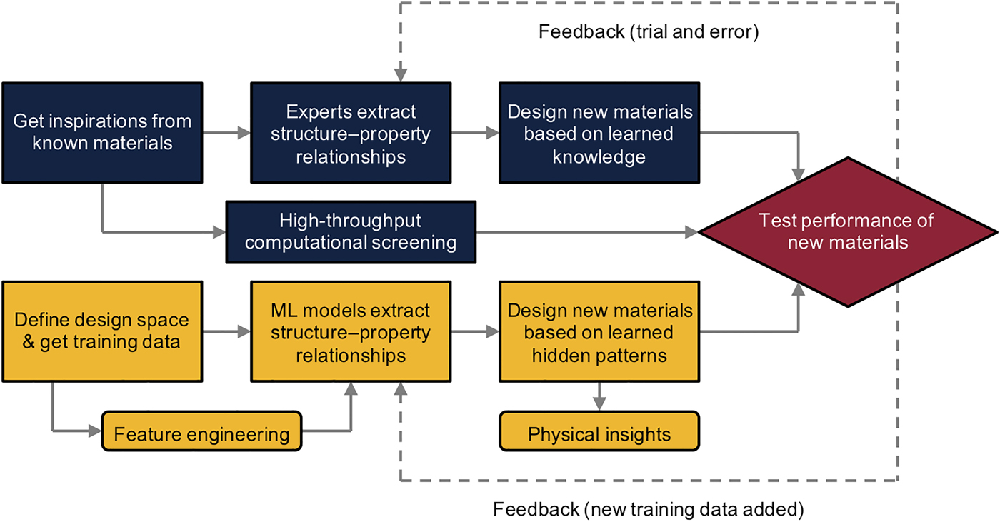
In addition to the old-fashioned materials’ design approaches mentioned above, data-driven approaches based on machine learning (ML) techniques may transform the approaches of materials’ design in the future as shown in Fig. 1. ML, a branch of artificial intelligence, uses a variety of statistical and probabilistic methods that allow computers to learn from experience and detect hidden patterns (the correlations between input and output variables) from large and oftentimes noisy datasets.[Reference Blum and Langley27–Reference Michalski, Carbonell and Mitchell30] Through evaluating only a portion of the possible data, ML algorithms can detect hidden patterns in the data and learn a target function that best maps input variables to an output variable (or output variables)—a procedure referred to as the training process. With the extracted patterns, predictions for unseen data points can be made and allow for generalizations with a limited amount of data rather than using an exhaustive approach to explore all possible data points. Recently, ML has turned our daily life to be more convenient in numerous ways by influencing image recognition, autonomous driving, e-mail spam detection, among others.[Reference Butler, Davies, Cartwright, Isayev and Walsh31–Reference Li, Yang, Zhang, Ye, Jesse, Kalinin and Vasudevan38]
In the field of materials science, most ML applications are concentrated on discovering new chemical compounds or molecules with desired properties. Those studies can be categorized into a subfield of ML for materials chemistry. One of the most challenging and active research topics in this subfield is finding a suitable representation (e.g., descriptors and fingerprints) of a molecule or crystal structure to be used as input variables in ML models.[Reference Faber, Lindmaa, von Lilienfeld and Armiento39,Reference Schütt, Glawe, Brockherde, Sanna, Müller and Gross40] This process is referred to as feature engineering (Fig. 1). Such representation can be coarse-level chemo-structural descriptors or something containing information of molecular electronic charge density.[Reference Pilania, Wang, Jiang, Rajasekaran and Ramprasad34] In this area, Dieb et al. applied ML models to search for the most stable structures of doped boron atoms in graphene[Reference Dieb, Hou and Tsuda41]. Hansen et al. applied a number of ML techniques to predict ground-state atomization energies of small molecules.[Reference Hansen, Montavon, Biegler, Fazli, Rupp, Scheffler, Von Lilienfeld, Tkatchenko and Müller:32] Botu et al. showed that energies and atomic forces may be predicted with chemical accuracy using an ML algorithm.[Reference Botu and Ramprasad28] In the work of Mannodi-Kanakkithodi et al., the authors used ML methods to design polymer dielectrics.[Reference Mannodi-Kanakkithodi, Pilania, Huan, Lookman and Ramprasad33] Meredig et al. showed that the thermodynamic stability of compounds can be predicted using an ML model.[Reference Meredig, Agrawal, Kirklin, Saal, Doak, Thompson, Zhang, Choudhary and Wolverton42] Pilania et al. used ML models trained on quantum mechanical calculations and compared properties such as atomization energy, lattice parameter, and electron affinity with their model.[Reference Pilania, Wang, Jiang, Rajasekaran and Ramprasad34] As with other applications, applying ML to discover new materials requires a large amount of training data, which can either be attained computationally or experimentally. In addition to generating required training data using physics-based modeling tools, numerous materials’ databases provide universal access to abundant materials’ data. Some of the most comprehensive materials’ databases include the Materials Project, Automatic Flow for Materials Discovery, Open Quantum Materials Database, and Novel Materials Discovery. De Jong et al. predicted bulk and shear moduli for polycrystalline inorganic compounds using training data from the Materials Project.[Reference De Jong, Chen, Notestine, Persson, Ceder, Jain, Asta and Gamst43] Ward et al. used training data from the Open Quantum Materials Database to discover new potential crystalline compounds for photovoltaic applications.[Reference Ward, Agrawal, Choudhary and Wolverton44]
There are many instructive and inspiring review papers in the literature on applying ML to accelerate the discovery of new compounds.[Reference Butler, Davies, Cartwright, Isayev and Walsh31,Reference Pilania, Wang, Jiang, Rajasekaran and Ramprasad34,Reference Ramprasad, Batra, Pilania, Mannodi-Kanakkithodi and Kim45–Reference Goh, Hodas and Vishnu48] In this prospective paper, we focus instead on another type of material—composite materials. Composites, composed of two or more base materials, are commonly used as structural materials.[Reference Studart2,Reference Wang, Cheng and Tang4,Reference Bauer, Hengsbach, Tesari, Schwaiger and Kraft49,Reference Dunlop and Fratzl50] The base materials oftentimes have vastly distinctive properties and the combined architecture built from the base materials allows composites to possess unprecedented properties. Despite the vast design space of composites, traditional manufacturing methods have limited composite architectures to mostly laminate structures. In the past, more complex composites with hierarchical and porous features were difficult to be realized. Recent advances in additive manufacturing, however, have opened up the design space of composites and allowed for the creation of complex materials with internal voids and multiple materials.[Reference Ding, Muñiz-Lerma, Trask, Chou, Walker and Brochu51–Reference Alsharif, Burkatovsky, Lissandrello, Jones, White and Brown60] With this newfound freedom when it comes to the realization of complex shapes, optimization of structures become essential to achieve superior materials.[Reference Bendsøe, Sigmund, Bendsøe and Sigmund61–Reference Zegard and Paulino65] Consequently, finding a rational way to select optimal architectures would be crucial when it comes to realizing the full potential of composite materials in engineering applications. Recently, ML has been perceived as a promising tool for the design and discovery of new composite materials.[Reference Santos, Nieves, Penya and Bringas35,Reference Gu, Chen, Richmond and Buehler66–Reference Yang, Yabansu, Al-Bahrani, Liao, Choudhary, Kalidindi and Agrawal70]
In this prospective paper, we discuss recent progress in the applications of ML to composite design. Here, the focus will be on the applications of using ML models to predict mechanical properties (e.g., toughness, strength, and stiffness) of composites as well as applying ML models to design composites with desired properties. We review some basic ML algorithms including linear regression, logistic regression, neural networks (NN), convolutional neural networks (CNN), and Gaussian process (GP) in the context of materials design. Recent studies (both experimental and computational) on applying those ML algorithms to composite research (including nanocomposites) is also discussed and highlighted in Table I. Lastly, we conclude with a summary and future prospects in this rapidly growing research field.
Recent studies on applying ML algorithms to composite research.

Linear regression
Numerous ML algorithms have been developed for different types of learning purposes such as supervised learning, semi-supervised learning, and unsupervised learning. Supervised learning (i.e., predictive modeling) is the most widely used learning approach in scientific and engineering fields. Among all supervised learning algorithms, linear regression is the most basic one and has been studied and used extensively. Unlike other more complex (deep) ML models (e.g., NN and CNN), which are often being considered as “black box” models because of their complexity, a linear (regression) model has high interpretability of the relationship between input and output variables. The hypothesis of linear regression is:
 $$y = \; {\bf w}^{\rm T}{\bf x}$$
where w represents the learnable parameters or weights (including a bias w 0), x represents the input variables (including a constant x 0 for the bias term), and y represents the output variable (dependent) of the model. One common technique to estimate the loss (error) in a regression model is using the mean squared error (MSE), which is used to quantify how close or far the predictions are from the actual quantities. The MSE is computed as follows:
 $$E = \displaystyle{1 \over N}\mathop \sum \limits_{n = 1}^N \lpar {y_n-{\hat{y}}_n} \rpar ^2$$
where N is the number of data points (samples) used to calculate the MSE, y n is the prediction of sample n (from ML models), and  $\hat{y}_n$ is the actual quantity of the sample (ground truth). Once the error function of a model is defined, the weights of the model can be calculated by an optimization algorithm such as the classical stochastic gradient descent or the Adam optimization algorithm. Linear regression has been widely applied to various research problems because of its simplicity and high interpretability. For the applications in composite materials, Tiryaki et al. showed that linear regression can be applied to predict the compressive strength of heat-treated wood based on experimental data (Table I).[Reference Tiryaki and Aydın71] In the authors’ work, the input variables include wood species, heat treatment temperature, and exposure time. The output variable is the compressive strength of heat-treated woods. Khademi et al. and Young et al. applied linear regression to predict concrete compressive strength, in which the input variables include experimentally measured concrete characteristics and mixture proportions (Table I).[Reference Khademi, Akbari, Jamal and Nikoo72,Reference Young, Hall, Pilon, Gupta and Sant73] In those studies, in addition to the linear models, the authors also performed more complex ML models such as NN models for their regression tasks. The authors showed that more complex ML models, in general, offered more accurate predictions. However, in those studies, the linear models provided valuable information like which input variables (e.g., treatment conditions and material features) were more important (with higher influences) to the prediction (e.g., compressive strength). Note that linear regression assumes a linear relationship between input variables and the prediction. Most problems have different degrees of nonlinear characteristics and linear regression is not appropriate for highly nonlinear problems in which the relationship between the input and output variables cannot be approximated by a linear function. However, it is always a good idea to try linear regression (or other simple ML algorithms) first to see how difficult the problem is before applying other more complex ML algorithms.
Logistic regression
Unlike linear regression which is used for the prediction of continuous quantities, logistic regression is mostly used for the prediction of discrete class labels. Logistic regression predicts the probabilities for classification problems with two possible categories. A logistic function is used in logistic regression to force the output variable to be between 0 and 1. Thus, the output variable can be used to represent the probability for a sample being in a category:
 $$h = \; \displaystyle{{{\rm e}^{{\bf w}^{\rm T}{\bf x}}} \over {1 + {\rm e}^{{\bf w}^{\rm T}{\bf x}}}}$$
where w represents the weights and x represents the input variables of the model. Logistic regression is a generalized linear model since the predicted probabilities only depend on the weighted sum of the input variables. As only two categories are considered in logistic regression, 0.5 is used as the classification threshold. For logistic regression, the cross-entropy error is often used to estimate the error in the model:
 $$E = \; \displaystyle{1 \over N}\mathop \sum \limits_{n = 1}^N {\rm ln}\lpar {1 + {\rm e}^{-{\hat{y}}_n{\bf w}^{\rm T}{\bf x}_n}} \rpar $$
where N is the number of samples used to calculate the cross-entropy error,  ${\bf x}_n$ represents the input variables of sample n, and $\hat{y}_n$ is the actual category of the sample (either 1 or −1). As mentioned above, logistic regression can only perform binary classification tasks. For multi-class classification tasks, Softmax regression, a generalization of logistic regression, is often applied, which extends logistic regression to multi-class classification.
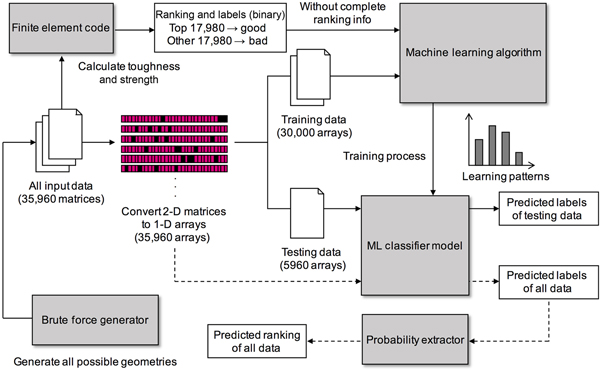
Using logistic regression algorithms, Gu et al. presented pioneer work on applying ML to the design of composites for Mode I fracture (Table I).[Reference Gu, Chen and Buehler74] Unlike the applications of using ML to predict the compressive strength of woods and concrete, in which experimental measurements were used as the training data,[Reference Tiryaki and Aydın71–Reference Young, Hall, Pilon, Gupta and Sant73] Gu et al. performed finite element analysis to generate the training data for their composite design problems. Figure 2 shows the ML approach using logistic regression (i.e., linear model) for an 8 by 8 composite system in the authors’ work. The input variables represent the topology of composites, where two base materials (stiff and soft) were considered and denoted as 0 and 1. As can be seen in the figure, instead of using the actual performance (i.e., toughness and strength) of composites to train a regression model, the training samples were categorized into two classes, namely “good” design and “bad” design, and logistic regression was performed for the classification task. After the training process, the linear model not only could distinguish whether an unseen composite design was a good or bad design but also could estimate how good (or how bad) the composite design was by comparing the probabilities of being in each class (Fig. 2). This study demonstrated that ML could be applied to learn structure–property relationships of materials even when the performance of materials could not be accurately measured. This ML approach could be applied to other material modeling and design problems in which the performance of materials is difficult (or expensive) to measure in experiments or simulations. The authors showed that using ML to predict mechanical properties of composites is orders of magnitude faster than conventional finite element analysis. Moreover, although it was shown in the authors’ work that the prediction accuracy could be improved when using a more complex ML model such as CNN, the linear model provided high interpretability of the relationship between input and output variables. Thus, after the linear model is trained, the optimal designs (the designs with the highest toughness or strength) of composites could be generated directly by using the information of the weights in the linear model, without requiring any sampling, optimizing, or searching process. In the authors’ work, the linear model generated optimal designs of composites with the toughness and strength orders of magnitude higher than the training samples, and required a much less computational cost compared with exhaustive methods.
Overall flow chart. The flow chart shows the ML approach using the linear model for an 8 by 8 system. The ML approach using the CNN model is similar to this flow chart but without the step of converting to 1-D arrays. Note that for a 16 by 16 system, the amount of input data, training data, and testing data are 1 million, 0.9 million, and 0.1 million, respectively. Reprinted with permission from Ref. Reference Gu, Chen and Buehler74. Copyright 2017 Elsevier.

Neural networks
Linear models assume that the relationship between input and output variables is linear. Thus, the learning capacity of linear models is limited. Although it is possible to increase the learning capacity by adding a few nonlinear terms (e.g., polynomials) to the hypothesis, it is not practical as there is an infinite number of nonlinear functions that can be chosen from and in general little is known which nonlinear functions are more suitable for our problems. An alternative approach to achieve high learning capacity is to use linear regression with an activation function to make an artificial neuron (perceptron) and connect a number of neurons to make an artificial NN. The most basic architecture of NNs is multilayer perceptron, which is also denoted to as NN here. It consists of multiple hidden layers (the layers except for the input and output layers) and each layer comprises a number of neurons. Nonlinear functions such as rectified linear unit and sigmoid are used as activation functions to introduce nonlinearity. The hidden layers in a NN are called the fully-connected layers as all the neurons in adjacent layers are fully connected. The output of the first layer goes into the second layer as input, and so on. On the basis of the universal approximation theorem, a NN with one hidden layer containing a finite number of neurons can approximate any continuous functions. In addition to NN, CNN is another widely used NN architecture, which is commonly applied to analyzing images and videos. The main building block in the CNN architecture is the convolution layer. The convolution layer comprises a number of convolution filters. Each filter is convolved with the input from the previous layer and generates feature maps, which are fed into the next layer as input. Compared with the fully-connected layers, this convolution operator can significantly reduce the number of weights needed in an ML model and makes the computation more efficient. The purpose of doing convolution is to extract relevant features from data. This feature learning ability is essential for image-related problems. In practice, CNN models usually outperform NN models on image classification tasks and many others.
NN and CNN have been applied to a few composite studies mostly for regression tasks. Qi et al. applied a NN model to predict the unconfined compressive strength of cemented paste backfill (Table I).[Reference Qi, Fourie and Chen75] In the authors’ work, the training data were collected from experiments. The input variables include the tailing type, cement-tailings ratio, solids content, and curing time while the output variable is the unconfined compressive strength of specimens. The authors applied particle swarm optimization to tune the architecture (the numbers of hidden layers and neurons) of their NN model and showed that their NN model can accurately predict and calculate the unconfined compressive strength of cemented paste backfill. For composite modeling and design problems, the topology of a composite can naturally be represented as an image (2-D or 3-D). The unit cells or base materials of a composite are converted to pixels (with different values) of the corresponding image. Accordingly, all the advantages of CNN found in image-related tasks are valid when applying to composite problems. Yang et al. applied CNN models to predict the effective stiffness of 3-D composites (Table I).[Reference Yang, Yabansu, Al-Bahrani, Liao, Choudhary, Kalidindi and Agrawal70] In the authors’ work, the training data were generated by 3-D Gaussian filters with different covariance matrixes. The performance of the training data was calculated by finite element analysis. The input variables include the topology of composites made up of two base materials (stiff and soft) and the output variable is the effective stiffness. Different architectures of CNN models were explored to tune hyperparameters (the numbers of layers and filters). The authors showed that their CNN models can produce highly accurate predictions of the effective stiffness of composites based on a given topology.
Recently, CNN has been employed to design hierarchical composites. Gu et al. applied CNN models to accelerate the design of bioinspired hierarchical composites (Table I).[Reference Gu, Chen, Richmond and Buehler66] In the authors’ work, three unit cells made up of stiff and soft materials were used to create hierarchical composites. Those unit cells exhibited distinctive anisotropy responses because of different geometrical configurations of stiff and soft materials in the unit cells. The input variables represent the topology of hierarchical composites, where the three unit cells are denoted as 1, 2, and 3. Compared with using complete microstructural data with the geometrical configuration of all local elements (stiff and soft), using macrostructural data with the geometrical configuration of unit cells drastically reduces the data space. Thus, a less complex ML architecture and fewer training samples are needed for this learning task. The output variable is the toughness of hierarchical composites calculated using finite element analysis. The idea of using unit cells to represent the topology of composites is similar to the homogenization process commonly applied in estimating effective material properties of composites. However, the conventional homogenization process requires to extract effective (homogenized) parameters of unit cells based on a rigorous mathematical theory,[Reference Michel, Moulinec and Suquet76] which is not required in the authors’ ML approach. Moreover, the fracture of composites occurs on the microstructural scale (local elements) and cannot be captured in a homogenized FEM model. Consequently, in homogenized finite element analysis, the localization process is required to convert the averaged strains of unit cells to the strains of local elements. In contrast, Gu et al. showed that the correlations between the geometrical configuration of unit cells (macrostructural data) and the corresponding toughness (microstructural property) can be learned by ML directly based on training data, without the need for conventional homogenization and localization processes. For this hierarchical composite problem, CNN was implemented to perform a regression task since linear regression was incapable of capturing the highly nonlinear correlations between the input and output variables. However, unlike linear models, CNN models (and most ML models) cannot generate optimal designs directly based on the values of weights. To overcome this limitation, Gu et al. further augmented CNN models to discover high-performing hierarchical composite designs with a self-learning algorithm. The concept of the self-learning algorithm is similar to that of the genetic algorithm. The sampling process consisted of many sampling loops. In each sampling loop, a large number of new composite designs (candidates) were fed into their CNN model and the model predicted the performance of those designs with a negligible computational cost. From there, high-performing candidates were identified and used to generate new candidates for the next sampling loop. The mechanical properties of the ML designs were then calculated using finite element analysis. As can be seen in Fig. 3, simulation results show that the ML designs are much tougher and stronger than the training samples. Most importantly, the simulation results were validated through additive manufacturing and experimental testing in the authors’ work. Note that knowing the optimal designs gives us an opportunity to probe design strategies and physical insights (Fig. 3) of how to create tougher and stronger hierarchical composites.
ML-generated designs. (a) Strength and toughness ratios of designs computed from training data and ML output designs. Strength ratio is the strength normalized by the highest training data strength value. Toughness ratio is the toughness normalized by the highest training data toughness value. The ML output designs are shown from training loops of 1000 and 1,000,000. Envelopes show that ML material properties exceed those of training data. (b) Effects of learning time on ML models for minimum, mean, and maximum toughness ratio start to converge as training loops increase. (c) Microstructures from partitions A (lowest toughness designs in training data) and B (highest toughness designs from ML) in part (a) of the figure with the corresponding colors for unit cell blocks (blue = U1, orange = U2, yellow = U3). Also shown in the right-most columns for the designs A and B are the strain distributions, which show lower strain concentration at the crack tip for the ML-generated designs[Reference Gu, Chen, Richmond and Buehler66].

Recently, Hanakata et al. applied ML to accelerate the design of stretchable graphene kirigami, which is a patterning graphene sheet with cuts (Table I).[Reference Hanakata, Cubuk, Campbell and Park77] In the authors’ work, NN and CNN models were applied to predict the yield stress and yield strain of graphene sheets based on the cutting pattern described by two unit cells. The input variables represent the topology of graphene sheets, where the two unit cells (with a cut and with no cut) are denoted as 0 and 1. The training data generated by MD and ML models was applied to perform a regression task to achieve accuracy close to the MD simulations. After the training process was completed, an iterative screening process was used to search for high-performing (high-yield strain) candidates. In each screening iteration, their CNN model was applied to search for high-performing candidates and the performance of those candidates was calculated using MD. The new simulation results were then added to the training data for the next iteration of training and screening processes. The authors showed that when more and more samples were used to train the CNN model, the yield strains of the high-performing candidates in each iteration were also improved.
Gaussian process
Although deep neural networks (e.g., NN and CNN) with many hidden layers and neurons, theoretically, can capture any complex patterns in data, they require a large amount of training data in order to learn the hidden patterns without overfitting. For some problems, simple ML algorithms cannot capture the complex patterns in data and generating a large amount of training data for deep learning algorithms is unfeasible due to the time and cost of conducting experiments or simulations. A GP, which is a non-parametric approach, serves as an alternative method for highly nonlinear problems. A GP is a collection of random variables and assumes that all input and output variables have joint Gaussian distributions. Instead of setting a hypothesis for an ML model and finding optimal values for the weights in the model, a GP produces a distribution of all possible functions that are consistent with the observed (training) data. Therefore, the number of parameters in a GP is unbounded and grows with the amount of training data. A GP is defined as:
 $$y = f\,({\bf x})\sim {\rm {\cal G}{\cal P}}(m({\bf x}),\; k({\bf x},{\bf {x}^{\prime}}))$$
where  $m({\bf x})$ is the mean function and $k({\bf x},{\bf {x}^{\prime}})$ is the covariance function. When a GP model is applied to predict the output value for an unseen data point, it generates a Gaussian distribution with a covariance matrix produced by a kernel function (e.g., squared exponential) which measures the similarity between points. Therefore, a GP model not only can make a prediction for an unseen data point based on the training data but also can naturally quantify the uncertainty of the prediction. In general, the uncertainty of the prediction for an unseen data point increases when the point is away from the training data points. Although a GP is a powerful and elegant method with numerous applications in ML and statistics, the implementation requires a computational cost which grows as O(n 3), where n is the number of training data points. Thus, conventional GP models have been mostly applied to problems with a small amount of training data. There are a number of sparse GP techniques proposed to reduce the computational cost for large data sets.[Reference Quiñonero-Candela and Rasmussen78,Reference Snelson and Ghahramani79]
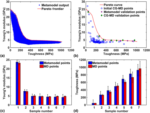
Tapia et al. applied a GP model to predict the porosity in metallic parts produced by selective laser melting, which is a laser-based additive manufacturing process (Table I).[Reference Tapia, Elwany and Sang80] In the authors’ work, the input variables are the laser power and laser scanning speed, which are two of the most influential processing parameters. The output variable is the porosity of specimens (17-4 PH stainless steel). A GP can be computationally very efficient when the amount of training data is small. The authors used the GP model to predict the porosity of specimens over the entire design space. Thus, the resulting porosity at any combination of the laser power and laser scanning speed was revealed. Recently, Hansoge et al. applied GP models to predict mechanical properties of assembled hairy nanoparticles (NPs) (Table I).[Reference Hansoge, Huang, Sinko, Xia, Chen and Keten81] Assembled hairy NPs is a type of polymer nanocomposite with relatively regular spacing between particles. In the authors’ work, the input variables are the polymer chain length, grafting density, polymer–NP interaction strength, and NP-edge length. The output variable is the modulus or toughness of assembled hairy NPs. The training data was generated using coarse-grained molecular dynamics (CG-MD) and GP models were applied to perform regression tasks based on the CG-MD simulation results. The authors used the GP models (metamodel) to predict the modulus and toughness of assembled hairy NPs over the entire design space. Figure 4 shows the modulus and toughness obtained from the metamodel by sampling 1 million assembled hairy NPs with different combinations of input variables. As can be seen in the figure, the predicted modulus and toughness obtained from the metamodel and those obtained from the CG-MD simulations are very close.
(a) Young's modulus versus toughness obtained from the metamodel. Pareto frontier obtained by sampling 1 million input parameters over the entire design space. (b) One hundred initial CG-MD designs (blue dots) are used to build the metamodel. Using the metamodel, a Pareto frontier (red curve) is obtained. Seven random points from the Pareto curve are chosen (purple squares) and tested by running CG-MD simulations (green diamonds). Comparison of (c) Young's modulus and (d) toughness obtained from the metamodel and CG-MD simulations. The error bars represent a 95% confidence interval. Reprinted with permission from Ref. Reference Hansoge, Huang, Sinko, Xia, Chen and Keten81. Copyright 2018 American Chemical Society.

Summary and future perspectives
This prospective paper presents recent progress in the applications of ML to composite materials. We give a brief overview of some basic ML algorithms and review recent studies using ML models to predict mechanical properties of composites. In those studies, ML models were applied to approximate physics-based modeling tools such as MD and FEM with a computational cost orders of magnitude less. Given the computing speed advantage of ML approaches compared with physics-based modeling tools, ML models were applied to explore the design space of composite design problems and to generate optimal designs of composites. By knowing the optimal designs obtained from ML for different composite design problems, it is possible to probe design strategies for achieving high-performing composites. Although ML models are often being considered as “black box” models, the discovered design strategies can provide new physical insights into how to make tougher and stronger composites.
Future implementations for further breakthroughs in ML applications on composite materials include developing more efficient topology representations for composites and more efficient inverse design techniques. Although the topology of a composite can naturally be represented as an image by converting the unit cells or base materials of the composite to pixels, this representation is not as efficient for large composite systems (e.g., aircraft wings). For example, considering each base element in an FEM model as an input variable for ML naturally causes computational problems when the model is large. Thus, developing new topology representations (with fewer variables) for large composite systems is imperative to apply ML to design large composite systems. In this prospective paper, we review recent studies using ML to solve inverse design problems. Gu et al. applied a linear model to generate optimal designs of composites by using the information of the weights in the model.[Reference Gu, Chen and Buehler74] However, the performance of the ML designs was limited to the learning ability of the linear model. In their later work, Gu et al. augmented CNN models with a self-learning algorithm to discover high-performing hierarchical composite designs.[Reference Gu, Chen, Richmond and Buehler66] Hanakata et al. applied ML with an iterative screening process to search for high-performing graphene kirigami.[Reference Hanakata, Cubuk, Campbell and Park77] Recently, Peurifoy et al. showed that NN models could be used to solve an inverse design problem for NPs by using backpropagation to train the inputs of the NN models.[Reference Peurifoy, Shen, Jing, Yang, Cano-Renteria, DeLacy, Joannopoulos, Tegmark and Soljačić82] Although the gradient in this inverse design approach is analytical, not numerical, it is still a gradient-based optimization approach. Thus, this approach can still get stuck in local minima or critical points. Note there is no optimization approach that can guarantee finding global minima of a non-convex optimization problem without exploring the entire design space. Future work on understanding the performance (theoretically or numerically) of different inverse design approaches for the applications of ML on composites is required for the accelerated discovery of new materials. Though true inverse design is currently a challenge in the field, it is believed that ML will play a promising role in this engineering problem in the future.
Acknowledgments
The authors acknowledge support from the Regents of the University of California, Berkeley.