


1. Introduction
Meaningful understanding of fluid-mechanical phenomena observed in nature can frequently be obtained through analogue laboratory experiments. This pertains to understanding the atmosphere (Rottman & Linden Reference Rottman and Linden2003), ocean (Simpson Reference Simpson1982), cryosphere (Robison, Huppert & Worster Reference Robison, Huppert and Worster2010), solid Earth (Huppert Reference Huppert1986) and planetary science (Johnson et al. Reference Johnson2016), for example. These fields involve large-scale fluid-mechanical processes, which can be scaled down to laboratory scales to test theoretical ideas experimentally. However, an underlying problem is that viscous fluids in the laboratory commonly obey the no-slip condition when in contact with a rigid substrate. This makes it difficult to experimentally capture natural fluid-mechanical phenomena that instead exhibit a degree of basal sliding.
An example is the flow of ice sheets, such as that of Greenland and Antarctica, which generally slide at their base. Such sliding results from lubrication by a thin layer of subglacial till, consisting of a mixture of subglacial sediment, clay and water (Schoof & Hewitt Reference Schoof and Hewitt2013). It is typical to model subglacial sliding using sliding laws that relate the basal velocity to the basal shear stress (Schoof & Hewitt Reference Schoof and Hewitt2013). The simplest example of such a sliding law is a Navier-type slip condition. However, reproducing basal sliding in the laboratory for fluid-mechanical experiments of ice sheets remains a challenge. Instead of obeying a sliding law, relevant experimental studies involve flows that obey the no-slip condition at the base. Examples include studies of the dynamics of confined (Robison et al. Reference Robison, Huppert and Worster2010; Kowal, Worster & Pegler Reference Kowal, Worster and Pegler2016) and unconfined (Pegler & Worster Reference Pegler and Worster2012; Sayag, Pegler & Worster Reference Sayag, Pegler and Worster2012) marine ice sheets. Although basal sliding is relevant to the vast majority of geophysical scenarios involving ice flows, there is a small number of exceptions. Exceptions include regions of ice that are frozen to the bedrock and ice sheets confined to very narrow channels, for which vertical shear is negligible in comparison to transverse shear (Pegler et al. Reference Pegler, Kowal, Hasenclever and Worster2013).
Motivated by these flows, attempts have been made to introduce slip at the base of a viscous fluid by injecting another less viscous fluid underneath it (Kowal & Worster Reference Kowal and Worster2015; Kumar et al. Reference Kumar, Zuri, Kogan, Gottlieb and Sayag2021; Gyllenberg & Sayag Reference Gyllenberg and Sayag2022). The slip velocity for such flows varies spatially, across the flow, and is dependent upon the dynamics of the underlying layer. While basal sliding is reproduced successfully at early stages of these experiments, the flow becomes susceptible to a new type of viscous fingering instability at intermediate and late stages of the experiments (Kowal & Worster Reference Kowal and Worster2015; Kumar et al. Reference Kumar, Zuri, Kogan, Gottlieb and Sayag2021; Gyllenberg & Sayag Reference Gyllenberg and Sayag2022). This instability impedes with the ability to reliably introduce slip at the base of a viscous gravity current through injection. It has been shown that the instability originates at the injection front (Kowal & Worster Reference Kowal and Worster2019a,Reference Kowal and Worsterb; Kowal Reference Kowal2021), and can be slightly suppressed by altering the rheology of the fluids (Leung & Kowal Reference Leung and Kowal2022a,Reference Leung and Kowalb). There is a similarity between this instability and the Saffman–Taylor instability in that both instabilities involve the intrusion of a less viscous fluid into a more viscous fluid. However, the Saffman–Taylor instability occurs in porous media (including Hele-Shaw cells), whereas the instability emerging here does not.
It is the aim of this study to configure an experimental set-up that provides for basal sliding that is effectively homogenous on the large scale and is unaffected by unwanted frontal instabilities. We also build into our framework the ability to adjust slip as desired. To characterise the resulting slip mathematically, we develop a theoretical model that captures basal sliding with an appropriate basal boundary condition, or what is effectively a linear sliding law. In particular, we consider the gravity-driven flow of a viscous fluid over a slippery substrate composed of a sequence of square cavities that are saturated with a less viscous fluid, as depicted in figure 1. The flow within each cavity is driven by an imposed shear stress exerted by the overlying layer, giving rise to a slip velocity at the interface between the two fluids. As the flow of the less viscous fluid is confined to its corresponding cavity, we eliminate viscous intrusion and the emergence of viscous fingering instabilities. This allows us to reliably generate slip, and to control it, as required. Such an experimental set-up and theoretical model aids the running of fluid-mechanical experiments in which basal sliding is important on the large scale.
Schematic of a two-dimensional thin film of viscous fluid flowing over a structured substrate consisting of a sequence of fluid-filled cavities (a), together with an inset (b), depicting streamlines within one of the cavities and a resultant interfacial velocity  $u=u_s$ (red arrow) between the two fluids. Although Moffatt eddies may form near the corners of the cavity, such flows are subdominant to the overarching circulation within each cavity, and are thus omitted from the schematic diagram.

Our choice of substrate is motivated by the structure of hydrophobic substrates involving small-scale gas-filled or liquid-filled cavities. This is because traditional hydrophobic surfaces promote slip in microscopic systems, such as droplets (McGraw et al. Reference McGraw, Chan, Maurer, Salez, Benzaquen, Raphaël, Brinkmann and Jacobs2016; Keiser et al. Reference Keiser, Keiser, Clanet and Quéré2017). The use of hydrophobic surfaces is motivated by a range of microfluidic applications, including the development of portable devices able to perform small-scale analytical tasks, e.g. the lab-on-a-chip (Stone, Stroock & Ajdari Reference Stone, Stroock and Ajdari2004). Experimental studies of slip over such substrates report surface roughnesses ranging from 2 Å to  $100\,\mathrm {\mu }{\rm m}$ and slip lengths ranging from $10\,{\rm nm}$ to $500\,\mathrm {\mu }{\rm m}$ for fluids such as water, mercury, glycerine and silicone oil (Lauga & Stone Reference Lauga and Stone2003). While such slip is appreciable for microfluidic applications, it is negligible for large-scale flows of the order of up to a metre. In particular, it has been shown by Richardson (Reference Richardson1973), using continuum arguments, that small-scale surface roughness effectively furnishes a no-slip boundary condition on length scales that are large in comparison to the surface roughness, even if there is perfect slip on the scale of the roughness (Lauga & Stone Reference Lauga and Stone2003). To overcome this obstacle and to nevertheless generate appreciable slip on the large scale, we consider a large-scale version of a hydrophobic surface, with liquid-filled cavities of the order of 1 cm. We show, theoretically and experimentally, that such a substrate gives rise to slip lengths of the order of 1 cm, which are appreciable for large-scale fluid-mechanical experiments. An additional advantage is that it is relatively simple to control the slip length in this setting by adjusting the viscosity of the saturating liquid. Another consideration for the choice of substrate is commercial availability and ease of use for experiments. We note that other configurations may well give rise to similar slip lengths. An example involves saturated porous substrates, building upon work on gravity currents propagating over porous beds (Acton, Huppert & Worster Reference Acton, Huppert and Worster2001; Pritchard & Hogg Reference Pritchard and Hogg2002).
We begin by presenting our theoretical model in § 2, followed by a discussion of results in § 3. We perform a series of demonstrative fluid-mechanical experiments, which we discuss and compare against our theoretical predictions in § 4. We conclude with final remarks in § 5.
2. Theory
Consider the two-dimensional flow of a thin film of viscous fluid, of surface height  $z=H$, density $\rho$ and dynamic viscosity $\mu$, spreading under gravity over a horizontal, structured substrate as depicted in figure 1. The substrate is composed of a sequence of square cavities of depth $h$, and is prewetted with another fluid of density $\rho _l\geq \rho$, viscosity $\mu _l\leq \mu$ and equal depth $h$. We assume that the interface between the two fluids remains horizontal at $z=0$ and that the effects of surface tension are negligible. We also assume that the thin film is much longer than it is deep and that it is resisted mainly by vertical viscous shear stresses, allowing us to apply the approximations of lubrication theory for the overlying layer. This assumption breaks down in the very slippery limit, in which the depth of the viscous gravity current is much smaller than the slip length. The overlying layer provides a shear stress to the underlying fluid, which drives a recirculating flow within each cavity. This flow gives rise to a resultant interfacial velocity $u=u_s$ indicated by a red arrow in the schematic of a single cavity depicted in figure 1. This is an effective slip velocity experienced at the base of the overlying layer.
In what follows, we develop a mathematical model for this slip velocity and demonstrate that it gives rise to a linear sliding law, or a Navier slip condition, at the base of the overlying viscous gravity current. To do so, we assume that the horizontal length scale  $h$ of the cavities is much smaller than the horizontal length scale associated with the flow of the overlying viscous gravity current. This allows us to average out over the small-scale inhomogeneities on the scale of each cavity and obtain a macroscopic sliding law, reflecting the effective slip experienced by the overlying viscous gravity current.
2.1. Flow within each cavity
Within each cavity, horizontal and vertical length scales are comparable and the flow is described by a balance of viscous and gravitational forces given by
 \begin{equation} \boldsymbol{0} ={-}\boldsymbol{\nabla} p_l - \rho_l g \boldsymbol{e}_z + \mu \nabla^2 \boldsymbol{u}_{l}, \end{equation}
where  $p_l$ and $\boldsymbol {u}_l$ denote the pressure and velocity of the fluid within each cavity, and $g$ is the acceleration due to gravity. Throughout this paper, the subscript $l$ denotes quantities related to the flow in each cavity. Additionally, the flow is incompressible, so that
 \begin{equation} \boldsymbol{\nabla}\boldsymbol{\cdot} \boldsymbol{u}_l = 0. \end{equation}
We assume no slip and no penetration,  $\boldsymbol {u}_l=\boldsymbol {0}$, on the walls of each cavity. We also assume continuity of shear stress at its upper interface, so that
 \begin{equation} \mu_l\left( \frac{\partial u_l}{\partial z} + \frac{\partial w_l}{\partial x} \right) = S, \quad \text{at} \ z=0, \end{equation}
where  $S$ is the shear stress exerted by the upper layer (determined in § 2.3).
As reflected in the governing equations above, the flow within each cavity is driven by an imposed shear stress at the interface. This results in a non-zero interfacial velocity, or slip velocity, at  $z=0$. To arrive at a macroscopic description of this interfacial velocity, we assume that the horizontal length scale, $h$, of each cavity is much smaller than the horizontal length scale $\mathscr {L}$ of the overlying viscous gravity current. That is, $\mathscr {L}\gg h$, which is valid when $t\gg {\unicode{x2113}}h/q_0$, where ${\unicode{x2113}}$ is the slip length (2.11) and $q_0$ is the source flux of the overlying viscous gravity current. Given such a separation of scales, the flow in each cavity experiences an essentially constant shear stress $S$, while the overlying gravity current experiences an effective slip velocity. We therefore approximate $S$ to be uniform over the horizontal span of each cavity.
The remainder of this section focuses on solving for the flow within in each cavity and obtaining the average slip velocity. Our derivations assume that the cross-section of the cavities are square, though other height-to-width ratios are possible, albeit not easily commercially available for running experiments. We expect deeper (shallower) cavities to give rise to higher (lower) interfacial slip velocities.
For convenience, we absorb the hydrostatic part of the pressure by defining  $\bar p_l = p_l + \rho _l g z$ and non-dimensionalize the flow within the cavity using the following length, velocity and pressure scales:
 \begin{equation} (x-x_n,z) = h(x^*,z^*), \quad \boldsymbol{u}_l= \frac{Sh}{\mu_l} \boldsymbol{u}_l^*, \quad \bar p_l = S \bar p_l^*. \end{equation}
Here,  $x_n$ is the position of the left-hand wall of the $n{\text {th}}$ cavity, so that $x^*=0$ denotes the left-hand wall of the $n{\text {th}}$ cavity in dimensionless variables. This gives rise to the dimensionless Stokes equations
 $$\begin{gather} \boldsymbol{0} ={-}\boldsymbol{\nabla}^*\bar p_l^* + \nabla^{*2} \boldsymbol{u_l^*}, \end{gather}$$
 $$\begin{gather}\boldsymbol{\nabla}^*\boldsymbol{\cdot} \boldsymbol{u_l^*}=\boldsymbol{0}, \end{gather}$$
which are subject to no-slip and no-penetration conditions on the walls as well as a prescribed upper-layer shear stress
 \begin{equation} u_{lz}^* + w^*_{lx} = 1 \end{equation}
at the interface. This shear stress drives a recirculating flow within each cavity, giving rise to a resultant interfacial slip velocity. Importantly, these dimensionless equations and boundary conditions are free of dimensionless parameters.
2.2. Sliding law and slip length
In this section we calculate the interfacial slip velocity and use it to find a dimensional slip length. In particular, we find the following approximate form:
 \begin{equation} u^*_l \approx \alpha \left[ x^*(1-x^*) \right]^\beta \end{equation}
for the slip velocity to within a tolerance of  $2\times 10^{-3}$. Here $\alpha \approx 0.50$ and $\beta \approx 0.92$. This was found by performing finite element numerical simulations for the weak formulation of the flow within a single cavity using the integrated development environment FreeFem++ (Hecht Reference Hecht2012). The form of the interfacial velocity is in line with similar calculations for structured substrates with mixed no-slip and no-shear boundary conditions (Philip Reference Philip1972) and flows over superhydrophobic gratings (Crowdy Reference Crowdy2021).
We note that small-scale variations in the velocity across the width of a single cavity have little effect on the large-scale flow of the overlying viscous gravity current, given the separation of scales. Instead, the overlying viscous gravity current experiences a net ‘average’ slip velocity at the fluid–fluid interface. Therefore, we average over the width of each cavity and obtain the following average slip velocity:
 \begin{equation} \bar u_s^* \equiv \int_0^1 u_s^* \,{\rm d}\kern 0.06em x^* \approx 0.095. \end{equation}
In dimensional terms, this becomes
 \begin{equation} \bar u_s = \frac{{\unicode{x2113}}}{\mu} S, \end{equation}
where
 \begin{equation} {\unicode{x2113}} \approx 0.095 \mathcal{M} h \end{equation}
is the dimensional slip length and  $\mathcal {M}=\mu /\mu _l$ is the viscosity ratio. In systems of practical interest, such as the experiments of § 4, the slip length ${\unicode{x2113}}$ ranges from the order of 0.1 cm to $10$ cm.
We show in § 2.3 that assuming an interfacial velocity of the form (2.10) is equivalent to assuming the Navier slip condition
 \begin{equation} u = {\unicode{x2113}}\, u_z \quad \text{at} \ z=0, \end{equation}
at the bottom boundary of the overlying viscous layer. In particular, both of these conditions give rise to the same effective velocity at the interface between the two fluids and the same depth-integrated flux of fluid in the overlying viscous layer. That is, averaging out the small-scale inhomogeneities of the structured substrate is equivalent to producing an effective Navier slip at the base of the overlying viscous gravity current.
Notably, the slip length is proportional to the viscosity ratio, as seen in (2.11). Therefore, the larger the viscosity ratio, the more slippery the substrate is. This is natural to expect on physical grounds as the flow within each of the cavities provides a smaller viscous drag when the viscosity of the viscous fluid within each cavity is comparatively small. Conversely, the smaller the viscosity ratio, the less slippery the substrate. This is because such a substrate gives rise to a larger effective shear stress when the viscosity of the fluid within each cavity is large in comparison with that of the overlying thin film of viscous fluid. The  $\mathcal {M}\to \infty$ limit corresponds to the no-slip limit of a viscous fluid propagating over a solid substrate.
2.3. The upper layer
Under the approximations of lubrication theory, the upper thin film of viscous fluid, spreading over the structured substrate, is governed by the momentum equation
 \begin{equation} \boldsymbol{0} ={-}\boldsymbol{\nabla} p - \rho g \boldsymbol{e}_z + \mu {u}_{zz} \boldsymbol{e}_x, \end{equation}
in dimensional variables. The pressure is hydrostatic within the layer, so that
 \begin{equation} p = \rho g (H-z) + p_0, \end{equation}
where  $p_0$ denotes the atmospheric pressure. Integrating the horizontal component of the momentum equation gives the expression
 \begin{equation} S = \mu \frac{\partial u}{\partial z} ={-}\rho g H H_x \quad \text{at}\ z=0, \end{equation}
for the interfacial shear stress  $S$. To arrive at this expression, we assumed that the upper surface is stress free. Integrating once more yields the velocity,
 \begin{equation} u = \frac{\rho g}{2\mu}(z^2-2Hz) H_x + \bar u_s, \end{equation}
which we obtained after applying the interfacial condition
 \begin{equation} u=\bar{u}_s \quad \text{at} \ z=h, \end{equation}
where  $\bar u_s$ denotes the interfacial velocity (2.10). The expression (2.16) for the velocity yields the depth-integrated flux, per unit width,
 \begin{equation} q = \int_0^H u \,{\rm d}z ={-}\frac{\rho g}{\mu} \left( \frac{1}{3}H^3H_x +{\unicode{x2113}} H^2H_x\right). \end{equation}
The first term is the usual contribution to the flux arising from the hydrostatic spreading of the viscous fluid under its own weight over a no-slip substrate, in line with Huppert (Reference Huppert1982). The second term is a plug-like contribution to the flow arising from the sliding of the thin film of viscous fluid over a slippery substrate.
Importantly, the same interfacial velocity (2.17) and depth-integrated flux (2.18) can be obtained by replacing the interfacial velocity condition (2.17) by the Navier slip condition (2.12) with a slip length  ${\unicode{x2113}}$. This indicates that averaging out all the inhomogeneities associated with the flow within each cavity gives rise to a macroscopic slip described by the Navier slip condition.
The upper surface of the thin film of viscous fluid is itself a free surface, which evolves according to the mass conservation equation
 \begin{equation} H_t={-}q_x. \end{equation}
We assume the viscous fluid is fed at constant flux at the source, so that
 \begin{equation} q=q_0 \quad \text{at} \ x=0, \end{equation}
and that the flux, and, hence, the thickness, of the thin film of viscous fluid vanishes at its leading edge  $x=x_N$, so that
 \begin{equation} q=0 \quad \text{at} \ x=x_N. \end{equation}
The leading edge  $x=x_N(t)$ is itself evolving, and to determine it, we note that total mass is conserved within the entire domain of the flow, so that
 \begin{equation} \int_0^{x_N} H \, {\rm d}\kern 0.06em x = q_0 t. \end{equation}
These governing equations and boundary conditions fully determine the evolution of the free surface.
2.4. Non-dimensionalization
We non-dimensionalize the governing equations and boundary conditions describing the flow of the overlying viscous gravity current, propagating over the slippery substrate, using the scalings
 \begin{equation} H = {\unicode{x2113}}\tilde{H}, \quad q = q_0 \tilde{q}, \quad x = \frac{\rho g {\unicode{x2113}}{}^4}{\mu q_0} \tilde{x}, \quad t = \frac{\rho g {\unicode{x2113}}{}^5}{\mu q_0^2} \tilde{t}, \end{equation}
involving the slip length  ${\unicode{x2113}}$. These scalings reflect the typical thickness, extent and time scale required for the viscous gravity current to reach a thickness comparable to the slip length of the substrate. Upon dropping tildes, for convenience, we obtain the set of dimensionless equations
 \begin{equation} H_t ={-}q_x \quad \text{and} \quad q ={-} \frac{1}{3}H^3H_x - H^2H_x, \end{equation}
within the domain  $0\leq x\leq x_N$, subject to the boundary conditions
 \begin{equation} q=1 \quad \text{at} \ x=0 \quad \text{and} \quad q=0 \quad \text{at}\ x=x_N, \end{equation}
and integral condition
 \begin{equation} \int_0^{x_N} H \, {\rm d}\kern 0.06em x = t. \end{equation}
These equations admit similarity solutions in various limits, which we discuss in the following sections. It is important to note, however, that no dimensionless parameters appear in the governing equations and boundary conditions, indicating that numerical solutions, as well as all experimental data, for the evolution of the frontal position, for example, should collapse onto a single curve under the choice of scaling (2.23a–d) involving the slip length  ${\unicode{x2113}}$, determined in § 2.1. This is indeed what happens for our series of experiments described in § 4.
3. Similarity solutions
We discuss similarity solutions that arise at early and late times, and compare to the full numerical solutions for intermediate times, in this section.
3.1. Early time similarity solution: very slippery limit
At early times,  $t\ll 1$, when the thickness of the thin film of viscous fluid is small relative to the slip length, or, equivalently, $H\ll 1$ in dimensionless terms, it follows that
 \begin{equation} H^3 H_x \ll H^2 H_x. \end{equation}
In this limit,
 \begin{equation} q ={-}H^2 H_x, \end{equation}
reflecting a mainly plug-like flow, in which the thin film of viscous fluid slides freely over the slippery substrate. This may be thought of as a very slippery limit. A similarity solution can be found in this scenario, in which
 \begin{equation} H(x,t)= {t}^{1/4}F(\eta), \quad \text{where} \ \eta = x{t}^{{-}3/4}. \end{equation}
The similarity solution satisfies the governing equation
 \begin{equation} \frac{1}{4}F - \frac{3}{4}\eta F' = (F^2F')', \end{equation}
boundary conditions
 \begin{equation} -F^2F'=1\ (\eta=0),\quad -F^2F'=0 \ (\eta=\eta_N), \end{equation}
and integral constraint
 \begin{equation} \int_0^{\eta_N}F(\eta)\,{\rm d}\eta=1. \end{equation}
An asymptotic analysis near the front  $\eta =\eta _N$ reveals a square-root frontal singularity,
 \begin{equation} F\sim \left[ \frac{3}{2}\eta_N(\eta_N-\eta)\right]^{1/2} \quad \text{as}\ \eta\to\eta_N. \end{equation}
This asymptotic solution, valid near the front, is depicted in figure 2 in comparison to the full numerical solution, valid over the whole domain. The structure of the frontal singularity in this limit contrasts with the typical cube-root singularity inherent to the front of thin films of viscous fluid over no-slip substrates, such as that found by Huppert (Reference Huppert1982), also depicted in figure 2. We note that the horizontal axis in figure 2 is scaled with the nose position, so as to fix both viscous gravity currents to the interval  $[0,1]$ and accent the difference in the functional form of the frontal singularity between the early time and the late time regimes.
Rescaled similarity solutions showing the shape of the thickness of the viscous gravity current for very slippery substrates  $t\ll$ (solid line) and no-slip substrates $t\gg 1$ (dashed line), together with square-root (3.7) and cube-root, Huppert (Reference Huppert1982), asymptotic solutions valid near the front (dots and squares, respectively).

A numerical solution of this problem reveals that the frontal position is given by approximately  $\eta _N\approx 1.116$, which yields the power law
 \begin{equation} x_N \sim 1.116 {t}^{3/4}, \end{equation}
for the position of the front as a function of time, as depicted in figure 3. In dimensional terms, this becomes
 \begin{equation} x_{N\,{dim}} \sim 1.116 \left( \frac{\rho g q_0^2 {\unicode{x2113}}}{\mu}\ \,\right)^{1/4} {t_{{dim}}}^{3/4}, \end{equation}
where the subscript  ${{dim}}$ denotes dimensional quantities. This power law involves a ${\unicode{x2113}}{}^{1/4}$ dependence, which is proportional to $\mathcal {M}^{1/4}$, reflecting the fact that the coefficient of the power law increases with the slip length, and hence, with the viscosity ratio. That is, the more slippery the substrate, the larger the coefficient and, hence, the faster the propagation of the front.

3.2. Late time similarity solution: no-slip limit
At late times,  $t\gg 1$, when the thickness of the thin film of viscous fluid greatly exceeds the slip length, or, equivalently, $H\gg 1$ in dimensionless terms, it follows that
 \begin{equation} H^3 H_x \gg H^2 H_x, \end{equation}
and so in this limit,
 \begin{equation} q ={-}\frac{1}{3}H^3 H_x, \end{equation}
reflecting the flow of a classical viscous gravity current propagating over a no-slip substrate, as considered by Huppert (Reference Huppert1982). As found by Huppert (Reference Huppert1982), such a flow is self-similar and the similarity solution is of the form
 \begin{equation} H= {t}^{1/5}F(\eta), \quad \text{where} \ \eta = x{t}^{{-}4/5}, \end{equation}
where
 \begin{gather} \frac{1}{5}F - \frac{4}{5}\eta F' = \frac{1}{3}(F^3F')', \end{gather}
 \begin{gather} -F^3F'=1\ (\eta=0),\quad -F^3F'=0 \ (\eta=\eta_N), \end{gather}
 \begin{gather} \int_0^{\eta_N}F(\eta)\,{\rm d}\eta=1. \end{gather}
The front exhibits a cube-root singularity,
 \begin{equation} F\sim \left[\frac{36}{5}\eta_N (\eta_N-\eta)\right]^{1/3} \quad \text{as}\ \eta\to\eta_N \end{equation}
(see Huppert Reference Huppert1982), as depicted in figure 2 in comparison to the full numerical solution. The former is valid near the nose only, while the latter is valid over the whole domain. In contrast to the early time regime, the front, instead, evolves like
 \begin{equation} x_N \sim 0.80 { t}^{4/5} \end{equation}
in the no-slip limit. This frontal propagation law is depicted in figure 3 in comparison to the similarity solution (3.8), valid in the early time, very slippery limit, and the full numerical solution, valid for intermediate times at which the thickness of the thin film of viscous fluid is comparable to the slip length. In dimensional terms, the frontal propagation law (3.17) becomes
 \begin{equation} x_{N\,{dim}} \sim 0.8 \left( \frac{\rho g q_0^3}{\mu} \right)^{1/5} {t_{{dim}}}^{4/5},\end{equation}
where, again, the subscript  ${{dim}}$ denotes dimensional quantities. In contrast to the prefactor, the power-law exponent does not change much from the early time, slippery limit to the late time, no-slip limit (the exponent changes from 3/4 to 4/5, respectively). However, there is a noteworthy change in the prefactor in dimensional form. Unlike the slippery, early time limit, the dimensional power law (3.18), and, in particular, its prefactor, is independent of the slip length ${\unicode{x2113}}$, and, hence, the viscosity ratio $\mathcal {M}$, in the no-slip limit. In particular, as the substrate becomes less slippery, that is, as ${\unicode{x2113}}\to 0$, the prefactor tends towards a constant that depends on the remaining physical parameters inherent to the upper layer alone. This contrasts with the prefactor for the dimensional power law (3.9) in the early time, slippery limit, which varies with the slip length as ${\unicode{x2113}}{}^{1/4}$.
3.3. Full numerical solution for intermediate times
To compare the two frontal propagation laws (3.8) and (3.17) against the frontal position for intermediate times, as depicted in figure 3, we solved the full system of partial differential equations (2.24a–d)–(2.26) numerically. This was done by mapping the evolving domain  $[0,x_N]$ to the fixed interval $[0,1]$, discretising using second-order accurate finite differences, and using a kinematic condition at the front to update the evolution of the frontal position; see Kowal & Worster (Reference Kowal and Worster2015) for a similar treatment.
The full numerical solution converges towards the asymptotic solution (3.8) for slippery currents, at early times, as seen in figure 3. Figure 3 also shows that the full numerical solution converges towards the asymptotic solution (3.17) for no-slip currents, at late times. The change of regimes, from the early time regime to the late time regime, occurs when the thickness of the thin film of viscous fluid is comparable to the slip length, which occurs when  $t=\mathcal {O}(1)$ under the scaling (2.23a–d). We can, therefore, expect slip to dominate the dynamics for times $t\ll 1$, and for it to have little effect for $t\gg 1$.
We note that under the choice of scaling (2.23a–d) involving the slip length  ${\unicode{x2113}}$, determined in § 2.1, the full numerical solution depends on no dimensionless parameters, indicating that all experimental data of the flow of thin films of viscous fluid over structured, slippery substrates should collapse onto a single curve. We test this scaling by performing a series of experiments described in § 4.
4. Experiments
We carried out a series of analogue fluid-mechanical experiments to test our theoretical predictions. As shown schematically in figure 4, the experiments were carried out in a perspex tank of dimensions  $201\,{\rm cm}\times 24.5\,{\rm cm}\times 20.2\,{\rm cm}$ underlain by a cellular substrate consisting of a sequence of open-top cavities of dimensions $1\,{\rm cm}\times 1\,{\rm cm}\times 20\,{\rm cm}$, arranged periodically, with period 1 cm, in the direction of flow.
Schematic of our experimental set-up.

Before each experiment, the cellular substrate was evenly pre-filled with low-viscosity, lubricating fluid consisting of golden syrup diluted with 10–20 % potassium carbonate solution of kinematic viscosity  $\nu _l \approx 3\unicode{x2013}50\,\text {cm}^{2}\,\text {s}^{-1}$ and density $\rho _l\approx 1.4\,\text {g}\,\text {cm}^{-3}$ up to constant height 1 cm, within an 0.025 cm error. We use potassium carbonate solution as an additive to golden syrup in order to decrease its viscosity without decreasing its density so that it can be used as the underlying fluid, saturating the substrate. A reservoir of high-viscosity fluid, consisting of golden syrup diluted with 0–5 % potassium carbonate solution, giving rise to a kinematic viscosity of $\nu \approx 50\unicode{x2013}320\,\text {cm}^{2}\,\text {s}^{-1}$ and density $\rho \approx 1.4\,\text {g}\,\text {cm}^{-3}$, was installed at the left-hand end of the tank. This high-viscosity fluid was subsequently released to form a viscous gravity current over the slippery, structured substrate, pre-filled with lubricating fluid.
Specifically, to initiate each experiment, the reservoir gate was lifted up to a specified height so that the high-viscosity fluid spread under its own weight over the structured, fluid-saturated substrate. The reservoir head was maintained constant during each experiment by manual replenishment to give rise to a constant flux of upper-layer fluid. The flux of upper-layer fluid was measured by comparing the mass of syrup used to the duration of the experiment. The errors in general measurement of mass and time are within  $\Delta m = \pm 5\,\text {g}$ and $\Delta t = \pm 1 \,\text {s}$, respectively, owing to residual losses and human errors in reaction time.
The densities of the two viscous fluids were prepared to match within an error of  $\Delta \rho \approx 0\unicode{x2013}0.017 \,\text {g}\,\text {cm}^{-3}$ by suitable adjustment of the concentration of potassium carbonate solution in water. We made sure that the lower-layer fluid was never less dense than the upper-layer fluid, in order to avoid Rayleigh–Taylor instabilities at the interface between the two viscous fluids. Different fluids were used for the two layers for all experiments apart for experiment A, for which we used golden syrup diluted with 8 % water, giving rise to a kinematic viscosity of $\nu = 37.2\,\text {cm}^2\,\text {s}^{-1}$ and density $\rho = 1.406\,\text {g}\,\text {cm}^{-3}$, for both layers. The full set of parameter values used in our experiments are shown in table 1.
Parameter values and slip lengths in our experiments.

The viscosities of both viscous fluids were measured using a Kinexus parallel-plate rheometer to within a relative error of  $\Delta \mu /\mu \approx \pm 3\,\%$, and the densities were measured using a hydrometer to within ${\pm }0.001\,\text {g}\,\text {cm}^{-3}$. As the viscosity of syrup is strongly dependent upon its temperature, the temperature of the laboratory was measured with a thermometer, to within an error of ${\pm }0.5\,^{\circ }\text {C}$, and the viscosity measurements were carried out under the same temperature. The error estimate for the viscosity measurement is based upon the fluctuations and error in the measurement of the temperature. It also originates from inherent differences in viscosity readings made in a sequence of measurements at different shear stresses and different samples used in the parallel-plate rheometer. The effect of mixing between the two viscous fluids was negligible on the time scale of our experiments.
Experimental data was recorded by digital camera set up to take a sequence of photographs of the side and top view of the experiments in one-second time intervals for each experiment. Image processing techniques in Mathematica were used to extract the frontal position  $x_N$ as a function of time. As our experimental tank was of finite width, the flow was not fully two dimensional as shear stresses owing to the presence of side walls were present within boundary layers of roughly 1 cm, resulting in a non-uniform frontal position when viewed from the top. To estimate this effect, a mirror was installed at an angle above the experimental tank oriented towards the camera, from which we conclude that this effect was insignificant.
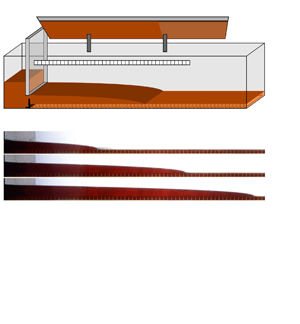
A supplementary movie of one of our experiments is available at https://doi.org/10.1017/jfm.2024.127. The interface between the two layers was observed to remain flat for all experiments apart from experiment C, as seen in the photographs of the side views of representative experiments in figure 5. This is in line with the assumptions of our theory. Colour variation owing to a difference in the concentration of food colouring was used to distinguish the two viscous fluids. For experiment C, the lower, lubricating layer was of sufficiently low viscosity that it was viscously sheared along with the upper, more viscous layer, leading to loss of lubricating fluid in the cells near the reservoir. Additional long-wave, longitudinal instabilities, of a wavelength much larger than the width of the cavities, emerged in this experiment. These have come about as a result of the large viscosity difference between the two layers. Such instabilities have been previously examined in a variety of contexts in which both fluids flowed over a planar substrate; see, e.g. Yih (Reference Yih1967), Wang, Seaborg & Lin (Reference Wang, Seaborg and Lin1978), Hinch (Reference Hinch1984) and Balmforth, Craster & Toniolo (Reference Balmforth, Craster and Toniolo2003). The onset of such long-wave instabilities is reduced over the cellular substrate. Specifically, higher viscosity ratios were observed to be required in order for instabilities to emerge over the cellular substrate. As the two fluids are miscible, there is no surface tension at the interface between them, so surface tension should not contribute to the onset of these long-wave instabilities, observed in experiment C.
A sequence of photographs of the side views of representative experiments. (a) Experiment A ( ${\mathcal {M}}\approx 1$) for $t=10,20,30$, (b) experiment D ( ${\mathcal {M}}\approx 13$) for $t=90, 180, 270$ and (c) experiment C ( ${\mathcal {M}}\approx 95$) for $t=30,90,150$. Depletion of the lower layer as well as the onset of a long-wave instability is observed for experiment C.

Raw experimental data for all of our experiments as well as a comparison of rescaled experimental data against our theoretical predictions for the frontal position as a function of time are shown in figure 6. The experimental data collapse onto a single curve in rescaled coordinates involving the viscosity ratio. The span of experimental data covers both the very slippery limit ( $t\ll 1$) and the no-slip limit $(t\gg 1)$ over several orders of magnitude, confirming the validity of the viscosity ratio as a measure of the slip length and the appropriateness of the identified scalings.
(a) Raw experimental data depicting the extent of slippery viscous gravity currents for all of our experiments. (b) Comparison of our experimental data (symbols) for the frontal position against our theoretical prediction (solid curve) in dimensionless coordinates.

Experimental data for the frontal position of experiment C, for which longitudinal instabilities and depletion of the lower layer have been observed, is consistently lower than the theoretical predictions. We attribute this to the combination of two factors. The first factor involves the depletion of the lower layer, which effectively reduces slip. The second factor involves excess lubricating fluid, which was viscously sheared along with the upper layer and has accumulated near the nose of the upper layer for this experiment. The accumulation of lower-layer fluid near the front of propagation of the upper layer induced a back pressure near the front. A secondary effect that starts manifesting itself in the very slippery limit is the effect of viscous extensional stress. While the experiment with the largest disagreements is experiment C (with the largest viscosity ratio), similar effects may affect experiments H and B (with the next largest viscosity ratios) to a lesser degree.
5. Conclusions
Motivated by gravity-driven flows of viscous fluids that slide at their base, we develop a theoretical and experimental framework for generating slip in the laboratory. We do so by examining flow over a slippery substrate consisting of periodic, fluid-filled cavities and develop a macroscopic mathematical framework for modelling such slip. An advantage of this framework is that it provides a simple mechanism for controlling the degree of slip experimentally. We also verify our findings by conducting a series of fluid-mechanical laboratory experiments with simple fluids.
In particular, we have shown that the slippery substrate considered in this study gives rise to effective basal sliding, which can be described macroscopically by a Navier slip condition, or a linear sliding law. This was shown by leveraging the separation of scales inherent to the problem and averaging out over the small-scale inhomogeneities associated with each cavity. We found that the slip length, characterising the slipperiness of the substrate, is proportional to the ratio of the viscosity of the overlying viscous gravity current to that of the underlying liquid saturating the structured substrate. The slip length is also proportional to the depth of each cavity. This means that a substrate saturated with a low-viscosity fluid gives rise to large slip lengths, as expected on physical grounds. The slip lengths seen in our experiments span two orders of magnitude, from 0.1 cm to 9 cm.
Two dynamical regimes appear: very slippery currents (at early times) and no-slip currents (at late times). Both of these limits yield similarity solutions. The critical time at which an exchange of regime occurs is the time at which the thickness of the thin film of overlying viscous fluid is comparable to the slip length. Essentially, slip is significant for flows of depth smaller than the slip length, and is insignificant for flows of depths larger than the slip length. Our experiments confirm a scaling relationship for the evolution of the front, up to the appearance of long-wave interfacial instabilities for high-viscosity ratios. In the very slippery limit, the similarity solution and scaling relationship for the frontal position reveals that its prefactor increases with the slip length and viscosity ratio as  ${\unicode{x2113}}{}^{1/4}$ and $\mathcal {M}^{1/4}$, respectively. This indicates that the slippier the substrate, the faster the propagation of the front. This also contrasts with the no-slip limit, for which the prefactor is independent of the slip length.
Supplementary movie
Supplementary movie of one of our experiments is available at https://doi.org/10.1017/jfm.2024.127.
Acknowledgements
We thank Dr M. Durey for proofreading this paper. We also thank Dr M. Hallworth and the technicians of the G.K. Batchelor Laboratory for assistance in the set-up of our experimental apparatus.
Funding
Z.Y. acknowledges the support of a summer studentship through the Trinity College Summer Studentship Scheme. K.N.K. acknowledges funding through L'Oréal-UNESCO UK and Ireland, For Women In Science (FWIS) and the Edinburgh Mathematical Society.
Declaration of interests
The authors report no conflict of interest.


 Open access