


1. Introduction and statement of the results
Euler investigated planar curves of constant density that minimize powers of the moment of inertia with respect to the origin  $0$ [Reference Euler11]. In polar coordinates $r=r(s)$, these curves $\gamma$ are minimizers of the energy $\int_\gamma r^\alpha\, ds$ for $\alpha\in\mathbb R$. Explicit parametrizations of the extremals can be found in [Reference Carathédory4, Reference Tonelli23]. When $\alpha=2$, the energy represents the moment of inertia with respect to $0$, and the extremals satisfy $ar^3=\mbox{sec}(3\theta+b)$ for constants $a,b\in\mathbb R$. For this value $\alpha=2$, Mason determined the minimizers joining two prescribed points in the plane [Reference Mason18].
Recently, the first author and G. Huisken generalized Euler’s problem to arbitrary dimensions [Reference Dierkes and Huisken8]. For surfaces in Euclidean  $3$-space $\mathbb R^3$, let $\Sigma$ be a connected, oriented surface and consider a smooth immersion $\Phi\colon \Sigma\to\mathbb R^3$ in $\mathbb R^3$. For $\alpha\in\mathbb R$, define the energy
 \begin{equation*}
E_\alpha[\Sigma]=\int_\Sigma |p|^\alpha\, d\Sigma,
\end{equation*}
\begin{equation*}
E_\alpha[\Sigma]=\int_\Sigma |p|^\alpha\, d\Sigma,
\end{equation*} where  $d\Sigma$ denotes the area element induced by the Euclidean metric $\langle,\rangle$, identifying $p\in\Sigma$ with its image $\Phi(p)$. To apply variational techniques, we assume that the origin $0$ of $\mathbb R^3$ does not lie on $\Sigma$. The first variation of $E_\alpha$ under compactly supported variations is
 \begin{equation}
E_\alpha'(0)=\int_\Sigma \left( \alpha\frac{\langle\nu(p),p\rangle}{|p|^2}-H(p)\right)|p|^\alpha\xi(p)\, d\Sigma,
\end{equation}
\begin{equation}
E_\alpha'(0)=\int_\Sigma \left( \alpha\frac{\langle\nu(p),p\rangle}{|p|^2}-H(p)\right)|p|^\alpha\xi(p)\, d\Sigma,
\end{equation} where  $H$ and $\nu$ denote the mean curvature and the unit normal vector of $\Sigma$, respectively, and $\xi$ is the normal component of the variational vector field. Our convention is that $H$ is the sum of the principal curvatures, so a sphere of radius $r \gt 0$ has $H=2/r$ with respect to the inward orientation. From (1.1), we characterize the critical points of $E_\alpha$ as follows.
Definition 1.1. A surface  $\Sigma$ of $\mathbb R^3-\{0\}$ is said to be a stationary surface of $E_\alpha$ if
 \begin{equation}
H(p)=\alpha\frac{\langle \nu(p),p\rangle}{|p|^2},\quad p\in\Sigma.
\end{equation}
\begin{equation}
H(p)=\alpha\frac{\langle \nu(p),p\rangle}{|p|^2},\quad p\in\Sigma.
\end{equation} When  $\alpha=0$, the energy $E_0$ coincides with the area functional, and stationary surfaces are minimal surfaces. We shall discard the case $\alpha=0$.
In [Reference Dierkes and Huisken8], the authors studied the stability of spheres and minimal cones, as well as minimizers of  $E_\alpha$; see also [Reference Dierkes7] and extensions to other energies in [Reference Cui and Xu5] and higher codimension in [Reference Morgan19]. As was pointed out in [Reference Dierkes and Huisken8], stationary surfaces for $E_\alpha$ can be viewed as critical points of the weighted area on $\mathbb R^3$ with density is $|p|^\alpha$. Hence, stationary surfaces satisfying (1.2) are weighted minimal surfaces for this density and, in particular, satisfy the maximum principle.
The purpose of this paper is to study and classify all axisymmetric stationary surfaces for the energy  $E_\alpha$. We also revisit the classification of closed stationary surfaces given in [Reference Dierkes and Huisken8], consider compact stationary surfaces with boundary, and finally classify helicoidal stationary surfaces.
The paper is organized as follows. In Section 2, we provide explicit examples of  $\alpha$-stationary surfaces, namely, vector planes (for all $\alpha$) and spheres (only for $\alpha=-2,-4$). Using the tangency principle, we prove that the only closed $\alpha$-stationary surfaces are spheres centred at the origin (Theorem 2.6), thus completing the classification initiated in [Reference Dierkes and Huisken8]. In Section 3, we apply the tangency principle to compact stationary surfaces with boundary. When $\alpha=-2$, we show in Theorem 3.2 that spherical caps are the only compact $(-2)$-stationary surfaces with circular boundary.
Sections 4, 5 and 6 form the core of the paper. We study axisymmetric stationary surfaces and classify those that meet the rotation axis. First, we analyze the relationship between the axis of rotation and the origin. Since the norm  $|p|$ is measured from $0$, the origin plays a distinguished role in (1.2). We prove that, except for spheres passing through the origin (which occur for $\alpha=-4$), the rotation axis must pass through $0$ (Prop. 4.1). In Section 5, we establish the existence of rotational stationary surfaces intersecting the rotation axis. Writing (1.2) in radial coordinates yields a singular equation when the surface meets the axis orthogonally. Using the Banach fixed point theorem, we prove the existence of such solutions (Theorem 5.1). We also prove a removability theorem for isolated singularities of Eq. (1.2) (Theorem 5.2).
Section 6 provides a classification of axisymmetric stationary surfaces, including a geometric description when they meet the rotation axis: see Theorems 6.1, 6.2, and 6.3. A summary of the classification is as follows.
(i) If $\alpha \gt 0$, then the surface is an entire graph.
(ii) If
$\alpha\in (-2,0)$, then the surface is a graph over a plane outside a compact set around
$0$.(iii) If
$\alpha=-2$, then the surface is a sphere centred at
$0$.(iv) If
$\alpha \lt -2$, then the surface together with the origin forms a closed surface that is non-smooth at
$0$, except when
$\alpha=-4$, in which case the surface is a sphere. If
$\alpha \lt 4$, this surface is embedded.


In Section 7, we investigate stationary surfaces of helicoidal type. We show that such surfaces are trivial in the sense that the pitch that determines the helicoidal motions must be zero; hence, the only helicoidal stationary surfaces are rotational surfaces (Theorem 7.1).
Recently, the authors have extensively studied the class of stationary surfaces of the energy  $E_\alpha$. The following progress has been made: existence of the Plateau problem [Reference Dierkes and López9], a relationship between $\alpha$-stationary surfaces and minimal surfaces [Reference López15], characterization of stationary surfaces with constant Gauss curvature [Reference López16], and classification of ruled stationary surfaces [Reference López17].
2. Examples of stationary surfaces and the tangency principle
In the first part of this section, we describe the class of transformations of Euclidean space  $\mathbb R^3$ that preserve stationary surfaces, and then we give examples of such surfaces.
In general, rigid motions of  $\mathbb R^3$ do not preserve solutions of Eq. (1.2) because of the term $|p|^2$. This is the case, for example, for translations of $\mathbb R^3$ or reflections about planes not containing the origin. The following result shows that stationary surfaces are preserved by vector isometries and by dilations about the origin.
(i) Let
$A\colon\mathbb R^3\to\mathbb R^3$ be an orthogonal transformation. If
$\Sigma$ satisfies (1.2), then
$A(\Sigma)$ also satisfies (1.2) with the same constant
$\alpha$.(ii) Let
$h\colon\mathbb R^3\to\mathbb R^3$ be a dilation centred at
$0\in\mathbb R^3$. If
$\Sigma$ satisfies (1.2), then
$h(\Sigma)$ satisfies (1.2) with the same constant
$\alpha$.


We now give explicit examples of stationary surfaces, focusing on isoparametric surfaces, namely, planes, spheres, and cylinders, which are precisely the surfaces with constant Gaussian and mean curvature. Among these surfaces, we determine which ones are stationary for the energy  $E_\alpha$.
Since a plane of  $\mathbb R^3$ has zero mean curvature, a plane $\Sigma$ is stationary for (1.2) if and only if $\langle\nu(p),p\rangle=0$ for all $p\in\Sigma$. This forces the origin to lie in the plane, and hence the plane must be a vector plane.
Proposition 2.2. A plane of  $\mathbb R^3$ is an $\alpha$-stationary surface if and only if it is a vector plane. This holds for all $\alpha\in\mathbb R$.
We now determine which spheres are stationary surfaces.
Proposition 2.3. The only stationary spheres are:
(i) any sphere centred at the origin (
$\alpha=-2$);(ii) any sphere passing through the origin (
$\alpha=-4$).


Proof. Let  $\Sigma$ be a sphere of radius $r \gt 0$ centred at $q=(q_1,q_2,q_3)\in\mathbb R^3$. A parametrization of $\Sigma$ is
 \begin{equation*}\Phi(s,t)=(q_1+r\cos s\cos t,q_2+r\cos s\sin t,q_3+r\sin s),\quad s,t\in\mathbb R.\end{equation*}
 Since  $H=2/r$, substituting into (1.2) yields an identity of the form
 \begin{equation*}A_0(s)+\left((4+\alpha)rq_1\cos s\right)\cos t+\left((4+\alpha)rq_2\cos s\right)\sin t=0.\end{equation*}
 for some function  $A_0$. Hence,
 \begin{equation}
(4+\alpha)q_1 \cos s=(4+\alpha)q_2 \cos s=0
\end{equation}
\begin{equation}
(4+\alpha)q_1 \cos s=(4+\alpha)q_2 \cos s=0
\end{equation} for all  $s\in\mathbb R$. We analyze cases.
(i) Case
$\alpha=-4$. Then Eq. (1.2) reduces to
$|q|^2-r^2=0$, which says that the sphere contains the origin.(ii) Case
$\alpha\not=-4$. Then (2.1) implies
$q_1=q_2=0$. Substituting into (1.2) gives
\begin{equation*}2q_3^2+(2+\alpha)r^2+rq_3(4+\alpha)\sin s=0.\end{equation*}Since this holds for all
$s\in\mathbb R$, we must have
$2q_3^2+(2+\alpha)r^2=0$ and
$rq_3(4+\alpha)=0$. It follows that
$q_3=0$ and
$\alpha=-2$. Thus
$q=0$.


The converse is immediate: the spheres in (1) and (2) satisfy (1.2).
Note that it is implicitly assumed that the origin does not lie in the vector planes of Prop. 2.2, nor in the spheres of Prop. 2.3. Finally, we show that there are no stationary circular cylinders.
Proposition 2.4. No circular cylinders are stationary surfaces.
Proof. Let  $\Sigma$ be a circular cylinder of radius $r \gt 0$ that also satisfies (1.2). By item (1) of Prop. 2.3 and after a suitable orthogonal transformation of $\mathbb R^3$, we may assume that the rotation axis of the cylinder is parallel to the $z$-axis and contained in the $xz$-plane. A parametrization of $\Sigma$ is
 \begin{equation*}\Phi(s,t)=(q_1+r\cos t ,q_2+r\sin t ,s),\quad s,t\in\mathbb R.\end{equation*}
 Since  $H=1/r$, substituting into (1.2) yields
 \begin{equation*}q_1^2+q_2^2+r(\alpha +2) \left(q_1 \cos (t)+ q_2 r \sin (t)\right)+(1+\alpha) r^2 +s^2=0.\end{equation*}
 This equation is polynomial in  $s$ with leading coefficient $1$, which is not possible.
We now focus on closed  $\alpha$-stationary surfaces. In [Reference Dierkes and Huisken8, Theorem 1.6], the following is proved:
(i) If
$\alpha \gt -2$, then there are no closed stationary surfaces.(ii) If
$\alpha=-2$, then the only stable closed stationary surfaces are spheres centred at the origin.(iii) If
$\alpha \lt -2$ and
$\Sigma$ is stationary (closed or not closed), then its closure
$\overline{\Sigma}$ must contain the origin.


The proofs of (1) and (3) use the maximum principle for the Laplacian of  $p\mapsto |p|$. In the case $\alpha=-2$, the statement is proved via the second variation of the energy $E_\alpha$. We now revisit these results using an appropriate maximum principle, removing the stability assumption in (2).
Stationary surfaces for the energy  $E_\alpha$ are weighted minimal surfaces in the sense of manifolds with density. In $\mathbb R^3$, consider a positive density $e^\phi\in C^\infty(\mathbb R^3)$ modifying the volume and area forms: $dV_\phi=e^\phi dV_0$ and $dA_\phi=e^\phi dA_0$, where $dV_0$ and $dA_0$ are the Euclidean volume and area of $\mathbb R^3$. This is not equivalent to conformally scaling the metric, since $\phi$ appears with the same exponent in $dV_\phi$ and $dA_\phi$. A surface $\Sigma$ is a critical point of $A_\phi$ under volume-preserving variations if and only if its weighted mean curvature
 \begin{equation}
H_\phi= H- \langle\nu,\overline{\nabla}\phi \rangle
\end{equation}
\begin{equation}
H_\phi= H- \langle\nu,\overline{\nabla}\phi \rangle
\end{equation} is constant, where  $\overline{\nabla}$ is the Euclidean gradient ([Reference Bayle2, Reference Morgan20]). Choosing $\phi(p)=\alpha\log(|p|)$, the condition $H_\phi=0$ coincides with (1.2). Thus, stationary surfaces are weighted minimal surfaces for the density $\alpha\log(|p|)$. Standard elliptic theory applies to Eq. (2.2): see the general reference [Reference Gilbarg and Trudinger12]. We recall the following comparison principle for surfaces tangent at a point [Reference Pucci and Serrin21]. Let $\partial\Sigma$ denote the boundary of $\Sigma$, and let $\mbox{int}(\Sigma)=\Sigma-\partial\Sigma$ the set of interior points.
Proposition 2.5. Let  $\Sigma_1$ and $\Sigma_2$ be oriented surfaces of $\mathbb R^3-\{0\}$ which are tangent at an interior point $p\in\Sigma_1\cap\Sigma_2$ with $\nu_1(p)=\nu_2(p)$. If $\Sigma_1$ lies above $\Sigma_2$ near $p$ with respect to this normal (denoted by $\Sigma_1\geq \Sigma_2$), then $H_\phi^1(p)\geq H_\phi^2(p)$. Moreover, if $H_\phi^1=H_\phi^2=\mbox{constant}$, then $\Sigma_1$ and $\Sigma_2$ coincide in a neighbourhood of $p$ (tangency principle). The same holds at boundary points $p$ provided $\partial\Sigma_1$ and $\partial \Sigma_2$ are tangent at $p$.
$p$.
If both surfaces satisfy  $H_\phi=0$, the orientation is irrelevant, since reversing the normal preserves the equation. We now apply the tangency principle.
In the theory of surfaces with constant mean curvature, the tangency principle is used in Alexandrov’s reflection method, which shows that spheres are the only embedded closed surfaces [Reference Alexandrov1]. This method does not apply here, since reflections do not preserve (1.2) (see Prop. 2.1). By comparison with spheres centred at the origin, we obtain an alternative proof of Theorem 1.6 of [Reference Dierkes and Huisken8] and strengthen the case  $\alpha=-2$ by removing the stability assumption.
Theorem 2.6. Spheres centred at the origin are the only closed  $\alpha$-stationary surfaces.
Proof. Let  $\Sigma$ be a closed $\alpha$-stationary surface. Choose $r \gt 0$ large enough so that $ \Sigma$ lies inside the ball bounded by the sphere $\mathbb S^2(r)$ of radius $r \gt 0$ centred at the origin. Let $r\searrow 0$ until the first contact point occurs at some point $p\in\Sigma\cap \mathbb S^2(r_0)$. Consider the weighted mean curvature $H_\phi$ given in (2.2). With respect to the inward orientation on $\mathbb S^2(r)$, we have
 \begin{equation*}H_\phi^{\mathbb S^2(r_0)}(p)=\frac{2}{r_0}-\alpha\frac{\langle\nu(p),p\rangle}{|p|^2}=\frac{2+\alpha}{r_0}.\end{equation*}
 For  $\Sigma$, we have $H_\phi^\Sigma=0$ for either orientation. Since $\Sigma\geq \mathbb S^2(r_0)$ near $p$, the comparison principle gives
 \begin{equation*}0\geq \frac{2+\alpha}{r_0},\end{equation*}
 so  $\alpha\leq -2$.
If  $\alpha=-2$, the tangency principle implies that $\mathbb S^2(r_0)$ and $\Sigma$ coincide in an open set around $p$, and by connectedness, $\mathbb S^2(r_0)=\Sigma$.
Finally, assume  $\alpha \lt -2$. Choose $r \gt 0$ small so that $\mathbb S^2(r)\cap\Sigma=\emptyset$, and increase $r\nearrow\infty $ until the first contact with $\Sigma$ at $r=r_1$. With the inward orientation on $\mathbb S^2(r_1)$, we have $\mathbb S^2(r_1)\geq \Sigma$ around the contact point and the comparison principle yields
 \begin{equation*}\frac{2+\alpha}{r_1}\geq 0,\end{equation*}
 which implies  $\alpha\geq -2$, a contradiction.
The last part in the proof implies the following (cf. [Reference Dierkes and Huisken8, Theorem 1.6]).
Corollary 2.7. Let  $\Sigma$ be a properly immersed $\alpha$-stationary surface. If $\alpha \lt -2$, then the closure of $\Sigma$ contains the origin.
3. Applications of the tangency principle
Once the class of closed stationary surfaces is fully classified, it is natural to study compact stationary surfaces with boundary. As usual, a surface  $\Sigma$ is said to span a curve $\Gamma\subset\mathbb R^3$ if there exists an immersion $\Phi\colon\Sigma\to\mathbb R^3$ such that $\Phi_{|\partial\Sigma}\colon\partial\Sigma\to\Gamma$ is a diffeomorphism. The simplest boundary curve is a circle. There exist examples of compact $\alpha$-stationary surfaces spanning a circle: round discs in vector planes (for all $\alpha$) and spherical caps in spheres ( $\alpha=-2,-4$). As we will prove in Section 5, there are rotational compact stationary surfaces spanning circles for other values of $\alpha$, obtained by taking appropriate pieces of rotational stationary surfaces intersecting the rotation axis orthogonally: see Fig. 1. Note again that the Alexandrov reflection method cannot be applied to conclude rotational symmetry of such surfaces.
Rotational stationary surfaces with circular boundary (black points). Here,  $\alpha=-3$ (left) and $\alpha=-5$ (right).

When  $\alpha=-2$, circles lying in spheres centred at the origin are rotationally symmetric about any axis through the origin. When $\alpha=-4$, circles lying in spheres passing through the origin are also rotationally symmetric, but the rotation axis need not pass through the origin.
In a broader context, we may ask how the geometry of a given curve in  $\mathbb R^3$ determines the geometry of the stationary surfaces that it spans. In this sense, the comparison and tangency principles allow one to control the shape of the surface in terms of the geometry of its boundary. The next result is illustrative.
Proposition 3.1. Let  $\Sigma$ be a compact $\alpha$-stationary surface whose boundary is a circle centred on the $z$-axis and lying in a horizontal plane. If $\alpha \gt -1$, then $\Sigma$ is contained in the vertical cylinder $D\times\mathbb R$, where $D$ is the horizontal round disc bounded by $\partial\Sigma$.
Proof. Let  $C_r$ denote the circular cylinder of radius $r \gt 0$ with axis the $z$-axis. With respect to its inward orientation,
 \begin{equation*}H_\phi^{C_r}(p)=\frac{1}{r}-\alpha\frac{\langle\nu(p),p\rangle}{|p|^2}=\frac{|p|^2+\alpha r^2}{r|p|^2}=
\frac{(1+\alpha)r^2+z^2}{r|p|^2}.\end{equation*}
\begin{equation*}H_\phi^{C_r}(p)=\frac{1}{r}-\alpha\frac{\langle\nu(p),p\rangle}{|p|^2}=\frac{|p|^2+\alpha r^2}{r|p|^2}=
\frac{(1+\alpha)r^2+z^2}{r|p|^2}.\end{equation*} If  $\alpha \gt -1$, then $H_\phi^{C_r} \gt 0$.
Choose  $r$ large enough so that $\Sigma$ lies inside the region bounded by $C_r$. Decrease $r$,
$r$,  $r\searrow 0$, until the first contact at $r=r_0$. If the touching point lies in $\mathrm{int}(\Sigma)$, orient $\Sigma$ so that $\Sigma\geq C_{r_0}$ near $p$. The comparison principle yields $0\geq H_\phi^{C_{r_0}}$, but $H_\phi^{C_{r_0}}$ is positive which it is a contradiction. Therefore, the first contact occurs at $\partial\Sigma$. Since $\partial\Sigma$ is a circle contained in $C_{r_0}$, the conclusion follows.
Figure 1 illustrates examples of compact  $\alpha$-stationary surfaces spanning a circle that are not contained in $D\times\mathbb R$: this occurs for $\alpha \lt -1$.
Using spheres instead of cylinders, we obtain the following uniqueness result.
Theorem 3.2. If  $\alpha=-2$, spherical caps are the only compact stationary surfaces bounded by a circle whose rotation axis passes through the origin.
Proof. Let  $\Gamma\subset\mathbb R^3$ be a circle whose rotation axis passes through the origin. Then $\Gamma$ lies on a sphere $\mathbb S^2(r_1)$ of radius $r_1 \gt 0$. Let $\Sigma$ be a compact $(-2)$-stationary surface spanning $\Gamma$. As in the proof of Theorem 2.6, choose $r \gt 0$ large enough so that $\Sigma$ is contained inside $\mathbb S^2(r)$, and decrease $r\searrow 0$ until the first contact occurs at $r_0\geq r_1$.
(i) If the contact point is interior to
$\Sigma$, the tangency principle implies that
$\Sigma\subset\mathbb S^2(r_0)$ and
$r_0=r_1$. Since
$\Gamma$ is a circle, then
$\Sigma$ is a spherical cap.(ii) If the contact point lies on
$\partial\Sigma$ and the tangent planes agree, then again
$\Sigma$ is a spherical cap. In both cases, the result is proved.


Suppose instead that at  $r=r_1$, the spheres first meet $\Sigma$ at a boundary point where the tangent planes do not agree. Then $ \mbox{int}(\Sigma)$ lies inside the round ball determined by $\mathbb S^2(r_1)$. We prove that this situation is not possible. Choose $r$ small so that $\Sigma$ lies outside $\mathbb S^2(r)$, and increase $r$,
$r$,  $r\nearrow\infty$, until the first contact at $r=r_2$. By assumption $r_2 \lt r_1$ because we are assuming that $\mbox{int}(\Sigma)\cap\mathbb S^2(r_1)=\emptyset$. Since the first contact between $\Sigma$ and $\mathbb S^2(r_1)$ is interior, the tangency principle applied to the stationary surfaces $\Sigma$ and $\mathbb S^2(r_2)$ yields $\Sigma\subset\mathbb S^2(r_2)$ and $\Sigma$ is a spherical cap of $\mathbb S^2(r_2)$. This is a contradiction because $r_1\not= r_2$.
In the theory of elliptic equations, the maximum principle is also used to ensure the uniqueness of solutions to the Dirichlet problem. However, this is not true in general for Eq. (1.2), because translations of  $\mathbb R^3$ do not preserve its solutions. Instead, for arguments of this type, planar graphs and radial graphs are appropriate, since solutions of (1.2) are preserved by dilations.
Proposition 3.3. Let  $\Omega$ be a domain of the unit sphere $\mathbb S^2$, and let $\varphi\in C^\infty(\partial\Omega)$ with $\varphi \gt 0$. Then there is at most one stationary radial graph on $\Omega$ with boundary data $\varphi$.
Proof. Let  $\Gamma$ be the radial graph of $\varphi$. Suppose $\Sigma_1$ and $\Sigma_2$ are two stationary radial graphs over $\Omega$ with $\partial\Sigma_1=\partial\Sigma_2=\Gamma$. Let $h_t$ denote the dilation of $\mathbb R^3$ with ratio $t \gt 0$ and let $\Sigma_2^t=h_t(\Sigma_2)$. By Prop. 2.1, $\Sigma_2^t$ is an $\alpha$-stationary surface. For $t$ sufficiently large, we have $\Sigma_2^t\cap\Sigma_1=\emptyset$. Let $t\searrow 0$ until the first contact point with $\Sigma_1$, occurring at $t=t_0$. Note that $t_0\geq 1$. Applying the arguments of Theorem 3.2, we conclude that $t_0=1$, hence $\Sigma_1=\Sigma_2$. We omit the details.
We conclude this section by revisiting Theorem 2.6 for  $\alpha\geq -2$. We provide a proof that uses only the divergence theorem, a simpler tool than the tangency principle
(i) If
$\alpha \gt -2$, there are no closed stationary surfaces.(ii) If
$\alpha=-2$, spheres centred at
$0$ are the only closed stationary surfaces.


Proof. For any surface  $\Sigma\subset\mathbb R^3$, the Laplacian of the restriction of the function $p\mapsto |p|^2$ to $\Sigma$ satisfies
 \begin{equation*}\Delta|p|^2=4+2H\langle\nu(p),p\rangle.\end{equation*}
 If  $\Sigma$ is an $\alpha$-stationary surface, Eq. (1.2) gives
 \begin{equation}
\Delta|p|^2=4+2\alpha\frac{\langle\nu(p),p\rangle^2}{|p|^2}.
\end{equation}
\begin{equation}
\Delta|p|^2=4+2\alpha\frac{\langle\nu(p),p\rangle^2}{|p|^2}.
\end{equation}(i) Suppose
$\Sigma $ is closed and
$\alpha \gt -2$. Integrating (3.1) over
$\Sigma$ and applying the divergence theorem, we obtain
\begin{equation*}0=\int_\Sigma \left(4+2\alpha\frac{\langle\nu(p),p\rangle^2}{|p|^2}\right)\, d\Sigma=2\int_\Sigma \frac{2|p|^2+\alpha \langle\nu(p),p\rangle^2}{|p|^2}\, d\Sigma.\end{equation*}If
$\alpha\geq 0$, the integrand is strictly positive, a contradiction. If
$-2 \lt \alpha \lt 0$, then since
$\langle\nu(p),p\rangle^2\leq |p|^2$ and
$\alpha \lt 0$, we have
\begin{equation*}\alpha\langle \nu(p),p\rangle^2\geq\alpha|p|^2.\end{equation*}Thus,
\begin{equation*}0= 2\int_\Sigma \left(\frac{2|p|^2+\alpha \langle\nu(p),p\rangle^2}{|p|^2}\right)\, d\Sigma\geq 2(2+\alpha)\mbox{area}(\Sigma) \gt 0,\end{equation*}a contradiction.
(ii) If
$\alpha= -2$, the same computation gives
\begin{equation*}0= 2\int_\Sigma \frac{2|p|^2-2 \langle\nu(p),p\rangle^2}{|p|^2}\, d\Sigma\geq 0.\end{equation*}Therefore
$\langle\nu(p),p\rangle^2=|p|^2$ for all
$p\in\Sigma$, which implies that
$\Sigma$ is a sphere centred at the origin.


4. The rotation axis of a stationary rotational surface
In the next sections, we investigate axisymmetric stationary surfaces, i.e., stationary surfaces invariant under a one-parametric group of rotations of  $\mathbb R^3$. In the definition of the energy $E_\alpha$, the origin $0\in\mathbb R^3$ is a distinguished point because the moment of inertia is computed with respect to $0\in\mathbb R^3$. A priori, there is no necessary relation between the rotation axis of an axisymmetric stationary surface and the origin. For example, if $\alpha=-4$, we know that any sphere containing the origin is stationary; such a sphere is a surface of revolution with respect to any line through its centre, and this line need not pass through $0$. However, in the next result, we show that this is the only exception.
Proposition 4.1. Let  $\Sigma$ be an axisymmetric surface about an axis $L$. If $\Sigma$ is stationary, then either $0\in L$ or $\Sigma$ is a sphere containing $0$.
$0$.
Proof. Using Prop. 2.1, and applying an isometry of  $\mathbb R^3$, we may assume that the rotation axis $L$ is parallel to the $z$-axis and contained in the $xz$-plane coordinate. Thus $L$ is given by the equations $\{x=q_1, y=0\}$ with $q_1\in\mathbb R$. A parametrization of $\Sigma$ is
 \begin{equation*}\Phi(s,t)=(q_1+x(s)\cos t, x(s)\sin t,z(s)),\quad s\in I, t\in\mathbb R,\end{equation*}
 where  $\gamma(s)=(x(s),0,z(s))$, $s\in I\subset\mathbb R$, is the generating curve of $\Sigma$. We must prove that either $q_1=0$ (and hence $0\in L$) or that $\Sigma$ is a sphere containing $0$.
$0$.
Without loss of generality, we assume that  $\gamma$ is parametrized by arc-length. Since $x'(s)^2+z'(s)^2=1$, there exists a smooth function $\psi$ such that
 \begin{equation*}
\begin{aligned}
x'(s)&=\cos\psi(s),\\
z'(s)&=\sin\psi(s).
\end{aligned}
\end{equation*}
\begin{equation*}
\begin{aligned}
x'(s)&=\cos\psi(s),\\
z'(s)&=\sin\psi(s).
\end{aligned}
\end{equation*} We compute the terms appearing in the stationary surface equation (1.2). The unit normal vector of  $\Sigma$ is
 \begin{equation*}\nu= (-\sin\psi\cos t,-\sin\psi\sin t,\cos\psi).\end{equation*}
The principal curvatures are
 \begin{equation}
\kappa_1=\psi',\quad \kappa_2=\frac{\sin\psi}{x},
\end{equation}
\begin{equation}
\kappa_1=\psi',\quad \kappa_2=\frac{\sin\psi}{x},
\end{equation}and so the mean curvature is
 \begin{equation*}H=\psi'+\frac{\sin\psi}{x}.\end{equation*}
Equation (1.2) becomes
 \begin{equation*}A_0(s)+A_1(s) \cos t=0,\end{equation*}
where
 \begin{equation}
\begin{aligned}
A_1 &=xq_1(2x\psi'+(2+\alpha)\sin\psi)\\
A_0&=\sin \psi \left(q_1^2+(\alpha +1) x^2+z^2\right)+x \psi ' (q_1^2+x^2+z^2)-\alpha x z \cos \psi .
\end{aligned}
\end{equation}
\begin{equation}
\begin{aligned}
A_1 &=xq_1(2x\psi'+(2+\alpha)\sin\psi)\\
A_0&=\sin \psi \left(q_1^2+(\alpha +1) x^2+z^2\right)+x \psi ' (q_1^2+x^2+z^2)-\alpha x z \cos \psi .
\end{aligned}
\end{equation} Thus  $A_0(s)=A_1(s)=0$ for all $s\in I$. From $A_1=0$, we have two possibilities. If $q_1=0$, then the rotation axis is the $z$-axis, which contains the origin. This gives the result in this case.
Assume now that  $q_1\not=0$. Then $A_1=0$ implies
 \begin{equation*}2x\psi'+(2+\alpha)\sin\psi =0\end{equation*}
 identically in  $I$, that is,
 \begin{equation}
\psi'=-\frac{(2+\alpha)\sin\psi}{2x}.
\end{equation}
\begin{equation}
\psi'=-\frac{(2+\alpha)\sin\psi}{2x}.
\end{equation} Substituting this expression for  $\psi'$ in $A_0$, we obtain
 \begin{equation}
\sin\psi (q_1^2-x^2+z^2)+2 x z \cos\psi =0.
\end{equation}
\begin{equation}
\sin\psi (q_1^2-x^2+z^2)+2 x z \cos\psi =0.
\end{equation} We now solve this equation. Since the analysis is local, let us write  $\gamma$ as a graph on the $z$-axis. First, we must ensure that $\sin\psi\not=0$. If $\sin\psi=0$ identically, then $z=z(s)$ is constant, so $\gamma$ is a horizontal line and $\Sigma$ is a horizontal plane. Since $\Sigma$ is stationary, this plane must be $z=0$, which is rotationally symmetric about the $z$-axis. This proves the proposition in this case.
Suppose now that  $\sin\psi\not=0$. We write $\gamma$ as the graph of a function $u$ over the $z$-axis by setting $r=z$ and $x=u(r)$. Then $u'=\cot\psi$. We will prove that $\Sigma$ is a sphere containing $0$. Equation (4.4) becomes
 \begin{equation*}2ruu'-u^2+r^2+q_1^2=0.\end{equation*}
The solution of this ODE is
 \begin{equation}
u(r)=\sqrt{q_1^2-r^2+rc},\quad c\in\mathbb R.
\end{equation}
\begin{equation}
u(r)=\sqrt{q_1^2-r^2+rc},\quad c\in\mathbb R.
\end{equation} Thus, the generating curve of  $\Sigma$ is $\gamma(r)=(q_1+u(r),0,r)$. Hence, $\gamma$ is a circle in the $(x,z)$-plane with centre $(q_1,\frac{c}{2})$ and radius $\frac{\sqrt{c^2+4q_1^2}}{2}$. Consequently, $\Sigma$ is a sphere containing $0$. This proves the result.
Proceeding further, we compute
 \begin{equation*}u''=-\frac{\psi'}{\sin^3\psi}.\end{equation*}
 Since  $\sin^2\psi=\frac{1}{1+u'^2}$, equation (4.3) becomes
 \begin{equation*}\frac{u''}{1+u'^2}=\frac{2+\alpha}{2u}.\end{equation*}
 Substituting the expression (4.5) into this equation leads to  $(4+\alpha)(4q_1^2+c^2)=0,$ which implies $\alpha=-4$, since $4q_1^2+c^2 \gt 0$.
Remark 4.2. If the rotation axis does not pass through the origin, then necessarily  $\alpha=-4$ and $\Sigma$ is a sphere. In Section 6, we will show that for $\alpha=-4$ there are non-spherical stationary surfaces that are axisymmetric about the $z$-axis.
5. Axisymmetric stationary surfaces intersecting the rotation axis
In this section, we prove the existence of axisymmetric stationary surfaces that intersect the rotation axis orthogonally. Let  $\Sigma$ be such a surface. By Prop. 4.1, the rotation axis passes through the origin. After a linear isometry of $\mathbb R^3$ (Prop. 2.1), we may assume that the rotation axis is the $z$-axis.
A parametrization of  $\Sigma$ is
 \begin{equation*}\Phi(s,t)=( x(s)\cos t, x(s)\sin t,z(s)),\quad s\in I\subset\mathbb R, t\in\mathbb R,\end{equation*}
 where  $\gamma(s)=(x(s),0,z(s))$ is the generating curve, with $x'^2+z'^2=1$. Computing again (1.2), or equivalently using $A_0=0$ in (4.2), we obtain
 \begin{equation}
\psi'+\frac{\sin\psi}{x} = \alpha\frac{z\cos\psi-x\sin\psi}{x^2+z^2}.
\end{equation}
\begin{equation}
\psi'+\frac{\sin\psi}{x} = \alpha\frac{z\cos\psi-x\sin\psi}{x^2+z^2}.
\end{equation} One naturally expects the existence of solutions intersecting the rotation axis orthogonally. However, Equation (5.1) is singular at  $x=0$ due to the left-hand side, so standard ODE techniques do not guarantee the existence of solutions.
To prove existence, we use a fixed point argument. Since we require that  $\gamma$ meets the $z$-axis orthogonally, we can assume that $\gamma$ is written as a graph on the $x$-axis. Thus, we reparametrize $\gamma$ as $\gamma(r)=(r,0,u(r))$, where $u=u(r)$ is a smooth function defined on an subinterval of $(0,\infty)$. Then Eq. (5.1) becomes
 \begin{equation}
\frac{u''}{(1+u'^2)^{3/2}}+\frac{u'}{r\sqrt{1+u'^2}}= \frac{\alpha(u-ru')}{(r^2+u^2)\sqrt{1+u'^2}}.
\end{equation}
\begin{equation}
\frac{u''}{(1+u'^2)^{3/2}}+\frac{u'}{r\sqrt{1+u'^2}}= \frac{\alpha(u-ru')}{(r^2+u^2)\sqrt{1+u'^2}}.
\end{equation} Multiplying by  $r$, we obtain
 \begin{equation*} \left( \dfrac{r u'(r)}{\sqrt{1+u'(r)^2}}\right)'=\alpha\frac{r(u-ru')}{(r^2+u^2) \sqrt{1+u'^2}}.\end{equation*}
 This equation is singular at  $r=0$. For $r_0\geq 0$, we consider the initial value problem
 \begin{equation}
\left\{\begin{array}{ll}
\left( \dfrac{r u'(r)}{\sqrt{1+u'(r)^2}}\right)'=\alpha\dfrac{r(u-ru')}{(r^2+u^2)\sqrt{1+u'^2}} ,&\mbox{in}\ (r_0,r_0+\delta)\\
u(r_0)=u_0& \\
u'(r_0)=0,&
\end{array}\right.
\end{equation}
\begin{equation}
\left\{\begin{array}{ll}
\left( \dfrac{r u'(r)}{\sqrt{1+u'(r)^2}}\right)'=\alpha\dfrac{r(u-ru')}{(r^2+u^2)\sqrt{1+u'^2}} ,&\mbox{in}\ (r_0,r_0+\delta)\\
u(r_0)=u_0& \\
u'(r_0)=0,&
\end{array}\right.
\end{equation} where  $u_0 \gt 0$. The next theorem establishes the existence of axisymmetric stationary surfaces intersecting the rotation axis orthogonally.
Theorem 5.1. For any  $u_0 \gt 0$, the initial value problem (5.3) with $r_0=0$ has a solution $u\in C^2([0,R])$ for some $R \gt 0$. Moreover, the solution depends continuously on the parameters $\alpha$ and $u_0$.
Proof. Let  $\mathbb R_0^+=\{r\in\mathbb R\colon r\geq 0\}$. Define
 \begin{equation*}f(y)=\frac{y}{\sqrt{1+y^2}},\qquad g(x,y,z)=\frac{\alpha(y-xz)}{(x^2+y^2)\sqrt{1+z^2}},\end{equation*}
 with  $f:\mathbb R\rightarrow\mathbb R$ and $g:\mathbb R_0^+\times\mathbb R^2\rightarrow\mathbb R$. A function $u\in C^2([0,R])$ is a solution of (5.3) if and only if
 \begin{equation*}\left\{
\begin{aligned}
(r f(u'))'&=r g(r,u,u')\\
u(0)&=u_0\\
u'(0)&=0.
\end{aligned}
\right.
\end{equation*}
\begin{equation*}\left\{
\begin{aligned}
(r f(u'))'&=r g(r,u,u')\\
u(0)&=u_0\\
u'(0)&=0.
\end{aligned}
\right.
\end{equation*} Integrating and inverting  $f$, we obtain
 \begin{equation*}u(r)=u_0+\int_0^rf^{-1}\left(\frac{1}{s}\int_0^s tg(t,u,u')\, dt\right)\, ds.\end{equation*}
 Fix  $R \gt 0$, to be chosen later. For $u\in C^1([0,R])$, define the operator
 \begin{equation*}
( \mathsf{T} u)(r)=u_0+\int_0^r f^{-1}\left( \int_0^s\frac{t}{s}g(t,u,u')\, dt\right)\, ds.
\end{equation*}
\begin{equation*}
( \mathsf{T} u)(r)=u_0+\int_0^r f^{-1}\left( \int_0^s\frac{t}{s}g(t,u,u')\, dt\right)\, ds.
\end{equation*} A fixed point of  $ \mathsf{T}$, $\mathsf{T}u=u$, solves (5.3). We apply the Banach fixed point theorem in the closed ball $\overline{\mathcal{B}(u_0,\epsilon)}\subset C^1([0,R])$ for suitably small $\epsilon \gt 0$. Here, $C^1([0,R])$ is endowed with the norm $\|u\|=\|u\|_\infty+\|u'\|_\infty$.
We proceed in three steps.
(i)
$ \mathsf{T}$ is well-defined. Since
\begin{equation*}f^{-1}\colon (-1,1)\to \mathbb R,\quad f^{-1}(x)=\frac{x}{\sqrt{1-x^2}},\end{equation*}we must ensure
\begin{equation*} \left|\int_0^s\frac{t}{s}g(t,u,u')\, dt\right| \lt 1,\mbox{for all}\ r\in [0,R].\end{equation*}Let
$\epsilon \lt \{1,u_0\}$. We restrict
$f^{-1}$ to
$[-\epsilon,\epsilon]$ and
$g$ to
$[-\epsilon,\epsilon]\times [u_0-\epsilon,u_0+\epsilon]\times[-\epsilon,\epsilon]$. An upper bound for
$|g|$ is
\begin{equation*}|g|\leq \frac{|\alpha|}{(u_0-\epsilon)^2}(u_0+\epsilon+\epsilon^2)\leq \frac{|\alpha|(u_0+2)}{(u_0-\epsilon)^2}:=M.\end{equation*}Choose
$R \lt \frac{1}{M}$. Then
\begin{equation*}\left| \int_0^s\frac{t}{s}g(t,u,u')\, dt\right|\leq \frac{Ms}{2}\leq \frac{MR}{2} \lt \frac{1}{2},\end{equation*}so
$T$ is well-defined.(ii) Prove the existence of
$\epsilon \gt 0$ such that
$ \mathsf{T}(\overline{\mathcal{B}(u_0,\epsilon)})\subset \overline{\mathcal{B}(u_0,\epsilon)}$. Choose
$R$ satisfying
(5.4)\begin{equation}
R \lt \min\{\frac{1}{M},\frac{\sqrt{3}}{2}\epsilon,\frac{2 \epsilon}{M\sqrt{4+\epsilon^2}}\}.
\end{equation}Since
$ f^{-1}$ is increasing,
\begin{equation*}
|( \mathsf{T} u)(r)-u_0|\leq \int_0^r f^{-1}\left(\int_0^s\frac{t}{s} M\, dt\right)\, ds
\leq \int_0^r f^{-1}\left(\frac{Ms}{2}\right)\, ds\leq \frac{R}{\sqrt{3}}.
\end{equation*}By using (5.4), we have
$|( \mathsf{T} u)(r)-u_0|\leq \epsilon/2$. Thus
$\| \mathsf{T} u-u_0\|_\infty\leq\frac{\epsilon}{2}$. Similarly, we have
\begin{equation*}
\begin{aligned}|( \mathsf{T} u)'-(u_0)'(r)|&\leq f^{-1}\left(\left|\int_0^r\frac{t}{r}g(t,u,u')\, dt\right|\right)\leq \left| f^{-1}\left(\frac{M}{2}r\right)\right|\\
&\leq \frac{MR}{\sqrt{4-M^2R^2}}\leq \frac{MR/2}{\sqrt{1-1/4}}=\frac{MR}{\sqrt{3}}\leq\frac{\epsilon}{2}
\end{aligned}
\end{equation*}because (5.4) again. Then
$\|( \mathsf{T} u-u_0)'\|_\infty\leq \epsilon/2$. Definitively, we have proved
$\| ( \mathsf{T} u-u_0)\|\leq \epsilon$.(iii)
$ \mathsf{T}\colon \overline{\mathcal{B}(u_0,\epsilon)}\to \overline{\mathcal{B}(u_0,\epsilon)}$ is a contraction. Let
$L_{f^{-1}}$ and
$L_g$ be the Lipschitz constants of
$ f^{-1}$ and
$g$ in the domains above. For all
$u,w\in C^1([0,R])$,
\begin{equation*}\| \mathsf{T} u- \mathsf{T}w\|=\| \mathsf{T} u- \mathsf{T}w\|_\infty+\|( \mathsf{T} u)'-( \mathsf{T}w)'\|_\infty,\end{equation*}Consider the first term
$\| \mathsf{T} u- \mathsf{T}w\|_\infty$. Given
$u,w\in \overline{\mathcal{B}(u_0,\epsilon)}$ and
$r\in [0,R]$, we have
(5.5)\begin{equation}
\begin{aligned}
|( \mathsf{T} u)(r)-( \mathsf{T}w)(r)|&\leq L_{f^{-1}} \left|\int_0^r \left(\int_0^r\frac{t}{s}(g(t,u,u')-g(t,w,w'))\, dt\right) \, ds\right|\\
& \leq L_{f^{-1}}L_g(\|u-w\|_\infty+\|u'-w'\|_\infty)\int_0^r(\int_0^s\frac{t}{s}\, dt)\, ds\\
&= L_{f^{-1}}L_g \frac{r^2}{4} \|u-w\| \leq L_{f^{-1}}L_g \frac{R^2}{4} \|u-w\| .
\end{aligned}
\end{equation}For the term
$\|( \mathsf{T} u)'-( \mathsf{T}w)'\|_\infty$, the argument is similar. Indeed,
(5.6)\begin{equation}
\begin{aligned}
|( \mathsf{T} u)'(r)-( \mathsf{T}w)'(r)| &\leq \left| f^{-1}\left(\int_0^r \frac{t}{r}(g(u,u')-g(w,w'))\, dt\right)\right|\\
&\leq L_{f^{-1}}L_g \|u-w\| \int_0^r \frac{t}{r}\, dt= L_{f^{-1}}L_g \frac{r}{2} \|u-w\| \\
&\leq L_{f^{-1}}L_g \frac{R}{2}\|u-w\|.
\end{aligned}
\end{equation}Let us change
$R$ by the condition (5.4) together with
\begin{equation*}R\leq \min\{\frac{1}{\sqrt{L_{f^{-1}}L_g}},\frac{1}{2L_{f^{-1}}L_g}\}.\end{equation*}Then we find from (5.5) and (5.6),
$\|\mathsf{T} u-\mathsf{T}w\|_\infty\leq\frac14\|u-w\|$ and
$\|(\mathsf{T} u)'-(\mathsf{T}w)'\|_\infty\leq\frac14\|u-w\|$, respectively. This gives
\begin{equation*}\| Tu-Tw\|\leq \frac12\|u-w\|.\end{equation*}Thus
$\mathsf{T}$ is a contraction.


Finally, letting  $r\to 0$ in (5.2) and applying L’Hôpital’s rule yields
 \begin{equation}
2u''(0)=\frac{\alpha}{u_0},
\end{equation}
\begin{equation}
2u''(0)=\frac{\alpha}{u_0},
\end{equation} hence  $u''(0)=\alpha/(2u_0)$.
In Theorem 5.1, we established the existence of radial solutions  $u$ of (5.3) in discs $B_R(0)\subset\mathbb R^2$ for sufficiently small $R$. At the same time, we proved regularity at $r=0$ for solutions satisfying the orthogonality condition $u'(0)=0$. In contrast, solutions of (5.3) with initial conditions at $r_0 \gt 0$ do not necessarily extend to $r=0$. This occurs, for instance, when $\alpha \gt -2$. Figure 2 displays solutions of (5.3) with $r_0=1$, $u(1)=1$, and $u'(1)=0$, which cannot be extended to $r=0$.
Two solutions of (5.3) that do not extend to  $r=0$. The initial conditions are $r_0=u_0=1$ and $\alpha=1$ (left) and $\alpha=-1$ (right).

If a solution of (5.3) with  $r_0 \gt 0$ can be extended to $r=0$, regularity at the origin is not automatic. In the next theorem, we address the issue of removable singularities for Eq. (1.2). We follow the general theory of mean curvature type equations. The classical example is the minimal surface equation, where isolated singularities are known to be removable [Reference Bers3, Reference Serrin22].
We write points of  $\mathbb R^2$ as $q=(x,y)\in\mathbb R^2$ and use $(\cdot)$ for the Euclidean product of $\mathbb R^2$. Equation (1.2) can be written in nonparametric form as
 \begin{equation}
\mbox{div}\left(\frac{Du}{\sqrt{1+|Du|^2}}\right)=\alpha\frac{u-(q\cdot Du)}{(x^2+u^2)\sqrt{1+|Du|^2}},
\end{equation}
\begin{equation}
\mbox{div}\left(\frac{Du}{\sqrt{1+|Du|^2}}\right)=\alpha\frac{u-(q\cdot Du)}{(x^2+u^2)\sqrt{1+|Du|^2}},
\end{equation} where the graph of  $u=u(x,y)$ is an $\alpha$-stationary surface.
Theorem 5.2. Let  $u$ be a $C^2$-solution of (5.8) in a punctured disk $B_r(0)-\{0\}$, and assume that $u$ is Lipschitz continuous on $B_r(0)$. Then $u$ extends analytically to $B_r(0)$.
Proof. We prove that  $u$ is a weak Lipschitz solution of (5.8) on $B_r(0)$. Choose a sequence $\{\eta_n\}\in C_c^\infty(B_r(0))$ such that:
(i)
$\mbox{supp}(\eta_n)\subset B_r(0)-\{0\}$, in particular,
$\eta_n= 0$ identically in a small neighbourhood around
$0$;(ii)
$0\leq \eta_n\leq 1$ and
$\eta_n\to 1$ a.e. in
$B_r(0)$;(iii)
$||D\eta_n||_{1,B_r}=\int_{B_r(0)}|D\eta_n|\, dxdy\to 0$ as
$n\to\infty$.


Given any  $\varphi\in C_c^\infty(B_r(0))$, set $\phi_n=\varphi\eta_n$, $n\in\mathbb{N}$. Then $\phi_n\in C_c^\infty(B_r(0)-\{0\})$, and applying (5.8) gives
 \begin{equation}
\int_{B_r(0)}\frac{Du\cdot D\phi_n}{\sqrt{1+|Du|^2}}\, dxdy=\alpha\int_{B_r(0)}\frac{((q\cdot Du)-u)\phi_n}{(x^2+u^2)\sqrt{1+|Du|^2}}\, dx dy.
\end{equation}
\begin{equation}
\int_{B_r(0)}\frac{Du\cdot D\phi_n}{\sqrt{1+|Du|^2}}\, dxdy=\alpha\int_{B_r(0)}\frac{((q\cdot Du)-u)\phi_n}{(x^2+u^2)\sqrt{1+|Du|^2}}\, dx dy.
\end{equation} Using  $D\phi_n=\eta_nD\varphi+\varphi D\eta_n$, together with (5.9) and items (2) and (3), we obtain
 \begin{equation*}\int_{B_r}\frac{Du\cdot D\varphi}{\sqrt{1+|Du|^2}}\, dx dy=\alpha\int_{B_r}\frac{(q\cdot Du)-u}{(x^2+u^2)\sqrt{1+|Du|^2}}\varphi\, dx dy.\end{equation*}
 Thus  $u$ is a Lipschitz continuous solution of (5.8) which, in addition, is of class $C^2$ on the punctured disc $B_r(0)-\{0\}$. Elliptic regularity then implies that $u\in C^2(B_r(0))$, and hence $u$ is analytic on $B_r(0)$.
As a consequence, if a radial solution  $u$ of (5.1) extends to $r=0$ and meets the $z$-axis non-tangentially, then it is analytic in the disk $B_{r_0}(0)$. Therefore, the intersection with the rotation axis must be orthogonal. If instead $\gamma$ meets the axis tangentially, one can show that the corresponding rotational graph $u$ is still a weak solution of (5.8), belonging to $ C^2(B_r(0)-\{0\})\cap H_1^1(B_r(0))$ [Reference Dierkes6].
6. Geometry properties of axisymmetric stationary surfaces
In this section, we classify the axisymmetric solutions of Eq. (1.2) that intersect the rotation axis orthogonally, and we describe their main geometric properties. Let the generating curve  $\gamma$ of the surface be parametrized by arc-length,
 \begin{equation*}\gamma(s)=(x(s),0,z(s)),\qquad x'^2+z'^2=1.\end{equation*}
 Using (5.1), the ODE system determining  $\gamma$ is
 \begin{equation}\left\{
\begin{aligned}
x'(s)&=\cos\psi(s),\\
z'(s)&=\sin\psi(s),\\
\psi'(s) &= \alpha\frac{z(s)\cos\psi(s)-x(s)\sin\psi(s)}{x(s)^2+z(s)^2}-\frac{\sin\psi(s)}{x(s)}.
\end{aligned}
\right.
\end{equation}
\begin{equation}\left\{
\begin{aligned}
x'(s)&=\cos\psi(s),\\
z'(s)&=\sin\psi(s),\\
\psi'(s) &= \alpha\frac{z(s)\cos\psi(s)-x(s)\sin\psi(s)}{x(s)^2+z(s)^2}-\frac{\sin\psi(s)}{x(s)}.
\end{aligned}
\right.
\end{equation} The initial conditions are  $x(0)=0$ and $\psi(0)=0$ (orthogonality to the axis). By Prop. 2.1, after an isometry we can assume $z(0) \gt 0$, and after a dilation, we set $z(0)=1$. Thus, we consider
 \begin{equation}
\left\{
\begin{aligned}
(x(0),z(0))&=(0,1),\\
\psi(0)&=0.
\end{aligned}
\right.
\end{equation}
\begin{equation}
\left\{
\begin{aligned}
(x(0),z(0))&=(0,1),\\
\psi(0)&=0.
\end{aligned}
\right.
\end{equation} To analyze the phase portrait of an autonomous system, it is convenient to introduce the polar angle  $\theta$ defined by
 \begin{equation}
\tan\theta=\frac{z}{x}.
\end{equation}
\begin{equation}
\tan\theta=\frac{z}{x}.
\end{equation}Using the first two equations of (6.1), we obtain
 \begin{equation*}\theta'=\cos^2\theta\frac{\sin\psi-\tan\theta\cos\psi}{x}=\frac{\cos\theta}{x}\sin(\psi-\theta).\end{equation*}
Similarly, the third equation in (6.1) becomes
 \begin{equation*}
\psi' =
\alpha\frac{\tan\theta\cos\psi-\sin\psi}{x(1+\tan^2\theta)}-\frac{\sin\psi}{x}=-\frac{\alpha\cos\theta \sin(\psi-\theta)+\sin\psi}{x},
\end{equation*}
\begin{equation*}
\psi' =
\alpha\frac{\tan\theta\cos\psi-\sin\psi}{x(1+\tan^2\theta)}-\frac{\sin\psi}{x}=-\frac{\alpha\cos\theta \sin(\psi-\theta)+\sin\psi}{x},
\end{equation*}and hence
 \begin{equation*}
\frac{d\psi}{d\theta}=\frac{\psi'(s)}{\theta'(s)}=- \frac{\alpha \cos \theta \sin(\psi-\theta) +\sin\psi}{\cos \theta \sin(\psi-\theta) }.
\end{equation*}
\begin{equation*}
\frac{d\psi}{d\theta}=\frac{\psi'(s)}{\theta'(s)}=- \frac{\alpha \cos \theta \sin(\psi-\theta) +\sin\psi}{\cos \theta \sin(\psi-\theta) }.
\end{equation*}This leads to the planar autonomous system
 \begin{equation}
\left\{
\begin{aligned}
\frac{d\psi}{dt}&:=h_1(\psi,\theta)= -\sin\psi-\alpha \cos \theta \sin(\psi-\theta),\\
\frac{d\theta}{dt}&:=h_2(\psi,\theta)=\cos \theta \sin(\psi-\theta).
\end{aligned}
\right.
\end{equation}
\begin{equation}
\left\{
\begin{aligned}
\frac{d\psi}{dt}&:=h_1(\psi,\theta)= -\sin\psi-\alpha \cos \theta \sin(\psi-\theta),\\
\frac{d\theta}{dt}&:=h_2(\psi,\theta)=\cos \theta \sin(\psi-\theta).
\end{aligned}
\right.
\end{equation} We study this system via Bendixson–Poincaré theory. From  $h_2(\psi,\theta)=0$, the equilibrium points of (6.4) are $(n\pi,k\pi)$ and $(n\pi,\frac{\pi}{2}+k\pi)$, where $n,k\in\mathbb{Z}$. Accordingly, the equilibrium points $(\psi,\theta)$ fall into three classes:
 \begin{equation*}
\begin{aligned}
P_1&=(2n\pi,k \pi),\\
P_2&=((2n-1)\pi,k\pi),\\
P_3&=(n\pi,\frac{\pi}{2}+k\pi),\\
\end{aligned}
\end{equation*}
\begin{equation*}
\begin{aligned}
P_1&=(2n\pi,k \pi),\\
P_2&=((2n-1)\pi,k\pi),\\
P_3&=(n\pi,\frac{\pi}{2}+k\pi),\\
\end{aligned}
\end{equation*} where  $n,k\in\mathbb{Z}$. We linearize the system near each type of equilibrium point. At the points of type $P_1$,
 \begin{equation}
\frac{\partial(h_1,h_2)}{\partial(\psi,\theta)}(P_1)=\begin{pmatrix}-1-\alpha&\alpha\\ 1&-1\end{pmatrix}.
\end{equation}
\begin{equation}
\frac{\partial(h_1,h_2)}{\partial(\psi,\theta)}(P_1)=\begin{pmatrix}-1-\alpha&\alpha\\ 1&-1\end{pmatrix}.
\end{equation} Depending on  $\alpha$, the equilibrium points are:
(i) If
$\alpha \gt 0$, then both eigenvalues are negative and
$P_1$ are stable nodes.(ii) If
$\alpha\in (-2,0)$, then we have complex eigenvalues with negative real parts. Then
$P_1$ are stable spirals.(iii) If
$\alpha=-2$, then the eigenvalues are
$\pm i$. Then
$P_1$ is a centre.(iv) If
$\alpha\in (-4,-2)$, then we have complex eigenvalues with positive real parts. Then
$P_1$ are unstable spirals.(v) If
$\alpha\leq -4$, then the eigenvalues are two positive real numbers. Thus
$P_1$ are unstable nodes.


At points of type  $P_2$,
 \begin{equation}
\frac{\partial(h_1,h_2)}{\partial(\psi,\theta)}(P_2)=\begin{pmatrix}1+\alpha&-\alpha\\ -1&1\end{pmatrix},
\end{equation}
\begin{equation}
\frac{\partial(h_1,h_2)}{\partial(\psi,\theta)}(P_2)=\begin{pmatrix}1+\alpha&-\alpha\\ -1&1\end{pmatrix},
\end{equation}yielding:
(i) If
$\alpha \gt 0$, then both eigenvalues are positive and
$P_2$ are unstable nodes.(ii) If
$\alpha\in (-2,0)$, we have complex eigenvalues where the real parts are positive. Then
$P_2$ are unstable spirals.(iii) If
$\alpha=-2$, then the eigenvalues are
$\pm i$. Then
$P_2$ is a centre.(iv) If
$\alpha\in (-4,-2)$, the eigenvalues are two complex numbers with negative real parts. Then
$P_2$ are stable spirals.(v) If
$\alpha\leq -4$, then the eigenvalues are negative and
$P_2$ are stable nodes.


The points  $P_3$ have the same behaviour regardless of the value of $\alpha$ because
 \begin{equation}
\frac{\partial(h_1,h_2)}{\partial(\psi,\theta)}(P_3)=\begin{pmatrix}-1&-\alpha\\ 0&1\end{pmatrix}
\end{equation}
\begin{equation}
\frac{\partial(h_1,h_2)}{\partial(\psi,\theta)}(P_3)=\begin{pmatrix}-1&-\alpha\\ 0&1\end{pmatrix}
\end{equation} and the eigenvalues are  $-1$ and $1$. Thus $P_3$ is always a saddle point, with stable manifold tangent to $(1,0)$ and unstable manifold $V_1$ tangent to $(- \alpha ,2)$.
We begin the discussion with the case  $\alpha \gt 0$.
Theorem 6.1. Suppose  $\alpha \gt 0$ and let $\gamma(s)=(x(s),0,z(s))$, $s\in I$, be a maximal solution of (6.1)-(6.2). Then $\gamma$ is a graph on the $x$-axis. Consequently, the corresponding axisymmetric $\alpha$-stationary surface is an entire graph on the plane $z=0$.
Proof. Since  $\psi'(0)=\frac{\alpha}{2} \gt 0$, the point $s=0$ is a local minimum of $z$, and $\psi$ is increasing at $s=0$. We claim that the function $\psi$ cannot increase until it reaches the value $\pi/2$. Indeed, if $s_1$ is the first point at which $\psi(s_1)=\pi/2$, then $\psi'(s_1)\geq 0$, but (6.1) gives
 \begin{equation*}\psi'(s_1)=-\alpha\frac{x(s_1)}{x(s_2)^2+z(s_1)^2}-\frac{1}{x(s_1)} \lt 0,\end{equation*}
 a contradiction. A similar argument shows that there is no  $s_1 \gt 0$ such that $s\to s_1$ and $\psi(s)\to\pi/2$ while $\lim_{s\to s_1}x(s) \lt \infty$.
On the other hand, after  $s=0$, the function $\psi$ cannot decrease and reach the value $0$. Indeed, if $s_2 \gt 0$ is the first point where $\psi(s_2)=0$, then we would have $\psi'(s_2)\leq 0$. However, (6.1) gives
 \begin{equation*}\psi'(s_2)=\alpha\frac{z(s_2)}{x(s_2)^2+z(s_2)^2} \gt 0,\end{equation*}
 a contradiction. Thus  $\psi$ remains in the interval $(0,\frac{\pi}{2})$ for all $s \gt 0$. Consequently, the function $z(s)$ is a graph on the $x$ axis, and therefore $\gamma$ is a graph on the $x$-axis. Moreover, since $s=0$ is the only critical point of $z$, the point $s=0$ is a global minimum of $z(s)$. See Fig. 3, right.


In Fig. 3, left, we plot the (black) trajectory in the phase plane of (6.4) going from  $P_3=(0,\frac{\pi}{2})$ to $P_1=(0,0)$. The point $P_3$ is a saddle point, and since $\psi(s) \gt 0$ and $\theta(s) \lt \pi/2$ near $s=0$, the trajectory starts along the unstable manifold $V_1$ and enters the fourth quadrant in the $(\psi,\theta)$-phase plane relative to $P_3$. The trajectory is directed along $(\alpha,-2)$. We observe that its final point is $P_1=(0,0)$, which is stable node.
Let  $P_2=(\pi,0)$ and $P_4=(\pi,\frac{\pi}{2})$ be the other equilibrium points on the right-hand side of the $(\psi,\theta)$-phase plane. The angle $\varphi$ of the line $P_3P_2$ satisfies $\tan\varphi=\frac{\pi}{\pi/2}=2$. Since the unstable direction $V_1$ has tangent $\frac{2}{\alpha}$ and $\alpha \gt 0$, we have $\frac{2}{\alpha} \lt 2=\tan\varphi$. Thus, the trajectory associated to $\gamma$ remains between the vertical line $P_3P_1$ and the line $P_3P_2$: see Fig. 3, left. Finally, the point $P_1$ is a stable node, and the trajectory converges to $P_1$.
We now consider the case  $\alpha\in (-2,0)$.
Theorem 6.2. Suppose  $\alpha\in (-2,0)$, and let $\gamma(s)=(x(s),0,z(s))$, $s\in I$, denote a maximal solution of (6.1)-(6.2). Then $\gamma$ tends to infinity while oscillating along the $x$-axis. Moreover, outside a compact neighbourhood of $0$, the curve $\gamma$ is a graph on the $x$-axis. The corresponding axisymmetric surface is a graph on the plane $z=0$ outside a compact set containing $0$.
$0$.
Proof. The function  $\psi$ is decreasing at $s=0$ because $\psi'(0)=\frac{\alpha}{2} \lt 0$. Since $\psi$ is negative for $s$ near $0$, the trajectory corresponding to the solution $\gamma$ initially follows the direction of the unstable manifold $V_1$ at $P_3=(0,\frac{\pi}{2})$. This direction is given by $(\alpha,-2)$, and the trajectory lies in the third quadrant of the phase plane near $P_3$: see Fig. 5, left.
As in the proof of Theorem 6.1, consider the equilibrium points on the left-hand side of the  $(\psi,\theta)$-phase plane: $P_2=(-\pi,0)$ and $P_4=(-\pi,\frac{\pi}{2})$. Using the fact that $\alpha \gt -4$, a similar argument shows that the trajectory remains between the lines $P_3P_1$ and $P_3P_2$ close to $P_3$: see Fig. 4, left. Since $P_1$ is a stable spiral node, the trajectory must converge to $P_1$. As $s\to\infty$, we have $(\psi(s),\theta(s))\to (0,0)$, which implies that $\gamma$ oscillates around the $x$-axis: see Fig. 5, right. Finally, the $\psi$-coordinate of the trajectory tends to $0$, so that $x'(s)=\cos\psi(s)\not=0$ as $s\to\infty$. This proves that $\gamma$ is a graph on the $x$-axis outside a compact neighbourhood of $s=0$.
Solutions of Eq. (5.3) when  $\alpha\in (-2,0)$. Here, $\alpha=-1$ (left) and $\alpha=-1.8$ (right).

The  $(\psi,\theta)$-phase plane of (6.4) for $\alpha=-1$ (left) and $\alpha=-1.8$ (right).

Finally, we consider the case  $\alpha\leq -2$.
Theorem 6.3. Suppose  $\alpha\leq -2$, and let $\gamma(s)=(x(s),0,z(s))$, $s\in I$, denote a maximal solution of (6.1)-(6.2). If $\alpha \lt -2$, then $\gamma(I)\cup\{0\}$ is an embedded closed curve, non-smooth at $0$ except when $\alpha=-4$. Moreover,
(i) If
$\alpha=-2$, then
$\gamma$ describes a circle centred at the origin.(ii) If
$\alpha\in (-4,-2)$, then
$\gamma$ has points in both half-planes
$z \gt 0$ and
$z \lt 0$.(iii) If
$\alpha=-4$, then
$\gamma$ describes a circle of radius
$\frac12$ centred at
$(0,\frac12)$.(iv) If
$\alpha \lt -4$, then
$\gamma$ lies entirely in the half-plane
$z \gt 0$ and is a bi-graph on the
$z$-axis. In particular,
$\gamma(I)\cup\{0\}$ is an embedded closed curve.


Proof. The cases  $\alpha=-2$ and $\alpha=-4$ follow directly from the uniqueness of solutions of (6.1)-(6.2). Suppose $\alpha\not= -2,-4$. By Cor. 2.7, we have $0\in\overline{\Sigma}$. Consequently, by the symmetries of solutions of (6.1)-(6.2) with respect to the $z$-axis, these solutions are defined on a finite interval $[0,s_1)$, where $\lim_{s\to s_1}\gamma(s)=(0,0)$.
At  $s=0$, we have $\psi'(0)=\alpha/2$, so $\psi=\psi(s)$ is decreasing at $s=0$. From (6.3), the initial point $P_3$ has coordinates $(\psi,\theta)=(0,\frac{\pi}{2})$ and $x(s) \gt 0$ near $0$. Therefore, the corresponding trajectory $\beta$ of $\gamma$ in the phase plane starts at $P_3$ and enters the third quadrant relative to $P_3$, following the unstable direction $(\alpha,-2)$. We denote the equilibrium points by
 \begin{equation*}P_1=(0,0),\quad P_2=(-\pi,0),\quad P_3=(0,\frac{\pi}{2}),\quad P_4=(-\pi,\frac{\pi}{2}).\end{equation*}
 Using the same arguments as in Theorems 6.1 and 6.2, the angle  $\varphi$ of the straight line $P_2P_3$ has $\tan\varphi=\frac{\pi/2}{\pi}=1/2$. Consequently, the trajectory $\beta$ lies between the vertical line $P_1P_2$ and the line $P_2P_3$ if $\frac{2}{-\alpha} \gt \frac12$, that is, if and only if $\alpha\in (-4,-2)$ near $P_3$. Similarly, $\beta$ lies between the horizontal line $P_3P_4$ and the line $ P_2P_3$ if $\alpha \lt -4$: see Figures 6 (left and right, respectively).
The  $(\psi,\theta)$-phase plane of (6.4) for $\alpha=-3$ (left) and $\alpha=-5$ (right).

(i) Case
$\alpha\in (-4,-2)$. The trajectory
$\beta$ starts between the lines
$P_1P_3$ and
$P_2P_3$. Since
$P_1$ is an unstable point,
$\beta$ cannot reach
$P_1$ and instead converges to
$P_2$. The trajectory
$\beta$ crosses the line
$P_1P_2$ with tangent vector
$(-(1+\alpha)\sin\psi,\sin\psi)$, and
$P_2$ is a stable spiral. In particular,
$\theta$ is negative, which implies that
$\gamma$ crosses the
$x$-axis infinitely many times as it approaches
$(0,0)$. See Fig. 7, left.(ii) Case
$\alpha \lt -4$. Near
$P_3$, the trajectory lies between the line
$P_2P_3$ and
$P_3P_4$. Since the flow crosses the vertical line
$P_2P_4$ inside the triangle
$P_2P_3P_4$, the trajectory
$\beta$ must remain inside this triangle. Consequently,
$\beta$ converges to
$P_3$, which is a stable node. Because
$\beta$ remains in the triangle
$P_2P_3P_4$, its
$\theta$-coordinate is positive, implying that the solution curve
$\gamma$ lies entirely in the upper half-plane
$z \gt 0$. Since this also holds for the
$\psi$-coordinate, we have
$z'(s)=\sin\psi(s)\not=0$, so
$\gamma$ is a graph on the
$z$-axis. See Fig. 7, right.


Solutions of Eq. (5.3) when  $\alpha=-3$ (left) and $\alpha=-5$ (right).

Remark 6.4. If  $\alpha=-4$, Theorem 6.3 asserts that the solution is a circle of radius $\frac12$ centred at $(0,\frac12)$. However, not every sphere passing through the origin, which is a $-4$-stationary surface, is axisymmetric about the $z$-axis.
The axisymmetric stationary surfaces intersecting the rotation axis orthogonally are determined by the initial conditions (6.2). In the final part of this section, we consider the interesting case in which the surface intersects the plane  $z=0$ orthogonally. For this, we consider the initial conditions
 \begin{equation}
\left\{
\begin{aligned}
(x(0),z(0))&=(1,0),\\
\psi(0)&=\frac{\pi}{2}.
\end{aligned}
\right.
\end{equation}
\begin{equation}
\left\{
\begin{aligned}
(x(0),z(0))&=(1,0),\\
\psi(0)&=\frac{\pi}{2}.
\end{aligned}
\right.
\end{equation} The condition  $\psi(0)=\frac{\pi}{2}$ ensures that $\gamma$ meets the $x$-axis orthogonally at $s=0$. The choice $x(0)=1$ is not restrictive since Eq. (6.1) is invariant under dilations. The first result is that the corresponding stationary surface is invariant with respect to the plane $z=0$.

Proof. If  $\{x,z,\psi\}$ is a solution of (6.1)-(6.8), then $\{\overline{x}(s)=x(-s),\overline{z}(s)=-z(-s),\overline{\psi}(s)=\pi-\psi(-s)\}$ is also a solution of (6.1)-(6.8). Uniqueness of ODE solutions then implies symmetry with respect to the $x$-axis.
In Figures 8 and 9, we show numerically solutions of (6.1)-(6.8) for various values of  $\alpha$. Consider first the case $\alpha \gt 0$. The trajectory in the phase plane (red curve in Fig. 3) corresponding to $\gamma$ passes through $(\frac{\pi}{2},0)$ and goes from $P_2=(\pi,0)$ (unstable node) to $P_1$ (stable node). Since the function $\theta$ does not reach $\pm \frac{\pi}{2}$, the solution does not intersect the $z$-axis: see Fig. 8, left.


In Figures 8 and 9, we also show solutions for other values of  $\alpha$. For $\alpha \lt -2$, the extended solution must approach $0$ by Cor. 2.7. Moreover, since $\gamma$ is symmetric about the $x$-axis, this implies that $\gamma$ is a closed curve with $0\in\gamma(I)$. Smoothness at $0$ is not guaranteed. This situation is similar to that described in Theorem 6.3. For example, if $\alpha \lt -4$, the curve $\gamma$ has no self-intersections, and the corresponding stationary surface is an embedded closed surface with a singularity at $0$.
$0$.
7. Helicoidal stationary surfaces
In this section, we study helicoidal stationary surfaces. A helicoidal motion of  $\mathbb R^3$ is a rotation about some line followed by a translation parallel to that line. A helicoidal surface $\Sigma$ in Euclidean space $\mathbb R^3$ is a surface invariant under a one-parameter group of helicoidal motions. The helicoidal group is determined by the twist axis and its pitch $h\in\mathbb R$. Without loss of generality, we assume that the twist axis is the $z$-axis. The group is then $\{\mathcal{H}_t\colon t\in\mathbb R\}$ where $\mathcal{H}_t\colon\mathbb R^3\to\mathbb R^3$ is given by
 \begin{equation}
\mathcal{H}_t(x,y,z)= (x\cos t - y\sin t, x \sin t + y \cos t, z+ht).
\end{equation}
\begin{equation}
\mathcal{H}_t(x,y,z)= (x\cos t - y\sin t, x \sin t + y \cos t, z+ht).
\end{equation} If  $h=0$, then $\Sigma$ is simply a surface of revolution about the $z$-axis. In the following theorem, we show that the only helicoidal stationary surfaces are rotational ones. As in the case of rotational stationary surfaces, there is no a priori relation between the twist axis of a helicoidal stationary surface and the origin.
Theorem 7.1. If  $\Sigma$ is a helicoidal stationary surface, then $h=0$, and thus $\Sigma$ is a surface of revolution.
Proof. The proof is by contradiction. Let  $\Sigma$ be a helicoidal stationary surface such that $h\not=0$. By Prop. 2.1, and after an orthogonal transformation of $\mathbb R^3$, we may assume that the twist axis $L$ is parallel to the $z$-axis and contained in the $xz$-plane. If the equations of $L$ are $\{x=q_1, y=0\}$, $q_1\geq 0$, then the helicoidal motions are as in (7.1), but with the twist axis translated to $L$. Hence,
 \begin{equation*}\mathcal{H}_t(x,y,z)=(q_1+(x-q_1)\cos t - y\sin t, (x-q_1)\sin t + y \cos t, z+ht).\end{equation*}
 The generating curve  $\gamma\colon I\subset\mathbb R\to\mathbb R^3$ is a planar curve contained in the $xz$-plane. We write $ \gamma(s)=(q_1+ x(s),0,z(s))$, where $x$ and $z$ are smooth functions and $x(s) \gt q_1$. A parametrization of $\Sigma$ is then
 \begin{equation}
\Phi(s,t)=(q_1+x(s)\cos t,x(s)\sin t,z(s)+ht).
\end{equation}
\begin{equation}
\Phi(s,t)=(q_1+x(s)\cos t,x(s)\sin t,z(s)+ht).
\end{equation} Without loss of generality, we assume that  $\gamma$ is parametrized by arc-length. Then $x'(s)=\cos\psi(s)$ and $z'(s) =\sin\psi(s)$ for some smooth function $\psi$. The regularity of $\Sigma$ requires that $W:=x^2+h^2 \cos^2\psi \gt 0$. The unit normal vector is
 \begin{equation}
\nu=\frac{1}{\sqrt{W}}\left(h\cos\psi\sin t-x\sin\psi\cos t,-h\cos\psi\cos t-x\sin\psi\sin t,x\cos\psi\right),
\end{equation}
\begin{equation}
\nu=\frac{1}{\sqrt{W}}\left(h\cos\psi\sin t-x\sin\psi\cos t,-h\cos\psi\cos t-x\sin\psi\sin t,x\cos\psi\right),
\end{equation}and the mean curvature is
 \begin{equation}
H = \frac{x (x^2+h^2) \psi '+\sin\psi \left(x^2+2 h^2 \cos ^2\psi \right)}{W^{3/2}}.
\end{equation}
\begin{equation}
H = \frac{x (x^2+h^2) \psi '+\sin\psi \left(x^2+2 h^2 \cos ^2\psi \right)}{W^{3/2}}.
\end{equation}After some computations, Equation (1.2) becomes
 \begin{equation}
A_0(s)+A_1(s)t+A_2(s)t^2+A_3(s)\sin t+A_4(s)\cos t=0,
\end{equation}
\begin{equation}
A_0(s)+A_1(s)t+A_2(s)t^2+A_3(s)\sin t+A_4(s)\cos t=0,
\end{equation} where each  $A_n=A_n(s)$ is a smooth function on $I$. Since the functions $\{1,t,t^2,\sin t,\cos t\}$ are linearly independent, all coefficients $A_n$ must vanish. A direct computation shows that
 \begin{equation*}A_3=\alpha h q_1\cos\psi W.\end{equation*}
 The equation  $A_3=0$ leads to two cases.
(i) Case
$q_1=0$. The twist axis is the
$z$-axis. In this case,
\begin{equation*}A_2=h^2 \left(x (x^2+h^2 ) \psi '+\sin \psi \left(x^2+2 h^2 \cos ^2\psi\right)\right).\end{equation*}Since
$h\not=0$, solving
$A_2=0$ yields
\begin{equation*}\psi'=-\frac{\sin\psi(x^2+2h^2\cos^2\psi)}{x(h^2+x^2)}.\end{equation*}Substituting this into
$A_1$ yields
\begin{equation*}A_1=\alpha h x\cos\psi W.\end{equation*}Thus
$A_1=0$ implies that
$\cos\psi=0$, and consequently,
$x(s)$ is constant. If
$x(s)=x_0$, then
$A_2=x_0^2h^2$, which contradicts
$x_0\not=0$ and
$h\not=0$.(ii) Case
$q_1\not=0$. Then
$A_3=0$ again implies
$\cos\psi=0$, so
$x(s)=x_0$ is constant. Similarly,
$A_2=x_0^2h^2$ leads to a contradiction.


This completes the proof.
The equation (1.2) for stationary surfaces is similar to the equation for shrinkers of the mean curvature flow (MCF), which arise from a similar density. More precisely, a surface  $\Sigma$ in $\mathbb R^3$ is called a shrinker of the MCF if $\Sigma$ is a weighted minimal surface for the density $\phi(p)=e^{\alpha|p|^2/2}$, where $\alpha\in\mathbb R$. The equation $H_\phi=0$ becomes $H=\alpha\langle \nu,p\rangle$. If $\alpha \lt 0$, the surface is a called a self-shrinker, while if $\alpha \gt 0$, it is a self-expander ([Reference Ecker and Huisken10]).
Helicoidal shrinkers form a rich family of examples ([Reference Halldorsson13, Reference Kleene and Moller14]). This contrasts with the situation of stationary surfaces for  $E_\alpha$, where the only helicoidal stationary surfaces are rotational (Theorem 7.1). As with stationary surfaces, there is no a priori relation between the twist axis of a helicoidal shrinker and the origin of $\mathbb R^3$. However, to the best of the authors’ knowledge, this issue has not been explicitly discussed in the literature, and it is usually assumed that the twist axis of a helicoidal shrinker passes through the origin. The following theorem clarifies this point.
Theorem 7.2. If  $\Sigma$ is a helicoidal shrinker, then the twist axis passes through the origin.
Proof. The proof is similar to Theorem 7.1, and we use the same notation. Solutions of  $H=\alpha\langle \nu,p\rangle$ are invariant under vector isometries of $\mathbb R^3$. Hence, we can assume that the twist axis is $L=\{x=q_1, y=0\}$. The goal is to prove that $q_1=0$. The equation $H=\alpha\langle \nu,z\rangle$ again leads to (7.5), but now $A_2$ is trivially zero. We distinguish two cases depending on whether $h=0$ or $h\not=0$.
(i) Case
$h\not=0$. We have
\begin{equation*}A_1=\alpha h x\cos\psi W.\end{equation*}Thus
$A_1=0$ implies
$\cos\psi=0$, so
$x(s)=x_0$ is constant. Then
$A_3$ is trivially
$0$, and
\begin{equation*}A_4=\alpha q_1 x_0^3,\end{equation*}which forces
$q_1=0$.(ii) Case
$h=0$. Now the surface is rotational, and the equation
$H=\alpha\langle\nu,p\rangle$ reduces to
\begin{equation*}A_0(s)+A_4(s)\cos t=0,\end{equation*}where
$A_4=\alpha q_1 x^3\sin\psi$. Thus
$A_4=0$ gives two possibilities: either
$q_1=0$ (and the proof is complete) or
$\sin\psi=0$. If
$q_1=0$, the result is proved. If
$q_1\not=0$, then
$\psi=0$ identically, so
$z(s)=z_0$ is constant. Now
$A_0=\alpha x^3z_0$, implying
$z_0=0$. Hence, the surface is the horizontal plane
$z=0$, which is rotational about the
$z$-axis. This proves the result in this case as well.


Acknowledgements
Rafael López has been partially supported by MINECO/MICINN/FEDER grant no. PID2023-150727NB-I00, and by the ‘María de Maeztu’ Excellence Unit IMAG, reference CEX2020-001105-M, funded by MCINN/AEI/10.13039/ 501100011033/ CEX2020-001105-M. Funding for open access charge: Universidad de Granada

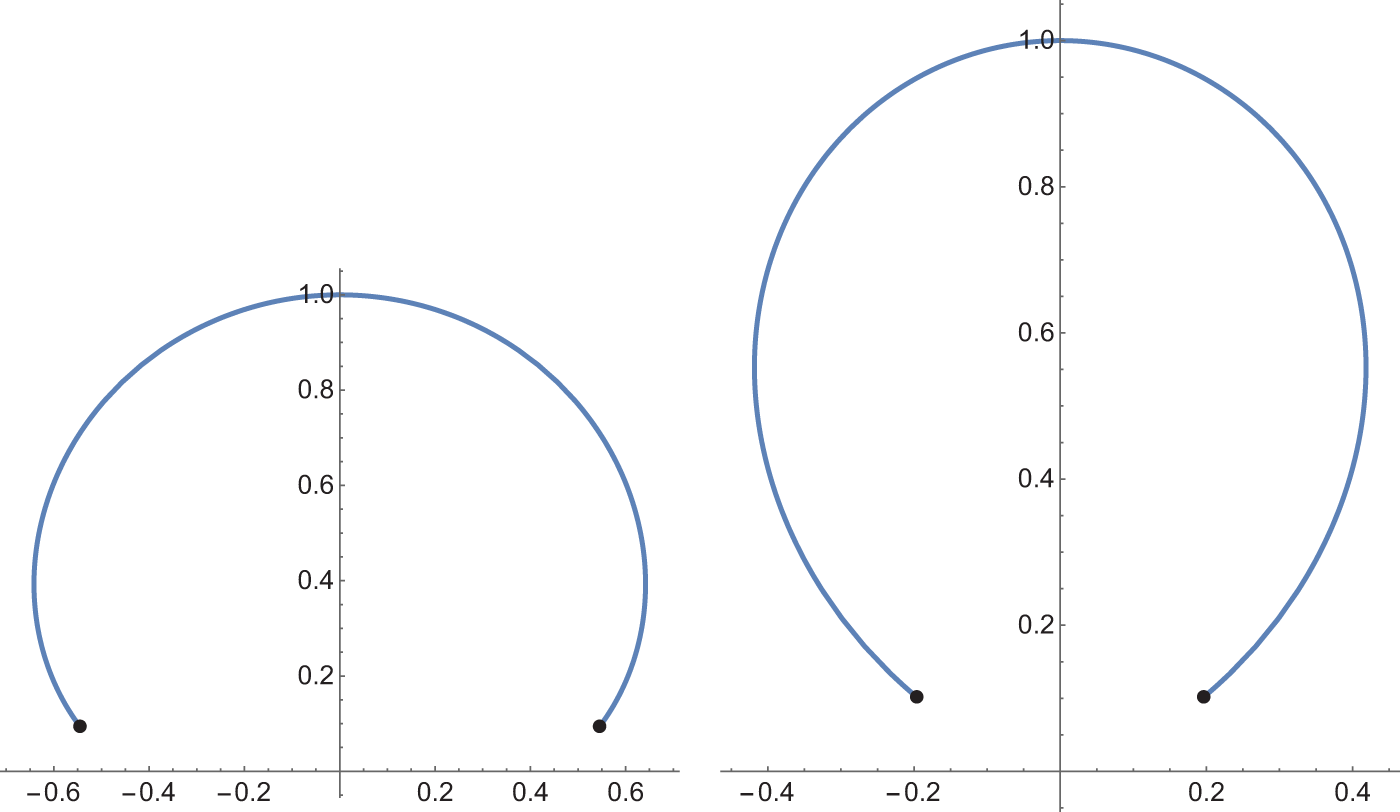


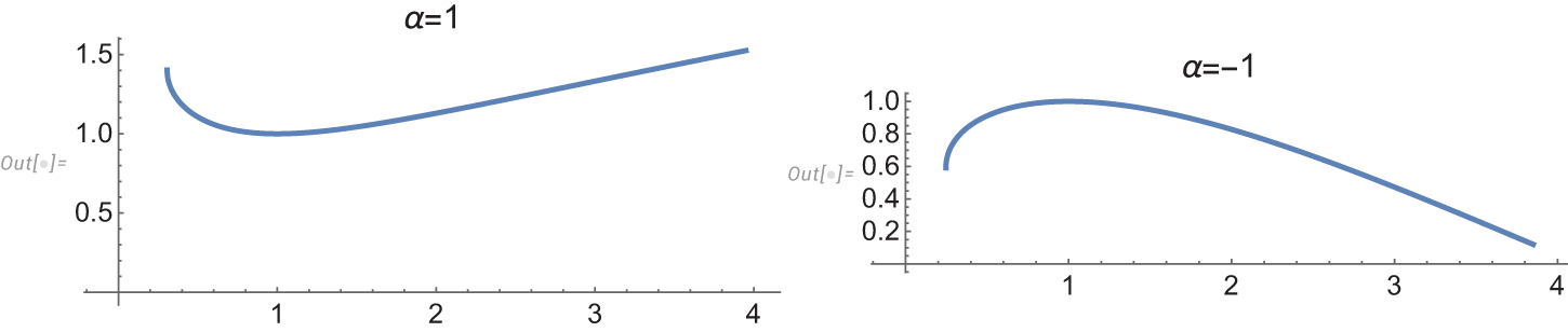


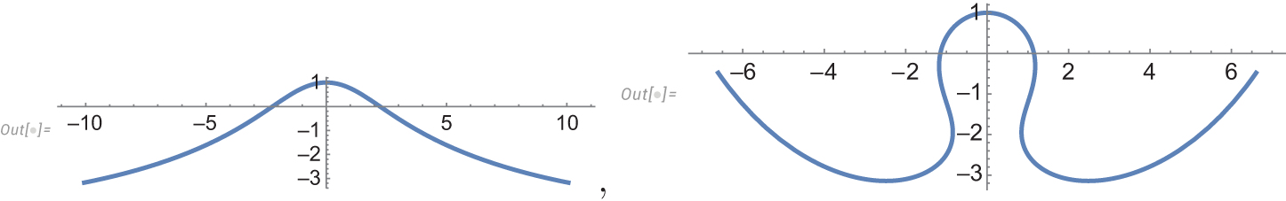


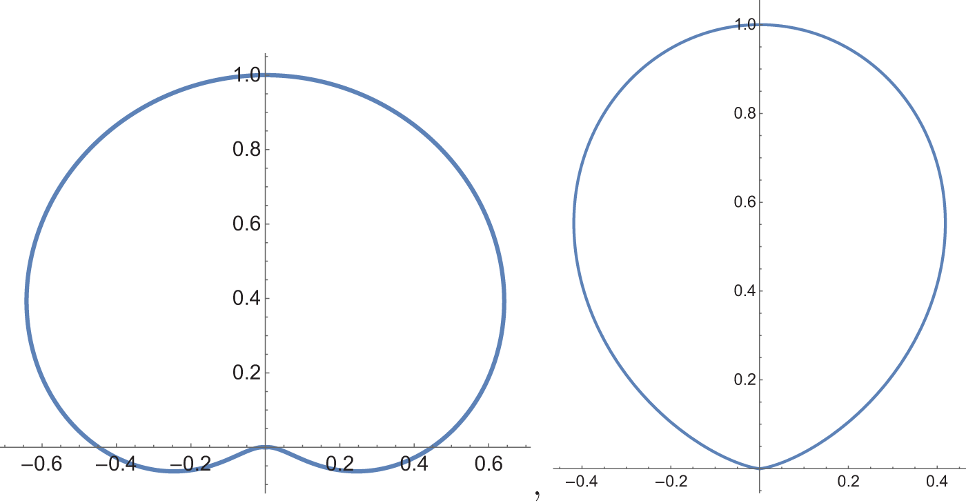


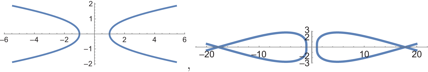


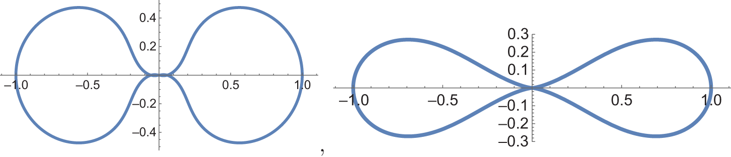


 Open access