2. Procedure

2.1. Numerical set-up

We consider the turbulent flow within a doubly periodic channel as sketched in figure 1 by means of DNS. Streamwise, wall-normal and spanwise directions are denoted through $x$, $y$ and $z$, whereas $u$, $v$ and $w$ are the respective velocity components. While most aspects of the present numerical experiment are standard for this flow geometry, the peculiarity of the present work is the wall boundary condition with a spanwise inhomogeneity, which is described in detail in § 2.2. For the time being, it is sufficient to know that the wall boundary condition, applied symmetrically to both walls, periodically varies in the spanwise direction with a period $2s$.

Figure 1.

A sketch of the channel with piecewise constant, spanwise variable roughness. For both SSBC and SLBC cases, the displayed shading is used to identify smooth and rough surface patches. In case of SSBC the grey shading indicates enhanced wall shear stress, in case of SLBC the grey patch corresponds to a region with spanwise slip.

The DNS in this work are performed using the open-source solver XCompact3D (Laizet & Lamballais Reference Laizet and Lamballais2009; Laizet & Li Reference Laizet and Li2010; Bartholomew et al. Reference Bartholomew, Deskos, Frantz, Schuch, Lamballais and Laizet2020), which adopts sixth-order compact finite differences for computing spatial derivatives. In the streamwise and spanwise directions, the mesh is homogeneous; in the wall-normal direction stretching is used to refine the mesh towards the wall such that the first node is placed at $y^{+}=1$. The discretisation parameters for all simulations are given in tables 1 and 2.

Table 1.

Grid properties.

Table 2.

Metadata of the simulations used for this paper. Abbreviations: NSBC: no-slip boundary condition, SSBC: shear stress boundary condition, SLBC: slip-length boundary condition, $T$ denotes the averaging time, — means ‘not applicable’.

All turbulent properties denoted with $\langle \cdot \rangle$ are averaged along directions of statistical homogeneity, namely the $x$-direction and time, for a time interval given in table 2. Moreover, all available symmetries of the problem are exploited in computing $\langle \cdot \rangle$, i.e. the symmetry about the channel centreplane ($y=\delta$) and the statistical periodicity of the flow above the likewise periodic wall boundary condition. Therefore, besides its dependency on $y$, $\langle \cdot \rangle$ depends upon $z$ only through the relative position $-1\leq z/s \leq 1$ above the spanwise periodic boundary condition. Additionally, $\overline \phi$ denotes quantities that are also averaged in the spanwise direction, e.g. $\bar {u}(y) = \frac {1}{2}\int _{-1}^{1} \langle u \rangle (y, z/s) \,{{\,\mathrm {d}}} (z/s)$.

The flow is advanced in time with an explicit third-order Runge–Kutta scheme and driven by a constant pressure gradient (CPG), so that the average wall shear stress $\overline {\tau _w}= \rho \overline {u_\tau }^{2}$, where $\rho$ is the fluid density and $\overline {u_\tau }$, the average friction velocity, is also prescribed. This amounts to prescribing the friction Reynolds number $Re_\tau = \delta \overline {u_\tau } / \nu$, where $\delta$ is the channel half-height and $\nu$ the kinematic viscosity of the fluid. Analogous to field quantities, local $u_\tau$ and local $\tau _w$ are phase averaged and a function of $z/s$. The non-dimensionalisation in viscous units, denoted through a $+$-sign is based on $\overline {u_\tau }$ unless stated otherwise (e.g. $\langle u\rangle ^{+} = \langle u\rangle / \overline {u_\tau }$).

2.2. Considered boundary conditions

Two kinds of boundary conditions are employed to model strip-type roughness: a shear stress boundary condition (SSBC) and a slip-length boundary condition (SLBC). As can be seen in figure 1, we consider spanwise alternating strips of width $s$.

The SSBC, already adopted e.g. by Chung, Monty & Ooi (Reference Chung, Monty and Ooi2014); Chung et al. (Reference Chung, Monty and Hutchins2018), prescribes a fixed wall-normal (instantaneous) derivative of the streamwise velocity. Naturally, a high wall shear stress is associated with rough wall regions, while a low wall shear stress represents a smooth wall. The boundary conditions on bottom ($y=0$) and top ($y=2\delta$) wall are defined by

(2.1)\begin{equation} \left.\frac{\partial {u}}{\partial {y}}\right|_{y=0} ={-} \left.\frac{\partial {u}}{\partial {y}}\right|_{y=2\delta} = \frac{\tau_w(z)}{\nu} =\frac{u_\tau(z)^{2}\rho}{\nu}, \end{equation}

where $\tau _w$ can be varied depending on the spanwise location $z$. At both walls impermeability $v=0$ holds and a free-slip boundary condition $\partial w / \partial y = 0$ is applied for the spanwise velocity component. We confirm the statement of Chung et al. (Reference Chung, Monty and Hutchins2018) that the alternative use of a no-slip condition for $w$ does not significantly affect the results. The spanwise profile of $\tau _w(z)$ is directly imposed with SSBC, thus particular care needs to be taken so that its mean value $\overline {\tau }_w$ matches the prescribed pressure gradient. Since only Neumann boundary conditions are imposed for $u$ at the wall, the mean velocity profile becomes undefined up to a constant additive value and so does the flow rate. A unique solution $\langle \tilde {u}\rangle (y,z/s)$ is found without losing generality by constraining the flow rate to a constant arbitrary value, chosen here to be zero. Henceforth, the streamwise velocity is plotted relative to the mean velocity at the wall, i.e. $\langle u\rangle (y,z/s)= \langle \tilde {u} \rangle (y,z/s) - \bar {\tilde {u}}(y=0)$.

A piecewise constant boundary condition with periodicity $2s$ is considered, as also employed by Chung et al. (Reference Chung, Monty and Hutchins2018). In the present study, we prescribe

(2.2)\begin{equation} \tau_w(z) = \left(1-\mathrm{sign}\cos\left(\frac{{\rm \pi} z}{s} \right)\right)\frac{\tau_h-\tau_l}{2} +\tau_l, \quad \tau_h = \frac 32 \bar \tau, \ \tau_l = \frac 12 \bar \tau, \ \bar \tau = \frac{{Re}_\tau^{2} \nu^{2} \rho}{\delta^{2}}, \end{equation}

i.e. strips of width $s$, a shear stress ratio of $3$ and where $z=0$ is the centre of the low shear stress region. In addition, a sigmoid transition of the patch interfaces between high ($\tau _h$) and low ($\tau _l$) wall shear stress is defined by

(2.3)\begin{equation} \tau_w(z) = \begin{cases} \dfrac{\tau_h - \tau_l}{1+\exp\left(4\dfrac{z - s/2}{\Delta}\right)} + \tau_l, & \text{for } z \in [0, s],\\ \dfrac{\tau_h - \tau_l}{1+\exp\left(4\dfrac{-z - s/2}{\Delta}\right)} + \tau_l, & \text{for } z \in [{-}s, 0), \end{cases} \end{equation}

for $z \in [-s, s]$; the function may be periodically repeated as needed. This formulation is used to investigate the influence of a gradual change in wall shear stress on the flow. The parameter $\Delta$ describes the transition length, with larger values resulting in a less steep transition between $\tau _h$ and $\tau _l$. For $\Delta \rightarrow \infty$, (2.2) is recovered. While the transition function is not differentiable at whole-number multiples of $s$, the exponential decay of the derivatives ensures that this is negligible in a numerical context. When the influence of the prescribed wall shear stress distribution on the obtained results is discussed in the following sections, the actual distribution of $\tau _w$ is included in the lower part of the corresponding figures for reference, see e.g. figure 3 or figure 7.

The SLBC employs a spanwise-varying slip length for the spanwise velocity component as a numerical model for roughness strips. A slip length (Navier Reference Navier1823) relates the wall slip velocity with the wall-normal velocity gradient at the wall. It can be understood as the distance between a virtual wall, where no slip is thought to apply, and the actual wall, which then has a non-zero velocity. For spanwise slip the boundary conditions are given by

(2.4a,b)\begin{equation} w_{y=0} = l_{s,w}(z) \left.\frac{\partial {w}}{\partial {y}}\right|_{y=0}, \quad w_{y=2\delta} ={-} l_{s,w}(z) \left.\frac{\partial {w}}{\partial {y}}\right|_{y=2 \delta}, \end{equation}

where $l_{s,w}(z)$ denotes the spanwise slip length, which is the quantity that can vary along the spanwise direction. We note that a slip in streamwise direction can be inserted in an analogous way with $l_{s,u}$ as streamwise slip length. It was confirmed that the present implementation of the slip lengths reproduces the data presented in Min & Kim (Reference Min and Kim2004).

Following the suggestion by Luchini (Reference Luchini2013) we employ a spanwise slip length to model the drag increasing effect of small roughness on the turbulent flow field. Especially from research on turbulent drag reduction via riblets, it is established knowledge that the change in drag is related to the difference $\Delta l = l_{s,u} - l_{s,w}$ between the streamwise and spanwise slip lengths, so that drag is reduced when $\Delta l$ is positive. In this context, the slip length is typically referred to as the ‘protrusion height’ and $\Delta l$ for streamwise and spanwise flow can be used to predict the achievable drag reduction rate for small riblets (Bechert & Bartenwerfer Reference Bechert and Bartenwerfer1989; Luchini et al. Reference Luchini, Manzo and Pozzi1991). In contrast, an increase of the spanwise slip length leads to enhanced near-wall turbulence and thus drag increase (Min & Kim Reference Min and Kim2004; Fukagata, Kasagi & Koumoutsakos Reference Fukagata, Kasagi and Koumoutsakos2006; Busse & Sandham Reference Busse and Sandham2012; Gómez-de Segura & García-Mayoral Reference Gómez-de Segura and García-Mayoral2020). In § 5, we employ $l_{s,u} = 0$ and $l_{s,w} > 0$ (and therefore a negative $\Delta l$) as a simple model for a rough surface. Standard no-slip $(u=0)$ and impermeability ($v=0$) conditions are applied for the streamwise and wall-normal velocity components at both walls. The boundary condition is discussed for a homogeneous rough surface before $l_{s,w} > 0$ is prescribed as a function of $z$ in order to model strip-type roughness. The coordinates are again chosen in such a way that $z=0$ is at the centre of a low shear stress patch which corresponds to a patch with standard no-slip conditions for $w$. The present formulation ensures that the boundary condition does not have any influence on laminar flow conditions but leads to enhanced drag for turbulent flow only. Note that under CPG conditions this drag enhancement corresponds to a reduction of the flow rate. Again, a piecewise constant slip length and a sigmoid transition between patches are considered; the definitions are analogous to (2.2) and (2.3).

Different from the SSBC, the use of a spanwise slip length to define roughness regions does not cause an undefined flow rate. Therefore, it is possible to evaluate the relative change of the bulk velocity $U_b$ with respect to a standard no-slip channel at the same pressure gradient. This change in $U_b$ can be used to evaluate the corresponding overall drag increase through the modification of the skin-friction coefficient $C_f = 2 \overline {u_\tau }^{2}/{U_b}^{2}$.

3. Heterogeneous shear-stress boundary condition in laminar flow

In this section, the effect of the SSBC on a fully developed laminar channel flow is addressed in order to verify whether aspects of the occurrence and character of secondary flows are visible in this simplified setting and can be traced back to the properties of the laminar solution. In particular, we will first utilise the laminar solution to assess the effect of the smoothness of the transition between strips of high and low shear stress on the streamwise velocity profile. Then, the emergence of a secondary flow is observed in the linear response of the laminar base profile with SSBC boundary condition to a specific small disturbance.

A laminar, steady, fully developed parallel flow along a channel of constant cross-section is described by the streamwise momentum equation:

(3.1)\begin{equation} \nu\left(\frac{\partial^{2} u}{\partial y^{2}} + \frac{\partial^{2} u}{\partial z^{2}}\right) ={-} \frac 1\rho \frac{{\rm d} p}{{\rm d} x}, \end{equation}

where the pressure gradient ${{\rm d}p}/{{\rm d}x}$ is constant and independent of $y$ and $z$. Without loss of generality, ${{\rm d}p}/{{\rm d}x}=-1$ and $\delta =1$ are assumed. This is a Stokes flow in the two dimensions $y \in [0, 2\delta ]$ and $z\in [-\infty, \infty ]$ with $2s$-periodicity in $z$.

How much the smoothness of the transition region between strips of $\tau _h$ and $\tau _l$ influences the streamwise velocity profile can be easily assessed by exploiting the linearity of (3.1), which allows us to express the Stokes solution as sum of elemental solutions. The periodic SSBC boundary condition can thus be transformed into Fourier space and the Stokes problem can be solved for each separate spanwise wavenumber $\kappa$, knowing that high wavenumber content relates to a steep transition.

We consider an SSBC with piecewise constant shear stress with periodicity $2s$, i.e.

(3.2)\begin{equation} \tau_w(z) = 1 + \frac 12 \mathrm{sign}\left(\sin \left(\frac{\rm \pi}{s} z\right)\right) , z \in ({-}s, s) . \end{equation}

Its Fourier transform is given by

(3.3)\begin{equation} \tau_w(z) = 1 + \frac{2}{\rm \pi} \sum_{n=0}^{\infty} \frac{\sin((2n+1) z\frac{\rm \pi}{s})}{2n+1}, \end{equation}

which is displayed in figure 2. Thanks to the linearity of equation (3.1), the solution is given as

(3.4)\begin{equation} u(y, z) ={-} \frac{(y - 1)^{2}}{2} - 2 \sum_{n=0}^{\infty} \frac{\sin(\kappa z) \cosh(\kappa(y - 1))}{s\kappa^{2}\sinh(\kappa)} \end{equation}

(with $\kappa = (2n+1) ({{\rm \pi} }/{s})$). It is clearly visible that lower wavenumbers in the boundary condition dominate the solution. In fact, their contribution to the solution scales as $\kappa ^{-2}$ at the wall and as $\kappa ^{-2} \exp (-\kappa )$ at the centreline. This means that higher wavenumbers not only contribute less to the solution, but that their contribution is limited to a thinner and thinner layer in the vicinity of the wall. Therefore, we can conclude that the details of the transition region for a given patch size play a secondary role in determining the flow solution, particularly farther from the wall, since these details are contained only in the high wavenumber part of the spectrum.

Figure 2.

Model boundary condition $\tau _w$ (dashed, (3.2)), and (solid) Fourier expansion of $\tau _w$ (3.3), truncated after 10 elements.

The solution of (3.4) also indicates that increasing the patch size $s$, which corresponds to a decrease of the lowest allowed wavenumber for $n=0$, yields an overall larger velocity difference between the regions of high and low wall shear stress. In the $s \rightarrow \infty$ limit, the parabolic velocity profile is recovered everywhere; while the absolute values of the velocity tend to $\pm \infty$.

The first two main results of this section are visualised in figure 3, which shows the solution of the Stokes problem for different transition functions at different patch sizes. (The spanwise coordinate of the figure has been translated to match the remaining figures of this paper.) First, it can be seen that the spanwise inhomogeneous boundary condition affects the longitudinal flow in the channel centre for large patch sizes only, here, $s/\delta =1$ (i.e. larger base wavelengths). For $s/\delta =0.25$ the depicted isolines of $u$ (referred to as isovels in the following) do not reveal any variation in spanwise direction for $y/\delta > 0.2$. With increasing strip width, the presence of HMP over the low stress region thus becomes more pronounced and is present up to larger wall distances. In addition, figure 3 includes results generated with either a sharp (solid black lines, (2.2)) or a smooth transition (dashed red lines, (2.3)) from high stress to low stress in the boundary condition. It is clearly visible that these different boundary conditions have only minor influence on the resulting momentum distribution under laminar flow conditions.

Figure 3.

Isolines of the laminar streamwise velocity for (a) $s/\delta =0.25$ and (b) $s/\delta =1$ for $\tau _h = 3 \tau _l$. The colour code refers to different transitions between $\tau _h$ and $\tau _l$: stepwise (solid black lines) and sigmoid with $\Delta /s = 0.5$ (dashed red lines). The upper part of the figure shows equidistant isolines (in arbitrary units), the lower part depicts the prescribed spanwise distribution of $\tau _w$.

In the following, the linear response of a laminar flow to infinitesimal perturbations is studied at $Re_\tau =180$ with SSBC boundary condition $\tau _h / \tau _l=3$ and $s/\delta =1$. The intention of this numerical experiment is to assess whether the linear response to such perturbation contains features that resemble the secondary flows which occur for the same boundary conditions and turbulent flow. A comprehensive analysis of the linear transient growth of optimal perturbations (Schmid & Henningson Reference Schmid and Henningson2001) is out of the scope of the present manuscript. Instead, we limit the consideration to a simple class of perturbations, which represents an extremely simplified model of spanwise velocity fluctuations as they may occur in the vicinity of a wall of a turbulent channel. An initial perturbation is added to the streamwise base flow $u(y,z)$ defined by (3.4) and shown in figure 3(b). This spanwise-homogeneous initial perturbation is prescribed as a spanwise velocity of the form

(3.5)\begin{equation} w(x,y,t=0) = c\, \overline{u_\tau}\, w_x(x) w_y(y) , \end{equation}

where $c = 10^{-10}$ is a constant determining the amplitude of the perturbation, while $w_x(x)$ and $w_y(y)$ are streamwise and spanwise shape functions, respectively. These are defined as

(3.6a,b)$$\begin{gather} w_x(x) = (x/\delta-\mu_x) \exp\left({-\frac{(x/\delta-\mu_x)^{2}}{2\sigma_x^{2}}}\right), \nonumber\\ w_y(y) = \frac{1}{y/\delta} \sigma_y \sqrt{2{\rm \pi}} \exp\Bigg({-\frac{(\ln(1 - |y/\delta-1|)-\mu_y)^{2}}{2\sigma_y^{2}}}\Bigg), \end{gather}$$

which resemble a normal and a log-normal distribution, respectively, so that the disturbance is localised in space, has zero streamwise average $\langle w\rangle _x$, is symmetric about the channel centre and fulfils the boundary conditions. The coefficients in (3.6a,b) are $\mu _x=4\delta$, $\sigma _x= \sigma _y=0.2$ and $\mu _y=\ln (0.08)+\sigma _y^{2}$, i.e. the disturbance is centred about $x/ \delta =4$ and $y/\delta = 0.08$. These parameters result in the initial disturbance distribution shown in figure 4.

Figure 4.

(a) Initial disturbance and its shape functions. (b) Temporal evolution of the initial disturbance at $t=0$, $tu_\tau /\delta =0.0127$ and $tu_\tau /\delta =0.0254$; isosurfaces of $w = \text {const.} = 1/4 \max (w(x,y,t=0))$. The isosurfaces are displayed as viewed by an observer moving with constant $x$ velocity to avoid overlap.

Applied to a flow with homogeneous wall boundary condition, for which the mean velocity profile is $u=u(y)$, the initial disturbance would only be sheared apart due to the effect of mean shear $\mathrm {d} u / \mathrm {d}y$ while retaining the spanwise homogeneity, and eventually vanish by viscosity without the generation of additional velocity components. On the other hand, the spanwise inhomogeneity of the velocity profile $u=u(y,z)$ over the SSBC strips will deform the original spanwise alignment of the disturbance, since its convection speed will generally be larger in region of $\tau _l$, as shown in figure 4(b). The loss of spanwise homogeneity, which is largest across the interface between strips, causes $\partial w / \partial z$ to become non-zero and thus implies the generation of further velocity components via continuity and yields a linear exponential growth of the disturbance. The linearity has been tested by progressive reduction of the $c$ constant, which showed an invariant solution once rescaled with the norm of the initial disturbance. If the flow is averaged in the streamwise direction during this exponential growth phase, the velocity field (shown in figure 5) exhibits non-zero streamwise-average velocity components $\langle v \rangle$ and $\langle w \rangle$ compatible with the secondary flows occurring in a turbulent channel. Region of upwelling motions are located above strips of $\tau _l$, while downwelling fluid is found over regions of $\tau _h$. This mechanism, that involves the shearing of spanwise velocity fluctuations and the consequent effect of continuity, is likely to occur also in fully developed turbulent channel flows and to be a contributor to the generation of secondary motions above strips of SSBC, as it will be discussed also in § 4. Qualitatively similar results are achieved for a number of different disturbances (not shown here), such as different wall-normal locations, asymmetric shape functions $w_y(x)$ or non-zero streamwise mean $\langle w(x)\rangle _x$. The result also generalises to other spanwise wavelengths $s$.

Figure 5.

The dominant mode after $tu_\tau /\delta =1.27$, the pointwise cross-stream velocity of this mode grows exponentially.

4. Heterogeneous SSBC in turbulent flow

We now employ the same SSBC as used in § 3 to a turbulent channel flow. The SSBC with the sharp jump from low to high stress values corresponds to the configuration studied by Chung et al. (Reference Chung, Monty and Hutchins2018). The main results of that study have been replicated and are discussed in comparison with the laminar result of the previous section in the following.

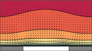
In contrast to the unperturbed laminar flow conditions, a vortical secondary flow is observed for turbulent flow conditions after averaging the resulting instantaneous velocity fields in time, streamwise direction and phase. This vortical motion induces downwelling over the patches with high shear stress and upwelling over patches with low shear stress. The corresponding results are visualised in figure 6(a) for $s/\delta = 1$. The secondary flow resembles the large-scale flow structures generated in the perturbed laminar flow at the same $s/\delta$ (cf. figure 5)

Figure 6.

(a,c) Time- and phase-averaged streamwise velocity contours in the channel cross-section, centred on the low shear stress region, for (a,b) $s/\delta =1$ and (c,d) $s/\delta =4$. Here $\tau _h = 3 \tau _l$, ${Re}_{\tau } = 180$, piecewise constant shear stress. The secondary flow $[\langle v \rangle, \langle w \rangle ] / \overline {u_\tau }$ in the plane is indicated with streamlines, with equally scaled width among the plots. (b,d) In-plane Reynolds stress $\langle v'w' \rangle ^{+}$.

Opposite to the unperturbed laminar flow, a HMP is present over the high stress (rough) region, whereas a LMP is found over the low stress (smooth) region. For larger $s/\delta$, a different distribution of streamwise mean velocity is found, as can be seen in figure 6(c). The secondary motion has the same rotational direction as in the case of $s/\delta = 1$. However, the flow conditions at the channel centreline reveal a HMP over the low stress region and a LMP over the high stress region. In particular, above the high stress region the downward motion of the secondary flow is located in a clearly pronounced LMP visualised through upward bulging isovels (isolines of longitudinal mean velocity).

Comparing the bulging of isovels between unperturbed laminar and turbulent flow conditions at the same $s/\delta =1$ (cf. figures 3b and 6a) reveals that the location of HMP and LMP differs between laminar and turbulent flow conditions, the difference obviously being caused by the secondary flow. In turbulent flow with heterogeneous SSBC, the secondary flow motion counteracts the tendency of the longitudinal flow to follow the path of lower resistance. This results in the flow phenomenon that the turbulent flow rate above the low stress (smooth) surface patches is smaller than the one over high stress (rough) patches, which is in agreement with the original experimental results by Hinze (Reference Hinze1967). The consideration of Hinze (Reference Hinze1967, Reference Hinze1973), that local overproduction of turbulent kinetic energy (TKE) is linked to the presence of secondary motions, also holds true for the present data. In the near-wall region the secondary motion carries fluid from high TKE regions (above the ‘rough’ patches) to low TKE ones.

For the present case of SSBC with $s/\delta =1$ (figure 6a), the downward bulging isovels of the laminar flow (figure 3b) are straightened by the secondary flow near the wall ($z=0, y/\delta \approx 0.05$) while the bulging direction is reversed at larger wall distance ($z=0, y/\delta \approx 0.2$). In the direct vicinity of the wall the distribution of the mean streamwise velocity is prescribed by the boundary condition, such that lower streamwise velocity prevails above the high shear region, similar to the laminar case (see zoomed in region of figure 6a). For larger $s/\delta$, the secondary flow also counteracts the laminar velocity distribution, but its visible impact is limited to a central region above the low shear stress strip. The upwelling in this region induces a local HMP above the intersection between high and low shear stress clearly visible around $y/\delta \approx 0.6$, $z/s\approx \pm 0.4$ in figure 6(c). Note that the isovels are very dense directly above the high shear stress region, indicating the anticipated large velocity gradients. As a direct consequence of the SSBC (see § 3), the simulations produce artificially large wall velocity differences where the difference $\langle u \rangle (y=0, z=0) - \langle u \rangle (y=0, z=-s)$ between patches increases with $s$. For $s/\delta = 4$, this difference is approximately $10.9 \overline {u_\tau }$; for $s/\delta =8$ it increases to $20.8 \overline {u_\tau }$ and is thus larger than the bulk mean velocity in a standard turbulent channel flow at the same ${Re}_\tau$. It is thus not surprising that the secondary flow is not able to invert the isovel bulging for large strip widths. As noted before, the reference velocity in the figure is chosen such that $\bar {u}(0)=0$. Therefore, the colour scale for $(\langle u \rangle - \langle u \rangle (0))/\overline {u_\tau }$ in figure 6 contains negative values. Those are limited to the direct vicinity of the high shear stress region and can thus only be identified in the enlargement provided for figure 6(a).

It is interesting to note that, contrary to turbulent secondary flows in non-circular ducts (or as observed over streamwise ridges), the secondary motions obtained with SSBC do not enhance but counteract the local curvature of the isolines of the streamwise velocity of the corresponding laminar flow. A possible explanation of this observation might be the mechanism described in § 3, where it was shown that near-wall spanwise perturbations in the laminar base flow with spanwise gradients of the (streamwise) velocity can induce large-scale vortical motions even in a linearised setting. This suggests that the secondary flow structures might not require the existence of the complex nonlinear scale interaction of turbulent flows for their initial generation.

The cross-stream motion is oriented from the high to the low shear stress region near the wall. Under laminar flow conditions these regions correspond to low and high streamwise velocity, respectively (see figure 3b). The turbulent secondary motion is thus expected to reduce the spanwise gradients of $\langle u \rangle$ near the wall compared with the laminar case, as indicated by the straightened isovels in this region. The related redistribution of streamwise momentum can induce a reversal of the isovel curvature (in the turbulent flow compared with its laminar counterpart) at larger wall distance ($y/\delta >0.5$) as observed for $s/\delta = 1$ and above the low shear stress region for $s/\delta = 4$.

Secondary motions above roughness strips are usually categorised as secondary motions of Prandtl's second kind (Wang & Cheng Reference Wang and Cheng2006). In the following, we discuss to which extent the secondary motions in turbulent flow over SSBC are in agreement with the original descriptions by Prandtl for this flow phenomenon. The driving mechanism of turbulent secondary flows originally proposed by Prandtl (Reference Prandtl1926) is based on the hypothesis that turbulent velocity fluctuations along isovels are larger than normal to their orientation. For isovels with inclined orientation in the present coordinate system, this suggests the presence of a correlation between $v$ and $w$. For curved isovels, this motion along the isovel induces forces directed to the convex side of the isovels. These forces, which are only present under turbulent flow conditions, increase with increasing curvature and induce a net transport of mean streamwise momentum (Prandtl Reference Prandtl1926).

Figure 6(b,d) shows the spatial distribution of $\langle v'w' \rangle$ for $s/\delta =1$ and $s/\delta =4$. Indeed, the correlation of $v$ and $w$ fluctuations is overall in very good agreement with the direction of the isovels depicted in figure 6(a,c). The enlargement provided for the near-wall region around the step change in boundary condition for figure 6(a) allows us to better identify the local isovel shape near the wall. In both cases a negative slope of the isoline corresponds to $\langle v'w' \rangle <0$, i.e. a negative correlation between $v'$ and $w'$, and vice versa. The hypothesis of Prandtl that in-plane velocity fluctuations are largest along isovels is thus confirmed for the present data. Also, the isovel curvature largely agrees with the direction of the secondary motion. However, we note that the distribution of $\langle v'w' \rangle$ is not in qualitative agreement with the one observed in DNS of immersed boundary method (IBM) resolved roughness strips (see figure 8 of Schäfer et al. (Reference Schäfer, Stroh, Forooghi and Frohnapfel2022) and the Appendix). We will return to the discussion of $\langle v'w' \rangle$ in comparison with the SLBC in § 5.2.

Finally, we address the influence of gradual vs sudden transition of the boundary condition for turbulent flow. It was shown in § 3 that a gradual instead of a step-change transition between high and low stress regions does not alter the laminar flow field except for the very near-wall region. Figure 7 shows a $y$–$z$ cross-section of the phase-averaged mean flow quantities for turbulent flow conditions at $s/\delta =1$ and different sigmoid transitions. For $\Delta /s=1/{16}, 1/8, 1/4$, a very similar secondary flow to the case of the piecewise constant reference case is observed. The secondary flow magnitude is slightly reduced for gradual wall shear stress changes. This also reflects in the bulging of the isovels, which are shown in direct comparison for $\Delta /s=0$ and $\Delta /s={1}/{4}$ for strip width $s/\delta =1$ and $s/\delta =4$ in figure 8. The dashed red line corresponds to the gradual change in the boundary condition. This sigmoid transition apparently leads to a slightly reduced spanwise inhomogeneity of the mean flow field, especially visible for $s/\delta =4$, which is in agreement with the presence of a slightly weaker secondary motion. However, the overall impact of the gradual change in boundary condition is very small.

Figure 7.

Time- and phase-averaged streamwise velocity contours in the channel cross-section, centred on the low shear stress region, for the different transitions with $\tau _h = 3 \tau _l$, ${Re}_{\tau } = 180$ and $s/\delta =1$. The secondary flow $[\langle v \rangle, \langle w \rangle ] / \overline {u_\tau }$ in the plane is indicated with vectors, with equally scaled length among the plots. The prescribed wall shear stress as a function of the spanwise coordinate $z$ is shown below each panel; (a) $\Delta /s = 0$, (b) $\Delta /s = 1/16$, (c) $\Delta /s = 1/8$, (d) $\Delta /s = 1/4$.

Figure 8.

Isolines of the time- and phase-averaged streamwise velocity for (a) $s/\delta =1$ and (b) $s/\delta =4$ at $\tau _h = 3 \tau _l$. The colour code refers to different transitions between $\tau _h$ and $\tau _l$: stepwise (solid black lines) and sigmoid with $\Delta /s = 1/4$ (dashed red lines).

5. Spanwise slip-length boundary condition in turbulent flow

5.1. Modelling homogeneous roughness

As introduced in § 2.2, we employ a transversal slip length to model the effect of a rough surface on a turbulent flow field. It has been established that a transversal slip increases near-wall turbulence and thus skin-friction drag; while a longitudinal slip leads to drag reduction (Min & Kim Reference Min and Kim2004). Fukagata et al. (Reference Fukagata, Kasagi and Koumoutsakos2006) and Busse & Sandham (Reference Busse and Sandham2012) suggested a relation between the dimensionless spanwise slip length and the resulting drag increase. Assuming only minor modifications to the shape of the turbulent velocity profile due to the imposed boundary condition, the corresponding reduction of $U_b^{+}$ can be translated into the Hama roughness function $\Delta U^{+}$, which is widely used to characterise turbulent flow over rough surfaces. Figure 9(a) shows the correlation proposed by Fukagata et al. (Reference Fukagata, Kasagi and Koumoutsakos2006) translated into $\Delta U^{+}$ for the present CPG conditions in comparison with simulation results. They are in excellent agreement. As noted by Fukagata et al. (Reference Fukagata, Kasagi and Koumoutsakos2006), the observed changes in $\Delta U^{+}$ are almost independent of Reynolds number, which we confirmed with additional simulations at $Re_\tau =540$ (not shown here). For a rough surface, $\Delta U^{+}$ is expected to increase with Reynolds number. Therefore, it should be noted that simulations with constant $l_s^{+}$ at different Reynolds number do not mimic the Reynolds number dependence of real rough surfaces. For such a study the prescription of a Reynolds number dependent $l_{s,w}^{+}$ would be required. In figure 9(a) it can be seen that the relationship between $\Delta U^{+}$ and the spanwise slip length is nonlinear. This saturation effect was previously reported by Gómez-de Segura & García-Mayoral (Reference Gómez-de Segura and García-Mayoral2020) and is in agreement with the finding of Luchini (Reference Luchini2013) that this type of boundary condition is suited for the representation of small roughness only. Nevertheless, a roughness function of the present order of magnitude corresponds to a significant drag increase. The related increase of $C_f$ under CPG conditions is of the order of $50\,\%$ for $l_{s,w}^{+} \approx 10$ ($\Delta U^{+} \approx 3$) at $Re_\tau =180$, as shown in figure 9(b). An increase in Reynolds number leads to a smaller change in skin-friction drag coefficient for a fixed $\Delta U^{+}$, as discussed by Gatti & Quadrio (Reference Gatti and Quadrio2016). This is confirmed for the present boundary condition at $Re_\tau =540$ where $l_{s,w}^{+} \approx 10$ corresponds to a drag increase of approximately $45\,\%$.

Figure 9.

(a) Relative velocity deficit $\Delta U^{+} = \langle u \rangle ^{+}|_\delta - \langle u \rangle ^{+}|_{\delta,{NSBC}}$ for ${Re}_\tau =180$ and (solid line) Relationship suggested by Fukagata et al. (Reference Fukagata, Kasagi and Koumoutsakos2006), adapted. (b) Relative change in skin-friction coefficient $C_f$ compared with the no-slip reference case (denoted by index 0) at the same $Re_\tau$ evaluated for $Re_\tau =180$ and $Re_\tau =540$.

The prescription of a spanwise slip length can thus reproduce the mean velocity profile of a turbulent flow over rough surfaces with roughness functions of the order of $\Delta U^{+} < 4$ (Fukagata et al. Reference Fukagata, Kasagi and Koumoutsakos2006). We note that the spanwise slip length has no direct relation to the roughness topography and cannot reproduce the specific flow signatures of a roughness sublayer (Chung et al. Reference Chung, Hutchins, Schultz and Flack2021), which is also the case for other roughness models employed in DNS, see e.g. Busse & Sandham (Reference Busse and Sandham2012). While a SLBC based roughness model has the advantage of replicating the roughness effect of not influencing the drag of laminar flows, the model requires a priori knowledge about the main flow direction as slip is prescribed for the transversal velocity component only.

5.2. Modelling heterogeneous roughness

In order to model alternating strips of rough and smooth surfaces, the SLBC is applied in the same configuration as in § 4; i.e. $Re_{\tau } = 180$, $s/\delta = 0.25, 1, 4$. We choose a slip length of $l_{s,w} = 0.05 \delta$ ($l_{s,w}^{+} = 9$), which corresponds to a roughness function of $\Delta U^{+} \approx 3$ for a homogeneously rough surface at $Re_{\tau } = 180$. The resulting velocity profiles for the heterogeneous case are presented in figure 10. The left column of plots is scaled with the global friction velocity $\overline {u_\tau }$, which is defined by the prescribed pressure gradient. Since the pressure gradient is equal in all considered cases, the plots in this column allow us to deduce statements on the flow rate in a given section of the inhomogeneous channel. The plots in the right column are scaled with the local friction velocity $u_\tau (z)$, which makes it possible to compare local flow conditions with the homogeneous reference cases.

Figure 10.

Velocity profile for different $z$ positions, scaled with (a,c,e) the mean friction velocity $\overline {u_\tau }$ and (b,d, f) the local friction velocity $u_\tau (z)$. (a,b) $s/\delta = 0.25$, (c,d) $s/\delta = 1$, (e, f) $s/\delta = 4$.

For $s \ll \delta$, the change in the boundary condition only affects the near-wall region; Townsend's outer layer similarity hypothesis holds (Townsend Reference Townsend1976). For $y > s$, the mean velocity profiles at different $z$ positions collapse when scaled with the global friction velocity $u_{\bar \tau }$ (figure 10a), suggesting spanwise homogeneity. The velocity profile in the outer layer falls between the limiting homogeneous cases. For $s \gg \delta$, the flow in each patch centre is barely affected by the change in the boundary condition. Above the two patches the flow conditions are relatively independent from each other. As a consequence, the local velocity profile agrees well with the respective homogeneous cases when scaled with the local friction velocity (which is higher in the $l_{s, w} > 0$ region), see figure 10( f). This suggests that the flow above the patches is in near equilibrium with the respective boundary condition which is not the case for the narrower strips, see figure 10(b,d). Since scaling the velocity profile with the local friction velocity $u_\tau (z)$ represents normalisation with the actual near-wall gradients of these profiles, the observed near-wall collapse of the profiles is expected.

As indicated in figure 10(e), the no-slip region provides a preferred pathway to the flow for $s \gg \delta$ due to the (relatively) lower skin friction. Therefore, a HMP is located above the no-slip region; i.e. the blue curve is located above the red one. For $s \approx \delta$, the opposite is observed, and the blue curve is located below the red one in figure 10(c). The redistribution of momentum due to the secondary motion obviously dominates over the effect of locally lower skin-friction drag and a LMP is located over the no-slip region.

The corresponding mean momentum distribution and secondary flow are presented in figure 11. As expected, for $s/\delta = 0.25$, the secondary motions are restricted to a region close to the wall. For $s=\delta$, the secondary vortices expand towards the channel centre and give rise to a high momentum pathway over the rough region. For $s/\delta = 4$, the secondary motions and the corresponding momentum transport is restricted to an approximately square region centred at the patch interface, giving rise to a weak local HMP on the rough side of the interface and a weak local LMP on the no-slip side. Such a configuration was also observed experimentally by Wangsawijaya et al. (Reference Wangsawijaya, Baidya, Chung, Marusic and Hutchins2020), but has to the authors’ knowledge not been reproduced in published simulations to date. The orientation and size of the secondary vortices observed in the cited experiments are correctly represented by the SLBC in all cases. In contrast, the SSBC exaggerates the difference between LMP and HMP for $s \gg \delta$, and predicts a larger lateral extent of the secondary flow structure (cf. § 4).

Figure 11.

Spanwise variable, piecewise constant $w$ slip length for different patch sizes. Contours: time-averaged streamwise velocity in the $y-z$ plane. The secondary flow $[\langle v \rangle, \langle w \rangle ] / \overline {u_\tau }$ in the plane is indicated with vectors, with equally scaled length among each column of plots. The $z$ limits are chosen to enable comparison with the experiments of Wangsawijaya et al. (Reference Wangsawijaya, Baidya, Chung, Marusic and Hutchins2020): figure 8(c,e,g). (b,d, f) Reynolds stress $\langle v'w' \rangle ^{+}$; (a,b) $s/\delta = 0.25$, (c,d) $s/\delta = 1$, (e, f) $s/\delta = 4$.

The spatial distribution of the Reynolds stress component $\langle v'w' \rangle$ is shown in figure 11(b,d, f). It clearly differs from the SSBC case (see figure 6) and is in better qualitative agreement with DNS results in which streamwise aligned roughness strips are resolved based on an IBM approach or modelled through a parametric forcing approach (PFA) (Schäfer et al. Reference Schäfer, Stroh, Forooghi and Frohnapfel2022). In particular, the qualitative agreement is achieved for the case of non-protruding roughness strips (cf. figure 8c,k in Schäfer et al. (Reference Schäfer, Stroh, Forooghi and Frohnapfel2022) vs figure 11b). Note that the spanwise wavelengths are different: Schäfer et al. (Reference Schäfer, Stroh, Forooghi and Frohnapfel2022) present results for $s/\delta =0.5$. Therefore, the Appendix contains a direct comparison of SSBC and SLBC at $s/\delta =0.5$ with the IBM resolved reference data.

Figure 12(a) presents the secondary flow and the momentum distribution for the case of a sigmoid transition of the $w$ slip length. The secondary flow is weaker than in the piecewise constant case (cf. figure 11c) while orientation and size of the secondary vortices are unchanged. The HMP also keeps its location over the rough patch. Figure 12(b) compares the isovels of the two transition types. It can be seen that HMP and LMP are slightly less pronounced for the sigmoid transition, which is in agreement with a weaker secondary flow. In addition, it is apparent that $U_b$ is reduced in case of the sigmoid transition. This follows from the nonlinear relation (saturation effect) between the slip length and the flow rate decrease (see figure 9); while the average slip length is kept constant, areas with half as much slip length lead to more than half as much drag increase, so the ‘average skin-friction coefficient’ increases.

Figure 12.

(a) Secondary flow and isovels for of the sigmoid transition with $s/\delta =1$, $l_{s,w} = 0.05$, the vectors are scaled as in figure 11. (b) Isovels for the same parameters, but different transition types. The transition between rough and smooth patches is distinguished using line styles: stepwise (solid black lines) and sigmoid with $\Delta /s = 1/4$ (dashed red lines) and the corresponding distribution of $l_{s,w}$ is shown in the lower parts of the figures.

The global skin-friction coefficient is not only governed by the relationship between $C_f$ and $l_{s,w}$, but also by additional contributions from the secondary flow. In order to quantify the latter, we assume that the skin-friction coefficient in flows with roughness strips but without any secondary motion can be computed based on the limiting case of two non-interacting channel parts (one smooth and one rough) that are both driven by the same pressure gradient (same $\overline {u_\tau }$). The identical pressure gradient in both channel parts ensures that no spanwise pressure gradient is generated, which in turn could drive a spanwise mean flow. The resulting flow rate for these two channel parts will naturally differ and the mean flow rate between the channels is given by $U_b = (U_{b,{rough}} + U_{b,{smooth}})/2$. The definition of the skin-friction coefficient $C_f = 2 \overline {u_\tau }^{2}/U_b^{2}$ then yields an expected global skin friction coefficient of

(5.1)\begin{equation} C_f = \left(\frac{1}{2}\left( \frac{1}{\sqrt{C_{f,{rough}}}} + \frac{1}{\sqrt{C_{f,{smooth}}}}\right) \right)^{{-}2}, \end{equation}

which is the ($p=-{1}/{2}$) power mean of the local skin-friction coefficients. The obtained value in comparison with the computed $C_f$ for different $s/\delta$ is is displayed in figure 13(a) in which $C_f$ of the smooth and rough homogeneous reference cases are also included. For the limiting case of small patches, (5.1) correctly predicts the global skin-friction coefficient. For patch sizes $s/\delta \approx 1$, the pronounced secondary flow is expected to increase the global skin-friction coefficient which is indeed the case. For very large patches $s/\delta \gg 1$, the secondary flow occupies only a small part of the channel (at the interface between the patches) and has thus little influence on $C_f$, so (5.1) holds again. The drag increase due to the presence of secondary motion (that is, the observed drag increase in relation to the prediction (5.1)) for piecewise constant boundary conditions is $2.9\,\%$ and $3.5\,\%$ for $s/\delta =1$ and $s/\delta =4$, respectively.

Figure 13.

(a) Skin-friction coefficient $C_f$ as a function of the strip width $s/\delta$ with stepwise change of the boundary condition and $l_{s,w,max}^{+} = 9$ in the rough patch. $C_f$ for the standard smooth wall, the homogeneous rough case with $l_{s,w}^{+} = 9$ and the prediction based on (5.1) are included for reference. (b) Estimation of the contribution of the secondary flow on the drag increase in case of the smooth transition between patches. ${Re}_\tau =180$ for all cases.

As discussed before, a continuous change of $l_{s,w}$ in spanwise direction (sigmoid transition) results in a global increase of the skin-friction coefficient due to the saturation effect of the employed boundary condition. An integral version of (5.1) can be employed to compute the related global skin-friction coefficient without the effect of secondary flow. A comparison with the DNS results of sigmoid $l_{s,w}$ transition reveals a drag increase of $2.0\,\%$ for $s/\delta =1$ due to the secondary flow. This procedure is visualised in figure 13(b). The drag increase thus appears to correlate with the strength of the secondary flow. It is, however, significantly smaller than the drag increase caused by the presence of ‘roughness’ alone (as computed using (5.1)), which is $20.8\,\%$ and $24.6\,\%$ for piecewise constant and sigmoid transition of the prescribed spanwise slip length, respectively.

We note that the definition of a percentage drag increase is not unambiguous for an internal flow with rough or structured surface. In the present data evaluation the channel half-height $\delta$ is a fixed geometrical property. This is in line with the inherent assumption for strip-type roughness of a large scale separation between the roughness height and the boundary layer thickness. However, if this scale separation does not hold, the influence of an effective channel height has to be taken into account as discussed in e.g. Schäfer et al. (Reference Schäfer, Stroh, Forooghi and Frohnapfel2022).

For a direct comparison with the $C_f$-changes presented in Schäfer et al. (Reference Schäfer, Stroh, Forooghi and Frohnapfel2022) we note that both Reynolds number and roughness function are larger than in the present case while the strip width is smaller. In addition, (5.1) was not applied in this case. Instead, the arithmetic mean of $C_f$ for smooth and rough walls was used as reference. Irrespective of the reference definition, i.e. as arithmetic mean or according to (5.1), the data of Schäfer et al. (Reference Schäfer, Stroh, Forooghi and Frohnapfel2022) indicate a much higher contribution of the secondary flow to drag increase than the present data. At the same time the isovel curvature due to the secondary flow is similar for the present data and non-protruding roughness strips of Schäfer et al. (Reference Schäfer, Stroh, Forooghi and Frohnapfel2022) (see their figure 5(c,j,k) or the Appendix). We suspect that this difference is related to drag effects on the protruding lateral sides of the smooth surface patches that were introduced in the IBM resolved and PFA modelled roughness DNS (Stroh et al. Reference Stroh, Schäfer, Frohnapfel and Forooghi2020; Schäfer et al. Reference Schäfer, Stroh, Forooghi and Frohnapfel2022). Those effects should disappear for large scale separation between the roughness length scale and the channel half-height (boundary layer thickness), which cannot be achieved with roughness resolving DNS. However, this scale separation is a likely property of engineering or environmental rough wall flows and can be realised experimentally. In fact, recent wind tunnel experiments with rough surface strips carried out in our laboratory indicate a smaller global drag increase when surface elevation differences between rough and smooth wall strips are minimised (von Deyn et al. Reference von Deyn, Stroh, Gatti and Frohnapfel2022).

6. Differences between SLBC and SSBC

As shown in the preceding sections, the SLBC is able to predict the effect of heterogeneous surface roughness in the form of streamwise oriented strips on a turbulent flow field. While providing the same numerical simplicity as the SSBC approach, i.e. no need for increased resolution for the rough region and the simplicity of a change in boundary condition only, the slip-length concept allows us to better capture the impact of heterogeneous roughness on near-wall turbulence properties.

From a global perspective, the first advantage of SLBC is the fact that it does not impact a laminar flow field. This is an important property since we expect a laminar flow not to be modified by the presence of roughness (in contrast to blockage effects related to larger surface structures). Therefore, the model allows us to directly investigate the influence of roughness on the turbulent flow field without the presence of any overlaying artefacts. In addition, the SLBC approach allows us to quantitatively evaluate the drag increase due to the presence of secondary flow, which is not possible with SSBC due to the unphysical flow rate (see Chung et al. (Reference Chung, Monty and Hutchins2018) for details).

The evaluation of the drag increase due to secondary flow for roughness strips with SLBC based on (5.1) assumes that in the absence of secondary flow there is no spanwise variation in wall shear stress. In fact for $s/\delta =16$ the wall shear stress (or $u_\tau$) is identical in the smooth and rough surface regions at sufficiently large distance from the interface between the two. The increased wall shear stress over the rough surface region is thus a consequence of the secondary motion which leads to an increase of the global $C_f$ compared with the prediction of (5.1), as shown in figure 13. In contrast, for SSBC the wall shear stress difference between smooth and rough surface regions is prescribed. Therefore, the wall shear stress distributions for SLBC and SSBC differ for very wide roughness strips.

In terms of secondary motion, the spatial extent of these large-scale motions in the case of wide strips ($s/\delta = 4$) appears to be correctly captured with SLBC (see figure 11e) while it is overpredicted with SSBC (see figure 6c) when compared with experimental literature results (see figure 8c of Wangsawijaya et al. Reference Wangsawijaya, Baidya, Chung, Marusic and Hutchins2020). This is likely to be related to the artificially large velocity differences near the wall between high and low shear stress regions in case of SSBC. As discussed in § 3, such a system is sensitive to spanwise disturbances under laminar flow conditions which can induce large-scale motions similar to the observed turbulent secondary motions. Therefore, the overprediction of the spanwise extent of the secondary flow in the case of SSBC is probably related to this instability mechanism and thus an artefact of the boundary condition.

For more narrow strips, the spatial extend of the secondary motion and its impact on the mean flow field are more similar for SSBC and SLBC (see figure 6(a) and 11(c) for $s/\delta = 1$ or the Appendix for $s/\delta = 0.5$). However, the related distributions of $\langle v'w' \rangle$ reveal significant differences in the near-wall region (sees figure 6b and 11d) where the SLBC shows qualitatively better agreement with roughness resolving DNS reference data (see the Appendix).

Finally, we note one interesting observation: for both boundary conditions investigated in the present study, a variation of $s/\delta$ (also beyond the presented parameter range) was never found to induce a reversal of the secondary motion or the occurrence of tertiary vortical structures. However, such phenomena were reported for increased strip width in the case of alternating slip and no-slip boundary conditions (Stroh et al. Reference Stroh, Hasegawa, Kriegseis and Frohnapfel2016) as well as for ridge-type roughness (Medjnoun, Vanderwel & Ganapathisubramani Reference Medjnoun, Vanderwel and Ganapathisubramani2020). The difference of the presently investigated boundary conditions compared with those studies is given by the fact that SSBC and SLBC both induce a spanwise variation of one velocity component only. SSBC induces a spanwise variation for the streamwise velocity component, while the heterogeneous SLBC is applied to the spanwise component only. The reason for the apparent insensitivity towards variations in $s/\delta$ might be related to this fact. This hypothesis, however, remains to be investigated in future studies. In the SLBC setting the introduction of an additional streamwise slip length might be suited to study this effect. The combination of streamwise and spanwise slip length can be imagined to represent the configuration of small streamwise ridges following the virtual origin framework (Gómez-de Segura & García-Mayoral Reference Gómez-de Segura and García-Mayoral2020). Unlike the SLBC considered here, one has to keep in mind that the introduction of a streamwise slip length leads to a configuration in which the ‘modelled roughness’ also modifies a laminar flow field – a fact that also holds true for ridge-type roughness.

7. Summary and concluding remarks

The flow over laterally inhomogeneous rough surfaces is studied by means of DNS in which two different models for the inhomogeneous surface condition are applied. Both models have the advantage that the resolution of individual roughness elements is not required, but the roughness effect is contained in an effective boundary condition instead such that the influence of the roughness height is eliminated. The first model, SSBC, was previously used in the literature (Chung et al. Reference Chung, Monty and Ooi2014, Reference Chung, Monty and Hutchins2018). It prescribes the wall shear stress such that a high wall shear stress region represents e.g. a streamwise aligned strip of rough surface which is flanked by smooth surface strips of lower wall shear stress. The second model, SLBC, based on a slip-length approach, has also been formulated in the literature before (Min & Kim Reference Min and Kim2004; Fukagata et al. Reference Fukagata, Kasagi and Koumoutsakos2006; Busse & Sandham Reference Busse and Sandham2012) and is known to induce drag increase. However, to the authors’ knowledge it was previously never employed to model inhomogeneous rough surfaces. This model introduces a slip length for the spanwise velocity component which can also be interpreted in terms of different protrusion heights (or virtual origins) for the streamwise and spanwise velocity components (Luchini et al. Reference Luchini, Manzo and Pozzi1991). In the present study a spanwise slip length is prescribed on ‘rough’ surface parts along with no-slip and impermeability conditions for the streamwise and wall-normal velocity components. The fact that this SLBC solely acts on the spanwise velocity component yields the advantage of influencing turbulent flow fields only, a property that is associated with hydraulically rough surfaces since the pioneering work of Nikuradse (Nikuradse Reference Nikuradse1933; Schlichting Reference Schlichting1979). It is shown that the relation between spanwise slip length and the Hama roughness function $\Delta U^{+}$ can be predicted based on available literature correlations (Fukagata et al. Reference Fukagata, Kasagi and Koumoutsakos2006). The roughness function achievable with the present SLBC is limited to $\Delta U^{+}<4$.

Heterogeneous rough surfaces in the form of streamwise aligned roughness strips lead to the formation of secondary flows of Prandtl's second kind in turbulent flows. Since the work of Hinze (Reference Hinze1967, Reference Hinze1973) it has been known that the secondary flow structures can lead to a pronounced redistribution of the streamwise momentum resulting in a flow field with larger flow rates above the rough than the smooth surface patches. Both modelling approaches addressed in the present study can capture this phenomenon in general. While the Reynolds stresses of the SLBC case resemble those of roughness resolving DNS with slightly recessed roughness strips, artificially large spanwise mean velocity gradients induced through SSBC lead to unphysical near-wall turbulence properties in this case. For both boundary conditions, the present results confirm the original hypothesis of Prandtl (Reference Prandtl1926), suggesting a prioritised turbulent motion in the direction parallel to isovels. This agreement between the isovel orientation and the sign of $\langle v'w' \rangle ^{+}$ holds true even in case of SSBC, where the extreme spanwise velocity gradients do not resemble realistic flow conditions.

These large spanwise gradients of streamwise velocity are a consequence of SSBC that is also present under laminar flow conditions. The resulting laminar flow field is shown to amplify small spanwise disturbances in such way that large-scale vortical motions with resemblance to the turbulent secondary flows emerge. This flow instability is likely to be the driving mechanism that induces the large lateral extent of secondary flow structures for SSBC in the case of a large structure wavelength (here $s/\delta = 4$), which is neither observed in experiments nor in the present DNS with SLBC. Therefore, numerical roughness models should be checked with respect to their impact on laminar flow conditions and potential artefacts that may arise therefrom.

The obtained results show that the spanwise gradient of the boundary condition has a small effect on the turbulent secondary flow only, irrespective of the employed roughness modelling approach. This leads to the conclusion that spanwise gradients in the boundary condition are not a critical issue as far as the formation of secondary flows is concerned. Sharp jumps of the boundary conditions can thus be avoided, which is an interesting aspect for numerical codes in which spatial derivatives are based on spectral discretisation. On the other hand, the impact of gradual roughness transitions that might occur in technical applications can be investigated with the simplification of step-like changes.

An additional advantage of SLBC is the fact that it allows us to quantitatively deduce the drag increase caused by the secondary flow. This drag increase amounts to a few per cent for the investigated cases only and is approximately one order of magnitude smaller than the roughness effect itself, a result that differs from previous findings obtained with roughness resolving DNS (Stroh et al. Reference Stroh, Schäfer, Frohnapfel and Forooghi2020) which show a significantly larger relative drag increase for roughness strips. We hypothesise that this difference reflects the inherent property of strip-type roughness, namely a negligible surface elevation of the rough or smooth surface parts compared with the boundary layer thickness. Such scale separation cannot be achieved with roughness resolving DNS. We therefore consider the SLBC an appropriate setting to numerically investigate the interplay between strip-type roughness and (very-)large-scale motions in turbulent boundary layers. This is likely to be relevant in the meteorology context where the relative roughness height (compared with the boundary layer thickness) is of the order of $10^{-3}$ and smaller (Anderson et al. Reference Anderson, Barros, Christensen and Awasthi2015) such that local deflections on protruding surface parts are expected to be negligible.

The fact that the SLBC acts on turbulence only also makes it a suitable set-up to further investigate the relevance of secondary flows for large-scale heterogeneous roughness in technical applications (Bons Reference Bons2002). These typically combine a streamwise and spanwise inhomogeneity of the surface roughness condition such that an additional development length scale of the secondary flow might become relevant. However, we note that both boundary conditions discussed in this paper require the a priori definition of the mean flow direction. While this requirement is easily satisfied for generic wall-bounded shear flows, its fulfilment can probably not be achieved for complex unsteady flow scenarios. Further modelling efforts will thus be required to enable the prediction of secondary flows of Prandtl's second kind under complex flow conditions.