


Impact Statement
This research examines the thermal behavior of surface materials in arid climates, offering crucial insights for enhancing urban sustainability and energy efficiency. Conducted in Antalya, Turkey, it evaluates materials like asphalt, concrete, and grass using thermal imaging and machine learning. The findings highlight the significant temperature variations, with materials like asphalt reaching over 50 °C in summer, impacting thermal comfort. This study offers valuable data for urban planners, architects, and policymakers, aiding the selection of materials that promote energy efficiency and comfort in hot climates. By integrating artificial intelligence with thermal imaging, the research also introduces innovative tools for sustainable architectural design. The study’s impact extends to industry, government, and academia, advancing sustainable urban planning and material selection.
1. Introduction
The landscape designer, who must focus on people-oriented space design, must make important decisions regarding the material to be used and how the planting design should be. Designs should respond not only to aesthetics but also to the functional needs of people. As always, the most important factor affecting their design selection is the climate and climatic comfort zone (Soydan and Benliay, Reference Soydan and Benliay2022). Previous studies show that well-designed landscape interventions can improve outdoor thermal conditions and reduce or increase physiological equivalent temperature by several degrees. The thermal properties of surface materials significantly influence microclimate regulation, energy balance, and outdoor thermal comfort. Diverse materials display distinct thermal characteristics, thereby affecting their capacity to absorb, reflect, and transmit thermal energy.
Knowledge of how different landscape surface materials partition energy should aid in the understanding of large-scale adoption of low water use landscapes. For this reflected spectral irradiance, albedo, net radiation, soil and sensible heat fluxes, and soil and surface temperatures of artificial turf, decomposed granite, hardwood mulch, and natural grass and simulated surface temperature during summer and winter days by means of a simplified energy balance model must be measured (Carvalho et al., Reference Carvalho, Chang, McInnes, Heilman, Wherley and Aitkenhead-Peterson2021). The difference between the apparent surface temperature of landscape elements and the ambient temperature is proportional to the amount of heat convected into the air, which can add to urban heat. The additional heat from landscape elements can make air and surface temperatures even more uncomfortable when summer temperatures are already high, hence summer is the most critical season to investigate. However, as some landscape elements exhibit high surface temperatures in spring and autumn, the effect of these seasons must also be considered by landscape designers, even for a warm temperate climate (Loveday et al., Reference Loveday, Loveday, Byrne and Ong2019).
Landscape architecture is pivotal in addressing issues pertaining to microclimate regulation, water management, and desertification within hot and arid environments. The interaction of residential surfaces with the atmosphere changes the surfaces’ microclimate effects. In addition, the proximity of the surface to the vegetation patch, such as the front and back lawns, also changes the surface temperature because of the humidity and evapotranspiration rates from the vegetation. Similarly, the pavements and walkways surrounded by residential buildings add to the surface temperature, while the swimming pools or fountains reduce the surface temperature (Saher et al., Reference Saher, Stephen and Ahmad2023).
Urban form and microclimate strongly influence one another. Specific urban structure can affect the microclimate because of the high radiation generated. On the other side, urban structure blocks the distribution of incoming wind. Urban structure changes how the microclimate influences the city. The successful urban structure influences how outdoor open spaces are used, while the quality of these spaces is strongly influenced by prevailing microclimatic comfort conditions (Wang et al., Reference Wang, Su, Koerniawan and Gao2022). With the continuous development of building surface cool material technology, the effect of cool materials on energy consumption is constantly investigated. However, the outdoor microclimate is bound to be affected when cool materials are applied to buildings throughout the neighborhood. Investigations of the effect of cool materials on the neighborhood wind and thermal environment, pollutant dispersion, and ventilation capacity are still scarce (Xu et al., Reference Xu, Zhang and Gao2023). The urban heat island effect can be reduced not only by careful planning of the urban structure, but also by a well-considered use of building materials and surfaces. Greening measures on the building scale (e.g., green walls and roofs) can have a decisive effect in terms of urban heat mitigation, which was shown in several research studies already (Teichmann et al., Reference Teichmann, Baumgartner and Horvath2021). Green infrastructure, facade greenings, urban water bodies, shadings, cooling materials, or reflective surfaces are promising approaches as they decrease the absorbed incoming radiation by a higher albedo or shift the partitioning of the surface energy balance towards latent instead of sensible heat flux (Herath et al., Reference Herath, Halwatura and Jayasinghe2018; Eingrüber et al., Reference Eingrüber, Korres and Schneider2022).
Infrared camera comparative measurement methods of thermal optical properties of materials are based on the measurement of infrared radiation emitted from the surface of the material that is heated to a higher temperature (Veselý and Honner, Reference Veselý and Honner2019). This approach leverages energy sources to elicit heat flow, and the resultant temperature distributions are scrutinized to ascertain material thickness and identify potential flaws (Holland and Reusser, Reference Holland and Reusser2016). Innovations in thermal imaging technology have considerably enhanced measurement precision and mitigated uncertainties, rendering them appropriate for quantitative evaluations (Hobbs et al., Reference Hobbs, Zhu, Grainger, Tan and Willmott2018). The integration of thermal imaging into design paradigms promotes enhanced material performance and reliability.
The assessment of surface temperature measurements utilizing artificial intelligence (AI) has progressed markedly, incorporating a variety of methodologies and applications (Yin et al., Reference Yin, Huang, Menne, Vose, Zhang, Adeyeye, Applequist, Gleason, Liu and Sánchez-Lugo2024). Novel techniques have realized significant advancements in both accuracy and bias mitigation. Recent investigations underscore the deployment of multilayer perceptrons and localized convolutional neural networks (CNNs) for the extraction of surface temperatures from remote sensing datasets, effectively addressing regional biases that may compromise model prognostications (Boucher et al., Reference Boucher, Aires and Pelle2023). Furthermore, the NOAA Global Surface Temperature dataset employs integrated AI methodologies to enhance data reconstruction in areas lacking observational data, such as the Arctic, showcasing superior robustness and precision in comparison to previous methodologies (Yin et al., Reference Yin, Huang, Menne, Vose, Zhang, Adeyeye, Applequist, Gleason, Liu and Sánchez-Lugo2024). The amalgamation of machine learning and deep learning with sensor technologies augments AI-driven sensing capabilities, culminating in enhanced efficacy for applications such as climate monitoring (Zhang et al., Reference Zhang, Wang and Lee2023; Chen et al., Reference Chen, Xia, Zhao, Fu and Chen2024). These advancements highlight the transformative influence of AI on methodologies and applications concerning surface temperature measurement.
In contrast to many AI-based surface temperature studies that depend heavily on satellite imagery or large aggregated datasets, this research uses thermal images obtained directly from on-site landscape surfaces and applies machine-learning models to these field measurements. By grounding the analysis in real physical environments rather than remote-sensing data alone, the study offers a distinctive methodological contribution to landscape thermal comfort research (Voogt and Oke, Reference Voogt and Oke2003; Weng, Reference Weng2009).
2. Materials and Methods
In this study, thermal photography activity was carried out with FLIR-C5 thermal imaging device in Dokumapark located in Kepez district of Antalya, Turkey (Figure 1), to examine the thermal properties of various surface materials according to seasons and hours of the day. In this area, measurements were made for at least 4 days for each month of the year and 3 different time periods during the day. Time periods were determined as early hours (08:00–10:00), noon (13:00–15:00), and evening (18:00–20:00).
Location of the study area.

In the image acquisition process, it was made to choose times when the sunlight was not blocked by clouds for the point where the photo was taken. Photography was not carried out in rainy or cloudy weather. A total of 864 thermal images were taken for six different surface materials: “Asphalt,” “Concrete,” “Granite,” “Wood,” “Grass,” and “Soil” for the appropriate days and time periods.
In the systematic imaging process, images were taken for each material, especially in terms of being in the shade and receiving direct sunlight. During this process, the ambient temperature was also recorded using a digital thermometer.
The custom software, which was developed using Python within the Visual Studio Code environment, employs libraries such as NumPy, Matplotlib, and Tkinter. The software was designed to convert pixel values from the thermal images into temperature readings in degrees Celsius (°C), as illustrated in Figure 2. The Python code of the software, which means Temperature Analysis application in Turkish, called “Sıcaklık Analizi,” is given in the Appendix.
Thermal camera image analysis software.

Using this software, a total of 1728 surface material temperature values were obtained, with the average information of temperature values in the shade and under the sun obtained from 864 separate images.
The FLIR C5 device is factory-calibrated with NIST-traceable standards. Users cannot perform internal hardware calibration themselves; recalibration is only possible by sending the device to FLIR support services. Previous studies have demonstrated that the FLIR C5 can be reliably used in scientific research.
However, to ensure the reliability of this study, reference thermometer comparisons were conducted using two handheld infrared thermometers available in the department: the Fluke 62 MAX+ and the Testo 830 T4. These measurements were compared with the values obtained from the FLIR C5 images. Although a mean difference of approximately (±0.2 °C) was observed, the device was considered sufficient and reliable for this study, since the focus was on evaluating the temperature differences between surface air and material surfaces rather than absolute surface temperatures.
In this study, all thermal images were captured at an average distance of 3 m to ensure sufficient pixel density and measurement accuracy. The camera was positioned parallel to the ground plane at a height of 1.50 m and oriented perpendicularly (90°) to the surface to minimize distortion. Repeated images were taken from the same location and angle as the initial measurement, and for shaded versus sunlit conditions, the same surface patch was used whenever possible. Emissivity settings were manually adjusted for each material using standard reference values (asphalt: 0.95, concrete: 0.92, granite: 0.90, wood: 0.94, grass: 0.98, soil: 0.93). These adjustments were applied before each measurement.
All measurements were made on flat, open surfaces within Dokumapark, with materials placed on level ground to avoid slope-induced variation. For grass and soil, natural plots were selected, while hardscape materials (asphalt, concrete, granite) were measured on existing paved surfaces. Transition zones were avoided by ensuring that the measured thermal frame covered only a single material type.
For creating a clearer relationship inquiry, the analysis results were further subjected to data mining. For each material, measured surface temperatures under sunlit and shaded conditions and ambient air temperatures were included in the dataset. The dataset features (“Month,” “Day,” “Time Slot,” and “Air Temperature”) were modeled individually for 12 material types, each representing a separate target (“Asphalt Sun,” “Asphalt Shade,” “Concrete Sun,” “Concrete Shade,” “Granite Sun,” “Granite Shade,” “Wood Sun,” “Wood Shade,” “Grass Sun,” “Grass Shade,” “Soil Sun,” and “Soil Shade”). Data mining processes were conducted using Orange Data Mining software.
Initially, statistical inferences were performed on the observed temperature values for each material surface. The relationships between temperature differences and solar energy reflection, absorption, and retention properties of materials were evaluated. The dataset was trained using seven machine learning models: AdaBoost, linear regression, neural network, random forest, SVM, and tree. Model performances were compared based on prediction accuracy and error rates. The best-performing model was selected for further evaluation within the study.
For the machine learning analysis, all models were first evaluated using the default parameter configurations provided by Orange Data mining. For the neural network and AdaBoost algorithms, parameter optimization was performed through a grid-search procedure, exploring different hidden-layer sizes for the neural network and varying the number of estimators for AdaBoost. The remaining models, random forest, SVM, linear regression, and tree, were used with their standard parameters, as further optimization did not provide meaningful improvements. Model performance was compared based on accuracy and error metrics to identify the most reliable algorithm.
Monthly average values between surface and air temperatures for various materials were analyzed to assess their thermal behavior. The results enabled the visualization of the solar energy reflection, absorption, and retention characteristics of materials. Moderate temperature differences indicated low heat accumulation and balanced thermal performance, while high-temperature differences suggested the potential for energy storage or heat retention. These findings provided crucial insights into the potential applications of materials in energy-efficient designs.
In the discussion section, comparisons were made based on material type and measurement times (month and hour). Differences between sunlit and shaded areas were analyzed. The methodology’s contributions to landscape design and future projections were critically examined in the conclusion section.
3. Results
Temperature data were collected from Antalya Dokumapark over 12 months, with measurements conducted on four separate days each month. Data collection was performed weekly and covered three distinct time intervals each day (morning, noon, and evening) across six different surface materials. A total of 1728 temperature values were obtained using custom-developed analysis software.
For the analysis, only the surface temperature and air temperature were considered. This allowed for a more focused assessment of the thermal behavior of the materials under varying environmental conditions. An example of the regional temperature difference data derived from the thermal image analysis software is presented in Table 1.
Sample regional temperature data determined via analysis software

Thermal image analysis software data converted into numerical values were transferred to Orange Data Mining software and evaluated in line with the flow given in Figure 3.
Workflow of Orange Data Mining machine learning modeling.

The diagram illustrates the complete workflow from raw thermal data acquisition to predictive modeling and visualization. The process begins with the thermal dataset, which is organized into a thermal table. The dataset undergoes multiple preprocessing steps: continuize, discretize, feature statistics, rank and distributions, allowing for data transformation, statistical assessment, and preparation for machine learning. A Data Sampler selects appropriate data subsets, which are used to train various predictive models, including AdaBoost, linear regression, neural network, random forest, SVM, and decision tree. To validate the model’s performance, the dataset was first partitioned into a 70% training set and a 30% testing set. Each learner is evaluated in the test and score step to assess model performance using the sample data. Predicted outcomes can be extracted through a query table and visualized via a scatter plot for exploratory analysis. For data visualization and interpretability, remaining unprocessed data is aggregated into a Pivot table, which facilitates the generation of a heat map to provide a comprehensive overview of the dataset’s patterns.
The machine learning models were evaluated for each target variable using the metrics MSE, RMSE, MAE, MAPE, and R 2. The metrics enable the selection of the most suitable model by comparing the accuracy and error rates are as follows:
-
• Mean squared error (MSE): Measures the average squared difference between predicted and actual values. Smaller values indicate better performance.
-
• Root mean squared error (RMSE): The square root of MSE, interpretable in the same units as the target variable.
-
• Mean absolute error (MAE): The average absolute difference between predicted and actual values. Smaller values are preferable.
-
• Mean absolute percentage error (MAPE): Expresses the error as a percentage. Lower values indicate better accuracy.
-
• Coefficient of determination (R 2): Measures how well the model explains the variability in the target variable. Values close to 1 indicate a better fit.
Table 2 presents the average values of these evaluation metrics for the machine learning models applied to the dataset.
Performance metrics for machine learning models

The neural network and AdaBoost models stand out as the most successful models in terms of overall performance. The neural network model achieved the highest explanatory power with an R 2 value of 0.9859, while also demonstrating low error metrics (MSE: 0.6115, RMSE: 0.7820, MAE: 0.6231). This model also shows the lowest mean absolute percentage error (MAPE) at 5.81% (0.058054). The AdaBoost model also showed highly competitive results, achieving the lowest mean absolute error (MAE) at 0.5876 and a strong fit with an R 2 value of 0.9848. These two models are preferable due to their low error rates and high explanatory power.
The random forest model exhibited slightly lower performance compared to the two top models but still demonstrated a notable R 2 value of 0.9774 and acceptable error metrics (MSE: 1.01251, RMSE: 1.0088, MAE: 0.7266). However, the tree model, although more successful than the linear regression and SVM models, still lagged the neural network and AdaBoost models. Particularly, the linear regression and SVM models showed weak performance on the dataset, with high error rates and low explanatory power.
In this evaluation, the neural network model, with its high accuracy and low error rates, was determined to be the most efficient model for the dataset. For prediction purposes, the feature (input) data, including the month, week, time zone, and the average temperature values determined at the measurement time, were used. The neural network model was employed to calculate the potential temperature difference for each different material based on this temperature value.
Prior to training, numerical features were normalized, and categorical variables were encoded using one-hot representation. The network architecture comprised three hidden layers with 64, 128, and 64 neurons, respectively, each employing the rectified linear unit (ReLU) activation function, followed by batch normalization and dropout layers to enhance convergence stability and reduce overfitting. The output layer utilized a linear activation to accommodate the continuous nature of the target variable.
The model was compiled with the Adam optimizer and trained using the mean squared error loss function, with mean absolute error as an additional metric. Early stopping and learning rate scheduling were applied to optimize training. This approach allows for accurate and physically consistent predictions of surface temperatures, supporting microclimate modeling and informed landscape design decisions. The model’s performance was evaluated by the software with the help of various statistical tools, in terms of prediction accuracy and error rates, achieving a high level of consistency. The neural network model demonstrated adequate proficiency in capturing the trends in the dataset. This suggests that surface temperatures can be directly correlated with air temperatures and time parameters, and this relationship is indeed modelable. The newly generated prediction tables were saved, merged, and presented in Table 3, which shows the calculated potential temperature values for monthly temperatures based on morning, noon, and evening measurements.
Monthly temperature estimations based on morning, noon, and evening measurements

In the table the term “Sun” refers to the data obtained from surfaces exposed directly to sunlight, while the term “Shade” refers to the data collected from the same material under tree shade. The air temperature values in the table are presented using a red, yellow, and green color scale. The red color stands for high air temperatures, yellow for medium air temperatures, and green for low average air temperatures. Concerning the values of surface material differences, red colors have been used to portray those cases where the temperature differences between the surfaces are considerably high, white colors for average values, and blue colors for data showing minimal temperature differences.
These temperature differentials between various materials and the ambient air temperatures monthly give us vital data in the estimation of thermal properties of the materials exposed to solar radiation. The table shows the variation in temperature differentials concerning the capacity of materials to reflect, absorb, and store solar energy. This attribute is especially advantageous in areas where there is a need to enhance energy efficiency. Moderate temperature differences show a balanced thermal performance, where materials absorb and dissipate heat. Red tones, showing high-temperature differences, mean that materials are very good at absorbing solar energy, which intense heat accumulation is possible.
In the morning, diminished temperature values predominantly emerge. This observation indicates that the thermal profile of material surfaces approximates air temperatures, with minimal heating of the materials during this phase when solar radiation remains comparatively low. For instance, in the morning, temperatures such as 6.88 °C in January and 9.50 °C in February are notably minor. This implies that, particularly with the morning sun at low angles, the thermal behavior of the materials exhibits minimal alterations.
During midday, when solar radiation reaches its zenith, a comprehensive increase in surface temperature differentials becomes evident. Elevated temperature readings in certain materials are prominent, signifying that these materials effectively absorb solar radiation, resulting in a substantial rise in their surface temperatures relative to air temperature. For example, temperature differentials at midday of 38.92 °C in August and 36.12 °C in September are considerably high. This suggests that materials exhibiting low reflectivity tend to accumulate greater amounts of heat.
In the evening, as anticipated, surface temperature differentials diminish in comparison to both the morning and noon periods. This confirms that with reduced solar radiation, material surfaces begin to cool quickly toward the air temperature levels.
This analysis yields valuable insights into comprehending the thermal responses exhibited by diverse materials in relation to solar radiation, thereby assisting in informed material selection. Nevertheless, the differentiation between conditions of solar exposure and shaded environments holds significant importance.
The highest temperature differences are generally observed around midday when air temperatures are high. This shows that the materials’ surface temperatures reach significantly high values compared to air temperatures, absorbing solar radiation intensely. For instance, with an air temperature of 38.92 °C in August, surface temperature differences reach high values such as 70.39 °C in asphalt, 55.66 °C in concrete, and 52.68 °C in granite. Especially at midday, materials with low reflectivity absorb solar radiation and cause significant warming of the surface. Similarly, at high temperatures such as a 36.12 °C air temperature average in September, distinct surface estimation values (e.g., 62.15 °C) are also observed. These materials could contribute to the urban heat island effect and cause excessive heating in outdoor surfaces exposed to intense sunlight. To improve energy efficiency, increasing their reflectivity with appropriate coatings is recommended.
The lowest temperature differences are generally observed in the morning hours, and these differences are particularly concentrated in winter months with lower air temperatures (e.g., 6.88 °C and 9.50 °C). Low-temperature differences indicate that the material surface temperatures are very close to air temperatures and that the material has a high ability to reflect solar radiation. Lower differences may be advantageous for reflective materials, especially in reducing cooling needs. Moderate temperature differences have also been observed, indicating that natural materials like wood, grass, and soil possess balanced heat management and have the potential to enhance energy savings.
Materials like asphalt, concrete, and granite paving stones, which are known to show high temperature differences, usually absorb solar radiation and, therefore, attain high temperatures. While this can be beneficial, for example, for energy storage, it may become a problem for climatic comfort, especially in dry regions like Antalya or areas with high solar radiation.
Surface temperatures within shaded areas are also of importance as they define the heat retention capacity of the material and how much it can cool overnight. For instance, materials able to store heat over long periods keep on emitting heat to the ambient environment throughout the night, which could have adverse effects on the microclimate. In this regard, surface material selection becomes one of the most critical design parameters intended to reduce the occurrence of overheating in summer while keeping a better level of thermal comfort. When material choices in architectural projects are made with these temperature differences in mind, energy-efficient and user-friendly living spaces can be created.
In this context, regional analyses of surface temperatures serve as an important guide in the determination of sustainable design criteria and in the planning processes of urban areas, such as Antalya, where high-temperature values are recorded. The monthly averages of surface materials for sun and shade conditions are provided in Table 4. For these values, the measurements for the morning, noon, or evening were combined, and a single data sequence was created.
Monthly average of estimated temperature values of surface materials

To determine seasonal relationships between surface materials, the data were combined into three-month data structures. Figure 4 shows a table of estimated seasonal temperature differences for sunny and shady conditions.
Estimated seasonal temperature differences (sun and shade).

The surface temperatures of asphalt, particularly during the summer months (June–August), are projected to exceed 52.2 °C, while in winter, they remain around 15–20 °C. Asphalt surfaces in shaded areas tend to be closer to air temperatures yet can still reach up to 36.3 °C during summer.
Concrete surfaces, under direct sunlight, show relatively stable temperatures ranging between 10.8 and 45 °C. In shaded areas, concrete surfaces can reach 35.7 °C during summer and decrease to approximately 8.5 °C – 12.9 °C during winter. The thermal behavior of concrete surfaces exhibits more balanced temperature variations compared to asphalt, with less extreme differences.
Granite paving stone surfaces generally exhibit temperatures ranging from 11.4 to 42.9 °C under sunlight, indicating a low heat absorption capacity. Granite surfaces in shaded areas remain close to air temperatures.
Wood surfaces display high temperatures, contrary to common belief, and can reach 40.3 °C in direct sunlight during summer. Shaded wood surfaces range between 8.5 °C and 35.2 °C.
Grass surfaces, even under direct sunlight, demonstrate temperatures much closer to (and slightly cooler than) air, peaking at ~32.8 °C. In shaded areas, they also remain slightly cooler than the air. In summer, grass surfaces, due to evapotranspiration, show a cooling effect compared to the ambient air.
Soil surfaces show moderate temperatures, ranging from 8.8 °C to 33.5 °C under sunlight and from 7.7 °C to 33.3 °C in shaded areas. The thermal behavior of the soil indicates a moderate heat retention capacity.
The clusters and heat maps of the estimated seasonal temperature differences of the study area surface materials are given in Figure 5. Each cluster represents locations with similar temperature variation patterns, and the heatmap visualizes the magnitude of these differences. This facilitates the identification of spatial and temporal patterns in temperature dynamics, supporting subsequent statistical analyses.
Cluster profiles and seasonal temperature difference heatmap.

In color classification, green represents areas with almost no change, while yellow to red indicates increasing warming, and shades of green to dark blue indicate decreasing temperatures. Low temperature difference estimates are very close to 0 °C. By this, the distribution generally falls within the blue and green color scheme.
An examination of cluster profiles reveals that these temperature values are distributed seasonally across three levels: first associated with Summer, then Autumn, then Spring, and finally Winter. Furthermore, surface materials are fundamentally divided into three groups. Asphalt, concrete, granite, and wood, particularly those exposed to sunlight, cluster in the hottest areas, while estimates for grass and soil areas form the cluster at the opposite extreme.
In winter (Dec–Feb), the average air temperature is 10.67 °C. Asphalt exhibits the highest temperature increase with an average difference of 6.50 °C relative to the air. Grass (−1.30 °C) and soil (−0.80 °C) present the most significant cooling effect, being the most effective materials in balancing surface temperature during winter. Concrete (2.33 °C) and granite (2.17 °C) show moderate positive differences, while wood exhibits a balanced performance with a difference of 1.37 °C.
During the spring (Mar–May) months, the average air temperature rises to 19.90 °C. Asphalt again exhibits the highest temperature increase, with a 9.00 °C average difference, peaking at 10.5 °C in May. Soil (−1.13 °C) and grass (−1.00 °C) consistently maintain a cooling effect. Concrete (4.50 °C) and granite (3.40 °C) perform steadily, while wood (2.87 °C) offers a balanced thermal performance.
In the summer (Jun–Aug) months, the average air temperature rises to 33.10 °C. Asphalt surfaces show the highest temperature difference, with an average increase of 14.40 °C, peaking at 15.8 °C in August. Grass (−2.53 °C) and soil (−1.80 °C) exhibit the strongest cooling differences. Grass remains one of the coolest surfaces during hot summer days. Concrete surfaces show the second-highest difference at 7.50 °C, while granite (5.83 °C) and wood (3.93 °C) provide moderate performance.
In autumn (Sep–Nov), the average air temperature decreases to 27.90 °C. Asphalt continues to show the most significant temperature difference at 9.93 °C. Grass (−2.13 °C) and soil (−1.50 °C) maintain their cooling effect, contributing to effective surface temperature regulation. Concrete (4.70 °C) and granite (3.43 °C) play an important role in thermal behavior, while wood (1.77 °C) shows a lower temperature difference. To determine the differences between the ambient air temperature and the forecasted surface temperatures, average and standard deviation of the differences between air temperature and forecasts for surface materials tables were created (Table 5).
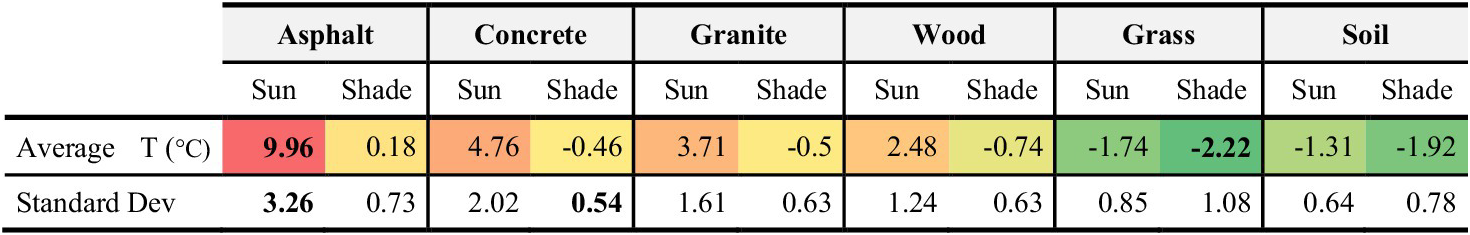
Average and standard deviation of the differences between air temperature and forecasts for surface materials

This statistical analysis confirms the significant thermal impact of different surface materials relative to the ambient air temperature. Sunlit asphalt demonstrates the most extreme urban heat island effect, averaging +9.96 °C warmer than the air. Natural and shaded surfaces show a distinct cooling effect. Grass in the shade is the most effective coolant, averaging −2.22 °C below air, while even sunlit grass (−1.74 °C) and soil (−1.31 °C) actively cool the surface via evapotranspiration. Mainly, all shaded surfaces (except asphalt) maintain an average temperature cooler than the air. The standard deviation data reveal the consistency of these effects: sunlit asphalt (3.26) shows the highest variability, meaning its temperature fluctuates dramatically with the seasons, while surfaces like shaded concrete (0.54), shaded granite (0.63), and sunlit soil (0.64) are the most stable, maintaining a highly consistent temperature difference from the air year-round.
4. Discussion
Surface material thermal performance across seasons varies significantly due to environmental temperatures and sunlight exposure. Materials like asphalt, which show a high-temperature increase, heat up significantly in both winter and summer, while grass and soil maintain thermal balance with low-temperature differences, supporting environmental harmony. These findings underscore the significance of integrating seasonal dynamics into material selection, which is essential for achieving sustainable and comfortable environmental design.
The thermal dynamics of materials at different times of the day are very important in the selection process of building materials. Materials that show minimal temperature differences in the morning are particularly beneficial in terms of energy efficiency. Conversely, materials that show significant temperature differences in the afternoon are susceptible to overheating, which further intensifies the urban heat island phenomenon. Materials characterized by significant heat retention capabilities in the evening require long periods to reach thermal equilibrium, making them advantageous for special applications such as energy storage or night heating.
In material selections aimed at landscape design, thermal properties are of great importance in terms of seasonality and hours of use. Materials that show low temperature differences in terms of energy efficiency are important in terms of condensation, humidity control, and energy saving. At the same time, they can also increase the durability of the material by reducing thermal stress and therefore by reducing maintenance costs. The opposite situation is that materials show high temperature differences.
The study results show that the temperature changes that occur at noon are greater than those that occur in the morning and evening. Although this situation shows that the thermal character changes during the day, the study findings show that the properties of the selected material are more effective. However, selected material can provide advantages in some cases and disadvantages in other cases. While heat-reflecting materials, that is, materials with high temperature differences, are advantageous for areas with high temperature differences, such as Antalya, energy storage materials with high temperature differences can be advantageous for areas that receive high-speed winds and are used intensively in winter.
Asphalt reached the highest values within the measurements taken within the study area. Its surface temperature exceeds 50 °C during the summer months, leading to significant overheating. Even in shaded areas, it still exhibits high-temperature values. Asphalt consistently shows the highest temperature differences in all seasons, particularly peaking in the summer and spring. This is a result of asphalt’s intense heat absorption.
Grass, being the material with the lowest surface temperatures, offers a significant advantage in terms of environmental sustainability. Its ability to remain cool, particularly during summer, shows that grass surfaces can effectively mitigate the urban heat island effect. Grass and soil stand out for their low-temperature differences in every season. This is linked to the fact that the surface temperatures of grass and soil stay closer to the surrounding air temperatures, and they retain less heat.
Wood and granite surfaces exhibit more balanced thermal behavior with limited heat absorption capacity, and these materials can often be preferred in landscape designs due to their potential to increase energy efficiency and, at the same time, provide aesthetic value without damaging the environment. Granite and wood generally exhibit moderate thermal performance and have more stable changes against seasonal changes.
Seasonal analyses clearly show the importance of thermal performance of surface materials in the design and material selection process. The use of materials that cause low temperature differences, especially in summer months, in landscape designs can contribute to the creation of a more sustainable and comfortable environment. This research presents an innovative approach to evaluate the seasonal and environmental effects of thermal properties of various surface materials, focusing on environmental sustainability and energy efficiency, and aims to contribute to other professional disciplines.
This study, presented as a methodological framework applied within the context of part of Antalya’s hot-summer Mediterranean climate. While our findings are specific to this region, the methodology is designed to be replicated in similar climate zones and for comparative studies. This approach provides a basis for future research to analyze the effects of local factors affecting surface temperature, such as vegetation density, urban geometry, and local wind regimes. The limitations and the transferability conditions of this methodology are highlighted to guide future research.
The factors such as tree-canopy density, vegetation cover, shading configuration, wind corridors, and material aging can significantly modify surface-temperature dynamics. These variables influence solar exposure, evapotranspiration, long-wave radiation exchange, and surface albedo. It should be noted that parameters were beyond the scope of this study, but microclimatic modifiers should be integrated to improve transferability across different Mediterranean urban geometries in future studies. This study differs from CNN-based models used in satellite remote sensing studies in that all terrestrial observations are designed to be taken at the desired time, from a distance of 3 meters from the object, and during sunny weather. This method is not subject to limitations such as cloud cover, satellite transit time (hour and day), or the cost of satellite imagery.
In landscape designs, surface materials should not only be selected in terms of aesthetic and durability properties but also evaluated within the framework of thermal balance and thermal comfort for the user. Careful selection of materials serves as an effective strategy to reduce the urban heat island effect, provide energy savings, and develop more livable environments. This study offers a new perspective on the scientific evaluation of thermal performance of surface materials and proposes a method with a sustainability goal that can be used later in design-oriented material selections. This research emphasizes once again the necessity of considering the thermal behavior of surface materials in architectural and urban design processes to optimize user comfort and reduce energy consumption.
Open peer review
To view the open peer review materials for this article, please visit http://doi.org/10.1017/eds.2025.10028.
Acknowledgements
We would like to express our sincere gratitude to Akdeniz University for providing the necessary resources and facilities for conducting this research.
Author contribution
Conceptualisation: AB, TA; Methodology: AB, TA; Formal analysis: AB, TA; Investigation: AB, TA; Data curation: AB, TA; Writing—original draft: AB, TA; Writing—review and editing: AB, TA; Project administration: AB, TA.
Competing interests
The authors declare that they have no known competing interests or personal relationships that could have appeared to influence the work reported in this paper.
Data availability statement
The software for analyzing digital images has been developed by the authors. The data is presented in the Appendix.
Ethics statement
The research meets all ethical guidelines, including adherence to the legal requirements of the study country.
Funding statement
The authors have no conflict of funding to declare.
Appendix - “Sıcaklık Analizi” application Python code
The code has been translated to English for the manuscript.
import cv2.
import numpy as np.
import matplotlib.pyplot as plt.
import tkinter as tk.
from tkinter import filedialog, simpledialog, messagebox.
from tkinter import ttk.
from PIL import Image, ImageTk.
class TemperatureAnalysisApp:
def __init__(self, root):
self.root = root.
self.root.title(“Temperature Analysis”).
# Initial variables.
self.image = None.
self.resized_image = None.
self.selected_roi = None.
self.min_temp = None.
self.max_temp = None.
self.rect_start = None.
self.rect_end = None.
self.width = None.
self.height = None.
# GUI Elements.
self.canvas = tk.Canvas(self.root, width = 800, height = 600).
self.canvas.pack().
self.load_button = tk.Button(self.root, text = “Load Image,” command = self.load_image).
self.load_button.pack().
self.temp_button = tk.Button (self.root, text = “Range of Temperature,” command = self.set_ temperature_range).
self.temp_button.pack().
self.plot_button = tk.Button(self.root, text = “Analyzes,” command = self.plot_and_table).
self.plot_button.pack().
self.canvas.bind(“<ButtonPress-1 > “, self.on_touch_down).
self.canvas.bind(“<B1-Motion>“, self.on_touch_move).
self.canvas.bind(“<ButtonRelease-1 > “, self.on_touch_up).
def load_image(self):
# Open file dialog.
file_path = filedialog.askopenfilename(title = “Select Image,” filetypes = [(“Image files,” “.jpg;.png;*.bmp”)]).
if file_path:
self.image = cv2.imread(file_path, cv2.IMREAD_GRAYSCALE).
self.resized_image = cv2.resize(self.image, (800, 600)).
self.height, self.width = self.image.shape.
self.display_image(self.resized_image).
def display_image(self, img):
# Display the image on the Tkinter canvas.
img = Image.fromarray(img).
img_tk = ImageTk.PhotoImage(img).
self.canvas.create_image(0, 0, anchor = “nw,” image = img_tk).
self.canvas.image = img_tk # Save a reference to avoid garbage collection.
def set_temperature_range(self):
# Set temperature range.
min_temp = simpledialog.askfloat(“Min Temperature,” “Minimum temperature (°C)”:)
max_temp = simpledialog.askfloat(“Max Temperature,” “Maximum temperature (°C)”:)
if min_temp is not None and max_temp is not None:
self.min_temp = min_temp.
self.max_temp = max_temp.
messagebox.showinfo(“Temperature Range,” f” Temperature range has been given: self.min_temp} °C - {self.max_temp} °C”).
else:
messagebox.showerror(“Error,” “Not a valid temperature”).
def on_touch_down(self, event):
# Record the rectangle start point.
self.rect_start = (event.x, event.y).
def on_touch_move(self, event):
# Continue drawing the rectangle.
if self.rect_start:
self.rect_end = (event.x, event.y).
self.update_rect().
def on_touch_up(self, event):
# Finalize the rectangle and save the ROI.
if self.rect_start and self.rect_end:
x1, y1 = self.rect_start.
x2, y2 = self.rect_end.
self.selected_roi = self.resized_image[min(y1, y2):max(y1, y2), min(x1, x2):max(x1, x2)].
print(f”Selected ROI: {self.selected_roi.shape}”).
def update_rect(self):
# Update the area on the canvas.
self.canvas.delete(“rect”).
x1, y1 = self.rect_start.
x2, y2 = self.rect_end.
self.canvas.create_rectangle(x1, y1, x2, y2, outline = “red,” width = 2, tags = “rect”).
def interpolate_temperature(self, pixel_value):
# Map pixel value (0–255) to temperature range.
return self.min_temp + (pixel_value/255) * (self.max_temp - self.min_temp).
def plot_and_table(self):
if self.selected_roi is not None and self.min_temp is not None and self.max_temp is not None:
# Convert pixel values to temperature.
temperatures = np.vectorize(self.interpolate_temperature)(self.selected_roi).
temperatures_flat = temperatures.flatten().
average_temp = np.mean(temperatures_flat).
plt.figure(figsize = (15, 5)).
# Display the selected region.
plt.subplot(1, 3, 1).
plt.imshow(self.selected_roi, cmap = “inferno”).
plt.title(“Selected area”).
plt.axis(“on”).
# Histogram.
plt.subplot(1, 3, 2).
plt.hist(temperatures_flat, bins = 20, color = ‘gray’, edgecolor = ‘black’).
plt.title(“Temperature Range”).
plt.xlabel(“Temperature (°C)”).
plt.ylabel(“Pixel Count”).
# Boxplot.
plt.subplot(1, 3, 3).
plt.boxplot(temperatures_flat, vert = False).
plt.title(“Statistics”).
plt.xlabel(“Temperature (°C)”).
plt.suptitle(f”Average Temperature for the selected area: {average_temp:.2f} °C″).
plt.tight_layout().
plt.show().
else:
messagebox.showerror(“Error,” “Please select the region.”)
if __name__ == “__main__”:
root = tk.Tk().
app = TemperatureAnalysisApp(root).
root.mainloop().


 Open access
Comments
Claire Monteleoni
Environmental Data Science Editor-In-Chief
Dear Editor,
Please consider the research paper titled “Utilization of Artificial Intelligence and Thermal Cameras in Material Analysis for Hot-Summer Mediterranean Climates” for publication in Environmental Data Science journal.
The manuscript aims to evaluate the thermal behaviors of surface materials in arid climates to enhance environmental sustainability and energy efficiency. The paper shows the importance of evaluating thermal properties in terms of energy efficiency and user comfort and therefore the material selection process. Also, it highlights the importance of materials to be selected according to their purpose for sustainable cities and shows the combined use of artificial intelligence and thermal imaging techniques can be an effective tool for ecological and sustainable architectural design.
I believe that these findings will be interesting to the readers of Environmental Data Science journal because they are in the scope of environmental sustainability studies, energy relations and application of research on arid lands.
This manuscript has not been published and is not under consideration for publication elsewhere. AI tools have been used for copy-editing the article using a generative AI tool/LLM to improve its language and readability. All the study and the findings are unique, and case related. The findings and the results are built on authors-created material, and the authors remains responsible for the original work.