


1 Introduction
The purpose of this article is to provide a far-reaching generalisation of the support theorem of Stroock and Varadhan [Reference Stroock and VaradhanSV72]. Recall that this result can be formulated as follows: Let $\{V_i\}_{i=0}^m$
be a finite collection of vector fields on
$\{V_i\}_{i=0}^m$
be a finite collection of vector fields on $\mathbf {R}^n$
that have bounded first and second derivatives, and consider the solution x to the system of stochastic differential equations given by
$\mathbf {R}^n$
that have bounded first and second derivatives, and consider the solution x to the system of stochastic differential equations given by
 $$ \begin{align} dX = V_0(X)dt + \sum_{i=1}^m V_i(X)\circ dW_i(t), \end{align} $$
where the $W_i$
are independent and identially distributed standard Wiener processes and
$W_i$
are independent and identially distributed standard Wiener processes and $\circ $
denotes Stratonovich integration [Reference StratonovičStr64]. Write
$\circ $
denotes Stratonovich integration [Reference StratonovičStr64]. Write $\mathbf {P}_x$
for the law of the solution to equation (1.1) with initial condition
$\mathbf {P}_x$
for the law of the solution to equation (1.1) with initial condition $X_0 = x$
on
$X_0 = x$
on $\mathcal {C}(\mathbf {R}_+, \mathbf {R}^n)$
. It follows from the Wong–Zakai theorem that if we write
$\mathcal {C}(\mathbf {R}_+, \mathbf {R}^n)$
. It follows from the Wong–Zakai theorem that if we write $X^{(\varepsilon )}$
for the solution to the random ordinary differential equation
$X^{(\varepsilon )}$
for the solution to the random ordinary differential equation
 $$ \begin{align} \dot X^{(\varepsilon)} = V_0\left(X^{(\varepsilon)}\right) + \sum_{i=1}^m V_i\left(X^{(\varepsilon)}\right) \dot W_i^{(\varepsilon)}, \end{align} $$
for $W^{(\varepsilon )}$
a smooth approximation to W (for example, convolution with a smooth mollifier), then
$W^{(\varepsilon )}$
a smooth approximation to W (for example, convolution with a smooth mollifier), then $X^{(\varepsilon )} \to X$
in probability. On the other hand, for any fixed
$X^{(\varepsilon )} \to X$
in probability. On the other hand, for any fixed $\varepsilon> 0$
, the topological support of the law
$\varepsilon> 0$
, the topological support of the law $\mathbf {P}_x^{(\varepsilon )}$
of
$\mathbf {P}_x^{(\varepsilon )}$
of $X^{(\varepsilon )}$
is contained in the closure
$X^{(\varepsilon )}$
is contained in the closure $R_x$
of the range of the continuous map
$R_x$
of the range of the continuous map $\mathcal {I}_x \colon \mathcal {C}^1(\mathbf {R}_+, \mathbf {R}^m) \to \mathcal {C}(\mathbf {R}_+, \mathbf {R}^n)$
, which maps any
$\mathcal {I}_x \colon \mathcal {C}^1(\mathbf {R}_+, \mathbf {R}^m) \to \mathcal {C}(\mathbf {R}_+, \mathbf {R}^n)$
, which maps any $\mathcal {C}^1$
function
$\mathcal {C}^1$
function $W^{(\varepsilon )}$
to the solution to equation (1.2).
$W^{(\varepsilon )}$
to the solution to equation (1.2).
Since the topological support is lower semicontinuous under weak convergence, this immediately implies that one also has $\operatorname {\mathrm {supp}} \mathbf {P}_x \subset R_x$
. What Stroock and Varadhan proved in [Reference Stroock and VaradhanSV72] is that one actually has
$\operatorname {\mathrm {supp}} \mathbf {P}_x \subset R_x$
. What Stroock and Varadhan proved in [Reference Stroock and VaradhanSV72] is that one actually has $\operatorname {\mathrm {supp}} \mathbf {P}_x = R_x$
. Our aim is to generalise this statement to a wide class of singular stochastic partial differential equations (SPDEs).
$\operatorname {\mathrm {supp}} \mathbf {P}_x = R_x$
. Our aim is to generalise this statement to a wide class of singular stochastic partial differential equations (SPDEs).
The general framework used in this article is that of [Reference Bruned, Hairer and ZambottiBHZ19, Reference Bruned, Chandra, Chevyrev and HairerBCCH17]. Loosely speaking, we consider systems of SPDEs of the form
 $$ \begin{align} \partial_t u_i = \mathcal{L}_i u_i + F_i(u, \nabla u, \dotsc) + \sum_{j\le n} F_i^j(u, \nabla u, \dotsc)\xi_j, \quad{i \le m}, \end{align} $$
where the $\mathcal {L}_i$
denote homogeneous differential operators on
$\mathcal {L}_i$
denote homogeneous differential operators on $\mathbf {R}^d$
, the spatial variable takes values in the torus
$\mathbf {R}^d$
, the spatial variable takes values in the torus $\mathbf {T}^d$
and the
$\mathbf {T}^d$
and the $\xi _i$
denote driving noises that are of the form
$\xi _i$
denote driving noises that are of the form $\xi _i = \mathcal {K}_i \star \eta _i$
, where
$\xi _i = \mathcal {K}_i \star \eta _i$
, where $\eta _i$
denotes space-time white noise (or possibly noise that is white in space and constant in time) and
$\eta _i$
denotes space-time white noise (or possibly noise that is white in space and constant in time) and $\mathcal {K}_i$
is a kernel which is self-similar in a neighbourhood of the origin and smooth otherwise. The
$\mathcal {K}_i$
is a kernel which is self-similar in a neighbourhood of the origin and smooth otherwise. The $F_i^j$
are local nonlinearities in the sense that the value of
$F_i^j$
are local nonlinearities in the sense that the value of $F_i^j(u, \nabla u, \dotsc )$
at a given space-time point is a smooth function of u and finitely many of its derivatives evaluated at that same point. We will assume throughout that the system (1.3) is locally subcritical in the sense of [Reference Bruned, Hairer and ZambottiBHZ19].
$F_i^j(u, \nabla u, \dotsc )$
at a given space-time point is a smooth function of u and finitely many of its derivatives evaluated at that same point. We will assume throughout that the system (1.3) is locally subcritical in the sense of [Reference Bruned, Hairer and ZambottiBHZ19].
Remark 1.1. The choice $\xi _i = \mathcal {K}_i \star \eta _i$
covers many interesting examples in which
$\xi _i = \mathcal {K}_i \star \eta _i$
covers many interesting examples in which $\xi _i$
is the solution of a linear equation driven by
$\xi _i$
is the solution of a linear equation driven by $\eta _i$
; in this case,
$\eta _i$
; in this case, $\mathcal {K}_i$
should be chosen as the Green’s function. For our support theorem we do not need
$\mathcal {K}_i$
should be chosen as the Green’s function. For our support theorem we do not need $\mathcal {K}_i$
to actually be the Green’s function of a PDE, but we do need the kernel to be homogeneous under rescaling. This assumption will be used heavily throughout this article (compare Assumption 4).
$\mathcal {K}_i$
to actually be the Green’s function of a PDE, but we do need the kernel to be homogeneous under rescaling. This assumption will be used heavily throughout this article (compare Assumption 4).
It was shown in [Reference Bruned, Hairer and ZambottiBHZ19] that one can associate to such an equation in a natural way a nilpotent Lie group $\mathcal {G}_-$
, usually called the renormalisation group in this context, as well as a construction of the following type: Write
$\mathcal {G}_-$
, usually called the renormalisation group in this context, as well as a construction of the following type: Write $\mathcal {X}$
for a suitable space of right-hand sides for equation (1.3) (i.e., an element of
$\mathcal {X}$
for a suitable space of right-hand sides for equation (1.3) (i.e., an element of $\mathcal {X}$
consists of the nonlinearities
$\mathcal {X}$
consists of the nonlinearities $F_i$
as well as
$F_i$
as well as $F_i^j$
that can be described by a regularity structure built from a fixed complete subcritical ‘rule’ as in [Reference Bruned, Hairer and ZambottiBHZ19, Section 5]) and write
$F_i^j$
that can be described by a regularity structure built from a fixed complete subcritical ‘rule’ as in [Reference Bruned, Hairer and ZambottiBHZ19, Section 5]) and write $\mathcal {X}_0 \subset \mathcal {X}$
for the ‘deterministic right-hand sides’, – that is, those elements such that
$\mathcal {X}_0 \subset \mathcal {X}$
for the ‘deterministic right-hand sides’, – that is, those elements such that $F_i^j \equiv 0$
.
$F_i^j \equiv 0$
.
One then has a map $\Upsilon \colon \mathcal {G}_- \times \mathcal {X} \to \mathcal {X}_0$
such that
$\Upsilon \colon \mathcal {G}_- \times \mathcal {X} \to \mathcal {X}_0$
such that $(g,F) \mapsto F + \Upsilon (g,F)$
yields a representation of
$(g,F) \mapsto F + \Upsilon (g,F)$
yields a representation of $\mathcal {G}_-$
on
$\mathcal {G}_-$
on $\mathcal {X}$
. (See Remark 1.3 for more details.)
$\mathcal {X}$
. (See Remark 1.3 for more details.)
Furthermore, given any natural regularisation $\xi ^{\varepsilon }$
of
$\xi ^{\varepsilon }$
of $\xi $
, one can find a sequence of elements
$\xi $
, one can find a sequence of elements $g_{\varepsilon } \in \mathcal {G}_-$
such that the solutions to
$g_{\varepsilon } \in \mathcal {G}_-$
such that the solutions to
 $$ \begin{align} \partial_t u^{\varepsilon}_{i} = \mathcal{L}_i u^{\varepsilon}_i + F_i(u^{\varepsilon}, \nabla u^{\varepsilon}, \dotsc) + \sum_{j\le n} F_i^j(u^{\varepsilon}, \nabla u^{\varepsilon}, \dotsc)\xi^{\varepsilon}_j + \bigl(\Upsilon (g_{\varepsilon},F) \bigr)_i(u^{\varepsilon}, \nabla u^{\varepsilon}, \dotsc), \end{align} $$
subject to suitable initial conditions $u^{\varepsilon }_i(0,\cdot ) = u^{\varepsilon ,(0)}_i$
, converge to a limit u. (The convergence takes place in probability in a space of Hölder continuous trajectories with possible finite-time blow-up.) These limits have a restricted uniqueness property in the sense that for any other regularisation
$u^{\varepsilon }_i(0,\cdot ) = u^{\varepsilon ,(0)}_i$
, converge to a limit u. (The convergence takes place in probability in a space of Hölder continuous trajectories with possible finite-time blow-up.) These limits have a restricted uniqueness property in the sense that for any other regularisation $\tilde {\xi }^{\varepsilon }$
of
$\tilde {\xi }^{\varepsilon }$
of $\xi $
, one can find a sequence of elements
$\xi $
, one can find a sequence of elements $\tilde {g}_{\varepsilon } \in \mathcal {G}_-$
such that the solutions to equation (1.4) with
$\tilde {g}_{\varepsilon } \in \mathcal {G}_-$
such that the solutions to equation (1.4) with $\xi ^{\varepsilon }$
replaced by
$\xi ^{\varepsilon }$
replaced by $\tilde {\xi }^{\varepsilon }$
and
$\tilde {\xi }^{\varepsilon }$
and $g_{\varepsilon }$
replaced by
$g_{\varepsilon }$
replaced by $\tilde {g}_{\varepsilon }$
converge to the same limit.
$\tilde {g}_{\varepsilon }$
converge to the same limit.
Remark 1.2. As in [Reference Bruned, Chandra, Chevyrev and HairerBCCH17, Section 2.7], the initial condition $u^{\varepsilon ,(0)}_i$
is dependent on
$u^{\varepsilon ,(0)}_i$
is dependent on $\varepsilon $
and taken in the form
$\varepsilon $
and taken in the form $u^{\varepsilon ,(0)} = v^{(0)} + \mathcal {S}^-_{\varepsilon }(\xi )(0,\cdot )$
, where
$u^{\varepsilon ,(0)} = v^{(0)} + \mathcal {S}^-_{\varepsilon }(\xi )(0,\cdot )$
, where $\mathcal {S}^-_{\varepsilon }(\xi )$
is a stationary process representing the rough part (i.e., the non-function-valued part) of the solution. In particular, it is in general not possible to choose as the initial condition a deterministic smooth function, unless solutions themselves are function-valued, in which case
$\mathcal {S}^-_{\varepsilon }(\xi )$
is a stationary process representing the rough part (i.e., the non-function-valued part) of the solution. In particular, it is in general not possible to choose as the initial condition a deterministic smooth function, unless solutions themselves are function-valued, in which case $\mathcal {S}^-_{\varepsilon } \equiv 0$
. An interesting equation where this happens is the so-called
$\mathcal {S}^-_{\varepsilon } \equiv 0$
. An interesting equation where this happens is the so-called $\Phi ^4_{4-\delta }$
equation (see [Reference Bruned, Chandra, Chevyrev and HairerBCCH17, Section 2.8.2] and Sections 1.2.1 and C.2). For many interesting examples, including generalised KPZ and generalised PAM, this issue is not apparent, and the initial condition can be chosen as any deterministic function (or even distribution) with sufficient regularity. An exceptional case is
$\Phi ^4_{4-\delta }$
equation (see [Reference Bruned, Chandra, Chevyrev and HairerBCCH17, Section 2.8.2] and Sections 1.2.1 and C.2). For many interesting examples, including generalised KPZ and generalised PAM, this issue is not apparent, and the initial condition can be chosen as any deterministic function (or even distribution) with sufficient regularity. An exceptional case is $\Phi ^4_3$
where
$\Phi ^4_3$
where $\mathcal {S}^-_{\varepsilon } \ne 0$
, but one can compensate for this by choosing
$\mathcal {S}^-_{\varepsilon } \ne 0$
, but one can compensate for this by choosing $v^{(0)}$
appropriately (compare Section C.1).
$v^{(0)}$
appropriately (compare Section C.1).
Remark 1.3. Writing $\mathscr {T}_-$
for the set of trees of negative degree associated to the class of SPDEs under consideration (see Section 2.2.1), one can explicitly set
$\mathscr {T}_-$
for the set of trees of negative degree associated to the class of SPDEs under consideration (see Section 2.2.1), one can explicitly set
 $$ \begin{align*} \Upsilon\colon (g,F) \mapsto \sum_{\tau \in \mathscr{T}_-} \frac{g(\tau)}{S(\tau)} \Upsilon^F[\tau], \end{align*} $$
where the space of nonlinearities $\mathcal {P}^{\mathfrak {L}_+}$
, combinatorial factor
$\mathcal {P}^{\mathfrak {L}_+}$
, combinatorial factor $S(\tau )$
and evaluation map
$S(\tau )$
and evaluation map $\Upsilon ^F$
are defined in [Reference Bruned, Chandra, Chevyrev and HairerBCCH17, Section 2.7]. In the right-hand side, we identify elements of
$\Upsilon ^F$
are defined in [Reference Bruned, Chandra, Chevyrev and HairerBCCH17, Section 2.7]. In the right-hand side, we identify elements of $\mathcal {G}_-$
with maps
$\mathcal {G}_-$
with maps $\mathscr {T}_- \to \mathbf {R}$
(characters on the free unital algebra generated by
$\mathscr {T}_- \to \mathbf {R}$
(characters on the free unital algebra generated by $\mathscr {T}_-$
).
$\mathscr {T}_-$
).
In this context, the purpose of $\Upsilon $
is to provide a formula for the counterterms required to renormalise our equation. As already noted in [Reference Bruned, Chandra, Chevyrev and HairerBCCH17], the same map also provides an expression for the expansion of the ‘abstract solution’ to our SPDE in the corresponding regularity structure. This is strongly reminiscent of the expression of the Taylor expansion of the solution to an ordinary differential equation in terms of a sum over trees [Reference ButcherBut72].
$\Upsilon $
is to provide a formula for the counterterms required to renormalise our equation. As already noted in [Reference Bruned, Chandra, Chevyrev and HairerBCCH17], the same map also provides an expression for the expansion of the ‘abstract solution’ to our SPDE in the corresponding regularity structure. This is strongly reminiscent of the expression of the Taylor expansion of the solution to an ordinary differential equation in terms of a sum over trees [Reference ButcherBut72].
We call a choice of $(\xi ^{\varepsilon }, g_{\varepsilon })_{\varepsilon> 0}$
a renormalisation procedure, and we consider two such procedures to be equivalent if they yield the same limit process for any system of SPDEs driven by
$(\xi ^{\varepsilon }, g_{\varepsilon })_{\varepsilon> 0}$
a renormalisation procedure, and we consider two such procedures to be equivalent if they yield the same limit process for any system of SPDEs driven by $\xi ^{\varepsilon }$
belonging to a suitable class of systems of the same form as the original one. (See [Reference Bruned, Chandra, Chevyrev and HairerBCCH17] for the definition of this class of equations given a ‘rule’ in the sense of [Reference Bruned, Hairer and ZambottiBHZ19].) Given two renormalisation procedures
$\xi ^{\varepsilon }$
belonging to a suitable class of systems of the same form as the original one. (See [Reference Bruned, Chandra, Chevyrev and HairerBCCH17] for the definition of this class of equations given a ‘rule’ in the sense of [Reference Bruned, Hairer and ZambottiBHZ19].) Given two renormalisation procedures $(\xi ^{\varepsilon }, g_{\varepsilon })$
and
$(\xi ^{\varepsilon }, g_{\varepsilon })$
and $\left (\tilde {\xi }^{\varepsilon }, \tilde {g}_{\varepsilon }\right )$
, it turns out that it is always possible to find one single element
$\left (\tilde {\xi }^{\varepsilon }, \tilde {g}_{\varepsilon }\right )$
, it turns out that it is always possible to find one single element $f \in \mathcal {G}_-$
such that
$f \in \mathcal {G}_-$
such that $\left (\tilde {\xi }^{\varepsilon }, \tilde {g}_{\varepsilon }\right )$
is equivalent to
$\left (\tilde {\xi }^{\varepsilon }, \tilde {g}_{\varepsilon }\right )$
is equivalent to $(\xi ^{\varepsilon }, f \circ g_{\varepsilon })$
. Given any fixed choice of compactly supported kernel
$(\xi ^{\varepsilon }, f \circ g_{\varepsilon })$
. Given any fixed choice of compactly supported kernel $\mathcal {K}_i$
such that
$\mathcal {K}_i$
such that $(\partial _t - \mathcal {L}_i)\mathcal {K}_i = \delta $
in a neighbourhood of the origin and any choice
$(\partial _t - \mathcal {L}_i)\mathcal {K}_i = \delta $
in a neighbourhood of the origin and any choice $\xi ^{\varepsilon }$
of smooth approximation to
$\xi ^{\varepsilon }$
of smooth approximation to $\xi $
(by convolution with a compactly supported mollifier, but this could in principle be more general), there is a distinguished choice of
$\xi $
(by convolution with a compactly supported mollifier, but this could in principle be more general), there is a distinguished choice of $g^{(\varepsilon )}_{\text {BPHZ}}$
(depending on
$g^{(\varepsilon )}_{\text {BPHZ}}$
(depending on $\xi ^{\varepsilon }$
), which we call the ‘BPHZ renormalisation’ (see [Reference Bruned, Hairer and ZambottiBHZ19]). In particular, this has the property that the
$\xi ^{\varepsilon }$
), which we call the ‘BPHZ renormalisation’ (see [Reference Bruned, Hairer and ZambottiBHZ19]). In particular, this has the property that the $(\xi ^{\varepsilon }, g^{(\varepsilon )}_{\textrm{BPHZ}})$
are all equivalent for different choices of
$(\xi ^{\varepsilon }, g^{(\varepsilon )}_{\textrm{BPHZ}})$
are all equivalent for different choices of $\xi ^{\varepsilon }$
, so that we can talk about ‘the’ BPHZ solution to equation (1.3).
$\xi ^{\varepsilon }$
, so that we can talk about ‘the’ BPHZ solution to equation (1.3).
At first sight, the natural generalisation of Stroock and Varadhan’s result for a system of equations of the type (1.3) may be that the support of the solutions starting at u coincides with the closure $R_u$
of the set of all solutions to equation (1.3) with the
$R_u$
of the set of all solutions to equation (1.3) with the $\xi _j$
replaced by smooth controls. A moment of thought reveals that this cannot be the case, for the simple reason that the formal expression (1.3) only determines a solution theory up to a choice of renormalisation procedure, and different renormalisation procedures may produce solutions with different supports. This is already apparent in the case of stochastic differential equations (SDEs) where an expression like
$\xi _j$
replaced by smooth controls. A moment of thought reveals that this cannot be the case, for the simple reason that the formal expression (1.3) only determines a solution theory up to a choice of renormalisation procedure, and different renormalisation procedures may produce solutions with different supports. This is already apparent in the case of stochastic differential equations (SDEs) where an expression like
 $$ \begin{align*} \dot x = V_0(x) + V_i(x)\xi_i \end{align*} $$
(summation over repeated indices is implicit) may be interpreted either in the Itô sense or in the Stratonovich sense, yielding solution theories with distinct supports in general.
It is also not difficult to see that in general one cannot hope to obtain the support of equation (1.3) as the closure $R_u^g$
of the set of all solutions to equation (1.4) with the
$R_u^g$
of the set of all solutions to equation (1.4) with the $\xi _j^{\varepsilon }$
replaced by smooth controls and
$\xi _j^{\varepsilon }$
replaced by smooth controls and $g_{\varepsilon }$
replaced by some fixed element g of the renormalisation group. Indeed, consider the system of SPDEs given by
$g_{\varepsilon }$
replaced by some fixed element g of the renormalisation group. Indeed, consider the system of SPDEs given by
 $$ \begin{align} \partial_t u = \partial_x^2 u + \xi,\qquad \partial_t v = \partial_x^2 v + (\partial_x u)^2. \end{align} $$
The relevant part of the renormalisation group for this system is simply $(\mathbf {R},+)$
, with the renormalised system being of the form
$(\mathbf {R},+)$
, with the renormalised system being of the form
 $$ \begin{align} \partial_t u = \partial_x^2 u + \xi,\qquad \partial_t v = \partial_x^2 v + ((\partial_x u)^2 - c). \end{align} $$
For any fixed value of c, solutions to equation (1.6) with smooth $\xi $
and vanishing initial condition are such that v is bounded below by
$\xi $
and vanishing initial condition are such that v is bounded below by $-ct$
. However, the solution to equation (1.5) should really be interpreted as the limit as
$-ct$
. However, the solution to equation (1.5) should really be interpreted as the limit as $\varepsilon \to 0$
of the solution to equation (1.6), with
$\varepsilon \to 0$
of the solution to equation (1.6), with $\xi $
replaced by
$\xi $
replaced by $\xi _{\varepsilon }$
and c replaced by
$\xi _{\varepsilon }$
and c replaced by $c_{\varepsilon }$
for a suitable choice of
$c_{\varepsilon }$
for a suitable choice of $c_{\varepsilon } \to +\infty $
.
$c_{\varepsilon } \to +\infty $
.
Furthermore, it was already remarked in [Reference HairerHai13] (in a slightly different setting) that for any fixed smooth h, the solutions to
 $$ \begin{align} \partial_t u = \partial_x^2 u + h + a \varepsilon^{-1}\cos\left(\varepsilon^{-1} x\right),\qquad \partial_t v = \partial_x^2 v + (\partial_x u)^2 - c \end{align} $$
converge as $\varepsilon \to 0$
to those of
$\varepsilon \to 0$
to those of
 $$ \begin{align*} \partial_t u = \partial_x^2 u + h,\qquad \partial_t v = \partial_x^2 v + (\partial_x u)^2 - \left(c - \tilde{c} a^2\right) \end{align*} $$
for some fixed positive constant $\tilde {c}$
. In other words, it is possible to emulate a decrease in the renormalisation constant c (but not an increase!) by adding a small (in a distributional sense) highly oscillatory term to h. This suggests that the support of the solution to equation (1.5) is given by the closure of the set of all solutions to
$\tilde {c}$
. In other words, it is possible to emulate a decrease in the renormalisation constant c (but not an increase!) by adding a small (in a distributional sense) highly oscillatory term to h. This suggests that the support of the solution to equation (1.5) is given by the closure of the set of all solutions to
 $$ \begin{align} \partial_t u = \partial_x^2 u + h,\qquad \partial_t v = \partial_x^2 v + (\partial_x u)^2 - c \end{align} $$
for any choice of smooth function h and any choice of constant $c \in \mathbf {R}$
. As a matter of fact, by considering perturbations of h of the type (1.7), but with an additional modulation of the highly oscillatory term, we will see in Theorem 1.15 that whatever the choice of renormalisation procedure, solutions to equation (1.5) have full support, so that this example exhibits some weak form of ‘hypoellipticity’.
$c \in \mathbf {R}$
. As a matter of fact, by considering perturbations of h of the type (1.7), but with an additional modulation of the highly oscillatory term, we will see in Theorem 1.15 that whatever the choice of renormalisation procedure, solutions to equation (1.5) have full support, so that this example exhibits some weak form of ‘hypoellipticity’.
1.1 The main theorem
We consider subcritical SPDEs of the form (1.3) such that Assumptions 2 and 3 hold. Subcriticality ensures that one can construct a problem-dependent regularity structure as in [Reference Bruned, Hairer and ZambottiBHZ19], and Assumptions 2 and 3 guarantee by [Reference Chandra and HairerCH16, Theorem 2.33] the convergence of the sequence of admissible models $\hat {Z}^{\varepsilon }$
to a random limit model
$\hat {Z}^{\varepsilon }$
to a random limit model $\hat {Z}$
, where
$\hat {Z}$
, where $\hat {Z}^{\varepsilon }$
denotes the renormalised canonical lift of the regularised noise
$\hat {Z}^{\varepsilon }$
denotes the renormalised canonical lift of the regularised noise $\xi ^{\varepsilon }$
(see Section 2.2.2). Furthermore, we can only expect a support theorem to hold if the integration kernels associated to our equations are homogeneous on small scales, and in order to not overcomplicate the presentation, we assume that our Green’s functions are self-similar under rescaling (compare Assumption 4). For convenience, we also restrict to the case of independent (space or space-time) Gaussian white noises
$\xi ^{\varepsilon }$
(see Section 2.2.2). Furthermore, we can only expect a support theorem to hold if the integration kernels associated to our equations are homogeneous on small scales, and in order to not overcomplicate the presentation, we assume that our Green’s functions are self-similar under rescaling (compare Assumption 4). For convenience, we also restrict to the case of independent (space or space-time) Gaussian white noises $\xi _i$
(but compare Remark 2.5). Our assumptions ensure that equation (1.3) can be lifted to an abstract fixed point problem as in [Reference HairerHai14, Theorem 7.8]. Finally, we need a technical assumption on the trees that appear in our regularity structure, which for ease of this introduction we will not comment on; we refer the interested reader to Assumptions 5 and 6 in Section 2.5.
$\xi _i$
(but compare Remark 2.5). Our assumptions ensure that equation (1.3) can be lifted to an abstract fixed point problem as in [Reference HairerHai14, Theorem 7.8]. Finally, we need a technical assumption on the trees that appear in our regularity structure, which for ease of this introduction we will not comment on; we refer the interested reader to Assumptions 5 and 6 in Section 2.5.
In order to have a well-behaved solution map, it is convenient to be in the slightly more restrictive setting of [Reference Bruned, Chandra, Chevyrev and HairerBCCH17], which guarantees in particular that the reconstructed solution to the abstract fixed point problem for $\hat {Z}^{\varepsilon }$
satisfies the regularised and renormalised SPDE (1.4). We thus assume for the sake of the main results – Theorems 1.6 and 1.7 – that the full assumptions of [Reference Bruned, Chandra, Chevyrev and HairerBCCH17] are satisfied.
$\hat {Z}^{\varepsilon }$
satisfies the regularised and renormalised SPDE (1.4). We thus assume for the sake of the main results – Theorems 1.6 and 1.7 – that the full assumptions of [Reference Bruned, Chandra, Chevyrev and HairerBCCH17] are satisfied.
Assumption 1. We assume that [Reference Bruned, Chandra, Chevyrev and HairerBCCH17, Equation 2.5, Assumptions 2.6, 2.8, 2.13, 2.15 and 2.16] are satisfied and that our Assumptions 2–5, 7 and 8 hold.
Remark 1.4. We will show in Section 4 that Assumptions 7 and 8 are implied by Assumptions 2–6 (without requiring the additional assumptions of [Reference Bruned, Chandra, Chevyrev and HairerBCCH17]).
Our main result then is a support theorem for the BPHZ renormalised model $\hat {Z}$
or indeed any model differing from
$\hat {Z}$
or indeed any model differing from $\hat {Z}$
by the action of an element of the renormalisation group
$\hat {Z}$
by the action of an element of the renormalisation group $\mathcal {G}_-$
associated to the class of equations under consideration. If we denote by
$\mathcal {G}_-$
associated to the class of equations under consideration. If we denote by $Z(h)$
the canonical lift of any
$Z(h)$
the canonical lift of any $h \in \mathcal {C}_0^{\infty }$
, a slightly informal version of our main result reads as follows:
$h \in \mathcal {C}_0^{\infty }$
, a slightly informal version of our main result reads as follows:
Theorem 1.5. There exist a subgroup $\mathcal {H} \subset \mathcal {G}_-$
and a left coset
$\mathcal {H} \subset \mathcal {G}_-$
and a left coset $g\mathcal {H}$
of
$g\mathcal {H}$
of $\mathcal {H}$
such that
$\mathcal {H}$
such that
 $$ \begin{align*} \operatorname{\mathrm{supp}} \hat{Z} = \overline{\left\{ \mathcal{R}^h Z(f): f \in \mathcal{C}_0^{\infty}, h \in g\mathcal{H}\right\}}. \end{align*} $$
One important remark here is that $\mathcal {H}$
is not determined solely by the regularity structure of the problem. Instead, it also incorporates information about the symmetries satisfied by the integration kernels associated to the problem. Extracting this ‘rigid’ algebraic data out of ‘soft’ analytic data is one of the main difficulties of this article.
$\mathcal {H}$
is not determined solely by the regularity structure of the problem. Instead, it also incorporates information about the symmetries satisfied by the integration kernels associated to the problem. Extracting this ‘rigid’ algebraic data out of ‘soft’ analytic data is one of the main difficulties of this article.
We also have a more concrete statement at the level of solutions, which we state now. Regarding solutions, our support theorem applies for u in any space $\mathcal {X}= \bigoplus _{i} \mathcal {X}_i$
such that the solution operator (mapping the space of admissible models for the regularity structure
$\mathcal {X}= \bigoplus _{i} \mathcal {X}_i$
such that the solution operator (mapping the space of admissible models for the regularity structure $\mathcal {T}$
into
$\mathcal {T}$
into $\mathcal {X}$
) is continuous. For instance, one could define the space
$\mathcal {X}$
) is continuous. For instance, one could define the space $\mathcal {X}_i$
as a version of the usual Hölder spaces allowing for finite-time blow-up as in [Reference Bruned, Chandra, Chevyrev and HairerBCCH17]. In situations where we know a priori that the solution survives until some deterministic time
$\mathcal {X}_i$
as a version of the usual Hölder spaces allowing for finite-time blow-up as in [Reference Bruned, Chandra, Chevyrev and HairerBCCH17]. In situations where we know a priori that the solution survives until some deterministic time $T>0$
almost surely, one can take alternatively for
$T>0$
almost surely, one can take alternatively for $\mathcal {X}_i$
the usual Hölder–Besov spaces
$\mathcal {X}_i$
the usual Hölder–Besov spaces $\mathcal {C}^{-\frac {\lvert {\mathfrak {s}}\rvert }{2} + \beta _i -\kappa }_{ \mathfrak {s}_{\Lambda } }((0,T) \times \mathbf {T}^e)$
. (Here
$\mathcal {C}^{-\frac {\lvert {\mathfrak {s}}\rvert }{2} + \beta _i -\kappa }_{ \mathfrak {s}_{\Lambda } }((0,T) \times \mathbf {T}^e)$
. (Here $\beta _i>0$
and the scaling
$\beta _i>0$
and the scaling ${ \mathfrak {s}_{\Lambda } } : \{0, \dotsc , e\} \to {\mathbf N}$
are determined by the linear part
${ \mathfrak {s}_{\Lambda } } : \{0, \dotsc , e\} \to {\mathbf N}$
are determined by the linear part $\partial _t - \mathcal {L}_i$
of our equations; see Assumption 4. The statement holds for any
$\partial _t - \mathcal {L}_i$
of our equations; see Assumption 4. The statement holds for any $\kappa>0$
.) The main theorem of this article is the following description of the topological support of u:
$\kappa>0$
.) The main theorem of this article is the following description of the topological support of u:
Theorem 1.6. Under Assumption 1, let $u^{\varepsilon }$
denote the classical solutions to the regularised and renormalised equation (1.4) with noise
$u^{\varepsilon }$
denote the classical solutions to the regularised and renormalised equation (1.4) with noise $\xi ^{\varepsilon }$
and renormalisation constants
$\xi ^{\varepsilon }$
and renormalisation constants $c^{\varepsilon }_{\tau } = h\circ g^{\varepsilon }_{\textrm{BPHZ}}(\tau )$
for some fixed
$c^{\varepsilon }_{\tau } = h\circ g^{\varepsilon }_{\textrm{BPHZ}}(\tau )$
for some fixed $h \in \mathcal {G}_-$
, and set
$h \in \mathcal {G}_-$
, and set $u := \lim _{\varepsilon \to 0}u^{\varepsilon }$
. Then one has the identity
$u := \lim _{\varepsilon \to 0}u^{\varepsilon }$
. Then one has the identity
 $$ \begin{align*} \operatorname{\mathrm{supp}} u=\bigcap_{\varepsilon>0} \overline{\bigcup_{\delta<\varepsilon} \operatorname{\mathrm{supp}} u^{\delta}} \end{align*} $$
in $\mathcal {X}$
.
$\mathcal {X}$
.
In Theorem 3.14 we show that Assumptions 2–5, 7 and 8 imply an analogous support theorem for the random models associated to u and $u^{\delta }$
. More precisely, we show that
$u^{\delta }$
. More precisely, we show that
 $$ \begin{align} \operatorname{\mathrm{supp}} \hat{Z}=\bigcap_{\varepsilon>0}\overline{\bigcup_{\delta<\varepsilon} \operatorname{\mathrm{supp}} \hat{Z}^{\delta}}, \end{align} $$
where $\hat {Z}^{\delta }$
denotes the BPHZ model associated to the noise
$\hat {Z}^{\delta }$
denotes the BPHZ model associated to the noise $\xi ^{\delta }$
and
$\xi ^{\delta }$
and $\hat {Z}$
denotes its limit, namely the BPHZ model associated to the limiting white noise
$\hat {Z}$
denotes its limit, namely the BPHZ model associated to the limiting white noise $\xi $
.
$\xi $
.
Once we know equation (1.9), Theorem 1.6 is a direct consequence of the continuity of the solution operator given in [Reference Bruned, Chandra, Chevyrev and HairerBCCH17, Theorem 2.21], combined with the fact that given a measure $\mu $
and a continuous map F,
$\mu $
and a continuous map F, $\operatorname {\mathrm {supp}} F^*\mu $
is given by the closure of
$\operatorname {\mathrm {supp}} F^*\mu $
is given by the closure of $F(\operatorname {\mathrm {supp}} \mu )$
. It will become clear from our proof that for a ‘tweaked’ choice of renormalisation constants
$F(\operatorname {\mathrm {supp}} \mu )$
. It will become clear from our proof that for a ‘tweaked’ choice of renormalisation constants $\tilde {c}^{\varepsilon }_{\tau } = k^{\varepsilon } \circ h \circ g^{\varepsilon }_{\textrm{BPHZ}}(\tau )$
with
$\tilde {c}^{\varepsilon }_{\tau } = k^{\varepsilon } \circ h \circ g^{\varepsilon }_{\textrm{BPHZ}}(\tau )$
with $k^{\varepsilon } \to \mathbf {1}^*$
as
$k^{\varepsilon } \to \mathbf {1}^*$
as $\varepsilon \to 0$
, one can show that denoting by
$\varepsilon \to 0$
, one can show that denoting by $\tilde {u}^{\varepsilon }$
the classical solution to the system(1.3) with renormalisation constants
$\tilde {u}^{\varepsilon }$
the classical solution to the system(1.3) with renormalisation constants $\tilde {c}^{\varepsilon }$
, one still has
$\tilde {c}^{\varepsilon }$
, one still has $\tilde {u}^{\varepsilon } \to u$
in probability in
$\tilde {u}^{\varepsilon } \to u$
in probability in $\mathcal {X}$
, but one has the stronger statement
$\mathcal {X}$
, but one has the stronger statement
 $$ \begin{align*} \operatorname{\mathrm{supp}} \tilde{u}^{\varepsilon}\subseteq \operatorname{\mathrm{supp}} u \end{align*} $$
for any $\varepsilon>0$
.
$\varepsilon>0$
.
We also have a characterisation of the support in the spirit of Stroock and Varadhan’s support theorem for SDEs [Reference Stroock and VaradhanSV72]. The ‘correct’ way to resolve the issue of divergent renormalisation constants in such a description turns out to be the following:
Theorem 1.7. Under Assumption 1, let $h \in \mathcal {G}_-$
and u be as in Theorem 1.6. There exist a Lie subgroup
$h \in \mathcal {G}_-$
and u be as in Theorem 1.6. There exist a Lie subgroup $\mathcal {H} \subseteq {\mathcal {G}_-}$
of the renormalisation group and a character
$\mathcal {H} \subseteq {\mathcal {G}_-}$
of the renormalisation group and a character $f \in {\mathcal {G}_-}$
independent of the choice of h in Theorem 1.6 such that the following holds: The support
$f \in {\mathcal {G}_-}$
independent of the choice of h in Theorem 1.6 such that the following holds: The support $\operatorname {\mathrm {supp}} u$
is given by the closure of all solutions
$\operatorname {\mathrm {supp}} u$
is given by the closure of all solutions $\varphi $
to
$\varphi $
to
 $$ \begin{align} \partial_t \varphi_{i} = \mathcal{L}_i \varphi_i + F_i(\varphi, \nabla \varphi, \dotsc) + \sum_{j\le n} F_i^j(\varphi, \nabla \varphi, \dotsc) \psi_j + (\Upsilon_i k)(\varphi, \nabla \varphi, \dotsc), \end{align} $$
for any character $k \in h \circ f \circ \mathcal {H}$
, initial conditionFootnote
1
$k \in h \circ f \circ \mathcal {H}$
, initial conditionFootnote
1 $\varphi (0,\cdot ) \in \Phi _0^k$
and smooth deterministic functions
$\varphi (0,\cdot ) \in \Phi _0^k$
and smooth deterministic functions $\psi _j$
,
$\psi _j$
, $j=1, \dotsc , n$
(depending only on space if
$j=1, \dotsc , n$
(depending only on space if $\xi _j$
is purely spatial white noise). Here we write
$\xi _j$
is purely spatial white noise). Here we write $\Upsilon _i k := \left (\Upsilon M^{k}\Omega _F \right )_i$
for simplicity.
$\Upsilon _i k := \left (\Upsilon M^{k}\Omega _F \right )_i$
for simplicity.
This theorem follows from Proposition 3.8, the properties of the shift operator, Theorem 2.4 and the continuity of the solution operator. The Lie subgroup $\mathcal {H}$
is given as the annihilator of a finite number of linear ‘constraints’ between the renormalisation constants. We refer the reader to Definition 3.3 for a precise definition. The tweaking by f is necessary, since the BPHZ characters respect these constraints only up to order
$\mathcal {H}$
is given as the annihilator of a finite number of linear ‘constraints’ between the renormalisation constants. We refer the reader to Definition 3.3 for a precise definition. The tweaking by f is necessary, since the BPHZ characters respect these constraints only up to order $1$
(a by-product of the fact that we use truncated integration kernels for its definition).
$1$
(a by-product of the fact that we use truncated integration kernels for its definition).
Remark 1.8. When we are in a situation in which we are allowed to choose the initial condition $u^{\varepsilon ,(0)} = v^{(0)}$
deterministically and independent of
$u^{\varepsilon ,(0)} = v^{(0)}$
deterministically and independent of $\varepsilon $
, the initial condition of the control problem (1.10) has to coincide with this choice, so that we have to set
$\varepsilon $
, the initial condition of the control problem (1.10) has to coincide with this choice, so that we have to set $\Phi _0^k = \left \{ v^{(0)} \right \}$
.
$\Phi _0^k = \left \{ v^{(0)} \right \}$
.
In order to also cover the case when the initial condition $u^{\varepsilon ,(0)}$
is a perturbation to
$u^{\varepsilon ,(0)}$
is a perturbation to $\mathcal {S}^-_{\varepsilon }(\xi )(0,\cdot )$
(compare Remark 1.2), we make use of the fact that
$\mathcal {S}^-_{\varepsilon }(\xi )(0,\cdot )$
(compare Remark 1.2), we make use of the fact that $\mathcal {S}^-_{\varepsilon }$
can be written as an explicit continuous function of the model
$\mathcal {S}^-_{\varepsilon }$
can be written as an explicit continuous function of the model $\hat {Z}^{\varepsilon }$
(compare [Reference Bruned, Chandra, Chevyrev and HairerBCCH17, Proposition 5.22, Equation 6.10]). In the notation of that paper, we define
$\hat {Z}^{\varepsilon }$
(compare [Reference Bruned, Chandra, Chevyrev and HairerBCCH17, Proposition 5.22, Equation 6.10]). In the notation of that paper, we define $\Phi _0^k$
as the set of all functions of the form
$\Phi _0^k$
as the set of all functions of the form $v^{(0)} + \left (\mathcal {R}^Z \mathcal {P}^Z \tilde {U}\right )(0,\cdot ) \in (\mathcal {C}^{\infty }(\mathbf {T}^e))^m$
, where Z is a renormalised canonical lift
$v^{(0)} + \left (\mathcal {R}^Z \mathcal {P}^Z \tilde {U}\right )(0,\cdot ) \in (\mathcal {C}^{\infty }(\mathbf {T}^e))^m$
, where Z is a renormalised canonical lift $Z = \mathcal {R}^k Z_{\mathrm {c}}(\psi )$
with
$Z = \mathcal {R}^k Z_{\mathrm {c}}(\psi )$
with $\psi \in \mathcal {C}_c^{\infty }(\mathbf {R}\times \mathbf {T}^e)^n$
. (The fact that we can choose the initial condition independent of the
$\psi \in \mathcal {C}_c^{\infty }(\mathbf {R}\times \mathbf {T}^e)^n$
. (The fact that we can choose the initial condition independent of the $\psi _j$
’s appearing in equation (1.10) comes from the fact that
$\psi _j$
’s appearing in equation (1.10) comes from the fact that $\left (\mathcal {R}^Z \mathcal {P}^Z \tilde {U}\right )(0,\cdot )$
depends only on the value of
$\left (\mathcal {R}^Z \mathcal {P}^Z \tilde {U}\right )(0,\cdot )$
depends only on the value of $\psi $
on negative times, whereas in equation (1.10) only the behaviour of
$\psi $
on negative times, whereas in equation (1.10) only the behaviour of $\psi $
for positive times matters.)
$\psi $
for positive times matters.)
Remark 1.9. It suffices to prove Theorems 1.6 and 1.7 for $h=\mathbf {1}^*$
. This follows, since by [Reference Bruned, Chandra, Chevyrev and HairerBCCH17, Theorem 2.13] there exists a action
$h=\mathbf {1}^*$
. This follows, since by [Reference Bruned, Chandra, Chevyrev and HairerBCCH17, Theorem 2.13] there exists a action $(F,h) \mapsto h \circ F$
of the renormalisation group
$(F,h) \mapsto h \circ F$
of the renormalisation group ${\mathcal {G}_-}$
onto the collection of vector fields
${\mathcal {G}_-}$
onto the collection of vector fields $F=(F_i)$
which leaves the class of vector fields considered in [Reference Bruned, Chandra, Chevyrev and HairerBCCH17] invariant and is such that
$F=(F_i)$
which leaves the class of vector fields considered in [Reference Bruned, Chandra, Chevyrev and HairerBCCH17] invariant and is such that $F_i + \Upsilon _i (h \circ g) = h \circ F_i + \Upsilon _i g$
for any
$F_i + \Upsilon _i (h \circ g) = h \circ F_i + \Upsilon _i g$
for any $h,g \in {\mathcal {G}_-}$
. Therefore, changing renormalisation can simply be viewed as changing the nonlinearity.
$h,g \in {\mathcal {G}_-}$
. Therefore, changing renormalisation can simply be viewed as changing the nonlinearity.
Remark 1.10. The set $f \circ \mathcal {H}$
used in Theorem 1.7 is in some sense the largest set of characters such that we can guarantee that the solution to equation (1.10) is in the support of u. In many situations we know a priori that there exists a smooth approximation
$f \circ \mathcal {H}$
used in Theorem 1.7 is in some sense the largest set of characters such that we can guarantee that the solution to equation (1.10) is in the support of u. In many situations we know a priori that there exists a smooth approximation $\xi ^{\varepsilon } = \xi \star \rho ^{\varepsilon }$
as before with the property that the BPHZ characters
$\xi ^{\varepsilon } = \xi \star \rho ^{\varepsilon }$
as before with the property that the BPHZ characters $g^{\varepsilon }$
take values in a fixed subset
$g^{\varepsilon }$
take values in a fixed subset $K \subseteq f \circ \mathcal {H}$
. In this case, combining Theorems 1.6 and 1.7 implies that the support
$K \subseteq f \circ \mathcal {H}$
. In this case, combining Theorems 1.6 and 1.7 implies that the support $\operatorname {\mathrm {supp}} u$
is given by the closure of the set of all solutions to the control problem (1.10) with
$\operatorname {\mathrm {supp}} u$
is given by the closure of the set of all solutions to the control problem (1.10) with $k \in K$
.
$k \in K$
.
Remark 1.11. The classical Stroock–Varadhan support theorem can be viewed as the case $d=0$
of our result with
$d=0$
of our result with $\mathcal {L}_i = 0$
. In this case, one has
$\mathcal {L}_i = 0$
. In this case, one has $\mathcal {G}_- \simeq (\mathbf {R},+)$
Footnote
2
and, in the notation of Theorem 1.7,
$\mathcal {G}_- \simeq (\mathbf {R},+)$
Footnote
2
and, in the notation of Theorem 1.7,
 $$ \begin{align*} (\Upsilon_i c)(u) = c F_k^j(u) \partial_k F_i^j(u),\quad c \in \mathbf{R} \simeq \mathcal{G}_-, \end{align*} $$
with summation over j and k implied. Furthermore, using the BPHZ model (and therefore setting $h = 0$
) leads to solutions in the Itô sense. Since there is only one renormalisation constant in this case and the ‘heat kernel’ is given by the Heaviside function, which is nontrivial, Definition 3.3 readily leads us to the conclusion that
$h = 0$
) leads to solutions in the Itô sense. Since there is only one renormalisation constant in this case and the ‘heat kernel’ is given by the Heaviside function, which is nontrivial, Definition 3.3 readily leads us to the conclusion that $\mathcal {J}$
is the unit ideal, so that its annihilator is given by
$\mathcal {J}$
is the unit ideal, so that its annihilator is given by $\mathcal {H} = \{0\}$
.
$\mathcal {H} = \{0\}$
.
Theorem 1.7 then states that there exists some constant c such that the support of the Itô solutions to
 $$ \begin{align*} du_i = F_i(u)dt + \sum_{j \le n} F_i^j(u)dW_j \end{align*} $$
is given by the closure of all solutions to
 $$ \begin{align} \dot u_i = F_i(u) + \sum_{j \le n} F_i^j(u)\psi_j + c \sum_{k \le m} \sum_{j \le n} F_k^j(u) \partial_k F_i^j(u), \end{align} $$
with smooth controls $\psi _j$
. Note that the correct value of c (corresponding to the character f in the statement) is not specified by the theorem. On the other hand, one can explicitly compute the ‘BPHZ character’ in this case and show that (again identifying
$\psi _j$
. Note that the correct value of c (corresponding to the character f in the statement) is not specified by the theorem. On the other hand, one can explicitly compute the ‘BPHZ character’ in this case and show that (again identifying $\mathcal {G}_-$
with
$\mathcal {G}_-$
with $\mathbf {R}$
) it converges as
$\mathbf {R}$
) it converges as $\varepsilon \to 0$
to
$\varepsilon \to 0$
to $-\textstyle {\frac {1}{2}}$
, and we conclude from Remark 1.10 that
$-\textstyle {\frac {1}{2}}$
, and we conclude from Remark 1.10 that $c = -\textstyle {\frac {1}{2}}$
in equation (1.11), thus recovering the Stroock–Varadhan support theorem.
$c = -\textstyle {\frac {1}{2}}$
in equation (1.11), thus recovering the Stroock–Varadhan support theorem.
Before we proceed, let us briefly discuss how these results compare to the existing literature. There are of course many support theorems for stochastic PDEs that do not require renormalisation – see, for example, [Reference Bally, Millet and Sanz-SoléBMS95, Reference Cardon-Weber and MilletCWM01, Reference Chueshov and MilletCM11, Reference Delgado-Vences and Sanz-SoléDVSS14]. In all of these cases, the statement is the one that one would expect, namely that the support is given by the closure of all solutions obtained by replacing the noises by suitable controls. In the case of singular SPDEs, information on the support follows in some special cases. For example, Jona-Lasinio and Mitter [Reference Jona-Lasinio and MitterJLM85] construct solutions to a type of Langevin equation for the $\Phi ^4_2$
measure by using Girsanov’s theorem, which yields full support as an immediate by-product. One of the earliest results on the support in cases that cannot be dealt with in this way is the work by Chouk and Friz [Reference Chouk and FrizCF18] in which they consider a generalised parabolic Anderson model of the form
$\Phi ^4_2$
measure by using Girsanov’s theorem, which yields full support as an immediate by-product. One of the earliest results on the support in cases that cannot be dealt with in this way is the work by Chouk and Friz [Reference Chouk and FrizCF18] in which they consider a generalised parabolic Anderson model of the form $\partial _t u = \Delta u + g(u) \xi $
in dimension
$\partial _t u = \Delta u + g(u) \xi $
in dimension $2$
and show that a suitably renormalised version of it has support given by the closure of all solutions to control problems of the type
$2$
and show that a suitably renormalised version of it has support given by the closure of all solutions to control problems of the type $\partial _t u = \Delta u + g(u) \phi + c (gg')(u)$
with
$\partial _t u = \Delta u + g(u) \phi + c (gg')(u)$
with $\phi $
a smooth function (constant in time) and c an arbitrary constant. This can be viewed as a special case of our result in a situation where
$\phi $
a smooth function (constant in time) and c an arbitrary constant. This can be viewed as a special case of our result in a situation where $\mathcal {H} = \mathcal {G} \approx (\mathbf {R},+)$
. The way we deal with the presence of renormalisation, while inspired by [Reference Chouk and FrizCF18], substantially differs from the construction given there. See the discussion at the start of Section 5 for more details.
$\mathcal {H} = \mathcal {G} \approx (\mathbf {R},+)$
. The way we deal with the presence of renormalisation, while inspired by [Reference Chouk and FrizCF18], substantially differs from the construction given there. See the discussion at the start of Section 5 for more details.
Using similar techniques, Tsatsoulis and Weber [Reference Tsatsoulis and WeberTW18] showed that the $\Phi ^4_2$
dynamic has full support. Finally, proofs of support theorems for stochastic ordinary differential equations based on rough-path techniques are by now very classical. It was already mentioned in [Reference LyonsLyo98] that the continuity properties of the solution map can be used for a straightforward proof of a support theorem, provided one has a support theorem for the enhanced Brownian motion. The latter was shown in a series of results – see for instance [Reference Ledoux, Qian and ZhangLQZ02] (for a support theorem for rough paths in the p-variation topology), [Reference Friz, Waymire and DuanFri05] (in Hölder topology), [Reference Friz and VictoirFV06] (for enhanced fractional Brownian motions) and [Reference Friz and VictoirFV10a] (for an implementation using deterministic shifts). For an introduction to the topic and more details, see [Reference Friz and HairerFH14, Section 9.3] or [Reference Friz and VictoirFV10b, Chapter 19].
$\Phi ^4_2$
dynamic has full support. Finally, proofs of support theorems for stochastic ordinary differential equations based on rough-path techniques are by now very classical. It was already mentioned in [Reference LyonsLyo98] that the continuity properties of the solution map can be used for a straightforward proof of a support theorem, provided one has a support theorem for the enhanced Brownian motion. The latter was shown in a series of results – see for instance [Reference Ledoux, Qian and ZhangLQZ02] (for a support theorem for rough paths in the p-variation topology), [Reference Friz, Waymire and DuanFri05] (in Hölder topology), [Reference Friz and VictoirFV06] (for enhanced fractional Brownian motions) and [Reference Friz and VictoirFV10a] (for an implementation using deterministic shifts). For an introduction to the topic and more details, see [Reference Friz and HairerFH14, Section 9.3] or [Reference Friz and VictoirFV10b, Chapter 19].
1.2 Applications
1.2.1 The $\Phi ^p_d$
equation
$\Phi ^p_d$
equation

The $\Phi ^p_d$
equation formally is given by
$\Phi ^p_d$
equation formally is given by
 $$ \begin{align} \partial_t u = \Delta u + \sum_{1 \le k \le p-1} a_k u^k + \xi \end{align} $$
with space-time white noise $\xi $
on
$\xi $
on ${\mathbf D} = \mathbf {R} \times \mathbf {T}^d$
. This equation is subcritical in the sense of [Reference HairerHai14, Reference Bruned, Hairer and ZambottiBHZ19], provided that
${\mathbf D} = \mathbf {R} \times \mathbf {T}^d$
. This equation is subcritical in the sense of [Reference HairerHai14, Reference Bruned, Hairer and ZambottiBHZ19], provided that $p < 2d/(d-2)$
. As already pointed out, in a formal sense, one can also consider equation (1.12) in dimension
$p < 2d/(d-2)$
. As already pointed out, in a formal sense, one can also consider equation (1.12) in dimension $d-\varepsilon $
, either by replacing
$d-\varepsilon $
, either by replacing $\Delta $
by
$\Delta $
by $-(-\Delta )^{1+\varepsilon }$
or by convolving
$-(-\Delta )^{1+\varepsilon }$
or by convolving $\xi $
with a slightly regularising Riesz kernel. We will restrict ourselves here to the cases
$\xi $
with a slightly regularising Riesz kernel. We will restrict ourselves here to the cases $d=2$
and p even,
$d=2$
and p even, $d =3$
and
$d =3$
and $p=4$
, and
$p=4$
, and $d = 4-\varepsilon $
and
$d = 4-\varepsilon $
and $p=4$
. We denote by ‘the’ solution to equation (1.12) the BPHZ solution in the sense of [Reference Bruned, Hairer and ZambottiBHZ19, Reference Chandra and HairerCH16] for any fixed truncation K of the heat kernel. All statements that follow are independent of the choice of cutoff.
$p=4$
. We denote by ‘the’ solution to equation (1.12) the BPHZ solution in the sense of [Reference Bruned, Hairer and ZambottiBHZ19, Reference Chandra and HairerCH16] for any fixed truncation K of the heat kernel. All statements that follow are independent of the choice of cutoff.
Note that in dimension $d=2$
, Assumption 6 is violated, but as is pointed out in Remark 2.23, Assumption 6 can be replaced by Assumptions 7 and 8, which are trivially true in this case (one has
$d=2$
, Assumption 6 is violated, but as is pointed out in Remark 2.23, Assumption 6 can be replaced by Assumptions 7 and 8, which are trivially true in this case (one has $\mathcal {J}:=\{ 0 \}$
and
$\mathcal {J}:=\{ 0 \}$
and $\mathcal {H} = \mathcal {G}_-$
). In dimension
$\mathcal {H} = \mathcal {G}_-$
). In dimension $d=3$
, all assumptions are satisfied. However, the ‘black-box’ theorem of [Reference Bruned, Chandra, Chevyrev and HairerBCCH17] only allows us to start the approximate equation at a perturbation of
$d=3$
, all assumptions are satisfied. However, the ‘black-box’ theorem of [Reference Bruned, Chandra, Chevyrev and HairerBCCH17] only allows us to start the approximate equation at a perturbation of $\mathcal {S}^-_{\varepsilon }(\xi )(0,\cdot )$
(compare Remark 1.2; in this case
$\mathcal {S}^-_{\varepsilon }(\xi )(0,\cdot )$
(compare Remark 1.2; in this case $\mathcal {S}^-_{\varepsilon }(\xi )(0,\cdot )$
is in law a smooth approximation to the Gaussian free field). As was already noticed in [Reference HairerHai14, Section 9.4], this issue can be circumvented, but this requires working with a model topology which is slightly stronger than the usual one. We show in Appendix C.1 that the support theorem still holds for this topology. If we emulate dimension
$\mathcal {S}^-_{\varepsilon }(\xi )(0,\cdot )$
is in law a smooth approximation to the Gaussian free field). As was already noticed in [Reference HairerHai14, Section 9.4], this issue can be circumvented, but this requires working with a model topology which is slightly stronger than the usual one. We show in Appendix C.1 that the support theorem still holds for this topology. If we emulate dimension $d=4-\varepsilon $
by slightly regularising the noises, then our assumptions on the noises are violated (since they are no longer white), but it is again possible to resolve this issue (see Appendix C.2). We will be interested in showing the ergodicity of equation (1.12), so that we will always assume that
$d=4-\varepsilon $
by slightly regularising the noises, then our assumptions on the noises are violated (since they are no longer white), but it is again possible to resolve this issue (see Appendix C.2). We will be interested in showing the ergodicity of equation (1.12), so that we will always assume that $a_{p-1} <0$
. Under this condition, we have the following consequence of Theorem 1.7:
$a_{p-1} <0$
. Under this condition, we have the following consequence of Theorem 1.7:
Theorem 1.12. Set $u_0 \in \mathcal {C}^{\eta }(\mathbf {T}^3)$
, where
$u_0 \in \mathcal {C}^{\eta }(\mathbf {T}^3)$
, where $\eta> -\frac {2}{3}$
if
$\eta> -\frac {2}{3}$
if $d=2,3$
and
$d=2,3$
and $\eta>-(\varepsilon \wedge \frac 23 )$
if
$\eta>-(\varepsilon \wedge \frac 23 )$
if $d=4-\varepsilon $
. Let u denote the solution to the
$d=4-\varepsilon $
. Let u denote the solution to the $\Phi ^p_d$
equation with the combinations of p and d already mentioned, with initial condition
$\Phi ^p_d$
equation with the combinations of p and d already mentioned, with initial condition $u_0 + \mathcal {S}^-(\xi )(0,\cdot )$
(in the sense of Remark 1.2). Then for any
$u_0 + \mathcal {S}^-(\xi )(0,\cdot )$
(in the sense of Remark 1.2). Then for any $T>0$
, u has full support in
$T>0$
, u has full support in $\mathcal {C}^{\alpha }_{\mathfrak {s}}\left ((0,T) \times \mathbf {T}^d\right )$
for
$\mathcal {C}^{\alpha }_{\mathfrak {s}}\left ((0,T) \times \mathbf {T}^d\right )$
for $\alpha = \frac {2-d}{2}-\kappa $
for any
$\alpha = \frac {2-d}{2}-\kappa $
for any $\kappa>0$
.
$\kappa>0$
.
For $d=2,3$
, let
$d=2,3$
, let $\alpha $
be as in the foregoing and consider the solution u with fixed initial condition
$\alpha $
be as in the foregoing and consider the solution u with fixed initial condition $u_0 \in \mathcal {C}^{\eta }\left (\mathbf {T}^3\right )$
for some
$u_0 \in \mathcal {C}^{\eta }\left (\mathbf {T}^3\right )$
for some $\eta \in (-\frac 23,\alpha ]$
. Then u has support in
$\eta \in (-\frac 23,\alpha ]$
. Then u has support in $\mathcal {C}\left ([0,T],\mathcal {C}^{\eta }\left (\mathbf {T}^d\right )\right )$
given by all functions with value
$\mathcal {C}\left ([0,T],\mathcal {C}^{\eta }\left (\mathbf {T}^d\right )\right )$
given by all functions with value $u_0$
at time
$u_0$
at time $0$
.
$0$
.
Proof . Global existence for these equation was shown in [Reference Tsatsoulis and WeberTW18] in $d=2$
and in [Reference Mourrat and WeberMW17, Reference Moinat and WeberMW20] in
$d=2$
and in [Reference Mourrat and WeberMW17, Reference Moinat and WeberMW20] in $d=3$
. For
$d=3$
. For $d=4-\varepsilon $
it will be a consequence of a forthcoming paper [Reference Chandra, Moinat and WeberCMW19]. The first statement then follows directly from Theorem 1.7, which shows that any trajectory can be realised, since the equation is driven by additive noise.
$d=4-\varepsilon $
it will be a consequence of a forthcoming paper [Reference Chandra, Moinat and WeberCMW19]. The first statement then follows directly from Theorem 1.7, which shows that any trajectory can be realised, since the equation is driven by additive noise.
The second statement does not follow immediately, because the topology of our model space is too weak for the solution map to be continuous as a map with values in $\mathcal {C}\left ([0,T],\mathcal {C}^{\eta }\left (\mathbf {T}^d\right )\right )$
. We show in Appendix C.1 that one can endow it with a slightly stronger topology in such a way that the solution map becomes continuous and our support theorem still holds.
$\mathcal {C}\left ([0,T],\mathcal {C}^{\eta }\left (\mathbf {T}^d\right )\right )$
. We show in Appendix C.1 that one can endow it with a slightly stronger topology in such a way that the solution map becomes continuous and our support theorem still holds.
A particular application of our support theorem in dimension $d \le 3$
is to the uniqueness of the invariant measure and exponential convergence to this measure:
$d \le 3$
is to the uniqueness of the invariant measure and exponential convergence to this measure:
Corollary 1.13. Assume that p, $d\le 3$
and
$d\le 3$
and $a_{p-1}$
are as before. Then the
$a_{p-1}$
are as before. Then the $\Phi ^p_d$
equation admits a unique invariant measure
$\Phi ^p_d$
equation admits a unique invariant measure $\mu $
on
$\mu $
on $\mathcal {C}^{\alpha }\left (\mathbf {T}^d\right )$
.
$\mathcal {C}^{\alpha }\left (\mathbf {T}^d\right )$
.
Moreover, if $p \ge 4$
, then we have uniform exponential convergence of the dynamical model to the invariant measure in the following sense: Let u be the solution starting from
$p \ge 4$
, then we have uniform exponential convergence of the dynamical model to the invariant measure in the following sense: Let u be the solution starting from $u_0$
as in Theorem 1.12. Then
$u_0$
as in Theorem 1.12. Then
 $$ \begin{align} \lVert (u_t)_*\mathbf{P} - \mu \rVert_{\mathrm{TV}} \le 1 \wedge C\exp (- \lambda t), \end{align} $$
for some $C,\lambda>0$
, uniformly over
$C,\lambda>0$
, uniformly over $t \ge 0$
and
$t \ge 0$
and $u_0 \in \mathcal {C}^{\alpha }\left (\mathbf {T}^d\right )$
. (Here,
$u_0 \in \mathcal {C}^{\alpha }\left (\mathbf {T}^d\right )$
. (Here, $f_*\mathbf {P}$
denotes the push-forward of the measure
$f_*\mathbf {P}$
denotes the push-forward of the measure $\mathbf {P}$
under the random variable f.)
$\mathbf {P}$
under the random variable f.)
Proof . This follows from Doeblin’s theorem (see, for instance, [Reference HairerHai16a, Theorem 3.6] with $V=0$
) that it suffices to show that for some
$V=0$
) that it suffices to show that for some $t>0$
, one hasFootnote
3
$t>0$
, one hasFootnote
3
 $$ \begin{align} \left\lVert \left(u_t^{v}\right)_*\mathbf{P} - \left(u_t^{w}\right)_*\mathbf{P} \right\rVert_{\mathrm{TV}} \le 1-\delta \end{align} $$
for some $\delta>0$
and all
$\delta>0$
and all $v,w \in \mathcal {C}^{\alpha }\left (\mathbf {T}^d\right )$
. Here
$v,w \in \mathcal {C}^{\alpha }\left (\mathbf {T}^d\right )$
. Here $u^{v}$
denotes the solution to equation (1.12) with initial condition v.
$u^{v}$
denotes the solution to equation (1.12) with initial condition v.
As a consequence of the ‘coming down from infinity’ property (see [Reference Tsatsoulis and WeberTW18, Equation 3.24] for $d=2$
, [Reference Mourrat and WeberMW17, Equation 1.27] for
$d=2$
, [Reference Mourrat and WeberMW17, Equation 1.27] for $d=3$
; see also [Reference Moinat and WeberMW20]), there exists a compact set
$d=3$
; see also [Reference Moinat and WeberMW20]), there exists a compact set $K \subseteq \mathcal {C}^{\alpha }\left (\mathbf {T}^d\right )$
such that
$K \subseteq \mathcal {C}^{\alpha }\left (\mathbf {T}^d\right )$
such that
 $$ \begin{align*} \inf_{v \in \mathcal{C}^{\alpha}\left(\mathbf{T}^d\right)} \mathbf{P}\left[u_1^{v} \in K\right] \ge {\frac{1}{2}}. \end{align*} $$
By the strong Feller property for $\Phi ^p_d$
shown in [Reference Hairer and MattinglyHM18] (see also [Reference Tsatsoulis and WeberTW18] for
$\Phi ^p_d$
shown in [Reference Hairer and MattinglyHM18] (see also [Reference Tsatsoulis and WeberTW18] for $d=2$
), the transition probabilities are continuous in the total variation norm, so that for some
$d=2$
), the transition probabilities are continuous in the total variation norm, so that for some $\varepsilon>0$
one has
$\varepsilon>0$
one has
 $$ \begin{align*} \left\lVert \left(u_1^{v}\right)_*\mathbf{P} - \left(u_1^{w}\right)_*\mathbf{P} \right\rVert_{\mathrm{TV}} \le {\frac{1}{2}} \end{align*} $$
for any v, w in the centred $\varepsilon $
-ball
$\varepsilon $
-ball $B_{\varepsilon }$
in
$B_{\varepsilon }$
in $\mathcal {C}^{\alpha }\left (\mathbf {T}^d\right )$
. Again by the continuity of the transition probabilities and the compactness of K, the infimum
$\mathcal {C}^{\alpha }\left (\mathbf {T}^d\right )$
. Again by the continuity of the transition probabilities and the compactness of K, the infimum
 $$ \begin{align*} \rho:=\inf_{v \in K} \mathbf{P}\left[u^{v}_1 \in B_{\varepsilon}\right] \end{align*} $$
is attained for some $\bar {v} \in K$
, and by Theorem 1.12, one has
$\bar {v} \in K$
, and by Theorem 1.12, one has $\rho> 0$
. It follows that formula (1.14) holds for
$\rho> 0$
. It follows that formula (1.14) holds for $t=3$
with
$t=3$
with $\delta = \frac {1}{4} \rho $
.
$\delta = \frac {1}{4} \rho $
.
Remark 1.14. We have to restrict to $d \le 3$
in Corollary 1.13 because it is not known whether the solution to
$d \le 3$
in Corollary 1.13 because it is not known whether the solution to $\Phi ^4_{4-\varepsilon }$
is a Markov process (although it is expected). Actually, at the current state it is even unclear whether one can start the equation at a fixed deterministic initial condition (compare Remark 1.2 for a discussion of this issue) or evaluate the solution at a fixed positive time.
$\Phi ^4_{4-\varepsilon }$
is a Markov process (although it is expected). Actually, at the current state it is even unclear whether one can start the equation at a fixed deterministic initial condition (compare Remark 1.2 for a discussion of this issue) or evaluate the solution at a fixed positive time.
1.2.2 The generalised KPZ equation
A natural analogue to the class of SDEs (1.1) is given by the class of SPDEs recently studied in [Reference HairerHai16b, Reference Bruned, Gabriel, Hairer and ZambottiBGHZ19], which can formally be written as
 $$ \begin{align} \partial_t u = \partial_x^2 u + \Gamma(u)(\partial_xu, \partial_x u) + h(u) + \sum_{i=1}^m \sigma_i(u)\xi_i, \end{align} $$
where $u \colon \mathbf {R}_+ \times S^1 \to \mathbf {R}^n$
, the
$u \colon \mathbf {R}_+ \times S^1 \to \mathbf {R}^n$
, the $\xi _i$
denote independent space-time white noises,
$\xi _i$
denote independent space-time white noises, $h:\mathbf {R}^n \to \mathbf {R}^n$
and
$h:\mathbf {R}^n \to \mathbf {R}^n$
and $\sigma _i :\mathbf {R}^n \to \mathbf {R}^n$
are smooth functions and
$\sigma _i :\mathbf {R}^n \to \mathbf {R}^n$
are smooth functions and $\Gamma $
is a smooth map from
$\Gamma $
is a smooth map from $\mathbf {R}^n$
into the space of symmetric bilinear maps
$\mathbf {R}^n$
into the space of symmetric bilinear maps $\mathbf {R}^n \times \mathbf {R}^n \to \mathbf {R}^n$
. This should be viewed as a connection on
$\mathbf {R}^n \times \mathbf {R}^n \to \mathbf {R}^n$
. This should be viewed as a connection on $\mathbf {R}^n$
, which is why we use the customary symbol
$\mathbf {R}^n$
, which is why we use the customary symbol $\Gamma $
for it, and it gives rise to a notion of covariant differentiation:
$\Gamma $
for it, and it gives rise to a notion of covariant differentiation:
 $$ \begin{align} (\nabla_X Y)^i(u) = X^j(u)\partial_j Y^i(u) + \Gamma^{i}_{j,k}(u)X^j(u)Y^k(u), \end{align} $$
for any two smooth vector fields $X,Y \colon \mathbf {R}^n \to \mathbf {R}^n$
.
$X,Y \colon \mathbf {R}^n \to \mathbf {R}^n$
.
One problem in trying to even guess the form of a support theorem for an equation like equation (1.15) is that there is typically no canonical notion of a solution associated to it. Instead, one has a whole family of solution theories that can be parametrised by a renormalisation group $\mathcal {G}_-$
. This already happens for SDEs where one has a natural one-parameter family of solution theories which include solutions in the sense of Itô, Stratonovich, backwards Itô, and so on, so that
$\mathcal {G}_-$
. This already happens for SDEs where one has a natural one-parameter family of solution theories which include solutions in the sense of Itô, Stratonovich, backwards Itô, and so on, so that $\mathcal {G}_- = (\mathbf {R},+)$
in this case. While
$\mathcal {G}_- = (\mathbf {R},+)$
in this case. While $\mathcal {G}_-$
is always a finite-dimensional Lie group, it can be quite large in general: Even after taking into account the
$\mathcal {G}_-$
is always a finite-dimensional Lie group, it can be quite large in general: Even after taking into account the $x \leftrightarrow -x$
symmetry and the fact that the noises
$x \leftrightarrow -x$
symmetry and the fact that the noises $\xi _i$
are Gaussian and independent and identically distributed, one has
$\xi _i$
are Gaussian and independent and identically distributed, one has $\mathcal {G}_- = \left (\mathbf {R}^{54},+\right )$
in the case of equation (1.15) (at least for n large enough; see [Reference Bruned, Gabriel, Hairer and ZambottiBGHZ19, Proposition 6.8]). Furthermore, there is typically no naïve analogue of the Wong–Zakai theorem: If one simply replaces
$\mathcal {G}_- = \left (\mathbf {R}^{54},+\right )$
in the case of equation (1.15) (at least for n large enough; see [Reference Bruned, Gabriel, Hairer and ZambottiBGHZ19, Proposition 6.8]). Furthermore, there is typically no naïve analogue of the Wong–Zakai theorem: If one simply replaces $\xi $
by a mollified version
$\xi $
by a mollified version $\xi ^{(\varepsilon )}$
, the resulting sequence of solutions
$\xi ^{(\varepsilon )}$
, the resulting sequence of solutions $u^{(\varepsilon )}$
typically fails to converge to any limit whatsoever. Instead, one needs to modify the right-hand side of the equation in an
$u^{(\varepsilon )}$
typically fails to converge to any limit whatsoever. Instead, one needs to modify the right-hand side of the equation in an $\varepsilon $
-dependent way in order to obtain a well-defined limit.
$\varepsilon $
-dependent way in order to obtain a well-defined limit.
In some cases, imposing additional desirable properties on the solution theory results in a reduction of the number of degrees of freedom but still leads to mollifier-dependent counterterms. For example, it is shown in [Reference Bruned, Gabriel, Hairer and ZambottiBGHZ19] that equation (1.15) admits a natural one-parameter family of solution theories, all of which satisfy all of the following properties simultaneously:
-
• The usual chain rule holds in the sense that if u solves equation (1.15) and
$v = \phi (u)$
for some diffeomorphism
$\phi \colon \mathbf {R}^n \to \mathbf {R}^n$
, then v solves the equation obtained from equation (1.15) by formally performing the corresponding change of variables as if the
$\xi _i$
were smooth. (This is analogous to the property of Stratonovich solutions to SDEs.) -
• If
$\{\tilde {\sigma }_j \}_{j=1}^{\tilde {m}}$
is a collection of smooth vector fields on
$\mathbf {R}^n$
such that then the solution to equation (1.15) is identical in law to the solution with the
$$ \begin{align*} \sum_{i=1}^m \sigma_i(u) \otimes \sigma_i(u) = \sum_{j=1}^{\tilde{m}} \tilde{\sigma}_j(u) \otimes \tilde{\sigma}_j(u), \end{align*} $$
$\sigma _i$
replaced by the
$\tilde {\sigma }_i$
. (This is analogous to the property of Itô solutions to SDEs.)
-
• Given equation (1.15), there exists a collection of
$12$
vector fieldsFootnote
4
$W_i$
on
$\mathbf {R}^n$
such that for any mollifier
$\rho $
, there exist constants
$c_i^{(\varepsilon )}$
such that, setting
$\xi _i^{(\varepsilon )} = \rho _{\varepsilon } \star \xi _i$
, solutions to equation (1.15) are given by
$u = \lim _{\varepsilon \to 0}u_{\varepsilon }$
with (1.17)Furthermore, the
$$ \begin{align} \partial_t u_{\varepsilon} = \partial_x^2 u_{\varepsilon} + \Gamma(u_{\varepsilon})(\partial_xu_{\varepsilon}, \partial_x u_{\varepsilon}) + h(u_{\varepsilon}) + \sum_{i=1}^m \sigma_i(u_{\varepsilon})\xi_i^{(\varepsilon)} - \sum_{j=1}^{12}c_j^{(\varepsilon)} W_j(u_{\varepsilon}). \end{align} $$
$W_j$
are such that for every
$u_{\star } \in \mathbf {R}^n$
such that
$\Gamma (u_{\star }) = 0$
and
$D \sigma _i(u_{\star }) = 0$
(for
$i> 0$
), one has
$W_j(u_{\star }) = 0$
for every j.


Given equation (1.15), we then define a number of auxiliary vector fields. First, for $\mu ,\nu =1,\dotsc ,m$
, we set
$\mu ,\nu =1,\dotsc ,m$
, we set
 $$ \begin{align*} X_{\mu\nu}(u) = (\nabla_{\sigma_{\mu}}\sigma_{\nu})(u), \end{align*} $$
and we also write $V_{\star }$
for the vector field
$V_{\star }$
for the vector field $H_{\Gamma ,\sigma }$
defined in [Reference Bruned, Gabriel, Hairer and ZambottiBGHZ19, Equation 1.9]. We then use the
$H_{\Gamma ,\sigma }$
defined in [Reference Bruned, Gabriel, Hairer and ZambottiBGHZ19, Equation 1.9]. We then use the $X_{\mu \nu }$
to define two additional vector fields
$X_{\mu \nu }$
to define two additional vector fields
 $$ \begin{align*} V = X_{\mu\mu},\qquad \hat{V} = \nabla_{X_{\mu\nu}} X_{\mu\nu}, \end{align*} $$
with implied summation over repeated indices.
As already mentioned, this class of equations admits a one-parameter canonical family of solution theories that combine the formal properties of both Stratonovich and Itô solutions. We fix once and for all one of these solution theories and call it henceforth ‘the’ solution to equation (1.15). Again, our statement is independent of the precise choice of solution theory as long as it belongs to the canonical family. (Actually, this can be further weakened; see Appendix C.3.) Under the assumption that $\Gamma $
, h and
$\Gamma $
, h and $\sigma $
are smooth functions, we have the following result, the proof of which is postponed to Appendix C.3:
$\sigma $
are smooth functions, we have the following result, the proof of which is postponed to Appendix C.3:
Theorem 1.15. Let u be the solution to equation (1.15) with deterministic initial condition $u(0) = u_0 \in \mathcal {C}^{\alpha }(\mathbf {T})$
for some
$u(0) = u_0 \in \mathcal {C}^{\alpha }(\mathbf {T})$
for some $\alpha \in (0, {\frac {1}{2}} )$
. Then there exists a constant
$\alpha \in (0, {\frac {1}{2}} )$
. Then there exists a constant $\hat {c}$
such that the support of the law of u in
$\hat {c}$
such that the support of the law of u in $\mathcal {C}^{\alpha }(\mathbf {R}_+\times \mathbf {T})$
is given by the closure of all solutions to
$\mathcal {C}^{\alpha }(\mathbf {R}_+\times \mathbf {T})$
is given by the closure of all solutions to
 $$ \begin{align} \partial_t u^i &= \partial_x^2 u^i + \Gamma^{i}_{j,k}(u) \partial_x u^j \partial_x u^k + h^i ( u ) + \hat{c} \hat{V}^i(u) + K_{\star} V_{\star}^i(u) + K V^i(u) + \sigma_{\mu}^i ( u ) \eta^{\mu} \end{align} $$
for arbitrary smooth controls $\eta ^{\mu }$
and arbitrary constants
$\eta ^{\mu }$
and arbitrary constants $K, K_{\star }$
.
$K, K_{\star }$
.
Remark 1.16. The appearance of the additional constants K and $\hat {c}$
in equation (1.18) may seem strange at first, although we have of course already seen in the discussion preceding equation (1.8) that one cannot expect to obtain the support of u by simply replacing noises by smooth controls in equation (1.18).
$\hat {c}$
in equation (1.18) may seem strange at first, although we have of course already seen in the discussion preceding equation (1.8) that one cannot expect to obtain the support of u by simply replacing noises by smooth controls in equation (1.18).
Remark 1.17. At this stage, we do not know whether one actually has $\hat {c} = 0$
(which would be natural) or whether the description already given even depends on the value of
$\hat {c} = 0$
(which would be natural) or whether the description already given even depends on the value of $\hat {c}$
. We do, however, know that both terms
$\hat {c}$
. We do, however, know that both terms $V_{\star }$
and V are required for the result to hold, as follows from the example
$V_{\star }$
and V are required for the result to hold, as follows from the example
 $$ \begin{align*} \partial_t u_1 = \partial_x^2 u_1 + \xi,\qquad \partial_t u_2 = \partial_x^2 u_2 + (\partial_x u_1)^2,\qquad \partial_t u_3 = \partial_x^2 u_3 + (\partial_x u_2)^2, \end{align*} $$
with $u(0) = 0$
, say. In this case,
$u(0) = 0$
, say. In this case, $V \propto (0,1,0)$
and
$V \propto (0,1,0)$
and $V_{\star } \propto (0,0,1)$
, so that Theorem 1.15 (when combined with Lemma C.4) shows that the law of u has full support, whereas we would have
$V_{\star } \propto (0,0,1)$
, so that Theorem 1.15 (when combined with Lemma C.4) shows that the law of u has full support, whereas we would have $u_2(t) \ge C_2 t$
,
$u_2(t) \ge C_2 t$
, $u_3(t) \ge C_3 t$
if we placed some constraints on the possible values of
$u_3(t) \ge C_3 t$
if we placed some constraints on the possible values of $K_{\star }$
and K.
$K_{\star }$
and K.
1.3 Outline
All equations in our setting can be lifted to abstract fixed point problems [Reference HairerHai14, Theorem 7.8] in a problem-dependent regularity structure $\mathcal {T}$
. Exploiting the continuity of the solution map – mapping the space of admissible models
$\mathcal {T}$
. Exploiting the continuity of the solution map – mapping the space of admissible models $\mathcal {M}_0$
(see Section 2.2.1) continuously into some solution space
$\mathcal {M}_0$
(see Section 2.2.1) continuously into some solution space $\mathcal {X}$
– we can redirect our focus toward showing Theorem 3.14, which gives a characterisation of the topological support of random models in complete analogy with Theorem 1.6. We are interested in random models
$\mathcal {X}$
– we can redirect our focus toward showing Theorem 3.14, which gives a characterisation of the topological support of random models in complete analogy with Theorem 1.6. We are interested in random models $\hat {Z}$
obtained as the limit of a sequence of smooth random models
$\hat {Z}$
obtained as the limit of a sequence of smooth random models $\hat {Z} = \lim _{\varepsilon \to 0} \hat {Z}^{\varepsilon }$
. The upper bound for the support of
$\hat {Z} = \lim _{\varepsilon \to 0} \hat {Z}^{\varepsilon }$
. The upper bound for the support of $\hat {Z}$
then follows from elementary probabilitytheory arguments. The basic idea to show the lower bound is to fix a deterministic model Z, for which we want to show
$\hat {Z}$
then follows from elementary probabilitytheory arguments. The basic idea to show the lower bound is to fix a deterministic model Z, for which we want to show $Z \in \operatorname {\mathrm {supp}} \hat {Z}$
, and to construct a sequence of ‘shifts’
$Z \in \operatorname {\mathrm {supp}} \hat {Z}$
, and to construct a sequence of ‘shifts’ $\xi +\zeta _{\delta }$
of the underlying Gaussian noise
$\xi +\zeta _{\delta }$
of the underlying Gaussian noise $\xi $
by a smooth random function
$\xi $
by a smooth random function $\zeta _{\delta } = \zeta _{\delta }(\xi )$
such that the ‘shifted model’
$\zeta _{\delta } = \zeta _{\delta }(\xi )$
such that the ‘shifted model’ $\hat {Z}_{\delta }$
, formally given by
$\hat {Z}_{\delta }$
, formally given by $\hat {Z}_{\delta }(\xi ) = \hat {Z}(\xi + \zeta _{\delta })$
, converges to Z almost surely as
$\hat {Z}_{\delta }(\xi ) = \hat {Z}(\xi + \zeta _{\delta })$
, converges to Z almost surely as $\delta \to 0$
. Since
$\delta \to 0$
. Since $\operatorname {\mathrm {supp}} \hat {Z}_{\delta } \subseteq \operatorname {\mathrm {supp}} \hat {Z}$
for any
$\operatorname {\mathrm {supp}} \hat {Z}_{\delta } \subseteq \operatorname {\mathrm {supp}} \hat {Z}$
for any $\delta>0$
(this is not completely obvious, since
$\delta>0$
(this is not completely obvious, since $\zeta _{\delta }$
is not adapted in general, so Girsanov’s theorem need not apply; but see Lemma 3.12 for a proof) and
$\zeta _{\delta }$
is not adapted in general, so Girsanov’s theorem need not apply; but see Lemma 3.12 for a proof) and $\operatorname {\mathrm {supp}} \hat {Z}$
is closed, this shows that
$\operatorname {\mathrm {supp}} \hat {Z}$
is closed, this shows that $Z \in \operatorname {\mathrm {supp}} \hat {Z}$
. While this is the broad strategy already used in [Reference Bally, Millet and Sanz-SoléBMS95, Reference Chouk and FrizCF18, Reference Tsatsoulis and WeberTW18], the identification of a suitable shift
$Z \in \operatorname {\mathrm {supp}} \hat {Z}$
. While this is the broad strategy already used in [Reference Bally, Millet and Sanz-SoléBMS95, Reference Chouk and FrizCF18, Reference Tsatsoulis and WeberTW18], the identification of a suitable shift $\zeta _{\delta }$
is significantly more involved in this case.
$\zeta _{\delta }$
is significantly more involved in this case.
We want to consider random shifts for reasons outlined in detail later (most crucially, our shifted noises are still of the type considered in [Reference Chandra and HairerCH16]). It is then not even clear a priori what we mean by a ‘shifted model’, since the law of $\xi + \zeta _{\delta }(\xi )$
is not necessarily absolutely continuous with respect to the law of
$\xi + \zeta _{\delta }(\xi )$
is not necessarily absolutely continuous with respect to the law of $\xi $
, so that simply evaluating the random limit model
$\xi $
, so that simply evaluating the random limit model $\hat {Z}$
at
$\hat {Z}$
at $\xi + \zeta _{\delta }(\xi )$
is in general not well defined. Instead we rely on a purely analytic shift operator
$\xi + \zeta _{\delta }(\xi )$
is in general not well defined. Instead we rely on a purely analytic shift operator $T_f$
(Theorem 2.4; see also [Reference Hairer and MattinglyHM18, Theorem 3.1]), acting continuously on the space of admissible models and satisfying
$T_f$
(Theorem 2.4; see also [Reference Hairer and MattinglyHM18, Theorem 3.1]), acting continuously on the space of admissible models and satisfying $\hat {Z}(\xi + f) = T_f \hat {Z}(\xi )$
for deterministic, smooth, compactly supported functions f (in which case
$\hat {Z}(\xi + f) = T_f \hat {Z}(\xi )$
for deterministic, smooth, compactly supported functions f (in which case $\hat {Z}(\xi + f)$
is well defined by the Cameron–Martin theorem), and we call
$\hat {Z}(\xi + f)$
is well defined by the Cameron–Martin theorem), and we call $\hat {Z}_{\delta }(\xi ):=T_{\zeta _{\delta }(\xi )} \hat {Z}(\xi )$
the shifted model. From the deterministic continuity of the shift operator, we infer in particular that any shift maps the support of
$\hat {Z}_{\delta }(\xi ):=T_{\zeta _{\delta }(\xi )} \hat {Z}(\xi )$
the shifted model. From the deterministic continuity of the shift operator, we infer in particular that any shift maps the support of $\hat {Z}$
into itself (this also works for random shifts; see Lemma 3.12), so that we are left to find the set of models Z for which a shift as discussed can be constructed.
$\hat {Z}$
into itself (this also works for random shifts; see Lemma 3.12), so that we are left to find the set of models Z for which a shift as discussed can be constructed.
For the type of statement we are looking for, it suffices to consider models Z of the form $Z = \mathcal {R}^h Z_{\mathrm {c}}(f)$
for some tuple of smooth functions
$Z = \mathcal {R}^h Z_{\mathrm {c}}(f)$
for some tuple of smooth functions $f = (f_i)_{i \le m}$
, where
$f = (f_i)_{i \le m}$
, where $f_i \in \mathcal {C}_c^{\infty }(\mathbf {R} \times \mathbf {T}^e)$
for any
$f_i \in \mathcal {C}_c^{\infty }(\mathbf {R} \times \mathbf {T}^e)$
for any $i \le m$
, and some character h in the renormalisation group
$i \le m$
, and some character h in the renormalisation group ${\mathcal {G}_-}$
. (See Section 2.2 for the notation used here;
${\mathcal {G}_-}$
. (See Section 2.2 for the notation used here; $f \mapsto Z_{\mathrm {c}}(f)$
denotes the canonical lift,
$f \mapsto Z_{\mathrm {c}}(f)$
denotes the canonical lift, $\mathcal {R}:{\mathcal {G}_-} \times {\mathcal {M}_0} \to {\mathcal {M}_0}$
denotes the action of the renormalisation group onto the set of admissible models.) In fact, since the shift operator commutes with the action of the renormalisation group (Theorem 2.4), it suffices to consider
$\mathcal {R}:{\mathcal {G}_-} \times {\mathcal {M}_0} \to {\mathcal {M}_0}$
denotes the action of the renormalisation group onto the set of admissible models.) In fact, since the shift operator commutes with the action of the renormalisation group (Theorem 2.4), it suffices to consider $f=0$
in the sense that we aim to find a set
$f=0$
in the sense that we aim to find a set $H \subseteq {\mathcal {G}_-}$
which is as large as possible such that for any
$H \subseteq {\mathcal {G}_-}$
which is as large as possible such that for any $h \in H$
one can find a sequence of smooth random shifts
$h \in H$
one can find a sequence of smooth random shifts $\zeta _{\delta }$
such that
$\zeta _{\delta }$
such that
 $$ \begin{align} \lim_{\delta \to 0} T_{\zeta_{\delta}} \hat{Z}(\xi) = \mathcal{R}^h Z_{\mathrm{c}}(0), \end{align} $$
where the limit is taken in the sense of convergence in probability in the space of models. Actually, since our proof draws on the results of [Reference Chandra and HairerCH16], we will automatically have convergence in $L^p$
for any
$L^p$
for any $p\ge 1$
.
$p\ge 1$
.
Since the limit we aim for as $\delta \to 0$
is deterministic, we are left to choose
$\delta \to 0$
is deterministic, we are left to choose $\zeta _{\delta }$
in such a way that the variance of the models goes to zero, while the expected value has the correct behaviour in the limit. The first point is ensured if
$\zeta _{\delta }$
in such a way that the variance of the models goes to zero, while the expected value has the correct behaviour in the limit. The first point is ensured if $\xi +\zeta _{\delta } \to 0$
in a strong enough sense, which will be formalised in Definition 2.13. Note that the space of noises introduced there is a subset of the one used in [Reference Chandra and HairerCH16], and our distance (formula (2.21)) is stronger (see Lemma 2.18). Our noises always live in a fixed inhomogeneous Wiener chaos with respect to some fixed Gaussian noise, which in particular allows us to work with a linear space of noises, and our distance is an actual norm on this space. The main issue is then to obtain equation (3.6), namely to ‘control’ the expected value
$\xi +\zeta _{\delta } \to 0$
in a strong enough sense, which will be formalised in Definition 2.13. Note that the space of noises introduced there is a subset of the one used in [Reference Chandra and HairerCH16], and our distance (formula (2.21)) is stronger (see Lemma 2.18). Our noises always live in a fixed inhomogeneous Wiener chaos with respect to some fixed Gaussian noise, which in particular allows us to work with a linear space of noises, and our distance is an actual norm on this space. The main issue is then to obtain equation (3.6), namely to ‘control’ the expected value $\hat {\Upsilon }^{\delta }\tau := {\mathbf E} T_{\zeta _{\delta }} \hat {\boldsymbol {\Pi }}^{\xi }\tau (0)$
of the finite number of trees
$\hat {\Upsilon }^{\delta }\tau := {\mathbf E} T_{\zeta _{\delta }} \hat {\boldsymbol {\Pi }}^{\xi }\tau (0)$
of the finite number of trees $\mathscr {T}_-$
of negative homogeneity, so that in the limit
$\mathscr {T}_-$
of negative homogeneity, so that in the limit $\delta \to 0$
they equal
$\delta \to 0$
they equal $h(\tau )$
. Here
$h(\tau )$
. Here $\hat {\boldsymbol {\Pi }}^{\xi }$
denotes the renormalised canonical lift of
$\hat {\boldsymbol {\Pi }}^{\xi }$
denotes the renormalised canonical lift of $\xi $
and
$\xi $
and $T_{\zeta _{\delta }}$
is, as before, the shift operator acting on the space of admissible models.
$T_{\zeta _{\delta }}$
is, as before, the shift operator acting on the space of admissible models.
These two properties are obviously necessary for the convergence (1.19) in $L^2$
in the space of models. To see this, note that if we write
$L^2$
in the space of models. To see this, note that if we write ${\boldsymbol {\Pi }}^g$
for the model
${\boldsymbol {\Pi }}^g$
for the model $\mathcal {R}^g Z_{\mathrm {c}}(0)$
, then we have
$\mathcal {R}^g Z_{\mathrm {c}}(0)$
, then we have ${\boldsymbol {\Pi }}^g \tau (0) = g(\tau )$
for any
${\boldsymbol {\Pi }}^g \tau (0) = g(\tau )$
for any $\tau \in \mathscr {T}_-$
. With a bit more effort (Proposition 3.21) it is possible to see that they are also sufficient. At this stage there are two main problems left to be solved, which we address respectively in Sections 4 and 5:
$\tau \in \mathscr {T}_-$
. With a bit more effort (Proposition 3.21) it is possible to see that they are also sufficient. At this stage there are two main problems left to be solved, which we address respectively in Sections 4 and 5:
-
1. What is the set H of characters h such that we can find a shift
$\zeta _{\delta }$
as discussed? In particular, we have to show that this set is large enough to ‘almost’ contain the BPHZ character
$g^{\varepsilon }$
(up to an
$o(1)$
tweaking; see the remark after Theorem 1.6 or the second statement of Theorem 3.14). -
2. Given
$h \in H$
, how does one construct a shift
$\zeta _{\delta }$
such that
$\xi +\zeta _{\delta } \to 0$
in some suitable space of admissible noises
${\mathfrak {M}_0}$
(see Definition 2.13) and such that
$\lim _{\delta \to 0} {\mathbf E} T_{\zeta _{\delta }} \hat {\boldsymbol {\Pi }}^{\xi }\tau (0) = h(\tau )$
for every
$\tau \in \mathscr {T}_-$
?


Let us first discuss the second question, since our solution to this problem motivates the choice of H. It is natural to make the ansatz $\zeta _{\delta } = -\xi ^{\delta } + k^{\delta }$
(see Section 5.1), where
$\zeta _{\delta } = -\xi ^{\delta } + k^{\delta }$
(see Section 5.1), where $\xi ^{\delta }$
is a smooth approximation of
$\xi ^{\delta }$
is a smooth approximation of $\xi $
at scale
$\xi $
at scale $\delta $
and
$\delta $
and $k^{\delta }$
is a random, centred, stationary and smooth function living only on high frequencies, or equivalently on small scales (think of scales much smaller than
$k^{\delta }$
is a random, centred, stationary and smooth function living only on high frequencies, or equivalently on small scales (think of scales much smaller than $\delta $
). The last property will ensure weak convergence of
$\delta $
). The last property will ensure weak convergence of $k^{\delta }$
to
$k^{\delta }$
to $0$
as
$0$
as $\delta \to 0$
. If we simply chose
$\delta \to 0$
. If we simply chose $k^{\delta }=0$
, then the quantity
$k^{\delta }=0$
, then the quantity $\hat {\Upsilon }^{\delta }\tau $
of some fixed tree
$\hat {\Upsilon }^{\delta }\tau $
of some fixed tree $\tau \in \mathscr {T}_-$
would in general blow up, as shown in the following example:
$\tau \in \mathscr {T}_-$
would in general blow up, as shown in the following example:
Example 1.18. Consider the ‘cherry’
![]() appearing in the regularity structure associated to the
appearing in the regularity structure associated to the $\Phi ^4_3$
equation. Setting
$\Phi ^4_3$
equation. Setting $\zeta _{\delta } = -\xi ^{\delta }$
(so
$\zeta _{\delta } = -\xi ^{\delta }$
(so $k^{\delta } = 0$
) and using the fact that by the definition of the BPHZ character one has
$k^{\delta } = 0$
) and using the fact that by the definition of the BPHZ character one has
 , one has

Here we use Feynman diagrams on the right-hand side to encode real constants in the same way as in, for example, [Reference HairerHai18] or [Reference HairerHai14, Section 10.5]. Straight lines represent the heat kernel, dotted lines represent the $\delta _0$
-distribution and wavy lines represent an approximation to
$\delta _0$
-distribution and wavy lines represent an approximation to $\delta _0$
at scale
$\delta _0$
at scale $\delta>0$
.
$\delta>0$
.
To see how a ‘high-frequency perturbation’ can solve this issue, consider adding a term of the form $k^{\delta } = a^{\delta } \xi ^{\lambda }$
with
$k^{\delta } = a^{\delta } \xi ^{\lambda }$
with $\lambda =\lambda _{\delta } \ll \delta $
and
$\lambda =\lambda _{\delta } \ll \delta $
and $a^{\delta } \in \mathbf {R}$
. Similar to equation (1.20), one obtains
$a^{\delta } \in \mathbf {R}$
. Similar to equation (1.20), one obtains

Fix now a number
. Then provided $\lambda \ll \delta $
, one can find
$\lambda \ll \delta $
, one can find $a^{\delta }$
such that
$a^{\delta }$
such that

. To see this, observe that in the regime $\lambda \ll \delta $
and
$\lambda \ll \delta $
and $a^{\delta } \ll 1$
, one has
$a^{\delta } \ll 1$
, one has $\delta ^{-1} \ll \lambda ^{-1}$
and
$\delta ^{-1} \ll \lambda ^{-1}$
and $\left (a^{\delta }\right )^2 \ll a^{\delta }$
, so that the third term dominates all other terms, and one can solve the fixed point problem
$\left (a^{\delta }\right )^2 \ll a^{\delta }$
, so that the third term dominates all other terms, and one can solve the fixed point problem

Remark 1.19. In this example, the term that ended up dominating the quantity
 was the tree in which exactly one white noise was replaced by the highly oscillating perturbation $k^{\delta }$
, while all other noises remained white. We will tailor our shift so that the trees with this property will always represent the dominating part; see Sections 5.2 and 5.4, in particular Lemmas 5.10 and 5.17.
$k^{\delta }$
, while all other noises remained white. We will tailor our shift so that the trees with this property will always represent the dominating part; see Sections 5.2 and 5.4, in particular Lemmas 5.10 and 5.17.
This strategy is complicated by two hurdles. First, one has to control various trees simultaneously, and it is a priori not clear that a perturbation designed to control one tree does not destroy the desired expected value of another. Indeed, it is not hard to see that with our strategy we are in general not able to control all trees $\tau \in \mathscr {T}_-$
at the same time to arbitrary values
$\tau \in \mathscr {T}_-$
at the same time to arbitrary values $h(\tau )$
, but we have to respect certain linear constraints between them – see Examples 4.2–4.5 for examples of such linear constrains in the context of various interesting SPDEs. (It is a crucial insight that these constraints are ‘almost’ satisfied by the BPHZ character; see the outline to follow and Assumption 8.)
$h(\tau )$
, but we have to respect certain linear constraints between them – see Examples 4.2–4.5 for examples of such linear constrains in the context of various interesting SPDEs. (It is a crucial insight that these constraints are ‘almost’ satisfied by the BPHZ character; see the outline to follow and Assumption 8.)
The second problem comes from the fact that we also have to bound the expected values of trees with more than two leaves. If one tries to use high-frequency perturbations which are Gaussian, then in general trees with one white noise replaced by such a perturbation would not dominate the expression $\hat {\Upsilon }^{\delta }\tau $
. There are even trees for which these expressions vanish identically for any Gaussian shift
$\hat {\Upsilon }^{\delta }\tau $
. There are even trees for which these expressions vanish identically for any Gaussian shift ${ { \zeta } }_{\delta }$
. An example is the tree
${ { \zeta } }_{\delta }$
. An example is the tree
![]() from the
from the $\Phi ^5_2$
equation, for which we obtain (in case of a Gaussian shift
$\Phi ^5_2$
equation, for which we obtain (in case of a Gaussian shift ${ { \zeta } }_{\delta }$
)
${ { \zeta } }_{\delta }$
)

Here, red nodes are new noise types and should be thought of as placeholders for the shift ${ { \zeta } }_{\delta }$
. Formally, the trees on the right-hand side of equation (1.21), which we call ‘shifted trees’, are elements of an enlarged regularity structure
${ { \zeta } }_{\delta }$
. Formally, the trees on the right-hand side of equation (1.21), which we call ‘shifted trees’, are elements of an enlarged regularity structure
![]() (see Section 5.1). The renormalisation group
(see Section 5.1). The renormalisation group ${\mathcal {G}_-}$
acts naturally on
${\mathcal {G}_-}$
acts naturally on
![]() by only considering contractions of original trees. In this way one can build for any
by only considering contractions of original trees. In this way one can build for any $\varepsilon ,\delta>0$
a ‘renormalised’ model
$\varepsilon ,\delta>0$
a ‘renormalised’ model $\hat {\boldsymbol {\Pi }}^{\xi _{\varepsilon },\zeta _{\delta }}_{\mathrm {en}}$
, which converges in the limit
$\hat {\boldsymbol {\Pi }}^{\xi _{\varepsilon },\zeta _{\delta }}_{\mathrm {en}}$
, which converges in the limit $\varepsilon \to 0$
to a model
$\varepsilon \to 0$
to a model $\hat {\boldsymbol {\Pi }}^{\xi ,\zeta _{\delta }}_{\mathrm {en}}$
, and we introduce the notation
$\hat {\boldsymbol {\Pi }}^{\xi ,\zeta _{\delta }}_{\mathrm {en}}$
, and we introduce the notation $\hat {\Upsilon }_{\mathrm {en}}^{\delta } \tau := {\mathbf E}\hat {\boldsymbol {\Pi }}^{\xi , \zeta _{\delta }}_{\mathrm {en}} \tau (0)$
. (Note that
$\hat {\Upsilon }_{\mathrm {en}}^{\delta } \tau := {\mathbf E}\hat {\boldsymbol {\Pi }}^{\xi , \zeta _{\delta }}_{\mathrm {en}} \tau (0)$
. (Note that $\hat {\boldsymbol {\Pi }}^{\xi , \zeta _{\delta }}_{\mathrm {en}}$
is very different from the BPHZ renormalisation
$\hat {\boldsymbol {\Pi }}^{\xi , \zeta _{\delta }}_{\mathrm {en}}$
is very different from the BPHZ renormalisation $\hat {\boldsymbol {\Pi }}^{\xi _{\varepsilon },\zeta _{\delta }}$
on the large regularity structure, in which case these quantities would vanish by the definition of the BPHZ character.) We will define just after equation (5.3) a shift operator
$\hat {\boldsymbol {\Pi }}^{\xi _{\varepsilon },\zeta _{\delta }}$
on the large regularity structure, in which case these quantities would vanish by the definition of the BPHZ character.) We will define just after equation (5.3) a shift operator
![]() , formally given by replacing blue nodes with red nodes in all possible ways, and we will show in Lemma 5.1 that
, formally given by replacing blue nodes with red nodes in all possible ways, and we will show in Lemma 5.1 that $\hat {\Upsilon }^{\delta } = \hat {\Upsilon }_{\mathrm {en}}^{\delta } \mathscr {S}$
.
$\hat {\Upsilon }^{\delta } = \hat {\Upsilon }_{\mathrm {en}}^{\delta } \mathscr {S}$
.
In the example earlier, $\hat {\Upsilon }_{\mathrm {en}}^{\delta }$
vanishes on any ‘shifted’ tree which does not appear on the right-hand side of equation (1.21). To clarify why, let us write
$\hat {\Upsilon }_{\mathrm {en}}^{\delta }$
vanishes on any ‘shifted’ tree which does not appear on the right-hand side of equation (1.21). To clarify why, let us write $\Upsilon _{\mathrm {en}}^{\varepsilon ,\delta } \tau := {\mathbf E} {\boldsymbol {\Pi }}^{\xi _{\varepsilon },{ { \zeta } }_{\delta }} \tau (0)$
, where
$\Upsilon _{\mathrm {en}}^{\varepsilon ,\delta } \tau := {\mathbf E} {\boldsymbol {\Pi }}^{\xi _{\varepsilon },{ { \zeta } }_{\delta }} \tau (0)$
, where ${\boldsymbol {\Pi }}^{\xi _{\varepsilon },{ { \zeta } }_{\delta }}$
denotes the canonical lift of
${\boldsymbol {\Pi }}^{\xi _{\varepsilon },{ { \zeta } }_{\delta }}$
denotes the canonical lift of $(\xi _{\varepsilon },{ { \zeta } }_{\delta })$
(think of
$(\xi _{\varepsilon },{ { \zeta } }_{\delta })$
(think of $\varepsilon \ll \delta $
) to a model in the enlarged regularity structure. Using equation (5.4), one shows that
$\varepsilon \ll \delta $
) to a model in the enlarged regularity structure. Using equation (5.4), one shows that

The second identity in this equation holds only if ${ { \zeta } }_{\delta }$
is Gaussian in general. This can be seen by using Wick’s rule of calculating the expected values of all trees involved, which shows that it identically vanishes for any fixed
${ { \zeta } }_{\delta }$
is Gaussian in general. This can be seen by using Wick’s rule of calculating the expected values of all trees involved, which shows that it identically vanishes for any fixed $\varepsilon> 0$
. Note also that the renormalisation constant of this tree vanishes identically – that is, one has
$\varepsilon> 0$
. Note also that the renormalisation constant of this tree vanishes identically – that is, one has
![]() for any smooth Gaussian noises
for any smooth Gaussian noises $\eta $
and the BPHZ character
$\eta $
and the BPHZ character $g^{\eta }$
, but the expectation after shifting the noise does not vanish, and with the choice
$g^{\eta }$
, but the expectation after shifting the noise does not vanish, and with the choice $\zeta _{\delta }=-\xi ^{\delta }$
would blow up as
$\zeta _{\delta }=-\xi ^{\delta }$
would blow up as $\delta \to 0$
.
$\delta \to 0$
.
One could now try to use shifted trees with more than one shifted noise to dominate the expression, but that would lead to two issues which seem difficult to resolve. First, in general it would now be subtrees of $\tau $
that dominate the behaviour of the shifted tree (in our example, it would be
$\tau $
that dominate the behaviour of the shifted tree (in our example, it would be
![]() ), and one may see constraints between these trees. Contrary to the constraints we end up with, such constraints (between trees of different homogeneity with different number of leaves) are not seen at the level of the BPHZ characters. Second, while the equation we needed to solve for
), and one may see constraints between these trees. Contrary to the constraints we end up with, such constraints (between trees of different homogeneity with different number of leaves) are not seen at the level of the BPHZ characters. Second, while the equation we needed to solve for
![]() was a perturbation of a linear equation, we would now have to solve a polynomial equation, which introduces nonlinear constraints (for example,
was a perturbation of a linear equation, we would now have to solve a polynomial equation, which introduces nonlinear constraints (for example, $\left (a^{\delta }\right )^2$
is always positive), and it is not clear if these polynomial equation can be solved (to worsen the matter, recall that we need to control various trees simultaneously, so that we end up with a system of polynomial equations).
$\left (a^{\delta }\right )^2$
is always positive), and it is not clear if these polynomial equation can be solved (to worsen the matter, recall that we need to control various trees simultaneously, so that we end up with a system of polynomial equations).
We opt for a different way. We introduce a shift $k^{\delta }$
such that trees with one noise replaced by a shifted noise give a nonvanishing contribution. We ensure this by choosing
$k^{\delta }$
such that trees with one noise replaced by a shifted noise give a nonvanishing contribution. We ensure this by choosing $k^{\delta }$
such that the cumulant of
$k^{\delta }$
such that the cumulant of $\left (k^{\delta },\xi ,\dotsc ,\xi \right )$
, with
$\left (k^{\delta },\xi ,\dotsc ,\xi \right )$
, with $m(\tau ):=\#L(\tau )-1$
instances of white noise
$m(\tau ):=\#L(\tau )-1$
instances of white noise $\xi $
, does not vanish. (Here
$\xi $
, does not vanish. (Here $L(\tau )$
denotes the number of ‘leaves’ of
$L(\tau )$
denotes the number of ‘leaves’ of $\tau $
.) The easiest way to guarantee this is to choose
$\tau $
.) The easiest way to guarantee this is to choose $k^{\delta }$
in the
$k^{\delta }$
in the $m(\tau )$
th homogeneous Wiener chaos with respect to
$m(\tau )$
th homogeneous Wiener chaos with respect to $\xi $
.
$\xi $
.
Example 1.20. Consider the tree

from the generalised KPZ equation, where we draw
and
to distinguish two different (hence independent) noise types. In this case we would choose our shift

where

is a suggestive way to write a kernel of the form
for some kernels
, and
denotes a third-order stochastic integral with respect to the joint law of
(see formula (2.9)). One then has the following graphical representation:

Here, a dark-red node represents an instance of $k^{\delta }$
. We would now rescale the kernels
$k^{\delta }$
. We would now rescale the kernels
to a scale $\lambda =\lambda _{\delta } \ll \delta $
at a homogeneity
$\lambda =\lambda _{\delta } \ll \delta $
at a homogeneity $\alpha $
, which is determined by the homogeneity
$\alpha $
, which is determined by the homogeneity

and

(see formula (5.7)).
(See Section 2.1 for the definition of the domain $\bar {\mathbf D}$
.)
$\bar {\mathbf D}$
.)
The strategy we have outlined is implemented in Section 5 as follows: In Section 5.1 we construct an enlarged regularity structure, containing additional noise types (5.2), large enough to be able to represent the regularised noise $\xi ^{\delta }_{\Xi }$
(for any noise type
$\xi ^{\delta }_{\Xi }$
(for any noise type $\Xi $
) and the highly oscillating perturbation
$\Xi $
) and the highly oscillating perturbation $k_{\left (\Xi ,\tau \right )}^{\delta }$
(for any tree
$k_{\left (\Xi ,\tau \right )}^{\delta }$
(for any tree $\tau $
and noise type
$\tau $
and noise type $\Xi \in \mathfrak {t}(L(\tau ))$
appearing in
$\Xi \in \mathfrak {t}(L(\tau ))$
appearing in $\tau $
). We thus construct the shift operator
$\tau $
). We thus construct the shift operator
![]() as in equation (5.3). We determine the set of trees
as in equation (5.3). We determine the set of trees ${ \mathscr {S}^{\uparrow } }[\tau ]$
in the image of the shift operator which will dominate the expected value in Definition 5.2. In Section 5.2 we construct in formula (5.12) a ‘highly oscillating perturbation’
${ \mathscr {S}^{\uparrow } }[\tau ]$
in the image of the shift operator which will dominate the expected value in Definition 5.2. In Section 5.2 we construct in formula (5.12) a ‘highly oscillating perturbation’ $\eta _{\left (\Xi ,\tau \right )}^{\delta }$
in the
$\eta _{\left (\Xi ,\tau \right )}^{\delta }$
in the $m(\tau )$
th Wiener chaos for any tree
$m(\tau )$
th Wiener chaos for any tree $\tau \in \mathfrak {T}_-$
(see later for the definition of
$\tau \in \mathfrak {T}_-$
(see later for the definition of $\mathfrak {T}_- \subseteq \mathscr {T}_-$
) and any
$\mathfrak {T}_- \subseteq \mathscr {T}_-$
) and any $\Xi \in \mathfrak {t}(L(\tau ))$
. The kernel
$\Xi \in \mathfrak {t}(L(\tau ))$
. The kernel $K_{\left (\Xi ,\tau \right )}^{\delta }$
(with respect to Gaussian integration) of this perturbation is a rescaled version of a fixed kernel
$K_{\left (\Xi ,\tau \right )}^{\delta }$
(with respect to Gaussian integration) of this perturbation is a rescaled version of a fixed kernel $\Phi _{\left (\Xi ,\tau \right )}$
(see formula (5.6)), at a homogeneity
$\Phi _{\left (\Xi ,\tau \right )}$
(see formula (5.6)), at a homogeneity $\alpha _{\left (\Xi ,\tau \right )}$
(see formula (5.7)), to a scale
$\alpha _{\left (\Xi ,\tau \right )}$
(see formula (5.7)), to a scale $\lambda ^{\delta }_{\tau }$
(we will discuss shortly the choice of these scales). The kernels
$\lambda ^{\delta }_{\tau }$
(we will discuss shortly the choice of these scales). The kernels $\Phi _{(\Xi ,\tau )}$
are chosen along the lines of Example 1.20 (there is a slight subtlety here in case of log-divergencies – see Example 5.7 – which we ignore for the sake of this introduction).
$\Phi _{(\Xi ,\tau )}$
are chosen along the lines of Example 1.20 (there is a slight subtlety here in case of log-divergencies – see Example 5.7 – which we ignore for the sake of this introduction).
A key result is Lemma 5.10, which determines the behaviour of the ‘dominating’ trees ${\tilde {\tau }} \in { \mathscr {S}^{\uparrow } }[\tau ]$
. It will be useful to introduce the function
${\tilde {\tau }} \in { \mathscr {S}^{\uparrow } }[\tau ]$
. It will be useful to introduce the function $F_{\tau }(a,\lambda ) := \hat {\Upsilon }^{\delta } \tau $
for
$F_{\tau }(a,\lambda ) := \hat {\Upsilon }^{\delta } \tau $
for $\tau \in \mathfrak {T}_-$
(see formula (5.20)), where
$\tau \in \mathfrak {T}_-$
(see formula (5.20)), where $a=a^{\delta }_{\tau }$
and
$a=a^{\delta }_{\tau }$
and $\lambda =\lambda ^{\delta }_{\tau }$
,
$\lambda =\lambda ^{\delta }_{\tau }$
, $\tau \in \mathfrak {T}_-$
. In Proposition 5.19 in Section 5.4, we then, for fixed
$\tau \in \mathfrak {T}_-$
. In Proposition 5.19 in Section 5.4, we then, for fixed $\lambda $
, recast the equation
$\lambda $
, recast the equation $F_{\tau }(a,\lambda ) = h(\tau )$
for
$F_{\tau }(a,\lambda ) = h(\tau )$
for $\tau \in \mathfrak {T}_-$
into a fixed point problem for a. This problem is a small perturbation of a solvable linear problem (linear because of the definition of
$\tau \in \mathfrak {T}_-$
into a fixed point problem for a. This problem is a small perturbation of a solvable linear problem (linear because of the definition of $k^{\delta }$
, solvable thanks to Lemma 5.10 and a small perturbation thanks to Lemma 5.17), which is therefore straightforward to solve. The tricky issue is that in order for Lemma 5.17 to hold, one needs to choose the scales
$k^{\delta }$
, solvable thanks to Lemma 5.10 and a small perturbation thanks to Lemma 5.17), which is therefore straightforward to solve. The tricky issue is that in order for Lemma 5.17 to hold, one needs to choose the scales $\lambda _{\tau }^{\delta }$
carefully. In Section 5.3 we determine an order
$\lambda _{\tau }^{\delta }$
carefully. In Section 5.3 we determine an order $\le $
on the set of trees
$\le $
on the set of trees $\mathfrak {T}_-$
, and we choose the scales such that
$\mathfrak {T}_-$
, and we choose the scales such that $\lambda _{\tau }^{\delta } \ll \lambda _{{\tilde {\tau }}} ^{\delta }$
whenever
$\lambda _{\tau }^{\delta } \ll \lambda _{{\tilde {\tau }}} ^{\delta }$
whenever $\tau ,{\tilde {\tau }} \in \mathfrak {T}_-$
with
$\tau ,{\tilde {\tau }} \in \mathfrak {T}_-$
with $\tau \le {\tilde {\tau }}$
. To formalise this idea, we introduce in Definition 5.14 the notion of an attainable statement, and we show at the end of Section 5.4 that the necessary bound of Lemma 5.17 is attainable in this sense.
$\tau \le {\tilde {\tau }}$
. To formalise this idea, we introduce in Definition 5.14 the notion of an attainable statement, and we show at the end of Section 5.4 that the necessary bound of Lemma 5.17 is attainable in this sense.
We now outline how we will address the first point mentioned earlier – that is, how to define the set H, which we do in Section 4. Every tree $\tau \in \mathcal {T}$
can be mapped onto a function
$\tau \in \mathcal {T}$
can be mapped onto a function $\mathcal {K}\tau : \mathbf {R}^{(d+1)L(\tau )} \to \mathbf {R}$
(see formula (3.1)). One should think of
$\mathcal {K}\tau : \mathbf {R}^{(d+1)L(\tau )} \to \mathbf {R}$
(see formula (3.1)). One should think of $\mathcal {K}\tau $
as the function obtained by anchoring the root to the origin and integrating out all other vertices except for the leaves.
$\mathcal {K}\tau $
as the function obtained by anchoring the root to the origin and integrating out all other vertices except for the leaves.
Example 1.21. In the case of the $\Phi ^4_3$
equation, one has, for instance,
$\Phi ^4_3$
equation, one has, for instance,

where we identify the set of leaves

, with $1$
denoting the leaf directly attached to the root, and where K denotes a truncation of the heat kernel.
$1$
denoting the leaf directly attached to the root, and where K denotes a truncation of the heat kernel.
Denote now by $\hat {\mathcal {K}}\tau $
the function defined in same way, but with K replaced by the actual (i.e., not truncated) heat kernel
$\hat {\mathcal {K}}\tau $
the function defined in same way, but with K replaced by the actual (i.e., not truncated) heat kernel $\hat {K}$
(we will later write
$\hat {K}$
(we will later write $\mathcal {K}_{\hat {K}}\tau $
for this). It is a priori not clear that these integrals are well defined on large scales, but we show in Theorem 4.19 that at least for trees
$\mathcal {K}_{\hat {K}}\tau $
for this). It is a priori not clear that these integrals are well defined on large scales, but we show in Theorem 4.19 that at least for trees $\tau $
of nonpositive homogeneity this is always the case. Let us furthermore write
$\tau $
of nonpositive homogeneity this is always the case. Let us furthermore write $\mathcal {K}_{\mathrm {sym}} \tau $
and
$\mathcal {K}_{\mathrm {sym}} \tau $
and $\hat {\mathcal {K}}_{\mathrm {sym}}\tau $
for the kernels obtained from
$\hat {\mathcal {K}}_{\mathrm {sym}}\tau $
for the kernels obtained from $\mathcal {K} \tau $
and
$\mathcal {K} \tau $
and $\hat {\mathcal {K}} \tau $
by symmetrisation under spatial reflections
$\hat {\mathcal {K}} \tau $
by symmetrisation under spatial reflections $(t,x) \mapsto (t,-x)$
and permutation of the variables. (If
$(t,x) \mapsto (t,-x)$
and permutation of the variables. (If $\tau $
contains more than one noise type, one should only symmetrise variables corresponding to the same noise type.)
$\tau $
contains more than one noise type, one should only symmetrise variables corresponding to the same noise type.)
From the foregoing discussion, it is clear that we cannot hope to control two trees $\tau ,{\tilde {\tau }}$
independently if
$\tau ,{\tilde {\tau }}$
independently if $\hat {\mathcal {K}}_{\mathrm {sym}}\tau $
and
$\hat {\mathcal {K}}_{\mathrm {sym}}\tau $
and $\hat {\mathcal {K}}_{\mathrm {sym}}{\tilde {\tau }}$
are linearly dependent. To make this more clear, consider the following example:
$\hat {\mathcal {K}}_{\mathrm {sym}}{\tilde {\tau }}$
are linearly dependent. To make this more clear, consider the following example:
Example 1.22. Continuing Example 1.20, one has

where we identify the leaves of
 with
with $\{1,2,3,4\}$
from left to right. Since one should think of
$\{1,2,3,4\}$
from left to right. Since one should think of
![]() as being rescaled to scales
as being rescaled to scales $\lambda \ll \delta $
, only the small-scale behaviour of
$\lambda \ll \delta $
, only the small-scale behaviour of $\mathcal {K}_{\mathrm {sym}}\tau $
matters, which is (essentially) the behaviour of the self-similar kernel
$\mathcal {K}_{\mathrm {sym}}\tau $
matters, which is (essentially) the behaviour of the self-similar kernel $\hat {\mathcal {K}}_{\mathrm {sym}}\tau $
. (The last statement is justified by Lemma 5.10, where we show that the difference between equation (1.24) with
$\hat {\mathcal {K}}_{\mathrm {sym}}\tau $
. (The last statement is justified by Lemma 5.10, where we show that the difference between equation (1.24) with $\mathcal {K}_{\mathrm {sym}}$
and with
$\mathcal {K}_{\mathrm {sym}}$
and with $\hat {\mathcal {K}}_{\mathrm {sym}}$
vanishes in the limit
$\hat {\mathcal {K}}_{\mathrm {sym}}$
vanishes in the limit $\delta \to 0$
.) It follows that if
$\delta \to 0$
.) It follows that if ${\tilde {\tau }} \in \mathscr {T}_-$
is another tree carrying the same noise types as
${\tilde {\tau }} \in \mathscr {T}_-$
is another tree carrying the same noise types as $\tau $
and such that
$\tau $
and such that $\hat {\mathcal {K}}_{\mathrm {sym}}{\tilde {\tau }} = c \hat {\mathcal {K}}_{\mathrm {sym}} \tau $
for some
$\hat {\mathcal {K}}_{\mathrm {sym}}{\tilde {\tau }} = c \hat {\mathcal {K}}_{\mathrm {sym}} \tau $
for some $c \in \mathbf {R}$
, then the shifted trees which are dominating (i.e., elements of
$c \in \mathbf {R}$
, then the shifted trees which are dominating (i.e., elements of ${ \mathscr {S}^{\uparrow } }[\tau ]$
and
${ \mathscr {S}^{\uparrow } }[\tau ]$
and ${ \mathscr {S}^{\uparrow } }[{\tilde {\tau }}]$
) satisfy the same linear relation in the limit
${ \mathscr {S}^{\uparrow } }[{\tilde {\tau }}]$
) satisfy the same linear relation in the limit $\delta \to 0$
.
$\delta \to 0$
.
Motivated by this example, we introduce in Definition 3.3 an ideal $\mathcal {J}\subset {\mathcal {T}_-}$
generated by linear combination of trees
$\mathcal {J}\subset {\mathcal {T}_-}$
generated by linear combination of trees $\sigma \in \mathcal {T}$
carrying the same noise types and such that
$\sigma \in \mathcal {T}$
carrying the same noise types and such that $\hat {\mathcal {K}}_{\mathrm {sym}} \sigma =0$
. Here we introduce the notation
$\hat {\mathcal {K}}_{\mathrm {sym}} \sigma =0$
. Here we introduce the notation ${\mathcal {T}_-}$
for the free, unital, commutative algebra generated by
${\mathcal {T}_-}$
for the free, unital, commutative algebra generated by $\mathscr {T}_-$
. We recall at this point [Reference Bruned, Hairer and ZambottiBHZ19] that
$\mathscr {T}_-$
. We recall at this point [Reference Bruned, Hairer and ZambottiBHZ19] that ${\mathcal {T}_-}$
is naturally endowed with a Hopf algebra structure with coproduct
${\mathcal {T}_-}$
is naturally endowed with a Hopf algebra structure with coproduct ${\Delta _-}$
(the character group of
${\Delta _-}$
(the character group of ${\mathcal {T}_-}$
is precisely the renormalisation group
${\mathcal {T}_-}$
is precisely the renormalisation group ${\mathcal {G}_-}$
already mentioned); see Section 2.2.1 for details and precise references.
${\mathcal {G}_-}$
already mentioned); see Section 2.2.1 for details and precise references.
We show in Section 4 that $\mathcal {J}$
is a Hopf ideal (see Assumption 7). The crucial implication is that its annihilator
$\mathcal {J}$
is a Hopf ideal (see Assumption 7). The crucial implication is that its annihilator $\mathcal {H}$
is a Lie subgroup of
$\mathcal {H}$
is a Lie subgroup of ${\mathcal {G}_-}$
. We show further Assumption 8, which states that the BPHZ character
${\mathcal {G}_-}$
. We show further Assumption 8, which states that the BPHZ character $g^{\varepsilon }$
of the regularised noise
$g^{\varepsilon }$
of the regularised noise $\xi ^{\varepsilon }$
‘almost’ belongs to this group, in the sense that one has
$\xi ^{\varepsilon }$
‘almost’ belongs to this group, in the sense that one has $g^{\varepsilon } \in f^{\varepsilon } \circ \mathcal {H}$
, for a sequence of characters
$g^{\varepsilon } \in f^{\varepsilon } \circ \mathcal {H}$
, for a sequence of characters $f^{\varepsilon } \in {\mathcal {G}_-}$
which converges to a finite limit
$f^{\varepsilon } \in {\mathcal {G}_-}$
which converges to a finite limit $f^{\xi }$
as
$f^{\xi }$
as $\varepsilon \to 0$
. It is crucial to note that we show this also for a class of non-Gaussian approximations
$\varepsilon \to 0$
. It is crucial to note that we show this also for a class of non-Gaussian approximations $\xi ^{\varepsilon }$
which is rich enough to contain the shift
$\xi ^{\varepsilon }$
which is rich enough to contain the shift $\zeta _{\delta }$
. Assumption 8 finally justifies the assertion already made that
$\zeta _{\delta }$
. Assumption 8 finally justifies the assertion already made that $g^{\varepsilon }$
‘almost’ satisfies the linear constraints. (In a perfect world,
$g^{\varepsilon }$
‘almost’ satisfies the linear constraints. (In a perfect world, $g^{\varepsilon }$
would satisfy these constraints precisely. The discrepancy stems from the fact that we use truncated kernels to define
$g^{\varepsilon }$
would satisfy these constraints precisely. The discrepancy stems from the fact that we use truncated kernels to define $g^{\varepsilon }$
.) Moreover, we have identified that the set
$g^{\varepsilon }$
.) Moreover, we have identified that the set $H \subseteq {\mathcal {G}_-}$
for which we can construct a shift as before is equal to the coset
$H \subseteq {\mathcal {G}_-}$
for which we can construct a shift as before is equal to the coset $f^{\xi } \circ \mathcal {H}$
. It may be useful to observe that while the character
$f^{\xi } \circ \mathcal {H}$
. It may be useful to observe that while the character $f^{\xi }$
is not uniquely defined, the coset
$f^{\xi }$
is not uniquely defined, the coset $f^{\xi } \circ \mathcal {H}$
is unique.
$f^{\xi } \circ \mathcal {H}$
is unique.
Section 4 shows that a under a technical assumption (Assumption 6), Assumptions 7 and 8 always hold. The latter two are formulated as assumptions (rather than theorems) because there are a range of interesting equations in which Assumption 6 is violated, whereas one can simply show Assumptions 7 and 8 by hand. (Examples are the $\Phi _2^p$
equations discussed in Section 1.2.1 and the 2D parabolic Anderson model.) The general proof, assuming Assumption 6 and given in Section 4, is motivated and outlined at the beginning of this section.
$\Phi _2^p$
equations discussed in Section 1.2.1 and the 2D parabolic Anderson model.) The general proof, assuming Assumption 6 and given in Section 4, is motivated and outlined at the beginning of this section.
We are left to link the two constructions we have outlined. In Definition 3.18 we define a set $\mathfrak {T}_- \subseteq \mathscr {T}_-$
, which is a maximal set with the property that
$\mathfrak {T}_- \subseteq \mathscr {T}_-$
, which is a maximal set with the property that $\mathop {\mathrm {Vec}} \mathfrak {T}_-$
and
$\mathop {\mathrm {Vec}} \mathfrak {T}_-$
and $\mathcal {J}$
are linearly independent (in other words, one has
$\mathcal {J}$
are linearly independent (in other words, one has $\mathop {\mathrm {Vec}} \mathfrak {T}_- \oplus \mathcal {J} = \mathcal {T}_-$
, where
$\mathop {\mathrm {Vec}} \mathfrak {T}_- \oplus \mathcal {J} = \mathcal {T}_-$
, where $\oplus $
denotes the direct sum of vector spaces). For any fixed character
$\oplus $
denotes the direct sum of vector spaces). For any fixed character $h \in f^{\xi } \circ \mathcal {H}$
, we will tailor a shift of the noise in Section 5 (see earlier in the outline) such that
$h \in f^{\xi } \circ \mathcal {H}$
, we will tailor a shift of the noise in Section 5 (see earlier in the outline) such that $\hat {\Upsilon }^{\delta } \tau \to h(\tau )$
as
$\hat {\Upsilon }^{\delta } \tau \to h(\tau )$
as $\delta \to 0$
for any
$\delta \to 0$
for any $\tau \in \mathfrak {T}_-$
. Using the fact that
$\tau \in \mathfrak {T}_-$
. Using the fact that $\mathop {\mathrm {Vec}} \mathfrak {T}_-$
has a complement in
$\mathop {\mathrm {Vec}} \mathfrak {T}_-$
has a complement in $\mathop {\mathrm {Vec}} \mathscr {T}_-$
which is a subset of the ideal
$\mathop {\mathrm {Vec}} \mathscr {T}_-$
which is a subset of the ideal $\mathcal {J}$
, we will show in Proposition 3.21 that the sequence of shifted models converges to
$\mathcal {J}$
, we will show in Proposition 3.21 that the sequence of shifted models converges to $\mathcal {R}^h Z_{\mathrm {c}}(0)$
almost surely, which shows in particular that
$\mathcal {R}^h Z_{\mathrm {c}}(0)$
almost surely, which shows in particular that
 $$ \begin{align*} \left\{ \mathcal{R}^h Z_{\mathrm{c}}(f) : h \in f^{\xi} \circ \mathcal{H} , f \in \mathcal{C}_c^{\infty} \right\} \subseteq \operatorname{\mathrm{supp}} \hat{Z}. \end{align*} $$
Philosophically, Proposition 3.21 fills in the ‘gap’ between $\mathfrak {T}_-$
and
$\mathfrak {T}_-$
and $\mathscr {T}_-$
, in the sense that we do not need any a priori information on how the shifted models behave on trees
$\mathscr {T}_-$
, in the sense that we do not need any a priori information on how the shifted models behave on trees $\tau \in \mathscr {T}_- \backslash \mathfrak {T}_-$
. This step relies of course on the relation between the set
$\tau \in \mathscr {T}_- \backslash \mathfrak {T}_-$
. This step relies of course on the relation between the set $\mathfrak {T}_-$
and the ideal
$\mathfrak {T}_-$
and the ideal $\mathcal {J}$
, and the fact that we choose
$\mathcal {J}$
, and the fact that we choose $h \in f^{\xi } \circ \mathcal {H}$
, where
$h \in f^{\xi } \circ \mathcal {H}$
, where $\mathcal {H}$
is the annihilator of
$\mathcal {H}$
is the annihilator of $\mathcal {J}$
. What is less obvious, it also uses crucially the fact that
$\mathcal {J}$
. What is less obvious, it also uses crucially the fact that $\mathcal {H}$
is indeed a subgroup of
$\mathcal {H}$
is indeed a subgroup of ${\mathcal {G}_-}$
(see Assumption 7). By Assumption 8, the ‘tweaked’ BPHZ character
${\mathcal {G}_-}$
(see Assumption 7). By Assumption 8, the ‘tweaked’ BPHZ character $f^{\xi } \circ (f^{\varepsilon })^{-1} \circ g^{\varepsilon }$
is an element of
$f^{\xi } \circ (f^{\varepsilon })^{-1} \circ g^{\varepsilon }$
is an element of $f^{\xi }\circ \mathcal {H}$
for any
$f^{\xi }\circ \mathcal {H}$
for any $\varepsilon>0$
, and using the fact that
$\varepsilon>0$
, and using the fact that $f^{\xi } \circ (f^{\varepsilon })^{-1} \to \mathbf {1}^*$
as
$f^{\xi } \circ (f^{\varepsilon })^{-1} \to \mathbf {1}^*$
as $\varepsilon \to 0$
concludes the proof.
$\varepsilon \to 0$
concludes the proof.
2 Notation and assumptions
2.1 Conventions on notation
For any integer $M\in {\mathbf N}$
we write
$M\in {\mathbf N}$
we write $[M]:=\{1,\dotsc , M\}$
, with the convention that
$[M]:=\{1,\dotsc , M\}$
, with the convention that
![]() . We fix a spatial dimension
. We fix a spatial dimension $e \ge 1$
and a space-time domain
$e \ge 1$
and a space-time domain ${\mathscr {D}}:= \mathbf {R} \times \mathbf {T}^{e}$
. We assume that all noises
${\mathscr {D}}:= \mathbf {R} \times \mathbf {T}^{e}$
. We assume that all noises $\xi _j$
in equation (1.3) are either space-time white noises or purely spatial white noises. In the first case, we define
$\xi _j$
in equation (1.3) are either space-time white noises or purely spatial white noises. In the first case, we define ${\mathbf D}:={\mathscr {D}}$
as the space-time domain with dimension
${\mathbf D}:={\mathscr {D}}$
as the space-time domain with dimension $d:=e+1$
; in the second case, we let
$d:=e+1$
; in the second case, we let ${\mathbf D} := \mathbf {T}^{e}$
be the purely spatial domain with dimension
${\mathbf D} := \mathbf {T}^{e}$
be the purely spatial domain with dimension $d:=e$
. In either case, we define
$d:=e$
. In either case, we define $\bar {\mathbf D} := \mathbf {R}^d$
, so that
$\bar {\mathbf D} := \mathbf {R}^d$
, so that ${\mathbf D}$
can be identified with the factor space of
${\mathbf D}$
can be identified with the factor space of $\bar {\mathbf D}$
modulo a suitable discrete group of translations. Given a distribution u on
$\bar {\mathbf D}$
modulo a suitable discrete group of translations. Given a distribution u on ${\mathbf D}$
, we can naturally view u as a distribution on
${\mathbf D}$
, we can naturally view u as a distribution on $\bar {\mathbf D}$
by periodic extension.
$\bar {\mathbf D}$
by periodic extension.
For any integer $m\in {\mathbf N}$
, we write
$m\in {\mathbf N}$
, we write $\mathcal {D}'(\mathbf {R}^m)$
for the space of distributions and
$\mathcal {D}'(\mathbf {R}^m)$
for the space of distributions and $\mathcal {C}_c^{\infty }(\mathbf {R}^m)$
for the space of compactly supported, smooth functions on
$\mathcal {C}_c^{\infty }(\mathbf {R}^m)$
for the space of compactly supported, smooth functions on $\mathbf {R}^m$
. For any distribution u and any multi-index
$\mathbf {R}^m$
. For any distribution u and any multi-index $k\in {\mathbf N}^d$
, we denote by
$k\in {\mathbf N}^d$
, we denote by $D^k u$
the kth distributional derivative of u. In the sequel, test functions that are compactly supported in the difference of their variables but invariant under simultaneous translations of all their arguments will play an important role. We capture this in the following definition:
$D^k u$
the kth distributional derivative of u. In the sequel, test functions that are compactly supported in the difference of their variables but invariant under simultaneous translations of all their arguments will play an important role. We capture this in the following definition:
Definition 2.1. For any finite set L, we define the space $\bar {\mathcal {C}}^{\infty }_c\left (\bar {\mathbf D}^{L}\right )$
as the set of smooth functions
$\bar {\mathcal {C}}^{\infty }_c\left (\bar {\mathbf D}^{L}\right )$
as the set of smooth functions $\phi \in \mathcal {C}^{\infty }\left (\bar {\mathbf D}^L\right )$
such that both of the following properties are satisfied:
$\phi \in \mathcal {C}^{\infty }\left (\bar {\mathbf D}^L\right )$
such that both of the following properties are satisfied:
-
1. The function
$\phi $
is invariant under simultaneous translation of all variables by any vector
$h\in \bar {\mathbf D}$
. In other words, we postulate that one has the identity for any
$$ \begin{align*} \phi((x_u)_{u\in L})=\phi((x_u+h)_{u\in L}) \end{align*} $$
$h\in \bar {\mathbf D}$
and any
$x\in \bar {\mathbf D}^{L}$
.
-
2. There exists
$R>0$
such that
$\phi ((x_u)_{u\in L})=0$
for any
$x\in \bar {\mathbf D}^{L}$
such that for some
$u,v\in L$
, one has
$\lvert x_u-x_v\rvert> R$
.


We will consider the usual topology of test-functions on this space.
Scalings
We write ${ \mathfrak {s}_{\Lambda } }$
for the scaling on
${ \mathfrak {s}_{\Lambda } }$
for the scaling on ${\mathscr {D}}$
(which we used already in the formulation of our main results, Theorems 1.6 and 1.7). Here
${\mathscr {D}}$
(which we used already in the formulation of our main results, Theorems 1.6 and 1.7). Here ${ \mathfrak {s}_{\Lambda } }$
is determined by the integration kernels (see Assumption 4). We will mostly work with the scaling
${ \mathfrak {s}_{\Lambda } }$
is determined by the integration kernels (see Assumption 4). We will mostly work with the scaling $\mathfrak {s}:[d] \to {\mathbf N}$
, defined by restricting
$\mathfrak {s}:[d] \to {\mathbf N}$
, defined by restricting ${ \mathfrak {s}_{\Lambda } }$
to
${ \mathfrak {s}_{\Lambda } }$
to ${\mathbf D}$
. We write
${\mathbf D}$
. We write $\lvert \mathfrak {s}\rvert :=\sum _{i=1}^d \mathfrak {s}(i)$
for the effective dimension. For a multi-index
$\lvert \mathfrak {s}\rvert :=\sum _{i=1}^d \mathfrak {s}(i)$
for the effective dimension. For a multi-index $k \in {\mathbf N}^{\left \{1, \dotsc , d \right \}}$
we write
$k \in {\mathbf N}^{\left \{1, \dotsc , d \right \}}$
we write $\lvert k\rvert _{\mathfrak {s}} := \sum _{i =1}^d \mathfrak {s}(i)k_i$
, and for
$\lvert k\rvert _{\mathfrak {s}} := \sum _{i =1}^d \mathfrak {s}(i)k_i$
, and for $z \in {\mathbf D}$
we write
$z \in {\mathbf D}$
we write $\lvert z\rvert _{\mathfrak {s}} := \sum _{i=1}^d \lvert z_i\rvert ^{\frac {1}{ \mathfrak {s}(i) } }$
. We use the convention that sums of the form
$\lvert z\rvert _{\mathfrak {s}} := \sum _{i=1}^d \lvert z_i\rvert ^{\frac {1}{ \mathfrak {s}(i) } }$
. We use the convention that sums of the form
 $$ \begin{align*} \sum_{\lvert k\rvert_{\mathfrak{s}}\le r} (\dotsb) \end{align*} $$
always run over all multi-indices $k \in {\mathbf N}^d$
, with
$k \in {\mathbf N}^d$
, with $\lvert k\rvert _{\mathfrak {s}} \le r$
. Finally, for any
$\lvert k\rvert _{\mathfrak {s}} \le r$
. Finally, for any $x \in \bar {\mathbf D}$
,
$x \in \bar {\mathbf D}$
, $\phi \in \mathcal {C}^{\infty }\left (\bar {\mathbf D}\right )$
and
$\phi \in \mathcal {C}^{\infty }\left (\bar {\mathbf D}\right )$
and $\lambda>0$
, we define
$\lambda>0$
, we define $\lambda ^{-\mathfrak {s}} x \in \bar {\mathbf D}$
and
$\lambda ^{-\mathfrak {s}} x \in \bar {\mathbf D}$
and $\phi ^{(\lambda )} \in \mathcal {C}^{\infty }\left (\bar {\mathbf D}\right )$
by
$\phi ^{(\lambda )} \in \mathcal {C}^{\infty }\left (\bar {\mathbf D}\right )$
by
 $$ \begin{align} \left(\lambda^{-\mathfrak{s}}x\right)_i := \lambda^{-\mathfrak{s}(i)} x_i, \ i \le d, \quad\text{and}\quad \phi^{(\lambda)}(x) := \lambda^{-\lvert\mathfrak{s}\rvert} \phi\left( \lambda^{-\mathfrak{s}} x \right). \end{align} $$
Multisets
Let A be a finite set. A multiset
![]() with values in A is an element of
with values in A is an element of ${\mathbf N}^A$
(i.e., a map
${\mathbf N}^A$
(i.e., a map $A \to {\mathbf N}$
counting the number of occurrences of each element). Given two multisets
$A \to {\mathbf N}$
counting the number of occurrences of each element). Given two multisets
![]() , we write
, we write
![]() for any
for any $a \in A$
. We also naturally identify a subset
$a \in A$
. We also naturally identify a subset $B\subseteq A$
with the multiset
$B\subseteq A$
with the multiset ${\mathbf I}_B : A \to \{0,1\}$
. Given a function
${\mathbf I}_B : A \to \{0,1\}$
. Given a function $f: A \to \mathbf {R}$
, we write
$f: A \to \mathbf {R}$
, we write
![]() . Given any finite set I and a map
. Given any finite set I and a map $\varphi : I \to A$
, we write
$\varphi : I \to A$
, we write $[I,\varphi ]$
for the multiset with values in A given by
$[I,\varphi ]$
for the multiset with values in A given by
 $$ \begin{align} [I,\varphi]_a := \#\{ i \in I : \varphi(i) = a \} \end{align} $$
for any $a \in A$
. Given a finite multiset
$a \in A$
. Given a finite multiset
![]() , it will be useful to define the index set
, it will be useful to define the index set
It will be useful to consider functions f with the property that their domain is intuitively given by
![]() for some set M and some multiset
for some set M and some multiset
![]() . Given sets M and N, we write
. Given sets M and N, we write
![]() as a shorthand for a function
as a shorthand for a function
![]() which is symmetric in the sense that
which is symmetric in the sense that $f\left (x_j\right ) = f\left (x_{\sigma \left (j\right )}\right )$
for every permutation
$f\left (x_j\right ) = f\left (x_{\sigma \left (j\right )}\right )$
for every permutation $\sigma $
of
$\sigma $
of
![]() preserving the ‘fibres’
preserving the ‘fibres’ $\{a\} \times {\mathbf N}$
for all
$\{a\} \times {\mathbf N}$
for all $a \in A$
. Note that if
$a \in A$
. Note that if
![]() , then any
, then any $f:M^{\left [I,\varphi \right ]} \to N$
can be identified with a function
$f:M^{\left [I,\varphi \right ]} \to N$
can be identified with a function $f_I : M^I \to N$
by choosing any bijection
$f_I : M^I \to N$
by choosing any bijection
![]() with the property that
with the property that $\psi _1 = \varphi $
, and setting
$\psi _1 = \varphi $
, and setting
![]() . The symmetry of f guarantees that
. The symmetry of f guarantees that $f_I$
is independent of the choice of bijection
$f_I$
is independent of the choice of bijection $\psi $
. If M and N are subsets of the euclidean space, we use the notation
$\psi $
. If M and N are subsets of the euclidean space, we use the notation
![]() , and so on, with the obvious meaning.
, and so on, with the obvious meaning.
Another way of viewing a multiset
![]() is to fix an arbitrary total order
is to fix an arbitrary total order $\preceq $
on A and implicitly identify
$\preceq $
on A and implicitly identify
![]() with the tuple
with the tuple
![]() defined as the (unique) order-preserving map
defined as the (unique) order-preserving map
![]() such that
such that
![]() for every
for every $a \in A$
.
$a \in A$
.
Remark 2.2. We now have three equivalent representations of multisets:
![]() ,
,
![]() and
and
![]() . We will mostly be working with the first, but depending on the context it will be helpful to have the notations
. We will mostly be working with the first, but depending on the context it will be helpful to have the notations
![]() and
and
![]() at hand.
at hand.
2.2 Regularity structures
Our driving noises $\xi $
are indexed by a finite set of noise types
$\xi $
are indexed by a finite set of noise types $\mathfrak {L}_-$
. These noises
$\mathfrak {L}_-$
. These noises $\xi _{\Xi }$
,
$\xi _{\Xi }$
, $\Xi \in \mathfrak {L}_-$
, should be thought of as independent Gaussian noises whose law is self-similar under rescaling. For simplicity, we will restrict to Gaussian space or space-time white noises (but see Remark 2.5). The components of our equation are indexed by a finite set of kernel types
$\Xi \in \mathfrak {L}_-$
, should be thought of as independent Gaussian noises whose law is self-similar under rescaling. For simplicity, we will restrict to Gaussian space or space-time white noises (but see Remark 2.5). The components of our equation are indexed by a finite set of kernel types $\mathfrak {L}_+$
, and to any component
$\mathfrak {L}_+$
, and to any component $\mathfrak {t} \in \mathfrak {L}_+$
we associate an integration kernel
$\mathfrak {t} \in \mathfrak {L}_+$
we associate an integration kernel $K_{\mathfrak {t}} \in \mathcal {C}_c^{\infty }\left ( \bar {\mathbf D} \setminus \{0\}\right )$
satisfying the ‘usual’ assumptions (see Section 2.2.2). We equip
$K_{\mathfrak {t}} \in \mathcal {C}_c^{\infty }\left ( \bar {\mathbf D} \setminus \{0\}\right )$
satisfying the ‘usual’ assumptions (see Section 2.2.2). We equip $\mathfrak {L} := \mathfrak {L}_+ \sqcup \mathfrak {L}_-$
with two homogeneity assignments
$\mathfrak {L} := \mathfrak {L}_+ \sqcup \mathfrak {L}_-$
with two homogeneity assignments $\lvert \cdot \rvert _{\mathfrak {s}}:\mathfrak {L}_{\star } \to \mathbf {R}_{\star }$
and
$\lvert \cdot \rvert _{\mathfrak {s}}:\mathfrak {L}_{\star } \to \mathbf {R}_{\star }$
and
for $\star \in \{+,-\}$
, where we think of
$\star \in \{+,-\}$
, where we think of
as the ‘real homogeneity’ of the noises (for instance, $\lvert \Xi \rvert _{\mathfrak {s}} = -\frac {\lvert {\mathfrak {s}}\rvert }{2}$
for space-time white noise), and we assume that
$\lvert \Xi \rvert _{\mathfrak {s}} = -\frac {\lvert {\mathfrak {s}}\rvert }{2}$
for space-time white noise), and we assume that
for some $\kappa>0$
(small enough).
$\kappa>0$
(small enough).
Recall [Reference Bruned, Hairer and ZambottiBHZ19, Definition 5.7] that a rule R is a collection $(R(\mathfrak {t}))_{\mathfrak {t} \in \mathfrak {L}_+}$
that assigns to any kernel type
$(R(\mathfrak {t}))_{\mathfrak {t} \in \mathfrak {L}_+}$
that assigns to any kernel type $\mathfrak {t} \in \mathfrak {L}_+$
a set
$\mathfrak {t} \in \mathfrak {L}_+$
a set $R(\mathfrak {t})$
of multisets with values in
$R(\mathfrak {t})$
of multisets with values in $\mathfrak {L}\times {\mathbf N}^{d}$
. In order to lift our problem to the abstract level of regularity structures, we assume that we are given a normal, subcritical (with respect to
$\mathfrak {L}\times {\mathbf N}^{d}$
. In order to lift our problem to the abstract level of regularity structures, we assume that we are given a normal, subcritical (with respect to $\lvert \cdot \rvert _{\mathfrak {s}}$
) and complete (compare [Reference Bruned, Hairer and ZambottiBHZ19, Definitions 5.7, 5.14, 5.22]) rule R which is ‘rich enough’ to treat the system at hand. (Such a rule is not hard to work out by hand in situations which are simple enough. For more involved examples, we refer the reader to [Reference Bruned, Chandra, Chevyrev and HairerBCCH17].)
$\lvert \cdot \rvert _{\mathfrak {s}}$
) and complete (compare [Reference Bruned, Hairer and ZambottiBHZ19, Definitions 5.7, 5.14, 5.22]) rule R which is ‘rich enough’ to treat the system at hand. (Such a rule is not hard to work out by hand in situations which are simple enough. For more involved examples, we refer the reader to [Reference Bruned, Chandra, Chevyrev and HairerBCCH17].)
In [Reference Bruned, Hairer and ZambottiBHZ19, Definition 5.26] the authors constructed an (extended) regularity structure ${\mathcal {T}^{\mathrm {ex}}}$
based on the rule R. We also write
${\mathcal {T}^{\mathrm {ex}}}$
based on the rule R. We also write $\mathcal {T} \subseteq {\mathcal {T}^{\mathrm {ex}}}$
for the reduced regularity structure obtained as in [Reference Bruned, Hairer and ZambottiBHZ19, Section 6.4]. (We will actually work with a slightly simplified extended decoration; compare Section 2.2.1.) We extend the homogeneity assignments
$\mathcal {T} \subseteq {\mathcal {T}^{\mathrm {ex}}}$
for the reduced regularity structure obtained as in [Reference Bruned, Hairer and ZambottiBHZ19, Section 6.4]. (We will actually work with a slightly simplified extended decoration; compare Section 2.2.1.) We extend the homogeneity assignments $\lvert \cdot \rvert _{\mathfrak {s}}$
and
$\lvert \cdot \rvert _{\mathfrak {s}}$
and
![]() to homogeneity assignments
to homogeneity assignments $\lvert \cdot \rvert _+$
and
$\lvert \cdot \rvert _+$
and
![]() (resp.,
(resp., $\lvert \cdot \rvert _-$
and
$\lvert \cdot \rvert _-$
and
![]() ) on
) on $\mathcal {T}^{\mathrm {ex}}$
in the usual way, taking into account (resp., neglecting) the extended decoration. On the reduced structure
$\mathcal {T}^{\mathrm {ex}}$
in the usual way, taking into account (resp., neglecting) the extended decoration. On the reduced structure $\mathcal {T}$
we set
$\mathcal {T}$
we set $\lvert \cdot \rvert _{\mathfrak {s}}:=\lvert \cdot \rvert _+=\lvert \cdot \rvert _-$
and
$\lvert \cdot \rvert _{\mathfrak {s}}:=\lvert \cdot \rvert _+=\lvert \cdot \rvert _-$
and
![]() . We also write
. We also write $\mathscr {T}^{\mathrm {ex}}$
and
$\mathscr {T}^{\mathrm {ex}}$
and $\mathscr {T}$
for the set of trees in
$\mathscr {T}$
for the set of trees in $\mathcal {T}^{\mathrm {ex}}$
and
$\mathcal {T}^{\mathrm {ex}}$
and $\mathcal {T}$
, respectively, so that
$\mathcal {T}$
, respectively, so that $\mathcal {T}^{\mathrm {ex}}$
and
$\mathcal {T}^{\mathrm {ex}}$
and $\mathcal {T}$
are freely generated by
$\mathcal {T}$
are freely generated by $\mathscr {T}^{\mathrm {ex}}$
and
$\mathscr {T}^{\mathrm {ex}}$
and $\mathscr {T}$
as linear spaces.
$\mathscr {T}$
as linear spaces.
2.2.1 Trees and algebras
Given a rooted tree T, we define a total order $\le $
on the vertex set
$\le $
on the vertex set $V(T)$
of T by setting
$V(T)$
of T by setting $u \le v$
if and only if u lies on the unique shortest path from v to the root
$u \le v$
if and only if u lies on the unique shortest path from v to the root $\rho _T$
, and we write edges
$\rho _T$
, and we write edges $e \in E(T)$
as ordered pairs
$e \in E(T)$
as ordered pairs $e=\left (e^{\uparrow }, e^{\downarrow }\right )$
, with
$e=\left (e^{\uparrow }, e^{\downarrow }\right )$
, with $e^{\uparrow } \ge e^{\downarrow }$
. If
$e^{\uparrow } \ge e^{\downarrow }$
. If $u \in V(T) \backslash \{\rho _T \}$
, then there exists a unique edge
$u \in V(T) \backslash \{\rho _T \}$
, then there exists a unique edge $e \in E(T)$
such that
$e \in E(T)$
such that $u = e^{\uparrow }$
, and in this case we write
$u = e^{\uparrow }$
, and in this case we write $u^{\downarrow } := e$
.
$u^{\downarrow } := e$
.
Basis elements $\tau \in \mathscr {T}^{\mathrm {ex}}$
can be written as typed, decorated trees
$\tau \in \mathscr {T}^{\mathrm {ex}}$
can be written as typed, decorated trees $\tau =\left (T^{\mathfrak {n},\mathfrak {o}}_{\mathfrak {e}}, \mathfrak {t}\right )$
, where T is a rooted tree with vertex set
$\tau =\left (T^{\mathfrak {n},\mathfrak {o}}_{\mathfrak {e}}, \mathfrak {t}\right )$
, where T is a rooted tree with vertex set $V(T)$
, edge set
$V(T)$
, edge set $E(T)$
and root
$E(T)$
and root $\rho _T$
; the map
$\rho _T$
; the map $\mathfrak {t} : E(T) \to \mathfrak {L}$
assigns types to edges; and the decorations
$\mathfrak {t} : E(T) \to \mathfrak {L}$
assigns types to edges; and the decorations $\mathfrak {n},\mathfrak {e},\mathfrak {o}$
are maps
$\mathfrak {n},\mathfrak {e},\mathfrak {o}$
are maps $\mathfrak {n}:N(T) \to {\mathbf N}^d$
,
$\mathfrak {n}:N(T) \to {\mathbf N}^d$
, $\mathfrak {e} : E(T) \to {\mathbf N}^d$
and
$\mathfrak {e} : E(T) \to {\mathbf N}^d$
and $\mathfrak {o} : N(T) \to (-\infty ,0]$
. We call
$\mathfrak {o} : N(T) \to (-\infty ,0]$
. We call $\mathfrak {o}$
the extended decoration. Here we define the decomposition of the set of edges into
$\mathfrak {o}$
the extended decoration. Here we define the decomposition of the set of edges into $E(T) = L(T) \sqcup K(T)$
with
$E(T) = L(T) \sqcup K(T)$
with $e \in L(T)$
(resp.,
$e \in L(T)$
(resp., $e \in K(T)$
) if and only if
$e \in K(T)$
) if and only if $\mathfrak {t}(e) \in \mathfrak {L}_-$
(resp.,
$\mathfrak {t}(e) \in \mathfrak {L}_-$
(resp., $\mathfrak {t}(e) \in \mathfrak {L}_+$
), and we write
$\mathfrak {t}(e) \in \mathfrak {L}_+$
), and we write $N(T) \subseteq V(T)$
for the set of
$N(T) \subseteq V(T)$
for the set of $u \in V(T)$
such that there does not exist
$u \in V(T)$
such that there does not exist $e \in L(\tau )$
such that
$e \in L(\tau )$
such that $u=e^{\uparrow }$
. We will often abuse notation slightly and leave the type map
$u=e^{\uparrow }$
. We will often abuse notation slightly and leave the type map $\mathfrak {t}$
and the root
$\mathfrak {t}$
and the root $\rho _{\tau }$
implicit. Recall that it follows from the fact that R is normal (compare [Reference Bruned, Hairer and ZambottiBHZ19, Definition 5.7]) that elements
$\rho _{\tau }$
implicit. Recall that it follows from the fact that R is normal (compare [Reference Bruned, Hairer and ZambottiBHZ19, Definition 5.7]) that elements $u \in V(T)\backslash N(T)$
are leaves of the tree T.
$u \in V(T)\backslash N(T)$
are leaves of the tree T.
Given a typed, decorated tree $\tau $
,
$\tau $
, $k \in {\mathbf N}^{d}$
and
$k \in {\mathbf N}^{d}$
and $\mathfrak {t} \in \mathfrak {L}_+$
, we write
$\mathfrak {t} \in \mathfrak {L}_+$
, we write $ \mathcal {J}_{\mathfrak {t}}^k \tau $
for the planted, decorated, typed tree obtained from
$ \mathcal {J}_{\mathfrak {t}}^k \tau $
for the planted, decorated, typed tree obtained from $\tau $
by attaching an edge
$\tau $
by attaching an edge $e = (\rho (\tau ), \rho ({\mathcal {J}_{\mathfrak {t}}^k \tau }))$
with type
$e = (\rho (\tau ), \rho ({\mathcal {J}_{\mathfrak {t}}^k \tau }))$
with type $\mathfrak {t}$
to the root
$\mathfrak {t}$
to the root $\rho (\tau )$
and
$\rho (\tau )$
and $\mathfrak {e}(e)=k$
, and moving the root
$\mathfrak {e}(e)=k$
, and moving the root $\rho ({\mathcal {J}_{\mathfrak {t}}^k \tau } )$
to the new vertex.
$\rho ({\mathcal {J}_{\mathfrak {t}}^k \tau } )$
to the new vertex.
We frequently use the Hopf algebras ${\mathcal {T}_-}$
and
${\mathcal {T}_-}$
and ${\mathcal {T}_-^{\kern3pt\mathrm {ex}}}$
associated to negative renormalisation [Reference Bruned, Hairer and ZambottiBHZ19, Equation 5.23, Section 6.4]. The character group
${\mathcal {T}_-^{\kern3pt\mathrm {ex}}}$
associated to negative renormalisation [Reference Bruned, Hairer and ZambottiBHZ19, Equation 5.23, Section 6.4]. The character group ${\mathcal {G}_-}$
of
${\mathcal {G}_-}$
of ${\mathcal {T}_-}$
is called the renormalisation group, and we write
${\mathcal {T}_-}$
is called the renormalisation group, and we write $\circ $
for the group product. We denote by
$\circ $
for the group product. We denote by ${\mathscr {T}_-}$
the set of trees of
${\mathscr {T}_-}$
the set of trees of $\tau \in \mathscr {T}$
with
$\tau \in \mathscr {T}$
with $\lvert \tau \rvert _{\mathfrak {s}} < 0$
and such that
$\lvert \tau \rvert _{\mathfrak {s}} < 0$
and such that $\tau $
is not planted, so that
$\tau $
is not planted, so that ${\mathcal {T}_-}$
is freely generated as a unital, commutative algebra from
${\mathcal {T}_-}$
is freely generated as a unital, commutative algebra from ${\mathscr {T}_-}$
. We will also frequently use the algebras
${\mathscr {T}_-}$
. We will also frequently use the algebras ${\hat {\mathcal {T}}_-}$
and
${\hat {\mathcal {T}}_-}$
and ${\hat {\mathcal {T}}_-^{\kern3pt\mathrm {ex}}}$
[Reference Bruned, Hairer and ZambottiBHZ19, Definition 5.26], which are freely generated as a unital, commutative algebra by
${\hat {\mathcal {T}}_-^{\kern3pt\mathrm {ex}}}$
[Reference Bruned, Hairer and ZambottiBHZ19, Definition 5.26], which are freely generated as a unital, commutative algebra by $\mathscr {T}$
and
$\mathscr {T}$
and ${\mathscr {T}^{\mathrm {ex}}}$
, respectively.
${\mathscr {T}^{\mathrm {ex}}}$
, respectively.
Recall [Reference Bruned, Hairer and ZambottiBHZ19, Proposition 5.35, Corollary 6.37] that the algebras ${\mathcal {T}_-}$
and
${\mathcal {T}_-}$
and ${\mathcal {T}_-^{\kern3pt\mathrm {ex}}}$
endowed with the coproduct
${\mathcal {T}_-^{\kern3pt\mathrm {ex}}}$
endowed with the coproduct ${\Delta _-}$
are Hopf algebras, and
${\Delta _-}$
are Hopf algebras, and ${\hat {\mathcal {T}}_-^{\kern3pt\mathrm {ex}}}$
with the coaction
${\hat {\mathcal {T}}_-^{\kern3pt\mathrm {ex}}}$
with the coaction ${\Delta _-} : {\hat {\mathcal {T}}_-^{\kern3pt\mathrm {ex}}} \to {\mathcal {T}_-^{\kern3pt\mathrm {ex}}} \otimes {\hat {\mathcal {T}}_-^{\kern3pt\mathrm {ex}}}$
is a comodule. Finally, we write
${\Delta _-} : {\hat {\mathcal {T}}_-^{\kern3pt\mathrm {ex}}} \to {\mathcal {T}_-^{\kern3pt\mathrm {ex}}} \otimes {\hat {\mathcal {T}}_-^{\kern3pt\mathrm {ex}}}$
is a comodule. Finally, we write ${\tilde {\mathcal {A}}_-} : \mathcal {T}_-^{\kern3pt\mathrm {ex}} \to \hat {\mathcal {T}}_-^{\mathrm {ex}}$
for the twisted antipode [Reference Bruned, Hairer and ZambottiBHZ19, Proposition 6.6].
${\tilde {\mathcal {A}}_-} : \mathcal {T}_-^{\kern3pt\mathrm {ex}} \to \hat {\mathcal {T}}_-^{\mathrm {ex}}$
for the twisted antipode [Reference Bruned, Hairer and ZambottiBHZ19, Proposition 6.6].
With this notation, we make the following assumption, which guarantees that the analytic BPHZ theorem of [Reference Chandra and HairerCH16] can be applied:
Assumption 2. For any tree $\tau \in \mathscr {T}$
with
$\tau \in \mathscr {T}$
with
![]() , one has
, one has
 $$ \begin{align} \lvert\tau\rvert_{\mathfrak{s}}> \left( -\frac{\lvert{\mathfrak{s}}\rvert}{2} \right) \lor \max_{u \in L(\tau)} \lvert\mathfrak{t}(u)\rvert_{\mathfrak{s}} \lor \left( - \lvert\mathfrak{s}\rvert - \min_{\Xi \in \mathfrak{L}_-} \lvert\Xi\rvert_{\mathfrak{s}} \right). \end{align} $$
We also impose the condition that for any $\tau \in \mathscr {T}$
and any
$\tau \in \mathscr {T}$
and any $e \in K(\tau )$
, one has
$e \in K(\tau )$
, one has $\lvert \mathfrak {t}(e)\rvert _{\mathfrak {s}} - \lvert \mathfrak {e}(e)\rvert _{\mathfrak {s}}> 0$
.
$\lvert \mathfrak {t}(e)\rvert _{\mathfrak {s}} - \lvert \mathfrak {e}(e)\rvert _{\mathfrak {s}}> 0$
.
We also make the simplifying assumption on the rule that we do not allow products or derivatives of noises to appear on the right-hand side of the equation. As was already remarked in [Reference Chandra and HairerCH16] and [Reference Bruned, Chandra, Chevyrev and HairerBCCH17], such an assumption does not seem to be crucial, but it simplifies certain arguments.
Assumption 3. We assume that for any $\mathfrak {t} \in \mathfrak {L}$
and any
$\mathfrak {t} \in \mathfrak {L}$
and any $N \in R(\mathfrak {t})$
, there exists at most one pair
$N \in R(\mathfrak {t})$
, there exists at most one pair $(\Xi ,k) \in \mathfrak {L}_- \times {\mathbf N}^{d+1}$
such that
$(\Xi ,k) \in \mathfrak {L}_- \times {\mathbf N}^{d+1}$
such that $N_{\left (\Xi ,k\right )} \ne 0$
, and in this case
$N_{\left (\Xi ,k\right )} \ne 0$
, and in this case $k=0$
and
$k=0$
and $N_{\left (\Xi ,0\right )}=1$
.
$N_{\left (\Xi ,0\right )}=1$
.
2.2.2 Kernels and models
We assume that for any $\mathfrak {t} \in \mathfrak {L}_+$
we are given a Green’s function
$\mathfrak {t} \in \mathfrak {L}_+$
we are given a Green’s function ${ P }_{\mathfrak {t}} \in \mathcal {C}^{\infty }\left (\bar {\mathbf D} \backslash \{0\}\right )$
, and we make the following assumption:
${ P }_{\mathfrak {t}} \in \mathcal {C}^{\infty }\left (\bar {\mathbf D} \backslash \{0\}\right )$
, and we make the following assumption:
Assumption 4. We assume that for any kernel type $\mathfrak {t} \in \mathfrak {L}_+$
, the kernel
$\mathfrak {t} \in \mathfrak {L}_+$
, the kernel $P_{\mathfrak {t}}$
is invariant under rescaling in the sense that
$P_{\mathfrak {t}}$
is invariant under rescaling in the sense that
 $$ \begin{align*} \lambda^{-\left\lvert{ \mathfrak{s}_{\Lambda} }\right\rvert + \lvert\mathfrak{t}\rvert_{\mathfrak{s}}} { P }_{\mathfrak{t}}\left(\lambda^{-{ \mathfrak{s}_{\Lambda} }} \cdot\right) = { P }_{\mathfrak{t}} \end{align*} $$
for any $\lambda>0$
. Furthermore, in case that the
$\lambda>0$
. Furthermore, in case that the $\xi _{\Xi }$
s are purely spatial white noises, we assume that
$\xi _{\Xi }$
s are purely spatial white noises, we assume that $\lvert \mathfrak {s}\rvert -\lvert \mathfrak {t}\rvert _{\mathfrak {s}}>\mathfrak {s}_0$
.
$\lvert \mathfrak {s}\rvert -\lvert \mathfrak {t}\rvert _{\mathfrak {s}}>\mathfrak {s}_0$
.
The last property ensures that in case of purely spatial white noise, the time integral ${\hat {K}} _{\mathfrak {t}}(x):= \int _{-\infty }^{\infty } { P }_{\mathfrak {t}}(t,x) dt$
is well defined and self-similar under scaling
${\hat {K}} _{\mathfrak {t}}(x):= \int _{-\infty }^{\infty } { P }_{\mathfrak {t}}(t,x) dt$
is well defined and self-similar under scaling $\lambda ^{-\lvert \mathfrak {s}\rvert + \lvert \mathfrak {t}\rvert } {\hat {K}}_{\mathfrak {t}}( \lambda ^{\mathfrak {s}} \cdot ) = \hat {K}_{\mathfrak {t}}$
for any
$\lambda ^{-\lvert \mathfrak {s}\rvert + \lvert \mathfrak {t}\rvert } {\hat {K}}_{\mathfrak {t}}( \lambda ^{\mathfrak {s}} \cdot ) = \hat {K}_{\mathfrak {t}}$
for any $\lambda>0$
. To avoid case distinctions, we set
$\lambda>0$
. To avoid case distinctions, we set $\hat {K}:= { P }$
in the case of space-time white noise.
$\hat {K}:= { P }$
in the case of space-time white noise.
It follows from Assumption 4 that ${\hat {K}}_{\mathfrak {t}}$
can be decomposed into
${\hat {K}}_{\mathfrak {t}}$
can be decomposed into ${\hat {K}}_{\mathfrak {t}} = K_{\mathfrak {t}} + R_{\mathfrak {t}}$
with
${\hat {K}}_{\mathfrak {t}} = K_{\mathfrak {t}} + R_{\mathfrak {t}}$
with $R_{\mathfrak {t}} \in \mathcal {C}^{\infty }\left (\bar {\mathbf D}\right )$
and such that
$R_{\mathfrak {t}} \in \mathcal {C}^{\infty }\left (\bar {\mathbf D}\right )$
and such that $K_{\mathfrak {t}} \in \mathcal {C}_c^{\infty }\left (\bar {\mathbf D}\backslash \{0\}\right )$
(smooth functions with bounded support) satisfies [Reference HairerHai14, Assumptions 5.1, 5.4]. It will be convenient in Section 4.6 to assume that
$K_{\mathfrak {t}} \in \mathcal {C}_c^{\infty }\left (\bar {\mathbf D}\backslash \{0\}\right )$
(smooth functions with bounded support) satisfies [Reference HairerHai14, Assumptions 5.1, 5.4]. It will be convenient in Section 4.6 to assume that $K_{\mathfrak {t}} = \hat {K}_{\mathfrak {t}} \phi $
, where
$K_{\mathfrak {t}} = \hat {K}_{\mathfrak {t}} \phi $
, where $\phi \in \mathcal {C}_c^{\infty }\left (\bar {\mathbf D}\right )$
is symmetric under
$\phi \in \mathcal {C}_c^{\infty }\left (\bar {\mathbf D}\right )$
is symmetric under $x_i \to -x_i$
for any
$x_i \to -x_i$
for any $i\le d$
and equal to
$i\le d$
and equal to $1$
in a neighbourhood of the origin. Given the kernel assignment
$1$
in a neighbourhood of the origin. Given the kernel assignment $(K_{\mathfrak {t}})_{\mathfrak {t} \in \mathfrak {L}_+}$
we recall the definition of admissible models [Reference HairerHai14, Definitions 2.7, 8.29]. We call a model
$(K_{\mathfrak {t}})_{\mathfrak {t} \in \mathfrak {L}_+}$
we recall the definition of admissible models [Reference HairerHai14, Definitions 2.7, 8.29]. We call a model $Z=(\Pi ,\Gamma )$
smooth if
$Z=(\Pi ,\Gamma )$
smooth if $\Pi _x \tau \in \mathcal {C}^{\infty }({\mathbf D})$
for any
$\Pi _x \tau \in \mathcal {C}^{\infty }({\mathbf D})$
for any $\tau \in \mathscr {T}^{\mathrm {ex}}$
and some (and therefore any)
$\tau \in \mathscr {T}^{\mathrm {ex}}$
and some (and therefore any) $x \in {\mathbf D}$
, and we call Z reduced if
$x \in {\mathbf D}$
, and we call Z reduced if $\Pi _x \tau $
does not depend on the extended decoration of
$\Pi _x \tau $
does not depend on the extended decoration of $\tau $
.
$\tau $
.
Given an admissible [Reference Bruned, Hairer and ZambottiBHZ19, Definition 6.8] and reduced linear map ${\boldsymbol {\Pi }} : \mathcal {T}^{\mathrm {ex}} \to \mathcal {C}^{\infty }({\mathbf D})$
, we write
${\boldsymbol {\Pi }} : \mathcal {T}^{\mathrm {ex}} \to \mathcal {C}^{\infty }({\mathbf D})$
, we write $\mathcal {Z}({\boldsymbol {\Pi }})$
for the model constructed as in [Reference Bruned, Hairer and ZambottiBHZ19, Equations 6.11, 6.12], whenever this is well defined, and we write
$\mathcal {Z}({\boldsymbol {\Pi }})$
for the model constructed as in [Reference Bruned, Hairer and ZambottiBHZ19, Equations 6.11, 6.12], whenever this is well defined, and we write $\mathcal {M}_{\infty }$
for the set of smooth, reduced, admissible models for
$\mathcal {M}_{\infty }$
for the set of smooth, reduced, admissible models for $\mathcal {T}^{\mathrm {ex}}$
. We write
$\mathcal {T}^{\mathrm {ex}}$
. We write $\mathcal {M}_0$
for the closure of
$\mathcal {M}_0$
for the closure of $\mathcal {M}_{\infty }$
in the space of models. We write
$\mathcal {M}_{\infty }$
in the space of models. We write $\Omega _{\infty }:= \Omega _{\infty }(\mathfrak {L}_-):= \mathcal {C}^{\infty }({\mathbf D})^{\mathfrak {L}_-}$
and, given
$\Omega _{\infty }:= \Omega _{\infty }(\mathfrak {L}_-):= \mathcal {C}^{\infty }({\mathbf D})^{\mathfrak {L}_-}$
and, given $f \in \Omega _{\infty }$
, we write
$f \in \Omega _{\infty }$
, we write $Z_{\mathrm {c}}(f)=Z^f= \mathcal {Z}\left ({\boldsymbol {\Pi }}^f\right )$
for the canonical lift of f to a model
$Z_{\mathrm {c}}(f)=Z^f= \mathcal {Z}\left ({\boldsymbol {\Pi }}^f\right )$
for the canonical lift of f to a model $Z^f \in \mathcal {M}_{\infty }$
(compare [Reference Bruned, Hairer and ZambottiBHZ19, Remark 6.12]).
$Z^f \in \mathcal {M}_{\infty }$
(compare [Reference Bruned, Hairer and ZambottiBHZ19, Remark 6.12]).
2.2.3 Renormalised models
Recall [Reference Bruned, Hairer and ZambottiBHZ19, Equation 6.23] that for a smooth noise $\eta $
(which we assume to be stationary and centred, with all its derivatives having moments of all orders), we can define a character
$\eta $
(which we assume to be stationary and centred, with all its derivatives having moments of all orders), we can define a character $\Upsilon ^{\eta }$
on
$\Upsilon ^{\eta }$
on $\hat {\mathcal {T}}_-^{\mathrm {ex}}$
by setting
$\hat {\mathcal {T}}_-^{\mathrm {ex}}$
by setting $\Upsilon ^{\eta } := {\mathbf E}({\boldsymbol {\Pi }}^{\eta } \tau )(0)$
for any tree
$\Upsilon ^{\eta } := {\mathbf E}({\boldsymbol {\Pi }}^{\eta } \tau )(0)$
for any tree $\tau \in \hat {\mathcal {T}}_-^{\mathrm {ex}}$
, and extending this linearly and multiplicatively, where
$\tau \in \hat {\mathcal {T}}_-^{\mathrm {ex}}$
, and extending this linearly and multiplicatively, where ${\boldsymbol {\Pi }}^{\eta }$
denotes the canonical lift of
${\boldsymbol {\Pi }}^{\eta }$
denotes the canonical lift of $\eta $
to an admissible random model. The BPHZ character
$\eta $
to an admissible random model. The BPHZ character $g^{\eta } \in \mathcal {G}_- \subset (\mathcal {T}_-^{\kern3pt\mathrm {ex}})^*$
is then given by
$g^{\eta } \in \mathcal {G}_- \subset (\mathcal {T}_-^{\kern3pt\mathrm {ex}})^*$
is then given by
 $$ \begin{align} g^{\eta} := \Upsilon^{\eta} {\tilde{\mathcal{A}}_-}, \end{align} $$
with ${\tilde {\mathcal {A}}_-} \colon \mathcal {T}_-^{\kern3pt\mathrm {ex}} \to \hat {\mathcal {T}}_-^{\mathrm {ex}}$
denoting the ‘twisted antipode’ as given in [Reference Bruned, Hairer and ZambottiBHZ19, Equation 6.8]. A character
${\tilde {\mathcal {A}}_-} \colon \mathcal {T}_-^{\kern3pt\mathrm {ex}} \to \hat {\mathcal {T}}_-^{\mathrm {ex}}$
denoting the ‘twisted antipode’ as given in [Reference Bruned, Hairer and ZambottiBHZ19, Equation 6.8]. A character $g \in \mathcal {G}_-$
defines a renormalisation map
$g \in \mathcal {G}_-$
defines a renormalisation map $M^g:{\mathcal {T}^{\mathrm {ex}}} \to {\mathcal {T}^{\mathrm {ex}}}$
by
$M^g:{\mathcal {T}^{\mathrm {ex}}} \to {\mathcal {T}^{\mathrm {ex}}}$
by
 $$ \begin{align*} M^g := (g \otimes \mathrm{Id}) {\Delta_-}, \end{align*} $$
and we recall that the BPHZ renormalised model $\hat {Z}^{\eta } = \mathcal {Z}\left (\hat {\boldsymbol {\Pi }}^{\eta }\right )$
for a smooth noise
$\hat {Z}^{\eta } = \mathcal {Z}\left (\hat {\boldsymbol {\Pi }}^{\eta }\right )$
for a smooth noise $\eta $
is given by [Reference Bruned, Hairer and ZambottiBHZ19, Theorem 6.17]
$\eta $
is given by [Reference Bruned, Hairer and ZambottiBHZ19, Theorem 6.17]
 $$ \begin{align} \hat{\boldsymbol{\Pi}}^{\eta} \tau := {\boldsymbol{\Pi}}^{\eta} M^{g^{\eta}}\tau \end{align} $$
for any $\tau \in \mathcal {T}^{\mathrm {ex}}$
. Finally, note that one has a continuous action
$\tau \in \mathcal {T}^{\mathrm {ex}}$
. Finally, note that one has a continuous action $g \mapsto \mathcal {R}^g$
of the renormalisation group
$g \mapsto \mathcal {R}^g$
of the renormalisation group $\mathcal {G}_-$
onto the space
$\mathcal {G}_-$
onto the space $\mathcal {M}_0$
of admissible models, given by
$\mathcal {M}_0$
of admissible models, given by
 $$ \begin{align} \mathcal{R}^g \mathcal{Z}({\boldsymbol{\Pi}}) := \mathcal{Z}\left( {\boldsymbol{\Pi}} M^g\right). \end{align} $$
(The fact that $\mathcal {M}_0$
is stable under this action is not obvious but was shown in [Reference Bruned, Hairer and ZambottiBHZ19, Theorem 6.15].)
$\mathcal {M}_0$
is stable under this action is not obvious but was shown in [Reference Bruned, Hairer and ZambottiBHZ19, Theorem 6.15].)
Remark 2.3. We will work with the convention that the renormalisation group product on ${\mathcal {G}_-}$
is given by
${\mathcal {G}_-}$
is given by
 $$ \begin{align*} g \circ h := (g \otimes h) {\Delta_-}. \end{align*} $$
With this convention, one obtains $M^{h \circ g} = M^g M^h$
for any
$M^{h \circ g} = M^g M^h$
for any $g,h \in {\mathcal {G}_-}$
, which follows from a quick computation
$g,h \in {\mathcal {G}_-}$
, which follows from a quick computation
 $$ \begin{align*} M^{h \circ g} = \left( (h \circ g) \otimes \mathrm{Id} \right) {\Delta_-} = (h \otimes g \otimes \mathrm{Id}) &({\Delta_-} \otimes \mathrm{Id}) {\Delta_-} \\ &= (h \otimes g \otimes \mathrm{Id}) ( \mathrm{Id} \otimes {\Delta_-} ) {\Delta_-} = \left(h \otimes M^g\right) {\Delta_-} = M^g M^h, \end{align*} $$
so that the group $\mathfrak {R}$
of ‘matrices’
$\mathfrak {R}$
of ‘matrices’ $M^g$
acting on
$M^g$
acting on $\mathcal {T}$
is naturally identified with the opposite group
$\mathcal {T}$
is naturally identified with the opposite group $\mathcal {G}_-^{\mathrm {op}}$
. Note, however, that the action
$\mathcal {G}_-^{\mathrm {op}}$
. Note, however, that the action $\mathcal {R}$
of
$\mathcal {R}$
of $\mathcal {G}_-$
onto the space of models satisfies
$\mathcal {G}_-$
onto the space of models satisfies $\mathcal {R}^{g \circ h} = \mathcal {R}^g \mathcal {R}^h$
for any
$\mathcal {R}^{g \circ h} = \mathcal {R}^g \mathcal {R}^h$
for any $g,h \in {\mathcal {G}_-}$
.
$g,h \in {\mathcal {G}_-}$
.
A central role will be played by the following ‘shift operator’:
Theorem 2.4. For any $h\in \Omega _{\infty }$
, there exists a continuous operator
$h\in \Omega _{\infty }$
, there exists a continuous operator $T_h:\mathcal {M}_0\to \mathcal {M}_0$
with the property that for any
$T_h:\mathcal {M}_0\to \mathcal {M}_0$
with the property that for any $f\in \Omega _{\infty }$
and any
$f\in \Omega _{\infty }$
and any $g\in \mathcal {G}_-$
, the canonical lift
$g\in \mathcal {G}_-$
, the canonical lift $Z_{\mathrm {c}}(f)$
of f satisfies
$Z_{\mathrm {c}}(f)$
of f satisfies
 $$ \begin{align} {\mathcal{R}^{g}} Z_{\mathrm{c}}(f+h)= T_{h} {\mathcal{R}^{g}} Z_{\mathrm{c}}(f) = {\mathcal{R}^{g}} T_h Z_{\mathrm{c}}(f). \end{align} $$
Moreover, this operator is continuous as a map $\Omega _{\infty }\times \mathcal {M}_0\to \mathcal {M}_0:(h,Z)\mapsto T_h Z$
, where we endow the space
$\Omega _{\infty }\times \mathcal {M}_0\to \mathcal {M}_0:(h,Z)\mapsto T_h Z$
, where we endow the space $\Omega _{\infty }\times \mathcal {M}_0$
with the product topology. We call
$\Omega _{\infty }\times \mathcal {M}_0$
with the product topology. We call $T_h$
the shift operator .
$T_h$
the shift operator .
Proof . The construction of $T_h$
and the verification of equation (2.8), as well as its continuity, are obtained very similarly to the verification of Assumption 10 in the proof of [Reference Hairer and MattinglyHM18, Theorem 5.1], so we give only a sketch of the proof.
$T_h$
and the verification of equation (2.8), as well as its continuity, are obtained very similarly to the verification of Assumption 10 in the proof of [Reference Hairer and MattinglyHM18, Theorem 5.1], so we give only a sketch of the proof.
Consider first an enlarged set of types
![]() such that
such that
![]() , but
, but
![]() . In other words, every original noise type
. In other words, every original noise type $\Xi $
comes with a new ‘shifted’ noise type
$\Xi $
comes with a new ‘shifted’ noise type
![]() . We then define a regularity structure
. We then define a regularity structure
![]() in the same way as
in the same way as $\mathcal {T}$
, but from an enlarged rule
$\mathcal {T}$
, but from an enlarged rule
![]() obtained from R by allowing us to replace any number of noises by their corresponding ‘shifted’ noises. We also write
obtained from R by allowing us to replace any number of noises by their corresponding ‘shifted’ noises. We also write
![]() for the space of admissible models analogous to
for the space of admissible models analogous to $\mathcal {M}_0$
, but for
$\mathcal {M}_0$
, but for
![]() . Finally, we fix
. Finally, we fix $a> 0$
sufficiently large so that, setting
$a> 0$
sufficiently large so that, setting
![]() for every shifted noise (the degrees of the original noises and kernels remain unchanged), one has
for every shifted noise (the degrees of the original noises and kernels remain unchanged), one has
![]() – that is, all newly added basis vectors of
– that is, all newly added basis vectors of
![]() have strictly positive degree.
have strictly positive degree.
As a consequence of this last condition, it is straightforward to show by repeated invocations of [Reference HairerHai14, Proposition 3.31] and [Reference HairerHai14, Theorem 5.14] that given any model $\mathcal {Z}({\boldsymbol {\Pi }}) \in \mathcal {M}_0$
and any
$\mathcal {Z}({\boldsymbol {\Pi }}) \in \mathcal {M}_0$
and any $h \in \Omega _{\infty }$
, there exists a unique model
$h \in \Omega _{\infty }$
, there exists a unique model
with the property that
Exactly as in [Reference Hairer and MattinglyHM18, Equation 5.9], one can then construct a continuous map
which has the effect of ‘adding the function represented by
to the distribution represented by $\Xi $
’. Setting
$\Xi $
’. Setting $T_h Z = \mathcal {Z}(\mathcal {Y}(h,Z))$
, the claim now follows from [Reference Hairer and MattinglyHM18, Equations 5.10, 5.11], combined with the continuity of both
$T_h Z = \mathcal {Z}(\mathcal {Y}(h,Z))$
, the claim now follows from [Reference Hairer and MattinglyHM18, Equations 5.10, 5.11], combined with the continuity of both $\mathcal {Y}$
and
$\mathcal {Y}$
and $\mathcal {Z}$
.
$\mathcal {Z}$
.
2.3 Driving noises
For simplicity, we restrict to the case in which our noises $(\xi _{\Xi })_{\Xi \in \mathfrak {L}_-}$
are independent Gaussian white noises on
$(\xi _{\Xi })_{\Xi \in \mathfrak {L}_-}$
are independent Gaussian white noises on ${\mathbf D}$
, so that one has
${\mathbf D}$
, so that one has
 $$ \begin{align*} {\mathbf E}[\xi_{\Xi} (\varphi) \xi_{\Xi'}(\varphi')] = \langle\varphi, \varphi' \rangle_{L^2({\mathbf D})} {\mathbf I}_{\Xi = \Xi'}, \end{align*} $$
and we set
 . We fix a smooth and compactly supported function $\rho \in \mathcal {C}_c^{\infty }\left (\bar {\mathbf D}\right )$
such that
$\rho \in \mathcal {C}_c^{\infty }\left (\bar {\mathbf D}\right )$
such that $\int \rho (x)dx=1$
, and, recalling for any
$\int \rho (x)dx=1$
, and, recalling for any $\varepsilon>0$
the notation
$\varepsilon>0$
the notation $\rho ^{(\varepsilon )}$
from formula (2.1), we define the random smooth noise
$\rho ^{(\varepsilon )}$
from formula (2.1), we define the random smooth noise $\xi ^{\varepsilon }$
by setting
$\xi ^{\varepsilon }$
by setting
 $$ \begin{align*} \xi_{\mathfrak{t}}^{\varepsilon}:=\xi_{\mathfrak{t}} \star\rho^{(\varepsilon)} \end{align*} $$
for any $\mathfrak {t}\in \mathfrak {L}_-$
.
$\mathfrak {t}\in \mathfrak {L}_-$
.
Remark 2.5. We do this in order to not complicate the presentation unnecessarily. In principle, the proof we give in this paper will hold (modulo some minor modifications) in the case in which $\xi $
is a family of independent, stationary, centred Gaussian noises with ‘self-similar’ covariance structure and the property that all smooth, compactly supported functions are included in the Cameron–Martin space. One can often relate these situations back to our setting by introducing a new kernel type; see, for instance, Appendix C.2, where this is made precise for the
$\xi $
is a family of independent, stationary, centred Gaussian noises with ‘self-similar’ covariance structure and the property that all smooth, compactly supported functions are included in the Cameron–Martin space. One can often relate these situations back to our setting by introducing a new kernel type; see, for instance, Appendix C.2, where this is made precise for the $\Phi ^4_{4-\varepsilon }$
equation.
$\Phi ^4_{4-\varepsilon }$
equation.
It is well known that $\xi $
admits a version which is a random element of
$\xi $
admits a version which is a random element of
 $$ \begin{align*} \Omega:=\bigoplus_{\Xi\in\mathfrak{L}_-} \mathcal{C}_{\mathfrak{s}}^{\lvert\Xi\rvert_{\mathfrak{s}}}({\mathbf D}). \end{align*} $$
We denote the law of $\xi _{\Xi }$
on
$\xi _{\Xi }$
on $\mathcal {C}_{\mathfrak {s}}^{\lvert \Xi \rvert _{\mathfrak {s}}}({\mathbf D})$
by
$\mathcal {C}_{\mathfrak {s}}^{\lvert \Xi \rvert _{\mathfrak {s}}}({\mathbf D})$
by ${\mathbf {Q}}$
, and we write
${\mathbf {Q}}$
, and we write $\mathbf {P}:= \bigotimes _{\Xi \in \mathfrak {L}_-} {\mathbf {Q}}$
for the law of
$\mathbf {P}:= \bigotimes _{\Xi \in \mathfrak {L}_-} {\mathbf {Q}}$
for the law of $\xi $
on
$\xi $
on $\Omega $
. Since only the law of
$\Omega $
. Since only the law of $\xi _{\Xi }$
is relevant in order to establish a support theorem, there is no loss of generality to assume that
$\xi _{\Xi }$
is relevant in order to establish a support theorem, there is no loss of generality to assume that $\xi :\Omega \to \Omega $
denotes the canonical process. We write
$\xi :\Omega \to \Omega $
denotes the canonical process. We write $H:= L^2({\mathbf D})^{\mathfrak {L}_-}\subseteq \Omega $
for the Cameron–Martin space of
$H:= L^2({\mathbf D})^{\mathfrak {L}_-}\subseteq \Omega $
for the Cameron–Martin space of $\mathbf {P}$
, and we recall the following well-known theorem:
$\mathbf {P}$
, and we recall the following well-known theorem:
Theorem 2.6 Cameron–Martin
For any fixed $h\in H$
, the laws of
$h\in H$
, the laws of $\xi $
and
$\xi $
and $\xi +h$
under
$\xi +h$
under $\mathbf {P}$
are equivalent.
$\mathbf {P}$
are equivalent.
Since smooth noises $\Omega _{\infty }$
are in general not in the Cameron–Martin space, we define the space of compactly supported smooth noises
$\Omega _{\infty }$
are in general not in the Cameron–Martin space, we define the space of compactly supported smooth noises $\Omega _{\infty ,c}:=\bigoplus _{\Xi \in \mathfrak {L}_-}\mathcal {C}_c^{\infty }({\mathbf D})$
. It will often be convenient to identify functions
$\Omega _{\infty ,c}:=\bigoplus _{\Xi \in \mathfrak {L}_-}\mathcal {C}_c^{\infty }({\mathbf D})$
. It will often be convenient to identify functions $h \in \mathcal {C}_c^{\infty }\left (\bar {\mathbf D}\right )$
with the element of
$h \in \mathcal {C}_c^{\infty }\left (\bar {\mathbf D}\right )$
with the element of $\mathcal {C}_c^{\infty }({\mathbf D})$
obtained by symmetrisation. We endow
$\mathcal {C}_c^{\infty }({\mathbf D})$
obtained by symmetrisation. We endow $\mathcal {C}_c^{\infty }({\mathbf D})$
with the usual topology (which induces convergence in the sense of test functions), and we define the seminorms
$\mathcal {C}_c^{\infty }({\mathbf D})$
with the usual topology (which induces convergence in the sense of test functions), and we define the seminorms
 $$ \begin{align*} \lVert f\rVert_{\alpha,K}:=\sup_{x\in K}\left\lvert D^{\alpha} f(x)\right\rvert \end{align*} $$
for $K\subseteq {\mathbf D}$
compact and
$K\subseteq {\mathbf D}$
compact and $\alpha \in {\mathbf N}^d$
.
$\alpha \in {\mathbf N}^d$
.
Recall [Reference BogachevBog98, Reference NualartNua06] that there is a canonical isomorphism $h \mapsto {I}(h)$
between the Cameron–Martin space H and a closed subspace
$h \mapsto {I}(h)$
between the Cameron–Martin space H and a closed subspace $\mathcal {H}_1$
of
$\mathcal {H}_1$
of $L^2(\Omega ,\mathbf {P})$
with the property that
$L^2(\Omega ,\mathbf {P})$
with the property that $( {I}(h))_{h \in H}$
are jointly Gaussian random variables. This extends to isomorphisms
$( {I}(h))_{h \in H}$
are jointly Gaussian random variables. This extends to isomorphisms ${I}_m$
between the symmetric tensor product
${I}_m$
between the symmetric tensor product $H^{\otimes _s m}$
and subspaces
$H^{\otimes _s m}$
and subspaces $\mathcal {H}_m$
of
$\mathcal {H}_m$
of $L^2(\Omega ,\mathbf {P})$
by setting
$L^2(\Omega ,\mathbf {P})$
by setting ${I}_m(h\otimes \dotsb \otimes h) = H_m({I}(h),\lVert h\rVert _H)$
, where
${I}_m(h\otimes \dotsb \otimes h) = H_m({I}(h),\lVert h\rVert _H)$
, where $H_m(x,c)$
denotes the mth Hermite polynomial with parameter c. These maps extend to contractions on the full tensor product spaces
$H_m(x,c)$
denotes the mth Hermite polynomial with parameter c. These maps extend to contractions on the full tensor product spaces $H^{\otimes m}$
by setting
$H^{\otimes m}$
by setting ${I}_m(h_1 \otimes \dotsb \otimes h_m):= {I}_m (h_1 \otimes _s \dotsb \otimes _s h_m)$
. We call
${I}_m(h_1 \otimes \dotsb \otimes h_m):= {I}_m (h_1 \otimes _s \dotsb \otimes _s h_m)$
. We call ${I}_m(h)$
the iterated integral of
${I}_m(h)$
the iterated integral of $h\in H^{\otimes m}$
with respect to
$h\in H^{\otimes m}$
with respect to $\mathbf {P}$
, and we write
$\mathbf {P}$
, and we write ${I}_m(h)[\xi ]$
if we want to emphasise the dependence of
${I}_m(h)[\xi ]$
if we want to emphasise the dependence of ${I}_m(h)$
on the noise
${I}_m(h)$
on the noise $\xi $
.
$\xi $
.
We write $\pi _{\Xi }: L^2({\mathbf D}) \to H$
for the isometry given by
$\pi _{\Xi }: L^2({\mathbf D}) \to H$
for the isometry given by $(\pi _{\Xi } h) _{\tilde {\Xi }} = h \mathbf {1}_{\tilde {\Xi } = \Xi }$
for any
$(\pi _{\Xi } h) _{\tilde {\Xi }} = h \mathbf {1}_{\tilde {\Xi } = \Xi }$
for any $h \in L^2({\mathbf D})$
. More generally, given
$h \in L^2({\mathbf D})$
. More generally, given $m \ge 1$
and a map
$m \ge 1$
and a map
, we write
for the isometry which satisfies
We then introduce the notation
for any $h \in \bigotimes ^m L^2({\mathbf D})$
. We will mostly need a stochastic integral whose output is a smooth stationary function on
$h \in \bigotimes ^m L^2({\mathbf D})$
. We will mostly need a stochastic integral whose output is a smooth stationary function on ${\mathbf D}$
rather than just a number, and we define
${\mathbf D}$
rather than just a number, and we define
Finally, recall from Remark 2.2 that given a total order $\preceq $
on
$\preceq $
on $\mathfrak {L}_-$
(which we assume to be fixed once and for all), we obtain a map
$\mathfrak {L}_-$
(which we assume to be fixed once and for all), we obtain a map
![]() for any multiset
for any multiset
![]() . We then abuse notation slightly and write
. We then abuse notation slightly and write
![]() .
.
2.4 Non-Gaussian noises
In this section, let
![]() be a finite set of noise types such that
be a finite set of noise types such that
![]() . A possible choice is of course
. A possible choice is of course
![]() , but we do not require this here. One should rather think of
, but we do not require this here. One should rather think of
![]() as an enlarged set of noise types (see Section 5). The noises
as an enlarged set of noise types (see Section 5). The noises
![]() which we will consider always take values in a fixed inhomogeneous Wiener chaos with respect to the (fixed) family of independent Gaussian white noises
which we will consider always take values in a fixed inhomogeneous Wiener chaos with respect to the (fixed) family of independent Gaussian white noises $\xi = (\xi _{\Xi })_{\Xi \in {\mathfrak {L}_-}}$
. For technical reasons we restrict ourselves to a class of noises
$\xi = (\xi _{\Xi })_{\Xi \in {\mathfrak {L}_-}}$
. For technical reasons we restrict ourselves to a class of noises $\eta $
such that the kernels of
$\eta $
such that the kernels of $\eta _{\Xi }$
(in the Wiener chaos decomposition) have a relatively simple structure. For this we write
$\eta _{\Xi }$
(in the Wiener chaos decomposition) have a relatively simple structure. For this we write ${ \mathcal {C}_{c,1}^{\infty }(\bar {\mathbf D}) } \subseteq { \mathcal {C}_{c}^{\infty }\left (\bar {\mathbf D}\right ) }$
for the space of smooth functions
${ \mathcal {C}_{c,1}^{\infty }(\bar {\mathbf D}) } \subseteq { \mathcal {C}_{c}^{\infty }\left (\bar {\mathbf D}\right ) }$
for the space of smooth functions $\varphi \in { \mathcal {C}_{c}^{\infty }\left (\bar {\mathbf D}\right ) }$
which are supported in a neighbourhood of
$\varphi \in { \mathcal {C}_{c}^{\infty }\left (\bar {\mathbf D}\right ) }$
which are supported in a neighbourhood of $\lvert \cdot \rvert _{\mathfrak {s}}$
radius
$\lvert \cdot \rvert _{\mathfrak {s}}$
radius $1$
around the origin. We also fix an integer
$1$
around the origin. We also fix an integer $r \in {\mathbf N}$
larger than
$r \in {\mathbf N}$
larger than $\frac {\lvert {\mathfrak {s}}\rvert }{2}$
, and given a homogeneity
$\frac {\lvert {\mathfrak {s}}\rvert }{2}$
, and given a homogeneity $\alpha <0$
and a kernel
$\alpha <0$
and a kernel $K \in \mathcal {C}_c^{\infty }\left (\bar {\mathbf D}\backslash \{0\}\right )$
, we write
$K \in \mathcal {C}_c^{\infty }\left (\bar {\mathbf D}\backslash \{0\}\right )$
, we write $\lVert K\rVert _{\alpha } \in [0,\infty ]$
for the smallest constant such that
$\lVert K\rVert _{\alpha } \in [0,\infty ]$
for the smallest constant such that
 $$ \begin{align} \left\lvert D^k K(x)\right\rvert \le \lVert K\rVert_{\alpha} \lvert x\rvert_{\mathfrak{s}}^{\alpha - \lvert k\rvert_{\mathfrak{s}}} \end{align} $$
for any $x \in \bar {\mathbf D} \backslash \{0\}$
and multi-index
$x \in \bar {\mathbf D} \backslash \{0\}$
and multi-index $k \in {\mathbf N}^d$
with
$k \in {\mathbf N}^d$
with $\lvert k\rvert _{\mathfrak {s}} <r$
, and such that
$\lvert k\rvert _{\mathfrak {s}} <r$
, and such that
 $$ \begin{align} \int x^k K(x) dx \le \lVert K\rVert_{\alpha} \end{align} $$
for any $k \in {\mathbf N}^d$
with
$k \in {\mathbf N}^d$
with $\lvert k\rvert _{\mathfrak {s}} \le {\left \lceil -\alpha -\lvert \mathfrak {s}\rvert \right \rceil } $
.
$\lvert k\rvert _{\mathfrak {s}} \le {\left \lceil -\alpha -\lvert \mathfrak {s}\rvert \right \rceil } $
.
Definition 2.7. For $n \in {\mathbf N}$
, let
$n \in {\mathbf N}$
, let ${ \mathcal {Y}_{\infty }^n }$
denote the space
${ \mathcal {Y}_{\infty }^n }$
denote the space
 $$ \begin{align} { \mathcal{Y}_{\infty}^n } = \bigotimes_{i=0}^n { \mathcal{C}_{c,1}^{\infty}(\bar{\mathbf D}) }. \end{align} $$
For any $\bar {\alpha } = \left (\bar {\alpha }_i\right )_{i =0, \dotsc , n} \in \mathbf {R}_-^{n+1}$
, we define a norm on
$\bar {\alpha } = \left (\bar {\alpha }_i\right )_{i =0, \dotsc , n} \in \mathbf {R}_-^{n+1}$
, we define a norm on ${ \mathcal {Y}_{\infty }^n }$
by
${ \mathcal {Y}_{\infty }^n }$
by
 $$ \begin{align} \lVert K_0 \otimes \dotsb \otimes K_n \rVert_{\bar{\alpha}} := \prod_{i = 0}^n \lVert K_i \rVert_{\bar{\alpha}_i}. \end{align} $$
Finally, given $\alpha <0$
we define for
$\alpha <0$
we define for $n\ge 2$
the norm
$n\ge 2$
the norm
 $$ \begin{align} \lVert K \rVert_{\alpha} := \sup_{\bar{\alpha}} \lVert K \rVert_{\bar{\alpha}}, \end{align} $$
where the supremum on the right-hand side runs over all $\bar {\alpha } \in \mathbf {R}_-^{n+1}$
such that
$\bar {\alpha } \in \mathbf {R}_-^{n+1}$
such that $\sum _{i=0}^n \bar {\alpha }_i = \alpha - \lvert \mathfrak {s}\rvert $
,
$\sum _{i=0}^n \bar {\alpha }_i = \alpha - \lvert \mathfrak {s}\rvert $
, $\bar {\alpha }_0>-\lvert \mathfrak {s}\rvert -1$
and
$\bar {\alpha }_0>-\lvert \mathfrak {s}\rvert -1$
and $\bar {\alpha }_i>-\lvert \mathfrak {s}\rvert $
for
$\bar {\alpha }_i>-\lvert \mathfrak {s}\rvert $
for $i = 1 , \dotsc , n$
. For
$i = 1 , \dotsc , n$
. For $n=1$
we define
$n=1$
we define $\lVert K_0 \otimes K_1 \rVert _{\alpha } := \lVert K_0 \star K_1 \rVert _{\alpha }$
.
$\lVert K_0 \otimes K_1 \rVert _{\alpha } := \lVert K_0 \star K_1 \rVert _{\alpha }$
.
Elements $K \in { \mathcal {Y}_{\infty }^n }$
define kernels
$K \in { \mathcal {Y}_{\infty }^n }$
define kernels $\mathcal {U} K \in { \mathcal {C}_{c}^{\infty }\left (\bar {\mathbf D}^{n}\right ) }$
in the following way:
$\mathcal {U} K \in { \mathcal {C}_{c}^{\infty }\left (\bar {\mathbf D}^{n}\right ) }$
in the following way:
Definition 2.8. We define a linear map $\mathcal {U} : { \mathcal {Y}_{\infty }^n } \to { \mathcal {C}_{c}^{\infty }\left (\bar {\mathbf D}^{n}\right ) }$
by setting
$\mathcal {U} : { \mathcal {Y}_{\infty }^n } \to { \mathcal {C}_{c}^{\infty }\left (\bar {\mathbf D}^{n}\right ) }$
by setting
 $$ \begin{align} \mathcal{U} K (x_1, \dotsc , x_n) = \int_{\bar{\mathbf D}} dy K_0(y) K_1 (x_1 - y) \dotsm K_n (x_n - y). \end{align} $$
We call kernels of the form $\mathcal {U} K$
simple kernels, and we write
$\mathcal {U} K$
simple kernels, and we write $\mathcal {K}^n$
for the linear space generated by simple kernels in n variables.
$\mathcal {K}^n$
for the linear space generated by simple kernels in n variables.
One should think of $\mathcal {U} K$
as a kernel with respect to stochastic integration (see Definition 2.13).
$\mathcal {U} K$
as a kernel with respect to stochastic integration (see Definition 2.13).
Remark 2.9. One has an obvious isomorphism between ${ \mathcal {C}_{c}^{\infty }\left (\bar {\mathbf D}^{n}\right ) }$
and
${ \mathcal {C}_{c}^{\infty }\left (\bar {\mathbf D}^{n}\right ) }$
and ${ \bar {\mathcal {C}}_{c}^{\infty }\left (\bar {\mathbf D} \times \bar {\mathbf D}^{n}\right ) }$
given by identifying K and
${ \bar {\mathcal {C}}_{c}^{\infty }\left (\bar {\mathbf D} \times \bar {\mathbf D}^{n}\right ) }$
given by identifying K and $(x, x_1, \dotsc , x_n) \mapsto K(x-x_1, \dotsc , x-x_n)$
. It will sometimes be useful to view simple kernels as elements of
$(x, x_1, \dotsc , x_n) \mapsto K(x-x_1, \dotsc , x-x_n)$
. It will sometimes be useful to view simple kernels as elements of ${ \bar {\mathcal {C}}_{c}^{\infty }\left (\bar {\mathbf D} \times \bar {\mathbf D}^{n}\right ) }$
in this way, which we will do implicitly later.
${ \bar {\mathcal {C}}_{c}^{\infty }\left (\bar {\mathbf D} \times \bar {\mathbf D}^{n}\right ) }$
in this way, which we will do implicitly later.
Remark 2.10. The ‘kernels’ $K_i$
that we have in mind for
$K_i$
that we have in mind for $i = 1, \dotsc , n$
are of the form
$i = 1, \dotsc , n$
are of the form $K_i = \lambda ^{\beta + \lvert \mathfrak {s}\rvert }\phi _i^{(\lambda )}$
for some fixed test function
$K_i = \lambda ^{\beta + \lvert \mathfrak {s}\rvert }\phi _i^{(\lambda )}$
for some fixed test function $\phi _i$
and some
$\phi _i$
and some $\lambda>0$
, where
$\lambda>0$
, where $\beta := n^{-1} \alpha $
, while
$\beta := n^{-1} \alpha $
, while $K_0$
will be of the form
$K_0$
will be of the form $K_0 := \phi _0^{(\lambda )}$
for some fixed test function
$K_0 := \phi _0^{(\lambda )}$
for some fixed test function $\phi _0$
integrating to zero. One then has
$\phi _0$
integrating to zero. One then has $\lVert K_i\rVert _{\bar {\alpha }_i} \simeq \lambda ^{\beta -\bar {\alpha }_i}$
and
$\lVert K_i\rVert _{\bar {\alpha }_i} \simeq \lambda ^{\beta -\bar {\alpha }_i}$
and $\lVert K_0\rVert _{\bar {\alpha }_0} \simeq \lambda ^{-\bar {\alpha }_0 -\lvert \mathfrak {s}\rvert }$
uniformly in
$\lVert K_0\rVert _{\bar {\alpha }_0} \simeq \lambda ^{-\bar {\alpha }_0 -\lvert \mathfrak {s}\rvert }$
uniformly in $0> \bar {\alpha }_i > -\lvert \mathfrak {s}\rvert $
,
$0> \bar {\alpha }_i > -\lvert \mathfrak {s}\rvert $
, $0> \bar {\alpha }_0 > -\lvert \mathfrak {s}\rvert -1$
and
$0> \bar {\alpha }_0 > -\lvert \mathfrak {s}\rvert -1$
and $\lambda>0$
, and thus
$\lambda>0$
, and thus
 $$ \begin{align} \lVert K_0 \otimes \dotsb \otimes K_n \rVert_{\alpha} \lesssim 1 \end{align} $$
uniformly in $\lambda>0$
. This is the type of kernel we will use when we define the shift of the noise in Section 5.
$\lambda>0$
. This is the type of kernel we will use when we define the shift of the noise in Section 5.
But we want the space of noises to be rich enough to encode not only the shifts but also an approximation to white noise itself. In this case one cannot choose $K_0$
to integrate to zero, which explains the slightly different definition of the norm
$K_0$
to integrate to zero, which explains the slightly different definition of the norm $\lVert \cdot \rVert _{\alpha }$
on
$\lVert \cdot \rVert _{\alpha }$
on ${ \mathcal {Y}_{\infty }^{1} }$
.
${ \mathcal {Y}_{\infty }^{1} }$
.
We fix a homogeneity
![]() with
with
 for
for $\kappa>0$
small enough, and we set
$\kappa>0$
small enough, and we set
 for any
![]() and any multiset
and any multiset
![]() .
.
Definition 2.11. For $N \in {\mathbf N}$
, we denote by
$N \in {\mathbf N}$
, we denote by ${ \mathfrak {Y}_{\infty }^N }$
the space of all families
${ \mathfrak {Y}_{\infty }^N }$
the space of all families
![]() , where
, where
![]() and
and
![]() runs over all multisets with values in
runs over all multisets with values in ${\mathfrak {L}_-}$
such that
${\mathfrak {L}_-}$
such that
![]() , and such that
, and such that
![]() . On
. On ${ \mathfrak {Y}_{\infty }^N }$
we define the norm
${ \mathfrak {Y}_{\infty }^N }$
we define the norm
![]() by setting
by setting

We write ${ \mathfrak {Y}_0^N }$
for the closure of
${ \mathfrak {Y}_0^N }$
for the closure of ${ \mathfrak {Y}_{\infty }^N }$
under this norm.
${ \mathfrak {Y}_{\infty }^N }$
under this norm.
Remark 2.12. We will shortly interpret the kernels
![]() as ‘stochastic integration kernels’ which define a translation-invariant noise in a fixed Wiener chaos (see Definition 2.13). The norm defined in formula (2.18) is then the natural norm to put on elements of
as ‘stochastic integration kernels’ which define a translation-invariant noise in a fixed Wiener chaos (see Definition 2.13). The norm defined in formula (2.18) is then the natural norm to put on elements of ${ \mathfrak {Y}_{\infty }^N }$
. In particular,
${ \mathfrak {Y}_{\infty }^N }$
. In particular,

which corresponds to [Reference Chandra and HairerCH16, Equation A.15], is automatically bounded by
![]() . See the proof of Lemma 2.18 for more details.
. See the proof of Lemma 2.18 for more details.
Definition 2.13. For $N \in {\mathbf N}$
, we denote by
$N \in {\mathbf N}$
, we denote by
![]() the space of tuples
the space of tuples
![]() given by
given by

for some $K \in { \mathfrak {Y}_{\infty }^N }$
with
$K \in { \mathfrak {Y}_{\infty }^N }$
with
![]() as in formula (2.3). We call any
as in formula (2.3). We call any $\eta \in {\mathfrak {M}_{\infty }^N}$
a smooth noise. On
$\eta \in {\mathfrak {M}_{\infty }^N}$
a smooth noise. On ${\mathfrak {M}_{\infty }^N}$
we define the norm
${\mathfrak {M}_{\infty }^N}$
we define the norm

where the infimum runs over all $K \in { \mathfrak {Y}_{\infty }^N }$
such that formula (2.20) holds, and we denote by
$K \in { \mathfrak {Y}_{\infty }^N }$
such that formula (2.20) holds, and we denote by
 the closure of the set of simple smooth noises under this norm. (The space ${\mathfrak {M}_0^N}$
depends on
${\mathfrak {M}_0^N}$
depends on
![]() , but we hide this dependence in the notation.) It will be convenient to write
, but we hide this dependence in the notation.) It will be convenient to write ${\mathfrak {M}_{\infty }} := \bigcup _N {\mathfrak {M}_{\infty }^N}$
and
${\mathfrak {M}_{\infty }} := \bigcup _N {\mathfrak {M}_{\infty }^N}$
and ${\mathfrak {M}_0} := \bigcup _N {\mathfrak {M}_0^N}$
.
${\mathfrak {M}_0} := \bigcup _N {\mathfrak {M}_0^N}$
.
Remark 2.14. We will see in Lemma 2.18 that any smooth noise in our setting is a smooth noise in the sense of [Reference Chandra and HairerCH16], and the distance $\lVert \cdot ;\cdot \rVert _{\mathfrak {c}}$
considered there is dominated by
$\lVert \cdot ;\cdot \rVert _{\mathfrak {c}}$
considered there is dominated by
![]() (provided the cumulant homogeneity
(provided the cumulant homogeneity $\mathfrak {c}$
is chosen appropriately; see later). One advantage of the restricted setting introduced here is that the spaces
$\mathfrak {c}$
is chosen appropriately; see later). One advantage of the restricted setting introduced here is that the spaces ${\mathfrak {M}_{\infty }}$
and
${\mathfrak {M}_{\infty }}$
and ${\mathfrak {M}_0}$
form linear spaces, and formula (2.21) is indeed a norm (this is very different from [Reference Chandra and HairerCH16], where
${\mathfrak {M}_0}$
form linear spaces, and formula (2.21) is indeed a norm (this is very different from [Reference Chandra and HairerCH16], where $\lVert \cdot ;\cdot \rVert _{\mathfrak {c}}$
is not even a distance in the metric sense).
$\lVert \cdot ;\cdot \rVert _{\mathfrak {c}}$
is not even a distance in the metric sense).
Remark 2.15. One motivation behind this definition is that cumulants formed by noises of this type are represented by Feynman diagrams, so we can use the results of [Reference HairerHai18]. This is of particular importance whenever we need results not covered in [Reference Chandra and HairerCH16] (for instance, bounds on their large-scale behaviour or conditions under which one does not see a $\log $
-divergence for the renormalisation constant of
$\log $
-divergence for the renormalisation constant of $0$
-order trees).
$0$
-order trees).
In order to apply the results from [Reference Chandra and HairerCH16], we will have to bound cumulants of orders higher than $2$
. The assumptions in [Reference Chandra and HairerCH16] are formulated on objects called cumulant homogeneities (see [Reference Chandra and HairerCH16, Definition A.14]). We define now such a cumulant homogeneity
$2$
. The assumptions in [Reference Chandra and HairerCH16] are formulated on objects called cumulant homogeneities (see [Reference Chandra and HairerCH16, Definition A.14]). We define now such a cumulant homogeneity $\mathfrak {c}$
consistent with
$\mathfrak {c}$
consistent with
![]() . (Later on we will show that the shift of our noise is bounded uniformly by this cumulant homogeneity.)
. (Later on we will show that the shift of our noise is bounded uniformly by this cumulant homogeneity.)
Given a homogeneity assignment
![]() , we define a cumulant homogeneity
, we define a cumulant homogeneity
![]() as follows. For any
as follows. For any $M\in {\mathbf N}$
, any map
$M\in {\mathbf N}$
, any map
![]() , any spanning tree
, any spanning tree $\mathbf {T}$
for
$\mathbf {T}$
for $[M]$
and any interior vertex
$[M]$
and any interior vertex $\nu \in \mathbf {T}^{\circ }$
, we define the quantity
$\nu \in \mathbf {T}^{\circ }$
, we define the quantity

where $\mathcal {C}_{\mathbf {T}}(\nu )$
denote the set of children of
$\mathcal {C}_{\mathbf {T}}(\nu )$
denote the set of children of $\nu $
in
$\nu $
in $\mathbf {T}$
and
$\mathbf {T}$
and $L\left (\mathbf {T}_{\mu }\right )$
denote the set of leaves u of
$L\left (\mathbf {T}_{\mu }\right )$
denote the set of leaves u of $\mathbf {T}$
such that
$\mathbf {T}$
such that $u\ge \mu $
with respect to the tree order. Note that in particular,
$u\ge \mu $
with respect to the tree order. Note that in particular, $L(\mathbf {T}_u)=\{u\}$
for any leaf
$L(\mathbf {T}_u)=\{u\}$
for any leaf $u\in L(\mathbf {T})$
.
$u\in L(\mathbf {T})$
.
Remark 2.16. In the notation of [Reference Chandra and HairerCH16], we always set $\mathfrak {L}_{{\mathrm {cum}}}:=\mathfrak {L}_{{\mathrm {cum}}}^{{\mathrm {all}}}$
.
$\mathfrak {L}_{{\mathrm {cum}}}:=\mathfrak {L}_{{\mathrm {cum}}}^{{\mathrm {all}}}$
.
As a first result we check the consistency [Reference Chandra and HairerCH16, Definition A.16] of
![]() and
and
![]() , and the superregularity of the shifted trees
, and the superregularity of the shifted trees $\tau $
. Here we call a tree
$\tau $
. Here we call a tree $\tau $
a ‘shifted tree’ if there exists
$\tau $
a ‘shifted tree’ if there exists ${\tilde {\tau }}=\left (T^{\mathfrak {n}}_{\mathfrak {e}},\mathfrak {t}\right ) \in \mathcal {T}$
such that
${\tilde {\tau }}=\left (T^{\mathfrak {n}}_{\mathfrak {e}},\mathfrak {t}\right ) \in \mathcal {T}$
such that $\tau = \left (T^{\mathfrak {n}}_{\mathfrak {e}},\mathfrak {t}'\right )$
, where
$\tau = \left (T^{\mathfrak {n}}_{\mathfrak {e}},\mathfrak {t}'\right )$
, where $\mathfrak {t}(e)=\mathfrak {t}'(e)$
for kernel-type edges
$\mathfrak {t}(e)=\mathfrak {t}'(e)$
for kernel-type edges $e \in K(\tau )$
and
$e \in K(\tau )$
and
![]() . (The basis vectors of the larger regularity structure which we construct in Section 5.1 are shifted trees in this sense.) The next lemma applies in particular in the case of
. (The basis vectors of the larger regularity structure which we construct in Section 5.1 are shifted trees in this sense.) The next lemma applies in particular in the case of
![]() and
and
![]() :
:
Lemma 2.17. The cumulant homogeneity
![]() is consistent with
is consistent with
![]() . Moreover, provided that
. Moreover, provided that
 for any
![]() , any shifted tree is
, any shifted tree is
![]() -superregular.
-superregular.
Proof . We first check consistency in the sense of [Reference Chandra and HairerCH16, Definition A.16]. Set $M\in {\mathbf N}$
and
$M\in {\mathbf N}$
and
. The fact that

follows directly from the definition. To see point 3 of [Reference Chandra and HairerCH16, Definition A.16], set $\nu \in \mathbf {T}^{\circ }$
such that
$\nu \in \mathbf {T}^{\circ }$
such that $\nu \ne \rho _{\mathbf {T}}$
. Then we have
$\nu \ne \rho _{\mathbf {T}}$
. Then we have

To see the last point, set $M\ge 3$
and
$M\ge 3$
and $\nu \in \mathbf {T}^{\circ }$
with
$\nu \in \mathbf {T}^{\circ }$
with $\lvert L(\mathbf {T}_{\nu })\rvert \le 3$
. Then
$\lvert L(\mathbf {T}_{\nu })\rvert \le 3$
. Then

since by assumption one has
for any noise type
.
We show next that any shifted tree $\tau = \left (T^{\mathfrak {n}}_{\mathfrak {e}},\mathfrak {t}\right )$
is superregular. Let
$\tau = \left (T^{\mathfrak {n}}_{\mathfrak {e}},\mathfrak {t}\right )$
is superregular. Let ${\tilde {\tau }} = \left (T^{\mathfrak {n}}_{\mathfrak {e}},\mathfrak {t}'\right )$
be as in the definition of shifted trees. Since the tree
${\tilde {\tau }} = \left (T^{\mathfrak {n}}_{\mathfrak {e}},\mathfrak {t}'\right )$
be as in the definition of shifted trees. Since the tree $\tau \in \mathcal {T}_-$
is
$\tau \in \mathcal {T}_-$
is $\mathfrak {s}$
-superregular by assumption, one has, for any subtree
$\mathfrak {s}$
-superregular by assumption, one has, for any subtree $S\subseteq T$
with the property that
$S\subseteq T$
with the property that $\# K(S)>1$
, the estimate
$\# K(S)>1$
, the estimate

Furthermore, we have in the notation of [Reference Chandra and HairerCH16, Definition A.24] the identity

Choose now a noise-type edge $v\in L(S)$
with the property that the maximum on the right-hand side of equation (2.23) is attained for v. If v is such that
$v\in L(S)$
with the property that the maximum on the right-hand side of equation (2.23) is attained for v. If v is such that $\mathfrak {t}(v) \ne \mathfrak {t}'(v)$
, then one has
$\mathfrak {t}(v) \ne \mathfrak {t}'(v)$
, then one has

where we use the fact that by the superregularity of $\tau $
, one has
$\tau $
, one has $\left \lvert \left (S^0_{\mathfrak {e}},\mathfrak {t}\right )\right \rvert _{\mathfrak {s}}> \lvert \mathfrak {t}(v)\rvert _{\mathfrak {s}}$
.
$\left \lvert \left (S^0_{\mathfrak {e}},\mathfrak {t}\right )\right \rvert _{\mathfrak {s}}> \lvert \mathfrak {t}(v)\rvert _{\mathfrak {s}}$
.
Finally, in the notation of [Reference Chandra and HairerCH16, Definition 2.26], we have for any leaf-typed sets A and B
 $$ \begin{align*} j_A(B)\ge\frac{\lvert{\mathfrak{s}}\rvert}{2}-\kappa, \end{align*} $$
and for $\kappa>0$
small enough we have
$\kappa>0$
small enough we have
 .
.
We recall the notation $\lVert \eta \rVert _{N,\mathfrak {c}}$
and
$\lVert \eta \rVert _{N,\mathfrak {c}}$
and $\left \lVert \eta; \bar {\eta } \right \rVert _{N,\mathfrak {c}}$
from [Reference Chandra and HairerCH16, Definitions A.18, A.19].
$\left \lVert \eta; \bar {\eta } \right \rVert _{N,\mathfrak {c}}$
from [Reference Chandra and HairerCH16, Definitions A.18, A.19].
Lemma 2.18. Fix $N, \bar {N} \in {\mathbf N}$
. Let
$N, \bar {N} \in {\mathbf N}$
. Let
![]() be a second homogeneity assignment such that
be a second homogeneity assignment such that
 , and set
![]() . For any
. For any $\eta \in {\mathfrak {M}_{\infty }^N}$
and
$\eta \in {\mathfrak {M}_{\infty }^N}$
and $C>0$
, one has
$C>0$
, one has
uniformly over all noises $\eta \in {\mathfrak {M}_{\infty }^N}$
with
$\eta \in {\mathfrak {M}_{\infty }^N}$
with
![]() .
.
If $\bar {\eta } \in \mathfrak {M}_{\infty }^N$
is another smooth noise, then one has
$\bar {\eta } \in \mathfrak {M}_{\infty }^N$
is another smooth noise, then one has
uniformly over all noises $\eta ,\bar {\eta }$
with
$\eta ,\bar {\eta }$
with
![]() .
.
Proof . We show only formula (2.24); the bound (2.25) follows similarly. Let $K \in { \mathfrak {Y}_{\infty }^N }$
be such that formula (2.20) holds and such that
$K \in { \mathfrak {Y}_{\infty }^N }$
be such that formula (2.20) holds and such that
. To continue the proof, we introduce some notation from [Reference Chandra and HairerCH16]. Given $M \in {\mathbf N}$
, we call
$M \in {\mathbf N}$
, we call $\mathbf {T}$
a spanning tree for M if
$\mathbf {T}$
a spanning tree for M if $\mathbf {T}$
is a binary, rooted tree with set of leaves given by
$\mathbf {T}$
is a binary, rooted tree with set of leaves given by $L(\mathbf {T}) = [M]$
. We denote by
$L(\mathbf {T}) = [M]$
. We denote by
the set of interior nodes of $\mathbf {T}$
, and we call an order-preserving map
$\mathbf {T}$
, and we call an order-preserving map
a labelling. Given a labelled spanning tree $(\mathbf {T},\mathbf {s})$
and a map
$(\mathbf {T},\mathbf {s})$
and a map
, we introduce the notation

and the set $D(\mathbf {T},\mathfrak {s}) \subseteq \bar {\mathbf D}^M$
as the set of
$D(\mathbf {T},\mathfrak {s}) \subseteq \bar {\mathbf D}^M$
as the set of $x \in \bar {\mathbf D}^M$
such that
$x \in \bar {\mathbf D}^M$
such that
 $$ \begin{align*} C^{-1} 2^{-\mathbf{s} \left(k \land_{\mathbf{T}} l\right)} \le \lvert x_k - x_l\rvert \le C 2^{-\mathbf{s} \left(k \land_{\mathbf{T}} l\right)} \end{align*} $$
for any $1 \le k,l \le M$
and for some constant
$1 \le k,l \le M$
and for some constant $C>0$
large enough. (Here
$C>0$
large enough. (Here $C>0$
is fixed but large enough so that the sets
$C>0$
is fixed but large enough so that the sets $D_{\left (\mathbf {T},\mathbf {s}\right )}$
cover all of
$D_{\left (\mathbf {T},\mathbf {s}\right )}$
cover all of $\bar {\mathbf D}^M$
.) With this notation one has
$\bar {\mathbf D}^M$
.) With this notation one has

where the first supremum runs over all labelled spanning trees $(\mathbf {T},\mathbf {s})$
for M.
$(\mathbf {T},\mathbf {s})$
for M.
We fix from now on $M \le {\bar {N}}$
, a type map
$M \le {\bar {N}}$
, a type map
and a spanning tree $\mathbf {T}$
for M. Writing
$\mathbf {T}$
for M. Writing ${\mathbf E}^c (X_k)_{k\le M}$
for the Mth joint cumulant of a collection of random variables
${\mathbf E}^c (X_k)_{k\le M}$
for the Mth joint cumulant of a collection of random variables $X_k$
, the cumulant of the noises
$X_k$
, the cumulant of the noises $\eta _{\mathfrak {t}(k)} (x_k)$
can be bounded by
$\eta _{\mathfrak {t}(k)} (x_k)$
can be bounded by

where the sum runs over all families
, where each
is a multiset with values in ${\mathfrak {L}_-}$
. We fix such a family from now on. We then write
${\mathfrak {L}_-}$
. We fix such a family from now on. We then write
, so that it suffices to show that

uniformly over all labelling $\mathbf {s}$
and
$\mathbf {s}$
and $x \in D_{\left (\mathbf {T},\mathbf {s}\right )}$
, where
$x \in D_{\left (\mathbf {T},\mathbf {s}\right )}$
, where

is as in formula (2.18). It suffices to show this bound uniformly over all simple tensors $K^{(k)} = K^{(k)}_0 \otimes \dotsb \otimes K^{(k)}_{m_k}$
, where
$K^{(k)} = K^{(k)}_0 \otimes \dotsb \otimes K^{(k)}_{m_k}$
, where
; the general case follows from the definition of the tensor norm.
We define $\Lambda :=\{ (k,l): 1 \le k \le M, 1 \le l \le m(k) \}$
. We think of
$\Lambda :=\{ (k,l): 1 \le k \le M, 1 \le l \le m(k) \}$
. We think of $\Lambda $
as indexing the variables of the kernels
$\Lambda $
as indexing the variables of the kernels $K^{(k)}$
which are integrated out by stochastic integration. We define
$K^{(k)}$
which are integrated out by stochastic integration. We define $\mathcal {P}$
as the set of pairings P of
$\mathcal {P}$
as the set of pairings P of $\Lambda $
with the following properties: We require that for any
$\Lambda $
with the following properties: We require that for any $\{(k,l), (m,n)\} \in P$
, one has
$\{(k,l), (m,n)\} \in P$
, one has $k \ne m$
and
$k \ne m$
and
![]() . (The first condition reflects the fact that our noises take values in homogeneous Wiener chaoses, so that self-contractions do not need to be considered; the second condition reflects the fact that the Gaussian noises
. (The first condition reflects the fact that our noises take values in homogeneous Wiener chaoses, so that self-contractions do not need to be considered; the second condition reflects the fact that the Gaussian noises $\xi _{\Xi }$
are independent.) We also require that the pairing be connected, in the sense that if
$\xi _{\Xi }$
are independent.) We also require that the pairing be connected, in the sense that if $\sim $
denotes the smallest equivalence relation on
$\sim $
denotes the smallest equivalence relation on $[M]$
with the property that
$[M]$
with the property that $k\sim l$
whenever there exists some
$k\sim l$
whenever there exists some $i,j$
such that
$i,j$
such that $\{(k,i), (l,j)\} \in P$
, then all elements of
$\{(k,i), (l,j)\} \in P$
, then all elements of $[M]$
are equivalent.
$[M]$
are equivalent.
The cumulant can then be written as

where
 $$ \begin{align} E_P(x) := \int_{\bar{\mathbf D}^{\Lambda}} dy_{\Lambda} \prod_{k=1}^M \mathcal{U} K^{(k)} \left( \left( x_k - y _{ \left(k,l\right) } \right) _{l \le m_{\mathfrak{t}(k)} } \right) \prod_{P=\left\{a,b\right\} \in \mathcal{P}} \delta(y_a - y_b), \end{align} $$
and we will show that for any $P \in \mathcal {P}$
, one has
$P \in \mathcal {P}$
, one has
 $$ \begin{align} \lvert E_P(x)\rvert \lesssim \prod_{k=1}^M \left\lVert K^{(k)}\right\rVert_{\beta^{(k)}} 2^{\left\langle \mathfrak{c}^{\mathfrak{t},[M]}_{\mathbf{T}},\mathbf{s}\right\rangle}. \end{align} $$
Let $J \subseteq [M]$
denote the set of indices
$J \subseteq [M]$
denote the set of indices $k \le M$
with
$k \le M$
with $m_k>1$
, and we write
$m_k>1$
, and we write
 $$ \begin{align*} E_P(x) = \int_{\bar{\mathbf D}^M} dz_M \prod_{k \in J} K_0^{(k)}(x_k - z_k) \prod_{k \notin J} \delta_0(x_k - z_k) \tilde{E}_P(z) dz, \end{align*} $$
with
 $$ \begin{align*} \tilde{E}_P(z) := \int_{\bar{\mathbf D}^{\Lambda}} dy_{\Lambda} \prod_{k=1}^M \tilde{\mathcal{U}} K^{(k)} \left( \left( x_k - y _{ \left(k,l\right) } \right) _{l \le m_{\mathfrak{t}(k)} } \right) \prod_{P=\left\{a,b\right\} \in \mathcal{P}} \delta(y_a - y_b), \end{align*} $$
where we set
 $$ \begin{align*} \tilde{\mathcal{U}} K^{(k)} := \begin{cases} \mathcal{U} ( \delta_0 \otimes K_1^{(k)} \otimes \dotsb \otimes K_{m_k}^{(k)} ) & \text{if } k \in J, \\ \mathcal{U} (K_0^{(k)} \otimes K_1^{(k)} ) & \text{if } k \notin j. \end{cases} \end{align*} $$
It suffices to show the bound uniformly over kernels with $\lVert K_0^{(k)} \rVert _{-\lvert \mathfrak {s}\rvert } = 1$
for any k. Then it suffices to show formula (2.27) with
$\lVert K_0^{(k)} \rVert _{-\lvert \mathfrak {s}\rvert } = 1$
for any k. Then it suffices to show formula (2.27) with $E_P$
replaced by
$E_P$
replaced by $\tilde {E}_P$
, and the bound for
$\tilde {E}_P$
, and the bound for $E_P$
can be argued as in [Reference Chandra and HairerCH16, Section B].
$E_P$
can be argued as in [Reference Chandra and HairerCH16, Section B].
By definition, for every choice of homogeneities $\beta ^{(k)}_i$
,
$\beta ^{(k)}_i$
, $k = 1 , \dotsc , M$
,
$k = 1 , \dotsc , M$
, $i = 1, \dotsc , m_k$
, with
$i = 1, \dotsc , m_k$
, with $-\lvert \mathfrak {s}\rvert -{\mathbf I}_{k \notin J}< \beta ^{(k)}_i < 0$
and
$-\lvert \mathfrak {s}\rvert -{\mathbf I}_{k \notin J}< \beta ^{(k)}_i < 0$
and $\sum _{i=1}^{m_k} \beta ^{(k)}_i = \beta ^{(k)}$
, one has the bound
$\sum _{i=1}^{m_k} \beta ^{(k)}_i = \beta ^{(k)}$
, one has the bound
 $$ \begin{align*} \left\lvert\tilde{E}_P(x)\right\rvert \lesssim \left( \prod_{k=1}^M \prod_{i=1}^{m_k} \left\lVert \tilde{K}_i^{(k)} \right\rVert_{\beta^{(k)}_i} \right) \prod_{\left\{\left(k,i\right),\left(l,j\right)\right\} \in \mathcal{P}} 2^{- \mathbf{s}\left(k \land_{\mathbf{T}} l\right) \left(\left(\beta^{(k)}_i + \beta^{(l)}_j + \lvert\mathfrak{s}\rvert\right) \land 0 \right) }. \end{align*} $$
Here we set $\tilde {K}^{(k)}_i := K^{(k)}_i$
if
$\tilde {K}^{(k)}_i := K^{(k)}_i$
if $k \in J$
and
$k \in J$
and $\tilde {K}^{(k)}_1 := K^{(k)}_0 \star K^{(k)}_1 = \tilde {\mathcal {U}}\left (K^{(k)}\right )$
if
$\tilde {K}^{(k)}_1 := K^{(k)}_0 \star K^{(k)}_1 = \tilde {\mathcal {U}}\left (K^{(k)}\right )$
if $k \notin J$
.
$k \notin J$
.
Since by definition one has the estimate
 $$ \begin{align*} \prod_{k=1}^M \prod_{i=1}^{m_k} \left\lVert \tilde{K}_i^{(k)} \right\rVert_{\beta^{(k)}_i} \le \prod_{k=1}^M \left\lVert K^{(k)}\right\rVert_{\beta^{(k)}}, \end{align*} $$
it remains to find a choice of $\beta ^{(k)}_i$
as before with the property that
$\beta ^{(k)}_i$
as before with the property that
 $$ \begin{align} -\sum_{\mu \ge \nu}\sum_{k,l: \left(k \land_{\mathbf{T}} l\right) = \mu } \left(\left(\beta^{(k)}_i + \beta^{(l)}_j + \lvert\mathfrak{s}\rvert\right) \land 0 \right) \le \sum_{\mu \ge \nu} \mathfrak{c}^{t,[M]}_{\mathbf{T}}(\mu) \end{align} $$
for any
![]() . Let
. Let
 be the injective map defined recursively by settingFootnote
5
be the injective map defined recursively by settingFootnote
5
 if
if $\nu $
is maximal in
$\nu $
is maximal in
![]() , and
, and

otherwise. (Recall that $L(\mathbf {T}_{\nu })$
denotes the set of leaves
$L(\mathbf {T}_{\nu })$
denotes the set of leaves $u \in L(\mathbf {T})$
such that
$u \in L(\mathbf {T})$
such that $u \ge \nu $
.) Note that
$u \ge \nu $
.) Note that
 for
for
 . Denote moreover by $k_1, k_2 \in [M]$
the two distinct elements of
$k_1, k_2 \in [M]$
the two distinct elements of $[M]$
not in the range of
$[M]$
not in the range of $\bar {k}$
, so that
$\bar {k}$
, so that
 .
.
Conversely, denote by
 the interior node of $\mathbf {T}$
with the property that
$\mathbf {T}$
with the property that $K^{(k)}$
‘collapses’ at
$K^{(k)}$
‘collapses’ at $\bar {\nu }(k)$
– that is,
$\bar {\nu }(k)$
– that is, $\bar {\nu }(k)$
is the maximum node
$\bar {\nu }(k)$
is the maximum node $\nu $
with the property that whenever
$\nu $
with the property that whenever $\{ (k,i), (l,j)\} \in P$
, one has
$\{ (k,i), (l,j)\} \in P$
, one has $k\land _{\mathbf {T}} l \ge \nu $
. Since we only have to consider ‘connected’ pairings, it is clear that
$k\land _{\mathbf {T}} l \ge \nu $
. Since we only have to consider ‘connected’ pairings, it is clear that
 $$ \begin{align*} \#\{ k \in [M] : \bar{\nu}(k) \ge \mu \} \le \# L\left(\mathbf{T}_{\mu}\right) -1 \end{align*} $$
for any
 . Let finally $i(k) \in \{1 ,\dotsc , m(k) \}$
denote some index such that
$i(k) \in \{1 ,\dotsc , m(k) \}$
denote some index such that $\{ (k,i(k)), (l,j) \} \in P$
for some
$\{ (k,i(k)), (l,j) \} \in P$
for some $(l,j) \in \Lambda $
such that
$(l,j) \in \Lambda $
such that $k \land _{\mathbf {T}} l = \bar {\nu }(k)$
.
$k \land _{\mathbf {T}} l = \bar {\nu }(k)$
.
We also choose an arbitrary index $j(k) \in \{1 ,\dotsc , m(k)\}$
such that
$j(k) \in \{1 ,\dotsc , m(k)\}$
such that $j(k) \ne i(k)$
whenever
$j(k) \ne i(k)$
whenever $k \in J$
(and hence
$k \in J$
(and hence $m(k)>1$
). With the choice
$m(k)>1$
). With the choice

one has $\sum _i \beta _i^{(k)} = \beta ^{(k)}$
and
$\sum _i \beta _i^{(k)} = \beta ^{(k)}$
and $\beta _i^{(k)}> -\lvert \mathfrak {s}\rvert - {\mathbf I}_{k \notin J}$
, so that it remains to show formula (2.28), which follows once we show that
$\beta _i^{(k)}> -\lvert \mathfrak {s}\rvert - {\mathbf I}_{k \notin J}$
, so that it remains to show formula (2.28), which follows once we show that

It is clear from the fact that the numbers $\bar {k}(\mu )$
were recursively chosen to maximise
$\bar {k}(\mu )$
were recursively chosen to maximise
, so that for any $A \subseteq L(\mathbf {T}_{\nu })$
with
$A \subseteq L(\mathbf {T}_{\nu })$
with $\# A \le \#L(\mathbf {T}_{\nu })-1$
, one has
$\# A \le \#L(\mathbf {T}_{\nu })-1$
, one has

Since $\bar {\nu }(k) \ge \nu $
implies
$\bar {\nu }(k) \ge \nu $
implies $k \in L(\mathbf {T}_{\nu })$
, the proof is finished.
$k \in L(\mathbf {T}_{\nu })$
, the proof is finished.
2.5 Additional technical assumptions
For the main result of this article we need a technical assumption that guarantees that ‘logarithmic’ trees which appear (modulo polynomial decoration) as subtrees of other ‘logarithmic’ trees are such that the BPHZ character vanishes automatically. This should also hold after we shift the noise. It turns out that in some examples (for instance, generalised KPZ; see Appendix C.3), this is not true if we consider arbitrary shifts. Instead, we exploit certain (anti-)symmetries of our integration kernels, and for this we need the expectation that our noise is invariant under these symmetries. To make this more concrete, we fix a finite symmetry group
![]() in d dimensions. The typical case one should have in mind (which suffices for our purpose) is when
in d dimensions. The typical case one should have in mind (which suffices for our purpose) is when
![]() is generated by finitely many spatial reflections.
is generated by finitely many spatial reflections.
To incorporate this symmetry into our definitions, we make the following definition:
Definition 2.19. We denote by ${ \mathcal {Y}_{\infty }^{\mathrm {s}, n} } \subseteq { \mathcal {Y}_{\infty }^n }$
the set of
${ \mathcal {Y}_{\infty }^{\mathrm {s}, n} } \subseteq { \mathcal {Y}_{\infty }^n }$
the set of $K \in { \mathcal {Y}_{\infty }^n }$
such that
$K \in { \mathcal {Y}_{\infty }^n }$
such that $\mathcal {U} K$
is invariant under simultaneous transformation of all variables by any
$\mathcal {U} K$
is invariant under simultaneous transformation of all variables by any
![]() . We also write
. We also write ${ \mathfrak {Y}_{\infty }^{\mathrm {s}, N} } \subseteq { \mathfrak {Y}_{\infty }^N }$
for the space of all
${ \mathfrak {Y}_{\infty }^{\mathrm {s}, N} } \subseteq { \mathfrak {Y}_{\infty }^N }$
for the space of all
![]() such that
such that
 for any
![]() and any
and any $\Xi $
, and we write
$\Xi $
, and we write ${ \mathfrak {Y}_0^{\mathrm {s}, N} } \subseteq { \mathfrak {Y}_0^N }$
for the closure of
${ \mathfrak {Y}_0^{\mathrm {s}, N} } \subseteq { \mathfrak {Y}_0^N }$
for the closure of ${ \mathfrak {Y}_{\infty }^{\mathrm {s}, N} }$
under the norm (2.18).
${ \mathfrak {Y}_{\infty }^{\mathrm {s}, N} }$
under the norm (2.18).
Later on it will be convenient to also introduce the notation ${ \mathcal {Y}_{\infty ,\star }^{\mathrm {s}, n} } \subseteq { \mathcal {Y}_{\infty }^{\mathrm {s}, n} }$
for the linear space spanned by
${ \mathcal {Y}_{\infty ,\star }^{\mathrm {s}, n} } \subseteq { \mathcal {Y}_{\infty }^{\mathrm {s}, n} }$
for the linear space spanned by $K_0 \otimes \dotsb \otimes K_n \in { \mathcal {Y}_{\infty }^{\mathrm {s}, n} }$
such that
$K_0 \otimes \dotsb \otimes K_n \in { \mathcal {Y}_{\infty }^{\mathrm {s}, n} }$
such that $\int K_0 = 0$
. Note that for any
$\int K_0 = 0$
. Note that for any $K \in { \mathcal {Y}_{\infty }^{\mathrm {s}, n} }$
, one can view
$K \in { \mathcal {Y}_{\infty }^{\mathrm {s}, n} }$
, one can view $\mathcal {U} K$
as an element
$\mathcal {U} K$
as an element
![]() . Here we let
. Here we let
![]() act on
act on $\bar {\mathbf D}^n$
via
$\bar {\mathbf D}^n$
via $A (x_i)_{i \le n} := (A x_i)_{i \le n}$
for any
$A (x_i)_{i \le n} := (A x_i)_{i \le n}$
for any
![]() . The following definition will play an important role:
. The following definition will play an important role:
Definition 2.20. We write ${\mathfrak {M}_{\infty }^{\mathrm {s}}} \subseteq {\mathfrak {M}_{\infty }}$
for the subspace of noises given as in formula (2.20) for some
${\mathfrak {M}_{\infty }^{\mathrm {s}}} \subseteq {\mathfrak {M}_{\infty }}$
for the subspace of noises given as in formula (2.20) for some $K \in { \mathfrak {Y}_{\infty }^{\mathrm {s}, N} }$
, and we write
$K \in { \mathfrak {Y}_{\infty }^{\mathrm {s}, N} }$
, and we write ${\mathfrak {M}_0^{\mathrm {s}}} \subseteq {\mathfrak {M}_0}$
for the closure of
${\mathfrak {M}_0^{\mathrm {s}}} \subseteq {\mathfrak {M}_0}$
for the closure of ${\mathfrak {M}_{\infty }^{\mathrm {s}}}$
under the norm (2.21). We call a smooth noise
${\mathfrak {M}_{\infty }^{\mathrm {s}}}$
under the norm (2.21). We call a smooth noise $\eta = (\eta _{\Xi })_{\Xi \in \mathfrak {L}_-} \in {\mathfrak {M}_{\infty }^{\mathrm {s}}}$
a ‘shifted smooth noise’.
$\eta = (\eta _{\Xi })_{\Xi \in \mathfrak {L}_-} \in {\mathfrak {M}_{\infty }^{\mathrm {s}}}$
a ‘shifted smooth noise’.
The terminology ‘shifted noise’ will become clear in Section 5.2. In order to formulate our assumption, let $\mathcal {V}$
denote the set of trees
$\mathcal {V}$
denote the set of trees $\tau \in \mathscr {T}_-$
with
$\tau \in \mathscr {T}_-$
with
![]() and which are ‘subtrees’ (modulo polynomial decoration) of a larger tree of zero homogeneity. More precisely, for any
and which are ‘subtrees’ (modulo polynomial decoration) of a larger tree of zero homogeneity. More precisely, for any $\tau \in \mathcal {V}$
there exist another tree
$\tau \in \mathcal {V}$
there exist another tree $\sigma = S^{\mathfrak {n}}_{\mathfrak {e}} \in \mathscr {T}_-$
with
$\sigma = S^{\mathfrak {n}}_{\mathfrak {e}} \in \mathscr {T}_-$
with
![]() , a proper subtree
, a proper subtree ${\tilde {\tau }} =\tilde {T}^{\mathfrak {n}}_{\mathfrak {e}}\subseteq \sigma $
of
${\tilde {\tau }} =\tilde {T}^{\mathfrak {n}}_{\mathfrak {e}}\subseteq \sigma $
of $\sigma $
(with ‘proper’ meaning that
$\sigma $
(with ‘proper’ meaning that $E({\tilde {\tau }}) \subsetneq E(\sigma )$
) and a decoration
$E({\tilde {\tau }}) \subsetneq E(\sigma )$
) and a decoration $\tilde {n}: N({\tilde {\tau }}) \to {\mathbf N}^d$
such that
$\tilde {n}: N({\tilde {\tau }}) \to {\mathbf N}^d$
such that $\tau = {\tilde {T}}^{\tilde {\mathfrak {n}}}_{\mathfrak {e}}$
. We also assume that
$\tau = {\tilde {T}}^{\tilde {\mathfrak {n}}}_{\mathfrak {e}}$
. We also assume that $\tilde {\tau }$
is connected to its complement in
$\tilde {\tau }$
is connected to its complement in $\sigma $
with more than one node, so that
$\sigma $
with more than one node, so that $\# \{ u \in N(\tilde {\tau }) : \exists e \in E(\sigma ) \setminus E(\tilde {\tau }) \text { with } u \in e\}> 1$
.
$\# \{ u \in N(\tilde {\tau }) : \exists e \in E(\sigma ) \setminus E(\tilde {\tau }) \text { with } u \in e\}> 1$
.
Assumption 5. We assume that for any $\tau \in \mathcal {V}$
and (not necessarily Gaussian) shifted smooth noise
$\tau \in \mathcal {V}$
and (not necessarily Gaussian) shifted smooth noise $\eta $
, one has
$\eta $
, one has $g^{\eta } (\tau ) = 0$
.
$g^{\eta } (\tau ) = 0$
.
Remark 2.21. The only place where Assumption 5 is used is the proof of Lemma 5.23. Loosely speaking, it ensures that if $\tau $
is a tree of
$\tau $
is a tree of $0$
homogeneity and only one of its noises is made slightly more regular, then the renormalisation constant does not present any logarithmic divergences anymore. We need this to ensure that renormalisation constants of ‘shifted’ trees are bounded by a constant depending only on the largest scale involved (we will have various shifts which are regularised on different scales). The strategy we employ relies on upper and lower bounds of the blow-up behaviour of renormalisation constants, from which we deduce exactly which ‘shifted’ tree is dominant. We do not show such a lower bound for log-divergences, which is why we need an additional assumption ensuring that there is only the ‘main’ log-divergence and no log-subdivergence.
$0$
homogeneity and only one of its noises is made slightly more regular, then the renormalisation constant does not present any logarithmic divergences anymore. We need this to ensure that renormalisation constants of ‘shifted’ trees are bounded by a constant depending only on the largest scale involved (we will have various shifts which are regularised on different scales). The strategy we employ relies on upper and lower bounds of the blow-up behaviour of renormalisation constants, from which we deduce exactly which ‘shifted’ tree is dominant. We do not show such a lower bound for log-divergences, which is why we need an additional assumption ensuring that there is only the ‘main’ log-divergence and no log-subdivergence.
Finally, denote by $\mathcal {V}_0$
the set of
$\mathcal {V}_0$
the set of $\tau \in \mathscr {T}_-$
with
$\tau \in \mathscr {T}_-$
with
![]() and
and $\# L(\tau ) = 2$
.
$\# L(\tau ) = 2$
.
Assumption 6. We assume that for any $\tau \in \mathcal {V}_0$
and (not necessarily Gaussian) shifted smooth noise
$\tau \in \mathcal {V}_0$
and (not necessarily Gaussian) shifted smooth noise $\eta $
, one has
$\eta $
, one has $g^{\eta } (\tau ) = 0$
.
$g^{\eta } (\tau ) = 0$
.
Assumption 6 is needed in Section 4, since the stability under removing the large-scale cutoff given in Theorem 4.19 fails in general for $\tau \in \mathcal {V}_0$
. Note that for
$\tau \in \mathcal {V}_0$
. Note that for $\tau \in \mathcal {V}_0$
, one has
$\tau \in \mathcal {V}_0$
, one has ${\mathbf E} {\boldsymbol {\Pi }}^{\eta } \tau (0) = -g^{\eta }(\tau ) = 0$
.
${\mathbf E} {\boldsymbol {\Pi }}^{\eta } \tau (0) = -g^{\eta }(\tau ) = 0$
.
Remark 2.22. We give an informal reason why Assumption 6 is needed in Theorem 4.19. There we consider the evaluation from Definition 4.17, which defines a constant based on the idea of integrating a tree $\tau $
with leaves
$\tau $
with leaves $u_1, \dotsc , u_n$
against a test function
$u_1, \dotsc , u_n$
against a test function $\phi (u_1, \dotsc , u_n)$
. We will assume in this context that
$\phi (u_1, \dotsc , u_n)$
. We will assume in this context that $\phi $
is a function of the differences of its arguments and compactly supported in these differences (i.e., there exists
$\phi $
is a function of the differences of its arguments and compactly supported in these differences (i.e., there exists $R>0$
so that
$R>0$
so that $\phi (u_1, \dotsc , u_n)=0$
whenever there exist
$\phi (u_1, \dotsc , u_n)=0$
whenever there exist $i,j \le n$
such that
$i,j \le n$
such that $\left \lvert u_i - u_j\right \rvert>R$
). Under this assumption, we will show that this evaluation remains bounded as one removes the large-scale cutoff from the integration kernels. The proof relies on a counting argument, which we use to apply the results from the last section of [Reference HairerHai18]. One can think of this as a generalisation of the fact that
$\left \lvert u_i - u_j\right \rvert>R$
). Under this assumption, we will show that this evaluation remains bounded as one removes the large-scale cutoff from the integration kernels. The proof relies on a counting argument, which we use to apply the results from the last section of [Reference HairerHai18]. One can think of this as a generalisation of the fact that $\int _{\mathbf {R}^d} (1+\lvert x\rvert )^p dx$
exists if and only if
$\int _{\mathbf {R}^d} (1+\lvert x\rvert )^p dx$
exists if and only if $p<-d$
to the case of generalised convolutions. In this analogy, the case
$p<-d$
to the case of generalised convolutions. In this analogy, the case $\tau \in \mathcal {V}_0$
is similar to the situation of trying to integrate
$\tau \in \mathcal {V}_0$
is similar to the situation of trying to integrate $(1+\lvert x\rvert )^{-d}$
, which diverges on large scales.
$(1+\lvert x\rvert )^{-d}$
, which diverges on large scales.
Note that we do not have this problem for trees with more than two leaves, even if they are logarithmically divergent. This is because we assume that $\phi $
is compactly supported in all differences between its arguments, which in some sense means that we ‘gain’ a degree
$\phi $
is compactly supported in all differences between its arguments, which in some sense means that we ‘gain’ a degree $\frac {\lvert \mathfrak {s}\rvert }{2}$
for every leaf, as far as the power-counting argument is concerned (formula (4.16) makes this more clear).
$\frac {\lvert \mathfrak {s}\rvert }{2}$
for every leaf, as far as the power-counting argument is concerned (formula (4.16) makes this more clear).
Remark 2.23. One can replace Assumption 6 by the weaker Assumptions 7 and 8 introduced in Section 3.1. We show in Section 4 that the former really implies the latter two. In some interesting examples, including stochastic differential equations, $\Phi ^p_2$
, Yang–Mills and the parabolic Anderson in two spatial dimensions, Assumptions 7 and 8 can be shown ‘by hand’ relatively easily, even though all of these examples violate Assumption 6. However, for many more convoluted examples, including
$\Phi ^p_2$
, Yang–Mills and the parabolic Anderson in two spatial dimensions, Assumptions 7 and 8 can be shown ‘by hand’ relatively easily, even though all of these examples violate Assumption 6. However, for many more convoluted examples, including $\Phi ^4_{4-\varepsilon }$
, generalised KPZ and the parabolic Anderson model in three dimensions, it seems difficult to show these assumptions by hand. We actually expect Assumptions 7 and 8 to always hold, so that one should be able to drop Assumption 6 with a little more technical effort.
$\Phi ^4_{4-\varepsilon }$
, generalised KPZ and the parabolic Anderson model in three dimensions, it seems difficult to show these assumptions by hand. We actually expect Assumptions 7 and 8 to always hold, so that one should be able to drop Assumption 6 with a little more technical effort.
3 A support theorem for random models
Recall that we fix a Gaussian (space or space-time) white noise $\xi = (\xi _{\Xi })_{\Xi \in \mathfrak {L}_-}$
, which we can view as an element of
$\xi = (\xi _{\Xi })_{\Xi \in \mathfrak {L}_-}$
, which we can view as an element of ${\mathfrak {M}_0^{\mathrm {s}}}$
(see Definition 2.20). We also fix a smooth mollifier
${\mathfrak {M}_0^{\mathrm {s}}}$
(see Definition 2.20). We also fix a smooth mollifier
![]() with
with $\int \rho = 1$
, so that
$\int \rho = 1$
, so that $\xi ^{\varepsilon }:=\xi \star \rho ^{(\varepsilon )} \in {\mathfrak {M}_{\infty }^{\mathrm {s}}}$
for any
$\xi ^{\varepsilon }:=\xi \star \rho ^{(\varepsilon )} \in {\mathfrak {M}_{\infty }^{\mathrm {s}}}$
for any $\varepsilon>0$
, and one has
$\varepsilon>0$
, and one has $\xi ^{\varepsilon } \to \xi $
in
$\xi ^{\varepsilon } \to \xi $
in ${\mathfrak {M}_0^{\mathrm {s}}}$
. We write
${\mathfrak {M}_0^{\mathrm {s}}}$
. We write $g^{\varepsilon } := g^{\xi ^{\varepsilon }}$
for the BPHZ character (2.5) and
$g^{\varepsilon } := g^{\xi ^{\varepsilon }}$
for the BPHZ character (2.5) and $\hat {Z}^{\varepsilon }:= \hat {Z}^{\xi ^{\varepsilon }}$
and
$\hat {Z}^{\varepsilon }:= \hat {Z}^{\xi ^{\varepsilon }}$
and $\hat {\boldsymbol {\Pi }}^{\varepsilon } := \hat {\boldsymbol {\Pi }}^{\xi ^{\varepsilon }}$
for the BPHZ-renormalised lift (2.6) of
$\hat {\boldsymbol {\Pi }}^{\varepsilon } := \hat {\boldsymbol {\Pi }}^{\xi ^{\varepsilon }}$
for the BPHZ-renormalised lift (2.6) of $\xi ^{\varepsilon }$
3.1 The ideal
$\mathcal {J}$

Let us first introduce the following notation, which we will use heavily in the forthcoming sections: Given a kernel assignment $(G_{\mathfrak {t}})_{\mathfrak {t} \in \mathfrak {L}_+}$
with
$(G_{\mathfrak {t}})_{\mathfrak {t} \in \mathfrak {L}_+}$
with $G_{\mathfrak {t}} \in \mathcal {C}_c^{\infty }\left (\bar {\mathbf D}\backslash \{0\}\right )$
absolutely integrable, we define for any tree
$G_{\mathfrak {t}} \in \mathcal {C}_c^{\infty }\left (\bar {\mathbf D}\backslash \{0\}\right )$
absolutely integrable, we define for any tree $\tau \in \mathcal {T}$
a function
$\tau \in \mathcal {T}$
a function $\mathcal {K}_G\tau : \bar {\mathbf D}^{L(\tau )} \to \mathbf {R}$
by
$\mathcal {K}_G\tau : \bar {\mathbf D}^{L(\tau )} \to \mathbf {R}$
by
 $$ \begin{align} \mathcal{K}_G \tau \left( x_ { L (\tau) } \right) &:= \int_{\bar{\mathbf D}^{N(\tau)}} dx \delta\left(x_{\rho_{\tau}}\right) \prod_{e\in K(\tau)} D^{\mathfrak{e}(e)} G_{\mathfrak{t}(e)} \left(x_{e^{\downarrow}}-x_{e^{\uparrow}}\right) \notag\\ &\quad \times \prod_{u\in N(\tau)} x_u^{\mathfrak{n}(u)} \prod_{e \in L(\tau)} \delta \left( x_e - x_{e^{\downarrow}} \right). \end{align} $$
We also write ${\hat {\mathcal {K}}} := \mathcal {K}_{\hat {K}}$
. Although
${\hat {\mathcal {K}}} := \mathcal {K}_{\hat {K}}$
. Although $\hat {K}$
does not have bounded support, this is well defined as a limiting distribution obtained by removing a cutoff (see Theorem 4.19). Given additionally a smooth function
$\hat {K}$
does not have bounded support, this is well defined as a limiting distribution obtained by removing a cutoff (see Theorem 4.19). Given additionally a smooth function $\varphi \in \bar {\mathcal {C}}^{\infty }_c\left ( \bar {\mathbf D}^{L(\tau )} \right )$
, it will be useful to introduce the notation
$\varphi \in \bar {\mathcal {C}}^{\infty }_c\left ( \bar {\mathbf D}^{L(\tau )} \right )$
, it will be useful to introduce the notation
 $$ \begin{align} { \left\langle \mathcal{K}_{G} {\tau} , \varphi \right\rangle } := \int_{\bar{\mathbf D}^{L(\tau)}} dx \mathcal{K}_G\tau ( x ) \varphi(x) \in \mathbf{R}. \end{align} $$
Example 3.1. We can graphically represent the action of $\mathcal {K}_G\tau $
. For instance, we write (slightly informally)
$\mathcal {K}_G\tau $
. For instance, we write (slightly informally)

where we leave G implicit on the right-hand side.
For two different trees $\tau ,{\tilde {\tau }}$
, one has by definition
$\tau ,{\tilde {\tau }}$
, one has by definition
![]() , so that
, so that $\mathcal {K}_G\tau $
and
$\mathcal {K}_G\tau $
and $\mathcal {K}_G{\tilde {\tau }}$
have disjoint domains of definition. However if
$\mathcal {K}_G{\tilde {\tau }}$
have disjoint domains of definition. However if
![]() , then after symmetrising one can naturally view
, then after symmetrising one can naturally view $\mathcal {K}_G\tau $
and
$\mathcal {K}_G\tau $
and $\mathcal {K}_G{\tilde {\tau }}$
as being defined on the same space
$\mathcal {K}_G{\tilde {\tau }}$
as being defined on the same space
![]() . In particular, the notation (3.2) extends naturally to
. In particular, the notation (3.2) extends naturally to
![]() . This motivates the following definition:
. This motivates the following definition:
Definition 3.2. We write ${\tilde {\Psi }}$
for the set of all families of test functions
${\tilde {\Psi }}$
for the set of all families of test functions
![]() , indexed by multisets
, indexed by multisets
![]() with values in
with values in ${\mathfrak {L}_-}$
, such that
${\mathfrak {L}_-}$
, such that
![]() . We also write
. We also write ${\tilde {\Psi }_{\circ }}$
for the set of
${\tilde {\Psi }_{\circ }}$
for the set of $\psi \in {\tilde {\Psi }}$
such that
$\psi \in {\tilde {\Psi }}$
such that
 for any
![]() . Here we fix some arbitrary
. Here we fix some arbitrary
![]() (it is clear that this definition does not depend on the choice of p). We then define an evaluation
(it is clear that this definition does not depend on the choice of p). We then define an evaluation ${ \left \langle \mathcal {K}_{G} {\tau } , \psi \right \rangle }$
for
${ \left \langle \mathcal {K}_{G} {\tau } , \psi \right \rangle }$
for $\tau \in \mathcal {T}$
and
$\tau \in \mathcal {T}$
and $\psi \in {\tilde {\Psi }}$
by setting
$\psi \in {\tilde {\Psi }}$
by setting
 $$ \begin{align*} { \left\langle \mathcal{K}_{G} {\tau} , \psi \right\rangle } := { \left\langle \mathcal{K}_{G} {\tau} , \psi_{[L(\tau),\mathfrak{t}]} \right\rangle }. \end{align*} $$
With this notation we now define an ideal ${\mathcal {J}}$
as follows:
${\mathcal {J}}$
as follows:
Definition 3.3. We define ${\mathcal {J}} \subseteq \mathcal {T}_-$
as the ideal generated by all elements
${\mathcal {J}} \subseteq \mathcal {T}_-$
as the ideal generated by all elements $\tau \in \mathop {\mathrm {Vec}} \mathscr {T}_-$
such that
$\tau \in \mathop {\mathrm {Vec}} \mathscr {T}_-$
such that ${ \left \langle \hat {\mathcal {K}} {\tau } , \psi \right \rangle } = 0$
for any
${ \left \langle \hat {\mathcal {K}} {\tau } , \psi \right \rangle } = 0$
for any $\psi \in {\tilde {\Psi }_{\circ }}$
. We then denote by
$\psi \in {\tilde {\Psi }_{\circ }}$
. We then denote by $\mathcal {H} \subseteq \mathcal {G}_-$
the annihilator of
$\mathcal {H} \subseteq \mathcal {G}_-$
the annihilator of $\mathcal {J}$
(given by the set of all characters
$\mathcal {J}$
(given by the set of all characters $g\in \mathcal {G}_-$
with the property that
$g\in \mathcal {G}_-$
with the property that $g(\sigma )=0$
for all
$g(\sigma )=0$
for all $\sigma \in \mathcal {J}$
).
$\sigma \in \mathcal {J}$
).
Note that by definition ${\mathcal {J}}$
is generated by linear combinations of trees (rather than linear combinations of products of trees). We will use this fact heavily later.
${\mathcal {J}}$
is generated by linear combinations of trees (rather than linear combinations of products of trees). We will use this fact heavily later.
Remark 3.4. There is a natural norm on $\lVert \cdot \rVert _{\mathcal {K}^+}$
on large-scale kernel assignments R (see formula (4.9)), and writing
$\lVert \cdot \rVert _{\mathcal {K}^+}$
on large-scale kernel assignments R (see formula (4.9)), and writing $\mathcal {K}^+_0$
for the closure of the space of smooth, compactly supported functions under this norm, one has indeed
$\mathcal {K}^+_0$
for the closure of the space of smooth, compactly supported functions under this norm, one has indeed $\hat {K}-K \in \mathcal {K}_0^+$
. Moreover, it is not hard to show that
$\hat {K}-K \in \mathcal {K}_0^+$
. Moreover, it is not hard to show that ${ \left \langle \mathcal {K}_{K+R} {\tau } , \psi \right \rangle }$
extends continuously to
${ \left \langle \mathcal {K}_{K+R} {\tau } , \psi \right \rangle }$
extends continuously to $R \in \mathcal {K}^+_0$
for any
$R \in \mathcal {K}^+_0$
for any $\tau \in \mathcal {T}_-$
and any
$\tau \in \mathcal {T}_-$
and any $\psi \in {\tilde {\Psi }_{\circ }}$
, so that
$\psi \in {\tilde {\Psi }_{\circ }}$
, so that ${ \left \langle \hat {\mathcal {K}} {\tau } , \psi \right \rangle }$
is well defined. The last claim follows from a straightforward counting argument as in [Reference HairerHai18, Section 4], which is carried out in Lemma 4.21.
${ \left \langle \hat {\mathcal {K}} {\tau } , \psi \right \rangle }$
is well defined. The last claim follows from a straightforward counting argument as in [Reference HairerHai18, Section 4], which is carried out in Lemma 4.21.
Remark 3.5. We choose $\psi $
in the definition of
$\psi $
in the definition of ${\tilde {\Psi }_{\circ }}$
to integrate to zero, since the cumulants of our ‘shifts’ will satisfy this property. This is needed to ensure weak convergence of the shift to zero.
${\tilde {\Psi }_{\circ }}$
to integrate to zero, since the cumulants of our ‘shifts’ will satisfy this property. This is needed to ensure weak convergence of the shift to zero.
Example 3.6. Consider as an example the KPZ equation $\partial _t h = \Delta h + \lvert \partial _x h\rvert ^2 + \xi $
, where
$\partial _t h = \Delta h + \lvert \partial _x h\rvert ^2 + \xi $
, where $\mathcal {T}_-$
is generated by the trees
$\mathcal {T}_-$
is generated by the trees

We show that $\mathcal {J}$
is the ideal generated by
$\mathcal {J}$
is the ideal generated by
. First note that we have
, since
. Next, we recall that $\mathcal {J}$
is generated by linear combinations of trees with the same number of leaves. Furthermore, by simply rescaling
$\mathcal {J}$
is generated by linear combinations of trees with the same number of leaves. Furthermore, by simply rescaling $\phi (x) \mapsto \phi \left (\varepsilon ^{-1}x\right )$
, we see that
$\phi (x) \mapsto \phi \left (\varepsilon ^{-1}x\right )$
, we see that $\mathcal {J}$
is generated by linear combinations of trees of the same number of leaves and the same homogeneity. It follows that no linear combination involving any of
$\mathcal {J}$
is generated by linear combinations of trees of the same number of leaves and the same homogeneity. It follows that no linear combination involving any of
,

or

belongs to $\mathcal {J}$
. The only nontrivial part is to deal with the remaining two trees
$\mathcal {J}$
. The only nontrivial part is to deal with the remaining two trees
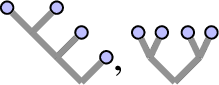
. We sketch the proof that they cannot form a linear combination that takes values in $\mathcal {J}$
. For this, fix test functions
$\mathcal {J}$
. For this, fix test functions $\psi _{i,j} : \bar {\mathbf D} \to \mathbf {R}$
and consider test functions
$\psi _{i,j} : \bar {\mathbf D} \to \mathbf {R}$
and consider test functions $\phi _{\varepsilon }$
of the form
$\phi _{\varepsilon }$
of the form $\phi _{\varepsilon }(x_1, x_2, x_3, x_4) = \sum _{\sigma } \sum _{1 \le i < j \le 4} \psi _{i,j}^{\varepsilon }\left (x_{\sigma (i)} - x_{\sigma \left (j\right )}\right )$
, where the first sum runs over all permutations
$\phi _{\varepsilon }(x_1, x_2, x_3, x_4) = \sum _{\sigma } \sum _{1 \le i < j \le 4} \psi _{i,j}^{\varepsilon }\left (x_{\sigma (i)} - x_{\sigma \left (j\right )}\right )$
, where the first sum runs over all permutations $\sigma $
of
$\sigma $
of $\{1,2,3,4\}$
. Here
$\{1,2,3,4\}$
. Here $\psi _{i,j}^{\varepsilon }(x) := \varepsilon ^{-\frac {3}{2}} \psi _{i,j}\left (\varepsilon ^{-\mathfrak {s}} x\right )$
if
$\psi _{i,j}^{\varepsilon }(x) := \varepsilon ^{-\frac {3}{2}} \psi _{i,j}\left (\varepsilon ^{-\mathfrak {s}} x\right )$
if $(i,j)\in \{(1,2), (3,4)\}$
, and
$(i,j)\in \{(1,2), (3,4)\}$
, and $\psi _{i,j}^{\varepsilon }(x) := \psi _{i,j}(x)$
otherwise. It is then not difficult to see that
$\psi _{i,j}^{\varepsilon }(x) := \psi _{i,j}(x)$
otherwise. It is then not difficult to see that

The reason for this is that the first tree contains only one subdivergence
of degree $-1$
, whereas the second tree contains two of them. From this it follows that no linear combination of these two trees can be an element of
$-1$
, whereas the second tree contains two of them. From this it follows that no linear combination of these two trees can be an element of $\mathcal {J}$
, thus leading to the claim.
$\mathcal {J}$
, thus leading to the claim.
We now state the two assumptions that we are going to need for this section. The first assumes that the annihilator $\mathcal {H}$
of
$\mathcal {H}$
of $\mathcal {J}$
forms indeed a group.
$\mathcal {J}$
forms indeed a group.
Assumption 7. The ideal $\mathcal {J}$
is a Hopf ideal in
$\mathcal {J}$
is a Hopf ideal in $\mathcal {T}_-$
. In particular, its annihilator
$\mathcal {T}_-$
. In particular, its annihilator $\mathcal {H}$
is a Lie subgroup of the renormalisation group
$\mathcal {H}$
is a Lie subgroup of the renormalisation group $\mathcal {G}_-$
.
$\mathcal {G}_-$
.
The next assumption relates the subgroup $\mathcal {H}$
to the BPHZ characters associated to smooth shifted noise. We recall the notation
$\mathcal {H}$
to the BPHZ characters associated to smooth shifted noise. We recall the notation ${\mathfrak {M}_{\infty }^{\mathrm {s}}}$
for the space of smooth shifted noises and
${\mathfrak {M}_{\infty }^{\mathrm {s}}}$
for the space of smooth shifted noises and ${\mathfrak {M}_0^{\mathrm {s}}}$
for its closure under the norm (2.21). In the following assumption we do not require the noise
${\mathfrak {M}_0^{\mathrm {s}}}$
for its closure under the norm (2.21). In the following assumption we do not require the noise $\eta $
to be Gaussian:
$\eta $
to be Gaussian:
Assumption 8. There exists a continuous map ${\mathfrak {M}_0^{\mathrm {s}}} \ni \eta \mapsto f^{\eta } \in \mathcal {G}_-$
with the property that
${\mathfrak {M}_0^{\mathrm {s}}} \ni \eta \mapsto f^{\eta } \in \mathcal {G}_-$
with the property that $f^{\mathbf 0} = \mathbf {1}^*$
, and such that
$f^{\mathbf 0} = \mathbf {1}^*$
, and such that $g^{\eta } \in f^{\eta } \circ \mathcal {H}$
for any
$g^{\eta } \in f^{\eta } \circ \mathcal {H}$
for any $\eta \in {\mathfrak {M}_{\infty }^{\mathrm {s}}}$
. Here
$\eta \in {\mathfrak {M}_{\infty }^{\mathrm {s}}}$
. Here $\mathbf 0$
denotes the
$\mathbf 0$
denotes the $0$
-noise.
$0$
-noise.
We will see in Corollary 3.23 that $\mathcal {H}$
is in fact the smallest Lie subgroup of
$\mathcal {H}$
is in fact the smallest Lie subgroup of $\mathcal {G}_-$
that has the property described in this assumption. As was already pointed out in Remark 2.23, we will show in Section 4 that the two assumptions given here are implied by Assumption 6 (which is the only argument in this paper where Assumption 6 is needed).
$\mathcal {G}_-$
that has the property described in this assumption. As was already pointed out in Remark 2.23, we will show in Section 4 that the two assumptions given here are implied by Assumption 6 (which is the only argument in this paper where Assumption 6 is needed).
3.2 A support theorem for random models
From now on, we will always assume that Assumptions 2–5, 7 and 8 hold, except when specified explicitly. The only exception is Section 4, where we prove that Assumptions 7 and 8 are implied by Assumptions 2–6.
Setting $\hat {Z}^{\varepsilon } = {\mathcal {R}^{g^{\varepsilon }}} Z_{\mathrm {c}}(\xi ^{\varepsilon })$
for the renormalised approximate model and
$\hat {Z}^{\varepsilon } = {\mathcal {R}^{g^{\varepsilon }}} Z_{\mathrm {c}}(\xi ^{\varepsilon })$
for the renormalised approximate model and $\hat {Z} = \lim _{\varepsilon \to 0}\hat {Z}^{\varepsilon }$
for its limit, we can rewrite it as
$\hat {Z} = \lim _{\varepsilon \to 0}\hat {Z}^{\varepsilon }$
for its limit, we can rewrite it as
 $$ \begin{align*} \hat{Z}^{\varepsilon}=T_{\xi^{\varepsilon}} {\mathcal{R}^{g^{\varepsilon}}} Z_{\mathrm{c}}(0). \end{align*} $$
Models obtained by acting on the canonical lift of $0$
with the renormalisation operators will later play an important role, so we introduce the following notation:
$0$
with the renormalisation operators will later play an important role, so we introduce the following notation:
Definition 3.7. For any character $g\in \mathcal {G}_-$
, we define the model
$g\in \mathcal {G}_-$
, we define the model ${\mathscr {Z}}(g)$
by letting the renormalisation operator act on the canonical lift of
${\mathscr {Z}}(g)$
by letting the renormalisation operator act on the canonical lift of $0$
to a model – that is, we set
$0$
to a model – that is, we set
 $$ \begin{align*} {\mathscr{Z}}(g):={\mathcal{R}^{g}} Z_{\mathrm{c}}(0). \end{align*} $$
We will see in Lemma 3.12 that the action of the translation operator maps the support into itself, so that the main part of the proof consists in understanding the set of characters $g\in \mathcal {G}_-$
such that
$g\in \mathcal {G}_-$
such that ${\mathcal {R}^{g}} Z_{\mathrm {c}}(0)\in \operatorname {\mathrm {supp}} \hat {Z}$
. We will show that this set is a coset
${\mathcal {R}^{g}} Z_{\mathrm {c}}(0)\in \operatorname {\mathrm {supp}} \hat {Z}$
. We will show that this set is a coset $f\circ \mathcal {H}$
of the Lie subgroup
$f\circ \mathcal {H}$
of the Lie subgroup $\mathcal {H}$
of
$\mathcal {H}$
of $\mathcal {G}_-$
already constructed.
$\mathcal {G}_-$
already constructed.
Proposition 3.8. Let $\mathcal {H}$
be the Lie subgroup of
$\mathcal {H}$
be the Lie subgroup of $\mathcal {G}_-$
defined in Definition 3.3 and let
$\mathcal {G}_-$
defined in Definition 3.3 and let $f^{\xi }\in \mathcal {G}_-$
be the character defined in Assumption 8. Then for any character
$f^{\xi }\in \mathcal {G}_-$
be the character defined in Assumption 8. Then for any character $g\in f^{\xi }\circ \mathcal {H}$
in the left coset determined by
$g\in f^{\xi }\circ \mathcal {H}$
in the left coset determined by $f^{\xi }$
and
$f^{\xi }$
and $\mathcal {H}$
, one has
$\mathcal {H}$
, one has
 $$ \begin{align*} {\mathscr{Z}}(g)\in\operatorname{\mathrm{supp}} \hat{Z}. \end{align*} $$
This proposition follows from Proposition 3.21, which in turn relies on the constructions carried out in Sections 3.3 and 5. Before we prove Proposition 3.8, we show now that it implies a support theorem for random models (see Theorem 3.14).
Remark 3.9. The converse of Proposition 3.8 is not true in general. An example of this is given by the rough paths $\mathbf {B} = (B,{\mathbf B} + {\mathbf M})$
, where
$\mathbf {B} = (B,{\mathbf B} + {\mathbf M})$
, where ${\mathbf B}^{i,j}_{s,t}:= \int _s^t \left (B^i_r- B^i_s\right ) \circ dB^j_r$
denotes the Stratonovich lift and
${\mathbf B}^{i,j}_{s,t}:= \int _s^t \left (B^i_r- B^i_s\right ) \circ dB^j_r$
denotes the Stratonovich lift and ${\mathbf M}_{s,t} = (t-s)M$
for a constant (in time) and skew-symmetric matrix M. These rough paths are known to have support independent of M, but
${\mathbf M}_{s,t} = (t-s)M$
for a constant (in time) and skew-symmetric matrix M. These rough paths are known to have support independent of M, but $\mathcal {H}=\{\mathbf {1}^*\}$
is trivial in this case. We just sketch the argument here that the support is really independent of M. Consider deterministic smooth shifts
$\mathcal {H}=\{\mathbf {1}^*\}$
is trivial in this case. We just sketch the argument here that the support is really independent of M. Consider deterministic smooth shifts $B^i_t \to B^i_t + \varepsilon ^{{\frac {1}{2}}}\cos \left (\varepsilon ^{-1} t\right )$
and
$B^i_t \to B^i_t + \varepsilon ^{{\frac {1}{2}}}\cos \left (\varepsilon ^{-1} t\right )$
and $B^j_t \to B^j_t + \varepsilon ^{{\frac {1}{2}}} \sin \left (\varepsilon ^{-1} t\right )$
. The translation operator transforms the second component into
$B^j_t \to B^j_t + \varepsilon ^{{\frac {1}{2}}} \sin \left (\varepsilon ^{-1} t\right )$
. The translation operator transforms the second component into
 $$ \begin{align*} {\mathbf B}^{i,j,\varepsilon}_{s,t} &= {\mathbf B}^{i,j}_{s,t} + \varepsilon^{-{\frac{1}{2}}}\int_s^t \left(B^i_u - B^i_s\right) \cos\left(\varepsilon^{-1} u\right) du \\ &\quad + \varepsilon^{\frac{1}{2}}\int_s^t \cos\left(\varepsilon^{-1} u \right) - \cos\left(\varepsilon^{-1} s\right) dB_u + \int_s^t \left( \cos\left(\varepsilon^{-1} u \right) - \cos\left(\varepsilon^{-1} s\right) \right) \cos\left(\varepsilon^{-1} u\right) du. \end{align*} $$
The last term converges to a positive constant times $(t-s)$
as
$(t-s)$
as $\varepsilon \to 0$
, and a quick computation shows that the two terms in the centre vanish in this limit.
$\varepsilon \to 0$
, and a quick computation shows that the two terms in the centre vanish in this limit.
Remark 3.10. Proposition 3.8 also gives information about limit models obtained from a different choice of renormalisation: For any $k\in \mathcal {G}_-$
and any
$k\in \mathcal {G}_-$
and any $g\in k\circ f^{\xi }\circ \mathcal {H}$
, one has
$g\in k\circ f^{\xi }\circ \mathcal {H}$
, one has
 $$ \begin{align*} {\mathscr{Z}}(g)\in \operatorname{\mathrm{supp}} {\mathcal{R}^{k}}\hat{Z}. \end{align*} $$
Before we state the main theorem, we derive some immediate identities.
Lemma 3.11. For any character $g\in \mathcal {G}_-$
and any smooth noise
$g\in \mathcal {G}_-$
and any smooth noise $h\in \mathfrak {M}_{\infty }$
, one has the equality
$h\in \mathfrak {M}_{\infty }$
, one has the equality
 $$ \begin{align*} {\mathcal{R}^{g}} Z_{\mathrm{c}}(h)=T_{h} {\mathscr{Z}}(g). \end{align*} $$
In particular, one has the identity
 $$ \begin{align*} \hat{Z}^{\varepsilon}[\xi]=T_{\xi^{\varepsilon}} {\mathscr{Z}}(g^{\varepsilon}) \end{align*} $$
almost surely for any $\varepsilon>0$
.
$\varepsilon>0$
.
Proof . In order to see the first identity, it is enough to apply Theorem 2.4 to $f\equiv 0$
. The second claim follows from the facts that
$f\equiv 0$
. The second claim follows from the facts that $\hat {Z}^{\varepsilon } = {\mathcal {R}^{g^{\varepsilon }}} Z^{\varepsilon }$
and
$\hat {Z}^{\varepsilon } = {\mathcal {R}^{g^{\varepsilon }}} Z^{\varepsilon }$
and $ Z^{\varepsilon }[\xi ]=T_{\xi ^{\varepsilon }}Z_{\mathrm {c}}(0) $
.
$ Z^{\varepsilon }[\xi ]=T_{\xi ^{\varepsilon }}Z_{\mathrm {c}}(0) $
.
The next lemma crucially states that shifting the noises by a random smooth function maps the support into itself.
Lemma 3.12. Set $h\in \Omega _{\infty }$
. Then one has the identity
$h\in \Omega _{\infty }$
. Then one has the identity
 $$ \begin{align*} T_h \hat{Z}[\xi]=\hat{Z}[\xi+h] \end{align*} $$
almost surely. Moreover, if $h\in \mathfrak {M}_{\infty }$
is any smooth random noise, then one has the identity
$h\in \mathfrak {M}_{\infty }$
is any smooth random noise, then one has the identity
 $$ \begin{align*} \operatorname{\mathrm{supp}} T_h \hat{Z}\subseteq \operatorname{\mathrm{supp}} \hat{Z}. \end{align*} $$
Proof . We show the first statement. By Cameron–Martin (Theorem 2.6), it follows that the laws of $\xi $
and
$\xi $
and $\xi +h$
are equivalent. In particular, the right-hand side is well defined
$\xi +h$
are equivalent. In particular, the right-hand side is well defined $\mathbf {P}$
-almost surely. To see the identity claimed in the statement, we use the fact that T is jointly continuous in h and Z. We then have
$\mathbf {P}$
-almost surely. To see the identity claimed in the statement, we use the fact that T is jointly continuous in h and Z. We then have
 $$ \begin{align*} \hat{Z}[\xi+h]=\lim_{\varepsilon\to 0}\hat{Z}^{\varepsilon}[\xi+h]=\lim_{\varepsilon\to 0}T_{h^{\varepsilon}}\hat{Z}^{\varepsilon}[\xi]=T_h \hat{Z}[\xi]. \end{align*} $$
In order to see the second statement, let first $h\in \Omega _{\infty }$
be deterministic. In this case we exploit again the fact that the laws of
$h\in \Omega _{\infty }$
be deterministic. In this case we exploit again the fact that the laws of $\xi $
and
$\xi $
and $\xi +h$
are equivalent, so that the laws of
$\xi +h$
are equivalent, so that the laws of $\hat {Z}[\xi ]$
and
$\hat {Z}[\xi ]$
and $T_h \hat {Z}[\xi ]=\hat {Z}[\xi +h]$
are equivalent as well and
$T_h \hat {Z}[\xi ]=\hat {Z}[\xi +h]$
are equivalent as well and $\operatorname {\mathrm {supp}} \hat {Z}=\operatorname {\mathrm {supp}} T_h \hat {Z}$
. Using Lemma 3.13, it follows that the continuous operator
$\operatorname {\mathrm {supp}} \hat {Z}=\operatorname {\mathrm {supp}} T_h \hat {Z}$
. Using Lemma 3.13, it follows that the continuous operator $T_h$
maps the support of
$T_h$
maps the support of $\hat {Z}$
into itself.
$\hat {Z}$
into itself.
Let now $h\in \mathfrak {M}_{\infty }$
be random and let
$h\in \mathfrak {M}_{\infty }$
be random and let $A\subseteq \Omega $
be the set of full
$A\subseteq \Omega $
be the set of full $\mathbf {P}$
-measure with the property that
$\mathbf {P}$
-measure with the property that $\hat {Z}(\omega )\in \operatorname {\mathrm {supp}}\hat {Z}$
for any
$\hat {Z}(\omega )\in \operatorname {\mathrm {supp}}\hat {Z}$
for any $\omega \in A$
. It then follows for
$\omega \in A$
. It then follows for $\omega \in A$
that
$\omega \in A$
that $T_{h(\omega )} \hat {Z}(\omega )\in \operatorname {\mathrm {supp}} \hat {Z}$
. In particular we have
$T_{h(\omega )} \hat {Z}(\omega )\in \operatorname {\mathrm {supp}} \hat {Z}$
. In particular we have $T_h \hat {Z}\in \operatorname {\mathrm {supp}} \hat {Z}$
almost surely.
$T_h \hat {Z}\in \operatorname {\mathrm {supp}} \hat {Z}$
almost surely.
In the previous proof we used the following lemma:
Lemma 3.13. Let $X,Y$
be two Polish spaces, let
$X,Y$
be two Polish spaces, let $T:X\to Y$
be a continuous map and let
$T:X\to Y$
be a continuous map and let $\mu $
be a probability measure on X. Then
$\mu $
be a probability measure on X. Then $\operatorname {\mathrm {supp}} T_*\mu = \overline {T(\operatorname {\mathrm {supp}} \mu )}$
.
$\operatorname {\mathrm {supp}} T_*\mu = \overline {T(\operatorname {\mathrm {supp}} \mu )}$
.
Proof . Since $x \in \operatorname {\mathrm {supp}} \mu $
for
$x \in \operatorname {\mathrm {supp}} \mu $
for $\mu $
-almost every
$\mu $
-almost every $x \in X$
, it follows that
$x \in X$
, it follows that $T(x) \in T(\operatorname {\mathrm {supp}} \mu ) \ \mu $
-almost surely, and hence
$T(x) \in T(\operatorname {\mathrm {supp}} \mu ) \ \mu $
-almost surely, and hence $\operatorname {\mathrm {supp}} T_* \mu \subseteq \overline {T(\operatorname {\mathrm {supp}} \mu )}$
. To see the inverse inclusion, let
$\operatorname {\mathrm {supp}} T_* \mu \subseteq \overline {T(\operatorname {\mathrm {supp}} \mu )}$
. To see the inverse inclusion, let $y=T(x)\in T(\operatorname {\mathrm {supp}} \mu )$
with
$y=T(x)\in T(\operatorname {\mathrm {supp}} \mu )$
with $x\in \operatorname {\mathrm {supp}} \mu $
, and let U be a neighbourhood of y in Y. By continuity it follows that
$x\in \operatorname {\mathrm {supp}} \mu $
, and let U be a neighbourhood of y in Y. By continuity it follows that $T^{-1}(U)$
is a neighbourhood of x in X, and by the definition of the support, it follows that
$T^{-1}(U)$
is a neighbourhood of x in X, and by the definition of the support, it follows that $\mu \{x:T(x)\in U\}=\mu \left (T^{-1}(U)\right )>0$
, and thus
$\mu \{x:T(x)\in U\}=\mu \left (T^{-1}(U)\right )>0$
, and thus $y \in \operatorname {\mathrm {supp}} T_* \mu $
. This shows that
$y \in \operatorname {\mathrm {supp}} T_* \mu $
. This shows that $T(\operatorname {\mathrm {supp}} \mu ) \subseteq \operatorname {\mathrm {supp}} T_*\mu $
and concludes the proof.
$T(\operatorname {\mathrm {supp}} \mu ) \subseteq \operatorname {\mathrm {supp}} T_*\mu $
and concludes the proof.
Assuming Proposition 3.8, we can now state and prove the main theorem of this section.
Theorem 3.14. For any $\varepsilon>0$
, let
$\varepsilon>0$
, let $\hat {Z}^{\varepsilon }$
denote the BPHZ renormalised lift of the regularised noise
$\hat {Z}^{\varepsilon }$
denote the BPHZ renormalised lift of the regularised noise $\xi ^{\varepsilon }$
to a random admissible model and let
$\xi ^{\varepsilon }$
to a random admissible model and let $k\in \mathcal {G}_-$
be any character. Then one has the identity
$k\in \mathcal {G}_-$
be any character. Then one has the identity
 $$ \begin{align} \operatorname{\mathrm{supp}} {\mathcal{R}^{k}} \hat{Z}=\bigcap_{\varepsilon>0}\overline{\bigcup_{\delta<\varepsilon} \operatorname{\mathrm{supp}} {\mathcal{R}^{k}} \hat{Z}^{\delta}}. \end{align} $$
Moreover, if we denote by $f^{\varepsilon }:=f^{\xi ^{\varepsilon }}\in \mathcal {G}_-$
the sequence of characters defined in Assumption 8 (so that
$f^{\varepsilon }:=f^{\xi ^{\varepsilon }}\in \mathcal {G}_-$
the sequence of characters defined in Assumption 8 (so that $f^{\varepsilon } \to f^{\xi }$
as
$f^{\varepsilon } \to f^{\xi }$
as $\varepsilon \to 0$
), then one has the stronger statement
$\varepsilon \to 0$
), then one has the stronger statement
 $$ \begin{align} \operatorname{\mathrm{supp}} {\mathcal{R}^{k}} \hat{Z}=\overline{\bigcup_{\varepsilon\in\left(0,1\right)}\operatorname{\mathrm{supp}} {\mathcal{R}^{k\circ f^{\xi}\circ\left(f^{\varepsilon}\right)^{-1}}}\hat{Z}^{\varepsilon}}. \end{align} $$
Proof . Remember that we assume Proposition 3.8. We first argue that equation (3.3) follows from equation (3.4). To see this, we introduce the sequence of characters $l^{\varepsilon } \in \mathcal {G}_-$
via the identity
$l^{\varepsilon } \in \mathcal {G}_-$
via the identity $k\circ f^{\xi }\circ (f^{\varepsilon })^{-1}=l^{\varepsilon }\circ k$
, and we note that since
$k\circ f^{\xi }\circ (f^{\varepsilon })^{-1}=l^{\varepsilon }\circ k$
, and we note that since $k\circ f^{\xi }\circ (f^{\varepsilon })^{-1}\to k$
in
$k\circ f^{\xi }\circ (f^{\varepsilon })^{-1}\to k$
in $\mathcal {G}_-$
, it follows that
$\mathcal {G}_-$
, it follows that $l^{\varepsilon }\to \mathbf {1}^*$
. By Lemma 3.13 and the continuity of the action of the renormalisation group, it follows that
$l^{\varepsilon }\to \mathbf {1}^*$
. By Lemma 3.13 and the continuity of the action of the renormalisation group, it follows that $\operatorname {\mathrm {supp}} {\mathcal {R}^{k}} \hat {Z}$
can be written as
$\operatorname {\mathrm {supp}} {\mathcal {R}^{k}} \hat {Z}$
can be written as
 $$ \begin{align*} \lim_{\varepsilon\to 0}\overline {\bigcup_{\delta<\varepsilon}\operatorname{\mathrm{supp}} {\mathcal{R}^{l^{\varepsilon} \circ k}} \hat{Z}^{\delta}} = \lim_{\varepsilon\to 0}\overline { {\mathcal{R}^{l^{\varepsilon}}} \bigcup_{\delta<\varepsilon} \operatorname{\mathrm{supp}} {\mathcal{R}^{k}} \hat{Z}^{\delta}} = \bigcap_{\varepsilon>0}\overline{\bigcup_{\delta<\varepsilon} \operatorname{\mathrm{supp}} {\mathcal{R}^{k}} { \hat{Z}^{\delta}} }. \end{align*} $$
It remains to show equation (3.4). The fact that $\operatorname {\mathrm {supp}} {\mathcal {R}^{k}} \hat {Z}$
is contained in the right-hand side follows trivially from the fact that
$\operatorname {\mathrm {supp}} {\mathcal {R}^{k}} \hat {Z}$
is contained in the right-hand side follows trivially from the fact that
 $$ \begin{align*} {\mathcal{R}^{k\circ f^{\xi}\circ\left(f^{\varepsilon}\right)^{-1}}}\hat{Z}^{\varepsilon}\to {\mathcal{R}^{k}} \hat{Z} \end{align*} $$
in probability in the space of models, so it remains to show the inverse inclusion. By Lemma 3.11 we have the identity
 $$ \begin{align*} \operatorname{\mathrm{supp}} {\mathcal{R}^{k\circ f^{\xi}\circ\left(f^{\varepsilon}\right)^{-1}}} \hat{Z}^{\varepsilon} = \overline{ \left\{T_h {\mathscr{Z}}\left(k\circ f^{\xi}\circ \hat{g}^{\varepsilon}\right): h\in\Omega_{\infty}\right\}, } \end{align*} $$
where we introduce the character $\hat {g}^{\varepsilon } \in \mathcal {G}_-$
via the identity
$\hat {g}^{\varepsilon } \in \mathcal {G}_-$
via the identity $f^{\varepsilon } \circ \hat {g}^{\varepsilon }= g^{\varepsilon }$
. By Assumption 8 one has
$f^{\varepsilon } \circ \hat {g}^{\varepsilon }= g^{\varepsilon }$
. By Assumption 8 one has $\hat {g}^{\varepsilon } \in \mathcal {H}$
, so Proposition 3.8 implies that
$\hat {g}^{\varepsilon } \in \mathcal {H}$
, so Proposition 3.8 implies that
 $$ \begin{align*} {\mathscr{Z}}\left(k\circ f^{\xi}\circ \hat{g}^{\varepsilon}\right)\in\operatorname{\mathrm{supp}} {\mathcal{R}^{k}} \hat{Z}. \end{align*} $$
It remains to show that the translation operator $T_h$
leaves the support of
$T_h$
leaves the support of ${\mathcal {R}^{k}} \hat {Z}$
invariant, in the sense that for any smooth function
${\mathcal {R}^{k}} \hat {Z}$
invariant, in the sense that for any smooth function $h\in \Omega _{\infty }$
one has
$h\in \Omega _{\infty }$
one has
 $$ \begin{align*} \operatorname{\mathrm{supp}} T_h {\mathcal{R}^{k}}\hat{Z} = \operatorname{\mathrm{supp}} {\mathcal{R}^{k}}\hat{Z}. \end{align*} $$
This in turn is a corollary of Lemma 3.12, the fact that renormalisation and translation commute (see Theorem 2.4) and Cameron and Martin’s theorem.
One consequence of Theorem 3.14 is that the support of the limit model does in general depend on the choice of renormalisation $k \in \mathcal {G}_-$
. In the next result we show that for any fixed
$k \in \mathcal {G}_-$
. In the next result we show that for any fixed $k \in \mathcal {G}_-$
, there exists a Lie subgroup
$k \in \mathcal {G}_-$
, there exists a Lie subgroup $\mathcal {H}^k$
of
$\mathcal {H}^k$
of $\mathcal {G}_-$
such that changing renormalisation from k to
$\mathcal {G}_-$
such that changing renormalisation from k to $l \circ k$
for some
$l \circ k$
for some $l \in \mathcal {H}^k$
does not change the support. More precisely, we have the following result:
$l \in \mathcal {H}^k$
does not change the support. More precisely, we have the following result:
Corollary 3.15. For any $k\in \mathcal {G}_-$
, let
$k\in \mathcal {G}_-$
, let $\bar {k} := k\circ f^{\xi }$
, and denote by
$\bar {k} := k\circ f^{\xi }$
, and denote by $\mathcal {H}^k$
the Lie subgroup of
$\mathcal {H}^k$
the Lie subgroup of $\mathcal {G}_-$
obtained from
$\mathcal {G}_-$
obtained from $\mathcal {H}$
by conjugation with
$\mathcal {H}$
by conjugation with $\bar {k}$
– that is, the subgroup given by
$\bar {k}$
– that is, the subgroup given by
 $$ \begin{align*} \mathcal{H}^k:= \bar{k} \circ \mathcal{H} \circ \bar{k}^{-1}. \end{align*} $$
Then for any $ l\in \mathcal {H}^k$
, one has
$ l\in \mathcal {H}^k$
, one has
 $$ \begin{align*} \operatorname{\mathrm{supp}} {\mathcal{R}^{l\circ k}} \hat{Z}=\operatorname{\mathrm{supp}} {\mathcal{R}^{k}} \hat{Z}. \end{align*} $$
Moreover, the groups $\mathcal {H}^k$
are invariant under composing k with any element of
$\mathcal {H}^k$
are invariant under composing k with any element of $\mathcal {H}^k$
– that is, one has
$\mathcal {H}^k$
– that is, one has $\mathcal {H}^k = \mathcal {H}^{l \circ k}$
for any
$\mathcal {H}^k = \mathcal {H}^{l \circ k}$
for any $l \in \mathcal {H}^k$
.
$l \in \mathcal {H}^k$
.
Proof . The supports of ${\mathcal {R}^{k}}\hat {Z}$
and
${\mathcal {R}^{k}}\hat {Z}$
and ${\mathcal {R}^{l\circ k}} \hat {Z}$
are respectively characterised as the closure of all smooth translations of all models of the form
${\mathcal {R}^{l\circ k}} \hat {Z}$
are respectively characterised as the closure of all smooth translations of all models of the form ${\mathscr {Z}}(h)$
and
${\mathscr {Z}}(h)$
and ${\mathscr {Z}}\left (\tilde {h}\right )$
for some
${\mathscr {Z}}\left (\tilde {h}\right )$
for some $h\in \bar {k} \circ \mathcal {H}$
and some
$h\in \bar {k} \circ \mathcal {H}$
and some $\tilde {h}\in l\circ \bar {k} \circ \mathcal {H}$
. We are thus left to show that
$\tilde {h}\in l\circ \bar {k} \circ \mathcal {H}$
. We are thus left to show that
 $$ \begin{align*} l \circ \bar{k} \circ \mathcal{H} = \bar{k} \circ \mathcal{H}, \end{align*} $$
which is true if and only if $l\in \mathcal {H}^k$
.
$l\in \mathcal {H}^k$
.
The fact that $\mathcal {H}^k$
is invariant under a change of renormalisation by
$\mathcal {H}^k$
is invariant under a change of renormalisation by $l\in \mathcal {H}^k$
follows from the fact that
$l\in \mathcal {H}^k$
follows from the fact that
 $$ \begin{align*} \mathcal{H}^{l\circ k} &= l\circ \left( \bar{k}\circ \mathcal{H}\circ \bar{k}^{-1} \right) \circ l^{-1} \\ &\subseteq \bar{k} \circ \mathcal{H}\circ \bar{k}^{-1} \circ \left( \bar{k} \circ \mathcal{H} \circ \bar{k}^{-1} \right) \circ \bar{k} \circ \mathcal{H} \circ \bar{k}^{-1} =\mathcal{H}^k, \end{align*} $$
whence the claim follows.
Remark 3.16. A consequence of this corollary is that, writing e for the unit in $\mathcal {G}_-$
, the collection of cosets
$\mathcal {G}_-$
, the collection of cosets $\{ k \circ \mathcal {H}^e : k\in \mathcal {G}_-\}$
yields a foliation of
$\{ k \circ \mathcal {H}^e : k\in \mathcal {G}_-\}$
yields a foliation of $\mathcal {G}_-$
into a family of manifolds of fixed dimension with the property that for any
$\mathcal {G}_-$
into a family of manifolds of fixed dimension with the property that for any $k \in \mathcal {G}_-$
, the support of
$k \in \mathcal {G}_-$
, the support of $\mathcal {R}^l \hat {Z}$
is independent of
$\mathcal {R}^l \hat {Z}$
is independent of $l \in k \circ \mathcal {H}^e$
.
$l \in k \circ \mathcal {H}^e$
.
3.3 Renormalisation-group argument
In light of the previous section, it remains to show Proposition 3.8. For this we fix from now on a character $h\in f^{\xi }\circ \mathcal {H}$
and we will construct a sequence
$h\in f^{\xi }\circ \mathcal {H}$
and we will construct a sequence ${ \zeta }_{\delta }\in \mathfrak {M}_{\infty }$
,
${ \zeta }_{\delta }\in \mathfrak {M}_{\infty }$
, $\delta>0$
, of random smooth noises such that
$\delta>0$
, of random smooth noises such that
 $$ \begin{align*} T_{{ \zeta }_{\delta}}\hat{Z} \to \mathscr{Z}(h) \quad\text{in probability in }\mathcal{M}_0 \end{align*} $$
as $\delta \to 0$
. Together with the continuity of the translation operator and Lemma 3.12, this immediately implies Proposition 3.8. This convergence essentially relies on two conditions. The first condition (formula (3.5)) guarantees that the noise cancels out in the limit
$\delta \to 0$
. Together with the continuity of the translation operator and Lemma 3.12, this immediately implies Proposition 3.8. This convergence essentially relies on two conditions. The first condition (formula (3.5)) guarantees that the noise cancels out in the limit $\delta \to 0$
, and the second condition (equation (3.6)) guarantees the correct behaviour of the expected values. Before stating the main proposition of this section, we introduce the following notation:
$\delta \to 0$
, and the second condition (equation (3.6)) guarantees the correct behaviour of the expected values. Before stating the main proposition of this section, we introduce the following notation:
Definition 3.17. Let $\sim $
denote the equivalence relation on
$\sim $
denote the equivalence relation on $\mathscr {T}_-$
given by setting
$\mathscr {T}_-$
given by setting $\tau \sim \tilde {\tau }$
if and only if
$\tau \sim \tilde {\tau }$
if and only if
![]() , and one has that the identity
, and one has that the identity $[L(\tau ),\mathfrak {t}]=[L(\tilde {\tau }),\mathfrak {t}]$
between multisets. We write
$[L(\tau ),\mathfrak {t}]=[L(\tilde {\tau }),\mathfrak {t}]$
between multisets. We write $\mathscr {T}_-/_{\sim }$
for the set of equivalence classes of
$\mathscr {T}_-/_{\sim }$
for the set of equivalence classes of $\mathscr {T}_-$
with respect to
$\mathscr {T}_-$
with respect to $\sim $
.
$\sim $
.
We also fix an arbitrary total order $\preceq $
on
$\preceq $
on $\mathscr {T}_-$
with the property that
$\mathscr {T}_-$
with the property that $\tau \preceq \tilde {\tau }$
whenever
$\tau \preceq \tilde {\tau }$
whenever $\tau ,\tilde {\tau } \in \mathscr {T}_-$
are two trees such that either
$\tau ,\tilde {\tau } \in \mathscr {T}_-$
are two trees such that either $\# E(\tau ) < \# E(\tilde {\tau })$
or
$\# E(\tau ) < \# E(\tilde {\tau })$
or $\# E(\tau ) = \# E(\tilde {\tau })$
and
$\# E(\tau ) = \# E(\tilde {\tau })$
and $\sum _{u \in N(\tau )}\mathfrak {n}(u) \le \sum _{u \in N\left (\tilde {\tau }\right )} \mathfrak {n}(u)$
. We write
$\sum _{u \in N(\tau )}\mathfrak {n}(u) \le \sum _{u \in N\left (\tilde {\tau }\right )} \mathfrak {n}(u)$
. We write $\mathscr {T}_-^{\preceq \tau }\subseteq \mathscr {T}_-$
and
$\mathscr {T}_-^{\preceq \tau }\subseteq \mathscr {T}_-$
and $\mathscr {T}_-^{\prec \tau }\subseteq \mathscr {T}_-$
, respectively, for the set of trees
$\mathscr {T}_-^{\prec \tau }\subseteq \mathscr {T}_-$
, respectively, for the set of trees $\tilde {\tau } \in \mathscr {T}_-$
such that
$\tilde {\tau } \in \mathscr {T}_-$
such that $\tilde {\tau }\preceq \tau $
and
$\tilde {\tau }\preceq \tau $
and $\tilde {\tau }\prec \tau $
. We denote the unital subalgebras of
$\tilde {\tau }\prec \tau $
. We denote the unital subalgebras of $\mathcal {T}_-$
generated by
$\mathcal {T}_-$
generated by $\mathscr {T}_-^{\prec \tau }$
and
$\mathscr {T}_-^{\prec \tau }$
and $\mathscr {T}_-^{\preceq \tau }$
by
$\mathscr {T}_-^{\preceq \tau }$
by $\mathcal {T}_-^{\prec \tau }$
and
$\mathcal {T}_-^{\prec \tau }$
and $\mathcal {T}_-^{\preceq \tau }$
, respectively, and we point out that it follows from the properties of the coproduct
$\mathcal {T}_-^{\preceq \tau }$
, respectively, and we point out that it follows from the properties of the coproduct ${\Delta _-}$
that both of these algebras form Hopf algebras.
${\Delta _-}$
that both of these algebras form Hopf algebras.
We use the total order $\preceq $
to select a subset of trees
$\preceq $
to select a subset of trees $\mathfrak {T}_- \subseteq \mathscr {T}_-$
in the following way:
$\mathfrak {T}_- \subseteq \mathscr {T}_-$
in the following way:
Definition 3.18. For any equivalence class $\Theta \in \mathscr {T}_-/_{\sim }$
, we write
$\Theta \in \mathscr {T}_-/_{\sim }$
, we write $\mathscr {T}_-(\Theta ) \subseteq \Theta $
for the set of trees
$\mathscr {T}_-(\Theta ) \subseteq \Theta $
for the set of trees $\tau \in \Theta $
with the property that there exists a linear combination of trees
$\tau \in \Theta $
with the property that there exists a linear combination of trees $\sigma \in \mathop {\mathrm {Vec}} {\left (\Theta \cap \mathscr {T}_-^{\prec \tau }\right )}$
such that
$\sigma \in \mathop {\mathrm {Vec}} {\left (\Theta \cap \mathscr {T}_-^{\prec \tau }\right )}$
such that
 $$ \begin{align*} \tau + \sigma \in \mathcal{J}. \end{align*} $$
(Here, $\mathcal {J}$
is the ideal in
$\mathcal {J}$
is the ideal in ${\mathcal {T}_-}$
defined in Definition 3.3.) We also write
${\mathcal {T}_-}$
defined in Definition 3.3.) We also write $\mathfrak {T}_-(\Theta ):=\Theta \backslash \mathscr {T}_-(\Theta )$
, and we define
$\mathfrak {T}_-(\Theta ):=\Theta \backslash \mathscr {T}_-(\Theta )$
, and we define $\mathfrak {T}_- := \bigsqcup _{\Theta \in \mathscr {T}_-/_{\sim }}\mathfrak {T}_-(\Theta )$
.
$\mathfrak {T}_- := \bigsqcup _{\Theta \in \mathscr {T}_-/_{\sim }}\mathfrak {T}_-(\Theta )$
.
In equation (3.8) we will give a linear subspace X of $\mathop {\mathrm {Vec}} \mathscr {T}_-$
for which we can show relatively easily that
$\mathop {\mathrm {Vec}} \mathscr {T}_-$
for which we can show relatively easily that $\mathcal {J}\cap \mathop {\mathrm {Vec}} \mathscr {T}_- \subseteq X$
, and our goal will be to show that
$\mathcal {J}\cap \mathop {\mathrm {Vec}} \mathscr {T}_- \subseteq X$
, and our goal will be to show that $X = \mathop {\mathrm {Vec}} \mathscr {T}_-$
. Definition 3.18 is set up so that it suffices to show that
$X = \mathop {\mathrm {Vec}} \mathscr {T}_-$
. Definition 3.18 is set up so that it suffices to show that $\mathfrak {T}_- \subseteq X$
. The total order
$\mathfrak {T}_- \subseteq X$
. The total order $\preceq $
is chosen in such a way that we can show this inductively in the number of edges and the polynomial decoration of
$\preceq $
is chosen in such a way that we can show this inductively in the number of edges and the polynomial decoration of $\tau \in \mathfrak {T}_-$
.
$\tau \in \mathfrak {T}_-$
.
Example 3.19. Consider the case of the 2D PAM equation, where

and where $\mathcal {J}$
is the ideal generated by
$\mathcal {J}$
is the ideal generated by
. Here a bold edge with label $k=1,2$
denotes the derivative of the Poisson kernel with respect to
$k=1,2$
denotes the derivative of the Poisson kernel with respect to $x_k$
, and a circle denotes an instance of spatial white noise. In this case we can choose the total order by setting
$x_k$
, and a circle denotes an instance of spatial white noise. In this case we can choose the total order by setting
. We then have
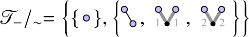
, and further,
and
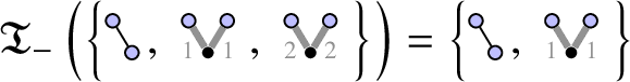
.
In particular, we have
 .
.
In Section 5 we will show the following proposition (see Proposition 5.19), for which we recall the notation $\Upsilon ^{\eta }$
from Section 2.2.3 and the spaces
$\Upsilon ^{\eta }$
from Section 2.2.3 and the spaces ${\mathfrak {M}_{\infty }^{\mathrm {s}}}$
and
${\mathfrak {M}_{\infty }^{\mathrm {s}}}$
and ${\mathfrak {M}_0}$
of smooth shifted noises and (rough) noises from Definition 2.13:
${\mathfrak {M}_0}$
of smooth shifted noises and (rough) noises from Definition 2.13:
Proposition 3.20. There exists a sequence ${ { \zeta } }_{\delta }\in {\mathfrak {M}_{\infty }^{\mathrm {s}}}$
,
${ { \zeta } }_{\delta }\in {\mathfrak {M}_{\infty }^{\mathrm {s}}}$
, $\delta>0$
, of smooth random noises such that
$\delta>0$
, of smooth random noises such that
 $$ \begin{align} \xi+{ { \zeta } }_{\delta}\to 0 \quad\text{in }{\mathfrak{M}_0} \end{align} $$
and such that for any $\tau \in \mathfrak {T}_-$
, one has
$\tau \in \mathfrak {T}_-$
, one has
 $$ \begin{align} \lim_{\delta\to 0}\lim_{\varepsilon\to 0} \Upsilon^{\xi^{\varepsilon}+{ { \zeta } }_{\delta}}M^{g^{\varepsilon}}\tau=h(\tau). \end{align} $$
Given this proposition, we can show the following result:
Proposition 3.21. Let ${ { \zeta } }_{\delta }$
be the sequence given by Proposition 3.20. Then one has
${ { \zeta } }_{\delta }$
be the sequence given by Proposition 3.20. Then one has
 $$ \begin{align*} \lim_{\delta\to 0}T_{{ { \zeta } }_{\delta}} \hat{Z}= {\mathscr{Z}}(h) \end{align*} $$
in probability in the space of admissible models.
Proof . We denote as before the BPHZ character for $\xi ^{\varepsilon }$
by
$\xi ^{\varepsilon }$
by $g^{\varepsilon }:=g^{\xi ^{\varepsilon }}$
, and we denote similarly by
$g^{\varepsilon }:=g^{\xi ^{\varepsilon }}$
, and we denote similarly by $g^{\varepsilon ,\delta }:=g^{\xi ^{\varepsilon }+{ { \zeta } }_{\delta }}$
the BPHZ character for the smooth noise
$g^{\varepsilon ,\delta }:=g^{\xi ^{\varepsilon }+{ { \zeta } }_{\delta }}$
the BPHZ character for the smooth noise $\xi ^{\varepsilon }+{ { \zeta } }_{\delta }$
. We define a character
$\xi ^{\varepsilon }+{ { \zeta } }_{\delta }$
. We define a character $h^{\varepsilon ,\delta }\in \mathcal {G}_-$
via the relation
$h^{\varepsilon ,\delta }\in \mathcal {G}_-$
via the relation
 $$ \begin{align} h^{\varepsilon,\delta}\circ g^{\varepsilon,\delta} =g^{\varepsilon}, \end{align} $$
where $\circ $
denotes the group product in
$\circ $
denotes the group product in ${\mathcal {G}_-}$
. We show inductively with respect to
${\mathcal {G}_-}$
. We show inductively with respect to $\prec $
that one has
$\prec $
that one has
 $$ \begin{align} \lim_{\delta \to 0} \lim_{\varepsilon \to 0} h^{\varepsilon,\delta}(\tau) = h(\tau). \end{align} $$
Let first $\tau \in \mathfrak {T}_-$
. Since, for any tree
$\tau \in \mathfrak {T}_-$
. Since, for any tree $\tau \in \mathscr {T}$
which contains at least one noise-type edge, one has
$\tau \in \mathscr {T}$
which contains at least one noise-type edge, one has
 $$ \begin{align*} \Upsilon^{\xi^{\varepsilon}+{ { \zeta } }_{\delta}}M^{g^{\varepsilon,\delta}} \tau\to 0 \end{align*} $$
in the limit $\varepsilon \to 0$
and
$\varepsilon \to 0$
and $\delta \to 0$
by Lemma 3.22, it follows that
$\delta \to 0$
by Lemma 3.22, it follows that
 $$ \begin{align*} h^{\varepsilon,\delta}(\tau) &=\Upsilon^{\xi^{\varepsilon}+{ { \zeta } }_{\delta}}M^{g^{\varepsilon,\delta}}M^{h^{\varepsilon,\delta}}\tau - \left(h^{\varepsilon,\delta}\otimes \Upsilon^{\xi^{\varepsilon}+{ { \zeta } }_{\delta}}M^{g^{\varepsilon,\delta}}\right)({\Delta_-}\mathfrak{i}- \mathrm{Id}\otimes\mathbf{1})\tau \\ &= \Upsilon^{\xi^{\varepsilon}+h_{\delta}}M^{g^{\varepsilon}}\tau + o(1), \end{align*} $$
where $o(1)\to 0$
as
$o(1)\to 0$
as $\varepsilon \to 0 $
and
$\varepsilon \to 0 $
and $\delta \to 0$
, so that equation (3.8) follows from equation (3.6).
$\delta \to 0$
, so that equation (3.8) follows from equation (3.6).
Set now $\tau \in \mathscr {T}_-\backslash \mathfrak {T}_-$
. Let
$\tau \in \mathscr {T}_-\backslash \mathfrak {T}_-$
. Let $\Theta \in \mathscr {T}_-/_{\sim }$
be the equivalence class of
$\Theta \in \mathscr {T}_-/_{\sim }$
be the equivalence class of $\tau $
, and let
$\tau $
, and let $\tilde {\tau }\in \mathop {\mathrm {Vec}} {\left (\Theta \cap \mathscr {T}_-^{\prec \tau }\right )} $
such that
$\tilde {\tau }\in \mathop {\mathrm {Vec}} {\left (\Theta \cap \mathscr {T}_-^{\prec \tau }\right )} $
such that $\sigma := \tau + \tilde {\tau } \in \mathcal {J}$
. We claim that
$\sigma := \tau + \tilde {\tau } \in \mathcal {J}$
. We claim that $(f^{\varepsilon })^{-1}\circ h^{\varepsilon ,\delta }(\sigma )\to 0$
in the limit
$(f^{\varepsilon })^{-1}\circ h^{\varepsilon ,\delta }(\sigma )\to 0$
in the limit $\varepsilon \to 0$
and
$\varepsilon \to 0$
and $\delta \to 0$
. Indeed, one has
$\delta \to 0$
. Indeed, one has
 $$ \begin{align*} (f^{\varepsilon})^{-1} \circ h^{\varepsilon,\delta}\circ f^{\varepsilon,\delta} \circ \hat{g}^{\varepsilon,\delta}= \hat{g}^{\varepsilon}, \end{align*} $$
where $f^{\varepsilon },\hat {g}^{\varepsilon }$
and
$f^{\varepsilon },\hat {g}^{\varepsilon }$
and $f^{\varepsilon ,\delta },\hat {g}^{\varepsilon ,\delta }$
are defined as in Assumption 8 for the noises
$f^{\varepsilon ,\delta },\hat {g}^{\varepsilon ,\delta }$
are defined as in Assumption 8 for the noises $\xi ^{\varepsilon }$
and
$\xi ^{\varepsilon }$
and $\xi ^{\varepsilon }+{ { \zeta } }_{\delta }$
, respectively, so that
$\xi ^{\varepsilon }+{ { \zeta } }_{\delta }$
, respectively, so that $f^{\varepsilon } \circ \hat {g}^{\varepsilon } = g^{\varepsilon }$
and
$f^{\varepsilon } \circ \hat {g}^{\varepsilon } = g^{\varepsilon }$
and $f^{\varepsilon ,\delta } \circ \hat {g}^{\varepsilon ,\delta } = g^{\varepsilon ,\delta }$
. By definition, one has that
$f^{\varepsilon ,\delta } \circ \hat {g}^{\varepsilon ,\delta } = g^{\varepsilon ,\delta }$
. By definition, one has that $\hat {g}^{\varepsilon ,\delta }\in \mathcal {H}$
and
$\hat {g}^{\varepsilon ,\delta }\in \mathcal {H}$
and $\hat {g}^{\varepsilon }\in \mathcal {H}$
, so that
$\hat {g}^{\varepsilon }\in \mathcal {H}$
, so that
 $$ \begin{align} (f^{\varepsilon})^{-1} \circ h^{\varepsilon,\delta} \circ f^{\varepsilon,\delta} = \hat{g}^{\varepsilon}\circ\left(\hat{g}^{\varepsilon,\delta}\right)^{-1} \in \mathcal{H}. \end{align} $$
By Assumption 8, the characters $f^{\varepsilon }$
and
$f^{\varepsilon }$
and $f^{\varepsilon ,\delta }$
converge to
$f^{\varepsilon ,\delta }$
converge to $f^{\xi }$
and
$f^{\xi }$
and $\mathbf {1}^*$
in
$\mathbf {1}^*$
in $\mathcal {G}_-$
, respectively. At this stage we would be done, if we knew a priori that
$\mathcal {G}_-$
, respectively. At this stage we would be done, if we knew a priori that $\lim _{\delta \to 0} \lim _{\varepsilon \to 0}h^{\varepsilon ,\delta }$
exists in
$\lim _{\delta \to 0} \lim _{\varepsilon \to 0}h^{\varepsilon ,\delta }$
exists in $\mathcal {G}_-$
on
$\mathcal {G}_-$
on $\mathcal {T}_-^{\preceq \tau }$
. By the induction hypothesis, this is true on
$\mathcal {T}_-^{\preceq \tau }$
. By the induction hypothesis, this is true on $\mathcal {T}_-^{\prec \tau }$
, so that it remains to show that
$\mathcal {T}_-^{\prec \tau }$
, so that it remains to show that $h^{\varepsilon ,\delta }(\tau )$
converges to something in the limit
$h^{\varepsilon ,\delta }(\tau )$
converges to something in the limit $\varepsilon \to 0$
and
$\varepsilon \to 0$
and $\delta \to 0$
. For this, note that equation (3.9) vanishes when applied to
$\delta \to 0$
. For this, note that equation (3.9) vanishes when applied to $\sigma $
, since
$\sigma $
, since $\sigma \in \mathcal {J}$
. On the other hand, one has
$\sigma \in \mathcal {J}$
. On the other hand, one has
 $$ \begin{align*} ({\Delta_-} \otimes \mathrm{Id}){\Delta_-}\sigma \in (\mathbf{1} \otimes \tau\otimes\mathbf{1}) + \left(\mathcal{T}_-^{\preceq\tau}\otimes \mathcal{T}_-^{\prec\tau}\otimes \mathcal{T}_-^{\preceq\tau}\right), \end{align*} $$
and we conclude using the induction hypothesis, which implies in particular that
 $$ \begin{align*} (f^{\varepsilon})^{-1} \otimes h^{\varepsilon,\delta} \otimes f^{\varepsilon,\delta} \end{align*} $$
converges on $\mathcal {T}_-^{\preceq \tau }\otimes \mathcal {T}_-^{\prec \tau }\otimes \mathcal {T}_-^{\preceq \tau }$
.
$\mathcal {T}_-^{\preceq \tau }\otimes \mathcal {T}_-^{\prec \tau }\otimes \mathcal {T}_-^{\preceq \tau }$
.
It follows that $\lim _{\delta \to 0}\lim _{\varepsilon \to 0}(f^{\varepsilon })^{-1}\circ h^{\varepsilon ,\delta } = \left (f^{\xi }\right )^{-1} \circ h$
on
$\lim _{\delta \to 0}\lim _{\varepsilon \to 0}(f^{\varepsilon })^{-1}\circ h^{\varepsilon ,\delta } = \left (f^{\xi }\right )^{-1} \circ h$
on $\mathcal {T}^{\preceq \tau }_-$
. Since
$\mathcal {T}^{\preceq \tau }_-$
. Since $\mathcal {T}_-^{\preceq \tau }$
is a Hopf subalgebra of
$\mathcal {T}_-^{\preceq \tau }$
is a Hopf subalgebra of $\mathcal {T}_-$
, we conclude that one also has
$\mathcal {T}_-$
, we conclude that one also has $\lim _{\delta \to 0}\lim _{\varepsilon \to 0} h^{\varepsilon ,\delta }=h$
on
$\lim _{\delta \to 0}\lim _{\varepsilon \to 0} h^{\varepsilon ,\delta }=h$
on $\mathcal {T}^{\preceq \tau }_-$
, and this concludes the proof of equation (3.8).
$\mathcal {T}^{\preceq \tau }_-$
, and this concludes the proof of equation (3.8).
The remaining proof is now straightforward. We first compute
 $$ \begin{align*} T_{{ { \zeta } }_{\delta}} \hat{Z}^{\varepsilon} = {\mathcal{R}^{g^{\varepsilon}}} Z_{\mathrm{c}}(\xi^{\varepsilon}+{ { \zeta } }_{\delta}) ={\mathcal{R}^{h^{\varepsilon,\delta}}} {\mathcal{R}^{g^{\varepsilon,\delta}}}Z_{\mathrm{c}}(\xi^{\varepsilon} + { { \zeta } }_{\delta}). \end{align*} $$
It follows from [Reference Chandra and HairerCH16, Theorem 2.33] that $\lim _{\delta \to 0}\lim _{\varepsilon \to 0}{\mathcal {R}^{g^{\varepsilon ,\delta }}}Z_{\mathrm {c}}(\xi ^{\varepsilon } + { { \zeta } }_{\delta })=Z_{\mathrm {c}}(0)$
in probability in the space of models. Using the fact that the renormalisation group
$\lim _{\delta \to 0}\lim _{\varepsilon \to 0}{\mathcal {R}^{g^{\varepsilon ,\delta }}}Z_{\mathrm {c}}(\xi ^{\varepsilon } + { { \zeta } }_{\delta })=Z_{\mathrm {c}}(0)$
in probability in the space of models. Using the fact that the renormalisation group $\mathcal {G}_-$
acts continuously onto the space of admissible models, together with the fact that
$\mathcal {G}_-$
acts continuously onto the space of admissible models, together with the fact that $\lim _{\delta \to 0}\lim _{\varepsilon \to 0} h^{\varepsilon ,\delta }=h$
, we obtain
$\lim _{\delta \to 0}\lim _{\varepsilon \to 0} h^{\varepsilon ,\delta }=h$
, we obtain
 $$ \begin{align*} \lim_{\delta\to 0}\lim_{\varepsilon\to 0} T_{{ { \zeta } }_{\delta}} \hat{Z}^{\varepsilon}={\mathcal{R}^{h}} Z_{\mathrm{c}}(0)= {\mathscr{Z}} (h), \end{align*} $$
and this concludes the proof.
Lemma 3.22. For any $\tau \in \mathcal {T}$
, the map
$\tau \in \mathcal {T}$
, the map $\eta \mapsto {\mathbf E}{\boldsymbol {\Pi }}^{\eta } M^{g^{\eta }}\tau (0)$
is continuous as a map from
$\eta \mapsto {\mathbf E}{\boldsymbol {\Pi }}^{\eta } M^{g^{\eta }}\tau (0)$
is continuous as a map from $\mathfrak {M}_0$
into
$\mathfrak {M}_0$
into $\mathbf {R}$
.
$\mathbf {R}$
.
Proof . The continuity of the map $\eta \mapsto {\mathbf E} \left ({\boldsymbol {\Pi }}^{\eta } M^{g^{\eta }} \tau \right )(\varphi )$
for any fixed test function
$\eta \mapsto {\mathbf E} \left ({\boldsymbol {\Pi }}^{\eta } M^{g^{\eta }} \tau \right )(\varphi )$
for any fixed test function $\varphi \in \mathcal {C}_c^{\infty }({\mathbf D})$
is a consequence of [Reference Chandra and HairerCH16]. To show the lemma, it thus suffices to find, for any fixed
$\varphi \in \mathcal {C}_c^{\infty }({\mathbf D})$
is a consequence of [Reference Chandra and HairerCH16]. To show the lemma, it thus suffices to find, for any fixed $\tau \in \mathcal {T}$
, a test function
$\tau \in \mathcal {T}$
, a test function $\varphi $
such that
$\varphi $
such that ${\mathbf E} {\boldsymbol {\Pi }}^{\eta } M^{g^{\eta }}\tau (0) = {\mathbf E} \left ({\boldsymbol {\Pi }}^{\eta } M^{g^{\eta }}\tau \right )(\varphi )$
for any smooth noise
${\mathbf E} {\boldsymbol {\Pi }}^{\eta } M^{g^{\eta }}\tau (0) = {\mathbf E} \left ({\boldsymbol {\Pi }}^{\eta } M^{g^{\eta }}\tau \right )(\varphi )$
for any smooth noise $\eta \in \mathfrak {M}_{\infty }$
. For this we recall that one has
$\eta \in \mathfrak {M}_{\infty }$
. For this we recall that one has
 $$ \begin{align} \left(\hat{\boldsymbol{\Pi}}^{\eta} \tau\right)(z) \sim \left(\hat{\boldsymbol{\Pi}}^{\eta} \otimes g_z\right) \Delta^+ \tau(0), \quad z \in {\mathbf D}, \end{align} $$
where $\Delta ^+$
denotes the coproduct on the structure group
$\Delta ^+$
denotes the coproduct on the structure group $\mathcal {G}_+$
and
$\mathcal {G}_+$
and $g_z \in \mathcal {G}_+$
is defined by setting
$g_z \in \mathcal {G}_+$
is defined by setting $g_z(X_i) := z_i$
, and
$g_z(X_i) := z_i$
, and $g_z(\tau ) = 0$
for any nonpolynomial
$g_z(\tau ) = 0$
for any nonpolynomial $\tau \in \mathcal {T}_+$
(in the language of [Reference Bruned, Hairer and ZambottiBHZ19, Definition 6.16], this follows from the fact that
$\tau \in \mathcal {T}_+$
(in the language of [Reference Bruned, Hairer and ZambottiBHZ19, Definition 6.16], this follows from the fact that $\hat {\boldsymbol {\Pi }}^{\eta }$
is stationary). It follows that
$\hat {\boldsymbol {\Pi }}^{\eta }$
is stationary). It follows that
 $$ \begin{align*} {\mathbf E}{\boldsymbol{\Pi}}^{\eta} M^{g^{\eta}}\tau (z)= \left(\left({\mathbf E} \hat{\boldsymbol{\Pi}}^{\eta}\right)\otimes g_z\right) \Delta^+ \tau (0) = : P^{\eta}(z), \end{align*} $$
where $P^{\eta }$
is a polynomial depending on
$P^{\eta }$
is a polynomial depending on $\eta $
with
$\eta $
with $\deg P^{\eta } \le \sum _{ u \in N(\tau ) }\lvert \mathfrak {n}(u)\rvert _{\mathfrak {s}}$
. Since for any fixed degree N, one can find a test function
$\deg P^{\eta } \le \sum _{ u \in N(\tau ) }\lvert \mathfrak {n}(u)\rvert _{\mathfrak {s}}$
. Since for any fixed degree N, one can find a test function $\varphi $
integrating to
$\varphi $
integrating to $1$
and such that
$1$
and such that $\int x^k \varphi (x)\,dx = 0$
for all
$\int x^k \varphi (x)\,dx = 0$
for all $0 < \lvert k\rvert \le N$
, we conclude that
$0 < \lvert k\rvert \le N$
, we conclude that $P^{\eta }(0) = \int P^{\eta }(z) \varphi (z)$
, and thus
$P^{\eta }(0) = \int P^{\eta }(z) \varphi (z)$
, and thus
 $$ \begin{align*} {\mathbf E}{\boldsymbol{\Pi}}^{\eta} M^{g^{\eta}}\tau (0)= {\mathbf E} \left(\hat{\boldsymbol{\Pi}}^{\eta} \tau\right)(\varphi), \end{align*} $$
which finishes the proof.
3.4 Corollaries
We get the following characterisation of $\mathcal {H}$
:
$\mathcal {H}$
:
Corollary 3.23. The group $\mathcal {H}$
is the smallest Lie subgroup of
$\mathcal {H}$
is the smallest Lie subgroup of $\mathcal {G}_-$
with the property that the statement of Assumption 8 holds.
$\mathcal {G}_-$
with the property that the statement of Assumption 8 holds.
Proof . Let $\mathcal {K}\subseteq \mathcal {G}_-$
be any Lie subgroup of
$\mathcal {K}\subseteq \mathcal {G}_-$
be any Lie subgroup of $\mathcal {G}_-$
such that the statement of Assumption 8 holds, and denote the corresponding characters for the noises
$\mathcal {G}_-$
such that the statement of Assumption 8 holds, and denote the corresponding characters for the noises $\xi ^{\varepsilon }$
and
$\xi ^{\varepsilon }$
and $\xi ^{\varepsilon }+{ { \zeta } }_{\delta }$
by
$\xi ^{\varepsilon }+{ { \zeta } }_{\delta }$
by $\tilde {f}^{\varepsilon }$
and
$\tilde {f}^{\varepsilon }$
and $\tilde {f}^{\varepsilon ,\delta }$
. It then follows that
$\tilde {f}^{\varepsilon ,\delta }$
. It then follows that $\tilde {f}^{\xi }:=\lim _{\varepsilon \to 0}\tilde {f}^{\varepsilon }$
exists and
$\tilde {f}^{\xi }:=\lim _{\varepsilon \to 0}\tilde {f}^{\varepsilon }$
exists and $\lim _{\delta \to 0}\lim _{\varepsilon \to 0}\tilde {f}^{\varepsilon ,\delta }=\mathbf {1}^*$
.
$\lim _{\delta \to 0}\lim _{\varepsilon \to 0}\tilde {f}^{\varepsilon ,\delta }=\mathbf {1}^*$
.
Let $h\in f^{\xi }\circ \mathcal {H}$
be any character and let
$h\in f^{\xi }\circ \mathcal {H}$
be any character and let ${ { \zeta } }_{\delta }$
be the sequence of smooth shifts defined in Proposition 3.20. Denoting as in the proof of Proposition 3.21 by
${ { \zeta } }_{\delta }$
be the sequence of smooth shifts defined in Proposition 3.20. Denoting as in the proof of Proposition 3.21 by $g^{\varepsilon }$
and
$g^{\varepsilon }$
and $g^{\varepsilon ,\delta }$
the BPHZ characters for
$g^{\varepsilon ,\delta }$
the BPHZ characters for $\xi ^{\varepsilon }$
and
$\xi ^{\varepsilon }$
and $\xi ^{\varepsilon }+{ { \zeta } }_{\delta }$
, and by
$\xi ^{\varepsilon }+{ { \zeta } }_{\delta }$
, and by $h^{\varepsilon ,\delta }\in \mathcal {G}_-$
the character defined via the relation (3.7), then it follows from equation (3.8) that
$h^{\varepsilon ,\delta }\in \mathcal {G}_-$
the character defined via the relation (3.7), then it follows from equation (3.8) that $h^{\varepsilon ,\delta }\to h$
. On the other hand,
$h^{\varepsilon ,\delta }\to h$
. On the other hand, $\mathcal {K}$
is a subgroup, and by definition one has
$\mathcal {K}$
is a subgroup, and by definition one has $\left (\tilde {f}^{\varepsilon }\right )^{-1} \circ g^{\varepsilon } \in \mathcal {K}$
and
$\left (\tilde {f}^{\varepsilon }\right )^{-1} \circ g^{\varepsilon } \in \mathcal {K}$
and $\left (g^{\varepsilon ,\delta }\right )^{-1} \circ \tilde {f}^{\varepsilon ,\delta } \in \mathcal {K}$
, so that
$\left (g^{\varepsilon ,\delta }\right )^{-1} \circ \tilde {f}^{\varepsilon ,\delta } \in \mathcal {K}$
, so that
 $$ \begin{align*} \left(\tilde{f}^{\varepsilon}\right)^{-1} \circ h^{\varepsilon,\delta} \circ \tilde{f}^{\varepsilon,\delta} \in \mathcal{K}. \end{align*} $$
Note now that since $\mathcal {K}$
is a Lie subgroup of a nilpotent (and therefore simply connected) Lie group, it is closed (see, for example, the introduction of [Reference Macias VirgósMV93]). Since
$\mathcal {K}$
is a Lie subgroup of a nilpotent (and therefore simply connected) Lie group, it is closed (see, for example, the introduction of [Reference Macias VirgósMV93]). Since $\tilde {f}^{\varepsilon } \to \tilde {f}^{\xi }$
and
$\tilde {f}^{\varepsilon } \to \tilde {f}^{\xi }$
and $\tilde {f}^{\varepsilon ,\delta }\to \mathbf {1}^*$
, one has
$\tilde {f}^{\varepsilon ,\delta }\to \mathbf {1}^*$
, one has $ h\in \tilde {f}^{\xi } \circ \mathcal {K} $
, whence it follows that
$ h\in \tilde {f}^{\xi } \circ \mathcal {K} $
, whence it follows that
 $$ \begin{align*} f^{\xi}\circ\mathcal{H}\subseteq \tilde{f}^{\xi}\circ \mathcal{K}. \end{align*} $$
Since the identity belongs to $\mathcal {H}$
and
$\mathcal {H}$
and $\mathcal {K}$
is a group, we conclude that
$\mathcal {K}$
is a group, we conclude that $\left (f^{\xi }\right )^{-1}\circ \tilde {f}^{\xi } \in \mathcal {K}$
and therefore that
$\left (f^{\xi }\right )^{-1}\circ \tilde {f}^{\xi } \in \mathcal {K}$
and therefore that $\mathcal {H}\subseteq \mathcal {K}$
.
$\mathcal {H}\subseteq \mathcal {K}$
.
An interesting, although somewhat unrelated, corollary is the following statement:
Corollary 3.24. Let $k,l\in \mathcal {G}_-$
be two characters, with
$k,l\in \mathcal {G}_-$
be two characters, with $k\ne l$
and
$k\ne l$
and $k(\Xi ) = l(\Xi ) = 0$
for any noise type
$k(\Xi ) = l(\Xi ) = 0$
for any noise type $\Xi \in \mathfrak {L}_-$
. Then the laws of
$\Xi \in \mathfrak {L}_-$
. Then the laws of ${\mathcal {R}^{k}} \hat {Z}$
and
${\mathcal {R}^{k}} \hat {Z}$
and ${\mathcal {R}^{l}} \hat {Z}$
are singular with respect to each other.
${\mathcal {R}^{l}} \hat {Z}$
are singular with respect to each other.
Remark 3.25. Even though the laws of ${\mathcal {R}^{k}} \hat {Z}$
and
${\mathcal {R}^{k}} \hat {Z}$
and ${\mathcal {R}^{l}} \hat {Z}$
are mutually singular, their topological supports may still be the same.
${\mathcal {R}^{l}} \hat {Z}$
are mutually singular, their topological supports may still be the same.
Proof . This is a corollary of Proposition 3.21. Indeed, for any random smooth noise ${ { \zeta } }$
such that
${ { \zeta } }$
such that ${ { \zeta } }:\Omega \to \Omega _{\infty }$
is continuous, we denote by
${ { \zeta } }:\Omega \to \Omega _{\infty }$
is continuous, we denote by $\tilde {T}_{ { \zeta } }:\mathcal {M}\to \mathcal {M}$
the continuous map
$\tilde {T}_{ { \zeta } }:\mathcal {M}\to \mathcal {M}$
the continuous map
 $$ \begin{align*} \tilde{T}_{ { \zeta } } \mathcal{Z}({\boldsymbol{\Pi}}):= T_{{ { \zeta } }\left(({\boldsymbol{\Pi}}\Xi)_{\Xi\in\mathfrak{L}_-}\right)}\mathcal{Z}({\boldsymbol{\Pi}}). \end{align*} $$
This is well defined, since the map $\mathcal {Z}({\boldsymbol {\Pi }})\mapsto ({\boldsymbol {\Pi }}\Xi )_{\Xi \in \mathfrak {L}_-}$
is continuous from
$\mathcal {Z}({\boldsymbol {\Pi }})\mapsto ({\boldsymbol {\Pi }}\Xi )_{\Xi \in \mathfrak {L}_-}$
is continuous from $\mathcal {M}$
into
$\mathcal {M}$
into $\Omega $
. In particular, for any
$\Omega $
. In particular, for any $k\in \mathcal {G}_-$
which acts trivially on
$k\in \mathcal {G}_-$
which acts trivially on $\mathfrak {L}_-$
, one has the identity
$\mathfrak {L}_-$
, one has the identity
 $$ \begin{align*} T_{\zeta\left(\xi\right)} {\mathcal{R}^{k}}\hat{Z}(\xi) = \tilde{T}_{\zeta} {\mathcal{R}^{k}} \hat{Z}(\xi). \end{align*} $$
If we now denote by ${ { \zeta } }_{\delta }$
the sequence defined in Proposition 3.21, then it follows that for a suitable subsequence
${ { \zeta } }_{\delta }$
the sequence defined in Proposition 3.21, then it follows that for a suitable subsequence $\delta \to 0$
sufficiently fast, we have the
$\delta \to 0$
sufficiently fast, we have the $\mathbf {P}$
-almost sure limit
$\mathbf {P}$
-almost sure limit
 $$ \begin{align*} \lim _{\delta \to 0}\tilde{T}_{{ { \zeta } }_{\delta}} {\mathcal{R}^{k}} \hat{Z} = {\mathscr{Z}}(k). \end{align*} $$
Since ${\mathscr {Z}}(k) \ne {\mathscr {Z}}(l)$
(and both are deterministic), the claim follows.
${\mathscr {Z}}(k) \ne {\mathscr {Z}}(l)$
(and both are deterministic), the claim follows.
Remark 3.26. In case of space-time white noise, we believe that the same statement holds for the laws of ${\mathcal {R}^{k}} \hat {Z}$
and
${\mathcal {R}^{k}} \hat {Z}$
and ${\mathcal {R}^{l}} \hat {Z}$
restricted to any open subset U of
${\mathcal {R}^{l}} \hat {Z}$
restricted to any open subset U of ${\mathscr {D}}$
which contains the initial time slice
${\mathscr {D}}$
which contains the initial time slice $\{t=0\}$
.
$\{t=0\}$
.
4 Constraints between renormalisation constants
The goal of this section is to show that Assumption 6, which in this section we assume holds, implies Assumptions 7 and 8:
Assumption 7 is proven in Corollary 4.63, and Assumption 8 follows from Lemmas 4.68 and 4.71. To get a feeling for the ideal $\mathcal {J}$
first we consider a couple of examples of generators.
$\mathcal {J}$
first we consider a couple of examples of generators.
Example 4.2. In the case of the $3$
-dimensional PAM equation, one has
$3$
-dimensional PAM equation, one has
As before, a bold edge with label $k=1,2,3$
denotes the derivative of the Poisson kernel with respect to
$k=1,2,3$
denotes the derivative of the Poisson kernel with respect to $x_k$
, and a circle denotes an instance of spatial white noise.The reason for this is the relation
$x_k$
, and a circle denotes an instance of spatial white noise.The reason for this is the relation
 $$ \begin{align*} K - \partial_1 K * \partial_1 K - \partial_2 K * \partial_2 K - \partial_3 K * \partial_3 K = 0 \end{align*} $$
for the Poisson kernel K in three dimensions. Note that the corresponding linear combination between the renormalisation constants does not vanish (since we work with a spatial truncation of the Poisson kernel), but it is easy to see that it is bounded uniformly in the limit.
Example 4.3. Another possible source of constraints is given by ‘total derivatives’. For instance, in the case of the generalised KPZ equation one has

where the gray circles denote instances of white noise (the circles are allowed to denote different instances of white noise, but with the convention that circles that appear at the same position in the three trees correspond to the same white noise). These two classes of constraints were recently used quite systematically in [Reference GerencsérGer20].
Example 4.4. A third possible constraint comes from symmetries; for instance, in the case of
 $$ \begin{align*} \partial_t u = -\Delta^2 u + g(u,\partial_x u) (-\Delta)^{1-\kappa} \eta, \end{align*} $$
with $\eta $
spatial white noise in two dimensions and
$\eta $
spatial white noise in two dimensions and $\kappa>0$
, one has
$\kappa>0$
, one has

Here an edge denotes the (truncation of the) Green’s function for $\partial _t-\Delta ^2$
, the bold edge denotes its spatial derivative (say with respect to
$\partial _t-\Delta ^2$
, the bold edge denotes its spatial derivative (say with respect to $x_1$
) and a node
$x_1$
) and a node
denotes an instance of $(-\Delta )^{1-\kappa }\eta $
.
$(-\Delta )^{1-\kappa }\eta $
.
Example 4.5. Finally, a possible source of constraints comes from moving the root. For instance, if one considers a couple of interacting forward-backward generalised KPZ equations, one has

where the red edge denotes the backward heat kernel.
Remark 4.6. Forward-backward equations appear naturally in the context of the dual to the tangent equation in studying the existence of densities for solutions to stochastic equations; see [Reference Gassiat and LabbéGL17, Reference SchönbauerSch18] for this construction in the context of SPDEs. Consider, for example, the KPZ equation $\partial _t h = \partial _x^2 h + \lvert \partial _x h\rvert ^2 + \xi $
with tangent equation
$\partial _t h = \partial _x^2 h + \lvert \partial _x h\rvert ^2 + \xi $
with tangent equation $\partial _t v = \partial _x^2 v + 2 \partial _x h \partial _x v + f$
, where f denotes a Cameron–Martin function. The dual of the tangent equation is given by
$\partial _t v = \partial _x^2 v + 2 \partial _x h \partial _x v + f$
, where f denotes a Cameron–Martin function. The dual of the tangent equation is given by $-\partial _t w = \partial _x^2 w - 2\partial _x h \partial _x w + g$
. Some of the trees needed to solve the coupled equation for
$-\partial _t w = \partial _x^2 w - 2\partial _x h \partial _x w + g$
. Some of the trees needed to solve the coupled equation for $(h,v,w)$
contain the backward heat kernel.
$(h,v,w)$
contain the backward heat kernel.
Remark 4.7. It is unclear at this point whether all constraints that show up in reasonable examples are of the form already described. One could of course always construct more contrived examples by simply choosing the integration kernels themselves to satisfy certain constraints. The approach chosen in this article aims for the largest possible generality while avoiding having to explicitly characterise these constraints. Instead, we show directly that the ideal generated by these constraints always has ‘nice’ algebraic properties (Assumption 7) and that the BPHZ characters are ‘well behaved’ in the sense that they respect these constraints up to discrepancies of order $1$
(Assumption 8).
$1$
(Assumption 8).
We first generalise the notation (3.1) by including noises. We define the space $\mathfrak {M}_{\infty }^{\star } := {\mathfrak {M}_{\infty }^{\mathrm {s}}} \sqcup \{\mathbf {1}\}$
and its closure
$\mathfrak {M}_{\infty }^{\star } := {\mathfrak {M}_{\infty }^{\mathrm {s}}} \sqcup \{\mathbf {1}\}$
and its closure ${\mathfrak {M}_0^{\mathrm {s}}}$
under the norm (2.21). Here, we let
${\mathfrak {M}_0^{\mathrm {s}}}$
under the norm (2.21). Here, we let $\mathbf {1}$
act on any noise type
$\mathbf {1}$
act on any noise type $\Xi \in \mathfrak {L}_-$
by setting
$\Xi \in \mathfrak {L}_-$
by setting $\mathbf {1}(\Xi ):=1$
.Footnote
6
With this notation, we now make the following key definition:
$\mathbf {1}(\Xi ):=1$
.Footnote
6
With this notation, we now make the following key definition:
Definition 4.8. Given a tree $\tau \in \mathcal {T}$
, we define for any
$\tau \in \mathcal {T}$
, we define for any $\eta \in \mathfrak {M}_{\infty }^{\star }$
, any
$\eta \in \mathfrak {M}_{\infty }^{\star }$
, any $\psi \in {\tilde {\Psi }}$
and any large-scale kernel assignment
$\psi \in {\tilde {\Psi }}$
and any large-scale kernel assignment $R=(R_{\mathfrak {t}})_{\mathfrak {t}\in \mathfrak {L}_+}$
with
$R=(R_{\mathfrak {t}})_{\mathfrak {t}\in \mathfrak {L}_+}$
with $R_{\mathfrak {t}} \in \mathcal {C}_c^{\infty }\left (\bar {\mathbf D}\right )$
the constant
$R_{\mathfrak {t}} \in \mathcal {C}_c^{\infty }\left (\bar {\mathbf D}\right )$
the constant
 $$ \begin{align} { \tilde{\Upsilon}_{R} ^{\eta,\psi} } \tau:= { \left\langle \mathcal{K}_{K+R} {\tau} , \zeta \right\rangle }, \end{align} $$
where $\zeta (x) := \left ( {\mathbf E} \prod _{e \in L(T)} \eta _{\mathfrak {t}(e)}(x_{e}) \right ) \psi (x)$
. We will write
$\zeta (x) := \left ( {\mathbf E} \prod _{e \in L(T)} \eta _{\mathfrak {t}(e)}(x_{e}) \right ) \psi (x)$
. We will write ${ \tilde {\Upsilon }_{R} ^{\psi } } := { \tilde {\Upsilon }_{R} ^{\mathbf {1},\psi } }$
.
${ \tilde {\Upsilon }_{R} ^{\psi } } := { \tilde {\Upsilon }_{R} ^{\mathbf {1},\psi } }$
.
As was already remarked after Definition 3.3, we will show in Theorem 4.19 that for any $\tau \in \mathscr {T}_-$
, the limit
$\tau \in \mathscr {T}_-$
, the limit ${ \tilde {\Upsilon }_{R} ^{\eta ,\psi } } \tau $
does indeed exist as the smooth kernels
${ \tilde {\Upsilon }_{R} ^{\eta ,\psi } } \tau $
does indeed exist as the smooth kernels $R_{\mathfrak {t}}$
approach
$R_{\mathfrak {t}}$
approach $\hat {K}_{\mathfrak {t}}-K_{\mathfrak {t}}$
, and we denote this limit by
$\hat {K}_{\mathfrak {t}}-K_{\mathfrak {t}}$
, and we denote this limit by ${ \tilde {\Upsilon }_{} ^{\eta ,\psi } }$
. We write also
${ \tilde {\Upsilon }_{} ^{\eta ,\psi } }$
. We write also ${ { \tilde {\Upsilon }_{} ^{\psi } } }:= { \tilde {\Upsilon }_{} ^{\mathbf {1},\psi } }$
. All operators introduced here are multiplicatively extended to characters on the Hopf algebra
${ { \tilde {\Upsilon }_{} ^{\psi } } }:= { \tilde {\Upsilon }_{} ^{\mathbf {1},\psi } }$
. All operators introduced here are multiplicatively extended to characters on the Hopf algebra $\mathcal {T}_-$
.
$\mathcal {T}_-$
.
Remark 4.9. Note that convergence when $R_{\mathfrak {t}}$
approaches
$R_{\mathfrak {t}}$
approaches $\hat {K}_{\mathfrak {t}}-K_{\mathfrak {t}}$
relies on the smooth cutoff function
$\hat {K}_{\mathfrak {t}}-K_{\mathfrak {t}}$
relies on the smooth cutoff function $\psi $
. This is the reason for introducing this cutoff in the definition (4.1).
$\psi $
. This is the reason for introducing this cutoff in the definition (4.1).
The following lemma gives a useful alternative description of $\mathcal {J}$
:
$\mathcal {J}$
:
Lemma 4.10. Under Assumption 6, the ideal $\mathcal {J}$
is generated by all
$\mathcal {J}$
is generated by all $\tau \in \mathop {\mathrm {Vec}}{\mathscr {T}_-}$
such that
$\tau \in \mathop {\mathrm {Vec}}{\mathscr {T}_-}$
such that ${ \tilde {\Upsilon }_{} ^{\eta ,\psi } } \tau = 0$
for any
${ \tilde {\Upsilon }_{} ^{\eta ,\psi } } \tau = 0$
for any $\eta \in \mathfrak {M}_{\infty }^{\star }$
and any
$\eta \in \mathfrak {M}_{\infty }^{\star }$
and any $\psi \in {\tilde {\Psi }}$
.
$\psi \in {\tilde {\Psi }}$
.
Proof . Comparing formula (4.1) and Definition 3.3, we have to show only that
 $$ \begin{align*} { \left\langle \hat{\mathcal{K}} {\tau} , \psi \right\rangle } =0 \end{align*} $$
for any $\tau \in \mathcal {J}$
and any
$\tau \in \mathcal {J}$
and any $\psi \in {\tilde {\Psi }}$
. Rescaling
$\psi \in {\tilde {\Psi }}$
. Rescaling $\psi \to \psi ^{\varepsilon }$
and exploiting the homogeneous behaviour of the integration kernels
$\psi \to \psi ^{\varepsilon }$
and exploiting the homogeneous behaviour of the integration kernels $\hat {K}_{\mathfrak {t}}$
, it suffices to consider linear combinations of trees
$\hat {K}_{\mathfrak {t}}$
, it suffices to consider linear combinations of trees $\tau =\sum _{i\le r} c_i \tau _i$
such that
$\tau =\sum _{i\le r} c_i \tau _i$
such that $[L(\tau _i),\mathfrak {t}]$
and
$[L(\tau _i),\mathfrak {t}]$
and
![]() do not depend on
do not depend on $i\le r$
. In particular, it suffices to consider the cases
$i\le r$
. In particular, it suffices to consider the cases $\tau _i \in \mathcal {V}_0$
for all
$\tau _i \in \mathcal {V}_0$
for all $i\le r$
or
$i\le r$
or $\tau _i \notin \mathcal {V}_0$
for all
$\tau _i \notin \mathcal {V}_0$
for all $i\le r$
. In the former case, Assumption 6 guarantees that
$i\le r$
. In the former case, Assumption 6 guarantees that ${ \left \langle \hat {\mathcal {K}} {\tau } , \psi \right \rangle }=0$
for any
${ \left \langle \hat {\mathcal {K}} {\tau } , \psi \right \rangle }=0$
for any $\psi \in {\tilde {\Psi }}$
. In the latter case, note that
$\psi \in {\tilde {\Psi }}$
. In the latter case, note that $\tau \in \mathcal {J}$
implies that
$\tau \in \mathcal {J}$
implies that
 $$ \begin{align} { \left\langle \hat{\mathcal{K}} {\tau} , \psi \right\rangle } = a(\tau) \int \psi \end{align} $$
for some $a(\tau ) \in \mathbf {R}$
and all
$a(\tau ) \in \mathbf {R}$
and all $\psi \in {\tilde {\Psi }}$
. However, the transformation
$\psi \in {\tilde {\Psi }}$
. However, the transformation $\psi ^{\varepsilon }(x):= \varepsilon ^{-\lvert \mathfrak {s}\rvert } \psi \left (\varepsilon ^{-\mathfrak {s}} x\right )$
leaves the right-hand side of equation (4.2) invariant, while the left-hand side is transformed as
$\psi ^{\varepsilon }(x):= \varepsilon ^{-\lvert \mathfrak {s}\rvert } \psi \left (\varepsilon ^{-\mathfrak {s}} x\right )$
leaves the right-hand side of equation (4.2) invariant, while the left-hand side is transformed as ${ \left \langle \hat {\mathcal {K}} {\tau } , \psi ^{\varepsilon } \right \rangle } = \varepsilon ^{\alpha + \left ({\frac {1}{2}} \#L\left (\tau _i\right ) - 1\right )\lvert \mathfrak {s}\rvert } { \left \langle \hat {\mathcal {K}} {\tau } , \psi \right \rangle }$
, which is a contradiction unless
${ \left \langle \hat {\mathcal {K}} {\tau } , \psi ^{\varepsilon } \right \rangle } = \varepsilon ^{\alpha + \left ({\frac {1}{2}} \#L\left (\tau _i\right ) - 1\right )\lvert \mathfrak {s}\rvert } { \left \langle \hat {\mathcal {K}} {\tau } , \psi \right \rangle }$
, which is a contradiction unless $\alpha = -\#L(\tau _i) \frac {\lvert {\mathfrak {s}}\rvert }{2} + \lvert \mathfrak {s}\rvert $
. Unless
$\alpha = -\#L(\tau _i) \frac {\lvert {\mathfrak {s}}\rvert }{2} + \lvert \mathfrak {s}\rvert $
. Unless $\#L(\tau _i)=2$
, one has
$\#L(\tau _i)=2$
, one has $\alpha \le -\frac {\lvert {\mathfrak {s}}\rvert }{2}$
, contradicting Assumption 2. If
$\alpha \le -\frac {\lvert {\mathfrak {s}}\rvert }{2}$
, contradicting Assumption 2. If $\#L(\tau _i)=2$
, then one has
$\#L(\tau _i)=2$
, then one has $\alpha =0$
and thus
$\alpha =0$
and thus $\tau \in \mathcal {V}_0$
, in contradiction of
$\tau \in \mathcal {V}_0$
, in contradiction of $\tau \notin \mathcal {V}_0$
.
$\tau \notin \mathcal {V}_0$
.
An important remark is that if the cutoff functions $\psi $
are chosen such that
$\psi $
are chosen such that $\psi \equiv 1$
in a large enough neighbourhood of the origin, then one has the identity
$\psi \equiv 1$
in a large enough neighbourhood of the origin, then one has the identity
 $$ \begin{align*} { \tilde{\Upsilon}_{0} ^{\eta,\psi} }\tau = {\mathbf E} {\boldsymbol{\Pi}}^{\eta} \tau (0) =: {\Upsilon^{\eta}} \tau \end{align*} $$
for any smooth noise $\eta \in \mathfrak {M}_{\infty }$
.
$\eta \in \mathfrak {M}_{\infty }$
.
One may wonder what the function $\psi $
in this notation is trying to accomplish. We want to study the limit of
$\psi $
in this notation is trying to accomplish. We want to study the limit of ${ \tilde {\Upsilon }_{R} ^{\eta ,\psi } }\tau $
in which
${ \tilde {\Upsilon }_{R} ^{\eta ,\psi } }\tau $
in which $R_{\mathfrak {t}}$
converges to
$R_{\mathfrak {t}}$
converges to $\hat {K}_{\mathfrak {t}} - K_{\mathfrak {t}}$
, where
$\hat {K}_{\mathfrak {t}} - K_{\mathfrak {t}}$
, where $\hat {K}_{\mathfrak {t}}: \bar {\mathbf D}\to \mathbf {R}$
is the homogeneous extension of the integration kernel to the whole space (see Section 2.2.2). Without the cutoff function
$\hat {K}_{\mathfrak {t}}: \bar {\mathbf D}\to \mathbf {R}$
is the homogeneous extension of the integration kernel to the whole space (see Section 2.2.2). Without the cutoff function $\psi $
, this quantity has no chance of converging in general. However, we will see that the presence of the cutoff
$\psi $
, this quantity has no chance of converging in general. However, we will see that the presence of the cutoff $\psi $
is sufficient for this limit to exist. The fact that we cannot get rid of the large-scale cutoff completely is no surprise. Indeed, even for
$\psi $
is sufficient for this limit to exist. The fact that we cannot get rid of the large-scale cutoff completely is no surprise. Indeed, even for $\eta =\mathbf {1}$
this is not true:
$\eta =\mathbf {1}$
this is not true:
Example 4.11. Consider the cherry tree
in $\Phi ^4_3$
. We obtain
$\Phi ^4_3$
. We obtain

where we identify $\psi \in \bar {\mathcal {C}}_c^{\infty }\left (\bar {\mathbf D}^{L(\tau )}\right ) \simeq \mathcal {C}_c^{\infty }\left (\bar {\mathbf D}\right )$
. We can only guarantee that this is finite as
$\psi \in \bar {\mathcal {C}}_c^{\infty }\left (\bar {\mathbf D}^{L(\tau )}\right ) \simeq \mathcal {C}_c^{\infty }\left (\bar {\mathbf D}\right )$
. We can only guarantee that this is finite as $R \to \hat {K} - K$
if
$R \to \hat {K} - K$
if $\psi $
is compactly supported.
$\psi $
is compactly supported.
On a more technical level, this issue is related to the bound on the degrees of tight partitions introduced in [Reference HairerHai18, Section 4].
There is, however, one big advantage of the large-scale cutoff introduced by $\psi $
over the one given by simply choosing a compactly supported kernel K: the latter ‘sees’ the interior structure of the tree
$\psi $
over the one given by simply choosing a compactly supported kernel K: the latter ‘sees’ the interior structure of the tree $\tau $
, whereas the former ‘sees’ only the noise-type edges. When we work out properties of the ideal
$\tau $
, whereas the former ‘sees’ only the noise-type edges. When we work out properties of the ideal $\mathcal {J}$
later on, this becomes crucial, as it can happen that two trees with the property that the evaluation (4.1) differs only due to the large-scale cutoff have distinct interior structures (compare, e.g., Example 4.2). However, such trees will always carry the same multiset of noise types, so that the cutoff introduced by
$\mathcal {J}$
later on, this becomes crucial, as it can happen that two trees with the property that the evaluation (4.1) differs only due to the large-scale cutoff have distinct interior structures (compare, e.g., Example 4.2). However, such trees will always carry the same multiset of noise types, so that the cutoff introduced by $\psi $
as in formula (4.1) will affect each of them in precisely the same way, thus not destroying exact identities between their renormalisation constants.
$\psi $
as in formula (4.1) will affect each of them in precisely the same way, thus not destroying exact identities between their renormalisation constants.
A motivating example
The main difficulty in proving Assumptions 7 and 8 is to determine the algebraic structure of a tree $\tau $
drawing only on the analytic information given by
$\tau $
drawing only on the analytic information given by $\mathcal {K}_{\hat {K}} \tau $
. The strategies to show the first of these results, namely that
$\mathcal {K}_{\hat {K}} \tau $
. The strategies to show the first of these results, namely that $\mathcal {J}$
is a Hopf ideal, and the second one, namely that the BPHZ characters
$\mathcal {J}$
is a Hopf ideal, and the second one, namely that the BPHZ characters $g^{\eta }$
‘almost’ annihilate
$g^{\eta }$
‘almost’ annihilate $\mathcal {J}$
, are quite similar. The main step is to show how
$\mathcal {J}$
, are quite similar. The main step is to show how $\mathcal {J}$
interacts with the coproducts
$\mathcal {J}$
interacts with the coproducts ${\Delta _-}$
and
${\Delta _-}$
and ${\Delta _-}\mathfrak {i}$
(compare formulas (4.51) and (4.50) in Proposition 4.60). The interaction property of
${\Delta _-}\mathfrak {i}$
(compare formulas (4.51) and (4.50) in Proposition 4.60). The interaction property of $\mathcal {J}$
with
$\mathcal {J}$
with ${\Delta _-}$
gives immediately the Hopf-ideal property, but the statement about the BPHZ characters needs a further argument, carried out in Section 4.6.
${\Delta _-}$
gives immediately the Hopf-ideal property, but the statement about the BPHZ characters needs a further argument, carried out in Section 4.6.
Consider as an example two trees coming from the generalised PAM equation in three dimensions. Recall that in this equation we consider purely spatial white noise, and the integration kernel is given by the 3D Poisson kernel P. One then has

This can be seen by noting that P is invariant under the transformation $x \mapsto -x$
. Here we use different colours to indicate different (hence independent) white noises. As part of the proof of Assumptions 7 and 8, we have to show, respectively, that
$x \mapsto -x$
. Here we use different colours to indicate different (hence independent) white noises. As part of the proof of Assumptions 7 and 8, we have to show, respectively, that

where the second statement is uniform over $\eta $
with
$\eta $
with $\lVert \eta \rVert _{\mathfrak {s}} \le C$
.
$\lVert \eta \rVert _{\mathfrak {s}} \le C$
.
Remark 4.12. The reason we have to bound the linear difference, rather than the ‘difference’ with respect to the group operation, is that these two turn out to be the same in the present example. In general, the second bound in formula (4.4) does not hold, and should be replaced with $ \left (\tilde {f}^{\eta } \circ g^{\eta }\right ) (\tau _1 - \tau _2) = 0$
, where
$ \left (\tilde {f}^{\eta } \circ g^{\eta }\right ) (\tau _1 - \tau _2) = 0$
, where $\left \lvert \tilde {f}^{\eta }\right \rvert \lesssim 1$
. (Here
$\left \lvert \tilde {f}^{\eta }\right \rvert \lesssim 1$
. (Here $\tilde {f}^{\eta } = (f^{\eta })^{-1}$
is the group inverse of the character defined in Assumption 8. Since
$\tilde {f}^{\eta } = (f^{\eta })^{-1}$
is the group inverse of the character defined in Assumption 8. Since $f \mapsto f^{-1}$
is a uniformly bounded operation on
$f \mapsto f^{-1}$
is a uniformly bounded operation on ${\mathcal {G}_-}$
, bounding
${\mathcal {G}_-}$
, bounding $f^{\eta }$
and
$f^{\eta }$
and $\tilde {f}^{\eta }$
are equivalent.) Of course, boundedness is not quite sufficient, and we will later show the stronger statement of continuity with respect to
$\tilde {f}^{\eta }$
are equivalent.) Of course, boundedness is not quite sufficient, and we will later show the stronger statement of continuity with respect to $\lVert \cdot \rVert _{\mathfrak {s}}$
. (This is not equivalent, since
$\lVert \cdot \rVert _{\mathfrak {s}}$
. (This is not equivalent, since $\eta \mapsto f^{\eta }$
is not a linear map.)
$\eta \mapsto f^{\eta }$
is not a linear map.)
Let us first convince ourselves ‘by hand’ that formula (4.4) holds. To see the first statement, it suffices to note that

and
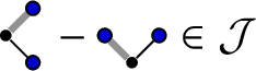
holds with the same argument as before. (In fact both of these trees are individually elements of $\mathcal {J}$
, for symmetry reasons. Actually, in this case one also has
$\mathcal {J}$
, for symmetry reasons. Actually, in this case one also has
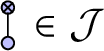
for symmetry reasons. Neither of these statements, however, is generic. They would, for instance, not hold if the Poisson kernel were replaced by a nonsymmetric kernel.) Here we draw a cross into the circle to denote a polynomial decoration, and a bold edge denotes an edge carrying a derivative decoration. For the second statement in formula (4.4), one can calculate

Note that the fact that this expression vanishes identically is not really intrinsic. For instance, the various Poisson kernels could be associated to different components of the equation, and in principle we could choose different large-scale cutoffs, which would make this expression nonzero (but it would remain order $1$
). This may not seem like a natural thing to do, but it is sometimes unavoidable (compare Example 4.2).
$1$
). This may not seem like a natural thing to do, but it is sometimes unavoidable (compare Example 4.2).
The goal of this section is to automatise these arguments, drawing only on the information that ${ { \tilde {\Upsilon }_{} ^{\psi } } }(\tau _1 - \tau _2) = 0$
for any smooth function
${ { \tilde {\Upsilon }_{} ^{\psi } } }(\tau _1 - \tau _2) = 0$
for any smooth function
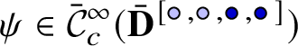
. We write elements in the domain as
. Let $\phi \in \mathcal {C}_c^{\infty } (\bar {\mathbf D} )$
be any smooth, symmetric (under
$\phi \in \mathcal {C}_c^{\infty } (\bar {\mathbf D} )$
be any smooth, symmetric (under $x \mapsto -x$
) test function, define
$x \mapsto -x$
) test function, define $\phi ^{(\varepsilon )}:= \varepsilon ^{-3}\phi (\varepsilon ^{-1} \cdot )$
, and let
$\phi ^{(\varepsilon )}:= \varepsilon ^{-3}\phi (\varepsilon ^{-1} \cdot )$
, and let
. We also write
, and we denote by

and
the quantity defined analogously to formula (4.1), but where the additional variable ${x_{\diamond }}$
corresponds to the node which was generated by contracting the subtree
${x_{\diamond }}$
corresponds to the node which was generated by contracting the subtree
(in the current examples, the only node without a noise). This rather ad hoc notation is resolved later on by the introduction of legs. We then arrive at the following diagram:

The equality in the first line is the analytic input we are given from formula (4.3). The uniform bounds on the differences vertically are a consequence of the analytic BPHZ theorem [Reference HairerHai18] (see also Proposition 4.49). The equality on the second line is what we infer. Note that in a first step we deduce only a uniform bound; however, we can make use of the fact that the integration kernels are homogeneous functions, so that we know a priori that the expressions in the second line are proportional to $\varepsilon ^{\alpha }$
for some homogeneity
$\varepsilon ^{\alpha }$
for some homogeneity $\alpha <0$
. Both statements can hold simultaneously only if the quantity vanishes identically. It then follows in particular that
$\alpha <0$
. Both statements can hold simultaneously only if the quantity vanishes identically. It then follows in particular that

for any symmetric test function $\phi ,\psi \in \mathcal {C}_c^{\infty }\left (\bar {\mathbf D}\right )$
(here we naturally identify
$\phi ,\psi \in \mathcal {C}_c^{\infty }\left (\bar {\mathbf D}\right )$
(here we naturally identify
 and
and
 with the space of symmetric functions in $\mathcal {C}_c^{\infty }\left (\bar {\mathbf D}\right )$
). Note that in general there may be more than one divergent subtree. We then perform the foregoing strategy with all possible divergent subtrees, by splitting the multiset
$\mathcal {C}_c^{\infty }\left (\bar {\mathbf D}\right )$
). Note that in general there may be more than one divergent subtree. We then perform the foregoing strategy with all possible divergent subtrees, by splitting the multiset
![]() in two parts in all possible ways (the derivation already given would then correspond to
in two parts in all possible ways (the derivation already given would then correspond to
![]() ).
).
Comparing equations (4.6) and (4.5), and using the fact that the function $\phi (x-y):={\mathbf E}[\eta (x)\eta (y)]$
is an element of
$\phi (x-y):={\mathbf E}[\eta (x)\eta (y)]$
is an element of $\mathcal {C}_c^{\infty }\left (\bar {\mathbf D}\right )$
, we deduce that
$\mathcal {C}_c^{\infty }\left (\bar {\mathbf D}\right )$
, we deduce that

for any smooth, centred, stationary noise $\eta $
. Here,
$\eta $
. Here, $\hat {g}^{\eta }$
is a character which is defined similarly to the BPHZ character, but where the large-scale cutoff of the integration kernels is removed and instead a large-scale cutoff is introduced between any pair of nodes (see Definition 4.17 and formula (4.27)).
$\hat {g}^{\eta }$
is a character which is defined similarly to the BPHZ character, but where the large-scale cutoff of the integration kernels is removed and instead a large-scale cutoff is introduced between any pair of nodes (see Definition 4.17 and formula (4.27)).
Let us review the outline so far from a more algebraic perspective. We have essentially proven that,

where $\hat {\mathcal {J}} \subseteq {\hat {\mathcal {T}}_-}$
is an ideal defined analogously to
$\hat {\mathcal {J}} \subseteq {\hat {\mathcal {T}}_-}$
is an ideal defined analogously to $\mathcal {J}$
. (We refrain from giving a precise definition here, since there are some subtleties – most notably the fact that
$\mathcal {J}$
. (We refrain from giving a precise definition here, since there are some subtleties – most notably the fact that ${ { \tilde {\Upsilon }_{} ^{\eta } } }$
is in general not well defined on trees of positive homogeneity. We refer to Definition 4.54 for the definition of an ideal that mirrors this idea.) We then use the facts that
${ { \tilde {\Upsilon }_{} ^{\eta } } }$
is in general not well defined on trees of positive homogeneity. We refer to Definition 4.54 for the definition of an ideal that mirrors this idea.) We then use the facts that ${\Delta _-} = (\mathrm {Id} \otimes \mathbf {p}_-) {\Delta _-}\mathfrak {i}$
and
${\Delta _-} = (\mathrm {Id} \otimes \mathbf {p}_-) {\Delta _-}\mathfrak {i}$
and $\mathcal {J} = \mathbf {p}_- \hat {\mathcal {J}}$
to conclude that
$\mathcal {J} = \mathbf {p}_- \hat {\mathcal {J}}$
to conclude that $\mathcal {J}$
is a Hopf ideal, which concludes the outline of the proof of Assumption 7. The remaining argument to conclude the outline of the proof of Assumption 8 is to bound the difference of
$\mathcal {J}$
is a Hopf ideal, which concludes the outline of the proof of Assumption 7. The remaining argument to conclude the outline of the proof of Assumption 8 is to bound the difference of $g^{\eta }$
and
$g^{\eta }$
and $\hat {g}^{\eta }$
with respect to the group product in
$\hat {g}^{\eta }$
with respect to the group product in ${\mathcal {G}_-}$
, which we do in Section 4.6.
${\mathcal {G}_-}$
, which we do in Section 4.6.
The problems ahead
There are several points that complicate this line of argument in general:
-
• One can have more complicated subdivergences; in particular, one can have divergent subforests instead of just single trees. To deal with this issue, we introduce a test function for each pair of noises (Definition 4.42), which will give us the flexibility to trigger any subdivergence by rescaling these test functions in all possible ways.
-
• A bigger issue is the presence of derivatives hitting the test function. Implementing the foregoing strategy without a proper algebraic framework leads to significant notational difficulties. Instead, we opt for a systematic extension of the algebraic framework by introducing the notion of ‘legs’, against which our test functions are integrated. Formally, we do this via an extension of the regularity structure (see Section 4.1 for the details). The point here is that legs can have nonvanishing derivative decorations.
-
• Every leg has a unique partner leg, and we call a tree properly legged (Definition 4.23) if for any pair of vertices u and v with
$u\ne v$
, and both u and v carrying noises, there exists a unique leg incident to u such that its partner is incident to v. We ultimately need to understand how this ‘properly legged’ property interacts with the coproduct, which leads to the construction of algebras
and
, which are related to the algebras
and
(we colour them to indicate that they are spaces generated by trees containing legs; compare Section 4.1). We refer to Section 4.3 for details. -
• Noises are in general indistinguishable. We need to distinguish them at the algebraic level to carry out the argument, and only afterwards factor out the necessary ideals given by ‘identifying’ noises that we made distinguishable (Definition 4.36). (Actually, it suffices for us to break the symmetry at the level of legs.)
-
• We need to make precise what exactly we need to subtract in general in order to see the cancellations inferred. For this we need a general strategy of rescaling the test functions (compare formulas (4.37) and (4.40)) and a general bound in the spirit of the BPHZ theorem (compare Proposition 4.49). We draw here on the results of [Reference HairerHai18] rather than [Reference Chandra and HairerCH16], since we deal with kernels of unbounded support.
-
• Finally, we have to show that the evaluation
${ \tilde {\Upsilon }_{} ^{\eta ,\psi } }\tau $
is well defined, at least on a large enough set of trees
$\tau $
. We refer the reader to Theorem 4.19 and Lemma 4.21.


Outline of the section
The plan is now as follows. We enlarge in Section 4.1 the regularity structures $\mathcal {T}$
to a regularity structure
$\mathcal {T}$
to a regularity structure
by adding a sufficient number of new types (which we call ‘leg types’ but treat as noise types with just slightly negative homogeneity), and we allow any number of them (up to a large enough constant) to be incident to any node u of any tree $\tau \in \mathcal {T}$
. We then construct spaces
$\tau \in \mathcal {T}$
. We then construct spaces
and
analogously to ${\mathcal {T}_-}$
and
${\mathcal {T}_-}$
and ${\hat {\mathcal {T}}_-^{\kern3pt\mathrm {ex}}}$
. We show that one can remove the large-scale cutoff in the sense that
${\hat {\mathcal {T}}_-^{\kern3pt\mathrm {ex}}}$
. We show that one can remove the large-scale cutoff in the sense that ${ { \tilde {\Upsilon }_{} ^{\eta } } }\tau $
exists (at least for a large class of trees
${ { \tilde {\Upsilon }_{} ^{\eta } } }\tau $
exists (at least for a large class of trees $\tau $
) in Section 4.2. The most cumbersome subsection is Section 4.3, in which we systematically factor out ideals in
$\tau $
) in Section 4.2. The most cumbersome subsection is Section 4.3, in which we systematically factor out ideals in
and
, arriving eventually at the following sequences of spaces:

The spaces
![]() and
and
![]() (see Definition 4.26) are merely auxiliary spaces, and we will mostly be working with the subspaces
(see Definition 4.26) are merely auxiliary spaces, and we will mostly be working with the subspaces
![]() and
and
 (see Definition 4.29) formed by properly legged trees. So far, symmetries of a tree, related to the fact that the same noise type appears multiple times, are not reflected in the legs, and we remedy this in
![]() and
and
![]() (see Definition 4.36). Finally, dropping ‘nonessential’ legs and identifying trees with nonvanishing derivative decoration on legs, we arrive at the space
(see Definition 4.36). Finally, dropping ‘nonessential’ legs and identifying trees with nonvanishing derivative decoration on legs, we arrive at the space
![]() (see Lemma 4.40), which turns out to be isomorphic as a Hopf algebra to
(see Lemma 4.40), which turns out to be isomorphic as a Hopf algebra to ${\mathcal {T}_-}$
(see Lemma 4.41). An analytic result generalising the ‘vertical’ cancellations in the diagram on page 44 will be derived in Proposition 4.49. A key result is Proposition 4.60, making precise the idea of formula (4.7) and in particular concluding the proof of Assumption 7 that
${\mathcal {T}_-}$
(see Lemma 4.41). An analytic result generalising the ‘vertical’ cancellations in the diagram on page 44 will be derived in Proposition 4.49. A key result is Proposition 4.60, making precise the idea of formula (4.7) and in particular concluding the proof of Assumption 7 that $\mathcal {J}$
is a Hopf ideal. Finally, in Section 4.6 we compare the characters
$\mathcal {J}$
is a Hopf ideal. Finally, in Section 4.6 we compare the characters $\hat {g}^{\eta }$
and
$\hat {g}^{\eta }$
and $g^{\eta }$
and show that their difference is continuous in the limit as
$g^{\eta }$
and show that their difference is continuous in the limit as $\eta $
approaches a rough limit noise (see Lemmas 4.68 and 4.71).
$\eta $
approaches a rough limit noise (see Lemmas 4.68 and 4.71).
4.1 Extension of the regularity structure
We assume that we are given a finite set ${ \mathtt {L} }$
, disjoint from
${ \mathtt {L} }$
, disjoint from $\mathfrak {L}$
, elements of which we call leg types. From an algebraic point of view, we treat
$\mathfrak {L}$
, elements of which we call leg types. From an algebraic point of view, we treat ${ \mathtt {L} }$
as a set of additional noise types, and we extend the homogeneity assignments
${ \mathtt {L} }$
as a set of additional noise types, and we extend the homogeneity assignments
![]() and
and ${ \left \lvert \cdot \right \rvert _{\mathfrak {s}} }$
to
${ \left \lvert \cdot \right \rvert _{\mathfrak {s}} }$
to
![]() by setting
by setting
![]() and
and ${ \left \lvert { \mathtt {l} }\right \rvert _{\mathfrak {s}} }:=-\kappa $
for some
${ \left \lvert { \mathtt {l} }\right \rvert _{\mathfrak {s}} }:=-\kappa $
for some $\kappa>0$
small enough (to be specified shortly) whenever
$\kappa>0$
small enough (to be specified shortly) whenever ${ \mathtt {l} } \in { \mathtt {L} }$
. From the extended set of types
${ \mathtt {l} } \in { \mathtt {L} }$
. From the extended set of types
![]() , we want to build a regularity structure
, we want to build a regularity structure
![]() as in [Reference Bruned, Hairer and ZambottiBHZ19, Section 5.5], for which we specify a rule
as in [Reference Bruned, Hairer and ZambottiBHZ19, Section 5.5], for which we specify a rule
![]() .
.
Let $M\in {\mathbf N}$
denote the maximum number of edges
$M\in {\mathbf N}$
denote the maximum number of edges $\# E(\tau )$
for any
$\# E(\tau )$
for any $\tau \in \mathscr {T}_-$
. We first define the rule
$\tau \in \mathscr {T}_-$
. We first define the rule
![]() by setting
by setting
for any $\mathfrak {t}\in \mathfrak {L}_+$
. Here R denotes the rule used to construct the regularity structure
$\mathfrak {t}\in \mathfrak {L}_+$
. Here R denotes the rule used to construct the regularity structure $\mathcal {T}$
(see Section 2.2). Note that in formula (4.8) we only allow B to be a proper set (or equivalently a multiset satisfying
$\mathcal {T}$
(see Section 2.2). Note that in formula (4.8) we only allow B to be a proper set (or equivalently a multiset satisfying $B\le 1$
), so that any tree conforming to
$B\le 1$
), so that any tree conforming to
![]() can be built from a tree conforming to R by adding to every node up to M edges of distinct types in
can be built from a tree conforming to R by adding to every node up to M edges of distinct types in ${ \mathtt {L} }$
. Provided that
${ \mathtt {L} }$
. Provided that $\kappa>0$
is small enough, we obtain a normal and subcritical [Reference Bruned, Hairer and ZambottiBHZ19, Definition 5.14] rule
$\kappa>0$
is small enough, we obtain a normal and subcritical [Reference Bruned, Hairer and ZambottiBHZ19, Definition 5.14] rule
![]() in this way, and we denote by
in this way, and we denote by
![]() its completion [Reference Bruned, Hairer and ZambottiBHZ19, Proposition 5.21].
its completion [Reference Bruned, Hairer and ZambottiBHZ19, Proposition 5.21].
Definition 4.13. We denote by
![]() (resp.,
(resp.,
![]() ) the extended (resp., reduced) regularity structure constructed as in [Reference Bruned, Hairer and ZambottiBHZ19, Section 5.5] from the rule
) the extended (resp., reduced) regularity structure constructed as in [Reference Bruned, Hairer and ZambottiBHZ19, Section 5.5] from the rule
![]() . Furthermore, we denote by
. Furthermore, we denote by
![]() and
and
![]() the algebras constructed as in [Reference Bruned, Hairer and ZambottiBHZ19, Definitions 5.26, 5.29] starting from the regularity structure
the algebras constructed as in [Reference Bruned, Hairer and ZambottiBHZ19, Definitions 5.26, 5.29] starting from the regularity structure
![]() .
.
As in [Reference Bruned, Hairer and ZambottiBHZ19, Proposition 5.35], the space
![]() forms a Hopf algebra. We will mostly work with the factor Hopf algebra
forms a Hopf algebra. We will mostly work with the factor Hopf algebra
![]() of
of
![]() given by neglecting the extended decoration. We write
given by neglecting the extended decoration. We write
![]() for the set of unplanted trees
for the set of unplanted trees
![]() of negative homogeneity, so that
of negative homogeneity, so that
![]() is generated freely as a unital, commutative algebra from
is generated freely as a unital, commutative algebra from
![]() .
.
For a tree
![]() , we denote by
, we denote by $L_{ \mathtt {L} }(\tau )\subseteq E(\tau )$
the set of leg-type edges – that is, the set of
$L_{ \mathtt {L} }(\tau )\subseteq E(\tau )$
the set of leg-type edges – that is, the set of $e \in E(\tau )$
such that
$e \in E(\tau )$
such that $\mathfrak {t}(e)\in { \mathtt {L} }$
– and by
$\mathfrak {t}(e)\in { \mathtt {L} }$
– and by $L(\tau )\subseteq E(\tau )$
the set of noise-type edges of
$L(\tau )\subseteq E(\tau )$
the set of noise-type edges of $\tau $
– that is, the set of
$\tau $
– that is, the set of $e \in E(\tau )$
such
$e \in E(\tau )$
such $\mathfrak {t}(e) \in \mathfrak {L}_-$
. We will often call an edge of leg type simply a leg. We write
$\mathfrak {t}(e) \in \mathfrak {L}_-$
. We will often call an edge of leg type simply a leg. We write $\mathcal {L}(\tau ) \subseteq N(\tau )$
(resp.,
$\mathcal {L}(\tau ) \subseteq N(\tau )$
(resp., ${ \mathcal {L}_{ \mathtt {L} } }(\tau )\subseteq N(\tau )$
) for the set of nodes
${ \mathcal {L}_{ \mathtt {L} } }(\tau )\subseteq N(\tau )$
) for the set of nodes $u\in N(\tau )$
that are adjacent to at least one noise-type (resp., leg-type) edge, and we write
$u\in N(\tau )$
that are adjacent to at least one noise-type (resp., leg-type) edge, and we write $\hat {\mathcal {L}}(\tau ) \subseteq N(\tau )$
for the set of nodes
$\hat {\mathcal {L}}(\tau ) \subseteq N(\tau )$
for the set of nodes $u \in N(\tau )$
with the property that
$u \in N(\tau )$
with the property that $\mathfrak {o}(u) < 0$
.
$\mathfrak {o}(u) < 0$
.
Example 4.14. In the following example, taken from the KPZ equation, we have coloured kernel-type edges $e \in K(\tau )$
grey (they are bold because they carry a derivative decoration) and noise-type edges
$e \in K(\tau )$
grey (they are bold because they carry a derivative decoration) and noise-type edges $e \in L(\tau )$
blue; drawn legs
$e \in L(\tau )$
blue; drawn legs $e \in L_{ \mathtt {L} }(\tau )$
as wavy lines; coloured nodes blue if they are elements of
$e \in L_{ \mathtt {L} }(\tau )$
as wavy lines; coloured nodes blue if they are elements of $\mathcal {L}(\tau )$
; and drawn nodes as squares (rather than circles) if they are elements of
$\mathcal {L}(\tau )$
; and drawn nodes as squares (rather than circles) if they are elements of ${ \mathcal {L}_{ \mathtt {L} } }(\tau )$
:
${ \mathcal {L}_{ \mathtt {L} } }(\tau )$
:

This is the only example in this paper in which we make noise-type edges explicit, since their position can always be inferred by $\mathcal {L}(\tau )$
. We will always make legs explicit (note that their position cannot be inferred from
$\mathcal {L}(\tau )$
. We will always make legs explicit (note that their position cannot be inferred from ${ { \mathcal {L}_{ \mathtt {L} } } }(\tau )$
, as there may be more than one leg incident to the same node). Conversely, since
${ { \mathcal {L}_{ \mathtt {L} } } }(\tau )$
, as there may be more than one leg incident to the same node). Conversely, since ${ { \mathcal {L}_{ \mathtt {L} } } }(\tau )$
can be inferred from
${ { \mathcal {L}_{ \mathtt {L} } } }(\tau )$
can be inferred from $L_{ \mathtt {L} }(\tau )$
, we will not draw them explicitly as boxes in the forthcoming examples.
$L_{ \mathtt {L} }(\tau )$
, we will not draw them explicitly as boxes in the forthcoming examples.
The space $\mathcal {T}^{\mathrm {ex}}$
can be identified with the linear subspace of
$\mathcal {T}^{\mathrm {ex}}$
can be identified with the linear subspace of
![]() spanned by all trees
spanned by all trees
![]() without legs. Similarly, the spaces
without legs. Similarly, the spaces $\hat {\mathcal {T}}_-^{\mathrm {ex}}$
,
$\hat {\mathcal {T}}_-^{\mathrm {ex}}$
, $\mathcal {T}_-^{\kern3pt\mathrm {ex}}$
and
$\mathcal {T}_-^{\kern3pt\mathrm {ex}}$
and $\mathcal {T}_-$
have natural interpretations as subalgebras of
$\mathcal {T}_-$
have natural interpretations as subalgebras of
![]() ,
,
![]() and
and
![]() , respectively (in this interpretation the latter two are Hopf subalgebras). Given any tree
, respectively (in this interpretation the latter two are Hopf subalgebras). Given any tree
![]() , we define a tree
, we define a tree $\pi \tau \in \mathcal {T}^{\mathrm {ex}}$
by simply removing all of its legs. The map
$\pi \tau \in \mathcal {T}^{\mathrm {ex}}$
by simply removing all of its legs. The map $\pi $
extends to a linear map
$\pi $
extends to a linear map
![]() and to an algebra morphism from the algebras
and to an algebra morphism from the algebras
![]() ,
,
![]() and
and
![]() onto
onto $\mathcal {T}_-^{\kern3pt\mathrm {ex}}$
,
$\mathcal {T}_-^{\kern3pt\mathrm {ex}}$
, $\hat {\mathcal {T}}_-^{\mathrm {ex}}$
and
$\hat {\mathcal {T}}_-^{\mathrm {ex}}$
and $\mathcal {T}_-$
, respectively.
$\mathcal {T}_-$
, respectively.
Finally, we denote by
![]() the character group of the Hopf algebra
the character group of the Hopf algebra
![]() , which is canonically isomorphic to the reduced renormalisation group constructed in [Reference Bruned, Hairer and ZambottiBHZ19, Theorem 6.28]. There exists a subgroup of
, which is canonically isomorphic to the reduced renormalisation group constructed in [Reference Bruned, Hairer and ZambottiBHZ19, Theorem 6.28]. There exists a subgroup of
![]() isomorphic to
isomorphic to $\mathcal {G}_-$
, given by the set of those characters that vanish on any tree
$\mathcal {G}_-$
, given by the set of those characters that vanish on any tree $\tau $
with
$\tau $
with
![]() . (The isomorphism
. (The isomorphism
![]() is given explicitly by mapping
is given explicitly by mapping $g\in \mathcal {G}_-$
to a character
$g\in \mathcal {G}_-$
to a character
![]() given by setting
given by setting $\varphi (g)(\tau ) = g(\tau )$
for
$\varphi (g)(\tau ) = g(\tau )$
for $\tau \in \mathscr {T}_-$
and
$\tau \in \mathscr {T}_-$
and $\varphi (g)(\tau ) = 0$
for
$\varphi (g)(\tau ) = 0$
for
![]() .)
.)
Remark 4.15. Since we view ${\mathcal {T}_-}$
as a subspace of
${\mathcal {T}_-}$
as a subspace of
![]() , the embedding
, the embedding
![]() is actually not ‘canonical’, although the projection
is actually not ‘canonical’, although the projection
![]() , given by restricting a character
, given by restricting a character
![]() to
to ${\mathcal {T}_-}$
, is canonical. The construction in the previous paragraph uses indirectly the fact that
${\mathcal {T}_-}$
, is canonical. The construction in the previous paragraph uses indirectly the fact that ${\mathcal {T}_-}$
is also naturally isomorphic to a factor Hopf algebra
${\mathcal {T}_-}$
is also naturally isomorphic to a factor Hopf algebra
![]() , where
, where
![]() is defined by killing trees
is defined by killing trees $\tau $
such that
$\tau $
such that
![]() . However, in the sequel we will continue to view
. However, in the sequel we will continue to view ${\mathcal {T}_-}$
as a subalgebra of
${\mathcal {T}_-}$
as a subalgebra of
![]() .
.
4.2 Large-scale behaviour of renormalised trees
We now fix a degree assignment $\deg _{\infty }(\mathfrak {t}) \in \mathbf {R}_-\sqcup \{-\infty \}$
for kernel types
$\deg _{\infty }(\mathfrak {t}) \in \mathbf {R}_-\sqcup \{-\infty \}$
for kernel types $\mathfrak {t} \in \mathfrak {L}_+$
. In order to avoid case distinctions later on, we also set
$\mathfrak {t} \in \mathfrak {L}_+$
. In order to avoid case distinctions later on, we also set $\deg _{\infty }(\Xi ):=0$
for any noise type
$\deg _{\infty }(\Xi ):=0$
for any noise type $\Xi \in \mathfrak {L}_-$
and
$\Xi \in \mathfrak {L}_-$
and $\deg _{\infty }({ \mathtt {l} }):=-\infty $
for any leg type
$\deg _{\infty }({ \mathtt {l} }):=-\infty $
for any leg type ${ \mathtt {l} } \in { \mathtt {L} }$
. We write
${ \mathtt {l} } \in { \mathtt {L} }$
. We write $\mathcal {K}^+_{\infty }$
for the set of kernel assignments
$\mathcal {K}^+_{\infty }$
for the set of kernel assignments $R =(R_{\mathfrak {t}})_{\mathfrak {t}\in \mathfrak {L}_+}$
such that
$R =(R_{\mathfrak {t}})_{\mathfrak {t}\in \mathfrak {L}_+}$
such that $R_{\mathfrak {t}}:\bar {\mathbf D}\to \mathbf {R}$
is smooth and compactly supported for any
$R_{\mathfrak {t}}:\bar {\mathbf D}\to \mathbf {R}$
is smooth and compactly supported for any $\mathfrak {t}\in \mathfrak {L}_+$
. We endow this space with the topology generated by the system of seminorms
$\mathfrak {t}\in \mathfrak {L}_+$
. We endow this space with the topology generated by the system of seminorms $\lVert \cdot \rVert _{\mathcal {K}^+,\mathfrak {t}}$
for
$\lVert \cdot \rVert _{\mathcal {K}^+,\mathfrak {t}}$
for $\mathfrak {t}\in \mathfrak {L}_+$
, where the latter is defined as the smallest constant such that
$\mathfrak {t}\in \mathfrak {L}_+$
, where the latter is defined as the smallest constant such that
 $$ \begin{align} \left\lvert D^k R_{\mathfrak{t}}(x)\right\rvert\le \lVert R\rVert_{\mathcal{K}^+,\mathfrak{t}} (1+\lvert x\rvert)^{\deg_{\infty}\mathfrak{t}} \end{align} $$
for any $x\in \bar {\mathbf D}$
and
$x\in \bar {\mathbf D}$
and $k\in {\mathbf N}^d$
with
$k\in {\mathbf N}^d$
with $\lvert k\rvert _{\mathfrak {s}}<r$
. We write
$\lvert k\rvert _{\mathfrak {s}}<r$
. We write $\mathcal {K}_0^+$
for the completion of
$\mathcal {K}_0^+$
for the completion of $\mathcal {K}_{\infty }^+$
with respect to the corresponding metric. We extend the notation of formulas (3.1) and (3.2) to the extended regularity structure, with
$\mathcal {K}_{\infty }^+$
with respect to the corresponding metric. We extend the notation of formulas (3.1) and (3.2) to the extended regularity structure, with $L(\tau )$
replaced by
$L(\tau )$
replaced by $L(\tau ) \sqcup L_{ \mathtt {L} }(\tau )$
, so that in particular one has
$L(\tau ) \sqcup L_{ \mathtt {L} }(\tau )$
, so that in particular one has $\mathcal {K}_G \tau : \bar {\mathbf D} ^{ L(\tau ) \sqcup L_{ \mathtt {L} }(\tau ) } \to \mathbf {R}$
and the integral in formula (3.2) ranges over
$\mathcal {K}_G \tau : \bar {\mathbf D} ^{ L(\tau ) \sqcup L_{ \mathtt {L} }(\tau ) } \to \mathbf {R}$
and the integral in formula (3.2) ranges over $\bar {\mathbf D} ^{ L(\tau ) \sqcup L_{ \mathtt {L} }(\tau ) }$
. Furthermore, we introduce the following space in analogy to Definition 3.2:
$\bar {\mathbf D} ^{ L(\tau ) \sqcup L_{ \mathtt {L} }(\tau ) }$
. Furthermore, we introduce the following space in analogy to Definition 3.2:
Definition 4.16. We write ${ \Psi }$
for the set of all families of test functions
${ \Psi }$
for the set of all families of test functions
![]() , indexed by multisets
, indexed by multisets
![]() with values in
with values in ${ \mathtt {L} }$
, such that
${ \mathtt {L} }$
, such that
![]() .
.
With this notation, we now define the following evaluations:
Definition 4.17. We define for any tree
![]() , any smooth noise
, any smooth noise $\eta \in \mathfrak {M}_{\infty }^{\star }$
, any
$\eta \in \mathfrak {M}_{\infty }^{\star }$
, any ${ \psi } \in { \Psi }$
and any large-scale kernel assignment
${ \psi } \in { \Psi }$
and any large-scale kernel assignment $R=(R_{\mathfrak {t}})_{\mathfrak {t}\in \mathfrak {L}_+}\in \mathcal {K}^+_{\infty }$
the constant
$R=(R_{\mathfrak {t}})_{\mathfrak {t}\in \mathfrak {L}_+}\in \mathcal {K}^+_{\infty }$
the constant
 $$ \begin{align} \bar{\Upsilon}^{\eta,{ \psi }}_R\tau:= { \left\langle \mathcal{K}_{K+R} {\tau} , \right\rangle }{ \zeta^ {\eta,{ \psi },\tau} } , \end{align} $$
where $\zeta ^ {\eta ,{ \psi },\tau } \in \bar {\mathbf D}^{L(\tau ) \sqcup L_{ \mathtt {L} }(\tau )}$
is defined by
$\zeta ^ {\eta ,{ \psi },\tau } \in \bar {\mathbf D}^{L(\tau ) \sqcup L_{ \mathtt {L} }(\tau )}$
is defined by
 $$ \begin{align*} \zeta ^ {\eta,{ \psi },\tau} (x) := \left({\mathbf E} \prod_{u\in L(T)} \eta_{\mathfrak{t}(u)}(x_{u})\right) D^{\mathfrak{e} \rvert_{L_{ \mathtt{L} }(\tau)}} \psi_{\left[L_{ \mathtt{L} }(\tau),\mathfrak{t}\right]} \left(x_{L_{ \mathtt{L} }(\tau)}\right) \end{align*} $$
for any $x \in \bar {\mathbf D} ^{L(\tau ) \sqcup L_{ \mathtt {L} }(\tau )}$
. Moreover, we define the ‘renormalised’ constant by
$x \in \bar {\mathbf D} ^{L(\tau ) \sqcup L_{ \mathtt {L} }(\tau )}$
. Moreover, we define the ‘renormalised’ constant by
 $$ \begin{align} \hat{\Upsilon}^{\eta,\psi}_R\tau:= \bar{\Upsilon}_R^{\eta,\psi} M^{g^{\eta}_{\textrm{BPHZ}}}\tau. \end{align} $$
Here, we use the notation $g^{\eta }_{\textrm{BPHZ}} \in \mathcal {G}_-$
for the BPHZ character of the noise
$g^{\eta }_{\textrm{BPHZ}} \in \mathcal {G}_-$
for the BPHZ character of the noise $\eta $
in the renormalisation group
$\eta $
in the renormalisation group $\mathcal {G}_-$
, which we view naturally as a character in
$\mathcal {G}_-$
, which we view naturally as a character in
![]() as before. We also set
as before. We also set ${ \bar {\Upsilon }_{R} ^{\psi } } := { \bar {\Upsilon }_{R} ^{\mathbf {1},\psi } }$
and
${ \bar {\Upsilon }_{R} ^{\psi } } := { \bar {\Upsilon }_{R} ^{\mathbf {1},\psi } }$
and ${ { \bar {\Upsilon }_{} ^{\psi } } } := { \bar {\Upsilon }_{\hat {K} - K} ^{\mathbf {1},\psi } }$
.
${ { \bar {\Upsilon }_{} ^{\psi } } } := { \bar {\Upsilon }_{\hat {K} - K} ^{\mathbf {1},\psi } }$
.
Remark 4.18. One has $g^{\eta }_{\textrm{BPHZ}}(\sigma ) = 0$
for any
$g^{\eta }_{\textrm{BPHZ}}(\sigma ) = 0$
for any
![]() such that
such that
![]() , so that
, so that $M^{g^{\eta }_{\textrm{BPHZ}}}$
maps
$M^{g^{\eta }_{\textrm{BPHZ}}}$
maps $\tau $
onto the span of trees
$\tau $
onto the span of trees $\tilde {\tau }$
with the property that
$\tilde {\tau }$
with the property that $[L(\tau ),\mathfrak {t}] = [L(\tilde {\tau }),\mathfrak {t}]$
. It follows that
$[L(\tau ),\mathfrak {t}] = [L(\tilde {\tau }),\mathfrak {t}]$
. It follows that $\hat {\Upsilon }^{\eta ,\psi }_R \tau $
really only depends on
$\hat {\Upsilon }^{\eta ,\psi }_R \tau $
really only depends on $\psi _{\left [L_{ \mathtt {L} }(\tau ),\mathfrak {t}\right ]}$
. We finally note that these notations do not depend on the extended decoration
$\psi _{\left [L_{ \mathtt {L} }(\tau ),\mathfrak {t}\right ]}$
. We finally note that these notations do not depend on the extended decoration $\mathfrak {o}$
.
$\mathfrak {o}$
.
Our goal is to show that under some natural assumptions on the degree assignment $\deg _{\infty }$
, the map
$\deg _{\infty }$
, the map ${ \bar {\Upsilon }_{R} ^{\eta ,\psi } }$
extends continuously to any large-scale kernel assignment
${ \bar {\Upsilon }_{R} ^{\eta ,\psi } }$
extends continuously to any large-scale kernel assignment $R\in \mathcal {K}_0^+$
, and
$R\in \mathcal {K}_0^+$
, and $\hat {\Upsilon }^{\eta ,\psi }_R$
extends continuously to the set of pairs
$\hat {\Upsilon }^{\eta ,\psi }_R$
extends continuously to the set of pairs $(\eta ,R)\in {\mathfrak {M}_0^{\mathrm {s}}} \times \mathcal {K}_0^+$
. Such a statement can only be true if we make an assumption on the degree assignment
$(\eta ,R)\in {\mathfrak {M}_0^{\mathrm {s}}} \times \mathcal {K}_0^+$
. Such a statement can only be true if we make an assumption on the degree assignment $\deg _{\infty }$
and the positions of the legs, which is in complete analogy to [Reference HairerHai18, Section 4]. We then consider partitions
$\deg _{\infty }$
and the positions of the legs, which is in complete analogy to [Reference HairerHai18, Section 4]. We then consider partitions $\mathcal {P}$
of the node set
$\mathcal {P}$
of the node set $N(\tau )$
such that
$N(\tau )$
such that $\#\mathcal {P}\ge 2$
and such that there exists
$\#\mathcal {P}\ge 2$
and such that there exists $P\in \mathcal {P}$
with
$P\in \mathcal {P}$
with ${ \mathcal {L}_{ \mathtt {L} } }(\tau )\subseteq P$
. We call partitions of
${ \mathcal {L}_{ \mathtt {L} } }(\tau )\subseteq P$
. We call partitions of $N(\tau )$
that satisfy these properties tight from now on. For any tight partition
$N(\tau )$
that satisfy these properties tight from now on. For any tight partition $\mathcal {P}$
, we denote by
$\mathcal {P}$
, we denote by $K(\mathcal {P})$
the set of kernel-type edges
$K(\mathcal {P})$
the set of kernel-type edges $e\in K(\tau )$
with the property that there does not exist
$e\in K(\tau )$
with the property that there does not exist $P\in \mathcal {P}$
such that
$P\in \mathcal {P}$
such that $e\subseteq P$
, and we set
$e\subseteq P$
, and we set
 $$ \begin{align} \deg_{\infty}\mathcal{P}:= \sum_{e\in K(\mathcal{P})} \deg_{\infty} \mathfrak{t}(e) + \sum_{u\in N(\tau)}\lvert\mathfrak{n}(u)\rvert_{\mathfrak{s}} + \lvert\mathfrak{s}\rvert(\#\mathcal{P}-1).\end{align} $$
Let ${\mathfrak {M}_0^{\star }}$
denote the closure of
${\mathfrak {M}_0^{\star }}$
denote the closure of ${\mathfrak {M}_{\infty }^{\star }}$
under the norm
${\mathfrak {M}_{\infty }^{\star }}$
under the norm $\lVert \cdot \rVert _{\mathfrak {s}}$
. The key result of this section is the following theorem:
$\lVert \cdot \rVert _{\mathfrak {s}}$
. The key result of this section is the following theorem:
Theorem 4.19. Let
![]() be such that
be such that $\deg _{\infty }\mathcal {P}<0$
for any tight partition
$\deg _{\infty }\mathcal {P}<0$
for any tight partition $\mathcal {P}$
of
$\mathcal {P}$
of $N(\tau )$
. Then for any fixed
$N(\tau )$
. Then for any fixed ${ \psi } \in { \Psi }$
and
${ \psi } \in { \Psi }$
and $\eta \in {\mathfrak {M}_0^{\star }}$
, the evaluation
$\eta \in {\mathfrak {M}_0^{\star }}$
, the evaluation
 $$ \begin{align} R \mapsto \bar{\Upsilon}^{\eta,{ \psi }}_R \tau \end{align} $$
extends continuously to the space $\mathcal {K}_0^+$
. Moreover, the evaluation
$\mathcal {K}_0^+$
. Moreover, the evaluation
 $$ \begin{align} (\eta,R) \mapsto \hat{\Upsilon}^{\eta,{ \psi }}_R \tau \end{align} $$
extends continuously to the space ${\mathfrak {M}_0^{\star }} \times \mathcal {K}_0^+$
. Finally, one has the bound
${\mathfrak {M}_0^{\star }} \times \mathcal {K}_0^+$
. Finally, one has the bound
 $$ \begin{align} \left\lvert\hat{\Upsilon}^{\eta,{ \psi }}_R\tau\right\rvert \lesssim \lVert\eta\rVert_{\mathfrak{s}} \left( \prod_{e\in K(\tau)} \lVert R_{\mathfrak{t}(e)}\rVert_{\mathcal{K}^+,\mathfrak{t}(e),r} + 1 \right) \end{align} $$
for $r\in {\mathbf N}$
any integer larger than
$r\in {\mathbf N}$
any integer larger than $-\min \{ \lvert \tau \rvert _{\mathfrak {s}} : \tau \in \mathcal {T}\}$
, uniformly over all
$-\min \{ \lvert \tau \rvert _{\mathfrak {s}} : \tau \in \mathcal {T}\}$
, uniformly over all $(\eta ,R) \in {\mathfrak {M}_0^{\star }} \times \mathcal {K}_0^+$
.Footnote
7
$(\eta ,R) \in {\mathfrak {M}_0^{\star }} \times \mathcal {K}_0^+$
.Footnote
7
Remark 4.20. This theorem should be viewed as a generalisation of [Reference HairerHai18, Theorem 4.3]. The main reason why it does not follow directly from that theorem is the presence of higher-order cumulants. In principle, one could formulate a statement analogous to [Reference HairerHai18, Theorem 4.3] for Feynman hypergraphs which would then imply the statement of Theorem 4.19. However, such a formulation is rather cumbersome, so we refrain from carrying out this construction.
Proof . This follows very similarly to [Reference HairerHai18, Theorem 4.3]. See Appendix A.3 for a proof.
The large-scale kernel assignment that we are interested in is given by $R_{\mathfrak {t}}=\hat {K}_{\mathfrak {t}} - K_{\mathfrak {t}}$
for any
$R_{\mathfrak {t}}=\hat {K}_{\mathfrak {t}} - K_{\mathfrak {t}}$
for any $\mathfrak {t} \in \mathfrak {L}_+$
, so that we have to choose
$\mathfrak {t} \in \mathfrak {L}_+$
, so that we have to choose
![]() for any kernel type
for any kernel type $\mathfrak {t} \in \mathfrak {L}_+$
. The next lemma shows that the assumption of superregularity implies that the condition of Theorem 4.19 holds automatically for a large class of trees
$\mathfrak {t} \in \mathfrak {L}_+$
. The next lemma shows that the assumption of superregularity implies that the condition of Theorem 4.19 holds automatically for a large class of trees
![]() :
:
Lemma 4.21. Let
![]() be a tree with
be a tree with
![]() and such that
and such that $\mathcal {L}(\tau )\cup \hat {\mathcal {L}}(\tau ) \subseteq { \mathcal {L}_{ \mathtt {L} } }(\tau )$
. Assume moreover that
$\mathcal {L}(\tau )\cup \hat {\mathcal {L}}(\tau ) \subseteq { \mathcal {L}_{ \mathtt {L} } }(\tau )$
. Assume moreover that $\tau \notin \mathcal {V}_0$
(see Section 2.5). Then one has
$\tau \notin \mathcal {V}_0$
(see Section 2.5). Then one has $\deg _{\infty } \mathcal {P} < 0$
for any tight partition
$\deg _{\infty } \mathcal {P} < 0$
for any tight partition $\mathcal {P}$
of
$\mathcal {P}$
of $N(\tau )$
.
$N(\tau )$
.
Proof . Let
![]() , assume first that
, assume first that
![]() , so that
, so that
![]() , and let
, and let $\mathcal {P}$
be a tight partition of
$\mathcal {P}$
be a tight partition of $N(T)$
. We denote by
$N(T)$
. We denote by $P^{\star }\in \mathcal {P}$
the set such that
$P^{\star }\in \mathcal {P}$
the set such that ${ { \mathcal {L}_{ \mathtt {L} } } }(\tau )\subseteq P^{\star }$
, and therefore, by assumption,
${ { \mathcal {L}_{ \mathtt {L} } } }(\tau )\subseteq P^{\star }$
, and therefore, by assumption, $\mathcal {L}(\tau ) \subseteq P^{\star }$
, and we write
$\mathcal {L}(\tau ) \subseteq P^{\star }$
, and we write $\mathcal {P}^{\star }:=\mathcal {P}\backslash \left \{P^{\star } \right \}$
. We need to show that
$\mathcal {P}^{\star }:=\mathcal {P}\backslash \left \{P^{\star } \right \}$
. We need to show that
 $$ \begin{align*} \deg_{\infty}(\mathcal{P}):=\sum_{e\in K(\mathcal{P})}\deg_{\infty}{\mathfrak{t}(e)}+\sum_{u\in N(T)} \lvert\mathfrak{n}(u)\rvert_{\mathfrak{s}}+ (\#\mathcal{P}-1)\lvert{\mathfrak{s}}\rvert<0. \end{align*} $$
Any $P \in \mathcal {P}^{\star }$
is a subset of
$P \in \mathcal {P}^{\star }$
is a subset of $N(\tau )$
and induces a subgraph
$N(\tau )$
and induces a subgraph $G_P= (V_P, E_P)$
of
$G_P= (V_P, E_P)$
of $\tau $
, where
$\tau $
, where $V_P := P$
and
$V_P := P$
and $E_P$
is the set of edges
$E_P$
is the set of edges $e \in K(\tau )$
such that
$e \in K(\tau )$
such that $e \subseteq P$
. It is sufficient to consider partitions
$e \subseteq P$
. It is sufficient to consider partitions $\mathcal {P}$
that have the property that this induced subgraph is connected for any
$\mathcal {P}$
that have the property that this induced subgraph is connected for any $P\in \mathcal {P}^{\star }$
; otherwise there exists a nontrivial way to write
$P\in \mathcal {P}^{\star }$
; otherwise there exists a nontrivial way to write $P=P_1\sqcup P_2$
such that there does not exist an edge e with the property that
$P=P_1\sqcup P_2$
such that there does not exist an edge e with the property that $e^{\uparrow }\in P_1$
and
$e^{\uparrow }\in P_1$
and $e^{\downarrow }\in P_2$
, or the other way around. One could then replace P with
$e^{\downarrow }\in P_2$
, or the other way around. One could then replace P with $\{P_1,P_2\}$
in
$\{P_1,P_2\}$
in $\mathcal {P}$
to create a tight partition
$\mathcal {P}$
to create a tight partition $\mathcal {Q}$
with
$\mathcal {Q}$
with $\deg _{\infty }(\mathcal {Q}) = \deg _{\infty }(\mathcal {P}) +\lvert \mathfrak {s}\rvert>\deg _{\infty }(\mathcal {P})$
. We now claim that it is even sufficient to consider partitions
$\deg _{\infty }(\mathcal {Q}) = \deg _{\infty }(\mathcal {P}) +\lvert \mathfrak {s}\rvert>\deg _{\infty }(\mathcal {P})$
. We now claim that it is even sufficient to consider partitions $\mathcal {P}$
with the property that any set
$\mathcal {P}$
with the property that any set $P\in \mathcal {P}^{\star }$
contains only a single vertex. Indeed, assume that
$P\in \mathcal {P}^{\star }$
contains only a single vertex. Indeed, assume that $P\in \mathcal {P}^{\star }$
contains more than one vertex. Then P induces a subtree
$P\in \mathcal {P}^{\star }$
contains more than one vertex. Then P induces a subtree $S\subseteq T$
that does not contain any
$S\subseteq T$
that does not contain any $u\in \mathcal {L}(T)$
, and thus one has
$u\in \mathcal {L}(T)$
, and thus one has
 $$ \begin{align*} \sum_{e\in K(T), \, e\subseteq P}\deg_{\infty}{\mathfrak{t}(e)}+(\#P-1)\lvert{\mathfrak{s}}\rvert=\left\lvert S_{\mathfrak{e}}^0\right\rvert_{\mathfrak{s}}>0, \end{align*} $$
by assumption. With a virtually identical argument one can assume that the partition $\mathcal {P}$
has the property that there exist a finite number of node-disjoint subtrees
$\mathcal {P}$
has the property that there exist a finite number of node-disjoint subtrees $S_1,\dotsc ,S_m$
of T for some
$S_1,\dotsc ,S_m$
of T for some $m\ge 1$
such that for any
$m\ge 1$
such that for any $1\le i\le m$
, one has that
$1\le i\le m$
, one has that
![]() , such that
, such that $L(T) = \bigsqcup _{i \le m} L(S_i)$
, and with the property that
$L(T) = \bigsqcup _{i \le m} L(S_i)$
, and with the property that $P^{\star }=\bigsqcup _{i\le m} N(S_i)$
. We also assume that the number of trees is minimal, so that for any
$P^{\star }=\bigsqcup _{i\le m} N(S_i)$
. We also assume that the number of trees is minimal, so that for any $i \ne j$
the subgraph induced by the node set
$i \ne j$
the subgraph induced by the node set $N(S_i) \sqcup N\left (S_j\right )$
is not connected. It follows that
$N(S_i) \sqcup N\left (S_j\right )$
is not connected. It follows that $K(\mathcal {P}) = K(T) \setminus \bigsqcup _{i \le m} K(S_i)$
.
$K(\mathcal {P}) = K(T) \setminus \bigsqcup _{i \le m} K(S_i)$
.
A straightforward calculation shows that

and a similar identity holds for any the subtree $S_i$
for any
$S_i$
for any $i\le m$
. Using the fact that
$i\le m$
. Using the fact that $\# K(\mathcal {P}) = \#K(T) - \sum _{i=1}^m \# K(S_i)$
, we get the identity
$\# K(\mathcal {P}) = \#K(T) - \sum _{i=1}^m \# K(S_i)$
, we get the identity

Set $Q:= \left \{ e^{\uparrow } : e \in K(\mathcal {P}) \right \}$
; then our definitions show that
$Q:= \left \{ e^{\uparrow } : e \in K(\mathcal {P}) \right \}$
; then our definitions show that
 $$ \begin{align*} Q = \left( \{ \rho(S_i) : i \le m \} \sqcup \mathcal{P}^{\star} \right) \setminus \{ \rho_T \}, \end{align*} $$
so that $\# K(\mathcal {P}) = \# Q = m + \#\mathcal {P} - 2$
, and thus
$\# K(\mathcal {P}) = \# Q = m + \#\mathcal {P} - 2$
, and thus

We now use the assumptions of the lemma, which imply on the one hand that
and on the other hand that
, from which it follows that
 $$ \begin{align} \deg_{\infty}(\mathcal{P})\le \left(1-\frac{m}{2}\right)\lvert{\mathfrak{s}}\rvert\le 0, \end{align} $$
with equality if and only if $m=2$
,
$m=2$
,
and
for any $i=1,2$
. By assumption, any tree
$i=1,2$
. By assumption, any tree $S \in \mathcal {T}$
such that
$S \in \mathcal {T}$
such that
is equal to some $\Xi \in \mathfrak {L}_-$
, so that
$\Xi \in \mathfrak {L}_-$
, so that $\# L(\tau )=2$
, and therefore
$\# L(\tau )=2$
, and therefore $\tau \in \mathcal {V}_0$
.
$\tau \in \mathcal {V}_0$
.
Assume now that
![]() is such that
is such that
![]() . Since
. Since
![]() , by [Reference Bruned, Hairer and ZambottiBHZ19, Lemma 5.25] there exist a tree
, by [Reference Bruned, Hairer and ZambottiBHZ19, Lemma 5.25] there exist a tree
 (that is, a tree with vanishing extended decoration such that
![]() ), a subforest
), a subforest $\mathcal {F} \in \mathop {\textrm {div}}(\tau )$
(here
$\mathcal {F} \in \mathop {\textrm {div}}(\tau )$
(here $\mathop {\textrm {div}}(\tau )$
denotes the set of subforests
$\mathop {\textrm {div}}(\tau )$
denotes the set of subforests $\mathcal {F}$
of
$\mathcal {F}$
of $\tau $
with the property that any connected component S of
$\tau $
with the property that any connected component S of $\mathcal {F}$
is of negative homogeneity; see Appendix A.1), and decorations
$\mathcal {F}$
is of negative homogeneity; see Appendix A.1), and decorations $\mathfrak {n}_{\mathcal {F}}$
and
$\mathfrak {n}_{\mathcal {F}}$
and $\mathfrak {e}_{\mathcal {F}}$
as in formula (A.3), with the property that one has
$\mathfrak {e}_{\mathcal {F}}$
as in formula (A.3), with the property that one has
 $$ \begin{align*} \tau = \left(\left(\bar{T} / \mathcal{F}\right)^ {\bar{\mathfrak{n}} - \mathfrak{n}_{\mathcal{F}}, [\mathfrak{o}]_{\mathcal{F}} } _{ \bar{\mathfrak{e}} + \mathfrak{e}_{\mathcal{F}} } , \bar{\mathfrak{t}} \right). \end{align*} $$
(Note that necessarily, $\tau $
has at least one divergent proper subtree, so that
$\tau $
has at least one divergent proper subtree, so that $\#L(\tau )>2$
. In particular,
$\#L(\tau )>2$
. In particular, $\tau $
is not the exceptional case from the first part of the proof.) We let
$\tau $
is not the exceptional case from the first part of the proof.) We let $\varphi _{\bar {T}}^{\mathcal {F}} : V\left (\bar {T}\right ) \to V(T)$
be the map defined in formula (A.1), and we write
$\varphi _{\bar {T}}^{\mathcal {F}} : V\left (\bar {T}\right ) \to V(T)$
be the map defined in formula (A.1), and we write $\varphi := \varphi _{\bar {T}}^{\mathcal {F}} \rvert _{N\left (\bar {\tau }\right )}: N(\bar {\tau }) \to N(\tau )$
for the restriction of this map to the set of nodes
$\varphi := \varphi _{\bar {T}}^{\mathcal {F}} \rvert _{N\left (\bar {\tau }\right )}: N(\bar {\tau }) \to N(\tau )$
for the restriction of this map to the set of nodes $N(\bar {\tau }) \subseteq V(\bar {\tau })$
.
$N(\bar {\tau }) \subseteq V(\bar {\tau })$
.
Let now $\mathcal {P}$
be a tight partition of
$\mathcal {P}$
be a tight partition of $N(T)$
, and write again
$N(T)$
, and write again $P^{\star } \in \mathcal {P}$
for the element such that
$P^{\star } \in \mathcal {P}$
for the element such that $\mathcal {L}(\tau ) \cup \hat {\mathcal {L}} ( \tau ) \subseteq P^{\star }$
. We define a partition
$\mathcal {L}(\tau ) \cup \hat {\mathcal {L}} ( \tau ) \subseteq P^{\star }$
. We define a partition $\mathcal {Q}$
of
$\mathcal {Q}$
of $N( \bar {\tau } )$
by setting
$N( \bar {\tau } )$
by setting
 $$ \begin{align*} \mathcal{Q} := \left\{ \varphi^{-1}(P) : P \in \mathcal{P}\right\}. \end{align*} $$
Since $\mathcal {L}( \bar {\tau } ) \subseteq \varphi ^{-1}(P^*)$
, the partition
$\mathcal {L}( \bar {\tau } ) \subseteq \varphi ^{-1}(P^*)$
, the partition $\mathcal {Q}$
is tight, and by the first part of the proof one has
$\mathcal {Q}$
is tight, and by the first part of the proof one has $\deg _{\infty } \mathcal {Q} <0$
. It thus remains to note that
$\deg _{\infty } \mathcal {Q} <0$
. It thus remains to note that $\deg _{\infty }\mathcal {P} \le \deg _{\infty } \mathcal {Q}$
, which follows from the definition of
$\deg _{\infty }\mathcal {P} \le \deg _{\infty } \mathcal {Q}$
, which follows from the definition of $\deg _{\infty } \mathcal {P}$
in formula (4.12), the fact that one has
$\deg _{\infty } \mathcal {P}$
in formula (4.12), the fact that one has $K(\mathcal {P}) = K(\mathcal {Q})$
,
$K(\mathcal {P}) = K(\mathcal {Q})$
, $\#\mathcal {P} = \# \mathcal {Q}$
and the fact that by definition,
$\#\mathcal {P} = \# \mathcal {Q}$
and the fact that by definition, $\sum _{ u \in N(\tau ) } \lvert \mathfrak {n}(u)\rvert _{\mathfrak {s}} = \sum _{ u \in N\left (\bar {\tau }\right ) } \lvert \bar {\mathfrak {n}}(u) - \mathfrak {n}_{\mathcal {F}}(u)\rvert _{\mathfrak {s}}$
.
$\sum _{ u \in N(\tau ) } \lvert \mathfrak {n}(u)\rvert _{\mathfrak {s}} = \sum _{ u \in N\left (\bar {\tau }\right ) } \lvert \bar {\mathfrak {n}}(u) - \mathfrak {n}_{\mathcal {F}}(u)\rvert _{\mathfrak {s}}$
.
Remark 4.22. The statement fails for trees $\tau \in \mathcal {V}_0$
. For such trees, however, one has
$\tau \in \mathcal {V}_0$
. For such trees, however, one has ${ \bar {\Upsilon }_{R} ^{\eta ,\psi } } \tau = \Upsilon ^{\eta }\tau = - g^{\eta }(\tau ) = 0$
for any
${ \bar {\Upsilon }_{R} ^{\eta ,\psi } } \tau = \Upsilon ^{\eta }\tau = - g^{\eta }(\tau ) = 0$
for any $\eta \in {\mathfrak {M}_{\infty }^{\mathrm {s}}}$
, where the first equality holds if
$\eta \in {\mathfrak {M}_{\infty }^{\mathrm {s}}}$
, where the first equality holds if $R=0$
, and
$R=0$
, and $\psi =1$
in a large enough neighbourhood of the origin (compare Lemma 4.44), and the last equality holds by Assumption 5. Using the homogeneity of the integration kernels, it is possible to find a sequence
$\psi =1$
in a large enough neighbourhood of the origin (compare Lemma 4.44), and the last equality holds by Assumption 5. Using the homogeneity of the integration kernels, it is possible to find a sequence $R_n \to \hat {K}-K$
so that
$R_n \to \hat {K}-K$
so that ${ \bar {\Upsilon }_{R_n} ^{\eta ,\psi } }$
vanishes for any n, so that at least for this particular choice of
${ \bar {\Upsilon }_{R_n} ^{\eta ,\psi } }$
vanishes for any n, so that at least for this particular choice of $R_n$
and
$R_n$
and $\psi $
a statement analogous to formula (4.14) holds. We will make use of this fact in the proof of Lemma 4.71.
$\psi $
a statement analogous to formula (4.14) holds. We will make use of this fact in the proof of Lemma 4.71.
The statement of Lemma 4.21 does clearly not hold in general for trees
with positive homogeneity if we assume only $\mathcal {L}(\tau ) \subseteq { \mathcal {L}_{ \mathtt {L} } }(\tau )$
. Keeping track of the ‘location’ of contracted subtrees (and thus a sufficient criterion for the positions at which we have to attach legs) is the only reason we keep track of the extended decoration
$\mathcal {L}(\tau ) \subseteq { \mathcal {L}_{ \mathtt {L} } }(\tau )$
. Keeping track of the ‘location’ of contracted subtrees (and thus a sufficient criterion for the positions at which we have to attach legs) is the only reason we keep track of the extended decoration $\mathfrak {o}$
instead of working directly with
$\mathfrak {o}$
instead of working directly with
. As mentioned in Lemma 4.21, this is irrelevant for trees $\tau $
such that
$\tau $
such that
, so that there is no need to keep the extended decoration when working with the Hopf algebra
. It will therefore be convenient for us to work with the two spaces
(keeping the extended decoration) and
(dropping the extended decoration), and we will view the operator ${\Delta _-}$
as acting between these spaces,
${\Delta _-}$
as acting between these spaces,
by dropping the extended decoration on the left component.
4.3 An algebraic construction
We want to work with a Hopf subalgebra (resp., subalgebra) of
![]() (resp.,
(resp.,
![]() ) generated by trees
) generated by trees $\tau $
such that Theorem 4.19 can be applied. In other words, we want to work with trees that contain enough legs so that the large-scale evaluation is well-defined. Also, we would like to work with trees that are properly legged (see Definition 4.23). Roughly speaking, we want every leg to have a unique ‘partner’. For this we assume that we are given a type map
$\tau $
such that Theorem 4.19 can be applied. In other words, we want to work with trees that contain enough legs so that the large-scale evaluation is well-defined. Also, we would like to work with trees that are properly legged (see Definition 4.23). Roughly speaking, we want every leg to have a unique ‘partner’. For this we assume that we are given a type map $ \mathtt {i} : { \mathtt {L} } \to \mathfrak {L}_- \times \mathfrak {L}_-$
and an involution
$ \mathtt {i} : { \mathtt {L} } \to \mathfrak {L}_- \times \mathfrak {L}_-$
and an involution ${ \mathtt {L} } \ni { \mathtt {l} } \mapsto \bar { \mathtt {l} } \in { \mathtt {L} }$
that switches the components of
${ \mathtt {L} } \ni { \mathtt {l} } \mapsto \bar { \mathtt {l} } \in { \mathtt {L} }$
that switches the components of $ \mathtt {i} $
in the sense that if
$ \mathtt {i} $
in the sense that if $ \mathtt {i} ({ \mathtt {l} })=(\mathfrak {t},\mathfrak {t}')$
, then
$ \mathtt {i} ({ \mathtt {l} })=(\mathfrak {t},\mathfrak {t}')$
, then $ \mathtt {i} \left (\bar { \mathtt {l} }\right )=(\mathfrak {t}',\mathfrak {t})$
. To avoid case distinctions, we also assume that
$ \mathtt {i} \left (\bar { \mathtt {l} }\right )=(\mathfrak {t}',\mathfrak {t})$
. To avoid case distinctions, we also assume that $\bar { \mathtt {l} } \ne { \mathtt {l} }$
.
$\bar { \mathtt {l} } \ne { \mathtt {l} }$
.
With this notation, we make the following key definition. Recall the notation $[\cdot ,\cdot ]$
for multisets from Section 2.1.
$[\cdot ,\cdot ]$
for multisets from Section 2.1.
Definition 4.23. We call a tree
![]() properly legged if
properly legged if
![]() and the following properties hold:
and the following properties hold:
-
1. Any leg type appears at most once – that is, one has
$[L_{ \mathtt {L} }( \tau ),\mathfrak {t}]\le 1$
. -
2. For any noise-type edge
$u \in L(\tau )$
and any leg
$e \in L_{ \mathtt {L} }(\tau )$
with
$e^{\downarrow }=u^{\downarrow }$
, one has
$ \mathtt {i} _1(\mathfrak {t}(e))=\mathfrak {t}(u)$
. -
3. For any leg
$e \in L_{ \mathtt {L} }(\tau )$
, there exists a leg
$\bar {e} \in L_{ \mathtt {L} }(\tau )$
, which we call the partner of e, with
$\mathfrak {t}(\bar {e}) = \overline {\mathfrak {t}(e)}$
, and one has
$e^{\downarrow } \ne \bar {e}^{\downarrow }$
. -
4. For any distinct
$u,\bar {u}\in \mathcal {L}(\tau )$
, there exists a unique leg e with
$e^{\downarrow } = u$
and
$\bar {e}^{\downarrow } = \bar {u}$
. -
5. For any
$u \in \hat {\mathcal {L}}(\tau )$
and any
$\bar {u} \in \mathcal {L}(\tau )$
,Footnote
8
there existsFootnote
9
a leg
$e\in L_{ \mathtt {L} }(\tau )$
such that
$e^{\downarrow } = u$
and
$\bar {e}^{\downarrow } = \bar {u}$
.


Remark 4.24. The leg e referred to in Definition 4.23(5) is not assumed to be unique (as opposed to in (4)): Given a tree $\tau $
and a subtree
$\tau $
and a subtree $\sigma \subseteq \tau $
, then after contracting
$\sigma \subseteq \tau $
, then after contracting $\sigma $
, we obtain a tree
$\sigma $
, we obtain a tree $\tilde {\tau } = \tau /\sigma $
. Let
$\tilde {\tau } = \tau /\sigma $
. Let $w \in \hat {\mathcal {L}}(\tilde {\tau })$
be the vertex generated by contracting
$w \in \hat {\mathcal {L}}(\tilde {\tau })$
be the vertex generated by contracting $\sigma $
. For any
$\sigma $
. For any $u \in \mathcal {L}(\tau ) \backslash \mathcal {L}(\sigma )$
and any
$u \in \mathcal {L}(\tau ) \backslash \mathcal {L}(\sigma )$
and any $v \in \mathcal {L}(\sigma )$
, there will be a pair of legs
$v \in \mathcal {L}(\sigma )$
, there will be a pair of legs $e,\bar {e}$
in
$e,\bar {e}$
in $\tilde {\tau }$
with
$\tilde {\tau }$
with $e^{\downarrow } = u$
and
$e^{\downarrow } = u$
and ${\bar {e}}^{\downarrow } = w$
.
${\bar {e}}^{\downarrow } = w$
.
Example 4.25. Consider the following example of a properly legged tree:

where straight lines denote kernel-type edges, circles denote noises (elements of $\mathcal {L}(\tau )$
) and coloured coiling edges denote legs. Here, we have coloured legs which are partners with the same colour, but with different wavy patterns to make them distinguishable. Note that we could remove only the gray edges without losing the property of being properly legged.
$\mathcal {L}(\tau )$
) and coloured coiling edges denote legs. Here, we have coloured legs which are partners with the same colour, but with different wavy patterns to make them distinguishable. Note that we could remove only the gray edges without losing the property of being properly legged.
We will mainly work with algebras
![]() and
and
 formed by properly legged trees. But if we simply defined these spaces as the algebras generated by properly legged trees, then they would not be closed under the action of the coproduct ${\Delta _-}$
. The main problem here is that Definition 4.23 enforces the existence of a partner for any leg
${\Delta _-}$
. The main problem here is that Definition 4.23 enforces the existence of a partner for any leg $e \in L_{ \mathtt {L} }(\tau )$
, and this property is not preserved under the coproduct. To circumvent this problem, we will define
$e \in L_{ \mathtt {L} }(\tau )$
, and this property is not preserved under the coproduct. To circumvent this problem, we will define
![]() and
and
 as subalgebras of factor algebras
![]() and
and
![]() , which are defined in the following way:
, which are defined in the following way:
Definition 4.26. Let
and
denote the ideals generated by the set of trees
or
, respectively, such that there exists a leg $e \in L_{ \mathtt {L} }(\tau )$
without a partner. (Recall from Definition 4.23(3) that
$e \in L_{ \mathtt {L} }(\tau )$
without a partner. (Recall from Definition 4.23(3) that $\bar {e} \in L_{ \mathtt {L} }(\tau )$
is a partner of e if
$\bar {e} \in L_{ \mathtt {L} }(\tau )$
is a partner of e if $\mathfrak {t}(\bar {e}) = \overline {\mathfrak {t}(e)}$
and
$\mathfrak {t}(\bar {e}) = \overline {\mathfrak {t}(e)}$
and $e^{\downarrow } \ne \bar {e}^{\downarrow }$
.) Then we define
$e^{\downarrow } \ne \bar {e}^{\downarrow }$
.) Then we define

and the canonical projections
and
.
Concerning
![]() and
and
![]() , we can now show the following lemma:
, we can now show the following lemma:
Lemma 4.27. The ideal $\mathcal {I}$
forms a Hopf ideal in
$\mathcal {I}$
forms a Hopf ideal in
![]() , so that in particular
, so that in particular
![]() is a Hopf algebra, and the factor algebra
is a Hopf algebra, and the factor algebra
![]() forms a comodule over the factor Hopf algebra
forms a comodule over the factor Hopf algebra
![]() .
.
Proof . The lemma follows once we show the identities
We show only formula (4.17), since formula (4.18) follows with almost the same proof. Let $\tau =T^{\mathfrak {n}}_{\mathfrak {e}}\in \mathcal {I}$
be a tree and fix a leg
$\tau =T^{\mathfrak {n}}_{\mathfrak {e}}\in \mathcal {I}$
be a tree and fix a leg $e \in L_{ \mathtt {L} }(\tau )$
such that all legs
$e \in L_{ \mathtt {L} }(\tau )$
such that all legs $\tilde {e} \in L_{ \mathtt {L} }(\tau )$
with the property that
$\tilde {e} \in L_{ \mathtt {L} }(\tau )$
with the property that $\mathfrak {t}(\tilde {e}) = \overline {\mathfrak {t}(e)}$
satisfy
$\mathfrak {t}(\tilde {e}) = \overline {\mathfrak {t}(e)}$
satisfy $e^{\downarrow } = \tilde {e}^{\downarrow }$
. By equation (A.2) we are left to show that for any forest
$e^{\downarrow } = \tilde {e}^{\downarrow }$
. By equation (A.2) we are left to show that for any forest $\mathcal {F} \in \mathop {\textrm {div}}(\tau )$
, one has
$\mathcal {F} \in \mathop {\textrm {div}}(\tau )$
, one has
 for any choice of decorations $\mathfrak {n}_{\mathcal {F}},\mathfrak {e}_{\mathcal {F}}$
. For this we distinguish two cases. In the first case, writing
$\mathfrak {n}_{\mathcal {F}},\mathfrak {e}_{\mathcal {F}}$
. For this we distinguish two cases. In the first case, writing $\bar {\mathcal {F}}$
for the set of connected components of
$\bar {\mathcal {F}}$
for the set of connected components of $\mathcal {F}$
, there exist
$\mathcal {F}$
, there exist $S \in \bar {\mathcal {F}}$
such that
$S \in \bar {\mathcal {F}}$
such that $e \in E(S)$
. From this it follows that whenever
$e \in E(S)$
. From this it follows that whenever $\mathfrak {t}(\tilde {e}) =\overline {\mathfrak {t}(e)}$
for some edge
$\mathfrak {t}(\tilde {e}) =\overline {\mathfrak {t}(e)}$
for some edge $\tilde {e} \in E(S)$
, then one has
$\tilde {e} \in E(S)$
, then one has $e^{\downarrow } = \tilde {e}^{\downarrow }$
and thus
$e^{\downarrow } = \tilde {e}^{\downarrow }$
and thus
![]() . In the second case, one has
. In the second case, one has $e \notin E(\mathcal {F})$
. In this case it suffices to note that whenever
$e \notin E(\mathcal {F})$
. In this case it suffices to note that whenever $\tilde {e} \notin E(\mathcal {F})$
is a leg with the property that
$\tilde {e} \notin E(\mathcal {F})$
is a leg with the property that $e^{\downarrow } = \tilde {e}^{\downarrow }$
in T, then this identity remains true in
$e^{\downarrow } = \tilde {e}^{\downarrow }$
in T, then this identity remains true in $T/\mathcal {F}$
as well, so that in this case one has
$T/\mathcal {F}$
as well, so that in this case one has $(T/\mathcal {F})^{\mathfrak {n}-\mathfrak {n}_{\mathcal {F}}}_{\mathfrak {e}+\mathfrak {e}_{\mathcal {F}}, [\mathfrak {o}]_{\mathcal {F}}} \in \mathcal {I}$
.
$(T/\mathcal {F})^{\mathfrak {n}-\mathfrak {n}_{\mathcal {F}}}_{\mathfrak {e}+\mathfrak {e}_{\mathcal {F}}, [\mathfrak {o}]_{\mathcal {F}}} \in \mathcal {I}$
.
The canonical embedding
![]() induces an embedding
induces an embedding
![]() . We denote by
. We denote by
![]() and
and
 the obvious embeddings, so that the range of
![]() is the algebra generated by trees with the property that any leg has at least one partner. We now have the following analogue of [Reference Bruned, Hairer and ZambottiBHZ19, Proposition 6.5] in this setting:
is the algebra generated by trees with the property that any leg has at least one partner. We now have the following analogue of [Reference Bruned, Hairer and ZambottiBHZ19, Proposition 6.5] in this setting:
Proposition 4.28. There exists a unique algebra homomorphism
![]() with the property that the identity
with the property that the identity

holds on
![]() . Moreover, in terms of the usual twisted antipode
. Moreover, in terms of the usual twisted antipode
![]() , this operator is uniquely determined by the relation
, this operator is uniquely determined by the relation
on
![]() , or equivalently by the relation
, or equivalently by the relation

on
![]() .
.
Proof . The fact that equation (4.19) determines a unique algebra homomorphism follows easily via induction in the number of edges (see also the proof of [Reference Bruned, Hairer and ZambottiBHZ19, Proposition 6.5]). Since
is surjective, equation (4.20) defines a unique operator
, so that we are left to show that this operator also satisfies equation (4.19). For this we use the identities
on
and
, from which it follows that

holds on
. Using equation (4.20), we can rewrite the right-hand side of this identity as

and since
is a surjective homomorphism, the statement follows. The equivalence with equation (4.21) follows at once from the fact that
on
.
Later on we will mostly work with subalgebras
![]() and
and
 of
of
![]() and
and
![]() , which are generated by properly legged trees.
, which are generated by properly legged trees.
Definition 4.29. We denote by
![]() and
and
 the subalgebras generated by properly legged trees.
Remark 4.30. Note that by definition, any tree
 satisfies
![]() . By the definition of
. By the definition of
![]() and the coproduct
and the coproduct ${\Delta _-}$
, one has
${\Delta _-}$
, one has
 , so that
 is a comodule over
![]() .
.
One of the facts that motivate the definition of properly legged trees is that for any tree
 , there exists a one-to-one correspondence between forests $\mathcal {F} \in \mathop {\textrm {div}}(\pi \tau )$
and forests
$\mathcal {F} \in \mathop {\textrm {div}}(\pi \tau )$
and forests $\mathcal {G} \in \mathop {\textrm {div}}(\tau )$
with the property that
$\mathcal {G} \in \mathop {\textrm {div}}(\tau )$
with the property that $\mathcal {F}$
and
$\mathcal {F}$
and $\mathcal {G}$
give nonvanishing contributions to the coproduct (see equation (4.23)). To state this correspondence we introduce the following notation: Given a tree
$\mathcal {G}$
give nonvanishing contributions to the coproduct (see equation (4.23)). To state this correspondence we introduce the following notation: Given a tree
![]() and a forest
and a forest $\mathcal {F} \in \mathop {\textrm {div}}(\pi \tau )$
, we write
$\mathcal {F} \in \mathop {\textrm {div}}(\pi \tau )$
, we write ${\underline {\mathcal {F}}}$
for the forest of
${\underline {\mathcal {F}}}$
for the forest of $\tau $
induced by the edge set
$\tau $
induced by the edge set
 $$ \begin{align} E\left({\underline{\mathcal{F}}}\right):= E(\mathcal{F}) \sqcup \bigsqcup_{S \in \bar{\mathcal{F}}}L_{ \mathtt{L} }(S), \end{align} $$
with $L_{ \mathtt {L} }(S) \subseteq L_{ \mathtt {L} }(T)$
defined as the set of legs
$L_{ \mathtt {L} }(S) \subseteq L_{ \mathtt {L} }(T)$
defined as the set of legs $e \in L_{ \mathtt {L} }(T)$
with the property that
$e \in L_{ \mathtt {L} }(T)$
with the property that $e^{\downarrow },\bar {e}^{\downarrow } \in N(S)$
, where
$e^{\downarrow },\bar {e}^{\downarrow } \in N(S)$
, where $\bar {e} \in L_{ \mathtt {L} }(T)$
denotes the partner of e in T as before. Here and later, we write
$\bar {e} \in L_{ \mathtt {L} }(T)$
denotes the partner of e in T as before. Here and later, we write $\bar {\mathcal {F}}$
for the set of connected components of
$\bar {\mathcal {F}}$
for the set of connected components of $\mathcal {F}$
. We sometimes write
$\mathcal {F}$
. We sometimes write ${\underline {\mathcal {F}}}[\tau ]$
if we want to emphasise the tree
${\underline {\mathcal {F}}}[\tau ]$
if we want to emphasise the tree $\tau $
.
$\tau $
.
With this notation, we have the following lemma, the proof of which is postponed to Appendix A.2:
Lemma 4.31. The space
![]() forms a Hopf subalgebra of
forms a Hopf subalgebra of
![]() , and
, and
 forms a comodule over
![]() . In particular, one has
. In particular, one has
 . Moreover, one has
 . Finally, the coproduct
 is explicitly given by

for any tree
 .
.
We will work with embeddings
![]() with the property that any tree
with the property that any tree $\tau \in \mathcal {T}_-$
is mapped onto a tree
$\tau \in \mathcal {T}_-$
is mapped onto a tree
![]() with the property that
with the property that $\pi \iota \tau = \tau $
, and
$\pi \iota \tau = \tau $
, and $\iota \tau $
is in some sense as simple as possible with this property. There is some freedom as to how to construct such embeddings, and many of the statements to come do not depend on the choice of embedding, as long as certain conditions are met, which we summarise in the following definition. We choose this way, rather than simply fixing such an embedding, because it will be convenient in the coming proofs to have some flexibility in this choice.
$\iota \tau $
is in some sense as simple as possible with this property. There is some freedom as to how to construct such embeddings, and many of the statements to come do not depend on the choice of embedding, as long as certain conditions are met, which we summarise in the following definition. We choose this way, rather than simply fixing such an embedding, because it will be convenient in the coming proofs to have some flexibility in this choice.
Definition 4.32. We call an algebra monomorphism
![]() an admissible embedding if all of the following properties hold for any
an admissible embedding if all of the following properties hold for any $\tau \in \mathscr {T}_-$
:
$\tau \in \mathscr {T}_-$
:
-
• The tree
$\iota \tau $
is constructed by attaching legs to
$\tau $
– that is, one has
$\pi \iota =\mathrm {Id}$
on
$\mathcal {T}_-$
. -
• There are only legs attached to nodes in
$\mathcal {L}(\tau )$
– that is, one has
${ \mathcal {L}_{ \mathtt {L} } }( \iota \tau )=\mathcal {L}( \iota \tau )$
. -
• The derivative decoration vanishes on legs – that is, all legs
$e \in L_{ \mathtt {L} }(\tau )$
satisfy
$\mathfrak {e}(e)=0$
.


We denote by
the subalgebra of
generated by all elements of the form $\iota \tau $
for some admissible embedding
$\iota \tau $
for some admissible embedding $\iota $
and some
$\iota $
and some $\tau \in \mathcal {T}_-$
. Note that
$\tau \in \mathcal {T}_-$
. Note that
is not closed under the coproduct, so that in particular
does not form a Hopf algebra. We will write

for the smallest subalgebra of

with the property that
. It follows from the definition of
and equation (4.23) that one actually has

Example 4.33. The following is an example of an admissible embedding:

The construction so far does not mirror the fact that noise types might appear multiple times on a given tree. In such a situation, the cumulants built between noises satisfy certain symmetry constraints, and we want to mirror these symmetries at the level of the legs. To this end, we perform the following construction:
Definition 4.34. We denote by $ {G_{ { \mathtt {L} } }} $
the group of all permutations
$ {G_{ { \mathtt {L} } }} $
the group of all permutations $\sigma $
of
$\sigma $
of ${ \mathtt {L} }$
such that
${ \mathtt {L} }$
such that $ \mathtt {i} $
is invariant under
$ \mathtt {i} $
is invariant under $\sigma $
and with the property that
$\sigma $
and with the property that $\overline {\sigma ({ { \mathtt {l} } })}=\sigma \left (\bar { { \mathtt {l} } }\right )$
for any
$\overline {\sigma ({ { \mathtt {l} } })}=\sigma \left (\bar { { \mathtt {l} } }\right )$
for any ${ { \mathtt {l} } } \in { { \mathtt {L} } }$
.
${ { \mathtt {l} } } \in { { \mathtt {L} } }$
.
We will often abuse notation and view elements $\sigma $
of
$\sigma $
of $ {G_{ { \mathtt {L} } }} $
as maps
$ {G_{ { \mathtt {L} } }} $
as maps $\sigma : \mathfrak {L} \sqcup { { \mathtt {L} } } \to \mathfrak {L} \sqcup { { \mathtt {L} } }$
by extending
$\sigma : \mathfrak {L} \sqcup { { \mathtt {L} } } \to \mathfrak {L} \sqcup { { \mathtt {L} } }$
by extending $\sigma $
as the identity on
$\sigma $
as the identity on $\mathfrak {L}$
. There exists an action
$\mathfrak {L}$
. There exists an action $\mathcal {S}$
of
$\mathcal {S}$
of $ {G_{ { \mathtt {L} } }} $
onto
$ {G_{ { \mathtt {L} } }} $
onto
![]() and
and
 given by linearly and multiplicatively extending the map $(g,(\tau ,\mathfrak {t}))\mapsto \mathcal {S}^g(\tau ,\mathfrak {t}):=(\tau ,\mathcal {S}^g\mathfrak {t})$
, and this action has the property that
$(g,(\tau ,\mathfrak {t}))\mapsto \mathcal {S}^g(\tau ,\mathfrak {t}):=(\tau ,\mathcal {S}^g\mathfrak {t})$
, and this action has the property that $\mathcal {S}^g$
is an algebra automorphism on
$\mathcal {S}^g$
is an algebra automorphism on
 and a Hopf algebra automorphism on
![]() . It will be useful to denote for
. It will be useful to denote for ${ { \mathtt {l} } }_1,{ { \mathtt {l} } }_2 \in { { \mathtt {L} } }$
with
${ { \mathtt {l} } }_1,{ { \mathtt {l} } }_2 \in { { \mathtt {L} } }$
with $ \mathtt {i} ({ { \mathtt {l} } }_1) = \mathtt {i} ({ { \mathtt {l} } }_2)$
by
$ \mathtt {i} ({ { \mathtt {l} } }_1) = \mathtt {i} ({ { \mathtt {l} } }_2)$
by ${ { \mathtt {l} } }_1 \leftrightarrow { { \mathtt {l} } }_2 \in {G_{ { \mathtt {L} } }} $
the group element given by sending
${ { \mathtt {l} } }_1 \leftrightarrow { { \mathtt {l} } }_2 \in {G_{ { \mathtt {L} } }} $
the group element given by sending ${ \mathtt {l} }_1$
to
${ \mathtt {l} }_1$
to ${ \mathtt {l} }_2$
,
${ \mathtt {l} }_2$
, $\bar {\mathtt {l}}_1$
to
$\bar {\mathtt {l}}_1$
to $\bar { \mathtt {l} }_2$
(and vice versa), and letting
$\bar { \mathtt {l} }_2$
(and vice versa), and letting ${({ \mathtt {l} }_1 \leftrightarrow { \mathtt {l} }_2)}(\mathfrak {t}) := \mathfrak {t}$
for any
${({ \mathtt {l} }_1 \leftrightarrow { \mathtt {l} }_2)}(\mathfrak {t}) := \mathfrak {t}$
for any $\mathfrak {t} \in { { \mathtt {L} } } \backslash \left \{ { \mathtt {l} }_1, { \mathtt {l} }_2, \bar { \mathtt {l} }_1, \bar { \mathtt {l} }_2 \right \}$
. Note that elements of the form
$\mathfrak {t} \in { { \mathtt {L} } } \backslash \left \{ { \mathtt {l} }_1, { \mathtt {l} }_2, \bar { \mathtt {l} }_1, \bar { \mathtt {l} }_2 \right \}$
. Note that elements of the form ${ { \mathtt {l} } }_1 \leftrightarrow { { \mathtt {l} } }_2$
generate
${ { \mathtt {l} } }_1 \leftrightarrow { { \mathtt {l} } }_2$
generate $ {G_{ { \mathtt {L} } }} $
.
$ {G_{ { \mathtt {L} } }} $
.
Example 4.35. As an example, with
one has

With this notation we introduce the following definition:
Definition 4.36. We denote by
![]() and
and
 the ideals generated by all elements of the form $\mathcal {S}^{g} \tau -\tau $
for some
$\mathcal {S}^{g} \tau -\tau $
for some
![]() and
and
 , respectively, for some $g \in {G_{ { \mathtt {L} } }} $
.
$g \in {G_{ { \mathtt {L} } }} $
.
We then denote by

the factor algebras with the canonical projections

and
.
As before, we define the natural embedding
![]() induced by
induced by
![]() . We have the following lemma:
. We have the following lemma:
Lemma 4.37. The ideal
![]() forms a Hopf ideal in
forms a Hopf ideal in
![]() , so that in particular the factor algebra
, so that in particular the factor algebra
![]() is a factor Hopf algebra. The algebra
is a factor Hopf algebra. The algebra
![]() is a comodule over
is a comodule over
![]() .
.
Proof . This follows from the facts that $\mathcal {S}^g$
is a comodule and a Hopf algebra automorphism on
$\mathcal {S}^g$
is a comodule and a Hopf algebra automorphism on
 and
and
![]() , respectively.
, respectively.
It will sometimes be convenient to view basis vectors
![]() (resp.,
(resp.,
![]() ) as basis vectors
) as basis vectors
![]() (resp.,
(resp.,
![]() ). For this we simply fix, once and for all, a right inverse
). For this we simply fix, once and for all, a right inverse
 (resp.,
 ) of the canonical projection, with the property that
![]() maps trees onto trees. Concerning the twisted antipode, we have the following analogue of Proposition 4.28:
maps trees onto trees. Concerning the twisted antipode, we have the following analogue of Proposition 4.28:
Proposition 4.38. There exists a unique algebra homomorphism
![]() such that the identity
such that the identity

holds on
![]() . Moreover, in terms of the operator
. Moreover, in terms of the operator
![]() , this operator is uniquely determined by the relation
, this operator is uniquely determined by the relation
on
![]() .
.
Proof . The proof is identical to the proof of Proposition 4.28.
Finally, we have the following result:
Lemma 4.39. The map
![]() is an algebra monomorphism and independent of the choice of admissible embedding
is an algebra monomorphism and independent of the choice of admissible embedding
![]() .
.
Proof . The fact that ${ \iota ^{\mathrm {sym}} } $
is independent of the admissible embedding follows directly from the definition. By definition,
${ \iota ^{\mathrm {sym}} } $
is independent of the admissible embedding follows directly from the definition. By definition, ${ \iota ^{\mathrm {sym}} } $
is a homomorphism of algebras, and the fact that
${ \iota ^{\mathrm {sym}} } $
is a homomorphism of algebras, and the fact that ${ \iota ^{\mathrm {sym}} } $
is one to one follows from the fact that
${ \iota ^{\mathrm {sym}} } $
is one to one follows from the fact that
![]() .
.
4.3.1 Hopf algebra isomorphism
We will now factor out a final ideal from
![]() to obtain a factor Hopf algebra
to obtain a factor Hopf algebra
![]() which is isomorphic as a Hopf algebra to
which is isomorphic as a Hopf algebra to $\mathcal {T}_-$
. There are two reasons why
$\mathcal {T}_-$
. There are two reasons why
![]() is not already isomorphic to
is not already isomorphic to $\mathcal {T}_-$
. The first is that trees may contain more legs than necessary to be properly legged, thus making
$\mathcal {T}_-$
. The first is that trees may contain more legs than necessary to be properly legged, thus making
![]() larger than
larger than $\mathcal {T}_-$
. The second reason is that legs may have nonvanishing derivative decoration, and thus the decoration of trees in
$\mathcal {T}_-$
. The second reason is that legs may have nonvanishing derivative decoration, and thus the decoration of trees in
![]() is richer than in
is richer than in $\mathcal {T}_-$
.
$\mathcal {T}_-$
.
To tackle the first issue, we denote for any tree
![]() by
by
![]() the tree obtained from
the tree obtained from $\tau $
by removing all legs which are not needed in order for
$\tau $
by removing all legs which are not needed in order for $\tau $
to be properly legged. More precisely, suppose that
$\tau $
to be properly legged. More precisely, suppose that $\tau = \left (T^{\mathfrak {n}}_{\mathfrak {e}},\mathfrak {t}\right )$
is a properly legged tree. Then there exists (by the definition of properly legged trees) for any pair of distinct vertices
$\tau = \left (T^{\mathfrak {n}}_{\mathfrak {e}},\mathfrak {t}\right )$
is a properly legged tree. Then there exists (by the definition of properly legged trees) for any pair of distinct vertices $u,v \in \mathcal {L}(\tau )$
a leg
$u,v \in \mathcal {L}(\tau )$
a leg $e \in L_{ \mathtt {L} }(\tau )$
such that
$e \in L_{ \mathtt {L} }(\tau )$
such that $e^{\downarrow } = u$
and
$e^{\downarrow } = u$
and $\bar {e}^{\downarrow } = v$
. We then call e and
$\bar {e}^{\downarrow } = v$
. We then call e and $\bar {e}$
essential legs, since we cannot remove them from
$\bar {e}$
essential legs, since we cannot remove them from $\tau $
if we want the resulting tree to be properly legged. On the other hand, any leg
$\tau $
if we want the resulting tree to be properly legged. On the other hand, any leg $e \in L_{ \mathtt {L} }(\tau )$
such that either
$e \in L_{ \mathtt {L} }(\tau )$
such that either $e^{\downarrow } \notin \mathcal {L}(\tau )$
or
$e^{\downarrow } \notin \mathcal {L}(\tau )$
or $\bar {e}^{\downarrow } \notin \mathcal {L}(\tau )$
is called superfluous, and we can remove it, together with its partner, while remaining properly legged. We then set
$\bar {e}^{\downarrow } \notin \mathcal {L}(\tau )$
is called superfluous, and we can remove it, together with its partner, while remaining properly legged. We then set
![]() , where
, where $\tilde {T} \subseteq T$
denotes the subtree of T obtained by removing all superfluous legs, and we extend
$\tilde {T} \subseteq T$
denotes the subtree of T obtained by removing all superfluous legs, and we extend
![]() to a linear and multiplicative map, so that
to a linear and multiplicative map, so that
![]() becomes an algebra homomorphism. (Note that
becomes an algebra homomorphism. (Note that
![]() acts as the identity on the image of any admissible embedding
acts as the identity on the image of any admissible embedding
![]() .) Composing to the left with the natural projection
.) Composing to the left with the natural projection
![]() and to the right with
and to the right with
 , we obtain an algebra homomorphism
![]() .
.
Similarly, we write
for the multiplicative projection that kills trees with nonvanishing derivative decoration on legs, formally given by

for any tree
. As before, we use the same symbol for the map
given by composing
with the natural projection and the embedding
.
Finally, we denote by
![]() the multiplicative projection given by
the multiplicative projection given by
![]() . (Note that the order of the operators matters here.) With this notation we now have the following straightforward result, the proof of which is postponed to Appendix A.2:
. (Note that the order of the operators matters here.) With this notation we now have the following straightforward result, the proof of which is postponed to Appendix A.2:
Lemma 4.40. The ideal
![]() is a Hopf ideal, so that in particular
is a Hopf ideal, so that in particular
![]() is a Hopf algebra.
is a Hopf algebra.
We now recall the projection
![]() given on a tree
given on a tree $\tau $
by simply removing all legs from
$\tau $
by simply removing all legs from $\tau $
, which we naturally view as a projection
$\tau $
, which we naturally view as a projection
![]() . Conversely, composing the embedding
. Conversely, composing the embedding
![]() of Lemma 4.39 with the canonical projection
of Lemma 4.39 with the canonical projection
![]() yields an embedding
yields an embedding
![]() . The next lemma shows that these two maps are actually Hopf algebra isomorphisms:
. The next lemma shows that these two maps are actually Hopf algebra isomorphisms:
Lemma 4.41. The maps
are Hopf algebra isomorphisms, and one has
.
Proof . By construction, the map
![]() is the identity on
is the identity on $\mathcal {T}_-$
. It is not hard to see that for any tree
$\mathcal {T}_-$
. It is not hard to see that for any tree $\tau \in \mathcal {T}_-$
, the tree
$\tau \in \mathcal {T}_-$
, the tree
![]() is the unique tree in
is the unique tree in
![]() with the property that
with the property that $\pi \sigma = \tau $
. Note for this that any tree
$\pi \sigma = \tau $
. Note for this that any tree
![]() with the property that
with the property that $\pi \sigma = \tau $
is the image of
$\pi \sigma = \tau $
is the image of $\tau $
under an admissible embedding. The claim then follows from Lemma 4.39. It follows that
$\tau $
under an admissible embedding. The claim then follows from Lemma 4.39. It follows that
![]() is an algebra isomorphism with inverse given by
is an algebra isomorphism with inverse given by
![]() . The fact that these maps are Hopf algebra isomorphisms follows from the explicit formulas for the coproducts in equations (4.23) and (A.2), respectively.
. The fact that these maps are Hopf algebra isomorphisms follows from the explicit formulas for the coproducts in equations (4.23) and (A.2), respectively.
It will be useful to introduce the notation
 for the canonical projection. Also, for later use we point out that the projection
![]() is also well defined on
is also well defined on
 and
and
![]() . (Note, however, that
. (Note, however, that
![]() is not!) Note also that one actually has
is not!) Note also that one actually has
![]() , and
, and
![]() is the identity on
is the identity on
![]() .
.
4.3.2 Evaluations and characters
We start by rephrasing the statement of Theorem 4.19 into a form that is more suited to our analysis. First we introduce the following terminology: We say that a typed set $(A,\mathfrak {t})$
with
$(A,\mathfrak {t})$
with $\mathfrak {t}: A \to { \mathtt {L} }$
is properly typed if
$\mathfrak {t}: A \to { \mathtt {L} }$
is properly typed if $\mathfrak {t}$
is injective and such that every
$\mathfrak {t}$
is injective and such that every $a \in A$
has a partner
$a \in A$
has a partner $\bar {a} \in A$
such that
$\bar {a} \in A$
such that $\mathfrak {t}(\bar {a})= \overline {\mathfrak {t}(a)}$
. We also call a subset
$\mathfrak {t}(\bar {a})= \overline {\mathfrak {t}(a)}$
. We also call a subset $A \subseteq { \mathtt {L} }$
properly typed if for any
$A \subseteq { \mathtt {L} }$
properly typed if for any ${ { \mathtt {l} } } \in A$
, one has
${ { \mathtt {l} } } \in A$
, one has $\bar { { \mathtt {l} } } \in A$
. A multiset
$\bar { { \mathtt {l} } } \in A$
. A multiset
![]() with values in
with values in ${ \mathtt {L} }$
is properly typed if it is a properly typed set. Note that
${ \mathtt {L} }$
is properly typed if it is a properly typed set. Note that $(L_{ \mathtt {L} }(\tau ),\mathfrak {t})$
is properly typed for any properly legged tree
$(L_{ \mathtt {L} }(\tau ),\mathfrak {t})$
is properly typed for any properly legged tree $\tau $
. For the next definition, we fix
$\tau $
. For the next definition, we fix $\bar {R}> \max _{\tau \in \mathscr {T}_-} \# K(\tau )$
, and fix an element
$\bar {R}> \max _{\tau \in \mathscr {T}_-} \# K(\tau )$
, and fix an element $\bar {\psi } \in \Psi $
such that
$\bar {\psi } \in \Psi $
such that
![]() for any
for any
![]() such that
such that $\left \lvert x_p-x_q\right \rvert _{\mathfrak {s}} \le \bar {R}$
for any
$\left \lvert x_p-x_q\right \rvert _{\mathfrak {s}} \le \bar {R}$
for any
![]() .
.
Definition 4.42. We denote by $\mathfrak {N}$
the set of all families
$\mathfrak {N}$
the set of all families $(\phi _{{ \mathtt {l} }})_{{ \mathtt {l} } \in { \mathtt {L} }}$
of smooth functions with the property that
$(\phi _{{ \mathtt {l} }})_{{ \mathtt {l} } \in { \mathtt {L} }}$
of smooth functions with the property that
![]() and
and $\phi _{{ \mathtt {l} }} = \phi _{\bar { \mathtt {l} }}(- \cdot )$
for any
$\phi _{{ \mathtt {l} }} = \phi _{\bar { \mathtt {l} }}(- \cdot )$
for any ${ \mathtt {l} } \in { \mathtt {L} }$
. We also impose that
${ \mathtt {l} } \in { \mathtt {L} }$
. We also impose that $\phi _{ \mathtt {l} }$
is supported in a centred scaled ball or radius
$\phi _{ \mathtt {l} }$
is supported in a centred scaled ball or radius $\bar {R}$
around the origin. Any such family
$\bar {R}$
around the origin. Any such family $\phi \in \mathfrak {N}$
determines an element
$\phi \in \mathfrak {N}$
determines an element $\hat {\phi } \in \Psi $
given by
$\hat {\phi } \in \Psi $
given by
 $$ \begin{align} \hat{\phi}_{A} ( x_A ):= \bar{\psi}_A (x_A) \prod_{ \left\{{ { \mathtt{l} } },\bar{ { \mathtt{l} } }\right\} \subseteq A } \phi_{ { { \mathtt{l} } } }\left(x_{{ { \mathtt{l} } }} - x_{\bar{ { \mathtt{l} } }}\right), \end{align} $$
for a properly typed set $A \subseteq { \mathtt {L} }$
. We simply set
$A \subseteq { \mathtt {L} }$
. We simply set
![]() if
if
![]() is not properly typed.
is not properly typed.
In formula (4.26) there is one factor for leg type ${ { \mathtt {l} } }$
and its partner
${ { \mathtt {l} } }$
and its partner $\bar { { \mathtt {l} } }$
. Note that the right-hand side is well defined, since
$\bar { { \mathtt {l} } }$
. Note that the right-hand side is well defined, since $\phi _{{ { \mathtt {l} } }}=\phi _{\bar { { \mathtt {l} } }}(-\cdot )$
. Without the function
$\phi _{{ { \mathtt {l} } }}=\phi _{\bar { { \mathtt {l} } }}(-\cdot )$
. Without the function $\psi $
, one would not have
$\psi $
, one would not have $\hat {\phi } \in \Psi $
, since
$\hat {\phi } \in \Psi $
, since $\hat {\phi }$
would not be compactly supported in the differences of its arguments. Note, however, that
$\hat {\phi }$
would not be compactly supported in the differences of its arguments. Note, however, that $\bar {\psi }$
plays no role in the definition of the evaluation
$\bar {\psi }$
plays no role in the definition of the evaluation ${ \bar {\Upsilon }_{R} ^{\eta ,\hat {\phi } } }$
, since by formulas (4.10) and (3.1), only the function
${ \bar {\Upsilon }_{R} ^{\eta ,\hat {\phi } } }$
, since by formulas (4.10) and (3.1), only the function
 $$ \begin{align*} (x_u) _{u \in { \mathcal{L}_{ \mathtt{L} } }} \mapsto \int dx_{{ L_{ \mathtt{L} } }(\tau)} \hat{\phi}\left(x_{{ L_{ \mathtt{L} } }(\tau)}\right) \prod_{e \in { L_{ \mathtt{L} } }(\tau)} \delta_0\left( x_e - x_{e^{\downarrow}}\right) \end{align*} $$
enters the definition of ${ \bar {\Upsilon }_{R} ^{\eta ,\hat {\phi }} }$
, and by the support properties of
${ \bar {\Upsilon }_{R} ^{\eta ,\hat {\phi }} }$
, and by the support properties of $\phi _{ { \mathtt {l} } }$
this expression does not depend on the choice of
$\phi _{ { \mathtt {l} } }$
this expression does not depend on the choice of $\bar {\psi }$
for any properly legged tree
$\bar {\psi }$
for any properly legged tree $\tau $
. Finally,
$\tau $
. Finally, $\bar {R}$
is chosen such that one can find a tuple
$\bar {R}$
is chosen such that one can find a tuple $\phi \in \mathfrak {N}$
with the property that equation (4.31) holds (recall that the truncated integration kernels
$\phi \in \mathfrak {N}$
with the property that equation (4.31) holds (recall that the truncated integration kernels $K_{\mathfrak {t}}$
are supported in the centred ball of radius
$K_{\mathfrak {t}}$
are supported in the centred ball of radius $1$
). We first have the following consequence of Theorem 4.19:
$1$
). We first have the following consequence of Theorem 4.19:
Corollary 4.43. Let
![]() be a properly legged tree, and set
be a properly legged tree, and set $\phi \in \mathfrak {N}$
. Then for any
$\phi \in \mathfrak {N}$
. Then for any $\eta \in \mathfrak {M}_{\infty }^{\star }$
, the evaluation
$\eta \in \mathfrak {M}_{\infty }^{\star }$
, the evaluation $R \mapsto \bar {\Upsilon }^{\eta ,\hat {\phi }}_R \tau $
extends continuously to
$R \mapsto \bar {\Upsilon }^{\eta ,\hat {\phi }}_R \tau $
extends continuously to $\mathcal {K}_0^+$
, and the evaluation
$\mathcal {K}_0^+$
, and the evaluation $(\eta ,R) \mapsto \hat {\Upsilon }^{\eta ,\hat {\phi }}_R \tau $
defined in formula (4.14) extends continuously to the space
$(\eta ,R) \mapsto \hat {\Upsilon }^{\eta ,\hat {\phi }}_R \tau $
defined in formula (4.14) extends continuously to the space $\mathfrak {M}_0^{\star } \times \mathcal {K}^+_0$
.
$\mathfrak {M}_0^{\star } \times \mathcal {K}^+_0$
.
We will abuse notation a bit and simply write $\hat {\Upsilon }^{\eta ,\phi }_R \tau := \hat {\Upsilon }^{\eta , \hat {\phi }}_R \tau $
, and similarly for
$\hat {\Upsilon }^{\eta ,\phi }_R \tau := \hat {\Upsilon }^{\eta , \hat {\phi }}_R \tau $
, and similarly for $\bar {\Upsilon }^{\eta ,\phi }_R$
,
$\bar {\Upsilon }^{\eta ,\phi }_R$
, ${ \bar {\Upsilon }_{R} ^{\phi } }$
and
${ \bar {\Upsilon }_{R} ^{\phi } }$
and ${ { \bar {\Upsilon }_{} ^{\phi } } }$
. Given a smooth noise
${ { \bar {\Upsilon }_{} ^{\phi } } }$
. Given a smooth noise $\eta \in \mathfrak {M}_{\infty }^{\star }$
, an element
$\eta \in \mathfrak {M}_{\infty }^{\star }$
, an element $\phi \in \mathfrak {N}$
and a large-scale kernel assignment
$\phi \in \mathfrak {N}$
and a large-scale kernel assignment $R\in \mathcal {K}^+_0$
, we want to define a character
$R\in \mathcal {K}^+_0$
, we want to define a character
 on
on
![]() which is defined analogously to the BPHZ character
which is defined analogously to the BPHZ character $g^{\eta }_{\textrm{BPHZ}}$
, but where the kernel assignment in the evaluations is replaced by
$g^{\eta }_{\textrm{BPHZ}}$
, but where the kernel assignment in the evaluations is replaced by $K+R$
, and where we introduce a cutoff according to
$K+R$
, and where we introduce a cutoff according to $\phi $
.
$\phi $
.
To this end, we first define a character on
 by linearly and multiplicatively extending the evaluation $\bar {\Upsilon }^{\eta ,\phi }_R$
. We then define a character
$\bar {\Upsilon }^{\eta ,\phi }_R$
. We then define a character
 on
on
![]() via the identity
via the identity

Let $\mathfrak {N}_{{\mathrm {sym}}}$
be defined as the set of families
$\mathfrak {N}_{{\mathrm {sym}}}$
be defined as the set of families $\phi \in \mathfrak {N}$
which are invariant under
$\phi \in \mathfrak {N}$
which are invariant under $ {G_{ { \mathtt {L} } }} $
in the sense that
$ {G_{ { \mathtt {L} } }} $
in the sense that $\phi _{g({ \mathtt {l} })} = \phi _{ \mathtt {l} }$
for any
$\phi _{g({ \mathtt {l} })} = \phi _{ \mathtt {l} }$
for any $g \in {G_{ { \mathtt {L} } }} $
. This definition ensures that one has the identity
$g \in {G_{ { \mathtt {L} } }} $
. This definition ensures that one has the identity
 $$ \begin{align*} \bar{\Upsilon}^{\eta,\phi}_R \mathcal{S}^{g} = \bar{\Upsilon}^{\eta,\phi}_R \end{align*} $$
for every $g \in {G_{ { \mathtt {L} } }} $
, and hence the character
$g \in {G_{ { \mathtt {L} } }} $
, and hence the character $\bar {\Upsilon }^{\eta ,\phi }_{R}$
vanishes on the ideal
$\bar {\Upsilon }^{\eta ,\phi }_{R}$
vanishes on the ideal
![]() which we used in Definition 4.36 to define the factor algebra
which we used in Definition 4.36 to define the factor algebra
![]() . It follows that
. It follows that $\bar {\Upsilon }^{\eta ,\phi }_{R}$
is well defined on
$\bar {\Upsilon }^{\eta ,\phi }_{R}$
is well defined on
![]() for any
for any $\phi \in \mathfrak {N}_{\mathrm {sym}}$
, and thus we can define a character
$\phi \in \mathfrak {N}_{\mathrm {sym}}$
, and thus we can define a character
 on
on
![]() via the identity
via the identity

(Comparing this with formula (4.27) and Proposition 4.38, one has
 on
on
![]() .)
.)
The following lemma shows the relation between the characters
 on
on
![]() on the one hand, and the usual BPHZ character
on the one hand, and the usual BPHZ character $g^{\eta }_{\textrm{BPHZ}}$
on
$g^{\eta }_{\textrm{BPHZ}}$
on $\mathcal {T}_-$
on the other hand:
$\mathcal {T}_-$
on the other hand:
Lemma 4.44. Set $\phi \in \mathfrak {N}$
and assume that for any
$\phi \in \mathfrak {N}$
and assume that for any ${ \mathtt {l} } \in { \mathtt {L} }$
, one has that
${ \mathtt {l} } \in { \mathtt {L} }$
, one has that $\phi _{ \mathtt {l} }=1$
in a large enough neighbourhood of the origin. Then for any
$\phi _{ \mathtt {l} }=1$
in a large enough neighbourhood of the origin. Then for any $\eta \in \mathfrak {M}_{\infty }$
, one has the identities
$\eta \in \mathfrak {M}_{\infty }$
, one has the identities

on
![]() and
and $\mathcal {T}_-$
, respectively, for any admissible embedding
$\mathcal {T}_-$
, respectively, for any admissible embedding
![]() .
.
Moreover, one has

on
 . Here on the left-hand side we view
![]() as in Section 4.1.
as in Section 4.1.
Proof . Let $\phi \in \mathfrak {N}$
be such that for any
$\phi \in \mathfrak {N}$
be such that for any ${ \mathtt {l} } \in { \mathtt {L} }$
, the test function
${ \mathtt {l} } \in { \mathtt {L} }$
, the test function $\phi _{ \mathtt {l} }$
is
$\phi _{ \mathtt {l} }$
is $1$
in a neighbourhood of the origin which is large enough so that one has, for any smooth noise
$1$
in a neighbourhood of the origin which is large enough so that one has, for any smooth noise $\eta \in \mathfrak {M}_{\infty }$
, the identity
$\eta \in \mathfrak {M}_{\infty }$
, the identity
 $$ \begin{align} \bar{\Upsilon}^{\eta,\phi}_0 \tau = \Upsilon^{\eta} \pi \tau \end{align} $$
for any tree
 , with the property that the derivative decoration $\mathfrak {e}$
vanishes on the set of legs
$\mathfrak {e}$
vanishes on the set of legs $L_{ \mathtt {L} }(\tau )$
.
$L_{ \mathtt {L} }(\tau )$
.
We first show equation (4.29). Note that with the same arguments that show equation (4.31), it also follows that one has $\bar {\Upsilon }^{\eta ,\phi }_0 \tau =0$
for any tree
$\bar {\Upsilon }^{\eta ,\phi }_0 \tau =0$
for any tree
 with the property that the derivative decoration $\mathfrak {e}$
does not vanish identically on the set of legs. Writing
$\mathfrak {e}$
does not vanish identically on the set of legs. Writing
![]() and
and
 for the multiplicative projections onto the respective subalgebra generated by trees
![]() and
and
 , respectively, with the property that the decoration $\mathfrak {e}$
vanishes identically on the set of legs of
$\mathfrak {e}$
vanishes identically on the set of legs of $\tau $
, the two previous observations are equivalent to the identity
$\tau $
, the two previous observations are equivalent to the identity

on
 .
.
Noting that one has
on $\mathcal {T}_-$
, we are left to show that
$\mathcal {T}_-$
, we are left to show that
on
, which, with the aid of equation (4.32) and the definition of the respective character, follows once we show the identity

on
. In order to see this, apply the operator on either side of this identity to some tree $\tau $
and proceed inductively in the number of edges of
$\tau $
and proceed inductively in the number of edges of $\tau $
. We then have the identities
$\tau $
. We then have the identities

and the claim follows.
We now show equation (4.30). Denote by
![]() the algebra homomorphism such that for any tree
the algebra homomorphism such that for any tree
![]() , one has
, one has $\mathbf {q} \tau = \pi \tau $
if
$\mathbf {q} \tau = \pi \tau $
if
![]() and
and $\mathbf {q}\tau = 0$
otherwise. Furthermore, denote by
$\mathbf {q}\tau = 0$
otherwise. Furthermore, denote by
![]() the multiplicative projection which on a tree
the multiplicative projection which on a tree
![]() acts by removing all legs
acts by removing all legs $e \in L_{ \mathtt {L} }(\tau )$
without a partner and such that
$e \in L_{ \mathtt {L} }(\tau )$
without a partner and such that $\mathfrak {e}(e) = 0$
, and set
$\mathfrak {e}(e) = 0$
, and set
 . Then one has

on
 . The first equality is a consequence of the embedding
![]() (compare in Section 4.1). The second equality is a consequence of the fact that the only legs e appearing in the right component of this tensor product which do not have a partner are such that there exists a leg
(compare in Section 4.1). The second equality is a consequence of the fact that the only legs e appearing in the right component of this tensor product which do not have a partner are such that there exists a leg $\bar {e}$
with
$\bar {e}$
with $\mathfrak {t}(\bar {e}) = \overline {\mathfrak {t}(e)}$
and
$\mathfrak {t}(\bar {e}) = \overline {\mathfrak {t}(e)}$
and $e^{\downarrow } = \bar {e}^{\downarrow }$
. Since
$e^{\downarrow } = \bar {e}^{\downarrow }$
. Since $\phi =1$
in a neighbourhood of the origin, if the derivative decoration of these legs is zero they do not contribute to the evaluation
$\phi =1$
in a neighbourhood of the origin, if the derivative decoration of these legs is zero they do not contribute to the evaluation ${ \bar {\Upsilon }_{R} ^{\eta ,\phi } }$
, whereas in the case that the derivative decoration does not vanish, they kill the evaluation
${ \bar {\Upsilon }_{R} ^{\eta ,\phi } }$
, whereas in the case that the derivative decoration does not vanish, they kill the evaluation ${ \bar {\Upsilon }_{R} ^{\eta ,\phi } }$
. Either way, inserting the projection
${ \bar {\Upsilon }_{R} ^{\eta ,\phi } }$
. Either way, inserting the projection ${ \mathbf {Q}_0 }$
does not change equation (4.33).
${ \mathbf {Q}_0 }$
does not change equation (4.33).
Next we note that one has

on
 , where we used equation (4.29), and combining equations (4.33) and (4.34), we are left to show that
on
 .
.
For this we use the forest expansion of ${\Delta _-}$
on
${\Delta _-}$
on
![]() given by equation (A.2) and on
given by equation (A.2) and on
 given by equation (4.23). First, due to the projection $\mathbf {q}$
on the right-hand side of equation (4.35), the first sum in equation (A.2) can be restricted to
$\mathbf {q}$
on the right-hand side of equation (4.35), the first sum in equation (A.2) can be restricted to $\mathcal {F} \in \mathop {\textrm {div}}(\pi \tau )$
. The sum over all polynomial decorations is already identical, but equation (A.2) includes a sum over edge decoration put on legs
$\mathcal {F} \in \mathop {\textrm {div}}(\pi \tau )$
. The sum over all polynomial decorations is already identical, but equation (A.2) includes a sum over edge decoration put on legs $e \in L_{ \mathtt {L} }\left (\underline {\mathcal {F}}\right )$
, where
$e \in L_{ \mathtt {L} }\left (\underline {\mathcal {F}}\right )$
, where $\underline {\mathcal {F}}$
is as in formula (4.22). Any term where
$\underline {\mathcal {F}}$
is as in formula (4.22). Any term where $\mathfrak {e}_{\mathcal {F}}$
does not vanish on such legs gets killed by
$\mathfrak {e}_{\mathcal {F}}$
does not vanish on such legs gets killed by ${ \mathbf {Q}_0 }$
, so that we can restrict the sum over
${ \mathbf {Q}_0 }$
, so that we can restrict the sum over $\mathfrak {e}_{\mathcal {F}}$
in equation (A.2) to
$\mathfrak {e}_{\mathcal {F}}$
in equation (A.2) to $\mathfrak {e}_{\underline {\mathcal {F}}}$
as in equation (4.23).
$\mathfrak {e}_{\underline {\mathcal {F}}}$
as in equation (4.23).
Now fix $\mathcal {F} \in \mathop {\textrm {div}}(\pi \tau )$
and decorations
$\mathcal {F} \in \mathop {\textrm {div}}(\pi \tau )$
and decorations $\mathfrak {n}_{\underline {\mathcal {F}}}$
and
$\mathfrak {n}_{\underline {\mathcal {F}}}$
and $\mathfrak {e}_{\underline {\mathcal {F}}}$
. We show that
$\mathfrak {e}_{\underline {\mathcal {F}}}$
. We show that

which concludes the proof.
If there exists a leg $e \in L_{ \mathtt {L} }\left (\underline {\mathcal {F}}\right )$
with
$e \in L_{ \mathtt {L} }\left (\underline {\mathcal {F}}\right )$
with $\mathfrak {e}(e)\ne 0$
, then both sides of equation (4.36) vanish. On the other hand, if
$\mathfrak {e}(e)\ne 0$
, then both sides of equation (4.36) vanish. On the other hand, if $\mathfrak {e}(e)=0$
for all legs
$\mathfrak {e}(e)=0$
for all legs $e \in L_{ \mathtt {L} }\left (\underline {\mathcal {F}}\right )$
, then one can remove the projection
$e \in L_{ \mathtt {L} }\left (\underline {\mathcal {F}}\right )$
, then one can remove the projection
from the right-hand side of equation (4.36), which then becomes

so that we are left to show that
 $$ \begin{align*} { \mathbf{Q}_0 } (T/\mathcal{F})^{\mathfrak{n}-\mathfrak{n}_{\underline{\mathcal{F}}}, [\mathfrak{o}]_{{\underline{\mathcal{F}}}}} _{\mathfrak{e} + \mathfrak{e}_{\underline{\mathcal{F}}}} = \left(T/{\underline{\mathcal{F}}}\right)^{\mathfrak{n}_{{\underline{\mathcal{F}}}}-\mathfrak{n}_{{\underline{\mathcal{F}}}}, [\mathfrak{o}]_{{\underline{\mathcal{F}}}}} _{\mathfrak{e} + \mathfrak{e}_{{\underline{\mathcal{F}}}}}, \end{align*} $$
which is a consequence of the definition of ${ \mathbf {Q}_0 }$
.
${ \mathbf {Q}_0 }$
.
4.4 An analytic result
In this section we are going to show an analytic result, Proposition 4.49, which we will then use as a black box in the next section. Our goal is to study how the evaluations ${\bar {\Upsilon }}^{\eta ,\phi }_R \tau $
for
${\bar {\Upsilon }}^{\eta ,\phi }_R \tau $
for $\phi \in \mathfrak {N}$
behave when the smooth functions
$\phi \in \mathfrak {N}$
behave when the smooth functions $\phi _{ \mathtt {l} }$
for
$\phi _{ \mathtt {l} }$
for ${ \mathtt {l} } \in { \mathtt {L} }$
are rescaled to small scales. More concretely, assume that we are given a degree assignment
${ \mathtt {l} } \in { \mathtt {L} }$
are rescaled to small scales. More concretely, assume that we are given a degree assignment $\deg : { \mathtt {L} } \to \mathbf {R}_-\cup \{{\circ }\}$
that is invariant under conjugation. For any family
$\deg : { \mathtt {L} } \to \mathbf {R}_-\cup \{{\circ }\}$
that is invariant under conjugation. For any family $\phi \in \mathfrak {N}$
, we define a rescaled family
$\phi \in \mathfrak {N}$
, we define a rescaled family $\phi ^{\varepsilon } \in \mathfrak {N}$
by setting
$\phi ^{\varepsilon } \in \mathfrak {N}$
by setting
 $$ \begin{align} \phi_{ \mathtt{l} }^{\varepsilon} := \begin{cases} \varepsilon^{2\deg({ \mathtt{l} })} \mathscr{S}^{[\varepsilon]} \phi_{ \mathtt{l} } &\text{if }\deg({ \mathtt{l} }) \in \mathbf{R}_-, \\ \phi_{ \mathtt{l} } &\text{if }\deg({ \mathtt{l} })={\circ}, \end{cases} \end{align} $$
for any ${ \mathtt {l} } \in { \mathtt {L} }$
and
${ \mathtt {l} } \in { \mathtt {L} }$
and $\varepsilon>0$
. Here, we define the rescaling operator
$\varepsilon>0$
. Here, we define the rescaling operator $\mathscr {S}^{[\varepsilon ]}$
by setting
$\mathscr {S}^{[\varepsilon ]}$
by setting
 $$ \begin{align*} \left(\mathscr{S}^{[\varepsilon]}\varphi\right) (x):= \varphi \left( \varepsilon^{-\mathfrak{s}} x\right) \end{align*} $$
for any $\varphi \in \mathcal {C}_c^{\infty }\left (\bar {\mathbf D}\right )$
.
$\varphi \in \mathcal {C}_c^{\infty }\left (\bar {\mathbf D}\right )$
.
We will now describe a particular way to choose degree assignments $\deg : { \mathtt {L} } \to \mathbf {R}_-\cup \{ {\circ } \}$
. We fix an arbitrary homogeneity assignment
$\deg : { \mathtt {L} } \to \mathbf {R}_-\cup \{ {\circ } \}$
. We fix an arbitrary homogeneity assignment ${ \left \lvert \kern-1pt\left \lvert \kern-1pt\left \lvert \cdot \right \rvert \!\right \rvert \!\right \rvert } _{\mathfrak {s}}$
on
${ \left \lvert \kern-1pt\left \lvert \kern-1pt\left \lvert \cdot \right \rvert \!\right \rvert \!\right \rvert } _{\mathfrak {s}}$
on $\mathfrak {L}_-$
with the property that one has
$\mathfrak {L}_-$
with the property that one has
![]() for any noise type
for any noise type $\Xi \in \mathfrak {L}_-$
. For any set
$\Xi \in \mathfrak {L}_-$
. For any set ${ \mathtt {I} } \subseteq { \mathtt {L} }$
of leg types which is closed under conjugation, we define a degree assignment
${ \mathtt {I} } \subseteq { \mathtt {L} }$
of leg types which is closed under conjugation, we define a degree assignment ${ \deg ^{ \mathtt {I} } } : { \mathtt {L} } \to \mathbf {R}_-\cup \{ {\circ } \}$
by setting
${ \deg ^{ \mathtt {I} } } : { \mathtt {L} } \to \mathbf {R}_-\cup \{ {\circ } \}$
by setting
 $$ \begin{align} { \deg^{ \mathtt{I} } } ( { \mathtt{l} } ) := \frac{ \frac{1}{2}\left( { \left\lvert\kern-1pt\left\lvert\kern-1pt\left\lvert \mathtt{i} _1({ \mathtt{l} }) \right\rvert\kern-1pt\right\rvert\kern-1pt\right\rvert}_{\mathfrak{s}} + { \left\lvert\kern-1pt\left\lvert\kern-1pt\left\lvert \mathtt{i} _2({ \mathtt{l} }) \right\rvert\kern-1pt\right\rvert\kern-1pt\right\rvert}_{\mathfrak{s}} \right) } {-\frac{1}{2}+\sqrt{\frac{1}{4} + \# { \mathtt{I} }}} \quad\text{if } { \mathtt{l} } \in { \mathtt{I} }, \end{align} $$
and ${ \deg ^{ \mathtt {I} } }( { \mathtt {l} } ):={\circ }$
if
${ \deg ^{ \mathtt {I} } }( { \mathtt {l} } ):={\circ }$
if ${ \mathtt {l} } \notin { \mathtt {I} }$
. The factor in formula (4.38) is chosen in such a way that one has for any tree
${ \mathtt {l} } \notin { \mathtt {I} }$
. The factor in formula (4.38) is chosen in such a way that one has for any tree
![]() the identity
the identity
 $$ \begin{align} \sum_{{ \mathtt{l} } \in { \mathtt{I} }} { \deg^{ \mathtt{I} } }({ \mathtt{l} }) = \sum_{e \in L(\tau)} { \left\lvert\kern-1pt\left\lvert\kern-1pt\left\lvert \mathfrak{t}(e) \right\rvert\kern-1pt\right\rvert\kern-1pt\right\rvert}, \end{align} $$
with ${ \mathtt {I} } = \{ \mathfrak {t}(e) : e \in L_{ \mathtt {L} }(\tau ) \}$
the set of leg types appearing in
${ \mathtt {I} } = \{ \mathfrak {t}(e) : e \in L_{ \mathtt {L} }(\tau ) \}$
the set of leg types appearing in $\tau $
. Let us sketch the argument for why equation (4.39) is true. Since
$\tau $
. Let us sketch the argument for why equation (4.39) is true. Since
![]() , there are no superfluous legs in
, there are no superfluous legs in $\tau $
, so that
$\tau $
, so that $\# { \mathtt {I} } = \# L(\tau ) (\# L(\tau )-1)$
. It follows that the denominator in formula (4.38) is simply given by
$\# { \mathtt {I} } = \# L(\tau ) (\# L(\tau )-1)$
. It follows that the denominator in formula (4.38) is simply given by $\# L(\tau ) - 1$
, which is equal to
$\# L(\tau ) - 1$
, which is equal to $\left \{ e \in L_{ \mathtt {L} }(\tau ) : e^{\downarrow } =u \right \}$
for any
$\left \{ e \in L_{ \mathtt {L} }(\tau ) : e^{\downarrow } =u \right \}$
for any $u \in \mathcal {L}(\tau )$
, and one has
$u \in \mathcal {L}(\tau )$
, and one has
 $$ \begin{align*} \sum_{{ \mathtt{l} } \in { \mathtt{I} }} { \deg^{ \mathtt{I} } } ({ \mathtt{l} }) = \sum_{u \in L(\tau)} \sum_{e \in L_{ \mathtt{L} }(\tau) : e^{\downarrow} = u^{\downarrow}} \frac{{ \left\lvert\kern-1pt\left\lvert\kern-1pt\left\lvert \mathfrak{t}(u) \right\rvert\kern-1pt\right\rvert\kern-1pt\right\rvert}_{\mathfrak{s}}} {\# L(\tau) - 1} =\sum_{e \in L(\tau)} { \left\lvert\kern-1pt\left\lvert\kern-1pt\left\lvert \mathfrak{t}(e) \right\rvert\kern-1pt\right\rvert\kern-1pt\right\rvert}. \end{align*} $$
More generally, assume that we are given a system ${ \mathfrak {P} }$
of nonempty, disjoint subsets of
${ \mathfrak {P} }$
of nonempty, disjoint subsets of ${ \mathtt {L} }$
such that each
${ \mathtt {L} }$
such that each ${ \mathtt {I} } \in { \mathfrak {P} }$
is invariant under conjugation (we allow
${ \mathtt {I} } \in { \mathfrak {P} }$
is invariant under conjugation (we allow
![]() , but we impose
, but we impose
![]() ). Then we define a degree assignment
). Then we define a degree assignment ${ \deg ^{\mathfrak {P}} }$
by setting
${ \deg ^{\mathfrak {P}} }$
by setting
 $$ \begin{align} { \deg^{\mathfrak{P}} } := \sum_{{ \mathtt{I} } \in { \mathfrak{P} }} { \deg^{ \mathtt{I} } }, \end{align} $$
with the convention that $\alpha + {\circ } := \alpha $
for any
$\alpha + {\circ } := \alpha $
for any $\alpha \in \mathbf {R}_- \cup \{ {\circ } \}$
. We write
$\alpha \in \mathbf {R}_- \cup \{ {\circ } \}$
. We write ${ \mathcal {P} }$
for the set of all systems
${ \mathcal {P} }$
for the set of all systems ${ \mathfrak {P} }$
.
${ \mathfrak {P} }$
.
We define for any ${ \mathfrak {P} } \in { \mathcal {P} }$
, any smooth tuple
${ \mathfrak {P} } \in { \mathcal {P} }$
, any smooth tuple $\phi \in \mathfrak {N}$
and any large-scale kernel assignment
$\phi \in \mathfrak {N}$
and any large-scale kernel assignment $R \in \mathcal {K}_0^+$
a character
$R \in \mathcal {K}_0^+$
a character $ h^{\phi }_{{ \mathfrak {P} },R} $
on
$ h^{\phi }_{{ \mathfrak {P} },R} $
on
![]() by setting
by setting
 $$ \begin{align} h^{\phi}_{{ \mathfrak{P} },R} \tau := - \sum_{{ \mathtt{I} } \in { \mathfrak{P} }} { \bar{\Upsilon}_{R} ^{\phi} } { P_{{ \mathtt{I} }} } \tau \end{align} $$
for any tree
![]() and extending this linearly and multiplicatively. Here, we introduce the linear (but not multiplicative!) projections
and extending this linearly and multiplicatively. Here, we introduce the linear (but not multiplicative!) projections
![]() onto the subspace of
onto the subspace of
![]() spanned by all trees
spanned by all trees
![]() with the property that
with the property that $\mathfrak {t}(L_{ \mathtt {L} }(\tau )) = { \mathtt {I} }$
. In analogy to earlier, we write
$\mathfrak {t}(L_{ \mathtt {L} }(\tau )) = { \mathtt {I} }$
. In analogy to earlier, we write $ h^{\phi }_{ { \mathfrak {P} } } := h^{ \phi }_{ { \mathfrak {P} } , \hat {K} - K } $
.
$ h^{\phi }_{ { \mathfrak {P} } } := h^{ \phi }_{ { \mathfrak {P} } , \hat {K} - K } $
.
Remark 4.45. We could make $P_{ \mathtt {I} }$
multiplicative without changing formula (4.41). However, we will later introduce the notation
$P_{ \mathtt {I} }$
multiplicative without changing formula (4.41). However, we will later introduce the notation $P_{ \mathfrak {P} }$
, where
$P_{ \mathfrak {P} }$
, where ${ \mathfrak {P} }$
is a system of subsets of
${ \mathfrak {P} }$
is a system of subsets of ${ { \mathtt {L} } }$
, in a similar way, projecting onto a subspace spanned by products of trees (see equation (4.52)). At this point we really want to consider the linear and not multiplicative projection, so we choose the definition introduced to be consistent.
${ { \mathtt {L} } }$
, in a similar way, projecting onto a subspace spanned by products of trees (see equation (4.52)). At this point we really want to consider the linear and not multiplicative projection, so we choose the definition introduced to be consistent.
The goal of the present section is to obtain bounds on the quantity
 $$ \begin{align*} \left( h^{\phi^{\varepsilon}}_{ { \mathfrak{P} } } \otimes { { \bar{\Upsilon}_{} ^{ \phi^{\varepsilon} } } } \right) {\Delta_-} \tau \end{align*} $$
as $\varepsilon \to 0$
for any
$\varepsilon \to 0$
for any
![]() , where
, where $\phi ^{\varepsilon }$
is defined as in formula (4.37) for the degree assignment
$\phi ^{\varepsilon }$
is defined as in formula (4.37) for the degree assignment ${ \deg ^{\mathfrak {P}} }$
.
${ \deg ^{\mathfrak {P}} }$
.
Example 4.46. Set
, and consider the following example from the generalised KPZ equation:

Here
, etc., is a shortcut for putting a derivative decoration $(0,1)$
on the respective edge. We also colour a node u blue if it contains an X-decoration – that is,
$(0,1)$
on the respective edge. We also colour a node u blue if it contains an X-decoration – that is, $\mathfrak {n}(u) = (0,1)$
. One has
$\mathfrak {n}(u) = (0,1)$
. One has
so that formula (4.38)) gives
. It follows that

as $\varepsilon \to 0$
. Note that the counterterms precisely cancel out the subdivergence in the big tree. The fact that one has
$\varepsilon \to 0$
. Note that the counterterms precisely cancel out the subdivergence in the big tree. The fact that one has
changes nothing, since there is no subtree of negative homogeneity in the image of
.
There are some technical subtleties in the proof that require us to put certain assumptions on the test tuple $\phi $
in order for good bounds to hold, and we summarise these assumptions in the following definition:
$\phi $
in order for good bounds to hold, and we summarise these assumptions in the following definition:
Definition 4.47. Given a system ${ \mathfrak {P} } \in { \mathcal {P} }$
, and
${ \mathfrak {P} } \in { \mathcal {P} }$
, and $\delta>0$
, we define the set
$\delta>0$
, we define the set $\mathfrak {N}({ \mathfrak {P} },\delta ) \subseteq \mathfrak {N}$
as the set of
$\mathfrak {N}({ \mathfrak {P} },\delta ) \subseteq \mathfrak {N}$
as the set of $\phi \in \mathfrak {N}$
such that both of the following properties hold for any
$\phi \in \mathfrak {N}$
such that both of the following properties hold for any ${ \mathtt {l} } \in { \mathtt {L} }$
:
${ \mathtt {l} } \in { \mathtt {L} }$
:
-
• If
${ \mathtt {l} } \notin \bigsqcup { \mathfrak {P} }$
, then one has that
$\phi _{ \mathtt {l} } = 0$
in the
$\delta $
-ball of the origin. -
• If
${ \deg ^{\mathfrak {P}} } { \mathtt {l} } \le -\frac {\lvert {\mathfrak {s}}\rvert }{2}$
, then one has that
$\int \phi _{ \mathtt {l} } (x) dx = 0$
.


We write $\mathfrak {N}({ \mathfrak {P} })$
for the union of
$\mathfrak {N}({ \mathfrak {P} })$
for the union of $\mathfrak {N}({ \mathfrak {P} },\delta )$
over
$\mathfrak {N}({ \mathfrak {P} },\delta )$
over $\delta>0$
.
$\delta>0$
.
Let us briefly comment why these assumptions will play a role later on. The first assumption ensures that under rescaling $\phi $
as in formula (4.37), all subtrees
$\phi $
as in formula (4.37), all subtrees $\sigma $
of a tree
$\sigma $
of a tree
![]() that trigger a divergence have the property that
that trigger a divergence have the property that $\mathfrak {t}(L_{ \mathtt {L} }(\sigma )) \in { \mathfrak {P} }$
. Without this assumption, one would have to consider additionally any subtree
$\mathfrak {t}(L_{ \mathtt {L} }(\sigma )) \in { \mathfrak {P} }$
. Without this assumption, one would have to consider additionally any subtree $\sigma $
with the property that
$\sigma $
with the property that $\mathfrak {t}(L_{ \mathtt {L} }(\sigma )) $
can be written as
$\mathfrak {t}(L_{ \mathtt {L} }(\sigma )) $
can be written as $\mathfrak {t}(L_{ \mathtt {L} }(\sigma )) = \bigsqcup _{i \le m} { \mathtt {I} }_i$
for some sets
$\mathfrak {t}(L_{ \mathtt {L} }(\sigma )) = \bigsqcup _{i \le m} { \mathtt {I} }_i$
for some sets ${ \mathtt {I} }_i \in { \mathfrak {P} }$
. In particular, this assumption means that we never have to deal with nested divergences. The second assumption simply ensures that the test functions
${ \mathtt {I} }_i \in { \mathfrak {P} }$
. In particular, this assumption means that we never have to deal with nested divergences. The second assumption simply ensures that the test functions $\phi ^{\varepsilon }$
converge to
$\phi ^{\varepsilon }$
converge to $0$
in the distributional sense under the rescaling (4.37). One always has
$0$
in the distributional sense under the rescaling (4.37). One always has $2\deg ^{\mathfrak {J}} {\mathtt {l}}> -\lvert \mathfrak {s}\rvert -1$
for any
$2\deg ^{\mathfrak {J}} {\mathtt {l}}> -\lvert \mathfrak {s}\rvert -1$
for any $\mathtt {l} \in {\mathtt {L}}$
, which follows from the assumption that
$\mathtt {l} \in {\mathtt {L}}$
, which follows from the assumption that
 for any $\Xi \in \mathfrak {L}_-$
.
$\Xi \in \mathfrak {L}_-$
.
In order to state the next result, we need a final piece of notation. Let
![]() be a tree. Given
be a tree. Given $M \subseteq \mathcal {L}(\tau )$
, we denote by
$M \subseteq \mathcal {L}(\tau )$
, we denote by ${ { \mathtt {L} } }(\tau , M)$
the set of leg types
${ { \mathtt {L} } }(\tau , M)$
the set of leg types $\mathfrak {t}(e) \in { { \mathtt {L} } }$
with
$\mathfrak {t}(e) \in { { \mathtt {L} } }$
with $e\in L_{ { \mathtt {L} } }(\tau )$
such that both e and
$e\in L_{ { \mathtt {L} } }(\tau )$
such that both e and $\bar {e}$
are incident to M. (Note in particular that
$\bar {e}$
are incident to M. (Note in particular that ${ { \mathtt {L} } }(\tau ,M)$
is closed under conjugation.) We also write
${ { \mathtt {L} } }(\tau ,M)$
is closed under conjugation.) We also write $\Lambda (\tau )$
for the set of all systems
$\Lambda (\tau )$
for the set of all systems $\mathcal {M}$
of disjoint, nonempty subsets of
$\mathcal {M}$
of disjoint, nonempty subsets of $\mathcal {L}(\tau )$
. (Note that one has
$\mathcal {L}(\tau )$
. (Note that one has
![]() , but for any
, but for any $\mathcal {M} \in \Lambda (\tau )$
, one has
$\mathcal {M} \in \Lambda (\tau )$
, one has
![]() .)
.)
Definition 4.48. We write ${ \mathcal {P} }(\tau )$
for the set of all
${ \mathcal {P} }(\tau )$
for the set of all ${ \mathfrak {P} } \in { \mathcal {P} }$
of the form
${ \mathfrak {P} } \in { \mathcal {P} }$
of the form
 $$ \begin{align} { \mathfrak{P} } = \{ { { \mathtt{L} } }(\tau,M) : M \in \mathcal{M} \} \end{align} $$
for some $\mathcal {M} \in \Lambda (\tau )$
.
$\mathcal {M} \in \Lambda (\tau )$
.
With these notations, we will show the following statement:
Proposition 4.49. Let
![]() be an admissible tree, let
be an admissible tree, let ${ \mathfrak {P} } \in { \mathcal {P} }(\tau )$
and let
${ \mathfrak {P} } \in { \mathcal {P} }(\tau )$
and let $\phi \in \mathfrak {N}({ \mathfrak {P} })$
be a tuple of smooth functions. Define the rescaled family
$\phi \in \mathfrak {N}({ \mathfrak {P} })$
be a tuple of smooth functions. Define the rescaled family $\phi ^{\varepsilon }$
as in formula (4.37) for the degree assignment
$\phi ^{\varepsilon }$
as in formula (4.37) for the degree assignment ${ \deg ^{\mathfrak {P}} }$
defined in formula (4.40). Finally, let
${ \deg ^{\mathfrak {P}} }$
defined in formula (4.40). Finally, let $R,R' \in \left \{0, \hat {K}-K \right \}$
be large-scale kernel assignments. Then there exists
$R,R' \in \left \{0, \hat {K}-K \right \}$
be large-scale kernel assignments. Then there exists $\beta>0$
such that one has the bound
$\beta>0$
such that one has the bound

uniformly over $\varepsilon>0$
.
$\varepsilon>0$
.
We will show Proposition 4.49 by applying the results of [Reference HairerHai18], which ultimately comes down to comparing the character h with the BPHZ character for a suitable space of Feynman diagrams. Since this proof is largely technical, we postpone it to Appendix B.
4.5 The ideal
$\mathcal {J}$
is a Hopf ideal

We will construct an ideal
![]() in
in
![]() that is related to the ideal
that is related to the ideal $\mathcal {J}$
given in Definition 3.3 via the projection
$\mathcal {J}$
given in Definition 3.3 via the projection $\pi $
(Lemma 4.58). We will work with the space
$\pi $
(Lemma 4.58). We will work with the space $\mathop {\mathrm {Vec}} \mathfrak {N}$
of formal linear combinations of elements of
$\mathop {\mathrm {Vec}} \mathfrak {N}$
of formal linear combinations of elements of $\mathfrak {N}$
. The notation (4.26) can be linearly extended to an operator
$\mathfrak {N}$
. The notation (4.26) can be linearly extended to an operator $\hat {\cdot } : \mathop {\mathrm {Vec}} \mathfrak {N} \to \Psi $
, where
$\hat {\cdot } : \mathop {\mathrm {Vec}} \mathfrak {N} \to \Psi $
, where $\Psi $
is as in Definition 4.16.
$\Psi $
is as in Definition 4.16.
Remark 4.50. For a fixed properly typed set $A \subseteq { \mathtt {L} }$
, the set
$A \subseteq { \mathtt {L} }$
, the set $\left \{ \hat {\phi }_{A} : \phi \in \mathop {\mathrm {Vec}} \mathfrak {N} \right \}$
is dense in
$\left \{ \hat {\phi }_{A} : \phi \in \mathop {\mathrm {Vec}} \mathfrak {N} \right \}$
is dense in
![]() (say with respect to the topology of
(say with respect to the topology of $\mathcal {C}^k$
, for any
$\mathcal {C}^k$
, for any $k>0$
). Note, however, that the definition of
$k>0$
). Note, however, that the definition of $\hat {\phi }$
puts nontrivial constraints between
$\hat {\phi }$
puts nontrivial constraints between $\hat {\phi }_A$
and
$\hat {\phi }_A$
and $\hat {\phi }_B$
whenever
$\hat {\phi }_B$
whenever $A \subseteq B$
.
$A \subseteq B$
.
Definition 4.51. Given a linear combination $\phi \in \mathop {\mathrm {Vec}} \mathfrak {N}$
, say
$\phi \in \mathop {\mathrm {Vec}} \mathfrak {N}$
, say $\phi = \sum _{i\le r}c_i \phi _i$
with
$\phi = \sum _{i\le r}c_i \phi _i$
with $c_i \in \mathbf {R}$
and
$c_i \in \mathbf {R}$
and $\phi _i \in \mathfrak {N}$
, we define the character
$\phi _i \in \mathfrak {N}$
, we define the character ${ { \bar {\Upsilon }_{} ^{\phi } } }$
on
${ { \bar {\Upsilon }_{} ^{\phi } } }$
on
 by setting
 $$ \begin{align*} { { \bar{\Upsilon}_{} ^{\phi} } } \tau := \sum_{i \le r} c_i { { \bar{\Upsilon}_{} ^{\phi_i} } } \tau, \end{align*} $$
for any tree
 , and extending this linearly and multiplicatively.
We now fix a partition ${ \mathscr {P} }$
of the set of leg types
${ \mathscr {P} }$
of the set of leg types ${ { \mathtt {L} } }$
with the property that for any fixed
${ { \mathtt {L} } }$
with the property that for any fixed $P \in { \mathscr {P} }$
, the noise type
$P \in { \mathscr {P} }$
, the noise type $\mathfrak {t}(P):= \mathtt {i} _1({ { \mathtt {l} } }) \in \mathfrak {L}_-$
does not depend on the representative
$\mathfrak {t}(P):= \mathtt {i} _1({ { \mathtt {l} } }) \in \mathfrak {L}_-$
does not depend on the representative ${ \mathtt {l} } \in P$
. We then introduce the following terminology:
${ \mathtt {l} } \in P$
. We then introduce the following terminology:
Definition 4.52. We call a tree
![]() or
or
 good if there exists an injection $\zeta : \mathcal {L}(\tau ) \to { \mathscr {P} }$
with the property that for any leg
$\zeta : \mathcal {L}(\tau ) \to { \mathscr {P} }$
with the property that for any leg $e \in L_{ { \mathtt {L} } }(\tau )$
with
$e \in L_{ { \mathtt {L} } }(\tau )$
with $e^{\downarrow } \in \mathcal {L}(\tau )$
, one has
$e^{\downarrow } \in \mathcal {L}(\tau )$
, one has $\mathfrak {t}(e) \in \zeta \left (e^{\downarrow }\right )$
. We write
$\mathfrak {t}(e) \in \zeta \left (e^{\downarrow }\right )$
. We write
![]() and
and
 for the subalgebras generated by good trees.
We can (and will) assume without loss of generality that ${ { \mathtt {L} } }$
is large enough and
${ { \mathtt {L} } }$
is large enough and ${ \mathscr {P} }$
is such that there exists an admissible embedding
${ \mathscr {P} }$
is such that there exists an admissible embedding
mapping any tree $\tau \in \mathcal {T}_-$
onto a good tree
$\tau \in \mathcal {T}_-$
onto a good tree
. We also note that these subalgebras are stable under the coproduct – namely, one has
and

Moreover, the following simple lemma will be helpful, which contains the motivation for the preceding definition:
Lemma 4.53. Assume that
![]() are good trees such that
are good trees such that $\mathfrak {t}(L_{ { \mathtt {L} } }(\tau )) = \mathfrak {t}(L_{ { \mathtt {L} } }(\bar {\tau }))$
. Then
$\mathfrak {t}(L_{ { \mathtt {L} } }(\tau )) = \mathfrak {t}(L_{ { \mathtt {L} } }(\bar {\tau }))$
. Then ${ \mathcal {P} }(\tau ) = { \mathcal {P} }(\bar {\tau })$
, where
${ \mathcal {P} }(\tau ) = { \mathcal {P} }(\bar {\tau })$
, where ${ \mathcal {P} }(\tau )$
is as in Definition 4.48.
${ \mathcal {P} }(\tau )$
is as in Definition 4.48.
Proof . Let $\zeta :\mathcal {L}(\tau ) \to { \mathscr {P} }$
and
$\zeta :\mathcal {L}(\tau ) \to { \mathscr {P} }$
and $\bar {\zeta }:\mathcal {L}(\bar {\tau }) \to { \mathscr {P} }$
be the injections used in the definition of good trees. Observe that the condition of the lemma implies that
$\bar {\zeta }:\mathcal {L}(\bar {\tau }) \to { \mathscr {P} }$
be the injections used in the definition of good trees. Observe that the condition of the lemma implies that $\zeta $
and
$\zeta $
and $\bar {\zeta }$
have the same range, so that
$\bar {\zeta }$
have the same range, so that $\eta := \bar {\zeta }^{-1} \circ \zeta $
defines a bijection from
$\eta := \bar {\zeta }^{-1} \circ \zeta $
defines a bijection from $\mathcal {L}(\tau )$
to
$\mathcal {L}(\tau )$
to $\mathcal {L}(\bar {\tau })$
. This induces a bijection from
$\mathcal {L}(\bar {\tau })$
. This induces a bijection from $\Lambda (\tau )$
to
$\Lambda (\tau )$
to $\Lambda (\bar {\tau })$
, and the result follows immediately from Definition 4.48.
$\Lambda (\bar {\tau })$
, and the result follows immediately from Definition 4.48.
With this notation, we define the following ideals:
Definition 4.54. We define
![]() as the ideal generated by all
as the ideal generated by all
![]() with the property that
with the property that
with
![]() as in Lemma 4.40. We also let
as in Lemma 4.40. We also let
![]() denote the ideal generated by all
denote the ideal generated by all
![]() such that equation (4.44) is satisfied.
such that equation (4.44) is satisfied.
Finally, we define
 as the ideal generated by all
 with the property that
 $$ \begin{align} { { \bar{\Upsilon}_{} ^{\phi} } } \sigma=0 \quad \text{for any } \phi\in \mathop{\mathrm{Vec}} \mathfrak{N}. \end{align} $$
Note that these ideals depend on ${ \mathscr {P} }$
, but we think of
${ \mathscr {P} }$
, but we think of ${ \mathscr {P} }$
as fixed from now on and hide this dependence in the notation. One has
${ \mathscr {P} }$
as fixed from now on and hide this dependence in the notation. One has
![]() , and since
, and since
![]() on
on
![]() , one has the identity
, one has the identity
as ideals on
![]() .
.
Remark 4.55. We use
![]() instead of just
instead of just $\sigma $
in equation (4.44) to ensure that formula (4.46) holds. If
$\sigma $
in equation (4.44) to ensure that formula (4.46) holds. If ${ { \bar {\Upsilon }_{} ^{\phi } } }(\tau +\tilde {\tau })=0$
for two trees
${ { \bar {\Upsilon }_{} ^{\phi } } }(\tau +\tilde {\tau })=0$
for two trees $\tau ,\tilde {\tau }$
and all
$\tau ,\tilde {\tau }$
and all $\phi \in \mathop {\mathrm {Vec}} \mathfrak {N}$
, we easily infer that
$\phi \in \mathop {\mathrm {Vec}} \mathfrak {N}$
, we easily infer that $\tau $
and
$\tau $
and $\tilde {\tau }$
contain the same leg types (unless the evaluation vanishes on both trees individually), but there is no reason for
$\tilde {\tau }$
contain the same leg types (unless the evaluation vanishes on both trees individually), but there is no reason for $\tau $
and
$\tau $
and $\tilde {\tau }$
to contain the same ‘essential leg types’ (i.e., the set of types of essential legs), so that there is no obvious relation between
$\tilde {\tau }$
to contain the same ‘essential leg types’ (i.e., the set of types of essential legs), so that there is no obvious relation between
![]() and
and
![]() . We cannot use
. We cannot use
![]() in equation (4.45), since this projection is not well defined on
in equation (4.45), since this projection is not well defined on
 . In particular, it does not hold that
![]() . However, if
. However, if
![]() is a linear combination of trees with
is a linear combination of trees with $\lvert \tau _i\rvert _- <0$
, and we know a priori that all the
$\lvert \tau _i\rvert _- <0$
, and we know a priori that all the $\tau _i$
contain the same essential leg types, then we can conclude that
$\tau _i$
contain the same essential leg types, then we can conclude that
![]() .
.
We use $\phi \in \mathop {\mathrm {Vec}} \mathfrak {N}$
in the preceding definition rather than
$\phi \in \mathop {\mathrm {Vec}} \mathfrak {N}$
in the preceding definition rather than $\phi \in \mathfrak {N}$
so that Lemma A.2 can be applied, which ensures that the ideals
$\phi \in \mathfrak {N}$
so that Lemma A.2 can be applied, which ensures that the ideals
![]() and
and
![]() are generated by linear combinations of trees (see Lemma 4.57). Note that if
are generated by linear combinations of trees (see Lemma 4.57). Note that if
![]() or
or
 is a linear combination of trees, then equation (4.44) for all $\phi \in \mathfrak {N}$
is equivalent to equation (4.44) for all
$\phi \in \mathfrak {N}$
is equivalent to equation (4.44) for all $\phi \in \mathop {\mathrm {Vec}} \mathfrak {N} $
. More generally, one has the following:
$\phi \in \mathop {\mathrm {Vec}} \mathfrak {N} $
. More generally, one has the following:
Lemma 4.56. Let
 (resp.,
![]() ) be of the form
) be of the form
 $$ \begin{align} \sigma = \sum_{i \le r} c_i \prod_{j \le m} \tau_{i,j} \end{align} $$
for some collection of trees
 (resp.,
 ) and some $m,r\ge 1$
. Assume that the multisets
$m,r\ge 1$
. Assume that the multisets $\mathfrak {m}_{i,j}:=\left [L_{ \mathtt {L} }\left (\tau _{i,j}\right ), \mathfrak {t}\right ]$
of leg types have the following two properties:
$\mathfrak {m}_{i,j}:=\left [L_{ \mathtt {L} }\left (\tau _{i,j}\right ), \mathfrak {t}\right ]$
of leg types have the following two properties:
-
1. For fixed
$j \le m$
, the trees
$\tau _{i,j}$
contain the same leg types for any
$i \le r$
– that is, one has that
$\mathfrak {m}_j := \mathfrak {m}_{i,j}$
is independent of
$i \le r$
. -
2. Any leg type appears at most once – that is, one has that
$\sum _{j \le m} \mathfrak {m}_j \le 1$
(in other words, the multisets
$\mathfrak {m}_j$
are really sets, and one has
for any
$j \ne k$
).


If equation (4.45) (resp., equation (4.44)) holds for $\sigma $
for any
$\sigma $
for any $\phi \in \mathfrak {N}$
, then one has
$\phi \in \mathfrak {N}$
, then one has
![]() (resp.,
(resp.,
![]() ).
).
Proof . We show only the statement for
![]() ; the one for
; the one for
![]() follows in the same way. Assume without loss of generality that
follows in the same way. Assume without loss of generality that
![]() . Let
. Let $l_0 \ge 1$
and let
$l_0 \ge 1$
and let $\phi =\sum _{l \le l_0} \gamma _l \phi ^l$
for some
$\phi =\sum _{l \le l_0} \gamma _l \phi ^l$
for some $\gamma _l \in \mathbf {R}$
and
$\gamma _l \in \mathbf {R}$
and $\phi ^l \in \mathfrak {N}$
for any
$\phi ^l \in \mathfrak {N}$
for any $l \le l_0$
. Given a finite sequence
$l \le l_0$
. Given a finite sequence $\alpha : [m] \to [l_0]$
, we define the tuple
$\alpha : [m] \to [l_0]$
, we define the tuple $\phi ^{\alpha } \in \mathfrak {N}$
by setting
$\phi ^{\alpha } \in \mathfrak {N}$
by setting
 $$ \begin{align*} \phi^{\alpha}_{\mathtt{l}} := \begin{cases} \phi^{\alpha_j}_{\mathtt{l}} & \text{if } {\mathtt{l}} \in \mathfrak{m}_j , j \le m, \\ 0 & \text{otherwise}, \end{cases} \end{align*} $$
for any $\mathtt {l} \in {\mathtt {L}}$
. Note that this is well defined, since it follows from Lemma 4.56(2) that the relation
$\mathtt {l} \in {\mathtt {L}}$
. Note that this is well defined, since it follows from Lemma 4.56(2) that the relation ${\mathtt {l}} \in \mathfrak {m}_j$
holds for at most one
${\mathtt {l}} \in \mathfrak {m}_j$
holds for at most one $j \le m$
. It follows from a simple application of the binomial expansion and the representation (4.47) that one has the identity
$j \le m$
. It follows from a simple application of the binomial expansion and the representation (4.47) that one has the identity
 $$ \begin{align*} \bar{\Upsilon}^{\phi} \sigma = \sum_{i \le r} c_i \prod_{j \le m} \sum_{l \le l_0} \gamma_l { { \bar{\Upsilon}_{} ^{\phi^l} } } \tau_{i,j} = \sum_{i \le r} c_i \sum_{\alpha : [m] \to \left[l_0\right]} \prod_{j \le m} \gamma_{\alpha_j} { { \bar{\Upsilon}_{} ^{\phi^{\alpha_j}} } } \tau_{i,j} = \sum_{\alpha : [m] \to \left[l_0\right]} { { \bar{\Upsilon}_{} ^{\phi^{\alpha}} } } \sigma. \end{align*} $$
In the last equality we used the fact that one has ${ { \bar {\Upsilon }_{} ^{\phi ^{\alpha _j}} } } \tau _{i,j} = { { \bar {\Upsilon }_{} ^{\phi ^{\alpha }} } } \tau _{i,j}$
for any
${ { \bar {\Upsilon }_{} ^{\phi ^{\alpha _j}} } } \tau _{i,j} = { { \bar {\Upsilon }_{} ^{\phi ^{\alpha }} } } \tau _{i,j}$
for any $i \le r$
and
$i \le r$
and $j \le m$
.
$j \le m$
.
The next lemma is crucial, since it shows that the ideals
![]() ,
,
![]() and
and
![]() are generated by linear combinations of trees:
are generated by linear combinations of trees:
Lemma 4.57. The ideals
![]() (
(
![]() ,
,
![]() ) are generated by all
) are generated by all
 , such that $\sigma $
can be written as a linear combination of good trees and such that equation (4.44) holds for any
$\sigma $
can be written as a linear combination of good trees and such that equation (4.44) holds for any $\phi \in \mathfrak {N}$
.
$\phi \in \mathfrak {N}$
.
Proof . This follows from Lemma A.2 applied to the algebras
 . Note that, for example, the set
 is indeed a linear space of linear functionals when restricted to
![]() . This was the motivation for using
. This was the motivation for using $\mathop {\mathrm {Vec}} \mathfrak {N}$
in the definition of these ideals.
$\mathop {\mathrm {Vec}} \mathfrak {N}$
in the definition of these ideals.
We now have the following lemma:
Lemma 4.58. Let ${\mathcal {J}}$
be the ideal defined in Definition 3.3. Then one has the identity
${\mathcal {J}}$
be the ideal defined in Definition 3.3. Then one has the identity
Proof . Since $\pi $
is an algebra homomorphism and both ideals are generated by linear combinations of trees (for
$\pi $
is an algebra homomorphism and both ideals are generated by linear combinations of trees (for
![]() this follows from Lemma 4.58 and formula (4.46); for
this follows from Lemma 4.58 and formula (4.46); for ${\mathcal {J}}$
it follows from Definition 3.3), it suffices to show that for any linear combination of trees
${\mathcal {J}}$
it follows from Definition 3.3), it suffices to show that for any linear combination of trees
![]() , one has
, one has
![]() if and only if
if and only if $\pi \sigma \in {\mathcal {J}}$
.
$\pi \sigma \in {\mathcal {J}}$
.
Let first
![]() be, as in Lemma 4.57, a linear combination of good trees
be, as in Lemma 4.57, a linear combination of good trees
![]() such that equation (4.44) holds. We assume without loss of generality that
such that equation (4.44) holds. We assume without loss of generality that
![]() .
.
We first claim that it suffices to consider $\sigma $
such that the set of leg types
$\sigma $
such that the set of leg types $L:=[L_{ { \mathtt {L} } }(\tau _i),\mathfrak {t}]$
does not depend on
$L:=[L_{ { \mathtt {L} } }(\tau _i),\mathfrak {t}]$
does not depend on $i \in I$
. Indeed, assume that the claim holds for all
$i \in I$
. Indeed, assume that the claim holds for all $\sigma $
with this property and let
$\sigma $
with this property and let
![]() be as before a linear combination of trees, but assume that
be as before a linear combination of trees, but assume that $[{ L_{ \mathtt {L} } }(\tau _i),\mathfrak {t}]$
is not independent of
$[{ L_{ \mathtt {L} } }(\tau _i),\mathfrak {t}]$
is not independent of $i\in I$
. We claim that there exists a proper nonempty subset
$i\in I$
. We claim that there exists a proper nonempty subset $J\subseteq I$
such that
$J\subseteq I$
such that
![]() , from which the result follows by induction. For this let
, from which the result follows by induction. For this let $ {{ \mathtt {l} }_{\circ }} \in { { \mathtt {L} } }$
, let
$ {{ \mathtt {l} }_{\circ }} \in { { \mathtt {L} } }$
, let $J:=\{i \in I: {{ \mathtt {l} }_{\circ }} \in { L_{ \mathtt {L} } }(\sigma _i) \}$
and assume that
$J:=\{i \in I: {{ \mathtt {l} }_{\circ }} \in { L_{ \mathtt {L} } }(\sigma _i) \}$
and assume that
![]() . Consider for any family
. Consider for any family $\phi \in \mathfrak {N}$
the family
$\phi \in \mathfrak {N}$
the family $\phi ^{\lambda }$
,
$\phi ^{\lambda }$
, $\lambda>0$
, defined by setting
$\lambda>0$
, defined by setting $\phi ^{\lambda }_{{{\mathtt {l}}_{\circ }}} := \lambda \phi _{{{\mathtt {l}}_{\circ }}}$
,
$\phi ^{\lambda }_{{{\mathtt {l}}_{\circ }}} := \lambda \phi _{{{\mathtt {l}}_{\circ }}}$
, $\phi ^{\lambda }_{{{\bar {\mathtt {l}}}_{\circ }} } := \lambda \phi _{ {{\bar { \mathtt {l} }}_{\circ }} }$
and
$\phi ^{\lambda }_{{{\bar {\mathtt {l}}}_{\circ }} } := \lambda \phi _{ {{\bar { \mathtt {l} }}_{\circ }} }$
and $\phi ^{\lambda }_{{ { \mathtt {l} } }}:=\phi _{{ { \mathtt {l} } }}$
for any
$\phi ^{\lambda }_{{ { \mathtt {l} } }}:=\phi _{{ { \mathtt {l} } }}$
for any ${ { \mathtt {l} } } \in { { \mathtt {L} } } \setminus \left \{ {{ \mathtt {l} }_{\circ }} , {{\bar { \mathtt {l} }}_{\circ }} \right \}$
. It follows that
${ { \mathtt {l} } } \in { { \mathtt {L} } } \setminus \left \{ {{ \mathtt {l} }_{\circ }} , {{\bar { \mathtt {l} }}_{\circ }} \right \}$
. It follows that
 $$ \begin{align*} { { \bar{\Upsilon}_{} ^{\phi^{\lambda}} } } \sigma_i = { { \bar{\Upsilon}_{} ^{\phi} } } \sigma_i ,\qquad { { \bar{\Upsilon}_{} ^{\phi^{\lambda}} } } \sigma_j \to 0, \end{align*} $$
as $\lambda \to 0$
, for any
$\lambda \to 0$
, for any $i \in I\setminus J$
and
$i \in I\setminus J$
and $j \in J$
, which implies that
$j \in J$
, which implies that
![]() .
.
Hence, we also have that $[L(\tau _i),\mathfrak {t}]$
is independent if
$[L(\tau _i),\mathfrak {t}]$
is independent if $i\in I$
. Let now
$i\in I$
. Let now $\zeta _i : \mathcal {L}(\tau _i) \to { \mathscr {P} }$
be the injection as in Definition 4.52, denote by
$\zeta _i : \mathcal {L}(\tau _i) \to { \mathscr {P} }$
be the injection as in Definition 4.52, denote by ${ \mathscr {Q} }$
its range (which is independent of i) and write as before
${ \mathscr {Q} }$
its range (which is independent of i) and write as before $\mathfrak {t}(P) \in \mathfrak {L}_-$
for the ‘type’ of
$\mathfrak {t}(P) \in \mathfrak {L}_-$
for the ‘type’ of $P \in { \mathscr {P} }$
. Let
$P \in { \mathscr {P} }$
. Let $H \subseteq {G_{ { \mathtt {L} } }} $
be the subgroup of those
$H \subseteq {G_{ { \mathtt {L} } }} $
be the subgroup of those $g \in {G_{ { \mathtt {L} } }} $
with the property that
$g \in {G_{ { \mathtt {L} } }} $
with the property that $g({ { \mathtt {l} } }) = { { \mathtt {l} } }$
for any
$g({ { \mathtt {l} } }) = { { \mathtt {l} } }$
for any ${ { \mathtt {l} } } \notin L$
. For
${ { \mathtt {l} } } \notin L$
. For ${ { \mathtt {l} } } \in { { \mathtt {L} } }$
, let
${ { \mathtt {l} } } \in { { \mathtt {L} } }$
, let $P({ { \mathtt {l} } }) \in { \mathscr {P} }$
be such that
$P({ { \mathtt {l} } }) \in { \mathscr {P} }$
be such that $ { { \mathtt {l} } } \in P({ { \mathtt {l} } })$
. One has
$ { { \mathtt {l} } } \in P({ { \mathtt {l} } })$
. One has
![]() , so that for any
, so that for any $\phi \in \mathfrak {N}$
we can define a function
$\phi \in \mathfrak {N}$
we can define a function
![]() by
by
 $$ \begin{align} \psi^{\phi}\left( x_{{ \mathscr{Q} }} \right):= \sum_{g \in H} \prod_{ { { \mathtt{l} } }, \bar{ { \mathtt{l} } } \in L } \phi_{ g({ { \mathtt{l} } }) }\left(x_{P({ { \mathtt{l} } })} - x_{P\left(\bar{ { \mathtt{l} } }\right)}\right). \end{align} $$
Recall that in the definition of multisets of the form $[{ \mathscr {Q} },\mathfrak {t}]$
, we ‘forget’ the domain
$[{ \mathscr {Q} },\mathfrak {t}]$
, we ‘forget’ the domain ${ \mathscr {Q} }$
, so that one has indeed
${ \mathscr {Q} }$
, so that one has indeed $[{ \mathscr {Q} },\mathfrak {t}] = [L(\tau _i),\mathfrak {t}]$
for any
$[{ \mathscr {Q} },\mathfrak {t}] = [L(\tau _i),\mathfrak {t}]$
for any $i \in I$
. Furthermore,
$i \in I$
. Furthermore, $\psi ^{\phi }$
is invariant under those perturbations of
$\psi ^{\phi }$
is invariant under those perturbations of ${ \mathscr {Q} }$
which leave the noise type
${ \mathscr {Q} }$
which leave the noise type $\mathfrak {t}(P)$
invariant for any
$\mathfrak {t}(P)$
invariant for any $P \in { \mathscr {Q} }$
. Hence
$P \in { \mathscr {Q} }$
. Hence $\psi ^{\phi }$
can indeed be viewed as having the domain
$\psi ^{\phi }$
can indeed be viewed as having the domain
![]() . Finally, in the product on the right-hand side of formula (4.49), we have one (and only one) factor for each pair leg
. Finally, in the product on the right-hand side of formula (4.49), we have one (and only one) factor for each pair leg ${ { \mathtt {l} } }$
and its partner
${ { \mathtt {l} } }$
and its partner $\bar { { \mathtt {l} } }$
. Since by definition g commutes with conjugation and
$\bar { { \mathtt {l} } }$
. Since by definition g commutes with conjugation and $\phi _{{ { \mathtt {l} } }} = \phi _{\bar { { \mathtt {l} } }}(- \cdot )$
, there is no ambiguity in this notation.
$\phi _{{ { \mathtt {l} } }} = \phi _{\bar { { \mathtt {l} } }}(- \cdot )$
, there is no ambiguity in this notation.
We claim that the linear space Y generated by functions of the form $\psi ^{\phi }$
for some
$\psi ^{\phi }$
for some $\phi \in \mathfrak {N}$
is dense in the space X of functions
$\phi \in \mathfrak {N}$
is dense in the space X of functions
which are supported in the set of
with $\left \lvert x_p-x_q\right \rvert \le \bar {R}$
for any
$\left \lvert x_p-x_q\right \rvert \le \bar {R}$
for any
with respect to uniform convergence. Then Y is the linear space generated by functions $\psi \in X$
such that there exist functions
$\psi \in X$
such that there exist functions
with

The claim now follows from Arzelá and Ascoli’s theorem.
For any fixed compact
![]() and any
and any $\tau \in \mathcal {T}_-$
, the evaluation
$\tau \in \mathcal {T}_-$
, the evaluation $\psi \mapsto { { \tilde {\Upsilon }_{} ^{\psi } } } \tau $
is continuous on the subspace of those
$\psi \mapsto { { \tilde {\Upsilon }_{} ^{\psi } } } \tau $
is continuous on the subspace of those
![]() with
with $\operatorname {\mathrm {supp}} \psi \subseteq K$
with respect to uniform convergence. This follows from the second part of Assumption 2, which implies a bound on the small scales, and Lemma 4.21 and [Reference HairerHai18, Section 4], which imply a bound on the large scales. It now suffices to show
$\operatorname {\mathrm {supp}} \psi \subseteq K$
with respect to uniform convergence. This follows from the second part of Assumption 2, which implies a bound on the small scales, and Lemma 4.21 and [Reference HairerHai18, Section 4], which imply a bound on the large scales. It now suffices to show $\tilde {\Upsilon }^{\psi ^{\phi }} \pi \sigma = 0$
for any
$\tilde {\Upsilon }^{\psi ^{\phi }} \pi \sigma = 0$
for any $\phi \in \mathfrak {N}$
. This follows from
$\phi \in \mathfrak {N}$
. This follows from
 $$ \begin{align*} { { \tilde{\Upsilon}_{} ^{\psi^{\phi}} } } \pi\sigma = { { \bar{\Upsilon}_{} ^{\phi} } } \sum_{g \in H} \mathcal{S}_g \sigma = 0, \end{align*} $$
so that $\pi \sigma \in {\mathcal {J}}$
.
$\pi \sigma \in {\mathcal {J}}$
.
The converse direction follows in almost the same way. Let $\sigma = \sum _{i\in I}c_i \sigma _i \in {\mathcal {J}}$
be a linear combination of trees and let
$\sigma = \sum _{i\in I}c_i \sigma _i \in {\mathcal {J}}$
be a linear combination of trees and let
![]() be an admissible embedding taking values in the set of good trees. Assume without loss of generality that the set of leg types
be an admissible embedding taking values in the set of good trees. Assume without loss of generality that the set of leg types $L:=L_{ { \mathtt {L} } }(\iota \sigma _i)$
does not depend on i, and let
$L:=L_{ { \mathtt {L} } }(\iota \sigma _i)$
does not depend on i, and let $H \subseteq {G_{ { \mathtt {L} } }} $
be as before. It then suffices to show that
$H \subseteq {G_{ { \mathtt {L} } }} $
be as before. It then suffices to show that
 $$ \begin{align*} { { \bar{\Upsilon}_{} ^{\phi} } } \sum_{g \in H} \mathcal{S}_g \iota \sigma = 0 \end{align*} $$
for any $\phi \in \mathfrak {N}$
. Reversing the previous arguments, we see that
$\phi \in \mathfrak {N}$
. Reversing the previous arguments, we see that
 $$ \begin{align*} { { \bar{\Upsilon}_{} ^{\phi} } } \sum_{g \in H} \mathcal{S}_g \iota \sigma = { { \bar{\Upsilon}_{} ^{\psi^{\phi}} } } \sigma = 0, \end{align*} $$
which concludes the proof.
We want to use Proposition 4.49. For this we need the following technical lemma, which shows that the ideals
![]() and
and
![]() can alternatively be defined by considering only
can alternatively be defined by considering only $\phi \in \mathfrak {N}({ \mathfrak {P} })$
for some
$\phi \in \mathfrak {N}({ \mathfrak {P} })$
for some ${ \mathfrak {P} } \in { \mathcal {P} }$
, where
${ \mathfrak {P} } \in { \mathcal {P} }$
, where $\mathfrak {N}({ \mathfrak {P} })$
is as in Definition 4.47:
$\mathfrak {N}({ \mathfrak {P} })$
is as in Definition 4.47:
Lemma 4.59. Set
 and assume that $\tau $
can be written as a linear combination of trees
$\tau $
can be written as a linear combination of trees $ \tau = \sum _{i=1}^r c_i \tau _i $
with
$ \tau = \sum _{i=1}^r c_i \tau _i $
with $r\ge 1$
,
$r\ge 1$
, $c_i\in \mathbf {R}$
and trees
$c_i\in \mathbf {R}$
and trees $\tau _i$
such that
$\tau _i$
such that ${ \mathtt {I} }:=[L_{ { \mathtt {L} } }(\tau _i),\mathfrak {t}]$
is independent of
${ \mathtt {I} }:=[L_{ { \mathtt {L} } }(\tau _i),\mathfrak {t}]$
is independent of $i \le r$
. Assume that there exists some system
$i \le r$
. Assume that there exists some system ${ \mathfrak {P} } \in { \mathcal {P} }$
such that
${ \mathfrak {P} } \in { \mathcal {P} }$
such that
![]() (resp.,
(resp., ${ { \bar {\Upsilon }_{} ^{\phi } } } \tau =0$
if
${ { \bar {\Upsilon }_{} ^{\phi } } } \tau =0$
if
 ) for any $\phi \in \mathfrak {N}({ \mathfrak {P} })$
. Then one has
$\phi \in \mathfrak {N}({ \mathfrak {P} })$
. Then one has
![]() .
.
Proof . We show only the statement about
![]() .
.
By Lemma 4.56, we need to show that equation (4.44) holds for any $\phi \in \mathfrak {N}$
. For this we recall the definition of
$\phi \in \mathfrak {N}$
. For this we recall the definition of ${ { \bar {\Upsilon }_{} ^{\phi } } }$
(formulas (4.26) and (4.10)). It suffices to consider the case that the
${ { \bar {\Upsilon }_{} ^{\phi } } }$
(formulas (4.26) and (4.10)). It suffices to consider the case that the $\tau _i$
s contain only essential legs, and we naturally identify the sets of legs
$\tau _i$
s contain only essential legs, and we naturally identify the sets of legs $L_{ { \mathtt {L} } }(\tau _i)$
with
$L_{ { \mathtt {L} } }(\tau _i)$
with ${ \mathtt {I} }$
for any
${ \mathtt {I} }$
for any $i \in I$
. This identification induces a natural identification of the sets of noise-type edges
$i \in I$
. This identification induces a natural identification of the sets of noise-type edges $L(\tau _i)$
with a subset
$L(\tau _i)$
with a subset ${ \mathscr {Q} } \subseteq { \mathscr {P} }$
as in the proof of Lemma 4.58. Then for any
${ \mathscr {Q} } \subseteq { \mathscr {P} }$
as in the proof of Lemma 4.58. Then for any $P,Q \in { \mathscr {Q} }$
with
$P,Q \in { \mathscr {Q} }$
with $P \ne Q$
, there exists a unique leg type
$P \ne Q$
, there exists a unique leg type ${ { \mathtt {l} } }(P,Q) \in { \mathtt {I} }$
such that
${ { \mathtt {l} } }(P,Q) \in { \mathtt {I} }$
such that ${ { \mathtt {l} } }(P,Q) \in P$
and
${ { \mathtt {l} } }(P,Q) \in P$
and $\bar { { \mathtt {l} } }(P,Q) \in Q$
. Conversely, for any leg type
$\bar { { \mathtt {l} } }(P,Q) \in Q$
. Conversely, for any leg type ${ { \mathtt {l} } } \in { \mathtt {I} }$
there exists a unique
${ { \mathtt {l} } } \in { \mathtt {I} }$
there exists a unique $P({ { \mathtt {l} } }) \in { \mathscr {Q} }$
such that
$P({ { \mathtt {l} } }) \in { \mathscr {Q} }$
such that ${ { \mathtt {l} } } \in P({ { \mathtt {l} } })$
.
${ { \mathtt {l} } } \in P({ { \mathtt {l} } })$
.
For
![]() , let
, let
![]() be defined by setting
be defined by setting
 $$ \begin{align*} \Pi \varphi\left( x_{{ \mathscr{Q} }}\right) := \int dx_{{ \mathtt{I} }} \varphi\left(x_{ \mathscr{Q} }\right) \prod_{{ { \mathtt{l} } } \in { \mathtt{I} }} \delta\left( x_{ { \mathtt{l} } } - x_{P({ { \mathtt{l} } })}\right). \end{align*} $$
It follows that
 $$ \begin{align*} 0 = { { \bar{\Upsilon}_{} ^{\phi} } }\tau = \left\langle \mathcal{K}_{\hat{K}} \tau, D ^{\mathfrak{e}\rvert_{{ \mathtt{I} }}} \hat{\phi}_{{ \mathtt{I} }} \right\rangle = \left\langle \mathcal{K}_{\hat{K}} \pi \tau, \Pi D ^{\mathfrak{e}\rvert_{{ \mathtt{I} }}} \hat{\phi}_{{ \mathtt{I} }} \right\rangle \end{align*} $$
for any $\phi \in \mathfrak {N}( { \mathfrak {P} } )$
. We need to show that this identity holds for any
$\phi \in \mathfrak {N}( { \mathfrak {P} } )$
. We need to show that this identity holds for any $\phi \in \mathfrak {N}$
.
$\phi \in \mathfrak {N}$
.
Assume first that $\# { \mathtt {I} }>2$
. We first claim that one has
$\# { \mathtt {I} }>2$
. We first claim that one has $\left \langle \mathcal {K}_{\hat {K}} \pi \tau , \Pi \hat {\phi }_{{ \mathtt {I} }} \right \rangle =0$
for any
$\left \langle \mathcal {K}_{\hat {K}} \pi \tau , \Pi \hat {\phi }_{{ \mathtt {I} }} \right \rangle =0$
for any $\phi \in \mathfrak {N}( { \mathfrak {P} } )$
– that is, one can get rid of the derivative decoration. Indeed, let
$\phi \in \mathfrak {N}( { \mathfrak {P} } )$
– that is, one can get rid of the derivative decoration. Indeed, let $R>0$
be such that
$R>0$
be such that $\operatorname {\mathrm {supp}} \phi _{ { \mathtt {l} } }$
is included in the centred ball of radius R for any
$\operatorname {\mathrm {supp}} \phi _{ { \mathtt {l} } }$
is included in the centred ball of radius R for any ${ { \mathtt {l} } } \in { \mathtt {I} }$
. Note that since
${ { \mathtt {l} } } \in { \mathtt {I} }$
. Note that since $\mathcal {K}_{\hat {K}} \pi \tau $
is homogeneous we may assume that R is as small as we want, so that in particular, we may assume that
$\mathcal {K}_{\hat {K}} \pi \tau $
is homogeneous we may assume that R is as small as we want, so that in particular, we may assume that $2 R \le \bar {R}$
. Fixing
$2 R \le \bar {R}$
. Fixing ${ { \mathtt {l} } }^* \in { \mathtt {I} }$
, we see that for any
${ { \mathtt {l} } }^* \in { \mathtt {I} }$
, we see that for any
![]() such that
such that $\tilde {\phi }$
vanishes inside the ball of radius
$\tilde {\phi }$
vanishes inside the ball of radius $2R$
, one has
$2R$
, one has $\Pi D^{\mathfrak {e}\rvert _{ \mathtt {I} }}\hat {\phi }_{ \mathtt {I} } = \Pi \left (D^{\mathfrak {e}\rvert _{ \mathtt {I} }}\hat {\phi }_{ \mathtt {I} } + \hat {\phi }^*_{ \mathtt {I} }\right )$
, where
$\Pi D^{\mathfrak {e}\rvert _{ \mathtt {I} }}\hat {\phi }_{ \mathtt {I} } = \Pi \left (D^{\mathfrak {e}\rvert _{ \mathtt {I} }}\hat {\phi }_{ \mathtt {I} } + \hat {\phi }^*_{ \mathtt {I} }\right )$
, where $\phi ^* _{{ { \mathtt {l} } }^*} := \tilde {\phi }$
and
$\phi ^* _{{ { \mathtt {l} } }^*} := \tilde {\phi }$
and $\phi ^*_{ { \mathtt {l} } } := \phi _{ { \mathtt {l} } }$
for
$\phi ^*_{ { \mathtt {l} } } := \phi _{ { \mathtt {l} } }$
for ${ { \mathtt {l} } } \ne { { \mathtt {l} } }^*$
. Since any smooth function
${ { \mathtt {l} } } \ne { { \mathtt {l} } }^*$
. Since any smooth function $\psi $
which is compactly supported in the centred ball of radius R agrees with a function of the form
$\psi $
which is compactly supported in the centred ball of radius R agrees with a function of the form $D^{\mathfrak {e}|_{{ \mathtt {I} }}} \phi _{ { \mathtt {l} } } + \tilde {\phi }$
(for
$D^{\mathfrak {e}|_{{ \mathtt {I} }}} \phi _{ { \mathtt {l} } } + \tilde {\phi }$
(for $\tilde {\phi }$
as before) inside the ball of radius
$\tilde {\phi }$
as before) inside the ball of radius $2R$
, the claim follows. With precisely the same argument we can remove the second constraint coming from Definition 4.47, so that the equality
$2R$
, the claim follows. With precisely the same argument we can remove the second constraint coming from Definition 4.47, so that the equality $\left \langle \mathcal {K}_{\hat {K}} \pi \tau , \Pi \hat {\phi }_{ \mathtt {I} } \right \rangle = 0$
holds for any
$\left \langle \mathcal {K}_{\hat {K}} \pi \tau , \Pi \hat {\phi }_{ \mathtt {I} } \right \rangle = 0$
holds for any $\phi \in \mathfrak {N}$
such that
$\phi \in \mathfrak {N}$
such that $\phi _{ { \mathtt {l} } }$
vanishes in a neighbourhood of the origin. At this point it remains to note that
$\phi _{ { \mathtt {l} } }$
vanishes in a neighbourhood of the origin. At this point it remains to note that $\mathcal {K}_{\hat {K}} \pi \tau $
is a locally integrable function, so the condition that the
$\mathcal {K}_{\hat {K}} \pi \tau $
is a locally integrable function, so the condition that the $\phi _{\mathfrak {l}}$
s vanish around the origin can be removed by a limit argument in
$\phi _{\mathfrak {l}}$
s vanish around the origin can be removed by a limit argument in $L^{\infty }\left (\bar {\mathbf D}\right )$
.
$L^{\infty }\left (\bar {\mathbf D}\right )$
.
The remaining case ${ \mathtt {I} } = \left \{ { { \mathtt {l} } }_0, \bar { { \mathtt {l} } }_0 \right \} \in { \mathfrak {P} }$
, so that
${ \mathtt {I} } = \left \{ { { \mathtt {l} } }_0, \bar { { \mathtt {l} } }_0 \right \} \in { \mathfrak {P} }$
, so that ${ \deg ^{\mathfrak {P}} } { { \mathtt {l} } }_0 \le -\frac {\lvert {\mathfrak {s}}\rvert }{2}$
, needs a slightly different argument. Using a simple rescaling argument, it is clear that it suffices to consider the case that
${ \deg ^{\mathfrak {P}} } { { \mathtt {l} } }_0 \le -\frac {\lvert {\mathfrak {s}}\rvert }{2}$
, needs a slightly different argument. Using a simple rescaling argument, it is clear that it suffices to consider the case that
![]() is independent of
is independent of $i\le r$
. (Note that in the case
$i\le r$
. (Note that in the case $\alpha =0$
, one has
$\alpha =0$
, one has $\bar {\Upsilon }^{\phi } \tau = 0$
by Assumption 5, so that there is nothing to show.) Our integration kernels are homogeneous, so that we can write
$\bar {\Upsilon }^{\phi } \tau = 0$
by Assumption 5, so that there is nothing to show.) Our integration kernels are homogeneous, so that we can write $\left \langle \mathcal {K}_{\hat {K}}\tau , D^{\mathfrak {e}\rvert _{ \mathtt {I} }} \hat {\phi }_{ \mathtt {I} }\right \rangle = \int \tilde {K}(x) \phi _{\mathfrak {l}_0}(x) dx$
for some function
$\left \langle \mathcal {K}_{\hat {K}}\tau , D^{\mathfrak {e}\rvert _{ \mathtt {I} }} \hat {\phi }_{ \mathtt {I} }\right \rangle = \int \tilde {K}(x) \phi _{\mathfrak {l}_0}(x) dx$
for some function $\tilde {K} \in \mathcal {C}^ \infty \left ( \bar {\mathbf D} \setminus \{0\} \right )$
satisfying
$\tilde {K} \in \mathcal {C}^ \infty \left ( \bar {\mathbf D} \setminus \{0\} \right )$
satisfying $\tilde {K}( \lambda x ) = \lambda ^{\alpha } K(x)$
for all
$\tilde {K}( \lambda x ) = \lambda ^{\alpha } K(x)$
for all $\lambda>0$
,
$\lambda>0$
, $x \in \bar {\mathbf D} \setminus \{0\}$
. (Here we have removed the derivative decoration by an integration by parts.) Since
$x \in \bar {\mathbf D} \setminus \{0\}$
. (Here we have removed the derivative decoration by an integration by parts.) Since $\alpha>-\lvert \mathfrak {s}\rvert $
, the function
$\alpha>-\lvert \mathfrak {s}\rvert $
, the function $\tilde {K}$
is locally integrable, and we remove the constraint that
$\tilde {K}$
is locally integrable, and we remove the constraint that $\phi _{{ { \mathtt {l} } }_0}$
vanishes around the origin by a limit argument in
$\phi _{{ { \mathtt {l} } }_0}$
vanishes around the origin by a limit argument in $L^{\infty }\left (\bar {\mathbf D}\right )$
. We still have the constraint
$L^{\infty }\left (\bar {\mathbf D}\right )$
. We still have the constraint $\int \phi _{{ { \mathtt {l} } }_0} = 0$
coming from Definition 4.47, which implies that
$\int \phi _{{ { \mathtt {l} } }_0} = 0$
coming from Definition 4.47, which implies that $\tilde {K}$
is a constant, and since
$\tilde {K}$
is a constant, and since $\alpha <0$
, this actually implies that
$\alpha <0$
, this actually implies that $\tilde {K}=0$
, as required.
$\tilde {K}=0$
, as required.
With these preliminaries we can now show the following proposition, which is the main result of this section:
Proposition 4.60. One has the identities


Proof . Let
![]() be a linear combination of trees with
be a linear combination of trees with
![]() and
and $c_i \in \mathbf {R}$
for
$c_i \in \mathbf {R}$
for $i\le r$
. As before, we can assume without loss of generality that the trees
$i\le r$
. As before, we can assume without loss of generality that the trees $\tau _i$
are such that the set of leg types
$\tau _i$
are such that the set of leg types $L := \mathfrak {t}(L_{ { \mathtt {L} } }(\tau _i))$
is independent of
$L := \mathfrak {t}(L_{ { \mathtt {L} } }(\tau _i))$
is independent of $i \le r$
, and thus so is
$i \le r$
, and thus so is ${ \bar {\mathcal {P}} } := { \mathcal {P} }(\tau _i)$
(recall equation (4.42) for the definition of this set). By the definition of the coproduct
${ \bar {\mathcal {P}} } := { \mathcal {P} }(\tau _i)$
(recall equation (4.42) for the definition of this set). By the definition of the coproduct ${\Delta _-}$
, it follows that one has the identity
${\Delta _-}$
, it follows that one has the identity

Here $P_{\mathfrak {P}}$
is the linear (but not multiplicative) projection of
$P_{\mathfrak {P}}$
is the linear (but not multiplicative) projection of
![]() onto the linear subspace
onto the linear subspace
![]() spanned by all products of trees of the form
spanned by all products of trees of the form $\tau = \prod _{{\mathtt {I}} \in {\mathfrak {P}}} \tau _{{\mathtt {I}}}$
with
$\tau = \prod _{{\mathtt {I}} \in {\mathfrak {P}}} \tau _{{\mathtt {I}}}$
with $\tau _{{\mathtt {I}}} \in \operatorname {\mathrm {{rng}}} P_{{\mathtt {I}}}$
(that is,
$\tau _{{\mathtt {I}}} \in \operatorname {\mathrm {{rng}}} P_{{\mathtt {I}}}$
(that is, $\mathfrak {t}(L_{{\mathtt {L}}}(\tau _{{\mathtt {I}}})) = {\mathtt {I} }$
). The projection
$\mathfrak {t}(L_{{\mathtt {L}}}(\tau _{{\mathtt {I}}})) = {\mathtt {I} }$
). The projection $P_{\mathfrak {P}}$
is uniquely defined if we specify additionally that it diagonalises on the basis (in the sense of linear spaces)
$P_{\mathfrak {P}}$
is uniquely defined if we specify additionally that it diagonalises on the basis (in the sense of linear spaces)
![]() containing
containing $\mathbf {1}$
and all possible products of trees.
$\mathbf {1}$
and all possible products of trees.
The crucial step is to show that for any fixed ${ \mathfrak {P} } \in { \bar {\mathcal {P}} }$
and any fixed
${ \mathfrak {P} } \in { \bar {\mathcal {P}} }$
and any fixed $\phi ^L\in \mathfrak {N}({ \mathfrak {P} })$
and
$\phi ^L\in \mathfrak {N}({ \mathfrak {P} })$
and $\phi ^R \in \mathfrak {N}({ \mathfrak {P} })$
, one has
$\phi ^R \in \mathfrak {N}({ \mathfrak {P} })$
, one has

Actually, since no leg type appears in both the left and the right factors of this tensor product simultaneously, it is enough to show this claim for $\phi ^L = \phi ^R \in \mathfrak {N}({ \mathfrak {P} })$
.
$\phi ^L = \phi ^R \in \mathfrak {N}({ \mathfrak {P} })$
.
More precisely: Assume we have shown this special case. Then we construct a tuple $\phi \in \mathfrak {N}({ \mathfrak {P} })$
by setting
$\phi \in \mathfrak {N}({ \mathfrak {P} })$
by setting $\phi _{{ { \mathtt {l} } }} := \phi ^L_{ { \mathtt {l} } }$
if there exists
$\phi _{{ { \mathtt {l} } }} := \phi ^L_{ { \mathtt {l} } }$
if there exists $P \in { \mathfrak {P} }$
such that one has
$P \in { \mathfrak {P} }$
such that one has ${ { \mathtt {l} } } \in P$
, and
${ { \mathtt {l} } } \in P$
, and $\phi _{ { \mathtt {l} } }:=\phi ^R_{ { \mathtt {l} } }$
otherwise. It follows that
$\phi _{ { \mathtt {l} } }:=\phi ^R_{ { \mathtt {l} } }$
otherwise. It follows that $\phi \in \mathfrak {N}( { \mathfrak {P} } )$
, and one has the identity
$\phi \in \mathfrak {N}( { \mathfrak {P} } )$
, and one has the identity
 $$ \begin{align*} \mathfrak{A}^{\phi} \tau = \mathfrak{A}^{\phi^L,\phi^R} \tau, \end{align*} $$
where $\mathfrak {A}^{\phi } :=\mathfrak {A}^{\phi ,\phi } $
, so that formula (4.53) follows indeed from the special case
$\mathfrak {A}^{\phi } :=\mathfrak {A}^{\phi ,\phi } $
, so that formula (4.53) follows indeed from the special case $\phi ^L = \phi ^R$
. In order to continue, we fix a family
$\phi ^L = \phi ^R$
. In order to continue, we fix a family $\phi \in \mathfrak {N}( { \mathfrak {P} } )$
. For
$\phi \in \mathfrak {N}( { \mathfrak {P} } )$
. For $\varepsilon>0$
we define a rescaled family
$\varepsilon>0$
we define a rescaled family $\phi ^{\varepsilon } \in \mathfrak {N}( { \mathfrak {P} } )$
as in formula (4.37) for the degree assignment
$\phi ^{\varepsilon } \in \mathfrak {N}( { \mathfrak {P} } )$
as in formula (4.37) for the degree assignment ${ \deg ^{\mathfrak {P}} }$
defined as in formula (4.40). With this notation, we define a function
${ \deg ^{\mathfrak {P}} }$
defined as in formula (4.40). With this notation, we define a function $f:(0,1] \to \mathbf {R}$
by setting
$f:(0,1] \to \mathbf {R}$
by setting
 $$ \begin{align*} f(\varepsilon) := \mathfrak{A}^{\phi^{\varepsilon}} \tau \end{align*} $$
for any $\varepsilon \in (0,1]$
. The proof of formula (4.53) is finished once we show that
$\varepsilon \in (0,1]$
. The proof of formula (4.53) is finished once we show that $f(1)=0$
.
$f(1)=0$
.
Lemma 4.61. One has
 $$ \begin{align} \lvert f(\varepsilon)\rvert\ge \lvert f(1)\rvert \end{align} $$
for $\varepsilon>0$
small enough.
$\varepsilon>0$
small enough.
Proof . We first note that one can write
 $$ \begin{align*} f(\varepsilon)= \mathfrak{A}^{\phi^{\varepsilon},\phi} \tau. \end{align*} $$
This follows from the fact that there is a projection $P_{ \mathfrak {P} }$
hitting the left component of formula (4.50), which ensures that no leg type
$P_{ \mathfrak {P} }$
hitting the left component of formula (4.50), which ensures that no leg type ${ { \mathtt {l} } } \in \bigcup { \mathfrak {P} }$
appears in the right component, together with the definition of
${ { \mathtt {l} } } \in \bigcup { \mathfrak {P} }$
appears in the right component, together with the definition of ${ \deg ^{\mathfrak {P}} }$
in formula (4.40). On the other hand, by a simple change of variables one can exploit the homogeneity of the kernels
${ \deg ^{\mathfrak {P}} }$
in formula (4.40). On the other hand, by a simple change of variables one can exploit the homogeneity of the kernels $\hat {K}$
, which implies that
$\hat {K}$
, which implies that
for any fixed tree $\sigma \in \operatorname {\mathrm {{rng}}} P_{ \mathtt {I} }$
for any
$\sigma \in \operatorname {\mathrm {{rng}}} P_{ \mathtt {I} }$
for any ${ \mathtt {I} } \in { \mathfrak {P} }$
. This is a consequence of the definition of
${ \mathtt {I} } \in { \mathfrak {P} }$
. This is a consequence of the definition of $P_{ \mathtt {I} }$
after formula (4.41) and
$P_{ \mathtt {I} }$
after formula (4.41) and ${ \deg ^{\mathfrak {P}} }$
. As a consequence,
${ \deg ^{\mathfrak {P}} }$
. As a consequence, $f(\varepsilon )$
can be written as a finite sum of terms
$f(\varepsilon )$
can be written as a finite sum of terms $\sum _{j\le J}f_j(\varepsilon )$
such that
$\sum _{j\le J}f_j(\varepsilon )$
such that $f_j(\varepsilon )=\varepsilon ^{\gamma _j}f_j(1)$
for some
$f_j(\varepsilon )=\varepsilon ^{\gamma _j}f_j(1)$
for some $\gamma _j\le 0$
and
$\gamma _j\le 0$
and $\varepsilon>0$
, from which the statement of the lemma easily follows.
$\varepsilon>0$
, from which the statement of the lemma easily follows.
We now proceed to show equation (4.52) by induction over $\# { \mathfrak {P} }$
. For
$\# { \mathfrak {P} }$
. For $\# { \mathfrak {P} } = 0$
, one has the identity
$\# { \mathfrak {P} } = 0$
, one has the identity
![]() , so that formula (4.53) follows from the fact that
, so that formula (4.53) follows from the fact that
![]() . Let now
. Let now $\#{ \mathfrak {P} } \ge 1$
and assume that formula (4.53) holds for any
$\#{ \mathfrak {P} } \ge 1$
and assume that formula (4.53) holds for any ${ \mathfrak {Q} }$
with
${ \mathfrak {Q} }$
with ${ \mathfrak {Q} } \subsetneq { \mathfrak {P} }$
. Then, using the induction hypothesis, we can rewrite
${ \mathfrak {Q} } \subsetneq { \mathfrak {P} }$
. Then, using the induction hypothesis, we can rewrite $f(\varepsilon )$
as
$f(\varepsilon )$
as

where $ h^{\phi ^{\varepsilon }}_{ { \mathfrak {P} } } $
denotes the character on
$ h^{\phi ^{\varepsilon }}_{ { \mathfrak {P} } } $
denotes the character on
![]() defined in formula (4.41) (compare also formula (B.15)). Since
defined in formula (4.41) (compare also formula (B.15)). Since $\phi \in \mathfrak {N}({ \mathfrak {P} })$
by assumption, we conclude from Proposition 4.49 that there exists
$\phi \in \mathfrak {N}({ \mathfrak {P} })$
by assumption, we conclude from Proposition 4.49 that there exists $\beta>0$
such that one has the estimate
$\beta>0$
such that one has the estimate
 $$ \begin{align*} \lvert f(\varepsilon)\rvert\lesssim \varepsilon^{\beta} \end{align*} $$
uniformly over $\varepsilon \in (0,1)$
. Comparing this with formula (4.54), it follows at once that one has
$\varepsilon \in (0,1)$
. Comparing this with formula (4.54), it follows at once that one has $f(1)=0$
, and this concludes the proof of formula (4.53).
$f(1)=0$
, and this concludes the proof of formula (4.53).
Since the left factor of formula (4.53) is an element of
![]() , one also has
, one also has

To see formula (4.50), we draw on the following simple lemma:
Lemma 4.62. Let X and Y be linear spaces and let $(f_i)_{i \in I}$
and
$(f_i)_{i \in I}$
and $\left (g_j\right )_{j \in J}$
be families of linear functionals on X and Y, respectively, for some index sets I and J. Then one has
$\left (g_j\right )_{j \in J}$
be families of linear functionals on X and Y, respectively, for some index sets I and J. Then one has
 $$ \begin{align*} \bigcap_{i,j}\ker \left(f_i \otimes g_j\right) = \left(\bigcap_i \ker f_i \right) \otimes Y + X \otimes \left(\bigcap_j \ker g_j \right) \end{align*} $$
as subspaces of the algebraic tensor product $X \otimes Y$
.
$X \otimes Y$
.
Proof . Denote the right- and left-hand sides by R and L, respectively. Let first $z \in R$
. Then by definition we can write
$z \in R$
. Then by definition we can write $z = z_1 + z_2$
, with
$z = z_1 + z_2$
, with $(f_i \otimes \mathrm {Id})(z_1) = \left (\mathrm {Id} \otimes g_j\right )(z_2) = 0$
for all
$(f_i \otimes \mathrm {Id})(z_1) = \left (\mathrm {Id} \otimes g_j\right )(z_2) = 0$
for all $i \in I$
and
$i \in I$
and $j \in J$
. It follows that
$j \in J$
. It follows that $\left (f_i \otimes g_j\right )(z_k) = 0$
for all
$\left (f_i \otimes g_j\right )(z_k) = 0$
for all $i\in I$
,
$i\in I$
, $j \in J$
and
$j \in J$
and $k=1,2$
, and thus
$k=1,2$
, and thus $z \in L$
.
$z \in L$
.
Let now $z = \sum _{k=1}^K x_k \otimes y_k \in L$
. We proceed inductively in K. For
$z = \sum _{k=1}^K x_k \otimes y_k \in L$
. We proceed inductively in K. For $K=1$
, one has
$K=1$
, one has $f_i(x_1) g_j(y_1) = 0$
for all
$f_i(x_1) g_j(y_1) = 0$
for all $i \in I$
and
$i \in I$
and $j \in J$
. Thus either
$j \in J$
. Thus either $f_i(x_1)=0$
for all
$f_i(x_1)=0$
for all $i \in I$
or
$i \in I$
or $g_j(y_1) = 0$
for all
$g_j(y_1) = 0$
for all $j \in J$
, and hence
$j \in J$
, and hence $x_1 \otimes y_1 \in R$
. For
$x_1 \otimes y_1 \in R$
. For $K>0$
we can assume that
$K>0$
we can assume that $x_K \otimes y_K \notin L$
. In particular, there exists
$x_K \otimes y_K \notin L$
. In particular, there exists ${i_{\circ }} \in I$
such that
${i_{\circ }} \in I$
such that $f_{{i_{\circ }}}(x_K) \ne 0$
. Define
$f_{{i_{\circ }}}(x_K) \ne 0$
. Define $b_k := \frac {f_{{i_{\circ }}}\left (x_k\right )}{f_{{i_{\circ }}}{\left (x_K\right )}}$
, so that by assumption one has
$b_k := \frac {f_{{i_{\circ }}}\left (x_k\right )}{f_{{i_{\circ }}}{\left (x_K\right )}}$
, so that by assumption one has
 $$ \begin{align} \sum_{k=1}^K b_k g_j(y_k) = 0 \quad \text{for all }j \in J. \end{align} $$
We can write
 $$ \begin{align*} z = \sum_{k=1}^{K-1} (x_k - b_k x_K) \otimes y_k + x_K \otimes \left( \sum_{k=1}^K b_k y_k \right). \end{align*} $$
From equation (4.57) we deduce $x_K \otimes \left ( \sum _{k=1}^K b_k y_k \right ) \in R \subseteq L$
, so that
$x_K \otimes \left ( \sum _{k=1}^K b_k y_k \right ) \in R \subseteq L$
, so that $\sum _{k=1}^{K-1} (x_k - b_k x_K) \otimes y_k \in L$
. We conclude using the induction hypothesis.
$\sum _{k=1}^{K-1} (x_k - b_k x_K) \otimes y_k \in L$
. We conclude using the induction hypothesis.
Applying this lemma to the families of linear functionals on
![]() and
and
 – given by
![]() and
and ${ { \bar {\Upsilon }_{} ^{\phi } } }$
, respectively, where
${ { \bar {\Upsilon }_{} ^{\phi } } }$
, respectively, where $\phi $
ranges over
$\phi $
ranges over $\mathfrak {N}({ \mathfrak {P} })$
(and recalling Lemma 4.59) – we conclude that formula (4.50) is a consequence of equation (4.56).
$\mathfrak {N}({ \mathfrak {P} })$
(and recalling Lemma 4.59) – we conclude that formula (4.50) is a consequence of equation (4.56).
In order to see formula (4.51), we now use the identity
on
. We still fix ${ \mathfrak {P} } \in { \bar {\mathcal {P}} }$
. For
${ \mathfrak {P} } \in { \bar {\mathcal {P}} }$
. For ${ { \mathtt {l} } } \in { { \mathtt {L} } }$
, denote by
${ { \mathtt {l} } } \in { { \mathtt {L} } }$
, denote by $P({ { \mathtt {l} } }) \in \mathscr {P}$
the set such that
$P({ { \mathtt {l} } }) \in \mathscr {P}$
the set such that ${ { \mathtt {l} } } \in P({ { \mathtt {l} } })$
(recall from before Definition 4.52 that
${ { \mathtt {l} } } \in P({ { \mathtt {l} } })$
(recall from before Definition 4.52 that $\mathscr {P}$
is a partition of the set of leg types). Let
$\mathscr {P}$
is a partition of the set of leg types). Let ${ \mathtt {L}^{\star } }$
denote the set of leg types
${ \mathtt {L}^{\star } }$
denote the set of leg types ${ { \mathtt {l} } } \in L$
with the property that
${ { \mathtt {l} } } \in L$
with the property that ${ { \mathtt {l} } }, \bar { { \mathtt {l} } } \notin \bigcup _{{ { \mathtt {l} } }' \in \bigcup { \mathfrak {P} }} P({ { \mathtt {l} } }')$
. It follows that the right factor of
${ { \mathtt {l} } }, \bar { { \mathtt {l} } } \notin \bigcup _{{ { \mathtt {l} } }' \in \bigcup { \mathfrak {P} }} P({ { \mathtt {l} } }')$
. It follows that the right factor of
takes values in the algebra generated by trees $\sigma $
such that the set of essential leg types of
$\sigma $
such that the set of essential leg types of $\sigma $
is given by
$\sigma $
is given by ${ \mathtt {L}^{\star } }$
. Letting
${ \mathtt {L}^{\star } }$
. Letting $\phi \to \phi ^{\varepsilon }$
, where we rescale
$\phi \to \phi ^{\varepsilon }$
, where we rescale $\phi $
as in formula (4.37) for the degree assignment
$\phi $
as in formula (4.37) for the degree assignment $\deg ^{{ \mathtt {L}^{\star } }}$
, shows that
$\deg ^{{ \mathtt {L}^{\star } }}$
, shows that

for any $\phi \in \mathfrak {N}$
.
$\phi \in \mathfrak {N}$
.
Finally, letting $\phi _{ \mathtt {l} } \to 1$
for any
$\phi _{ \mathtt {l} } \to 1$
for any ${ \mathtt {l} } \in { \mathtt {I} } := { \mathtt {L} }\setminus \left ({ \mathtt {L}^{\star } } \cup \bigcup { \mathfrak {P} }\right )$
, we can show that
${ \mathtt {l} } \in { \mathtt {I} } := { \mathtt {L} }\setminus \left ({ \mathtt {L}^{\star } } \cup \bigcup { \mathfrak {P} }\right )$
, we can show that

Indeed, recall that
. From Assumption 2 it follows that divergent subtrees $\sigma $
never touch noise-type edges e – that is, one has either
$\sigma $
never touch noise-type edges e – that is, one has either $e \in L(\sigma )$
or
$e \in L(\sigma )$
or $e^{\downarrow } \notin N(\sigma )$
. It follows from this that the coproduct never produces a derivative decoration on noise-type edges. In precisely the same way, we see that the coproduct does not produce a derivative decoration on essential legs on the right-hand side. Hence every tree on the right-hand side of
$e^{\downarrow } \notin N(\sigma )$
. It follows from this that the coproduct never produces a derivative decoration on noise-type edges. In precisely the same way, we see that the coproduct does not produce a derivative decoration on essential legs on the right-hand side. Hence every tree on the right-hand side of
contains at least one nonessential leg e such that $\mathfrak {e}(e)>0$
. Assume now that
$\mathfrak {e}(e)>0$
. Assume now that $\phi _{ { \mathtt {l} } } \equiv 1$
in a neighbourhood of the origin for
$\phi _{ { \mathtt {l} } } \equiv 1$
in a neighbourhood of the origin for ${ { \mathtt {l} } } \in { \mathtt {I} }$
, and define
${ { \mathtt {l} } } \in { \mathtt {I} }$
, and define $\phi _{ { \mathtt {l} } }^{\varepsilon ,N}:= \phi _{ { \mathtt {l} } }^{\varepsilon }\left ( N^{-1} \cdot \right )$
for
$\phi _{ { \mathtt {l} } }^{\varepsilon ,N}:= \phi _{ { \mathtt {l} } }^{\varepsilon }\left ( N^{-1} \cdot \right )$
for ${ { \mathtt {l} } } \in { \mathtt {I} }$
and
${ { \mathtt {l} } } \in { \mathtt {I} }$
and $\phi _{ { \mathtt {l} } }^{\varepsilon ,N}:=\phi _{ { \mathtt {l} } }^{\varepsilon }$
for
$\phi _{ { \mathtt {l} } }^{\varepsilon ,N}:=\phi _{ { \mathtt {l} } }^{\varepsilon }$
for ${ { \mathtt {l} } } \in { { \mathtt {L} } }\backslash { \mathtt {I} }$
. We see that
${ { \mathtt {l} } } \in { { \mathtt {L} } }\backslash { \mathtt {I} }$
. We see that

In exactly the same way, we see that

On the other hand, the quantity

for
is independent of $N\in {\mathbf N}$
(for
$N\in {\mathbf N}$
(for
this quantity vanishes, by equation (4.58); for
, the independence of N follows because the projection
removes nonessential legs on the right factor, but these are the only ones that come with a type which we rescale). This concludes the proof.
Finally, the key result of this section is the following corollary, which finishes the proof of Assumption 7:
Corollary 4.63. The ideal ${\mathcal {J}}$
is a Hopf ideal in
${\mathcal {J}}$
is a Hopf ideal in $\mathcal {T}_-$
.
$\mathcal {T}_-$
.
4.6 Rigidities between renormalisation constants
In this section we are going to prove Assumption 8. We first build for any smooth shifted noise $\eta \in \mathfrak {M}_{\infty }$
characters
$\eta \in \mathfrak {M}_{\infty }$
characters $\hat {g}^{\eta }\in \mathcal {H}$
and
$\hat {g}^{\eta }\in \mathcal {H}$
and $f^{\eta } \in \mathcal {G}_-$
such that
$f^{\eta } \in \mathcal {G}_-$
such that $g^{\eta }= f^{\eta }\circ \hat {g}^{\eta }$
. Recall that
$g^{\eta }= f^{\eta }\circ \hat {g}^{\eta }$
. Recall that $\mathcal {H}$
is the annihilator of the ideal
$\mathcal {H}$
is the annihilator of the ideal $\mathcal {J}$
defined in Definition 3.3. We also recall for this the notation introduced in Section 4.2, which we will use heavily in this section. As before, we always set
$\mathcal {J}$
defined in Definition 3.3. We also recall for this the notation introduced in Section 4.2, which we will use heavily in this section. As before, we always set
![]() for any kernel type
for any kernel type $\mathfrak {t} \in \mathfrak {L}_+$
, and we fix from now on the homogeneous large-scale kernel assignment
$\mathfrak {t} \in \mathfrak {L}_+$
, and we fix from now on the homogeneous large-scale kernel assignment $R_{\mathfrak {t}}:=\hat {K}_{\mathfrak {t}}-K_{\mathfrak {t}}$
for any
$R_{\mathfrak {t}}:=\hat {K}_{\mathfrak {t}}-K_{\mathfrak {t}}$
for any $\mathfrak {t}\in \mathfrak {L}_+$
. Recall that with this definition, one has
$\mathfrak {t}\in \mathfrak {L}_+$
. Recall that with this definition, one has $(R_{\mathfrak {t}})_{\mathfrak {t}\in \mathfrak {L}_+}\in \mathcal {K}^+_0$
.
$(R_{\mathfrak {t}})_{\mathfrak {t}\in \mathfrak {L}_+}\in \mathcal {K}^+_0$
.
Furthermore, we fix a smooth, compactly supported function
![]() , symmetric under
, symmetric under
![]() , such that
, such that $\varphi \equiv 1$
in a neighbourhood of the origin. Given this function
$\varphi \equiv 1$
in a neighbourhood of the origin. Given this function $\varphi $
, we build an element
$\varphi $
, we build an element $\phi \in \mathfrak {N}_{\mathrm {sym}}$
by setting
$\phi \in \mathfrak {N}_{\mathrm {sym}}$
by setting $\phi _{{\mathtt {l}}}=\varphi $
for any
$\phi _{{\mathtt {l}}}=\varphi $
for any $\mathtt {l}\in {\mathtt {L}}$
.
$\mathtt {l}\in {\mathtt {L}}$
.
With this notation we introduce for any smooth noise $\eta \in \mathfrak {M}_{\infty }$
a character
$\eta \in \mathfrak {M}_{\infty }$
a character $\hat {g}^{\eta }\in \mathcal {G}_-$
by setting
$\hat {g}^{\eta }\in \mathcal {G}_-$
by setting

where

is the character on
defined in formula (4.28), and we define $f^{\eta }\in \mathcal {G}_-$
by
$f^{\eta }\in \mathcal {G}_-$
by
 $$ \begin{align} g^{\eta}=f^{\eta}\circ\hat{g}^{\eta}. \end{align} $$
One has the identity
, where

is as in formula (4.27) for any admissible embedding
. We assume that $\varphi \equiv 1$
holds in a large enough neighbourhood of the origin, so that Lemma 4.44 applies.
$\varphi \equiv 1$
holds in a large enough neighbourhood of the origin, so that Lemma 4.44 applies.
Lemma 4.64. For any smooth shifted noise $\eta \in {\mathfrak {M}_{\infty }^{\mathrm {s}}}$
, one has that
$\eta \in {\mathfrak {M}_{\infty }^{\mathrm {s}}}$
, one has that $\hat {g}^{\eta }\in \mathcal {H}$
, where
$\hat {g}^{\eta }\in \mathcal {H}$
, where $\mathcal {H}$
denotes the annihilator of
$\mathcal {H}$
denotes the annihilator of $\mathcal {J}$
(see Definition 3.3).
$\mathcal {J}$
(see Definition 3.3).
Proof . Fix an admissible embedding
![]() . We have to show that
. We have to show that
 vanishes on $\mathcal {J}$
, so that it suffices to show that
$\mathcal {J}$
, so that it suffices to show that
 vanishes on
![]() . Recalling that
. Recalling that
![]() , we see that
, we see that
![]() , and since the character
, and since the character
 is invariant under the symmetry group $ {G_{ { \mathtt {L} } }} $
, it suffices to show that
$ {G_{ { \mathtt {L} } }} $
, it suffices to show that
 vanishes on
![]() . For this we use the fact that
. For this we use the fact that
![]() (compare Proposition 4.60), and the fact that by definition the character
(compare Proposition 4.60), and the fact that by definition the character $\bar {\Upsilon }^{\eta ,\phi }_R$
vanishes on
$\bar {\Upsilon }^{\eta ,\phi }_R$
vanishes on
![]() .
.
We are left to show that the map $\eta \mapsto f^{\eta }$
extends continuously to
$\eta \mapsto f^{\eta }$
extends continuously to $\eta \in {\mathfrak {M}_0^{\mathrm {s}}}$
. A possible approach to show such a statement would be to use an inductive argument in the number of edges of a tree
$\eta \in {\mathfrak {M}_0^{\mathrm {s}}}$
. A possible approach to show such a statement would be to use an inductive argument in the number of edges of a tree $\tau \in \mathcal {T}_-$
, and the fact that we can rewrite the definition of
$\tau \in \mathcal {T}_-$
, and the fact that we can rewrite the definition of $f^{\eta }$
in equation (4.60) as
$f^{\eta }$
in equation (4.60) as
 $$ \begin{align} f^{\eta}\tau = g^{\eta}\tau - \left(f^{\eta}\otimes\hat{g}^{\eta}\right)( {\Delta_-} -\mathrm{Id}\otimes\mathbf{1})\tau. \end{align} $$
One could then exploit the properties of the coproduct, from which it follows that the character $f^{\eta }$
on the right-hand side of equation (4.61) gets hit only by trees that have strictly fewer edges than
$f^{\eta }$
on the right-hand side of equation (4.61) gets hit only by trees that have strictly fewer edges than $\tau $
, so that one could try to match the diverging terms coming from
$\tau $
, so that one could try to match the diverging terms coming from $g^{\eta }$
and
$g^{\eta }$
and $\hat {g}^{\eta }$
on the right-hand side. At this point, however, this approach leads to relatively complicated expressions, and our arguments are greatly simplified by bounding the linearised expression and using an integration argument.
$\hat {g}^{\eta }$
on the right-hand side. At this point, however, this approach leads to relatively complicated expressions, and our arguments are greatly simplified by bounding the linearised expression and using an integration argument.
We first recast the problem into a problem of characters acting on
![]() .
.
Lemma 4.65. For $\eta \in {\mathfrak {M}_{\infty }^{\mathrm {s}}}$
, let
$\eta \in {\mathfrak {M}_{\infty }^{\mathrm {s}}}$
, let
![]() be the character of
be the character of
![]() defined by
defined by

If the map
 extends continuously to ${\mathfrak {M}_0^{\mathrm {s}}}$
, then so does the map
${\mathfrak {M}_0^{\mathrm {s}}}$
, then so does the map $\eta \mapsto f^{\eta }$
.
$\eta \mapsto f^{\eta }$
.
Proof . For $\eta \in {\mathfrak {M}_{\infty }^{\mathrm {s}}}$
, let
$\eta \in {\mathfrak {M}_{\infty }^{\mathrm {s}}}$
, let $\tilde {f}^{\eta } := \left (f^{\eta }\right )^{-1}$
, where the inverse is taken in the character group
$\tilde {f}^{\eta } := \left (f^{\eta }\right )^{-1}$
, where the inverse is taken in the character group ${\mathcal {G}_-}$
of
${\mathcal {G}_-}$
of ${\mathcal {T}_-}$
. The operation of taking inverses is a homeomorphism of
${\mathcal {T}_-}$
. The operation of taking inverses is a homeomorphism of $\mathcal {G}_-$
, so that it suffices to show that
$\mathcal {G}_-$
, so that it suffices to show that $\tilde {f}^{\eta }$
extends continuously to
$\tilde {f}^{\eta }$
extends continuously to ${\mathfrak {M}_0^{\mathrm {s}}}$
. We claim that one has
${\mathfrak {M}_0^{\mathrm {s}}}$
. We claim that one has
 , which concludes the proof, since the map
![]() ,
,
![]() , is continuous. To see this claim, we are left to show that
, is continuous. To see this claim, we are left to show that
 . Recall that one has

so that we are left to show that

Note that this identity does not follow immediately, since ${ \iota ^{\mathrm {sym}} } $
is not a Hopf algebra homomorphism. However, using Lemmas 4.40 and 4.41, we can show that
${ \iota ^{\mathrm {sym}} } $
is not a Hopf algebra homomorphism. However, using Lemmas 4.40 and 4.41, we can show that
Indeed, note first that
![]() , so that with Lemma 4.62 we are left to show that
, so that with Lemma 4.62 we are left to show that
![]() on
on
![]() . By Lemma 4.41, the map
. By Lemma 4.41, the map
![]() is a Hopf isomorphism, and by Lemma 4.40 and the definition of a Hopf factor algebra, one has
is a Hopf isomorphism, and by Lemma 4.40 and the definition of a Hopf factor algebra, one has
![]() on
on
![]() , and hence formula (4.65) follows.
, and hence formula (4.65) follows.
We now show equation (4.64), which concludes the proof. By the definition of admissible embeddings, the definition of ${\Delta _-}$
and
${\Delta _-}$
and
![]() , one has
, one has
![]() on
on ${\mathcal {T}_-}$
, so that we deduce from formula (4.65) the stronger inclusion
${\mathcal {T}_-}$
, so that we deduce from formula (4.65) the stronger inclusion
![]() It remains to note that
It remains to note that
 , which follows because we chose $\phi =1$
in a large neighbourhood of the origin (compare Lemma 4.44).
$\phi =1$
in a large neighbourhood of the origin (compare Lemma 4.44).
In order to continue, we define for $r>0$
the family of large-scale integration kernels
$r>0$
the family of large-scale integration kernels $R^{(r)}=(R^{(r)}_{\mathfrak {t}})_{\mathfrak {t}\in \mathfrak {L}_+}$
by setting
$R^{(r)}=(R^{(r)}_{\mathfrak {t}})_{\mathfrak {t}\in \mathfrak {L}_+}$
by setting
 $$ \begin{align*} R^{(r)}_{\mathfrak{t}}(x) := \hat{K}_{\mathfrak{t}} \phi \left((r+1)^{-\mathfrak{s}} \cdot \right) - K_{\mathfrak{t}} \end{align*} $$
for any $\mathfrak {t}\in \mathfrak {L}_+$
, where
$\mathfrak {t}\in \mathfrak {L}_+$
, where $\phi $
is as in Section 2.2.2. This particular way of removing the cutoff has the advantage that
$\phi $
is as in Section 2.2.2. This particular way of removing the cutoff has the advantage that $R^{(r)}_{\mathfrak {t}} + K_{\mathfrak {t}} = \hat {K}_{\mathfrak {t}} \phi \left ((r+1)^{-\mathfrak {s}} \cdot \right )$
for any
$R^{(r)}_{\mathfrak {t}} + K_{\mathfrak {t}} = \hat {K}_{\mathfrak {t}} \phi \left ((r+1)^{-\mathfrak {s}} \cdot \right )$
for any $r>0$
, which will be helpful in the proof of Lemma 4.71. We also denote by
$r>0$
, which will be helpful in the proof of Lemma 4.71. We also denote by
the character of
defined by

Note that one has $\lim _{r\to 0} R^{(r)}=0$
and
$\lim _{r\to 0} R^{(r)}=0$
and $\lim _{r \to \infty }R^{(r)}=R$
, so that it follows from Corollary 4.43 that one has
$\lim _{r \to \infty }R^{(r)}=R$
, so that it follows from Corollary 4.43 that one has

as $r\to \infty $
for any fixed
$r\to \infty $
for any fixed $\eta \in \mathfrak {M}_{\infty }$
. We define the character
$\eta \in \mathfrak {M}_{\infty }$
. We define the character
analogously via the identity
. It follows from the continuity of the group operation that one has
and
as $r\to \infty $
. Moreover, it follows easily from the fact both
$r\to \infty $
. Moreover, it follows easily from the fact both $R_{\mathfrak {t}}$
and
$R_{\mathfrak {t}}$
and $\phi $
are smooth that the maps
$\phi $
are smooth that the maps
and
are smooth functions in $r>0$
for any fixed smooth noises
$r>0$
for any fixed smooth noises $\eta \in {\mathfrak {M}_{\infty }^{\mathrm {s}}}$
. We are going to study a differential equation that
$\eta \in {\mathfrak {M}_{\infty }^{\mathrm {s}}}$
. We are going to study a differential equation that
satisfies for $r>0$
. To this end, we introduce the following notation:
$r>0$
. To this end, we introduce the following notation:
Definition 4.66. We call a linear map
![]() an infinitesimal character if for any
an infinitesimal character if for any
![]() , one has
, one has $k(\tau _1\tau _2)=\mathbf {1}^*(\tau _1) k(\tau _2)+k(\tau _1)\mathbf {1}^*(\tau _2)$
.
$k(\tau _1\tau _2)=\mathbf {1}^*(\tau _1) k(\tau _2)+k(\tau _1)\mathbf {1}^*(\tau _2)$
.
Note that an infinitesimal character k vanishes on elements which are not linear combination of trees. In particular, one has $k(\mathbf {1})=0$
, where
$k(\mathbf {1})=0$
, where $\mathbf {1}$
is the unity for multiplication. We extend the operation
$\mathbf {1}$
is the unity for multiplication. We extend the operation $\circ $
to act on any pair of linear maps
$\circ $
to act on any pair of linear maps
![]() by setting
by setting $g\circ h:=(g\otimes h)\Delta $
, where
$g\circ h:=(g\otimes h)\Delta $
, where $\Delta $
denotes the coproduct of the Hopf algebra
$\Delta $
denotes the coproduct of the Hopf algebra
![]() . With this definition,
. With this definition, $g\circ h$
is in particular well defined whenever g and h are characters or infinitesimal characters, and in the case that both are infinitesimal characters, then
$g\circ h$
is in particular well defined whenever g and h are characters or infinitesimal characters, and in the case that both are infinitesimal characters, then $g\circ h-h\circ g$
is again an infinitesimal character. The following is well known:
$g\circ h-h\circ g$
is again an infinitesimal character. The following is well known:
Lemma 4.67. Let $\mathfrak {g}$
denote the space of infinitesimal characters of
$\mathfrak {g}$
denote the space of infinitesimal characters of
![]() , and define the bilinear map
, and define the bilinear map $[\cdot ,\cdot ]:\mathfrak {g} \times \mathfrak {g} \to \mathfrak {g}$
by
$[\cdot ,\cdot ]:\mathfrak {g} \times \mathfrak {g} \to \mathfrak {g}$
by $ [k,l]:=k\circ l-l\circ k. $
Then
$ [k,l]:=k\circ l-l\circ k. $
Then $\mathfrak {g}$
is the Lie algebra of the character group
$\mathfrak {g}$
is the Lie algebra of the character group
![]() of
of
![]() .
.
Proof . See, for instance, [Reference Bogfjellmo, Dahmen and SchmedingBDS18, Theorem 3.9].
It is well known that the Lie algebra $\mathfrak {g}$
is naturally isomorphic to the tangent space
$\mathfrak {g}$
is naturally isomorphic to the tangent space
![]() of
of
![]() at the counit
at the counit
![]() , and for fixed
, and for fixed
![]() , both right and left translations
, both right and left translations $k \mapsto k\circ h$
and
$k \mapsto k\circ h$
and $k \mapsto h \circ k$
induce isomorphisms between
$k \mapsto h \circ k$
induce isomorphisms between $\mathfrak {g}$
and the tangent space of
$\mathfrak {g}$
and the tangent space of
![]() at h. We are going to study the differential equation
at h. We are going to study the differential equation
with initial condition
 . Note that the identity (4.66) defines an infinitesimal character
![]() . The reason for studying equation (4.66) is the following lemma:
. The reason for studying equation (4.66) is the following lemma:
Lemma 4.68. Assume that for any fixed $\eta \in {\mathfrak {M}_{\infty }^{\mathrm {s}}}$
, the map
$\eta \in {\mathfrak {M}_{\infty }^{\mathrm {s}}}$
, the map
![]() is an element of
is an element of $L^1(0,\infty )$
, and assume that this map extends to a continuous map
$L^1(0,\infty )$
, and assume that this map extends to a continuous map
![]() from
from ${\mathfrak {M}_0^{\mathrm {s}}}$
into
${\mathfrak {M}_0^{\mathrm {s}}}$
into $L^1(0,\infty )$
. Then the map
$L^1(0,\infty )$
. Then the map
![]() extends continuously to
extends continuously to ${\mathfrak {M}_0^{\mathrm {s}}}$
.
${\mathfrak {M}_0^{\mathrm {s}}}$
.
Proof . Let $\lVert \cdot \rVert $
denote a norm on
$\lVert \cdot \rVert $
denote a norm on $\mathfrak {g}$
and let
$\mathfrak {g}$
and let $d(\cdot ,\cdot )$
be the induced metric on
$d(\cdot ,\cdot )$
be the induced metric on
. Then one has, for any $\eta ,\tilde {\eta }\in \mathfrak {M}_{\infty }$
, the estimate
$\eta ,\tilde {\eta }\in \mathfrak {M}_{\infty }$
, the estimate

from which the statement follows immediately from the assumption of the lemma.
Fix from now on a rough noise $\eta \in {\mathfrak {M}_0^{\mathrm {s}}}$
and let
$\eta \in {\mathfrak {M}_0^{\mathrm {s}}}$
and let $\eta ^{\varepsilon }\in {\mathfrak {M}_{\infty }^{\mathrm {s}}}$
be any sequence such that
$\eta ^{\varepsilon }\in {\mathfrak {M}_{\infty }^{\mathrm {s}}}$
be any sequence such that $\eta ^{\varepsilon }\to \eta $
in
$\eta ^{\varepsilon }\to \eta $
in ${\mathfrak {M}_0^{\mathrm {s}}}$
as
${\mathfrak {M}_0^{\mathrm {s}}}$
as $\varepsilon \to 0$
. We will use the simplified notation
$\varepsilon \to 0$
. We will use the simplified notation
,
and similar for the other characters. By Lebesgue’s theorem it is sufficient to show that the sequence
converges as $\varepsilon \to 0$
for any fixed
$\varepsilon \to 0$
for any fixed $r>0$
, as well as the estimate
$r>0$
, as well as the estimate
. This is equivalent to showing that there exist infinitesimal characters
such that one has

for all
. In the remainder of this section we show formula (4.67), which completes the proof. For simplicity, we are going to write

for the character on
from now on. With this notation, we have the following representation of the infinitesimal character
:
Lemma 4.69. One has the identity

for any tree
.
Remark 4.70. The significance of this formula is that the right-hand side depends only on the character
![]() on proper subtrees of
on proper subtrees of $\tau $
. This identity is thus well adapted to an inductive argument; see the proofs of expressions (4.69) and (4.70).
$\tau $
. This identity is thus well adapted to an inductive argument; see the proofs of expressions (4.69) and (4.70).
Proof . The key point is that by the definition of the character
in
and the definition of the twisted antipode
, one has

on
for any $r>0$
, where we use the usual notation
$r>0$
, where we use the usual notation $ M^g := (g \otimes \mathrm {Id}) \Delta _-^{\mathrm {ex}} $
on
$ M^g := (g \otimes \mathrm {Id}) \Delta _-^{\mathrm {ex}} $
on
for any character g of
. Differentiating equation (4.68) with respect to r, one obtains

on
. In the last equality we use the fact that

As a consequence, we have the following sufficient condition for formula (4.67) to hold:
Lemma 4.71. Let
![]() be a tree and assume that formula (4.67) holds on the Hopf subalgebra
be a tree and assume that formula (4.67) holds on the Hopf subalgebra
![]() generated by all trees
generated by all trees
![]() with strictly fewer edges than
with strictly fewer edges than $\tau $
. Then one has that
$\tau $
. Then one has that

converges to a finite limit $\varepsilon \to 0$
for any
$\varepsilon \to 0$
for any $r>0$
, and its supremum over
$r>0$
, and its supremum over $\varepsilon \in (0,1)$
is moreover bounded in
$\varepsilon \in (0,1)$
is moreover bounded in $L^1(0,\infty )$
as a function in r. Furthermore, for any properly legged tree
$L^1(0,\infty )$
as a function in r. Furthermore, for any properly legged tree
![]() with
with $\lvert \sigma \rvert _+<0$
and with strictly fewer edges than
$\lvert \sigma \rvert _+<0$
and with strictly fewer edges than $\tau $
, one has that
$\tau $
, one has that

converges to a finite limit as $\varepsilon \to 0$
, and is moreover bounded uniformly in
$\varepsilon \to 0$
, and is moreover bounded uniformly in $r>0$
and
$r>0$
and $\varepsilon \in (0,1)$
. In particular, formula (4.67) holds for
$\varepsilon \in (0,1)$
. In particular, formula (4.67) holds for $\tau $
.
$\tau $
.
Remark 4.72. The relative simplicity of expressions (4.69) and (4.70) over the corresponding expressions one would get in the strategy outlined in equation (4.61) is the main motivation for choosing this approach.
Proof . Using Lemma 4.69, it is clear that expressions (4.69) and (4.70) imply formula (4.67). Note that in expression (4.70) it is sufficient to consider $\sigma $
with strictly fewer edges than
$\sigma $
with strictly fewer edges than $\tau $
, since
$\tau $
, since
![]() is an infinitesimal character and vanishes on the unit element
is an infinitesimal character and vanishes on the unit element $\mathbf {1}$
.
$\mathbf {1}$
.
In order to see the converse, we first show expression (4.70). Recall that the large-scale integration kernels $K^{(r)}$
converge to
$K^{(r)}$
converge to $\hat {K} - K$
in
$\hat {K} - K$
in $\mathcal {K}_0^+$
as
$\mathcal {K}_0^+$
as $r \to \infty $
, and the smooth noises
$r \to \infty $
, and the smooth noises $\eta ^{\varepsilon }$
converge to
$\eta ^{\varepsilon }$
converge to $\eta $
in
$\eta $
in ${\mathfrak {M}_0^{\mathrm {s}}}$
as
${\mathfrak {M}_0^{\mathrm {s}}}$
as $\varepsilon \to 0$
. Since
$\varepsilon \to 0$
. Since $\sigma $
is properly legged by assumption, the convergence of the expression
$\sigma $
is properly legged by assumption, the convergence of the expression

and the uniform boundedness of
in $\varepsilon>0$
and
$\varepsilon>0$
and $r>0$
are a consequence of Theorem 4.19, Lemma 4.21 and equation (4.30). (If
$r>0$
are a consequence of Theorem 4.19, Lemma 4.21 and equation (4.30). (If $\sigma \in \mathcal {V}_0$
, then this expression vanishes for any
$\sigma \in \mathcal {V}_0$
, then this expression vanishes for any $\varepsilon ,r>0$
.) The remaining obstacle is therefore the presence of the character
$\varepsilon ,r>0$
.) The remaining obstacle is therefore the presence of the character
instead of
in expression (4.70). However, by definition one has
, so that it suffices to show that the character
restricted to
is uniformly bounded in $\varepsilon ,r>0$
and converges as
$\varepsilon ,r>0$
and converges as $\varepsilon \to 0$
to a finite limit. This is a consequence of formula (4.67), which holds on
$\varepsilon \to 0$
to a finite limit. This is a consequence of formula (4.67), which holds on
by assumption.
In order to derive the bound (4.69), we make the following construction: Consider the extended set of kernel types $\bar {\mathfrak {L}}_+:=\mathfrak {L}_+\sqcup \partial \mathfrak {L}_+$
, where
$\bar {\mathfrak {L}}_+:=\mathfrak {L}_+\sqcup \partial \mathfrak {L}_+$
, where $\partial \mathfrak {L}_+:=\{\partial \mathfrak {t}:\mathfrak {t}\in \mathfrak {L}_+\}$
is a disjoint copy of
$\partial \mathfrak {L}_+:=\{\partial \mathfrak {t}:\mathfrak {t}\in \mathfrak {L}_+\}$
is a disjoint copy of $\mathfrak {L}_+$
. We let
$\mathfrak {L}_+$
. We let $\lvert \partial \mathfrak {t}\rvert _{\mathfrak {s}}:=\lvert \mathfrak {t}\rvert _{\mathfrak {s}}$
for any
$\lvert \partial \mathfrak {t}\rvert _{\mathfrak {s}}:=\lvert \mathfrak {t}\rvert _{\mathfrak {s}}$
for any $\mathfrak {t}\in \mathfrak {L}_+$
, and we extend the rule R to a rule
$\mathfrak {t}\in \mathfrak {L}_+$
, and we extend the rule R to a rule $\bar {R}$
by allowing any kernel type
$\bar {R}$
by allowing any kernel type $\mathfrak {t}$
to be replaced by
$\mathfrak {t}$
to be replaced by $\partial \mathfrak {t}$
. We denote by
$\partial \mathfrak {t}$
. We denote by
![]() ,
,
![]() and
and
![]() the respective spaces constructed in Section 4.2 starting from the rule
the respective spaces constructed in Section 4.2 starting from the rule $\bar {R}$
. Finally, we introduce a linear operator
$\bar {R}$
. Finally, we introduce a linear operator
![]() by setting for any tree
by setting for any tree $\tau =\left (T^{\mathfrak {n},\mathfrak {o}}_{\mathfrak {e}},\mathfrak {t}\right )$
 $$ \begin{align*} \mathcal{D}\tau:=\sum_{e \in K(T)} \left(T^{\mathfrak{n},\mathfrak{o}}_{\mathfrak{e}},\partial^e \mathfrak{t}\right), \end{align*} $$
where $\partial ^e \mathfrak {t}:K(T)\sqcup L(T)\to \bar {\mathfrak {L}}_+\sqcup \mathfrak {L}_-$
is defined by setting
$\partial ^e \mathfrak {t}:K(T)\sqcup L(T)\to \bar {\mathfrak {L}}_+\sqcup \mathfrak {L}_-$
is defined by setting $(\partial ^e \mathfrak {t})_{f}:=\mathfrak {t}_f$
for any
$(\partial ^e \mathfrak {t})_{f}:=\mathfrak {t}_f$
for any $f\in K(T)\backslash \{e\} \sqcup L(T)$
, and
$f\in K(T)\backslash \{e\} \sqcup L(T)$
, and $(\partial ^e\mathfrak {t})_e:=\partial \mathfrak {t}_e$
. We extend this to a linear operator
$(\partial ^e\mathfrak {t})_e:=\partial \mathfrak {t}_e$
. We extend this to a linear operator
![]() by imposing that the Leibnitz rule
by imposing that the Leibnitz rule $\mathcal {D}(\tau \sigma )= \mathcal {D}(\tau ) \sigma + \tau \mathcal {D}(\sigma )$
holds.
$\mathcal {D}(\tau \sigma )= \mathcal {D}(\tau ) \sigma + \tau \mathcal {D}(\sigma )$
holds.
Finally, we define the kernel assignments $K_{\partial \mathfrak {t}}=0$
and
$K_{\partial \mathfrak {t}}=0$
and $R^{(r)}_{\partial \mathfrak {t}}:=\partial _r R^{(r)}_{\mathfrak {t}}$
for any
$R^{(r)}_{\partial \mathfrak {t}}:=\partial _r R^{(r)}_{\mathfrak {t}}$
for any $\mathfrak {t}\in \mathfrak {L}_+$
, and we write again
$\mathfrak {t}\in \mathfrak {L}_+$
, and we write again
for the character on
. It follows that expression (4.69) is equal to

where we view
as a character on
by setting
for any tree
which contains an edge $e \in K(\tau )$
such that
$e \in K(\tau )$
such that $\mathfrak {t}(e) \in \partial \mathfrak {L}_+$
.
$\mathfrak {t}(e) \in \partial \mathfrak {L}_+$
.
Using the induction hypothesis and an argument identical to before (using the identity
and the fact that by formula (4.67), the sequence
is bounded), it is now sufficient to bound

which is again bounded uniformly in $\varepsilon>0$
and
$\varepsilon>0$
and $r>0$
as a consequence of Theorem 4.19. It remains to show that this expression is absolutely integrable over
$r>0$
as a consequence of Theorem 4.19. It remains to show that this expression is absolutely integrable over $r\in (0,\infty )$
and that this integral is uniformly bounded in
$r\in (0,\infty )$
and that this integral is uniformly bounded in $\varepsilon>0$
. For this, note that
$\varepsilon>0$
. For this, note that $\mathcal {D} \tau $
satisfies the conditions of Theorem 4.19 with the degree assignment
$\mathcal {D} \tau $
satisfies the conditions of Theorem 4.19 with the degree assignment
for $\mathfrak {t} \in \mathfrak {L}_+$
. With this degree assignment, however, it follows that one has
$\mathfrak {t} \in \mathfrak {L}_+$
. With this degree assignment, however, it follows that one has $\left \lVert R_{\partial \mathfrak {t}}^{(r)}\right \rVert _{\mathcal {K}^+,\partial \mathfrak {t}}\lesssim r^{-\kappa -1}\land 1$
uniformly in
$\left \lVert R_{\partial \mathfrak {t}}^{(r)}\right \rVert _{\mathcal {K}^+,\partial \mathfrak {t}}\lesssim r^{-\kappa -1}\land 1$
uniformly in $r>0$
, and we conclude with formula (4.15).
$r>0$
, and we conclude with formula (4.15).
5 The construction of the shift
We fix a character $h \in f^{\xi } \circ \mathcal {H}$
, and we finally construct a sequence
$h \in f^{\xi } \circ \mathcal {H}$
, and we finally construct a sequence ${ { \zeta } }_{\delta }\in {\mathfrak {M}_{\infty }^{\mathrm {s}}}$
for
${ { \zeta } }_{\delta }\in {\mathfrak {M}_{\infty }^{\mathrm {s}}}$
for $\delta>0$
such that formulas (3.5) and (3.6) hold. Let us first motivate the construction to follow. The convergence in formula (3.5) requires us to choose
$\delta>0$
such that formulas (3.5) and (3.6) hold. Let us first motivate the construction to follow. The convergence in formula (3.5) requires us to choose ${ { \zeta } }_{\delta }$
in such a way that for any
${ { \zeta } }_{\delta }$
in such a way that for any $\mathfrak {t}\in \mathfrak {L}_-$
, one has
$\mathfrak {t}\in \mathfrak {L}_-$
, one has
 $$ \begin{align} \xi_{\mathfrak{t}}+({ { \zeta } }_{\delta})_{\mathfrak{t}}\to 0 \end{align} $$
in ${\mathfrak {M}_0^{\mathrm {s}}}$
. This could simply be accomplished by setting
${\mathfrak {M}_0^{\mathrm {s}}}$
. This could simply be accomplished by setting $({ { \zeta } }_{\delta })_{\mathfrak {t}}=-\xi _{\mathfrak {t}}^{\delta }$
, where
$({ { \zeta } }_{\delta })_{\mathfrak {t}}=-\xi _{\mathfrak {t}}^{\delta }$
, where $\xi ^{\delta }$
is a
$\xi ^{\delta }$
is a $\delta $
-regularisation of
$\delta $
-regularisation of $\xi $
. However, with this choice there is no hope of satisfying equation (3.6) as well. At this point we make the observation that introducing a perturbation of
$\xi $
. However, with this choice there is no hope of satisfying equation (3.6) as well. At this point we make the observation that introducing a perturbation of $-\xi ^{\delta }_{\mathfrak {t}}$
, which lives on scales much smaller than
$-\xi ^{\delta }_{\mathfrak {t}}$
, which lives on scales much smaller than $\delta $
, may not destroy the convergence (5.1). On the other hand, such small-scale perturbations of
$\delta $
, may not destroy the convergence (5.1). On the other hand, such small-scale perturbations of $-\xi ^{\delta }_{\mathfrak {t}}$
generate resonances in expressions of the type of equation (3.6), and the fact that a tree
$-\xi ^{\delta }_{\mathfrak {t}}$
generate resonances in expressions of the type of equation (3.6), and the fact that a tree $\tau $
has negative homogeneity implies that perturbations weak enough not to destroy formula (5.1) might at the same time give nonvanishing contributions to equation (3.6).
$\tau $
has negative homogeneity implies that perturbations weak enough not to destroy formula (5.1) might at the same time give nonvanishing contributions to equation (3.6).
Let us briefly compare this idea to the strategy used in [Reference Chouk and FrizCF18] to show a support theorem for the 2D multiplicative heat equation with purely spatial white noise, known as the 2D PAM equation. Although the setup in that paper differs slightly from ours (those authors use the theory of paracontrolled distributions rather than regularity structures, and hard cutoffs of the noise in Fourier space rather than regularisations via convolution), the spirits of the two approaches are similar. At this stage the authors of [Reference Chouk and FrizCF18] use deterministic perturbations of $-\xi ^{\delta }$
at a fixed frequency in order to generate the required resonances. Deterministic perturbations do not fall in our setting, since we assume our noises to be stationary and centred (one could of course use randomly shifted oscillations at a fixed frequency, but this does not seem to generalise well). There are two major reasons why we prefer to use perturbations which are random instead of deterministic.
$-\xi ^{\delta }$
at a fixed frequency in order to generate the required resonances. Deterministic perturbations do not fall in our setting, since we assume our noises to be stationary and centred (one could of course use randomly shifted oscillations at a fixed frequency, but this does not seem to generalise well). There are two major reasons why we prefer to use perturbations which are random instead of deterministic.
The first reason concerns the type of expression one gets when calculating expected values in the form of equation (3.6). By considering random stationary shifts, we ensure that these expressions are constant (as opposed to space-time dependent). Moreover, by choosing the shift to be non-Gaussian, we have freedom to control the cumulants built between the original noise and the shift. This will be crucial in controlling the expected value of all $\tau \in \mathfrak {T}_-$
(see Definition 3.18) simultaneously.
$\tau \in \mathfrak {T}_-$
(see Definition 3.18) simultaneously.
The second reason concerns the bound of variances of the shifted model, once the expectation can be controlled. This argument was carried out in Proposition 3.20. The proof of this proposition uses crucially the results of [Reference Chandra and HairerCH16], which in turn requires the shift to be stationary and centred.
Both of these points were carried out in [Reference Chouk and FrizCF18] by hand, and the success of this strategy seems to rely heavily on the fact that the corresponding regularity structure is relatively simple (in particular, the set $\mathfrak {T}_-$
contains only a single tree).
$\mathfrak {T}_-$
contains only a single tree).
5.1 Enlarging the regularity structure
Following the foregoing discussion, we will choose the shift ${ { \zeta } }_{\delta } = -\xi ^{\delta } + k^{\delta }$
for some random perturbation
${ { \zeta } }_{\delta } = -\xi ^{\delta } + k^{\delta }$
for some random perturbation $k^{\delta }$
living on scales much smaller than
$k^{\delta }$
living on scales much smaller than $\delta $
. The random smooth function
$\delta $
. The random smooth function $k^{\delta }$
in turn will be written as a sum over functions
$k^{\delta }$
in turn will be written as a sum over functions $k^{\delta }_{\left (\Xi ,\tau \right )}$
, where
$k^{\delta }_{\left (\Xi ,\tau \right )}$
, where $(\Xi ,\tau )$
runs over all pairs of noise types
$(\Xi ,\tau )$
runs over all pairs of noise types $\Xi \in \mathfrak {L}_-$
and trees
$\Xi \in \mathfrak {L}_-$
and trees $\tau \in \mathfrak {T}_-$
with the property that
$\tau \in \mathfrak {T}_-$
with the property that $\Xi \in \mathfrak {t}(L(\tau ))$
. In order to keep the notation clean, we will introduce an extended set of noise types as follows: For any type
$\Xi \in \mathfrak {t}(L(\tau ))$
. In order to keep the notation clean, we will introduce an extended set of noise types as follows: For any type $\Xi \in \mathfrak {L}_-$
, we let
$\Xi \in \mathfrak {L}_-$
, we let $\tilde {\Xi }$
be a new symbol such that
$\tilde {\Xi }$
be a new symbol such that $\tilde {\Xi }\notin \mathfrak {L}_-$
. We then define for any type
$\tilde {\Xi }\notin \mathfrak {L}_-$
. We then define for any type $\Xi \in \mathfrak {L}_-$
the set (recall that
$\Xi \in \mathfrak {L}_-$
the set (recall that $\mathfrak {L}_- \subseteq \mathcal {J}$
if one identifies elements of
$\mathfrak {L}_- \subseteq \mathcal {J}$
if one identifies elements of $\mathfrak {L}_-$
with elements of
$\mathfrak {L}_-$
with elements of $\mathcal {T}_-$
– see Definition 3.3 – so that
$\mathcal {T}_-$
– see Definition 3.3 – so that $\tau \in \mathfrak {T}_-$
implies
$\tau \in \mathfrak {T}_-$
implies $\lvert L(\tau )\rvert \ge 2$
)
$\lvert L(\tau )\rvert \ge 2$
)

Consider then the construction given in [Reference Chandra, Chevyrev, Hairer and ShenCCHS20, Section 5], in particular the class of natural transformations considered in their Remark 5.18, the direct sum decompositions of their Section 5.3 and the construction of regularity structures and associated spaces in their Sections 5.5–5.8. Recall that the purpose of this construction is the following: Take a set of types $\mathfrak {L}$
and a rule R as before, as well as a ‘space assignment’ V, namely a collection of finite-dimensional vector spaces
$\mathfrak {L}$
and a rule R as before, as well as a ‘space assignment’ V, namely a collection of finite-dimensional vector spaces $V_{\Xi }$
, one for every type
$V_{\Xi }$
, one for every type $\Xi \in \mathfrak {L}$
. Then [Reference Chandra, Chevyrev, Hairer and ShenCCHS20, Section 5.6] describes a way of using this data to build regularity structures
$\Xi \in \mathfrak {L}$
. Then [Reference Chandra, Chevyrev, Hairer and ShenCCHS20, Section 5.6] describes a way of using this data to build regularity structures $\mathcal {T}, \mathcal {T}^{\mathrm {ex}}$
, spaces
$\mathcal {T}, \mathcal {T}^{\mathrm {ex}}$
, spaces $\mathcal {T}_+, \mathcal {T}_-$
, and so on, which is analogous to the construction of [Reference Bruned, Hairer and ZambottiBHZ19] but with a copy of
$\mathcal {T}_+, \mathcal {T}_-$
, and so on, which is analogous to the construction of [Reference Bruned, Hairer and ZambottiBHZ19] but with a copy of $V_{\Xi }$
‘attached’ to every edge of type
$V_{\Xi }$
‘attached’ to every edge of type $\Xi $
, so that a tree
$\Xi $
, so that a tree $\tau $
now is not a basis vector of
$\tau $
now is not a basis vector of $\mathcal {T}$
but defines a subspace
$\mathcal {T}$
but defines a subspace $\mathcal {T}[\tau ]$
that is isomorphic to a suitable symmetrisation of
$\mathcal {T}[\tau ]$
that is isomorphic to a suitable symmetrisation of $\bigotimes _{e \in E} V_{\mathfrak {t}(e)}$
, where E denotes the edge set of
$\bigotimes _{e \in E} V_{\mathfrak {t}(e)}$
, where E denotes the edge set of $\tau $
and
$\tau $
and $\mathfrak {t}(e)$
is the type of an edge e. (Symmetrisation is needed, for example, for
$\mathfrak {t}(e)$
is the type of an edge e. (Symmetrisation is needed, for example, for $\tau = \Xi ^2$
, which is isomorphic to the symmetric tensor product
$\tau = \Xi ^2$
, which is isomorphic to the symmetric tensor product $V_{\Xi } \otimes _s V_{\Xi }$
.) The ‘classical’ construction of these spaces is then obtained as the special case of the space assignment
$V_{\Xi } \otimes _s V_{\Xi }$
.) The ‘classical’ construction of these spaces is then obtained as the special case of the space assignment $\mathbf {R}$
which simply assigns
$\mathbf {R}$
which simply assigns $\mathbf {R}$
to every type.
$\mathbf {R}$
to every type.
The construction is functorial in the sense that one constructs ‘abstract’ counterparts $\mathbf {\mathcal {T}}$
,
$\mathbf {\mathcal {T}}$
, $\mathbf {\mathcal {T}}_+$
and so on of the spaces
$\mathbf {\mathcal {T}}_+$
and so on of the spaces $\mathcal {T}$
,
$\mathcal {T}$
, $\mathcal {T}_+$
and so on, as well as of the various linear maps
$\mathcal {T}_+$
and so on, as well as of the various linear maps $\Delta $
,
$\Delta $
, $\Delta _+$
and so on between them as objects and morphisms of a monoidal category of ‘symmetric structures’. Every space assignment V then yields a functor
$\Delta _+$
and so on between them as objects and morphisms of a monoidal category of ‘symmetric structures’. Every space assignment V then yields a functor $\mathbf {F}_V$
mapping the abstract objects to their ‘concrete’ counterparts. Furthermore, given two vector-space assignments V and W, as well as a collection of linear maps
$\mathbf {F}_V$
mapping the abstract objects to their ‘concrete’ counterparts. Furthermore, given two vector-space assignments V and W, as well as a collection of linear maps $A_{\Xi } \colon V_{\Xi } \to W_{\Xi }$
, [Reference Chandra, Chevyrev, Hairer and ShenCCHS20, Remark 5.18] yields a natural transformation from
$A_{\Xi } \colon V_{\Xi } \to W_{\Xi }$
, [Reference Chandra, Chevyrev, Hairer and ShenCCHS20, Remark 5.18] yields a natural transformation from $\mathbf {F}_V$
to
$\mathbf {F}_V$
to $\mathbf {F}_W$
. In other words, for any ‘abstract’ space
$\mathbf {F}_W$
. In other words, for any ‘abstract’ space $\boldsymbol {\mathcal {A}}$
, A determines a linear map
$\boldsymbol {\mathcal {A}}$
, A determines a linear map $A\colon \mathbf {F}_V(\boldsymbol {\mathcal {A}}) \to \mathbf {F}_W(\boldsymbol {\mathcal {A}})$
(note the symbol overload here) intertwining
$A\colon \mathbf {F}_V(\boldsymbol {\mathcal {A}}) \to \mathbf {F}_W(\boldsymbol {\mathcal {A}})$
(note the symbol overload here) intertwining $\mathbf {F}_V(f)$
and
$\mathbf {F}_V(f)$
and $\mathbf {F}_W(f)$
for any morphism
$\mathbf {F}_W(f)$
for any morphism $f \colon \boldsymbol {\mathcal {A}}_1 \to \boldsymbol {\mathcal {A}}_2$
.
$f \colon \boldsymbol {\mathcal {A}}_1 \to \boldsymbol {\mathcal {A}}_2$
.
Note now that formula (5.2) yields a vector-space assignment V by setting
![]() for
for $\Xi \in \mathfrak {L}_-$
and
$\Xi \in \mathfrak {L}_-$
and $V_{\Xi } = \mathbf {R}$
for
$V_{\Xi } = \mathbf {R}$
for $\Xi \in \mathfrak {L}_+$
. We henceforth use the convention that
$\Xi \in \mathfrak {L}_+$
. We henceforth use the convention that
![]() , and similarly for
, and similarly for
![]() ,
,
![]() and so on. For every
and so on. For every $\Xi \in \mathfrak {L}_-$
, we have a natural embedding
$\Xi \in \mathfrak {L}_-$
, we have a natural embedding $\iota _{\Xi } \colon \mathbf {R} \to V_{\Xi }$
mapping
$\iota _{\Xi } \colon \mathbf {R} \to V_{\Xi }$
mapping $1$
to
$1$
to $\Xi $
, so that the natural transformation of [Reference Chandra, Chevyrev, Hairer and ShenCCHS20, Remark 5.18] yields natural embeddings
$\Xi $
, so that the natural transformation of [Reference Chandra, Chevyrev, Hairer and ShenCCHS20, Remark 5.18] yields natural embeddings
![]() and so on, which we henceforth simply write as
and so on, which we henceforth simply write as
![]() and so on. We also write
and so on. We also write $\iota _{\Xi }^* \colon V_{\Xi } \to \mathbf {R}$
for the ‘adjoint’ obtained by mapping
$\iota _{\Xi }^* \colon V_{\Xi } \to \mathbf {R}$
for the ‘adjoint’ obtained by mapping $\Xi $
to
$\Xi $
to $1$
and all elements of
$1$
and all elements of
![]() to
to $0$
. Similarly, this yields projections
$0$
. Similarly, this yields projections
![]() and so on. In particular,
and so on. In particular, $\iota ^*$
yields an embedding
$\iota ^*$
yields an embedding
![]() obtained by mapping any
obtained by mapping any $\mathcal {G}_- \ni \ell \colon {\mathcal {T}_-} \to \mathbf {R}$
to
$\mathcal {G}_- \ni \ell \colon {\mathcal {T}_-} \to \mathbf {R}$
to
![]() .
.
One important remark is given by the ‘direct sum decomposition’ verified in [Reference Chandra, Chevyrev, Hairer and ShenCCHS20, Section 5.3]. When combined with the construction of [Reference Chandra, Chevyrev, Hairer and ShenCCHS20, Sections 5.5, 5.6], it yields a canonical identification of
![]() (and
(and
![]() ,
,
![]() and so on) with the regularity structure built from the set of symbols
and so on) with the regularity structure built from the set of symbols
![]() with the rule
with the rule
![]() obtained from R by allowing the replacement of any given instance of
obtained from R by allowing the replacement of any given instance of $\Xi $
by an arbitrary element of
$\Xi $
by an arbitrary element of
![]() .
.
Our construction comes with a natural ‘summation map’ $\mathscr {S}_{\Xi }\colon \mathbf {R} \to V_{\Xi }$
given by
$\mathscr {S}_{\Xi }\colon \mathbf {R} \to V_{\Xi }$
given by

which yields linear maps
![]() and so on that also commute with all the operations built in [Reference Chandra, Chevyrev, Hairer and ShenCCHS20, Sections 5.5, 5.6], so for example
and so on that also commute with all the operations built in [Reference Chandra, Chevyrev, Hairer and ShenCCHS20, Sections 5.5, 5.6], so for example
 $$ \begin{align} (\mathscr{S} \otimes \mathscr{S}) \Delta = \Delta \mathscr{S},\qquad (\mathscr{S} \otimes \mathscr{S}) {\Delta_-} = {\Delta_-} \mathscr{S} \end{align} $$
and so on. Similarly, we have its ‘adjoint’
![]() defined from the linear maps
defined from the linear maps $\mathscr {S}_{\Xi }^* \colon V_{\Xi } \to \mathbf {R}$
mapping every element of
$\mathscr {S}_{\Xi }^* \colon V_{\Xi } \to \mathbf {R}$
mapping every element of
![]() to
to $1$
. It will be convenient to write
$1$
. It will be convenient to write $\mathscr {S}[\tau ]$
for the collection of those canonical basis vectors
$\mathscr {S}[\tau ]$
for the collection of those canonical basis vectors
![]() such that
such that $\mathscr {S}^* \bar {\tau } = \tau $
.
$\mathscr {S}^* \bar {\tau } = \tau $
.
We denote by
![]() the set of smooth noises as in Definitions 2.13 and 2.20, and
the set of smooth noises as in Definitions 2.13 and 2.20, and
![]() for its closure under the norm (2.21). Since
for its closure under the norm (2.21). Since
![]() , we can define
, we can define
![]() by
by $\mathscr {S}^* \eta = \eta \circ \mathscr {S}$
, and similarly for
$\mathscr {S}^* \eta = \eta \circ \mathscr {S}$
, and similarly for $\iota ^*$
.
$\iota ^*$
.
The following lemma connects the construction of this section to the discussion of the previous section:
Lemma 5.1. Let $\xi \in \mathfrak {M}_{\infty }$
be a smooth noise, let
$\xi \in \mathfrak {M}_{\infty }$
be a smooth noise, let
![]() be a smooth noise extending
be a smooth noise extending $\xi $
in the sense that
$\xi $
in the sense that $\iota ^* \eta = \xi $
and let
$\iota ^* \eta = \xi $
and let ${ { \zeta } } \in \mathfrak {M}_{\infty }$
be defined by
${ { \zeta } } \in \mathfrak {M}_{\infty }$
be defined by ${ { \zeta } }:=\mathscr {S}^*\eta -\xi $
. Then one has, for any
${ { \zeta } }:=\mathscr {S}^*\eta -\xi $
. Then one has, for any $\tau \in \mathcal {T}$
,
$\tau \in \mathcal {T}$
,
 $$ \begin{align} \left(T_{{ { \zeta } }}\hat{\boldsymbol{\Pi}}^{\xi}\right)\tau ={\boldsymbol{\Pi}}^{\xi + { { \zeta } }} M^{g^{\xi}}\tau ={\boldsymbol{\Pi}}^{\eta} \mathscr{S} M^{{g}^{\xi}}\tau. \end{align} $$
Proof . This follows from Theorem 2.4.
We will show that there exists a double sequence
![]() ,
, $\varepsilon , \delta>0$
, of smooth, random noises with the property that
$\varepsilon , \delta>0$
, of smooth, random noises with the property that $\eta ^{\varepsilon ,\delta }$
extends
$\eta ^{\varepsilon ,\delta }$
extends $\xi ^{\varepsilon }$
; one has
$\xi ^{\varepsilon }$
; one has $\mathscr {S}^* \eta ^{\varepsilon ,\delta } \to 0$
in
$\mathscr {S}^* \eta ^{\varepsilon ,\delta } \to 0$
in
![]() in the limit
in the limit $\varepsilon \to 0$
and
$\varepsilon \to 0$
and $\delta \to 0$
; and one has
$\delta \to 0$
; and one has $\lim _{\delta \to 0} \lim _{\varepsilon \to 0} \Upsilon ^{\eta ^{\varepsilon ,\delta }}M^{g^{\varepsilon }} \mathscr {S} \tau = h(\tau )$
for any
$\lim _{\delta \to 0} \lim _{\varepsilon \to 0} \Upsilon ^{\eta ^{\varepsilon ,\delta }}M^{g^{\varepsilon }} \mathscr {S} \tau = h(\tau )$
for any $\tau \in \mathfrak {T}_-$
. Setting
$\tau \in \mathfrak {T}_-$
. Setting ${ { \zeta } }:= \mathscr {S}^*\eta -\xi $
then concludes the proof of Proposition 3.20.
${ { \zeta } }:= \mathscr {S}^*\eta -\xi $
then concludes the proof of Proposition 3.20.
We now identify those trees $\sigma \in \mathscr {S}[\tau ]$
that have the property that their expected value depends linearly on the shift. They will give the dominating contribution to
$\sigma \in \mathscr {S}[\tau ]$
that have the property that their expected value depends linearly on the shift. They will give the dominating contribution to $\Upsilon ^{\eta ^{\varepsilon ,\delta }}M^{g^{\varepsilon }} \mathscr {S} \tau $
.
$\Upsilon ^{\eta ^{\varepsilon ,\delta }}M^{g^{\varepsilon }} \mathscr {S} \tau $
.
Definition 5.2. For any $\tau \in \mathfrak {T}_-$
, we define
$\tau \in \mathfrak {T}_-$
, we define ${ \mathscr {S}^{\uparrow } }[\tau ]$
as the set of
${ \mathscr {S}^{\uparrow } }[\tau ]$
as the set of $\sigma \in \mathscr {S}[\tau ]$
such that there exists a noise-type edge
$\sigma \in \mathscr {S}[\tau ]$
such that there exists a noise-type edge $u\in L(\sigma )$
such that
$u\in L(\sigma )$
such that
-
• one has
$\mathfrak {t}(u) = (\Xi ,\tilde {\tau })$
for some
$\Xi \in \mathfrak {L}_-$
and
$\tilde {\tau } \in \mathfrak {T}_-$
with
$\tilde {\tau } \sim \tau $
, and -
• for any noise-type edge
$v\in L(\sigma )\backslash \{ u \}$
, one has
$\mathfrak {t}(v)\in \mathfrak {L}_-$
.


Recall Definition 3.17 for the definition of the equivalence relation $\sim $
used here. We also set
$\sim $
used here. We also set ${ \mathscr {S}^{\downarrow } }[\tau ]:=\mathscr {S}[\tau ]\backslash \left ({ \mathscr {S}^{\uparrow } }[\tau ] \sqcup \{\tau \}\right )$
. With this notation, we define
${ \mathscr {S}^{\downarrow } }[\tau ]:=\mathscr {S}[\tau ]\backslash \left ({ \mathscr {S}^{\uparrow } }[\tau ] \sqcup \{\tau \}\right )$
. With this notation, we define
 $$ \begin{align*} { \mathscr{S}^{\uparrow} }\tau := \sum_{ \sigma \in { \mathscr{S}^{\uparrow} }[\tau] } \sigma \qquad{\text{and}}\qquad { \mathscr{S}^{\downarrow} }\tau := \sum_{ \sigma \in { \mathscr{S}^{\downarrow} }[\tau] } \sigma. \end{align*} $$
Note that one has the identity $ \mathscr {S}={ \mathscr {S}^{\uparrow } }+{ \mathscr {S}^{\downarrow } }+\mathrm {Id}. $
Example 5.3. We visualise this construction on the example of the tree

from the generalised KPZ equation. Here the set

is given by

Here a leaf drawn as square
is a placeholder for an element in
, and similar for
and
. Hence every tree drawn here (except the first one) is really a placeholder for a finite family of trees. The set
is then given by

where now
runs only over extended noise types
of the form
, where $\tilde {\tau } \in \mathfrak {T}_-$
is a tree with exactly two noises of type
$\tilde {\tau } \in \mathfrak {T}_-$
is a tree with exactly two noises of type
and two noises of type
(and no other noises); and similar for
and
5.2 Construction of the shift as Wiener chaos
We will choose the perturbation ${\eta }^{\varepsilon ,\delta }_{\left (\Xi ,\tau \right )}$
in a homogeneous Wiener chaos of fixed order, so that
${\eta }^{\varepsilon ,\delta }_{\left (\Xi ,\tau \right )}$
in a homogeneous Wiener chaos of fixed order, so that ${\eta }^{\varepsilon ,\delta }_{\left (\Xi ,\tau \right )}$
is determined by specifying a kernel
${\eta }^{\varepsilon ,\delta }_{\left (\Xi ,\tau \right )}$
is determined by specifying a kernel $K_{\left (\Xi ,\tau \right )}^{\varepsilon ,\delta }$
. (To clarify the idea behind the construction to follow, consider Example 1.20).
$K_{\left (\Xi ,\tau \right )}^{\varepsilon ,\delta }$
. (To clarify the idea behind the construction to follow, consider Example 1.20).
The kernels will be constructed by fixing a smooth, compactly supported function and rescaling it to scales much smaller than $\delta $
at some homogeneity
$\delta $
at some homogeneity
![]() (see formulas (5.8) and (5.9)). It will be crucial that we choose this homogeneity
(see formulas (5.8) and (5.9)). It will be crucial that we choose this homogeneity
![]() carefully in such a way that shifted trees
carefully in such a way that shifted trees $\sigma $
as in Example 1.20 (i.e., where exactly one noise
$\sigma $
as in Example 1.20 (i.e., where exactly one noise $\Xi $
of some tree
$\Xi $
of some tree $\tau \in \mathfrak {T}_-$
is replaced by
$\tau \in \mathfrak {T}_-$
is replaced by $(\Xi ,\tau )$
) have just slightly negative homogeneity. For this, we fix
$(\Xi ,\tau )$
) have just slightly negative homogeneity. For this, we fix $\bar {\kappa }>0$
small enough and we define a homogeneity assignment
$\bar {\kappa }>0$
small enough and we define a homogeneity assignment
![]() in the following way:
in the following way:
Definition 5.4. Set
for any noise type $\Xi \in \mathfrak {L}_-$
, and
$\Xi \in \mathfrak {L}_-$
, and
for any kernel type $\mathfrak {t} \in \mathfrak {L}_+$
. For any noise type of the form
$\mathfrak {t} \in \mathfrak {L}_+$
. For any noise type of the form
, set
We now have two homogeneity assignments $\mathfrak {s}$
and
$\mathfrak {s}$
and
![]() , with
, with
![]() on
on
![]() . For any
. For any $\varepsilon>0$
and
$\varepsilon>0$
and $\delta>0$
, we are going to define a random smooth noise
$\delta>0$
, we are going to define a random smooth noise
![]() satisfying the following:
satisfying the following:
-
• For any noise type
$\Xi \in \mathfrak {L}_-$
, one has
${\eta }^{\varepsilon ,\delta }_{\Xi }=\xi ^{\varepsilon }_{\Xi }$
and
${\eta }^{\varepsilon ,\delta }_{\tilde {\Xi }}=-\xi ^{\delta }_{\Xi }$
. -
• For any noise type
, the noise
is independent of
$\varepsilon $
. -
• For any noise type of the form
$(\Xi ,\tau )$
, the noise
${\eta }^{\varepsilon ,\delta }_{\left (\Xi ,\tau \right )}$
is a random centred stationary smooth function that takes values in the
th homogeneous Wiener chaos with respect to
$\xi $
, where
. (Note that
$[L(\tau ),\mathfrak {t}] \backslash \{ \Xi \}$
denotes the multiset where exactly one instance of
$\Xi $
is removed from
$[L(\tau ),\mathfrak {t}]$
.)


We also write
![]() for any
for any $\Xi \in \mathfrak {L}_-$
. We now define for any
$\Xi \in \mathfrak {L}_-$
. We now define for any
![]() a smooth kernel
a smooth kernel $K^{\delta }_{\left (\Xi ,\tau \right )} \in { \mathcal {Y}_{\infty }^{m(\tau ) } }$
, where
$K^{\delta }_{\left (\Xi ,\tau \right )} \in { \mathcal {Y}_{\infty }^{m(\tau ) } }$
, where $m(\tau ):=\#L(\tau )-1$
, depending only on
$m(\tau ):=\#L(\tau )-1$
, depending only on $\delta>0$
(compare equation (2.13) for the notation used here). We define
$\delta>0$
(compare equation (2.13) for the notation used here). We define $K^{\delta }_{\left (\Xi ,\tau \right )}$
by rescaling a fixed kernel
$K^{\delta }_{\left (\Xi ,\tau \right )}$
by rescaling a fixed kernel $\Phi _{\left (\Xi ,\tau \right )} \in { \mathcal {Y}_{\infty }^{m(\tau )} }$
, independent of
$\Phi _{\left (\Xi ,\tau \right )} \in { \mathcal {Y}_{\infty }^{m(\tau )} }$
, independent of $\delta>0$
, which will be determined in Lemma 5.10. In order to avoid case distinctions, we also define for any noise type
$\delta>0$
, which will be determined in Lemma 5.10. In order to avoid case distinctions, we also define for any noise type $\Xi \in \mathfrak {L}_-$
the kernels
$\Xi \in \mathfrak {L}_-$
the kernels
 $$ \begin{align*} \Phi_{\Xi} := \rho, \qquad \Phi_{\tilde{\Xi}} := -\rho, \end{align*} $$
so that $\Phi _{\Xi }, \Phi _{\tilde {\Xi }} \in { \mathcal {Y}_{\infty }^{1} }$
. Recall that
$\Phi _{\Xi }, \Phi _{\tilde {\Xi }} \in { \mathcal {Y}_{\infty }^{1} }$
. Recall that $\rho $
is a compactly supported smooth cutoff function integrating to one. Before we choose the kernels
$\rho $
is a compactly supported smooth cutoff function integrating to one. Before we choose the kernels $\Phi _{\left (\Xi ,\tau \right )}$
, we describe how we rescale them in order to obtain the kernels
$\Phi _{\left (\Xi ,\tau \right )}$
, we describe how we rescale them in order to obtain the kernels $K_{\left (\Xi ,\tau \right )} ^{\delta }$
. Let us first define for any
$K_{\left (\Xi ,\tau \right )} ^{\delta }$
. Let us first define for any $n \ge 1$
, any scale
$n \ge 1$
, any scale $\lambda>0$
and any homogeneity
$\lambda>0$
and any homogeneity $\alpha \in \mathbf {R}$
the rescaling operator
$\alpha \in \mathbf {R}$
the rescaling operator $\mathcal {S}(\lambda , \alpha ) : { \mathcal {Y}_{\infty }^n } \to { \mathcal {Y}_{\infty }^n }$
:
$\mathcal {S}(\lambda , \alpha ) : { \mathcal {Y}_{\infty }^n } \to { \mathcal {Y}_{\infty }^n }$
:
 $$ \begin{align} \mathcal{S}(\lambda,\alpha) (K_0 \otimes \dotsb \otimes K_n) := \lambda^{\alpha-\lvert\mathfrak{s}\rvert} \left(K_0\left(\lambda^{-\mathfrak{s}} \cdot\right) \otimes \dotsb \otimes K_n\left( \lambda^{-\mathfrak{s}} \cdot\right)\right). \end{align} $$
Note that $\mathcal {U} K$
transforms as
$\mathcal {U} K$
transforms as
 $$ \begin{align*} (\mathcal{U} \mathcal{S}(\lambda,\alpha) K) (x_1, \dotsc, x_n) = \lambda^{\alpha} (\mathcal{U} K) \left(\lambda^{-\mathfrak{s}} x_1, \dotsc ,\lambda^{-\mathfrak{s}} x_n\right) \end{align*} $$
for any $K \in { \mathcal {Y}_{\infty }^n }$
.
$K \in { \mathcal {Y}_{\infty }^n }$
.
The correct homogeneity to rescale a kernel $\Phi _{{\left (\Xi ,\tau \right )}}$
so that the random variable
$\Phi _{{\left (\Xi ,\tau \right )}}$
so that the random variable ${\eta }^{\varepsilon ,\delta }_{\left (\Xi ,\tau \right )}$
is of order
${\eta }^{\varepsilon ,\delta }_{\left (\Xi ,\tau \right )}$
is of order $1$
for the homogeneity
$1$
for the homogeneity
![]() is given by
is given by

for any
![]() . (Recall that
. (Recall that $m(\tau ) =\#L(\tau )-1$
.) This follows from the fact that the covariance of
$m(\tau ) =\#L(\tau )-1$
.) This follows from the fact that the covariance of ${\eta }^{\varepsilon ,\delta }_{\left (\Xi ,\tau \right )}$
is given by
${\eta }^{\varepsilon ,\delta }_{\left (\Xi ,\tau \right )}$
is given by $\left \lvert {\mathbf E}\left [{\eta }^{\varepsilon ,\delta }_{\left (\Xi ,\tau \right )}(z) {\eta }^{\varepsilon ,\delta }_{\left (\Xi ,\tau \right )}(\bar {z})\right ]\right \rvert = \left \lvert \int dx K_{\left (\Xi ,\tau \right )}^{\delta }(z,x) K_{\left (\Xi ,\tau \right )}^{\delta }(\bar {z},x)\right \rvert \lesssim \lvert z-\bar {z}\rvert ^{2\alpha _{\left (\Xi ,\tau \right )} + m(\tau )\lvert \mathfrak {s}\rvert }$
.We will later choose for any
$\left \lvert {\mathbf E}\left [{\eta }^{\varepsilon ,\delta }_{\left (\Xi ,\tau \right )}(z) {\eta }^{\varepsilon ,\delta }_{\left (\Xi ,\tau \right )}(\bar {z})\right ]\right \rvert = \left \lvert \int dx K_{\left (\Xi ,\tau \right )}^{\delta }(z,x) K_{\left (\Xi ,\tau \right )}^{\delta }(\bar {z},x)\right \rvert \lesssim \lvert z-\bar {z}\rvert ^{2\alpha _{\left (\Xi ,\tau \right )} + m(\tau )\lvert \mathfrak {s}\rvert }$
.We will later choose for any $\delta>0$
and any tree
$\delta>0$
and any tree $\tau \in \mathfrak {T}_-$
a scale
$\tau \in \mathfrak {T}_-$
a scale $\lambda ^{\delta }_{\tau }\in (0,1)$
and a real constant
$\lambda ^{\delta }_{\tau }\in (0,1)$
and a real constant $a^{\delta }_{\tau }\in \mathbf {R}$
. Set
$a^{\delta }_{\tau }\in \mathbf {R}$
. Set ${{\mathbf A}} := \mathbf {R}^{\mathfrak {T}_-}$
and denote by
${{\mathbf A}} := \mathbf {R}^{\mathfrak {T}_-}$
and denote by ${ \tilde {\Lambda }^{\dagger } }$
the set of scales
${ \tilde {\Lambda }^{\dagger } }$
the set of scales $\lambda \in (0,1)^{\mathfrak {T}_- \sqcup \left \{ \star , \dagger \right \}}$
such that
$\lambda \in (0,1)^{\mathfrak {T}_- \sqcup \left \{ \star , \dagger \right \}}$
such that $\lambda _{\tau }$
depends only on the equivalence class
$\lambda _{\tau }$
depends only on the equivalence class $[\tau ]_{\sim }$
of
$[\tau ]_{\sim }$
of $\tau $
. (This property will be useful in the proof of Lemma 5.10.) For fixed scales
$\tau $
. (This property will be useful in the proof of Lemma 5.10.) For fixed scales $\lambda _{\tau } \in { \tilde {\Lambda } }$
and constants
$\lambda _{\tau } \in { \tilde {\Lambda } }$
and constants $a_{\tau } \in { \tilde {\Lambda }^{\dagger } }$
, we now make the following definition:
$a_{\tau } \in { \tilde {\Lambda }^{\dagger } }$
, we now make the following definition:
Definition 5.5. For any $(a,\lambda ) \in {{\mathbf A}} \times { \tilde {\Lambda }^{\dagger } }$
and any
$(a,\lambda ) \in {{\mathbf A}} \times { \tilde {\Lambda }^{\dagger } }$
and any
![]() with
with
![]() , we define the kernel
, we define the kernel
 $$ \begin{align} K_{\left(\Xi,\tau\right)}^{{a,\lambda}}:= a_{\tau}\mathcal{S} \left( {\lambda_{\tau}}, \alpha_{\left(\Xi,\tau\right)} \right) \Phi_{\left(\Xi,\tau\right)}. \end{align} $$
For
![]() we use a slightly different definition
we use a slightly different definition
 $$ \begin{align} K_{\left(\Xi,\tau\right)}^{{a,\lambda}}:= a_{\tau} \frac{1}{N^{\lambda} _{\tau}} \sum_{k=0}^{N^{\lambda}_{\tau}-1} 2^{-\bar{\kappa} k} \mathcal{S} \left( {2^{-k}\lambda_{\tau}},\alpha_{\left(\Xi,\tau\right)} \right) \Phi_{\left(\Xi,\tau\right)}, \end{align} $$
where $N^{\lambda } _{\tau }$
is the smallest integer larger then
$N^{\lambda } _{\tau }$
is the smallest integer larger then $(\lambda _{\tau })^{-1}$
.
$(\lambda _{\tau })^{-1}$
.
We also set
 $$ \begin{align} K^{{a,\lambda}}_{\Xi}:=\mathcal{S}(\varepsilon,-\lvert\mathfrak{s}\rvert)\rho \qquad\text{and}\qquad K^{{a,\lambda}}_{\tilde{\Xi}}:= \mathcal{S}(\delta,-\lvert\mathfrak{s}\rvert)\rho, \end{align} $$
where we write $\delta := \lambda _{\star }$
and
$\delta := \lambda _{\star }$
and $\varepsilon :=\lambda _{\dagger }$
.
$\varepsilon :=\lambda _{\dagger }$
.
Remark 5.6. We include $\varepsilon $
and
$\varepsilon $
and $\delta $
in the data
$\delta $
in the data $\lambda $
in order to avoid case distinctions in some expressions to follow. Sometimes it will be useful to make
$\lambda $
in order to avoid case distinctions in some expressions to follow. Sometimes it will be useful to make $\varepsilon $
explicit. In these cases we write
$\varepsilon $
explicit. In these cases we write $\eta ^{\varepsilon ,{a,\lambda }}$
and
$\eta ^{\varepsilon ,{a,\lambda }}$
and $K^{\varepsilon ,{a,\lambda }}$
, with
$K^{\varepsilon ,{a,\lambda }}$
, with $a \in {{\mathbf A}}$
and
$a \in {{\mathbf A}}$
and $\lambda \in { \tilde {\Lambda } }:= (0,1)^{ \mathfrak {T}_- \sqcup \{ \star \}}$
.
$\lambda \in { \tilde {\Lambda } }:= (0,1)^{ \mathfrak {T}_- \sqcup \{ \star \}}$
.
Example 5.7. To understand formula (5.9), consider first a tree $\tau \in \mathfrak {T}_-$
with
$\tau \in \mathfrak {T}_-$
with
![]() , and assume for simplicity that
, and assume for simplicity that $\tau $
does not contain any divergent proper subtree. Consider two trees
$\tau $
does not contain any divergent proper subtree. Consider two trees ${\tilde {\tau }},{\bar {\tau }} \in \mathscr {S}[\tau ]$
, where in
${\tilde {\tau }},{\bar {\tau }} \in \mathscr {S}[\tau ]$
, where in ${\tilde {\tau }}$
(resp.,
${\tilde {\tau }}$
(resp., ${\bar {\tau }}$
) exactly one noise type
${\bar {\tau }}$
) exactly one noise type $\Xi $
(resp., two noise types
$\Xi $
(resp., two noise types $\Xi , \tilde {\Xi }$
) is replaced by
$\Xi , \tilde {\Xi }$
) is replaced by $(\Xi ,\tau )$
(resp.,
$(\Xi ,\tau )$
(resp., $(\Xi ,\tau ), (\tilde {\Xi },\tau )$
), so that in the notation of Definition 5.2, one has
$(\Xi ,\tau ), (\tilde {\Xi },\tau )$
), so that in the notation of Definition 5.2, one has ${\tilde {\tau }} \in { \mathscr {S}^{\uparrow } }[\tau ]$
and
${\tilde {\tau }} \in { \mathscr {S}^{\uparrow } }[\tau ]$
and ${\bar {\tau }} \in { \mathscr {S}^{\downarrow } }[\tau ]$
. It then follows from a simple scaling argument and formula (5.8) that one has
${\bar {\tau }} \in { \mathscr {S}^{\downarrow } }[\tau ]$
. It then follows from a simple scaling argument and formula (5.8) that one has
 $$ \begin{align} \left\lvert\Upsilon^{ \eta^{\varepsilon,a,\lambda} } {\tilde{\tau}}\right\rvert \simeq a_{\tau} \lambda_{\tau}^{-\bar{\kappa}} \quad \text{and} \quad \left\lvert\Upsilon^{ \eta^{\varepsilon,a,\lambda} } {\bar{\tau}}\right\rvert \lesssim a_{\tau}^2. \end{align} $$
The second bound follows from the fact that
![]() . We will choose
. We will choose $a_{\tau }$
such that
$a_{\tau }$
such that $\Upsilon ^{ \eta ^{\varepsilon ,a,\lambda } } {\tilde {\tau }}$
is of order
$\Upsilon ^{ \eta ^{\varepsilon ,a,\lambda } } {\tilde {\tau }}$
is of order $1$
as
$1$
as $\lambda _{\tau } \to 0$
, and hence
$\lambda _{\tau } \to 0$
, and hence $a_{\tau } \simeq \lambda _{\tau }^{\bar {\kappa }}$
. Thus, one has
$a_{\tau } \simeq \lambda _{\tau }^{\bar {\kappa }}$
. Thus, one has $\Upsilon ^{ \eta ^{\varepsilon ,a,\lambda } } {\bar {\tau }} \to 0$
.
$\Upsilon ^{ \eta ^{\varepsilon ,a,\lambda } } {\bar {\tau }} \to 0$
.
This argument uses crucially the fact that
![]() , which fails in the case that
, which fails in the case that
![]() , where one has
, where one has
![]() and
and
![]() . It follows that if we simply defined
. It follows that if we simply defined $K_{\left (\Xi ,\tau \right )}^{a,\lambda }$
via formula (5.8) in this case, we would get that
$K_{\left (\Xi ,\tau \right )}^{a,\lambda }$
via formula (5.8) in this case, we would get that $\lvert \Upsilon ^{ \eta ^{\varepsilon ,a,\lambda } } {\bar {\tau }}\rvert $
is of order
$\lvert \Upsilon ^{ \eta ^{\varepsilon ,a,\lambda } } {\bar {\tau }}\rvert $
is of order $1$
. In order to continue, we ‘spread out’ the kernel
$1$
. In order to continue, we ‘spread out’ the kernel $K_{\left (\Xi ,\tau \right )}^{a,\lambda }$
in frequency space via formula (5.9). One can readily check that the first relation in formula (5.11) still holds, while for the second relation essentially only the resonant terms contribute (compare the proof of Lemma 5.23, where this is made precise), and we obtain the bound
$K_{\left (\Xi ,\tau \right )}^{a,\lambda }$
in frequency space via formula (5.9). One can readily check that the first relation in formula (5.11) still holds, while for the second relation essentially only the resonant terms contribute (compare the proof of Lemma 5.23, where this is made precise), and we obtain the bound
 $$ \begin{align*} \left\lvert\Upsilon^{ \eta^{\varepsilon,a,\lambda} } {\bar{\tau}}\right\rvert \lesssim \frac{a_{\tau}^2 }{\left(N_{\tau}^{\lambda}\right)^2} \sum_{k=0}^{N_{\tau}^{\lambda}-1} 2^{-2\bar{\kappa} k} \left(2^{2\bar{\kappa} k}\lambda_{\tau}^2\right)\lesssim \left(N_{\tau}^{\lambda}\right)^{-1}, \end{align*} $$
which converges to $0$
as
$0$
as $N_{\tau }^{\lambda } \to \infty $
.
$N_{\tau }^{\lambda } \to \infty $
.
We are now given a family of kernels
 and a multiset
![]() for any noise type
for any noise type
![]() , where
, where
![]() . (Think of
. (Think of
![]() as being defined as discussed after Definition 5.4.) With this notation we now make the following definition, for which we recall Definition 2.13:
as being defined as discussed after Definition 5.4.) With this notation we now make the following definition, for which we recall Definition 2.13:
Definition 5.8. Let ${ \mathfrak {K} }^{{a,\lambda }} \in { \mathfrak {Y}_{\infty }^N }$
be defined by setting
${ \mathfrak {K} }^{{a,\lambda }} \in { \mathfrak {Y}_{\infty }^N }$
be defined by setting
 for any multiset
![]() with values in
with values in ${\mathfrak {L}_-}$
and any
${\mathfrak {L}_-}$
and any
![]() . We then define the smooth noises
. We then define the smooth noises
![]() by setting, for any noise type
by setting, for any noise type
![]() ,
,

From formula (2.20) it follows that
 . Recall from equation (2.16) that the operator $\mathcal {U}$
is given by
$\mathcal {U}$
is given by
 $$ \begin{align} \mathcal{U} K (x_1, \dotsc , x_n) = \int_{\bar{\mathbf D}} dy K_0(y) K_1 (x_1 - y) \dotsm K_n (x_n - y). \end{align} $$
The following is then a simple consequence of this definition:
Lemma 5.9. For any ${\left ({a,\lambda }\right )} \in { \tilde {\Lambda }^{\dagger } }$
and any
${\left ({a,\lambda }\right )} \in { \tilde {\Lambda }^{\dagger } }$
and any $\Xi \in \mathfrak {L}_-$
, one has
$\Xi \in \mathfrak {L}_-$
, one has $\eta _{\Xi }^{ {a,\lambda } }=\xi ^{\varepsilon }_{\Xi }$
and
$\eta _{\Xi }^{ {a,\lambda } }=\xi ^{\varepsilon }_{\Xi }$
and $\eta _{\tilde {\Xi }}^{ {a,\lambda } }=-\xi ^{\delta }_{\Xi }$
.
$\eta _{\tilde {\Xi }}^{ {a,\lambda } }=-\xi ^{\delta }_{\Xi }$
.
In order to determine our shift, we are left to choose for any
![]() a compactly supported kernel
a compactly supported kernel $\Phi _{\left (\Xi ,\tau \right )}$
, and for any
$\Phi _{\left (\Xi ,\tau \right )}$
, and for any $\delta>\varepsilon > 0$
a choice of parameters
$\delta>\varepsilon > 0$
a choice of parameters $({a,\lambda }) \in {{\mathbf A}} \times { \tilde {\Lambda }^{\dagger } }$
with
$({a,\lambda }) \in {{\mathbf A}} \times { \tilde {\Lambda }^{\dagger } }$
with $\lambda _{\dagger } = \varepsilon $
and
$\lambda _{\dagger } = \varepsilon $
and $\lambda _{\star } = \delta $
.
$\lambda _{\star } = \delta $
.
The following lemma determines a choice of smooth kernels $\Phi _{\left (\Xi ,\mathfrak {t}\right )}$
:
$\Phi _{\left (\Xi ,\mathfrak {t}\right )}$
:
Lemma 5.10. Let ${ \mathscr {S}^{\uparrow } }$
be the operator from Definition 5.2 and let
${ \mathscr {S}^{\uparrow } }$
be the operator from Definition 5.2 and let $g^{\varepsilon }$
be the BPHZ character for the noise
$g^{\varepsilon }$
be the BPHZ character for the noise $\xi ^{\varepsilon }$
as in Section 2.2.3, which we view as an element of
$\xi ^{\varepsilon }$
as in Section 2.2.3, which we view as an element of
![]() as in Section 5.1. Then there exists a choice of kernels
as in Section 5.1. Then there exists a choice of kernels $\Phi _{\left (\Xi ,\tau \right )}\in { \mathcal {Y}_{\infty ,\star }^{\mathrm {s}, m(\tau )} }$
for any
$\Phi _{\left (\Xi ,\tau \right )}\in { \mathcal {Y}_{\infty ,\star }^{\mathrm {s}, m(\tau )} }$
for any
![]() such that the following holds: For any tree
such that the following holds: For any tree $\tau \in \mathfrak {T}_-$
and any
$\tau \in \mathfrak {T}_-$
and any $C>0$
, one has the identity
$C>0$
, one has the identity
 $$ \begin{align*} \lim_{\varepsilon \to 0} \Upsilon^{\eta^{\varepsilon,{a,\lambda}}} M^{g^{\varepsilon}}{ \mathscr{S}^{\uparrow} }\tau = a_{\tau} (\lambda_{\tau})^{-\bar{\kappa}}+o\left((\lambda_{\tau})^{-\bar{\kappa}}\right), \end{align*} $$
where the constant $o\left ((\lambda _{\tau }^{\delta })^{-\bar {\kappa }}\right )$
is such that
$o\left ((\lambda _{\tau }^{\delta })^{-\bar {\kappa }}\right )$
is such that
 $$ \begin{align*} \left(\lambda_{\tau}^{\delta}\right)^{\bar{\kappa}}o\left(\left(\lambda_{\tau}^{\delta}\right)^{-\bar{\kappa}}\right) \to 0 \end{align*} $$
as $\lambda _{\tau } \to 0$
uniformly over
$\lambda _{\tau } \to 0$
uniformly over $\lambda \in { \tilde {\Lambda } }$
and
$\lambda \in { \tilde {\Lambda } }$
and $a \in {{\mathbf A}}$
, with
$a \in {{\mathbf A}}$
, with $\lvert a\rvert _{\infty }<C$
.
$\lvert a\rvert _{\infty }<C$
.
Proof . Fix for the entire proof an equivalence class $\Theta \in \mathfrak {T}_-/_{\sim }$
. Set
$\Theta \in \mathfrak {T}_-/_{\sim }$
. Set $\tau \in \Theta $
and
$\tau \in \Theta $
and $\sigma = \left (S^{\mathfrak {n}}_{\mathfrak {e}},\mathfrak {t}\right ) \in { \mathscr {S}^{\uparrow } }[\tau ]$
, and let
$\sigma = \left (S^{\mathfrak {n}}_{\mathfrak {e}},\mathfrak {t}\right ) \in { \mathscr {S}^{\uparrow } }[\tau ]$
, and let $w\in L(\sigma )$
be the unique noise-type edge such that
$w\in L(\sigma )$
be the unique noise-type edge such that $\mathfrak {t}(w)=(\Xi ,\tilde {\tau })$
for some
$\mathfrak {t}(w)=(\Xi ,\tilde {\tau })$
for some $\Xi \in \mathfrak {L}_-$
and some
$\Xi \in \mathfrak {L}_-$
and some $\tilde {\tau }\in \Theta $
. It follows that
$\tilde {\tau }\in \Theta $
. It follows that
 $$ \begin{align*} \Upsilon^{\eta^{\varepsilon,{a,\lambda}}}M^{g^{\varepsilon}}\sigma &= \Upsilon^{\eta^{\varepsilon, {a,\lambda}}}\sigma \\ &= \int_{\bar{\mathbf D}^{L(\tau)}} dx \left( \mathcal{K}_K \tau \right) \left((x_u)_{u\in L(\tau)}\right) {\mathbf E}^c\left[ \left(\left(\xi^{\varepsilon}_{\mathfrak{t}(u)} (x_u)\right) _{u\in L(\tau)\backslash\{w\}}, \eta _{\left(\Xi,\tilde{\tau}\right)}^{\varepsilon,{a,\lambda}}(x_w)\right) \right]. \end{align*} $$
(Both equalities are consequences of the fact that $\eta ^{\varepsilon ,{a,\lambda }}_{\mathfrak {t}(w)}$
is in a homogeneous Wiener chaos of order
$\eta ^{\varepsilon ,{a,\lambda }}_{\mathfrak {t}(w)}$
is in a homogeneous Wiener chaos of order $m(\tau ) = \#L(\tau )-1$
.) In the limit
$m(\tau ) = \#L(\tau )-1$
.) In the limit $\varepsilon \to 0$
, we obtain
$\varepsilon \to 0$
, we obtain

For
this expression is equal to
 $$ \begin{align} a_{\tilde{\tau}} \zeta_{\tau,\Xi} \int_{\bar{\mathbf D}^{L(\tau)}} dx \left( \mathcal{K}_K \tau \right)(x) \mathcal{S}\left(\lambda_{\tau} , \alpha_{\left(\Xi,\tau\right)}\right) \mathcal{U}\Phi_{\left(\Xi,\tilde{\tau}\right)}\left(x_w; x \circ \phi^{-1}\right), \end{align} $$
where we use the facts that $\lambda _{\tau } = \lambda _{\tilde {\tau }}$
and
$\lambda _{\tau } = \lambda _{\tilde {\tau }}$
and $\alpha _{\left (\Xi ,\tau \right )} = \alpha _{\left (\Xi ,\tilde {\tau }\right )}$
, where
$\alpha _{\left (\Xi ,\tau \right )} = \alpha _{\left (\Xi ,\tilde {\tau }\right )}$
, where $\zeta _{\tau ,\Xi }\in {\mathbf N}$
denotes a symmetry factor and where
$\zeta _{\tau ,\Xi }\in {\mathbf N}$
denotes a symmetry factor and where
denotes an arbitrary bijection with the property that $\mathfrak {t}(u)=\phi _1(u)$
for any
$\mathfrak {t}(u)=\phi _1(u)$
for any $u \in L(\tau )\backslash \{w\}$
. It follows from the definition of
$u \in L(\tau )\backslash \{w\}$
. It follows from the definition of
that such a bijection exists, and from the symmetry properties of $\Phi _{\left (\Xi ,\tilde {\tau }\right )}$
that the integral is independent of this choice. (Here we assume without loss of generality that
$\Phi _{\left (\Xi ,\tilde {\tau }\right )}$
that the integral is independent of this choice. (Here we assume without loss of generality that $\Phi _{\left (\Xi ,\tau \right )}$
is symmetric under all permutations of
$\Phi _{\left (\Xi ,\tau \right )}$
is symmetric under all permutations of $[m(\tau )]$
which leave the noise type
$[m(\tau )]$
which leave the noise type $\mathfrak {t}$
invariant, where
$\mathfrak {t}$
invariant, where $\mathfrak {t}:[m(\tau )] \to {\mathfrak {L}_-}$
is the unique order-preserving map such that
$\mathfrak {t}:[m(\tau )] \to {\mathfrak {L}_-}$
is the unique order-preserving map such that
.) Recall now the definition of $\alpha _{\left (\Xi ,\tau \right )}$
from formula (5.7), and note that after a change of integration
$\alpha _{\left (\Xi ,\tau \right )}$
from formula (5.7), and note that after a change of integration $x \to \lambda _{\tau }^{\mathfrak {s}} x$
, we obtain the expression
$x \to \lambda _{\tau }^{\mathfrak {s}} x$
, we obtain the expression
 $$ \begin{align*} a_{\tilde{\tau}} \zeta_{\tau,\Xi}(\lambda_{\tau})^{-\bar{\kappa}} \int_{\bar{\mathbf D}^{L(\tau)}} dx \left( \mathcal{K}_{K^{(R)}} \tau \right)(x) \mathcal{U}\Phi_{\left(\Xi,\tilde{\tau}\right)}\left(x_w;x \circ \phi^{-1}\right), \end{align*} $$
where $R=(\lambda _{\tau })^{-1}$
and the assignment
$R=(\lambda _{\tau })^{-1}$
and the assignment $K^{(R)}$
is given by
$K^{(R)}$
is given by $K^{(R)}_{\mathfrak {t}} (x) = R^{\lvert \mathfrak {s}\rvert -\lvert \mathfrak {t}\rvert _{\mathfrak {s}}} K_{\mathfrak {t}}\left (R^{-\mathfrak {s}} x\right )$
for any
$K^{(R)}_{\mathfrak {t}} (x) = R^{\lvert \mathfrak {s}\rvert -\lvert \mathfrak {t}\rvert _{\mathfrak {s}}} K_{\mathfrak {t}}\left (R^{-\mathfrak {s}} x\right )$
for any $\mathfrak {t} \in \mathfrak {L}_+$
.
$\mathfrak {t} \in \mathfrak {L}_+$
.
As $\lambda _{\tau }\to 0$
, the integral in the last expression converges to
$\lambda _{\tau }\to 0$
, the integral in the last expression converges to
 $$ \begin{align} \int_{\bar {\mathbf D}^{L(\tau)}} dx \left( \mathcal{K}_{\hat{K}}\tau \right)(x) \mathcal{U}\Phi_{\left(\Xi,\tilde{\tau}\right)}\left(x_w;x \circ \phi^{-1}\right). \end{align} $$
(The integrand is absolutely integrable. The fact that this integral is finite on small scales is easy to see; the bound on large scales follows from the assumption that $\mathcal {U}\Phi _{\left (\Xi ,\tilde {\tau }\right )}$
is compactly supported and Lemma 4.21. One could also see this directly from a simple power-counting argument, or equivalently from [Reference HairerHai18, Theorem 4.3].)
$\mathcal {U}\Phi _{\left (\Xi ,\tilde {\tau }\right )}$
is compactly supported and Lemma 4.21. One could also see this directly from a simple power-counting argument, or equivalently from [Reference HairerHai18, Theorem 4.3].)
For
![]() , expression (5.15) follows almost identically. Indeed, in this case expression (5.14) should be replaced by
, expression (5.15) follows almost identically. Indeed, in this case expression (5.14) should be replaced by
 $$ \begin{align} a_{\tilde{\tau}} \zeta_{\tau,\Xi} \frac{1}{N_{\tau}^{\lambda}} \sum_{k=0}^{N_{\tau}^{\lambda}-1} 2^{-\bar{\kappa} k} \int_{\bar{\mathbf D}^{L(\tau)}} dx \left( \mathcal{K}_K \tau \right)(x) \mathcal{S}\left(2^{-k}\lambda_{\tau} , \alpha_{\left(\Xi,\tau\right)}\right) \mathcal{U}\Phi_{\left(\Xi,\tilde{\tau}\right)}\left(x_w; x \circ \phi^{-1}\right), \end{align} $$
which as before gives $a_{\tilde {\tau }} \zeta _{\tau ,\Xi } (\lambda _{\tau })^{-\bar {\kappa }}$
times an integral expression which converges to
$a_{\tilde {\tau }} \zeta _{\tau ,\Xi } (\lambda _{\tau })^{-\bar {\kappa }}$
times an integral expression which converges to
 $$ \begin{align} \frac{1}{N_{\tau}^{\lambda}} \sum_{k=0}^{N_{\tau}^{\lambda}-1} 2^{-\bar{\kappa} k} 2^{\bar{\kappa} k} \int_{\bar{\mathbf D}^{L(\tau)}} dx \left( \mathcal{K}_{\hat{K}}\tau \right)(x) \mathcal{U}\Phi_{\left(\Xi,\tilde{\tau}\right)}\left(x_w;x \circ \phi^{-1}\right), \end{align} $$
so that we recover expression (5.15).
It remains to argue that there exists a choice of $\Phi _{\left (\Xi ,\tau \right )} \in { \mathcal {Y}_{\infty ,\star }^{\mathrm {s}, m(\tau )} }$
for any
$\Phi _{\left (\Xi ,\tau \right )} \in { \mathcal {Y}_{\infty ,\star }^{\mathrm {s}, m(\tau )} }$
for any
![]() such that for any
such that for any $\tau , \tilde {\tau } \in \mathfrak {T}_-$
with
$\tau , \tilde {\tau } \in \mathfrak {T}_-$
with $\tau \sim \tilde {\tau }$
, the expression in expression (5.15) is equal to
$\tau \sim \tilde {\tau }$
, the expression in expression (5.15) is equal to $\zeta _{\tau ,\Xi }^{-1}\delta _{\tau ,\tilde {\tau }}$
. For this we recall that
$\zeta _{\tau ,\Xi }^{-1}\delta _{\tau ,\tilde {\tau }}$
. For this we recall that $\mathcal {J}\cap \mathop {\mathrm {Vec}} \mathfrak {T}_- = \{ 0 \}$
by Definition 3.18. Moreover, the space of functions of the form
$\mathcal {J}\cap \mathop {\mathrm {Vec}} \mathfrak {T}_- = \{ 0 \}$
by Definition 3.18. Moreover, the space of functions of the form
![]() for
for $\Phi \in { \mathcal {Y}_{\infty ,\star }^{\mathrm {s}, m(\tau )} }$
which is symmetric under permutations of
$\Phi \in { \mathcal {Y}_{\infty ,\star }^{\mathrm {s}, m(\tau )} }$
which is symmetric under permutations of $[m]$
which preserve the noise type in the same sense as before is dense in
$[m]$
which preserve the noise type in the same sense as before is dense in
![]() . The claim now follows from the definition of the ideal
. The claim now follows from the definition of the ideal $\mathcal {J}$
in Definition 3.3.
$\mathcal {J}$
in Definition 3.3.
Finally, we want to bound the norm
 for homogeneity assignments
![]() (compare formula (2.21)). As long as
(compare formula (2.21)). As long as
![]() , with
, with
![]() as in Definition 5.4, we obtain a bound uniformly in
as in Definition 5.4, we obtain a bound uniformly in $\lambda \in { \tilde {\Lambda }^{\dagger } }$
. If this condition is violated, a uniform bound of this form is in general not true. However, it is still possible to derive a bound on this quantity in terms of the scales
$\lambda \in { \tilde {\Lambda }^{\dagger } }$
. If this condition is violated, a uniform bound of this form is in general not true. However, it is still possible to derive a bound on this quantity in terms of the scales $\lambda _{\tau }$
in the following way:
$\lambda _{\tau }$
in the following way:
Lemma 5.11. Let
be a homogeneity assignment. For any scale $\lambda \in { \tilde {\Lambda }^{\dagger } }$
, we define the quantity
$\lambda \in { \tilde {\Lambda }^{\dagger } }$
, we define the quantity
For any natural number $N\in {\mathbf N}$
and any
$N\in {\mathbf N}$
and any $\underline \lambda>0$
, there exists a constant
$\underline \lambda>0$
, there exists a constant $C_{N}\left (\underline \lambda \right )>0$
such that the following holds: For any
$C_{N}\left (\underline \lambda \right )>0$
such that the following holds: For any $A>0$
, one has the bound
$A>0$
, one has the bound

uniformly for $\lambda \in { \tilde {\Lambda }^{\dagger } }$
and
$\lambda \in { \tilde {\Lambda }^{\dagger } }$
and $a_{\tau } \in \mathbf {R}$
, with the property that
$a_{\tau } \in \mathbf {R}$
, with the property that $\lvert a\rvert _{\infty } < A$
.
$\lvert a\rvert _{\infty } < A$
.
In particular, the convergence (3.5) holds, provided that $a_{\tau }^{\left (\delta \right )}\to 0$
as
$a_{\tau }^{\left (\delta \right )}\to 0$
as $\delta \to 0$
for any
$\delta \to 0$
for any $\tau \in \mathfrak {T}_-$
.
$\tau \in \mathfrak {T}_-$
.
Proof . We have to bound
for any
, and ${ \lVert { \mathfrak {K} }^{{a,\lambda }} \rVert _{\mathrm {var} } }$
(compare formula (2.18)). Fix
${ \lVert { \mathfrak {K} }^{{a,\lambda }} \rVert _{\mathrm {var} } }$
(compare formula (2.18)). Fix
and assume first that
. We treat only the slightly more difficult case $m(\tau ) \ge 2$
in detail. We show bounds uniform in
$m(\tau ) \ge 2$
in detail. We show bounds uniform in $\bar {\alpha }$
as in formula (2.14), so that
$\bar {\alpha }$
as in formula (2.14), so that $\bar {\alpha }_i \in \mathbf {R}_-$
,
$\bar {\alpha }_i \in \mathbf {R}_-$
,
, is such that $\bar {\alpha }_0> -\lvert \mathfrak {s}\rvert -1$
,
$\bar {\alpha }_0> -\lvert \mathfrak {s}\rvert -1$
, $\bar {\alpha }_i> -\lvert \mathfrak {s}\rvert $
and
$\bar {\alpha }_i> -\lvert \mathfrak {s}\rvert $
and
. For the purpose of this proof, we assume for notational simplicity that $\Phi _{\left (\Xi ,\tau \right )}$
is a simple tensor product (in general, it is a linear combination of such terms, but since the number of summands does not change under rescaling, one can repeat the argument given here for each summand individually). Write
$\Phi _{\left (\Xi ,\tau \right )}$
is a simple tensor product (in general, it is a linear combination of such terms, but since the number of summands does not change under rescaling, one can repeat the argument given here for each summand individually). Write $\Phi _{\left (\Xi ,\tau \right )} := \Phi _0 \otimes \dotsb \otimes \Phi _n$
, so that
$\Phi _{\left (\Xi ,\tau \right )} := \Phi _0 \otimes \dotsb \otimes \Phi _n$
, so that

Since
by definition, one has
, and for $i \ge 1$
one has
$i \ge 1$
one has
, both uniformly over all $\bar {\alpha }$
as before. It follows that
$\bar {\alpha }$
as before. It follows that

Since
implies
, the required bound follows.
In the case that
![]() , one proceeds in the same way, using the fact that
, one proceeds in the same way, using the fact that $\sum _{k \ge 0} 2^{-\kappa k}$
is finite.
$\sum _{k \ge 0} 2^{-\kappa k}$
is finite.
Finally, bounding the ‘variances’ (2.19) is a simple exercise using the facts that
 integrates to zero and
![]() .
.
5.3 A recursive strategy for choosing
$\lambda _{\mathfrak {t}}^{\varepsilon ,\delta }$

Our shift ${ { \zeta } }_{\delta }$
is defined up to specifying a sequence of constants
${ { \zeta } }_{\delta }$
is defined up to specifying a sequence of constants $a^{\delta } \in {{\mathbf A}}$
and a sequence of scales
$a^{\delta } \in {{\mathbf A}}$
and a sequence of scales $\lambda ^{ \delta } \in { \tilde {\Lambda } }$
with
$\lambda ^{ \delta } \in { \tilde {\Lambda } }$
with $\lambda ^{ \delta }_{\star } = \delta $
for any
$\lambda ^{ \delta }_{\star } = \delta $
for any $\delta>0$
.
$\delta>0$
.
The constants $a_{\tau }^{\delta }$
will be chosen in the subsequent section as solutions to a fixed point problem which we will show has a solution, provided that the scales
$a_{\tau }^{\delta }$
will be chosen in the subsequent section as solutions to a fixed point problem which we will show has a solution, provided that the scales $\lambda ^{\delta }_{\tau }$
are chosen in a good way. We will choose the scales
$\lambda ^{\delta }_{\tau }$
are chosen in a good way. We will choose the scales $\lambda _{\tau }^{\delta }$
depending only on the homogeneity
$\lambda _{\tau }^{\delta }$
depending only on the homogeneity
and the number of leaves of $\tau $
. (In particular, the scale depends only on the equivalence class
$\tau $
. (In particular, the scale depends only on the equivalence class $[\tau ]_{\sim }$
of
$[\tau ]_{\sim }$
of $\tau $
, so that
$\tau $
, so that $\lambda ^{\delta } \in { \tilde {\Lambda } }$
.) To this end, we write
$\lambda ^{\delta } \in { \tilde {\Lambda } }$
.) To this end, we write
, and we define the set
On $\mathcal {I}$
we define the total order
$\mathcal {I}$
we define the total order
 $$ \begin{align*} (\gamma,l)\le (\beta,r) \end{align*} $$
if and only if either $\gamma <\beta $
or
$\gamma <\beta $
or $\gamma = \beta $
and
$\gamma = \beta $
and $l\ge r$
. (Note the reversed direction of the second inequality!)
$l\ge r$
. (Note the reversed direction of the second inequality!)
Example 5.12. Consider as an example the KPZ equation, where one has

By the definition of $\mathcal {J}$
, one has
$\mathcal {J}$
, one has
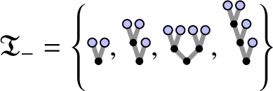
, and $\mathcal {I}=\left \{(-1,2), \left (-{\frac {1}{2}},3\right ), (0,4)\right \}$
.
$\mathcal {I}=\left \{(-1,2), \left (-{\frac {1}{2}},3\right ), (0,4)\right \}$
.
It will also be convenient to introduce the set $\mathcal {I}^{\star }:=\mathcal {I}\cup \{\star \}$
, where we extend the total order
$\mathcal {I}^{\star }:=\mathcal {I}\cup \{\star \}$
, where we extend the total order $\le $
to
$\le $
to $\mathcal {I}^{\star }$
by setting
$\mathcal {I}^{\star }$
by setting
![]() for any
for any
![]() . As before, we always set
. As before, we always set $\lambda _{\star }^{\delta }:=\delta $
for any
$\lambda _{\star }^{\delta }:=\delta $
for any $\delta>0$
.
$\delta>0$
.
The arguments showing the existence of a solution to the fixed point problem we will be looking at (compare equation (5.25)) will in general only hold if one chooses the scales
 such that $\lambda _{\left (\gamma , l\right )}^{\delta }$
is ‘small enough’ compared to
$\lambda _{\left (\gamma , l\right )}^{\delta }$
is ‘small enough’ compared to $\lambda _{\left (\beta ,r\right )}^{\delta }$
whenever
$\lambda _{\left (\beta ,r\right )}^{\delta }$
whenever $(\gamma ,l)\le (\beta ,r)$
. In order to make the arguments more systematic, we introduce the set
$(\gamma ,l)\le (\beta ,r)$
. In order to make the arguments more systematic, we introduce the set

We will view ${ \Lambda }$
as a subset of
${ \Lambda }$
as a subset of ${ \tilde {\Lambda } }$
by setting
${ \tilde {\Lambda } }$
by setting
![]() for any
for any $\tau \in \mathfrak {T}_-$
and any
$\tau \in \mathfrak {T}_-$
and any $\lambda \in { \Lambda }$
.
$\lambda \in { \Lambda }$
.
Remark 5.13. It follows that in our notation we have
 for any $\tau \in \mathfrak {T}_-$
and any
$\tau \in \mathfrak {T}_-$
and any $\Xi \in \mathfrak {L}_-$
such that
$\Xi \in \mathfrak {L}_-$
such that
![]() .
.
We also introduce a bit of notation for general finite totally ordered sets $(I,\le )$
. For notational convenience, we formulate statements for
$(I,\le )$
. For notational convenience, we formulate statements for $(I,\le ) = ([M],\le )$
, where
$(I,\le ) = ([M],\le )$
, where $M \in {\mathbf N}$
is given by
$M \in {\mathbf N}$
is given by $M=\#I$
.
$M=\#I$
.
Definition 5.14. Let $([M],\le )$
be a finite totally ordered set and let
$([M],\le )$
be a finite totally ordered set and let $S=S(\lambda )$
be any statement depending on
$S=S(\lambda )$
be any statement depending on $\lambda \in (0,1)^M$
. We define recursively in the number of elements M the notion of an attainable statement. If
$\lambda \in (0,1)^M$
. We define recursively in the number of elements M the notion of an attainable statement. If $M=1$
, then we call S an attainable statement if there exists
$M=1$
, then we call S an attainable statement if there exists $\bar {\lambda }_1>0$
such that
$\bar {\lambda }_1>0$
such that $S(\lambda _1)$
holds for any
$S(\lambda _1)$
holds for any $\lambda _1 \in \left (0,\bar {\lambda }_1\right )$
. For
$\lambda _1 \in \left (0,\bar {\lambda }_1\right )$
. For $M \ge 2$
and any fixed
$M \ge 2$
and any fixed $\lambda _{M}>0$
, we denote by
$\lambda _{M}>0$
, we denote by $(S\mid \lambda _M)(\lambda _{i_1},\dotsc ,\lambda _{{M-1}})$
the statement depending on
$(S\mid \lambda _M)(\lambda _{i_1},\dotsc ,\lambda _{{M-1}})$
the statement depending on $\lambda _{1},\dotsc ,\lambda _{{M-1}}$
defined by
$\lambda _{1},\dotsc ,\lambda _{{M-1}}$
defined by
 $$ \begin{align*} (S\mid\lambda_{M})(\lambda_{1},\dotsc,\lambda_{{M-1}})\Longleftrightarrow S(\lambda_{1},\dotsc,\lambda_{M}). \end{align*} $$
We then call the statement S attainable if there exists $\bar {\lambda }_M>0$
such that for any
$\bar {\lambda }_M>0$
such that for any $\lambda _{M}<\bar {\lambda }_M$
, the statement
$\lambda _{M}<\bar {\lambda }_M$
, the statement $(S\mid \lambda _{M})$
is attainable.
$(S\mid \lambda _{M})$
is attainable.
We will often use the following lemma, which is a direct consequence of the definition of attainable statements:
Lemma 5.15. Let I be a finite, totally ordered set and let $R,S$
be attainable statements on I. Then the conjunction
$R,S$
be attainable statements on I. Then the conjunction $R\land S$
is attainable.
$R\land S$
is attainable.
The strategy of the following sections will be as follows: We will show various lemmas whose statements are attainable statements for the family $\lambda \in (0,1)^{\mathcal {I}^{\star }}$
. These (finitely many) statements in conjunction imply that equation (5.25) can be solved, so that the existence of a solution is an attainable statement. This in particular implies that there exists a choice of scales
$\lambda \in (0,1)^{\mathcal {I}^{\star }}$
. These (finitely many) statements in conjunction imply that equation (5.25) can be solved, so that the existence of a solution is an attainable statement. This in particular implies that there exists a choice of scales $\lambda ^{\delta } \in { \Lambda }$
for any
$\lambda ^{\delta } \in { \Lambda }$
for any $\delta>0$
small enough such that the statement holds true, and this concludes the proof.
$\delta>0$
small enough such that the statement holds true, and this concludes the proof.
5.4 A fixed point argument
Our goal is to find a family $\left (a^{\delta },\lambda ^{\delta }\right ) \in {{\mathbf A}} \times { \Lambda }$
for
$\left (a^{\delta },\lambda ^{\delta }\right ) \in {{\mathbf A}} \times { \Lambda }$
for $\delta>0$
, converging to
$\delta>0$
, converging to $0$
as
$0$
as $\delta \to 0 $
, such that
$\delta \to 0 $
, such that
 $$ \begin{align*} \lim_{\delta\to 0}\lim_{\varepsilon\to 0} \Upsilon ^{\eta^{\varepsilon}\left(a^{\delta},\lambda^{\delta}\right)} M^{ g^{\varepsilon}}\mathscr{S}\tau = h(\tau) \end{align*} $$
for any $\tau \in \mathfrak {T}_-$
. Here and later, we write
$\tau \in \mathfrak {T}_-$
. Here and later, we write $\eta ^{\varepsilon }(a,\lambda ):= \eta ^{\varepsilon ,a,\lambda }$
in order to make some expressions more readable. For
$\eta ^{\varepsilon }(a,\lambda ):= \eta ^{\varepsilon ,a,\lambda }$
in order to make some expressions more readable. For $\tau \in \mathscr {T}_-$
we introduce the function
$\tau \in \mathscr {T}_-$
we introduce the function $F_{\tau } : { {{\mathbf A}} } \times { \Lambda } \to \mathbf {R}$
by setting
$F_{\tau } : { {{\mathbf A}} } \times { \Lambda } \to \mathbf {R}$
by setting
 $$ \begin{align} F_{\tau} (a, \lambda):= \lim_{\varepsilon\to 0} \Upsilon^{\eta^{\varepsilon}\left(a,\lambda\right)} M^{g^{\varepsilon}}\mathscr{S}\tau. \end{align} $$
Note that restricted to $\tau \in \mathfrak {T}_-$
, we obtain a map
$\tau \in \mathfrak {T}_-$
, we obtain a map
 $$ \begin{align*} F : { {{\mathbf A}} } \times { \Lambda } \to { {{\mathbf A}} }. \end{align*} $$
We also define the functions $ F^{\uparrow } $
and
$ F^{\uparrow } $
and $ F^{\downarrow } $
in the same way, with
$ F^{\downarrow } $
in the same way, with $\mathscr {S}$
replaced by
$\mathscr {S}$
replaced by ${ \mathscr {S}^{\uparrow } }$
and
${ \mathscr {S}^{\uparrow } }$
and ${ \mathscr {S}^{\downarrow } }$
, respectively (see Definition 5.2). Since
${ \mathscr {S}^{\downarrow } }$
, respectively (see Definition 5.2). Since $\mathscr {S}={ \mathscr {S}^{\uparrow } }+{ \mathscr {S}^{\downarrow } }+\mathrm {Id}$
and
$\mathscr {S}={ \mathscr {S}^{\uparrow } }+{ \mathscr {S}^{\downarrow } }+\mathrm {Id}$
and $\Upsilon ^{\eta ^{\varepsilon }\left (a,\lambda \right )} M^{ g^{\varepsilon } }\tau =0$
for any
$\Upsilon ^{\eta ^{\varepsilon }\left (a,\lambda \right )} M^{ g^{\varepsilon } }\tau =0$
for any $\tau \in \mathscr {T}_-$
one has
$\tau \in \mathscr {T}_-$
one has $F= F^{\uparrow } + F^{\downarrow } $
.
$F= F^{\uparrow } + F^{\downarrow } $
.
Remark 5.16. For fixed $(a,\lambda ) \in {{ {{\mathbf A}} } \times { \tilde {\Lambda } }}$
, the noise
$(a,\lambda ) \in {{ {{\mathbf A}} } \times { \tilde {\Lambda } }}$
, the noise
![]() is independent of
is independent of $\varepsilon $
unless
$\varepsilon $
unless
![]() . On the other hand, the expression
. On the other hand, the expression $M^{g^{\varepsilon }}\mathscr {S}\tau $
coincides with the BPHZ renormalisation, if the homogeneity of the noise types
$M^{g^{\varepsilon }}\mathscr {S}\tau $
coincides with the BPHZ renormalisation, if the homogeneity of the noise types
![]() is viewed as zero (or more precisely, as
is viewed as zero (or more precisely, as $-\kappa $
for some
$-\kappa $
for some $\kappa $
small enough; compare Lemma 5.21 for a precise statement). In this sense, the right-hand side of formula (5.20) is just the expectation of
$\kappa $
small enough; compare Lemma 5.21 for a precise statement). In this sense, the right-hand side of formula (5.20) is just the expectation of ${\boldsymbol {\Pi }}\tau (0)$
, where
${\boldsymbol {\Pi }}\tau (0)$
, where ${\boldsymbol {\Pi }}$
denotes the BPHZ-renormalised (in the sense of the previous sentence) canonical lift of
${\boldsymbol {\Pi }}$
denotes the BPHZ-renormalised (in the sense of the previous sentence) canonical lift of $\eta ^{\varepsilon }(a,\lambda )$
. It follows in particular that the right-hand side of formula (5.20) is indeed convergent.
$\eta ^{\varepsilon }(a,\lambda )$
. It follows in particular that the right-hand side of formula (5.20) is indeed convergent.
Note, however, that this expression does not vanish. This is not a contradiction to the characterisation [Reference Bruned, Hairer and ZambottiBHZ19, Equation 6.25] of the BPHZ character, since with respect to the homogeneity constructed in the previous paragraph, $\mathscr {S}$
does not leave homogeneity invariant. In fact, any tree
$\mathscr {S}$
does not leave homogeneity invariant. In fact, any tree $\sigma \in \mathscr {S}[\tau ] \backslash \{\tau \}$
is of positive homogeneity in this sense. The identity [Reference Bruned, Hairer and ZambottiBHZ19, Equation 6.25], on the other hand, is only guaranteed to hold for trees of negative homogeneity.
$\sigma \in \mathscr {S}[\tau ] \backslash \{\tau \}$
is of positive homogeneity in this sense. The identity [Reference Bruned, Hairer and ZambottiBHZ19, Equation 6.25], on the other hand, is only guaranteed to hold for trees of negative homogeneity.
Our intuition behind this definition is that $ F^{\downarrow } _{\tau }$
should be small compared to
$ F^{\downarrow } _{\tau }$
should be small compared to $ F^{\uparrow } _{\tau }$
, in the sense that a statement of the form
$ F^{\uparrow } _{\tau }$
, in the sense that a statement of the form $ F^{\downarrow } _{\tau }(a,\lambda ) \ll F^{\uparrow } _{\tau }(a,\lambda )$
is an attainable statement. It turns out that this is not quite true, since in general there will be subdivergences of
$ F^{\downarrow } _{\tau }(a,\lambda ) \ll F^{\uparrow } _{\tau }(a,\lambda )$
is an attainable statement. It turns out that this is not quite true, since in general there will be subdivergences of $\tau $
that cause
$\tau $
that cause $ F^{\downarrow } _{\tau }$
to become dominant. However, assuming that we have good bounds on these subdivergences, this statement becomes attainable. More precisely, we have the following result:
$ F^{\downarrow } _{\tau }$
to become dominant. However, assuming that we have good bounds on these subdivergences, this statement becomes attainable. More precisely, we have the following result:
Lemma 5.17. For any $\tau \in \mathfrak {T}_-$
, there exists a smooth function
$\tau \in \mathfrak {T}_-$
, there exists a smooth function $G_{\tau }:\mathbf {R}^{\mathfrak {T}_-}\times \mathbf {R}^{\mathscr {T}_-^{\prec \tau }} \times { \Lambda } \to \mathbf {R}$
such that
$G_{\tau }:\mathbf {R}^{\mathfrak {T}_-}\times \mathbf {R}^{\mathscr {T}_-^{\prec \tau }} \times { \Lambda } \to \mathbf {R}$
such that
 $$ \begin{align} G_{\tau}\left(a, \left(F_{\tilde{\tau}}(a,\lambda)\right)_{\tilde{\tau}\in\mathscr{T}_-^{\prec\tau}}, \lambda\right)= F^{\downarrow} _{\tau}(a,\lambda) \end{align} $$
for any $(a,\lambda ) \in { {{\mathbf A}} } \times { \Lambda }$
, and such that for any fixed
$(a,\lambda ) \in { {{\mathbf A}} } \times { \Lambda }$
, and such that for any fixed $\rho> 0$
and
$\rho> 0$
and $\beta>0$
the following bound is attainable:
$\beta>0$
the following bound is attainable:

uniformly over all $(a,b) \in { {{\mathbf A}} } \times { \mathbf {R}^{\mathscr {T}_-^{\prec \tau }} }$
such that
$(a,b) \in { {{\mathbf A}} } \times { \mathbf {R}^{\mathscr {T}_-^{\prec \tau }} }$
such that $\max _{\tilde {\tau }\in \mathfrak {T}_-}\left \lvert a_{\tilde {\tau }}\right \rvert \lor \max _{\tilde {\tau }\in \mathscr {T}_-^{\prec \tau }}\left \lvert b_{\tilde {\tau }}\right \rvert \le \rho $
.
$\max _{\tilde {\tau }\in \mathfrak {T}_-}\left \lvert a_{\tilde {\tau }}\right \rvert \lor \max _{\tilde {\tau }\in \mathscr {T}_-^{\prec \tau }}\left \lvert b_{\tilde {\tau }}\right \rvert \le \rho $
.
Before we prove this lemma, we show how to use it to finish the proof of Proposition 3.20. We first argue that one can strengthen the statement of the lemma:
Lemma 5.18. For any $\tau \in \mathfrak {T}_-$
and
$\tau \in \mathfrak {T}_-$
and $\rho>0$
, there exists a continuous function
$\rho>0$
, there exists a continuous function $\tilde {G} _{\tau }:{ {{\mathbf A}} } \times { \mathbf {R}^{\mathfrak {T}_-^{\prec \tau }} } \times { \Lambda } \to \mathbf {R}$
such that
$\tilde {G} _{\tau }:{ {{\mathbf A}} } \times { \mathbf {R}^{\mathfrak {T}_-^{\prec \tau }} } \times { \Lambda } \to \mathbf {R}$
such that
 $$ \begin{align} \tilde{G}_{\tau}\left(a, \left(F_{\tilde{\tau}}(a,\lambda)\right) _{\tilde{\tau}\in\mathfrak{T}_-^{\prec\tau}} , \lambda\right) = F^{\downarrow} _{\tau}(a,\lambda) \end{align} $$
holds for any $(a,\lambda ) \in { {{\mathbf A}} } \times { \Lambda }$
with
$(a,\lambda ) \in { {{\mathbf A}} } \times { \Lambda }$
with $\sup _{{\tilde {\tau }} \in \mathfrak {T}_-}\left \lvert a_{\tilde {\tau }}\right \rvert \lor \sup _{{\tilde {\tau }} \in \mathfrak {T}_-^{\prec \tau }}\left \lvert F_{\tilde {\tau }} (a,\lambda ) \right \rvert \le \rho $
, and for any
$\sup _{{\tilde {\tau }} \in \mathfrak {T}_-}\left \lvert a_{\tilde {\tau }}\right \rvert \lor \sup _{{\tilde {\tau }} \in \mathfrak {T}_-^{\prec \tau }}\left \lvert F_{\tilde {\tau }} (a,\lambda ) \right \rvert \le \rho $
, and for any $\beta>0$
the bound
$\beta>0$
the bound

uniformly over $(a,b) \in { {{\mathbf A}} } \times { \mathbf {R}^{\mathfrak {T}_-^{\prec \tau }} }$
such that
$(a,b) \in { {{\mathbf A}} } \times { \mathbf {R}^{\mathfrak {T}_-^{\prec \tau }} }$
such that $\max _{\tilde {\tau }\in \mathfrak {T}_-}\left \lvert a_{\tilde {\tau }}\right \rvert \lor \max _{\tilde {\tau }\in \mathfrak {T}_-^{\prec \tau }}\left \lvert b_{\tilde {\tau }}\right \rvert \le \rho $
is attainable.
$\max _{\tilde {\tau }\in \mathfrak {T}_-}\left \lvert a_{\tilde {\tau }}\right \rvert \lor \max _{\tilde {\tau }\in \mathfrak {T}_-^{\prec \tau }}\left \lvert b_{\tilde {\tau }}\right \rvert \le \rho $
is attainable.
Proof . Let $A_{\rho }$
denote the set of
$A_{\rho }$
denote the set of $a \in { {{\mathbf A}} }$
such that
$a \in { {{\mathbf A}} }$
such that $\sup _{{\tilde {\tau }} \in \mathfrak {T}_-}\left \lvert a_{\tilde {\tau }}\right \rvert \lor \sup _{{\tilde {\tau }} \in \mathfrak {T}_-^{\prec \tau }}\left \lvert F_{\tilde {\tau }} (a,\lambda ) \right \rvert \le \rho $
. We first argue that there exists
$\sup _{{\tilde {\tau }} \in \mathfrak {T}_-}\left \lvert a_{\tilde {\tau }}\right \rvert \lor \sup _{{\tilde {\tau }} \in \mathfrak {T}_-^{\prec \tau }}\left \lvert F_{\tilde {\tau }} (a,\lambda ) \right \rvert \le \rho $
. We first argue that there exists $R>0$
such that one has
$R>0$
such that one has $\left \lvert F_{{\tilde {\tau }}}(a,\lambda )\right \rvert \le R$
for any
$\left \lvert F_{{\tilde {\tau }}}(a,\lambda )\right \rvert \le R$
for any ${\tilde {\tau }} \in \mathscr {T}_-^{\prec \tau }$
and any
${\tilde {\tau }} \in \mathscr {T}_-^{\prec \tau }$
and any $(a, \lambda ) \in A_{\rho } \times { \Lambda }$
. Once this is shown, it is not hard to see that the function
$(a, \lambda ) \in A_{\rho } \times { \Lambda }$
. Once this is shown, it is not hard to see that the function
 $$ \begin{align*} \tilde{G}_{\tau}( a, b, \lambda) := G_{\tau}\left( a, \left(b_{\bar{\tau}}\right)_{{\bar{\tau}} \in \mathfrak{T}_-^{\prec\tau}} \sqcup \left(F_{\bar{\tau}}(a, \lambda) \land R \right)_{{\bar{\tau}} \in \mathscr{T}_-^{\prec\tau} \backslash \mathfrak{T}_-^{\prec\tau}}, \lambda\right) \end{align*} $$
has all the properties we are looking for.
We denote by
the BPHZ character for the noise $\eta ^{\varepsilon }(a,\lambda )$
, and we define
$\eta ^{\varepsilon }(a,\lambda )$
, and we define
via the identity
, so that one has

for any ${\tilde {\tau }} \in \mathscr {T}_-$
, where we suppress the dependence on
${\tilde {\tau }} \in \mathscr {T}_-$
, where we suppress the dependence on $(a,\lambda )$
in the notation on the right-hand side. By Lemma 5.11, the noise
$(a,\lambda )$
in the notation on the right-hand side. By Lemma 5.11, the noise $\eta ^{\varepsilon }(a,\lambda )$
is uniformly bounded with respect to
$\eta ^{\varepsilon }(a,\lambda )$
is uniformly bounded with respect to $\lVert \cdot \rVert _{\mathfrak {s} - \bar {\kappa }}$
over
$\lVert \cdot \rVert _{\mathfrak {s} - \bar {\kappa }}$
over $(a,\lambda ) \in A_{\rho } \times { \Lambda }$
and
$(a,\lambda ) \in A_{\rho } \times { \Lambda }$
and $\varepsilon>0$
, and it follows from [Reference Chandra and HairerCH16] that
$\varepsilon>0$
, and it follows from [Reference Chandra and HairerCH16] that

for any
uniformly over $(a,\lambda ) \in A_{\rho } \times { \Lambda }$
and
$(a,\lambda ) \in A_{\rho } \times { \Lambda }$
and $\varepsilon>0$
. We recall at this point (Lemma 5.4) that
$\varepsilon>0$
. We recall at this point (Lemma 5.4) that $\mathscr {S}$
commutes with the coproduct, so that it remains to show that
$\mathscr {S}$
commutes with the coproduct, so that it remains to show that
is bounded for any ${\tilde {\tau }} \in \mathcal {T}_-$
uniformly over
${\tilde {\tau }} \in \mathcal {T}_-$
uniformly over $(a,\lambda ) \in A_{\rho } \times { \Lambda }$
and
$(a,\lambda ) \in A_{\rho } \times { \Lambda }$
and $\varepsilon>0$
. We denote by
$\varepsilon>0$
. We denote by $h^{\varepsilon ,\delta } \in \mathcal {G}_-$
the character from Proposition 3.21 for the shift
$h^{\varepsilon ,\delta } \in \mathcal {G}_-$
the character from Proposition 3.21 for the shift $\zeta _{\delta } := \mathscr {S}^*\eta ^{\varepsilon }(a,\lambda )-\xi ^{\varepsilon }$
, and we claim that one has
$\zeta _{\delta } := \mathscr {S}^*\eta ^{\varepsilon }(a,\lambda )-\xi ^{\varepsilon }$
, and we claim that one has
on $\mathcal {T}_-$
. Indeed, one has
$\mathcal {T}_-$
. Indeed, one has

on ${\mathcal {T}_-}$
, and since this relation characterises the BPHZ character, one has
${\mathcal {T}_-}$
, and since this relation characterises the BPHZ character, one has
. It remains to argue that
on ${\mathcal {T}_-}$
. We can now argue inductively with respect to
${\mathcal {T}_-}$
. We can now argue inductively with respect to $\prec $
in the same way as in the proof of equation (3.8). The only difference is that in equation (3.8) we showed convergence based on the assumption that
$\prec $
in the same way as in the proof of equation (3.8). The only difference is that in equation (3.8) we showed convergence based on the assumption that $F_{\tilde {\tau }} (a,\lambda )$
converges for
$F_{\tilde {\tau }} (a,\lambda )$
converges for $\tilde {\tau } \in \mathfrak {T}_-^{\prec \tau }$
. Now we show boundedness based on the assumption that these quantities are bounded.
$\tilde {\tau } \in \mathfrak {T}_-^{\prec \tau }$
. Now we show boundedness based on the assumption that these quantities are bounded.
With this we can finish the proof of Proposition 3.20. We recall at this point that we fixed $h \in f^{\xi } \circ \mathcal {H}$
at the beginning of Section 3.3 (see also equation (3.6)).
$h \in f^{\xi } \circ \mathcal {H}$
at the beginning of Section 3.3 (see also equation (3.6)).
Proposition 5.19. For any $\delta>0$
, the following is an attainable statement: There exists a family of constants
$\delta>0$
, the following is an attainable statement: There exists a family of constants $a\in \mathbf {R}^{\mathfrak {T}_-}$
such that
$a\in \mathbf {R}^{\mathfrak {T}_-}$
such that $\sup _{\tau \in \mathfrak {T}_-} \lvert a_{\tau }\rvert \le \delta $
and such that
$\sup _{\tau \in \mathfrak {T}_-} \lvert a_{\tau }\rvert \le \delta $
and such that
 $$ \begin{align} F_{\tau}(a,\lambda)=h(\tau) \end{align} $$
for any $\tau \in \mathfrak {T}_-$
.
$\tau \in \mathfrak {T}_-$
.
In particular, one can choose a sequence of scales $\lambda ^{\delta } \in { \Lambda }$
and a sequence of constants
$\lambda ^{\delta } \in { \Lambda }$
and a sequence of constants $a^{\delta } \in { {{\mathbf A}} }$
, both converging to
$a^{\delta } \in { {{\mathbf A}} }$
, both converging to $0$
as
$0$
as $\delta \to 0$
, such that the statement of Proposition 3.20 holds for the corresponding shift
$\delta \to 0$
, such that the statement of Proposition 3.20 holds for the corresponding shift ${ { \zeta } }_{\delta } = \mathscr {S}^* \eta ^{\varepsilon }(a,\lambda )-\xi ^{\varepsilon }$
.
${ { \zeta } }_{\delta } = \mathscr {S}^* \eta ^{\varepsilon }(a,\lambda )-\xi ^{\varepsilon }$
.
Proof . The key step is to find a solution $a \in { {{\mathbf A}} }$
with
$a \in { {{\mathbf A}} }$
with $\max _{\tau \in \mathfrak {T}_- } \lvert a_{\tau }\rvert <\delta $
to the system of equations
$\max _{\tau \in \mathfrak {T}_- } \lvert a_{\tau }\rvert <\delta $
to the system of equations
 $$ \begin{align} F^{\uparrow} _{\tau}(a,\lambda)+ \tilde{G}_{\tau} \left( a, \left(h({\tilde{\tau}})\right)_{{\tilde{\tau}} \in \mathfrak{T}_-^{\prec\tau}} , \lambda \right) = h(\tau), \quad{\tau \in \mathfrak{T}_-}, \end{align} $$
where $\tilde {G}_{\tau }$
is as in Lemma 5.18 for
$\tilde {G}_{\tau }$
is as in Lemma 5.18 for $\rho := 2 \max _{\tau \in \mathfrak {T}_-} h(\tau ) \land 2\delta $
. We then argue inductively: Fixing
$\rho := 2 \max _{\tau \in \mathfrak {T}_-} h(\tau ) \land 2\delta $
. We then argue inductively: Fixing $\tau \in \mathfrak {T}_-$
and assuming that
$\tau \in \mathfrak {T}_-$
and assuming that $F_{\tilde {\tau }}(a, \lambda ) = h({\tilde {\tau }})$
for any
$F_{\tilde {\tau }}(a, \lambda ) = h({\tilde {\tau }})$
for any ${\tilde {\tau }}\in \mathfrak {T}_-^{\prec \tau }$
, then the assumptions of equation (5.23) are met for
${\tilde {\tau }}\in \mathfrak {T}_-^{\prec \tau }$
, then the assumptions of equation (5.23) are met for $\tau $
, so that the left-hand side of equation (5.26) is equal to
$\tau $
, so that the left-hand side of equation (5.26) is equal to $F_{\tau }(a, \lambda )$
.
$F_{\tau }(a, \lambda )$
.
We rephrase equation (5.26) slightly into a fixed point problem. Define the function $g : { {{\mathbf A}} } \times { \Lambda } \to { {{\mathbf A}} }$
by
$g : { {{\mathbf A}} } \times { \Lambda } \to { {{\mathbf A}} }$
by

for any $\tau \in \mathfrak {T}_-$
. Then
$\tau \in \mathfrak {T}_-$
. Then $a \in { {{\mathbf A}} }$
with
$a \in { {{\mathbf A}} }$
with $\max _{\tau \in \mathfrak {T}_- } \lvert a_{\tau }\rvert <\delta $
is a fixed point of
$\max _{\tau \in \mathfrak {T}_- } \lvert a_{\tau }\rvert <\delta $
is a fixed point of $g(\cdot , \lambda )$
if and only if
$g(\cdot , \lambda )$
if and only if $(a,\lambda )$
is a solution to equation (5.25). It follows from Lemma 5.10 that
$(a,\lambda )$
is a solution to equation (5.25). It follows from Lemma 5.10 that
as $\lambda \to 0$
uniformly over
$\lambda \to 0$
uniformly over $a \in { {{\mathbf A}} }$
, as before, and from Lemma 5.18 that for any
$a \in { {{\mathbf A}} }$
, as before, and from Lemma 5.18 that for any $\beta>0$
the bound
$\beta>0$
the bound

for any $a \in { {{\mathbf A}} }$
as before is an attainable statement.
$a \in { {{\mathbf A}} }$
as before is an attainable statement.
It follows that the statement
 $$ \begin{align*} \max_{\tau\in\mathfrak{T}_-} \lvert a_{\tau}\rvert\le \delta \text{ implies } \max_{\tau\in\mathfrak{T}_-} \lvert g_{\tau}(a,\lambda)\rvert \le \delta \end{align*} $$
is attainable, and by Schauder’s fixed point theorem there exists a solution a to equation (5.27) in the $\delta $
-neighbourhood of the origin.
$\delta $
-neighbourhood of the origin.
It remains to show Lemma 5.17. We fix
with the property that
and such that
for any tree
with $\#K(\tau )\ge 1$
. For fixed
$\#K(\tau )\ge 1$
. For fixed
we introduce a homogeneity assignment
on
which treats noises regularised on scales larger than
as smooth. More precisely, we set
and
for any $\Xi \in \mathfrak {L}_-$
, and we define
$\Xi \in \mathfrak {L}_-$
, and we define

for any noise type
. Here we use the total order $\le $
on
$\le $
on $\mathcal {I}$
introduced in Section 5.3.
$\mathcal {I}$
introduced in Section 5.3.
Lemma 5.20. Set
and set
. For any $A>0$
there exists a constant
$A>0$
there exists a constant
, such that for any $N\in {\mathbf N}$
the bound
$N\in {\mathbf N}$
the bound
holds uniformly over all families $\lambda \in { \Lambda }$
and
$\lambda \in { \Lambda }$
and $a \in { {{\mathbf A}} }$
with
$a \in { {{\mathbf A}} }$
with $\max _{\tau \in \mathfrak {T}_-} \lvert a_{\tau }\rvert < A$
.
$\max _{\tau \in \mathfrak {T}_-} \lvert a_{\tau }\rvert < A$
.
Proof . This follows directly from Lemma 5.11.
We denote by
![]() the unital subalgebra generated by trees of negative
the unital subalgebra generated by trees of negative
![]() -homogeneity. Note that
-homogeneity. Note that
![]() was chosen small enough so that for any tree
was chosen small enough so that for any tree
![]() , one has
, one has
![]() if and only if for any noise-type edge
if and only if for any noise-type edge $ e \in L(\tau )$
one has either
$ e \in L(\tau )$
one has either $\mathfrak {t}(e) \in \mathfrak {L}_-$
or
$\mathfrak {t}(e) \in \mathfrak {L}_-$
or $\mathfrak {t}(e) = (\Xi ,\tau )$
, with
$\mathfrak {t}(e) = (\Xi ,\tau )$
, with
![]() . We denote by
. We denote by
![]() the multiplicative projection of
the multiplicative projection of
![]() onto
onto
![]() , and we define
, and we define
 (we usually suppress the dependence of $(a,\lambda )$
in this notation).
$(a,\lambda )$
in this notation).
It follows that
![]() restricted to
restricted to
![]() is just the BPHZ character for the homogeneity assignment
is just the BPHZ character for the homogeneity assignment
![]() and the evaluation
and the evaluation $\eta ^{\varepsilon }$
. Applying the results of [Reference Chandra and HairerCH16] to the homogeneity assignment
$\eta ^{\varepsilon }$
. Applying the results of [Reference Chandra and HairerCH16] to the homogeneity assignment
![]() , we obtain the following estimate:
, we obtain the following estimate:
Lemma 5.21. For any
, there exists a constant
such that for any
, the bound

holds uniformly over all families $\lambda \in { \Lambda }$
and
$\lambda \in { \Lambda }$
and $a \in { {{\mathbf A}} }$
with
$a \in { {{\mathbf A}} }$
with $\max _{\tau \in \mathfrak {T}_-} \lvert a_{\tau }\rvert < A$
.
$\max _{\tau \in \mathfrak {T}_-} \lvert a_{\tau }\rvert < A$
.
Moreover,

exists and is a continuous function in $(a,\lambda )$
.
$(a,\lambda )$
.
Proof . Both statements follow from Lemma 5.20 and [Reference Chandra and HairerCH16, Theorem 2.31].
We are finally in a position to prove Lemma 5.17.
Proof of Lemma 5.17. We fix from now on a tree $\tau \in \mathfrak {T}_-$
and assume that the statement of Lemma 5.17 holds for any
$\tau \in \mathfrak {T}_-$
and assume that the statement of Lemma 5.17 holds for any ${\tilde {\tau }} \in \mathfrak {T}_-^{\prec \tau }$
. We set
${\tilde {\tau }} \in \mathfrak {T}_-^{\prec \tau }$
. We set
and we define a character
by

It then follows that for any ${\tilde {\tau }} \in \mathscr {T}_-^{\prec \tau }$
, one has
${\tilde {\tau }} \in \mathscr {T}_-^{\prec \tau }$
, one has

It follows from this identity and the definition of the coproduct that there exists a fixed polynomial $P_{\tilde {\tau }}$
in
$P_{\tilde {\tau }}$
in $\mathscr {T}_-^{\preceq {\tilde {\tau }}} \times \mathscr {T}$
variables such that
$\mathscr {T}_-^{\preceq {\tilde {\tau }}} \times \mathscr {T}$
variables such that

We prove inductively in $\prec $
that for any
$\prec $
that for any ${\tilde {\tau }} \in \mathscr {T}_-^{\prec \tau }$
, there exists a continuous function
${\tilde {\tau }} \in \mathscr {T}_-^{\prec \tau }$
, there exists a continuous function
such that
is equal to equation (5.29) in the limit $\varepsilon \to 0$
for any
$\varepsilon \to 0$
for any $(a,\lambda ) \in { {{\mathbf A}} } \times { \Lambda }$
, and such that for any
$(a,\lambda ) \in { {{\mathbf A}} } \times { \Lambda }$
, and such that for any $C>0$
, the estimate
$C>0$
, the estimate

holds uniformly over all $(a,b) \in { {{\mathbf A}} } \times { \mathbf {R}^{\mathscr {T}_-^{\prec \tau }} }$
such that
$(a,b) \in { {{\mathbf A}} } \times { \mathbf {R}^{\mathscr {T}_-^{\prec \tau }} }$
such that $\sup _{{\bar {\tau }} \in \mathfrak {T}_-}\left \lvert a_{{\bar {\tau }}}\right \rvert \lor \sup _{{\bar {\tau }} \in \mathscr {T}_-^{\prec \tau }}\left \lvert b_{{\bar {\tau }}}\right \rvert <C$
and
$\sup _{{\bar {\tau }} \in \mathfrak {T}_-}\left \lvert a_{{\bar {\tau }}}\right \rvert \lor \sup _{{\bar {\tau }} \in \mathscr {T}_-^{\prec \tau }}\left \lvert b_{{\bar {\tau }}}\right \rvert <C$
and $\varepsilon>0$
small enough (where ‘small enough’ may depend on
$\varepsilon>0$
small enough (where ‘small enough’ may depend on $(a,b)$
). We can write
$(a,b)$
). We can write

which is bounded in the required way by Lemma 5.21 and the induction hypothesis. In order to continue, we now make the claim that for any tree
, one has
if at least one of the following three properties is satisfied:
-
1. One has
${\tilde {\tau }}\in \mathcal {T}_-$
. -
2. For any partition
$\pi \in \mathcal {P}(L({\tilde {\tau }}))$
, one has (5.31)for any
$$ \begin{align} \prod_{P\in\pi}{\mathbf E}^c\left[\left(\eta^{\varepsilon}_{t(e)}(x_e)\right)_{e\in P}\right]= 0 \end{align} $$
$(x_e)_{e\in L({\tilde {\tau }})}\in \left (\bar {\mathbf D}\right )^{L\left ({\tilde {\tau }}\right )}$
, where
denotes the type map of
${\tilde {\tau }}$
.
-
3. One has
.


The first claim follows from the fact that $\mathcal {T}_-$
is a Hopf subalgebra of
$\mathcal {T}_-$
is a Hopf subalgebra of
, and on $\mathcal {T}_-$
the characters
$\mathcal {T}_-$
the characters $g^{\varepsilon }$
and
$g^{\varepsilon }$
and
agree. For the second claim, we denote by
the ideal in
generated by all trees
with the property that equation (5.31) holds. Then $\mathcal {I}$
forms a Hopf ideal, and by the definition of the BPHZ character it follows that both
$\mathcal {I}$
forms a Hopf ideal, and by the definition of the BPHZ character it follows that both $g^{\varepsilon }$
and
$g^{\varepsilon }$
and
vanish on $\mathcal {I}$
. The claim now follows from the fact that the annihilator of any Hopf ideal forms a subgroup of
$\mathcal {I}$
. The claim now follows from the fact that the annihilator of any Hopf ideal forms a subgroup of
. The third claim follows similarly, noting that ${\Delta _-}$
preserves the
${\Delta _-}$
preserves the
-homogeneity, in the sense that
, where on the left-hand side we add up the homogeneities of products of trees. It follows that the ideal
in
generated by trees
such that
is a Hopf ideal. Moreover, since
and $g^{\varepsilon }$
vanish on
$g^{\varepsilon }$
vanish on
, the claim follows again from the fact that annihilators of Hopf ideals are subgroups.
As a corollary, we obtain the identity

Indeed, set ${\tilde {\tau }}\in { \mathscr {S}^{\uparrow } } [\tau ]$
. Then there exists a unique noise-type edge
${\tilde {\tau }}\in { \mathscr {S}^{\uparrow } } [\tau ]$
. Then there exists a unique noise-type edge $e\in L({\tilde {\tau }})$
such that
$e\in L({\tilde {\tau }})$
such that $\mathfrak {t}(e)\notin \mathfrak {L}_-$
, and for this edge
$\mathfrak {t}(e)\notin \mathfrak {L}_-$
, and for this edge $\eta ^{\varepsilon }_{\mathfrak {t}(e)}$
is an element of the
$\eta ^{\varepsilon }_{\mathfrak {t}(e)}$
is an element of the $m(\tau )$
th homogeneous Wiener chaos. It follows that whenever
$m(\tau )$
th homogeneous Wiener chaos. It follows that whenever ${\bar {\tau }}\ne \mathbf {1}$
is a proper subtree of
${\bar {\tau }}\ne \mathbf {1}$
is a proper subtree of ${\tilde {\tau }}$
, so that in particular
${\tilde {\tau }}$
, so that in particular $L({\bar {\tau }}) \subsetneq L({\tilde {\tau }})$
, then either the first or the second of the foregoing properties is satisfied. The claim then follows, since on the one hand
$L({\bar {\tau }}) \subsetneq L({\tilde {\tau }})$
, then either the first or the second of the foregoing properties is satisfied. The claim then follows, since on the one hand
![]() for any
for any $k \in {\mathbf N}^{d}\backslash \{0\}$
, and on the other hand
$k \in {\mathbf N}^{d}\backslash \{0\}$
, and on the other hand
![]() implies that
implies that
![]() . Here we use the fact that
. Here we use the fact that
![]() was chosen in such a way that
was chosen in such a way that
![]() for any
for any ${\tilde {\tau }}\in { \mathscr {S}^{\uparrow } } [\tau ]$
.
${\tilde {\tau }}\in { \mathscr {S}^{\uparrow } } [\tau ]$
.
As a second corollary, we get that if $\tau $
is such that
$\tau $
is such that
![]() , then
, then

To see this, let ${\tilde {\tau }}\in { \mathscr {S}^{\downarrow } }[\tau ]$
. It is clear that whenever there exists
${\tilde {\tau }}\in { \mathscr {S}^{\downarrow } }[\tau ]$
. It is clear that whenever there exists $e \in L({\tilde {\tau }})$
such that either
$e \in L({\tilde {\tau }})$
such that either $\mathfrak {t}(e)=\tilde {\Xi }$
for some
$\mathfrak {t}(e)=\tilde {\Xi }$
for some $\Xi \in \mathfrak {L}_-$
or
$\Xi \in \mathfrak {L}_-$
or $\mathfrak {t}(e) = (\Xi ,{\bar {\tau }})$
with
$\mathfrak {t}(e) = (\Xi ,{\bar {\tau }})$
with
![]() , then one has
, then one has
![]() , and by the third of the foregoing properties it follows that
, and by the third of the foregoing properties it follows that
 . Thus, we can assume that $\mathfrak {t}(e) \in \mathfrak {L}_-$
or
$\mathfrak {t}(e) \in \mathfrak {L}_-$
or $\mathfrak {t}(e) = (\Xi ,{\bar {\tau }})$
with
$\mathfrak {t}(e) = (\Xi ,{\bar {\tau }})$
with
![]() for all
for all $e \in L(\tau )$
.
$e \in L(\tau )$
.
Assume now that in addition there are two distinct $e,f\in L({\tilde {\tau }})$
such that
$e,f\in L({\tilde {\tau }})$
such that $\mathfrak {t}(e),\mathfrak {t}(f)\notin \mathfrak {L}_-$
– say
$\mathfrak {t}(e),\mathfrak {t}(f)\notin \mathfrak {L}_-$
– say $\mathfrak {t}(e)=({\bar {\Xi }},{\bar {\tau }})$
and
$\mathfrak {t}(e)=({\bar {\Xi }},{\bar {\tau }})$
and $\mathfrak {t}(f)=({\hat {\Xi }},{\hat {\tau }})$
. Then the assumption
$\mathfrak {t}(f)=({\hat {\Xi }},{\hat {\tau }})$
. Then the assumption
![]() implies that
implies that
![]() . Upon choosing
. Upon choosing $\bar {\kappa }$
small enough, one has
$\bar {\kappa }$
small enough, one has

In the remaining case there exists a unique $e\in L({\tilde {\tau }})$
such that
$e\in L({\tilde {\tau }})$
such that $\mathfrak {t}(e)\notin \mathfrak {L}_-$
, say
$\mathfrak {t}(e)\notin \mathfrak {L}_-$
, say $\mathfrak {t}(e)=\left ({\bar {\Xi }},{\bar {\tau }}\right )$
. We distinguish the case
$\mathfrak {t}(e)=\left ({\bar {\Xi }},{\bar {\tau }}\right )$
. We distinguish the case
and
(by the earlier discussion, we have
, so that the case
is ruled out). In the first case, we have by the definition of $\le $
and
$\le $
and ${ \mathscr {S}^{\downarrow } }$
that
${ \mathscr {S}^{\downarrow } }$
that $\#L({\bar {\tau }})>\#L(\tau )$
, so that
$\#L({\bar {\tau }})>\#L(\tau )$
, so that $\eta ^{\varepsilon }_{\mathfrak {t}(e)}$
takes values in a homogeneous Wiener chaos of order strictly greater than
$\eta ^{\varepsilon }_{\mathfrak {t}(e)}$
takes values in a homogeneous Wiener chaos of order strictly greater than $m(\tau )$
, so that the second of the foregoing properties applies. In the second case it follows similarly to before that
$m(\tau )$
, so that the second of the foregoing properties applies. In the second case it follows similarly to before that
so that the third of the foregoing properties applies, and this finishes the proof of the claim.
We now conclude that in the case
, it follows from equations (5.32) and (5.33) that

and using the definition of
in formula (5.30) together with Lemma 5.21, this can be rewritten as

so that
has the desired form (5.21).
It remains to treat the case
![]() , where the estimate (5.34) fails in general. However, we will show that a slightly weaker statement than equation (5.33) still holds – namely, there exists a constant
, where the estimate (5.34) fails in general. However, we will show that a slightly weaker statement than equation (5.33) still holds – namely, there exists a constant
 such that

Proceeding identically to before, this suffices to finish the proof of Lemma 5.17.
To show formula (5.35), we recall that by Assumption 5 one has for any ${\tilde {\tau }} \in \mathcal {V}$
and any
${\tilde {\tau }} \in \mathcal {V}$
and any ${\bar {\tau }} \in \mathscr {S}[{\tilde {\tau }}]$
that
${\bar {\tau }} \in \mathscr {S}[{\tilde {\tau }}]$
that
. It follows from this, equation (5.28) and the fact that the unital algebra generated by $\bigcup _{\tau \in \mathcal {V}} \mathscr {S}[\tau ]$
is a Hopf subalgebra of
$\bigcup _{\tau \in \mathcal {V}} \mathscr {S}[\tau ]$
is a Hopf subalgebra of
that one also has

for any ${\bar {\tau }} \in \mathscr {S}[{\tilde {\tau }}]$
and any
${\bar {\tau }} \in \mathscr {S}[{\tilde {\tau }}]$
and any ${\tilde {\tau }} \in \mathcal {V}$
. In particular,
${\tilde {\tau }} \in \mathcal {V}$
. In particular,

The estimate (5.35) now follows from formula (5.36), using the fact that one has the identity

for any tree
such that

.
Remark 5.22. The last step of this proof, relating
 and
and
 , does not need Assumption 5, although the argument is greatly simplified. The assumption is, however, needed in the proof of formula (5.36).
Lemma 5.23. Let $\tau \in \mathscr {T}_-$
satisfy
$\tau \in \mathscr {T}_-$
satisfy
![]() , and let
, and let ${\tilde {\tau }}\in { \mathscr {S}^{\downarrow } }[\tau ]$
be such that
${\tilde {\tau }}\in { \mathscr {S}^{\downarrow } }[\tau ]$
be such that
![]() . Then for any noise-type edge
. Then for any noise-type edge $e \in L({\tilde {\tau }})$
, one
$e \in L({\tilde {\tau }})$
, one $\mathfrak {t}(e)=\Xi $
or
$\mathfrak {t}(e)=\Xi $
or $\mathfrak {t}(e)=\tilde {\Xi }$
for some
$\mathfrak {t}(e)=\tilde {\Xi }$
for some $\Xi \in \mathfrak {L}_-$
, or
$\Xi \in \mathfrak {L}_-$
, or $\mathfrak {t}(e) = (\Xi ,{\bar {\tau }})$
with
$\mathfrak {t}(e) = (\Xi ,{\bar {\tau }})$
with ${\bar {\tau }}\in \mathfrak {T}_-$
such that
${\bar {\tau }}\in \mathfrak {T}_-$
such that
![]() .
.
Moreover, setting
![]() , for any
, for any $\rho>0$
the bound
$\rho>0$
the bound

uniformly over $a \in { {{\mathbf A}} }$
with
$a \in { {{\mathbf A}} }$
with $\max _{\tau \in \mathfrak {T}_-}\lvert a_{\tau }\rvert <\rho $
, is attainable.
$\max _{\tau \in \mathfrak {T}_-}\lvert a_{\tau }\rvert <\rho $
, is attainable.
Proof . The first statement follows directly from the definition. For formula (5.36) we distinguish three cases.
First case. There exists $e \in L({\tilde {\tau }})$
with
$e \in L({\tilde {\tau }})$
with
– that is, one has either $\mathfrak {t}(e) = \tilde {\Xi } \in \tilde {\mathfrak {L}}_-$
or
$\mathfrak {t}(e) = \tilde {\Xi } \in \tilde {\mathfrak {L}}_-$
or $\mathfrak {t}(e)= (\Xi ,{\bar {\tau }})$
with
$\mathfrak {t}(e)= (\Xi ,{\bar {\tau }})$
with
and $\# L({\bar {\tau }})< \# L({\tilde {\tau }})$
. In this case, consider the homogeneity assignment
$\# L({\bar {\tau }})< \# L({\tilde {\tau }})$
. In this case, consider the homogeneity assignment
given by
for any
, where
. Then one has
. Let
be the BPHZ character for this homogeneity assignment and the noise $\eta ^{\varepsilon }$
. From Assumption 5 it follows that
$\eta ^{\varepsilon }$
. From Assumption 5 it follows that

Here we use the fact that by construction,
. We also use the fact that whenever ${\bar {\tau }}^{\mathfrak {n}}_{\mathfrak {e}} \subseteq {\tilde {\tau }}$
is a proper subtree such that for some polynomial decoration
${\bar {\tau }}^{\mathfrak {n}}_{\mathfrak {e}} \subseteq {\tilde {\tau }}$
is a proper subtree such that for some polynomial decoration $\tilde {\mathfrak {n}}$
one has
$\tilde {\mathfrak {n}}$
one has

and $\mathfrak {t}(e) \in \mathfrak {t}(L({\bar {\tau }}))$
, then
$\mathfrak {t}(e) \in \mathfrak {t}(L({\bar {\tau }}))$
, then

, so that
. On the other hand, by Assumption 5 one also has
.
Second case. There exists a unique noise-type edge $e \in L({\tilde {\tau }})$
with
$e \in L({\tilde {\tau }})$
with $\mathfrak {e}(e) \notin \mathfrak {L}_-$
. We only need to consider the case that
$\mathfrak {e}(e) \notin \mathfrak {L}_-$
. We only need to consider the case that $\mathfrak {t}(e)$
is of the form
$\mathfrak {t}(e)$
is of the form $(\Xi ,{\bar {\tau }})$
for some
$(\Xi ,{\bar {\tau }})$
for some ${\bar {\tau }} \in \mathscr {T}_-$
with
${\bar {\tau }} \in \mathscr {T}_-$
with
![]() and
and $\# L({\bar {\tau }})> \# L({\tilde {\tau }})$
; otherwise either the first case applies or
$\# L({\bar {\tau }})> \# L({\tilde {\tau }})$
; otherwise either the first case applies or ${\tilde {\tau }} \in { \mathscr {S}^{\uparrow } }[\tau ]$
. In this case, however, we recall that
${\tilde {\tau }} \in { \mathscr {S}^{\uparrow } }[\tau ]$
. In this case, however, we recall that $\eta ^{\varepsilon }_{\left (\Xi ,{\bar {\tau }}\right )}$
takes values in the
$\eta ^{\varepsilon }_{\left (\Xi ,{\bar {\tau }}\right )}$
takes values in the $(\#L({\bar {\tau }})-1)$
th Wiener chaos, and since
$(\#L({\bar {\tau }})-1)$
th Wiener chaos, and since $\# L({\bar {\tau }})-1 \ge \# L({\tilde {\tau }})$
and all other noise-type edges (there are only
$\# L({\bar {\tau }})-1 \ge \# L({\tilde {\tau }})$
and all other noise-type edges (there are only $\#L({\tilde {\tau }})-1$
such edges) carry Gaussian noises, there is no nonvanishing cumulant, and one has
$\#L({\tilde {\tau }})-1$
such edges) carry Gaussian noises, there is no nonvanishing cumulant, and one has
![]() .
.
Third case. In the final case there exist $r\ge 2$
distinct noise-type edges
$r\ge 2$
distinct noise-type edges $e_1, \dotsc , e_r \in L({\tilde {\tau }})$
with
$e_1, \dotsc , e_r \in L({\tilde {\tau }})$
with $\mathfrak {t}(e_i)=\left (\bar {\Xi }_i,{\bar {\tau }}_i\right )$
, and one has
$\mathfrak {t}(e_i)=\left (\bar {\Xi }_i,{\bar {\tau }}_i\right )$
, and one has
![]() and
and $\#L ({\bar {\tau }}_i) \ge \# L({\tilde {\tau }})$
. At this point we recall the definition (5.9) of
$\#L ({\bar {\tau }}_i) \ge \# L({\tilde {\tau }})$
. At this point we recall the definition (5.9) of $K_{\left (\bar {\Xi }_i,{\bar {\tau }}_i\right )}$
, from which it follows that these two kernels are sums over
$K_{\left (\bar {\Xi }_i,{\bar {\tau }}_i\right )}$
, from which it follows that these two kernels are sums over $N_i:=N_{{\bar {\tau }}_i}$
kernels respectively, and we write
$N_i:=N_{{\bar {\tau }}_i}$
kernels respectively, and we write
 $$ \begin{align*} K_{\left(\bar{\Xi}_i,{\bar{\tau}}_i\right)} = \frac{a_{{\bar{\tau}}_i}}{N_i} \lambda_{\tau_i}^{- \bar{\kappa} } \sum_{m=0}^{N_i - 1}K^m_{i} \end{align*} $$
with (recall that $\alpha _{\left (\bar {\Xi }_i,{\bar {\tau }}_i\right )} = -\#L(\tau _i) \frac {\lvert {\mathfrak {s}}\rvert }{2} -\bar {\kappa }$
)
$\alpha _{\left (\bar {\Xi }_i,{\bar {\tau }}_i\right )} = -\#L(\tau _i) \frac {\lvert {\mathfrak {s}}\rvert }{2} -\bar {\kappa }$
)
 $$ \begin{align*} K_i^m := \lambda^{-\bar{\kappa} m} \mathcal{S} \left( {2^{-m}\lambda_{\tau_i}}, \#L(\tau_i) \frac{\lvert{\mathfrak{s}}\rvert}{2} \right) \Phi_{ \left(\bar{\Xi}_i,{\bar{\tau}}_i\right) }. \end{align*} $$
In order to simplify the argument to come, we assume that the noise types $\left (\bar {\Xi }_i,{\bar {\tau }}_i\right )$
are all different. (If this is not the case, extend the regularity structure at this point by introducing sufficiently many distinct copies of the noise types
$\left (\bar {\Xi }_i,{\bar {\tau }}_i\right )$
are all different. (If this is not the case, extend the regularity structure at this point by introducing sufficiently many distinct copies of the noise types $\left (\bar {\Xi }_i, {\bar {\tau }}_i\right )$
, and extend
$\left (\bar {\Xi }_i, {\bar {\tau }}_i\right )$
, and extend $\eta ^{\varepsilon }$
such that it acts identically on each copy of any given noise type. The argument to follow can then be applied to the extended regularity structure and the extended set of noise types.)
$\eta ^{\varepsilon }$
such that it acts identically on each copy of any given noise type. The argument to follow can then be applied to the extended regularity structure and the extended set of noise types.)
Given $n = (n_1, \dotsc , n_r)$
with
$n = (n_1, \dotsc , n_r)$
with $n_i \in \{ 0, \dotsc , N_i-1 \}$
, we write
$n_i \in \{ 0, \dotsc , N_i-1 \}$
, we write $\eta ^{\varepsilon }_{n}$
for the noise defined by formula (5.12), but with
$\eta ^{\varepsilon }_{n}$
for the noise defined by formula (5.12), but with $ K_{\left (\bar {\Xi }_i,{\bar {\tau }}_i\right )}$
replaced by
$ K_{\left (\bar {\Xi }_i,{\bar {\tau }}_i\right )}$
replaced by $ K^{n_i}_i$
, and we write
$ K^{n_i}_i$
, and we write
for the BPHZ character for the noise $\eta ^{\varepsilon }_{n}$
. It follows that with
$\eta ^{\varepsilon }_{n}$
. It follows that with $a = a_{{\bar {\tau }}_1} \dotsm a_{{\bar {\tau }}_n}$
, one has
$a = a_{{\bar {\tau }}_1} \dotsm a_{{\bar {\tau }}_n}$
, one has

By Corollary A.24, there exists $\theta>0$
such that
$\theta>0$
such that

We can assume that $\lambda _1 \le \lambda _2 \le \dotsb \le \lambda _r$
and hence also
$\lambda _1 \le \lambda _2 \le \dotsb \le \lambda _r$
and hence also $N_1 \ge N_2 \ge \dotsb \ge N_r$
. At this point we recall that the scales are ‘well separated’, and in particular there is no loss of generality to assume that whenever
$N_1 \ge N_2 \ge \dotsb \ge N_r$
. At this point we recall that the scales are ‘well separated’, and in particular there is no loss of generality to assume that whenever $\lambda _{\tau _i}> \lambda _{\tau _j}$
, one also has
$\lambda _{\tau _i}> \lambda _{\tau _j}$
, one also has $2^{-N_i} \lambda _{\tau _i}> \lambda _{\tau _j}$
. Then one has the bound
$2^{-N_i} \lambda _{\tau _i}> \lambda _{\tau _j}$
. Then one has the bound

Up to a combinatorial factor, we can restrict the sum to the regime $n_1 \ge \dotsb \ge n_r$
. Changing variables in the sum so that
$n_1 \ge \dotsb \ge n_r$
. Changing variables in the sum so that $k=(\max _i n_i) - (\min _i n_i) = n_1 - n_r$
, we obtain the bound
$k=(\max _i n_i) - (\min _i n_i) = n_1 - n_r$
, we obtain the bound
 $$ \begin{align*} \sum_{n_1=0}^{N_1 - 1} \dotso \sum_{n_r = 0}^{N_r - 1} 2^{-\theta\left(\max_i n_i - \min_i n_i\right) } \lesssim \sum_k \sum_{n_2 =0}^{N_2 - 1} \dotso \sum_{n_r = 0}^{N_r - 1} 2^{-\theta k} \lesssim N_2 \dotsm N_r. \end{align*} $$
With formula (5.40), we obtain

and recalling that $N_1 \sim \lambda _1^{-1}$
, it remains to choose
$N_1 \sim \lambda _1^{-1}$
, it remains to choose $\bar {\kappa }$
small enough so that
$\bar {\kappa }$
small enough so that $\bar {r} \bar {\kappa }<1$
, where
$\bar {r} \bar {\kappa }<1$
, where $\bar {r}$
denotes the maximal number of noise-type edges appearing in any tree
$\bar {r}$
denotes the maximal number of noise-type edges appearing in any tree $\tau \in \mathscr {T}_-$
.
$\tau \in \mathscr {T}_-$
.
A Technical proofs and notations
A.1 The coproduct via forests
In some of the arguments we are going to perform a construction for which it will be important to first derive certain identities involving the coproduct. The proofs of some of these statements are relatively straightforward but turn out to be a bit fiddly; these arguments become clearer using some notation that we introduce in this section.
Definition A.1. For a rooted, typed tree $(T,\mathfrak {t})$
, we say that
$(T,\mathfrak {t})$
, we say that $\mathcal {F}$
is a subforest of T if
$\mathcal {F}$
is a subforest of T if $\mathcal {F}$
is a subgraph of
$\mathcal {F}$
is a subgraph of $\tau $
without isolated vertices. We call
$\tau $
without isolated vertices. We call $\mathcal {F}$
a subtree if
$\mathcal {F}$
a subtree if $\mathcal {F}$
is nonempty and connected. We write
$\mathcal {F}$
is nonempty and connected. We write $T/\mathcal {F}$
for the rooted, typed tree obtained by contracting any connected component of T to a single vertex.
$T/\mathcal {F}$
for the rooted, typed tree obtained by contracting any connected component of T to a single vertex.
We write $\bar {\mathcal {F}}$
for the set of the connected components of
$\bar {\mathcal {F}}$
for the set of the connected components of $\mathcal {F}$
. In a natural way, one can view any connected component of
$\mathcal {F}$
. In a natural way, one can view any connected component of $S \in \bar {\mathcal {F}}$
again as a rooted, typed tree
$S \in \bar {\mathcal {F}}$
again as a rooted, typed tree $(S,\mathfrak {t})$
, where the type
$(S,\mathfrak {t})$
, where the type $\mathfrak {t}$
is simply taken over from T. The set of vertices
$\mathfrak {t}$
is simply taken over from T. The set of vertices $V(T/\mathcal {F})$
can now be naturally identified with the set
$V(T/\mathcal {F})$
can now be naturally identified with the set $(V(T)\backslash V(\mathcal {F}))\sqcup \left \{ u_A : A \in \bar {\mathcal {F}} \right \}$
, where
$(V(T)\backslash V(\mathcal {F}))\sqcup \left \{ u_A : A \in \bar {\mathcal {F}} \right \}$
, where $u_A \in V(T / \mathcal {F})$
denotes the vertex obtained by contracting the subtree A of T. It follows that there exists a map
$u_A \in V(T / \mathcal {F})$
denotes the vertex obtained by contracting the subtree A of T. It follows that there exists a map $\varphi _T^{\mathcal {F}} : V(T) \to V(\mathcal {F}/T)$
defined by
$\varphi _T^{\mathcal {F}} : V(T) \to V(\mathcal {F}/T)$
defined by
 $$ \begin{align} \varphi_T^{\mathcal{F}} (u) := \begin{cases} u_A & \text{if } u \in V(A) \text{ with } A \in \bar{\mathcal{F}}, \\ u & \text{if } u \in V(T) \backslash V(\mathcal{F}). \end{cases} \end{align} $$
Given a tree $\tau \in {\mathcal {T}^{\mathrm {ex}}}$
,
$\tau \in {\mathcal {T}^{\mathrm {ex}}}$
, $\tau $
is of the form
$\tau $
is of the form $\tau =T^{\mathfrak {n},\mathfrak {o}}_{\mathfrak {e}}$
for some rooted, typed tree T, and we say that
$\tau =T^{\mathfrak {n},\mathfrak {o}}_{\mathfrak {e}}$
for some rooted, typed tree T, and we say that $\mathcal {F}$
is a subforest of
$\mathcal {F}$
is a subforest of $\tau $
if
$\tau $
if $\mathcal {F}$
is a subforest of T.
$\mathcal {F}$
is a subforest of T.
Given a tree $\tau =T^{\mathfrak {n},\mathfrak {o}}_{\mathfrak {e}} \in {\mathcal {T}^{\mathrm {ex}}}$
, we write
$\tau =T^{\mathfrak {n},\mathfrak {o}}_{\mathfrak {e}} \in {\mathcal {T}^{\mathrm {ex}}}$
, we write $\mathop {\textrm {div}}(\tau )$
for the set of subforests
$\mathop {\textrm {div}}(\tau )$
for the set of subforests $\mathcal {F}$
of
$\mathcal {F}$
of $\tau $
with the property that for any
$\tau $
with the property that for any $S \in \bar {\mathcal {F}}$
, one has
$S \in \bar {\mathcal {F}}$
, one has $\left \lvert S^0_{\mathfrak {e}}\right \rvert _{\mathfrak {s}}<0$
. We write
$\left \lvert S^0_{\mathfrak {e}}\right \rvert _{\mathfrak {s}}<0$
. We write $\partial _{\mathcal {F}} E(\tau ) \subseteq E(\tau )$
for the set of
$\partial _{\mathcal {F}} E(\tau ) \subseteq E(\tau )$
for the set of $e \in E(\tau )$
with the property that
$e \in E(\tau )$
with the property that $e \notin E(\mathcal {F})$
but
$e \notin E(\mathcal {F})$
but $e^{\downarrow } \in N(\mathcal {F})$
. For a map
$e^{\downarrow } \in N(\mathcal {F})$
. For a map
, we write
for the map defined by

Finally, if $\mathfrak {m} : N(\tau ) \to \mathbf {Z}^d \oplus \mathbf {Z}(\mathfrak {L})$
, then we define
$\mathfrak {m} : N(\tau ) \to \mathbf {Z}^d \oplus \mathbf {Z}(\mathfrak {L})$
, then we define $\mathfrak {m}/\mathcal {F}: N(\tau /\mathcal {F}) \to \mathbf {Z}^d \oplus \mathbf {Z}(\mathfrak {L})$
by setting
$\mathfrak {m}/\mathcal {F}: N(\tau /\mathcal {F}) \to \mathbf {Z}^d \oplus \mathbf {Z}(\mathfrak {L})$
by setting $(\mathfrak {m}/\mathcal {F})(u):= \mathfrak {m}(u)$
of
$(\mathfrak {m}/\mathcal {F})(u):= \mathfrak {m}(u)$
of $u \in N(\tau )\backslash N(\mathcal {F})$
and
$u \in N(\tau )\backslash N(\mathcal {F})$
and
 $$ \begin{align*} (\mathfrak{m}/\mathcal{F})(u) := \sum_{v \in N(S)} \mathfrak{m}(v) \end{align*} $$
if $u \in N(\tau /\mathcal {F})$
was generated by contracting the subtree
$u \in N(\tau /\mathcal {F})$
was generated by contracting the subtree $S \in \bar {\mathcal {F}}$
. With this notation we have the following formula for the coproduct
$S \in \bar {\mathcal {F}}$
. With this notation we have the following formula for the coproduct ${\Delta _-} : \mathcal {T}^{\mathrm {ex}} \to \mathcal {T}_- \otimes \mathcal {T}^{\mathrm {ex}}$
from [Reference Bruned, Hairer and ZambottiBHZ19, Definitions 3.3, 3.18]:
${\Delta _-} : \mathcal {T}^{\mathrm {ex}} \to \mathcal {T}_- \otimes \mathcal {T}^{\mathrm {ex}}$
from [Reference Bruned, Hairer and ZambottiBHZ19, Definitions 3.3, 3.18]:

where
. Here we use the same convention as in [Reference Bruned, Hairer and ZambottiBHZ19, Definition 3.3]: Given a typed tree $\tau $
and a subforest
$\tau $
and a subforest $\mathcal {F}$
of
$\mathcal {F}$
of $\tau $
, the notations
$\tau $
, the notations $\mathfrak {n}_{\mathcal {F}}$
and
$\mathfrak {n}_{\mathcal {F}}$
and
always denote decorations $\mathfrak {n}_{\mathcal {F}} : N(\tau ) \to {\mathbf N}^d$
and
$\mathfrak {n}_{\mathcal {F}} : N(\tau ) \to {\mathbf N}^d$
and
with the property that
 $$ \begin{align} \operatorname{\mathrm{supp}} \mathfrak{n}_{\mathcal{F}} \subseteq N(\mathcal{F}) \qquad\text{and}\qquad \operatorname{\mathrm{supp}} \mathfrak{e}_{\mathcal{F}} \subseteq \partial_{\mathcal{F}} E(\tau). \end{align} $$
We furthermore use the convention that a sum over $\mathfrak {n}_{\mathcal {F}}$
and
$\mathfrak {n}_{\mathcal {F}}$
and $\mathfrak {e}_{\mathcal {F}}$
ranges over all decorations satisfying formula (A.3).
$\mathfrak {e}_{\mathcal {F}}$
ranges over all decorations satisfying formula (A.3).
A.2 Some technical proofs
Proof of Lemma 4.31. Note first that for an undecorated tree S, one has that $S^{\mathfrak {n}}_{\mathfrak {e}} \in \mathcal {I}$
holds either for all choices of decorations
$S^{\mathfrak {n}}_{\mathfrak {e}} \in \mathcal {I}$
holds either for all choices of decorations $\mathfrak {n},\mathfrak {e}$
or for no choice of decoration; for the purpose of this proof we write
$\mathfrak {n},\mathfrak {e}$
or for no choice of decoration; for the purpose of this proof we write $S \in \mathcal {I}^{\star }$
in the first case.
$S \in \mathcal {I}^{\star }$
in the first case.
In order to see that equation (4.23) holds, we only need to show that for any forest $\mathcal {F} \in \mathop {\textrm {div}}(\tau )$
which is not of the form
$\mathcal {F} \in \mathop {\textrm {div}}(\tau )$
which is not of the form ${\underline {\mathcal {G}}}$
for some
${\underline {\mathcal {G}}}$
for some $\mathcal {G} \in \mathop {\textrm {div}}(\pi \tau )$
, one has
$\mathcal {G} \in \mathop {\textrm {div}}(\pi \tau )$
, one has

If there exists $S \in \bar {\mathcal {F}}$
such that
$S \in \bar {\mathcal {F}}$
such that $E(S) = L_{ \mathtt {L} }(S)$
(i.e., such that S consists only of the root with a finite number of legs attached to it), then formula (A.4) follows at once. Otherwise, we write
$E(S) = L_{ \mathtt {L} }(S)$
(i.e., such that S consists only of the root with a finite number of legs attached to it), then formula (A.4) follows at once. Otherwise, we write $\pi \mathcal {F}$
for the subforest of
$\pi \mathcal {F}$
for the subforest of $\mathcal {F}$
given by removing all legs – that is,
$\mathcal {F}$
given by removing all legs – that is, $\pi \mathcal {F}$
is the subgraph of
$\pi \mathcal {F}$
is the subgraph of $\pi \tau $
induced by the edge set
$\pi \tau $
induced by the edge set
 $$ \begin{align*} E(\pi\mathcal{F}) := E(\mathcal{F}) \backslash L_{ \mathtt{L} }(\tau). \end{align*} $$
Then one has $\pi \mathcal {F} \in \mathop {\textrm {div}}(\pi \tau )$
, and since
$\pi \mathcal {F} \in \mathop {\textrm {div}}(\pi \tau )$
, and since $\mathcal {F} \ne {\underline {\pi \mathcal {F}}}$
by assumption, there exists
$\mathcal {F} \ne {\underline {\pi \mathcal {F}}}$
by assumption, there exists $S \in \mathcal {F}$
with the property such that
$S \in \mathcal {F}$
with the property such that $L_{ \mathtt {L} }(S) \ne L_{ \mathtt {L} }\left ({\underline {\pi S}}\right )$
. Assume first that
$L_{ \mathtt {L} }(S) \ne L_{ \mathtt {L} }\left ({\underline {\pi S}}\right )$
. Assume first that $L_{ \mathtt {L} }(S)$
contains a leg e with the property that
$L_{ \mathtt {L} }(S)$
contains a leg e with the property that $e \notin L_{ \mathtt {L} }\left ({\underline {\pi S}}\right )$
. Then, since
$e \notin L_{ \mathtt {L} }\left ({\underline {\pi S}}\right )$
. Then, since $\tau $
is properly legged, the leg e has a unique partner
$\tau $
is properly legged, the leg e has a unique partner $\tilde {e} \in L_{ \mathtt {L} }(T)$
in T and one has
$\tilde {e} \in L_{ \mathtt {L} }(T)$
in T and one has $\tilde {e}^{\downarrow } \notin N(S)$
(since otherwise one would have
$\tilde {e}^{\downarrow } \notin N(S)$
(since otherwise one would have $e^{\downarrow }, \tilde {e}^{\downarrow }\in N(S)$
and hence
$e^{\downarrow }, \tilde {e}^{\downarrow }\in N(S)$
and hence $e,\tilde {e}\in L_{ \mathtt {L} }\left ({\underline {\pi S}}\right )$
by the definition of
$e,\tilde {e}\in L_{ \mathtt {L} }\left ({\underline {\pi S}}\right )$
by the definition of ${\underline { \pi S }}$
). Thus, e does not have a partner in S, and hence
${\underline { \pi S }}$
). Thus, e does not have a partner in S, and hence $S \in \mathcal {I}^{\star }$
. Otherwise,
$S \in \mathcal {I}^{\star }$
. Otherwise, $L_{ \mathtt {L} }(S) \subsetneq L_{ \mathtt {L} }\left ({\underline {\pi S}}\right )$
. Then there exist legs
$L_{ \mathtt {L} }(S) \subsetneq L_{ \mathtt {L} }\left ({\underline {\pi S}}\right )$
. Then there exist legs $e, \tilde {e}\in L_{ \mathtt {L} }\left ( {\underline { \pi S}}\right )$
such that
$e, \tilde {e}\in L_{ \mathtt {L} }\left ( {\underline { \pi S}}\right )$
such that $\{\mathfrak {t}(e),\mathfrak {t}(\tilde {e})\}\in \mathtt {L}$
and such that at least one of these two legs is not an element of
$\{\mathfrak {t}(e),\mathfrak {t}(\tilde {e})\}\in \mathtt {L}$
and such that at least one of these two legs is not an element of $L_{ \mathtt {L} }(S)$
. If
$L_{ \mathtt {L} }(S)$
. If $e \in L_{ \mathtt {L} }(S)$
but
$e \in L_{ \mathtt {L} }(S)$
but $\tilde {e} \notin L_{ \mathtt {L} }(S)$
(or the other way round), then one has
$\tilde {e} \notin L_{ \mathtt {L} }(S)$
(or the other way round), then one has $S \in \mathcal {I}^{\star }$
. If
$S \in \mathcal {I}^{\star }$
. If $e,\tilde {e} \notin L_{ \mathtt {L} }(S)$
, then one has
$e,\tilde {e} \notin L_{ \mathtt {L} }(S)$
, then one has $e^{\downarrow } = \tilde {e}^{\downarrow }$
in
$e^{\downarrow } = \tilde {e}^{\downarrow }$
in $T/\mathcal {F}$
(since the vertices
$T/\mathcal {F}$
(since the vertices $e^{\downarrow }$
and
$e^{\downarrow }$
and $\tilde {e}^{\downarrow }$
in T belong to the same connected component of
$\tilde {e}^{\downarrow }$
in T belong to the same connected component of $\mathcal {F}$
), and thus
$\mathcal {F}$
), and thus $T/\mathcal {F} \in \hat {\mathcal {I}}^{\star }$
.
$T/\mathcal {F} \in \hat {\mathcal {I}}^{\star }$
.
We now show that
![]() is a Hopf subalgebra; the claim that
is a Hopf subalgebra; the claim that
 is a comodule follows very similarly. We need to show that
![]() . For this it is sufficient to show that
. For this it is sufficient to show that
 for any properly legged tree
![]() , which in turn follows once we show that any subforest
, which in turn follows once we show that any subforest $\mathcal {F}={\underline {\mathcal {G}}}$
for some
$\mathcal {F}={\underline {\mathcal {G}}}$
for some $\mathcal {G}\in \mathop {\textrm {div}}(\pi \tau )$
has the property that the trees
$\mathcal {G}\in \mathop {\textrm {div}}(\pi \tau )$
has the property that the trees $S \in \bar {\mathcal {F}}$
and the tree
$S \in \bar {\mathcal {F}}$
and the tree $T/\mathcal {F}$
are all properly legged.
$T/\mathcal {F}$
are all properly legged.
It follows from the definition of the coproduct that if $\tau $
is properly legged, then Definition 4.23(1) carries over to any subtree
$\tau $
is properly legged, then Definition 4.23(1) carries over to any subtree $S\in \mathcal {F}$
and also to
$S\in \mathcal {F}$
and also to $T/\mathcal {F}$
. Moreover, Definition 4.23(2) also immediately carries over to subtrees
$T/\mathcal {F}$
. Moreover, Definition 4.23(2) also immediately carries over to subtrees $S \in \mathcal {F}$
. To see that this point is inherited also by
$S \in \mathcal {F}$
. To see that this point is inherited also by $T/\mathcal {F}$
, we note that by assumption on the regularity structure, it follows that whenever
$T/\mathcal {F}$
, we note that by assumption on the regularity structure, it follows that whenever $ S$
is a subtree of
$ S$
is a subtree of $\pi \tau $
with
$\pi \tau $
with
 , then for any $u \in L(\tau )$
one has
$u \in L(\tau )$
one has $u \in L(S)$
if and only if
$u \in L(S)$
if and only if $u^{\downarrow } \in N(S)$
. Applying this fact to the trees
$u^{\downarrow } \in N(S)$
. Applying this fact to the trees $S \in \mathcal {G}$
, it follows that one has
$S \in \mathcal {G}$
, it follows that one has $\mathcal {L}(\tau /\mathcal {F}) = \mathcal {L}(\tau ) \backslash N(\mathcal {F})$
, and moreover, for any
$\mathcal {L}(\tau /\mathcal {F}) = \mathcal {L}(\tau ) \backslash N(\mathcal {F})$
, and moreover, for any $u \in \mathcal {L}(\tau /\mathcal {F})$
, the sets
$u \in \mathcal {L}(\tau /\mathcal {F})$
, the sets $E(u,\tau /\mathcal {F})$
and
$E(u,\tau /\mathcal {F})$
and $E(u,\tau )$
, given respectively as the sets containing all edges
$E(u,\tau )$
, given respectively as the sets containing all edges $e \in E(\tau /\mathcal {F})$
and
$e \in E(\tau /\mathcal {F})$
and $e \in E(\tau )$
with
$e \in E(\tau )$
with $e^{\downarrow } = u$
, coincide. Together these imply that Definition 4.23(2) holds with
$e^{\downarrow } = u$
, coincide. Together these imply that Definition 4.23(2) holds with $ \mathtt {i} = \mathtt {i} \rvert _{\mathcal {L}\left (\tau /\mathcal {F}\right )}$
.
$ \mathtt {i} = \mathtt {i} \rvert _{\mathcal {L}\left (\tau /\mathcal {F}\right )}$
.
The fact that Definition 4.23(3) and (4) hold for any $S \in \bar {\mathcal {F}}$
follows from the definition of
$S \in \bar {\mathcal {F}}$
follows from the definition of $\mathcal {F} = {\underline {\mathcal {G}}}$
. The fact that (4) holds for
$\mathcal {F} = {\underline {\mathcal {G}}}$
. The fact that (4) holds for $T/\mathcal {F}$
follows from the fact that
$T/\mathcal {F}$
follows from the fact that $E(u,\tau ) = E(u, \tau /\mathcal {F})$
for any
$E(u,\tau ) = E(u, \tau /\mathcal {F})$
for any $u \in \mathcal {L}(\tau )$
. A very similar argument shows that (3) holds also for
$u \in \mathcal {L}(\tau )$
. A very similar argument shows that (3) holds also for $T/\mathcal {F}$
. Finally, note that Definition 4.23(5) holds trivially for the left component of
$T/\mathcal {F}$
. Finally, note that Definition 4.23(5) holds trivially for the left component of $\Delta _-^{\mathrm {ex}} \tau $
, since by definition this component does not contain coloured vertices. The fact that (5) holds for
$\Delta _-^{\mathrm {ex}} \tau $
, since by definition this component does not contain coloured vertices. The fact that (5) holds for $T/\mathcal {F}$
can be argued very similarly as for (4).
$T/\mathcal {F}$
can be argued very similarly as for (4).
Proof of Lemma 4.40. Using Lemma 4.62, it suffices to show that
![]() , which follows once we show that
, which follows once we show that
![]() . This in turn is a consequence of
. This in turn is a consequence of
for any
![]() . Since both sides are linear and multiplicative, it suffices to show this for trees
. Since both sides are linear and multiplicative, it suffices to show this for trees
![]() .
.
In the case that the derivative decoration $\mathfrak {e}$
of
$\mathfrak {e}$
of $\tau $
does not vanish identically on legs, identity (A.5) follows directly from the fact that the coproduct
$\tau $
does not vanish identically on legs, identity (A.5) follows directly from the fact that the coproduct ${\Delta _-}$
never decreases the decoration
${\Delta _-}$
never decreases the decoration $\mathfrak {e}$
, so that either the right or the left component of
$\mathfrak {e}$
, so that either the right or the left component of ${\Delta _-}\tau $
contains at least one leg with nonvanishing derivative decoration. Hence, both sides in equation (A.5) vanish.
${\Delta _-}\tau $
contains at least one leg with nonvanishing derivative decoration. Hence, both sides in equation (A.5) vanish.
In the remaining case one has $\mathfrak {e}\rvert _{L_{ { \mathtt {L} } }(\tau )} = 0$
and thus
$\mathfrak {e}\rvert _{L_{ { \mathtt {L} } }(\tau )} = 0$
and thus
. Recall that one has
on
. We then note that one has
, so that from equation (4.23) we infer

where
. If we compare the second sum in this identity to the corresponding sum in equation (4.23), we see that they differ only by the range of the decoration $\mathfrak {e}_{{\underline {\mathcal {F}}}}$
, since the sum here puts derivatives also on superfluous legs. If we write
$\mathfrak {e}_{{\underline {\mathcal {F}}}}$
, since the sum here puts derivatives also on superfluous legs. If we write $L_{ \mathtt {L} }^{*}(\tau ) \subseteq L_{ \mathtt {L} }(\tau )$
for the set of superfluous legs of
$L_{ \mathtt {L} }^{*}(\tau ) \subseteq L_{ \mathtt {L} }(\tau )$
for the set of superfluous legs of $\tau $
, it follows that one has the idenity
$\tau $
, it follows that one has the idenity

where this time ${\underline {\mathcal {F}}} = {\underline {\mathcal {F}}}[\tau ]$
. Since any term on the right-hand side of equation (4.23) with
${\underline {\mathcal {F}}} = {\underline {\mathcal {F}}}[\tau ]$
. Since any term on the right-hand side of equation (4.23) with $\mathfrak {e}_{{\underline {\mathcal {F}}}}$
non vanishing on
$\mathfrak {e}_{{\underline {\mathcal {F}}}}$
non vanishing on $L_{ \mathtt {L} }^*(\tau )$
yields an element of
$L_{ \mathtt {L} }^*(\tau )$
yields an element of
, the claim follows.
Lemma A.2. Let $\mathcal {A}$
be the symmetric algebra of a finite-dimensional vector space
$\mathcal {A}$
be the symmetric algebra of a finite-dimensional vector space $\mathcal {B}$
, and let
$\mathcal {B}$
, and let $\Phi \subseteq \mathcal {B}^*$
be a linear subspace of the dual space
$\Phi \subseteq \mathcal {B}^*$
be a linear subspace of the dual space $\mathcal {B}^*$
of
$\mathcal {B}^*$
of $\mathcal {B}$
. For any
$\mathcal {B}$
. For any $f \in \mathcal {B}^*$
, denote by
$f \in \mathcal {B}^*$
, denote by $f_* \in {\mathcal {A}^*}$
the unique character of
$f_* \in {\mathcal {A}^*}$
the unique character of $\mathcal {A}$
extending f. Finally, for any
$\mathcal {A}$
extending f. Finally, for any $C \subseteq \mathcal {A}$
, write
$C \subseteq \mathcal {A}$
, write $\mathcal {J}(C)$
for the ideal in
$\mathcal {J}(C)$
for the ideal in $\mathcal {A}$
generated by C.
$\mathcal {A}$
generated by C.
Then one has $\mathcal {I} := \mathcal {J}\left (\bigcap _{\varphi \in \Phi } \ker \varphi \right ) = \bigcap _{\varphi \in \Phi } \ker \varphi _* =: \bar {\mathcal {I}}$
.
$\mathcal {I} := \mathcal {J}\left (\bigcap _{\varphi \in \Phi } \ker \varphi \right ) = \bigcap _{\varphi \in \Phi } \ker \varphi _* =: \bar {\mathcal {I}}$
.
Proof. The inclusion $\mathcal {I} \subseteq \bar {\mathcal {I}}$
is trivial, so we only need to show that
$\mathcal {I} \subseteq \bar {\mathcal {I}}$
is trivial, so we only need to show that $\bar {\mathcal {I}} \subseteq \mathcal {I}$
.
$\bar {\mathcal {I}} \subseteq \mathcal {I}$
.
Define $\Phi ^{\perp } \subseteq \mathcal {B}$
by
$\Phi ^{\perp } \subseteq \mathcal {B}$
by $ \Phi ^{\perp } := \bigcap _{\varphi \in \Phi } \ker \varphi $
. Let X be a basis of
$ \Phi ^{\perp } := \bigcap _{\varphi \in \Phi } \ker \varphi $
. Let X be a basis of $\Phi ^{\perp }$
, let Y be a basis of a complement of
$\Phi ^{\perp }$
, let Y be a basis of a complement of $\Phi ^{\perp }$
in
$\Phi ^{\perp }$
in $\mathcal {B}$
and observe that
$\mathcal {B}$
and observe that $X \cup Y$
generates
$X \cup Y$
generates $\mathcal {A}$
freely as a commutative, unital algebra. So for any
$\mathcal {A}$
freely as a commutative, unital algebra. So for any $a \in \mathcal {A}$
, there exist
$a \in \mathcal {A}$
, there exist $r \ge 0$
,
$r \ge 0$
, $c_i \in \mathbf {R}$
and
$c_i \in \mathbf {R}$
and $b_i \colon X\cup Y \to {\mathbf N}$
such that
$b_i \colon X\cup Y \to {\mathbf N}$
such that
 $$ \begin{align} a = \sum_{i \le r} c_i \prod_{x \in X} x^{b_i(x)} \prod_{y \in Y} y^{b_i(y)}. \end{align} $$
We will always assume that this sum is minimal in the sense that $c_i \ne 0$
and
$c_i \ne 0$
and $i \ne j \Rightarrow b_i \ne b_j$
, which makes the representation unique, modulo a permutation of the index set
$i \ne j \Rightarrow b_i \ne b_j$
, which makes the representation unique, modulo a permutation of the index set $\{1, \dotsc , r\}$
.
$\{1, \dotsc , r\}$
.
The ideal $\mathcal {I}$
consists precisely of those elements
$\mathcal {I}$
consists precisely of those elements $a \in \mathcal {A}$
such that in the representation (A.6), one has
$a \in \mathcal {A}$
such that in the representation (A.6), one has $b_i \mathord {\upharpoonright } X \ne 0$
for all i. For
$b_i \mathord {\upharpoonright } X \ne 0$
for all i. For $a \in \bar {\mathcal {I}}$
, we can therefore write
$a \in \bar {\mathcal {I}}$
, we can therefore write $a = a_0 + a_1$
with
$a = a_0 + a_1$
with $a_1 \in \mathcal {I}$
and
$a_1 \in \mathcal {I}$
and $a_0$
belonging to the subalgebra
$a_0$
belonging to the subalgebra $\mathcal {A}_Y \subset \mathcal {A}$
generated by Y. Assuming by contradiction that
$\mathcal {A}_Y \subset \mathcal {A}$
generated by Y. Assuming by contradiction that $a_0 \neq 0$
, one can find a character
$a_0 \neq 0$
, one can find a character $\varphi $
of
$\varphi $
of $\mathcal {A}_Y$
such that
$\mathcal {A}_Y$
such that $\phi (a_0) \neq 0$
. If we extend
$\phi (a_0) \neq 0$
. If we extend $\varphi $
to all of
$\varphi $
to all of $\mathcal {A}$
by setting
$\mathcal {A}$
by setting $\varphi (x)=0$
for
$\varphi (x)=0$
for $x \in X$
, then
$x \in X$
, then $\varphi \in \left (\Phi ^{\perp }\right )^{\perp } = \Phi $
, so that
$\varphi \in \left (\Phi ^{\perp }\right )^{\perp } = \Phi $
, so that $\varphi (a_0) = 0$
and therefore
$\varphi (a_0) = 0$
and therefore $\varphi (a) \neq 0$
, in contradiction of the assumption that
$\varphi (a) \neq 0$
, in contradiction of the assumption that $a \in \bar {\mathcal {I}}$
.
$a \in \bar {\mathcal {I}}$
.
A.3 Feynman diagrams
We state and sketch the proof of (a slight generalisation of) [Reference HairerHai18, Theorems 3.1, 4.3]. For this, let $\mathcal {L}_{\star }$
be a nonempty set of types and set
$\mathcal {L}_{\star }$
be a nonempty set of types and set $\mathcal {L}:=\mathcal {L}_{\star } \sqcup \{ \delta \}$
. In analogy to [Reference HairerHai18, Definition 2.1], we make the following definition:
$\mathcal {L}:=\mathcal {L}_{\star } \sqcup \{ \delta \}$
. In analogy to [Reference HairerHai18, Definition 2.1], we make the following definition:
Definition A.3. A Feynman diagram is a finite directed graph $\Gamma =(V,E)$
endowed with the following additional data:
$\Gamma =(V,E)$
endowed with the following additional data:
-
• An ordered set of distinct vertices
$\bar {V}=\{ [1], \dotsc , [k]\} \subseteq V$
such that each
$[i]$
has exactly one outgoing edge called a ‘leg’ and no incoming edge, and such that each connected component of
$\Gamma $
contains at least one leg. We write
$V_{\star } := V \setminus \bar {V}$
and
$E_{\star } \subseteq E$
for the set of internal edges – that is, edges which are not legs. For each
$[i] \in \bar {V}$
we denote by
$i_{\star }$
the vertex such that
$([i],i_{\star }) \in E$
. -
• A distinguished vertex
$v_{\star }\left (\tilde {\Gamma }\right )$
for every connected component
$\tilde {\Gamma }$
of
$\Gamma $
. For any
$u \in V$
we write
$u_{\star }$
for the distinguished vertex
$v_{\star }\left (\tilde {\Gamma }\right )$
of the connected component
$\tilde {\Gamma }$
which contains u. -
• Decorations
$\mathfrak {t}: E \to \mathcal {L}$
such that
$\mathfrak {t}(e) = \delta $
if and only if e is a leg,
$\mathfrak {e} : E \to {\mathbf N}^d$
and
$\mathfrak {n} : V_{\star } \to {\mathbf N}^d$
.


We write $\Gamma ^{\mathfrak {n}}_{\mathfrak {e}}$
whenever we want to make the decorations explicit.
$\Gamma ^{\mathfrak {n}}_{\mathfrak {e}}$
whenever we want to make the decorations explicit.
This definition differs slightly from [Reference HairerHai18, Definition 2.1] because we include a polynomial decoration $\mathfrak {n}$
.
$\mathfrak {n}$
.
As in [Reference HairerHai18, Definition 2.7], we define a vacuum diagram as a Feynman diagram $\Gamma $
such that each connected component contains exactly one leg. We write
$\Gamma $
such that each connected component contains exactly one leg. We write $\mathcal {D}$
for the linear space generated by all Feynman diagrams, and we write
$\mathcal {D}$
for the linear space generated by all Feynman diagrams, and we write $\hat {\mathcal {D}}_-$
for the algebra of all vacuum diagrams such that each connected component contains at least one internal edge. As in [Reference HairerHai18] we factor out a subspace (resp., an ideal) on which the valuation (which we will define) vanishes. We define
$\hat {\mathcal {D}}_-$
for the algebra of all vacuum diagrams such that each connected component contains at least one internal edge. As in [Reference HairerHai18] we factor out a subspace (resp., an ideal) on which the valuation (which we will define) vanishes. We define $\partial \mathcal {D}$
(resp.,
$\partial \mathcal {D}$
(resp., $\partial \hat {\mathcal {D}}_-$
) as the smallest subspace of
$\partial \hat {\mathcal {D}}_-$
) as the smallest subspace of $\mathcal {D}$
(resp., the smallest ideal in
$\mathcal {D}$
(resp., the smallest ideal in $\hat {\mathcal {D}}_-$
) which contains the expressions [Reference HairerHai18, Equations 2.16, 2.17, 2.18] for any connected Feynman diagram, and we set
$\hat {\mathcal {D}}_-$
) which contains the expressions [Reference HairerHai18, Equations 2.16, 2.17, 2.18] for any connected Feynman diagram, and we set
 $$ \begin{align*} \mathcal{H} := \mathcal{D} / \partial\mathcal{D} \qquad\text{and}\qquad \hat{\mathcal{H}}_- := \hat{\mathcal{D}}_- / \partial\hat{\mathcal{D}}_-. \end{align*} $$
Degree assignments
In [Reference HairerHai18] it was assumed that we are given a degree assignment $\deg : \mathcal {L} \to \mathbf {R}_-$
, and for any
$\deg : \mathcal {L} \to \mathbf {R}_-$
, and for any $C>0$
, bounds were derived uniformly in kernel assignments K such that
$C>0$
, bounds were derived uniformly in kernel assignments K such that $\lVert K_{\mathfrak {t}}\rVert _{\deg \mathfrak {t}}<C$
for any
$\lVert K_{\mathfrak {t}}\rVert _{\deg \mathfrak {t}}<C$
for any $\mathfrak {t} \in \mathcal {L}$
. We will generalise this setting slightly to allow some of the kernels to ‘exchange’ homogeneity. This is possible from the fact that the bounds we are interested in depend only on the product
$\mathfrak {t} \in \mathcal {L}$
. We will generalise this setting slightly to allow some of the kernels to ‘exchange’ homogeneity. This is possible from the fact that the bounds we are interested in depend only on the product $\prod _{e \in E(\Gamma )}\left \lVert K_{\mathfrak {t}(e)}\right \rVert _{\deg \mathfrak {t}(e)}$
.
$\prod _{e \in E(\Gamma )}\left \lVert K_{\mathfrak {t}(e)}\right \rVert _{\deg \mathfrak {t}(e)}$
.
Example A.4. As a typical example, consider two edges $e,f \in E(\Gamma )$
and two smooth, compactly supported functions
$e,f \in E(\Gamma )$
and two smooth, compactly supported functions $\varphi ,\psi $
, and assume that
$\varphi ,\psi $
, and assume that
 $$ \begin{align*} K_{\mathfrak{t}(e)} (x) := \lambda^{\alpha} \varphi\left(\lambda^{-\mathfrak{s}} x\right) \qquad\text{and}\qquad K_{\mathfrak{t}\left(f\right)}(x) := \lambda^{\beta} \psi\left(\lambda^{-\mathfrak{s}} x\right) \end{align*} $$
for some $\alpha ,\beta <0$
and
$\alpha ,\beta <0$
and $\lambda \in (0,1)$
. While
$\lambda \in (0,1)$
. While $\deg \mathfrak {t}(e)=\alpha $
and
$\deg \mathfrak {t}(e)=\alpha $
and $\deg \mathfrak {t}(f)=\beta $
seem the most natural choices, if we are interested in bounds uniformly in
$\deg \mathfrak {t}(f)=\beta $
seem the most natural choices, if we are interested in bounds uniformly in $\lambda>0$
we could make any choice of the form
$\lambda>0$
we could make any choice of the form $\deg \mathfrak {t}(e)=\alpha -\theta $
and
$\deg \mathfrak {t}(e)=\alpha -\theta $
and $\deg \mathfrak {t}(f)=\beta +\theta $
for some
$\deg \mathfrak {t}(f)=\beta +\theta $
for some $\theta \in \mathbf {R}$
(as long as
$\theta \in \mathbf {R}$
(as long as $\alpha -\theta <0$
and
$\alpha -\theta <0$
and $\beta +\theta <0$
).
$\beta +\theta <0$
).
Tweaking the degrees in this way may alter the renormalisation structure (i.e., the degree of a subdiagram may cross a nonpositive integer), so that one could try to find a degree assignment which minimises the number of subdiagrams that need to be renormalised. Unfortunately, in the situations we are interested in, this turns out to be impossible: Given any ‘tweaked’ choice of degrees, there are always subgraphs which appear divergent but are actually completely fine.
To overcome this issue we consider the following construction: Assume that we are given a partition $\mathcal {L} = \bigsqcup _{\mathbf {l}\in \mathbf {L}} \mathcal {L}_{\mathbf {l}}$
of the set of types. We then call a type
$\mathcal {L} = \bigsqcup _{\mathbf {l}\in \mathbf {L}} \mathcal {L}_{\mathbf {l}}$
of the set of types. We then call a type $\mathfrak {t} \in \mathcal {L}$
strong if
$\mathfrak {t} \in \mathcal {L}$
strong if $\{\mathfrak {t}\}=\mathfrak {L}_{\mathbf {l}}$
for some
$\{\mathfrak {t}\}=\mathfrak {L}_{\mathbf {l}}$
for some $\mathbf {l} \in \mathbf {L}$
, and weak otherwise, and we write
$\mathbf {l} \in \mathbf {L}$
, and weak otherwise, and we write ${ \mathcal {L}_{\mathrm {s}} }$
and
${ \mathcal {L}_{\mathrm {s}} }$
and ${ \mathcal {L}_{\mathrm {w}} }$
for the subsets of strong and weak types, respectively. We always assume that
${ \mathcal {L}_{\mathrm {w}} }$
for the subsets of strong and weak types, respectively. We always assume that $\delta $
is a strong type.
$\delta $
is a strong type.
Definition A.5. A Feynman diagram $\Gamma $
is called admissible if any weak type
$\Gamma $
is called admissible if any weak type $\mathfrak {t}$
appears at most once in
$\mathfrak {t}$
appears at most once in $\Gamma $
, and for any
$\Gamma $
, and for any $\mathbf {l} \in \mathbf {L}$
with
$\mathbf {l} \in \mathbf {L}$
with
![]() , one has
, one has $\mathcal {L}_{\mathbf {l}} \subseteq \mathfrak {t}(E(\Gamma ))$
and there exists a vertex u with the property that all
$\mathcal {L}_{\mathbf {l}} \subseteq \mathfrak {t}(E(\Gamma ))$
and there exists a vertex u with the property that all $e \in E(\Gamma )$
with type
$e \in E(\Gamma )$
with type $\mathfrak {t}(e) \in \mathcal {L}_{\mathbf {l}}$
are connected to u.
$\mathfrak {t}(e) \in \mathcal {L}_{\mathbf {l}}$
are connected to u.
The last part of this definition rules out the possibility that for some $\mathbf {l} \in \mathbf {L}$
there are two nonoverlapping subgraphs which contain the edges
$\mathbf {l} \in \mathbf {L}$
there are two nonoverlapping subgraphs which contain the edges $e \in E(\Gamma )$
with
$e \in E(\Gamma )$
with $\mathfrak {t}(e) \in \mathcal {L}_{\mathbf {l}}$
(in which case we may be able to avoid either subdivergence, but possibly not both at the same time).
$\mathfrak {t}(e) \in \mathcal {L}_{\mathbf {l}}$
(in which case we may be able to avoid either subdivergence, but possibly not both at the same time).
Example A.6. A typical example to which we apply this setting is given by a Feynman diagram where the ‘strong’ edges are the kernel-type edges of an underlying tree $\tau \in \mathcal {T}$
and the ‘weak’ edges represent kernels of noises living in fixed homogeneous Wiener chaoses. For instance, one could look at the following Feynman diagram:
$\tau \in \mathcal {T}$
and the ‘weak’ edges represent kernels of noises living in fixed homogeneous Wiener chaoses. For instance, one could look at the following Feynman diagram:

Here we draw bold lines for strong edges and dotted lines for weak edges, and we colour weak edges according to the partition $\bigsqcup _{\mathbf {l} \in \mathbf {L}} \mathcal {L}_{\mathbf {l}}$
.
$\bigsqcup _{\mathbf {l} \in \mathbf {L}} \mathcal {L}_{\mathbf {l}}$
.
We assume we are given a degree assignment $\mathop { \mathop {\mathrm {Deg}}}: \mathbf {L} \to \mathbf {R}_-$
, such that
$\mathop { \mathop {\mathrm {Deg}}}: \mathbf {L} \to \mathbf {R}_-$
, such that $\mathop { \mathop {\mathrm {Deg}}}(\delta ) = -\lvert \mathfrak {s}\rvert $
. Here and later we write
$\mathop { \mathop {\mathrm {Deg}}}(\delta ) = -\lvert \mathfrak {s}\rvert $
. Here and later we write $\mathop { \mathop {\mathrm {Deg}}}(\mathfrak {t}) := \mathop { \mathop {\mathrm {Deg}}}(\mathbf {l})$
if
$\mathop { \mathop {\mathrm {Deg}}}(\mathfrak {t}) := \mathop { \mathop {\mathrm {Deg}}}(\mathbf {l})$
if $\mathfrak {t} \in { \mathcal {L}_{\mathrm {s}} }$
is a strong type such that
$\mathfrak {t} \in { \mathcal {L}_{\mathrm {s}} }$
is a strong type such that $\mathcal {L}_{\mathbf {l}}=\{ \mathfrak {t} \}$
. Finally, we assume we are given a homogeneity assignment
$\mathcal {L}_{\mathbf {l}}=\{ \mathfrak {t} \}$
. Finally, we assume we are given a homogeneity assignment ${ \mathop { \overline \deg } }:\mathcal {L} \to \mathbf {R}_-$
such that
${ \mathop { \overline \deg } }:\mathcal {L} \to \mathbf {R}_-$
such that ${ \mathop { \overline \deg } } \mathfrak {t} := \mathop { \mathop {\mathrm {Deg}}} \mathfrak {t}$
for any strong type
${ \mathop { \overline \deg } } \mathfrak {t} := \mathop { \mathop {\mathrm {Deg}}} \mathfrak {t}$
for any strong type $\mathfrak {t} \in { \mathcal {L}_{\mathrm {s}} }$
. We then write
$\mathfrak {t} \in { \mathcal {L}_{\mathrm {s}} }$
. We then write
 $$ \begin{align*} \mathop{{ \overline {\mathop{\mathrm{Deg}}}}} := \left\{ \deg : \mathcal{L} \to \mathbf{R}_- : \deg \ge { \mathop{ \overline \deg } } \text{ and for all } \mathbf{l} \in \mathbf{L}, \text{ one has } \sum_{\mathfrak{t} \in \mathcal{L}_{\mathbf{l}}} \deg\mathfrak{t} = \mathop{ \mathop{\mathrm{Deg}}} \mathbf{l} \right\}, \end{align*} $$
and for any Feynman diagram $\Gamma ^{\mathfrak {n}}_{\mathfrak {e}}$
we define the quantity
$\Gamma ^{\mathfrak {n}}_{\mathfrak {e}}$
we define the quantity
 $$ \begin{align*} \mathop{ \mathop{\mathrm{Deg}}} \Gamma := \sup_{\deg \in \mathop{\mathrm{Deg}}} \sum_{ e \in E(\Gamma) } (\deg \mathfrak{t}(e) - \lvert\mathfrak{e}(e)\rvert_{\mathfrak{s}}) + \sum_{ u \in V(\Gamma) } \lvert\mathfrak{n}(u)\rvert_{\mathfrak{s}} + \lvert\mathfrak{s}\rvert(\# V(\Gamma) - 1). \end{align*} $$
(Note that the expression inside the $\sup $
does not depend on
$\sup $
does not depend on $\deg \in \mathop {\mathrm {Deg}}$
for admissible Feynman diagrams.)
$\deg \in \mathop {\mathrm {Deg}}$
for admissible Feynman diagrams.)
Example A.7. Consider two nonadmissible, overlapping (but not nested) subdiagrams $\tilde {\Gamma }_1$
,
$\tilde {\Gamma }_1$
, $\tilde {\Gamma }_2$
with
$\tilde {\Gamma }_2$
with $\mathop { \mathop {\mathrm {Deg}}}\tilde {\Gamma }_i>0$
. Consider furthermore a spanning tree
$\mathop { \mathop {\mathrm {Deg}}}\tilde {\Gamma }_i>0$
. Consider furthermore a spanning tree $\mathbf {T}$
such that
$\mathbf {T}$
such that $\tilde {\Gamma }_1$
collapses for
$\tilde {\Gamma }_1$
collapses for $\mathbf {T}$
(i.e., for some interior node
$\mathbf {T}$
(i.e., for some interior node $\mu $
of
$\mu $
of $\mathbf {T}$
, one has that
$\mathbf {T}$
, one has that $V\left (\tilde {\Gamma }_1\right )$
is given by the set of
$V\left (\tilde {\Gamma }_1\right )$
is given by the set of $u \in V(\Gamma )$
such that
$u \in V(\Gamma )$
such that $u \ge \mu $
with respect to the tree order). By definition we can find a degree assignment
$u \ge \mu $
with respect to the tree order). By definition we can find a degree assignment $\deg \in \mathop {\mathrm {Deg}}$
such that
$\deg \in \mathop {\mathrm {Deg}}$
such that $\tilde {\Gamma }_1$
is of positive degree, and since
$\tilde {\Gamma }_1$
is of positive degree, and since $\tilde {\Gamma }_2$
is overlapping with
$\tilde {\Gamma }_2$
is overlapping with $\tilde {\Gamma }_1$
, it does not collapse. Consequently, neither of these two subdiagrams needs to be renormalised. An identical argument works in the case that
$\tilde {\Gamma }_1$
, it does not collapse. Consequently, neither of these two subdiagrams needs to be renormalised. An identical argument works in the case that $\tilde {\Gamma }_2$
is collapsing. However, there may not exist a fixed degree assignment
$\tilde {\Gamma }_2$
is collapsing. However, there may not exist a fixed degree assignment $\deg \in \mathop {\mathrm {Deg}}$
such that both statements are true at the same time.
$\deg \in \mathop {\mathrm {Deg}}$
such that both statements are true at the same time.
Finally, we fix another degree assignment $\deg _{\infty } : \mathcal {L} \to [-\infty ,0]$
with
$\deg _{\infty } : \mathcal {L} \to [-\infty ,0]$
with $\deg _{\infty }(\delta ):= - \infty $
.
$\deg _{\infty }(\delta ):= - \infty $
.
Kernel assignments and valuations
We write $\mathcal {C}_1$
for the space of smooth functions
$\mathcal {C}_1$
for the space of smooth functions $\phi \in \mathcal {C}_c^{\infty }\left ( \bar {\mathbf D} \right )$
supported in the
$\phi \in \mathcal {C}_c^{\infty }\left ( \bar {\mathbf D} \right )$
supported in the $\mathfrak {s}$
-unit ball of radius
$\mathfrak {s}$
-unit ball of radius $1$
. We then write
$1$
. We then write $\mathcal {K}^-_{\infty }$
for the set of kernel assignments
$\mathcal {K}^-_{\infty }$
for the set of kernel assignments $(K_{\mathfrak {t}})_{\mathfrak {t} \in \mathcal {L}}$
such that
$(K_{\mathfrak {t}})_{\mathfrak {t} \in \mathcal {L}}$
such that $K_{\mathfrak {t}} \in \mathcal {C}_1$
for any
$K_{\mathfrak {t}} \in \mathcal {C}_1$
for any $\mathfrak {t} \in \mathcal {L}$
, and
$\mathfrak {t} \in \mathcal {L}$
, and $\mathcal {K}^+_{\infty }$
for the set of kernel assignments
$\mathcal {K}^+_{\infty }$
for the set of kernel assignments $(R_{\mathfrak {t}})_{\mathfrak {t} \in \mathcal {L}}$
such that
$(R_{\mathfrak {t}})_{\mathfrak {t} \in \mathcal {L}}$
such that $R_{\mathfrak {t}} \in \mathcal {C}_c^{\infty }\left (\bar {\mathbf D}\right )$
for any
$R_{\mathfrak {t}} \in \mathcal {C}_c^{\infty }\left (\bar {\mathbf D}\right )$
for any $\mathfrak {t} \in \mathcal {L}$
and
$\mathfrak {t} \in \mathcal {L}$
and $R_{\mathfrak {t}}:=0$
for any weak type
$R_{\mathfrak {t}}:=0$
for any weak type $\mathfrak {t} \in { \mathcal {L}_{\mathrm {w}} }$
. We also set
$\mathfrak {t} \in { \mathcal {L}_{\mathrm {w}} }$
. We also set $l_i := \mathfrak {e}([i], i_{\star })$
for
$l_i := \mathfrak {e}([i], i_{\star })$
for $i=1,\dotsc ,k$
, and with this notation we define an valuation
$i=1,\dotsc ,k$
, and with this notation we define an valuation $\Pi ^{K,R}$
on
$\Pi ^{K,R}$
on $\mathcal {H}$
by setting
$\mathcal {H}$
by setting
 $$ \begin{align*} \left(\Pi^{K,R} \Gamma\right)(\varphi) & := \int_{\bar{\mathbf D}^{V_{\star}}} \prod_{e \in E_{\star}} D^{ \mathfrak{e}( e ) } (K+R)_{ \mathfrak{t} ( e ) } \left(x_{e_+} - x_{e_-} \right) \\ &\quad \prod_{u \in V_{\star}} \left( x_u - x_{u_{\star}} \right)^{ \mathfrak{n} ( u ) } \left(D^{l_1}_1 \dotsm D^{l_k}_k \varphi\right) \left(x _{ v _1 } , \dotsc , x _{ v _k } \right)dx, \end{align*} $$
for any $(K,R) \in \mathcal {K}^-_{\infty } \times \mathcal {K}_{\infty }^+$
.
$(K,R) \in \mathcal {K}^-_{\infty } \times \mathcal {K}_{\infty }^+$
.
Recall that we want to allow types $\mathfrak {t},\tilde {\mathfrak {t}} \in \mathcal {L}_{\mathbf {l}}$
to ‘exchange homogeneity’, and as a consequence there is no natural norm on
$\mathfrak {t},\tilde {\mathfrak {t}} \in \mathcal {L}_{\mathbf {l}}$
to ‘exchange homogeneity’, and as a consequence there is no natural norm on ${ \mathcal {K}_{\infty }^- }$
which we can use. Instead we are forced to work with tensor products, which is very similar to Definition 2.7. For any
${ \mathcal {K}_{\infty }^- }$
which we can use. Instead we are forced to work with tensor products, which is very similar to Definition 2.7. For any $\mathbf {l} \in \mathbf {L}$
we define the space
$\mathbf {l} \in \mathbf {L}$
we define the space
 $$ \begin{align*} { \tilde{\mathcal{K}}_{\infty}^{\mathbf{l},-} } := \bigotimes_{\mathfrak{t} \in \mathcal{L}_{\mathbf{l}}} \mathcal{C}_1 \end{align*} $$
together with the norm
 $$ \begin{align} { \left\lvert\kern-1pt\left\lvert\kern-1pt\left\lvert K \right\rvert\kern-1pt\right\rvert\kern-1pt\right\rvert_{\mathop{ \mathop{\mathrm{Deg}}}\mathbf{l}}} := \sup_{\deg \in \mathop{{ \overline {\mathop{\mathrm{Deg}}}}}} \prod_{\mathfrak{t} \in \mathcal{L}_{\mathbf{l}}} \lVert K_{\mathfrak{t}} \rVert_{\deg\mathfrak{t}}, \end{align} $$
where $\lVert \cdot \rVert _{\deg \mathfrak {t}}$
is as in formulas (2.11) and (2.12), and we define
$\lVert \cdot \rVert _{\deg \mathfrak {t}}$
is as in formulas (2.11) and (2.12), and we define ${ \tilde {\mathcal {K}}_0^{\mathbf {l},-} }$
as the closure of
${ \tilde {\mathcal {K}}_0^{\mathbf {l},-} }$
as the closure of ${ \tilde {\mathcal {K}}_{\infty }^{\mathbf {l},-} }$
under this norm. We also write
${ \tilde {\mathcal {K}}_{\infty }^{\mathbf {l},-} }$
under this norm. We also write
 $$ \begin{align*} { \tilde{\mathcal{K}}_{\infty}^- } := \bigoplus_{\mathbf{l} \in \mathbf{L}} { \tilde{\mathcal{K}}_{\infty}^{\mathbf{l},-} } \qquad\text{and}\qquad { \tilde{\mathcal{K}}_0^- } := \bigoplus_{\mathbf{l} \in \mathbf{L}} { \tilde{\mathcal{K}}_0^{\mathbf{l},-} }. \end{align*} $$
We next note that for admissible Feynman diagrams $\Gamma $
, one can define
$\Gamma $
, one can define $\Pi ^{K,R}\Gamma $
for any
$\Pi ^{K,R}\Gamma $
for any $(K,R) \in { \tilde {\mathcal {K}}_{\infty }^- } \times { \mathcal {K}_{\infty }^+ }$
in a canonical way by imposing this to be linear on each component
$(K,R) \in { \tilde {\mathcal {K}}_{\infty }^- } \times { \mathcal {K}_{\infty }^+ }$
in a canonical way by imposing this to be linear on each component ${ \tilde {\mathcal {K}}_{\infty }^{\mathbf {l},-} }$
. To be more precise, for fixed
${ \tilde {\mathcal {K}}_{\infty }^{\mathbf {l},-} }$
. To be more precise, for fixed $K \in { \mathcal {K}_{\infty }^- }$
, define
$K \in { \mathcal {K}_{\infty }^- }$
, define $\tilde {K} \in { \tilde {\mathcal {K}}_{\infty }^- }$
by setting
$\tilde {K} \in { \tilde {\mathcal {K}}_{\infty }^- }$
by setting
 $$ \begin{align} \tilde{K}_{\mathbf{l}} := \bigotimes_{\mathfrak{t} \in \mathcal{L}_{\mathbf{l}}} K_{\mathfrak{t}} \end{align} $$
for any $\mathbf {l} \in \mathbf {L}$
. Then if
$\mathbf {l} \in \mathbf {L}$
. Then if $\Gamma $
is admissible, the quantity
$\Gamma $
is admissible, the quantity
 $$ \begin{align*} \Pi^{\tilde{K},R} \Gamma := \Pi^{K,R} \Gamma \end{align*} $$
is well defined (recall that $R_{\mathfrak {t}}=0$
for any weak type
$R_{\mathfrak {t}}=0$
for any weak type $\mathfrak {t} \in { \mathcal {L}_{\mathrm {w}} }$
) and can be linearly extended to
$\mathfrak {t} \in { \mathcal {L}_{\mathrm {w}} }$
) and can be linearly extended to $\tilde {K} \in { \tilde {\mathcal {K}}_{\infty }^- }$
.
$\tilde {K} \in { \tilde {\mathcal {K}}_{\infty }^- }$
.
We finally define ${ \mathcal {K}_0^+ }$
analogously to [Reference HairerHai18, Section 4] as the closure of
${ \mathcal {K}_0^+ }$
analogously to [Reference HairerHai18, Section 4] as the closure of ${ \mathcal {K}_{\infty }^+ }$
under the norm
${ \mathcal {K}_{\infty }^+ }$
under the norm $\lVert R\rVert _{\infty ,\deg _{\infty }}$
given by the smallest constant such that
$\lVert R\rVert _{\infty ,\deg _{\infty }}$
given by the smallest constant such that
 $$ \begin{align*} \left\lvert D^k R_{\mathfrak{t}}(x)\right\rvert \le \lVert R\rVert_{\infty,\deg_{\infty} } (1+\lvert x\rvert)^{\deg_{\infty} \mathfrak{t}} \end{align*} $$
for all $\mathfrak {t} \in \mathcal {L}$
,
$\mathfrak {t} \in \mathcal {L}$
, $x \in \bar {\mathbf D}$
and
$x \in \bar {\mathbf D}$
and $\lvert k\rvert _{\mathfrak {s}} < r$
.
$\lvert k\rvert _{\mathfrak {s}} < r$
.
Renormalisation
We denote by $\mathcal {H}_-$
the algebras of Feynman vacuum diagrams defined as in [Reference HairerHai18, after Remark 2.9]. Recall that
$\mathcal {H}_-$
the algebras of Feynman vacuum diagrams defined as in [Reference HairerHai18, after Remark 2.9]. Recall that $\mathcal {H}_-$
can be identified with the factor algebra
$\mathcal {H}_-$
can be identified with the factor algebra $\hat {\mathcal {H}}_-/\mathcal {J}_+$
, where
$\hat {\mathcal {H}}_-/\mathcal {J}_+$
, where $\mathcal {J}_+ \subseteq \hat {\mathcal {H}}_-$
denotes the ideal generated by connected vacuum diagrams of positive
$\mathcal {J}_+ \subseteq \hat {\mathcal {H}}_-$
denotes the ideal generated by connected vacuum diagrams of positive $\mathop { \mathop {\mathrm {Deg}}}$
-degree. We introduce a coproduct
$\mathop { \mathop {\mathrm {Deg}}}$
-degree. We introduce a coproduct $\Delta _- : \mathcal {X} \to \mathcal {H}_- \otimes \mathcal {X}$
for
$\Delta _- : \mathcal {X} \to \mathcal {H}_- \otimes \mathcal {X}$
for $\mathcal {X} \in \left \{\mathcal {H}, \hat {\mathcal {H}}_- , \mathcal {H}_-\right \}$
in analogue to [Reference HairerHai18, Equations 2.19, 2.24] by setting
$\mathcal {X} \in \left \{\mathcal {H}, \hat {\mathcal {H}}_- , \mathcal {H}_-\right \}$
in analogue to [Reference HairerHai18, Equations 2.19, 2.24] by setting
 $$ \begin{align} \Delta_- \Gamma^{\mathfrak{n}}_{\mathfrak{e}} = \sum_{\tilde{\Gamma} \subseteq \Gamma} \sum_{\tilde{\mathfrak{e}}, \tilde{\mathfrak{n}}} \frac{(-1)^{\left\lvert{\operatorname{\mathrm{{out}}}}\tilde{\mathfrak{e}}\right\rvert}}{\tilde{\mathfrak{e}} !} \binom{\mathfrak{n}}{\tilde{\mathfrak{n}}} \tilde{\Gamma}^{\tilde{\mathfrak{n}}+\pi\tilde{\mathfrak{e}}}_{\mathfrak{e}} \otimes \left(\Gamma/\tilde{\Gamma}\right)^{\mathfrak{n}-\tilde{\mathfrak{n}}}_{\left[\tilde{\mathfrak{e}}\right]+ \mathfrak{e}}, \end{align} $$
where we use the convention that the first sum runs over full subgraphsFootnote
10 $\tilde {\Gamma }$
of
$\tilde {\Gamma }$
of $\Gamma $
with the property that any connected component of
$\Gamma $
with the property that any connected component of $\tilde {\Gamma }^0_{\mathfrak {e}}$
is of negative degree, and the second sum runs over all decorations
$\tilde {\Gamma }^0_{\mathfrak {e}}$
is of negative degree, and the second sum runs over all decorations $\tilde {\mathfrak {e}}: \partial _{\tilde {\Gamma }} E(\Gamma ) \to {\mathbf N}^d$
and
$\tilde {\mathfrak {e}}: \partial _{\tilde {\Gamma }} E(\Gamma ) \to {\mathbf N}^d$
and $\tilde {\mathfrak {n}} : V(\Gamma ) \to {\mathbf N}^d$
such that
$\tilde {\mathfrak {n}} : V(\Gamma ) \to {\mathbf N}^d$
such that $\operatorname {\mathrm {supp}} \tilde {\mathfrak {n}} \subseteq V\left (\tilde {\Gamma }\right )$
. Here we write
$\operatorname {\mathrm {supp}} \tilde {\mathfrak {n}} \subseteq V\left (\tilde {\Gamma }\right )$
. Here we write $\partial _{\tilde {\Gamma }} E(\Gamma )$
for the set of half-edges
$\partial _{\tilde {\Gamma }} E(\Gamma )$
for the set of half-edges $(e,v)$
with
$(e,v)$
with $e \in E(\Gamma ) \backslash E\left (\tilde {\Gamma }\right )$
and
$e \in E(\Gamma ) \backslash E\left (\tilde {\Gamma }\right )$
and $v \in e \cap V\left (\tilde {\Gamma }\right )$
, and we write
$v \in e \cap V\left (\tilde {\Gamma }\right )$
, and we write $[\tilde {\mathfrak {e}}](e):=\sum _{u \in e}\tilde {\mathfrak {e}}(e,u)$
. We call a subgraph
$[\tilde {\mathfrak {e}}](e):=\sum _{u \in e}\tilde {\mathfrak {e}}(e,u)$
. We call a subgraph $\bar {\Gamma }$
of
$\bar {\Gamma }$
of $\Gamma $
full if it has the property that
$\Gamma $
full if it has the property that $E\left (\bar {\Gamma }\right )$
is given by the set of all
$E\left (\bar {\Gamma }\right )$
is given by the set of all $e=(u,v) \in E(\Gamma )$
such that
$e=(u,v) \in E(\Gamma )$
such that $\{u,v\}\subseteq V\left (\bar {\Gamma }\right )$
. This definition agrees (apart from the fact the we restrict to full subgraphs) with [Reference HairerHai18, Equation 2.24] in the case that
$\{u,v\}\subseteq V\left (\bar {\Gamma }\right )$
. This definition agrees (apart from the fact the we restrict to full subgraphs) with [Reference HairerHai18, Equation 2.24] in the case that $\mathcal {X} \in \left \{ \hat {\mathcal {H}}_-, \mathcal {H}_- \right \}$
and is a slight generalisation of [Reference HairerHai18, Equation 2.19] in the case that
$\mathcal {X} \in \left \{ \hat {\mathcal {H}}_-, \mathcal {H}_- \right \}$
and is a slight generalisation of [Reference HairerHai18, Equation 2.19] in the case that $\mathcal {X} = \mathcal {H}$
, since we include polynomial decorations.
$\mathcal {X} = \mathcal {H}$
, since we include polynomial decorations.
We moreover write $\tilde {\Delta }_-$
for the coproducts acting between the same spaces, which are defined similarly to equation (A.9) but where
$\tilde {\Delta }_-$
for the coproducts acting between the same spaces, which are defined similarly to equation (A.9) but where $\bar {\Gamma }$
ranges also over subgraphs which are not necessarily full. We define the twisted antipode
$\bar {\Gamma }$
ranges also over subgraphs which are not necessarily full. We define the twisted antipode $\hat {\mathcal {A}} : \mathcal {H}_- \to \hat {\mathcal {H}}_-$
as in [Reference HairerHai18, Equation 2.28] as the unique multiplicative map satisfying
$\hat {\mathcal {A}} : \mathcal {H}_- \to \hat {\mathcal {H}}_-$
as in [Reference HairerHai18, Equation 2.28] as the unique multiplicative map satisfying $\mathcal {M}\left (\hat {\mathcal {A}} \otimes \mathrm {Id}\right )\Delta _- \Gamma =0$
for any
$\mathcal {M}\left (\hat {\mathcal {A}} \otimes \mathrm {Id}\right )\Delta _- \Gamma =0$
for any $\Gamma \in \hat {\mathcal {H}}_-$
such that
$\Gamma \in \hat {\mathcal {H}}_-$
such that $\mathop { \mathop {\mathrm {Deg}}}\Gamma < 0$
, and we write
$\mathop { \mathop {\mathrm {Deg}}}\Gamma < 0$
, and we write $\tilde {\mathcal {A}} : \mathcal {H}_- \to \hat {\mathcal {H}}_-$
for the operator that satisfies the same identity with
$\tilde {\mathcal {A}} : \mathcal {H}_- \to \hat {\mathcal {H}}_-$
for the operator that satisfies the same identity with $\Delta _-$
replaced by
$\Delta _-$
replaced by $\tilde {\Delta }_-$
. It follows with arguments identical to those carried out in [Reference HairerHai18] that the spaces
$\tilde {\Delta }_-$
. It follows with arguments identical to those carried out in [Reference HairerHai18] that the spaces $\mathcal {H}_-$
and
$\mathcal {H}_-$
and $\hat {\mathcal {H}}_-$
equipped with the full coproduct
$\hat {\mathcal {H}}_-$
equipped with the full coproduct $\Delta _-$
form a Hopf algebra and a comodule, respectively. When we refer to
$\Delta _-$
form a Hopf algebra and a comodule, respectively. When we refer to $\mathcal {H}_-$
as a Hopf algebra, and in particular when we refer to the group product in the character group of
$\mathcal {H}_-$
as a Hopf algebra, and in particular when we refer to the group product in the character group of $\mathcal {H}_-$
, it is always the full coproduct
$\mathcal {H}_-$
, it is always the full coproduct $\Delta _-$
that we have in mind.
$\Delta _-$
that we have in mind.
Finally, given a smooth kernel assignment $K \in { \mathcal {K}_{\infty }^- }$
, we write
$K \in { \mathcal {K}_{\infty }^- }$
, we write $g(K)$
and
$g(K)$
and $g^{\mathrm {full}}(K)$
for the respective BPHZ characters, defined as characters on the Hopf algebra
$g^{\mathrm {full}}(K)$
for the respective BPHZ characters, defined as characters on the Hopf algebra $\mathcal {H}_-$
via the identities
$\mathcal {H}_-$
via the identities
 $$ \begin{align*} g(K) := \Pi^{K} \hat{\mathcal{A}} \quad \text{and}\quad \tilde{g}(K) := \Pi^{K} \tilde{\mathcal{A}}. \end{align*} $$
It then follows from [Reference HairerHai18, Proposition 3.11] that one has
 $$ \begin{align} \hat{\Pi}^K := \left(g(K) \otimes \Pi^K\right) \Delta_- = \left(\tilde{g} (K) \otimes \Pi^K \right) \tilde{\Delta}_- \end{align} $$
on $\mathcal {H}$
. We first show a simple lemma that extends formula (A.10) to the situation where one has nonvanishing large-scale kernel assignments.
$\mathcal {H}$
. We first show a simple lemma that extends formula (A.10) to the situation where one has nonvanishing large-scale kernel assignments.
Lemma A.8. Assume that R is a smooth, compactly supported large-scale kernel assignment as in [Reference HairerHai18, Section 4] and assume that $\Gamma \in \hat {\mathcal {H}}_-$
is a connected vacuum diagram with the following property: Whenever
$\Gamma \in \hat {\mathcal {H}}_-$
is a connected vacuum diagram with the following property: Whenever $\tilde {\Gamma } \subseteq \Gamma $
is a connected subgraph such that
$\tilde {\Gamma } \subseteq \Gamma $
is a connected subgraph such that $\mathop { \mathop {\mathrm {Deg}}} \tilde {\Gamma } <0$
, then for any
$\mathop { \mathop {\mathrm {Deg}}} \tilde {\Gamma } <0$
, then for any $e=(u,v) \in E(\Gamma )\backslash E\left (\tilde {\Gamma }\right )$
with
$e=(u,v) \in E(\Gamma )\backslash E\left (\tilde {\Gamma }\right )$
with $\{u,v\} \subseteq V\left (\tilde {\Gamma }\right )$
, one has
$\{u,v\} \subseteq V\left (\tilde {\Gamma }\right )$
, one has $R_{\mathfrak {t}(e)}=0$
. Then one has
$R_{\mathfrak {t}(e)}=0$
. Then one has
 $$ \begin{align*} \hat{\Pi}^{K,R} \Gamma:= \left(g(K) \otimes \Pi^{K,R}\right) \Delta_- \Gamma= \left(\tilde{g} (K) \otimes \Pi^{K,R} \right) \tilde{\Delta}_-\Gamma. \end{align*} $$
Proof. We only sketch how to adapt the proof of [Reference HairerHai18, Proposition 3.11] to our situation. Using that notation, the difference from our case is that in [Reference HairerHai18, Equation 3.16] the evaluations $\Pi _-$
and
$\Pi _-$
and $\Pi $
are built on different kernel assignments (since the former ignores the large-scale kernel assignment). Without the extra assumption made in the statement of our lemma, [Reference HairerHai18, Equation 3.16] is not independent of
$\Pi $
are built on different kernel assignments (since the former ignores the large-scale kernel assignment). Without the extra assumption made in the statement of our lemma, [Reference HairerHai18, Equation 3.16] is not independent of $\mathcal {B}$
whenever there is an element
$\mathcal {B}$
whenever there is an element $\gamma ^{{\textrm{cl}}} \in \mathcal {B}$
which is a root of the forest
$\gamma ^{{\textrm{cl}}} \in \mathcal {B}$
which is a root of the forest $\mathcal {F}^p \cup \mathcal {F}_{\diamond }^{{\mathrm {full}}} \cup \mathcal {B}$
. By definition,
$\mathcal {F}^p \cup \mathcal {F}_{\diamond }^{{\mathrm {full}}} \cup \mathcal {B}$
. By definition, $\gamma ^{\textrm{cl}}$
is the closure of some root
$\gamma ^{\textrm{cl}}$
is the closure of some root $\gamma $
of
$\gamma $
of $\mathcal {F}^p$
. Thanks to the additional assumption made in our lemma, the two evaluations
$\mathcal {F}^p$
. Thanks to the additional assumption made in our lemma, the two evaluations $\Pi ^K$
and
$\Pi ^K$
and $\Pi ^{K,R}$
act identically when applied to an edge
$\Pi ^{K,R}$
act identically when applied to an edge $e \in E\left (\gamma ^{\textrm{cl}}\right ) \backslash E(\gamma )$
, and the proof can be finished as in [Reference HairerHai18, Proposition 3.11].
$e \in E\left (\gamma ^{\textrm{cl}}\right ) \backslash E(\gamma )$
, and the proof can be finished as in [Reference HairerHai18, Proposition 3.11].
Finally, note that as before, for admissible Feynman diagrams $\Gamma $
the quantity
$\Gamma $
the quantity $\hat {\Pi }^{K,R}\Gamma $
is well defined for
$\hat {\Pi }^{K,R}\Gamma $
is well defined for $K \in { \tilde {\mathcal {K}}_{\infty }^- }$
by linear extension.
$K \in { \tilde {\mathcal {K}}_{\infty }^- }$
by linear extension.
Remark A.9. The character $g(K)$
is in general not well defined for
$g(K)$
is in general not well defined for $K \in { \tilde {\mathcal {K}}_{\infty }^- }$
. This is because divergent subgraphs
$K \in { \tilde {\mathcal {K}}_{\infty }^- }$
. This is because divergent subgraphs $\tilde {\Gamma }$
of an admissible Feynman diagram
$\tilde {\Gamma }$
of an admissible Feynman diagram $\Gamma $
need not be admissible. However, the map
$\Gamma $
need not be admissible. However, the map $K \mapsto \left (g(K) \otimes \Pi ^{K,R}\right ) \Delta _- \Gamma $
, for
$K \mapsto \left (g(K) \otimes \Pi ^{K,R}\right ) \Delta _- \Gamma $
, for $K \in { \mathcal {K}_{\infty }^- }$
, has the multilinearity property previously described, and can therefore be extended uniquely to
$K \in { \mathcal {K}_{\infty }^- }$
, has the multilinearity property previously described, and can therefore be extended uniquely to ${ \tilde {\mathcal {K}}_{\infty }^- }$
by linearity.
${ \tilde {\mathcal {K}}_{\infty }^- }$
by linearity.
A slight generalisation of [Reference HairerHai18]
We now state a generalisation of the results of [Reference HairerHai18]. For this we recall that for any Feynman diagram $\Gamma $
with legs
$\Gamma $
with legs $1_{\star }, \dotsc , k_{\star }$
, we call a partition
$1_{\star }, \dotsc , k_{\star }$
, we call a partition $\mathcal {P}$
of
$\mathcal {P}$
of $V_{\star }$
tight if
$V_{\star }$
tight if $\#\mathcal {P}\ge 2$
and all legs are contained in the same element – that is, there exists
$\#\mathcal {P}\ge 2$
and all legs are contained in the same element – that is, there exists $P_{\star } \in \mathcal {P}$
such that for all
$P_{\star } \in \mathcal {P}$
such that for all $1 \le i \le k$
, one has
$1 \le i \le k$
, one has $i_{\star } \in P_{\star }$
. For any such partition, we introduce the notation
$i_{\star } \in P_{\star }$
. For any such partition, we introduce the notation $E_{\mathcal {P}}$
for the set of edges
$E_{\mathcal {P}}$
for the set of edges $e \in E_{\star }$
such that e is not a subset of any
$e \in E_{\star }$
such that e is not a subset of any $P \in \mathcal {P}$
, and the notation
$P \in \mathcal {P}$
, and the notation $V_{\mathcal {P}}$
for the set of vertices
$V_{\mathcal {P}}$
for the set of vertices $u \in V_{\star }$
such that
$u \in V_{\star }$
such that $\{u,u_{\star }\}$
is not a subset of any
$\{u,u_{\star }\}$
is not a subset of any $P \in \mathcal {P}$
. We then define
$P \in \mathcal {P}$
. We then define
 $$ \begin{align*} \deg_{\infty} \mathcal{P} := \sum_{e \in E_{\mathcal{P}}} \deg_{\infty} \mathfrak{t}(e) - \lvert\mathfrak{e}(e)\rvert_{\mathfrak{s}} + \sum_{u \in V_{\mathcal{P}}} \lvert\mathfrak{n}(u)\rvert + \lvert\mathfrak{s}\rvert(\#\mathcal{P} -1 ). \end{align*} $$
This differs slightly from [Reference HairerHai18, p. 43], since we include polynomial decorations.
Theorem A.10. Let $\Gamma $
be an admissible Feynman diagram such that
$\Gamma $
be an admissible Feynman diagram such that $\deg _{\infty } \mathcal {P}<0$
for any tight partition of V. Then for fixed
$\deg _{\infty } \mathcal {P}<0$
for any tight partition of V. Then for fixed $K \in { \tilde {\mathcal {K}}_0^- }$
, the map
$K \in { \tilde {\mathcal {K}}_0^- }$
, the map $R \mapsto \Pi ^{K,R}\Gamma $
extends continuously to the space
$R \mapsto \Pi ^{K,R}\Gamma $
extends continuously to the space $\mathcal {K}_0^+$
and the map
$\mathcal {K}_0^+$
and the map $(K,R) \mapsto \hat {\Pi }^{K,R}\Gamma $
extends continuously to the space
$(K,R) \mapsto \hat {\Pi }^{K,R}\Gamma $
extends continuously to the space ${ \tilde {\mathcal {K}}_0^- } \times \mathcal {K}_0^+$
.
${ \tilde {\mathcal {K}}_0^- } \times \mathcal {K}_0^+$
.
Proof. We only sketch the difference from [Reference HairerHai18]. Let us first discuss the bound on small scales – that is, the continuous extension of $K \mapsto \hat {\Pi }^{K,0} \Gamma $
to
$K \mapsto \hat {\Pi }^{K,0} \Gamma $
to ${ \tilde {\mathcal {K}}_0^- }$
. There are two differences from the case treated in [Reference HairerHai18, Section 3]. One is that we allow
${ \tilde {\mathcal {K}}_0^- }$
. There are two differences from the case treated in [Reference HairerHai18, Section 3]. One is that we allow $\Gamma $
to have polynomial decoration
$\Gamma $
to have polynomial decoration $\mathfrak {n}$
; the other is the presence of weak types.
$\mathfrak {n}$
; the other is the presence of weak types.
It is straightforward to convince oneself that the proof given in [Reference HairerHai18] works without any changes for nonvanishing polynomial decoration. To see that weak edges cause no problem, we recall a few pieces of notation. We write $\mathfrak {F}_{\Gamma }^-$
for the set of all forests
$\mathfrak {F}_{\Gamma }^-$
for the set of all forests $\mathcal {F}$
of
$\mathcal {F}$
of $\Gamma $
. Recall [Reference HairerHai18, Section 3.1] that a forest
$\Gamma $
. Recall [Reference HairerHai18, Section 3.1] that a forest $\mathcal {F}$
is a family of divergent subgraphs of
$\mathcal {F}$
is a family of divergent subgraphs of $\Gamma $
such that any two elements of
$\Gamma $
such that any two elements of $\mathcal {F}$
are nonoverlapping (i.e., either node-disjoint or nested). Recall further that a forest interval
$\mathcal {F}$
are nonoverlapping (i.e., either node-disjoint or nested). Recall further that a forest interval ${\mathbf M}$
is a subset of
${\mathbf M}$
is a subset of $\mathfrak {F}_{\Gamma }^-$
with the property that there exist
$\mathfrak {F}_{\Gamma }^-$
with the property that there exist $\overline {\mathbf M}, \underline {\mathbf M} \in \mathfrak {F}_{\Gamma }^-$
such that
$\overline {\mathbf M}, \underline {\mathbf M} \in \mathfrak {F}_{\Gamma }^-$
such that ${\mathbf M}$
contains exactly those forests
${\mathbf M}$
contains exactly those forests $\mathcal {F}\in \mathfrak {F}_{\Gamma }^-$
such that
$\mathcal {F}\in \mathfrak {F}_{\Gamma }^-$
such that $\underline {\mathbf M} \subseteq \mathcal {F} \subseteq \overline {\mathbf M}$
. The bound in [Reference HairerHai18] is then obtained by fixing a Hepp sector
$\underline {\mathbf M} \subseteq \mathcal {F} \subseteq \overline {\mathbf M}$
. The bound in [Reference HairerHai18] is then obtained by fixing a Hepp sector $\mathbf {T}$
[Reference HairerHai18, Definition 3.5], which allows us to partition the set of forests into a family of forest intervals indexed by safe forests for
$\mathbf {T}$
[Reference HairerHai18, Definition 3.5], which allows us to partition the set of forests into a family of forest intervals indexed by safe forests for $\mathbf {T}$
. The main step of the proof [Reference HairerHai18, Equations 3.9, 3.10; Lemmas 3.7, 3.8] is then performed for each of these forest intervals separately. The only difference in the present setup is that we have a set
$\mathbf {T}$
. The main step of the proof [Reference HairerHai18, Equations 3.9, 3.10; Lemmas 3.7, 3.8] is then performed for each of these forest intervals separately. The only difference in the present setup is that we have a set $\mathop {{ \overline {\mathop {\mathrm {Deg}}}}}$
of possible degree assignments to choose from. By our definitions, a subgraph
$\mathop {{ \overline {\mathop {\mathrm {Deg}}}}}$
of possible degree assignments to choose from. By our definitions, a subgraph $\tilde {\Gamma }$
is divergent if and only if
$\tilde {\Gamma }$
is divergent if and only if $\deg \tilde {\Gamma }<0$
for any
$\deg \tilde {\Gamma }<0$
for any $\deg \in \mathop {{ \overline {\mathop {\mathrm {Deg}}}}}$
, so that the definition of the set of forests
$\deg \in \mathop {{ \overline {\mathop {\mathrm {Deg}}}}}$
, so that the definition of the set of forests $\mathfrak {F}_{\Gamma }^-$
does not depend on a choice
$\mathfrak {F}_{\Gamma }^-$
does not depend on a choice $\deg \in \mathop {{ \overline {\mathop {\mathrm {Deg}}}}}$
. Neither do the notions of a forest interval or a safe forest. We can then use exactly the same proof as in [Reference HairerHai18]. The only difference is that we first fix a Hepp sector
$\deg \in \mathop {{ \overline {\mathop {\mathrm {Deg}}}}}$
. Neither do the notions of a forest interval or a safe forest. We can then use exactly the same proof as in [Reference HairerHai18]. The only difference is that we first fix a Hepp sector $\mathbf {T}$
and a safe forest
$\mathbf {T}$
and a safe forest $\mathcal {F}_s =\underline {\mathbf M}$
. Only afterwards do we choose
$\mathcal {F}_s =\underline {\mathbf M}$
. Only afterwards do we choose $\deg \in \mathop {{ \overline {\mathop {\mathrm {Deg}}}}}$
in such a way to make sure that for any subgraph
$\deg \in \mathop {{ \overline {\mathop {\mathrm {Deg}}}}}$
in such a way to make sure that for any subgraph $\tilde {\Gamma }$
of
$\tilde {\Gamma }$
of $\Gamma $
which is unsafe for
$\Gamma $
which is unsafe for $\mathcal {F}_s$
, one has
$\mathcal {F}_s$
, one has $\deg \tilde {\Gamma } = \mathop {{ \overline {\mathop {\mathrm {Deg}}}}}\tilde {\Gamma }$
. This is always possible, since by definition, for any weak type
$\deg \tilde {\Gamma } = \mathop {{ \overline {\mathop {\mathrm {Deg}}}}}\tilde {\Gamma }$
. This is always possible, since by definition, for any weak type $\mathbf {l}$
, all edges
$\mathbf {l}$
, all edges $e \in E(\Gamma )$
of type
$e \in E(\Gamma )$
of type $\mathfrak {t}(e) \in \mathcal {L}_{\mathbf {l}}$
are connected to the same vertex. If we denote by
$\mathfrak {t}(e) \in \mathcal {L}_{\mathbf {l}}$
are connected to the same vertex. If we denote by $E_{\mathbf {l}} \subseteq E(\Gamma )$
the set of these edges and
$E_{\mathbf {l}} \subseteq E(\Gamma )$
the set of these edges and
 the node of the spanning tree at which e collapses, then the fact that all $e \in E_{\mathbf {l}}$
have a vertex in common implies that
$e \in E_{\mathbf {l}}$
have a vertex in common implies that $\{ \nu _e : e \in E_{\mathbf {l}} \}$
is a totally ordered set with respect to the tree order. It follows that one can recursively choose
$\{ \nu _e : e \in E_{\mathbf {l}} \}$
is a totally ordered set with respect to the tree order. It follows that one can recursively choose $\deg \in \mathop {{ \overline {\mathop {\mathrm {Deg}}}}}$
to optimise the degree of subdiagrams containing edges
$\deg \in \mathop {{ \overline {\mathop {\mathrm {Deg}}}}}$
to optimise the degree of subdiagrams containing edges $e \in E_{\mathbf {l}}$
.
$e \in E_{\mathbf {l}}$
.
We finally discuss the bound on large scales. In [Reference HairerHai18, Section 4], the analogous statement was shown again without polynomial decorations and weak types. It is again easy to convince oneself that polynomial decorations pose no problems. Furthermore, the proof of [Reference HairerHai18, Theorem 4.3] uses the bound on small scales (i.e., the continuous extension of $\hat {\Pi }^{K,0}$
to
$\hat {\Pi }^{K,0}$
to $K \in { \tilde {\mathcal {K}}_0^- }$
) as a black box; otherwise only the a priori bounds on large-scale kernel assignments are used. It remains to point out that since
$K \in { \tilde {\mathcal {K}}_0^- }$
) as a black box; otherwise only the a priori bounds on large-scale kernel assignments are used. It remains to point out that since $R_{\mathfrak {t}}=0$
for weak types
$R_{\mathfrak {t}}=0$
for weak types $\mathfrak {t} \in { \mathcal {L}_{\mathrm {w}} }$
, it suffices to consider in [Reference HairerHai18, p. 45] subsets
$\mathfrak {t} \in { \mathcal {L}_{\mathrm {w}} }$
, it suffices to consider in [Reference HairerHai18, p. 45] subsets $\tilde {E}$
of the set of edges E such that each
$\tilde {E}$
of the set of edges E such that each $e \in \tilde {E}$
has a strong type, and for such sets
$e \in \tilde {E}$
has a strong type, and for such sets $\mathcal {U}\left (\Gamma ,\tilde {E}\right )$
constructed in [Reference HairerHai18, p. 45] is again an admissible Feynman diagram.
$\mathcal {U}\left (\Gamma ,\tilde {E}\right )$
constructed in [Reference HairerHai18, p. 45] is again an admissible Feynman diagram.
An important application of the previous theorem is the proof of Theorem 4.19 (see the end of Appendix A.3.1).
A scale-dependent bound
We also show that one can infer a scale-dependent bound from [Reference HairerHai18] (even though this is not explicitly stated in this paper). Given a Feynman diagram $\Gamma \in \mathcal {H}$
, we write
$\Gamma \in \mathcal {H}$
, we write $\bar {\mathfrak {F}}_{\Gamma }^- \subseteq \mathfrak {F}_{\Gamma }^-$
for the set of all forests
$\bar {\mathfrak {F}}_{\Gamma }^- \subseteq \mathfrak {F}_{\Gamma }^-$
for the set of all forests $\mathcal {F} \in \mathfrak {F}_{\Gamma }^-$
of
$\mathcal {F} \in \mathfrak {F}_{\Gamma }^-$
of $\Gamma $
such that
$\Gamma $
such that $\Gamma \notin \mathcal {F}$
. To any forest interval
$\Gamma \notin \mathcal {F}$
. To any forest interval ${\mathbf M}$
we associate a linear combination of Feyman diagrams
${\mathbf M}$
we associate a linear combination of Feyman diagrams $\hat {\mathcal {R}}_{\mathbf M} \Gamma $
as in [Reference HairerHai18, Equation 3.7].
$\hat {\mathcal {R}}_{\mathbf M} \Gamma $
as in [Reference HairerHai18, Equation 3.7].
Remark A.11. A reader who is not familiar with [Reference HairerHai18] should think of $\hat {\mathcal {R}}_{\mathbf M}\Gamma $
as a sum over all possible ways of ‘pulling out and contracting’ the divergent subdiagrams in
$\hat {\mathcal {R}}_{\mathbf M}\Gamma $
as a sum over all possible ways of ‘pulling out and contracting’ the divergent subdiagrams in $\overline {\mathbf M}$
, with the restriction that any element of
$\overline {\mathbf M}$
, with the restriction that any element of $\underline {\mathbf M}$
is always pulled out, and adjusting the sign according to the number of subdiagrams which are pulled out. One specific property of
$\underline {\mathbf M}$
is always pulled out, and adjusting the sign according to the number of subdiagrams which are pulled out. One specific property of $\hat {\mathcal {R}}_{\mathbf M}$
is that we view the vertex set of every Feynman diagram that we sum over in
$\hat {\mathcal {R}}_{\mathbf M}$
is that we view the vertex set of every Feynman diagram that we sum over in $\hat {\mathcal {R}}_{\mathbf M}\Gamma $
as equal to
$\hat {\mathcal {R}}_{\mathbf M}\Gamma $
as equal to $V(\Gamma )$
. This can be obtained by ‘reattaching’ one vertex of the pulled-out subdiagram to the vertex which has been created by contracting it. (This is not canonical, but depends on a choice of distinct vertex in the pulled-out diagram. The ambiguity can be removed by fixing an arbitrary total order on
$V(\Gamma )$
. This can be obtained by ‘reattaching’ one vertex of the pulled-out subdiagram to the vertex which has been created by contracting it. (This is not canonical, but depends on a choice of distinct vertex in the pulled-out diagram. The ambiguity can be removed by fixing an arbitrary total order on $V(\Gamma )$
.) Note that this last property forces us to abstain from viewing
$V(\Gamma )$
.) Note that this last property forces us to abstain from viewing $\hat {\mathcal {R}}_{\mathbf M}$
as an operator acting on the algebra
$\hat {\mathcal {R}}_{\mathbf M}$
as an operator acting on the algebra $\mathcal {H}$
(the operator viewed in this way is denoted by
$\mathcal {H}$
(the operator viewed in this way is denoted by $\mathcal {R}_{\mathbf M}$
in [Reference HairerHai18]).
$\mathcal {R}_{\mathbf M}$
in [Reference HairerHai18]).
We then write $\hat {\mathcal {R}}:= \sum _{{\mathbf M} \in \mathcal {P}} \hat {\mathcal {R}}_{\mathbf M}$
, where
$\hat {\mathcal {R}}:= \sum _{{\mathbf M} \in \mathcal {P}} \hat {\mathcal {R}}_{\mathbf M}$
, where $\mathcal {P}$
is some partition of
$\mathcal {P}$
is some partition of $\bar {\mathfrak {F}}_{\Gamma }^-$
into forest intervals (the definition of
$\bar {\mathfrak {F}}_{\Gamma }^-$
into forest intervals (the definition of $\hat {\mathcal {R}}$
is independent of this choice), and we write
$\hat {\mathcal {R}}$
is independent of this choice), and we write ${\mathcal {W}}^K$
for the map defined after [Reference HairerHai18, Equation 3.7], so that
${\mathcal {W}}^K$
for the map defined after [Reference HairerHai18, Equation 3.7], so that
 $$ \begin{align*} {\mathcal{W}}^K \Gamma \in \mathcal{C}_c^{\infty}\left( { \bar{\mathbf D} }^{V(\Gamma)}\right) \end{align*} $$
for any $K \in \mathcal {K}_{\infty }^-$
. The function
$K \in \mathcal {K}_{\infty }^-$
. The function ${\mathcal {W}}^K \Gamma $
should be thought of as introducing for every edge
${\mathcal {W}}^K \Gamma $
should be thought of as introducing for every edge $e \in E(\Gamma )$
a factor
$e \in E(\Gamma )$
a factor $D^{\mathfrak {e}(e)} K_{\mathfrak {t}(e)}$
evaluated between its endpoints. Note that by the definition of
$D^{\mathfrak {e}(e)} K_{\mathfrak {t}(e)}$
evaluated between its endpoints. Note that by the definition of $\hat {\mathcal {R}} \Gamma $
, one has
$\hat {\mathcal {R}} \Gamma $
, one has ${\mathcal {W}}^K \hat {\mathcal {R}} \Gamma \in \mathcal {C}_c^{\infty } ( { \bar {\mathbf D} }^{V(\Gamma )} )$
. It follows as in [Reference HairerHai18, Lemma 3.4] that one has
${\mathcal {W}}^K \hat {\mathcal {R}} \Gamma \in \mathcal {C}_c^{\infty } ( { \bar {\mathbf D} }^{V(\Gamma )} )$
. It follows as in [Reference HairerHai18, Lemma 3.4] that one has
 $$ \begin{align} g^{\mathrm{full}}(K)\Gamma = \int_{{ \bar{\mathbf D} }^{V(\Gamma)}} dx \delta\left(x_{v_{\star}}\right) \left({\mathcal{W}}^K \hat{\mathcal{R}}\Gamma\right) (x) \end{align} $$
if $\deg \Gamma \le 0$
, whereas in the case that
$\deg \Gamma \le 0$
, whereas in the case that $\deg \Gamma>0$
, the right-hand side of equation (A.11) is equal to
$\deg \Gamma>0$
, the right-hand side of equation (A.11) is equal to $\hat {\Pi }^K_{\textrm{BPHZ}} \Gamma $
. We define the ‘scale’
$\hat {\Pi }^K_{\textrm{BPHZ}} \Gamma $
. We define the ‘scale’ ${ \mathfrak {m} }(x)$
of
${ \mathfrak {m} }(x)$
of $x \in { \bar {\mathbf D} }\backslash \{0\}$
as the largest integer smaller than
$x \in { \bar {\mathbf D} }\backslash \{0\}$
as the largest integer smaller than $-\ln _2(\lvert x\rvert _{\mathfrak {s}})$
(so that
$-\ln _2(\lvert x\rvert _{\mathfrak {s}})$
(so that $\lvert x\rvert _{\mathfrak {s}}$
is of order
$\lvert x\rvert _{\mathfrak {s}}$
is of order $2^{-{ \mathfrak {m} }(x)}$
), and we set
$2^{-{ \mathfrak {m} }(x)}$
), and we set
 $$ \begin{align} { \mathcal{Y}_n^{K,\Gamma} } := \int_{{ \bar{\mathbf D} }^{V(\Gamma)}} dx \delta\left(x_{v_{\star}}\right) {\mathcal{W}}^K \hat{\mathcal{R}}\Gamma(x) {\mathbf I}\left\{\min_{u,v \in V(\Gamma)} { \mathfrak{m} }(\lvert x_u - x_v\rvert)= n\right\}. \end{align} $$
The indicator function ensures that we integrate only over point configurations x such that the maximal distance $\lvert x_u - x_v\rvert $
for
$\lvert x_u - x_v\rvert $
for $u,v \in V(\Gamma )$
is of order
$u,v \in V(\Gamma )$
is of order $2^{-n}$
, and the sum
$2^{-n}$
, and the sum
 $$ \begin{align*} \sum_{n \ge 0} { \mathcal{Y}_n^{K,\Gamma} } \end{align*} $$
is equal to the right-hand side of equation (A.11). The following result follows as in [Reference HairerHai18]:
Theorem A.12. Let $\Gamma $
be an admissible Feynman diagram. Then one has the bound
$\Gamma $
be an admissible Feynman diagram. Then one has the bound
 $$ \begin{align} \left\lvert{ \mathcal{Y}_n^{K,\Gamma} }\right\rvert \lesssim \left( \prod_{e \in E(\Gamma)} \left\lVert K_{\mathfrak{t}(e)}\right\rVert_{\deg\mathfrak{t}(e)} \right) 2^{-n \mathop{ \mathop{\mathrm{Deg}}}\Gamma} \end{align} $$
for any $\deg \in \mathop {\mathrm {Deg}}$
. (Note that the right-hand side does not depend on
$\deg \in \mathop {\mathrm {Deg}}$
. (Note that the right-hand side does not depend on $\deg \in \mathop {\mathrm {Deg}}$
.) Here the implicit constant depends only on
$\deg \in \mathop {\mathrm {Deg}}$
.) Here the implicit constant depends only on $\Gamma $
and
$\Gamma $
and $\mathop { \mathop {\mathrm {Deg}}}$
, but is uniform in n and
$\mathop { \mathop {\mathrm {Deg}}}$
, but is uniform in n and $K \in { \tilde {\mathcal {K}}_{\infty }^- }$
.
$K \in { \tilde {\mathcal {K}}_{\infty }^- }$
.
Proof. Given a decorated spanning tree $(\mathbf {T},\mathbf {n})$
for
$(\mathbf {T},\mathbf {n})$
for $V(\Gamma )$
with
$V(\Gamma )$
with
![]() , we denote by
, we denote by $D_{\left (\mathbf {T},\mathbf {n}\right )} \subseteq { \bar {\mathbf D} }^{V(\Gamma )}$
the Hepp sector associated to
$D_{\left (\mathbf {T},\mathbf {n}\right )} \subseteq { \bar {\mathbf D} }^{V(\Gamma )}$
the Hepp sector associated to $(\mathbf {T},\mathbf {n})$
defined via [Reference HairerHai18, Equation 2.10], and for
$(\mathbf {T},\mathbf {n})$
defined via [Reference HairerHai18, Equation 2.10], and for $n\in {\mathbf N}$
we write
$n\in {\mathbf N}$
we write $D_{\mathbf {T},n}:= \bigcup _{\mathbf {n}: \mathbf {n}\left (\rho _{\mathbf {T}}\right )=n} D_{\left (\mathbf {T},\mathbf {n}\right )}$
. Given furthermore a forest interval
$D_{\mathbf {T},n}:= \bigcup _{\mathbf {n}: \mathbf {n}\left (\rho _{\mathbf {T}}\right )=n} D_{\left (\mathbf {T},\mathbf {n}\right )}$
. Given furthermore a forest interval ${\mathbf M}$
of
${\mathbf M}$
of $\bar {\mathfrak {F}}_{\Gamma }^-$
, we write
$\bar {\mathfrak {F}}_{\Gamma }^-$
, we write ${ \bar {\mathcal {Y}}_{\mathbf {T},n}^{K,\Gamma ,{\mathbf M}} }$
for the constant given by
${ \bar {\mathcal {Y}}_{\mathbf {T},n}^{K,\Gamma ,{\mathbf M}} }$
for the constant given by
 $$ \begin{align} { \bar{\mathcal{Y}}_{\mathbf{T},n}^{K,\Gamma,{\mathbf M}} } := \int_{D_{\mathbf{T},n}} \left\lvert dx \delta\left(x_{v_{\star}}\right) {\mathcal{W}}^K \hat{\mathcal{R}}_{\mathbf M}\Gamma(x)\right\rvert, \end{align} $$
so that it follows from the definitions that
 $$ \begin{align*} \left\lvert{ \mathcal{Y}_n^{K,\Gamma} }\right\rvert \lesssim \sum_{\mathbf{T}}\sum_{{\mathbf M} \in \mathcal{P}_{\mathbf{T}}}\sum_{m=n-n_0}^{n+n_0} { \bar{\mathcal{Y}}_{\mathbf{T},m}^{K,\Gamma,{\mathbf M}} }, \end{align*} $$
where $n_0 \in {\mathbf N}$
depends only on the choice of C in [Reference HairerHai18, Equation 2.10]. Here
$n_0 \in {\mathbf N}$
depends only on the choice of C in [Reference HairerHai18, Equation 2.10]. Here $\mathcal {P}_{\mathbf {T}}$
is the partition of
$\mathcal {P}_{\mathbf {T}}$
is the partition of $\bar {\mathfrak {F}}_{\Gamma }^-$
defined as in [Reference HairerHai18, p. 29]. It suffices to show the bound (A.13) for
$\bar {\mathfrak {F}}_{\Gamma }^-$
defined as in [Reference HairerHai18, p. 29]. It suffices to show the bound (A.13) for ${ \bar {\mathcal {Y}}_{\mathbf {T},m}^{K,\Gamma ,{\mathbf M}} }$
for any spanning tree
${ \bar {\mathcal {Y}}_{\mathbf {T},m}^{K,\Gamma ,{\mathbf M}} }$
for any spanning tree $\mathbf {T}$
, any
$\mathbf {T}$
, any $m \in {\mathbf N}$
and any
$m \in {\mathbf N}$
and any ${\mathbf M} \in \bar {\mathfrak {F}}_{\Gamma }^-$
separately.
${\mathbf M} \in \bar {\mathfrak {F}}_{\Gamma }^-$
separately.
We now choose a degree assignment $\deg \in \mathop {\mathrm {Deg}}$
with the property for that any subgraph
$\deg \in \mathop {\mathrm {Deg}}$
with the property for that any subgraph $\tilde {\Gamma }$
of
$\tilde {\Gamma }$
of $\Gamma $
which collapses for
$\Gamma $
which collapses for $\mathbf {T}$
, one has
$\mathbf {T}$
, one has $ {\left \lceil \deg {\tilde {\Gamma }} \right \rceil } = {\left \lceil \mathop { \mathop {\mathrm {Deg}}}{\tilde {\Gamma }} \right \rceil } $
. Identically to [Reference HairerHai18, Equation 3.9], we obtain the bound
$ {\left \lceil \deg {\tilde {\Gamma }} \right \rceil } = {\left \lceil \mathop { \mathop {\mathrm {Deg}}}{\tilde {\Gamma }} \right \rceil } $
. Identically to [Reference HairerHai18, Equation 3.9], we obtain the bound

where $\eta _i(v)$
is defined as in [Reference HairerHai18, Equation 3.17] for the degree assignment
$\eta _i(v)$
is defined as in [Reference HairerHai18, Equation 3.17] for the degree assignment $\deg $
. We can show [Reference HairerHai18, Equation 3.10] for any
$\deg $
. We can show [Reference HairerHai18, Equation 3.10] for any
exactly as in [Reference HairerHai18, p. 34], and it follows that

where we used the fact that
for any $i \in I$
.
$i \in I$
.
One application is the following corollary, which shows the absence of logarithmic divergences in certain situations. Before we state the next definition, we introduce a piece of notation. Given a Feynman diagram $\Gamma _{\mathfrak {e}}^{\mathfrak {n}}$
and a subgraph
$\Gamma _{\mathfrak {e}}^{\mathfrak {n}}$
and a subgraph $\tilde {\Gamma } \subseteq \Gamma $
, we want to identify all polynomial decorations
$\tilde {\Gamma } \subseteq \Gamma $
, we want to identify all polynomial decorations $\tilde {\mathfrak {n}} : V\left (\tilde {\Gamma }\right ) \to {\mathbf N}^d$
such that
$\tilde {\mathfrak {n}} : V\left (\tilde {\Gamma }\right ) \to {\mathbf N}^d$
such that $\tilde {\Gamma }^{\tilde {\mathfrak {n}}}_{\mathfrak {e}}$
appears on the right-hand side of the coproduct
$\tilde {\Gamma }^{\tilde {\mathfrak {n}}}_{\mathfrak {e}}$
appears on the right-hand side of the coproduct $\Delta _-$
applied to
$\Delta _-$
applied to $\Gamma ^{\mathfrak {n}}_{\mathfrak {e}}$
. For this we write
$\Gamma ^{\mathfrak {n}}_{\mathfrak {e}}$
. For this we write $\mathcal {N}\left (\tilde {\Gamma }\right )$
for the set of decorations
$\mathcal {N}\left (\tilde {\Gamma }\right )$
for the set of decorations $\tilde {\mathfrak {n}} : V\left (\tilde {\Gamma }\right ) \to {\mathbf N}^d$
such that for any
$\tilde {\mathfrak {n}} : V\left (\tilde {\Gamma }\right ) \to {\mathbf N}^d$
such that for any $u \in V\left (\tilde {\Gamma }\right )$
with the property that there does not exist
$u \in V\left (\tilde {\Gamma }\right )$
with the property that there does not exist $e \in E(\Gamma ) \setminus E\left (\tilde {\Gamma }\right )$
with
$e \in E(\Gamma ) \setminus E\left (\tilde {\Gamma }\right )$
with $u \in e$
, one has
$u \in e$
, one has $\tilde {\mathfrak {n}}(u) \le \mathfrak {n}(u)$
.
$\tilde {\mathfrak {n}}(u) \le \mathfrak {n}(u)$
.
Definition A.13. Let $\Gamma = \Gamma ^{\mathfrak {n}}_{\mathfrak {e}}$
be an admissible Feynman diagram such that
$\Gamma = \Gamma ^{\mathfrak {n}}_{\mathfrak {e}}$
be an admissible Feynman diagram such that $\mathop { \mathop {\mathrm {Deg}}}\Gamma ^{\mathfrak {n}}_{\mathfrak {e}}=0$
and set
$\mathop { \mathop {\mathrm {Deg}}}\Gamma ^{\mathfrak {n}}_{\mathfrak {e}}=0$
and set $\mathbf {l} \in \mathbf {L}$
. We say that a kernel assignment
$\mathbf {l} \in \mathbf {L}$
. We say that a kernel assignment $K \in { \tilde {\mathcal {K}}_{\infty }^- }$
is log-avoiding for
$K \in { \tilde {\mathcal {K}}_{\infty }^- }$
is log-avoiding for $\Gamma $
and
$\Gamma $
and $\mathbf {l}$
if
$\mathbf {l}$
if $\mathcal {L}_{\mathbf {l}} \subseteq \mathfrak {t}(E(\Gamma ))$
and, for any proper subgraph
$\mathcal {L}_{\mathbf {l}} \subseteq \mathfrak {t}(E(\Gamma ))$
and, for any proper subgraph $\tilde {\Gamma } \subseteq \Gamma $
with
$\tilde {\Gamma } \subseteq \Gamma $
with
![]() and any polynomial decoration
and any polynomial decoration $\tilde {\mathfrak {n}} \in \mathcal {N}\left (\tilde {\Gamma }\right )$
such that
$\tilde {\mathfrak {n}} \in \mathcal {N}\left (\tilde {\Gamma }\right )$
such that $\mathop { \mathop {\mathrm {Deg}}} \tilde {\Gamma }^{\tilde {\mathfrak {n}}}_{\mathfrak {e}}=0$
, one has
$\mathop { \mathop {\mathrm {Deg}}} \tilde {\Gamma }^{\tilde {\mathfrak {n}}}_{\mathfrak {e}}=0$
, one has $g(K)\tilde {\Gamma }^{\tilde {\mathfrak {n}}}_{\mathfrak {e}}=0$
.
$g(K)\tilde {\Gamma }^{\tilde {\mathfrak {n}}}_{\mathfrak {e}}=0$
.
Given $\mathbf {l} \in \mathbf {L}$
and
$\mathbf {l} \in \mathbf {L}$
and $\theta>0$
, we also introduce the seminorm
$\theta>0$
, we also introduce the seminorm
 $$ \begin{align*} { \left\lvert K \right\rvert_{\mathbf{l}, \theta} } := { \left\lvert\kern-1pt\left\lvert\kern-1pt\left\lvert K_{\mathbf{l}} \right\rvert\kern-1pt\right\rvert\kern-1pt\right\rvert_{\mathop{ \mathop{\mathrm{Deg}}}\mathbf{l} + \theta}} { \left\lvert\kern-1pt\left\lvert\kern-1pt\left\lvert K_{\mathbf{l}} \right\rvert\kern-1pt\right\rvert\kern-1pt\right\rvert_{\mathop{ \mathop{\mathrm{Deg}}}\mathbf{l} - \theta}} \end{align*} $$
for $K \in { \tilde {\mathcal {K}}_0^- }$
. We then have the following statement:
$K \in { \tilde {\mathcal {K}}_0^- }$
. We then have the following statement:
Corollary A.14. In the foregoing setting, let $\Gamma $
be an admissible Feynman diagram, set
$\Gamma $
be an admissible Feynman diagram, set $\mathbf {l_{\circ }} \in \mathbf {L}$
and let
$\mathbf {l_{\circ }} \in \mathbf {L}$
and let $K \in { \tilde {\mathcal {K}}_{\infty }^- }$
be a kernel assignment which is log-avoiding for
$K \in { \tilde {\mathcal {K}}_{\infty }^- }$
be a kernel assignment which is log-avoiding for $\Gamma $
and
$\Gamma $
and $\mathbf {l_{\circ }}$
. Then for all
$\mathbf {l_{\circ }}$
. Then for all $\theta>0$
small enough, one has
$\theta>0$
small enough, one has
 $$ \begin{align} \lvert g(K)\Gamma\rvert \lesssim { \left\lVert K \right\rVert_{{ \tilde{\mathcal{K}}_0^- }} } + { \left\lvert K\right\rvert_{\mathbf{l_{\circ}}, \theta} } \end{align} $$
uniformly over all $K \in { \tilde {\mathcal {K}}_{\infty }^- }$
.
$K \in { \tilde {\mathcal {K}}_{\infty }^- }$
.
Moreover, if $\mathbf {l_1} \in \mathbf {L}$
is such that K is also log-avoiding for
$\mathbf {l_1} \in \mathbf {L}$
is such that K is also log-avoiding for $\Gamma $
and
$\Gamma $
and $\mathbf {l_1}$
, then for all
$\mathbf {l_1}$
, then for all $\theta>0$
small enough, one has
$\theta>0$
small enough, one has
 $$ \begin{align} \lvert g(K)\Gamma\rvert \lesssim {{ \left\lvert\kern-1pt\left\lvert\kern-1pt\left\lvert K _{\mathbf{l_{\circ}}} \right\rvert\kern-1pt\right\rvert\kern-1pt\right\rvert_{\mathop{ \mathop{\mathrm{Deg}}} \mathbf{l_{\circ}} + \theta}}} {{ \left\lvert\kern-1pt\left\lvert\kern-1pt\left\lvert K_{ \mathbf{l_1} } \right\rvert\kern-1pt\right\rvert\kern-1pt\right\rvert}_{ \mathop{ \mathop{\mathrm{Deg}}} \mathbf{l_1} - \theta}} \end{align} $$
uniformly over $K \in { \tilde {\mathcal {K}}_{\infty }^- }$
such that
$K \in { \tilde {\mathcal {K}}_{\infty }^- }$
such that ${ \left \lVert K \right \rVert _{{ \tilde {\mathcal {K}}_0^- }} }\lesssim 1$
.
${ \left \lVert K \right \rVert _{{ \tilde {\mathcal {K}}_0^- }} }\lesssim 1$
.
Proof. First note that formula (A.15) is a consequence of formula (A.16) with $\mathbf {l_{\circ }} = \mathbf {l_1}$
. We consider two degree assignments
$\mathbf {l_{\circ }} = \mathbf {l_1}$
. We consider two degree assignments $\mathop { \mathop {\mathrm {Deg}}_+}$
and
$\mathop { \mathop {\mathrm {Deg}}_+}$
and $\mathop { \mathop {\mathrm {Deg}}_-}$
on
$\mathop { \mathop {\mathrm {Deg}}_-}$
on $\mathbf {L}$
such that
$\mathbf {L}$
such that $\mathop { \mathop {\mathrm {Deg}}_+} \mathbf {l} = \mathop { \mathop {\mathrm {Deg}}} \mathbf {l}$
except for
$\mathop { \mathop {\mathrm {Deg}}_+} \mathbf {l} = \mathop { \mathop {\mathrm {Deg}}} \mathbf {l}$
except for $\mathbf {l} = \mathbf {l_{\circ }}$
and
$\mathbf {l} = \mathbf {l_{\circ }}$
and $\mathop { \mathop {\mathrm {Deg}}_-} \mathbf {l} = \mathop { \mathop {\mathrm {Deg}}} \mathbf {l}$
except for
$\mathop { \mathop {\mathrm {Deg}}_-} \mathbf {l} = \mathop { \mathop {\mathrm {Deg}}} \mathbf {l}$
except for $\mathbf {l} = \mathbf {l_1}$
, which are defined by
$\mathbf {l} = \mathbf {l_1}$
, which are defined by $\mathop { \mathop {\mathrm {Deg}}_+} \mathbf {l_{\circ }} := \mathop { \mathop {\mathrm {Deg}}} \mathbf {l_{\circ }}+\theta $
and
$\mathop { \mathop {\mathrm {Deg}}_+} \mathbf {l_{\circ }} := \mathop { \mathop {\mathrm {Deg}}} \mathbf {l_{\circ }}+\theta $
and $\mathop { \mathop {\mathrm {Deg}}_-} \mathbf {l_1} := \mathop { \mathop {\mathrm {Deg}}} \mathbf {l_1}-\theta $
. If we denote by
$\mathop { \mathop {\mathrm {Deg}}_-} \mathbf {l_1} := \mathop { \mathop {\mathrm {Deg}}} \mathbf {l_1}-\theta $
. If we denote by $g_+(K)$
and
$g_+(K)$
and $g_-(K)$
the BPHZ characters for K and the degree assignments
$g_-(K)$
the BPHZ characters for K and the degree assignments $\mathop { \mathop {\mathrm {Deg}}_+}$
and
$\mathop { \mathop {\mathrm {Deg}}_+}$
and $\mathop { \mathop {\mathrm {Deg}}_-}$
, respectively, then it is not hard to see that for
$\mathop { \mathop {\mathrm {Deg}}_-}$
, respectively, then it is not hard to see that for $\theta>0$
small enough, one has
$\theta>0$
small enough, one has
 $$ \begin{align*} g_-(K)\Gamma^{\mathfrak{n}}_{\mathfrak{e}}= g(K)\Gamma^{\mathfrak{n}}_{\mathfrak{e}} = \Pi^{K}M^{g_+(K)}\Gamma^{\mathfrak{n}}_{\mathfrak{e}}. \end{align*} $$
Indeed, the first identity follows from the fact that $ {\left \lceil \mathop { \mathop {\mathrm {Deg}}}\tilde {\Gamma } \right \rceil } = {\left \lceil \mathop { \mathop {\mathrm {Deg}}_-}\tilde {\Gamma } \right \rceil } $
for any Feynman diagram
$ {\left \lceil \mathop { \mathop {\mathrm {Deg}}}\tilde {\Gamma } \right \rceil } = {\left \lceil \mathop { \mathop {\mathrm {Deg}}_-}\tilde {\Gamma } \right \rceil } $
for any Feynman diagram $\tilde {\Gamma }$
and for any
$\tilde {\Gamma }$
and for any $\theta>0$
small enough. The second identity is a bit more subtle, since in general the ‘divergence structure’ of
$\theta>0$
small enough. The second identity is a bit more subtle, since in general the ‘divergence structure’ of $\Gamma $
is not the same for the homogeneity assignments
$\Gamma $
is not the same for the homogeneity assignments $\mathop { \mathop {\mathrm {Deg}}}$
and
$\mathop { \mathop {\mathrm {Deg}}}$
and $\mathop { \mathop {\mathrm {Deg}}_+}$
. But writing
$\mathop { \mathop {\mathrm {Deg}}_+}$
. But writing $\Delta _-^{\mathop { \mathop {\mathrm {Deg}}}}$
and
$\Delta _-^{\mathop { \mathop {\mathrm {Deg}}}}$
and $\Delta _-^{\mathop { \mathop {\mathrm {Deg}}_+}}$
for the coproducts obtained from the respective homogeneity assignments, one has
$\Delta _-^{\mathop { \mathop {\mathrm {Deg}}_+}}$
for the coproducts obtained from the respective homogeneity assignments, one has $\Delta _-^{\mathop { \mathop {\mathrm {Deg}}_+}}= ({ \mathbf {p} } \otimes \mathrm {Id})\Delta _-^{\mathop { \mathop {\mathrm {Deg}}}}$
, with
$\Delta _-^{\mathop { \mathop {\mathrm {Deg}}_+}}= ({ \mathbf {p} } \otimes \mathrm {Id})\Delta _-^{\mathop { \mathop {\mathrm {Deg}}}}$
, with ${ \mathbf {p} }$
the projection onto the algebra generated by diagrams of nonpositive
${ \mathbf {p} }$
the projection onto the algebra generated by diagrams of nonpositive $\mathop { \mathop {\mathrm {Deg}}_+}$
-degree, so that it suffices to show that
$\mathop { \mathop {\mathrm {Deg}}_+}$
-degree, so that it suffices to show that $g_+(K) { \mathbf {p} } \tilde {\Gamma }^{\tilde {\mathfrak {n}}}_{\mathfrak {e}} = g(K) \tilde {\Gamma } ^{\tilde {\mathfrak {n}}} _{\mathfrak {e}}$
for any subdiagram
$g_+(K) { \mathbf {p} } \tilde {\Gamma }^{\tilde {\mathfrak {n}}}_{\mathfrak {e}} = g(K) \tilde {\Gamma } ^{\tilde {\mathfrak {n}}} _{\mathfrak {e}}$
for any subdiagram $\tilde {\Gamma }$
of
$\tilde {\Gamma }$
of $\Gamma $
such that
$\Gamma $
such that $\mathop { \mathop {\mathrm {Deg}}} \tilde {\Gamma } ^{\tilde {\mathfrak {n}}} _{\mathfrak {e}} \le 0$
. If we assume inductively that this is true for all proper subdiagrams of
$\mathop { \mathop {\mathrm {Deg}}} \tilde {\Gamma } ^{\tilde {\mathfrak {n}}} _{\mathfrak {e}} \le 0$
. If we assume inductively that this is true for all proper subdiagrams of $\tilde {\Gamma }$
, then we observe that if
$\tilde {\Gamma }$
, then we observe that if $\theta>0$
is small enough, then
$\theta>0$
is small enough, then $\mathop { \mathop {\mathrm {Deg}}_+} \tilde {\Gamma } ^{\tilde {\mathfrak {n}}} _{\mathfrak {e}}> 0$
implies
$\mathop { \mathop {\mathrm {Deg}}_+} \tilde {\Gamma } ^{\tilde {\mathfrak {n}}} _{\mathfrak {e}}> 0$
implies $\mathop { \mathop {\mathrm {Deg}}} \tilde {\Gamma }^{\tilde {\mathfrak {n}}}_{\mathfrak {e}} = 0$
, and hence also
$\mathop { \mathop {\mathrm {Deg}}} \tilde {\Gamma }^{\tilde {\mathfrak {n}}}_{\mathfrak {e}} = 0$
, and hence also $g(K)\tilde {\Gamma }^ {\tilde {\mathfrak {n}}} _{\mathfrak {e}}=0$
(by assumption), and otherwise
$g(K)\tilde {\Gamma }^ {\tilde {\mathfrak {n}}} _{\mathfrak {e}}=0$
(by assumption), and otherwise
 $$ \begin{align*} g(K){\tilde{\Gamma}^{\tilde{\mathfrak{n}}}_{\mathfrak{e}}} &= -(g(K) \otimes \mathrm{Id} ) \left(\Delta _-^{\mathop{ \mathop{\mathrm{Deg}}}} - \mathrm{Id} \otimes \mathbf{1}\right) {\tilde{\Gamma}^{\tilde{\mathfrak{n}}}_{\mathfrak{e}}} = -\left(g_+(K) \otimes \mathrm{Id} \right) \left(\Delta _-^{\mathop{ \mathop{\mathrm{Deg}}_+}} - \mathrm{Id} \otimes \mathbf{1}\right) {\tilde{\Gamma}^{\tilde{\mathfrak{n}}}_{\mathfrak{e}}} \\ &= g_+(K) {\tilde{\Gamma}^{\tilde{\mathfrak{n}}}_{\mathfrak{e}}}, \end{align*} $$
which proves the claim.
Let now $\lambda>0$
be such that
$\lambda>0$
be such that ${{ \left \lvert \kern-1pt\left \lvert \kern-1pt\left \lvert K _{\mathbf {l_{\circ }}} \right \rvert \kern-1pt\right \rvert \kern-1pt\right \rvert _{\mathop { \mathop {\mathrm {Deg}}} \mathbf {l_{\circ }} + \theta }}} = \lambda ^{-\theta }$
, so that one also has
${{ \left \lvert \kern-1pt\left \lvert \kern-1pt\left \lvert K _{\mathbf {l_{\circ }}} \right \rvert \kern-1pt\right \rvert \kern-1pt\right \rvert _{\mathop { \mathop {\mathrm {Deg}}} \mathbf {l_{\circ }} + \theta }}} = \lambda ^{-\theta }$
, so that one also has $ \left \lvert \kern-1pt\left \lvert \kern-1pt\left \lvert K_{ \mathbf {l_1} } \right \rvert \kern-1pt\right \rvert \kern-1pt\right \rvert_{ \mathop { \mathop {\mathrm {Deg}}} \mathbf {l_1} - \theta } \le C(\theta ) \lambda ^{\theta }$
, where
$ \left \lvert \kern-1pt\left \lvert \kern-1pt\left \lvert K_{ \mathbf {l_1} } \right \rvert \kern-1pt\right \rvert \kern-1pt\right \rvert_{ \mathop { \mathop {\mathrm {Deg}}} \mathbf {l_1} - \theta } \le C(\theta ) \lambda ^{\theta }$
, where $C(\theta )$
denotes the right-hand side of formula (A.16). Moreover, set
$C(\theta )$
denotes the right-hand side of formula (A.16). Moreover, set $m \in {\mathbf N}$
such that
$m \in {\mathbf N}$
such that $2^{-m-1} \le \lambda < 2^m$
. We estimate the sum over large scales using formula (A.13) for the degree assignment
$2^{-m-1} \le \lambda < 2^m$
. We estimate the sum over large scales using formula (A.13) for the degree assignment $\mathop { \mathop {\mathrm {Deg}}_-}$
, so that
$\mathop { \mathop {\mathrm {Deg}}_-}$
, so that
 $$ \begin{align*} \sum_{n \le m} \left\lvert{ \mathcal{Y}_n^{K,\Gamma} }\right\rvert \lesssim 2^{m \theta} \lambda^{\theta} \simeq C(\theta), \end{align*} $$
and the sum over small scales using formula (A.13) for the degree assignment $\mathop { \mathop {\mathrm {Deg}}_+}$
, so that
$\mathop { \mathop {\mathrm {Deg}}_+}$
, so that
 $$ \begin{align*} \sum_{n \ge m} \left\lvert{ \mathcal{Y}_n^{K,\Gamma} }\right\rvert \lesssim 2^{-m \theta} \lambda^{-\theta} \simeq 1, \end{align*} $$
where both estimates hold uniformly over $K \in { \tilde {\mathcal {K}}_{\infty }^- }$
such that
$K \in { \tilde {\mathcal {K}}_{\infty }^- }$
such that ${ \left \lVert K \right \rVert _{{ \tilde {\mathcal {K}}_0^- }} } \le C$
.
${ \left \lVert K \right \rVert _{{ \tilde {\mathcal {K}}_0^- }} } \le C$
.
A.3.1 Application to trees
We want to apply the result of Appendix A.3 to models obtained from smooth noises $\eta \in \mathfrak {M}_{\infty }$
(see Section 2.4). In Sections 4 and 5 we consider two different enlargements of the regularity structure (by including legs and enlarging the set of noise types, respectively). We want to use the construction carried out in this appendix in both cases, so we simply formulate our results on the regularity structure which is enlarged in both ways. We write
$\eta \in \mathfrak {M}_{\infty }$
(see Section 2.4). In Sections 4 and 5 we consider two different enlargements of the regularity structure (by including legs and enlarging the set of noise types, respectively). We want to use the construction carried out in this appendix in both cases, so we simply formulate our results on the regularity structure which is enlarged in both ways. We write
![]() for the enlarged set of noise types (not including leg types) and
for the enlarged set of noise types (not including leg types) and ${ \mathtt {L} }$
for the set of leg types, and we write
${ \mathtt {L} }$
for the set of leg types, and we write
![]() . We then use the notation
. We then use the notation
![]() and so on as in Section 4.1, with
and so on as in Section 4.1, with $\mathfrak {L}_-$
replaced by
$\mathfrak {L}_-$
replaced by
![]() . (Note that this is not really a generalisation, since all assumptions which Section 4 puts on
. (Note that this is not really a generalisation, since all assumptions which Section 4 puts on ${\mathfrak {L}_-}$
and
${\mathfrak {L}_-}$
and $\mathcal {T}$
are satisfied for the enlargement
$\mathcal {T}$
are satisfied for the enlargement
![]() and
and
![]() as well.)
as well.)
Moreover, in order not to overcomplicate the presentation here, we assume that for any
![]() we are given a multiset
we are given a multiset
![]() with values in
with values in ${\mathfrak {L}_-}$
, and we write
${\mathfrak {L}_-}$
, and we write
![]() for the set of kernels
for the set of kernels
![]() such that for any
such that for any
![]() one has
one has
![]() unless
unless
![]() . For
. For
![]() , we simply write
, we simply write
 . We set
![]() .
.
Define the set of labels

and write $\mathcal {H}$
for the linear space of Feynman diagrams as before. We also define the partition
$\mathcal {H}$
for the linear space of Feynman diagrams as before. We also define the partition $\mathbf {L}$
of
$\mathbf {L}$
of $\mathcal {L}$
given by
$\mathcal {L}$
given by
where
if
and
if
.
Trees
![]() contain a finite number of legs
contain a finite number of legs $e \in L_{ \mathtt {L} }(\tau )$
and a finite number of noise-type edges
$e \in L_{ \mathtt {L} }(\tau )$
and a finite number of noise-type edges $f \in L(\tau )$
. The formulation of this appendix will be cleaner by focusing on trees
$f \in L(\tau )$
. The formulation of this appendix will be cleaner by focusing on trees
![]() with the property that any leg type
with the property that any leg type ${ \mathtt {l} }$
and any noise type
${ \mathtt {l} }$
and any noise type
![]() appear at most once in
appear at most once in $\tau $
, so that
$\tau $
, so that $[L_{ \mathtt {L} }(\tau ),\mathfrak {t}]$
and
$[L_{ \mathtt {L} }(\tau ),\mathfrak {t}]$
and $[L(\tau ),\mathfrak {t}]$
are proper sets. We write
$[L(\tau ),\mathfrak {t}]$
are proper sets. We write
![]() for the subspace generated by such trees. We will also work with the Hopf subalgebra
for the subspace generated by such trees. We will also work with the Hopf subalgebra
![]() generated by such trees. We also fix an arbitrary total order
generated by such trees. We also fix an arbitrary total order $\le $
on
$\le $
on ${ \mathtt {L} }$
, and we note that
${ \mathtt {L} }$
, and we note that $\le $
induces an order
$\le $
induces an order $\le $
on
$\le $
on $L_{ \mathtt {L} }(\tau )$
for any tree
$L_{ \mathtt {L} }(\tau )$
for any tree
![]() .
.
Given $\mathfrak {K} \in { \mathfrak {Y}_{\infty }^N }$
(see Definition 2.11), we always write
$\mathfrak {K} \in { \mathfrak {Y}_{\infty }^N }$
(see Definition 2.11), we always write $\eta := { J } \mathfrak {K}$
for ease of notation. We first construct continuous linear operators
$\eta := { J } \mathfrak {K}$
for ease of notation. We first construct continuous linear operators

with the property that for any tree
, ${ \mathcal {W} }\tau $
takes values in the span of Feynman diagrams
${ \mathcal {W} }\tau $
takes values in the span of Feynman diagrams $\Gamma $
with exactly
$\Gamma $
with exactly $k(\tau ) := \# L_{ \mathtt {L} }(\tau )$
legs, and such that
$k(\tau ) := \# L_{ \mathtt {L} }(\tau )$
legs, and such that
 $$ \begin{align} \left(\Pi^{{ { L }\mathfrak{K} }, R} { \mathcal{W} } \tau\right)(\psi_{\tau}) = { \bar{\Upsilon}_{R} ^{\eta,\psi} } \tau \end{align} $$
for any
,
and $\psi \in \Psi $
. Here we write
$\psi \in \Psi $
. Here we write $\psi _{\tau } = \psi _{\left ( k(\tau ), \mathfrak {t}_{\tau } \right )} \in \mathcal {C}_c^{\infty }\left ( \bar {\mathbf D} ^{k(\tau )}\right )$
, where
$\psi _{\tau } = \psi _{\left ( k(\tau ), \mathfrak {t}_{\tau } \right )} \in \mathcal {C}_c^{\infty }\left ( \bar {\mathbf D} ^{k(\tau )}\right )$
, where $\mathfrak {t}_{\tau } : k(\tau ) \to \mathfrak {t}(L_{ \mathtt {L} }(\tau ))$
denotes the unique order-preserving map.
$\mathfrak {t}_{\tau } : k(\tau ) \to \mathfrak {t}(L_{ \mathtt {L} }(\tau ))$
denotes the unique order-preserving map.
Fix a tree
![]() and denote the legs of
and denote the legs of $\tau $
by
$\tau $
by $e_1, \dotsc , e_{k(\tau )}$
in increasing order. Set
$e_1, \dotsc , e_{k(\tau )}$
in increasing order. Set $\Lambda := \{ (u,k) : u \in L(\tau ) , 1 \le k \le m(\mathfrak {t}(u)) \}$
.
$\Lambda := \{ (u,k) : u \in L(\tau ) , 1 \le k \le m(\mathfrak {t}(u)) \}$
.
Definition A.15. We denote by ${\mathcal {P}}$
the set of pairings
${\mathcal {P}}$
the set of pairings ${P}$
of
${P}$
of $\Lambda $
with the property that for any
$\Lambda $
with the property that for any $\{ (u,k), (v,l) \} \in {P}$
, one has
$\{ (u,k), (v,l) \} \in {P}$
, one has $u \ne v$
and
$u \ne v$
and
![]() . For
. For $u \in L(\tau )$
and
$u \in L(\tau )$
and ${P} \in {\mathcal {P}}$
, we write
${P} \in {\mathcal {P}}$
, we write ${P}[u] \subseteq {P}$
for all elements of the form
${P}[u] \subseteq {P}$
for all elements of the form $\{(u,k), (v,l) \} \in {P}$
for some
$\{(u,k), (v,l) \} \in {P}$
for some $v \in L(\tau )$
and
$v \in L(\tau )$
and $k,l \in {\mathbf N}$
.
$k,l \in {\mathbf N}$
.
For any pairing ${P} \in {\mathcal {P}}$
, we now construct a connected, direct graph
${P} \in {\mathcal {P}}$
, we now construct a connected, direct graph $\Gamma _{\tau }^{P} = \left (V^{P}_{\tau }, E_{\tau }^{P}\right )$
. Let
$\Gamma _{\tau }^{P} = \left (V^{P}_{\tau }, E_{\tau }^{P}\right )$
. Let $L_{> 1}(\tau )$
denote the set of noise-type edges
$L_{> 1}(\tau )$
denote the set of noise-type edges $u \in L(\tau )$
such that
$u \in L(\tau )$
such that $m(\mathfrak {t}(u))> 1$
and
$m(\mathfrak {t}(u))> 1$
and ${L_{= 1}} (\tau ) := L(\tau ) \setminus {L_{> 1}}$
. We first set
${L_{= 1}} (\tau ) := L(\tau ) \setminus {L_{> 1}}$
. We first set
 $$ \begin{align*} V^P_{\tau} := N(\tau) \sqcup {P} \sqcup \left\{ u^* : u \in L_{> 1}(\tau) \right\} \sqcup \{ [1] , \dotsc, [k(\tau)] \}. \end{align*} $$
We define for any $u \in {L_{> 1}}(\tau )$
the set
$u \in {L_{> 1}}(\tau )$
the set $E_u :=\{ (q, u^*) : q \in {P}[u] \}\sqcup \left \{ \left (u^*, u^{\downarrow } \right )\right \}$
, and for
$E_u :=\{ (q, u^*) : q \in {P}[u] \}\sqcup \left \{ \left (u^*, u^{\downarrow } \right )\right \}$
, and for $u \in {L_{= 1}}(\tau )$
we simply set
$u \in {L_{= 1}}(\tau )$
we simply set $E_u :=\left \{ \left (q, u^{\downarrow }\right ) : q \in {P}[u] \right \}$
. To avoid case distinctions, we also set
$E_u :=\left \{ \left (q, u^{\downarrow }\right ) : q \in {P}[u] \right \}$
. To avoid case distinctions, we also set $u^* := u^{\downarrow }$
for any
$u^* := u^{\downarrow }$
for any $u \in {L_{= 1}}(\tau )$
. (As always,
$u \in {L_{= 1}}(\tau )$
. (As always, $u^{\downarrow } \in N(\tau )$
denotes the unique node to which the noise-type edge u is connected.) We then set
$u^{\downarrow } \in N(\tau )$
denotes the unique node to which the noise-type edge u is connected.) We then set
 $$ \begin{align*} E^{P}_{\tau} := K(\tau) \sqcup \bigsqcup_{u \in L(\tau)} E_u \sqcup \left\{ \left([i] , e_i^{\downarrow}\right) : 1 \le i \le k(\tau) \right\}. \end{align*} $$
We also fix an edge decoration $\mathfrak {e} : E_{\tau }^P \to {\mathbf N}^d$
and a node decoration
$\mathfrak {e} : E_{\tau }^P \to {\mathbf N}^d$
and a node decoration $\mathfrak {n} : V_{\tau }^P \to {\mathbf N}^d$
by extending the corresponding decorations coming from
$\mathfrak {n} : V_{\tau }^P \to {\mathbf N}^d$
by extending the corresponding decorations coming from $\tau $
and setting them to zero everywhere else. We choose as the ‘special’ vertex the root
$\tau $
and setting them to zero everywhere else. We choose as the ‘special’ vertex the root $u_{\star }\left (\Gamma _{\tau }^P\right ) := \rho _{\tau } \in N(\tau )$
.
$u_{\star }\left (\Gamma _{\tau }^P\right ) := \rho _{\tau } \in N(\tau )$
.
Example A.16. To illustrate this construction, we take the following tree as an example, where nodes $u \in L(\tau )$
are coloured and legs are drawn as short thick grey edges:
$u \in L(\tau )$
are coloured and legs are drawn as short thick grey edges:

We then have $k(\tau ) = 4$
, and we assume that
$k(\tau ) = 4$
, and we assume that
and
. In particular, we have
, and for the current example we will write
and
. Finally, we fix a pairing

The resulting diagram $\Gamma _{\tau }^P$
can then visualised as
$\Gamma _{\tau }^P$
can then visualised as

It remains to specify a type map $\mathfrak {t}: \left (E_{\tau }^P\right )_{\star } \to \mathcal {L}$
to obtain an element of
$\mathfrak {t}: \left (E_{\tau }^P\right )_{\star } \to \mathcal {L}$
to obtain an element of $\mathcal {H}$
. On
$\mathcal {H}$
. On $K(\tau )$
we define
$K(\tau )$
we define $\mathfrak {t}$
to be equal to the type map of
$\mathfrak {t}$
to be equal to the type map of $\tau $
. On edges
$\tau $
. On edges $(q, u^*) \in E_u$
for
$(q, u^*) \in E_u$
for $u \in L(\tau )$
and
$u \in L(\tau )$
and $q \in P[u]$
, we set
$q \in P[u]$
, we set $\mathfrak {t}(q, u^*):= (\mathfrak {t}(u),k)$
, where
$\mathfrak {t}(q, u^*):= (\mathfrak {t}(u),k)$
, where $k \le m(\mathfrak {t}(u))$
is the unique integer such that
$k \le m(\mathfrak {t}(u))$
is the unique integer such that $(u,k) \in q$
. Finally, we define
$(u,k) \in q$
. Finally, we define $\mathfrak {t}\left (u^*, u^{\downarrow }\right ) := (\mathfrak {t}(u),0)$
for any
$\mathfrak {t}\left (u^*, u^{\downarrow }\right ) := (\mathfrak {t}(u),0)$
for any $u \in {L_{> 1}}(\tau )$
.
$u \in {L_{> 1}}(\tau )$
.
We then set
 $$ \begin{align} {\mathcal{W}} \tau := \sum_{{P} \in {\mathcal{P}}} \Gamma^{P}_{\tau}, \end{align} $$
and we extend ${ \mathcal {W} }$
to a linear operator
${ \mathcal {W} }$
to a linear operator
![]() .
.
Next we define a kernel assignment ${ { L }\mathfrak {K} } \in { \tilde {\mathcal {K}}_{\infty }^- }\left (\tilde {\mathcal {L}}\right )$
for any
${ { L }\mathfrak {K} } \in { \tilde {\mathcal {K}}_{\infty }^- }\left (\tilde {\mathcal {L}}\right )$
for any
. For this we set, for any
with
,
where we identify
with
, so that the space (A.8) with
is naturally isomorphic to equation (2.13) with
. For
with
, we set
. We extend any element $K \in { \tilde {\mathcal {K}}_{\infty }^- }\left (\tilde {\mathcal {L}}\right )$
to a kernel assignment
$K \in { \tilde {\mathcal {K}}_{\infty }^- }\left (\tilde {\mathcal {L}}\right )$
to a kernel assignment $K \in { \tilde {\mathcal {K}}_{\infty }^- }(\mathcal {L})$
by defining
$K \in { \tilde {\mathcal {K}}_{\infty }^- }(\mathcal {L})$
by defining $K_{\mathfrak {t}}$
to agree with the truncated integration kernel (see Section 2.2.2). Finally, we fix a degree assignment
$K_{\mathfrak {t}}$
to agree with the truncated integration kernel (see Section 2.2.2). Finally, we fix a degree assignment $\deg _{\infty } : \mathcal {L} \to [-\infty ,0]$
such that
$\deg _{\infty } : \mathcal {L} \to [-\infty ,0]$
such that $\deg _{\infty } \mathfrak {t} := -\infty $
for any
$\deg _{\infty } \mathfrak {t} := -\infty $
for any $\mathfrak {t} \in \tilde {\mathcal {L}}$
. It then follows directly from the definition that one has the following identity:
$\mathfrak {t} \in \tilde {\mathcal {L}}$
. It then follows directly from the definition that one has the following identity:
Lemma A.17. One has
 $$ \begin{align*} \left(\Pi^{{ { L }\mathfrak{K} }, R} { \mathcal{W} } \tau)(\psi_{\tau}\right) = { \bar{\Upsilon}_{R} ^{\eta,\psi} } \tau \end{align*} $$
for any
![]() , any
, any
![]() , any
, any $R \in \mathcal {K}_{\infty }^+$
and
$R \in \mathcal {K}_{\infty }^+$
and $\psi \in \Psi $
. Here
$\psi \in \Psi $
. Here $\psi _{\tau }$
is as in equation (A.18). Here we write, as before,
$\psi _{\tau }$
is as in equation (A.18). Here we write, as before, $\eta := { J } \mathfrak {K}$
.
$\eta := { J } \mathfrak {K}$
.
Proof. This follows almost directly from the definition. See the proof of Lemma B.5 for a very similar statement.
Our next goal is to show that a similar identity holds for the BPHZ-renormalised evaluations. (Actually, this will only be true modulo an order $1$
change in renormalisation; see later). As in Section 2.4, we fix a homogeneity
$1$
change in renormalisation; see later). As in Section 2.4, we fix a homogeneity
![]() with
with
 (for some $\kappa>0$
small enough), and we define a degree assignment
$\kappa>0$
small enough), and we define a degree assignment $\mathop { \mathop {\mathrm {Deg}}}:\mathbf {L} \to \mathbf {R}_-$
by setting
$\mathop { \mathop {\mathrm {Deg}}}:\mathbf {L} \to \mathbf {R}_-$
by setting

for any $\mathfrak {t} \in \mathfrak {L}_+$
and
$\mathfrak {t} \in \mathfrak {L}_+$
and
![]() . We also set
. We also set
![]() and
and
![]() for any
for any $k \ge 1$
. The degree assignments
$k \ge 1$
. The degree assignments $\mathop { \mathop {\mathrm {Deg}}}$
and
$\mathop { \mathop {\mathrm {Deg}}}$
and ${ \mathop { \overline \deg } }$
give us a natural norm on
${ \mathop { \overline \deg } }$
give us a natural norm on ${ \tilde {\mathcal {K}}_{\infty }^{\mathbf {l},-} }$
as in formula (A.7), and with respect to this norm and formula (2.18), the map
${ \tilde {\mathcal {K}}_{\infty }^{\mathbf {l},-} }$
as in formula (A.7), and with respect to this norm and formula (2.18), the map
 constructed becomes a bounded linear map. We extend
![]() to
to
![]() by setting
by setting
![]() for any leg type
for any leg type ${ \mathtt {l} } \in { \mathtt {L} }$
. Then a quick computation shows the following:
${ \mathtt {l} } \in { \mathtt {L} }$
. Then a quick computation shows the following:
Lemma A.18. For any tree
![]() and any pairing
and any pairing ${P} \in {\mathcal {P}}$
, one has
${P} \in {\mathcal {P}}$
, one has
![]() , and
, and $\Gamma _{\tau }^{P}$
is an admissible Feynman diagram.
$\Gamma _{\tau }^{P}$
is an admissible Feynman diagram.
We still fix a tree
![]() and a pairing
and a pairing $P \in {\mathcal {P}}$
.
$P \in {\mathcal {P}}$
.
Definition A.19. We call a subtree $\sigma \subseteq \tau $
closed for
$\sigma \subseteq \tau $
closed for ${P}$
if for any
${P}$
if for any $\{ (u,k), (v,l) \} \in {P}$
one has either
$\{ (u,k), (v,l) \} \in {P}$
one has either $\{ u,v\} \subseteq L(\sigma )$
or
$\{ u,v\} \subseteq L(\sigma )$
or
![]() .
.
Let $\sigma \subseteq \tau $
be a closed subtree. Then we denote by
$\sigma \subseteq \tau $
be a closed subtree. Then we denote by $\Gamma ^P_{\tau }(\sigma ) \subseteq \Gamma $
the full connected subgraph of
$\Gamma ^P_{\tau }(\sigma ) \subseteq \Gamma $
the full connected subgraph of $\Gamma ^P_{\tau }$
which is induced by the vertex set
$\Gamma ^P_{\tau }$
which is induced by the vertex set
 $$ \begin{align*} V\left(\Gamma^P_{\tau}(\sigma)\right):= N(\sigma) \sqcup \left\{u^*: u \in {L_{> 1}}(\sigma) \right\} \sqcup\{q: q \in {P}[u], u \in L(\sigma) \}. \end{align*} $$
We show next that divergent subgraphs $\tilde {\Gamma }$
of
$\tilde {\Gamma }$
of $\Gamma ^P_{\tau }$
correspond (almost) to closed divergent subtrees
$\Gamma ^P_{\tau }$
correspond (almost) to closed divergent subtrees $\sigma $
of
$\sigma $
of $\tau $
.
$\tau $
.
Lemma A.20. Set $P \in {\mathcal {P}}$
and let
$P \in {\mathcal {P}}$
and let $\sigma \subseteq \tau $
be a closed subtree of
$\sigma \subseteq \tau $
be a closed subtree of $\tau $
. Then one has
$\tau $
. Then one has
 . Conversely, if $\tilde {\Gamma } \subseteq \Gamma ^P_{\tau }$
is a connected full subgraph such that
$\tilde {\Gamma } \subseteq \Gamma ^P_{\tau }$
is a connected full subgraph such that $\mathop { \mathop {\mathrm {Deg}}} \tilde {\Gamma }^0_{\mathfrak {e}} \le 0$
, then either
$\mathop { \mathop {\mathrm {Deg}}} \tilde {\Gamma }^0_{\mathfrak {e}} \le 0$
, then either $\tilde {\Gamma } = \Gamma ^P_{\tau }(\sigma )$
for a closed subtree
$\tilde {\Gamma } = \Gamma ^P_{\tau }(\sigma )$
for a closed subtree $\sigma \subseteq \tau $
or there does not exist an edge
$\sigma \subseteq \tau $
or there does not exist an edge $e \in E\left (\tilde {\Gamma }\right )$
with
$e \in E\left (\tilde {\Gamma }\right )$
with $\mathfrak {t}(e) \in \mathfrak {L}_+$
.
$\mathfrak {t}(e) \in \mathfrak {L}_+$
.
Proof. The first statement follows from Lemma A.18. For the second statement, let $E_{\mathrm {trees}}$
denote the set of edges
$E_{\mathrm {trees}}$
denote the set of edges $e \in \tilde {E}:= E\left (\tilde {\Gamma }\right )$
with
$e \in \tilde {E}:= E\left (\tilde {\Gamma }\right )$
with $\mathfrak {t}(e) \in \mathfrak {L}_+$
, and assume that
$\mathfrak {t}(e) \in \mathfrak {L}_+$
, and assume that
![]() . Moreover, let
. Moreover, let $E_{\psi }$
(resp.,
$E_{\psi }$
(resp., $E_{\mathrm {noise}}$
) denote the set of edges
$E_{\mathrm {noise}}$
) denote the set of edges $e \in E\left (\tilde {\Gamma }\right )$
with
$e \in E\left (\tilde {\Gamma }\right )$
with
![]() (resp.,
(resp.,
![]() ,
, $k \ge 1$
) for some
$k \ge 1$
) for some
![]() . Set also
. Set also $\tilde {V} := V\left (\tilde {\Gamma }\right )$
. The set
$\tilde {V} := V\left (\tilde {\Gamma }\right )$
. The set $\tilde {V}$
induces a subforest
$\tilde {V}$
induces a subforest $\sigma \subseteq \tau $
with
$\sigma \subseteq \tau $
with $N(\sigma ) := \tilde {V} \cap N(\tau )$
,
$N(\sigma ) := \tilde {V} \cap N(\tau )$
, $K(\sigma ) := \{ e \in K(\tau ) : e \subseteq N(\sigma ) \}$
, and
$K(\sigma ) := \{ e \in K(\tau ) : e \subseteq N(\sigma ) \}$
, and $L(\sigma ) := \left \{ u \in L(\tau ) : u^{\downarrow } \in \tilde {V} \right \}$
. We also set
$L(\sigma ) := \left \{ u \in L(\tau ) : u^{\downarrow } \in \tilde {V} \right \}$
. We also set
![]() .
.
Special case. Assume that $E_{\psi }$
contains all edge
$E_{\psi }$
contains all edge $e \in E$
with
$e \in E$
with
![]() for some
for some
![]() and
and
![]() .
.
Let $N \ge 1$
denote the number of connected components of
$N \ge 1$
denote the number of connected components of $\sigma $
. Furthermore, let
$\sigma $
. Furthermore, let $H \subseteq E_{\mathrm {noise}}$
denote the set of edges
$H \subseteq E_{\mathrm {noise}}$
denote the set of edges $e \in E_{\mathrm {noise}}$
which are ‘hanging’ in the following sense. Since
$e \in E_{\mathrm {noise}}$
which are ‘hanging’ in the following sense. Since $e \in E_{\mathrm {noise}}$
, one has
$e \in E_{\mathrm {noise}}$
, one has $e = (q, u^*)$
for some
$e = (q, u^*)$
for some $u \in L(\tau )$
and
$u \in L(\tau )$
and $q \in P[u]$
, say
$q \in P[u]$
, say $q = \{ (u,k) , (v,l) \}$
. Consequently,
$q = \{ (u,k) , (v,l) \}$
. Consequently, $(q, v^*) \in E\left (\Gamma ^P_{\tau }\right )$
, and we set
$(q, v^*) \in E\left (\Gamma ^P_{\tau }\right )$
, and we set $e \in H$
if
$e \in H$
if $(q, v^*) \notin E_{\mathrm {noise}}$
. Finally, let
$(q, v^*) \notin E_{\mathrm {noise}}$
. Finally, let $Q \subseteq L(\sigma )$
denote the set of noise-type edges
$Q \subseteq L(\sigma )$
denote the set of noise-type edges $u \in L(\sigma )$
such that
$u \in L(\sigma )$
such that $u^{\downarrow } \in \tilde {V}$
but there exists
$u^{\downarrow } \in \tilde {V}$
but there exists $q \in P[u]$
such that
$q \in P[u]$
such that $(q,u^*) \notin E_{\mathrm {noise}}$
. The proof of the first step is finished if we can show that
$(q,u^*) \notin E_{\mathrm {noise}}$
. The proof of the first step is finished if we can show that $N=1$
and
$N=1$
and
. We have the bound

where
denotes the sum of the homogeneities of each connected component $\hat {\sigma }$
of
$\hat {\sigma }$
of $\sigma $
. Since
$\sigma $
. Since
for any tree
, one has

, so that, provided $\kappa $
and
$\kappa $
and ${ \kappa _{\circ } }$
are small enough, one has has
${ \kappa _{\circ } }$
are small enough, one has has $N=1$
, since the left-hand side is nonpositive by assumption. It follows that
$N=1$
, since the left-hand side is nonpositive by assumption. It follows that $\sigma $
is a tree, and since
$\sigma $
is a tree, and since $\sigma $
contains at least one kernel-type edge by assumption, one has
$\sigma $
contains at least one kernel-type edge by assumption, one has
. Hence one has $\# H = 0$
.
$\# H = 0$
.
Now denote by $a \ge 0$
the number of edges of the form
$a \ge 0$
the number of edges of the form $(q,u^*)$
for some
$(q,u^*)$
for some $u \in Q$
and
$u \in Q$
and $q \in P[u]$
such that
$q \in P[u]$
such that $(q,u^*) \notin E_{\mathrm {noise}}$
. Then we have the bound
$(q,u^*) \notin E_{\mathrm {noise}}$
. Then we have the bound

so that with the same argument as before one has $a=0$
and hence
$a=0$
and hence
.
General case. Define $\hat {\Gamma } \subseteq \Gamma ^P_{\tau }$
as the subgraph induced by the edge set
$\hat {\Gamma } \subseteq \Gamma ^P_{\tau }$
as the subgraph induced by the edge set

Then $\hat {\Gamma }$
is a connected subgraph of
$\hat {\Gamma }$
is a connected subgraph of $\Gamma $
and one has
$\Gamma $
and one has $\mathop { \mathop {\mathrm {Deg}}} \hat {\Gamma } \le \mathop { \mathop {\mathrm {Deg}}} \tilde {\Gamma }$
. Hence
$\mathop { \mathop {\mathrm {Deg}}} \hat {\Gamma } \le \mathop { \mathop {\mathrm {Deg}}} \tilde {\Gamma }$
. Hence $\hat {\Gamma }$
satisfies the conditions of the special case, so that in particular
$\hat {\Gamma }$
satisfies the conditions of the special case, so that in particular $\hat {\Gamma } = \Gamma ^P_{\tau }(\sigma )$
for some closed subtree
$\hat {\Gamma } = \Gamma ^P_{\tau }(\sigma )$
for some closed subtree $\sigma \subseteq \tau $
. Now set
$\sigma \subseteq \tau $
. Now set $e \in E\left (\hat {\Gamma }\right ) \setminus E\left (\tilde {\Gamma }\right )$
. Then necessarily
$e \in E\left (\hat {\Gamma }\right ) \setminus E\left (\tilde {\Gamma }\right )$
. Then necessarily
for some
, and from the definition we infer
. The first part of the proof shows that $e \subseteq V\left (\tilde {\Gamma }\right )$
, hence
$e \subseteq V\left (\tilde {\Gamma }\right )$
, hence $\mathop { \mathop {\mathrm {Deg}}} \tilde {\Gamma }> \mathop { \mathop {\mathrm {Deg}}} \hat {\Gamma } + \lvert \mathfrak {s}\rvert >0$
, in contradiction to the assumption. Hence we must have
$\mathop { \mathop {\mathrm {Deg}}} \tilde {\Gamma }> \mathop { \mathop {\mathrm {Deg}}} \hat {\Gamma } + \lvert \mathfrak {s}\rvert >0$
, in contradiction to the assumption. Hence we must have $\hat {\Gamma } = \tilde {\Gamma }$
, and this concludes the proof.
$\hat {\Gamma } = \tilde {\Gamma }$
, and this concludes the proof.
We denote by $g({ { L }\mathfrak {K} })$
BPHZ characters on
$g({ { L }\mathfrak {K} })$
BPHZ characters on $\mathcal {H}_-$
and by
$\mathcal {H}_-$
and by $g^{{ J }\mathfrak {K}} \in {\mathcal {G}_-}$
the BPHZ character on
$g^{{ J }\mathfrak {K}} \in {\mathcal {G}_-}$
the BPHZ character on ${\mathcal {T}_-}$
. We introduce furthermore a character
${\mathcal {T}_-}$
. We introduce furthermore a character $g_{\mathrm {trees}}(L\mathfrak {K})$
on
$g_{\mathrm {trees}}(L\mathfrak {K})$
on $\mathcal {H}_-$
which corresponds to
$\mathcal {H}_-$
which corresponds to $g^{\eta }$
. For this we introduce the canonical projection
$g^{\eta }$
. For this we introduce the canonical projection $\mathbf {p}_- : \hat {\mathcal {H}}_- \to \mathcal {H}_-$
. We write
$\mathbf {p}_- : \hat {\mathcal {H}}_- \to \mathcal {H}_-$
. We write ${ \mathbf {i} }: \mathcal {H}_- \to \hat {\mathcal {H}}_-$
for the embedding which is a right inverse of
${ \mathbf {i} }: \mathcal {H}_- \to \hat {\mathcal {H}}_-$
for the embedding which is a right inverse of $\mathbf {p}_-$
such that the range of
$\mathbf {p}_-$
such that the range of ${ \mathbf {i} }$
is given by the subalgebra of
${ \mathbf {i} }$
is given by the subalgebra of $\hat {\mathcal {H}}_-$
generated by Feynman diagrams of nonpositive homogeneity. Furthermore, we write
$\hat {\mathcal {H}}_-$
generated by Feynman diagrams of nonpositive homogeneity. Furthermore, we write $\mathcal {H}^{\mathrm {trees}}_-$
for the unital subalgebra of
$\mathcal {H}^{\mathrm {trees}}_-$
for the unital subalgebra of $\mathcal {H}_-$
generated by connected vacuum Feynman diagrams
$\mathcal {H}_-$
generated by connected vacuum Feynman diagrams $\Gamma $
such that there exists an edge
$\Gamma $
such that there exists an edge $e \in E(\Gamma )$
with
$e \in E(\Gamma )$
with $\mathfrak {t}(e) \in \mathfrak {L}_+$
, and we denote by
$\mathfrak {t}(e) \in \mathfrak {L}_+$
, and we denote by $\mathcal {J}_{\mathrm {noise}}$
and
$\mathcal {J}_{\mathrm {noise}}$
and $\mathcal {H}_-^{\mathrm {noise}}$
(resp.,
$\mathcal {H}_-^{\mathrm {noise}}$
(resp., $\hat {\mathcal {J}}_{\mathrm {noise}}$
and
$\hat {\mathcal {J}}_{\mathrm {noise}}$
and $\hat {\mathcal {H}}_-^{\mathrm {noise}}$
) the ideal and unital subalgebras of
$\hat {\mathcal {H}}_-^{\mathrm {noise}}$
) the ideal and unital subalgebras of $\mathcal {H}_-$
(resp.,
$\mathcal {H}_-$
(resp., $\hat {\mathcal {H}}_-$
) generated by Feynman vacuum diagrams
$\hat {\mathcal {H}}_-$
) generated by Feynman vacuum diagrams $\Gamma $
with the property
$\Gamma $
with the property $\mathfrak {t}(e) \in \tilde {\mathcal {L}}$
for any edge
$\mathfrak {t}(e) \in \tilde {\mathcal {L}}$
for any edge $e \in E(\Gamma )$
. Finally, we define
$e \in E(\Gamma )$
. Finally, we define $\mathbf {p}_{\mathrm {trees}} : \mathcal {H}_- \to \mathcal {H}_-^{\mathrm {trees}}$
as the multiplicative projection which is the identity on
$\mathbf {p}_{\mathrm {trees}} : \mathcal {H}_- \to \mathcal {H}_-^{\mathrm {trees}}$
as the multiplicative projection which is the identity on $\mathcal {H}_-^{\mathrm {trees}}$
and annihilates
$\mathcal {H}_-^{\mathrm {trees}}$
and annihilates $\mathcal {J}_{\mathrm {noise}}$
.
$\mathcal {J}_{\mathrm {noise}}$
.
With this notation we define $g_{\mathrm {trees}}({ { L }\mathfrak {K} })$
as the unique character on
$g_{\mathrm {trees}}({ { L }\mathfrak {K} })$
as the unique character on $\mathcal {H}_-$
which satisfies the two relations
$\mathcal {H}_-$
which satisfies the two relations
 $$ \begin{align} \left(g_{\mathrm{trees}}({ { L }\mathfrak{K} }) \otimes \Pi^{{ { L }\mathfrak{K} }}\right) {\Delta_-} { \mathbf{i} } & = 0 \quad \text{on } \mathcal{H}_{\mathrm{trees}}, \end{align} $$
 $$ \begin{align} \hphantom{A\left(\otimes \Pi^{{ { L }\mathfrak{K} }}\right) {\Delta_-} { \mathbf{i} }} g_{\mathrm{trees}}({ { L }\mathfrak{K} }) & = 0 \quad \text{on } \mathcal{J}_{\mathrm{noise}}. \end{align} $$
Let finally $h({ { L }\mathfrak {K} })$
be the character defined by
$h({ { L }\mathfrak {K} })$
be the character defined by
 $$ \begin{align*} h({ { L }\mathfrak{K} }) \circ g_{{\mathrm{trees}}}({ { L }\mathfrak{K} }) = g({ { L }\mathfrak{K} }). \end{align*} $$
We would like to show that h is bounded in the character group uniformly over
![]() such that
such that
![]() . This is not quite true, but it is true if h is restricted to the Hopf subalgebra
. This is not quite true, but it is true if h is restricted to the Hopf subalgebra ${{\mathcal {H}}_{-}^{\mathrm {s}}} \subseteq \mathcal {H}_-$
generated by all connected vacuum diagrams of the form
${{\mathcal {H}}_{-}^{\mathrm {s}}} \subseteq \mathcal {H}_-$
generated by all connected vacuum diagrams of the form $\Gamma ^P_{\tau }$
for some
$\Gamma ^P_{\tau }$
for some
![]() and some
and some $P \in {\mathcal {P}}$
.
$P \in {\mathcal {P}}$
.
Lemma A.21. Let $\Gamma \in \mathcal {H}_-^{\mathrm {noise}} \cap {{\mathcal {H}}_{-}^{\mathrm {s}}}$
be a connected vacuum diagram. Then either
$\Gamma \in \mathcal {H}_-^{\mathrm {noise}} \cap {{\mathcal {H}}_{-}^{\mathrm {s}}}$
be a connected vacuum diagram. Then either $\Gamma $
contains exactly one edge e, and one has
$\Gamma $
contains exactly one edge e, and one has
![]() for any
for any
![]() with
with
![]() , or
, or $\Gamma $
‘represents a covariance’ in the sense that
$\Gamma $
‘represents a covariance’ in the sense that $\Gamma $
is of the form
$\Gamma $
is of the form

Here we have coloured edges e with weak types $\mathfrak {t}(e)$
belonging to the same element of the partition
$\mathfrak {t}(e)$
belonging to the same element of the partition $\mathcal {L}_{\mathbf {l}}$
in the same colour.
$\mathcal {L}_{\mathbf {l}}$
in the same colour.
Proof. Set
![]() and fix a pairing
and fix a pairing $P \in {\mathcal {P}}$
. Assume that we are given a family
$P \in {\mathcal {P}}$
. Assume that we are given a family $L=(L_i)_{i\le n}$
of disjoint subsets
$L=(L_i)_{i\le n}$
of disjoint subsets $L_i \subseteq L(\tau )$
,
$L_i \subseteq L(\tau )$
, $i=1, \dotsc , n$
, such that each
$i=1, \dotsc , n$
, such that each $L_i$
is ‘closed’ under P in the sense that whenever
$L_i$
is ‘closed’ under P in the sense that whenever $\{ (u,k) , (v,l) \} \in P$
for any
$\{ (u,k) , (v,l) \} \in P$
for any $u \in L_i$
and
$u \in L_i$
and $k,l \in {\mathbf N}$
, then one has
$k,l \in {\mathbf N}$
, then one has $v \in L_i$
as well. Each set
$v \in L_i$
as well. Each set $L_i$
defines a connected subgraph
$L_i$
defines a connected subgraph $\Gamma _i \subseteq \Gamma ^P_{\tau }$
,
$\Gamma _i \subseteq \Gamma ^P_{\tau }$
, $i=1, \dotsc , n$
, induced by the vertex set
$i=1, \dotsc , n$
, induced by the vertex set $V(\Gamma _i) := \left \{ u^* , u^{\downarrow }, q : u \in L_i, q \in P[u] \right \}$
. Then we define the ‘contraction’
$V(\Gamma _i) := \left \{ u^* , u^{\downarrow }, q : u \in L_i, q \in P[u] \right \}$
. Then we define the ‘contraction’ $\Gamma ^P_{\tau }\mid L \in \mathcal {H}_-^{\mathrm {trees}}$
by contracting each subdiagram
$\Gamma ^P_{\tau }\mid L \in \mathcal {H}_-^{\mathrm {trees}}$
by contracting each subdiagram $L_i$
to a single vertex.
$L_i$
to a single vertex.
We claim that the unital algebra ${\tilde {\mathcal {H}}_{-}^{\mathrm {s}}} \subseteq \mathcal {H}_-$
generated by connected vacuum diagrams of the form
${\tilde {\mathcal {H}}_{-}^{\mathrm {s}}} \subseteq \mathcal {H}_-$
generated by connected vacuum diagrams of the form $\Gamma ^P_{\tau }\mid L$
, where L is as a (possible empty) family as before and diagram (A.23) forms a Hopf algebra. This immediately concludes the proof.
$\Gamma ^P_{\tau }\mid L$
, where L is as a (possible empty) family as before and diagram (A.23) forms a Hopf algebra. This immediately concludes the proof.
Fix
![]() and
and $P \in {\mathcal {P}}$
and let
$P \in {\mathcal {P}}$
and let $\mathcal {F}$
be a forest of
$\mathcal {F}$
be a forest of $\Gamma ^P_{\tau }$
– that is,
$\Gamma ^P_{\tau }$
– that is, $\mathcal {F}$
is a collection of node-disjoint subgraphs
$\mathcal {F}$
is a collection of node-disjoint subgraphs $\tilde {\Gamma } \subseteq \Gamma ^P_{\tau }$
such that
$\tilde {\Gamma } \subseteq \Gamma ^P_{\tau }$
such that $\mathop { \mathop {\mathrm {Deg}}} \tilde {\Gamma }_{\mathfrak {e}}^0 \le 0$
. We first show that for any
$\mathop { \mathop {\mathrm {Deg}}} \tilde {\Gamma }_{\mathfrak {e}}^0 \le 0$
. We first show that for any $\tilde {\Gamma } \in \mathcal {F}$
and any polynomial decoration
$\tilde {\Gamma } \in \mathcal {F}$
and any polynomial decoration $\mathfrak {n} : V(\tilde {\Gamma }) \to {\mathbf N}^d$
, one has
$\mathfrak {n} : V(\tilde {\Gamma }) \to {\mathbf N}^d$
, one has $\tilde {\Gamma }_{\mathfrak {e}}^{\mathfrak {n}} \in {\tilde {\mathcal {H}}_{-}^{\mathrm {s}}}$
. First it follows with the same arguments as in the proof of Lemma A.20 that
$\tilde {\Gamma }_{\mathfrak {e}}^{\mathfrak {n}} \in {\tilde {\mathcal {H}}_{-}^{\mathrm {s}}}$
. First it follows with the same arguments as in the proof of Lemma A.20 that $\tilde {\Gamma }$
is admissible. If
$\tilde {\Gamma }$
is admissible. If $\tilde {\Gamma } \in \mathcal {H}^{\mathrm {trees}}_-$
, then
$\tilde {\Gamma } \in \mathcal {H}^{\mathrm {trees}}_-$
, then $\tilde {\Gamma } = \Gamma ^P_{\tau }(\sigma )$
for some subtree
$\tilde {\Gamma } = \Gamma ^P_{\tau }(\sigma )$
for some subtree $\sigma \subseteq \tau $
by Lemma A.20, and the latter is an element of
$\sigma \subseteq \tau $
by Lemma A.20, and the latter is an element of ${\tilde {\mathcal {H}}_{-}^{\mathrm {s}}}$
by definition. Otherwise there exists
${\tilde {\mathcal {H}}_{-}^{\mathrm {s}}}$
by definition. Otherwise there exists $\tilde {\mathbf {L}} \subseteq \mathbf {L}$
such that
$\tilde {\mathbf {L}} \subseteq \mathbf {L}$
such that $\mathfrak {t}\left (E\left (\tilde {\Gamma }\right )\right ) = \bigsqcup _{\mathbf {l} \in \tilde {\mathbf {L}}} \mathcal {L}_{\mathbf {l}}$
, and it follows that
$\mathfrak {t}\left (E\left (\tilde {\Gamma }\right )\right ) = \bigsqcup _{\mathbf {l} \in \tilde {\mathbf {L}}} \mathcal {L}_{\mathbf {l}}$
, and it follows that
 $$ \begin{align*} \mathop{ \mathop{\mathrm{Deg}}} \tilde{\Gamma} \ge -n\left(\frac{\lvert{\mathfrak{s}}\rvert}{2}+\kappa\right) + (n-1)\lvert\mathfrak{s}\rvert, \end{align*} $$
where $n := \# \tilde {\mathbf {L}}$
. This can only be negative if
$n := \# \tilde {\mathbf {L}}$
. This can only be negative if $n\le 2$
. If
$n\le 2$
. If $n=1$
, say
$n=1$
, say
![]() , then
, then
 , so that
![]() and hence
and hence $\Gamma $
contains a single leg. Otherwise
$\Gamma $
contains a single leg. Otherwise $n=2$
, and hence
$n=2$
, and hence $\Gamma $
is of the form of diagram (A.23).
$\Gamma $
is of the form of diagram (A.23).
Now let $\hat {\Gamma }$
be the Feynman diagram generated by contracting each graph
$\hat {\Gamma }$
be the Feynman diagram generated by contracting each graph $\tilde {\Gamma } \in \mathcal {F}$
to a single vertex. Since the operation of contracting node-disjoint subgraphs is commutative, we can first contract those elements
$\tilde {\Gamma } \in \mathcal {F}$
to a single vertex. Since the operation of contracting node-disjoint subgraphs is commutative, we can first contract those elements $\tilde {\Gamma }$
of
$\tilde {\Gamma }$
of $\mathcal {F}$
for which
$\mathcal {F}$
for which $\tilde {\Gamma } \in \mathcal {H}_-^{\mathrm {trees}}$
. By Lemma A.20, for any such
$\tilde {\Gamma } \in \mathcal {H}_-^{\mathrm {trees}}$
. By Lemma A.20, for any such $\tilde {\Gamma }$
there exists a closed subtree
$\tilde {\Gamma }$
there exists a closed subtree $\sigma \left (\tilde {\Gamma }\right ) \subseteq \tau $
such that
$\sigma \left (\tilde {\Gamma }\right ) \subseteq \tau $
such that $\tilde {\Gamma } = \Gamma ^P_{\tau }\left (\sigma \left (\tilde {\Gamma }\right )\right )$
. The Feynman diagram resulting from this contraction is then again of the form
$\tilde {\Gamma } = \Gamma ^P_{\tau }\left (\sigma \left (\tilde {\Gamma }\right )\right )$
. The Feynman diagram resulting from this contraction is then again of the form $\Gamma ^{\hat {P}}_{\hat {\tau }}$
, where
$\Gamma ^{\hat {P}}_{\hat {\tau }}$
, where
![]() is the tree obtained by contracting each
is the tree obtained by contracting each $\sigma \left (\tilde {\Gamma }\right )$
to a single vertex and
$\sigma \left (\tilde {\Gamma }\right )$
to a single vertex and $\hat {P}$
is the pairing induced by P. To proceed, we can hence assume that each connected component
$\hat {P}$
is the pairing induced by P. To proceed, we can hence assume that each connected component $\tilde {\Gamma }$
of
$\tilde {\Gamma }$
of $\mathcal {F}$
is an element of
$\mathcal {F}$
is an element of $\mathcal {H}_-^{\mathrm {noise}}$
. Then each
$\mathcal {H}_-^{\mathrm {noise}}$
. Then each $\tilde {\Gamma }$
induces a subset
$\tilde {\Gamma }$
induces a subset $L\left (\tilde {\Gamma }\right ) \subseteq L(\tau )$
by setting
$L\left (\tilde {\Gamma }\right ) \subseteq L(\tau )$
by setting $L\left (\tilde {\Gamma }\right ) := \left \{ u \in L(\tau ) : u^{\downarrow } \in V\left (\tilde {\Gamma }\right ) \right \}$
and thus
$L\left (\tilde {\Gamma }\right ) := \left \{ u \in L(\tau ) : u^{\downarrow } \in V\left (\tilde {\Gamma }\right ) \right \}$
and thus $\hat {\Gamma } = \Gamma ^P_{\tau }\mid L$
, and this concludes the proof.
$\hat {\Gamma } = \Gamma ^P_{\tau }\mid L$
, and this concludes the proof.
The next lemma shows that when restricted to ${{\mathcal {H}}_{-}^{\mathrm {s}}}$
, the character h is uniformly bounded:
${{\mathcal {H}}_{-}^{\mathrm {s}}}$
, the character h is uniformly bounded:
Lemma A.22. For any $C>0$
the character
$C>0$
the character $h({ { L }\mathfrak {K} })$
restricted to the Hopf subalgebra
$h({ { L }\mathfrak {K} })$
restricted to the Hopf subalgebra ${{\mathcal {H}}_{-}^{\mathrm {s}}}$
is bounded uniformly over all noises
${{\mathcal {H}}_{-}^{\mathrm {s}}}$
is bounded uniformly over all noises
![]() with
with
![]() .
.
Proof. By the definition of the BPHZ character $g({ { L }\mathfrak {K} })$
, one has
$g({ { L }\mathfrak {K} })$
, one has
 $$ \begin{align*} 0 = \left(g({ { L }\mathfrak{K} }) \otimes \Pi^{{ { L }\mathfrak{K} }} \right) {\Delta_-} { \mathbf{i} } &= \left(h \otimes g_{\mathrm{trees}}({ { L }\mathfrak{K} }) \otimes \Pi^{{ { L }\mathfrak{K} }}\right) ({\Delta_-} \otimes \mathrm{Id}) {\Delta_-} { \mathbf{i} } \\ &= \left(h \otimes \left(g_{\mathrm{trees}}({ { L }\mathfrak{K} }) \otimes \Pi^{{ { L }\mathfrak{K} }}\right) {\Delta_-}\right) {\Delta_-} { \mathbf{i} }. \end{align*} $$
Since $\left (g_{\mathrm {trees}}({ { L }\mathfrak {K} }) \otimes \Pi ^{{ { L }\mathfrak {K} }}\right ) {\Delta _-} = \Pi ^{{ { L }\mathfrak {K} }}$
on
$\left (g_{\mathrm {trees}}({ { L }\mathfrak {K} }) \otimes \Pi ^{{ { L }\mathfrak {K} }}\right ) {\Delta _-} = \Pi ^{{ { L }\mathfrak {K} }}$
on $\hat {\mathcal {H}}_-^{\mathrm {noise}}$
, it follows that
$\hat {\mathcal {H}}_-^{\mathrm {noise}}$
, it follows that $h = g$
on
$h = g$
on $\mathcal {H}_-^{\mathrm {noise}}$
. The fact that
$\mathcal {H}_-^{\mathrm {noise}}$
. The fact that $\lvert g({ { L }\mathfrak {K} }) \Gamma \rvert \lesssim 1$
for any
$\lvert g({ { L }\mathfrak {K} }) \Gamma \rvert \lesssim 1$
for any $\Gamma \in \mathcal {H}_-^{\mathrm {noise}} \cap {{\mathcal {H}}_{-}^{\mathrm {s}}}$
is straightforward from the definitions.
$\Gamma \in \mathcal {H}_-^{\mathrm {noise}} \cap {{\mathcal {H}}_{-}^{\mathrm {s}}}$
is straightforward from the definitions.
We now show inductively in the number of edges of connected Feynman diagrams $\Gamma $
, and in the quantity
$\Gamma $
, and in the quantity $\sum _{u \in N(\Gamma )} \lvert \mathfrak {n}(u)\rvert _{\mathfrak {s}}$
, that one has
$\sum _{u \in N(\Gamma )} \lvert \mathfrak {n}(u)\rvert _{\mathfrak {s}}$
, that one has $h({ { L }\mathfrak {K} })\Gamma = 0$
for any
$h({ { L }\mathfrak {K} })\Gamma = 0$
for any $\Gamma \in \mathcal {H}_-^{\mathrm {trees}}$
. Indeed, one has
$\Gamma \in \mathcal {H}_-^{\mathrm {trees}}$
. Indeed, one has
 $$ \begin{align} \hspace{-18pt} h({ { L }\mathfrak{K} })\Gamma &= -\left( h({ { L }\mathfrak{K} }) \otimes \left(g_{\mathrm{trees}}({ { L }\mathfrak{K} }) \otimes \Pi^{{ { L }\mathfrak{K} }}\right) {\Delta_-} \right) ({\Delta_-} - \mathrm{Id} \otimes \mathbf{1}) { \mathbf{i} } \Gamma \end{align} $$
 $$ \begin{align} \hphantom{h({ { L }\mathfrak{K} })\ \Gamma}\ &= -\left( h({ { L }\mathfrak{K} }) \mathbf{p}_{\mathrm{noise}} \otimes \left(g_{\mathrm{trees}}({ { L }\mathfrak{K} }) \otimes \Pi^{{ { L }\mathfrak{K} }}\right) {\Delta_-} \right) ({\Delta_-} - \mathrm{Id} \otimes \mathbf{1}) { \mathbf{i} }\Gamma, \end{align} $$
where we have used the induction hypothesis to get the projection $\mathbf {p}_{\mathrm {noise}}$
onto
$\mathbf {p}_{\mathrm {noise}}$
onto $\mathcal {H}_-^{\mathrm {noise}}$
in the last line.
$\mathcal {H}_-^{\mathrm {noise}}$
in the last line.
One has
 $$ \begin{align} (\mathbf{p}_{\mathrm{noise}} \otimes \mathrm{Id}) ({\Delta_-} - \mathrm{Id} \otimes \mathbf{1}) { \mathbf{i} } \Gamma \subseteq \mathcal{H}_-^{\mathrm{noise}} \otimes \hat{\mathcal{H}}_-^{\mathrm{trees}}. \end{align} $$
(Note that the second component contains an edge e of type $\mathfrak {t}(e) \in \mathfrak {L}_+$
; otherwise such an edge would be in the left component, and thus the term would be killed by the projection.) Since
$\mathfrak {t}(e) \in \mathfrak {L}_+$
; otherwise such an edge would be in the left component, and thus the term would be killed by the projection.) Since $\left (g_{\mathrm {trees}}({ { L }\mathfrak {K} }) \otimes \Pi ^{{ { L }\mathfrak {K} }}\right ) {\Delta _-} { \mathbf {i} }$
vanishes on
$\left (g_{\mathrm {trees}}({ { L }\mathfrak {K} }) \otimes \Pi ^{{ { L }\mathfrak {K} }}\right ) {\Delta _-} { \mathbf {i} }$
vanishes on $\mathcal {H}_-^{\mathrm {trees}}$
by definition, it remains to show that the right component of formula (A.26) is of nonpositive degree. But this follows for
$\mathcal {H}_-^{\mathrm {trees}}$
by definition, it remains to show that the right component of formula (A.26) is of nonpositive degree. But this follows for $\kappa>0$
small enough, since any connected diagram
$\kappa>0$
small enough, since any connected diagram $\Gamma \in \mathcal {H}_-^{\mathrm {trees}}$
satisfies
$\Gamma \in \mathcal {H}_-^{\mathrm {trees}}$
satisfies $\mathop { \mathop {\mathrm {Deg}}} \Gamma \ge - n \kappa $
, where
$\mathop { \mathop {\mathrm {Deg}}} \Gamma \ge - n \kappa $
, where $n> 0$
denotes the number of nodes
$n> 0$
denotes the number of nodes $w \in V(\Gamma )$
of the form
$w \in V(\Gamma )$
of the form $w=u^*$
for some
$w=u^*$
for some $u \in L(\tau )$
. (We omit the details of this argument, which is very similar to the one carried out in the proof of Lemma A.20.)
$u \in L(\tau )$
. (We omit the details of this argument, which is very similar to the one carried out in the proof of Lemma A.20.)
Finally, we have the following relation between the renormalised valuations on $\mathcal {H}$
and
$\mathcal {H}$
and
![]() :
:
Proposition A.23. One has the identity
 $$ \begin{align} g_{\mathrm{trees}}({ { L }\mathfrak{K} }) { \mathcal{W} } \mathbf{q} = g^{\eta} \end{align} $$
on
![]() . Here
. Here
![]() denotes the projection which kills trees
denotes the projection which kills trees
![]() such that
such that
![]() , and we write as before
, and we write as before $\eta := { J } \mathfrak {K}$
. Moreover, one has
$\eta := { J } \mathfrak {K}$
. Moreover, one has
 $$ \begin{align} \left(\Pi^{{ { L }\mathfrak{K} },R} M^{g_{\mathrm{trees}}({ { L }\mathfrak{K} })}{ \mathcal{W} } \tau\right)(\psi_{\tau}) = { \bar{\Upsilon}_{R} ^{\eta,\psi} } M^{g^{\eta}} \tau \end{align} $$
for any
![]() , any
, any
![]() , any
, any $R \in \mathcal {K}_{\infty }^+$
and
$R \in \mathcal {K}_{\infty }^+$
and $\psi \in \Psi $
. Here
$\psi \in \Psi $
. Here $\psi _{\tau }$
is as in equation (A.18).
$\psi _{\tau }$
is as in equation (A.18).
Proof. We show equation (A.27). The character $g^{\eta }$
when viewed as a character of the Hopf algebra
$g^{\eta }$
when viewed as a character of the Hopf algebra
is determined by the relations

where

denotes the ideal generated by trees
that contain legs. The second identity holds for the character $g_{\mathrm {trees}}({ { L }\mathfrak {K} }) { \mathcal {W} } \mathbf {q}$
by the definition of
$g_{\mathrm {trees}}({ { L }\mathfrak {K} }) { \mathcal {W} } \mathbf {q}$
by the definition of $\mathbf {q}$
. To see the first one, note that
$\mathbf {q}$
. To see the first one, note that
 $$ \begin{align*} \left(g_{\mathrm{trees}}({ { L }\mathfrak{K} }) { \mathcal{W} } \mathbf{q} \otimes \Upsilon^{\eta} \right) {\Delta_-}\mathfrak{i} = \left(g_{\mathrm{trees}}({ { L }\mathfrak{K} }) \otimes \Pi^{{ { L }\mathfrak{K} }}\right) ({ \mathcal{W} } \mathbf{q} \otimes { \mathcal{W} }) {\Delta_-}\mathfrak{i} \end{align*} $$
on
. From Lemma A.20 and the definition of the respective coproducts, we infer that
 $$ \begin{align*} ({ \mathcal{W} } \mathbf{q}\otimes { \mathcal{W} } ){\Delta_-}\mathfrak{i} = (\mathbf{p}_{\mathrm{trees}} \otimes \mathrm{Id}){\Delta_-} { \mathbf{i} } { \mathcal{W} } \end{align*} $$
on
, which together with equation (A.21) concludes the proof.
The proof of equation (A.28) is very similar. One has
 $$ \begin{align*} { \bar{\Upsilon}_{R} ^{\eta,\psi} } M^{g^{\eta}} \tau = \left(g_{\mathrm{trees}}( { { L }\mathfrak{K} }) { \mathcal{W} } \mathbf{q} \otimes \Pi^{{ { L }\mathfrak{K} }}{ \mathcal{W} }\right) {\Delta_-} \end{align*} $$
on
![]() , where we use equations (A.18) and (A.27). Using the identity
, where we use equations (A.18) and (A.27). Using the identity
 $$ \begin{align*} ({ \mathcal{W} } \mathbf{q}\otimes { \mathcal{W} } ){\Delta_-} = (\mathbf{p}_{\mathrm{trees}} \otimes \mathrm{Id}){\Delta_-} { \mathcal{W} } \end{align*} $$
on
![]() concludes the proof.
concludes the proof.
As an important application of this construction, we prove Theorem 4.19.
Proof of Theorem 4.19. We fix a tree
![]() and assume without loss of generality that leg types and noise types are unique in
and assume without loss of generality that leg types and noise types are unique in $\tau $
, so that
$\tau $
, so that
![]() .
.
By Lemma A.17, the continuous extension of $R \mapsto { \bar {\Upsilon }_{R} ^{\eta ,\psi } }$
to
$R \mapsto { \bar {\Upsilon }_{R} ^{\eta ,\psi } }$
to $\mathcal {K}_0^+$
is a consequence of the continuous extension of the evaluation
$\mathcal {K}_0^+$
is a consequence of the continuous extension of the evaluation $R \mapsto \Pi ^{{ \mathcal {W} } \eta , R}$
, which in turn is the content of the first part of Theorem A.10.
$R \mapsto \Pi ^{{ \mathcal {W} } \eta , R}$
, which in turn is the content of the first part of Theorem A.10.
The continuous extension of the map $(\eta ,R) \mapsto \hat {\Upsilon }^{\eta ,{ \psi }}_R \tau $
to the space
$(\eta ,R) \mapsto \hat {\Upsilon }^{\eta ,{ \psi }}_R \tau $
to the space ${\mathfrak {M}_0^{\star }} \times \mathcal {K}_0^+$
is a consequence of equation (A.28), Lemma A.22 and the second part of Theorem A.10.
${\mathfrak {M}_0^{\star }} \times \mathcal {K}_0^+$
is a consequence of equation (A.28), Lemma A.22 and the second part of Theorem A.10.
Another consequence is the following corollary, for which we assume as in Section 2.4 that we are given a set of types
![]() such that
such that
![]() and a homogeneity assignment
and a homogeneity assignment
![]() :
:
Corollary A.24. Assume that Assumption 5 holds. Set $N \in {\mathbf N}$
and let
$N \in {\mathbf N}$
and let
![]() , and assume the following:
, and assume the following:
-
• One has
for any
and any mulitset
(see Definition 2.19 for the definition of this space), and -
• one has
for any
$\Xi \in {\mathfrak {L}_-}$
and multiset
with
.


Fix
![]() such that
such that
![]() and set
and set
![]() . Finally, set
. Finally, set $\eta := { J }({ \mathfrak {K} }) \in {\mathfrak {M}_{\infty }}$
and denote by
$\eta := { J }({ \mathfrak {K} }) \in {\mathfrak {M}_{\infty }}$
and denote by
![]() the BPHZ character for
the BPHZ character for $\eta $
. Then for any
$\eta $
. Then for any
![]() there exists
there exists $\theta>0$
such that one has
$\theta>0$
such that one has

uniformly over all ${ \mathfrak {K} }$
as before such that
${ \mathfrak {K} }$
as before such that
![]() . Here the supremum runs over all multisets
. Here the supremum runs over all multisets
![]() with values in
with values in ${\mathfrak {L}_-}$
and such that
${\mathfrak {L}_-}$
and such that
![]() . (See Definition 2.11 for the definition of
. (See Definition 2.11 for the definition of
![]() .)
.)
Proof. Fix a tree
![]() . We can assume that any noise type
. We can assume that any noise type
![]() is unique, so that
is unique, so that $\mathfrak {t}(L(\tau ))$
is a proper set. Note that
$\mathfrak {t}(L(\tau ))$
is a proper set. Note that $\mathfrak {K}$
can be written as a finite sum
$\mathfrak {K}$
can be written as a finite sum
![]() , where the sum runs over all families
, where the sum runs over all families
![]() ,
,
![]() , of multisets
, of multisets
![]() with values in
with values in ${\mathfrak {L}_-}$
and such that
${\mathfrak {L}_-}$
and such that
![]() , and where
, and where
![]() (see Appendix 1.3.1). Since one has
(see Appendix 1.3.1). Since one has
![]() , where
, where
![]() , it suffices to assume that
, it suffices to assume that
![]() . By equation (A.27), it then suffices to bound
. By equation (A.27), it then suffices to bound $g_{\mathrm {trees}}({ { L }\mathfrak {K} }) { \mathcal {W} } \tau $
, and by the definition of
$g_{\mathrm {trees}}({ { L }\mathfrak {K} }) { \mathcal {W} } \tau $
, and by the definition of ${ \mathcal {W} }$
in formula (A.19), it suffices to fix a pairing
${ \mathcal {W} }$
in formula (A.19), it suffices to fix a pairing $P\in {\mathcal {P}}$
and bound
$P\in {\mathcal {P}}$
and bound $g_{\mathrm {trees}}({ { L }\mathfrak {K} }) \Gamma _{\tau }^P$
.
$g_{\mathrm {trees}}({ { L }\mathfrak {K} }) \Gamma _{\tau }^P$
.
We want to use the second statement of Corollary A.14, which is formulated in terms of $g({ { L }\mathfrak {K} })$
rather than
$g({ { L }\mathfrak {K} })$
rather than $g_{\mathrm {trees}}({ { L }\mathfrak {K} })$
. We recall that one has
$g_{\mathrm {trees}}({ { L }\mathfrak {K} })$
. We recall that one has
 $$ \begin{align*} g_{\mathrm{trees}}({ { L }\mathfrak{K} }) = h({ { L }\mathfrak{K} })^{-1} \circ g({ { L }\mathfrak{K} }), \end{align*} $$
and by Lemma A.22 the character $h({ { L }\mathfrak {K} })$
is uniformly bounded when restricted to
$h({ { L }\mathfrak {K} })$
is uniformly bounded when restricted to ${{\mathcal {H}}_{-}^{\mathrm {s}}}$
. It follows from the proof of Lemma A.22 that
${{\mathcal {H}}_{-}^{\mathrm {s}}}$
. It follows from the proof of Lemma A.22 that $h({ { L }\mathfrak {K} })$
vanishes on
$h({ { L }\mathfrak {K} })$
vanishes on $\mathcal {H}^{\mathrm {trees}}_- \cap {{\mathcal {H}}_{-}^{\mathrm {s}}}$
. Moreover,
$\mathcal {H}^{\mathrm {trees}}_- \cap {{\mathcal {H}}_{-}^{\mathrm {s}}}$
. Moreover, $h({ { L }\mathfrak {K} })\tilde {\Gamma } = 0$
for any subgraph
$h({ { L }\mathfrak {K} })\tilde {\Gamma } = 0$
for any subgraph $\tilde {\Gamma } \in {{\mathcal {H}}_{-}^{\mathrm {s}}} \cap \mathcal {H}^{\mathrm {noise}}_-$
which contains a type
$\tilde {\Gamma } \in {{\mathcal {H}}_{-}^{\mathrm {s}}} \cap \mathcal {H}^{\mathrm {noise}}_-$
which contains a type
![]() with
with
![]() . To see this, recall from Lemma A.21 that
. To see this, recall from Lemma A.21 that $\tilde {\Gamma }$
represents a variance as in diagram (A.23), so that
$\tilde {\Gamma }$
represents a variance as in diagram (A.23), so that $\tilde {\Gamma }$
has no proper subdivergences, and
$\tilde {\Gamma }$
has no proper subdivergences, and $g(\tilde {\Gamma } ) = 0 = g_{\mathrm {trees}} (\tilde {\Gamma } )$
, where the first equality follows from
$g(\tilde {\Gamma } ) = 0 = g_{\mathrm {trees}} (\tilde {\Gamma } )$
, where the first equality follows from
 and the second follows from equation (A.22). It follows that the only subgraphs $\tilde {\Gamma }$
of
$\tilde {\Gamma }$
of $\Gamma ^P_{\tau }$
on which
$\Gamma ^P_{\tau }$
on which $h({ { L }\mathfrak {K} })\tilde {\Gamma }^{\tilde {\mathfrak {n}}}_{\mathfrak {e}}$
does not vanish have the property that every edge
$h({ { L }\mathfrak {K} })\tilde {\Gamma }^{\tilde {\mathfrak {n}}}_{\mathfrak {e}}$
does not vanish have the property that every edge $e \in E (\tilde {\Gamma } )$
is of type
$e \in E (\tilde {\Gamma } )$
is of type $\mathfrak {t}(e) = (0,\Xi )$
for some
$\mathfrak {t}(e) = (0,\Xi )$
for some $\Xi \in {\mathfrak {L}_-}$
. We denote by
$\Xi \in {\mathfrak {L}_-}$
. We denote by $\mathcal {E} \subseteq E (\Gamma ^P_{\tau } )$
the set of edges
$\mathcal {E} \subseteq E (\Gamma ^P_{\tau } )$
the set of edges $e \in E (\Gamma ^P_{\tau } )$
with the property that
$e \in E (\Gamma ^P_{\tau } )$
with the property that $\{\mathfrak {t}(e)\} = (\Xi ,0)$
with
$\{\mathfrak {t}(e)\} = (\Xi ,0)$
with $\Xi \in {\mathfrak {L}_-}$
, and we write
$\Xi \in {\mathfrak {L}_-}$
, and we write $A(\tau ,P)$
for the collection of diagrams of the form
$A(\tau ,P)$
for the collection of diagrams of the form $\Gamma ^{\tau }_P\rvert \tilde {\mathcal {E}}$
which are obtained from
$\Gamma ^{\tau }_P\rvert \tilde {\mathcal {E}}$
which are obtained from $\Gamma ^{\tau }_P$
by fixing
$\Gamma ^{\tau }_P$
by fixing $\tilde {\mathcal {E}} \subseteq \mathcal {E}$
and contracting each edge in
$\tilde {\mathcal {E}} \subseteq \mathcal {E}$
and contracting each edge in $\tilde {\mathcal {E}}$
to one vertex. Then this paragraph implies in particular that one has
$\tilde {\mathcal {E}}$
to one vertex. Then this paragraph implies in particular that one has
 $$ \begin{align} (h({ { L }\mathfrak{K} }) \otimes \mathrm{Id}) \Delta_- \mathop{\mathrm{Vec}} A(\tau,P) \subseteq \mathop{\mathrm{Vec}} A(\tau,P). \end{align} $$
It now remains to show that for any fixed $\Gamma \in A(\tau ,P)$
, one has that
$\Gamma \in A(\tau ,P)$
, one has that $g({ { L }\mathfrak {K} }) \Gamma $
is bounded by the right-hand side of formula (A.29). For this we note first that
$g({ { L }\mathfrak {K} }) \Gamma $
is bounded by the right-hand side of formula (A.29). For this we note first that
. Fix now
and set
and
(see formula (A.17)). Then one has
and
, and by definition (A.7) and formula (2.15), one has

It remains to show that ${ { L }\mathfrak {K} }$
is log-avoiding for
${ { L }\mathfrak {K} }$
is log-avoiding for $\Gamma $
and
$\Gamma $
and
for any
. First note that
. (In the first equality we use the fact that $\mathop { \mathop {\mathrm {Deg}}} \mathfrak {t}(e) = -\lvert \mathfrak {s}\rvert $
for any
$\mathop { \mathop {\mathrm {Deg}}} \mathfrak {t}(e) = -\lvert \mathfrak {s}\rvert $
for any $e \in \mathcal {E}$
; the second equality holds by construction, and the third by assumption.) Fix a type
$e \in \mathcal {E}$
; the second equality holds by construction, and the third by assumption.) Fix a type
and let $\tilde {\Gamma } \subseteq \Gamma $
be a subgraph with
$\tilde {\Gamma } \subseteq \Gamma $
be a subgraph with
and let $\tilde {\mathfrak {n}} \in \mathcal {N}\left (\tilde {\Gamma }\right )$
be a polynomial decoration such that
$\tilde {\mathfrak {n}} \in \mathcal {N}\left (\tilde {\Gamma }\right )$
be a polynomial decoration such that $\mathop { \mathop {\mathrm {Deg}}} \tilde {\Gamma }^{\tilde {\mathfrak {n}}}_{\mathfrak {e}} = 0$
. We have to show that
$\mathop { \mathop {\mathrm {Deg}}} \tilde {\Gamma }^{\tilde {\mathfrak {n}}}_{\mathfrak {e}} = 0$
. We have to show that $g({ { L }\mathfrak {K} }) \tilde {\Gamma }^{\tilde {\mathfrak {n}}}_{\mathfrak {e}} = 0$
. If
$g({ { L }\mathfrak {K} }) \tilde {\Gamma }^{\tilde {\mathfrak {n}}}_{\mathfrak {e}} = 0$
. If $\tilde {\Gamma } \in {{\mathcal {H}}_{-}^{\mathrm {s}}} \cap \mathcal {H}_-^{\mathrm {noise}}$
, then
$\tilde {\Gamma } \in {{\mathcal {H}}_{-}^{\mathrm {s}}} \cap \mathcal {H}_-^{\mathrm {noise}}$
, then $g\left (\tilde {\Gamma }^{\tilde {\mathfrak {n}}}_{\mathfrak {e}}\right )=0$
with the same argument as before. Otherwise, note that
$g\left (\tilde {\Gamma }^{\tilde {\mathfrak {n}}}_{\mathfrak {e}}\right )=0$
with the same argument as before. Otherwise, note that $\tilde {\Gamma }$
can be written as
$\tilde {\Gamma }$
can be written as $\hat {\Gamma }\mid \left (\tilde {\mathcal {E}} \cap E\left (\hat {\Gamma }\right )\right )$
for some subdiagram
$\hat {\Gamma }\mid \left (\tilde {\mathcal {E}} \cap E\left (\hat {\Gamma }\right )\right )$
for some subdiagram $\hat {\Gamma }$
of
$\hat {\Gamma }$
of $\Gamma ^P_{\tau }$
and
$\Gamma ^P_{\tau }$
and $\tilde {\mathcal {E}}$
as before, where
$\tilde {\mathcal {E}}$
as before, where $E\left (\hat {\Gamma }\right ):=E\left (\tilde {\Gamma }\right ) \sqcup \left \{ e\in \tilde {\mathcal {E}} : e \subseteq V\left (\tilde {\Gamma }\right ) \right \}$
. By Lemma A.20 there exists a closed subtree
$E\left (\hat {\Gamma }\right ):=E\left (\tilde {\Gamma }\right ) \sqcup \left \{ e\in \tilde {\mathcal {E}} : e \subseteq V\left (\tilde {\Gamma }\right ) \right \}$
. By Lemma A.20 there exists a closed subtree $\sigma \subseteq \tau $
such that
$\sigma \subseteq \tau $
such that $\hat {\Gamma } = \Gamma ^P_{\tau }(\sigma )$
, and it follows that
$\hat {\Gamma } = \Gamma ^P_{\tau }(\sigma )$
, and it follows that $\tilde {\Gamma }^{\tilde {\mathfrak {n}}}_{\mathfrak {e}} \in A\left (\sigma ^{\tilde {\mathfrak {n}}}_{\mathfrak {e}},P\right )$
. We can assume that
$\tilde {\Gamma }^{\tilde {\mathfrak {n}}}_{\mathfrak {e}} \in A\left (\sigma ^{\tilde {\mathfrak {n}}}_{\mathfrak {e}},P\right )$
. We can assume that $\sigma $
is connected to its complement in
$\sigma $
is connected to its complement in $\tau $
with at least two nodes (otherwise one has
$\tau $
with at least two nodes (otherwise one has $g({ { L }\mathfrak {K} })\Gamma =0$
and there is nothing to show). By formula (A.30), it suffices to show that
$g({ { L }\mathfrak {K} })\Gamma =0$
and there is nothing to show). By formula (A.30), it suffices to show that $g_{\mathrm {trees}}({ { L }\mathfrak {K} })$
vanishes on
$g_{\mathrm {trees}}({ { L }\mathfrak {K} })$
vanishes on $A\left (\sigma ^{\tilde {\mathfrak {n}}}_{\mathfrak {e}}, P\right )$
. By equation (A.27), one has
$A\left (\sigma ^{\tilde {\mathfrak {n}}}_{\mathfrak {e}}, P\right )$
. By equation (A.27), one has $g_{\mathrm {trees}}({ { L }\mathfrak {K} }) \hat {\Gamma }^{\tilde {\mathfrak {n}}}_{\mathfrak {e}} = g^{\eta } \sigma ^{\tilde {\mathfrak {n}}}_{\mathfrak {e}} = 0$
, where the last equality follows from Assumption 5, which shows the required identity for
$g_{\mathrm {trees}}({ { L }\mathfrak {K} }) \hat {\Gamma }^{\tilde {\mathfrak {n}}}_{\mathfrak {e}} = g^{\eta } \sigma ^{\tilde {\mathfrak {n}}}_{\mathfrak {e}} = 0$
, where the last equality follows from Assumption 5, which shows the required identity for
. In general, we obtain the identity via a limit argument. Set $\hat {\mathcal {E}} := \tilde {\mathcal {E}} \cap E\left (\hat {\Gamma }\right )$
and let
$\hat {\mathcal {E}} := \tilde {\mathcal {E}} \cap E\left (\hat {\Gamma }\right )$
and let $\mathfrak {K}^{\varepsilon }$
be defined by setting, for any
$\mathfrak {K}^{\varepsilon }$
be defined by setting, for any $\Xi \in {\mathfrak {L}_-}$
such that
$\Xi \in {\mathfrak {L}_-}$
such that $(\Xi ,0) \in \mathfrak {t}\left (\tilde {\mathcal {E}}\right )$
,
$(\Xi ,0) \in \mathfrak {t}\left (\tilde {\mathcal {E}}\right )$
,

where $\rho ^{\varepsilon } \to \delta _0$
as
$\rho ^{\varepsilon } \to \delta _0$
as $\varepsilon \to 0$
(note that
$\varepsilon \to 0$
(note that
by assumption). For any
which is not of this type, we set
. Then one has
 $$ \begin{align*} g_{\mathrm{trees}}\left({ { L }\mathfrak{K} }^{\varepsilon}\right) \hat{\Gamma}^{\tilde{\mathfrak{n}}}_{\mathfrak{e}} = g^{\eta^{\varepsilon}} \sigma^{\tilde{\mathfrak{n}}}_{\mathfrak{e}} = 0 \end{align*} $$
for any $\varepsilon>0$
, where
$\varepsilon>0$
, where $\eta ^{\varepsilon } := { J } \left (\mathfrak {K}^{\varepsilon }\right )$
, and on the other hand one has
$\eta ^{\varepsilon } := { J } \left (\mathfrak {K}^{\varepsilon }\right )$
, and on the other hand one has
 $$ \begin{align*} g_{\mathrm{trees}}\left({ { L }\mathfrak{K} }^{\varepsilon}\right) \hat{\Gamma}^{\tilde{\mathfrak{n}}}_{\mathfrak{e}} \to g_{\mathrm{trees}}({ { L }\mathfrak{K} }) \hat{\Gamma}^{\tilde{\mathfrak{n}}}_{\mathfrak{e}}\mid\hat{\mathcal{E}} \quad\text{as }\varepsilon \to 0, \end{align*} $$
which concludes the proof.
B Proof of Proposition 4.49
We will work with Proposition 4.49, although this proposition is not formulated in the most natural way and is not well adapted to the proof we will give. We will now state a more general (but essentially equivalent) formulation. For this we start with the following definition:
Definition B.1. Given a system ${ \mathfrak {P} } \in { \mathcal {P} }$
, a compact set
${ \mathfrak {P} } \in { \mathcal {P} }$
, a compact set $K \subseteq \bar {\mathbf D}$
and
$K \subseteq \bar {\mathbf D}$
and $\delta>0$
, we define the set
$\delta>0$
, we define the set $\mathfrak {N}({ \mathfrak {P} },K,\delta ) \subseteq \mathfrak {N}$
as the set of
$\mathfrak {N}({ \mathfrak {P} },K,\delta ) \subseteq \mathfrak {N}$
as the set of $\phi \in \mathfrak {N}({ \mathfrak {P} },\delta )$
such that additionally one has
$\phi \in \mathfrak {N}({ \mathfrak {P} },\delta )$
such that additionally one has $\operatorname {\mathrm {supp}} \phi _{{\mathtt {l}}} \subseteq K$
for any
$\operatorname {\mathrm {supp}} \phi _{{\mathtt {l}}} \subseteq K$
for any $\mathtt {l} \in {\mathtt {L}}$
. On the space
$\mathtt {l} \in {\mathtt {L}}$
. On the space $\mathfrak {N}({ \mathfrak {P} },K,\delta )$
, we introduce the norm
$\mathfrak {N}({ \mathfrak {P} },K,\delta )$
, we introduce the norm $\lVert \cdot \rVert _{{ \mathfrak {P} }}$
, given as the smallest constant such that
$\lVert \cdot \rVert _{{ \mathfrak {P} }}$
, given as the smallest constant such that
 $$ \begin{align} \left\lvert D^k \phi_{{\mathtt{l}}} (x)\right\rvert \le \lVert\phi\rVert_{{ \mathfrak{P} }} \lvert x\rvert_{\mathfrak{s}} ^{{ \deg^{\mathfrak{P}} }{\mathtt{l}} - \lvert k\rvert_{\mathfrak{s}}} \end{align} $$
for any $\mathtt {l} \in {\mathtt {L}}$
,
$\mathtt {l} \in {\mathtt {L}}$
, $k \in {\mathbf N}^d$
with
$k \in {\mathbf N}^d$
with $\lvert k\rvert _{\mathfrak {s}} < r$
, and
$\lvert k\rvert _{\mathfrak {s}} < r$
, and $x \in \bar {\mathbf D}$
.
$x \in \bar {\mathbf D}$
.
With this notation, we will show the following proposition:
Proposition B.2. Set
![]() and
and ${ \mathfrak {P} } \in { \mathcal {P} }(\tau )$
, let
${ \mathfrak {P} } \in { \mathcal {P} }(\tau )$
, let $K \subseteq \bar {\mathbf D}$
be a compact set, let
$K \subseteq \bar {\mathbf D}$
be a compact set, let $\delta>0$
and let
$\delta>0$
and let ${ \deg ^{\mathfrak {P}} }$
be the degree assignment defined in formula (4.40). Then one has for any
${ \deg ^{\mathfrak {P}} }$
be the degree assignment defined in formula (4.40). Then one has for any $C>0$
the bound
$C>0$
the bound

uniformly over $\phi \in \mathfrak {N}({ \mathfrak {P} }, K, \delta )$
and
$\phi \in \mathfrak {N}({ \mathfrak {P} }, K, \delta )$
and $R, \tilde {R} \in \mathcal {K}^+_0$
with
$R, \tilde {R} \in \mathcal {K}^+_0$
with $\lVert \phi \rVert _{{ \mathfrak {P} }} \lor \lVert R\rVert _{\mathcal {K}^+} \lor \left \lVert \tilde {R}\right \rVert _{\mathcal {K}^+} < C$
.
$\lVert \phi \rVert _{{ \mathfrak {P} }} \lor \lVert R\rVert _{\mathcal {K}^+} \lor \left \lVert \tilde {R}\right \rVert _{\mathcal {K}^+} < C$
.
The proof of this proposition is the content of the next three sections (see in particular Appendix B.3). We end this section by showing that Proposition 4.49 follows from Proposition B.2.
Proof of Proposition 4.49. We apply Proposition B.2 for ${ \left \lvert \kern-1pt\left \lvert \kern-1pt\left \lvert \cdot \right \rvert \kern-1pt\right \rvert \kern-1pt\right \rvert }_{\mathfrak {s}}^{\left (\beta \right )} := { \left \lvert \kern-1pt\left \lvert \kern-1pt\left \lvert \cdot \right \rvert \kern-1pt\right \rvert \kern-1pt\right \rvert }_{\mathfrak {s}} - \beta $
, where
${ \left \lvert \kern-1pt\left \lvert \kern-1pt\left \lvert \cdot \right \rvert \kern-1pt\right \rvert \kern-1pt\right \rvert }_{\mathfrak {s}}^{\left (\beta \right )} := { \left \lvert \kern-1pt\left \lvert \kern-1pt\left \lvert \cdot \right \rvert \kern-1pt\right \rvert \kern-1pt\right \rvert }_{\mathfrak {s}} - \beta $
, where $\beta>0$
is small enough that one still has
$\beta>0$
is small enough that one still has ${ \left \lvert \kern-1pt\left \lvert \kern-1pt\left \lvert \Xi \right \rvert \kern-1pt\right \rvert \kern-1pt\right \rvert }_{\mathfrak {s}}^{\left (\beta \right )}> { \left \lvert \Xi \right \rvert _{\mathfrak {s}} }$
for any
${ \left \lvert \kern-1pt\left \lvert \kern-1pt\left \lvert \Xi \right \rvert \kern-1pt\right \rvert \kern-1pt\right \rvert }_{\mathfrak {s}}^{\left (\beta \right )}> { \left \lvert \Xi \right \rvert _{\mathfrak {s}} }$
for any $\Xi \in \mathfrak {L}_-$
. We denote by
$\Xi \in \mathfrak {L}_-$
. We denote by $\deg ^{{ \mathfrak {P} },\beta } : \mathtt {L} \to \mathbf {R}_- \cup \{0\}$
the degree assignment defined as in formulas (4.38) and (4.40), but with
$\deg ^{{ \mathfrak {P} },\beta } : \mathtt {L} \to \mathbf {R}_- \cup \{0\}$
the degree assignment defined as in formulas (4.38) and (4.40), but with ${ \left \lvert \kern-1pt\left \lvert \kern-1pt\left \lvert \cdot \right \rvert \kern-1pt\right \rvert \kern-1pt\right \rvert }_{\mathfrak {s}}$
replaced by
${ \left \lvert \kern-1pt\left \lvert \kern-1pt\left \lvert \cdot \right \rvert \kern-1pt\right \rvert \kern-1pt\right \rvert }_{\mathfrak {s}}$
replaced by ${ \left \lvert \kern-1pt\left \lvert \kern-1pt\left \lvert \cdot \right \rvert \kern-1pt\right \rvert \kern-1pt\right \rvert }_{\mathfrak {s}}^{\left (\beta \right )}$
, and we write
${ \left \lvert \kern-1pt\left \lvert \kern-1pt\left \lvert \cdot \right \rvert \kern-1pt\right \rvert \kern-1pt\right \rvert }_{\mathfrak {s}}^{\left (\beta \right )}$
, and we write $\lVert \phi \rVert _{{ \mathfrak {P} },\beta }$
for the norm defined as in formula (B.1) with
$\lVert \phi \rVert _{{ \mathfrak {P} },\beta }$
for the norm defined as in formula (B.1) with $\deg ^{ \mathfrak {P} }$
replaced by
$\deg ^{ \mathfrak {P} }$
replaced by $\deg ^{{ \mathfrak {P} },\beta }$
. We choose a compact set
$\deg ^{{ \mathfrak {P} },\beta }$
. We choose a compact set $K \subseteq \bar {\mathbf D}$
that supports the functions
$K \subseteq \bar {\mathbf D}$
that supports the functions $\phi _{{\mathtt {l}}}^{\varepsilon }$
for any
$\phi _{{\mathtt {l}}}^{\varepsilon }$
for any $\mathtt {l} \in {\mathtt {L}}$
and
$\mathtt {l} \in {\mathtt {L}}$
and $\varepsilon>0$
, so that one has
$\varepsilon>0$
, so that one has $\phi ^{\varepsilon } \in \mathfrak {N}({ \mathfrak {P} },K,\delta )$
for any
$\phi ^{\varepsilon } \in \mathfrak {N}({ \mathfrak {P} },K,\delta )$
for any $\varepsilon \in (0,1]$
.
$\varepsilon \in (0,1]$
.
Let now $\tilde {\mathtt {l}} \in {\mathtt {L}}$
be such that
$\tilde {\mathtt {l}} \in {\mathtt {L}}$
be such that $\tilde {{\mathtt {l}}} \in \mathfrak {t}(L_{ \mathtt {L} }(\tau ))$
and
$\tilde {{\mathtt {l}}} \in \mathfrak {t}(L_{ \mathtt {L} }(\tau ))$
and $\tilde {{\mathtt {l}}} \in {\mathtt {I}} \in { \mathfrak {P} }$
, and define for
$\tilde {{\mathtt {l}}} \in {\mathtt {I}} \in { \mathfrak {P} }$
, and define for $0<\varepsilon \le 1$
the tuple
$0<\varepsilon \le 1$
the tuple $\tilde {\phi }^{\varepsilon } \in \mathfrak {N}({ \mathfrak {P} },K,\delta )$
by setting
$\tilde {\phi }^{\varepsilon } \in \mathfrak {N}({ \mathfrak {P} },K,\delta )$
by setting $\tilde {\phi }^{\varepsilon }_{\tilde {{\mathtt {l}}}} := \varepsilon ^{-\frac {\beta }{2}} \phi ^{\varepsilon }_{\tilde {{\mathtt {l}}}}$
and
$\tilde {\phi }^{\varepsilon }_{\tilde {{\mathtt {l}}}} := \varepsilon ^{-\frac {\beta }{2}} \phi ^{\varepsilon }_{\tilde {{\mathtt {l}}}}$
and $\tilde {\phi }^{\varepsilon }_{{\mathtt {l}}} := \phi ^{\varepsilon }_{{\mathtt {l}}}$
for any
$\tilde {\phi }^{\varepsilon }_{{\mathtt {l}}} := \phi ^{\varepsilon }_{{\mathtt {l}}}$
for any $\mathtt {l} \in {\mathtt {L}} \backslash \left \{ \tilde {{\mathtt {l}}} \right \}$
. It follows that
$\mathtt {l} \in {\mathtt {L}} \backslash \left \{ \tilde {{\mathtt {l}}} \right \}$
. It follows that $\left \lVert \tilde {\phi }^{\varepsilon } \right \rVert _{{ \mathfrak {P} },\beta } \lesssim 1$
. Since, moreover,
$\left \lVert \tilde {\phi }^{\varepsilon } \right \rVert _{{ \mathfrak {P} },\beta } \lesssim 1$
. Since, moreover, $\deg _{\infty }$
was chosen in such a way that
$\deg _{\infty }$
was chosen in such a way that $\left \lVert \hat {K} - K\right \rVert _{\mathcal {K}^+}$
is finite, it follows from formula (B.2) that one has
$\left \lVert \hat {K} - K\right \rVert _{\mathcal {K}^+}$
is finite, it follows from formula (B.2) that one has

for $ R \in \left \{ 0 , \hat {K} - K \right \}$
.
$ R \in \left \{ 0 , \hat {K} - K \right \}$
.
It remains to show that the left-hand side of formula (B.3) is equal to $\varepsilon ^{-\frac {\beta }{2}}$
times the left-hand side of formula (4.43). For this, let
$\varepsilon ^{-\frac {\beta }{2}}$
times the left-hand side of formula (4.43). For this, let $\mathcal {F}$
be a subforest of
$\mathcal {F}$
be a subforest of $\tau $
and choose decorations
$\tau $
and choose decorations $\mathfrak {n}_{\mathcal {F}}$
and
$\mathfrak {n}_{\mathcal {F}}$
and
![]() as in formula (A.3). We then distinguish two cases. In the first case, one has
as in formula (A.3). We then distinguish two cases. In the first case, one has $\tilde { { \mathtt {l} } } \in \mathfrak {t}(L_{ \mathtt {L} }( T/\mathcal {F} ))$
, and it follows that
$\tilde { { \mathtt {l} } } \in \mathfrak {t}(L_{ \mathtt {L} }( T/\mathcal {F} ))$
, and it follows that ${ { \bar {\Upsilon }_{} ^{\tilde {\phi }^{\varepsilon }} } } (T/\mathcal {F})^{\mathfrak {n}- \mathfrak {n}_{\mathcal {F}}}_{\mathfrak {e} + \mathfrak {e}_{\mathcal {F}}} = \varepsilon ^{-\frac {\beta }{2}} { { \bar {\Upsilon }_{} ^{\phi ^{\varepsilon }} } } (T/\mathcal {F})^{\mathfrak {n}- \mathfrak {n}_{\mathcal {F}}}_{\mathfrak {e} + \mathfrak {e}_{\mathcal {F}}}$
. In the second case, there exists
${ { \bar {\Upsilon }_{} ^{\tilde {\phi }^{\varepsilon }} } } (T/\mathcal {F})^{\mathfrak {n}- \mathfrak {n}_{\mathcal {F}}}_{\mathfrak {e} + \mathfrak {e}_{\mathcal {F}}} = \varepsilon ^{-\frac {\beta }{2}} { { \bar {\Upsilon }_{} ^{\phi ^{\varepsilon }} } } (T/\mathcal {F})^{\mathfrak {n}- \mathfrak {n}_{\mathcal {F}}}_{\mathfrak {e} + \mathfrak {e}_{\mathcal {F}}}$
. In the second case, there exists $S \in \bar {\mathcal {F}}$
such that
$S \in \bar {\mathcal {F}}$
such that $\tilde { { \mathtt {l} } } \in \mathfrak {t}(L_{ \mathtt {L} }(S))$
, and in this case it follows that
$\tilde { { \mathtt {l} } } \in \mathfrak {t}(L_{ \mathtt {L} }(S))$
, and in this case it follows that $ h^{\phi ^{\varepsilon }}_{ { \mathfrak {P} } ,R} S^{\mathfrak {n}_{\mathcal {F}}}_{\mathfrak {e}_{\mathcal {F}}} = \varepsilon ^{-\frac {\beta }{2}} h^{\phi ^{\varepsilon }}_{ { \mathfrak {P} } ,R} S^{\mathfrak {n}_{\mathcal {F}}}_{\mathfrak {e}_{\mathcal {F}}}.$
B.1 Feynman diagrams
We are going to show Proposition B.2 by applying the results of [Reference HairerHai18]. To this end, we recall the notation of Appendix A.3 about Feynman diagrams, which we are going to apply to the type set $\mathcal {L}:= { \mathtt {M} } \sqcup \mathfrak {L}_+$
, where we define
$\mathcal {L}:= { \mathtt {M} } \sqcup \mathfrak {L}_+$
, where we define ${ \mathtt {M} }$
as the set of all
${ \mathtt {M} }$
as the set of all $\left ({ { \mathtt {l} } }, \bar { { \mathtt {l} } }\right ) \in { \mathtt {L} }\times { \mathtt {L} }$
with
$\left ({ { \mathtt {l} } }, \bar { { \mathtt {l} } }\right ) \in { \mathtt {L} }\times { \mathtt {L} }$
with ${ { \mathtt {l} } } < \bar { { \mathtt {l} } }$
. Fix a system
${ { \mathtt {l} } } < \bar { { \mathtt {l} } }$
. Fix a system ${ \mathfrak {P} }\in { \mathcal {P} }$
. We then define a degree assignment
${ \mathfrak {P} }\in { \mathcal {P} }$
. We then define a degree assignment ${ \deg ^{\mathfrak {P}} }$
on
${ \deg ^{\mathfrak {P}} }$
on $\mathcal {L}$
by setting
$\mathcal {L}$
by setting ${ \deg ^{\mathfrak {P}} }\left ({ { \mathtt {l} } },\bar { { \mathtt {l} } }\right ) :=2{ \deg ^{\mathfrak {P}} }({ { \mathtt {l} } })$
for
${ \deg ^{\mathfrak {P}} }\left ({ { \mathtt {l} } },\bar { { \mathtt {l} } }\right ) :=2{ \deg ^{\mathfrak {P}} }({ { \mathtt {l} } })$
for $\left ({ { \mathtt {l} } },\bar { { \mathtt {l} } }\right ) \in { \mathtt {M} }$
and
$\left ({ { \mathtt {l} } },\bar { { \mathtt {l} } }\right ) \in { \mathtt {M} }$
and ${ \deg ^{\mathfrak {P}} } \mathfrak {t}:= \lvert \mathfrak {t}\rvert _{\mathfrak {s}} - \lvert \mathfrak {s}\rvert $
for any kernel type
${ \deg ^{\mathfrak {P}} } \mathfrak {t}:= \lvert \mathfrak {t}\rvert _{\mathfrak {s}} - \lvert \mathfrak {s}\rvert $
for any kernel type $\mathfrak {t} \in \mathfrak {L}_+$
.
$\mathfrak {t} \in \mathfrak {L}_+$
.
Given an element $\phi \in \mathfrak {N}$
and a large-scale kernel assignment
$\phi \in \mathfrak {N}$
and a large-scale kernel assignment $R \in \mathcal {K}^+_0$
, we define
$R \in \mathcal {K}^+_0$
, we define
 $$ \begin{align} \mathcal{K}_{\mathfrak{t}} := \begin{cases} K_{\mathfrak{t}} &\text{if } \mathfrak{t} \in \mathfrak{L}_+, \\ \phi_{{ { \mathtt{l} } }} &\text{if } \mathfrak{t}=\left({ { \mathtt{l} } }, \bar{ { \mathtt{l} } }\right) \in { \mathtt{M} }, \end{cases} \quad \text{and} \quad \mathcal{R}_{\mathfrak{t}} := \begin{cases} R_{\mathfrak{t}} &\text{if } \mathfrak{t} \in \mathfrak{L}_+, \\ 0 &\text{if } \mathfrak{t} \in { \mathtt{M} }. \end{cases} \end{align} $$
In the notation of Proposition B.2, let $\mathcal {K}=\mathcal {K}(\phi )$
be defined as in formula (B.4) from some tuple
$\mathcal {K}=\mathcal {K}(\phi )$
be defined as in formula (B.4) from some tuple $\phi \in \mathfrak {N}({ \mathfrak {P} }, K, \delta )$
, and let
$\phi \in \mathfrak {N}({ \mathfrak {P} }, K, \delta )$
, and let $\mathcal {R}$
and
$\mathcal {R}$
and $\tilde {\mathcal {R}}$
be the large-scale kernel assignments defined as in formula (B.4) from R and
$\tilde {\mathcal {R}}$
be the large-scale kernel assignments defined as in formula (B.4) from R and $\tilde {R}$
. Then we have the following result, which is an immediate corollary of [Reference HairerHai18, Theorem 4.3]:
$\tilde {R}$
. Then we have the following result, which is an immediate corollary of [Reference HairerHai18, Theorem 4.3]:
Theorem B.3. Assume that $\Gamma \in \hat {\mathcal {H}}_-$
is a connected vacuum diagram that has the property described in Lemma A.8, and let
$\Gamma \in \hat {\mathcal {H}}_-$
is a connected vacuum diagram that has the property described in Lemma A.8, and let $\mathcal {K}=\mathcal {K}(\phi )$
be as before. Then for any
$\mathcal {K}=\mathcal {K}(\phi )$
be as before. Then for any $C>0$
, one has the bound
$C>0$
, one has the bound
 $$ \begin{align} \left\lvert\left( g^{\mathrm{full}} (\mathcal{K}) \otimes \Pi^{\mathcal{K},\tilde{\mathcal{R}}} \right) \Delta_-^{\mathrm{full}} \Gamma \right\rvert \lesssim 1 \end{align} $$
uniformly over $\phi \in \mathfrak {N}({ \mathfrak {P} },K,\delta )$
and
$\phi \in \mathfrak {N}({ \mathfrak {P} },K,\delta )$
and $\tilde {\mathcal {R}} \in \mathcal {K}_{\infty }^+$
, with
$\tilde {\mathcal {R}} \in \mathcal {K}_{\infty }^+$
, with $\lVert \phi \rVert _{{ \mathfrak {P} }} \lor \left \lVert \tilde {\mathcal {R}}\right \rVert _{\mathcal {K}^+} \le C$
.
$\lVert \phi \rVert _{{ \mathfrak {P} }} \lor \left \lVert \tilde {\mathcal {R}}\right \rVert _{\mathcal {K}^+} \le C$
.
Proof. Comparing this formulation to [Reference HairerHai18, Theorem 4.3], we only need to note that one has $\lVert \mathcal {K}(\phi )\rVert _{ \mathcal {K}^- } \lesssim \lVert \phi \rVert _{{ \mathfrak {P} }}$
uniformly over all
$\lVert \mathcal {K}(\phi )\rVert _{ \mathcal {K}^- } \lesssim \lVert \phi \rVert _{{ \mathfrak {P} }}$
uniformly over all $\phi \in \mathfrak {N}({ \mathfrak {P} }, K, \delta )$
, where the norm
$\phi \in \mathfrak {N}({ \mathfrak {P} }, K, \delta )$
, where the norm $\lVert \cdot \rVert _{\mathcal {K}^-}$
is defined as the smallest constant such that
$\lVert \cdot \rVert _{\mathcal {K}^-}$
is defined as the smallest constant such that
 $$ \begin{align*} \left\lvert D^k \mathcal{K}_{\mathfrak{t}}(x)\right\rvert \le \lVert \mathcal{K} \rVert_{\mathcal{K}^-} \lvert x\rvert ^{\deg^{\mathfrak{J}} \mathfrak{t} - \lvert k\rvert_{\mathfrak{s}}} \end{align*} $$
for any $\mathfrak {t} \in \mathcal {L}$
and
$\mathfrak {t} \in \mathcal {L}$
and $k \in {\mathbf N}^{d+1}$
with
$k \in {\mathbf N}^{d+1}$
with $\lvert k\rvert _{\mathfrak {s}} < r$
(compare [Reference HairerHai18, Equation 2.2]).
$\lvert k\rvert _{\mathfrak {s}} < r$
(compare [Reference HairerHai18, Equation 2.2]).
B.2 Embedding the tree algebra into the Feynman-diagram algebra
We now construct for any properly legged tree
 a Feynman vacuum diagram $\Gamma (\tau ) := (V_{\Gamma }(\tau ),E_{\Gamma }(\tau ))$
together with the necessary decorations
$\Gamma (\tau ) := (V_{\Gamma }(\tau ),E_{\Gamma }(\tau ))$
together with the necessary decorations $\mathfrak {l} : E_{\Gamma }(\tau ) \to \mathcal {L}$
and
$\mathfrak {l} : E_{\Gamma }(\tau ) \to \mathcal {L}$
and $\mathfrak {n} : V_{\Gamma }(\tau ) \to {\mathbf N}^d$
. To this end, we first introduce the notation that for
$\mathfrak {n} : V_{\Gamma }(\tau ) \to {\mathbf N}^d$
. To this end, we first introduce the notation that for $e \in E_{\Gamma }(\tau )$
, we write
$e \in E_{\Gamma }(\tau )$
, we write $e^+,e^- \in V_{\Gamma }(\tau )$
for the two vertices such that e is an edge from
$e^+,e^- \in V_{\Gamma }(\tau )$
for the two vertices such that e is an edge from $e^-$
to
$e^-$
to $e^+$
.Footnote
11
The total order
$e^+$
.Footnote
11
The total order $\le $
on
$\le $
on ${ \mathtt {L} }$
induces a total order
${ \mathtt {L} }$
induces a total order $\le $
on
$\le $
on $L_{ \mathtt {L} }(\tau )$
, and we define
$L_{ \mathtt {L} }(\tau )$
, and we define $\mathcal {E}_{ \mathtt {L} }(\tau )$
as the set of all ordered pairs
$\mathcal {E}_{ \mathtt {L} }(\tau )$
as the set of all ordered pairs $(e, \bar {e})$
with
$(e, \bar {e})$
with $e\le \bar {e}$
(recall that
$e\le \bar {e}$
(recall that $\bar {e}$
denotes the partner of e). We interpret any
$\bar {e}$
denotes the partner of e). We interpret any $(e,\bar {e}) \in \mathcal {E}_{ \mathtt {L} }(\tau )$
as an edge by setting
$(e,\bar {e}) \in \mathcal {E}_{ \mathtt {L} }(\tau )$
as an edge by setting $(e, \bar {e})^- := e^{\downarrow }$
and
$(e, \bar {e})^- := e^{\downarrow }$
and $(e, \bar {e})^+ := \bar {e}^{\downarrow }$
, and with this notation we set
$(e, \bar {e})^+ := \bar {e}^{\downarrow }$
, and with this notation we set
 $$ \begin{align*} V_{\Gamma}(\tau) := N(\tau) \quad \text{and} \quad E_{\Gamma}(\tau) := \mathcal{E}_{ \mathtt{L} }(\tau) \sqcup K(\tau). \end{align*} $$
The decoration $\mathfrak {n}$
is then taken over from
$\mathfrak {n}$
is then taken over from $\tau $
, and the decoration
$\tau $
, and the decoration $\mathfrak {l} : E_{\Gamma }(\tau ) \to \mathcal {L}$
is defined by setting
$\mathfrak {l} : E_{\Gamma }(\tau ) \to \mathcal {L}$
is defined by setting $\mathfrak {l}(e):=\mathfrak {t}(e)^{\left (\mathfrak {e}(e)\right )}$
for any
$\mathfrak {l}(e):=\mathfrak {t}(e)^{\left (\mathfrak {e}(e)\right )}$
for any $e\in K(\tau )$
and
$e\in K(\tau )$
and $\mathfrak {l}(e, \bar {e}):= (\mathfrak {t}(e),\mathfrak {t}(\bar {e})) ^{\left (\mathfrak {e}(e)+\mathfrak {e}\left (\bar {e}\right )\right )}$
for any
$\mathfrak {l}(e, \bar {e}):= (\mathfrak {t}(e),\mathfrak {t}(\bar {e})) ^{\left (\mathfrak {e}(e)+\mathfrak {e}\left (\bar {e}\right )\right )}$
for any $(e,\bar {e}) \in \mathcal {E}_{ \mathtt {L} }(\tau )$
. We finally specify that the distinguished vertex in
$(e,\bar {e}) \in \mathcal {E}_{ \mathtt {L} }(\tau )$
. We finally specify that the distinguished vertex in $V_{\Gamma }(\tau )$
is given by
$V_{\Gamma }(\tau )$
is given by $v_{\star } := \rho (\tau ) \in V_{\Gamma }(\tau )$
. This specifies a Feynman vacuum diagram, and we summarise this in the following lemma:
$v_{\star } := \rho (\tau ) \in V_{\Gamma }(\tau )$
. This specifies a Feynman vacuum diagram, and we summarise this in the following lemma:
Lemma B.4. For any properly legged tree
 , the vacuum diagram $\Gamma (\tau )=(\Gamma (\tau ),\mathfrak {n},\mathfrak {l},v_{\star })$
is a connected vacuum diagram and an element of the algebra
$\Gamma (\tau )=(\Gamma (\tau ),\mathfrak {n},\mathfrak {l},v_{\star })$
is a connected vacuum diagram and an element of the algebra $\hat {\mathcal {H}}_-$
.
$\hat {\mathcal {H}}_-$
.
In plain words, we can view $\Gamma (\tau )$
as the Feynman diagram obtained from
$\Gamma (\tau )$
as the Feynman diagram obtained from $\tau $
by killing the noise-type edge
$\tau $
by killing the noise-type edge $e \in L(\tau )$
and marrying each leg of
$e \in L(\tau )$
and marrying each leg of $\tau $
with its respective partner. We also set
$\tau $
with its respective partner. We also set
 $$ \begin{align} \mathcal{V}\tau := (-1)^{m(\tau)} \Gamma(\tau), \end{align} $$
where we define for any properly legged tree
the quantity
 $$ \begin{align*} m(\tau) := \sum_{ \left(e,\bar{e}\right) \in \mathcal{E}_{ \mathtt{L} }(\tau) } \mathfrak{e}(e). \end{align*} $$
If we extend $\mathcal {V}$
multiplicatively to a map on
$\mathcal {V}$
multiplicatively to a map on

, we obtain an algebra monomorphism

We now have the following relation between the evaluations $\Pi $
on
$\Pi $
on $\hat {\mathcal {H}}_-$
and
$\hat {\mathcal {H}}_-$
and $\bar {\Upsilon }$
on
$\bar {\Upsilon }$
on

, respectively:
Lemma B.5. For any $\phi \in \mathfrak {N}$
and any large-scale kernel assignment
$\phi \in \mathfrak {N}$
and any large-scale kernel assignment $R \in \mathcal {K}^+_{\infty }$
, one has the identity
$R \in \mathcal {K}^+_{\infty }$
, one has the identity
 $$ \begin{align} \Pi^{\mathcal{K},\mathcal{R}} \mathcal{V} = { \bar{\Upsilon}_{R} ^{\phi} } \end{align} $$
on
 , where $\mathcal {K}$
and
$\mathcal {K}$
and $\mathcal {R}$
are constructed from
$\mathcal {R}$
are constructed from $\phi $
and R as in formula (B.4).
$\phi $
and R as in formula (B.4).
Proof. Let
 be a tree. We have to compare the definition of $\bar {\Upsilon } ^{\mathbf {1},\phi } _R \tau $
in formula (4.10), with
$\bar {\Upsilon } ^{\mathbf {1},\phi } _R \tau $
in formula (4.10), with $\psi $
given by equation (4.26), to the definition of
$\psi $
given by equation (4.26), to the definition of $\Pi ^{\mathcal {K},\mathcal {R}}\mathcal {V} \tau $
in [Reference HairerHai18, Equations 2.15, 4.3]. We rewrite the integrand in [Reference HairerHai18, Equations 2.15, 4.3] as
$\Pi ^{\mathcal {K},\mathcal {R}}\mathcal {V} \tau $
in [Reference HairerHai18, Equations 2.15, 4.3]. We rewrite the integrand in [Reference HairerHai18, Equations 2.15, 4.3] as
 $$ \begin{align} & (-1)^{m(\tau)} \delta_0\left(x_{\rho}\right) \prod_{ e \in K(\tau) } D^{\mathfrak{e}(e)}{(K+R)}_{\mathfrak{t}(e)} \left( x_{e^+} - x_{e^-} \right)\notag\\[-2pt] &\hspace{158pt} \prod_{ \substack { e,\bar{e} \in \mathcal{E}_{ \mathtt{L} }(\tau) } } D^{\mathfrak{e}(e) + \mathfrak{e}\left(\bar{e}\right)} \phi_{ \mathfrak{t}(e) } \left(x_{e^{\downarrow}} - x_{\bar{e}^{\downarrow}}\right)\prod_{ u \in N(\tau) } x_u^{\mathfrak{n}(u)}. \end{align} $$
Moreover, we have the identity
 $$ \begin{align} & \prod_{ \substack { e,\bar{e} \in \mathcal{E}_{ \mathtt{L} }(\tau) } } D^{\mathfrak{e}(e) + \mathfrak{e}\left(\bar{e}\right)} \phi_{ \mathfrak{t}(e) } \left(x_{v^{\downarrow}} - x_{u^{\downarrow}}\right) \notag\\[-2pt] &\hspace{116pt} =(-1)^{m(\tau)} \int_{L_{ \mathtt{L} }(\tau)} dx \prod_{e \in L_{ \mathtt{L} }(\tau)} D^{ \mathfrak{e}( e ) } \delta_0\left(x_{u^{\downarrow}} - x_u\right ) \hat{\phi}_{L_{ { \mathtt{L} } }(\tau)} \left(x_{L_{ \mathtt{L} }(\tau)}\right), \end{align} $$
where $\hat {\phi }_{L_{ { \mathtt {L} } }(\tau )}$
is as in equation (4.26). Comparing this with equation (4.26), the lemma follows at once.
$\hat {\phi }_{L_{ { \mathtt {L} } }(\tau )}$
is as in equation (4.26). Comparing this with equation (4.26), the lemma follows at once.
In a the next step, we would like to understand the relation between the coproducts ${\Delta _-}$
and
${\Delta _-}$
and ${\Delta _-}$
on
${\Delta _-}$
on
 and
and $\hat {\mathcal {H}}_-$
, respectively. This in general quite messy, as for general trees
$\hat {\mathcal {H}}_-$
, respectively. This in general quite messy, as for general trees
 there is no obvious relation between the homogeneity $\left \lvert {\tilde {\tau }}\right \rvert _{\mathfrak {s}}$
and the degree
$\left \lvert {\tilde {\tau }}\right \rvert _{\mathfrak {s}}$
and the degree ${ \deg ^{ \mathtt {I} } } \Gamma \left ({\tilde {\tau }}\right )$
for subtrees
${ \deg ^{ \mathtt {I} } } \Gamma \left ({\tilde {\tau }}\right )$
for subtrees ${\tilde {\tau }}$
of
${\tilde {\tau }}$
of $\tau $
. However, the situation is much nicer for trees of the form
$\tau $
. However, the situation is much nicer for trees of the form
![]() for some
for some
![]() with the property that
with the property that ${ \mathfrak {P} } \in { \mathcal {P} }(\tau )$
.
${ \mathfrak {P} } \in { \mathcal {P} }(\tau )$
.
Lemma B.6. Let
![]() , set
, set ${ \mathfrak {P} } \in { \mathcal {P} }(\tau )$
and set
${ \mathfrak {P} } \in { \mathcal {P} }(\tau )$
and set $(\Gamma , \mathfrak {n}, \mathfrak {l}) := \Gamma (\tau )$
. Then the set of full, connected subgraphs
$(\Gamma , \mathfrak {n}, \mathfrak {l}) := \Gamma (\tau )$
. Then the set of full, connected subgraphs $\tilde {\Gamma }$
of
$\tilde {\Gamma }$
of $\Gamma $
with
$\Gamma $
with ${ \deg ^{\mathfrak {P}} } \tilde {\Gamma }^0_{\mathfrak {e}}<0$
coincides with the set of subgraphs
${ \deg ^{\mathfrak {P}} } \tilde {\Gamma }^0_{\mathfrak {e}}<0$
coincides with the set of subgraphs $\tilde {\Gamma }$
of
$\tilde {\Gamma }$
of $\Gamma $
that satisfy one of the following two criteria:
$\Gamma $
that satisfy one of the following two criteria:
-
1. There exists a subtree
$\tilde {\tau }=\tilde {T}^0_{\mathfrak {e}}$
of
$\tau $
with
$\left \lvert \tilde {\tau }\right \rvert _{\mathfrak {s}}<0$
such that
$\tilde {\Gamma }$
is the full subgraph of
$\Gamma $
induced by
$N\left (\tilde {\tau }\right )$
. -
2. The graph
$\tilde {\Gamma }$
contains a single edge e with the property that
$\mathfrak {l}(e)={\mathtt {l}}^{\left (k\right )}$
for some
${\mathtt {l}} \in { \mathtt {M} }$
and
$k \in {\mathbf N}^d$
.


In the first case one has ${ \left \lvert \kern-1pt\left \lvert \kern-1pt\left \lvert \tilde {T}^0_{\mathfrak {e}} \right \rvert \kern-1pt\right \rvert \kern-1pt\right \rvert }_{\mathfrak {s}} = { \deg ^{\mathfrak {P}} } \mathcal {V} \tilde {\Gamma }^0_{\mathfrak {e}}$
and
${ \left \lvert \kern-1pt\left \lvert \kern-1pt\left \lvert \tilde {T}^0_{\mathfrak {e}} \right \rvert \kern-1pt\right \rvert \kern-1pt\right \rvert }_{\mathfrak {s}} = { \deg ^{\mathfrak {P}} } \mathcal {V} \tilde {\Gamma }^0_{\mathfrak {e}}$
and $\tilde {\Gamma } = \Gamma \left ({\underline {\pi \tilde {\tau }}}\right )$
, where
$\tilde {\Gamma } = \Gamma \left ({\underline {\pi \tilde {\tau }}}\right )$
, where $\pi $
is, as before, the projection that removes legs and
$\pi $
is, as before, the projection that removes legs and ${\underline {\pi \tilde {\tau }}}$
is as in formula (4.22). Finally, there exists
${\underline {\pi \tilde {\tau }}}$
is as in formula (4.22). Finally, there exists $\bar {\mathcal {M}} \subseteq \mathcal {M}$
such that
$\bar {\mathcal {M}} \subseteq \mathcal {M}$
such that $\mathcal {L}\left (\tilde {\tau }\right ) = \bigsqcup \bar {\mathcal {M}}$
, where
$\mathcal {L}\left (\tilde {\tau }\right ) = \bigsqcup \bar {\mathcal {M}}$
, where $\mathcal {M}$
is as in equation (4.42) for
$\mathcal {M}$
is as in equation (4.42) for ${ \mathfrak {P} }$
.
${ \mathfrak {P} }$
.
Proof. Let $\tilde {\Gamma }$
be a connected, full subgraph of
$\tilde {\Gamma }$
be a connected, full subgraph of $\Gamma (\tau )$
such that
$\Gamma (\tau )$
such that ${ \deg ^{\mathfrak {P}} } \tilde {\Gamma }_{\mathfrak {e}}^0<0$
, and let
${ \deg ^{\mathfrak {P}} } \tilde {\Gamma }_{\mathfrak {e}}^0<0$
, and let $\hat {\tau }$
be the subgraph of
$\hat {\tau }$
be the subgraph of $\tau $
induced by the edge set
$\tau $
induced by the edge set $E\left (\hat {\tau }\right ):= K(\tau )\cap E\left (\tilde {\Gamma }\right )$
. We first argue that either
$E\left (\hat {\tau }\right ):= K(\tau )\cap E\left (\tilde {\Gamma }\right )$
. We first argue that either $\hat {\tau }$
is a subtree of
$\hat {\tau }$
is a subtree of $\tau $
or criterion (2) applies. For this we denote by
$\tau $
or criterion (2) applies. For this we denote by $\hat {\tau }_1, \dotsc , \hat {\tau }_m$
for some
$\hat {\tau }_1, \dotsc , \hat {\tau }_m$
for some $m \ge 1$
the connected components of
$m \ge 1$
the connected components of $\hat {\tau }$
, so that
$\hat {\tau }$
, so that $\hat {\tau }_i$
is a subtree of
$\hat {\tau }_i$
is a subtree of $\tau $
for any
$\tau $
for any $i \le m$
. We obtain another tree
$i \le m$
. We obtain another tree $\tilde {\tau }_i$
from
$\tilde {\tau }_i$
from $\tilde {\tau }_i$
by adding all noise-type edges
$\tilde {\tau }_i$
by adding all noise-type edges $e \in L(\tau )$
incident to
$e \in L(\tau )$
incident to $\hat {\tau }_i$
, so that
$\hat {\tau }_i$
, so that $\tilde {\tau }_i$
is the subtree of
$\tilde {\tau }_i$
is the subtree of $\tau $
induced by the edge set
$\tau $
induced by the edge set $E\left (\tilde {\tau }_i\right ) := E\left ( \hat {\tau } _i \right ) \sqcup \left \{ e \in L(\tau ) : e^{\downarrow } \in N\left (\hat {\tau }_i\right ) \right \}$
. It now follows from a counting argument identical to equation (4.39) that
$E\left (\tilde {\tau }_i\right ) := E\left ( \hat {\tau } _i \right ) \sqcup \left \{ e \in L(\tau ) : e^{\downarrow } \in N\left (\hat {\tau }_i\right ) \right \}$
. It now follows from a counting argument identical to equation (4.39) that ${\deg ^{\mathfrak {P}} } \tilde {\Gamma }^0_{\mathfrak {e}}$
is given by
${\deg ^{\mathfrak {P}} } \tilde {\Gamma }^0_{\mathfrak {e}}$
is given by
 $$ \begin{align} \sum_{i=1}^m \sum_{e \in K\left(\hat{\tau}_i\right)} (\lvert\mathfrak{t}(e)\rvert_{\mathfrak{s}} &- \lvert\mathfrak{e}(e)\rvert_{\mathfrak{s}}) + (m-1)\lvert\mathfrak{s}\rvert\notag \\ &\,+ \sum_{ \substack{ \left(e,\bar{e}\right) \in \mathcal{E}_{ \mathtt{L} }(\tau) \cap E\left(\hat{\Gamma}\right) }}{ \deg^{\mathfrak{P}} }(\mathfrak{t}(e)) + { \deg^{\mathfrak{P}} }(\mathfrak{t}(\bar{e}))+ \sum_{u \in V\left(\tilde{\Gamma}\right)} \lvert\mathfrak{n}(u)\rvert_{\mathfrak{s}}\notag\\ &\hspace{178pt} \ge \sum_{i=1}^m { \left\lvert\kern-1pt\left\lvert\kern-1pt\left\lvert \left(\tilde{\tau}_i\right)^0_{\mathfrak{e}} \right\rvert\kern-1pt\right\rvert\kern-1pt\right\rvert}_{\mathfrak{s}} + (m-1)\lvert\mathfrak{s}\rvert. \end{align} $$
Now, by our assumption on the regularity structure one has ${ \left \lvert \kern-1pt\left \lvert \kern-1pt\left \lvert \left (\tilde {\tau }_i\right )^0_{\mathfrak {e}} \right \rvert \kern-1pt\right \rvert \kern-1pt\right \rvert }_{\mathfrak {s}}>-\frac {\lvert {\mathfrak {s}}\rvert }{2}$
unless
${ \left \lvert \kern-1pt\left \lvert \kern-1pt\left \lvert \left (\tilde {\tau }_i\right )^0_{\mathfrak {e}} \right \rvert \kern-1pt\right \rvert \kern-1pt\right \rvert }_{\mathfrak {s}}>-\frac {\lvert {\mathfrak {s}}\rvert }{2}$
unless $\tilde {\tau }_i = \Xi $
for some
$\tilde {\tau }_i = \Xi $
for some $\Xi \in \mathfrak {L}_-$
with
$\Xi \in \mathfrak {L}_-$
with
 . It follows that this expression can only be negative for $m=1$
or for
$m=1$
or for $m=2$
, and in the second case one has necessarily that
$m=2$
, and in the second case one has necessarily that $\hat {\tau }_i$
is the trivial tree for
$\hat {\tau }_i$
is the trivial tree for $i=1,2$
, so that criterion (2) applies.
$i=1,2$
, so that criterion (2) applies.
Assume for the rest of the proof that $m=1$
and hence
$m=1$
and hence $\tilde {\tau }$
is a subtree of
$\tilde {\tau }$
is a subtree of $\tau $
. It then follows that
$\tau $
. It then follows that $\tilde {\Gamma }$
is the full subgraph of
$\tilde {\Gamma }$
is the full subgraph of $\Gamma $
induced by set
$\Gamma $
induced by set $N(\tilde {\tau })$
of nodes of
$N(\tilde {\tau })$
of nodes of $\tilde {\tau }$
. Moreover, from formula (B.10) we infer that
$\tilde {\tau }$
. Moreover, from formula (B.10) we infer that ${ \left \lvert \kern-1pt\left \lvert \kern-1pt\left \lvert \tilde {\tau }^0_{\mathfrak {e}} \right \rvert \kern-1pt\right \rvert \kern-1pt\right \rvert }_{\mathfrak {s}}<0$
. We are left to show that
${ \left \lvert \kern-1pt\left \lvert \kern-1pt\left \lvert \tilde {\tau }^0_{\mathfrak {e}} \right \rvert \kern-1pt\right \rvert \kern-1pt\right \rvert }_{\mathfrak {s}}<0$
. We are left to show that $\mathcal {L}(\tilde {\tau })$
can be written as a disjoint union of some
$\mathcal {L}(\tilde {\tau })$
can be written as a disjoint union of some $\bar {\mathcal {M}} \subseteq \mathcal {M}$
. Assume this does not hold. We distinguish two cases. In the first case there exists
$\bar {\mathcal {M}} \subseteq \mathcal {M}$
. Assume this does not hold. We distinguish two cases. In the first case there exists $u \in \mathcal {L}(\tilde {\tau })$
such that one has
$u \in \mathcal {L}(\tilde {\tau })$
such that one has $u \notin \bigsqcup \mathcal {M}$
. Let
$u \notin \bigsqcup \mathcal {M}$
. Let $e \in L_{ \mathtt {L} }(\tilde {\tau })$
be the noise-type edge with
$e \in L_{ \mathtt {L} }(\tilde {\tau })$
be the noise-type edge with $e^{\downarrow } = u$
, and observe that similar to formula (B.10), one gets the estimate
$e^{\downarrow } = u$
, and observe that similar to formula (B.10), one gets the estimate
 $$ \begin{align*} { \deg^{\mathfrak{P}} } \tilde{\Gamma}^0_{\mathfrak{e}} \ge { \left\lvert\kern-1pt\left\lvert\kern-1pt\left\lvert \tilde{\tau}^0_{\mathfrak{e}} \right\rvert\kern-1pt\right\rvert\kern-1pt\right\rvert} _{\mathfrak{s}} - { \left\lvert\kern-1pt\left\lvert\kern-1pt\left\lvert \mathfrak{t}(e) \right\rvert\kern-1pt\right\rvert\kern-1pt\right\rvert}_{\mathfrak{s}}>0. \end{align*} $$
The last inequality follows again from the assumptions made on the regularity structure. In the second case there exists $M \in \mathcal {M}$
such that
$M \in \mathcal {M}$
such that
![]() , but
, but $M \nsubseteq \mathcal {L}(\tilde {\tau })$
. Then we set
$M \nsubseteq \mathcal {L}(\tilde {\tau })$
. Then we set $\alpha := \max \left \{ { \left \lvert \kern-1pt\left \lvert \kern-1pt\left \lvert \mathfrak {t}(e) \right \rvert \kern-1pt\right \rvert \kern-1pt\right \rvert }_{\mathfrak {s}} : e \in L(\tilde {\tau }), \ e^{\downarrow } \in M \cap \mathcal {L}(\tilde {\tau })\right \}$
, and similar to formula (B.10), we have the estimate
$\alpha := \max \left \{ { \left \lvert \kern-1pt\left \lvert \kern-1pt\left \lvert \mathfrak {t}(e) \right \rvert \kern-1pt\right \rvert \kern-1pt\right \rvert }_{\mathfrak {s}} : e \in L(\tilde {\tau }), \ e^{\downarrow } \in M \cap \mathcal {L}(\tilde {\tau })\right \}$
, and similar to formula (B.10), we have the estimate
 $$ \begin{align} { \deg^{\mathfrak{P}} } \tilde{\Gamma}^0_{\mathfrak{e}}&\ge { \left\lvert\kern-1pt\left\lvert\kern-1pt\left\lvert \tilde{\tau}^0_{\mathfrak{e}} \right\rvert\kern-1pt\right\rvert\kern-1pt\right\rvert}_{\mathfrak{s}} - \sum_{e \in L\left(\tilde{\tau}\right) , \, e^{\downarrow} \in M \cap \mathcal{L}\left(\tilde{\tau}\right)} \frac{\# M - \# (M \cap \mathcal{L}(\tilde{\tau}))}{\#M -1} { \left\lvert\kern-1pt\left\lvert\kern-1pt\left\lvert \mathfrak{t}(e) \right\rvert\kern-1pt\right\rvert\kern-1pt\right\rvert}_{\mathfrak{s}} \end{align} $$
 $$ \begin{align} & \ge { \left\lvert\kern-1pt\left\lvert\kern-1pt\left\lvert \tilde{\tau}_{\mathfrak{e}}^0 \right\rvert\kern-1pt\right\rvert\kern-1pt\right\rvert}_{\mathfrak{s}} - \frac{\# M - \# (M \cap \mathcal{L}(\tilde{\tau}))}{\#M -1} \# (M \cap \mathcal{L}(\tilde{\tau})) \alpha. \phantom{aaaaa}\end{align} $$
Since $1\le \# (M \cap \mathcal {L}(\tilde {\tau })) \le \#M-1$
, we can bound this expression by
$1\le \# (M \cap \mathcal {L}(\tilde {\tau })) \le \#M-1$
, we can bound this expression by
 $$ \begin{align*} { \left\lvert\kern-1pt\left\lvert\kern-1pt\left\lvert \tilde{\tau}^0_{\mathfrak{e}} \right\rvert\kern-1pt\right\rvert\kern-1pt\right\rvert}_{\mathfrak{s}} - \alpha \ge 0. \end{align*} $$
The last inequality follows again from the assumption on the regularity structure and the fact that there exists a noise-type edge $e \in L(\tilde {\tau })$
such that
$e \in L(\tilde {\tau })$
such that ${ \left \lvert \kern-1pt\left \lvert \kern-1pt\left \lvert \mathfrak {t}(e) \right \rvert \kern-1pt\right \rvert \kern-1pt\right \rvert }_{\mathfrak {s}} = \alpha $
.
${ \left \lvert \kern-1pt\left \lvert \kern-1pt\left \lvert \mathfrak {t}(e) \right \rvert \kern-1pt\right \rvert \kern-1pt\right \rvert }_{\mathfrak {s}} = \alpha $
.
We are now in a position to show an identity between the coproducts on the respective spaces. For this we introduce the canonical projection $\mathbf {p}_- : \hat {\mathcal {H}}_- \to \mathcal {H}_-$
, and we define the projection
$\mathbf {p}_- : \hat {\mathcal {H}}_- \to \mathcal {H}_-$
, and we define the projection $\mathbf {p}_{\mathrm {trees}} : \mathcal {H}_- \to \mathcal {H}_-$
as the multiplicative projection onto the subalgebra of
$\mathbf {p}_{\mathrm {trees}} : \mathcal {H}_- \to \mathcal {H}_-$
as the multiplicative projection onto the subalgebra of $\mathcal {H}_-$
generated by connected vacuum diagrams
$\mathcal {H}_-$
generated by connected vacuum diagrams $\left (\Gamma ^{\mathfrak {n}}_{\mathfrak {e}},\mathfrak {l}\right ) \in \mathcal {H}$
with the property that there exists an edge
$\left (\Gamma ^{\mathfrak {n}}_{\mathfrak {e}},\mathfrak {l}\right ) \in \mathcal {H}$
with the property that there exists an edge $e \in E(\Gamma )$
such that
$e \in E(\Gamma )$
such that $\mathfrak {l}(e) \in \mathfrak {L}_+$
. With this notation, we have the following lemma:
$\mathfrak {l}(e) \in \mathfrak {L}_+$
. With this notation, we have the following lemma:
Lemma B.7. One has the identity
on
![]() .
.
Proof. Since the expressions on both sides are multiplicative and linear, it suffices to show this identity for trees, and we fix for the entire proof a tree
![]() . We start with the expression given by applying the right-hand side of the equation to
. We start with the expression given by applying the right-hand side of the equation to $\tau $
and transform it into the left-hand side.
$\tau $
and transform it into the left-hand side.
By definition one has

where we use the convention that the first sum runs over subgraphs $\tilde {\Gamma }$
of
$\tilde {\Gamma }$
of $\Gamma ^{\mathfrak {n}}_{\mathfrak {e}} := \mathcal {V} \tau $
with the property that any connected component of
$\Gamma ^{\mathfrak {n}}_{\mathfrak {e}} := \mathcal {V} \tau $
with the property that any connected component of $\tilde {\Gamma }^0_{\mathfrak {e}}$
is divergent, and the second sum runs over all decorations
$\tilde {\Gamma }^0_{\mathfrak {e}}$
is divergent, and the second sum runs over all decorations $\tilde {\mathfrak {e}}: \partial _{\tilde {\Gamma }} E(\Gamma ) \to {\mathbf N}^d$
and
$\tilde {\mathfrak {e}}: \partial _{\tilde {\Gamma }} E(\Gamma ) \to {\mathbf N}^d$
and $\tilde {\mathfrak {n}} : V(\Gamma ) \to {\mathbf N}^d$
such that
$\tilde {\mathfrak {n}} : V(\Gamma ) \to {\mathbf N}^d$
such that $\operatorname {\mathrm {supp}} \tilde {\mathfrak {n}} \subseteq V\left (\tilde {\Gamma }\right )$
. Here we write
$\operatorname {\mathrm {supp}} \tilde {\mathfrak {n}} \subseteq V\left (\tilde {\Gamma }\right )$
. Here we write $\partial _{\tilde {\Gamma }} E(\Gamma )$
for the set of half-edges
$\partial _{\tilde {\Gamma }} E(\Gamma )$
for the set of half-edges $(e,v)$
with
$(e,v)$
with $e \in E(\Gamma ) \backslash E\left (\tilde {\Gamma }\right )$
and
$e \in E(\Gamma ) \backslash E\left (\tilde {\Gamma }\right )$
and $v \in e \cap V\left (\tilde {\Gamma }\right )$
, and we write
$v \in e \cap V\left (\tilde {\Gamma }\right )$
, and we write $\left [\tilde {\mathfrak {e}}\right ](e):=\sum _{u \in e}\tilde {\mathfrak {e}}(e,u)$
.
$\left [\tilde {\mathfrak {e}}\right ](e):=\sum _{u \in e}\tilde {\mathfrak {e}}(e,u)$
.
After applying $\mathbf {p}_{\mathrm {trees}}\otimes \mathrm {Id}$
to this identity, we restrict the first sum to those subgraphs
$\mathbf {p}_{\mathrm {trees}}\otimes \mathrm {Id}$
to this identity, we restrict the first sum to those subgraphs $\tilde {\Gamma }$
with the property that each connected component of
$\tilde {\Gamma }$
with the property that each connected component of $\tilde {\Gamma }$
is of the first type in Lemma B.6. In this case we can write this graph in the form
$\tilde {\Gamma }$
is of the first type in Lemma B.6. In this case we can write this graph in the form $\tilde {\Gamma } = \prod _{S \in {\underline {\bar {\mathcal {F}}}}} \Gamma (S)$
for some forest
$\tilde {\Gamma } = \prod _{S \in {\underline {\bar {\mathcal {F}}}}} \Gamma (S)$
for some forest $\mathcal {F} \in \mathop {\textrm {div}}^{\star }(\pi \tau )$
, where we write
$\mathcal {F} \in \mathop {\textrm {div}}^{\star }(\pi \tau )$
, where we write $\mathop {\textrm {div}}^{\star }(\pi \tau ) \subseteq \mathop {\textrm {div}}(\pi \tau )$
for the set of forests
$\mathop {\textrm {div}}^{\star }(\pi \tau ) \subseteq \mathop {\textrm {div}}(\pi \tau )$
for the set of forests $\mathcal {F} \in \mathop {\textrm {div}}(\pi \tau )$
with the property that each tree
$\mathcal {F} \in \mathop {\textrm {div}}(\pi \tau )$
with the property that each tree $S \in \bar {\mathcal {F}}$
satisfies the first condition of Lemma B.6. We can now write
$S \in \bar {\mathcal {F}}$
satisfies the first condition of Lemma B.6. We can now write

where $\left \langle \mathfrak {e}_{\mathcal {F}} \right \rangle :=\left \lvert \sum _ { \left ( u , v \right ) \in \mathcal {E}_{ \mathtt {L} } ( \tau ) } \mathfrak {e}_{\mathcal {F}}(u)\right \rvert $
. The sums here run over all decorations
$\left \langle \mathfrak {e}_{\mathcal {F}} \right \rangle :=\left \lvert \sum _ { \left ( u , v \right ) \in \mathcal {E}_{ \mathtt {L} } ( \tau ) } \mathfrak {e}_{\mathcal {F}}(u)\right \rvert $
. The sums here run over all decorations $\mathfrak {n}_{{\underline {\mathcal {F}}}}$
and
$\mathfrak {n}_{{\underline {\mathcal {F}}}}$
and
satisfying the condition that $\deg \Gamma ( S)^{\mathfrak {n}_{{\underline {\mathcal {F}}}} + \pi \mathfrak {e}_{{\underline {\mathcal {F}}}}} _{ \mathfrak {e} } <0$
for any
$\deg \Gamma ( S)^{\mathfrak {n}_{{\underline {\mathcal {F}}}} + \pi \mathfrak {e}_{{\underline {\mathcal {F}}}}} _{ \mathfrak {e} } <0$
for any $S \in {\underline {\bar {\mathcal {F}}}}$
, which, due to Lemma B.6, is equivalent to
$S \in {\underline {\bar {\mathcal {F}}}}$
, which, due to Lemma B.6, is equivalent to $\left \lvert S^{\mathfrak {n}_{{\underline {\mathcal {F}}}} + \pi \mathfrak {e}_{{\underline {\mathcal {F}}}}} _{ \mathfrak {e} } \right \rvert _{\mathfrak {s}}<0$
. Moreover, again with Lemma B.6, it follows that this condition is violated for any
$\left \lvert S^{\mathfrak {n}_{{\underline {\mathcal {F}}}} + \pi \mathfrak {e}_{{\underline {\mathcal {F}}}}} _{ \mathfrak {e} } \right \rvert _{\mathfrak {s}}<0$
. Moreover, again with Lemma B.6, it follows that this condition is violated for any $\mathcal {F} \in \mathop {\textrm {div}} (\tau ) \backslash \mathop {\textrm {div}}^{\star }(\tau )$
for any choice of decoration, so that we can rewrite this expression further as
$\mathcal {F} \in \mathop {\textrm {div}} (\tau ) \backslash \mathop {\textrm {div}}^{\star }(\tau )$
for any choice of decoration, so that we can rewrite this expression further as

Comparing this with the definition of the coproduct $\Delta _-^{\mathrm {ex}}$
in equation (4.23), and noting that the extended
$\Delta _-^{\mathrm {ex}}$
in equation (4.23), and noting that the extended $\mathfrak {o}$
-decoration is irrelevant due to the definition of the operator
$\mathfrak {o}$
-decoration is irrelevant due to the definition of the operator $\mathcal {V}$
, concludes the proof.
$\mathcal {V}$
, concludes the proof.
We now construct a character $h(\mathcal {K},\mathcal {R})$
on
$h(\mathcal {K},\mathcal {R})$
on $\mathcal {H}_-$
in an analogous way to formula (4.41). Given a set
$\mathcal {H}_-$
in an analogous way to formula (4.41). Given a set ${ \mathtt {I} } \subseteq { { \mathtt {L} } }$
which is closed under conjugation, we write
${ \mathtt {I} } \subseteq { { \mathtt {L} } }$
which is closed under conjugation, we write $\mathcal {H}_-^{ \mathtt {I} } \subseteq \mathcal {H}_- $
and
$\mathcal {H}_-^{ \mathtt {I} } \subseteq \mathcal {H}_- $
and $\hat {\mathcal {H}}_-^{ \mathtt {I} } \subseteq \hat {\mathcal {H}}_-$
for the linear subspaces of
$\hat {\mathcal {H}}_-^{ \mathtt {I} } \subseteq \hat {\mathcal {H}}_-$
for the linear subspaces of $\mathcal {H}_-$
and
$\mathcal {H}_-$
and $\hat {\mathcal {H}}_-$
, respectively, spanned by all connected Feynman diagrams
$\hat {\mathcal {H}}_-$
, respectively, spanned by all connected Feynman diagrams $\Gamma = (\mathcal {V}, \mathcal {E})$
with the property that for any
$\Gamma = (\mathcal {V}, \mathcal {E})$
with the property that for any $e \in \mathcal {E}$
one has either
$e \in \mathcal {E}$
one has either $\mathfrak {t}(e) \in \mathfrak {L}_+$
or
$\mathfrak {t}(e) \in \mathfrak {L}_+$
or $\mathfrak {t}(e)=\left ({ { \mathtt {l} } },\bar { { \mathtt {l} } }\right ) \in { { \mathtt {L} } }/_-$
with
$\mathfrak {t}(e)=\left ({ { \mathtt {l} } },\bar { { \mathtt {l} } }\right ) \in { { \mathtt {L} } }/_-$
with ${ { \mathtt {l} } } \in { \mathtt {I} }$
, and we write
${ { \mathtt {l} } } \in { \mathtt {I} }$
, and we write $P_{ \mathtt {I} } : \mathcal {H}_- \to \mathcal {H}_-^{ \mathtt {I} }$
for the canonical projection.
$P_{ \mathtt {I} } : \mathcal {H}_- \to \mathcal {H}_-^{ \mathtt {I} }$
for the canonical projection.
With this notation we define a character $h(\mathcal {K},\mathcal {R})$
on
$h(\mathcal {K},\mathcal {R})$
on $\mathcal {H}_-$
by setting
$\mathcal {H}_-$
by setting
 $$ \begin{align} h(\mathcal{K},\mathcal{R})\Gamma: = - \sum_{{ \mathtt{I} } \in { \mathfrak{P} }} \Pi^{\mathcal{K},\mathcal{R}} P_{ \mathtt{I} } \Gamma \end{align} $$
for any connected vacuum Feynman diagram $\Gamma $
, and extending this linearly and multiplicatively. We leave the set
$\Gamma $
, and extending this linearly and multiplicatively. We leave the set ${ \mathfrak {P} }$
implicit in this notation, since it is fixed for the entire proof anyway.
${ \mathfrak {P} }$
implicit in this notation, since it is fixed for the entire proof anyway.
Before we state the next lemma, let us give an equivalent definition of the characters $h(\mathfrak {J},\phi ,R)$
and
$h(\mathfrak {J},\phi ,R)$
and $h(\mathcal {K},\mathcal {R})$
defined in formulas (4.41) and (B.14).
$h(\mathcal {K},\mathcal {R})$
defined in formulas (4.41) and (B.14).
First note that we introduce linear projections
![]() and
and $P_{ \mathtt {I} } : \mathcal {H}_- \to \mathcal {H}_-$
. We generalise this notation to systems
$P_{ \mathtt {I} } : \mathcal {H}_- \to \mathcal {H}_-$
. We generalise this notation to systems ${ \mathfrak {Q} } \in { \mathcal {P} }$
in the following way: We write
${ \mathfrak {Q} } \in { \mathcal {P} }$
in the following way: We write
![]() (resp.,
(resp., $\mathcal {H}_-^{ \mathfrak {Q} } \subseteq \mathcal {H}_-$
) for the linear subspaces spanned by all products of trees
$\mathcal {H}_-^{ \mathfrak {Q} } \subseteq \mathcal {H}_-$
) for the linear subspaces spanned by all products of trees $\prod _{{ \mathtt {I} } \in { \mathfrak {Q} }}\tau _{ \mathtt {I} }$
(resp., vacuum diagrams
$\prod _{{ \mathtt {I} } \in { \mathfrak {Q} }}\tau _{ \mathtt {I} }$
(resp., vacuum diagrams $\prod _{{ \mathtt {I} } \in { \mathfrak {Q} }}\Gamma _{ \mathfrak {Q} }$
) with the property that
$\prod _{{ \mathtt {I} } \in { \mathfrak {Q} }}\Gamma _{ \mathfrak {Q} }$
) with the property that $\mathfrak {t}(L_{ { \mathtt {L} } }(\tau _{ \mathtt {I} }))={ \mathtt {I} }$
(resp.,
$\mathfrak {t}(L_{ { \mathtt {L} } }(\tau _{ \mathtt {I} }))={ \mathtt {I} }$
(resp., $\Gamma _{ \mathtt {I} } \in \mathcal {H}_-^{ \mathtt {I} }$
) for any
$\Gamma _{ \mathtt {I} } \in \mathcal {H}_-^{ \mathtt {I} }$
) for any ${ \mathtt {I} } \in { \mathfrak {Q} }$
. We then write
${ \mathtt {I} } \in { \mathfrak {Q} }$
. We then write $P_{ \mathfrak {Q} }$
for the linear projections onto
$P_{ \mathfrak {Q} }$
for the linear projections onto
![]() and
and $\mathcal {H}_-^{ \mathfrak {Q} }$
, respectively. We overload the notation
$\mathcal {H}_-^{ \mathfrak {Q} }$
, respectively. We overload the notation $P_{ \mathfrak {Q} }$
here because these projections are closely related (compare equation (B.18)). With this notation, we have the following identities:
$P_{ \mathfrak {Q} }$
here because these projections are closely related (compare equation (B.18)). With this notation, we have the following identities:
 $$ \begin{align} h^{\phi}_{ { \mathfrak{P} } ,R} &:= \sum_{{ \mathfrak{Q} } \subseteq { \mathfrak{P} }} (-1)^{\# { \mathfrak{Q} }} {\bar{\Upsilon}}^{\mathbf{1}, \phi}_R P_{ \mathfrak{Q} }, \end{align} $$
 $$ \begin{align} h(\mathcal{K}, \mathcal{R}) &:= \sum_{{ \mathfrak{Q} } \subseteq { \mathfrak{P} }} (-1)^{\# { \mathfrak{Q} }} \Pi^{\mathcal{K},\mathcal{R}} P_{ \mathfrak{Q} }, \end{align} $$
on
![]() and
and $\mathcal {H}_-$
, respectively.
$\mathcal {H}_-$
, respectively.
Lemma B.8. Let $\mathcal {K}$
,
$\mathcal {K}$
, $\mathcal {R}$
and
$\mathcal {R}$
and $\tilde {\mathcal {R}}$
be constructed from
$\tilde {\mathcal {R}}$
be constructed from $\phi $
, R and
$\phi $
, R and $\tilde {R}$
as in formula (B.4). Then one has the identity
$\tilde {R}$
as in formula (B.4). Then one has the identity

on
![]() .
.
Proof. We first claim that one has the identity
 $$ \begin{align} P_{ \mathfrak{Q} } \mathcal{V} = \mathcal{V} P_{ \mathfrak{Q} } \end{align} $$
on
![]() for any
for any ${ \mathfrak {Q} } \subseteq { \mathfrak {P} }$
. By the definition of
${ \mathfrak {Q} } \subseteq { \mathfrak {P} }$
. By the definition of $P_{ \mathfrak {Q} }$
, it is clear that it is enough to show this identity for
$P_{ \mathfrak {Q} }$
, it is clear that it is enough to show this identity for ${ \mathfrak {Q} }=\{{ \mathtt {I} }\}$
for any
${ \mathfrak {Q} }=\{{ \mathtt {I} }\}$
for any ${ \mathtt {I} } \in { \mathfrak {P} }$
. Let
${ \mathtt {I} } \in { \mathfrak {P} }$
. Let
![]() be a tree, and observe that one has
be a tree, and observe that one has $\tau \in \operatorname {\mathrm {{rng}}} P_{ \mathtt {I} }$
if and only if
$\tau \in \operatorname {\mathrm {{rng}}} P_{ \mathtt {I} }$
if and only if $\mathfrak {t}(L_{ \mathtt {L} }(\tau )) = { \mathtt {I} }$
. This implies in particular that
$\mathfrak {t}(L_{ \mathtt {L} }(\tau )) = { \mathtt {I} }$
. This implies in particular that $\mathcal {V} \tau \in \mathcal {H}_-^{ \mathtt {I} }$
, so that
$\mathcal {V} \tau \in \mathcal {H}_-^{ \mathtt {I} }$
, so that
 $$ \begin{align*} P_{ \mathtt{I} } \mathcal{V} \tau = \mathcal{V} P_{ \mathtt{I} } \tau = \mathcal{V} \tau. \end{align*} $$
Conversely, assume that $\mathfrak {t}(L_{ { \mathtt {L} } }(\tau ))\ne { \mathtt {I} }$
. Then this implies in particular that
$\mathfrak {t}(L_{ { \mathtt {L} } }(\tau ))\ne { \mathtt {I} }$
. Then this implies in particular that $\mathcal {V} \tau \notin \mathcal {H}_-^{ \mathtt {I} }$
by construction, so that both sides of the claimed identity vanish.
$\mathcal {V} \tau \notin \mathcal {H}_-^{ \mathtt {I} }$
by construction, so that both sides of the claimed identity vanish.
Now using expression (B.15) for $h({ \mathfrak {P} },\phi ,R)$
, we can rewrite the left-hand side of equation (B.17) as
$h({ \mathfrak {P} },\phi ,R)$
, we can rewrite the left-hand side of equation (B.17) as

Using Lemmas B.5 and B.7, we can rewrite this as

We now note that the projection $\mathbf {p}_{\mathrm {trees}}$
on the right-hand side is irrelevant, since the only divergent connected subgraphs of
$\mathbf {p}_{\mathrm {trees}}$
on the right-hand side is irrelevant, since the only divergent connected subgraphs of $\mathcal {V}\iota \tau $
that get killed by
$\mathcal {V}\iota \tau $
that get killed by $\mathbf {p}_{\mathrm {trees}}$
are of type 2 in Lemma B.6, and thus get killed by
$\mathbf {p}_{\mathrm {trees}}$
are of type 2 in Lemma B.6, and thus get killed by $\Pi ^{\mathcal {K},\mathcal {R}}$
anyway. Using formula (B.16), we see that this expression is equal to the right-hand side of equation (B.17), as required.
$\Pi ^{\mathcal {K},\mathcal {R}}$
anyway. Using formula (B.16), we see that this expression is equal to the right-hand side of equation (B.17), as required.
B.3 Proof of Proposition B.2
For $\varepsilon>0$
, let
$\varepsilon>0$
, let $\left (\bar {K}^{\varepsilon }_{\mathfrak {t}}\right )_{\mathfrak {t} \in \mathfrak {L}_+}$
be a kernel assignment such that
$\left (\bar {K}^{\varepsilon }_{\mathfrak {t}}\right )_{\mathfrak {t} \in \mathfrak {L}_+}$
be a kernel assignment such that $\bar {K}^{\varepsilon }_{\mathfrak {t}} \in \mathcal {C}_c^{\infty }\left (\bar {\mathbf D} \backslash \{0\}\right )$
for any
$\bar {K}^{\varepsilon }_{\mathfrak {t}} \in \mathcal {C}_c^{\infty }\left (\bar {\mathbf D} \backslash \{0\}\right )$
for any $\mathfrak {t} \in \mathfrak {L}_+$
and
$\mathfrak {t} \in \mathfrak {L}_+$
and $\varepsilon>0$
, and such that
$\varepsilon>0$
, and such that $\bar {K}^{\varepsilon }_{\mathfrak {t}}$
is equal to
$\bar {K}^{\varepsilon }_{\mathfrak {t}}$
is equal to $\hat {K}^{\varepsilon }_{\mathfrak {t}}$
in some neighbourhood of the origin but compactly supported in a ball of radius
$\hat {K}^{\varepsilon }_{\mathfrak {t}}$
in some neighbourhood of the origin but compactly supported in a ball of radius $\frac {\delta }{M}$
around the origin, where
$\frac {\delta }{M}$
around the origin, where $\delta $
is as in Proposition 4.49 and M is the maximal number of edges appearing in some tree
$\delta $
is as in Proposition 4.49 and M is the maximal number of edges appearing in some tree $\tau \in \mathscr {T}_-$
. Let also
$\tau \in \mathscr {T}_-$
. Let also $\bar {\mathcal {K}}$
be defined as in formula (B.4), with K replaced by
$\bar {\mathcal {K}}$
be defined as in formula (B.4), with K replaced by $\bar {K}$
. We first have the following lemma:
$\bar {K}$
. We first have the following lemma:

Proof. Set
![]() . It is sufficient to show that
. It is sufficient to show that
 $$ \begin{align} g^{\mathrm{full}}\left(\bar{\mathcal{K}}\right)\tilde{\Gamma}_{\mathfrak{e}}^{\tilde{\mathfrak{n}}} = h\left(\bar{\mathcal{K}}, 0\right) \tilde{\Gamma}_{\mathfrak{e}}^{\tilde{\mathfrak{n}}} \end{align} $$
for any connected, full subgraph $\tilde {\Gamma }$
of
$\tilde {\Gamma }$
of $\Gamma $
and any node decoration
$\Gamma $
and any node decoration $\tilde {\mathfrak {n}}$
with the property that
$\tilde {\mathfrak {n}}$
with the property that ${ \deg ^{\mathfrak {P}} } \tilde {\Gamma }^{\tilde {\mathfrak {n}}}_{\mathfrak {e}} <0$
. Assume first that
${ \deg ^{\mathfrak {P}} } \tilde {\Gamma }^{\tilde {\mathfrak {n}}}_{\mathfrak {e}} <0$
. Assume first that $\tilde {\Gamma }$
satisfies Lemma B.6(2), and let e be the unique edge of
$\tilde {\Gamma }$
satisfies Lemma B.6(2), and let e be the unique edge of $\tilde {\Gamma }$
. Then
$\tilde {\Gamma }$
. Then $h\left (\bar {\mathcal {K}},0\right )$
vanishes by definition, and one has
$h\left (\bar {\mathcal {K}},0\right )$
vanishes by definition, and one has
 $$ \begin{align*} g^{\mathrm{full}}\left(\bar{\mathcal{K}}\right)\tilde{\Gamma} = -\Pi^{\bar{\mathcal{K}}}\tilde{\Gamma} = -\int \phi_{\mathfrak{l}(e)}(x)dx = 0, \end{align*} $$
where the last equality follows from the definition of $\mathfrak {N}({ \mathfrak {P} },\delta )$
. Otherwise, one has that
$\mathfrak {N}({ \mathfrak {P} },\delta )$
. Otherwise, one has that $\tilde {\Gamma }$
satisfies Lemma B.6(1), and we denote by
$\tilde {\Gamma }$
satisfies Lemma B.6(1), and we denote by $\tilde {\tau }$
the subtree of
$\tilde {\tau }$
the subtree of $\tau $
such that
$\tau $
such that $\tilde {\Gamma }$
is induced as a full subgraph of
$\tilde {\Gamma }$
is induced as a full subgraph of $\Gamma $
by
$\Gamma $
by $N(\tilde {\tau })$
. Then one has
$N(\tilde {\tau })$
. Then one has $\mathcal {L}(\tilde {\tau }) = \bigsqcup \bar {\mathcal {M}}$
for some
$\mathcal {L}(\tilde {\tau }) = \bigsqcup \bar {\mathcal {M}}$
for some $\bar {\mathcal {M}} \subseteq \mathcal {M}$
with
$\bar {\mathcal {M}} \subseteq \mathcal {M}$
with $\# \mathcal {M} \ge 1$
. In the case that
$\# \mathcal {M} \ge 1$
. In the case that $\# \bar {\mathcal {M}} = 1$
, one has that all full subgraphs
$\# \bar {\mathcal {M}} = 1$
, one has that all full subgraphs $\hat {\Gamma }$
of
$\hat {\Gamma }$
of $\tilde {\Gamma }$
of negative degree are of type (2) in Lemma B.6, so that equation (B.20) follows from
$\tilde {\Gamma }$
of negative degree are of type (2) in Lemma B.6, so that equation (B.20) follows from
 $$ \begin{align*} g^{\mathrm{full}}\left(\bar{\mathcal{K}}\right)\tilde{\Gamma} ^{\tilde{\mathfrak{n}}} _{\mathfrak{e}} &= -\left(g^{\mathrm{full}}\left(\bar{\mathcal{K}}\right) \otimes \Pi^{\bar{\mathcal{K}}}\right) \sum_{\hat{\Gamma} \subsetneq \tilde{\Gamma}} \sum_{\hat{\mathfrak{e}}, \hat{\mathfrak{n}}} \frac{(-1)^{\left\lvert\operatorname{\mathrm{{out}}} \hat{\mathfrak{e}}\right\rvert}}{\hat{\mathfrak{e}} !} \binom{\mathfrak{n}}{\hat{\mathfrak{n}}} \hat{\Gamma}^{\hat{\mathfrak{n}}+\pi\hat{\mathfrak{e}}}_{\mathfrak{e}} \otimes \Gamma^{\mathfrak{n}-\hat{\mathfrak{n}}}_{\hat{\mathfrak{e}}}/\left(\hat{\Gamma},\pi\hat{\mathfrak{e}}\right)\\ &= - \Pi^{\bar{\mathcal{K}}} \tilde{\Gamma}^{\tilde{\mathfrak{n}}}_{\mathfrak{e}} =h\left(\bar{\mathcal{K}},0\right) \tilde{\Gamma} ^{\tilde{\mathfrak{n}}} _{\mathfrak{e}}. \end{align*} $$
In the case that $\# \bar {\mathcal {M}} \ge 2$
, one has
$\# \bar {\mathcal {M}} \ge 2$
, one has $h\left (\bar {\mathcal {K}},0\right )\tilde {\Gamma }_{\mathfrak {e}}^{\tilde {\mathfrak {n}}}=0$
by definition. On the other hand, there exist distinct
$h\left (\bar {\mathcal {K}},0\right )\tilde {\Gamma }_{\mathfrak {e}}^{\tilde {\mathfrak {n}}}=0$
by definition. On the other hand, there exist distinct $M,N \in \bar {\mathcal {M}} $
with
$M,N \in \bar {\mathcal {M}} $
with $M\ne N$
, and we can choose elements
$M\ne N$
, and we can choose elements $u \in M$
and
$u \in M$
and $v \in {\mathbf N}$
. There exists a unique edge
$v \in {\mathbf N}$
. There exists a unique edge $e \in E\left (\tilde {\Gamma }\right )$
connecting u and v. By the definition of
$e \in E\left (\tilde {\Gamma }\right )$
connecting u and v. By the definition of $\mathcal {M}$
(compare equation (4.42)), one has
$\mathcal {M}$
(compare equation (4.42)), one has $\mathfrak {l}(e) \notin \bigsqcup { \mathfrak {P} }/_-$
, and by the definition of
$\mathfrak {l}(e) \notin \bigsqcup { \mathfrak {P} }/_-$
, and by the definition of $\mathfrak {N}({ \mathfrak {P} },\delta )$
, one has
$\mathfrak {N}({ \mathfrak {P} },\delta )$
, one has $\phi _{ \mathfrak {l}(e)}=0$
in a
$\phi _{ \mathfrak {l}(e)}=0$
in a $\delta $
-neighbourhood of the origin. Combined with the support properties of the kernel assignment
$\delta $
-neighbourhood of the origin. Combined with the support properties of the kernel assignment $\bar {K}$
, we infer that one has
$\bar {K}$
, we infer that one has $\Pi ^{\bar {\mathcal {K}}}\tilde {\Gamma }^{\tilde {\mathfrak {n}}}_{\mathfrak {e}} =0$
. The same reasoning applies to any other Feynman diagram containing an edge of type
$\Pi ^{\bar {\mathcal {K}}}\tilde {\Gamma }^{\tilde {\mathfrak {n}}}_{\mathfrak {e}} =0$
. The same reasoning applies to any other Feynman diagram containing an edge of type $\mathfrak {l}(e)$
. It follows thus from the definition of the coproduct that one has
$\mathfrak {l}(e)$
. It follows thus from the definition of the coproduct that one has $g^{\mathrm {full}}\left (\bar {\mathcal {K}}\right )\hat {\Gamma }^{\hat {\mathfrak {n}}}_{\hat {\mathfrak {e}}}=0$
.
$g^{\mathrm {full}}\left (\bar {\mathcal {K}}\right )\hat {\Gamma }^{\hat {\mathfrak {n}}}_{\hat {\mathfrak {e}}}=0$
.
With this lemma, comparing equation (B.5) and the right-hand side of formula (B.17), we are left to compare the characters
 $$ \begin{align*} h(\mathcal{K},\mathcal{R}) = h\left(\bar{\mathcal{K}}, \bar{\mathcal{R}}\right) \qquad\text{and}\qquad h\left(\bar{\mathcal{K}},0\right), \end{align*} $$
where we define $\bar {\mathcal {R}} := \mathcal {R} - \bar {\mathcal {K}} + \mathcal {K}$
. We first claim that for any
$\bar {\mathcal {R}} := \mathcal {R} - \bar {\mathcal {K}} + \mathcal {K}$
. We first claim that for any
![]() one has
one has
 $$ \begin{align*} \left(f \circ h\left(\bar{\mathcal{K}},0\right)\right) (\mathcal{V} \tau) = f(\mathcal{V} \tau) + h\left(\bar{\mathcal{K}},0\right)(\mathcal{V} \tau) \end{align*} $$
for any character f in the character group of $\mathcal {H}_-$
. This can been seen in a way very similar to the last step of the proof of Lemma B.9, since whenever
$\mathcal {H}_-$
. This can been seen in a way very similar to the last step of the proof of Lemma B.9, since whenever $\tilde {\Gamma }$
is a nonempty, proper subgraph of
$\tilde {\Gamma }$
is a nonempty, proper subgraph of $\Gamma = \mathcal {V} \tau $
of negative homogeneity, there exists an edge
$\Gamma = \mathcal {V} \tau $
of negative homogeneity, there exists an edge $e \in E\left (\Gamma / \tilde {\Gamma }\right )$
with
$e \in E\left (\Gamma / \tilde {\Gamma }\right )$
with $\mathfrak {l}(e) \notin \bigsqcup {\mathfrak {P}}/_-$
, so that
$\mathfrak {l}(e) \notin \bigsqcup {\mathfrak {P}}/_-$
, so that $h\left (\bar {K},0\right )\left (\Gamma ^{\mathfrak {n}}_{\mathfrak {e}}/\left (\tilde {\Gamma }, \tilde {\mathfrak {e}}\right )\right )$
vanishes for any such subdiagram.
$h\left (\bar {K},0\right )\left (\Gamma ^{\mathfrak {n}}_{\mathfrak {e}}/\left (\tilde {\Gamma }, \tilde {\mathfrak {e}}\right )\right )$
vanishes for any such subdiagram.
It remains to show that the expression
 $$ \begin{align*} f\left(\bar{\mathcal{K}}, \bar{\mathcal{R}}\right)\Gamma := h\left(\bar{\mathcal{K}}, \bar{\mathcal{R}}\right) \Gamma - h\left(\bar{\mathcal{K}}, 0\right) \Gamma \end{align*} $$
is bounded by a constant uniformly over $\phi \in \mathfrak {N}({\mathfrak {P}}, K, \delta )$
and
$\phi \in \mathfrak {N}({\mathfrak {P}}, K, \delta )$
and $\bar {\mathcal {R}} \in \mathcal {K}^+_0$
such that
$\bar {\mathcal {R}} \in \mathcal {K}^+_0$
such that $\lVert \phi \rVert _{{\mathfrak {P}}} \lor \left \lVert \bar {\mathcal {R}} \right \rVert _{\mathcal {K}^+} \le C$
for any
$\lVert \phi \rVert _{{\mathfrak {P}}} \lor \left \lVert \bar {\mathcal {R}} \right \rVert _{\mathcal {K}^+} \le C$
for any $\Gamma \in \mathcal {H}_-$
. By definition, it is sufficient to show this for connected Feynman diagrams
$\Gamma \in \mathcal {H}_-$
. By definition, it is sufficient to show this for connected Feynman diagrams $\Gamma \in \mathcal {H}^I_-$
for any
$\Gamma \in \mathcal {H}^I_-$
for any $I \in { \mathfrak {P} }$
. In this case one has
$I \in { \mathfrak {P} }$
. In this case one has
 $$ \begin{align*} f\left(\bar{\mathcal{K}}, \bar{\mathcal{R}}\right) \Gamma = \left(\Pi^{\bar{\mathcal{K}},\bar{\mathcal{R}}} - \Pi^{\bar{\mathcal{K}},0}\right)\Gamma, \end{align*} $$
and since $\Gamma $
does not contain any subdivergences in this case, this expression is bounded in the required way as a consequence of [Reference HairerHai18, Section 4] and Lemma 4.21.
$\Gamma $
does not contain any subdivergences in this case, this expression is bounded in the required way as a consequence of [Reference HairerHai18, Section 4] and Lemma 4.21.
C Applications
C.1 The
$\Phi ^4_{3}$
equation

We show that our support theorem applies to the solution to $\Phi ^4_3$
started at any deterministic initial condition
$\Phi ^4_3$
started at any deterministic initial condition $u_0 \in \mathcal {C}^{\eta }\left (\mathbf {T}^3\right )$
with
$u_0 \in \mathcal {C}^{\eta }\left (\mathbf {T}^3\right )$
with $\eta> -\frac {2}{3}$
, which then concludes the proof of Theorem 1.12. While it is known that u is a Markov process which can be started from a deterministic initial condition and is a continuous function in time [Reference HairerHai14, Section 9.4], none of these statements follows immediately from [Reference Bruned, Chandra, Chevyrev and HairerBCCH17]. In case of
$\eta> -\frac {2}{3}$
, which then concludes the proof of Theorem 1.12. While it is known that u is a Markov process which can be started from a deterministic initial condition and is a continuous function in time [Reference HairerHai14, Section 9.4], none of these statements follows immediately from [Reference Bruned, Chandra, Chevyrev and HairerBCCH17]. In case of $\Phi ^4_3$
, the process
$\Phi ^4_3$
, the process $\mathcal {S}^-(\xi ) = \lim _{\varepsilon \to 0} \mathcal {S}^-_{\varepsilon }(\xi )$
is the stationary solution to the stochastic heat equation on
$\mathcal {S}^-(\xi ) = \lim _{\varepsilon \to 0} \mathcal {S}^-_{\varepsilon }(\xi )$
is the stationary solution to the stochastic heat equation on $\mathbf {T}^3$
, so that
$\mathbf {T}^3$
, so that $\mathcal {S}^-_{\varepsilon }(\xi )(0,\cdot )$
is (in law) a smooth approximation of the Gaussian free field. In order to see that one can start the equation at a deterministic initial condition, one has to use the fact that the critical regularity for the initial condition is
$\mathcal {S}^-_{\varepsilon }(\xi )(0,\cdot )$
is (in law) a smooth approximation of the Gaussian free field. In order to see that one can start the equation at a deterministic initial condition, one has to use the fact that the critical regularity for the initial condition is $-\frac {2}{3}$
[Reference HairerHai14, Equation 9.13], and hence lower than the regularity of the Gaussian free field. One can now choose the initial condition for the remainder
$-\frac {2}{3}$
[Reference HairerHai14, Equation 9.13], and hence lower than the regularity of the Gaussian free field. One can now choose the initial condition for the remainder $\varepsilon $
-dependent of the form
$\varepsilon $
-dependent of the form $v^{(0)}-\mathcal {S}^-_{\varepsilon }(\xi )(0,\cdot )$
, use the fact that this converges in probability in
$v^{(0)}-\mathcal {S}^-_{\varepsilon }(\xi )(0,\cdot )$
, use the fact that this converges in probability in $\mathcal {C}^{-\frac {2}{3} + \kappa }\left (\mathbf {T}^3\right )$
for any
$\mathcal {C}^{-\frac {2}{3} + \kappa }\left (\mathbf {T}^3\right )$
for any $\kappa < \frac {1}{6}$
and argue with the fact that the solution constructed in [Reference Bruned, Chandra, Chevyrev and HairerBCCH17, Theorem 2.13] is almost surely continuous as a functional of the initial condition. The last statement follows from the second bullet in [Reference Bruned, Chandra, Chevyrev and HairerBCCH17, Theorem 2.13], with
$\kappa < \frac {1}{6}$
and argue with the fact that the solution constructed in [Reference Bruned, Chandra, Chevyrev and HairerBCCH17, Theorem 2.13] is almost surely continuous as a functional of the initial condition. The last statement follows from the second bullet in [Reference Bruned, Chandra, Chevyrev and HairerBCCH17, Theorem 2.13], with $\mathcal {C}^{\mathrm {ireg}} := \mathcal {C}^{\eta }\left (\mathbf {T}^3\right )$
and
$\mathcal {C}^{\mathrm {ireg}} := \mathcal {C}^{\eta }\left (\mathbf {T}^3\right )$
and $\eta \in \left (-\frac {3}{2}, -{\frac {1}{2}}\right )$
.
$\eta \in \left (-\frac {3}{2}, -{\frac {1}{2}}\right )$
.
While this procedure provides a robust interpretation of what we mean by a solution to $\Phi ^4_3$
starting from a deterministic initial condition
$\Phi ^4_3$
starting from a deterministic initial condition $v^{(0)} \in \mathcal {C}^{\mathrm {ireg}}$
, the process defined in this way fails to be a continuous function of the model. Note that while
$v^{(0)} \in \mathcal {C}^{\mathrm {ireg}}$
, the process defined in this way fails to be a continuous function of the model. Note that while $\mathcal {S}^-_{\varepsilon }(\xi )$
is a continuous function of the model with values in
$\mathcal {S}^-_{\varepsilon }(\xi )$
is a continuous function of the model with values in $\mathcal {C}^{-{\frac {1}{2}}-\kappa }_{\mathfrak {s}}({\mathscr {D}})$
, evaluating at a fixed time is not well defined on this space, so that
$\mathcal {C}^{-{\frac {1}{2}}-\kappa }_{\mathfrak {s}}({\mathscr {D}})$
, evaluating at a fixed time is not well defined on this space, so that $\mathcal {S}^-_{\varepsilon }(\xi )(0,\cdot )$
fails to be a continuous function of the model.
$\mathcal {S}^-_{\varepsilon }(\xi )(0,\cdot )$
fails to be a continuous function of the model.
To overcome this difficulty we work with a slightly stronger topology on the space of models (compare [Reference HairerHai14, Proposition 9.8]), generated by the system of pseudo-metrics

for any $T>0$
. Here
$T>0$
. Here ${ \left \lvert \kern-1pt\left \lvert \kern-1pt\left \lvert Z, \tilde {Z} \right \rvert \kern-1pt\right \rvert \kern-1pt\right \rvert }_{\gamma ,\left [-T,T\right ]\times \mathbf {T}^3}$
denotes the usual metric on the model space as in [Reference HairerHai14, Equation 2.17]. With respect to this topology, it is clear that
${ \left \lvert \kern-1pt\left \lvert \kern-1pt\left \lvert Z, \tilde {Z} \right \rvert \kern-1pt\right \rvert \kern-1pt\right \rvert }_{\gamma ,\left [-T,T\right ]\times \mathbf {T}^3}$
denotes the usual metric on the model space as in [Reference HairerHai14, Equation 2.17]. With respect to this topology, it is clear that $\mathcal {S}^-_{\varepsilon }(\xi )(0,\cdot ) = (K \star {\boldsymbol {\Pi }}^{\hat {Z}^{\varepsilon }} \Xi ) (0,\cdot )$
is a continuous function of the model with values in
$\mathcal {S}^-_{\varepsilon }(\xi )(0,\cdot ) = (K \star {\boldsymbol {\Pi }}^{\hat {Z}^{\varepsilon }} \Xi ) (0,\cdot )$
is a continuous function of the model with values in $\mathcal {C}^{\mathrm {ireg}}$
. The fact that the BPHZ renormalised model converges in this stronger topology follows from [Reference HairerHai14, Proposition 9.5]. To show that our support theorem holds for
$\mathcal {C}^{\mathrm {ireg}}$
. The fact that the BPHZ renormalised model converges in this stronger topology follows from [Reference HairerHai14, Proposition 9.5]. To show that our support theorem holds for $\Phi ^4_3$
, it remains to argue that the proof of the support theorem for random models also applies in this stronger topology. For this we first note that once Proposition 3.8 is proved, the arguments carried out in Section 3.2 use only the fact that the shift operator and the renormalisation group act continuously on the space of models, which is still true in this stronger topology. As in
$\Phi ^4_3$
, it remains to argue that the proof of the support theorem for random models also applies in this stronger topology. For this we first note that once Proposition 3.8 is proved, the arguments carried out in Section 3.2 use only the fact that the shift operator and the renormalisation group act continuously on the space of models, which is still true in this stronger topology. As in $d=2$
, Assumptions 7 and 8 are trivial in this case, so that Section 4 is not needed.
$d=2$
, Assumptions 7 and 8 are trivial in this case, so that Section 4 is not needed.
Remark C.1. We outline the proof that $\mathcal {J}$
is the ideal generated by
$\mathcal {J}$
is the ideal generated by $\Xi $
. Recall that
$\Xi $
. Recall that $\mathcal {J}$
is generated by linear combinations of trees with same number of leaves. From this we already infer that the only possible generator of
$\mathcal {J}$
is generated by linear combinations of trees with same number of leaves. From this we already infer that the only possible generator of $\mathcal {J}$
other than
$\mathcal {J}$
other than
must be a linear combination of

and

. We can rule out that such a linear combination is element of $\mathcal {J}$
by choosing a sequence of test functions
$\mathcal {J}$
by choosing a sequence of test functions $\psi _{\varepsilon }(x_1, x_2, x_3, x_4) = \prod _{1 \le i < j \le 4} \psi _{i,j,\varepsilon }\left (x_i-x_j\right )$
for smooth symmetric functions
$\psi _{\varepsilon }(x_1, x_2, x_3, x_4) = \prod _{1 \le i < j \le 4} \psi _{i,j,\varepsilon }\left (x_i-x_j\right )$
for smooth symmetric functions $\psi _{i,j}$
, where we set
$\psi _{i,j}$
, where we set $\psi _{i,j,\varepsilon } := \psi _{i,j}^{(\varepsilon )}$
if
$\psi _{i,j,\varepsilon } := \psi _{i,j}^{(\varepsilon )}$
if $\{i,j\} \in \{ \{1,2\},\{3,4\} \}$
and
$\{i,j\} \in \{ \{1,2\},\{3,4\} \}$
and $\psi _{i,j,\varepsilon } = \psi _{i,j}$
otherwise. The divergence structure of the two trees in question then implies the asymptotic behaviour
$\psi _{i,j,\varepsilon } = \psi _{i,j}$
otherwise. The divergence structure of the two trees in question then implies the asymptotic behaviour

Section 5 is formulated entirely at the level of the space of noises $\mathfrak {M}_0$
and never refers to the topology on the model space. The remaining caveat is Section 3.3. The topology on the model space enters explicitly in the final step of the proof of Proposition 3.21 via the identity
$\mathfrak {M}_0$
and never refers to the topology on the model space. The remaining caveat is Section 3.3. The topology on the model space enters explicitly in the final step of the proof of Proposition 3.21 via the identity
 $$ \begin{align*} \lim_{\delta\to 0}\lim_{\varepsilon\to 0}{\mathcal{R}^{g^{\varepsilon,\delta}}}Z_{\mathrm{c}}(\xi^{\varepsilon} + { { \zeta } }_{\delta})=Z_{\mathrm{c}}(0), \end{align*} $$
so we need to show that this convergence holds also with respect to the stronger topology we are using here. Using [Reference HairerHai14, Proposition 9.5], which shows that $K \star \xi ^{\varepsilon } \to K\star \xi $
in
$K \star \xi ^{\varepsilon } \to K\star \xi $
in $\mathcal {C}\left ( [-T,T] , \mathcal {C}^{\mathrm {ireg}}\right )$
almost surely, we need to provide an additional argument showing that
$\mathcal {C}\left ( [-T,T] , \mathcal {C}^{\mathrm {ireg}}\right )$
almost surely, we need to provide an additional argument showing that
 $$ \begin{align*} K \star \zeta_{\delta} \to 0 \quad \text{in }\mathcal{C}\left( [-T,T] , \mathcal{C}^{\mathrm{ireg}}\right) \end{align*} $$
as $\delta \to 0$
in probability. This can be shown with an argument very similar to the proof of [Reference HairerHai14, Equation 9.15]. Indeed, setting
$\delta \to 0$
in probability. This can be shown with an argument very similar to the proof of [Reference HairerHai14, Equation 9.15]. Indeed, setting $\mathcal {X} := \mathcal {C}^{\frac {\tilde {\kappa }}{2}} \left ([-T,T] , \mathcal {C}^{\eta +\tilde {\kappa }}\left (\mathbf {T}^3\right )\right )$
, where
$\mathcal {X} := \mathcal {C}^{\frac {\tilde {\kappa }}{2}} \left ([-T,T] , \mathcal {C}^{\eta +\tilde {\kappa }}\left (\mathbf {T}^3\right )\right )$
, where $\eta \in (-\frac {3}{2}, -{\frac {1}{2}} )$
is as before and
$\eta \in (-\frac {3}{2}, -{\frac {1}{2}} )$
is as before and $\tilde {\kappa }>0$
is small enough that
$\tilde {\kappa }>0$
is small enough that $\eta +2\tilde {\kappa }<-{\frac {1}{2}}$
, it suffices to bound
$\eta +2\tilde {\kappa }<-{\frac {1}{2}}$
, it suffices to bound $K \star \zeta _{\delta }$
uniformly in
$K \star \zeta _{\delta }$
uniformly in $\mathcal {X}$
. Write
$\mathcal {X}$
. Write $K = \sum _{n \ge 0} K_n$
, where
$K = \sum _{n \ge 0} K_n$
, where $K_n$
is supported in an annulus of order
$K_n$
is supported in an annulus of order $2^{-n}$
as in [Reference HairerHai14, Assumption 5.1]. By Kolmogorov’s continuity criterion and the fact that
$2^{-n}$
as in [Reference HairerHai14, Assumption 5.1]. By Kolmogorov’s continuity criterion and the fact that $\zeta _{\delta }$
belongs to a Wiener chaos of fixed order and therefore enjoys equivalence of moments, it suffices to show that for some
$\zeta _{\delta }$
belongs to a Wiener chaos of fixed order and therefore enjoys equivalence of moments, it suffices to show that for some $r>0$
one has
$r>0$
one has
 $$ \begin{align} {\mathbf E} \left( \int \psi^{\lambda}(x) (K_n *\zeta_{\delta}(x,t) - K_n * \zeta_{\delta}(x,0)) dx \right)^2 \lesssim 2^{-r n} \lvert t\rvert^{\tilde{\kappa} + r} \lambda^{2\eta + 2 \tilde{\kappa} + r}. \end{align} $$
This expression is of the form of [Reference HairerHai14, Equation 9.17], with white noise $\xi $
replaced by
$\xi $
replaced by $\zeta _{\delta }$
. For the proof we can now proceed along the same lines as in [Reference HairerHai14], noting that by definition
$\zeta _{\delta }$
. For the proof we can now proceed along the same lines as in [Reference HairerHai14], noting that by definition $\zeta _{\delta }$
is a linear combination (with uniformly bounded coefficients) of random stationary smooth functions
$\zeta _{\delta }$
is a linear combination (with uniformly bounded coefficients) of random stationary smooth functions $\eta ^{\delta }_{\left (\Xi ,\tau \right )}$
, with the property that
$\eta ^{\delta }_{\left (\Xi ,\tau \right )}$
, with the property that
 $$ \begin{align*} \rho^{\delta}_{\left(\Xi,\tau\right)}(x,t) := {\mathbf E} \eta^{\delta}_{\left(\Xi,\tau\right)}(x,t) \eta^{\delta}_{\left(\Xi,\tau\right)}(0,0) \end{align*} $$
satisfies the scaling relation

The proof is now straightforward in the case that
, where the right-hand side can be estimated by an approximate $\delta _0$
. In the case that
$\delta _0$
. In the case that
, the fact that these covariances integrate to zero comes to the rescue in the same way as in the proof of formula (2.19).
C.2 The
$\Phi ^4_{4-\kappa }$
equation

The $\Phi ^4_{4- \kappa }$
equation with
$\Phi ^4_{4- \kappa }$
equation with $\kappa $
irrational satisfies all our assumptions, except that the noise is not white. Recall that the space-time scaling is given by
$\kappa $
irrational satisfies all our assumptions, except that the noise is not white. Recall that the space-time scaling is given by $\mathfrak {s}=(2,1,1,1,1)$
, with
$\mathfrak {s}=(2,1,1,1,1)$
, with $\lvert \mathfrak {s}\rvert =6$
. We assume that
$\lvert \mathfrak {s}\rvert =6$
. We assume that $\xi = P \star \tilde {\xi }$
, where
$\xi = P \star \tilde {\xi }$
, where $\tilde {\xi }$
is space-time white noise on
$\tilde {\xi }$
is space-time white noise on $\mathbf {T}^4 \times \mathbf {R}$
, the symbol
$\mathbf {T}^4 \times \mathbf {R}$
, the symbol $\star $
denotes spatial convolution and
$\star $
denotes spatial convolution and $P \in \mathcal {C}_c^{\infty }\left (\mathbf {R}^4 \backslash \{0\}\right )$
is some integration kernel on
$P \in \mathcal {C}_c^{\infty }\left (\mathbf {R}^4 \backslash \{0\}\right )$
is some integration kernel on $\mathbf {R}^4$
which is homogeneous on small scales
$\mathbf {R}^4$
which is homogeneous on small scales $P(\lambda x) = \lambda ^{-4+\kappa } P(x)$
for any
$P(\lambda x) = \lambda ^{-4+\kappa } P(x)$
for any $\lambda \in (0,1)$
and
$\lambda \in (0,1)$
and $x \in \mathbf {R}^4$
with
$x \in \mathbf {R}^4$
with $\lvert x\rvert \le {\frac {1}{2}}$
(say). Here we assume that
$\lvert x\rvert \le {\frac {1}{2}}$
(say). Here we assume that $\kappa>0$
is irrational (in order to avoid log-divergencies, which could destroy Assumption 5). There exists a unique homogeneous kernel
$\kappa>0$
is irrational (in order to avoid log-divergencies, which could destroy Assumption 5). There exists a unique homogeneous kernel $\hat {P}:\mathbf {T}^4 \backslash \{0\} \to \mathbf {R}$
such that
$\hat {P}:\mathbf {T}^4 \backslash \{0\} \to \mathbf {R}$
such that $\hat {P} = P$
in a neighbourhood of the origin. We denote by
$\hat {P} = P$
in a neighbourhood of the origin. We denote by $\hat {K}$
the heat kernel, and we assume that
$\hat {K}$
the heat kernel, and we assume that $\hat {P}$
is such that
$\hat {P}$
is such that $\hat {K} \star \hat {P}$
can be decomposed as in Section 2.2.2. (This is certainly possible for
$\hat {K} \star \hat {P}$
can be decomposed as in Section 2.2.2. (This is certainly possible for $\hat {P}(x) = \lvert x\rvert ^{-4+\kappa }$
, which is a natural choice.)
$\hat {P}(x) = \lvert x\rvert ^{-4+\kappa }$
, which is a natural choice.)
We fix a set of two kernel types $\mathfrak {L}_+:=\{\mathfrak {t}, {\mathfrak {t}'}\}$
, representing heat kernel
$\mathfrak {L}_+:=\{\mathfrak {t}, {\mathfrak {t}'}\}$
, representing heat kernel $\hat {K}$
and the convolution
$\hat {K}$
and the convolution $\hat {K}\star \hat {P}$
, respectively, with
$\hat {K}\star \hat {P}$
, respectively, with
and
, and we fix a single noise type $\mathfrak {L}_-:=\{\Xi \}$
representing white noise with
$\mathfrak {L}_-:=\{\Xi \}$
representing white noise with
and $\lvert \Xi \rvert =-3-\bar {\kappa }$
for some
$\lvert \Xi \rvert =-3-\bar {\kappa }$
for some $\bar {\kappa }>0$
small enough. A rule R is given by the completion of
$\bar {\kappa }>0$
small enough. A rule R is given by the completion of $\bar {R}$
, defined by setting
$\bar {R}$
, defined by setting

Provided that $\bar {\kappa }<\kappa $
, the rule
$\bar {\kappa }<\kappa $
, the rule $\bar {R}$
(and hence R) is subcritical [Reference Bruned, Hairer and ZambottiBHZ19, Definition 5.14]. We fix truncations
$\bar {R}$
(and hence R) is subcritical [Reference Bruned, Hairer and ZambottiBHZ19, Definition 5.14]. We fix truncations $K_{\mathfrak {t}}$
and
$K_{\mathfrak {t}}$
and $K_{\mathfrak {t}'}$
of
$K_{\mathfrak {t}'}$
of $\hat {K}$
and
$\hat {K}$
and $\hat {K} \star \hat {P}$
as in Section 2.2.2, we denote by
$\hat {K} \star \hat {P}$
as in Section 2.2.2, we denote by $\hat {Z}^{\varepsilon }$
the BPHZ-renormalised canonical lift of the regularised white noise
$\hat {Z}^{\varepsilon }$
the BPHZ-renormalised canonical lift of the regularised white noise $\xi ^{\varepsilon }$
and we write
$\xi ^{\varepsilon }$
and we write $\hat {Z} := \lim _{\varepsilon \to 0} \hat {Z}^{\varepsilon }$
. The existence of this limit follows from [Reference Chandra and HairerCH16] (see also [Reference Chandra, Moinat and WeberCMW19]). Moreover, the solution to the
$\hat {Z} := \lim _{\varepsilon \to 0} \hat {Z}^{\varepsilon }$
. The existence of this limit follows from [Reference Chandra and HairerCH16] (see also [Reference Chandra, Moinat and WeberCMW19]). Moreover, the solution to the $\Phi ^4_{4-\kappa }$
equation is path-wise continuous in
$\Phi ^4_{4-\kappa }$
equation is path-wise continuous in $\hat {Z}$
.
$\hat {Z}$
.
We now argue why Assumptions 1 through 6 hold, which finalises the proof that Theorem 3.14 can be applied to $\hat {Z}$
. Assumptions 1 through 3 are shown in [Reference Bruned, Chandra, Chevyrev and HairerBCCH17, Section 2.8.2]. The heat kernel is homogeneous, so Assumption 4 is satisfied. Finally, for irrational
$\hat {Z}$
. Assumptions 1 through 3 are shown in [Reference Bruned, Chandra, Chevyrev and HairerBCCH17, Section 2.8.2]. The heat kernel is homogeneous, so Assumption 4 is satisfied. Finally, for irrational $\kappa $
there are no trees of integer degree (and in particular no tree of zero degree), hence Assumptions 5 and 6 hold.
$\kappa $
there are no trees of integer degree (and in particular no tree of zero degree), hence Assumptions 5 and 6 hold.
C.3 Proof of Theorem 1.15
Recall that we are interested in characterising the support of the solutions, in the sense of [Reference Bruned, Gabriel, Hairer and ZambottiBGHZ19, Theorem 1.2], to
 $$ \begin{align} \partial_t u^i = \partial_x^2 u^i + \Gamma^{i}_{j,k}(u) \partial_x u^j \partial_x u^k + h^i ( u ) + \sigma_{\mu}^i ( u ) \xi^{\mu}. \end{align} $$
As before, $i,j,k=1,\dotsc ,n$
,
$i,j,k=1,\dotsc ,n$
, $\mu = 1,\dotsc ,m$
, and Einstein’s convention is used. We also denote (as in equation (1.16)) by
$\mu = 1,\dotsc ,m$
, and Einstein’s convention is used. We also denote (as in equation (1.16)) by $\nabla $
the connection on
$\nabla $
the connection on $\mathbf {R}^n$
given by
$\mathbf {R}^n$
given by $\Gamma $
.
$\Gamma $
.
We first show that the generalised KPZ equation (C.2) satisfies Assumptions 2 through 6. Assumption 2 was shown in [Reference Bruned, Gabriel, Hairer and ZambottiBGHZ19], and Assumptions 3 and 4 are clear. To see Assumption 5 we choose
and we note that

Here, thin black lines denote the heat kernel, whereas thick grey lines denote its spatial derivative. We write
for an instance of white noise and polynomial label
,
for a node with white noise and polynomial label
and
for a node without noise and with polynomial label
. We drop the type decoration from the noises, for simplicity, so that any tree in $\mathcal {V}$
should be thought of as a finite collection of trees. I t is easy to see that the kernels
$\mathcal {V}$
should be thought of as a finite collection of trees. I t is easy to see that the kernels ${\hat {\mathcal {K}}}\tau $
for
${\hat {\mathcal {K}}}\tau $
for $\tau \in \mathcal {V}$
are all antisymmetric under the transformation
$\tau \in \mathcal {V}$
are all antisymmetric under the transformation $(t,x) \mapsto (t,-x)$
, and since the covariance of a shifted noise is symmetric under this transformation, one has
$(t,x) \mapsto (t,-x)$
, and since the covariance of a shifted noise is symmetric under this transformation, one has ${\mathbf E}{\boldsymbol {\Pi }}^{\eta }\tau (0)=0$
, as required. Assumption 6 is then trivially satisfied, since in this example one has
${\mathbf E}{\boldsymbol {\Pi }}^{\eta }\tau (0)=0$
, as required. Assumption 6 is then trivially satisfied, since in this example one has $\mathcal {V}_0 = \mathcal {V}$
.
$\mathcal {V}_0 = \mathcal {V}$
.
Write now $\mathcal {S}_{\textrm{geo}} \subset \mathop {\mathrm {Vec}}{\mathscr {T}_-}$
for the linear subspace of dimension
$\mathcal {S}_{\textrm{geo}} \subset \mathop {\mathrm {Vec}}{\mathscr {T}_-}$
for the linear subspace of dimension $15$
generated by the ‘geometric’ counterterms, as defined in [Reference Bruned, Gabriel, Hairer and ZambottiBGHZ19, Definition 3.2] and characterised in [Reference Bruned, Gabriel, Hairer and ZambottiBGHZ19, Proposition 6.11, Remark 6.17]. We also write
$15$
generated by the ‘geometric’ counterterms, as defined in [Reference Bruned, Gabriel, Hairer and ZambottiBGHZ19, Definition 3.2] and characterised in [Reference Bruned, Gabriel, Hairer and ZambottiBGHZ19, Proposition 6.11, Remark 6.17]. We also write $\Upsilon _{\Gamma ,\sigma } \colon \mathcal {S}_{\textrm{geo}} \to \mathcal {C}^{\infty }(\mathbf {R}^n,\mathbf {R}^n)$
for the evaluation map defined in [Reference Bruned, Gabriel, Hairer and ZambottiBGHZ19, Equation 2.6] (but note also the remark just before Equation 6.2 in that article). We can interpret
$\Upsilon _{\Gamma ,\sigma } \colon \mathcal {S}_{\textrm{geo}} \to \mathcal {C}^{\infty }(\mathbf {R}^n,\mathbf {R}^n)$
for the evaluation map defined in [Reference Bruned, Gabriel, Hairer and ZambottiBGHZ19, Equation 2.6] (but note also the remark just before Equation 6.2 in that article). We can interpret $\left (\mathcal {S}_{\textrm{geo}},+\right )$
as a subgroup of the renormalisation group
$\left (\mathcal {S}_{\textrm{geo}},+\right )$
as a subgroup of the renormalisation group $\mathcal {G}_-$
, and its action on the space of right-hand sides for equation (C.2) is given by
$\mathcal {G}_-$
, and its action on the space of right-hand sides for equation (C.2) is given by $\tau \mapsto \Upsilon _{\Gamma ,\sigma }\tau $
. As in [Reference Bruned, Gabriel, Hairer and ZambottiBGHZ19, Remark 2.9], it will be convenient to introduce on
$\tau \mapsto \Upsilon _{\Gamma ,\sigma }\tau $
. As in [Reference Bruned, Gabriel, Hairer and ZambottiBGHZ19, Remark 2.9], it will be convenient to introduce on $\mathcal {T}_-$
(and therefore also on
$\mathcal {T}_-$
(and therefore also on $\mathcal {S}_{\textrm{geo}}$
) an inner product by specifying that any two trees are orthogonal and their norm squared is given by their symmetry factor. We will use the suggestive notation of [Reference Bruned, Gabriel, Hairer and ZambottiBGHZ19] for elements of
$\mathcal {S}_{\textrm{geo}}$
) an inner product by specifying that any two trees are orthogonal and their norm squared is given by their symmetry factor. We will use the suggestive notation of [Reference Bruned, Gabriel, Hairer and ZambottiBGHZ19] for elements of $\mathcal {S}_{\textrm{geo}}$
, so that, for example,
$\mathcal {S}_{\textrm{geo}}$
, so that, for example,

We are now in a position to apply Theorem 1.7. First we have the following result:
Lemma C.2. Let $\mathcal {H}$
be the subspace of
$\mathcal {H}$
be the subspace of $\mathop {\mathrm {Vec}}{\mathscr {T}_-}$
defined in Theorem 1.7. Then one has
$\mathop {\mathrm {Vec}}{\mathscr {T}_-}$
defined in Theorem 1.7. Then one has $\mathcal {H} \subseteq \mathcal {S}_{\textrm{geo}}$
.
$\mathcal {H} \subseteq \mathcal {S}_{\textrm{geo}}$
.
Remark C.3. The renormalisation group for the generalised KPZ equation is naturally isomorphic to $(\mathop {\mathrm {Vec}}{\mathscr {T}_-}^*,+)$
, so that it is more convenient to work with the linear space
$(\mathop {\mathrm {Vec}}{\mathscr {T}_-}^*,+)$
, so that it is more convenient to work with the linear space $\mathop {\mathrm {Vec}}{\mathscr {T}_-}$
instead of the full algebra
$\mathop {\mathrm {Vec}}{\mathscr {T}_-}$
instead of the full algebra $\mathcal {T}_-$
. The scalar product introduced provides an isomorphism
$\mathcal {T}_-$
. The scalar product introduced provides an isomorphism $\mathop {\mathrm {Vec}}{\mathscr {T}_-} \simeq \mathop {\mathrm {Vec}}{\mathscr {T}_-}^*$
via Riesz identification. In the statement of the lemma we have made a slight abuse of notation and identified
$\mathop {\mathrm {Vec}}{\mathscr {T}_-} \simeq \mathop {\mathrm {Vec}}{\mathscr {T}_-}^*$
via Riesz identification. In the statement of the lemma we have made a slight abuse of notation and identified $\mathcal {H}$
with a subset of
$\mathcal {H}$
with a subset of $\mathop {\mathrm {Vec}}{\mathscr {T}_-}$
given by the Riesz identification of the set
$\mathop {\mathrm {Vec}}{\mathscr {T}_-}$
given by the Riesz identification of the set $\mathcal {H}$
viewed as a subspace of
$\mathcal {H}$
viewed as a subspace of $\mathop {\mathrm {Vec}}{\mathscr {T}_-}^*$
.
$\mathop {\mathrm {Vec}}{\mathscr {T}_-}^*$
.
Proof. Let $\sigma ^i_l$
and
$\sigma ^i_l$
and $\Gamma ^{i}_{j,k}$
be smooth functions on
$\Gamma ^{i}_{j,k}$
be smooth functions on $\mathbf {R}^m$
for
$\mathbf {R}^m$
for $i,j,k \le m$
and
$i,j,k \le m$
and $l \le n$
. Furthermore, let
$l \le n$
. Furthermore, let $\varphi : \mathbf {R}^m \to \mathbf {R}^m$
be a diffeomorphism, and define
$\varphi : \mathbf {R}^m \to \mathbf {R}^m$
be a diffeomorphism, and define $\varphi \cdot \Gamma $
and
$\varphi \cdot \Gamma $
and $\varphi \cdot T$
for any tensor T by the usual transformation rules for Christoffel symbols and tensors under the diffeomorphism
$\varphi \cdot T$
for any tensor T by the usual transformation rules for Christoffel symbols and tensors under the diffeomorphism $\varphi $
, see [Reference Bruned, Gabriel, Hairer and ZambottiBGHZ19, Equation 1.6]. By [Reference Bruned, Gabriel, Hairer and ZambottiBGHZ19, Theorem 1.2] there exists a sequence of elements
$\varphi $
, see [Reference Bruned, Gabriel, Hairer and ZambottiBGHZ19, Equation 1.6]. By [Reference Bruned, Gabriel, Hairer and ZambottiBGHZ19, Theorem 1.2] there exists a sequence of elements $g^{\varepsilon } \in \mathcal {S}_{\textrm{geo}}$
such that
$g^{\varepsilon } \in \mathcal {S}_{\textrm{geo}}$
such that $g^{\varepsilon }-g^{\varepsilon }_{{\textrm{BPHZ}}}$
converges to a finite limit
$g^{\varepsilon }-g^{\varepsilon }_{{\textrm{BPHZ}}}$
converges to a finite limit $f_{\circ } \in \mathop {\mathrm {Vec}}{\mathscr {T}_-}$
as
$f_{\circ } \in \mathop {\mathrm {Vec}}{\mathscr {T}_-}$
as $\varepsilon \to 0$
. We set
$\varepsilon \to 0$
. We set $\hat {Z}^{\varepsilon } := \mathcal {R}^{g^{\varepsilon }} Z_{\mathrm {c}}(\xi ^{\varepsilon })$
and
$\hat {Z}^{\varepsilon } := \mathcal {R}^{g^{\varepsilon }} Z_{\mathrm {c}}(\xi ^{\varepsilon })$
and $\hat {Z} := \lim _{\varepsilon \to 0} \hat {Z}^{\varepsilon }$
.
$\hat {Z} := \lim _{\varepsilon \to 0} \hat {Z}^{\varepsilon }$
.
Fix $h \in f_{\circ } + f^{\xi } + \mathcal {H}$
, where
$h \in f_{\circ } + f^{\xi } + \mathcal {H}$
, where $f^{\xi }$
is the character defined in Assumption 8 (which holds by Proposition 4.1). It suffices to show that
$f^{\xi }$
is the character defined in Assumption 8 (which holds by Proposition 4.1). It suffices to show that $h \in \mathcal {S}_{\textrm{geo}}$
(note that this proves furthermore that
$h \in \mathcal {S}_{\textrm{geo}}$
(note that this proves furthermore that $f_{\circ } + f^{\xi } \in \mathcal {S}_{\textrm{geo}}$
), which by [Reference Bruned, Gabriel, Hairer and ZambottiBGHZ19, Definition 3.2] is equivalent to the property that
$f_{\circ } + f^{\xi } \in \mathcal {S}_{\textrm{geo}}$
), which by [Reference Bruned, Gabriel, Hairer and ZambottiBGHZ19, Definition 3.2] is equivalent to the property that $\Upsilon _{\varphi \cdot \Gamma , \varphi \cdot \sigma } h = \varphi \cdot \Upsilon _{\Gamma ,\sigma }h$
for any
$\Upsilon _{\varphi \cdot \Gamma , \varphi \cdot \sigma } h = \varphi \cdot \Upsilon _{\Gamma ,\sigma }h$
for any $\Gamma $
,
$\Gamma $
, $\sigma $
and
$\sigma $
and $\varphi $
as before. Fix an initial condition
$\varphi $
as before. Fix an initial condition $v_0 \in \mathcal {C}^{{\frac {1}{2}}^-}(\mathbf {T})$
and let v and w denote the images of the model
$v_0 \in \mathcal {C}^{{\frac {1}{2}}^-}(\mathbf {T})$
and let v and w denote the images of the model $\mathcal {Z}(h)$
under the solution maps for
$\mathcal {Z}(h)$
under the solution maps for $(\Gamma ,\sigma )$
and
$(\Gamma ,\sigma )$
and $(\varphi \cdot \Gamma , \varphi \cdot \sigma )$
, respectively, with initial conditions
$(\varphi \cdot \Gamma , \varphi \cdot \sigma )$
, respectively, with initial conditions $v(0) = v_0$
and
$v(0) = v_0$
and $w(0) = w_0 := \varphi (v_0)$
, so that
$w(0) = w_0 := \varphi (v_0)$
, so that
 $$ \begin{align} \partial_t v &= \partial_x^2 v + \Gamma(v) \partial_x v \partial_x v + \left(\Upsilon_{\Gamma,\sigma} h\right)(v), \phantom{AAAAAA}\end{align} $$
 $$ \begin{align} \partial_t w &= \partial_x^2 w + (\varphi\cdot\Gamma)(w) \partial_x w \partial_x w +\left(\Upsilon_{\varphi\cdot\Gamma, \varphi \cdot \sigma} h\right)(w). \end{align} $$
(Here we omit the indices for simplicity.) Note that $\varphi (v)$
satisfies an equation analogous to equation (C.4) but with counterterm given by
$\varphi (v)$
satisfies an equation analogous to equation (C.4) but with counterterm given by $\varphi \cdot \Upsilon _{\Gamma ,\sigma }h$
, so that by a simple special case of [Reference Bruned, Gabriel, Hairer and ZambottiBGHZ19, Theorem 3.5], the proof is complete if we can show that
$\varphi \cdot \Upsilon _{\Gamma ,\sigma }h$
, so that by a simple special case of [Reference Bruned, Gabriel, Hairer and ZambottiBGHZ19, Theorem 3.5], the proof is complete if we can show that $w = \varphi (v)$
. By Proposition 3.21 there exists a sequence of smooth random functions
$w = \varphi (v)$
. By Proposition 3.21 there exists a sequence of smooth random functions $\zeta _{\delta }$
such that
$\zeta _{\delta }$
such that $Z^{\varepsilon ,\delta } := T_{\zeta _{\delta }} \hat {Z}^{\varepsilon } \to \mathcal {Z}(h)$
as
$Z^{\varepsilon ,\delta } := T_{\zeta _{\delta }} \hat {Z}^{\varepsilon } \to \mathcal {Z}(h)$
as $\varepsilon \to 0$
and
$\varepsilon \to 0$
and $\delta \to 0$
. Similar to before, denote by
$\delta \to 0$
. Similar to before, denote by $v^{\varepsilon ,\delta }$
and
$v^{\varepsilon ,\delta }$
and $w^{\varepsilon ,\delta }$
the images of the (random) model
$w^{\varepsilon ,\delta }$
the images of the (random) model $Z^{\varepsilon ,\delta }$
under the solution map for the data
$Z^{\varepsilon ,\delta }$
under the solution map for the data $(\Gamma ,\sigma )$
and
$(\Gamma ,\sigma )$
and $(\varphi \cdot \Gamma , \varphi \cdot \sigma )$
, so that
$(\varphi \cdot \Gamma , \varphi \cdot \sigma )$
, so that $v^{\varepsilon ,\delta } \to v$
and
$v^{\varepsilon ,\delta } \to v$
and $w^{\varepsilon ,\delta } \to w$
in probability. But since
$w^{\varepsilon ,\delta } \to w$
in probability. But since $g^{\varepsilon } \in \mathcal {S}_{\textrm{geo}}$
, one has
$g^{\varepsilon } \in \mathcal {S}_{\textrm{geo}}$
, one has $w^{\varepsilon ,\delta } = \varphi \left (v^{\varepsilon ,\delta }\right )$
, and this concludes the proof.
$w^{\varepsilon ,\delta } = \varphi \left (v^{\varepsilon ,\delta }\right )$
, and this concludes the proof.
Write $\mathord {\mathrm {Moll}} \subset \mathcal {C}_0^{\infty }\left (\mathbf {R}^2\right )$
for the collection of test functions that are supported in the unit ball and integrate to
$\mathord {\mathrm {Moll}} \subset \mathcal {C}_0^{\infty }\left (\mathbf {R}^2\right )$
for the collection of test functions that are supported in the unit ball and integrate to $1$
. It then follows from [Reference Bruned, Gabriel, Hairer and ZambottiBGHZ19, Theorem 1.2] that there exist
$1$
. It then follows from [Reference Bruned, Gabriel, Hairer and ZambottiBGHZ19, Theorem 1.2] that there exist $\tau _{\star } \in \mathcal {S}_{\textrm{geo}}$
as well as maps
$\tau _{\star } \in \mathcal {S}_{\textrm{geo}}$
as well as maps $\mathord {\mathrm {Moll}} \ni \rho \mapsto \tau _{\rho } \in \mathcal {S}_{\textrm{geo}}$
and
$\mathord {\mathrm {Moll}} \ni \rho \mapsto \tau _{\rho } \in \mathcal {S}_{\textrm{geo}}$
and $\mathord {\mathrm {Moll}} \ni \rho \mapsto C_{\rho } \in \mathbf {R}$
such that for every mollifier
$\mathord {\mathrm {Moll}} \ni \rho \mapsto C_{\rho } \in \mathbf {R}$
such that for every mollifier $\rho \in \mathord {\mathrm {Moll}}$
and for
$\rho \in \mathord {\mathrm {Moll}}$
and for $\xi _{\varepsilon }^{\mu } = \rho _{\varepsilon } \star \xi ^{\mu }$
, one has
$\xi _{\varepsilon }^{\mu } = \rho _{\varepsilon } \star \xi ^{\mu }$
, one has $u = \lim _{\varepsilon \to 0} u_{\varepsilon }$
with
$u = \lim _{\varepsilon \to 0} u_{\varepsilon }$
with

Combining this with Theorem 1.6 and Remark 1.10, we conclude that there exists $\bar {\tau } \in \mathcal {S}_{\textrm{geo}}$
such that the support
$\bar {\tau } \in \mathcal {S}_{\textrm{geo}}$
such that the support $S_u$
of the law of u is given by the closure in
$S_u$
of the law of u is given by the closure in $\mathcal {C}^{\alpha }$
of all solutions to
$\mathcal {C}^{\alpha }$
of all solutions to

for arbitrary smooth controls $\eta ^{\mu }$
and arbitrary constants
$\eta ^{\mu }$
and arbitrary constants $K_{\star }$
and
$K_{\star }$
and $K_0$
. Note that
$K_0$
. Note that
is nothing but the vector field V in Theorem 1.15, and $\Upsilon _{\Gamma ,\sigma }\tau _{\star } = V_{\star }$
. We also write
$\Upsilon _{\Gamma ,\sigma }\tau _{\star } = V_{\star }$
. We also write $\hat {\tau } \in \mathcal {S}_{\textrm{geo}}$
for the element such that
$\hat {\tau } \in \mathcal {S}_{\textrm{geo}}$
for the element such that $\Upsilon _{\Gamma ,\sigma }\hat {\tau } = \hat {V}$
with
$\Upsilon _{\Gamma ,\sigma }\hat {\tau } = \hat {V}$
with $\hat {V}$
as in Theorem 1.15, so that
$\hat {V}$
as in Theorem 1.15, so that
We also introduce the following notation: Given two collections $\mathcal {A}, \bar {\mathcal {A}} \subset \mathcal {C}^{\infty }(\mathbf {R}^n, \mathbf {R}^n)$
and
$\mathcal {A}, \bar {\mathcal {A}} \subset \mathcal {C}^{\infty }(\mathbf {R}^n, \mathbf {R}^n)$
and $H \in \mathcal {C}^{\infty }(\mathbf {R}^n, \mathbf {R}^n)$
, we write
$H \in \mathcal {C}^{\infty }(\mathbf {R}^n, \mathbf {R}^n)$
, we write $\mathcal {U}\left (H,\mathcal {A},\bar {\mathcal {A}}\right )$
for the closure in
$\mathcal {U}\left (H,\mathcal {A},\bar {\mathcal {A}}\right )$
for the closure in $\mathcal {C}^{\alpha }$
of all solutions to
$\mathcal {C}^{\alpha }$
of all solutions to
 $$ \begin{align*} \partial_t u &= \partial_x^2 u + \Gamma(u_{\varepsilon})(\partial_x u, \partial_x u) + H ( u ) + \sum_{A \in \mathcal{A}} \eta_A A + \sum_{B \in \bar{\mathcal{A}}} K_B B, \end{align*} $$
where the $\eta _A$
are arbitrary smooth functions and the
$\eta _A$
are arbitrary smooth functions and the $K_B$
are arbitrary real constants. An important remark is that one has the identity
$K_B$
are arbitrary real constants. An important remark is that one has the identity
 $$ \begin{align} \mathcal{U}\left(H,\mathcal{A},\bar{\mathcal{A}}\right) = \mathcal{U}\left(H + \bar{H}, \mathcal{A}, \bar{\mathcal{A}} \cup \mathcal{B}\right) \end{align} $$
for any $\bar {H} \in \mathop {\mathrm {Vec}}{\left (\mathcal {A} \cup \bar {\mathcal {A}}\right )}$
and any
$\bar {H} \in \mathop {\mathrm {Vec}}{\left (\mathcal {A} \cup \bar {\mathcal {A}}\right )}$
and any $\mathcal {B} \subset \mathop {\mathrm {Vec}}{\mathcal {A}}$
.
$\mathcal {B} \subset \mathop {\mathrm {Vec}}{\mathcal {A}}$
.
To complete the proof of Theorem 1.15, it then remains to show that for any $\bar {\tau } \in \mathcal {S}_{\textrm{geo}}$
, there exists
$\bar {\tau } \in \mathcal {S}_{\textrm{geo}}$
, there exists $\hat {c}$
such that
$\hat {c}$
such that

thus reducing the dimensionality of the unknown quantity from $15$
to
$15$
to $1$
. Here we implicitly identify elements of
$1$
. Here we implicitly identify elements of $\mathcal {S}_{\textrm{geo}}$
with elements of
$\mathcal {S}_{\textrm{geo}}$
with elements of $\mathcal {C}^{\infty }(\mathbf {R}^n,\mathbf {R}^n)$
via
$\mathcal {C}^{\infty }(\mathbf {R}^n,\mathbf {R}^n)$
via $\Upsilon _{\Gamma ,\sigma }$
to shorten notations. To show equation (C.7), we will make extensive use of the following result:
$\Upsilon _{\Gamma ,\sigma }$
to shorten notations. To show equation (C.7), we will make extensive use of the following result:
Lemma C.4. Let $\hat {H} \colon \mathbf {R}_+ \times \mathbf {T} \times \mathbf {R}^n \to \mathbf {R}^n$
,
$\hat {H} \colon \mathbf {R}_+ \times \mathbf {T} \times \mathbf {R}^n \to \mathbf {R}^n$
, $A, B \colon \mathbf {R}^n \to \mathbf {R}^n$
and
$A, B \colon \mathbf {R}^n \to \mathbf {R}^n$
and $\zeta , \hat {\zeta }, \eta , \hat {\eta } \colon \mathbf {R}_+ \times \mathbf {T} \to \mathbf {R}$
be smooth functions and set
$\zeta , \hat {\zeta }, \eta , \hat {\eta } \colon \mathbf {R}_+ \times \mathbf {T} \to \mathbf {R}$
be smooth functions and set $C \in \mathbf {R}$
. Then there exist
$C \in \mathbf {R}$
. Then there exist $C_{\varepsilon } \in \mathbf {R}$
and smooth functions
$C_{\varepsilon } \in \mathbf {R}$
and smooth functions $\eta _{\varepsilon }, \hat {\eta }_{\varepsilon } \colon \mathbf {R}_+ \times \mathbf {T} \to \mathbf {R}^m$
such that the solution to
$\eta _{\varepsilon }, \hat {\eta }_{\varepsilon } \colon \mathbf {R}_+ \times \mathbf {T} \to \mathbf {R}^m$
such that the solution to
 $$ \begin{align} \partial_t u_{\varepsilon} &= \partial_x^2 u_{\varepsilon} + \Gamma(u_{\varepsilon})(\partial_x u_{\varepsilon}, \partial_x u_{\varepsilon}) + \hat{H}(t,x,u_{\varepsilon}) \notag \\ &\quad + A(u_{\varepsilon}) \eta_{\varepsilon} + B(u_{\varepsilon}) \hat{\eta}_{\varepsilon} + {C_{\varepsilon}} \bigl(\nabla_{A}A\bigr)(u_{\varepsilon}) \end{align} $$
converges in $\mathcal {C}^{\alpha }$
as
$\mathcal {C}^{\alpha }$
as $\varepsilon \to 0$
to the solution u to
$\varepsilon \to 0$
to the solution u to
 $$ \begin{align*} \partial_t u &= \partial_x^2 u + \Gamma(u)(\partial_x u, \partial_x u) + \hat{H} (t,x,u) \\ &\quad + A(u) \eta + B(u) \hat{\eta} + \bigl(\nabla_A B\bigr)(u) \zeta + \bigl(\nabla_B A\bigr)(u) \hat{\zeta} + {C} \bigl(\nabla_{A}A\bigr)(u). \end{align*} $$
Proof. We consider the singular SPDE given by
 $$ \begin{align*} \partial_t u &= \partial_x^2 u + \Gamma(u)(\partial_x u, \partial_x u) + \hat{H} (t,x,u) \\ &\quad + A(u) \eta + B(u) \hat{\eta} + \bigl(\nabla_A B\bigr)(u) \zeta + \bigl(\nabla_B A\bigr)(u) \hat{\zeta} + {C} \bigl(\nabla_{A}A\bigr)(u)\\ &\quad + A(u) \tilde{\xi}_{\varepsilon} + B(u) \left(\zeta \cdot \xi_{\varepsilon} + \hat{\zeta} \cdot \hat{\xi}_{\varepsilon}\right), \end{align*} $$
driven by the three ‘noises’ $\xi _{\varepsilon } \in \mathcal {C}^{\kappa -1}$
,
$\xi _{\varepsilon } \in \mathcal {C}^{\kappa -1}$
, $\hat {\xi }_{\varepsilon } \in \mathcal {C}^{\kappa -1}$
and
$\hat {\xi }_{\varepsilon } \in \mathcal {C}^{\kappa -1}$
and $\tilde {\xi }_{\varepsilon } \in \mathcal {C}^{-1-3\kappa }$
. If we choose
$\tilde {\xi }_{\varepsilon } \in \mathcal {C}^{-1-3\kappa }$
. If we choose $\kappa $
sufficiently small, the only symbols of negative degree appearing in the corresponding regularity structure (besides those representing the noises themselves and the one representing the product of
$\kappa $
sufficiently small, the only symbols of negative degree appearing in the corresponding regularity structure (besides those representing the noises themselves and the one representing the product of $\xi _{\varepsilon }$
with the spatial coordinate) are
$\xi _{\varepsilon }$
with the spatial coordinate) are
where we denote the symbol representing $\tilde {\xi }_{\varepsilon }$
by
$\tilde {\xi }_{\varepsilon }$
by
, the one representing $\xi _{\varepsilon }$
by
$\xi _{\varepsilon }$
by
and the one representing $\hat {\xi }_{\varepsilon }$
by
$\hat {\xi }_{\varepsilon }$
by
. Thin lines represent the heat kernel and thick lines its spatial derivative, as usual.
One then proceeds as follows: Choose first a symmetric function $\tilde {\rho } \in \mathcal {C}_0^{\infty }$
such that
$\tilde {\rho } \in \mathcal {C}_0^{\infty }$
such that $\int \left (\tilde {\rho }\star \tilde {\rho }\right )(z)P(z)dz = 1$
for P the heat kernel on the whole space and
$\int \left (\tilde {\rho }\star \tilde {\rho }\right )(z)P(z)dz = 1$
for P the heat kernel on the whole space and $z = (t,x) \in \mathbf {R}^2$
, and set
$z = (t,x) \in \mathbf {R}^2$
, and set $\tilde {\xi }_{\varepsilon } = \varepsilon ^{-1-2\kappa } \tilde {\rho }_{\varepsilon } \star \xi $
, where
$\tilde {\xi }_{\varepsilon } = \varepsilon ^{-1-2\kappa } \tilde {\rho }_{\varepsilon } \star \xi $
, where $\xi $
is space-time white noise and
$\xi $
is space-time white noise and $\tilde {\rho }_{\varepsilon }(t,x) = \tilde {\rho }\left (t/\varepsilon ^2,x/\varepsilon \right )$
. One then fixes two asymmetric
$\tilde {\rho }_{\varepsilon }(t,x) = \tilde {\rho }\left (t/\varepsilon ^2,x/\varepsilon \right )$
. One then fixes two asymmetric $\mathcal {C}_0^{\infty }$
functions
$\mathcal {C}_0^{\infty }$
functions $\rho $
and
$\rho $
and $\hat {\rho }$
such that the following identities hold:
$\hat {\rho }$
such that the following identities hold:
 $$ \begin{align} \int P(z) (\tilde{\rho} \star \rho)(z)dz &= 1, & \int P(-z) (\tilde{\rho} \star \rho)(z)dz &= 0, \\ \int P(z) (\tilde{\rho} \star \hat{\rho})(z)dz &= 0, & \int P(-z) (\tilde{\rho} \star \hat{\rho})(z)dz &= 1. \nonumber \end{align} $$
With this choice, we then set
 $$ \begin{align*} \xi_{\varepsilon} = \varepsilon^{2\kappa-1} \rho_{\varepsilon} \star \xi,\qquad \hat{\xi}_{\varepsilon} = \varepsilon^{2\kappa-1} \hat{\rho}_{\varepsilon} \star \xi. \end{align*} $$
Since all of these noises weakly converge to $0$
, it is immediate from [Reference Chandra and HairerCH16] (but in this case this is also a simple exercise along the lines of the examples treated in [Reference HairerHai14]) that the BPHZ model associated to this choice converges to the canonical lift of
$0$
, it is immediate from [Reference Chandra and HairerCH16] (but in this case this is also a simple exercise along the lines of the examples treated in [Reference HairerHai14]) that the BPHZ model associated to this choice converges to the canonical lift of $0$
.
$0$
.
Furthermore, as a consequence of equation (C.9), the scaling of the noise and the identity
 $$ \begin{align*} \partial_x P \star \partial_x \bar{P} = \frac{1}{2}\left(P + \bar{P}\right), \end{align*} $$
where $\bar {P}(z) = P(-z)$
, the BPHZ character
$\bar {P}(z) = P(-z)$
, the BPHZ character $g^{\varepsilon }$
for our choice of ‘noise’ is given by
$g^{\varepsilon }$
for our choice of ‘noise’ is given by

It then suffices to apply the results of [Reference HairerHai14, Reference Bruned, Chandra, Chevyrev and HairerBCCH17] to conclude that the BPHZ-renormalised equation solves equation (C.8) with the choice $\hat {\eta }_{\varepsilon } = \hat {\eta } + \zeta \cdot \xi _{\varepsilon } + \hat {\zeta } \cdot \hat {\xi }_{\varepsilon }$
and
$\hat {\eta }_{\varepsilon } = \hat {\eta } + \zeta \cdot \xi _{\varepsilon } + \hat {\zeta } \cdot \hat {\xi }_{\varepsilon }$
and $\eta _{\varepsilon } = \eta + \tilde {\xi }_{\varepsilon }$
, so that the claim follows.
$\eta _{\varepsilon } = \eta + \tilde {\xi }_{\varepsilon }$
, so that the claim follows.
Corollary C.5. One has the identity
 $$ \begin{align*} \mathcal{U}\left(H,\mathcal{A},\bar{\mathcal{A}}\right) = \mathcal{U}\left(H, \mathcal{A} \cup \{\nabla_AB,\nabla_BA\}, \bar{\mathcal{A}}\right), \end{align*} $$
for any $A, B \in \mathcal {A}$
such that
$A, B \in \mathcal {A}$
such that $\nabla _AA \in \bar {A}$
.
$\nabla _AA \in \bar {A}$
.
Define now a sequence of collections of vector fields $\mathcal {A}_k$
by setting (for
$\mathcal {A}_k$
by setting (for $k \ge 1$
)
$k \ge 1$
)
 $$ \begin{align*} \mathcal{A}_1 = \left\{\sigma_{\mu}\mid \mu=1,\dotsc,m\right\},\qquad \mathcal{A}_{k+1} = \{\nabla_{A} B, \nabla_B A\mid A\in \mathcal{A}_1,\ B \in \mathcal{A}_k\}. \end{align*} $$
It now follows for the same reason as in Lemma C.4 that for any two of the noises appearing in equation (C.2) (denote them by
and
, say), one has
and the kernels associated to
and
are linearly independent. This shows in particular that

so that first applying Theorem 1.7 (combined with Definition 3.3) and then Corollary C.5 implies that for any vector field H and any finite collection of vector fields $\mathcal {B}$
, one has
$\mathcal {B}$
, one has

(We could have added any of the $\mathcal {A}_k$
s to the right-hand side, but only
$\mathcal {A}_k$
s to the right-hand side, but only $\mathcal {A}_2$
and
$\mathcal {A}_2$
and $\mathcal {A}_4$
matter for the sequel.) Setting
$\mathcal {A}_4$
matter for the sequel.) Setting
 $$ \begin{align*} \mathcal{S}_{\textrm{geo}}^{\star} = \left\{\tau \in \mathcal{S}_{\textrm{geo}}: \Upsilon_{\Gamma,\sigma}\tau \in \mathop{\mathrm{Vec}}{(\mathcal{A}_2 \cup \mathcal{A}_4)}\right\} \end{align*} $$
and combining the description of $\mathcal {S}_{\textrm{geo}}$
given in [Reference Bruned, Gabriel, Hairer and ZambottiBGHZ19, Equation 1.8] with the definition of the
$\mathcal {S}_{\textrm{geo}}$
given in [Reference Bruned, Gabriel, Hairer and ZambottiBGHZ19, Equation 1.8] with the definition of the $\mathcal {A}_i$
, we see that one has the decomposition
$\mathcal {A}_i$
, we see that one has the decomposition

Similarly, it follows from [Reference Bruned, Gabriel, Hairer and ZambottiBGHZ19, Equation 3.22] that there exists a constant c such that

Setting
and combining this with equations (C.6) and (C.10), we conclude that there exist constants $\hat {c}_0$
and
$\hat {c}_0$
and $ \tilde {c}$
such that the support of u is given by
$ \tilde {c}$
such that the support of u is given by

In order to eliminate $\tilde {\tau }$
, we note that as a consequence of [Reference Bruned, Gabriel, Hairer and ZambottiBGHZ19, Equation 6.19], setting
$\tilde {\tau }$
, we note that as a consequence of [Reference Bruned, Gabriel, Hairer and ZambottiBGHZ19, Equation 6.19], setting

and writing $\pi \colon \mathcal {S}_{\textrm{geo}} \to \mathop {\mathrm {Vec}}\{\sigma _1,\sigma _2\}$
for the orthogonal projection, we have
$\pi \colon \mathcal {S}_{\textrm{geo}} \to \mathop {\mathrm {Vec}}\{\sigma _1,\sigma _2\}$
for the orthogonal projection, we have
 $$ \begin{align*} \pi \mathcal{S}_{\textrm{geo}}^{\star} = 0,\qquad \pi \tilde{\tau} = \sigma_1,\qquad \pi \hat{\tau} = \pi \tau_{\star} = \sigma_2. \end{align*} $$
Furthermore, since $\sigma _1 \not \in \mathcal {J}$
by Definition 3.3, there exists
$\sigma _1 \not \in \mathcal {J}$
by Definition 3.3, there exists $\tilde {\sigma } \in \mathcal {H}$
with
$\tilde {\sigma } \in \mathcal {H}$
with $\left \langle \tilde {\sigma }, \sigma _1\right \rangle \neq 0$
, and therefore, by Lemma C.2,
$\left \langle \tilde {\sigma }, \sigma _1\right \rangle \neq 0$
, and therefore, by Lemma C.2, $\left \langle \tilde {\sigma }, \tilde {\tau }\right \rangle \neq 0$
. We conclude that there exists
$\left \langle \tilde {\sigma }, \tilde {\tau }\right \rangle \neq 0$
. We conclude that there exists $\hat {c}$
such that the support of u is given by
$\hat {c}$
such that the support of u is given by

thus concluding the proof of Theorem 1.15. Here the last identity follows from the fact that the preceding sequence of identities holds for any choice of h.
D Symbolic index
Here we collect some of the most-used symbols in the article, together with their meaning and the page where they were first introduced.


E Overview of assumptions

Assumptions 1, 2 and 3 are needed for the results from [Reference Bruned, Chandra, Chevyrev and HairerBCCH17] and [Reference Chandra and HairerCH16] to apply. Assumption 4 on the scale invariance of kernels is crucial for our argument in Lemma 5.10, which gives lower bounds on the blowup of certain renormalisation constants. Assumption 5 is needed for a technical argument in Lemma 5.23. Finally, we show in Section 4 that Assumption 6 implies Assumptions 7 and 8. We believe that the latter two assumptions are satisfied for all naturally occurring classes of SPDEs.
Acknowledgments
We are grateful to all three referees for their very careful reading of the original manuscript, which led to several improvements in the exposition.
Funding statement
The first author gratefully acknowledges financial support from the Leverhulme Trust through a leadership award, from the European Research Council through a consolidator grant (project 615897) and from the Royal Society through a research professorship.
Competing Interests
None


 Open access