


1. Introduction
Reinsurance has been one of the most prevailing risk hedging tools in the insurance industry. The study of optimal reinsurance design has therefore been important in actuarial science. A reinsurance contract comprises two components: an indemnity function  $I(x)$, which maps the insurable loss to indemnity, and a deterministic premium $\pi$. Such a contract is bargained for between the insurer and the reinsurer, and needs to be determined before the realization of any losses. Since the seminal works of Borch [Reference Borch12] and Arrow [Reference Arrow1], numerous results have been developed along different directions. Early researches focus on the models which aim to maximize the expected utility (EU) or minimize the risk exposure of insurer or its counterparty (i.e., reinsurer). These models then evolve to take account of more general risk measures, heterogeneous beliefs, incentive compatibility, and risk exposure constraints. See, for example, [Reference Asimit, Cheung, Chong and Hu4,Reference Cheung, Chong and Lo20,Reference Chi21,Reference Chi and Zhuang23,Reference Ghossoub27,Reference Lo33] for some of the most recent advances.
Although huge efforts have been devoted to generalize the models of Borch [Reference Borch12] and Arrow [Reference Arrow1], most of the works still center around unilateral problems. It is understandable that a contract which is appealing to one party may not be acceptable to the other party. The conflicting interests between the insurer and the reinsurer have drawn extensive attention, and authors propose the design of reciprocal reinsurance treaties. For instance, Cai et al. [Reference Cai, Lemieux and Liu14] proposed to study a social welfare objective function that is formulated as a weighted sum of the risks of the insurer and reinsurer. Any solution of this social welfare function is Pareto-optimal [Reference Miettinen35], which means that there does not exist another solution that is better for both agents (insurer and reinsurer) and strictly better for at least one agent. We follow this approach in order to characterize Pareto-optimal reinsurance contracts via the maximizing of a social welfare function. Some other developments on Pareto-optimality of reinsurance contracts and weighted-sum objectives can be found in [Reference Asimit and Boonen2,Reference Asimit, Boonen, Chi and Chong5,Reference Assa and Boonen6,Reference Cai, Liu and Wang15,Reference Golubin28,Reference Lo and Tang34].
In the aforementioned papers, it is assumed that the reinsurer always stays solvent and is able to fulfill its financial obligations. This assumption may not hold true if the reinsurer is protected by limited liability. In case of limited liability, the reinsurer can opt to default, and the policyholders face the risk that the indemnities are not fully paid out. For instance, Cummins and Mahul [Reference Cummins and Mahul24] study optimal insurance with full default, which means that no indemnity is paid to the policyholder in case of a default. Bernard and Ludkovski [Reference Bernard and Ludkovski7] and Boonen and Jiang [Reference Boonen and Jiang10] study the case of multiplicative default risk in which the effective indemnity is determined by a random recovery rate and the promised indemnity, and these papers differ in the objective of the insurer. Bernard and Ludkovski [Reference Bernard and Ludkovski7] study expected utility and Boonen and Jiang [Reference Boonen and Jiang10] study mean-variance preferences. In [Reference Bernard and Ludkovski7,Reference Boonen and Jiang10,Reference Cummins and Mahul24], default is modeled as an exogenous event, which is unaffected by the insurance contract. Li and Li [Reference Li and Li31] extend the work of Bernard and Ludkovski [Reference Bernard and Ludkovski7] to a bilateral setting in the presence of information asymmetry. Asimit et al. [Reference Asimit, Badescu and Cheung3] assume a constant default probability and recovery rate and study the optimal indemnity function in a risk minimization framework.
This paper studies a one-period economy and aims to show optimal reinsurance contracts (premium and indemnity function) in the sense of Pareto-optimality in a bilateral bargaining setting. This means that we take into account the preferences of the insurer and the reinsurer jointly. Default happens when the reinsurance indemnity exceeds the reinsurer's end-of-period wealth. In particular, we assume that the reinsurer can invest a fraction of its income in the risky asset. This is in fact an agency problem where the reinsurer may invest as much as it can to purchase risky asset if the expected return is large enough, while the insurer may prefer the reinsurer to invest more safely to lower the insolvency probability.
This paper is most related to [Reference Boonen8,Reference Cai, Lemieux and Liu13,Reference Filipović, Kremslehner and Muermann25]. Cai et al. [Reference Cai, Lemieux and Liu13] proposed a model with default risk where the reinsurer's capital reserve is regulated by the Value-at-Risk (VaR) of its promised indemnity. This means that the reinsurance contract itself or the investments do not affect the likelihood of the default event. On the other hand, Filipović et al. [Reference Filipović, Kremslehner and Muermann25] and Boonen [Reference Boonen8] both assume that the default event is endogenously affected by the premium and investment decisions of reinsurer. Filipović et al. [Reference Filipović, Kremslehner and Muermann25] assume full insurance and derive the optimal investment decision and premium with and without solvency regulation in a principal-agent model. The regulation is modeled via a constraint with a convex risk measure. Boonen [Reference Boonen8] studies an optimal insurance model with multiple policyholders that are assumed to be symmetric (or, more specifically, exchangeable). The main result of Boonen [Reference Boonen8] shows that a partial equilibrium exists, and provides the optimal allocation of remaining assets in the case of default. However, a major drawback of this approach is that there is only full insurance, and thus it is not possible to reinsure with a deductible or via coinsurance. This is a main motivation of this paper, and instead of focusing on multiple policyholders, we extend the literature by allowing for generic indemnity functions in the reinsurance contract. Moreover, and in contrast to Filipović et al. [Reference Filipović, Kremslehner and Muermann25], we model regulation by a constraint on the probability of default. This constraint translates to a constraint generated from the VaR, which is a non-convex risk measure, and such constraint is also used in Solvency II regulation for insurers in the European Union.
Comparing with the existing literature on optimal reinsurance subject to default risk, we summarize the main contributions of this paper in the following.
• First, by assuming a risk-averse insurer and a risk-neutral reinsurer, the Pareto-optimal indemnity function exhibits excess-of-loss form in the absence of solvency regulation. The optimal fraction invested in the risky asset is equal to 100%, and the remaining objective function as a function of the premium is shown to be concave. To the best of our knowledge, this finding is new for the static optimal reinsurance problem.
• Second, we show the impact of a solvency regulation constraint on the optimal indemnity function when the regulator is only regulating the reinsurance contract. Less indemnity is provided by the reinsurer via coinsurance in the optimal reinsurance contract. If the loss and investment return are independent, we further show that the obtained optimal indemnity function is increasing and satisfies the 1-Lipschitz continuity.
• Third, when restricting to the class of excess-of-loss indemnity functions, we show the effect on the optimal retention level when solvency regulation is able to restrict jointly the reinsurance indemnity function and the investment decision of reinsurer.
The rest of this paper is organized as follows. Section 2 introduces the reinsurance market. Section 3 studies the case where no solvency regulation is imposed and thoroughly solves the problem under some mild regularity assumptions. Section 4 explores the impact of solvency regulation on both the indemnity function and investment decision. Section 5 concludes. The proofs are delegated to the Appendix.
2. Reinsurance market
Throughout the paper, we use the following notations:  $x\wedge y=\min \{x,y\}$, $x\vee y=\max \{x,y\}$ and $(x)_+=0\vee x$.
Let the insurer be endowed with an insurable loss random variable  $X$ on a fixed probability space, which is non-negative and integrable. The insurer gets indemnified $I(x)$ by the reinsurer if the realized loss is given by $x$, which means that the insurer retains the risk $x-I(x)$. An indemnity function is a function in the following class
 $$\mathcal{C}:=\{I:\mathbb{R}_+\to\mathbb{R}_+\,|\,I(0)=0,\ 0\le I(x)\le x \}.$$
In return for the reinsurance indemnity, the reinsurer receives a premium  $\pi \in [0,\pi _0]$, where $\pi _0>0$ is the maximum premium that the insurer is able to pay.
The reinsurer has access to a risk-free asset and a risky asset. The risk-free rate is equal to  $r\geq 0$, and the risky asset has an excess return of $R$, so that the total return of the risky asset is $1+r+R$ and $R$ is a random variable whose range is a subset of $[-(1+r),\infty )$. We assume that the expected excess rate of return is finite and positive: $0<\mathbb {E}[R]<\infty$. The distribution of $(R,X)$ is given and known by the insurer and reinsurer.
For the risk attitudes of the insurer and reinsurer, we adopt the same setting as in [Reference Boonen8,Reference Filipović, Kremslehner and Muermann25]. That is, the insurer is risk-averse and equipped with a concave and increasingFootnote 1 utility function  $u$ while the reinsurer is risk-neutral. We further assume that $u$ is twice differentiable and satisfies the following Inada conditions:
 $$\lim_{x\to-\infty}u'(x)=\infty,\quad \lim_{x\to\infty}u'(x)=0.$$
Suppose that the reinsurer is endowed with the initial wealth  $w_{{\rm Re}}$, charges a premium $\pi \in [0,\pi _0]$, and invests a fraction $\alpha \in [0,1]$ of its wealth in a risky asset. The final wealth of the reinsurer is equal to
 $$K(\alpha,\pi)=(w_{{\rm Re}}+\pi)((1-\alpha)(1+r)+\alpha(1+r+R))=(w_{{\rm Re}}+\pi)(1+r+\alpha R).$$
As the reinsurer is assumed to be risk-neutral and only able to pay the indemnity when  $K(\alpha,\pi )\ge I(x)$, its objective is to maximize
 \begin{equation} U_{{\rm Re}}(I, \alpha, \pi)=\mathbb{E}[(K(\alpha,\pi)-I(X))_+]. \end{equation}
Moreover, the insurer's objective is to maximize
 \begin{equation} U_{{\rm In}}(I,\alpha,\pi)=\mathbb{E}[u(w_{{\rm In}}-X+K(\alpha,\pi)\wedge I(X)-\pi)], \end{equation}
where  $w_{{\rm In}}\in \mathbb {R}$ is the initial wealth of the insurer. Note that the insurable loss $X$ of the insurer may contain exposure to the risky asset, and this exposure to the risky asset is considered to be fixed and common knowledge.
The following assumption is similar to Assumption 3.1 in [Reference Boonen8], but adjusted to our setting with reinsurance indemnities.
Assumption 1.
(i) $R$ is non-negatively correlated with $\mathbf {1}_{S(I,\alpha,\pi )}$ for all $(I,\alpha,\pi )\in \mathcal {C}\times [0,1]\times [0,\pi _0]$, where $S(I,\alpha,\pi )=\{K(\alpha,\pi )\ge I(X)\}$ is the no-default (solvency) event.
(ii) The distribution of
$(R,X)$ admits a jointly continuous density function and is such that $U_{{\rm In}}$ and $U_{{\rm Re}}$ are twice partially differentiable with respect to $(\alpha,\pi )$.(iii)
$\mathbb {P}(S(X,\alpha,\pi ))>0$ for all $(\alpha,\pi )\in [0,1]\times [0,\pi _0]$.


Here,  $\mathbb{1}_{S(I,\alpha,\pi )}=1$ if $S(I,\alpha,\pi )$ holds and $\mathbb{1}_{S(I,\alpha,\pi )}=0$ otherwise.
Assumption 1(ii) ensures that we can interchange integration and differentiation [Reference Boonen8]. Boonen [Reference Boonen8] allows only for full insurance, and thus we wish to interpret Assumption 1(i) in case of general indemnity functions. The following proposition provides a sufficient condition under which this assumption holds.
Proposition 2.1. If  $R$ and $X$ are independent, then Assumption 1(i) holds.
3. Pareto-optimal policies without solvency regulation
In this section, we study a Pareto-optimal reinsurance problem without considering any solvency regulation. A reinsurance contract is modeled as the pair  $(I,\pi )$. The reinsurer unilaterally selects the fraction $\alpha$ that is invested in the risky asset. The insurer has no influence on $\alpha$, while the reinsurance contract is modeled via a risk-sharing mechanism between the insurer and the reinsurer. Our focus is on Pareto-optimal reinsurance contracts. We first provide a definition of Pareto-optimality of a pair $(I,\pi )$.
Definition 3.1 (Pareto-optimal pair)
A pair  $(I,\pi )\in \mathcal {C}\times [0,\pi _0]$ is said to be Pareto-optimal if there does not exist another pair $(\tilde {I},\tilde {\pi })\in \mathcal {C}\times [0,\pi _0]$ such that
 $$U_{{\rm In}}(I,\alpha,\pi)\le U_{{\rm In}}(\tilde{I},\tilde{\alpha},\tilde{\pi}),\quad U_{{\rm Re}}(I,\alpha,\pi)\le U_{{\rm Re}}(\tilde{I},\tilde{\alpha},\tilde{\pi})$$
with  $\alpha \in \arg\max_{\alpha '\in [0,1]}\ U_{{\rm Re}}(I,\alpha ',\pi )$, $\tilde {\alpha }\in \arg\max_{\alpha '\in [0,1]}\ U_{{\rm Re}}(\tilde {I},\alpha ',\tilde {\pi })$, and with at least one inequality strict.
The main problem of this section is formulated as follows.
Problem 1. For  $\beta >0$, solve
 \begin{align*} & \max_{(I,\pi)\in\mathcal{C}\times[0,\pi_0]}\quad & U_{{\rm In}}(I,\alpha^{*},\pi)+\beta\cdot U_{{\rm Re}}(I,\alpha^{*},\pi), \\ & \text{s.t.}\quad & \alpha^{*}\in \arg\max_{\alpha\in[0,1]}\ U_{{\rm Re}}(I,\alpha,\pi). \end{align*}
The parameter  $\beta$ represents the relative negotiation power of the reinsurer and takes value in $(0,\infty )$. Problem 1 is called the weighting method, and solutions to Problem 1 are Pareto-optimal [Reference Miettinen35]. We emphasize that although the weighting method is one of the simplest methods to locate a Pareto-optimal solution, it may not be able to find all Pareto-optimal solutions (or the efficient frontier) due to the possible non-concavity of the risk preferences. Also, this method allows us to have an explicit objective that considers both the interests of the insurer and the reinsurer simultaneously [Reference Cai, Lemieux and Liu14]. Figure 1 shows the relation between the insurer, the reinsurer and the financial market.

FIGURE 1. Schematic diagram of Problem 1; the relation between the insurer, the reinsurer and the financial market.
Under Assumption 1, it holds that
 \begin{align} \frac{\partial }{\partial \alpha}U_{{\rm Re}}(I,\alpha,\pi) & = \frac{\partial }{\partial \alpha}\mathbb{E}[((w_{{\rm Re}}+\pi)(1+r+\alpha R)-I(X))_+]=(w_{{\rm Re}}+\pi)\mathbb{E}[R \cdot\mathbb{1}_{S(I,\alpha,\pi)}] \nonumber\\ & =(w_{{\rm Re}}+\pi)\mathbb{E}[R|S(I,\alpha,\pi)]\mathbb{P}(S(I,\alpha,\pi)) \nonumber\\ & \geq (w_{{\rm Re}}+\pi)\mathbb{E}[R]\cdot\mathbb{P}(S(I,\alpha,\pi))>0, \end{align}
where the second equality is a result of Leibniz’ rule (cf. [Reference Boonen8]). Hence, for any  $I\in \mathcal {C}$ and $\pi \in [0,\pi _0]$, it holds
 \begin{equation} \arg\max_{\alpha\in[0,1]}\ U_{{\rm Re}}(I,\alpha,\pi)=\{1\}. \end{equation}
This implies that the optimal investment fraction can be written as
 $$\alpha^{*}(I,\pi):= \arg\max_{\alpha\in[0,1]}\ U_{{\rm Re}}(I,\alpha,\pi)=1=\alpha^{*},$$
for all  $(I,\pi )\in \mathcal {C}\times [0,\pi _0]$; the optimal investment decision $\alpha ^{*}$ is thus single-valued, and independent of the reinsurance contract $(I,\pi )$.
We propose a step-wise approach to deal with multiple-variable optimization problem. First, we optimize the indemnity function only, and treat the premium and investment decision as given. To have a slightly more general setting, we fix the investment fraction  $\alpha$ in the following Problem to be any $[0,1]$-valued constant.
Problem 1a. For  $\beta >0$, $\alpha \in [0,1]$ and $\pi \in [0,\pi _0]$, solve
 $$\max_{I\in\mathcal{C}}\ U_{{\rm In}}(I,\alpha,\pi)+\beta\cdot U_{{\rm Re}}(I,\alpha,\pi).$$
Proposition 3.1. Let Assumption 1 hold. For given  $\beta >0$, $\alpha \in [0,1]$ and $\pi \in [0,\pi _0]$, the Pareto-optimal indemnity function $I^{*}_{\pi }$ which solves Problem 1a is of the excess-of-loss form, that is, $I^{*}_{\pi }(x)=I_{d(\pi )}(x):=(x-d(\pi ))_+$ for all $x\in \mathbb {R}_+$, where $d(\pi )=0\vee (w_{{\rm In}}-\pi -[u']^{-1}(\beta ))$.
The optimal indemnity function given by Proposition 3.1 implies that either a larger  $\pi$ or a larger $\beta$ results in a smaller retention point. This is intuitive as more coverage will be provided if the reinsurer charges more premium and less coverage will be provided if the reinsurer has more bargaining power in the negotiation. The value of $\alpha$ does not affect the optimality of $I_{d(\pi )}$. Similar results appear in continuous-time or dynamic models [Reference Cao, Landriault and Li16,Reference Li, Li and Young32].
In the sequel of this section, we fix  $\alpha ^{*}=1$: the investment decision is selected by the reinsurer in an optimal way. Moreover, the insurer and reinsurer should be better off (or at least not worse off) after the reinsurance transaction. With (3.2), this implies the following individual rationality constraints for both parties:
 \begin{equation} \left\{ \begin{aligned} & U_{{\rm In}}(I,1,\pi)\ge U_{{\rm In}}(0,1,0), \\ & U_{{\rm Re}}(I,1,\pi)\ge U_{{\rm Re}}(0,1,0). \end{aligned}\right. \end{equation}
If Problem 1 admits a solution which satisfies the above constraints, then the Pareto-optimal frontier should cross the first quadrant (see Figure 2). Otherwise, no agreement will be reached.
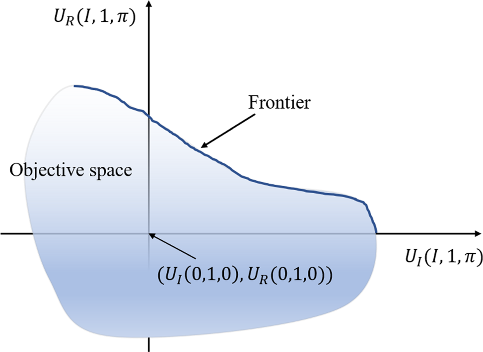
FIGURE 2. The illustrative objective space (shaded area) and Pareto-optimal frontier. The objective space illustrates the attainable utility levels for the insurer and reinsurer jointly, and the Pareto-optimal frontier is the subset of the objective space of the joint utility levels that can be obtained by a Pareto-optimal reinsurance contract.
With the constraints in (3.3), the Lagrangian function for Problem 1a is
 \begin{align*} & U_{{\rm In}}(I,1,\pi)+\beta\cdot U_{{\rm Re}}(I,1,\pi)+\lambda_1\cdot( U_{{\rm In}}(I,1,\pi)-U_{{\rm In}}(0,1,0))+\lambda_2\cdot( U_{{\rm Re}}(I,1,\pi)-U_{{\rm Re}}(0,1,0)) \\ & \quad =(1+\lambda_1)\cdot U_{{\rm In}}(I,1,\pi)+(\beta+\lambda_2)\cdot U_{{\rm Re}}(I,1,\pi)+\text{constants} \\ & \quad =(1+\lambda_1)\cdot\left(U_{{\rm In}}(I,1,\pi)+\frac{\beta+\lambda_2}{1+\lambda_1}\cdot U_{{\rm Re}}(I,1,\pi)\right)+\text{constants}, \end{align*}
where  $\lambda _1, \lambda _2\ge 0$ are the fixed Lagrangian coefficients associated with the constraints in (3.3). Then, for fixed Lagrangian coefficients and fixed $\pi \in [0,\pi _0]$, maximizing the above Lagrangian function is equivalent to
 \begin{equation} \max_{I\in\mathcal{C}}\ U_{{\rm In}}(I,1,\pi)+\tilde{\beta}\cdot U_{{\rm Re}}(I,1,\pi), \end{equation}
where  $\tilde {\beta }={(\beta +\lambda _2)}/{(1+\lambda _1)}\in [0,\infty )$. By the Lagrangian sufficiency theorem, solutions of the Problem (3.4) that satisfy the constraints (3.3) are solutions of Problem 1a subject to (3.3). For some specific $\beta \in [0,\infty )$, if the unconstrained solution $I$ to Problem 1a happens to satisfy (3.3), then $\lambda _1=\lambda _2=0$ and $\tilde {\beta }=\beta$. However, if the unconstrained solution $I$ violates (3.3), then at least one of $\lambda _1$ and $\lambda _2$ is not equal to $0$ and thus at least one of the individual rationality constraints is binding. Based on the Lagrangian function, this leads to $\tilde {\beta }\neq \beta$. For a feasible solution to exist, it must hold that the fixed premium $\pi \in [0,\pi _0]$ is such that $U_{{\rm In}}(X,1,\pi )\ge U_{{\rm In}}(0,1,0)$. We follow Jiang et al. [Reference Jiang, Hong and Ren29] by treating $\beta$ as a parameter in our problem and solve Problem 1a for different values of $\beta$ until we find a point on the frontier and within the first quadrant. This does not raise any technical difficulties if one can solve Problem 1a for a generic $\beta >0$. So, we only focus on Problem 1a for a generic $\beta >0$.
The last step in solving Problem 1 is deriving the optimal premium  $\pi$. We define the function
 $$Q(I_{d(\pi)},1,\pi)=U_{{\rm In}}(I_{d(\pi)},1,\pi)+\beta\cdot U_{{\rm Re}}(I_{d(\pi)},1,\pi).$$
Via Proposition 3.1, Problem 1 simplifies to the following problem:
 \begin{equation} \max_{\pi\in[0,\pi_0]} Q(I_{d(\pi)},1,\pi).\end{equation}
A closed-form expression of the optimal solution of (3.5) is generally difficult to obtain. We present the next theorem that shows concavity of the optimization problem (3.5).
Theorem 3.1. Let Assumption 1 hold. The mapping  $\pi \mapsto Q(I_{d(\pi )},1,\pi )$ is concave, and thus the optimal premium $\pi ^{*}$ solving (3.5) is given by the first-order condition:
 \begin{equation} \left.\frac{dQ(I_{d(\pi)},1,\pi)}{d\pi}\right|_{\pi=\pi^{*}}\left\{\begin{array}{ll} \leq 0, & \text{if }\pi^{*}=0,\\ = 0, & \text{if }0<\pi^{*}<\pi_0,\\ \geq 0, & \text{if }\pi^{*}=\pi_0. \end{array}\right.\end{equation}
To sum up, (3.2), Proposition 3.1 and Theorem 3.1 jointly characterize the structure of optimal solutions to Problem 1.
Clearly, a larger  $\beta$ will make the agreement more advantageous to the reinsurer. The next proposition echoes this point from the perspective of optimal premium.
Proposition 3.2. Let Assumption 1 hold. The optimal premium  $\pi ^{*}$, as shown in (3.6), is increasing with respect to $\beta$.
With Theorem 3.1 and Proposition 3.2, we gain insight about the optimal premium  $\pi ^{*}$. We provide a comparative analysis to end this section. By concavity of $\pi \mapsto Q(I_{d(\pi )},1,\pi )$, if ${d Q(I_{d(\pi )},1,\pi )}/{d\pi }|_{\pi =\pi _1}\ge 0$ for some $\pi _1\in (0,\pi _0]$, then $\pi ^{*}\in [\pi _1,\pi _0)$ and otherwise $\pi ^{*}\in [0,\pi _1)$. As the optimal deductible level is given by $d=0\vee (w_{{\rm In}}-\pi -[u']^{-1}(\beta ))$, we are interested in knowing whether it holds that $\pi ^{*}> w_{{\rm In}}-[u']^{-1}(\beta )$: then full insurance is optimal. For brevity, we denote by $\hat f_{X|R}(x|R;\alpha,\pi )$ the conditional density function $f_{X|R}(x+K(\alpha,\pi )|R)$. This conditional density function also plays a role in Section 4.2. A sufficient condition for optimality of full insurance is provided in the following proposition.
Proposition 3.3. Let Assumption 1 hold. Let  $\pi _1=w_{{\rm In}}-[u']^{-1}(\beta )$. If
 \begin{equation} \mathbb{E}[R\cdot \hat f_{X|R}(x|R;1,\pi_1)]\ge 0,\quad \text{for all }x\in\mathbb{R}_+, \end{equation}
then  $\pi ^{*}\in (\pi _1,\infty )\cap [0,\pi _0]$ and a full insurance should be agreed between the insurer and reinsurer.
If (3.7) holds, then  $\int _{0}^{\infty }\mathbb {E}[R\cdot \hat f_{X|R}(x|R;1,\pi _1)]dx=\mathbb {E}[R\mathbb{1}_{S^{c}(I_{d(\pi _1)},1,\pi _1)}]\ge 0$, where $S^{c}$ is defined as the complement of $S$. This indicates that the expected excess return rate is non-negative also conditional on the default event to hold. Then, since the reinsurer is assumed to be risk-neutral but protected by limited liability, the reinsurer is willing to sell full insurance in exchange for a high premium that yields a higher amount invested in the risky asset.
This section solves Problem 1 by giving the explicit formulation of  $I^{*}$. Although the explicit optimal premium, $\pi ^{*}$, is hard to derive in a general setting, we show the concavity of the objective function with respect to the premium and this facilitates the development of an efficient algorithm to locate the optimal premium. We conclude this section with an example.
Example 3.1. In the absence of the solvency regulation, we adopt the following setup for the numerical example which examines the optimal premiums and optimal retention points under different negotiation powers and risk aversion parameters.
• The reinsurer is endowed with an initial capital of
$600$. Note that because the insurer is endowed with exponential utility function, the risk preferences are unaffected by the initial capital of the insurer $w_0$, and we set it equal to $500$. The risk-free rate is $r=0.05$.• The random variables
$X$ and $R$ are independent, $X$ is exponentially distributed with mean $400$, and $1+r+R$ is log-normally distributed with log-mean $0$ and log-variance $0.4$. This means that $\mathbb {E}[R]\approx 0.17$.• The insurer's utility function is an exponential utility function
$u(w)=-e^{-\psi w}$ where $\psi >0$. For each risk aversion parameter $\psi$, the maximum premium that the insurer is willing to pay to fully insure $X$ (indifference premium) is determined by the exponential premium [Reference Gerber and Pafumi26]. In this example, we take $\psi \in [10^{-3}, 2\times 10^{-3}]$ such that the exponential premium ranges from $1.3$ to $2$ times the expected loss.• For range of risk aversion parameters, we chose a range of negotiation powers
$\beta$ such that the participation incentive constraints are satisfied.


We show the effect of  $\psi$ and $\beta$ on the optimal premium and retention level in Figure 3. Moreover, we show the corresponding implies default probability in Figure 4. We make the following observations.
• The optimal premium increases with respect to the negotiation power (cf. Proposition 3.2). However, it does not show a monotonic relationship with the insurer's risk aversion parameter as there are two conflicting effects. On the one hand, a larger
$\psi$ is associated with a lower retention point, and this leads to an increase in the premium. For a constant retention point $d$, a larger $\psi$ implies that the insurer's value of the utility function is getting closer to zero, and thus the premium gets smaller to maximize the objective function.• The optimal retention point increases with respect to the negotiation power
$\beta$ and decreases with respect to the insurer's risk aversion parameter. Note that a component in the retention point is $[u']^{-1}(\beta )$, which in this example equals ${\log (\beta /\psi )}/{\psi }$. This component monotonically increases with respect to $\beta$, and monotonically decreases with respect to $\psi$.• The default probability of the reinsurer decreases with respect to the negotiation power
$\beta$ and increases with respect to the insurer's risk aversion parameter $\psi$. Both a lower value of $\beta$ and a larger value of $\psi$ lead to a relatively low premium compared to the retention level, and this yields a higher probability of default for the reinsurer.


FIGURE 3. (Left) The effect of  $\psi$ and $\beta$ on the optimal premium $\pi ^{*}$; (Right) The effect of $\psi$ and $\beta$ on the optimal retention point $d^{*}$.

FIGURE 4. The effect of  $\psi$ and $\beta$ on the probability of default.
4. Pareto-optimal policies with solvency regulation
It has been well-known that the solvency regulation would greatly impact the indemnity function. For instance, in [Reference Filipović, Kremslehner and Muermann25], the solvency regulation is imposed by constraining the risk of the insurance seller (reinsurer) through a convex risk measure such as the tail Value-at-Risk (TVaR). In this section, we instead assume that the solvency constraint is given by a constraint on the probability of default, and this is equivalent to a VaR constraint. The VaR risk measure is used in the insurance industry in, for example, Solvency II regulation for European insurers. In our context, as the indemnity structure could be negotiated, the reinsurer can either sell less coverage or invest less in the risky asset to improve its solvency status. In Subsection 4.1, we study optimal reinsurance contracts when the regulator can only regulate the reinsurance contract. In Subsection 4.2, the regulator can also regulate the investment decision of the reinsurer.
4.1. Regulation constraint on the indemnity function
Let there be a regulator, whose objective is to constrain the probability of default of the reinsurer. The regulator evaluates the reinsurance contract  $(I,\pi )$, and assumes that the reinsurer will invest such that only the utility of the reinsurer is optimized. The general problem that we consider in this subsection is defined as follows.
Problem 2. For  $\beta >0$ and $\xi \in (0,1)$, solve
 \begin{align*} \max_{(I,\pi)\in\mathcal{C}\times[0,\pi_0]}\quad & U_{{\rm In}}(I,\alpha^{*},\pi)+\beta\cdot U_{{\rm Re}}(I,\alpha^{*},\pi) \\ \text{s.t.}\quad & \mathbb{P}(K(\alpha^{*},\pi)\ge I(X))\ge \xi, \\ & \alpha^{*}\in \arg\max_{\alpha\in[0,1]}\ U_{{\rm Re}}(I,\alpha,\pi). \end{align*}
The solvency regulation imposes a constraint on the reinsurer's solvency probability. Problem 2 could also be treated as a game where a social planner (consisting of the insurer and reinsurer) decides the optimal reinsurance contract first and then the reinsurer determines the investment decision in response to the indemnity function. In our game, the social planner can foresee the reinsurer's action, and the regulator can only evaluate the decision of the optimal reinsurance contract made by the social planner.
We remark that Problem 2 is different from that of Filipović et al. [Reference Filipović, Kremslehner and Muermann25], who assume that the solvency regulation constraint is on the investment decision  $\alpha$ only, and so the reinsurer may not be able to invest all wealth in the risky asset. The solvency regulation constraint in our problem, however, takes the optimal investment decision as input, and the investment decision is therefore not affected by regulation. We will study a relaxation of this assumption in Section 4.2.
We first recall from (3.2) that  $\arg\max_{\alpha \in [0,1]}\ U_{{\rm Re}}(I,\alpha,\pi )=\{1\}$. We do not solve Problem 2 in full generality, but we use a step-wise approach to understand the structure of optimal solutions. More precisely, we first fix the premium $\pi$ and solve the following problem, and thereafter we solve Problem 2 numerically in an example.
Problem 2a. For  $\beta >0$, $\xi \in (0,1)$ and $\pi \in [0,\pi _0]$, solve
 \begin{align*} \max_{I\in\mathcal{C}}\quad & U_{{\rm In}}(I,1,\pi)+\beta\cdot U_{{\rm Re}}(I,1,\pi) \\ \text{s.t.}\quad& \mathbb{P}(K(1,\pi)\ge I(X))\ge \xi. \end{align*}
Before presenting the main result of this section, we impose the following assumption.
Assumption 2. The conditional hazard rate function of  $R$, that is, $H_R(\zeta |X=x):={f_{R|X}(\zeta |X=x)}/{(1-F_{R|X}(\zeta |X=x))}$, is increasing with respect to $\zeta \in [-1-r,\infty )$ for all $x\in \mathbb {R}_+$.
Assumption 2 actually states that the likelihood that the investment return will keep growing given that it exceeds some threshold is decreasing. The monotone hazard rate assumption is satisfied if and only if the survival function  $1-F_{R|X}(\cdot |X=x)$ is log-concave, and holds for a variety of distributions, for example, the uniform, the normal, the Pareto, the logistic and the exponential distribution. Such an assumption is commonly adopted in economics literature [Reference Nocke, Peitz and Rosar38,Reference Tirole39].
As an example, suppose that the conditional distribution of  $R|X=x$ follows a shifted Weibull distribution. Then, the hazard rate function is decreasing if its shape parameter $k$ is smaller than 1 and increasing if its shape parameter $k$ is larger than 1. In [Reference Mittnik and Rachev37], the Weibull distribution is said to be with reversion tendency (RT) if $k>1$ and with diversion tendency (DT) if $k<1$. If returns are RT-distributed, explosive bubbles are not expected to last. For asset returns satisfying a Weibull distribution under Assumption 2, the RT property holds. For the modeling of financial returns with Weibull distributions, it is shown in [Reference Mittnik and Rachev36] that $k>1$ is commonly observed.
The following theorem states the main result of this section.
Theorem 4.1. Under Assumptions 1 and 2, for a fixed  $\pi \in [0,\pi _0]$, the indemnity function $I^{*}$ that solves Problem 2a is given by $I^{*}(x)=x\wedge (0\vee y(x;\lambda ))$, where $y(x;\lambda )\in \mathbb {R}$ solves
 \begin{equation} u'(w_{{\rm In}}-x+y(x;\lambda)-\pi)=\beta+\lambda\cdot \frac{H_R(g^{{-}1}(y(x;\lambda))|X=x)}{(w_{{\rm Re}}+\pi)}, \end{equation}
where  $g^{-1}(x)={x}/{(w_{{\rm Re}}+\pi )}-1-r$ and $\lambda \ge 0$ is chosen such that $\lambda \cdot (\mathbb {P}(K(1,\pi )\ge I^{*}(X))-\xi )=0$.
The optimal indemnity function in Theorem 4.1 depends on the distribution function of  $X$ only via the Lagrangian parameter $\lambda$.
It is worth mentioning that, in the literature, the following class of indemnity functions is usually popular
 $$\tilde{\mathcal{C}}:=\left\{I:\mathbb{R}_+\to\mathbb{R}_+ \left|\, \begin{array}{l} I(0)=0\ \text{and} \\ 0\le I(x_2)-I(x_1)\le x_2-x_1\ \text{for}\ 0\le x_1\le x_2 \end{array}\right.\right\},$$
where it clearly holds that  $\tilde {\mathcal {C}}\subset \mathcal {C}$. If the optimal indemnity function belongs to $\tilde {\mathcal {C}}$, the increment of indemnity will not exceed the increment of loss.Footnote 2, Footnote 3 In this case, the insurer has no incentive to over- or under-report the insurable loss and this avoids ex post moral hazard. Note that $I_{d(\pi )}\in \tilde {\mathcal {C}}$, where $I_{d(\pi )}$ is the optimal reinsurance indemnity of Problem 1 without regulation as shown in Proposition 3.1. The following proposition gives a specific case when the indemnity function derived from (4.1) is in $\tilde {\mathcal {C}}$.
Proposition 4.1. If Assumption 2 holds,  $R$ and $X$ are independent and the distribution of $R$ admits a differentiable density function, then the indemnity function characterized by (4.1) is in the class $\tilde {\mathcal {C}}$.
In general, the solution to Eq. (4.1) is implicit and this complicates the derivation of the explicit optimal  $\pi$ in the next step. As such, the optimal $\pi$ is to be sought in a numerical manner.
To show the impact of solvency regulation constraint on the optimal indemnity function, we study a simple example to end this section.
Example 4.1. Empirical distributions of asset returns often exhibit leptokurtic patterns and thus may not be fully depicted by a normal distribution. Among leptokurtic distributions, the Weibull distribution turns out to be an appropriate, stable distribution for the modeling of asset returns [Reference Mittnik and Rachev37]. Chen and Gerlach [Reference Chen and Gerlach18] apply a Weibull distribution to model conditional financial asset return distributions and show that the Weibull distribution performs at least as well as other distributions for VaR forecasting.
For simplicity, we assume that the excess return  $R$ is independent of $X$. Furthermore, we assume that the excess return $R$ follows a shifted Weibull distribution whose probability density function and cumulative distribution function are given by
 $$f_R(\zeta)=\frac{k}{\theta}\left(\frac{\zeta+1+r}{\theta}\right)^{k-1}e^{-({(\zeta+1+r)}/{\theta})^{k}},\quad F_R(\zeta)=1-e^{-({(\zeta+1+r)}/{\theta})^{k}}.$$
Furthermore, to get an increasing hazard rate function, we let  $k>1$ and pick $k=2$.
Assume that the insurer's utility function is a quadratic utility function:
 \begin{equation} u(w)=\left\{\begin{array}{ll} -\dfrac{1}{2}\gamma w^{2}+w, & w\le\dfrac{1}{\gamma}, \\[6pt] \dfrac{1}{2\gamma}, & w>\dfrac{1}{\gamma}, \end{array}\right. \end{equation}
where  ${1}/{\gamma }$ is called the saturation point, beyond which the insurer's utility will not be increased. To this end, Eq. (4.1) becomes
 $$-\gamma(w_{{\rm In}}-x+y(x;\lambda)-\pi)+1=\beta+\frac{\lambda}{w_{{\rm Re}}+\pi}\cdot\frac{2}{\theta^{2}}\cdot\frac{y(x;\lambda)}{w_{{\rm Re}}+\pi}.$$
As per Theorem 4.1, the optimal indemnity function for Problem 2a is given by
 \begin{equation} I^{*}(x)=x\wedge \frac{\gamma}{\gamma+\frac{2\lambda}{\theta^{2}(w_{{\rm Re}}+\pi)^{2}}}\left(x-(w_{{\rm In}}-\pi-\frac{1-\beta}{\gamma})\right)_+, \end{equation}
where  $\pi \in [0,\pi _0]$ is fixed. As a comparison, the optimal indemnity function for Problem 1a is given by
 \begin{equation} I_{d(\pi)}(x)=x\wedge \left(x-(w_{{\rm In}}-\pi-\frac{1-\beta}{\gamma})\right)_+. \end{equation}
We illustrate the two indemnity functions in (4.3) and (4.4) in Figure 5. We make the following observations.
• The solvency regulation requires the reinsurer to sell less coverage so that the solvency status could be maintained.
• The smaller the value of
$\xi$ is, or equivalently the stronger the solvency regulation is (larger $\lambda$), the less the coverage is (smaller ${\gamma }/{(\gamma +{2\lambda }/{\theta ^{2}(w_{{\rm Re}}+\pi )^{2}})}$).• The cheaper the policy is (smaller
$\pi$), the less the coverage is (smaller ${\gamma }/{(\gamma +{2\lambda }/{\theta ^{2}(w_{{\rm Re}}+\pi )^{2}})}$ and larger $d(\pi )$).


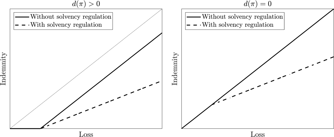
FIGURE 5. Comparison between the indemnity functions with and without solvency regulation (for Example 4.1).
Example 4.1 shows an explicit solution for Problem 2a. The following numerical example relates the optimal premium with the intensity of solvency regulation and the negotiation power.
Example 4.2. In this example, we investigate the effect of solvency regulation on the indemnity function. As an explicit indemnity function facilitates the computation, we adopt a similar setup as Example 4.1.
• The insurer and reinsurer are endowed with initial capital
$200$ and $500$, respectively. The risk-free rate is $r=0.05$.• The random variables
$X$ and $R$ are independent, $X$ is exponentially distributed with mean $500$ and $1+r+R$ follows a Weibull distribution with scale parameter $1.3$ and shape parameter $2$. Under this setup, it holds that $\mathbb {E}[R]\approx 11\%$.• The insurer's utility function is given by the quadratic utility function (see (4.2)) with
$\gamma =1/700$ such that the quadratic premium exists [Reference Gerber and Pafumi26]. In this case, the maximum premium that the insurer is willing to pay to fully insure $X$ is equal to two times the expected loss.


As the optimal indemnity function takes the form  $I^{*}(x)=x\wedge \{c\cdot (x-d)_+\}$ (see (4.3)), we show in Table 1 the effect of the negotiation power $\beta$Footnote 4 and solvency probability $\xi$ on the optimal premium and indemnity function.
TABLE 1. The effect of the negotiation power  $\beta$ and solvency probability $\xi$ on the optimal premium and indemnity function. Here, $I^{*}(x)=x\wedge \{c\cdot (x-d)_+\}$.

From Table 1, we observe that the optimal premium still increases with respect to the insurer's negotiation power  $\beta$. Moreover, the proportion of ceded loss decreases with respect to the required solvency probability $\xi$, and the optimal premium also decreases with respect to the required solvency probability. We illustrate these optimal indemnity functions in Figure 6.

FIGURE 6. A graphical comparison between the cases presented in Table 1.
4.1.1. The case when $H_R(\zeta |X=x)$ is decreasing

The derivation of the indemnity function in Section 4.1 is due to the increasingness of the conditional hazard rate function  $H_R(\zeta |X=x)$. If $H_R(\zeta |X=x)$ is decreasing, then without more assumptions on the utility and hazard rate functions, the objective is no more concave, and the first-order condition may no longer yield a global maximum.
Note that
 $$H_R(\zeta|X=x)={-}\frac{d \log(S_{R|X}(\zeta|X=x))}{d \zeta}$$
and therefore
 \begin{align*} H_R(\zeta|X=x)\ \text{is decreasing}\ & \Longleftrightarrow\ \log(S_{R|X}(\zeta|X=x))\ \text{is convex} \\ & \Longleftrightarrow\ \log(S_{K|X}(k|X=x))\ \text{is convex}. \end{align*}
Applying Jensen's inequality leads to
 \begin{align*} \mathbb{P}(K\ge I(X))& =\exp(\log(\mathbb{P}(K\ge I(X)))) =\exp(\log(\mathbb{E}_X[S_{K|X}(I(X)|X)])) \\ & \ge \exp(\mathbb{E}_X[\log(S_{K|X}(I(X)|X))]) \ge \exp(\log(S_K(\mathbb{E}_X[I(X)])))\\ & =\mathbb{P}(K\ge \mathbb{E}_X[I(X)]), \end{align*}
where the first inequality is due to the concavity of  $\log (\cdot )$ and the second inequality is due to the convexity of $\log (S_{K|X}(\cdot |X=x))$. Therefore, $\mathbb {P}(K\ge \mathbb {E}[I(X)])\ge \xi$ implies $\mathbb {P}(K\ge I(X))\ge \xi$, and thus imposing $\mathbb {P}(K\ge \mathbb {E}[I(X)])\ge \xi$ is more strict than imposing $\mathbb {P}(K\ge I(X))\ge \xi$. Since $R$ is a continuous random variable (see Assumption 1), we have that $\mathbb {P}(K\ge \mathbb {E}[I(X)])\ge \xi$ is equivalent to
 $$\mathbb{E}[I(X)]\le F_{1-\xi}^{{-}1}(K),$$
where  $F_{1-\xi }^{-1}(K)$ is also called the $(1-\xi )$-quantile of the continuous random variable $K$.
$K$.
Instead of Problem 2a, we investigate the following problem in this subsection.
Problem 2b. For  $\beta >0, \xi \in (0,1)$ and $\pi \in [0,\pi _0]$, solve
 \begin{align*} \max_{I\in\mathcal{C}}\quad & U_{{\rm In}}(I,1,\pi)+\beta\cdot U_{{\rm Re}}(I,1,\pi) \\ \text{s.t.}\quad & \mathbb{E}[I(X)]\le F_{1-\xi}^{{-}1}(K). \end{align*}
As the constraint of Problem 2b is more strict than that of Problem 2a, the solution to Problem 2b is not necessarily a solution to Problem 2a. However, the solution to Problem 2b is feasible to Problem 2a.
Note that the solution of Problem 2b is also a solution of Problem 2a if  $X$ is deterministic.
Theorem 4.2. If  $H_R(\zeta |X=x)$ is decreasing, then for a fixed $\pi \in [0,\pi _0]$, the indemnity function $I^{*}$ that solves Problem 2b is given by $I^{*}(x)=x\wedge (0\vee y(x;\lambda ))$ where $y(x;\lambda )\in \mathbb {R}$ solves
 \begin{equation} u'(w_{{\rm In}}-x+y(x;\lambda)-\pi)=\beta+\frac{\lambda}{S_{R|X}(g^{{-}1}(y(x;\lambda))|X=x)}, \end{equation}
where  $g^{-1}(x)= {x}/{(w_{{\rm Re}}+\pi )}-1-r$ and $\lambda \ge 0$ is chosen such that $\lambda \cdot (\mathbb {P}(K(1,\pi )\ge \mathbb {E}[I^{*}(X)])-\xi )=0$.
The proof is similar to that for Theorem 4.1 and thus omitted. Note that since  ${1}/{S_{R|X}(g^{-1}(\cdot ))|X=x)}$ is increasing, Eq. (4.5) admits a unique solution on $\mathbb {R}$. Similar to Proposition 4.1, if $X$ and $R$ are independent, we again have $I^{*}\in \tilde {\mathcal {C}}$.
We close this section by presenting an example, which compares the solutions of Problems 2a and 2b for a specific case.
Example 4.3. As in Example 4.1, we assume that the insurer is endowed with a quadratic utility function and that  $X$ and $R$ are independent. We further assume that $1+r+R$ follows the Weibull distribution with mean $\mu$ ( $=\theta \cdot \Gamma (1+{1}/{k}$)). In contrast to Example 4.1, we let $k=0.5$ here so that the hazard rate function of $R$ is decreasing. The optimal indemnity functions for Problems 2a and 2b are given by $I^{*}(x)=x\wedge (y(x;\lambda )\vee 0)$ where $y(x;\lambda )$ is a solution of
 $$u'(w_{{\rm In}}-x+y(x;\lambda)-\pi)=\beta+\frac{0.5\cdot \lambda}{\sqrt{\theta\cdot(w_{{\rm Re}}+\pi)}}\cdot \frac{1}{\sqrt{y(x;\lambda)}}\quad \text{for Problem 2a},$$
and
 $$u'(w_{{\rm In}}-x+y(x;\lambda)-\pi)=\beta+\lambda\cdot e^{\sqrt{\frac{y(x;\lambda)}{\theta\cdot(w_{{\rm Re}}+\pi)}}}\quad \text{for Problem 2b}.$$
Note that the first equation may admit more than one solution and thus the optimal indemnity function might have jumps. Therefore, solutions to Problem 2a may not be in  $\tilde {\mathcal {C}}$, while it must hold that solutions to Problem 2b are in $\tilde {\mathcal {C}}$. Figure 7 shows the indemnity functions for two different cases of expected loss parameter $\mu$.


In this example, the indemnity function that solves Problem 2b covers small losses more and provides less coverage for large losses compared with the solution of Problem 2a. Moreover, the two indemnity functions get closer to each other when  $\mu$ increases. This is as expected since the riskiness of investment returns then increases relative to the riskiness of $X$. Moreover, when $\mu$ increases, the indemnity functions that solve Problems 2a and 2b both get closer to the optimal indemnity function for the case without regulation constraint. This is as expected since larger investment returns lead to more capacity for the reinsurer to cover insurance risk.
4.2. Regulation constraint with regulation on the insurance indemnity and the investment decision of the reinsurer
In Section 4.1, the investment decision is not affected by regulation since the regulation constraint directly takes the optimal investment decision as given. A more realistic situation is to impose the constraint jointly on the reinsurance contract and the parameter  $\alpha$. In this case, the complexity of the problem is enhanced substantially as the indemnity function $I$ and the fraction $\alpha$ jointly affect the probability of default. For simplicity, we restrict ourselves to the class of excess-of-loss functions only, that is, $\{I_d(x)=(x-d)_+,\ d\ge 0\}$, and study the following problem with a fixed premium.
Problem 3. For  $\beta >0$, $\xi \in (0,1)$ and $\pi \in [0,\pi _0]$, solve
 \begin{align*} \max_{d\in [0,\infty)}\quad & \mathcal{F}(d):=U_{{\rm In}}(I_d,\alpha^{*},\pi)+\beta\cdot U_{{\rm Re}}(I_d,\alpha^{*},\pi) \\ \text{s.t.}\quad & \alpha^{*}\in \arg\max_{\alpha\in[0,1]}\ U_{{\rm Re}}(I_d,\alpha,\pi) \text{ s.t. } \mathbb{P}(K(\alpha,\pi)\ge I_d(X))\ge \xi. \end{align*}
From (3.1), it follows that  $U_{{\rm Re}}(I_d,\alpha,\pi )$ is increasing in $\alpha$ under Assumption 1. If $\mathbb {P}(K(\alpha,\pi )\ge I_d(X))$ would be increasing in $\alpha$, then Problem 3 is solved by a solution with $\alpha ^{*}=1$, and Problem 3 has the same solutions as the solutions of Problem 1 (the unconstrained problem). This is however a strong assumption and, in general, $\mathbb {P}(K(\alpha,\pi )\ge I_d(X))$ depends on the joint distribution of $X$ and $R$ and is not necessarily monotone. We make the following assumption for simplification.
Assumption 3. For every  $\pi \in [0,\pi _0]$ and $d\in [0,\infty )$, the probability $\mathbb {P}(K(\alpha,\pi )\ge I_d(X))$ is decreasing in $\alpha$.
Under Assumption 3, investing more in the risky asset leads to a higher probability of default. The risky asset does not serve as a hedge of  $I_d(X)$ in order to mitigate default risk, but rather increases the probability of default for the reinsurer. Under Assumption 3, we get
 \begin{align} \frac{\partial \mathbb{P}(K(\alpha,\pi)\ge I_d(X))}{\partial \alpha}& = \frac{\partial}{\partial \alpha}\int_{{-}1-r}^{\infty}\int_{0}^{(w_{{\rm Re}}+\pi)(1+r+\alpha\zeta)+d} f_{X,R}(x,\zeta) dx d\zeta \nonumber\\ & =(w_{{\rm Re}}+\pi)\int_{{-}1-r}^{\infty}\zeta\cdot f_{X,R}((w_{{\rm Re}}+\pi)(1+r+\alpha\zeta)+d,\zeta) d\zeta \nonumber\\ & =(w_{{\rm Re}}+\pi)\int_{{-}1-r}^{\infty}\zeta\cdot f_{X,R}(K(\alpha,\pi)+d,\zeta) d\zeta\le 0. \end{align}
Recall the notation used in Proposition 3.3. We readily derive from (4.6) the following result.
Proposition 4.2. Assumption 3 is equivalent to
 \begin{equation} \mathbb{E}[R\cdot \hat f_{X|R}(x|R;\alpha,\pi)]\le 0,\quad \text{for all }x\in\mathbb{R}_+. \end{equation}
Recall that  $\hat {f}_{X|R}(x|R;\alpha,\pi )=f_{X|R}(x+K(\alpha,\pi )|R)$. The standard formula in Solvency II assumes a negative linear correlation between the insurance risk $X$ and the market risk $R$. Since $K(\alpha,\pi )$ is an increasing function of $R$, the conditional density function $f_{X|R}(x+K(\alpha,\pi )|R)$ may take large values for small $R$ and small values for large $R$. To see more practical implications, one can take the integral of $\mathbb {E}[R\cdot \hat f_{X|R}(x|R;\alpha,\pi )]$ over an infinitesimal interval $[d,d+\Delta d]$ of $x$:
$x$:
 \begin{align*} \int_{d}^{d+\Delta d}\mathbb{E}[R\cdot \hat f_{X|R}(x|R;\alpha,\pi)]dx& =\int_{d}^{d+\Delta d}\int_{{-}1-r}^{\infty}\zeta f(K+x,\zeta)dxd\zeta \\ & =\int_{{-}1-r}^{\infty}\zeta\left\{\int_{d}^{d+\Delta d}f(K+x,\zeta)dx \right\}d\zeta\\ & =\int_{{-}1-r}^{\infty}\zeta\left\{\int_{K+d}^{K+d+\Delta d}f(t,\zeta)dt\right\}d\zeta \\ & =\int_{{-}1-r}^{\infty}\int_{K+d}^{\infty}\zeta f(t,\zeta)dtd\zeta-\int_{{-}1-r}^{\infty}\int_{K+d+\Delta d}^{\infty}\zeta f(t,\zeta)dtd\zeta \\ & =\mathbb{E}[R\cdot \mathbb{1}_{S^{c}(I_{d},\alpha,\pi)}]-\mathbb{E}[R\cdot\mathbb{1}_{S^{c}(I_{d+\Delta d},\alpha,\pi)}] \\ & =\mathbb{E}[R\cdot \mathbb{1}_{S(I_{d+\Delta d},\alpha,\pi)}]-\mathbb{E}[R\cdot\mathbb{1}_{S(I_{d},\alpha,\pi)}], \end{align*}
which is non-positive if (4.7) holds. Note that  $S(I_d,\alpha,\pi )\subseteq S(I_{d+\Delta d},\alpha,\pi )$, and so (4.7) indicates that the expected investment return conditional on solvency is larger when the reinsurer provides more coverage (a lower deductible). Moreover, the integral of (4.7) over the full range of $x$ leads to $\int _{0}^{\infty }\mathbb {E}[R\cdot \hat f_{X|R}(x+d|R;\alpha,\pi )]dx=\mathbb {E}[R\cdot \mathbb{1}_{S^{c}(I_d,\alpha,\pi )}]\le 0$, and so $\mathbb {E}[R\cdot \mathbb{1}_{S(I_d,\alpha,\pi )}]\ge \mathbb {E}[R]$ for all $d\geq 0$. This is a stronger assumption than Assumption 1(i). Conditional on being solvent, the expected investment returns are higher than the unconditional expected investment returns. Based on this derivation, the following proposition provides a sufficient condition under which Assumption 3 holds.
Proposition 4.3. If  $R|S^{c}(X,0,0)\leq 0$, then Assumption 3 holds.
The condition  $R|S^{c}(X,0,0)\leq 0$ is quite strong, and implies that in all scenarios in which the reinsurer defaults without investing in the risky technology, increasing the investment exposure $\alpha$ will be only more harmful as the excess return $R$ is then negative. Thus, investments cannot be used to “gamble for resurrection,” as the investment returns will not help to avoid default.
Since  $I_d(x)$ is decreasing with respect to $d$ for fixed $x$, the probability $\mathbb {P}(K(\alpha,\pi )\ge I_d(X))$ is increasing with respect to $d$. In a limit case, $\lim _{d\to \infty } I_d(x)=0$ and thus
 $$\lim_{d\to \infty} \mathbb{P}(K(\alpha,\pi)\ge I_d(X))=1>\xi,$$
for any  $\alpha \in [0,1]$. Define
 \begin{align} \bar{d}& :=\inf\{d\in\mathbb{R}_+: \mathbb{P}(K(1,\pi)\ge I_d(X))\ge \xi\}, \end{align}
 \begin{align} \underline{d}& :=\inf\{d\in\mathbb{R}_+: \mathbb{P}(K(0,\pi)\ge I_d(X))\ge \xi\}, \end{align}
then, by (3.1),
 \begin{equation} \alpha^{*}=\left\{\begin{array}{ll} 1, & \bar{d}< d, \\ \alpha(d), & \underline{d}\le d\le \bar{d}, \end{array}\right. \end{equation}
where  $\alpha (d)$ is such that $\mathbb {P}(K(\alpha (d),\pi )\ge I_d(X))=\xi$. Assume that $\mathbb {P}(K(\alpha,\pi )\ge I_d(X))$ is strictly decreasing in $\alpha$ for all $d\in (\underline {d},\bar {d})$. Then, we get from the implicit function theorem that
 $$\frac{\partial \mathbb{P}(K(\alpha(d),\pi)\ge I_d(X))}{\partial d}=0\ \Longrightarrow\ \alpha'(d)=\frac{-\int_{{-}1-r}^{\infty}f_{X,R}(K(\alpha,\pi)+d,\zeta)d\zeta}{\int_{{-}1-r}^{\infty}\zeta\cdot f_{X,R}(K(\alpha,\pi)+d,\zeta)d\zeta}\cdot\frac{1}{w_{{\rm Re}}+\pi}\ge 0.$$
Note that the objective in Problem 3 with  $\alpha ^{*}$ above is continuous in $d$ on the interval $[\underline {d},\bar d]$ and, if the solution $d^{*}$ is such that $d^{*}>\bar {d}$, then it must hold by Proposition 3.1 that $d^{*}=\tilde d$, with
 \begin{equation} \tilde{d}=0\vee (w_{{\rm In}}-\pi-[u']^{{-}1}(\beta)). \end{equation}
We next identify several sufficient conditions under which the optimal deductible level is still  $\tilde {d}$ and under which the optimal deductible level is different from $\tilde {d}$. For this purpose, we define the following function:
 \begin{align*} \mathbf{Q}(x;d):& =\frac{\int_{0}^{x}\mathbb{E}[R\cdot \hat f_{X|R}(t+d|R;\alpha^{*},\pi)]dt}{\mathbb{E}[R\cdot\mathbb{1}_{S^{c}(I_d,\alpha^{*},\pi)}]}\\ & =\frac{\mathbb{E}[R\cdot \mathbb{1}_{S^{c}(I_d,\alpha^{*},\pi)}]-\mathbb{E}[R\cdot\mathbb{1}_{S^{c}(I_{d+x},\alpha^{*},\pi)}]}{\mathbb{E}[R\cdot\mathbb{1}_{S^{c}(I_d,\alpha^{*},\pi)}]}\\ & =1-\frac{\mathbb{E}[R\cdot\mathbb{1}_{S^{c}(I_{d+x},\alpha^{*},\pi)}]}{\mathbb{E}[R\cdot\mathbb{1}_{S^{c}(I_d,\alpha^{*},\pi)}]}. \end{align*}
Here,  $\mathbf {Q}(x;d)$ is equal to the relative change of the expected excess of return in an insolvent environment when the retention point changes from $d$ to $d+x$. Moreover, $\mathbf {Q}(x;d)$ is increasing in $x$,
$x$,  $\mathbf {Q}(0;d)=0$ and $\lim _{x\to \infty }\mathbf {Q}(x;d)=1$, and so $\mathbf {Q}(\cdot ;d)$ is a cumulative distribution function.
Theorem 4.3. Recall  $\tilde d$ from (4.11) and $\underline {d},\bar d$ from (4.8) and (4.9). Let $G(x;d)=u'(w_{{\rm In}}-x-d-\pi )$, Assumptions 1 and 3 hold and let $\mathbb {P}(K(\alpha,\pi )\ge I_d(X))$ be strictly decreasing in $\alpha$ for all $d\in (\underline {d},\bar {d})$. Then, the following statements hold.
(i) If
$\tilde {d}\ge \bar {d}$, then the optimal retention point that solves Problem 3 exists and is equal to $\tilde {d}$.(ii) If
$\underline {d}<\tilde {d}<\bar {d}$ and $\int _{0}^{\infty }G(x;d)d\mathbf {Q}(x;\tilde {d})+\beta \cdot {\mathbb {E}[R\cdot \mathbb{1}_{S(I_{\tilde {d}},\alpha ^{*},\pi )}]}/{\mathbb {E}[R\cdot \mathbb{1}_{S^{c}(I_{\tilde {d}},\alpha ^{*},\pi )}]}\ge 0$, then the optimal retention point that solves Problem 3 exists and is in $[\underline {d}, \tilde {d}]$.(iii) If
$\tilde {d}\le \underline {d}$, then the optimal retention point that solves Problem 3 exists and is in $[\underline {d},\bar {d}]$.


Theorem 4.3 states that if the optimal retention point without regulation allows for a full investment of the risky asset, the optimal retention point with regulation is still given by  $\tilde {d}$. Moreover, if the insurer is very risk-averse (large $G(x;d)$) and if the optimal retention point without regulation does not allow for full investment of the risky asset in the constrained Problem 3, then the optimal investment is less than 100% in the risky asset and the optimal retention point might be different from $\tilde {d}$.
We next discuss an implication of Theorem 4.3(ii) and its sufficient condition. The next corollary presents a case with specific utility function, loss distribution, and dependence structure.
Corollary 4.1. Let Assumptions 1 and 3 hold,  $\mathbb {P}(K(\alpha,\pi )\ge I_d(X))$ be strictly decreasing in $\alpha$ for all $d\in (\underline {d},\bar {d})$, and moreover,
1. the loss
$X$ and excess rate of return $R$ are independent;2. the loss
$X$ follows an exponential distribution with parameter $\mu >0$: $f_X(x)=({1}/{\mu })e^{-{x}/{\mu }}$ for all $x\geq 0$;3. the insurer is endowed with an exponential utility function with parameter
$\psi >0$.


Let  $\mathcal {K}(d)=\mu -{\mu }/{\mathbb {E}[R]}\cdot \int _{-1-r}^{\infty }e^{-{(K+d)}/{\mu }}\cdot \zeta \cdot f_R(\zeta )d\zeta$. If $\underline {d}<\tilde {d}<\bar {d}$ and $\mathcal {K}(\tilde {d})\ge {1}/{\psi }$, then the optimal retention point that solves Problem 3 is in $[\underline {d},\tilde {d}]$.
Note that  $\mu \cdot \psi <1$ is equivalent to assuming the exponential premium to be finite [Reference Boonen and Liu11]. The condition $\mathcal {K}(\tilde {d})\ge {1}/{\psi }$ in Corollary 4.1 is equivalent to
 $$\mu\cdot\psi\ge 1+\frac{\mathbb{E}[R\cdot\mathbb{1}_{S^{c}(I_{\tilde{d}},\alpha^{*},\pi)}]}{\mathbb{E}[R\cdot\mathbb{1}_{S(I_{\tilde{d}},\alpha^{*},\pi)}]}.$$
The above inequality holds when: (i) the insurer is very risk-averse ( $\psi$ is large); (ii) the expected loss $\mu$ is large and (iii) the event $S^{c}(I_{\tilde {d}},\alpha ^{*},\pi )$ occurs with large probability. In such circumstance, the insurer would require substantial coverage (a small retention point) under the same premium level.
Example 4.4. We adopt the following setting in this example.
• The insurer and reinsurer are endowed with initial capital
$300$ and $500$, respectively. The risk-free rate is $r=0.05$.• The loss
$X$ follows the exponential distribution with mean 400 and the excess of return $R$ follows the log-normal distribution with log-mean $0$ and log-variance $0.4$ such that $\mathbb {E}[R]\approx 0.17$. Moreover, we assume that the joint distribution function of $X$ and $R$ is given by
where$$F_{X,R}(x,\eta)=C_G(F_X(x),F_R(\eta); \rho),$$
$C_G(\cdot,\cdot ;\rho )$ denotes the Gaussian copula function with $\rho$ as the linear correlation coefficient. In this example, we let $\rho =-0.25$ so that $X$ and $R$ are negatively correlated as in the standard formula of Solvency II regulations.• The insurer's utility function is an exponential utility function with
$\psi$ being one of the following three different levels: $10^{-3}$, $1.1\times 10^{-3}$ and $1.2\times 10^{-3}$. For each $\psi$, the maximum premium, denoted by $p_{\max }$, that the insurer is willing to pay is determined by indifference premium (exponential premium) of $X$.


Figure 8 provides an example of the probability  $\mathbb {P}(K(\alpha,\pi )\ge I_d(X))$ for a fixed premium with $\pi =100$ and for selected five values of $d$. The probability $\mathbb {P}(K(\alpha,\pi )\ge I_d(X))$ is then decreasing with respect to $\alpha$.

FIGURE 8. An illustration of  $\mathbb {P}(K(\alpha,\pi )\ge I_d(X))$ with respect to $\alpha$ for various choices of the retention level $d$.
$d$.
In Problem 3, the premium level is fixed. Next, we numerically solve the optimal premium by maximizing the function  $\pi \mapsto U_{{\rm In}}(I_{d^{*}},\alpha ^{*},\pi )+\beta \cdot U_{{\rm Re}}(I_{d^{*}},\alpha ^{*},\pi )$ over the range $[0,p_{\max }]$. In Table 2, we show the optimal reinsurance parameters $(d^{*},\alpha ^{*}, \pi ^{*})$ for various choices of the solvency probability $\xi$, the negotiation power $\beta$ and the insurer's risk aversion parameter $\psi$.
TABLE 2. The optimal reinsurance parameters  $(d^{*},\alpha ^{*},\pi ^{*})$ as a function of the model parameters $(\beta,xi,\psi)$.

We make the following observations.
• The optimal premium decreases with respect to the negotiation power.
• The optimal retention point moves in the opposite direction of the optimal premium.
• In many cases in this example, the optimal fraction of investment
$\alpha ^{*}$ decreases at first and then increases with respect to the required solvency probability $\xi$. This might be attributed to the fact that with an increased solvency probability $\xi$, if the reinsurer decides to sell more coverage for a high premium, the optimal fraction of investment $\alpha ^{*}$ should decrease to meet the solvency regulation constraint. If the reinsurer decides to reduce the coverage and charge less, there is more room to increase $\alpha ^{*}$ under the solvency constraint and the reinsurer increases $\alpha ^{*}$ to maximize its utility.


5. Concluding remarks and future research
This paper studies a one-period optimal reinsurance problem when the reinsurer is allowed to invest its wealth in some risky assets and is protected by limited liability. The optimal reinsurance policy is determined by optimizing a weighted average of the utilities of the insurer and reinsurer. In the absence of solvency regulation constraint, excess-of-loss contracts are shown to be optimal, while the premium follows from solving a concave objective function.
We model solvency regulation as a constraint on the probability of default of the reinsurer, and we show how this affects the shape of optimal indemnities if the regulator can only affect the reinsurance contract. If the regulator can jointly regulate the reinsurer's investment behavior and the reinsurance contract, we show sufficient conditions under which the reinsurer will decrease the exposure to the risky asset. We show this in the setting where the reinsurance indemnity has to be of an excess-of-loss form. For further research, we propose to study reinsurance markets in which the indemnities are allowed to take more general functional forms.
A main assumption in our model is symmetric information, as the joint distribution of the insurable loss and the investment return is known by the insurer and reinsurer. Also, our focus is on a single insurer, and the reinsurer is not endowed with background risk that arises from the selling of multiple insurance policies. For future research, we also suggest to study the impact of asymmetric information and the effect of the presence of multiple insurers.
Acknowledgments
W. Jiang acknowledges the financial support received from the Natural Sciences and Engineering Research Council (RGPIN-2020-04204, DGECR-2020-00332) of Canada. W. Jiang is also grateful to the start-up grant received from the University of Calgary.
Conflicts of interest
The authors declare no conflict of interest.
Appendix
Proof of Proposition 2.1
Let  $I\in \mathcal {C}$, $\alpha \in [0,1]$ and $\pi \in [0,\pi _0]$. Moreover, assume that $R$ and $X$ are independent. Then, for all $x\in \mathbb {R}_+$, we know that $1_{S(I,\alpha,\pi )}|X=x$ is an increasing function of $R$. Thus, $\mathbb {E}[R1_{S(I,\alpha,\pi )}|X=x]\geq \mathbb {E}[R|X=x]\mathbb {E}[1_{S(I,\alpha,\pi )}|X=x]$. Then, the result follows directly from
 \begin{align*} \mathbf{C}{\rm ov}(R,1_{S(I,\alpha,\pi)})& =\mathbb{E}[R1_{S(I,\alpha,\pi)}]-\mathbb{E}[R]\mathbb{E}[1_{S(I,\alpha,\pi)}]\\ & =\mathbb{E}[\mathbb{E}[R1_{S(I,\alpha,\pi)}|X]]-\mathbb{E}[R]\mathbb{E}[1_{S(I,\alpha,\pi)}]\\ & \geq\mathbb{E}[\mathbb{E}[R|X]\mathbb{E}[1_{S(I,\alpha,\pi)}|X]]-\mathbb{E}[R]\mathbb{E}[1_{S(I,\alpha,\pi)}]\\ & =\mathbb{E}[R]\cdot\mathbb{E}[\mathbb{E}[1_{S(I,\alpha,\pi)}|X]]-\mathbb{E}[R]\mathbb{E}[1_{S(I,\alpha,\pi)}]\\ & = \mathbb{E}[R]\cdot\mathbb{E}[1_{S(I,\alpha,\pi)}]-\mathbb{E}[R]\mathbb{E}[1_{S(I,\alpha,\pi)}]=0. \end{align*}
This concludes the proof.
Proof of Proposition 3.1
For brevity, we write  $K(\alpha,\pi )$ as $K$, where $\alpha \in [0,1]$ and $\pi \in [0,\pi _0]$. The range of $K$ is $[\underline {k},\infty )$, where $\underline {k}=(w_{{\rm Re}}+\pi )(1-\alpha )(1+r)$. Furthermore, we denote by $f_{K|X}(\cdot |X=x)$ and $F_{K|X}(\cdot |X=x)$ respectively the probability density function and distribution function of $K$ conditional on $X=x$.
Using the double expectation formula, the objective function in Problem 1a can be written as
 $$\mathbb{E}_X[\mathbb{E}_K[u(w_{{\rm In}}-x+K\wedge I(x)-\pi)\big|X=x]+\beta\cdot \mathbb{E}_K[(K-I(x))_+|X=x]].$$
Therefore, solving Problem 1a is equivalent to maximizing the integrand within  $\mathbb {E}_X[\cdot ]$ element-wisely. In other words,
 $$I^{*}(x)= \arg\max_{y\in[0,x]}\ L(y)$$
where
 \begin{equation} L(y)=\mathbb{E}_K[u(w_{{\rm In}}-x+K\wedge y-\pi)\big|X=x]+\beta\cdot \mathbb{E}_K[(K-y)_+\big|X=x]. \end{equation}
Expanding (A.1) yields
 $$L(y)=\left\{\begin{array}{ll} \displaystyle\int_{\underline{k}}^{\infty}u(w_{{\rm In}}-x+y-\pi)dF_{K|X}(k|X=x)+\beta\cdot\int_{\underline{k}}^{\infty}(k-y)dF_{K|X}(k|X=x), & 0\le y\le \underline{k}, \\ \displaystyle\int_{0}^{y}u(w_{{\rm In}}-x+k-\pi)dF_{K|X}(k|X=x)+\int_{y}^{\infty}u(w_{{\rm In}}-x+y-\pi)dF_{K|X}(k|X=x) & \\ \displaystyle\quad +\beta\cdot\int_{y}^{\infty}(k-y)dF_{K|X}(k|X=x), & \underline{k}< y. \end{array}\right.$$
Then,
 $$L'(y)=\left\{\begin{array}{ll} u'(w_{{\rm In}}-x+y-\pi)-\beta, & 0\le y\le\underline{k}, \\ (1-F_{K|X}(y\,|\,X=x))\cdot(u'(w_{{\rm In}}-x+y-\pi)-\beta), & \underline{k}< y. \end{array}\right.$$
Note that  $\lim _{y\to \underline {k}-}L'(y)=\lim _{y\to \underline {k}+}L'(y)$ and $L(y)$ is concave on both $[0,\underline {k}]$ and $(\underline {k},\infty )$, the maximum of $L(y)$ is reached when $L'(y)=0$, that is, $u'(w_{{\rm In}}-x+\hat {y}-\pi )=\beta$ or $\hat {y}=x-(w_{{\rm In}}-\pi -[u']^{-1}(\beta ))$. To this end, $I^{*}(x)=x\wedge (0\vee (x-(w_{{\rm In}}-\pi -[u']^{-1}(\beta ))))=(x-d)_+$ where $d=0\vee (w_{{\rm In}}-\pi -[u']^{-1}(\beta ))$.
Proof of Theorem 3.1
Recall  $\alpha =1$ in (3.5), and let
 $$\tilde{K}(\zeta)=(w_{{\rm Re}}+\pi)(1+r+\zeta),$$
where  $\zeta$ is the realization of $R$. Denote by $f(x,\zeta )$ the joint probability density function of $X$ and $R$. Then,
 \begin{align*} Q(I_{d(\pi)},1,\pi)& =\int_{{-}1-r}^{\infty}\int_{0}^{d}u(w_{{\rm In}}-x-\pi)f(x,\zeta)dxd\zeta+\int_{{-}1-r}^{\infty}\int_{d}^{\tilde{K}(\zeta)+d}u(w_{{\rm In}}-d-\pi)f(x,\zeta)dxd\zeta \\ & \quad +\int_{{-}1-r}^{\infty}\int_{\tilde{K}(\zeta)+d}^{\infty}u(w_{{\rm In}}-x+\tilde{K}(\zeta)-\pi)f(x,\zeta)dxd\zeta \\ & \quad+\beta\cdot\int_{{-}1-r}^{\infty}\int_{0}^{d}\tilde{K}(\zeta)f(x,\zeta)dxd\zeta +\beta\cdot\int_{{-}1-r}^{\infty}\int_{d}^{\tilde{K}(\zeta)+d}(\tilde{K}(\zeta)-x+d)f(x,\zeta)dxd\zeta. \end{align*}
We now compute the second-order derivative of  $Q(I_{d(\pi )},1,\pi )$ with respect to $\pi$ in the following two cases.
• If
$d(\pi )=0$, then $\beta \le u'(w_{{\rm In}}-\pi )$ and
\begin{align*} \frac{\partial Q(I_{d(\pi)},1,\pi)}{\partial \pi}& ={-}\int_{{-}1-r}^{\infty}\int_{0}^{\tilde{K}(\zeta)}u'(w_{{\rm In}}-\pi)f(x,\zeta)dxd\zeta \\ & \quad +\int_{{-}1-r}^{\infty}\int_{\tilde{K}(\zeta)}^{\infty}u'(w_{{\rm In}}-x+\tilde{K}(\zeta)-\pi)(r+\zeta)f(x,\zeta)dxd\zeta \\ & \quad+\beta\cdot\int_{{-}1-r}^{\infty}\int_{0}^{\tilde{K}(\zeta)}(1+r+\zeta)f(x,\zeta)dxd\zeta,\\ \frac{\partial^{2} Q(I_{d(\pi)},1,\pi)}{\partial \pi^{2}}& =\int_{{-}1-r}^{\infty}\int_{\tilde{K}(\zeta)}^{\infty}(r+\zeta)^{2}u''(w_{{\rm In}}-x+\tilde{K}(\zeta)-\pi)f(x,\zeta)dxd\zeta \\ & \quad+\int_{{-}1-r}^{\infty}(1+r+\zeta)^{2}[\beta-u'(w_{{\rm In}}-\pi)]f(\tilde{K}(\zeta),\zeta)d\zeta\leq 0. \end{align*}
• If
$d(\pi )>0$, then $d(\pi )=w_{{\rm In}}-\pi -[u']^{-1}(\beta )$ and
\begin{align*} \frac{\partial Q(I_{d(\pi)},1,\pi)}{\partial \pi}& ={-}\int_{{-}1-r}^{\infty}\int_{0}^{d(\pi)}u'(w_{{\rm In}}-x-\pi)f(x,\zeta)dxd\zeta \\ & \quad +\int_{{-}1-r}^{\infty}\int_{\tilde{K}(\zeta)+d(\pi)}^{\infty}u'(w_{{\rm In}}-x+\tilde{K}(\zeta)-\pi)(r+\zeta)f(x,\zeta)dxd\zeta \\ & \quad +\beta\cdot \int_{{-}1-r}^{\infty}\int_{0}^{\tilde{K}(\zeta)+d(\pi)}(r+\zeta)f(x,\zeta)dxd\zeta+\beta\cdot \int_{{-}1-r}^{\infty}\int_{0}^{d(\pi)}f(x,\zeta)dxd\zeta, \\ \frac{\partial^{2} Q(I_{d(\pi)},1,\pi)}{\partial \pi^{2}}& =\int_{{-}1-r}^{\infty}\int_{0}^{d(\pi)}u''(w_{{\rm In}}-x-\pi)f(x,\zeta)dxd\zeta \\ & \quad +\int_{{-}1-r}^{\infty}\int_{\tilde{K}(\zeta)+d(\pi)}^{\infty}u''(w_{{\rm In}}-x+\tilde{K}(\zeta)-\pi)(r+\zeta)^{2}f(x,\zeta)dxd\zeta \leq 0. \end{align*}


Moreover, it could be easily shown that  ${\partial Q(I_{d(\pi )},1,\pi )}/{\partial \pi }$ is continuous at $\pi =w_{{\rm In}}-[u']^{-1}(\beta )$. Therefore, $\pi \mapsto Q(I_{d(\pi )},1,\pi )$ is concave. This concludes the proof.□
Proof of Proposition 3.2
We show this by analyzing the first-order derivative of  $Q(I_{d(\pi )},1,\pi )$ with respect to $\pi$. As is shown in the proof for Theorem 3.1, $Q(I_{d(\pi )},1,\pi )$ is concave with respect to $\pi$.
Let
 $$FQ(\pi,\beta)=\frac{d (U_{{\rm In}}(I_{d(\pi)},1,\pi)+\beta\cdot U_{{\rm Re}}(I_{d(\pi)},1,\pi))}{d\pi}.$$
Suppose that the maximum is reached in the interior of  $[0,\pi _0]$, which then follows from the first-order condition:
 $$FQ(\pi,\beta)=0.$$
Again, we discuss two cases.
• If
$\pi \in [w_{{\rm In}}-[u']^{-1}(\beta ),w_0)$, then $d(\pi )=0$ and
with$$\frac{\partial FQ(\pi,\beta)}{\partial \beta}=\int_{{-}1-r}^{\infty}\int_{0}^{\tilde{K}(\zeta)}(1+r+\zeta)f(x,\zeta)dxd\zeta=\frac{d U_{{\rm Re}}(I_{d(\pi)},1,\pi)}{d \pi},$$
and thus\begin{align*} \frac{d U_{{\rm Re}}(I_{d(\pi)},1,\pi)}{d \pi}& =\mathbb{E}[(1+r+R)1_{S(I,1,\pi)}]\\ & =(1+r+\mathbb{E}[R|S(I,1,\pi)])\mathbb{P}(S(I,1,\pi))>0, \end{align*}
$FQ(\pi,\beta )$ is strictly increasing in $\beta$ in this case.• If
$\pi \in (0,w_{{\rm In}}-[u']^{-1}(\beta )]$, then $d(\pi )>0$ and in the same way as above we have
Note that in this case$$\frac{\partial FQ(\pi,\beta)}{\partial \beta}=\frac{d U_{{\rm Re}}(I_{d(\pi)},1,\pi)}{d \pi}.$$
Then,$$U_{{\rm Re}}(I_{d(\pi)},1,\pi)=\mathbb{E}[((w_{{\rm Re}}+\pi)(1+r+R)-(X-w_{{\rm In}}+[u']^{{-}1}(\beta)+\pi)_+)_+].$$
under Assumption 1. Hence,\begin{align*} \frac{d U_{{\rm Re}}(I_{d(\pi)},1,\pi)}{d \pi}& =\mathbb{E}[(1+r+R)1_{S(I_{d(\pi)},1,\pi)}-1_{X\geq w_{{\rm In}}-[u']^{{-}1}(\beta)-\pi}1_{S(I_{d(\pi)},1,\pi)}]\\ & \geq(1+r+\mathbb{E}[R|S(I_{d(\pi)},1,\pi)])\mathbb{P}(S(I_{d(\pi)},1,\pi))- \mathbb{P}(S(I_{d(\pi)},1,\pi))\\ & >(1+r)\mathbb{P}(S(I_{d(\pi)},1,\pi))-\mathbb{P}(S(I_{d(\pi)},1,\pi))\\ & =r \mathbb{P}(S(I_{d(\pi)},1,\pi))\geq 0, \end{align*}
$FQ(\pi,\beta )$ is strictly increasing in $\beta$.


As  $FQ(\pi,\beta )$ is continuous and strictly increasing in $\beta$ and continuous and decreasing in $\pi$, the result follows directly.
Remark. If  $FQ(\pi,\beta )$ is strictly decreasing in $\pi$, we are even able to derive an explicit expression of ${d\pi }/{d\beta }$. By the implicit function theorem, taking the derivative on both sides of $FQ(\pi,\beta )=0$ with respect to $\beta$ yields
 $$\frac{\partial FQ(\pi,\beta)}{\partial \beta}=FQ_1(\pi,\beta)\cdot\frac{d\pi}{d\beta}+FQ_2(\pi,\beta)=0,$$
where  $FQ_i(\cdot,\cdot )$ denotes the partial derivative of $FQ(\cdot,\cdot )$ with respect to the $i$th component. Rearranging the above equation yields
 $$\frac{d\pi}{d\beta}={-}\frac{FQ_2(\pi,\beta)}{FQ_1(\pi,\beta)}>0.$$
□
Proof of Proposition 3.3
Note that  $\pi _1=w_{{\rm In}}-[u']^{-1}(\beta )$ and thus
 \begin{align} FQ(\pi_1,\beta)& =\int_{{-}1-r}^{\infty}\int_{K(1,\pi_1)}^{\infty}u'([u']^{{-}1}(\beta)-x+K(1,\pi_1)) (r+\zeta)f(x,\zeta)dxd\zeta \nonumber\\ & \quad +\beta\int_{{-}1-r}^{\infty}\int_{0}^{K(1,\pi_1)}(r+\zeta)f(x,\zeta)dxd\zeta \nonumber\\ & =\beta(r+\mathbb{E}[R])+r\int_{{-}1-r}^{\infty}\int_{0}^{\infty}\{u'([u']^{{-}1}(\beta)-t)-\beta\}f(t+K(1,\pi_1),\zeta)dtd\zeta\nonumber\\ & \quad +\int_{0}^{\infty}\left\{\int_{{-}1-r}^{\infty}\zeta\cdot f(t+K(1,\pi_1),\zeta)d\zeta\right\}\cdot\{u'([u']^{{-}1}(\beta)-t)-\beta\}dt, \end{align}
where  $K(1,\pi _1)=(w_{{\rm In}}+\pi _1)(1+r+R)$. Note that
 $$\int_{{-}1-r}^{\infty}\zeta\cdot f(t+K(1,\pi_1),\zeta)d\zeta=\mathbb{E}[R\cdot\hat{f}_{X|R}(t|R; 1, \pi_1)],$$
If  $\mathbb {E}[R\cdot \hat {f}_{X|R}(t|R; 1, \pi _1)]\ge 0$ for all $t\in \mathbb {R}_+$, the right-hand side of (A.2) are all positive since $u'([u']^{-1}(\beta )-t)\ge \beta$ for $t\in \mathbb {R}_+$. This shows that $FQ(\pi _1,\beta )>0$ and therefore $\pi ^{*}\in (\pi _1,\pi _0]$. □
Proof of Theorem 4.1
First, note that  $K$ is an affine increasing transformation of $R$, that is, $K=g(R)$ for an affine and increasing function $g$. Apply the change of variable leads to
 $$H_K(k|X=x)=H_{g(R)}(k|X=x)=\frac{f_{R|X}(g^{{-}1}(k)|X=x)}{1-F_{R|X}(g^{{-}1}(k)|X=x)} \cdot(g^{{-}1}(k))'=H_R(g^{{-}1}(k)|X=x)(g^{{-}1}(k))'$$
where  $g^{-1}(\cdot )$ is an affine increasing function. Therefore, $H_K(k|X=x)$ is increasing in $k$.
$k$.
With the solvency regulation constraint, we solve the Lagrangian form of Problem 2a:
 \begin{equation} \max_{I\in\mathcal{C}} \mathbb{E}[u(w_{{\rm In}}-X+K\wedge I(X)-\pi)]+\beta\cdot \mathbb{E}[(K-I(X))_+]+\lambda\cdot(\mathbb{P}(K\ge I(X))-\xi). \end{equation}
Note that
 $$\mathbb{P}(K\ge I(X))=\mathbb{E}_X[1-F_{K|X}(I(x)\,|\,X=x)].$$
Then, similar to the proof of Theorem 3.1, we could write the objective function of (B.1) as
 \begin{align*} & \mathbb{E}_X[\mathbb{E}_K[u(w_{{\rm In}}-x+K\wedge I(x)-\pi)\,|\,X=x]+\beta\cdot \mathbb{E}_K[(K-I(x))_+\,|\,X=x]\\ & \quad +\lambda\cdot (1-F_{K|X}(I(x)\,|\,X=x))]. \end{align*}
Again, we element-wisely maximize the integrand within  $\mathbb {E}_X[\cdot ]$. Thus,
 \begin{equation} I^{*}(x)= \arg\max_{y\in[0,x]} L(y), \end{equation}
where
 $$L(y)=\mathbb{E}_K[u(w_{{\rm In}}-x+K\wedge y-\pi)\,|\,X=x]+\beta\cdot \mathbb{E}_K[(K-y)_+\,|\,X=x]+\lambda\cdot(1-F_{K|X}(y\,|\,X=x)).$$
We solve this first by expanding the domain of  $y$ in (A.3) from $[0,x]$ to $\mathbb {R}$. Taking the derivative of $L(y)$ leads to
 \begin{align*} L'(y)& =(1-F_{K|X}(y\,|\,X=x))\cdot(u'(w_{{\rm In}}-x+y-\pi)-\beta)-\lambda\cdot f_{K|X}(y\,|\,X=x) \\ & =(1-F_{K|X}(y\,|\,X=x))\cdot(u'(w_{{\rm In}}-x+y-\pi)-\beta-\lambda\cdot H_K(y\,|\,X=x)). \end{align*}
Since  $u'(w_{{\rm In}}-x+y-\pi )$ is decreasing and $H_K(y\,|\,X=x)$ is increasing in $y$, the function $u'(w_{{\rm In}}-x+y-\pi )-\beta -\lambda \cdot H_K(y\,|\,X=x)$ is decreasing in $y$, and $L$ is thus concave.
Since
 $$\lim_{y\to\infty} u'(w_{{\rm In}}-x+y-\pi)-\beta-\lambda\cdot H_K(y\,|\,X=x)<0$$
and
 $$\lim_{y\to -\infty} u'(w_{{\rm In}}-x+y-\pi)-\beta-\lambda\cdot H_K(y\,|\,X=x)>0,$$
the equation
 \begin{equation} u'(w_{{\rm In}}-x+y-\pi)-\beta-\lambda\cdot H_K(y\,|\,X=x)=0 \end{equation}
admits a solution  $y(x;\lambda )\in (-\infty,\infty )$. Then, $L'(y)\ge 0$ on $(-\infty,y(x;\lambda )]$ and $L'(y)\le 0$ on $[y(x;\lambda ),\infty )$. Therefore $y(x;\lambda )$ maximizes $L(y)$. To this end, $I^{*}(x)=x\wedge (0\vee y(x;\lambda ))$.
At last, we prove the existence of  $\lambda \in [0,\infty )$. For that purpose, we write $I^{*}(x;\lambda )$ instead of $I^{*}(x)$ to emphasize the effect of $\lambda$ on the solution. By Eq. (A.4), the function $I^{*}(x;\lambda )$ is continuously decreasing in $\lambda$ and $\lim _{\lambda \to \infty }I^{*}(x;\lambda )=0$ and $\lim _{\lambda \to 0}I^{*}(x;\lambda )=I^{*}_{\pi }(x)$. Assume $\{\lambda _i\}_{i=1,2,\dots }\to \lambda _0$, we have $\{I^{*}(x;\lambda _i)\}_{i=1,2,\dots }\to I^{*}(x;\lambda _0)$. Note that
 $$\mathbb{P}(K\ge I^{*}(X;\lambda))=\mathbb{E}_X[1-F_K(I^{*}(X;\lambda))]$$
and  $1-F_K(I^{*}_{\pi }(x))\le 1-F_K(I^{*}(x;\lambda ))\le 1$. By the Lebesgue dominated convergence theorem, $\mathbb {P}(K\ge I^{*}(X;\lambda ))$ is continuous with respect to $\lambda$. Thus, for $\xi \in [0,1]$, there exists a $\lambda \in [0,\infty )$ such that the regulation constraint is satisfied. □
Proof of Proposition 4.1
To show  $I^{*}\in \tilde {\mathcal {C}}$, we only need to show that $y'(x;\lambda )\in [0,1]$. Note that if $R$ and $X$ are independent, we can write $H_K(y\,|\,X=x)=H_K(y)$. Also, $H_K$ is differentiable because $R$ admits a differentiable density function and $K$ is an affine transformation of $R$.
$R$.
Since  $R$ and $X$ are independent and $y(x;\lambda )$ solves (A.4), that is,
 $$u'(w_{{\rm In}}-x+y(x;\lambda)-\pi)-\beta-\lambda\cdot H_K(y(x;\lambda))=0,$$
taking the derivative of the above equation on both sides with respect to  $x$ yields
 \begin{align*} & u''(w_{{\rm In}}-x+y(x;\lambda)-\pi)(y'(x;\lambda)-1)=\lambda\cdot y'(x;\lambda)\cdot H_K'(y(x;\lambda)) \\ \Longrightarrow\ & y'(x;\lambda)=\frac{u''(w_{{\rm In}}-x+y(x;\lambda)-\pi)}{u''(w_{{\rm In}}-x+y(x;\lambda)-\pi)-\lambda\cdot H_K'(y(x;\lambda))}\in[0,1]. \end{align*}
This concludes the proof. □
Proof of Proposition 4.3
We directly note that  $S^{c}(X,0,0)=\{K(0,0)< X\}=\{w_{{\rm Re}}(1+r)< X\}$ and $S^{c}(I_d,0,\pi )\subseteq S^{c}(X,0,0)$ for all $d\geq 0$ and all $\pi \geq 0$. Let $S^{c}(X,0,0)$ hold. Then, we discuss two scenarios of the tuple $(I_d,0,\pi )$:
• if
$S^{c}(I_d,0,\pi )$, then
where the strict inequality is due to\begin{align*} K(\alpha,\pi)-I_d(X)& =K(0,\pi)+(w_{{\rm Re}}+\pi)\alpha R-I_d(X)=[K(0,\pi)-I_d(X)]+(w_{{\rm Re}}+\pi)\alpha R\\ & <(w_{{\rm Re}}+\pi)\alpha R\leq 0, \end{align*}
$S^{c}(I_d,0,\pi )$ and the weak inequality is due to $S^{c}(I_d,0,\pi )\subseteq S^{c}(X,0,0)$ and $R|S^{c}(X,0,0)\leq 0$. Hence, $S^{c}(I_d,\alpha,\pi )$ holds for all $\alpha \in [0,1]$, and thus $\mathbf {1}_{S(I_d,\alpha,\pi )}$ is decreasing in $\alpha$;• if
$S(I_d,0,\pi )$, then $K(0,\pi )-I_d(X)\geq 0$ and thus $\mathbf {1}_{S(I_d,0,\pi )}=1$. Moreover, $K(\alpha,\pi )-I_d(X)=K(0,\pi )-I_d(X)+(w_{{\rm Re}}+\pi )\alpha R$ is affine in $\alpha$, and thus, $\mathbf {1}_{S(I_d,\alpha,\pi )}$ is decreasing in $\alpha$.


To sum up,  $\mathbf {1}_{S(I_d,\alpha,\pi )}$ is decreasing in $\alpha$, and hence, $\mathbb {P}(S(I_d,\alpha,\pi ))=\mathbb {P}(K(\alpha,\pi )\geq I_d(X))$ is decreasing in $\alpha$. This concludes the proof. □
Proof of Theorem 4.3
For brevity, we write  $K(\alpha,\pi )$ as $K$ in this proof. The objective function in Problem 3 equals
 \begin{align*} \mathcal{F}(d)& =\int_{{-}1-r}^{\infty}\int_{0}^{d}u(w_{{\rm In}}-x-\pi)f(x,\zeta)dxd\zeta+\int_{{-}1-r}^{\infty}\int_{d}^{K+d}u(w_{{\rm In}}-d-\pi)f(x,\zeta)dxd\zeta \\ & \quad +\int_{{-}1-r}^{\infty}\int_{K+d}^{\infty}u(w_{{\rm In}}-x+K-\pi)f(x,\zeta)dxd\zeta+\beta\cdot\int_{{-}1-r}^{\infty}\int_{0}^{d}K f(x,\zeta)dxd\zeta \\ & \quad+\beta\cdot\int_{{-}1-r}^{\infty}\int_{d}^{K+d}(K+d-x)f(x,\zeta)dxd\zeta. \end{align*}
We first check the first-order derivative of  $\mathcal {F}(d)$:
• when
$d>\bar {d}$
$$\mathcal{F}'(d)=(\beta-u'(w_{{\rm In}}-d-\pi))\cdot \int_{{-}1-r}^{\infty}\int_{d}^{K+d}f(x,\zeta)dxd\zeta.$$
• when
$\underline {d}\le d\le \bar {d}$
where\begin{align*} \mathcal{F}'(d)& =\int_{{-}1-r}^{\infty}u(w_{{\rm In}}-d-\pi)f(d,\zeta)d\zeta+\int_{{-}1-r}^{\infty}u(w_{{\rm In}}-d-\pi)(K'(d)+1)f(K+d,\zeta)d\zeta \\ & \quad -\int_{{-}1-r}^{\infty}u(w_{{\rm In}}-d-\pi)f(d,\zeta)d\zeta-\int_{{-}1-r}^{\infty}\int_{d}^{K+d}u'(w_{{\rm In}}-d-\pi)f(x,\zeta)dxd\zeta \\ & \quad -\int_{{-}1-r}^{\infty}u(w_{{\rm In}}-d-\pi)(K'(d)+1)f(K+d,\zeta)d\zeta \\ & \quad +\int_{{-}1-r}^{\infty}\int_{K+d}^{\infty}u'(w_{{\rm In}}-x+K-\pi)K'(d)f(x,\zeta)dxd\zeta+\beta\cdot\int_{{-}1-r}^{\infty}Kf(d,\zeta)d\zeta \\ & \quad +\beta\cdot\int_{{-}1-r}^{\infty}\int_{0}^{d}K'(d)f(x,\zeta)d\zeta+\beta\cdot \int_{{-}1-r}^{\infty}\int_{d}^{K+d}(K'(d)+1)f(x,\zeta)dxd\zeta\\ & \quad -\beta\cdot\int_{{-}1-r}^{\infty}Kf(d,\zeta)d\zeta \\ & =(w_{{\rm Re}}+\pi)\cdot\alpha'(d)\cdot\left\{ \int_{{-}1-r}^{\infty}\int_{K+d}^{\infty}u'(w_{{\rm In}}-x+K-\pi)\zeta f(x,\zeta)dxd\zeta\right.\\ & \quad \left.+\beta\cdot \int_{{-}1-r}^{\infty}\int_{0}^{K+d}\zeta f(x,\zeta)dxd\zeta \right\}+(\beta-u'(w_{{\rm In}}-d-\pi))\cdot\int_{{-}1-r}^{\infty}\int_{d}^{K+d}f(x,\zeta)dxd\zeta, \end{align*}
$K(d)=K(\alpha (d),\pi )$.


The statement (i) is straightforward. If  $\tilde {d}\ge \bar {d}$, then as per (4.10) the optimal fraction invested in the risky asset could take $1$ when taking $\tilde {d}$ as the retention point. Note that $I_{\tilde {d}}$ solves Problem 1a (Proposition 3.1), and $(I,\alpha )=(I_{\tilde {d}},1)$ is feasible to Problem 3. Therefore, $\tilde {d}$ solves Problem 3.
To prove (ii), let
 $$\mathcal{G}(d):=\int_{{-}1-r}^{\infty}\int_{K+d}^{\infty}u'(w_{{\rm In}}-x+K-\pi)\zeta f(x,\zeta)dxd\zeta+\beta\cdot \int_{{-}1-r}^{\infty}\int_{0}^{K+d}\zeta f(x,\zeta)dxd\zeta,$$
whose first-order derivative is
 \begin{align*} \mathcal{G}'(d)& =\{\beta-u'(w_{{\rm In}}-d-\pi)\}\cdot\left\{(w_{{\rm Re}}+\pi)\alpha'(d)\int_{{-}1-r}^{\infty}\zeta^{2} f(K+d,\zeta)d\zeta+\int_{{-}1-r}^{\infty}\zeta f(K+d,\zeta)d\zeta\right\} \\ & \quad +(w_{{\rm Re}}+\pi)\alpha'(d)\int_{{-}1-r}^{\infty}\int_{K+d}^{\infty}u''(w_{{\rm In}}-x+K-\pi)\zeta^{2} f(x,\zeta)dxd\zeta. \end{align*}
Since
 \begin{align*} \left|\int_{{-}1-r}^{\infty}\zeta f(K+d,\zeta)d\zeta\right|^{2}& \le \left(\int_{{-}1-r}^{\infty}|\zeta|f(K+d,\zeta)dxd\zeta\right)^{2} \\ & =\left(\int_{{-}1-r}^{\infty}\sqrt{f(K+d,\zeta)}\cdot |\zeta|\sqrt{f(K+d,\zeta)}d\zeta\right)^{2}\\ & \le \left(\int_{{-}1-r}^{\infty}f(K+d,\zeta)d\zeta\right)\cdot\left(\int_{{-}1-r}^{\infty}\zeta^{2} f(K+d,\zeta)d\zeta\right), \end{align*}
where the last inequality is based on the Cauchy–Schwarz inequality,
 \begin{align*} & (w_{{\rm Re}}+\pi)\alpha'(d)\int_{{-}1-r}^{\infty}\zeta^{2} f(K+d,\zeta)d\zeta+\int_{{-}1-r}^{\infty}\zeta f(K+d,\zeta)d\zeta\\ & \quad ={-}\frac{\int_{{-}1-r}^{\infty}f(K+d,\zeta)d\zeta\cdot \int_{{-}1-r}^{\infty}\zeta^{2} f(K+d,\zeta)d\zeta}{\int_{{-}1-r}^{\infty}\zeta f(K+d,\zeta)d\zeta}+\int_{{-}1-r}^{\infty}\zeta f(K+d,\zeta)d\zeta\ge 0. \end{align*}
Therefore,  $\mathcal {G}'(d)\le 0$ on $[\tilde {d},\bar {d}]$.
Under the condition  $\int _{0}^{\infty }G(x)d\mathbf {Q}(x;\tilde {d})\ge -\beta \cdot {\mathbb {E}[R\cdot \mathbb{1}_{S(I_{\tilde {d}},\alpha,\pi )}]}/{\mathbb {E}[R\cdot \mathbb{1}_{S^{c}(I_{\tilde {d}},\alpha,\pi )}]}$, it is easy to derive that $\mathcal {G}'(\tilde {d})\le 0$ and thus $\mathcal {F}'(\tilde {d})\le 0$. Since $\mathcal {G}'(d)\le 0$ on $[\tilde {d},\bar {d}]$, we have $\mathcal {F}'(d)\le 0$ on $[\tilde {d},\infty )$ and therefore the optimal retention point is in $[\underline {d},\tilde {d}]$.
The statement (iii) is also straightforward. As  $u'(w_{{\rm In}}-\pi -d)\ge \beta$ when $d\ge \tilde {d}$, it holds that $\mathcal {F}'(d)\le 0$ on $[\bar {d},\infty )$. Hence $d^{*}\in [\underline {d},\bar {d}]$.


 Open access