


1 Introduction
Let
 $\Sigma $
be a closed compact surface of rank larger than 2 and let
$\Sigma $
be a closed compact surface of rank larger than 2 and let
 $P=\langle X | R\rangle $
be a presentation of its fundamental group
$P=\langle X | R\rangle $
be a presentation of its fundamental group
 $G:=\pi _1(\Sigma )$
. Since the rank is larger than 2, the surface
$G:=\pi _1(\Sigma )$
. Since the rank is larger than 2, the surface
 $\Sigma $
is hyperbolic in the geometrical sense, G is a hyperbolic group in the sense of Gromov [Reference Ghys and de la Harpe18, Reference Gromov20] and its boundary
$\Sigma $
is hyperbolic in the geometrical sense, G is a hyperbolic group in the sense of Gromov [Reference Ghys and de la Harpe18, Reference Gromov20] and its boundary
 $\partial G$
is homeomorphic to the circle
$\partial G$
is homeomorphic to the circle
 $S^1$
. We consider the Cayley graph of the group presentation
$S^1$
. We consider the Cayley graph of the group presentation
 $\textrm {Cay}^1(G,P)$
and the Cayley 2-complex
$\textrm {Cay}^1(G,P)$
and the Cayley 2-complex
 $\textrm {Cay}^2(G,P)$
. The presentation P is called geometric if
$\textrm {Cay}^2(G,P)$
. The presentation P is called geometric if
 $\textrm {Cay}^2(G,P)$
is homeomorphic to a plane. In particular,
$\textrm {Cay}^2(G,P)$
is homeomorphic to a plane. In particular,
 $\textrm {Cay}^1(G,P)$
is a planar graph. This property is satisfied by the classical presentations of any surface group (see for instance [Reference Stillwell30]).
$\textrm {Cay}^1(G,P)$
is a planar graph. This property is satisfied by the classical presentations of any surface group (see for instance [Reference Stillwell30]).
For a hyperbolic group G with a presentation
 $P=\langle X | R\rangle $
, let
$P=\langle X | R\rangle $
, let
 $\mathcal {X}$
be the generating set, defined as the set of generators of the presentation and their inverses (by abuse of language, sometimes we will use the term generator to refer to any element of
$\mathcal {X}$
be the generating set, defined as the set of generators of the presentation and their inverses (by abuse of language, sometimes we will use the term generator to refer to any element of
 $\mathcal {X}$
). For any
$\mathcal {X}$
). For any
 $g\in G$
, the length of g, denoted by
$g\in G$
, the length of g, denoted by
 $\operatorname {\mathrm {length}}(g)$
, is the number of symbols of a minimal word in the alphabet
$\operatorname {\mathrm {length}}(g)$
, is the number of symbols of a minimal word in the alphabet
 $\mathcal {X}$
representing g. It coincides with the number of edges in any geodesic segment (shortest path) in the Cayley graph
$\mathcal {X}$
representing g. It coincides with the number of edges in any geodesic segment (shortest path) in the Cayley graph
 $\textrm {Cay}^1(G,P)$
connecting the identity element of G to the vertex g. The growth function
$\textrm {Cay}^1(G,P)$
connecting the identity element of G to the vertex g. The growth function
 $$ \begin{align} \sigma_m := \operatorname{Card}\{g \in G \colon \operatorname{length}(g) = m\}, \end{align} $$
which is also the number of vertices at distance m from the identity in the Cayley graph, plays a central role in geometric group theory [Reference Cannon and Wagreich15, Reference Floyd and Plotnick17, Reference Grigorchuk and de la Harpe19]. Its exponential growth rate is called the volume entropy, defined as
 $$ \begin{align} h_{\mathrm{vol}}(G,P)=\lim_{m \rightarrow \infty} \frac{1}{m}\log(\sigma_m ). \end{align} $$
However, a geometric presentation P of a surface group G allows to define a dynamical system given by a piecewise homeomorphism of the circle
 $\Phi _P:S^1\rightarrow S^1$
, in the sense that
$\Phi _P:S^1\rightarrow S^1$
, in the sense that
 $S^1$
has a finite partition by intervals and
$S^1$
has a finite partition by intervals and
 $\Phi _P$
, restricted to each interval of the partition, is a homeomorphism onto its image [Reference Los21]. The construction of the map
$\Phi _P$
, restricted to each interval of the partition, is a homeomorphism onto its image [Reference Los21]. The construction of the map
 $\Phi _P$
from a geometric presentation P is based on an idea initially due to Bowen [Reference Bowen11] and Bowen and Series [Reference Bowen and Series12]. The dynamical complexity of this map can be measured by its topological entropy, a notion first introduced in [Reference Adler, Konheim and McAndrew4, Reference Bowen10] for continuous maps of compact metric spaces that can be extended to piecewise monotone and discontinuous maps of the circle [Reference Misiurewicz and Ziemian25]. The topological entropy of a map f will be denoted by
$\Phi _P$
from a geometric presentation P is based on an idea initially due to Bowen [Reference Bowen11] and Bowen and Series [Reference Bowen and Series12]. The dynamical complexity of this map can be measured by its topological entropy, a notion first introduced in [Reference Adler, Konheim and McAndrew4, Reference Bowen10] for continuous maps of compact metric spaces that can be extended to piecewise monotone and discontinuous maps of the circle [Reference Misiurewicz and Ziemian25]. The topological entropy of a map f will be denoted by
 $h_{\mathrm {top}}(f)$
.
$h_{\mathrm {top}}(f)$
.
Recall that the maps defined in [Reference Bowen11, Reference Bowen and Series12] and in [Reference Los21] satisfy several important properties.
-
• The maps are Markov and expanding.
-
• The maps and the group G are orbit equivalent. For this statement, the group G is viewed as acting on its Gromov boundary
 $\partial G = S^1$
by homeomorphisms and is considered as a discrete subgroup of
$\textrm {Homeo}(S^1)$
.
$\partial G = S^1$
by homeomorphisms and is considered as a discrete subgroup of
$\textrm {Homeo}(S^1)$
. -
• For the particular map
$\Phi _P$
defined in [Reference Los21], the topological entropy
$h_{\mathrm {top}}(\Phi _P)$
of the map and the volume entropy
$h_{\mathrm {vol}}(G,P)$
of the group presentation are equal.


In the original construction of Bowen and Series [Reference Bowen and Series12], a map is defined from the group G, considered as a Fuchsian group, via a particular action of G on the hyperbolic plane
 $\mathbb {H}^2$
and the restriction of this action to the boundary
$\mathbb {H}^2$
and the restriction of this action to the boundary
 $\partial \mathbb {H}^2=S^1$
. In this context, the restriction of each group element to
$\partial \mathbb {H}^2=S^1$
. In this context, the restriction of each group element to
 $S^1$
is well known to be a Möbius diffeomorphism and the Bowen–Series maps are piecewise Möbius diffeomorphisms. A similar construction, with the same ingredients but with a different class of action, was obtained several years later by Adler and Flato [Reference Adler and Flatto3] and much more recently in [Reference Abrams, Katok and Ugarcovici1, Reference Abrams, Katok and Ugarcovici2]. In these two works, a parametric family of piecewise Möbius diffeomorphisms is studied from an entropy point of view, both measure theoretic and topological. The actions considered in these constructions are quite interesting; in particular, they are directly related to the classical Teichmüller space of the underlying surface
$S^1$
is well known to be a Möbius diffeomorphism and the Bowen–Series maps are piecewise Möbius diffeomorphisms. A similar construction, with the same ingredients but with a different class of action, was obtained several years later by Adler and Flato [Reference Adler and Flatto3] and much more recently in [Reference Abrams, Katok and Ugarcovici1, Reference Abrams, Katok and Ugarcovici2]. In these two works, a parametric family of piecewise Möbius diffeomorphisms is studied from an entropy point of view, both measure theoretic and topological. The actions considered in these constructions are quite interesting; in particular, they are directly related to the classical Teichmüller space of the underlying surface
 $\Sigma $
, when G is abstractly
$\Sigma $
, when G is abstractly
 $G=\pi _1(\Sigma )$
(see [Reference Schaller29]). From a geometric group theory point of view, these actions also define some particular geometric presentations of the groups
$G=\pi _1(\Sigma )$
(see [Reference Schaller29]). From a geometric group theory point of view, these actions also define some particular geometric presentations of the groups
 $G=\pi _1(\Sigma )$
.
$G=\pi _1(\Sigma )$
.
The Bowen–Series maps have also been of central importance recently in another context, connected with complex dynamics and geometry, for particular surfaces: the punctured spheres (see [Reference Mj and Mukherjee26, Reference Mj and Mukherjee27]). The orbit equivalence property, satisfied by the classical Bowen–Series maps, is central in these works.
In this paper, we define, for a given geometric presentation P, a family of Bowen–Series-like maps
 $\Phi _\Theta $
indexed by a set of
$\Phi _\Theta $
indexed by a set of
 $2N$
parameters
$2N$
parameters
 $\Theta $
, where N is the number of generators in P. The map
$\Theta $
, where N is the number of generators in P. The map
 $\Phi _P$
above is a particular member of this much wider family. We prove then that the topological entropy of any map in the family is equal to the volume entropy (2) of the presentation. As we will see, this result has a strong computational implication: the volume entropy of any given geometric presentation P becomes easily computable by a purely combinatorial procedure. To define the family of maps
$\Phi _P$
above is a particular member of this much wider family. We prove then that the topological entropy of any map in the family is equal to the volume entropy (2) of the presentation. As we will see, this result has a strong computational implication: the volume entropy of any given geometric presentation P becomes easily computable by a purely combinatorial procedure. To define the family of maps
 $\Phi _\Theta $
, let us recall some known facts.
$\Phi _\Theta $
, let us recall some known facts.
The boundary of a hyperbolic geodesic metric space is a topological, metric space [Reference Gromov20]. Any point in the boundary is an equivalence class of geodesic rays that remain at a uniform bounded distance from each of the others. For finitely generated groups, the metric space is a Cayley graph and the hyperbolic property, as well as the topological boundary, does not depend on the presentation. For our group G with a given presentation, a geodesic ray starting at
 $\mathrm {Id}_G$
is described as an infinite word W in the generating set
$\mathrm {Id}_G$
is described as an infinite word W in the generating set
 $\mathcal {X}$
such that any finite subword of W is geodesic. We denote by
$\mathcal {X}$
such that any finite subword of W is geodesic. We denote by
 $[\zeta ]$
a particular expression of a geodesic ray representing the point
$[\zeta ]$
a particular expression of a geodesic ray representing the point
 $\zeta \in \partial G$
, and by
$\zeta \in \partial G$
, and by
 $[\zeta ]_m$
the initial word of length
$[\zeta ]_m$
the initial word of length
 $m\geq 1$
of the infinite word
$m\geq 1$
of the infinite word
 $[\zeta ]$
. For
$[\zeta ]$
. For
 $x\in \mathcal {X}$
, the cylinder set (of length one)
$x\in \mathcal {X}$
, the cylinder set (of length one)
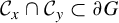
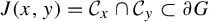
 ${\mathcal {C}}_x $
is the subset of
${\mathcal {C}}_x $
is the subset of
 $\partial G$
defined by
$\partial G$
defined by
 $$ \begin{align} {\mathcal{C}}_x = \lbrace \zeta \in \partial G : \mbox{ there exists } [\zeta] \mbox{ with } [\zeta]_1 = x \rbrace. \end{align} $$
This notion of cylinder set is naturally extended to all lengths. If
 $g\in G$
is an element of length
$g\in G$
is an element of length
 $m\geq 1$
and
$m\geq 1$
and
 $\{g\}$
is the set of all geodesic expressions of g, we denote
$\{g\}$
is the set of all geodesic expressions of g, we denote
 $$ \begin{align} {\mathcal{C}}_g = \lbrace \zeta \in \partial G : \mbox{ there exists } [\zeta] \mbox{ with }[\zeta]_m \in \{ g \} \rbrace. \end{align} $$
In combinatorial dynamics, a cylinder set, say of one letter, is the set of infinite words starting with that letter. Here, the infinite word is replaced by the notion of geodesic ray and the set of infinite words is replaced by the boundary of the hyperbolic space. The main difference, if the space is not a tree, is that many geodesic rays might define the same point on the boundary. Therefore, cylinder sets intersect in general. This notion of cylinder sets for hyperbolic spaces is sometimes called ‘shadow’ in the geometry literature [Reference Calegari13].
In our particular situation of a Cayley graph for a geometric presentation of a surface group, the cylinder sets satisfy particular properties [Reference Los21]:
-
(I)
${\mathcal {C}}_x$
is a connected interval of
$S^1=\partial G$
for each generator
$x\in \mathcal {X}$
; -
(II)
${\mathcal {C}}_x \cap {\mathcal {C}}_y \neq \emptyset $
if and only if x and y are two adjacent generators, with respect to the cyclic ordering induced by the planarity of the Cayley graph
$\textrm {Cay}^1(G,P)$
. In addition, if this intersection is non-empty, then it is a connected interval.


It is well known that a hyperbolic group acts on its boundary by homeomorphisms. Here, we obtain that the group G can be seen as a discrete subgroup of
 $\textrm {Homeo}(S^1)$
.
$\textrm {Homeo}(S^1)$
.
Definition 1. Let
 $\Sigma $
be a closed, compact surface of negative Euler characteristic and let P be a geometric presentation of
$\Sigma $
be a closed, compact surface of negative Euler characteristic and let P be a geometric presentation of
 $G:=\pi _1(\Sigma )$
. We denote the elements of the generating set
$G:=\pi _1(\Sigma )$
. We denote the elements of the generating set
 $\mathcal {X}$
as
$\mathcal {X}$
as
 $x_1,x_2,\ldots ,x_{2N}$
, where the indices are defined modulo
$x_1,x_2,\ldots ,x_{2N}$
, where the indices are defined modulo
 $2N$
(with
$2N$
(with
 $1,2,\ldots ,2N$
as representatives of the classes modulo
$1,2,\ldots ,2N$
as representatives of the classes modulo
 $2N$
) so that
$2N$
) so that
 $x_j$
is adjacent to
$x_j$
is adjacent to
 $x_{j\pm 1}$
. From property (II) above, there are
$x_{j\pm 1}$
. From property (II) above, there are
 $2N$
disjoint intervals
$2N$
disjoint intervals
 $$ \begin{align*} J_j := {\mathcal{C}}_{x_{j-1}} \cap {\mathcal{C}}_{x_{j}} \subset S^1. \end{align*} $$
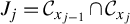
For each
 $\Theta :=(\theta _1,\theta _2,\ldots ,\theta _{2N}) \in J_1 \times J_2 \times \cdots \times J_{2N}$
, we consider the intervals
$\Theta :=(\theta _1,\theta _2,\ldots ,\theta _{2N}) \in J_1 \times J_2 \times \cdots \times J_{2N}$
, we consider the intervals
 $I_j:=[\theta _{j},\theta _{j+1})\subset S^1$
and the map
$I_j:=[\theta _{j},\theta _{j+1})\subset S^1$
and the map
Such a map is called a Bowen–Series-like map. Each point
 $\theta _i$
will be called a cutting point and
$\theta _i$
will be called a cutting point and
 $\Theta $
will be called a cutting parameter.
$\Theta $
will be called a cutting parameter.
The notation
 $x_j^{-1}(z)$
in Definition 1 stands for the action, by homeomorphism, of the group element
$x_j^{-1}(z)$
in Definition 1 stands for the action, by homeomorphism, of the group element
 $x_j^{-1}$
on the boundary
$x_j^{-1}$
on the boundary
 $\partial G=S^1$
. The map
$\partial G=S^1$
. The map
 $\Phi _{\Theta }$
is, therefore, a piecewise homeomorphism. More precisely, the intervals
$\Phi _{\Theta }$
is, therefore, a piecewise homeomorphism. More precisely, the intervals
 $I_j$
define a partition of the space
$I_j$
define a partition of the space
 $S^1$
and
$S^1$
and
 $\Phi _{\Theta }\big \rvert _{I_j}$
is a homeomorphism onto its image.
$\Phi _{\Theta }\big \rvert _{I_j}$
is a homeomorphism onto its image.
With all these ingredients, we are ready to state the main result of this paper.
Theorem A. Let
 $\Sigma $
be a closed, compact surface of negative Euler characteristic and let P be any geometric presentation of
$\Sigma $
be a closed, compact surface of negative Euler characteristic and let P be any geometric presentation of
 $G:=\pi _1(\Sigma )$
. Then, for any cutting parameter
$G:=\pi _1(\Sigma )$
. Then, for any cutting parameter
 $\Theta \in J_1\times J_2\times \cdots \times J_{2N}$
, the Bowen–Series-like map
$\Theta \in J_1\times J_2\times \cdots \times J_{2N}$
, the Bowen–Series-like map
 $\Phi _{\Theta }$
satisfies:
$\Phi _{\Theta }$
satisfies:
-
(a)
$h_{\mathrm {top}}(\Phi _{\Theta })=h_{\mathrm {vol}}(G,P)=\log (\unicode{x3bb} )$
, where
$1/\unicode{x3bb} $
is the smallest root in
$(0,1)$
of an integer polynomial
$Q_P(t)$
that can be explicitly computed from P; -
(b)
$\Phi _{\Theta }$
is topologically conjugate to a piecewise affine map
$\widetilde {\Phi _{\Theta }}$
whose slope is constant for all intervals
$I_j$
and is equal to
$\pm \unicode{x3bb} $
.


A priori, Theorem A is a surprising result, since the dynamics of two different maps in the family are quite different; in particular, they are not pairwise topologically conjugate or even semi-conjugate. For some choices of the parameters
 $\Theta $
, the map
$\Theta $
, the map
 $\Phi _{\Theta }$
satisfies the Markov property, while for some other choices, the map is not Markov.
$\Phi _{\Theta }$
satisfies the Markov property, while for some other choices, the map is not Markov.
In addition, for many geometric presentations (in particular for the classical ones) and for an open set of parameters
 $\Theta $
, the corresponding maps
$\Theta $
, the corresponding maps
 $\Phi _\Theta $
satisfy the assumptions of [Reference Los and Viana Bedoya.22], where it is proved that such maps are orbit equivalent to the surface group action on
$\Phi _\Theta $
satisfy the assumptions of [Reference Los and Viana Bedoya.22], where it is proved that such maps are orbit equivalent to the surface group action on
 $S^1$
. This implies that for many presentations and many parameters
$S^1$
. This implies that for many presentations and many parameters
 $\Theta $
, two different maps are orbit equivalent to each other since they are both orbit equivalent to the same group action. The orbit equivalence is a much weaker relation than the conjugacy and, a priori, does not preserve the topological entropy. These observations imply that the family
$\Theta $
, two different maps are orbit equivalent to each other since they are both orbit equivalent to the same group action. The orbit equivalence is a much weaker relation than the conjugacy and, a priori, does not preserve the topological entropy. These observations imply that the family
 $\Phi _{\Theta }$
shows some surprising stability properties. The question of the orbit equivalence to the group action for all parameters and all geometric presentations is not considered here. Some works are in progress on that problem.
$\Phi _{\Theta }$
shows some surprising stability properties. The question of the orbit equivalence to the group action for all parameters and all geometric presentations is not considered here. Some works are in progress on that problem.
Remark 1.1. The map
 $\Phi _{\Theta }$
is defined by the action of the generators of the group G on some intervals of the circle, which, as the Gromov boundary of G, is just a topological space. After the conjugacy given by Theorem A(b),
$\Phi _{\Theta }$
is defined by the action of the generators of the group G on some intervals of the circle, which, as the Gromov boundary of G, is just a topological space. After the conjugacy given by Theorem A(b),
 $\widetilde {\Phi _{\Theta }}$
is piecewise affine with a constant slope, the algebraic integer
$\widetilde {\Phi _{\Theta }}$
is piecewise affine with a constant slope, the algebraic integer
 $\unicode{x3bb} $
. For this new map, the circle, that is, the boundary of the group, admits a well-defined metric that reflects the growth property of the group presentation. This is an intriguing property. Recall that for the Bowen–Series maps [Reference Bowen and Series12], as well as for the maps in [Reference Abrams, Katok and Ugarcovici1–Reference Adler and Flatto3], the circle
$\unicode{x3bb} $
. For this new map, the circle, that is, the boundary of the group, admits a well-defined metric that reflects the growth property of the group presentation. This is an intriguing property. Recall that for the Bowen–Series maps [Reference Bowen and Series12], as well as for the maps in [Reference Abrams, Katok and Ugarcovici1–Reference Adler and Flatto3], the circle
 $S^1$
admits a differentiable structure such that those maps are piecewise-Möbius diffeomorphisms. In our approach, the maps are only piecewise homeomorphisms and Theorem A(a) is a generalized version of the rigidity result in [Reference Abrams, Katok and Ugarcovici2]. Indeed, the particular action considered in that work defines, in our setting, a particular geometric presentation P of the group G. The equality
$S^1$
admits a differentiable structure such that those maps are piecewise-Möbius diffeomorphisms. In our approach, the maps are only piecewise homeomorphisms and Theorem A(a) is a generalized version of the rigidity result in [Reference Abrams, Katok and Ugarcovici2]. Indeed, the particular action considered in that work defines, in our setting, a particular geometric presentation P of the group G. The equality
 $h_{\mathrm {vol}}(G,P)=h_{\mathrm {top}}(\Phi _{\Theta })$
for all
$h_{\mathrm {vol}}(G,P)=h_{\mathrm {top}}(\Phi _{\Theta })$
for all
 $\Theta $
, which generalizes a previous result in [Reference Los21], gives a conceptual explanation of the rigidity. Observe that both results were obtained independently and roughly at the same time.
$\Theta $
, which generalizes a previous result in [Reference Los21], gives a conceptual explanation of the rigidity. Observe that both results were obtained independently and roughly at the same time.
An interesting part of Theorem A is the computational property stated in part (a). Since the polynomial invariant of the presentation
 $Q_P(t)$
does not depend on the cutting parameter
$Q_P(t)$
does not depend on the cutting parameter
 $\Theta $
, it is possible to choose a particular
$\Theta $
, it is possible to choose a particular
 $\Theta $
for which the Milnor–Thurston invariants [Reference Milnor and Thurston23] can be easily computed using elementary algebraic operations. The computation is, in the end, quite ‘simple’ and can be arranged in the form of a purely combinatorial algorithm that takes as input the presentation of the group and prints out the polynomial
$\Theta $
for which the Milnor–Thurston invariants [Reference Milnor and Thurston23] can be easily computed using elementary algebraic operations. The computation is, in the end, quite ‘simple’ and can be arranged in the form of a purely combinatorial algorithm that takes as input the presentation of the group and prints out the polynomial
 $Q_P(t)$
and the corresponding volume entropy. The explicit algorithm and some examples are provided in §9. This algorithm is based on dynamical systems tools and is, as a consequence, of a completely different nature from the automatic groups approach [Reference Cannon14, Reference Epstein, Cannon, Holt, Levy, Paterson and Thurston16] (see also [Reference Rees28]), which uses regular languages and finite state automata.
$Q_P(t)$
and the corresponding volume entropy. The explicit algorithm and some examples are provided in §9. This algorithm is based on dynamical systems tools and is, as a consequence, of a completely different nature from the automatic groups approach [Reference Cannon14, Reference Epstein, Cannon, Holt, Levy, Paterson and Thurston16] (see also [Reference Rees28]), which uses regular languages and finite state automata.
The paper is organized as follows. In §2, we gather the relevant properties of the family
 $\Phi _{\Theta }$
by reviewing some known facts from previous works. In §3, we describe a new ‘tree-like’ structure associated to each intersection interval
$\Phi _{\Theta }$
by reviewing some known facts from previous works. In §3, we describe a new ‘tree-like’ structure associated to each intersection interval
 $J_i$
. This structure defines some particular cutting parameters
$J_i$
. This structure defines some particular cutting parameters
 $\theta _j\in J_j$
, where the map exhibits possibly different dynamical behaviours. Section 4 is concerned with the geometric description of the set of all geodesics connecting two vertices of the Cayley graph. In §5, we define, for each interval
$\theta _j\in J_j$
, where the map exhibits possibly different dynamical behaviours. Section 4 is concerned with the geometric description of the set of all geodesics connecting two vertices of the Cayley graph. In §5, we define, for each interval
 $J_i$
, an open subinterval
$J_i$
, an open subinterval
 $C(J_i)\subset J_i$
that we call central. We show that when the cutting parameter
$C(J_i)\subset J_i$
that we call central. We show that when the cutting parameter
 $\Theta $
is central, that is,
$\Theta $
is central, that is,
 $\theta _j\in C(J_j)$
for all j, the dynamics of
$\theta _j\in C(J_j)$
for all j, the dynamics of
 $\Phi _{\Theta }$
at each cutting point is specially simple: for some
$\Phi _{\Theta }$
at each cutting point is specially simple: for some
 $k_j$
, the
$k_j$
, the
 $k_j$
th iterates of
$k_j$
th iterates of
 $\Phi _\Theta $
from the left and the right coincide at
$\Phi _\Theta $
from the left and the right coincide at
 $\theta _j$
. In §6, we define a particular central parameter, which we call the middle parameter. In §7, we prove, independently of the parameter
$\theta _j$
. In §6, we define a particular central parameter, which we call the middle parameter. In §7, we prove, independently of the parameter
 $\Theta $
, two inequalities comparing the rates of increase of the two entropy functions, one for the group presentation and one for the dynamics of
$\Theta $
, two inequalities comparing the rates of increase of the two entropy functions, one for the group presentation and one for the dynamics of
 $\Phi _{\Theta }$
. This step, together with the use of the middle parameter and the techniques from the Milnor–Thurston kneading theory, which are summarized in §8, leads to the proof of Theorem A. Finally, in §9, we fully describe the algorithm that computes the polynomial invariant
$\Phi _{\Theta }$
. This step, together with the use of the middle parameter and the techniques from the Milnor–Thurston kneading theory, which are summarized in §8, leads to the proof of Theorem A. Finally, in §9, we fully describe the algorithm that computes the polynomial invariant
 $Q_P(t)$
and give some explicit examples for several presentations.
$Q_P(t)$
and give some explicit examples for several presentations.
2 Review of the Bowen–Series-like maps
$\Phi _\Theta $

In this section, we gather some properties, from [Reference Los21], of geometric presentations for hyperbolic surface groups and of the maps of type
 $\Phi _{\Theta }$
. Recall that a presentation
$\Phi _{\Theta }$
. Recall that a presentation
 ${P=\langle X|R\rangle }$
of a surface group is called geometric if the Cayley 2-complex
${P=\langle X|R\rangle }$
of a surface group is called geometric if the Cayley 2-complex
 $\textrm {Cay}^2(G,P)$
is planar. The next result (from [Reference Los21, Lemma 2.1]) states some elementary consequences of this planarity property.
$\textrm {Cay}^2(G,P)$
is planar. The next result (from [Reference Los21, Lemma 2.1]) states some elementary consequences of this planarity property.
Lemma 2.1. Let G be a co-compact hyperbolic surface group and let
 $P=\langle X|R\rangle =\langle g_1,\ldots ,g_N|R_1,\ldots ,R_k\rangle $
be a geometric presentation of G. The following conditions hold.
$P=\langle X|R\rangle =\langle g_1,\ldots ,g_N|R_1,\ldots ,R_k\rangle $
be a geometric presentation of G. The following conditions hold.
-
(a) The set
$\{g_1^{\pm 1},g_2^{\pm 1},\ldots ,g_N^{\pm 1}\}$
admits a cyclic ordering that is preserved by the group action. -
(b) There exists a planar fundamental domain
$\Delta _P$
. -
(c) Each generator appears exactly twice (with
$+$
or
$-$
exponent) in the set of relations R. -
(d) Let
$a,b$
be a pair of adjacent generators according to the cyclic ordering given by condition (a). Then, there is exactly one relation
$R_i$
such that a cyclic shift of
$R_i$
contains either
$b^{-1}a$
or
$a^{-1}b$
as a sub-word.


Here, we recall the standing notation introduced in Definition 1. The elements of the generating set
 $\mathcal {X}:=\{g_1^{\pm 1},g_2^{\pm 1},\ldots ,g_N^{\pm 1}\}$
are denoted as
$\mathcal {X}:=\{g_1^{\pm 1},g_2^{\pm 1},\ldots ,g_N^{\pm 1}\}$
are denoted as
 $x_1,x_2,\ldots ,x_{2N}$
in such a way that
$x_1,x_2,\ldots ,x_{2N}$
in such a way that
 $x_{i\pm 1}$
are the elements adjacent to
$x_{i\pm 1}$
are the elements adjacent to
 $x_i$
with respect to the cyclic ordering from Lemma 2.1(a). We also adopt the convention that
$x_i$
with respect to the cyclic ordering from Lemma 2.1(a). We also adopt the convention that
 $x_i$
is on the left of
$x_i$
is on the left of
 $x_{i+1}$
(see Figure 1). This convention defines a clockwise orientation of the plane
$x_{i+1}$
(see Figure 1). This convention defines a clockwise orientation of the plane
 $\mathrm {Cay}^2(G,P)$
.
$\mathrm {Cay}^2(G,P)$
.
The clockwise labelling of the generating set associated to the cyclic ordering given by Lemma 2.1(a).

It is easy to see that a presentation containing a relation of the form
 $x_i^2$
does not satisfy Lemma 2.1(a) and, thus, it cannot be geometric. However, a relation of the form
$x_i^2$
does not satisfy Lemma 2.1(a) and, thus, it cannot be geometric. However, a relation of the form
 $x_ix_j$
is simply a trivial identification of the generators
$x_ix_j$
is simply a trivial identification of the generators
 $x_i$
and
$x_i$
and
 $x_j^{-1}$
. So, all presentations considered in this paper will not contain relations of length two by hypothesis. The following purely technical observation will be necessary to exclude unwanted particular situations in some proofs.
$x_j^{-1}$
. So, all presentations considered in this paper will not contain relations of length two by hypothesis. The following purely technical observation will be necessary to exclude unwanted particular situations in some proofs.
Remark 2.2. Assume that our presentation P has
 $N=3$
generators. By Lemma 2.1(c), the sum of the lengths of all relations in P is 6. It is easy to see that a presentation with 3 generators and 2 relations of length 3 corresponds either to a torus or to a Klein bottle, the rank 2 cases, that are not hyperbolic. Since we are excluding, by principle, relations of length 2, it follows that the only possible geometric presentation with
$N=3$
generators. By Lemma 2.1(c), the sum of the lengths of all relations in P is 6. It is easy to see that a presentation with 3 generators and 2 relations of length 3 corresponds either to a torus or to a Klein bottle, the rank 2 cases, that are not hyperbolic. Since we are excluding, by principle, relations of length 2, it follows that the only possible geometric presentation with
 $N=3$
generators has only one relation of length 6.
$N=3$
generators has only one relation of length 6.
A bigon in
 $\textrm {Cay}^1(G,P)$
between two vertices
$\textrm {Cay}^1(G,P)$
between two vertices
 $v,w$
is a pair
$v,w$
is a pair
 $\{\gamma ,\gamma '\}$
of disjoint geodesic segments connecting v to w. We denote by
$\{\gamma ,\gamma '\}$
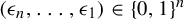
of disjoint geodesic segments connecting v to w. We denote by
 $B(x,y)$
the set of bigons, starting at
$B(x,y)$
the set of bigons, starting at
 $\mathrm {Id}$
, so that one of the two geodesics starts with x and the other one starts with y. Note that both words have the same length, which will be called the length of the bigon. A bigon ray is a pair of disjoint geodesic rays connecting a vertex in
$\mathrm {Id}$
, so that one of the two geodesics starts with x and the other one starts with y. Note that both words have the same length, which will be called the length of the bigon. A bigon ray is a pair of disjoint geodesic rays connecting a vertex in
 $\textrm {Cay}^1(G,P)$
to a point on the boundary
$\textrm {Cay}^1(G,P)$
to a point on the boundary
 $\partial G$
. The following result is a combination of Lemma 2.8 and Corollary 2.11 of [Reference Los21].
$\partial G$
. The following result is a combination of Lemma 2.8 and Corollary 2.11 of [Reference Los21].
Proposition 2.3. Let
 $P=\langle X|R\rangle $
be a geometric presentation of a hyperbolic surface group G. Then, we have the following.
$P=\langle X|R\rangle $
be a geometric presentation of a hyperbolic surface group G. Then, we have the following.
-
(a)
$B(x,y)\neq \emptyset $
if and only if x and y are adjacent in the cyclic ordering of
$\mathcal {X}$
. -
(b) If x and y are adjacent generators in
$\mathcal {X}$
, then there exists a unique bigon
$\beta (x,y)\in B(x,y)$
of minimal length.


A point
 $z\in \partial G$
is the limit of possibly many geodesic rays starting at the identity. We denote by
$z\in \partial G$
is the limit of possibly many geodesic rays starting at the identity. We denote by
 $[z]$
the expression of one geodesic ray in
$[z]$
the expression of one geodesic ray in
 $\textrm {Cay}^1(G,P)$
converging to z, this is an infinite word in the alphabet
$\textrm {Cay}^1(G,P)$
converging to z, this is an infinite word in the alphabet
 $\mathcal {X}$
.
$\mathcal {X}$
.
Recall from (3) that the cylinder set
 ${\mathcal {C}}_x$
, for a generator
${\mathcal {C}}_x$
, for a generator
 $x\in \mathcal {X}$
, is the subset of points
$x\in \mathcal {X}$
, is the subset of points
 $\zeta \in \partial G$
such that there exists
$\zeta \in \partial G$
such that there exists
 $[\zeta ]$
, a ray at
$[\zeta ]$
, a ray at
 $\mathrm {Id}$
converging to
$\mathrm {Id}$
converging to
 $\zeta $
, such that
$\zeta $
, such that
 $[\zeta ]$
starts with x.
$[\zeta ]$
starts with x.
The following result is a direct consequence of [Reference Los21, §3]. It is illustrated in Figure 2.
The bigon
 $\beta (x_j,x_{j+1})$
and the cutting point
$\beta (x_j,x_{j+1})$
and the cutting point
 $\theta _{j+1}$
.
$\theta _{j+1}$
.

Proposition 2.4. The cylinder sets satisfy the following.
-
(a) For any
$x\in \mathcal {X}$
,
${\mathcal {C}}_x$
is connected and
${\mathcal {C}}_x \cap {\mathcal {C}}_y\neq \emptyset $
if and only if x and y are adjacent generators. In this case, it is an interval. -
(b) For any
$\theta \in {\mathcal {C}}_x \cap {\mathcal {C}}_y$
, there is an infinite word W in the alphabet
$\mathcal {X}$
so that
$\theta \in \partial G$
has two geodesic ray expressions
$[\theta ]_{-}=L_{x}W$
and
$ [\theta ]_{+}=L_{y}W$
, where
$ \{ L_{x}, L_{y} \}$
are the two geodesic segments of the minimal bigon
$\beta (x,y)$
.


In Proposition 2.4, the infinite word W might not be unique and the possible non-uniqueness will play a key role later.
The map
 $\Phi _{\Theta }$
defined in (5) is a piecewise homeomorphism of
$\Phi _{\Theta }$
defined in (5) is a piecewise homeomorphism of
 $S^1=\partial G$
. Each interval
$S^1=\partial G$
. Each interval
 $I_j$
of the partition of
$I_j$
of the partition of
 $S^1=\bigcup _{j=1}^{2N} I_j$
is defined by
$S^1=\bigcup _{j=1}^{2N} I_j$
is defined by
 $I_j=[\theta _{j},\theta _{j+1})$
, where
$I_j=[\theta _{j},\theta _{j+1})$
, where
 $\theta _j \in {\mathcal {C}}_{x_{j-1}} \cap {\mathcal {C}}_{x_{j}} $
is called a cutting point. See Figure 12 for a particular example. The map is defined as
$\theta _j \in {\mathcal {C}}_{x_{j-1}} \cap {\mathcal {C}}_{x_{j}} $
is called a cutting point. See Figure 12 for a particular example. The map is defined as
 $$ \begin{align*} \Phi_{\Theta} (z) = x_j^{-1} (z) \quad\mbox{if } z \in I_j. \end{align*} $$
The definition implies, for each
 $j\in \{1,2,\ldots ,2N\}$
, that
$j\in \{1,2,\ldots ,2N\}$
, that
 $I_j \subset {\mathcal {C}}_{x_j}$
and the map
$I_j \subset {\mathcal {C}}_{x_j}$
and the map
 ${\Phi _{\Theta }}\big \rvert _{I_j}$
is a homeomorphism onto its image. At the cutting points, the map is not continuous. From the definition of the cylinder sets
${\Phi _{\Theta }}\big \rvert _{I_j}$
is a homeomorphism onto its image. At the cutting points, the map is not continuous. From the definition of the cylinder sets
 ${\mathcal {C}}_{x_j}$
, if
${\mathcal {C}}_{x_j}$
, if
 $z\in I_j$
, then there exists a geodesic ray, starting at
$z\in I_j$
, then there exists a geodesic ray, starting at
 $\mathrm {Id}$
in the Cayley graph, denoted by
$\mathrm {Id}$
in the Cayley graph, denoted by
 $[z]$
and converging to
$[z]$
and converging to
 $z\in \partial G$
, such that
$z\in \partial G$
, such that
 $[z]=x_jA$
, where A is an infinite word in the alphabet
$[z]=x_jA$
, where A is an infinite word in the alphabet
 $\mathcal {X}$
. The map applied to the point z thus gives
$\mathcal {X}$
. The map applied to the point z thus gives
 $$ \begin{align} \textrm{if } z \in I_j\quad \textrm{then } [z]=x_jA \textrm{ and } [ \Phi_{\Theta}(z)] = A. \end{align} $$
In other words,
 $\Phi _{\Theta }$
is a standard ‘shift map’ for the particular coding of the boundary
$\Phi _{\Theta }$
is a standard ‘shift map’ for the particular coding of the boundary
 $\partial G$
obtained from the intervals
$\partial G$
obtained from the intervals
 $I_j$
. Different choices of the cutting parameter
$I_j$
. Different choices of the cutting parameter
 $\Theta $
in
$\Theta $
in
 $J_1\times J_2\times \cdots \times J_{2N}$
define different maps and thus different codings of
$J_1\times J_2\times \cdots \times J_{2N}$
define different maps and thus different codings of
 $\partial G$
.
$\partial G$
.
There is another important consequence of the results in [Reference Los21] that will be used to prove statement (b) of Theorem A. As it has been mentioned in §1, the map
 $\Phi _P$
defined in [Reference Los21] is nothing but a Bowen–Series-like map
$\Phi _P$
defined in [Reference Los21] is nothing but a Bowen–Series-like map
 $\Phi _\Theta $
for a particular choice of the parameter
$\Phi _\Theta $
for a particular choice of the parameter
 $\Theta $
. Among other properties, [Reference Los21, Proposition 5.3] states that, when no generator appears twice in a relation of length 3,
$\Theta $
. Among other properties, [Reference Los21, Proposition 5.3] states that, when no generator appears twice in a relation of length 3,
 $\Phi _P$
is topologically transitive in the sense that, for any two open intervals
$\Phi _P$
is topologically transitive in the sense that, for any two open intervals
 $U,V\subset S^1$
, there exists
$U,V\subset S^1$
, there exists
 $n\ge 0$
such that
$n\ge 0$
such that
 $\Phi _P^n(U)\cap V\ne \emptyset $
. It is easy to see that the arguments for proving the transitivity can be directly generalized to any
$\Phi _P^n(U)\cap V\ne \emptyset $
. It is easy to see that the arguments for proving the transitivity can be directly generalized to any
 $\Phi _\Theta $
independently of the parameter
$\Phi _\Theta $
independently of the parameter
 $\Theta $
, and that the condition about the generators is, from the point of view of the transitivity, also irrelevant. So, we have the following result.
$\Theta $
, and that the condition about the generators is, from the point of view of the transitivity, also irrelevant. So, we have the following result.
Proposition 2.5. For any parameter
 $\Theta $
, the Bowen–Series-like map
$\Theta $
, the Bowen–Series-like map
 $\Phi _\Theta $
is topologically transitive.
$\Phi _\Theta $
is topologically transitive.
3 A tree-like structure for each parameter interval
In this section, we study some particular sequences of points in the intervals
 ${J_j {\kern-1pt}={\kern-1pt} {\mathcal {C}}_{x_{j-1}} {\kern-1pt}\cap{\kern-1pt} {\mathcal {C}}_{x_{j}}}$
. These points are limits of a tree-like set in the Cayley graph. They are interpreted as the parameters where the dynamics of the map could potentially change, so in some sense, they are like ‘bifurcation’ parameters. The starting point is a characterization of the extreme points of
${J_j {\kern-1pt}={\kern-1pt} {\mathcal {C}}_{x_{j-1}} {\kern-1pt}\cap{\kern-1pt} {\mathcal {C}}_{x_{j}}}$
. These points are limits of a tree-like set in the Cayley graph. They are interpreted as the parameters where the dynamics of the map could potentially change, so in some sense, they are like ‘bifurcation’ parameters. The starting point is a characterization of the extreme points of
 $J_j$
obtained in [Reference Bamba and Diarrassouba9]. To simplify the notation and avoid too many indices, we consider a pair of adjacent generators
$J_j$
obtained in [Reference Bamba and Diarrassouba9]. To simplify the notation and avoid too many indices, we consider a pair of adjacent generators
 $(x,y)$
and the corresponding minimal bigon
$(x,y)$
and the corresponding minimal bigon
 $\beta (x,y)$
with the convention that the generator x is on the left of y in the cyclic ordering induced by our clockwise orientation of
$\beta (x,y)$
with the convention that the generator x is on the left of y in the cyclic ordering induced by our clockwise orientation of
 $S^1$
. We consider also the minimal bigons
$S^1$
. We consider also the minimal bigons
 $\beta _v(x,y)$
starting at a vertex v, possibly different from the identity, with length denoted by
$\beta _v(x,y)$
starting at a vertex v, possibly different from the identity, with length denoted by
 $k(x,y)$
. To fit with this notation, we denote
$k(x,y)$
. To fit with this notation, we denote
 $J(x,y)$
as the interval
$J(x,y)$
as the interval
 ${\mathcal {C}}_{x} \cap {\mathcal {C}}_{y}$
.
${\mathcal {C}}_{x} \cap {\mathcal {C}}_{y}$
.
Assume that the minimal bigon
 $\beta (x, y ) = \{ L_{x} , L_{y} \}$
given by Proposition 2.3(b) is
$\beta (x, y ) = \{ L_{x} , L_{y} \}$
given by Proposition 2.3(b) is
 $$ \begin{align} L_{x} = x\cdot x_{j_2}\cdots x_{j_k} \quad\textrm{and}\quad L_{y} = y\cdot y_{j_2}\cdots y_{j_k} \textrm{, with } k = k(x,y), \end{align} $$
where the various
 $x_{j_m},y_{j_n}$
are generators in
$x_{j_m},y_{j_n}$
are generators in
 $\mathcal {X}$
.
$\mathcal {X}$
.
Consider the last edge along the geodesic segment
 $L_x$
, with label
$L_x$
, with label
 $x_{j_k}$
. It starts at the vertex
$x_{j_k}$
. It starts at the vertex
 $v_{k-1}^{0}$
, which is also the terminal vertex of the geodesic path labelled
$v_{k-1}^{0}$
, which is also the terminal vertex of the geodesic path labelled
 $x\cdot x_{j_2}\cdots x_{j_{k-1}}$
starting at the identity. Symmetrically, consider the last edge, labelled
$x\cdot x_{j_2}\cdots x_{j_{k-1}}$
starting at the identity. Symmetrically, consider the last edge, labelled
 $y_{j_k}$
, starting at the vertex
$y_{j_k}$
, starting at the vertex
 $v_{k-1}^{1}$
along the segment
$v_{k-1}^{1}$
along the segment
 $L_y$
.
$L_y$
.
Consider the minimal bigon
 $\beta _{v_{k-1}^{0}}(x_{j_1}^{0},x_{j_k})$
, based at
$\beta _{v_{k-1}^{0}}(x_{j_1}^{0},x_{j_k})$
, based at
 $v_{k-1}^{0}$
, where we denote by
$v_{k-1}^{0}$
, where we denote by
 $x_{j_1}^{0}$
the generator that is adjacent to
$x_{j_1}^{0}$
the generator that is adjacent to
 $x_{j_k}$
on the left at the vertex
$x_{j_k}$
on the left at the vertex
 $v_{k-1}^{0}$
. Symmetrically, we consider
$v_{k-1}^{0}$
. Symmetrically, we consider
 $\beta _{v_{k-1}^{1}}(y_{j_k},y_{j_1}^{1})$
, the minimal bigon based at
$\beta _{v_{k-1}^{1}}(y_{j_k},y_{j_1}^{1})$
, the minimal bigon based at
 $v_{k-1}^{1}$
, and the generator
$v_{k-1}^{1}$
, and the generator
 $y_{j_1}^{1}$
adjacent to
$y_{j_1}^{1}$
adjacent to
 $y_{j_k}$
on the right.
$y_{j_k}$
on the right.
We define now two binary operations on bigons that are called extensions:
 $$ \begin{align}\begin{aligned} & {\mathcal{E}} (0; \beta(x,y) ) := \beta (x,y) \otimes_{x_{j_k}} \beta_{ v_{k-1}^{0} }( x_{j_1}^{0}, x_{j_k}), \\ & {\mathcal{E}} (1; \beta(x,y) ) := \beta (x,y) \otimes_{y_{j_k}} \beta_{ v_{k-1}^{1} }( y_{j_k}, y_{j_1}^{1}), \end{aligned}\end{align} $$
where the symbol
 $\otimes _{a}$
means the concatenation of the two bigons along their common edge a. More precisely, if
$\otimes _{a}$
means the concatenation of the two bigons along their common edge a. More precisely, if
 $\beta _{ v_{k-1}^{0} }( x_{j_1}^{0}, x_{j_k})=\{x_{j_1}^{0} x_{j_2}^{0}\cdots x_{j_{k^0}}^{0};x_{j_k} y_{j_2}^{0}\cdots y_{j_{k^0}}^{0}\}$
, the 0-extension is
$\beta _{ v_{k-1}^{0} }( x_{j_1}^{0}, x_{j_k})=\{x_{j_1}^{0} x_{j_2}^{0}\cdots x_{j_{k^0}}^{0};x_{j_k} y_{j_2}^{0}\cdots y_{j_{k^0}}^{0}\}$
, the 0-extension is
 $$ \begin{align} {\mathcal{E}} (0; \beta(x,y) ) = \{ x\cdot x_{j_2}\cdots x_{j_{k-1}}\ast x_{j_1}^{0} x_{j_2}^{0}\cdots x_{j_{k^0}}^{0};y\cdot y_{j_2}\cdots y_{j_k} \ast y_{j_2}^{0}\cdots y_{j_{k^0}}^{0} \}, \end{align} $$
where the symbol
 $\ast $
represents the location where the paths are concatenated. Symmetrically, if
$\ast $
represents the location where the paths are concatenated. Symmetrically, if
 $\beta _{ v_{k-1}^{1} }( y_{j_k}, y_{j_1}^{1})=\{ y_{j_k} x_{j_2}^{1}\cdots x_{j_{k^1}}^{1}; y_{j_1}^{1} y_{j_2}^{1}\cdots y_{j_{k^1}}^{1}\}$
, the 1-extension is
$\beta _{ v_{k-1}^{1} }( y_{j_k}, y_{j_1}^{1})=\{ y_{j_k} x_{j_2}^{1}\cdots x_{j_{k^1}}^{1}; y_{j_1}^{1} y_{j_2}^{1}\cdots y_{j_{k^1}}^{1}\}$
, the 1-extension is
 $$ \begin{align} {\mathcal{E}} (1; \beta(x,y) ) = \{ x\cdot x_{j_2}\cdots x_{j_{k}}\ast x_{j_2}^{1}\cdots x_{j_{k^1}}^{1}; y\cdot y_{j_2}\cdots y_{j_{k-1}} \ast y_{j_1}^{1}\cdots y_{j_{k^1}}^{1} \}. \end{align} $$
These operations are represented in Figure 3. Observe that the minimal bigons occurring above have, a priori, different lengths, denoted as
 $k=k(x,y)$
,
$k=k(x,y)$
,
 $k^0=k(x_{j_1}^{0},x_{j_k})$
and
$k^0=k(x_{j_1}^{0},x_{j_k})$
and
 $k^1=k(y_{j_k},y_{j_1}^{1})$
.
$k^1=k(y_{j_k},y_{j_1}^{1})$
.
The left (0) and right (1) extensions of a minimal bigon.

Proposition 3.1. The extensions
 $ {\mathcal {E}} (0; \beta (x,y) )$
and
$ {\mathcal {E}} (0; \beta (x,y) )$
and
 $ {\mathcal {E}} (1; \beta (x,y) )$
are well-defined bigons in
$ {\mathcal {E}} (1; \beta (x,y) )$
are well-defined bigons in
 $B(x,y)$
.
$B(x,y)$
.
Proof. We first observe that the four concatenations of paths in (9) and (10) are well defined, that is, the terminal vertex of the initial path coincides with the initial vertex of the next one. The four concatenations of (9) and (10) start at the identity. For the 0-extension, the terminal vertex of the two paths in (9) is the terminal vertex of the bigon
 $\beta _{ v_{k-1}^{0} }( x_{j_1}^{0}, x_{j_k})$
and, similarly, the terminal vertex of the 1-extension in (10) is the terminal vertex of
$\beta _{ v_{k-1}^{0} }( x_{j_1}^{0}, x_{j_k})$
and, similarly, the terminal vertex of the 1-extension in (10) is the terminal vertex of
 $\beta _{v_{k-1}^{1}}(y_{j_k}, y_{j_1}^{1})$
.
$\beta _{v_{k-1}^{1}}(y_{j_k}, y_{j_1}^{1})$
.
It remains to check that each concatenation is a geodesic. This is a direct consequence of [Reference Los21] (see Lemma 2.9), more details can be found in [Reference Bamba and Diarrassouba9]. The two extensions are thus two bigons in the set
 $B(x,y)$
.
$B(x,y)$
.
To simplify the notation, we now write the two extensions as
 ${\mathcal {E}} (0/1; \beta )$
. The extension operations start with a bigon
${\mathcal {E}} (0/1; \beta )$
. The extension operations start with a bigon
 $\beta \in B(x,y)$
and give two well-defined bigons in
$\beta \in B(x,y)$
and give two well-defined bigons in
 $B(x,y)$
. Therefore, we can iterate the extension construction.
$B(x,y)$
. Therefore, we can iterate the extension construction.
We simplify again the notation and we denote
 $$ \begin{align*} {\mathcal{E}} (\epsilon_2, \epsilon_1; \beta ) := {\mathcal{E}} ( \epsilon_2; {\mathcal{E}} (\epsilon_1; \beta ) ) \quad\mbox{for } (\epsilon_1, \epsilon_2) \in \{0, 1\}^2, \end{align*} $$
and by a finite iteration, we obtain
 $$ \begin{align} {\mathcal{E}} (\epsilon_n,\ldots, \epsilon_1; \beta ) := {\mathcal{E}} ( \epsilon_n; {\mathcal{E}} (\epsilon_{n-1},\ldots, \epsilon_1; \beta ) ) \quad\textrm{for } (\epsilon_1, \ldots, \epsilon_n) \in \{0, 1\}^n. \end{align} $$
Lemma 3.2. Let
 $(x,y)$
be a pair of adjacent generators. Then, we have the following.
$(x,y)$
be a pair of adjacent generators. Then, we have the following.
-
(a) For all
$n \in \mathbb {N}$
and all
$(\epsilon _n,\ldots ,\epsilon _1)\in \{0, 1\}^n$
, the collection of level n extensions
${\mathcal {E}} (\epsilon _n,\ldots ,\epsilon _1;\beta (x,y))$
are well-defined bigons in
$B(x,y)$
. -
(b) The limit sequences, when
$n\rightarrow \infty $
, define a collection of bigon rays in
$B(x,y)$
and, for each
$\mathbf {E }\in \{0, 1\}^{\mathbb {N}}$
, the limit is a well-defined point
$$ \begin{align*} \Omega (\mathbf{E }; \beta(x,y) ) \in {\mathcal{C}}_x \cap {\mathcal{C}}_y \subset \partial G. \end{align*} $$


Proof. By Proposition 2.3, there is a unique minimal bigon for each pair of adjacent generators. There are thus finitely many minimal bigons, each one with a length
 $k(j) \geq 2$
. Let us prove part (a). For each
$k(j) \geq 2$
. Let us prove part (a). For each
 $n \in {\mathbb {N}}$
and each
$n \in {\mathbb {N}}$
and each
 $(\epsilon _n, \ldots , \epsilon _1) \in \{0, 1\}^n$
, the finite extension
$(\epsilon _n, \ldots , \epsilon _1) \in \{0, 1\}^n$
, the finite extension
 ${\mathcal {E}}(\epsilon _n,\ldots , \epsilon _1; \beta (x,y))$
is well defined by repeatedly applying Proposition 3.1. The length of each such bigon is an explicit additive function of the lengths of the various bigons
${\mathcal {E}}(\epsilon _n,\ldots , \epsilon _1; \beta (x,y))$
is well defined by repeatedly applying Proposition 3.1. The length of each such bigon is an explicit additive function of the lengths of the various bigons
 $\beta _v$
occurring in the finite extension
$\beta _v$
occurring in the finite extension
 ${\mathcal {E}}(\epsilon _n,\ldots ,\epsilon _1;\beta (x,y))$
. For instance, in (8), the length is
${\mathcal {E}}(\epsilon _n,\ldots ,\epsilon _1;\beta (x,y))$
. For instance, in (8), the length is
 $k(x,y)+k(x_{j_1}^{0},x_{j_k})-1$
. The length of the bigons
$k(x,y)+k(x_{j_1}^{0},x_{j_k})-1$
. The length of the bigons
 ${\mathcal {E}} (\epsilon _n,\ldots ,\epsilon _1;\beta (x,y))$
is strictly increasing with n, since
${\mathcal {E}} (\epsilon _n,\ldots ,\epsilon _1;\beta (x,y))$
is strictly increasing with n, since
 $k(j)\geq 2$
for each j.
$k(j)\geq 2$
for each j.
To prove part (b), note that
 ${\mathcal {E}}(\epsilon _n,\ldots ,\epsilon _1;\beta )$
define sequences of bigons in
${\mathcal {E}}(\epsilon _n,\ldots ,\epsilon _1;\beta )$
define sequences of bigons in
 $B(x,y)$
whose lengths go to infinity when
$B(x,y)$
whose lengths go to infinity when
 $n\rightarrow \infty $
. For each
$n\rightarrow \infty $
. For each
 $\mathbf {{ E }} \in \{0, 1\}^{\mathbb {N}}$
, the set of geodesic rays in
$\mathbf {{ E }} \in \{0, 1\}^{\mathbb {N}}$
, the set of geodesic rays in
 ${\mathcal {E}} (\mathbf {{ E }}; \beta (x,y) )$
remains at a finite distance from each other. More precisely, let
${\mathcal {E}} (\mathbf {{ E }}; \beta (x,y) )$
remains at a finite distance from each other. More precisely, let
 ${K:=\max \big \{k(m); m\in \{1,2,\ldots ,2N\}\big \}}$
, where
${K:=\max \big \{k(m); m\in \{1,2,\ldots ,2N\}\big \}}$
, where
 $k(m)$
is the length of a minimal bigon. Then, two points, at distance M from the identity along the geodesic rays of
$k(m)$
is the length of a minimal bigon. Then, two points, at distance M from the identity along the geodesic rays of
 ${\mathcal {E}} (\mathbf {{ E }}; \beta (x,y))$
, remain at a distance less than K from each other, for all M. By definition of the Gromov boundary [Reference Ghys and de la Harpe18, Reference Gromov20], the geodesic rays in
${\mathcal {E}} (\mathbf {{ E }}; \beta (x,y))$
, remain at a distance less than K from each other, for all M. By definition of the Gromov boundary [Reference Ghys and de la Harpe18, Reference Gromov20], the geodesic rays in
 ${\mathcal {E}} (\mathbf {{ E }}; \beta (x,y) )$
, for each
${\mathcal {E}} (\mathbf {{ E }}; \beta (x,y) )$
, for each
 $\mathbf {{ E}} \in \{0, 1\}^{\mathbb {N}}$
, converge to the same point in
$\mathbf {{ E}} \in \{0, 1\}^{\mathbb {N}}$
, converge to the same point in
 $\partial G$
. In addition, each
$\partial G$
. In addition, each
 ${\mathcal {E}} (\epsilon _n,\ldots ,\epsilon _1;\beta (x,y))$
is a bigon in
${\mathcal {E}} (\epsilon _n,\ldots ,\epsilon _1;\beta (x,y))$
is a bigon in
 $B(x,y)$
and, by definition of the cylinder sets, the limit point
$B(x,y)$
and, by definition of the cylinder sets, the limit point
 $\Omega (\mathbf {{E}};\beta (x,y))$
belongs to
$\Omega (\mathbf {{E}};\beta (x,y))$
belongs to
 ${\mathcal {C}}_x\cap {\mathcal {C}}_y\subset \partial G$
.
${\mathcal {C}}_x\cap {\mathcal {C}}_y\subset \partial G$
.
As it is clear from the definition, the infinite extension construction is a ‘tree-like’ process and the underlying tree is rooted and binary.
Lemma 3.3. For any adjacent pair of generators
 $(x,y)$
, there is a well-defined map
$(x,y)$
, there is a well-defined map
 $$ \begin{align*} \begin{array}{rcl} \Omega : \big\{0, 1\big\}^{\mathbb{N}} & \longrightarrow & {\mathcal{C}}_x \cap {\mathcal{C}}_y \subset \partial G, \\ \mathbf{{ E}} \in \{0, 1\}^{\mathbb{N}} & \longrightarrow & \Omega (\mathbf{{ E}}; \beta(x,y)) \end{array} \end{align*} $$
satisfying:
-
(a)
$\Omega $
is injective; -
(b)
$\Omega $
is order preserving on
$\partial G$
for the ordering of
$\{0, 1\}^{\mathbb {N}}$
induced by
$ 0 < 1$
.


Proof. The fact that
 $\Omega $
is a well-defined map is a direct consequence of Lemma 3.2. Let us prove item (a). The fact that
$\Omega $
is a well-defined map is a direct consequence of Lemma 3.2. Let us prove item (a). The fact that
 $\Omega $
is injective comes from Proposition 2.3(a). Indeed, if
$\Omega $
is injective comes from Proposition 2.3(a). Indeed, if
 $\mathbf {{E}} \neq \mathbf {{ E ' }}$
in
$\mathbf {{E}} \neq \mathbf {{ E ' }}$
in
 $\{0, 1\}^{\mathbb {N}}$
, then there is a first integer n so that
$\{0, 1\}^{\mathbb {N}}$
, then there is a first integer n so that
 $\epsilon _n \neq \epsilon ^{\prime }_n$
. From the extension construction, there is a vertex
$\epsilon _n \neq \epsilon ^{\prime }_n$
. From the extension construction, there is a vertex
 $v_n$
in the Cayley graph such that
$v_n$
in the Cayley graph such that
 ${v_n \in {\mathcal {E}} ( \epsilon _n, \ldots , \epsilon _1; \beta (x,y) ) \cap {\mathcal {E}} ( \epsilon ^{\prime }_n, \ldots , \epsilon ^{\prime }_1; \beta (x,y) )}$
and, starting from
${v_n \in {\mathcal {E}} ( \epsilon _n, \ldots , \epsilon _1; \beta (x,y) ) \cap {\mathcal {E}} ( \epsilon ^{\prime }_n, \ldots , \epsilon ^{\prime }_1; \beta (x,y) )}$
and, starting from
 $v_n$
, the geodesic rays, say
$v_n$
, the geodesic rays, say
 $\gamma $
and
$\gamma $
and
 $\gamma '$
, are different in
$\gamma '$
, are different in
 ${\mathcal {E}}(\mathbf {{E}};\beta (x,y))$
and in
${\mathcal {E}}(\mathbf {{E}};\beta (x,y))$
and in
 ${\mathcal {E}}(\mathbf {{E'}};\beta (x,y))$
. Here, being different means that the two geodesic rays based at
${\mathcal {E}}(\mathbf {{E'}};\beta (x,y))$
. Here, being different means that the two geodesic rays based at
 $v_n$
start by two non-adjacent generators (see Figure 3 for
$v_n$
start by two non-adjacent generators (see Figure 3 for
 $n=1$
). These two geodesic rays cannot converge to the same point in
$n=1$
). These two geodesic rays cannot converge to the same point in
 $\partial G$
since otherwise, they would define a bigon ray, which is impossible by Proposition 2.3(a).
$\partial G$
since otherwise, they would define a bigon ray, which is impossible by Proposition 2.3(a).
Let us prove item (b). If
 $\mathbf {{E}}<\mathbf {{E'}}$
, then, by the arguments above, there is n such that
$\mathbf {{E}}<\mathbf {{E'}}$
, then, by the arguments above, there is n such that
 $\epsilon _n<\epsilon ^{\prime }_n$
, meaning
$\epsilon _n<\epsilon ^{\prime }_n$
, meaning
 $\epsilon _n=0$
and
$\epsilon _n=0$
and
 $\epsilon ^{\prime }_n=1$
. The two geodesic rays
$\epsilon ^{\prime }_n=1$
. The two geodesic rays
 $\gamma $
and
$\gamma $
and
 $\gamma '$
described above and based at the vertex
$\gamma '$
described above and based at the vertex
 $v_n$
are such that
$v_n$
are such that
 $\gamma $
starts at
$\gamma $
starts at
 $v_n$
by a generator
$v_n$
by a generator
 $y^{0\ast }_{j_2}$
and
$y^{0\ast }_{j_2}$
and
 $\gamma '$
starts at
$\gamma '$
starts at
 $v_n$
by a generator
$v_n$
by a generator
 $x^{1\ast }_{j_2}$
, with the notation (9) and (10) (for
$x^{1\ast }_{j_2}$
, with the notation (9) and (10) (for
 $n=1$
, see Figure 3). By the cyclic ordering at
$n=1$
, see Figure 3). By the cyclic ordering at
 $v_n$
and with our conventions, we observe that
$v_n$
and with our conventions, we observe that
 $y^{0\ast }_{j_2}<x^{1\ast }_{j_2}$
. By Proposition 2.3(a), the two geodesic rays
$y^{0\ast }_{j_2}<x^{1\ast }_{j_2}$
. By Proposition 2.3(a), the two geodesic rays
 $\gamma $
and
$\gamma $
and
 $\gamma '$
cannot intersect after the vertex
$\gamma '$
cannot intersect after the vertex
 $v_n$
since otherwise, they would define a bigon starting with non-adjacent generators at
$v_n$
since otherwise, they would define a bigon starting with non-adjacent generators at
 $v_n$
. Therefore, the two rays converge to two points on
$v_n$
. Therefore, the two rays converge to two points on
 $\partial G$
and the cyclic ordering at
$\partial G$
and the cyclic ordering at
 $v_n$
is preserved on the boundary. Thus, we obtain
$v_n$
is preserved on the boundary. Thus, we obtain
 $\Omega (\mathbf {{E}};\beta (x,y))<\Omega (\mathbf {{E'}};\beta (x,y))$
.
$\Omega (\mathbf {{E}};\beta (x,y))<\Omega (\mathbf {{E'}};\beta (x,y))$
.
The idea of the extension construction appeared in [Reference Bamba and Diarrassouba9] for the special cases
 ${\mathcal {E}}(0^{\infty };\beta )$
and
${\mathcal {E}}(0^{\infty };\beta )$
and
 ${\mathcal {E}}(1^{\infty };\beta )$
, where they are called ‘ladders’.
${\mathcal {E}}(1^{\infty };\beta )$
, where they are called ‘ladders’.
Theorem 3.4. With the above notation,
 $\Omega (0^{\infty };\beta (x,y))$
and
$\Omega (0^{\infty };\beta (x,y))$
and
 $\Omega (1^{\infty };\beta (x,y))$
are the two extreme points of the interval
$\Omega (1^{\infty };\beta (x,y))$
are the two extreme points of the interval
 $J(x,y)={\mathcal {C}}_x \cap {\mathcal {C}}_y \subset \partial G$
.
$J(x,y)={\mathcal {C}}_x \cap {\mathcal {C}}_y \subset \partial G$
.
This result from [Reference Bamba and Diarrassouba9] is a characterization of the intersection of cylinder sets and therefore of the cylinder sets. These special points are thus quite important for the study of the family
 $\Phi _{\Theta }$
.
$\Phi _{\Theta }$
.
4 Staircases and galleries
In this section, we analyse the geometric structure of the subgraph of the Cayley graph composed by all geodesics joining two given elements of G. The characterization of this subgraph will be one of the tools to prove statement (a) of Theorem A.
For any pair
 $v,w\in G$
, consider a geodesic segment in the Cayley graph
$v,w\in G$
, consider a geodesic segment in the Cayley graph
 $\textrm {Cay}^1(G,P)$
connecting the vertices v and w. We keep the same notation
$\textrm {Cay}^1(G,P)$
connecting the vertices v and w. We keep the same notation
 $v,w$
for the corresponding elements in the group G. It is represented as a word W of minimal length in the generating set
$v,w$
for the corresponding elements in the group G. It is represented as a word W of minimal length in the generating set
 $\mathcal {X}$
. The distance between v and w, denoted as
$\mathcal {X}$
. The distance between v and w, denoted as
 $d(v,w)$
, is the number of symbols in W.
$d(v,w)$
, is the number of symbols in W.
Let
 $v,w\in G$
. A subgraph S of
$v,w\in G$
. A subgraph S of
 $\textrm {Cay}^1(G,P)$
will be called a staircase between v and w if S is either a minimal bigon between v and w or the union of all minimal bigons concatenated in an extension (see Lemma 3.2) between v and w. See Figure 4 for an example. Note that if
$\textrm {Cay}^1(G,P)$
will be called a staircase between v and w if S is either a minimal bigon between v and w or the union of all minimal bigons concatenated in an extension (see Lemma 3.2) between v and w. See Figure 4 for an example. Note that if
 $S_{v,w}$
is a staircase between v and w, and
$S_{v,w}$
is a staircase between v and w, and
 $d(v,w)=n$
, then for all
$d(v,w)=n$
, then for all
 $1\le j<n$
, there are exactly two vertices in
$1\le j<n$
, there are exactly two vertices in
 $S_{v,w}$
at distance j from v.
$S_{v,w}$
at distance j from v.
(a) An extension
 $\mathcal {E}(0,1;\beta (x,y))$
between v and w. The dashed edges do not belong to the extension. (b) Corresponding staircase between v and w.
$\mathcal {E}(0,1;\beta (x,y))$
between v and w. The dashed edges do not belong to the extension. (b) Corresponding staircase between v and w.

Remark 4.1. Let L and R be the left and right geodesic segments connecting v to w and defining a staircase between v and w. For every vertex
 $x\in L\cup R$
, the number of edges in the Cayley graph departing from x and contained in the bounded component of
$x\in L\cup R$
, the number of edges in the Cayley graph departing from x and contained in the bounded component of
 ${\mathbb {R}^2\setminus {(L\cup R)}}$
is at most two. Having two of such edges is only possible when the presentation P has relations of length 3.
${\mathbb {R}^2\setminus {(L\cup R)}}$
is at most two. Having two of such edges is only possible when the presentation P has relations of length 3.
Let
 $S_{v,w}$
be a staircase between v and w associated to an extension
$S_{v,w}$
be a staircase between v and w associated to an extension
 $\mathcal {E}$
from v to w. By Lemma 3.2(a),
$\mathcal {E}$
from v to w. By Lemma 3.2(a),
 $\mathcal {E}$
is a bigon between v and w. The left and right geodesic segments from v to w defining this bigon will be respectively denoted by
$\mathcal {E}$
is a bigon between v and w. The left and right geodesic segments from v to w defining this bigon will be respectively denoted by
 $S_{v,w}^L$
and
$S_{v,w}^L$
and
 $S_{v,w}^R$
. Note that, in general,
$S_{v,w}^R$
. Note that, in general,
 $S_{v,w}$
contains other geodesics going from v to w.
$S_{v,w}$
contains other geodesics going from v to w.
A gallery between
 $v,w\in G$
is a subgraph of the Cayley graph given by a finite set of k staircases
$v,w\in G$
is a subgraph of the Cayley graph given by a finite set of k staircases
 $S_{v_1,w_1},\ldots ,S_{v_k,w_k}$
and
$S_{v_1,w_1},\ldots ,S_{v_k,w_k}$
and
 $k+1$
simple paths
$k+1$
simple paths
 $\gamma _{v,v_1},\gamma _{w_1,v_2},\ldots ,\gamma _{w_k,w}$
(some of them possibly degenerated to a point) such that
$\gamma _{v,v_1},\gamma _{w_1,v_2},\ldots ,\gamma _{w_k,w}$
(some of them possibly degenerated to a point) such that
 $$ \begin{align*} \gamma_{v,v_1}S_{v_1,w_1}^L\gamma_{w_1,v_2}\ldots S_{v_k,w_k}^L \gamma_{w_k,w} \quad\textrm{and} \quad\gamma_{v,v_1}S_{v_1,w_1}^R\gamma_{w_1,v_2}\ldots S_{v_k,w_k}^R \gamma_{w_k,w} \end{align*} $$
are geodesics. See Figure 5 for an example.
If
 $F_{v,w}$
is a gallery between v and w, we denote by
$F_{v,w}$
is a gallery between v and w, we denote by
 $F_{v,w}^L$
and
$F_{v,w}^L$
and
 $F_{v,w}^R$
the corresponding geodesic paths defined above, and call them the left and right sides of
$F_{v,w}^R$
the corresponding geodesic paths defined above, and call them the left and right sides of
 $F_{v,w}$
.
$F_{v,w}$
.
Note that if
 $F_{v,w}$
is a gallery between v and w, and
$F_{v,w}$
is a gallery between v and w, and
 $d(v,w)=n$
, then for all
$d(v,w)=n$
, then for all
 $1\le j<n$
, there are at most two vertices in
$1\le j<n$
, there are at most two vertices in
 $F_{v,w}$
at distance j from v.
$F_{v,w}$
at distance j from v.
A gallery
 $F_{v,w}$
between v and w. The fat edges correspond to the geodesic path
$F_{v,w}$
between v and w. The fat edges correspond to the geodesic path
 $F^L_{v,w}$
.
$F^L_{v,w}$
.

Lemma 4.2. Let L be a geodesic path between
 $v,w\in G$
. Then, there are at least three different edges
$v,w\in G$
. Then, there are at least three different edges
 $x_{i_1},x_{i_2},x_{i_3}$
such that
$x_{i_1},x_{i_2},x_{i_3}$
such that
 $Lx_{i_1},Lx_{i_2},Lx_{i_3}$
are geodesics paths.
$Lx_{i_1},Lx_{i_2},Lx_{i_3}$
are geodesics paths.
Proof. This result is a direct consequence of [Reference Los21, Lemma 2.9].
Lemma 4.3. Let
 $L_1,L_2$
be two geodesic paths between
$L_1,L_2$
be two geodesic paths between
 $v,w\in G$
such that
$v,w\in G$
such that
 $L_1\cap L_2=\{v,w\}$
. Then, the bounded component of
$L_1\cap L_2=\{v,w\}$
. Then, the bounded component of
 $\mathbb {R}^2\setminus \{L_1\cup L_2\}$
does not contain vertices of the Cayley graph.
$\mathbb {R}^2\setminus \{L_1\cup L_2\}$
does not contain vertices of the Cayley graph.
Proof. Assume, for the sake of contradiction, that there exists a vertex g in the bounded component of
 $\mathbb {R}^2\setminus \{L_1\cup L_2\}$
. Let W be a geodesic path between v and g. By Lemma 4.2, there exist at least three different edges
$\mathbb {R}^2\setminus \{L_1\cup L_2\}$
. Let W be a geodesic path between v and g. By Lemma 4.2, there exist at least three different edges
 $x_{i_1},x_{i_2},x_{i_3}$
such that
$x_{i_1},x_{i_2},x_{i_3}$
such that
 $Wx_{i_1},Wx_{i_2},Wx_{i_3}$
are still geodesic paths. By applying iteratively Lemma 4.2, each of these three geodesic paths can be continued up to a point in
$Wx_{i_1},Wx_{i_2},Wx_{i_3}$
are still geodesic paths. By applying iteratively Lemma 4.2, each of these three geodesic paths can be continued up to a point in
 $L_1\cup L_2$
. From each of these three points, we can continue along
$L_1\cup L_2$
. From each of these three points, we can continue along
 $L_1$
or
$L_1$
or
 $L_2$
up to w. We get then three geodesics from v to w passing through g. It follows that we have three different geodesics from g to w starting respectively with the edges
$L_2$
up to w. We get then three geodesics from v to w passing through g. It follows that we have three different geodesics from g to w starting respectively with the edges
 $x_{i_1},x_{i_2},x_{i_3}$
. Two of these edges are not adjacent. As a consequence, we have obtained a bigon associated to a pair of non-adjacent edges, in contradiction with Proposition 2.3.
$x_{i_1},x_{i_2},x_{i_3}$
. Two of these edges are not adjacent. As a consequence, we have obtained a bigon associated to a pair of non-adjacent edges, in contradiction with Proposition 2.3.
Lemma 4.4. Let
 $L_1,L_2$
be two geodesic paths between
$L_1,L_2$
be two geodesic paths between
 $v,w\in G$
such that
$v,w\in G$
such that
 $L_1\cap L_2=\{v,w\}.$
Then,
$L_1\cap L_2=\{v,w\}.$
Then,
 $L_1$
and
$L_1$
and
 $L_2$
are the left and right sides of a staircase between v and w.
$L_2$
are the left and right sides of a staircase between v and w.
Proof. Let
 $n=d(v,w)$
. For all
$n=d(v,w)$
. For all
 $1\le i<n$
, let
$1\le i<n$
, let
 $v_i$
(respectively
$v_i$
(respectively
 $w_i$
) be the point in
$w_i$
) be the point in
 $L_1$
(respectively
$L_1$
(respectively
 $L_2$
) satisfying
$L_2$
) satisfying
 $d(v_i,v)=i$
(respectively
$d(v_i,v)=i$
(respectively
 $d(w_i,v)=i$
).
$d(w_i,v)=i$
).
We prove the lemma by induction on n. So, assume that the result is true for all lengths less than n. Let A be the bounded component of
 $\mathbb {R}^2\setminus (L_1\cup L_2)$
. By Lemma 4.3, any path of the Cayley graph contained in A reduces to a single edge. Since
$\mathbb {R}^2\setminus (L_1\cup L_2)$
. By Lemma 4.3, any path of the Cayley graph contained in A reduces to a single edge. Since
 $L_1$
and
$L_1$
and
 $L_2$
are geodesics, there are no edges contained in A joining points in
$L_2$
are geodesics, there are no edges contained in A joining points in
 $L_1$
(respectively
$L_1$
(respectively
 $L_2$
). So, if there exists some edge in A, it must connect a point in
$L_2$
). So, if there exists some edge in A, it must connect a point in
 $L_1$
to a point in
$L_1$
to a point in
 $L_2$
. Again, since
$L_2$
. Again, since
 $L_1$
and
$L_1$
and
 $L_2$
are geodesics, any edge that begins at
$L_2$
are geodesics, any edge that begins at
 $v_i$
and ends at
$v_i$
and ends at
 $L_2$
must go either to
$L_2$
must go either to
 $w_i$
, and we call this edge horizontal, or to
$w_i$
, and we call this edge horizontal, or to
 $w_j$
with
$w_j$
with
 $j\in \{i+1,i-1\}$
, and we call this edge sloping. If there are no sloping edges, then the pair
$j\in \{i+1,i-1\}$
, and we call this edge sloping. If there are no sloping edges, then the pair
 $\{L_1,L_2\}$
defines a minimal bigon and there is nothing to prove. See Figure 6(a). Otherwise, let i be the smallest index such that there is a sloping edge beginning at
$\{L_1,L_2\}$
defines a minimal bigon and there is nothing to prove. See Figure 6(a). Otherwise, let i be the smallest index such that there is a sloping edge beginning at
 $v_i$
. Assume for instance that there is an edge from
$v_i$
. Assume for instance that there is an edge from
 $v_i$
to
$v_i$
to
 $w_{i+1}$
(the other case follows by a symmetric argument). See Figure 6(b). Then, the paths
$w_{i+1}$
(the other case follows by a symmetric argument). See Figure 6(b). Then, the paths
 $\tilde L_1:=v_{i+1}\cdots v_{n-1}$
and
$\tilde L_1:=v_{i+1}\cdots v_{n-1}$
and
 $\tilde L_2:=w_{i+1}\cdots w_{n-1}$
between
$\tilde L_2:=w_{i+1}\cdots w_{n-1}$
between
 $v_i$
and w satisfy the hypothesis of the lemma and have length less than n. By the induction hypothesis, they are the left and right sides of a staircase. However, the pair
$v_i$
and w satisfy the hypothesis of the lemma and have length less than n. By the induction hypothesis, they are the left and right sides of a staircase. However, the pair
 $\{\widehat {L}_1,\widehat {L}_2\}$
, where
$\{\widehat {L}_1,\widehat {L}_2\}$
, where
 $\widehat {L}_1:=v_1 v_2\cdots v_i$
and
$\widehat {L}_1:=v_1 v_2\cdots v_i$
and
 $\widehat {L}_2:=w_1 w_2\cdots w_i$
, defines a minimal bigon between v and
$\widehat {L}_2:=w_1 w_2\cdots w_i$
, defines a minimal bigon between v and
 $w_{i+1}$
, since there are no sloping edges in the interior of the bounded component of
$w_{i+1}$
, since there are no sloping edges in the interior of the bounded component of
 $\mathbb {R}^2\setminus (\widehat {L}_1\cup \widehat {L}_2)$
. So, the result follows from the definition of a staircase.
$\mathbb {R}^2\setminus (\widehat {L}_1\cup \widehat {L}_2)$
. So, the result follows from the definition of a staircase.
Lemma 4.5. Let
 $L_1,L_2$
be two different geodesic paths between
$L_1,L_2$
be two different geodesic paths between
 $v,w\in G$
. Then,
$v,w\in G$
. Then,
 $L_1$
and
$L_1$
and
 $L_2$
are the left and right sides of a gallery between v and w.
$L_2$
are the left and right sides of a gallery between v and w.
The two cases in the proof of Lemma 4.4.

Proof. We prove the lemma by induction on n, the length of the geodesics. If n is less than the minimum length of a minimal bigon, then there is nothing to prove. If n is the minimum length of a minimal bigon, then the pair
 $\{L_1,L_2\}$
defines a minimal bigon and the result follows. Assume now that the result is true for all lengths smaller than n. If
$\{L_1,L_2\}$
defines a minimal bigon and the result follows. Assume now that the result is true for all lengths smaller than n. If
 $L_1\cap L_2=\{v,w\}$
, then the result follows from Lemma 4.5. If not, let
$L_1\cap L_2=\{v,w\}$
, then the result follows from Lemma 4.5. If not, let
 $z\in L_1\cap L_2$
. Then, the result follows by applying the induction hypothesis to
$z\in L_1\cap L_2$
. Then, the result follows by applying the induction hypothesis to
 $\tilde L_1$
and
$\tilde L_1$
and
 $\tilde L_2$
, the portions of
$\tilde L_2$
, the portions of
 $L_1$
and
$L_1$
and
 $L_2$
joining v and z, and applying also the induction hypothesis to
$L_2$
joining v and z, and applying also the induction hypothesis to
 $\widehat {L}_1$
and
$\widehat {L}_1$
and
 $\widehat {L}_2$
, the portions of
$\widehat {L}_2$
, the portions of
 $L_1$
and
$L_1$
and
 $L_2$
joining z and w.
$L_2$
joining z and w.
Proposition 4.6. The subgraph of all geodesics joining two elements of G is a gallery.
Proof. Let H be the set of all geodesics from v to w. Let
 $L_1$
and
$L_1$
and
 $L_2$
be respectively the leftmost and the rightmost geodesic paths in H from v to w. From Lemma 4.5, they are the left and right sides of some gallery
$L_2$
be respectively the leftmost and the rightmost geodesic paths in H from v to w. From Lemma 4.5, they are the left and right sides of some gallery
 $F_{v,w}$
. From the definition of a gallery, it easily follows that
$F_{v,w}$
. From the definition of a gallery, it easily follows that
 $H=F_{v,w}$
.
$H=F_{v,w}$
.
The results of this section can be naturally extended to infinite geodesic rays. Recall that a bigon ray has been defined in §2 as a pair of disjoint infinite geodesic rays starting (for example) at the identity element
 $\mathrm {Id}$
and representing the same point in
$\mathrm {Id}$
and representing the same point in
 $S^1$
. In Lemma 3.2(b), we showed that if L and R are respectively the left and right sides of an infinite extension of bigons, then the pair
$S^1$
. In Lemma 3.2(b), we showed that if L and R are respectively the left and right sides of an infinite extension of bigons, then the pair
 $\{L,R\}$
defines a bigon ray. The corresponding point in
$\{L,R\}$
defines a bigon ray. The corresponding point in
 $S^1$
was denoted by
$S^1$
was denoted by
 $\Omega (\mathbf {E};\beta (x,y))$
in the statement of Lemma 3.2(b), where
$\Omega (\mathbf {E};\beta (x,y))$
in the statement of Lemma 3.2(b), where
 $\mathbf {E}\in \{0,1\}^{\mathbb {N}}$
is the coding for the infinite extension and
$\mathbf {E}\in \{0,1\}^{\mathbb {N}}$
is the coding for the infinite extension and
 $\beta (x,y)$
is the initial bigon of the extension. The arguments used in the proofs of Lemmas 4.3 and 4.4 can be trivially adapted to prove the following converse result, which states that any bigon ray has precisely this form.
$\beta (x,y)$
is the initial bigon of the extension. The arguments used in the proofs of Lemmas 4.3 and 4.4 can be trivially adapted to prove the following converse result, which states that any bigon ray has precisely this form.
Lemma 4.7. Let
 $L,R$
be two disjoint infinite geodesic rays starting at
$L,R$
be two disjoint infinite geodesic rays starting at
 $\mathrm {Id}$
. If L and R represent the same point
$\mathrm {Id}$
. If L and R represent the same point
 $\zeta \in S^1$
, then L and R are respectively the left and right sides of an infinite extension of bigons. That is, there exist a pair of adjacent generators
$\zeta \in S^1$
, then L and R are respectively the left and right sides of an infinite extension of bigons. That is, there exist a pair of adjacent generators
 $x,y$
and
$x,y$
and
 $\mathbf {E}\in \{0,1\}^{\mathbb {N}}$
such that
$\mathbf {E}\in \{0,1\}^{\mathbb {N}}$
such that
 $\zeta =\Omega (\mathbf {E};\beta (x,y))$
.
$\zeta =\Omega (\mathbf {E};\beta (x,y))$
.
5 Dynamical properties in the family
$\Phi _{\Theta }$

In this section, we study how the dynamics of the maps
 $\Phi _{\Theta }$
might change with the parameters
$\Phi _{\Theta }$
might change with the parameters
 $\Theta \in J_1\times J_2\times \cdots \times J_{2N}$
. We show, in particular, the importance of the points in the Cantor set
$\Theta \in J_1\times J_2\times \cdots \times J_{2N}$
. We show, in particular, the importance of the points in the Cantor set
 $\Omega (\mathbf {{E}};\beta (x,y))\in J(x,y)$
as defined in Lemma 3.2.
$\Omega (\mathbf {{E}};\beta (x,y))\in J(x,y)$
as defined in Lemma 3.2.
Let us consider the following interval, called central in
 $J(x,y)$
(see Figure 7):
$J(x,y)$
(see Figure 7):
 $$ \begin{align} C(J(x,y)):=(\Omega(1^{\infty} 0;\beta(x,y)),\Omega(0^{\infty} 1;\beta(x,y))). \end{align} $$
The property (a) in the next result was called the eventual coincidence condition (EC) in [Reference Los and Viana Bedoya.22] and the two properties in part (b) were called the conditions (E+), (E−) when all relations in the presentation P have even length.
Lemma 5.1. (Eventual coincidence of length k)
If
 $\Theta \in C(J_1)\times C(J_2)\times \cdots \times C(J_{2N})$
, then we have the following.
$\Theta \in C(J_1)\times C(J_2)\times \cdots \times C(J_{2N})$
, then we have the following.
-
(a) For all
$j\in \{1,\ldots ,2N\}$
,
$ \Phi _{\Theta }^{k(j)}(\theta _{j (-)}) = \Phi _{\Theta }^{k(j)}(\theta _{j (+)})$
, where
$k(j)$
is the length of
$\beta (x_{j-1},x_{j})$
and the notation
$\Phi _{\Theta }^{k(j)}(\theta _{j(\pm )})$
stands for the iterates from the left or the right of the cutting point. -
(b) If
$\beta (x_{j-1},x_{j})=\{x_{j-1} x_{j_2}\cdots x_{j_k};x_{j} y_{j_2}\cdots y_{j_k} \}$
, then, for each
$1\leq m\leq k(j)-1$
,
$\Phi _{\Theta }^{m}(\theta _{j (-)})\in I_{x_{j_{m+1}}}$
and
$\Phi _{\Theta }^{m}(\theta _{j (+)})\in I_{y_{j_{m+1}}}$
.


Proof. We use again the notation
 $(x,y)$
for a pair of adjacent generators, as well as
$(x,y)$
for a pair of adjacent generators, as well as
 $\beta (x,y)$
for a minimal bigon and
$\beta (x,y)$
for a minimal bigon and
 $k(x,y)$
for its length. Let us write
$k(x,y)$
for its length. Let us write
 $$ \begin{align*} \beta(x,y)=\{x\cdot x_{j_2}\cdots x_{j_k};y\cdot y_{j_2}\cdots y_{j_k}\}. \end{align*} $$
The extension construction defined in (11) is obtained by an infinite sequence of bigon concatenations from the initial minimal bigon
 $\beta (x,y)$
. It is well defined by Lemma 3.2, and is parametrized by
$\beta (x,y)$
. It is well defined by Lemma 3.2, and is parametrized by
 $\mathbf {E}\in \{0,1\}^{\mathbb {N}}$
.
$\mathbf {E}\in \{0,1\}^{\mathbb {N}}$
.
The central interval
 $C(J(x,y)) $
.
$C(J(x,y)) $
.

At a finite step of level n, given by
 $\epsilon =(\epsilon _n,\ldots ,\epsilon _1)\in \{0,1\}^{n}$
, there is a bigon that we denote by
$\epsilon =(\epsilon _n,\ldots ,\epsilon _1)\in \{0,1\}^{n}$
, there is a bigon that we denote by
 $\beta ^{\epsilon =(\epsilon _n,\ldots ,\epsilon _1 )}$
, expressed as
$\beta ^{\epsilon =(\epsilon _n,\ldots ,\epsilon _1 )}$
, expressed as
 $$ \begin{align} \beta^{\epsilon}=\{x_1^{\epsilon} x_{2}^{\epsilon}\cdots x_{k_{\epsilon}}^{\epsilon};y_1^{\epsilon} y_{2}^{\epsilon}\cdots y_{k_{\epsilon}}^{\epsilon} \}. \end{align} $$
There are two bigons at the next level,
 $\beta ^{(0,\epsilon )}$
and
$\beta ^{(0,\epsilon )}$
and
 $\beta ^{(1,\epsilon )}$
, and the concatenation operation is obtained by the identifications
$\beta ^{(1,\epsilon )}$
, and the concatenation operation is obtained by the identifications
 $x_{k_{\epsilon }}^{\epsilon }=y_{1}^{(0,\epsilon )}$
and
$x_{k_{\epsilon }}^{\epsilon }=y_{1}^{(0,\epsilon )}$
and
 $y_{k_{\epsilon }}^{\epsilon }=x_{1}^{(1,\epsilon )}$
.
$y_{k_{\epsilon }}^{\epsilon }=x_{1}^{(1,\epsilon )}$
.
By Proposition 2.4, the parameter
 $\theta (x,y)\in \mathcal {C}_x\cap \mathcal {C}_y$
has two expressions as a geodesic ray:
$\theta (x,y)\in \mathcal {C}_x\cap \mathcal {C}_y$
has two expressions as a geodesic ray:
 $$ \begin{align} [\theta(x,y)]_{(-)} = x\cdot x_{j_2}\cdots x_{j_k}\cdot\alpha\cdot W \quad\mbox{and}\quad [\theta(x,y)]_{(+)} = y\cdot y_{j_2}\cdots y_{j_k}\cdot\alpha\cdot W, \end{align} $$
where
 $\alpha \in \mathcal {X}$
and W is an infinite word in the alphabet
$\alpha \in \mathcal {X}$
and W is an infinite word in the alphabet
 $\mathcal {X}$
that might not be unique. The expression
$\mathcal {X}$
that might not be unique. The expression
 $\alpha \cdot W$
is one possible geodesic ray continuation of the two geodesics in
$\alpha \cdot W$
is one possible geodesic ray continuation of the two geodesics in
 $\beta (x,y)$
. This implies in particular that
$\beta (x,y)$
. This implies in particular that
 $\alpha \neq (x_{j_k})^{-1}$
and
$\alpha \neq (x_{j_k})^{-1}$
and
 $\alpha \neq (y_{j_k})^{-1}$
. The two extensions of level 1 of
$\alpha \neq (y_{j_k})^{-1}$
. The two extensions of level 1 of
 $\beta (x,y)$
are, with the notation above,
$\beta (x,y)$
are, with the notation above,
 $$ \begin{align*} \beta^{0} = \{ x_1^{0} x_{2}^{0} \cdots x_{k_{0}}^{0};y_1^{0} y_{2}^{0}\cdots y_{k_{0}}^{0}\}\quad\mbox{and}\quad\beta^{1}=\{x_1^{1} x_{2}^{1}\cdots x_{k_{1}}^{1};y_1^{1} y_{2}^{1}\cdots y_{k_{1}}^{1}\}. \end{align*} $$
We start by proving part (b). Definition (5) of
 $\Phi _{\Theta }$
implies, by (6), that
$\Phi _{\Theta }$
implies, by (6), that
 $$ \begin{align*} \Phi_{\Theta} ( [\theta (x, y)]_{(-)}) = x_{j_2} \cdots x_{j_k}\cdot\alpha\cdot W\quad\mbox{and}\quad\Phi_{\Theta}([\theta(x,y)]_{(+)})=y_{j_2}\cdots y_{j_k}\cdot\alpha\cdot W. \end{align*} $$
By definition of the cylinder sets, we obtain that
 $\Phi _{\Theta }([\theta (x,y)]_{(-)})\in \mathcal {C}_{x_{j_2}}$
. Let us prove that
$\Phi _{\Theta }([\theta (x,y)]_{(-)})\in \mathcal {C}_{x_{j_2}}$
. Let us prove that
 $\Phi _{\Theta }([\theta (x,y)]_{(-)})\in I_{x_{j_2}}\subset \mathcal {C}_{x_{j_2}}$
. We check that
$\Phi _{\Theta }([\theta (x,y)]_{(-)})\in I_{x_{j_2}}\subset \mathcal {C}_{x_{j_2}}$
. We check that
 $\Phi _{\Theta }([\theta (x, y)]_{(-)})$
cannot belong to the two adjacent cylinders. The generator
$\Phi _{\Theta }([\theta (x, y)]_{(-)})$
cannot belong to the two adjacent cylinders. The generator
 $x_{j_2}$
is adjacent to
$x_{j_2}$
is adjacent to
 $x_{j_2 \pm 1}$
.
$x_{j_2 \pm 1}$
.
 $\bullet $
On the right side,
$\bullet $
On the right side,
 $x_{j_2+1}$
is either
$x_{j_2+1}$
is either
 $x^{-1}$
or another generator
$x^{-1}$
or another generator
 $x'$
. This second possibility occurs only if x and y belong to a relation of length 3 (namely,
$x'$
. This second possibility occurs only if x and y belong to a relation of length 3 (namely,
 $x\cdot x'\cdot y^{-1} = \mathrm {Id},$
). In this case, a direct checking shows that for all
$x\cdot x'\cdot y^{-1} = \mathrm {Id},$
). In this case, a direct checking shows that for all
 $\Theta $
we have
$\Theta $
we have
 $\Phi _{\Theta }([\theta (x,y)]_{(-)})\notin \mathcal {C}_{x^{-1}}$
or
$\Phi _{\Theta }([\theta (x,y)]_{(-)})\notin \mathcal {C}_{x^{-1}}$
or
 $\Phi _{\Theta }([\theta (x,y)]_{(-)})\notin \mathcal {C}_{x'}$
. The same conclusion follows similarly when x and y belong to a relation of odd length. If x and y belong to a relation of even length, then the hypothesis
$\Phi _{\Theta }([\theta (x,y)]_{(-)})\notin \mathcal {C}_{x'}$
. The same conclusion follows similarly when x and y belong to a relation of odd length. If x and y belong to a relation of even length, then the hypothesis
 $\theta (x,y)\in C(J(x,y))$
is needed. Indeed, from the expression of
$\theta (x,y)\in C(J(x,y))$
is needed. Indeed, from the expression of
 $\theta (x,y)$
in (14), the geodesic continuation
$\theta (x,y)$
in (14), the geodesic continuation
 $\alpha \cdot W$
satisfies
$\alpha \cdot W$
satisfies
 $\alpha \neq (x_{j_k})^{-1}$
and
$\alpha \neq (x_{j_k})^{-1}$
and
 $\alpha \neq (y_{j_k})^{-1}$
, but
$\alpha \neq (y_{j_k})^{-1}$
, but
 $\alpha $
might be adjacent to
$\alpha $
might be adjacent to
 $y_{j_k}^{-1}$
on the left, this is the worst case. Since
$y_{j_k}^{-1}$
on the left, this is the worst case. Since
 $\theta (x,y) \in C(J(x,y))$
, the geodesic ray expression
$\theta (x,y) \in C(J(x,y))$
, the geodesic ray expression
 $[\theta (x,y)]_{(+)} = y\cdot y_{j_2}\cdots y_{j_k}\cdot \alpha \cdot W$
diverges at some level from the ray
$[\theta (x,y)]_{(+)} = y\cdot y_{j_2}\cdots y_{j_k}\cdot \alpha \cdot W$
diverges at some level from the ray
 $ \Omega ( 0^{\infty }\cdot 1; \beta (x,y) )$
on its left. In this worst case, the image
$ \Omega ( 0^{\infty }\cdot 1; \beta (x,y) )$
on its left. In this worst case, the image
 $\Phi _{\Theta } ( [\theta (x, y)]_{(-)}) = x_{j_2} \cdots x_{j_k}\cdot \alpha \cdot W$
diverges, on the left, from the ray
$\Phi _{\Theta } ( [\theta (x, y)]_{(-)}) = x_{j_2} \cdots x_{j_k}\cdot \alpha \cdot W$
diverges, on the left, from the ray
 $ \Omega ( 0^{\infty }; \beta (x_{j_2}, x^{-1}) )$
. This implies that
$ \Omega ( 0^{\infty }; \beta (x_{j_2}, x^{-1}) )$
. This implies that
 $\Phi _{\Theta }([\theta (x,y)]_{(-)}) \notin \mathcal {C}_{x^{-1}}$
.
$\Phi _{\Theta }([\theta (x,y)]_{(-)}) \notin \mathcal {C}_{x^{-1}}$
.
 $\bullet $
The generator on the left side of
$\bullet $
The generator on the left side of
 $x_{j_2}$
is
$x_{j_2}$
is
 $x_{j_2-1}$
which, together with
$x_{j_2-1}$
which, together with
 $x_{j_2}$
, defines a minimal bigon
$x_{j_2}$
, defines a minimal bigon
 $\beta (x_{j_2-1},x_{j_2})$
. The point
$\beta (x_{j_2-1},x_{j_2})$
. The point
 $\Phi _{\Theta }([\theta (x, y)]_{(-)})=x_{j_2} x_{j_3}\cdots x_{j_k}\cdots $
could belong to the adjacent cylinder
$\Phi _{\Theta }([\theta (x, y)]_{(-)})=x_{j_2} x_{j_3}\cdots x_{j_k}\cdots $
could belong to the adjacent cylinder
 ${\mathcal {C}}_{x_{j_2 - 1}}$
only if the initial part of
${\mathcal {C}}_{x_{j_2 - 1}}$
only if the initial part of
 $x_{j_3}\cdots x_{j_k}\cdots $
is part of the bigon
$x_{j_3}\cdots x_{j_k}\cdots $
is part of the bigon
 $\beta (x_{j_2-1},x_{j_2})$
. This is impossible by Proposition 2.3, since
$\beta (x_{j_2-1},x_{j_2})$
. This is impossible by Proposition 2.3, since
 $x_{j_3}$
and the generator along
$x_{j_3}$
and the generator along
 $\beta (x_{j_2-1},x_{j_2})$
following
$\beta (x_{j_2-1},x_{j_2})$
following
 $x_{j_2}$
cannot be adjacent. Therefore, we obtain
$x_{j_2}$
cannot be adjacent. Therefore, we obtain
 $$ \begin{align} \Phi_{\Theta} ( [\theta (x, y)]_{(-)}) \in I_{x_{j_2}} \quad\textrm{and, symmetrically,}\quad \Phi_{\Theta} ( [\theta (x, y)]_{(+)}) \in I_{y_{j_2}}. \end{align} $$
Note that for the symmetric case, we swap left and right. The same arguments apply for all
 $1\leq m<k-1$
, and we obtain
$1\leq m<k-1$
, and we obtain
 $$ \begin{align} \Phi_{\Theta}^m(\theta(x,y)_{(-)})\in I_{x_{j_{m+1}}} \quad\mbox{and}\quad\Phi_{\Theta}^m(\theta(x,y)_{(+)})\in I_{y_{j_{m+1}}}. \end{align} $$
A potential difficulty could occur for the iterate
 $m=k-1$
. In this case, the above arguments, on the left, using Proposition 2.3, do not apply. At this step, the extension operations in (9) or (10) are used. From (16), we obtain
$m=k-1$
. In this case, the above arguments, on the left, using Proposition 2.3, do not apply. At this step, the extension operations in (9) or (10) are used. From (16), we obtain
 $$ \begin{align} \Phi_{\Theta}^{k-1} ( [\theta (x, y)]_{(-)}) = x_{j_k}\cdot\alpha\cdot W \quad\mbox{and}\quad\Phi_{\Theta}^{k-1}([\theta(x,y)]_{(+)})=y_{j_k}\cdot\alpha\cdot W. \end{align} $$
This implies that
 $\Phi _{\Theta }^{k-1} ( [\theta (x, y)]_{(-)}) \in \mathcal {C}_{x_{j_k}}$
and
$\Phi _{\Theta }^{k-1} ( [\theta (x, y)]_{(-)}) \in \mathcal {C}_{x_{j_k}}$
and
 $\Phi _{\Theta }^{k-1} ( [\theta (x, y)]_{(+)}) \in \mathcal {C}_{y_{j_k}}$
. Observe that the generator
$\Phi _{\Theta }^{k-1} ( [\theta (x, y)]_{(+)}) \in \mathcal {C}_{y_{j_k}}$
. Observe that the generator
 $x_{j_k}$
is adjacent to
$x_{j_k}$
is adjacent to
 $x_1^0$
on the left and to
$x_1^0$
on the left and to
 $x_{j_{k-1}}^{-1}$
on the right. By the argument giving (15), we get that
$x_{j_{k-1}}^{-1}$
on the right. By the argument giving (15), we get that
 $$ \begin{align*} \Phi_{\Theta}^{k-1}([\theta(x,y)]_{(-)})\notin{\mathcal{C}}_{x_{j_{k-1}}^{-1}}. \end{align*} $$
The main assumption of the lemma is that
 $\theta (x,y)\in C(J(x,y))$
. It implies (see Figure 7) that
$\theta (x,y)\in C(J(x,y))$
. It implies (see Figure 7) that
 $\Phi _{\Theta }^{k-1}([\theta (x,y)]_{(-)})\notin {\mathcal {C}}_{x_1^0}$
, and thus, by definition of the intervals
$\Phi _{\Theta }^{k-1}([\theta (x,y)]_{(-)})\notin {\mathcal {C}}_{x_1^0}$
, and thus, by definition of the intervals
 $I_x$
, we obtain
$I_x$
, we obtain
 $$ \begin{align} \Phi_{\Theta}^{k-1} ( [\theta (x, y)]_{(-)}) \in I_{x_{j_k}} \quad\mbox{and}\quad \Phi_{\Theta}^{k-1} ( [\theta (x, y)]_{(+)}) \in I_{y_{j_k}}. \end{align} $$
This completes the argument for part (b) of the lemma.
The proof of part (a) is direct from (17) and (18), since the definition of the map yields
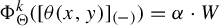 $\Phi _{\Theta }^{k}([\theta (x, y)]_{(-)})= \alpha \cdot W$
and
$\Phi _{\Theta }^{k}([\theta (x, y)]_{(-)})= \alpha \cdot W$
and
 $\Phi _{\Theta }^{k}([\theta (x,y)]_{(+)})=\alpha \cdot W$
, where
$\Phi _{\Theta }^{k}([\theta (x,y)]_{(+)})=\alpha \cdot W$
, where
 $k=k(x,y)$
.
$k=k(x,y)$
.
Lemma 5.1 shows that for an open set in the parameter space, the family
 $\Phi _{\Theta }$
satisfies a strong dynamical property: the eventual coincidence condition of ‘minimal’ length, that is, the length of the minimal bigon. The dynamics of the maps for parameters not in this open set is a priori different and quite interesting in its own right.
$\Phi _{\Theta }$
satisfies a strong dynamical property: the eventual coincidence condition of ‘minimal’ length, that is, the length of the minimal bigon. The dynamics of the maps for parameters not in this open set is a priori different and quite interesting in its own right.
6 Centred continuations and the middle parameter
In this section, we define a particular cutting parameter
 $\Theta ^0$
that we call middle. As we will see in §9, this choice of
$\Theta ^0$
that we call middle. As we will see in §9, this choice of
 $\Theta ^0$
allows us to perform particularly simple computations to get the volume entropy of the presentation. Many other parameters would allow the same computations, in particular, many parameters in the central interval defined in §5, but
$\Theta ^0$
allows us to perform particularly simple computations to get the volume entropy of the presentation. Many other parameters would allow the same computations, in particular, many parameters in the central interval defined in §5, but
 $\Theta ^0$
is very simple to define.
$\Theta ^0$
is very simple to define.
For each
 $1\le i\le 2N$
, we define the opposite to
$1\le i\le 2N$
, we define the opposite to
 $x_i$
as the symbol
$x_i$
as the symbol
 $x_{i+N}$
(recall that the subindexes in the generating set
$x_{i+N}$
(recall that the subindexes in the generating set
 $\{x_1,x_2,\ldots ,x_{2N}\}$
are taken modulo
$\{x_1,x_2,\ldots ,x_{2N}\}$
are taken modulo
 $2N$
, with
$2N$
, with
 $1,\ldots ,2N$
as representatives of the classes modulo
$1,\ldots ,2N$
as representatives of the classes modulo
 $2N$
).
$2N$
).
Let
 $g\in G$
and let
$g\in G$
and let
 $W=x_{i_0}x_{i_1}\cdots x_{i_{m-1}}$
be a geodesic expression of g. The infinite word
$W=x_{i_0}x_{i_1}\cdots x_{i_{m-1}}$
be a geodesic expression of g. The infinite word
 $Wx_{i_m}x_{i_{m+1}}\cdots $
such that
$Wx_{i_m}x_{i_{m+1}}\cdots $
such that
 $x_{i_j}$
is the opposite to
$x_{i_j}$
is the opposite to
 $(x_{i_{j-1}})^{-1}$
for each
$(x_{i_{j-1}})^{-1}$
for each
 $j\ge m$
will be called the centred continuation of W. Note that, from the vertex g of the Cayley graph, the last generator
$j\ge m$
will be called the centred continuation of W. Note that, from the vertex g of the Cayley graph, the last generator
 $x_{i_{m-1}}$
in the word W reads as the edge labelled
$x_{i_{m-1}}$
in the word W reads as the edge labelled
 $(x_{i_{m-1}})^{-1}$
. See Figure 8. From [Reference Los21, Lemma 2.9], the centred continuation of a geodesic expression of g is a geodesic ray. By definition, the corresponding point in
$(x_{i_{m-1}})^{-1}$
. See Figure 8. From [Reference Los21, Lemma 2.9], the centred continuation of a geodesic expression of g is a geodesic ray. By definition, the corresponding point in
 $S^1$
belongs to
$S^1$
belongs to
 $\mathcal {C}_g$
. It will be called the W-middle point.
$\mathcal {C}_g$
. It will be called the W-middle point.
The centred continuation of a geodesic W.

The next result will be used to prove one of the two inequalities stated in Proposition 7.3, a central result of §7.
Lemma 6.1. Let
 $g\in G$
and let
$g\in G$
and let
 $W=x_{i_0}x_{i_1}\cdots x_{i_{m-1}}$
be a geodesic expression of g. Let
$W=x_{i_0}x_{i_1}\cdots x_{i_{m-1}}$
be a geodesic expression of g. Let
 $Wx_{i_m}x_{i_{m+1}}\cdots $
be the centred continuation of W and let
$Wx_{i_m}x_{i_{m+1}}\cdots $
be the centred continuation of W and let
 $\zeta \in \partial G$
be the W-middle point. Then, any geodesic ray representing
$\zeta \in \partial G$
be the W-middle point. Then, any geodesic ray representing
 $\zeta $
has the form
$\zeta $
has the form
 $\hat {W}x_{i_m}x_{i_{m+1}}\cdots $
, where
$\hat {W}x_{i_m}x_{i_{m+1}}\cdots $
, where
 $\hat {W}$
is a geodesic expression of g.
$\hat {W}$
is a geodesic expression of g.
Proof. Set
 $L=Wx_{i_m}x_{i_{m+1}}\cdots $
and, for
$L=Wx_{i_m}x_{i_{m+1}}\cdots $
and, for
 $0\le i\le m$
, let us denote by
$0\le i\le m$
, let us denote by
 $v_i$
the vertex at distance i from
$v_i$
the vertex at distance i from
 $\mathrm {Id}$
inside the geodesic segment W. So,
$\mathrm {Id}$
inside the geodesic segment W. So,
 $v_0=\mathrm {Id}$
and
$v_0=\mathrm {Id}$
and
 $v_m=g$
. Let us assume, by way of contradiction, that there exists a geodesic ray R whose vertex at distance m from the identity is
$v_m=g$
. Let us assume, by way of contradiction, that there exists a geodesic ray R whose vertex at distance m from the identity is
 $g'\ne g$
. Assume without loss of generality, just to fix ideas and fit to the notation
$g'\ne g$
. Assume without loss of generality, just to fix ideas and fit to the notation
 $L/R$
, that
$L/R$
, that
 $g'$
is on the right of g in the obvious orientation induced in the Cayley graph by the clockwise orientation of the circle. Let j be the largest index in
$g'$
is on the right of g in the obvious orientation induced in the Cayley graph by the clockwise orientation of the circle. Let j be the largest index in
 $\{0,1,\ldots ,m\}$
such that
$\{0,1,\ldots ,m\}$
such that
 $v_j\in R$
. We are assuming that
$v_j\in R$
. We are assuming that
 $j<m$
. Now, we have two cases.
$j<m$
. Now, we have two cases.
Assume first that L and R intersect beyond
 $v_j$
. Let w be the vertex in
$v_j$
. Let w be the vertex in
 $L\cap R$
at least distance from
$L\cap R$
at least distance from
 $\mathrm {Id}$
larger than m. Then, the segments
$\mathrm {Id}$
larger than m. Then, the segments
 $\bar {L}\subset L$
and
$\bar {L}\subset L$
and
 $\bar {R}\subset R$
connecting
$\bar {R}\subset R$
connecting
 $v_j$
and w are geodesics and
$v_j$
and w are geodesics and
 $\bar {L}\cap \bar {R}=\{v_j,w\}$
. By Lemma 4.4, they are the left and right sides of a staircase between
$\bar {L}\cap \bar {R}=\{v_j,w\}$
. By Lemma 4.4, they are the left and right sides of a staircase between
 $v_j$
and w. Remarks 2.2 and 4.1 imply then that, given any vertex in
$v_j$
and w. Remarks 2.2 and 4.1 imply then that, given any vertex in
 $\bar {L}$
, there can be at most one edge of the Cayley graph contained in the bounded component K of
$\bar {L}$
, there can be at most one edge of the Cayley graph contained in the bounded component K of
 $\mathbb {R}^2\setminus (\bar {L}\cup \bar {R})$
. However, by definition of the centred continuation,
$\mathbb {R}^2\setminus (\bar {L}\cup \bar {R})$
. However, by definition of the centred continuation,
 $x_{i_m}$
is the edge opposite to
$x_{i_m}$
is the edge opposite to
 $(x_{i_{m-1}})^{-1}$
. Since
$(x_{i_{m-1}})^{-1}$
. Since
 $2N\ge 6$
, this implies that there are at least two edges departing from
$2N\ge 6$
, this implies that there are at least two edges departing from
 $g\in \bar {L}$
and contained in K (see Figure 8), which is a contradiction that proves the result in this case.
$g\in \bar {L}$
and contained in K (see Figure 8), which is a contradiction that proves the result in this case.
Assume now that L and R do not intersect beyond
 $v_j$
. Therefore, the infinite rays
$v_j$
. Therefore, the infinite rays
 $\bar {L}\subset L$
and
$\bar {L}\subset L$
and
 $\bar {R}\subset R$
starting at
$\bar {R}\subset R$
starting at
 $v_j$
define a bigon ray based at
$v_j$
define a bigon ray based at
 $v_j$
. Then, from Lemma 4.7, it follows that
$v_j$
. Then, from Lemma 4.7, it follows that
 $\bar {L}$
and
$\bar {L}$
and
 $\bar {R}$
are respectively the left and right sides of an infinite extension of bigons based at
$\bar {R}$
are respectively the left and right sides of an infinite extension of bigons based at
 $v_j$
, and we get a contradiction using exactly the same arguments as in the previous case.
$v_j$
, and we get a contradiction using exactly the same arguments as in the previous case.
The centred continuation allows us to define a particular choice
 $\Theta $
of the cutting parameter so that the dynamics of any cutting point by
$\Theta $
of the cutting parameter so that the dynamics of any cutting point by
 $\Phi _{\Theta }$
is specially simple.
$\Phi _{\Theta }$
is specially simple.
For each
 $1\le i\le 2N$
, let
$1\le i\le 2N$
, let
 $L_i^l$
and
$L_i^l$
and
 $L_i^r$
be the left and right geodesic segments of length
$L_i^r$
be the left and right geodesic segments of length
 $k(i):=k(x_{i-1},x_i)$
defining the minimal bigon
$k(i):=k(x_{i-1},x_i)$
defining the minimal bigon
 $\beta (x_{i-1},x_i)$
. The cutting parameter
$\beta (x_{i-1},x_i)$
. The cutting parameter
 $\Theta ^0 =(\theta ^0_1,\theta ^0_2,\ldots ,\theta ^0_{2N})$
such that
$\Theta ^0 =(\theta ^0_1,\theta ^0_2,\ldots ,\theta ^0_{2N})$
such that
 $\theta ^0_i$
is the
$\theta ^0_i$
is the
 $L_i^l$
-middle point for
$L_i^l$
-middle point for
 $i\in \{1,2,\ldots ,2N\}$
will be called the middle parameter.
$i\in \{1,2,\ldots ,2N\}$
will be called the middle parameter.
Remark 6.2. Let
 $\Theta ^0=(\theta ^0_1,\theta ^0_2,\ldots ,\theta ^0_{2N})$
be the middle parameter. Then, for each
$\Theta ^0=(\theta ^0_1,\theta ^0_2,\ldots ,\theta ^0_{2N})$
be the middle parameter. Then, for each
 ${1\le j\le 2N}$
, the cutting point
${1\le j\le 2N}$
, the cutting point
 $\theta ^0_j$
belongs to the central interval
$\theta ^0_j$
belongs to the central interval
 $C(J_j)$
defined in §5. Indeed, if z is the last generator in the word
$C(J_j)$
defined in §5. Indeed, if z is the last generator in the word
 $L_j^l$
, then the next generator along the centred continuation is the opposite to
$L_j^l$
, then the next generator along the centred continuation is the opposite to
 $z^{-1}$
that does not belong to the bigon extension (8) of
$z^{-1}$
that does not belong to the bigon extension (8) of
 $\beta (x_{j-1},x_j)$
.
$\beta (x_{j-1},x_j)$
.
In view of Remark 6.2, the first
 $k(j)$
iterates from the left and the right of
$k(j)$
iterates from the left and the right of
 $\theta ^0_j$
by
$\theta ^0_j$
by
 $\Phi _{\Theta ^0}$
are controlled by properties (a) and (b) of Lemma 5.1. The subsequent iterates satisfy the property stated in the next result.
$\Phi _{\Theta ^0}$
are controlled by properties (a) and (b) of Lemma 5.1. The subsequent iterates satisfy the property stated in the next result.
Lemma 6.3. Let
 $\Theta ^0=(\theta ^0_1,\theta ^0_2,\ldots ,\theta ^0_{2N})$
be the middle parameter. Then, for each
$\Theta ^0=(\theta ^0_1,\theta ^0_2,\ldots ,\theta ^0_{2N})$
be the middle parameter. Then, for each
 ${1\le j\le 2N}$
,
${1\le j\le 2N}$
,
 $\Phi _{\Theta ^0}^m(\theta ^0_j)$
is not a cutting point for any
$\Phi _{\Theta ^0}^m(\theta ^0_j)$
is not a cutting point for any
 $m\ge k(j)$
.
$m\ge k(j)$
.
Proof. The definition of the centred continuation implies that
 $\Phi _{\Theta ^0}^{k(j)}(\theta ^0_j)$
belongs to an interval
$\Phi _{\Theta ^0}^{k(j)}(\theta ^0_j)$
belongs to an interval
 $I_{x_{n}}$
and more precisely to
$I_{x_{n}}$
and more precisely to
 $I_{x_{n}}\setminus (J_{x_{n -1}}\cup J_{x_{n + 1}})$
. Indeed, along the geodesic ray
$I_{x_{n}}\setminus (J_{x_{n -1}}\cup J_{x_{n + 1}})$
. Indeed, along the geodesic ray
 $[\theta ^0_j]$
defining
$[\theta ^0_j]$
defining
 $\theta ^0_j$
, after the initial bigon
$\theta ^0_j$
, after the initial bigon
 $\beta (x_i,x_{i+1})$
, there is never two adjacent generators and thus there is never a subword of a bigon. Therefore, all iterates
$\beta (x_i,x_{i+1})$
, there is never two adjacent generators and thus there is never a subword of a bigon. Therefore, all iterates
 $\Phi _{\Theta ^0}^{m} (\theta ^0_j)$
, for
$\Phi _{\Theta ^0}^{m} (\theta ^0_j)$
, for
 $m \ge k(j)$
, belong to some interval
$m \ge k(j)$
, belong to some interval
 $I_{x_{r(m)}}\setminus (J_{x_{r(m) -1}} \cup J_{x_{r(m)+ 1}})$
for some
$I_{x_{r(m)}}\setminus (J_{x_{r(m) -1}} \cup J_{x_{r(m)+ 1}})$
for some
 $r(m) \in \{1, 2, \ldots , 2N\}$
. As a consequence,
$r(m) \in \{1, 2, \ldots , 2N\}$
. As a consequence,
 $\Phi _{\Theta ^0}^{m}(\theta ^0_j)$
is not a cutting point for all
$\Phi _{\Theta ^0}^{m}(\theta ^0_j)$
is not a cutting point for all
 $m \ge k(j)$
.
$m \ge k(j)$
.
7 Comparison of entropy functions
We start this section by recalling how the topological entropy of a piecewise monotone discontinuous map of the circle can be computed as the exponential growth rate of a function
 $X_m$
that counts the number of itineraries of length m associated to a given partition of
$X_m$
that counts the number of itineraries of length m associated to a given partition of
 $S^1$
such that the map is monotone on each interval of the partition (Lemma 7.2). Then, we prove Proposition 7.3, that compares the dynamical counting function
$S^1$
such that the map is monotone on each interval of the partition (Lemma 7.2). Then, we prove Proposition 7.3, that compares the dynamical counting function
 $X_m$
with the growth function
$X_m$
with the growth function
 $\sigma _m$
defined in (1). As a corollary, we get Theorem 7.4 that states the equality between the topological entropy of any Bowen–Series-like map and the volume entropy of the group presentation.
$\sigma _m$
defined in (1). As a corollary, we get Theorem 7.4 that states the equality between the topological entropy of any Bowen–Series-like map and the volume entropy of the group presentation.
The maps in the family
 $\Phi _{\Theta }$
are defined by a partition
$\Phi _{\Theta }$
are defined by a partition
 $S^1=\bigcup _{j=1}^{2N} I_j$
, where the intervals
$S^1=\bigcup _{j=1}^{2N} I_j$
, where the intervals
 $I_j=[\theta _j,\theta _{j+1})$
depend on the cutting parameter and the restriction of
$I_j=[\theta _j,\theta _{j+1})$
depend on the cutting parameter and the restriction of
 $\Phi _{\Theta }$
to each
$\Phi _{\Theta }$
to each
 $I_j$
is a homeomorphism. The intervals
$I_j$
is a homeomorphism. The intervals
 $I_j$
will be called basic intervals from now on. The generating set
$I_j$
will be called basic intervals from now on. The generating set
 $\mathcal {X}$
of the group G is in bijection with the set of basic intervals, for all parameters
$\mathcal {X}$
of the group G is in bijection with the set of basic intervals, for all parameters
 $\Theta $
. Each point
$\Theta $
. Each point
 $z\in S^1$
has an orbit which is described by an itinerary, that is, an ordered sequence
$z\in S^1$
has an orbit which is described by an itinerary, that is, an ordered sequence
 $$ \begin{align*} It(z):=(j_0,j_1,\ldots,j_m,\ldots) \quad\mbox{such that } \Phi_{\Theta}^m(z) \in I_{j_m} \text{ for all }\, m\ge0. \end{align*} $$
For
 $m\in \mathbb {N}$
, the itinerary intervals of level m are defined as
$m\in \mathbb {N}$
, the itinerary intervals of level m are defined as
 $$ \begin{align*} I_{j_0,j_1,\ldots,j_{m-1}}:=I_{j_0}\cap\Phi^{-1}_{\Theta}(I_{j_1})\cap\ldots\cap\Phi^{-(m-1)}_{\Theta}(I_{j_{m-1}}) \end{align*} $$
and the dynamical counting function is given by
 $$ \begin{align*} X_{m} \textrm{ is the number of non-empty intervals } I_{j_0,j_1,\ldots,j_{m-1}}\textrm{ of level } m. \end{align*} $$
Since each
 $\Phi _{\Theta }$
is a piecewise homeomorphism, there is at most one connected component in
$\Phi _{\Theta }$
is a piecewise homeomorphism, there is at most one connected component in
 $I_{j_0}$
such that
$I_{j_0}$
such that
 $\Phi _{\Theta }(I_{j_0})\cap I_{j_1}\neq \emptyset $
. As a consequence, the itinerary intervals are well defined.
$\Phi _{\Theta }(I_{j_0})\cap I_{j_1}\neq \emptyset $
. As a consequence, the itinerary intervals are well defined.
Remark 7.1. Note that if
 $I_{j_0,j_1,\ldots ,j_{m-1}}$
is a non-empty interval, then there exists
$I_{j_0,j_1,\ldots ,j_{m-1}}$
is a non-empty interval, then there exists
 $z\in S^1$
admitting a
$z\in S^1$
admitting a
 $\Phi _{\Theta }$
-orbit that visits
$\Phi _{\Theta }$
-orbit that visits
 $I_{x_{j_0}},I_{x_{j_1}},\ldots ,I_{x_{j_{m-1}}}$
. Therefore, if
$I_{x_{j_0}},I_{x_{j_1}},\ldots ,I_{x_{j_{m-1}}}$
. Therefore, if
 $I_{j_0,j_1,\ldots ,j_{m-1}}\ne \emptyset $
, then the path
$I_{j_0,j_1,\ldots ,j_{m-1}}\ne \emptyset $
, then the path
 $x_{j_0}x_{j_1}\cdots x_{j_{m-1}}$
is a geodesic path in the Cayley graph and the element
$x_{j_0}x_{j_1}\cdots x_{j_{m-1}}$
is a geodesic path in the Cayley graph and the element
 $g=x_{j_0}x_{j_1}\cdots x_{j_{m-1}}$
has length m.
$g=x_{j_0}x_{j_1}\cdots x_{j_{m-1}}$
has length m.
The itinerary intervals satisfy the following properties that follow immediately from the definitions:
-
(a)
$\text { for all } z\in I_{j_0,j_1,\ldots ,j_m},\, \Phi ^{r}_{\Theta }(z)\in I_{j_r}$
for
$0\le r\le m$
; -
(b)
$\text { for all } z \in I_{j_0,j_1,\ldots ,j_m},\, \Phi ^{m+1}_{\Theta }(z)=g^{-1}z$
, where
$g=x_{j_0}x_{j_1}\cdots x_{j_m}$
; -
(c)
$I_{j_0,j_1,\ldots ,j_m} $
is a subinterval of
$I_{j_0,j_1,\ldots ,j_{m-1}}$
.


Lemma 7.2. With the above notation, for each cutting parameter
 $\Theta \in J_1 \times \cdots \times J_{2N}$
, the following equality holds:
$\Theta \in J_1 \times \cdots \times J_{2N}$
, the following equality holds:
 $h_{\mathrm {top}}(\Phi _{\Theta })=\lim _{m \rightarrow \infty }({1}/{m})\log (X_m)$
.
$h_{\mathrm {top}}(\Phi _{\Theta })=\lim _{m \rightarrow \infty }({1}/{m})\log (X_m)$
.
Proof. The original definition of the topological entropy [Reference Adler, Konheim and McAndrew4] uses a counting function for coverings of the space. The definition holds for continuous self-maps on compact spaces. Bowen in [Reference Bowen10] extended this notion to non-necessarily continuous self-maps. In [Reference Misiurewicz and Ziemian25], Misiurewicz and Ziemian showed that, for piecewise continuous and piecewise monotone interval maps, the entropy can be computed from mono-covers, namely partitions of the interval by subintervals such that the map restricted to each element in the partition is continuous and monotone. With this partition, we denote by
 $Y_m$
the number of different itineraries of length m. Then, Misiurewicz and Ziemian showed that the entropy of the map coincides with
$Y_m$
the number of different itineraries of length m. Then, Misiurewicz and Ziemian showed that the entropy of the map coincides with
 $$ \begin{align*} \lim_{m \rightarrow\infty} \frac{\log Y_m}{m}.\end{align*} $$
It is straightforward to adapt the previous result to the case of piecewise continuous and piecewise monotone maps of the circle.
In view of Lemma 7.2 and the definition (2) of the volume entropy, which uses the counting function
 $\sigma _m$
introduced in (1), we need to compare the rates of increasing with m of
$\sigma _m$
introduced in (1), we need to compare the rates of increasing with m of
 $X_m$
and
$X_m$
and
 $\sigma _m$
. This is the aim of the next result.
$\sigma _m$
. This is the aim of the next result.
Proposition 7.3. With the above notation, the following inequalities are satisfied for each parameter
 $\Theta \in J_1\times J_2\times \cdots \times J_{2N}$
:
$\Theta \in J_1\times J_2\times \cdots \times J_{2N}$
:
 $$ \begin{align*} \sigma_m \le X_m\le m\sigma_m. \end{align*} $$
Proof. Let
 $g\in G$
be an element of length m. We will show that the number of non-empty intervals
$g\in G$
be an element of length m. We will show that the number of non-empty intervals
 $I_{j_0,\ldots ,j_{m-1}}$
such that
$I_{j_0,\ldots ,j_{m-1}}$
such that
 $x_{j_0}x_{j_1}\cdots x_{j_{m-1}}=g$
is between 1 and m.
$x_{j_0}x_{j_1}\cdots x_{j_{m-1}}=g$
is between 1 and m.
Consider a geodesic word
 $W=x_{i_0}x_{i_1}\cdots x_{i_{m-1}}$
representing g. Let
$W=x_{i_0}x_{i_1}\cdots x_{i_{m-1}}$
representing g. Let
 $Wx_{i_m}x_{i_{m+1}}\cdots $
be the centred continuation of W and let
$Wx_{i_m}x_{i_{m+1}}\cdots $
be the centred continuation of W and let
 $\rho \in S^1$
be the corresponding W-middle point. For
$\rho \in S^1$
be the corresponding W-middle point. For
 $0\le i<m$
, let
$0\le i<m$
, let
 $I_{x_{j_i}}$
be the only interval of the partition
$I_{x_{j_i}}$
be the only interval of the partition
 $\{I_{x_j}\}_{j=1}^{2N}$
of
$\{I_{x_j}\}_{j=1}^{2N}$
of
 $S^1$
containing
$S^1$
containing
 $\Phi _{\Theta }^i(\rho )$
. Then, the itinerary interval
$\Phi _{\Theta }^i(\rho )$
. Then, the itinerary interval
 $I_{j_0,j_1,\ldots ,j_{m-1}}$
is non-empty and, by Remark 7.1,
$I_{j_0,j_1,\ldots ,j_{m-1}}$
is non-empty and, by Remark 7.1,
 $x_{j_0}x_{j_1}\cdots x_{j_{m-1}}$
is a geodesic path in the Cayley graph. Then, from Lemma 6.1, it follows that
$x_{j_0}x_{j_1}\cdots x_{j_{m-1}}$
is a geodesic path in the Cayley graph. Then, from Lemma 6.1, it follows that
 $x_{j_0}x_{j_1}\cdots x_{j_{m-1}}=g$
. This shows that
$x_{j_0}x_{j_1}\cdots x_{j_{m-1}}=g$
. This shows that
 $\sigma _m \le X_m$
.
$\sigma _m \le X_m$
.
Let us prove now the second inequality. Clearly, if
 $I_{j_0,\ldots ,j_{m-1}}\ne \emptyset $
, then the path in the Cayley graph corresponding to the word
$I_{j_0,\ldots ,j_{m-1}}\ne \emptyset $
, then the path in the Cayley graph corresponding to the word
 $g:=x_{j_0}x_{j_1}\cdots x_{j_{m-1}}$
is a geodesic between the vertices
$g:=x_{j_0}x_{j_1}\cdots x_{j_{m-1}}$
is a geodesic between the vertices
 $\mathrm {Id}$
and g. So, it is contained in the set of all geodesics joining
$\mathrm {Id}$
and g. So, it is contained in the set of all geodesics joining
 $\mathrm {Id}$
and g which, by Lemma 4.6, is a gallery that we will denote by
$\mathrm {Id}$
and g which, by Lemma 4.6, is a gallery that we will denote by
 $H_{\mathrm {Id},g}$
. From the definition of a gallery, there are at most two edges in
$H_{\mathrm {Id},g}$
. From the definition of a gallery, there are at most two edges in
 $H_{\mathrm {Id},g}$
departing from the identity. This implies that the cylinder set
$H_{\mathrm {Id},g}$
departing from the identity. This implies that the cylinder set
 ${\mathcal {C}}_g$
defined in (4) of all infinite geodesic rays passing through g is contained in a set K that is either a basic interval or the union of two adjacent basic intervals. Since
${\mathcal {C}}_g$
defined in (4) of all infinite geodesic rays passing through g is contained in a set K that is either a basic interval or the union of two adjacent basic intervals. Since
 $H_{\mathrm {Id},g}$
is a gallery and the length of g is m,
$H_{\mathrm {Id},g}$
is a gallery and the length of g is m,
 $H_{\mathrm {Id},g}$
contains k minimal bigons for some
$H_{\mathrm {Id},g}$
contains k minimal bigons for some
 $0\le k<m$
. We denote by
$0\le k<m$
. We denote by
 $g_1,g_2,\ldots ,g_k$
the vertices at which such bigons are based. See Figure 9. Let
$g_1,g_2,\ldots ,g_k$
the vertices at which such bigons are based. See Figure 9. Let
 $\theta _{i_1},\theta _{i_2},\ldots ,\theta _{i_k}$
be the corresponding cutting points associated to each of these bigons. For
$\theta _{i_1},\theta _{i_2},\ldots ,\theta _{i_k}$
be the corresponding cutting points associated to each of these bigons. For
 $1\le j\le k$
, set
$1\le j\le k$
, set
 $\tilde \theta _j:=g_j\theta _{i_j}$
. Note that the cardinality of the set
$\tilde \theta _j:=g_j\theta _{i_j}$
. Note that the cardinality of the set
 $\{\tilde {\theta }_j\}_{j=1}^k$
, which is contained in K by construction, is between 1 and k (see Figure 9 for an example). Therefore,
$\{\tilde {\theta }_j\}_{j=1}^k$
, which is contained in K by construction, is between 1 and k (see Figure 9 for an example). Therefore,
 $$ \begin{align*} K\setminus \{\tilde \theta_1,\ldots,\tilde\theta_k\}\end{align*} $$
is the union of at most
 $k+1$
disjoint intervals that we denote by
$k+1$
disjoint intervals that we denote by
 $K_1,K_2,\ldots ,K_{k+1}$
.
$K_1,K_2,\ldots ,K_{k+1}$
.
The points
 $g_i$
as defined in the proof of Proposition 7.3.
$g_i$
as defined in the proof of Proposition 7.3.

We claim that in each of such intervals, there is at most one non-empty interval
 $I_{j_0,\ldots ,j_{m-1}}$
satisfying
$I_{j_0,\ldots ,j_{m-1}}$
satisfying
 $x_{j_0}x_{j_1}\cdots x_{j_{m-1}} = g$
. Indeed, assume in contrast that for some l, there are two non-empty intervals
$x_{j_0}x_{j_1}\cdots x_{j_{m-1}} = g$
. Indeed, assume in contrast that for some l, there are two non-empty intervals
 $I_{j_0,\ldots ,j_{m-1}}$
and
$I_{j_0,\ldots ,j_{m-1}}$
and
 $I_{h_0,\ldots ,h_{m-1}}$
contained in
$I_{h_0,\ldots ,h_{m-1}}$
contained in
 $K_l$
such that
$K_l$
such that
 $x_{j_0}x_{j_1}\cdots x_{j_{m-1}} = x_{h_0}x_{h_1}\cdots x_{h_{m-1}} = g$
.
$x_{j_0}x_{j_1}\cdots x_{j_{m-1}} = x_{h_0}x_{h_1}\cdots x_{h_{m-1}} = g$
.
The corresponding geodesic segments are thus contained in the gallery
 $H_{\mathrm {Id},g}$
. Let s be the least index such that
$H_{\mathrm {Id},g}$
. Let s be the least index such that
 $j_s\ne h_s$
. Then,
$j_s\ne h_s$
. Then,
 $x_{j_0}x_{j_1}\cdots x_{j_{s-1}} = x_{h_0}x_{h_1}\cdots x_{h_{s-1}} = g_r$
for some
$x_{j_0}x_{j_1}\cdots x_{j_{s-1}} = x_{h_0}x_{h_1}\cdots x_{h_{s-1}} = g_r$
for some
 $g_r$
being the origin of a minimal bigon
$g_r$
being the origin of a minimal bigon
 $\beta _{g_r}\subset H_{\mathrm {Id},g}$
associated to some cutting point
$\beta _{g_r}\subset H_{\mathrm {Id},g}$
associated to some cutting point
 $\theta _{i_r}$
. The bigon
$\theta _{i_r}$
. The bigon
 $\beta _{g_r}$
starts at
$\beta _{g_r}$
starts at
 $g_r$
by the edges labelled
$g_r$
by the edges labelled
 $x_{j_s}$
and
$x_{j_s}$
and
 $x_{h_s}$
. Therefore, the two itinerary intervals
$x_{h_s}$
. Therefore, the two itinerary intervals
 $I_{j_0,\ldots ,j_{m-1}}$
and
$I_{j_0,\ldots ,j_{m-1}}$
and
 $I_{h_0,\ldots ,h_{m-1}}$
contained in
$I_{h_0,\ldots ,h_{m-1}}$
contained in
 $K_l$
have a preimage of order s of the cutting point
$K_l$
have a preimage of order s of the cutting point
 $\theta _{i_r}$
between them, that is,
$\theta _{i_r}$
between them, that is,
 $\Phi _{\Theta }^{-s}(\theta _{i_r}) = g_r (\theta _{i_r})$
. Thus,
$\Phi _{\Theta }^{-s}(\theta _{i_r}) = g_r (\theta _{i_r})$
. Thus,
 $g_r (\theta _{i_r}) = \tilde { \theta }_{i_r}$
is contained in the interior of
$g_r (\theta _{i_r}) = \tilde { \theta }_{i_r}$
is contained in the interior of
 $K_l$
, which is a contradiction that proves the claim.
$K_l$
, which is a contradiction that proves the claim.
Since
 $k+1\le m$
, it follows that there are at most m non-empty intervals
$k+1\le m$
, it follows that there are at most m non-empty intervals
 $I_{j_0,\ldots ,j_{m-1}}$
such that
$I_{j_0,\ldots ,j_{m-1}}$
such that
 $x_{j_0} x_{j_1}\cdots x_{j_{m-1}} = g$
.
$x_{j_0} x_{j_1}\cdots x_{j_{m-1}} = g$
.
Finally, we get the desired equality between the entropies.
Theorem 7.4. Let
 $\Sigma $
be a compact closed hyperbolic surface with a geometric presentation P for the group
$\Sigma $
be a compact closed hyperbolic surface with a geometric presentation P for the group
 $G:=\pi _1(\Sigma )$
. Then,
$G:=\pi _1(\Sigma )$
. Then,
 $$ \begin{align*} h_{\mathrm{vol}}(G,P)=h_{\mathrm{top}}(\Phi_{\Theta})\quad\mbox{for all }\Theta\in J_1 \times\cdots\times J_{2N}. \end{align*} $$
8 Proof of Theorem A
The proof of Theorem A strongly uses the Milnor–Thurston theory [Reference Alsedà and Mañosas8, Reference Milnor and Thurston23] of kneading invariants. We start this section by reviewing the main ingredients of the theory. Then, we see how the results of Milnor and Thurston apply to our context. Finally, we prove Theorem A.
Kneading theory of Milnor and Thurston was stated for piecewise monotone and continuous maps of the interval. For such a map ![]() , the lap number
, the lap number
 $l(f)$
is the number of maximal intervals of monotonicity of f. Each point separating different maximal intervals of monotonicity is called a turning point. In this situation, the limit
$l(f)$
is the number of maximal intervals of monotonicity of f. Each point separating different maximal intervals of monotonicity is called a turning point. In this situation, the limit
 $s(f):=\lim (l(f^n))^{{1}/{n}}$
exists and is called the growth number of f. It is well known [Reference Misiurewicz and Szlenk24] that the topological entropy of f is precisely
$s(f):=\lim (l(f^n))^{{1}/{n}}$
exists and is called the growth number of f. It is well known [Reference Misiurewicz and Szlenk24] that the topological entropy of f is precisely
 $h_{\mathrm {top}}(f)=\log (s(f))$
.
$h_{\mathrm {top}}(f)=\log (s(f))$
.
Let
 $I_1,I_2,\ldots ,I_l$
be the laps associated to the map f, numbered in the natural ordering along I, and let
$I_1,I_2,\ldots ,I_l$
be the laps associated to the map f, numbered in the natural ordering along I, and let
 $v_1<v_2<\cdots <v_{l-1}$
be the corresponding turning points. The address
$v_1<v_2<\cdots <v_{l-1}$
be the corresponding turning points. The address
 $A(x)$
for a point
$A(x)$
for a point
 $x\in I$
will be the formal symbol
$x\in I$
will be the formal symbol
 $I_j$
if
$I_j$
if
 $x\in I_j$
or the formal symbol
$x\in I_j$
or the formal symbol
 $C_j$
if
$C_j$
if
 $x=v_j$
. The itinerary of x is the infinite sequence of symbols
$x=v_j$
. The itinerary of x is the infinite sequence of symbols
 $$ \begin{align*} I(x)=A(x),A(f(x)),A(f^2(x)),\ldots \end{align*} $$
To each address
 $A(x)$
, we assign the number
$A(x)$
, we assign the number
 $$ \begin{align*} \epsilon(A(x)):= \begin{cases} 1 & \text{if }f\text{ is increasing at }x, \\ -1 & \text{if }f\text{ is decreasing at }x, \\ 0 & \text{if }x\text{ is a turning point}, \end{cases} \end{align*} $$
and define a new infinite sequence
 $\omega (x)=(\omega _0(x),\omega _1(x),\ldots ,\omega _n(x),\ldots )$
given by
$\omega (x)=(\omega _0(x),\omega _1(x),\ldots ,\omega _n(x),\ldots )$
given by
 $$ \begin{align*} \omega_j(x)=\epsilon_j(x)A(f^j(x)), \quad\mbox{where } \epsilon_j(x)=\epsilon(A(x))\epsilon(A(f(x)))\cdots\epsilon(A(f^{j-1}(x))). \end{align*} $$
Note that
 $$ \begin{align*}\epsilon_j(x)= \begin{cases} 1 & \text{if }f^{j-1}\text{ is increasing at }x ,\\ -1 & \text{if }f^{j-1}\text{ is decreasing at }x ,\\ 0 & \text{if }f^k(x)\text{ is a turning point for some }k<j-1. \end{cases}\end{align*} $$
For any
 $x\in I$
and
$x\in I$
and
 $k\in \mathbb {N}$
, it is clear that
$k\in \mathbb {N}$
, it is clear that
 $\omega _k(y)$
is constant in a neighbourhood
$\omega _k(y)$
is constant in a neighbourhood
 $(x-\delta _k,x)$
. We denote the corresponding symbol by
$(x-\delta _k,x)$
. We denote the corresponding symbol by
 $\omega _k(x^-)$
. In the symmetric way, we define
$\omega _k(x^-)$
. In the symmetric way, we define
 $\omega _k(x^+)$
. Finally, we define the jump at x as the series
$\omega _k(x^+)$
. Finally, we define the jump at x as the series
 $$ \begin{align*}\Omega_x(t)=\sum_{i=0}^{\infty}(\omega_i(x^+)-\omega_i(x^-))t^i.\end{align*} $$
Note that if for all
 $n\in N,\,\,f^n(x)$
is not a turning point, then
$n\in N,\,\,f^n(x)$
is not a turning point, then
 $\Omega _x(t)$
is identically zero. The j-kneading invariant is defined as the jump at the jth turning point, that is,
$\Omega _x(t)$
is identically zero. The j-kneading invariant is defined as the jump at the jth turning point, that is,
 $$ \begin{align*} \nu_j(t)=\Omega_{v_j}(t)=\sum_{i=0}^{\infty}(\omega_i(v_j^+)-\omega_i(v_j^-))t^i. \end{align*} $$
It is clear that
 $\nu _j(t)=N_{j 1}I_1+\cdots N_{j l}I_l$
for any
$\nu _j(t)=N_{j 1}I_1+\cdots N_{j l}I_l$
for any
 $j\in \{1,2,\ldots ,l-1\}$
, where
$j\in \{1,2,\ldots ,l-1\}$
, where
 $N_{j i}$
belongs to the ring of formal power series with integer coefficients
$N_{j i}$
belongs to the ring of formal power series with integer coefficients
 $\mathbb {Z}[[t]]$
.
$\mathbb {Z}[[t]]$
.
At this moment, we define the
 $(l-1)\times l$
kneading matrix
$(l-1)\times l$
kneading matrix
 $M_f$
whose entries are the
$M_f$
whose entries are the
 $N_{ij}$
power series. Let us denote by
$N_{ij}$
power series. Let us denote by
 $D_i$
the determinant of the matrix obtained by deleting the ith column of the kneading matrix. The following is the first result of the above construction.
$D_i$
the determinant of the matrix obtained by deleting the ith column of the kneading matrix. The following is the first result of the above construction.
Theorem 8.1. With the above notation, the series
 $D(t)=(-1)^{i+1}({D_i}/({1-\epsilon (I_i)t}))$
is a fixed element of
$D(t)=(-1)^{i+1}({D_i}/({1-\epsilon (I_i)t}))$
is a fixed element of
 $\mathbb {Z}[[t]],$
independently of the choice of i. It has leading coefficient 1, converges for
$\mathbb {Z}[[t]],$
independently of the choice of i. It has leading coefficient 1, converges for
 $|t|<1$
and
$|t|<1$
and
 $D(t)\ne 0$
if
$D(t)\ne 0$
if
 $|t|<1/s(f)$
. Moreover, the first zero of
$|t|<1/s(f)$
. Moreover, the first zero of
 $D(t)$
in the interval
$D(t)$
in the interval
 $[0,1)$
occurs at
$[0,1)$
occurs at
 $({1}/{s(f)})$
if
$({1}/{s(f)})$
if
 $s(f)\ge 1$
, while
$s(f)\ge 1$
, while
 $D(t)$
has no zeros in the open unit disk if
$D(t)$
has no zeros in the open unit disk if
 $s(f)=1$
.
$s(f)=1$
.
In short, Theorem 8.1 says that the entropy of a map can be computed knowing the itineraries of the turning points.
Another important result from the Milnor–Thurston theory is the semi-conjugacy of any piecewise monotone map f of the interval to a piecewise affine map with constant absolute value of the slopes. Next, we give a brief explanation on how to construct the semi-conjugacy. See [Reference Milnor and Thurston23] for details. First of all, consider the series
 $$ \begin{align*} L(t)=\sum_{i=0}^\infty l(f^n)t^n. \end{align*} $$
Clearly,
 $L(t)$
converges for
$L(t)$
converges for
 $t<1/s(f)$
and has a pole at
$t<1/s(f)$
and has a pole at
 $t=1/s(f)$
. For any subinterval J of I, we define
$t=1/s(f)$
. For any subinterval J of I, we define
 $$ \begin{align*} L[J](t)=\sum_{i=0}^\infty l(f^n\vert_J)t^n, \end{align*} $$
where
 $l(f^n\vert _J)$
denotes the number of laps of
$l(f^n\vert _J)$
denotes the number of laps of
 $f^n$
that intersect J. Now, we define
$f^n$
that intersect J. Now, we define
 $$ \begin{align*} \mu(J):=\lim_{t\to 1/s(f)}\frac{L[J](t)}{L(t)}. \end{align*} $$
It is not difficult to see that
 $\mu $
satisfies the following properties:
$\mu $
satisfies the following properties:
-
(i)
$0\le \mu (J)\le 1$
; -
(ii) if
$J_1\cap J_2$
reduces to a single point, then
$\mu (J_1\cup J_2)=\mu (J_1)+\mu (J_2)$
; -
(iii) the number
$\mu (J)$
depends continuously on the endpoints of J; -
(iv) if J is contained in single lap of f, then
$\mu (f(J))=s(f)\mu (J)$
.


Properties (i)–(iv) imply that
 $\mu $
gives rise to a measure on the interval I. Now, consider the map
$\mu $
gives rise to a measure on the interval I. Now, consider the map ![]() defined as
defined as
 $$ \begin{align} h(x)=\mu([a,x]), \end{align} $$
where a is the left endpoint of I. From properties (i)–(iv) above, it follows that h is a continuous and non-decreasing map from I onto
 $[0,1]$
. Moreover, it is not difficult to see that if f is topologically transitive, then h is a homeomorphism (see for instance [Reference Alsedà, Llibre and Misiurewicz7, Proposition 4.6.9]). Lastly, we have the following result, which is essentially [Reference Milnor and Thurston23, Theorem 7.4].
$[0,1]$
. Moreover, it is not difficult to see that if f is topologically transitive, then h is a homeomorphism (see for instance [Reference Alsedà, Llibre and Misiurewicz7, Proposition 4.6.9]). Lastly, we have the following result, which is essentially [Reference Milnor and Thurston23, Theorem 7.4].
Theorem 8.2. Let ![]() be a piecewise monotone continuous map of an interval I and let
be a piecewise monotone continuous map of an interval I and let ![]() be the corresponding non-decreasing map defined by (⋆). Then, there exists a unique piecewise linear map
be the corresponding non-decreasing map defined by (⋆). Then, there exists a unique piecewise linear map ![]() with constant slope
with constant slope
 $\pm s(f)$
such that
$\pm s(f)$
such that
 $$ \begin{align*} F(h(x))=h(f(x)). \end{align*} $$
Moreover, if f is topologically transitive, then h is a homeomorphism.
In [Reference Alsedà and Mañosas5], Theorems 8.1 and 8.2 have been generalized to piecewise monotone maps f of degree one of the circle by considering its lifting
 $\tilde {f}$
and the map
$\tilde {f}$
and the map ![]() defined by
defined by
 $\widehat {f}(x)=\tilde {f}(x)-E(\tilde {f}(x))$
, where
$\widehat {f}(x)=\tilde {f}(x)-E(\tilde {f}(x))$
, where
 $E(y)$
denotes the integer part of y. The map
$E(y)$
denotes the integer part of y. The map
 $\widehat {f}$
is also piecewise monotone, but it is discontinuous. Therefore, it is necessary to consider the discontinuity points as turning points. In [Reference Alsedà and Mañosas8], the same results have been also generalized to discontinuous piecewise monotone maps of the circle. Now, all the discontinuities are considered as turning points.
$\widehat {f}$
is also piecewise monotone, but it is discontinuous. Therefore, it is necessary to consider the discontinuity points as turning points. In [Reference Alsedà and Mañosas8], the same results have been also generalized to discontinuous piecewise monotone maps of the circle. Now, all the discontinuities are considered as turning points.
Let us go back to our Bowen–Series-like maps. The next result states that, when
 $\Theta $
is the middle parameter as defined in §6, the jump series of
$\Theta $
is the middle parameter as defined in §6, the jump series of
 $\Phi _{\Theta }$
in all turning points are in fact polynomials.
$\Phi _{\Theta }$
in all turning points are in fact polynomials.
Lemma 8.3. Let
 $\Theta ^0=(\theta ^0_1,\theta ^0_2,\ldots ,\theta ^0_{2N})$
be the middle parameter. Then, the jump series
$\Theta ^0=(\theta ^0_1,\theta ^0_2,\ldots ,\theta ^0_{2N})$
be the middle parameter. Then, the jump series
 $\Omega _{\theta ^0_i}(t)$
for the map
$\Omega _{\theta ^0_i}(t)$
for the map
 $\Phi _{\Theta ^0}$
is a polynomial of degree at most
$\Phi _{\Theta ^0}$
is a polynomial of degree at most
 $k(x_{i-1},x_i)-1$
for every
$k(x_{i-1},x_i)-1$
for every
 ${1\le i\le 2N}$
. As a consequence, the kneading invariants of the map
${1\le i\le 2N}$
. As a consequence, the kneading invariants of the map
 $\Phi _{\Theta ^0}$
are integer polynomials.
$\Phi _{\Theta ^0}$
are integer polynomials.
Proof. We denote by
 $\tilde \Phi _{\Theta ^0}$
a lifting of
$\tilde \Phi _{\Theta ^0}$
a lifting of
 $\Phi _{\Theta ^0}$
. Identifying our topological
$\Phi _{\Theta ^0}$
. Identifying our topological
 $S^1$
with the unit circle in the complex plane, let
$S^1$
with the unit circle in the complex plane, let
 $z_1,z_2,\ldots ,z_{2N}\in [0,1)$
be such that
$z_1,z_2,\ldots ,z_{2N}\in [0,1)$
be such that
 $e^{2\pi z_i}=\theta ^0_i$
. Without loss of generality, we can assume that
$e^{2\pi z_i}=\theta ^0_i$
. Without loss of generality, we can assume that
 $z_1=0$
. For
$z_1=0$
. For
 $i=1,2,\ldots ,2N$
, we set
$i=1,2,\ldots ,2N$
, we set
 $I_i:=(z_i,z_{i+1})$
(where
$I_i:=(z_i,z_{i+1})$
(where
 $z_{2N+1}=0$
). As explained, we will consider the map
$z_{2N+1}=0$
). As explained, we will consider the map
 $\widehat {\Phi _{\Theta ^0}}$
, denoted by
$\widehat {\Phi _{\Theta ^0}}$
, denoted by
 $\Phi $
from now on to simplify the notation. Observe that some of the intervals
$\Phi $
from now on to simplify the notation. Observe that some of the intervals
 $I_i$
may split into two laps denoted by
$I_i$
may split into two laps denoted by
 $I_i^l$
and
$I_i^l$
and
 $I_i^r$
(standing for left and right) separated by one pre-image of
$I_i^r$
(standing for left and right) separated by one pre-image of
 $0$
, denoted by
$0$
, denoted by
 $m_i$
. The map
$m_i$
. The map
 $\Phi $
has, say, l laps and
$\Phi $
has, say, l laps and
 $l-1$
turning points, namely
$l-1$
turning points, namely
 $z_2,\ldots ,z_{2N}$
plus the set of points
$z_2,\ldots ,z_{2N}$
plus the set of points
 $m_i$
. See Figure 13 in §9 for a particular example, where the crosses in the horizontal axis mark the positions of the points
$m_i$
. See Figure 13 in §9 for a particular example, where the crosses in the horizontal axis mark the positions of the points
 $m_i$
.
$m_i$
.
Recall now the notation
 $\mathcal {X} = \{x_1,x_2,\ldots ,x_{2N}\}$
introduced in Definition 1 for the elements of the generating set. For each
$\mathcal {X} = \{x_1,x_2,\ldots ,x_{2N}\}$
introduced in Definition 1 for the elements of the generating set. For each
 $1\le j\le 2N$
, let
$1\le j\le 2N$
, let
 $\beta _j$
be the minimal bigon
$\beta _j$
be the minimal bigon
 $\beta (x_{j-1},x_j)$
and let us denote its length by
$\beta (x_{j-1},x_j)$
and let us denote its length by
 $k_j$
. Each bigon
$k_j$
. Each bigon
 $\beta _j$
is defined by two geodesics
$\beta _j$
is defined by two geodesics
 $L_j^l=x_{j-1}x_{j_2}\cdots x_{j_{k_j}}$
and
$L_j^l=x_{j-1}x_{j_2}\cdots x_{j_{k_j}}$
and
 $L_j^r=x_jy_{j_2}\cdots y_{j_{k_j}}\kern-1.3pt{.}$
By Remark 6.2, each cutting point
$L_j^r=x_jy_{j_2}\cdots y_{j_{k_j}}\kern-1.3pt{.}$
By Remark 6.2, each cutting point
 $\theta ^0_j$
belongs to the central interval
$\theta ^0_j$
belongs to the central interval
 $C(J_j)$
. As a consequence, we can apply Lemma 5.1(a). It follows that
$C(J_j)$
. As a consequence, we can apply Lemma 5.1(a). It follows that
 $$ \begin{align*} \lim_{h\to 0^+} \Phi^{k_j}(z_j+h)=\lim_{h\to 0^-} \Phi^{k_j} (z_j+h)=:\pi_j. \end{align*} $$
Now, we claim that
 $\epsilon _{k_j}(z_j^+)=\epsilon _{k_j}(z_j^-)$
. Indeed, since
$\epsilon _{k_j}(z_j^+)=\epsilon _{k_j}(z_j^-)$
. Indeed, since
 $\theta ^0_j \in C(J_j)$
, it can be written as two different geodesic rays
$\theta ^0_j \in C(J_j)$
, it can be written as two different geodesic rays
 $L_j^lW,L_j^rW$
. At a symbolic level,
$L_j^lW,L_j^rW$
. At a symbolic level,
 $\Phi ^{k_j}(\theta _j^0)_{(+)}$
corresponds to shifting the first
$\Phi ^{k_j}(\theta _j^0)_{(+)}$
corresponds to shifting the first
 $k_j$
letters of
$k_j$
letters of
 $L_j^lW$
, so giving W (see Lemma 5.1). Now, if we apply
$L_j^lW$
, so giving W (see Lemma 5.1). Now, if we apply
 $(\Phi ^{-1})^{k_j}_{(-)}$
, which corresponds to the left multiplication by
$(\Phi ^{-1})^{k_j}_{(-)}$
, which corresponds to the left multiplication by
 $L_j^r$
, we get
$L_j^r$
, we get
 $L_j^rW$
. So, the composition
$L_j^rW$
. So, the composition
 $(\Phi ^{-1})^{k_j}_{(-)}\circ \Phi ^{k_j}_{(+)}$
is the identity map on a neighbourhood of
$(\Phi ^{-1})^{k_j}_{(-)}\circ \Phi ^{k_j}_{(+)}$
is the identity map on a neighbourhood of
 $\theta ^0_j \in C(J_j)$
. At a group theoretic level, this identity is nothing but a relation in the group, seen as a subgroup of
$\theta ^0_j \in C(J_j)$
. At a group theoretic level, this identity is nothing but a relation in the group, seen as a subgroup of
 $\textrm {Homeo}(S^1)$
. As a consequence,
$\textrm {Homeo}(S^1)$
. As a consequence,
 $\Phi ^{k_j}_{(-)}$
and
$\Phi ^{k_j}_{(-)}$
and
 $\Phi ^{k_j}_{(+)}$
are either both increasing or both decreasing. From this fact and the definition of the terms of the jump series, the claim follows.
$\Phi ^{k_j}_{(+)}$
are either both increasing or both decreasing. From this fact and the definition of the terms of the jump series, the claim follows.
From the previous claim, we get that
 $$ \begin{align*} \Omega_{z_j}(t)=\sum_{i=0}^{k_{j-1}}(\omega_i(z_j^+)-\omega_i(z_j^-))t^i+\epsilon_{k_j}(z_j)t^{k_j}\Omega(\pi_j).\end{align*} $$
Since the orbit of
 $\pi _j$
does not visit any cutting point by Lemma 6.3, then
$\pi _j$
does not visit any cutting point by Lemma 6.3, then
 $\Omega (\pi _j)=0$
.
$\Omega (\pi _j)=0$
.
With all these ingredients, we are ready to prove Theorem A.
Proof of Theorem A
The equality between the entropies stated in statement (a) follows from Theorem 7.4. The fact that
 $1/\unicode{x3bb} $
is the smallest root in
$1/\unicode{x3bb} $
is the smallest root in
 $(0,1)$
of an integer polynomial follows from Lemma 8.3 and Theorem 8.1, which states that for the middle parameter, the entries of the kneading matrix are integer polynomials.
$(0,1)$
of an integer polynomial follows from Lemma 8.3 and Theorem 8.1, which states that for the middle parameter, the entries of the kneading matrix are integer polynomials.
The proof of statement (b) follows from Proposition 2.5 and the generalization of Theorem 8.2 to circle maps [Reference Alsedà and Mañosas5, Reference Alsedà and Mañosas8].
9 Effective computations and examples
In this section, we give some examples of computation of the volume entropy associated to a geometric presentation. The whole process is based on Theorem A and the Milnor–Thurston theory outlined in §8. Moreover, the power of such techniques has allowed us to organize the computation in a systematic way to produce an algorithm that takes as input any presentation P given by a list R of relations, and prints out the associated volume entropy provided that P is geometric (otherwise, the program reports that P is not geometric). The procedure has been written in Maple and is available at https://github.com/CombTopDynamics-cat/VolEntropyAlgorithm.git. A forthcoming open source version of the code will be soon available at the same repository. Next, we show the code of the main program, just because it clearly sets out the main steps of the computation.

See Table 1 for some examples of execution of the program. The third column shows the polynomial factor of the kneading determinant with roots in
 $[0,1)$
.
$[0,1)$
.
9.1 Checking relations
The procedure CheckRelations(R) checks whether R verifies the following syntax conventions. The set R of relations must be a list of lists of integers. Any generator is entered as a positive integer k, while its inverse is
 $-k$
. The set of absolute values of all integers in R has to be
$-k$
. The set of absolute values of all integers in R has to be
 $\{1,2,\ldots ,n\}$
for some
$\{1,2,\ldots ,n\}$
for some
 $n\ge 3$
. By Remark 2.2, we exclude presentations having relations of length 2, and also the presentation having 3 generators and 2 relations of length 3. As an example, next, we show the inputs satisfying the conventions of the program for the following presentations (from now on, the inverse of an element a will be written as
$n\ge 3$
. By Remark 2.2, we exclude presentations having relations of length 2, and also the presentation having 3 generators and 2 relations of length 3. As an example, next, we show the inputs satisfying the conventions of the program for the following presentations (from now on, the inverse of an element a will be written as
 $\bar {a}$
):
$\bar {a}$
):
 $$ \begin{align*} P_1 = \langle a,b,c,d\, |\,adac,cbdb\rangle\longrightarrow R=[ [1,4,1,3],[3,2,4,2] ], \end{align*} $$
 $$ \begin{align*} P_2 = \langle a,b,c,d,e\, |\,abc,ce\bar{a},b\bar{c}d^2\rangle\longrightarrow R=[ [1,2,3],[3,5,-1],[2,-3,4,4] ], \end{align*} $$
 $$ \begin{align*} P_3 = \langle a,b,c,d\, |\,aba\bar{b}d,c^2d\rangle\longrightarrow R=[ [1,2,1,-2,4],[3,3,4] ]. \end{align*} $$
Some outputs of the algorithm.

9.2 Computing the cyclic ordering
Once we have a syntactically admissible list of relations R, we have to test whether it corresponds to a geometric presentation. This task is assigned to the procedure CyclicOrdering(R), based on properties (a), (c) and (d) of Lemma 2.1, which is in fact a characterization of the geometric presentations of co-compact hyperbolic surface groups. As a first test of geometricity, we check whether each generator appears twice (with
 $+$
or
$+$
or
 $-$
sign) in R (Lemma 2.1(c)). This test excludes the presentation
$-$
sign) in R (Lemma 2.1(c)). This test excludes the presentation
 $P_2$
above as non-geometric, while
$P_2$
above as non-geometric, while
 $P_1$
and
$P_1$
and
 $P_3$
pass the test. It turns out, however, that
$P_3$
pass the test. It turns out, however, that
 $P_3$
is geometric while
$P_3$
is geometric while
 $P_1$
is not. The reason is that
$P_1$
is not. The reason is that
 $P_3$
, unlike
$P_3$
, unlike
 $P_1$
, satisfies property (a): it is possible to find a cyclic ordering in the generating set that is preserved by the action of the group. Let us briefly sketch how to decide whether such a cyclic ordering exists for a presentation
$P_1$
, satisfies property (a): it is possible to find a cyclic ordering in the generating set that is preserved by the action of the group. Let us briefly sketch how to decide whether such a cyclic ordering exists for a presentation
 $P=\langle X|R\rangle $
and, in the affirmative, how to find it.
$P=\langle X|R\rangle $
and, in the affirmative, how to find it.
First, we fix the identity element
 $\mathrm {Id}$
of the group as the base vertex of the Cayley 2-complex
$\mathrm {Id}$
of the group as the base vertex of the Cayley 2-complex
 $\textrm {Cay}^2(G,P)$
. If this 2-complex is planar, then the boundary of each cell adjacent to
$\textrm {Cay}^2(G,P)$
. If this 2-complex is planar, then the boundary of each cell adjacent to
 $\mathrm {Id}$
is a closed path from
$\mathrm {Id}$
is a closed path from
 $\mathrm {Id}$
to itself that, read in the clockwise direction, is (a cyclic shift of) a relation in
$\mathrm {Id}$
to itself that, read in the clockwise direction, is (a cyclic shift of) a relation in
 $R\cup \bar {R}$
. We choose an arbitrary relation
$R\cup \bar {R}$
. We choose an arbitrary relation
 $g_1g_2\cdots g_k$
in R and think of it as the first cell, drawn in the clockwise direction. So, we are fixing
$g_1g_2\cdots g_k$
in R and think of it as the first cell, drawn in the clockwise direction. So, we are fixing
 $g_1$
as the first generator in the cyclic ordering, while the second one (to the right in the plane and read from the base vertex
$g_1$
as the first generator in the cyclic ordering, while the second one (to the right in the plane and read from the base vertex
 $\mathrm {Id}$
) is
$\mathrm {Id}$
) is
 $\bar {g_k}$
. Now, to get the next generator to the right in the cyclic ordering, we have to choose a cyclic shift of a relation in
$\bar {g_k}$
. Now, to get the next generator to the right in the cyclic ordering, we have to choose a cyclic shift of a relation in
 $R\cup \bar {R}$
starting by
$R\cup \bar {R}$
starting by
 $\bar {g_k}$
, say
$\bar {g_k}$
, say
 $\bar {g_k}f_2\cdots f_l$
. The next right generator will be
$\bar {g_k}f_2\cdots f_l$
. The next right generator will be
 $\bar {f_l}$
. The condition is that
$\bar {f_l}$
. The condition is that
 $\bar {f_l}$
must not be a previously found generator.
$\bar {f_l}$
must not be a previously found generator.
As an example, take for instance the presentation
 $P_1$
above. Set
$P_1$
above. Set
 $R_1=adac$
,
$R_1=adac$
,
 $R_2=cbdb$
. The process is illustrated in Figure 10. After three steps, we get the generators
$R_2=cbdb$
. The process is illustrated in Figure 10. After three steps, we get the generators
 $a,\bar {c},b,\bar {d}$
, but in the fourth step, it is not possible to continue: we cannot use the shift
$a,\bar {c},b,\bar {d}$
, but in the fourth step, it is not possible to continue: we cannot use the shift
 $\bar {d}\bar {b}\bar {c}\bar {b}$
of
$\bar {d}\bar {b}\bar {c}\bar {b}$
of
 $\bar {R_2}$
(previously used in step 3) and we are forced to use the shift
$\bar {R_2}$
(previously used in step 3) and we are forced to use the shift
 $\bar {d}\bar {a}\bar {c}\bar {a}$
of
$\bar {d}\bar {a}\bar {c}\bar {a}$
of
 $\bar {R_1}$
, which gives rise to a as the next generator. Since a was the starting generator and we have not yet completed the round (of all 4 generators and their inverses), it follows that the presentation
$\bar {R_1}$
, which gives rise to a as the next generator. Since a was the starting generator and we have not yet completed the round (of all 4 generators and their inverses), it follows that the presentation
 $P_1$
cannot be geometric.
$P_1$
cannot be geometric.
A non-geometric presentation. The circles numbered by i indicate the angles used to attach the cell at step i of the algorithm.

However, the previous procedure applied to the presentation
 $P_3$
above does give a complete cycle of all 4 generators and their inverses. The obtained cyclic ordering, together with all cells adjacent to the base vertex
$P_3$
above does give a complete cycle of all 4 generators and their inverses. The obtained cyclic ordering, together with all cells adjacent to the base vertex
 $\mathrm {Id}$
, are shown in Figure 11(a).
$\mathrm {Id}$
, are shown in Figure 11(a).
(a) Cells adjacent to the base vertex
 $\mathrm {Id}$
and the cyclic ordering associated to the presentation
$\mathrm {Id}$
and the cyclic ordering associated to the presentation
 $P_3$
. (b) Attaching cells to get the minimal bigons.
$P_3$
. (b) Attaching cells to get the minimal bigons.

9.3 Computing the minimal bigons
Once a cyclic ordering has been found for a presentation, the next step is to compute what we call the minimal bigons (see Proposition 2.3). Given two generators
 $x,y$
consecutive in the cyclic ordering, Proposition 2.3(b) states that there exists a unique bigon
$x,y$
consecutive in the cyclic ordering, Proposition 2.3(b) states that there exists a unique bigon
 $\beta (x,y)$
of minimal length. Such a bigon is given by a pair of geodesics
$\beta (x,y)$
of minimal length. Such a bigon is given by a pair of geodesics
 $\gamma _1,\gamma _2$
connecting the base vertex
$\gamma _1,\gamma _2$
connecting the base vertex
 $\mathrm {Id}$
and another vertex w, with
$\mathrm {Id}$
and another vertex w, with
 $\gamma _1$
starting at
$\gamma _1$
starting at
 $\mathrm {Id}$
by the edge labelled x and
$\mathrm {Id}$
by the edge labelled x and
 $\gamma _2$
starting at
$\gamma _2$
starting at
 $\mathrm {Id}$
by y. Since both geodesics must have the same length,
$\mathrm {Id}$
by y. Since both geodesics must have the same length,
 $\gamma _1\bar {\gamma _2}$
is a closed path of even length that, read clockwise, starts with the edge x and ends with the edge
$\gamma _1\bar {\gamma _2}$
is a closed path of even length that, read clockwise, starts with the edge x and ends with the edge
 $\bar {y}$
. Recall that the length of the bigon
$\bar {y}$
. Recall that the length of the bigon
 $\beta $
has been defined as the length of any of the two geodesics
$\beta $
has been defined as the length of any of the two geodesics
 $\gamma _1,\gamma _2$
and is denoted by
$\gamma _1,\gamma _2$
and is denoted by
 $k(x,y)$
.
$k(x,y)$
.
The existence of the minimal bigons is proved in [Reference Los21, Proposition 2.6]. The proof is algorithmic and is implemented in the procedure MinimalBigons(R,co). In short and taking the above presentation
 $P_3$
as an example: consider the cell of the 2-complex
$P_3$
as an example: consider the cell of the 2-complex
 $\textrm {Cay}^2(P_3)$
adjacent to a, whose boundary B reads clockwise as
$\textrm {Cay}^2(P_3)$
adjacent to a, whose boundary B reads clockwise as
 $aba\bar {b}d$
(Figure 11(a)). Since its length is odd, it cannot define a minimal bigon. So, we take its central symbol, a, look for the shift of a word in
$aba\bar {b}d$
(Figure 11(a)). Since its length is odd, it cannot define a minimal bigon. So, we take its central symbol, a, look for the shift of a word in
 $R\cup \bar {R}$
starting by a, and glue together both cells along a. By Lemma 2.1(c), there are exactly two of such shifts in
$R\cup \bar {R}$
starting by a, and glue together both cells along a. By Lemma 2.1(c), there are exactly two of such shifts in
 $R\cup \bar {R}$
, in this case,
$R\cup \bar {R}$
, in this case,
 $Y:=aba\bar {b}d$
and
$Y:=aba\bar {b}d$
and
 $Z:=a\bar {b}dab$
. Since Y is in fact a shift of
$Z:=a\bar {b}dab$
. Since Y is in fact a shift of
 $\bar {B}$
, using Y would yield a boundary containing the cancellation
$\bar {B}$
, using Y would yield a boundary containing the cancellation
 $b\bar {b}$
that cannot be geodesic. So, we are forced to use Z. From Lemma 2.1(d), it easily follows that using Z cannot produce cancellations. Once both cells are attached, in this case, the obtained boundary has length 8, which thus defines a minimal bigon of length 4. See Figure 11(b). If the length of the boundary was odd, this procedure can be iterated and yields the minimal bigon after a finite number of steps.
$b\bar {b}$
that cannot be geodesic. So, we are forced to use Z. From Lemma 2.1(d), it easily follows that using Z cannot produce cancellations. Once both cells are attached, in this case, the obtained boundary has length 8, which thus defines a minimal bigon of length 4. See Figure 11(b). If the length of the boundary was odd, this procedure can be iterated and yields the minimal bigon after a finite number of steps.
9.4 Choosing the cutting points and computing the kneading invariants
The final stage of the whole process is the computation of the kneading matrix introduced in §8. This task is assigned to the procedure KneadingMatrix(co,bigons,R). According to Theorem A, the volume entropy of the presentation equals the topological entropy of the Bowen–Series-like map
 $\Phi _\Theta $
for any choice of the set of cutting points
$\Phi _\Theta $
for any choice of the set of cutting points
 $\Theta $
(note that specifying a particular map
$\Theta $
(note that specifying a particular map
 $\Phi _\Theta $
is equivalent to specifying
$\Phi _\Theta $
is equivalent to specifying
 $\Theta $
). As a consequence, we are free to choose the set of cutting points
$\Theta $
). As a consequence, we are free to choose the set of cutting points
 $\Theta $
for the kneading matrix of the corresponding map
$\Theta $
for the kneading matrix of the corresponding map
 $\Phi _\Theta $
to be particularly simple. However, it is remarkable that a lot of information about any map
$\Phi _\Theta $
to be particularly simple. However, it is remarkable that a lot of information about any map
 $\Phi _\Theta $
in the family is independent of
$\Phi _\Theta $
in the family is independent of
 $\Theta $
and can be algorithmically extracted just from the combinatorial data encoded in the set of minimal bigons.
$\Theta $
and can be algorithmically extracted just from the combinatorial data encoded in the set of minimal bigons.
To illustrate it, we continue with the presentation
 $P_3$
above, whose minimal bigons are shown in Figure 11(b). The cyclic ordering reads clockwise as
$P_3$
above, whose minimal bigons are shown in Figure 11(b). The cyclic ordering reads clockwise as
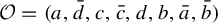 $\mathcal {O}=(a,\bar {d},c,\bar {c},d,b,\bar {a},\bar {b})$
.
$\mathcal {O}=(a,\bar {d},c,\bar {c},d,b,\bar {a},\bar {b})$
.
The definition of the interval
 $I_a$
for the geometric presentation
$I_a$
for the geometric presentation
 $P_3$
.
$P_3$
.

Assume that for any pair
 $x,y$
of adjacent generators, we have an (unspecified) cutting point
$x,y$
of adjacent generators, we have an (unspecified) cutting point
 $\theta _y$
in the intersection of the cylinders
$\theta _y$
in the intersection of the cylinders
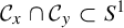 $\mathcal {C}_x\cap \mathcal {C}_y\subset S^1$
, and set
$\mathcal {C}_x\cap \mathcal {C}_y\subset S^1$
, and set
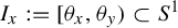 $I_x:=[\theta _x,\theta _y)\subset S^1$
. See Figure 12. Let us see how to find the left and right images of any cutting point by a Bowen–Series-like map
$I_x:=[\theta _x,\theta _y)\subset S^1$
. See Figure 12. Let us see how to find the left and right images of any cutting point by a Bowen–Series-like map
 $\Phi $
. As an example, the reader will find it useful to get
$\Phi $
. As an example, the reader will find it useful to get
 $\Phi (\theta _a)_{(-)}$
and
$\Phi (\theta _a)_{(-)}$
and
 $\Phi (\theta _a)_{(+)}$
following the picture shown in Figure 12. By the characterization of the intersection of cylinders given by Theorem 3.4, the cutting point
$\Phi (\theta _a)_{(+)}$
following the picture shown in Figure 12. By the characterization of the intersection of cylinders given by Theorem 3.4, the cutting point
 $\theta _a$
has to be represented by two infinite words of the form
$\theta _a$
has to be represented by two infinite words of the form
 $a\bar {b}\bar {c}\cdots $
and
$a\bar {b}\bar {c}\cdots $
and
 $\bar {b}\bar {a}c\cdots $
. Considering
$\bar {b}\bar {a}c\cdots $
. Considering
 $\theta _a$
as
$\theta _a$
as
 $a\bar {b}\bar {c}\cdots $
(a point of the cylinder
$a\bar {b}\bar {c}\cdots $
(a point of the cylinder
 $\mathcal {C}_a$
) and taking into account that, by definition,
$\mathcal {C}_a$
) and taking into account that, by definition,
 $\Phi $
acts as a shift, it follows that
$\Phi $
acts as a shift, it follows that
 $\Phi (\theta _a)_{(+)}$
is an infinite word starting by
$\Phi (\theta _a)_{(+)}$
is an infinite word starting by
 $\bar {b}\bar {c}\cdots $
. In other words,
$\bar {b}\bar {c}\cdots $
. In other words,
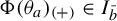 $\Phi (\theta _a)_{(+)}\in I_{\bar {b}}$
by Lemma 5.1(b). Analogously,
$\Phi (\theta _a)_{(+)}\in I_{\bar {b}}$
by Lemma 5.1(b). Analogously,
 $\Phi (\theta _a)_{(-)}$
can be read as an infinite word starting by
$\Phi (\theta _a)_{(-)}$
can be read as an infinite word starting by
 $\bar {a}c\cdots $
. Thus,
$\bar {a}c\cdots $
. Thus,
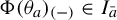 $\Phi (\theta _a)_{(-)}\in I_{\bar {a}}$
. As a quick recipe and after some practice, the reader will find it easy to be convinced that, for any interval
$\Phi (\theta _a)_{(-)}\in I_{\bar {a}}$
. As a quick recipe and after some practice, the reader will find it easy to be convinced that, for any interval
 $I_x=[\theta _x,\theta _y)$
, the right image of the left endpoint
$I_x=[\theta _x,\theta _y)$
, the right image of the left endpoint
 $\theta _x$
belongs to
$\theta _x$
belongs to
 $I_z$
, where z is the generator following x along the bigon that, read counterclockwise, starts by x, while the left image of the right endpoint
$I_z$
, where z is the generator following x along the bigon that, read counterclockwise, starts by x, while the left image of the right endpoint
 $\theta _y$
belongs to
$\theta _y$
belongs to
 $I_w$
, where w is the generator following x along the bigon that, read clockwise, starts by x.
$I_w$
, where w is the generator following x along the bigon that, read clockwise, starts by x.
At this moment, we know which intervals contain the right and left images respectively of the left and right endpoints of any interval
 $I_x$
. Since we know that
$I_x$
. Since we know that
 $\Phi $
is a homeomorphism on each
$\Phi $
is a homeomorphism on each
 $I_x$
, we can simply connect the dots to get an approximate graph of
$I_x$
, we can simply connect the dots to get an approximate graph of
 $\Phi $
. However, when connecting the dots, the question arises whether the map is increasing or decreasing on each interval. For instance, take the interval
$\Phi $
. However, when connecting the dots, the question arises whether the map is increasing or decreasing on each interval. For instance, take the interval
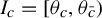 $I_c=[\theta _c,\theta _{\bar {c}})$
. The previous recipe using the minimal bigons tells us that
$I_c=[\theta _c,\theta _{\bar {c}})$
. The previous recipe using the minimal bigons tells us that
 $\Phi (\theta _c)_{(+)}\in I_{\bar {d}}$
and
$\Phi (\theta _c)_{(+)}\in I_{\bar {d}}$
and
 $\Phi (\theta _{\bar {c}})_{(-)}\in I_b$
. Now, check Figure 11(b) to see that three clockwise consecutive edges
$\Phi (\theta _{\bar {c}})_{(-)}\in I_b$
. Now, check Figure 11(b) to see that three clockwise consecutive edges
 $\bar {c},c,\bar {d}$
depart from the group element (vertex) c. Note that these three symbols are consecutive in the cyclic ordering
$\bar {c},c,\bar {d}$
depart from the group element (vertex) c. Note that these three symbols are consecutive in the cyclic ordering
 $\mathcal {O}$
, but in the counterclockwise direction. In other words, the cyclic ordering of the edges departing from c is the reverse of
$\mathcal {O}$
, but in the counterclockwise direction. In other words, the cyclic ordering of the edges departing from c is the reverse of
 $\mathcal {O}$
. It easily follows that the map has to be orientation reversing in
$\mathcal {O}$
. It easily follows that the map has to be orientation reversing in
 $I_c$
. See Figure 13 for a sketch of a Bowen–Series-like map
$I_c$
. See Figure 13 for a sketch of a Bowen–Series-like map
 $\Phi $
corresponding to the presentation
$\Phi $
corresponding to the presentation
 $P_3$
, where the horizontal axis, which represents
$P_3$
, where the horizontal axis, which represents
 $S^1$
, has been duplicated in the vertical direction. The reader can use again Figure 11 to check that the edges departing from vertices
$S^1$
, has been duplicated in the vertical direction. The reader can use again Figure 11 to check that the edges departing from vertices
 $c,\bar {c},b,\bar {b}$
are organized clockwise as the reverse of the cyclic ordering
$c,\bar {c},b,\bar {b}$
are organized clockwise as the reverse of the cyclic ordering
 $\mathcal {O}$
, and so the map is decreasing on the corresponding intervals
$\mathcal {O}$
, and so the map is decreasing on the corresponding intervals
 $I_c,I_{\bar {c}},I_b,I_{\bar {b}}$
.
$I_c,I_{\bar {c}},I_b,I_{\bar {b}}$
.
A sketch of the graph of
 $\Phi $
for the geometric presentation
$\Phi $
for the geometric presentation
 $P_3$
, where each interval
$P_3$
, where each interval
 $I_x$
has been labelled by x. The preimages of the leftmost point are marked with crosses in the horizontal axis.
$I_x$
has been labelled by x. The preimages of the leftmost point are marked with crosses in the horizontal axis.

To apply the theory of Milnor–Thurston invariants, we have to consider the lifting
 $\tilde {\Phi }$
of
$\tilde {\Phi }$
of
 $\Phi $
and the map
$\Phi $
and the map ![]() defined by
defined by
 $\widehat {\Phi }(F)(x)=\tilde {\Phi }(x)-E(\tilde {\Phi }(x))$
, where
$\widehat {\Phi }(F)(x)=\tilde {\Phi }(x)-E(\tilde {\Phi }(x))$
, where
 $E(y)$
denotes the integer part of y (for simplicity and abuse of language,
$E(y)$
denotes the integer part of y (for simplicity and abuse of language,
 $\widehat {\Phi }$
will be denoted by
$\widehat {\Phi }$
will be denoted by
 $\Phi $
from now on). It is then clear that
$\Phi $
from now on). It is then clear that
 $\Phi $
is a piecewise monotone and discontinuous map. The set of points separating maximal intervals of monotonicity (turning points) is precisely the set
$\Phi $
is a piecewise monotone and discontinuous map. The set of points separating maximal intervals of monotonicity (turning points) is precisely the set
 $\Theta $
of all cutting points plus the set of preimages of the leftmost cutting point,
$\Theta $
of all cutting points plus the set of preimages of the leftmost cutting point,
 $\theta _a$
. There is at most one of such preimages,
$\theta _a$
. There is at most one of such preimages,
 $m_x$
, in any interval
$m_x$
, in any interval
 $I_x$
, and in this case, the interval
$I_x$
, and in this case, the interval
 $I_x$
splits into two subintervals separated by
$I_x$
splits into two subintervals separated by
 $m_x$
, which we will call
$m_x$
, which we will call
 $I_x^l$
and
$I_x^l$
and
 $I_x^r$
(standing for left and right). See Figure 13. The ordered set of turning points for our presentation
$I_x^r$
(standing for left and right). See Figure 13. The ordered set of turning points for our presentation
 $P_3$
is then
$P_3$
is then
 $$ \begin{align*} \theta_a<m_a<\theta_{\bar{d}}<m_{\bar{d}}<\theta_c<m_c<\theta_{\bar{c}}<m_{\bar{c}}<\theta_d<m_d<\theta_b<\theta_{\bar{a}}<\theta_{\bar{b}}<m_{\bar{b}}. \end{align*} $$
Now, we must choose the set of cutting points
 $\Theta $
. Recall the notation
$\Theta $
. Recall the notation
 $\{x_1,x_2,\ldots ,x_{2N}\}$
introduced in Definition 1 for the elements of the generating set. For each
$\{x_1,x_2,\ldots ,x_{2N}\}$
introduced in Definition 1 for the elements of the generating set. For each
 $1\le i\le 2N$
, let
$1\le i\le 2N$
, let
 $L_i^l$
and
$L_i^l$
and
 $L_i^r$
be the left and right geodesic segments of length
$L_i^r$
be the left and right geodesic segments of length
 $k(x_{i-1},x_i)$
defining the minimal bigon
$k(x_{i-1},x_i)$
defining the minimal bigon
 $\beta (x_{i-1},x_i)$
. Let
$\beta (x_{i-1},x_i)$
. Let
 $\Theta $
be the middle parameter according to the definition introduced in §6. This means that, for any
$\Theta $
be the middle parameter according to the definition introduced in §6. This means that, for any
 $1\le i\le 2N$
,
$1\le i\le 2N$
,
 $\theta _i$
is the
$\theta _i$
is the
 $L_i^l$
-middle point. To see how this notation fits to our example, consider for instance the generator
$L_i^l$
-middle point. To see how this notation fits to our example, consider for instance the generator
 $\bar {d}$
. We have that
$\bar {d}$
. We have that
 $(x_1,x_2,\ldots ,x_8)=(a,\bar {d},c,\bar {c},d,b,\bar {a},\bar {b})$
, so that
$(x_1,x_2,\ldots ,x_8)=(a,\bar {d},c,\bar {c},d,b,\bar {a},\bar {b})$
, so that
 $\bar {d}=x_2$
. Then,
$\bar {d}=x_2$
. Then,
 $\beta (x_1,x_2)=\beta (a,\bar {d})=\{L_2^l,L_2^r\}=\{ab\bar {d}b,\bar {d}bba\}$
(see Figure 14). Now, we consider the centred continuation of
$\beta (x_1,x_2)=\beta (a,\bar {d})=\{L_2^l,L_2^r\}=\{ab\bar {d}b,\bar {d}bba\}$
(see Figure 14). Now, we consider the centred continuation of
 $L_2^l=ab\bar {d}b$
, which reads as
$L_2^l=ab\bar {d}b$
, which reads as
 $ab\bar {d}b\bar {c}\cdots $
since the opposite to
$ab\bar {d}b\bar {c}\cdots $
since the opposite to
 $\bar {b}$
is
$\bar {b}$
is
 $\bar {c}$
. Although this is all the information we will need to proceed, one can check that, in fact, the centred continuation of
$\bar {c}$
. Although this is all the information we will need to proceed, one can check that, in fact, the centred continuation of
 $L_2^l$
is
$L_2^l$
is
 $ab\bar {d}b(\bar {c}\bar {a}db)^\infty $
. The cutting point
$ab\bar {d}b(\bar {c}\bar {a}db)^\infty $
. The cutting point
 $\theta _2=\theta _{\bar {d}}$
is the point of
$\theta _2=\theta _{\bar {d}}$
is the point of
 $S^1$
corresponding to this geodesic ray.
$S^1$
corresponding to this geodesic ray.
Computing the left and right itineraries of the turning point
 $\theta _{\bar {d}}$
.
$\theta _{\bar {d}}$
.

Now, it is time to compute the kneading invariants for all turning points. To do it, we have to find the left and right itineraries of each turning point. We can use Lemma 5.1(a,b) to find the first k symbols of the itinerary, where k is the length of the corresponding bigon. For an example, consider again the point
 $\theta _{\bar {d}}$
. Moving along the minimal bigon
$\theta _{\bar {d}}$
. Moving along the minimal bigon
 $\beta (a,\bar {d})$
, of length
$\beta (a,\bar {d})$
, of length
 $k=4$
(see Figure 14), Lemma 5.1 states that the first four right iterates of
$k=4$
(see Figure 14), Lemma 5.1 states that the first four right iterates of
 $\theta _{\bar {d}}$
are
$\theta _{\bar {d}}$
are
 $$ \begin{align*} \theta_{\bar{d}(+)}\in I_{\bar{d}},\ \Phi(\theta_{\bar{d}})_{(+)}\in I_b,\ \Phi^2(\theta_{\bar{d}})_{(+)}\in I_b,\ \Phi^3(\theta_{\bar{d}})_{(+)}\in I_a. \end{align*} $$
Analogously, the first four left iterates are
 $$ \begin{align*} \theta_{\bar{d}(-)}\in I_a,\ \Phi(\theta_{\bar{d}})_{(-)}\in I_b,\ \Phi^2(\theta_{\bar{d}})_{(-)}\in I_{\bar{d}},\ \Phi^3(\theta_{\bar{d}})_{(-)}\in I_b. \end{align*} $$
When an iterate belongs to an interval
 $I_x$
that splits into
$I_x$
that splits into
 $I_x^l\cup I_x^r$
, we can precise whether the iterate belongs either to
$I_x^l\cup I_x^r$
, we can precise whether the iterate belongs either to
 $I_x^l$
or to
$I_x^l$
or to
 $I_x^r$
simply taking into account the graph of the map shown in Figure 13. For instance,
$I_x^r$
simply taking into account the graph of the map shown in Figure 13. For instance,
 $\Phi ^2(\theta _{\bar {d}})_{(-)}\in I_{\bar {d}}$
but, since
$\Phi ^2(\theta _{\bar {d}})_{(-)}\in I_{\bar {d}}$
but, since
 $\Phi ^3(\theta _{\bar {d}})_{(-)}\in I_b$
, then
$\Phi ^3(\theta _{\bar {d}})_{(-)}\in I_b$
, then
 $\Phi ^2(\theta _{\bar {d}})_{(-)}$
belongs to the subinterval of
$\Phi ^2(\theta _{\bar {d}})_{(-)}$
belongs to the subinterval of
 $I_{\bar {d}}$
that is mapped onto
$I_{\bar {d}}$
that is mapped onto
 $I_b$
, which is
$I_b$
, which is
 $I_{\bar {d}}^l$
. Analogously, we have that
$I_{\bar {d}}^l$
. Analogously, we have that
 $$ \begin{align*} \theta_{\bar{d}(-)}\in I_a^r,\ \Phi(\theta_{\bar{d}})_{(-)}\in I_b,\ \Phi^2(\theta_{\bar{d}})_{(-)}\in I_{\bar{d}}^l,\ \Phi^3(\theta_{\bar{d}})_{(-)}\in I_b, \end{align*} $$
 $$ \begin{align*} \theta_{\bar{d}(+)}\in I_{\bar{d}}^l,\ \Phi(\theta_{\bar{d}})_{(+)}\in I_b,\ \Phi^2(\theta_{\bar{d}})_{(+)}\in I_b,\ \Phi^3(\theta_{\bar{d}})_{(+)}\in I_a^l\cup I_a^r. \end{align*} $$
Now, we should determine whether
 $\Phi ^3(\theta _{\bar {d}})_{(+)}$
belongs either to
$\Phi ^3(\theta _{\bar {d}})_{(+)}$
belongs either to
 $I_a^l$
or to
$I_a^l$
or to
 $I_a^r$
. This fact depends on the next symbol (the fifth one) in the infinite geodesic ray representing the cutting point
$I_a^r$
. This fact depends on the next symbol (the fifth one) in the infinite geodesic ray representing the cutting point
 $\theta _{\bar {d}}$
. Since this symbol is
$\theta _{\bar {d}}$
. Since this symbol is
 $\bar {c}$
, then
$\bar {c}$
, then
 $\Phi ^3(\theta _{\bar {d}})_{(+)}\in I_a^r$
.
$\Phi ^3(\theta _{\bar {d}})_{(+)}\in I_a^r$
.
See Figure 14 for the complete set of symbols continuing the infinite rays at the vertices opposite to the identity in all minimal bigons. Now, we can compute the first k terms of the jump series. Going back again to the turning point
 $\theta _{\bar {d}}$
, using the notation introduced in §8 and taking into account the increasing/decreasing character of
$\theta _{\bar {d}}$
, using the notation introduced in §8 and taking into account the increasing/decreasing character of
 $\Phi $
on each interval, we get
$\Phi $
on each interval, we get
 $$ \begin{align*} \omega_0(\theta_{\bar{d}}^+)=I_{\bar{d}}^l,\ \omega_1(\theta_{\bar{d}}^+)=I_b,\ \omega_2(\theta_{\bar{d}}^+)=-I_b,\ \omega_3(\theta_{\bar{d}}^+)=I_a^r,\end{align*} $$
 $$ \begin{align*} \omega_0(\theta_{\bar{d}}^-)=I_a^r,\ \omega_1(\theta_{\bar{d}}^-)=I_b,\ \omega_2(\theta_{\bar{d}}^-)=-I_{\bar{d}}^l,\ \omega_3(\theta_{\bar{d}}^-)=-I_b.\end{align*} $$
Let us summarize what we have. Our algorithm has chosen a set of symbols
 $Z:=\{z_1,z_2,\ldots ,z_{2N}\}$
such that
$Z:=\{z_1,z_2,\ldots ,z_{2N}\}$
such that
 $z_i$
is the opposite to the inverse of the last symbol in
$z_i$
is the opposite to the inverse of the last symbol in
 $L_i^l$
. Note that Z is totally determined by the minimal bigons. From this information and the previous paragraphs, we have been able to compute the first
$L_i^l$
. Note that Z is totally determined by the minimal bigons. From this information and the previous paragraphs, we have been able to compute the first
 $k(x_{i-1},x_i)$
terms of the jump series
$k(x_{i-1},x_i)$
terms of the jump series
 $\Omega _{\theta _i}(t)$
. By Lemma 8.3, all the remaining terms vanish in all cutting points. Since, by Theorem A, the volume entropy of the presentation is independent from
$\Omega _{\theta _i}(t)$
. By Lemma 8.3, all the remaining terms vanish in all cutting points. Since, by Theorem A, the volume entropy of the presentation is independent from
 $\Theta $
, it follows that, from an algorithmic point of view, the information encoded in the minimal bigons is all we need to compute the volume entropy.
$\Theta $
, it follows that, from an algorithmic point of view, the information encoded in the minimal bigons is all we need to compute the volume entropy.
Here follows the complete list of kneading invariants for all turning points that results from our particular choice of the cutting points. For brevity,
 $I_x$
,
$I_x$
,
 $I_x^l$
and
$I_x^l$
and
 $I_x^r$
will be respectively denoted by x,
$I_x^r$
will be respectively denoted by x,
 $x_l$
and
$x_l$
and
 $x_r$
from now on:
$x_r$
from now on:
 $$ \begin{align*} &\nu_{\theta_a}(t)=(a_l-\bar{b}_r)+(\bar{b}_l+\bar{a})t+(-\bar{c}_r+c_r)t^2;\\[2pt]&\nu_{m_a}(t)=(a_r-a_l)+t\nu_{\theta_a}(t);\\[2pt]&\nu_{\theta_{\bar{d}}}(t)=(\bar{d}_l-a_r)+(-b+\bar{d}_l)t^2+(a_r+b)t^3;\\[2pt]&\nu_{m_{\bar{d}}}(t)=(\bar{d}_r-\bar{d}_l)+t\nu_{\theta_a}(t);\\[2pt]&\nu_{\theta_c}(t)=(c_l-\bar{d}_r)+(-\bar{d}_l-c_r)t;\\[2pt]&\nu_{m_c}(t)=(c_r-c_l)+t\nu_{\theta_a}(t);\\[2pt]&\nu_{\theta_{\bar{c}}}(t)=(\bar{c}_l-c_r)+(-a_r+b)t+(-b-\bar{a})t^2;\\[2pt]&\nu_{m_{\bar{c}}}(t)=(\bar{c}_r-\bar{c}_l)+t\nu_{\theta_a}(t);\\[2pt]&\nu_{\theta_d}(t)=(d_l-\bar{c}_r)+(\bar{c}_r+d_l)t;\\[2pt]&\nu_{m_d}(t)=(d_r-d_l)+t\nu_{\theta_a}(t);\\[2pt]&\nu_{\theta_b}(t)=(b-d_r)+(-\bar{a}-a_r)t+(-\bar{a}-d_r)t^2+(-\bar{b}_l-a_r)t^3;\\[2pt]&\nu_{\theta_{\bar{a}}}(t)=(\bar{a}-b)+(\bar{d}_l+a_r)t+(\bar{a}+a_l)t^2+(\bar{d}_r+\bar{b}_l)t^3;\\[2pt]&\nu_{\theta_{\bar{b}}}(t)=(\bar{b}_l-\bar{a})+(-d_l-\bar{b}_r)t+(-\bar{b}_r+\bar{b}_l)t^2+(\bar{a}-d_l)t^3;\\[2pt]&\nu_{m_{\bar{b}}}(t)=(\bar{b}_r-\bar{b}_l)+t\nu_{\theta_a}(t). \end{align*} $$
Finally, we formally write the above kneading invariants as a linear combination of the base
 $(a_l,a_r,\bar {d}_l,\bar {d}_r,c_l,c_r,\bar {c}_l,\bar {c}_r,d_l,d_r,b,\bar {a},b_l,b_r)$
and organize the coefficients of all invariants but the first one in matrix form, obtaining the following
$(a_l,a_r,\bar {d}_l,\bar {d}_r,c_l,c_r,\bar {c}_l,\bar {c}_r,d_l,d_r,b,\bar {a},b_l,b_r)$
and organize the coefficients of all invariants but the first one in matrix form, obtaining the following
 $13\times 14$
kneading matrix:
$13\times 14$
kneading matrix:
 $$ \begin{align*} \left( \begin{array}{cccccccccccccc} -1+t & 1 & 0 & 0 & 0 & t^3 & 0 & -t^3 & 0 & 0 & 0 & t^2 & t^2 & -t \\ 0 & -1+t^3 & 1+t^2 & 0 & 0 & 0 & 0 & 0 & 0 & 0 & -t^2+t^3 & 0 & 0 & 0 \\ t & 0 & -1 & 1 & 0 & t^3 & 0 & -t^3 & 0 & 0 & 0 & t^2 & t^2 & -t \\ 0 & 0 & -t & -1 & 1 & -t & 0 & 0 & 0 & 0 & 0 & 0 & 0 & 0 \\ t & 0 & 0 & 0 & -1 & 1+t^3 & 0 & -t^3 & 0 & 0 & 0 & t^2 & t^2 & -t \\ 0 & -t & 0 & 0 & 0 & -1 & 1 & 0 & 0 & 0 & t-t^2 & -t^2 & 0 & 0 \\ t & 0 & 0 & 0 & 0 & t^3 & -1 & 1-t^3 & 0 & 0 & 0 & t^2 & t^2 & -t \\ 0 & 0 & 0 & 0 & 0 & 0 & 0 & -1+t & 1+t & 0 & 0 & 0 & 0 & 0 \\ t & 0 & 0 & 0 & 0 & t^3 & 0 & -t^3 & -1 & 1 & 0 & t^2 & t^2 & -t \\ 0 & -t-t^3 & 0 & 0 & 0 & 0 & 0 & 0 & 0 & -1-t^2 & 1 & -t-t^2 & -t^3 & 0 \\ t^2 & t & t & t^3 & 0 & 0 & 0 & 0 & 0 & 0 & -1 & 1+t^2 & t^3 & 0 \\ 0 & 0 & 0 & 0 & 0 & 0 & 0 & 0 & -t-t^3 & 0 & 0 & -1+t^3 & 1+t^2 & -t-t^2 \\ t & 0 & 0 & 0 & 0 & t^3 & 0 & -t^3 & 0 & 0 & 0 & t^2 & -1+t^2 & 1-t \end{array} \right). \end{align*} $$
Now, we delete any column (for instance, the first one) and compute the determinant D of the obtained
 $13\times 13$
matrix. The only factor of D containing real roots in
$13\times 13$
matrix. The only factor of D containing real roots in
 $[0,1)$
is
$[0,1)$
is
 $$ \begin{align*} t^{10}-3t^9-14t^8-13t^7-17t^6-12t^5-17t^4-13t^3-14t^2-3t+1, \end{align*} $$
and the smallest root is
 $\unicode{x3bb} \approx 0.170554162$
. From Theorem 8.1, it follows that the volume entropy of the presentation
$\unicode{x3bb} \approx 0.170554162$
. From Theorem 8.1, it follows that the volume entropy of the presentation
 $P_3$
is
$P_3$
is
 $\log (1/\unicode{x3bb} )\approx \log (5.86324007)$
.
$\log (1/\unicode{x3bb} )\approx \log (5.86324007)$
.
We end this section providing the relevant computation details for the classical presentations for the orientable and non-orientable surfaces of genus 2, which are respectively
 $$ \begin{align*} P_4=\langle a,b,c,d\, |\, ab\bar{a}\bar{b}cd\bar{c}\bar{d}\rangle,\quad P_5=\langle a,b,c,d\, |\, a^2b^2c^2d^2\rangle. \end{align*} $$
The above presentations are minimal in the sense that the number of generators equals the rank of the group. Note first that the volume entropy of any minimal presentation has to be the same. Indeed, the number of vertices at distance m from the identity vertex depends only on the shape of the Cayley graph as defining a tiling of the plane. Since any minimal presentation of a surface of genus 2 has one single relation of length 8, the Cayley graph gives a tiling of the plane by octagons in all cases.
For
 $P_4$
, the cyclic ordering is
$P_4$
, the cyclic ordering is
 $(a,d,\bar {c},\bar {d},c,b,\bar {a},\bar {b})$
. In this case, all minimal bigons have length 4. The set of cutting points defines a partition
$(a,d,\bar {c},\bar {d},c,b,\bar {a},\bar {b})$
. In this case, all minimal bigons have length 4. The set of cutting points defines a partition
 $$ \begin{align*} \theta_a<m_a<\theta_{\bar{b}}<m_{\bar{b}}<\theta_{\bar{a}}<\theta_b<m_b<\theta_c<m_c<\theta_{\bar{d}}<\theta_{\bar{c}}<m_{\bar{c}}<\theta_d<m_d \end{align*} $$
and the map is orientation preserving in all intervals. The kneading matrix is
 $$ \begin{align*} \left( \begin{array}{cccccccccccccc} -1+t & 1 & 0 & -t^3+t^4 & 0 & -t^4 & 0 & 0 & 0 & -t^2 & 0 & t^3 & t^2 & -t \\ 0 & -1 & 1 & 0 & 0 & t^3 & t^2 & 0 & t & 0 & -t & -t^2 & 0 & -t^3 \\ t & 0 & -1 & 1-t^3+t^4 & 0 & -t^4 & 0 & 0 & 0 & -t^2 & 0 & t^3 & t^2 & -t \\ t^2 & -t^3 & 0 & -1 & 1 & -t & 0 & -t^2 & 0 & 0 & t & 0 & 0 & t^3 \\ t & 0 & 0 & -t^3+t^4 & -1 & 1-t^4 & 0 & 0 & 0 & -t^2 & 0 & t^3 & t^2 & -t \\ 0 & -t^2+t^3 & 0 & 0 & t & -1 & 1 & -t & 0 & 0 & t^2-t^3 & 0 & 0 & 0 \\ t & 0 & 0 & -t^3+t^4 & 0 & -t^4 & -1 & 1 & 0 & -t^2 & 0 & t^3 & t^2 & -t \\ 0 & -t & 0 & 0 & t^2 & 0 & t & -1 & 1 & 0 & -t^2+t^3 & -t^3 & 0 & 0 \\ t & 0 & 0 & -t^3+t^4 & 0 & -t^4 & 0 & 0 & -1 & 1-t^2 & 0 & t^3 & t^2 & -t \\ t & 0 & 0 & -t & 0 & -t^2 & -t^3 & 0 & 0 & -1 & 1 & t^3 & t^2 & 0 \\ 0 & 0 & t & 0 & 0 & 0 & t^3 & 0 & t^2-t^3 & 0 & -1 & 1-t & 0 & -t^2 \\ 0 & 0 & t^2-t^3 & 0 & 0 & 0 & 0 & 0 & t^3 & -t^2 & 0 & -1+t & 1 & -t \\ t & 0 & 0 & -t^3+t^4 & 0 & -t^4 & 0 & 0 & 0 & -t^2 & 0 & t^3 & -1+t^2 & 1-t \end{array} \right). \end{align*} $$
The relevant polynomial factor of the determinant obtained after deleting the first column is
 $$ \begin{align*} t^4-6t^3-6t^2-6t+1, \end{align*} $$
the well-known growth polynomial for the minimal geometric presentations of surface groups [Reference Alsedà, Juher, Los and Mañosas6, Reference Cannon and Wagreich15], whose smallest root is approximately
 $0.143269846$
. The volume entropy of presentation
$0.143269846$
. The volume entropy of presentation
 $P_4$
(and, thus, of
$P_4$
(and, thus, of
 $P_5$
) is then approximately
$P_5$
) is then approximately
 $\log (6.97983577)$
. The same is true for the following minimal and geometric presentations
$\log (6.97983577)$
. The same is true for the following minimal and geometric presentations
 $P_6$
and
$P_6$
and
 $P_7$
corresponding respectively to the orientable and non-orientable surfaces of genus 2. These presentations were called symmetric in [Reference Alsedà, Juher, Los and Mañosas6]:
$P_7$
corresponding respectively to the orientable and non-orientable surfaces of genus 2. These presentations were called symmetric in [Reference Alsedà, Juher, Los and Mañosas6]:
 $$ \begin{align*} P_6=\langle a,b,c,d\, |\, abcd\bar{a}\bar{b}\bar{c}\bar{d}\rangle,\quad P_7=\langle a,b,c,d\, |\, abcdcba\bar{d}\rangle. \end{align*} $$
It is worth noticing that previous computations of the volume entropy via Bowen–Series-like maps [Reference Alsedà, Juher, Los and Mañosas6, Reference Los21] require to deal with determinants of much bigger matrices (for instance, a
 $57 \times 57$
matrix for the presentation
$57 \times 57$
matrix for the presentation
 $P_4$
above).
$P_4$
above).
Acknowledgements
This work has been possible due to the financial support of our respective institutions, the MCIU grant numbers PID2020-118281GB-C31 and PID2023-146424NB-I00, and the Generalitat de Catalunya grant number 2021 SGR 00113.

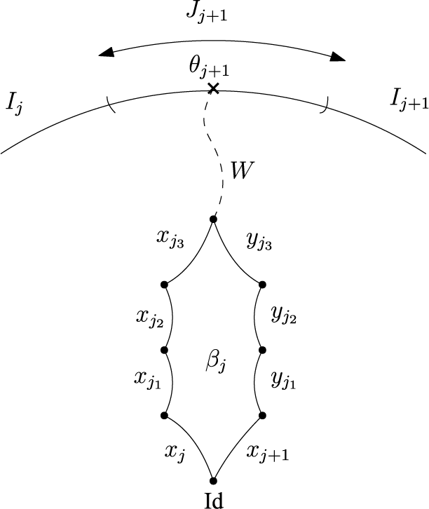


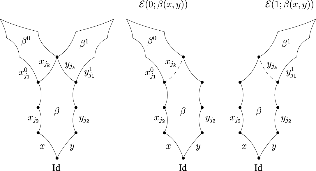
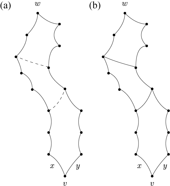

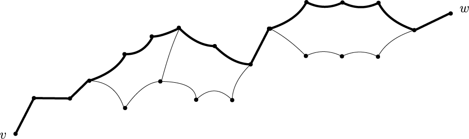


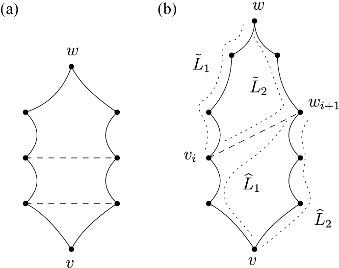
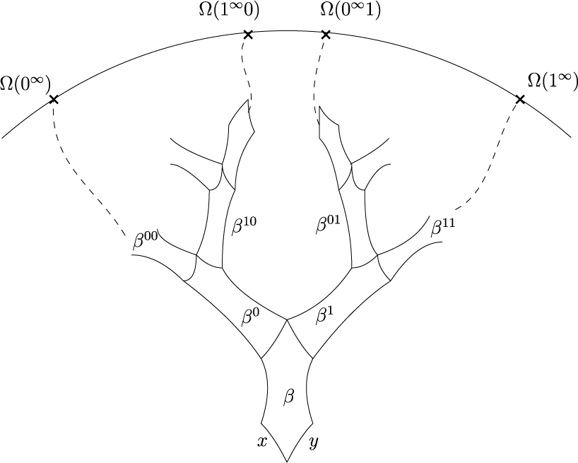

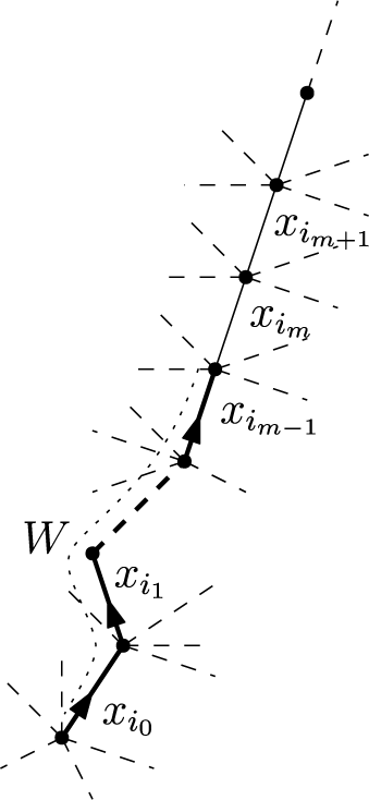
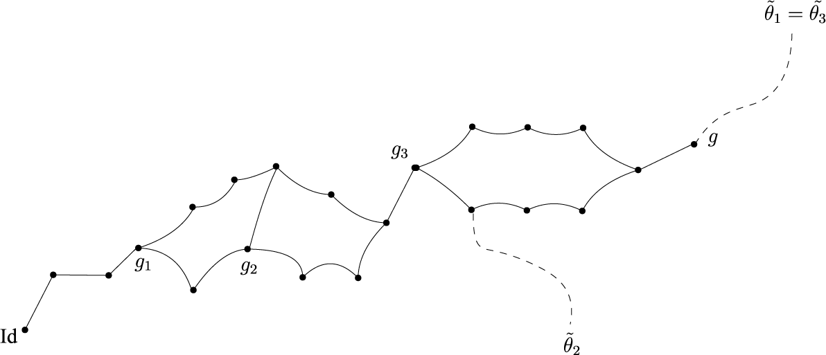

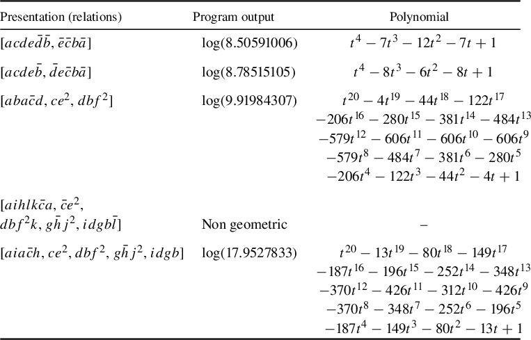

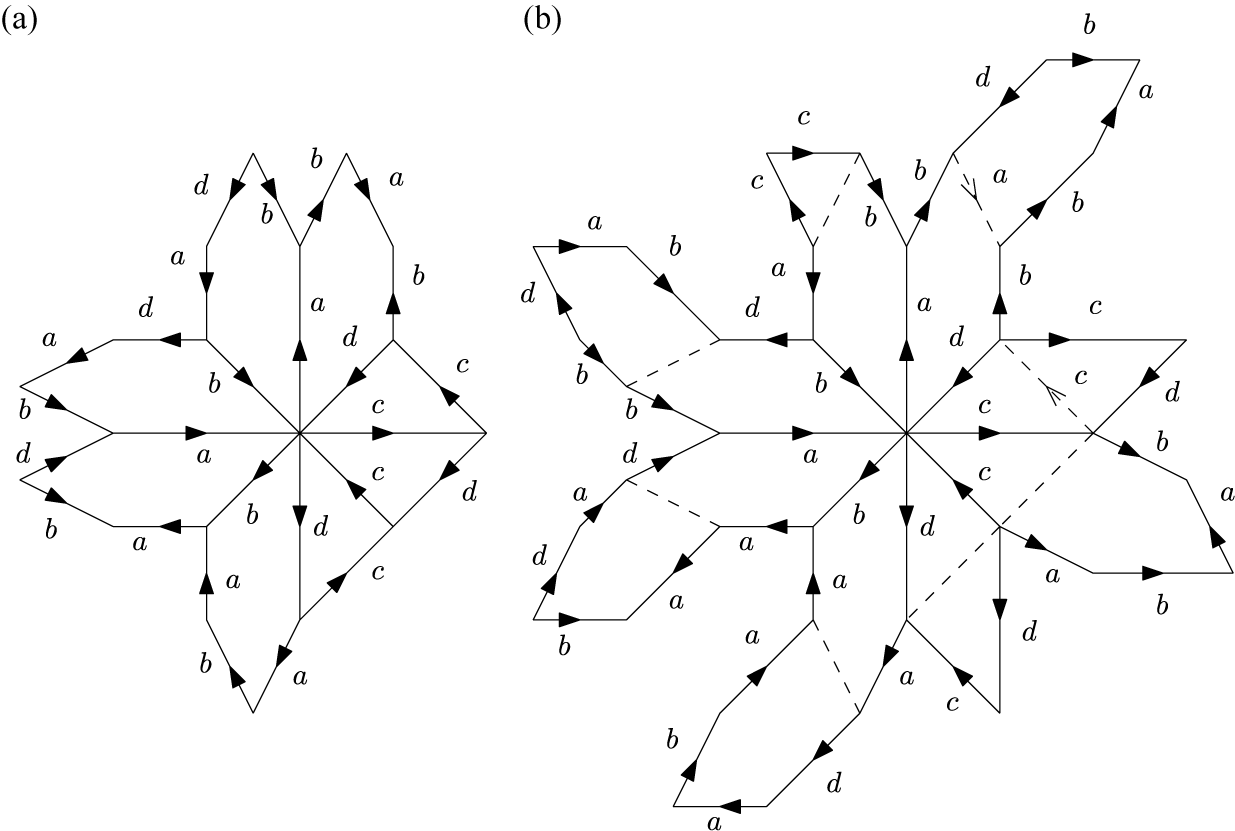


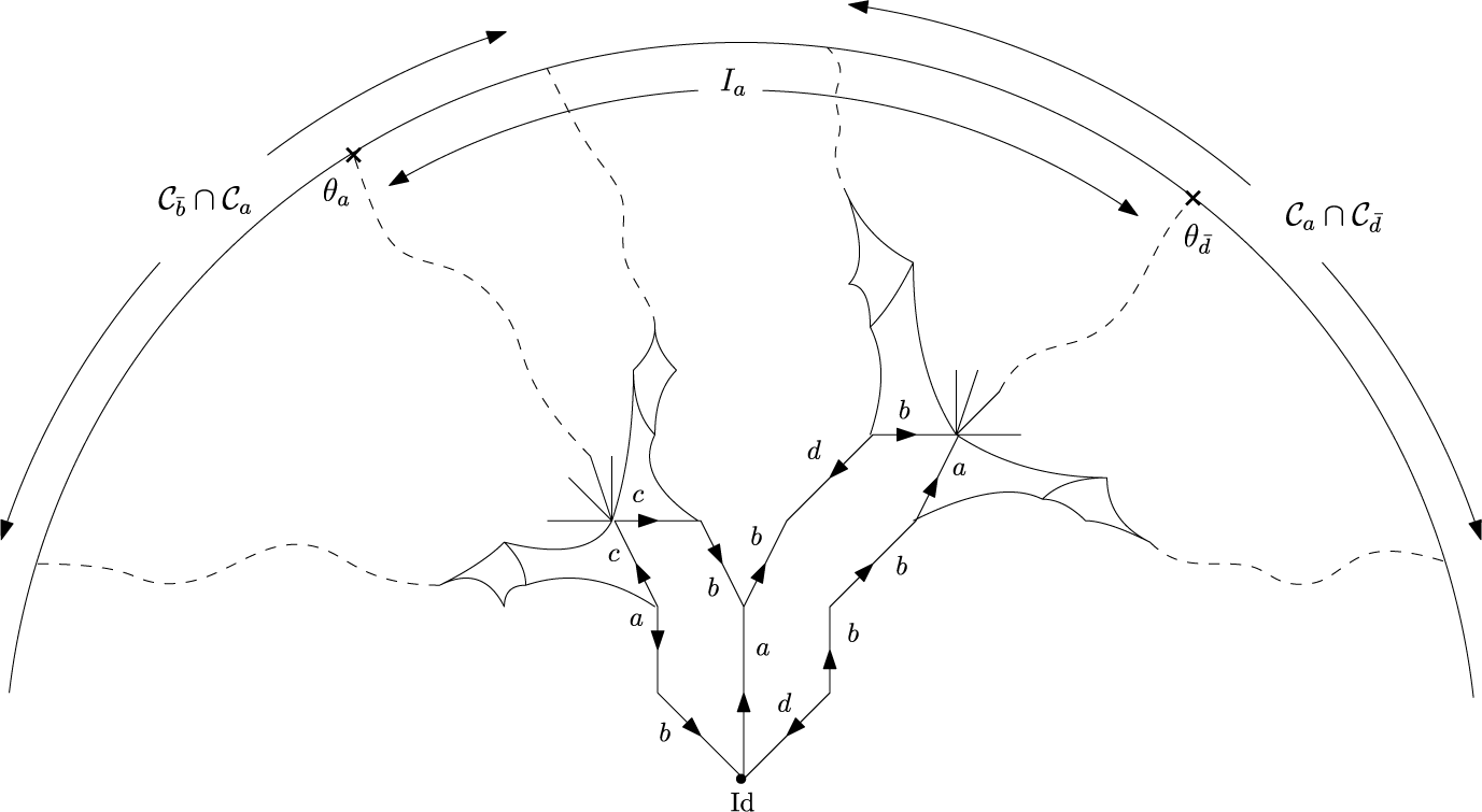


 Open access